arX

iv:0

910.

4984

v2 [

cond

-mat

.sta

t-m

ech]

4 F

eb 2

010

Stochastic Turing patterns in the Brusselator model

Tommaso BiancalaniDipartimento di Fisica, Universita degli Studi di Firenze,

via G. Sansone 1, 50019 Sesto Fiorentino, Florence, Italy

Duccio FanelliDipartimento di Energetica, Universita degli Studi di Firenze,

via S. Marta 3, 50139 Florence, Italy and INFN, Sezione di Firenze.

Francesca Di PattiDipartimento di Fisica “Galileo Galilei”, Universita degli Studi di Padova, via F. Marzolo 8, 35131 Padova, Italy

A stochastic version of the Brusselator model is proposed and studied via the system size ex-pansion. The mean-field equations are derived and shown to yield to organized Turing patternswithin a specific parameters region. When determining the Turing condition for instability, we payparticular attention to the role of cross diffusive terms, often neglected in the heuristic derivationof reaction diffusion schemes. Stochastic fluctuations are shown to give rise to spatially orderedsolutions, sharing the same quantitative characteristic of the mean-field based Turing scenario, interm of excited wavelengths. Interestingly, the region of parameter yielding to the stochastic self-organization is wider than that determined via the conventional Turing approach, suggesting thatthe condition for spatial order to appear can be less stringent than customarily believed.

PACS numbers: 87.23.Cc, 87.10.Mn, 0250.Ey,05.40.-a

I. INTRODUCTION

Turing instability constitutes a universal paradigm for the spontaneous generation of spatially organized patterns[1]. It formally applies to a wide category of phenomena, which can be modeled via the so called reaction diffusionschemes. These are mathematical models that describe the coupled evolution of spatially distributed species, as drivenby microscopic reactions and freely diffusing in the embedding medium. Diffusion can potentially seed the instabilityby perturbing the mean-field homogeneous state, through an activator-inhibitor mechanism, and so yielding to theemergence of patched, spatially inhomogeneous, density distribution [2]. The realm of application of the Turingideas encompasses different fields, ranging from chemistry to biology, from ecology to physics. The most astonishingexamples, as already evidenced in Turing original paper, are perhaps encountered in the context of morphogenesis,the branch of embryology devoted to investigating the development of patterns and forms in biology [3] .Beyond the qualitative agreement, one difficulty in establishing a quantitative link between theory and empirical

observations has to do with the strict conditions for which the organized Turing patterns are predicted to occur. Inparticular, and with reference to simple predator-prey competing populations, the relative degree of diffusivity of theinteracting species has to be large according to the theory prescriptions, and at variance with the direct experimentalevidence. Moreover, patterns formation appears to be rather robust in nature, as opposed to the Turing predictivescenario, where a fine tuning of the parameters is often necessary.In [4] it was demonstrated that collective temporal oscillations can spontaneously emerge in a model of population

dynamics, as due to a resonance mechanism that amplifies the unavoidable intrinsic noise, originating from thediscreteness of the system. Later on an extension of the model was proposed [5] so to explicitly account for thenotion of space. It was in particulary shown that the number density of the interacting species oscillates both intime and space, a macroscopic effect resulting from the amplification of the stochastic fluctuations about the timeindependent solution of the deterministic equations. More recently, Butler and Goldenfeld [6] proved that persistentspatial patterns and temporal oscillations induced by demographic noise, can develop in a simple predator-prey modelof plankton-herbivore dynamics. The model considered by the authors of [6] exhibits a Turing order in the meanfield theory. The effect of intrinsic noise translates however into an enlargement of the parameter region yielding tothe Turing mechanism, when compared to its homologous domain predicted within the conventional linear stabilityanalysis. This is an individual based effect, which has to be accommodated for in any sensible model of naturalphenomena, and which lacks in the Turing interpretative scenario, that formally applies to the idealized continuumlimit. Interestingly, as reported in [7], the discreteness of the scrutinized medium can yield to robust spatio-temporal

2

structures, also when the system does not undergo Turing order in its mean-field, deterministic version.Starting from this setting, we present the results of our investigations carried out for a spatial version of the

Brusselator model, which we shall be introducing in the forthcoming section. As opposed to the analysis in [6],we will operate within the so called urn protocol, where individual elements belonging to the inspected speciesare assumed to populate an assigned container. The proposed formulation of the Brusselator differs from the onecustomarily reported in the literature. Additional terms are in fact obtained building on the underlying microscopicpicture. These latter contributions are generally omitted, an assumption that we interpret as working in a dilutedlimit. Interestingly, the phase diagram of the homogeneous (aspatial) version of the model, is remarkably differentfrom its diluted analogue, a fact we will substantiate in the following.Furthermore, when constructing the mean-field dynamics from the assigned microscopic rules, one recovers non-

trivial cross diffusive terms, as previously remarked in [5]. These are derived within a self-consistent analysis andultimately stands from assuming a finite carrying capacity in a given spatial patch. As such, they potentially bearan important physical meaning which deserves to be further elucidated. This scheme, alternative to conventionalreaction-diffusion models, calls for an extension of the original Turing condition, that we will derive in the following.This is the second result of the paper.Finally, by making use of the van Kampen system size expansion, we are able to estimate the power spectrum of

fluctuations analytically and so delineate the boundaries of the spatially ordered domain in the relevant parameters’space. As already remarked in [6], the role played by the intimate grainess can impact dramatically the Turing vision,returning a generalized scenario that holds promise to bridge the gap with observations.

II. A SPATIAL VERSION OF THE BRUSSELATOR MODEL

The Brusselator model represents a paradigmatic example of an autocatalytic chemical reaction. This scheme wasoriginally devised in 1971 by Prigogine and Glandsdorff [8] and quickly gained its reputation as the prototype modelfor oscillating chemical reaction of the Belosouv-Zhabotinsky [9, 10] type. In the following we shall consider a slightlymodified version of the original formulation, where the number of reactants X and Y is conserved and totals in N ,including the empties, here called E [4]. Moreover we will consider a spatially extended system composed of Ω cells,each of size l, where reactions are supposed to occur [13]. Practically each cell hosts a replica of the Brusselatorsystem: The molecules are however allowed to migrate between adjacent cells, which in turn implies an effectivespatial coupling imputed to the microscopic molecular diffusion. A periodic geometry is also assumed so to restorethe translational invariance. Although the calculation can be carried out in any space dimension D (see [5, 7]) weshall here mainly refer to the D = 1 case study, so to privilege the clarity of the message over technical complications.It should be however remarked that our conclusions are general and remain unchanged in extended spatial settings.Mathematically the model can be cast in the form:

A+ Eia→ A+Xi,

Xi +Bb→ Yi +B,

2Xi + Yic→ 3Xi,

Xid→ Ei,

where the index i runs from 1 to Ω and identifies the cell where the molecules are located. The autocatalytic speciesof interest to us are Xi and Yi. The elements A and B work as enzymatic activators, and keep constant in number.As such, they can be straightforwardly absorbed into the definition of the reaction rates. Let us label with ni (resp.mi and oi) the number of element of type Xi (resp. Yi and Ei) populating cell i. Then, assuming N to identify themaximum number of available cases within each cell, one gets N = ni+mi+ oi a condition which can be exploited toreduce the actual number of dynamical variables to two. The dynamics of the model is ultimately related to studyingthe coupled interaction between the discrete species ni and mi. The migration between neighbors cells is specifiedthrough:

Xi + Ejµ→ Ei +Xj ,

Yi + Ejδ→ Ei + Yj .

3

Assuming a perfect mixing in each individual cell i, the transition probabilities T (·|·) read [4]:

T (ni + 1,mi|ni,mi) = aN − ni −mi

NΩ,

T (ni − 1,mi + 1|ni,mi) = bniNΩ

,

T (ni + 1,mi − 1|ni,mi) = dni

2mi

N3Ω,

T (ni − 1,mi|ni,mi) = cniNΩ

,

(1)

where according to the standard convention, the rightmost input specifies the original state and the other entry stemsfor the final one. In addition, the migration mechanism between neighbors cell is controlled by:

T (ni − 1, nj + 1|ni, nj) = µniN

N − nj −mj

NΩz,

T (mi − 1,mj + 1|mi,mj) = δmi

N

N − nj −mj

NΩz,

(2)

where the positive constants µ and δ quantify the diffusion ability of the two species and z stands for the number offirst neighbors. To complete the notation setting, we introduce the Ω-dimensional vectors n and m to identify thestate of the system. Their i− th components respectively read ni and mi.The aforementioned system is intrinsically stochastic. At time t there exists a finite probability to observe the

system in the state characterized by n and m. Let us label P (n,m, t) such a probability. One can then write downthe so called master equation, a differential equation which governs the dynamical evolution of the quantity P (n,m, t).The master equation for the case at hand takes the form

∂

∂tP (n,m, t) =

Ω∑

i

[

(ǫ−Xi− 1) T (ni + 1,mi|ni,mi) + (ǫ+Xi

− 1) T (ni − 1,mi, |ni,mi)

+ (ǫ+Xiǫ−Y,i − 1) T (ni − 1,mi + 1|ni,mi) + (ǫ−Xi

ǫ+Yi− 1) T (ni + 1,mi − 1|ni,mi)

+∑

j∈i

[

(ǫ+Xiǫ−Xj

− 1) T (ni − 1, nj + 1|ni, nj)+

+ (ǫ+Yiǫ−Yj

− 1) T (mi − 1,mj + 1|mi,mj)]

]

P (n,m, t),

(3)

where use has been made of the definition of the step operators

ǫ±Xif(. . . , ni, . . . ,m) = f(. . . , ni ± 1, . . . ,m), ǫ±Yi

f(n, . . . ,mi, . . .) = f(n, . . . ,mi ± 1, . . .), (4)

and where the second sum in equation (3) runs on first neighbors j ∈ i. Equation (3) is exact, the underlyingdynamics being a Markov process. The master equation (3) contains information on both the ideal mean–fielddynamics (formally recovered in the limit of diverging system size) and the finite N corrections. To bring intoevidence those two components, one can proceed according to the prescriptions of van Kampen [11], and write thenormalized concentration relative to the interacting species as:

niN

= φi(t) +ξi√N,

mi

N= ψi(t) +

ηi√N, (5)

where ξi and ηi stand for the stochastic contribution. The ansatz (5) is motivated by the central limit theorem and

holds provided the dynamics evolve far from the absorbing boundaries (extinction condition). Here 1/√N plays the

role of a small parameter and paves the way to a perturbative analysis of the master equation. At the leading orderone recovers the mean–field equations, while the fluctuations are characterized as next to leading corrections. Thefollowing section is devoted to discussing the system dynamics, according to its mean–field approximation.

III. THE MEAN–FIELD APPROXIMATION AND THE TURING INSTABILITY

Performing the perturbative calculation one ends up with the following system of partial differential equations forthe φi(t) and ψi(t) in cell i:

4

∂τφi =− bφi − dφi + a (1− φi − ψi) + cφ2iψi + µ[

∆φi + φi∆ψi − ψi∆φi]

,

∂τψi = bφi − cφ2iψi + δ[

∆ψi + ψi∆φi − φi∆ψi]

,(6)

where τ = t/(NΩ). In eq. (6) we have introduced the discrete Laplacian operator ∆ acting on a generic function fias

∆fi =2

z

∑

j∈i

(

fj − fi)

. (7)

The above sum runs on the first neighbors which we assume to total in z. The limit Ω → ∞ corresponds to shrinkingthe lattice spacing l to zero and so obtaining the continuum mean-field description. In this limit the system (6)converges to:

∂τφ = − bφ− dφ+ a (1− φ− ψ) + cφ2ψi + µ[

∇2φ+ φ∇2ψ − ψ∇2φ],

∂τψ = bφ− cφ2ψ + δ[

∇2ψ + ψ∇2φ− φ∇2ψ],(8)

where the population fractions go over the population densities and the rescaling µ → µl2 and δ → δl2 have beenperformed [14]. As also remarked in [5], cross diffusive terms of the type φ∇2ψ − ψ∇2φ appear in the mean-fieldequations, as a relic of the microscopic rules of interaction. More precisely, they arise as a direct consequence ofthe finite carrying capacity hypothesis. This observation materializes in a crucial difference with respect to theheuristically proposed reaction diffusion schemes and points to the need for an extended Turing analysis, i.e. derivethe generalized conditions yielding to organized spatial structures. Before addressing this specific issue, we start bydiscussing the homogeneous fixed point of (8). From hereon we will set a = d = 1, a choice already made in [12] forthe original Brusselator model and which will make possible to visualize our conclusion in the reference plan (b, c) forany fixed ratio of the diffusivity amount δ and µ.

A. The homogeneous fixed points

Plugging a = d = 1 into equations (8) and looking for homogeneous solutions implies:

φ = (1− φ− ψ)− (1 + b)φ+ cφ2ψ,

ψ = bφ− cφ2ψ.(9)

As an important remark we notice that in the diluted limit φ, ψ << 1, the system tends to the mean-field ofthe original Brusselator model, as e.g. reported in [12]. For a proper tuning of the chemical parameters (assigningsignificantly different strength) one can prove that, if initialized so to verify the diluted limit, the system staysdiluted all along its subsequent evolution. As a corollary, the diluted solution is contained in the formulation ofthe Brusselator here considered, this latter being therefore regarded as a sound generalization of the former. Noticethat when operating under diluted conditions, the cross diffusive terms appearing in the spatial equations (8) can beneglected and the standard reaction-diffusion scheme recovered. Again, let us emphasize that it is the finite carryingcapacity assumption that modifies the mean-field description.System (9) admits three fixed points, namely:

φ1 = 0,

ψ1 = 1,

φ2 = c−√−8bc+c2

4c,

ψ2 = 1

2+

√−8bc+c2

2c,

φ3 = c+√−8bc+c2

4c,

ψ3 = 1

2−

√−8bc+c2

2c.

(10)

The first of the above corresponds to the extinction of the species X : It exists for any choice of the freely changingparameters b, c and corresponds to a stable attractor for the dynamics. This solution is not present in the originalBrusselator mean–field equations and its origin can be traced back to the role played by the limited capacity of thecontainer.The remaining two fixed points are respectively a saddle point and a (non trivial) stable attractor. They both

manifest when the condition −8b + c > 0 is fulfilled. The saddle point partitions the available phase space into twodomains, each defining the basin of attraction of the stable points. When c = 8b a saddle-node bifurcation occurs: the

fixed points (φ2, ψ2) and (φ3, ψ3) collide to eventually disappear. The finite carrying capacity that follows the “urnrepresentation” of the Brusselator dynamics destroys the limit cycle solution which is instead found in its celebrated

5

classical analogue [12]: No periodic solutions are found in the mean-field approximation, unless the diluted limit is

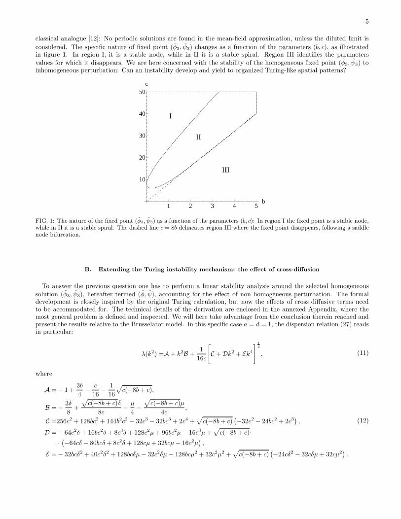
considered. The specific nature of fixed point (φ3, ψ3) changes as a function of the parameters (b, c), as illustratedin figure 1. In region I, it is a stable node, while in II it is a stable spiral. Region III identifies the parameters

values for which it disappears. We are here concerned with the stability of the homogeneous fixed point (φ3, ψ3) toinhomogeneous perturbation: Can an instability develop and yield to organized Turing-like spatial patterns?

I

II

III

1 2 3 4 5b

10

20

30

40

50c

FIG. 1: The nature of the fixed point (φ3, ψ3) as a function of the parameters (b, c): In region I the fixed point is a stable node,while in II it is a stable spiral. The dashed line c = 8b delineates region III where the fixed point disappears, following a saddlenode bifurcation.

B. Extending the Turing instability mechanism: the effect of cross-diffusion

To answer the previous question one has to perform a linear stability analysis around the selected homogeneous

solution (φ3, ψ3), hereafter termed (φ, ψ), accounting for the effect of non homogeneous perturbation. The formaldevelopment is closely inspired by the original Turing calculation, but now the effects of cross diffusive terms needto be accommodated for. The technical details of the derivation are enclosed in the annexed Appendix, where themost general problem is defined and inspected. We will here take advantage from the conclusion therein reached andpresent the results relative to the Brusselator model. In this specific case a = d = 1, the dispersion relation (27) readsin particular:

λ(k2) =A+ k2B +1

16c

[

C +Dk2 + Ek4]

1

2

, (11)

where

A =− 1 +3b

4− c

16− 1

16

√

c(−8b+ c),

B =− 3δ

8+

√

c(−8b+ c)δ

8c− µ

4−

√

c(−8b+ c)µ

4c,

C =256c2 + 128bc2 + 144b2c2 − 32c3 − 32bc3 + 2c4 +√

c(−8b+ c)(

−32c2 − 24bc2 + 2c3)

,

D =− 64c2δ + 16bc2δ + 8c3δ + 128c2µ+ 96bc2µ− 16c3µ+√

c(−8b+ c)··(

−64cδ − 80bcδ + 8c2δ + 128cµ+ 32bcµ− 16c2µ)

,

E =− 32bcδ2 + 40c2δ2 + 128bcδµ− 32c2δµ− 128bcµ2 + 32c2µ2 +√

c(−8b+ c)(

−24cδ2 − 32cδµ+ 32cµ2)

.

(12)

6

The perturbation gets amplified if λ(k2) > 0 over a finite interval of k values. The edges, k1 and k2, of the intervalare identified by imposing λ(k2) = 0 which returns the following results:

k1,2 =1

2√2bδµ

[

2cδ(b− 1) + 8b2(µ− δ)− bcµ+√

c(−8b+ c)(2δ − 2bδ − bµ)±(

F +√

c(−8b+ c) G)

1

2

]1

2

, (13)

where

F = 2(4c2δ2 − 8bc(2 + c)δ2 + 32b4(δ − µ)2 − 4b3c(8δ2 − 2δµ+ 3µ2) + b2c(4(12 + c)δ2 + cµ2)),

G = 2(−4cδ2 + 8bcδ2 + 8b3(2δ2 − δµ− µ2) + b2(−4(4 + c)δ2 − 16δµ+ cµ2)).(14)

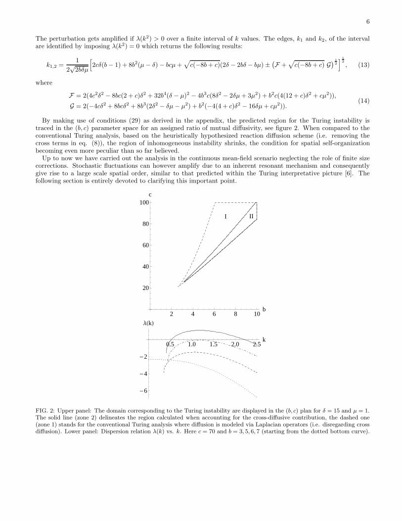
By making use of conditions (29) as derived in the appendix, the predicted region for the Turing instability istraced in the (b, c) parameter space for an assigned ratio of mutual diffusivity, see figure 2. When compared to theconventional Turing analysis, based on the heuristically hypothesized reaction diffusion scheme (i.e. removing thecross terms in eq. (8)), the region of inhomogeneous instability shrinks, the condition for spatial self-organizationbecoming even more peculiar than so far believed.Up to now we have carried out the analysis in the continuous mean-field scenario neglecting the role of finite size

corrections. Stochastic fluctuations can however amplify due to an inherent resonant mechanism and consequentlygive rise to a large scale spatial order, similar to that predicted within the Turing interpretative picture [6]. Thefollowing section is entirely devoted to clarifying this important point.

I II

2 4 6 8 10b

20

40

60

80

100c

0.5 1.0 1.5 2.0 2.5k

-6

-4

-2

ΛHkL

FIG. 2: Upper panel: The domain corresponding to the Turing instability are displayed in the (b, c) plan for δ = 15 and µ = 1.The solid line (zone 2) delineates the region calculated when accounting for the cross-diffusive contribution, the dashed one(zone 1) stands for the conventional Turing analysis where diffusion is modeled via Laplacian operators (i.e. disregarding crossdiffusion). Lower panel: Dispersion relation λ(k) vs. k. Here c = 70 and b = 3, 5, 6, 7 (starting from the dotted bottom curve).

7

IV. THE ROLE OF STOCHASTIC NOISE AND THE POWER SPECTRUM OF FLUCTUATIONS

At the next to leading order in the van Kampen perturbative development one ends up with a Fokker-Planckequation for the probability distribution of the fluctuations Π(ξ,η, t) = P (n,m, t) where the vectors ξ and η havedimensions Ω and respective components ξi and ηi. The derivation is lengthy but straightforward and the reader canrefer to e.g. [5, 7] for a detailed account on the mathematical technicalities. We will here report on the outcome ofthe calculation in terms of the predicted power spectra of the fluctuations close to equilibrium. In complete analogywith e.g. equation (36) and (37) of [5] the latter can be written as:

Pk,X(ω) =< |ξk(ω)|2 >

Pk,Y (ω) =< |ηk(ω)|2 >

where the ω and k stand respectively for Fourier temporal and spatial frequencies[15] . Exploiting the formal analogybetween the governing Fokker-Planck equation and the equivalent Langevin equation one eventually obtains (see eqs.(38) and (39) in [5]):

Pk,X(ω) =C1 +Bk,11ω

2

(ω2 − Ω2k,0)

2 + Γ2kω

2,

Pk,Y (ω) =C2 +Bk,22ω

2

(ω2 − Ω2k,0)

2 + Γ2kω

2,

where:

Ck,X(ω) = Bk,11M2k,22 − 2Bk,12Mk,12Mk,22 +Bk,22M

2k,12, (15)

Ck,Y (ω) = Bk,22M2k,11 − 2Bk,12Mk,21Mk,11 +Bk,11M

2k,21. (16)

The 2× 2 matrix Mk of elements Mk,ij reads

Mk =

−2− b+ 2cφψ + µ(

1− ψ)

∆k −1 + cφ2 + µφ∆k

b− 2cφψ + δψ∆k −cφ2 + δ(

1− φ)

∆k

, (17)

and the elements Bk,ij respectively are:

Bk,11 = 1 + bφ− ψ + cφ2ψ − 2µφ∆k + 2µφ2∆k + 2µφψ∆k, (18)

Bk,12 = −bφ− cφ2ψ, (19)

Bk,22 = bφ+ cφ2ψ − 2δψ∆k + 2δφψ∆k + 2δψ2∆k, (20)

with the additional condition Bk,12 = Bk,21. Finally, Ω2k,0 = detMk, Γk = −trMk and the Fourier transform of the

Laplacian ∆k = 2[cos(kl)− 1]. In the continuum limit, the cell size goes to zero and ∆k scales as ∆k ∼ k2 [5].We are now in a position to represent the power spectrum of the fluctuations as predicted by the system size

expansion. In figure 3 we display a selection of power spectra relative to one population and for different values of theparameter b, at fixed c and diffusivity amount (see caption). The snapshots refer to a region of the parameter space forwhich we do not expect spatial order to appear, based on the Turing paradigm. However, and beyond the simplifiedmean-field viewpoint, a clear spatial peak is displayed, which gains in potency as the boundary of the Turing domainis being approached. Physically, it seems plausible to assume that the demographic noise can modify the dispersionrelation. As a consequence, the curve λ(k), negative defined beyond the region of Turing instability, can locally crossthe zero line, taking positive values in correspondence of specific k. These latter modes get therefore destabilized,yielding to quasi-Turing structures. Clearly, the k candidate to drive the stochastic instabilities are the ones close tokmax, the wave number that identifies the position of the maximum of the dispersion relation. If the above scenariois correct, kmax should then be reasonably similar to the k value that locates the peak position in the power spectraP (k, ·)(0). In figure (4) such comparison is drawn, for both species and over a window of b values, confirming theadequacy of the proposed interpretation. Based on the above, we can convincingly argue that the spatial modes herepredicted represent an ideal continuation of the Turing structures beyond the region of parameters deputed to themean–field instability and, for this reason, we suggest to refer to them as to stochastic Turing patterns.

8

The fact that spatial order appears for a wider range of the control parameter is further confirmed by visualinspection of figure 5, where the region of stochastic induced spatial organization, delineated from the power spectracalculated above, is depicted and compared to the corresponding mean–field prediction. Notice that the domainsyielding to stochastic Turing patterns structures are different depending on the considered species. This observationmarks yet another difference with respect to the standard mean-field theory. We can in fact expect to observe spatiallyordered structures for just one of the two species, while the other is homogenously distributed.As an additional a point, we consider the case δ = µ = 1. This choice cannot yield to the genuine Turing order, a

pronounced difference in the relative diffusivity rates being an unavoidable pre-requisite. As opposed to the classicalpicture, stochastic Turing patterns can still emerge as demonstrated in figure 6.From the above expressions for the power spectra, one can also show that for µ = δ = 0 (the aspatial limit) quasi-

periodic time oscillations manifest in the concentrations. This is an effect of inner stochastic noise which restores theoscillations destroyed by the introduction od the carrying capacity. In general terms, self-oscillatory dynamics couldbe possibly understood, as resulting from the discrete nature of the medium, a scenario alternative to any ad hoc

mean–field interpretation.

0.00.5

1.0

1.5

2.0

Ω

0

2

4

k

0.1

0.2

0.3

0.00.5

1.01.5

2.0

Ω

0

2

4

k

0.51.01.52.0

1 2 3 4 5k

0.1

0.2

0.3

PXHΩ=0, kL

1 2 3 4 5k

0.5

1.0

1.5

2.0

PXHΩ=0, kL

FIG. 3: Upper panels: The power spectra Pk,X(ω) for c = 70 and b = 3, 6 (going from left to right). Here δ = 15 and µ = 1.The selected values of b and c fall outside the region of Turing instability, as follows the mean–field linear stability calculation(see figure 2). Lower panels: The power spectra Pk,X(0) plotted vs. k so to enable one to appreciating the range of excitedspatial wavelengths. This latter approximately matches that found in the realm of the Turing mean–field calculation (see figure2), implying similar characteristic of the spatially ordered structures.

V. CONCLUSION

Spatially organized patterns are reported to occur in a large gallery of widespread applications and are currentlyinterpreted by resorting to the paradigmatic Turing picture. This vision, though successful, relies on a mean-fielddescription of the relevant reaction diffusion schemes, often guessed on purely heuristic basis. An alternative scenariowould require accounting for the intimate microscopic dynamics and so encapsulating the effect of the small scalegrainess. This latter translates into stochastic fluctuations that, under specific conditions, can amplify and so giverise to organized spatio-temporal patterns. In this paper we have considered a microscopic model of Brusselator,

9

4.0 4.5 5.0 5.5 6.0 6.5 7.0b

0.2

0.4

0.6

0.8

1.0

1.2

1.4

kmax

4.0 4.5 5.0 5.5 6.0 6.5 7.0b

0.2

0.4

0.6

0.8

1.0

1.2

1.4

kmax

FIG. 4: Left panel: Symbols refer to the values in k that identify the maximum of the function Pk,X(0), here plotted as afunction of b. The solid line stands for the position of the maximum of the mean–field dispersion relation λ(k). Parameters areset as in figure 3. Right panel: as in the left panel, but now the symbols refer to species Y .

2 4 6 8 10b

20

40

60

80

100c

FIG. 5: The extended domain of Turing like instability predicted by the stochastic based analysis: the dashed line refers tospecies X, while the dot-dashed to species Y . The stochastic Turing region is confronted to the corresponding mean–fieldsolution (solid line, also depicted in figure 3).

0.00.5

1.01.5

2.0Ω

0

2

4

k

1234

1 2 3 4 5k

0.5

1.0

1.5

2.0PXHΩ=0, kL

FIG. 6: Left panel: The power spectra Pk,X(ω) for a = d = 1, c = 70 and b = 8. Spatial and temporal peaks appear now tobe decoupled. Right panel: The corresponding power spectra Pk,X(0) plotted vs. k. A clear peak is displayed.

10

and shown that Turing like patterns can indeed emerge beyond the parameter region predicted by the conventionalTuring theory and due to the role of finite size corrections to the mean-field idealized dynamics. This result isobtained via a system size expansion which enables us to return closed analytical expressions for the power spectra offluctuations. Our results agree with the conclusion reached in [6] for another model and employing different analyticaltools. Organized patterns can therefore occur more easily than expected, an observation that can potentially helpreconciling theory and observations. In particular we find stochastic Turing patterns to emerge for δ ∼ µ, a conditionfor which Turing order is prevented to occur.

Acknowledgments

D.F. wishes to thank Alan J. McKane for interesting discussions and for pointing out reference [6]. F.D.P. wishes tothank Javier Buceta for stimulating discussion. F.D.P thanks financial support from the ESF Short Visit Grant withinthe framework of the ESF activity entitled ”Functional Dynamics in Complex Chemical and Biological Systems”.

VI. APPENDIX

Let us start by the generic set of partial differential equations:

∂tφ = f(φ, ψ) + µ[

∇2φ+ φ∇2ψ − ψ∇2φ]

,

∂tψ = g(φ, ψ) + δ[

∇2ψ + ψ∇2φ− φ∇2ψ]

,(21)

which explicitly allow for cross diffusive contributions. We choose to deal with zero flux boundary conditions.

Assume that in absence of diffusion (homogeneous setting) the model tends towards a fixed point specified by (φ, ψ).

In other words, φ, ψ, do not depend over space variables. Allowing for diffusion, and imposing µ 6= δ, can make thesystem unstable to spatial perturbation. To clarify this point, let us start by considering the Jacobian matrix forµ = δ = 0:

J =

(

fφ fψgφ gψ

)

. (22)

The fixed point (φ, ψ) is linearly stable if J has positive determinant and negative trace:

detJ = fφgψ − gφfψ > 0, trJ = fφ + gψ < 0. (23)

Assuming (23) to hold one can proceed with a linearization of (21) (with µ, δ 6= 0) around (φ, ψ) and so looking for

the sought condition of instability. Define x =(φ−φψ−ψ

)

, then (21) become

∂t x = J x+D∇2x, D =

(

µ (1 − ψ) µ φ

δ ψ δ (1− φ)

)

. (24)

Define the eigenfunctions of the Laplacian operator as:

(

∇2 + k2)

Wk(r) = 0, r ∈ H,

and write the solution to eq.(24) in the form:

x(t, r) =∑

k

eλt ak Wk(r). (25)

Assume µ = 1, or equivalently label with δ the ratio of the two diffusivities (after proper rescaling of the ratecoefficients). Substituting ansatz (25) into eq. (24) yields:

eλt[

J− k2 D− λ1]

Wk = 0,

which implies that the system admits a solution iff the matrix J− k2 D− λ1 is singular, i.e.:

11

det(J− k2 D− λ1) = 0. (26)

Label the solutions of (26) as λ1(k2) and λ2(k

2): They can be interpreted as dispersion relation, specifying thetime scale of departure (or convergence) of the k-th mode towards the deputed fixed point. If at least one of thetwo solutions displays a positive real part, the mode is unstable, and drives the system dynamics towards a non-homogeneous configuration in response to the initial perturbation. Manipulating the determinant, (26) takes theform:

λ2 + λ q(k2) + h(k2) = 0, (27)

where

q(k2) = k2 + k2δ(1− φ− ψ)− fφ − gψ,

h(k2) = k4δ − k4φ δ − k4ψ δ − k2δfφ + k2φ δfφ + k2ψ δfψ + k2φgφ−fψ gφ − k2gψ + k2ψ gψ + fφ gψ.

λ1(k2) and λ2(k

2) are obtained as roots of (27). The actual dispersion relation, λ(k2) in the main body of the paper,is the one that displays the largest real part. We notice that (i) q(k2) is always positive as δ > 0 by definition; (ii)

(1 − φ − ψ) > 0 as φ and ψ are concentrations; (iii) −fφ − gψ > 0 due to (23). Left-hand side of equation ((27))is hence a parabola with the concavity pointing upward and the minimum positioned in the half-plane of negativeabscissa. In conclusion a necessary and sufficient condition for the existence of real roots is h < 0 where:

h(k2) = ak4 + bk2 + c,

a = δ(1 − φ− ψ),

b = −δfφ − gψ + φ(δfφ + gφ) + ψ(δfψ + gψ),

c = detJ,

(28)

with a > 0, c > 0. The condition for h < 0 corresponds to b < 0 and b2 − 4ac > 0. Summing up the condition for thegeneralized Turing instability reads:

(δfφ + gψ)− φ (δfφ + gφ)− ψ (δfψ + gψ) > 0,[

(δfφ + gψ)− φ (δfφ + gφ)− ψ (δfψ + gψ)]2> 4 δ(1− φ− ψ) detJ,

(29)

together with (23).

[1] A. M. Turing Phils. Trans. R. Soc. London Ser. B, 237 37 (1952).[2] J. Buceta and K. Lindenberg, Phys. Rev. E 66, 046202 (2002).[3] J.D. Murray, Mathematical Biology, Second Edition, Springer.[4] A.J. McKane and T.J. Newmann Phys. Rev. Lett. 94, 218102 (2005)[5] C. Lugo, A.J. McKane, Phys. Rev. E 78, 051911 (2008).[6] T. Butler and N. Goldenfeld Phys. Rev. E, 80, 030902(R) (2009).[7] P. de Anna, F. Di Patti, D. Fanelli, A.J. McKane, T. Dauxois submitted to Phys. Rev. E (2010), cond-mat arXiv:1001.4908.[8] P. Glandsdorff and I. Prigogine, Thermodynamics theory of structure stability and fluctuations, Wiley, New York (1971).[9] B.P. Belousov, A periodic reaction and its mechanism in Collection of short papers on radiation medicine for 1958, Med.

Publ. Moschow, 1959; A. M. Zhabotinsky, Biofizika, 9, 306-311 (1964).[10] S. Strogatz, Non linear dynamics and chaos: With applications to Physics, Biology, Chemistry and Engineering, Perseus

Book Group (2001).[11] N. G. van Kampen. Stochastic Processes in Physics and Chemistry (Elsevier, Amsterdam, 2007). Third edition.[12] R.P. Boland, T. Galla, A.J. McKane Phys. Rev. E 79, 051131 (2009).[13] Working with the empties E implies imposing a finite carrying capacity in each micro-cell. This procedure defines the

so called “urn protocol”, and allows for a technically easier implementation of the van Kampen expansion as presentedin [4]. On the other hand, and besides technical reasons, assuming a limited capacity in space is a reasonable physicalrequest. It is therefore interesting to explore how such a choice reflects on the subsequent analysis. Let us anticipate thatthe presence of the empties E will sensibly modify the mean-field phase diagram of the Brusselator model, as concernsboth the homogeneous and the spatial dynamics. Conversely, the observation that the Turing region gets enlarged bydemographic noise holds true, irrespectively of the specific urn representation here invoked [6].

12

[14] The original parameters µ and δ quantify the ability of the molecules to exit/enter a given patch of size l. When l getsreduced, µ (resp. δ) should correspondingly increase, so that the quantity µl2 (resp. δl2) converges to a finite value (thephysical diffusivity) when the limit Ω → ∞ is taken. This latter value is in turn the one that enters the continuous equations(8).

[15] We define the Fourier transform fk of a function fj defined on a one dimensional lattice with spacing l as fk = l∑

jexp(−ik·

lj)fj, see [5].