SINGLE TIMESCALE STOCHASTIC APPROXIMATIONFOR STOCHASTIC NASH GAMES IN COGNITIVE RADIO SYSTEMS

Jayash Koshal, Angelia Nedic and Uday V. Shanbhag†

Department of Industrial and Enterprise Systems Engineering,University of Illinois, Urbana IL 61801.

Email: koshal1,angelia,udaybag@illinois.edu

ABSTRACTIn the face of increasing demand for wireless services, thedesign of spectrum assignment policies has gained enormousrelevance. We consider one such instance in cognitive radiosystems where recent efforts have focused on the applicationof game-theoretic approaches. Much of this work has been re-stricted to deterministic regimes and this paper considers dis-tributed schemes in the stochastic regime. The correspondingproblems are seen to be stochastic Nash games over continu-ous strategy sets. Notably, the gradient map of player utilitiesis seen to be monotone mappping over the cartesian productof strategy sets, leading to a monotone stochastic variationalinequality. We consider the application of projection-basedstochastic approximation schemes. However, such techniquesare characterized by a key shortcoming: they can accommo-date strongly monotone mappings only with standard exten-sions of stochastic approximation schemes for merely mono-tone mappings is natively a two-timescale scheme. Accord-ingly, we consider the development of single timescale tech-niques for computing equilibria when the associated gradi-ent map does not admit strong monotonicity. We developconvergence theory for distributed single-timescale stochas-tic approximation schemes, namely stochastic iterative prox-imal point method which requires exactly one projection stepat every step. Finally we apply this framework to the de-sign of cognitive radio systems in uncertain regimes undertemperature-interference constraints.

Index Terms— Stochastic approximation, VI, Game the-ory, Cognitive Radio, Communication

1. INTRODUCTION

Game-theoretic models have proved to be useful in the mod-eling of strategic behavior in a host of problems in commu-nication networks, including power control and flow man-agement, amongst others. More recently, game-theoretic ap-proaches have assumed relevance in cognitive radio (CR) sys-tems. Such questions have become increasingly relevant in†This work has been supported by NSF CMMI 09-48905 EAGER

ARRA award.

the face of growing demand for wireless services and the in-efficiencies associated with fixed assignment policies. Cog-nitive radio systems represent a possible resolution by pro-viding radio nodes with intelligence (or cognitive abilities)that allow for sensing electromagnetic variations and the abil-ity to optimize resources. One proposal for designing spec-trum sharing is through a hierarchical framework that dis-tinguishes primary users (PUs) from secondary users (SUs);specifically, PUs are licensed spectrum holders while SUs arepermitted to share the spectrum without introducing intolera-ble interference to PUs. The interaction of SUs can be mod-eled through a noncooperative game [1, 7] where each SUmaximizes its information subject to interference constraints,given adversarial decisions. Prior work in [7] considers per-fect channel state information (CSI) between primary and sec-ondary users while imperfect CSI is assumed in [12]. In thispaper we further extend this to imperfect CSI between SUsas in [5] and assume the gradient maps across players arestrictly monotone. Distributed schemes for computing equi-libria, such as waterfilling methods that are leveraged for ob-taining best responses, have received significant attention inthe recent past [7].

In this paper, we consider instances of such games wherethe player utilities contain expectations; the resulting classof games is a stochastic Nash game over continuous strategysets. The associated equilibrium conditions of this game maybe compactly stated as a stochastic variational inequality, forwhich we consider projection-based stochastic approxima-tion algorithms. Such schemes have been recently employedfor the solution of stochastic variational inequalities [4] withstrongly monotone and co-coercive maps (see [3] for a def-inition), which to the best of our knowledge, appears to bethe only existing work considering stochastic approximationmethods for variational inequalities. The typical stochasticapproximation procedure, first introduced by Robbins andMonro [9], works toward finding an extremum of a functionh(x) using the following iterative scheme:

xk+1 = xk + ak(∇h(xk) +Mk+1),

where Mk+1 is a martingale difference sequence. Under rea-sonable assumptions on the stochastic errors Mk, stochastic

approximation schemes ensure that xk converges almostsurely to an optimal solution of the problem. Jiang and Xu [4]consider the use of stochastic approximation for the solutionof stochastic variational inequalities with strongly monotoneand Lipschitz continuous maps. The use of stochastic approx-imation methods has a long tradition in stochastic optimiza-tion, commencing with the work of Robbins and Monro [9]for differentiable problems and Ermoliev [2] for nondifferen-tiable problems.

This paper is motivated by the challenges associated withsolving stochastic variational problems when the mappingslose strong monotonicity. In solving deterministic variationalinequalities, such a departure is ably handled through tech-niques, such as Tikhonov regularization [11] and proximal-point [6]. Such schemes, in general, require a solution of aregularized (well-posed) problem and an iterative process isoften needed to obtain the solution. While Tikhonov regu-larization approach suffers from a potential drawback due tothe computational aspect proximal-point method proposed byMartinet [6] (cf. [3]) and further investigated by Rockafel-lar [10] alleviates this problem. Proximal point methods havegained attention from various application areas communica-tion network being one of them.

A remark is in order regarding our proposed scheme.Our goal lies in developing single timescale gradient-baseddistributed schemes characterized by low complexity. Suchschemes lie at one end of the spectrum of best-responsemethods, where a gradient step is taken towards obtaininga best-response. While these techniques are not necessarilysuperior from the standpoint of convergence rate, they remainadvantageous from the standpoint of implementability. Animportant question is why should players adopt this gradient-based approach, particularly if they are selfish in nature?There are two possible answers: (1) First, the game-theoreticapproach can be viewed as an avenue for obtaining solutionsto the multi-user centralized optimization problem allowingis to mandate the decision-making structure for each player.Second, a different viewpoint is one where we contend withequilibrium seeking in a bounded rationality setting whereagents cannot take any arbitrary step; instead, they need totake “gradient steps” with an arbitrary steplength selectedfrom a prescribed range. Note that a standard applicationof regularization techniques would require the solution ofa sequence of strongly monotone problems with increasingexactness. Obtaining increasingly exact solutions inducessignificant computational burden and the need to developalternate approaches is paramount.

The rest of the paper is organized as follows. In Sec-tion 2, we discuss a N -person stochastic Nash game and itsassociated equilibrium conditions, as given by a stochasticvariational inequality. A projection-based single timescalestochastic iterative proximal point method is proposed andanalyzed for this problem in Section 3 and its convergenceis estabilished under an assumption of strict monotonicity of

the mapping. Convergence of the resulting sequence of it-erates is proved in an almost-sure sense, in a regime whereplayers steplengths require limited coordination but are notnecessarily identical across players. In Section 4, we modelthe competitive interactions in cognitive radio systems undertemperature-interference constraints. Further, player’s utili-ties contain expectations and the associated gradient maps areassumed to be strictly monotone. Numerical results on theperformance of algorithms on one such system is presented.Finally, in Section 5, we provide some concluding remarks.

Throughout this paper, we view vectors as columns andwrite xT to denote the transpose of a vector x, and xT y todenote the inner product of vectors x and y. We use ‖x‖ todenote the Euclidean norm of a vector x, i.e., ‖x‖ =

√xTx.

We use ΠX to denote the Euclidean projection operator ontoa set X , i.e., ΠX(x) , argminz∈X ‖x− z‖. The expectationof a random variable V is denoted by E[V ]. Finally, we oftenuse a.s. for almost surely.

2. PROBLEM DESCRIPTION

We consider an N -person stochastic Nash game in which theith agent solves the parameterized problem

minimize E[fi(xi, x−i, ξi)]

subject to xi ∈ Ki , (1)

where x−i denotes the collection xj , j 6= i of decisionsof all players j other than player i. For each i, the vari-able ξi is random with ξi : Ωi → Rni , and the functionE[fi(xi, x−i, ξi)] is convex in xi for all x−i ∈

∏j 6=iKj .

For every i, the set Ki ⊆ Rni is a closed convex set.The equilibrium conditions of the game, denoted by G, canbe characterized by scalar variational inequality problem de-noted by VI(K,F ) where

F (x) ,

∇x1E[f1(x, ξ1)]

...∇xN

E[fN (x, ξN )]

, K =

N∏i=1

Ki, (2)

with x , (x1, . . . , xN )T and xi ∈ Ki for i = 1, . . . , N.Recall that VI(K,F ) requires determining a vector x∗ ∈ Ksuch that

(x− x∗)TF (x∗) ≥ 0 for all x ∈ K. (3)

We let n =∑Ni=1 ni, and note that the set K is closed and

convex set in Rn, whenever the setsKi are closed and convex,for i = 1, . . . , N . The mapping F is a single-valued mapfrom K to Rn.

Standard deterministic algorithms for obtaining solutionsto a variational inequality VI(K,F ) require an analyticalform for the gradient of the expected-value function. Yet,when the expectation is over a general measure space, such

analytical forms are often hard to obtain. In such settings,stochastic approximation schemes assume relevance. In theremainder of this section, we describe the basic frameworkof stochastic approximation and the supporting convergenceresults.

Consider the Robbins-Monro stochastic approximationscheme for solving the stochastic variational inequalityVI(K,F ) in (2)–(3), given by

xk+1 = ΠK [xk − αk(F (xk) + wk)] for k ≥ 0, (4)

where x0 ∈ K is an initial point, F (xk) is the true valueof F (x) at x = xk, αk is the step-size, wk = −F (xk) +F (xk, ξki ) is the stochastic error,

F (xk, ξk) ,

∇x1f1(xk, ξk1 )...

∇xNfN (xk, ξkN )

and ξk ,

ξk1...ξkN

.

In recent work [4], the projection scheme (4) is shown to beconvergent when the mapping F is strongly monotone andLipschitz continuous . In the sequel, we examine how theuse of regularization methods can alleviate the need for thestrong monotonicity requirement and, in fact, we show thatstrict monotonicity suffices.

In our analysis we use some well-known results on super-martingale convergence, which we provide for convenience.The next two results are from [8], Lemma 10, page 49.

Lemma 1 (Lemma 10, Pg. 49 [8]). Let Vk be a sequenceof non-negative random variables adapted to σ−algebra Fkand such that almost surely

E[Vk+1 | Fk] ≤ (1− uk)Vk + βk for all k ≥ 0,

where 0 ≤ uk ≤ 1, βk ≥ 0, and

∞∑k=0

uk =∞,∞∑k=0

βk <∞,βkuk→ 0.

Then, Vk → 0 a.s.

Lemma 2 (Lemma 11, Pg. 50 [8]). Let Vk, uk, βk and γkbe non-negative random variables adapted to Fk. If almostsurely

∑∞k=1 uk <∞,

∑∞k=1 βk <∞, and

E[Vk+1 | Fk] ≤ (1 + uk)Vk − γk + βk for all k ≥ 0,

then Vk is convergent a.s. and∑∞k=1 γk <∞.

Throughout the rest of the paper, we use Fk to denote thesigma-field generated by the initial point x0 and errors w` for` = 0, 1, . . . , k, i.e.,

Fk = x0, (w`, ` = 0, 1, . . . , k) for k ≥ 0.

Now, we specify our assumptions for VI(K,F ) in (2)–(3)and the algorithm (4).

Assumption 1. Let the following hold:

(a) The sets Ki ⊆ Rni are closed and convex;

(b) The mapping F : K → Rn is strictly monotone and Lip-schitz with constant L over the set K;

(c) The stochastic error is such that E[wk | Fk] = 0 and∑∞k=1 α

2kE[‖wk‖2 | Fk] <∞ a.s.

Since the map F is strictly monotone, the solution toVI(K,F ) is unique whenever it exists (see 2.3.3 Theoremin [3]). Note, however, that the strict monotonicity of F isnot enough to guarantee the existence of a solution when theset K is closed and convex.

We note that if Assumption 1(b) is strengthened to Fbeing strongly monotone and the stepsize αk is such that∑∞k=1 αk = ∞, then we immediately have almost sure con-

vergence of the algorithm, which has been established in [4].

3. STOCHASTIC ITERATIVE PROXIMAL-POINTSCHEMES

Proximal-point methods, a class of techniques that appear tohave been first studied by Martinet [6], and subsequently byRockafellar [10] has a long history for addressing monotonevariational inequalities. A more recent description in the con-text of maximal-monotone operators can be found in [3]. Webegin with a description of such methods in the context of amonotone variational inequality VI(K,F ) where F is a con-tinuous and monotone mapping. Recall that Tikhonov-basedtechniques require the construction of a sequence xk, wherexk is the unique solution of VI(K,F + εkI) and εk > 0. Un-der suitable assumptions and given a positive sequence εkwith εk → 0, we have that limk→∞ xk = x∗, where x∗

is some solution of VI(K,F ). In proximal-point methods,the convergence to a single solution of VI(K,F ) is obtainedthrough the addition of a proximal term θ(xk − xk−1), whereθ is a fixed positive parameter. In effect, xk = SOL(K,F +θ(I−xk−1)) and convergence may be guaranteed under suit-able assumptions.

When employing a proximal-point method for solving theVI(K,F ) associated with problem (1), a crucial shortcomingof standard proximal-point schemes lies in the need to solvea sequence of variational problems, a natively two-timescalescheme. Accordingly we develop a single time-scale stochas-tic iterative proximal point method (IPP) in which the cen-tering term xk−1 is updated after every projection step ratherthan when obtains an accurate solution of VI(K,F + θ(I −xk−1)). The distributed stochastic form of the proximal-pointscheme is given by

xk+1i = ΠKi [x

ki − αk,i(Fi(xk) + θk(xki − xk−1i ) + wki )],

(5)

where αk,i is the stepsize chosen by the ith user at the kthiterate, θk > 0 is the prox-parameter.

Before providing a detailed analysis of the convergenceproperties of this scheme, we examine the relationship be-tween the proposed iterative proximal point method and thestandard gradient projection method. An iterative proximal-point scheme for VI(K,F ) necessitates an update given by

xk+1 = ΠK [xk − γk(F (xk) + θ(xk − xk−1))]

= ΠK [((1− γkθ)xk + γkθxk−1)− γkF (xk)]

= ΠK [xk(θ)− γkF (xk)],

where xk(θ) , (1 − γkθ)xk + γkθxk−1. Therefore, whenθ ≡ 0, the method reduces to the standard gradient projectionscheme. More generally, one can view the proximal-pointmethod as employing a convex combination of the old iteratexk−1 and xk instead of xk in the standard gradient scheme.Furthermore, as γk → 0, the update rule starts resemblingthe standard gradient scheme more closely. In our discussion,we allow θ to vary at every iteration; in effect, we employ asequence θk which can grow to +∞ but at a sufficiently slowrate.

We now examine the global convergence of the distributedstochastic proximal-point scheme given by (5) obtained for astrictly monotone F . We impose the following conditions onthe stepsizes and the prox-parameter sequence θk.

Assumption 2. Let αk,max = max1≤i≤Nαk,i, αk,min =min1≤i≤Nαk,i and the following hold:

(a) αk,maxθk ≤(

1 + 2α2k,maxL

2)αk−1,minθk−1 for all k ≥

1, and

limk→∞

α2k,maxθk

αk,min= c with c ∈ [0, 1/2) ;

(b)∑∞k=0 αk,i =∞ and

∑∞k=0 α

2k,i <∞ for all i;

(c)∑∞k=0 (αk,max − αk,min) <∞.

In the next proposition, using Assumption 2 we show al-most sure convergence of the method. Immediately after thisresult, we provide an example for the stepsizes and prox pa-rameters satisfying Assumption 2.

Proposition 1. Let Assumption 1 hold and assume that theVI(K,F ) has a solution. Also, let the steplengths and theprox-parameters satisfy Assumption 2. Then, the sequencexk generated by method (5) converges almost surely to thesolution x∗ of VI(K,F ).

Proof. By using x∗i = ΠKi [x∗i − αk,iFi(x

∗)] and the non-expansivity of the Euclidean projection operator we observe

that ‖xk+1i − x∗i ‖ can be expressed as follows

‖xk+1i − x∗i ‖2

= ‖ΠKi[xki − αk,i(Fi(xk) + θk(xki − xk−1i ) + wki )]

−ΠKi[x∗i − αk,iFi(x∗)]‖2

≤∥∥(xki − x∗i )− αk,i

(Fi(x

k)− Fi(x∗))

αk,i(θk(xki − xk−1i ) + wki

)∥∥2 .Further, the right hand side of preceding relation can be ex-panded as

RHS = ‖xki − x∗i ‖2 + α2k,i‖Fi(x

k)− Fi(x∗)‖2 + α2k,i‖w

ki ‖2

+ (αk,iθk)2‖xki − xk−1i ‖2 − 2αk,i(x

ki − x∗i )T (Fi(x

k)− Fi(x∗))

− 2αk,iθk(xki − x∗i )T (xki − xk−1i )− 2αk,i(x

ki − x∗i )Twki

+ 2α2k,iθk(Fi(x

k)− Fi(x∗))T (xki − xk−1i )

+ 2α2k,i(Fi(x

k)− Fi(x∗))Twki + 2α2k,iθk(xki − x

k−1i )Twki .

Taking expectation and using E[wki | Fk] = 0 (Assump-tion 1(c)), we obtain

E[‖xk+1i − x∗i ‖2 | Fk]

≤ ‖xki − x∗i ‖2 + α2k,i‖Fi(xk)− Fi(x∗)‖2 + α2

k,i‖wki ‖2

+ (αk,iθk)2‖xki − xk−1i ‖2 − 2αk,iθk(xki − x∗i )T (xki − xk−1i )

− 2αk,i(xki − x∗i )T (Fi(x

k)− Fi(x∗))+ 2α2

k,iθk(Fi(xk)− Fi(x∗))T (xki − xk−1i ). (6)

Letαk,max = max1≤i≤Nαk,i andαk,min = min1≤i≤Nαk,i.Summing over all i and using Lipschitz continuity of F (As-sumption 1(b)) we arrive at

E[‖xk+1 − x∗‖2 | Fk] (7)

≤ (1 + α2k,maxL

2)‖xk − x∗‖2 + α2k,maxE[‖wk‖2 | Fk]

+ (αk,maxθk)2‖xk − xk−1‖2

− 2

N∑i=1

αk,i(xki − x∗i )T (Fi(x

k)− Fi(x∗))︸ ︷︷ ︸Term 1

− 2

N∑i=1

αk,iθk(xki − x∗i )T (xki − xk−1i )︸ ︷︷ ︸Term 2

− 2

N∑i=1

α2k,iθk(Fi(x

k)− Fi(x∗))T (xki − xk−1i )︸ ︷︷ ︸Term 3

. (8)

By adding and subtracting 2αk,min(xki − x∗i )T (Fi(xk)−

Fi(x∗)) to the each term of Term 1 we see that

Term 1 = −2αk,min

N∑i=1

(xki − x∗i )T (Fi(xk)− Fi(x∗))

− 2

N∑i=1

(αk,i − αk,min)(xki − x∗i )T (Fi(xk)− Fi(x∗))

≤ −2αk,min(xk − x∗)T (F (xk)− F (x∗))

+ 2(αk,max − αk,min)

N∑i=1

‖xki − x∗i ‖‖F (xk)− F (x∗)‖

≤ −2αk,min(xk − x∗)T (F (xk)− F (x∗))

+ 2(αk,max − αk,min)‖xk − x∗‖‖F (xk)− F (x∗)‖

≤ −2αk,min(xk − x∗)T (F (xk)− F (x∗))

+ 2(αk,max − αk,min)L‖xk − x∗‖2, (9)

by Holder’s inequality and Lipschitz continuity of F.We next estimate Term 2. Since 2(x − y)T (x − z) =

‖x− y‖2 + ‖x− z‖2 − ‖y − z‖2, it follows thatTerm 2

= −N∑i=1

αk,iθk

[‖xki − x∗i ‖2 + ‖xki − x

k−1i ‖2 − ‖xk−1

i − x∗i ‖2]

≤ −αk,minθk

N∑i=1

[‖xki − x∗i ‖2 + ‖xki − x

k−1i ‖2

]

+ αk,maxθ

N∑i=1

‖xk−1i − x∗i ‖2

= −αk,minθk

[‖xk − x∗‖2 + ‖xk − xk−1‖2

]+ αk,maxθk‖xk−1 − x∗‖2. (10)

We now consider Term 3. Using 2xT y ≤ ‖x‖2 + ‖y‖2and Lipschitz continuity of F, we obtain

Term 3 ≤N∑i=1

α2k,i

(‖Fi(xk)− Fi(x∗)‖2 + θ2k‖x

ki − x

k−1i ‖2

)

≤ α2k,max

N∑i=1

(‖Fi(xk)− Fi(x∗)‖2 + θ2k‖x

ki − x

k−1i ‖2

)≤ α2

k,max

(‖F (xk)− F (x∗)‖2 + θ2k‖x

k − xk−1‖2)

≤ α2k,max

(L2‖xk − x∗‖2 + θ2k‖x

k − xk−1‖2). (11)

Combining (7) with (9), (10) and (11) we obtain

E[‖xk+1 − x∗‖2 | Fk]

≤(1 + 2α2

k,maxL2 + 2(αk,max − αk,min)L

)‖xk − x∗‖2

+ αk,maxθk‖xk−1 − x∗‖2 − αk,minθk‖xk − x∗‖2

− αk,minθk

(1−

2α2k,maxθk

αk,min

)‖xk − xk−1‖2

− 2αk,min(xk − x∗)T (F (xk)− F (x∗))

+ α2k,maxE[‖wk‖2 | Fk], (12)

By Assumption 2(a) we haveαk,maxθk ≤

(1 + 2α2

k,maxL2)αk−1,minθk−1

≤(

1 + 2α2k,maxL

2 + 2(αk,max − αk,min)L)αk−1,minθk−1.

Using this, moving the term −αk,minθk‖xk − x∗‖2 on theother side of inequality (12), and noting that

2α2k,maxθk

αk,min≤ d for some d ∈ (0, 1) and for k ≥ K,

with sufficiently large K (since2α2

k,maxθkαk,min

→ 2c with 2c < 1

by Assumption 2(a)), we further see that for k ≥ K,

E[‖xk+1 − x∗‖2 | Fk] + αk,minθk‖xk − x∗‖2

≤(1 + 2α2

k,maxL2 + 2(αk,max − αk,min)L

)(‖xk − x∗‖2 + αk−1,minθk−1‖xk−1 − x∗‖2

)− αk,minθk (1− d) ‖xk − xk−1‖2 + α2

k,maxE[‖wk‖2 | Fk]

− 2αk,min(xk − x∗)T (F (xk)− F (x∗)). (13)

Thus, according to Lemma 2 (that holds for all k largeenough) we have for the solution x∗,

‖xk−x∗‖2+αk−1θk−1‖xk−1−x∗‖2 converges a.s. (14)

∞∑k=0

αk(xk − x∗)T (F (xk)− F (x∗)) <∞ a.s. (15)

Relation (14) implies that the sequence xk is almost surelybounded, so it has accumulation points almost surely. SinceK is closed and xk ⊂ K, it follows that all the accu-mulation points of xk belong to K. By (15) and thecondition

∑∞k=0 αk = ∞ (Assumption 2(b)) it follows that

(xk−x∗)T (F (xk)−F (x∗))→ 0 along a subsequence almostsurely. This and strict monotonicity imply that xk has oneaccumulation point, say x, that must coincide with the solu-tion x∗. By relation (14) it follows that the whole sequencemust converge to the random point x almost surely.

It is worth mentioning that there exist stepsize sequencesαk,i and centering term sequence θk such that the con-ditions of Assumption 2 are satisfied. Here, we discuss howone may go about selecting such sequences. Consider useri stepsize αk,i of the the form αk,i = (k + ηi)

−a for somea ∈ (1/2, 1] and a random ηi with uniform distribution overan interval [−η, η] for some η > 0. Let θk =

αk,min

αk,maxθk−1.

Then, the conditions of Assumption 2 are satisfied. (the veri-fication can be omitted due to space requirement) To see this,we first show the limit condition in Assumption 2(a). We have

limk→∞

αk,max

αk,minαk,maxθk = lim

k→∞αk,maxθk−1.

Since 0 <αk,min

αk,max≤ 1 for all k, from the form of θk we see

that

limk→∞

θk = limk→∞

αk,max

k−1∏j=1

αj,min

αj,maxθ0 ≤ lim

k→∞αk,maxθ0.

Since limk→∞ αk,max = 0, it follows that limk→∞ θk = 0.Therefore

limk→∞

αk,max

αk,minαk,maxθk = lim

k→∞αk,max lim

k→∞θk−1 = 0.

The conditions of Assumption 2(b) hold trivially for a ∈(1/2, 1]. Also, if we let ηmax = max1≤i≤Nηi and ηmin =min1≤i≤Nηi, then for the condition of Assumption 2(c),we have

αk,max − αk,min

= (k + ηmin)−a − (k + ηmax)−a

= (k + ηmax)−a(

(k + ηmin)−a

(k + ηmax)−a− 1

)= (k + ηmax)−a

((1−

ηmax − ηmin

k + ηmax

)−a− 1

)

≈ (k + ηmax)−a(

1 + aηmax − ηmin

k + ηmax+O(1/k2)− 1

)= O(1/k1+a),

which is summable for a ≥ 0. It remains to verify the relationin Assumption 2(a). For this, we note that

(1 + 2α2k,maxL

2)αk−1,minθk−1

αk,maxθk≥ αk−1,minθk−1

αk,maxθk

≥ αk,minθk−1αk,maxθk

= 1

were we use the decreasing nature of αk,min to concludeαk−1,minθk−1 ≥ αk,minθk−1. Therefore an acceptable choiceof θk is given by θk =

αk,minθk−1

αk,maxand for such a choice all

the conditions of Assumption 2 are satisfied.For the above given user stepsize choice, another possible

choice for prox parameter θk is θk = θ where θ is a positiveconstant. In this case, it can be seen that Assumption 2 holdsfor η ∈ [0, 1/2]. We verify the relation in Assumption 2(a) forcompleteness. We do this by showing the non-negativity ofthe expression C =

(1 + 2α2

k,maxL2)αk−1,minθ − αk,maxθ

for η ∈ [0, 1/2]. For this, by the form of the users stepsizes,we have

C = θ((

1 + 2α2k,maxL

2)

(k − 1 + ηmax)−a − (k + ηmin)−a).

Through the use of the expansion (1 + 1/k)n ≈ 1 + n/k +O(1/k2), we further have

C ≈ θk−a((

1 + 2α2k,maxL

2)(

1 + a1− ηmax

k

)−(

1− aηmin

k

))≥ θk−a

(1 + 2α2

k,maxL2 + a

1− ηmax

k− 1 + a

ηmin

k

)≥ θk−a

(2α2k,maxL

2 + a1− 2η

k

)≥ 0,

where we use ηmax ≤ η, ηmin ≥ −η and η ∈ [0, 1/2].

4. COGNITIVE RADIO SYSTEMS

In this section, we consider the application of the proposedscheme to the design of cognitive radio systems. Game-theoretic approaches in such regimes were developed in [7]and extended to stochastic settings in [13]. The use of cogni-tive radio (CR) has attracted a lot of interest from researchersdue to its ability to provide a game0theoretic model throughwhich efficient allocation of frequency resource is made. Thesystem allows for coexistence of P primary (licensed) users(PUs) andQ secondary (unlicensed) users (SUs) each formedby single transmitter receiver, using the same bandwidth.This bandwidth is assumed to be divided into N subcarriers.The systems coexisting in the network are noncooperative andit is assumed that there is no central authority. The transmitstrategy of SU q is the power allocation vector pqpq(n)Nn=1

over N subcarriers, subject to the constraints

Pq ,

p ∈ RN :

N∑n=1

p(n) ≤ Pq, 0 ≤ p ≤pmaxq

. (16)

If the channel state is time varying then it cannot be assumedthat perfect channel state information (CSI) is available (per-fect CSI is assumed in [7] while imperfect CSI is consid-ered in [13]). Under imperfect CSI the channel transfer func-tion Hqq(n, ξ

nqq)Nn=1 and cross channel transfer function

Hqr(n, ξnqr)n,r 6=q can be assumed to be random variables

with some known mean and bounded variance (Rayleigh fad-ing channel assumption leads to Rayleigh distributed transferfunctions). Under this setup the maximum expected informa-tion on link q for a power profile pq is given as:

rq(pq ,p−q) =

N∑n=1

E

[log

(1 +

|Hqq(n, ξnqq)|2pq(n)

σ2q (n) +

∑r 6=q |Hqr(n, ξnqr)|2pr(n)

)],

(17)where p−q , (pr)r 6=q. The transmission from SUs on theoverlapping spectrum with the PUs causes interference re-sulting in degradation of quality of PU’s performance. Weconsider the following expected value interference toleranceconstraints, for each user p = 1, . . . , P

Q∑q=1

N∑n=1

E[|H(P,S)

pq (n, ξnpq)|2]pq(n) ≤ P ave

p,tot,

Q∑q=1

E[|H(P,S)

pq (n, ξnpq)|2]pq(n) ≤ P peak

p,n , ∀n, (18)

where HP,Spq (n, ξnpq) is the channel transfer function between

the transmitter of the qth secondary user and the receiver ofthe pth primary user, P peak

p,n is the maximum interference oversubcarrier n and P ave

p,tot is the temperature interference limitfor pth user. Under imperfect CSI, for any PU-SU pair p-qthe channel H(P,S)

pq (n, ξnpq) is a random variable.

Under this scenario, the problem faced by each secondaryuser q is to maximize the expected information in (17) un-der the constraints in (16) and (18). However to deal withthe global constraint, we introduce a pricing mechanism, con-trolled by primary users, leading to the following problem:

maxpq

rq(pq,p−q)

−P∑p=1

N∑n=1

(λpeakp,n E

[|H(P,S)

pq (n, ξnpq)|2]pq(n)− P peak

p,n

)

−P∑p=1

λp,tot

(N∑n=1

E[|H(P,S)

pq (n, ξnpq)|2]pq(n)− P ave

p,tot

)s.t. pq ∈ Pq, (19)

where λp = (λpeakp,1 , . . . , λ

peakp,N , λp,tot)

T is the price vector ofprimary player p for the constraints in (18) which can be com-pactly written as λ = (λ1, . . . , λN )T . Thus the preceding canbe viewed as a Lagrangian function L (p, λ) defined as:

E[L (p, λ, ξ)] ,

(rq(pq ,p−q)

−P∑p=1

N∑n=1

λpeakp,n

(E[|H(P,S)pq (n, ξnpq)|2

]pq(n)− P peak

p,n

)

−P∑p=1

λp,tot

(N∑n=1

E[|H(P,S)pq (n, ξnpq)|2

]pq(n)− P ave

p,tot

)Qq=1

,

where ξ : Ω → R(Q+P )QN accounts for the uncertainty invarious transfer functions. If we let x = (p, λ) then a pairxNE = (pNE, λNE) solves the Nash equilibrium problem ifand only if xNE ∈ SOL(P × RP (N+1)

+ ,Φ) where P = P1 ×. . .× PQ and

Φ(x) = Φ(p, λ) , (−∇pE[L (p, λ, ξ)],∇λE[L (p, λ, ξ)]).

In [7] the mapping F(p) , (F1(p), . . . ,FQ(p)T )T witheach Fq(p) = −∇pqrq(pq,p−q) is assumed to be eitherstrongly monotone or uniformly P-function over the set P andsufficient conditions for the same are also provided. Howeverin our case we assume that F is strictly monotone and furtherthe mapping Φ is merely monotone. To this end consider theregularized mapping Φε defined as

Φε , (−∇pE[L (p, λ, ξ)],∇λE[L (p, λ, ξ)] + ελ),

where ε > 0 is the regularization constant. Note that the reg-ularized map Φε is strictly monotone which is due to the factthat mapping F is strictly monotone. Now we are in a positionto implement the IPP in the following distributed form:pk+1q = ΠPq

[pkq − αq(−∇pqE[L (p, λ, ξ)] + θk(pkq − pk−1q ) + wkq )],

λk+1p = ΠRN+1

+[λkp − αp(∇λpL (p, λ) + ελkp + θk(λkp − λk−1

p ) + wkp)],

where wk = −∇E[L (p, λ, ξ)] + ∇L (p, λ, ξk), is thestochastic error vector with

∇L (p, λ, ξk) ,

∇x1L (p, λ, ξk1 ))

...∇xP+QL (p, λ, ξkP+Q)

and ξk ,

ξk1...

ξkP+Q

.

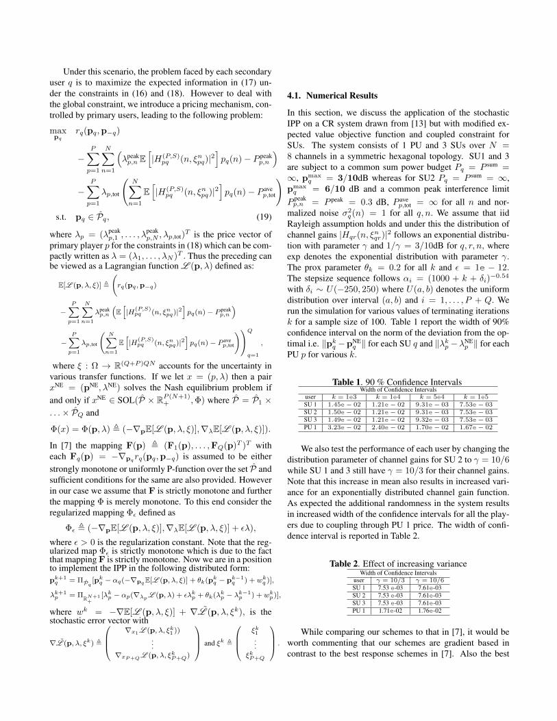
4.1. Numerical Results

In this section, we discuss the application of the stochasticIPP on a CR system drawn from [13] but with modified ex-pected value objective function and coupled constraint forSUs. The system consists of 1 PU and 3 SUs over N =8 channels in a symmetric hexagonal topology. SU1 and 3are subject to a common sum power budget Pq = P sum =∞, pmax

q = 3/10dB whereas for SU2 Pq = P sum = ∞,pmaxq = 6/10 dB and a common peak interference limitP peakp,n = P peak = 0.3 dB, P ave

p,tot = ∞ for all n and nor-malized noise σ2

q (n) = 1 for all q, n. We assume that iidRayleigh assumption holds and under this the distribution ofchannel gains |Hqr(n, ξ

nqr)|2 follows an exponential distribu-

tion with parameter γ and 1/γ = 3/10dB for q, r, n, whereexp denotes the exponential distribution with parameter γ.The prox parameter θk = 0.2 for all k and ε = 1e − 12.The stepsize sequence follows αi = (1000 + k + δi)

−0.54

with δi ∼ U(−250, 250) where U(a, b) denotes the uniformdistribution over interval (a, b) and i = 1, . . . , P + Q. Werun the simulation for various values of terminating iterationsk for a sample size of 100. Table 1 report the width of 90%confidence interval on the norm of the deviation from the op-timal i.e. ‖pkq −pNE

q ‖ for each SU q and ‖λkp −λNEp ‖ for each

PU p for various k.

Table 1. 90 % Confidence IntervalsWidth of Confidence Intervals

user k = 1e3 k = 1e4 k = 5e4 k = 1e5SU 1 1.45e− 02 1.21e− 02 9.31e− 03 7.53e− 03SU 2 1.50e− 02 1.21e− 02 9.31e− 03 7.53e− 03SU 3 1.49e− 02 1.21e− 02 9.32e− 03 7.53e− 03PU 1 3.23e− 02 2.40e− 02 1.70e− 02 1.67e− 02

We also test the performance of each user by changing thedistribution parameter of channel gains for SU 2 to γ = 10/6while SU 1 and 3 still have γ = 10/3 for their channel gains.Note that this increase in mean also results in increased vari-ance for an exponentially distributed channel gain function.As expected the additional randomness in the system resultsin increased width of the confidence intervals for all the play-ers due to coupling through PU 1 price. The width of confi-dence interval is reported in Table 2.

Table 2. Effect of increasing varianceWidth of Confidence Intervals

user γ = 10/3 γ = 10/6SU 1 7.53 e-03 7.61e-03SU 2 7.53 e-03 7.61e-03SU 3 7.53 e-03 7.61e-03PU 1 1.71e-02 1.76e-02

While comparing our schemes to that in [7], it would beworth commenting that our schemes are gradient based incontrast to the best response schemes in [7]. Also the best

response scheme relies on an explicit form for best responseand thus difficult to implement in a stochastic regime.

5. CONCLUDING REMARKS

This paper is motivated by the need to compute equilib-ria arising in cognitive radio systems in uncertain regimes.Specifically, such systems lead to stochastic Nash gamesin which the mappings do not display a desirable strongmonotonicity property. Past work by Jiang and Xu [4] con-sidered how stochastic approximation procedures can addressstochastic variational inequalities when the mappings werestrongly monotone. Yet, these schemes cannot easily con-tend with weaker requirements (such as strict monotonicity)while retaining the single-timescale structure. Instead, a sim-ple regularization-based extension leads to a two timescalemethod, that is generally harder to implement in networkedsettings.

Accordingly, in this paper we develop a single-timescaleproximal point methods in which the centering term is up-dated at every iterate and provide almost-sure convergence ofthe resulting scheme. We analyze this method under commonand different steplengths across players and implement the al-gorithm on a Nash equilibrium problem arising in the designof cognitive radio with temperature interference constraintswhen the players utility have strictly monotone gradient maps.

6. REFERENCES

[1] M. Bloem, T. Alpcan, and T. Basar, A stackelberggame for power control and channel allocation in cog-nitive radio networks, ValueTools ’07: Proceedings ofthe 2nd international conference on Performance eval-uation methodologies and tools (ICST, Brussels, Bel-gium, Belgium), ICST (Institute for Computer Sciences,Social-Informatics and Telecommunications Engineer-ing), 2007, pp. 1–9.

[2] Y. Ermoliev, Stochastic programming methods, Nauka,Moscow, 1976.

[3] F. Facchinei and J.-S. Pang, Finite-Dimensional Varia-tional Inequalities and Complementarity Problems, vol.1 and 2, Springer-Verlag Inc., New York, 2003.

[4] H. Jiang and H. Xu, Stochastic approximation ap-proaches to the stochastic variational inequality prob-lem, IEEE Transactions on Automatic Control, 53(2008), no. 6, 1462–1475.

[5] P-H. Lin, S-C. Lin, and H-J. Su, Cognitive radiowith partial channel state information at the transmit-ter, IEEE International Conference on Communications,2008, pp. 1065–1071.

[6] B. Martinet, Regularisation d’inequations variation-nelles par approximations successives, Rev. FrancaiseInformat. Recherche Operationnelle 4 (1970), no. Ser.R-3, 154–158. MR 0298899 (45 #7948)

[7] J-S. Pang, G. Scutari, D.P. Palomar, and F. Facchinei,Design of cognitive radio systems under Temperature-Interference constraints: A variational inequality ap-proach, IEEE Transactions on Signal Processing, 58(2010), no. 6, 3251–3271.

[8] B.T. Polyak, Introduction to optimisation, OptimizationSoftware, Inc., New York, 1987.

[9] H. Robbins and S. Monro, A stochastic approxima-tion method, The Annals of Mathematical Statistics 22(1951), no. 3, 400–407.

[10] R.T. Rockafellar, Augmented lagrangians and applica-tions of the proximal point algorithm in convex program-ming, Mathematics of Operations Research 1 (1976),no. 2, 97–116.

[11] A.N. Tikhonov, On the solution of incorrectly put prob-lems and the regularisation method, Outlines Joint Sym-pos. Partial Differential Equations (Novosibirsk, 1963),Acad. Sci. USSR Siberian Branch, Moscow, 1963,pp. 261–265. MR MR0211218 (35 #2100)

[12] J. Wang and D.P. Palomar, Worst-Case robust MIMOtransmission with imperfect channel knowledge, IEEETransactions on Signal Processing, 57 (2009), no. 8,3086–3100.

[13] J. Wang, G. Scutari, and D.P. Palomar, Robust cognitiveradio via game theory, 2010 IEEE International Sympo-sium on Information Theory Proceedings (ISIT), 2010,pp. 2073–2077.