arX

iv:a

stro

-ph/

0404

416v

1 2

1 A

pr 2

004

Accepted, ApJ 10 August 2004Preprint typeset using LATEX style emulateapj v. 6/22/04

THE DEEP LENS SURVEY TRANSIENT SEARCH I : SHORT TIMESCALE AND ASTROMETRICVARIABILITY

A.C. Becker1,2,3, D.M. Wittman1,4, P.C. Boeshaar4,5, A. Clocchiatti6, I.P. Dell’Antonio7, D.A. Frail8,J. Halpern9, V.E. Margoniner1,4, D. Norman10, J.A. Tyson1,4, R.A. Schommer†

Accepted, ApJ 10 August 2004

ABSTRACT

We report on the methodology and first results from the Deep Lens Survey (DLS) transient search.We utilize image subtraction on survey data to yield all sources of optical variability down to 24th

magnitude. Images are analyzed immediately after acquisition, at the telescope and in near–realtime, to allow for followup in the case of time–critical events. All classes of transients are posted tothe web upon detection. Our observing strategy allows sensitivity to variability over several decadesin timescale. The DLS is the first survey to classify and report all types of photometric and as-trometric variability detected, including solar system objects, variable stars, supernovae, and shorttimescale phenomena. Three unusual optical transient events were detected, flaring on thousand–second timescales. All three events were seen in the B passband, suggesting blue color indices for thephenomena. One event (OT 20020115) is determined to be from a flaring Galactic dwarf star of spec-

tral type dM4. From the remaining two events, we find an overall rate of η = 1.4 events deg−2 day−1

on thousand–second timescales, with a 95% confidence limit of η < 4.3. One of these events (OT20010326) originated from a compact precursor in the field of galaxy cluster Abell 1836, and itsnature is uncertain. For the second (OT 20030305) we find strong evidence for an extended extra-galactic host. A dearth of such events in the R passband yields an upper 95% confidence limit on shorttimescale astronomical variability between 19.5 < MR < 23.4 of ηR < 5.2 events deg−2 day−1. Wereport also on our ensemble of astrometrically variable objects, as well as an example of photometricvariability with an undetected precursor.Subject headings: gamma rays: bursts — minor planets, asteroids — stars: variables: other — super-

novae: general — surveys

1. OPTICAL ASTRONOMICAL VARIABILITY

Characterization of the variable optical sky is one ofthe new observational frontiers in astrophysics, with vastregions of parameter space remaining unexplored. Atthe faint flux levels reached by this optical transientsearch, previous surveys were only able to probe downto timescales of hours. An increase in observational sen-sitivity at short timescale and low peak flux holds the

1 Bell Laboratories, Lucent Technologies, 600 Mountain Avenue,Murray Hill, NJ 07974Email: acbecker,dwittman,tyson,vm21@lucent.com

2 NIS-2, Space and Remote Sciences Group, Los AlamosNational Laboratory, Los Alamos, NM 87545

3 Astronomy Department, University of Washington, Seattle,WA 98195

4 Physics Department, University of California, Davis, CA 95616Email: boeshaar,margoniner,tyson,wittman@physics.ucdavis.edu

5 Drew University, Madison, NJ, 07940Email: pboeshaa@drew.edu

6 Pontificia Universidad Catolica de Chile, Departamento deAstronomia y Astrofisica, Casilla 306, Santiago 22, ChileEmail: aclocchi@astro.puc.cl

7 Physics Department, Brown University, Providence, R.I.02912Email: ian@het.brown.edu

8 National Radio Astronomy Observatory, P.O. Box ’O’,Socorro, NM 87801Email: dfrail@nrao.edu

9 Department of Astronomy, Columbia University, New York,NY, 10025-6601Email: jules@astro.columbia.edu

10 Cerro Tololo Inter–American Observatory, National OpticalAstronomy Observatory, Casilla 603, La Serena, ChileEmail: dnorman@ctio.noao.edu

† Deceased 2001 December 12

promise of detection and characterization of rare, violentevents, as well as new astrophysics.

The detection of transient optical emission providesa window into a range of known astrophysical events,from stellar variability and explosions to the mergers ofcompact stellar remnants. Known types of catastrophicstellar explosions, such as supernovae and gamma–raybursts (GRBs), produce prompt optical transients decay-ing with timescales of hours to months. Some classes ofGRBs result from the explosion of massive stars – thesehypernovae are known to produce bright optical flashesdecaying with hour–long timescales due to emission froma reverse shock plowing into ejecta from the explosion. Inaddition, GRBs produce optical afterglows, decaying onday to week timescales, resulting from jet–like relativis-tic shocks expanding into a circumstellar medium. Evenmore interesting are explosive events yet to be discovered,such as mergers among neutron stars and black holes.These may have little or no high-energy emission, andhence may be discoverable only at longer wavelengths(Li & Paczynski 1998). Finally, there is the opportunityto find rare examples of variability, as well as the poten-tial for discovering new, unanticipated phenomena.

One of the primary science goals of this transientsearch is the rate and distribution of short timescale as-tronomical variability. However, we catalogue and re-port all classes of photometric or astrometric variabilitywith equal consideration. A weakness in many surveyswith targeted science is that serendipitous informationis discarded as background – a counterexample is the

2

wealth of stellar variability information being gleanedfrom microlensing survey data. The DLS survey geom-etry and observation cadence are not optimal for max-imizing the overall number of detected transients (e.g.Nemiroff 2003), being driven instead by weak lensing sci-ence requirements. However, given the current lack ofconstraints at short timescales and to significant depth,the potential remains for the discovery of new types ofastronomical variability.

The search for variability without population bias isone of the primary goals of the Large-aperture SynopticSurvey Telescope (LSST, Tyson 2002). Efforts such asthe DLS transient search are a useful and necessary test-ing ground for the software design and implementationneeded to reduce, in real–time, LSST’s expected dataflow of 20 TB nightly.

2. VARIABILITY SURVEYS

The field of optical variability surveys has been revo-lutionized by the adaption of CCD devices to astronomy,and by Moore’s progression of computing power. Theformer has yielded wide field imaging systems on largeaperture telescopes, and the latter ensures their datacan be reduced in quick order, if not real–time. Suchadvances have lead to modern variability surveys char-acterized by successively more extreme combinations ofdepth, cadence, and sky coverage.

The advent of microlensing surveys advanced by ordersof magnitude the known number of variable objects, driv-ing the forefront of wide–field (0.1–1 deg2) imaging onmeter–class telescopes (e.g. EROS: Afonso et al. 2003;MACHO: Alcock et al. 2000b; MEGA: Alves et al. 2003;MOA: Sumi et al. 2003; OGLE I,II,III: Wozniak et al.2001; POINT-AGAPE: Paulin-Henriksson et al. 2003;SuperMACHO: Rest et al. 2004). The cadences are typ-ically of order 1 image per day per field, although vari-ous strategies have been employed for sensitivity to shortevents or fine structure in longer events. Such surveys aretraditionally directed at crowded systems of stars servingto backlight a foreground microlensing population. Thisstellar background, however, also serves as a foregroundthat obfuscates sources at cosmological distances.

Surveys for supernovae at cosmological distances avoidsuch crowded foregrounds, employing similar resourcesand attaining similar sky coverage, but reaching deeperthan the microlensing searches (e.g. High-z: Tonry et al.2003; SCP: Knop et al. 2003). The original surveys’cadence of field reacquisition was typically of order amonth, short enough to avoid confusion by active galacticnuclei but long enough to ensure a handful of new super-nova per observing run. These surveys were designedonly for event discovery, with subsequent lightcurve cov-erage provided by narrower field followup resources.Given the successes of the original supernovae surveys,subsequent efforts have been allocated resources for anadvanced observing cadence allowing both detection andself–followup, such as the IfA Deep (Barris et al. 2003)and ESSENCE (Smith et al. 2002b) supernova surveys.The Nearby Supernova Factory is expecting ∼ 100 typeIa supernova per year from their moderate aperture(1.2–meter) telescope and large (9 deg2) field of view(Aldering et al. 2002). However, dedicated systems witha small field of view (0.01 deg2), similar depth, and a ca-dence of several days can lead to a wealth of supernova

detections (e.g. LOSS: Filippenko et al. 2001).Asteroid and Near Earth Object (NEO) searches

cover of order thousands of degrees per night, primar-ily in the ecliptic, and near opposition (e.g. LONEOS:Howell et al. 1996; LINEAR: Stokes et al. 2000; NEAT:Pravdo et al. 1999). Their photometric depths are shal-lower than supernova surveys and the cadence morerapid, given the requirement of recovering objects in mo-tion. The images are typically of poorer seeing and imagesampling, given less stringent photometric requirements.

Truly wide–field systems (10 to 100 deg2) incorpo-rating small apertures and limiting survey depths of12–17th magnitudes are able to cover the entirety ofthe sky in a given night, or a given large regionof sky multiple instances per night (e.g. GROSCE:Akerlof et al. 1993; ROTSE-III: Akerlof et al. 2003;RAPTOR: Vestrand et al. 2002; ASAS-3: Pojmanski2001). Such systems are optimized for the detection andfollowup of fast optical transients, such as optical coun-terparts to GRBs. These systems compromise Nyquistsampling of the point spread function (PSF) and pho-tometric depth for breadth and real–time agility. RAP-TOR’s advanced implementation includes a narrow–fieldfovea to optimally study localized transients. The North-ern Sky Variability Survey (NSVS: Wozniak et al. 2004)makes use of ROTSE-I survey data, which sampled theentire local sky up to twice nightly and provides variabil-ity information on ∼ 14 million objects between 8–15.5th

magnitudes.Additional variability surveys include the QUEST RR

Lyrae survey (Vivas et al. 2001), which is to cover 700deg2 to V = 21st magnitude in the Galactic equator, withsensitivity to several timescales of variability. The SloanDigital Sky Survey has a sequence of multi–color tempo-ral information for over 700 deg2 at multiple timescales(Ivezic et al. 2003). The Palomar-Quest synoptic skysurvey drift–scans 500 deg2 per night, with scans sepa-rated by time baselines of days to months (Mahabal et al.2003). The Deep Ecliptic Survey monitors 13 deg2 pernight near the ecliptic in a search for Kuiper Belt Objects(KBOs), using 4–meter telescopes and 2 exposures sepa-rated by 2–3 hours and a third within a day (Millis et al.2002). Finally, the Faint Sky Variability Survey (FSVS:Groot et al. 2003) is a study of overall optical and as-trometric variability at faint magnitudes on a 2.5–metertelescope. Point source limiting magnitudes reach to 25over a field of ∼ 0.1 deg2, and the cadence of field reacqui-sitions is staggered for sensitivity at several timescales,and thus to multiple phenomena. Of all on–going vari-ability surveys, the FSVS is most similar to the DLStransient search.

3. THE DEEP LENS SURVEY

The Deep Lens Survey (DLS) is a 5–year NOAO surveyoperating on the 4–meter Blanco and Mayall telescopes+ MOSAIC imagers at the Cerro Tololo and Kitt Peakobservatories, respectively (Wittman et al. 2002). Thesurvey is undertaking very deep multicolor imaging offive 2 × 2 fields chosen at high Galactic latitude, andcomposed of 9 subfields apiece. Exposure times and fil-ters are chosen to reach limiting magnitudes of B, V, R, z′

to 29/29/29/28 mag per square arcsecond surface bright-ness, with images typically acquired near new moon. Atthese limiting magnitudes, we expect to measure ac-

3

curately the shapes and color–redshifts of ∼ 100, 000galaxies per square degree for weak lensing science. Anoverview of the survey and public data releases are avail-able at http://dls.bell-labs.com/. The survey is ex-pected to conclude observations in March, 2005.

Full exposure depth requires 20 exposures per pass-band in each of our 45 subfields. The images are ob-tained, with some exceptions, in sets of 5–pointing dithersequences, with offsets of 100′′ and 200′′ around the ini-tial central pointing to fill gaps between MOSAIC chipsand enable super–sky–flat construction. Typical expo-sure times are 600 seconds in B, V , and z′, and 900 sec-onds in R, yielding limiting magnitudes per exposure forpoint sources of approximately 24. The weak lensing sci-ence goals of the survey require co–adding these images.In the co–addition process, however, variable sources areclipped out, or averaged away. Here we pursue an or-thogonal approach, which instead analyzes differences inthese data, at the pixel level, to extract this variability.This paper summarizes our transient search to date.

4. DLS TRANSIENT SEARCH

Starting in December 1999, we began analysis of ouracquired images in near–real time, which we define aswithin the duration of a dither sequence of observa-tions. True real–time reductions ideally occur within thetimescale it takes to acquire the subsequent observation,or, given a target population of events, shorter than thetimescale of the variability being searched for. Recog-nizing variability in near–real time with current CCDmosaics requires data analysis of several GB nightly ofimages on–site. To this end, we maintain computers inthe control rooms of both the Kitt Peak and Cerro–Tololo 4–meter telescopes. At Kitt Peak, we have aquad–processor 700 MHz machine, and at Cerro–Tololoa quad–processor 550 MHz machine. Both systems rununder the Linux operating environment, and execute thecustom data reduction pipeline described in Section 4.2.

The ensemble of Deep Lens Survey images consideredfor this publication was taken from 14 observing runs be-tween 2002 November and 2003 April where the transientpipeline was operating efficiently. Figure 1 displays thedistribution (dotted line) of temporal intervals betweensubfield reacquisitions, integrated over all subfields. Thesolid line shows this same quantity, but only for reac-quisitions in the same filter as the previous observation.Since variability is detected through comparison of ob-servations taken in similar filters, the integral under thissolid subfield–filter histogram up to timescale τ definesour overall sensitivity to transients at timescale τ . Theintegral under the dotted histogram represents our fol-lowup capability at a given τ .

Figure 1 indicates our primary sensitivity is to vari-ability on thousand–second timescales. In this subset wehave a total integrated exposure time of 10.2 days dis-tributed over 425 B–band, 464 V –band, and 393 R–bandimages. At 0.6 × 0.6 per image, this yields a total ex-posure E of 3.7 deg2–days for sensitivity to 103 secondevents down to 24th magnitude. We have a factor of17 smaller E for inter–night observation intervals at 105

seconds, and also at inter–month observation intervals at106 seconds. A planned re–analysis of all survey data fortransients will allow for a precise determination of E atall available timescales.

4.1. Pre–pipeline Image Calibration

Our typical subfield observation comes as a 5–image dither pattern controlled using the IRAF12 scriptmosdither. Standardized information is written in eachof the images’ FITS headers, and is used in the pipelineto automatically associate each quintuple of images.

Basic image calibration is done before each imageis sent to the transient pipeline. The IRAF taskmscred.ccdproc is used to correct for cross–talk, applyoverscan correction and trim the image, and bias andflat–field correct the images (we generally take calibra-tion sequences in the afternoon to allow for real–timereductions). In the case of z′–band data, we need toapply a fringing correction, requiring an accumulation ofimages that generally precludes real–time reductions. Fi-nally, the images are registered to the World CoordinateSystem (WCS) on the sky using mscred.msccmatchwiththe NOAO:USNO-A2 (Monet et al. 1998) catalog. Theimages are then copied to a directory that is continuouslysearched by the transient pipeline image reaper.

4.2. Automatic Pipeline

Our transient pipeline uses the OPUS environment(Rose et al. 1995) as a backbone sequencing a series ofPython and Perl language scripts, each defining a “stage”in our pipeline. These stages are defined as follows:

• IN : copy an image via the SCP protocol from theIRAF reduction machine to the transient pipelinemachine.

• RI : register and pixel–wise resample an incomingimage to a fiducial template image of the subfield.WCS information is used as a starting point fordetermining the registration coefficients. The as-trometric template is the same for all passbands,and is constructed from the very first observationof a subfield.

• CI : detect and catalog objects in the registeredimage using SExtractor (Bertin & Arnouts 1996).For our detection thresholds, we use SExtractorparameters DETECT THRESH = ANALYSIS THRESH =2.5.

• HI : difference each dither against the first point-ing, using a modified version of the Alard (2000)algorithm. Modifications include internal methodsto register and remap pixels based upon WCS in-formation, comprehensive discrimination of appro-priate regions to determine the image convolutionkernel, figures of merit to determine the directionof convolution, robust methods to ensure completespatial constraint on the variation of the kernel,and the propagation of noise through the convolu-tion process

• FI : catalog the difference image and filter objectdetections, including the calculation of adaptivesecond moments (Bernstein & Jarvis 2002). These

12 IRAF is distributed by the National Optical Astronomy Ob-servatories, which are operated by the Association of Universitiesfor Research in Astronomy, Inc., under cooperative agreement withthe National Science Foundation.

4

moments, originally designed for accurate shapemeasurements in our weak lensing pipeline, areused here to verify the integrity of each candidate.Cuts on the results of this analysis (e.g size criteriafor cosmic ray rejection) help to reject a significantfraction of the noise and false positives, as well as afraction of the actual transients present. This stageyields the short–timescale transients in each dithersequence, primarily solar system objects, but alsoincluding stellar and unknown sources of variabil-ity.

To algorithmically cull false detections from ourobject lists, we first construct exclusion zonesaround bright stars, using the NOAO:USNO-A2(Monet et al. 1998) catalog, and along bad CCDcolumns, using bad pixel masks supplied with themscred package. Given a list of candidates SEx-tracted from the difference image, we further ana-lyze each object in both the original input imageand the difference image. In the input image, werequire the object’s semi–minor axis, as computedfrom adaptive second moments, to be greater than1 pixel (0.27′′) as a cut against cosmic rays. Inthe difference image, we further require second mo-ments greater than 0.9 pixels, uncertainties in theorthogonal ellipticity components less than 0.5 pix-els, and integrated flux measurements greater than0 counts. We also examine all pixels within 20 pix-els of a candidate, and require 50% of all pixels tobe neither negative nor masked, and 70% of non–masked pixels to be positive valued. These addi-tional cuts safeguard against bad registrations orsubtractions, which tend to leave a number of con-tiguous pixels above the detection threshold, butalso regions of systematic dipole residuals. Thisdoes impact our efficiencies for slowly moving ob-jects such as KBOs. By correctly propagating noisearrays through the remapping and difference imag-ing process, it is possible to compare projectednoise properties of the image to empirical measure-ments, and automatically identify and reject suchregions.

At this point, the individual images are co–added tomake a deeper representation of the subfield and searchedfor longer timescale transients :

• SI : co–add the dither sequence of images into asingle deep image of the subfield, providing com-plete spatial coverage by filling in MOSAIC chipgaps.

• IT : identify prior templates of the same subfield,in the same filter, to use as templates for detectingvariability on longer timescales.

• HS : difference the deep image stack constructed instage SI against the prior templates.

• FS : catalog and filter the deep difference images.Longer timescale transients are revealed at thisstage, primarily supernova and active galactic nu-clei (AGN), and stellar variability. We employ sim-ilar object cuts as in stage FI.

• CL : clean up and archive data files, and inform theobservers that the sequence of observations is readyto be reviewed.

Our automated cuts typically reduce the number ofcandidates per image from several hundreds to severaltens. After the last stage of the pipeline, the observermust manually categorize the remaining candidates. Agraphical user interface displays the sequence of differ-ence images. Each is presented as a triplet of postagestamps centered on the candidate and showing the priortemplate, current image, and difference between them.The nature of the transient is determined using a vari-ety of factors, which can be divided into temporal andcontextual information. Temporal discriminants includeastrometric motion of the transient, indicative of solarsystem origin, as well as the timescale of photometricvariability for stationary objects, which can help dis-criminate between populations of variability with knowntimescales, or to single out an object varying with un-expected rapidity. Contextual discriminants include theexistence of a precursor or host object, and the proximityand relative location of the transient event.

During visual classification of a transient, a set of datafiles are automatically generated locally on disk, aftercross–checking for spatial coincidence with previous tran-sients, or proximity to approximate ephemerides for mov-ing objects. An ephemeris is generated for moving ob-jects, and for stationary objects, a finding chart. Thesefiles are copied to our remote web server where a peri-odic daemon executes a command to regenerate our webpage based upon the data files present. Thus, every 15minutes our web page is brought into sync with the tran-sients detected at the telescope. At the conclusion of eachrun, all moving objects are reported to the Minor PlanetCenter13 and the most convincing supernova candidatesto the Central Bureau for Astronomical Telegrams14.

The magnitudes resulting from photometry on differ-ence images are denoted by the symbol M. This rep-resents the magnitude of a static object whose bright-ness is equal to the measured change in flux ∆f , M ≡−2.5 log (∆f) + m0, where m0 is the photometric zero–point of the template image. This quantity can be re-lated to the change in magnitude ∆M of an object withquiescent magnitude M through the relation

∆M = −2.5 log(

10(M−M)

2.5 + 1)

. (1)

In the limit where the variability comes from a precursorfainter than the detection limit, such as for supernovae,then M represents the magnitude of the transient itself.In the following, we report all magnitudes derived fromdifference imaging in units of M.

We are further pursuing algorithms that might auto-matically and optimally discriminate between transientclasses, which will be a necessity for larger scale transientsearches. One such example is the GENetic Imagery Ex-ploration software package (GENIE: Perkins et al. 2000).GENIE uses genetic algorithms to assemble a sequenceof image operators that optimally extract features frommulti–spectral data, and might be naturally be appliedinstead to our multi–temporal sequences.

13 http://cfa-www.harvard.edu/iau/mpc.html14 http://cfa-www.harvard.edu/iau/cbat.html

5

All archived transients are made available on the inter-net at http://dls.bell-labs.com/transients.html,generally within a few hours of observations. Transientsare broadly categorized as “moving” (slow or fast objectsare highlighted), “variable star”, “supernova”, “agn orsupernova” (if this cannot be distinguished based on thehost morphology and transient location), or “unknown”,a broad category indicating objects whose astrophysicalnature is uncertain. This includes very rapidly varyingobjects, or transients with no obvious precursor or host.

5. ASTROMETRICALLY VARIABLE OBJECTS

Roughly 75% of the transients detected in the DLSare astrometrically variable solar system objects. Fourof the five DLS fields are within 15 of the ecliptic, andin these fields we generally find of order ten moving ob-jects per subfield visit. The total number of moving ob-jects detected through spring 2003 is 3651, with 900 de-tected in B, 1508 detected in V , and 1487 detected in R(some were detected in multiple filters). Our detectionefficiency for moving objects has not been modeled.

Because of our observing pattern, most of the movingobjects are observed on a single night and never recov-ered. A main belt asteroid moving at ∼30′′ hr−1 nearopposition leaves a subfield within a few days. As a re-sult, only about one-third of our moving objects havebeen observed on multiple nights, and 333 of these havereceived Minor Planet Center provisional designations,which are listed on our website. Similarly, we are ableto measure colors for only a fairly small fraction of theseobjects. Therefore, we do not attempt a thorough anal-ysis of orbital parameters, albedos, and sizes. Rather,we give an overview of the dataset and then detail a fewespecially interesting objects.

Figure 2 shows the magnitude distribution of all mov-ing objects discovered, separately for B, V , and R. Notethat the magnitude range is displaced from the magni-tude range in which our efficiency for stationary pointsources is nonzero (Figure 12). This is because the vastmajority of moving objects are significantly trailed dur-ing our 600 or 900 second exposures. An asteroid at thebright end can therefore be much brighter than a pointsource before saturation sets in, and at the faint end mustalso be brighter to rise above the detection threshold.

Figure 3 shows the moving objects’ velocity distribu-tion in ecliptic coordinates, highlighting a pair of KuiperBelt objects (KBOs) detailed below. Figure 4 providestentative classifications into asteroid families (main belt,Trojans, Centaurs, NEOs, etc.) based upon ecliptic ve-locities, adopting the boundaries of Ivezic et al. (2001).

5.1. Kuiper Belt Objects

The 2003 April CTIO run yielded two Kuiper Belt Ob-jects (KBOs). Our pipeline does not include an orbit cal-culator, so KBOs are not automatically flagged. Thesetwo examples were selected manually on the basis of theirsmall (< 3′′ hr−1) angular motions near opposition.

Transient 207 from the 2003 April CTIO run was dis-covered on 2003 April 1 (UT), moving at 2.9′′ hr−1 nearopposition, with a median R magnitude of 21.5. Usingthe method of Bernstein & Khushalani (2000), we finda semimajor axis, a, of 41.0 AU, eccentricity e of 0.022,and inclination i of 20.1, making this a classical KBO.Assuming an albedo of 0.1, the diameter of this object

is ∼475 km, making it one of the larger KBOs known.Transient 587 from the same run was discovered on 2003March 31 (UT) at a B magnitude of 23.3, moving at 2.6′′

hr−1, also near opposition. Our orbit calculation yieldsa = 42.8, e = 0.178, and i = 1.1, making it a likelyscattered KBO. For an albedo of 0.1, this object is ∼410km in diameter. Our observations provide orbital arcs of5 and 4 days for these KBOs, respectively.

5.2. Near-Earth Objects

The detection efficiency for fast movers declines withvelocity, as their reflected light is trailed over larger area.The DLS, with its long exposures, is therefore far fromoptimal for detecting Near-Earth Objects (NEOs). Nev-ertheless, we have detected a sizable sample, as shown inFigure 4. Here we highlight one that was moving withan unusual velocity, Transient 1363 from the 2003 MarchKPNO run. This object is the fastest solar system objectseen during the transient search, moving at 80′′ hr−1.The box near the top of Figure 4 indicates this object’sremote position in the ecliptic velocity diagram.

6. PHOTOMETRICALLY VARIABLE OBJECTS

We focus here on those transients that have beennoted to flare on thousand second timescales and aredetected in at least two images, as well as on longer–term variability with no detectable originating host orprecursor. However, our transient catalog also includesa selection of several hundred variable stars, as well asover 100 supernova candidates, 18 of which pass therequirements for recognition as defined by the CentralBureau for Astronomical Telegrams. These include :2000bj (Kirkman et al. 2000), 2000fq (Wittman et al.2000), 2002aj, 2002ak, 2002al, 2002am (Becker et al.2002c), 2002ax, 2002ay, 2002az, 2002ba, 2002bb, 2002bc,2002bd, 2002be (Becker et al. 2002a), 2003bx, 2003by,2003bz, 2003ca (Becker et al. 2003).

6.1. Image Calibration

We have re–run the difference imaging algorithm forthis paper, using 2k x 2k (8.6′ x 8.6′) arrays centeredon the selected optical transients (OTs). We have gen-erally been able to construct deeper, higher signal–to–noise (S/N) template images than those available to usat the time of detection. For photometric calibration,we need only calibrate the zero points of these tem-plate images, as the difference imaging convolution nor-malizes each input image to the template’s photometricscale. The B, V , and R templates are normalized to theLandolt (1992) system, with additional errors (typically5%) added in quadrature to account for instrumental dif-ferences between the KPNO, CTIO, and Landolt (1992)systems. All z′ templates are initially calibrated to theSmith et al. (2002a) AB system, and presented here inthe Vega system by adopting an offset of 0.54 magni-tudes (z′V ega = z′AB − 0.54). The transformation be-tween photometric systems depends on the instrumentalfilter response and on Vega’s spectral energy distribution,adding an additional 0.08 magnitude uncertainty to ourz′ = z′V ega measurements.

The template brightnesses of the precursor, or host,objects were determined using MAG BEST from SExtrac-tor (Bertin & Arnouts 1996), except in the case of

6

OT 20010326 (Section 6.3.1 below). For this precur-sor, which appears unresolved, we first used the IRAFnoao.digiphot.daophot.psf package to determine thelocal PSF from nearby isolated stars, and subtractedthese stars and the transient precursor from the imageusing noao.digiphot.daophot.allstar.

For those template images where we are not able to de-tect the OT precursor/host, we define the point sourcedetection limit in accordance with the NOAO Archivedefinition of photometric depth (T. Lauer, private com-munication), as

ml = m0 − 2.5 log(1.2 W σsky n), (2)

where m0 is the magnitude of one ADU, W is the seeingin pixels, σsky is the dispersion of the image around itsmodal sky value, and we choose n = 3 σ as our detectionlimit. We determine detection limits in the differenceimages by measuring directly our ability to recover inputstellar PSFs.

For the difference imaging, we choose the best–fit con-volution kernel that varies spatially to order one acrossour 2k x 2k subimage, and a sky background with asimilar degree of variation. We fit these spatial vari-ations over a 20 x 20 grid, using a convolution kernelwith a half–width of 10 pixels. The function of the con-volution kernel is to degrade the higher quality imageto match the PSF of the lesser quality image. Objectsare detected in each grid element to constrain locallythe convolution kernel through a pixel–by–pixel compar-ison between images. A global fit is next performed,using each element as a constraint on spatial variationof the kernel. Several sigma–clipping iterations ensurethat sources of variability, such as variable stars or as-teroids, are not used as constraints for this kernel. If suchan element is rejected from the global fit, a replacementobject within this element is chosen to ensure maximalspatial constraint. Application of the final convolutionkernel to the entire image and pixel–by–pixel subtrac-tion yields the difference between the two images, witha resulting point spread function of the lesser qualityimage, and photometric normalization to the templateimage. The transient fluxes were determined using theIRAF noao.digiphot.apphot.phot package. The rel-ative transient magnitudes are typically determined tobetter than ∼ 4%, with the remaining uncertainty dueto absolute calibration of the template zero–point.

6.2. Optical Transients Without Hosts

We have detected several optical transients with no ob-vious hosts, and which are seen to vary over the timescaleof months (e.g. Becker 2003a), similar to supernovaeand GRB afterglows. One of the more luminous exam-ples of this class of objects is OT 20020112 (Becker et al.2002b), originally reported as Transient 139 from our2002 January run 15. Information on this event is sum-marized in Table 1, including the DLS subfield in whichit was detected (F4p13), and position on the sky in J2000coordinates. We include limits on a precursor or host forthis event, which is not detected to deeper than 27th mag-nitudes in the B, V , and R passbands, and ∼ 25th magni-tude in z′. Table 1 also lists limits on the precursor/hostbrightness after taking into account Galactic reddening,

15 http://dls.bell-labs.com/transients/Jan-2002/trans139.html

assuming a RV = 3.1 extinction curve (Schlegel et al.1998).

OT 20020112 was detected in observations taken 2002January 12. Previous subfield observations were taken2001 March 27, so the age of the transient at detec-tion is poorly constrained. Information on this tran-sient was quickly posted to the Variable Star NETwork(VSNET16), prompting a sequence of followup observa-tions from the 1.3m McGraw–Hill telescope (MDM). Thelightcurve for this transient is shown in Figure 5, andrepresents a daily averaged lightcurve of all observationsfrom the DLS and MDM. The event was re–imaged 35days after detection as part of DLS survey observations,and had faded and reddened significantly. Detailed pho-tometry for this event is listed in Table 2. The mag-nitudes listed are in differential flux magnitudes M –however, given the non–detection of a precursor or host,this also represents the traditional magnitude M of thistransient.

OT 20020112 was also observed spectroscopically withthe Las Campanas Observatory 6.5-m Baade telescope(+ dual imager/spectrograph LDSS2) on 2002 January18. The spectrum in Figure 6 is characterized by a bluecontinuum with no obvious broad features, and marginalevidence for emission lines Hα at z = 0.038 and [NII]6583 at z = 0.039. The continuum features and lackof short timescale variability are consistent with a TypeII SN caught close to maximum brightness. However atz = 0.038, the observed brightness (V ∼ B ∼ 22.1) is3 magnitudes dimmer than a typical Type II SN nearmaximum. The blue continuum makes a reddened SNexplanation unlikely. Examination of the FIRST 1.4 GHzradio catalog (White et al. 1997) yields a limit of 0.94mJy/beam at this position, with no object closer than2.4′. A search of the ROSAT source catalog (Voges et al.2000), and a more comprehensive search of archival X–ray and gamma–ray data through HEASARC17 yields noarchival sources within 10′.

Thus the nature of this object remains unknown, a sit-uation compounded by the lack of an obvious host galaxyto R > 27.6. We note the observed B − V color changeduring the event is inconsistent with a spectral energydistribution of the form Fν ∝ νβ , such as that expectedfor GRB afterglows (e.g. Sari et al. 1998, Nakar et al.2002). However, evolution of the index β could lead tothe observed behavior. Future OT searches will requirefacilities dedicated to followup of such events, to asso-ciate or distinguish them from the expected supernovaand GRB afterglow populations.

6.3. Rapid Variability Optical Transients

Over the course of the survey we have also detectedthree optical transients on thousand–second timescalesthat were present in multiple images, and whose pre-cursors were not immediately recognized as stellar in allavailable passbands. In all cases, we were able to identifya precursor or host object after the fact. These are des-ignated OT 20010326, OT 20020115, and OT 20030305.

16 http://vsnet.kusastro.kyoto-u.ac.jp/vsnet/index.html17 A service of the Laboratory for High Energy Astrophysics

(LHEA) at NASA/ GSFC and the High Energy AstrophysicsDivision of the Smithsonian Astrophysical Observatory (SAO),http://heasarc.gsfc.nasa.gov/db-perl/W3Browse/w3browse.pl

7

Table 1 lists the observed characteristics of the precur-sors or hosts for these transients in their quiescent state.Table 1 also includes magnitudes corrected for Galacticreddening for OT 20010326 and OT 20030305, in the casethat they lie outside the Galactic dust layer.

When putting our subsequent results in a cosmolog-ical context, we assume a WMAP cosmology of H0 =71, ΩM = 0.27, ΩΛ = 0.73 (Spergel et al. 2003).

6.3.1. OT 20010326 : Mar 2001, Transient 52

OT 20010326 was detected 2001 March 26.2 as the 52nd

transient during that particular run 18. Photometry forthis event lightcurve, including the constraining obser-vations immediately preceding and following the event,is listed in Table 2. After verification, an alert was dis-persed via e–mail on Mar 26.4 requesting immediate fol-lowup observations.

The event lightcurve is shown in Figure 7, and is char-acterized by a null detection in B, followed by a B–bandpeak and immediate fall–off. Given the range of allowedturn–on times, from 100s before the start of the detec-tion observation (to account for read–out time betweenimages) to 1s before the shutter closes in the detectionimage, we can limit a power–law index for the flux decayf ∝ t−α of 0.80 < α < 1.2.

Radio observations of this OT were undertaken at theVLA on 2001 March 30. Limits on radio flux at 8.5 GHzare −0.1±0.3 mJy. Subsequent observations of the eventrevealed a host galaxy or precursor object visible in theV , R, and z′ passbands, and a limit of B > 26.4.

This event occurred in the field of galaxy cluster Abell1836, at a redshift of z = 0.037. Figure 7 also shows an8.6′ x 8.6′ R–band template image centered on the tran-sient event. The precursor/host is displayed at higherresolution in the upper–right corner as the dim object3.5′′ north–west of the brighter star. A single archivalHST image of cluster galaxy PKS 1358-11 also covers thelocation of the observed transient. This 500s integrationin the F606W filter was obtained Jan 25, 1995 as partof a nearby AGN survey by Malkan et al. (1998). Theprecursor appears unresolved in this image. We comparethis precursor position with the location of two back-ground galaxies, and over a baseline of 7.0 years findproper motion limits of 0.004 ± 0.004′′yr−1.

It is particularly difficult to photometer and calibratethis OT precursor/host, as it occurs 3.5′′ from a brightstar that is saturated, or nearly so, in all of our images.There is also a very strong background gradient from thenearby elliptical galaxy PKS 1358-11 and spiral galaxyLCRS B135905.8-112006. If the OT host is a memberof Abell 1836, it lies only 49 kpc in projection from thecore of PKS 1358-11, and 53 kpc in projection from thecenter of LCRS B135905.8-112006. The HST resolutionlimit at the distance of Abell 1836 is around 70 parsecs,which does not immediately preclude a globular clusterhost. However, at a distance modulus of 36.0, the hostabsolute magnitude of MV = −11.7 would be consider-ably brighter than the globular cluster systems in ourown Galaxy (Van Den Bergh 2003). In addition, the ob-served V −R = 1.1 color of the object makes it unlikely tobe an unresolved globular cluster system (K.A.G. Olsen,private communication).

18 http://dls.bell-labs.com/transients/Mar-2001/trans52.html

6.3.2. OT 20020115 : Jan 2002, Transient 337

Our second fast optical transient, OT 20020115, wasinitially reported as Transient 337 from the run ongo-ing 2002 January 15.319. The lightcurve, whose data arepresented in Table 2 and displayed in Figure 8, is verysimilar to that of OT 20010326, including B–band de-tection, but it reaches a brighter MB, and decays muchmore rapidly. The flux decay power–law index α is con-strained to 1.5 ≤ α ≤ 2.4.

This event was quickly reported as a potential GRB op-tical counterpart to the GRB Circular Network (GCN,Becker et al. 2002d). We obtained spectra of the sourcesoon thereafter – Figure 9 shows 3 x 10 minutes of ex-posure on the source with the Magellan 1 telescope +LDSS2 dual image/grism spectrograph, taken 2002 Jan-uary 18.3. The appearance of zero-redshift emissionand absorption features in these spectra are evidencefor Galactic origin, and the GCN alert was amended(Clocchiatti et al. 2002).

Subsequent observations in R and z′ revealed a verybright, red precursor object, consistently saturated in R–band images. We also recover the precursor object in theB and V bands. With a quiescent magnitude of B = 21.3and measured peak MB = 20.7, Equation 1 indicates theprecursor varied by more than 1 magnitude, averagedover the duration of our 600s exposure.

The analysis of the photometric observations and ob-ject spectrum (Figure 9) shows OT 20020115 has thecolors and spectrum of a dM4 post–UV Ceti type flarestar. The spectrum shows the clear presence of late–type M-dwarf spectral indicators: molecular bands ofTiO, CaOH (5530-60A and centered at 6250A), plusCaH at 6385A, in addition to weak Hα and Hβ in emis-sion. With a V magnitude of 19.67 ± 0.05, and colorsB−V = 1.58±0.09 and V − z′ = 3.39±0.10, these dataare consistent with an M dwarf of spectral type dM4, i.e.a late type flare star in the quiescent state. Assuming atypical MV = 12, OT 20020115 would lie at a distanceof approximately 350 pc, and 250 pc above the Galacticplane, well within the scale height for disk population Mdwarfs.

6.3.3. OT 20030305 : Mar 2003, Transient 153

The most dynamic transient, OT 20030305, was de-tected as Transient 153 from our 2003 March run20. Thisis the only event detected in the V –band, and we imme-diately acquired a sequence of B–band observations afterthe V –band series. The event lightcurve is shown in Fig-ure 10. Also displayed are the series of images of thisevent. The top row represents the precursor/host of theevent in its quiescent state, in the R, I, and z′–bands,from left to right. Included in each panel is the magni-tude of this precursor/host in its quiescent state, exceptfor the I band where we have no calibration data. Thisprecursor/host is not visible in B or V , and appears unre-solved in the z′ images but measurably elliptical in bothI and R. The subsequent panels, reading from left toright and top to bottom, show the emergence of the OTin our time series of images, as well as OT magnitudesand time elapsed from the detection observation. All im-ages are separated by approximately 700s except for the

19 http://dls.bell-labs.com/transients/Jan-2002/trans337.html20 http://dls.bell-labs.com/transients/Mar-2003/trans153.html

8

final image, which was obtained more than 2 days afterthe event. The event was also announced via the IAUCirculars (Becker 2003b).

The OT lightcurve shows more complex behavior thanthe previous events, and cannot be described as simplepower–law flux decay. The second temporal peak indi-cates either a second round of brightening or spectralevolution of the flare.

As noted above, the precursor/host object appears re-solved and elliptical in the R and I passbands. Theobject’s position angles in R and I, derived with theadaptive second moment method of Bernstein & Jarvis(2002), agree to within 0.09, indicating an extended ob-ject. We have characterized the expected PSF at thelocation of the host object by first identifying candi-date stars, based on their position in the size–magnitudeplane, in the R–band template image. We then fit forthe spatial variation of the moments of these candidates,clipping at 3σ to reject interloping small galaxies. A χ2

test comparing the shape of the host with the predictedshape of the PSF at its position yields χ2 = 11.4 for 3degrees of freedom, for a confidence level of 99% that apoint source would not have the measured shape of theprecursor object. We consider the above as strong evi-dence for a resolved, extragalactic host for OT 20030305.

6.4. Discussion

A primary discriminant between Galactic stellarevents, such as OT 20020115, and extragalactic eventsis the measured shape of the precursor or host object.OT 20010326 is shown to be unresolved in HST imaging,implying Galactic origin, although potentially originat-ing from a compact extragalactic host. OT 20030305 hasan apparent resolved host that is inconsistent with theR–band PSF interpolated at its position. This arguesstrongly for an extragalactic origin.

It is suggestive that all of our OTs are detected in the Bpassband. We consider various stellar and extragalacticpossibilities for the origin of these events in turn.

6.4.1. Galactic Flare Stars

Since we are certain OT 20020115 is from a flaringdwarf star, we investigate the possibility that one, oreven both, of the other OTs are similar in nature. Weexamine the peak of the disk dwarf luminosity function,which is occupied by dM4 – dM6 (MV = 12 − 16) stars(Reid et al. 1995). This region is occupied by the mostactive UV Ceti–type flare stars, with event timescales oforder minutes and flare B − V colors of approximately0.0 to 0.3 (Kunkel 1975). Gurzadian (1980) further char-acterizes the “Type I” outburst lightcurves expected ofUV Ceti–type stars, with rise times of seconds to a fewminutes, and decay times of minutes to about one hour,qualitatively similar to our observed events.

From Figure 2 of Boeshaar et al. (2003), and Figure 11here, the precursor R − z′ color of OT 20010326 im-plies a spectral type of dM4 were it a flare star. WithB − R > 3.1, this object lies 1σ from the color–definedlocus of disk main sequence stars. However, using a V –band dM4 distance modulus of between 11.5 and 12.5magnitudes, this object would be approximately 2.0–3.2kpc distant, and 1.5–2.4 kpc above the Galactic plane.This instead suggests association with the sdM halo sub-dwarf population, consistent with our proper motion lim-

its. However, these stars are not known to flare. The sit-uation is similar for OT 20030305, which is far too faintat V > 27.1 mag to belong to the disk population. As-suming an R− z′ derived spectral type of approximatelydM6, its distance modulus yields d & 1.7 kpc.

For a typical DLS field at b(II) = 45, we expect tofind approximately 100 – 150 dM4 – dM6 disk stars persubfield out to their Galactic scale height of 350 pcs,which is verified through direct examination of severalsubfields. Since flare events do not follow Poisson statis-tics, and show large scatter in total energy, peak lightand duration, it is difficult to calculate the exact numberexpected in each sequence of B exposures. In addition,selection effects in most previous studies have biased dis-covery towards stars of greatest flare visibility.

Until recently, one of the only ways to estimate theexpected rate of flare star activity was to extrapolateEquation 5 from Kunkel (1973). This relation was de-rived using data for a selected few of the most activeflare stars in the immediate solar neighborhood. Scal-ing Kunkel’s relation to our B passband, and assumingthat 5% of all dM4–6 stars exhibit strong flaring activity(i.e. ∆B of 1 mag or greater), we may place an up-per limit of approximately 0.08 flare events expected persubfield in each 600 sec exposure. Given the extreme se-lection bias in Kunkel’s sample, it is not unexpected todiscover that this estimate (N < 34) is much differentthan what we find (1 ≤ N ≤ 3). We also examine thestellar flare survey data of Fresneau et al. (2001). Utiliz-ing astrographic plates covering 520 deg2 at low Galac-tic latitude to apparent B magnitude of 10–14, they find8% of their stars show flare events of > 0.4 mag over20–30 minutes. If half of these stars are M dwarfs, ofwhich approximately 1% are types dM4–6 based on thevolume of the sample limited by the luminosity of thosespectral types, we expect an upper limit of 0.01 flare of> 0.4 mag per 100 stars in each 600 sec B–band expo-sure. Having analyzed 425 accumulated B–band imagesfor this publication, we expect an upper limit of 6.4 flar-ing events > 0.4 magnitudes. The distribution functionof the amplitudes of flaring events in these stars is notwell known, but in general the brighter flares make up asmaller fraction of the total number of events (Gurzadian1980). Thus the discovery of only one certain flare eventof ∆B > 1 mag is consistent with this upper limit. Giventhe lack of unbiased flare star samples down to our limit-ing magnitudes, a direct comparison with other surveysrequires the analysis of more modern variability datasets(e.g FSVS: Groot et al. 2003).

6.4.2. Active Galactic Nuclei (AGN)

Vanden Berk et al. (2002) have reported a highly lumi-nous OT event from the Sloan Digital Sky Survey, withan underlying host galaxy at z = 0.385. Gal-Yam et al.(2002) have determined, using in part archival opticaland radio data, that the event is likely due to a radio–loud AGN. Heeding the suggestions of Gal-Yam et al.(2002), we search archival data sources for observationsof the fields of OT 20010326 and OT 20030305. We in-clude in these searches the FIRST 1.4 GHz radio cat-alog (White et al. 1997), 1.4 GHz NVSS radio cata-log (Condon et al. 1998), and 4.8 GHz PMN catalogs(Griffith & Wright 1993).

The only survey that covers the field of OT 20010326

9

is the PMN tropical survey, which detects no sourcescloser than 1.7′. In combination with our VLA detec-tion limits 4 days after the event, this argues against aradio variable source. Null detections are also reportedfor OT 20030305 in the FIRST, NVSS, and PMN equa-torial catalogs, with an explicit limit from FIRST of 0.94mJy/beam. Overall, these null detections seem to rejectradio–loud AGN as sources for this variability.

We have also searched the archival X–ray and gamma–ray catalogs through HEASARC, and while OT 20010326returns several matches corresponding to components ofAbell 1836, no matches are found within 2′. A searcharound OT 20030305 finds no matches within 10′. Thisweighs against a variety of accretion scenarios, includingAGN and other Galactic X–ray sources.

6.4.3. Gamma Ray Bursts (GRBs)

There is an expected population of optical transientsassociated with the observed rate of gamma ray bursts.However, the connection between the two event rates isvery uncertain, given the variety of means to draw opticalemission from hydrodynamic evolution of a GRB event.These means include “orphan” GRBs, where a highly col-limated GRB points at large enough angle away from theobserver that gamma ray emission is avoided but opticalafterglow radiation is not (Rhoads 1997); and “dirty”or “failed” fireballs whose ejecta comprise a significantamount of baryons and/or have a small Lorentz factor(≪ 100, e.g. Dermer et al. 1999, Huang et al. 2002).Distinguishing between these possibilities requires fineconstraints on the time decay slope α, radio observations,and/or multiwavelength observations at the time of theso–called GRB “jet break” (Rhoads 2003). Given theour poor temporal resolution, and lack of simultaneousmulti–wavelength coverage, we are not uniquely sensitiveto the micro–physics expected to drive the early evo-lution of GRB lightcurves, and whose resolution mightdistinguish between the above possibilities. Within theresolution and timescale of our observations, all GRBvariants effectively yield the same characteristic isolatedfading object.

The thousand second timescale of the observed eventsis of similar duration to the early lightcurve break ob-served in GRB 021211 (Li et al. 2003). After this break,the power law flux decay index α was seen to decreasefrom 1.8 to 0.8 – before this time, the transient dimmedby more than 2.5 magnitudes. If our already faint,rapidly declining optical transients represent a similarearly phase of gamma–ray dark GRB lightcurves, theirsubsequent evolution would be below our detection limit.

We also note that the spectral energy distribution(SED) of the GRB afterglow component is modeled asa synchrotron emission spectrum (e.g. Sari et al. 1998,Granot et al. 2000). The expected spectral shape scaleslike Fν ∝ ν−β. Thus it is surprising that our distri-bution of B:V :R–detected transients is 2:1:0 (where OT20030305 contributes to both the B and V event rate)if these events are drawn from a population of eventscharacterized by a synchrotron SED.

Recent submillimeter and radio observations of local-ized GRB host galaxies show they are bluer than se-lected galaxies at similar redshifts, indicative of star for-mation or relatively low dust content (e.g. Berger et al.2003, Le Floc’h et al. 2003). Host galaxies for localized

X–ray Flashes (XRFs) also appear to exhibit the samecharacteristics (Bloom et al. 2003). However, our puta-tive hosts are considerably redder than these samples ofGRB or XRF–selected host galaxies, and are unlikelyto be drawn from the same population. The R − z′

colors of our OT hosts are, however, loosely consistentwith the observed population of Extremely Red Objects(EROs), which comprise old or dusty star–forming galax-ies. If EROs represent highly obscured starburst activityat moderate redshift (z ∼ 1), they contribute a signifi-cant fraction of the overall star formation at that epoch(Smail et al. 2002). Assuming our population of OTstraces star formation, we expect some association withEROs. The absence of extremely red GRB host galaxiessuggests detection of GRBs is biased against dusty galax-ies. If our OTs arise from dust enshrouded galaxies, thisbias would seem lesser for optically detected events.

7. EVENT RATE

We map our detection of these objects into a quanti-tative statement describing the rate of short timescaleastrophysical variability. We derive general constraintswithout bias towards a particular OT model.

7.1. Efficiency

To account for inefficiencies in our pipeline, we modelour efficiency E at recovering transients throughout arange in brightness. We calibrate the efficiency via MonteCarlo runs in which we add point source transients. Wedefine an efficiency run as the generation of 32 randomamplitude point sources, with the integrated flux chosenas a uniform deviate in the exponent of f = 101.5≤x≤6,which are placed within a dither sequence of survey data.Positions are randomly selected within the limits of theprimary exposure, and are placed at the same astronom-ical position within each of the subsequent 4 dithers. Wedo not bias our results by assuming a temporal shape forthe variability. Instead, we generate an overall efficiencyfor recovering a given amount of input flux, averaged overthe spatial coverage of our dither sequence.

We include in our analysis B, V , and R–band surveydata (z′–band data are infrequently reduced in real–timedue to fringing complications). We account for varia-tions in observing conditions by choosing 19 night–filter–subfield combinations of survey data to submit for effi-ciency analysis. In total, we initiated 8028 efficiency runsyielding 256896 total efficiency points, approximately85000 per passband. The magnitudes of these transientsare calibrated to the Landolt (1992) system. Image zero–point offsets were calculated from directly calibrated im-ages of each subfield. One subfield was calibrated usingpublicly available NOAO Deep Wide–Field Survey data(Jannuzi & Dey 1999).

After placing additional flux in each image, we passthem through our difference imaging pipeline. The num-ber of input objects recovered is tallied, searching boththe unfiltered and filtered object catalogs generated atthe FI stage in our pipeline. This yields an unfiltereddetection efficiency (dotted histogram in Figure 12) aswell as the efficiency of passing our cuts (solid histogramin Figure 12). The difference between the two histogramsdemonstrates the rejection of true positives in our filter-ing process, yielding an overall decrease in efficiency. Weuse the solid histogram in the subsequent event rate anal-

10

ysis. We note that approximately 3% of our sky coveragelands in gaps between MOSAIC chips, and the ditheringprocedure shifts 10% and 20% of the template images’common sky area off of the subsequent dithers. Thusour maximum possible efficiency is ∼ 82%. Our overallOT detection efficiency of E ∼ 63% indicates our filteringefficiency is ∼ 77%. We expect substantial improvementsin the context of a future automated classification envi-ronment.

Figure 12 shows our efficiency is fairly constant be-tween the saturation limit on the bright end, and ourdetection limits on the faint end. We thus expect littlebias against faint transient detection in this given range.On the bright end, there appears to be non–zero E forobjects brighter than saturation. These are systematicartifacts that result from the detection of unsaturatedand unmasked wings of saturated efficiency objects, inclose enough proximity to the input object itself to war-rant a positional match. In the following analysis, weset E ≡ 0 brighter than the average saturation limits ofMB = 18.6,MV = 18.8 and MR = 19.5.

7.2. General Constraints on Variability

To average over unknown inefficiencies in the humanelement of our transient pipeline, we require that a tran-sient be confirmed in a subsequent image, which we con-sider a human observer 100% efficient at classifying asreal. Thus our limits on short timescale variability cor-respond to twice our typical exposure time, plus 100s ofreadout between images. Our efficiencies in Figure 12are relatively constant between the bright and faint lim-its, which we can approximate by a constant efficiency〈E〉 without loss of specificity. However, due to the dif-fering 〈E〉 per passband, differences in typical exposuretimes, and in number of events detected, we also quoteevent rates for each passband individually. The observedrate for each passband, averaged over all combinationsof detectable variability amplitudes, is

η =N

〈E〉2

Eevents deg−2 day−1 (3)

where N is the number of observed events, E the ap-propriate exposure, and 〈E〉 is the averaged efficiency,squared due to the requirement of two detections. Wenote that OT 20030305 contributes to both the V and Bevent rate, as it was discovered in both sets of images.

For the B passband with 3 detected transients, ouroverall rate for variability on 1300s timescales, between18.6 < MB < 23.8, is η = 6.5 events deg−2 day−1.We recognize at least one of these events as Galactic inorigin. Having detected no more than two cosmologicalevents, Poisson statistics exclude at the 95% level anyOT model that predicts a mean number of detectablecosmological events NB > 6.3, implying ηB < 14 eventsdeg−2 day−1. Table 3 lists, for a given number of con-sidered events, experimental rates and limits on η. Wehave detected zero short timescale events in the R pass-band, constraining overall 1900s astronomical variabil-ity between 19.5 < MR < 23.4 to η95% < 5.2 eventsdeg−2 day−1.

In our total summed exposure of 3.7 deg2–days from allpassbands, assuming 〈E〉 = 0.63 and 4 events (3 uniqueevents), we find an overall rate of short timescale astro-

nomical variability of η = 2.7 (2.0) events deg−2 day−1,

with η95% < 6.3 (5.3). These are the first general con-straints on short timescale variability at such depths.

8. CONCLUSIONS

We have reported on the structure of and first resultsfrom our wide–field image subtraction pipeline. An im-portant characterization of our transient survey is the ex-posure E at a given timescale and to a given depth. TheDLS transient search is primarily sensitive to ∼ 1000svariability from 19th to deeper than 23rd magnitudes inB, V , and R. Within this envelope of sensitivity, we havedetected three short timescale optical transient events.

OT 20010326 occurred in the field of galaxy clusterAbell 1836. One archival HST image of the cluster in-cludes this region, and the transient precursor is presentand unresolved. This indicates a compact precursor, stel-lar in nature if it resides in our Galaxy. The colors of thisobject are consistent at the 1σ level with those expectedof Galactic dwarf stars (Figure 11), whose flaring activ-ity presents a known background. However, the objectwould be too far out of the Galactic plane to belong tothe disk population of dwarf stars, and halo subdwarfsare not known to flare. It is also possible the precursorresides in, or behind, the Abell cluster, but overall its na-ture remains uncertain. OT 20020115 is identified as aGalactic M dwarf of spectral type dM4, exhibiting classi-cal flare star activity. Finally, the host for OT 20030305appears consistently elliptical in the R and I passbands,and inconsistent with the R–band stellar PSF, which weconsider a strong argument for a resolved host, extra-galactic in nature. We find OT 20030305 the strongestcandidate so far for optically detected, short timescalecosmological variability.

The precursor or host objects for OTs 20010326 and20030305 are definitively redder than galaxies that areknown to host GRBs and XRFs. If our events are cos-mological in nature, this suggests that optical and highenergy events arise from different mechanisms, or, giventhe dearth of GRBs from dusty star–forming galaxies,a stronger bias against GRBs and XRFs from a dustyenvironment. If our lightcurves evolve analogous to theprompt stage of GRBs emission, the rapid decline cou-pled with their intrinsic faintness would make them diffi-cult to monitor beyond several hours. Finally, we em-phasize the diversity of variable objects in the stellarmenagerie, and thus it is not straightforward to rule outGalactic stars as the sources for our OTs. Spectroscopicinformation will ultimately help to clarify their nature,and such followup observations are planned.

Our search has also yielded SN–like events that appearto have no host galaxy to significant (> 27) limiting mag-nitude – OT 20020112 is one such example. In addition,our catalog of SN candidates, classified as supernovaeprimarily due to their proximity to a host galaxy, mightalso contain sources with unusual temporal evolution.

Overall, the DLS transient search is well suited to ex-plore the parameter space of OTs with small energy bud-gets, a population that could plausibly have escaped de-tection by gamma–ray and X–ray satellite missions. Thisraises the possibility that the phenomena detected repre-sent a new class of astronomical variability. Coordinatedphotometric followup of future optical transients is abso-lutely necessary to reveal fully the diversity of variabilityat faint optical magnitudes. A primary goal of future

11

variability surveys must be to enable the photometricand spectroscopic followup of detected events throughtimely release of information and ease of access to avail-able data.

The wealth of information that can be gleaned fromreal–time synoptic transient science, only a subset ofwhich is covered in this paper, strengthens the sciencecase for the expansion of deep, wide astronomical sur-veys into the short timescale regime. Expected futuresurveys like the LSST and PAN–STARRS (Kaiser et al.2002) will survey thousands of square degrees per night,and will benefit greatly from modern development in thisfield.

ACKNOWLEDGMENTS

We thank the many observers who have assisted inreviewing transients during the course of our survey, in-cluding M. Lopez-Caniego Alcarria, P. Baca, H. Khiaba-nian, J. Kubo, D. Loomba, C. Navarro, and R. Wilcox.We thank G. Bernstein for orbit calculations, R. Sariand S. Hawley for useful discussions, and G. Bravo, M.

Hamui, D. Kirkman, C. Smith, and C. Stubbs for assis-tance. We are very grateful for the skilled support of thestaff at CTIO and KPNO. The Deep Lens Survey is sup-ported by NSF grants AST-0307714 and AST-0134753.AC acknowledges the support of CONICYT, throughgrant FONDECYT 1000524. This work made use of im-ages and/or data products provided by the NOAO DeepWide-Field Survey, which is supported by the NationalOptical Astronomy Observatory (NOAO). NOAO is op-erated by AURA, Inc., under a cooperative agreementwith the National Science Foundation. This research hasmade use of NASA’s Astrophysics Data System Biblio-graphic Services. This work made use of images obtainedwith the Magellan I (Baade) Telescope, operated by theObservatories of the Carnegie Institution of Washington.Includes observations made with the NASA/ESA Hub-ble Space Telescope, obtained from the data archive atthe Space Telescope Science Institute. STScI is oper-ated by the Association of Universities for Research inAstronomy, Inc. under NASA contract NAS 5-26555.

REFERENCES

Afonso, C., et al. 2003, A&A, 400, 951Akerlof, C., et al. 1993, in BATSE Gamma Ray Burst Workshop,

21–23, 2Akerlof, C. W., et al. 2003, PASP, 115, 132Alard, C. 2000, A&AS, 144, 363Alcock, C., et al. 2000b, ApJ, 542, 281Aldering, G., Adam, G., Antilogus, P., Astier, P., Bacon, R.,

Bongard, S., Bonnaud, C., Copin, Y., Hardin, D., Henault, F.,Howell, D. A., Lemonnier, J., Levy, J., Loken, S. C., Nugent,P. E., Pain, R., Pecontal, A., Pecontal, E., Perlmutter, S.,Quimby, R. M., Schahmaneche, K., Smadja, G., & Wood-Vasey, W. M. 2002, in Survey and Other Telescope Technologiesand Discoveries. Edited by Tyson, J. Anthony; Wolff, Sidney.Proceedings of the SPIE, Volume 4836, pp. 61-72 (2002)., 61–72

Alves, D. R., et al. 2003, in IAU Symposium 220Barris, B., et al. 2003, SubmittedBecker, A. 2003a, IAU Circ., 8093, 2—. 2003b, IAU Circ., 8094, 2Becker, A., et al. 2002a, IAU Circ., 7833, 1Becker, A., Loomba, D., & Wilcox, R. 2003, IAU Circ., 8093, 1Becker, A., et al. 2002b, IAU Circ., 7803, 2Becker, A., et al. 2002c, IAU Circ., 7804, 1Becker, A. C., et al. 2002d, GRB Circular Network, 1217, 1Berger, E., et al. 2003, ApJ, 588, 99Bernstein, G. & Khushalani, B. 2000, AJ, 120, 3323Bernstein, G. M. & Jarvis, M. 2002, AJ, 123, 583Bertin, E. & Arnouts, S. 1996, A&AS, 117, 393Bloom, J. S., et al. 2003, ApJ, 599, 957Boeshaar, P. C., Margoniner, V., & The Deep Lens Survey Team.

2003, in IAU Symposium 211, E. Martin, ed., Astron. Soc.Pacific. 203

Clocchiatti, A., et al. 2002, GRB Circular Network, 1218, 1Coleman, G. D., Wu, C.-C., & Weedman, D. W. 1980, ApJS, 43,

393Condon, J. J., et al. 1998, AJ, 115, 1693Dermer, C. D., Chiang, J., & Bottcher, M. 1999, ApJ, 513, 656Filippenko, A. V., et al. 2001, in ASP Conf. Ser. 246: IAU Colloq.

183: Small Telescope Astronomy on Global Scales, 121–+Fresneau, A., et al. 2001, AJ, 121, 517Gal-Yam, A., et al. 2002, PASP, 114, 587Granot, J., Piran, T., & Sari, R. 2000, ApJ, 534, L163Griffith, M. R. & Wright, A. E. 1993, AJ, 105, 1666Groot, P. J., et al. 2003, MNRAS, 339, 427Gurzadian, G. A. 1980, Oxford Pergamon Press International

Series on Natural Philosophy, 101Howell, S. B., et al. 1996, AJ, 112, 1302Huang, Y. F., Dai, Z. G., & Lu, T. 2002, MNRAS, 332, 735Ivezic, Z., et al. 2003, Memorie della Societa Astronomica Italiana,

74, 978Ivezic, Z., et al. 2001, AJ, 122, 2749

Jannuzi, B. T. & Dey, A. 1999, in ASP Conf. Ser. 191: PhotometricRedshifts and the Detection of High Redshift Galaxies, 111–+

Kaiser, N., et al. 2002, in Survey and Other Telescope Technologiesand Discoveries. Edited by Tyson, J. Anthony; Wolff, Sidney.Proceedings of the SPIE, Volume 4836, pp. 154-164 (2002)., 154–164

Kirkman, D., et al. 2000, IAU Circ., 7398, 2Knop, R. A., et al. 2003, ApJ, 598, 102Kunkel, W. E. 1973, ApJS, 25, 1Kunkel, W. E. 1975, in IAU Symp. 67: Variable Stars and Stellar

Evolution, 15–46Landolt, A. U. 1992, AJ, 104, 340Le Floc’h, E., et al. 2003, A&A, 400, 499Li, L. & Paczynski, B. 1998, ApJ, 507, L59Li, W., et al. 2003, ApJ, 586, L9Mahabal, A., et al. 2003, American Astronomical Society Meeting,

203,Malkan, M. A., Gorjian, V., & Tam, R. 1998, ApJS, 117, 25Millis, R. L., et al. 2002, AJ, 123, 2083Monet, D. B. A., et al. 1998, VizieR Online Data Catalog, 1252, 0Nakar, E., Piran, T., & Granot, J. 2002, ApJ, 579, 699Nemiroff, R. J. 2003, AJ, 125, 2740Paulin-Henriksson, S., et al. 2003, A&A, 405, 15Perkins, S., et al. 2000, in Proceedings of SPIE, Vol. 4120, 52–62Pickles, A. J. 1998, PASP, 110, 863Pojmanski, G. 2001, in ASP Conf. Ser. 246: IAU Colloq. 183: Small

Telescope Astronomy on Global Scales, 53–+Pravdo, S. H., et al. 1999, AJ, 117, 1616Reid, I. N., Hawley, S. L., & Gizis, J. E. 1995, AJ, 110, 1838Rest, A., et al. 2004, In preparationRhoads, J. E. 1997, ApJ, 487, L1+—. 2003, ApJ, 591, 1097Rose, J., et al. 1995, in ASP Conf. Ser. 77: Astronomical Data

Analysis Software and Systems IV, 429–+Sari, R., Piran, T., & Narayan, R. 1998, ApJ, 497, L17+Schlegel, D. J., Finkbeiner, D. P., & Davis, M. 1998, ApJ, 500,

525+Smail, I., et al. 2002, ApJ, 581, 844Smith, J. A., et al. 2002a, AJ, 123, 2121Smith, R. C., et al. 2002b, American Astronomical Society Meeting,

201, 0Spergel, D. N., et al. 2003, ApJS, 148, 175Stokes, G. H., et al. 2000, Icarus, 148, 21Sumi, T., et al. 2003, ApJ, 591, 204Tonry, J. L., et al. 2003, ApJ, 594, 1Tyson, J. A. 2002, in Survey and Other Telescope Technologies

and Discoveries. Edited by Tyson, J. Anthony; Wolff, Sidney.Proceedings of the SPIE, Volume 4836, pp. 10-20 (2002)., 10–20

Van Den Bergh, S. 2003, ApJ, 590, 797Vanden Berk, D. E., et al. 2002, ApJ, 576, 673

12

Fig. 1.— Distribution of sampling intervals between subfield observations using DLS transient survey data. The dotted histogramrepresents this quantity regardless of the filter of observation, whereas the solid histogram represents the same interval restricted toidentical subfield–filter combinations.

Vestrand, W. T., et al. 2002, in Advanced Global CommunicationsTechnologies for Astronomy II. Edited by Kibrick, Robert I.Proceedings of the SPIE, Volume 4845, pp. 126-136 (2002)., 126–136

Vivas, A. K., et al. 2001, ApJ, 554, L33Voges, W., et al. 2000, VizieR Online Data Catalog, 9029, 0White, R. L., et al. 1997, ApJ, 475, 479Wittman, D. M., et al. 2000, IAU Circ., 7551, 1

Wittman, D. M., et al. 2002, in Survey and Other TelescopeTechnologies and Discoveries. Edited by Tyson, J. Anthony;Wolff, Sidney. Proceedings of the SPIE, Volume 4836, pp. 73-82 (2002)., 73–82

Wozniak, P. R., et al. 2001, Acta Astronomica, 51, 175Wozniak, P. R., et al. 2004, AJin press, astro-ph/0401217

13

18 20 22 241

10

100

Fig. 2.— Magnitude distribution of moving objects detected in the DLS. Detections in the B, V , and R passbands are represented bydotted, dashed, and solid lines, respectively. Some objects were detected in more than one filter, but most were not.

14

Fig. 3.— The moving object velocity distributions in ecliptic coordinates. Two Kuiper Belt objects detailed in Section 5.1 are markedwith a red box. They clearly stand out from the main belt vλ distribution, and neighboring points are also likely KBOs. Overall, KBOsdo not stand out in the vβ distribution.

15

Fig. 4.— Tentative classification of moving objects into asteroid families, based on velocities. The object boxed at top is the fast-movingobject detailed in Section 5.2.

16

Fig. 5.— Lightcurve OT 20020112 in differential flux magnitudes M in the B (square datapoints), V (triangle), and R (circle) passbands.The data were obtained at the CTIO 4–m Blanco telescope and the KPNO 1.3m MDM telescope. All data from a given MJD are averagedtogether after being placed on similar magnitude systems during the difference imaging process. Lightcurve information is presented inTable 2. There is no apparent host for this variability in images obtained prior to and subsequent to the observed event.

17

OT 20020112

Wavelength (A)

4000 5000 6000 7000

Flu

x (

erg

/cm

^2

/s/A

)

1E−17

Fig. 6.— Spectrum of OT 20020112 obtained 6 days after detection. The phase of the event is uncertain. Weak emission features indicatea possible redshift of z = 0.038. However, we are unable to detect a host to R > 27.6. This transient represents a class of objects that varyon timescales of tens of days, much like supernovae or potentially optical GRB orphans, but have no apparent host galaxy.

Fig. 7.— B and R–band lightcurve (square and circular symbols, respectively) in differential flux magnitudes M (see Equation 1), and8.6′ x 8.6′ R–band template image, of OT 20010326. The latter shows its position in the field of Abell 1836, at z = 0.036. The precursor isto the immediate north–west of the (saturated) brighter star, where north is up and east is to the left. Radio source and elliptical galaxyPKS 1358-11 is to the south, and spiral galaxy LCRS B135905.8-112006 is to the north–east.

18

Fig. 8.— B–band temporal lightcurve of OT 20020115 in differential flux magnitudes M.

19

Fig. 9.— Post–event spectrum of OT 20020115. The spectrum was obtained with the Magellan 1 telescope 3 days after the transientevent depicted in Figure 8. The clear emission in Hα and absorption by TiO bands indicates Galactic origin. Overall, the spectral featuresand composite colors are consistent with a late type (dM4) flare star.

Fig. 10.— Lightcurve of OT 20030305, in differential flux magnitudes M, in the B and V passbands (square and triangular datapoints,respectively). The image sequence corresponding to these data points is shown in 40′′ x 40′′ panels to the right. The top 3 images show thehost, or precursor, of the transient in R, I, and z′ (we have no calibration data for the I–band image). The images below show the timeevolution of the event, from the constraining image 700s before, to the first image 2 days after where it was undetected in V . The time ofeach observation relative to the detection of the event is indicated, as well as the measured brightness of the transient, where these numberswere derived from photometry on the difference images. Our first detection of this transient landed on the boundary of a MOSAIC chip,the dark region in the above detection image. In all images, north is up and east is to the left.

20

Fig. 11.— B − R vs. R − z′ diagram for the precursor/host objects of OT 20010326 and OT 20030305. The open squares represent thePickles (1998) stellar library of energy distributions, with solid squares indicating the approximate positions of dM3–6 dwarf stars. Thetracks indicate K–corrected colors for elliptical (circle), irregular (triangle), and Sb (diamond) galaxies with increasing redshift (steps ofz = 1 are indicated by filled symbols, starting with the large open symbol at z = 0) based on galaxy spectral templates from Coleman et al.(1980). These are shown to indicate regions where contamination of stellar precursor identifications by compact high redshift galaxies isexpected.

21

Fig. 12.— Transient point–source detection efficiency as a function of magnitude in the difference image (M), for the B, V , and Rpassbands. The dotted histograms are our raw point source detection efficiencies, while the solid histograms represent our efficienciesafter cuts. The bright end cutoff represents the level at which the objects become saturated, with additional efficiency coming from therecovery of the wings of the saturated object. In our efficiency analysis, we explicity set our efficiency for objects brighter than saturation(MB ≤ 18.6,MV ≤ 18.8 and MR ≤ 19.5) equal to zero. The dim cutoff represents the 2.5 σ detection limit of single images in ourtransient search.

22

TABLE 1Unusual Transient Event Summary

Event DLS Subfield RA (J2000) DEC (J2000) B V R z′

OT 20020112 F4p13 10:49:32.8 -04:31:45 > 27.3 > 27.2 > 27.7 > 24.9· · · > 27.2 > 27.0 > 27.6 > 24.8

OT 20010326 F5p31 14:01:42.2 -11:35:15 > 26.4 24.48 ± 0.10 23.30 ± 0.12 21.16 ± 0.11· · · > 26.2 24.27 ± 0.10 23.13 ± 0.12 21.06 ± 0.11

OT 20020115 F4p23 10:48:56.1 -05:00:41 21.25 ± 0.07 19.67 ± 0.05 < 19.5 16.28 ± 0.09

OT 20030305 F4p31 10:53:45.8 -05:37:44 > 27.2 > 27.1 24.58 ± 0.10 21.38 ± 0.13· · · > 27.0 > 27.0 24.50 ± 0.10 21.34 ± 0.13

Note. — Summary of selected optical transients (OTs) from the DLS transient survey. OT 20020112 varied on the timescaleof months, and we fail to detect a host or precursor object to the reported limiting magnitudes. The other three events variedon thousand–second timescales, and were resolved in multiple survey images. Magnitudes are Vega–based and represent anydetected precursor or host in its quiescent state. A second set of magnitudes takes into account Schlegel et al. (1998) correctionsfor Galactic reddening, assuming a RV = 3.1 extinction curve, except for OT 20020115 which is known to be Galactic in origin.Point source limits from Equation 2 are quoted for null detections.

TABLE 2Optical Transient Event Photometry

Event MJD Passband M MC

OT 20020112 52285.3 V 22.24 ± 0.11 22.11 ± 0.1152286.2 B 22.24 ± 0.06 22.07 ± 0.0652287.2 R 22.10 ± 0.08 22.00 ± 0.0852287.4 V 22.17 ± 0.15 22.04 ± 0.1552288.2 R 22.23 ± 0.04 22.13 ± 0.0452288.2 B 22.32 ± 0.08 22.15 ± 0.0852288.3 V 22.18 ± 0.11 22.05 ± 0.1152290.2 B 22.42 ± 0.07 22.25 ± 0.0752290.3 V 22.31 ± 0.11 22.18 ± 0.1152319.2 V 24.07 ± 0.11 23.94 ± 0.1152321.3 B 25.46 ± 0.14 25.29 ± 0.14

OT 20010326 51994.2315949 B > 24.8 > 24.451994.2397245 B 22.76 ± 0.06 22.50 ± 0.0651994.2478576 B 23.70 ± 0.07 23.44 ± 0.0751994.2646898 R > 24.7 > 24.5

OT 20020115 52289.2963074 B > 25.0 · · ·52289.3044363 B 20.73 ± 0.07 · · ·52289.3125651 B 23.83 ± 0.07 · · ·52290.2594999 B > 24.8 · · ·

OT 20030305 52703.1732501 V > 23.8 > 23.752703.1813791 V 20.99 ± 0.12 20.89 ± 0.1252703.1895094 V 22.22 ± 0.09 22.12 ± 0.0952703.1995017 B 22.50 ± 0.08 22.37 ± 0.0852703.2076305 B 21.57 ± 0.06 21.44 ± 0.0652703.2157589 B 21.49 ± 0.06 21.36 ± 0.0652703.2249089 B 21.70 ± 0.06 21.57 ± 0.0652703.2330383 B 21.77 ± 0.07 21.64 ± 0.0752705.3304513 V > 23.9 > 23.8

Note. — Differential flux magnitudes M for each optical transient, in theVega system. Also listed are the Modified Julian Day (MJD) and filter foreach observation. OT 20020112 varied on a month-long timescale, and thephotometry listed represents the MJD–averaged brightness. The constrainingobservations preceding and following the event are also listed for the shorttimescale transients. Limits on M are determined by adding input PSFs tothe difference images. Error bars include systematic calibration errors addedin quadrature with the experimental uncertainties in the measurement. MC

represents Schlegel et al. (1998) corrected magnitudes, assuming a source out-side the Galactic extinction layer, except for OT 20020115 which is known tobe Galactic in origin.

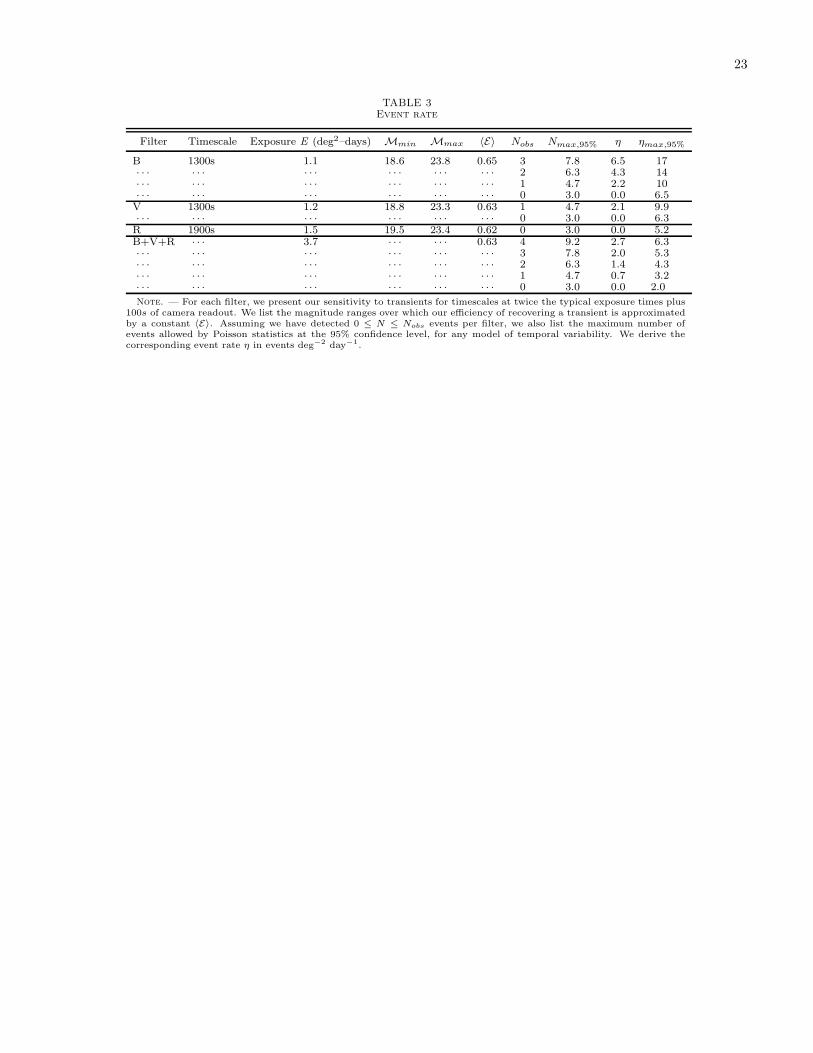
23

TABLE 3Event rate

Filter Timescale Exposure E (deg2–days) Mmin Mmax 〈E〉 Nobs Nmax,95% η ηmax,95%

B 1300s 1.1 18.6 23.8 0.65 3 7.8 6.5 17· · · · · · · · · · · · · · · · · · 2 6.3 4.3 14· · · · · · · · · · · · · · · · · · 1 4.7 2.2 10· · · · · · · · · · · · · · · · · · 0 3.0 0.0 6.5V 1300s 1.2 18.8 23.3 0.63 1 4.7 2.1 9.9· · · · · · · · · · · · · · · · · · 0 3.0 0.0 6.3R 1900s 1.5 19.5 23.4 0.62 0 3.0 0.0 5.2B+V+R · · · 3.7 · · · · · · 0.63 4 9.2 2.7 6.3· · · · · · · · · · · · · · · · · · 3 7.8 2.0 5.3· · · · · · · · · · · · · · · · · · 2 6.3 1.4 4.3· · · · · · · · · · · · · · · · · · 1 4.7 0.7 3.2· · · · · · · · · · · · · · · · · · 0 3.0 0.0 2.0

Note. — For each filter, we present our sensitivity to transients for timescales at twice the typical exposure times plus100s of camera readout. We list the magnitude ranges over which our efficiency of recovering a transient is approximatedby a constant 〈E〉. Assuming we have detected 0 ≤ N ≤ Nobs events per filter, we also list the maximum number ofevents allowed by Poisson statistics at the 95% confidence level, for any model of temporal variability. We derive thecorresponding event rate η in events deg−2 day−1.