The ESPRI project: astrometric exoplanet search with PRIMA

Astronomy & Astrophysics manuscript no. 20569 c©ESO 2012December 12, 2012

The ESPRI project: astrometric exoplanet search with PRIMA

I. Instrument description and performance of first light observations?

J. Sahlmann1, T. Henning2, D. Queloz1, A. Quirrenbach3, N.M. Elias II3, R. Launhardt2, F. Pepe1, S. Reffert3,D. Ségransan1, J. Setiawan2, R. Abuter4, L. Andolfato4, P. Bizenberger2, H. Baumeister2, B. Chazelas1, F. Delplancke4,

F. Dérie4, N. Di Lieto4, T.P. Duc4, M. Fleury1, U. Graser2, A. Kaminski3, R. Köhler2, 3, S. Lévêque4, C. Maire1,D. Mégevand1, A. Mérand5, Y. Michellod6, J.-M. Moresmau4, M. Mohler2, A. Müller2, P. Müllhaupt6, V. Naranjo2,L. Sache7, Y. Salvade8, C. Schmid4, N. Schuhler5, T. Schulze-Hartung2, D. Sosnowska1, B. Tubbs2, G.T. van Belle9,

K. Wagner2, L. Weber1, L. Zago10, and N. Zimmerman2

1 Observatoire de Genève, Université de Genève, 51 Chemin Des Maillettes, 1290 Versoix, Switzerlande-mail: [email protected]

2 Max-Planck-Institut für Astronomie, Königstuhl 17, 69117 Heidelberg, Germany3 Landessternwarte, Zentrum für Astronomie der Universität Heidelberg, Königstuhl 12, D-69117 Heidelberg, Germany4 European Southern Observatory, Karl-Schwarzschild-Str. 2, 85748 Garching bei München, Germany5 European Southern Observatory, Alonso de Córdova 3107, Vitacura-Santiago, Chile6 Automatic Control Laboratory, Ecole Polytechnique Fédérale de Lausanne, Switzerland7 Laboratoire de Systèmes Robotiques, Ecole Polytechnique Fédérale de Lausanne, 1015 Lausanne, Switzerland8 Ecole d’ingénieur ARC, 2610 St. Imier, Switzerland9 Lowell Observatory, 1400 West Mars Hill Road, Flagstaff, Arizona, 86001, USA

10 Centre Suisse d’Electronique et Microtechnique, 2007 Neuchâtel, Switzerland

Received 15 October 2012 / Accepted 5 December 2012

ABSTRACT

Context. The ESPRI project relies on the astrometric capabilities offered by the PRIMA facility of the Very Large Telescope In-terferometer for discovering and studying planetary systems. Our survey consists of obtaining high-precision astrometry for a largesample of stars over several years to detect their barycentric motions due to orbiting planets. We present the operation’s principle, theinstrument’s implementation, and the results of a first series of test observations.Aims. We give a comprehensive overview of the instrument infrastructure and present the observation strategy for dual-field relativeastrometry in the infrared K-band. We describe the differential delay lines, a key component of the PRIMA facility that was deliv-ered by the ESPRI consortium, and discuss their performance within the facility. This paper serves as reference for future ESPRIpublications and for the users of the PRIMA facility.Methods. Observations of bright visual binaries were used to test the observation procedures and to establish the instrument’sastrometric precision and accuracy. The data reduction strategy for the astrometry and the necessary corrections to the raw data arepresented. Adaptive optics observations with NACO were used as an independent verification of PRIMA astrometric observations.Results. The PRIMA facility was used to carry out tests of astrometric observations. The astrometric performance in terms ofprecision is limited by the atmospheric turbulence at a level close to the theoretical expectations and a precision of 30 µas wasachieved. In contrast, the astrometric accuracy is insufficient for the goals of the ESPRI project and is currently limited by systematicerrors that originate in the part of the interferometer beamtrain that is not monitored by the internal metrology system.Conclusions. Our observations led to defining corrective actions required to make the facility ready for carrying out the ESPRI searchfor extrasolar planets.

Key words. Instrumentation: interferometers – Techniques: interferometric – Astrometry – Atmospheric effects – planetary systems– binaries: visual – stars: individual: HD 10360, HD 66598, HD 202730

1. Introduction

High-precision astrometry will become a key method for the de-tection and physical characterisation of close-in (<10 AU) ex-trasolar planets thanks to the onset of instruments that promisea long-term accuracy of 10–100 micro-arcseconds (µas) and theassociated surveys of large stellar samples. So far, the study of

? Part of this work is based on technical observations collected atthe European Southern Observatory at Paranal, Chile. Public datacan be downloaded at http://www.eso.org/sci/activitiess/toBeInserted .

exoplanet populations has been dominated by the radial veloc-ity technique (e.g. Mayor et al. 2011) and by transit photom-etry (e.g. Borucki et al. 2011). The application of astrometrywas mostly limited to the characterisation of particular objectswith very massive companions (Zucker & Mazeh 2001; Pravdoet al. 2005; Benedict et al. 2010; Lazorenko et al. 2011; Reffert &Quirrenbach 2011; Sahlmann et al. 2011a; Anglada-Escudé et al.2012). The population of very massive planets and brown dwarfcompanions was studied with HIPPARCOS astrometry, which re-sulted in an observational upper mass limit of ∼35 Jupiter masses(MJ) for the formation of close-in planets around Sun-like stars

Article published by EDP Sciences Article number, page 1 of 32

arX

iv:1

212.

2227

v1 [

astr

o-ph

.IM

] 1

0 D

ec 2

012

http://www.eso.org/sci/activitiess/toBeInserted

http://www.eso.org/sci/activitiess/toBeInserted

http://www.edpsciences.org

and a robust determination of the frequency of close brown-dwarf companions of G/K dwarfs (Sahlmann et al. 2011b). Todetect the barycentric motion of a nearby Sun-like star causedby a close Jupiter-mass planet, an astrometric accuracy of betterthan one milli-arcsec (mas) per measurement is needed (Black& Scargle 1982; Sozzetti 2005; Sahlmann 2012). At present,only a few instruments are capable of satisfying this require-ment. Among them are the HST-FGS (Benedict et al. 2001), in-frared adaptive optics observations (Gillessen et al. 2009), op-tical seeing-limited imaging with large telescopes (Lazorenkoet al. 2009), and optical interferometry.Construction of optical interferometers was in part motivated bytheir capability of performing precise (a few mas) global astrom-etry (Shao et al. 1990) and very precise (∼10 µas) narrow-anglerelative astrometry (Shao & Colavita 1992). The latter requiresa dual feed configuration to observe two stars simultaneously,which was demonstrated at the Palomar Testbed Interferometer(PTI) (Lane & Colavita 2003). Using the PTI infrastructure butobserving sub-arcsecond-scale binary stars within the resolutionlimit of one single feed, precisions of tens of µas were obtainedin this very-narrow angle mode (Muterspaugh et al. 2005). Thepossibility of using infrared interferometry for astrometric de-tection of extrasolar planets was described by Shao & Colavita(1992). Consequently, a demonstration experiment was set upat the PTI (Colavita et al. 1999) and the interferometric facili-ties at the Keck and Very Large Telescope (VLT) observatories,which were being built at that time, included provisions for thedual-field astrometric mode. On the basis of the feasibility studyby Quirrenbach et al. (1998) for the VLT interferometer (VLTI),the development of this mode of operation was started and itsimplementation began with the hardware deployment at the ob-servatory in 2008. The infrastructure for dual-feed operation andrelative astrometry at the VLTI is named PRIMA, an acronym forphase-referenced imaging and micro-arcsecond astrometry.

1.1. The ESPRI project

The goals of the ESPRI project (extrasolar planet search withPRIMA, Launhardt et al. 2008) are to characterise known radialvelocity planets by measuring the orbit inclination and to de-tect planets in long period orbits around nearby main-sequencestars and young stars, i.e. in a parameter space which is diffi-cult to access with other planet detection techniques. The ES-PRI consortium consists of three institutes: Max Planck Insti-tut für Astronomie Heidelberg, Observatoire Astronomique del’Université de Genève, and Landessternwarte Heidelberg. A de-tailed description of the science goals, organisation, and prepara-tory programme of ESPRI is given in a accompanying paper(Launhardt et al., in prep). Formally, the ESPRI consortium con-tributes to the PRIMA facility with the differential delay lines(DDL), the astrometric observation preparation software (APES),and the astrometric data reduction pipeline, all of which areeventually delivered to ESO, hence become publicly available.In return, ESPRI obtains guaranteed time observations (GTO) tocarry out its scientific programme. In practice, ESPRI also con-tributes significantly to the commissioning of the PRIMA astrom-etry mode, which includes making the facility functional, carry-ing out the observations, and reducing and analysing the data.The paper is organised as follows: In Sect. 2, we discuss themeasurement principle and the interferometric baseline defini-tion. The PRIMA facility is described in Sect. 3 and the designand performance of the differential delay lines is presented inSect. 4. The astrometric data reduction and modelling is intro-duced in Sects. 5 and 6, respectively. The results in terms of

measurement precision and accuracy are summarised in Sect. 7.We conclude in Sect. 8. Auxiliary information is collected in theappendices.

2. Principles of narrow-angle astrometry

The measurement principle of narrow-angle relative astrometrywith an interferometer is to observe two stars simultaneously andto measure the relative position of the two fringe patterns in de-lay space (Fig. 1).

Baseline

Beam combination

T1

Ref. Target

T2

Optical delay

∆OPD

Fig. 1. Principle of PRIMA astrometry: reference and target starare observed simultaneously with two telescopes (left). Light of bothstars is made to interfere and the location of the two interference fringepatterns is measured in delay space (right). The fringe separation ∆OPDis proportional to the projected separation of the stars.

In stellar interferometry, the astrometric information is encodedin the fringe position measured in delay space. The internal de-lay that is necessary to observe interference therefore containsinformation on the star’s position, hence a series of delay mea-surements can be used for the determination of accurate stellarpositions (e.g. Shao et al. 1990; Hummel et al. 1994). The rela-tion between the optical delay w and the stellar position definedby the unit vector s in direction of the star is

w = B · s, (1)

where B = T2 − T1 is the baseline vector connecting two tele-scopes with coordinates Ti. When observing two stars identifiedby unit vectors s1 and s2 simultaneously, the differential delay∆w can be written as difference of the respective w-terms

∆w = w2 − w1 = B · s2 − B · s1 = B · ∆s. (2)

The potential for high-precision astrometry of this observationmode stems from the combination of a large effective apertureand the fact that the noise originating in atmospheric pistonmotion is correlated over small fields (Shao & Colavita 1992).In conventional imaging astrometry, the achievable astrometricprecision depends on the aperture size D of the telescope (La-zorenko et al. 2009). Shao & Colavita (1992) showed that in thecase of dual-field interferometry, where D is effectively replacedby the projected baseline length Bp, and under the narrow anglecondition

Θh < Bp , (3)

where Θ is the field size and h is the turbulence layer height, theastrometric error σa due to atmospheric turbulence is

σa = qsiteΘ

B2/3p T 1/2

or σ2a ∼

Θ2

B4/3p T

, (4)

with Bp in metres, Θ in radians, and T in hours. The param-eter qsite depends on the atmospheric profile and in the case of

Article number, page 2 of 32

J. Sahlmann et al.: The ESPRI project: astrometric exoplanet search with PRIMA

a Mauna Kea model is 300′′ m2/3 h1/2 rad−1. Based on Eq. 4,the expected atmospheric limit to the astrometric precision for abaseline length of 100 m, a separation between the stars of 10′′,and an integration time of 1 h is ∼10 µas.In the horizontal coordinate system, the elevation E and azimuthA of a star at local sidereal time ts are related to the right ascen-sion α and declination δ in the equatorial coordinate system bythe hour angle ha = ts − α and the equations

sin E = sin δ sin L + cos δ cos ha cos Lcos E cos A = sin δ cos L − cos δ cos ha sin Lcos E sin A = − cos δ sin ha

⇒ tan A =− cos δ sin ha

sin δ cos L − cos δ cos ha sin L ,

(5)

where L is the observer’s geographic latitude. The unit vector sin direction of the star is

s =

cos E cos Acos E sin Asin E

(6)

and the baseline vector B in the horizontal coordinate system is

B =

BNorthBEastBElev

, (7)

where the component BNorth is the ground projection of B mea-sured northward, BEast is the ground projection of B measuredeastward, and BElev is the elevation difference of B measured up-ward. The instantaneous optical path difference (OPD) w is thus(Fomalont & Wright 1974; Dyck 2000)

w = B · s= cos E cos A BNorth + cos E sin A BEast + sin E BElev (8)

and the differential OPD ∆w can be written as

∆w = BNorth (cos E2 cos A2 − cos E1 cos A1)+ BEast (cos E2 sin A2 − cos E1 sin A1)+ BElev (sin E2 − sin E1) . (9)

In the equatorial system the baseline coordinates are BxByBz

=

− sin L 0 cos L0 −1 0

cos L 0 sin L

· BNorth

BEastBElev

(10)

and the u-v-w-coordinate system describing the tangential planein the sky are given by u

vw

=

sin H cos H 0− sin δ cos H sin δ sin H cos δ

cos δ cos H − cos δ sin H sin δ

· Bx

ByBz,

(11)

yielding the optical path difference

w = cos δ cos H Bx − cos δ sin H By + sin δ Bz. (12)

For completeness, we note that the projected baseline length isBp =

√u2 + v2 and the projected baseline angle θB is defined by

tan θB = v/u and that the VLTI baseline BVLTI is defined using adifferent convention from Eq. 7:

BVLTI =

BSouthBWestBElev

=

−1−1

1

B, (13)

where the -symbol indicates element-wise multiplication.

2.1. Interferometric baselines

In the theoretical description above, the interferometric baselineB is a well defined quantity. In practice, its definition is notstraight-forward because the telescopes and other optical ele-ments are moving during the observation and the simple def-inition as the vector connecting telescope T1 and T2 becomesambiguous. Furthermore, PRIMA is used to observe two starssimultaneously and effectively realises two interferometers atthe same time, thus making a clarification in the interpretationof the baseline necessary. The following conceptual descrip-tion neglects any effect related to off-axis observations, opticalaberrations, refraction, and dispersion and applies in the hori-zontal coordinate system. The device allowing us to determinethe astrometric baseline is a laser metrology that monitors theoptical path lengths of the optical train travelled by the stellarbeams inside the interferometer. The two terminal points defin-ing the monitored optical path of each beam are the metrologyendpoints. Let Li be the optical path length measured with themetrology in beam i and let w = Li − L j be the instantaneousmeasured optical path difference between the two arms of an in-terferometer observing a star defined by the pointing vector s.Note that the metrology yields the internal delay only in the caseof ideal fringe tracking, i.e. when the fringe packet as seen bythe fringe sensor is centred at all times. Thus for a real system,measurements by the fringe tracking system and their potentialsystematics have to be considered when using metrology read-ings.

2.1.1. Wide-angle astrometric baseline

The unique vector BWide that relates the metrology measurementof optical path difference w to the pointing vector s at all timesvia the equation

w = BWide · s + c (14)

is called the wide-angle astrometric baseline, where c is a con-stant term. The wide-angle astrometric baseline can be deter-mined by measuring the metrology delays w1...k when observinga set of 1...k stars with coordinates s1...k, selected such that theresulting system of equations 14 allows for the non-degeneratesolution for the three components of BWide (e.g. Shao et al. 1990;Buscher 2012).The pivot point of an ideal telescope is defined as the intersec-tion between the altitude and azimuth axes and remains at a fixedposition in the horizontal coordinate system at all times. It is therelative position of the two pivot points that determines the op-tical path lengths travelled by the stellar beams inside the inter-ferometer. Thus, ideally we would like to make the metrologyendpoints at one end coincide with the pivot points and at theother end be located at the location of beam combination. In thisconfiguration, Eq. 14 would be exact. In practice, several com-plications occur. First, due to the telescope design, misalign-ments, or flexures, the pivot point may not exist, be ill-defined,or does not remain fixed at all times. Second, the pivot point ishardly accessible and the metrology endpoints are located else-where in the beam train. Third, there may be a non-common pathbetween the metrology and stellar beams, i.e. potential changesin stellar path length are not monitored by the metrology. ThusEq. 14 needs to be complemented with two terms

w + ε = (BWide − µ1 + µ2) · s + c, (15)

where ε is the OPD mismatch between the metrology and stel-lar beams caused by the non-common path, and µi is the offset


vector between the pivot point of telescope i and the respectivemetrology endpoint. Both terms are time dependent and haveto be modelled, but one term can be eliminated by placing themetrology endpoints either in the entrance pupils, then ε = 0, orat the pivot points, then µi = µ j = 0.The PRIMA facility realises a dual-feed interferometer and at firstit can be modelled as two independent interferometers, denotedfeed A and feed B, observing the star sA and sB, respectively.Thus there are four stellar and four metrology beams and eachinterferometer has a wide-angle baseline defined by

wA = L3 − L1 = BA,Wide · sA + cA

wB = L4 − L2 = BB,Wide · sB + cB (16)

2.1.2. Narrow-angle astrometric baseline

The goal of the experiment is to measure the angular separationvector ∆s = sA − sB between the two targets in the sky. Al-though in principle we could use Eq. 16 to achieve this task,the required accuracy on the wide-angle baseline knowledge be-comes unachievable for the level of accuracy anticipated for ∆s.Instead, both interferometers can be tied together by a commonmetrology system measuring the difference of optical path dif-ferences ∆w = wA − wB. The unique vector BAX that relates ∆wto the separation vector ∆s at all times via the equation

∆w = BAX · ∆s + c∆ (17)

is called the narrow-angle astrometric baseline. We can rewriteEq. 17 as

∆w = L3−L1−L4 + L2 = BA,Wide · sA−BB,Wide · sB + cA−cB (18)

which shows that in order to satisfy Eq. 17, the identity BA,Wide =BB,Wide = BAX is a necessary condition, which requires thatthe metrology endpoints corresponding to the beams L1/L2 andL3/L4 coincide in telescope 1 and 2, respectively. We are stillnot done, because in practice the unknown terms introduced inEq. 15 have to be considered. We obtain

∆w(t) + ∆ε(t) =[BA,Wide − µA,1(t) + µA,2(t)

]· sA(t) + cA

−[BB,Wide − µB,1(t) + µB,2(t)

]· sB(t) + cB (19)

where time dependencies are explicitly noted. Because of the re-quirement of coinciding metrology endpoints in each telescope,we have BA,Wide = BB,Wide and µA,i = µB,i = µi and it follows

∆w(t) + ∆ε(t) =[BAX − µ1(t) + µ2(t)

]· ∆s(t) + c∆, (20)

where ∆ε(t) is the differential OPD caused by non-common pathbetween stellar and metrology beams and c∆ = cA − cB is a con-stant.Because of the differential measurement, the requirements onthe measurement accuracy of BAX are relaxed, but the terms∆ε(t) and µi(t) have to be minimised by the optical design andconsequently modelled (Sect. 7.6). The vectors µi(t) can for in-stance be determined by accurate modelling combined with ex-ternal measurement devices, which monitor the telescope mo-tion (Hrynevych et al. 2004). Alternatively, the narrow-anglebaseline can be determined by measuring several star pairs withdifferent and known separation vectors and solving the systemof equations Eq. 20 for BAX.

2.1.3. Imaging baseline

The imaging baseline determines the orientation and value ofthe spatial frequency sampled with the interferometer, i.e. the u-v-coordinates (Eq. 11), and it is related to the sky-projected con-figuration of the interfering partial wavefronts. To distinguishbetween imaging and wide-angle baseline the following exam-ple can be useful: If half of one telescope aperture is maskedduring the observation of an on-axis source, this will not changethe wide-angle baseline (the fringe position in delay space re-mains constant) but it will alter the imaging baseline, becausethe interfering wavefront portions are changing.

2.1.4. Model applied for initial PRIMA tests

The theoretical description of the narrow-angle baseline givenabove does not strictly apply to PRIMA observations and sev-eral second-order terms have to be considered (e.g. Colavita2009). Additionally, the wide-angle baseline of PRIMA B′Wideis determined using the delay line metrology that measures wDL(Sect. 6.2), whereas the differential delay is measured using thededicated PRIMA metrology having different endpoints yieldingthe quantity ∆L. For the analysis of the initial astrometric mea-surements relying on Eq. 20, we will assume that the unknownquantities vanish, i.e. ∆ε(t) = 0 and µi(t) = 0, that the end-points of the differential metrology coincide, and that the mea-sured quantities are given by ∆w(t) = ∆L(t) and BAX = B′Wide.Those assumptions may not necessarily be fulfilled and we dis-cuss potential effects in the text.

3. PRIMA at the Very Large Telescope Interferometer

The PRIMA facility consists of a considerable amount of subsys-tems, which are distributed both physically on the observatoryplatform and systematically over the VLTI control system. Itsinstallation necessitated the enhancement of every VLTI build-ing block, i.e. of the telescopes, the delay lines, the laboratoryinfrastructure, and the control system. PRIMA is a multi-purposefacility with several observing modes, which was added to theexisting VLTI framework under the requirement not to impactthe already operating instruments. Therefore PRIMA cannot beconsidered an astronomical instrument in the classic sense. Gen-eral descriptions of PRIMA are given by Delplancke et al. (2006)and van Belle et al. (2008). A detailed description of the PRIMAfringe sensors and an assessment of their performance for fringe-tracking is given by Sahlmann et al. (2009). The astrometric in-strument that uses the PRIMA facility is named PACMAN (Abuteret al. 2010). The status of the VLTI and its subsystems is givenby Haguenauer et al. (2008, 2010).The various subsystems of PRIMA were tested individually atthe Paranal observatory since August 2008. Testing of thePRIMA facility began in July 2010, when dual-feed fringes wererecorded for the first time. Astrometric observations becamepossible in January 2011 and PACMAN ’first light’ was achievedon January 26, 2011. For PRIMA astrometry observations, theinteractions between the PRIMA and VLTI subsystems are nu-merous and flawless interplay is required for the basic function-ality. Furthermore, the accuracy goal for PRIMA astrometry setsstringent requirements on the performance of every subsystem,and measurement biases can originate virtually anywhere alongthe beam train. Thus, a detailed description of the VLTI-PRIMAsystem is required and given below.



H/K split

FSUA21

21FSUB

21 3 4

IRISAT3

DDL: Differential Delay Line

1

Fringe Sensors3

4

2

VLTI Laboratory

1

2

3

4

DDL

Beam Compressor

Switchyard

DL2

Tunnel

M12M12 M16

AT4DL: Main Delay LineAT: Auxiliary Telescope

STS: Star SeparatorIRIS: IR Image SensorFSU: Fringe Sensor Unit STS

STS

DL4

Fig. 2. Schematic of the stellar beam pathsfor PRIMA astrometric observations showingthe main subsystems and their relative locations(not to scale). The beams propagate through un-derground light ducts from the telescopes to thedelay line tunnel from where they are relayedinto the beam combination laboratory. The in-put channel number of each beam is shown inbold. The PRIMA metrology monitors the pathlengths of the four beams between the respec-tive endpoints in the FSU and STS. The twometrology beams that monitor the FSUB feedare shown as dashed lines.

3.1. Design goal for the astrometric accuracy

The design goal for PRIMA was that measurement errors intro-duced by instrument terms shall be smaller than 10 µas for ob-servations of two objects in a field of ∼1′ and with a baselineof ∼100 m, i.e. inferior to the atmospheric limit for 1 h of in-tegration. We can use Eq. 17 to estimate how this requirementtranslates into the required accuracy of measured quantities. Forsimplicity we set the astrometric accuracy to σΘ = 10 µas forthe separation between two targets located in a Θ = 10′′ field.The relative accuracy is σΘ/Θ = 10−6 and thus the astrometricbaseline BAX has to be known at this accuracy level, correspond-ing to 100 µm for a baseline length of 100 m. This also illus-trates why we cannot get away with measuring the two wide-angle baselines and using Eq. 16, because the accuracy require-ment on BWide would be orders of magnitude more stringent, thusnot reachable. The expected differential delay is of the order of5 mm, thus the required accuracy in the differential delay mea-surement is 5 nm for optical path lengths reaching several hun-dred metres.

3.2. PRIMA subsystems and beam train

A schematic overview of the PRIMA-VLTI system is shown inFig. 2. Below, a short description of the involved subsystem isgiven in order of incidence, which can be used together with theschematic to follow the path of an incoming stellar beam. Themain subsystems are briefly described in the next sections.

– Telescope: Two VLTI Auxiliary Telescopes are used.– Star separator: Splits the image plane between the two tar-

gets and generates separated output beams for each of them.– M12: A passive folding mirror located in the delay line tun-

nel that sends the stellar beams coming from an auxiliarytelescope light duct towards a main delay line.

– Main delay line: The main delay line is used for fringe track-ing on the primary star. The carriage moves on rails andis capable of introducing optical delay in both feeds withnanometre accuracy over ∼120 m and with a high bandwidth.

– M16: These are configurable mirrors that fold the beams intothe laboratory feeding the desired input channel.

– Beam compressor: Each beam is downsized from 80 mm to18 mm by passing through a parallel telescope.

– Switchyard: A set of configurable mirrors, which for PRIMAastrometry fold the beams towards the differential delaylines.

– Differential delay line (DDL): One of the four DDLs is usedto compensate for the differential delay between the two starfeeds and for fringe tracking on the secondary star.

– H/K-dichroic mirror: Folds the H-band light towards the in-frared image sensor (IRIS) and transmits the K-band lighttowards the fringe sensor unit.

– Fringe Sensor Unit (FSU): Combines two K-band inputbeams from one star and detects the fringe signals. The twinsensors FSUB and FSUA are driving the primary and sec-ondary fringe tracking loops, respectively.

– IRIS: Images the H-band beams and measures the point-spread-function (PSF) position and motion for feedback tothe control system (Gitton et al. 2004).

In total, the stellar beams are reflected on 38 optical surfacesbefore being injected into the single-mode fibres of the FSU, seeTable C.1. These are 13 reflections more than in the single-feedcase, for which Sahlmann et al. (2009) estimated a total effectivetransmission (including effects of injection fluctuations) in K-band of 4 ± 1 %. If we assume an average reflectivity of 0.98 or0.95 per mirror, the additional decrease in transmission for thenominal dual-feed case is 23 % or 49 %, respectively. A detailedanalysis and description of the measured transmission in dual-feed is outside the scope of this work.

3.3. Auxiliary telescopes, derotator, and star separator

The Auxiliary Telescopes (AT, Koehler et al. 2002, 2006) of theVLTI have a 1.8 m diameter primary mirror in altitude-azimuthmount and a coudé beam train as shown in Figs. 3 and 4. Sev-eral actuators are used to manipulate the stellar beam: the sec-ondary mirror M2 can be controlled in lateral position (X,Y),in longitudinal position for focus adjustment (Z), and in tip andtilt. A first-order image stabilisation system is implemented toattenuate the fast atmospheric image motion: a quadcell sensorbased on avalanche photo diodes is located below the star separa-tor and receives the visible light transmitted by the M9 dichroicmirror (Fig. 6). It measures the image centroid and sends off-sets to the fast tip-tilt mirror M6 located upstream, hence re-alising a closed-loop control system for image motion, capableof very low-order wavefront control. The derotator is locatedbelow the telescope and above the star separator. Its role is togenerate a fixed field image for the star separator, i.e. to removethe field motion caused by the Earth rotation. The derotator is


Figure 2: AT telescope with de-rotator and star separator

Figure 3: Optical layout of AT Star Separator

Proc. of SPIE Vol. 7013 70133F-3

Fig. 3. The cross-section of an auxiliary telescope indicating thelocation of the derotator and the star separator below the main telescopestructure. From Nijenhuis et al. (2004).

2001LIACo..36..203D

Fig. 4. Beam tracing inside the auxiliary telescope indicating themirror designations. From Delrez et al. (2001). The derotator is locatedbetween M8 in the AT and M9 in the STS, see also Fig. 5.

implemented as a reflective K-prism assembly mounted on a mo-torised rotation stage, such that a 180 derotator motion resultsin 360 field rotation.The star separator (Nijenhuis et al. 2008) has three main func-tionalities: (a) it splits the field between the two observed objectsand generates two output beams, each containing the light fromone sub-field; (b) it supplies the end-point for the PRIMA metrol-ogy; (c) it controls the image position measured downstream inthe laboratory and the lateral pupil position.

ability of nearby faint objects. (up to 120” separation on sky). Objects that were first unobservable by interferometry due to the atmospheric turbulence now become visible. These faint objects become visible because:

1. The bright star (guide star) is used to compensate the turbulence induced by the atmosphere (by making short exposures during which the atmospheric turbulence is “frozen” and by correcting for the measured delay).

2. The turbulence is then also compensated in the direct environment of the star and the signal on the very faint object (called science star) is not “diluted” anymore, can be integrated longer and finally detected.

This means that two objects in the field of view of the telescope are to be observed simultaneously. The instrument to facilitate this feature is called the Star Separator (STS), which is part of the PRIMA facility3. Its location is shown in Figure 1 while the instrument itself is shown in Figure 2 and sizes to about Ø 1 x 0.4 m3.

Figure 2: Overview of Star Separator

354 Proc. of SPIE Vol. 5528

Downloaded from SPIE Digital Library on 08 Nov 2011 to 134.171.17.170. Terms of Use: http://spiedl.org/terms

The core section of this instrument is shown in Figure 3. It shows the way the major functional requirements of the STS are implemented. The Coude focus of the telescope coincides with the rooftop mirror M10 that separates the telescope Field of View into two sections. The de-rotator (see Figure 1) in front of the STS assures that the guide star and the science object are re-imaged at either side of the rooftop. M10 re-images the telescope pupil on both flat folding mirrors M11. Mirror M12 re-images the Coude focus on M14. Because the pupil coincides with M11 it is possible to point at any re-imaged object on M10 by a small rotation around two perpendicular axes of M11 (TNO TPD patent). Presently TNO TPD is developing this instrument. The design of the instrument has been finished while production is well on its way. Within a year the instrument will be delivered to ESO. The key element of the instrument, being the mechanism that operates M11, has already been produced, tested and performs even better than required.

2. THE MECHANISM DESIGN 1. Major requirements for the Star Separator in relation to the mechanisms. The STS-mechanism has to enable the following major requirements:

1. Pointing at the re-imaged science object (e.g. a star) in the Coude focus of the telescope. A pointing repeatability (here same as accuracy) of 0.01” on sky is needed with a resolution of 0.002”. The total pointing range should be 68” on sky. Small pointing corrections during observations are needed at 10 Hz but preferably at 50Hz.

2. Chopping i.e. pointing alternating at the science object and its celestial background at 1 Hz and preferably at 5 Hz.

3. Correction of beam tilt introduced by the re-location of the telescope. (for optimal observations ESO can relocate each AT at a number of fixed docking stations at the observatory)

These features will enable ESO to point with two to four telescopes to two objects using a closed loop control system that drives the mechanisms. 2. Design considerations Because the mechanism is part of an interferometer stability is of utmost importance. Therefore temperature changes, vibrations due to e.g. earthquakes etc. should have negligible consequences. Furthermore friction inside the mechanism is not allowed because of the resulting hysteresis. The size of M11 is only Ø25 mm and guarantees that the moving mass is low and will not hamper the dynamics of the mechanism during chopping. By rotating M11 around two orthogonal axes it is possible to point at the object of interest that is re-imaged anywhere on M10. The following table specifies the requirements for the mechanism.

Requirement Required value Requirement Required value Pointing range 14.6 mrad (both axes) ≈ 1° Pointing correction freq. 50 Hz Pointing accuracy 2.1 µrad Chopping frequency 5 Hz Pointing resolution 0.43 µrad Chopping accuracy 94 µrad

Table 1: Mechanism requirements

Figure 3: Optical lay-out of STS

Proc. of SPIE Vol. 5528 355

Downloaded from SPIE Digital Library on 08 Nov 2011 to 134.171.17.170. Terms of Use: http://spiedl.org/terms

Fig. 5. Top: Optical layout of one star separator. Bottom: Top viewof the STS optical layout identifying the mirror names. M11 (FSM) isthe field selector mirror acting on the image and M14 (STS-VCM) isthe variable curvature mirror acting on the pupil. From Nijenhuis et al.(2004).

Field splitting: After reflection on M9, the infrared stellar lightis focused on M10, which is a roof mirror that separates thefield in two and generates two beams (Fig. 5). The telescopeand the derotator are adjusted such that the middle positionbetween the two objects is located on the M10 edge and theobjects are imaged on either side of the edge (Fig. 9). Thetelescope guiding and the derotator motion ensure that thissituation is maintained during the observation.

Metrology end point: The PRIMA metrology beams originatedownstream in the laboratory and overlap at the location ofthe dichroic M9, which they traverse towards an assemblyof two spherical mirrors and a compensation plate (Fig. 6),that serve to reflect the beams on themselves. The metrol-ogy beams are folded back into the stellar beams, traverseM9 again, and return towards the laboratory. The endpointis realised by RR3 in Fig. 6, which is where by design bothmetrology beams have total overlap (RR3 is in a pupil plane).

Image and pupil positioning: M11 is the first mirror down-stream of the field separator and is located in a pupil plane. Itis mounted on a piezo tip-tilt stage which is used to positionthe image location in the laboratory, i.e. for fine-pointing theobject. M11 is called the field selector mirror (FSM). M14is located in an image plane and mounted on a piezo tip-tiltstage, which is used to adjust the output pupil lateral posi-tion. This mirror is also used to set the pupil’s longitudinalposition, defined by the mirror’s radius of curvature. It isplanned to achieve this dynamically with a variable curva-ture mirror (VCM), but it was not implemented at the time



of writing and a fixed curvature mirror is used instead. Still,M14 is named STS-VCM.

Doc VLT-TRE-ESO-15730-4092Issue 1Date 29/9/06Page 56 of 62

PRIMA Metrology as-built status

The same principle will be used for the UT’s. The retro-reflector will be mounted behind M9 and. It will consist in 3optical elements: 1 correction plate, 1 doublet and 1 spherical mirrors. All these elements will be located inside amechanical tube fixed on the Coude mechanical structure.

Figure 37 Design of the AT-STS end-points

Figure 38 Design of the UT-STS end-points,

Fig. 6. Optical layout of the metrology endpoint. This side view showsthe stellar beam coming from the telescope (above) being reflected to-wards M10 and the metrology beams coming from the laboratory beingreflected on themselves by the assembly of the spherical mirrors RR2and RR3 and the compensation plate RR1. In this view, the metrologybeams enter horizontally from the right, after reflection off M10. Thelight that is seen to traverse M9 downwards is the visible portion of thestellar beam propagating towards the fast quadcell image sensor.

The location of the metrology end points in the star separatorshows that there is a substantial non-common path between thestellar and metrology beams inside the telescope. The stellarlight path from the primary mirror M1 to the dichroic M9 andin particular inside the derotator is not monitored by the PRIMAmetrology. Conversely, the retro-reflector assembly of three op-tical elements is monitored by the metrology, but is not part ofthe stellar beam path.

3.4. Main delay lines

The VLTI main delay lines (Hogenhuis et al. 2003) are precisioncarts carrying a cat’s eye-type reflector and used to introducevariable optical delay inside the interferometer. The rail lengthof ∼60 m limits the maximum optical delay to ∼120 m per de-lay line. Real-time delay control at nanometre level over the fullrange is achieved with a two-stage system composed of a coarsemechanism moving the full cart and a fine piezo actuator, com-bined with an internal metrology system measuring the positionof the cart along the rail (Fig. 7). The main delay line has dual-feed capability, i.e. it accepts two beams which will experiencethe same optical delay. A variable curvature mirror (DL-VCM,Ferrari et al. 2003) is part of the cat’s eye assembly and it isdynamically adjusted along the delay line trajectory to keep thelongitudinal pupil position constant in the laboratory and to pre-serve the field-of-view of the interferometer. It is realised bya mechanism consisting of a steel mirror connected to an over-pressure chamber of tunable pressure.

The Delay line controls the optical path by a two-stage translation system. This two-stage concept includes a LinearMotor drive system (LM) to bring the OPD within the range of the second stage, a piezo actuator system for extremelyfine control. A 2 kHz control ioop is responsible for the real time performance ofthe OPD during observations at speedsup to 5 mm/sec. This performance is reached by sending a force command to the LM that is based on feedback from theposition error and a friction prediction. The remaining error is controlled by the second stage, the piezo actuator, in afeed forward ioop. The position sensor is a long range, high resolution metrology system placed at the start of the railtrack. Data communication is wireless via a laser transceiver system (optical datalink), resulting in a wheel/rail contactonly with bearing friction as mechanical interference in the stage control.

FINE METROLOGY

LINEAR MOTOR

• AT1VE COIL= SHORT CIRCUITED COIL= MAGNET BLOCK

y Lines s/n #1 and VLT interferometer

Figure 1 Functional block diagram of Delay Line concept

An impression of the Delay Lines in the interferometer tunnel at Paranal is given in Figure 2 below:

Proc. of SPIE Vol. 4838 1149

Downloaded from SPIE Digital Library on 11 Jan 2012 to 134.171.184.223. Terms of Use: http://spiedl.org/terms

Fig. 7. Drawing of a main delay line showing the rail, the carriageholding the cat’s eye assembly, and the delay line metrology beams.The wheelbase is 2.25 m. The tertiary mirror M3 is the variable cur-vature mirror DL-VCM, which is mounted on a fast piezo stage. FromHogenhuis et al. (2003) .

Table 1. Details of the PRIMA metrology system.

Feed FSUA FSUBInput channela IP3 IP1 IP4 IP2Polarisation p s p sMonitored path (m) L3 L1 L4 L2δνb (MHz) +38.65 +38.00 −39.55 −40.00OPD (m) ∆LA = L3 − L1 ∆LB = L4 − L2Beat frequency (kHz) 650 450Diff. delay (m) ∆L = ∆LA − ∆LB

Constants:∆νP

c (MHz) 78.1νP

d (MHz) 227 257 330.6λP

e (nm) 1 319.176183

Notes. (a) The input channel (IP) refers to the physical location of thebeam at the switchyard level. There are eight input channels at VLTI.(b) Frequency shift relative to the laser frequency νP. (c) Frequency shiftbetween both feeds introduced to avoid crosstalk. (d) Calibrated laserfrequency. (e) Laser vacuum wavelength.

3.5. Differential delay lines

There is one differential delay line (DDL) for each of the fourPRIMA beams, i.e. the optical delay can be adjusted for eachbeam individually. The DDL concept is very similar to the maindelay lines with the difference that they are kept under vacuum.A motor for coarse actuation is combined with a fine piezo actua-tor and an internal laser metrology to achieve optical path lengthcontrol at nanometre level and high bandwidth. A detailed de-scription of the DDL is given in Sect. 4.

3.5.1. PRIMA metrology

The PRIMA metrology (Leveque et al. 2003; Schuhler 2007;Sahlmann et al. 2009) is a 4-beam, frequency-stabilised infraredlaser metrology with the purpose of measuring the internal dif-ferential optical path difference (DOPD) between the two PRIMAfeeds. The metrology beams have a diameter of 1 mm at in-jection and propagate within the central obscuration of the stel-lar beams, which originates from the telescope secondary mir-ror. Metrology endpoints are given by the fringe sensors’ beamcombiners and the star separator modules (Fig. 6). The PRIMAmetrology system gives access to two delays: the differential de-lay ∆L between both feeds, which is the main observable for as-trometry and is named PRIMET, and the optical path difference ofone feed ∆LB corresponding to FSUB (Sect. 3.6), hence is namedPRIMETB. Both are based on incremental measurements after afringe counter reset, which is triggered by the instrument, mean-ing that the metrology has no pre-defined zero-point. The PRIMAmetrology beams are also used to stabilise the lateral stellar pupilposition. A quadcell sensor located on the fringe sensors’ opti-cal bench measures the lateral position of the metrology returnbeams and stabilises their positions with the STS-VCM mirroractuators in closed loop. Under the condition that the metrologyand stellar beams are co-aligned and superimposed, the lateralpupil positions of the four stellar beams are stabilised. Detailson the metrology measurement architecture are given in Table 1.

3.6. Fringe sensor unit

The stellar beams are combined by the fringe sensor unit (FSU,Sahlmann et al. 2009). There are two combiners, named FSUAand FSUB, each receiving two beams of one stellar object. The


FSU contains the interface for the injection and extraction of thePRIMA metrology beams. The output delay measurements andfluxes are used for real-time control and recorded by the astro-metric instrument, constituting the scientific data. Because of itscentral role within the PRIMA facility, the detailed spectroscopicand photometric characterisation of the FSU is required. Thecalibration of the sensors is necessary to optimise their perfor-mance in the control system and to minimise systematic effectson the astrometric measurement. An exhaustive description ofthe FSU is given by Sahlmann et al. (2009).

3.7. Critical aspects of the PRIMA-VLTI control system

Several control loops acting on the stellar beams via the opto-mechanical components listed above are required to makePRIMA observations possible and they are listed in Table C.4.The fast communication between distributed subsystems relieson a fibre network realising a kHz-bandwidth shared memory(Abuter et al. 2008; Sahlmann et al. 2009). When observing,the number of active loops totals at 19, if we consider equiv-alent instances for different beams, which illustrates the com-plexity required to orchestrate the facility. All control loops arediscussed in this work except for the fringe tracking loops thatare of critical importance for the efficiency of the observations.The fringe tracking loops are implemented in the OPD controller(OPDC) and the differential OPD controller (DOPDC). So far,both controllers were operating independently and with identicalalgorithms and parameters, which use both group and phase de-lay measurements of the FSU to track on zero group delay andrely on the FSU delivered S/N to switch between three states:search, idle, and track (Sahlmann et al. 2009, 2010). Whenclosed, the inner phase controller tracks a time varying targetΦtarget designed to maintain the group delay at zero. The dis-cretised expressions prescribing the command RT offset (real timeoffset) sent to the delay line in addition to the predicted side-real motion are given in Eqs. 21 and 22, where φ and GD is theunwrapped phase (in rad) and group delay (in m) delivered bythe fringe sensor, respectively, and κ = 0.2586267825 · 10−6 is aconstant.

Φtargetk = Φ

targetk−1 + p0 GDk (21)

RT offsetk = RT offset

k−1 + p1 κ(Φ

targetk − φk

)+ p2 κ

(Φ

targetk−1 − φk−1

)(22)

The subscript k indicates the value at each time step and in-creases by one every 500 µs, i.e. the controller has a samplingrate of 2 kHz. The control gains p0 = 0.001, p1 = 0.007 andp2 = 0.063 were determined for robust operation under vary-ing atmospheric conditions and were kept unchanged during thecomplete test campaign. The outer group delay loop is thus im-plemented as integral controller and the inner phase loop realisesa proportional-integral controller. The fringe tracking strategyfor PRIMA astrometry observations can be optimised by cou-pling both control loops and by adapting the gains of the dif-ferential controller, which is an ongoing activity at the time ofwriting.

3.8. Observing with the astrometric instrument

The astrometric instrument of PRIMA is named PACMAN(Abuter et al. 2010) and is materialised by a computer, con-nected to the interferometer control system and the rapid fibrelink between the real-time computers. The instrument executes

Fig. 8. Left: Layout of the Paranal observatory platform indicating thebaseline used during the commissioning as shown by the APES soft-ware. Right: Not accessible regions in the sky due to delay line limits(dotted regions) and UT shadowing (grey patches) for the baseline G2-J2 as shown by the VLTI observer panel. Labels mark the elevationangle.

the observation blocks by commanding the interferometer con-trol system to preset the system to the specified configuration,acquire the target with telescopes and delay lines, and eventu-ally by triggering the data recording. So far, PRIMA astrometriccommissioning observations were made with the auxiliary tele-scope AT3 in station G2 and the telescope AT4 in station J2, re-sulting in a baseline length of ∼91.2 m (Fig. 8). The main delaylines DL2 and DL4 were used and despite of their long stroke,observations in the north-western sky were prohibited becausethe available internal optical delay is not sufficient.

3.8.1. Normal-swapped sequence

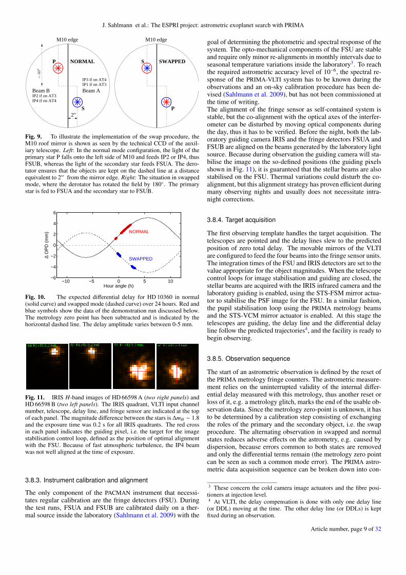
The observation strategy to calibrate the metrology zero-pointand to minimise differential errors between the two feeds is toobtain a sequence of normal and swapped observations. Thephysical swap procedure is executed by the derotator located be-tween telescope and star separator. It rotates mechanically by90 resulting in 180 field rotation so that the primary and sec-ondary object fall on either side of the STS-M10 roof mirror andswitch position after the operation (Fig. 9). Consequently, theexternal differential delay between the two objects is inverted,which has to be compensated internally by the DDL. The typ-ical amplitude of differential delay is tens of mm with a slowdependence on hour angle, see Fig. 10.

3.8.2. Planning and definition

The definition of astrometric observations with PRIMA followsthe standard ESO scheme. Observation blocks (OB) are pre-pared with the P2PP1 tool and transferred to the broker for ob-serving blocks (BOB) on the instrument workstation, which ex-ecutes the sequence of observing templates defined by the pa-rameter settings in the OB. The PRIMA astrometric observationpreparation software APES2 allows the user to plan the observa-tion blocks of target stars defined in a user-provided catalogueand to export them to text files, which can be loaded in P2PP.

1 http://www.eso.org/sci/observing/phase2/P2PPTool.html2 http://obswww.unige.ch/~segransa/apes/tutorial.html


http://www.eso.org/sci/observing/phase2/P2PPTool.html

http://obswww.unige.ch/~segransa/apes/tutorial.html


IP4 if on AT4

IP1 if on AT3

Beam A

IP3 if on AT4

M10 edgeM10 edge

2"

NORMAL SWAPPEDS

PS

P

IP2 if on AT3Beam B

∼60

"

Fig. 9. To illustrate the implementation of the swap procedure, theM10 roof mirror is shown as seen by the technical CCD of the auxil-iary telescope. Left: In the normal mode configuration, the light of theprimary star P falls onto the left side of M10 and feeds IP2 or IP4, thusFSUB, whereas the light of the secondary star feeds FSUA. The dero-tator ensures that the objects are kept on the dashed line at a distanceequivalent to 2′′ from the mirror edge. Right: The situation in swappedmode, where the derotator has rotated the field by 180. The primarystar is fed to FSUA and the secondary star to FSUB.

−10 −5 0 5 10−6

−4

−2

0

2

4

6

Hour angle (h)

∆ O

PD

(m

m) NORMAL

SWAPPED

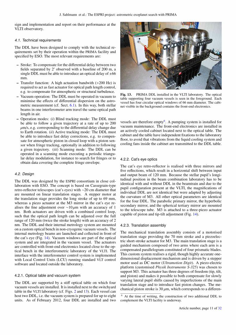
Fig. 10. The expected differential delay for HD 10360 in normal(solid curve) and swapped mode (dashed curve) over 24 hours. Red andblue symbols show the data of the demonstration run discussed below.The metrology zero point has been subtracted and is indicated by thehorizontal dashed line. The delay amplitude varies between 0-5 mm.

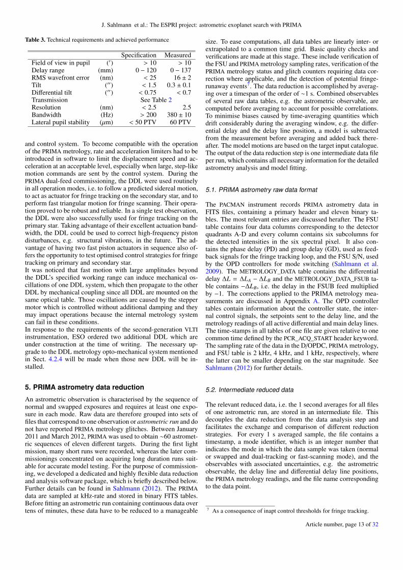
Fig. 11. IRIS H-band images of HD 66598 A (two right panels) andHD 66598 B (two left panels). The IRIS quadrant, VLTI input channelnumber, telescope, delay line, and fringe sensor are indicated at the topof each panel. The magnitude difference between the stars is ∆mH ∼ 1.8and the exposure time was 0.2 s for all IRIS quadrants. The red crossin each panel indicates the guiding pixel, i.e. the target for the imagestabilisation control loop, defined as the position of optimal alignmentwith the FSU. Because of fast atmospheric turbulence, the IP4 beamwas not well aligned at the time of exposure.

3.8.3. Instrument calibration and alignment

The only component of the PACMAN instrument that necessi-tates regular calibration are the fringe detectors (FSU). Duringthe test runs, FSUA and FSUB are calibrated daily on a ther-mal source inside the laboratory (Sahlmann et al. 2009) with the

goal of determining the photometric and spectral response of thesystem. The opto-mechanical components of the FSU are stableand require only minor re-alignments in monthly intervals due toseasonal temperature variations inside the laboratory3. To reachthe required astrometric accuracy level of 10−6, the spectral re-sponse of the PRIMA-VLTI system has to be known during theobservations and an on-sky calibration procedure has been de-vised (Sahlmann et al. 2009), but has not been commissioned atthe time of writing.The alignment of the fringe sensor as self-contained system isstable, but the co-alignment with the optical axes of the interfer-ometer can be disturbed by moving optical components duringthe day, thus it has to be verified. Before the night, both the lab-oratory guiding camera IRIS and the fringe detectors FSUA andFSUB are aligned on the beams generated by the laboratory lightsource. Because during observation the guiding camera will sta-bilise the image on the so-defined positions (the guiding pixelsshown in Fig. 11), it is guaranteed that the stellar beams are alsostabilised on the FSU. Thermal variations could disturb the co-alignment, but this alignment strategy has proven efficient duringmany observing nights and usually does not necessitate intra-night corrections.

3.8.4. Target acquisition

The first observing template handles the target acquisition. Thetelescopes are pointed and the delay lines slew to the predictedposition of zero total delay. The movable mirrors of the VLTIare configured to feed the four beams into the fringe sensor units.The integration times of the FSU and IRIS detectors are set to thevalue appropriate for the object magnitudes. When the telescopecontrol loops for image stabilisation and guiding are closed, thestellar beams are acquired with the IRIS infrared camera and thelaboratory guiding is enabled, using the STS-FSM mirror actua-tor to stabilise the PSF image for the FSU. In a similar fashion,the pupil stabilisation loop using the PRIMA metrology beamsand the STS-VCM mirror actuator is enabled. At this stage thetelescopes are guiding, the delay line and the differential delayline follow the predicted trajectories4, and the facility is ready tobegin observing.

3.8.5. Observation sequence

The start of an astrometric observation is defined by the reset ofthe PRIMA metrology fringe counters. The astrometric measure-ment relies on the uninterrupted validity of the internal differ-ential delay measured with this metrology, thus another reset orloss of it, e.g. a metrology glitch, marks the end of the usable ob-servation data. Since the metrology zero-point is unknown, it hasto be determined by a calibration step consisting of exchangingthe roles of the primary and the secondary object, i.e. the swapprocedure. The alternating observation in swapped and normalstates reduces adverse effects on the astrometry, e.g. caused bydispersion, because errors common to both states are removedand only the differential terms remain (the metrology zero pointcan be seen as such a common mode error). The PRIMA astro-metric data acquisition sequence can be broken down into con-

3 These concern the cold camera image actuators and the fibre posi-tioners at injection level.4 At VLTI, the delay compensation is done with only one delay line(or DDL) moving at the time. The other delay line (or DDLs) is keptfixed during an observation.


ceptually equal blocks, which are executed either in normal or inswapped mode in the following order:

1. Photometric calibration: sky-background, sky-flat, andcombined flat exposures are taken to calibrate the FSU(Sahlmann et al. 2009). These steps use the STS-FSM mir-rors to apply an offset from the star in order to measure e.g.the sky background level. The IRIS and FSU camera back-grounds are taken simultaneously.

2. Fringe detection scan: The actual fringe position in the pri-mary and secondary feed differ by typically less than 1 mmfrom the model prediction. To facilitate the start of fringetracking, a scan in OPD of ∼5 mm is performed with themain delay line while recording FSU data. The processingof the resulting file yields the fringe positions in delay spaceof both primary and secondary feed and an estimate of thefringe S/N in the respective feed. The OPD control loop isthen closed and fringes are tracked with the main delay line.

3. Scanning observations: While fringe tracking on the primarystar with the main delay line, a series of fast scans across thefringes of the secondary star is performed with one DDL andrecorded (typically 400 scans). The data can be used bothfor astrometry and to measure the spectral response of thePRIMA-VLTI system. The scanning observation is optionaland not always executed.

4. Tracking observations: The secondary fringe tracking loopis closed with one DDL and data is recorded in dual-fringetracking (typically 5 min of data). This represents the stan-dard astrometry data.

After these 4 steps, the swap or unswap procedure is executed,which consists of opening the fringe tracking and beam guidingloops and of turning the field by 180, thus sending the light ofstellar objects into the respective other feed. After closing thetelescope and laboratory guiding loops again, the sequence ofsteps 1.-4. is repeated. An astrometric measurement becomespossible after two sequences, i.e. when at least one observationin normal mode and one in swapped mode have been made, sincethe zero-point of the metrology can be determined. The basiccharacteristics and differences of the normal and swapped oper-ation modes are listed below:

Normal mode: FSUB is used to track the primary star fringeswith the main delay line via OPDC. FSUA is used to track thesecondary star fringes with DDL1 via DOPDC. The internaldifferential OPD is controlled with DDL1, which can be usedfor fast scanning or fringe tracking.

Swapped mode: FSUA is used to track the primary star fringeswith the main delay line via OPDC. FSUB is used to track thesecondary star fringes with DDL2 via DOPDC. The internaldifferential OPD is controlled with DDL2, which can be usedfor fast scanning or fringe tracking.

3.8.6. Hardware inadequacies affecting the instrumentperformance

All astrometric observations reported herein were obtained be-tween November 2010 and January 2012. During this time,the PRIMA -VLTI subsystems exhibited the following hardwareproblems, which did not impede astrometric observations, butsignificantly reduced the instrument performance in terms of ac-cessible stellar magnitude range and the data quality.

Optical aberrations of AT3-STS: The two stellar beams comingfrom AT3-STS suffered from optical aberrations, which an

Fig. 12. PRIMA pupils measured after the acquisition of HD 10360in swapped mode on November 19, 2011. The input channels are IP1- IP4 from left to right. While all pupils show signs of vignetting, thetwo rightmost coming from AT4 are strongly obscured.

observer can interpret as different focus positions. At thetime of writing, the optical aberrations had not been cor-rected, yet. In practice, the best focus position of an auxiliarytelescopes is found by the operator using the remote adjust-ment of the secondary mirror and the image quality as seenon IRIS. In the PRIMA case and because there is one com-mon focus actuator for both beams (the telescope secondarymirror), an intermediate focus position had to be determinedby minimising the optical aberrations of both beams appar-ent on IRIS. This is problematic because of the fast injectiondegradation with de-focus and the fast temporal change offocus position. During PRIMA observations the AT foci areadjusted approximately every 30 minutes.

Pupil vignetting of stellar beams: The shape of the PRIMApupils can be measured with a pupil camera located betweenthe switchyard and the fringe sensors. Figure 12 shows anexample taken in November 2011.

APD assembly of AT4-STS for image correction: The tip-tiltcorrection system of the VLTI auxiliary telescopes has beenupgraded by implementing a new assembly of the lenses infront of the avalanche photo diodes, resulting in improvedimage correction quality especially in good seeing condi-tions (Haguenauer et al. 2010). The AT3-STS has undergonethe upgrade, whereas AT4-STS was operating with the oldsystem, thus operating in non-optimal conditions.

FSUA fibre transmission and cold camera alignment: Duringthe integration of the FSU at the VLTI, a degraded transmis-sion of FSUA compared to FSUB was noticed (Sahlmannet al. 2009). Additionally, the cold camera alignment ofFSUA was not optimised resulting in a distorted spectralresponse function. Eventually, the fluoride glass fibreassembly of FSUA was exchanged in March 2011 andthe cold camera was aligned, which improved the camerathroughput5 and spectral response.

4. Differential delay lines for PRIMA

When observing two stars with a dual-field interferometer, thedifferential optical delay ∆w between the stellar beams has to becompensated dynamically to make the simultaneous observationof both fringe packets possible. For PRIMA, this is realised withthe differential delay lines (DDL), which were delivered by theESPRI consortium. To make the system symmetric and min-imise differential errors, there are four DDL, i.e. one per tele-scope and per star. In preparation of a potential extension ofPRIMA to operation with four telescopes, the DDL system canaccommodate up to eight DDL. A detailed description of theDDL before installation at the observatory was given by Pepeet al. (2008). Here, we present a concise overview of their de-

5 The cold camera flux loss in March 2009 was 13 % and 5 %, com-pared to 10 % and 4 % in November 2011 for FSUA and FSUB, respec-tively. The uncertainties are 1 %.



sign and implementation and report on their performance at theVLTI observatory.

4.1. Technical requirements

The DDL have been designed to comply with the technical re-quirements set by their operation within the PRIMA facility andspecified by ESO. The most relevant requirements are:

– Stroke: To compensate for the differential delay between twofields separated by 2′ observed with a baseline of 200 m, asingle DDL must be able to introduce an optical delay of ±66mm.

– Transfer function: A high actuation bandwith (>200 Hz) isrequired to act as fast actuator for optical path length control,e.g. to compensate for atmospheric or structural turbulence.

– Vacuum operation: The DDL must be operated in vacuum tominimise the effects of differential dispersion on the astro-metric measurement (cf. Sect. 6.1). In this way, both stellarbeams in one interferometer arm travel the same optical pathlength in air.

– Operation modes: (i) Blind tracking mode: The DDL mustbe able to follow a given trajectory at a rate of up to 200µm/s, e.g. corresponding to the differential delay change dueto Earth rotation. (ii) Active tracking mode: The DDL mustbe able to introduce fast delay corrections, e.g. to compen-sate for atmospheric piston in closed loop with a piston sen-sor when fringe tracking, optionally in addition to followinga given trajectory. (iii) Scanning mode: The DDL can beoperated in a scanning mode executing a periodic triangu-lar delay modulation, for instance to search for fringes or toobtain data covering the complete fringe envelope.

4.2. Design

The DDL was designed by the ESPRI consortium in close col-laboration with ESO. The concept is based on Cassegrain-typeretro-reflector telescopes (cat’s eyes) with ∼20 cm diameter thatare mounted on linear translation stages. A stepper motor atthe translation stage provides the long stroke of up to 69 mm,whereas a piezo actuator at the M3 mirror in the cat’s eye re-alises the fine adjustment over ∼10 µm with an accuracy of 1nm. Both actuators are driven with a combined control loop,such that the optical path length can be adjusted over the fullrange of 120 mm (twice the stroke length) with an accuracy of 2nm. The DDL and their internal metrology system are mountedon a custom optical bench in non-cryogenic vacuum vessels. Theinternal metrology beams are launched and collected in front ofthe cat’s eye (Fig. 14). Vacuum windows are part of the opticalsystem and are integrated in the vacuum vessel. The actuatorsare controlled with front-end electronics located close to the op-tical bench in the interferometric laboratory of the VLTI. Theinterface with the interferometer control system is implementedwith Local Control Units (LCU) running standard VLT controlsoftware and located outside the laboratory.

4.2.1. Optical table and vacuum system

The DDL are supported by a stiff optical table on which fourvacuum vessels are installed. It is installed next to the switchyardtable in the VLTI laboratory (cf. Figs. 2 and 13). Each vessel canhost two DDL, i.e. the vacuum system is prepared for up to eightunits. As of February 2012, four DDL are installed and two

Fig. 13. PRIMA DDL installed in the VLTI laboratory. The opticaltable supporting four vacuum vessels is seen in the foreground. Eachvessel has four circular optical windows of 66 mm diameter. The cabi-net visible in the background contains the front-end electronics.

vessels are therefore empty6. A pumping system is installed forvacuum maintenance. The front-end electronics are installed inan actively cooled cabinet located next to the optical table. Thecabinet and the table have independent fixations to the laboratoryfloor, to avoid that vibrations from the liquid cooling system andcooling fans inside the cabinet are transmitted to the DDL table.

4.2.2. Cat’s eye optics

The cat’s eye retro-reflector is realised with three mirrors andfive reflections, which result in a horizontal shift between inputand output beam of 120 mm. Because the stellar pupil’s longi-tudinal position in the beam combination laboratory has to beidentical with and without DDL in the beamtrain and due to thepupil configuration present at the VLTI, the magnifications ofindividual DDL are not identical but were adapted by adjustingthe curvature of M3. All other optical parameters are identicalfor the four DDL. The parabolic primary mirror, the hyperbolicsecondary mirror, and the spherical tertiary mirror are mountedto the telescope tube. M3 is attached to a three-piezo actuatorcapable of piston and tip-tilt adjustment (Fig. 14).

4.2.3. Translation assembly

The mechanical translation assembly consists of a motorisedtranslation stage providing the 70 mm stroke and a piezoelec-tric short-stroke actuator for M3. The main translation stage is aguided mechanism composed of two arms where each arm is acompensated parallelogram constituted of four prismatic blades.This custom system realises a rigid, though highly accurate one-dimensional displacement mechanism and is driven by a steppermotor used as DC motor (Ultramotion Digit). A piezo-electricplatform (customised Physik Instrumente S-325) was chosen tosupport M3. This actuator has three degrees of freedom (tip, tilt,and piston) and makes it possible to both compensate for slowlyvarying lateral pupil shifts caused by imperfections of the maintranslation stage and to introduce fast piston changes. The me-chanical piston stroke is 30 µm, which corresponds to a differen-6 At the time of writing, the construction of two additional DDL tocomplement the VLTI facility is underway.


Fig. 14. Schematic and longitudinal section of two DDL. The transla-tion stage supporting the optics is visible below the telescope tubes. TheM3 mirror is mounted on a fast piston and tip-tilt piezo actuator. Stellarbeams are shown in yellow and internal metrology beams are red.

tial optical stroke of ±30µm, and the mechanical tip/tilt range is±4 milli-rad.

4.2.4. Internal metrology

The purpose of the internal metrology is to measure the instan-taneous optical position of the DDL, thus the optical delay in-troduced in the stellar beam. The system is based on commer-cially available technology for displacement measurement (Ag-ilent), which is also used in the main delay lines. Each singleDDL has its own metrology receiver such that its position can bemeasured independently. A folding mirror directs the metrologylaser beam into the vacuum vessel where it is split in two beams,one for each of the two DDL enclosed in the vessel. Each beamfeeds a Mach-Zehnder type interferometer, whose interferencesignals are detected with optical receivers. The front-end elec-tronics convert optical to electric signals and the back-end elec-tronics (VME boards) compute the interferometric phase witha resolution of 2π/256, corresponding to an OPD resolution of2.47 nm.After several months of operation at the observatory, opto-mechanical drifts were detected in the metrology system whichmade regular alignment necessary. Consequently, a slightlymodified design leading to a more robust system has been de-vised and will replace the current system in 2013.

4.2.5. Instrument and translation control

The instrument control hardware is composed of VLT standardcomponents and the software complies with the VLT commonsoftware package for instrumentation. The real-time control al-gorithms are coded in the ESO software architecture TAC (toolsfor advanced control). To achieve optimal control of the two-stage system composed of the piezo actuator and the motor, theirrespective controllers are interfaced by an ’observer’. In thisway, a non-degenerate closed loop control system is realised,where the feedback is given by the laser metrology measure-ment. The first resonance of the motorised translation occurs at

∼100 Hz. Because this stage does not need to be very fast, weavoid excitation of this mode by limiting the bandwidth of themotor stage to .10 Hz and by low-pass filtering the referencefed to the motor controller. The motorised stage therefore off-loads the piezo at low frequency. Because the mirror attached tothe piezo-electric stage is very light (∼3.5 g), the amplifier (PI E-509) and the input capacitance of the piezo itself are determinantfor the system bandwidth.

4.3. Laboratory performance

The DDL system was thoroughly tested before delivery to theobservatory to confirm that it complies with the technical re-quirements and the detailed optical performance is reported inPepe et al. (2008). We therefore briefly summarise the mostimportant values: The throughput of the DDL’s optical systemcomposed of cat’s eyes and windows is shown in Table 2. Thetransfer function of the DDL is shown in Fig. 15. The responsesof the single DDL units were made to match by tuning their con-trol parameters and the actuation bandwidth is 380± 10 Hz witha quality factor of ∼0.7. This setup was chosen for increasedrobustness, but can further be tuned if the operation conditionsat the observatory make it necessary. The maximum velocity

3025201510

505

Gain

(dB

)

100 101 102 103

Frequency (Hz)

300250200150100

500

Phase

(deg)

Fig. 15. DDL transfer function gain (top) and phase (bottom) as afunction of frequency. Different colours identify the four DDL units.The dashed line in the top panel indicates the −3 dB threshold.

of the DDL is 5.38 ± 0.01 mm/s. A summary of the achievedperformance is given in Table 3.

4.4. Performance at the observatory

After integration at the VLTI, it was verified that the DDL instand-alone operation comply with the performance establishedin the laboratory in Europe. Thereafter they were introduced andcommissioned as a part of the interferometer opto-mechanical

Table 2. Total optical transmittance of the DDL system

Bandpass Transmittancea

(µm) Requirement Windows (2×) Cat’s eye Total0.6 − 1.0 0.60 − 0.80 0.86 0.80 0.691.0 − 2.0 > 0.80 0.93 0.90 0.842.0 − 2.5 > 0.85 0.93 0.93 0.862.5 − 28 > 0.90 (no windows) 0.91 0.91

1.319 > 0.80 0.99 0.90 0.89

Notes. (a) Theoretical throughputs are calculated from the transmittancecurves of individual components provided by the manufacturers.



Table 3. Technical requirements and achieved performance

Specification MeasuredField of view in pupil (′) > 10 > 10Delay range (mm) 0 − 120 0 − 137RMS wavefront error (nm) < 25 16 ± 2Tilt (′′) < 1.5 0.3 ± 0.1Differential tilt (′′) < 0.75 < 0.7Transmission See Table 2Resolution (nm) < 2.5 2.5Bandwidth (Hz) > 200 380 ± 10Lateral pupil stability (µm) < 50 PTV 60 PTV

and control system. To become compatible with the operationof the PRIMA metrology, rate and acceleration limiters had to beintroduced in software to limit the displacement speed and ac-celeration at an acceptable level, especially when large, step-likemotion commands are sent by the control system. During thePRIMA dual-feed commissioning, the DDL were used routinelyin all operation modes, i.e. to follow a predicted sidereal motion,to act as actuator for fringe tracking on the secondary star, and toperform fast triangular motion for fringe scanning. Their opera-tion proved to be robust and reliable. In a single test observation,the DDL were also successfully used for fringe tracking on theprimary star. Taking advantage of their excellent actuation band-width, the DDL could be used to correct high-frequency pistondisturbances, e.g. structural vibrations, in the future. The ad-vantage of having two fast piston actuators in sequence also of-fers the opportunity to test optimised control strategies for fringetracking on primary and secondary star.It was noticed that fast motion with large amplitudes beyondthe DDL’s specified working range can induce mechanical os-cillations of one DDL system, which then propagate to the otherDDL by mechanical coupling since all DDL are mounted on thesame optical table. Those oscillations are caused by the steppermotor which is controlled without additional damping and theymay impact operations because the internal metrology systemcan fail in these conditions.In response to the requirements of the second-generation VLTIinstrumentation, ESO ordered two additional DDL which areunder construction at the time of writing. The necessary up-grade to the DDL metrology opto-mechanical system mentionedin Sect. 4.2.4 will be made when those new DDL will be in-stalled.

5. PRIMA astrometry data reduction

An astrometric observation is characterised by the sequence ofnormal and swapped exposures and requires at least one expo-sure in each mode. Raw data are therefore grouped into sets offiles that correspond to one observation or astrometric run and donot have reported PRIMA metrology glitches. Between January2011 and March 2012, PRIMA was used to obtain ∼60 astromet-ric sequences of eleven different targets. During the first lightmission, many short runs were recorded, whereas the later com-missionings concentrated on acquiring long duration runs suit-able for accurate model testing. For the purpose of commission-ing, we developed a dedicated and highly flexible data reductionand analysis software package, which is briefly described below.Further details can be found in Sahlmann (2012). The PRIMAdata are sampled at kHz-rate and stored in binary FITS tables.Before fitting an astrometric run containing continuous data overtens of minutes, these data have to be reduced to a manageable

size. To ease computations, all data tables are linearly inter- orextrapolated to a common time grid. Basic quality checks andverifications are made at this stage. These include verification ofthe FSU and PRIMA metrology sampling rates, verification of thePRIMA metrology status and glitch counters requiring data cor-rection where applicable, and the detection of potential fringe-runaway events7. The data reduction is accomplished by averag-ing over a timespan of the order of ∼1 s. Combined observablesof several raw data tables, e.g. the astrometric observable, arecomputed before averaging to account for possible correlations.To minimise biases caused by time-averaging quantities whichdrift considerably during the averaging window, e.g. the differ-ential delay and the delay line position, a model is subtractedfrom the measurement before averaging and added back there-after. The model motions are based on the target input catalogue.The output of the data reduction step is one intermediate data fileper run, which contains all necessary information for the detailedastrometry analysis and model fitting.

5.1. PRIMA astrometry raw data format

The PACMAN instrument records PRIMA astrometry data inFITS files, containing a primary header and eleven binary ta-bles. The most relevant entries are discussed herafter. The FSUtable contains four data columns corresponding to the detectorquadrants A-D and every column contains six subcolumns forthe detected intensities in the six spectral pixel. It also con-tains the phase delay (PD) and group delay (GD), used as feed-back signals for the fringe tracking loop, and the FSU S/N, usedby the OPD controllers for mode switching (Sahlmann et al.2009). The METROLOGY_DATA table contains the differentialdelay ∆L = ∆LA − ∆LB and the METROLOGY_DATA_FSUB ta-ble contains −∆LB, i.e. the delay in the FSUB feed multipliedby −1. The corrections applied to the PRIMA metrology mea-surements are discussed in Appendix A. The OPD controllertables contain information about the controller state, the inter-nal control signals, the setpoints sent to the delay line, and themetrology readings of all active differential and main delay lines.The time-stamps in all tables of one file are given relative to onecommon time defined by the PCR_ACQ_START header keyword.The sampling rate of the data in the D/OPDC, PRIMA metrology,and FSU table is 2 kHz, 4 kHz, and 1 kHz, respectively, wherethe latter can be smaller depending on the star magnitude. SeeSahlmann (2012) for further details.

5.2. Intermediate reduced data

The relevant reduced data, i.e. the 1 second averages for all filesof one astrometric run, are stored in an intermediate file. Thisdecouples the data reduction from the data analysis step andfacilitates the exchange and comparison of different reductionstrategies. For every 1 s averaged sample, the file contains atimestamp, a mode identifier, which is an integer number thatindicates the mode in which the data sample was taken (normalor swapped and dual-tracking or fast-scanning mode), and theobservables with associated uncertainties, e.g. the astrometricobservable, the delay line and differential delay line positions,the PRIMA metrology readings, and the file name correspondingto the data point.

7 As a consequence of inapt control thresholds for fringe tracking.


5.3. Dual fringe tracking data

Tracking files are named PACMAN_OBJ_ASTRO[...] and containdual-feed fringe tracking data. For the reduction, only samplesin dual fringe tracking are kept and this criterion is based on thecontroller states of OPDC and DOPDC, both required to be ’7’.The astrometric observable AXobs is a linear combination of thedifferential delay ∆L measured with the PRIMA metrology, thegroup delay GDA of FSUA, and the group delay GDB of FSUB,directly taken from the respective binary tables:

AXobs = ∆L −GDA −GDB, (23)

where the signs have been determined empirically. Figure C.3of the appendix shows an example of this first analysis step.Equation 23 is sufficient for a first performance evaluation ofthe astrometric instrument. In the future, it could be improvedfor instance by considering the phase delay, which has lowernoise compared to the group delay but has to be corrected fordispersion, and/or by implementing an optimised group delay al-gorithm. For the science-grade data reduction, it is envisaged toaccount for the near real-time spectral response of the beamtrainand to obtain optimal and unbiased estimators for the astrometricobservable on the basis of the raw pixel counts.

5.4. Scanning data

Scanning files are named PACMAN_OBJ_SCAN[...]8 and containdata taken while fringe tracking on the primary and performingfast fringe scans on the secondary feed using a DDL. The basicreduction is slightly more complex than for the tracking data andit involves the following steps: (1) Scan identification and dataassociation. (2) Interpolation on a regular OPD grid and fluxnormalisation. (3) Computation of the wavelet transform (Tor-rence & Compo 1998)9 for fringe localisation. (4) Eliminationof low-quality scans based on S/N and primary fringe trackingquality criteria. The astrometric observable is now given by

AXobs = ∆Lw −GDtrack, (24)

where ∆Lw is the PRIMA metrology value at the secondary’sfringe position determined with the wavelet method and GDtrackis the average group delay of the primary measured by the track-ing FSU during the scan.In the simplest implementation, the wavelet method is applied tothe two white-light flux differences A–C and B–D, both pairs areclose to phase-opposition, and the final fringe position is a com-bination of both results. Figures 16 and 17 illustrate the reduc-tion procedure. The above algorithm is sufficient for a first per-formance evaluation and proved that astrometric data obtained indual tracking or fringe scanning mode are equivalent at the µm-level, see e.g. Fig. 28, with the scanning data having a slightlyhigher noise. The scanning data are rich in information aboutthe photometric fluctuations during the observations, the instan-taneous phase-shifts and effective wavelengths of the FSU quad-rants or pixels, and the dispersion effects on the fringe packet,which we have started to characterise.

8 The filenames PACMAN_OBJ_SPECTRUM[...] andPACMAN_SKY_VLTIRESPONSE[...] contain equivalent data butwere taken with a different template to obtain the star’s spectrum andthe interferometer’s spectral response, respectively.9 A modified version of the code available at http://paos.colorado.edu/research/wavelets/ was used.

−10

0

10

Inte

nsity

(A

DU

)

PACMAN_OBJ_SCAN_330_0003

Per

iod

(µm

) 1.5

2

2.5

3Power

0 50 100 150 200 2500

200

400

OPD (µm)

Avg

var

ianc

e

Fig. 16. Illustration of the wavelet analysis. Top: The time se-ries showing the fringe signal (here A-C in white light). Middle: Thecontour plot shows the fringe localisation by the wavelet transform inboth delay and frequency space. Only data between the two horizontaldashed lines are considered. Bottom: Projection of the wavelet powerin the time domain. Right: Projection of the wavelet power in the fre-quency domain.

PACMAN_OBJ_SCAN_330_0003 FSU SNR

Sca

n nu

mbe

r

OPD (µm)−100 −80 −60 −40 −20 0 20 40 60 80 100

50

100

150

200

250

300

350

Fig. 17. Raw S/N delivered by the FSU in the scanning channel asa function of differential delay (measured with the PRIMA metrology)and scan number shown on the vertical axis. A loss of lock on theprimary fringe tracking occurs at the scan 220.

6. PRIMA astrometry data modelling

We describe the data analysis principles that are applied to char-acterise the observations and eventually lead to the astrometricmeasurement of the target pair’s separation. We first discuss themodelling of the main delay, before proceeding to the differen-tial delay fitting. With the help of one observation sequence, weillustrate the individual steps of the data analysis up to the fit ofa separation vector. Error bars are usually derived from MonteCarlo simulations. Three binary stars play an important role inthe initial system characterisation and are therefore presented inTable C.3 and briefly discussed below.

– HD 202730 is separated by 7′′ from the secondary GJ 9733B. The separation change measured over 150 years is wellapproximated with a linear motion and this binary is includedin the Catalog of Rectilinear Elements.

– HD 10360 is separated by 11′′ from the secondary HD10361. Both stars are very bright in K-band and have nearlyequal masses (Takeda et al. 2007). This visual binary showsconsiderable orbital motion over the available separationmeasurements of 200 years and an orbital solution was given


http://paos.colorado.edu/research/wavelets/

http://paos.colorado.edu/research/wavelets/

http://www.usno.navy.mil/USNO/astrometry/optical-IR-prod/wds/lin1


N

E

PΦ

∆δρ

S∆α⋆

Fig. 18. The target pair separation ρ and position angle Φ definethe relative position of the secondary star S and primary star P. Theseparation vector points towards S and has the rectangular components∆α? and ∆δ. North is up and East is left.

by van Albada (1957). This is the pair observed during therun used for illustration below.

– HD 66598 is separated by 36′′ from the secondary HD 66598B. So far, it is the widest pair observed with PRIMA. Asindicated by the available measurements in the literature, thisbinary does not exhibit a significant separation change overthe last 100 years.

6.1. Correction of atmospheric refraction and main delayfitting

The VLTI-internal main delay is introduced by the main delaylines and the effect of the Earth rotation makes it a dynamicquantity. We have access to two measurements of its value,one is the internal metrology of the main delay line (Helium-Neon laser, λDL ∼ 633 nm) and the other is the FSUB arm ofthe PRIMA metrology named PRIMETB (Nd:YAG laser, λP ∼

1319 nm), which in addition to the tunnel measures the opticalpath within the laboratory and the light ducts up to the retro-reflectors inside the star separators of the auxiliary telescopes(Fig. 2). Both have to be corrected for atmospheric refraction.For astrometric interferometry, the following terms related tochromatic and achromatric refraction have to be considered:

1. Correction of laser metrology measurements: The purposeof a metrology system is to measure the optical path lengthbetween its endpoints. Usually, the vacuum laser wavelengthis known and used to convert phases to delays. If air-filledbeam trains are used, the effective laser wavelength is alteredand the delays have to be corrected for the refractive indexrepresentative of the air inside the interferometer.

2. Effect of wavelength difference between stellar and metrol-ogy beams: If the stellar and metrology bandpasses are notidentical, the chromaticity of the refractive index creates amismatch between the optical path difference experienced bythe stellar beam and the one determined with the metrology.

3. Atmospheric refraction: For conventional imaging instru-ments, atmospheric refraction results in an offset betweenthe true source vector s0 and the apparent, refracted sourcevector s (e.g. Gubler & Tytler 1998). In the case of an in-terferometer, the first order term of this effect is removed ifeither vacuum delay lines are used or if the effects 1. and2. are accurately corrected. This is because the geometricpath difference GPD is equal to the vacuum optical pathdifference B · s0 occurring outside the atmosphere, wheren = 1, and it is equal to the external optical path differencen1,FSU B · s experienced within the atmosphere of refractiveindex n1,FSU, where the second subscript indicates that theindex is computed for the bandpass accepted by the instru-ment (e.g. Daigne & Lestrade 2003). To observe fringes,

it is compensated by an optical path difference n2,FSU D in-ternal to the interferometer, where D is the internal vacuumdelay. The laser metrology system measures the internal op-tical path difference L = n2,MET D, where n2,MET is taken atthe metrology wavelength and is determined by the atmo-sphere at the delay lines, cf. Fig. 19. It follows that

GPD = B · s0 = n1,FSU B · s = n2,FSU D =n2,FSU

n2,METL, (25)

where n1 and n2 are determined for the detected stellar band-pass and the metrology wavelength, respectively, with thelocal atmospheric parameters. Note that the angle of s de-pends on n1 through Snell’s law. If the delay lines are evac-uated, n2 = 1 and B · s0 = L. Second order terms appearfor instance because the zenith direction is different for twoseparated telescopes (Mozurkewich et al. 1988) and due tothe elongation of the stellar images by chromatic refractionacross the bandpass.

Laboratory

Vacuum

Atmosphere~s · ~B

n = n2

~s0 · ~B~s0

L/2

~B

~s

n = 1

n = n1

Fig. 19. Schematic of an interferometer with baseline B observing asource at true position s0 through a plan-parallel atmosphere of refrac-tive index n1.

4. Dispersion effects due to chromatic refraction: When the ex-ternal vacuum delay is compensated in air, the chromatic de-pendence of the index of refraction distorts the fringe packetand reduces fringe visibility (Tango 1990). Depending onhow the astrometric measurement is performed, biases canoccur.

The first two effects are usually dominant and are discussed here.A couple of remarks are appropriate to underline the particulari-ties of PRIMA-VLTI:

– The vacuum wavelengths of all delay line metrology systems(Model Agilent 5519-A) are identical λDL,vac = 632.991354nm and are supposed to be stable within 2 · 10−8. However,the VLTI control system was implemented such that a modi-fied wavelength λDL,mod = 632.863000 nm is applied instead,presumably to account for an ’average’ refraction.

– The PRIMA metrology ∆LB in the B feed (PRIMETB) has tobe corrected for refraction in the infrared. It is measuringat ∼1.3 µm and the accepted stellar bandpass is centred at∼2.25 µm.

– Conversely, the differential value ∆L does not need to becorrected, because the differential delay is introduced by theDDL that are under vacuum. The same applies to the delayvalue of the DDL internal metrology. This assumes that any


0

10

20

30O

PD

(m

)MAIN Delays AXrun 3−12

DL FDBKPRIMETB

−0.5 0 0.5 1 1.5 2 2.5 3

−2

−1

0

1

Diff

. (m

m)

Hour angle (h)

Fig. 20. Internal delay corrected for refraction measured with delayline and PRIMA metrologies (top) and their difference (bottom), whichis shown in red and blue for normal and swapped mode data, respec-tively.

effect on ∆L caused by gradients of temperature, pressure,and humidity between the two interferometer feeds outsideof the DDL vacuum vessels can be neglected.

The refraction terms are calculated with the formulae of Birch &Downs (1993) and Mathar (2007) for visible and infrared wave-lengths, respectively. We assumed dry air, i.e. neglected any de-pendence on humidity. Pressure and temperature readings wereextracted from the file headers and we assumed that the pres-sure is global and given by the observatory monitoring system.There are considerable temperature gradients within the facil-ity, which typically amount to ∼1 K along the tunnel and up to∼4 K between ambient and inside the laboratory, depending onthe season. Temperature variations during an observation areusually much smaller than the gradient. Refraction terms werecomputed for each file separately, but only the global averageover the tunnel having four temperature sensors was used to es-timate nDL. For the terms applied to the PRIMA metrology andfor the instrument bandpass, we used the global average obtainedwith nine temperature sensors between the outside and the labo-ratory, and we made the approximation nFSU = n1,FSU ≈ n2,FSU.Table C.2 lists the calculated refractive index at the prominentwavelengths, e.g. nDL = 1 + 2.025 · 10−4. Because the delay linesystem does not apply the vacuum wavelength, three correctionsare necessary to convert the delivered metrology value ΩDL intothe corrected value Ω′DL

Ω′DL =ρmod

nDLΩDL nFSU =

ΩDL

n′nFSU, (26)

where ρmod = λDL,vac/λDL,mod = 1 + 2.028 · 10−4. Similarly weget

∆L′B =∆LB

nPnFSU. (27)

Figures 20 and 21 show both corrected measurements and theirdifference, which is very small in normal mode. The variableoffset in swapped mode appears because PRIMETB sees the dif-ferential delay introduced by the DDL in swapped mode. Toquantify the agreement between both measurements in normalmode, we determined an average mismatch factor ncorr by ad-justing the linear model

∆L′B = γcorr + ncorr Ω′DL, (28)

where γcorr is an offset. The value of ncorr − 1 is smaller than 1 ·10−6 and comparable to the uncertainties in the applied refractionindices of Table C.2, thus validating our approach.

0

10

20

PR

IME

TB

(m

)

DLFDBK wavelength AXrun 3−12

−0.5 0 0.5 1 1.5 2

−10

0

10

O−

C (

µm)

Hour angle (h)

Fig. 21. PRIMETB internal delay (top) and the residuals after fittingthe delay line delays to it (bottom) using the model Eq. 28.

Table 4. Targets used for baseline calibration

Nr. Target RA DEC(h:m:s) (d:m:s)

1 HIP 14146 03 02 23.50 -23 37 28.102 HIP 20384 04 21 53.33 -63 23 11.013 HIP 22449 04 49 50.41 +06 57 40.604 HIP 24659 05 17 29.09 -34 53 42.745 HIP 34088 07 04 06.53 +20 34 13.086 HIP 36795 07 34 03.18 -22 17 45.847 HIP 50799 10 22 19.58 -41 38 59.868 HIP 50954 10 24 23.71 -74 01 53.809 HIP 56647 11 36 56.93 -00 49 25.49

6.2. Determination of the wide-angle baseline

The relationship Eq. 14 shows that the interferometric delay de-pends on both the target’s position in the sky and on the wide-angle baseline vector B. An astrometric measurement on the ba-sis of a measured delay is thus possible if the baseline is known.In most cases, a simultaneous adjustment of both target coordi-nates and baseline is prohibited by the degeneracy of the modelfunction. Consequently, the strategy consists of determining thebaseline from a dedicated set of observations and to assume thatthe baseline calibration remains valid for the astrometric obser-vations obtained thereafter. The principle of the baseline cali-bration is to observe a set of stars with accurately known co-ordinates and distributed over a preferably large sky-area. Foreach star, the internal delay corresponding to the fringe positionis recorded. Thus, the corresponding system of equations 14 canbe solved for four unknowns: a global zero-point and the threecomponents of the baseline vector. Currently, the only VLTI sys-tem capable of precisely measuring the internal delay is the delayline metrology, because the PRIMETB zero-point is not tied to aphysical reference10.During the night of November 21, 2011, the observations for abaseline model were collected. The stars were chosen from theFK6 catalogue (Wielen et al. 1999) based on their K-magnitude,observability, and sky distribution, which is constrained by thedelay line limits as shown in Fig. 8. Since these stars usuallyare single, a fake secondary star at +8′′ in right ascension wasconsidered for each observation. The telescopes thus pointedat 4′′ from the target. To investigate the baseline in normal

10 The zero-point of the main delay line metrology is defined for eachnight by a mechanical reference in the tunnel. A similar procedure isimaginable for the PRIMA metrology in the future.



E

N

W

S

10

30

45

60

Fig. 22. Orientation and zenith angle of the nine observed stars.

−60

−40

−20

0

Del

ay (

m)

Baseline calibration ALL

0 2 4 6 8

−100

0

100

Time (h)

O−

C (

µm)

Fig. 23. Top: The measured delays, where normal mode data is shownin red, swapped mode data is shown in blue. Bottom: Residuals of thebaseline fit as a function of time and their distribution. The RMS is 46µm.

and swapped mode, each target was observed in both modes.Note that the measurements in normal mode yield the wide-angle baseline BB,Wide of the FSUB feed, whereas the swappedmode data determine a modified wide-angle baseline B′A,Wide ofthe FSUA feed, because the derotator is not in the nominal po-sition. Nine stars were observed and are listed in Table 4. Theaccurate instantaneous coordinates were computed accountingfor proper motion correction, precession, and nutation, using theparameters of the FK6 catalogue.Three different datasets were modelled. In the first case all datain both modes were considered, whereas in the second and thirdcase only data in normal or swapped mode were used, respec-tively. When doing the combined model, the model functionEq. 14 has to account for an additional parameter which is theinternal DOPD ∆int which offsets the delay between normal andswapped states (see Sect. 6.1):

ΩDL

n′nFSU = BWide · s0 + B0 +HS ∆int, (29)

where ΩDL is the delay line metrology measurement, n′ and nFSUare the wavelength-dependent refraction terms introduced in theprevious section, BWide in the ’average’ wide-angle baseline ofboth normal and swapped configuration, B0 is a constant internaldelay, andHS is the Heaviside-type function

HS =

0 in normal mode1 in swapped mode (30)

for the swapped mode. Thus the model for the baseline fit of alldata combined has 5 parameters: BX , BY , BZ , B0, and ∆int, where

the offsets B0 and ∆int are assumed constant over the night. Forthe actual data, the refraction terms n′ − 1 and nFSU − 1 were ofthe order of (1 ± 0.4) · 10−6 and (1.997 ± 0.007) · 10−4, respec-tively. The result of the global fit to all data is shown in Fig. 23.Over the 9-hour timespan of the observations, the atmosphereappears to introduce an OPD variation of ∼ 250 µm peak-to-valley. The residual’s RMS after the 5-parameter fit is 46 µm.At first sight, no obvious systematics or correlations with ele-vation, azimuth angle, hour angle, or stellar coordinates can beidentified. It rather appears like the apparent structure is causedby slowly varying atmospheric parameters with the effect thatthe residual’s distribution does not resemble a Gaussian curve.Normal and swapped data were also separately adjusted with a4-parameter model. The resulting graphs are shown in Fig. 24and reveal that the fit quality is comparably poor in both cases,presumably due to atmospheric turbulence.

Table 5. Baseline fit results. Numbers in brackets indicate the MonteCarlo derived errors in the last significant digit (here µm).

ALL NORMAL SWAPPED(m) (m) (m)

BWide BB,Wide B′A,WideB0 −60.920729 (59) −60.920707 (59) −60.920536 (98)Bx 76.387823 (42) 76.387792 (35) 76.387839 (70)By −49.877600 (24) −49.877595 (12) −49.877606 (52)Bz −0.017542 (62) −0.017527 (62) −0.017533 (105)∆int 0.000193 (15) . . . . . .RMS 0.000045 0.000038 0.000050

Tables 5 and 6 summarise the results. Formal error bars wereobtained from Monte Carlo simulations and some parameters arestrongly correlated (e.g. B0 and Bz). The internal DOPD appearshere in the difference between B0 in normal and swapped. Weconclude that the differences between the average, the normal,and the swapped baseline are not significant and that the formaluncertainties are compatible with the requirement in Sect. 3.1.We will use the baseline BWide obtained from the combined datain all of the following analysis, i.e. as wide-angle baseline and asapproximation of the narrow-angle baseline, which is only validas zeroth order approximation.

Table 6. Baseline fit results: differences between normal and swappedmode data.

NORM – SWAP ALL – NORM ALL – SWAP(µm) (µm) (µm)

B0 −173± 115 −22± 85 −195± 116Bx −47± 78 30± 55 −16± 82By 11± 53 −5± 27 6± 57Bz 4± 121 −13± 88 −8± 123

6.3. Fitting the main delay line feedback

Assuming the baseline is known, the main delay ΩDL measuredwith the main delay line internal metrology during an astrometricobservation can be used to determine the position of the primarystar11. The corresponding model has four free parameters: anoffset γDL, the primary star coordinates in RA αP and DEC δP,and an internal DOPD ∆int. The internal DOPD corresponds tothe difference of zero-OPD positions of FSUA and FSUB, which

11 We neglect any effect related to the off-axis pointing by ρ/2 of thetelescope.


0 2 4 6 8

−100

−50

0

50

100

Time (h)

O−

C (

µm)

Baseline calibration NORMAL

0 1 2 3 4 5−100

−50

0

50

100

Time (h)

O−

C (

µm)

Baseline calibration SWAPPED

Fig. 24. Top: Residuals of the baseline fit to normal mode data only.The RMS is 38 µm. Bottom: The same for swapped mode only. TheRMS is 50 µm.

Table 7. Results of main delay fitting

Parameter Unit DL feedback PRIMETBγDL (m) −12.36546 ± 0.00002 . . .γPB (m) . . . 32.27081 ± 0.00002∆αP (′′) −0.42 ± 0.05 −1.25 ± 0.09∆δP (′′) −0.40 ± 0.02 −0.20 ± 0.03∆int (mm) −0.123 ± 0.001 . . .% (′′) . . . 11.445 ± 0.013Φ (deg) . . . 188.00 ± 0.04

in principle is arbitrary, because the VLTI does not provide theinstruments with a common OPD reference. We have to take itinto account, because we model combined normal and swappedobservations and ∆int is added to the DL position in one modebut not in the other. We assume ∆int is constant in time andarbitrarily assigned it to the swapped observation.

Ω′DL = γDL + w(αP, δP) +HS ∆int, (31)

where w models the OPD (Eq. 12). The baseline is assumedto be BWide determined in Sect. 6.2. The fit result is shown inFig. 25 and summarised in Table 7. The table lists coordinateoffsets ∆αP and ∆δP instead of absolute coordinates. These off-sets are computed relative to the instantaneous target position,after proper motion and precession correction. The fit residu-als show the atmospheric piston effect, which introduces varia-tions of typically ±50 µm with an RMS of 24.0 µm. The largervariations of ±90 µm at large hour angle > 2.5 h correspond toobservations at high airmass of 1.35− 1.45. Atmospheric condi-tions were stable with an average coherence time of τ0 ∼ 1.8 msand seeing of ∼1.2′′, as reported by the observatory monitoringsystem measuring in the optical.

6.4. Fitting the PRIMETB main delay

The PRIMETB delay ∆LB is modelled similarly to the main de-lay line OPD, but the model function is slightly different. Theinternal DOPD ∆int does not have to be modelled, because it istransparent to PRIMETB, see Fig. 2: in normal mode, ∆int is com-pensated by the differential delay actuator DDL1, which is not

−40

−30

−20

OP

D (

m)

DLFDBK delay AXrun 3−12

−0.5 0 0.5 1 1.5 2 2.5 3

−50

0

50

100

O−

C (

µm)

Hour angle (h)

Fig. 25. Top: Main delay measured with the DL metrology duringthe demonstration run. Bottom: Residuals after adjusting the modelEq. 31 including offsets to the primary coordinates. The atmosphericperturbations are visible and have a total RMS of 24.0 µm.

0

10

20

30

OP

D (

m)

PRIMETB delay AXrun 3−12

−0.5 0 0.5 1 1.5 2 2.5 3

−50

0

50

O−

C (

µm)

Hour angle (h)

Fig. 26. Top: Change of PRIMETB during the observation for Run 9.Bottom: Residuals after adjusting the model Eq. 32. The residual RMSis 23.1 µm.

seen by PRIMETB. In swapped mode, ∆int is introduced by boththe tracking DL (seen by PRIMETB) and by the differential de-lay actuator DDL2 (also seen by PRIMETB) and the net effecton PRIMETB is therefore zero. However, PRIMETB measuresthe differential delay introduced by DDL2 in swapped mode tocompensate for the external differential delay. Thus, we can usePRIMETB to obtain a first estimate of the pair separation % andposition angle Φ. The complete model function is

∆L′B = γPB + w(αP, δP) +HS ∆w(αP, δP, %,Φ), (32)

where γPB is an offset and ∆w models the differential delay(Eq. 9). The results are summarised in Table 7 and Fig. 26 showsthe fit residuals. The best fit coordinate offsets agree with theresults of the main delay line fit in the previous section within0.8′′ in RA and within 0.2′′ in DEC. The separation fit yieldsfirst realistic estimates of % and Φ.

6.4.1. Comparison of the residuals when fitting PRIMETBand main delay

Ideally, the residuals shown in Fig. 25 and 26 should be identi-cal, but in practice we expect differences because the monitoredoptical path is not the same: PRIMETB propagates in the cen-tral obscuration of the stellar beams from the beam combiner tothe retroreflector at the telescope, whereas the delay line metrol-ogy measures only within the DL tunnel. Additionally, the laser



wavelengths are different with PRIMETB in the near infrared(∼ 1.3 µm) and the delay line in the visible (∼ 0.6 µm). Fig-ure 27 shows the residual difference and reveals variations of theorder of 20 µm PTV with an RMS of 6.4 µm. This residual dif-ference could be caused by the atmospheric turbulence presentin the beam-path not common to the two metrology systems, i.e.in the beam combination laboratory or between the delay linetunnel and the telescopes. Fluctuations in temperature, pressure,and humidity during the observation and the associated chro-matic variations of the refractive index of air can also contributeto the observed turbulence.

−0.5 0 0.5 1 1.5 2 2.5 3

−15

−10

−5

0

5

10

Residuals DL − PRIMETB AXrun 3−12

Res

idua

l diff

eren

ce (µ

m)

Hour angle (h)

Fig. 27. Difference between the residuals measured in Fig. 25. Theresidual RMS is 4.2 µm.

6.5. Astrometry fit of a separation vector

The astrometric observable AXobs is a linear combination of thedifferential delay measured with the PRIMA metrology and thetwo fringe positions of primary and secondary object measuredwith the two fringe sensors. The model function for the relativeastrometry fit isAXobs = ∆L −GDA −GDB

= c +HN ∆w(%,Φ,BAX) +HS ∆w(%,Φ,−BAX), (33)where BAX is the narrow-angle astrometric baseline vector andHN is the Heaviside-type function

HN =

1 in normal mode0 in swapped mode (34)

for the normal mode. The constant c is the PRIMA metrologyzero-point, which depends on the interferometer configurationat the last metrology fringe counter reset. In this description,the swapped observation corresponds to an observation with in-verted baseline orientation compared to the normal mode. Weinitially make the coarse approximation that BAX = BWide, thusthe three free parameters in the model Eq. 33 are the metrologyzero point c, the target separation %, and the position angle Φ asdefined in Fig. 18. Figure 28 shows the result of the astrometryfit and the corresponding best-fit parameter values are listed inTable 8. The errors given in Table 8 reflect the precision of themeasurement, but not its accuracy. As is shown in Fig. 28, themodel Eq. 33 does not reproduce the data accurately, because thefit residuals exhibit strong systematics. The accuracy is thereforenot limited by the measurement precision on the astrometric ob-servable, but by a systematic effect that is not taken into accountin the model. On this target with ∼11′′ separation, the RMS ofthe residuals is of the order of 1 µm and corresponds to ∼2 mason the sky for a 100 m baseline.

Table 8. Astrometry fit results for the demonstration run on HD 10360.

Parameter Unit Valuec (mm) −1.34971 ± 0.00002% (mas) 11434.53 ± 0.15Φ () −172.1640 ± 0.0007σAX (µm) 1.025

6.6. Auxiliary data of critical elements

The anticipated astrometric accuracy sets tight requirements onthe alignment and stability of the VLTI-PRIMA optical train.Whereas thermal drifts of passive mirrors are difficult to mon-itor, the information about the instantaneous configuration ofcontrollable mirrors can be recorded during the observation forposterior inspection. Basic information about moving systemsis included in the file header keywords, i.e. at relatively low ca-dence. For the commissioning, a low-level recording tool wasdevised to collect data at higher cadence and continuously. Asan example, the motion of the derotator is discussed below, but adetailed presentation of other available data and their character-istics is given in Sahlmann (2012).Figure C.4 shows the position angle of the derotators in thestar separator modules of AT3 and AT4 during the demonstra-tion run. The angle ωrot is the only degree of freedom of thederotator implemented with a relative encoder in the sense that370 = 10. Fast changes by 90 correspond to swap/unswapmotions, because the field rotates by twice the derotator an-gle. The derotator mechanical range is limited to 0-180 andboth derotators execute the swap procedure in equal fashion. InFig. C.4 the derotator of AT3 reaches the software limit at anhour angle of ∼2.8 h and wraps by 180.

7. PRIMA astrometry precision and accuracy as ofFebruary 2012

Characterising the precision and accuracy of the PRIMA astro-metric measurements is not straight-forward because of the largenumber of external effects to be considered and the resultinglarge parameter space to be explored. For the initial analysis,we apply the simplest three-parameter model and assume thatthe astrometric baseline is given by the wide-angle baseline de-termined in November 2011. This model is applied to all as-trometric sequences collected so far with the aim of obtaining ageneral picture of the performances.

7.1. Amplitude and structure of the residuals

Depending on the target separation, the time coverage of the ob-servation sequence, and the amount of collected data, the am-plitude and structure of the residuals about the best astrometryfit changes dramatically. For wide separation binaries the resid-ual structure is orders of magnitude larger than the measurementnoise and can reach a peak-to-valley amplitude of ∼30 µm. Forsmall separation targets, the levels of systematic and measure-ment noise can become comparable and the residual’s dispersioncan fall below the µm level. Figure 29 shows the residual am-plitude for different targets and sequence lengths. To distinguishbetween measurement noise and systematic biases, the disper-sion of the binned residuals are shown (one bin per file). We seethat short sequences tend to have small residuals and the residuallevel at separations of ∼10′′ is much lower than at ∼35′′. The in-termediate separation range is poorly covered with observations.


2

3

4

HD10360 2011−11−23 AXrun 3−12

|AX

− c

| (m

m)

−5

0

5

Rec

t. O

−C

(µm

)

−0.5 0 0.5 1 1.5 2 2.5 3−1

0

1

2

Rec

t. O

−C

(µm

)

Hour angle (h)

Fig. 28. Top: Absolute value of the measureddifferential delay |AXobs − c| for the demonstra-tion run as a function of hour angle. Normalmode data are shown in red and swapped modedata in blue. Middle: Rectified residuals of theastrometric fit. Open and filled symbols indi-cate scanning and tracking data, respectively.File-average bins are shown in black. Bottom:Rectified and binned residuals with error barsthat rely on Gaussian statistics (error of themean).

One has to be cautious when using solely the residuals to charac-terise the quality of an observation. The fact that short sequenceshave smaller residuals does not necessarily mean that those areof better quality. Instead, it is the consequence of the fitting pro-cedure which determines the best-fit parameters for the respec-tive sequence. For instance, if the sequence consists of only onenormal and one swapped observation, any systematic error be-tween these will be absorbed by the metrology zero-point whichis a free fit parameter, thus biasing the other free parameters sep-aration and position angle.Already when analysing the first light data, we found hints formeasurement biases that seemed to correlate with the field rota-tion, which appear as a wavelike structure in the residuals. Sincethe field rotation is not seen by the PRIMA metrology whichprovides us with the astrometric observable, biases that are re-lated to field rotation are not calibrated with the swap procedurebut conversely are amplified and appear with opposite signs innormal and swapped mode. This led to the idea to ’rectify’ theobserved residuals to ease their visual interpretation, as is illus-trated in Fig. C.5. Whenever the residuals were rectified, thisis indicated by the axis labelling. The dependency of the resid-ual’s amplitude on target separation is also illustrated in Fig. C.7,which shows that the wavelike pattern is similar for different ob-jects with an amplitude that depends on the separation.

7.2. Astrometric precision and the atmospheric limit

The residuals for the tight binary HD 202730 shown in Fig. C.7yield an approximately normal distribution shown in Fig. 30. Itis therefore reasonable to assume that the systematic errors forthis specific observation are smaller than the measurement noise,thus hidden by it. Inspection of the residuals’ periodogram inFig. 31 confirms that the noise of this observation is approx-imately white down to the lowest accessible frequency. Thisis in strong contrast to the observation of HD 10360 shown inFig. 28, where the systematic errors cause a large excess of low-

0 10 20 30 400

5

10

Separation (arcsec)

ST

D(O

−C

) binn

ed (

µm)

Fig. 29. Dispersion of the binned residuals for 48 astrometric runs ob-tained on 10 different target pairs as a function of target separation. Thesymbol size is proportional to the observation time span. The dashedline is at 1 µm.

frequency noise12. In the case of HD 202730, we can thereforeassume Gaussian statistics and determine the formal errors onthe fit parameters by Monte Carlo simulations. The distribu-tion of the secondary star position is also displayed in Fig. 30and shows that the separation vector is best constrained alongthe projected baseline orientation, as expected. The observationtime span was ∼1.6 h during which the projected baseline ro-tated, resulting in a less tight but still considerable constraintacross the principal baseline orientation. The average projectedbaseline length during this observation was Bp ' 86 m and the fitresidual’s dispersion isσO−C = 0.48 µm for a total of Nmes = 865data points, representing the 1 s averages of an effective observa-tion time of 0.24 h. Under the assumption of Gaussian statistics,the expected astrometric precision σAX can be estimated as

σAX =σO−C√

Nmes Bprad ' 0.039 mas. (35)

A principal component analysis of the uncertainy ellipse in the

12 For this comparison, only tracking data was considered and scanningdata was discarded.



−1 0 1 20.00

0.02

0.04

0.06

O−C [microns]

Dis

t

Data : avg= 0.04208278 rms= 0.47923930 dist(avg)= 0.37246721 med= 0.05009319 dist(med)= 0.29804400

Gauss fit : mod= 0.10034384 σ = 0.42892079 Amp = 0.06954571

−1.5−1.0−0.50.00.51.01.5

−1.5

−1.0

−0.5

0.0

0.5

1.0

1.5

∆α* (mas)∆δ

(m

as)

Fig. 30. Left: Residual’s histogram of the HD 202730 observationshown in Fig. C.7 and the best Gaussian fit to it. Right: The two-dimensional distribution of the relative secondary’s position in the skyfor 10 000 Monte Carlo simulations is shown in grey-shading. Con-tour lines indicate 1,2,3-σ confidence intervals. The blue line indicatesthe position angle of the binary, the red circles show the equivalent u-v-coordinates of the observations, and the solid red line illustrates theaverage projected baseline orientation.

10−4

10−3

10−2

10−1

100

101

102

Frequency (Hz)

Nor

mal

ised

am

plitu

de

Fig. 31. Lomb Scargle periodogram (Press et al. 1986) of the 1-secondaverage residuals for the observations of HD 202730 (black curve, seeFigs. 30 and C.7) and of HD 10360 (grey curve) shown in Fig. 28.

sky shown in Fig. 30 yields a dispersion of 0.436 mas acrossthe baseline orientation and of 0.038 mas along the baseline ori-entation. Thus both approaches of estimating the measurementprecision along the principal direction yield a comparable re-sult, which is of the order of 40 micro-arcseconds. Using therelationships of Shao & Colavita (1992), the expected astromet-ric error caused by atmospheric turbulence alone for this obser-vation is 0.018 mas, where we neglected the influence of theactual atmospheric conditions and the difference between theatmospheric profiles at Mauna Kea and Paranal and, which isjustified considering the measurements obtained at Cerro Arma-zones, a neighbour of Cerro Paranal at 22 km (e.g. Schöck et al.2009). Thus, the astrometric precision achievable with PRIMAin the described configuration and with the above data reduc-tion and analysis techniques is approximately two times worsethan the expected atmospheric limit. This performance can po-tentially be improved by refining the data reduction, in particularthe estimation of the astrometric observable Eq. 23. On the otherhand, the excess noise presumably can be attributed to the sys-tematic errors of the measurement, which stand out clearly ontargets with a wider separation.The above observation is not one with the best precisionachieved. For instance, the observation of HD 10360 on Au-gust 26, 2011, taken over ∼1.3 h and presented in Sahlmannet al. (2012) yield a residual dispersion of σO−C = 0.40 µm for

Nmes = 937 data points (∼0.26 h effective observation time) foran average baseline length of 90 m. The corresponding error el-lipse has a 1-σ dispersion of 0.032 mas along the baseline, whichis comparable to the estimation of 0.030 mas through Eq. 35 andto the theoretical limit of 0.027 mas (Shao & Colavita 1992).Some observations of HD 10360 discussed in Sect. 7.5 yieldeven better precision with 1-σ uncertainties of 0.022–0.025 masalong the baseline.We stress that precision is not equal to accuracy and the astro-metric precision derived above reflects how well the fringes canbe tracked and how precisely the internal differential delay canbe measured, i.e. the stability of the differential delay measure-ments on short time scales. In this case, a high precision doesnot ensure that the best-fit separation is equally accurate, i.e.corresponds to reality. We estimate the astrometric accuracy ofPRIMA in Section 7.4.

7.3. Combination of multiple epochs

Since several targets have been observed multiple times, the as-trometric fit can be applied to the combination of multi-epochdata. The simplest case applies when the targets’ relative posi-tion change can be neglected and the model function only has toaccount for the different metrology zero-points

AXobs = HN ∆w(%,Φ,BAX) +HS ∆w(%,Φ,−BAX) +∑

j

c jH j,

(36)

where, the constant c j is the PRIMA metrology zero point atepoch j, which is applied via the Heaviside-type function

H j =

1 if data taken in epoch j0 else. (37)

The model has thus 2 + N j free parameters, where N j is thenumber of epochs. The relative motion of HD 66598 is uncer-tain but expected to be . 10 mas yr−1, because the separationchange over 100 years recorded in the WDS catalogue (Masonet al. 2001) is approximately 1′′. The largest expected motionbetween November 2011 and January 2012 is thus about 1 masand much smaller than the measurement uncertainty due to thelarge systematic residuals of this target. Thus the simple com-bined fit is justified and Fig. C.6 shows the resulting residuals,which reveal that their principal structure is repeatable over sev-eral nights and occurs on hour-angle scales of several hours.A similar analysis for the tight binary HD 10360 of five epochsspanning 5 days is shown in in Fig. 32 and confirms the previousfindings, however with a down-scaled amplitude. The residualsof several epochs align with each other and show a structure onhour-long timescales. The discontinuity at hour angle ∼3 h co-incides with a 180 rotation of the telescope derotator in AT3,due to the software limit as shown in Fig. C.4. Although thefield rotates by 360 and the system’s configuration should thusbe identical before and after this event, the step change in theresiduals proves that it is not the case. The observed step changeof ∼2 µm is a strong hint that the systematic errors are at leastpartially related to the derotator’s position angle.

7.4. Astrometric accuracy and plate scale

The first step to determine the astrometric accuracy is to exam-ine the repeatability of the measurement results. In the case ofthe commissioning data for PRIMA astrometry, the observation


2

4

HD10360 3−06 3−12 3−18 3−24 3−23

|AX

− c

| (m

m)

−2

0

2

4

6

Rec

t. O

−C

(µm

)

−1 0 1 2 3 4

0

2

4

Rec

t. O

−C

(µm

)

Hour angle (h)

Fig. 32. Result of the combined fit of five epochs spanning over5 days for HD 10360. The colour coding is like in Fig. C.6. In thebottom panel, the vertical dashed line indicates the STS-AT3 derotatorwrapping.

epochs are typically separated by days or weeks. The measure-ment precision is in the range of 0.1 mas, which sets the stabilityrequirement for the relative separation of an ideal calibration tar-get. It turns out that most of the observed targets show relativemotions of this order of magnitude per day, i.e. these targets haveto be characterised in detail before they can be used as referencefor the PRIMA astrometry. The following sections present two ofthose targets and the corresponding PRIMA measurements.

7.4.1. Relative motion of HD 202730

To characterise the relative motion of the binary HD 202730 -GJ 9733 B, we used the measurements of the Washington doublestar catalogue (Mason et al. 2001). It shows considerable lin-ear motion over the 160 year time base and rectilinear elementsare given in the respective catalogue13. Because of the need foraccurate error estimation, we used the raw WDS data and de-termined the linear elements in the following way. The modelfunction is

x = R sin Θ = x0 + µx(t− < t >)y = R cos Θ = y0 + µy(t− < t >), (38)

where the separation R and the position angle Θ are given bythe WDS. We used uniform weighting after an initial sigma-clipping that resulted in discarding 19 of 76 valid measurements.The global linear fit yields the elements listed in Table 9, whichare reasonably close to the catalogue values and imply a sepa-ration change of 0.070 and 0.027 mas per day in RA and DECrespectively. The data, the best fit motion, and the residuals areshown in Fig. C.2. Using the obtained parameters, the expectedseparation at the time of PRIMA observations can be estimated,which is shown in Fig. 33. The axes of the PRIMA measure-ment ellipses correspond to the 3-σ dispersion along the respec-tive principal orientations defined by the baseline orientation (cf.Fig 30).The relative positions measured with PRIMA are in agreementwith the predicted position within the admittedly large error of33 mas coming from the WDS extrapolation. However, the scat-ter of the PRIMA measurements of ∼10 mas is much larger than13 http://www.usno.navy.mil/USNO/astrometry/optical-IR-prod/wds/lin1

their precision and can not be explained by the expected separa-tion change, which is an order of magnitude smaller. Instead, wenote that the hour-angle coverage is not identical for these obser-vations and the Aug. 26 epoch is covering the meridian passage.

Table 9. Linear elements of the HD 202730 separation change describedby Eq. 38

Parameter Unit Valuex0 (′′) −5.4991 ± 0.0174y0 (′′) +0.6341 ± 0.0174µx (′′ yr−1) −0.0256 ± 0.0004µy (′′ yr−1) −0.0100 ± 0.0004σO−C (′′) 0.130

−7.28−7.26−7.24−7.22

−0.07

−0.06

−0.05

−0.04

−0.03

−0.02

∆ α* (arcsec)

∆ δ

(arc

sec)

−7.235−7.23−7.225−7.22−7.215

−0.035

−0.03

−0.025

−0.02

Aug 24

∆ α* (arcsec)

Aug 26

Aug 29

Fig. 33. Left: The expected separation of HD 202730 at the endof August 2011 (red triangle) and its error ellipse (black curve). The3-σ formal error ellipses of PRIMA measurements are visible at theupper left. Right: Close-up view showing the large scatter relative tothe expected motion of ∼0.35 mas during the 5 day timespan shown bythe black arrow.

7.4.2. Orbital motion of HD 10360 - HD 10361

HD 10360 is a very bright visual binary and a solution for therelative orbit has been published (van Albada 1957). The WDSlists 162 valid measurements and the comparison between thepublished orbit and the more recent data from the WDS showedsignificant disagreement. Thus, we fitted an updated orbit con-sidering uniform weighting and the WDS data remaining afteran initial sigma-clipping, which discarded 9 measurements. Theresult is shown in Fig. C.1 and Table 10. The new orbit is com-parable in angular size, but has a considerably shorter orbitalperiod, a higher eccentricity, and a smaller inclination. For thepurpose of comparison with PRIMA astrometry, it is importantthat the model motion fits well the recent WDS measurements,which is the case. The separation change in 2011 and 2012 cor-responding to this orbit is 129 ± 5 µas/day eastwards.HD 10360 was extensively observed with PRIMA for test pur-poses already before the astrometry facility became operational.Using dual-feed data taken in November 2010, we could recoverastrometric observations by using the internal metrology signalof the DDL to construct the astrometric observable, thus thosemeasurements are intrinsically less accurate. Then HD 10360was observed once in July 2011 and five times in November2011. Figure 34 shows that the PRIMA measurements do not co-incide with the predicted separation based on the updated orbitwithin the latter’s error ellipses of 25 − 55 mas size, but they arelocated within ∼3-σ. Considering the incomplete orbital cov-erage and the uncertain error bars of the WDS measurements,





−1.6−1.55−1.5−1.45

−11.34

−11.32

−11.3

−11.28

−11.26

−11.24

−11.22

∆ α* (arcsec)

∆ δ

(arc

sec)

WDS

PRIMA

NACO

−1.62−1.6−1.58−1.56−11.34

−11.33

−11.32

−11.31

−11.3

−11.29

∆ α* (arcsec)

Nov 2010

Jul 2011

Nov 2011

Fig. 34. Left: Close up view of the updated HD 10360 model orbit (black curve) showing the predicted positions (triangles) and their 1-σ errorellipses for Nov. 2010, July 2011, and Nov. 2011 in red, blue, and green, respectively. The PRIMA error ellipses are visible towards to lower rightof the panel. The 1-σ error ellipse of the NACO measurement taken in Nov. 2011 is shown in black. Right: The 3-σ error ellipses of the PRIMAmeasurements for the single epochs in Nov. 2010 and Jul. 2011 and the five epochs in Nov. 2011. The black arrows correspond to the expectedseparation change between the epochs.

Table 10. Updated orbital elements of HD 10360

Parameter Unit van Albada (1957) This workP (Yr) 483.7 312.4 ± 13.3e 0.53 0.74 ± 0.03T0 (JDB) −16575 −14024 ± 322ω () 18.37 −49 ± 5Ω () 13.12 −20 ± 2i () 142.8 130.3 ± 3.3arel (′′) 7.82 7.77 ± 0.27σO−C (′′) . . . 0.137

the updated orbit solution may be subject to systematic errors,which could explain the disagreement between the orbit modeland the PRIMA measurements. With PRIMA we systematicallymeasure a ∼ 60 mas larger separation and a larger position an-gle, which indicates that these measurements are coherent. Thisis also enforced by the observation that the separation changeof HD 10360 over 1 year is measured with the correct order ofmagnitude, cf. Fig. 34 right.In addition these results were obtained under the assumptionthat the astrometric baseline is the same for all epochs, whichis certainly not justified at the required level of precision. Overthe 1 year time base, the telescopes and the STS were moved,aligned, and possibly modified. Also we did not consider anyeffect related to the fit residual structure and the November 2010epoch was recovered from non-astrometric observations. Thusthe shown results are affected by unquantified systematic errors,which cause the observed inconsistencies. But these measure-ments provide us with a starting point for the necessary improve-ment by several orders of magnitude.

7.4.3. Adaptive optics observation with NACO

As shown above, the quality assessment of PRIMA measure-ments of HD 10360 is limited by the knowledge of the pair’sorbital motion, which is not going to improve significantly inthe near future because high precision measurements over longtime-spans will be necessary. Thus we used an independentmethod to obtain a high-precision reference measurement forthis target and obtained technical observation time with NACO,the adaptive optics assisted infrared camera at the VLT (Lenzenet al. 2003; Rousset et al. 2003). In the night of November

3.5

4

4.5

HD10360 2011−11−20 AXrun 3−6

|AX

− c

| (m

m)

−2

0

2

4

Rec

t. O

−C

(µm

)

2 2.5 3 3.5 4 4.5−1

−0.5

0

0.5

1

Rec

t. O

−C

(µm

)

Hour angle (h)

Fig. 35. Simultaneous observation of HD 10360 with PRIMA andNACO. Left: Result of the PRIMA astrometry fit. Right: NACO K-band image of HD 10360 (top) and HD 10361 (bottom).

−1.56−1.55−1.54

−11.345

−11.34

−11.335

−11.33

−11.325

20(06)

∆α* (mas)

∆δ (

mas

)

Fig. 36. The separation of HD 10360 on November 20, 2011 mea-sured with NACO (black) and PRIMA (green) are consistent within theformer’s error ellipse.

20, 2011, HD 10360 was observed simultaneously with PRIMAand NACO (Fig. 35). We used the 2.17 µm Brγ filter of theNACO S27 camera to obtain a total of 218 s exposure timein 2000 individual frames. To calibrate the NACO plate scale,we subsequently observed an area of the Trapezium cluster andused the astrometry of selected cluster stars published by Closeet al. (2012), and the measurement was corrected for differen-tial refraction. Because of the target separation of ∼11′′, theplate scale calibration limits the NACO astrometric accuracy to


13 mas. The formal solution of the PRIMA measurement is aseparation of ρ = (11.4361 ± 0.0001)′′ and a position angleof Φ = (187.829 ± 0.001). Figure 36 shows that the NACOand PRIMA measurements agree within the NACO error bar of∼ 13 mas, which confirms that the orbit solution based on WDSdata alone is biased towards smaller separations and a larger po-sition angle, cf. Fig 34. The overlap of both independent mea-surements and the robust astrometric calibration of NACO allowus to conclude that the plate scale of PRIMA is correct at the∼13 mas level for a 11.4′′ binary, i.e. exhibits a relative errorsmaller than 1.1 · 10−3 14.

7.5. A closer look at the November 2011 epochs

The five epochs on HD 10360 taken over a time base of five daysin November 2011 offer the opportunity to study the short termstability of the measurement. The raw PRIMA measurementsshow a scatter of the order of ±5 mas as shown in Fig. 37. For

−505

−2

0

2

4

6

8

20(06)23(12)

24(18)

25(23)

25(24)

∆α* (mas)

∆δ (

mas

)

−8−6−4−20

−4

−3

−2

−1

0

1

2

(06)

(24)

(12)

(18)

(23)

∆α* (mas)

Fig. 37. Left: PRIMA error ellipses from the analysis of the raw dataon HD 10360 for the five epochs in November 2011. The offsets to aconstant vector are shown. Numbers indicate the datum in November2011 and numbers in brackets show the run number of the respectivemeasurement. Right: The same, but after limiting the hour angle rangeof three epochs (blue). The black curve is the error ellipse section ofNACO shown in Fig. 34.

the following discussion, it is necessary to list the sequence ofobservations and their conditions.

November 20, 2011: Simultaneous observations with NACOand PRIMA are obtained and the latter cover a hour anglerange of 2 - 4.5 (run 06).

November 21, 2011: Observations to determine the baselinemodel are made, which are discussed in Sect. 6.2.

November 22, 2011: Failure of the technical CCD of AT4 at thebeginning of the night prevents observations. ConsequentlyAT4 was moved and the star separator module was taken outof the telescope station to give access to the telescope elec-tronics. The system was then reassembled and thus may haveshifted within the mechanical tolerances.

November 23, 2011: PRIMA observations in the hour anglerange of -0.5 - 3 (run 12).

November 24, 2011: PRIMA observations in the hour anglerange of -1.5 - 1.5 (run 18).

November 25, 2011: PRIMA observations in the hour anglerange of 0 - 1.5 (run 23) and 2 - 4.5 (run 24).

Three runs are affected by the AT3 derotator unwrapping at hourangle ∼2.8. In Fig. 37 we see that the observations obtained at

14 Since PRIMA is not a field imaging instrument, its plate scale refersto the absolute scale fidelity, which for instance can be affected by anerror in the astrometric baseline or in the metrology wavelength.

large hour angle (runs 6 and 24) yield similar separation and po-sition angle, whereas the observations at small hour angles (runs12, 18, and 23) result in a systematically higher position angle(westward shift) and a higher spread in separation. Run 18 isoffset relative to the other runs, which may be explicable by thelarge hour angle coverage symmetric about meridian passage. Inan attempt to limit the effects of unequal hour angle range, weexcluded data of those three runs outside HA = [−0.2, 1.6] andthe results are shown in Fig. 37 (right). The error ellipse of run18 is now close to the other measurements at small hour angles.From the analysis of the HD 10360 data several conclusions canbe drawn: (a) The measurement dispersion is of order ±3 masand is dominated by hour-angle dependent biases which aremuch larger than the formal uncertainties. (b) The expected east-ward separation change of ∼130 µas/day can therefore not be de-tected. (c) The effect of the telescope and star separator reloca-tion on the astrometric measurement was smaller than ∼2 mas.(d) The uncontrolled biases appear to have a stronger influenceon the position angle than on the separation.

7.6. Identifying the sources of systematic errors

Recalling Eq. 20

∆w(t) + ∆ε(t) =[BAX − µ1(t) + µ2(t)

]· ∆s(t) + c∆,

we note that there are two terms capable of introducing biasesthat reach an amplitude of up to tens of micro-metres, i.e. farlarger than one fringe packet and close to the coherence lengthof the PRIMA bandpass. One is the non-common path error ∆ε(t)between metrology and stellar beams, and the other is the time-dependent relative position change µi(t) between the metrologyend-point and the telescope pivot point. A possibility to distin-guish between the different error terms may be to compare thedifferential delay measured with the PRIMA metrology to the dif-ferential delay line position, which is discussed in Appendix B.To make accurate astrometry at 10 µas level possible, those termshave to be quantified, measured, and calibrated at the 5 nm levelfor the non-common path error and at the 100 µm level for µi(t).The fit residuals shown in Fig. C.6 and 32 indicate that they arecorrelated with the field rotation ω. To verify this hypothesis, weadded a bias term to the astrometric model function Eq. 33:

AXobs = c + HN ∆w(%,Φ,B) +HS ∆w(%,Φ,−B)+ sign(mode) · (r1 + r2 ω), (39)

where r1 is an offset and r2 models a linear dependency on thefield angle, and sign(mode) is +1 in normal mode and −1 inswapped mode. Instead of computing the field rotation angle, weobtained it from the auxiliary data of the derotator angles ωrot,3and ωrot,4 of STS3 and STS4, respectively, from the relation ω =(ωrot,3+ωrot,4)/2. When applying the modified model function toa suitable test sequence on the wide binary HD 66598 taken onNovember 23, 2011, the binned residual dispersion σO−C,binneddecreases by more than a factor of 10 as is shown in Fig. 38and Table 11. This is a compelling evidence that the dominantsystematic errors in the PRIMA astrometry data are correlatedwith field rotation.The physical cause was discovered in January 2012, when im-portant and pointing-dependent obscurations of the stellar pupilsand a significant lateral pupil run-out as a function of the tele-scope azimuth angle of both telescopes were detected, whichpoints at insufficient alignment of the PRIMA-VLTI optics. Thealignment of the auxiliary telescopes (primarily of M4) used for



−2.5 −2 −1.5 −1 −0.5 0 0.5−10

0

10

20R

ect.

O−

C (µ

m)

Hour angle (h)

Fig. 38. Rectified and binned residuals of HD 66598 observations afteradjustment of the standard model (red open squares, 5.53 µm RMS) andwith the modifed, 5-parameter model (blue circles, 0.43 µm RMS).

Table 11. Fit results with standard and modified model function.

Parameter Unit Standard model Model Eq. 39c (mm) −10.08724 ± 0.00009 −10.0860 ± 0.0002ρ (′′) 35.7789 ± 0.0007 36.162 ± 0.024Φ () 134.677 ± 0.003 134.449 ± 0.024r1 (µm) . . . −644 ± 37r2 (µm/) . . . 3.9 ± 0.2σO−C,binned (µm) 5.53 0.43

|AX

− c

| (m

m)

Nov. 2011

Mar. 2012

14.4

14.6

14.8

15

15.2

15.4

−0.6 −0.5 −0.4 −0.3 −0.2 −0.1 0 0.1 0.2−2

−1

0

1

2

3

Rec

t. O

−C

(µm

)

Hour angle (h)

Nov. 2011Mar. 2012

Fig. 39. Observations of HD 66598 before and after telescope re-alignment. Top: Differential delay of both sequences. For better read-ability, the Nov. 2011 sequence was shifted by -0.5 mm. Bottom:Binned residuals before (dashed line and open squares) and after (solidline and filled circles) the alignment intervention. The binned residualdispersion decreases from 1.46 µm to 0.27 µm. Error bars are smallerthan the symbol size.

PRIMA was improved in March 2012, which resulted in a signif-icant reduction of residual amplitude. Figure 39 shows the effectwith the help of observations of HD 66598, which were selectedto lie within the same hour-angle range and have a comparableamount of collected data. Before the intervention, the residualsshow a u-shaped pattern with several µm amplitude typical forobservations of a wide-separation binary close to meridian. Af-ter the intervention, the remaining residuals have decreased bymore than a factor of five in RMS. This significant decrease ofthe systematic error supports the idea that it is introduced in thepart of the optical beamtrain that is not monitored by the PRIMAmetrology, i.e. above M9 in the derotator and the telescope.

8. Discussion and conclusions

The concept of narrow-angle astrometry with a dual-feed inter-ferometer has been developed two decades ago and PRIMA at

the VLTI is the first large scale facility to implement this modeof operation with the goal of offering it to the astronomical com-munity. PRIMA was integrated in the VLTI and several techni-cal runs and three astrometric commissionings have taken placein 2011/12 with the purpose of establishing the instrument’s as-trometric capabilities. The technical challenges of operatingPRIMA have been overcome and allowed us to collect data ofgood quality to test the system and obtain first estimates of theachievable astrometric precision and accuracy.As a critical instrument hardware contribution, the ESPRI con-sortium has successfully built, installed, and tested differentialdelay lines for PRIMA according to the technical requirementsset by ESO. The differential delay lines are now permanentlyinstalled at VLTI and integrated in the interferometer infrastruc-ture. They implement robust and fast piston actuators for fourbeams with a possible extension to eight beams, and are avail-able for PRIMA astrometry and for the use in conjunction withother and future VLTI instruments.The astrometric precision of PRIMA observations is limited bythe atmosphere at a level close to the theoretical expectations anda value of ∼0.04 mas was obtained for 0.24 h effective observa-tion time on a bright and small-separation binary. This confirmsthat the anticipated scientific programme, requiring uncertaintiesin the 0.01 milli-arcsecond range, is feasible with this facility ifa long-term stability at the same level can be achieved, which isnot the case with the present setup:For wide-separation binaries (&10′′) and long (>2 h) observingsequences, large systematic errors that are correlated with thefield rotation are observed. Those errors can amount to sev-eral tens of micro-metres in differential delay corresponding totens of milli-arcseconds in astrometry. The astrometric accuracyobtained so far is not sufficient and several equivalent PRIMAmeasurements exhibit a scatter much larger than the individualmeasurement uncertainty. On a bright 11′′ binary, for instance,the measurement repeatability over five days is of order 3 milli-arcsec. The dominant systematic errors originate in the beamtrain above M9 that is not monitored by the PRIMA metrologyand can therefore be attributed to the non-common path term∆ε(t) of the model function Eq. 20. So far, the large amplitude ofthis term has prevented us from quantifying the contributions ofthe other error terms and potential biases occurring at the fringeposition measurement level. An extension of the metrology end-point up to M2 or beyond would mitigate a large fraction of theobserved systematic errors and allow us to significantly improvethe astrometric accuracy. The necessary modification to the tele-scope and star separator systems are under study at ESO.To verify the PRIMA astrometric measurement independently,we obtained calibrated NACO astrometry of a 11′′ binary simul-taneously with a PRIMA observation. Both measurement agreewithin the NACO uncertainty of 13 mas, which allows us to con-clude that the PRIMA astrometric plate scale is correct at the∼0.1% level. Similar measurements will be helpful to confirmthe PRIMA accuracy, which has to reach the 10−5 − 10−6 level tomeet the ESPRI science requirement.In conclusion, the present astrometric performance of PRIMA isnot sufficient to start the ESPRI astrometric search for extrasolarplanets. The factors that limit the astrometric accuracy are be-ing identified and corrected, which will be an iterative processin which the true error sources are eliminated in descending or-der of the introduced error magnitude. The dominant contributorhas been identified to be the unmonitored beamtrain between M9and M1.In this paper, we have described the interferometer infrastruc-ture and the setup of the PRIMA astrometric instrument. The


operation principles and the data reduction and analysis strate-gies were introduced. Our findings show that modifications tothe metrology system are necessary to monitor a larger part ofthe stellar beamtrain. Despite the changes in the setup provokedby those improvements in the future, the described PRIMA ob-servation principles retain their validity.

8.1. Outlook

The immediate future of the PRIMA and ESPRI projects will befocussed on establishing the astrometric performance necessaryfor the ESPRI science programme. Once this is accomplished,we will use PRIMA astrometry to constrain the mass distribu-tion of giant planets around Sun-like stars and to advance ourknowledge on long-period planets around young stars. This re-search will be pioneering the era of the GAIA astrometry mission(e.g. Lindegren 2010), which in the intermediate future will havegrand influence on the exoplanet field (Casertano et al. 2008) andwill bring the application of high-precision astrometry for exo-planet research to maturity.Because the future of the ASTRA project (Woillez et al. 2010) isuncertain due to ceasing operations at the Keck Interferometer,PRIMA is the only dual-feed interferometer facility worldwide.The future GRAVITY instrument (Eisenhauer et al. 2011) is basedon similar operational principles and will take the realisation ofhigh-precision interferometric astrometry one step further.

Acknowledgements. For the research presented in this paper, we have made useof the databases at the Centre de Données astronomiques de Strasbourg (CDS)and of NASA’s Astrophysics Data System Service (ADS). This research hasmade use of the Washington Double Star Catalog (WDS) maintained at the U.S.Naval Observatory. J.S. thanks J. Woillez for sharing his astrometric baselinedescription and S. Lacour for insightful discussions on the interferometer mod-elling. J.S. kindly acknowledges support as a visitor at the Centro de Astro-biología in Villanueva de la Cañada (Madrid), where parts of this paper havebeen written. All authors are grateful to the technicians, engineers, and scientistsof the PRIMA, VLT/VLTI, and ESPRI teams that made the deployment of thePRIMA facility possible. We thank M. Accardo, J. Alonso, H. Bonnet, P. Bour-get, A. Cortes, R. Frahm, B. Gilli, P. Gitton, N. Gomes, S. Guisard, P. Hague-nauer, C. Hummel, L. Jocou, A. Jost, C. Maire, S. Ménardi, S. Morel, J. Ott,R. Palsa, E. Pedretti, I. Percheron, A. Pino, D. Popovic, E. Pozna, F. Puech, A.Ramirez, F. Somboli, I. Stilz, G. Valdes, and many others. We thank A. Kauferfor granting us NACO technical time and D. Mawet and L. Tacconi-Garman forkindly preparing and executing the NACO observations.

ReferencesAbuter, R., Popovic, D., Pozna, E., Sahlmann, J., & Eisenhauer, F. 2008, in Proc.

SPIE 7013Abuter, R., Sahlmann, J., & Pozna, E. 2010, in Proc. SPIE, Vol. 7734Anglada-Escudé, G., Boss, A. P., Weinberger, A. J., et al. 2012, ApJ, 746, 37Benedict, G. F., McArthur, B. E., Bean, J. L., et al. 2010, AJ, 139, 1844Benedict, G. F., McArthur, B. E., Franz, O. G., et al. 2001, AJ, 121, 1607Birch, K. P. & Downs, M. J. 1993, Metrologia, 30, 155Black, D. C. & Scargle, J. D. 1982, ApJ, 263, 854Borucki, W. J., Koch, D. G., Basri, G., et al. 2011, ApJ, 728, 117Buscher, D. 2012, A&A, 539, A89Casertano, S., Lattanzi, M. G., Sozzetti, A., et al. 2008, A&A, 482, 699Close, L. M., Puglisi, A., Males, J. R., et al. 2012, ApJ, 749, 180Colavita, M. M. 2009, New A Rev., 53, 344Colavita, M. M., Wallace, J. K., Hines, B. E., et al. 1999, ApJ, 510, 505Daigne, G. & Lestrade, J.-F. 2003, A&A, 406, 1167Delplancke, F., Derie, F., Lévêque, S., et al. 2006, in Proc. SPIE 6268Delrez, C., Schumacher, J.-M., Flebus, C., Gloesener, P., & Koehler, B. 2001, in

Liege International Astrophysical ColloquiaDyck, H. M. 2000, Interferometry with Two Telescopes, Principles of Long

Baseline Stellar Interferometry. Course notes from the 1999 Michelson Sum-mer School

Eisenhauer, F., Perrin, G., Brandner, W., et al. 2011, The Messenger, 143, 16Ferrari, M., Lemaitre, G. R., Mazzanti, S. P., et al. 2003, in Proc. SPIE 4838

Fomalont, E. B. & Wright, M. C. H. 1974, Chapter on Interferometry and Aper-ture Synthesis in "Galactic and Extra-Galactic Radio Astronomy" (Springer-Verlag, New-York), 256

Gillessen, S., Eisenhauer, F., Trippe, S., et al. 2009, ApJ, 692, 1075Gitton, P. B., Leveque, S. A., Avila, G., & Phan Duc, T. 2004, in Proc. SPIE

5491Gubler, J. & Tytler, D. 1998, PASP, 110, 738Haguenauer, P., Abuter, R., Alonso, J., et al. 2008, in Proc. SPIE 7013Haguenauer, P., Alonso, J., Bourget, P., et al. 2010, in Proc. SPIE 7734Høg, E., Fabricius, C., Makarov, V. V., et al. 2000, A&A, 355, L27Hogenhuis, H., Visser, M., & Derie, F. 2003, in Proc. SPIE 4838Hrynevych, M. A., Ligon, III, E. R., & Colavita, M. M. 2004, in Proc. SPIE 5491Hummel, C. A., Mozurkewich, D., Elias, II, N. M., et al. 1994, AJ, 108, 326Koehler, B., Flebus, C., Dierickx, P., et al. 2002, The Messenger, 110, 21Koehler, B., Kraus, M., Moresmau, J. M., et al. 2006, in Proc. SPIE 6268Lane, B. F. & Colavita, M. M. 2003, AJ, 125, 1623Launhardt, R., Queloz, D., Henning, T., et al. 2008, in Proc. SPIE 7013Lazorenko, P. F., Mayor, M., Dominik, M., et al. 2009, A&A, 505, 903Lazorenko, P. F., Sahlmann, J., Ségransan, D., et al. 2011, A&A, 527, A25+Lenzen, R., Hartung, M., Brandner, W., et al. 2003, in Proc. SPIE 4841Leveque, S. A., Wilhelm, R., Salvade, Y., Scherler, O., & Daendliker, R. 2003,

in Proc. SPIE 4838Lindegren, L. 2010, in IAU Symposium, Vol. 261, 296–305Mason, B. D., Wycoff, G. L., Hartkopf, W. I., Douglass, G. G., & Worley, C. E.

2001, AJ, 122, 3466Mathar, R. J. 2007, Journal of Optics A: Pure and Applied Optics, 9, 470Mayor, M., Marmier, M., Lovis, C., et al. 2011, ArXiv e-printsMozurkewich, D., Hutter, D. J., Johnston, K. J., et al. 1988, AJ, 95, 1269Muterspaugh, M. W., Lane, B. F., Konacki, M., et al. 2005, AJ, 130, 2866Nijenhuis, J., Visser, H., de Man, H., et al. 2008, in Proc. SPIE 7013Nijenhuis, J. R., Giesen, P., & Delplancke, F. 2004, in Proc. SPIE 5528Pepe, F., Queloz, D., Henning, T., et al. 2008, in Proc. SPIE 7013Pravdo, S. H., Shaklan, S. B., & Lloyd, J. 2005, ApJ, 630, 528Press, W. H., Flannery, B. P., & Teukolsky, S. A. 1986, Numerical recipes. The

art of scientific computing (Cambridge University Press)Quirrenbach, A., Coude Du Foresto, V., Daigne, G., et al. 1998, in Proc. SPIE

3350Reffert, S. & Quirrenbach, A. 2011, A&A, 527, A140+Rousset, G., Lacombe, F., Puget, P., et al. 2003, in Proc. SPIE 4839Sahlmann, J. 2012, PhD thesis, Université de GenèveSahlmann, J., Abuter, R., Ménardi, S., et al. 2010, in Proc. SPIE, Vol. 7734Sahlmann, J., Lovis, C., Queloz, D., & Ségransan, D. 2011a, A&A, 528, L8+Sahlmann, J., Ménardi, S., Abuter, R., et al. 2009, A&A, 507, 1739Sahlmann, J., Ségransan, D., Mérand, A., et al. 2012, in Proc. SPIE 8445Sahlmann, J., Ségransan, D., Queloz, D., et al. 2011b, A&A, 525, A95+Schöck, M., Els, S., Riddle, R., et al. 2009, PASP, 121, 384Schuhler, N. 2007, PhD thesis, Université de Strasbourg, http://scd-theses.u-strasbg.fr/1246/

Shao, M. & Colavita, M. M. 1992, A&A, 262, 353Shao, M., Colavita, M. M., Hines, B. E., et al. 1990, AJ, 100, 1701Sozzetti, A. 2005, PASP, 117, 1021Takeda, G., Ford, E. B., Sills, A., et al. 2007, ApJS, 168, 297Tango, W. J. 1990, Appl. Opt., 29, 516Torrence, C. & Compo, G. P. 1998, Bulletin of the American Meteorological

Society, 79, 61van Albada, G. B. 1957, Contributions from the Bosscha Observervatory, 5, 1van Belle, G. T., Sahlmann, J., Abuter, R., et al. 2008, The Messenger, 134, 6Wielen, R., Schwan, H., Dettbarn, C., et al. 1999, Veroeffentlichungen des As-

tronomischen Rechen-Instituts Heidelberg, 35, 1Woillez, J., Akeson, R., Colavita, M., et al. 2010, in Proc. SPIE, Vol. 7734Zucker, S. & Mazeh, T. 2001, ApJ, 562, 549


http://cds.u-strasbg.fr/

http://adsabs.harvard.edu/abstract_service.html

http://ad.usno.navy.mil/wds/

http://scd-theses.u-strasbg.fr/1246/

http://scd-theses.u-strasbg.fr/1246/


Appendix A: Corrections to PRIMA metrologymeasurements

Appendix A.1: Correcting PRIMA metrology fringe counteroverflows

The PRIMA metrology measurements of differential delay (∆L,PRIMET) and internal delay of the FSUB feed (∆LB, PRIMETB)rely on fringe counters which are stored internally in a memorylocation using Nbit,FC bits. The value of Nbit,FC defines the maxi-mum measurement range. The PRIMA metrology fringe counteroverflows are flagged by the respective PACMAN file header key-words and the counter size is Nbit,FC = 31 bits. The laser fre-quency has been calibrated with a laser frequency comb systemand is stabilised to λP = 1319.1762 nm during operation. Thevalue of the offset caused by an overflow is

∆FC =λP

2∆νP

νP2Nbit,FC ' 486.783 µm, (A.1)

where νP is the PRIMA metrology laser frequency and ∆νP is thefrequency shift given in Table 1. The factor ∆νP/νP originates inthe heterodyne detection principle of the system and the neces-sary phase error compensation. Two counters are involved andthe corresponding overflows occur approximately every 80 min,provoking an upward offset by +∆FC followed by a downwardoffset of −∆FC a few seconds later, because of the Doppler-shiftdue to the moving delay line. During the data reduction, thoseoffsets are detected and corrected.

Appendix A.2: Correcting PRIMETB wrapping

The PRIMA metrology system PRIMETB measures the internaldelay ∆LB of the FSUB feed. By design, PRIMETB has a wrap-ping period of LPM caused by fringe counter overflows in thephasemeter:

LPM =λP

22Nbit,PM ' 345.814121 mm, (A.2)

where cP is the vacuum speed of light and Nbit,PM = 19 isthe number of bits allocated for this counter. Before using thePRIMETB data for analysis, it has to be uwrapped accurately.More details about the corrections can be found in Sahlmann(2012).

Appendix B: Difference between differential OPDmeasured with PRIMA metrology and DDLfeedback

During the observation, the differential delay is introduced withthe DDL and measured with the PRIMA metrology. Ideally,the measurements of the internal DDL laser metrology δΩDDL(λDDL = 632.991 µm) and the PRIMA metrology (∆L) shouldbe equal except for a constant offset. In reality, their differ-ence varies in time and has offsets between normal and swappedstates. Figure B.1 shows the PRIMA metrology reading minusthe DDL feedback as a function of time. The sequence startswith normal mode observations, where the DDL feedback cor-responds to DDL2. In swapped mode, the DDL feedback cor-responds to DDL1. Without assuming an underlying physicalmodel, we fitted a linear dependence in time to quantify the ap-parent variations. The model function is

∆L − δΩDDL = cDDL + mDDL t +HS γDDL, (B.1)

−2

0

2

4

Diff

. (µm

)

PRIMET−DDLFDBK AXrun 3−12

−0.5 0 0.5 1 1.5 2 2.5 3

−2

−1

0

1

2

O−

C (

µm)

Hour angle (h)

Fig. B.1. Top: PRIMA metrology minus DDL feedback during theobservations of run 3-12. The black dots show the best linear fit witha first order polynomial. Bottom: Residuals after adjusting the modelEq. B.1 with three parameters (offset, slope, step change amplitude).

where cDDL is an offset, mDDL is the observed slope, t is thetime, and γDDL is the additional offset visible in swapped mode.The difference shows a linear drift of −1.004 µm h−1 and astep change at each normal-swapped cycle with an amplitudeof ∼ 2.163 µm. Table B.1 shows the fit results, where σDDL isthe RMS of the fit residuals. A look at the residuals reveals thatthis simple model does not account for all systematics apparentin the data.

Table B.1. Results of PRIMET – DDL modelling

Parameter Unit Run 3-12cDDL (mm) −1.48732 ± 0.00002mDDL (µm h−1) −1.00368101 ± 0.00000001γDDL (µm) 2.16259646 ± 0.00000002σDDL (µm) 0.591

Since the DDL are controlled in closed loop by the fringe sensorscombining the stellar beams and the PRIMA metrology is a pas-sive system measuring the differential delay up to its endpointsand thus does not cover the complete internal stellar beam-train,the difference shown in Fig. B.1 may carry essential informationabout the non-common path error of the PRIMA system and theinterpretation of the astrometric observable and the astrometricbaselines. This motivates a closer investigation of the observeddrift and the following hypotheses are proposed:

– Refraction: Differential chromatic refraction between themetrologies of PRIMA and DDL and between the two feedsare suppressed because the DDL are kept under vacuum.However, second order differential effects due to gradientsalong the VLTI beam train are possible and remain to bequantified.

– One or several of the non-tracking DDL introduce the driftand offsets: The internal metrologies of all four DDL havebeen examined and only the tracking one shows values dif-ferent from zero. The passive DDL are controlled internallyon the basis of their respective independent metrology sys-tem. A large drift of the internal metrology wavelength dur-ing the observation could explain the observed drift, becauseit would not appear in the data, but the required amplitudeappears unreasonable.

– An error in the PRIMA metrology or DDL metrology laserwavelength: In Sect 6.1, we have shown that the PRIMAwavelength appears to be accurate, thus the DDL wavelength


can be suspected. A DDL wavelength error would result ina linear drift as a function of DDL position and should notresult in normal-swap offsets. The corresponding model fityields a value for the drift of about −1.1 µm/m, i.e. an errorof order 10−3, which is very large and does not explain thenormal-swap offsets. A DDL wavelength error is thereforean unlikely cause.

– An error introduced by the delay line variable curvature mir-ror, which is located in an image plane: The delay line VCMcurvature depends linearly on the DL position. The effect ofthe DL VCM curvature on the PRIMET measurement andon the DOPD between the two interferometer feeds has to bestudied and understood, thus remains a possible explanation.

We can also examine the problem using the baseline formalismdeveloped in Sect. 2. When neglecting both constant terms anderror terms, the delays measured with delay line (ΩDL) and dif-ferential delay line (δΩDDL) metrologies are related to the wide-angle baselines. In normal mode, we have

ΩDL + δΩDDL1 = BA,Wide · sA

ΩDL = BB,Wide · sB, (B.2)

because it is DDL1 that introduces the differential delay and itfollows

δΩDDL1 = BA,Wide · sA − BB,Wide · sB (B.3)

When considering non-common path errors of the delay linemetrologies εDL, the correction terms relating the metrologyterms to the pivot points µDL, and biases introduced by the fringeposition measurements of the FSU ηFSU we obtain

δΩDDL1 + εN,DL =(BA,Wide − µA1,DL + µA2,DL

)· sA + ηFSUA

−(BB,Wide − µB1,DL + µB2,DL

)· sB + ηFSUB

(B.4)

and the equivalent relation in swapped mode, where the primedquantities stand for the potential baseline modification by turn-ing the derotators:

δΩDDL2 + εS ,DL =(B′A,Wide − µ

′A1,DL + µ′A2,DL

)· sB + η′FSUA

−(B′B,Wide − µ

′B1,DL + µ′B2,DL

)· sA + η′FSUB.

(B.5)

Note that in swapped mode, the secondary star (sA) is in theB feed and observed with FSUB. The equation for the PRIMAmetrology measurement is (cf. Eq. 19)

Normal : ∆L + ε∆L =(BA,Wide − µA1,∆L + µA2,∆L

)· sA + ηFSUA

−(BB,Wide − µB1,∆L + µB2,∆L

)· sB + ηFSUB

(B.6)

Swapped : ∆L + ε∆L =(B′A,Wide − µ

′A1,∆L + µ′A2,∆L

)· sB + η′FSUA

−(B′B,Wide − µ

′B1,∆L + µ′B2,∆L

)· sA + η′FSUB,

(B.7)

where ε∆L is the 4-beam non-common path error of the PRIMAmetrology, and the µ∆L model the offsets from the respective end-points to the pivot points. Subtraction of Eq. B.4 from Eq. B.6

yields the observable plotted in Fig. B.1:

Normal :∆L − δΩDDL1 = ε∆L − εN,DL

+(−µA1,∆L + µA2,∆L + µA1,DL − µA2,DL

)· sA

−(−µB1,∆L + µB2,∆L + µB1,DL − µB2,DL

)· sB

Swapped :∆L − δΩDDL2 = ε∆L − εS ,DL

+(−µ′A1,∆L + µ′A2,∆L + µ′A1,DL − µ

′A2,DL

)· sB

−(−µ′B1,∆L + µ′B2,∆L + µ′B1,DL − µ

′B2,DL

)· sA

(B.8)

There are thus several terms that can alter the difference ∆L −δΩDDL and they are either attributable to non-common path er-rors or to changes in the relative positions of metrology end-points and telescope pivot points. At the actual state of the anal-ysis, we are unable to conclude on the dominant effect.

Appendix C: Tables and figures

HD10360

HD10361

−8−7−6−5−4−3−2−1 0 1 2 3 4 5

−10

−8

−6

−4

−2

0

2

0 20 40 60 80 100 120 140 160 180

−1.0

−0.5

0.0

0.5

∆α* (arcsec)

∆δ (

arcs

ec)

Years since 1826

O−

C (

arcs

ec)

Fig. C.1. Top: The relative motion of HD 10361 (blue circles) andHD 10360 (black cross) in the sky and the updated orbital fit (solidcurve). Bottom: The fit residuals in RA (red) and DEC (blue). Datamarked with green symbols was not used for the fit.



−0.5 0 0.5 1 1.5 2 2.5 3

20

40

60

80

100

120

140

160

Hour angle (h)

ST

S m

ec. p

os. (

deg)

STS3STS4

Fig. C.4. Derotator angle of STS3 (red) and STS4 (blue) duringthe demonstration run. The data is available continuously but only theinterpolation on the astrometry data points is shown.

1414.5

1515.5

HD66598 2012−01−18 AXrun 4−3

|AX

− c

| (m

m)

−10

0

10

20

O −

C (

µm)

0 0.5 1 1.5 2 2.5 3−20

0

20

O −

C (

µm)

Hour angle (h)

1414.5

1515.5

HD66598 2012−01−18 AXrun 4−3

|AX

− c

| (m

m)

−20

−10

0

Rec

t. O

−C

(µm

)

0 0.5 1 1.5 2 2.5 3−20

−10

0

10

Rec

t. O

−C

(µm

)

Hour angle (h)

Fig. C.5. Illustration of the fit residuals for HD 66598 (ρ ∼ 36′′).Colour coding and panel definition as in Fig. 28. Top: Nominal resid-uals. Bottom: Rectified residuals: the O-C of swapped mode data aremultiplied with −1.

10

15

HD66598 3−13 3−20 3−27 4−03

|AX

− c

| (m

m)

−10

0

10

Rec

t. O

−C

(µm

)

−3 −2 −1 0 1 2 3

−10

0

10

Rec

t. O

−C

(µm

)

Hour angle (h)

Fig. C.6. Result of the combined fit of four epochs spanning over 56days for HD 66598. The colour coding and panel definition is similar toFig. 28, except that each colour in the bottom panel marks the data ofone epoch.


Table C.1. Number of reflections before injection into the FSU fibre when using ATs.

Mode Element AT STS M12 DL M16 BCa SYb DDL FSUc AllDual Reflections 8 8 1 5 1 3 1 5 6 38Single Reflections 11 - 1 5 1 - 1 - 6 25

Notes. (a) Beam Compressor. (b) Switchyard. (c) This includes the folding mirror before the FSU and excludes the IRIS H/K-dichroic passed intransmission.

Table C.2. Metrology wavelengths and calculated index of refraction for the demonstration run.

Applied valuea Vac. value Refract. indexλDL (nm) 632.863000 632.991354 nDL − 1 = 2.025 ± 0.003 · 10−04

λDDL (nm) 632.991000 632.991372 0λP (nm) 1 319.176183 1 319.176183 nP − 1 = 2.007 ± 0.008 · 10−04

λFS U (nm) ∼2 250 . . . nFSU − 1 = 2.003 ± 0.008 · 10−04

Pressure (mbar) 745.4 ± 0.3Rel. humidity (%) 6.8 ± 0.6Avg. temp. (C) 15.6 ± 1.1

Notes. (a) The applied value of wavelength multiplies the fringe count to yield the length reported by the real-time system. The refraction correctionapplied to this length is described in the text.

Table C.3. Characteristics of selected targets.

System HD10360 HD202730 HD66598Name HD 10360 HD 10361 HD 202730 GJ 9733 B HD 66598 HD 66598 BSp. Type K2V K0V A5V A7V K2.5III . . .mV (mag) 5.96 5.07 4.40 7.20 5.82 8.81mK (mag) 3.56 3.51 4.10 5.42 3.04 4.63mH (mag) 6.68 . . . 5.51 . . . 3.17 4.92µα? (mas/yr) 282 302 107 97 -12 -1µδ (mas/yr) 22 -14 -66 -70 8 8

α (h:m:s) 01:39:47.55a 21:19:51.98 08:03:04.16δ (d:m:s) -56:11:36.16a -53:26:57.93 -32:27:48.78$ (mas) 148 33.0 6.9ρ (′′) 10.941 7.067 35.630Φ () 180.656 267.014 134.242∆α? (′′) -0.125 -7.057 25.527∆δ (′′) -10.940 -0.368 -24.859

Notes. (a) The coordinates of HD 10360 originate from the Tycho catalogue (Høg et al. 2000), which lists this target with zero proper motion. Thismakes a proper motion correction from the Tycho epoch to ICRS necessary.

−8−6−4−20

−1

0

1

2

∆ α* (arcsec)

∆ δ

(arc

sec)

1852.75

2011.74HD202730

GJ9733B

1850 1900 1950 2000

−0.2

0

0.2

Year

O−

C (

arcs

ec)

Fig. C.2. Linear fit to the relative motionof HD 202730. Left: The location of primary(black star) and secondary (blue circles) and thebest linear fit (black line) are shown. Open cir-cles identify measurements not considered forthe fit. The expected separation in August 2011is shown with the red triangle. Right: The fitresiduals in RA (red) and DEC (blue).



Table C.4. PRIMA-VLTI control loops acting on the stellar beams.

Function Sensor Actuator Bandwidthf FBa Band #e

(Hz)Telescope tracking (Alt.+Az.) Encoders Torque motors ∼ 5 1 . . . 2Telescope guiding (Alt.+Az.) CCD Torque motors ∼ 5 1 V 2Image stabilisation telescope STRAPb M6 ∼ 5-10 1 V 2Image stabilisation laboratory IRIS STS-FSM ∼ 1 1 H 4Lateral pupil stabilisationc Quadcell STS-VCM ∼ 1 1 1.3 µm 4Primary fringe tracking FSUB/FSUA One delay line ∼ 10 1 K 1Secondary fringe tracking FSUA/FSUB One DDL ∼ 5-10 1 K 1Longitudinal pupil positiond . . . DL-VCM . . . 0 . . . 1Image position on STS-M10 . . . Derotator . . . 0 . . . 2Telescope focusg (manual) IRIS M2 . . . 0 H 2Angle trackingh (optional) IRIS FSU-ACU ∼ 5 0 H 4

Notes. (a) The flag indicates whether it is a feedback loop. (b) Quadcell sensor based on avalanche photo diodes. (c) The prima metrology beams arestabilised. (d) A linear model depending on the carriage position is used to blindly adjust the mirror curvature. (e) Number of instances. (f) Lowestfrequency of -3 dB gain loss. (g) The telescope focussing is done manually by the operator. (h) The angle tracking (IFG) consists of offloading theresidual image offsets measured with IRIS onto the image actuators of the FSU (Sahlmann et al. 2009). It is usually not used during astrometricobservations.

Fig. C.3. Summary graphic of a fringe tracking file. The top panel shows the raw group delays, the middle panel shows the change of differentialdelay measured with the DDL metrology, the PRIMA metrology, and the astrometric observable. The raw model-subtracted astrometric observableis shown in red in the lowermost panel and the 1-second averages are shown as solid black circles.


13.514

14.515

15.5

HD66598 2011−01−29 AXrun 0−9

|AX

− c

| (m

m)

−10

0

10

Rec

t. O

−C

(µm

)

−1.5 −1 −0.5 0 0.5 1−20

−10

0

10

Rec

t. O

−C

(µm

)

Hour angle (h)

7.4

7.6

7.8

HD10268 2011−08−28 AXrun 2−5

|AX

− c

| (m

m)

−4

−2

0

2

Rec

t. O

−C

(µm

)

−1 −0.5 0 0.5−5

0

5

Rec

t. O

−C

(µm

)

Hour angle (h)

3.5

4

4.5

HD10360 2011−11−25 AXrun 3−24

|AX

− c

| (m

m)

−2

0

2

Rec

t. O

−C

(µm

)

2 2.5 3 3.5 4 4.5−1

0

1

Rec

t. O

−C

(µm

)

Hour angle (h)

2.552.6

2.652.7

2.75

HD202730 2011−08−25 AXrun 2−2

|AX

− c

| (m

m)

−2

−1

0

1

Rec

t. O

−C

(µm

)

−1 −0.5 0 0.5−0.5

0

0.5R

ect.

O−

C (µ

m)

Hour angle (h)

Fig. C.7. Fit residuals for different target separations. Top left: HD 66598 (ρ ∼ 36′′, σO−C,binned = 7.9 µm). Top right: HD 10268 (ρ ∼ 20′′,σO−C,binned = 1.9 µm). Bottom left: HD 10360 (ρ ∼ 11′′, σO−C,binned = 0.33 µm). Bottom right: HD 202730 (ρ ∼ 7′′, σO−C,binned = 0.08 µm).


The ESPRI project: astrometric exoplanet search with PRIMA

Documents

Transcript of The ESPRI project: astrometric exoplanet search with PRIMA