Open Research OnlineThe Open University’s repository of research publicationsand other research outputs

Exoplanet Transit Observations with Small ApertureGround-Based TelescopesThesisHow to cite:

Salisbury, Mark (2021). Exoplanet Transit Observations with Small Aperture Ground-Based Telescopes. PhDthesis The Open University.

For guidance on citations see FAQs.

c© 2021 Mark Salisbury

https://creativecommons.org/licenses/by-nc-nd/4.0/

Version: Version of Record

Link(s) to article on publisher’s website:http://dx.doi.org/doi:10.21954/ou.ro.00013d4d

Copyright and Moral Rights for the articles on this site are retained by the individual authors and/or other copyrightowners. For more information on Open Research Online’s data policy on reuse of materials please consult the policiespage.

oro.open.ac.uk

Exoplanet Transit Observations

with Small Aperture Ground-Based

Telescopes

Mark A Salisbury BSc (Open)

A thesis presented for the Degree of

Doctor of Philosophy

School of Physical Sciences

The Open University

Supervisors: Dr U. Kolb,

Prof A. Norton, Prof C. Haswell

June 2021

Abstract

In this thesis I investigate using small aperture ground-based telescopes to contribute to

transiting exoplanet science. 95 transits were obtained of three case study systems, HAT-

P-23b, WASP-12b and WASP-52b over multiple seasons, using three (∼ 0.4m) telescopes.

Observations were made either side of GPS timing control installation at the OU Open-

Science Observatories and its impact quantified. The transit lightcurves were analysed using

open-source applications combined with published data providing precise timing and system

parameters. HAT-P-23 and WASP-12 were monitored separately outside of transits.

Transit timing analysis confirms and refines the linear ephemeris for HAT-P-23b and

quadratic ephemeris for WASP-12b. Transit timing of WASP-52b indicates preference for a

previously unreported non-linear ephemeris.

HAT-P-23 monitoring revealed variability with a period of 7.015d, interpreted as stellar

rotation due to surface spots. No variability was unambiguously detected for WASP-12 over 4

seasons. J0630+2942, located 2′ from WASP-12 and commonly used as a comparison star for

observations of WASP-12b was discovered to be variable with an amplitude that declined over

four seasons. The results show OSO PIRATE telescope can achieve a monitoring precision

better than 0.01Magnitude over multiple seasons.

I confirm the disputed eccentricity for HAT-P-23b is consistent with zero and determine

a planetary radius and mass of 1.157+0.023−0.022R� and 1.063+0.063

−0.060M�, 3.8% and 5.9% smaller

respectively than reported at discovery. WASP-52b lightcurves exhibit no detectable spot

crossings as seen in previous seasons while the star remains variable, indicating the spot

latitude has likely migrated from the transit chord.

The effects of different observing modes are quantified and general best practice identified

for photometry of transiting exoplanets with small aperture ground-based telescopes. This

includes observing transits using the CCD in 1 × 1 binning mode and an ideal minimum

Transit SNR (TSNR) of 10-12. GPS implementation at the OSO halved the transit timing

measurement scatter. The results demonstrate the capability and efficiency of small aperture

ground-based telescopes to contribute to our understanding of transiting hot Jupiter systems.

2

Acknowledgements

Firstly I would like to thank my supervisors, Dr Ulrich Kolb, Prof Andrew Norton and Prof

Carole Haswell for their tireless support, encouragement and guidance while working on my

PHD and during my years of part time undergraduate study with the Open University.

I thank my wife, Diane, for your boundless love, support and understanding, providing

me the space and encouragement to follow my dream. To my boys Daniel and Thomas,

even though you never understood my endless fascination with “squiggly lines on a computer

screen”, I hope you have the same opportunities to follow your dreams in life.

Finally, to my parents for always believing in me.

I wish to acknowledge the following resources which I have made regular use of during my

research.

• The NASA Exoplanet Archive, which is operated by the California Institute of Tech-

nology, under contract with the National Aeronautics and Space Administration under

the Exoplanet Exploration Program.

• The Exoplanet Transit Database, provided and supported by the Variable Star and

Exoplanet section of the Czech Astronomical Society (Poddany et al., 2010).

• Astropy (http://www.astropy.org) a community-developed core Python package for

Astronomy (Robitaille et al., 2013; Price-Whelan et al., 2018).

• The AAVSO Photometric All-Sky Survey. APASS is a public service to the astronomical

community, and was funded through generous contributions from the Robert Martin

Ayers Sciences Fund, the National Science Foundation (NSF AST 1412587) and the

AAVSO endowment.

This thesis is entirely my own work. Chapter 3 is based on work previously published in

collaboration with my thesis supervisors, U. Kolb, A. Norton and C. Haswell as Salisbury

et al. (2021).

3

Foreword

It has long been a source of fascination for me that, armed with a just modest aperture

commercial telescope, it is possible to observe the signature of planets around other stars

across the galaxy from my back garden in a small Kent village. These planets are often very

different to anything we have in our solar system or that we could even have imagined prior

the first discovery by the Nobel prize winning Michael Mayor and Didier Queloz in 1995

(Mayor and Queloz, 1995). Since then we have discovered over 4000 planets around other

stars, many hundreds of which are so called hot Jupiters, planets the size of Jupiter but so

close to the parent stars they orbit in a matter of days rather then the leisurely 12 years

Jupiter takes to orbit the Sun. As is often the way, it is these unexpected discoveries that

drive huge leaps in our understanding and the field of exoplanet research has grown into a

dynamic and diverse community over the last 26 years. Planets are a familiar topic that the

general public, young students and amateur astronomers can grasp and thus they provide a

unique opportunity for public engagement and inspiring the next generation of scientists.

In making the observations used in this thesis I have been fortunate to have the opportu-

nity to make extensive use of the Open Universities telescope facilities. When I started my

PHD journey the OU Physics Innovations Robotic Telescope Explorer (PIRATE) telescope

was also on a journey, first from it’s home on the island of Mallorca to a temporary base in

Mammendorf, Germany and then on to the superb Observatorios de Canarias on the island

of Tenerife where it was joined by a second telescope, the COmpletely Autonomous Service

Telescope (COAST). It was fascinating to be involved in the testing and commissioning of

this fantastic facility for teaching and research in astronomy and on several occasions to to

be able to support students using the observatory on their own journey’s of discovery.

The future of Exoplanet science is bright with dedicated missions TESS1 and CHEOPS2

currently in orbit and PLATO3 and Ariel4 scheduled for launch in the coming decade the

field is transitioning from discovery to characterisation and understanding. These dedicated

1https://tess.mit.edu/2https://www.esa.int/Science Exploration/Space Science/Cheops3https://sci.esa.int/web/plato4https://arielmission.space/

4

missions will be supported by the next generation of observatories including Webb space

telescope5 and ground based extremely large telescopes currently under construction6, all of

which will be focusing a significant proportion of their available time on Exoplanet research.

These grand projects will undoubtedly provide giant steps forward in our understanding of

exoplanetary systems but to do so they require support to both plan and help place the

detailed observations they make in context. An excellent example of this is the Exoclock

project7 bringing together amateur and student observers to refine the ephemerides of Ariel’s

target star list and monitor for host star activity, both important for efficient scheduling of

valuable space telescope time.

5https://www.nasa.gov/mission pages/webb/main/index.html6E.g. https://elt.eso.org/telescope/7https://www.exoclock.space/

5

Contents

1 Exoplanet Transit Timing 11

1.1 Introduction . . . . . . . . . . . . . . . . . . . . . . . . . . . . . . . . . . . . . 11

1.2 Transit Timing Variations . . . . . . . . . . . . . . . . . . . . . . . . . . . . . 12

1.2.1 Inner perturbers . . . . . . . . . . . . . . . . . . . . . . . . . . . . . . 12

1.2.2 Outer perturbers on eccentric orbits . . . . . . . . . . . . . . . . . . . 14

1.2.3 MMR or close to MMR systems . . . . . . . . . . . . . . . . . . . . . 15

1.2.4 Near Resonant Systems . . . . . . . . . . . . . . . . . . . . . . . . . . 15

1.2.5 Transit Duration Variations . . . . . . . . . . . . . . . . . . . . . . . . 16

1.2.6 Solving the Inverse problem . . . . . . . . . . . . . . . . . . . . . . . . 17

1.2.7 Bias in TTV measurements . . . . . . . . . . . . . . . . . . . . . . . . 17

1.2.8 Exomoons . . . . . . . . . . . . . . . . . . . . . . . . . . . . . . . . . . 18

1.3 Orbital decay . . . . . . . . . . . . . . . . . . . . . . . . . . . . . . . . . . . . 19

1.3.1 Period Decay in the Literature . . . . . . . . . . . . . . . . . . . . . . 20

1.4 Apsidal and nodal precession. . . . . . . . . . . . . . . . . . . . . . . . . . . . 22

1.5 Applegate effect . . . . . . . . . . . . . . . . . . . . . . . . . . . . . . . . . . . 24

1.6 Light travel time, the Rømer effect. . . . . . . . . . . . . . . . . . . . . . . . . 25

1.7 Exoplanet Host Star Variability . . . . . . . . . . . . . . . . . . . . . . . . . . 26

1.7.1 Star Spots and Activity Cycles . . . . . . . . . . . . . . . . . . . . . . 26

1.7.2 Measuring Stellar Rotation . . . . . . . . . . . . . . . . . . . . . . . . 28

1.7.3 Effect of Stellar Activity on Transit Measurement . . . . . . . . . . . 30

1.7.4 Exoplanet Effects on Host Stars . . . . . . . . . . . . . . . . . . . . . 32

1.8 Why Study Transit Times? . . . . . . . . . . . . . . . . . . . . . . . . . . . . 32

1.8.1 Discovery of additional planetary bodies . . . . . . . . . . . . . . . . . 33

1.8.2 Formation Process and Dynamical Histories of Hot Jupiter Systems . 36

1.8.3 Multi Transiting Systems . . . . . . . . . . . . . . . . . . . . . . . . . 40

1.8.4 Period Changes Unrelated to Companion Planets . . . . . . . . . . . . 41

1.8.5 System Ages . . . . . . . . . . . . . . . . . . . . . . . . . . . . . . . . 42

1.9 Summary . . . . . . . . . . . . . . . . . . . . . . . . . . . . . . . . . . . . . . 43

6

2 Methods 47

2.1 Introduction . . . . . . . . . . . . . . . . . . . . . . . . . . . . . . . . . . . . . 47

2.2 Telescopes Used . . . . . . . . . . . . . . . . . . . . . . . . . . . . . . . . . . . 47

2.2.1 OSO Telescopes . . . . . . . . . . . . . . . . . . . . . . . . . . . . . . 47

2.2.2 POST Observatory . . . . . . . . . . . . . . . . . . . . . . . . . . . . . 48

2.2.3 Timing Of Exoplanet Transits . . . . . . . . . . . . . . . . . . . . . . 49

2.3 Target selection and planning . . . . . . . . . . . . . . . . . . . . . . . . . . . 50

2.3.1 Target Selection . . . . . . . . . . . . . . . . . . . . . . . . . . . . . . 50

2.3.2 Observation Scheduling . . . . . . . . . . . . . . . . . . . . . . . . . . 52

2.4 Transit Observations . . . . . . . . . . . . . . . . . . . . . . . . . . . . . . . . 52

2.5 Data Reduction . . . . . . . . . . . . . . . . . . . . . . . . . . . . . . . . . . . 56

2.6 Transit Lightcurve Photometry . . . . . . . . . . . . . . . . . . . . . . . . . . 57

2.6.1 Photometry Optimisation . . . . . . . . . . . . . . . . . . . . . . . . . 58

2.6.2 Photometric Uncertainties . . . . . . . . . . . . . . . . . . . . . . . . . 60

2.6.3 Scintillation Noise . . . . . . . . . . . . . . . . . . . . . . . . . . . . . 61

2.7 Transit model fitting . . . . . . . . . . . . . . . . . . . . . . . . . . . . . . . . 64

2.7.1 ExofastV2 . . . . . . . . . . . . . . . . . . . . . . . . . . . . . . . . . . 64

2.7.2 Transit Lightcurve files . . . . . . . . . . . . . . . . . . . . . . . . . . 65

2.7.3 RV files . . . . . . . . . . . . . . . . . . . . . . . . . . . . . . . . . . . 65

2.7.4 Photometry files . . . . . . . . . . . . . . . . . . . . . . . . . . . . . . 65

2.7.5 Model Priors file . . . . . . . . . . . . . . . . . . . . . . . . . . . . . . 66

2.7.6 Arguments files . . . . . . . . . . . . . . . . . . . . . . . . . . . . . . . 67

2.8 Monitoring Observations . . . . . . . . . . . . . . . . . . . . . . . . . . . . . . 68

3 WASP-52b and HAT-P-23b 69

3.1 Introduction . . . . . . . . . . . . . . . . . . . . . . . . . . . . . . . . . . . . . 69

3.1.1 HAT-P-23b . . . . . . . . . . . . . . . . . . . . . . . . . . . . . . . . . 69

3.1.2 WASP-52b . . . . . . . . . . . . . . . . . . . . . . . . . . . . . . . . . 70

3.2 Methods . . . . . . . . . . . . . . . . . . . . . . . . . . . . . . . . . . . . . . . 71

3.2.1 Observations . . . . . . . . . . . . . . . . . . . . . . . . . . . . . . . . 71

3.2.2 Analysis . . . . . . . . . . . . . . . . . . . . . . . . . . . . . . . . . . . 74

3.3 Results . . . . . . . . . . . . . . . . . . . . . . . . . . . . . . . . . . . . . . . . 77

3.3.1 HAT-P-23b System Parameters . . . . . . . . . . . . . . . . . . . . . . 77

3.3.2 HAT-P-23b Ephemeris Calculation . . . . . . . . . . . . . . . . . . . . 79

3.3.3 HAT-P-23 Variability . . . . . . . . . . . . . . . . . . . . . . . . . . . 80

3.3.4 WASP-52b System Parameters . . . . . . . . . . . . . . . . . . . . . . 81

7

3.3.5 WASP-52b Ephemeris Calculation . . . . . . . . . . . . . . . . . . . . 82

3.3.6 WASP-52 Variability . . . . . . . . . . . . . . . . . . . . . . . . . . . . 86

3.4 Discussion . . . . . . . . . . . . . . . . . . . . . . . . . . . . . . . . . . . . . . 94

3.4.1 HAT-P-23b . . . . . . . . . . . . . . . . . . . . . . . . . . . . . . . . . 94

3.4.2 WASP-52b . . . . . . . . . . . . . . . . . . . . . . . . . . . . . . . . . 97

3.5 Summary . . . . . . . . . . . . . . . . . . . . . . . . . . . . . . . . . . . . . . 101

4 WASP-12b 107

4.1 Introduction . . . . . . . . . . . . . . . . . . . . . . . . . . . . . . . . . . . . . 107

4.2 WASP-12b Background . . . . . . . . . . . . . . . . . . . . . . . . . . . . . . 108

4.3 The Observations . . . . . . . . . . . . . . . . . . . . . . . . . . . . . . . . . . 112

4.3.1 Monitoring Observations . . . . . . . . . . . . . . . . . . . . . . . . . . 112

4.3.2 Transit Observations . . . . . . . . . . . . . . . . . . . . . . . . . . . . 112

4.4 Data Analysis . . . . . . . . . . . . . . . . . . . . . . . . . . . . . . . . . . . . 115

4.4.1 Monitoring Data Analysis . . . . . . . . . . . . . . . . . . . . . . . . . 115

4.4.2 Transit Analysis in ExofastV2 . . . . . . . . . . . . . . . . . . . . . . . 115

4.5 Results . . . . . . . . . . . . . . . . . . . . . . . . . . . . . . . . . . . . . . . . 130

4.5.1 J0630+2942 . . . . . . . . . . . . . . . . . . . . . . . . . . . . . . . . . 130

4.5.2 WASP-12 Monitoring . . . . . . . . . . . . . . . . . . . . . . . . . . . 133

4.5.3 WASP-12b Transit Timing . . . . . . . . . . . . . . . . . . . . . . . . 141

4.5.4 WASP-12b System Parameters . . . . . . . . . . . . . . . . . . . . . . 144

4.6 Discussion . . . . . . . . . . . . . . . . . . . . . . . . . . . . . . . . . . . . . . 146

4.6.1 J0630+2942 . . . . . . . . . . . . . . . . . . . . . . . . . . . . . . . . . 146

4.6.2 WASP-12 Monitoring . . . . . . . . . . . . . . . . . . . . . . . . . . . 149

4.6.3 WASP-12b Transit Timing . . . . . . . . . . . . . . . . . . . . . . . . 154

4.6.4 WASP-12b System Parameters . . . . . . . . . . . . . . . . . . . . . . 156

4.7 Summary of findings . . . . . . . . . . . . . . . . . . . . . . . . . . . . . . . . 157

5 Small Aperture Telescope Performance 158

5.1 Introduction . . . . . . . . . . . . . . . . . . . . . . . . . . . . . . . . . . . . . 158

5.1.1 There is ‘binning’ and there is ‘binning’ . . . . . . . . . . . . . . . . . 158

5.2 Data Quality . . . . . . . . . . . . . . . . . . . . . . . . . . . . . . . . . . . . 159

5.2.1 Signal to Noise Ratio . . . . . . . . . . . . . . . . . . . . . . . . . . . . 159

5.2.2 Systematic Noise . . . . . . . . . . . . . . . . . . . . . . . . . . . . . . 162

5.2.3 Tracking Performance and Impact on Photometry . . . . . . . . . . . 171

5.2.4 Lightcurve Comparison with Published Observations . . . . . . . . . . 176

5.2.5 On Chip CCD Binning . . . . . . . . . . . . . . . . . . . . . . . . . . . 178

8

5.3 Transit Parameter Determination . . . . . . . . . . . . . . . . . . . . . . . . . 181

5.4 Monitoring Photometry . . . . . . . . . . . . . . . . . . . . . . . . . . . . . . 184

5.5 Transit Mid-Time Precision . . . . . . . . . . . . . . . . . . . . . . . . . . . . 193

5.5.1 WASP-12b . . . . . . . . . . . . . . . . . . . . . . . . . . . . . . . . . 193

5.5.2 HAT-P-23b and WASP-52b . . . . . . . . . . . . . . . . . . . . . . . . 198

5.5.3 Transit Mid-Time Uncertainty . . . . . . . . . . . . . . . . . . . . . . 200

5.6 Simultaneous Transit Observations . . . . . . . . . . . . . . . . . . . . . . . . 203

5.7 Summary of Key Findings . . . . . . . . . . . . . . . . . . . . . . . . . . . . . 213

6 Conclusion and Discussion 215

6.1 Transit timing . . . . . . . . . . . . . . . . . . . . . . . . . . . . . . . . . . . 215

6.2 Parameter Determination . . . . . . . . . . . . . . . . . . . . . . . . . . . . . 217

6.3 Host Star Monitoring . . . . . . . . . . . . . . . . . . . . . . . . . . . . . . . . 219

6.4 Monitoring Transiting Exoplanet Systems with Small aperture ground-based

Telescopes . . . . . . . . . . . . . . . . . . . . . . . . . . . . . . . . . . . . . . 221

6.5 Looking Forward . . . . . . . . . . . . . . . . . . . . . . . . . . . . . . . . . . 223

9

Introduction

In this era of having a large and rapidly growing catalogue of planetary systems but lim-

ited resources available to make all the observations astronomers desire, I demonstrate the

science value that observations made using small aperture telescopes can bring to the field

of exoplanet science. Transit photometry of selected hot Jupiters was undertaken with the

aim of measuring transiting timing variations, refining orbital ephemerides and providing

high precision system parameters. To place these observations in context I also undertake

long term monitoring of the host stars to search for variability and better understand these

host stars, a critical step in better understanding the planets that orbit them. This type of

monitoring is often overlooked in published studies of transiting exoplanet systems as it is

telescope time intensive and is therefore well suited to small aperture robotic observatories.

In the Summer of 2018 a series of upgrades were made to the OpenScience Observatories,

including the installation of GPS time controllers. I undertook observations of two selected

transiting exoplanets both before and after these changes, the results of which form the first

research chapter in this thesis (Chapter 3). This was also the subject of a paper published

in New Astronomy (Salisbury et al., 2021) and a poster presentation at the Ariel community

conference in January 2020.

Studying transiting exoplanets over extend time periods provides the opportunity to de-

tect long term changes occurring such as orbital decay or apsidal precession. This is the

subject of the second research chapter (Chapter 4) where transit and host star monitoring

observations of the WASP-12 system were undertaken over four observing seasons between

2016 and 2020.

In the final chapter I look at the performance and capabilities of the small aperture

telescopes used in this study before finishing by summarising my key findings, developing

best practice guidance and looking forward to some of the exciting future opportunities for

observing transiting exoplanets with small aperture telescopes.

10

Chapter 1

Exoplanet Transit Timing

1.1 Introduction

In the absence of any perturbing force a planet orbiting its host star will do so following the

laws of Keplerian motion. For a transiting exoplanet following a strictly Keplerian orbit the

transits should occur exactly periodically, any deviation from this strictly periodic orbital

motion will manifest as variations in the measured transit timing. There are a number of

external forces that can act on the star-planet system to drive deviations from the expected

periodic orbit, including;

• Another body in the system interacting gravitationally with the planet, the star or

both.

• Gravitational tides raised on the planet, star or both as a result of their small orbital

separation.

• Precession of the line of apsides in systems where the planetary orbit is not circular.

• Changes in the magnetic moment of the host star, the Applegate effect (Applegate,

1992).

There are also astrophysical effects that can degrade our ability to accurately measure

transit times and in some cases mimic changes in transit timing such as stellar surface ac-

tivity (star spots). Measuring and understanding these transit timing variations can inform

us about the planetary system, E.g. if there are additional planets or moons present and

can provide information to inform theories on the formation and dynamical history of the

planetary system. Variations in transit mid-times arising from any of the effects above can

be seen when the observed transit time is plotted against the calculated time of transit in an

observed minus calculated (O-C) diagram. An O-C diagram provides a plot of the residuals

11

of the timing data arising from fitting the data with a calculated ephemeris and serves to

highlight deviations from the expected behaviour (Steffen et al., 2007; Southworth, 2014).

In this section I look first at the periodic transit timing variations (TTVs) that can arise

from the presence of another planetary body in the system followed by how other processes

can lead to periodic TTVs. I then look at how other processes can lead to non-periodic

changes such as tidal interactions finishing with a look at how the presence (or otherwise) of

these timing variations can inform us about the planetary system.

1.2 Transit Timing Variations

In this section I look at the mathematical descriptions and physical principles underlying the

causes of transit timing variations (TTVs) resulting from interaction with companion planets.

I focus on three main scenarios. The first is where the perturbing planet on an orbit interior

to the transiting planet. Secondly the scenario where the perturbing planet on an eccentric

orbit exterior to the transiting planet and finally the case of an exterior perturbing planet

in or close to mean motion resonance. The discussion of these scenarios relies heavily on the

seminal work by Agol et al. (2005) and its subsequent description in “Transiting Exoplanets”,

Haswell (2010). I then look at the related transit duration variations and the methods for

inverting TTV measurements to physical parameters along with possible sources of bias in

these measurements. Finally, I consider all these points in the context of this project to

measure TTVs of hot Jupiter systems with multiple small aperture ground-based telescopes.

1.2.1 Inner perturbers

In this case the host star of a transiting planet is also orbited by a planet on an interior orbit

to that of the transiting planet. The star and planets all orbit the system barycentre. It is

assumed that both planets are in coplanar circular orbits and thus any timing variations are

due to the reflex motion of the host star around the system barycentre. The assumption of

circular orbits is reasonable for hot Jupiter systems where the inner planet would have a very

small semi-major axis and is therefore highly likely to have had its orbit tidally circularised

(Howard 2013). This is confirmed from the orbital eccentricity of 241 known transiting hot

Jupiters with masses between 0.5-15 Jupiter masses (MJ) and period (P) < 10 days where 197

(81.7%) have an orbital eccentricity less than 0.1 and 219 (90.9%) have an orbital eccentricity

below 0.21. The inner planet displaces the host star as they orbit their barycentre thus the

line of sight from the observer to star when the outer planet is in transit will be seen to move,

changing the time of the mid transit. The displacement x of the host star as a function of

1NASA Exoplanet Archive, December 2019.

12

time is given by Equation 8 from Agol et al. (2005);

xt = −aµ1 sin

[2π(t− t0)

P1

](1.1)

where a1 and P1 are the semi major axis and period of the inner planet and µ1 is the reduced

mass of the inner planet-star system;

µ1 =M1

M? +M1≈ M1

M?(1.2)

where M? and M1 are the stellar and planetary mass respectively. As the semi major axis

of a planet interior to a hot Jupiter will be small, significant perturbations would only be

expected for high mass inner planets orbiting low mass stars. This is shown schematically in

Figure 1, also adapted from Agol et al. (2005).

Equation 9 from Agol et al. (2005) provides the expected amplitude of the timing variation

for the nth transit of the outer planet;

δt2 = −P2a1µ1 sin [2π(nP2 − t0)/P1]

2πa2(1.3)

The maximum amplitude in the variation will occur when the value of the sine function

is at its greatest or smallest (±1) which allows us to calculate the maximum expected TTV

amplitude for a given scenario. HAT-P-44b has an orbital period of 4.3 days. Using Equation

1.3 to calculate the TTV generated by an interior 0.5MJ planet on a 1.3d orbit shows the

maximum TTV to be a little over 13 seconds. For an Earth mass inner planet on the same

orbit the maximum variation amplitude is just a few hundredths of a second. This maximum

variation amplitude is significantly below the typical ±50 seconds timing precision possible

with small aperture telescopes from the ground, Salisbury (2015), see also Tables 3.3 and

3.5. Unseen inner perturbing planets would be expected to be uncommon as, following

the assumption of circular co-planar orbits, the inner planet would be expected to create a

detectable transit signature. Multi-planet systems containing hot Jupiters are known to be

rare, of the 241 systems in the NASA Exoplanet database only 7 are known to be members of

multi-planet systems. Of these seven, three have inner orbiting planets also known through

their own transits. It can be seen from Equation 1.3 that for a given system only the sine term

will vary from one orbit to the next. If the two planets are in a resonant orbital configuration

such that P2 = jP1 and j is an integer, then the value of the sine function will be the same

for each orbit and no variation in the timing of transits for the outer planet would occur.

13

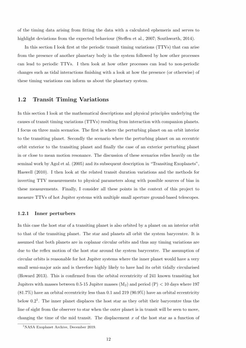
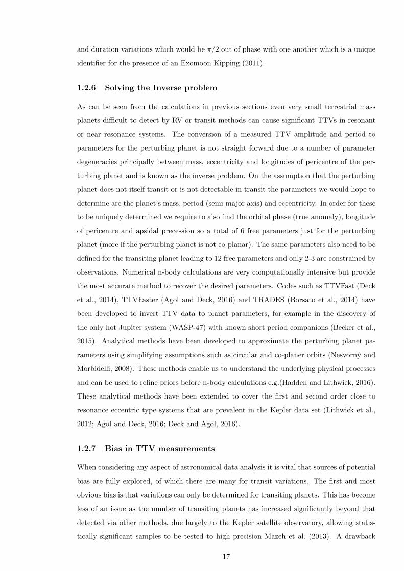
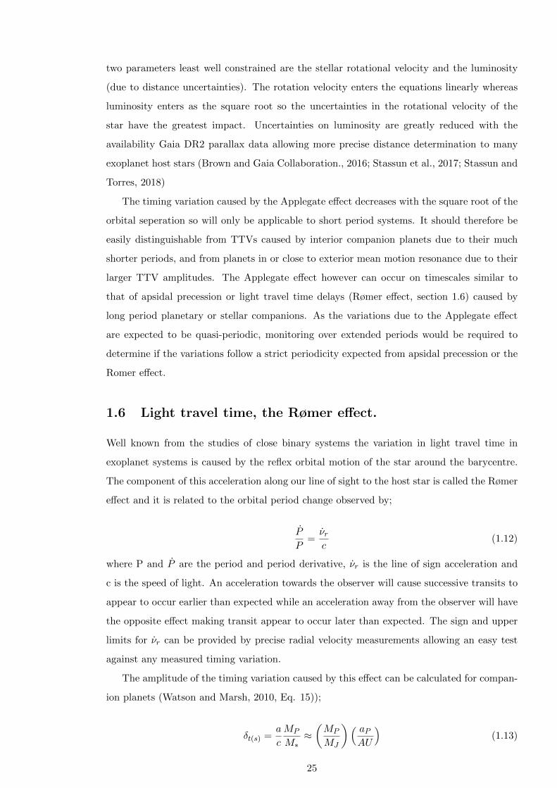
Figure 1.1: A simple sketch (not to scale) of TTV geometry for an inner perturber shown in

plan view, adapted from (Agol et al., 2005). All the bodies in the system orbit the common

barycentre. In [a] the presence of the inner planet has caused the transit of the outer planet

to occur early. In [b] the system is aligned to the observer and the transit is on time. In [c]

the transit occurs later.

1.2.2 Outer perturbers on eccentric orbits

An outer companion to a hot Jupiter could cause a measurable TTV if it is in a non-circular

orbit. This is a planet-planet interaction whereas the previous case was a planet-star inter-

action. As the outer planets’ orbit is eccentric the distance between the two planets varies

with time causing a varying acceleration of the inner planet on the timescale of the outer

planet’s orbit. The amount of acceleration at a given time depends on the location of the

outer planet in its orbit, the true anomaly, which would generally not be known. Following

(Haswell, 2010, Eq. 7.29) it is possible to calculate an approximate maximum TTV of an

inner transiting planet for a given system.

δt1 ≈ µ2e2

(a1

a2

)3

P2 (1.4)

Again using the example of the HAT-P-44b system but this time with an exterior Jupiter

mass planet in a 100 day orbit and an eccentricity of 0.6 we can calculate that the maximum

transit timing variation will be just 5.1 seconds. As with the previous example this is also

well below the detection threshold for ground-based timing with small telescopes. Despite

these very small potential TTVs a growing number of hot Jupiter systems have been found

through trends in their RV residuals to harbour massive planets in long period orbits around

transiting systems (Knutson et al., 2014).

14

1.2.3 MMR or close to MMR systems

So far the chances of detecting TTVs seem poor however a much more interesting opportunity

for TTV detection arises if two planets in a system are in a mean motion resonance (MMR).

For a first order MMR with j+1:j the two planets will undergo a conjunction at the same

longitude for each jth orbit of the outer planet. This repeated alignment cumulatively tugs on

the orbit of the inner planet creating an eccentricity which adds coherently over subsequent

orbits. As the conjunction precesses over time the longitude of the conjunction and thus the

semi major axis of the inner planet shifts through 360°known as a libration cycle. It is this

libration that leads to a change in the transit timing over time, betraying the presence of the

MMR companion. Agol et al. (2005) calculated an approximate analytical expression for the

amplitude of the timing variation as (their equation 33)

δt2 ≈P2

4.5j

M1

M1 +M2(1.5)

where δt2, P2 and M2 are the timing variation, period and mass of the inner transiting planet

and M1 is the mass of the outer perturbing planet. Unlike Equations 1.3 and 1.4, the timing

variation does not depend on the mass of the star, only on the masses of the planets. As the

stellar mass is often of the order of a thousand times that of the planet we should expect a

much larger maximum amplitude for the timing variation. The downside is that the variation

occurs over the libration cycle period not the orbital period of the perturbing planet which

is approximately given by Agol et al. (2005), Eq 34.

PLib ≈ 0.5j− 4/3µ

− 2/32 P2 (1.6)

To consider an example again based on the HAT-P-44b system but this time with a ter-

restrial mass companion planet in an outer 3:2 MMR orbit where j=2 the δtmax would be 5.9

minutes. The libration period over which this variation would occur would be approximately

165 days, over 25 times the outer planet’s orbital period. As j increases δtmax and the libra-

tion period decrease. Agol et al. (2005) compared the results of these analytical expressions

to numerical modelling and found them to be accurate to within 10% for j≥2 but only to

about 40% for j=1.

1.2.4 Near Resonant Systems

The above discussion considers systems in exact MMR configurations expected to be stable

for significant periods of time. Analysis of TTVs from Kepler data has showed a large

fraction of systems exhibiting TTVs are in a near MMR configuration (Lithwick et al., 2012;

Steffen et al., 2013). These systems will be stable over long periods but may be far enough

15

from resonance that the libration period is significantly shortened, increasing the chances of

monitoring full or multiple cycles (Jontof-Hutter et al., 2016). The duration of the “super

period” ( Pj) in a near resonance system was shown by Lithwick et al. (2012) to be;

Pj =POuter

j + 1×∆j(1.7)

Where ∆j is given by Lithwick et al. (2012) Eq. 6, and is equal to half the ratio difference

from MMR where the near resonance is given by (j+ 1) : j. Thus for a system with a period

ratio of 2.02:1, ∆j = 0.01. Taking the example again of HAT-P-44b but this time assuming

the outer planet is in a 3.04:2 near resonance then the super period would be approximately 17

times the outer planet’s orbital period (rather than 25 times for the MMR libration period).

Also in their 2012 paper Lithwick et al. (2012) separate the eccentricity of the perturbing

planet into a free component unrelated to the resonance and a component forced by the

closeness to resonance. They discuss how both components of eccentricity can be damped

away but how the forced component is replenished by the planet-planet interaction reducing

orbital energy and helping explain the increase in the number of planets found in orbits just

wide of resonance.

The free component of the eccentricity can be determined from the phase of the two sets

of TTVs in a dual planet system where both planets transits can be measured. If they are

in phase (i.e. crossing zero at the same time) then free eccentricity is zero and mass can be

uniquely determined. The amount of free eccentricity can also be informative for formation

and dynamical history theories.

1.2.5 Transit Duration Variations

Another potentially measurable variation is the duration of the transit. TDV’s that are in or

close to phase with the timing variations can be caused by interactions between companion

planets on or close to MMR. The effect of an outer perturbing planet is to alter the orbital

velocity of the inner transiting planet leading to duration variations E.g. (Nesvorny et al.,

2013). For a planet in a non-circular orbit, variations in the transit duration could be caused

by apsidal precession where the ellipse of the orbit rotates in its own plane thus varying

the orbital speed of the planet across the face of the star from the observers view point.

Nodal variations lead to changes in the orbital plane varying the impact parameter and thus

the transit duration and would be detectable for planets in circular orbits. Nodal variation

would be expected to be most profound for planets in grazing transits where changes to the

orbital plane could even move a planet out of transit. Additional possible causes or TDV’s

include exomoons orbiting a planet. An exomoon could be the cause of both transit time

16

and duration variations which would be π/2 out of phase with one another which is a unique

identifier for the presence of an Exomoon Kipping (2011).

1.2.6 Solving the Inverse problem

As can be seen from the calculations in previous sections even very small terrestrial mass

planets difficult to detect by RV or transit methods can cause significant TTVs in resonant

or near resonance systems. The conversion of a measured TTV amplitude and period to

parameters for the perturbing planet is not straight forward due to a number of parameter

degeneracies principally between mass, eccentricity and longitudes of pericentre of the per-

turbing planet and is known as the inverse problem. On the assumption that the perturbing

planet does not itself transit or is not detectable in transit the parameters we would hope to

determine are the planet’s mass, period (semi-major axis) and eccentricity. In order for these

to be uniquely determined we require to also find the orbital phase (true anomaly), longitude

of pericentre and apsidal precession so a total of 6 free parameters just for the perturbing

planet (more if the perturbing planet is not co-planar). The same parameters also need to be

defined for the transiting planet leading to 12 free parameters and only 2-3 are constrained by

observations. Numerical n-body calculations are very computationally intensive but provide

the most accurate method to recover the desired parameters. Codes such as TTVFast (Deck

et al., 2014), TTVFaster (Agol and Deck, 2016) and TRADES (Borsato et al., 2014) have

been developed to invert TTV data to planet parameters, for example in the discovery of

the only hot Jupiter system (WASP-47) with known short period companions (Becker et al.,

2015). Analytical methods have been developed to approximate the perturbing planet pa-

rameters using simplifying assumptions such as circular and co-planer orbits (Nesvorny and

Morbidelli, 2008). These methods enable us to understand the underlying physical processes

and can be used to refine priors before n-body calculations e.g.(Hadden and Lithwick, 2016).

These analytical methods have been extended to cover the first and second order close to

resonance eccentric type systems that are prevalent in the Kepler data set (Lithwick et al.,

2012; Agol and Deck, 2016; Deck and Agol, 2016).

1.2.7 Bias in TTV measurements

When considering any aspect of astronomical data analysis it is vital that sources of potential

bias are fully explored, of which there are many for transit variations. The first and most

obvious bias is that variations can only be determined for transiting planets. This has become

less of an issue as the number of transiting planets has increased significantly beyond that

detected via other methods, due largely to the Kepler satellite observatory, allowing statis-

tically significant samples to be tested to high precision Mazeh et al. (2013). A drawback

17

of many of the Kepler targets is that they are too faint for radial velocity follow up and so

rely on the TTV measurements for mass determination. An interesting aspect of bias caused

by TTVs was highlighted by Garcıa-Melendo et al. (2011) who discuss how systems with

TTVs could be missed by planet search algorithms altogether. They highlight three possible

scenarios where the period variations due to TTVs could lead to transits being missed, thus

explaining the lack of hot Jupiter systems with significant TTVs. Firstly the transits folded

over the wrong period can be individually smeared into the background noise resulting in

non-detection in the first place. Secondly the transit is detected but with the wrong Period

(P) or epoch (T0) leading to non-detection in follow up observations, and lastly the transit

shape can be deformed leading to rejection as a blended or binary star source.

1.2.8 Exomoons

Moons orbiting transiting exoplanets are another potential source of TTVs and TDV’s (Kip-

ping, 2013). The reflex motion of a planet orbiting the planet-moon barycentre will change

the timing from successive orbits which would be detectable as periodic TTVs. Additionally

the duration of the planetary transit can be varied by this orbital motion around the barycen-

tre. Following equations 3.1 and 3.2 in Kipping (2013) it is straightforward to calculate the

TTV and TDV effects of an exomoon for circular co-planar orbits. These calculations show

that for an Earth mass exomoon orbiting WASP-48b at the same distance as Io orbits Jupiter

the maximum timing variation amplitude would be ∼ 48 seconds whist the effect on the tran-

sit duration would be only 3.6 seconds. A Europa mass exomoon orbiting WASP-48b at

Europa’s distance from Jupiter the TTV amplitude would be just 0.6 seconds and the TDV

0.02 seconds.

A TTV amplitude of 48 seconds is in principle within the detection range of small aperture

ground-based telescopes and the existence of exomoons would need to be considered for any

suspected TTV. The phase of TDV’s with the TTVs would be π/2 which would enable

confirmation or rejection of an exomoon hypothesis but TDV detection is extremely difficult

and well beyond that achievable with small aperture telescopes from the ground.

The difficulty of detecting exomoons is highlighted by the recent case of Kepler-1625b-i,

the first credible (but still not confirmed) detection of of a Neptune radius moon orbiting

a Jupiter radius planet (Teachey and Kipping, 2018). Three Kepler observations of Kepler

1625b show ' 25 minute TTVs and HST observations of a fourth transit show a decrease in

the out of transit flux at the location expected from the TTV phase. Together the evidence

of the first Exomoon detection is compelling however the authors caution that the quality of

the detection is highly dependent on the HST lightcurve detrending methodology applied and

the Neptuanian size and inclined orbit around the host planet require explanation. With an

18

orbital period of ∼ 287 days, further follow up observations are complicated by the difficulty

of forward predicting the moons location from the TTV phase.

1.3 Orbital decay

A possible cause of departure from strictly Keplerian orbit is orbital decay where a planet

orbit is spiralling in towards its host star. This change in orbital radius would manifest

as a continuous reduction in the orbital period resulting in a quadratic departure from the

expected linear ephemeris, Equation 1.8 (Maciejewski et al., 2016);

TC(E) = t0 + PE + 0.5δP

δEE2 (1.8)

where TC(E) is the calculated transit mid-time, t0 is the reference epoch, P is the period

and E is the number of periods since the reference epoch. This is the same as a linear

ephemeris, the quadratic component 0.5 δPδEE2 accounts for the change in period with each

epoch (assuming a constant period change). From measurements of the period derivative it

is simple to calculate the period change per day and thus the cumulative annual change;

δP

δt=

1

P

δP

δE(1.9)

This quadratic ephemeris is discernible from other causes of transit time variations due

to the unique non-periodic shape of the fit to the measured transit times in an O-C diagram.

Another test for the presence of orbital decay is occulation timing which should be correlated

with the transit timing. As the baseline of observations of hot Jupiters over many epochs

has grown it has become possible to test for orbital decay in the systems where this could be

expected.

In systems where the orbital period is shorter than the stellar rotation period the most

commonly proposed mechanism driving orbital decay is dissipation due to dynamical tides

raised within the host star. This leads to the raising of a tidal bulge on the stellar surface

(much like the Moon does for the Earth) but as the orbital angular velocity is greater than

the stellar rotational velocity this tidal bulge lags behind the orbit of the planet and exerts

a tidal torque on the planet. Angular momentum is transferred from the planets orbit to

the stellar rotation resulting in an increased rotational velocity for the star and a reduction

in the orbital period, which we see as orbital decay and potentially increased stellar activity

(Poppenhaeger, 2016).

In this model, the rate of period decay is dependant on the stellar tidal dissipation rate,

often expressed as the dimensionless reduced tidal quality factor, Q′∗. With the simplifying

assumptions that the planetary orbit is circular, the stellar rotation angular velocity � the

19

orbital angular velocity and that we can neglect tidal dissipation in the planet, the rate of

decay is given by (Patra et al., 2020);

δP

δt= − 27π

2Q′∗

MP

M∗

(R∗a

)5

(1.10)

where Q′∗ = 1.5Q∗/κ∗,2, with Q∗ being the stellar tidal quality factor and κ∗,2 is the Love

number, a measure of the central condensation of the star (Patra et al., 2020). Orbital decay

has only been detected or is suspected in a very small number of hot Jupiter exoplanet systems

(see Section 1.3.1) limiting our ability to identify the full range of Q′∗ values we should expect

for these systems so alternative approaches have been sought to bound the expected values of

Q′∗ for exoplanet host stars. Penev et al. (2016) used the tidal spin up of two hot Jupiter host

stars to infer Q′∗ in the range 106.4−7.4 which was extended to 188 host stars where the range

of Q′∗ was found to increase from 105 to 107 as the tidal forcing frequency increased (Penev

et al., 2018). Hamer and Schlaufman (2019) used Gaia DR2 results to show hot Jupiter

hosts have a lower galactic velocity dispersion than field stars of similar population without

a known hot Jupiter. As galactic velocity dispersion is correlated with age they conclude

that the known hot Jupiters systems are young and that this is best explained by engulfment

while the host stars are on the main sequence, in turn requiring Q′∗ to be . 107.

The stability, or otherwise, of planetary systems to tidal decay has been considered by

Levrard et al. (2009) who find that for a system in which angular momentum is conserved but

energy is dissipated there are two possible end states defined by the ratio between the systems

total angular momentum (Ltot) and a critical angular momentum value (Lc). Lc depends

on the masses and polar moments of inertia of the planet and star (their Eq.1). Where

Ltot < Lc, i.e. where the total angular momentum is less than the critical value, the system

is unstable to tidal decay regardless of the model for the tidal dissipation. Alternatively where

Ltot > Lc there are two possible equilibrium states, the further distance which is greater than

the orbital distance for Ltot = Lc is stable. The other where the orbital distance is less than

the equilibrium orbital distance for Ltot = Lc is unstable. Of the 26 transiting systems known

at the time of of the study by Levrard et al. (2009), only one, HAT-P-2b, has Ltot > Lc and

thus the remaining systems will be expected to undergo orbital decay towards their host stars.

HAT-P-2b on the other-hand has an orbital distance slightly greater than the equilibrium

orbital distance for Ltot = Lc and will decay asymptotically towards the equilibrium orbital

distance.

1.3.1 Period Decay in the Literature

As the baseline of timing observations for many exoplanet systems approaches decade long

durations we can now start to search for orbital period decay. With their close proximity and

20

high orbital angular velocity the ultra short period hot Jupiters with periods . a few days

should provide the best candidates to test for this effect.

WASP-43b is a 1.81MJ ultra short period hot Jupiter on a 0.81 day orbit around a low

(0.58M�) star. Using Spitzer observations of secondary eclipses combined with primary

transits taken from the Exoplanet Planet Transit Database (ETD), a database of mainly

amateur observations made with small aperture telescopes, Blecic et al. (2014) tentatively

reported an orbital decay rate −0.095± 0.036 syr−1. This was later revised down by a factor

of 3 (Jiang et al., 2016) and subsequently called into question altogether following further

refinements of the ephemeris (Hoyer et al., 2016). With an orbital period of 0.79 days, WASP-

19b is a another ultra short period Jupiter mass (MP = 1.11MJ) planet orbiting a solar type

(M∗ = 0.9M�) star predicted to show a period shift of at least 34 seconds after 10 years for

tidal quality factors 106 − 108 (Valsecchi and Rasio, 2014). Analysis of 60 transit times by

Espinoza et al. (2019) suggested detection of a high significance approximately −40 second

timing change between 2014 and 2017. Petrucci et al. (2020) undertook a homogeneous

reanalysis of 74 transit data sets and find that a linear ephemeris is the best fit to the data

with an upper limit to any period change P = −2.294 ms yr−1.

Kepler-1658b was the first planet discovered (KOI-4.01) by the Kepler space mission

and is a massive planet orbiting a evolved sub-giant star on a longer period orbit than the

examples above (M∗ = 1.45M�,MP = 5.88MJ, P = 3.85 days). Using all 4 years data from

the Kepler main mission Chontos et al. (2019) find a 3σ upper limit to an orbital decay

rate of P = −0.42 ms yr−1, though the authors note their result is consistent with a linear

ephemeris at 1σ.

The hot Jupiter WASP-4b (M∗ = 0.865M�,MP = 1.19MJ , P = 1.33 days) was observed

for 18 transits by the TESS mission which occurred 81.6± 11.7s earlier than predicted from

the linear ephemeris (Bouma et al., 2019). The authors calculated a decay rate of P =

−12.6 ± 1.2 ms yr−1 though were unable to conclusively distinguish between orbital decay

or apsidal precession as the cause. Baluev et al. (2019) reported a homogeneous analysis of

56 published transit times and 10 new observations, excluding those from TESS, and were

unable to support the period decay seen by Bouma et al. (2019). When the authors included

the TESS transit times and other published transit times where the original data was not

available for reanalysis the quadratic ephemeris becomes significant, though with a reduced

decay rate. Southworth et al. (2019) added 22 new transit times spanning almost 3000

epochs and find a quadratic ephemeris is best fit to the data though with rate of change of

P = −9.2± 1.1 ms yr−1, 3σ lower than reported by (Bouma et al., 2019). The result implies

a modified tidal quality factor (Q′∗) somewhat lower than expected from values reported in

the literature, so both orbital decay and apsidal precession are consistent with the data but

21

each is not without its drawbacks.

Probably the most secure and best studied example of orbital period decay is that of

WASP-12b, a 1.47MJ planet orbiting a 1.4M� star every 1.09 days (Hebb et al., 2009).

WASP-12b is known to be losing mass via Roche overflow of its extended exosphere (Haswell

et al., 2012; Haswell, 2018). Period change was first reported by Maciejewski et al. (2016) and

subsequently extensively studied by a large number of authors (Patra et al., 2017; Maciejewski

et al., 2018; Ozturk and Erdem, 2019; Baluev et al., 2019; Yee et al., 2019). Both orbital

period decay and apsidal precession have been proposed as viable drivers of the period change

observed. The most robust way to determine between these two hypothesis is with occlutation

measurements which, in the case of apsidal precession will be π/2 out of phase with the transit

times whereas for period decay the occultations and transits will be in phase. Yee et al. (2019)

have reported four additional occultation measurements separated by 16 epochs obtained with

the Spitzer space telescope, along with ten new ground-based transit measurements. Their

analysis indicates the occulations are in phase thus preferring the orbital decay hypothesis

for the measured period change of P = −29.9 ± 2 ms yr−1 (Yee et al., 2019). WASP-12b

was observed by TESS between December 2019 and January 2020 and the results from the

timing analysis of the 21 transits obtained support the orbital decay model (Turner et al.,

2021).

A different approach using radial velocity measurements to detect the radial velocity of

the tidally raised bulge on the surface of WASP-12 has been investigated by Maciejewski

et al. (2020). The period of this RV signal would be half the orbital period and its phase is

related to the planetary orbital motion such that it cam mimic non-zero orbital eccentricity

with a longitude of periastron (ω) of 270°. The authors separate the orbital and tidally

induced RV semi amplitudes and determine a value of 7.5 ± 1.2ms−1 for the latter with ω

close to 270°. This is the first such detection of tidally induced RV variations which may

be detectable in other systems which exhibit a non zero eccentricity with ω ∼ 270°such as

WASP-18b (Maciejewski et al., 2020).

1.4 Apsidal and nodal precession.

Apsidal precession is the rotation of the point of periastron of an elliptical orbit around

the orbital plane while nodal precession is the precession of an orbit around the rotation

axis which can be different to the orbital plane. Taking a star-planet system if both bodies

were completely spherical and the orbit circular there would be no precession. As the stars

and planets themselves rotate they generate rotational flattening and this departure from a

purely spherical state creates a gravitational quadrupole field which causes the line of apsides

22

to rotate (precess) around the orbit. For an exoplanet with an eccentric orbit this results in

changes in the transit time over the period of the precession.

The rotation periods of hot Jupiter’s would be expected to be synchronised to the orbital

period, reducing the planets rotational flattening and thus the precession. However the same

proximity between star and planet can lead to the raising of tidal bulges on both components.

Ragozzine and Wolf (2009) showed [their equation 13] that the total precession is a linear

summation of all the contributing components and that for hot Jupiters this planetary tidal

bulge is the most significant contributor to apsidal precession.

ωtotal = ωtideP + ωgr + ωrotP + ωtide∗ + ωrot∗ + ωP2 (1.11)

Equation 1.11 lists the contributing components in order of importance for a hot Jupiter

where ωtideP and ωrotP are the contribution from the planets tidal and rotation bulges, ωtide∗

and ωrot∗ are the contribution from the stellar tidal and rotational bulges. ωgr is the compo-

nent due to relativistic precession and ωP2 is that due to a second planet in the system. An

excellent summary of the relative contribution of these components to the apsidal precession

total is given in Perryman (2014), chapter 6.4.13.

Unless the orbit of the planet around the star is eccentric then apsidal precession will not

have any effect on transit timing. Ragozzine and Wolf (2009) calculated apsidal precession

rates for a number of hot Jupiters known at the time and showed that for WASP-12b the

precession of perastron could be as much as 19.9◦yr−1, completing a full 360°rotation of the

line of apsides in just over 18 years with a maximum timing variation amplitude of ∼ 25

minutes over the apsidal rotation period. This is significant and well within the detection

limits for small aperture, ground-based, telescopes.

Apsidal precession of an eccentric orbit would also be expected to exhibit transit duration

variations and variations in the timing between primary and secondary eclipses. In the latter

case the timing variation of the transits and occultations would occur π/2 degrees out of phase

with each other, providing a mechanism to determine between timing changes due to apsidal

precession and those due to other effects such as tidal decay.

Non detection of TTVs caused by apsidal precession also allows tight upper limits to be

placed on the planet’s orbital eccentricity. Measuring orbital precession is not only important

to exclude from possible companion planet discovery but it also allows the planet Love number

κ2 to be determined, providing information on the central concentration of mass within the

planet (Ragozzine and Wolf, 2009). This allows us a ’view’ inside the planetary structure

without being able to see the planet.

The departure from a pure sphere for the star and the consequent quadrupole gravitational

field also means the gravitational force on the planet is not directly toward the centre of the

23

host star, but is offset toward the equator. If the planet is not orbiting in the rotational plane

of the star it will experience a pull toward the stellar equator causing a precession of the line

of nodes. As also calculated by Ragozzine and Wolf (2009) this nodal precession effect is an

order of magnitude less than for apsidal precession and is not detectable even with Kepler

quality photometry. We can therefore safely ignore nodal precession in timing measurements

made with ground-based small telescopes.

Apsidal precession has been considered as the cause of the non linear ephemeris for WASP-

12b (Maciejewski et al., 2016; Patra et al., 2017) where the observed quadratic ephemeris is

simply part of a longer sinusoidal apsidal precession with a period of 14 ± 2 years (Patra

et al., 2017). Subsequent observations of occultations Yee et al. (2019) indicates they occur

in phase with the primary transits, ruling out apsidal precession as a cause of the observed

non-linear ephemeris for WASP-12b.

1.5 Applegate effect

The Applegate effect (Applegate, 1987, 1992) was proposed to explain the changes in the

observed orbital periods of binary stars that could not be attributed to mass transfer or loss.

In this model, as applied to exoplanets, changes in the stellar quadrupole moment lead to

changes in the oblateness of the star which in turn impacts the non-spherical component of

the gravitational field experienced by the orbiting planet. The planet in turn has to react to

the changing gravitational field by changing its orbital velocity and thus in order to conserve

angular momentum the orbital period will change (Watson and Marsh, 2010). In this way

an increase in oblateness will lead to an increased velocity and reduced orbital period while

a reduction in oblateness will lead to a reduced velocity and an increased orbital period.

The mechanism proposed to drive the change in the quadrupole moment is internal an-

gular momentum transfer from the stellar core to the envelope (and back again) driven by

changes in the magnetic field of the star (Applegate, 1992). Thus the changes will occur on

the quasi-periodic timescales of the stellar magnetic activity cycle and will apply for relatively

low mass stars with a convective envelope capable of dynamo generation of a magnetic field.

It happens that, largely through selection effects, many detected exoplanets orbit this type

of star.

Theoretical Applegate effect TTV amplitudes for a number of exoplanet host stars known

at the time have been calculated by Watson and Marsh (2010) for theoretical magnetic cycle

periods of 11, 22 and 50 years. These show amplitudes ranging from 0.1 seconds over 11

years to more than 6 minutes over a 50-year period. The size of potential O-C variations

is calculated in equation 13 of Watson and Marsh (2010) where it can be seen that the

24

two parameters least well constrained are the stellar rotational velocity and the luminosity

(due to distance uncertainties). The rotation velocity enters the equations linearly whereas

luminosity enters as the square root so the uncertainties in the rotational velocity of the

star have the greatest impact. Uncertainties on luminosity are greatly reduced with the

availability Gaia DR2 parallax data allowing more precise distance determination to many

exoplanet host stars (Brown and Gaia Collaboration., 2016; Stassun et al., 2017; Stassun and

Torres, 2018)

The timing variation caused by the Applegate effect decreases with the square root of the

orbital seperation so will only be applicable to short period systems. It should therefore be

easily distinguishable from TTVs caused by interior companion planets due to their much

shorter periods, and from planets in or close to exterior mean motion resonance due to their

larger TTV amplitudes. The Applegate effect however can occur on timescales similar to

that of apsidal precession or light travel time delays (Rømer effect, section 1.6) caused by

long period planetary or stellar companions. As the variations due to the Applegate effect

are expected to be quasi-periodic, monitoring over extended periods would be required to

determine if the variations follow a strict periodicity expected from apsidal precession or the

Romer effect.

1.6 Light travel time, the Rømer effect.

Well known from the studies of close binary systems the variation in light travel time in

exoplanet systems is caused by the reflex orbital motion of the star around the barycentre.

The component of this acceleration along our line of sight to the host star is called the Rømer

effect and it is related to the orbital period change observed by;

P

P=νrc

(1.12)

where P and P are the period and period derivative, νr is the line of sign acceleration and

c is the speed of light. An acceleration towards the observer will cause successive transits to

appear to occur earlier than expected while an acceleration away from the observer will have

the opposite effect making transit appear to occur later than expected. The sign and upper

limits for νr can be provided by precise radial velocity measurements allowing an easy test

against any measured timing variation.

The amplitude of the timing variation caused by this effect can be calculated for compan-

ion planets (Watson and Marsh, 2010, Eq. 15));

δt(s) =a

c

MP

M∗≈(MP

MJ

)( aPAU

)(1.13)

25

where MP and aP are the mass and semi-major axis of the outer perturbing companion.

Thus for a Jupiter mass planet in a Jupiter wide orbit of 5AU around a solar mass star,

the amplitude of the timing variation due to light travel effects is 5 seconds. This variation

will be strictly periodic over successive 12-year orbital periods. Large amplitude variations

caused by massive companions on wide orbits can be ruled out through high precision radial

velocity measurements

1.7 Exoplanet Host Star Variability

Intrinsic stellar variability can arise in many forms including periodic or quasi-periodic varia-

tions due to stellar pulsations, surface spots caused by magnetic activity tracking the stellar

rotation and stochastic events such as flares. Stellar magnetic variability driven by the dy-

namo effect in F, G, K and M type stars is of particular interest to the study of exoplanets,

especially the short period hot Jupiters. Surface spots and faculae on these stars can affect

the shape of the transit lightcurve with the resulting asymmetry leading to an offset in the

measured transit mid-time. This effect can result in a false transit timing variation without

appropriately inflating the fitted errors, emphasising the importance of a complete under-

standing of exoplanet host stars when determining planetary parameters. In this section I

look at how star spots occur (1.7.1), how they are used to measure stellar rotation (1.7.2)

and finally how they affect exoplanet transit measurements (1.7.3).

1.7.1 Star Spots and Activity Cycles

Star spots are dark regions that rotate with the stellar surface at the latitude at which they

form. They are best studied for the Sun where they can be as large as 30,000km and are

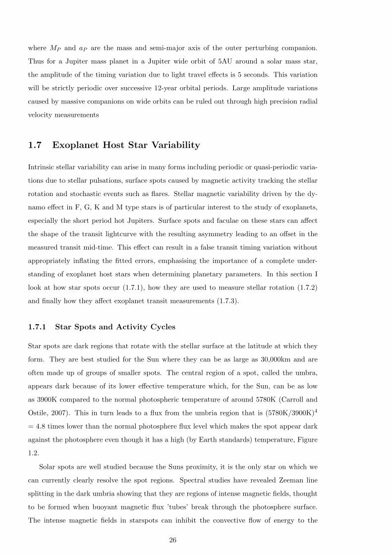
often made up of groups of smaller spots. The central region of a spot, called the umbra,

appears dark because of its lower effective temperature which, for the Sun, can be as low

as 3900K compared to the normal photospheric temperature of around 5780K (Carroll and

Ostile, 2007). This in turn leads to a flux from the umbria region that is (5780K/3900K)4

= 4.8 times lower than the normal photosphere flux level which makes the spot appear dark

against the photosphere even though it has a high (by Earth standards) temperature, Figure

1.2.

Solar spots are well studied because the Suns proximity, it is the only star on which we

can currently clearly resolve the spot regions. Spectral studies have revealed Zeeman line

splitting in the dark umbria showing that they are regions of intense magnetic fields, thought

to be formed when buoyant magnetic flux ’tubes’ break through the photosphere surface.

The intense magnetic fields in starspots can inhibit the convective flow of energy to the

26

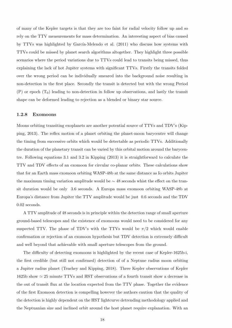
Figure 1.2: . SOHO MDI image from 21st May 2016 showing sunspot 2546 near the centre

of the solar disk. Added above is Jupiter’s disk to scale and below the spot is the Earths disk

to scale. Solar disk image, SOHO 2016 http://sohowww.nascom.nasa.gov/sunspots/

surface leading to the lower temperatures in spots than the surrounding photosphere. This

interpretation is supported by the observation that Sun spots and spot groups form in pairs

that trail one another with opposite magnetic polarity. Star spots (and Sun spots) are not

simple dark structures, the umbria is surrounded by the penumbria, a region of intermediate

flux that shows linear structures indicative of a strong magnetic field. In contrast to the

darker spots bright plages are regions of increased brightness associated with spots and spot

groups on the solar photosphere and are brightest when viewed in Hα emission.

Bright faculae are another manifestation of magnetic activity in the photosphere appear-

ing as large bright regions best observed closer to the limb. Faculae and plages are often

associated with Sunspots and can remain after the spot themselves have disappeared. Fac-

ulae are best seen near the limb where we can see into the hotter side walls of the granules

which can, in principle, lead to an overall brightening of the local stellar limb in contrast to

the expected limb darkening (Herrero et al., 2012).

At first glance the spot activity on the Sun appears random and unordered however when

looked at over long timescales it becomes obvious that the activity levels are in fact structured

and even predictable. Solar spot activity waxes and wanes with an 11-year period which is

half the 22-year solar magnetic cycle period. This creates maximums in spot activity every 11

years with minimums 5.5 years later. The spot coverage, or filling factor, many times greater

at maximum than at minimum when the solar surface can be spot free for extended periods

of time while at solar maximum spots coverage can reach as high as 0.5% of the projected

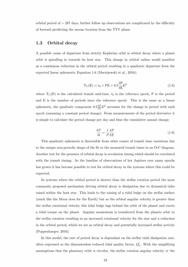
solar disk Figure 1.3 (bottom).

27

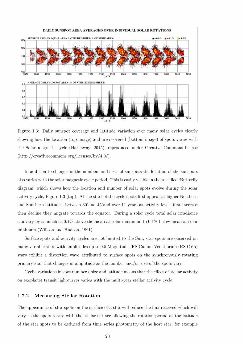
Figure 1.3: Daily sunspot coverage and latitude variation over many solar cycles clearly

showing how the location (top image) and area covered (bottom image) of spots varies with

the Solar magnetic cycle (Hathaway, 2015), reproduced under Creative Commons license

(http://creativecommons.org/licenses/by/4.0/).

In addition to changes in the numbers and sizes of sunspots the location of the sunspots

also varies with the solar magnetic cycle period. This is easily visible in the so called ‘Butterfly

diagram’ which shows how the location and number of solar spots evolve during the solar

activity cycle, Figure 1.3 (top). At the start of the cycle spots first appear at higher Northern

and Southern latitudes, between 30°and 45°and over 11 years as activity levels first increase

then decline they migrate towards the equator. During a solar cycle total solar irradiance

can vary by as much as 0.1% above the mean at solar maximum to 0.1% below mean at solar

minimum (Willson and Hudson, 1991).

Surface spots and activity cycles are not limited to the Sun, star spots are observed on

many variable stars with amplitudes up to 0.5 Magnitude. RS Canum Venatiorum (RS CVn)

stars exhibit a distortion wave attributed to surface spots on the synchronously rotating

primary star that changes in amplitude as the number and/or size of the spots vary.

Cyclic variations in spot numbers, size and latitude means that the effect of stellar activity

on exoplanet transit lightcurves varies with the multi-year stellar activity cycle.

1.7.2 Measuring Stellar Rotation

The appearance of star spots on the surface of a star will reduce the flux received which will

vary as the spots rotate with the stellar surface allowing the rotation period at the latitude

of the star spots to be deduced from time series photometry of the host star, for example

28

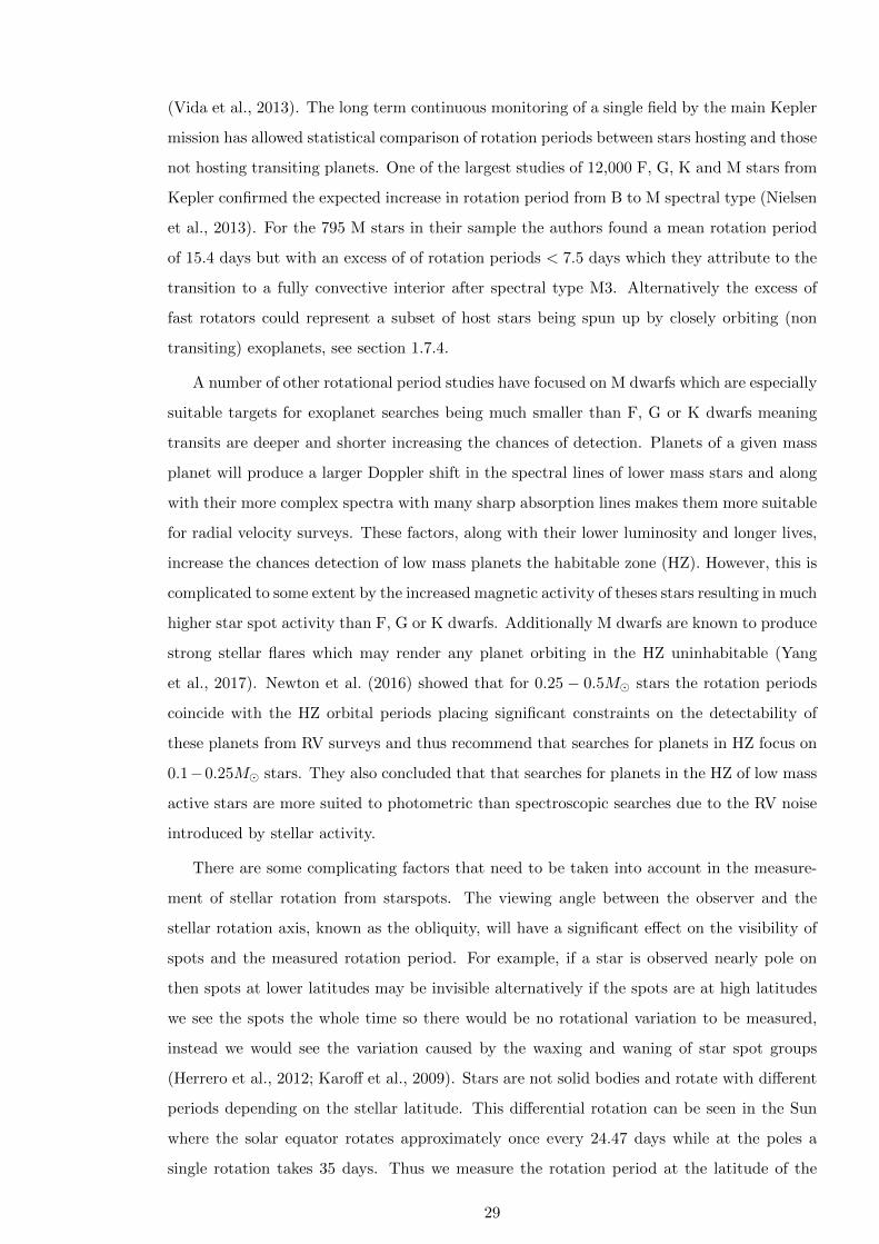
(Vida et al., 2013). The long term continuous monitoring of a single field by the main Kepler

mission has allowed statistical comparison of rotation periods between stars hosting and those

not hosting transiting planets. One of the largest studies of 12,000 F, G, K and M stars from

Kepler confirmed the expected increase in rotation period from B to M spectral type (Nielsen

et al., 2013). For the 795 M stars in their sample the authors found a mean rotation period

of 15.4 days but with an excess of of rotation periods < 7.5 days which they attribute to the

transition to a fully convective interior after spectral type M3. Alternatively the excess of

fast rotators could represent a subset of host stars being spun up by closely orbiting (non

transiting) exoplanets, see section 1.7.4.

A number of other rotational period studies have focused on M dwarfs which are especially

suitable targets for exoplanet searches being much smaller than F, G or K dwarfs meaning

transits are deeper and shorter increasing the chances of detection. Planets of a given mass

planet will produce a larger Doppler shift in the spectral lines of lower mass stars and along

with their more complex spectra with many sharp absorption lines makes them more suitable

for radial velocity surveys. These factors, along with their lower luminosity and longer lives,

increase the chances detection of low mass planets the habitable zone (HZ). However, this is

complicated to some extent by the increased magnetic activity of theses stars resulting in much

higher star spot activity than F, G or K dwarfs. Additionally M dwarfs are known to produce

strong stellar flares which may render any planet orbiting in the HZ uninhabitable (Yang

et al., 2017). Newton et al. (2016) showed that for 0.25 − 0.5M� stars the rotation periods

coincide with the HZ orbital periods placing significant constraints on the detectability of

these planets from RV surveys and thus recommend that searches for planets in HZ focus on

0.1−0.25M� stars. They also concluded that that searches for planets in the HZ of low mass

active stars are more suited to photometric than spectroscopic searches due to the RV noise

introduced by stellar activity.

There are some complicating factors that need to be taken into account in the measure-

ment of stellar rotation from starspots. The viewing angle between the observer and the

stellar rotation axis, known as the obliquity, will have a significant effect on the visibility of

spots and the measured rotation period. For example, if a star is observed nearly pole on

then spots at lower latitudes may be invisible alternatively if the spots are at high latitudes

we see the spots the whole time so there would be no rotational variation to be measured,

instead we would see the variation caused by the waxing and waning of star spot groups

(Herrero et al., 2012; Karoff et al., 2009). Stars are not solid bodies and rotate with different

periods depending on the stellar latitude. This differential rotation can be seen in the Sun

where the solar equator rotates approximately once every 24.47 days while at the poles a

single rotation takes 35 days. Thus we measure the rotation period at the latitude of the

29

spots which is likely different to the equatorial rotation period and which can change as spots

migrate in latitude over a stellar cycle.

1.7.3 Effect of Stellar Activity on Transit Measurement

As a transiting planet crosses our line of sight to a surface star spot the amount of starlight

occulted by the planet will be reduced due to the lower luminosity of the cooler starspot. This

manifests itself as a ‘bump’ in the transit light curve and the size of this bump can be used

to determine the temperature difference and, along with knowledge of the stellar rotation

velocity, the size of the occulted spot. The visual impact of a given starspot on a transit

lightcurve will be greatest when the spot is in the centre of the disk where limb darkening is

minimised and therefore the contrast between the bright photosphere and the cooler starspot

is greatest. If an occultation of a starspot occurs away from the centre of the stellar disk,

then the brightness contrast will be reduced and the viewing angle will foreshorten the size

of the starspot resulting in a reduced impact on the lightcurve. The contrast between the

cooler star spot and the photosphere is greater at shorter wavelengths so observations in blue

or UV filters will be more affected by spot crossing events than those made in longer red or

IR wavebands.

Stars emit a stream of material in the form of a stellar wind through which an orbiting

planet has to pass. The wind density is greater closer to the star implying short period

planets pass through the densest regions of the stellar wind outflow. The possibility of a

planetary magnetospheric bow shock affecting the near UV transit shape was investigated

by Llama et al. (2013) following HST observations that appeared to show an early ingress

transit asymmetry for HD189733b (Ben-Jaffel and Ballester, 2013). The observation could be

explained by a bow shock preceding the planet by 16.7RP , increasing the Hydrogen column

density within the shock and therefore modifying the near-UV transit shape, Figure 1.4.

Changes in the stellar wind density at the planet resulting from stellar rotation will lead to

significant variations in the near UV transit asymmetry.

The impact of star spots on transit time measurements has been considered by several

authors (Oshagh et al., 2013; Ioannidis et al., 2016). Barros et al. (2013) identified spot

transits as the cause of TTVs in WASP-10b previously postulated to be the result of an

unseen companion planet. Ioannidis et al. (2016) showed that timing from higher precision

lightcurves is more affected by stellar spots and define the transit SNR (TSNR) as the ratio of

out of transit noise to the transit depth. They demonstrated that for TSNR . 15 the system-

atic timimg errors introduced by spot crossing events are indistinguishable from the random

noise. They also showed that the magnitude of the effect of spots on timing measurements is

determined by the spots longitude on the stellar surface, peaking at λ = ±70°, reducing the

30

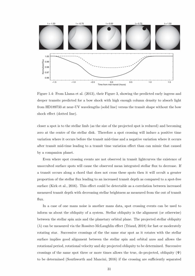
Figure 1.4: From Llama et al. (2013), their Figure 3, showing the predicted early ingress and

deeper transits predicted for a bow shock with high enough column density to absorb light

from HD189733 at near-UV wavelengths (solid line) versus the transit shape without the bow

shock effect (dotted line).

closer a spot is to the stellar limb (as the size of the projected spot is reduced) and becoming

zero at the centre of the stellar disk. Therefore a spot crossing will induce a positive time

variation where it occurs before the transit mid-time and a negative variation where it occurs

after transit mid-time leading to a transit time variation effect than can mimic that caused

by a companion planet.

Even where spot crossing events are not observed in transit lightcurves the existence of

unocculted surface spots will cause the observed mean integrated stellar flux to decrease. If

a transit occurs along a chord that does not cross these spots then it will occult a greater

proportion of the stellar flux leading to an increased transit depth as compared to a spot-free

surface (Kirk et al., 2016). This effect could be detectable as a correlation between increased

measured transit depth with decreasing stellar brightness as measured from the out of transit

flux.

In a case of one mans noise is another mans data, spot crossing events can be used to

inform us about the obliquity of a system. Stellar obliquity is the alignment (or otherwise)

between the stellar spin axis and the planetary orbital plane. The projected stellar obliquity

(λ) can be measured via the Rossiter-McLaughlin effect (Triaud, 2018) for fast or moderately

rotating star. Successive crossings of the the same star spot as it rotates with the stellar

surface implies good alignment between the stellar spin and orbital axes and allows the

rotational period, rotational velocity and sky projected obliquity to be determined. Successive

crossings of the same spot three or more times allows the true, de-projected, obliquity (Ψ)

to be determined (Southworth and Mancini, 2016) if the crossing are sufficiently separated

31

in longitude.

Other than using photometric monitoring of stars for spot driven variability, spectroscopic

methods can also be used to determine magnetic activity through chromosphere activity lev-

els. The most commonly used measures are the Mount-Wilson S-index (Vaughan et al., 1978)

and the RHK index (Middelkoop, 1982). The S-index is a measure of the emission-line cores

of the Ca II H and K lines in two narrow bands normalised to immediately adjacent con-

tinuum bands. The RHK activity index is similar to the S-index but it gives the emission

in the same narrow bands normalised to the total bolometric brightness of the star. Chro-

mospheric activity will also be apparent as increased X-ray luminosity where, for example,

doppler imaging of chromospheric line profiles above active photospheric regions can be used

to map spot locations (E.g. Seward and Charles, 2010).

For transit observations there are several possible routes to mitigating the effects of spot

crossing events. Using longer wavelength filters minimises the spot contrast. In transit

modelling the affected data can be masked (E.g. Bruno et al. (2018)) or alternativly modelled

using code that allows the effect of the spot to be factored into the transit model such as

SPOTROD (Beky, 2014) or PyTranSpot (Juvan et al., 2018).

1.7.4 Exoplanet Effects on Host Stars

Until now I have considered the effect of the stellar activity on the exoplanet however for hot

Jupiters on short period orbits there exists the potential for the planet to affect its host star

in ways that are measurable.

Typically single stars would be expected to show a reducing rate of stellar spin as they age

as angular momentum is lost through their stellar winds. The opposite case of stellar spin-up

can occur through accretion of mass in to the star or via tidal interaction with a companion

planet transferring orbital angular momentum to the star as the orbital separation decreases

(Vidotto, 2019). Magnetic activity is linked to the strength of a stars magnetic dynamo

which is in turn linked to its rotation velocity, thus stellar spin up through planetary tidal

interaction and subsequent orbital decay can lead to increased magnetic activity. The natural

end point of this process is planetary engulfment by the host star and studies of fast rotating

evolved red giant stars have suggested their fast rotation rates could be the signature of

planetary engulfment (Privitera, 2019; Privitera et al., 2016).

1.8 Why Study Transit Times?

The study hot Jupiter transit timing and duration variations can be used to reveal additional

information about the systems under study such as orbital period change or the discovery of

32

additional planetary bodies, which in turn can be used to inform theories of formation and

dynamical histories. TTVs and TDV’s can also be used to break some of the model parameter

degeneracies resulting in more accurate determination of a systems physical characteristics.

Having looked at causes of transit timing variations I now consider the current state of

research and opportunities for further research, especially that involving smaller aperture

telescopes.

1.8.1 Discovery of additional planetary bodies

As discussed in section 1.2, the presence of another body orbiting in the same system as a

hot Jupiter can cause periodic perturbations in the motion of the hot Jupiter or the host

star. The detection of these effects is simple in principle, requiring timing measurements of

multiple transits spread over a period of time.

Stars that already have 1 transiting planet could reasonably be expected to have a higher

probability of hosting additional planets than random field stars thus searches for timing

variations can lead to an increased discovery rate (Beatty and Seager, 2010). This detection

probability is enhanced as the companion planets do not themselves need to transit to produce

detectable TTVs.

It has been shown that TTVs are sensitive to lower mass planets than currently detectable

through radial velocity techniques (Steffen, 2016), allowing the detection of Earth mass com-

panions to transiting planets even if they do not transit themselves. The detection of multi

planet systems allows the mass of both components to be determined and if both planets

transit then their radius and thus bulk density is accessible as well, thus multi transiting sys-

tems provide a ‘Rosetta Stone’ for interpreting results from wider TTV studies (Ragozzine

and Holman, 2010).

Planets that are in a low order mean motion resonance will produce the largest amplitude

TTVs. For example, a transiting hot Jupiter orbiting with a 3-day period accompanied by

a terrestrial mass companion in a 2:1 MMR will exhibit TTVs of approximately 3 minutes

over a period of 35 days. This would be easily detectable with ground-based telescopes.

Measuring TTVs is also efficient on telescope time given that the calculated times of transit

are well known and only the transit needs to be observed rather than monitoring the star for

extended periods of time as would be required to search for companion transiting planets.

1.8.1.1 ground-based Observations

Hot Jupiter’s have short periods of a few days and large radii allowing many transits to be

measured with modest telescopes. In practice achieving precise timing measurements using

ground-based telescopes has not proved simple for a number of reasons including poor SNR,

33

telescope availability and non-continuous coverage. This in turn has led to observations by

multiple groups using different equipment and analysis methods being combined, which brings

challenges in itself. For these reasons the unambiguous detection of TTVs using ground-based

telescopes has not produced a bounty of results and many of those claimed have subsequently

been questioned or refuted. Some examples are discussed below.

In HAT-P-13b the presence of a companion planet was first detected in the discovery

follow-up RV data showing planet c on a 428 day highly eccentric orbit, but no transits or

TTVs were seen in the discovery measurements (Bakos et al., 2009). A third planet on a

much longer and unconstrained outer orbit has also been reported from a residual trend in

the RV measurements (Winn et al., 2010; Knutson et al., 2014). Searches for transits by

planet c have so far been unsuccessful (Szabo et al., 2010). In 2011 a large and sudden 0.015d

TTV was reported as could be expected from a companion on a highly eccentric orbit (Pal

et al., 2011) however the parameters did not match those for planet c. Further support for

the sudden TTV came from additional observations by (Nascimbeni et al., 2011). These

claims led to increased studies of HAT-P-13b which greatly refined the planet and host star

parameters but found no evidence of TTVs (Fulton et al., 2011; Southworth et al., 2012) even

though planet c is known to exist.

WASP-10b is a 3MJ planet orbiting a late K star every 3.09 days (Christian et al., 2009).

In 2011 Maciejewski et al. (2011a) published 9 transit observations claiming a periodic timing

variation with an amplitude of 3.5 minutes which they interpreted as a 0.1MJ companion on

a 5.23 day orbit, i.e. close to the outer 5:3 mean motion resonance. This claim was challenged

when observations showed transit depth variations attributed to star spot crossing events.

A further 8 transits and reanalysis of previous results using a model that accounted for the

active nature of WASP-10 showed no variations from a linear ephemeris (Barros et al., 2013).

WASP-3b is another well-studied system where TTVs were first reported showing evidence

for a 15M⊕ planet in a 2:1 resonant orbit (Maciejewski et al., 2010). Once again though this

claim was quickly disputed as more data was gathered showing no evidence of TTVs or RV

trends (Maciejewski et al., 2013b; Montalto et al., 2012). Additional observations backed the

lack of TTVs but the data showed evidence for a deviation from a linear ephemeris however

no period could be determined (Nascimbeni et al., 2012). Further studies have also shown

evidence of TDV’s with a 3-4 minute amplitude, though again no periodic behaviour could

be determined (Eibe et al., 2012). The existence of timing variations for WASP-3b remains

an open question.

It has taken until the discovery of WASP-148b (Hebrard et al., 2020) for the first con-

firmed discovery of an interacting planetary system with TTVs from the ground. The initial

discovery was made via large residuals in the single planet fit to the follow up RV monitoring

34

of a singly transiting planet discovered by the SuperWASP survey. Subsequent follow up

photometry revealed transiting timing variation in the first 8.8 day period planet of up to 30

minutes, the second planet with a period of 34.5 days has yet to be detected in transit. Such

large TTVs would be easily detectable in timing measurement with small aperture telescopes,

indeed some of the follow up lightcurves in the discovery paper were obtained with the 0.4m

NITES telescope.

In order to try and address some of the issues associated with long term monitoring of

systems for timing variations the Czech Astronomical Society created the Exoplanet Transit

Database (ETD) to collate observations from professional and amateurs (Poddany et al.,

2010). This database of almost 10,000 transit observations has been used by a number of

authors to look for trends in timing measurements. The planet TrEs-5c was found from

timing measurements using predominantly data from the ETD (Sokov et al., 2018).

The main issue with searching for timing variations in transit timing data from multiple

ground-based telescopes is its uncontrolled and heterogeneous nature. The data, often spo-

radic with varying signal to noise ratios, comes from many sources, mostly amateur observers,

using a variety of equipment (such as different or no filters). Analysis methods and capa-

bilities vary widely with no governance on the methods used to measure the timestamps of

the photometric data used to derive the transit parameters. The wide variety of equipment,

methods and atmospheric conditions make detection of periodic trends on the timescales

of days, weeks or months difficult. For these reasons only longer-term trends are reliably

detected. The recent Exoclock project Kokori et al. (2021) to refine planetary ephemerides

ahead of the ARIEL mission are attempting to mitigate as many of these effects as possi-

ble through the provision of standard software, processes, observer training and providing

feedback to contributors.

Several extensive studies have re-analysed the available data to look for timing variations

and, although they have successfully recovered the long term quadratic trend in the ephemeris

for WASP-12b and WASP-4b (Section 1.3.1), no further transiting timing variations have

been positively detected (Baluev et al., 2015, 2019).

Of course the lack of detection of significant TTVs in hot Jupiter systems studied is in

itself a significant result which will be discussed further when I look at how this informs

analysis of the formation and dynamical history of these systems (Section 1.8.2). If detecting

TTVs from the ground is difficult, detecting transit duration variations will be even more so

given that the variation is expected to be around half that of any TTV (Millholland et al.,

2016), and that uncertainties in duration measurement are around twice that for transit

mid-time.

35

1.8.1.2 Kepler Observations

Where ground-based observations of TTVs and TDV’s have been fraught with difficulty

the space based Kepler telescope, with exquisite photometric precision and uninterrupted

viewing, has undoubtedly been extremely successful. KOI-142, called “The King of Transit

Timing Variations”, orbits in 10.95 days and exhibits a nearly 12 hour amplitude TTV with

a 630 day period (Nesvorny et al., 2013, and references therein). The authors presented a

‘river’ chart showing the TTVs over a large number of orbits and they also detected TDV’s

in phase with the TTVs. The amplitude of TTVs in KOI-142 appears to be changing over

time as well (Nesvorny et al., 2013).

K2-19b/c is a system of two Neptune sized planets in a 3:2 MMR orbit discovered during

the extended Kepler mission, where both components exhibit measurable TTVs (Armstrong

et al., 2015). Both planets are seen to transit the host star and these transits have been ob-

served with the small aperture (0.4m) NITES telescope, highlighting the ability of telescopes

in this aperture range to follow up transiting timing variations of systems discovered by or-

biting observatories, which generally are only able to follow individual systems for limited

periods.

As additional Kepler data sets were released a flood of additional planet discoveries were

announced (Steffen et al., 2013; Xie, 2013, 2014). Probably the largest single study, the most

recent in a series of papers, provides a catalogue of 2599 KOI’s (Holczer et al., 2016) from

which 274 objects with detectable TTVs have been catalogued. Some of these systems were

previously known and published on a web site run by Eric B Ford (Ford, 2014). Many of

these catalogued systems show significant long-term trends with TTVs amplitudes of a few

minutes to several hours. Some of these systems are, in principle detectable using ground-

based telescopes enabling the baseline of observations to be extended now that the primary

Kepler mission is complete. One of the most important results for the K2 mission is the

detection of two companion planets through TTVs in the previously known hot Jupiter

WASP-47b (Becker et al., 2015). Apart from the fact that all three planets can be seen in

transit what makes this system stand out is that it is the first and only discovery of super

Earth mass companions on both interior and exterior orbits with a hot Jupiter. The WASP-47

system will be important for studies of planetary formation mechanisms.

1.8.2 Formation Process and Dynamical Histories of Hot Jupiter Systems

Prior to the discovery of the current zoo of exoplanets, planet formation theories were based

on the only example we had available, the Solar System. These theories sought to explain the

ordered structure of the Solar system with its eight planets moving sedately in near circular,

36

coplanar and prograde orbits. A theory of formation from the solar nebula explained these

facets as well as the four inner rocky planets that formed near the young Sun where the solar

nebula was hot allowing only refractory material to condense. The two gas giants formed

out near the snow line where much more material was available to form large masses quickly

and finally the ice giants formed further out where their slow growth was cut short by the

dispersion of the solar nebula (Nesvorny, 2018). The grand tack model later showed how

the migration of Jupiter first inwards through the disk and then back outwards explains the

planets orbital spacing, the existence of the asteroid belt and why the ice giants orbit at

such large distances (Walsh et al., 2011). While this ordered and relatively straight forward

model of planet formation has been very successful in explaining the formation of our Solar

system it has been unable to explain the widely varied range of exoplanet system architectures

discovered to date. These include extremes such as Jupiter mass planets orbiting host stars

in only a few days or less (short and ultra-short period hot Jupiters) or systems of tightly

packed planets (STIPS) which are mini solar systems with multiple planets all orbiting inside

the equivalent orbital distance of Mercury in our own Solar system.

Hot Jupiters and planets on short orbital periods are the easiest to detect having the

greatest impact on the radial velocity of their host star and their proximity to the host star

increases the likelihood of transiting. Statistical studies have to take this discovery bias into

account but as time has progressed and techniques have improved more and more planets

have been discovered, many in multi-planet systems a number of real trends becoming visible

in hot Jupiter exoplanet systems. Key amongst these are;

1. Hot Jupiters are a relatively rare phenomenon amongst exoplanet systems. While most

stars are expect to harbour a planetary system, Wright et al. (2012) finds an occurrence

rate for hot Jupiters of just 1.2% ± 0.38% around F, G and K stars measured as part

of the California Planet Survey.

2. The orbital pile-up at very short periods is unlikely to be real when selection bias is

properly accounted for (Winn, 2015).

3. Hot Jupiters have a lack of companion planets on short to medium period orbits (Steffen

et al., 2012).

Focussing on hot Jupiters two formation mechanisms have been proposed, formation in

situ or formation further out from the host star followed by an inward migration (Ford,

2014). For a long time formation so close to the host star where the disk is hot was thought

impossible and thus theoretical efforts focussed on models to explain the inward migration

following a rapid planet formation out near the ice line. Again two broad models exist for the

37

migration mechanism, either a slow inward migration through the remaining disk material

or through excitation of eccentricity followed by tidal circularisation at a short period. Both

models have their drawbacks but fortunately both make different and testable predictions for

the resulting planetary system.

Disk migration is a relatively well understood process which can rapidly reduce the orbital

period of a giant planet through angular momentum exchange with a gaseous disk. Stopping

the planet’s migration rather than it being accreted by the star is the key problem. If the

host star creates a magnetospheric cavity then migration can be halted at the edge of the

disk (E.g. Rice et al., 2012, and references therein). Thus, in this model, the survival of a

hot Jupiter depends on the host star having the time and magnetic field strength to clear a

cavity before that planet has formed and migrated. Alternative mechanisms to halt inward

migration at short orbital periods include Roche lobe overflow from the planet to the star

and tidal dissipation, similar to the Earth moon system (Lin et al., 1996; Trilling et al.,

1998). Another mechanism that can be invoked to explain the survival of planets is the co-

rotation radius, the orbital radius at which the planet orbits in the same period as the stellar

rotation. Inside this radius planets can lose angular momentum to their host star through

tidal interactions leading to a reducing semi-major axis. Outside of this radius the opposite

occurs and the semi-major axis can increase at the expense of the stellar rotation, similar

to the Earth-Moon system. Stars are born with a high rotation rate and as they age and

slow down the co-rotation radius moves outwards. Thus planets can initially be pushed away

from a fast rotating young star and then pulled inwards later at stellar evolutionary stages,

(Vidotto, 2019, and references therein).

Disk migration models predict that the resulting hot Jupiters would be on low eccentricity,

co-planar and prograde orbits. Any large mass planet core migrating through a disk will gain

more mass from the disk and would disrupt any other forming planets with inner planets being

forced into the host star and outer planets being shepherded into MMR orbits (Raymond

et al., 2006). The model struggles to explain hot Jupiters at very short orbital periods but

the relative rarity of hot Jupiters would be explained if the majority of formed planets were

accumulated by the host star with only a few being saved by late migration through the disk

being stopped by one of the processes outlined above.

Eccentricity excitation and tidal damping naturally explains the short orbital periods

and, in contrast to disk migration models, predicts that the resulting planets would have

randomly inclined or even retrograde orbits. The process of eccentricity excitation would be

expected to remove other short period companions from the system, either through ejection

or collision (Ford, 2014, and references therein).

The key unknown for eccentricity excitation and damping is the method of exciting the

38

eccentricity. Several mechanisms exist to achieve this excitation such as planet-planet scatter-

ing or secular excitation from a long period planetary or stellar companion, possibly through

the Kozai-Lidov cycles (Kozai, 1962; Lidov, 1962) where the outer companion with a mutual

inclination causes the eccentricity and inclination of the inner planet to oscillate periodically

(Fabrycky and Tremaine, 2007; Naoz et al., 2011; Shevchenko, 2017). This oscillation in

eccentricity can reduce the pericentre of the inner planets’ orbit, bringing it in close to the

host star where tidal dissipation can circularise the orbit. It is entirely likely that different

methods are at play in different systems.

Thus both models for migration are testable through searches for additional companions

of which transit timing variations are a key method along with determining the planetary

obliquity via the Rossiter-McLaughlin effect or detection of multiple spot crossing events.

Discoveries of long period companions to hot Jupiters have shown that around 50% of hot

Jupiters have long period giant companions with masses 1 − 20MJ and orbital separations

of 5-20AU (Knutson et al., 2014; Bryan et al., 2016). These same studies have not found

any statistical evidence of a correlation between hot Jupiter obliquity and the presence of a

long period companion. Recent studies have also shown that hot Jupiter host stars have a

significant population of long period stellar companions which, for separation between 50-

2000AU, is significantly enhanced over the field star population rate (Ngo et al., 2016). In

contrast systems with a hot Jupiter show a distinct lack of stellar companions at separation

of 1-50AU when compared to the field star population (Ngo et al., 2015). These findings

lead to the conclusion that eccentricity excitation via the Kozi-Lidov mechanism may not be

the primary cause of hot Jupiter migration and implies that hot Jupiter formation may be

preferentially enhanced in systems with high mass or stellar companions (Ngo et al., 2015).

The discovery of super Earth mass planets at short periods and the prevalence of tightly

packed short period systems (STIPS) discovered by Kepler (Boley et al., 2016) has led to

reconsideration of in-situ giant planet formation close to the host star. These models consider

the likelihood of a giant planet core forming close to the star being able to gather enough gas

prior to disk dispersion (Batygin et al., 2016). As with the various migration possibilities, in-

situ formation makes testable predictions for the final system architecture including a trend

towards higher mass hot Jupiter cores, and companion planets with 50 < P < 100 days that

have been scattered to high inclinations and thus are unlikely to transit (Batygin et al., 2016).

So far these predictions seem at odds with current observational data though the models can

explain short period giants without a gaseous atmosphere as these could not have formed via

migration where they would be expected to accumulate a large amount of gas from the disk.

WASP-47b is the only hot Jupiter system discovered to date with two short period com-

panions (Becker et al., 2015). The two companions of with masses < 22M⊕ and 15.2M⊕ orbit

39

in 0.79 and 9 days respectively, either side of the 341M⊕ previously known hot Jupiter in its

4-day orbit. All three planets are in non-resonant, near co-planar, circular and prograde or-

bits indicating that a least some hot Jupiter’s can form in a dynamically quiet way providing

support for disk migration theories or potentially even in-situ formation. At almost the same

time RV evidence was presented for the presence of a long period (572± 7 day) Jupiter mass

companion in the WASP-47 system (Neveu-VanMalle et al., 2016) making this an important

system for the study of hot Jupiter formation and dynamical history. The various models for

hot Jupiter formation and dynamical history make testable predictions regarding the likely

existence and location of companion planets. Thus the discovery or exclusion of companion

planets to known hot Jupiters is key to being able to distinguish between these models. TTVs

are a key tool to test for these companions being sensitive to low masses, especially those in

MMR, and more suitable than RV techniques for faint stars. The method is able to exclude

or at least place limits on the existence of companions, thus for the models of formation, a

‘non-discovery’ is just as important as a positive discovery.

Looking again at WASP-47b, which orbits a relatively bright magnitude 11.9 host star, the

transit depth of 0.011 mag is easily detectable from ground with small telescopes. The TTV

amplitude detected in the Kepler data is 0.63 minutes, previous testing of mid transit timing

precision has shown that errors of ±30 − 50 seconds are reasonable (Salisbury, 2015). Thus

it is unlikely that the TTVs could have been detected using small ground-based telescopes.

WASP-47d has a much larger TTV amplitude of 7.3 minutes, easily detectable but the transit

depth is ten times shallower than WASP-47b ruling out detection with ground-based small

telescopes.

A number of other known hot Jupiters have been observed by the as part of the extended

Kepler mission K2 mission. 19 transits of WASP-157 were observed with as part of the K2

mission in long cadence mode and thus were only able to constrain the existence of TTVs to

an upper limit of ∼ 1minute over an 80-day period. K2 also observed WASP-85, this time in

short cadence mode, obtaining 30 transits over an 82-day period. The TTV analysis showed

a possible 7.8s amplitude variation with a 14.7-day period. However, this is suspiciously

close to the 13.6-day rotational period of this star which is also shown to be active with

recurring starspots. These results seem to reinforce the general finding that hot Jupiters lack

companions at short periods (Steffen et al., 2012).

1.8.3 Multi Transiting Systems

The value of using TTVs to characterise systems is significantly enhanced if both (or more)

bodies in the system transit the host star. In these systems the period of each planet is

well constrained and their radii can be determined from transit model fitting. The TTVs

40

must also be self-consistent allowing tight constraints on additional perturbing bodies and

rejection of false-positive detections (Ragozzine and Holman, 2010). Multiple transits can

also be observed even if the mutual inclination is high if the system is observed along the line

of nodes. Multi -transiting systems also have the potential for planet-planet transit events.

Where two (or more) planets interact gravitationally to produce TTVs each of the mass

ratios can be determined independently and, when combined with the RV semi-amplitude

and the stellar density (obtainable from the transit lightcurve alone), the absolute mass and

radius of the star can be determined without relying on theoretical stellar models (Agol et al.,

2005). Probably the most famous application of this method is for the 7 low mass planets

orbiting TRAPPIST-1 in a near resonant chain (Gillion et al., 2017; Luger et al., 2017).

Determining absolute system parameters using TTVs requires that any mutual orbital

inclination between the planets is accounted for. For a given stellar radius transit duration

is determined by the planets orbital velocity and the impact factor as a proxy for orbital in-

clination. The transit duration of individual planets transiting the same star can be used as

indicator of the mutual inclinations. If the planets are co-planar the duration would be a sim-

ple function of semi-major axis with planets on longer orbits having longer transit durations.

Any divergence from this trend would indicate differences in impact parameter and thus

inclination (Winn, 2015; Fabrycky et al., 2014). With well constrained orbital inclinations,

radial velocity measurements can uniquely determine planetary mass allowing their expected

gravitationally induced TTV’s to be calculated compared with timing measurements. Mu-

tual events (where planets transit each other) when combined with transit durations allow

the tightest constraints on mutual inclination (Ragozzine and Holman, 2010; Hirano et al.,

2012).

The increasing numbers of detections of TTVs and derivations of planetary parameters has

enabled a comparison of mass determined by two separate methods – radial velocity and TTV.

Doppler studies of WASP-47b have yielded masses comparable to those from TTVs within

the still rather large measurement errors (Dai et al., 2015). Bulk density calculated from

RV and TTV masses shows a systematic bias towards lower density for TTV measurements.

This is attributed to a sensitivity bias from RV measurements being more sensitive to high

mass shorter period planets (Steffen, 2016).

1.8.4 Period Changes Unrelated to Companion Planets

Long term period changes due to apsidal precession or tidally driven orbital decay can be

used to infer details regarding the stellar and planetary structures. For apsidal precession

the largest contribution to the rate of precession comes from the the tidal deformation of

the planet (ωP ), Ragozzine and Wolf (2009), see Equation 1.11. Their Equation (14) shows

41

that the rate of precession for a given planet is dependent on the planetary Love number, κ2

which is a measure of the central condensation of matter within the planet with small Love

numbers corresponding to greater central condensation of mass. Thus measurements of the

rate of apsidal precession can provide information on the interior structure of an exoplanet

helping inform formation theories such as core accretion and collapse models which make

different predictions for the central condensation of matter within the planet.

Similarly Patra et al. (2017) showed in their Equation (14) that in the case of orbital decay

through tidal interactions the rate of period change is related to the modified tidal quality

factor (Q′∗), a dimensionless ratio encapsulating the stars response to tidal deformation and

the stellar Love number κ2. Thus orbital decay due to constant phase lag tidal interaction

can provide information on the central condensation of matter within the star.

1.8.5 System Ages

Determining ages for isolated single stars is a long standing problem in astronomy. For young

stars, activity indicators such as Ca H and K or surface Lithium abundances can be used

with stellar evolution models. For main sequence exoplanet hosting stars two main methods

are commonly used, stellar isochrone fitting and Gyrochronology. Isochrone fitting relies

on fitting observable parameters such as metalicity, Teff and absolute magnitude to stellar

models in which age is one of a number of free parameters. Gyrochronology relies on the fact

that all stars are born with an intrinsic spin and also they lose mass, and therefore angular

momentum, through the expulsion of stellar winds which results in a slowing of their spin

rates as stars age. Measurement of the stellar rotation, determined either from spectroscopic

methods or photometric monitoring where the star exhibits spots that impose a brightness

modulation as the star rotates, are compared with models based on initial mass and spectral

type to allow an age to be estimated.

Fitting isochrone ages relies on the accuracy of the stellar evolution models adopted.

These models make assumptions about factors such as convective mixing processes and metal-

licity that may not apply precisely to the stars in question. These factors are not easily

encompassed in the errors on the gyrochronological ages (Brown, 2014).

One restriction with isochrone fitting has been the requirement to interpolate between ei-

ther absolute magnitude or stellar surface gravity and Teff . Determining absolute magnitudes

requires knowledge of distance to the system being studied which has previously introduced

large uncertainties, therefore it has been more common for stellar density, which can me mea-

sured independently using transit photometry to be used with Teff (Brown, 2014). Accurate

distance measurements now available from the Gaia mission (Brown and Gaia Collaboration.,

2018) along with detailed dust extinction mapping allow these limitations to be lifted.

42

Discrepancies in the results from these two methods of determining age can be used to

determine if exoplanets are transferring angular momentum to their host stars (Brown, 2014;

Maxted et al., 2015). Angular momentum transfer can occur through either mass transfer or

via tidal interaction with a binary stellar or short period planetary companion. Both Brown

(2014) and Maxted et al. (2015) have found evidence of significant discrepancies between

isochrone and gyrochronological ages determined in large samples of exoplanet host stars

potentially indicating spin up of exoplanet host stars through angular momentum transfer.

An extreme example is WASP-52b, studied in detail in section 3, which is a 0.4MJ planet

orbiting a 0.85M� star every 1.75d, for which as gyrochronological age of 0.4+0.3−0.2Gyr was

found by Hebrard et al. (2013). Using using stellar isochrone fitting Mancini et al. (2017)

find an age of 9.4+1.2−1.4Gyr, while in section 3, using MIST stellar isochrone fitting constrained

with accurate distance priors from Gaia DR2, I find an age of 8.5+3.7−4.6Gyr. Different methods

for determining age were also compared for WASP-135b (Spake et al., 2016) who found a

mean isochrone age from fitting three different isochrone models of 4.4 ± 2.5Gyr compared

with a Lithium abundance age of 0.60+1.40−0.35Gyr and an upper limit to the gyrochronological

age of 0.82+0.41−0.23 Gyr.

1.9 Summary

In this section I have looked at the astrophysical scenarios that can lead to the generation of

a transit timing signal in transiting exoplanet systems and why these signals are important

to our understanding of transiting exoplanets. From the examples of the potential variation

amplitude and period, the detection of planets in inner or outer circular orbits with even

multiples of Jupiter mass are unlikely to be possible with small ground-based telescopes.

However systems in or near a mean motion resonance on the other hand show variations of

several to many minutes and should easily be detectable if they exist. This is clearly seen

in results from the Kepler space mission which show systems with TTVs from 5 minutes

to over 1000 minutes (Mazeh et al., 2013)). The contribution to exoplanet science from

the completed Kepler mission continues as the data are still being analysed while on-going

dedicated exoplanet missions such as TESS and CHEOPS and planned missions including

PLATO and ARIEL are expected to significantly enhance our knowledge of planetary systems,

their host stars and interactions. Other missions, not completely focussed on exoplanet

research such as JWST and GAIA, will also prove vital to these studies. In the context

of the research focus of this thesis, the combination of the exquisite astrometric data from

GAIA with new transit observations and radial velocity data will enable significantly tighter

constraints to be placed on the properties of exoplanet systems.

43

Changes in period due to orbital decay accumulate very slowly and require a decade or

more of observation to become detectable and to allow differentiation between other causes

of longer term periodic variation such as apsidal precession and Rømer effect or from quasi-

periodic variations due to stellar activity or the Applegate effect. The timescales of changes

to transit timing for many of the scenarios outlined in the preceding sections are very long,

much longer than the typical observing program available at large professional observatories.

This is where monitoring with small aperture ground-based telescopes that can be dedicated

to this sort of long term project can make an important contribution. Such a campaign would

require long term stable observations over many years and homogenous data reduction and

analysis to minimise systematics. Many results to date have shown that having incomplete

data sets missing single or groups of transits (due to poor weather or visibility from a given

observatory location) can severely hamper the measurement of transit times leading to the

need to combine data from multiple telescopes, ideally in good quality locations spread over

a range of longitudes.

Table 1.1 below summarises the amplitude and periods of transit timing variations po-

tentially detectable with small telescope observations from the ground expected from the

scenarios discussed above and how they can be distinguished.

44

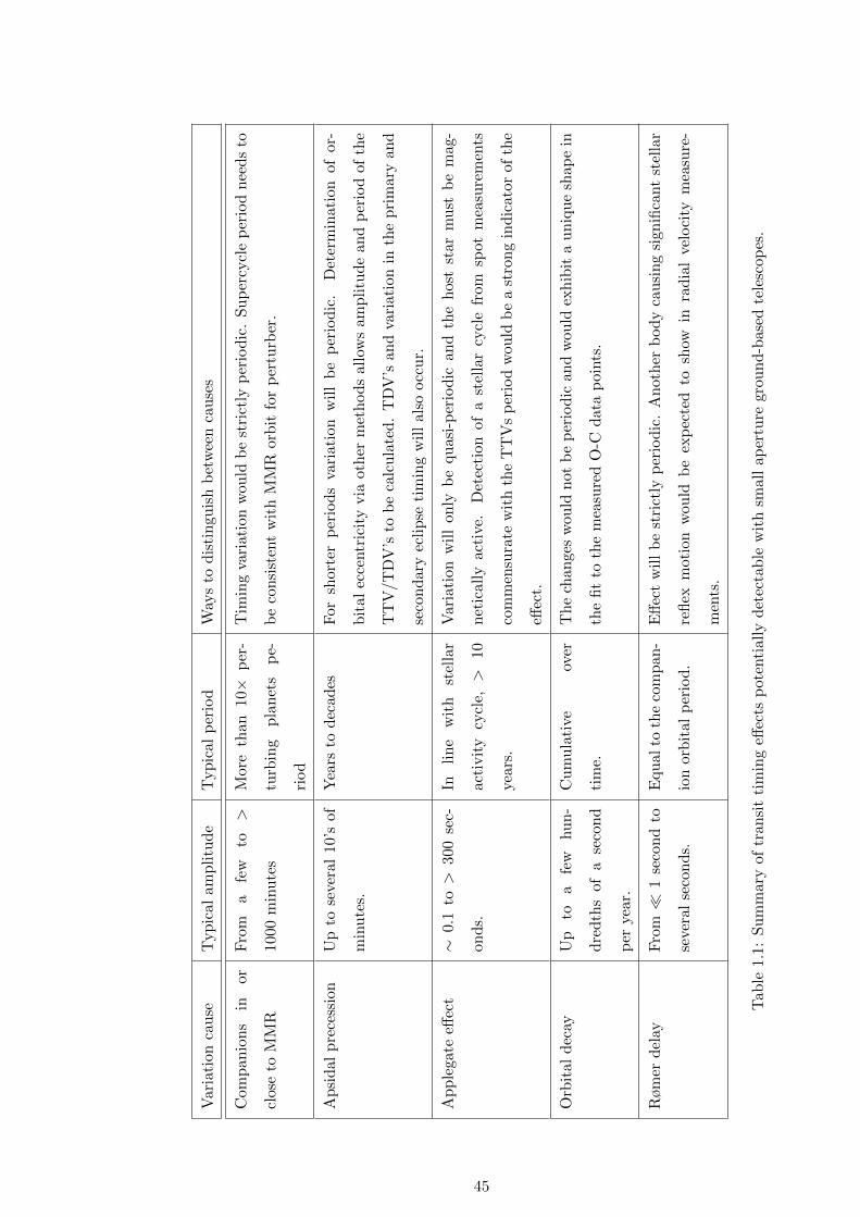
Var

iati

onca

use

Typ

ical

amp

litu

de

Typ

ical

per

iod

Way

sto

dis

tin

guis

hb

etw

een

cau

ses

Com

pan

ion

sin

or

clos

eto

MM

R

Fro

ma

few

to>

1000

min

ute

s

Mor

eth

an10×

per

-

turb

ing

pla

net

sp

e-

riod

Tim

ing

vari

atio

nw

ould

be

stri

ctly

per

iod

ic.

Su

per

cycl

ep

erio

dn

eed

sto

be

con

sist

ent

wit

hM

MR

orb

itfo

rp

ertu

rber

.

Ap

sid

alp

rece

ssio

nU

pto

seve

ral

10’s

of

min

ute

s.

Yea

rsto

dec

ades

For

shor

ter

per

iod

sva

riati

on

wil

lb

ep

erio

dic

.D

eter

min

ati

on

of

or-

bit

alec

centr

icit

yvia

oth

erm

eth

od

sall

ows

am

pli

tude

an

dp

erio

dof

the

TT

V/T

DV

’sto

be

calc

ula

ted

.T

DV

’san

dva

riati

on

inth

ep

rim

ary

an

d

seco

nd

ary

ecli

pse

tim

ing

wil

lals

oocc

ur.

Ap

ple

gate

effec

t∼

0.1

to>

300

sec-

ond

s.

Inli

ne

wit

hst

ella

r

acti

vit

ycy

cle,

>10

year

s.

Var

iati

onw

ill

only

be

quasi

-per

iod

ican

dth

eh

ost

star

mu

stb

em

ag-

net

ical

lyac

tive

.D

etec

tion

of

ast

ella

rcy

cle

from

spot

mea

sure

men

ts

com

men

sura

tew

ith

the

TT

Vs

per

iod

wou

ldb

ea

stro

ng

ind

icato

rof

the

effec

t.

Orb

ital

dec

ayU

pto

afe

whu

n-

dre

dth

sof

ase

con

d

per

year

.

Cu

mu

lati

veov

er

tim

e.

Th

ech

ange

sw

ould

not

be

per

iod

icand

wou

ldex

hib

ita

un

iqu

esh

ap

ein

the

fit

toth

em

easu

red

O-C

data

poin

ts.

Røm

erd

elay

Fro

m�

1se

con

dto

seve

ral

seco

nd

s.

Equ

alto

the

com

pan

-

ion

orb

ital

per

iod

.

Eff

ect

wil

lb

est

rict

lyp

erio

dic

.A

noth

erb

od

yca

usi

ng

sign

ifica

nt

stel

lar

refl

exm

otio

nw

ould

be

exp

ecte

dto

show

inra

dia

lve

loci

tym

easu

re-

men

ts.

Tab

le1.

1:S

um

mar

yof

tran

sit

tim

ing

effec

tsp

oten

tial

lyd

etec

tab

lew

ith

smal

lap

ertu

regro

un

d-b

ase

dte

lesc

op

es.

45

Previous research using small ground-based telescopes has shown typical measurement

uncertainties of ±50 seconds reducing to ±30 seconds for the very highest quality transit

measurements (Salisbury, 2015). Therefore the photometric and timing precision achievable

with small telescopes means the value of these observations comes from monitoring exoplanet

systems over long periods in order to highlight any systems of interest for follow up by

professional observatories. Two key areas where small aperture ground-based telescopes are

able to contribute to exoplanet science are analysed in this thesis;

1. Decades long periods of monitoring of transit timing.

• Ephemeris recovery/refinement.

• Identification of long period large amplitude timing variations due to MMR super-

periods, companion planets on long period orbits (via Rømer effect) or apsidal

precession.

• Identification of non-periodic timing changes due to orbital decay

2. Photometric monitoring of exoplanet host stars.

• To determine rotation rates and activity cycle lengths.

• To inform professional observatories of optimal times to undertake transmission

spectroscopy which can be severely affected by stellar activity.

To be achievable with small aperture ground-based telescopes these types of observations

need to be restricted to transits measurable with sufficient SNR with small aperture telescopes

such as for the short period hot Jupiters. Fortunately these are also the type of systems where

many of these effects are expected to occur.

46

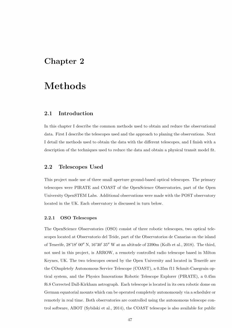
Chapter 2

Methods

2.1 Introduction

In this chapter I describe the common methods used to obtain and reduce the observational

data. First I describe the telescopes used and the approach to planing the observations. Next

I detail the methods used to obtain the data with the different telescopes, and I finish with a

description of the techniques used to reduce the data and obtain a physical transit model fit.

2.2 Telescopes Used

This project made use of three small aperture ground-based optical telescopes. The primary

telescopes were PIRATE and COAST of the OpenScience Observatories, part of the Open

University OpenSTEM Labs. Additional observations were made with the POST observatory

located in the UK. Each observatory is discussed in turn below.

2.2.1 OSO Telescopes

The OpenScience Observatories (OSO) consist of three robotic telescopes, two optical tele-

scopes located at Observatorio del Teide, part of the Observatorios de Canarias on the island

of Tenerife, 28°18′ 00′′ N, 16°30′ 35′′ W at an altitude of 2390m (Kolb et al., 2018). The third,

not used in this project, is ARROW, a remotely controlled radio telescope based in Milton

Keynes, UK. The two telescopes owned by the Open University and located in Tenerife are

the COmpletely Autonomous Service Telescope (COAST), a 0.35m f11 Schmit-Casegrain op-

tical system, and the Physics Innovations Robotic Telescope Explorer (PIRATE), a 0.45m

f6.8 Corrected Dall-Kirkham astrograph. Each telescope is located in its own robotic dome on

German equatorial mounts which can be operated completely autonomously via a scheduler or

remotely in real time. Both observatories are controlled using the autonomous telescope con-

trol software, ABOT (Sybilski et al., 2014), the COAST telescope is also available for public

47

use as part of telescope.org. PIRATE is equipped with an FLI ProLine 16803 4k× 4k, 9µ pixel

CCD camera producing a field of view 42′ square with plate scale of 0.62′′/pixel. Prior to 21st

May 2018 COAST was equipped with an SBIG STL-1001E CCD camera with 1024×1024 24µ

pixels providing a field of view 22′ square with a plate scale of 1.25′′/pixel. After 21st May

2018 COAST was equipped with an FLI ProLine 9000 3k× 3k 12µ pixel CCD camera pro-

ducing a field of view 32′ square with plate scale of 0.63′′/pixel. Both FLI CCD cameras were

operated at a temperature of -30℃. The FLI cameras can be configured to read the CCD

at either 8MHz or 1MHz, the latter providing lower read noise at the expense of a an eight

times increase in read time. At 8MHz a PIRATE CCD frame can be read in 4 seconds, a

process that takes 32 seconds at 1MHz. Therefore both FLI cameras are set for 8MHz read

out to minimise deadtime between exposure and improve the efficiency of the telescopes.

In July 2018 both telescopes were upgraded with the addition of a GPS controlled shutter

timing system, see Section 2.2.3. Prior to 21st May 2018 PIRATE was configured with Baader

broadband R, G and B filters. After this date Johnson-Cousins B, V and Rc filters were

installed and this filter set was extended in July 2018 when U and Ic filters were added. The

Baader R, G and B filters on COAST were replaced with Johnson-Cousins B, V and Rc filters

in July 2018.

Both telescopes are operated without any form of automated guiding, relying instead

on the precise polar alignment of the mounts. ABOT automatically focuses the telescope

for each scheduled observation, therefore deliberate defocusing of the telescope to improve

photometric precision was not possible in scheduled observation mode. The scheduler will

updated in due course to support this functionality.

2.2.2 POST Observatory

The Post Office Small Telescope (POST) is a private observatory owned by the author,

located at 51°15′ 51′′, 01°14′ 58′′E at 20m altitude. POST hosts a 0.4m, f6.8 Optimised Dall-

Kirkham (ODK) telescope on a German Equatorial mount. POST has a carbon fibre optical

tube to minimise thermal expansion and the resulting changes in focus. It is equipped with

an SBIG ST10-XME 2184× 1472 6.8µ pixel CCD camera providing a field of view 19′ × 13′

with a plate scale of 0.52′′/pixel, a full suite of Johnson-Cousins U, B, V, Rc and Ic filters

are available. Figure 2.1 shows the filter bandpasses1 overlaid with the ST-10XME CCD

Quantum Efficiency (QE)2 and the QE for the PIRATE CCD3. POST supports closed loop

on and off axis guiding options to ensure accurate tracking. Most commonly used is the SBIG

1Astrodon, private communication2http://www.company7.com/library/sbig/sbwhtmls/st10.htm3https://www.flicamera.com/proline/

48

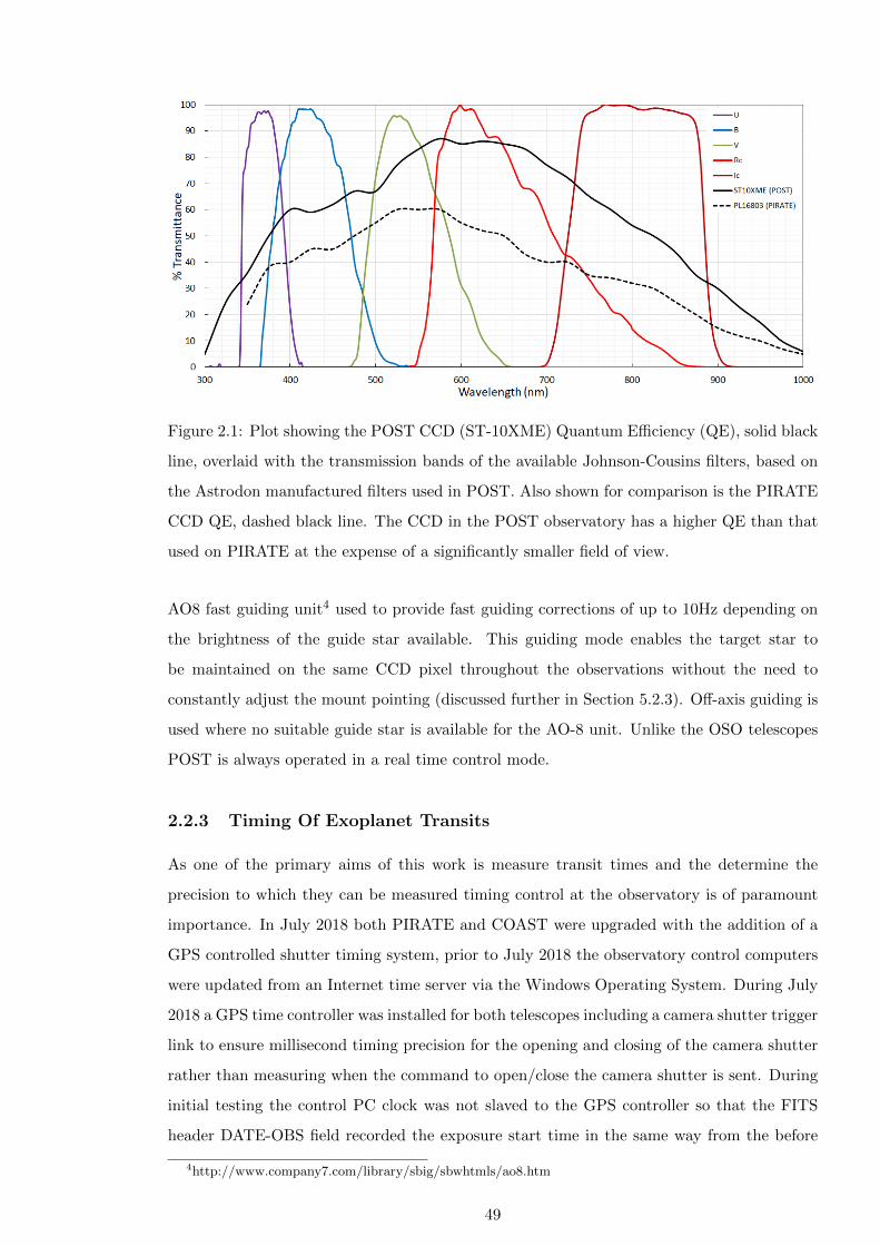
Figure 2.1: Plot showing the POST CCD (ST-10XME) Quantum Efficiency (QE), solid black

line, overlaid with the transmission bands of the available Johnson-Cousins filters, based on

the Astrodon manufactured filters used in POST. Also shown for comparison is the PIRATE

CCD QE, dashed black line. The CCD in the POST observatory has a higher QE than that

used on PIRATE at the expense of a significantly smaller field of view.

AO8 fast guiding unit4 used to provide fast guiding corrections of up to 10Hz depending on

the brightness of the guide star available. This guiding mode enables the target star to

be maintained on the same CCD pixel throughout the observations without the need to

constantly adjust the mount pointing (discussed further in Section 5.2.3). Off-axis guiding is

used where no suitable guide star is available for the AO-8 unit. Unlike the OSO telescopes

POST is always operated in a real time control mode.

2.2.3 Timing Of Exoplanet Transits

As one of the primary aims of this work is measure transit times and the determine the

precision to which they can be measured timing control at the observatory is of paramount

importance. In July 2018 both PIRATE and COAST were upgraded with the addition of a

GPS controlled shutter timing system, prior to July 2018 the observatory control computers

were updated from an Internet time server via the Windows Operating System. During July

2018 a GPS time controller was installed for both telescopes including a camera shutter trigger

link to ensure millisecond timing precision for the opening and closing of the camera shutter

rather than measuring when the command to open/close the camera shutter is sent. During

initial testing the control PC clock was not slaved to the GPS controller so that the FITS

header DATE-OBS field recorded the exposure start time in the same way from the before

4http://www.company7.com/library/sbig/sbwhtmls/ao8.htm

49

the GPS upgrade while the GPS trigger start and end times were recorded in separate FITS

header fields. This enabled a comparison of the difference in exposure start time between the

two timing control methods to be measured and it was found to vary by ±3 seconds. To solve

this discrepancy the PC clock was also slaved to the GPS controller and subsequently the only

difference in image start time stamps was the time between the exposure being requested and

operation of the camera shutter, of the order of milliseconds. The AstroImageJ photometric

software uses the DATE-OBS field from the FITS header and adds half the integration time

to calculate the exposure mid-time, therefore for science observations made in the period

between GPS installation and PC clock time being slaved to the GPS controller the GPS-

START time was copied to the DATE-OBS field in the FITS headers using a routine written

in Python prior to photometric analysis. ABOT has since been updated to write only the

GPS measured start time to the DATE-OBS filed of the FITS headers.

At the time of the observations for this thesis POST was not equipped with a GPS

controller and instead used the freeware Dimension45 to update the control PC clock from

an Internet time server. Although timing updates can be obtained from Internet time servers

by the computer operating system the use of a separate application to carry out this function

allows direct control over the time server synchronisation and reporting. For POST, which is

not left powered all the time unlike COAST and PIRATE, this reporting often showed clock

drifts of many tens of seconds between observations which could be separated by several

weeks.

2.3 Target selection and planning

2.3.1 Target Selection

Targets for observation had to meet a number of criteria including;

• Being visible from both OSO and POST observatory locations.

• Being brighter than magnitude 14 to keep exposure durations reasonable.

• Having a transit depth minimum of 0.5% to ensure an expected minimum transit SNR

(Chapter 5.2.1) of 2.5 - 5 with an assumed expected photometric scatter of 1-2 millmag.

• Being short period to enable multiple transits to be obtained in each observing season.

• Having an outstanding scientific question that could potentially be addressed using

small aperture ground-based telescope observations.

5http://www.thinkman.com/dimension4/

50

The first target, WASP-12b, was selected to be observed during all available observing

seasons with the first observations being made in January 2016 and the last ones completed

in January 2020. Historic observations going back to 2014 were also available from the POST

observatory. WASP-12b is an example of a short period hot Jupiter orbiting its F type host

star every 1.09 days Hebb et al. (2009) and suspected of losing mass through atmospheric

ablation and possibly star-planet interaction (Haswell et al., 2012). Due to this short period

and suspected mass loss WASP-12b has been the subject of many transit timing studies over

the duration of this thesis to search for non-linear ephemeris variations. In 2016 Maciejewski

et al. (2016) presented the first timing analysis indicating a quadratic ephemeris for WASP-

12b and orbital decay has subsequently been confirmed for WASP-12b (Yee et al., 2019;

Turner et al., 2021). WASP-12 has been shown to have a low rotation rate for its stellar type

(Hebb et al., 2009; Nielsen et al., 2013) possibly indicative of a very low, pole-on, inclination

Fossati et al. (2010) however no long term monitoring has been undertaken to search for

photometric variability in WASP-12, thus monitoring was carried out over three seasons

between 2016 and 2019.

A block of observing time occurred in the Summer of 2018 timed to coincide with the

period of the upgrades to PIRATE and COAST. The primary aim was to determine the

improvement in transit time measurement resulting from the installation of the of the GPS

time controllers. Two targets, HAT-P-23b and WASP-52b, both observable over this period,

were selected for observation. HAT-P-23b is a short period hot Jupiter orbiting a V = 12.43

magnitude star with a period 1.21 days and a transit depth of 1.4%. At discovery HAT-P-23b

was found to have inflated radius and an eccentric orbit Bakos et al. (2011), while subsequent

results agreed with the discovery paper (Sada and Ramon-Fox, 2016) others have found a

smaller radius or adopted a circular orbit in the analysis (Ciceri et al., 2015; Maciejewski

et al., 2018). With an orbital period similar to that of WASP-12b which has been shown

to have a decaying orbital period (Yee et al., 2019), hence HAT-P-23b could be expected to

show similar behaviour. Published transit times by Ciceri et al. (2015) appear to display a

quadratic component while the transits times gathered by amateur observers on ETD appear

to show a step change in O-C values between epochs 1900 to 2050, see Figure 3.1. Sada and

Ramon-Fox (2016) also report a suspected photometric variation in HAT-P-23 host star so

nightly monitoring observations were carried out in addition to the transit observations. The

second system selected was WASP-52b, another hot Jupiter with an orbital period of 1.75

days around a small 0.79R� host star producing very deep 2.7% transits (Hebrard et al.,

2013). WASP-52 is known to be active with reported results often showing the effects of spot

crossing events on measured lightcurves (Mancini et al., 2017).

51

2.3.2 Observation Scheduling

Slightly different approaches were taken to the planing and scheduling of observation on

the OSO and POST observatories. This was to account for the UK location of the POST

observatory which, being weather limited, only allowed observations on a few nights per

month. For POST the online ephemeris provided as part of the Exoplanet Transit Database

(ETD) 6 was consulted for the visibility of a transit of any of the target systems when

weather permitted. Targets above the local horizon for their entire transit duration were

observed whenever possible. The observing conditions for PIRATE and COAST are far

more predictable, with an estimated 280 clear nights per year at Mt. Teide observatory,

allowing observations to be scheduled far in advance using the OpenScience Observatories

online Scheduler. The OSO schedulers offers two modes for scheduling of observations, timed

requests that need to occur at specific dates/times and filler requests which are undertaken

anytime the target is visible and the scheduler determines time is available to make the

observations with timed requests always having a higher priority than filler requests. The

queuing of the scheduled targets is set by a combination of factors, including how long a

request has already been in the queue and when the target is visible, as well as a user-set job

priority (which in turn is constrained by the user’s access rights). To create the observing

schedules a long duration ephemeris was downloaded from an on-line ephemeris calculator7

and converted to a text file of the correct format for use in the OSO scheduler. The suitability

of all transit targets was checked using the object visibility tool provided by Isaac Newton

Group of Telescopes.8 The finalised text file includes the target co-ordinates, observation

start and end times as well as exposure, filter and CCD binning parameters.

Scheduling of host star monitoring observations were made as filler requests specifying a

number of exposures per image set and number of images sets per night that the system would

attempt to schedule. This was generally 6 exposures per image set and one or two image sets

per night. A minimum altitude for observation could also be specified and was generally set

at 40° depending on the target. Due to the weather limitations and need to operate POST

in attended mode, monitoring observation were only carried out with PIRATE.

2.4 Transit Observations

Prior to the Summer of 2018 all observations were made with OSO telescopes and POST

in 2 × 2 on-chip inning mode to improve sensitivity, reduce exposure duration, file size and

download times. After 21st July 2018 observations were switched to unbinned mode which

6http://var2.astro.cz/ETD/predictions.php7http://astroutils.astronomy.ohio-state.edu/exofast/8http://catserver.ing.iac.es/

52

also required a commensurate increase in exposure times to maintain signal to noise ratio

but was found to offer improved photometric precision with significantly reduced scatter in

the photometry, discussed further in Chapter 5.

Exposure times were calculated to ensure the ADU counts remained within the CCD

linear response region between 10,000 and 44,000 ADU’s. The lower limit was chosen to

ensure sufficient counts were recorded while the upper limit was determined from the response

graphs of the CCD’s. Figure 2.2 shows the response plots for PIRATE in 1 × 1 and 2 × 2

binning mode which were obtained using star measurements from the same Landolt standard

star field as no stable flat field light source is available at the observatory. The upper limit to

the linear response region was set at a the value of 44,000 ADU below which the response of

the CCD remains linear. The plots in Figure 2.2 show the linear region is defined is consistent

between 1 × 1 and 2 × 2 on chip binning. The plots in Figure 2.2 clearly show less scatter

about the linear response using the unbinned (1 × 1) CCD mode compared with the 2 × 2

binned mode. The RMS scatter in ADU within the linear region is 2649 for the 2×2 binning

and 1434 for the 1 × 1 binning. his may be contributing factor to the improvement seen

in the photometric precision after moving from 2 × 2 to 1 × 1 on-chip binning. However

due to needing to use star fields to obtain this data it may be a systematic effect arising

from changing conditions or different airmass at the time the data was obtained. The values

used the define the linearity region are conservative, the increase in scatter seen for 2 × 2

observation would warrant further investigation.

De-focusing of the telescope has been shown to improve the photometric precision achiev-

able as the flat fielding errors decrease according to the square-root of the number of pixels

in the stellar point spread function PSF; (Southworth et al., 2009a). The technique also

allows very bright stars to be observed which would otherwise saturate the CCD if focused.

Spreading the starlight over a larger area however has a significant impact on the exposure

duration required to achieve the same SNR. For example increasing the FWHM from 3′′ to

10′′ spreads a given stars flux over 11 times the area on the CCD, requiring an 11 times

increase in exposure duration. For 0.4 meter class telescopes typical exposure durations for

the targets observed in this project when focused range from ∼0.5 to 3 minutes. The in-

crease in exposure time to compensate for de-focusing may not allow a transit lightcurve to

be sufficiently sampled. For stars where focused observations require 30 second exposures

de-focusing to 6′′ requires just a four fold increase in exposure time to 2 minutes. When em-

ploying telescope de-focusing great care has to be taken to avoid overlapping stellar PSFs as

this will result in contamination of the photometric aperture leading to errant transit depth

determination. Scheduled observations with PIRATE and COAST do not currently support

de-focusing (though this can be readily achieved with POST) so an alternative approach to

53

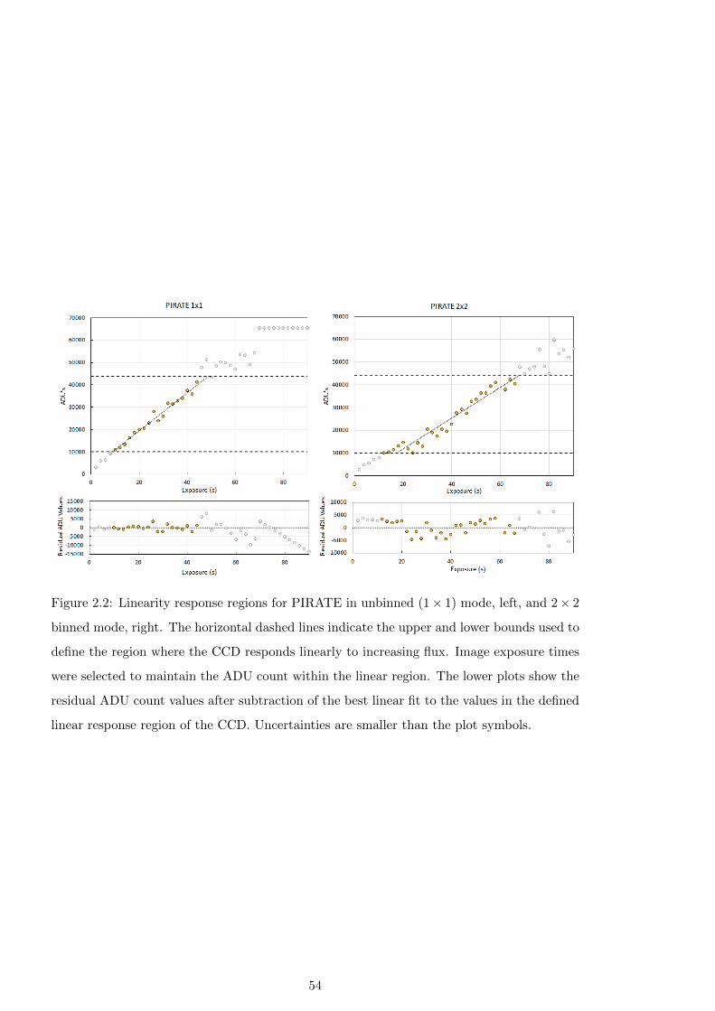
Figure 2.2: Linearity response regions for PIRATE in unbinned (1× 1) mode, left, and 2× 2

binned mode, right. The horizontal dashed lines indicate the upper and lower bounds used to

define the region where the CCD responds linearly to increasing flux. Image exposure times

were selected to maintain the ADU count within the linear region. The lower plots show the

residual ADU count values after subtraction of the best linear fit to the values in the defined

linear response region of the CCD. Uncertainties are smaller than the plot symbols.

54

de-focusing explored in this thesis (see Chapter 5) is oversampling of the stellar PSF.

Niquist sampling theorem requires that the stellar FWHM is covered by at least 2 CCD

pixels9. Seeing conditions at Observatorio del Teide are typically of the order of 1′′10, more

often typical FWHM achieved is 2′′ for PIRATE and COAST, likely due to imperfect auto-

mated focus or possibly to different seeing conditions at the location of the telescopes being

slightly lower than those of the seeing monitors. This requires a plate scale of ∼ 1′′ per

pixel while for POST with typical seeing of 3′′ − 4′′ this requires ∼ 1.5′′ − 2′′ per pixel. With

plate scales of 0.63′′, 0.64′′ and 0.52′′ per pixel for COAST, PIRATE and POST respectively,

2x2 on-chip CCD binning for the OSO telescopes with their superior seeing conditions falls

slightly short of the Niquist sampling criteria while POST slightly exceeds it. Oversampling

the stellar PSF spreads the flux over a greater number of pixels, generating some of the

benefits of de-focusing, avoids flux overlap, maintains reasonable exposure times and allows

on-axis guiding to be employed on POST.

In order to allow the observations from multiple telescopes to be analysed together all

observations were filtered. The Johnson B filter was used for some observations, mainly where

both COAST and PIRATE were scheduled to observe the same transit to allow two colour

data to be gathered. The Cousins Rc filter was used for the majority of transit observations

(broadband Red in earlier observations). A red filter such as the Rc offers a number of

benefits including;

• Reducing effects of atmospheric scintillation.

• Of 335 stars listed on the NASA Exoplanet Database as discovered using the transit

method with a recorded host star spectral type (accessed 6th Oct 2021), 76% are G,K

and M stars with spectral energy distributions that peak in the red. Observing in the

red bandpass will collect more photons per second than for shorter wavelength bandpass

filters allowing a theoretically higher SNR to be achieved.

• Commercial CCD cameras tend to have a higher quantum efficiency in the red part of

the spectrum minimising the impact of flux lost due to the filter transmission charac-

teristics.

• Limb darkening effects are minimised for transits observed at longer wavelengths thus

the lightcurves have more sharply defined transition points (E.g. Knutson et al., 2007,

Fig. 2). This improves the transit model fit providing increased transit timing precision.

9http://www.vikdhillon.staff.shef.ac.uk/teaching/phy217/instruments/phy217 inst sampling.html10https://www.iac.es/en/observatorios-de-canarias/sky-quality/sky-quality-in-real-time

55

2.5 Data Reduction

Data reduction is a vital step to correct individual images for the impact on the incoming flux

introduced by the optical system and the characteristics of the CCD. Prior to data reduction

being carried out all frames are plate solved in AstroImageJ using a link to the Astrometry.net

web portal11 (Lang et al., 2010) and WCS results are added for the individual frames FITS

headers. There are three basic types of calibration frame required:

• Bias frames are obtained with a zero duration exposure setting while the CCD shutter

is closed. This does not allow any thermal noise to accumulate thus a bias frame is a

map of the read out noise from the CCD for each pixel and of the noise accumulated

from reading out the CCD, including from the camera electronics and data transfer to

the control PC. All bias frames are taken at the same CCD temperature used for the

science frames.

• Dark frames are exposures taken with the shutter closed to provide a map of the ther-

mal noise of the CCD at the same temperature as the science frames. For the POST

telescope dark frames of the same duration as the science frames were obtained. PI-

RATE and COAST use a standard 60 second dark frame which is scaled to the science

frame exposure duration in AstroImageJ. All data obtained for this thesis was reduced

in the standard fashion using dark frames however subsequent testing with PIRATE

has shown that, operating at -30℃, insufficient thermal current builds up in 60 seconds

resulting in total thermal noise significantly less than the read noise (Jackson et al.,

2021). A single PIRATE lightcurve of WASP-12b was analysed both with and without

dark frames, the resulting differences in flux measurement were of the order of ten times

smaller than the photometric measurement uncertainty, showing either approach would

be valid for lightcurves obtained with PIRATE.

• Flat field frames are short exposure frames taken of a uniform light source through the

same filter and with the same CCD temperature as the science frames. A flat field

provides a map of the effects of the optical path on the data frames such as dust on

the optical surfaces or vignetting in the optical system. The flat field also maps any

defects in the CCD including pixel to pixel variations in the CCD response.

In the POST observatory the flat fields are obtained using a variable brightness lightbox

located immediately in front of the optical tube in the telescopes parked position. The ability

to vary the brightness of the lightbox ensures an exposure time of 5-12 seconds for different

filter and pixel binning combinations can be used. This range of exposure durations for the

11https://nova.astrometry.net/

56

flat field frames ensures no shutter artefacts remain in the images and at least 27 frames can

be obtained with an ADU count of two thirds of the CCD full well count in a reasonable

time. With PIRATE and COAST dusk and dawn sky flats are obtained each evening and

morning in a sequence controlled by ABOT. This allows a small number of flat field frames

to be obtained through each filter each night and therefore frames from multiple nights are

used after visually checking for consistency between frames from different nights. The sky

flats often contain stars especially as the exposures increase while the sky is getting darker

so the telescope pointing is adjusted slightly (dithered) between each exposure so any star

images fall on different pixels in each flat field frame.

Data reduction for all observations was carried out using the Data Processing (DP) module

within AstroImageJ. DP median combines the individual frames from each group of bias, dark

and flat field frames into individual master calibration frames before applying to the science

frames. Using a median combine method minimises the impact of any image artifacts such as

stars in the flat field frames. The master dark is bias corrected by subtracting the master bias

frame. The flat field master is bias and dark corrected by subtracting the bias and exposure

duration corrected dark master frames. The final step is to reduce the science frames by

subtracting the master bias and dark frames and dividing by the master flat field frame to

produce a calibrated science frame. The DP module also allows for modified time stamps to

be created and written to the FITS header for each science frame. Based on the observatory

location and target co-ordinates the UTC stamp recording the exposure start time in the

FITS header is converted to dynamic barycentric, BJDTDB time and half the exposure time

is added to record the frame mid exposure time which is recorded in the FITS header.

2.6 Transit Lightcurve Photometry

AstroImageJ has been specifically created for photometry of transiting exoplanets and in-

cludes routines for simultaneous photometry and transit model fitting (Collins et al., 2017b).

Below I describe the process used to produce transit lightcurves which follows from the com-

pletion of data reduction described in Section 2.5.

Ensemble photometry is used to combine multiple comparison stars, minimising any sys-

tematic noise arising from any individual comparison star. For the ensemble photometry up

to 24 comparison stars are selected from across the entire field (avoiding stars close to the

edges of the frames) with the same sized apertures as the target star. Checks are carried out

to ensure that none of the selected comparison stars are known variable stars and that all have

ADU counts below the set non-linearity limit. In this approach the most suitable comparison

57

stars are selected independently for each transit data set, as such the ensemble photometry is

optimised for each data set. It was not always practical to use the same comparison stars in

the ensemble for every transit data set from a given target due to the differing fields of view

between the telescopes used, changes in the FWHM resulting from focus changes between

nights and differing on-chip binning and filters used.

The target star is selected and the first photometry aperture applied with an initial

aperture radius set to 1.7×FWHM of the target star in the first frame. The inner radius

of the sky-background annulus is set to 1.9×FWHM and the outer radius to 2.55×FWHM.

These radii provide equal numbers of pixels in the aperture and sky-background annulus which

are later refined during the photometry optimisation process (Section 2.6.1) and detrended

(Section 2.6.1.1) to minimise photometric scatter. Prior to 7th June 2019 AIJ counted only

whole pixels inside the star aperture and the sky annulus, release 3.3.0 after this date allows

exact partial pixel counting, improving photometric precision for smaller apertures.

AIJ calculates the target star flux relative to the sum of the comparison star fluxes, both

corrected for the sky background. The use of a large number of comparison stars from across

the entire field of view averages out variations due to second order effects arising from colour

changes as the airmass changes during the observations.

2.6.1 Photometry Optimisation

Optimising the photometry is an iterative process of modifying the ensemble of comparison

stars and photometric apertures to achieve the minimum possible scatter in the resulting

residuals to a model of the transit. First the model parameters are defined in AIJ using values

from the literature and quadratic limb darkening coefficients for the filter used calculated

using an on-line tool 12 (Eastman et al., 2013) which interpolates the limb darkening tables

from Claret and Bloemen (2011). AIJ uses a simple stellar model that assumes the host star

is on the Zero-Age Main Sequence (ZAMS) and as such does not allow the stellar parameters

such as spectral type, effective temperature, mass and radius to be varied independently.

For transit photometry the stellar radius is more important than spectral type or Teff in

determining the lightcurve parameters so this was set based on the best published value.

Once the ensemble photometry has been calculated for the target star from every frame

in the time series data, AIJ fits a transit model based on the formalisation of Mandel and

Agol (2002) to the resulting lightcurve. The best fit model is found through minimising the

χ2 of the model residuals. AIJ reports the quality of the model fit to the data providing the

residual RMS value, χ2ν and the Bayesian Information Criterion (BIC) defined as

12http://astroutils.astronomy.ohio-state.edu/exofast/limbdark.shtml

58

BIC = χ2 + p× ln(n) (2.1)

Here p is the number of fitted parameters and n is the number of data points in the

lightcurve (Collins et al., 2017b). This process is then repeated for a range of different star

aperture and sky annulus radii to determine the values that produce the smallest residual

RMS and BIC values. AIJ also provides the option to vary the star aperture based on the

target star FWHM from each frame in the time series data which can produce superior results

where seeing conditions are changeable through the night or where the focus drifts due to

external temperature changes. In this mode AIJ applies a user defined multiplier to the

measured FWHM value in each frame to calculate the star aperture radius. Values of the

FWHM multiplier are stepped through to find the values that result in the smallest RMS

residuals and BIC value. Care is taken to ensure the star aperture radius does not exceed

the inner radius of the background annulus.

In both fixed and variable aperture modes the radius of background annulus is selected

such that it contains at least the same number of pixels as the star aperture. This will

sometimes result in background stars, or hot pixels remaining after reduction, being included

in the background annulus. To minimise the effect on the photometry AIJ carries out an

iterative 2σ cleaning of the sky background (see Section 5.2.3 for an example). For this

reason the sky annuli were set to contain a larger number of pixels than the star aperture to

allow for pixels to be removed by this process.

Although AIJ can remove hot pixels from the sky background annulus with the interative

2σ cleaning, this is not possible for the star aperture. This can lead to circumstances where

the target star or one or more comparison stars can be affected by transient hot pixels,

not corrected for by the data reductions process. Therefore in the final step the lightcurve

was visually checked for outlying data points and these were removed from the data where

the images revealed artefacts affecting the photometry such as cosmic ray hits or cloud

obscuration.

2.6.1.1 Lightcurve Detrending

The above optimisation process for the photometry apertures is undertaken with detrending

applied to the lightcurve for airmass and, where required, pier flip offset. The detrending

is calculated by including a χ2 contribution for each detrend parameter in the lightcurve fit

following Equation 5 in Collins et al. (2017b). Linear and second order polynomial detrending

options are available, the latter being suitable for airmass detrending which uses the airmass

values added to the FITS header during the data reduction process. The time of the pier

flip is manually set within AIJ before calculating the ensemble photometry. To ensure any

59

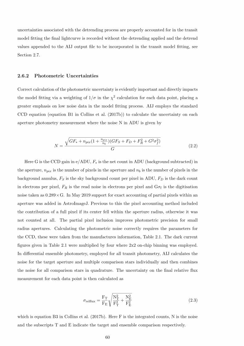
uncertainties associated with the detrending process are properly accounted for in the transit

model fitting the final lightcurve is recorded without the detrending applied and the detrend

values appended to the AIJ output file to be incorporated in the transit model fitting, see

Section 2.7.

2.6.2 Photometric Uncertainties

Correct calculation of the photometric uncertainty is evidently important and directly impacts

the model fitting via a weighting of 1/σ in the χ2 calculation for each data point, placing a

greater emphasis on low noise data in the model fitting process. AIJ employs the standard

CCD equation (equation B1 in Collins et al. (2017b)) to calculate the uncertainty on each

aperture photometry measurement where the noise N in ADU is given by

N =

√GF∗ + npix(1 +

npixnb

)(GFS + FD + F 2R +G2σ2

f )

G(2.2)

Here G is the CCD gain in e/ADU, F∗ is the net count in ADU (background subtracted) in

the aperture, npix is the number of pixels in the aperture and nb is the number of pixels in the

background annulus, FS is the sky background count per pixel in ADU, FD is the dark count

in electrons per pixel, FR is the read noise in electrons per pixel and Gσf is the digitisation

noise taken as 0.289×G. In May 2019 support for exact accounting of partial pixels within an

aperture was added in AstroImageJ. Previous to this the pixel accounting method included

the contribution of a full pixel if its center fell within the aperture radius, otherwise it was

not counted at all. The partial pixel inclusion improves photometric precision for small

radius apertures. Calculating the photometric noise correctly requires the parameters for

the CCD, these were taken from the manufactures information, Table 2.1. The dark current

figures given in Table 2.1 were multiplied by four where 2x2 on-chip binning was employed.

In differential ensemble photometry, employed for all transit photometry, AIJ calculates the

noise for the target aperture and multiple comparison stars individually and then combines

the noise for all comparison stars in quadrature. The uncertainty on the final relative flux

measurement for each data point is then calculated as

σrelflux =FT

FE

√N2

T

F2T

+N2

E

F2E

(2.3)

which is equation B3 in Collins et al. (2017b). Here F is the integrated counts, N is the noise

and the subscripts T and E indicate the target and ensemble comparison respectively.

60

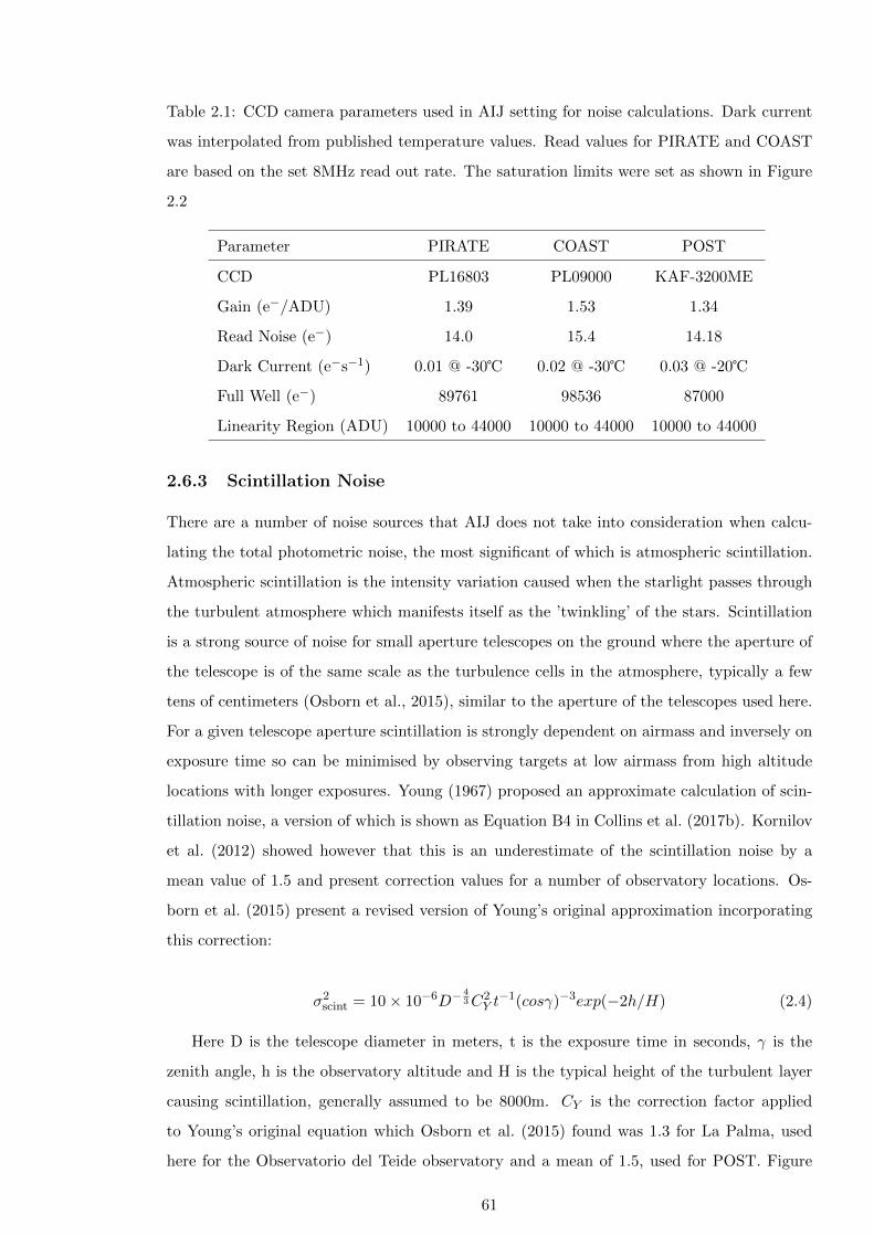
Table 2.1: CCD camera parameters used in AIJ setting for noise calculations. Dark current

was interpolated from published temperature values. Read values for PIRATE and COAST

are based on the set 8MHz read out rate. The saturation limits were set as shown in Figure

2.2

Parameter PIRATE COAST POST

CCD PL16803 PL09000 KAF-3200ME

Gain (e−/ADU) 1.39 1.53 1.34

Read Noise (e−) 14.0 15.4 14.18

Dark Current (e−s−1) 0.01 @ -30℃ 0.02 @ -30℃ 0.03 @ -20℃

Full Well (e−) 89761 98536 87000

Linearity Region (ADU) 10000 to 44000 10000 to 44000 10000 to 44000

2.6.3 Scintillation Noise

There are a number of noise sources that AIJ does not take into consideration when calcu-

lating the total photometric noise, the most significant of which is atmospheric scintillation.

Atmospheric scintillation is the intensity variation caused when the starlight passes through

the turbulent atmosphere which manifests itself as the ’twinkling’ of the stars. Scintillation

is a strong source of noise for small aperture telescopes on the ground where the aperture of

the telescope is of the same scale as the turbulence cells in the atmosphere, typically a few

tens of centimeters (Osborn et al., 2015), similar to the aperture of the telescopes used here.

For a given telescope aperture scintillation is strongly dependent on airmass and inversely on

exposure time so can be minimised by observing targets at low airmass from high altitude

locations with longer exposures. Young (1967) proposed an approximate calculation of scin-

tillation noise, a version of which is shown as Equation B4 in Collins et al. (2017b). Kornilov

et al. (2012) showed however that this is an underestimate of the scintillation noise by a

mean value of 1.5 and present correction values for a number of observatory locations. Os-

born et al. (2015) present a revised version of Young’s original approximation incorporating

this correction:

σ2scint = 10× 10−6D−

43C2

Y t−1(cosγ)−3exp(−2h/H) (2.4)

Here D is the telescope diameter in meters, t is the exposure time in seconds, γ is the

zenith angle, h is the observatory altitude and H is the typical height of the turbulent layer

causing scintillation, generally assumed to be 8000m. CY is the correction factor applied

to Young’s original equation which Osborn et al. (2015) found was 1.3 for La Palma, used

here for the Observatorio del Teide observatory and a mean of 1.5, used for POST. Figure

61

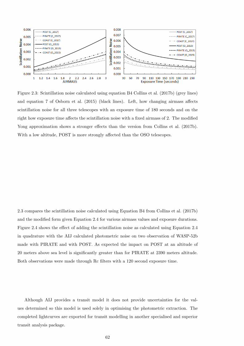
Figure 2.3: Scintillation noise calculated using equation B4 Collins et al. (2017b) (grey lines)

and equation 7 of Osborn et al. (2015) (black lines). Left, how changing airmass affects

scintillation noise for all three telescopes with an exposure time of 180 seconds and on the

right how exposure time affects the scintillation noise with a fixed airmass of 2. The modified

Yong approximation shows a stronger effects than the version from Collins et al. (2017b).

With a low altitude, POST is more strongly affected than the OSO telescopes.

2.3 compares the scintillation noise calculated using Equation B4 from Collins et al. (2017b)

and the modified form given Equation 2.4 for various airmass values and exposure durations.

Figure 2.4 shows the effect of adding the scintillation noise as calculated using Equation 2.4

in quadrature with the AIJ calculated photometric noise on two observation of WASP-52b

made with PIRATE and with POST. As expected the impact on POST at an altitude of

20 meters above sea level is significantly greater than for PIRATE at 2390 meters altitude.

Both observations were made through Rc filters with a 120 second exposure time.

Although AIJ provides a transit model it does not provide uncertainties for the val-

ues determined so this model is used solely in optimising the photometric extraction. The

completed lightcurves are exported for transit modelling in another specialised and superior

transit analysis package.

62

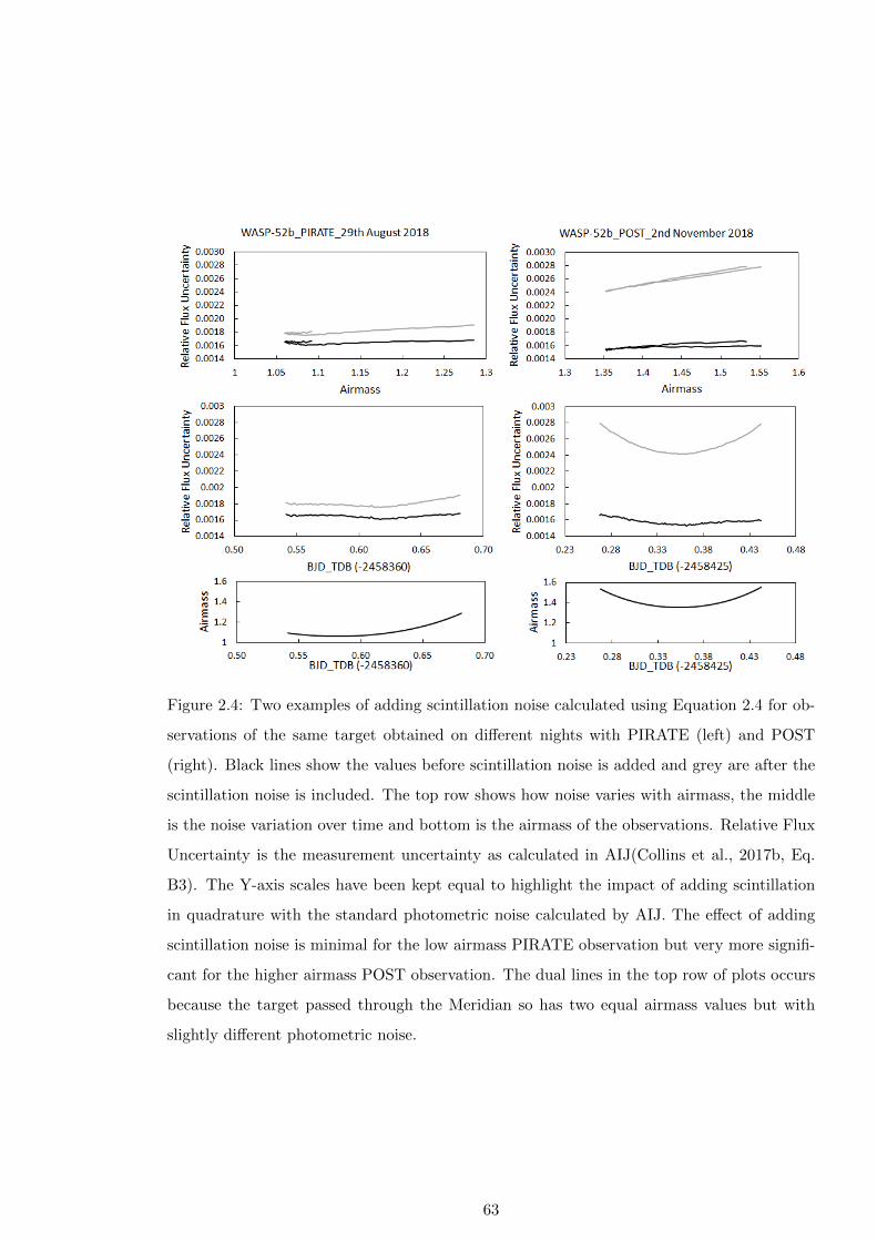
Figure 2.4: Two examples of adding scintillation noise calculated using Equation 2.4 for ob-

servations of the same target obtained on different nights with PIRATE (left) and POST

(right). Black lines show the values before scintillation noise is added and grey are after the

scintillation noise is included. The top row shows how noise varies with airmass, the middle

is the noise variation over time and bottom is the airmass of the observations. Relative Flux

Uncertainty is the measurement uncertainty as calculated in AIJ(Collins et al., 2017b, Eq.

B3). The Y-axis scales have been kept equal to highlight the impact of adding scintillation

in quadrature with the standard photometric noise calculated by AIJ. The effect of adding

scintillation noise is minimal for the low airmass PIRATE observation but very more signifi-

cant for the higher airmass POST observation. The dual lines in the top row of plots occurs

because the target passed through the Meridian so has two equal airmass values but with

slightly different photometric noise.

63

2.7 Transit model fitting

2.7.1 ExofastV2

All transit analysis was carried out using ExofastV2, a publicly available general exoplanet

fitting code released in the Summer 2019 (Eastman et al., 2019). ExofastV2 is written in

IDL but is available to run with or without an IDL licence on a Windows PC, with a licence

ExofastV2 supports multithreading substantially reducing calculation time. ExofastV2 offers

a number of features making it well suited to anayslying the transit lightcurves obtained for

this thesis:

• Previous versions of the code have been widely used in peer reviewed publications (E.g.

Collins et al., 2017a; Basturk et al., 2019; Zellem et al., 2020).

• Support for simultaneous fitting of multiple transit and radial velocity (RV) data sets

from different instruments and with different filters.

• It allows transit timing, depth and duration variations to be modelled.

• Uses a differential evolution Markov chain Monte Carlo DE-MCMC optimisation.

• Provides multiple options for modelling stellar parameters including MESA Isochrones

and Stellar Tracks (MIST), Yonsi-Yale isochrone fitting and Torres relationship (see

Eastman et al., 2019, and references therein).

• Fits broadband stellar Spectral Energy Distribution (SED) with prior constraints from

the Gaia DR2 catalogue (Brown and Gaia Collaboration., 2018) to significantly improve

stellar radius determination.

• Allows multi-parameter lightcurve detrending simultaneously with the transit fit to

ensure uncertainties arising from detrending are correctly propagated through the model

fit.

• ExofastV2 is well documented and provides diagnostic reports to help ensure correct

operation.

The one drawback of using ExofastV2 is the time required for the DE-MCMC to converge

in a multi-transit and RV fit can take many days running on a Windows PC with a 2.60GHz

CPU, the computing platform available for this work. One reason for this is that without an

IDL licence ExofastV2 can only use a single CPU core so is limited by the CPU clock speed.

ExofastV2 requires the preparation of a number of input files before being executed. The

methods and sources used to create these files are described below.

64

2.7.2 Transit Lightcurve files

To allow transit timing, duration and depth variations to be modelled ExofastV2 requires

each transit lightcurve to be input as a separate text file allowing the baseline flux and its

variance to be calculated for each transit lightcurve. The individual lightcurves were output

from AIJ as text files containing a single row for each data-point. The data columns included

were the BJDTDB mid-time of the observation, the normalised flux measurement without

detrending, the photometric uncertainty (including scintillation noise) and then columns for

each of the detrending parameters such as airmass and pier flip as required. The transit date,

telescope and filter used for each lightcurve are set for ExofastV2 within the lightcurve file

name.

2.7.3 RV files

No new radial velocity measurements were obtained as part of this work so catalogue radial

velocity data was used with RV data sets obtained from the literature, the NASA Exoplanet

Archive 13 or from VizieR14. The files contained the date of observation, radial velocity and

uncertainty in ms−1. Dates were converted to BJDTDB as required using the on-line date

conversion tool provided by the author of ExofastV215 . Care was taken to ensure that

measurements from different instruments or those widely separated in time were provided as

separate input files to allow individual velocity zero points and jitter values to be calculated for

each. RV data sets containing predominantly measurements at transit mid-time for Rossiter-

McLoughlin analysis were not included.

2.7.4 Photometry files

Photometric input files used to build the broadband SED were created for each target host

star using a subroutine in Exofast to query trusted photometry catalogues including TYCHO

(Høg et al., 2000), ALLWISE (Cutri, 2013) and 2MASS (Skrutskie et al., 2006). Additional

photometry in the Johnson B and V bands and SDSS g′, r′ and i′ bands was obtained from

the AAVSO AllSky Photometric Survey (APASS) Data Release 1016 (Henden, 2019). It is

important that the broadband photometry is not blended with flux from close by stars as

this will affect the brightness of the the star leading to a larger radius determination. The

literature was checked for reports of close companions to any the systems studied such as

lucky imaging studies (E.g. Bergfors et al., 2013). Gaia EDR3 multi-peak flag, a sign a star

13https://exoplanetarchive.ipac.caltech.edu/index.html14https://vizier.u-strasbg.fr/viz-bin/VizieR15http://astroutils.astronomy.ohio-state.edu/time/16https://www.aavso.org/apass

65

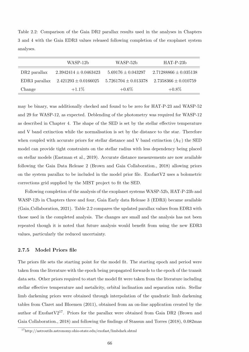
Table 2.2: Comparison of the Gaia DR2 parallax results used in the analyses in Chapters

3 and 4 with the Gaia EDR3 values released following completion of the exoplanet system

analyses.

WASP-12b WASP-52b HAT-P-23b

DR2 parallax 2.3942414± 0.0463423 5.69176± 0.043297 2.71288866± 0.035138

EDR3 parallax 2.421293± 0.0166025 5.7261704± 0.013378 2.7358366± 0.010759

Change +1.1% +0.6% +0.8%

may be binary, was additionally checked and found to be zero for HAT-P-23 and WASP-52

and 29 for WASP-12, as expected. Deblending of the photometry was required for WASP-12

as described in Chapter 4. The shape of the SED is set by the stellar effective temperature

and V band extinction while the normalisation is set by the distance to the star. Therefore

when coupled with accurate priors for stellar distance and V band extinction (AV) the SED

model can provide tight constraints on the stellar radius with less dependency being placed

on stellar models (Eastman et al., 2019). Accurate distance measurements are now available

following the Gaia Data Release 2 (Brown and Gaia Collaboration., 2018) allowing priors

on the system parallax to be included in the model prior file. ExofastV2 uses a bolometric

corrections grid supplied by the MIST project to fit the SED.

Following completion of the analysis of the exoplanet systems WASP-52b, HAT-P-23b and

WASP-12b in Chapters three and four, Gaia Early data Release 3 (EDR3) became available

(Gaia Collaboration, 2021). Table 2.2 compares the updated parallax values from EDR3 with

those used in the completed analysis. The changes are small and the analysis has not been

repeated though it is noted that future analysis would benefit from using the new EDR3

values, particularly the reduced uncertainty.

2.7.5 Model Priors file

The priors file sets the starting point for the model fit. The starting epoch and period were

taken from the literature with the epoch being propagated forwards to the epoch of the transit

data sets. Other priors required to start the model fit were taken from the literature including

stellar effective temperature and metalicity, orbital inclination and separation ratio. Stellar

limb darkening priors were obtained through interpolation of the quadratic limb darkening

tables from Claret and Bloemen (2011), obtained from an on-line application created by the

author of ExofastV217. Priors for the parallax were obtained from Gaia DR2 (Brown and

Gaia Collaboration., 2018) and following the findings of Stassun and Torres (2018), 0.082mas

17http://astroutils.astronomy.ohio-state.edu/exofast/limbdark.shtml

66

is added to the reported parallax and 0.033 mas is added in quadrature to the DR2 reported

uncertainty. An upper limit for the V band extinction parameter (AV) for each system was

obtained from the updated dust maps from Schlafly and Finkbeiner (2011) 18 and multiplied

by 3.1 to convert to the V band extinction used in ExofastV2 before being applied as a

prior to the SED fit. Prior widths were either set as Gaussian values where the prior value

is taken as the mean of the Gaussian distribution, as maximum-minimum limits (for dust

extinction) or excluded. For Gaussian prior widths ExofastV2 applies a penalty equal to

((value− prior)/uncertainty)2 to the χ2 at each step of the model fit. Where minimum or

maximum limits are set any models exceeding these limits are dropped and if no width is

set the prior is used as starting point with no penalty applied for diverging from this value.

No transit model parameters were fixed at their starting values (prior width = 0). Poor or

uncertain starting priors can result in very long convergence times or convergence failure so

initial model fits of a few thousand steps were run and the output from those used as the

input prior file for subsequent model runs. This iterative process of refining the prior values

enabled model fits with large numbers of steps to converge more quickly, reducing overall

run time. The probability function diagnostic plots were checked after each run to ensure

consistency.

2.7.6 Arguments files

The arguments file contains the run parameters for the model. For all systems analysed stellar

parameter determination was achieved through the combination of the MIST evolutionary

models with SED fitting. The arguments file allow flags to be set for a number of other model

parameters such as fixing the orbit as circular and including outputs for timing, duration and

depth variations. The number of steps for the DE-MCMC chains is set and is a free value, care

was taken to ensure the number of steps was sufficient to ensure the chains were fully mixed

while managing the model run duration and memory usage which are directly proportional

to the number of steps. Because adjacent steps are highly correlated ExofastV2 provides

a parameter called NTHIN which allows the code to discard a user configurable number of

adjacent steps, significantly reducing the memory required for a model fit while allowing

the same parameter space to be explored. Thus a 10,000 step, NTHIN = 6 model run is

equivalent to a 60,000 step, NTHIN=1 model run but with a significant reduction in memory

required.

18https://irsa.ipac.caltech.edu/applications/DUST/

67

2.8 Monitoring Observations

Snap shot monitoring observations were obtained using PIRATE scheduled to take six frames

per group of a given target using the B or Rc filter when the target was higher than 40

degrees altitude. The number of frames obtained each night varied due to weather and

telescope commitments. The analysis of the monitoring data photometry was undertaken

using a template created in AIJ incorporating stars from the UCAC4 catalogue with known

B, V and r′ filter magnitudes. A star with r′ magnitude and B-V colour index close to the

target star was selected as a check star (after checking for known variability). The same

template was used for all data of the same target. AIJ does not take into account catalogue

magnitude uncertainties so I report the uncertainties for the calculated magnitudes based on

the standard error in the measurements of the check star. Observations were obtained in

both 2x2 and 1x1 on-chip binning mode and was therefore analysed separately before being

combined into the overall monitoring data set.

Periodicity analysis for each target and check star was undertaken using a Lomb-Scargle

period analysis as implemented in the AstroPy Python 3 library19.

19https://docs.astropy.org/en/stable/timeseries/lombscargle.html

68

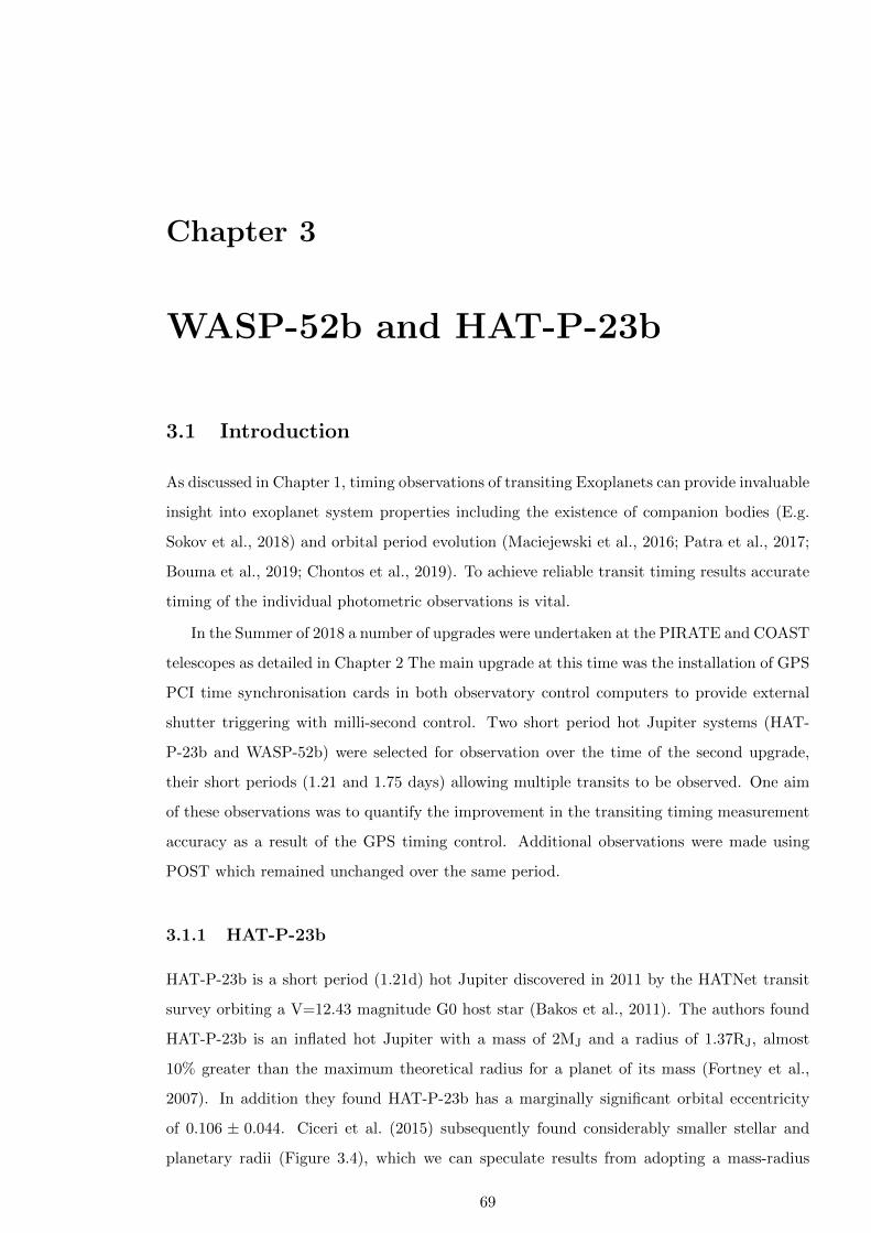
Chapter 3

WASP-52b and HAT-P-23b

3.1 Introduction

As discussed in Chapter 1, timing observations of transiting Exoplanets can provide invaluable

insight into exoplanet system properties including the existence of companion bodies (E.g.

Sokov et al., 2018) and orbital period evolution (Maciejewski et al., 2016; Patra et al., 2017;

Bouma et al., 2019; Chontos et al., 2019). To achieve reliable transit timing results accurate

timing of the individual photometric observations is vital.

In the Summer of 2018 a number of upgrades were undertaken at the PIRATE and COAST

telescopes as detailed in Chapter 2 The main upgrade at this time was the installation of GPS

PCI time synchronisation cards in both observatory control computers to provide external

shutter triggering with milli-second control. Two short period hot Jupiter systems (HAT-

P-23b and WASP-52b) were selected for observation over the time of the second upgrade,

their short periods (1.21 and 1.75 days) allowing multiple transits to be observed. One aim

of these observations was to quantify the improvement in the transiting timing measurement

accuracy as a result of the GPS timing control. Additional observations were made using

POST which remained unchanged over the same period.

3.1.1 HAT-P-23b

HAT-P-23b is a short period (1.21d) hot Jupiter discovered in 2011 by the HATNet transit

survey orbiting a V=12.43 magnitude G0 host star (Bakos et al., 2011). The authors found

HAT-P-23b is an inflated hot Jupiter with a mass of 2MJ and a radius of 1.37RJ, almost

10% greater than the maximum theoretical radius for a planet of its mass (Fortney et al.,

2007). In addition they found HAT-P-23b has a marginally significant orbital eccentricity

of 0.106 ± 0.044. Ciceri et al. (2015) subsequently found considerably smaller stellar and

planetary radii (Figure 3.4), which we can speculate results from adopting a mass-radius

69

relationship based on a younger age for HAT-P-23 and using a fixed circular orbit in their

transit modelling. Measurement of the Rossiter-McLaughlin effect has shown HAT-P-23b is

in an aligned prograde orbit with a projected angle between the orbital plane and the stellar

equatorial plane of 15°±22°(Moutou et al., 2011). Previous studies have taken different

approaches to the suspected eccentricity with some authors leaving eccentricity as a free

parameter, e.g. Bakos et al. (2011); Sada and Ramon-Fox (2016), while others have fixed the

orbit as circular in their analyses e.g. Ciceri et al. (2015); Maciejewski et al. (2018). HAT-

P-23b has a similar orbital period to that of WASP-12b which has been shown to exhibit a

decreasing orbit (Maciejewski et al., 2016; Patra et al., 2017; Maciejewski et al., 2018; Yee

et al., 2019) hence HAT-P-23b could be expected to exhibit a similar decreasing orbital period

which may require transit measurements over decades to detect. Ciceri et al. (2015) presented

O-C results (their Figure 6) that appear to show a quadratic deviation indicative of period

change, but this was not commented upon (see section 3.3.2). The transit timing observations

available on the Exoplanet Transit Database1 (ETD) show a change in reported O-C values

over the period between transit epochs 1900 and 2050, Figure 3.1. After HAT-P-23b had been

selected and the transit observations obtained, Maciejewski et al. (2018) published results of

a further 13 new transits and reanalysis of the previously published transit times looking for

evidence of orbital decay. They conclude that the best fit ephemeris is linear and that there

is no sign of orbital period change which they attributed to inefficient tidal dissipation in the

main sequence host star.

3.1.2 WASP-52b

WASP-52b is an inflated hot Jupiter on a 1.75d circular orbit around a K2V star (Hebrard

et al., 2013). The 0.79R� stellar radius and the inflated 1.27RJ planet radius results in 3%

deep transits. Due to the planets large radius and low mass (0.45MJ), the difference in transit

depth of a single scale height equates to 4.4×10−4 (Kirk et al., 2016). This makes WASP-52b

an excellent target for transit spectroscopy; such studies reveal that WASP-52b has a cloudy

atmosphere with no indication of Rayleigh scattering (Kirk et al., 2016; Louden et al., 2017),

in which sodium has been detected (Chen et al., 2017).

WASP-52 is an active star with transit photometry often showing spot crossing events

complicating the analysis of transit spectroscopy results. Photometrically determined ro-

tational periods between 13.1 ± 0.4d to 17.79 ± 0.05d have been reported, possibly indica-

tive of differential rotation at changing spot latitudes (Hebrard et al., 2013; Mancini et al.,

2017; Louden et al., 2017). Measurements of crossings of the same spot has allowed the sky

projected and real orbital obliquities to be determined as 3.8°±8.4°and 20°±50°respectively,

1http://var2.astro.cz/ETD/.

70

Figure 3.1: Plot of O-C values for HAT-P-23b as recorded on the Exoplanet Transit Database

showing the apparent step change in O-C values that occurred between epochs 1900 - 2050.

providing the first measurement of a true orbital obliquity using this method (Mancini et al.,

2017).

This chapter is laid out as follows. In section 3.2 I describe the observations, in the section

3.3 I present the results and their analysis. In section 3.4 discusses the results and places

them in the context of the published literature. In the final section I briefly summarise the

key findings. The published paper included a section discussing the data and performance of

small aperture ground-based telescopes which has now been integrated into Chapter 5.

3.2 Methods

3.2.1 Observations

Transit observations of both targets made using PIRATE and COAST were scheduled in

advance and obtained in autonomous mode, observations with the POST observatory were

made in attended mode with hands-on control of the telescope during each observation. The

observations were planned using existing ephemerides and timed to include pre and post

transit data where possible. Observations with all telescopes were made with the CCD on-

chip binning of 2×2 or 1×1. Exposure times were set to ensure ADU counts remained within

the linear response region of the CCD for the target and comparison stars, the same exposure

duration was used throughout each individual transit observation. The Cousins Rc filter was

71

used for all new observations. Three archive observations obtained with the POST telescope

were available, one of HAT-P-23b obtained in 2017 using a V filter and two of WASP-52b

obtained in 2013 and 2017 using an Rc filter. These archive lightcurves were reanalysed in a

way consistent with the new observations. In total the transit observations resulted in 1821

and 695 individual photometric measurements covering 17 and 13 transits of HAT-P-23b and

WASP-52b respectively, Table 3.1.

Monitoring observations were obtained of HAT-P-23b using PIRATE scheduled to take

up to six 150 second frames per night using the Rc filter with the CCD in 1x1 bin mode

when the target was higher than 40 degrees altitude. 218 observations covering 39 nights

over a 78 day period were made between 18th August 2018 and 4th November 2018. The

number of frames obtained each night varied depending on weather conditions and telescope

schedule commitments. Out-of-transit measurements from before and after each transit,

where available, were added to the monitoring data to extend the measurement timeline

and allow HAT-P-23’s magnitude to be measured at the time of each transit recorded with

PIRATE.

Dark, bias and sky flat-field calibration frames were obtained for each night of science

observation. Due to the limited number of dusk/dawn flat frames obtainable by PIRATE

each night frames from multiple nights either side of the observation were combined. For

POST a flat field light box is used so an average of 27 flat field frames was obtained on each

night of observation. Data reduction was carried out as detailed in Chapter 2.

72

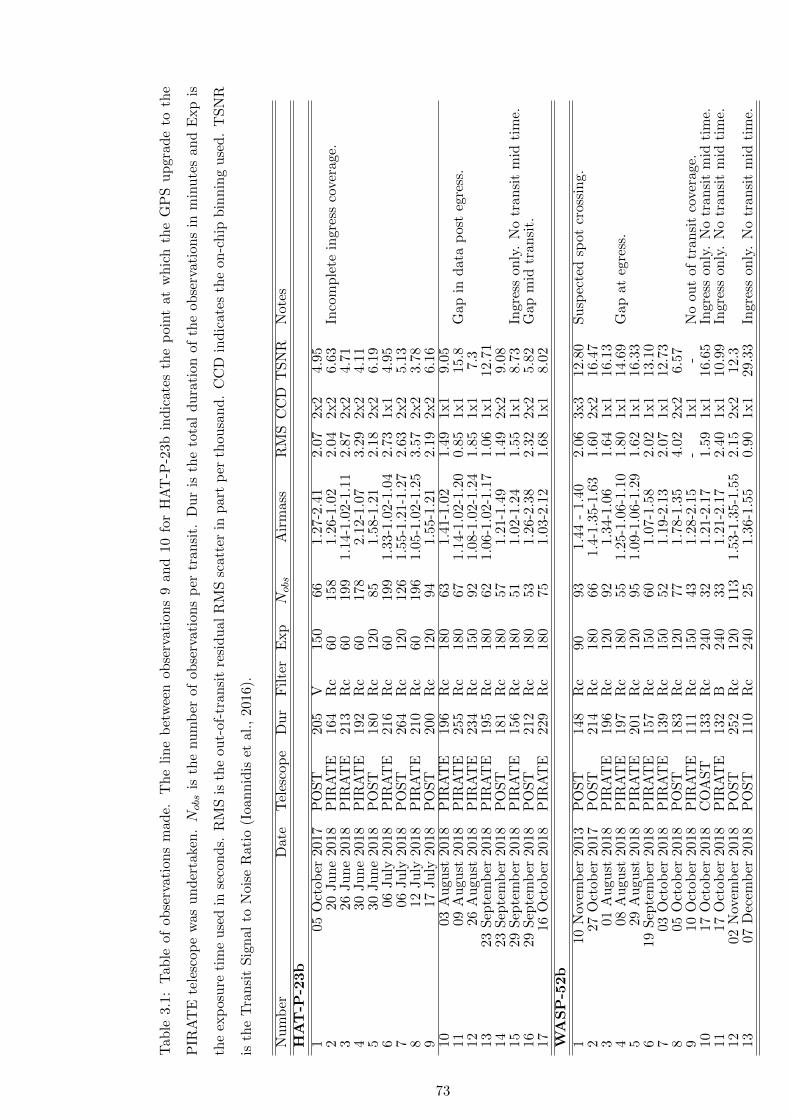
Tab

le3.

1:T

able

ofob

serv

atio

ns

mad

e.T

he

lin

eb

etw

een

obse

rvat

ion

s9

and

10fo

rH

AT

-P-2

3bin

dic

ate

sth

ep

oin

tat

wh

ich

the

GP

Su

pgra

de

toth

e

PIR

AT

Ete

lesc

ope

was

un

der

take

n.Nobs

isth

enu

mb

erof

obse

rvat

ion

sp

ertr

ansi

t.D

ur

isth

eto

tal

du

rati

on

of

the

ob

serv

ati

on

sin

min

ute

san

dE

xp

is

the

exp

osu

reti

me

use

din

seco

nds.

RM

Sis

the

out-

of-t

ran

sit

resi

du

alR

MS

scat

ter

inp

art

per

thou

san

d.

CC

Din

dic

ate

sth

eon

-ch

ipb

inn

ing

use

d.

TS

NR

isth

eT

ran

sit

Sig

nal

toN

oise

Rat

io(I

oan

nid

iset

al.,

2016

).

Nu

mb

erD

ate

Tel

esco

pe

Du

rF

ilte

rE

xp

Nobs

Air

mas

sR

MS

CC

DT

SN

RN

ote

sH

AT

-P-2

3b

105

Oct

ober

2017

PO

ST

205

V15

066

1.27

-2.4

12.

072x2

4.9

52

20Ju

ne

2018

PIR

AT

E16

4R

c60

158

1.26

-1.0

22.

042x2

6.6

3In

com

ple

tein

gre

ssco

vera

ge.

326

Ju

ne

2018

PIR

AT

E21

3R

c60

199

1.14

-1.0

2-1.

112.

872x2

4.7

14

30Ju

ne

2018

PIR

AT

E19

2R

c60

178

2.12

-1.0

73.

292x2

4.1

15

30Ju

ne

2018

PO

ST

180

Rc

120

851.

58-1

.21

2.18

2x2

6.1

96

06Ju

ly20

18P

IRA

TE

216

Rc

6019

91.

33-1

.02-

1.04

2.73

1x1

4.9

57

06Ju

ly20

18P

OS

T26

4R

c12

012

61.

55-1

.21-

1.27

2.63

2x2

5.1

38

12Ju

ly20

18P

IRA

TE

210

Rc

6019

61.

05-1

.02-

1.25

3.57

2x2

3.7

89

17Ju

ly20

18P

OS

T20

0R

c12

094

1.55

-1.2

12.

192x2

6.1

610

03A

ugu

st20

18P

IRA

TE

196

Rc

180

631.

41-1

.02

1.49

1x1

9.0

511

09A

ugu

st20

18P

IRA

TE

255

Rc

180

671.

14-1

.02-

1.20

0.85

1x1

15.8

Gap

ind

ata

post

egre

ss.

1226

Au

gust

2018

PIR

AT

E23

4R

c15

092

1.08

-1.0

2-1.

241.

851x1

7.3

1323

Sep

tem

ber

2018

PIR

AT

E19

5R

c18

062

1.06

-1.0

2-1.

171.

061x1

12.7

114

23S

epte

mb

er20

18P

OS

T18

1R

c18

057

1.21

-1.4

91.

492x2

9.0

815

29S

epte

mb

er20

18P

IRA

TE

156

Rc

180

511.

02-1

.24

1.55

1x1

8.7

3In

gre

sson

ly.

No

tran

sit

mid

tim

e.16

29S

epte

mb

er20

18P

OS

T21

2R

c18

053

1.26

-2.3

82.

322x2

5.8

2G

ap

mid

tran

sit.

1716

Oct

ober

2018

PIR

AT

E22

9R

c18

075

1.03

-2.1

21.

681x1

8.0

2W

AS

P-5

2b

110

Nov

emb

er20

13P

OS

T14

8R

c90

931.

44-

1.40

2.06

3x3

12.8

0Su

spec

ted

spot

cross

ing.

227

Oct

ober

2017

PO

ST

214

Rc

180

661.

4-1.

35-1

.63

1.60

2x2

16.4

73

01A

ugu

st20

18P

IRA

TE

196

Rc

120

921.

34-1

.06

1.64

1x1

16.1

34

08A

ugu

st20

18P

IRA

TE

197

Rc

180

551.

25-1

.06-

1.10

1.80

1x1

14.6

9G

ap

at

egre

ss.

529

Au

gust

2018

PIR

AT

E20

1R

c12

095

1.09

-1.0

6-1.

291.

621x1

16.3

36

19S

epte

mb

er20

18P

IRA

TE

157

Rc

150

601.

07-1

.58

2.02

1x1

13.1

07

03O

ctob

er20

18P

IRA

TE

139

Rc

150

521.

19-2

.13

2.07

1x1

12.7

38

05O

ctob

er20

18P

OS

T18

3R

c12

077

1.78

-1.3

54.

022x2

6.5

79

10O

ctob

er20

18P

IRA

TE

111

Rc

150

431.

28-2

.15

-1x1

-N

oou

tof

tran

sit

cove

rage.

1017

Oct

ober

2018

CO

AS

T13

3R

c24

032

1.21

-2.1

71.

591x1

16.6

5In

gre

sson

ly.

No

tran

sit

mid

tim

e.11

17O

ctob

er20

18P

IRA

TE

132

B24

033

1.21

-2.1

72.

401x1

10.9

9In

gre

sson

ly.

No

tran

sit

mid

tim

e.12

02N

ovem

ber

2018

PO

ST

252

Rc

120

113

1.53

-1.3

5-1.

552.

152x2

12.3

1307

Dec

emb

er20

18P

OS

T11

0R

c24

025

1.36

-1.5

50.

901x1

29.3

3In

gre

sson

ly.

No

tran

sit

mid

tim

e.

73

Table 3.2: Broadband photometry used in Exofastv2 SED fitting.

Band HAT-P-23 WASP-52 Catalogue

B(T) 13.362± 0.378 - TychoV(T) 12.061± 0.195 - TychoB 12.965± 0.036 13.116± 0.042 APASS R10V 12.189± 0.047 12.231± 0.062 APASS R10gSDSS 12.586± 0.043 12.617± 0.025 APASS R10rSDSS 11.969± 0.089 11.901± 0.095 APASS R10iSDSS 11.774± 0.143 11.698± 0.047 APASS R10J 11.103± 0.020 10.588± 0.020 2MASS(via UCAC4)H 10.846± 0.020 10.186± 0.030 2MASS(via UCAC4)K 10.791± 0.020 10.086± 0.030 2MASS(via UCAC4)WISE1 10.748+0.030

−0.023 10.011+0.030−0.023 AllWISE

WISE2 10.793+0.030−0.020 10.094+0.030

−0.021 AllWISEWISE3 10.816± 0.122 9.983± 0.061 AllWISEGaia 12.174+0.020

−0.001 11.954+0.020−0.001 Gaia DR2

GaiaBP 12.518+0.020−0.002 12.444+0.020

−0.004 Gaia DR2

GaiaRP 11.679+0.020−0.002 11.331+0.020

−0.003 Gaia DR2

3.2.2 Analysis

Combined transit and radial velocity model fitting was carried out with the most recent

version of ExofastV2 (Eastman et al., 2019) using the new transit data and previously pub-

lished radial velocity (RV) measurements. For HAT-P-23b 13 radial velocity measurements

obtained using the HIRES instrument on the Keck telescope (Bakos et al., 2011) were used.

For WASP-52b 16 measurements obtained with CORALIE instrument on the ESO Euler

telescope and 29 measurements obtained with the SOPHIE instrument on the 1.93m OHP

telescope (Hebrard et al., 2013) were used. The RV data from SOPHIE was divided into

separate inputs for the High-Efficiency mode (HE1, HE2) and High-Resolution mode (HR)

measurements allowing different zero-points to be set for each. The data set obtained in HE

mode covering the Rossiter-McLaughlin effect measurements (HE-RM) over a short period

during transit was not used in the analysis. Broadband photometry was taken from known

trusted catalogues, see Table 3.2. Priors and argument files were created for ExofastV2 input

as described in Section 2.7.1.

All transit lightcurves, including those with partial coverage but excluding the 2013 transit

of WASP-52b which showed a significant suspected spot crossing event, were included to

produce a single global model fit in ExofastV2 for each system. The transit mid-time for each

lightcurve was allowed to vary within the global model fit and the transit mid-times were

output from ExofastV2 and combined with previously published transit times to calculate a

refined ephemeris for each system. Only transits with full coverage of all transition points

t1 to t4 were used in the ephemeris analysis. All transit lightcurves with their best fit Exofast

models can be found in Figure 3.2 for HAT-P-23b and in Figure 3.3 for WASP-52b.

74

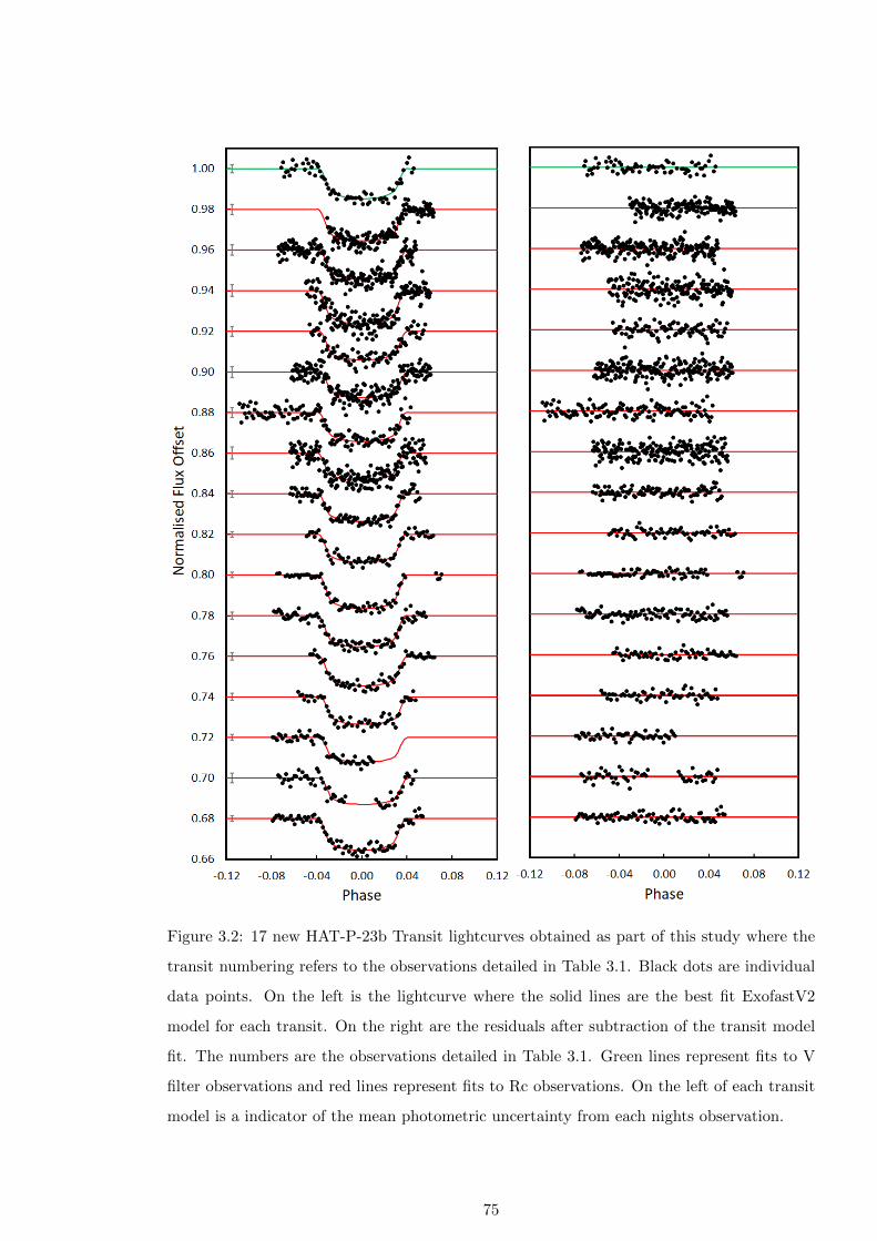
Figure 3.2: 17 new HAT-P-23b Transit lightcurves obtained as part of this study where the

transit numbering refers to the observations detailed in Table 3.1. Black dots are individual

data points. On the left is the lightcurve where the solid lines are the best fit ExofastV2

model for each transit. On the right are the residuals after subtraction of the transit model

fit. The numbers are the observations detailed in Table 3.1. Green lines represent fits to V

filter observations and red lines represent fits to Rc observations. On the left of each transit

model is a indicator of the mean photometric uncertainty from each nights observation.

75

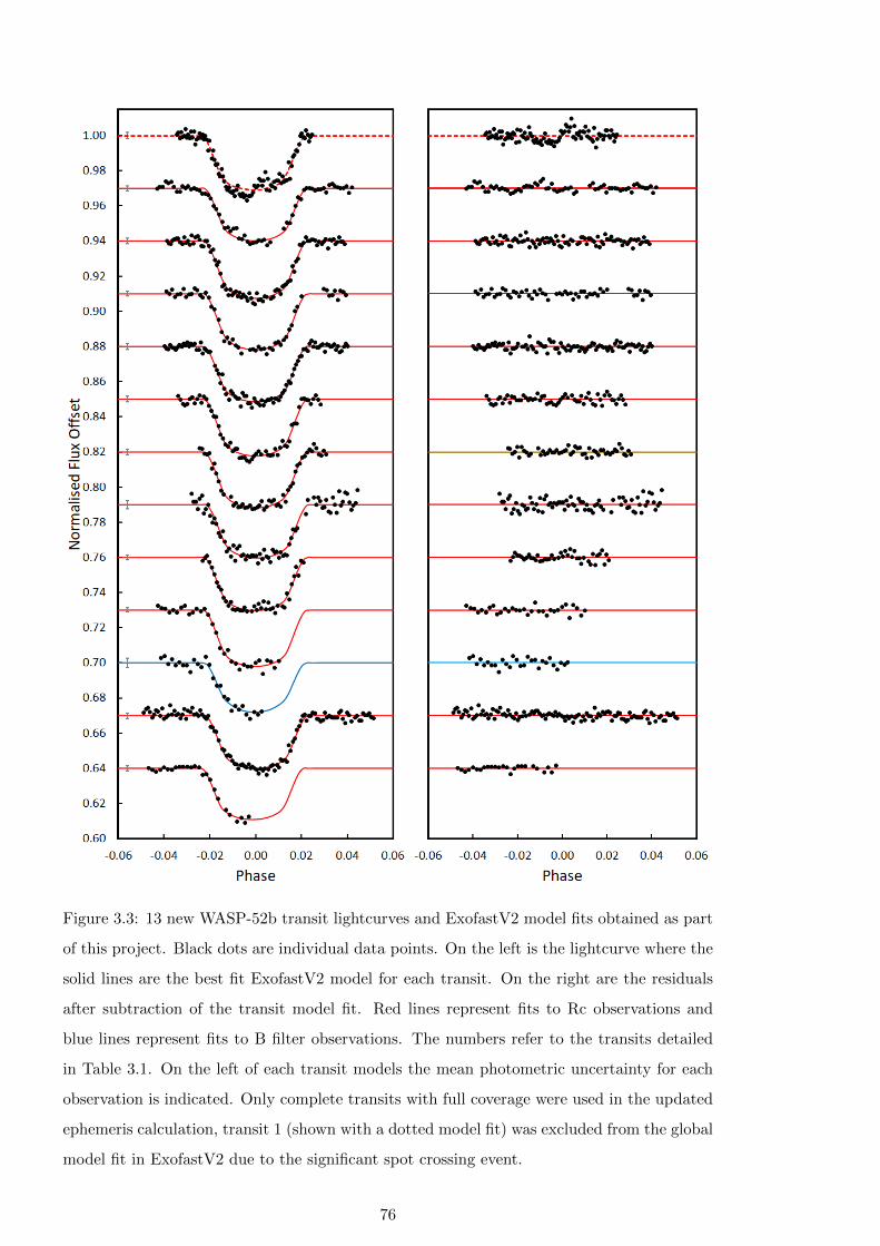
Figure 3.3: 13 new WASP-52b transit lightcurves and ExofastV2 model fits obtained as part

of this project. Black dots are individual data points. On the left is the lightcurve where the

solid lines are the best fit ExofastV2 model for each transit. On the right are the residuals

after subtraction of the transit model fit. Red lines represent fits to Rc observations and

blue lines represent fits to B filter observations. The numbers refer to the transits detailed

in Table 3.1. On the left of each transit models the mean photometric uncertainty for each

observation is indicated. Only complete transits with full coverage were used in the updated

ephemeris calculation, transit 1 (shown with a dotted model fit) was excluded from the global

model fit in ExofastV2 due to the significant spot crossing event.

76

For the HAT-P-23 monitoring data a photometry template was created in AIJ incorporating

stars from the UCAC4 catalogue (Zacharias et al., 2013) with known B, V and r′ filter

magnitudes. Six suitable comparison stars were selected and a seventh, with B-V=1.375

similar to HAT-P-23 (B-V=1.301), was used as a check star. AIJ does not take into account

catalogue magnitude uncertainties so the uncertainties for the calculated magnitudes are

based on the standard error in the measurements of the check star.

3.3 Results

3.3.1 HAT-P-23b System Parameters

At discovery Bakos et al. (2011) found a marginally significant orbital eccentricity of 0.106±

0.044. The subsequent study by Sada and Ramon-Fox (2016) also found an orbital eccen-

tricity of 0.096± 0.024, however using secondary occulatation measurements O’Rourke et al.

(2014) determined that the orbit was probably circular, a result supported by subsequent

RV studies (Bonomo et al., 2017). Subsequent studies of HAT-P-23b made by Ciceri et al.

(2015) and Maciejewski et al. (2018) therefore assumed a circular orbit. Maciejewski et al.

(2018) reported that the increased value they found for the scaled system parameter a/R∗,

over that seen by Bakos et al. (2011) and Sada and Ramon-Fox (2016) is due to the adoption

of a non zero eccentricity in those studies.

To ensure the results were not biased by a prior determination of eccentricity the orbital

eccentricity was left as a free parameter. This resulted in e = 0.027+0.029−0.019, consistent with a

circular orbit within 1.4σ. The same model was also calculated with eccentricity forced to zero

resulting in the same value for the scaled a/R∗ parameter as found when the eccentricity left

as a free parameter. This would be expected given the near zero eccentricity determined when

it is left as a free parameter and the argument of periastron (ω∗) is close to 180°, resulting in

e sinω∗ = 0.000(to 3 dp.). The result found for a/R∗ is consistent with that determined by

Bakos et al. (2011) and Sada and Ramon-Fox (2016), Figure 3.4, indicating free eccentricity

alone may not the cause of the differences in a/R∗ seen by Maciejewski et al. (2018).

From the global model fit the stellar radius and mass of HAT-P-23 were found to be

1.157+0.023−0.022R� and 1.063+0.063

−0.060M�, which is 3.8% and 5.9% smaller respectively than found

by Bakos et al. (2011). The results are also 6.2% larger and 3.7% smaller respectively than

the only other published stellar mass and radius values by Ciceri et al. (2015). The revised

radius found for HAT-P-23b is 1.308+0.044−0.043RJ. It is notable that the radius determined by

Ciceri et al. (2015) of 1.224 ± 0.036 is 2σ smaller than the newly determined value and 4σ

smaller than that found by Bakos et al. (2011), a fact commented on by the independent

reviewer of the published version of this chapter. The planetary radius found by Ciceri

77

et al. (2015) moved HAT-P-23b out of the region of the mass-radius diagram occupied by

inflated hot Jupiter systems. The transits obtained by Ciceri et al. (2015) were modelled

using JKTEBOP2 (Southworth, 2013), with the authors assuming circular orbits and a fixed

mass ratio. The fits of the light curves were performed using theoretical values of the limb

darkening coefficients. Although not explicitly stated in their published paper, there is no

discussion of the use of RV data so it is unlikely a joint fit of transit and RV data was applied.

In the same paper the authors also analysed transit data for WASP-48b and similarly report

lower stellar and planetary radii compared with the discovery paper, R∗ = 1.519± 0.051R�

vs 1.75± 0.09R� and Rp = 1.396± 0.051RJ vs 1.67± 0.1RJ.

The transit lightcurves obtained by Ciceri et al. (2015) are available online via the VizieR

database3. This includes six transits with full coverage obtained with the Calar Alto 1.23m

telescope using the same Rc filter as used for the PIRATE and POST observations. These six

transits were modelled using Exofastv2 in the same way as for the new lightcurves, using the

same priors, RV and photometric values to see whether the result obtained by Ciceri et al.

(2015) could be replicated. The transit fits were computed twice, once with eccentricity left

as free parameter and again with a forced circular orbit as used by Ciceri et al. (2015).

The results for the ExofastV2 model computed with eccentricity left free resulted in

planetary radius Rp = 1.312+0.031−0.003RJ, within 1% of the result obtained from the analysis of

the new PIRATE and POST lightcurves but 7% larger than found by Ciceri et al. (2015).

Similarly the stellar radius R∗ = 1.146± 0.024R�, is within 1% of the value determined from

the PIRATE and POST lightcurves. The forced circular ExofastV2 model fit resulted R∗ =

1.133+0.019−0.020R� and Rp = 1.303± 0.028RJ. Thus the results for R∗ and Rp from the forced

circular analysis of the Ciceri et al. (2015) lightcurves gave values within approximately 1%

of the free eccentricity model.

It cannot be stated with certainty but seems likely the combination of the radius derived

from the theoretical models using the mass/age relationship possibly along with the fixed cir-

cular orbit for HAT-P-23b have led to the smaller radius determination. The other significant

difference in the two approaches was that Ciceri et al. (2015) fit the lightcurves only.

The value for a/R∗ = 4.22+0.11−0.10 is consistent with the previous studies which assumed

a non zero eccentricity (Bakos et al., 2011; Sada and Ramon-Fox, 2016) and approximately

6% smaller than that found by studies which fixed orbital eccentricity to zero (Ciceri et al.,

2015; Maciejewski et al., 2018). Key stellar and planetary parameters are compared with the

previously published values in Figure 3.4 and all newly derived parameters can be found in

Table 3.6.

2https://www.astro.keele.ac.uk/jkt/codes/jktebop.html3https://vizier.u-strasbg.fr/viz-bin/VizieR

78

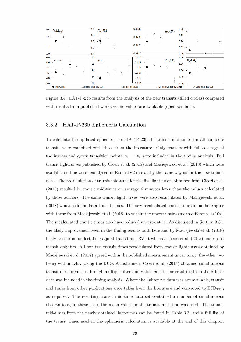
Figure 3.4: HAT-P-23b results from the analysis of the new transits (filled circles) compared

with results from published works where values are available (open symbols).

3.3.2 HAT-P-23b Ephemeris Calculation

To calculate the updated ephemeris for HAT-P-23b the transit mid times for all complete

transits were combined with those from the literature. Only transits with full coverage of

the ingress and egress transition points, t1 − t4 were included in the timing analysis. Full

transit lightcurves published by Ciceri et al. (2015) and Maciejewski et al. (2018) which were

available on-line were reanalysed in ExofastV2 in exactly the same way as for the new transit

data. The recalculation of transit mid-time for the five lightcurves obtained from Ciceri et al.

(2015) resulted in transit mid-times on average 6 minutes later than the values calculated

by those authors. The same transit lightcurves were also recalculated by Maciejewski et al.

(2018) who also found later transit times. The new recalculated transit times found here agree

with those from Maciejewski et al. (2018) to within the uncertainties (mean difference is 10s).

The recalculated transit times also have reduced uncertainties. As discussed in Section 3.3.1

the likely improvement seen in the timing results both here and by Maciejewski et al. (2018)

likely arise from undertaking a joint transit and RV fit whereas Ciceri et al. (2015) undertook

transit only fits. All but two transit times recalculated from transit lightcurves obtained by

Maciejewski et al. (2018) agreed within the published measurement uncertainty, the other two

being within 1.4σ. Using the BUSCA instrument Ciceri et al. (2015) obtained simultaneous

transit measurements through multiple filters, only the transit time resulting from the R filter

data was included in the timing analysis. Where the lightcurve data was not available, transit

mid times from other publications were taken from the literature and converted to BJDTDB

as required. The resulting transit mid-time data set contained a number of simultaneous

observations, in these cases the mean value for the transit mid-time was used. The transit

mid-times from the newly obtained lightcurves can be found in Table 3.3, and a full list of

the transit times used in the ephemeris calculation is available at the end of this chapter.

79

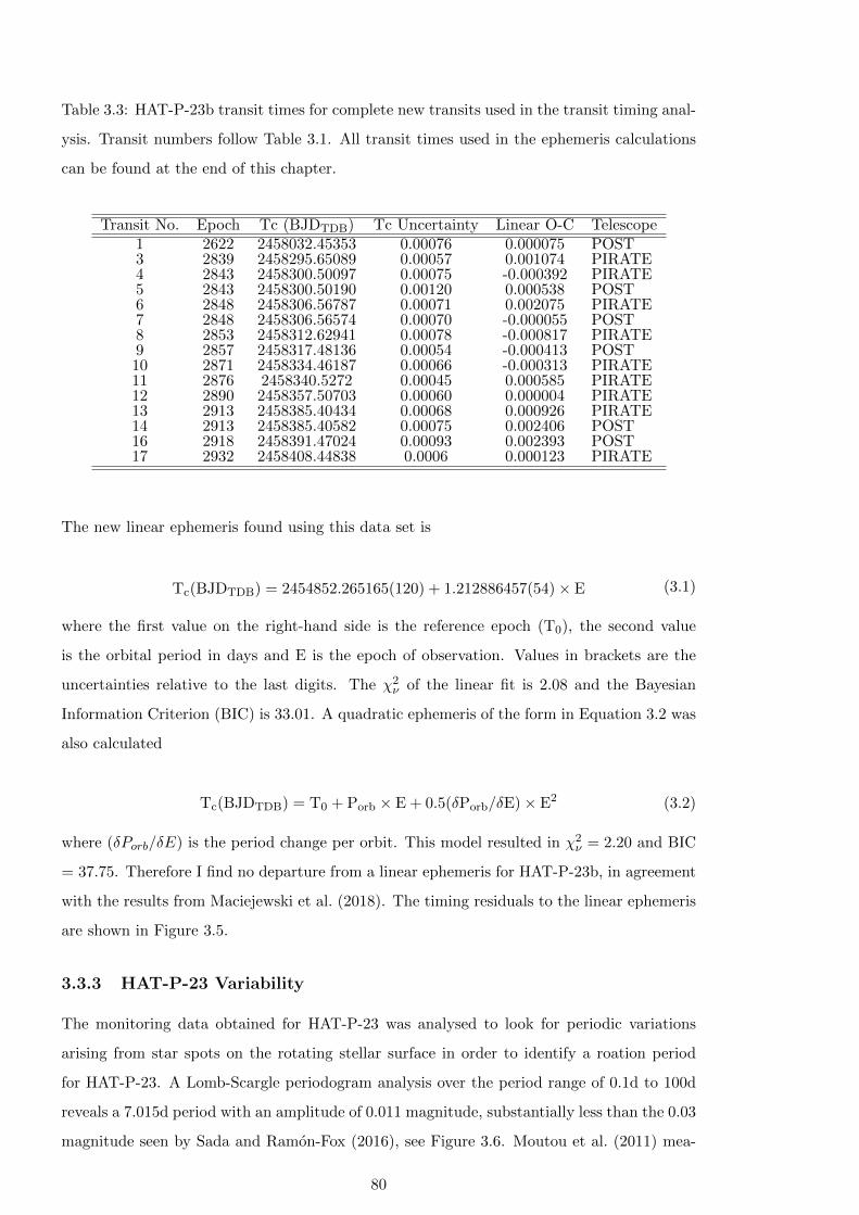
Table 3.3: HAT-P-23b transit times for complete new transits used in the transit timing anal-

ysis. Transit numbers follow Table 3.1. All transit times used in the ephemeris calculations

can be found at the end of this chapter.

Transit No. Epoch Tc (BJDTDB) Tc Uncertainty Linear O-C Telescope1 2622 2458032.45353 0.00076 0.000075 POST3 2839 2458295.65089 0.00057 0.001074 PIRATE4 2843 2458300.50097 0.00075 -0.000392 PIRATE5 2843 2458300.50190 0.00120 0.000538 POST6 2848 2458306.56787 0.00071 0.002075 PIRATE7 2848 2458306.56574 0.00070 -0.000055 POST8 2853 2458312.62941 0.00078 -0.000817 PIRATE9 2857 2458317.48136 0.00054 -0.000413 POST10 2871 2458334.46187 0.00066 -0.000313 PIRATE11 2876 2458340.5272 0.00045 0.000585 PIRATE12 2890 2458357.50703 0.00060 0.000004 PIRATE13 2913 2458385.40434 0.00068 0.000926 PIRATE14 2913 2458385.40582 0.00075 0.002406 POST16 2918 2458391.47024 0.00093 0.002393 POST17 2932 2458408.44838 0.0006 0.000123 PIRATE

The new linear ephemeris found using this data set is

Tc(BJDTDB) = 2454852.265165(120) + 1.212886457(54)× E (3.1)

where the first value on the right-hand side is the reference epoch (T0), the second value

is the orbital period in days and E is the epoch of observation. Values in brackets are the

uncertainties relative to the last digits. The χ2ν of the linear fit is 2.08 and the Bayesian

Information Criterion (BIC) is 33.01. A quadratic ephemeris of the form in Equation 3.2 was

also calculated

Tc(BJDTDB) = T0 + Porb × E + 0.5(δPorb/δE)× E2 (3.2)

where (δPorb/δE) is the period change per orbit. This model resulted in χ2ν = 2.20 and BIC

= 37.75. Therefore I find no departure from a linear ephemeris for HAT-P-23b, in agreement

with the results from Maciejewski et al. (2018). The timing residuals to the linear ephemeris

are shown in Figure 3.5.

3.3.3 HAT-P-23 Variability

The monitoring data obtained for HAT-P-23 was analysed to look for periodic variations

arising from star spots on the rotating stellar surface in order to identify a roation period

for HAT-P-23. A Lomb-Scargle periodogram analysis over the period range of 0.1d to 100d

reveals a 7.015d period with an amplitude of 0.011 magnitude, substantially less than the 0.03

magnitude seen by Sada and Ramon-Fox (2016), see Figure 3.6. Moutou et al. (2011) mea-

80

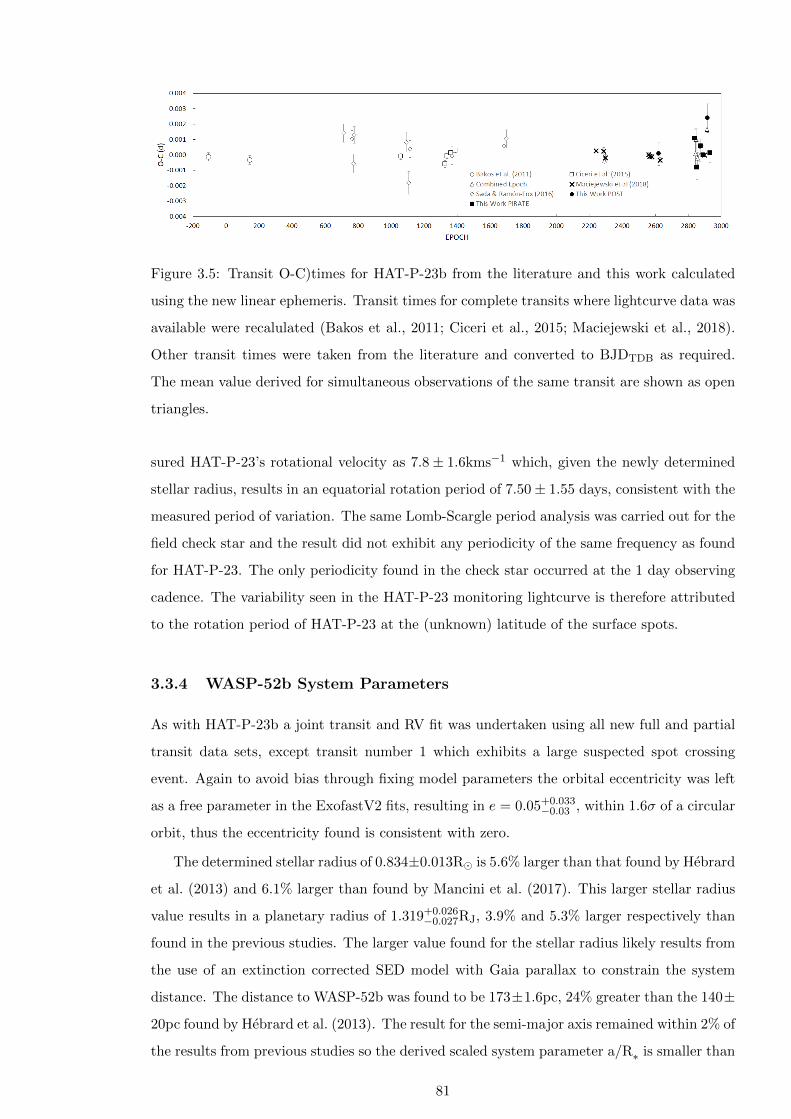
Figure 3.5: Transit O-C)times for HAT-P-23b from the literature and this work calculated

using the new linear ephemeris. Transit times for complete transits where lightcurve data was

available were recalulated (Bakos et al., 2011; Ciceri et al., 2015; Maciejewski et al., 2018).

Other transit times were taken from the literature and converted to BJDTDB as required.

The mean value derived for simultaneous observations of the same transit are shown as open

triangles.

sured HAT-P-23’s rotational velocity as 7.8± 1.6kms−1 which, given the newly determined

stellar radius, results in an equatorial rotation period of 7.50± 1.55 days, consistent with the

measured period of variation. The same Lomb-Scargle period analysis was carried out for the

field check star and the result did not exhibit any periodicity of the same frequency as found

for HAT-P-23. The only periodicity found in the check star occurred at the 1 day observing

cadence. The variability seen in the HAT-P-23 monitoring lightcurve is therefore attributed

to the rotation period of HAT-P-23 at the (unknown) latitude of the surface spots.

3.3.4 WASP-52b System Parameters

As with HAT-P-23b a joint transit and RV fit was undertaken using all new full and partial

transit data sets, except transit number 1 which exhibits a large suspected spot crossing

event. Again to avoid bias through fixing model parameters the orbital eccentricity was left

as a free parameter in the ExofastV2 fits, resulting in e = 0.05+0.033−0.03 , within 1.6σ of a circular

orbit, thus the eccentricity found is consistent with zero.

The determined stellar radius of 0.834±0.013R� is 5.6% larger than that found by Hebrard

et al. (2013) and 6.1% larger than found by Mancini et al. (2017). This larger stellar radius

value results in a planetary radius of 1.319+0.026−0.027RJ, 3.9% and 5.3% larger respectively than

found in the previous studies. The larger value found for the stellar radius likely results from

the use of an extinction corrected SED model with Gaia parallax to constrain the system

distance. The distance to WASP-52b was found to be 173±1.6pc, 24% greater than the 140±

20pc found by Hebrard et al. (2013). The result for the semi-major axis remained within 2% of

the results from previous studies so the derived scaled system parameter a/R∗ is smaller than

81

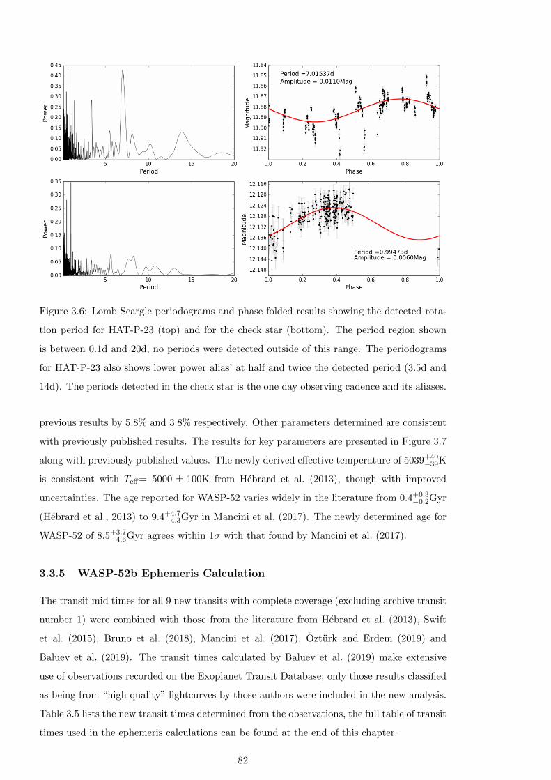
Figure 3.6: Lomb Scargle periodograms and phase folded results showing the detected rota-

tion period for HAT-P-23 (top) and for the check star (bottom). The period region shown

is between 0.1d and 20d, no periods were detected outside of this range. The periodograms

for HAT-P-23 also shows lower power alias’ at half and twice the detected period (3.5d and

14d). The periods detected in the check star is the one day observing cadence and its aliases.

previous results by 5.8% and 3.8% respectively. Other parameters determined are consistent

with previously published results. The results for key parameters are presented in Figure 3.7

along with previously published values. The newly derived effective temperature of 5039+40−39K

is consistent with Teff= 5000 ± 100K from Hebrard et al. (2013), though with improved

uncertainties. The age reported for WASP-52 varies widely in the literature from 0.4+0.3−0.2Gyr

(Hebrard et al., 2013) to 9.4+4.7−4.3Gyr in Mancini et al. (2017). The newly determined age for

WASP-52 of 8.5+3.7−4.6Gyr agrees within 1σ with that found by Mancini et al. (2017).

3.3.5 WASP-52b Ephemeris Calculation

The transit mid times for all 9 new transits with complete coverage (excluding archive transit

number 1) were combined with those from the literature from Hebrard et al. (2013), Swift

et al. (2015), Bruno et al. (2018), Mancini et al. (2017), Ozturk and Erdem (2019) and

Baluev et al. (2019). The transit times calculated by Baluev et al. (2019) make extensive

use of observations recorded on the Exoplanet Transit Database; only those results classified

as being from “high quality” lightcurves by those authors were included in the new analysis.

Table 3.5 lists the new transit times determined from the observations, the full table of transit

times used in the ephemeris calculations can be found at the end of this chapter.

82

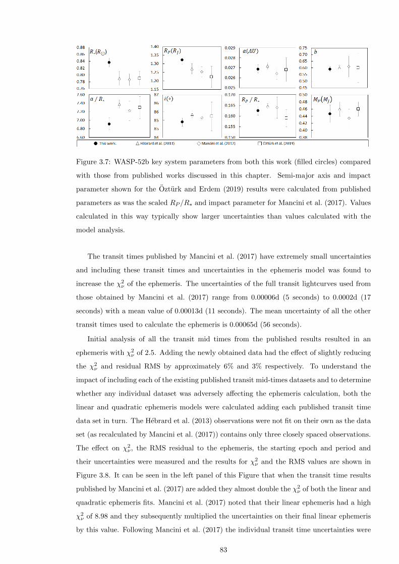
Figure 3.7: WASP-52b key system parameters from both this work (filled circles) compared

with those from published works discussed in this chapter. Semi-major axis and impact

parameter shown for the Ozturk and Erdem (2019) results were calculated from published

parameters as was the scaled RP /R∗ and impact parameter for Mancini et al. (2017). Values

calculated in this way typically show larger uncertainties than values calculated with the

model analysis.

The transit times published by Mancini et al. (2017) have extremely small uncertainties

and including these transit times and uncertainties in the ephemeris model was found to

increase the χ2ν of the ephemeris. The uncertainties of the full transit lightcurves used from

those obtained by Mancini et al. (2017) range from 0.00006d (5 seconds) to 0.0002d (17

seconds) with a mean value of 0.00013d (11 seconds). The mean uncertainty of all the other

transit times used to calculate the ephemeris is 0.00065d (56 seconds).

Initial analysis of all the transit mid times from the published results resulted in an

ephemeris with χ2ν of 2.5. Adding the newly obtained data had the effect of slightly reducing

the χ2ν and residual RMS by approximately 6% and 3% respectively. To understand the

impact of including each of the existing published transit mid-times datasets and to determine

whether any individual dataset was adversely affecting the ephemeris calculation, both the

linear and quadratic ephemeris models were calculated adding each published transit time

data set in turn. The Hebrard et al. (2013) observations were not fit on their own as the data

set (as recalculated by Mancini et al. (2017)) contains only three closely spaced observations.

The effect on χ2ν , the RMS residual to the ephemeris, the starting epoch and period and

their uncertainties were measured and the results for χ2ν and the RMS values are shown in

Figure 3.8. It can be seen in the left panel of this Figure that when the transit time results

published by Mancini et al. (2017) are added they almost double the χ2ν of both the linear and

quadratic ephemeris fits. Mancini et al. (2017) noted that their linear ephemeris had a high

χ2ν of 8.98 and they subsequently multiplied the uncertainties on their final linear ephemeris

by this value. Following Mancini et al. (2017) the individual transit time uncertainties were

83

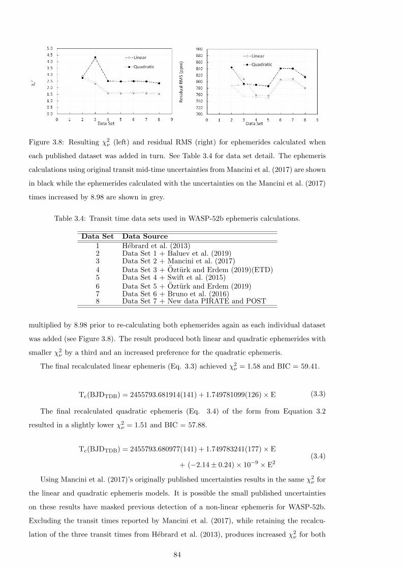
Figure 3.8: Resulting χ2ν (left) and residual RMS (right) for ephemerides calculated when

each published dataset was added in turn. See Table 3.4 for data set detail. The ephemeris

calculations using original transit mid-time uncertainties from Mancini et al. (2017) are shown

in black while the ephemerides calculated with the uncertainties on the Mancini et al. (2017)

times increased by 8.98 are shown in grey.

Table 3.4: Transit time data sets used in WASP-52b ephemeris calculations.

Data Set Data Source

1 Hebrard et al. (2013)2 Data Set 1 + Baluev et al. (2019)3 Data Set 2 + Mancini et al. (2017)4 Data Set 3 + Ozturk and Erdem (2019)(ETD)5 Data Set 4 + Swift et al. (2015)6 Data Set 5 + Ozturk and Erdem (2019)7 Data Set 6 + Bruno et al. (2016)8 Data Set 7 + New data PIRATE and POST

multiplied by 8.98 prior to re-calculating both ephemerides again as each individual dataset

was added (see Figure 3.8). The result produced both linear and quadratic ephemerides with

smaller χ2ν by a third and an increased preference for the quadratic ephemeris.

The final recalculated linear ephemeris (Eq. 3.3) achieved χ2ν = 1.58 and BIC = 59.41.

Tc(BJDTDB) = 2455793.681914(141) + 1.749781099(126)× E (3.3)

The final recalculated quadratic ephemeris (Eq. 3.4) of the form from Equation 3.2

resulted in a slightly lower χ2ν = 1.51 and BIC = 57.88.

Tc(BJDTDB) = 2455793.680977(141) + 1.749783241(177)× E

+ (−2.14± 0.24)× 10−9 × E2(3.4)

Using Mancini et al. (2017)’s originally published uncertainties results in the same χ2ν for

the linear and quadratic ephemeris models. It is possible the small published uncertainties

on these results have masked previous detection of a non-linear ephemeris for WASP-52b.

Excluding the transit times reported by Mancini et al. (2017), while retaining the recalcu-

lation of the three transit times from Hebrard et al. (2013), produces increased χ2ν for both

84

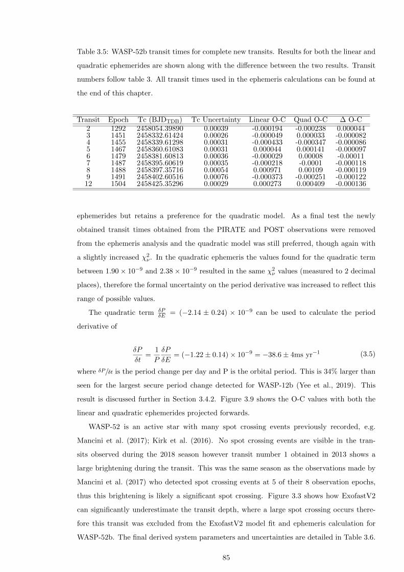
Table 3.5: WASP-52b transit times for complete new transits. Results for both the linear and

quadratic ephemerides are shown along with the difference between the two results. Transit

numbers follow table 3. All transit times used in the ephemeris calculations can be found at

the end of this chapter.

Transit Epoch Tc (BJDTDB) Tc Uncertainty Linear O-C Quad O-C ∆ O-C2 1292 2458054.39890 0.00039 -0.000194 -0.000238 0.0000443 1451 2458332.61424 0.00026 -0.000049 0.000033 -0.0000824 1455 2458339.61298 0.00031 -0.000433 -0.000347 -0.0000865 1467 2458360.61083 0.00031 0.000044 0.000141 -0.0000976 1479 2458381.60813 0.00036 -0.000029 0.00008 -0.000117 1487 2458395.60619 0.00035 -0.000218 -0.0001 -0.0001188 1488 2458397.35716 0.00054 0.000971 0.00109 -0.0001199 1491 2458402.60516 0.00076 -0.000373 -0.000251 -0.00012212 1504 2458425.35296 0.00029 0.000273 0.000409 -0.000136

ephemerides but retains a preference for the quadratic model. As a final test the newly

obtained transit times obtained from the PIRATE and POST observations were removed

from the ephemeris analysis and the quadratic model was still preferred, though again with

a slightly increased χ2ν . In the quadratic ephemeris the values found for the quadratic term

between 1.90× 10−9 and 2.38× 10−9 resulted in the same χ2ν values (measured to 2 decimal

places), therefore the formal uncertainty on the period derivative was increased to reflect this

range of possible values.

The quadratic term δPδE = (−2.14 ± 0.24) × 10−9 can be used to calculate the period

derivative of

δP

δt=

1

P

δP

δE= (−1.22± 0.14)× 10−9 = −38.6± 4ms yr−1 (3.5)

where δP/δt is the period change per day and P is the orbital period. This is 34% larger than

seen for the largest secure period change detected for WASP-12b (Yee et al., 2019). This

result is discussed further in Section 3.4.2. Figure 3.9 shows the O-C values with both the

linear and quadratic ephemerides projected forwards.

WASP-52 is an active star with many spot crossing events previously recorded, e.g.

Mancini et al. (2017); Kirk et al. (2016). No spot crossing events are visible in the tran-

sits observed during the 2018 season however transit number 1 obtained in 2013 shows a

large brightening during the transit. This was the same season as the observations made by

Mancini et al. (2017) who detected spot crossing events at 5 of their 8 observation epochs,

thus this brightening is likely a significant spot crossing. Figure 3.3 shows how ExofastV2

can significantly underestimate the transit depth, where a large spot crossing occurs there-

fore this transit was excluded from the ExofastV2 model fit and ephemeris calculation for

WASP-52b. The final derived system parameters and uncertainties are detailed in Table 3.6.

85

Figure 3.9: Predicted transit times for WASP-52b based on both the linear and quadratic

ephemerides shows that it should be possible to clearly differentiate between the two models

with data from the 2021 observing season.

3.3.6 WASP-52 Variability

Unfortunately concurrent photometric monitoring of WASP-52 over the 2018 season is not

available; instead the stellar magnitude was measured using out of transit data from four

transits observed using PIRATE with sufficient unbroken data available on both sides of

the transit (transits 3 to 6 in Table 3.1). As for HAT-P-23, a photometry template was

generated using comparison stars from the UCAC4 catalogue. Eight stars were used in the

range r′ = 13.00 to 14.90 magnitude. WASP-52 itself has no B, V or r′ photometry in the

UCAC4 catalogue so B − V = 0.9 was taken from Hebrard et al. (2013) and a check star of

similar B−V = 0.86 was selected from UCAC4. Although this data set contained data from

only 4 observations a variation of ∆Rc = 0.03 mag, similar to the WASP-52b transit depth

is clearly visible. The standard deviation between the mean nightly values (red squares in

Figure 3.10) is 0.0143 for WASP-52 but 10 times smaller at 0.0014 for the check star indicating

the magnitude variations seen in WASP-52 are real, Figure 3.10.

3.3.6.1 Transit depth correlation with magnitude.

If stellar spots at a latitude different to the transit chord are reducing the stellar flux this

would result in the transit chord crossing a brighter part of the star, blocking a greater

proportion of the flux and a greater transit depth would be recorded when spots are present

compared to when they not. As a result we would expect to see a correlation between transit

depth and stellar brightness with the transit depth being greater when the star is fainter. A

Kendall Rank Correlation was used due to the small number of data points giving τb = 0.66

and p-value = 0.17 indicating a strong positive, but not statistically significant, correlation

is seen for the four data points available, see Figure 3.12. Due to the small number of data

points and large uncertainties, particularly in transit depth, further observations would be

required to determine if this effect is real.

86

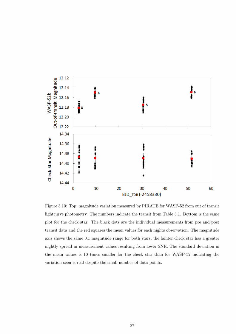
Figure 3.10: Top; magnitude variation measured by PIRATE for WASP-52 from out of transit

lightcurve photometry. The numbers indicate the transit from Table 3.1. Bottom is the same

plot for the check star. The black dots are the individual measurements from pre and post

transit data and the red squares the mean values for each nights observation. The magnitude

axis shows the same 0.1 magnitude range for both stars, the fainter check star has a greater

nightly spread in measurement values resulting from lower SNR. The standard deviation in

the mean values is 10 times smaller for the check star than for WASP-52 indicating the

variation seen is real despite the small number of data points.

87

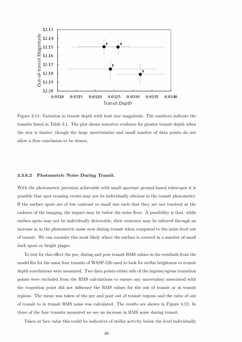
Figure 3.11: Variation in transit depth with host star magnitude. The numbers indicate the

transits listed in Table 3.1. The plot shows tentative evidence for greater transit depth when

the star is fainter, though the large uncertainties and small number of data points do not

allow a firm conclusion to be drawn.

3.3.6.2 Photometric Noise During Transit.

With the photometric precision achievable with small aperture ground-based telescopes it is

possible that spot crossing events may not be individually obvious in the transit photometry.

If the surface spots are of low contrast or small size such that they are not resolved at the

cadence of the imaging, the impact may be below the noise floor. A possibility is that, while

surface spots may not be individually detectable, their existence may be inferred through an

increase in in the photometric noise seen during transit when compared to the noise level out

of transit. We can consider this most likely where the surface is covered in a number of small

dark spots or bright plages.

To test for this effect the pre, during and post transit RMS values in the residuals from the

model fits for the same four transits of WASP-52b used to look for stellar brightness vs transit

depth correlations were measured. Two data points either side of the ingress/egress transition

points were excluded from the RMS calculations to ensure any uncertainty associated with

the transition point did not influence the RMS values for the out of transit or in transit

regions. The mean was taken of the pre and post out of transit regions and the ratio of out

of transit to in transit RMS noise was calculated. The results are shown in Figure 3.12. In

three of the four transits measured we see an increase in RMS noise during transit.

Taken at face value this could be indicative of stellar activity below the level individually

88

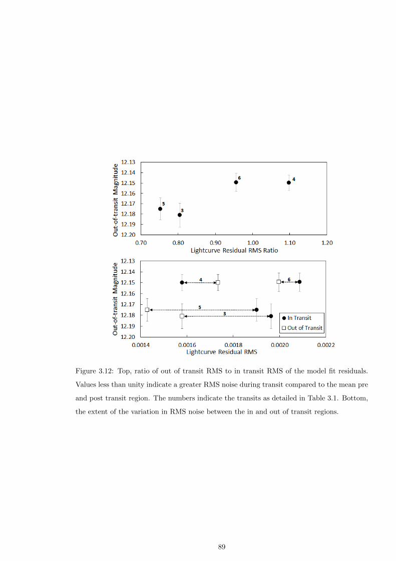
Figure 3.12: Top, ratio of out of transit RMS to in transit RMS of the model fit residuals.

Values less than unity indicate a greater RMS noise during transit compared to the mean pre

and post transit region. The numbers indicate the transits as detailed in Table 3.1. Bottom,

the extent of the variation in RMS noise between the in and out of transit regions.

89

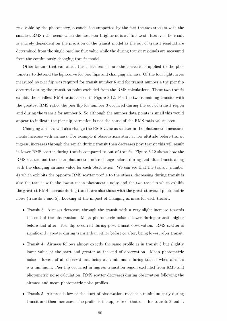
resolvable by the photometry, a conclusion supported by the fact the two transits with the

smallest RMS ratio occur when the host star brightness is at its lowest. However the result

is entirely dependent on the precision of the transit model as the out of transit residual are

determined from the single baseline flux value while the during transit residuals are measured

from the continuously changing transit model.

Other factors that can affect this measurement are the corrections applied to the pho-

tometry to detrend the lightcurve for pier flips and changing airmass. Of the four lightcurves

measured no pier flip was required for transit number 6 and for transit number 4 the pier flip

occurred during the transition point excluded from the RMS calculations. These two transit

exhibit the smallest RMS ratio as seen in Figure 3.12. For the two remaining transits with

the greatest RMS ratio, the pier flip for number 3 occurred during the out of transit region

and during the transit for number 5. So although the number data points is small this would

appear to indicate the pier flip correction is not the cause of the RMS ratio values seen.

Changing airmass will also change the RMS value as scatter in the photometric measure-

ments increase with airmass. For example if observations start at low altitude before transit

ingress, increases through the zenith during transit then decreases post transit this will result

in lower RMS scatter during transit compared to out of transit. Figure 3.12 shows how the

RMS scatter and the mean photometric noise change before, during and after transit along

with the changing airmass value for each observation. We can see that the transit (number

4) which exhibits the opposite RMS scatter profile to the others, decreasing during transit is

also the transit with the lowest mean photometric noise and the two transits which exhibit

the greatest RMS increase during transit are also those with the greatest overall photometric

noise (transits 3 and 5). Looking at the impact of changing airmass for each transit:

• Transit 3. Airmass decreases through the transit with a very slight increase towards

the end of the observation. Mean photometric noise is lower during transit, higher

before and after. Pier flip occurred during post transit observation. RMS scatter is

significantly greater during transit than either before or after, being lowest after transit.

• Transit 4. Airmass follows almost exactly the same profile as in transit 3 but slightly

lower value at the start and greater at the end of observation. Mean photometric

noise is lowest of all observations, being at a minimum during transit when airmass

is a minimum. Pier flip occurred in ingress transition region excluded from RMS and

photometric noise calculation. RMS scatter decreases during observation following the

airmass and mean photometric noise profiles.

• Transit 5. Airmass is low at the start of observation, reaches a minimum early during

transit and then increases. The profile is the opposite of that seen for transits 3 and 4.

90

Photometric noise is very similar to observation 3 but overall highest of all observations.

The value changes minimally given the larger airmass change through the observation.

Pier flip occurs early during transit at the same time as airmass is at a minimum. RMS

scatter shows the greatest increase during transit. The value post transit is greater

than pre transit as expected from airmass change profile.

• Transit 6. Airmass is low at the start of observation, reaches a minimum early during

transit and then increases to the highest value of all observations. Photometric noise is

minimum during transit and greatest after transit when airmass is greatest. No pier flip

was required during the observation. RMS scatter is greater during transit and lower

before and after despite the significantly greater airmass at the end of observation.

Overall there is no common trend between the RMS scatter and observational parameters

of mean photometric noise, airmass and pier flip. Therefore it remains a possibility that the

in-transit increase in RMS scatter from the model residuals has a physical origin in the

activity of the host star with the transit chord crossing regions where spots exist on the

stellar surface which are individually undetectable in the photometry. The possibility of the

effect seen being due to the imperfect transit model fitting, especially in lightcurves with

higher noise, also remains a strong likelihood.

91

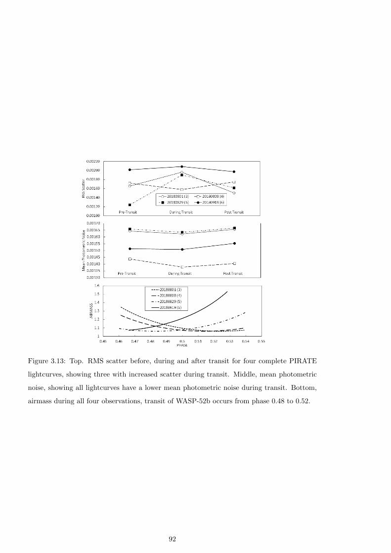
Figure 3.13: Top. RMS scatter before, during and after transit for four complete PIRATE

lightcurves, showing three with increased scatter during transit. Middle, mean photometric

noise, showing all lightcurves have a lower mean photometric noise during transit. Bottom,

airmass during all four observations, transit of WASP-52b occurs from phase 0.48 to 0.52.

92

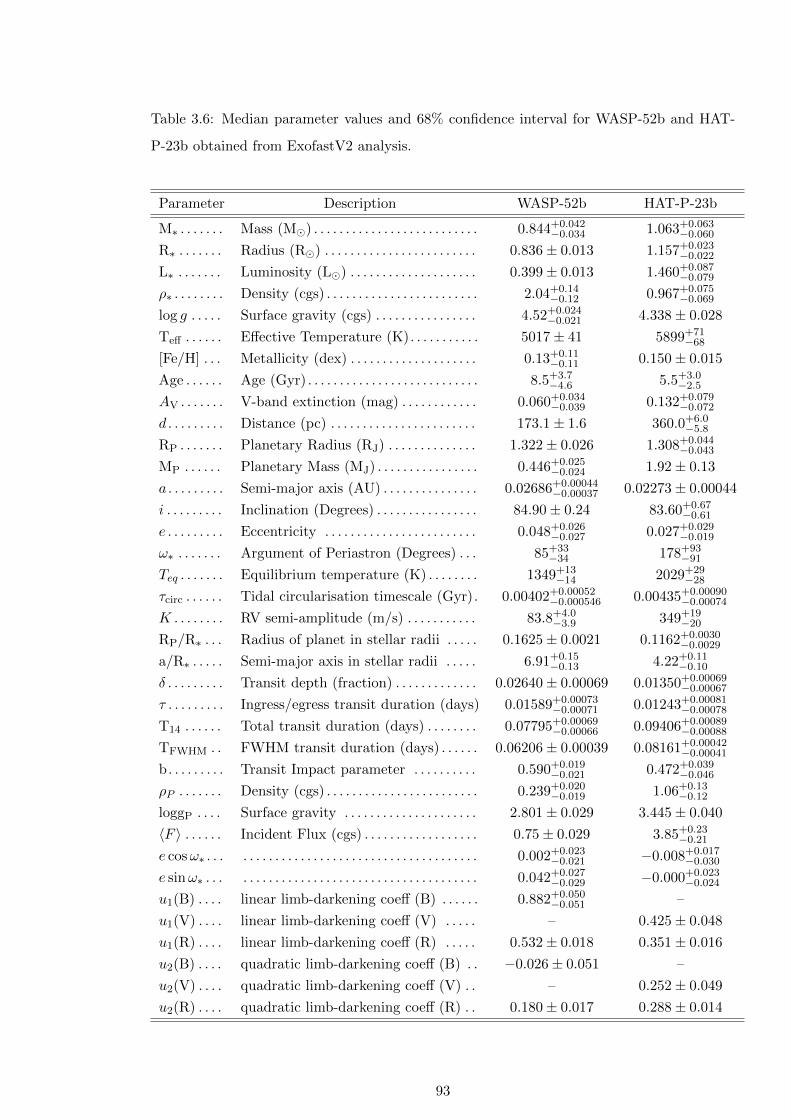
Table 3.6: Median parameter values and 68% confidence interval for WASP-52b and HAT-

P-23b obtained from ExofastV2 analysis.

Parameter Description WASP-52b HAT-P-23b

M∗ . . . . . . . Mass (M�) . . . . . . . . . . . . . . . . . . . . . . . . . . 0.844+0.042−0.034 1.063+0.063

−0.060

R∗ . . . . . . . Radius (R�) . . . . . . . . . . . . . . . . . . . . . . . . 0.836± 0.013 1.157+0.023−0.022

L∗ . . . . . . . Luminosity (L�) . . . . . . . . . . . . . . . . . . . . 0.399± 0.013 1.460+0.087−0.079

ρ∗ . . . . . . . . Density (cgs) . . . . . . . . . . . . . . . . . . . . . . . . 2.04+0.14−0.12 0.967+0.075

−0.069

log g . . . . . Surface gravity (cgs) . . . . . . . . . . . . . . . . 4.52+0.024−0.021 4.338± 0.028

Teff . . . . . . Effective Temperature (K). . . . . . . . . . . 5017± 41 5899+71−68

[Fe/H] . . . Metallicity (dex) . . . . . . . . . . . . . . . . . . . . 0.13+0.11−0.11 0.150± 0.015

Age . . . . . . Age (Gyr) . . . . . . . . . . . . . . . . . . . . . . . . . . . 8.5+3.7−4.6 5.5+3.0

−2.5

AV . . . . . . . V-band extinction (mag) . . . . . . . . . . . . 0.060+0.034−0.039 0.132+0.079

−0.072

d . . . . . . . . . Distance (pc) . . . . . . . . . . . . . . . . . . . . . . . 173.1± 1.6 360.0+6.0−5.8

RP . . . . . . . Planetary Radius (RJ) . . . . . . . . . . . . . . 1.322± 0.026 1.308+0.044−0.043

MP . . . . . . Planetary Mass (MJ) . . . . . . . . . . . . . . . . 0.446+0.025−0.024 1.92± 0.13

a . . . . . . . . . Semi-major axis (AU) . . . . . . . . . . . . . . . 0.02686+0.00044−0.00037 0.02273± 0.00044

i . . . . . . . . . Inclination (Degrees) . . . . . . . . . . . . . . . . 84.90± 0.24 83.60+0.67−0.61

e . . . . . . . . . Eccentricity . . . . . . . . . . . . . . . . . . . . . . . . 0.048+0.026−0.027 0.027+0.029

−0.019

ω∗ . . . . . . . Argument of Periastron (Degrees) . . . 85+33−34 178+93

−91

Teq . . . . . . . Equilibrium temperature (K) . . . . . . . . 1349+13−14 2029+29

−28

τcirc . . . . . . Tidal circularisation timescale (Gyr). 0.00402+0.00052−0.000546 0.00435+0.00090

−0.00074

K . . . . . . . . RV semi-amplitude (m/s) . . . . . . . . . . . 83.8+4.0−3.9 349+19

−20

RP/R∗ . . . Radius of planet in stellar radii . . . . . 0.1625± 0.0021 0.1162+0.0030−0.0029

a/R∗ . . . . . Semi-major axis in stellar radii . . . . . 6.91+0.15−0.13 4.22+0.11

−0.10

δ . . . . . . . . . Transit depth (fraction) . . . . . . . . . . . . . 0.02640± 0.00069 0.01350+0.00069−0.00067

τ . . . . . . . . . Ingress/egress transit duration (days) 0.01589+0.00073−0.00071 0.01243+0.00081

−0.00078

T14 . . . . . . Total transit duration (days) . . . . . . . . 0.07795+0.00069−0.00066 0.09406+0.00089

−0.00088

TFWHM . . FWHM transit duration (days) . . . . . . 0.06206± 0.00039 0.08161+0.00042−0.00041

b. . . . . . . . . Transit Impact parameter . . . . . . . . . . 0.590+0.019−0.021 0.472+0.039

−0.046

ρP . . . . . . . Density (cgs) . . . . . . . . . . . . . . . . . . . . . . . . 0.239+0.020−0.019 1.06+0.13

−0.12

loggP . . . . Surface gravity . . . . . . . . . . . . . . . . . . . . . 2.801± 0.029 3.445± 0.040

〈F 〉 . . . . . . Incident Flux (cgs) . . . . . . . . . . . . . . . . . . 0.75± 0.029 3.85+0.23−0.21

e cosω∗ . . . . . . . . . . . . . . . . . . . . . . . . . . . . . . . . . . . . . . . . 0.002+0.023−0.021 −0.008+0.017

−0.030

e sinω∗ . . . . . . . . . . . . . . . . . . . . . . . . . . . . . . . . . . . . . . . . 0.042+0.027−0.029 −0.000+0.023

−0.024

u1(B) . . . . linear limb-darkening coeff (B) . . . . . . 0.882+0.050−0.051 –

u1(V) . . . . linear limb-darkening coeff (V) . . . . . – 0.425± 0.048

u1(R) . . . . linear limb-darkening coeff (R) . . . . . 0.532± 0.018 0.351± 0.016

u2(B) . . . . quadratic limb-darkening coeff (B) . . −0.026± 0.051 –

u2(V) . . . . quadratic limb-darkening coeff (V) . . – 0.252± 0.049

u2(R) . . . . quadratic limb-darkening coeff (R) . . 0.180± 0.017 0.288± 0.014

93

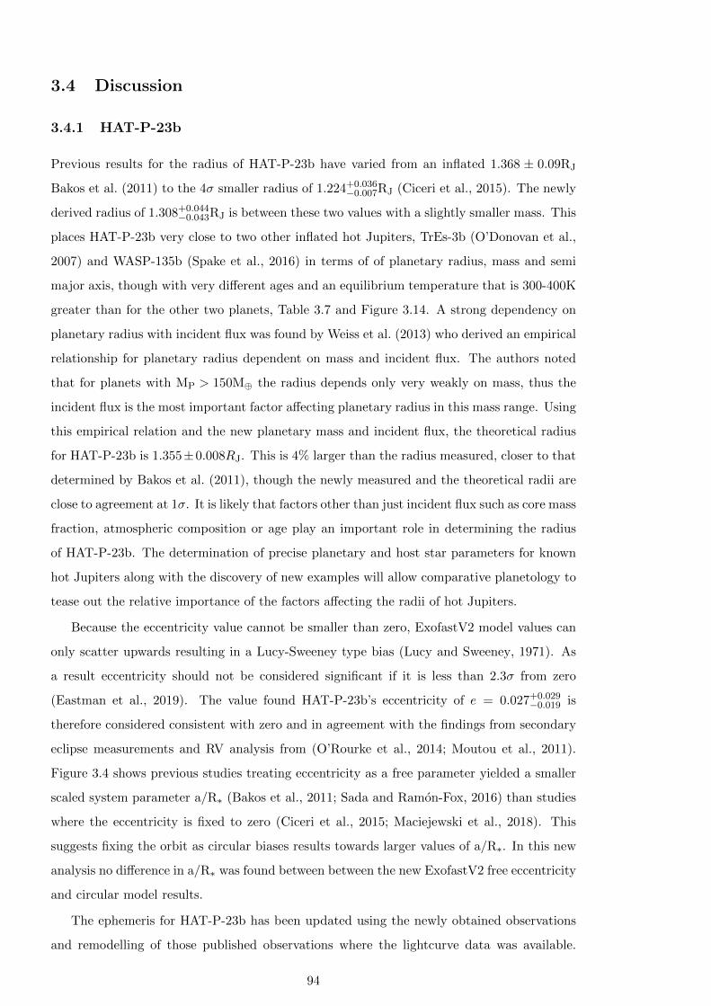
3.4 Discussion

3.4.1 HAT-P-23b

Previous results for the radius of HAT-P-23b have varied from an inflated 1.368 ± 0.09RJ

Bakos et al. (2011) to the 4σ smaller radius of 1.224+0.036−0.007RJ (Ciceri et al., 2015). The newly

derived radius of 1.308+0.044−0.043RJ is between these two values with a slightly smaller mass. This

places HAT-P-23b very close to two other inflated hot Jupiters, TrEs-3b (O’Donovan et al.,

2007) and WASP-135b (Spake et al., 2016) in terms of of planetary radius, mass and semi

major axis, though with very different ages and an equilibrium temperature that is 300-400K

greater than for the other two planets, Table 3.7 and Figure 3.14. A strong dependency on

planetary radius with incident flux was found by Weiss et al. (2013) who derived an empirical

relationship for planetary radius dependent on mass and incident flux. The authors noted

that for planets with MP > 150M⊕ the radius depends only very weakly on mass, thus the

incident flux is the most important factor affecting planetary radius in this mass range. Using

this empirical relation and the new planetary mass and incident flux, the theoretical radius

for HAT-P-23b is 1.355±0.008RJ. This is 4% larger than the radius measured, closer to that

determined by Bakos et al. (2011), though the newly measured and the theoretical radii are

close to agreement at 1σ. It is likely that factors other than just incident flux such as core mass

fraction, atmospheric composition or age play an important role in determining the radius

of HAT-P-23b. The determination of precise planetary and host star parameters for known

hot Jupiters along with the discovery of new examples will allow comparative planetology to

tease out the relative importance of the factors affecting the radii of hot Jupiters.

Because the eccentricity value cannot be smaller than zero, ExofastV2 model values can

only scatter upwards resulting in a Lucy-Sweeney type bias (Lucy and Sweeney, 1971). As

a result eccentricity should not be considered significant if it is less than 2.3σ from zero

(Eastman et al., 2019). The value found HAT-P-23b’s eccentricity of e = 0.027+0.029−0.019 is

therefore considered consistent with zero and in agreement with the findings from secondary

eclipse measurements and RV analysis from (O’Rourke et al., 2014; Moutou et al., 2011).

Figure 3.4 shows previous studies treating eccentricity as a free parameter yielded a smaller

scaled system parameter a/R∗ (Bakos et al., 2011; Sada and Ramon-Fox, 2016) than studies

where the eccentricity is fixed to zero (Ciceri et al., 2015; Maciejewski et al., 2018). This

suggests fixing the orbit as circular biases results towards larger values of a/R∗. In this new

analysis no difference in a/R∗ was found between between the new ExofastV2 free eccentricity

and circular model results.

The ephemeris for HAT-P-23b has been updated using the newly obtained observations

and remodelling of those published observations where the lightcurve data was available.

94

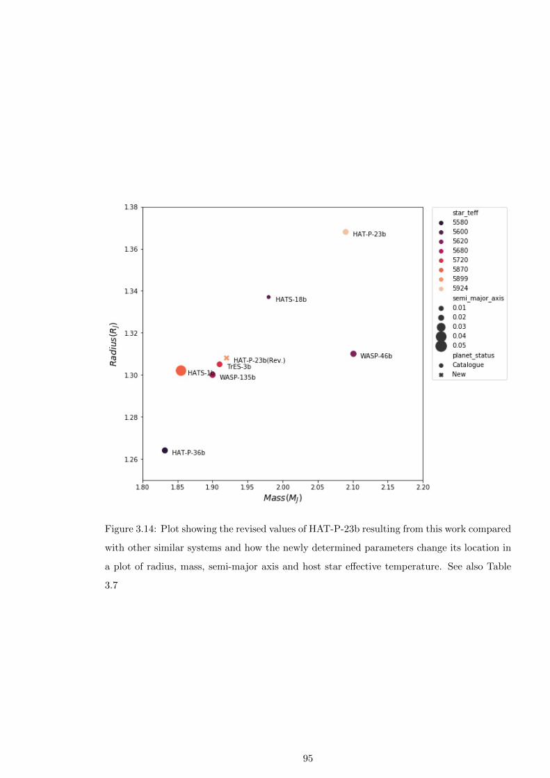
Figure 3.14: Plot showing the revised values of HAT-P-23b resulting from this work compared

with other similar systems and how the newly determined parameters change its location in

a plot of radius, mass, semi-major axis and host star effective temperature. See also Table

3.7

95

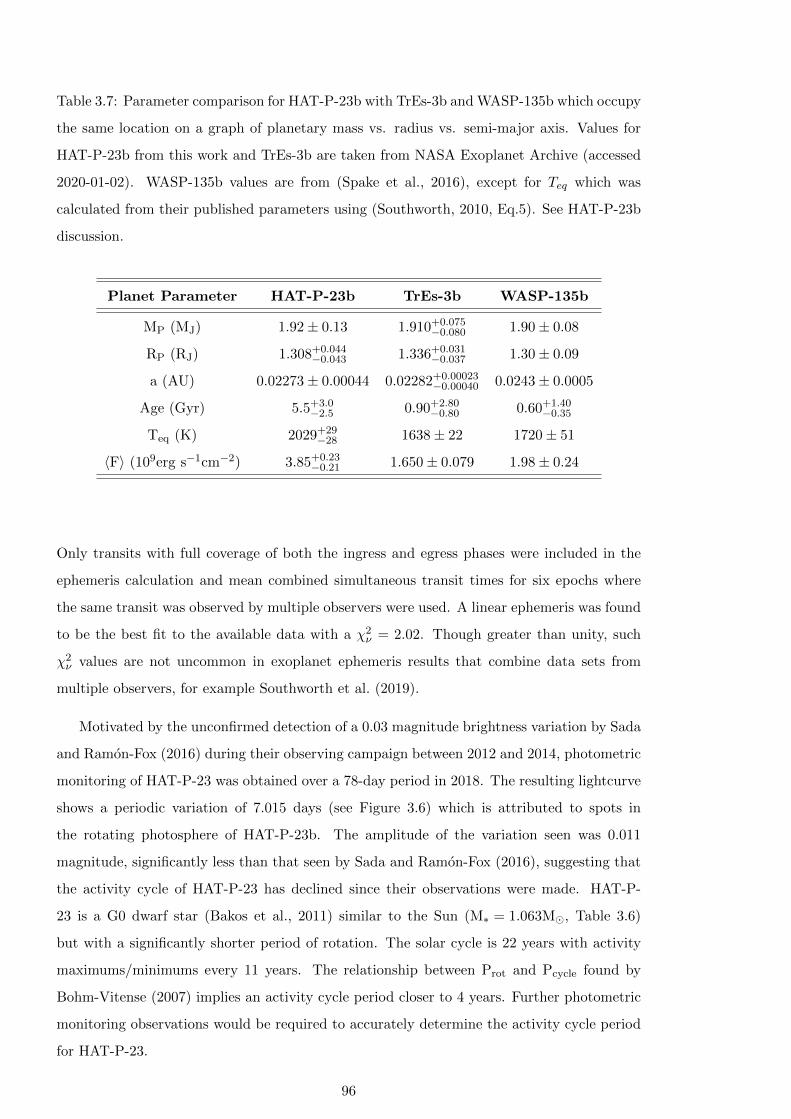
Table 3.7: Parameter comparison for HAT-P-23b with TrEs-3b and WASP-135b which occupy

the same location on a graph of planetary mass vs. radius vs. semi-major axis. Values for

HAT-P-23b from this work and TrEs-3b are taken from NASA Exoplanet Archive (accessed

2020-01-02). WASP-135b values are from (Spake et al., 2016), except for Teq which was

calculated from their published parameters using (Southworth, 2010, Eq.5). See HAT-P-23b

discussion.

Planet Parameter HAT-P-23b TrEs-3b WASP-135b

MP (MJ) 1.92± 0.13 1.910+0.075−0.080 1.90± 0.08

RP (RJ) 1.308+0.044−0.043 1.336+0.031

−0.037 1.30± 0.09

a (AU) 0.02273± 0.00044 0.02282+0.00023−0.00040 0.0243± 0.0005

Age (Gyr) 5.5+3.0−2.5 0.90+2.80

−0.80 0.60+1.40−0.35

Teq (K) 2029+29−28 1638± 22 1720± 51

〈F〉 (109erg s−1cm−2) 3.85+0.23−0.21 1.650± 0.079 1.98± 0.24

Only transits with full coverage of both the ingress and egress phases were included in the

ephemeris calculation and mean combined simultaneous transit times for six epochs where

the same transit was observed by multiple observers were used. A linear ephemeris was found

to be the best fit to the available data with a χ2ν = 2.02. Though greater than unity, such

χ2ν values are not uncommon in exoplanet ephemeris results that combine data sets from

multiple observers, for example Southworth et al. (2019).

Motivated by the unconfirmed detection of a 0.03 magnitude brightness variation by Sada

and Ramon-Fox (2016) during their observing campaign between 2012 and 2014, photometric

monitoring of HAT-P-23 was obtained over a 78-day period in 2018. The resulting lightcurve

shows a periodic variation of 7.015 days (see Figure 3.6) which is attributed to spots in

the rotating photosphere of HAT-P-23b. The amplitude of the variation seen was 0.011

magnitude, significantly less than that seen by Sada and Ramon-Fox (2016), suggesting that

the activity cycle of HAT-P-23 has declined since their observations were made. HAT-P-

23 is a G0 dwarf star (Bakos et al., 2011) similar to the Sun (M∗ = 1.063M�, Table 3.6)

but with a significantly shorter period of rotation. The solar cycle is 22 years with activity

maximums/minimums every 11 years. The relationship between Prot and Pcycle found by

Bohm-Vitense (2007) implies an activity cycle period closer to 4 years. Further photometric

monitoring observations would be required to accurately determine the activity cycle period

for HAT-P-23.

96

3.4.2 WASP-52b

Long term monitoring of known transiting hot Jupiters has revealed several systems suspected

of exhibiting a non-linear ephemeris such as WASP-12b (Maciejewski et al., 2016), WASP-4b

(Bouma et al., 2019) and Kepler-1658 (Chontos et al., 2019). Orbital decay is postulated as

the cause of the declining orbits while apsidal precession is an alternative explanation and it is

difficult to distinguish between these explanations with the available timeline of observations.

This is one motivation for extending the timeline of precise transit mid-time observations

for short period hot Jupiter systems using readily available small aperture ground-based

telescopes.

The new transit timing results obtained with multiple small aperture ground-based tele-

scopes combined with previously published data finds a quadratic ephemeris provides the

best fit to the available data. The ∆χ2ν = 0.07 and ∆BIC = 1.53 between the linear and

quadratic ephemerides are small and have not been reported in previous analysis of transit

times for WASP-52b, (Mancini et al., 2017; Ozturk and Erdem, 2019; Baluev et al., 2019).

The BIC is used to determine whether adding additional free parameters to a model provides

a better fit to the data with a smaller BIC indicating a preference for the inclusion of the ad-

ditional parameters. A BIC decrease of 2.0 is typically the threshold for clearly indicating the

inclusion of the additional parameter is preferred. The ∆BIC of 1.53 found for the quadratic

over the linear ephemeris is slightly below this threshold. Extrapolating both ephemerides

shows that with timing measurements from the 2021 observing season it should be possible

to determine if the linear or quadratic model is correct, see Figure 3.9.

Below I consider some possible causes for the period change implied by the quadratic

ephemeris model result.

3.4.2.1 Orbital Decay

The result for the period change (Equation 3.5) implies a decay time (based on linear decay

to a = 0) of 4.1± 0.4 Myr, approximately 0.05 ± 0.03% of the derived age for WASP-52.

Following equation 14 from Patra et al. (2017) and using δP/δt = −1.22 ± 0.14 × 10−9 the

modified tidal quality factor is found to be Q′∗ = 1.1±0.2×103. This is at least 2-3 orders of

magnitude smaller than typically expected (Patra et al., 2017, and references therein), ruling

out tidal decay as a potential cause of the observed period change.

3.4.2.2 Apsidal Precession

Apsidal precession requires the planet has an eccentric orbit and the new results presented

indicate an eccentricity consistent with zero. If a small eccentricity exists, with a short

97

1.75d period, a method of maintaining that eccentricity is not clear. Due to the mass ratio,

circularisation timescales are dominated by tides raised on the planet (Goldreich and Soter,

1966; Adams and Laughlin, 2006). Aassuming a value for QP of 106 the tidal circularisation

timescale (τcirc) is just 4Myr, significantly less than the 8.5+3.7−4.6Gyr age of the system. The

ExofastV2 analysis finds no significant evidence for a departure from a circular orbit, however

it is noted that a small eccentricity is possible and additional radial velocity monitoring or

secondary occultation observations would be required to confirm the existence, or otherwise,

of a small orbital eccentricity.

3.4.2.3 Applegate Effect

In the Applegate effect (Applegate, 1992), changes in the stellar quadrupole moment drive

angular momentum transfer within the star over the magnetic cycle period of the star. If

angular momentum is transferred from the core to the stellar envelope the star will become

more oblate. An orbiting planet period change due to the Applegate effect has been con-

sidered by Watson and Marsh (2010). To maintain a constant angular momentum in the

changing gravitation potential as the star becomes more oblate the orbital speed must in-

crease and therefore the period decrease. The opposite is true if the oblateness of the star

decreases, the period will increase, giving rise to a sinusoidal change in the orbiting planets

transit times. Following Equation 13 from Watson and Marsh (2010), setting the time-scale

over which the quadrupole changes occur to either the approximate 7.5 years duration of

WASP-52b observations, or twice this value, the amplitude of period change is 0.244 or 0.59

seconds respectively. This equates to a maximum period change of 37 ± 10ms yr−1 for the

7.5 year quadrupole change or 53± 14ms yr−1 if the cycle is 15 years. This is consistent with

the detected period change value of −38.6 ± 4ms yr−1 so orbital period changes due to the

Applegate effects cannot be ruled out. For a given set of stellar parameters the magnitude

of the O-C value arising from the Applegate effect is sensitive to both the stellar rotation

period and the assumed modulation period, with longer a rotation period reducing the O-C

value and longer modulation periods increasing it. The stellar rotation period from Hebrard

et al. (2013) is dependent on the poorly constrained inclination of the system. Based on

spot crossing events Mancini et al. (2017) derived a rotation period of 15.3± 1.96d which

yields period change values of 28 ± 5ms yr−1 for an assumed 7.5 year modulation period.

The modulation period is therefore the main unknown parameter and will require further

observations to determine.

98

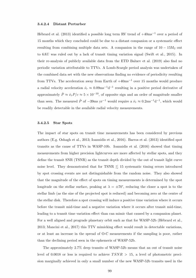
3.4.2.4 Distant Perturber

Hebrard et al. (2013) identified a possible long term RV trend of +40ms−1 over a period of

15 months which they concluded could be due to a distant companion or a systematic effect

resulting from combining multiple data sets. A companion in the range of 10 − 15MJ out

to 6AU was ruled out by a lack of transit timing variation signal (Swift et al., 2015). In

their re-analysis of publicly available data from the ETD Baluev et al. (2019) also find no

periodic variation attributable to TTVs. A Lomb-Scargle period analysis was undertaken of

the combined data set with the new observations finding no evidence of periodicity resulting

from TTVs. The acceleration away from Earth of +40ms−1 over 15 months would produce

a radial velocity acceleration νr ≈ 0.09ms−1d−1 resulting in a positive period derivative of

approximately P ≈ νrP/c ≈ 5 × 10−10, of opposite sign and an order of magnitude smaller

than seen. The measured P of −39ms yr−1 would require a νr ≈ 0.2ms−1d−1, which would

be readily detectable in the available radial velocity measurements.

3.4.2.5 Star Spots

The impact of star spots on transit time measurements has been considered by previous

authors (E.g. Oshagh et al., 2013; Ioannidis et al., 2016). Barros et al. (2013) identified spot

transits as the cause of TTVs in WASP-10b. Ioannidis et al. (2016) showed that timing

measurements from higher precision lightcurves are more affected by stellar spots, and they

define the transit SNR (TSNR) as the transit depth divided by the out of transit light curve

noise level. They demonstrated that for TSNR . 15 systematic timing errors introduced

by spot crossing events are not distinguishable from the random noise. They also showed

that the magnitude of the effect of spots on timing measurements is determined by the spot

longitude on the stellar surface, peaking at λ = ±70°, reducing the closer a spot is to the

stellar limb (as the size of the projected spot is reduced) and becoming zero at the centre of

the stellar disk. Therefore a spot crossing will induce a positive time variation where it occurs

before the transit mid-time and a negative variation where it occurs after transit mid-time,

leading to a transit time variation effect than can mimic that caused by a companion planet.

For a well aligned and prograde planetary orbit such as that for WASP-52b (Hebrard et al.,

2013; Mancini et al., 2017) this TTV mimicking effect would result in detectable variations,

or at least an increase in the spread of O-C measurements if the sampling is poor, rather

than the declining period seen in the ephemeris of WASP-52b.

The approximately 2.7% deep transits of WASP-52b means that an out of transit noise

level of 0.0018 or less is required to achieve TSNR > 15, a level of photometric preci-

sion marginally achieved in only a small number of the new WASP-52b transits used in the

99

ephemeris calculation. Therefore it would not expected that the transit mid-time measure-

ments be systematically affected by spot crossing events. While no spot crossing events were

positively identified in the new photometry obtained in the 2017-18 season the 2013 archive

observation from the UK shows a clear brightening during transit. This observation was

obtained during the same period as those by Mancini et al. (2017) who positively detected

spot crossing events at 5 of their 7 epochs with full transit coverage. The absence of spot

crossing events in the 2017-18 transits could indicate that the photometric precision achieved

is insufficient to resolve the spot crossings or that since the 2012-2014 seasons WASP-52’s

stellar cycle has either quieted or the spot latitude has migrated away from the transit chord.

If the spots have ceased or migrated to a different latitude from the transit chord this would

be apparent in photometric monitoring of WASP-52. Stellar spots occurring at a latitude

different to the transit chord would be visible as stellar variability and potentially detectable

as a correlation between stellar flux and transit depth (E.g. Kirk et al., 2016). If WASP-52

is in a reduced activity phase of its stellar cycle it would not be expected to see either effect.

Taken together the lack of transit spot crossing events in the 2017-18 season, along with

the brightness variation seen in WASP-52 and the tentative indication that transit depth is

greater when stellar brightness is lower, indicate WASP-52 is still active but that the activity

latitude has likely migrated away from the transit chord. Observations in future seasons,

ideally with a B filter to increase spot contrast, would be required to follow the stellar

activity cycle and determine its periodicity. This result shows how observations obtained

using small aperture ground-based telescopes can provide monitoring of transiting systems

to identify activity cycles. This information can help advise the planning of transmission

spectroscopy observations which are complicated by activity on the host star. Identifying the

stellar cycle period will also enable any timing variation due to the Applegate effect to be

better characterised (see Section 3.4.2.3.

Long term out of transit photometric monitoring is required to gain a better understanding

of the activity levels and stellar cycles of exoplanet host stars. The results presented here

show that monitoring can be achieved with small aperture ground-based telescopes as part of

ongoing transit monitoring campaigns of specific systems. General photometric monitoring

could be obtained from long term all sky surveys such as the All Sky Automated Survey

4 with decadal photometric archives. Future exoplanet host monitoring photometry will

become available from the Vera C.Rubin Observatory 5 which will measure the entire visible

night sky every few nights.

4http://www.astrouw.edu.pl/asas/5https://www.lsst.org/

100

Table 3.8: Ephemeris values for WASP-52b and HAT-P-23b. Epoch is shown as 2450000+.

Planet Ephemeris Epoch Period Quadratic χ2ν BIC

WASP-52b Linear 5793.681914(141) 1.749781099(126) – 1.58 59.41

WASP-52b Quadratic 5793.680977(141) 1.749783241(177) −2.14(24) 1.51 57.88

HAT-P-23b Linear 4852.265165(120) 1.212886457(54) – 2.08 33.01

3.5 Summary

17 new transits for HAT-P-23b and 13 new transits of WASP-52b are presented along with

contemporaneous photometric monitoring for HAT-P-23, all made with 0.4m class telescopes.

For HAT-P-23b the combined radial velocity and new transit analysis results in an orbital

eccentricity consistent with zero, in contrast the some previous studies (Bakos et al., 2011;

Sada and Ramon-Fox, 2016), but consistent with the assumption of circular orbit by other

authors (Maciejewski et al., 2018; Ciceri et al., 2015). The new radius found for HAT-P-23b

between previously published values. The planet should still be considered inflated, though

the mechanism driving the inflation is not clear as the radius is smaller than that indicated by

the empirical mass/incident flux relation for planetary radius derived by Weiss et al. (2013).

The monitoring observations of HAT-P-23 have revealed a photometric modulation of 0.011

mag with a period of 7.015 days which is interpreted as the rotation period of HAT-P-23 due

to stellar surface spots.

The WASP-52b observations show no evidence for the large spot crossing events seen in

previous works. The detection of continuing brightness variations indicates that the spot

latitude has migrated away from the transit chord. The analysis of the new and previously

published transit times slightly prefers a quadratic ephemeris but only with a ∆χ2ν = 0.07

and ∆BIC = 1.53. The effects of removing different new and published transit timing data

sets have been investigated and find the quadratic model is preferred in all scenarios except

where the very small uncertainties in the timing from Mancini et al. (2017) are taken at

face value. Predicting the ephemerides forwards shows that transit observations in the 2021

season will likely be able to reveal if the quadratic ephemeris is real.

The results for HAT-P-23b and WASP-52b presented here have demonstrated that small

aperture ground-based telescopes can be used to make valuable contributions to transiting

exoplanet studies when deployed for long term monitoring campaigns. In this chapter I have

presented results from observations of HAT-P-23b and WASP-52b obtained in a single season.

In the next chapter I extend this work to multi-season observations of WASP-12b, a system

showing the best evidence yet for orbital decay amongst the hot Jupiter population.

101

Table 3.9: All transit times used in the ephemeris calculation for HAT-P-23b. Ramon-Fox

and Sada (2013) times taken from Sada and Ramon-Fox (2016)

BJDTDB Error Source Epoch Linear Calc Linear O-C

2454723.69908 0.00027 Bakos et al. (2011) -106 2454723.699201 -0.0001212455026.92049 0.0003 Bakos et al. (2011) 144 2455026.920815 -0.0003252455715.84175 0.0006 Ramon-Fox et al. (2013) 712 2455715.840322 0.0014282455777.69855 0.00058 Ramon-Fox et al. (2013) 763 2455777.697532 0.0010182455789.82583 0.00062 Ramon-Fox et al. (2013) 773 2455789.826396 -0.0005662455794.67924 0.00054 Ramon-Fox et al. (2013) 777 2455794.677942 0.0012982456135.49893 0.0002 Ciceri et al. (2015) 1058 2456135.499037 -0.0001072456176.73801 0.00064 Sada et al. (2016) 1092 2456176.737176 0.0008342456193.71578 0.00075 Sada et al. (2016) 1106 2456193.717586 -0.0018062456204.63395 0.00056 Sada et al. (2016) 1115 2456204.633565 0.0003852456460.55201 0.00022 Ciceri et al. (2015) 1326 2456460.552607 -0.0005972456477.53294 0.00015 Ciceri et al. (2015) 1340 2456477.533017 -0.0000772456505.42953 0.00033 Ciceri et al. (2015) 1363 2456505.429406 0.0001242456512.70668 0.00058 Sada et al. (2016) 1369 2456512.706725 -0.0000452456539.39052 0.00016 Ciceri et al. (2015) 1391 2456539.390227 0.0002932456894.76653 0.00052 Sada et al. (2016) 1684 2456894.765959 0.0005712456911.74741 0.0006 Sada et al. (2016) 1698 2456911.746369 0.0010412457571.55687 0.00014 Maciejewski et al (2018) 2242 2457571.556602 0.0002682457627.34962 0.00025 Maciejewski et al (2018) 2288 2457627.349379 0.0002412457633.41347 0.00018 Maciejewski et al (2018) 2293 2457633.413811 -0.0003412457633.41302 0.00029 Maciejewski et al (2018) 2293 2457633.413811 -0.0007912457633.41381 0.00014 Maciejewski et al (2018) 2293 2457633.413811 -0.0000012457639.47805 0.00024 Maciejewski et al (2018) 2298 2457639.478243 -0.0001932457958.46740 0.00015 Maciejewski et al (2018) 2561 2457958.467381 0.0000192457964.53171 0.00015 Maciejewski et al (2018) 2566 2457964.531814 -0.0001042457981.51210 0.00016 Maciejewski et al (2018) 2580 2457981.512224 -0.0001242458032.45353 0.00076 This work. 2622 2458032.453455 0.0000752458043.36908 0.00018 Maciejewski et al (2018) 2631 2458043.369433 -0.0003532458295.65089 0.00057 This work. 2839 2458295.649816 0.0010742458300.50097 0.00075 This work. 2843 2458300.501362 -0.0003922458300.50190 0.0012 This work. 2843 2458300.501362 0.0005382458306.56787 0.00071 This work. 2848 2458306.565795 0.0020752458306.56574 0.0007 This work. 2848 2458306.565795 -0.0000552458312.62941 0.00078 This work. 2853 2458312.630227 -0.0008172458317.48136 0.00054 This work. 2857 2458317.481773 -0.0004132458317.48176 0.00025 Maciejewski et al (2018) 2857 2458317.481773 -0.0000132458334.46187 0.00066 This work. 2871 2458334.462183 -0.0003132458334.46250 0.00018 Maciejewski et al (2018) 2871 2458334.462183 0.0003172458340.52720 0.00045 This work. 2876 2458340.526615 0.0005852458357.50703 0.0006 This work. 2890 2458357.507026 0.0000042458368.42299 0.00011 Maciejewski et al (2018) 2899 2458368.423004 -0.0000142458385.40434 0.00068 PIRATE 2913 2458385.403414 0.0009262458385.40582 0.00075 This work. 2913 2458385.403414 0.0024062458391.47024 0.00093 This work. 2918 2458391.467847 0.0023932458408.44838 0.0006 This work. 2932 2458408.448257 0.000123

102

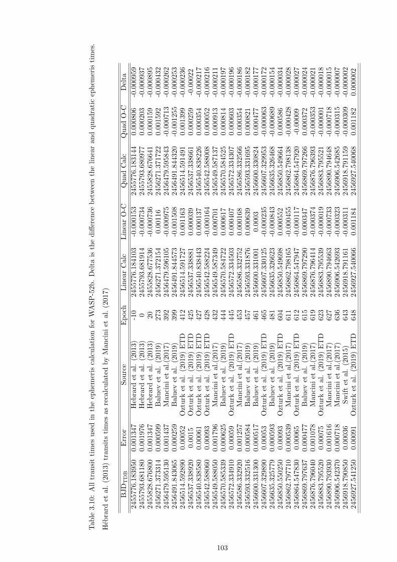
Tab

le3.

10:

All

tran

sit

tim

esu

sed

inth

eep

hem

eris

calc

ula

tion

for

WA

SP

-52b

.D

elta

isth

ed

iffer

ence

bet

wee

nth

eli

nea

ran

dqu

ad

rati

cep

hem

eris

tim

es.

Heb

rard

etal

.(2

013)

tran

sits

tim

esas

reca

lcu

late

dby

Man

cin

iet

al.

(201

7)

BJD

TD

BE

rror

Sou

rce

Ep

och

Lin

ear

Cal

cL

inea

rO

-CQ

uad

Calc

Qu

ad

O-C

Del

ta

2455

776.

1839

500.

0013

47H

ebra

rdet

al.

(201

3)-1

024

5577

6.18

4103

-0.0

00153

2455776.1

83144

0.0

00806

-0.0

00959

2455

793.

6811

800.

0019

76H

ebra

rdet

al.

(201

3)0

2455

793.

6819

14-0

.000

734

2455793.6

80977

0.0

00203

-0.0

00937

2455

828.

6768

000.

0013

47H

ebra

rdet

al.

(201

3)20

2455

828.

6775

36-0

.000

736

2455828.6

76641

0.0

00159

-0.0

00895

2456

271.

3733

140.

0005

99B

alu

evet

al.

(201

9)27

324

5627

1.37

2154

0.00

116

2456271.3

71722

0.0

01592

-0.0

00432

2456

479.

5951

300.

0014

37M

anci

ni

etal

.(20

17)

392

2456

479.

5961

05-0

.000

975

2456479.5

95843

-0.0

00713

-0.0

00262

2456

491.

8430

650.

0002

59B

alu

evet

al.

(201

9)39

924

5649

1.84

4573

-0.0

01508

2456491.8

44320

-0.0

01255

-0.0

00253

2456

514.

5928

900.

0005

2O

ztu

rket

al.

(201

9)E

TD

412

2456

514.

5917

270.

0011

63

2456514.5

91491

0.0

01399

-0.0

00236

2456

537.

3389

200.

0015

Ozt

urk

etal

.(2

019)

ET

D42

524

5653

7.33

8881

0.00

0039

2456537.3

38661

0.0

00259

-0.0

0022

2456

540.

8385

800.

0006

1O

ztu

rket

al.

(201

9)E

TD

427

2456

540.

8384

430.

0001

37

2456540.8

38226

0.0

00354

-0.0

00217

2456

542.

5880

600.

0009

3O

ztu

rket

al.

(201

9)E

TD

428

2456

542.

5882

24-0

.000

164

2456542.5

88008

0.0

00052

-0.0

00216

2456

549.

5880

500.

0017

96M

anci

ni

etal

.(20

17)

432

2456

549.

5873

490.

0007

01

2456549.5

87137

0.0

00913

-0.0

00211

2456

570.

5853

390.

0006

25B

alu

evet

al.

(201

9)44

424

5657

0.58

4722

0.00

0617

2456570.5

84525

0.0

00814

-0.0

00197

2456

572.

3349

100.

0005

9O

ztu

rket

al.

(201

9)E

TD

445

2456

572.

3345

030.

0004

07

2456572.3

34307

0.0

00603

-0.0

00196

2456

586.

3329

200.

0012

57M

anci

ni

etal

.(20

17)

453

2456

586.

3327

520.

0001

68

2456586.3

32566

0.0

00354

-0.0

00186

2456

593.

3325

160.

0005

84B

alu

evet

al.

(201

9)45

724

5659

3.33

1876

0.00

0639

2456593.3

31695

0.0

00821

-0.0

00182

2456

600.

3313

000.

0005

17B

alu

evet

al.

(201

9)46

124

5660

0.33

1001

0.00

032456600.3

30824

0.0

00477

-0.0

00177

2456

607.

3298

900.

0005

3O

ztu

rket

al.

(201

9)E

TD

465

2456

607.

3301

25-0

.000

235

2456607.3

29953

-0.0

00063

-0.0

00172

2456

635.

3257

790.

0005

93B

alu

evet

al.

(201

9)48

124

5663

5.32

6623

-0.0

00843

2456635.3

26468

-0.0

00689

-0.0

00154

2456

850.

5502

500.

0009

3O

ztu

rket

al.

(201

9)E

TD

604

2456

850.

5496

980.

0005

52

2456850.5

49664

0.0

00586

-0.0

00034

2456

862.

7977

100.

0005

39M

anci

ni

etal

.(20

17)

611

2456

862.

7981

65-0

.000

455

2456862.7

98138

-0.0

00428

-0.0

00028

2456

864.

5478

300.

0006

5O

ztu

rket

al.

(201

9)E

TD

612

2456

864.

5479

47-0

.000

117

2456864.5

47920

-0.0

0009

-0.0

00027

2456

869.

7976

370.

0004

77B

alu

evet

al.

(201

9)61

524

5686

9.79

7290

0.00

0347

2456869.7

97266

0.0

00372

-0.0

00024

2456

876.

7960

400.

0010

78M

anci

ni

etal

.(20

17)

619

2456

876.

7964

14-0

.000

374

2456876.7

96393

-0.0

00353

-0.0

00021

2456

883.

7955

200.

0007

5O

ztu

rket

al.

(201

9)E

TD

623

2456

883.

7955

39-0

.000

019

2456883.7

95521

-0.0

00001

-0.0

00018

2456

890.

7939

300.

0016

16M

anci

ni

etal

.(20

17)

627

2456

890.

7946

63-0

.000

733

2456890.7

94648

-0.0

00718

-0.0

00015

2456

906.

5423

700.

0007

18M

anci

ni

etal

.(20

17)

636

2456

906.

5426

93-0

.000

323

2456906.5

42685

-0.0

00315

-0.0

00007

2456

918.

7908

500.

0003

6S

wif

tet

al.

(201

5)64

324

5691

8.79

1161

-0.0

00311

2456918.7

91159

-0.0

00309

-0.0

00002

2456

927.

5412

500.

0009

1O

ztu

rket

al.

(201

9)E

TD

648

2456

927.

5400

660.

0011

84

2456927.5

40068

0.0

01182

0.0

00002

103

Con

tinu

edfr

omT

able

3.10

BJD

TD

BE

rror

Sou

rce

Ep

och

Lin

ear

Cal

cL

inea

rO

-CQ

uad

Calc

Qu

ad

O-C

Del

ta

2456

950.

2865

300.

0005

2O

ztu

rket

al.

(201

9)E

TD

661

2456

950.

2872

20-0

.000

6924

5695

0.2

87232

-0.0

00702

0.0

00011

2456

957.

2867

650.

0004

81B

alu

evet

al.

(201

9)66

524

5695

7.28

6345

0.00

042

2456

957.

286359

0.0

00406

0.0

00014

2457

013.

2797

160.

0003

23B

alu

evet

al.

(201

9)69

724

5701

3.27

9340

0.00

0376

2457

013.2

79376

0.0

0034

0.0

00036

2457

013.

2792

300.

0003

2O

ztu

rket

al.

(201

9)E

TD

697

2457

013.

2793

40-0

.000

1124

5701

3.2

79376

-0.0

00146

0.0

00036

2457

027.

2767

520.

0004

53B

alu

evet

al.

(201

9)70

524

5702

7.27

7589

-0.0

0083

724

5702

7.277630

-0.0

00878

0.0

00041

2457

027.

2777

300.

0004

2O

ztu

rket

al.

(201

9)E

TD

705

2457

027.

2775

890.

0001

4124

5702

7.277630

0.0

001

0.0

00041

2457

221.

5052

740.

0005

65B

alu

evet

al.

(201

9)81

624

5722

1.50

3291

0.00

1983

2457

221.5

03389

0.0

01885

0.0

00098

2457

221.

5035

500.

0004

5O

ztu

rket

al.

(201

9)E

TD

816

2457

221.

5032

910.

0002

5924

5722

1.503389

0.0

00161

0.0

00098

2457

242.

5015

620.

0003

34B

alu

evet

al.

(201

9)82

824

5724

2.50

0664

0.00

0898

2457

242.5

00767

0.0

00795

0.0

00103

2457

242.

5009

300.

0003

1O

ztu

rket

al.

(201

9)E

TD

828

2457

242.

5006

640.

0002

6624

5724

2.500767

0.0

00163

0.0

00103

2457

263.

4979

770.

0001

55B

alu

evet

al.

(201

9)84

024

5726

3.49

8037

-0.0

0006

2457

263.

498144

-0.0

00167

0.0

00107

2457

291.

4935

100.

0004

7O

ztu

rket

al.

(201

9)E

TD

856

2457

291.

4945

35-0

.001

025

2457

291.4

94647

-0.0

01137

0.0

00113

2457

296.

7439

500.

0006

Ozt

urk

etal

.(2

019)

ET

D85

924

5729

6.74

3878

0.00

0072

2457

296.7

43991

-0.0

00041

0.0

00113

2457

298.

4934

000.

0006

3O

ztu

rket

al.

(201

9)E

TD

860

2457

298.

4936

59-0

.000

259

2457

298.4

93773

-0.0

00373

0.0

00114

2457

326.

4900

900.

0010

3O

ztu

rket

al.

(201

9)E

TD

876

2457

326.

4901

57-0

.000

067

2457

326.4

90275

-0.0

00185

0.0

00118

2457

333.

4887

900.

0009

2O

ztu

rket

al.

(201

9)E

TD

880

2457

333.

4892

81-0

.000

491

2457

333.4

89400

-0.0

0061

0.0

00119

2457

335.

2395

200.

0006

2O

ztu

rket

al.

(201

9)E

TD

881

2457

335.

2390

620.

0004

5824

5733

5.239182

0.0

00338

0.0

0012

2457

347.

4861

390.

0007

53B

alu

evet

al.

(201

9)88

824

5734

7.48

7530

-0.0

0139

124

5734

7.487651

-0.0

01512

0.0

00121

2457

347.

4873

500.

0007

3O

ztu

rket

al.

(201

9)E

TD

888

2457

347.

4875

30-0

.000

1824

5734

7.4

87651

-0.0

00301

0.0

00121

2457

571.

4599

000.

0006

Ozt

urk

etal

.(2

019)

1016

2457

571.

4595

110.

0003

8924

5757

1.459645

0.0

00255

0.0

00135

2457

578.

4589

000.

0003

Ozt

urk

etal

.(2

019)

1020

2457

578.

4586

350.

0002

6524

5757

8.458770

0.0

0013

0.0

00135

2457

585.

4589

000.

0004

Ozt

urk

etal

.(2

019)

1024

2457

585.

4577

590.

0011

4124

5758

5.457894

0.0

01006

0.0

00134

2457

599.

4569

000.

0006

Ozt

urk

etal

.(2

019)

1032

2457

599.

4560

080.

0008

9224

5759

9.456142

0.0

00758

0.0

00134

2457

606.

4552

900.

0005

3O

ztu

rket

al.

(201

9)E

TD

1036

2457

606.

4551

330.

0001

5724

5760

6.4

55266

0.0

00024

0.0

00134

2457

613.

4539

850.

0008

94B

alu

evet

al.

(201

9)10

4024

5761

3.45

4257

-0.0

0027

224

5761

3.454390

-0.0

00405

0.0

00133

2457

613.

4536

100.

0004

3O

ztu

rket

al.

(201

9)E

TD

1040

2457

613.

4542

57-0

.000

647

2457

613.

454390

-0.0

0078

0.0

00133

2457

627.

4528

210.

0004

13B

alu

evet

al.

(201

9)10

4824

5762

7.45

2506

0.00

0315

2457

627.4

52638

0.0

00182

0.0

00133

2457

627.

4558

000.

0018

Ozt

urk

etal

.(2

019)

1048

2457

627.

4525

060.

0032

9424

5762

7.452638

0.0

03162

0.0

00133

104

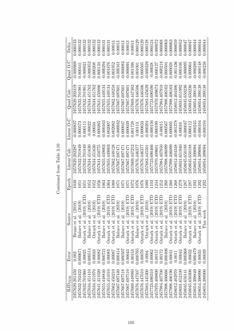
Con

tinu

edfr

omT

able

3.10

BJD

TD

BE

rror

Sou

rce

Ep

och

Lin

ear

Cal

cL

inea

rO

-CQ

uad

Calc

Qu

ad

O-C

Del

ta

2457

629.

2014

500.

002

Bru

no

etal

.(2

018)

1049

2457

629.

2022

87-0

.000

837

2457629.2

02419

-0.0

00969

0.0

00133

2457

632.

7024

220.

0006

71B

alu

evet

al.

(201

9)10

5124

5763

2.70

1849

0.00

0573

2457632.7

01981

0.0

00441

0.0

00132

2457

632.

7019

600.

0002

5O

ztu

rket

al.

(201

9)E

TD

1051

2457

632.

7018

490.

0001

11

2457632.7

01981

-0.0

00021

0.0

00132

2457

634.

4514

100.

0005

14B

alu

evet

al.

(201

9)10

5224

5763

4.45

1630

-0.0

0022

2457634.4

51762

-0.0

00352

0.0

00132

2457

634.

4519

700.

0003

3O

ztu

rket

al.

(201

9)10

5224

5763

4.45

1630

0.00

034

2457634.4

51762

0.0

00208

0.0

00132

2457

641.

4510

200.

0008

2O

ztu

rket

al.

(201

9)E

TD

1056

2457

641.

4507

550.

0002

65

2457641.4

50886

0.0

00134

0.0

00132

2457

655.

4488

400.

0007

21B

alu

evet

al.

(201

9)10

6424

5765

5.44

9003

-0.0

00163

2457655.4

49134

-0.0

00294

0.0

00131

2457

655.

4510

100.

0008

3O

ztu

rket

al.

(201

9)E

TD

1064

2457

655.

4490

030.

0020

07

2457655.4

49134

0.0

01876

0.0

00131

2457

662.

4502

100.

0008

7O

ztu

rket

al.

(201

9)E

TD

1068

2457

662.

4481

280.

0020

82

2457662.4

48258

0.0

01952

0.0

0013

2457

667.

6974

400.

0004

14B

alu

evet

al.

(201

9)10

7124

5766

7.69

7471

-0.0

00032

2457667.6

97601

-0.0

00161

0.0

0013

2457

667.

6975

180.

0005

07B

alu

evet

al.

(201

9)10

7124

5766

7.69

7471

0.00

0047

2457667.6

97601

-0.0

00083

0.0

0013

2457

667.

6975

100.

0004

3O

ztu

rket

al.

(201

9)E

TD

1071

2457

667.

6974

710.

0000

39

2457667.6

97601

-0.0

00091

0.0

0013

2457

669.

4489

800.

0015

3O

ztu

rket

al.

(201

9)E

TD

1072

2457

669.

4472

520.

0017

28

2457669.4

47382

0.0

01598

0.0

0013

2457

676.

4475

070.

0007

65B

alu

evet

al.

(201

9)10

7624

5767

6.44

6377

0.00

113

2457676.4

46506

0.0

01001

0.0

00129

2457

676.

4470

100.

0007

6O

ztu

rket

al.

(201

9)E

TD

1076

2457

676.

4463

770.

0006

33

2457676.4

46506

0.0

00505

0.0

00129

2457

683.

4453

000.

0004

Ozt

urk

etal

.(2

019)

1080

2457

683.

4455

01-0

.000

201

2457683.4

45629

-0.0

00329

0.0

00128

2457

723.

6903

100.

0006

2O

ztu

rket

al.

(201

9)E

TD

1103

2457

723.

6904

66-0

.000

156

2457723.6

90590

-0.0

0028

0.0

00124

2457

970.

4098

000.

0015

7O

ztu

rket

al.

(201

9)E

TD

1244

2457

970.

4096

010.

0001

99

2457970.4

09673

0.0

00127

0.0

00072

2457

984.

4077

000.

0017

2O

ztu

rket

al.

(201

9)E

TD

1252

2457

984.

4078

50-0

.000

15

2457984.4

07918

-0.0

00218

0.0

00068

2457

998.

4066

660.

0004

06B

alu

evet

al.

(201

9)12

6024

5799

8.40

6099

0.00

0567

2457998.4

06162

0.0

00504

0.0

00063

2457

998.

4061

900.

0004

1O

ztu

rket

al.

(201

9)E

TD

1260

2457

998.

4060

990.

0000

91

2457998.4

06162

0.0

00028

0.0

00063

2458

012.

4029

700.

0011

Ozt

urk

etal

.(2

019)

ET

D12

6824

5801

2.40

4348

-0.0

01378

2458012.4

04406

-0.0

01436

0.0

00059

2458

031.

6521

000.

0004

3O

ztu

rket

al.

(201

9)E

TD

1279

2458

031.

6519

400.

0001

62458031.6

51992

0.0

00108

0.0

00052

2458

045.

6501

410.

0003

68B

alu

evet

al.

(201

9)12

8724

5804

5.65

0188

-0.0

00047

2458045.6

50236

-0.0

00095

0.0

00047

2458

045.

6503

000.

0003

2O

ztu

rket

al.

(201

9)E

TD

1287

2458

045.

6501

880.

0001

12

2458045.6

50236

0.0

00064

0.0

00047

2458

054.

3988

490.

0004

79B

alu

evet

al.

(201

9)12

9224

5805

4.39

9094

-0.0

00245

2458054.3

99138

-0.0

00289

0.0

00044

2458

054.

3989

900.

0003

5O

ztu

rket

al.

(201

9)E

TD

1292

2458

054.

3990

94-0

.000

104

2458054.3

99138

-0.0

00148

0.0

00044

2458

054.

3989

000.

0003

9T

his

wor

k12

9224

5805

4.39

9094

-0.0

00194

2458054.3

99138

-0.0

00238

0.0

00044

105

Con

tinu

edfr

omT

able

3.10

BJD

TD

BE

rror

Sou

rce

Ep

och

Lin

ear

Cal

cL

inea

rO

-CQ

uad

Calc

Qu

ad

O-C

Del

ta

2458

080.

6449

200.

0004

7O

ztu

rket

al.

(201

9)E

TD

1307

2458

080.

6458

10-0

.000

8924

5808

0.64

5845

-0.0

00925

0.0

00035

2458

096.

3944

000.

001

Ozt

urk

etal

.(2

019)

ET

D13

1624

5809

6.39

3840

0.00

056

2458

096.

393869

0.0

00531

0.0

00029

2458

325.

6165

470.

0006

4B

alu

evet

al.

(201

9)14

4724

5832

5.61

5164

0.00

1383

2458

325.

615086

0.0

01461

-0.0

00078

2458

325.

6150

900.

0004

7O

ztu

rket

al.

(201

9)E

TD

1447

2458

325.

6151

64-0

.000

074

2458

325.

615086

0.0

00004

-0.0

00078

2458

332.

6142

400.

0002

6T

his

wor

k14

5124

5833

2.61

4289

-0.0

0004

924

5833

2.614207

0.0

00033

-0.0

00082

2458

339.

6129

800.

0003

1T

his

wor

k14

5524

5833

9.61

3413

-0.0

0043

324

5833

9.613327

-0.0

00347

-0.0

00086

2458

346.

6117

940.

0003

Bal

uev

etal

.(2

019)

1459

2458

346.

6125

37-0

.000

743

2458

346.

612448

-0.0

00654

-0.0

0009

2458

346.

6118

770.

0006

53B

alu

evet

al.

(201

9)14

5924

5834

6.61

2537

-0.0

0066

124

5834

6.612448

-0.0

00571

-0.0

0009

2458

346.

6120

000.

0004

1O

ztu

rket

al.

(201

9)E

TD

1459

2458

346.

6125

37-0

.000

537

2458

346.

612448

-0.0

00448

-0.0

0009

2458

348.

3609

600.

0012

3O

ztu

rket

al.

(201

9)E

TD

1460

2458

348.

3623

19-0

.001

359

2458

348.

362228

-0.0

01268

-0.0

0009

2458

353.

6120

080.

0005

38B

alu

evet

al.

(201

9)14

6324

5835

3.61

1662

0.00

0346

2458

353.

611568

0.0

00439

-0.0

00093

2458

353.

6115

000.

0003

3O

ztu

rket

al.

(201

9)E

TD

1463

2458

353.

6116

62-0

.000

162

2458

353.

611568

-0.0

00068

-0.0

00093

2458

360.

6108

300.

0003

1T

his

wor

k14

6724

5836

0.61

0786

0.00

0044

2458

360.

610689

0.0

00141

-0.0

00097

2458

369.

3592

000.

0004

5O

ztu

rket

al.

(201

9)E

TD

1472

2458

369.

3596

92-0

.000

492

2458

369.

359589

-0.0

00389

-0.0

00102

2458

381.

6081

300.

0003

6T

his

wor

k14

7924

5838

1.60

8159

-0.0

0002

924

5838

1.608050

0.0

0008

-0.0

0011

2458

383.

3600

200.

0010

5O

ztu

rket

al.

(201

9)E

TD

1480

2458

383.

3579

410.

0020

7924

5838

3.35

7830

0.0

0219

-0.0

00111

2458

388.

6073

900.

0007

1O

ztu

rket

al.

(201

9)E

TD

1483

2458

388.

6072

840.

0001

0624

5838

8.60

7170

0.0

0022

-0.0

00114

2458

390.

3571

760.

0006

58B

alu

evet

al.

(201

9)14

8424

5839

0.35

7065

0.00

0111

2458

390.

356950

0.0

00225

-0.0

00115

2458

390.

3574

900.

0005

3O

ztu

rket

al.

(201

9)E

TD

1484

2458

390.

3570

650.

0004

2524

5839

0.35

6950

0.0

0054

-0.0

00115

2458

395.

6061

900.

0003

5T

his

wor

k14

8724

5839

5.60

6408

-0.0

0021

824

5839

5.606290

-0.0

001

-0.0

00118

2458

397.

3571

600.

0005

4T

his

wor

k14

8824

5839

7.35

6189

0.00

0971

2458

397.

356070

0.0

0109

-0.0

00119

2458

402.

6051

600.

0007

6T

his

wor

k14

9124

5840

2.60

5533

-0.0

0037

324

5840

2.605411

-0.0

00251

-0.0

00122

2458

404.

3557

100.

0011

7O

ztu

rket

al.

(201

9)E

TD

1492

2458

404.

3553

140.

0003

9624

5840

4.35

5191

0.0

00519

-0.0

00123

2458

411.

3540

440.

0003

9B

alu

evet

al.

(201

9)14

9624

5841

1.35

4438

-0.0

0039

424

5841

1.35

4311

-0.0

00267

-0.0

00127

2458

411.

3537

900.

0003

Ozt

urk

etal

.(2

019)

ET

D14

9624

5841

1.35

4438

-0.0

0064

824

5841

1.35

4311

-0.0

00521

-0.0

00127

2458

425.

3542

910.

0006

76B

alu

evet

al.

(201

9)15

0424

5842

5.35

2687

0.00

1604

2458

425.

352551

0.0

01739

-0.0

00136

2458

425.

3529

000.

0004

8O

ztu

rket

al.

(201

9)E

TD

1504

2458

425.

3526

870.

0002

1324

5842

5.35

2551

0.0

00349

-0.0

00136

2458

425.

3529

600.

0002

9T

his

wor

k15

0424

5842

5.35

2687

0.00

0273

2458

425.

352551

0.0

00409

-0.0

00136

2458

451.

5989

900.

0008

1O

ztu

rket

al.

(201

9)E

TD

1519

2458

451.

5994

03-0

.000

413

2458

451.

599251

-0.0

00261

-0.0

00152

106

Chapter 4

WASP-12b

4.1 Introduction

In the previous chapter I considered observations made of two systems over a single season.

I now move on to consider observations made of a single target, WASP-12b, using the same

small aperture ground-based telescopes over multiple observing seasons. This enables a longer

term, and therefore more in depth, study but introduces additional complexities of combining

data obtained in different seasons with different observing modes.

Its relatively bright host star (V=11.57), deep transits (1.4%) and very short period

(1.09d) make WASP-12b an excellent candidate for follow up with small aperture telescopes

on the ground over long, multi season, observing campaigns. Host star monitoring was carried

out between 2016 and 2019 and transit observations were made from 2016 to 2020 using the

PIRATE, COAST and POST telescopes as described in Chapter 2 with the aim of:

• To monitor WASP-12 over multiple seasons for photometric variations that may result

from stellar activity or rotation.

• To determine the precision and accuracy (in comparison with the literature) of the plan-

etary and stellar parameters determined from transit observations made with multiple

small aperture ground-based telescopes.

• To measure transit times obtained over multiple observing seasons in the search for

periodic and secular timing variations.

• To analyse of the ability of the small aperture ground-based telescope observations to

detect transit timing changes over multiple seasons.

This chapter is laid out as follows. First I discuss the current state of knowledge for

the WASP-12 system. I then detail the observations made, followed by the data reduction

107

and analysis. Next I report results for the host star monitoring, transit analysis and transit

timing. Finally I consider the results from the small aperture ground-based telescopes in the

context of the current understanding of WASP-12 system.

4.2 WASP-12b Background

WASP-12b is a highly irradiated hot Jupiter orbiting a late F-type star in just 1.09 days

(Hebb et al., 2009) and has become one of the most heavily studied exoplanets, thought to

be highly bloated and losing mass (Li et al., 2010; Fossati et al., 2010; Haswell et al., 2012). In

2014 WASP-12 was discovered to be part of a hierarchical triple system when the previously

known companion was resolved, through lucky imaging techniques, to be composed of two

M0V stars (Bechter et al., 2014).

Observations in the near-UV made with the Hubble Space Telescope showed that WASP-

12b is surrounded by an extended and diffuse exosphere of near-UV absorbing gas that

extends beyond WASP-12b’s Roche lobe (Haswell et al., 2012). Further observations with

Hubble supported these findings and confirmed that the near-UV gas surrounding WASP-

12b is patchy in nature suggesting variable mass loss from the planet (Fossati et al., 2010;

Haswell et al., 2012). Swain et al. (2013) found an IR brightness temperature for WASP-12b

of 3000K, similar to that of an M class dwarf star.

In their near UV measurements made with HST Fossati et al. (2010) detected an early

transit ingress, the UV transit ingress occurring before the optical ingress implying the ex-

istence of UV absorbing material ahead of WASP-12b. Llama et al. (2011) considered the

possibility of a bow shock as the cause, where the planet moves supersonically through the

local stellar outflow. If bow shocks exist they provide a unique way to measure the planetary

and stellar magnetic fields and their interaction. Subsequent ground-based searches have not

detected this early ingress (Turner et al., 2016). A variation in the homogeneity of the gas

surrounding WASP-12 is not unexpected, two near UV transits observed with HST 184 days

apart showed differences in the transit depth indicating changes in the distribution of the

surrounding gas (Haswell et al., 2012). Stellar activity could lead to such variation in the gas

surrounding WASP-12 through which the planet orbits, highlighting the importance of long

term monitoring to characterise hot Jupiter host stars.

Due to its extremely short period, several studies have focused on measuring transit

timings to detect variations indicative of companion planets in exterior orbits. A search of

the SuperWASP data by Smith et al. (2009) looking for additional transit events with a

period between 5-25 days found no evidence of an additional transiting planet. The first

claim of timing variations came from two transit timing observations that suggested a TTV

108

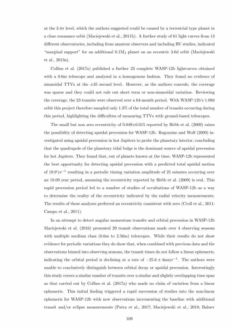
at the 3.4σ level, which the authors suggested could be caused by a terrestrial type planet in

a close resonance orbit (Maciejewski et al., 2011b). A further study of 61 light curves from 13

different observatories, including from amateur observers and including RV studies, indicated

“marginal support” for an additional 0.1MJ planet on an eccentric 3.6d orbit (Maciejewski

et al., 2013a).

Collins et al. (2017a) published a further 23 complete WASP-12b lightcurves obtained

with a 0.6m telescope and analysed in a homogenous fashion. They found no evidence of

sinusoidal TTVs at the ±35 second level. However, as the authors concede, the coverage

was sparse and they could not rule out short term or non-sinusoidal variation. Reviewing

the coverage, the 23 transits were observed over a 64-month period. With WASP-12b’s 1.09d

orbit this project therefore sampled only 1.3% of the total number of transits occurring during

this period, highlighting the difficulties of measuring TTVs with ground-based telescopes.

The small but non zero eccentricity of 0.049±0.015 reported by Hebb et al. (2009) raises

the possibility of detecting apsidal precession for WASP-12b. Ragozzine and Wolf (2009) in-

vestigated using apsidal precession in hot Jupiters to probe the planetary interior, concluding

that the quadrupole of the planetary tidal bulge is the dominant source of apsidal precession

for hot Jupiters. They found that, out of planets known at the time, WASP-12b represented

the best opportunity for detecting apsidal precession with a predicted total apsidal motion

of 19.9°yr−1 resulting in a periodic timing variation amplitude of 25 minutes occurring over

an 18.09 year period, assuming the eccentricity reported by Hebb et al. (2009) is real. This

rapid precession period led to a number of studies of occultations of WASP-12b as a way

to determine the reality of the eccentricity indicated by the radial velocity measurements.

The results of these analyses preferred an eccentricity consistent with zero (Croll et al., 2011;

Campo et al., 2011).

In an attempt to detect angular momentum transfer and orbital precession in WASP-12b

Maciejewski et al. (2016) presented 29 transit observations made over 4 observing seasons

with multiple medium class (0.6m to 2.56m) telescopes. While their results do not show

evidence for periodic variations they do show that, when combined with previous data and the

observations binned into observing seasons, the transit times do not follow a linear ephemeris,

indicating the orbital period is declining at a rate of −25.6± 4msyr−1. The authors were

unable to conclusively distinguish between orbital decay or apsidal precession. Interestingly

this study covers a similar number of transits over a similar and slightly overlapping time span

as that carried out by Collins et al. (2017a) who made no claim of variation from a linear

ephemeris. This initial finding triggered a rapid succession of studies into the non-linear

ephemeris for WASP-12b with new observations incrementing the baseline with additional

transit and/or eclipse measurements (Patra et al., 2017; Maciejewski et al., 2018; Baluev

109

et al., 2019; Ozturk and Erdem, 2019). Observations of occultations of WASP-12b are key to

determining between the orbital and apsidal precession models. In the case of a precessing

orbit the occurrence of the transits and occultations will be 180° out of phase, while in the case

of orbital decay they will occur in phase (Patra et al., 2017). Yee et al. (2019) published new

transit times and a further 9 previously unpublished occultation times showing the transits

and occultations are occurring in phase and therefore confirming the orbital decay model for

WASP-12b. The same authors also presented additional RV data, extending the baseline

of measurements and improving the precision of the line of sight acceleration of WASP-12

( |υ| < 0.005m s−1 day−1 ), ruling out the Rømer effect as a significant contribution to the

changing period. Observations of 21 transits with TESS in 2020 support the orbital decay

model (Turner et al., 2021).

One of the largest studies of transits of WASP-12b was carried out by Baluev et al.

(2019) who homogeneously analysed 280 transit light curves obtained over an 11 year period

comprised mostly of amateur observations recorded on the Exoplanet Transit Database. They

were able to successfully recover the quadratic ephemeris for orbital decay (they did not fit

for apsidal precession), though with an approximately 10% smaller rate of decay.

The existence of orbital decay in WASP-12b requires a mechanism to dissipate the orbital

energy. The commonly invoked mechanism for this is raising of tides and their subsequent

dissipation within the host star. Main sequence F type stars have small convective cores

with largely radiative envelopes surrounded by a thin outer convective envelope. Studies

have determined tidal dissipation within this stellar structure is insufficient to explain the

orbital rate decay seen (Chernov et al., 2017; Weinberg et al., 2017). However once an F star

evolves onto the sub-giant branch its core becomes radiative allowing the tidal wave breaking

at much smaller radii and making tidal dissipation in a sub-giant host star a better fit to

the observed decay rate (Weinberg et al., 2017). This explanation also provides an answer

to how WASP-12b has survived for the 1-2 Gyr life of the host star, tidal decay would only

have commenced as the star evolved on to the sub-giant branch. Furthermore this finding

would be consistent with the measured slow rotation for WASP-12 as tidal spin up would

only affect the very small core of a sub-giant which would be insufficient to spin up the

outer envelope (Weinberg et al., 2017). Further analysis by Bailey and Goodman (2019)

finds that while neither main sequence or sub giant models fit all the observational data,

specifically a disagreement between spectroscopically derived Teff and metalicity with the

Gaia derived luminosity (an issue the authors note would exist regardless of orbital decay),

the main sequence models are less discrepant leaving the question of the source of the tidal

damping open.

Using a combination of published and new RV data Maciejewski et al. (2020) confirmed

110

the existence of a tidal bulge on the surface of WASP-12 through measurement of an RV

period of half that of the orbital period with an amplitude of just a few meters per second.

This signal mimics a non zero eccentricity with a longitude of periastron of 270°. The authors

find e = 0.035± 0.006 and ω = 270.7± 0.6°, a 5.8σ detection of eccentricity indicating a tidal

bulge height of approximately 150km is being raised on WASP-12 by the orbiting hot Jupiter.

The authors predict the tidal bulge should cause a photometric variation of 80ppm, potentially

detectable with space based telescopes. This result also neatly explains why eccentricity has

been found from RV studies but occultation timing studies have indicated a circular orbit.

When discovered, WASP-12 was determined to have a low rotation speed for a late F type

star with a projected stellar υsini = 2.2± 1.5 km s−1 (Hebb et al., 2009). The same authors

were also unable to detect any signs of a Rossiter-McLaughlin (RM) effect, consistent with a

low projected rotational velocity. A study of 12,000 stars observed by the Kepler telescope

finds a mean equatorial velocity of 10− 40 km s−1 and rotation periods of 2 to 4 days for

F7 stellar types (Nielsen et al., 2013). The implication being that either WASP-12 is an

abnormally slow rotator or is viewed at a very low inclination, i.e. near pole on. Fossati et al.

(2010) determined that the stellar macro-turbulence is greater than the measured rotation

velocity, leaving the RM effect as the only spectroscopic approach to determining rotational

velocity. Husnoo et al. (2012) obtained 16 spectroscopic measurements during a single transit

and found a weak RM signal but their analysis of the sky projected spin-orbit angle (λ) was

inconclusive. Albrecht et al. (2012) obtained 38 radial velocity measurement before, during

and after transit. In their analysis they find an orbital misalignment of λ = 59+15−20° and

υsini = 1.6+0.8−0.4 k ms−1. Their conclusion is that we observe WASP-12 at low stellar rotational

inclination and therefore the orbit of WASP-12b the planet must be significantly misaligned.

No long term photometric monitoring of WASP-12 has been found in the literature.

The existence of secular period changes has important implications for theories of plane-

tary formation and dynamical history, whether the cause is apsidal precession, orbital decay

or due to a long period companion . Despite the intense scrutiny WASP-12b has received in

recent years, especially since the discovery of the non linear ephemeris, long term monitoring

of this (and similar systems) is required to follow the detected period change over multiple

observing seasons.

111

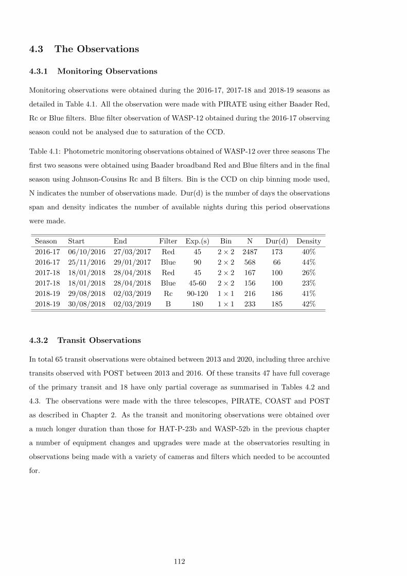
4.3 The Observations

4.3.1 Monitoring Observations

Monitoring observations were obtained during the 2016-17, 2017-18 and 2018-19 seasons as

detailed in Table 4.1. All the observation were made with PIRATE using either Baader Red,

Rc or Blue filters. Blue filter observation of WASP-12 obtained during the 2016-17 observing

season could not be analysed due to saturation of the CCD.

Table 4.1: Photometric monitoring observations obtained of WASP-12 over three seasons The

first two seasons were obtained using Baader broadband Red and Blue filters and in the final

season using Johnson-Cousins Rc and B filters. Bin is the CCD on chip binning mode used,

N indicates the number of observations made. Dur(d) is the number of days the observations

span and density indicates the number of available nights during this period observations

were made.

Season Start End Filter Exp.(s) Bin N Dur(d) Density

2016-17 06/10/2016 27/03/2017 Red 45 2× 2 2487 173 40%

2016-17 25/11/2016 29/01/2017 Blue 90 2× 2 568 66 44%

2017-18 18/01/2018 28/04/2018 Red 45 2× 2 167 100 26%

2017-18 18/01/2018 28/04/2018 Blue 45-60 2× 2 156 100 23%

2018-19 29/08/2018 02/03/2019 Rc 90-120 1× 1 216 186 41%

2018-19 30/08/2018 02/03/2019 B 180 1× 1 233 185 42%

4.3.2 Transit Observations

In total 65 transit observations were obtained between 2013 and 2020, including three archive

transits observed with POST between 2013 and 2016. Of these transits 47 have full coverage

of the primary transit and 18 have only partial coverage as summarised in Tables 4.2 and

4.3. The observations were made with the three telescopes, PIRATE, COAST and POST

as described in Chapter 2. As the transit and monitoring observations were obtained over

a much longer duration than those for HAT-P-23b and WASP-52b in the previous chapter

a number of equipment changes and upgrades were made at the observatories resulting in

observations being made with a variety of cameras and filters which needed to be accounted

for.

112

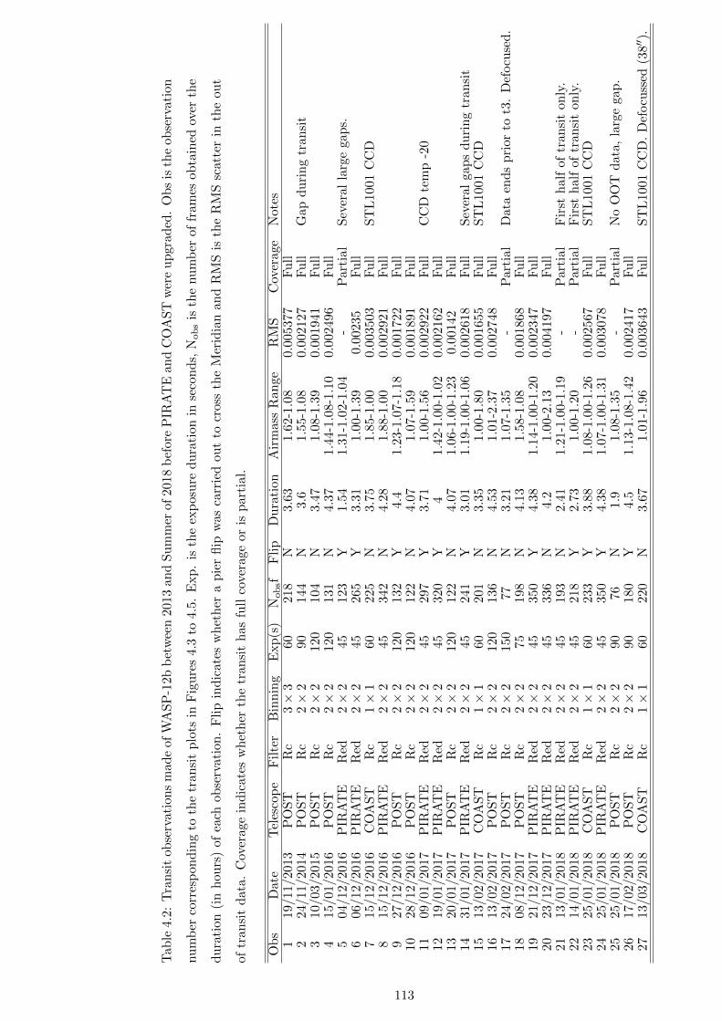
Tab

le4.

2:T

ran

sit

obse

rvat

ion

sm

ade

ofW

AS

P-1

2bb

etw

een

2013

and

Su

mm

erof

2018

bef

ore

PIR

AT

Eand

CO

AST

wer

eup

gra

ded

.O

bs

isth

eob

serv

ati

on

nu

mb

erco

rres

pon

din

gto

the

tran

sit

plo

tsin

Fig

ure

s4.

3to

4.5.

Exp

.is

the

exp

osu

red

ura

tion

inse

con

ds,

Nob

sis

the

nu

mb

erof

fram

esob

tain

edov

erth

e

du

rati

on(i

nh

ours

)of

each

obse

rvat

ion

.F

lip

ind

icat

esw

het

her

ap

ier

flip

was

carr

ied

out

tocr

oss

the

Mer

idia

nan

dR

MS

isth

eR

MS

scatt

erin

the

ou

t

oftr

ansi

td

ata.

Cov

erag

ein

dic

ates

wh

eth

erth

etr

ansi

th

asfu

llco

vera

geor

isp

arti

al.

Ob

sD

ate

Tel

esco

pe

Fil

ter

Bin

nin

gE

xp

(s)

Nob

sfF

lip

Du

rati

onA

irm

ass

Ran

ge

RM

SC

over

age

Note

s1

19/1

1/20

13P

OS

TR

c3×

360

218

N3.

631.

62-1

.08

0.0

05377

Fu

ll2

24/1

1/20

14P

OS

TR

c2×

290

144

N3.

61.

55-1

.08

0.0

02127

Fu

llG

ap

du

rin

gtr

an

sit

310

/03/

2015

PO

ST

Rc

2×

212

010

4N

3.47

1.08

-1.3

90.0

01941

Fu

ll4

15/0

1/20

16P

OS

TR

c2×

212

013

1N

4.37

1.44

-1.0

8-1.

10

0.0

02496

Fu

ll5

04/1

2/20

16P

IRA

TE

Red

2×

245

123

Y1.

541.

31-1

.02-

1.04

-P

art

ial

Sev

eral

larg

egap

s.6

06/1

2/20

16P

IRA

TE

Red

2×

245

265

Y3.

311.

00-1

.39

0.0

0235

Fu

ll7

15/1

2/20

16C

OA

ST

Rc

1×

160

225

N3.

751.

85-1

.00

0.0

03503

Fu

llS

TL

1001

CC

D8

15/1

2/20

16P

IRA

TE

Red

2×

245

342

N4.

281.

88-1

.00

0.0

02921

Fu

ll9

27/1

2/20

16P

OS

TR

c2×

212

013

2Y

4.4

1.23

-1.0

7-1.

18

0.0

01722

Fu

ll10

28/1

2/20

16P

OS

TR

c2×

212

012

2N

4.07

1.07

-1.5

90.0

01891

Fu

ll11

09/0

1/20

17P

IRA

TE

Red

2×

245

297

Y3.

711.

00-1

.56

0.0

02922

Fu

llC

CD

tem

p-2

012

19/0

1/20

17P

IRA

TE

Red

2×

245

320

Y4

1.42

-1.0

0-1.

02

0.0

02162

Full

1320

/01/

2017

PO

ST

Rc

2×

212

012

2N

4.07

1.06

-1.0

0-1.

23

0.0

0142

Fu

ll14

31/0

1/20

17P

IRA

TE

Red

2×

245

241

Y3.

011.

19-1

.00-

1.06

0.0

02618

Fu

llS

ever

al

gap

sd

uri

ng

tran

sit

1513

/02/

2017

CO

AS

TR

c1×

160

201

N3.

351.

00-1

.80

0.0

01655

Fu

llS

TL

1001

CC

D16

13/0

2/20

17P

OS

TR

c2×

212

013

6N

4.53

1.01

-2.3

70.0

02748

Fu

ll17

24/0

2/20

17P

OS

TR

c2×

215

077

N3.

211.

07-1

.35

-P

art

ial

Data

end

sp

rior

tot3

.D

efocu

sed

.18

08/1

2/20

17P

OS

TR

c2×

275

198

N4.

131.

58-1

.08

0.0

01868

Fu

ll19

21/1

2/20

17P

IRA

TE

Red

2×

245

350

Y4.

381.

14-1

.00-

1.20

0.0

02347

Fu

ll20

23/1

2/20

17P

IRA

TE

Red

2×

245

336

N4.

21.

00-2

.13

0.0

04197

Fu

ll21

13/0

1/20

18P

IRA

TE

Red

2×

245

193

N2.

411.

21-1

.00-

1.19

-P

art

ial

Fir

sth

alf

of

tran

sit

only

.22

14/0

1/20

18P

IRA

TE

Red

2×

245

218

Y2.

731.

00-1

.20

-P

art

ial

Fir

sth

alf

of

tran

sit

on

ly.

2325

/01/

2018

CO

AS

TR

c1×

160

233

Y3.

881.

08-1

.00-

1.26

0.0

02567

Fu

llS

TL

1001

CC

D24

25/0

1/20

18P

IRA

TE

Red

2×

245

350

Y4.

381.

07-1

.00-

1.31

0.0

03078

Fu

ll25

25/0

1/20

18P

OS

TR

c2×

290

76N

1.9

1.08

-1.3

5-

Part

ial

No

OO

Td

ata

,la

rge

gap

.26

17/0

2/20

18P

OS

TR

c2×

290

180

Y4.

51.

13-1

.08-

1.42

0.0

02417

Fu

ll27

13/0

3/20

18C

OA

ST

Rc

1×

160

220

N3.

671.

01-1

.96

0.0

03643

Fu

llS

TL

1001

CC

D.

Def

ocu

ssed

(38′′ )

.

113

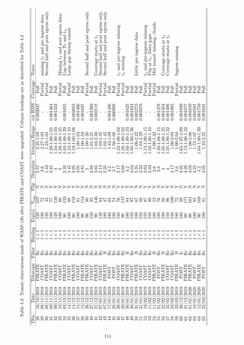
Tab

le4.

3:T

ran

sit

obse

rvat

ion

sm

ade

ofW

AS

P-1

2baf

ter

PIR

AT

Ean

dC

OA

ST

wer

eup

grad

ed.

Col

um

nh

ead

ings

are

as

des

crib

edfo

rT

ab

le4.2

Ob

s.D

ate

Tel

esco

pe

Fil

ter

Bin

nin

gE

xp

(s)

Nob

sF

lip

Du

rati

onA

irm

ass

Ran

geoot

RM

SC

over

age

Note

s28

16/1

0/20

18P

IRA

TE

Rc

1×

112

010

7N

3.57

2.25

-1.0

40.

0030

47F

ull

29

08/1

1/20

18C

OA

ST

Rc

1×

118

072

N3.

62.

27-1

.03

-P

art

ial

mis

sin

gt 1

an

dp

rein

gre

ssd

ata

30

08/1

1/20

18P

IRA

TE

Rc

1×

112

043

N1.

431.

23-1

.04

-P

art

ial

Sec

on

dh

alf

an

dp

ost

egre

sson

ly.

31

09/1

1/20

18C

OA

ST

Rc

1×

118

077

Y3.

851.

29-1

.00-

1.05

0.00

1464

Fu

ll32

09/1

1/20

18P

IRA

TE

Rc

1×

112

012

0Y

41.

34-1

.00-

1.03

0.00

1333

Full

33

10/1

1/20

18C

OA

ST

Rc

1×

118

060

Y3

1.28

-1.0

0-1.

25-

Part

ial

Mis

sin

gt 4

an

dp

ost

egre

ssd

ata

.34

03/1

2/20

18P

IRA

TE

Rc

1×

190

133

Y3.

331.

03-1

.00-

1.29

0.00

1655

Fu

llG

ap

bet

wee

nT

can

dt 3

.35

14/1

2/20

18C

OA

ST

Rc

1×

118

069

Y3.

451.

24-1

.00-

1.10

-P

art

ial

Larg

egap

du

rin

gtr

an

sit

3614

/12/

2018

PIR

AT

ER

c1×

190

158

Y3.

951.

19-1

.00-

1.08

0.00

2055

Fu

ll37

15/1

2/20

18C

OA

ST

Rc

1×

118

081

Y4.

051.

00-1

.63

0.00

1466

Fu

ll38

15/1

2/20

18P

IRA

TE

Rc

1×

190

154

Y3.

851.

00-1

.59

0.00

1697

Fu

ll39

26/1

2/20

18P

IRA

TE

Rc

1×

190

80N

21.

00-1

.20

-P

art

ial

Sec

on

dh

alf

an

dp

ost

egre

sson

ly.

4027

/12/

2018

CO

AS

TR

c1×

115

093

N3.

881.

01-2

.25

0.00

1269

Fu

ll41

27/1

2/20

18P

IRA

TE

Rc

1×

190

146

N3.

651.

02-2

.30

0.00

2118

Fu

llC

over

age

start

sat

t 142

07/0

1/20

19C

OA

ST

Rc

1×

112

064

N2.

131.

03-1

.35

-P

art

ial

Sec

on

dh

alf

an

dp

ost

egre

sson

ly.

4307

/01/

2019

PIR

AT

EB

1×

118

047

N2.

351.

03-1

.42

-P

art

ial

Sec

on

dh

alf

an

dp

ost

egre

sson

ly.

4417

/01/

2019

PO

ST

Rc

1×

124

063

N4.

21.

43-1

.09

0.00

1486

Fu

ll45

28/0

1/20

19P

OS

TR

c1×

118

074

N3.

71.

56-1

.08

0.00

0995

Fu

ll46

29/0

1/20

19C

OA

ST

Rc

1×

115

076

Y3.

171.

22-1

.00-

1.02

-P

art

ial

t 1an

dp

re-i

ngre

ssm

issi

ng

4729

/01/

2019

PIR

AT

ER

c1×

190

147

Y3.

681.

28-1

.00-

1.02

-P

art

ial

t 1m

issi

ng

4830

/01/

2019

PIR

AT

EB

1×

118

084

Y4.

21.

03-1

.00-

1.33

0.00

1625

Fu

ll49

30/0

1/20

19C

OA

ST

Rc

1×

115

097

Y4.

041.

05-1

.00-

1.36

0.00

1824

Fu

ll50

31/0

1/20

19P

IRA

TE

B1×

118

067

N3.

351.

06-2

.22

0.00

2273

Fu

llL

ittl

ep

rein

gre

ssd

ata

5131

/01/

2019

CO

AS

TR

c1×

115

080

N3.

331.

04-2

.29

0.00

2079

Fu

ll52

10/0

2/20

19C

OA

ST

Rc

1×

115

087

Y3.

631.

13-1

.00-

1.15

-P

art

ial

t 1an

dp

re-i

ngre

ssm

issi

ng

5311

/02/

2019

CO

AS

TR

c1×

115

080

Y3.

331.

02-1

.00-

1.43

-P

art

ial

Fli

pat

t 1.

Data

gap

s.54

11/0

2/20

19P

IRA

TE

B1×

118

052

Y2.

61.

00-1

.42

-P

art

ial

Mid

tran

sit

mis

sin

g,

clou

ds.

55

21/0

2/20

19P

OS

TR

c1×

118

076

N3.

81.

20-1

.08-

1.15

0.00

1378

Fu

ll56

22/0

2/20

19P

IRA

TE

B1×

118

080

Y4

1.05

-1.0

0-1.

250.

0014

54F

ull

Cov

erage

start

sat

t 157

22/0

2/20

19C

OA

ST

Rc

1×

115

096

Y4

1.05

-1.0

0-1.

320.

0014

06F

ull

Cov

erage

start

sat

t 158

23/0

2/20

19C

OA

ST

Rc

1×

115

010

0N

4.17

1.00

-2.0

40.

0018

65F

ull

5923

/02/

2019

PIR

AT

EB

1×

118

072

Y3.

61.

00-2

.04

-P

art

ial

Ingre

ssm

issi

ng

6030

/12/

2019

PO

ST

Ic1×

118

099

N4.

951.

65-1

.07-

1.09

0.00

1899

Fu

ll61

31/1

2/20

19P

IRA

TE

Rc

1×

190

171

Y4.

281.

13-1

.00-

1.22

0.00

1677

Fu

ll62

01/0

1/20

20P

IRA

TE

Rc

1×

190

161

N4.

031.

00-2

.08

0.00

3349

Fu

ll63

10/0

1/20

20P

OS

TR

c1×

118

085

N4.

251.

72-1

.07

0.00

3581

Fu

ll64

12/0

1/20

20P

IRA

TE

Rc

1×

190

168

Y4.

21.

04-1

.00-

1.39

0.00

1759

Fu

ll65

22/0

3/20

20P

OS

TR

c1×

118

081

N4.

051.

10-2

.22

0.00

1631

Fu

ll

114

4.4 Data Analysis

Data reduction was undertaken as documented in Chapter 2.

4.4.1 Monitoring Data Analysis

Ensemble photometry was carried out for each season and filter in AstroImageJ using the

comparison and check stars shown in Tables 4.4, 4.5 and 4.6. Scintillation noise was calcu-

lated and added to the photometric uncertainties generated by AstroImageJ as detailed in

Chapter 3.2. As the formal uncertainties on the UCAC4 catalogue magnitudes dominate the

measurement uncertainties by at least an order of magnitude and contribute a constant value

to every uncertainty value only the photometric uncertainties were used.

After photometric extraction the seasonal data sets were corrected as follows before period

analysis was carried out;

1. A linear trend for each individual data group (filter, exposure and mount direction)

was identified separately and corrected for.

2. As with the transit data an offset is seen between observations made when the optical

tube was on the East or the West side of the mount. The difference in measured

magnitude (offset) was identified between each different mount direction data set and

corrected for by adding or subtracting half the offset value as appropriate.

An example of before and after correction for the 2016-17 season observations obtained

through the Red filter is shown in Figure 4.1. The final detrended monitoring data sets for

each season and filter were analysed both individually and together as a whole using a Lomb-

Scargle period analysis to allow any variation in any detected periodicities between seasons

to be identified.

A suitable check star was selected based on having a similar magnitude and B-V colour

index to WASP-12. The check star was analysed as a target in the same way as for WASP-12.

4.4.2 Transit Analysis in ExofastV2

The large number of transit lightcurves to be analysed simultaneously using Exofastv2 places

limits on the number of MCMC steps that could be completed in a reasonable run time and

within the computer memory available. Therefore a stepwise iterative approach was adopted

starting with an initial priors file, 1000 steps and nthin set at 1. The parameter nthin sets the

number of adjacent (and therefore highly correlated) steps to be discarded thereby reducing

memory requirement (Eastman et al., 2019). Once complete the output from this short run

was used to create the starting priors file for a longer 4000 step run with nthin = 1. This was

115

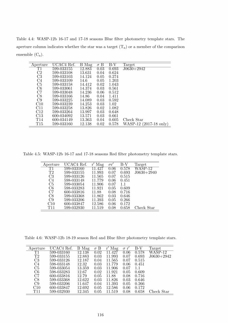
Table 4.4: WASP-12b 16-17 and 17-18 seasons Blue filter photometry template stars. The

aperture column indicates whether the star was a target (Tn) or a member of the comparison

ensemble (Cn).

Aperture UCAC4 Ref. B Mag σ B B-V TargetT1 599-033155 12.883 0.03 0.693 J0630+2942C2 599-033108 13.631 0.04 0.624C3 599-033103 14.124 0.05 0.274C4 599-033109 14.6 0.05 1.203C5 599-033158 14.412 0.02 1.043C6 599-033061 14.374 0.03 0.561C7 599-033048 14.236 0.06 0.512C8 599-033166 14.86 0.04 1.411C9 599-033225 14.089 0.03 0.592C10 599-033239 14.253 0.03 1.02C11 599-033258 13.826 0.02 1.082C12 599-033264 13.997 0.03 0.648C13 600-034092 13.571 0.03 0.661T14 600-034149 13.363 0.04 0.605 Check StarT15 599-033160 12.138 0.02 0.578 WASP-12 (2017-18 only)

Table 4.5: WASP-12b 16-17 and 17-18 seasons Red filter photometry template stars.

Aperture UCAC4 Ref. r′ Mag σr′ B-V TargetT1 599-033160 11.427 0.06 0.578 WASP-12T2 599-033155 11.993 0.07 0.693 J0630+2940C3 599-033126 11.565 0.07 0.515C4 598-033148 11.779 0.06 0.451C5 599-033054 11.906 0.07 1.1C6 598-033283 11.921 0.05 0.609C7 600-033816 11.88 0.08 0.716C8 599-033368 11.862 0.03 0.646C9 599-033206 11.393 0.05 0.266C10 600-033847 12.586 0.06 0.172T11 599-032930 11.519 0.08 0.658 Check Star

Table 4.6: WASP-12b 18-19 season Red and Blue filter photometry template stars.

Aperture UCAC4 Ref. B Mag σ B r′ Mag σ r′ B-V TargetT1 599-033160 12.138 0.02 11.427 0.06 0.578 WASP-12T2 599-033155 12.883 0.03 11.993 0.07 0.693 J0630+2942C3 599-033126 12.187 0.04 11.565 0.07 0.515C4 598-033148 12.32 0.03 11.779 0.06 0.451C5 599-033054 13.359 0.03 11.906 0.07 1.1C6 598-033283 12.67 0.02 11.921 0.05 0.609C7 600-033816 12.79 0.05 11.88 0.08 0.716C8 599-033368 12.622 0.03 11.826 0.03 0.646C9 599-033206 11.647 0.04 11.393 0.05 0.266C10 600-033847 12.692 0.05 12.586 0.06 0.172T11 599-032930 12.345 0.05 11.519 0.08 0.658 Check Star

116

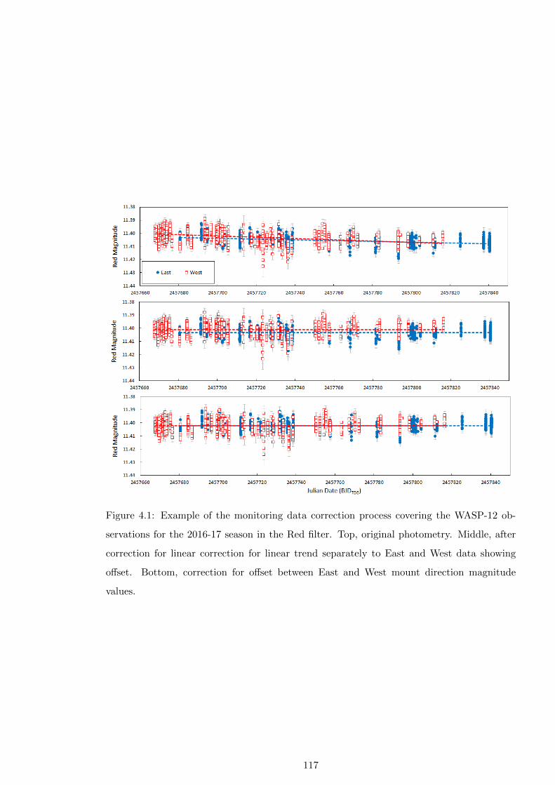
Figure 4.1: Example of the monitoring data correction process covering the WASP-12 ob-

servations for the 2016-17 season in the Red filter. Top, original photometry. Middle, after

correction for linear correction for linear trend separately to East and West data showing

offset. Bottom, correction for offset between East and West mount direction magnitude

values.

117

followed by a 4000 step run with nthin = 3 giving 12,000 steps, updating the starting priors

with the previous output each time. A final run was carried with 4000 steps and nthin = 50,

giving 200,000 steps. At each stage the output was checked for consistency before being used

to create the priors file for the next stage. The initial starting priors values and sources are

shown in Table 4.7. Detrending of the transit lightcurves was carried out in Exofastv2 using

airmass values and where applicable pier flip offsets.

Table 4.7: Priors and sources used in the starting Exofastv2 fit. As recommended by Eastman

et al. (2019) the starting epoch was forward projected closer to the time of the first observation

from 2013. A Gaussian prior width was not used for the dust extinction value, instead the

prior width was set with a minimum of zero and a maximum equal to value determined from

the dust maps.

Prior Description Value σ Sourcerstar Star Radius (R�) 1.619 0.076 Bonomo et al. (2017)mstar Star Mass (M�) 1.38 0.19 Knutson et al. (2014)teff Star Temp.(K) 6360 140 Chakrabarty and Sengupta (2019)feh Star Metalicity 0.32 0.12 Fossati et al. (2010).AV Extinction 0.3238 0 to 0.5528 https://irsa.ipac.caltech.edu

/applications/DUST/parallax Parallax (mas) 2.3942413534 0.04634231 https://gea.esac.esa.int/archive/period Orbital Period (d) 1.09142245 Stassun 2017tc Start Epoch 2456615.36 Fist transit minus 1 × period.ideg Inclination (°) 83.3 1.1 Southworth et al. (2012)dr Ratio d to rstar 3.039 0.034 Collins et al. (2017a)u1(B) Linear LD B filter 0.5223791473 Limb darkening fromu2(B) Quad LD B filter 0.1901998266 http://astroutils.astronomy.u1(I) Linear LD I filter 0.2429178297 ohio-state.eduu2(I) Quad LD I filter 0.0807106464 /exofast/limbdark.shtml.u1(R) Linear LD R filter 0.2955668909u2(R) Quad LD R filter 0.3082340871

Two different red filters were used to obtain the transit data, broadband red and Cousins

Rc which could potentially lead to differing transit depth measurements. The filter transmis-

sion and CCD quantum efficiency are plotted in Figure 4.2 showing the overlap between the

two filters. Also shown are the prominent absorption line locations for NaI and, Hα which

could affect the transit depth measurement (Jensen et al., 2018). Both absorption lines fall

within the bandpass of both filters confirming that absorption in these bands will not cause

a depth variation between the filters and that the lightcurves obtained can be treated as the

same Red band input for the ExofastV2 models.

4.4.2.1 RV Data

RV data files used for the joint fit in Exofastv2 were obtained from the sources detailed

over. Separate Exofastv2 input RV files created for each to allow each RV data set to be

individually fitted with its own zero point and jitter values.

118

Figure 4.2: Plot of the broadband and John-Cousins filters used for transit measurements,

focusing on the overlap between the two red band filters employed. Also shown are the

CCD QE and the prominent absorption lines for NaI and, Hα, both of which fall within the

bandpass for both filters.

• Hebb et al. (2009) provides 21 measurements made with SOPHIE in high efficiency

(HE) mode on the 1.93m OHP telescope between 12/2/2008 and 22/02/2008. The

data was downloaded from NASA Exoplanet Archive. The BJDUTC timestamp was

converted to BJDTDB in line with Eastman et al. (2013). The number of leap seconds

to apply is 33 for all dates, no leap second increments occurred during observation

period. The BJDUTC to BJDTDB correction is therefore 32.184s+33s = 65.184s. It is

noted this correction is significantly less than 15 to 18 minute SOPHIE exposures used

but ensures all rv data uses the same time standard.

• Husnoo et al. (2011) made 29 radial velocity measurements for WASP-12 (16 during a

single night, and 13 at various values of orbital phase) also obtained with SOPHIE in

high efficiency (HE) mode on the 1.93m OHP telescope. The 16 data points obtained

during transit to measure the Rossiter-McLaughlin effect were excluded, the remaining

data was obtained between 26/2/2009 and 27/03/2010. Again the BJDUTC timestamp

was converted to BJDTDB, the number of leap seconds to apply is 34 for all dates,

again no leap second increment occurred during observation period. The BJDUTC to

BJDTDB correction is therefore 32.184s+34s = 66.184s. The authors note the velocity

zero point determined with SOPHIE can drift by up several dozen m s−1 over a time

span of several months. The authors correct for this drift “as far as possible” however

to allow for any remaining differences in the zero point the RV measurements were split

into two input files, one covering measurements obtained over a 46 day period and the

119

other over a 14 day period, separated by almost a year.

• Bonomo et al. (2017) made 15 measurements with HARPS-N which were downloaded

from the catalogue published on VIZIER (https://vizier.u-strasbg.fr/viz-bin/

VizieR). The table as downloaded stated the RV measurements are m s−1 but are

actually km s−1 so were multiplied by 1000 to convert to m s−1 as required by Exofastv2.

The time stamps states the observation are in BJDUTC. The first observation above

was made on 13/11/2012 and the last was made on 07/01/2015. Leap seconds were

added on 30/6/2012 and 30/06/2015. The number of leap seconds to apply is 35 for

all dates, again no leap second increment occurred during the observation period. The

BJDUTC to BJDTDB correction is therefore 32.184s+35s = 67.184s.

• Yee et al. (2019) published the Knutson et al. (2014) data set with three new measure-

ments to extend the coverage baseline to six years. The new and existing data were

uniformly analysed using the standard California Planet Search pipeline in mid-2019

resulting in RV values updated by an average of −6m s−1 so this data set was used

in place of the original RV observations published by Knutson et al. (2014)1. Obser-

vations obtained to measure the Rossiter-McLaughlin effect were excluded leaving 31

measurements covering just over 9 years.

• Seventeen measurements published by Maciejewski et al. (2020) with the HARPS-N

instrument between 02/01/2013 and 16/11/2017.

The full transit lightcurves along with the best fitting ExofastV2 transit models can be

found in Figures 4.3, 4.4 and 4.5. The best fit RV model is shown in Figure 4.6.

1Confirmed by private communication with the author

120

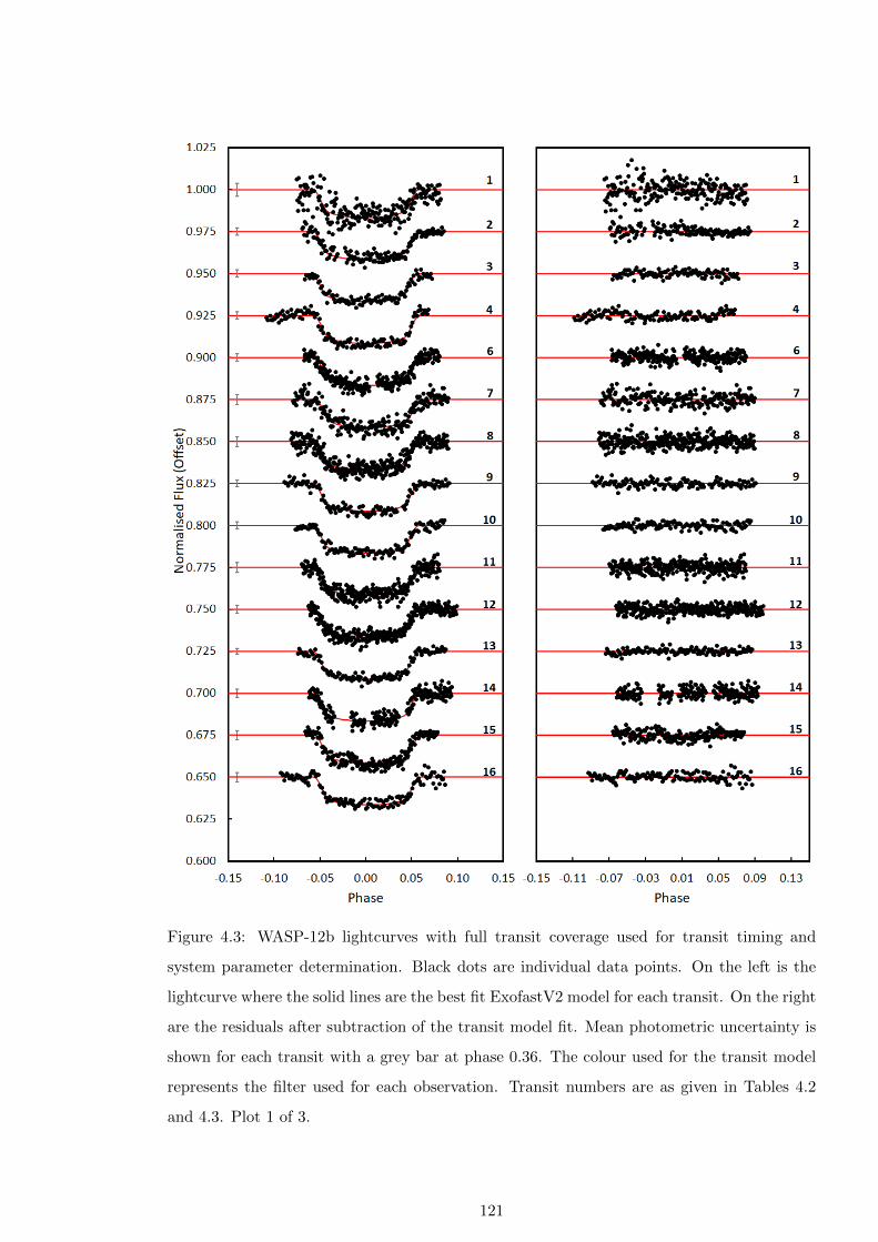
Figure 4.3: WASP-12b lightcurves with full transit coverage used for transit timing and

system parameter determination. Black dots are individual data points. On the left is the

lightcurve where the solid lines are the best fit ExofastV2 model for each transit. On the right

are the residuals after subtraction of the transit model fit. Mean photometric uncertainty is

shown for each transit with a grey bar at phase 0.36. The colour used for the transit model

represents the filter used for each observation. Transit numbers are as given in Tables 4.2

and 4.3. Plot 1 of 3.

121

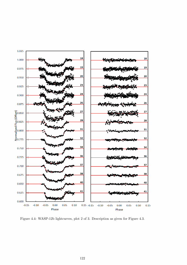
Figure 4.4: WASP-12b lightcurves, plot 2 of 3. Description as given for Figure 4.3.

122

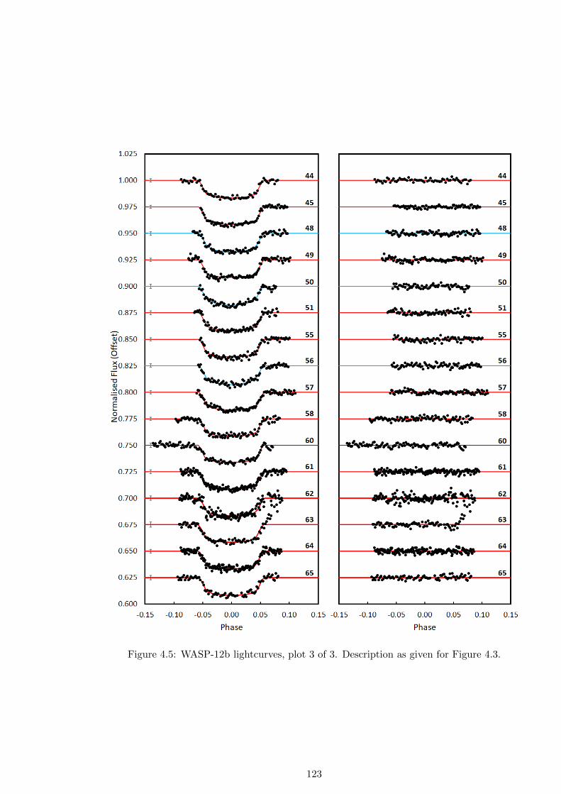
Figure 4.5: WASP-12b lightcurves, plot 3 of 3. Description as given for Figure 4.3.

123

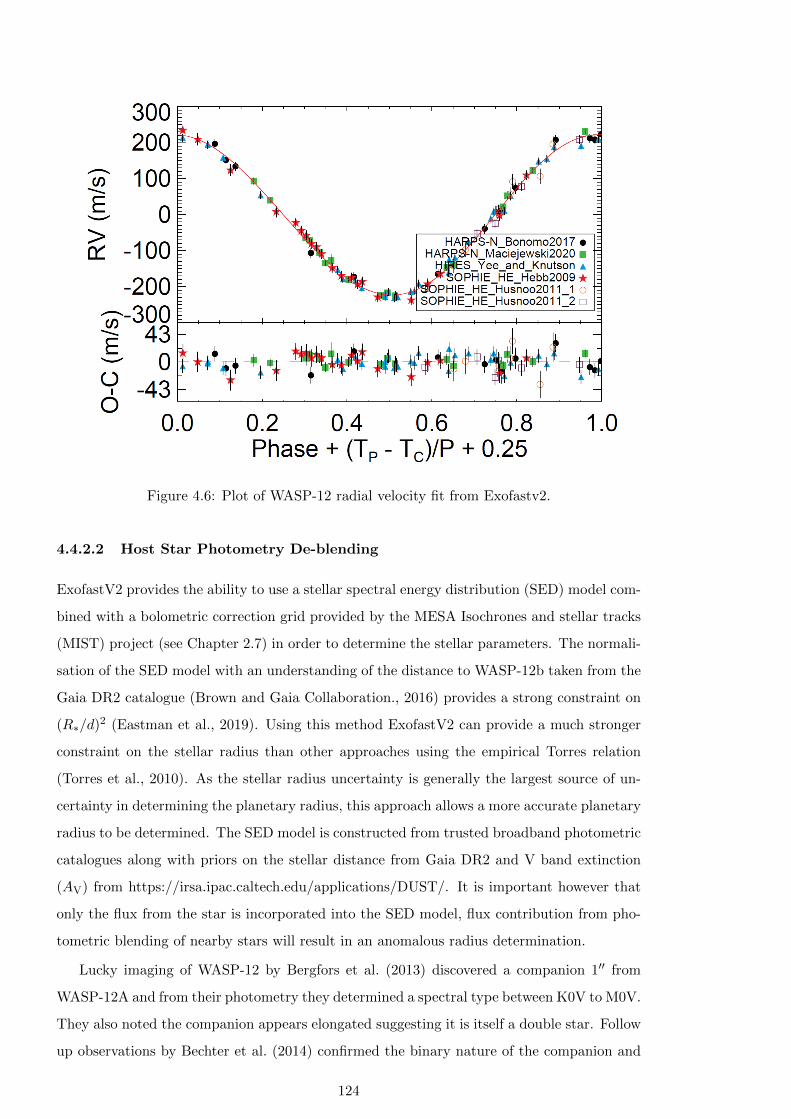
Figure 4.6: Plot of WASP-12 radial velocity fit from Exofastv2.

4.4.2.2 Host Star Photometry De-blending

ExofastV2 provides the ability to use a stellar spectral energy distribution (SED) model com-

bined with a bolometric correction grid provided by the MESA Isochrones and stellar tracks

(MIST) project (see Chapter 2.7) in order to determine the stellar parameters. The normali-

sation of the SED model with an understanding of the distance to WASP-12b taken from the

Gaia DR2 catalogue (Brown and Gaia Collaboration., 2016) provides a strong constraint on

(R∗/d)2 (Eastman et al., 2019). Using this method ExofastV2 can provide a much stronger

constraint on the stellar radius than other approaches using the empirical Torres relation

(Torres et al., 2010). As the stellar radius uncertainty is generally the largest source of un-

certainty in determining the planetary radius, this approach allows a more accurate planetary

radius to be determined. The SED model is constructed from trusted broadband photometric

catalogues along with priors on the stellar distance from Gaia DR2 and V band extinction

(AV) from https://irsa.ipac.caltech.edu/applications/DUST/. It is important however that

only the flux from the star is incorporated into the SED model, flux contribution from pho-

tometric blending of nearby stars will result in an anomalous radius determination.

Lucky imaging of WASP-12 by Bergfors et al. (2013) discovered a companion 1′′ from

WASP-12A and from their photometry they determined a spectral type between K0V to M0V.

They also noted the companion appears elongated suggesting it is itself a double star. Follow

up observations by Bechter et al. (2014) confirmed the binary nature of the companion and

124

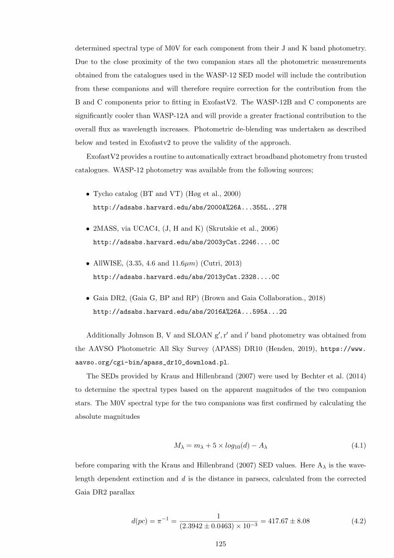
determined spectral type of M0V for each component from their J and K band photometry.

Due to the close proximity of the two companion stars all the photometric measurements

obtained from the catalogues used in the WASP-12 SED model will include the contribution

from these companions and will therefore require correction for the contribution from the

B and C components prior to fitting in ExofastV2. The WASP-12B and C components are

significantly cooler than WASP-12A and will provide a greater fractional contribution to the

overall flux as wavelength increases. Photometric de-blending was undertaken as described

below and tested in Exofastv2 to prove the validity of the approach.

ExofastV2 provides a routine to automatically extract broadband photometry from trusted

catalogues. WASP-12 photometry was available from the following sources;

• Tycho catalog (BT and VT) (Høg et al., 2000)

http://adsabs.harvard.edu/abs/2000A%26A...355L..27H

• 2MASS, via UCAC4, (J, H and K) (Skrutskie et al., 2006)

http://adsabs.harvard.edu/abs/2003yCat.2246....0C

• AllWISE, (3.35, 4.6 and 11.6µm) (Cutri, 2013)

http://adsabs.harvard.edu/abs/2013yCat.2328....0C

• Gaia DR2, (Gaia G, BP and RP) (Brown and Gaia Collaboration., 2018)

http://adsabs.harvard.edu/abs/2016A%26A...595A...2G

Additionally Johnson B, V and SLOAN g′, r′ and i′ band photometry was obtained from

the AAVSO Photometric All Sky Survey (APASS) DR10 (Henden, 2019), https://www.

aavso.org/cgi-bin/apass_dr10_download.pl.

The SEDs provided by Kraus and Hillenbrand (2007) were used by Bechter et al. (2014)

to determine the spectral types based on the apparent magnitudes of the two companion

stars. The M0V spectral type for the two companions was first confirmed by calculating the

absolute magnitudes

Mλ = mλ + 5× log10(d)−Aλ (4.1)

before comparing with the Kraus and Hillenbrand (2007) SED values. Here Aλ is the wave-

length dependent extinction and d is the distance in parsecs, calculated from the corrected

Gaia DR2 parallax

d(pc) = π−1 =1

(2.3942± 0.0463)× 10−3= 417.67± 8.08 (4.2)

125

Figure 4.7: Calculated absolute J and K magnitudes for WASP-12B (Blue) and WASP-12C

(Amber) from the aparent magnitudes reported in Bechter et al. (2014), showing the close

match of each star to the SED for a M0V star. The red crosses indicate the combined SLOAN

i′andz′ observations of the B and C components from Bergfors et al. (2013) who estimated

a spectral type between M0V and K0V, K7V SED is shown for reference. Filled circles are

the magnitudes from Kraus and Hillenbrand (2007) and the open cirlces are the interpolated

values for filter bands used in the SED for WASP-12 not specified by Kraus and Hillenbrand

(2007).

where π is the parallax obtained from Gaia DR2 (Brown and Gaia Collaboration., 2018)

corrected by adding 82µas to the reported value and adding 33µas in quadrature to the

uncertainty following the results of Stassun and Torres (2018).

The extinction value (Aλ) in the same bandpass as the apparent magnitude measure-

ment were obtained from the tables at https://irsa.ipac.caltech.edu/workspace/TMP_

8OTzpo_5751/DUST/WASP-12.v0002/extinction.html. The resulting absolute magnitudes

in J and KS are shown in Figure 4.7 along with the SED for a M0V star (Kraus and Hillen-

brand, 2007).

The SEDs provided by Kraus and Hillenbrand (2007) include discrete magnitude values

in the u′, g′, r′, i′, z′, J, H and KS bands. To obtain values for the B, V GaiaG, GaiaBP

and GaiaRP bands the SEDs were interpolated using the published mid filter wavelength.

For the very broad Gaia bandpasses this was taken as the FWHM mid point for each of the

126

three filters. It was not possible to extend the corrections to the WISE IR bandpasses as

the Kraus and Hillenbrand (2007) SEDs do not extend beyond K band. No other suitable

published SEDs extending into this region are available.

This provided absolute magnitudes for an M0V star in the same filter bandpasses available

for the WASP-12 SED. The apparent magnitudes were calculated in each filter by reversing

Equation 4.2. The final de-blending step was to subtract the contribution of the two M0V

companion stars from the WASP-12 flux for each filter,

mAcorrλ = −2.512× log10(10−0.4mAλ − 10−0.4mBλ − 10−0.4mCλ) (4.3)

where mAcorrλ is the de-blended apparent magnitude for each filter. The original catalogue

and resulting de-blended photometry are shown in Table 4.8.

Table 4.8: De-blended photometry results. The catalogue values shown for WASP-12A are

the values taken from the on-line catalogues listed. The de-blended values are the apparent

magnitudes after correction.

Band WASP-12A Catalogue WASP-12A De-blended Source Catalogue

B(T) 12.259± 0.207 12.32± 0.21 Tycho

V(T) 11.635± 0.160 11.70± 0.16 Tycho

B 12.192± 0.043 12.25± 0.04 APASS R10

V 11.607± 0.049 11.67± 0.05 APASS R10

gSDSS 11.878± 0.053 11.94± 0.05 APASS R10

rSDSS 11.427± 0.04 11.49± 0.04 APASS R10

iSDSS 11.332± 0.06 11.41± 0.06 APASS R10

J 10.477± 0.02 10.595± 0.02 2MASS(via UCAC4)

H 10.228± 0.02 10.383± 0.02 2MASS(via UCAC4)

K 10.188± 0.02 10.363± 0.02 2MASS(via UCAC4)

WISE1 10.111+0.03−0.022 - AllWISE

WISE2 10.109+0.03−0.021 - AllWISE

WISE3 10.121± 0.073 - AllWISE

GaiaG 11.500+0.02−0.001 11.58± 0.020 Gaia DR2

GaiaBP 11.804+0.02−0.003 11.88± 0.020 Gaia DR2

GaiaRP 11.036+0.02−0.003 11.12± 0.020 Gaia DR2

127

4.4.2.3 Testing the De-blended Photometry

To test the effect of using the de-blended photometry to calculate a SED in ExofastV2 models

for the WASP-12 system a number of tests were run. The tests used all the RV data obtained

from the literature as detailed in Section 4.4.2.1 along with three full transit light curves, one

from each telescope, all obtained using an Rc filter. Three lightcurves were used to provide

a test between the different models without needing the multi-day time to run as is required

when modelling with all 47 transits. The ExofastV2 tests made were;

1. Using the original catalogue photometry as shown in Table 4.8.

2. Using the original catalogue photometry as shown in Table 4.8, but excluding the WISE

photometry.

3. Using the de-blended photometry which excludes the WISE photometry.

4. Using the empirical Torres relationship which does not use the broadband photometry

SED or priors on extinction and parallax.

The aim of the second test was to determine whether there was any effect on the results

from removing the WISE photometry. The fourth test, using a different method to determine

the system parameters, was run as a control test. The results from the tests for key system

parameters are plotted in Figure 4.8.

In all cases the transit depth is deeper than the values recorded in the NASA Exoplanet

Archive, the difference being 5σ or greater. This results in a larger scaled system parameter

RP /R∗ than seen in the archive. It is noted that there is a 25-fold spread for the uncertainty

values reported in the NASA Exoplanet Archive for RP /R∗. Ozturk and Erdem (2019) report

the largest value of 0.119±0.004 while the smallest value reported is 0.1119±0.0002, (Albrecht

et al., 2012). The first two tests using the catalogue photometric values with and without the

mid-IR photometry from WISE agree with each other within the calculated uncertainties.

Without the WISE photometry ExofastV2 calculates a stellar radius 2% smaller than when

the WISE photometry is included.

The de-blended photometry results in R∗ smaller than both the original photometry and

the archive values, by 3% in the latter case. RP is in close agreement with the mean literature

value. The results from the de-blended photometry and the model test just using the Torres

relationship are in closer agreement than the results using the original photometry. Results

using the Torres relationship generally show larger uncertainties. Distance determined using

the de-blended photometry matches that calculated from the Gaia DR2 parallax. σ SED is

the amount the photometric uncertainties have to be multiplied by to remain consistent with

128

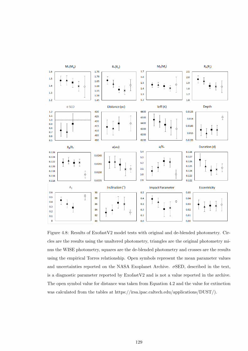
Figure 4.8: Results of ExofastV2 model tests with original and de-blended photometry. Cir-

cles are the results using the unaltered photometry, triangles are the original photometry mi-

nus the WISE photometry, squares are the de-blended photometry and crosses are the results

using the empirical Torres relationship. Open symbols represent the mean parameter values

and uncertainties reported on the NASA Exoplanet Archive. σSED, described in the text,

is a diagnostic parameter reported by ExofastV2 and is not a value reported in the archive.

The open symbol value for distance was taken from Equation 4.2 and the value for extinction

was calculated from the tables at https://irsa.ipac.caltech.edu/applications/DUST/).

129

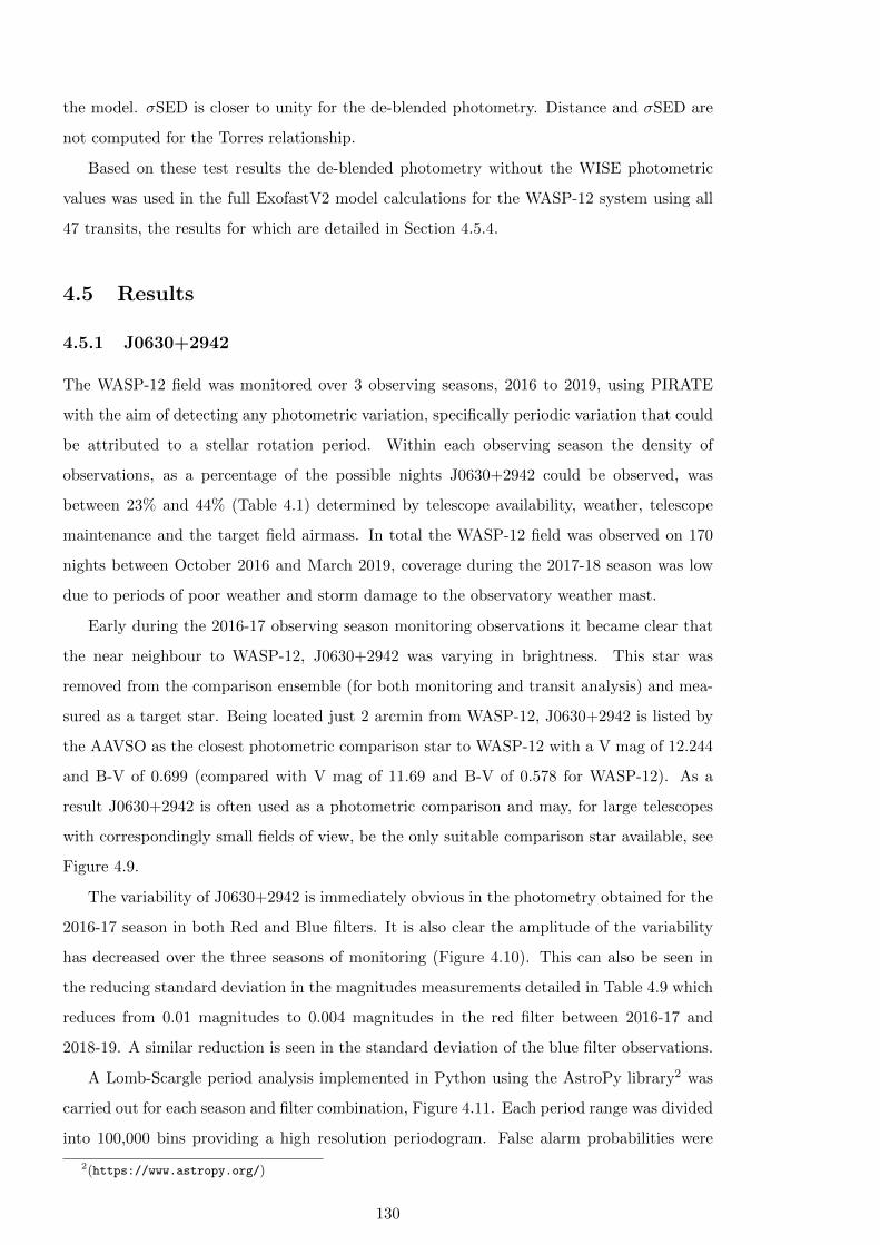
the model. σSED is closer to unity for the de-blended photometry. Distance and σSED are

not computed for the Torres relationship.

Based on these test results the de-blended photometry without the WISE photometric

values was used in the full ExofastV2 model calculations for the WASP-12 system using all

47 transits, the results for which are detailed in Section 4.5.4.

4.5 Results

4.5.1 J0630+2942

The WASP-12 field was monitored over 3 observing seasons, 2016 to 2019, using PIRATE

with the aim of detecting any photometric variation, specifically periodic variation that could

be attributed to a stellar rotation period. Within each observing season the density of

observations, as a percentage of the possible nights J0630+2942 could be observed, was

between 23% and 44% (Table 4.1) determined by telescope availability, weather, telescope

maintenance and the target field airmass. In total the WASP-12 field was observed on 170

nights between October 2016 and March 2019, coverage during the 2017-18 season was low

due to periods of poor weather and storm damage to the observatory weather mast.

Early during the 2016-17 observing season monitoring observations it became clear that

the near neighbour to WASP-12, J0630+2942 was varying in brightness. This star was

removed from the comparison ensemble (for both monitoring and transit analysis) and mea-

sured as a target star. Being located just 2 arcmin from WASP-12, J0630+2942 is listed by

the AAVSO as the closest photometric comparison star to WASP-12 with a V mag of 12.244

and B-V of 0.699 (compared with V mag of 11.69 and B-V of 0.578 for WASP-12). As a

result J0630+2942 is often used as a photometric comparison and may, for large telescopes

with correspondingly small fields of view, be the only suitable comparison star available, see

Figure 4.9.

The variability of J0630+2942 is immediately obvious in the photometry obtained for the

2016-17 season in both Red and Blue filters. It is also clear the amplitude of the variability

has decreased over the three seasons of monitoring (Figure 4.10). This can also be seen in

the reducing standard deviation in the magnitudes measurements detailed in Table 4.9 which

reduces from 0.01 magnitudes to 0.004 magnitudes in the red filter between 2016-17 and

2018-19. A similar reduction is seen in the standard deviation of the blue filter observations.

A Lomb-Scargle period analysis implemented in Python using the AstroPy library2 was

carried out for each season and filter combination, Figure 4.11. Each period range was divided

into 100,000 bins providing a high resolution periodogram. False alarm probabilities were

2(https://www.astropy.org/)

130

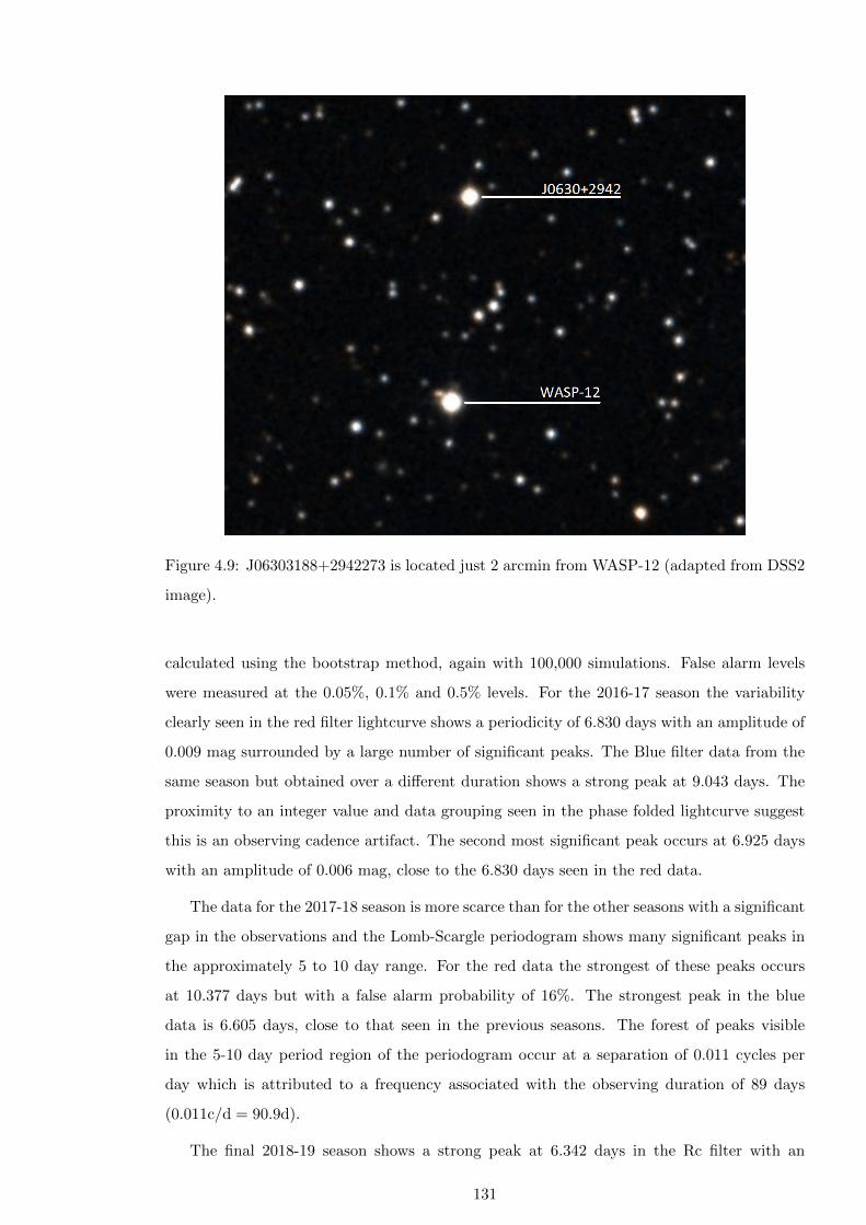
Figure 4.9: J06303188+2942273 is located just 2 arcmin from WASP-12 (adapted from DSS2

image).

calculated using the bootstrap method, again with 100,000 simulations. False alarm levels

were measured at the 0.05%, 0.1% and 0.5% levels. For the 2016-17 season the variability

clearly seen in the red filter lightcurve shows a periodicity of 6.830 days with an amplitude of

0.009 mag surrounded by a large number of significant peaks. The Blue filter data from the

same season but obtained over a different duration shows a strong peak at 9.043 days. The

proximity to an integer value and data grouping seen in the phase folded lightcurve suggest

this is an observing cadence artifact. The second most significant peak occurs at 6.925 days

with an amplitude of 0.006 mag, close to the 6.830 days seen in the red data.

The data for the 2017-18 season is more scarce than for the other seasons with a significant

gap in the observations and the Lomb-Scargle periodogram shows many significant peaks in

the approximately 5 to 10 day range. For the red data the strongest of these peaks occurs

at 10.377 days but with a false alarm probability of 16%. The strongest peak in the blue

data is 6.605 days, close to that seen in the previous seasons. The forest of peaks visible

in the 5-10 day period region of the periodogram occur at a separation of 0.011 cycles per

day which is attributed to a frequency associated with the observing duration of 89 days

(0.011c/d = 90.9d).

The final 2018-19 season shows a strong peak at 6.342 days in the Rc filter with an

131

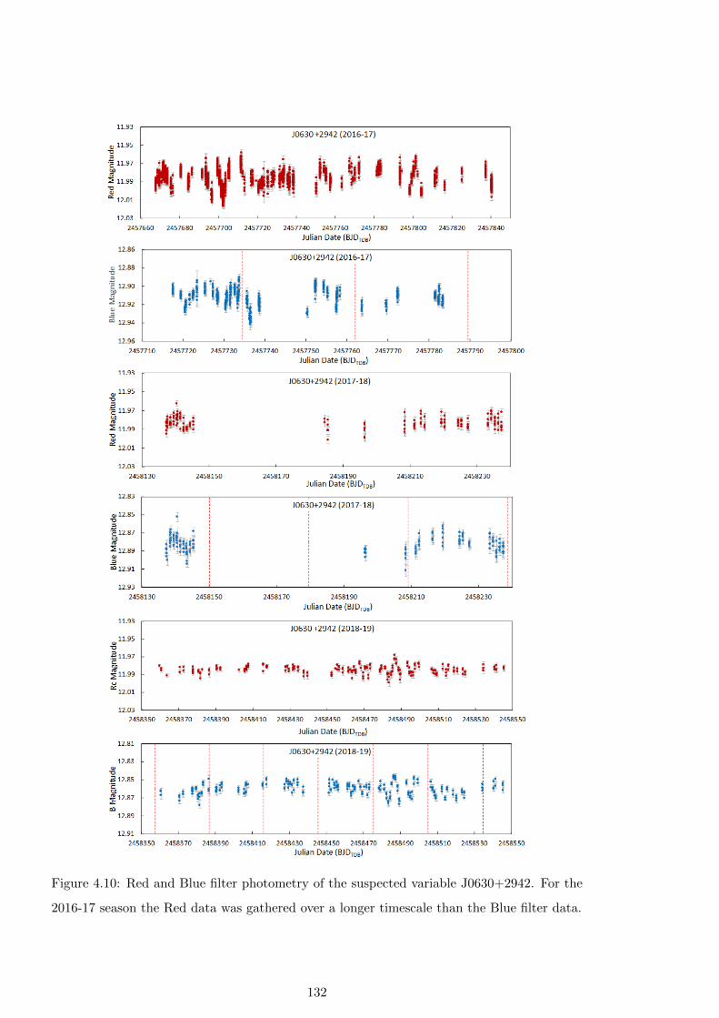
Figure 4.10: Red and Blue filter photometry of the suspected variable J0630+2942. For the

2016-17 season the Red data was gathered over a longer timescale than the Blue filter data.

132

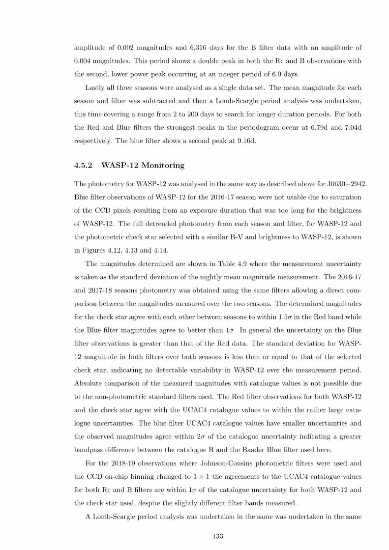
amplitude of 0.002 magnitudes and 6.316 days for the B filter data with an amplitude of

0.004 magnitudes. This period shows a double peak in both the Rc and B observations with

the second, lower power peak occurring at an integer period of 6.0 days.

Lastly all three seasons were analysed as a single data set. The mean magnitude for each

season and filter was subtracted and then a Lomb-Scargle period analysis was undertaken,

this time covering a range from 2 to 200 days to search for longer duration periods. For both

the Red and Blue filters the strongest peaks in the periodogram occur at 6.79d and 7.04d

respectively. The blue filter shows a second peak at 9.16d.

4.5.2 WASP-12 Monitoring

The photometry for WASP-12 was analysed in the same way as described above for J0630+2942.

Blue filter observations of WASP-12 for the 2016-17 season were not usable due to saturation

of the CCD pixels resulting from an exposure duration that was too long for the brightness

of WASP-12. The full detrended photometry from each season and filter, for WASP-12 and

the photometric check star selected with a similar B-V and brightness to WASP-12, is shown

in Figures 4.12, 4.13 and 4.14.

The magnitudes determined are shown in Table 4.9 where the measurement uncertainty

is taken as the standard deviation of the nightly mean magnitude measurement. The 2016-17

and 2017-18 seasons photometry was obtained using the same filters allowing a direct com-

parison between the magnitudes measured over the two seasons. The determined magnitudes

for the check star agree with each other between seasons to within 1.5σ in the Red band while

the Blue filter magnitudes agree to better than 1σ. In general the uncertainty on the Blue

filter observations is greater than that of the Red data. The standard deviation for WASP-

12 magnitude in both filters over both seasons is less than or equal to that of the selected

check star, indicating no detectable variability in WASP-12 over the measurement period.

Absolute comparison of the measured magnitudes with catalogue values is not possible due

to the non-photometric standard filters used. The Red filter observations for both WASP-12

and the check star agree with the UCAC4 catalogue values to within the rather large cata-

logue uncertainties. The blue filter UCAC4 catalogue values have smaller uncertainties and

the observed magnitudes agree within 2σ of the catalogue uncertainty indicating a greater

bandpass difference between the catalogue B and the Baader Blue filter used here.

For the 2018-19 observations where Johnson-Cousins photometric filters were used and

the CCD on-chip binning changed to 1 × 1 the agreements to the UCAC4 catalogue values

for both Rc and B filters are within 1σ of the catalogue uncertainty for both WASP-12 and

the check star used, despite the slightly different filter bands measured.

A Lomb-Scargle period analysis was undertaken in the same was undertaken in the same

133

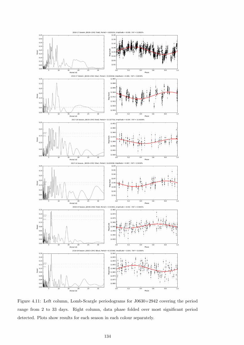
Figure 4.11: Left column, Lomb-Scargle periodograms for J0630+2942 covering the period

range from 2 to 33 days. Right column, data phase folded over most significant period

detected. Plots show results for each season in each colour separately.

134

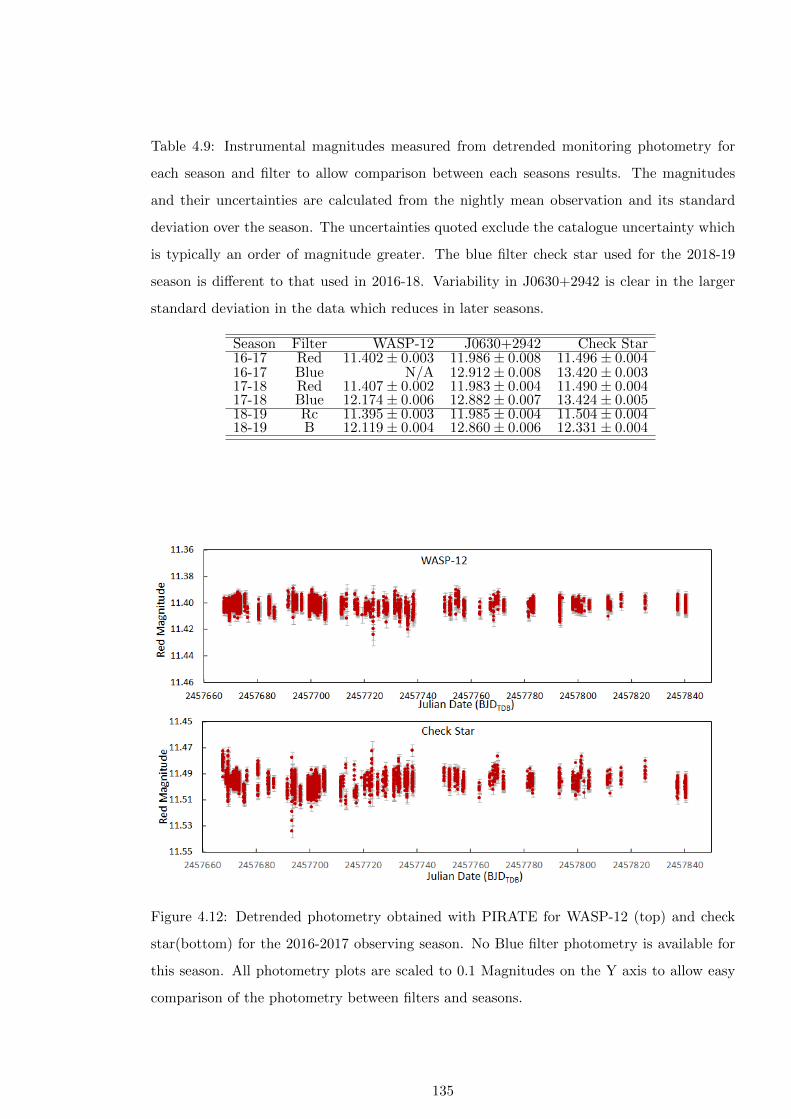
Table 4.9: Instrumental magnitudes measured from detrended monitoring photometry for

each season and filter to allow comparison between each seasons results. The magnitudes

and their uncertainties are calculated from the nightly mean observation and its standard

deviation over the season. The uncertainties quoted exclude the catalogue uncertainty which

is typically an order of magnitude greater. The blue filter check star used for the 2018-19

season is different to that used in 2016-18. Variability in J0630+2942 is clear in the larger

standard deviation in the data which reduces in later seasons.

Season Filter WASP-12 J0630+2942 Check Star16-17 Red 11.402± 0.003 11.986± 0.008 11.496± 0.00416-17 Blue N/A 12.912± 0.008 13.420± 0.00317-18 Red 11.407± 0.002 11.983± 0.004 11.490± 0.00417-18 Blue 12.174± 0.006 12.882± 0.007 13.424± 0.00518-19 Rc 11.395± 0.003 11.985± 0.004 11.504± 0.00418-19 B 12.119± 0.004 12.860± 0.006 12.331± 0.004

Figure 4.12: Detrended photometry obtained with PIRATE for WASP-12 (top) and check

star(bottom) for the 2016-2017 observing season. No Blue filter photometry is available for

this season. All photometry plots are scaled to 0.1 Magnitudes on the Y axis to allow easy

comparison of the photometry between filters and seasons.

135

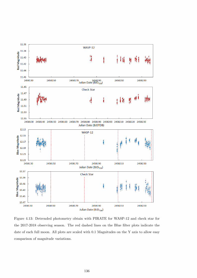
Figure 4.13: Detrended photometry obtain with PIRATE for WASP-12 and check star for

the 2017-2018 observing season. The red dashed lines on the Blue filter plots indicate the

date of each full moon. All plots are scaled with 0.1 Magnitudes on the Y axis to allow easy

comparison of magnitude variations.

136

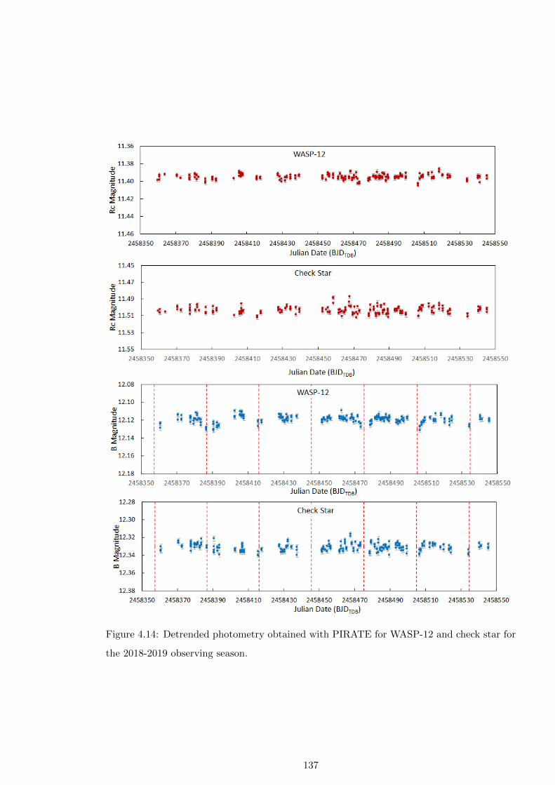
Figure 4.14: Detrended photometry obtained with PIRATE for WASP-12 and check star for

the 2018-2019 observing season.

137

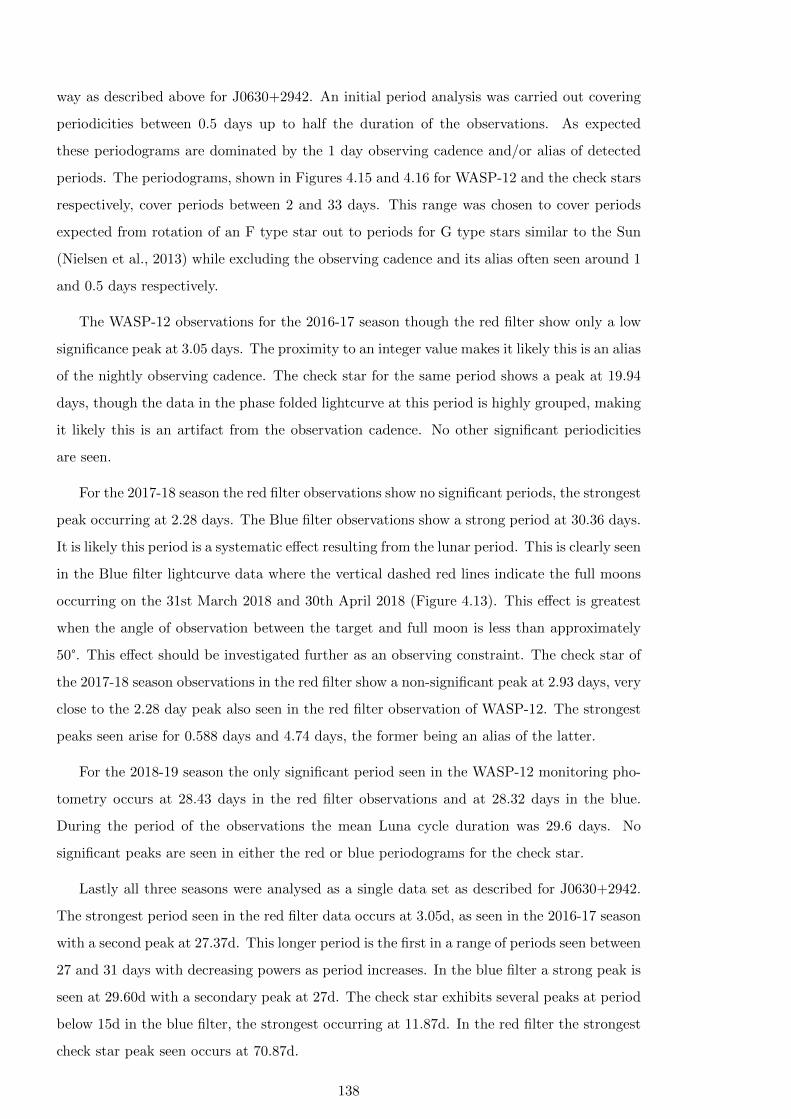
way as described above for J0630+2942. An initial period analysis was carried out covering

periodicities between 0.5 days up to half the duration of the observations. As expected

these periodograms are dominated by the 1 day observing cadence and/or alias of detected

periods. The periodograms, shown in Figures 4.15 and 4.16 for WASP-12 and the check stars

respectively, cover periods between 2 and 33 days. This range was chosen to cover periods

expected from rotation of an F type star out to periods for G type stars similar to the Sun

(Nielsen et al., 2013) while excluding the observing cadence and its alias often seen around 1

and 0.5 days respectively.

The WASP-12 observations for the 2016-17 season though the red filter show only a low

significance peak at 3.05 days. The proximity to an integer value makes it likely this is an alias

of the nightly observing cadence. The check star for the same period shows a peak at 19.94

days, though the data in the phase folded lightcurve at this period is highly grouped, making

it likely this is an artifact from the observation cadence. No other significant periodicities

are seen.

For the 2017-18 season the red filter observations show no significant periods, the strongest

peak occurring at 2.28 days. The Blue filter observations show a strong period at 30.36 days.

It is likely this period is a systematic effect resulting from the lunar period. This is clearly seen

in the Blue filter lightcurve data where the vertical dashed red lines indicate the full moons

occurring on the 31st March 2018 and 30th April 2018 (Figure 4.13). This effect is greatest

when the angle of observation between the target and full moon is less than approximately

50°. This effect should be investigated further as an observing constraint. The check star of

the 2017-18 season observations in the red filter show a non-significant peak at 2.93 days, very

close to the 2.28 day peak also seen in the red filter observation of WASP-12. The strongest

peaks seen arise for 0.588 days and 4.74 days, the former being an alias of the latter.

For the 2018-19 season the only significant period seen in the WASP-12 monitoring pho-

tometry occurs at 28.43 days in the red filter observations and at 28.32 days in the blue.

During the period of the observations the mean Luna cycle duration was 29.6 days. No

significant peaks are seen in either the red or blue periodograms for the check star.

Lastly all three seasons were analysed as a single data set as described for J0630+2942.

The strongest period seen in the red filter data occurs at 3.05d, as seen in the 2016-17 season

with a second peak at 27.37d. This longer period is the first in a range of periods seen between

27 and 31 days with decreasing powers as period increases. In the blue filter a strong peak is

seen at 29.60d with a secondary peak at 27d. The check star exhibits several peaks at period

below 15d in the blue filter, the strongest occurring at 11.87d. In the red filter the strongest

check star peak seen occurs at 70.87d.

138

Figure 4.15: Left column, Lomb-Scargle periodograms for WASP-12 covering the period range

from 2 to 33 days. Right column, data phase folded over most significant period detected.

Plots show results for each season in each colour separately.

139

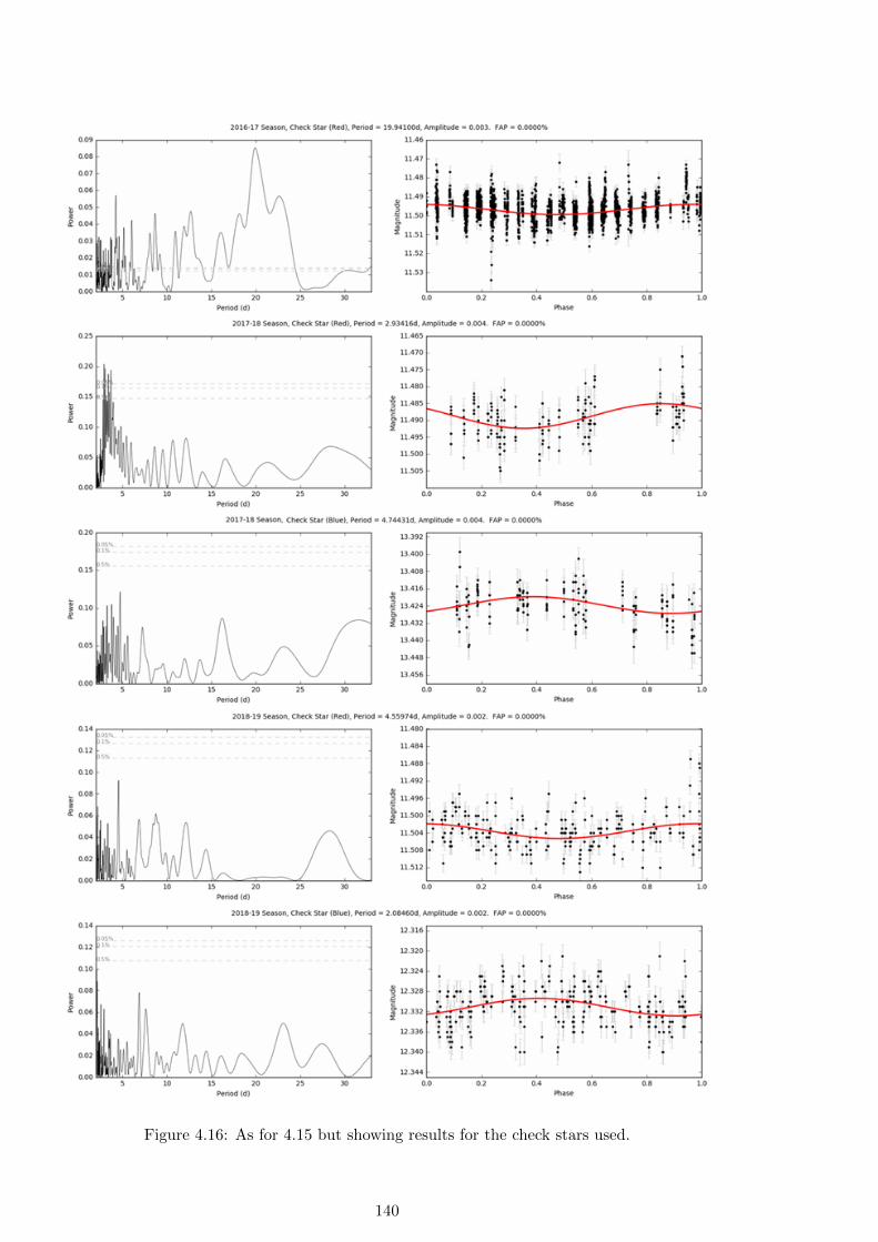
Figure 4.16: As for 4.15 but showing results for the check stars used.

140

4.5.3 WASP-12b Transit Timing

Before undertaking an ephemeris fit to the newly obtained transit times a test fit was carried

out using the transit times published by Yee et al. (2019) to ensure the published results could

be reproduced. All 139 published primary transit times were used with the linear ephemeris

value published by Yee et al. (2019) as the starting value. The fit converged to values that

are in excellent agreement, well within the uncertainties on both the new and published

ephemerides, Table 4.10. The newly calculated ephemeris has slightly larger uncertainties

than those published by Yee et al. (2019).

The following data sets were modeled independently to understand the impact of various

data inputs on the derived ephemeris and to inform the optimum approach to integrating

the new observations with those within Yee et al. (2019), hereafter Y19. The results of the

ephemeris calculations are summarised in Table 4.10 and Figure 4.18.

4.5.3.1 All 47 new transit time observations only.

The new data set consists of 47 transit observations covering seven seasons from 2013 to 2020.

Coverage was greatest in the 2016-17, 2017-18 and 2018-19 seasons with only 10 observations

available for the other four seasons. The four data points covering the first three seasons

were exclusively from the POST observatory. The starting epoch, period and P for the

quadratic ephemeris obtained are compared with the results from Y19 in Figure 4.18, left.

The calculated epoch agrees with Y19 within 42 seconds but the quadratic period found is

1.15× 10−6d greater and the value found for P is almost twice the value determined by Y19.

Using this data set it is not possible differentiate between a linear or quadratic ephemeris

with χ2ν = 3.1 for the linear and χ2

ν = 3.2 for the quadratic ephemerides. The uncertainties

on the determined quadratic epoch and period are approximately 25 times greater than found

from modelling just the Y19 data set while the P uncertainty is 10 times greater.

4.5.3.2 All 47 new transit times integrated with those from Y19.

The two data sets of 139 measurement from Y19 and the 47 new measurements were combined

to a single data set. The new data overlaps with seasonal observations in the Y19 data set

except for the 2019-20 season not covered in the Y19 data. The result confirms a strong

preference for a quadratic ephemeris (χ2ν = 1.60, BIC = 99.93) over a linear ephemeris (χ2

ν

= 3.10, BIC = 217.84). The result confirm the findings of Y19 with the same or improved

uncertainties. Although the uncertainties on the ephemeris are reduced the newly determined

χ2ν values are approximately 60% greater than found by Y19. For seasons with more than a

single measurement, the mean seasonal scatter in timing measurements divided by the mean

141

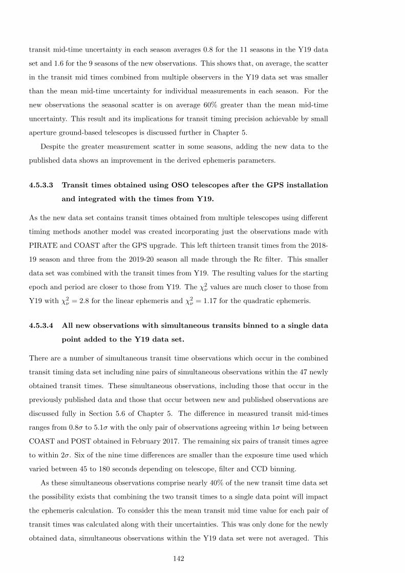
transit mid-time uncertainty in each season averages 0.8 for the 11 seasons in the Y19 data

set and 1.6 for the 9 seasons of the new observations. This shows that, on average, the scatter

in the transit mid times combined from multiple observers in the Y19 data set was smaller

than the mean mid-time uncertainty for individual measurements in each season. For the

new observations the seasonal scatter is on average 60% greater than the mean mid-time

uncertainty. This result and its implications for transit timing precision achievable by small

aperture ground-based telescopes is discussed further in Chapter 5.

Despite the greater measurement scatter in some seasons, adding the new data to the

published data shows an improvement in the derived ephemeris parameters.

4.5.3.3 Transit times obtained using OSO telescopes after the GPS installation

and integrated with the times from Y19.

As the new data set contains transit times obtained from multiple telescopes using different

timing methods another model was created incorporating just the observations made with

PIRATE and COAST after the GPS upgrade. This left thirteen transit times from the 2018-

19 season and three from the 2019-20 season all made through the Rc filter. This smaller

data set was combined with the transit times from Y19. The resulting values for the starting

epoch and period are closer to those from Y19. The χ2ν values are much closer to those from

Y19 with χ2ν = 2.8 for the linear ephemeris and χ2

ν = 1.17 for the quadratic ephemeris.

4.5.3.4 All new observations with simultaneous transits binned to a single data

point added to the Y19 data set.

There are a number of simultaneous transit time observations which occur in the combined

transit timing data set including nine pairs of simultaneous observations within the 47 newly

obtained transit times. These simultaneous observations, including those that occur in the

previously published data and those that occur between new and published observations are

discussed fully in Section 5.6 of Chapter 5. The difference in measured transit mid-times

ranges from 0.8σ to 5.1σ with the only pair of observations agreeing within 1σ being between

COAST and POST obtained in February 2017. The remaining six pairs of transit times agree

to within 2σ. Six of the nine time differences are smaller than the exposure time used which

varied between 45 to 180 seconds depending on telescope, filter and CCD binning.

As these simultaneous observations comprise nearly 40% of the new transit time data set

the possibility exists that combining the two transit times to a single data point will impact

the ephemeris calculation. To consider this the mean transit mid time value for each pair of

transit times was calculated along with their uncertainties. This was only done for the newly

obtained data, simultaneous observations within the Y19 data set were not averaged. This

142

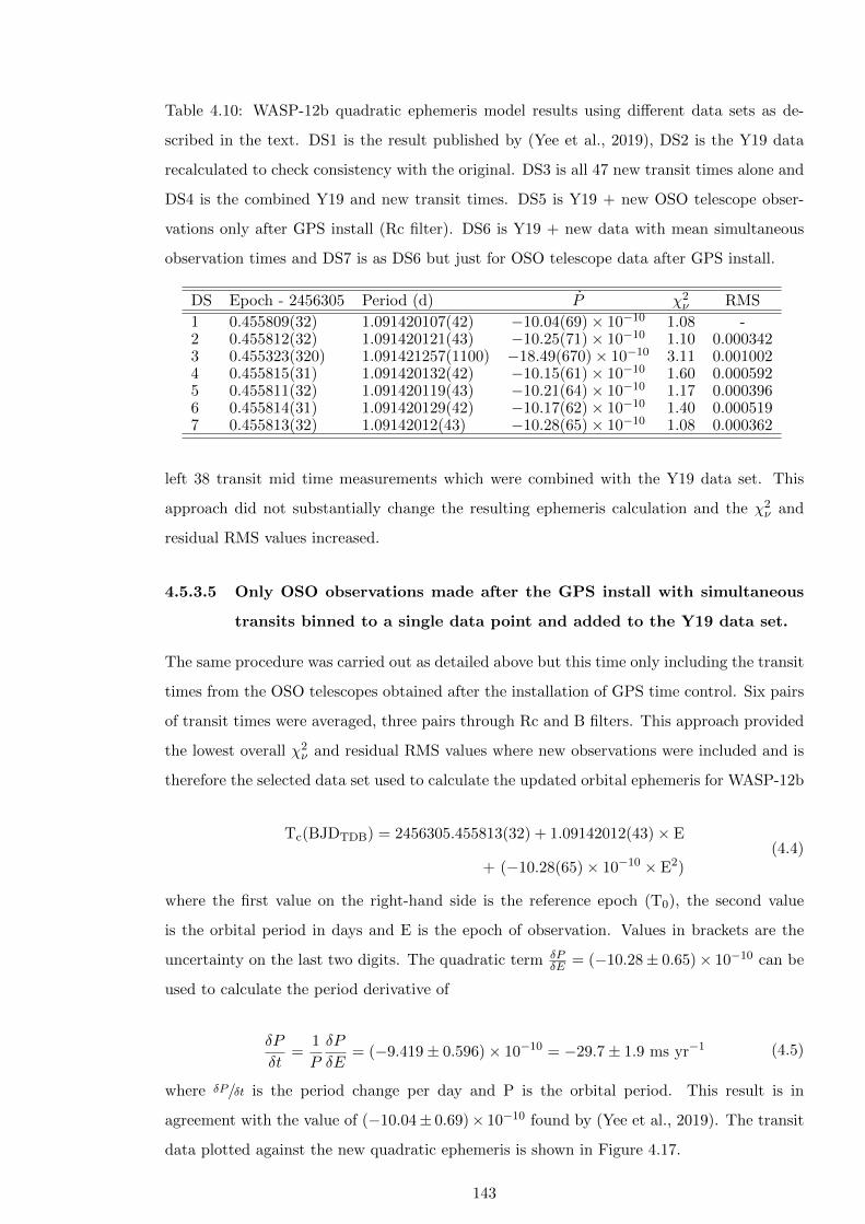
Table 4.10: WASP-12b quadratic ephemeris model results using different data sets as de-

scribed in the text. DS1 is the result published by (Yee et al., 2019), DS2 is the Y19 data

recalculated to check consistency with the original. DS3 is all 47 new transit times alone and

DS4 is the combined Y19 and new transit times. DS5 is Y19 + new OSO telescope obser-

vations only after GPS install (Rc filter). DS6 is Y19 + new data with mean simultaneous

observation times and DS7 is as DS6 but just for OSO telescope data after GPS install.

DS Epoch - 2456305 Period (d) P χ2ν RMS

1 0.455809(32) 1.091420107(42) −10.04(69)× 10−10 1.08 -2 0.455812(32) 1.091420121(43) −10.25(71)× 10−10 1.10 0.0003423 0.455323(320) 1.091421257(1100) −18.49(670)× 10−10 3.11 0.0010024 0.455815(31) 1.091420132(42) −10.15(61)× 10−10 1.60 0.0005925 0.455811(32) 1.091420119(43) −10.21(64)× 10−10 1.17 0.0003966 0.455814(31) 1.091420129(42) −10.17(62)× 10−10 1.40 0.0005197 0.455813(32) 1.09142012(43) −10.28(65)× 10−10 1.08 0.000362

left 38 transit mid time measurements which were combined with the Y19 data set. This

approach did not substantially change the resulting ephemeris calculation and the χ2ν and

residual RMS values increased.

4.5.3.5 Only OSO observations made after the GPS install with simultaneous

transits binned to a single data point and added to the Y19 data set.

The same procedure was carried out as detailed above but this time only including the transit

times from the OSO telescopes obtained after the installation of GPS time control. Six pairs

of transit times were averaged, three pairs through Rc and B filters. This approach provided

the lowest overall χ2ν and residual RMS values where new observations were included and is

therefore the selected data set used to calculate the updated orbital ephemeris for WASP-12b

Tc(BJDTDB) = 2456305.455813(32) + 1.09142012(43)× E

+ (−10.28(65)× 10−10 × E2)(4.4)

where the first value on the right-hand side is the reference epoch (T0), the second value

is the orbital period in days and E is the epoch of observation. Values in brackets are the

uncertainty on the last two digits. The quadratic term δPδE = (−10.28± 0.65)× 10−10 can be

used to calculate the period derivative of

δP

δt=

1

P

δP

δE= (−9.419± 0.596)× 10−10 = −29.7± 1.9 ms yr−1 (4.5)

where δP/δt is the period change per day and P is the orbital period. This result is in

agreement with the value of (−10.04± 0.69)× 10−10 found by (Yee et al., 2019). The transit

data plotted against the new quadratic ephemeris is shown in Figure 4.17.

143

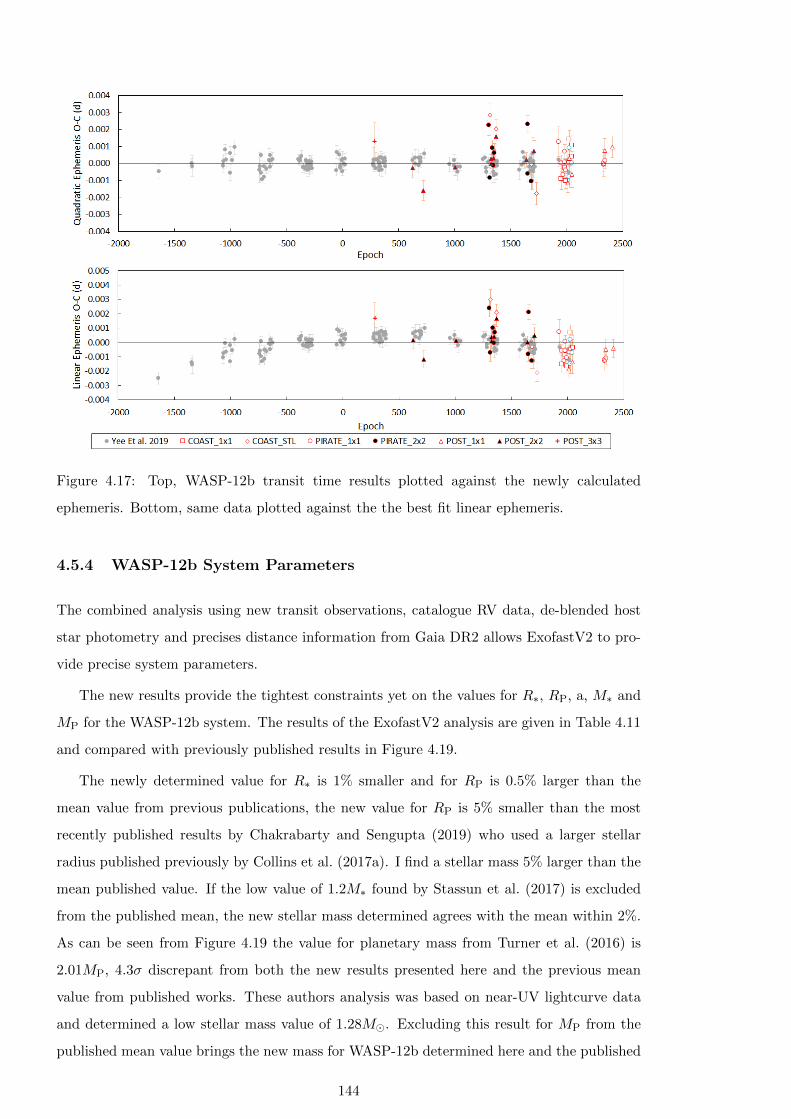
Figure 4.17: Top, WASP-12b transit time results plotted against the newly calculated

ephemeris. Bottom, same data plotted against the the best fit linear ephemeris.

4.5.4 WASP-12b System Parameters

The combined analysis using new transit observations, catalogue RV data, de-blended host

star photometry and precises distance information from Gaia DR2 allows ExofastV2 to pro-

vide precise system parameters.

The new results provide the tightest constraints yet on the values for R∗, RP, a, M∗ and

MP for the WASP-12b system. The results of the ExofastV2 analysis are given in Table 4.11

and compared with previously published results in Figure 4.19.

The newly determined value for R∗ is 1% smaller and for RP is 0.5% larger than the

mean value from previous publications, the new value for RP is 5% smaller than the most

recently published results by Chakrabarty and Sengupta (2019) who used a larger stellar

radius published previously by Collins et al. (2017a). I find a stellar mass 5% larger than the

mean published value. If the low value of 1.2M∗ found by Stassun et al. (2017) is excluded

from the published mean, the new stellar mass determined agrees with the mean within 2%.

As can be seen from Figure 4.19 the value for planetary mass from Turner et al. (2016) is

2.01MP, 4.3σ discrepant from both the new results presented here and the previous mean

value from published works. These authors analysis was based on near-UV lightcurve data

and determined a low stellar mass value of 1.28M�. Excluding this result for MP from the

published mean value brings the new mass for WASP-12b determined here and the published

144

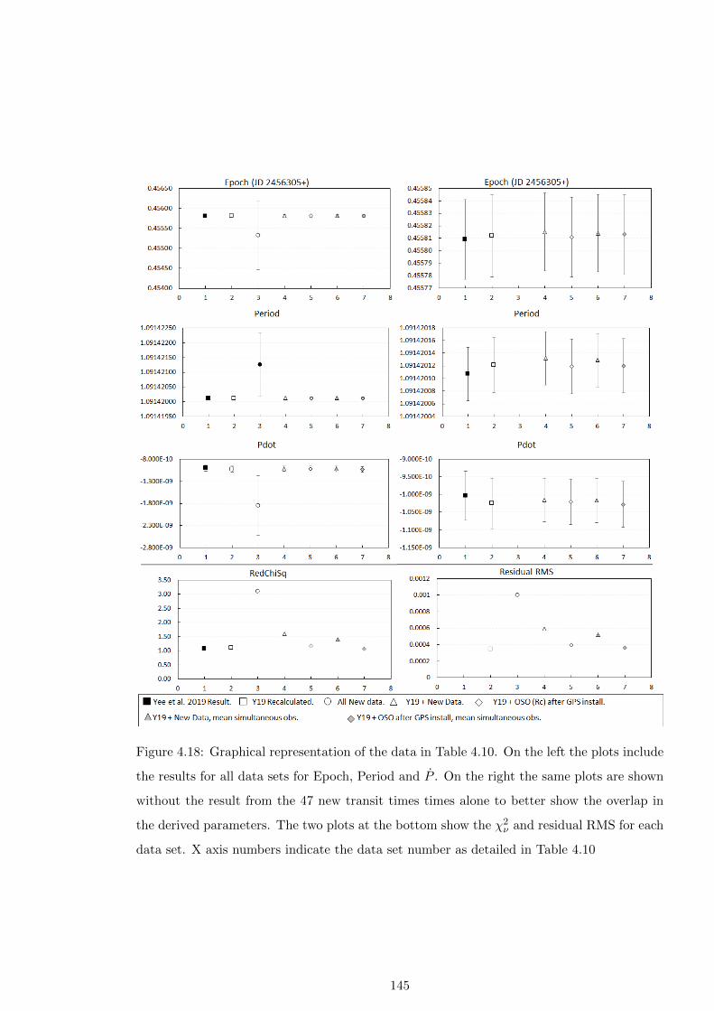
Figure 4.18: Graphical representation of the data in Table 4.10. On the left the plots include

the results for all data sets for Epoch, Period and P . On the right the same plots are shown

without the result from the 47 new transit times times alone to better show the overlap in

the derived parameters. The two plots at the bottom show the χ2ν and residual RMS for each

data set. X axis numbers indicate the data set number as detailed in Table 4.10

145

mean value into almost perfect agreement.

Although the new results are in excellent general agreement with the range of values

previously found the precise measurements mean that the differences are significant. This

is apparent in the new value for the scaled system parameter a/R∗ which is found to be

3.2σ greater than the mean value of the previously published results. Orbital inclination is

2.7σ larger and transit depth is 6.0σ greater. The results provide a smaller value for orbital

eccentricity of 0.028+0.008−0.009, a 3σ detection which is smaller than the most recently published

value of 0.035±0.006 (Maciejewski et al., 2020) while the determined argument of periastron,

ω = 265°±9° is in excellent agreement with their result (270.7°±0.6°). The tidal circularistion

timescale of 0.36Myr is significantly less than the derived age of 1.76Gyr. The distance to

WASP-12b was calculated as 419.3+7.3−7.1pc in agreement with the value calculated in Eq. 4.2

but with slightly smaller uncertainty.

4.6 Discussion

4.6.1 J0630+2942

The close companion star to WASP-12, J6030+2942, is variable. The period was seen to

change from 6.83 days in 2016/17 to 6.34 days in 2018/19, at the same time the amplitude

of the photometric variation decreased from 0.01 mag to 0.004 mag. If the photometric

variation is due to spots and therefore following the (differential) stellar surface rotation then

the changing period would be due to spots at different latitudes while the change in amplitude

would indicate smaller or less dark spots. It is therefore possible that J0630+2942 is in a

phase of its stellar cycle declining towards minimum activity. This would also provide an

explanation to why the star is listed as a photometric standard by the AAVSO if it were

catalogued during a period of quiescence.

Due to its similarity and proximity to WASP-12, J0630+2942 makes an ideal photometric

comparison star, the variability detected could lead to variations in the flux measured for

WASP-12b transits. As a precaution this star was excluded from the photometry comparison

ensemble used for all new transit and monitoring measurements. The maximum amplitude

variation observed was 0.01 mag in the Red filter during the 2016-17 season with a periodicity

of 6.83 d meaning that J0630+2942 changes brightness by a maximum of 0.02 mag in half

this period, a brightness change greater than the transit depth of WASP-12b. The transit

duration for WASP-12b is 3 hours so an optimal observing session would cover 50% of the

duration either side of the transit for a total observing time of 6 hours. The mean maximum

to minimum rate of change for J0630+2942 in the 2016-17 data is 244 ppm hr−1 giving total

magnitude change of 1.5 milli-mag over the optimal 6 hour observation. The maximum rate

146

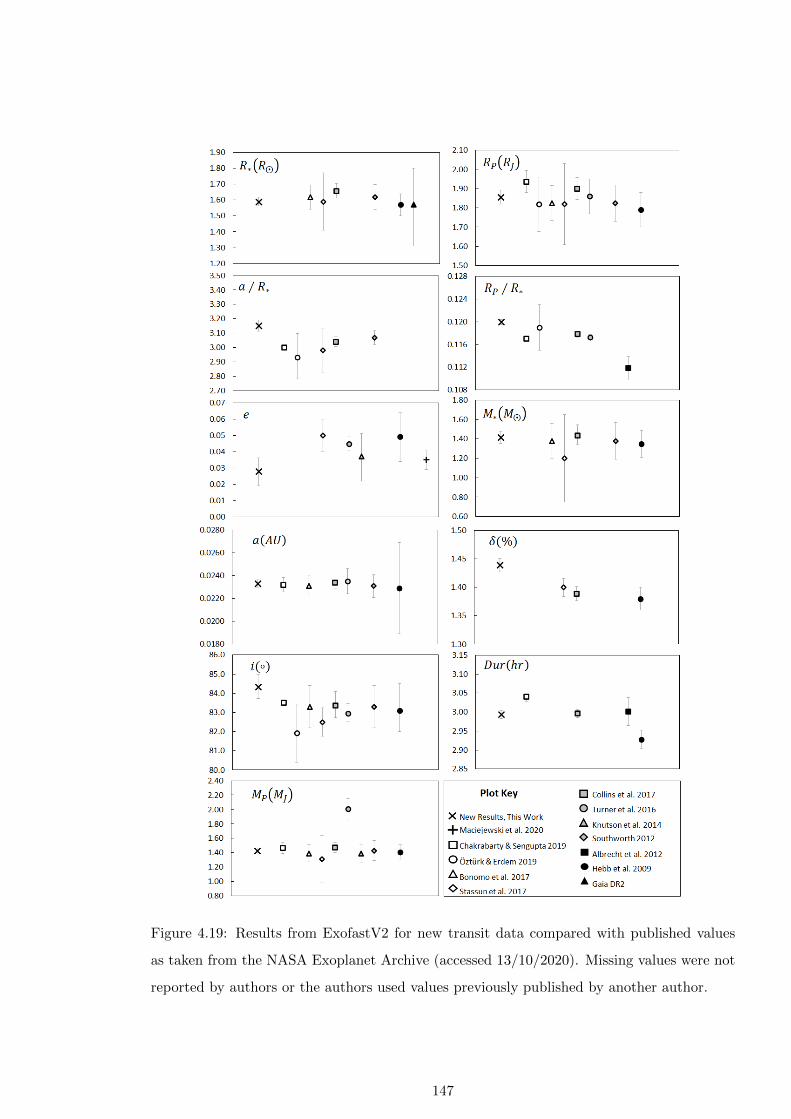
Figure 4.19: Results from ExofastV2 for new transit data compared with published values

as taken from the NASA Exoplanet Archive (accessed 13/10/2020). Missing values were not

reported by authors or the authors used values previously published by another author.

147

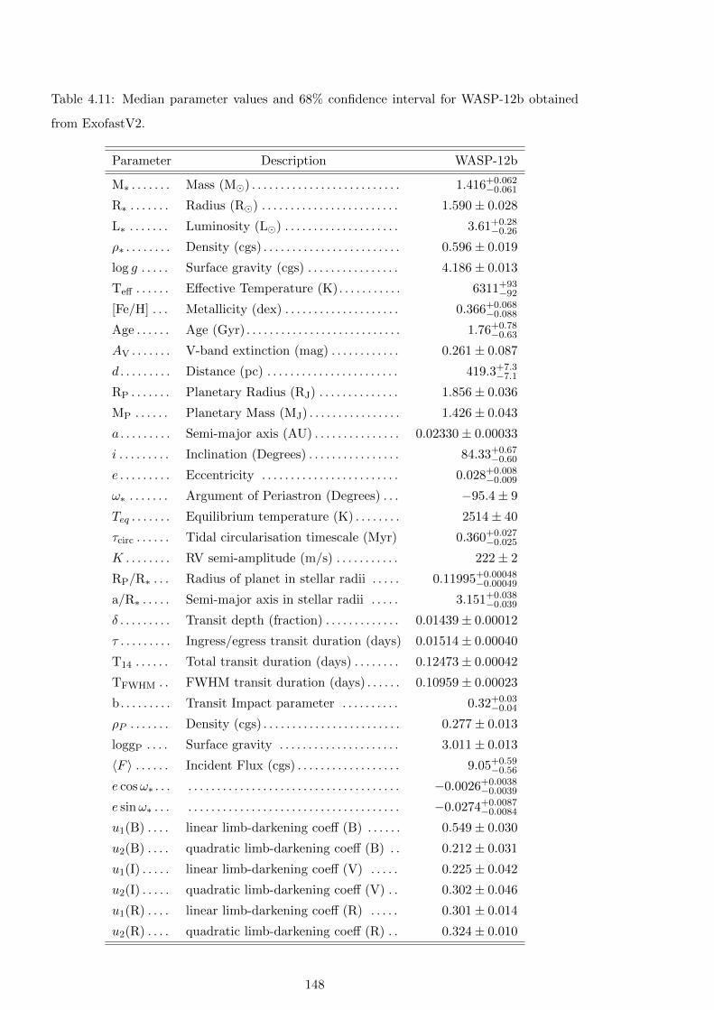
Table 4.11: Median parameter values and 68% confidence interval for WASP-12b obtained

from ExofastV2.

Parameter Description WASP-12b

M∗ . . . . . . . Mass (M�) . . . . . . . . . . . . . . . . . . . . . . . . . . 1.416+0.062−0.061

R∗ . . . . . . . Radius (R�) . . . . . . . . . . . . . . . . . . . . . . . . 1.590± 0.028

L∗ . . . . . . . Luminosity (L�) . . . . . . . . . . . . . . . . . . . . 3.61+0.28−0.26

ρ∗ . . . . . . . . Density (cgs) . . . . . . . . . . . . . . . . . . . . . . . . 0.596± 0.019

log g . . . . . Surface gravity (cgs) . . . . . . . . . . . . . . . . 4.186± 0.013

Teff . . . . . . Effective Temperature (K). . . . . . . . . . . 6311+93−92

[Fe/H] . . . Metallicity (dex) . . . . . . . . . . . . . . . . . . . . 0.366+0.068−0.088

Age . . . . . . Age (Gyr) . . . . . . . . . . . . . . . . . . . . . . . . . . . 1.76+0.78−0.63

AV . . . . . . . V-band extinction (mag) . . . . . . . . . . . . 0.261± 0.087

d . . . . . . . . . Distance (pc) . . . . . . . . . . . . . . . . . . . . . . . 419.3+7.3−7.1

RP . . . . . . . Planetary Radius (RJ) . . . . . . . . . . . . . . 1.856± 0.036

MP . . . . . . Planetary Mass (MJ) . . . . . . . . . . . . . . . . 1.426± 0.043

a . . . . . . . . . Semi-major axis (AU) . . . . . . . . . . . . . . . 0.02330± 0.00033

i . . . . . . . . . Inclination (Degrees) . . . . . . . . . . . . . . . . 84.33+0.67−0.60

e . . . . . . . . . Eccentricity . . . . . . . . . . . . . . . . . . . . . . . . 0.028+0.008−0.009

ω∗ . . . . . . . Argument of Periastron (Degrees) . . . −95.4± 9

Teq . . . . . . . Equilibrium temperature (K) . . . . . . . . 2514± 40

τcirc . . . . . . Tidal circularisation timescale (Myr) 0.360+0.027−0.025

K . . . . . . . . RV semi-amplitude (m/s) . . . . . . . . . . . 222± 2

RP/R∗ . . . Radius of planet in stellar radii . . . . . 0.11995+0.00048−0.00049

a/R∗ . . . . . Semi-major axis in stellar radii . . . . . 3.151+0.038−0.039

δ . . . . . . . . . Transit depth (fraction) . . . . . . . . . . . . . 0.01439± 0.00012

τ . . . . . . . . . Ingress/egress transit duration (days) 0.01514± 0.00040

T14 . . . . . . Total transit duration (days) . . . . . . . . 0.12473± 0.00042

TFWHM . . FWHM transit duration (days) . . . . . . 0.10959± 0.00023

b. . . . . . . . . Transit Impact parameter . . . . . . . . . . 0.32+0.03−0.04

ρP . . . . . . . Density (cgs) . . . . . . . . . . . . . . . . . . . . . . . . 0.277± 0.013

loggP . . . . Surface gravity . . . . . . . . . . . . . . . . . . . . . 3.011± 0.013

〈F 〉 . . . . . . Incident Flux (cgs) . . . . . . . . . . . . . . . . . . 9.05+0.59−0.56

e cosω∗ . . . . . . . . . . . . . . . . . . . . . . . . . . . . . . . . . . . . . . . . −0.0026+0.0038−0.0039

e sinω∗ . . . . . . . . . . . . . . . . . . . . . . . . . . . . . . . . . . . . . . . . −0.0274+0.0087−0.0084

u1(B) . . . . linear limb-darkening coeff (B) . . . . . . 0.549± 0.030

u2(B) . . . . quadratic limb-darkening coeff (B) . . 0.212± 0.031

u1(I) . . . . . linear limb-darkening coeff (V) . . . . . 0.225± 0.042

u2(I) . . . . . quadratic limb-darkening coeff (V) . . 0.302± 0.046

u1(R) . . . . linear limb-darkening coeff (R) . . . . . 0.301± 0.014

u2(R) . . . . quadratic limb-darkening coeff (R) . . 0.324± 0.010

148

of change is greater at 382 ppm hr−1 giving total magnitude change of 2.3 milli-mag over a 6

hour observation. Thus the variation over a 6 hour period is comparable to the photometric

uncertainty in the transit data, typically between 1.3 - 3.5 milli-mag depending on the quality

of the observation, and is equal to approximately 15% of the transit depth for WASP-12b. If

J0630+2942 is used as part of a large number of comparison stars in a photometric ensemble

the effect would be significantly reduced but if J0630+2942 is used as the sole comparison

star this effect will require correcting for, in turn requiring knowledge of the amplitude of the

variation over time. The amplitude of the variation was significantly reduced in the 2018-19

season at 0.004 mag, giving a mean and maximum rate of change over 6 hours of 0.6 milli-mag

and 0.9 milli-mag respectively, less than the typical photometric uncertainties.

Variability in J0630+2942 was not searched for in individual time series transit data. In

the 2016-17 season, when the variability amplitude in J0630+2942 was was at its greatest, the

mean variation in J0630+2942 was less than 1 milli-mag over the mean observing duration

of 3.9 hr. Thus the mean change in flux from J0630+2942 was only 40% of the mean transit

lightcurve RMS scatter in the transit data for this seasons. Higher precision photometry

was obtained in the 2018-19 season but the reduction in amplitude of variations seen in

J0630+2942 means the expected mean magnitude change over the typical transit observation

duration was even less, just 25% of the mean RMS scatter.

4.6.2 WASP-12 Monitoring

No periodic variability attributable to rotation was unambiguously detected in the photome-

try of WASP-12 obtained over three observing season between 2016 and 2019. The detection

of photometric variability in field star J0630+2942 provides a variability detection threshold

of 2 millimags for the data collected, any variability in WASP-12 at this level or greater should

be detected. The 29.6d periodicity seen strongly in the blue filter and similar periods seen less

strongly in the red filter suggest a systematic effect of lunar illumination variation affecting

the photometry rather than a physical attribute of WASP-12. This is seen especially clearly

seen in the blue filter photometry from the 2017-18 season. The same strong periodicity is

not seen in the check star and J0630+2942 measurements which remains unexplained. It is

worth noting that given the newly calculated radius of WASP-12, a 29.6d period implies a ro-

tation velocity of 2.7 km s−1, in general agreement with the values of υsini = 2.2±1.5 km s−1

reported by (Hebb et al., 2009) and υsini = 1.6+0.8−0.4 km s−1 (Albrecht et al., 2012)). While

it remains possible that the true rotation period for WASP-12 is close to the lunar month

duration, the matching phase (see Figure 4.14 for example) makes a systematic effect the

more likely explanation.

The lack of conclusively detected variability in WASP-12 over all three seasons of moni-

149

toring implies that the system is (1) being viewed at a high inclination with respect to the

stellar rotation pole, (2) it was at a quiet stage of its stellar cycle when observed, (3) the

photometric modulations are below the PIRATE detection threshold, or that (4) WASP-12 is

anomalously quiescent. Each of these have implications for our understanding of the system.

Schlaufman (2010) used a Monte Carlo simulation to determine the range of observable

νsini expected for a control sample of almost 900 field stars. The same simulation was per-

formed for known exoplanet host stars under assumption of spin-orbit alignment. Comparison

of the host stars with a random sample allowed systems with significantly slower than ex-

pected νsini to be identified as misaligned. 10 out of 75 systems were identified, including

WASP-12, as being either anomalously slow rotators or aligned close to pole on to our line

of sight.

Using the method of Schlaufman (2010), Albrecht et al. (2012) calculated the expected

equatorial rotation velocity for WASP-12 as 13.7± 2.5 kms−1. Their measured rotation ve-

locity of νsini = 1.6+0.8−0.4 kms−1 implies we are viewing WASP-12 just 6.7° from pole on. Using

the newly calculated value for the radius of WASP-12 the projected rotation period would

be 5.8 days for the estimated νsini and 50 days for the measured νsini. No matching period

is seen in the monitoring photometry.

Both anomalously slow rotation or spin-orbit misalignment are consistent with the non-

detection of the Rossiter-McLaughlin effect in spectroscopic observations of WASP-12b (Al-

brecht et al., 2012; Husnoo et al., 2011).

The Sun shows a repeatable pattern of sunspots (the butterfly diagram seen in Figure 1.3)

appearing at latitudes as high as 60° at the start of each solar cycle and migrating towards

the equator as the cycle progresses. If WASP-12 is viewed at a high stellar inclination only

surface spots at high latitudes early in the stellar cycle would be visible to produce photo-

metric variations. Spots at high latitudes may be visible for complete stellar rotations and

would not produce the expected periodic photometric variations. Instead any photometric

variation would occur at the timescales of the spot lifetimes and would therefore only produce

irregular variations as spots are formed and dissipate at the visible latitudes. Surface spots

would become less visible as they migrate to lower latitudes implying the stellar cycle could

be detected in the level of variation of stellar brightness between observing seasons. The

difference seen in the mean red magnitude of WASP-12 between the 16-17 and 17-18 seasons

was 0.005 Mag, comparable to the measured 1σ uncertainty of 0.004 Mag, so not significant.

Blue filter data is not available for the 16-17 season and the change in filters for the 18-19

season means direct comparison is not possible.

There is no a-priori reason to suspect WASP-12 is an anomalously slow rotator, the

detection of the orbital decay for WASP-12b Yee et al. (2019) shows that angular momentum

150

is being transferred from the planetary orbit to the host star which would be expected to

result in a faster rotation for WASP-12. Weinberg et al. (2017) showed that this would not

be inconsistent with observations of slow rotation if WASP-12 is on the sub-giant branch as

the transfer of angular momentum would occur very close to the stellar core, resulting in spin

up of the core while leaving the extended stellar envelope unaffected. This result was not

supported by subsequent analysis preferring the conclusion that WASP-12 is a main sequence

star (Bailey and Goodman, 2019).

The extremely short orbital period of WASP-12b, well below any likely stellar rotational

period, can result in star-planet interactions through either the raising of tidal bulges on

the stellar surface or through magnetic interaction. The orbit of WASP-12b will raise tidal

bulges on the surface of WASP-12 at both the sub-planetary point and its antipode, resulting

in two bulges thus any signal arising from this equilibrium tidal approximation would occur

at half the orbital period. A signal consistent with the predictions from this equilibrium

tide approximation have been observed in RV measurements(Maciejewski et al., 2020). The

authors predict tides would be raised with a height of 150km and they predict the photometric

variation resulting from this departure from the spherical would cause a photometric variation

of 80ppm, well below the detection threshold from ground-based observations. Another

potential source of photometric variation arises from magnetic interaction between the planet

and the star which could be expected to create a hot or cool spot on the stellar surface where

the magnetic field interact (Vidotto, 2019). Unlike tidal bulges, this effect would at occur

only at (or close to) the sub-planetary point, causing any variation to occur at the orbital

period.

Apart from their small amplitude the difficulty in detecting any photometric variation

caused by star-planet interaction is compounded in WASP-12 by two other effects. Firstly

the orbital period of 1.09-day being so close to the ground-based observational cadence. The

second issue results from the simple fact that WASP-12b transits and this signal has been

removed from the monitoring photometry. It would therefore not be expected that any

variation due to magnetic interaction occurring at Porb would be detectable it this data set.

A period search around both Porb and Porb/2 do not reveal any signal other than the alias

created by the observing cadence.

There is the possibility that the surface spots exist but that they are below the detection

threshold of the small aperture ground-based telescope photometric precision, either due to

small size, low contrast or geometric effects arising from a near pole-on stellar orientation

of WASP-12. To investigate this the Spot Oscillation And Planet (SOAP)3 (Boisse et al.,

2011) software was used to model the effects of different size spots at varying latitudes for

3http://www.astro.up.pt/soap/

151

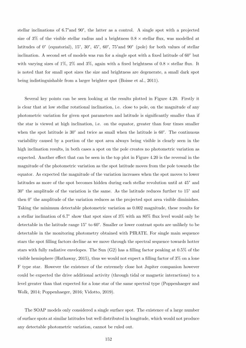
stellar inclinations of 6.7°and 90°, the latter as a control. A single spot with a projected

size of 3% of the visible stellar radius and a brightness 0.8 × stellar flux, was modelled at

latitudes of 0° (equatorial), 15°, 30°, 45°, 60°, 75°and 90° (pole) for both values of stellar

inclination. A second set of models was run for a single spot with a fixed latitude of 60° but

with varying sizes of 1%, 2% and 3%, again with a fixed brightness of 0.8 × stellar flux. It

is noted that for small spot sizes the size and brightness are degenerate, a small dark spot

being indistinguishable from a larger brighter spot (Boisse et al., 2011).

Several key points can be seen looking at the results plotted in Figure 4.20. Firstly it

is clear that at low stellar rotational inclination, i.e. close to pole, on the magnitude of any

photometric variation for given spot parameters and latitude is significantly smaller than if

the star is viewed at high inclination, i.e. on the equator, greater than four times smaller

when the spot latitude is 30° and twice as small when the latitude is 60°. The continuous

variability caused by a portion of the spot area always being visible is clearly seen in the

high inclination results, in both cases a spot on the pole creates no photometric variation as

expected. Another effect that can be seen in the top plot in Figure 4.20 is the reversal in the

magnitude of the photometric variation as the spot latitude moves from the pole towards the

equator. As expected the magnitude of the variation increases when the spot moves to lower

latitudes as more of the spot becomes hidden during each stellar revolution until at 45° and

30° the amplitude of the variation is the same. As the latitude reduces further to 15° and

then 0° the amplitude of the variation reduces as the projected spot area visible diminishes.

Taking the minimum detectable photometric variation as 0.002 magnitude, these results for

a stellar inclination of 6.7° show that spot sizes of 3% with an 80% flux level would only be

detectable in the latitude range 15° to 60°. Smaller or lower contrast spots are unlikely to be

detectable in the monitoring photometry obtained with PIRATE. For single main sequence

stars the spot filling factors decline as we move through the spectral sequence towards hotter

stars with fully radiative envelopes. The Sun (G2) has a filling factor peaking at 0.5% of the

visible hemisphere (Hathaway, 2015), thus we would not expect a filling factor of 3% on a lone

F type star. However the existence of the extremely close hot Jupiter companion however

could be expected the drive additional activity (through tidal or magnetic interactions) to a

level greater than that expected for a lone star of the same spectral type (Poppenhaeger and

Wolk, 2014; Poppenhaeger, 2016; Vidotto, 2019).

The SOAP models only considered a single surface spot. The existence of a large number

of surface spots at similar latitudes but well distributed in longitude, which would not produce

any detectable photometric variation, cannot be ruled out.

152

Figure 4.20: SOAP model results. Top, single surface spot of 3% with 80% brightness at a

range of latitudes for stellar inclination of 6.7°. Second from top, as per the plot above but

for stellar inclination of 90°, i.e. seen equator on. Third from top, a range of spot sizes with

fixed brightness of 80% and fixed 60°latitude. Bottom, as for the plot above but for stellar

inclination of 90°.

153

4.6.3 WASP-12b Transit Timing

It was not possible to determine between a linear and quadratic ephemeris using only the

47 newly obtained transit times. This is likely a result of the shorter coverage duration

and greater scatter in transit mid-time measurement than seen in the Y19 data set. The

first three seasons of the new data set (2013/14, 2014/15 and 2015/16) have only four data

points available. Over the four seasons (3.5 years) from 2016/17 to 2019/20 with greater

coverage the visible change in transit mid-time resulting from the quadratic component of

the ephemeris in 4.5 (page 143) when compared to a linear ephemeris is -61 seconds. This is

slightly greater than the mean transit mid-time uncertainty of ±50 seconds seen over the same

period for the new transit measurements. The spread in transit mid-time determination was

greater than the mid-time uncertainty, ranging from a minimum of 76 seconds in the 2019/20

season to a maximum 361 seconds in the 2017/18 season. The typical spread in seasonal

mid-time measurement in the data set published by Yee et al. (2019) was ∼ 62s. It was this

large spread in seasonal transit mid-time measurement, particularly during the three seasons

2016/17 to 2018/19, that resulted in the quadratic ephemeris not being positively detected

on the new data set. The causes of this large spread in transit mid-time measurements are

discussed further in Chapter 5 where I analyse further the performance of the small aperture

telescope observations.

Combining the new data with existing published results provided results in close agree-

ment to those from Yee et al. (2019), Figure 4.18. Combining all 47 new transit times with

the 139 times from Y19 provided an ephemeris result with smaller uncertainties than just

the Y19 data on its own. A smaller data set based on the Y19 transit times combined with

those obtained from COAST and PIRATE observations made after the installation of the

GPS time control and using a mean Tc for simultaneous observations provided an ephemeris

model with the smallest χ2ν and residual RMS values, so this was selected as the updated

ephemeris.

The typical per-season standard deviation in transit mid-time measurements in the Y19

data set is 2 to 3 times smaller than that seen for the newly obtained data. This level of

spread in transit time measurements obtained for WASP-12b is greater than seen in the

HAT-P-23b or WASP-52b measurements, a periodicity search does not reveal any intrinsic

periodicity that may explain this. It is noted that for the 2019/20 season of data, not covered

by the Y19 data, the standard deviation in mid-times is closer to that seen in the Y19 data.

Three observations obtained by PIRATE over a 12 day period in 2020 show an extremely

low transit mid-time scatter of just 0.00009d, 16% of the mean mid-time uncertainty for the

three observations (0.00056d).

154

The analysis includes a number of simultaneous transit times where the same transit

was observed by two different telescopes or observers. Two observations made as part of

this project were simultaneous with observations in the Y19 data set and show a mid-time

difference of 0.8σ. A further nine simultaneous transit mid-time obtained with different

telescopes used in this project varied between 0.8σ and 5.1σ with a mean of 1.72σ. Both the

greatest and smallest difference was seen prior to the installation of the GPS system. After the

GPS upgrade the transit mid-time between pairs observed ranged from 1.5σ to 3.27σ. This

is not greatly at odds with results seen for the same transit observations in the data compiled

by Yee et al. (2019) where the the transit mid-time differences for simultaneous observations

varied between 0.8σ and 3.4σ. The simultaneous transit measurements for WASP-12b and

for HAT-P-23b are discussed further in Chapter 5.

The existence of tidal decay implies ongoing tidal dissipation between the planetary orbit

and the host star, parameterised by the tidal quality factor Q′∗, (Yee et al., 2019).

P = − 27π

2Q′∗

(MP

M∗

)(R∗a

)5

(4.6)

Q′∗ = −27π

2P−1

(MP

M∗

)(R∗a

)5

. (4.7)

Using the newly determined value for the period change of−9.419±0.596×10−10d and other

parameters taken from Table 4.11, the tidal quality factor is Q′∗ = 1.35 ± 0.15 × 105 which

compares with Q′∗ = 1.75+0.13

−0.11×105 reported by Yee et al. (2019). This is a continuation of the

downward trend in values calculated for Q′∗ as more data have become available. Maciejewski

et al. (2016) reported a value for Q′∗ of 2.5× 105, a year later Patra et al. (2017) reported a

value of 2× 105 and in 2019, Yee et al. (2019) reported a value of 1.75× 105.

As can be seen from Equation 4.7 the value of Q′∗ is extremely sensitive to R∗/a, a small

R∗/a value will increase Q′∗ while a large value of R∗/a value will decrease Q

′∗. Keeping all

other values fixed but using the smallest value reported for R∗/a, Ozturk and Erdem (2019),

results in a determination for Q′∗ that is ≈ 30% larger. Thus variations in the distance ratios

used to calculate Q′∗ can easily account for the range of values seen in the literature.

Equation 4.7 assumes a constant mass ratio and thus neglects any mass loss from the

planet. We know that WASP-12b is losing mass (Haswell et al., 2012) but it is unknown how

much mass is being lost and whether this is conservative, non-conservative or a combination

of both (Haswell, 2018). In the extreme case of fully conservative mass transfer the amount of

mass required to produce the orbital decay seen would be in the region of 2.5× 1025 kg yr−1.

This is significantly in excess of the extreme mass loss scenario calculated by Lai et al. (2010)

of ≈ 10−7 MJ yr−1. Although we can rule out conservative mass transfer as the cause of the

155

period change, the impact of mass loss from WASP-12b is still an open question (Haswell,

2018).

4.6.4 WASP-12b System Parameters

The new results provide the tightest constraints yet on the values for R∗, RP, a, M∗ and MP

for the WASP-12b system showing that large number of filtered observations obtained with

small aperture ground-based telescopes, primarily for the purposes of transit timing, can be

combined with published RV and photometric data to retrieve precise system parameters.

The age determined for WASP-12b of 1.76 Gyr and the tidal circularisation time scale

of 0.36Myr imply that, unless we consider we seeing WASP-12b at a special time, the orbit

of WASP-12b should not be eccentric. Maciejewski et al. (2020) reported a 5.8σ detection

of orbital eccentricity in WASP-12b of e = 0.035 ± 0.006 and ω = 270.7 ± 0.6°. This result

was interpreted resulting from a combination of the RV signal arising from a circular orbit

combined with the signal arising from tides being raised on the surface host star by the closely

orbiting planet which the authors determine will mimic an apparent non-zero eccentricity

with an argument of periastron at 270°. My finding from the combined RV and transit

analysis for WASP-12b orbital eccentricity and argument of periastron of e = 0.028+0.008−0.009 and

ω = 265± 9° are in agreement with the values found by Maciejewski et al. (2020) within the

quoted uncertainties and which is consistent with the calculated age and tidal circularisation

timescale for the system.

Comparison with the results for parameter determination from other authors is not always

straightforwards for a number of reasons. As can be seen from Figure 4.19 many authors do

not publish a standard set of values for systems under study. It is trivial to calculate some

specific values such as semi major axis given R∗ and a/R∗, however simple combination of

uncertainties in standard fashion often results in greater uncertainties for values calculated

in this way rather than being modelled by the transit analysis software used. Authors do not

publish the values used for scaling their results to Solar System values, potentially introducing

a source of systematic error if different transit analysis software makes use of different values.

For example IAU 2015 resolution B3 provides values for the polar and equatorial radii of

Jupiter, if the analysis reports the results using units of mean Jupiter radius the planetary

radius will be over reported. ExofastV2 publishes the constants used in calculating and

reporting results with the equatorial radius of Jupiter being used for reporting planetary

radii. Some authors use previously published values as fixed parameters in their model fits.

Chakrabarty and Sengupta (2019) used R∗ and M∗ from Collins et al. (2017a) while Ozturk

and Erdem (2019) use values for R∗ and M∗ and MP published by Hebb et al. (2009).

These duplicate values were not presented in the comparison of the new results with existing

156

published data in Figure 4.19. The updated WASP-12 system parameter values reported in

Table 4.11 used ExofastV2 to provide a homogeneous set of results.

4.7 Summary of findings

1. No periodicity was detected in the photometry of WASP-12. The balance of evidence

favours a scenario where we see WASP-12 almost pole on significantly reducing the

magnitude of any photometric variation resulting from rotation of stellar spots. Models

using SOAP indicate any spots will need to be larger than 3% of the stellar surface (with

an 80% flux level) and residing between latitudes 15° to 60° to generate a photometric

variation detectable with PIRATE.

2. A periodic variation was detected on J0630+2942 just 2′ from WASP-12 which is at-

tributed to rotational modulation caused by surface spots. The period and amplitude

were seen to vary over the 3 seasons of observations. Further photometric monitoring

will be required to measure the long term variation and thus the stellar cycle period.

3. The analysis of transit mid-times combined with the existing published data highlights

the requirement for very long term (decade+) accurate transit mid-time monitoring to

detect orbital period changes. In conclusion the new observations complement the Y19

data set and extend it by a further season allowing a revision of the ephemeris which

is in excellent agreement with that published by Y19.

4. The new results provide the tightest constraints yet on many key values for the WASP-

12b system and clearly demonstrate the use of large numbers of transit lightcurves,

obtained using small aperture ground-based telescopes for transit timing purposes can

be used to provide precise system parameters.

In this and the previous chapter I have considered the results of transit observations

made with multiple small aperture ground-based telescopes measuring transit timing, system

parameters and host star variability. In the final chapter I look at the performance of the

small aperture ground-based telescope observations and consider the suitability of and role

for these observations to contribute to exoplanet science.

157

Chapter 5

Small Aperture Telescope

Performance

5.1 Introduction

In this chapter I take a closer look at the performance of the small aperture ground-based

telescopes used to make the observations of HAT-P-23b, WASP-12b and WASP-52b discussed

in the preceding chapters. The aim is to quantify the capabilities of small aperture ground-

based telescopes for making observations of transiting exoplanets and to identify best best

practice methods.

In the first section I look at the data quality in general achieved with each telescope in

the different observing modes, considering the effect of different CCD binning, photometric

SNR and systematic noise. In the second and third sections I look at the ability to define

precise systems parameters from single and multiple observations and the quality of the long

term photometric monitoring of exoplanet host stars. In the fourth section I look at how

the data quality and observing modes affect the transiting timing measurements. In the final

section I consider results from simultaneous observations of the same transit with multiple

telescopes.

5.1.1 There is ‘binning’ and there is ‘binning’

Before continuing it is worth just briefly covering the two contexts where the wording “bin-

ning” is used in the following discussions. The first relates to on chip binning of the CCD

cameras used to gather the photometric data. This is referred to as “CCD” or “on chip”

binning and refers to the settings used in the camera control where the camera is operated in

un-binned or 1× 1 mode, or where individual CCD pixels are binned into groups of 4 (2× 2

binning) or even 9 (3x3) and read out from the CCD camera as single larger pixels.

158

The second use of the word binning is where individual measurements are combined

usually into time related groups of data. An example is where photometric data points in

phase folded lightcurves are combined into 5-minute bins. The use is stated where the context

of the surrounding discussion does not make it clear which use of the term applies.

5.2 Data Quality

5.2.1 Signal to Noise Ratio

There are a number of measures for the quality of a transit lightcurve, one such measure is the

Transit SNR (TSNR) (Ioannidis et al., 2016) which is the ratio of transit depth (δ) to out-of-

transit (oot) measurement scatter, measured as the RMS of the detrended data points before

and after ingress and egress. Figure 5.1 shows the mean TSNR and mean oot RMS broken

down by system observed and telescope/CCD mode used. The observations made with the

CCD camera in 1 × 1 on chip binning mode show a lower mean oot RMS and therefore a

greater mean TSNR. For the WASP-12b observations both the smaller aperture COAST and

POST telescopes, operating in 1 × 1 binning mode, show a greater mean TSNR/lower oot

RMS than the PIRATE 1× 1 observations.

To understand how the photometric SNR impacts the RMS scatter and thus TSNR,

mean oot RMS and mean photometric SNR were plotted by telescope and binning mode.

Figure 5.2 shows clear correlation between increasing SNR and decreasing oot RMS scatter

in the measurements which in turn leads to an increased TSNR with photometric SNR. The

observations binned 1 × 1 dominate the higher SNR/lower oot RMS end of the curve, but

there is considerable scatter. The data in Figure 5.2 is fit with two power law curves for

SNR−1, grey line and SNR−0.95, black line. The results show that mean oot RMS is not

quite a perfect inverse proportionality, the best fit power is -0.95, indicating a slightly greater

SNR requirement to achieve a given oot RMS value. SNR values above 1000 show little

improvement in reducing scatter.

As TSNR = δ/oot RMS, we can can substitute the relation found between oot RMS

and photometric SNR to calculate the expected TSNR for a given photometric SNR or,

alternatively, to estimate the photometric SNR required to achieve a given TSNR

TSNR = δ × SNR0.95. (5.1)

Figure 5.3 plots the TSNR against mean photometric SNR for each of the three systems

along with the result of Equation 5.1. The plots show that Eq.5.1 is a good fit for the

results for WASP-12b, HAT-P-23b achieved a greater TSNR for a given mean photometric

SNR, though the plot is dominated by two high TSNR measurements. WASP-52b has the

159

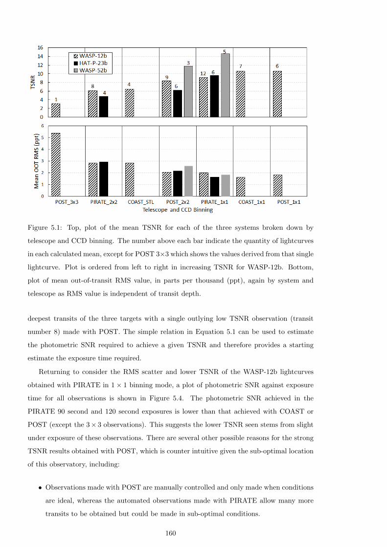
Figure 5.1: Top, plot of the mean TSNR for each of the three systems broken down by

telescope and CCD binning. The number above each bar indicate the quantity of lightcurves

in each calculated mean, except for POST 3×3 which shows the values derived from that single

lightcurve. Plot is ordered from left to right in increasing TSNR for WASP-12b. Bottom,

plot of mean out-of-transit RMS value, in parts per thousand (ppt), again by system and

telescope as RMS value is independent of transit depth.

deepest transits of the three targets with a single outlying low TSNR observation (transit

number 8) made with POST. The simple relation in Equation 5.1 can be used to estimate

the photometric SNR required to achieve a given TSNR and therefore provides a starting

estimate the exposure time required.

Returning to consider the RMS scatter and lower TSNR of the WASP-12b lightcurves

obtained with PIRATE in 1× 1 binning mode, a plot of photometric SNR against exposure

time for all observations is shown in Figure 5.4. The photometric SNR achieved in the

PIRATE 90 second and 120 second exposures is lower than that achieved with COAST or

POST (except the 3× 3 observations). This suggests the lower TSNR seen stems from slight

under exposure of these observations. There are several other possible reasons for the strong

TSNR results obtained with POST, which is counter intuitive given the sub-optimal location

of this observatory, including:

• Observations made with POST are manually controlled and only made when conditions

are ideal, whereas the automated observations made with PIRATE allow many more

transits to be obtained but could be made in sub-optimal conditions.

160

Figure 5.2: The relationship between mean photometric SNR and mean oot transit RMS

plotted for exoplanet system and CCD binning mode. The grey line is SNR−1 the black line

is SNR−0.95

• The limited horizon at POST prevents observations at higher airmass. The highest

airmass observation obtained with POST is 1.65, while with PIRATE it is 2.30. Higher

airmass observations will be at start or end of observation (or both), systematically

affecting oot RMS measurements and therefore TSNR for the whole lightcurve.

• POST uses a higher sensitivity CCD camera (at the expense of a much smaller field of

view) allowing higher photometric SNR to be achieved in similar exposure times.

• Flat field calibration frames are obtained on the same night as the observations removing

the need to combine frames from multiple different nights.

• The POST images were autoguided, maintaining the target star on the same pixel, see

Section 5.2.3.

• During the 2018-19 and 2019-20 season PIRATE exhibited trailing in a number of

WASP-12b lightcurves caused by an oscillation in the RA axis. This is thought to be

caused by the RA balance of the OTA being too perfect making the OTA susceptible to

wind driven vibration. This will be rectified by offsetting the counter balance weights

slightly to ensure better RA gear meshing. As a result a number of science frames

from some observations had to be discarded while those retained in order to ‘save the

161

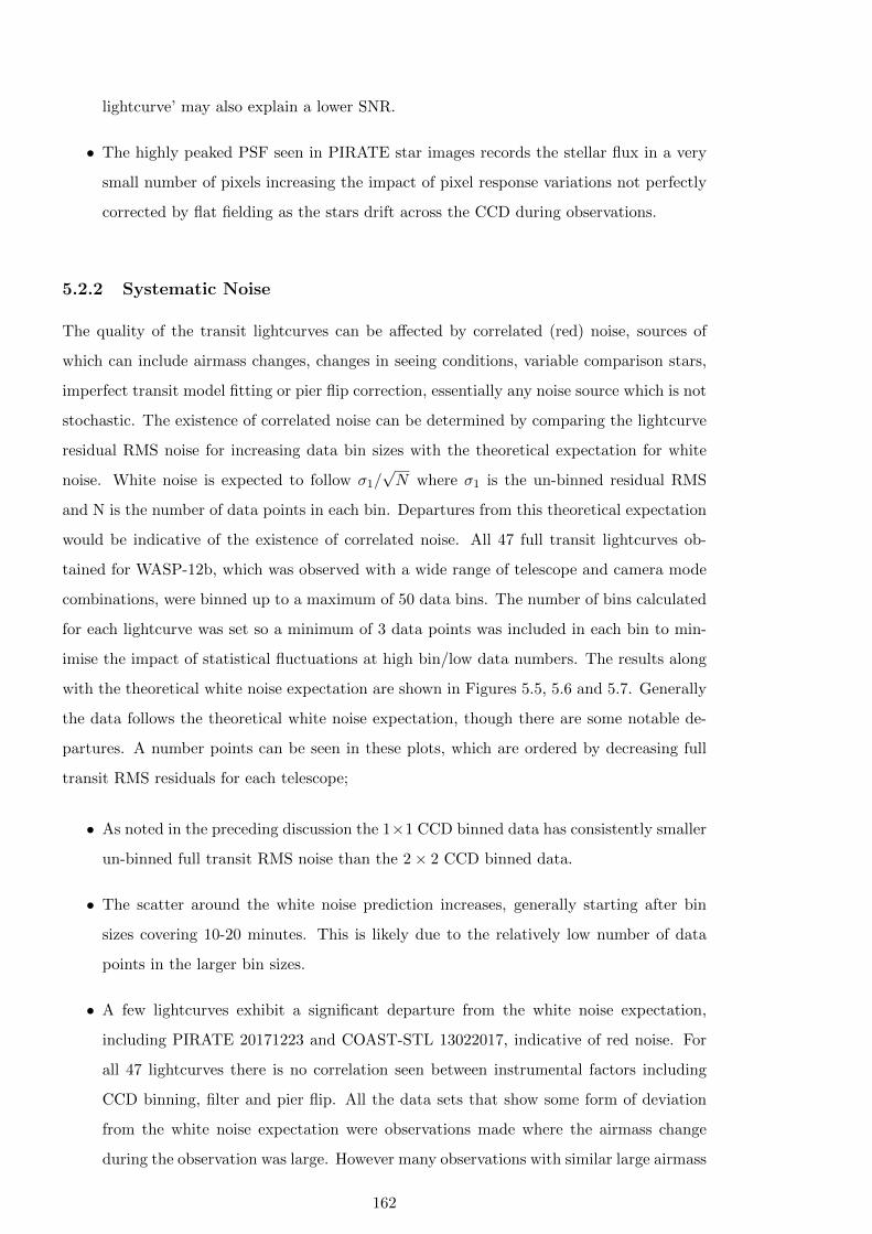
lightcurve’ may also explain a lower SNR.

• The highly peaked PSF seen in PIRATE star images records the stellar flux in a very

small number of pixels increasing the impact of pixel response variations not perfectly

corrected by flat fielding as the stars drift across the CCD during observations.

5.2.2 Systematic Noise

The quality of the transit lightcurves can be affected by correlated (red) noise, sources of

which can include airmass changes, changes in seeing conditions, variable comparison stars,

imperfect transit model fitting or pier flip correction, essentially any noise source which is not

stochastic. The existence of correlated noise can be determined by comparing the lightcurve

residual RMS noise for increasing data bin sizes with the theoretical expectation for white

noise. White noise is expected to follow σ1/√N where σ1 is the un-binned residual RMS

and N is the number of data points in each bin. Departures from this theoretical expectation

would be indicative of the existence of correlated noise. All 47 full transit lightcurves ob-

tained for WASP-12b, which was observed with a wide range of telescope and camera mode

combinations, were binned up to a maximum of 50 data bins. The number of bins calculated

for each lightcurve was set so a minimum of 3 data points was included in each bin to min-

imise the impact of statistical fluctuations at high bin/low data numbers. The results along

with the theoretical white noise expectation are shown in Figures 5.5, 5.6 and 5.7. Generally

the data follows the theoretical white noise expectation, though there are some notable de-

partures. A number points can be seen in these plots, which are ordered by decreasing full

transit RMS residuals for each telescope;

• As noted in the preceding discussion the 1×1 CCD binned data has consistently smaller

un-binned full transit RMS noise than the 2× 2 CCD binned data.

• The scatter around the white noise prediction increases, generally starting after bin

sizes covering 10-20 minutes. This is likely due to the relatively low number of data

points in the larger bin sizes.

• A few lightcurves exhibit a significant departure from the white noise expectation,

including PIRATE 20171223 and COAST-STL 13022017, indicative of red noise. For

all 47 lightcurves there is no correlation seen between instrumental factors including

CCD binning, filter and pier flip. All the data sets that show some form of deviation

from the white noise expectation were observations made where the airmass change

during the observation was large. However many observations with similar large airmass

162

Figure 5.3: A plot showing the relationship between TSNR and mean photometric SNR by

CCD binning mode. Each system is shown separately as TSNR is dependent on transit depth

which is different for each system. The dash-dot line is from Equation 5.1

163

Figure 5.4: A plot showing how mean photometric SNR varied with exposure duration for

each telescope and CCD binning mode for each exoplanet system. Plots show only full

transits obtained through R filters. As expected SNR increases as√

Exposure with the long

exposure/high SNR region dominated by the 1× 1 binning observation despite the four fold

increase in pixels for the 1 × 1 vs 2 × 2 binned observations. The plot for WASP-12b also

indicates the apparent under-exposure for the PIRATE 1 × 1 observations where the 90

second exposures only average SNR values of 600 versus 800 for the 150 second exposures

with COAST.

164

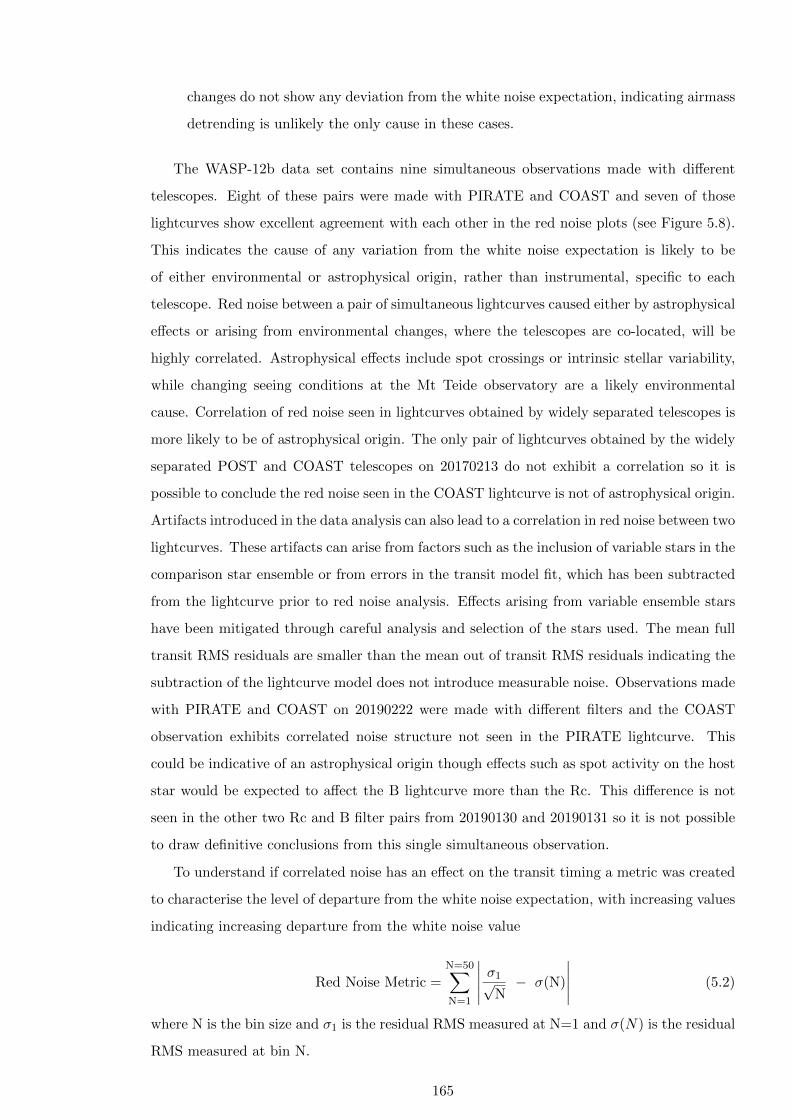
changes do not show any deviation from the white noise expectation, indicating airmass

detrending is unlikely the only cause in these cases.

The WASP-12b data set contains nine simultaneous observations made with different

telescopes. Eight of these pairs were made with PIRATE and COAST and seven of those

lightcurves show excellent agreement with each other in the red noise plots (see Figure 5.8).

This indicates the cause of any variation from the white noise expectation is likely to be

of either environmental or astrophysical origin, rather than instrumental, specific to each

telescope. Red noise between a pair of simultaneous lightcurves caused either by astrophysical

effects or arising from environmental changes, where the telescopes are co-located, will be

highly correlated. Astrophysical effects include spot crossings or intrinsic stellar variability,

while changing seeing conditions at the Mt Teide observatory are a likely environmental

cause. Correlation of red noise seen in lightcurves obtained by widely separated telescopes is

more likely to be of astrophysical origin. The only pair of lightcurves obtained by the widely

separated POST and COAST telescopes on 20170213 do not exhibit a correlation so it is

possible to conclude the red noise seen in the COAST lightcurve is not of astrophysical origin.

Artifacts introduced in the data analysis can also lead to a correlation in red noise between two

lightcurves. These artifacts can arise from factors such as the inclusion of variable stars in the

comparison star ensemble or from errors in the transit model fit, which has been subtracted

from the lightcurve prior to red noise analysis. Effects arising from variable ensemble stars

have been mitigated through careful analysis and selection of the stars used. The mean full

transit RMS residuals are smaller than the mean out of transit RMS residuals indicating the

subtraction of the lightcurve model does not introduce measurable noise. Observations made

with PIRATE and COAST on 20190222 were made with different filters and the COAST

observation exhibits correlated noise structure not seen in the PIRATE lightcurve. This

could be indicative of an astrophysical origin though effects such as spot activity on the host

star would be expected to affect the B lightcurve more than the Rc. This difference is not

seen in the other two Rc and B filter pairs from 20190130 and 20190131 so it is not possible

to draw definitive conclusions from this single simultaneous observation.

To understand if correlated noise has an effect on the transit timing a metric was created

to characterise the level of departure from the white noise expectation, with increasing values

indicating increasing departure from the white noise value

Red Noise Metric =

N=50∑N=1

∣∣∣∣∣ σ1√N− σ(N)

∣∣∣∣∣ (5.2)

where N is the bin size and σ1 is the residual RMS measured at N=1 and σ(N) is the residual

RMS measured at bin N.

165

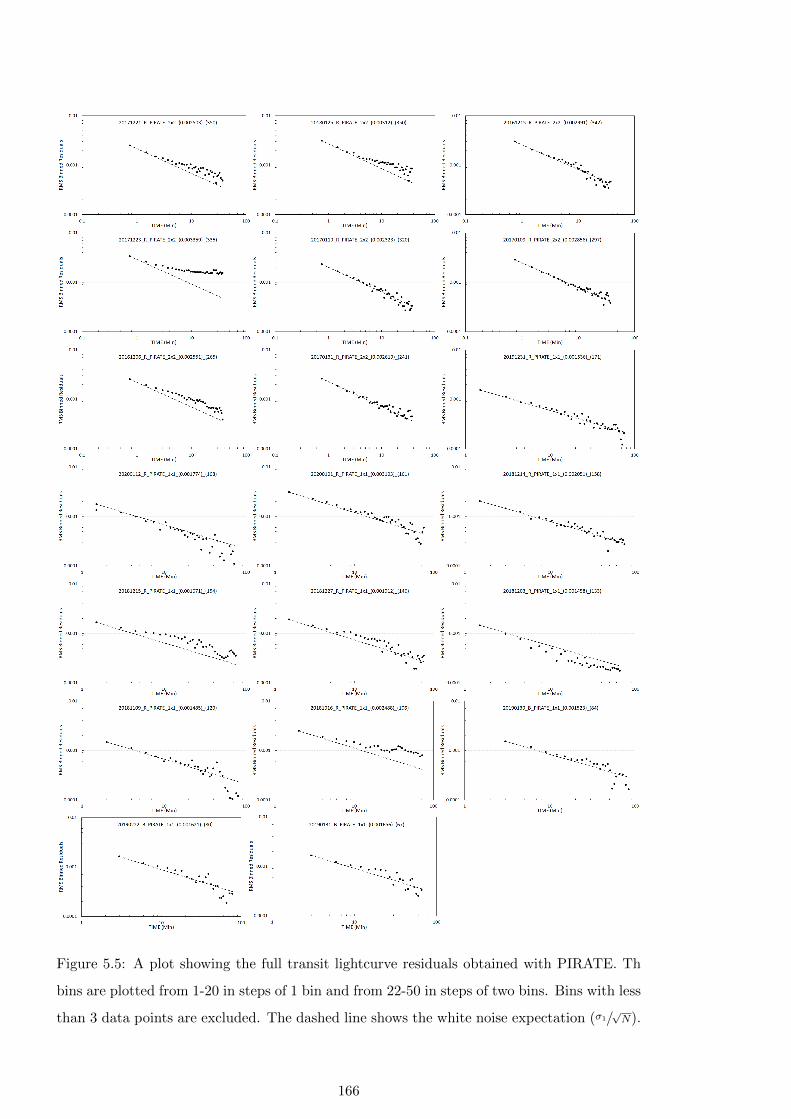
Figure 5.5: A plot showing the full transit lightcurve residuals obtained with PIRATE. Th

bins are plotted from 1-20 in steps of 1 bin and from 22-50 in steps of two bins. Bins with less

than 3 data points are excluded. The dashed line shows the white noise expectation (σ1/√N).

166

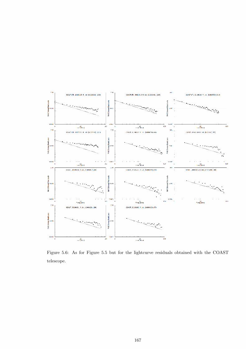
Figure 5.6: As for Figure 5.5 but for the lightcurve residuals obtained with the COAST

telescope.

167

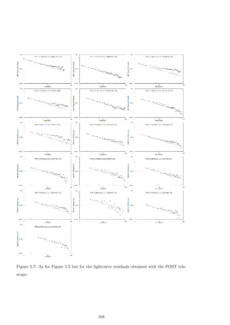
Figure 5.7: As for Figure 5.5 but for the lightcurve residuals obtained with the POST tele-

scope.

168

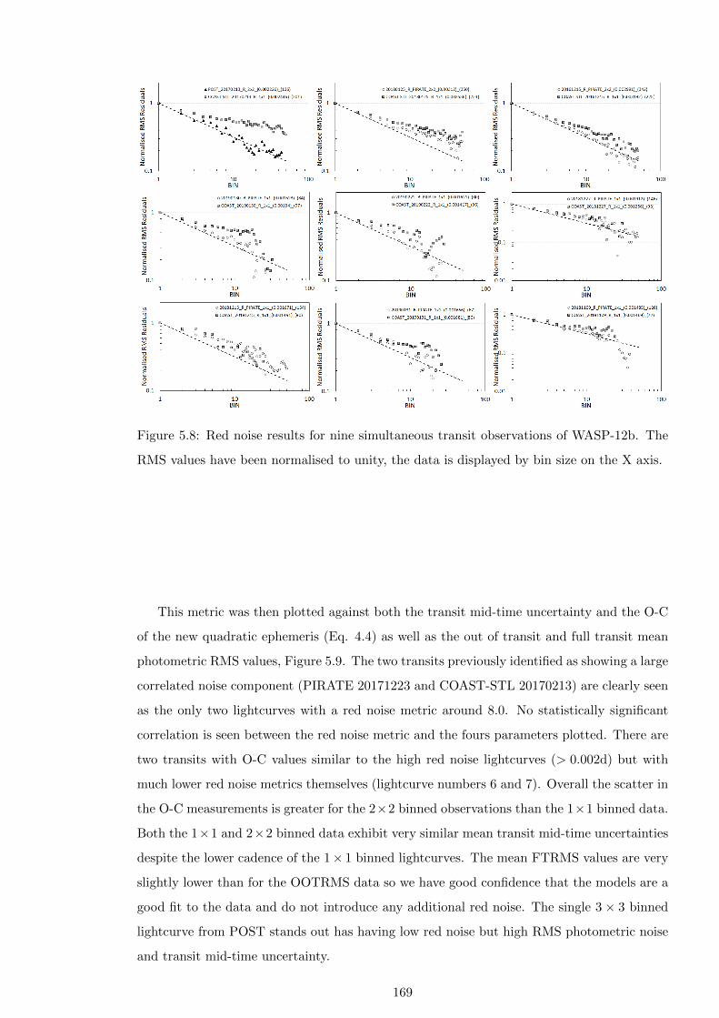
Figure 5.8: Red noise results for nine simultaneous transit observations of WASP-12b. The

RMS values have been normalised to unity, the data is displayed by bin size on the X axis.

This metric was then plotted against both the transit mid-time uncertainty and the O-C

of the new quadratic ephemeris (Eq. 4.4) as well as the out of transit and full transit mean

photometric RMS values, Figure 5.9. The two transits previously identified as showing a large

correlated noise component (PIRATE 20171223 and COAST-STL 20170213) are clearly seen

as the only two lightcurves with a red noise metric around 8.0. No statistically significant

correlation is seen between the red noise metric and the fours parameters plotted. There are

two transits with O-C values similar to the high red noise lightcurves (> 0.002d) but with

much lower red noise metrics themselves (lightcurve numbers 6 and 7). Overall the scatter in

the O-C measurements is greater for the 2×2 binned observations than the 1×1 binned data.

Both the 1×1 and 2×2 binned data exhibit very similar mean transit mid-time uncertainties

despite the lower cadence of the 1× 1 binned lightcurves. The mean FTRMS values are very

slightly lower than for the OOTRMS data so we have good confidence that the models are a

good fit to the data and do not introduce any additional red noise. The single 3× 3 binned

lightcurve from POST stands out has having low red noise but high RMS photometric noise

and transit mid-time uncertainty.

169

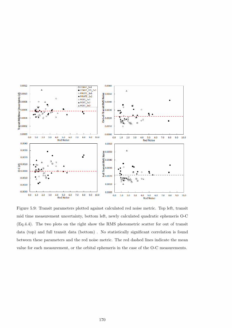
Figure 5.9: Transit parameters plotted against calculated red noise metric. Top left, transit

mid time measurement uncertainty, bottom left, newly calculated quadratic ephemeris O-C

(Eq.4.4). The two plots on the right show the RMS photometric scatter for out of transit

data (top) and full transit data (bottom) . No statistically significant correlation is found

between these parameters and the red noise metric. The red dashed lines indicate the mean

value for each measurement, or the orbital ephemeris in the case of the O-C measurements.

170

5.2.3 Tracking Performance and Impact on Photometry

The OSO telescopes are operated in unguided mode, relying on the precision of the polar

alignment, mechanical capability of the German Equatorial mounts and of the pointing model

which automatically updates the tracking to minimise star trailing in images. This approach

proved perfectly capable of ensuring no trailing was seen in individual exposures up to 3

minutes duration, the maximum exposure used. However time series observations of a full

transit typically last between 3 and 5 hours and over these timescales drift in the centroid

position of the target star is apparent. Conversely POST uses closed loop guiding to correct

for imperfect polar alignment of the mount, Chapter 2.

Figure 5.10: Guiding precision from a simultaneous observation of a HAT-P-23b transit from

30th June 2018. Left, POST with AO-8 fast guiding optics and right, PIRATE unguided

observation. The POST fast guiding maintains the target star centriod on the same pixel for

the 3 hour duration of the observation. Both CCDs were used in binning x 2 mode.

One potentially significant source of photometric noise arises from imperfect flat field

correction for pixel response variations which can be mitigated by maintaining the stellar

PSF on the same pixels for the duration of the observations or, to some extent, by defocusing

(Southworth et al., 2009b). Maintaining a star on the same pixel for the multi-hour duration

of a transit observation places high demands on a telescope system requiring closed-loop

guiding. To see whether the quality of the guiding has a material effect on the quality

of the photometry of transits obtained with small aperture ground-based telescopes a test

observation was made of HAT-P-56b using POST on the 9th January 2021. HAT-P-56b was

observed for 4.6 hours, without a pier flip, using exposures of 90 seconds (103 second cadence)

through an Rc filter. The data was reduced and analysed as detailed in Chapter 2. For flat

fielding a master frame was created from a median combine of 19 individual frames obtained

using an artificial light source on the same night. The observations were initially guided using

the AO8 fast guider with a correction rate of 1Hz. Shortly before half way through the transit

observation the autoguiding guiding was switched off. Data reduction and photometry was

171

Figure 5.11: Left, stellar centriod for HAT-P-56b on the CCD. The inset shows a single

pixel during AO8 guiding with the red cross indicating the mean value. On the right is the

roundness of the stellar PSF where the dash line indicates perfectly round stars. It can be

seen that even when guiding the PSF is slightly elongated by approximately 10% in the Y

axis (RA), after guiding was disabled the X axis (Dec) shows a reduction in the mean width

and an increase in the Y axis width as the stars become elongated in the RA direction.

In both plots filled circles are measurements during guiding and open circles are unguided

measurements.

carried out using AstroImageJ with a variable star aperture set at 1.2 × FWHM to ensure

any changes in FWHM during the experiment were correctly captured in the photometry

extraction.

During autoguiding at 1Hz the target star centroid was maintained on a single pixel. After

guiding was disabled the field drifted due to imperfect polar alignment moving 31 arcsec in

the X-direction (Declination) and 55 arcsec in the Y-direction (Right Ascension), Figure 5.11,

left. The rate of drift was 0.41 arcsec per minute which equates to 1.2 pixels per exposure

which is visible as an increase in the elongation of the stellar FWHM along the RA axis,

Figure 5.11 right. Figure 5.12 shows the transit data along with airmass, FWHM and SNR

over the observation. Airmass decreased from 1.45 at the start of the observation to 1.09

before increasing again slightly to 1.12. During the autoguided section of the observation the

airmass decreased and the SNR increased as expected, the FWHM stayed constant. After

guiding was disabled the FWHM mean remained the same but the scatter increased notably.

To analyse the quality of the photometry the out of transit data as indicated in Fig-

ure 5.12 was analysed. Before transit the flux value was 0.3570 ± 0.0004 and after transit

0.3570 ± 0.0006, with the uncertainties being the standard deviation on the measurements.

The maximum spread in measured flux values was 1.968×10−3 before ingress and 2.232×10−3

after egress, a 13% increase. The mean photometric uncertainty calculated by AstroImageJ

was 391.6±2.5×10−6 before transit and improved slightly to 389.5±2.1×10−6 after transit.

172

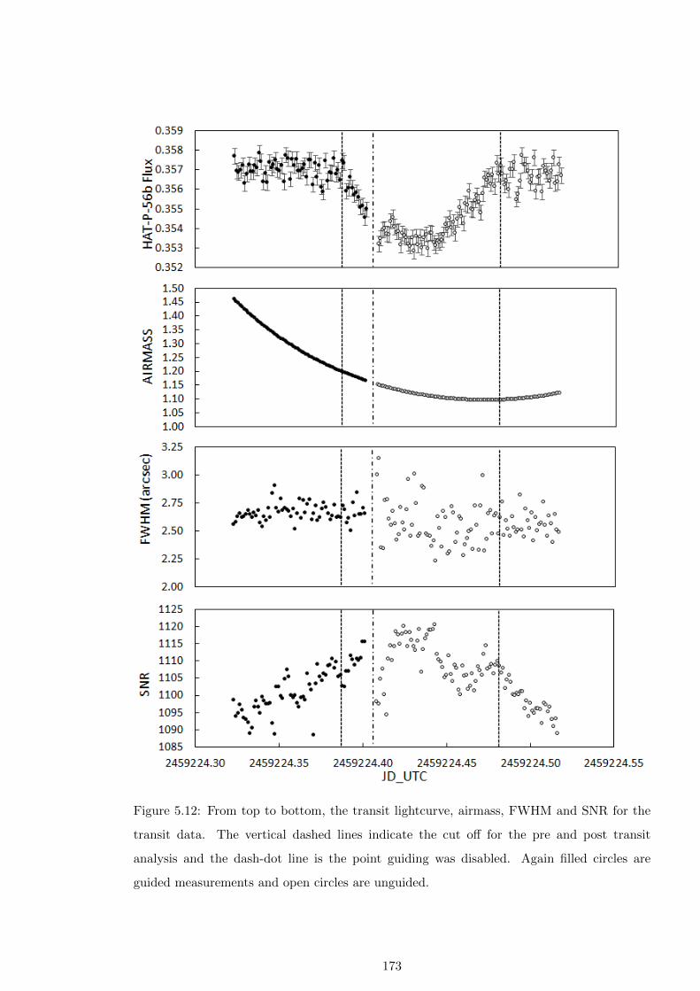
Figure 5.12: From top to bottom, the transit lightcurve, airmass, FWHM and SNR for the

transit data. The vertical dashed lines indicate the cut off for the pre and post transit

analysis and the dash-dot line is the point guiding was disabled. Again filled circles are

guided measurements and open circles are unguided.

173

The increase in photometric scatter after egress while unguided is clear as is the increased

scatter in FWHM. Airmass was greater before ingress excluding that as a cause. The SNR

values remain similar, varying by only 3% over the duration of the 4.6 hour observation. It

seems therefore that the increase in photometric scatter is a direct result of the drift of the

target star on the CCD likely arising due variations in CCD pixel response not completely

corrected for by the flat field process. Additional experiments testing alternative approaches

to the flat field calibration, such median combining a significantly larger number of individual

calibration frames or using sky flats, would determine whether the photometric scatter for

unguided imaging could be reduced further. Transit photometry precision is notably improved

by minimising drift of the target and ideally maintaining the target on the same pixels. While

PIRATE and COAST operate unguided, the superior polar alignment means the drift on

the CCD is 0.2 pixels (0.12 arcsec) per minute, over three times less than for POST. Not

enough to affect the stellar PSF during typical exposures of 30-180 seconds but over a 5 hour

observation this still amounts to approximately 60 pixels (43 arcsec) of drift. It therefore

seems likely the photometry from PIRATE and COAST could be improved further through

the implementation of sub-pixel autoguiding.

Another potential noise source arising from imperfect guiding is the transition of any

hot or cold pixels, not corrected for in the data reduction process, through the photometry

apertures. An example of this effect can be seen in a transit lightcurve of the hot Jupiter

XO-2b obtained with COAST-STL on the 4th January 2017, Figure 5.13, where hot pixels

appear close to comparison star C8 on frames 159 to 213 of 242. The cause of the hot pixels

is unexplained but during the near 4 hour observation the centroid of comparison star C8

drifted across the hot pixels. AIJ provides an iterative 2σ cleaning of hot pixels from the

sky annulus which successfully corrected for the effects but cannot be applied to the star

aperture. The contribution from the hot pixels resulted in an increase in the measured stellar

flux for the period the star aperture crossed the location of the hot pixels. The overall effect

was to increase the measured transit depth by 2.8%, introducing a systematic error in transit

depth measurement. The effect also resulted in a change in the measured transit mid-time by

23 seconds and increased the transit duration by 16 seconds. In this case with the anomaly

occurring over the transition to egress (t3), the greatest effect is on the full transit time from

the end of ingress (t2) to the start of egress (t3), excluding ingress/egress, which is reduced

by 36 seconds.

This type of noise, which is clear in the C8 comparison star flux measurements, highlights

the importance of visually checking the photometry output.

174

Figure 5.13: Transit of XO-2b obtained with COAST on 4th January 2017 showing the

impact of uncorrected hot pixels. Top, open black data points and black AIJ transit model

are without the affected star included in the photometry ensemble. The red circles and red

AIJ transit model include the affected star in the photometry ensemble. Grey dots show the

flux from the affected star which is shown in the inset composite image with the hot pixels

crossing the sky and star apertures. The central blue band highlights the data points affected

while the hot pixels were crossing the star aperture and the light blue bands either side show

where the hot pixels were present in the sky annulus. Bottom, difference between the transit

lightcurve calculated with and without the affected C8 comparison star.

175

5.2.4 Lightcurve Comparison with Published Observations

In Table 5.1 I compare the photometric precision achieved with the small aperture ground-

based telescopes used in this work with those from the literature often using larger aperture

telescopes. In Figure 5.14 I show the phase folded individual measurements and binned data

for HAT-P-23b and WASP-52b along with previously published observations made with the

telescopes compared in Table 5.1. The phase folded lightcurve for HAT-P-23b comprised 1821

individual measurements (17 full and partial transits) and a total observation time of 3337

minutes was binned by 25 data points. By comparison Mancini et al. (2017) used the Calar

Alto 2.2m telescope which has a primary mirror area approximately 24 times greater than the

telescopes used in this study and obtained a single transit observation of 244 minutes duration.

Defining a metric of telescope mirror area multiplied by the duration of observations I find

that, in the absence of spot crossing events, the binned photometric results obtained with

the small aperture ground-based result in a lightcurve with the same or better photometric

precision in half the mirror area × observation time of the 2.2m telescope observation. A

similar result was found when the phase folded and binned WASP-52b transits were compared

with those obtained using the Danish 1.54m telescope Ciceri et al. (2015).

The WASP-12b data set is larger with 42 full transits obtained through a Red filter. These

42 transits, comprising 6956 individual measurements, were phase folded and then binned to

2, 3 and 5 minute cadence achieving an out of transit RMS of 359ppm, 186ppm and 119ppm

respectively. Collins et al. (2017a) published 23 lightcurves of WASP-12b obtained with the

0.6m MORC telescope and achieved an RMS precision of 183ppm for 5 minute sample bins.

The precision would be expected to improve with√N where N is number of phase folded

lightcurves. The result of 119ppm for 42 lightcurves is ∼ 12% better than expected from just

the greater number of lightcurves used. WASP-12b was observed by the NASA Transiting

Exoplanet Survey Satellite (TESS) covering 21 new transits (Turner et al., 2021). These

observations were obtained from EXOMAST1, phase folded around the same ephemeris and

binned to a 5 minute cadence. The TESS observations provide full phase coverage so the out of

transit RMS was measured over the same phase region used for the 42 new transits, resulting

in an RMS scatter value of 204ppm. Again the difference in the two 5 minute binned RMS

values is slightly better than expected from the difference in the number of transits observed.

The phase folded lightcurves provide confidence that the lightcurves are not affected by a

correlated noise component. These results demonstrate the capability of of small aperture

ground-based telescope observations as an efficient way to collect high precision lightcurves

for system characterisation while obtaining transit timing measurements.

1https://exo.mast.stsci.edu/

176

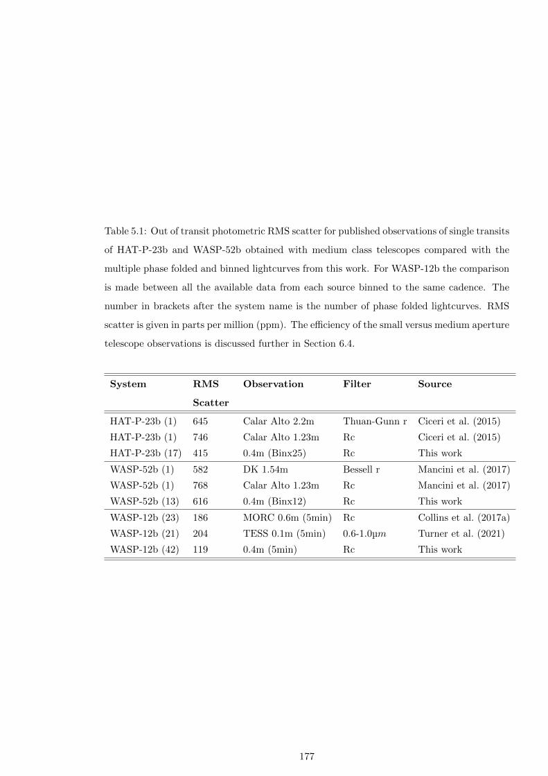
Table 5.1: Out of transit photometric RMS scatter for published observations of single transits

of HAT-P-23b and WASP-52b obtained with medium class telescopes compared with the

multiple phase folded and binned lightcurves from this work. For WASP-12b the comparison

is made between all the available data from each source binned to the same cadence. The

number in brackets after the system name is the number of phase folded lightcurves. RMS

scatter is given in parts per million (ppm). The efficiency of the small versus medium aperture

telescope observations is discussed further in Section 6.4.

System RMS

Scatter

Observation Filter Source

HAT-P-23b (1) 645 Calar Alto 2.2m Thuan-Gunn r Ciceri et al. (2015)

HAT-P-23b (1) 746 Calar Alto 1.23m Rc Ciceri et al. (2015)

HAT-P-23b (17) 415 0.4m (Binx25) Rc This work

WASP-52b (1) 582 DK 1.54m Bessell r Mancini et al. (2017)

WASP-52b (1) 768 Calar Alto 1.23m Rc Mancini et al. (2017)

WASP-52b (13) 616 0.4m (Binx12) Rc This work

WASP-12b (23) 186 MORC 0.6m (5min) Rc Collins et al. (2017a)

WASP-12b (21) 204 TESS 0.1m (5min) 0.6-1.0µm Turner et al. (2021)

WASP-12b (42) 119 0.4m (5min) Rc This work

177

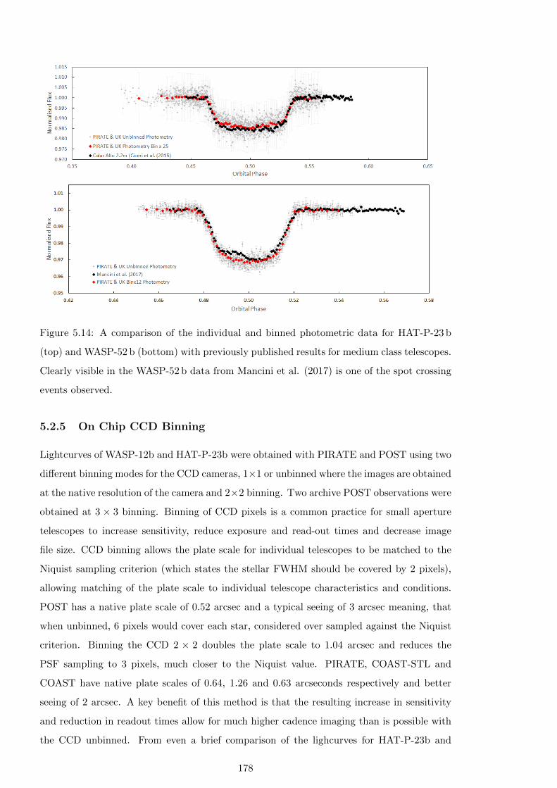
Figure 5.14: A comparison of the individual and binned photometric data for HAT-P-23 b

(top) and WASP-52 b (bottom) with previously published results for medium class telescopes.

Clearly visible in the WASP-52 b data from Mancini et al. (2017) is one of the spot crossing

events observed.

5.2.5 On Chip CCD Binning

Lightcurves of WASP-12b and HAT-P-23b were obtained with PIRATE and POST using two

different binning modes for the CCD cameras, 1×1 or unbinned where the images are obtained

at the native resolution of the camera and 2×2 binning. Two archive POST observations were

obtained at 3 × 3 binning. Binning of CCD pixels is a common practice for small aperture

telescopes to increase sensitivity, reduce exposure and read-out times and decrease image

file size. CCD binning allows the plate scale for individual telescopes to be matched to the

Niquist sampling criterion (which states the stellar FWHM should be covered by 2 pixels),

allowing matching of the plate scale to individual telescope characteristics and conditions.

POST has a native plate scale of 0.52 arcsec and a typical seeing of 3 arcsec meaning, that

when unbinned, 6 pixels would cover each star, considered over sampled against the Niquist

criterion. Binning the CCD 2 × 2 doubles the plate scale to 1.04 arcsec and reduces the

PSF sampling to 3 pixels, much closer to the Niquist value. PIRATE, COAST-STL and

COAST have native plate scales of 0.64, 1.26 and 0.63 arcseconds respectively and better

seeing of 2 arcsec. A key benefit of this method is that the resulting increase in sensitivity

and reduction in readout times allow for much higher cadence imaging than is possible with

the CCD unbinned. From even a brief comparison of the lighcurves for HAT-P-23b and

178

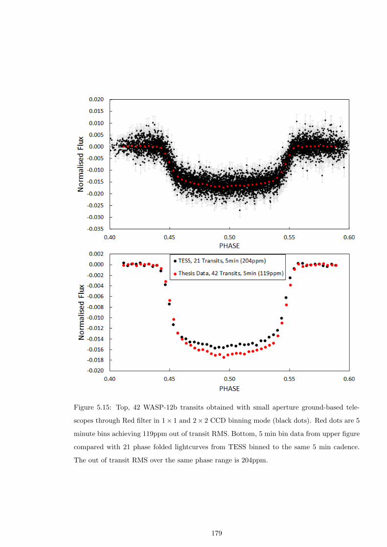
Figure 5.15: Top, 42 WASP-12b transits obtained with small aperture ground-based tele-

scopes through Red filter in 1× 1 and 2× 2 CCD binning mode (black dots). Red dots are 5

minute bins achieving 119ppm out of transit RMS. Bottom, 5 min bin data from upper figure

compared with 21 phase folded lightcurves from TESS binned to the same 5 min cadence.

The out of transit RMS over the same phase range is 204ppm.

179

WASP-12b it is clear that the lightcurves obtained using on chip binning contain many more

measurements but show considerably greater scatter in the photometry than those obtained

unbinned. The question I address in this sub-section is whether the higher cadence/higher

noise binned observations or lower cadence/lower noise un-binned observations provide more

accurate and precise transit measurements for small aperture ground-based telescope follow

up of transiting exoplanets. The natural assumption, my null hypothesis, is that higher

cadence imaging should produce greater transit timing precision as the lightcurve is sampled

more frequently.

Figure 5.16 plots the mean photometric signal versus the mean photometric noise in

ADU per second of exposure (excluding download time). A clear differentiation is seen in

the SNR between PIRATE 1 × 1 and 2 × 2 lightcurves for all three systems. The same

trend of higher noise with higher signal is seen in both but with a lower noise value for

the unbinned observations. There is a single unbinned outlying point where a lightcurve of

HAT-P-23b was erroneously obtained unbinned but with the exposure settings used for the

binned observation. For POST only WASP-12b was observed with 1 × 1 and 2 × 2 CCD

binning but the same separation is not seen. It is clear from the plot for PIRATE that the

unbinned observations provide a greater reduction in noise than signal, leading to overall

higher SNR than the 2 × 2 binned observations. The longer exposure durations used for

the unbinned observations more than offset the greater sensitivity expected for the 2 × 2

binned lightcurves. The increased exposure durations used for the unbinned observations

were typically 2 - 3 times the 2× 2 binned exposure duration rather than four times, as may

be expected from additional sensitivity implied by combining the electron count from four

pixels in 2× 2 binning.

In Section 5.5 I compare the transit timing results in detail. Here I consider further

the effect of cadence and RMS scatter on the transit timing measurements by comparing

observations taken at high cadence in 2 × 2 mode, binned to the same cadence as the 1 × 1

observations. A number of lightcurves obtained using PIRATE, both unbinned and binned

2×2, are available for WASP-12b and HAT-P-23b. Two average lightcurves were selected for

each system obtained in 2 × 2 on-chip binning mode and the lightcurves binned in software

to the same lower cadence as the lightcurves obtained at the CCD native resolution.

The transit model independent out-of-transit RMS for the lightcurves is compared in

Table 5.2. For both systems binning the 2 × 2 observations to the same cadence as the

1× 1 data reduced the oot RMS by 30%. The RMS of the time binned lightcurves was still

greater than the un-binned data. The result shows that time binning higher cadence single

lightcurve data obtained with 2× 2 on-chip binning produces inferior lightcurve precision to

lower cadence lightcurves obtained in un-binned mode.

180

Figure 5.16: Sky subtracted signal and noise for unbinned and 2× 2 binned observations of

all three systems observed with PIRATE as calculated in AIJ. The values for signal and noise

are in ADU’s per second. The lower noise for a given signal value of unbinned over 2 × 2

binning is clear. Blue symbols are observations of WASP-12b made through B filter, all other

observations are R filter.

The transit mid-times uncertainties and O-C values for the test lightcurves are also shown

in Table 5.2. Binning the 2×2 lightcurves to the same cadence as the 1×1 lightcurves resulted

in transit mid-time uncertainties that are significantly worse than the original lightcurves

and worse than the control lightcurves obtained at 1 × 1. The scatter about the calculated

ephemeris also increased or remained unchanged. This result clearly shows that lower ca-

dence/lower noise transits obtained with the CCD read out in unbinned (1×1) mode provide

more precise and accurate timing results than higher cadence/higher noise lightcurves.

5.3 Transit Parameter Determination

The majority of transit observations obtained with small aperture telescopes are used individ-

ually to determine a transit mid-time in order to calculate and improve the orbital ephemeris.

In Chapters 3 and 4 I used the transit lightcurves to also derive parameters for each of the

three systems observed and compared the results with those previously published, see Figures

3.4, 3.7 and 4.19.

The determination of R∗ in Exofast V2 was achieved using MIST stellar models with a

photometric SED and distance prior from Gaia DR2 along with dust extinction estimation.

181

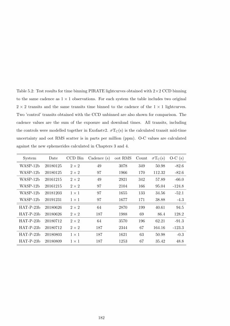
Table 5.2: Test results for time binning PIRATE lightcurves obtained with 2×2 CCD binning

to the same cadence as 1 × 1 observations. For each system the table includes two original

2 × 2 transits and the same transits time binned to the cadence of the 1 × 1 lightcurves.

Two ’control’ transits obtained with the CCD unbinned are also shown for comparison. The

cadence values are the sum of the exposure and download times. All transits, including

the controls were modelled together in Exofastv2. σTC(s) is the calculated transit mid-time

uncertainty and oot RMS scatter is in parts per million (ppm). O-C values are calculated

against the new ephemerides calculated in Chapters 3 and 4.

System Date CCD Bin Cadence (s) oot RMS Count σTC(s) O-C (s)

WASP-12b 20180125 2× 2 49 3078 349 50.98 -82.6

WASP-12b 20180125 2× 2 97 1966 170 112.32 -82.6

WASP-12b 20161215 2× 2 49 2921 342 57.89 -66.0

WASP-12b 20161215 2× 2 97 2104 166 95.04 -124.8

WASP-12b 20181203 1× 1 97 1655 133 34.56 -52.1

WASP-12b 20191231 1× 1 97 1677 171 38.88 -4.3

HAT-P-23b 20180626 2× 2 64 2870 199 40.61 94.5

HAT-P-23b 20180626 2× 2 187 1988 69 86.4 128.2

HAT-P-23b 20180712 2× 2 64 3570 196 62.21 -91.3

HAT-P-23b 20180712 2× 2 187 2344 67 164.16 -123.3

HAT-P-23b 20180803 1× 1 187 1621 63 50.98 -0.3

HAT-P-23b 20180809 1× 1 187 1253 67 35.42 48.8

182

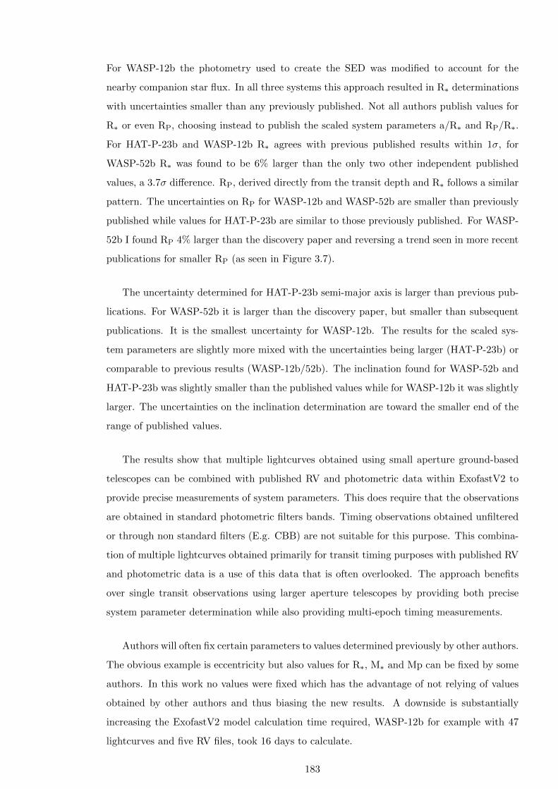
For WASP-12b the photometry used to create the SED was modified to account for the

nearby companion star flux. In all three systems this approach resulted in R∗ determinations

with uncertainties smaller than any previously published. Not all authors publish values for

R∗ or even RP, choosing instead to publish the scaled system parameters a/R∗ and RP/R∗.

For HAT-P-23b and WASP-12b R∗ agrees with previous published results within 1σ, for

WASP-52b R∗ was found to be 6% larger than the only two other independent published

values, a 3.7σ difference. RP, derived directly from the transit depth and R∗ follows a similar

pattern. The uncertainties on RP for WASP-12b and WASP-52b are smaller than previously

published while values for HAT-P-23b are similar to those previously published. For WASP-

52b I found RP 4% larger than the discovery paper and reversing a trend seen in more recent

publications for smaller RP (as seen in Figure 3.7).

The uncertainty determined for HAT-P-23b semi-major axis is larger than previous pub-

lications. For WASP-52b it is larger than the discovery paper, but smaller than subsequent

publications. It is the smallest uncertainty for WASP-12b. The results for the scaled sys-

tem parameters are slightly more mixed with the uncertainties being larger (HAT-P-23b) or

comparable to previous results (WASP-12b/52b). The inclination found for WASP-52b and

HAT-P-23b was slightly smaller than the published values while for WASP-12b it was slightly

larger. The uncertainties on the inclination determination are toward the smaller end of the

range of published values.

The results show that multiple lightcurves obtained using small aperture ground-based

telescopes can be combined with published RV and photometric data within ExofastV2 to

provide precise measurements of system parameters. This does require that the observations

are obtained in standard photometric filters bands. Timing observations obtained unfiltered

or through non standard filters (E.g. CBB) are not suitable for this purpose. This combina-

tion of multiple lightcurves obtained primarily for transit timing purposes with published RV

and photometric data is a use of this data that is often overlooked. The approach benefits

over single transit observations using larger aperture telescopes by providing both precise

system parameter determination while also providing multi-epoch timing measurements.

Authors will often fix certain parameters to values determined previously by other authors.

The obvious example is eccentricity but also values for R∗, M∗ and Mp can be fixed by some

authors. In this work no values were fixed which has the advantage of not relying of values

obtained by other authors and thus biasing the new results. A downside is substantially

increasing the ExofastV2 model calculation time required, WASP-12b for example with 47

lightcurves and five RV files, took 16 days to calculate.

183

5.4 Monitoring Photometry

As discussed in Chapters 3 and 4 for HAT-P-23 and WASP-12 I used the results of host star

monitoring to look for any variability due to rotation. In this section I review the monitoring

photometry obtained over multiple observing seasons, discuss the quality of the observations

and analyse the suitability of PIRATE to undertake long term, multi season monitoring

observations of exoplanet host stars. Understanding host star variability helps us understand

the host star itself, identifying rotation periods and stellar cycles which in turn can be used

to plan spectroscopic atmosphere observations when activity is at a minimum, E.g. inform

ARIEL observation scheduling.

PIRATE was used to undertake all the monitoring observations of both systems, POST

was not used for this purpose due to its semi-manual operation and small number of cloud

free nights. For the HAT-P-23 field the nightly observations were made with groups of 6

frames which exhibited a typical spread of 0.007 mag for each a night. The mean photometric

uncertainty was 0.002 mag. The stability of the long term photometry can be seen by studying

the stable check star observed in the same field as the target star. The standard error of

the nightly mean magnitude is 0.002 mag over 93 days, equal to the mean measurement

uncertainty, see Figure 5.17, top panel. This is a significant improvement over the nightly

spread in measurements, highlighting the importance of combining multiple observations per

night. The uncertainty on the individual data points were combined in quadrature giving a

nightly uncertainty of 0.005 magnitude. For HAT-P-23b the monitoring observations were

supplemented with measurements obtained from the out of transit portion of the lightcurve

on nights transits were observed. The magnitude measurements obtained from the out of

transit data were found to have a -0.01 mag offset for the 2 × 2 on-chip binning compared

to the un-binned monitoring observations which was corrected for prior to the analysis. The

monitoring observations conducted with PIRATE were clearly able to detect the 0.011 mag

variation of HAT-P-23 in measurements spanning 93 days.

As with the transit observations a different mean magnitude is observed depending on

whether the optical tube is located on the East or West side of the German equatorial mount,

this effect amounted to a difference of 0.002 mag for the check star which was corrected by

bringing the observations made when pointing East or West together by half the difference

so the resulting magnitude determined is the mean of the East and West measurements.

The resulting instrumental magnitude of the check star determined was 12.351±0.002 which

compares with 12.349±0.01 from UCAC4 but as the observations were made using Johnson-

Cousins Rc filter and the comparison ensemble were measured using the SDSS r′ filter the

measured and catalogue values cannot be directly compared.

184

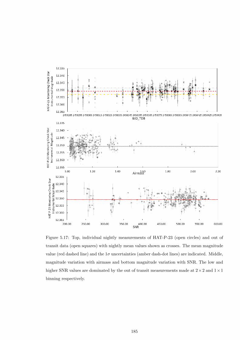
Figure 5.17: Top, individual nightly measurements of HAT-P-23 (open circles) and out of

transit data (open squares) with nightly mean values shown as crosses. The mean magnitude

value (red dashed line) and the 1σ uncertainties (amber dash-dot lines) are indicated. Middle,

magnitude variation with airmass and bottom magnitude variation with SNR. The low and

higher SNR values are dominated by the out of transit measurements made at 2×2 and 1×1

binning respectively.

185

The middle and bottom panels of Figure 5.17 show how the detrended check star photom-

etry was affected by changing airmass and SNR of the observations. No trend of changing

magnitude with increasing airmass is seen following detrending. The SNR plot at bottom

clearly shows the out of transit measurements dominating the low and high end of the SNR

range for 2× 2 and 1× 1 on-chip binning respectivly. Again no trend of changing magnitude

is seen with SNR though the lower SNR . 350 show slightly increased scatter. The stability

of the SNR for the monitoring observations was aided by the use of a variable star aperture in

AstroImageJ which ensured all the stellar flux was contained within the photometry aperture

regardless of any night to night FWHM variations.

No variability was detected in WASP-12 but previously undetected variability was found

in J0630+2942. As with the HAT-P-23 data here I focus on the quality of the check star

observations obtained this time over multiple seasons and with different filters, bin modes and

exposure durations. For the WASP-12 monitoring observations the first two seasons data,

2016/17 and 2017/18 were obtained through Baader red and blue filters with the CCD camera

operating 2× 2 binning mode. Exposures for all red filter observations were 45 seconds and

for the blue filter 90 seconds were used for 2016/17 season and 60 seconds for the 2017/18

season, though a small number of blue filter observations were obtained inadvertently with

45 second exposures for the second season. The data was detrended and offset corrected as

described in Chapter 4. The 2016-17 season represents the densest data set with up to 169

measurements in a single night. For the 2018/19 season Johnson-Cousins Rc and B filters

were used with the CCD in 1 × 1 binning mode. Exposures were either 120 second or 90

second for the Rc filter and 180 seconds for B filter.

The monitoring observation schedule made multiple observations per night in groups of

6 after the initial 2016-17 season. On many occasions multiple groups of observations were

obtained each, sometimes with the optical tube on different sides of the mount. The aim of

taking multiple observations each night being to increase photometric precision. Table 5.3

compares the spread in nightly measurements to the photometric error, the whole season

standard deviation and the whole season standard deviation with the data binned to a single

mean data point for each night. For the first two WASP-12 seasons the nightly spread in

measurements reached almost 0.02 mag for the blue filter data, over 6 times larger than the

standard deviation in the mean nightly values over the whole season. This result clearly

highlights the need to make multiple monitoring observations of a given target each night. It

is also clear that the WASP-12 2018-19 and HAT-P-23b 2018 seasons observations made using

the CCD in 1 × 1 binned mode with subsequently longer exposures produced significantly

more stable measurements. Fewer but longer exposures at 1× 1 binning produce more stable

results than a greater number of shorter exposures at 2× 2 binning.

186

Table 5.3: Comparison of mean nightly and seasonal monitoring precision. Spread is the

mean min-max spread in measurements obtained each night. The seasonal 1σ is the standard

deviation in detrended measurements over the whole season and and the nightly 1σ value is

the standard deviation calculated from the nightly mean magnitudes. Observations obtained

with the CCD camera in 1×1 binning mode produced more consistent results. σ is the mean

individual measurement uncertainty.

Season Filter Spread Seasonal 1σ Nightly 1σ σc

WASP-12 Check Star

2016-17 Red 0.018 0.006 0.004 0.003

2016-17 Blue 0.019 0.006 0.003 0.004

2017-18 Red 0.010 0.006 0.004 0.004

2017-18 Blue 0.019 0.008 0.005 0.006

2018-19 Rc 0.004 0.004 0.004 0.002

2018-19 B 0.004 0.004 0.004 0.002

HAT-P-23 Check Star

2018 Rc 0.007 0.003 0.002 0.002

As with HAT-P-23 the airmass-magnitude plots show that there is no remaining trend in

the magnitude measurements with increasing airmass after detrending, out to the limit of the

observations around an airmass of 2. Similarly the SNR-magnitude plots also show no trend

in magnitude values. It can be seen, especially in the 2016-17 season data, that observations

made with an SNR < 300 show considerably greater scatter in magnitude measurement. For

the Red filter observations the scatter in the magnitude measurement doubles from 0.005 to

0.01 for SNR < 300. Similarly for the blue filter the scatter increases from 0.005 to 0.007. In

both cases the mean magnitude values agree within the uncertainties. For the 2018-19 season

obtained in 1× 1 mode a similar trend of increasing scatter in the magnitude measurements

can be seen for SNR < 550. This is less apparent in the HAT-P-23 data which was all

obtained with a SNR below this value. Within each nights observations the SNR value is

negatively correlated with changes in airmass. Observations over multiple nights show a

wide range of SNR values for a given airmass resulting from different FWHM values due

in part to possible seeing changes but most likely due to different focus positions, SNR is

strongly correlated with FWHM. This correlation is not seen between FWHM and determined

magnitude measurement indicating the photometry aperture selection correctly accounts for

changes in FWHM over a season.

Again as for HAT-P-23 the monitoring photometry was corrected for a constant offset

between the magnitude measurements when the telescope was on the East or West side of

187

Figure 5.18: Example of the target star positioning in the PIRATE CCD frame from the

2018-19 season B filter observations showing the consistent centering of the WASP-12 target

and the change in location of the check star caused by pier flips for Meridian crossing. Insets

show detail of each stars position.

the mount. Individual offset corrections were calculated for each star, filter and season.

For the WASP-12b 2016-17 and 2017-18 seasons the offset correction values for WASP-12,

J0630+2942 and the check star in each filter are in good agreement with each other. The

offset value is always greater in R than B and is greater for the check star than either WASP-

12 or J0630+2942. The same results are seen for the 2018-19 season data obtained at 1× 1

binning through standard filters with the exception that the offset values for Rc and B are in

much closer agreement. Figure 5.18 shows an example of the target stars positioning on the

CCD chip for the 2018-19 season B filter data. This shows that PIRATE exhibits excellent

repeatability in placing the target star at the CCD centre, minimising position changes on

the CCD before and after pier flips. J0630+2942 being located close to WASP-12 is affected

slightly more by pier flip while the check star, being located closer to the edge of the frame,

is affected the most. This indicates that the magnitude of the measurement offset is likely

related to the amount of position change on the CCD. That the effect is greater in R filter

bands than B would seem to rule out Luna illumination as the cause, the CCD camera has

greater sensitivity in the red regions than in the blue. The pier flip offset effect is common in

German Equatorial mounted telescopes and is also seen in transit data obtained with all three

telescopes indicating any cause is not local to the PIRATE telescope. Further investigation

is required to positively identify the cause.

For long term monitoring the photometric consistency between seasons is of key impor-

tance. The 2016-17 and 2017-18 season observations o WASP-12 were obtained with the same

parameters allowing direct comparison, see Table 4.9. The Red filter magnitude from each

season agree to 1.5σ with the same seasonal measurement uncertainty of 0.004 mag. The

blue filter data similarly agree though, the uncertainty on the 2017-18 season blue data is

greater where it is affected more by Luna illumination later in the season (Figure 5.20). The

188

2018-19 season data was obtained using different filters so is not directly comparable, though

the seasonal uncertainty values are similar. The 2018-19 season data obtained through a

Johnson B filter is the only data directly comparable with the UCAC4 catalogue values. The

UCAC4 value for the check star used is 12.345± 0.05 and the seasonal mean measured with

PIRATE is 12.331± 0.004, providing a 10 fold increase in measured magnitude precision.

The results show that

• Snapshot monitoring observations should ideally be constrained to airmass below 2.

• Multiple snap-shot observations per night are required to provide precise results, single

magnitude measurements would provide significantly inferior results.

• SNR values & 350 for 2 × 2 on-chip binned observations and & 550 for un-binned

observations are required to minimise the uncertainty in the magnitude measurements.

• The magnitude measurements obtained in given filters have proved to be stable over

multiple seasons.

• Correction of the magnitude offset seen between observations made when the telescope

is pointing to the East or West is required.

• The wide field of view of small aperture telescopes is well suited to this task, ensuring

many catalogue reference stars are available and allowing monitoring of stars used in

transit lightcurve comparison ensembles to also be monitored for variability.

• The scheduling methods adopted for PIRATE (also available for COAST) with the

ability to schedule “filler” observations within set parameters that can be made in

between observing higher priority targets makes efficient use of available telescope time

for monitoring observations.

189

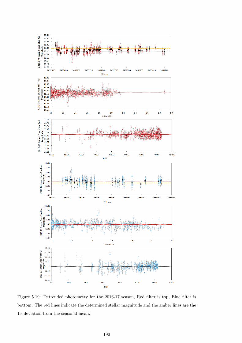
Figure 5.19: Detrended photometry for the 2016-17 season, Red filter is top, Blue filter is

bottom. The red lines indicate the determined stellar magnitude and the amber lines are the

1σ deviation from the seasonal mean.

190

Figure 5.20: As Figure 5.19 but for the the 2017-18 season.

191

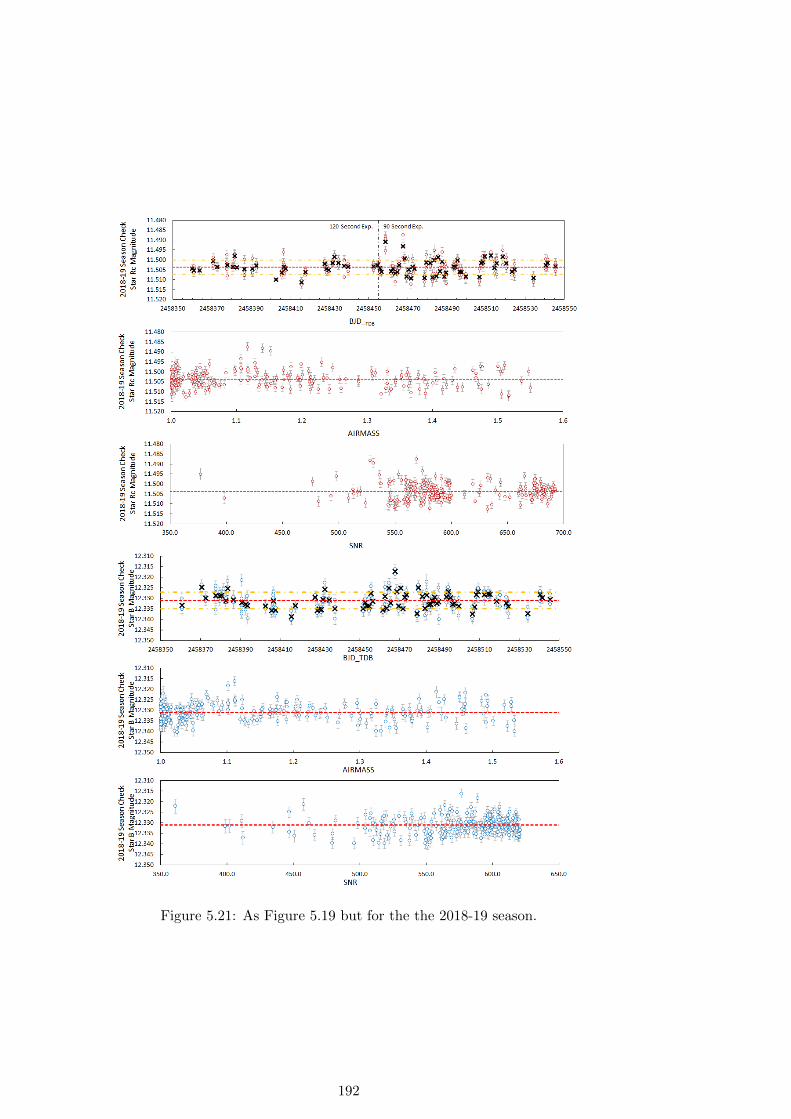
Figure 5.21: As Figure 5.19 but for the the 2018-19 season.

192

5.5 Transit Mid-Time Precision

5.5.1 WASP-12b

Table 5.4 summarises the mean transit timing measurements obtained for 47 transits of

WASP-12b using the quadratic ephemeris from equation 4.4 from before and after the instal-

lation of GPS timing control for COAST and PIRATE and the replacement of the COAST

CCD. The observations made before the GPS upgrade with all telescopes were made at 2× 2

binning and after all are 1 × 1 binning, POST was not part of the GPS upgrade but the

observing mode was changed to 1 × 1 binning at the same time so serves as a comparison

with PIRATE and COAST. The PIRATE values include three transits obtained through the

B filter and POST includes a single Ic filter transit the remainder are broadband red or Rc.

The O-C measurements and change in measurement spread are plotted in Figure 5.22.

Table 5.4: Mean transit time measurements for WASP-12b from the three telescopes, shown

by pre and post GPS upgrade date. σ(O−C) is the standard deviation in the O-C calculations.

All values have units of day.

PIRATE COAST POST

Pre upgrade O-C Mean 0.000424 0.000757 0.000230

Pre upgrade σ(O−C) 0.001327 0.002088 0.000890

Mean timing error (CCD bin 2× 2) 0.000520 0.000633 0.000587

Post upgrade O-C Mean 0.000098 0.000090 0.000036

Post upgrade σ(O−C) 0.000606 0.000928 0.000815

Mean timing error (CCD bin 1× 1) 0.000558 0.000529 0.000597

Table 5.4 shows that, following the OSO telescopes upgrade and the switch to 1 × 1

binning, the mean O-C value is much closer to the calculated ephemeris. The fact that this

is seen for all three telescopes indicates the improvement in timing precision is due to the

switch to 1×1 binning. Following the upgrade the the mean O-C value for the OSO telescopes

lightcurves is ∼ 8 seconds, the improvement is most obvious for COAST with the new CCD

camera where this was ∼ 65 seconds before the upgrade.

The values for the transit mid-time standard deviation (σ(O−C)) show that for PIRATE

and COAST the spread in timing measurements has more than halved following the upgrade.

At the same time POST shows a minimal 9% reduction, indicating the that improvement

in the measurement scatter arises from the GPS upgrade rather than the change to 1 × 1

binning.

For all three telescopes the measurement uncertainty remained comparable before and

after the upgrade, indicating the change to 1 × 1 binning with the associated decrease in

193

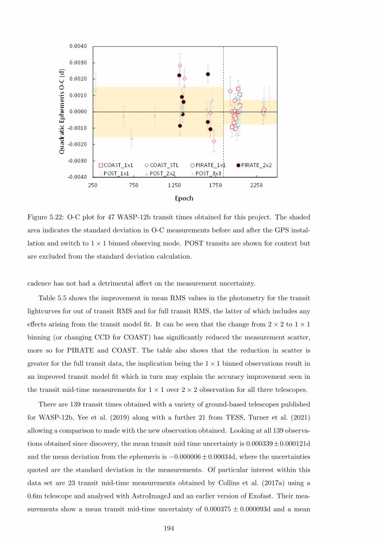
Figure 5.22: O-C plot for 47 WASP-12b transit times obtained for this project. The shaded

area indicates the standard deviation in O-C measurements before and after the GPS instal-

lation and switch to 1× 1 binned observing mode. POST transits are shown for context but

are excluded from the standard deviation calculation.

cadence has not had a detrimental affect on the measurement uncertainty.

Table 5.5 shows the improvement in mean RMS values in the photometry for the transit

lightcurves for out of transit RMS and for full transit RMS, the latter of which includes any

effects arising from the transit model fit. It can be seen that the change from 2× 2 to 1× 1

binning (or changing CCD for COAST) has significantly reduced the measurement scatter,

more so for PIRATE and COAST. The table also shows that the reduction in scatter is

greater for the full transit data, the implication being the 1× 1 binned observations result in

an improved transit model fit which in turn may explain the accuracy improvement seen in

the transit mid-time measurements for 1× 1 over 2× 2 observation for all three telescopes.

There are 139 transit times obtained with a variety of ground-based telescopes published

for WASP-12b, Yee et al. (2019) along with a further 21 from TESS, Turner et al. (2021)

allowing a comparison to made with the new observation obtained. Looking at all 139 observa-

tions obtained since discovery, the mean transit mid time uncertainty is 0.000339±0.000121d

and the mean deviation from the ephemeris is −0.000006±0.00034d, where the uncertainties

quoted are the standard deviation in the measurements. Of particular interest within this

data set are 23 transit mid-time measurements obtained by Collins et al. (2017a) using a

0.6m telescope and analysed with AstroImageJ and an earlier version of Exofast. Their mea-

surements show a mean transit mid-time uncertainty of 0.000375 ± 0.000093d and a mean

194

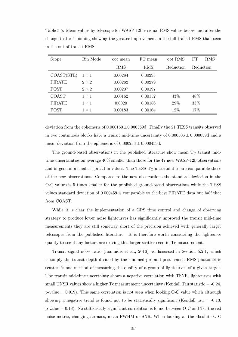
Table 5.5: Mean values by telescope for WASP-12b residual RMS values before and after the

change to 1× 1 binning showing the greater improvement in the full transit RMS than seen

in the out of transit RMS.

Scope Bin Mode oot mean

RMS

FT mean

RMS

oot RMS

Reduction

FT RMS

Reduction

COAST(STL) 1× 1 0.00284 0.00293

PIRATE 2× 2 0.00282 0.00279

POST 2× 2 0.00207 0.00197

COAST 1× 1 0.00162 0.00152 43% 48%

PIRATE 1× 1 0.0020 0.00186 29% 33%

POST 1× 1 0.00183 0.00164 12% 17%

deviation from the ephemeris of 0.000160±0.000369d. Finally the 21 TESS transits observed

in two continuous blocks have a transit mid-time uncertainty of 0.000505± 0.000059d and a

mean deviation from the ephemeris of 0.000233± 0.000459d.

The ground-based observations in the published literature show mean TC transit mid-

time uncertainties on average 40% smaller than those for the 47 new WASP-12b observations

and in general a smaller spread in values. The TESS TC uncertainties are comparable those

of the new observations. Compared to the new observations the standard deviation in the

O-C values is 5 times smaller for the published ground-based observations while the TESS

values standard deviation of 0.000459 is comparable to the best PIRATE data but half that

from COAST.

While it is clear the implementation of a GPS time control and change of observing

strategy to produce lower noise lightcurves has significantly improved the transit mid-time

measurements they are still someway short of the precision achieved with generally larger

telescopes from the published literature. It is therefore worth considering the lightcurve

quality to see if any factors are driving this larger scatter seen in Tc measurement.

Transit signal noise ratio (Ioannidis et al., 2016) as discussed in Section 5.2.1, which

is simply the transit depth divided by the summed pre and post transit RMS photometric

scatter, is one method of measuring the quality of a group of lightcurves of a given target.

The transit mid-time uncertainty shows a negative correlation with TSNR, lightcurves with

small TNSR values show a higher Tc measurement uncertainty (Kendall Tau statistic = -0.24,

p-value = 0.019). This same correlation is not seen when looking O-C value which although

showing a negative trend is found not to be statistically significant (Kendall tau = -0.13,

p-value = 0.18). No statistically significant correlation is found between O-C and Tc, the red

noise metric, changing airmass, mean FWHM or SNR. When looking at the absolute O-C

195

value , i.e. just the magnitude of the deviation from the ephemeris without its sign, more

of the lightcurve quality measures show a statistically significant correlation. For example

TSNR, red noise metric, total out of transit coverage and the change in airmass over the

duration of the observation are all correlated with the magnitude of the O-C. This indicates

that these quality factors do affect the precision of the transit mid-time measurements by

increasing the spread in measurement value but they do so in a way that affects the amplitude

of the spread without preference for whether the derived O-C value is positive or negative.

This provides confidence that although the timing measurements exhibit a greater spread

than seen in the literature, their mean value is a true representation of the transit ephemeris.

With a fixed transit depth (for a given filter) the TSNR depends only on the out of

transit RMS scatter in the measurements taken as a mean from the pre and post transit

coverage. The TSNR metric does not take into account how this RMS may change during

an observation, for example from changing airmass which may result in significantly different

RMS values either side of the transit. Excluding transits with two or fewer data points on

either side of transit, the individual WASP-12b transits exhibit the same RMS value (to 5dp).

No correlation is seen between the ratio of pre to post RMS and the O-C value or with the

transit mid-time uncertainty.

Having out of transit coverage is important for the transit model fitting solution. It is

conceivable that the duration of out of transit coverage or differences between pre and post

transit coverage could affect the TC measurement. The TC uncertainty shows no statistically

significant correlation with the pre-transit, post transit or total out-of-transit duration. The

O-C measurements do show a statistically significant negative correlation with the post transit

coverage duration (Kendall tau = -0.24, p-value = 0.016) that is not seen with the pre-transit

or total out of transit duration. As a result the pre-transit to post transit coverage ratio show

shows a moderate correlation with O-C, (Kendall tau = 0.18, p-value = 0.071).

Of the 19 transits observed with the OSO telescopes in the 2018-20 seasons after the

GPS upgrade and all using 1 × 1 binning, 12 have pre-transit coverage shorter than the

ingress/egress duration, Table 5.6. These 12 transits have a mean absolute O-C value that

is double the value for the 7 transits where pre-transit coverage exceeds the ingress/egress

duration and the spread in O-C is 77% greater. This result confirms that transit times are

more consistent where pre-transit coverage duration equals or exceeds the ingress duration.

Finally the data was analysed to see if the occurrence of a pier flip for a meridian crossing

during the transit observation affected the O-C mean or scatter. 21 of the 47 transits con-

tained a pier flip and they show a mean closer to the ephemeris than those transits without

a flip with a smaller scatter in the O-C measurements, Table 5.7. Therefore the pier flip

detrending carried out in ExofastV2 does not adversely affect the derived transit times.

196

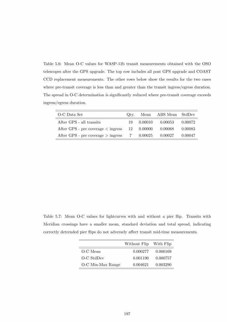
Table 5.6: Mean O-C values for WASP-12b transit measurements obtained with the OSO

telescopes after the GPS upgrade. The top row includes all post GPS upgrade and COAST

CCD replacement measurements. The other rows below show the results for the two cases

where pre-transit coverage is less than and greater than the transit ingress/egress duration.

The spread in O-C determination is significantly reduced where pre-transit coverage exceeds

ingress/egress duration.

O-C Data Set Qty. Mean ABS Mean StdDev

After GPS - all transits 19 0.00010 0.00053 0.00072

After GPS - pre coverage < ingress 12 0.00000 0.00068 0.00083

After GPS - pre coverage > ingress 7 0.00025 0.00027 0.00047

Table 5.7: Mean O-C values for lightcurves with and without a pier flip. Transits with

Meridian crossings have a smaller mean, standard deviation and total spread, indicating

correctly detrended pier flips do not adversely affect transit mid-time measurements.

Without Flip With Flip

O-C Mean 0.000277 0.000169

O-C StdDev 0.001190 0.000757

O-C Min-Max Range 0.004621 0.003290

197

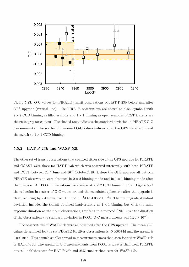
Figure 5.23: O-C values for PIRATE transit observations of HAT-P-23b before and after

GPS upgrade (vertical line). The PIRATE observations are shown as black symbols with

2× 2 CCD binning as filled symbols and 1× 1 binning as open symbols. POST transits are

shown in grey for context. The shaded area indicates the standard deviation in PIRATE O-C

measurements. The scatter in measured O-C values reduces after the GPS installation and

the switch to 1× 1 CCD binning.

5.5.2 HAT-P-23b and WASP-52b

The other set of transit observations that spanned either side of the GPS upgrade for PIRATE

and COAST were those for HAT-P-23b which was observed intensively with both PIRATE

and POST between 20th June and 16th October2018. Before the GPS upgrade all but one

PIRATE observation were obtained in 2 × 2 binning mode and in 1 × 1 binning mode after

the upgrade. All POST observations were made at 2 × 2 CCD binning. From Figure 5.23

the reduction in scatter of O-C values around the calculated ephemeris after the upgrade is

clear, reducing by 2.4 times from 1.017× 10−3d to 4.38× 10−4d. The pre upgrade standard

deviation includes the transit obtained inadvertently at 1 × 1 binning but with the same

exposure duration as the 2× 2 observations, resulting in a reduced SNR. Over the duration

of the observations the standard deviation in POST O-C measurements was 1.26× 10−3.

The observations of WASP-52b were all obtained after the GPS upgrade. The mean O-C

values determined for the six PIRATE Rc filter observations is -0.000074d and the spread is

0.000194d. This a much smaller spread in measurement times than seen for either WASP-12b

or HAT-P-23b. The spread in O-C measurements from POST is greater than from PIRATE

but still half that seen for HAT-P-23b and 25% smaller than seen for WASP-12b.

198

Figure 5.24: Plots of TSNR against O-C spread and O-C mean values. Black fill symbols

are WASP-12b, grey are HAT-P-23b and open symbols are WASP-52b. Square symbols are

OSO measurements obtained before the GPS upgrade and circles are after. The triangles are

POST 2×2 CCD binning and the diamond is POST 1×1. The plots clearly show increasing

TSNR values reduce the spread in measurements but have minimal effect on the mean O-C

values.

Returning to the question of the impact of TSNR on the timing results for all three

systems, figure 5.24 shows the strong correlation between TSNR and measured O-C spread

and between TSNR and O-C scatter where no correlation is found for all three systems and

observing modes. This implies that that high TSNR is required to provide precise results

explaining the reduced scatter seen for WASP-52b with its 3% deep transits.

TSNR is significantly negatively correlated with O-C spread (Kendall Tau = -0.66, p-

value=0.012) while no significant correlation is seen with O-C mean value (Kendall Tau =

-0.22, p-value=0.4). The O-C scatter increases three fold for halving the TSNR (where TSNR

=12, O-C spread is approximately 400ppm, where TSNR =6 the O-C spread is approximately

1200ppm).

199

5.5.3 Transit Mid-Time Uncertainty

The measured transit mid-time uncertainty (σTc) for all telescopes and observing modes

varies between 0.0004d to 0.0008d (35 to 70 seconds) with a mean of 0.00056d (48 seconds).

The Transit Error Estimator (TEE) (Deeg and Tingley, 2017), provides a method to cal-

culate an expected timing precision, providing an opportunity to compare the theoretical

expectation with the σTc measured using the small aperture ground-based telescopes. The

parameters required to calculated the expected measurement uncertainty using TEE are the

out of transit RMS, the number of data points covering ingress/egress, the duration over

which the RMS noise is measured, the ingress/egress duration and the transit depth. The

uncertainty can then be calculated using the general form of TEE (Eq.5, Deeg and Tingley

(2017)).

σt =σFτ2∆F

√τT∇ (5.3)

where σt is the calculated transit mid-time uncertainty, σFτ is the RMS noise measured over

duration τ . ∆F is the transit depth and T∇ is the ingress and egress duration summed.

To calculate the theoretical timing uncertainties using TEE the transit ingress/egress du-

ration and depth in a given filter band were taken from the results for each system. The RMS

white noise was calculated from the out of transit coverage and the number of data points

covering ingress/egress was calculated from the ingress duration divided by the observing

cadence. The TEE timing uncertainty was calculated for all new transits of WASP-12b,

WASP-52b and HAT-P-23b used to determine the ephemerides in Chapters 3 and 4.

Figure 5.25 plots the measured values of σTc against those calculated using TEE. The

left hand plot shows the uncertainties by telescope and observing mode while on the right the

same data is shown by exoplanet system. It can be seen that for σTc values below 0.005, TEE

underestimates the measured uncertainties observed. For greater values of σTc the values are

widely spread around the diagonal indicating agreement between measured and calculated

values. It can also be seen that as the uncertainty increases so does the scatter between

measured σTc and TEE. The plot on the right in Figure 5.25 shows that overall the σTc

magnitude is governed by the transit depth with increasing values for σTc and TEE as we

moves from WASP-52b with a 2.6% transit depth, through WASP-12b (1.4%) to HAT-P-23b

at 1.3%.

Although the measured and TEE calculated uncertainties have a large scatter looking at

the mean values by telescope and observing mode reveals a more stable picture. The mean

σTc varies between being 7% less to 20% greater than the value from TEE, Table 5.8. The

largest mean difference occurring for the POST 3x3 observations, it is noted that there are

200

Figure 5.25: Plots of measured σTc against the mid-time uncertainty calculated using TEE

Eq. 5.3. On the left the data is shown by telescope and observing mode. On the right the

data is shown by system observed. The diagonal line indicate perfect agreement between

TEE and the measured values.

only two observations made in this mode. Excluding the POST 3x3 observation the range

of mean value agreement is −7% to 11%. Both COAST and PIRATE show a mean σTc

larger than calculated using TEE while the values measured with POST are slightly smaller.

Transit time uncertainty calculated using TEE shows a significantly greater spread of values

than seen in the measured results for all observing modes, in the most extreme cases the

standard deviation in the mean for TEE results is 2.5 times greater than the mean in the

measured values.

Plotting the ratio of σTc measured to calculated using TEE against the total out of

transit duration we can see that the values are best agreement for out of transit coverage

values between approximately 0.05 to 0.07 days (72 to 100 minutes), Figure 5.26. Less total

coverage than this leads to a larger σTc than estimated using TEE. Where out of transit

coverage is longer TEE over estimates the uncertainty. The power law nature of the plot

shows lightcurves with little out of transit coverage will be most affected.

The results indicate that the measured σTc values are more stable than the calculations

using TEE would suggest, either the values calculated using Eq.5 have some factor that affects

the timing uncertainty missing or the observations are in some way limited to a smaller range

of possible σTc values. The value of the RMS noise is the most significant factor as the

number of data points covering ingress/egress resulting from the observing cadence enters

Eq. 5.3 only as the square root. TEE also makes the assumption that the RMS noise is

201

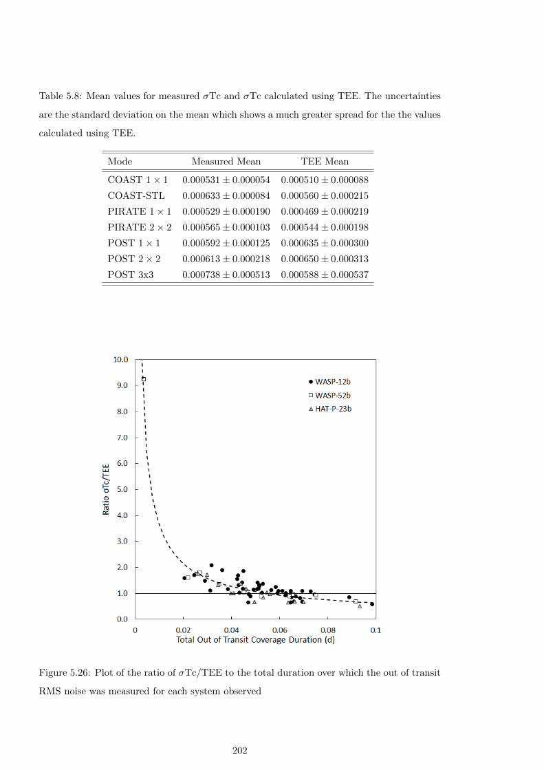
Table 5.8: Mean values for measured σTc and σTc calculated using TEE. The uncertainties

are the standard deviation on the mean which shows a much greater spread for the the values

calculated using TEE.

Mode Measured Mean TEE Mean

COAST 1× 1 0.000531± 0.000054 0.000510± 0.000088

COAST-STL 0.000633± 0.000084 0.000560± 0.000215

PIRATE 1× 1 0.000529± 0.000190 0.000469± 0.000219

PIRATE 2× 2 0.000565± 0.000103 0.000544± 0.000198

POST 1× 1 0.000592± 0.000125 0.000635± 0.000300

POST 2× 2 0.000613± 0.000218 0.000650± 0.000313

POST 3x3 0.000738± 0.000513 0.000588± 0.000537

Figure 5.26: Plot of the ratio of σTc/TEE to the total duration over which the out of transit

RMS noise was measured for each system observed

202

white noise with no red noise component. No correlation is seen with the calculated TEE

uncertainty or its difference from the measured value with the red noise metric for the WASP-

12b data, indicating this is a safe assumption for the WASP-12b data set. The oot RMS and

ratio of σTc/TEE is significantly correlated for all three systems (tau=-0.23, p-value=0.004),

the ratio of σTc/TEE decreases as RMS noise increases.

5.6 Simultaneous Transit Observations

Observations of the same transit with two or more telescopes allow us to compare the timing

results and potentially understand any systematic effects that influence these results. There

are a number of simultaneous transit time observations which occur in the combined transit

timing data sets for WASP-12b and HAT-P-23b, Figures 5.27 and 5.28. These fall into three

categories, simultaneous transit times in the already published results, simultaneous transit

times for published and new observations and simultaneous transit times for observations

made by two telescopes in the newly obtained data. The HAT-P-23b timing data contains

only the second and third categories, no simultaneous observations are available between

previously published results, Tables 5.9 and 5.10. The WASP-52b timing data set does not

contain any true simultaneous observations.

In the set of transit times for WASP-12b published by Yee et al. (2019), which pulls

together 139 previously published primary transit times from multiple sources, there are

5 pairs of observations made of the same transit by the same or different observers. This

includes three pairs of measurements made of the same transits with the MuSCAT telescope in

g′ and r′, obtained by Patra et al. (2020). In four of these five measurements the difference in

reported transit mid time is greater than largest of the two quoted transit time uncertainties,

and in two cases the uncertainties do not overlap, see Table 5.9. For the three simultaneous

transits observed by Patra et al. (2020) the exposure time for the r′ band is half that of the

g′, resulting in correspondingly smaller uncertainties on the transit mid-time reported for

the r′ measurements. It is noted that the authors transit observation on 12th February 2018

missed the t1 ingress transition point and has no pre-transit data which would be expected

to result in a poorer transit mid-time determination. Instead the full transit observations

made on 27th January 2017 have the largest transit mid-time uncertainties and a 3σ mid time

difference, explained by the authors as being due to transparency variations during egress

and having to exclude several data points as outliers.

Two simultaneous transit observations between the new data obtained for this project and

published observations made by (Maciejewski et al., 2016, 2018) occur at epochs 624 (POST)

and 1345 (PIRATE). The difference in reported transit mid-times for the two pairs are 38

203

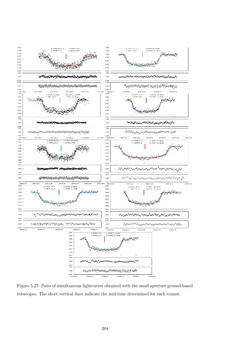
Figure 5.27: Pairs of simultaneous lightcurves obtained with the small aperture ground-based

telescopes. The short vertical lines indicate the mid-time determined for each transit.

204

Figure 5.28: As Figure 5.27 but for HAT-P-23b simultaneous lightcurves.

205

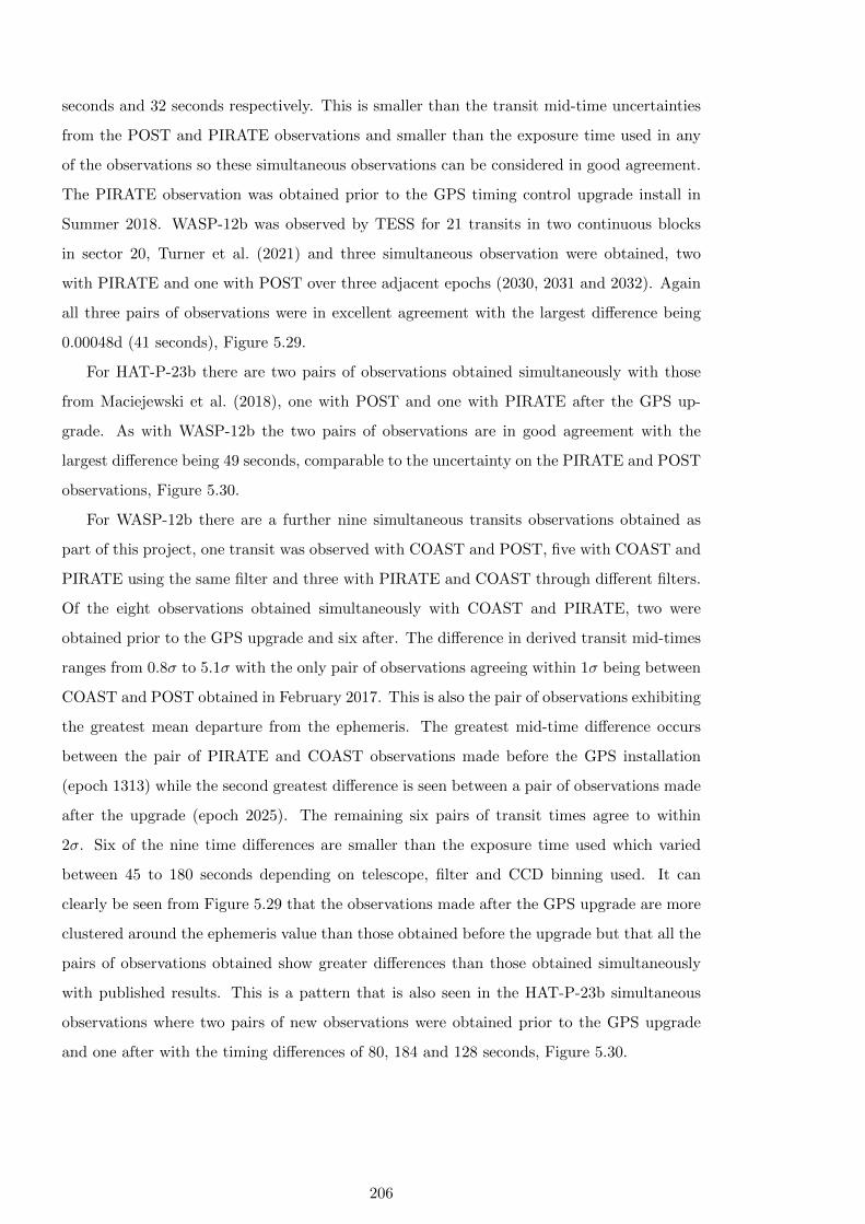
seconds and 32 seconds respectively. This is smaller than the transit mid-time uncertainties

from the POST and PIRATE observations and smaller than the exposure time used in any

of the observations so these simultaneous observations can be considered in good agreement.

The PIRATE observation was obtained prior to the GPS timing control upgrade install in

Summer 2018. WASP-12b was observed by TESS for 21 transits in two continuous blocks

in sector 20, Turner et al. (2021) and three simultaneous observation were obtained, two

with PIRATE and one with POST over three adjacent epochs (2030, 2031 and 2032). Again

all three pairs of observations were in excellent agreement with the largest difference being

0.00048d (41 seconds), Figure 5.29.

For HAT-P-23b there are two pairs of observations obtained simultaneously with those

from Maciejewski et al. (2018), one with POST and one with PIRATE after the GPS up-

grade. As with WASP-12b the two pairs of observations are in good agreement with the

largest difference being 49 seconds, comparable to the uncertainty on the PIRATE and POST

observations, Figure 5.30.

For WASP-12b there are a further nine simultaneous transits observations obtained as

part of this project, one transit was observed with COAST and POST, five with COAST and

PIRATE using the same filter and three with PIRATE and COAST through different filters.

Of the eight observations obtained simultaneously with COAST and PIRATE, two were

obtained prior to the GPS upgrade and six after. The difference in derived transit mid-times

ranges from 0.8σ to 5.1σ with the only pair of observations agreeing within 1σ being between

COAST and POST obtained in February 2017. This is also the pair of observations exhibiting

the greatest mean departure from the ephemeris. The greatest mid-time difference occurs

between the pair of PIRATE and COAST observations made before the GPS installation

(epoch 1313) while the second greatest difference is seen between a pair of observations made

after the upgrade (epoch 2025). The remaining six pairs of transit times agree to within

2σ. Six of the nine time differences are smaller than the exposure time used which varied

between 45 to 180 seconds depending on telescope, filter and CCD binning used. It can

clearly be seen from Figure 5.29 that the observations made after the GPS upgrade are more

clustered around the ephemeris value than those obtained before the upgrade but that all the

pairs of observations obtained show greater differences than those obtained simultaneously

with published results. This is a pattern that is also seen in the HAT-P-23b simultaneous

observations where two pairs of new observations were obtained prior to the GPS upgrade

and one after with the timing differences of 80, 184 and 128 seconds, Figure 5.30.

206

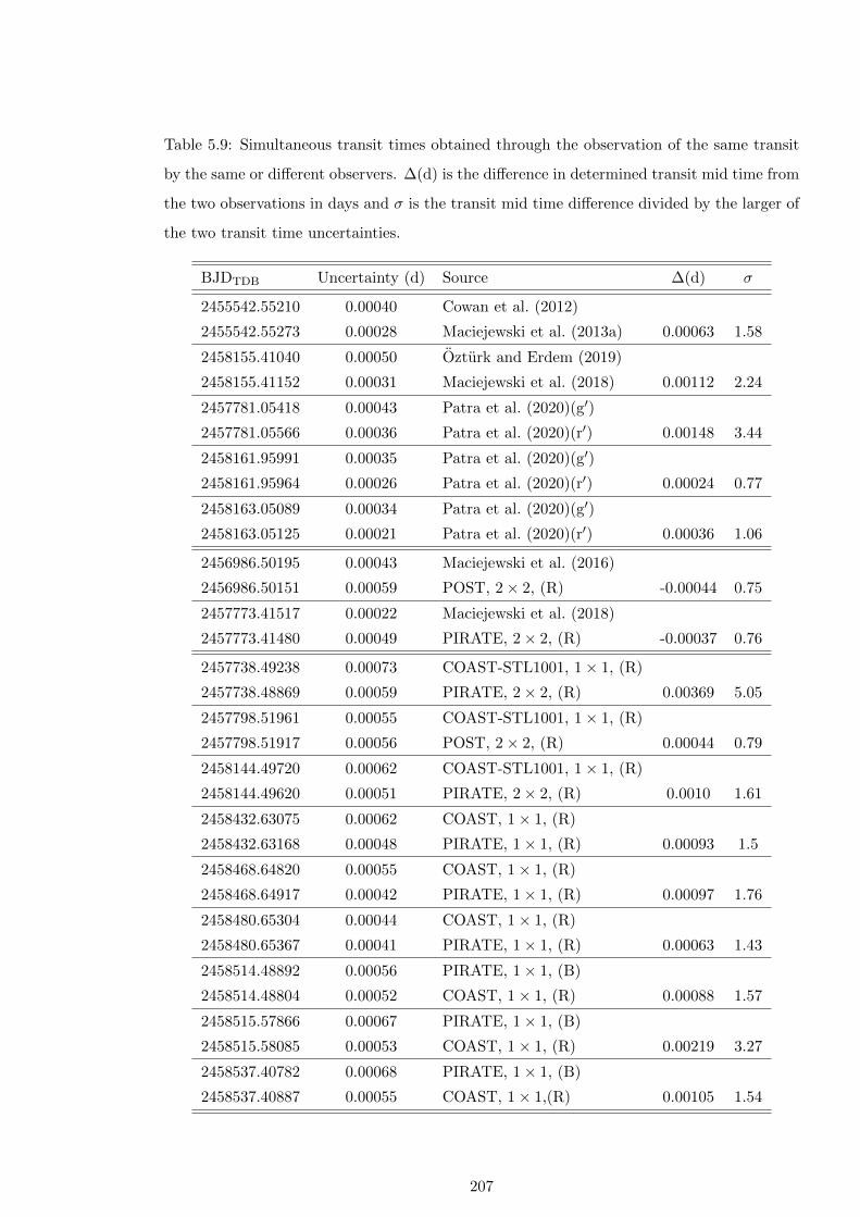
Table 5.9: Simultaneous transit times obtained through the observation of the same transit

by the same or different observers. ∆(d) is the difference in determined transit mid time from

the two observations in days and σ is the transit mid time difference divided by the larger of

the two transit time uncertainties.

BJDTDB Uncertainty (d) Source ∆(d) σ

2455542.55210 0.00040 Cowan et al. (2012)

2455542.55273 0.00028 Maciejewski et al. (2013a) 0.00063 1.58

2458155.41040 0.00050 Ozturk and Erdem (2019)

2458155.41152 0.00031 Maciejewski et al. (2018) 0.00112 2.24

2457781.05418 0.00043 Patra et al. (2020)(g′)

2457781.05566 0.00036 Patra et al. (2020)(r′) 0.00148 3.44

2458161.95991 0.00035 Patra et al. (2020)(g′)

2458161.95964 0.00026 Patra et al. (2020)(r′) 0.00024 0.77

2458163.05089 0.00034 Patra et al. (2020)(g′)

2458163.05125 0.00021 Patra et al. (2020)(r′) 0.00036 1.06

2456986.50195 0.00043 Maciejewski et al. (2016)

2456986.50151 0.00059 POST, 2× 2, (R) -0.00044 0.75

2457773.41517 0.00022 Maciejewski et al. (2018)

2457773.41480 0.00049 PIRATE, 2× 2, (R) -0.00037 0.76

2457738.49238 0.00073 COAST-STL1001, 1× 1, (R)

2457738.48869 0.00059 PIRATE, 2× 2, (R) 0.00369 5.05

2457798.51961 0.00055 COAST-STL1001, 1× 1, (R)

2457798.51917 0.00056 POST, 2× 2, (R) 0.00044 0.79

2458144.49720 0.00062 COAST-STL1001, 1× 1, (R)

2458144.49620 0.00051 PIRATE, 2× 2, (R) 0.0010 1.61

2458432.63075 0.00062 COAST, 1× 1, (R)

2458432.63168 0.00048 PIRATE, 1× 1, (R) 0.00093 1.5

2458468.64820 0.00055 COAST, 1× 1, (R)

2458468.64917 0.00042 PIRATE, 1× 1, (R) 0.00097 1.76

2458480.65304 0.00044 COAST, 1× 1, (R)

2458480.65367 0.00041 PIRATE, 1× 1, (R) 0.00063 1.43

2458514.48892 0.00056 PIRATE, 1× 1, (B)

2458514.48804 0.00052 COAST, 1× 1, (R) 0.00088 1.57

2458515.57866 0.00067 PIRATE, 1× 1, (B)

2458515.58085 0.00053 COAST, 1× 1, (R) 0.00219 3.27

2458537.40782 0.00068 PIRATE, 1× 1, (B)

2458537.40887 0.00055 COAST, 1× 1,(R) 0.00105 1.54

207

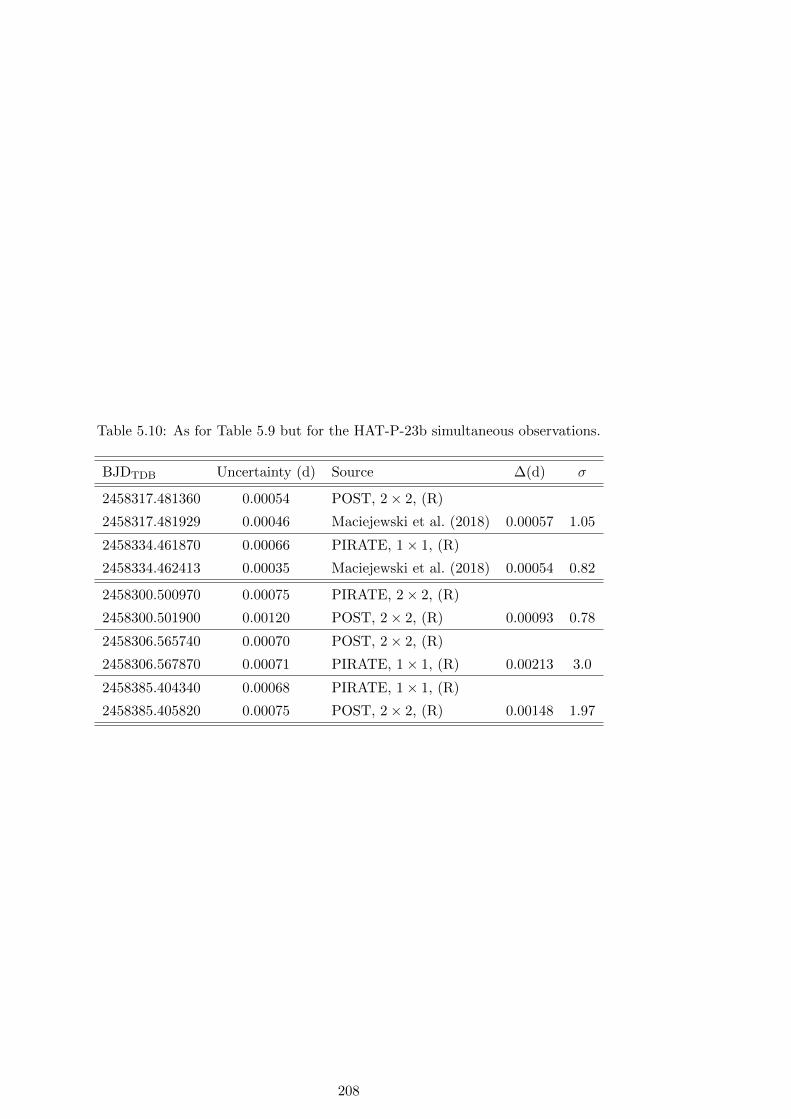
Table 5.10: As for Table 5.9 but for the HAT-P-23b simultaneous observations.

BJDTDB Uncertainty (d) Source ∆(d) σ

2458317.481360 0.00054 POST, 2× 2, (R)

2458317.481929 0.00046 Maciejewski et al. (2018) 0.00057 1.05

2458334.461870 0.00066 PIRATE, 1× 1, (R)

2458334.462413 0.00035 Maciejewski et al. (2018) 0.00054 0.82

2458300.500970 0.00075 PIRATE, 2× 2, (R)

2458300.501900 0.00120 POST, 2× 2, (R) 0.00093 0.78

2458306.565740 0.00070 POST, 2× 2, (R)

2458306.567870 0.00071 PIRATE, 1× 1, (R) 0.00213 3.0

2458385.404340 0.00068 PIRATE, 1× 1, (R)

2458385.405820 0.00075 POST, 2× 2, (R) 0.00148 1.97

208

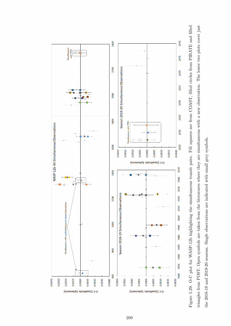
Fig

ure

5.29

:O

-Cp

lot

for

WA

SP

-12b

hig

hli

ghti

ng

the

sim

ult

aneo

us

tran

sit

pai

rs.

Fil

lsq

uar

esar

efr

om

CO

AS

T,

fill

edci

rcle

sfr

om

PIR

AT

Ean

dfi

lled

tria

ngl

esfr

omP

OS

T.

Op

ensy

mb

ols

are

taken

from

the

lite

ratu

res

wh

ere

they

are

sim

ult

aneo

us

wit

ha

new

ob

serv

ati

on

.T

he

low

ertw

op

lots

cove

rju

st

the

2018

-19

and

2019

-20

seas

ons.

Sin

gle

obse

rvat

ions

are

ind

icat

edw

ith

smal

lgr

eysy

mb

ols.

209

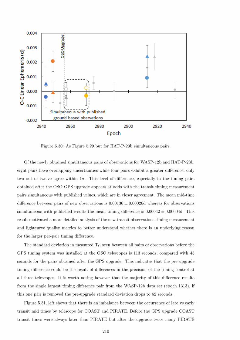
Figure 5.30: As Figure 5.29 but for HAT-P-23b simultaneous pairs.

Of the newly obtained simultaneous pairs of observations for WASP-12b and HAT-P-23b,

eight pairs have overlapping uncertainties while four pairs exhibit a greater difference, only

two out of twelve agree within 1σ. This level of difference, especially in the timing pairs

obtained after the OSO GPS upgrade appears at odds with the transit timing measurement

pairs simultaneous with published values, which are in closer agreement. The mean mid-time

difference between pairs of new observations is 0.00136 ± 0.00026d whereas for observations

simultaneous with published results the mean timing difference is 0.00042 ± 0.00004d. This

result motivated a more detailed analysis of the new transit observations timing measurement

and lightcurve quality metrics to better understand whether there is an underlying reason

for the larger per-pair timing difference.

The standard deviation in measured TC seen between all pairs of observations before the

GPS timing system was installed at the OSO telescopes is 113 seconds, compared with 45

seconds for the pairs obtained after the GPS upgrade. This indicates that the pre upgrade

timing difference could be the result of differences in the precision of the timing control at

all three telescopes. It is worth noting however that the majority of this difference results

from the single largest timing difference pair from the WASP-12b data set (epoch 1313), if

this one pair is removed the pre-upgrade standard deviation drops to 62 seconds.

Figure 5.31, left shows that there is an imbalance between the occurrence of late vs early

transit mid times by telescope for COAST and PIRATE. Before the GPS upgrade COAST

transit times were always later than PIRATE but after the upgrade twice many PIRATE

210

times are later than COAST. This effect is not seen in POST observations simultaneous with

one of the OSO telescopes which are evenly split between late and early. Figure 5.31 right

shows how the mean O-C and spread in pair timing measurements between COAST and

PIRATE changes dramatically after the GPS upgrade with a mean significantly closer to the

ephemeris as is also seen for all the single observations timing results as well. The standard

deviation in COAST measurements is reduced by half but increases for PIRATE, possible

due to the smaller number of before upgrade observations. After the upgrade the standard

deviation in COAST time measurements is approximately 60% greater than for PIRATE

measurements. This could be attributable to the smaller aperture of COAST (0.35m vs

0.425m), however the COAST mean photometric SNR value is 50% greater than PIRATE

(resulting from longer exposures and the use of the B filter in 3 PIRATE observations) and

the TSNR values are comparable which argue against aperture alone being the cause of this

difference. The red noise metric is an indicator of the extent to which individual transits are

affected by correlated noise, the mean red noise metric for COAST is almost double that of

PIRATE, while the spread in PIRATE red noise metric is greater than seen for COAST. The

timing SNR values calculated using Eq.2 from Deeg and Tingley (2017) are comparable for

COAST and PIRATE.

A search for correlations between the transit time difference for each pair of simultane-

ous observations and the available lightcurve quality measures was undertaken. For each

lightcurve pair the Kendall-Tau statistical test (due to the small sample size) was used to

look at the difference, sum and ratio of the lightcurve quality measures. Only two correlations

were found to be statistically significant, the difference between TSNR values, ∆TSNR, (tau

= -0.6, p-value = 0.007) for each pair and difference in pre-transit RMS, (tau = 0.5, p-value

= 0.023). The negative correlation of ∆TSNR with timing difference results in a smaller

timing difference as the difference between TSNR increases, intuitively it would be expected

for the time difference be less when the lightcurves were of a similar quality, whereas this

result implies the difference is less where one lightcurve is a lower quality than the other.

The correlation between ∆Tc and pre-transit RMS shows that the timing difference reduces

as the pre transit RMS for the early transit in each pair increases or equivalently as the

RMS noise for the late transit decreases. No significant correlation with transit RMS values

(post transit, all out of transit and full transit measurements) is found. Both correlations be-

come statistically insignificant when considering only the post GPS install data for PIRATE

and COAST. Although not having the greatest per-pair time difference the three pairs with

greatest mean O-C value also have the greatest TSNR difference, WASP-12b epochs 1368

and 1993 and HAT-P-23b epoch 2913 have ∆TSNR of 4.0, 5.3 and 3.6 respectively. The

mean ∆TSNR value for the other nine pairs is 1.06. Further simultaneous observations using

211

Figure 5.31: Left, pairs of COAST-PIRATE simultaneous WASP-12b transit observations.

Before the GPS upgrade and switch to CCD 1 × 1 binning there were only two pairs of

observations and in both the PIRATE transit mid-time was earlier than than for COAST.

After the GPS installation there were six pairs of observations where for four COAST was

earlier than PIRATE and two where COAST was later than PIRATE. Right, plot showing

change in mean transit mid-time and spread in measurements before and after the GPS

upgrade/switch to CCD 1× 1 binning showing the significant improvement in accuracy and

reduction in spread for COAST.

the OSO telescopes would be required to determine if any correlation with lightcurve quality

factors are real.

Of note are the three Blue filter PIRATE observations simultaneous with Rc filter COAST

observations. All three PIRATE observations are missing any pre transit data. However the

spread of the B filter O-C values is smaller than for the Rc filter COAST measurements.

This was also seen in the simultaneous MUSCAT measurements (Patra et al., 2020) where

one transit had no pre-ingress data but doesn’t show the largest timing discrepancy which

arises from a transit with good coverage but higher noise.

For WASP-12b the mean timing difference in six previously published simultaneous obser-

vation pairs is 0.0019d (164s). Three of these pairs were observed by same telescope through

different filters and as a result the mean difference is much reduced at 0.0007d, but still larger

than the typical mid-time measurement uncertainty. By contrast for the five pairs of transits

where one is from the published literature and the other from a new observation (including

three from TESS) the timing difference is 0.00036d (31s), less than the typical transit mid-

time uncertainty. Across both WASP-12b and HAT-P-23b the pairs of observations obtained

before the GPS upgraded at the OSO telescopes was 0.00164d (142s) and after the upgrade

was 0.00116 (100s). While this is a 30% reduction in timing spread and an improvement over

the values seen between published pairs of observations it is still almost double the typical

mid-time measurement uncertainty. At the same time it can be seen the three individual

212

PIRATE observations obtained over 12 days in the 2019-20 season have a mean O-C value

of 0.00003d (2.6s). No upgrades or changes were made at the OSO telescopes between these

observing seasons. Comparing the WASP-12b data sets from the 2018-19 and 2019-2020

season two factors stand out as potential causes for the larger spread in O-C values seen

in the 2018-19 season. Firstly it can be seen from looking at Figures 4.4 and 4.5 that the

transit observations during 2018-19 season (transit numbers 28 to 58) have in general much

less pre-transit data than those obtained in the 2019-20 season (transit numbers 60-65). Of

the 19 full transits obtained with all telescopes during the 2018-19 season, including the 6

simultaneous pairs, 14 have pre-transit data coverage shorter than the ingress duration and

5 have none or only 2 measurements before ingress. As was shown in Table 5.6 transits with

pre-ingress coverage less than ingess/egress duration show a greater scatter in O-C. All 2019-

2020 observations have pre-transit data coverage at least twice the ingress duration. This

may also explain why no correlation was seen between the transit time spread and out of

transit coverage for the simultaneous pairs, as all transits had little or no pre-transit coverage.

The second point of note is that the PIRATE observation obtained during the 2019-20 season

were more defocussed than those from the 2018-19 season with an FWHM typically 3 times

greater.

5.7 Summary of Key Findings

Analysis of the transit timing measurements before and after the implementation of the

GPS timing control for PIRATE and COAST has shown that the timing accuracy improved

significantly. Observations of HAT-P-23b clearly show the scatter in O-C measurements

reducing by 2.4× after the GPS upgrade. At the same time the results show that making

observations with a longer cadence in 1× 1 binning mode provide more precise results than

faster cadence in 2× 2 binning mode.

TSNR is a useful measure of the precision with which transit times can be measured and

the results show that a higher TSNR gives a lower spread in transit mid-time measurement.

Out-of-transit RMS has been shown to be proportional to SNR−0.95 providing a guide that

photometric SNR greater than 600 is required to provide the best timing precision for ob-

servations in 1 × 1 binning mode using an Rc filter. Transit photometry with PIRATE and

COAST regularly achieved oot RMS of 0.0015 showing that 3σ detection of transits with a

depth of 0.5% can be achieved in single a observation. With a few exceptions observations

made with all telescopes show minimal red noise and no correlation is found between a cal-

culated red noise metric and the transit timing results. A test of guiding precision has shown

precise guiding will reduce the RMS scatter in the photometric measurements by 13%.

213

Using multiple transit observations obtained and analysed in a homogeneous way can

be combined with catalogue data to provide high precision system parameters. Long term

photometric monitoring with PIRATE is stable over multiple seasons and provides precision

sufficient to measure periodicity’s in exoplanet host star at least at the 0.01 magnitude level.

In this chapter I have quantified the performance capabilities of the small aperture ground-

based telescopes used to make short and long term timing observations of transiting exoplan-

ets and how those observations can be used, in combination with published data, to provide

high precision system parameters. I have also quantified the ability of PIRATE to undertake

long term monitoring observations over multiple seasons to search for and quantify Exo-

planet host star variability. In the final chapter I review the key finding from the study of

the selected transiting exoplanets with small aperture ground-based telescopes, identify best

practice approaches for obtaining the most accurate and precise system parameters and at

future developments and possibilities for the OpenScience Observatories and small aperture

ground-based telescopes to contribute to the field of exoplanet research.

214

Chapter 6

Conclusion and Discussion

In this thesis I used multiple small aperture ground-based telescopes to look for transiting

timing variations, refine orbital ephemerides and provide high precision system parameters. I

also undertook long term monitoring of selected exoplanet host stars to search for variability

in order to better understand the host stars of transiting hot Jupiter planets.

Here I summarise the key findings for the systems observed and then consider the suit-

ability of small aperture ground-based telescopes for undertaking follow-up observations of

transiting exoplanets. I’ll finish by looking ahead to potential future exoplanet observation

projects suitable for small aperture ground-based telescopes including developments planned

for the OpenScience Observatories.

6.1 Transit timing

New observations of three transiting hot Jupiter systems were obtained. HAT-P-23b and

WASP-52b were observed over a single season in 2018 while WASP-12b was observed over

four seasons between 2016 and 2020. Where available, archive observations obtained using

the POST observatory were used to extend the observation baselines.

No periodic variation in the transit timing measurements was seen in the new measure-

ments for any of the three systems observed. This is in agreement with studies that have

suggested hot Jupiter planets are likely to be isolated (E.g. Huang et al., 2016; Lillo-Box

et al., 2016; Hamer and Schlaufman, 2019). However it also remains possible that short

periods of observation along with generally sparse coverage are preventing the detection of

TTVs. The calculated linear ephemeris for HAT-P-23b agrees well with that independently

published shortly after my observations were obtained (Maciejewski et al., 2018).

Combining new and published transit times for WASP-52b initially resulted an ephemeris

with a high χ2ν of 2.5. This motivated an analysis of the transit times from different authors

which highlighted the transits times with very small uncertainties published by Mancini et al.

215

(2017) which were responsible increasing the χ2ν of the calculated ephemeris.

The authors noted that their linear ephemeris had a high χ2ν of 8.98 and they subse-

quently multiplied the uncertainties on their final linear ephemeris by this value. Multiplying

the individual transit time uncertainties by this χ2ν value of 8.98 prior to re-calculating the

ephemerides reduced the χ2ν of the ephemeris fit from 2.4 to 1.51. This also resulted in a slight

preference for a quadratic ephemeris with a rate of change of δP/δt = −38.6 ± 4ms yr−1.

This highlights the care required when combining transit time data from multiple sources.

Forward projecting the linear and quadratic ephemerides shows that this period change could

be confirmed by transit timing observations made in the 2021 season.

In early 2016 observations started to show evidence for a non linear ephemeris for WASP-

12b (Maciejewski et al., 2016). A subsequent analysis postulated either apsidal precession or

orbital decay as the cause (Patra et al., 2017). A flurry of published results have confirmed

the period change is due to orbital decay (Weinberg et al., 2017; Maciejewski et al., 2018;

Bailey and Goodman, 2019; Baluev et al., 2019; Ozturk and Erdem, 2019; Yee et al., 2019;

Turner et al., 2021). Transit times from the 47 new transits with full coverage obtained with

the three telescopes used for this project were insufficient to detect the quadratic ephemeris

on their own. This was due to very sparse coverage of archive transit observation from POST

with only 4 transits available between 2013 to 2016. The first two seasons of observations

with PIRATE and COAST showed a significant scatter in the timing measurements, being

greater than double the scatter in published values, see Figure 4.17. The final two seasons of

observation, 2018 to 2020, showed less scatter in timing measurements.

The improvement in timing measurements is attributed to two changes in the way the

transit lightcurves were obtained. Firstly, in the Summer of 2018, the OSO telescopes were

upgraded with GPS time controllers connected to the CCD camera shutter trigger to give

precise time stamps for when the shutter opens and closes. The control PCs were also slaved

to the GPS controllers to ensure they maintained accurate UTC time. Prior to this the

observatories had relied on the control PC operating systems to update system times from an

Internet time server. The second key change was from using the CCD in 2x2 on-chip binning

mode to unbinned (1x1). The improvement in transit time measurements obtained using

COAST and PIRATE is clearly seen in the results for both HAT-P-23b and WASP-12b. The

standard deviation for HAT-P-23b transit times reduced by 2.4 times following the changes,

while for WASP-12b the standard deviation halved.

The installation of the GPS controller along with higher precision lightcurves resulting

from making unbinned observations combined to improve both the accuracy and precision

of the timing measurements. The GPS time controller provides milli-second accurate timing

stamps for exposures made using PIRATE and COAST while the higher precision photometric

216

measurements resulting from using the CCD camera unbinned increased the transit signal

to noise ratio (TSNR). The results show that while increased TSNR had minimal effect on

individual transit mid-time uncertainty, it was correlated with reducing scatter in the transit

time measurements. Figure 7.24 shows that for the spread in O-C measurements to match

typical measurement uncertainty of 0.0005 day, a minimum TSNR of 10-12 is required. For a

given transit depth the TSNR depends only on the out of transit photometric scatter; Figure

5.2 can be used to estimate the photometric SNR required to achieve a TSNR of 10-12 for a

target transit observation.

The theoretical transit timing uncertainties (σTc) were calculated using TEE (Deeg and

Tingley, 2017) and showed that the measured uncertainty achieved using the three small

aperture telescopes is in generally good agreement with theoretical predictions. Figure 5.25

shows that for σTc < 0.0005d the measured σTc is approximately 10% greater than predicted

by TEE. Measured transit uncertainties showed less scatter than suggested by the theoreti-

cal calculations. The standard deviation in the measured uncertainties were smaller for all

telescopes and observing modes.

The importance of out-of-transit (oot) coverage is highlighted by the 2018-19 season obser-

vations of WASP-12b where 15 out of 19 transits have oot coverage less than the ingress/egress

duration and a greater scatter in Tc determination. Figure 5.26 shows that transits with little

total oot coverage show much greater σTc, with measured and theoretical values reaching

agreement for oot coverage in the range 0.05 to 0.07d, indicating 30 to 50 minutes of oot

coverage is required either site of transit. Little improvement in σTc is seen for longer oot

coverage.

6.2 Parameter Determination

Multiple lightcurves obtained over extended periods of time for the primary purpose of transit

timing have been analysed in conjunction with published radial velocity and photometric data

to provide updated system parameters. Combining multiple transit lightcurves in this way

enables the extraction of the maximum information from the available observations making

the most efficient use of the telescope time used to obtain these data sets

The same care was taken in selecting and incorporating previously published data used

in the analyses as was applied to the gathering of new data. Radial velocity data sets were

treated individually to allow independent zero point and jitter determinations. Where authors

suggested zero points may vary over long durations the data sets were separated into short

time spans. Timestamps were updated to BJDTDB where required. Photometric data used

in the building of the SEDs was taken from multiple trusted sources and where required de-

217

blended to remove the contribution from unresolved companions. Distance information was

taken from Gaia DR2 parallax data corrected for known systematics (E.g. Stassun et al., 2017)

and V-band extinction values applied from dust reddening maps. To minimise any potential

bias resulting from previous results all parameters were freely determined. No stellar, orbital

or planetary parameters were fixed based on previously published results. This is in contrast

to previous studies of these systems which often do this (E.g. Ozturk and Erdem, 2019). The

analysis of the new transit data using ExofastV2 produced an homogenous set of results for

transit times and system parameters.

The analysis for HAT-P-23b provide the most precise measurements yet for the stellar

radius and result in stellar and planetary radii between the values previously published,

confirming its inflated nature. The analysis for WASP-52b finds somewhat larger values

for R∗ and RP than previous studies. No close companion to WASP-52 is identified in

the literature however Hebrard et al. (2013) note a ’hint’ of an approximately +40 ms−1

RV drift over 15 months which could be due to an unresolved companion. A blend with

the host star cannot be ruled out without high resolution imaging, not possible with small

aperture ground-based telescopes. The distance to WASP-52 was found to be 24% greater

than that estimated in the discovery paper. The combined analysis shows both systems have

an eccentricity within 2.4σ of zero and are therefore consistent with circular orbits (Eastman

et al., 2019).

Similarly the newly presented results for WASP-12b provide the most precise determi-

nations yet for R∗, RP, a, M∗ and MP. The determinations of e and ω∗ are in agreement

with the values reported by Maciejewski et al. (2020) who suggest the apparent eccentricity

of WASP-12b results from tidal bulges being raised by the planet on the host star.

The transit depth measured for WASP-12b was 4σ deeper than the small number of depth

values published on the NASA Exoplanet Archive. The two different red filters used both

cover the same key NaI and Hα absorption bands and hence cannot be the cause of this

difference. Phase folding the lightcurves did not reveal any depth differences. WASP-12b has

been observed by amateur astronomers for many years with the results being recorded on the

Exoplanet Transit Database. Taking 21 of the most precise (data quality 1 and 2) R filter

lightcurves the mean transit depth measured is 0.0186± 0.003. This is greater still than the

0.01439± 0.00012 measured from the 47 new transits and the mean value from the exoplanet

archive of 0.01390± 0.00016.

Combining data from small aperture ground-based telescopes to provide precise exoplanet

system parameters is an often overlooked use of large number of transit data obtained for

timing purposes. The results presented have demonstrated that results achievable are compa-

rable with those obtained from single or small number transit observations using significantly

218

larger telescopes.

6.3 Host Star Monitoring

Monitoring of exoplanet host stars concurrently with transit observations is a generally ne-

glected task that has the capability to reveal further information about exoplanet systems

not provided by observing transit events alone. This activity is well suited to small aperture

automated telescopes such as PIRATE and COAST with schedulers capable of obtaining

monitoring observations in a way that makes most efficient use of available telescope time.

Monitoring of HAT-P-23 over a single season in 2018 through an Rc filter detected vari-

ation with a period of 7.015 days and an amplitude of 0.011 magnitude. This is interpreted

as the rotation period of HAT-P-23 at the latitude of surface spots. The measured am-

plitude was much lower than a previous tentative detection of variation of 0.03 magnitude

seen by Sada and Ramon-Fox (2016), suggesting evolution of amplitude over time possibly

due to HAT-P-23’s ongoing stellar cycle. Further monitoring over multiple seasons would be

required to detect any periodic variation in the amplitude to support this hypothesis.

Three years of monitoring of WASP-12 detected no definitive sign of periodic variation.

The previously measured very slow rotational velocities for a late F spectral type star (Hebb

et al., 2009; Albrecht et al., 2012) imply a rotation period in the range 21-66 days for WASP-

12. Periodicities between 27-30 days seen in some seasons data are attributed to a systematic

effect arising from lunar illumination. The conclusion reached by Albrecht et al. (2012) that

we are seeing WASP-12 at a high stellar inclination, just 6.7° from pole explains the observed

slow rotational velocity, the previous non-detections of the Rossiter McLaughlin effect and

non-detection of photometric modulation in this work. Modelling with SOAP suggests that

in order to detect rotational modulation due to spots with PIRATE on WASP-12b the spots

need to be larger than 3% of the stellar surface (with an 80% flux level) and residing between

latitudes 15°to 60°to generate a photometric variation. The possibility that WASP-12 was

simply in a quiescent stage of its stellar cycle during the observations could be confirmed or

refuted by ongoing monitoring.

Another reason to monitor exoplanet host star fields is to confirm, or otherwise, the sta-

bility of photometric comparison stars. Small aperture ground-based telescopes with a wide

field of view are well suited to this task. Periodic variation was detected in J0630+2942, just

2′ from WASP-12, the amplitude of which was seen to vary over multiple observing seasons.

This star is of similar brightness and colour index to WASP-12 and was previously thought to

be a photometrically stable comparison star. The maximal rate of flux variation indicated by

the period and greatest amplitude measured during the 2016-17 season indicates a change in

219

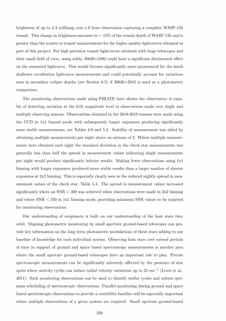
brightness of up to 2.3 millimag over a 6 hour observation capturing a complete WASP-12b

transit. This change in brightness amounts to ∼ 15% of the transit depth of WASP-12b and is

greater than the scatter in transit measurements for the higher quality lightcurves obtained as

part of this project. For high precision transit lightcurves obtained with large telescopes and

their small field of view, using solely J0630+2492 could have a significant detrimental effect

on the measured lightcurve. This would become significantly more pronounced for the much

shallower occultation lightcurve measurements and could potentially account for variations

seen in secondary eclipse depths (see Section 6.5) if J0630+2942 is used as a photometric

comparison.

The monitoring observations made using PIRATE have shown the observatory is capa-

ble of detecting variation at the 0.01 magnitude level in observations made over single and

multiple observing seasons. Observations obtained in the 2018-2019 seasons were made using

the CCD in 1x1 binned mode with subsequently longer exposures producing significantly

more stable measurements, see Tables 4.9 and 5.3. Stability of measurement was aided by

obtaining multiple measurements per night above an airmass of 2. Where multiple measure-

ments were obtained each night the standard deviation in the check star measurements was

generally less than half the spread in measurement values indicating single measurements

per night would produce significantly inferior results. Making fewer observations using 1x1

binning with longer exposures produced more stable results than a larger number of shorter

exposures at 2x2 binning. This is especially clearly seen in the reduced nightly spread in mea-

surement values of the check star, Table 5.3. The spread in measurement values increased

significantly where an SNR < 300 was achieved when observations were made in 2x2 binning

and where SNR < 550 in 1x1 binning mode, providing minimum SNR values to be targeted

for monitoring observations.

Our understanding of exoplanets is built on our understanding of the host stars they

orbit. Ongoing photometric monitoring by small aperture ground-based telescopes can pro-

vide key information on the long term photometric modulations of these stars adding to our

baseline of knowledge for each individual system. Observing host stars over extend periods

of time in support of ground and space based spectroscopy measurements is another area

where the small aperture ground-based telescopes have an important role to play. Precise

spectroscopic measurements can be significantly adversely affected by the presence of star

spots where activity cycles can induce radial velocity variations up to 25 ms−1 (Lovis et al.,

2011). Such monitoring observations can be used to identify stellar cycles and inform opti-

mum scheduling of spectroscopic observations. Parallel monitoring during ground and space

based spectroscopic observations to provide a variability baseline will be especially important

where multiple observations of a given system are required. Small aperture ground-based

220

telescope monitoring of host stars therefore has an important role even where the planet

transit is not detectable or where the planets do not transit at all.

6.4 Monitoring Transiting Exoplanet Systems with Small aper-

ture ground-based Telescopes

Throughout the observing programme undertaken for this thesis significant improvements

were made in the precision of the lightcurves obtained when measured as the RMS scatter

in the oot measurements. The best practice developed for the three telescopes used here can

be extended more generally for small aperture ground-based telescopes.

Transit timing results from observations of HAT-P-23b and WASP-12b before and af-

ter implementation of GPS timing control have highlighted the requirement for accurate,

consistent timing control for observations. Control systems based on standard PCs in an

observatory can be subject to large temperature variations which they were not designed for,

leading to significant variations in internal clocks. Relying on operating systems to keep clocks

updated via the Internet can lead to synchronisation delays, adding up to unpredictable vari-

ations in timing measurements. GPS controlled timing is the gold standard and as a result

of this work POST has subsequently been upgraded with GPS timing control. GPS systems

may not be viable for all small aperture ground-based telescopes often owned by individuals,

in which case dedicated software such as D4 to manage timing synchronisation is the next

best approach. Portable telescopes without GPS control and where no Internet connectivity

is available can present problems. Mobile Internet connectivity is commonly available and

cost effective but where this is not available control laptops should be time synchronised

before travelling to the observing site.

The second change implemented was to use the CDD in unbinned mode with longer

exposures, resulting in improved photometric precision. This observing mode results in an

oversampling of the stellar PSF akin to defocusing (Collins et al., 2017a) which is an often

used method to improve the photometric precision (E.g. Southworth et al., 2004; Hinse et al.,

2015). Spreading the flux over a larger number of pixels reduces the impact of inter-pixel

variations not completely corrected for if the flat fielding is imperfect. Secondary terms in

the standard CCD equation (E.g. Collins et al., 2017b) show that noise increases with the

number of pixels in the photometry aperture. In modern low noise cooled CCDs, the decrease

in interpixel variations more than offsets the increase in noise resulting from a greater number

of pixels, see Figure 5.16.

Another approach for improving photometric precision gaining in popularity is the use of

engineered diffusers (Stefansson et al., 2017; von Essen et al., 2019). These devices provide a

221

controlled PSF with a square profile, unlike defocusing which typically results in a “donut”

profile to the PSF. Oversampling has two key benefits over both defocusing and engineered

diffusers. Firstly in crowded fields these methods can lead to overlapping of the extended

PSFs, blending the flux of multiple stars resulting in shallower transit depth determinations.

Secondly well focused oversampled imaging allows the use of on-axis guiding to further reduce

the effect of inter-pixel variations by maintaining the stellar centroid on the same pixels

throughout an observation. A test undertaken using POST to compare unguiding imaging

with precise autoguiding showed a 13% reduction in photometric scatter where a stellar

centroid was maintained on the same pixel. This improvement would be expected to be

greater where flat fielding is not perfect which may arise for PIRATE and COAST master

flat fields as these are built from individual flat field frames obtained over multiple nights

(Jackson et al., 2021).

To further minimise photometric scatter the photometry analysis used an iterative ap-

proach, testing multiple target and sky aperture radii along with removing comparison stars

from the ensemble in turn to test for reductions in RMS scatter and BIC. Implemented in

AstroImageJ (Collins et al. (2017b) this was a manual process for the lightcurves analysed

in this thesis but this approach should be adopted into any automated photometry pipeline.

As discussed in Section 6.1, a TSNR of 10-12 should be considered the minimum for consis-

tent transit timing retrieval along with out of transit coverage that exceeds the ingress/egress

duration either side of the transit. Later lightcurves obtained with PIRATE and COAST in

this work have out of transit RMS scatter in the region of 0.0013 to 0.0015. Transit depths of

1.3% to 1.5% are detectable with TSNR of 10-12 and transits depths of 0.5% are detectable

at TSNR = 3 for single observations.

Phase folding of multiple observations has shown that the observations are an efficient way

of obtaining extremely high precision transit lightcurves compared to single transit measure-

ments from much larger 2m class ground-based telescopes. To achieve these results requires a

greater time investment for the small telescopes to obtain the multiple observations required,

which automation greatly simplifies. Using a metric of telescope mirror area multiplied by

the duration of observations the results show that, in the absence of spot crossing events,

the binned photometric results obtained with the small telescopes result in a lightcurve with

the same or better out of transit photometric precision in half the mirror area × observation

time of the 2m class telescopes.

Phase folding 42 Red filter lightcurves obtained for WASP-12b in this thesis resulted in

an out of transit RMS of 119ppm, which I compared to a similar phase fold of 21 TESS

lightcurves which result in an out of transit RMS of 204ppm.

222

Table 6.1: Comparison of mean transit mid uncertainty and mean absolute O-C for HAT-P-

23b.

ETD ExoClock PIRATE

Number of measurements 121 24 5

Mean Tc Uncertainty (d) 0.001 0.00075 0.0006

Mean —O-C— (d) 0.0056 0.001 0.0004

6.5 Looking Forward

A number of further improvements are planned to upgrade the capability for the Open Uni-

versity OpenScience Observatories. Chief amongst these is the replacement of the current

0.45m PIRATE OTA with a new 0.6m OTA of the same optical type while the 0.45m OTA

from PIRATE will replace the 0.35m f11 optical tube on COAST. Taking the greater sec-

ondary mirror into consideration this will provide a mirror area 2.5 times greater than the

current COAST telescope and twice as large as PIRATE. Other developments are planed

including the implementation of a focus offset for automated observing of bright targets and

a data reduction pipeline tailor-made for transit observations.

Zellem et al. (2020) showed that our ability to accurately predict transit mid-times in the

future is most dependent on the precision of the period determination which requires multiple

transit mid-time measurements with low scatter in order to calculate precise ephemerides.

The example of HAT-P-23b in table 6.1 compares the results obtained using PIRATE after

the GPS installation with measurements from ETD and Exoclock. The results demonstrate

the capability of PIRATE/COAST to contribute accurate and precise timing measurements

to programmes such as ExoClock in support of the ESA ARIEL mission.

Combined analysis of transit lightcurves, RV and photometric data with accurate dis-

tances now available from Gaia was used in Exofastv2 to determine accurate stellar radii.

This approach will produce a discrepant result where the flux of the target star is blended

with that of close, unresolved companion(s). This fact could be used to systematically iden-

tify systems exhibiting “excess” stellar radii over other methods used to determine stellar

radius such as the Torres relationship. These systems would make suitable follow up tar-

gets for high resolution or “lucky” imaging to identify close companions contaminating the

photometric data which would also impact precision spectroscopic studies.

The level of lightcurve precision achieved when phase folding multiple observations opens

the possibility for the detection of very shallow primary transits or even secondary occul-

tations. Using the results from phase folding the 42 Red filter lightcurves of WASP-12b a

transit depth of 0.06% would be detectable with a TSNR of 5. This is equivalent to a 2.7R⊕

223

planet orbiting a Sun like star, or an Earth radius planet orbiting a red dwarf host star.

Occultations of WASP-12b have been measured using ground-based telescopes in the filter

bandpasses available for PIRATE and COAST and appear to indicate significant variability

in the occultation depths. Hooton et al. (2019) observed two occultations a year apart

in the i′ band using 2m class telescopes and measured single event depths of 0.97 ± 0.14

mmag and 0.44 ± 0.21 mmag. Using an engineered diffuser on the 2.5m Nordic Optical

Telescope, von Essen et al. (2019) measured three occultations in the V band separated by

24 days and with varying depths of 1.16±0.17 parts per thousand (ppt), −0.03±0.17ppt and

0.28± 0.1ppt. Hooton et al. (2019) speculate that while systematic errors are likely leading

to some of the variation seen they cannot rule out temperature variations of several hundred

Kelvin in the dayside temperature of WASP-12b. A potential cause of systematic errors in

occulatation depth measurement separated by years could arise from the use of J0630+2942

as a comparison. Hooton et al. (2019) used an ensemble of 5 comparison stars, it is unclear

if this ensemble included J0630+2942.

Occultation depths of 0.97 and 0.44 mmag could be detected at the 8σ and 3.7σ level

respectively with PIRATE given the precision achieved in this work. The quantum efficiency

of the FLI PL16803 camera on PIRATE at 800nm, in the centre of the Ic band, is about

40% lower than at 600nm in the Rc band, a deficit more than made up for with the aperture

increase when moved to the new 0.6m telescope. The level of lightcurve precision achieved

required the phase folding of many lightcurves over several seasons, not an optimal approach

for a time variable target. Due to its 1.09 day orbit transits (and occultations) occur in groups

of three on successive nights where all three occur when WASP-12b is above 30° altitude for

the entire transit/occultation. The best single night PIRATE lightcurve achieved an out

of transit RMS precision of 0.85 mmag when binned to 5 minute cadence, which could be

expected to be improved to 0.49 mmag by phase folding three similar quality lightcurves.

This would enable a 2σ detection of the occultation at the greatest depth seen by Hooton

et al. (2019) over 3 successive nights, minimising the likelihood of intrinsic variability.

The study of transiting exoplanets is one of the few areas of astronomical research where ob-

servations made with small aperture ground-based telescopes, whether as part of a dedicated

professional project, individual educational facility or amateurs are able to make a worth-

while contribution to the field. Groups of interested amateurs with access to small aperture

ground-based telescopes are being organised around specific projects such the ARIEL Ex-

oclock project or around existing national amateur astronomy societies such as the BAA

and AAVSO exoplanet groups. These groups provide a level of organisation and education

outreach, bringing like minded observers together and providing training in the specifics of

224

exoplanet transit observation. This in turn helps increase awareness of the field with the

general public and science educators. As these groups grow in size and capability the op-

portunity to undertake specific targeted projects, especially those that foster international

collaboration, will be a natural outcome. Such projects include transit timing and host star

monitoring, micro-lensing event follow-up, long duration (multi-day) transit coverage, single

transit event follow-up and combining observations of occultations to name just a few.

As was shown in Chapter 5, combining multiple transit observations from small aperture

ground-based telescopes is an efficient way to obtain high precision lightcurves for follow up

observations of known transiting exoplanets.

A typical commercial, off the shelf, 0.6m observatory telescope provides 0.22m2 unob-

structed mirror area while a medium class 4m ground-based telescope such as the 4m Lowell

Discovery Channel Telescope (LDCT)1 or the planned New Robotic Telescope (NRT)2 pro-

vide in the region of 13m2, an aperture ratio of 59/1. The costs of medium class telescopes are

undoubtedly reducing with the adoption of modern technologies such as segmented mirrors

but they are still significant investments with the LDCT having a price tag of $53m while the

NRT is expected to cost $24m. A typical cost for an off the shelf 0.6m observatory telescope

including OTA, mount, camera system and enclosure would be in the region of $150,000. 59

such telescopes would the same mirror area as the 4m class telescopes for a sixth of the LDCT

cost and a third the NRT cost. Projects such as MEarth3 based on two automated observa-

tories each with eight 0.6m telescopes already exist for specific purposes. Combining small

aperture ground-based telescopes into similar observatory groups would, in principle, allow

10 such observatories (80 telescopes) to be set up around the globe for half the NRT cost.

Spread over a range of latitude and longitude multiple observatories could provide almost

continuous coverage of the entire night sky, with overlap redundancy for weather conditions

at individual locations. Such an observatory capability would be very flexible providing high

quality, multi-filter transit follow-up, host and comparison star monitoring and other tran-

sient target follow-up such as for micro-lensing events, over a longer duration than could be

achieved with a satellite observatory. This approach would provide significant opportunities

for education and outreach, a model used by the Las Cumbres Observatory (LCO), a global

network of 0.4m to 2m class robotic telescopes for transient follow up with a strong focus on

education and outreach4. Such a network of observatories could be operated on a day-to-day

basis by educational groups or even volunteer groups such national astronomical societies.

1https://en.wikipedia.org/wiki/Lowell_Discovery_Telescope2https://www.robotictelescope.org3https://lweb.cfa.harvard.edu/MEarth/Welcome.html4https://lco.global/about/

225

Bibliography

F. C. Adams and G. Laughlin. Long-Term Evolution of Close Planets Including the Effects of

Secular Interactions. The Astrophysical Journal, 649(2):1004–1009, 2006. ISSN 0004-637X.

doi: 10.1086/506145.

E. Agol and K. Deck. Transit timing to first order in eccentricity. The Astrophysical Journal,

818(2), 2016. URL http://arxiv.org/abs/1509.01623.

E. Agol, J. Steffen, W. Clarkson, R. Sari, and W. Clarkson. On detecting terrestrial

planets with timing of giant planet transits. Monthly Notices of the Royal Astronom-

ical Society, 359(2):567–579, 5 2005. ISSN 0035-8711. doi: 10.1111/j.1365-2966.2005.

08922.x. URL http://mnras.oxfordjournals.org/cgi/doi/10.1111/j.1365-2966.

2005.08922.xhttp://mnras.oxfordjournals.org/content/359/2/567.short.

S. Albrecht, J. N. Winn, J. A. Johnson, A. W. Howard, G. W. Marcy, R. P. Butler,

P. Arriagada, J. D. Crane, S. A. Shectman, I. B. Thompson, T. Hirano, G. Bakos, and

J. D. Hartman. Obliquities of hot jupiter host stars: Evidence for tidal interactions and

primordial misalignments. Astrophysical Journal, 757(1), 2012. ISSN 15384357. doi:

10.1088/0004-637X/757/1/18.

J. Applegate, J; Patterson. Magnetic activity, tides, and orbital period changes in close

binaries. ASTROPHYSICAL JOURNAL, 322:99–102, 1987.

J. H. Applegate. A mechanism for orbital period modulation in close binaries. The Astro-

physical Journal, 385(2):621, 1992. ISSN 0004-637X. doi: 10.1086/170967. URL http:

//stacks.iop.org/1538-4357/669/i=2/a=L93%5Cnhttp://adsabs.harvard.edu/abs/

1992ApJ...385..621A%5Cnhttp://adsabs.harvard.edu/doi/10.1086/170967.

D. J. Armstrong, D. Veras, S. C. C. Barros, O. Demangeon, J. McCormac, H. P. Osborn,

J. Lillo-Box, A. Santerne, M. Tsantaki, J.-M. Almenara, D. Barrado, I. Boisse, A. S.

Bonomo, F. Bouchy, D. J. a. Brown, G. Bruno, J. R. Cerda, B. Courcol, M. Deleuil,

R. F. Dıaz, A. P. Doyle, G. Hebrard, J. Kirk, K. W. F. Lam, D. L. Pollacco, A. Ra-

jpurohit, J. Spake, and S. R. Walker. One of the closest planet pairs to the 3:2

226

Mean Motion Resonance, confirmed with K2 observations and Transit Timing Varia-

tions: EPIC201505350. Astronomy & Astrophysics, 33(582), 2015. ISSN 14320746. doi:

10.1051/0004-6361/201526008. URL http://arxiv.org/abs/1503.00692.

A. Bailey and J. Goodman. Understanding WASP-12b. Monthly Notices of the Royal Astro-

nomical Society, 482(2):1872–1882, 2019. ISSN 13652966. doi: 10.1093/mnras/sty2805.

A. G. Bakos, J. Hartman, G. Torres, D. W. Latham, G. Kovcs, R. W. Noyes, D. A. Fischer,

J. A. Johnson, G. W. Marcy, A. W. Howard, D. Kipping, G. A. Esquerdo, A. Shporer,

B. Beky, L. A. Buchhave, G. Perumpilly, M. Everett, D. D. Sasselov, R. P. Stefanik,

J. Lazar, I. Papp, and P. Sari. HAT-P-20b-HAT-P-23b: Four massive transiting extrasolar

planets. Astrophysical Journal, 742(2), 2011. ISSN 15384357. doi: 10.1088/0004-637X/

742/2/116.

G. A. Bakos, A. W. Howard, R. W. Noyes, J. Hartman, G. Torres, G. Kovacs, D. A.

Fischer, D. W. Latham, J. A. Johnson, G. W. Marcy, D. D. Sasselov, R. P. Ste-

fanik, B. Sipocz, G. Kovacs, G. A. Esquerdo, A. Pal, J. Lazar, I. Papp, and P. Sari.

HAT-P-13b,c: A Transiting Hot Jupiter with a Massive Outer Companion on an

Eccentric Orbit. The Astrophysical Journal, 707(1):446–456, 2009. ISSN 0004-637X.

doi: 10.1088/0004-637X/707/1/446. URL http://adsabs.harvard.edu/cgi-bin/

nph-data_query?bibcode=2009ApJ...707..446B&link_type=ABSTRACT%5Cnpapers2:

//publication/doi/10.1088/0004-637X/707/1/446.

R. V. Baluev, E. N. Sokov, V. S. Shaidulin, I. A. Sokova, H. R. A. Jones, M. Tuomi,

G. Anglada-escud, P. Benni, C. A. Colazo, M. E. Schneiter, C. S. V. D. Angelo, A. Y.

Burdanov, and E. Fern. Benchmarking the power of amateur observatories for the TTV

exoplanets detection. Monthly Notices of the Royal Astronomical Society, 450(January):

3101, 2015.

R. V. Baluev, E. N. Sokov, H. R. A. Jones, V. S. Shaidulin, I. A. Sokova, L. D. Nielsen,

P. Benni, E. M. Schneiter, C. V. D Angelo, E. Fernandez-Lajus, R. P. Di Sisto, O. Bas-

turk, M. Bretton, A. Wunsche, V. P. Hentunen, S. Shadick, Y. Jongen, W. Kang, T. Kim,

E. Pakstiene, J. K. T. Qvam, C. R. Knight, P. Guerra, A. Marchini, F. Salvaggio, R. Pa-

pini, P. Evans, M. Salisbury, F. Garcia, D. Molina, J. Garlitz, N. Esseiva, Y. Ogmen,

Y. Karavaev, S. Rusov, M. A. Ibrahimov, and R. G. Karimov. Homogeneously derived

transit timings for 17 exoplanets and reassessed TTV trends for WASP-12 and WASP-

4. Monthly Notices of the Royal Astronomical Society, 490(1):1294 – 1312, 2019. doi:

10.1093/mnras/stz2620. URL http://arxiv.org/abs/1908.04505.

227

S. Barros, G. Boue, N. P. Gibson, D. L. Pollacco, A. Santerne, F. P. Keenan, I. Skillen, and

R. A. Street. Transit timing variations in WASP-10b induced by stellar activity. Monthly

Notices of the Royal Astronomical Society, 430(4):3032–3047, 2013. ISSN 00358711. doi:

10.1093/mnras/stt111.

O. Basturk, E. M. Esmer, S. Torun, S. Yalcınkaya, F. E. Helweh, E. Karamanli, M. Oncu,

H. O. Albayrak, F. A. M. Akram, M. G. Kahraman, S. Sufi, M. Uzumcu, and F. Davoudi.

Transit Timing Variations of Five Transiting Planets. American Institute of Physics Con-

ference Series, 2019.

K. Batygin, P. H. Bodenheimer, and G. P. Laughlin. In Situ Formation and Dynamical

Evolution of Hot Jupiter Systems. The Astrophysical Journal, 829(2):1–17, 2016. URL

http://arxiv.org/abs/1511.09157.

T. G. Beatty and S. Seager. Transit Probabilities for Stars With Stellar Inclination Con-

straints. The Astrophysical Journal, 712(2):1433–1442, 2010. ISSN 0004-637X. doi:

10.1088/0004-637X/712/2/1433. URL http://stacks.iop.org/0004-637X/712/i=2/a=

1433?key=crossref.2ee4753be6fa36acc6c34e3a1277cadc.

E. B. Bechter, J. R. Crepp, H. Ngo, H. a. Knutson, K. Batygin, S. Hinkley, P. S. Muirhead,

J. A. Johnson, A. W. Howard, B. T. Montet, C. T. Matthews, and T. D. Morton. WASP-

12b AND HAT-P-8b ARE MEMBERS OF TRIPLE STAR SYSTEMS. The Astrophysical

Journal, 788:2, 2014. ISSN 0004-637X. doi: 10.1088/0004-637X/788/1/2.

J. C. Becker, A. Vanderburg, F. C. Adams, S. A. Rappaport, and H. M. Schwengeler.

Wasp-47: a Hot Jupiter System With Two Additional Planets Discovered By K2. The

Astrophysical Journal, 812(2):L18, 2015. ISSN 2041-8213. doi: 10.1088/2041-8205/

812/2/L18. URL http://stacks.iop.org/2041-8205/812/i=2/a=L18?key=crossref.

5f4173b9e2b0879f176c0aa9e1c6a45a.

B. Beky. Development and Application of Tools to Characterize Transiting Astrophysical

Systems. PHD Thesis, 2014. URL http://dash.harvard.edu/handle/1/12274130.

L. Ben-Jaffel and G. Ballester. Hubble Space Telescope detection of carbon and oxygen in

the atmosphere of exoplanet HD 189733b. Astronomy & Astrophysics, 52:1–12, 2013. ISSN

0004-6361. doi: 10.1051/0004-6361/201221014. URL http://arxiv.org/abs/1303.4232.

C. Bergfors, W. Brandner, S. Daemgen, B. Biller, S. Hippler, M. Janson, N. Kudryavtseva,

K. Gei??ler, T. Henning, and R. K??hler. Stellar companions to exoplanet host stars: Lucky

Imaging of transiting planet hosts. Monthly Notices of the Royal Astronomical Society, 428

(1):182–189, 2013. ISSN 00358711. doi: 10.1093/mnras/sts019.

228

J. Blecic, J. Harrington, N. Madhusudhan, K. B. Stevenson, R. a. Hardy, P. E. Cubillos,

M. Hardin, O. Bowman, S. Nymeyer, D. R. Anderson, C. Hellier, A. M. S. Smith, and

A. C. Cameron. SPITZER OBSERVATIONS OF THE THERMAL EMISSION FROM

WASP-43b. The Astrophysical Journal, 781:116, 2014. ISSN 0004-637X. doi: 10.1088/

0004-637X/781/2/116. URL http://stacks.iop.org/0004-637X/781/i=2/a=116?key=

crossref.f5300a03c9e6b83bed1f503d8665fdde.

E. Bohm-Vitense. Chromospheric Activity in G and K Main-Sequence Stars, and What It

Tells Us about Stellar Dynamos. The Astrophysical Journal, 657(1):486–493, 2007. ISSN

0004-637X. doi: 10.1086/510482. URL http://stacks.iop.org/0004-637X/657/i=1/a=

486.

I. Boisse, F. Bouchy, G. Hebrard, X. Bonfils, N. Santos, and S. Vauclair. Disentangling be-

tween stellar activity and planetary signals. Astronomy & Astrophysics, 6(S276):A4, 2011.

ISSN 1743-9213. doi: 10.1017/S1743921311020515. URL http://adsabs.harvard.edu/

abs/2011A&A...528A...4B%5Cnhttp://adsabs.harvard.edu/abs/2011IAUS..273.

.281B%5Cnhttp://adsabs.harvard.edu/abs/2011IAUS..276..399B.

A. C. Boley, A. P. G. Contreras, and B. Gladman. The In Situ Formation of Giant Planets

at Short Orbital Periods. The Astrophysical Journal Letters, 817(2):1–17, 2016. URL

http://arxiv.org/abs/1510.04276.

A. S. Bonomo, S. Desidera, S. Benatti, F. Borsa, S. Crespi, M. Damasso, A. F. Lanza,

A. Sozzetti, G. Lodato, F. Marzari, C. Boccato, R. U. Claudi, R. Cosentino, E. Covino,

R. Gratton, A. Maggio, G. Micela, E. Molinari, I. Pagano, G. Piotto, E. Poretti,

R. Smareglia, L. Affer, K. Biazzo, A. Bignamini, M. Esposito, P. Giacobbe, G. Hebrard,

L. Malavolta, J. Maldonado, L. Mancini, A. M. Fiorenzano, S. Masiero, V. Nascimbeni,

M. Pedani, M. Rainer, and G. Scandariato. The GAPS Programme with HARPS-N@TNG

XIV. Investigating giant planet migration history via improved eccentricity and mass de-

termination for 231 transiting planets. Astronomy & Astrophysics, 602(A107):1–16, 2017.

ISSN 0004-6361. doi: 10.1051/0004-6361/201629882. URL http://arxiv.org/abs/1704.

00373%0Ahttp://dx.doi.org/10.1051/0004-6361/201629882.

L. Borsato, F. Marzari, V. Nascimbeni, G. Piotto, V. Granata, L. R. Bedin, and L. Mala-

volta. TRADES: A new software to derive orbital parameters from observed transit

times and radial velocities. Astronomy & Astrophysics, 571:A38, 2014. ISSN 0004-

6361. doi: 10.1051/0004-6361/201424080. URL http://labs.adsabs.harvard.edu/

adsabs/abs/2014A&A...571A..38B/%5Cnhttp://arxiv.org/abs/1408.2844%5Cnhttp:

//www.aanda.org/10.1051/0004-6361/201424080.

229

L. G. Bouma, J. N. Winn, C. Baxter, W. Bhatti, F. Dai, T. Daylan, J. M. Desert,

M. L. Hill, S. R. Kane, K. G. Stassun, J. Villasenor, G. R. Ricker, R. Vanderspek,

D. W. Latham, S. Seager, J. M. Jenkins, Z. Berta-Thompson, K. Colon, M. Fausnaugh,

A. Glidden, N. Guerrero, J. E. Rodriguez, J. D. Twicken, and B. Wohler. WASP-4b

Arrived Early for the TESS Mission. Astronomical Journal, 157(6):217, 2019. URL

http://arxiv.org/abs/1903.02573.

A. G. A. Brown and Gaia Collaboration. Gaia Data Release 1 Summary of the astrometric,

photometric, and survey properties. Astronomy & Astrophysics, 2016. doi: 10.1051/

0004-6361/201629512.

A. G. A. Brown and Gaia Collaboration. Astrophysics Special issue Gaia Data Release 2.

Astronomy & Astrophysics, 616(A1):1–22, 2018.

D. J. Brown. Discrepancies between isochrone fitting and gyrochronology for exoplanet host

stars? Monthly Notices of the Royal Astronomical Society, 442(2):1844–1862, 2014. ISSN

13652966. doi: 10.1093/mnras/stu950.

G. Bruno, M. Deleuil, J. M. Almenara, S. C. Barros, A. F. Lanza, M. Montalto, I. Boisse,

A. Santerne, A. M. Lagrange, and N. Meunier. Disentangling planetary and stellar activity

features in the CoRoT-2 light curve. Astronomy and Astrophysics, 595:1–14, 2016. ISSN

14320746. doi: 10.1051/0004-6361/201527699. URL http://arxiv.org/abs/1608.01855.

G. Bruno, N. K. Lewis, K. B. Stevenson, J. Filippazzo, M. Hill, J. D. Fraine, H. R. Wakeford,

D. Deming, M. Lopez-Morales, and M. K. Alam. Starspot Occultations in Infrared Transit

Spectroscopy: The Case of WASP-52b. The Astronomical Journal, 156(3):124, 2018. ISSN

1538-3881. doi: 10.3847/1538-3881/aac6db. URL http://stacks.iop.org/1538-3881/

156/i=3/a=124?key=crossref.d4ef34444f840a2904934c8407a92cf0.

M. L. Bryan, H. A. Knutson, A. W. Howard, H. Ngo, K. Batygin, J. R. Crepp, B. J. Fulton,

S. Hinkley, H. Isaacson, J. A. Johnson, G. W. Marcy, and J. T. Wright. Statistics of Long

Period Gas Giant Planets in Known Planetary Systems. The Astrophysical Journal, 821(2):

89, 2016. ISSN 1538-4357. doi: 10.3847/0004-637X/821/2/89. URL http://stacks.iop.

org/0004-637X/821/i=2/a=89?key=crossref.39863e2249694376455eca5eb6d7630d.

C. J. Campo, J. Harrington, R. A. Hardy, K. B. Stevenson, S. Nymeyer, D. Ragozzine, N. B.

Lust, D. R. Anderson, A. Collier-Cameron, J. Blecic, C. B. Britt, W. C. Bowman, P. J.

Wheatley, T. J. Loredo, D. Deming, L. Hebb, C. Hellier, P. F. Maxted, D. Pollaco, and

R. G. West. On the orbit of exoplanet WASP-12b. Astrophysical Journal, 727(2), 2011.

ISSN 15384357. doi: 10.1088/0004-637X/727/2/125.

230

B. Carroll and D. Ostile. An Introduction to Modern Astrophysics. Pearson International,

second edition, 2007. ISBN 0-321-44284-9.

A. Chakrabarty and S. Sengupta. Precise Photometric Transit Follow-up Observations of Five

Close-in Exoplanets: Update on Their Physical Properties. The Astronomical Journal, 158

(1):39, 2019. ISSN 0004-6256. doi: 10.3847/1538-3881/ab24dd. URL http://dx.doi.

org/10.3847/1538-3881/ab24dd.

G. Chen, L. Nortmann, F. Murgas, H. Parviainen, and G. Nowak. The GTC exoplanet

transit spectroscopy survey VI . Detection of sodium in WASP-52b ’ s cloudy atmosphere.

Astrophysics Letter to the E ditor, 11:1–6, 2017.

S. V. Chernov, P. B. Ivanov, and J. C. Papaloizou. Dynamical tides in exoplanetary systems

containing hot Jupiters: Confronting theory and observations. Monthly Notices of the

Royal Astronomical Society, 470(2):2054–2068, 2017. ISSN 13652966. doi: 10.1093/mnras/

stx1234.

A. Chontos, D. Huber, D. W. Latham, A. Bieryla, V. Van Eylen, T. R. Bedding, T. Berger,

L. A. Buchhave, T. L. Campante, W. J. Chaplin, I. L. Colman, J. L. Coughlin, G. Davies,

T. Hirano, A. W. Howard, and H. Isaacson. The Curious Case of KOI 4: Confirming

Kepler’s First Exoplanet. Astronomical Journal, 157(5):192, 2019. URL http://arxiv.

org/abs/1903.01591.

D. J. Christian, N. P. Gibson, E. K. Simpson, R. a. Street, I. Skillen, D. Pollacco, A. Col-

lier Cameron, Y. C. Joshi, F. P. Keenan, H. C. Stempels, C. a. Haswell, K. Horne, D. R.

Anderson, S. Bentley, F. Bouchy, W. I. Clarkson, B. Enoch, L. Hebb, G. Hebrard, C. Hel-

lier, J. Irwin, S. R. Kane, T. a. Lister, B. Loeillet, P. Maxted, M. Mayor, I. McDonald,

C. Moutou, a. J. Norton, N. Parley, F. Pont, D. Queloz, R. Ryans, B. Smalley, a. M. S.

Smith, I. Todd, S. Udry, R. G. West, P. J. Wheatley, and D. M. Wilson. WASP-10b: A 3M

J, gas-giant planet transiting a late-type K star. Monthly Notices of the Royal Astronomical

Society, 392:1585–1590, 2009. ISSN 00358711. doi: 10.1111/j.1365-2966.2008.14164.x.

S. Ciceri, L. Mancini, J. Southworth, I. Bruni, N. Nikolov, G. D’Ago, T. Schroder, V. Bozza,

J. Tregloan-Reed, and T. Henning. Physical properties of the HAT-P-23 and WASP-48

planetary systems from multi-colour photometry. Astronomy & Astrophysics, 577(A54),

2015. ISSN 0004-6361. doi: 10.1051/0004-6361/201425449. URL http://www.aanda.org/

10.1051/0004-6361/201425449.

a. Claret and S. Bloemen. Gravity and limb-darkening coefficients for the Kepler , CoRoT,

Spitzer , uvby , UBVRIJHK , and Sloan photometric systems. Astronomy & Astro-

231

physics, 529:A75, 2011. ISSN 0004-6361. doi: 10.1051/0004-6361/201116451. URL

http://adsabs.harvard.edu/abs/2011A&A...529A..75C.

K. A. Collins, J. F. Kielkopf, and K. G. Stassun. Transit Timing Variation Measurements of

WASP-12b and Qatar-1b: No Evidence for Additional Planets. The Astronomical Journal,

153(2), 2017a.

K. A. Collins, J. F. Kielkopf, and K. G. Stassun. AstroImageJ: Image Processing and Photo-

metric Extraction for Ultra-Precise Astronomical Light Curves. The Astronomical Journal,

153(2), 2017b.

N. B. Cowan, P. MacHalek, B. Croll, L. M. Shekhtman, A. Burrows, D. Deming, T. Greene,

and J. L. Hora. Thermal phase variations of WASP-12b: Defying predictions. Astrophysical

Journal, 747(1), 2012. ISSN 15384357. doi: 10.1088/0004-637X/747/1/82.

B. Croll, D. Lafreniere, L. Albert, R. Jayawardhana, J. J. Fortney, and N. Murray. Near-

infrared thermal emission from wasp-12b: Detections of the secondary eclipse in Ks, H, and

J. Astronomical Journal, 141(2), 2011. ISSN 00046256. doi: 10.1088/0004-6256/141/2/30.

R. Cutri. VizieR Online Data Catalog: AllWISE Data Release. VizieR Online Data Catalog:

AllWISE Data Releas, II/328, 2013.

F. Dai, J. N. Winn, P. Arriagada, R. P. Butler, J. D. Crane, J. A. Johnson, S. A. Shectman,

J. K. Teske, I. B. Thompson, A. Vanderburg, and R. A. Wittenmyer. Doppler Monitoring of

the Wasp-47 Multiplanet System. The Astrophysical Journal, 813(1):L9, 2015. ISSN 2041-

8213. doi: 10.1088/2041-8205/813/1/L9. URL http://stacks.iop.org/2041-8205/813/

i=1/a=L9?key=crossref.4ff04386ebc5999f7e4a30bb111198dc.

K. M. Deck and E. Agol. Transit timing variations for planets near eccentricity-type mean

motion resonances. The Astrophysical Journal, 821(2), 2016. URL http://arxiv.org/

abs/1509.08460.

K. M. Deck, E. Agol, M. J. Holman, and D. Nesvorny. TTVFast: An efficient and

accurate code for transit timing inversion problems. The Astrophysical Journal, 787

(2), 2014. ISSN 0004-637X. doi: 10.1088/0004-637X/787/2/132. URL http://

arxiv.org/abs/1403.1895http://dx.doi.org/10.1088/0004-637X/787/2/132http:

//arxiv.org/abs/1403.1895%0Ahttp://dx.doi.org/10.1088/0004-637X/787/2/132.

H. J. Deeg and B. Tingley. TEE, a simple estimator for the precision of eclipse and transit

minimum times. Astronomy & Astrophysics, 599(A93):1–7, 2017. ISSN 14320746. doi:

10.1051/0004-6361/201629350. URL http://arxiv.org/abs/1612.02237%0Ahttp://dx.

doi.org/10.1051/0004-6361/201629350.

232

J. Eastman, B. S. Gaudi, and E. Agol. EXOFAST: A fast exoplanetary fitting suite in

IDL. Publications of the Astronomical Society of the Pacific, 125(923):83–112, 2013.

ISSN 00046280. doi: 10.1086/669497. URL http://adsabs.harvard.edu/cgi-bin/

nph-data_query?bibcode=2012arXiv1206.5798E&link_type=ABSTRACT%5Cnpapers:

//ada43e77-f677-4abf-a73e-6493805a76d2/Paper/p23857.

J. D. Eastman, J. E. Rodriguez, E. Agol, K. G. Stassun, T. G. Beatty, A. Vanderburg, B. S.

Gaudi, K. A. Collins, and R. Luger. EXOFASTv2: A public, generalized, publication-

quality exoplanet modeling code. arXiv preprint arXiv:1907.09480, 2019. URL http:

//arxiv.org/abs/1907.09480.

M. T. Eibe, L. Cuesta, A. Ullan, A. Perez-Verde, and J. Navas. Analysis of variations in tran-

sit time and transit duration in WASP-3. Evidence of secular perturbations reconsidered.

Monthly Notices of the Royal Astronomical Society, 423:1381–1389, 2012. ISSN 00358711.

doi: 10.1111/j.1365-2966.2012.20962.x.

N. Espinoza, B. V. Rackham, A. Jordan, D. Apai, M. Lopez-Morales, D. J. Osip, S. L.

Grimm, J. Hoeijmakers, P. A. Wilson, A. Bixel, C. McGruder, F. Rodler, I. Weaver, N. K.

Lewis, J. J. Fortney, and J. Fraine. Access: A featureless optical transmission spectrum for

WASP-19b from Magellan/IMACS. Monthly Notices of the Royal Astronomical Society,

482(2):2065–2087, 2019. ISSN 13652966. doi: 10.1093/mnras/sty2691.

D. C. Fabrycky and S. Tremaine. Shrinking Binary and Planetary Orbits by Kozai

Cycles with Tidal Friction. The Astrophysical Journal, 669:1298, 2007. ISSN

1538-4357. doi: 10.1086/521702. URL http://adsabs.harvard.edu/cgi-bin/

nph-data_query?bibcode=2007ApJ...669.1298F&link_type=ABSTRACT%5Cnpapers:

//0be24a46-325a-4116-a3c6-fd8a3b614472/Paper/p9420.

D. C. Fabrycky, J. J. Lissauer, D. Ragozzine, J. F. Rowe, J. H. Steffen, E. Agol, T. Barclay,

N. Batalha, W. Borucki, D. R. Ciardi, E. B. Ford, T. N. Gautier, J. C. Geary, M. J.

Holman, J. M. Jenkins, J. Li, R. C. Morehead, R. L. Morris, A. Shporer, J. C. Smith,

M. Still, and J. Van Cleve. Architecture of Kepler ’S Multi-Transiting Systems. Ii. New

Investigations With Twice As Many Candidates. The Astrophysical Journal, 790(2):146,

2014. ISSN 0004-637X. doi: 10.1088/0004-637X/790/2/146. URL http://ads.nao.ac.

jp/abs/2014ApJ...790..146F.

E. B. Ford. Architectures of planetary systems and implications for their for-

mation. Proceedings of the National Academy of Sciences of the United States

of America, 111(35):12616–21, 9 2014. ISSN 1091-6490. doi: 10.1073/pnas.

233

1304219111. URL http://www.pubmedcentral.nih.gov/articlerender.fcgi?artid=

4156699&tool=pmcentrez&rendertype=abstract.

J. J. Fortney, M. S. Marley, and J. W. Barnes. Planetary Radii across Five Orders of

Magnitude in Mass and Stellar Insolation: Application to Transits. The Astrophysical

Journal, 659(2):1661–1672, 2007. ISSN 0004-637X. doi: 10.1086/512120.

L. Fossati, S. Bagnulo, A. Elmasli, C. A. Haswell, S. Holmes, O. Kochukhov, E. L. Shkolnik,

D. V. Shulyak, D. Bohlender, B. Albayrak, C. Froning, and L. Hebb. A detailed spec-

tropolarimetric analysis of the planet-hosting star WASP-12. Astrophysical Journal, 720

(1):872–886, 2010. ISSN 15384357. doi: 10.1088/0004-637X/720/1/872.

B. J. Fulton, A. Shporer, J. N. Winn, M. J. Holman, A. Pal, and J. Zachary Gazak. LONG-

TERM TRANSIT TIMING MONITORING AND REFINED LIGHT CURVE PARAM-

ETERS OF HAT-P-13b. The Astronomical Journal, 142(3):84, 2011. ISSN 0004-6256.

doi: 10.1088/0004-6256/142/3/84. URL http://stacks.iop.org/1538-3881/142/i=3/

a=84?key=crossref.f8cc879018b2910b99568da2ecb96dd0.

Gaia Collaboration. Special Issue Gaia Early Data Release 3. Astronomy & Astrophysics,

649(A1):1–20, 2021.

E. Garcıa-Melendo, M. Lopez-Morales, E. Garcia-Melendo, and M. Lopez-Morales. Potential

biases in the detection of planetary systems with large transit timing variations. Monthly

Notices of the Royal Astronomical Society Letters, 20:no–no, 2011. ISSN 17453925. doi:

10.1111/j.1745-3933.2011.01111.x. URL http://doi.wiley.com/10.1111/j.1745-3933.

2011.01111.x.

M. Gillion, A. Triaud, B.-O. Demory, E. Jehin, E. Agol, NASA, University of Bern, and

STAR Institute. Seven temperate terrestrial planets around the nearby ultracool dwarf

star TRAPPIST-1. NATURE, 452:456–460, 2017. doi: 10.1038/nature21360. URL https:

//www.ncbi.nlm.nih.gov/labs/articles/28230125/.

P. Goldreich and S. Soter. Q in the solar system. Icarus, 5(1-6):375–389, 1966. ISSN 10902643.

doi: 10.1016/0019-1035(66)90051-0.

S. Hadden and Y. Lithwick. Numerical and Analytical Modelling of Transit Time Variations.

The Astrophysical Journal, 828(1), 2016. URL http://arxiv.org/abs/1510.02476.

J. H. Hamer and K. C. Schlaufman. Hot Jupiters are Destroyed by Tides While Their Host

Stars are on the Main Sequence. The Astronomical Journal, 158(5):190–198, 2019. ISSN

1538-3881. doi: 10.3847/1538-3881/ab3c56. URL http://arxiv.org/abs/1908.06998.

234

C. A. Haswell. Transiting Exoplanets. Cambridge University Press in association with THE

OPEN UNIVERSITY, 2010. ISBN 9780521133203.

C. A. Haswell. WASP-12b: A Mass-Losing Extremely Hot Jupiter. Handbook of Exoplanets,

pages 2585–2602, 2018. doi: 10.1007/978-3-319-55333-7{\ }97.

C. A. Haswell, L. Fossati, T. Ayres, K. France, C. S. Froning, S. Holmes, U. C. Kolb, R. Busut-

til, R. A. Street, L. Hebb, A. C. Cameron, B. Enoch, V. Burwitz, J. Rodriguez, R. G. West,

D. Pollacco, P. J. Wheatley, and A. Carter. Near-Ultraviolet Absorption, Chromospheric

Activity, and Star-Planet Interactions in the Wasp-12 System. The Astrophysical Journal,

760(1):79, 2012. ISSN 0004-637X. doi: 10.1088/0004-637X/760/1/79.

D. H. Hathaway. The solar cycle. Living Reviews in Solar Physics, 12(1), 2015. ISSN

16144961. doi: 10.1007/lrsp-2015-4.

L. Hebb, A. Collier-Cameron, B. Loeillet, D. Pollacco, G. Hebrard, R. a. Street, F. Bouchy,

H. C. Stempels, C. Moutou, E. Simpson, S. Udry, Y. C. Yoshi, R. G. West, I. Skillen,

D. M. Wilson, I. McDonald, N. P. Gibson, and t. S. Consortium. WASP-12b: The hottest

transiting planet yet discovered. The Astrophysical Journal, 693(2):1920–1928, 2009. ISSN

0004-637X. doi: 10.1088/0004-637X/693/2/1920. URL http://arxiv.org/abs/0812.

3240.

G. Hebrard, A. Collier Cameron, D. J. A. Brown, R. F. Dıaz, F. Faedi, B. Smalley,

D. R. Anderson, D. Armstrong, S. C. C. Barros, J. Bento, F. Bouchy, A. P. Doyle,

B. Enoch, Y. Gomez Maqueo Chew, E. M. Hebrard, C. Hellier, M. Lendl, T. A. Lis-

ter, P. F. L. Maxted, J. McCormac, C. Moutou, D. Pollacco, D. Queloz, A. Santerne,

I. Skillen, J. Southworth, J. Tregloan-Reed, A. H. M. J. Triaud, S. Udry, M. Van-

huysse, C. A. Watson, R. G. West, and P. J. Wheatley. WASP-52b, WASP-58b, WASP-

59b, and WASP-60b: Four new transiting close-in giant planets. Astronomy & Astro-

physics, 549:A134, 2013. ISSN 0004-6361. doi: 10.1051/0004-6361/201220363. URL

http://www.aanda.org/10.1051/0004-6361/201220363.

G. Hebrard, R. Diaz, A. Correia, A. Collier Cameron, J. Laskar, D. Pollacco, and al. Discovery

and characterization of the exoplanets WASP-148b and c. A transiting system with two

interacting giant planets. Astronomy & Astrophysics, 2020. ISSN 0004-6361. doi: 10.1051/

0004-6361/202038296.

A. Henden. APASS DR10. JAVSO, 47(1), 2019.

E. Herrero, I. Ribas, C. Jordi, J. C. Morales, and A. F. Lanza. Modelling the photosphere of

active stars. Highlights in Spanish Astrophysics, VII(July 9-13):699–707, 2012.

235

T. C. Hinse, W. Han, J.-n. Yoon, and S. R. Mar. Photometric defocus observations of

transiting extrasolar planets. Journal of Astronomy ans Space Sciences, 32(1):1–12, 2015.

doi: http://dx.doi.org/10.5140/JASS.2015.32.1.21.

T. Hirano, N. Narita, E. Sato, Y. H. Takahashi, K. Masuda, Y. Takeda, W. Aoki, M. Tamura,

and Y. Suto. PLANET–PLANET ECLIPSE AND THE ROSSITER–McLAUGHLIN EF-

FECT OF A MULTIPLE TRANSITING SYSTEM: JOINT ANALYSIS OF THE SUB-

ARU SPECTROSCOPY AND THE KEPLER PHOTOMETRY. The Astrophysical Jour-

nal Letters, 759:36–5, 2012. ISSN 2041-8205. doi: 10.1088/2041-8205/759/2/L36.

E. Høg, C. Fabricius, V. V. Makarov, S. Urban, T. Corbin, G. Wycoff, U. Bastian, P. Schwek-

endick, and A. Wicenec. The Tycho-2 Catalogue of the 2.5 million brightest stars. Astron-

omy and Astrophysics, 363(1):27–30, 2000. ISSN 00046361.

T. Holczer, T. Mazeh, G. Nachmani, D. Jontof-Hutter, E. B. Ford, D. Fabrycky, D. Ragozzine,

M. Kane, and J. H. Steffen. Transit Timing Observations from Kepler. IX. Catalog of the

Full Long-Cadence Data Set. The Astrophysical Journal Supplement Series, 225(1), 2016.

URL http://arxiv.org/abs/1606.01744.

M. J. Hooton, E. J. De Mooij, C. A. Watson, N. P. Gibson, F. J. Galindo-Guil, R. Clavero,

and S. R. Merritt. Storms or systematics the changing secondary eclipse depth of WASP-

12b. Monthly Notices of the Royal Astronomical Society, 486(2):2397–2406, 2019. ISSN

13652966. doi: 10.1093/mnras/stz966.

S. Hoyer, E. Palle, D. Dragomir, and F. Murgas. Ruling Out the Orbital Decay of the Wasp-

43B Exoplanet. The Astronomical Journal, 151(6):137, 2016. ISSN 1538-3881. doi: 10.

3847/0004-6256/151/6/137. URL http://stacks.iop.org/1538-3881/151/i=6/a=137?

key=crossref.0ca20778df25db88df65c08cbfa50804.

C. Huang, Y. Wu, and A. H. M. J. Triaud. Warm Jupiters Are Less Lonely Than Hot

Jupiters: Close Neighbors. The Astrophysical Journal, 825(2):98, 2016. ISSN 1538-4357.

doi: 10.3847/0004-637X/825/2/98. URL http://stacks.iop.org/0004-637X/825/i=2/

a=98?key=crossref.d35c4d2422977bef07e354ad7a23a97e.

N. Husnoo, F. Pont, G. Hebrard, E. Simpson, T. Mazeh, F. Bouchy, C. Moutou, L. Arnold,

I. Boisse, R. F. Dıaz, A. Eggenberger, and A. Shporer. Orbital eccentricity of WASP-12

and WASP-14 from new radial velocity monitoring with SOPHIE. Monthly Notices of

the Royal Astronomical Society, 413(4):2500–2508, 2011. ISSN 00358711. doi: 10.1111/j.

1365-2966.2011.18322.x.

236

N. Husnoo, F. Pont, T. Mazeh, D. Fabrycky, G. Hebrard, F. Bouchy, and A. Shporer.

Observational constraints on tidal effects using orbital eccentricities. Monthly No-

tices of the Royal Astronomical Society, 422(4):3151–3177, 2012. ISSN 00358711. doi:

10.1111/j.1365-2966.2012.20839.x.

P. Ioannidis, K. F. Huber, and J. H. M. M. Schmitt. How do starspots influence the tran-

sit timing variations of exoplanets? Simulations of individual and consecutive transits.

Astronomy & Aastrophysics, 585:A72, 2016. URL http://arxiv.org/abs/1510.03276.

S. L. Jackson, U. C. Kolb, and S. F. Green. Asteroid Photometry with PIRATE: Optimisa-

tions and Techniques for Small Aperture Telescopes. In preparation, 2021.

A. G. Jensen, P. W. Cauley, S. Redfield, W. D. Cochran, and M. Endl. HYDROGEN AND

SODIUM ABSORPTION IN THE OPTICAL TRANSMISSION SPECTRUM OF WASP-

12b. The Astronomical Journal, 156(4), 2018.

I.-G. Jiang, C.-Y. Lai, A. Savushkin, D. Mkrtichian, K. Antonyuk, E. Griv, H.-F. Hsieh, and

L.-C. Yeh. The Possible Orbital Decay and Transit Timing Variations of the Planet WASP-

43b. The Astronomical Journal, 151(1), 2016. URL http://arxiv.org/abs/1511.00768.

D. Jontof-Hutter, E. B. Ford, J. F. Rowe, J. J. Lissauer, D. C. Fabrycky, C. Van Laerhoven,

E. Agol, K. M. Deck, T. Holczer, and T. Mazeh. Robust TTV Mass Measurements: Ten

Kepler Exoplanets between 3 and 8 Earth Masses with Diverse Densities and Incident

Fluxes. The Astrophysical Journal, 830(39):39, 2016. ISSN 1538-4357. doi: 10.3847/

0004-637X/820/1/39. URL http://arxiv.org/abs/1512.02003.

I. G. Juvan, M. Lendl, P. E. Cubillos, L. Fossati, H. Lammer, E. W. Guenther, and

A. Hanslmeier. PyTranSpot: A tool for multiband light curve modeling of planetary

transits and stellar spots. Astronomy & Astrophysics, 15:1–17, 2018.

C. Karoff, T. S. Metcalfe, W. J. Chaplin, Y. Elsworth, H. Kjeldsen, T. Arentoft, and

D. Buzasi. Sounding stellar cycles with Kepler - I. Strategy for selecting targets. Monthly

Notices of the Royal Astronomical Society, 399(2):914–923, 2009. ISSN 00358711. doi:

10.1111/j.1365-2966.2009.15323.x.

D. M. Kipping. The Transits of Extrasolar Planets with Moons. PHD Thesis, 2011.

doi: 10.1007/978-3-642-22269-6. URL http://books.google.com/books?hl=en&lr=

&id=qXVi-zJ__7cC&oi=fnd&pg=PR9&dq=The+Transits+of+Extrasolar+Planets+with+

Moons&ots=EF8jcqlx-N&sig=YKOKWG8vl9j8R0IPaqsgaFCAMOghttp://books.google.

com/books?hl=en&lr=&id=qXVi-zJ__7cC&oi=fnd&pg=PR9&dq=The+transits+of+.

237

D. M. Kipping. In Search of Exomoons. Frank N. Bash Symposium 2013: New Horizons in

Astronomy (BASH 2013), page 18, 2013. URL http://arxiv.org/abs/1405.1455.

J. Kirk, P. J. Wheatley, T. Louden, S. P. Littlefair, C. M. Copperwheat, D. J. Armstrong,

T. R. Marsh, and V. S. Dhillon. Transmission spectroscopy of the inflated exoplanet

WASP-52b, and evidence for a bright region on the stellar surface. Monthly Notices of the

Royal Astronomical Society, 463(3):2922–2931, 2016. ISSN 13652966. doi: 10.1093/mnras/

stw2205.

H. A. Knutson, D. Charbonneau, R. W. Noyes, T. M. Brown, and R. L. Gilliland. Using

Stellar Limb-Darkening to Refine the Properties of HD 209458b. The Astrophysical Journal,

655(1):564–575, 2007. ISSN 0004-637X. doi: 10.1086/510111.

H. a. Knutson, B. J. Fulton, B. T. Montet, M. Kao, H. Ngo, W. Andrew, K. Batygin,

J. A. Johnson, J. R. Crepp, S. Hinkley, A. Gaspar, T. D. Morton, P. S. Muirhead, A. W.

Howard, J. R. Crepp, S. Hinkley, G. A. Bakos, K. Batygin, J. A. Johnson, T. D. Morton,

and P. S. Muirhead. Friends of hot jupiters i: a radial velocity search for massive, long-

period companions to close-in gas giant planets. ASTROPHYSICAL JOURNAL, 785(2):

126–148, 2014. ISSN 0004-637X. doi: 10.1088/0004-637X/785/2/126.

A. Kokori, A. Tsiaras, B. Edwards, M. Rocchetto, G. Tinetti, A. Wunsche, N. Paschalis,

V. K. Agnihotri, M. Bachschmidt, M. Bretton, H. Caines, M. Calo, R. Casali, M. Crow,

S. Dawes, M. Deldem, D. Deligeorgopoulos, R. Dymock, P. Evans, C. Falco, S. Ferrat-

fiat, M. Fowler, S. Futcher, P. Guerra, F. Hurter, A. Jones, W. Kang, T. Kim, R. Lee,

C. Lopresti, A. Marino, M. Mallonn, F. Mortari, M. Morvan, L. V. Mugnai, A. Nastasi,

V. Perroud, C. Pereira, M. Phillips, P. Pintr, M. Raetz, F. Regembal, J. Savage, D. Sedita,

N. Sioulas, I. Strikis, G. Thurston, A. Tomacelli, and A. Tomatis. ExoClock project: an

open platform for monitoring the ephemerides of Ariel targets with contributions from the

public. Experimental Astronomy, 2021. ISSN 15729508. doi: 10.1007/s10686-020-09696-3.

U. Kolb, M. Brodeur, N. Braithwaite, and S. Minocha. A Robotic Telescope For University-

Level Distance Teaching. RTSRE Proceedings, 1(1):127–136, 2018. URL http://adsabs.

harvard.edu/abs/2018RTSRE...1..127K.

V. Kornilov, M. Sarazin, A. Tokovinin, T. Travouillon, and O. Voziakova. Compar-

ison of the scintillation noise above different observatories measured with MASS in-

struments. Astronomy and Astrophysics, 546(A41):1–13, 2012. ISSN 00046361. doi:

10.1051/0004-6361/201219954.

238

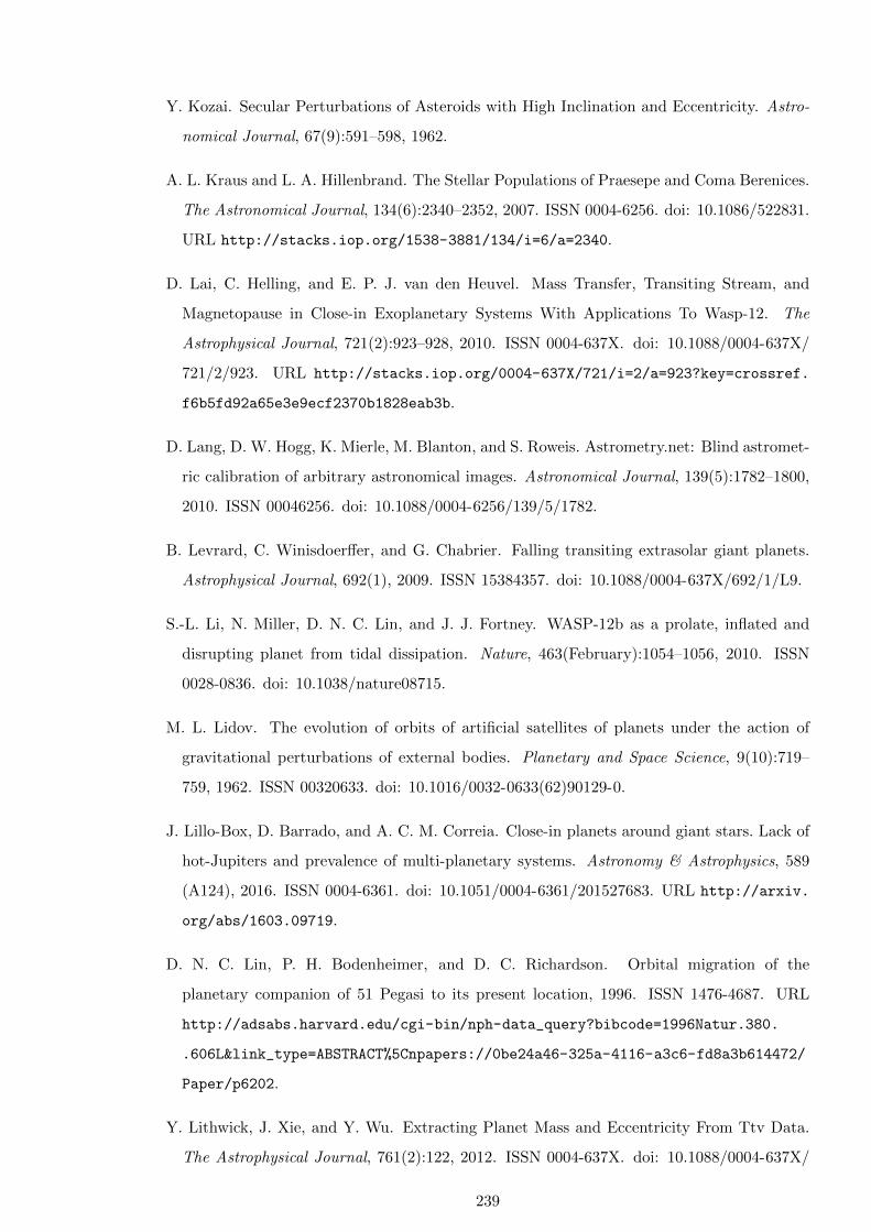
Y. Kozai. Secular Perturbations of Asteroids with High Inclination and Eccentricity. Astro-

nomical Journal, 67(9):591–598, 1962.

A. L. Kraus and L. A. Hillenbrand. The Stellar Populations of Praesepe and Coma Berenices.

The Astronomical Journal, 134(6):2340–2352, 2007. ISSN 0004-6256. doi: 10.1086/522831.

URL http://stacks.iop.org/1538-3881/134/i=6/a=2340.

D. Lai, C. Helling, and E. P. J. van den Heuvel. Mass Transfer, Transiting Stream, and

Magnetopause in Close-in Exoplanetary Systems With Applications To Wasp-12. The

Astrophysical Journal, 721(2):923–928, 2010. ISSN 0004-637X. doi: 10.1088/0004-637X/

721/2/923. URL http://stacks.iop.org/0004-637X/721/i=2/a=923?key=crossref.

f6b5fd92a65e3e9ecf2370b1828eab3b.

D. Lang, D. W. Hogg, K. Mierle, M. Blanton, and S. Roweis. Astrometry.net: Blind astromet-

ric calibration of arbitrary astronomical images. Astronomical Journal, 139(5):1782–1800,

2010. ISSN 00046256. doi: 10.1088/0004-6256/139/5/1782.

B. Levrard, C. Winisdoerffer, and G. Chabrier. Falling transiting extrasolar giant planets.

Astrophysical Journal, 692(1), 2009. ISSN 15384357. doi: 10.1088/0004-637X/692/1/L9.

S.-L. Li, N. Miller, D. N. C. Lin, and J. J. Fortney. WASP-12b as a prolate, inflated and

disrupting planet from tidal dissipation. Nature, 463(February):1054–1056, 2010. ISSN

0028-0836. doi: 10.1038/nature08715.

M. L. Lidov. The evolution of orbits of artificial satellites of planets under the action of

gravitational perturbations of external bodies. Planetary and Space Science, 9(10):719–

759, 1962. ISSN 00320633. doi: 10.1016/0032-0633(62)90129-0.

J. Lillo-Box, D. Barrado, and A. C. M. Correia. Close-in planets around giant stars. Lack of

hot-Jupiters and prevalence of multi-planetary systems. Astronomy & Astrophysics, 589

(A124), 2016. ISSN 0004-6361. doi: 10.1051/0004-6361/201527683. URL http://arxiv.

org/abs/1603.09719.

D. N. C. Lin, P. H. Bodenheimer, and D. C. Richardson. Orbital migration of the

planetary companion of 51 Pegasi to its present location, 1996. ISSN 1476-4687. URL

http://adsabs.harvard.edu/cgi-bin/nph-data_query?bibcode=1996Natur.380.

.606L&link_type=ABSTRACT%5Cnpapers://0be24a46-325a-4116-a3c6-fd8a3b614472/

Paper/p6202.

Y. Lithwick, J. Xie, and Y. Wu. Extracting Planet Mass and Eccentricity From Ttv Data.

The Astrophysical Journal, 761(2):122, 2012. ISSN 0004-637X. doi: 10.1088/0004-637X/

239

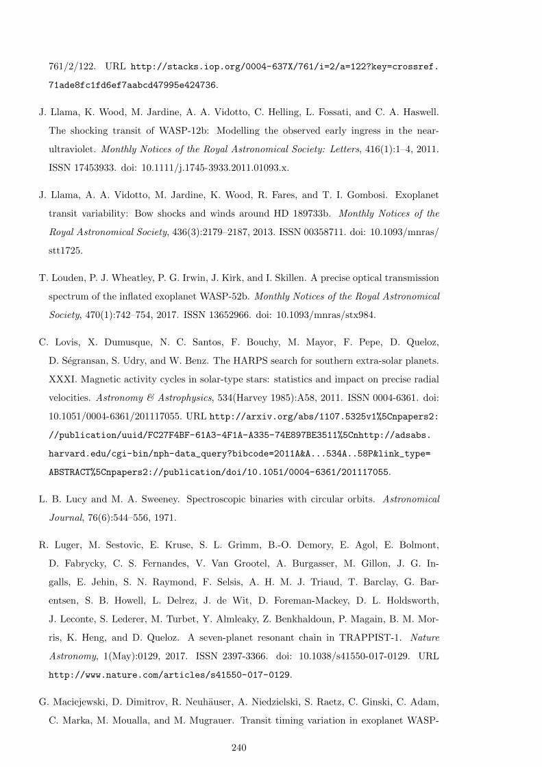
761/2/122. URL http://stacks.iop.org/0004-637X/761/i=2/a=122?key=crossref.

71ade8fc1fd6ef7aabcd47995e424736.

J. Llama, K. Wood, M. Jardine, A. A. Vidotto, C. Helling, L. Fossati, and C. A. Haswell.

The shocking transit of WASP-12b: Modelling the observed early ingress in the near-

ultraviolet. Monthly Notices of the Royal Astronomical Society: Letters, 416(1):1–4, 2011.

ISSN 17453933. doi: 10.1111/j.1745-3933.2011.01093.x.

J. Llama, A. A. Vidotto, M. Jardine, K. Wood, R. Fares, and T. I. Gombosi. Exoplanet

transit variability: Bow shocks and winds around HD 189733b. Monthly Notices of the

Royal Astronomical Society, 436(3):2179–2187, 2013. ISSN 00358711. doi: 10.1093/mnras/

stt1725.

T. Louden, P. J. Wheatley, P. G. Irwin, J. Kirk, and I. Skillen. A precise optical transmission

spectrum of the inflated exoplanet WASP-52b. Monthly Notices of the Royal Astronomical

Society, 470(1):742–754, 2017. ISSN 13652966. doi: 10.1093/mnras/stx984.

C. Lovis, X. Dumusque, N. C. Santos, F. Bouchy, M. Mayor, F. Pepe, D. Queloz,

D. Segransan, S. Udry, and W. Benz. The HARPS search for southern extra-solar planets.

XXXI. Magnetic activity cycles in solar-type stars: statistics and impact on precise radial

velocities. Astronomy & Astrophysics, 534(Harvey 1985):A58, 2011. ISSN 0004-6361. doi:

10.1051/0004-6361/201117055. URL http://arxiv.org/abs/1107.5325v1%5Cnpapers2:

//publication/uuid/FC27F4BF-61A3-4F1A-A335-74E897BE3511%5Cnhttp://adsabs.

harvard.edu/cgi-bin/nph-data_query?bibcode=2011A&A...534A..58P&link_type=

ABSTRACT%5Cnpapers2://publication/doi/10.1051/0004-6361/201117055.

L. B. Lucy and M. A. Sweeney. Spectroscopic binaries with circular orbits. Astronomical

Journal, 76(6):544–556, 1971.

R. Luger, M. Sestovic, E. Kruse, S. L. Grimm, B.-O. Demory, E. Agol, E. Bolmont,

D. Fabrycky, C. S. Fernandes, V. Van Grootel, A. Burgasser, M. Gillon, J. G. In-

galls, E. Jehin, S. N. Raymond, F. Selsis, A. H. M. J. Triaud, T. Barclay, G. Bar-

entsen, S. B. Howell, L. Delrez, J. de Wit, D. Foreman-Mackey, D. L. Holdsworth,

J. Leconte, S. Lederer, M. Turbet, Y. Almleaky, Z. Benkhaldoun, P. Magain, B. M. Mor-

ris, K. Heng, and D. Queloz. A seven-planet resonant chain in TRAPPIST-1. Nature

Astronomy, 1(May):0129, 2017. ISSN 2397-3366. doi: 10.1038/s41550-017-0129. URL

http://www.nature.com/articles/s41550-017-0129.

G. Maciejewski, D. Dimitrov, R. Neuhauser, A. Niedzielski, S. Raetz, C. Ginski, C. Adam,

C. Marka, M. Moualla, and M. Mugrauer. Transit timing variation in exoplanet WASP-

240

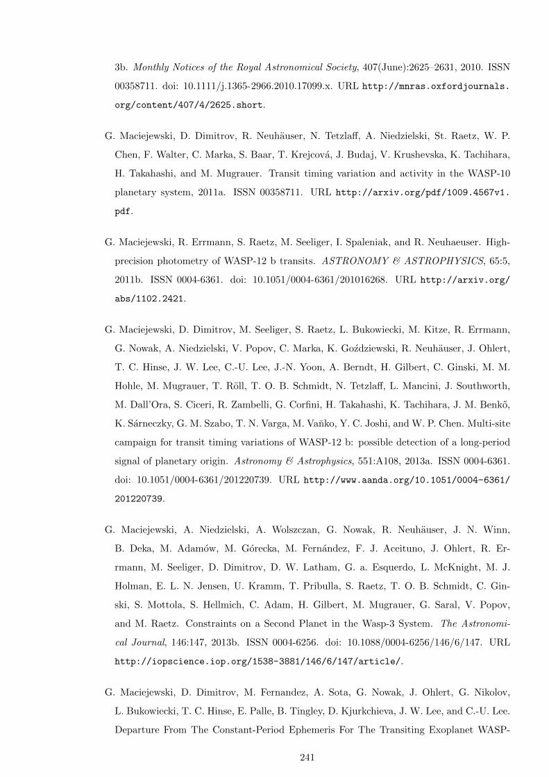
3b. Monthly Notices of the Royal Astronomical Society, 407(June):2625–2631, 2010. ISSN

00358711. doi: 10.1111/j.1365-2966.2010.17099.x. URL http://mnras.oxfordjournals.

org/content/407/4/2625.short.

G. Maciejewski, D. Dimitrov, R. Neuhauser, N. Tetzlaff, A. Niedzielski, St. Raetz, W. P.

Chen, F. Walter, C. Marka, S. Baar, T. Krejcova, J. Budaj, V. Krushevska, K. Tachihara,

H. Takahashi, and M. Mugrauer. Transit timing variation and activity in the WASP-10

planetary system, 2011a. ISSN 00358711. URL http://arxiv.org/pdf/1009.4567v1.

pdf.

G. Maciejewski, R. Errmann, S. Raetz, M. Seeliger, I. Spaleniak, and R. Neuhaeuser. High-

precision photometry of WASP-12 b transits. ASTRONOMY & ASTROPHYSICS, 65:5,

2011b. ISSN 0004-6361. doi: 10.1051/0004-6361/201016268. URL http://arxiv.org/

abs/1102.2421.

G. Maciejewski, D. Dimitrov, M. Seeliger, S. Raetz, L. Bukowiecki, M. Kitze, R. Errmann,

G. Nowak, A. Niedzielski, V. Popov, C. Marka, K. Gozdziewski, R. Neuhauser, J. Ohlert,

T. C. Hinse, J. W. Lee, C.-U. Lee, J.-N. Yoon, A. Berndt, H. Gilbert, C. Ginski, M. M.

Hohle, M. Mugrauer, T. Roll, T. O. B. Schmidt, N. Tetzlaff, L. Mancini, J. Southworth,

M. Dall’Ora, S. Ciceri, R. Zambelli, G. Corfini, H. Takahashi, K. Tachihara, J. M. Benko,

K. Sarneczky, G. M. Szabo, T. N. Varga, M. Vanko, Y. C. Joshi, and W. P. Chen. Multi-site

campaign for transit timing variations of WASP-12 b: possible detection of a long-period

signal of planetary origin. Astronomy & Astrophysics, 551:A108, 2013a. ISSN 0004-6361.

doi: 10.1051/0004-6361/201220739. URL http://www.aanda.org/10.1051/0004-6361/

201220739.

G. Maciejewski, A. Niedzielski, A. Wolszczan, G. Nowak, R. Neuhauser, J. N. Winn,

B. Deka, M. Adamow, M. Gorecka, M. Fernandez, F. J. Aceituno, J. Ohlert, R. Er-

rmann, M. Seeliger, D. Dimitrov, D. W. Latham, G. a. Esquerdo, L. McKnight, M. J.

Holman, E. L. N. Jensen, U. Kramm, T. Pribulla, S. Raetz, T. O. B. Schmidt, C. Gin-

ski, S. Mottola, S. Hellmich, C. Adam, H. Gilbert, M. Mugrauer, G. Saral, V. Popov,

and M. Raetz. Constraints on a Second Planet in the Wasp-3 System. The Astronomi-

cal Journal, 146:147, 2013b. ISSN 0004-6256. doi: 10.1088/0004-6256/146/6/147. URL

http://iopscience.iop.org/1538-3881/146/6/147/article/.

G. Maciejewski, D. Dimitrov, M. Fernandez, A. Sota, G. Nowak, J. Ohlert, G. Nikolov,

L. Bukowiecki, T. C. Hinse, E. Palle, B. Tingley, D. Kjurkchieva, J. W. Lee, and C.-U. Lee.

Departure From The Constant-Period Ephemeris For The Transiting Exoplanet WASP-

241

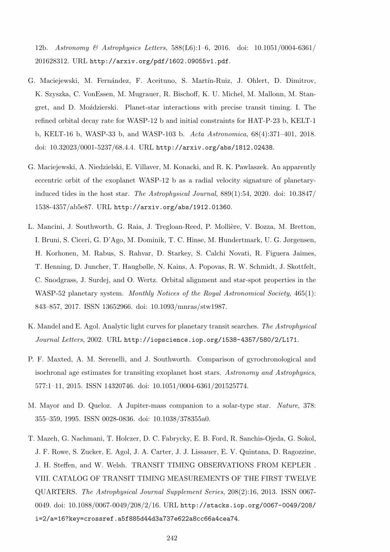
12b. Astronomy & Astrophysics Letters, 588(L6):1–6, 2016. doi: 10.1051/0004-6361/

201628312. URL http://arxiv.org/pdf/1602.09055v1.pdf.

G. Maciejewski, M. Fernandez, F. Aceituno, S. Martın-Ruiz, J. Ohlert, D. Dimitrov,

K. Szyszka, C. VonEssen, M. Mugrauer, R. Bischoff, K. U. Michel, M. Mallonn, M. Stan-

gret, and D. Mozdzierski. Planet-star interactions with precise transit timing. I. The

refined orbital decay rate for WASP-12 b and initial constraints for HAT-P-23 b, KELT-1

b, KELT-16 b, WASP-33 b, and WASP-103 b. Acta Astronomica, 68(4):371–401, 2018.

doi: 10.32023/0001-5237/68.4.4. URL http://arxiv.org/abs/1812.02438.

G. Maciejewski, A. Niedzielski, E. Villaver, M. Konacki, and R. K. Pawlaszek. An apparently

eccentric orbit of the exoplanet WASP-12 b as a radial velocity signature of planetary-

induced tides in the host star. The Astrophysical Journal, 889(1):54, 2020. doi: 10.3847/

1538-4357/ab5e87. URL http://arxiv.org/abs/1912.01360.

L. Mancini, J. Southworth, G. Raia, J. Tregloan-Reed, P. Molliere, V. Bozza, M. Bretton,

I. Bruni, S. Ciceri, G. D’Ago, M. Dominik, T. C. Hinse, M. Hundertmark, U. G. Jørgensen,

H. Korhonen, M. Rabus, S. Rahvar, D. Starkey, S. Calchi Novati, R. Figuera Jaimes,

T. Henning, D. Juncher, T. Haugbølle, N. Kains, A. Popovas, R. W. Schmidt, J. Skottfelt,

C. Snodgrass, J. Surdej, and O. Wertz. Orbital alignment and star-spot properties in the

WASP-52 planetary system. Monthly Notices of the Royal Astronomical Society, 465(1):

843–857, 2017. ISSN 13652966. doi: 10.1093/mnras/stw1987.

K. Mandel and E. Agol. Analytic light curves for planetary transit searches. The Astrophysical

Journal Letters, 2002. URL http://iopscience.iop.org/1538-4357/580/2/L171.

P. F. Maxted, A. M. Serenelli, and J. Southworth. Comparison of gyrochronological and

isochronal age estimates for transiting exoplanet host stars. Astronomy and Astrophysics,

577:1–11, 2015. ISSN 14320746. doi: 10.1051/0004-6361/201525774.

M. Mayor and D. Queloz. A Jupiter-mass companion to a solar-type star. Nature, 378:

355–359, 1995. ISSN 0028-0836. doi: 10.1038/378355a0.

T. Mazeh, G. Nachmani, T. Holczer, D. C. Fabrycky, E. B. Ford, R. Sanchis-Ojeda, G. Sokol,

J. F. Rowe, S. Zucker, E. Agol, J. A. Carter, J. J. Lissauer, E. V. Quintana, D. Ragozzine,

J. H. Steffen, and W. Welsh. TRANSIT TIMING OBSERVATIONS FROM KEPLER .

VIII. CATALOG OF TRANSIT TIMING MEASUREMENTS OF THE FIRST TWELVE

QUARTERS. The Astrophysical Journal Supplement Series, 208(2):16, 2013. ISSN 0067-

0049. doi: 10.1088/0067-0049/208/2/16. URL http://stacks.iop.org/0067-0049/208/

i=2/a=16?key=crossref.a5f885d44d3a737e622a8cc66a4cea74.

242

F. Middelkoop. Magnetic structure in cool stars. Astronomy & Astrophysics, 107:31–35,

1982.

S. Millholland, S. Wang, and G. Laughlin. on the Detection of Non-Transiting Hot Jupiters

in Multiple-Planet Systems. The Astrophysical Journal, 823(1):L7, 2016. ISSN 2041-8213.

doi: 10.3847/2041-8205/823/1/L7. URL http://stacks.iop.org/2041-8205/823/i=1/

a=L7?key=crossref.12a97172ee6e3d3db3c6f07adf500f1d.

M. Montalto, J. Gregorio, G. Boue, A. Mortier, I. Boisse, M. Oshagh, M. Maturi, P. Figueira,

S. Sousa, and N. C. Santos. A new analysis of the WASP-3 system: No evidence for an

additional companion. Monthly Notices of the Royal Astronomical Society, 427:2757–2771,

2012. ISSN 00358711. doi: 10.1111/j.1365-2966.2012.21926.

C. Moutou, R. F. Dıaz, S. Udry, G. Hebrard, F. Bouchy, A. Santerne, D. Ehrenreich,

L. Arnold, I. Boisse, X. Bonfils, X. Delfosse, A. Eggenberger, T. Forveille, A.-M. Lagrange,

C. Lovis, P. Martinez, F. Pepe, C. Perrier, D. Queloz, N. C. Santos, D. Segransan, D. Tou-

blanc, J. P. Troncin, M. Vanhuysse, and A. Vidal-Madjar. Spin-orbit inclinations of the

exoplanetary systems HAT-P-8b, HAT-P-9b, HAT-P-16b, and HAT-P-23b. Astronomy &

Astrophysics, 533:A113, 2011. ISSN 0004-6361. doi: 10.1051/0004-6361/201116760. URL

http://www.aanda.org/10.1051/0004-6361/201116760.

S. Naoz, W. M. Farr, Y. Lithwick, F. A. Rasio, and J. Teyssandier. Hot Jupiters from

secular planet-planet interactions. Nature, 473(7346):187–189, 2011. ISSN 0028-0836. doi:

10.1038/nature10076. URL http://dx.doi.org/10.1038/nature10076.

V. Nascimbeni, G. Piotto, L. R. Bedin, M. Damasso, L. Malavolta, and L. Bor-

sato. TASTE. II. A new observational study of transit time variations in HAT-P-

13b. Astronomy & Aastrophysics, 532:5, 2011. ISSN 0004-6361. doi: 10.1051/

0004-6361/201116830. URL http://www.aanda.org/index.php?option=com_article&

access=doi&doi=10.1051/0004-6361/201116830&Itemid=129.

V. Nascimbeni, A. Cunial, S. Murabito, P. V. Sada, A. Aparicio, G. Piotto, L. R. Bedin,

a. P. Milone, A. Rosenberg, L. Borsato, M. Damasso, V. Granata, and L. Malavolta.

TASTE. III. A homogeneous study of transit time variations in WASP-3b. Astronomy

& Astrophysics, 30:10, 2012. ISSN 00046361. doi: 10.1051/0004-6361/201219601. URL

http://arxiv.org/abs/1210.3045.

D. Nesvorny. Dynamical Evolution of the Early Solar System. Annual Review of

Astronomy and Astrophysics, 56:137–174, 2018. ISSN 00664146. doi: 10.1146/

annurev-astro-081817-052028.

243

D. Nesvorny and A. Morbidelli. Mass and Orbit Determination from Transit Timing Varia-

tions of Exoplanets. The Astrophysical Journal, 688:636–646, 2008. ISSN 0004-637X. doi:

10.1086/592230.

D. Nesvorny, D. Kipping, D. Terrell, J. Hartman, G. A. Bakos, and L. A. Buch-

have. Koi-142, the King of Transit Variations, Is a Pair of Planets Near the 2:1

Resonance. The Astrophysical Journal, 777(1):3, 2013. ISSN 0004-637X. doi: 10.

1088/0004-637X/777/1/3. URL http://stacks.iop.org/0004-637X/777/i=1/a=3?key=

crossref.fce3e49bce2ae77779104a784d8e271c.

M. Neveu-VanMalle, D. Queloz, D. Anderson, D. Brown, A. Collier Cameron, L. Delrez,

R. Diaz, M. Gillon, C. Hellier, E. Jehin, T. Lister, F. Pepe, P. Rojo, D. Segransan, A. H.

M. J. Triaud, and O. D. Turner. Hot Jupiters with relatives : discovery of additional

planets in orbit around WASP-41 and WASP-47. Astronomy & Astrophysics, 586(A93),

2016.

E. R. Newton, J. Irwin, D. Charbonneau, Z. K. Berta-Thompson, and J. A. Dittmann. the

Impact of Stellar Rotation on the Detectability of Habitable Planets Around M Dwarfs.

The Astrophysical Journal, 821(1):L19, 2016. ISSN 2041-8213. doi: 10.3847/2041-8205/

821/1/L19. URL http://stacks.iop.org/2041-8205/821/i=1/a=L19?key=crossref.

0d5836e5a79602634f48ede8311416ab.

H. Ngo, H. A. Knutson, S. Hinkley, J. R. Crepp, E. B. Bechter, K. Batygin, A. W. Howard,

J. A. Johnson, T. D. Morton, and P. S. Muirhead. Friends of Hot Jupiters. Ii. No Cor-

respondence Between Hot-Jupiter Spin-Orbit Misalignment and the Incidence of Directly

Imaged Stellar Companions. The Astrophysical Journal, 800(2):138, 2015. ISSN 1538-

4357. doi: 10.1088/0004-637X/800/2/138. URL http://stacks.iop.org/0004-637X/

800/i=2/a=138?key=crossref.ab38ac455dedffad91d5f83518699a4f.

H. Ngo, H. A. Knutson, S. Hinkley, M. Bryan, J. R. Crepp, K. Batygin, I. Cross-

field, B. Hansen, A. W. Howard, J. A. Johnson, D. Mawet, T. D. Morton, P. S.

Muirhead, and J. Wang. FRIENDS OF HOT JUPITERS. IV. STELLAR COM-

PANIONS BEYOND 50 au MIGHT FACILITATE GIANT PLANET FORMATION,

BUT MOST ARE UNLIKELY TO CAUSE KOZAI–LIDOV MIGRATION. The As-

trophysical Journal, 827(1):8, 2016. ISSN 1538-4357. doi: 10.3847/0004-637X/827/1/

8. URL http://arxiv.org/abs/1606.07102http://stacks.iop.org/0004-637X/827/

i=1/a=8?key=crossref.8fb98170bdefb0584cf6c47b8dca4cb4.

M. B. Nielsen, L. Gizon, H. Schunker, and C. Karoff. Rotation periods of 12 000 main-

sequence Kepler stars: Dependence on stellar spectral type and comparison with v sin i

244

observations. Astronomy & Astrophysics, 557:L10, 2013. ISSN 0004-6361. doi: 10.1051/

0004-6361/201321912. URL http://www.aanda.org/10.1051/0004-6361/201321912.

F. T. O’Donovan, D. Charbonneau, G. A. Bakos, G. Mandushev, E. W. Dunham, T. M.

Brown, D. W. Latham, G. Torres, A. Sozzetti, G. Kovacs, M. E. Everett, N. Baliber,

M. G. Hidas, G. a. Esquerdo, M. Rabus, H. J. Deeg, J. a. Belmonte, L. a. Hillenbrand, and

R. P. Stefanik. TrES-3: A Nearby, Massive, Transiting Hot Jupiter in a 31-Hour Orbit.

The Astrophysical Journal, 663(1):37–40, 2007. ISSN 0004-637X. doi: 10.1086/519793.

URL http://arxiv.org/abs/0705.2004.

J. G. O’Rourke, H. A. Knutson, M. Zhao, J. J. Fortney, A. Burrows, E. Agol, D. Deming, J. M.

Desert, A. W. Howard, N. K. Lewis, A. P. Showman, and K. O. Todorov. Warm spitzer and

palomar near-ir secondary eclipse photometry of two hot jupiters: Wasp-48b and hat-p-23b.

Astrophysical Journal, 781(2), 2014. ISSN 15384357. doi: 10.1088/0004-637X/781/2/109.

J. Osborn, D. Fohring, V. S. Dhillon, and R. W. Wilson. Atmospheric scintillation in astro-

nomical photometry. Monthly Notices of the Royal Astronomical Society, 452(2):1707–1716,

2015. ISSN 13652966. doi: 10.1093/mnras/stv1400.

M. Oshagh, N. C. Santos, I. Boisse, G. Boue, M. Montalto, X. Dumusque, and N. Haghigh-

ipour. Effect of stellar spots on high-precision transit light-curve. Astronomy & As-

trophysics, 556:A19, 2013. ISSN 0004-6361. doi: 10.1051/0004-6361/201321309. URL

http://arxiv.org/abs/1306.0739.

O. Ozturk and A. Erdem. New photometric analysis of five exoplanets: CoRoT-2b, HAT-

P-12b, TrES-2b, WASP-12b and WASP-52b. Monthly Notices of the Royal Astronomical

Society, 2, 2019. ISSN 0035-8711. doi: 10.1093/mnras/stz747. URL https://academic.

oup.com/mnras/advance-article/doi/10.1093/mnras/stz747/5380787.

A. Pal, K. Sarneczky, G. M. Szabo, A. Szing, L. L. Kiss, G. Mezo, Z. Regaly, and G. Mezo.

Transit timing variations in the HAT-P-13 planetary system. Monthly Notices of the Royal

Astronomical Society: Letters, 46:5, 2011. ISSN 17453925. doi: 10.1111/j.1745-3933.2011.

01029.x. URL http://arxiv.org/abs/1102.0525%5Cnhttp://doi.wiley.com/10.1111/

j.1745-3933.2011.01029.x.

K. C. Patra, J. N. Winn, M. J. Holman, L. Yu, D. Deming, and F. Dai. The Apparently

Decaying Orbit of WASP-12. The Astronomical Journal, 154(1), 2017. URL http://

arxiv.org/abs/1703.06582.

K. C. Patra, J. N. Winn, M. J. Holman, M. Gillon, A. Burdanov, E. Jehin, L. Delrez, F. J.

Pozuelos, K. Barkaoui, Z. Benkhaldoun, N. Narita, A. Fukui, N. Kusakabe, K. Kawauchi,

245

Y. Terada, L. G. Bouma, N. N. Weinberg, and M. Broome. The continuing search for

evidence of tidal orbital decay of hot Jupiters. The Astronomical Journal, 159(4), 2020.

URL http://arxiv.org/abs/2002.02606.

K. Penev, J. D. Hartman, G. A. Bakos, S. Ciceri, R. Brahm, D. Bayliss, J. Bento, A. Jordan,

Z. Csubry, W. Bhatti, M. d. Val-Borro, N. Espinoza, G. Zhou, L. Mancini, M. Rabus,

V. Suc, T. Henning, B. Schmidt, R. W. Noyes, J. Lazar, I. Papp, and P. Sari. Hats-18B: an

Extreme Short-Period Massive Transiting Planet Spinning Up Its Star. The Astronomical

Journal, 152(5):127, 2016. ISSN 1538-3881. doi: 10.3847/0004-6256/152/5/127. URL

http://dx.doi.org/10.3847/0004-6256/152/5/127.

K. Penev, L. G. Bouma, J. N. Winn, and J. D. Hartman. Empirical Tidal Dissipation

in Exoplanet Hosts From Tidal Spin-up. The Astronomical Journal, 155(4):165, 2018.

ISSN 1538-3881. doi: 10.3847/1538-3881/aaaf71. URL http://dx.doi.org/10.3847/

1538-3881/aaaf71.

M. Perryman. Resource Letter Exo-1: Exoplanets. American Journal of Physics, 82(6):

552–563, 2014. ISSN 0002-9505. doi: 10.1119/1.4830455. URL http://scitation.aip.

org/content/aapt/journal/ajp/82/6/10.1119/1.4830455.

R. Petrucci, E. Jofr, M. Chew, T. C. Hinse, M. Maˇ, and T. Tan. Discarding orbital de-

cay in WASP-19b after one decade of transit observations. Monthly Notices of the Royal

Astronomical Society, 491(1):1243–1259, 2020. doi: 10.1093/mnras/stz3034. URL Decay.

S. Poddany, L. Brat, and O. Pejcha. Exoplanet Transit Database. Reduction and processing

of the photometric data of exoplanet transits. New Astronomy, 15(September 2009):297–

301, 2010. ISSN 13841076. doi: 10.1016/j.newast.2009.09.001.

K. Poppenhaeger. Tidal effects on stellar activity. Proceedings of the International Astro-

nomical Union, 12(328):308–314, 2016. ISSN 17439221. doi: 10.1017/S1743921317004045.

K. Poppenhaeger and S. J. Wolk. Indications for an influence of hot Jupiters on the rotation

and activity of their host stars. Astronomy & Astrophysics, 565:L1, 2014. ISSN 0004-

6361. doi: 10.1051/0004-6361/201423454. URL http://www.aanda.org/articles/aa/

full_html/2014/05/aa23454-14/aa23454-14.html.

A. M. Price-Whelan, B. M. Sipocz, H. M. Gunther, and P. L. Lim. The Astropy Project:

Building an Open-science Project and Status of the v2.0 Core Package. The Astronomical

Journal, 156(3):123, 2018. ISSN 0004-6256. doi: 10.3847/1538-3881/aabc4f.

G. Privitera. Star-planet interactions II. Astronomy & Aastrophysics, 593(A128), 2019. doi:

10.1051/0004-6361/201628758.

246

G. Privitera, G. Meynet, P. Eggenberger, A. A. Vidotto, E. Villaver, and M. Bianda. Star-

planet interactions: I. Stellar rotation and planetary orbits. Astronomy & Astrophysics,

pages 1–14, 2016. URL http://arxiv.org/abs/1604.06005.

D. Ragozzine and M. J. Holman. The Value of Systems with Multiple Transiting Planets.

Bulletin of the American Astronomical Society, 41:929, 2010. URL http://arxiv.org/

abs/1006.3727.

D. Ragozzine and A. S. Wolf. Probing the Interiors of Very Hot Jupiters Using Transit

Light Curves. The Astrophysical Journal, 698(2):1778–1794, 2009. ISSN 0004-637X. doi:

10.1088/0004-637X/698/2/1778.

F. G. Ramon-Fox and P. V. Sada. Parameters of recent transits of HAT-P-23b. Revista

Mexicana de Astronomia y Astrofisica, 49(1):71–77, 2013. ISSN 01851101.

S. N. Raymond, A. M. Mandell, and S. Sigurdsson. Exotic Earths Forming Habitable Worlds-

Giant Planet.pdf. Science, 313(5792):1413–1416, 2006.

W. K. M. Rice, J. Veljanoski, and a. C. Cameron. Tidal evolution of close-in giant planets:

Evidence of type II migration? Monthly Notices of the Royal Astronomical Society, 425:

2567–2575, 2012. ISSN 00358711. doi: 10.1111/j.1365-2966.2012.21728.x.

T. P. Robitaille, E. J. Tollerud, and P. Greenfield. Astropy: A community Python package

for astronomy. Astronomy and Astrophysics, 558:1–9, 2013. ISSN 00046361. doi: 10.1051/

0004-6361/201322068.

P. V. Sada and F. G. Ramon-Fox. Exoplanet Transits Registered at the Universidad de

Monterrey Observatory. Part I: HAT-P-12b, HAT-P-13b, HAT-P-16b, HAT-P-23b and

WASP-10b. Publications of the Astronomical Society of the Pacific, 128(960), 2016. ISSN

00046280. doi: 10.1088/1538-3873/128/960/024402. URL http://arxiv.org/abs/1601.

02292.

M. Salisbury. An investigation into the precision with which exoplanet transit timing can be

measured with two small telescopes . SXP390 Project, Unpublished, 2015.

M. A. Salisbury, U. C. Kolb, A. J. Norton, and C. A. Haswell. Monitoring of transiting

exoplanets and their host stars with small aperture telescopes. New Astronomy, 83(April

2020):101477, 2021. ISSN 13841076. doi: 10.1016/j.newast.2020.101477. URL https:

//doi.org/10.1016/j.newast.2020.101477.

E. F. Schlafly and D. P. Finkbeiner. Measuring reddening with Sloan Digital Sky Survey

247

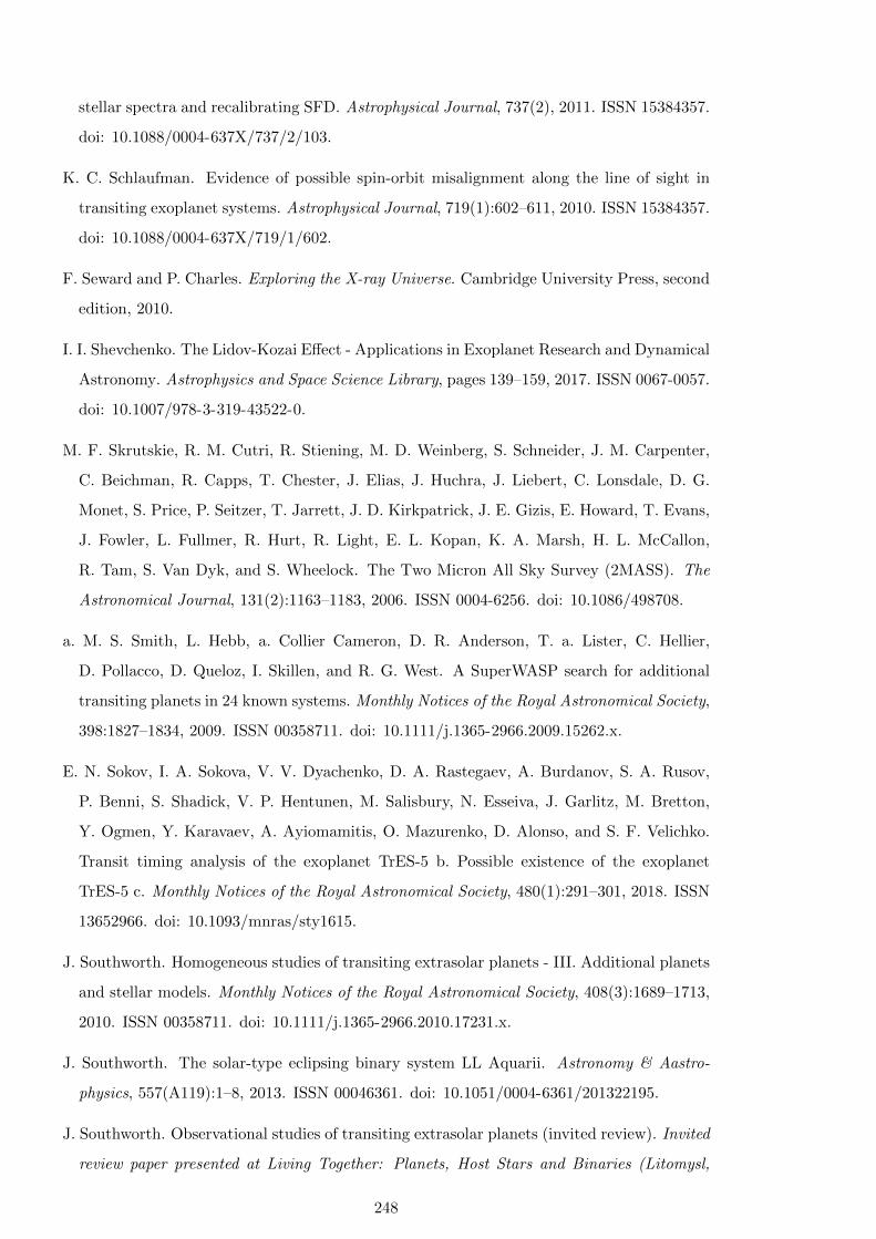
stellar spectra and recalibrating SFD. Astrophysical Journal, 737(2), 2011. ISSN 15384357.

doi: 10.1088/0004-637X/737/2/103.

K. C. Schlaufman. Evidence of possible spin-orbit misalignment along the line of sight in

transiting exoplanet systems. Astrophysical Journal, 719(1):602–611, 2010. ISSN 15384357.

doi: 10.1088/0004-637X/719/1/602.

F. Seward and P. Charles. Exploring the X-ray Universe. Cambridge University Press, second

edition, 2010.

I. I. Shevchenko. The Lidov-Kozai Effect - Applications in Exoplanet Research and Dynamical

Astronomy. Astrophysics and Space Science Library, pages 139–159, 2017. ISSN 0067-0057.

doi: 10.1007/978-3-319-43522-0.

M. F. Skrutskie, R. M. Cutri, R. Stiening, M. D. Weinberg, S. Schneider, J. M. Carpenter,

C. Beichman, R. Capps, T. Chester, J. Elias, J. Huchra, J. Liebert, C. Lonsdale, D. G.

Monet, S. Price, P. Seitzer, T. Jarrett, J. D. Kirkpatrick, J. E. Gizis, E. Howard, T. Evans,

J. Fowler, L. Fullmer, R. Hurt, R. Light, E. L. Kopan, K. A. Marsh, H. L. McCallon,

R. Tam, S. Van Dyk, and S. Wheelock. The Two Micron All Sky Survey (2MASS). The

Astronomical Journal, 131(2):1163–1183, 2006. ISSN 0004-6256. doi: 10.1086/498708.

a. M. S. Smith, L. Hebb, a. Collier Cameron, D. R. Anderson, T. a. Lister, C. Hellier,

D. Pollacco, D. Queloz, I. Skillen, and R. G. West. A SuperWASP search for additional

transiting planets in 24 known systems. Monthly Notices of the Royal Astronomical Society,

398:1827–1834, 2009. ISSN 00358711. doi: 10.1111/j.1365-2966.2009.15262.x.

E. N. Sokov, I. A. Sokova, V. V. Dyachenko, D. A. Rastegaev, A. Burdanov, S. A. Rusov,

P. Benni, S. Shadick, V. P. Hentunen, M. Salisbury, N. Esseiva, J. Garlitz, M. Bretton,

Y. Ogmen, Y. Karavaev, A. Ayiomamitis, O. Mazurenko, D. Alonso, and S. F. Velichko.

Transit timing analysis of the exoplanet TrES-5 b. Possible existence of the exoplanet

TrES-5 c. Monthly Notices of the Royal Astronomical Society, 480(1):291–301, 2018. ISSN

13652966. doi: 10.1093/mnras/sty1615.

J. Southworth. Homogeneous studies of transiting extrasolar planets - III. Additional planets

and stellar models. Monthly Notices of the Royal Astronomical Society, 408(3):1689–1713,

2010. ISSN 00358711. doi: 10.1111/j.1365-2966.2010.17231.x.

J. Southworth. The solar-type eclipsing binary system LL Aquarii. Astronomy & Aastro-

physics, 557(A119):1–8, 2013. ISSN 00046361. doi: 10.1051/0004-6361/201322195.

J. Southworth. Observational studies of transiting extrasolar planets (invited review). Invited

review paper presented at Living Together: Planets, Host Stars and Binaries (Litomysl,

248

Czech Republic, September 2014), pages 1–15, 11 2014. URL http://arxiv.org/abs/

1411.5517v1.

J. Southworth and L. Mancini. Orbital obliquities of transiting planets from starspot occul-

tations. The 19th CambridgeWorkshop on Cool Stars, Stellar Systems, and the Sun Edited

by G. A. Feiden, 1:3–8, 2016. URL http://arxiv.org/abs/1608.03095.

J. Southworth, P. F. L. Maxted, and B. Smalley. Eclipsing binaries in open clusters - II. V453

Cyg in NGC 6871. Monthly Notices of the Royal Astronomical Society, 351(4):1277–1289,

2004. ISSN 00358711. doi: 10.1111/j.1365-2966.2004.07871.x.

J. Southworth, T. C. Hinse, M. J. Burgdorf, M. Dominik, a. Hornstrup, U. G. Jørgensen,

C. Liebig, D. Ricci, C. C. Thone, T. Anguita, V. Bozza, S. C. Novati, K. Harpsøe,

L. Mancini, G. Masi, M. Mathiasen, S. Rahvar, G. Scarpetta, C. Snodgrass, J. Surdej,

and M. Zub. High-precision photometry by telescope defocussing - II. the transiting plan-

etary system WASP-4. Monthly Notices of the Royal Astronomical Society, 399:287–294,

2009a. ISSN 00358711. doi: 10.1111/j.1365-2966.2009.15283.x.

J. Southworth, T. C. Hinse, U. G. Jørgensen, M. Dominik, D. Ricci, M. J. Burgdorf, A. Horn-

strup, P. J. Wheatley, T. Anguita, V. Bozza, S. C. Novati, K. Harpsøe, P. Kjærgaard,

C. Liebig, L. Mancini, G. Masi, M. Mathiasen, S. Rahvar, G. Scarpetta, C. Snodgrass,

J. Surdej, C. C. Thone, and M. Zub. High-precision photometry by telescope defocusing

- I. the transiting planetary system WASP-5. Monthly Notices of the Royal Astronomical

Society, 396(2):1023–1031, 2009b. ISSN 00358711. doi: 10.1111/j.1365-2966.2009.14767.x.

J. Southworth, I. Bruni, L. Mancini, and J. Gregorio. Refined physical properties of the

HAT-P-13 planetary system. Monthly Notices of the Royal Astronomical Society, 420(3):

2580–2587, 2012. ISSN 00358711. doi: 10.1111/j.1365-2966.2011.20230.x.

J. Southworth, M. Dominik, U. G. Jørgensen, M. I. Andersen, V. Bozza, M. J. Burgdorf,

G. D’Ago, S. Dib, R. F. Jaimes, Y. I. Fujii, S. Gill, L. K. Haikala, T. C. Hinse, M. Hun-

dertmark, E. Khalouei, H. Korhonen, P. Longa-Pena, L. Mancini, N. Peixinho, M. Rabus,

S. Rahvar, S. Sajadian, J. Skottfelt, C. Snodgrass, P. Spyratos, J. Tregloan-Reed, E. Unda-

Sanzana, and C. von Essen. Transit timing variations in the WASP-4 planetary system*.

Monthly Notices of the Royal Astronomical Society, 490(3):4230–4236, 2019. ISSN 0035-

8711. doi: 10.1093/mnras/stz2602.

J. J. Spake, D. J. Brown, A. P. Doyle, G. Hebrard, J. McCormac, D. J. Armstrong, D. Pol-

lacco, Y. G. M. Chew, D. R. Anderson, S. C. Barros, F. Bouchy, P. Boumis, G. Bruno,

A. Collier Cameron, B. Courcol, G. R. Davies, F. Faedi, C. Hellier, J. Kirk, K. W. Lam,

249

A. Liakos, T. Louden, P. F. Maxted, H. P. Osborn, E. Palle, J. Prieto Arranz, S. Udry,

S. R. Walker, R. G. West, and P. J. Wheatley. WASP-135b: A highly irradiated, inflated

hot jupiter orbiting a G5V star. Publications of the Astronomical Society of the Pacific,

128(960):24401, 2016. ISSN 00046280. doi: 10.1088/1538-3873/128/960/024401. URL

http://dx.doi.org/10.1088/1538-3873/128/960/024401.

K. G. Stassun and G. Torres. Evidence for a Systematic Offset of 80 micro arcsec in the Gaia

DR2 Parallaxes. The Astrophysical Journal, 862(61), 2018. doi: 10.3847/1538-4357/aacafc.

K. G. Stassun, K. A. Collins, and B. S. Gaudi. Accurate, Empirical Radii and Masses of

Planets and their Host Stars with Gaia Parallaxes. The Astronomical Journal, 153(136),

2017. ISSN 1538-3881. doi: 10.3847/1538-3881/aa5df3. URL http://arxiv.org/abs/

1609.04389%0Ahttp://dx.doi.org/10.3847/1538-3881/aa5df3.

G. Stefansson, S. Mahadevan, L. Hebb, J. Wisniewski, J. Huehnerhoff, B. Morris, S. Halver-

son, M. Zhao, J. Wright, J. O’rourke, H. Knutson, S. Hawley, S. Kanodia, Y. Li, L. M. Z.

Hagen, L. J. Liu, T. Beatty, C. Bender, P. Robertson, J. Dembicky, C. Gray, W. Ketze-

back, R. McMillan, and T. Rudyk. Towards Space-like Photometric Precision from the

Ground with Beam-Shaping Diffusers. The Astrophysical Journal, 848(1):9, 2017. ISSN

1538-4357. doi: 10.3847/1538-4357/aa88aa. URL http://arxiv.org/abs/1710.01790%

0Ahttp://dx.doi.org/10.3847/1538-4357/aa88aa.

J. H. Steffen. Sensitivity bias in the mass-radius distribution from Transit Timing Variations

and Radial Velocity measurements. Monthly Notices of the Royal Astronomical Society,

457, 2016. URL http://arxiv.org/abs/1510.04750.

J. H. Steffen, B. S. Gaudi, E. B. Ford, E. Agol, and M. J. Holman. Detecting and Charac-

terizing Planetary Systems with Transit Timing. White paper submitted to the Exoplanet

Task Force, 2007. URL http://arxiv.org/abs/0704.0632.

J. H. Steffen, D. Ragozzine, D. C. Fabrycky, J. a. Carter, E. B. Ford, M. J. Holman, J. F.

Rowe, W. F. Welsh, W. J. Borucki, A. P. Boss, D. R. Ciardi, and S. N. Quinn. Kepler

constraints on planets near hot Jupiters. Proceedings of the National Academy of Sciences of

the United States of America, 109(21):7982–7, 5 2012. ISSN 1091-6490. doi: 10.1073/pnas.

1120970109. URL http://www.pubmedcentral.nih.gov/articlerender.fcgi?artid=

3361435&tool=pmcentrez&rendertype=abstract.

J. H. Steffen, D. C. Fabrycky, E. Agol, E. B. Ford, R. C. Morehead, W. D. Cochran, J. J.

Lissauer, E. R. Adams, W. J. Borucki, S. Bryson, D. a. Caldwell, A. Dupree, J. M. Jenkins,

P. Robertson, J. F. Rowe, S. Seader, S. Thompson, and J. D. Twicken. Transit timing

250

observations from Kepler - VII. Confirmation of 27 planets in 13 multiplanet systems via

transit timing variations and orbital stability. Monthly Notices of the Royal Astronomical

Society, 428(2):1077–1087, 10 2013. ISSN 00358711. doi: 10.1093/mnras/sts090. URL

http://mnras.oxfordjournals.org/cgi/doi/10.1093/mnras/sts090.

M. Swain, P. Deroo, G. Tinetti, M. Hollis, M. Tessenyi, M. Line, H. Kawahara, Y. Fujii, A. P.

Showman, and S. N. Yurchenko. Probing the extreme planetary atmosphere of WASP-12b.

Icarus, 225(1):432–445, 2013. ISSN 00191035. doi: 10.1016/j.icarus.2013.04.003. URL

http://dx.doi.org/10.1016/j.icarus.2013.04.003.

J. J. Swift, J. A. Johnson, J. T. Wright, R. A. Wittenmyer, P. S. Muirhead, C. H. Blake,

T. G. Beatty, S. I. Barnes, S. R. Gibson, P. Gardner, C. Robinson, D. H. Sliski, J. D.

Vera, and A. Szentgyorgyi. Miniature Exoplanet Radial Velocity Array I : design , com-

missioning , and early photometric results Miniature Exoplanet Radial Velocity Array I :

design , commissioning , and early photometric results. Journal of Astronomical Telescopes,

Instruments, and Systems, 1(2), 2015. doi: 10.1117/1.JATIS.1.2.027002.

P. W. Sybilski, R. Paw laszek, S. K. Koz lowski, M. Konacki, M. Ratajczak, and K. G.

He lminiak. Software for autonomous astronomical observatories: challenges and oppor-

tunities in the age of big data. Software and Cyberinfrastructure for Astronomy III, 9152:

91521C, 2014. doi: 10.1117/12.2055836.

G. M. Szabo, L. L. Kiss, J. M. Benko, G. Mezo, J. Nuspl, Z. Regaly, K. Sarneczky, A. E.

Simon, G. Leto, R. Z. Sanchez, C.-C. C. Ngeow, Z. Kovari, R. Szabo, and R. Zan-

mar Sanchez. HAT-P-13: a multi-site campaign to detect the transit of the second

planet in the system. Astronomy and Astrophysics, 523:5, 2010. ISSN 0004-6361. doi:

10.1051/0004-6361/201015172. URL http://www.aanda.org/index.php?option=com_

article&access=doi&doi=10.1051/0004-6361/201015172&Itemid=129.

A. Teachey and D. M. Kipping. Evidence for a large exomoon orbiting Kepler-1625b. Science

Advances, 4(10):1–10, 2018. ISSN 23752548. doi: 10.1126/sciadv.aav1784.

G. Torres, J. Andersen, and A. Gimenez. Accurate masses and radii of normal stars: Modern

results and applications. Astronomy & Astrophysics Review, 18(1), 2010. ISSN 09354956.

doi: 10.1007/s00159-009-0025-1.

A. H. Triaud. The rossiter-McLaughlin effect in exoplanet research. Handbook of Exoplanets,

pages 1375–1401, 2018. doi: 10.1007/978-3-319-55333-7{\ }2.

D. E. Trilling, W. Benz, T. Guillot, J. I. Lunine, W. B. Hubbard, and A. Burrows.

Orbital Evolution and Migration of Giant Planets: Modeling Extrasolar Planets. The

251

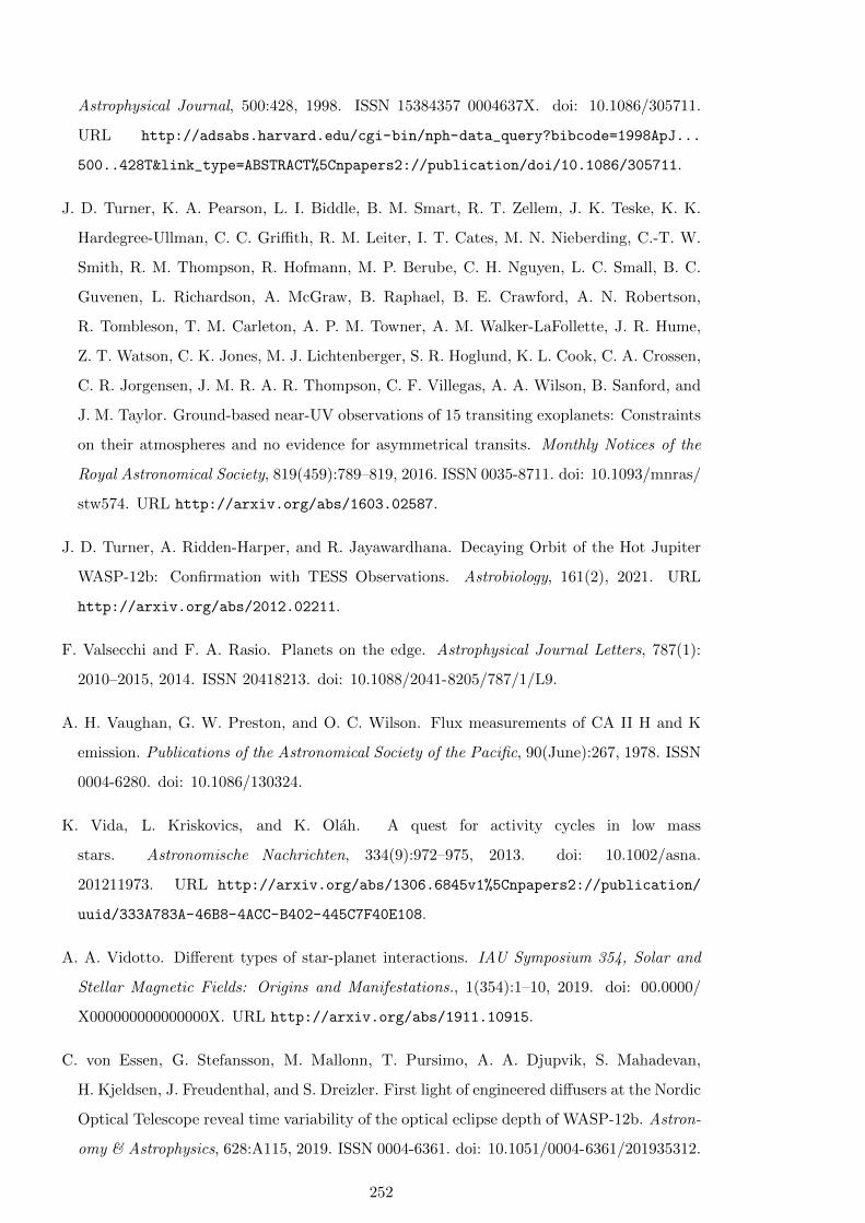
Astrophysical Journal, 500:428, 1998. ISSN 15384357 0004637X. doi: 10.1086/305711.

URL http://adsabs.harvard.edu/cgi-bin/nph-data_query?bibcode=1998ApJ...

500..428T&link_type=ABSTRACT%5Cnpapers2://publication/doi/10.1086/305711.

J. D. Turner, K. A. Pearson, L. I. Biddle, B. M. Smart, R. T. Zellem, J. K. Teske, K. K.

Hardegree-Ullman, C. C. Griffith, R. M. Leiter, I. T. Cates, M. N. Nieberding, C.-T. W.

Smith, R. M. Thompson, R. Hofmann, M. P. Berube, C. H. Nguyen, L. C. Small, B. C.

Guvenen, L. Richardson, A. McGraw, B. Raphael, B. E. Crawford, A. N. Robertson,

R. Tombleson, T. M. Carleton, A. P. M. Towner, A. M. Walker-LaFollette, J. R. Hume,

Z. T. Watson, C. K. Jones, M. J. Lichtenberger, S. R. Hoglund, K. L. Cook, C. A. Crossen,

C. R. Jorgensen, J. M. R. A. R. Thompson, C. F. Villegas, A. A. Wilson, B. Sanford, and

J. M. Taylor. Ground-based near-UV observations of 15 transiting exoplanets: Constraints

on their atmospheres and no evidence for asymmetrical transits. Monthly Notices of the

Royal Astronomical Society, 819(459):789–819, 2016. ISSN 0035-8711. doi: 10.1093/mnras/

stw574. URL http://arxiv.org/abs/1603.02587.

J. D. Turner, A. Ridden-Harper, and R. Jayawardhana. Decaying Orbit of the Hot Jupiter

WASP-12b: Confirmation with TESS Observations. Astrobiology, 161(2), 2021. URL

http://arxiv.org/abs/2012.02211.

F. Valsecchi and F. A. Rasio. Planets on the edge. Astrophysical Journal Letters, 787(1):

2010–2015, 2014. ISSN 20418213. doi: 10.1088/2041-8205/787/1/L9.

A. H. Vaughan, G. W. Preston, and O. C. Wilson. Flux measurements of CA II H and K

emission. Publications of the Astronomical Society of the Pacific, 90(June):267, 1978. ISSN

0004-6280. doi: 10.1086/130324.

K. Vida, L. Kriskovics, and K. Olah. A quest for activity cycles in low mass

stars. Astronomische Nachrichten, 334(9):972–975, 2013. doi: 10.1002/asna.

201211973. URL http://arxiv.org/abs/1306.6845v1%5Cnpapers2://publication/

uuid/333A783A-46B8-4ACC-B402-445C7F40E108.

A. A. Vidotto. Different types of star-planet interactions. IAU Symposium 354, Solar and

Stellar Magnetic Fields: Origins and Manifestations., 1(354):1–10, 2019. doi: 00.0000/

X000000000000000X. URL http://arxiv.org/abs/1911.10915.

C. von Essen, G. Stefansson, M. Mallonn, T. Pursimo, A. A. Djupvik, S. Mahadevan,

H. Kjeldsen, J. Freudenthal, and S. Dreizler. First light of engineered diffusers at the Nordic

Optical Telescope reveal time variability of the optical eclipse depth of WASP-12b. Astron-

omy & Astrophysics, 628:A115, 2019. ISSN 0004-6361. doi: 10.1051/0004-6361/201935312.

252

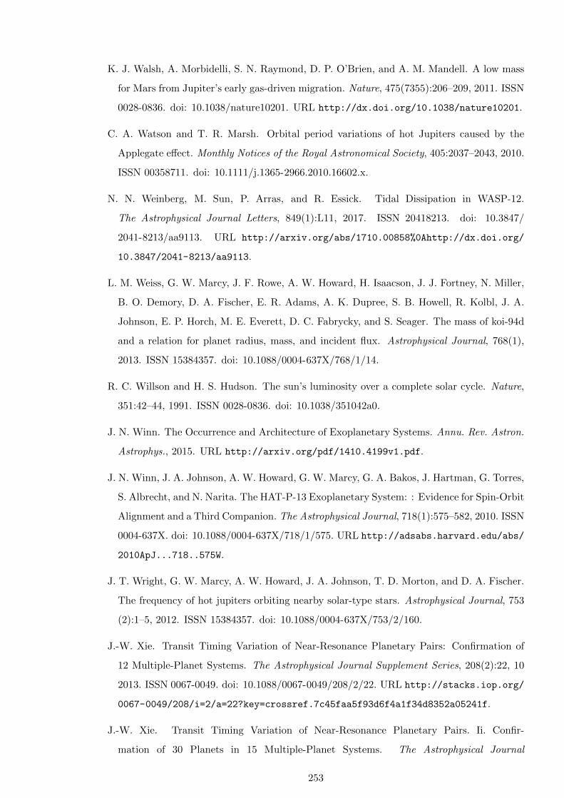
K. J. Walsh, A. Morbidelli, S. N. Raymond, D. P. O’Brien, and A. M. Mandell. A low mass

for Mars from Jupiter’s early gas-driven migration. Nature, 475(7355):206–209, 2011. ISSN

0028-0836. doi: 10.1038/nature10201. URL http://dx.doi.org/10.1038/nature10201.

C. A. Watson and T. R. Marsh. Orbital period variations of hot Jupiters caused by the

Applegate effect. Monthly Notices of the Royal Astronomical Society, 405:2037–2043, 2010.

ISSN 00358711. doi: 10.1111/j.1365-2966.2010.16602.x.

N. N. Weinberg, M. Sun, P. Arras, and R. Essick. Tidal Dissipation in WASP-12.

The Astrophysical Journal Letters, 849(1):L11, 2017. ISSN 20418213. doi: 10.3847/

2041-8213/aa9113. URL http://arxiv.org/abs/1710.00858%0Ahttp://dx.doi.org/

10.3847/2041-8213/aa9113.

L. M. Weiss, G. W. Marcy, J. F. Rowe, A. W. Howard, H. Isaacson, J. J. Fortney, N. Miller,

B. O. Demory, D. A. Fischer, E. R. Adams, A. K. Dupree, S. B. Howell, R. Kolbl, J. A.

Johnson, E. P. Horch, M. E. Everett, D. C. Fabrycky, and S. Seager. The mass of koi-94d

and a relation for planet radius, mass, and incident flux. Astrophysical Journal, 768(1),

2013. ISSN 15384357. doi: 10.1088/0004-637X/768/1/14.

R. C. Willson and H. S. Hudson. The sun’s luminosity over a complete solar cycle. Nature,

351:42–44, 1991. ISSN 0028-0836. doi: 10.1038/351042a0.

J. N. Winn. The Occurrence and Architecture of Exoplanetary Systems. Annu. Rev. Astron.

Astrophys., 2015. URL http://arxiv.org/pdf/1410.4199v1.pdf.

J. N. Winn, J. A. Johnson, A. W. Howard, G. W. Marcy, G. A. Bakos, J. Hartman, G. Torres,

S. Albrecht, and N. Narita. The HAT-P-13 Exoplanetary System: : Evidence for Spin-Orbit

Alignment and a Third Companion. The Astrophysical Journal, 718(1):575–582, 2010. ISSN

0004-637X. doi: 10.1088/0004-637X/718/1/575. URL http://adsabs.harvard.edu/abs/

2010ApJ...718..575W.

J. T. Wright, G. W. Marcy, A. W. Howard, J. A. Johnson, T. D. Morton, and D. A. Fischer.

The frequency of hot jupiters orbiting nearby solar-type stars. Astrophysical Journal, 753

(2):1–5, 2012. ISSN 15384357. doi: 10.1088/0004-637X/753/2/160.

J.-W. Xie. Transit Timing Variation of Near-Resonance Planetary Pairs: Confirmation of

12 Multiple-Planet Systems. The Astrophysical Journal Supplement Series, 208(2):22, 10

2013. ISSN 0067-0049. doi: 10.1088/0067-0049/208/2/22. URL http://stacks.iop.org/

0067-0049/208/i=2/a=22?key=crossref.7c45faa5f93d6f4a1f34d8352a05241f.

J.-W. Xie. Transit Timing Variation of Near-Resonance Planetary Pairs. Ii. Confir-

mation of 30 Planets in 15 Multiple-Planet Systems. The Astrophysical Journal

253

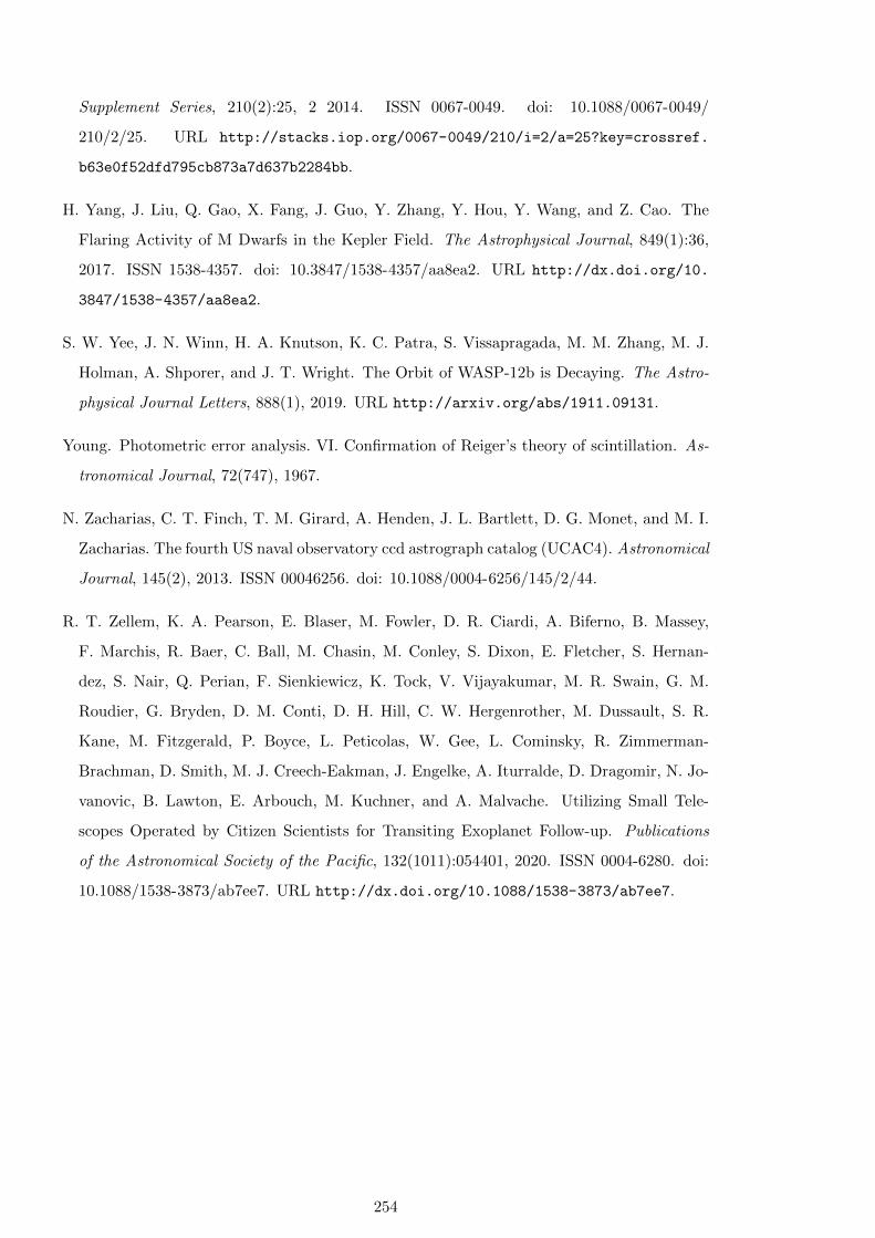
Supplement Series, 210(2):25, 2 2014. ISSN 0067-0049. doi: 10.1088/0067-0049/

210/2/25. URL http://stacks.iop.org/0067-0049/210/i=2/a=25?key=crossref.

b63e0f52dfd795cb873a7d637b2284bb.

H. Yang, J. Liu, Q. Gao, X. Fang, J. Guo, Y. Zhang, Y. Hou, Y. Wang, and Z. Cao. The

Flaring Activity of M Dwarfs in the Kepler Field. The Astrophysical Journal, 849(1):36,

2017. ISSN 1538-4357. doi: 10.3847/1538-4357/aa8ea2. URL http://dx.doi.org/10.

3847/1538-4357/aa8ea2.

S. W. Yee, J. N. Winn, H. A. Knutson, K. C. Patra, S. Vissapragada, M. M. Zhang, M. J.

Holman, A. Shporer, and J. T. Wright. The Orbit of WASP-12b is Decaying. The Astro-

physical Journal Letters, 888(1), 2019. URL http://arxiv.org/abs/1911.09131.

Young. Photometric error analysis. VI. Confirmation of Reiger’s theory of scintillation. As-

tronomical Journal, 72(747), 1967.

N. Zacharias, C. T. Finch, T. M. Girard, A. Henden, J. L. Bartlett, D. G. Monet, and M. I.

Zacharias. The fourth US naval observatory ccd astrograph catalog (UCAC4). Astronomical

Journal, 145(2), 2013. ISSN 00046256. doi: 10.1088/0004-6256/145/2/44.

R. T. Zellem, K. A. Pearson, E. Blaser, M. Fowler, D. R. Ciardi, A. Biferno, B. Massey,

F. Marchis, R. Baer, C. Ball, M. Chasin, M. Conley, S. Dixon, E. Fletcher, S. Hernan-

dez, S. Nair, Q. Perian, F. Sienkiewicz, K. Tock, V. Vijayakumar, M. R. Swain, G. M.

Roudier, G. Bryden, D. M. Conti, D. H. Hill, C. W. Hergenrother, M. Dussault, S. R.

Kane, M. Fitzgerald, P. Boyce, L. Peticolas, W. Gee, L. Cominsky, R. Zimmerman-

Brachman, D. Smith, M. J. Creech-Eakman, J. Engelke, A. Iturralde, D. Dragomir, N. Jo-

vanovic, B. Lawton, E. Arbouch, M. Kuchner, and A. Malvache. Utilizing Small Tele-

scopes Operated by Citizen Scientists for Transiting Exoplanet Follow-up. Publications

of the Astronomical Society of the Pacific, 132(1011):054401, 2020. ISSN 0004-6280. doi:

10.1088/1538-3873/ab7ee7. URL http://dx.doi.org/10.1088/1538-3873/ab7ee7.

254