Coded Aperture Computed Tomography

Kerkil Choi and David J. Brady

The Department of Electrical and Computer Engineering, Duke University, Durham, NC,27708 USA

ABSTRACT

Diverse physical measurements can be modeled by X-ray transforms. While X-ray tomography is the canon-ical example, reference structure tomography (RST) and coded aperture snapshot spectral imaging (CASSI)are examples of physically unrelated but mathematically equivalent sensor systems. Historically, most x-raytransform based systems sample continuous distributions and apply analytical inversion processes. On the otherhand, RST and CASSI generate discrete multiplexed measurements implemented with coded apertures. Thismultiplexing of coded measurements allows for compression of measurements from a compressed sensing per-spective. Compressed sensing (CS) is a revelation that if the object has a sparse representation in some basis,then a certain number, but typically much less than what is prescribed by Shannon’s sampling rate, of randomprojections captures enough information for a highly accurate reconstruction of the object. This paper investi-gates the role of coded apertures in x-ray transform measurement systems (XTMs) in terms of data efficiencyand reconstruction fidelity from a CS perspective. To conduct this, we construct a unified analysis using RSTand CASSI measurement models. Also, we propose a novel compressive x-ray tomography measurement schemewhich also exploits coding and multiplexing, and hence shares the analysis of the other two XTMs. Using thisanalysis, we perform a qualitative study on how coded apertures can be exploited to implement physical randomprojections by “regularizing” the measurement systems. Numerical studies and simulation results demonstrateseveral examples of the impact of coding.

Keywords: Coded aperture, computed tomography, compressive sensing, multiplexing, x-ray transform

1. INTRODUCTION

Several physical measurements may be modeled by X-ray transform measurements (XTM). The X-ray transformdenoted by g(y, φ) is defined by

g(y, φ) =∫R

f(y + αφ)dα, y ∈ P⊥, (1)

where f(x) denotes a density function describing an object, x ∈ Rn, y ∈ Rn−1 and φ ∈ Sn−1, Sn−1 denotesthe (n − 1)-dimensional hyper-sphere. The X-ray transform is collected in the hyperplane P⊥ defined by theassociated normal φ (i.e., y · φ = 0). Equation (1) also represents the 2D Radon transform for n = 2, butproduces a function that resides in a higher-dimensional space for n ≥ 3. Measurement compression strategies,such as the vertex path commonly applied to cone-beam tomography,1 can be applied for n ≥ 3 to sub-samplethe measurement space while maintaining a well-posed system. The transformation in Eq. (1) is commonly usedin X-ray tomography. It also appears in optical projection tomography. While X-ray transform may be appliedwithin the focal field of simple cameras,2 the projection model is particularly relevant to high depth of fieldimagers using, for example, pinholes or coded apertures,3 wave front coding,4 or interferometric imaging.5

The X-ray transform model arises from a different perspective in spectral imaging, where the object liestypically in a 3D datacube that consists of 2 spatial dimensions and 1 spectral dimension. Spatio-spectraldispersion of the 3D datacube by dispersive elements such as prisms or gratings enables collection of X-ray

Further author information: (Send correspondence to Kerkil Choi)Kerkil Choi: E-mail: kerkil.choi@duke.edu, Telephone: 1 919 660 5108David J. Brady: E-mail: david.brady@duke.edu, Telephone: 1 919 660 5394

Adaptive Coded Aperture Imaging, Non-Imaging, and Unconventional Imaging Sensor Systems, edited by Stanley Rogers, David P. Casasent, Jean J. Dolne, Thomas J. Karr, Victor L. Gamiz, Proc. of SPIE

Vol. 7468, 74680B · © 2009 SPIE · CCC code: 0277-786X/09/$18 · doi: 10.1117/12.825277

Proc. of SPIE Vol. 7468 74680B-1

transforms. Spectral imaging systems based on X-ray transforms have been explored by several groups in theearly and mid-1990’s.6–9

Because Eq. (1) can be analytically inverted in a straightforward manner in 2D and 3D, a majority of researchon XTM inverse problems over the past several decades has been devoted to discrete sampling, interpolationand estimation methods. Major innovations in X-ray tomography based on changes in illumination source anddetector geometry result in the transition from parallel beam to fan beam to cone beam systems.

Meanwhile, the compressive sensing (CS) field has emerged10–12 and introduced a new perspective on mea-surement dimensionality. CS is based on the innovative concept that measurements (RM ) in a considerablylower-dimensional space (M � N) than the space (RN ) in which a signal resides can be designed to containenough information to accurately infer the original signal with high accuracy. CS builds its strength based ontwo feasible assumptions: 1) many signals are either sparse or compressible in some basis,13 and 2) a relativelysmall number of random projections of a sparse signal can grab enough information to allow for a highly accuraterecovery. CS particularly emphasizes the significance of the way in which a (sparse or compressible) signal iscollected: namely, the measurement basis vectors should remain as nearly orthogonal as possible in the mea-surement space.14 The “conventional” wisdom of CS focuses on implementing such measurements using randomprojections. While such random projections are useful and have numerous scientific and engineering applications,they are often not physically implementable in common XTM systems.

We propose a practically implementable method for acquiring CS measurements for XTMs through the con-cept of physical coding by using a coded aperture. Our group investigated compressive sensing measurements ina tomographic instrument called reference structure tomography (RST)15 based on physical coding.16 Recently,our group also exploited physical coding from RST in demonstrating CS measurements in spectral imaging.17

This paper explores coding in these compressive sensing XTMs.

In this paper, we propose a unified approach to the construction of mathematical forward models for XTMsincluding coded aperture snapshot spectral imager (CASSI). The approach is extended to propose a compressiveX-ray tomography (CXT) system. While previous theoretical work considers general analysis,13 we focus onthe interpretation of practical implications of CS theory for physical XTMs and their mathematical models viavarious numerical studies.

2. ANALYSIS MODELS FOR CODED APERTURE COMPUTED TOMOGRAPHY

This section develops a unified analysis approach of compressive XTMs (CXTMs). We start with an analysisof CASSI that illustrates the essential concept of generalized sampling via coding and multiplexing to generatecompressive measurements. The CASSI model is then extended to construct a CXT model.

2.1 Coded Aperture Snapshot Spectral Imaging (CASSI)

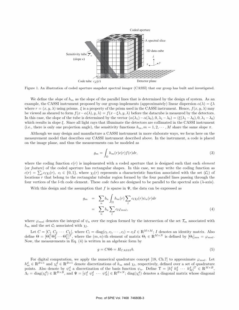
CASSI is a tomographic hyperspectral imaging modality17 that reconstructs a 3D datacube from a 2D snapshotprojection from only one angle prescribed by a system design in which a coded aperture and dispersive elementsencode the 3D datacube. The 3D datacube represents a collection of spatial images over a range of wavelengths.The 2D snapshot projection data can be interpreted as multiplexed X-ray transform measurements that arecoded. The coding in CASSI may be viewed as modulating X-ray projections such that different locations alongan X-ray in computing the X-ray transform have different weights determined by the coding structure.

Let f(r) define the 3D object power spectral density representing the datacube. When there is no code, themeasurement recorded by the m-th detector may be modeled by

gm =∫

Ω

hm(r)f(r)dr, (2)

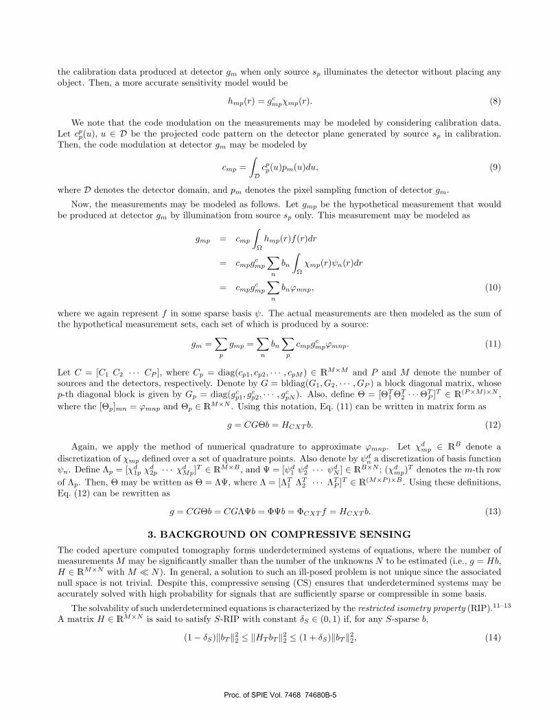
where hm(r) is the sensitivity function which, we assume, is a characteristic function associated with the set ofall locations r ∈ Ω in a rectangular tubular region Tm (see Fig. 1) formed by four parallel lines passing throughthe four vertices of the m-th detector. More accurately, hm may be modeled as a weighted characteristic functionto incorporate, for instance, detector gain non-uniformity. In such cases, calibration may be used to find andincorporate such weights.

Proc. of SPIE Vol. 7468 74680B-2

λ

yx

3D data cube

A spectral slice

Coded aperture

Detector plane

Sensitivity tube Tm

(slope κ)

Code tube clχl(r)

Figure 1. An illustration of coded aperture snapshot spectral imager (CASSI) that our group has built and investigated.

We define the slope of hm as the slope of the parallel lines that is determined by the design of system. As anexample, the CASSI instrument proposed by our group implements (approximately) linear dispersion α(λ) = ξλwhere r = (x, y, λ) using prisms. ξ is a property of the prism used in the CASSI instrument. Hence, f(x, y, λ) maybe viewed as sheared to form f(x−α(λ), y, λ) = f(x−ξλ, y, λ) before the datacube is measured by the detectors.In this case, the slope of the tube is determined by the vector (α(λ1)−α(λ0), 0, λ1−λ0) = (ξ(λ1−λ0), 0, λ1−λ0)which results in slope ξ. Since all light rays that illuminate the detectors are collimated in the CASSI instrument(i.e., there is only one projection angle), the sensitivity functions hm,m = 1, 2, · · · ,M share the same slope π.

Although we may design and manufacture a CASSI instrument in more elaborate ways, we focus here on themeasurement model that describes our CASSI instrument described above. In the instrument, a code is placedon the image plane, and thus the measurements can be modeled as

gm =∫

Ω

hm(r)c(r)f(r)dr, (3)

where the coding function c(r) is implemented with a coded aperture that is designed such that each element(or feature) of the coded aperture has rectangular shapes. In this case, we may write the coding function asc(r) =

∑l clχl(r), cl ∈ {0, 1}, where χl(r) represents a characteristic function associated with the set (Cl) of

locations r that belong to the rectangular tubular region formed by the four parallel lines passing through thefour vertices of the l-th code element. These code tubes are designed to be parallel to the spectral axis (λ-axis).

With this design and the assumption that f is sparse in Ψ, the data can be expressed as

gm =∑

n

bn

∫Ω

hm(r)∑

l

clχl(r)ψn(r)dr

=∑

n

bn∑

l

clϕmnl, (4)

where ϕmnl denotes the integral of ψn over the region formed by the intersection of the set Tm associated withhm and the set Cl associated with χl.

Let C = [C1 C2 · · · CL], where Cl = diag(cl, cl, · · · , cl) = clI ∈ RM×M ; I denotes an identity matrix. Alsodefine Θ = [ΘT

1 ΘT2 · · ·ΘT

L]T , where the (m,n)-th element of matrix Θl ∈ RM×N is defined by [Θl]mn = ϕmnl.Now, the measurements in Eq. (4) is written in an algebraic form by

g = CΘb = HCASSIb. (5)

For digital computation, we apply the numerical quadrature concept [18, Ch.7] to approximate ϕmnl. Lethd

m ∈ RB×1 and χdl ∈ RB×1 denote discretizations of hm and χl, respectively, defined over a set of quadrature

points. Also denote by ψdn a discretization of the basis function ψn. Define Υ = [hd

1 hd2 · · · hd

M ]T ∈ RM×B,Λl = diag(χd

l ) ∈ RB×B, and Ψ = [ψd1 ψ

d2 · · · ψd

N ] ∈ RB×N ; diag(χdl ) denotes a diagonal matrix whose diagonal

Proc. of SPIE Vol. 7468 74680B-3

Codedaperture

Projected code pattern c

mp

Source sp

Objectregion

Detector plane

(a)

Sensitivity function h

mp

Source sp

A detector element

Code element(s)

Projected code elementon axial slices

(b)

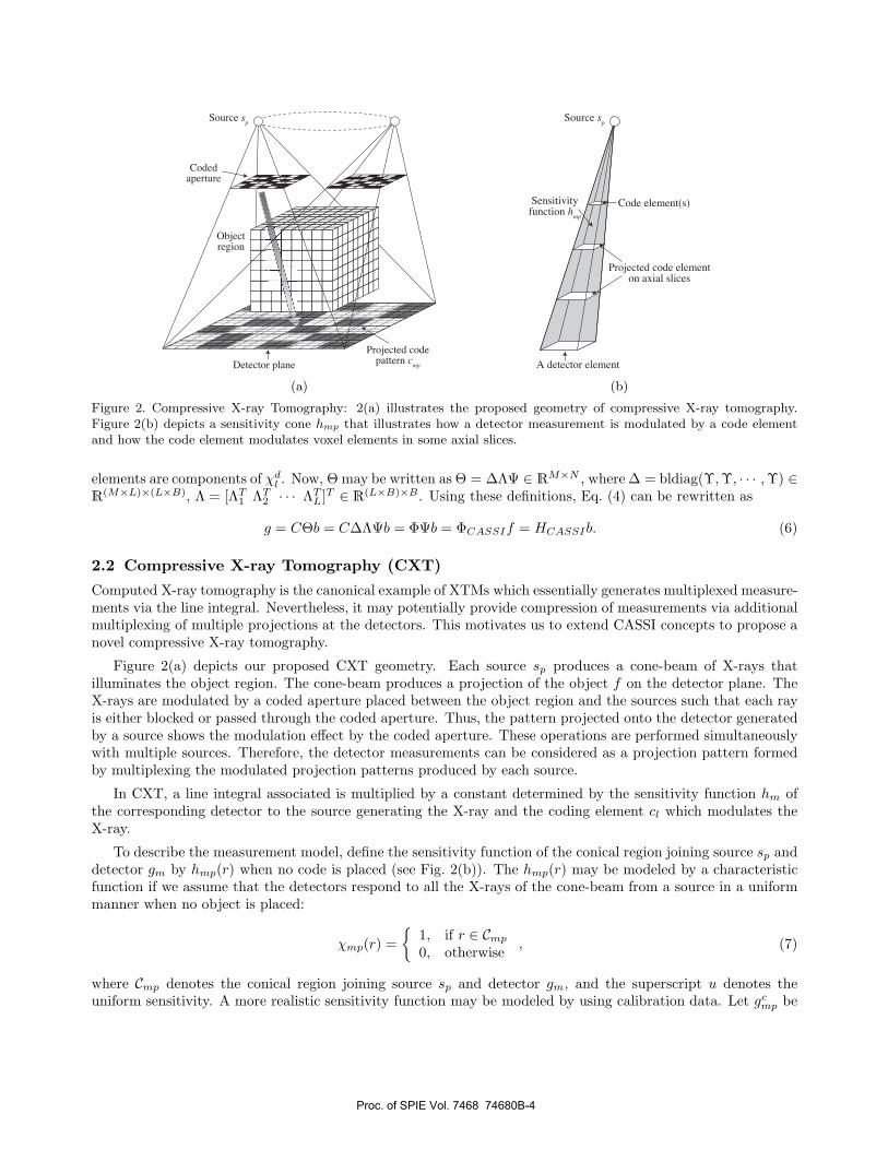
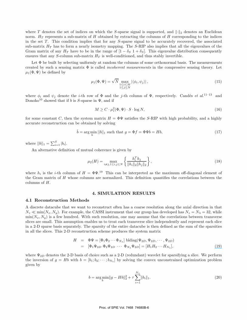
Figure 2. Compressive X-ray Tomography: 2(a) illustrates the proposed geometry of compressive X-ray tomography.Figure 2(b) depicts a sensitivity cone hmp that illustrates how a detector measurement is modulated by a code elementand how the code element modulates voxel elements in some axial slices.

elements are components of χdl . Now, Θ may be written as Θ = ΔΛΨ ∈ RM×N , where Δ = bldiag(Υ,Υ, · · · ,Υ) ∈

R(M×L)×(L×B), Λ = [ΛT1 ΛT

2 · · · ΛTL]T ∈ R(L×B)×B. Using these definitions, Eq. (4) can be rewritten as

g = CΘb = CΔΛΨb = ΦΨb = ΦCASSIf = HCASSIb. (6)

2.2 Compressive X-ray Tomography (CXT)

Computed X-ray tomography is the canonical example of XTMs which essentially generates multiplexed measure-ments via the line integral. Nevertheless, it may potentially provide compression of measurements via additionalmultiplexing of multiple projections at the detectors. This motivates us to extend CASSI concepts to propose anovel compressive X-ray tomography.

Figure 2(a) depicts our proposed CXT geometry. Each source sp produces a cone-beam of X-rays thatilluminates the object region. The cone-beam produces a projection of the object f on the detector plane. TheX-rays are modulated by a coded aperture placed between the object region and the sources such that each rayis either blocked or passed through the coded aperture. Thus, the pattern projected onto the detector generatedby a source shows the modulation effect by the coded aperture. These operations are performed simultaneouslywith multiple sources. Therefore, the detector measurements can be considered as a projection pattern formedby multiplexing the modulated projection patterns produced by each source.

In CXT, a line integral associated is multiplied by a constant determined by the sensitivity function hm ofthe corresponding detector to the source generating the X-ray and the coding element cl which modulates theX-ray.

To describe the measurement model, define the sensitivity function of the conical region joining source sp anddetector gm by hmp(r) when no code is placed (see Fig. 2(b)). The hmp(r) may be modeled by a characteristicfunction if we assume that the detectors respond to all the X-rays of the cone-beam from a source in a uniformmanner when no object is placed:

χmp(r) ={

1, if r ∈ Cmp

0, otherwise , (7)

where Cmp denotes the conical region joining source sp and detector gm, and the superscript u denotes theuniform sensitivity. A more realistic sensitivity function may be modeled by using calibration data. Let gc

mp be

Proc. of SPIE Vol. 7468 74680B-4

the calibration data produced at detector gm when only source sp illuminates the detector without placing anyobject. Then, a more accurate sensitivity model would be

hmp(r) = gcmpχmp(r). (8)

We note that the code modulation on the measurements may be modeled by considering calibration data.Let cpp(u), u ∈ D be the projected code pattern on the detector plane generated by source sp in calibration.Then, the code modulation at detector gm may be modeled by

cmp =∫Dcpp(u)pm(u)du, (9)

where D denotes the detector domain, and pm denotes the pixel sampling function of detector gm.

Now, the measurements may be modeled as follows. Let gmp be the hypothetical measurement that wouldbe produced at detector gm by illumination from source sp only. This measurement may be modeled as

gmp = cmp

∫Ω

hmp(r)f(r)dr

= cmpgcmp

∑n

bn

∫Ω

χmp(r)ψn(r)dr

= cmpgcmp

∑n

bnϕmnp, (10)

where we again represent f in some sparse basis ψ. The actual measurements are then modeled as the sum ofthe hypothetical measurement sets, each set of which is produced by a source:

gm =∑

p

gmp =∑

n

bn∑

p

cmpgcmpϕmnp. (11)

Let C = [C1 C2 · · · CP ], where Cp = diag(cp1, cp2, · · · , cpM ) ∈ RM×M and P and M denote the number ofsources and the detectors, respectively. Denote by G = bldiag(G1, G2, · · · , GP ) a block diagonal matrix, whosep-th diagonal block is given by Gp = diag(gc

p1, gcp2, · · · , gc

pN ). Also, define Θ = [ΘT1 ΘT

2 · · ·ΘTP ]T ∈ R(P×M)×N ,

where the [Θp]mn = ϕmnp and Θp ∈ RM×N . Using this notation, Eq. (11) can be written in matrix form as

g = CGΘb = HCXT b. (12)

Again, we apply the method of numerical quadrature to approximate ϕmnp. Let χdmp ∈ RB denote a

discretization of χmp defined over a set of quadrature points. Also denote by ψdn a discretization of basis function

ψn. Define Λp = [χd1p χ

d2p · · · χd

Mp]T ∈ RM×B, and Ψ = [ψd

1 ψd2 · · · ψd

N ] ∈ RB×N ; (χdmp)T denotes the m-th row

of Λp. Then, Θ may be written as Θ = ΛΨ, where Λ = [ΛT1 ΛT

2 · · · ΛTP ]T ∈ R(M×P )×B. Using these definitions,

Eq. (12) can be rewritten as

g = CGΘb = CGΛΨb = ΦΨb = ΦCXT f = HCXT b. (13)

3. BACKGROUND ON COMPRESSIVE SENSING

The coded aperture computed tomography forms underdetermined systems of equations, where the number ofmeasurements M may be significantly smaller than the number of the unknowns N to be estimated (i.e., g = Hb,H ∈ RM×N with M � N). In general, a solution to such an ill-posed problem is not unique since the associatednull space is not trivial. Despite this, compressive sensing (CS) ensures that underdetermined systems may beaccurately solved with high probability for signals that are sufficiently sparse or compressible in some basis.

The solvability of such underdetermined equations is characterized by the restricted isometry property (RIP).11–13

A matrix H ∈ RM×N is said to satisfy S-RIP with constant δS ∈ (0, 1) if, for any S-sparse b,

(1 − δS)‖bT‖22 ≤ ‖HT bT‖2

2 ≤ (1 + δS)‖bT ‖22, (14)

Proc. of SPIE Vol. 7468 74680B-5

where T denotes the set of indices on which the S-sparse signal is supported, and ‖·‖2 denotes an Euclideannorm. HT represents a sub-matrix of H obtained by extracting the columns of H corresponding to the indicesin the set T . This condition implies that for any S-sparse signal to be accurately recovered, the associatedsub-matrix HT has to form a nearly isometry mapping. The S-RIP also implies that all the eigenvalues of theGram matrix of any HT have to be in the range of [1 − δS 1 + δS ]. This eigenvalue distribution consequentlyensures that any S-column sub-matrix HT is well-conditioned, and thus stably invertible.

Let Φ be built by selecting uniformly at random the columns of some orthonormal basis. The measurementscreated by such a sensing matrix Φ is called incoherent measurements in the compressive sensing theory. Letμ1(Φ,Ψ) be defined by

μ1(Φ,Ψ) =√N max

1≤i≤M1≤j≤N

|〈φi, ψj〉| , (15)

where φi and ψj denote the i-th row of Φ and the j-th column of Ψ, respectively. Candes et al.11–13 andDonoho10 showed that if b is S-sparse in Ψ, and if

M ≥ C · μ21(Φ,Ψ) · S · logN, (16)

for some constant C, then the system matrix H = ΦΨ satisfies the S-RIP with high probability, and a highlyaccurate reconstruction can be obtained by solving

b = arg minb

||b||1 such that g = Φf = ΦΨb = Hb, (17)

where ||b||1 =∑S

i=1 |bi|.An alternative definition of mutual coherence is given by

μ2(H) = maxi�=j,1≤i,j≤N

{hT

i hj

‖hi‖2‖hj‖2

}, (18)

where hi is the i-th column of H = ΦΨ.19 This can be interpreted as the maximum off-diagonal element ofthe Gram matrix of H whose columns are normalized. This definition quantifies the correlations between thecolumns of H .

4. SIMULATION RESULTS

4.1 Reconstruction Methods

A discrete datacube that we want to reconstruct often has a coarse resolution along the axial direction in thatNz � min(Nx, Ny). For example, the CASSI instrument that our group has developed has Nz = Nλ = 32, whilemin(Nx, Ny) is a few hundred. With such resolution, one may assume that the correlations between transverseslices are small. This assumption enables us to treat each transverse slice independently and represent each slicein a 2-D sparse basis separately. The sparsity of the entire datacube is then defined as the sum of the sparsitiesin all the slices. This 2-D reconstruction scheme produces the system matrix

H = ΦΨ = [Φ1Φ2 · · ·ΦNλ] bldiag(Ψ2D,Ψ2D, · · · ,Ψ2D)

= [Φ1Ψ2D Φ2Ψ2D · · · ΦNλΨ2D] = [H1H2 · · ·HNλ

], (19)

where Ψ2D denotes the 2-D basis of choice such as a 2-D (redundant) wavelet for sparsifying a slice. We performthe inversion of g = Hb with b = [b1; b2; · · · ; bNλ

] by solving the convex unconstrained optimization problemgiven by

b = arg minb

‖g −Hb‖22 + τ

Nλ∑i=1

‖bi‖1. (20)

Proc. of SPIE Vol. 7468 74680B-6

Note that we write the overall sparsity as the sum of the sparsities induced by 2-D wavelets of all slices to clarifythat we apply the 2-D sparse basis to each slice: ‖b‖1 =

∑Nλ

i=1‖bi‖1.

Often, we also use an implicit sparse basis (or dictionary) such as total variation (TV)20 by minimizing thetotal-variation norm which seeks the minimum sum of the nonzero gradients, which is equivalent to minimizingthe number of nonzero gradients provided that M is large enough. The sparse basis is implicit in that we do notexplicitly utilize the inverse total-variation operator. In total-variation minimization, we solve an unconstrainedoptimization problem given by

f = arg minf

‖g − Φf‖22 + τ

Nλ∑i=1

‖fi‖TV , (21)

where the TV norm ‖fi‖TV is defined by

‖fi‖TV =Nx∑

nx=1

Ny∑ny=1

|∇(fi)nx,ny |, (22)

where |∇(fi)nx,ny | denotes the magnitude of the gradient at spatial location (nx, ny) in the i-th transverse slice,and the gradient is approximated by finite differences. Note that we ignore the boundary conditions.

When the axial resolution is comparable to the transverse resolution, we may alternatively perform 3Dinversion by solving

f = arg minf

‖g − Φf‖22 + τ‖f‖TV , (23)

where the TV norm ‖f‖TV , in this case, is defined by

‖f‖TV =Nz∑

nz=1

Nx∑nx=1

Ny∑ny=1

|∇fnx,ny,nz |, (24)

where |∇fnx,ny,nz | denotes the magnitude of the 3D gradient at spatial location (nx, ny, nz).

4.2 Reconstructions Using 2-D and 3-D Sparse Bases

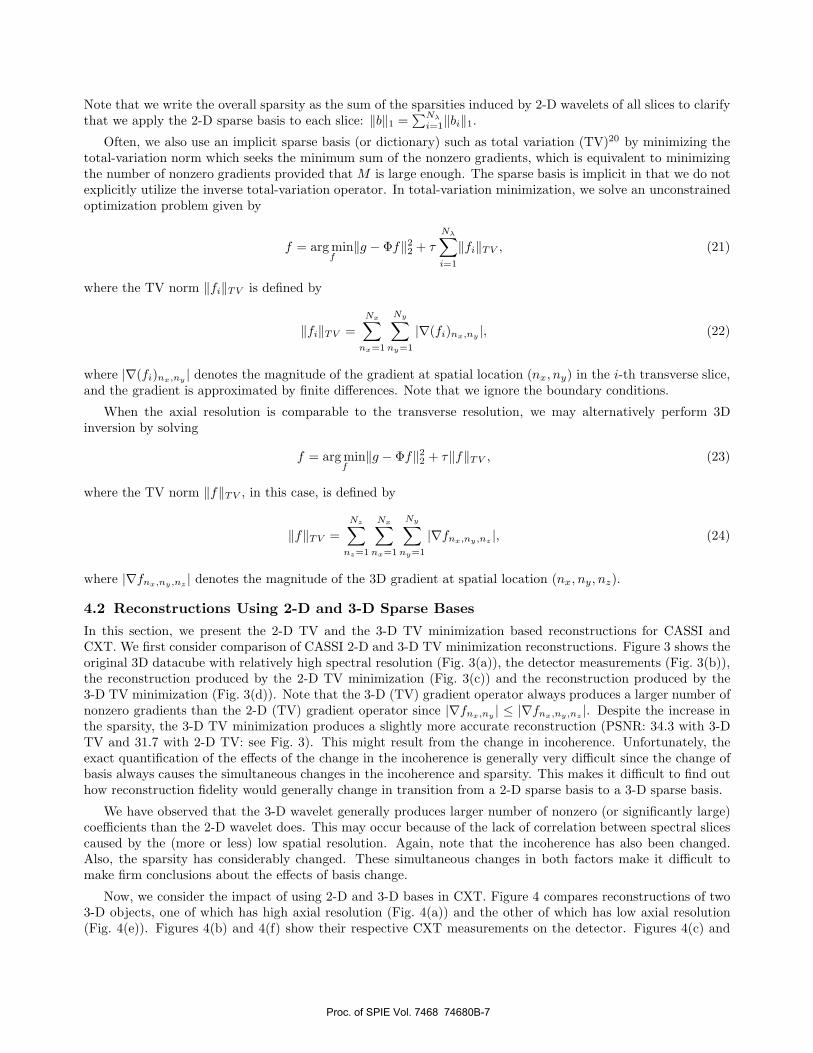
In this section, we present the 2-D TV and the 3-D TV minimization based reconstructions for CASSI andCXT. We first consider comparison of CASSI 2-D and 3-D TV minimization reconstructions. Figure 3 shows theoriginal 3D datacube with relatively high spectral resolution (Fig. 3(a)), the detector measurements (Fig. 3(b)),the reconstruction produced by the 2-D TV minimization (Fig. 3(c)) and the reconstruction produced by the3-D TV minimization (Fig. 3(d)). Note that the 3-D (TV) gradient operator always produces a larger number ofnonzero gradients than the 2-D (TV) gradient operator since |∇fnx,ny | ≤ |∇fnx,ny,nz |. Despite the increase inthe sparsity, the 3-D TV minimization produces a slightly more accurate reconstruction (PSNR: 34.3 with 3-DTV and 31.7 with 2-D TV: see Fig. 3). This might result from the change in incoherence. Unfortunately, theexact quantification of the effects of the change in the incoherence is generally very difficult since the change ofbasis always causes the simultaneous changes in the incoherence and sparsity. This makes it difficult to find outhow reconstruction fidelity would generally change in transition from a 2-D sparse basis to a 3-D sparse basis.

We have observed that the 3-D wavelet generally produces larger number of nonzero (or significantly large)coefficients than the 2-D wavelet does. This may occur because of the lack of correlation between spectral slicescaused by the (more or less) low spatial resolution. Again, note that the incoherence has also been changed.Also, the sparsity has considerably changed. These simultaneous changes in both factors make it difficult tomake firm conclusions about the effects of basis change.

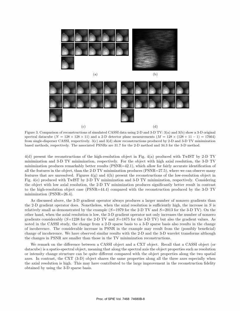
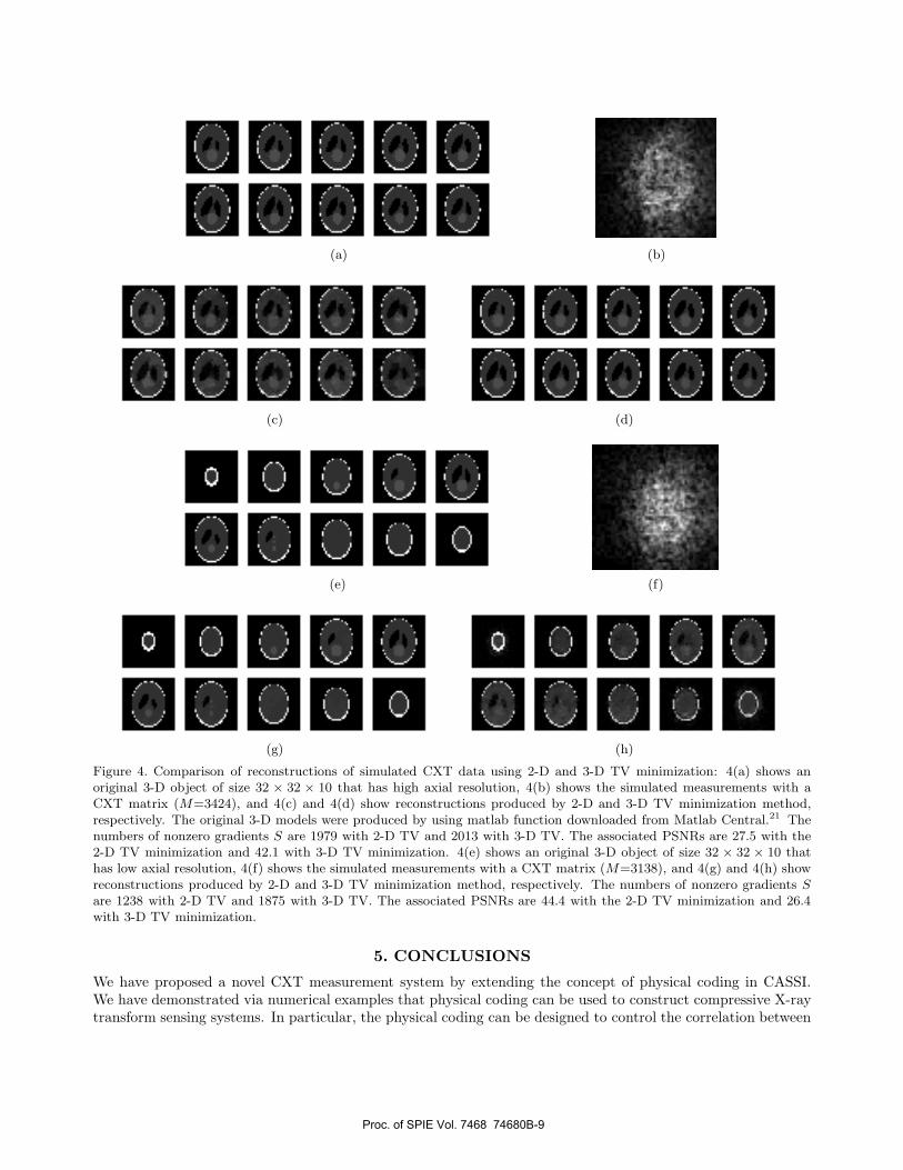
Now, we consider the impact of using 2-D and 3-D bases in CXT. Figure 4 compares reconstructions of two3-D objects, one of which has high axial resolution (Fig. 4(a)) and the other of which has low axial resolution(Fig. 4(e)). Figures 4(b) and 4(f) show their respective CXT measurements on the detector. Figures 4(c) and

Proc. of SPIE Vol. 7468 74680B-7

*IiIipIiIiii

SdS4

-USd-U54 U

14

V1454

14Sd Pu

p. Pu a

Pu Pu a

p. a-

Pu a

p. a-

P. a- p.

(a) (b)

(c) (d)

Figure 3. Comparison of reconstructions of simulated CASSI data using 2-D and 3-D TV: 3(a) and 3(b) show a 3-D originalspectral datacube (N = 128 × 128 × 11) and a 2-D detector plane measurements (M = 128 × (128 + 11 − 1) = 17664)from single-disperser CASSI, respectively. 3(c) and 3(d) show reconstructions produced by 2-D and 3-D TV minimizationbased methods, respectively. The associated PSNRs are 31.7 for the 2-D method and 34.3 for the 3-D method.

4(d) present the reconstructions of the high-resolution object in Fig. 4(a) produced with TwIST by 2-D TVminimization and 3-D TV minimization, respectively. For the object with high axial resolution, the 3-D TVminimization produces remarkably better results (PSNR=42.1), which allow for fairly accurate identification ofall the features in the object, than the 2-D TV minimization produces (PSNR=27.5), where we can observe manyfeatures that are unresolved. Figures 4(g) and 4(h) present the reconstructions of the low-resolution object inFig. 4(e) produced with TwIST by 2-D TV minimization and 3-D TV minimization, respectively. Consideringthe object with low axial resolution, the 2-D TV minimization produces significantly better result in contrastto the high-resolution object case (PSNR=44.4) compared with the reconstruction produced by the 3-D TVminimization (PSNR=26.4).

As discussed above, the 3-D gradient operator always produces a larger number of nonzero gradients thanthe 2-D gradient operator does. Nonetheless, when the axial resolution is sufficiently high, the increase in S isrelatively small as demonstrated by the example (S=1979 for the 2-D TV and S=2013 for the 3-D TV). On theother hand, when the axial resolution is low, the 3-D gradient operator not only increases the number of nonzerogradients considerably (S=1238 for the 2-D TV and S=1875 for the 3-D TV) but also the gradient values. Asnoted in the CASSI study, the change from a 2-D sparse basis to a 3-D sparse basis also results in the changeof incoherence. The considerable increase in PSNR in the example may result from the (possibly beneficial)change of incoherence. We have observed similar results with the 2-D and the 3-D wavelet transforms althoughthe changes in PSNR are smaller than those in the TV minimization reconstructions.

We remark on the difference between a CASSI object and a CXT object. Recall that a CASSI object (ordatacube) is a spatio-spectral object, meaning that along the spectral axis the object properties such as resolutionor intensity change structure can be quite different compared with the object properties along the two spatialaxes. In contrast, the CXT (3-D) object shares the same properties along all the three axes especially whenthe axial resolution is high. This may have contributed to the large improvement in the reconstruction fidelityobtained by using the 3-D sparse basis.

Proc. of SPIE Vol. 7468 74680B-8

(a)

(b)

(c) (d)

(e) (f)

(g) (h)

Figure 4. Comparison of reconstructions of simulated CXT data using 2-D and 3-D TV minimization: 4(a) shows anoriginal 3-D object of size 32 × 32 × 10 that has high axial resolution, 4(b) shows the simulated measurements with aCXT matrix (M=3424), and 4(c) and 4(d) show reconstructions produced by 2-D and 3-D TV minimization method,respectively. The original 3-D models were produced by using matlab function downloaded from Matlab Central.21 Thenumbers of nonzero gradients S are 1979 with 2-D TV and 2013 with 3-D TV. The associated PSNRs are 27.5 with the2-D TV minimization and 42.1 with 3-D TV minimization. 4(e) shows an original 3-D object of size 32 × 32 × 10 thathas low axial resolution, 4(f) shows the simulated measurements with a CXT matrix (M=3138), and 4(g) and 4(h) showreconstructions produced by 2-D and 3-D TV minimization method, respectively. The numbers of nonzero gradients Sare 1238 with 2-D TV and 1875 with 3-D TV. The associated PSNRs are 44.4 with the 2-D TV minimization and 26.4with 3-D TV minimization.

5. CONCLUSIONS

We have proposed a novel CXT measurement system by extending the concept of physical coding in CASSI.We have demonstrated via numerical examples that physical coding can be used to construct compressive X-raytransform sensing systems. In particular, the physical coding can be designed to control the correlation between

Proc. of SPIE Vol. 7468 74680B-9

the measurement vectors.

ACKNOWLEDGMENTS

This research was supported by a DARPA under AFOSR contract FA9550-06-1-0230.

REFERENCES[1] Buzug, T. M., [Computed Tomography: From Photon Statistics to Modern Cone-Beam CT ], Springer (2008).[2] Marks, D. L., Stack, R., Johnson, A. J., Brady, D. J., and Munson, D. C., “Cone-beam tomography with a

digital camera,” Appl. Opt. 40(11), 1795–1805 (2001).[3] Marks, D. L. and Brady, D. J., “Three-dimensional source reconstruction with a scanned pinhole camera,”

Opt. Lett. 23(11), 820–822 (1998).[4] Marks, D. L., Stack, R. A., Brady, D. J., and van der Gracht, J., “Three-dimensional tomography using a

cubic-phase plate extended depth-of-field system,” Opt. Lett. 24(4), 253–255 (1999).[5] Marks, D. L., Stack, R. A., Brady, D. J., Munson, David C., J., and Brady, R. B., “Visible Cone-Beam

Tomography With a Lensless Interferometric Camera,” Science 284(5423), 2164–2166 (1999).[6] Mooney, J. M., Vickers, V. E., An, M., and Brodzik, A. K., “High-throughput hyperspectral infrared

camera,” J. Opt. Soc. Am. A 14(11), 2951–2961 (1997).[7] Bernhardt, P. A., “Direct reconstruction methods for hyperspectral imaging with rotational spectrotomog-

raphy,” J. Opt. Soc. Am. A 12(9), 1884–1901 (1995).[8] Descour, M. and Dereniak, E., “Computed-tomography imaging spectrometer: experimental calibration and

reconstruction results,” Appl. Opt. 34(22), 4817–4826 (1995).[9] Okamoto, T. and Yamaguchi, I., “Simultaneous acquisition of spectral image information,” Opt. Lett. 16(16),

1277–1279 (1991).[10] Donoho, D. L., “Compressed sensing,” Information Theory, IEEE Transactions on 52, 1289–1306 (April

2006).[11] Candes, E. J. and Tao, T., “Near-optimal signal recovery from random projections: Universal encoding

strategies?,” Information Theory, IEEE Transactions on 52, 5406–5425 (Dec. 2006).[12] Candes, E. J., Romberg, J. K., and Tao, T., “Stable signal recovery from incomplete and inaccurate mea-

surements,” Communications on Pure and Applied Mathematics 59, 1207–1223 (2006).[13] Candes, E. J., “Compressive sampling,” Proceedings of the International Congress of Mathematics, Madrid,

Spain (2006).[14] Tropp, J. A., “Just relax: convex programming methods for identifying sparse signals in noise,” Information

Theory, IEEE Transactions on 52, 1030–1051 (March 2006).[15] Brady, D. J., Pitsianis, N. P., and Sun, X., “Reference structure tomography,” J. Opt. Soc. Am. A 21(7),

1140–1147 (2004).[16] Brady, D. J., [Optical Imaging and Spectroscopy ], Wiley (2009).[17] Wagadarikar, A., John, R., Willett, R., and Brady, D., “Single disperser design for coded aperture snapshot

spectral imaging,” Appl. Opt. 47(10), B44–B51 (2008).[18] Isaacson, E. and Keller, H. B., [Analysis of numerical methods ], Dover, New York (1994).[19] Gribonval, R. and Nielsen, M., “Sparse representations in unions of bases,” Information Theory, IEEE

Transactions on 49, 3320–3325 (Dec. 2003).[20] Bioucas-Dias, J. M. and Figueiredo, M. A. T., “A new twist: Two-step iterative shrinkage/thresholding

algorithms for image restoration,” Image Processing, IEEE Transactions on 16, 2992–3004 (Dec. 2007).[21] [online] http://www.mathworks.com/matlabcentral/fileexchange/9416.

Proc. of SPIE Vol. 7468 74680B-10