M O D E L S F O R S Y N T H E T I C A P E RT U R E R A D A R I M A G E

A N A LY S I S

ALEJANDRO C. FRERY1 ANTONIO CORREIA2 CAMILO D. RENNÓ2

CORINA DA C. FREITAS2 JULIO JACOBO-BERLLES3

KLAUS L. P. VASCONCELLOS4 MARTA MEJAIL3

SIDNEI J. S. SANT’ANNA2

1UNIVERSIDADE FEDERAL DE PERNAMBUCO DEPARTAMENTO DE INFORMÁTICA

CP 7851 50732-970 RECIFE, PE

BRAZIL

2INSTITUTO NACIONAL DE PESQUISAS ESPACIAIS DIVISÃO DE PROCESSAMENTO DE IMAGENS

AV. DOS ASTRONAUTAS, 1758 12227-010 SÃO JOSÉ DOS CAMPOS, SP

BRAZIL

3UNIVERSIDAD DE BUENOS AIRES FACULTAD DE C IENCIAS EXACTAS Y NATURALES

DEPARTAMENTO DE COMPUTACIÓN PABELLÓN I

CIUDAD UNIVERSITARIA 1428 BUENOS AIRES

ARGENTINA

4UNIVERSIDADE FEDERAL DE PERNAMBUCO DEPARTAMENTO DE ESTATÍSTICA CCEN - CIDADE UNIVERSITÁRIA

50740-540 RECIFE, PE BRAZIL

2

AB STRA CT

After reviewing some classical statistical hypothesis commonly used in image processing and analysis, this paper presents some models that are useful in synthetic aperture radar (SAR) image analysis. The main focus is on how these models deviate from the classical ones, and on the impact these departures have on processing and analysis techniques. The multiplicative model, an important tool for SAR data modeling and analysis, and the Potts model, which plays a central role in image classification, are recalled. A selection of books and papers is collected, aiming at presenting some bibliographic references for the interested reader.

INTROD UCTION

One of the biggest challenges nowadays is the precise understanding of the Earth environment, with respect to the land use, land cover changes, and exploration and conservation of the natural resources. This knowledge is essential for government actions towards a sustainable development, which implies in improving the quality of life without degrading the environment. Countries like Brazil, with a continental dimension, have a need for information in large scale, which might be provided by remote sensing.

Statistical tools have long been used to tackle some problems related to images. The stochastic nature of these objects, and the excellent results frequently obtained with this statistical approach, has stimulated the development of a vast bulk of methods and techniques.

Most of these tools are based either on quite mild hypothesis (for instance, histogram equalization that assumes no distribution at all) or on the Gaussian distribution (Wiener filter, usual maximum likelihood classification etc.). The weaker the hypothesis about the distributional properties of the data the smaller the chances of making a mistake and, usually, the weaker the derived tools. When no hypothesis is made about the distributional properties of the data, the risk of making a mistake does not exist but, as an expected counterpart, the strength of the derived tools is quite limited. It is, therefore, desirable to tailor techniques to appropriate models, in order to have successful methods for processing and understanding the data. The reader interested in those general techniques is encouraged to check, for instance, the textbooks [26], [27] or [40].

Two different though complementary models will be discussed in this work, one for the observations (where the Gaussian hypothesis will be replaced by the Multiplicative Model) and one for the classes (where the usual assumption of spatial independence and equal probability for each class will be abandoned in favor of the Potts model). In this work the concept of “class” refers to the unobservable choice that nature makes in every coordinate of the image, c.f. river, bare soil, virgin forest, urban spots etc.

The Gaussian distribution is frequently used to model the observed data in images because, among other reasons, there are many techniques associated to this hypothesis. This distribution has been granted as the default data model for two centuries, its

3

properties are well known and many computational methods are available to deal with it. An additional appeal of the Gaussian distribution is that the sum of many small random contributions tends to behave, under certain mild conditions, as a random variable governed by a Gaussian law.

This last statement, known as the Central Limit Theorem, says that the behavior of a complex system may be characterized by the Gaussian distribution if this behavior is seen through the sum of a large number of small contributions, which are not too heavily correlated. This result is extremely useful, since it allows the modeling of virtually any random process, provided it can be posed in the proper form.

Most classical tools, i.e., those deriving from this Central Limit Theorem, rely on the Gaussian hypothesis. These tools aim at improving the visual quality of the data (contrast enhancement and filters, for instance), at reducing the number of variables at each pixel (principal component transformation, spectral rotation), and at segmenting or classifying images (maximum likelihood classification, cluster analysis, etc.). The validity of that hypothesis is seldom contrasted with real data in practice, since experience shows that it can be assumed valid, at least for optical images under some conditions.

In the last decades, there was an increasing interest in sensors operating in the microwave region of the spectrum, such as synthetic aperture radars (SAR). This is due to the fact that these sensors have some advantages, such as being almost weather independent (and, therefore, very attractive for monitoring tropical regions), and supplying complementary information from optical data.. The study of the statistical properties of this type of data has lead researchers to doubt the adequacy of the classical tools. When SAR images are used instead of optical data, the Gaussian hypothesis is seldom verified. Therefore, there exists a great need for developing adequate tools for SAR image processing and analysis.

When SAR images are used, instead of optical data, the exception becomes the rule: the Gaussian hypothesis is seldom confirmed. This is mainly due to the coherent nature of the illumination, and the consequences of this departure are poor results, when classical tools are applied, and the need of studying and proposing new methods for SAR image processing and analysis.

The observed data are, in the context of this work, the tree that hides the forest, being the latter the classes underlying the data. The conceptual framework for this approach is Bayesian, and proposes that the nature chooses a certain map of classes (which remains unobserved thereof) and that the sensor transforms these classes into observations. The most used assumption for the map of classes is the independence among them, and that they occur with same probabilities.

This assumption of uniform distribution for the classes arises basically from the fact that it is the easiest way to derive a tool that works in the practice and that satisfies a great community of users: the Maximum Likelihood classification. When the Gaussian hypothesis is incorporated into this framework, users have the well known Gaussian Maximum Likelihood classification procedure, which is present, as far as the authors of this work know, in every image processing platform.

4

The greatest difficulty encountered to incorporate more sophisticated (and possibly accurate) models for the spatial distribution of the classes is the fact that it is not trivial to derive classification procedures that are as easy to use as the aforementioned one. Many users are reluctant to new techniques, that may require a new understanding, even if they produce better results.

A solution to this situation is presented in [19], where the Potts model is used as the distribution for the classes and a user-friendly implementation of the Iterated Conditional Modes (ICM) is provided such that users are not required to have any special training, but patience. The Potts model incorporates the spatial dependence among classes, in a simple parametric way, and it has been widely studied for many years (see [1] for details and references). The version employed in our studies uses a single real parameter to model the interaction between neighboring classes, and the estimation of this parameter (using a technique called "Pseudo-likelihood") permits the implementation of a system that requires no intervention. Results using this system are here presented.

The final purpose of this work is presenting the main ideas and models behind some of the most successful techniques for synthetic aperture radar analysis, being the usability of these techniques one of the main goals in the choice and development of procedures.

SAR IMAGES

Why using SAR images, if most of the tools we already have do not work properly with them?

In spite of this disadvantage (and this is not the only one, as we will see), SAR images are considered one of the greatest technological leaps in remote sensing. The reader is invited to browse any remote sensing Journal and count the number of papers devoted to this technology. This subject is treated in general remote sensing books (as [40] for instance), and references [39], [48], [50] and [52] are among those solely devoted to remote sensing with SAR. Some virtues of this kind of images are briefly commented below.

• They are related to the dielectric properties of the target returning, thus, information that may not be visible to optical sensors. In other words, the information retrieved by SAR and optical sensors is very different.

• SAR systems can operate at different frequencies and polarizations, and each combination extracts different kinds of information from the same target.

• They are sensitive to microtextures as, for instance, differences between calm and rippled water surfaces. In this way, it is possible to infer the presence or absence of wind over lakes, the sea etc.

• Their spatial resolution is related to the power of the emitted signal and to the kind of processing. Fine spatial resolutions can be attained, even with orbital platforms.

• Good quality digital elevation models can be generated.

5

• Microwave radiation penetrates, to some extent, the soil and vegetal canopies, depending on frequency, polarization and other physical parameters.

• These images are almost weather-independent since the wavelength used is basically unaffected by clouds, fog, rain etc.

• Radar sensors are able to operate during the night, because they are active and, thus, carry their own source of illumination.

These advantages, and the forthcoming disadvantages, are the direct consequence of the technology used. It is quite far from the aim of this paper to present a detailed discussion about the generation of SAR images. The interested reader is referred to [39], [48] and to [52]. It should suffice to say that a SAR image is formed by sending a microwave signal towards the target and by recording and processing the reflected echo. The illumination used is coherent, and it can be proved (see [21] for instance) that when this technique is used a special kind of noise appears: speckle noise.

Other disadvantage arises from the need of delicate, dedicated and expensive systems for SAR image generation. It is convenient to recall that these images are formed using electromagnetic signals, complex by nature. Figure 1 (from [39]) shows the same area, as seen in the real and imaginary components of the image and, after some processing, in the linear (amplitude) and intensity (quadratic) detections. More examples about representations or formats of SAR data can be seen in [39].

In the complex components it is utterly impossible to see any information. This is due to the fact that, in that format, different targets are separated by different variances; nature led our visual system to develop the ability to separate different objects by their means (brightness) or their colors. Natural selection was not aware that mankind would eventually build SAR systems!

6

Figure 1: Same area in three SAR formats - complex (upper), amplitude (lower left) and intensity (lower right).

The mere visual interpretation of these images is a delicate problem, as the reader may feel looking again at Figure 1. Another difficulty arises when one tries to relate the observed data to physical parameters, such as vegetation type, biomass, etc. Visual interpretation is not obvious when the source of information is SAR data, mainly because most visual interpreters have been trained with optical data.

Other problem related to these images is their geometric distortion, caused by the fact that the SAR measures distances to the targets (RADAR is an acronym from RAdio Detection And Ranging). This geometric distortion is heavier to taller objects (such as mountains, trees, buildings, etc.). The three main effects due to this distortion are foreshortening, shadowing and layover, and they are heavier in airborne SAR systems than in orbital platforms.

Speckle noise is one of the most serious disadvantages of SAR images. It defies every classical hypothesis, since it is not Gaussian, it enters the signal in a non-additive fashion, and it depends on the true value. In order to combat this noise there is, besides filters, a technique called Multilook Processing, that aims at speckle reduction. This technique is often applied during the image formation process, and its use (as the use of filters) yields a resolution loss. In this manner, there is a tradeoff between the visual quality related to noise and the resolution.

In the following sections a very successful (statistical) model for this noise, and for SAR images, will be seen. It will be the main subject of the forthcoming sections. Before jumping into statistical modeling, we should convince ourselves that it is worth the effort. Let us recall that visual improvement (contrast enhancement, filtering, etc.), segmentation, classification, and analysis all depend on the quality of the available models for data. At this point, the reader is required to believe that there are good

7

statistical models for the images we are considering in this work. These models are encompassed by the so called Multiplicative Model.

THE MU LTIPLICATI VE MODEL

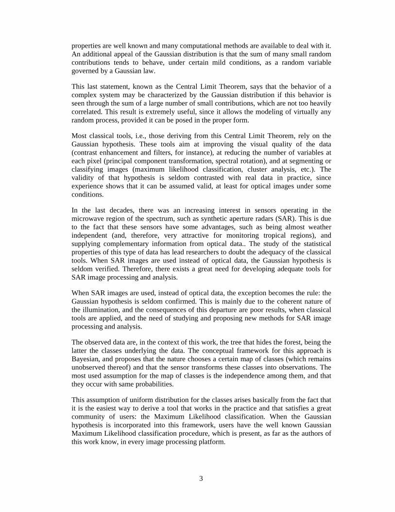
There are essentially two ways of modeling SAR images: with an ad hoc approach and through the use of physical models. The former indicates that the first thing to do is fitting Gaussian distributions to the data; the result of doing this, for three different areas, is shown in Figure 2.

In this figure three samples of extended areas were selected, corresponding to pasture, forest and an urban region. The mean and standard deviation of three Gaussian distributions were estimated, and the corresponding histograms and fitted densities are shown. It is quite clear that this sample of pasture (top) could be modeled by this distribution to some extent, but is it is noticeable that forest (middle) and urban data (bottom) are quite far from admitting this hypothesis.

The ad hoc approach requires discarding the Gaussian distribution whenever it is not acceptable, and looking for another one, and so on until a suitable distribution is found. The success of this approach depends, essentially, on the size of the available set of distributions.

This way of applying statistics eventually leads to a distribution that fits well the data, but it is not immediate how to associate a meaning to that fitting. Some usual distributions belonging to this statistical vocabulary are the Weibull (see [14]), the Log-normal (used, for instance, in [39]) and the scaled Beta. The use of these and other distributions is presented in [56], and in many of the references therein.

The other approach, namely the one based on the use of the Multiplicative Model, instead of looking for the distribution that best suits the data, offers a limited set of distributions, but all of them have a physical interpretation. This modeling, based on the physics of the image formation, can be seen in detail in [22] and in [39]. It is based on the fact that the illumination is made with coherent radiation, and also on that the involved signals interfere in a constructive and destructive manner, introducing a certain degree of roughness in the observed targets.

8

Figure 2: Three areas, their histograms and fitted Gaussian densities.

At this point it is convenient to recall that the speckle noise, which is suitably modeled within the multiplicative model, appears in every image obtained with coherent illumination. Examples of these are SAR, sonar, ultrasound and laser images.

9

For the sake of simplicity, only quadratic detection (intensity data) will be treated here. The curious reader is referred to [14], [16] and [18] for a treatment of the other cases, namely complex and amplitude data.

The multiplicative model states that the observed intensity data is the outcome of the random variable Z which, in turn, is the product of two independent random variables: X , associated to the terrain backscatter, and Y , which models the speckle noise. The distribution for the return depends on the distributions associated to both the backscatter and the speckle.

In the next sections, models for monospectral data (one band and one polarization) and polarimetric data (one band and various polarization) will be presented. For the first case, models for speckle, backscatter and intensity return are considered. When the return is given in intensity or amplitude the phase of the received signal is lost, which does not happen when complex polarimetric data are used.

MONOSPECTRAL DATA

SPECKLE NOISE

In the complex format, it is usually considered that the speckle noise YC has a bivariate Gaussian distribution, and its real ( ℜY ) and imaginary ( ℑY ) components are independent and identically distributed, with zero mean and variance equal to 1/2. The relations between the complex format and intensity and amplitude formats of the speckle are

given by 2

CI YY = and 22ℑℜ +== YYYY CA , respectively. For this situation, which is

called 1-look, it can be proved that IY has an exponential distribution and that AY has a Rayleigh distribution (see [32]).

The n looks intensity image (multi-look processing) is built by averaging n independent samples of IY , leading this random variable to a Gamma distribution, denoted by

),(~)( nnY nI Γ and given by:

0,)exp(

)()( 1

)( >−Γ

= − ynnyyn

nyf n

n

Y nI

. (1)

In multi-look case, the amplitude is obtained by extracting the square root of multi-look

intensity data, that is, )()( nI

nA YY = , where )(n

IY has the distribution given by eq. (1). In

this way, the random variable )(nAY will have a Square Root of Gamma distribution.

Though the number of looks n should, in principle, be an integer, seldom this is the case when this quantity is estimated from real data, due to, among another reasons, the fact that the mean of intensity is taken over correlated observations. Therefore, n is, in general, called equivalent number of looks. For high values of n the Γ(n,n) distribution approaches the Gaussian distribution, which can be explained by the Central Limit Theorem [57].

10

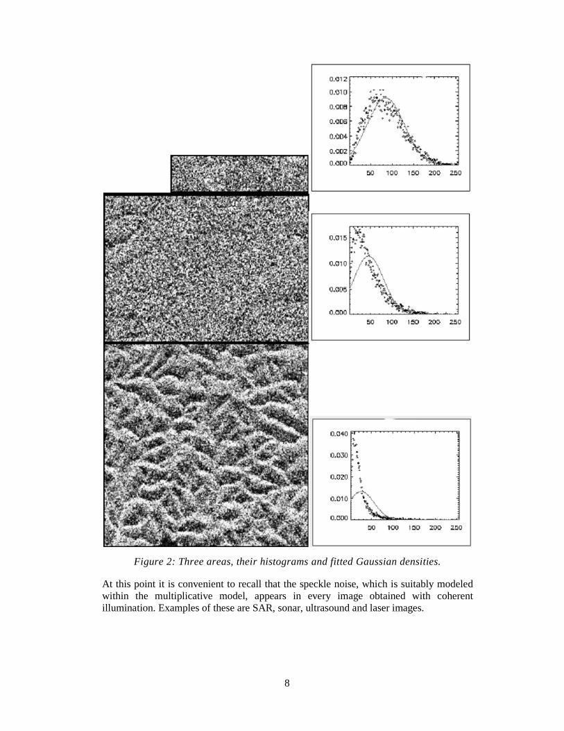
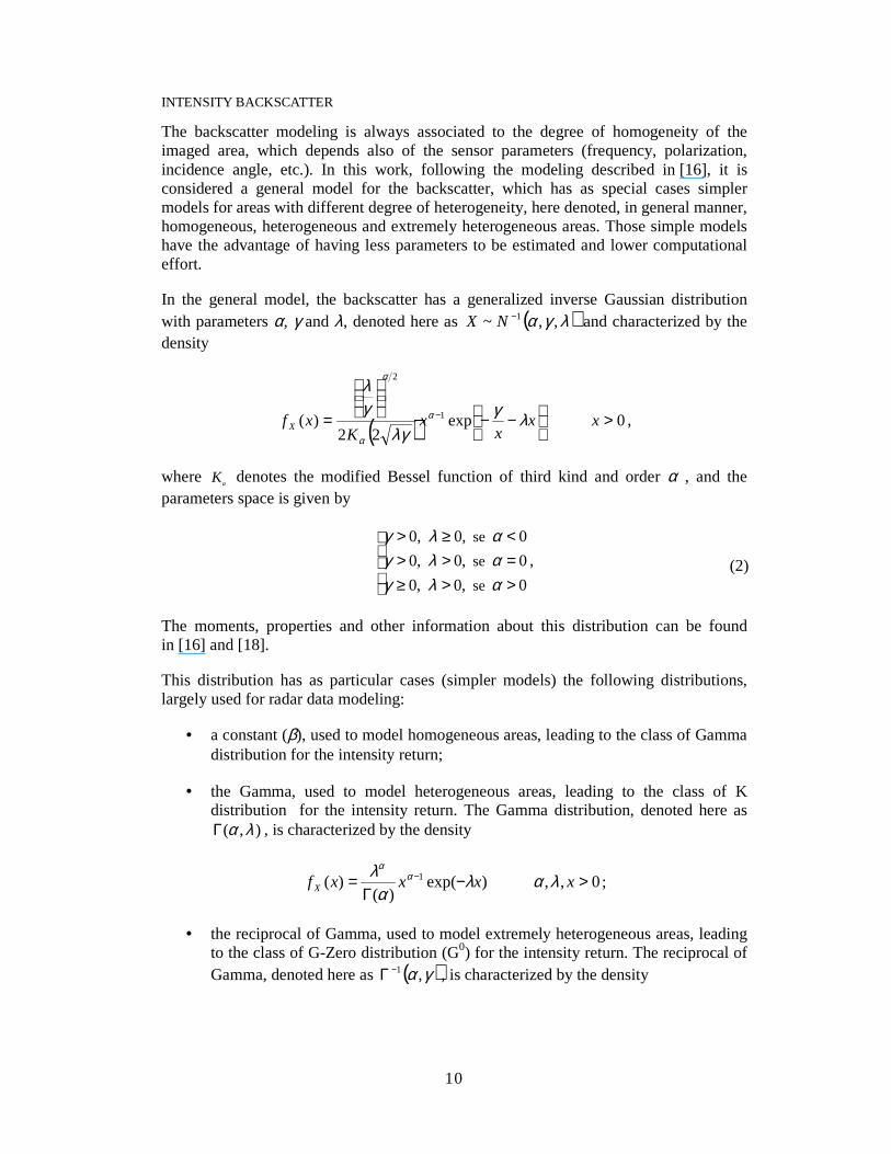
INTENSITY BACKSCATTER

The backscatter modeling is always associated to the degree of homogeneity of the imaged area, which depends also of the sensor parameters (frequency, polarization, incidence angle, etc.). In this work, following the modeling described in [16], it is considered a general model for the backscatter, which has as special cases simpler models for areas with different degree of heterogeneity, here denoted, in general manner, homogeneous, heterogeneous and extremely heterogeneous areas. Those simple models have the advantage of having less parameters to be estimated and lower computational effort.

In the general model, the backscatter has a generalized inverse Gaussian distribution with parameters α, γ and λ, denoted here as ( )λγα ,,~ 1−NX and characterized by the density

( ) 0exp22

)( 1

2

>

−−

= − xxx

xK

xf X λγλγ

γλ

α

α

α

,

where αK denotes the modified Bessel function of third kind and order α , and the

parameters space is given by

>>≥=>><≥>

0,0,0

0,0,0

0,0,0

se

se

se

αλγαλγαλγ

, (2)

The moments, properties and other information about this distribution can be found in [16] and [18].

This distribution has as particular cases (simpler models) the following distributions, largely used for radar data modeling:

• a constant (β), used to model homogeneous areas, leading to the class of Gamma distribution for the intensity return;

• the Gamma, used to model heterogeneous areas, leading to the class of K distribution for the intensity return. The Gamma distribution, denoted here as

),( λαΓ , is characterized by the density

0,,)exp()(

)( 1 >−Γ

= − xxxxf X λαλα

λ αα

;

• the reciprocal of Gamma, used to model extremely heterogeneous areas, leading to the class of G-Zero distribution (G0) for the intensity return. The reciprocal of Gamma, denoted here as ( )γα ,1−Γ , is characterized by the density

11

( ) 0,,exp)(1

>

−

−Γ=

−

x-x

xxf X γαγ

αγ α

α

.

The relations between the ( )λγα ,,N 1− distribution and its particular cases can be summarized in the following diagram:

D

D

Homogeneous),,(1 λγα−N

ExtremelyHeterogeneous

),(1 γα−Γ

Heterogeneous

),( λαΓ

2β

0,0>

→λα

γ

0,

0>−

→γα

λ2/1

2/

,−→−

∞→−βγα

γα

P

/

,λαλα

→∞→

P

2/11

β

1β

where D and P denote convergence in distribution and in probability, respectively, of the associated random variables.

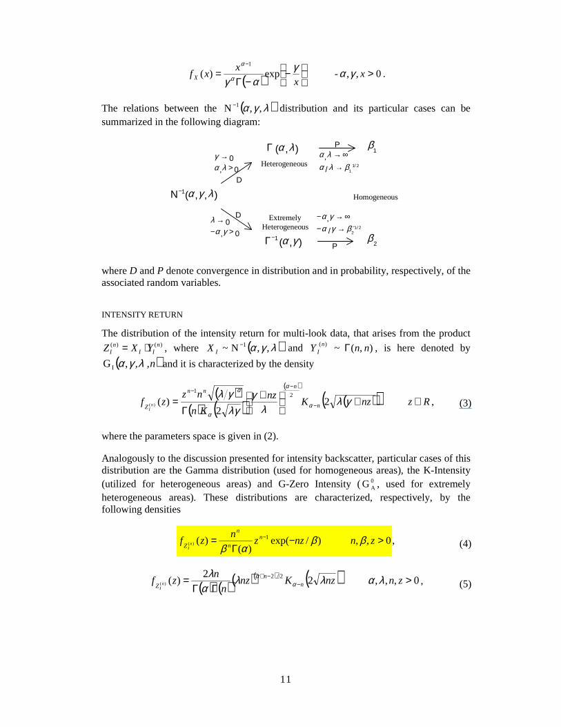
INTENSITY RETURN

The distribution of the intensity return for multi-look data, that arises from the product )()( n

IIn

I YXZ ⋅= , where ( )λγα ,,N~ 1−IX and ),(~)( nnY n

I Γ , is here denoted by

( )n ,,λγα,G I and it is characterized by the density

( )( ) ( )

( )

( )( ) RznzKnz

Kn

nzzf n

nnn

Z nI

∈+

+

Γ= −

−−

γλλ

γλγγλ

α

α

α

α

22

)(2

1

)( , (3)

where the parameters space is given in (2).

Analogously to the discussion presented for intensity backscatter, particular cases of this distribution are the Gamma distribution (used for homogeneous areas), the K-Intensity (utilized for heterogeneous areas) and G-Zero Intensity ( 0

AG , used for extremely heterogeneous areas). These distributions are characterized, respectively, by the following densities

0,,)/exp(

)()( 1

)( >−Γ

= − znnzzn

zf n

n

n

Z nI

ββαβ

, (4)

( ) ( )( )( ) ( ) 0,,,22

)( 2/2)( >

ΓΓ= −

−+ znnzKnzn

nzf n

n

Z nI

λαλλα

λα

α, (5)

12

( )( ) ( )( )

0,,,)(1

)( >+−ΓΓ

−= −

−

zn-nzn

znnzf

n

nn

Z nI

γαγαγ

αΓαα

, (6)

The relations among these distributions are summarized in the following diagram:

D

D

Heterogeneous

ExtremelyHeterogeneous

Homogeneous),,,(G I nλγα

),,(G0I nγα

),,(K I nλα )/,( 1βnnΓ

),( 2βnnΓ

0,

0>

→λα

γ

0,

0>−

→γα

λ

1/

,βλα

λα→

∞→

2/

,βγα

γα→−

∞→−

D

D

where D denotes convergence in distribution of the associated random variable.

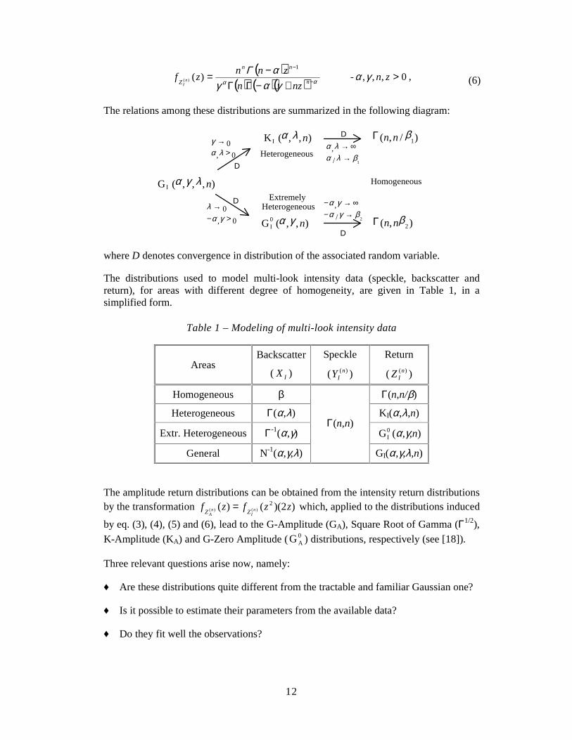
The distributions used to model multi-look intensity data (speckle, backscatter and return), for areas with different degree of homogeneity, are given in Table 1, in a simplified form.

Table 1 – Modeling of multi-look intensity data

Areas Backscatter

( IX )

Speckle

( )(nIY )

Return

( )(nIZ )

Homogeneous β Γ(n,n/β)

Heterogeneous Γ(α,λ) KI(α,λ,n)

Extr. Heterogeneous Γ-1(α,γ) 0IG (α,γ,n)

General N-1(α,γ,λ)

Γ(n,n)

GI(α,γ,λ,n)

The amplitude return distributions can be obtained from the intensity return distributions by the transformation )2)(()( 2

)()( zzfzf nI

nA ZZ

= which, applied to the distributions induced

by eq. (3), (4), (5) and (6), lead to the G-Amplitude (GA), Square Root of Gamma (Γ1/2),

K-Amplitude (KA) and G-Zero Amplitude ( 0AG ) distributions, respectively (see [18]).

Three relevant questions arise now, namely:

♦ Are these distributions quite different from the tractable and familiar Gaussian one?

♦ Is it possible to estimate their parameters from the available data?

♦ Do they fit well the observations?

13

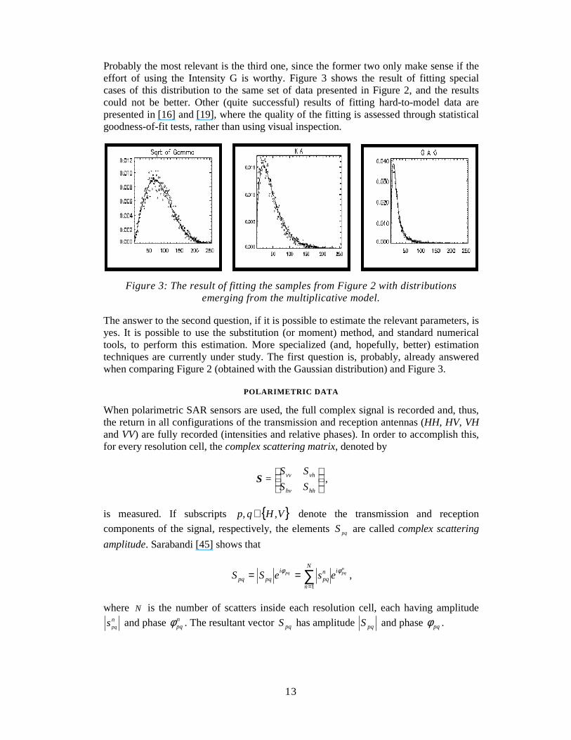
Probably the most relevant is the third one, since the former two only make sense if the effort of using the Intensity G is worthy. Figure 3 shows the result of fitting special cases of this distribution to the same set of data presented in Figure 2, and the results could not be better. Other (quite successful) results of fitting hard-to-model data are presented in [16] and [19], where the quality of the fitting is assessed through statistical goodness-of-fit tests, rather than using visual inspection.

Figure 3: The result of fitting the samples from Figure 2 with distributions emerging from the multiplicative model.

The answer to the second question, if it is possible to estimate the relevant parameters, is yes. It is possible to use the substitution (or moment) method, and standard numerical tools, to perform this estimation. More specialized (and, hopefully, better) estimation techniques are currently under study. The first question is, probably, already answered when comparing Figure 2 (obtained with the Gaussian distribution) and Figure 3.

POLARIMETRIC DATA

When polarimetric SAR sensors are used, the full complex signal is recorded and, thus, the return in all configurations of the transmission and reception antennas (HH, HV, VH and VV) are fully recorded (intensities and relative phases). In order to accomplish this, for every resolution cell, the complex scattering matrix, denoted by

SS

SS=

hhhv

vhvv

S ,

is measured. If subscripts { }VHqp ,, ∈ denote the transmission and reception

components of the signal, respectively, the elements pqS are called complex scattering

amplitude. Sarabandi [45] shows that

npqpq i

N

n

npq

ipqpq eseSS

φφ ∑=

==1

,

where N is the number of scatters inside each resolution cell, each having amplitude npqs and phase n

pqφ . The resultant vector pqS has amplitude pqS and phase pqφ .

14

Ulaby and Elachy [51] show that, for a monostatic satellite (which is the usual case), it is possible to assume that VHHV SS = . Therefore, the complex scattering matrix can be reduced, without loss of information to

=

vv

hv

hh

C

S

S

S

Z ,

where ZC denotes a complex vector.

The multiplicative model can be also applied to the polarimetric data. In this case, due to the number of polarizations, the speckle (YC) is modeled by a multivariate complex Gaussian distribution. Therefore, the return ZC (here represented by the vector ZC) has a multivariate complex Gaussian distribution, when the backscatter (X) is modeled by a constant (homogeneous areas).

The vector ZC characterizes the 1-look polarimetric data, and for being complex and having different polarizations (components), produces a large volume of data over the imaged surface. Therefore, the polarimetric SAR data are frequently processed in order to increase the number of looks (multi-look), for data compression and speckle reduction. A fixed number, n, of independent outcomes of ZC are averaged to form the n-looks covariance matrix, given by [31]

∑

==

n

1k

T*CC

(n)C kk

n

1)()( ZZZ , (7)

where )(kT*

CZ denotes the transpose conjugate of ZC(k).

The advantage of dealing with the covariance matrix, when a constant is used to model the backscatter (homogeneous areas), is that the matrix (n)

CC nZA = exhibits a multivariate complex Wishart distribution [48]. Therefore, the density associated to the matrix (n)

CZ , is given by:

0,

),(

)](exp[)(

)(

)( >−

=−−

qnqnK

nTr nf

n

q nqn

Z nC

C

1C

C

zCzz , (8)

where q denotes the dimension of the vector ZC , )1()(),( )1()2/1( +−ΓΓ= − qn nqnK q q

�π , Tr( ) denote the trace of the matrix,

][T*

CCC E ZZC = , and E() denotes the expected value.

The use of Equation (8) with multivariate polarimetric SAR data implies in high computational effort. Therefore, [31], [32] and [35] derived, from Equation (8) (considering a constant backscatter, that is, homogeneous areas), some univariate (phase difference, ratio of intensities) and bivariate (pair of intensities and pair intensity-phase) distributions. The following subsections describe these distributions.

15

DISTRIBUTION OF PAIR OF MULTI-LOOK INTENSITY IMAGES

Consider two multi-look intensity images, represented by the random variables Z1 and Z2, obtained from two components Sr and Ss of the scattering matrix, using the equations

∑=

=n

kr kS

nZ

1

2

1 )(1

and ∑=

=n

ks kS

nZ

1

2

2 )(1

.

The distribution of the pair of multi-look intensity images, derived in [32], is given by:

( )

−−Γ

−+

−

= −−

+

−+

2211

2121

122

1

2211

2221112

1

211

21),(1

)1(

1exp

)(21 hh

zzn2I

)(n()hh

hzhzn)zz(n

,zzfc

cn

n

cc

)n(

2

c

)n(n

ZZρ

ρ

ρρ

ρ, (9)

where ][ 111 ZEh = , ][ 222 ZEh = , and

ξρρ ic

sr

src e

SESE

SSE==

∗

][][

][22

,

and cρ and ξ are the modulus and phase of the multi-look complex correlation

coefficient, respectively, 1−=i and 1−nI is the modified Bessel function of order

1−n .

DISTRIBUTION OF THE MULTI-LOOK PHASE DIFFERENCE IMAGE

Consider a multi-look phase difference image, represented by the random variable Ψ, obtained from two components Sr and Ss of the scattering matrix, using the equation (see [32]):

= ∑

=

∗n

ksr kSkS

nArg

1

)()(1Ψ ,

where Arg() denotes the argument of a complex number. Then, the distribution of Ψ, derived in [34], is given by:

)(),(2

)1(

)1)((2

)1)(2/1()( 12

2

2/12

2

πψπδπ

ρδπ

δρψΨ ≤

−+

−Γ

−+Γ=

+<- 1/2; 1; nF

n

nf 2

nc

n

nc , (10)

where )cos( ξψρδ −= c , 2F1 denotes the Gaussian hypergeometric function [23] and ξ

is the phase of the complex correlation coefficient.

16

DISTRIBUTION OF MULTI-LOOK INTENSITY RATIO IMAGES

From two multi-look intensity image, represented by the random variables Z1 and Z2, the distribution of the ratio

21ZZW = was derived in [32], and is given by

2/)12(222

12

]4))[((

)()1)(2()(

+

−

−+Γ

+−Γ=

nc

nnc

n

Ww wn

wwn wf

ρττ

τρτ, (11)

where 2211 hh =τ .

DISTRIBUTION OF PAIR OF MULTI-LOOK INTENSITY-PHASE DIFFERENCE IMAGES

Consider two multi-look images, one intensity and other phase difference, represented by the random variables Z1 and Ψ, respectively. Consider an image represented by the random variable B1, defined by (see [31])

11

1

2

11

11

)(

h

kS

h

ZnB

n

kr∑

=== .

The joint distribution of B1 and Ψ is given by

dn

d

bb

d

b ; ;F

n

d

bb

bf

nn

B)(2

)1(exp

2

11

)(2

exp

),(

212

1

1

12

11

111

1),( 1 Γ

−−

+

Γ

−

=

−−

π

δδδ

πψΨ , (12)

where 2

1 cd ρ−= and 1F1( ) denotes the confluent or degenerated hypergeometric

function (see [1]).

Parameter estimators techniques for the distributions given in eq. (9) to (12) can be seen in [10].

POLARIMETRIC MODELLING UNDER THE PRESENCE OF ROUGHNESS

As presented in previous sections, the assumption of constant backscatter (that leads to Gamma, Square root of Gamma and Wishart distributions for intensity, amplitude and multivariate polarimetric returns, respectively) only works in regions of small roughness. When heterogeneous and extremely heterogeneous areas are observed, it is imperative to introduce some variability in the backscatter, for instance using Gamma or Reciprocal of Gamma distributions, or their square roots if amplitude or complex format are being modeled.

Let us first consider the situation of modeling heterogeneity. Similarly to the amplitude case, the Gamma distribution can be used to characterize the backscatter through the random variable G below and, thus, the complex scattering matrix can be now posed as

17

CC GUZ = . (13)

Novak et al [40] derive this distribution, called multivariate single look K, while Lee et al [35] derive the multilook case that has density

( ) ( ) ( ) ( )

( )( )

21

12

1) (

)(),(

)(22)( qn

C

n

C

Cqn

qnqn

Z

TrqnK

TrnKnf n

C−

−−

−

−

+−

Γ= α

α

α

α

αα

zCC

zCzz , (14)

Though this model fits very well heterogeneous data, it again fails to explain the variability of extremely heterogeneous targets. In order to alleviate this situation the fully polarimetric multilook GA0 distribution is proposed in [10]. It is obtained using the Reciprocal of Gamma distribution for the intensity backscatter and the same multiplicative scheme presented in eq. (13). The density that characterizes this distribution is

( ) ( )

( ) ( ) [ ] )(),(

1

) (

)( αα αααα

−−

−

−−Γ−

−Γ= qn

C

n

C

qnqn

Z

nTrqnK

qnnf n

C zCC

zz . (15)

PARAMETERS AND NATURE

We have been dealing with very general statistical models, stated in a single class of distributions, that aim at describing every possible return in SAR images. We have also seen that these models perform well. A relevant question remains open: what does it mean?

Fortunately, the multiplicative model allows us to use a single parameter in order to characterize the homogeneity of the observed target. This parameter is α and, as seen in the parameters space, it spans the whole real line.

The other two parameters associated to the backscatter (namely λ and γ ) work as scale parameters and, thus, are related to the brightness of the scene. The speckle has only one parameter associated to it, namely n .

Going back to α , what does it mean selecting an interesting area and estimating its parameter with a certain estimator α̂ (the reader is required to believe that there are suitable estimators to perform this task (see, for instance [53], [56] and [57])? Fortunately, that value means a lot. This parameter is a measure of the homogeneity of the considered area. The higher its absolute value, the more homogeneous the observed data. Homogeneous areas are associated, for certain SAR sensors, to agricultural, pasture or deforested regions, so if a suspicious area yields to 3.17ˆ =α , a human and/or automatic interpreter should fire an alarm because α̂ is too big for being related to a

peaceful primary forest (that should be heterogeneous). Such result of an estimation procedure would be enough evidence of a deforestation. Complementarily, if an area previously classified as pasture suddenly exhibits 9.1ˆ −=α that value could be used as evidence of newly born manmade structures where cows should be feeding.

18

While modeling and analyzing, which is what we have been doing so far, is quite interesting per se, all this effort is fully rewarded when we use this framework to tackle other kind of problems. The reader might be worried, with the impression that only three classes of land use can be detected with SAR images, namely those corresponding to homogeneous, heterogeneous and extremely heterogeneous returns. The technical report [57] shows how this is a mere didactic simplification, presenting in detail many more intermediate situations.

Other measures that can be derived from SAR images can be seen in [37], in [47] and in [58]. They are used, respectively, to retrieve biomass in regenerating tropical forests, to discriminate types of crops and to relate SAR data to tropical forest regeneration stages. Some of these quantities are of statistical nature, but not directly related to the multiplicative model.

MODELING CLASSE S AND THE P RACTICE OF BAYE SIAN IM AGE CLA SSIFICATION

In the previous sections the Multiplicative Model has been posed as an interesting tool for the characterization of SAR data. Let us now turn to the problem of describing the classes in an image, bearing in mind that this modeling is, in principle, worthy for any image independently of the sensor that provides it.

A very general model for image formation (see [5], [21] and the references therein) builds the image from the classes and from the observations associated to each class. The former and their spatial distribution are chosen by the nature, they are not observed, and this is the information sought by the user. The latter is imposed by the imaging system, depends on the technology employed to observe the nature and, for SAR images, the already presented Multiplicative Model will be used.

Since the 80’s many techniques based on the use of Markov random fields have proved their usefulness in image processing and understanding applications. Such techniques use the Bayesian framework, and assume that the true image obeys a probabilistic law that incorporates spatial dependence.

The eldest antecedent of those models can be traced upon the 20’s: the celebrated Ising model, originally proposed as a means of explaining the phenomenon of spontaneous magnetization exhibited by ferromagnetic materials. Ising could not pursue his work successfully, but his model is still receiving the attention of a large community of researchers worldwide.

A wide class of models that incorporate dependence among neighboring random variables is called Markov random field, since it is a natural extension of Markov chains to the multidimensional case. Its adequacy as an image model arises from the fact that it can successfully model local homogeneity and, at the same time, sharp transitions. This feature is useful since classes (the unobserved types of region present in the image), and even radiometries (the observed values), exhibit both characteristics in many images.

Geman and Geman [21] and Carnevalli, Coletti and Patarnello [7], in their pioneering (and apparently independent) works showed how the Markovian approach can be a serious competitor to more classical techniques for image blur and noise reduction,

19

classification, segmentation etc. Regarding the application of Markov random fields to image processing and analysis, the reader is referred to the work by Besag ([1], [3] and [4], for instance), Bustos et al [6], Dubes and Jain [12] and Wrinkler [55].

The number of published works where Markov random fields play a central role in image processing has grown explosively in the last years, and most of the results obtained with this modeling are impressive.

In this work the Potts model will be used to model the choice of the class map. This choice is made by the nature, and the chosen map is unavailable. Consider the image defined on the finite Euclidean grid }1,,0{}1,,0{ −×−= nmS �� of size nm × .

Assume that every coordinate in Ss ∈ has an associated neighborhood s∂ of elements

(different from s ) in the grid. This neighborhood ranges from the empty set ∅ to the rest of the coordinates sS \ , and it is the set that will influence choice of a class in coordinate s given the rest of the map. The only restriction that neighborhoods must satisfy is that ts ∂∈ if and only if st ∂∈ .

Assume that in every coordinate one class among the classes of the set Ξ will be chosen. In principle this set could be different in different coordinates, but we will restrict our attention to the models used in the applications we bear in mind. The set Ξ describes the possible targets in the image, such as “grass”, “river”, “urban area”, “corn” etc. In this modeling the elements in Ξ do not possess any order relationship.

Now imagine that in every coordinate s a random variable sX chooses a class among the available ones in the set Ξ . This choice will be influenced by the classes already chosen by its neighbors. In other words, the conditional distribution of sX given the rest of the image, only depends on the classes observed in the neighboring coordinates, i.e., for every Ss ∈ )|Pr()|Pr( \\ ssjssSsSjs XX ∂∂ ===== xXxX ξξ , where Ξ∈jξ and

AX denotes the set of random variables indexed by the set SA ∈ . This model is conceptually very attractive, since it is expected that distant coordinates do not heavily influence the structure of the map. Notice that this definition extends the notion of Markov chain to a situation where the indexes no longer belong to the real line, but where they are part of an arbitrary space. The notion of present, past and future is, thus, no longer relevant.

The class of distributions governing the set of random variables SssX ∈)( induced by conditions as presented in the previous equation (if it exists) is called Markov random field. A detailed study of their properties and special cases, always within the context of image modeling, can be seen in [6].

The Potts model used in image classification is a special Markov random field, where

}):{#exp()|Pr( jtsjs xtXss

ξβξ =∂∈∝== ∂∂ xX ,

where β is a real number and ∝ denotes proportionality. This model incorporates the notion of spatial dependence whenever 0≠β . If 0>β then one has an attractive model, in the sense that clusters of equal classes will be favored against chessboard-like

20

outcomes, and the reciprocal if 0<β . When 0=β there is no influence of neighboring sites, and one returns to the independent equally probable class model.

This model can be extended in many directions. A possible modification is the use of different marginal probabilities for different classes in Ξ . Another extension consist of using different parameters for each direction. These extensions could be of theoretical interest, but in the applications here commented they yielded no noticeable improvement and they made the algorithms considerably slower.

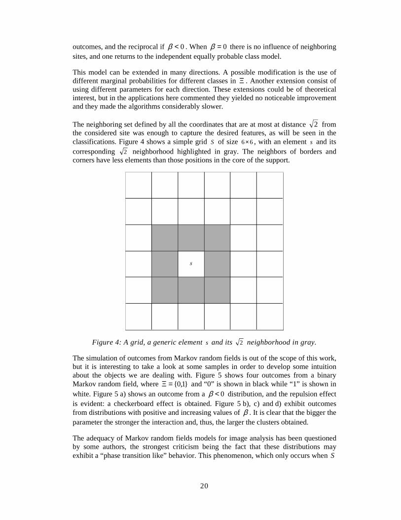
The neighboring set defined by all the coordinates that are at most at distance 2 from the considered site was enough to capture the desired features, as will be seen in the classifications. Figure 4 shows a simple grid S of size 66 × , with an element s and its corresponding 2 neighborhood highlighted in gray. The neighbors of borders and corners have less elements than those positions in the core of the support.

Figure 4: A grid, a generic element s and its 2 neighborhood in gray.

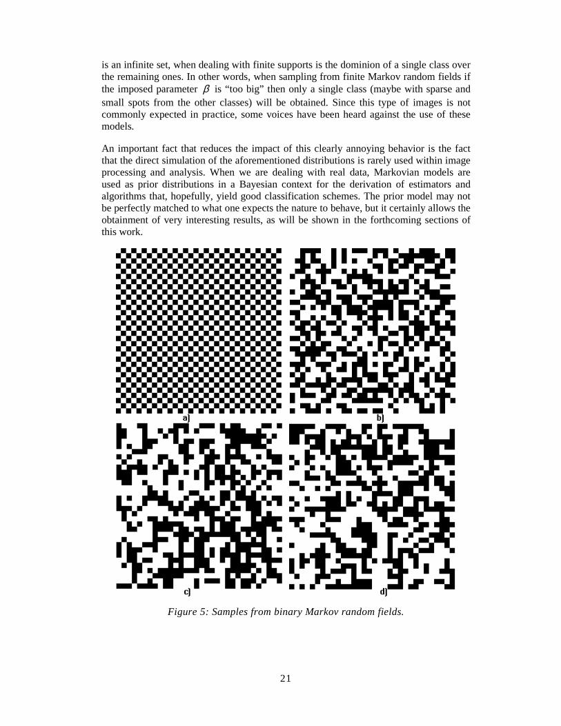
The simulation of outcomes from Markov random fields is out of the scope of this work, but it is interesting to take a look at some samples in order to develop some intuition about the objects we are dealing with. Figure 5 shows four outcomes from a binary Markov random field, where }1,0{=Ξ and “0” is shown in black while “1” is shown in white. Figure 5 a) shows an outcome from a 0<β distribution, and the repulsion effect is evident: a checkerboard effect is obtained. Figure 5 b), c) and d) exhibit outcomes from distributions with positive and increasing values of β . It is clear that the bigger the parameter the stronger the interaction and, thus, the larger the clusters obtained.

The adequacy of Markov random fields models for image analysis has been questioned by some authors, the strongest criticism being the fact that these distributions may exhibit a “phase transition like” behavior. This phenomenon, which only occurs when S

21

is an infinite set, when dealing with finite supports is the dominion of a single class over the remaining ones. In other words, when sampling from finite Markov random fields if the imposed parameter β is “too big” then only a single class (maybe with sparse and small spots from the other classes) will be obtained. Since this type of images is not commonly expected in practice, some voices have been heard against the use of these models.

An important fact that reduces the impact of this clearly annoying behavior is the fact that the direct simulation of the aforementioned distributions is rarely used within image processing and analysis. When we are dealing with real data, Markovian models are used as prior distributions in a Bayesian context for the derivation of estimators and algorithms that, hopefully, yield good classification schemes. The prior model may not be perfectly matched to what one expects the nature to behave, but it certainly allows the obtainment of very interesting results, as will be shown in the forthcoming sections of this work.

Figure 5: Samples from binary Markov random fields.

22

One of the most useful transformations in image processing is called classification. It takes an image as input, and generates a map as output; in other words, it turns numbers into information. There are many ways of doing this: using neural networks, decision rules, mathematical morphology etc. In this work only the statistical approach is considered.

The preferred statistical classification technique is called maximum likelihood. It consists of associating to every coordinate in the image that class which makes a certain measure of plausibility highest. This measure of plausibility is calculated using the densities that characterize every class. Examples of fitting densities to classes were presented in Figure 2 and Figure 3, where it was also shown that the Gaussian distribution seldom is a good hypothesis for SAR data. A comparison of classification techniques is available in [44], for instance.

In [19] it is presented a study on the effect of using the Gaussian and the correct (under the multiplicative model) distributions on the classification of areas using SAR data. It was concluded that, though the use of the multiplicative model significantly improves the classification (in more than 50%), the low signal-to-noise ratio of these images requires additional efforts to attain acceptable results.

This additional effort was made using a Bayesian framework for the classification, and deriving an iterative and deterministic scheme for the obtainment of maps: the ICM algorithm. This was performed with the user in mind and, thus, all the techniques were developed “behind” user-friendly interfaces and within the context of a goal-driven system.

The aforementioned Potts model was used to assign a pior distribution for the classes, and the set of distributions associated to the Multiplicative Model was incorporated as the models for the observations given the classes.

Once this Bayesian framework is established, one has to propose and implement an estimator for the unobserved class map given the observations. There are, basically, two estimators and an algorithm to perform this task, being the former the MAP (maximum a posteriori) and MPM (marginal posterior modes). In both cases it is impossible to derive them in a general and direct manner. MAP requires the use of global minimization techniques, as simulated annealing, and MPM imposes the use of stochastic simulation of the posterior model. In both cases, there is a plethora of unknown parameters which are crucial for the obtainment of good results.

An intermediate solution is the use of the Iterative Conditional Modes, ICM. This deterministic algorithm requires an initial classification, that will be improved using both the observed value and the contextual information in every pixel. Assume

Sss kxk ∈= ))(ˆ()(x̂ denotes the classification at stage k . In our work )0(x̂ is the maximum likelihood classification.

The classification at stage 1+k is obtained replacing in every Ss ∈ the class )(ˆ kxs by

the one that maximizes the conditional distribution ),|Pr(ssz ∂xξ which, with the

aforementioned assumptions is given by )()|Pr( szfs ξξ ∂x , where s∂ denotes the

23

neighborhood of the coordinate under inspection and )( szfξ is the density of the

distribution associated to class ξ evaluated in the observed value sz . In other words, the

method maximizes in every coordinate the likelihood of the observed value )( szfξ

weighted by the contextual evidence )|Pr(s∂xξ .

This contextual evidence, which is expected to favor the occurrence of clusters of the same class, depends on a single real parameter, namely β , which is unknown. Our approach consists of estimating it from the previous classification through the maximization of the pseudo-likelihood function, which is given by

∏ ∈ ∂=Ss s s

xPL )|(Pr)|( xx ββ , and can be obtained using standard numerical tools.

When 8# =∂ s , as is our implementation, this equation involves sixty-seven terms, and each term involves the counting of times certain local configurations occur and a rational function of polynomials of exponential terms (for details see [54]).

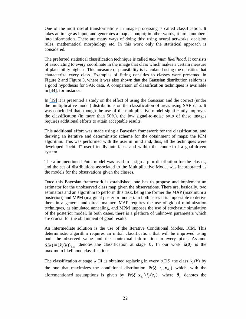
Figure 6 shows the result of using this classification procedure with amplitude data, where it is quite evident that there is an important improvement from the first (maximum likelihood) to the second (ICM) classification. In both classifications, cyan depicts primary forest, magenta clear cut and yellow second regrowth. The original image is from the JERS-1 over Tapajós.

Figure 6: (from left to right) Original JERS-1 image; Best Fit Maximum Likelihood classification (under the multiplicative model) and Best Fit ICM

classification.

As previously presented, polarimetric data is a good candidate for having more information than either intensity or amplitude formats. It was then implemented the ICM classification scheme under the multiplicative model for the already presented distribution for reduced data. The objective of this implementation was twofold: first, delivering an easy-to-use tool for the obtainment of good classifications; second, the

24

evaluation of the information content in those different formats and in two frequencies (bands L and C) and all available polarizations (HH, HV and VV).

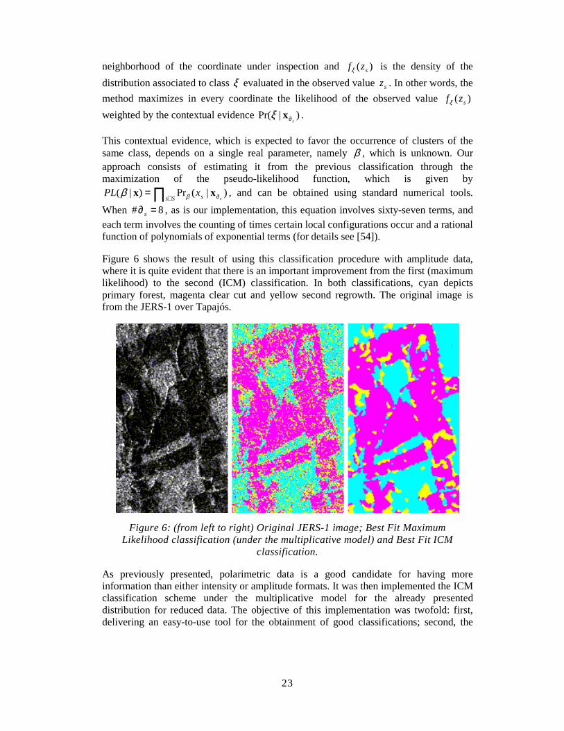
The original data, in the form of a color composite image, is shown in Figure 7. The results, whose complete description is available in [11], are shown in Figure 8. Only the best classifications obtained are shown here.

It is important to say that even tough the Pair of intensities L-HVVV ICM classification had given the best classification (quantitatively assessed), it was not possible to discriminate all classes of interest in this classification. The river and prepared soil classes were better classified with C band, while the other classes were better classified with L band. Besides, there was a high confusion between Soybean2 and Corn2 classes.

Those results show that it is not possible to discriminate in a single classification, using the uni/bivariates polarimetric distributions, more than three classes with C band and more than six classes with L band for the Bebedouro image. However, depending on the type of application and the modeling used (utilization of the contextual information), the use of uni/bivariates polarimetric data can produce good results, specially if the phase information is available, showing the complementary aspect of this kind of data

Caatinga

Corn1

Corn2

Tillage

River

Soybean1

Soybean2

Soybean3

Prepared soil

Figure 7: Color composition (R-HH, G-HV and B-VV) of Bebedouro image with the training samples of the classes of interest.

25

(a) (b) (c)

(d) (e)

Figure 8: ICM classification of reduced polarimetric data: Pair of intensity images (a) C-HVVV, (b) L-HVVV, (c) L-HHVV, (d) Ratio of intensity images

L-HHVV, (e) Pair intensity-phase L-HHVV.

This ICM implementation, using iterative estimation of the parameter with pseudo-likelihood, has been implemented for most of the distributions associated to the Multiplicative Model, and also for the multivariate normal distribution. Since the implementation was performed as a plug-in of a commonly used image processing system, the community of users of this tool is growing.

FILTERS UNDER THE MULTIPLICATI VE MOD EL

Filters are a very important class of tools. They transform the original images into new images, aiming at attaining certain goals. Some common goals are: reducing atmospheric attenuation (when optical images are used), reducing noise and enhancing certain characteristics in an image.

As has been previously seen, under the multiplicative model the parameter α is a measure of homogeneity. In [38] this was used to produce a texture image aiming at detecting regrowth stages. This image was built calculating α̂ over small areas (called windows) in the image, and the resulting image was used as input for classification algorithms. It was there seen that this α̂ image retrieved very important information that, though present in the original data, was not evident without this processing stage. In [44] the same procedure was used to derive new features for Radarsat (a Canadian SAR sensor) image classification.

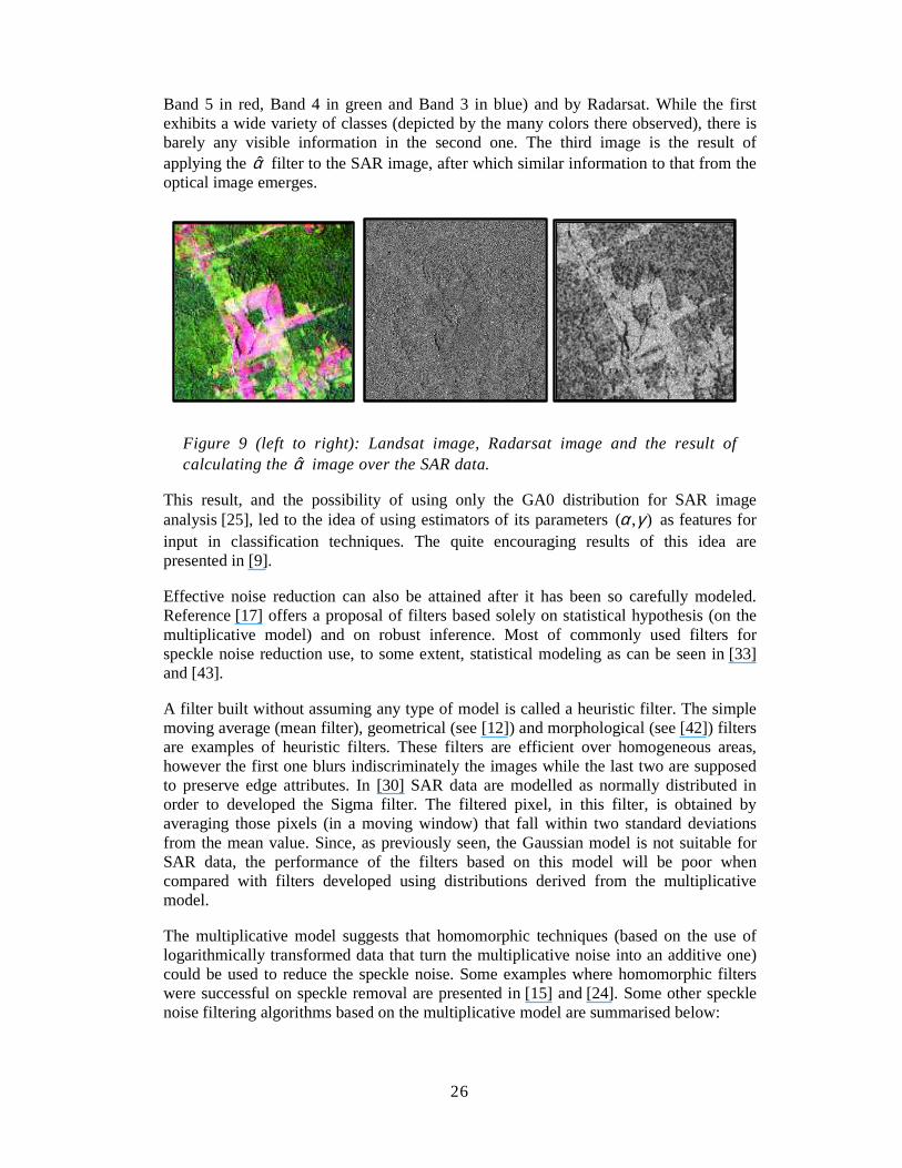
In order to illustrate this point, Figure 9 shows an area (corresponding to a region where primary forest coexists with heavily managed parcels, secondary regrowth, etc., in Tapajós, Pará state, Brazil) as seen by Landsat-TM (optical data, in a color composite:

26

Band 5 in red, Band 4 in green and Band 3 in blue) and by Radarsat. While the first exhibits a wide variety of classes (depicted by the many colors there observed), there is barely any visible information in the second one. The third image is the result of applying the α̂ filter to the SAR image, after which similar information to that from the optical image emerges.

Figure 9 (left to right): Landsat image, Radarsat image and the result of calculating the α̂ image over the SAR data.

This result, and the possibility of using only the GA0 distribution for SAR image analysis [25], led to the idea of using estimators of its parameters ),( γα as features for input in classification techniques. The quite encouraging results of this idea are presented in [9].

Effective noise reduction can also be attained after it has been so carefully modeled. Reference [17] offers a proposal of filters based solely on statistical hypothesis (on the multiplicative model) and on robust inference. Most of commonly used filters for speckle noise reduction use, to some extent, statistical modeling as can be seen in [33] and [43].

A filter built without assuming any type of model is called a heuristic filter. The simple moving average (mean filter), geometrical (see [12]) and morphological (see [42]) filters are examples of heuristic filters. These filters are efficient over homogeneous areas, however the first one blurs indiscriminately the images while the last two are supposed to preserve edge attributes. In [30] SAR data are modelled as normally distributed in order to developed the Sigma filter. The filtered pixel, in this filter, is obtained by averaging those pixels (in a moving window) that fall within two standard deviations from the mean value. Since, as previously seen, the Gaussian model is not suitable for SAR data, the performance of the filters based on this model will be poor when compared with filters developed using distributions derived from the multiplicative model.

The multiplicative model suggests that homomorphic techniques (based on the use of logarithmically transformed data that turn the multiplicative noise into an additive one) could be used to reduce the speckle noise. Some examples where homomorphic filters were successful on speckle removal are presented in [15] and [24]. Some other speckle noise filtering algorithms based on the multiplicative model are summarised below:

27

• Frost Filter [20]: it is linear and convolutional, derived from the minimisation of the mean square error over a multiplicative noise model. It is adaptive and the dependence among observations is incorporated through an exponential spatial correlation function.

• Lee Filter [29]: it is a local linear minimum mean square error filter, derived from a linearization of the model, by Taylor expansion, around the mean. This approximation transforms the multiplicative model into an additive one, and then the Wiener filter is applied.

• Kuan/Nathan Filter [28]: it is similar to the previous one. The difference is that this filter does not make any approximation. It is, also, an adaptive algorithm.

• MAP Filters (see [36] and [43]): they consist on computing the maximum a posteriori estimative of a random variable which represents the backscatter given an outcome of another random variable that represents the observation. There is a great variety of filters of this kind, because they depend on the distributions used to model the backscatter and the observations.

• Robust Filters: they are based on robust estimates of random variables which represent the backscatter. Six different robust estimators were used in [17] to recover the backscatter value, yielding six robust filters. The estimators used in that work are the median, the trimmed moments (TMO), the trimmed maximum likelihood (TML), the inter quartil range (IQR), the median absolute deviation (MAD) and the best linear unbiased estimator (BLUE). Three of them are based upon the trimming of extreme observations, and three based upon order statistics, and all of them assume a particular distribution belonging to the multiplicative model.

New filtering techniques and schemes for speckle removal are always appearing in the literature. The intent of this section was to present concepts of some filters for speckle reduction, which have a very wide bibliography. Interested readers can find more details about this subject in the references contained in this section and those therein.

CONC LUSIONS

The main consequences of a delicate statistical modeling of SAR data were presented. Though the topics covered here only scratch the surface of the subject, it has been shown how these images defy the classical Gaussian hypothesis. Nothing has been said about the analysis of phase, for instance, but every time SAR data appears, the reader must be prepared to gracefully abandon the comfortable hypothesis that sustained the analysis and processing of optical images.

The central idea is that a careful assessment of the statistical properties of synthetic aperture radar images is not only an academic exercise. This gymnastics, when properly performed, also yield to algorithms, techniques and methodologies that clearly improve the results and aid the use and analysis of this kind of images.

28

Far from being a closed subject, the statistical modeling and analysis of SAR images is an active research area, being some of its greatest challenges finding suitable models, estimators and relations between parameters and physical quantities.

ACKNOWLEDGE MENTS

This work was partially supported by grants from CNPq (Proc. 523469/96-9) and FACEPE (APQ 0707-1.03/97). Hans J. Müller (Deutsche Forschungsanstalt für Luft-und Raumfahrt, Institut für Hochfrequenztechnik, Germany) kindly provided some of the images used in this work.

REFERENC ES

[1] Abramowitz, M; Stegun, I. Handbook of mathematical functions: with formulas, graphs, and mathematical tables. New York: Dover, 1965.

[2] Besag, J.E. Nearest-neighbour Systems and the auto-logistic model for binary data, Jr. R. Stat. Soc. B, v 1, pp 75–83, 1972.

[3] Besag, J.E. Spatial interaction and the statistical analysis of lattice systems (with discussion). Jr. R. Stat. Soc. B, v. 2, pp 192–236, 1974.

[4] Besag, J.E. On the statistical analysis of dirty pictures (with discussion). Jr. R. Stat. Soc. B, v 48, pp 259–302, 1986.

[5] Bustos, O.H.; Frery, A.C. A contribution to the study of Markovian degraded images: an extension of a theorem by Geman and Geman. Computational and Applied Mathematics, v. 11, n. (1,3), pp 17–29, 281–285, 1992.

[6] Bustos, O.H; Frery, A.C.; Ojeda, S.M. Strong Markov processes in image modelling. Brazilian Journal of Probability and Statistics (REBRAPE), in press, 1999.

[7] Carnevalli, P.; Coletti, L.; Patarnello, S. Image processing by simulated annealing. IBM Journal of Research and Development, v. 29, pp. 569–579, 1985.

[8] Caves, R.C. Automatic matching of features in synthetic aperture radar data to digital map data. (PhD Thesis) — University of Sheffield, Sheffield, England, 1993.

[9] Chomczimsky, W.; Mejail, M.; Jacobo-Berlles, J.; Varela, A.; Kornblit, F.; Frery, A.C. Classification of SAR images based on estimates of the parameters of the GA0 distribution. In: SPIE 43rd Annual Meeting, San Diego, CA, USA, 1998. Mathematical Modeling and Estimation Techniques in Computer Vision. USA, SPIE, , p. 202-208, 1998. (SPIE v. 3457).

29

[10] Correia, A. H. Projeto, desenvolvimento e avaliação de classificadores estatísticos pontuais e contextuais para imagens SAR polarimétricas. Dissertação de Mestrado em Sensoriamento Remoto, Instituto Nacional de Pesquisas Espaciais, São José dos Campos, 1998.

[11] Correia, A.H.; Freitas, C.C.; Frery, A.C.; Sant´Anna, S.J.S. A user friendly statistical system for polarimetric SAR image classification. Teledetección, in press, 1999.

[12] Crimmins, T.R. Geometric filter for speckle reduction. Applied Optics, 24(10):1438-1443, 1985

[13] Dubes, R.C.; Jain, A.K. Random field models in image analysis. Journal of Applied Statistics, v. 16, pp 131–164, 1989.

[14] Fernandes, D. Formação de imagens de radar de abertura sintética e modelos da relação “speckle”-textura. (PhD Thesis) — Instituto Tecnológico da Aeronáutica, São José dos Campos, SP, Brazil, 1993.

[15] Franceschetti, G.; Pascazio, V.; Schirinzi, G. Iterative homomorphic techniques for speckle reduction in synthetic aperture radar imaging. Journal of the Optical Society of America A, 12(4):686-694, 1995.

[16] Frery, A.C.; Müller, H.-J.; Yanasse, C.C.F.; Sant'Anna, S.J.S. A model for extremely heterogeneous clutter. IEEE Transactions on Geoscience and Remote Sensing, 35(3):648–659, 1997.

[17] Frery, A.C.; Sant’Anna, S.J.S.; Mascarenhas, N.D.A.; Bustos, O.H. Robust inference techniques for speckle noise reduction in 1-look SAR images. Applied Signal Processing, 4(2):61–76, 1997.

[18] Frery, A.C.; Yanasse, C.C.F.; Sant’Anna, S.J.S. Alternative distributions for the multiplicative model in SAR images. In: 1995 International Geoscience and Remote Sensing Symposium, Italy, Jul. 10-14 1995. Quantitative remote sensing for science and applications. Florence, Italy, IEEE, v. 1, p. 169–171.

[19] Frery, A.C.; Yanasse, C.C.F.; Vieira, P.R.; Sant’Anna, S.J.S.; Rennó, C.D. A user-friendly system for synthetic aperture radar image classification based on grayscale distributional properties and context. Simpósio Brasileiro de Computação Gráfica e Processamento de Imagens, 10., 1997. Los Alamitos, CA, USA, IEEE Computer Society, p 211–218, 1997.

[20] Frost V.S.; Stiles J.A.; Shanmugan K.S.; Holtzman J.C. A model for radar images and its applications to adaptive digital filtering of multiplicative noise. IEEE Transactions on Pattern Analysis and Machine Intelligence, PAMI-4:157-166, 1982.

[21] Geman, S; Geman, D. Stochastic relaxation, Gibbs distributions and the Bayesian restoration of images. IEEE Trans. Pat. An. Mach. Intel., v. 6, pp 721–741, 1984.

30

[22] Goodman, J.W. Statistical optics. New York, Wiley, 1985. (Pure and Applied Optics).

[23] Gradshteyn, I.S.; Ryzhik, I.M. Table of integrals, series, and products. New York Academic Press, 1980.

[24] Harvey E.R. and April, G.V. Speckle reduction in synthetic aperture radar imagery, Optics Letters, 15(13):740-742, 1990.

[25] Jacobo-Berlles, J.; Mejail, M.; Frery, A.C. GA0 distribution model in edge-preserving parameter estimation of SAR images. In: SPIE 43rd Annual Meeting, San Diego, CA, USA, 1998. Mathematical Modeling and Estimation Techniques in Computer Vision. USA, SPIE, p 209-215, 1998. (SPIE v. 3457).

[26] Jain, A.K. Fundamentals of digital image processing. Englewood Cliffs, NJ, Prentice-Hall International Editions, 1989.

[27] Jänne, B. Digital image processing: concepts, algorithms, and scientific applications. Berlin, Springer-Verlag, 1995.

[28] Kuan, D.T.; Sawchuk, A.A.; Strand, T.C.; Chavel, P. Adaptive restoration of images with speckle. IEEE Transactions on Acoustics Speech and Signal Processing; ASSP-35:373-383, 1987.

[29] Lee J.S. Digital image enhancement and filtering by use of local statistics IEEE Transactions on Pattern Analysis and Machine Intelligence, 2(2):165-168, 1980.

[30] Lee, J.S. A simple speckle smoothing algorithm for synthetic aperture radar images. IEEE Transactions on Systems, Man and Cybernetics, SMC-13:85-89, 1983.

[31] Lee, J.S.; Du, L.; Schuler, D.L.; Grunes, M.R. Statistical analysis and segmentation of multi–look SAR imagery using partial polarimetric data. In: IGARSS’95 International Geoscience and Remote Sensing Symposium, Firenze, July 10–14, 1995. Quantitative Remote Sensing for Science and Applications. Piscataway: IEEE, 1995. v.3, p.1422–1424.

[32] Lee, J.S.; Hoppel, K.W.; Mango, S.A.; Miller, A.R. Intensity and phase statistics of multi–look polarimetric and interferometric SAR imagery. IEEE Transactions on Geoscience and Remote Sensing, 32(5):1017–1028, Sept, 1994.

[33] Lee, J. S.; Jurkevich, I.; Dewaele, P.; Wambacq, P.; Oosterlink, A. Speckle filtering of synthetic aperture radar images: a review. Remote Sensing Reviews, 8:313–340, 1994.

[34] Lee, J.S.; Miller, A.R.; Hoppel, K.W. Statistics of phase difference and product magnitude of multi-look processed Gaussian signals. Waves in Random Media, 4:307-319, 1994.

31

[35] Lee, J.S.; Schuler, D.L.; Lang, R.H.; Ranson, K.J. K–distribution for multi–look processed polarimetric SAR imagery. In: IGARSS’94 International Geoscience and Remote Sensing Symposium, Pasadena, Aug. 8–12, 1994. Surface and Atmospheric Remote Sensing: technologies, data analysis and interpretation. Piscataway: IEEE, 1994c, v. 4, p. 2179–2181.

[36] Lopes, A.; Nezry, E.; Touzi, R.; Laur, H. Maximum a posteriori speckle filtering and first order texture models for SAR images. International Geoscience and Remote Sensing Symposium (IGARSS’90), pp.2409-2412, 1990.

[37] Luckman, A.J.; Baker, J.; Kuplich, T.M.; Yanasse, C.C.F.; Frery, A.C. A study of the relationship between radar backscatter and regenerating tropical forest biomass for spaceborne SAR instruments. Remote Sensing of Environment, 59(2):180–190, 1997.

[38] Luckman, A.J.; Frery, A.C.; Yanasse, C.C.F.; Groom, G.B. Texture in airborne SAR imagery of tropical forest and its relationship to forest regeneration stage. International Journal of Remote Sensing, 18(6):1333–1349, 1997.

[39] Oliver, C.; Quegan, S. Understanding synthetic aperture radar images. Boston, Artech House, 1998.

[40] Novak, L. M.; Sechtin, M. B.; Cardullo, M. J. Studies on target detection algorithms which use polarimetric radar data. IEEE Transactions on Aerospace Electronic Systems, v.25,n.2,p.150–165, March, 1989.

[41] Richards, J.A. Remote sensing digital image analysis: an introduction. Berlin, Springer-Verlag, 1986.

[42] Safa, F. and Flouzat, G. Speckle removal on radar imagery based on mathematical morphology. Signal Processing, 16:319-333, 1989

[43] Sant’Anna, S.J.S. Avaliação do desempenho de filtros redutores de speckle em imagens de radar de abertura sintética. (MSc Thesis in Remote Sensing) — Instituto Nacional de Pesquisas Espaciais, São José dos Campos, Brazil, 1995.

[44] Sant'Anna, S.J.S.; Yanasse, C.C.F.; Frery, A.C. Estudo comparativo de alguns classificadores utilizando-se imagens RADARSAT da região de Tapajós. In: Primeras Jornadas Latinoamericanas de Percepción Remota por Radar: Técnicas de Procesamiento de Imágenes, Buenos Aires, dec. 1996. Paris, ESA, 1997, p. 187–194. (ESA SP 407)

[45] Sarabandi, K. Derivations of phase statistics from the Mueller matrix. Radio Science, 27(5):553–560, 1992.

[46] Silva, L.B.; Vasconcellos, K.L.P.; Frery, A.C. Bias correction for covariance parameters estimates in polarimetric SAR data models. In: Second Latinoamerican Seminar on Radar Remote Sensing: Image Processing Techniques. ESA, Santos, SP, Brazil, 1998, p. 45–48.

32

[47] Soares, J.V.; Rennó, C.D.; Formaggio, A.R.; Yanasse, C.C.F.; Frery, A.C. Evaluation of texture features for crops discrimination using SAR. Remote Sensing of Environment, 59(2):234–247, 1997.

[48] Srivastava, M.S. On the complex Wishart distribution. Annals of Mathematical Statistics, 36(1):313–315, 1963.

[49] Trevett, J.W. Imaging radar for resources surveys. New York, Chapman and Hall, 1986.

[50] Ulaby, F.T.; Dobson, M.C. Handbook of radar scattering statistics for terrain. Norwood, MA, Artech House, 1989.

[51] Ulaby, F.T.; Elachi, C. Radar polarimetriy for geoscience applications. Norwood: Artech House, 1990. 364p.

[52] Ulaby, F.T.; Moore, R.K.; Fung, A.K. Microwave remote sensing active and passive. Washington D.C., Addison-Wesley, 1982.

[53] Vasconcellos, K.; Frery, A.C. Improving estimation for intensity SAR data. Interstat, 4(2):1-25, March 1998. URL: http://interstat.stat.vt.edu/interstat/

[54] Vieira, P.R. Desenvolvimento de classificadores de máxima verossimilhança pontuais e ICM para imagens de radar de abertura sintética. MSc thesis in Remote Sensing, INPE, Brasil, 1996.

[55] Wrinkler, G. Image analysis, random fields and dynamic Monte Carlo methods - a mathematical introduction. Berlin, Springer-Verlag, 1995

[56] Yanasse, C.C.F.; Frery, A.C.; Sant’Anna, S.J.S.; Hernandez, P.F.; Dutra, L.V. Statistical analysis of SAREX data over Tapajós – Brazil. In: SAREX-92: South American Radar Experiment, ESA Headquarters, Paris, 6–8 Dec. 1993. Workshop Proceedings. Paris, ESA, 1993, p. 25–40. (ESA WPP-76).

[57] Yanasse, C.C.F.; Frery, A.C.; Sant’Anna, S.J.S. Stochastic distributions and the multiplicative model: relations, properties, estimators and applications to SAR image analysis. INPE, São José dos Campos, 1995. (INPE-5630-NTC/318).

[58] Yanasse, C.C.F.; Sant'Anna, S.J.S.; Frery, A.C.; Rennó C.D.; Soares, J.V.; Luckman, A.J. Exploratory study of the relationship between tropical forest regeneration stages and SIR-C L and C data. Remote Sensing of Environment, 59(2):180–190, 1997.