
Radar Design Principles
724
Radar Design Principles Signal Processing and the Environment Fred E. Nathanson Georgia Tech Research lnstitute Rockville, Maryland with J. Patrick Reilly The Johns Hopkins University Applied Physics Laboratory Laurel, Maryland Marvin N. Cohen Georgia Tech Research lnstitute Georgia lnstitute of Technology Atlanta, Georgia Second Edition ~ sc;3 PUBLISHING, IRC. MENDHAM, NEW JERSEY
-
Upload
khangminh22 -
Category
Documents
-
view
0 -
download
0
Transcript of Radar Design Principles

Radar Design Principles
Signal Processing and the Environment
Fred E. Nathanson Georgia Tech Research lnstitute
Rockville, Maryland
with
J. Patrick Reilly The Johns Hopkins University
Applied Physics Laboratory Laurel, Maryland
Marvin N. Cohen Georgia Tech Research lnstitute Georgia lnstitute of Technology
Atlanta, Georgia
Second Edition
~ s c ; 3 PUBLISHING, IRC.
MENDHAM, NEW JERSEY

This is a reprinting of the 199 1 edition originally published by McGraw-Hill, Inc.
0 1999 by Marvin N. Cohen, Allan J. Nathanson, Lila H. Nathanson, Janice N. Smith, J. Patrick Reilly
0 1991, 1969 by McGmw-Hill, Inc.
All rights reserved. No part of this book may be reproduced or used in any form whatsoever without written permission from the publisher. For information, contact the publisher, SciTech Publishing, Inc., 89 Dean Road, Mendham, NJ 07945
Printed in the United States of America
10 9 8 7 6 5 4 3 2 1
ISBN 1-891 121-09-X
SciTech books may be purchased at quantity discounts for educational, business, or sales promotional use. For information, contact the publisher:
SciTech Publishing, Inc. 89 Dean Road Mendham, NJ 07945 e-mail: [email protected] www. scitechpub .com
IEEE members may order directly from the association.
The Institute of Electrical and Electronics Engineers, Inc. PO Box 133 1,445 Hoes Lane Piscataway, NJ 08855-1331 USA e-mail : customer. service@ieee . org www.ieee .org IEEE Order No.: PC5822

Acknowledgments
The dramatic advances in radar systems and especially in radar signal processing are the result of the efforts of many individuals in many fields. To help me assimilate this information, I enlisted the aid of a number of knowledgeable coworkers in the radar field.
The primary credit goes to J . Patrick Reilly of the Johns Hopkins University, Applied Physics Laboratory, for both the original book and this edition. He authored Chap. 9 and significant portions of Chap. 1, 2 ,3 ,5 ,6 , and 7. Dr. Marvin Cohen of Georgia Tech Research Institute (GTRI) contributed a new version of Chap. 12 and contributed to the rewrite of Chap. 13.
I thank Dr. Mark Richards (GTRI) who contributed the new section on pulse Doppler signal processor architecture; Me1 Belcher (GTRI) for the CFAR section in Chap. 4; A. Corbeil, J . DiDomizio, and R. DiDomizio of Technology Service Corporation, Trumbull, Connecticut for the new material on track before detect in Chap. 4; and Allen Sinsky of Allied- Signal for updating the ambiguity function material in Chap. 8.
I remain indebted to those at the Applied Physics Laboratory who assisted with the first edition, and to my colleagues during 18 years at Technology Service Corporation where much of the new material evolved from various programs and short courses.
I wish to thank Drs. E. K. Reedy, J . L. Eaves, and Jim Wiltse of Georgia Tech Research Institute for their encouragement and support in preparing this edition.
I greatly appreciate the assistance of Janice Letow for typing, assembling, and keeping the manuscript on track.
My final thanks to the patience and understanding of my wife, Lila, who supported me while I underestimated the effort of a new edition. Finally, thanks to my daughter and son-in-law, and to my son who expected me to build him a radar 20 years ago. I still do not know if I will ever get to build him one.
xiii

McGraw-Hill Reference Books of Interest
Handbooks
AVALONE AND BAUMEISTER Standard Handbook for Mechanical Engineers COOMBS Basic Electronic Instrument Handbook COOMBS Printed Circuits Handbook CROFT AND SUMMERS American Electricians’ Handbook DI GIACOMO Digital Bus Handbook DI GIACOMO VLSI Handbook FINK AND BEATY Standard Handbook for Electrical Engineers FINK AND CHRISTIANSEN Electronics Engineers’ Handbook HICKS Standard Handbook of Engineering Calculations INGLIS Electronic Communications Handbook JOHNSON A N D JASIK Antenna Engineering Handbook JURAN Quality Control Handbook KAUFMAN AND SEIDMAN Handbook for Electronics Engineering Technicians KAUFMAN AND SEIDMAN Handbook of Electronics Calculations KURT2 Handbook of Engineering Economics SKOLNIK Radar Handbook STOUT AND KAUFMAN Handbook of Microcircuit Design and Application STOUT AND KAUFMAN Handbook of Operational Amplifier Design Turn Engineering Mathematics Handbook W l L L I m s Designer’s Handbook of Integrated Circuits WILLIAMS AND TAYLOR Electronic Filter Design Handbook
Dictionaries
Dictionary of Computers Dictionary of Electrical and Electronic Engineering Dictionary of Engineering Dictionary of Scientific and Technical Terms MARKUS Electronics Dictionary
Other Books
BOITHIAS Radiowave Propagation GKiwirm- z rKci7owaue Arnpfcflers ana‘ Usciliiaators JOHNSON AND JASIK Antenna Applications Reference Guide MILLICAN Modern Antenna Design SKOLNIK Introduction to Radar Systems

ABOUT THE AUTHOR
A specialist in radar search techniques, radar systems, radar signal processing, and electro-optical devices, Fred E. Nathanson has supervised laboratory and prototype search and radar development and served with numerous evaluation and advisory groups. He is currently Principal Research Engineer with Georgia Tech Research Institute in Rockville, Maryland. Mr. Nathanson holds a B.E. in Electrical Engineering from John Hopkins University, and an M.S. from Columbia. A Fellow of the IEEE “for contributions to radar systems” and a member of the Radar Systems Panel, he has published many technical articles and taught intensive short courses worldwide.

Preface
The first version of this book was written in the late 1960s. At that time the relationships between the radar waveform, the carrier frequency, the signal processing, and the environment were understood well enough to project some highly capable systems. The digital age was just beginning, but implementation was still cumbersome and expensive. During the late 1970s and early 1980s a number of sophisticated but highly successful radars were developed using the knowledge of the environment to select the waveforms and taking advantage of the rapid progress in digital technology.
As the 1980s evolved, radar was beginning to be called a mature technology until the Exocet missile, “stealth targets, sophisticated electronic countersurveillance measures (ECM), drug interdiction requirements, etc., demanded a new look at radar design and technology. This in turn requires further knowledge of the details of target reflectivity, natural clutter and clutter artifacts, and a radar’s susceptibility to electronic interference. The potential of remote sensing and space-based radars also requires a better understanding of the environment and signal processing.
Thus the emphasis of this book is on radar design to cope with the “total environment” rather than any single performance goal. The total enuzronrnent, as defined here, includes the unwanted reflections from the sea, land areas, precipitation, and chaff, as well as thermal noise and jamming. It also recognizes that mapping, weather sensing, terrain avoidance, altimetry, etc., may be designed for a single-function radar or as modes of a multifunction radar.
As in the first edition, the book is divided into three parts. The first four chapters contain an introduction to radar; expanded material on the fundamentals of antennas, transmitters, multipath and ducting problems; and a review of the radar equations for the detection of targets in the presence of noise and natural and man-made interference. This is followed by descriptions of the statistics of target detection and the techniques for obtaining automatic detection with considerable new material on advanced constant false alarm techniques and track- before-detect.
xi

xii Preface
Chapter 5 contains a mostly new and thorough survey and analysis of the available material on the reflectivity of both natural and man- made targets. It includes the spectral, polarization, and wavelength properties since they all have been shown to have a substantial effect on the choice of processing technique. Chapter 6 contains greatly expanded material on propagation and the reflectivity from precipitation and chaff. This includes statistics on their occurrence, carrier-frequency selection, and frequency-agility effects, wind shear phenomena, the bright band, anomalous echoes, etc. with statistical descriptors to evaluate signal-processing techniques. Chapter 7 follows in the same format to describe sea and land clutter with new models, and statistical descriptions that must be included when analyzing high- resolution radar detection of low-flying targets. Reflectivity is related to carrier frequency, polarization, and ducting effects. Bistatic data are included.
Chapters 8 through 13 contain descriptions of the various signal- processing techniques that are widely used or proposed for future radar systems. After a general discussion of processing concepts, specific techniques are discussed for the detection of moving targets by use of the Doppler effect (CW, MTI, pulse Doppler), FFTs, and fast convolvers and the pulse compression techniques (phase-coding, frequency-coding, and linear FM). In most of these signal-processing chapters there is a discussion of the theory of operation, and diagrams of typical processors with emphasis on the new digital implementations and the limitations and losses. The equations for performance evaluation, along with advantages and disadvantages of each technique, are generally included.
Chapter 14 describes some newer or more specialized techniques such as the moving target detector (MTD) and clutter maps; ground, airborne, and space-based meteorological radars often using pulse-pair processors; and surveillance radars on aerostats. The final section contains a description on how to analyze or simulate coherent radars including the limitations and related loss terms.
It is not suggested that there is an optimum radar or even a generally optimum waveform, but that in the impending era of adaptive radar, the radar will sense the environment and adapt to this information.
While not specifically written as a textbook, the earlier edition was used for a number of graduate courses on radar and in many intensive short courses. An attempt has been made to better organize the material, while retaining the chapter structure for those familiar with the first edition. Supplementary material and further derivations are available in the 800 references.
Fred E. Nathanson

Contents
Preface xi Acknowledgments xiii
Chapter 1. Radar and Its Composite Environment 1
F. E. Nathanson and J. P. Reilly
1.1 Radar Functions and Applications 1 1.2 Evolution of Radar Signal Processing 3 1.3 Radar and the Radar Equation 5 1.4 Functions of Various Types of Radar 9 1.5 Target-Detection Radars for Aircraft, Missiles, and Satellites 11
1.7 Surface and Low-Altitude Target Detection 21 1.6 Radar Frequency Bands and Carrier Selection 17
1.8 Criteria for Choice of Signal-Processing Techniques 24 1.9 Antenna and Array Considerations 26
1.10 Transmitters 31 1.11
1.12 Forward-Scatter Effects 41
Radar Grazing Angle for Refractive Conditions-?4 Earth Approximation 33
Chapter 2. Review of Radar Range Performance Computations 49
F. E. Nathanson and J. P. Reilly
2.1 General Radar Range Equation 49 2.2 Radar Detection with Noise Jamming or Interference 60 2.3 Beacon and Repeater Equations 64 2.4 Bistatic Radar 65 2.5 Radar Detection Equations in Distributed Clutter (Volume Reflectors)
for Pulse Radars 67 2.6 Pulse-Radar Detection Equations for Area Clutter 71
V

vi Contents
Chapter 3. Statistical Relationships for Various Detection Processes 77
F. E. Nathanson and J. P. Reilly
3.1 Introduction and Definitions 77 3.2 Target Detection by a Pulsed Radar 80 3.3 Additional Results of the Marcum and Swerling Analysis 83 3.4 Noncoherent Integration Losses 87 3.5 Postdetection Integration with Partially Correlated Noise 88
3.7 Digital Integrators and Limits on Independent Sampling 98 3.6 Independent Sampling of Clutter Echoes 95
3.8 Cumulative Detection of a Radar Target 99 3.9 Detection Range for an Approaching Target 101
3.10 Summary 104
Chapter 4. Automatic Detection by Nonlinear, Sequential, and Adaptive Processes 107
F. E. Nathanson
4.1 Introduction 107 4.2 Dynamic Range Problems-STC and IAGC 109 4.3 Effects of Limiters on Target Detection 111
4.6 Summary of Limiter Effects 119
4.4 Effects of Interfering Signals in Systems with Limiters 113 4.5 Limiting in Pulse Compression and Pulse Doppler Systems 116
4.7 Sequential Detection and Track-Before-Detect Processing 120
4.8 Adaptive Threshold Techniques (M. Belcher) 129 4.9 Dynamic Range of Rayleigh Signals 142
4.10 Overall False Alarm Control 143
(with A. Corbeil, J. DiDomizio, and R. DiDomizio)
Chapter 5. Radar Targets 147
F. E. Nathanson and J. P. Reilly
5.1 General Scattering Properties-Simple Shapes 147 5.2 Polarization Scattering Matrix 153 5.3 Complex Targets-Backscatter and Distributions 165 5.4 Measured Aircraft and Missile RCS Distributions 171 5.5 Missile and Satellite Cross Sections 175 5.6 Marine Targets 178 5.7 Miscellaneous Airborne Reflections and Clear Air Echoes 184 5.8 Spectra of Radar Cross-Section Fluctuations 187 5.9 Frequency-Agility Effects on Target Detection and Tracking 198
5.10 Bistatic Radar Cross Section of Targets 208

Contents vii
Chapter 6. Atmospheric Effects, Weather, and Chaff 21 5
F. E. Nathanson and J. P. Reilly
6.1 Standard Atmospheric Attenuation 21 6 6.2 Precipitation Occurrence and Extent 21 8 6.3 Attenuation in Hydrometeors and Foliage 224 6.4 Backscatter Coefficient of Rain, Snow, and Clouds 231 6.5 Radar Precipitation Doppler Spectra 239 6.6 Frequency Correlation of Precipitation Echoes 248 6.7 Spatial Uniformity of Rain Backscatter 250 6.8 Tropospheric Refraction Effects 255 6.9 General Properties of Chaff 260
6.10 Spectra of Chaff Echoes 265
Chapter 7. Sea and Land Backscatter 269
F. E. Nathanson and J. P. Reilly
7.1 Backscatter from the Sea-Monostatic 269 7.2 Empirical Sea Backscatter Models for Low Grazing Angles 274 7.3 Sea Clutter near Vertical Incidence 281 7.4 Polarization and Wind-Direction Effects on Reflectivity 282 7.5 Spectrum of Sea Clutter Echoes 284 7.6 Spatial and Frequency Correlation of Sea Clutter 291 7.7 Short-Pulse Sea Clutter Echoes or Spikes 296 7.8 Sea Clutter under Ducting Conditions 301 7.9 Short-Range Clutter 308
7.10 Backscatter from Various Terrain Types 31 4 7.1 1 Composite Terrain at Low Grazing Angles 324 7.12 Composite Terrain at Mid-Angles 329
7.14 Bistatic Sea and Land Clutter 342 7.13 Composite Terrain-Spatial and Temporal Distributions 334
Chapter 8. Signal-Processing Concepts and Waveform Design 351
F. E. Nathanson
8.1 Radar Requirements as We Approach the Year 2000 352 8.2 Matched Filters 355 8.3 The Radar Ambiguity Function 360 8.4 The Radar Environmental Diagram (with J. Patrick Reilly) 369 8.5 Optimum Waveforms for Detection in Clutter 374 8.6 Desirability of Range-Doppler Ambiguity 377 8.7 Classes of Waveforms 381 8.8 Digital Representation of Signals 383

viii Contents
Chapter 9. Moving Target Indicators (MTI) 387
J. Patrick Reilly
9.1 MTI Configurations 388 9.2 Limitations on MTI Performance-Clutter Fluctuations 400 9.3 Digital MTI Limitations 41 2 9.4 Noncoherent and Nonlinear Processes 41 8 9.5 Ambiguous-Range Clutter 424 9.6 Airborne MTI 430 9.7 System Limitations 433
Chapter 10. Environmental Limitations of CW Radars 445
F. E. Nathanson
10.1 Transmitter Spillover and Noise Limitations 446 10.2 CW, FM-CW, and ICW Transmissions 448 10.3 456 10.4 Sea and Land Clutter Power for Surface Antennas 459 10.5 Clutter Spectrum for Airborne Radars 463
Rain Clutter Power for Separate Transmit and Receive Antennas
Chapter 11. Pulse Doppler and Burst Waveforms 469
F. E. Nathanson
11.1 Terminology and General Assumptions 469 11.2 Range Doppler Limitations 472
11.4 Amplitude, Phase, and Pulse-Width Tapering of Finite Pulse Trains 481 11.5 Block Diagrams for Pulse Doppler Receivers 487
11.7 Architecture for Pulse-Train Processors (M. Richards) 502 11.8 Range Computations for Pulse Doppler Radars 51 4 11.9 Clutter Computations 517
11.10 Truncated Pulse Trains 524 11.11 Summary 529
11.3 Ambiguity Diagrams for Single-Carrier Pulse Trains 474
11.6 Fast Fourier Transform Processing 495
Chapter 12. Phase-Coding Techniques 533
12.1 Principles of Phase Coding 533 12.2 The Barker, MPS, and Other Useful Codes 537 12.3 Random and (Maximal-Length) Pseudorandom Codes 543 12.4 Sidelobe Suppression of Phase-Coded Words 555 12.5 Polyphase-Coded Words 559
M. N. Cohen and F. E. Nathanson
12.6 Compression Techniques-All-Range Compressors 564

Contents ix
12.7 Cross Correlators and Tracking Techniques 574 12.8 Phase-Coded Words-Noise and Clutter Performance 57 8
Chapter 13. Frequency-Modulated Pulse Compression Waveforms 583
F. E. Nathanson and M. N. Cohen
13.1 Multiplicity of Frequency-Modulation Techniques 583 13.2 Linear FM Pulses (Chirp) 587 13.3 Generation and Decoding of FM Waveforms 587 13.4 Distortion Effects on Linear FM Signals 592 13.5 Spectrum of a Comb of Frequencies 595 13.6 Waveform Analysis for Discrete Frequencies 599 13.7 Capabilities for Extreme Bandwidths and “Stretch” Techniques 605 13.8 Resolution Properties of Frequency-Coded Pulses 61 0 13.9 Sidelobe Reduction 61 2
13.10 Pulse Compression Decoders and Limiter Effects 61 8 13.11 Nonlinear FM 624 13.12 Ambiguity Diagrams for FM Waveforms 626 13.1 3 Digital Decoders 632
Chapter 14. Hybrid Processors, Meteorological Radar, and System Performance Analysis 635
F. E. Nathanson
14.1 The Moving Target Detector (MTD) 635 14.2 Meteorological Radar 642 14.3 Aerostat Surveillance Radars 656 14.4 Performance Estimation for Coherent Pulse Radars 657
Bibliography and References 681
Index 715

Chapter
1 Radar and
Its Composite Environment
F. E. Nathanson J. P. Reilly
1.1 Radar Functions and Applications
The two most basic functions of radar are inherent in the word, whose letters stand for RAdio Detection And Ranging. Measurement of target angles has been included as a basic function of most radars, and Doppler velocity is often measured directly as a fourth basic quantity. Discrim- ination of the desired target from background noise and clutter is a prerequisite to detection and measurement, and resolution of surface features is essential to mapping or imaging radar.
The block diagram of a typical pulsed radar is shown in Fig. 1.1. The equipment has been divided arbitrarily into seven subsystems, corre- sponding to the usual design specialties within the radar engineering field. The radar operation in more complex systems is controlled by a computer with specific actions initiated by a synchronizer, which in turn controls the time sequence of transmissions, receiver gates and gain settings, signal processing, and display. When called for by the synchronizer, the modulator applies a pulse of high voltage to the radio frequency (RF) amplifier, simultaneously with an RF drive signal from
1

2 Chapter One
~ A ~ G N Z - - - T - f ~ i s M & R 1 I
_ _ _ - - - - - - - - - - - - - - I I I I I I I - - - - - I
I I I I I I I I I I I L
L - - - - - - - - - - Figure 1.1 Block diagram of typical pulsed radar.
the exciter. The resulting high-power RF pulse is passed through trans- mission line or waveguide to the duplexer, which connects it to the antenna for radiation into space. The antenna shown is of the reflector type, steered mechanically by a servo-driven pedestal. A stationary array may also be used, with electrical steering of the radiated beam. After reflection from a target, the echo signal reenters the antenna, which is connected to the receiver preamplifier or mixer by the duplexer. A local oscillator signal furnished by the exciter translates the echo frequency to one or more intermediate frequencies (IFs), which can be amplified, filtered, envelope or quadrature detected, and subjected to more refined signal processing. Data to control the antenna steering and to provide outputs to an associated computer are extracted from the time delay and modulation on the signal. There are many variations from the diagram of Fig. 1.1 that can be made in radars for specific applications, but the operating sequence described in the foregoing forms the basis of most common radar systems.
This chapter and Chap. 2 provide the basics of radar and many of the relationships that are common to most forms of target-detection radar. The emphasis is on the goals established for the radar or the system that contains the radar. The following two chapters provide the statistics of the detection process. It is shown in general that the re- quirements for detection are separable from the goals of target location,

Radar and its Composite Environment 3
clutter discrimination, and interference rejection. Since signal pro- cessing is a subtitle of the book, it is useful to start with a description of its evolution.
1.2 Evolution of Radar Signal Processing
The term radar signal processing encompasses the choice of transmit waveforms for various radars, detection theory, performance evalua- tion, and the circuitry between the antenna and the displays or data- processing computers. The relationship of signal processing to radar design is analogous to modulation theory in communication systems. Both fields continually emphasize communicating a maximum of in- formation in a specified bandwidth and minimizing the effects of in- terference. The somewhat slow evolution of signal processing as a subject can be related to the time lags between the telegraph, voice communication, and color television.
Although P. M. Woodward‘s book [7791* Probability and Information Theory with Applications to Radar in 1953 laid the basic ground rules, the term radar signal processing was not used until the late 1950s. During World War I1 there were numerous studies on how to design radar receivers in order to optimize the signal-to-noise ratio for pulse and continuous waue (CW) transmissions. These transmitted signals were basically simple, and most of the effort was to relate performance to the limitations of the components available at the time. For about 10 years after 1945, most of the effort was on larger-power transmitters and antennas and receiver-mixers with lower noise figures. When the practical peak transmitted power was well into the megawatts, the merit of further increases became questionable, from the financial as- pect if not from technical limitations. The pulse length of these high- powered radars was being constsntly increased because of the ever present desire for longer detection and tracking ranges. The coarseness of the resulting range measurement led to the requirement for what is now commonly referred to as pulse compression. The development of the power amplifier chain (klystron amplifiers, etc.) gave the radar designer the opportunity to transmit complex waveforms at microwave frequencies. This led to the development of the “chirp” system and to some similar efforts in coding of the transmissions by phase reversal, whereby better resolution and measurements of range could be obtained without significant change in the detection range of the radar. I prefer to think of this as the beginning of signal processing as a subject in itself.
* Numbers in brackets indicate works listed in Bibliography and References at the back of the book.

4 Chapter One
At about the same time, diode mixers gave way to the parametric amplifier, and in some cases the traveling wave tube. The promise of vastly increased sensitivity seemed to open the way for truly long- range systems. Unfortunately, the displays of these sensitive, high- powered radars became cluttered by rain, land objects, sea reflections, clouds, birds, etc. The increased sensitivity also made it possible for an enemy to jam the radars with low-power wideband noise or pulses at approximately the transmit frequency. These problems led to experi- ments and theoretical studies on radar reflections from various envi- ronmental reflectors. It was soon realized that the reflectivity of natural objects varied by a factor of over lo8 with frequency, incidence angle, polarization, etc. This made any single set of measurements of little general value. At the same time that moving target indicator (MTI) systems were being expanded to include multiple cancellation tech- niques, pulse Doppler systems appeared to take advantage of the res- olution of pulse radars, chirp systems were designed using various forms of linear and nonlinear frequency modulation, and frequency coding was added to numerous forms of phase coding.
As the range of the radars increased and their resolution became finer, the operator viewing the conventional radar scope was faced with too much information to handle, especially in air defense radar net- works. The rapid reaction time required by military applications led to attempts to implement automatic detection in surface radars for detecting both aircraft and missiles.
In the 1950s, proliferation of signal-processing techniques and the resulting hardware too often preceded the analysis of their overall effectiveness. To a great extent, this was caused by an insufficient understanding of the statistics of the radar environment and an absence of standard terminology (e.g., subclutter visibility or interference rejec- tion). By 1962, with the help of such radar texts as M. I. Skolnik’s Introduction to Radar Systems [6711, the target-detection range of a completely designed radar could be predicted to within about 50 percent when limited by receiver noise, and to perhaps within a factor of 2 when limited by simple countermeasures. As late as 1975, however, the estimated range performance of a known technique in an environ- ment of rain, chaff, sea, or land clutter often varied by a factor of 2, and the performance of untried “improvements” even exceeded this factor.
While the calculations of radar performance may never achieve the accuracy expected in other fields of engineering, it has become necessary for the radar engineer to be able to predict performance in the total radar environment and to present both the system designer and the customer with the means for comparing the multitude of radar wave- forms and receiver configurations. A goal of this book is to accomplish

Radar and Its Composite Environment 5
the foregoing requirements. In order to do this, it is necessary to sum- marize what is known about the radar environment and to present quantitative estimates of the amplitude and the statistical distributions of radar targets and clutter. This book is not a panacea for the radar designer in that no unique waveform is proposed nor is a single receiver configuration suggested that is applicable to a wide range of radars. There is considerable emphasis on the choice of transmit frequency for a given environment, but it is likely that radar carrier frequencies will continue to span over four orders of magnitude and that the general technology will also cover sonic and optical regions. In the processing chapters (8 through 141, examples are given of current digital processors that extend the processing capabilities and allow more reliable hard- ware.
1.3 Radar and the Radar Equation
In this section the basic radar relations are reviewed in order to es- tablish the terminology to be used throughout the book. The emphasis in this book is on radars radiating a pulsed sinusoid of duration T . This duration is related to distance units by c d 2 , where c is the velocity of propagation of electromagnetic waves. The factor of 2 accounts for the two-way path and appears throughout the radar equations. If the pulse is a sample of a sine wave without modulation, T is often called the range resolution in time units and cd2 the range resolution in distance units. This is illustrated in Fig. 1.2. To a first approximation, the echo power from all targets within the radar beam over a distance cd2 are added. Inasmuch as the target phases are random, the average power
ELEVATION BEAMWIDTH
PULSE LENGTH
BEA MW I DTH
Figure 1.2 Geometry for pulse radar and volume reflectors.
6 Chapter One
returned is the sum of the power reflected by the individual targets. The precise total power reflected is a function of the power backscat- tered from each target and the relative phases of each reflected signal of amplitude ak. More specifically, the voltage return from a collection of N targets in a single resolution cell from a single transmitted pulse may be written
N E(t) = c ak cos (wt + 0,) (1.1)
where 0k is the phase angle of the return signal from the Kth target. The instantaneous power return can be written
k = l
N
k = l ~ ( t ) = C a 3 2 ( 1 . 2 )
Since the instantaneous power at the radar varies in a statistical man- ner, the tools of probability theory are required for its study. A much more precise formulation and discussion of distributed targets or clutter problems is given in Chaps. 2 , 5 , 6 , and 7.
Doppler shift
One of the principal techniques used to separate real targets from background clutter (clutter is the undesired echo signal from precipi- tation, chaff, sea, or ground) is the use of the Doppler shift phenomenon. It relies on the fact that, although most targets of interest have a radial range rate with respect to the radar, most clutter has near-zero range rate for ground-based radars. (Airborne and shipboard radars present more difficult problems.) If target and clutter radial velocities do not at least partially differ, Doppler discrimination does not work.
The Doppler shift for a CW signal is given by
(1.3) 2R 2ur
fd = - f = - C x
where c = propagation velocity (3 x 10' d s ) .
v,. or R = range rate.
For f = lo9 Hz, and R = 300 d s , the Doppler shift fd = 2 kHz. It is apparent that either a continuous signal or more than one pulse must be used in a radar to take advantage of Doppler shift. (A single pulse
f = transmit frequency.

Radar and Its Composite Environment 7
usually has a bandwidth measured in hundreds of kilohertz or megahertz. 1 It should be noted that relativistic effects have been ne- glected. For typical monostatic radar (transmitter and receiver co- located) applications, no problem arises. For radars used to track spacecraft, the error made by neglecting relativistic effects might be- come important. It is thus possible to discriminate between targets in the same range resolution cell if the targets possess different range rates. A quantitative assessment of the discrimination depends on both the vagaries of nature (how stationary is a tree with its leaves moving in the wind?) (see Chap. 7) and equipment limitations (what spurious signals are generated in the radar?).
Antenna-gain beamwidth relations
If power PT were to be radiated from an omnidirectional antenna, the power density (power per unit area) at a range R would be given by PT/4.srR2 since 4nR2 is the surface area of a sphere with radius R . Such an omnidirectional antenna is physically unrealizable, but it does serve as a reference to which real antennas may be compared. For example, the gain GT of a transmitting antenna is the ratio of its maximum radiation intensity to the intensity that would be realized with a lossless omnidirectional antenna if both were driven at equal power levels.
To obtain some appreciation for the relationships between antenna gain, antenna size, and directivity, consider a linear array of 2N + 1 omnidirectional radiators separated by one-half wavelength with each element radiating the same in-phase signal
E = coswt (1 .4)
At a great distance from the antenna, the resultant radiation pat- tern is
N
E(0) = A C COS w t - ~
k = N -N [ ( “A;:0)] (1.5)
= A c cos(ot - k.srsin8) k = - N
where A = a constant depending on range c = the propagation velocity 8 = the angle measured from broadside X = the wavelength
This particular sum may be evaluated to yield
sin[(2N + 1)(7~/2) sin 81 (2N + 1) sin ( (d2) sin 01 E ( @ ) = A (1.6)

8 Chapter One
It can be seen that for an antenna array many wavelengths long, the radiated energy is concentrated in a narrow beam. For small 8, sin 8 can be approximated by 8, and the half-power beamwidth (3-dB one- way beamwidth) is approximately
degrees (1.7)
In addition, it can be determined from Eq. (1.6) that the first sidelobes are down 13.2 dB from the mainlobe. The narrower the antenna beam becomes, the greater the gain G T becomes. For a lossless antenna, the gain may be computed once the antenna pattern is known.
A concept of special interest is that of effective antenna aperture. If an antenna intercepts a portion of a wave with a given power density (namely, P(w)/m2), the power available at the antenna terminals is the power intercepted by the effective area of the antenna. The relationship between effective area A, and gain is [411, 751
102 (2N + 1)
radians = 1.77
cpl = (2N + 1)
(1.8) Gh2
e 4Tr A = -
Antenna configurations are discussed in Sec. 1.8.
Transmitted and received power
If a pulse of peak power P T is radiated, the peak power density at a target at range R is obtained from the inverse square law
PTGT
4nR2
If it is assumed that the target reradiates the intercepted power, the peak power density at the radar receive aperture is
(1.9) P T G T ~ ~
( 4 ~ r ) ~ R ~
where ut is the radar cross-sectional area defined in Chap. 5. The peak power received by the radar is then
(1.10)
where A, is the effective receiving area of the antenna. If the relation- ship between effective area and receive antenna gain G R = 47rA,/h2 is used
" i )TGTUt P, = ~
(4nI2R4 Ae

Radar and Its Composite Environment 9
~ P T ~ r ~ R h 2 m , P , = (1.11)
It is shown in Sec. 2.1 that the ability to detect the pulse reflected by the target depends on the pulse energy rather than its peak power. Thus, including system noise power density, the range of the pulse radar may be described by
(47rI3R4
PT, GTGRh%, (4?r)3KTS(S/N)
R4 z (1.12)
where T = the pulse duration (S/N) = required signal-to-noise
K = Boltzmann’s constant T, = the system noise temperature
It is also shown that for surveillance radars the receive aperture area, A,,, is primary rather than GT or GR.
The preceding simplified relationships neglected such things as at- mospheric attenuation, solar and galactic noise, clutter, jamming, and system losses. Further discussion of the radar range equations in a normal, a jammed, and a clutter environment are given in Chap. 2.
1.4 Functions of Various Types of Radar
The rather simple algebraic equation that is given for radar detection range is often misleading in that it does not emphasize either the multiplicity of functions that are expected from the modern radar or the performance of the radar in adverse environments. Before any treatise on signal processing can begin, it is necessary to discuss some criteria for measuring the quality of performance of a radar system. It is well to start by paraphrasing those postulated in a paper by Siebert [6541 and to expand on them as appropriate. The relative importance of these criteria depends on the particular radar problem.
1. Reliability of detection includes, not only the maximum detection range, but also the probability or percentage of the time that the desired targets will be detected at any range. Since detection is inherently a statistical problem, this measure of performance must also include the probability of mistaking unwanted targets or noise for the true target.
2. Accuracy is measured with respect to target parameter estimates. These parameters include target range; angular coordinates; range and angular rates; and, in more recent radars, range and angular accel- erations.
3. A third quality criterion is the extent to which the accuracy pa-

10 Chapter One
rameters can be measured without ambiguity or, alternately, the dif- ficulty encountered in resolving any ambiguities that may be present. 4. Resolution is the degree to which two or more targets may be
separated in one or more spatial coordinates, in radial velocity or in acceleration. In the simplest sense, resolution measures the ability to distinguish between the radar echoes from similar aircraft in a for- mation or to distinguish a missile from possible decoys. In the more sophisticated sense, resolution in ground-mapping radars includes the separation of a multitude of targets with widely divergent radar-echoing areas without self-clutter or cross-talk between the various reflec- tors.
5. To these four quality factors a fifth must be added: discrimination capability of the radar. Discrimination is the ability to detect or to track a target echo in the presence of environmental echoes (clutter). It can be thought of as the resolution of echoes from different classes of targets. It is convenient to include here the discrimination of a missile or an aircraft from man-made dipoles (chaff) or decoys or deceptive jamming signals, target identification from radar signatures, and the ability to separate the echoes of missiles from their launch platforms.
6. In a military radar system, another measure of performance must be defined: the relative electronic countermeasure or jamming im- munity. This has been summarized by Schlesinger [6371. Countermea- sure immunity is: ( a ) “Selection of a transmitted signal to give the enemy the least pos- sible information from reconnaissance (Elint”) compatible with the requirements of receiver signal processing.” ( b ) “Selection of those pro- cessing techniques to make the best use of the identifying character- istics of the desired signal, while making as much use as possible of the known characteristics of the interfering noise or signals.” ( c ) “In some cases, the information received by two or more receivers, or de- rived by two or more complete systems at different locations or utilizing different principles, parameters, or operation may be compared (cor- related) to provide useful discrimination between desired and undesired signals.”
7. Finally, a term must be added to describe a radar’s performance in the presence of friendly interference or radio frequency interference (RFI). The increasing importance of this item results from the prolif- eration of both military and civil radar systems. Immunity to radio frequency interference measures the ability of a radar system to perform its mission in close proximity to other radar systems. It includes both the ability to inhibit detection or display of the transmitted signals
.I Electronic Intelligence.

Radar and Its Composite Environment 11
(direct or reflected) from another radar and the ability to detect the desired targets in the presence of another radar's signals. RFI immunity is often called electromagnetic compatibility.
Perhaps it would have been desirable to have written this entire book using these quality factors as an outline, but this author feels that such a book would be suitable only for a particular class of radars and that a separate volume would then be needed for each class of radar. Instead, this book outlines the functions of the various radars in this chapter and reviews the detection of targets in the first part of the book. The discussion of clutter and false-target discrimination, which is empha- sized in later chapters, is preceded by a detailed discussion of the appropriate radar backscatter characteristics of targets and clutter, The goal is to provide a background of those properties of radar target clutter echoes that allow discrimination to take place. Measures of ambiguity and resolution are introduced in Chap. 8 on signal processing concepts and waveform design and are expanded on in the remaining chapters. The immunity of a system to electronic countermeasures (ECM) and RFI is not discussed as such but is implied in any discussion of signal-processing techniques. Chapter 2 presents the basic ECM equations, and Chap. 4 discusses automatic detection.
1.5 Target-Detection Radars for Aircraft, Missiles, and Satellites
The radar-processing techniques described in this book emphasize the detection, discrimination, and resolution of man-made targets rather than of those targets important to mapping and meteorological radars. This emphasis is consistent with the general trend of radar research, which in recent years has concentrated on improving the capability of radars searching for usually distant targets of small radar cross section.
The problem of detection of small airborne or space targets is gen- erally characterized by the large volume of space that is to be searched and by the multitude of competing environmental reflectors, both nat- ural and man-made. The advent of satellites and small:': missiles would have made the military radar problem almost impossible if it were not for velocity-discrimination techniques. It is perhaps this combination of small radar cross section and a complex environment that justifies the heavy emphasis placed here on this type of radar. In most of this book, the discussion of radar processing applies to a radar located on the surface of the earth. These discussions may be applied to satellite, missile, or airplane radars without much difficulty except for the effect
.l: Small in the sense of having a low or reduced radar cross section.

12 Chapter One
of the radar backscatter from the surface of the earth, which is discussed in detail in Chap. 7 and in [482, 4311.
The detection and tracking of low-altitude aircraft or missiles require a specialized analysis. There are several unique problems that are discussed in later sections.
1. The vertical lobing effect of low-frequency radars due to forward scatter causes nulls in the antenna patterns due to reflections from the earth (discussed in this chapter in the sections on surface targets and forward scatter).
2. The target echoes must compete with the backscatter or clutter from surface features of the earth.
3. The tracking radar may attempt to track the target’s reflected sig- nals or to track the clutter itself [600, 2111.
4. Propagation conditions can significantly affect the target echo power (Sec. 1.7) and the competing clutter (Sec. 7.8).
Several other factors must be considered before a discussion of the numerous signal-processing techniques for surface radars can begin. In order to determine the applicability of the various processing tech- niques discussed in the text, it is useful to make a checklist to determine whether the system specifications constrain the receiver design or some parts of the radar design have been “frozen” and limit the choice. As an example, a checklist for an air surveillance radar might include the following:
1. Can the transmitter support complex waveforms? 2. Is the transmitter suitable for pulsed or continuous wave trans-
missions? Is there a minimum duty factor as solid-state transmit- ters imply?
3. Is there an unavoidable bandwidth limitation in the transmitter, receiver, or antenna?
4. Has the transmitter carrier frequency been chosen? Is frequency shifting from pulse to pulse practical?
5 . How much time is allotted to scan the volume of interest? How much time per beam position?
6. Is there a requirement to detect crossing targets (zero radial ve- locity) or stationary targets?
7. Is there an all-weather requirement? How much rain, etc. should be used for the design case?
8. Will the radar be subject to jamming or chaff? 9. Is the radar likely to detect undesired targets, birds, insects, and
enemy decoys, etc., and interpret them as true targets?

Radar and Its Composite Environment 13
10. Is automatic detection of the target a requirement, or does an operator make the decisions? Is the radar to be unattended?
11. Will nearby radars cause interference (RFI)? 12. Are the transmit and receive antenna polarizations fixed? Can the
transmit and receive polarizations be switched from pulse to pulse? Can dual polarization be used?
13. What is the accuracy that is needed in range, velocity, and angle? How much smoothing time can be allowed?
14. Is there more than one target to be expected within the beamwidth of the antenna?
15. Does the target need to be identified using the surveillance or other waveforms?
Ideally, the choice of signal-processing technique should be estab- lished at the earliest possible time in the design of the radar system so that arbitrary decisions on transmitters, antennas, carrier frequen- cies, etc. do not lead to unnecessarily complex processing. As an ex- ample, a change in one frequency band (typically a factor of 1.5 or 2 to 1) may have little effect on the detection range of a radar on a clear day, but the higher-frequency radar may require an additional factor of 10 in rejection of unwanted weather echoes, since weather back- scatter generally varies as the fourth power of the carrier frequency.
In order to avoid continual repetition throughout the book, several general assumptions are made for subsequent discussions of radar signal-processing techniques and surveillance radars.
1. The bandwidth of the radar transmission is assumed to be small compared with the carrier frequency.
2. The target is assumed to be physically small compared with the volume defined by the pulse length and the antenna beamwidths at the target range.
3. The targets are assumed to have either a zero or constant radial velocity, allowing target acceleration effects to be neglected. This radial velocity is small enough compared with the speed of light to neglect relativity effects, and the Doppler frequency shift is small compared with the carrier frequency.
4. The compression of the envelope of the target echoes due to the radial velocity of high-speed targets is neglected.
5. Positive Doppler frequencies correspond to inbound targets; neg- ative Doppler frequencies, to outbound targets. (See Chap. 8.)
6 . The receiver implementations that are shown fall into the general class of real-time processors, meaning that the radar output, whether it be a detection or an estimate of a particular parameter, occurs within

14 Chapter One
a fraction of a second after reception of the target echoes. This does not preclude the increasingly prevalent practice of storing the input data in digital memory or with digital logic, which in general means the insertion of the storage elements into the appropriate block dia- grams.
7. The variations in electronic gain required for different processors are neglected since the cost of amplification is negligible compared with other parts of the processors unless the signal bandwidth is in excess of 100 MHz.
The environment for the surveillance radar is emphasized in much of the discussion of signal-processing techniques. Some of the reasons for this emphasis are:
1. While many radar engineers can design radars and predict their performance to an acceptable degree in the absence of weather, sea, or land clutter, radar design and analysis in adverse environments leave much to be desired.
2. It requires relatively little chaff, interference, or jamming power to confuse many large and powerful surveillance radars.
3. Both natural and man-made environments create tremendous demands on the dynamic range of the receiver of the surveillance radar to avoid undesired nonlinearities. 4. In the missile era, the demand for rapid identification of potential
enemy targets has led to increasing requirements for automatic or semiautomatic detection plus some form of identification. Inadequate dynamic range is often the problem in many current radars, rather than inadequate signal-to-noise or signal-to-clutter ratios.
5. As the radar cross sections of missile targets are decreased by using favorable geometric designs or by using radar-absorbing mate- rials (RAM), the target echoes are reduced to those of small natural scatterers. For example, the theoretical radar cross section of an object shaped like a cone-sphere may be less than that of a single, metallic, half-wave dipole at microwave frequencies. The use of high-resolution radar for detecting these targets is a subject in itself, often calling for combinations of several of the techniques discussed in later chapters.
6 . Finally, in this era of intense competition for large radar contracts, the proposals for new radars are required to be quite explicit for all environments. Both the system engineer and the potential customer need to know how to make performance computations and apply figures of merit under all environments.
Chapters 2 , 3 , and 4 on the review of radar range performance equa- tions, statistical relationships for various detection processes; and au- tomatic detection by nonlinear, sequential, and adaptive techniques provide the basis for computation of detection capability in the presence

Radar and Its Composite Environment 15
of noiselike interference. Chapter 5 on radar targets then allows the choice of the best statistical model for the target cross section term.
Later chapters emphasize that the noise of the radar is often the backscatter from objects other than the desired targets. When these echoes are larger than the effective receiver noise power, the ratio of target cross sections ut to an equivalent clutter cross section uc dom- inates the radar performance computations. Chapters 6 and 7 on at- mospheric effects, weather, chaff, and sea and land clutter are included in this book to allow a better estimate of the appropriate values of the clutter backscatter. Figure 1.3 illustrates in a simplified way the mag- nitude of the problem for a typical, but fictitious, narrow-beamwidth, pulsed air surveillance radar with a C-band (5600 MHz) carrier fre- quency. The presentation is somewhat unusual in that most of the radar’s parameters have been held constant. The echoes from the en- vironmental factors are plotted versus radar range; the left ordinate shows the equivalent radar cross section. The slopes of the various lines illustrate the different range dependencies of the different kinds of environmental factors discussed in later chapters. The rapid drop of the sea and land clutter curves illustrates the rapid reduction of back- scatter echoes at the radar horizon in a rather arbitrary way. Also shown on the graph is the equivalent receiver noise power in the band- width of the transmitted pulse. This is the amount of receiver noise power that is equal to the target power into the radar that is returned from a particular range.* The right-hand ordinate is the typical target cross section ut that can be detected at the various ranges, assuming that the signal-to-mean clutter power ratio is typicallyt 20 to 1 (13 dB). The other major assumption is that the clutter does not appear at ambiguous ranges (second-time-around echoes, etc.). A similar graph of environmental effects, but at 3000 MHz, appears in Fig. 4.1. The effects of forward scatter of the radar waves have been neglected in both figures. In normalizing these graphs to radar cross section, back- scatter following an R - 4 law,$ such as targets or land or sea clutter echoes at low grazing angles (small angles from the horizon), appears as a constant cross section, and echo power from uniform rain and chaff appears to increase as the square of range.
There are two significant features of this graph.
* If the target echo, which usually varies as R 4, is held constant, then noise power,
t The choice of this number is arbitrary, but it has been found to be widely useful in
$The use of R - 4 rather than the usual R s is a generalization of the data in
which is usually constant with R, effectively increases as R4.
evaluating surveillance radars.
Chap. 7.
16 Chapter One
10 200 - ~ - - -
5 -
6 -
4-
- - 100
- SEA STATE 5
2-
z- 0.8 - o _ -
U E 0.3-
z -I
I- Y
t-
- w - 0
I- 0.06 - 0.0s -
I 1 I I l l l l I I I I l l 1 1 2 3 4 5 6 8 1 0 20 30 40 SO 6 0 80 100 200
-10 dB NOISE FIGURE HOR. POL.
0.03 L
0.02-
0.01
RADAR RANGE, nrni
Figure 1.3 Environment for typical C-band surveillance radar.
1. The surface radar, especially in a military environment, is rarely receiver noise limited except a t high elevation angles on a clear day (at frequencies of 3000 MHz and above).
2. Even the relatively short 1-ks pulse (150 m in radar range) in the example needs further processing for the echoes from small targets to be sufficiently above the mean backscatter from the clutter.
In summary, some form of clutter, and perhaps electronic-counter- measure rejection, is required for detection of small (- 1 m2) radar cross-section targets to ranges of 100 nmi (185 km).

Radar and Its Composite Environment 17
In the processing chapters, the reduction of the clutter echoes from a single uncoded transmitted pulse as compared to those of the target is called the improvement factor 1. The basic equations are given in Chap. 2; quantitative values for the undesired clutter are given in Chaps. 6 and 7. Since the clutter shown in the figure generally has considerable extent, it is generally desirable to minimize the antenna beamwidths and usually the pulse length. Another appropriate gen- eralization is that the clutter signals, as well as the target echoes, increase with increasing transmitted power. In designing a noise-lim- ited surface radar system, the system engineer can increase the trans- mit energy, reduce the receiver noise density, or increase the antenna size. In the cluttered environment, increased antenna size is usually most desirable.
1.6 Radar Frequency Bands and Carrier Selection
While radar techniques can be used at any frequency, from a few megahertz up into the optical and ultraviolet ( f > 3 x 10¹⁵ Hz, A < 1 O - 7 m), most equipment has been built for microwave bands between 0.4 and 40 GHz. The IEEE has adopted as a standard the letter band system, which has been used in engineering literature since World War 11. The 1984 revision is shown in Table 1.1. Note that only a small portion of each band is allocated for radar usage.
One reason for identifying these separate radar bands, rather than using the coarser International Telecommunications Union (ITU) des- ignation of UHF, SHF, and EHF, is that the propagation characteristics and applications of radar tend to change quite rapidly in the microwave region. Attenuation in rain (measured in decibels) varies about f2.', and backscatter from rain and other small particles varies as f", over most of the microwave region. Ionospheric effects vary inversely with frequency, and can be important at frequencies below about 3 GHz. Backscatter from the aurora is significant near the polar regions at frequencies below about 2 GHz.
The dimensions of the radar resolution cell tend to vary inversely with frequency, unless antenna size and percentage bandwidth of the signal are changed. These factors lead to the following general pref- erences in use of the different bands as illustrated in Table 1.2. After a several-year period of using the Electronic Warfare Bands, the U.S. Department of Defense readopted those in Table 1.1 for radar systems. The IEEE updates the radar bands on a 7- to 10-year cycle. It is believed that there will be no changes in the next revision. Note the designation of V- and W-bands for the 40- to 100-GHz region. A comparison with the ITU and Electronic Warfare nomenclature is shown in Table 1.3.

18 Chapter One
TABLE 1.1 Standard Radar-Frequency Letter Band Nomenclature
Specific frequency ranges for Band Nominal radar based on ITU assignments for
designation frequency range region 2, see note (1)
HF 3-30 MHz Note (2)
VHF 30-300 MHz 138-144 MHz 216-225 MHz
UHF 300-1000 MHz (Note 3) 420-450 MHz (Note 4) 890-942 MHz (Note 5)
L 1000-2000 MHz 1215-1400 MHz S 2000-4000 MHz 2300-2500 MHz
2700-3700 MHz C 4000-8000 MHz 5250-5925 MHz X 8000-12,000 MHz 8500-10,680 MHz
K" 12.0-18 GHz 13.4-14.0 GHz 15.7-17.7 GHz
K 18-27 GHz 24.05-24.25 GHz K, 27-40 GHz 33.4-36.0 GHz V 40-75 GHz 59-64 GHz W 75-110 GHz 76-81 GHz
92-1 00 GHz mm (Note 6) 110-300 GHz 126-142 GHz
144-149 GHz 231-235 GHz 238-248 GHz (Note 7 )
NOTES: (1) These frequency assignments are based on the results of the World Adminis- trative Radio Conference of 1979. The ITU defines no specific service for radar, and the assignments are derived from those radio services which use radar: radiolocation, radio- navigation, meteorological aids, earth exploration satellite, and space research.
(2) There are no official ITU radiolocation bands a t HF. So-called HF radars might operate anywhere from just above the broadcast band (1.605 MHz) to 40 MHz or higher.
(3) The official ITU designation for the ultra-high-frequency band extends to 3000 MHz. In radar practice, however, the upper limit is usually taken as 1000 MHz, L- and S-bands being used to describe the higher UHF region. (4) Sometimes called P-band, but use is rare. (5) Sometimes included in L-band. (6) The designation mm is derived from millimeter wave radar, and is also used to refer to
V- and W-bands when general information relating to the region above 40 GHz is to be conveyed. (7) The region from 300 GHz-3000 GHz is called the submillimeter band.

Radar and Its Composite Environment 19
TABLE 1.2 Radar Frequency Bands and Usage
Radar letter Frequency band designation range Usage
HF 3-30 MHz Over the horizon radar VHF 30-300 MHz Very-long-range surveillance UHF 300-1000 MHz Very-long-range surveillance L 1-2 GHz Long-range surveillance
S 2-4 GHz Moderate-range surveillance Enroute traffic control
Terminal air traffic control Long-range weather (200 nmi.)
Airborne weather detection
Missile guidance Mapping marine radar Airborne weather radar Airborne intercept
C 4-8 GHz Long-range tracking
X 9-12 Short-range tracking
K" 12-18 High-resolution mapping
K 18-27 Little used (water vapor) K* 27-40 Very-high-resolution mapping
satellite altimetry
Short-range tracking Airport surveillance
v , w 40-110 Smart munitions, remote sensing Millimeter 110+ Experimental, remote sensing
The common usage of the radar bands can be summarized:
H F Over-the-horizon radar, combining very long range with lower resolution and accuracy. More useful over the oceans. Long-range, line-of-sight surveillance with low to medium resolution and accuracy and freedom from weather effects.
L-band Long-range surveillance with medium resolution and slight weather effects (200 nmi).
S-band Short-range surveillance (60 nmi), long-range tracking with medium accuracy. Subject to mod- erate weather effects in heavy rain or snow.
VHF and UHF
h
aM
Z
Q
f g
s
Eh
3
b
:: C
3.;;
ma“
C
8
0
.d
C Y
8 3
3
w 5
3
4
e Q
m 3
.3
c)
I=
g
.3
.$ rn g
s
a“ ‘0
a 28 m“
3s
g!g
$ g.5
a g
2E
g s A
-E
k7
J &
f?
0 c
$ 2%
5s
0 s
i
w
-I
m
c .El ‘5
Q
U
?! I&
4 z Q
I2 5
u-
8 3
BE ‘-
5
&
h
QC
c!
4 h
S3
3 2
4
r
an
rd
c2 2a.a c)*
NN
zz
NN
NN
NN
~~
~
Ns EE3zzzzzaaa 3:
““
“y
yq
CJ
~~
% xz
ggoaaaaa~~,
00
ddd-Dam
dm -?a
40
c)
m o
.3
a0
z&
3$
8e
&J
.5.z
z4
1
~$
~~
J+
~~
~2
3;
cr h
z m
3 “
5
k@
5
r(
+a
Q,
2
rl
s a 0
0
BB
zo
8 8
@
A& 3
0 I
m
3 g
z
m
m
m
I
NN
N
N
N
N
Nzz
NSs
N
xz
zz
za
a
ozza*
Ad
d2
2 3 &iiA&&i
ge
ss
3 a
c3
aa
ao
o
5R
am
u
x&
&>
3E
hlw
c-
o“
rlo
rlr
lul
er
lm
m
m-
m
mo
m
rl
E

Radar and Its Composite Environment 21
C-band Short-range surveillance, long-range tracking with high accuracy. Subject to increased weather effects in light to medium rain. Short-range surveillance in clear weather or light rain; long-range tracking with high accuracy in clear weather, reduced to short range in rain. Short-range tracking, real and synthetic aperture imaging, especially when antenna size is very lim- ited and when all-weather operation is not required or ranges are short. Limited to short ranges in a relatively clear atmo- sphere, very short ranges in rain. Generally for tracking and missile homing and “smart seekers” with very small antennas. Remote sensing of clouds.
Note that the words long range appear in the lower band usage, and resolution and accuracy appear a t the higher bands. There are good reasons for these preferences. It is shown in later sections that long- range detection requires large antenna apertures. At lower carrier frequencies (longer wavelengths) these are easier to construct since tolerances are based on fractions of a wavelength. Also, a t lower fre- quencies antenna reflectors need not be solid, and mesh or grid types are utilized.
At the higher bands, the radar antennas are often constrained in size to fit aircraft, spacecraft, or missiles; and the shorter wavelengths are needed for the desired resolutions or accuracies. It is shown in later sections that clutter problems may dominate radar carrier-frequency selection.
There are, of course, many cases in which band usage is stretched, for example, to provide accurate tracking at L-band with very large antennas and compensation for ionospheric refraction, or to search a t C- or X-band with special Doppler processing to reject rain clutter and with high power to overcome attenuation and limited aperture size. However, once a radar band and overall size and power are established, its potential for search and tracking functions is fairly well constrained.
X-band
K,- and K,-band
V-, W-, and mm-bands
1.7 Surface and Low-Altitude Target Detection
Radars for detection of surface ships, submarines, land vehicles, human targets, and low-altitude missiles and aircraft face common problems caused by three special limitations:
1. The shadowing (or horizon) effect of the earth‘s surface or surface features

22 Chapter One
2. The forward scatter of electromagnetic waves causing multipath interference (The term scattered is used throughout the book to denote all energy that is not absorbed; forward scatter denotes all reflections away from the transmitter; and backscatter denotes all energy redirected toward the receiver.)
3. The clutter backscatter from the surface of the earth and “cultural” features in the vicinity of the target, which are discussed in depth in Chap. 7
In addition, there is the general problem, discussed in Chap. 6, of absorption of radio waves in the atmosphere and the special problem of the attenuation of electromagnetic energy by vegetation in woods or jungles and by cultural features in developed areas. These latter lim- itations are discussed in Chap. 7 in conjunction with land clutter.
When considering the shadowing effect and multipath interference, it is not just the height of the target that counts, but the combined effect of the height of the target and the radar antenna. It is well known by now that if detection by radar is to be avoided, one of the best tactics is to fly “below” the radar coverage. The effectiveness of this technique was plainly illustrated by the use of Exocet missiles in the Middle East and Falkland Islands conflicts in the 1980s, and by evasion efforts by drug smuggling and similar aircraft.
While subsequent discussions divide the problem into the shadowing or horizon effect and the effect of multipath reflections, it is best to compute performance with algorithms that combine these geometric limitations. Two examples are the software packages developed by Naval Ocean Systems Command (NOSC) by Dr. H. V. Hitney, A. E. Barrios, and G. E. Lindhem and called EREPS (Engineers Refractive Effects Prediction System) [3391; and by Technology Service Corpo- ration (TSC) in their Radar Workstation [5711. Both of these are for the IBM-PC family of computers and include some form of the radar equation. The TSC version contains many other radar computation algorithms.
AnothGr version called EMPE [405,253] was developed by the Applied Physics Laboratory/JHU. It includes provisions for inhomogeneities in the horizontal plane.
An example for an L-band aerostat radar tethered at 10,000-ft al- titude with EREPS is shown in Fig. 1.4A for 2-m2 targets with an effective height of 5, 10, or 20 ft. The lowest line is the sea echo-to- noise ratio.” A full printout would also show other key radar para- meters. Figure 1.4B shows the same radar at an altitude of 50 ft. Note the dramatic change of detection range (where the signals are above the threshold). Neither of these cases includes ducting; other atmo- spheric conditions are shown in Secs. 1.10 and 7.8.
* The sea clutter corresponds to a steady 10-knot wind.

80-
40-
% ; 4 J o =
5 -40- P
-80 -
-1 zoo
FREQUENCY, MHz 1300 POLARIZATION VER RADAR HEIGHT,ft 10,000 TARGET HEIGHT, ft
\
'\
EVD HEIGHT, m 0 SBD HEIGHT, rn 0
1 5 5
TARGET HEIGHT Y 2 0 f t
- - % - - - - - __ - - -\- - - - 3 3 3 7 5 ABSOLUTE HUMIDITY g/m3
SEA C L U T T E ~ . , \.> L J B S WIND WIND SPEED, DIRECTION, hts degrees 10 0
't, CLUTTER BASEDON COMP PULSEWIDTH, micros 1 HORIZONTAL BEAMWIDTH, degrees 1 9
VISIBILITY FACTOR ---- CLUTTER I I I I I - -_ - - _ _
5 6 84 112 140 2s

24 Chapter One
Unfortunately, the backscatter from the sea at low grazing angles also increases rapidly with carrier frequency, and the sea clutter echoes usually far exceed receiver noise. as shown in Fig. 1.3. The sea clutter on a radar display generally appears to have long persistence and a “spikier” appearance than receiver noise I151 1. In Chaps. 2 and 3 target detection equations are given for which sea clutter echoes are consid- ered to be “colored,” or partially correlated, noise.
The backscatter from ships of 100-ft length or longer is generally greater than from typical sea clutter echoes; however, this is not gen- erally the case for small boats, buoys, snorkels, and periscopes. Since the height h, of these targets is only a few feet, the forward-scatter interference tends to reduce the reflected signals even above 3000 MHz. The obvious, though not always successful, technique for detecting these targets is to use a radar having a very narrow bandwidth and a very short pulse length. Unfortunately, this tends to resolve the ocean waves, and a careful study of the nature of sea backscatter is necessary for proper choice of parameters. Confirmation that it is a real target rather than a sea spike can take from many tens of seconds to several minutes.
The detection of men and land vehicles by a field radar primarily involves the major problems resulting from clutter echoes from the terrain and cultural features, the attenuation resulting from natural or man-made obstacles and wooded areas, and forward-scatter phe- nomena. Doppler radars have been successful in detecting and mea- suring the velocities of vehicles with proper siting of the radar (i.e., police traffic radars). If the radar has sufficient sensitivity, the detection range of a man or vehicle can be estimated by using the radar cross sections given in Chap. 5 , together with the land-clutter reflectivity data of Chap. 7, as inputs to the clutter-range equations of Chap. 2. When obscured by foliage, the radar must have a higher transmit power than for the free-space situation since the attenuation can be significant. This is discussed in Chap. 7.
1.8 Criteria for Choice of Signal-Processing Techniques
The desire for ever greater detection and tracking ranges for weapon- system radars forced the peak power of the radars of the post-World War I1 era well into the megawatt region. Even then, the detection ranges were not considered adequate for short-pulse radar transmis- sions. When longer pulses were transmitted, target resolution and ac- curacy became unacceptable. Despite efforts to increase detection range with low-noise receivers, it became apparent that external noise and clutter in the military all-weather environments would negate the im-

Radar and Its Composite Environment 25
provements in noise figure. Siebert [6541 and others pointed out that the detection range for a given radar and target was dependent only on the ratio of the received signal energy to noise power spectral density and was independent of the waveform. The efforts at most radar lab- oratories then switched from attempts to construct higher-power trans- mitters to attempts to use pulses that were of longer duration than the range-resolution and accuracy requirements would allow. These pulses were then internally coded in some way to regain the resolution.
There is a conflict in obtaining range resolution and accuracy and simultaneously obtaining velocity resolution and accuracy with simple waveforms. Range resolution is defined here as the ability to separate two targets of similar reflectivity. For a pulsed sinusoid, resolution can be approximated by AR = (l/B), where AR is the range resolution in time units and B is the transmission 3-dB bandwidth of a pulsed si- nusoidal signal.
The range accuracy or ability to measure the distance from the radar to the target is described by Woodward [7791. For a single-pulse trans- mission when the target velocity is known and acceleration is neglected,
(1.13) 1
(TT = p(2E/N0)1’2
where (T, = the standard deviation of range error in time units. 2E/N0 = the signal energy to noise power per hertz of the double-
sided spectrum assuming white gaussian noise. For near- optimum receivers, and considering only the real part of the noise, this is numerically equal to SIN, the peak signal- to-noise power at the output of the receiver matched filter.
p = root-mean-square (angular) bandwidth of the signal envelope about the mean frequency. p2 is the normalized second moment of the spectrum about the mean (taken here to be zero frequency) [6711.
Neglecting the pulse shape for a moment, it can be shown that for uncoded pulses p -- 1 /~ , where T is the 3-dB duration of the pulse. Thus, both range-resolution and accuracy requirements generally are in di- rect opposition to detectability requirements, which vary as Pt7 (peak power times pulse length) for simple pulses.
In its simplest form, velocity resolution, i.e., the ability to separate two targets separated in Doppler, can be expressed by AV = 1/T, where AV is Doppler resolution in frequency units and T is time duration of the waveform. As one would expect, the longer the duration of the signal, the easier it is to measure accurately the Doppler shift. It has

26 Chapter One
been shown that the accuracy with which Doppler frequency can be determined (when range is known) is given by [6711.
(1.14)
wheread = the standard deviation of the Doppler frequency meas-
1 te(2EIN0)l"
a d =
urement t , = the effective time duration of the waveform
The measurement of radial velocity is often made by successive mea- surements of range; or, preferably, by the rate of change of phase with time. In practice this latter technique is implemented by taking the difference in phase between adjacent pairs of pulses and averaging this difference over subsequent pairs. This technique, usually called the pulse-pair processor, is discussed in the "Meteorological Radar" section in Chap. 14 and in Chap. 11.
Skolnik [6721 has an excellent treatment of the basis of radar ac- curacy. He shows that radial velocity is best estimated by the deriv- atives of phase versus time or by Doppler as compared with the more conventional range rate. He also points out that range can be deter- mined from the rate of change of phase with carrier frequency at a particular time and geometry. Thus, with multiple carriers, it is pos- sible to estimate range unambiguously without the usual time-delay estimate.
In a similar manner, measures of angle and angle rate are obtained from the derivatives of phase versus spatial separation of the receive antenna elements. With two receive elements, this is the familiar in- terferometer. This technique is an alternate to scanning the beam of a surveillance radar and looking for the peak signal. The phase mono- pulse tracking configuration effectively measures the phase difference between two halves of the antenna.
With any of the various implementations, the estimation of velocity and the requirement for velocity resolution imply long-time-duration waveforms. The desire for range accuracy and resolution depends on short-time-duration waveform. The solution to this apparent paradox involves the use of wideband waveforms, discussed in Chaps. 8,11,12, and 13.
1.9 Antenna and Array Considerations
In military radar systems prior to the mid-l960s, the conflicting re- quirements for detection, resolution, and accuracy were often resolved by having two or more different radars, each of which was most suited

Radar and its Composite Environment 27
to a particular function. These would include search radars, height finders, track radars, and sometimes gunfire control and missile guid- ance radars. In civil radars for airports there is often a functional division into general air-surveillance radars, and meteorological ra- dars. To circumvent this need for separate radars, many programs combine the goals into a single multifunction radar. It is worthwhile to point out some of the compromises that are necessary in the design of multifunction radars.
It can be seen from Eq. (1.10) that long-range target detection re- quires having a large effective receiving aperture area; however, large aperture areas imply narrow beamwidths as can be seen from the following relationships for a rectangular aperture.
4nAe 4n G = - z=- (1.15) A2 8141
where G = the antenna gain A, = the effective antenna aperture
A = the transmit wavelength 81+1 = one-way 3-dB beamwidths,* radians
These terms are elaborated on in Chap. 2. The angular cross section of the radar beam is
(1.16) A2
01+1 = - At?
Thus, beamwidth decreases as a increases. If good angular reso- lution is also desired, the wavelength is usually kept small. When the radar requirement includes surveillance of the entire hemisphere, the number of beam positions to be searched, NB, with some overlap of the beam, is
2n 2nAe G N B > - =--- - 81+1 A2 2
(1.17)
For A, = 10 m2, the number of beams in the hemisphere is about 6000 at a wavelength A = 10 cm (S-band). If the desired scan time is 10 s, there are about 600 beam positions to be observed per second or 1.6 ms per beam position. The significance for signal processing is that pulse-compression techniques, MTI, or short bursts of coherent pulses can often yield adequate performance in detecting aircraft in a 1.6-ms
*With uniform illumination, “4-dB beamwidth along the principal axes” is a more precise definition for Eq. 1.15.

28 Chapter One
period and that CW or pulse Doppler techniques are generally more time consuming. However, with stealth aircraft or small missiles a good bit more time is required per beam for clutter rejection. The relationship of performance to dwell time per beam is analyzed in the chapters on the individual techniques.
A related problem with narrow-beam surveillance radars is the dif- ficulty of achieving reliable detection of complex targets with only one or two pulses per beamwidth. It is shown in Chap. 3, “Statistical Re- lationships for Various Detection Processes,” and in Chap. 5, “Radar Targets,” that greater total energy is needed to have a high probability of detecting a slowly fluctuating target in a single pulse than if several pulses are transmitted such that independent target reflections are obtained. This has been verified with both automatic detection systems and operator displays.
The desire to place radar energy where it is most needed and to change the mode or waveform rapidly has led to greater use of the electronically steered array. With a planar aperture, steering can be in either one or two dimensions. Additional functions such as tracking, mapping, and missile guidance are incorporated into military radars.
While arrays were slowly introduced into production in the 1970s (the AWACS, the Aegis SPY-1, and the Patriot), the ultralow sidelobes of the AWACS array proved to be a great advantage in military jamming environments, and in the 1980s other planar arrays were being updated with lower sidelobe designs.
The broadside gain of an array is a slightly more exact definition than Eq. (1.17). (See Cheston and Frank [1191.)
G = T N ~ = T N ~ L ~ , (1.18)
where q = antenna efficiency composed of antenna losses qL and ap- erture weighting losses qa, when scanned in one plane to an angle 8,
G(8) = T N ~ COS 8
The beamwidth increases as
(1.19) 01 oscanned = - cos e
where O1 is the one-way broadside beamwidth. Amplitude tapering of an aperture to reduce spatial sidelobes is a
special topic that is best decribed in antenna texts, but is quite similar to the weighting of pulse trains to reduce Doppler sidelobes, discussed in Chap. 11.
For frequency- or phase-scanned array antennas, the usable spec-

Radar and its Composite Environment 29
trum of the transmitted waveform is limited because of the beam dis- persion as bandwidth is increased. This is generally not a significant problem with conventional dish antennas. With a frequency-scanned antenna [671], the transmission bandwidth limit is obvious since a change in carrier frequency is deliberately used to steer the beam in elevation or azimuth. However, with a phase-scanned antenna the limitations are somewhat more subtle. These limitations can be sep- arated into at least two classes: the phase approximation to time delay and transient effects. The phase approximation results from the wide- spread use of array phase shifters rather than time delays that are limited to a maximum of about 360" variation (modulo 27r). When arrays whose linear dimensions are many wavelengths are steered more than a few beamwidths from the boresight position, the modulo 257 phase approximation to the desired wavefront is accurate only over a narrow band of carrier frequencies. The reduction in antenna gain (one way) for a parallel-fed antenna as a function of scan (steering) angle from boresight, for short-pulse or compressed-pulse systems, can be ap- proximated by [6671
2
L = 0.72 (5) in dB, for (5) 5 2 (1.20)
where U = sine of the steering angle from boresight at which L is measured
T = -3-dB pulse duration at the matched-filter output, in seconds
a = sine of the one-way beamwidth at boresight and the center frequency, measured in the plane through boresight and the steering angle
f , = center frequency of the transmission, Hz
It can also be shown [651 that at a 60" scan angle a reasonable maximum transmission bandwidth occurs where
Transmission bandwidth boresight beamwidth, degrees (1.21)
At lesser scan angles the antenna gain is reduced by less than 1 dB (two way) from the gain at the single frequency for which the phase approximation was made if this criterion is satisfied. The highest an- tenna sidelobe remains 10 dB below the main beam.
The second transient-like effect introduces an antenna bandwidth limitation when a linear array is excited from its center or from one end. If a rectangular pulse of RF energy is fed to one end of an antenna array, the signal will immediately begin propagating into space. Until the array becomes fully energized, the radiated energy originates from
- - Carrier frequency 100
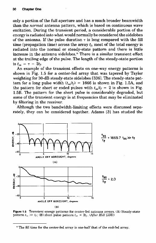
0
m - -20 < 0 LL
g -40
- W
-6Ob
%is - = 2.0 tf

Radar and Its Composite Environment 31
combined effect and shows that the parallel-fed antenna has broader bandwidth at boresight and that the series-fed antenna degrades some- what less at high scan angles. Antenna tapering increases the allowable bandwidth of both types of antennas. For arrays of subarrays there are different relationships that are described in Chap. 7 of the Radar Handbook [6731.
1 .I 0 Transmitters
This section briefly describes the primary devices for radar transmitters and how they affect the overall systems design. They are covered in much more detail by Weil in Chap. 4 of the Radar Handbook [6731.
Transmitters are often developed for continuous radiation in com- munication, electronic warfare system, or continuous wave (CW) ra- dars, but the emphasis here is on pulsed transmitters that are developed for the majority of radar uses. There are five primary types of devices: the magnetron, the crossed-field amplifier (CFA), the kly- stron, the traveling waue tube (TWT), and the solid-state amplifier. The selection depends on the required power levels, the carrier frequency band, the desired efficiency, coherence or stability requirements, noise radiation, and size cost.
The magnetron is a crossed-field device that was developed during World War I1 and was widely used in the earlier days of radar. It is still quite common in low-cost radars that do not require much clutter rejection. The magnetron is basically an oscillator that is turned on by a modulator. Unfortunately, when the oscillation is initiated, the initial phase is random and “coherency” from pulse to pulse is not easily achieved. With random phase there is a noise-like modulation to the transmitted waveform. That is, with multipulse waveforms such as in moving target indicator (MTI) or pulse Doppler (PD) systems, it is difficult to separate targets and clutter by the differences in their radial velocities (Doppler effect) without the coherence from pulse to pulse.
Numerous attempts have been made to lock the phase of a magnetron by injecting signals from a stable source. Some success has been achieved that allows clutter rejection of 30 to 35 dB. In a few cases there have been reports of 40- to 45-dB clutter rejection. While this is adequate in some designs, modern systems generally require consid- erably more.
A second limitation is that there is a broadband noise component radiated with the desired waveform. In these days of increasing crowd- ing in the allocated radar spectrum, this noise tends to interfere with other systems in the radar band. As a result, frequency allocations are often withheld from systems with high-power magnetrons.
32 Chapter One
The remaining devices are primarily used as amplifiers in a master- oscillatorpower-amplifier (MOPA) chain. Signals from stable oscillators are mixed or multiplied to the desired carrier frequency, then amplified to the required levels. Thus, the desired stability depends on both the process to get the signal to the desired frequency and the properties of the amplifier devices themselves.
The crossed-field amplifier (CFA) is used in many higher-power ground-based systems due to its high efficiency (25 to 65 percent) and low operating voltages. It is linear and relatively easy to modulate. It has relatively low gain (7 to 16 dB), and must be driven by other CFAs, TWTs or klystrons. The noise output is much better than a magnetron, but it is still higher than other devices. Some operational systems have achieved clutter rejections of 60 dB, but 40 to 45 dB is more common. The CFA appears to be chosen more often when transmit pulse widths are 2 p s or greater. The average power output of a CFA can be quite high, especially at C-band or lower carrier frequencies. The RF band- width can be up to about 10 to 15 percent of the carrier frequency. There are several efforts to improve the gain and lower the noise output of the CFA family of transmitters.
The klystron amplifier is characterized by high-gain and high-power capabilities. Devices with high power (megawatts) and excellent reli- ability are used in air traffic control and long-range weather radars at 3 GHz with multikilowatt klystrons available well into the millimeter wave bands. The noise output is quite low, making them suitable for coherent multipulse waveforms.
The limitations of the klystron include relatively narrow bandwidths and the high voltages required for high power and efficiency. The band- width can be increased with some sacrifice in other properties.
Like the klystron, the traveling wave tube (TWT) amplifier can de- liver high power with low noise up to the millimeter wave bands. The additional benefit is that it can be used over an extremely high-per- centage bandwidth. The gain of a TWT often exceeds 45 dB and it can be easily modulated. Unfortunately, the operating voltages are high and the phase sensitivity to changes in these voltages is much higher than with CFAs. Thus, much of the stability problem is transferred to the power supply design. The influence of various transmitter insta- bilities on radar performance is discussed in Chaps. 9 and 14.
The newest and most rapidly evolving transmitters are those based on solid-state devices. The reason for their rapid development and use in current operating systems is the promise of dramatically increased reliability. They are currently used in the 450-MHz FPS-115 (Pave Paws) radars and in a family of GE long-range surveillance radars such as the L-band Marine Corps TPS-59 and the related Air Force AN/FPS- 117 Seen Igloo radars, plus most of the new airborne weather radars

Radar and Its Composite Environment 33
at C- and X-band. The other primary advantages include low power supply voltage requirements and good stability.
There are two basic configurations. The first is the tube replacement configuration in which the power output of a number of devices is summed to form a module of moderately high power. Since the required power output of most land-based, long-range systems requires many devices, the microwave-combining circuits can become quite complex. If numerous devices are properly combined, the failure of one only decreases radiated power by a small amount. This is called thegraceful degradation feature.
The other way of generating high power is the use of an active array in which a device or power module is matched to a radiating element of a phased-array radar. The array steering is accomplished by phase shifts and time delays, usually at the inputs to the amplifiers. In many proposed configurations a low-noise receiver element is also included at the array element level. In the FPS-115, over 300 W are delivered to each of about 1800 elements. The future of array technology is quite promising in that the entire transmiffreceive module may be fabricated by mass production techniques providing low-cost, reliable, active ar- rays.
There are two primary limitations to solid-state power amplifiers. The first is that high-power modules are efficient only at the lower microwave frequencies (currently about 3 GHz). This figure increases in frequency as development continues. The second limitation is that the solid-state devices are peak-power limited, and overall energy efficiency is best obtained with duty factors of well over 10 percent. It is shown in later chapters that this creates some waveform design problems for pulse-train waveform systems.
Ultimately the solid-state power amplifiers will dominate most radar transmitter design tradeoffs if the cost savings in mass production and the millions of hours of reliability per device are realized.
All the transmit devices summarized here operate more efficiently at the lower microwave frequencies and require higher operating volt- ages at the higher frequencies.
1.1 1 Radar Grazing Angle for Refractive Conditions--4/3 Earth Approximation
In radars designed for detecting or tracking targets near or on the surface of the earth, it is not always adequate to neglect the bending of electromagnetic waves passing through the atmosphere. To account for the curved propagation path in radar computations, the ‘4 earth approximation is used. In this approximation the radius of the earth is considered to be four-thirds the actual radius and the curved path

34 Chapter One
is considered straight [75, p. 491." This approximation is traditional for surface radars observing targets near the optical or geometric ho- rizon. This section consists of a derivation of the true grazing angle + of the radiation in terms of the elevation of the radar above the surface of the earth h and of the depression angle of the radar beam a.
The simplified equations are based on a straight-line propagation path. This path is in reality a curved line. The curved path can be transformed into a straight line by substituting an equivalent earth radius re = '5 ro in place of the true earth radius ro. Ref. 593 gives a good discussion of this transformation and its equivalence to the phys- ical picture. The important results are summarized here.
Figure 1.6A shows a sketch of a propagating ray, which is a curved line because of the refractive-index rate of change with height. The symbols are defined as follows:
A t = time to traverse P-Q e = ground range = roe
ro = actual earth radius a = depression angle of the ray with respect to local horizontal
A h l A t = change in height with distance
We also define a variable s such that s+l
n = (:) (1.22)
where n = the refractive index r = a radial distance from the center of the earth to the point
at which n is measured
Consider a new sketch with the following conditions (Fig. 1.6B):
1. s' = - 1 (implies constant refractivity gradient) 2. a' = a
3. r60' = roe 4. rb = -rds (experimentally, s = -3/4 on the average)?
* The ?4 radius of the earth is taken to be 8493 km or 4587 nmi. See also Sec. 7.8. t The value of 11s varies with time and location. Refs. 593 and 671 explain that values
for l/s may vary over the United States from - 1.25 to - 1.45 for altitudes less than 1 km. Values considerably greater than - 1.3 have been reported near England [3541. It is also pointed out that l/s = -% is an average for overland propagation that is al- most independent of frequency up to very high radar frequencies. For the visible region, 11s -- -1.20,

Radar and its Composite Environment 35
INDEX OF INDEX OF REFRACTION = n REFRACTION = n'
(A ) ( 6 )
Figure 1.6 Propagation paths for electromagnetic energy. (A) Actual path; (B) straight-line path equivalent earth transformation.
Because of condition ( 1 ) there is no bending of the rays. Condition ( 2 ) implies both situations have equivalent depression angles. Condi- tion ( 3 ) imposes the constraint that in both situations the point at which the ray strikes the earth occurs at the same ground range. Condition ( 4 ) requires an equivalent earth radius of rk = re = 4/3 ro. With these conditions, two important relationships are proven in [6341
(1.23) Ah Ah' At = At' and - - - - A t A t '
The first relationship establishes the fact that the time for the energy to traverse both paths is the same. The second indicates that the grazing angles are the same for both pictures (the angle between the local horizontal at the target and the radar beam direction).
The exact expression for the depression angle a of a radar beam illuminating a point Q is
a = sin-1 (,re, + h2 + R ~ ) (1.24)
Equation (1.24) applies to the configuration shown in Fig. 1.6. P is the location of the radar, Q is the location of the target, a is the depression angle of the radar, h is the antenna height, re is the radius of earth (Y3 actual radius), and R is the slant range of target. In most instances Eq. (1.24) may be simplified because hlr, << 1 and h 2 / 2 r 3 << (hlR + R/2re). This simplification yields
2R(re + h )
a = sin-' - + - (1.25) (; :I

Chapter One36
(1.26)
Figures 1.7 and 1.8 show Eq. (1.26) in graphical form. By comparingEqs. (1.25) and (1.26), we can see that the sines of the grazing anddepression angles differ by approximately 2R/r e.
s .SLANT RANGE, It
2.5
.0/
2.0
;.
~.
"V
1&1..J~z 1.5~
~z
N~~~
+
~
~
~
o.~
~. s \00.000
"~
.) 200 .00 600 800
ANTENNA ELEVATION, It
Figure 1.7 Grazing angle versus antenna height for low grazing angles andmedium antenna heights.
1.~

._
__
._
__
_.._
~
~.
~-
~
-
..
__
_
__
__
--.. -~
- 0
0.
.o
m
0

38 Chapter One
Propagation conditions over the ocean*
The influence of the atmosphere on radar propagation is frequently accounted for using an equivalent earth radius model as previously described. This depiction is justified if the vertical gradient of the mi- crowave index of refraction is approximately constant, in which case refractive effects can be accounted for using an earth radius multiplier. The radius multiplier k = 4/3 is often used, and is referred to as a standard atmosphere condition. Despite this nomenclature, the con- stant refractivity gradient is exceptional for near-surface microwave propagation over the ocean.
Low-altitude propagation over the ocean may be subject to surface- based ducts and evaporation ducts [3391. Surface-based ducts generally arise due to temperature inversions that result when a warm, dry air mass lies above a cool, moist air mass. Evaporation ducts, on the other hand, are formed primarily by the rapid decrease in humidity with increasing altitude just above the ocean’s surface [369, 2871. This hu- midity gradient is always present over the ocean, but the altitude at which the humidity achieves the nominal ambient value varies greatly. Table 1.4 lists data concerning average heights of evaporation ducts and surface-based ocean ducts for various areas of the world. In this table, the average heights of surface-based ducts were determined con- ditioned on the fact that such a duct is present. A separate column in the table lists the frequency of occurrence of the surface-based duct. The tabulated average heights for evaporation ducts, on the other hand, are taken unconditionally. Surface-based ducts can occur with rather
* Adapted from Reilly and Dockery 15831.
TABLE 1.4. Average* Duct Heights for Various Global Regions
Evaporation SFC-based Occurrence duct height duct height SFC duct
Area descriptor (m) (m) (%)
Northern Atlantic 5.3 42 1.3 Eastern Atlantic 7.4 64 2.8 Canadian Atlantic 5.8 86 4.1 Western Atlantic 14.1 118 9.8 Mediterranean 11.8 125 13.4 Persian Gulf 14.7 202 45.5 Indian Ocean 15.9 110 13.4 Tropics 15.9 99 13.6 Northern Pacific 7.8 74 6.2 Worldwide average 13.1 85 8.0
contrast, averages for evaporation ducts are taken unconditionally. * Averages for surface-based duct are conditioned on the presence of that type of duct. In
DATA SOURCE: Hitney (1988) 13391.

LL 20 I I I I - 15 - - - -
- 1 0 - -
- 5 - -
0 . I I

1.0 - I 1 I I I I 1 I - i
hd = 30rn
20
- - u) W
0 - W U
W _1
U W - z - N - U Grazing angle K - - W Neutrally buoyant atmsphere
- - - - ? - -
- -
2 0.1 = - - - - - - - - -
0.01 I I I I I I I I I I I I I I l l 1
1.0 L I I 1 1 1 1 1 1 ~ I I I I I I I I J u) W
m al 73 - W _1 (3 z z m m W - a a - Depression angle - W n
- - - P - -
-
- -
- - Q 0.1 =-
E! - - - -
-
Neutrally buoyant atmosphere I I I I I I l l 1 I I 1 0.01

Radar and Its Composite Environment 41
are virtually identical to the analytic expressions given in Eqs. 1.24 and 1.26. In this figure, the calculations have been based on evapora- tion duct refractive index of refraction profiles defined by Hitney et al. [3391 as:
M ( h ) = M(O) + 0.125h - 0.125hd1n(h/ho) (1.27)
where M = the modified index of refraction h = height above the surface, m
h d = duct height, m ho = 0.00015 m
Equation (1.27) applies to neutrally buoyant conditions. Once the gra- dient dM/dh reaches the standard value of 0.118 M units per meter, it is frozen to that value for high altitudes.
For evaporation duct heights that are lower than the antenna height, geometric optics calculations result in a limiting range RL beyond which no rays strike the surface; the last ray that reaches the surface is referred to as the limiting ray. This behavior reflects the fact that geometric optics are too simplified to indicate the coupling of energy into these ducts when the antenna is not in the duct. With the exception of the hd = 30-m curve, the curves in Fig. 1.10 were cut off at ap- proximately R L .
The grazing angles for the various ducts shown in Fig. 1.10 approach asymptotic minima +L at R L . This observation suggests the assumption that the energy propagated beyond R L is also associated with the angle $L. This assumption is intuitive, for instance, for duct height and fre- quency combinations that result in the propagation of a single- waveguide mode with its associated angle. The assumption has yet to be verified experimentally or with a more rigorous analytic study.
Geometric optics results are frequency independent and correspond to propagation in the limit of very high frequencies. As a result, even small ducting structures (such as a 2-m evaporation duct) have the maximum effect on the calculated grazing angles. The accuracy of these angle estimates depends on the size of the duct (or other refractive- index structures), as well as the frequency. Although the frequencies at which the geometric optics calculations become inaccurate for each duct height have yet to be determined, angle estimates are expected to be quite good for UHF frequencies and higher.
1.1 2 Forward-Scatter Effects
A radar target situated near the earth's surface intercepts energy from a ground-based radar along two paths (Fig. 1.11). One path is the direct line between the source and the target; the other path is a line reflected from the earth's surface. This multipath propagation results in two

42 Chapter One
TARGET
,(REFLECTED RAY)
OF ANTENNA
REFLECTING SURFACE
Figure 1.11 Propagation over a reflecting surface.
effects that are generally deleterious to radar performance: (1) an in- terference pattern between the two rays’ results, which causes a wide variation in the reflected-power-versus-elevation angle (lobing); and (2) false target images are created, which degrade the angular accuracy of the radar [2111. This section summarizes how the surface properties of the earth alter the magnitude and phase of the scattered signals. Since multipath effects are most severe for a specularly reflected wave (angle of incidence equal to angle of reflection), the results empha- size specular reflection. Backscatter toward the radar is discussed in Chap. 7.
As illustrated in Fig. 1.12, the total electric field ET of the signal intercepted by a target is the sum of a direct field component Ed and a reflected component E,
ET = Ed (1 f 2) (1.28)
The vector ratio &./Ed is normally expressed in terms of a reflection coefficient R, which is the ratio E, . /&, for an isotropic radiator. Equation (1.28) can be expressed in terms of the reflection coefficient
ET = Ed(1 + K f 2 R,)
a
(1.29)
where R, = E,/& for an isotropic radiator KO = the power gain of the antenna at the angle of the reflected
wave relative to the gain at the target angle
The relative phase of the reflection coefficient R, is usually separated into two factors: one that accounts for the relative phase of E, due to

Radar and Its Composite Environment 43
REFLECTED
E,
Ed R,= REFLECTION COEFFICIENT = -
Figure 1.12 Vector diagram of the field intensity for propagation composed of a direct component and a reflected component from a rough surface.
the path length difference R - (rl + r2) and one that accounts for the phase due to the electrical properties of the reflecting surface, that is,
R, = (R, + r,eLPY@e1"
where+ = phase due to the electrical properties of the reflecting surface of the reflected ray relative to the ray incident on the surface
a = ( 2 ~ / h ) [ R - (rl + r2)] = phase of the reflected ray relative to the direct ray at the target from the target-radar geometry
E, = magnitude of coherent part of reflection coefficient r, = magnitude of incoherent part of reflection coefficient p = phase of the incoherent part relative to the coherent part
(p is uniformly distributed between 0 and 2 ~ )
The vector diagram of Fig. 1.12 illustrates that the reflected wave E, is composed of a coherent part E, and an incoherent, or random,

44 Chapter One
part ErL. Because of the random nature of the incoherent component, the reflection coefficient must be described statistically.
The average power in the total field is proportional to*
P --z = E2(1 + K E ) (1.30)
(the bar indicates average values). Notice that this expression allows us to specify the amount of power in the reflected beam relative to that
in the main beam. @ is broken into a coherent power term -2 and an
incoherent power term uRZ. R,
The relative coherent reflected power -2 is derived for a rough sur-
face; it can be related to the reflection coefficient for a smooth surface Ro and a surface parameter i [571 by?
R,
2 - R, = p2(DRo)2 (1.31)
where R, = reflection coefficient for specular reflection from a rough
Ro = reflection coefficient for specular reflection from a smooth
D = divergence factor, which accounts for the fact that the
surface
surface
reflecting surface is spherical (viz., the earth)
The quantity c is defined by
(1.32) - p = e - d 2
wheregl2 = (1/A2)8n2 a: sin2 IJ A = radar wavelength
IJ = grazing angle u: = variance of the surface height about the mean height
The value of uh required to evaluate Eq. (1.31) may be related to significant wave height (and in turn to the hydrographic sea state) through the Burling relationship$ HIl3 = 4.0 uh . Eq. (1.32) is plotted for several values of sea state and radar wavelength in Fig. 1.13.
- - *This result makes use of the assumption that cos CY = 0 because the surface is
fluctuating. t Equation (1.31) is derived from the assumption that the height distribution and the
spatial correlation function are both gaussian and that the reflection is in the specular direction. The author further assumed a uniformly rough surface of infinite conductivity. Although the sea is not a perfect conductor, the error introduced is not serious since the scattered field is determined more by the surface roughness than by the surface con- ductivity. For small grazing angles, Eq. (1.31) must be modified by a shadowing function.
$ See Sec. 7.1.

Radar and Its Composite Environment 45
I-
; 1.0 L U. W 0 U (1
K W I- I-
5 0.8
s w 0.6 0
K W >
k 0.4 W n 3 t z (1 4 0.2 I 11
'rp
O t 0. I 0.4 0.6 0.8 1.0 2.0 4.0 6.0 8.0 10.0
p= RADAR GRAZING ANGLE, degrees
Figure 1.13 Typical surface coefficient for scattering from seas of various sea states SS (for horizontal or vertical polarization).
The only additional information needed to specify the coherent re- flected wave is the value of the average relative phase angle +; Figs. 4.8 and 4.10 of [443] illustrate the variation of the phase of the reflection coefficient as a function of grazing angle for smooth seas. Experimental data on the influence of waves are given by Beard and Katz [50-531.
The power in the incoherent portion of the reflection wave u;, cannot be completely defined because of the present lack of knowlege about the spatial correlation function of the sea's surface (see Chap. 7). The appendix of [3971 contains plots from which D may be evaluated. The value of the smooth surface reflection coefficient Ro may be determined by Figs. 4 through 6 of [4431. Beckmann 155, 561 has shown that for small depression angles the value of R, must be multiplied by a shad- owing function to account for the reduction in scattered power caused by the shadowing effect that the hills of the surface have on the valleys.
The previous theoretical consideration used a number of simplifi- cations that are not strictly correct, namely:
1. Perfectly conducting reflector. 2. Gaussian height distribution.

Chapter One46
3. Gaussian spatial correlation function.
4. Uniform surface conditions.
5. Constant grazing angle within the illuminated area,
In spite of these simplifications, the theory compares favorably withexperimental findings, as illustrated in Fig. 1.14 [389], which comparesexperimental values of the coherent term p = liJDRo with those de-termined from Eq. (1.30). Although the experimental data for the in-coherent term cannot be quantitatively compared with theory , noticethat the peak value of the experimental curve (corresponding to(Jhl\1/).. = 100 mils) occurs at approximately the value predicted«(Jhl\1/).. = 80 mils).
The calculation of the effects of forward scatter on the detection andtracking of low-altitude or surface targets is quite complex. Numerousapproximations [75, 45] are needed to accurately determine the detec-tion ranges. As an example consider an L-band radar (1.3 GHz) situated60 ft above sea level searching for targets over a smooth ocean. Fortargets at a range of 16 nmi with altitudes of 50, 100, and 200 ft, thereceived power computed from free-space equations must be modified
0 50 loo 150 200 250 300
ROUGHNESS PARAMETER f, mil.
Figure 1.14 Coherent and incoherent reflection components for rough ocean surfaces(for horizontal or vertical polarization). (From Katz [389])

Radar and Its Composite Environment 47
by about - 17, - 7, and + 9 dB, respectively. If the sea becomes rough, the coherent reflection will decrease and the free-space equations will be more appropriate; however, the backscatter from rough seas is much greater than for calm seas, and the target echoes may be obscured by sea clutter. Some examples of the received power from ship targets near the horizon are shown in Chap. 5.
The tracking radar has similar problems. If the surface is smooth, the radar may try to track the target or its image. If the surface is rough, the tracking error may be dominated by the clutter signals [600]. One series of X-band tests overland (p = 0.4) showed elevation tracking errors of about -+ 2 mils for targets near zero elevation [211]. A graph of elevation error versus grazing angle is given by Barton [45, p. 3301 from C-band tracking radar tests. The approximate rms elevation error can be written
(1.33) P4) u+ = ~
(8G, )1’2
where p = the coefficient of reflectivity (0.3-0.4 for typical land) G, = the power ratio of mainlobe (sum pattern) to sidelobe gain
for the error pattern at an angle of 2E below the beam axis E = the elevation angle of target + = the elevation beamwidth

Chapter
2 Review of Radar Range
Performance Computations
F. E. Nathanson J. P. Reilly
This chapter reviews the basic forms of the radar equation and the variations needed to calculate the performance of a radar that is at- tempting to detect targets masked by the basic thermal noise of the radar receiver. Subsequently this development is extended to cover a general environment, which includes the multitude of superfluous re- turns that often exceed the basic receiver noise. These returns include electronic countermeasures, friendly interference, sky noise, and the backscatter from atmospheric effects, land, seas, and chaff.
2.1 General Radar Range Equation
The following general radar equation for pulse radars shown includes a larger number of parameters than is commonly used in current radar texts by Barton [39], Blake [75], and Skolnik [671]. The separation of certain loss terms from the basic parameters facilitates rewriting the equations for the various external environments. The loss terms in this book are less than unity or are subtracted from the numerator when
49

50 Chapter Two
the equation is expressed in decibel form. The backscattered power received from a target of radar cross section ut at the first mixer or preamplifier can be written
(2.1) ~ p&TL&RLRi2LPLSL&aut ( 4 ~ r ) ~ R ~
P, =
where P, is peak received power. Before elaborating on the terms of this equation, it is useful to convert
the received power P, to the minimum detectable received power Smin and to rewrite the equation in terms of the detection range R for a pulse radar. Then
(2.2)
where R = the detection range of the desired target with the statistics of detection to be defined later.
PT = the peak transmit power (the average power during the pulse) at what is arbitrarily defined as the output of the transmitter unit.
GT = the transmit power gain of the antenna with respect to an omnidirectional radiator. This is a dimensionless quantity equal to 4nA,/X2. This term generally refers to the centerline of the antenna beam. The pattern factor c is included in Lp in this book.
A, = the effective aperture of the antenna, which is equal to the projected area in the direction of the target times the efficiency. This includes the fractional losses due to spill over and tapering of the aperture to reduce the sidelobes. Then considering the losses,A, = EA whereA is the physical projection of the antenna area and E -- 0.4 to 0.8. A, can also be defined as the area that, when multiplied by the power density at the receive aperture, equals the received power.
R4 = P&TL&RLRA2LPLSLdaut (4~)~Smin
X = the wavelength of the radiation. LT = the losses between the transmitter output and free space
including transmitlreceive duplexers, power dividers, waveguide or coax, radomes, and any other losses not included in A,. It is preferred to include in this term any losses that do not affect the beamwidth of the radar. LT is less than unity, or negative in decibel terms.
G R = the receive power gain of the radar defined in a manner similar to the transmit gain.

Review of Radar Range Performance Computations 51
L R = the receive antenna losses defined in a manner similar to the transmit losses. However, in the case of sensitive receivers, the losses must be included in the effective system noise temperature T,. These are defined in conjunction with the minimum detectable signal.
L p = the beam shape and scanning and pattern factor losses,* which include several factors to compensate for the antenna-gain terms being calculated on the centerline or nose of the beam. A typical target for a search radar tends to have an arbitrary position with respect to this line, and the ground and sea reflections create a lobing pattern resulting from the relative phase of the free space and reflected signals. An analogous loss occurs in conical scan tracking radars where the beam is nutated, or scanned such that the full gain of the antenna is not continuously pointed at the target. A typical value for search radars is 1.6 dB for each dimension of scan and for 50-percent detection probability. Similar losses caused by finite range gates and Doppler filters are covered in the chapters on processing techniques. The pattern factors caused by forward scatter are quite complex, as described in Sec. 1.12. They are dependent on the grazing angle with respect to the land or sea and the height of terrain objects (trees, hills, buildings) or ocean waves at the point of reflection. Chapter 7 on sea clutter effects gives additional experimental data for rough sea conditions and some of the basic properties of the reflected signal. There is further discussion of lobing effects as they affect detection of targets near the horizon in Secs. 1.7,5.6, and 7.8. The description of beam shape losses is slightly expanded in the section on detection statistics. A more thorough treatment is found in Barton 1391 and Blake [741.
La = the two-way pattern absorption or propagation losses of the medium. These are calculated separately since they are usually a function of the target range, the elevation of the target, and the type of interference. It is a common practice to compute the free-space range and then adjust for these losses, as in Fig. 2.1, rather than complicate the radar equation. La is often expressed as exp ( - 2&), where a is the attenuation constant of the medium and the factor 2 is for a two-way path.
* Including F of Blake’s notation. See Barton 1391, Blake L74J, and Skolnik L6731.

52 Chapter Two
1.m - - - - - - -
-
100 - - E 1
z - 0
< I
W I-
3
w -
- n
-
I y I- 4
10 - - - -
I I I I l I I I 100 1poo
IO
FREE-SPACE RANGE, nml
Figure 2.1 Free-space radar range versus attenuated radar range for one-way attenuation rates of a dBkm. (From Skolnik 167.2 I )
Ls = signal-processing losses that occur for virtually every waveform and implementation. The typical values are discussed with the processors in Chaps. 9 through 14.
LL = lens-effect loss for radars located near the earth's surface. The atmosphere acts as a lens, and the beam divergence in the vertical plane reduces the power density on a target near the horizon. Schrader and Weil[7601 show loss curves for surface radars amounting to 0.9 dB at 200 nmi for a 0" elevation beam and about 0.5 dB for a 1.5" elevation. At 400 nmi these are almost doubled. The losses are halved for distributed atmospheric target (rain and chaff). This loss may be pessimistic for pencil-beam phased arrays or radars with "stacked beams in elevation as it slightly reduces the pattern loss (Lp in elevation). This loss is dropped from later versions of the radar equation and

Review of Radar Range Performance Computations 53
should probably be folded into Lp or the pattern factors F1 F2 used in other texts.
ut = the radar cross-sectional area of the object that is being detected and is equal to
) power reflected toward the receiving aperturehnit solid angle
(incident power densityl4n) (
ut =
The definition has a simple physical significance only for the case of a large metallic sphere, in which the physical cross section is equal to the radar cross section (when the diameter is large with respect to the radar wavelength). (See Chap. 5. ) The use of the term cross section is expanded to include the amplitude and spectral distributions of the reflectivity in the chapter on targets. The radar return from land or cultural features appears as the target for an airborne mapping radar but often forms the noise level for an Airborne Early-Warning System (AEW) or surface- surveillance radar.
Smin = the minimum detectable target-signal power that, with a given probability of success, the radar can be said to detect, acquire, or truck in the presence of its own thermal noise or some external interference. Since all these factors (including the target return itself) are generally noiselike, the criterion for a detection can be described only by some form of probability distribution with an associated probability of detection Po and a probability that, in the absence of a target signal, one or more noise or interference samples will be mistaken for the target of interest. This latter probability is often called the false alarm probability PF or P N . The related term of false alarm time TF or n' is elaborated on in the next chapter. The use of this terminology implies a threshold detector, which is established with respect to the noise level.
The most definitive treatments of the statistical problem of target detection by a pulse radar are the works of Marcum and Swerling presented from 1947 through 1954 and republished by the IRE [4611. Numerous graphs have been presented in the technical journals with slight variations; the most appropriate ones are presented in Chap. 3. Figure 2.2 gives the signal-to-noise ratio to achieve a given probability of detection of a target signal in a single look. The false alarm number n' is the parameter. The solid lines apply when the target echo is a

54 Chapter Two
- - -
FALSE ALARM NUMBER n.
- - ANONFLUCTUATINGTARCET
< - I-
L
K
0: w -
P 0
CASES 1 AND 2
m D
- 7
- 3
0.01 0.05 0.2 1 2 S IO 20 30 50 70 90 95 99 99.8 99.99
PROBABILITY OF DETECTION, ?&
Figure 2.2 Signal-to-noise ratio versus probability of detection in a single look. (After Fehlner [225] and Marcum and Swerling [4611)
constant sinusoid and the noise is gaussian; the dashed lines apply when the target echo is fluctuating. These curves are for single-pulse detection. Multipulse detection curves with a more detailed explanation are given in Chap. 3.
The classic radar equation is based on the assumption that the ther- mal noise of the receiver is the fundamental limitation on minimum detectable target signal. As more sensitive receivers have been devel- oped, the effects of antenna noise and sky noise and the effects of the sun, galaxies, and the earth must be included, Blake [741. Since this text emphasizes signal processing, it suffices to define the thermal noise power of the receiver as
N = KT,B, (2.3)

Review of Radar Range Performance Computations 55
where K = Boltzmann's constant [equal to 1.38 x l O - 2 3 W/(Hz)("K)]. T, = system noise temperature, including the antenna tem-
perature, environmental effects, and the noise of the re- ceiver itself. It should be remembered that the effective temperature T, of the receiver noise itself is not simply equated to the noise factor (or noise figure) F by T 2 . T, can usually be replaced by To@ - l), where To is the reference temperature of the system and is assumed to be 290°K. It is also assumed that the receiver does not respond to the noise at the image frequency of a heterodyne receiver.* Then
T, = (P - 1)290"K or T, = T, + TA
where TA is the antenna noise temperature with ap- propriate consideration for losses between the antenna and receiver.? (See [63, 45, 751.) If TA is small compared to T,, the term To is sometimes combined with K and then expressed in decibels.
KTo = -204 dBW/Hz KT, = -204 dBW/Hz + 10 10g(F - 1)
The noise figure of typical solid-state microwave receivers is shown in Fig. 2.3. Various GaAs FET and high electron mobility transistors (HEMT) are represented.
B N = noise bandwidth of the receiver in hertz after amplification but before envelope detection. The actual noise bandwidth varies with the transfer function of the filter or set of filters prior to detection and with the type of waveform. For a simple radar transmitting a rectangular pulse, the op- timum B N is the bandwidth of the matched filter that is described in Sec. 8.1. In practice the matched'filter is not frequently implemented since the filter skirts (or sidelobes) do not fall off rapidly and the receiver becomes more susceptible to jamming or interference. In the same vein, transmit pulses are trapezoidal rather than rectangular to minimize the spectral interference to other receivers. In the United States there are requirements on the maximum transmitted signals allowed at frequencies away from the carrier.
* See "Description of Noise Performance of Amplifiers and Receiving Systems," Proc.
t In this equation T A is often written as T A J L R . IEEE, vol. 51, no. 3, pp. 436442, 1963.
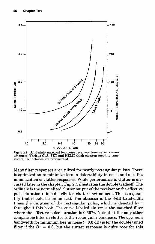
4.0 -
3.0 -
a 2.0 - W’ a P
0
3
U. W
g z 1.0 -
0.1
1
- 440
-290
Y al
-170 6 W-
a2 0
K 3 2 B E
-75 w g
P
I-
z
- 7
I I I I I I I I I I I ‘ .o 3.0 6.0 10 30 60 90

Review of Radar Range Performance Computations 57
10.0
: 8.0 P 1- 6.0 8 5.0 Gi ,- 4.0
(L 3.0 w (3
2 Y
9 2.0 \
W ln z ln B
E 0.8
E 1.0 W
3
d 0.6 0.5 2.0 3.0 4.0 5 0 60 8.0 10 0.1 0.2 0.3 0.4 0.5 0.6 0.8 1.0
B T ( 3 - d B BANDWIDTH x PULSE DURATION)
Figure 2.4 Equivalent pulse length for rectangular pulse and various if bandwidth filters. (Courtesy L. W. Brooks)
bandwidth. For the rectangular band-pass filter, the optimum BT = 1.3 for noise and the loss is 0.8 to 0.9 dB. This is also near optimum for clutter. The use of trapezoidal pulses alters these values slightly. Also, the noise bandwidth BN is somewhat greater than the 3-dB band- width B. In most computations BN is assumed to be 1 / ~ unless more exact calculations are necessary. In clutter calculations, T’ should be used for more accuracy. A physical way of observing Fig. 2.4 is that a narrow filter smears the clutter in range while an overly wide filter has little effect.
In practice, receiver filters are generally slightly wider than optimum to allow for target Doppler and slight mistuning of the transmitter or local oscillator. The matched-filter loss can be entered into the radar equation in Ls or by increasing BN.
With the preceding assumptions, the minimum detectable signal can be written
Smin = KT,BN (SIN) - (2.4)
where (S/N) = a dimensionless parameter that is the acceptable value by which the desired signal exceeds the rms noise level with respect to the function of the overall radar system.*
(3
* In detection equations W N ) is usually the required signal-to-noise ratio or visibility factor, and in this text SIN represents the actual power ratio for the stated conditions.

58 Chapter Two
L, = collapsing loss, which results when two or more samples of unwanted noise, interference, or clutter are added to the desired signal. Several examples occur when the bandwidth of the receiver is excessive compared to the matched-filter bandwidth, when numerous elevation beams are “collapsed” onto a conventional plan position indicator (PPI) display, or when numerous azimuth positions are “collapsed” onto a range height indicator (RHI). This term is expanded to include the undesired back- scatter from clouds, rain, or electronic counter-mea- sures, which occur in several radar beams. A special, but not uncommon, case is when there is no interfer- ence in the beam in which the target is located, but in- terference may be present only in the collapsed beam positions. The radar return from a low flying aircraft may be obscured on a PPI by rain clouds at 10,000-ft altitude, even though there is no rain at the target location. The collapsing ratio p, another common term, is defined as
m + n P = y
where m is the number of samples containing noise alone and n is the number of samples containing signal plus noise. The collapsing loss (in dB) can then be found from the curves on integration loss for n samples integrated incoherently (Chap. 3). The loss L, is determined for n + m samples (in dB) and then subtracted from the loss (in dB) for n samples. Similar collapsing losses for PPI displays, as taken from Barton E451, are based on
117 + !mu ! m u
P =
for insufficient video bandwidth where B, is the video bandwidth (Hz). In the foregoing cases the increase in the total number of noise samples presented to the detector or operator must be taken into account when evaluating the statistics of the detection process. This type of calculation is expanded on in Chap. 3. The collapsing loss L, is expressed here as a fraction less

Review of Radar Range Performance Computations
than unity or in decibel form where this loss should be subtracted from the numerator of the radar equations.
Before discussing what constitutes an acceptable value of (SIN) it is useful to write the full radar equation and some of its variations. The pulse radar equation is
59
(2.5)
for the receiver (and antenna) noise limited case, and where L, is the signal processing loss, which will be loosely defined as the deviation from a linear receiver with a perfectly matched filter. The numerical value to be used is expanded on in Chap. 4 on automatic and adaptive detection and in the various signal processing chapters. This loss varies in the presence of clutter and jamming because of the change in the power spectrum and amplitude distribution of the interference.
Since the noise bandwidth BN is approximately equal to 1h for a system approximating a matched filter, a more descriptive presentation of the detection properties of a radar system is to replace
R4 = i’&TL#RLRA2Ll’LaL&sut ( ~ ~ T ) ~ K T , B&3IN)
with Pu = E - PT
BN
where E is the transmitted energy per pulse in joules. This substitution illustrates that the detection properties of a particular radar (for target obscured by receiver noise) are dependent only on the transmitted energy and the noise per Hz (KT,). It can be shown that the relationship is essentially independent of the pulse length or transmitted waveform. This substitution also allows simpler extension to the CW (continuous wave), FM, and pulse Doppler radars, where it can be shown that the average power determines the detection performance if the receiver can be made to approach the matched filter.
The radar equation expressed in the foregoing form is somewhat misleading in that it implies a A2 dependence on detection range by using the gain of the antenna as a parameter. In a search radar, higher gain with the resulting narrower beamwidth means that less time or energy or fewer pulses can be radiated in any one direction if it is necessary to search a volume that is large compared to the cross- sectional area of any one beam. Another common form of the radar equation substitutes 4mA,IA2 for GR and results in the preferred search radar equation
(2.6) R4 = i’&TL&&RL€’LaL&.sut (47~ )2KT, BN(SIN)

60 Chapter Two
which has no wavelength dependence. Hall [3021 has shown (with different notation) that to search a solid
angle 9 with a given observation time for a single beam T, the minimum total search time (Tsc) is
9 Tsc = T - R
where R = the solid angle of the radar beam 9 = the total solid angle to be searched
T,, = time allowed in seconds to search a total solid angle 9
The solid angle of the radar beam, however, can be expressed as a = 4 d G ~ . The average power PT is equal to PTdT for a pulse radar, and BG = 1 from Eq. (2.4). Then substituting for BN in Eq. (2.6) gives the volume search-radar equation
(2.7)
In a similar manner the transmit gain GTcan be converted to aperture area. This form also has misleading effects in countermeasures and in clutter-limited situations but applies where there is a firm constraint on antenna size. For a common transmit-and-receive antenna, Eq. (2.6) becomes the antenna size limited equation
R4 = PTL&&RLPLaL&satTsc 4nKTS(SlN9
(2.8)
This form with the inverse h2 dependence is useful for aircraft, satellite, and missile radar computations where transmit frequencies of over 10,000 MHz are common. The greater detection range implied for higher-frequency radars is often negated by increased atmospheric and weather attenuation and a tendency of receiver noise temperatures to increase with frequency. In addition, the number of beam positions to search a given volume increases, and time may become a major con- straint.
R4 = PTL&2LRL&aLcLsat ~ X ~ K T , BN (SIN)
2.2 Radar Detection with Noise Jamming or Interference
It is convenient at this point to introduce the detection equations for noise jamming or interference as they follow the basic radar equation in form and do not require the introduction of statistical distributions other than wideband gaussian noise. The simplest geometry to consider

Review of Radar Range Performance Computations 61
is where the target is carrying a relatively high-power noise source to attempt to deny knowledge of the target's location to a search radar or to prevent a tracking radar from acquiring the target.*
The noise power radiated from a broadband jammer (barrage jam- mer) has a power density at the search radar of
-
Power density at radar = - ' J G J ~ W/unit area (2.9) 4nR j
where pJ = the average power of jammer at its antenna input G j = gain of jammer antenna, including losses R j = range from jammer to radar
FJGJ is commonly called effective radiated power (ERP). The power entering the radar and added to the receiver noise is dependent on the aperture area of the radar and the relative bandwidth of the jammer Bj and the radar receiver BN. It is convenient to assume that B j L BN (otherwise the jammer would be a spot jammer and the radar system response would become intimately involved with the type of signal processing). At the receiver input the total noise power is
N = KT,BN + FJGJBNAeLRLb (2.10)
where LA is the one-way propagation loss. This term can replace KT,BN - in the previous radar equations, but it is more common to replace Pj/Bj by the jammer power per unit bandwidth.?
If the barrage jammer is to have any effect on the radar it must be large enough to make
4nR j2B j
PJGJACRLh , KT, 4nR j2B J
that is, the jamming noise density must be greater than the system noise density. With this simplification the radar equation can be written for the jammer at the target range and angle as the self-screening range equation
P & T ~ T ~ b ~ ; ~ & b (2.11)
Rss2 = ~ I T B N ( S / J ) (&) * For general references see Waddell L7381, Schlesinger 16371. t Despite the confusion of units, F.,IB., is often called P., and is usually expressed in
W/MHz if B N and B., are in MHz. It is also assumed in all discussions that the total jamming noise does not saturate the receiver.

62 Chapter Two
where Rss = self-screening range of the radar, or the range at which a target of cross section ut can be detected in jamming noise
Lb = one-way scanning and pattern losses of the radar since the jamming signal also has similar losses
LA = one-way atmospheric or weather losses from radar to target
(S /J ) = signal-to-jam ratio, which is defined in a manner analogous to (S/N)
LA = collapsing losses only in the receiver itself since the jammer is assumed to occupy only one beam
LL = signal-processing losses applicable to jamming (includes image losses, etc.)
PJ = jammer power density (WMHz if B N in M H z )
In operational analysis it has been found convenient to express the self-screening equation as
112
Rss = OL (e+- (Lh)ll'
where (PflJ/crt) is expressed in W/(MHz)(m2) and the remaining terms form a. if B N is expressed in M H z . The term a is then the range on a 1-m2 target radiating 1 W/MHz.
(y = r&TLTLPL&L)1'2 ~ I T B N ( S / J ) (2.11a)
If the jammer is attempting to screen another target (stand-off jam- mer) at another range the equation is rewritten and sometimes called the "burn-through" range equation. Neglecting atmospheric losses, the stand-off jammer equation is
114
RBT = (&j)112 t (2.12) (GJ where RBT is the detection range of the target that is not carrying the jammer. If the jammer is in the radar antenna receive sidelobes, as is the common case for a stand-off jammer, the range equation is written
RBT = (&j)112 (p>J1'4 - (5J4 (2.13)
where (GR/G') is the ratio of the antenna gain in the direction of the target to the antenna gain in the direction of the jammer.

Review of Radar Range Performance Computations 63
It can also be shown that the fractional range with barrage jam- ming is
4
(2.14) 4.rrKT3 J' e) = P&&~&RLA + 4.rrKT3j2
or 4
(2.15) e) = A2PflflRLR + (~IT)~KT,$J~
If the jammer is in the radar sidelobes, PJGJ is reduced by the appro- priate sidelobe ratio.
It is also useful to derive the volume search radar equation for the self-screening jammer environment in the same manner as Eq. (2.8). If a solid angle 9 is believed to contain a jamming target and the search time is defined as Tsc, it is convenient to assume that
PT* Tsc = -
Pa GT BN
( 4 ~ r ) ~ K T 3 5'
1 T = - 4.rr a=-
Substituting for GT in Eq. (2.11), the equation for the detection range of a jamming target located within a solid angle * becomes the volume search equation in jamming
F T ~ T ~ ~ ~ ~ ~ & ~ ~ s c WSIJ) (F%) Rss2 =
where PJ is the jammer power density in WfHz. It should be noted that this equation is independent of both transmit
frequency and antenna size with the assumption that the jammer has a constant power density.
A sample calculation for a typical S-band surveillance radar against a moderately powerful jammer is
Rss2 = p&TBjat ~TP~G,BN(S/J),,
wherePT = lo6 W A = 0.1 m
pj = 103 w GT = 1.78 x io4 Bj = 500 MHz
ut = 1 m2 BN = lo6 HZ

64 Chapter Two
Gj = 10 (S/JIreq = 10
The self-screening range Rss is 2.68 km.
2.3 Beacon and Repeater Equations
The radar echoes from targets are often augmented as for tracking satellites, for air traffic control, and for identification purposes. These augmentors may be passive reflectors, beacon transponders, or re- peaters.
The common passive reflectors include Luneburg lenses with partial metallic coatings, corner reflectors, and sometimes directive antennas with appropriate termination. The beacon transponder generates a return signal on the appropriate frequency when it receives an adequate illumination signal from the radar. Since only one-way transmission losses need be considered if the beacon power is high enough to be detected by the radar, the simple radar beacon illumination equa- tion is
(2.16) PT G T L ~ ~ Z ~
4TSB RE2 =
where R E = radar-to-beacon detection range AB = receive aperture area of the beacon antenna including
LA = one-way atmospheric loss L), = antenna pattern losses one way SE = minimum detectable signal to beacon
losses
The return signal from the beacon can be calculated by inserting the appropriate parameters in the same equation.
A more complicated equation is needed for the case of the repeater, which amplifies the radar signals and retransmits them to the radar. These repeaters may be used for enhancing the signal at the radar or may be used by an enemy as a jamming technique. Two calculations must be made to cover the two cases when
1. The maximum power output of the repeater is insufficient to be detected by the radar.
2. The noise level of the repeater itself is sufficiently high compared to the signal it receives from the radar [Eq. (2.16)l that the noise output of the repeater is essentially jamming the radar.

Review of Radar Range Performance Computations 65
If neither of these limitations is reached, the search-radar equation [Eq. (2.611 can be written
R4 = pTGTL!P%&RLPLaL&sABGBGE (2.17)
if PRBGE 5 P,,, of the repeater and PRB/sB >> SIN in the appropriate bandwidth, which depends on the type of processing and where GB = retransmit gain including losses of the beacon or repeater
(~T~)'KT$N (SIN)
antenna * GE = electronic gain of the repeater including losses
PRB = receive power at the beacon calculated by solving Eq. (2.16)
P,,, = maximum peak power output of the repeater transmitter
The detection range for the power-output-limited case of the repeater can be obtained by using the one-way equation [Eq. (2.1611 and by substituting P,,, for P T , GB for GTLT, and Smin (for the radar) for Sg.
The equations for the repeater-noise-limited case can be solved from the appropriate jamming equations by replacing KTSG~Gg with P j G j with selection of the proper receiver bandwidth and by replacing ut in the same manner as was used in obtaining Eq. (2.17).
2.4 Bistatic Radar
While the majority of this text relates mainly to monostatic radars (common location of transmit and receive antennas), it has become increasingly important to study the performance of bistatic radars where there is considerable separation of transmit and receive anten- nas. The advent of the antiradiation missile (ARM) is making it de- sirable to separate the transmitter from the remainder of the system by placing it on an aircraft or satellite. The other, and most common, application of this technique is the semiactive homing missile system in which the transmitter and its antenna are located on the ground or in an airplane and the receiver or seeker is located in a missile. This generally allows a larger transmitter and transmit antenna to be used while keeping the size and weight of the receiver system to a minimum. The basic radar detection range for this case is obtained from Eq. (2.5) of Sec. 2.1 and is the bistatic range equation
with PRB substituted for Sg
(2.18) PT GTLTGRLRh'LPLaTLaRL,atb ( ~ ~ F ) ~ K T , BNSIN (RTRR)2 =
* The total gain for small signals is GBGE.

66 Chapter Two
where (RTRR) = range product of the system RT = range from the transmitter to the target RR = range from the target to the receiver LaT = propagation loss from the transmitter to the target LaR = propagation loss from the target to the receiver
(Ttb = the bistatic radar cross section of the target
The range computation is quite similar to that for the monostatic radar with the exception of the propagation loss terms and the target cross-section definition. Since in general the propagation paths are not the same and since the receiver may be at high altitude, both the atmospheric and the propagation losses are considerably reduced. The bistatic cross section is defined in a similar manner to the monostatic cross section. They usually have a comparable average value with re- spect to all aspect angles of the target if the bistatic angle* is small with respect to 180" and the wavelength is small compared with the dimensions of the target. For a discussion of bistatic cross sections of targets and the unique case of forward scatter (where the bistatic an- gle = 180") see Willis [7781 and Chaps. 1 and 5.
When a self-screening jammer is used, the self-screening range is independent of RR if proper adjustment is made for the gain of the jammer in the direction of the receiver. Then from Eq. (2.111-l the bistatic self-screening range is
Rss2 = R 2 = PfiTLTLbLfLaT (2) (2.19)
where G; is the jammer gain in the direction of the receiver. If the jammer is at a different location than the target, the burn-through range can be written as the bistatic burn-through range
~ T B N ( S / J ) PjG; T
RBT2 = pTGTLTLbL") ( u t b ) (&') rx)2 (2.20) ( ~ T B N ( S / J ) PJGJ LJR RTR
where RBT = radar transmitter to target range at which the target will be detected with the probabilities associated with (S/J) neglecting receiver noise
LjR = fractional propagation loss between the jammer and the receiver
RjR = range between the jammer and the receiver RTR = range between the target and the receiver
* The angle between the transmitter and receiver as seen from the target. t Jamming-noise power density is assumed to be >> KT,.

Review of Radar Range Performance Computations 67
~ P ~ J R
0 - w w b RANGE Fa
T R ANSMITT ER R E C E I V ER T A R G E T JAMMER
- R T R 2 4 Figure 2.5 Stand-off jammer diagram.
Substituting a2 for the first bracket per Eq. (2.11a)
RBT = (Y ( - u t b r!"j'"(s) (2.21)
In many cases the ratio RJRIRTR is not known, but it can often be assumed that the four locations are in a straight line as shown in Fig. 2.5.
PJGJ LJR RTR
In this case
(2.22) ~ R T R f RJ)(LaT/LJR)1'2 (Y(L,T/LjR )l f2 + RTR(Pj G j /Utb )'I2
RBT =
where R j is the range from transmitter to jammer. In many cases the factor LaT/LJR can be assumed to be unity because
of the short ranges involved and their tendency to cancel each other for typical geometries.
Again it must be emphasized that if PJGJIutb is expressed in the conventional W/(MHz)(m2) the term (Y should be calculated with BN in MHz.
2.5 Radar Detection Equations in Distributed Clutter (Volume Reflectors) for Pulse Radars
If a radar target is situated in a region of space that contains a large number of undesired radar scatterers, such as raindrops, snowflakes, or chaff dipoles, the summation of the reflected radar signals from these objects may well determine the minimum detectable target signal of the radar. Signals reflected from these scatterers form part of the environmental noise and are commonly called radar clutter. These ob- jects, however, may be the targets of interest, as, for example, in a weather radar. This section defines the equations that can be used to determine the received power from clutter and the range at which a target will be detected in the presence of clutter signals. Chapter 6 contains the scattering coefficients and other statistics that are re- quired to solve the radar detection equations and describe the spectra of the clutter.

68 Chapter Two
The power density that is incident on a volume of scatterers at a range R (see Fig. 1.2) is
(2.23) P, = P T G T I ~ c ~ , + ) 1 2 ~ T ~ ;
4nR2
where P, = power density at the clutter cell GTlf(8, + ) I 2 = transmit gain of the antenna with respect to an
omnidirectional radiator including the effects of the decreases* in gain at angles 8 and + from the beam centerline, where
Ae GT = 47~- h2
L; = the one-way attenuation loss in the transmission me-
Then, the reflected power from an elemental volume of scatterers in
dium
the far zone of the radar aperture is
~ T G T I f @ , +)l2L&ZUdV 4nR2
where Zu is the backscattering cross-section coefficient per unit volume (preferably in m2/m3) assuming that the scatterers fill the volume dV. The symbol q is often used interchangeably with Xu, but often with different units.
Similarly, the echo received by the receive antenna of effective ap- erture Aelf(8, + ) I 2 can be expressed as
(2.24)
This equation includes the assumptions that there are no ambiguous or second-time-around clutter signals and that the transmitter and receiver are at the same location. For Eq. (2.24)
AJf(8, +)I2 = effective aperture as a function of angle from the clutter
pTGTlf(8, +)14L~La&&%dv (47~)~R~ dPc =
PC = returned power from the clutter.
cell to the radar beam centerline. dV = volume element of the clutter cell.
* This factor constitutes part of the pattern loss for targets Lp described earlier.

Review of Radar Range Performance Computations 69
Note that for pulse lengths short with respect to R, dV = R2(c~/2)dlR, C T / 2 is the pulse length or cell length in distance units, and d R is the elemental solid angle of the beam.
To obtain the total clutter power for long pulse or continuous wave systems, an integration of Eq. (2.24) should be performed over range. In the chapter on CW radars this is carried out, but for the present it is assumed that 12712 << R .
To eliminate the antenna pattern shape I f ( & $ ) I 4 term and integrate over the solid angle 0, Probert-Jones [563] has shown that for a gaus- sian beam pattern and a circular antenna
(2.25)
where O1 and $1 are the one-way, 3-dB beamwidths of the beam pattern. Almost identical results are obtained for a uniformly illuminated cir- cular aperture including the clutter power from the first few sidelobes. The factor for rectangular apertures should be somewhat smaller than this value when using the usual definitions for beamwidth. Substituting in Eq. (2.24) yields the clutter return power for single-aperture radar*
pc = [ B , C T L T A J A ] (4nI2R2 [ Cu(cT/2)'n8141 8 In 2 ] (2.26)
7Fe1 h1 I,lf(e, 4414da = - 8 In 2
or by substituting for A,
] (2.27)
A note of caution: The foregoing equations are valid only for equal transmit and receive beamwidths and antennas with a high ratio of main beam to sidelobe gain. If the antenna beamwidth or the gains of the antennas are not known, a good approximation can be obtained by substituting
P T ~ T ~ T ~ R ~ , ~ 2 ~ , C U ( C T / ~ Y ~ O ~ +1
pc = [ (47r)3R2 ] [ 81n2
7F2
4 $1 G = -
The foregoing equations are adequate for measuring the rain, snow, or chaff backscattered power using the values of Ca from Chap. 6 . In most cases these reflectors are clutter and act as noise with a similar amplitude distribution to receive noise. If the backscatter noise PC is small compared to the system noise KTsBN, the effect on detection range is negligible. In the usual case of interest Pc >> KTSBN. Then
* The T' is used when accuracy is required. See Fig. 2.4.

70 Chapter Two
the received power from the target can be expressed from Eq. (2.1) of Sec. 2.1 as
(2.28)
where L, is the collapsing loss introduced since distributed clutter is often folded onto a two-dimensional display from radar beams other than the one of interest.
To detect a target in a volume of uniformly distributed clutter, the ratio of the target power PR to that of the clutter return Pc must exceed a value (S /C) in a similar manner to the requirements on signal-to- noise ratio (SIN) or the signal-to-jam ratio (SIJ). Then from Eqs. (2.27) and (2.28)
P , G ~ L , G ~ L ~ ~ ~ L , atLpL, ( ~ T ) ~ R ’ (7) PR =
(2.28a)
where L6 is the signal processing loss for clutter greater than receiver noise. Solving for range gives the detection range in clutter noise for pulse radars
PRLH LpLJ&,(8 In 2) (S /C) = - = Pc T R ~ Z C T ( C T / ~ ) ’ ~ ~ $1
(2.29)
The term (.rr/4)8, +1 is the usual 3-dB beamwidth definition of the cross section of a circular radar beam and (cd2)’ is the effective pulse length. The remaining undefined term (2 In 2)* is effectively the inverse of the beam pattern loss for the clutter. The fractional pattern loss for the target was defined as Lp, but its numerical value is a complex function of the beam shape, scanning pattern, and the number of pulses in a search or acquisition radar. While the pattern losses Lp for the target often exceed the factor of (2 In 2 ) for rain in a pencil-beam search radar, a useful approximation for a pulse radar is the detection range in rain, snow, or chaff
LpL&.ot 2 In 2 R2 = if Pc >> K T S N
(.rr/4)e1 +1 ( cT /2 ) ’ ( s / c ) xu
(2.30) R2 = atLJL6 (.rr/4)e1 +1 (c7 /2) ‘ (s /c ) xu
where ut = the radar cross section, m2 cd2 = the pulse length, m Co = backscatter coefficient of the scatterers, m2/m3
* Numerically equal to 1.39 or 1.4 dB.

Review of Radar Range Performance Computations 71
8, +1 = the 3-dB beamwidths in radians for a circular aperture * R = the detection range of the target located in a volume filled
(S/C) = the ratio of the required target echo power to the power
LH = the signal-processing loss based on the spectrum and
with clutter, m
received from the clutter cell for detection
distribution function of the clutter returns
By substituting G/(r2) for Mel +1)
4GatLJH R2 = (2.31)
The detection range in the case in which the clutter return does not substantially exceed the noise can be found by adding Pc to KTa,; substituting this sum in Eq. (2.51, Sec. 2.1; and solving for R.
The single pulse (S/C) required for detection in Rayleigh distributed clutter for matched-filter receivers? is usually assumed to be equal to the single pulse (SIN) with respect to detection in noise. This is not generally the case with integration of multiple pulses since the clutter returns are partially correlated from pulse to pulse.
Another problem in defining (S/C), which is expanded on in Chap. 4 on automatic detection, is caused by the effective clutter bandwidth not always being equal to the' noise bandwidth of the receiver. The determination of the target detection statistics from the signal-to-clut- ter ratio (SIC) and the processing loss L6 varies with the transmitted waveform and the implementation of the receiver.
r3(c7/2)'(S/C) Ca
2.6 Pulse-Radar Detection Equations for Area Clutter
The development of the range equation for targets in area clutter is similar to that for volume clutter; however, in this case the integral involving the beam pattern shape is usually programmed on a com- puter. Therefore, the approach used in this section is somewhat sim- plified. This development also neglects effects of sidelobe clutter and is valid only in the far-field region. Furthermore, because of the sim- plifications used, the results must be restricted to a pulse radar system.
The power density at a clutter element is given by Eq. (2.32). (Since
* A similar approximation for the case in which the transmit and receive beamwidths are different is to use the smaller set of the beamwidths assuming that the target is in the smaller beam.
t This is the most common distribution for rain, chaff, or snow.

72 Chapter Two
the pattern shape factor is not used in this development, a closer ap- proximation is the use of the two-way, rather than the one-way, beam- width.)
(2.32) P , G ~ L ~ L ; 4nR2 Pd =
The reflected clutter power is*
(2.33)
wherecro = the backscatter cross section per unit area (m2/m2) of a reflecting surface; the mean value unless stated otherwise.
P T G T L ~ L ; [ ~ ~ A,] 4nR2 Prefl =
A, = area of the cluttered cell.
The clutter power at the receiver preamplifier is
( ~ o A,) (2.34)
In considering the clutter area A,, two cases are of interest depending on whether the pulse length is large or small compared with the pro- jected length in the radial direction of the beam. These two cases lead to different results. In either case the formulation is based on a flat earth approximation, in which case grazing and depression angles are identical. For greater accuracy, the 4/3 earth approximation may be used (Chap. 1).
As suggested by Fig. 2.6, the intercepted clutter area may be ap- proximated by the clutter cell limited by beamwidths
P T GTLTL~LA
( 4 7 ~ ) ~ R * P, =
(2.35) 62 $2 tan +2 R A, = nR2 tan - tan - csc 9 for tan q >
or by the clutter cell limited by pulse length
A, = 2R - tan - sec 9 for tan q <
2 2 CTt/2
(2.36)
The choice of either Eq. (2.35) or (2.36) depends on the grazing angle 9. For small, two-way beamwidths 82 +2 (less than = 10")A, is defined
CT' 82 tan +2 R 2 2 CT'/2
by
* The complete equation, including the beam-shape factor and antenna sidelobes, is derived in the chapter on CW systems and in [3251.
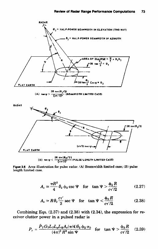
Review of Radar Range Performance Computations 73
RADAR
e2 = HALF-POWER BEAMWIDTH IN AZIMUTH
2R tan(02/Z) (A) ‘ M Y ) ’ .- =,2 , (BEAMWIDTH LIMITED CASE)
RADAR
FLAT EARTH
2R S i n ( 0 2 / 2 ) (6) *any,< cr,2 , (PULSE LENGTH LIMITED CASE)
Figue 2.6 Area illustration for pulse radar. (A) Beamwidth limited case; (B) pulse length limited case.
(2.37) TR2 42 R A, = - O2 42 csc g for tan g > - 4 CT1/2
(2.38)
Combining Eqs. (2.37) and (2.38) with (2.34), the expression for re-
CT’ 42 R A, = Re2 - sec W for tan 9 -= - 2 CT’/2
ceiver clutter power in a pulsed radar is
PTG&&&RAJTI~)O~ $2 uo for t a n g >-- 42R (2.39) P, = ( 4 ~ ) ~ R2 sin Y CT1/2

74 Chapter Two
~TGTLTL,L,A, (CT/~) '~~ uo for tan 9 < __ P, = ' 2 R (2.40)
Using a procedure similar to that used in the previous section, the ratio of the equations for PR and P, [Eq. (2.3913 results in the following range equation for area clutter-limited cases. This equation applies only when P, >> KTJ3 , and the target is in the clutter. The pulse radar range equation for area clutter is
( ~ I T ) ~ R ~ cos 9 C T / 2
(2.41) L z p L , (sin *)at $2 R R2 = for t a n 9 > ~ (.rr/4)e2 + 2 ( ~ / ~ ) a o CT/2
where Lp = beam pattern losses for the target echo. LJ = signal-processing loss in a clutter limited environment.
For a circular aperture* G = ,rr2/02 $2 2 In 2 and using the approx- imation? as explained in the previous section, we have
(2.42)
Another form may be obtained by substituting sin 9 = h/R, where h is the antenna height, and assuming a flat earth
4GLJL, (sin *)ut R2 = n3(S/C)ao
(2.43)
The equation for the case in which (tan 9 < e2R/c7/2) is obtained by taking the ratio of PR to P, [Eq. (2.4011 and solving for R. The pulse- radar range equation for area clutter is
4G LJ L, hat R3 = IT3(S/C)ao
(2.44) LJLpL, cos *ut $2 €2 R = for t a n 9 <- (S/C)(CT/2)82 (To CT'/2
As stated previously, the symbols are defined as
GT = transmit gain of antenna L6 = signal-processing loss in the clutter-limited case Lp = beam shape and pattern losses for the target echo L, = collapsing loss of processor or display 9 = grazing angle of radiation on clutter cell
* For different transmit and receive antennas the gain corresponding to the smaller
t Lp = I/Z In 2. beamwidth should be used.

Review of Radar Range Performance Computations 75
(SIC) = signal-to-clutter power ratio required for detection. uo = reflectivity per unit cross section of clutter (dimensionless).
e,, +2 = 3-dB beamwidth in azimuth and elevation, respectively (two- way path). In general, 19, = 0.7101, +2 = 0.71~$~.
In later sections the prime in c7'/2 is dropped, but it is assumed that a calculation will be made where accuracy is deemed important.

Chapter
3 Statistical Relationships
for Various Detection Processes
F. E. Nathanson J. P. Reilly
3.1 introduction and Definitions*
As alluded to in the previous chapter, the detection of signals in noise or interference is best described in statistical terms although the use of gaussian wideband noise is not always sufficient to describe per- formance in a given environment. The first part of this chapter describes the statistics for detection of steady targets in white gaussiant noise. The discussion is then extended to target signals that have a fluctuating amplitude with various correlation times. This case is es- sential to prediction of the performance where the target’s returns are immersed in clutter signals. This is followed by a brief summary of radar displays and human operator performance. The techniques of
* For general references see Marcum and Swerling [461], Siebert [6541, Fehlner 12251, Wainstein and Zubakov 17401, Barton [451, Nolan et al. L5131, DiFranco and Rubin 11791.
t See Berkowitz 163, Chaps. 2, 3, and 4 by W. R. Bennett].
77

78 Chapter Three
detection by sequential, adaptive, or automatic means are covered in Chap. 4.
There is a multitude of excellent texts and papers on the statistics of radar detection [514, 461, 75, 1791. The purpose of this chapter is to summarize the useful relationships on this topic in engineering terms rather than to delve into the theory. Before proceeding, it is essential to define the terminology to be used here. When in parentheses, ( S N ) refers to the required signal-to-noise ratio to achieve certain detection statistics.
1. Signal-to-noise ratio SIN: The ratio of the signal power (when the signal is present) to the average noise power after the matched filter but before detection or postdetection integration.
2. Radar cell: A term used to describe a volume from which return signals are received. The most common usage is for a pulse radar where the cell volume is defined by the pulse length and the half-power beam- width of the antennas. A clutter cell is a volume of this size containing undesired scatterers. The target cell is the same volume containing a target even though it may occupy only a portion of the cell. The number of cells of a simple pulse radar in a given time such as the scan time of the radar, neglecting Doppler cells, can be written
Number Of (PRF)(scan time)(display timehweep) cells in =
one scan pulse duration
The PRF is thepulse repetition frequency. It is assumed that the display time per beam is less than the interpulse period.
3. Pulse integration: The summation of target return signals (from the same location) and noise from two or more successive transmit pulses. The purpose is usually to improve the probability of detection or to permit more accurate parameter estimation.
4. Coherent: (a) Two or more radar signals are said to be coherent when the amplitudes and relative phases of the signals have a known relationship* even though they may be considerably separated in time. (b) This term is applied to an oscillator that is sufficiently stable to predict the phase at a given time later than the start of the transmis- sion. (c) Signals on two or more frequencies may be called coherent if they were derived, by frequency multiplication or mixing, from the same basic frequency which is stable as specified in (b).
5. Coherent integration (predetection integration): The addition of coherent radar signals prior to envelope detection where the signals are summed vectorially (voltagewise). For perfect integration of con-
'' Phase shifts due to unknown target velocity do not alter this definition.

Statistical Relationships for Various Detection Processes 79
stant-amplitude coherent signals the SIN increases linearly as the num- ber of these signals, assuming that the noise is uncorrelated. A predetection matched filter can be considered as a coherent integrator for complex signals. For example, a narrow-band IF filter is a coherent integrator for a single-frequency signal. Coherent signals on different frequencies can be added coherently with certain restrictions on the times that this can occur (see Chap. 13) with respect to the relative phases.
6. Correlated: While coherency implies a complete predictability of relative phase (and sometimes amplitude) between a set of radar sig- nals, the term correlated is used in a number of cases where the second, third, fourth, etc., signal of a set is in some way related in phase, amplitude, or power to the first of the set or to each other. The ter- minology derives from the autocorrelation and cross-correlation func- tions of signals.
7. Correlation functions and related distributions: (a) Temporal- describes to what degree the value of a time function f ( t ) at one time is correlated with another value T time units later. Usually, unless otherwise specified, the term autocorrelation function refers to the tem- poral function. For a random function f ( t )
T R(T) = lim L 1 f ( t ) f ( t + T ) dt
In practice the finite limits are taken long enough so that a sufficient degree of accuracy is obtained. As stated by the Wiener-Kintchine the- orem, the autocorrelation function is simply the Fourier transform of the power spectral density function. Other properties are
T-;. 2T -T
P(T) = - '('I R(0)'
the normalized autocorrelation function
R ( T ) 5 R(0)
R(T) = R( - T )
(b) Frequency-describes how well a signal corresponding to a certain transmitted frequencyfo is correlated* with another signal whose trans- mitted frequency is different by Af units. (The two signals are assumed to occur close enough together in time and space so that they are not decorrelated because of the time interval or spatial separation.) The mathematical form is identical to that for the temporal function except that the temporal variable t is replaced by a frequency variable f and
* Since the correlation in phase of these signals is dependent on the coherency and time delays involved, correlated radar returns generally refer to the power of the returns.

80 Chapter Three
the frequency separation Af replaces T. ( c ) Spatial-describes how well the signal reflected from one cell is correlated with another signal reflected from a distant cell. (The two signals are assumed to occur close enough together in time and transmit frequency so that they are not decorrelated because of the time interval or frequency spacing.) The mathematical form is identical with that for the temporal function, except that the temporal variables t and T are replaced by spatial variables.
8. Probability density function &)-defines the probability of a ran- dom variable taking on a value within a small interval. The expression p ( x ) dx gives the probability that a random variable X will lie in the interval x 5 X 5 x + dx. The gaussian distribution, often called the normal distribution, has the density function
1 (x - a2 p ( x ) = ~ V2FGexp [ - - 3 - 1
where X is the mean value. The variance (second central moment) is
u2 = (x - z)2
3.2 Target Detection by a Pulsed Radar
J. I. Marcum and P. Swerling [4611 treated the statistical problem of target detection by a pulse radar. Their papers have withstood the test of time. Similar studies were made by Rice [592, 5931, Blake [751, Kaplan [3841, Hall [3021, North 6141, and others and with proper interpretation are in close agreement.
Swerling [6891 extended Marcum’s results to the case of a radar target with an echo of fluctuating strength. Swerling’s analytic results are used in this section to extend the numerical data beyond that given in [4611.
The text and graphs of these papers, however, are presented in terms so highly mathematical that the results may not appear as useful as they really are. The majority of this section is paraphrased from Fehl- ner’s report [225], which clarified the earlier papers.
Marcum’s contribution is the definition of the relationship between a threshold value of radar return signal-to-noise power SIN and of the probability that values in excess of the threshold will exist in the presence of both noise and echoes. These threshold crossings will be reported as target detections and will include both false and real reports of targets .
The problem starts with noise. Suppose that the voltage caused by

Statistical Relationships for Various Detection Processes 81
C A I
0
A
t-
Figure 3.1 Threshold detection of noise.
noise alone varies with time as shown in Figure 3.1. During the period shown, the noise exceeded threshold voltage level A seven times; level B, five times; and level C, only twice. Obviously, the higher the thresh- old, the longer will be the average time between occasions when noise alone exceeds the threshold. This time is of considerable concern be- cause if it is too short the system will be too frequently faced with false alarms and, if too long, excessive radiated energy will be required to achieve reasonable probabilities of target detection. Marcum defined it as the time during which the probability is Po that there will not be a false alarm. For purposes of standardization, Po is taken to be 0.5. (Not all authors use this definition.)
PN is the probability that a false alarm is obtained each time there is an opportunity. The false-alarm number n‘ is the number of inde- pendent opportunities for a false alarm in the false-alarm time. Then
(3.1)
where Po = the probability of no false alarm during the false-alarm
PN = the probability of a false alarm on each opportunity.
Po = (1 - P,ln’ = 0.5
time.
(Marcum, Eq. 10)”
rz’ = the false-alarm number, the number of independent op- portunities for detection.
For a pulse radar (one Doppler channel)
(3.2) n TFA n’ = -=- mN TmN
where n = the number of pulse lengths T in the false-alarm time TFA. m = the number of pulses integrated coherently (21) . N = the number of pulses integrated incoherently (21).
The probability of a false alarm in the absence of echoes is given by Eq. (3.1). For rz’ >> 1, a very close approximation is
* These references are to equations in Rand Res. Memo RM 753 from [4611, but they are not necessarily quoted verbatim. For example, Marcum used n for false-alarm number instead of n’.

INCOHERENT INTEGRATOR -THRESHoLD
SQUARE- LAW
DVPLEXER RANGE -MATCHED GATE F'LTER - DETECTOR -
MULTIPLY ROOT- TRANS- BY Y b MEAN-SQUARE
NOISE MITTER BIAS L E V E L
DETERMINATION

Statistical Relationships for Various Detection Processes 83
Since the relationships have been established among the bias level, the false alarm number n’, and the number of pulses integrated N, the probability of detection can now be related to n’ and N . These rela- tionships are shown in Figs. 3.3 through 3.6, which also show fluctu- ating target-detection curves. The single-pulse case was shown as Fig. 2.2. Simple expressions for determining thresholds are given in 13061.
Hansen [3061 derived a simple method for calculating the bias level for either a square law or linear detector for virtually all values of PN and N . With gaussian noise he reports the accuracy to be better than 0.1 dB.
3.3 Additional Results of the Marcum and Swerling Analysis
Marcum made a limited number of calculations for a linear detector and integrator. A comparison with the square-law results shows very small differences. For example, at a detection probability of 0.5, the
- - -
FALSE ALARM NUMBER, n’
A F 100-
% - * - - - - I - a 0 - K - W P
E - 5 K -
- 7
- 3
0.01 0.05 0.2 0.5 1 2 5 10 20 30 405060 70 80 90 9.5 98 99 99.8 W.99
PROBABILITY OF DETECTION, %
Figure 3.3 Signal-to-noise ratio versus PI, for a fluctuating target-ases 3 and 4 (N = 1). (After Fehlner 12251)

84 Chapter Three
looL - - F A U E ALARM NUMBER n' - -
-CASE 1
--CASE 2 - -
- - T VI -
- K Y - o
c - m -0
2
- 3
0.01 0.05 0.2 0.5 1 2 5 IO 20 3 0 4 0 5 0 6 0 7 0 8 0 90 95 98 99 99.8 99.99
PROBABILITY OF.DETECTION, 70
Figure 3.4 Signal-to-noise ratio versus PD for a fluctuating target ( N = 6). (After Fehlner [2251)
required signal-to-noise ratio is the same for both laws for N = 1 and N = 70, where N is the number of pulses integrated. For N = 10, the square law requires about 2.5 percent more power ratio than the linear law. For very large N the linear law approaches a requirement of about 4.5 percent more signal-to-noise ratio than the square law. These re- sults are ample justification for preferring the more easily obtained square-law data. Graphs of the linear-rectifier detector detectability factor with an explanation of the relationships to (SIN) are given in Blake [75, 741.
Marcum proves rigorously that there is a best possible detector law for each signal strength (Marcum, Eq. 217). For small signals the best possible law closely approximates the square law. For large signals, it is the linear law. The numerical results for these extreme cases, how- ever, are not very different, so that if faced with a choice, there is not

Statistical Relationships for Various Detection Processes 85
10.0
li--
I--106
----
10;.
10
10'0--
----" -- -
~
-3
v /
/ID~
z,
~w"'-'~no~wnoO~.~~w
~no
~0zO1-:, 0.1.z9
-10
(/1FALSE ALARM NUMBER n
/
-13-N=6--N = 30
-17
, I I I ---L
0.010.050.20.51 2 5 10 20304050607080 9095 9899 99.8 99.99
PROBABILITY OF DETECTION, %
Figure 3.5 Signal-to-noise ratio versus PD for a steady target. (After Fehlner
[225])
much reason to prefer one to the other on the basis of detection prob-ability. (See DiFranco and Rubin [179, p. 370].) The linear law, however,has one practical advantage in that a linear detector requires lessdynamic range.
Swerling extended Marcum's square-law results to four differentcases in which targets return echoes of fluctuating strength.* Cases 1and 2 apply to targets that can be represented as a number of inde-pendently fluctuating reflectors of about equal echoing area. The den-sity function is the chi-square distribution with two degrees of freedom.
w(x, x) = i exp ( -~ ) x;2:Q (3.4)
* A detailed discussion of these cases is given in Chap. 5 on targets.

Chapter Three86
10
FALSE ALARM NUMBER n'
~~w~~~~w~0~-c~~w~0~w"'02;01-;0-'-c%
~
~"0
-10
-13
-17
-200.010.050.20.512 510 203040506070809095, 989999.8 99.99
PROBABILITY OF DETECTION, %
Figure 3.6 Signal-to-noise ratio versus PD for a steady target (N = 100).
where x is the average signal-to-noise ratio over all target fluctuations.
(See Chap. 5.)Cases 3 and 4 were derived from the density function of Eq. (3.5), It
was said to apply to targets that can be represented as one largereflector together with a number of small reflectors or as one largereflector subject to small changes in orientation.
-~) (3.5)x2:Q4x
w(x, x) = =2 expx
Cases 1 and 3 apply when echo fluctuations are statistically inde-pendent from scan to scan, but perfectly correlated pulse to pulse. Cases2 and 4 apply when fluctuations occur from pulse to pulse.
Swerling did not give the exact expression for PN for case 4. The

Statistical Relationships for Various Detection Processes 87
equations were derived by Roll 12251 from the characteristic function for case 4 given in [4611.
The relationships among PO, Z, N, and n’ are shown in Figs. 3.3 through 3.6. A far more extensive set is available in Fehlner [225].
In practice, the false-alarm rate is established, in the absence of a target, by a counter at the output of the threshold circuit of Fig. 3.2.
The preceding discussion has assumed that the integrator was linear. Other integrator types are:
1. A recursive delay line integrator with a feedback gain of less than unity, which permits the older information to decay as new infor- mation is added. This is common with mechanically scanning radars.
2. A digital integrator in which the input amplitude is quantized into several levels with the integration performed in a digital memory.
It can be shown that the additional loss introduced by these tech- niques is small while a considerable saving in hardware is obtained.
3.4 Noncoherent Integration Losses
The graphs shown in Figs. 3.3 to 3.6 can be used to obtain the required signal-to-noise ratios per pulse for a given detection criterion. It is often more interesting to know the integration loss or the difference between perfect coherent integration and incoherent techniques. Before this loss can be determined, it is necessary to define the false alarm statistics in more consistent terms in order to resolve differences in the reported curves of integration loss. The primary reason for the discrepancy is that after integration of many noise samples, the number of opportu- nities for a false alarm is reduced by the number of integrations. If it is desired to keep the time between false alarms Tf, constant, the threshold or bias level can be lowered, and a higher probability of a single sample of noise exceeding this threshold PN can be accepted. Barton [441 has shown that this accounts for most of the differences between earlier publications. The graphs published in this section are for a constant false alarm probability PN and for the false alarm time increasing with the number of integrations. This allows the estimation of the number of false alarms per beam position to be computed from a knowledge of the number of noise samples in the instrumented range.
It has also been shown [441 that the fluctuation losses* of the various Swerling cases are essentially independent of the loss from incoherent
* The increase in target echo to achieve the same detection statistics as a steady target of the same radar cross section.

88 Chapter Three
integration of many pulses. Since these losses are dependent on the various detection and false alarm criteria, the required (SIN) per pulse as a function of the number of pulses can be drawn only ,“or special cases. Figures 3.7 and 3.8 are from Barton [441 (see also [391), who used Fehlner’s computations of the Marcum and Swerling equations.
Figure 3.7 shows the required (SIN) per pulse for N pulses for a detection probability Po of 50 percent and a false alarm probability PN of 1O-6. This is a common case for a low-resolution search radar. Both coherent and incoherent integration are included. The integration loss is the difference in the ordinate between the two cases for a given number of pulses integrated. Figure 3.8 is for a Po = 80 percent and PN = 1O-6. This is a common value for acquisition by a tracking radar.
Another comparison is the required signal-to-noise ratio (Fig. 3.9) for the single-pulse case for the various fluctuation models. At desired single-scan detection probabilities Po between 0.2 and 0.4 it makes little difference which target fluctuation model is assumed; however, at a Po = 0.9 an average of 8 dB more SIN is required to detect a slowly fluctuating target for the illustrated case of lo6 false alarm number.
The choice of a particular false alarm number n‘ has not been em- phasized as it is generally less important than the fluctuation model of the target when using search radars and when the number of in- tegrations is small.
The required signal-to-noise ratio versus the false alarm number for Po equal to 0.5 is shown in Fig. 3.10 [7821 in which the number of pulses integrated N is the parameter. The target model is the Swerling case 1.
It can be seen that even for the case of 0.5 detection probability and a fluctuating target, only a 2-dB increase in SIN is required to increase the false alarm number from lo5 to lo9 for 10 pulses integrated. At the lo5 false alarm number, a 7-dB smaller signal-to-noise ratio would be required to detect a constant echo.
Since these curves were also drawn from Fehlner’s [2251 compu- tations, they can be used to interpolate the previous figures in this chapter.
3.5 Postdetection Integration with Partially Correlated Noise
Marcum and Swerling [4611 showed that for postdetection integration the required signal-to-noise ratio per pulse may be reduced by a factor somewhat between T N and N (the number of pulses integrated). These results were obtained for white, gaussian noise; and it was assumed that every pulse processed contained a statistically independent sample

89

0
-c
0
Bp '3S
llld
M3d O
llVM
3S
ION
-OI-lV
N9
IS
ii
90

Statistical Relationships for Various Detection Processes 91
0 + 5 4 IO 4 I5 + 20 + 25 t 30 SIGNAL-TO-NOISE RATIO PER PULSE, dB
Figure 3.9 Detection probabilities for various target fluctuation models.
of the noise. The theory may be extended to include interference that is time correlated, such as clutter echoes, by accounting for the fact that the number of independent samples of the interference may be much smaller than the actual number of pulses processed.
The basic incoherent processor that was illustrated in Fig. 3.2 con- sists of a square-law detector followed by a linear integrator that forms the sample average of N samples in each resolution cell. Figure 3.11 illustrates the signal that might be observed on an A scope. To simplify

92
u:!~,,~00.-0%
-1.cO.-0-...%
~00U
O.J
--Uw
%
~Q
U:
U~
:!0.Jo~
.JW~
"'1&1
"'-'~4.I&.
O~1&1
~~~zII
IIZ
"'+
IIy
0 ,,-
-++
9P
'03!1lnO3!1
OIJ.Y
!I 351
...IIZ
mo
" -
z ~
f9II7
OH
-OJ. -1V
H!)IS
0:;"z
~"~

10 (t)
AVERAGE OF N SWEEPS
-- MEAN-SQUARED FLUCTUATION = -on2/N1
A -/ ---- --

94 Chapter Three
N - 1
a: = a: c Ng p(kT) (dependent samples) (3.8) k = - ( N - l ) N
where
[xi - T ] [ ~ z + k - 31 2 p(KT) = -
(3.9) U X
T = sampling interval
The quantity p(kT) is the normalized autocorrelation coefficient. It follows that an equivalent number of independent samples Nz may be expressed as
1 N - 1
NI = 3 c [N -Ikllp(kT) (3.10)
As the actual number of samples averaged in a given integration time T, becomes very large, the sample variance becomes that for continuous sampling (continuous integration)
k = - ( N - l )
T b
u: = ux 2 1- Ts 9 P(T) dT (3.11)
where
Ts [ x ( t ) - a][x(t + T) - TI dt P(T) = - 2 2T 'I -Ts U X
T, = total integration time.
The quantity T, is also referred to as the observation time. By analogy with Eq. (3.7) the definition for the equivalent number of independent samples is
(3.12) 1 u: - '' T, - 171
P(T) dT _ - Nz - -3 fTx - L T S T
Thus, Eq. (3.12) demonstrates that the number of statistically inde- pendent samples obtainable in the interval T, is dependent on the normalized autocorrelation function ~(7); this in turn depends on the power spectral density function of the clutter.

Statistical Relationships for Various Detection Processes 95
3.6 Independent Sampling of Clutter Echoes
The gaussian power spectral density* function has been shown to pro- vide a reasonable description of clutter spectra, namely,
S ( f ) = so e-f2'2uff2 (3.13)
where uf is the second moment of the spectrum. By taking the Fourier transform of Eq. (3.131, the normalized autocorrelation function, which is also a gaussian function, is obtained
p(T) = e - T 2 / 2 U ~ 2 (3.14)
where a: is the second moment of the correlation function. Equations (3.13) and (3.14) are related by
(3.15) 1
0, = - 2mJf
By substituting the correlation function into Eq. (3.121, one obtains
1 - erf( v'%ufT,)
1 _ - NI G u f T , (3.16)
[exp( - 2.rr2ufT3 - 11 1
21~~4 T: -
where erf is the error function. Lhermitte [4351 has shown that for correlated samples, the difference
between continuous integration [Eq. (3.1611 and the sum of NI discrete samples equally spaced in time T, [Eq. (3.811 is small. Thus, in Eq. (3.16) we make the substitutions
N T = - (for dependent sampling) 8 f r
and
2% af = - (the Doppler equation) A
* Although this section analyzes independent sampling for clutter having gaussian spectra, the results are not very sensitive to the precise spectrum shape. Lhermitte [4351, for example, shows that nearly identical results are obtained for triangular or rectangular spectra.

96 Chapter Three
where N = the actual number of samples. fr = the sampling frequency. uu = the standard deviation of the velocity distribution of the
clutter scatterers. A = the radar wavelength.
As the total observation time is increased, the second term of Eq. (3.16) becomes insignificant compared with the first. At the same time erf(v% ufTJ = 1. Thus,
NI zz v% ufTS = 2.\/2;; - upTs (for T, large) (3.17)
This result leads to the definition of the equivalent time for indepen- dence
A
A - (3.18)
Equation (3.18) is illustrated in Fig. 3.12. We may interpret TI as the time required between samples for independence; sampling at a more rapid rate gives practically no new information.
Assume that a given sampling frequency gives independent samples. As that frequency is increased, a point is reached at which the samples become dependent. The transition between independent and dependent sampling is quite abrupt, as shown in Fig. 3.13, occurring approxi-
TS 1 NI v % ~ f ~Gu,
T I = - = - -
SPECTRUM STANDARD DEVIATION e,, m/sac
Figure 3.1 2 Equivalent independent sampling time for radar clutter.

Statistical Relationships for Various Detection Processes 97
CORRELATION AT INTERPULSE TIME p(T)
DEPENDENT
0.001 0.01 0.1 I
2” xf, - G f / 2 f i
Figure 3.13 Independent samples for partially correlated waveforms (gaussian correlation function assumed).
mately at a , / A f r = 0.2. This figure has been derived from Eq. (3.8).* Thus, we may state, with only a small error, for
9<0.4 or a”<0.2 f r hfr
NI may be determined by using Eq. (3.16) or Fig. 3.13. For
?> 0.4 or -!?K > 0.2
NI may be determined by NI = N. Alternately NI may be exactly determined from Eq. (3.10).
The concept of independent sampling may be applied to detection calculations in clutter where, for target models with scan-to-scan in- dependence, the number of pulses integrated is understood to equal NI. Marcum and Swerling’s results were obtained for noise with a chi- squared distribution of degree 2N, which is the distribution one obtains (after low-pass filtering) when adding N independent squared gaussian variates. To be completely rigorous, one must also show that the mean
f r hfr
* Adapted from Lhermitte [435] The spectrum width parameter cr, used in this section refers to the width after envelope detection. If the predetection spectral width is available it should be multiplied by a.
98 Chapter Three
value over the period T of a correlated variable follows the chi-squared distribution of degree 2NI. This seems to be a reasonable assumption, since NI was defined in such a way that the second moment of the distribution of the mean correlated variates corresponds to that of the 2Nrdegree chi-squared distribution, but equality of higher-order mo- ments is not necessarily assured. Residues of moving target indicator (MTI) processors are partly correlated and discussed in Chap. 14.
3.7 Digital Integrators and Limits on Independent Sampling
Virtually all postdetection integration is currently performed digitally. The actual implementation depends on the speed, and the architecture at the radar processor. The memory of the detected signals at all range gates is stored for one or more interpulse periods. This can be accom- plished in a shift register configuration or in a random-access memory. With a phased array, it is often convenient to add the linear (or square- law detected) signals for the duration of the transmissions in a given duration and test the sums against a threshold. These integrated values are then “dumped before the beam is pointed in the next direction. This is sometimes called integrate and dump.
With a rotating antenna, the values at each range gate are added, but 1/K times the sum at each range is subtracted after each trans- mission. This is a recursive or leaky integrator. K is a value that is smaller than or equal to the number of pulses transmitted per beam- width. The value of K is usually a binary value for simplicity of im- plementation. The summation is tested against a threshold after every transmission. There is a small loss in this latter technique, but the ideal is difficult to achieve since the power at a given range is not constant from pulse to pulse due to the shape of the beam pattern (two- way).
The previous sections show that there are several benefits to post- detection of independent samples. In observing the target models, it was shown that detection is easier if the target fluctuates from pulse to pulse rather than fluctuates slowly if a high detection probability is desired. With a slow fluctuation, there is a significant probability that the target will be at an aspect angle that yields low reflections, and that its aspect may not change sufficiently in the integration time. If the target echo is decorrelated, the high echoes will average with the low ones. With clutter, the echo at any given time may be at a peak, and if there is little decorrelation, it may stay there for the integration time. Thus, if postdetection integration is to yield its full benefit, both target and clutter echoes should be uncorrelated. In the foregoing dis- cussion we are referring to the temporal correlation.

Statistical Relationships for Various Detection Processes 99
Two important phenomena limit signal-to-clutter improvements by pulse integration. One is the nonstationary and nonergodic nature of the clutter statistics. The mean radar cross section of land and weather is nonuniform in space. Therefore, although pulse integration can re- duce the time fluctuation of the clutter signals, this technique has no effect on spatial nonuniformities. Thus, one must set the threshold according to the statistics of the spatial fluctuation as well as those of the temporal fluctuation.
The second limitation is due to long-term correlations of some types of clutter. Sea clutter has some residual spatial and temporal corre- lation even after several seconds. (Ocean waves are physical structures that persist for many seconds.) Thus, the correlation functions have "tails" for several seconds and numerous range gates.
In a clutter-free environment, the threshold can be set based on the noise level and number of pulses. This is much more complicated in a clutter-plus-noise environment. One must have a measure of the num- ber of independent samples of clutter plus noise. The best way to obtain this is to measure after the integration by determining at least the mean and variance of the output and assuming that this output be- longed to some distribution family. An alternate procedure is to assume some minimum spectral width that results in a minimum number of independent samples and accept the small loss. Other procedures are given in Chap. 4.
3.8 Cumulative Detection of a Radar Target
In the previous chapter the radar equations were written to determine the range at which a target can be detected with a certain probability Po on a single scan. In many radar situations the primary purpose is to detect approaching targets before they reach a given range. In gen- eral, the typical surveillance radar has been searching for targets for a considerable period of time before the SIN ratio has increased to a level that yields the desired detection probability. The probability that the target has been detected on at least one of j scans (or dwells)" can be written
P, = 1 - (1 - PDy (3.19)
where P, is the cumulative probability of at least one detection i n j scans and PD is the single-scan (or dwell) detection probability.
* The term dwell is introduced here since a surveillance radar often transmits several pulses in a single direction during one scan. Thus, the time between dwells is generally a few milliseconds, while the time between scans is a few seconds.

100 Chapter Three
The first question to be addressed in this section is whether to build a linear integrator or simply to wait for a detection to occur in one of j scans. The false alarm number n’ for the entire process is lo6 in the examples.
The efficiency of looking more often and setting a higher threshold per dwell versus using a linear integrator is a function of the fluctuation characteristics of the targets and the desired certainty of detecting the target.
The required value of (SIN) per dwell has been calculated using Fehlner’s [2251 curves for a fluctuating target. The overall detection probability Po is 0.9. Table 3.1 shows the (SIN) per dwell required for 1 through 1000 dwells. In one case, the threshold is slightly raised, and 90 percent of the time the target signal plus noise (at the target location) will add and exceed the threshold on one or more of the dwells. The required SIN per dwell is shown in the fourth column. The second case assumes the use of a linear integrator as discussed in Sec. 3.2. The last column in the table shows the relative improvement obtained by the use of the linear integrator.
The steady or nonfluctuating target is not very common in radar. Table 3.2 shows the relative performance of waiting for a detection versus linear integration for the Swerling case 2 fluctuating target (independent fluctuation from pulse to pulse). The last column shows that there is relatively less improvement for linear integrators with fluctuating targets. If the fluctuation is slow compared to the interpulse period, the computation becomes more difficult; but Johnson [3751 has shown that cumulative detection allows only a 2-dB reduction in the required signal-to-noise ratio for j = 4, Po = 0.9, PN = l o p 6 and a Swerling case 3 target. If the target had the same amplitude distri- bution but fluctuated rapidly (case 41, the required signal-to-noise ratio
TABLE 3.1 Cumulative Detection and Incoherent Integration for Steady Targets’
Number of integration improvement
dwells, (SIN) per (SIN) per factor, j PO, n‘ dwell, dB dwell, dB dB
1 0.90 1 O6 13.1 13.1 2 0.684 2 x lo6 12.2 10.8 1.4 3 0.535 3 x lo6 11.8 9.4 2.4 4 0.44 4 x lo6 11.4 8.5 2.9 6 0.32 6 x lo6 11.1 7.0 4.1
10 0.206 lo7 10.6 5.5 5.1 30 0.074 3 x lo7 9.7 2.0 7.7
100 0.023 lo8 9.2 - 1.2 10.4 1000 0.002 109 8.0 - 6.8 14.8
* Steady-target detection probability = 0.9, and overall false alarm number R’ = lo6.
Incoherent Integration Cumulative detection statistics

Statistical Relationships for Various Detection Processes
TABLE 3.2 Cumulative Detection and Incoherent Integration for Fluctuating Targets'
Number of integration improvement
dwells, (SIN) per (SIN) per factor, j P D , n' dwell, dB dwell, dB dB
1 0.90 1 O6 21.1 21.1 2 0.684 2 x lo6 15.6 15.0 0.6 3 0.535 3 X lo6 13.5 12.4 1.1 6 0.32 6 x lo6 11.1 8.9 2.1
10 0.206 lo7 9.7 6.8 2.9 30 0.074 3 x lo7 7.5 2.8 4.7
100 0.023 10' 6.0 - 0.5 6.5 1000 0.002 109 3.9 - 6.0 9.9
* Fluctuatingtarget detection probability = 0.9, and Swerling case 2; overall n' = lo6.
101
Incoherent Integration Cumulative detection statistics
is reduced by about 5.8 dB. This emphasizes the need fofobtaining several independent looks on targets that fluctuate slowly if high de- tection probabilities are desired. This can be accomplished by me- chanically (or electronically) scanning the antenna more rapidly so that there are several scans (and probably independent observations of the target) in the desired detection time. Alternate techniques are pulse- to-pulse frequency or polarization shifting.
Barton [45] discusses the apportionment of the number of pulses per beamwidth per scan for a given total number of pulses, and he concludes that about four scans should be used for Po = 0.9, PN = lo-'. This is based on the rapidly fluctuating target and also considers beam shape losses. It would seem tha t j = 4 to 6 is also a good value for the slowly fluctuating target since the fluctuation loss vanishes* at Po = 0.33. This assumes that the target return is uncorrelated from scan to scan. If there is clutter or interference, the fluctuation rate of the clutter would also have to be accounted for in the optimization of the number of scans. The linear integrator has the additional advantage of reducing the relative fluctuations of the clutter (discussed in Sec. 3.5).
3.9 Detection Range for an Approaching Target
Another implication of the use of cumulative detection is that the basic volume search radar equation must be modified for the case of an approaching target with uniform radial velocity. The volume search radar equation from Chap. 2 was written as
* For values of Po of less than 0.33 at PN = 1O-6, less (SIN) is needed for fluctuating than for steady targets.

102 Chapter Three
(3.20)
where Tsc is the scan time of the surveillance radar and 6 is the total solid angle to be searched.
In the approaching target case, the time that the target is within the instrumented maximum range may well be many times TSc. Mallett and Brennan [4591 showed that there is an optimum choice of Tsc (the frame time in their paper) for a constant velocity target and with the other radar parameters fixed. They make the substitution
R4 = pTLTA&RLPLaLc@tTSC 4 ~ r KT, IJJ( S/N)
A vc _ - - Tsc
where A = the radial distance traversed by the target in the scan time Tsc.
V, = the radial closing velocity of the target.
They then define (in the notation of the previous sections)
R; = AR: (3.21)
(3.22) R f =
where Ro = the detection range for ( S / N = 1.
p&TA&RLPLaLcut Q; 47-r KT, IJJV,
R, = an artificial range used in their optimization of A including the parameters of the radar.
Q; = a correction factor less than unity relating to the amount of incoherent integration performed during one scan and for false alarm numbers other than lo6.
The interesting feature derived from this equation is that for coherent integration on each beam position, the detection range varies as the cube root of the power-aperture product for the optimum scan time.
The optimization parameter 6 is then defined
(3.23) A 6 = -
and varies with the desired P, and the fluctuation model but is inde- pendent of the beamwidth, transmit frequency, waveform, and receiver bandwidth. The value of A for optimum performance is thus propor- tional to R1, and longer-range radars should have longer frame times for a given target velocity. The frame time expression is
R1

" a _____ or--
NONFLUCTUATI NG

104 Chapter Three
(0.042)R 0.27R z-
Tsc = V,(0.155) V,
For a 200,000-ft detection range (-33 nmi) and V, = 2000 ftIs, Tsc = 27 s. For very high-velocity targets, such as ballistic missiles with V, = 20,000 ftIs, the optimum scan time for 2 x lo6 ft detection (330 nmi) is also about 27 s, showing that coherent integration should be carried out as long as possible even for the fluctuating target with P, = 0.9 and n' = lo8. The signal-to-noise ratio required is about 18.7 dB as compared to 21.1 dB for the single look.* For the same criteria and a steady target, the optimum scan time would be about 41 s. The use of the term optimum is not intended to imply an optimum detection process since it will be shown in Sec. 4.7 that track-before-detect or sequential detection can further increase the detection range. The det- rimental case of a slowly fluctuating target can also be avoided for many targets by changing the transmit frequency from pulse to pulse. This has the effect of changing a Swerling case 1 or 3 target to a rapidly fluctuating target. This effect is expanded on in Chap. 5 on radar targets.
The discussion in Chap. 2 dealt with the basic range equation and the losses involved in detecting targets. The SIN ratio graphs (Figs. 2.2 and 3.3) considered the single-target pulse detection cases. In most radar displays the multiplicity of return pulses per beam position re- duces the required (SIN) considerably for given detection criteria. The operator or the cathode-ray tube (CRT) display also acts as an integrator in a manner similar to integration in the mathematical sense as de- scribed by Marcum [4611.
Detectability on displays is degraded by correlated clutter in a similar fashion to threshold devices, but the statistics are not known. In prac- tice an operator usually can obtain the results attributed to cumulative detection probabilities. By focusing attention on apeak of a scintillating target, the operator can usually track the target through the nulls since the observations are localized on the display.
3.10 Summary
The basic statistics of the detection problem have been summarized without regard to the type or complexity of the receiver, the processing technique, or the transmitted waveform. It has also been shown that the amplitude distribution and fluctuating characteristics of the target have a strong effect on the required (SIN) and thus the detection range.
b The assumption in this case is that the target is uncorrelated after time TSC

Statistical Relationships for Various Detection Processes 105
These characteristics are discussed in Chap. 5 on the available exper- imental measurements and some of the theories.
The statistics of environmental noise with a significant correlation time have been covered; specific values are given in the individual chapters on clutter. The chapters on sea and land clutter also indicate where the amplitude and spatial distributions deviate from the Ray- leigh law.
Various losses from coherent processing have been shown for inco- herent linear integration and for displays, but it must be emphasized that detection was the criterion. In the cases where parameter esti- mation is the goal, the input SIN is usually high with respect to unity, and the detector losses may become trivial.
The basic shortcoming of all the information in this chapter is the assumption that there is a prior knowledge of the rms value of the noise. With clutter or jamming and in some cases when looking near the sun, galaxies, or even the surface of the earth, this information is not available; and a measurement of the total noise in any portion of space is required when setting a threshold for detection. This uncer- tainty also occurs with radar displays that generally have 12- to 15- dB dynamic range above receiver noise. Several of the techniques for automatically or adaptively setting a threshold are discussed in the next chapter.

Chapter
4 Automatic Detection
by Nonlinear, Sequential, and Adaptive Processes
4.1 Introduction
The radar equations and the statistics of detection described in the previous chapters were based on the return signal from a target ex- ceeding a fixed threshold. It was assumed that this threshold was established with respect to either the rms value of the system noise or the environmental noise prior to searching for the target.* In the typical surface-radar situation, environmental effects or electronic counter- measures make that assumption of limited value. Figure 4.1 shows, in an overly simplified way, the effects of the range dependence of the mean radar backscatter from various types of clutter at a transmit frequency of 3000 MHz (S-band). In this figure backscatter is normal- ized to the radar cross section of a target at a given range (left-hand ordinate); the right-hand ordinate is an estimate of the radar cross section of a target that can be detected in the presence of the clutter at the corresponding range. The required target signal-to-clutter ratio
* The block diagram used with the Marcum and Swerling analysis (Chap. 3) shows that the mean-square noise is measured at the time of arrival of the target echo.
107

108 Chapter Four
- OPEN LAND - - - - - 100
1.0 &l..c PULSE, - 2 O X Z0 BEAMWIDTH,
- 1 MW POWER; -10 dB NOISE FIGURE; - HORIZONTAL POLARIZATION
SEA STATE 5
n - E - 2- - 0 -
SEA STATE 4
U I- z
Y -
Y
-
0.01 . I I I I I I I I I I I I I 1 1 1 1 0.2
i IO 100 200
RADAR RANGE, nmi
Figure 4.1 Environment for typical S-band surveillance radar (3000 MHz).
is assumed to be 20 to 1 (13 dB). This is a typical value for a narrow- beam surveillance radar. The purpose of this plot is to illustrate that:
1. The various types of radar clutter have different range dependencies and considerable time variations of intensity (rainfall rate, chaff density, sea state).
2. For the chosen parameters of the radar, the clutter effects exceed the receiver noise by several orders of magnitude.

Automatic Detection by Nonlinear, Sequential, and Adaptive Processes 109
3. The radar cross section of rural clutter is comparable to that of small aircraft (1 to 10 m2) and far exceeds the cross sections attributed to small missiles or reentry bodies. Cultural features can be two to three orders of magnitude higher.
A graph of this nature (see also Fig. 1.2) can be prepared from the clutter equations of Chap. 2 and the clutter cross sections of Chaps. 6 and 7. It illustrates the dynamic range requirements of the receiver and the amount of clutter rejection that should be obtained with signal processing. This graph was drawn for a surface radar that is scanning the horizon* from an elevation of about 150 ft, but a similar situation exists in airborne radars. While radars for detection or tracking of satellites or planets receive less clutter backscatter, they are usually one to two orders of magnitude more sensitive and are subject to vari- able solar and galactic noises, atmospheric anomalies, and varying antenna system temperatures, especially at low elevation angles.
The electronic jamming problem can easily be illustrated by assuming a noise jammer with l-W/MHz power density ( P j ) and a 10-dB antenna gain (Gj). If the jammer is located at a range of 50 nmi from the radar and the radar receiver bandwidth is 1.0 MHz, the jamming noise power will exceed the receiver noise by about 50 dB.
It is obvious then that in addition to being designed for clutter re- jection, the radar must ultimately include a threshold detector that adapts in some way to the interference at the time when (or location where) the statistical test for detection is to be carried out.
The following sections summarize some methods for accomplishing this, including the use of various nonlinear amplifiers and truly “adap- tive” techniques.
4.2 Dynamic Range Problems- STC and IAGC
The dynamic range limitation of radar receivers was one of the first problems encountered in radar design. The dynamic range of a system is defined here as the larger of two ratios: the ratio of the return signal power that will saturate the receiver to the minimum detectable signal; or the ratio of the saturation signal power to the mean-square noise level.
The best operator performance is obtained with the receiver noise
* The rapidly sloping plot of sea and land clutter backscatter beyond the horizon is arbitrary. The land horizon from a ship effectively occurs a t greater range than the sea clutter horizon because of hills, etc., which extend above the geometric horizon. Quan- titative values of reflectivity are given in Sec. 5 on ship targets and in Chaps. 6 and 7.

110 Chapter Four
visible on a PPI display. The dynamic range under these conditions is only 15 to 20 dB for the PPI and perhaps 20 to 30 dB for the A scope. Since the hypothetical radar environment shown in Fig. 4.1 has a ratio of signals in excess of 10'' (70 dB) at a range of 5 nmi, some form of compression of the amplitude of the signals must precede the display.
One of the earliest and most widespread techniques used to cope with this problem is the sensitivity time control (STC) circuit. This circuit simply reduces the gain of the amplifiers at close range where maximum sensitivity is not generally required. The gain may be varied as R", where n may be chosen between a value of 2 for weather effects and as much as 4 for land and sea clutter. The maximum gain is reached at the range where the clutter barely exceeds the noise. Modern radars have the value of n selected by an operator. Some manufacturers have the STC before the low-noise preamplifier, while others have it follow- ing. The choice is partially dependent on the dynamic range of the receiver system.
A second technique for eliminating saturation is the instantaneous automatic gain control (IAGC). IAGC acts in a similar manner to the automatic volume control on a radio or TV receiver. The rectified output of the detector is integrated for several pulse widths in a low-pass filter, and this output is used as negative feedback to vary the gain of the amplifier that precedes the detector. This reduces the overall gain for extensive clutter with a slight loss in the detectability of the target signal. An alternate version of this technique can be used to counteract rapid variations in the noise level due to broadband electronic jamming. If the bandwidth of the system, including the IF amplifiers, is wider than that of the matched filter, the noise level can be sampled prior to the matched filter. If the total input noise is sufficiently broadband, the number of independent samples of the noise can be increased by the ratio of the IF to matched-filter bandwidths. This allows a better estimate of the mean-square noise. A study of such a system with a bandwidth ratio of 5 was reported by Manske [4721. With Monte Carlo methods, he showed that the degradation in the required signal-to- noise ratio was less than 1 dB compared with having a complete knowl- edge of the mean noise power for signal-to-noise ratios of less than 10 dB.
A third technique is based on the knowledge that the target return signal for a pulse radar has approximately the same width as the transmit pulse. By contrast, clutter returns or interference may be many pulse widths in duration. The optimization of the receiver for a given pulse width may take the form of a high-pass filter [fast-time- constant (FTC) circuit] or a pulse-width discriminator. The pulse-width discriminator inhibits return signals that are either shorter or longer than the expected target return signal. Since the spatial distribution

Automatic Detection by Nonlinear, Sequential, and Adaptive Processes
of most clutter returns includes many signals with an extent com- parable to the pulse width, clutter rejection by these techniques alone is quite limited.
The fourth of the basic techniques is the use of a logarithmic amplifier to reduce the dynamic range of the input signals. The logarithmic receiver, when used by itself (prior to the detector), has little effect on detection* or on performance in clutter. The log-FTC circuit is discussed in [4981.
4.3 Effects of Limiters on Target Detection
The use of a bandpass limiter? in the IF amplifiers of a receiver in order to compress the dynamic range of radar target signals, noise, and clutter appears to be one of the simplest means available to achieve automatic or adaptive detection of targets. On the other hand, the choice of waveform and receiver parameters (bandwidths, location, and char- acteristics of the matched filters, limiting level, etc.) and the calculation of the losses incurred in detection are quite complex. This section de- scribes some of the general properties of limiters and the classes of radar waveforms that are amenable to various forms of limiting. In the absence of a detailed nonlinear analysis or simulation, it is possible only to place upper and lower bounds on some of the effects. The em- phasis is on the target detection properties as a function of the various parameters, rather than on the maintenance of the fidelity of the input signal. The ability to maintain a constant false alarm rate (CFAR) for a wide dynamic range of input signals is also emphasized, along with some of the design compromises that are necessary.
The basic block diagram of a bandpass limited receiver is shown in Fig. 4.2.
Not all the blocks are necessary for all waveforms, and in some cases the functions are combined:
Sl(t) = target signal of interest at a carrier frequency f 1 .
S&) = interfering signal, such as clutter, jamming, or interference
Nl( t ) = system noise (gaussian) with a bandwidth >> Sl(t) prior to
11 1
from other radars.
filter B1.
* When the outputs of a logarithmic amplifier are added incoherently, it has been shown [2941 that there is 0.5-dB loss in detectability for 10-pulse integration and a 1.0- dB loss for 100-pulse integration.
t The terminology is standard but awkward. The amplitude of the waveform is limited by a symmetrical clipper, and, simultaneously, the bandpass of the waveform is limited in the frequency domain by a linear filter.

s1 ( 1 ) + THRESHOLD N1 ( 1 )
v +. INPUT BAND- P ASS FILTER
(BAND-PASS
OUTPUT BAND-PASS FILTER - MATCHED
FILTER (BAND-PASS

Automatic Detection by Nonlinear, Sequential, and Adaptive Processes 11 3
The output (S/N)o is almost a linear function of the input (SIN)i, and the maximum loss compared with a linear receiver is d 4 or 1.0 dB.* Davenport also showed that if the hard limiter were replaced by a “softer” square-root circuit, the maximum loss would be considerably smaller than 1.0 dB.
The analyses of Davenport were extended by Manasse, Price, and Lerner [4281, who showed that the 1-dB loss occurred only if the noise out of B1 was narrow-band. They showed that, if the input signal-to- noise ratio was small and the bandwidth of the noise (at the output of B , ) approached infinity, the loss in SIN approaches 0. When the signal and noise bandwidths are about equal, the maximum loss is only 0.6 dB.? They also indicated that the limiter degradation could be reduced by proper choice of the spectrum of the noise or even by adding noise whose spectrum fell outside of the filter Bz.
4.4 Effects of Interfering Signals in Systems with Limiters
Cahn [ lol l showed that there is an additional degradation in the signal- to-noise ratio if there is an interfering signal Sz(t) in addition to the desired signal Sl(t) and receiver noise. His analysis applies when the desired signal Sl(t) is much smaller than S2(t) at the limiter output. When Sz(t) is also small compared to the noise, the loss approaches the 1.0-dB value reported by Davenport. On the other hand, when Sz(t ) is much larger than the noise [and also the desired signal Sl(t)l the loss in the ratio of S1/Sz approaches 6 dB. This is the small-signal suppression effect that is common in FM radio systems. In radar prob- lems, Sz(t) may represent clutter returns, the echoes from an undesired target, or interference from other radars.
Jones [3771 also examined the case of two signals Sl(t) and Sz(t ) and noise in a hard-limited receiver; two of his graphs are reproduced as Figs. 4.3 and 4.4. Figure 4.3 shows the ratio of the output signal-to- noise (S/N)o to the input signal-to-noise (SINi as a function of (SIN)i with the ratio of the interference Sz/Sl as a parameter.$
The uppermost curve Sz/Sl = l O - 3 is the same as that derived by Davenport and shows a 1-dB maximum loss. When the interference ratio reaches 0.2 and both signals are above the noise, S,(t) affects the signal-to-noise ratio of the desired signal. When S2/Sl 2 10 and both
* The curve illustrating this effect can be seen as the uppermost one in Fig. 4.3.
i. If the interference had a distribution function other than gaussian, the maximum
$ Rubin and Kamen [623] have analyzed the case where S , ( t ) and Sa(t) are separately loss remains quite small.
filtered after limiting.

114 Chapter Four
(S(/N)i
Figure 4.3 Ratio of the output SNR to the input SNR as a function of the latter for the ideal bandpass limiter. (From Jones [377])
are much greater than the noise, the signal-to-noise ratio of the desired signal is reduced by 3 dB. The intermediate cases are best described by the graph itself.
In Fig. 4.4 the ratios of the output signals are shown versus the signal-to-noise ratio of the larger signal. If both signals are less than the noise, the limiter is essentially a linear device. For two large signals, the smaller signal is suppressed by 6 dB. Some tentative conclusions would include:
1. If (SIN)I is very small, the limiting loss approaches d4 until S&) dominates the limiter.
1.4
1.2
1 .o
0 ._ 0.8 ^ ^ ;/p c c 0.6
0.4
0.2
0 10-2 10-1 I 101 1 02 1 o3
(s 1 /N )i
Figure 4.4 Ratio of output signal-to-signal power ratio to the input signal-to-signal ratio as a function of the larger input SNR. (From Jones, IRE [377])

Automatic Detection by Nonlinear, Sequential, and Adaptive Processes 11 5
2. If the interference ratio S2/S1 is large and (SIN), is also large, the loss in the (SIN), of the desired signal is 3 dB.
3. If the interference ratio is much less than unity, the loss of the desired signal in all cases is small; there is actually an improvement in (SIN), for (SIN), greater than unity. The increase in the (SIN), for large (SIN), does not improve detectability and may be applicable only to problems involving parameter estimation. An analogy can be drawn with the square-law envelope detector, which increases the output signal-to-noise ratio for large input signal-to-noise ratios but does not improve detectability, which is determined by the am- plitude distribution of signal plus noise.
4. If Sl( t ) is within about 20 percent of Sz(t ) and they are both large with respect to the rms noise, the loss in signal strength of either the signal or the interference may exceed 6 dB with respect to the noise." The loss in SIN never exceeds 6 dB for the desired signal Sl(t), assuming that Sz(t) is the noise of the system.
5. The effects of the limiter are determined by the signals and noise levels at the limiter input. The limiter loss (i.e., loss in signal-to- noise ratio) and the suppression of the desired signal can be reduced by increasing the prelimiter bandwidth to a point where it is much greater than bz.
The previous discussion was based on CW systems, and the results are not easily related to the general pulse-radar detection problem. It is difficult to interpret the output of a threshold detector following a limiter and bandpass filter B2 where the input is continuous, and its bandwidth and the noise bandwidth are identical. If the signal and noise spectra were identical and at the same carrier frequency, the amplitude of the limiter output would be almost constant with or with- out the signal being present. The implementation of a threshold type of detection system can be more easily visualized if the input noise bandwidth is much larger than the spectrum of the input signal, and the output passband bz is very small compared to b1 (Bl will be assumed to limit the noise bandwidth). In this case, the output of Bz will be small? compared with the maximum possible output of the limiter.$ It is then easy to picture a threshold device that is set well above the
* Both (S /N)I and (SIN), a t the output will remain greater than unity.
t The output noise power of the filter B, will be approximately bdb, times the maximum power output of the limiter for hard limiting in the absence of signal.
$ By definition, the power output of a hard limiter has a constant value for any nonzero level of input signal, noise, or combination thereof. Alternatively, since noise, a t least, is always present, a hard limiter is always saturated.

11 6 Chapter Four
Figure 4.5 Postdetection inte- gration of 32 hard-limited pulses. 10 dB limiting, 10-ps trace; b1/b2 = 4; WN), = - 3 dB in bl
detected output of B2 for noise alone, but below the maximum output for limiter-filter combination for S l ( t ) alone. As the input signal Sl(t) is increased, the output of B2 will increase almost linearly until the input signal is about equal to the total noise power into the limiter. The linear behavior of the output as Sl(t) is increased is caused by the “softening” of the limiter by the wideband noise that is passed by B1. On the other hand, the output at the detector will not be increased by an increase in noise alone if the noise spectrum is flat over the entire passband ofBl since the added noise is mostly outside ofB2. An example of this effect is illustrated in Fig. 4.5 where bllb2 is a factor of 4 and there is postdetection integration of 32 pulses. Even though the mean- square value of the input noise was 10 times that needed to limit, the output from each pulse was only about one-fourth the maximum signal output. The noise level on the display remained constant, and a signal equal to the noise could easily be seen. This represents one case of a constant false-alarm rate (CFAR) system in which the number of threshold crossings due to noise (or jammming) is independent of the total power of the input noise as long as the noise spectrum is flat.
4.5 Limiting in Pulse Compression and Pulse Doppler Systems
Experimental results were reported by Bogotch and Cook 1801 who used a linear FM pulse compression signal (chirp) having a time-bandwidth product (compression ratio) of 35 to 1. In their limiter tests, bl = b2 = the frequency deviation of the FM pulse. With a dispersed signal, the znstantaneous signal input to the limiter is smaller than the equiv- alent simple pulse by the compression ratio (for the same pulse energy). Their detection tests were concerned with the case of input signal-to- noise ratios less than unity, which is common in pulse compression (PC) systems. They showed that to achieve a given probability of de- tection, an increase in signal-to-noise ratio of 1.0 to 2.0 dB above a

Automatic Detection by Nonlinear, Sequential, and Adaptive Processes 117
linear system was required for various values of limiting level above the rms noise.* In other tests, they report that the (SIN) for detection, with the PC system, was 1.0 dB poorer than a linear pulsed CW mode followed by a 1.217 bandpass filter. It appears from their experiments that for a typical pulse compression system the sum of the filter mis- match and limiting losses can be held below 1.5 dB if the compression ratio is large enough and if there is no interference other than broad- band noise.
In multiple-pulse coherent radar systems, such as pulse Doppler systems, the limiting loss can be minimized by a small increase in predetection bandwidth above a matched filter. It has been reported by Silber [6611 that for a 30-pulse system with single pulse (SIN), = 0.5 and bl/b2 = 2, the detection probability dropped from 0.9 (linear system) to 0.7 (limiting). The noise was limited at its rms value, and the false-alarm probability was lo-’. For higher numbers of pulses the loss in detectability drops rapidly even with small bandwidth ratios.
When the number of pulses integrated in a hard-limited coherent pulse radar system is small, the prelimiter bandwidth must be widened to permit a threshold to satisfy two conditions:
1. The threshold level must be well above the sum of the detected rms noise samples out of the filter B2 to achieve the desired false-alarm probability.
2. The threshold level must be set below the maximum possible output of the combination of the limiter, postlimiter filter B2, and the de- tector.
If there were only 10 pulses to be integrated, and b2/bl = 1, the average sum of the noise samples would be only about 10 dB below the sum of the 10 coherently integrated signal pulses if there were no noise. The two conditions stated above could not be met for low false- alarm probabilities. The same difficulty exists for pulse compression systems with low compression ratios.
The effect of increasing the prelimiter bandwidth can be seen in Table 4.1, derived from Silber’s analysis. The false-alarm probability is lo-’, the limiting is hard, and the desired detection probability is 0.5 for 20 pulses coherently integrated.
The limiting loss in this case is the deviation of the required input signal-to-noise from the computations for a linear system. The results are pessimistic because of the low false-alarm probability (PN = lo-’)
j: The 1.0-dB value was for limiting at the rms noise level, and the 2.0-dB loss was for about 40 dB of limiting. (The rms noise was 40 dB greater than a signal that would barely limit.) The false-alarm probability was 2 x 10 ‘.

118 Chapter Four
TABLE 4.1 Limiting Loss for Multiple-Pulse Coherent Radar
bJbz Nbllbz (SIN), Limiting loss, dB
I
1 20 >> 10 - + x
2 40 1.1 = 3.2 3 60 0.57 2.1 4 80 0.38 1.6 5 100 0.29 1.4 X X 0 1.0 NOTES: N = 20pulses rms noise = 20 times the limit level
PD = 0.5,PN = 10 9
(SIN), = ratio of the signal power to total noise power in filter B, (per pulse)
and the assumption that the rms noise is at least 13 dB above the limit level (very hard limiting). It can be seen that as the prelimiter band- width is increased and the input signal-to-noise ratio approaches zero, the 1-dB loss figure reported by Davenport is reached. A more general curve from Silber [661] (Fig. 4.6) shows the limiting
loss as a function of the ratio of rms noise-to-limit level for several values of input signal-to-noise ratio. As the input noise-to-limit level ratio is decreased, the limiting loss is decreased; however, at the same time the CFAR action of the limiter is degraded, and an increase in the input noise level due to narrow-band jamming or clutter increases the false-alarm rate PN by several orders of magnitude. The 1.0-dB increase in the limiting loss in going from 0 to 40 dB limiting, reported by Bogotch and Cook [801, is in agreement with Fig. 4.6. Their input signal-to-noise ratio varied from - 15 dB to unity.
-14 -12 -10 - 8 -6 - 4 -2 0 2 4 6 8 10 12 14
RMS NOISE LIMIT L E V E L , dB
Figure 4.6 Signal loss due to limiting as a function of hardness of lim- iting with input signal to noise as a parameter. (From Silber, IEEE [6611)

Automatic Detection by Nonlinear, Sequential, and Adaptive Processes 11 9
4.6 Summary of Limiter Effects
The broadening of the spectrum of the noise input to the limiter has been shown to be effective in minimizing the limiter loss while main- taining a constant false alarm probability PN. The retention of a low value of PN in the presence of clutter Sz(t) is a much more difficult problem. The spectrum of the clutter echoes has approximately the same width as the transmit signal SI@) in pulse radar systems, and a widening of the input filter will only have a second-order effect unless both Sl ( t ) and Sz(t) are small. Since the clutter looks like a signal, the output of the postlimiter filter B2 can also approach the maximum signal output for simple pulse radar systems with only clutter signals.
In multipulse or pulse compression systems, radar clutter often ap- pears noiselike at the limiter. If the clutter is similar to noise and the number of pulses or the compression ratio is very large, the loss would seem to revert to the 1.0-dB maximum of Davenport’s continuous signal analysis with narrow-band noise. The results of an experimental work on the influence of strong interference is the previously cited paper by Bogotch and Cook [801. They added a second chirp signal S2(t) to their limiter, displaced in time from the desired chirp signal S,(t), and mea- sured the detection probabilities of S,(t) as a function of the overlap of the signals and the ratio S2(t)lS,(t). The probability of detection of the desired signal dropped rapidly as Sz(t)lSl(t) exceeded unity for the case of 75-percent overlap. The limiting loss in these cases was quite high when the input signal-to-noise ratio (SIN), = +0.8 dB, and was sub- stantial even when (SIN), was -5.2 dB. These severe losses can be attributed to two design requirements that are of great importance in the use of limiters for pulse radars as contrasted with communication systems:
1. The compression ratio or time-bandwidth product in the Bogotch and Cook experiment 1801 was only 35 to 1 and leaves little margin between the threshold and the maximum signal output. This can be seen from Table 4.1 (from Silber’s analysis) by noting the loss for values of Nbllbz between 20 and 40. High pulse compression ratios are needed for CFAR action in the presence of clutter echoes. The required ratio depends on PN.
2. In a pulse radar detection system, the important criterion is the false-alarm rate in the absence of a target signal. The suppression of the noise by interference allows a reduced threshold only if the interference exists continuously. The cited studies of continuous interference can only lead to quantitative clutter calculations if the results can be modified for intermittent interference. If the system designer is to take advantage of the noise reduction by intermittent

120 Chapter Four
interference, the threshold level must be adaptive. This is discussed in Sec. 4.10.
Some special cases of limiting and digital quantization are expanded in connection with phase coding and digital processors, described in Chaps. 12 and 14 and in Ref. 16951.
4.7 Sequential Detection and Track-Before- Detect Processing
In the previous discussions of detection by means of setting a threshold after the detector, no justification was given as to what constitutes an optimal decision procedure. A technique, which has enjoyed wide ac- ceptance in hypothesis testing, is known as the mdthod of maximum likelihood or probability ratio test 11611. The likelihood function is the ratio of the probability density of signal-plus-noise to noise alone. From this function a statistical test for radar detection can be established that minimizes two errors:
1. Declaring that a target is present when in fact there is only noise (or clutter, jamming, etc.). The probability of this occurrence is the false alarm probability PN.
2. Declaring that a target is not present when in fact there is a target signal. The probability of this “false dismissal” is simply 1 minus the probability of detection Po. ;
From the likelihood function (or its logarithm) it is possible to com- pute the signal-to-noise ratio out of a matched filter that is required for a given Po and PN. This procedure will yield graphs similar to Figs. 3.3 through 3.6. If the returns from N incoherent pulses are collected and the signal-to-noise ratio on each pulse is small, a square-law de- tector followed by a linear integrator is a good approximation to a maximum-likelihood detection criterion 13281.
Sequential detection
In the analysis of Chap. 3 it was assumed that N was fixed for a given beam position. In sequential testing the same procedures may be fol- lowed except that the sample size N is not fixed and two thresholds are used [742,5611. One pulse is transmitted, and the echo is observed for a given range cell. A decision as to whether a target is or is not present can often be made on this information, and there is no need for further transmissions in that beam position. If, on the other hand, the signal has an intermediate value and a decision cannot be made,

Automatic Detection by Nonlinear, Sequential, and Adaptive Processes 121
a second pulse is transmitted in the same direction as the first, and its echo is added to the first. This is illustrated by Fig. 4.7 [561]. The upper and lower thresholds are represented by the dashed lines, and the ordinate is the integrated video voltage. A “decision” is made when- ever the integrated video either exceeds the upper threshold (a detec- tion) or falls below the lower threshold, indicating that a target echo of a given strength is not likely (a dismissal). Pulses are transmitted in the same direction until one or the other decision is made in the range cell of interest. It was shown that on the average fewer are required (less transmission time) in a given beam position than with a fixed sample size [3281. For a single range bin Preston [5511 has shown that for Po = 0.9 and PN = 1O-8, less than one-tenth the time of that of a classical detector is needed to determine the absence of a threshold signal. In the presence of a threshold signal about one-half the time is required. Alternately, the time saving can be traded for increased sensitivity.
In a search radar, numerous range cells must be observed in a given beam position, and the absence of a signal crossing the lower threshold in any one of these bins becomes less likely. For a Po = 0.86 and PN = 3 x l o -” with 30-, loo-, and 300-range cells per sweep, the probability ratio sequential detector yielded 4.4-dB, 3.6-dB, and 3.2- dB improved sensitivity. These values were for binary quantized video and would be somewhat higher for linear integration. Similar improve- ments are reported by Helstrom [3281.
With a rotating radar the practical improvement is less dramatic since the time saved cannot be used to transmit pulses in another beam position. Alternately, if both thresholds are lowered to increase the sensitivity, the number of samples may increase to where the test has
6
: 5
I-
0 4
s e 1
s 2 n W
0 w + I I
0 1 2 3 4 5 6 7 8 9 1 0 1 1 I 2 1 3
PULSE NUMBER
Figure 4.7 Pulse sequence illustrating probability ratio sequential detec- tor for single range bin (After Preston, IRE 1561 1 )

122 Chapter Four
not been completed before the antenna has moved to a new beam position because of near-threshold signals or clutter. For these reasons the primary interest in sequential detection is in array radars or in cases where average transmitter power needs to be reduced part of the time.
The problems of the time-varying threshold of the radar “hanging up” in a given beam direction have precluded the recommendation of “basic” sequential detection even for array radars. Several simpler procedures have been proposed to limit the number of decisions and the maximum time per beam position. Helstrom [327] proposed a two- step procedure in which the integrated sum of n pulses is compared with a threshold. If the threshold is not crossed in any of the range cells, the antenna beam is moved to the next sector. If the threshold is crossed in one of the cells, m additional pulses are transmitted and added to the previous n. The sum is then compared to a second thresh- old, and a firm decision is made as to whether there is a target. Es- sentially “most signal detection takes place in the first stage, with the second stage serving to keep down the rate of false alarms” [3271. The improvement over a single-threshold system varies with the input sig- nal-to-noise ratio and the choice of n and m, but 2- to 3-dB improvement is reasonable.
A somewhat similar procedure has been described by Finn, which he calls energy variant sequential detection [228, 2311. A single pulse (or pulse train if more energy is required) is transmitted, and the return compared with a threshold. If the threshold is crossed, a second, higher- energy pulse is transmitted and the signals compared with a second threshold. If both thresholds are crossed in the same range bin, a detection is declared. For 100- or 300-range bins per sweep 3- to 4-dB power savings are obtained. An additional 0.5 dB is gained by adding a third step to the process. Brennan and Hill [89] studied the cumulative detection probability using this technique for the four Swerling target models. Similar improvements are obtained, and they show that for the slowly fluctuating targets (cases 1 and 31, it is desirable to transmit the second pulse immediately after the first, since first-pulse detection implies a favorable target cross section ut at that time. Unfortunately, if a clutter echo has crossed the first threshold, it will probably cross the second one as a result of the relatively long correlation times of clutter echoes. Finn and Johnson [2311 studied the situation in which strong clutter signals are present, but these clutter signals are uncor- related from pulse to pulse. Significant improvement is still obtained over the simple threshold if the clutter can be decorrelated by leaving sufficient time between transmissions or by frequency agility; however, both types of detections till suffer from the existence of the strong clut- ter signals.

Automatic Detection by Nonlinear, Sequential, and Adaptive Processes 123
A final limitation on the use of sequential detection is the current tendency toward high-resolution radar. For most of the sequential tech- niques, the improvement drops to about 2.5 dB for 1000 range or Dop- pler cells per sweep and even less for 10,000 cells (with energy variant sequential detection). With 100 or more cells per sweep the second transmission should have considerably more energy than the first. When high resolution (many cells) is a requirement for target sorting, it is desirable to use a lower-resolution waveform for the first pulse followed by a second or third waveform of higher resolution.
Track-before-detect processing*
Track-before-detect (TBD) processing accomplishes many of the goals of noncoherent integration. As with other forms of integration, the primary objective of TBD is to enhance target detectability, either by increasing the detection range for a given radar cross section (RCS) or by maintaining the detection range of the system as the RCS is reduced. Unlike other forms of integration. TBD is applied over multiple ob- servation intervals, or dwells, of the radar rather than over the mul- tiple-pulse repetition intervals of the radar waveform that constitute an individual dwell. Consequently, the time between updates of the TBD process is typically on the order of seconds, not milliseconds. Significant target motion can occur between updates. Thus, it is nec- essary to associate over several updates the resolution cells that cor- respond to possible target motions. The name track-before-detect is derived from the fact that a sequence of associated resolution cells, comprising a time history of target position or track, exists in the mem- ory of the radar signal processor before a detection is declared.
To minimize the processing load that is imposed by TBD, integration of the signal from dwell to dwell is performed by means of coincidence, or M-out-of-N, methods rather than by direct summation of the am- plitudes of the received signals. For each value ofN there is an optimum value of M, which has been shown to yield an integration gain of, nominally, N to 1.
Assuming a scanning coherent radar with the ability to measure the range (R), range rate ( V I , and azimuth angle (0) of the target, the TBD algorithm consists of the following set of procedures:
1. Coherently integrate the received radar signals over the dwell time of the scanning radar beam.
' Contributed by A. Corbeil, J. DiDomizio, and R. DiDomizio; Technology Service Corporation, Trumbull, Connecticut.

124 Chapter Four
2. Compare the integrated signals in each resolution cell on each scan
3. Over a number of scans N, form sets of associated cells, called tem-
4. In each template, count the number of scans for which the amplitude
5. Declare a target detection if in a template m 2 M, where M is a
6. Continue to form new templates and extend those that have yielded
to an amplitude threshold, which is set lower than normal.
plates, which correspond to possible target motions.
threshold is exceeded, calling this number m.
selected integer less than N .
detections by repeated application of the rules of association.
The pulse-to-pulse integration in the first step is typically performed in each range-azimuth resolution cell by means of a pulse Doppler processor often using the complex FFT algorithm. In each range-azi- muth-Doppler cell that results, a magnitude is computed from the in- phase and quadrature outputs of the FFT and compared to the am- plitude threshold. The amplitude threshold is typically set 0.5 to 1.0 dB lower than normal to increase the detectability of the target. The increased number of potential false alarms that are generated is eliminated by the formation of the templates in steps 3, 4, and 5.
Template formation involves predicting the future position of a target from measured data and postulated maneuvers. The predicted positions are accompanied by multidimensional windows to allow for the uncer- tainties in target motion. Any given threshold crossing is associated with a previous threshold crossing if it falls within the association window. Range-Doppler and range-azimuth windows are shown in Figs. 4.8 and 4.9. The windows are projected ahead from the range, velocity, and azimuth values (RE, uz, and 8,) for each threshold crossing on scan i. The size of the windows is a function of the radar measurement errors ( S R , SV, and Ss = RS6,), the elapsed time between threshold crossings ( A t ) , and the maximum velocity and acceleration (urnax and a ) that are assumed for the target. If it is assumed that the range change between successive threshold crossings is related to the velocities measured on the two scans, then the rectangular range-Doppler association window in Fig. 4.8 is reduced to the narrow diagonal strip, or correlation win- dow, as shown.
The simulated range-azimuth and range-Doppler displays of Figs. 4.10 to 4.13 illustrate the advantages of the correlation form ofTBD pro- cessing. Each range-azimuth display extends from 10 km to 70 km, and covers a sector of 120". Each range-Doppler map covers the same 60-km range swath, and extends from -160 m / s to +160 m/s. The radar is assumed to have a scan period of 5 s and resolutions of

I Y I 4 +- I I I I
I I
I I 80
I I ( R i t v i ) * I ,
' /
I I ''1'
LZL-- - v i A t -
-::- I
'R3, -++ ;
; ; + +;A I I a A t
I I ) I 1''
I
I I I

126 Chapter Four
v A t e = e.-- V m a x A t ' e = e.+=
1 R i 1 R i I I
I I 1 _ _ _ - _ _ _ 1 R = R i + v m a x A t + L R - - I I -- _ / - - -
I I I
:r=j7--$ ' ( R i + v i A t , €Ii )
2 I
I '.2?w- I - - I
1 . 1 I ( R i t e i ) I I I I I I I I I I I I I I I I I I I I I I I I I
rnaxAt-'R - + - 4 - 5 = Ri-v 4
\ / I f ' \ 0
, I I 0 .
Figure 4.9 Definition of range-azimuth windows.
Figures 4.10 and 4.11 show the threshold crossings on all 100 scans for the normal setting, which yields an input probability of false alarm in each resolution cell Pfa) of l O - 7 , and the TBD correlation setting, for which pfa = 1.9 x 10 -6. The association windows, which are gen- erated for each threshold crossing, are shown in Fig. 4.12, assuming a maximum target velocity of 160 m/s and a maximum target accel- eration of 10 m/s2. The TBD outputs are shown in Fig. 4.13, for a 2- of-10 coincidence logic, which is optimum for a 10-scan process. The number of false alarms in Fig. 4.13 is, on the average, equal to the number of false alarms in Fig. 4.10.
A quantitative assessment of TBD processing is provided in Table 4.2, assuming an output probability of detection (Pn) of 0.8 and an

(A)
W u 'FYI &I+++ +
+ g CK W
+ ii + + o + + n + RANGE CELLS
(B)
Figure 4.10 Single-scan threshold crossings. (A) Range-azimuth coordinates; (B) range-Doppler coordinates.
(A) 'gl +b++++++++ +" ++++ + c + : + + + + +*
V ++ + + ++*e++ + + + * + - + + + w +
m
i++ + *.+++++ + ++
K f + + , Q: 1 ++++ ++ *+*+ t + + + + w + + + + + + + + + ?+ d ++++ 8 +* +++ ++ + ;+ +++ n + +;+ + + + +
+ + + ++ + + + * + + *+
RANGE CELLS
(B) Figure 4.1 1 TBD correlation threshold crossings. (A) Range-azimuth coor- dinates; (B) range-Doppler coordinates.
127

/
m J -I w 0 IT W J
a 0
a
n RANGE CELLS
(B)
Figure 4.12 Formation of association windows. (A) Range-azimuth coordi- nates; (B) range-Doppler coordinates.
(A)
CY W J
a a B 22 RANGE (B) CELLS
Figure 4.13 TBD correlation outputs. (A) Range-azimuth coordinates; (B) range-Doppler coordinates
128

Automatic Detection by Nonlinear, Sequential, and Adaptive Processes 129
TABLE 4.2 Comparison of Integration Performance
SNR ASNR Process M N Pf, P d (dB) (dB)
Single scan 1 1 1.0 x 10⁻⁷ 0.800 18.5 0.0 TBD-association 2 10 3.6 x 10 7 0.271 10.1 8.4 TBD-correlation 2 10 1.9 x 10 6 0.271 9.6 8.9 Coincidence 3 10 1.3 X l O - 3 0.381 7.7 10.8 Summation . . . . 10 1.0 x 10 7 0.037 5.9 12.6
output probability of false alarm (P,) of 1O-7. The table compares five processes in order of increasing SNR improvement (ASNR). For single- scan detection, the input probabilities of false alarm and detection P d are equal to the output probabilities. For a Swerling 1 target, an SNR of 18.5 dB is required to achieve a Po of 0.8. TBD association and correlation require 8.4 and 8.9 dB less SNR, using the optimum 10- scan logic. Correlation processing is superior to association processing because of the smaller window dimensions. Coincidence detection is nominally 2 dB better than TBD integration, but 2 dB worse than the noncoherent summation of target amplitudes. The calculations for both coincidence detection and noncoherent integration assume that the location of the target is known to within a single resolution cell. Thus, the corresponding performance measures represent the upper bounds on scan-to-scan integration improvement. Coincidence performance is quoted for 3-of-10 logic because, with no position uncertainty, 3-of-10 logic is superior to 2-of-10 logic. The noncoherent integration calcu- lation uses Swerling 2 statistics, because the target is assumed to decorrelate from sample to sample.
Integrating over 10 scans, TBD is able to provide a significant in- crease in detection performance while allowing for the uncertainties of target motion and imposing only a relatively modest increase in signal processing. SNR improvements of 8.5 to 8.9 dB are equivalent to increasing the maximum range of a system by 60 to 70 percent. Alternatively, targets having an RCS nearly an order of magnitude smaller than normal can be detected to the original maximum range.
4.8 Adaptive Threshold Techniques Melvin L. Belcher, Jr.
The use of hard limiters, sensitivity time control, and logarithmic am- plifiers followed by the various forms of pulse width discrimination constitutes an attempt to adapt the radar to its environment by acting on the total signal prior to the threshold detector. A more robust al- ternative is to estimate the total signal input in a reference channel close to the time when a possible target signal arrives at the threshold.

130 Chapter Four
Some parameter of the total signal that is measured over a period of time F and Doppler is then used to vary the threshold level by some statistical law (maximum likelihood, etc. 1.
This technique is not new; it is implied in the analysis of Marcum [4611, in which he assumed that the noise level is measured prior to the determination of the threshold. The same procedure can be used for a general environment composed of noise, jamming, and clutter if the probability density function and power spectral density of the in- terference are known. The threshold is established as a function of the reference channel, which must contain a sufficient number of samples of the environment so that its output is an accurate measure of what will occur in the signal channel.
Constant false alarm rate detection processing
The input to the detection processor is generally the sampled range- gate/Doppler-filter outputs. A single-dwell detection processor is de- picted in Fig. 4.14. Signal processing prior to this point emulates matched filtering subject to hardware implementation and sidelobe weighting constraints so as to maximize signal-to-noise ratio. Matched filtering provides appropriate signal processing for the detection and amplitude estimation of signals embedded in gaussian noise inde- pendent of the statistical criterion utilized in the detection processor [6201.
The detector law operation at the input to the detection processor
D U P P L E R - F I L T E R j/ ' x i R A N G E - G A T E /
O U T P U T S ' ' ' xN, C'YF
r_:1 i s(x lag ,x lead ) ~ ~, flag( X 109) f I d ( X 4
INTERFERENCE ESTIMATOR C O M P A R A T O R ;p.. ...- .~~ LOOK UP
CFAR TABLE MULTIPLIER kES I COMMANDEO Prr
PROCESSOR/ I .-_--A 'L1 OPE RATOR
GENERATE 1- ~ ~ DELCCTlON REPORT DETECTION
REPORT
-._ ~-
_ _ ~ ~ _ _ ___ . -
fI(K1) = STATISTICAL PARAMETER ESTIMATOR OF
g(^xt ,^xm) = COMPOSITE STATISTICAL PARAMETER ESTIMATOR
I t h REFERENCE WINDOW SEGMENT
Figure 4.14 Generalized CFAR processor (PI , = 0.9).

Automatic Detection by Nonlinear, Sequential, and Adaptive Processes
denotes the conversion of the IF or in-phase and quadrature baseband signal components into unipolar video. The video-converted samples are input to the detection-decision processor. Detection-decision pro- cessing consists of a binary decision at the output of each range-gate/ Doppler-filter cell between two hypotheses: target-absent Ho, and tar- get-plus-interference-present H I . This decision is generally imple- mented by comparing the test sample magnitude x , with a threshold value such that
x, < T implies Ho > T implies H I
131
Detection processors are generally designed to provide constant false alarm rate (CFAR) performance. The processor adjusts the detection threshold as a function of the local interference estimate based on the design false alarm probability and the CFAR algorithm. The actual short-term false alarm rate varies from that implied by the design value. CFAR thresholding prevents data processor or operator per- formance from being degraded by excessive return reports due to the combined effects of thermal noise, clutter returns, and other interfer- ence sources.
Each sampled range-gate/Doppler-filter output is termed a cell; the test cell denotes the output undergoing the detection decision test, X,. Interference is estimated across a local area termed the reference win- dow, which is centered around the test cell. The CFAR window may be implemented across range, Doppler, angle, time, or some combi- nation of these measurement dimensions such that the associated in- terference samples can be assumed as generally homogeneous and representative of the test sample. Similarly, the extent of the reference window is generally constrained by the anticipated correlation interval of the background interference.
As indicated in Fig. 4.14, fiead(Xlead) and fiag(Xlag) are the interference estimation functions applied to the subwindows adjoining the test cell whereXl is the data-vector of samples composing the Zth window region. The interference estimates from the two subwindows are combined to form the composite interference estimate via the g(X,erd X,arl operation depicted in the figure. It is assumed for convenience that each sub- window is composed of N/2 samples and that fiead(X) and f i a g ( X ) are iden- tical estimation functions.
CFAR processors often utilize one-parameter processing where the assumed local interference probability density function within this re- gion is characterized by a single statistical parameter, such as the mean. The associated detection threshold can be calculated by multi- plying this interference estimate by a constant termed the CFAR mul- tiplier.

132 Chapter Four
The CFAR multiplier can be derived by following the approach of Neyman and Pearson and devising a likelihood test [2301. In short, this approach satisfies the CFAR criterion of maintaining a constant probability of false alarm while maximizing detection probability. Cal- culation of the CFAR multiplier presupposes a specific probability den- sity function for the background interference as well as the desired probability of false alarm.
Characterization of the background as homogeneous denotes that each sample output possesses the same probability density function with identical statistical moments. The radar output cells are generally modeled as an ensemble of independent samples of the interference. In practice, range gates, Doppler filters, and beam positions overlap to suppress straddling losses so that significant intercell correlation ex- ists. Intercell correlation reduces the number of independent samples available to estimate the local interference statistical parameter as described in Secs. 3.5 to 3.7.
Most operational CFAR processors employ some variation of cell- averaging CFAR (CA-CFAR or CA). CA-CFAR provides an unbiased minimum variance statistical estimate of homogeneous interference within the reference window. The detection threshold is calculated for a one-dimensional CA-CFAR window containing N samples as
["' i = l T = k,, C X ~ + Z x L " 1 i = N12
Note that the 1lN factor has been incorporated into the CFAR multi- plier. This implementation eliminates the real-time division that would be required to compute the mean.
The test cell should not be included in the local interference esti- mation. A strong target return present in the reference window would cause the local interference level to be overestimated and elevate the detection threshold. The summation should also omit the central L cells on each side of the test cell. These guard cells prevent a cell-straddling target return from contaminating the interference estimate.
The probability of detection for a single-pulse Swerling 1 return may be calculated as
P o = [ 1 + pi11N 1 + SIN - ' I - " where SIN is the average signal-to-noise ratio of the target.
CFAR techniques are often evaluated in terms of CFAR loss. CFAR loss is the incremental SIN required by a given CFAR threshold esti- mation scheme to achieve a specified detection probability over that required with known background interference. CFAR loss is effectively

6 o
50
4 0 %
s 6 3 0 ~
2 A 2 0
1 0
1 \
T \ '\;!
\%\\ ,:; 0
< " k. 4k 10 ,
-K x =-1- Figure 4.15 Adaptive detection or CFAR loss for Swerling 1 targets - -2- + versus number of independent noise
- =+-JLE *

134 Chapter Four
terize the limiting detection probability cases for infinit'e target SIN with an interfering return located in the CA-CFAR reference window for all combinations of Swerling targets and interferers [2591. Ritchey has developed an expression to calculate SIN-dependent detection prob- ability for a Swerling 1 target with reference cells contaminated by interfering Swerling 1 and nonfluctuating targets [5981. Figure 4.16 compares CA-CFAR detection performance as a function of average SIN for various interference cases. Note that a relatively modest av- erage ratio of interfering signal to target return results in significantly degraded detection performance. Similar masking effects occur when the edge of an extended clutter region is located within the reference window.
In most applications, the system level impact of masking should be evaluated in terms of its impact on cumulative detection range [911. Cumulative detection range is the range by which a radar system attains a specified cumulative probability of detection across multiple scans for a given target model, closing-rate and scan-period product, and
100
t I- 7 10-1 z a m 0 E a z I- u W
W D
R
t- 10-2
1 o - ~ 5 10 15 20 25 30
SIGNAL-TO-NOISE RATIO, dB
Figure 4.16 CA-CFAR detection performance with masking. Case 1: ho- mogeneous interference; case 2: 1 nonfluctuating interferer with INR = 10 dB; case 3: 1 nonfluctuating interferer and 1 fluctuating interferer with INR = 10 dB; case 4: 2 nonfluctuating interferers with INR = 10 dB; case 5: 1 fluctuating interferer with INR = 30 dB.

Automatic Detection by Nonlinear, Sequential, and Adaptive Processes 135
environment scenario. Assessment of detection performance in hetero- geneous interference environment requires consideration of scan-to- scan target and interference fluctuations as well as statistical char- acterization of extended clutter regions. Single-scan detection perform- ance is important in scenarios such as those involving detection constrained by the radar horizon.
Clutter region transitions in the CA-CFAR reference window also elevate the false alarm probability beyond the design value. Specifically, the presence of relatively weak interference samples in the reference window taken outside the clutter field causes the detection threshold to be underestimated relative to a strong clutter return with the test cell. Moore and Lawrence noted that clutter region transition in in- terference power results in the false alarm probability increasing from a nominal value of 1O-6 to l O - 3 for CA processing with N = 32 [4831.
Techniques for heterogeneous interference
A number of modifications have been proposed to enhance the robust- ness of CA-CFAR performance against heterogeneous interference by changing the detector law or incorporating a n element of decision mak- ing into the interference estimation process. CFAR techniques designed to afford more robust performance in heterogeneous interference im- pose a larger CFAR loss than CA loss against homogeneous interfer- ence, assuming identical reference window sizes. This performance disadvantage is potentially offset by the corresponding capability to support larger reference windows without significant performance deg- radation. Robust CFAR processors may be designed with improved homogeneous interference performance by employing larger reference windows than could be tolerated by CA operation in a heterogeneous interference environment. Greater-of-cell-averaging CFAR (GOCA-CFAR) uses the larger of the
lead-window mean and lag-window mean as the local interference mean. This technique effectively suppresses false alarms at clutter edges while imposing an additional CFAR loss on the order of 0.1 to 0.3 dB [3121. However, GOCA degrades target-masking performance as the detection decision threshold is captured by a strong interferer in either window.
Trunk suggested the use of smaller-of-cell-averaging CFAR (SOCA- CFAR) to suppress target masking [7011. SOCA uses the lesser of the lead-window mean and lag-window mean as the local interference es- timate. This technique is effective in preventing target masking if strong interference is limited to one of the two windows. However, the SOCA false alarm probability increases markedly at clutter edges. Hence, it appears unsuited for interference environments characterized

136 Chapter Four
by relatively high interfering signal density or extended interference regions.
Moreover, this technique imposes a large homogeneous CFAR loss for small N [763]. A minimum window size of approximately 32 samples is required at typical false alarm rates to hold excess CFAR loss relative to CA to less than 1 dB.
The detection capability of all three CA-CFAR variations is illus- trated in Fig. 4.17 for the case of a single interfering target in the reference window.
Under log-cell-averaging CFAR (LCA-CFAR), a logarithmic detector law is used prior to detection processing. This technique has been suggested to improve CFAR performance against heterogeneous in- terference [5151. The log detector output is processed via CA or one of the modified variants such as GOCA. However, the CFAR multiplier of Fig. 4.14 is replaced by a corresponding additive term klca. It can be shown that the corresponding interference estimate is equal to the product of the reference samples taken to the 1/N power.
Estimation of the interference from the reference window samples’ ensemble prdduct rather than the sum as in conventional CA reduces masking degradation. LCA imposes a larger loss than CA-CFAR. Han- sen has derived the expression
Nlog = 1.65NI,, - 0,65
CA-CFAR - GO-CFAR ----
0 8 - SO-CFAR -e--.*
r’ k
0 Lz a Z 0
0 w k- W
H I- 0 4 -
------ n
5 0 10 0 150 2 0 0 2 5 0 300 SNR, dB
Figure 4.17 Detection performance of CNGOCNSOCA CFAR with one interferer ([259] 0 IEEE, 1988)

Automatic Detection by Nonlinear, Sequential, and Adaptive Processes 137
- SWERLING 2
0.8 -
- I-
- n LL
- -
0 r l l ' l l ' l l l l ' ' ' l 2 4 6 8 10 12 14 16 18
TARGET-TO-CLUTTER RATIO, dB
Figure 4.18 Detection probability versus SNR L-CA-CFAR (N = 8, Pfa = 10 ~ 3 2-pulse noncoherent integration). ([SI51 0 ZEEE, 1988)
to define the number of LCA-CFAR samples Nlog required to provide equivalent homogeneous interference CFAR performance to CA-CFAR with Nlin reference samples [3111.
The relative advantage of CA over LCA dissipates with increasing degree of noncoherent integration and increasing reference window size. Detection performance for a design false alarm probability of 1O-3 , a reference window size of 8 samples, two-pulse noncoherent integra- tion, and a Swerling 2 target is depicted in Fig. 4.18. The one-target case corresponds to a single target embedded in homogeneous inter- ference while the two-target case corresponds to the presence of an interfering target in the reference window.
Weber et al. have determined that LCA suffers worse clutter-edge false alarms than CA [759]. LCA emphasizes lower-power reference cells so as to underestimate the detection threshold when the test cell is near a clutter edge.
Ordered-statistic CFAR (OS-CFAR) has been proposed to mitigate masking degradation [616, 6181. In this case, the interference is esti- mated by rank ordering the reference window samples. The data set 2 is derived by rank ordering the reference window samples X such that

138 Chapter Four
zhl>zN-l > ‘ * * >zk > ’*‘>z1
The decision threshold is estimated as the product of the kth largest reference window sample, zk, and a CFAR multiplier. The CFAR mul- tiplier is calculated as a function of k, N, and the design false alarm probability and is conditioned on the assumed interference probability density function.
Rohling has suggested that k be set to approximately 0.75N in order to provide acceptable performance in a heterogeneous environment while minimizing CFAR loss. Typically, OS-CFAR imposes 0.5 to 1 dB more homogeneous CFAR loss than CA. OS-CFAR loss varies with k for a given N with the detectability loss increasing significantly for small k. CFAR loss may be calculated as described by Levanon [430].
OS-CFAR mitigates target masking in cases in which the number of reference window cells contaminated by interfering signals r is less than N - k. The resulting lack of target masking can be perceived in the thresholding example of Fig. 4.19. Significant masking degradation occurs for r greater than N - k.
Some detectability loss occurs even if r is less thanN - k; the number of reference samples used to estimate the test cell background inter- ference is effectively reduced by r. Hence, the detection decision thresh- old is overestimated, resulting in a detectability loss and reduced false alarm probability.
Blake has calculated homogeneous CFAR losses of 0.71 and 0.48 dB, respectively, for OS-CFAR processing using k = 54 and N = 64, and CA-CFAR processors of equivalent reference window size; this calcu- lation is conditioned on a design false alarm probability of 1 O - 6 and an average SIN of 20 dB [721. The detectability loss increases to 0.90 dB and 4.35 dB, respectively, for the same case with the addition of an equal-power, single interfering return located in the reference window.
Gandhi and Kassam have determined that the OS-CFAR false alarm probability can increase markedly at clutter transitions in which the test cell and one-half the reference window are contaminated [2591.
Censored cell-averaging CFAR (CCA-CFAR), or trimmed-mean CFAR, has been suggested in an attempt to exploit the best charac- teristics of CA and OS C259, 598,609, 763,5601. Under this technique, the H largest and L smallest reference window samples are edited from the reference window prior to CA-CFAR estimation. The primary ben- efit in heterogeneous CFAR applications accrues from setting L = 0 and setting H 2 the number of strong-interference-contaminated ref- erence cells anticipated. Examination of Presley’s and Ritchey’s anal- yses suggests that H should be set to between 0.25N and 0.5N to

- 80
- 90 -
! -100 - m 0
E -110- )I 3 i (1) \--‘LL.,< , wwTwd’--‘ .
2 -120
i J -1 30
-140. i , b , , Ijb,! .~.lj,bj,,d, 11,. h l 1 1 , 1 1 ,, &&I&

7 -
6 -
m 5 -
cn' n
2 4 - (L U b 3
2 -
0 -
4
1.3
I = 2
'\ '. 1 . 1 .-- - - --- I N R = 10 dB
- - 1 =o 1 -
' ' I I ' 1 I I I I ' ' I I ' I I )

Automatic Detection by Nonlinear, Sequential, and Adaptive Processes 141
The CCA false alarm rate increases at clutter edges. Ritchey and Hines have suggested dividing the reference window into leading and lagging components, performing separate CCA threshold estimation, and choosing the greater of the two to suppress clutter-edge false alarms [6081.
Goldstein suggested the use of a two-parameter LCA-CFAR variation for automatic detection of targets embedded in log-normal or Weibull interference [2771. Weber and Haykin have developed a two-sample modification of OS-CFAR to accommodate two-parameter interference PDFs [231. Two-parameter thresholding techniques generally result in increased CFAR loss. The performance of two-parameter C AR tech- niques against heterogeneous interference has not been addressed in general form.
In principle, CFAR techniques that are insensitive to the interference PDF are an elegant solution to the problem of variation in interference probability density functions. These so-called distribution-free tech- niques (DF-CFAR) provide CFAR performance across a class of inter- ference PDFs that include those of all anticipated interference sources [701,351. DF techniques typically impose significantly larger loss. The robustness of DF-CFAR effectively results in degraded detectability as these techniques do not exploit knowledge of the interference inherent in a known probability density function.
Rank-order techniques are the most widely utilized DF-CFAR im- plementation [5801. CFAR performance is provided across all contin- uous interference PDFs. Thresholding can be implemented by counting the number of times a given test cell exceeds a specified rank order threshold over a specified number of scans. Rank ordering DF tech- niques typically imposes losses on the order of 3 to 4 dB against ho- mogeneous interference [1821.
T
Adaptive detection summary
The heterogeneous interference environment encountered by most ra- dar systems degrades conventional cell-averaging performance via masking and elevated clutter-edge false alarm probability. CFAR schemes employing some manner of rank ordering, such as ordered statistic or censored cell averaging, appear to mitigate these difficulties. The relative merits are driven by the particular environment scenarios specified. Distribution-free techniques appear attractive against inter- ference environments characterized by significant probability density function variation at the cost of increased CFAR loss.
Signal processors in current radar systems are seldom designed to implement rank ordering at the high data rates required for detection processing. Hence, modified detector laws and decision-driven CA-

142 Chapter Four
CFAR modifications are sometimes implemented to enhance perfor- mance against heterogeneous interference. Log-cell-averaging CFAR significantly mitigates masking degradation if the increased homoge- neous CFAR loss and increased heterogeneous interference false alarm rate can be tolerated. Greater-of CFAR and smaller-of CFAR appear attractive under specialized circumstances.
Finn has also compared detection statistics of clutter echoes having the Rice distribution with those having the Rayleigh distribution. The Rice distribution is characterized by a coherent or steady component in addition to an incoherent, fluctuating component. This distribution is often attributed to the temporal fluctuation of ground clutter returns (but not to the spatial distribution). For the case in which the threshold has been mistakenly set on the assumption of a Rayleigh distribution, the threshold is set higher than need be; and the target detection and false alarm probabilities are considerably reduced. For example, if the threshold is set for Pry = 10- 8 on the basis of a Rayleigh-distributed sample of 30 cells and the actual signals have a ratio of the coherent to incoherent component of 2 to 1, the false alarm probability drops to 4 x lo-15. This causes an additional loss of several decibels in target detectability above the value obtained if the correct distribution had been assumed. The opposite assumption can also be made, and an expected 2-to-1 ratio of coherent to incoherent component can be used to set the threshold. In this case there is a relatively minor increase in PN from IO-’ to 3 x io-5.
As a final note on CFAR, the radar design community puts itself in a bad light in the eyes of management and customers by showing high CFAR losses in nonuniform clutter. They give the impression that if they were better designers they would not have such high values. The losses are primarily due to the nature of the environment and second- arily to the skill of the designer. While it is not the current standard, it would seem preferable to define environmental loss as the environ- ment-induced loss and reserve the term CFAR loss for the inability to estimate the parameters of the distribution and optimally set the threshold.
4.9 Dynamic Range of Rayleigh Signals
The effectiveness of an adaptive technique using a “reference” channel is to some extent dependent on the dynamic range of the reference channel. A related design problem, one that is especially important in digital receivers, is that of choosing where to set the available dynamic range with respect to the mean or median levels of the input signals. A graph to aid in this determination is shown in Fig. 4.21 from Ward 17481. The left ordinate is the input signal voltage expressed in decibels,

Automatic Detection by Nonlinear, Sequential, and Adaptive Processes 143
> W -I
-I 4: - = 0.830 z -30 ’
0 10 20 30 40 50 60 70
DYNAMIC RANGE, dB
Figure 4.21 Dynamic range bounds for minimum probability of ex- cluding a Rayleigh-distributed signal. (From Ward [7481)
and the abscissa is the dynamic range of the channel of interest. The probability that a signal will lie outside the dynamic range is shown as the right ordinate. The line marked “Mean AGC Level” is equal to the mean signal level for large dynamic ranges. The criterion of min- imum probability of exceeding the dynamic range may not be optimum from the standpoint of detection, but it would seem reasonable to have a low probability that the peaks of the interference would exceed the available dynamic range.
4.10 Overall False Alarm Control
Previous sections discussed basic detection theory and the signal-to- noise ratios required for detection and the maintenance of a low false alarm probability. Initially, the assumption was that the noise was uncorrelated and had a constant mean value over time. The discussion was extended to include noise jamming and CFAR techniques to mea-

144 Chapter Four
sure the mean value of the noise or jamming to allow threshold setting in a time-varying noise, jamming, or clutter environment.
It was noted that if the target is fluctuating, and especially when the clutter was spatially nonuniform, the threshold was required to be set far above the mean value of these interferences. Thus, a strong target echo was required, mandating high transmitter power and so- phisticated processing. In recent years, and especially with the advent of fast and inexpensive digital processing, it has been found preferable to spread the false alarm control throughout the system, which is de- fined here to include the software that is not usually included in the definition of a radar.
This is illustrated in Fig. 4.22, which describes overall false alarm control in a surveillance radar such as a terminal or enroute air traffic control system. The blocks shown are one way of describing the flow of signals through a system. In this figure the emphasis is on the interfering signals rather than on the targets. The “Words per scan” row describes the bandwidth of the analog signal at the front end of the radar, the number of range gates after the signal is digitized (or combinations of range gates and Doppler filters), and finally the number of words that describe what are believed to be targets. The two lower rows describe the function of the block and the basis for discrimination of targets from interference.
The first block denotes the sidelobe blanker or canceler. It basically measures the interference entering the radar sidelobes, and an aux- iliary broad-beam antenna. In the case of the blanker, it takes the ratio of the signals from a wide spatial angle to those entering the main antenna. If this ratio is high, it is assumed that it is a sidelobe inter- fering signal and blanks the main channel from declaring a mainlobe target at that location. The sidelobe canceler is more sophisticated in that it processes both antenna signals coherently, and effectively places a “null” in the mainlobe antenna pattern at the angular location of the interference. For this discussion the signal entering the next block is assumed to come from the mainlobe of the radar. The signal-processing block is the coherent signal-processing portion described in Chaps. 8 through 14. It is here that an attempt is made to separate targets from clutter, jamming, and any other interfering signal. Processing is in either the range or Doppler domain or both. At this output, assume that the sample rate is 3/ps, and that in-phase and quadrature signals are detected to form 3 x lo6 words.
The next boxes are the CFAR and integration functions in which thresholds to establish the false alarm rate are established. The exact configuration or order is not important for this discussion. The key point is that if the desired false alarm rate for the system is to be held to a few per 10-s scan, the threshold would have to be inordinately

A i -5 n
Y
z 8gij E
AI-G
2!!!4 #
sE
$
$3
u
re
j
pi
f
..
2
gA
kg -: si 0
D
A+g nF H
a ~
82
; .
.
ZHZ
$I-
g A
g --P
ge
e
US
d" ~
2 rig 2
2
a&
F h
-I
*;z
B Ag
Be8
$e?:
gp
%OF-
0
t
gr:: q
- ea39, .. ..
$8 $
2
05
p
&I
k; sa z
:# f
...
2 a
a
k
B5
f 2"::
n
P e
5iT 2
22 $
; 8 0 n
3 8
5 E5
z E!
5ne D
IU
no
1 0 Y
5%
2
!$-la li g s
ag ;:E
+
298
0%
$
+E
5%
; $92
z B
I 1
F 2
2
1L
5
: IS
..
$0
-luo
zuz
O"
<
sa
: "E$ -u
58
a
an
usg5
ggs J
+g=
e z
a
y:
z
2
n-
$H
3
23"u ?
q
8 B 9 E g 53
5g
z ;g:
i%
$2:
:a #E92 -u
2 :
&
;; P
$
*9
e
s E
!$ 0
FU
ZL
+a0
n Y
t- O
YZ
1g
y
Yb
e
.e
3
5
(I)
8 N
2s 2
"C
e g
mo1
E D
iL

146 Chapter Four
high above the mean (15dB?) to allow for large discrete clutter or other interference effects. In the figure it is shown that 2000 “hits” are al- lowed at this point, which might allow the threshold to be dropped by 10 dB in a discrete land clutter environment. Of this 2000, 1500 to 1800 may be cultural artifacts, moving vehicles, flocks of birds, etc.
The clutter map block (see Sec. 14.1) has previously stored the location of the fixed objects that leak through the signal processing, and will inhibit new detections at this location. The assumption here is that 1500 out of 2000 of the previous hits are rejected here. The digital target extraction block will then take hits on adjacent ranges or azi- muths and attempt to decide whether there is one or more targets in an area. It will also reject a few other uncorrelated “targets.” At this point there are perhaps 300 potential targets. They will be tracked for several scans to determine if they fit the allowable velocities of the desired targets. As an example, perhaps one-half of these are ground vehicles or targets currently being tracked, and the remaining ones are the 150 targets in the track file.

Chapter
5 Radar Targets
F. E. Nathanson J. P. Reilly
5.1 General Scattering Properties- Simple Shapes
The radar range equation expresses the range at which a target may be detected with a given probability by a radar having a given set of parameters. This equation includes the target's radar cross section (RCS), which is a measure of the proportion of the incident energy reflected back to the radar." This returned energy varies with a mul- titude of parameters such as transmitted wavelength, target geometry, orientation, and reflectivity.
The radar cross section of an object is proportional to the far-field ratio of reflected to incident power density, that is
power reflected back to receivedunit solid angle incident power density/li.rr
u =
Using this definition, consider the RCS of a perfectly conducting iso- tropic scatterer. The power intercepted by the radiator is the product
* A monostatic radar is assumed except in Sec. 5.10.
147

148 Chapter Five
of the incident power density PI and its geometric projected area AI. The power of an isotropic scatterer is uniformly distributed over 4n steradians, in which case
P#IIl4T ~i = 4~ [TI = AI (5.1)
Thus, the RCS of such an isotropic reflector is its geometric projected area. The RCS of any reflector may be thought of as the projected area of an equivalent isotropic reflector which would return the same power per unit solid angle. A reflector that concentrates its reflected energy over a limited angular direction may have an RCS for that direction that exceeds its projected area. This indicates that, when specifying cross sections, one must also specify the aspect of the target. The RCS is also dependent on other parameters besides aspect angle.
The scattering properties of a metallic sphere serve to illustrate the nature of the RCS wavelength dependence [671, p. 411. Three distinct regions of behavior for the RCS of a sphere of radius a are illustrated in Fig. 5.1. In the region for which 2nalA < 1 (Rayleigh region) the RCS is proportional to K 4 . As the wavelength is decreased beyond the point where 2nalA = 1, the Mie or resonance region is entered where the RCS oscillates between ever diminishing values approaching the optical cross section. Finally, for very small A the optical region is
10 I I I 1 ! 1 l 1 , I I I I I 1 1 1 1 - - 3 - - - ----- - - - - - - -
MIEOR RESONANCE OPTICAL - REGION REGION - - - - - - - - -
- - - - - - - - - I I I I I I l l 1 I I I I I I 1 1 1
0.1 0 2 0.3 0.4 0 5 08 1.0 2 1 4 5 6 8 1 0 20
CIRCUMFERENCE /WAVELENGTH = 277s/x
Figure 5.1 Behavior of the RCS (of a sphere) with wavelength Rayleigh region: A large compared with dimensions; u = A - 4 . Resonance or MZE region: A comparable to dimensions, u oscillates with increasing A; u may be greater than physical area. Optical region: A small compared with dimensions, surface and edge scattering occurs; u + physical area.

Radar Targets 149
entered where the fluctuations converge to the optical cross section nu2. The following paragraphs give a basic description of scattering behavior for each region for perfectly conducting objects.
Rayleigh region
Although radar targets do not usually fall within the Rayleigh region (target dimensions smaller than the transmitted wavelength), other scatterers such as precipitation particles do. The wavelength depen- dence of the RCS for a sphere in this region is proportional to K4, which also applies to most objects that have overall dimensions that are small compared with a wavelength. Siege1 [3461 shows that the critical parameter in determining RCS is the volume, slightly modified to account for the gross features of the shape. He finds that, for most bodies of revolution, the RCS at an aspect along the axis of symmetry is closely approximated by
4 u = - k4VP (5 .2)
where k = 2dA, V is the volume of the scatterers in m3, and F is a dimensionless factor that depends on the gross shape of the body. This shape factor may be neglected for spheroids except those of the very flat, oblate variety. Shape factors for other geometric shapes are also derived in Siegel's paper. This approach was found to lose accuracy as the scatterer became more flat; a flat surface has zero volume, but a nonzero cross section.
The RCS of any object in the Rayleigh region will be sensitive to polarization and aspect angle if one major dimension is small compared with another. This is discussed in the section on Circular Polarization.
Optical region [80, 3401
The optical region in which most radar targets of practical interest reside is so named because the ray techniques of geometric optics may be applied to the problem of RCS estimation. Any smooth, curved sur- face nearly normal to the incident field will give a specular return. In the optical region the RCS behavior with wavelength is monotonic, although the RCS does not necessarily converge to a constant value. The RCS behavior with wavelength may be classified for many simple objects in terms of the principal radii of curvature at the point where the normal to the surface is parallel to the direction of incidence: This is illustrated in Table 5.1. It is assumed that the objects are metallic and the dimensions of the shapes are large compared with the radar wavelength.
Tr

150 Chapter Five
TABLE 5.1 Scattering Cross-Sections for Simple Shapes (Radius a >> A, Area A >> A*
Variation with Radar cross wavelength Targeuaspect section, u
x - 2 Flat surface of arbitrary shape and area 4mA2
4ma4 3h2
2 m L 2
- A, normal h2
- Triangular corner reflector with edge length a
Cylinder of length L and radius a, normal to - axis A A-'
A0 Prolate spheroid with semimajor axis a and B4 semiminor axis B =z
PP%
ah A' Cylinder of length L and radius a (averaged - over several lobes about an angle 0 off normal) 2m02
h2 - tan4 Bo 1 6 ~
Paraboloid with apex radius of curvature po
Infinite cone with half cone angle Oo h2
For the flat plate perpendicular to the radar line of sight, the RCS can be considered to be the product of A (the area that is intercepting the radar energy) and 4nA2/A2 (the directive gain of the flat plate toward the radar). For a 1-m2 flat plate at S-Band (0.1 m), the RCS is ap- proximately 1200 m2. Note that RCS increases as frequency squared. If the flat plate is tilted in one plane, this value is reduced by the sidelobe levels of a flat plate antenna aperture at the corresponding angles. For tilts of up to about 20°, the average RCS will still exceed lo2 m2. The cylinder acts like a one-dimensional antenna. For sphe- roids, the RCS is independent of wavelength, and is related to the physical cross-sectional area. The RCS of a sphere is about 1 m2.
When the radar is looking into the point of an infinite cone or a cone with a half sphere at the opposite end from the point, the RCS is drastically reduced. The RCS of a cone with apex angle 33" is only about 2 x l op6 m2 (assuming no imperfections). Note the X2 depen- dence. This has been known for over 25 years, and is one reason why ballistic missile warheads were shaped in this general form.
The RCS of a flat plate is dramatically increased over the previously described shapes. A variation known as a corner reflector also augments the RCS as illustrated in Fig. 5.2. Its advantage is that the RCS is high over a broad range of angles as can be seen from simple optics. With a triangular corner reflector the mainlobe width is about 40". Corner reflectors can be constructed from triangular or rectangular

Radar Targets 151
-4 CT = AG 4 T A G T A 2
= A X - A2 = 7
( A ) aA LARGE USEFUL ANGLE - 45-
(81
REFLECTING -SURFACE
Figure 5.2 Targets with high reflec- tivityhnit area. (A) Flat plate; (B) tri- angular corner reflector; (C) Luneberg LARGE USEFUL ANGLE 3 (CI lens.
plates. A triangular corner reflector with improper angle alignment will degrade by 3 dB if all three edges deviate by 0.35h or a single edge deviates by 0.7X. The Luneberg lens is another variation of an aug- mented shape. The dielectric constant is graded along the radius such that the incoming rays are focused on the surface away from the radar, similarly to an optical lens. This surface often has a metal coating to reflect the energy. It is also possible to make a Luneberg lens with a single dielectric.
Corner reflectors and Luneberg lenses are often used for testing and calibration and on small boats that wish to be visible on marine radars.
The RCS of large, complex reflectors may often be approximated by breaking the body into individual reflectors and assuming that the parts do not interact. In this case the total RCS is just the vector sum of the individual cross sections
(5.3) u = \ Z k G exp ( , j 4 ~ d ~ l A ) ( ~

152 Chapter Five
where Uk is the RCS of the kth scatterer and dk is the distance between the kth scatterer and the receiver. This formula has an important application in estimating the RCS of an array of scatterers.
The greatest use of the optical approximation is the calculation of specular returns or their sidelobes. This method may fail when there is a surface singularity such as an edge or a shadow; in this case the wavelength dependence is generally of a lower order than for a specular return alone. Surface singularities cause second-order effects, including “creeping” or “traveling” waves, which may actually be the dominant source of reflections when specular returns are weak [6461.
Resonance region
Approximate methods can provide a good estimate of the RCS when the characteristic size of the body is much smaller than the wavelength (Rayleigh region) or when it is much greater than the wavelength (optical region). In between lies a region where the geometry of the body is a critical factor, and neither the optical nor the Rayleigh meth- ods can be easily applied to the problem of RCS estimation. Although a few techniques for RCS estimation in this region are available, no simple generalizations are possible. This subject is treated in several books [153,673], and in short courses currently offered by Georgia Tech Research Institute.
f h
30GW l c m
3GHZ 1Ocm
~ M H Z im
0.1 cm 1 cm lOcm I m 10m l W m lOOOm APPROXIMATE CIRCUMFERENCE
Figure 5.3 Sizes of typical radar targets relative to their wavelengths.

Radar Targets 153
While Fig. 5.1 is accurate only for metallic objects, the general shape also applies to dielectrics. The relation of typical target RCS to the carrier frequency is illustrated in Fig. 5.3. The horizontal extent of each band illustrates the size range for objects often seen by radar. The slanted lines delineate the approximate reflectivity regions. Insects and raindrops are in the Rayleigh region for typical radar carrier fre- quencies. Their reflectivity increases with wavelength about as P. Birds are often in the resonance region. Large ones are a problem with L- and S-band surveillance radars. Aircraft, vehicles, and ships are large compared to most wavelengths, and even most of their parts are relatively large. Thus, these targets have relatively little frequency dependence.
5.2 Polarization Scattering Matrix
Consider a linearly polarized plane wave, propagating along the line of sight of the antenna, that is incident on a target. The incident field at the target can be resolved into components of electric field EL and E? along the H and V axes, respectively.* In general, the component of scattered electric field E' resulting from the incident H component only has both H and V components. Expressed in terms of scattering coefficients, the H component of the scattered field is
E& = C L H H E ~
and the V (orthogonal) component is
E$ = aWE5
The first subscript in am is for the transmitted component; the second, for receive. The total scattered energy is the vector sum of that due to E& and E$. When both components of incident field are present, the scattered field can be concisely stated in terms of the scattering matrix. (See [63, 262, 291, 4491.)
1:) = i: 2i:) A similar polarization matrix exists for circular or elliptical polariza- tion. Expressed in terms of right and left circularly polarized waves ER and EL,
* While the axes are arbitrary, this text uses only the more conventional horizontal H and vertical V axes (H or V polarization).

154 Chapter Five
(;) = i"- -)(;) ~ L R ~ L L
Circular polarization is illustrated in Fig. 5.4. If the reflector has circular symmetry about the line-of-sight axis, then the matrices have the properties
(5.4) am = avH = 0 and aHH, a w # 0 am = aLL = 0 and am, aLR f 0
and, for most cases, regardless of symmetry
am = am, am = aLR (5.5)
One important consequence of these properties is that a radar using the same circularly polarized antenna for both transmission and re- ception receives little or no power from approximately spherical targets, such as raindrops, whereas the same transmit and receive linearly polarized antenna receives most of the energy. This property has been used to ascertain the ellipticity of raindrops and to reject weather clutter on both military and air traffic control radars. Both backscatter and attenuation vary with polarization for elliptical raindrops.
/
1 CROSSED DIPOLE
RADIATOR
ON OF RIGHT-HAND ATION CIRCULAR ROTATION OF POLARIZATION VECTORS
Figure 5.4 Field rotation of circular polarization. (From Hill [3371, Courtesy Watkins Johnson C O . )

Radar Targets 155
Circular polarization
When a radar transmits a circularly polarized electromagnetic wave, the receive aperture does not respond to the reflections from spherical objects if the transmit and receive apertures have the same “sense” of polarization. Reflections from complex scatters such as aircraft undergo a 2- to 6-dB “loss” in the process relative to linear polarization, but still appear in the receiver. This is addressed later in the section. It is perhaps appropriate first to discuss polarization properties of simple objects such as raindrops.
The reflectivity of spherical objects (e.g., small raindrops) depends on several factors. The primary factor currently under control of the radar designer is the ellipticity of the antenna polarization (or the departure from circularity). With circular antennas having pencil beams, values of 0.96 to 0.98 are reasonable. The following observations are important with circular polarization:
1. Large raindrops become elliptical. This occurs especially in thun- derstorms and near the “bright band” or melting layer.
2. The attenuation of the horizontally polarized component of the ra- diation differs from that of the vertically polarized component, es- pecially with larger drops. Thus, in the more distant parts of a storm, the attenuated waves become more elliptical, especially when the reflections occur from the closer parts of the storm.
3. Forward-scattered reflections from the ground have quite different strength for the horizontally and vertically polarized components, especially over seas, rivers, etc. Thus, the vector sum of the signal components including multipath is elliptically polarized when the forward-scattered reflection coefficient is high.
Ellipticity due to differential attenuation
Since larger raindrops are asymmetrical, the absorption coefficients differ for horizontally and vertically polarized components. Oguchi has calculated that for moderately heavy rain (12.5 mm/hr), the attenuation for spherical raindrops is about 10 d B h each way at 4 GHz and 6.8 dB at 9 GHz. Thus, the differential attenuation between H and V polarization is 0.06 dB at 4 GHz and 0.8 dB at 9 GHz.
A receiver having the same-sense polarization would be effective in rejecting all but 1.5 percent of the 4-GHz echo, but would pass 20 percent of the 9-GHz echo. These values would apply to the echoes at the extreme range of the storm, with the vertically polarized component predominating. A good example of the effect of differential attenuation is given by the experiments of McConnick and Hendry, as shown in

156 Chapter Five
TABLE 5.2 Circular Polarization Cancellation (dB) for Adjacent 0.5-km Range Gates (Received Power Ratio for Oppositesense Versus Same-sense Circular Polarization, dB)
Light rain
32 32 30 28 30 32 29 27 25 31 31 30 28 30 32 29 27 26 32 31 30 28 30 32 29 27 26 31 32 30 29 31 32 29 27 26
Heavy rain
19 18 15 14 12 10 8 6 5 19 19 15 14 12 10 8 6 4 18 19 15 14 12 10 7 5 3 19 18 15 14 13 10 7 5 2
Melting* layer
25 25 25 24 23 10* 19* 29 29 27 26 26 25 24 10 19 29 29 27 27 27 26 24 9 19 28 28 26 26 26 26 23 9 19 27 28
Dry snow
32 31 32 32 33 33 33 33 32 31 32 32 33 33 33 33 33 33 32 32 32 33 33 33 33 33 33 32 32 32 33 33 33 33 32 33
@ SOURCE: From Hendry and McCormick [3291.
Table 5.2. The numerical values in the table are the cancellation ratios in decibels. Range increases from left to right in 0.5-km increments and the rows represent time samples. The cancellation ratio is 19 dB at the near range, but only 2 to 5 dB at the distant range for heavy rain. This is at a relatively high carrier frequency of 16.5 kHz.
Polarization sensitivity of backscatter due to drop deformation
Large raindrops, hailstones, and water-coated ice particles near the melting layer are not spherical, and thus their reflection coefficients differ for the horizontally and vertically polarized components of cir- cular polarization. The analysis of this effect has been performed by Oguchi and others and is fairly complicated. However, 2-mm-radius raindrops (moderate rain) falling at terminal velocity have an elliptical shape with a greater horizontal dimension and a minor-to-major axis ratio of about 0.8. Drops of 4-mm mean radius have a ratio of only 0.6. As might be expected, the differential backscatter can become quite large.

Radar Targets 157
The experiments reported in Table 5.2 show that the measured can- cellation ratio is often 10 dB poorer than theoretical for rainstorms, even at 5.5 GHz and below, where attenuation is not significant. The items in the table show the sharp reduction in the cancellation ratio at the melting layer (last two columns) due to the nonspherical shape of water-coated ice. The result of this effect is to have elliptically po- larized echoes with the horizontal component predominating.
Ellipticity due to multipath
In many radar situations, especially those involving surface radars, the electromagnetic wave arriving at a rainstorm is the vector sum of the direct signal and the reflected signal from the surface of the earth (multipath). The lobing structure of the resultant pattern is quite fa- miliar, but there is an additional factor with circular polarization. The reflection coefficient at grazing angles of 2 to lo" is considerably lower on the vertically polarized component, especially over seas, lakes, riv- ers, and marsh areas. Thus, the horizontally polarized component is canceled to a greater extent at some elevation angles, leaving the echoes from precipitations elliptically polarized with the vertical component predominating.
The overall effects on rain and targets from numerous sources are summarized in Table 5.3. The measurements at 9.35, 70, and 95 GHz were made on Florida storms by Richard, 1988 [5951. The average rejection ratio ranged from 20 dB at 9 GHz to 18 dB at 95 GHz. The primary use of polarization in meteorological radar is to determine the state of the hydrometeors. The ratio of the echoes on two orthogonal polarizations is a measure of the shape. Experiments have provided information from the ratio of the power on two polarizations. Further information is available from the full polarization matrix, but the over- all benefit is not yet clear.
The echoes from chaff have the property of a higher horizontally polarized component. This is discussed in Chap. 6.
It is possible to improve the rejection of precipitation echoes, without implementing a full polarization matrix processor, by the use of an adaptive processor [5021. If circular polarization is transmitted and both senses of circular polarization are available in the receiver, the target echo will be divided between the two receive channels, but most of the precipitation will appear in the opposite sense channel. An im- plementation to improve the rain rejection is shown in Fig. 5.5.
The implementation is essentially that of an adaptive canceler. In simple terms, a time average is obtained of both the difference in amplitude and the difference in phase of the two channels. A portion of the signal in the larger channel (mostly rain) is scaled in amplitude to approximate the echoes in the smaller echo channel. The signals

a
- E - a C e
.- E $ s 5 z Q
x w
0
r
E
Q)
.- I n
!? n C
0
a
N
.- - .- - 0
rn .E
c.
.- >
.- c. 8 d = C
C
0
0 3
- .- 9. B 2 w
A
I- m a
158
ln
o
* 4
4
5-0
o
w
-ln
m
Tq
YT
TO
m
m
10
si
om
m-
wln
c
mq
4 r!-ob*2
w
r- I 1
0.
1
bb
%I
$$
GS
4
W
W
Lo
e4
I
I
v
;g %;
;& II
;3w
27
ln: e4
m
nl
bb
m U
4 .
-
- .* - .e
hi 8
%
u-
0
tt Z
ZZ
Z7
53
$-
ua
la
l
I I
oo
mm
mw
~O
~(
f~
mm
4
v
I I
I I
I az
oy
g I
I
g&
0)
04
4
..
..
.
e
0
3:
$
Z
2
.I
u e E 2
3 e (d
44
(dm
a
m
m z
m
ms
(d
al
Le
e.
ale
e 0,
L
Q)
eb
.I
- '5
'5 a,; m
m m
a.2 m m .-
-g g 9 g g
e&
g.3
.4 g:.3.393:
-m
0
00
COO^
IO" A
&&
%
I I
I b
"c
?
cu
rl
Ea
@
md,
ZuG
I uu
d>
Em
m4
sr
nm
s@
+
0
r- 39
g-2 z
kfk
f
rl
zm
2
m"m
m
---A
%e
d s
's's
's'
.s .s
Po
z &&&A
% .2 .4
m
u Ei
3e
r
a
z.5
.5.5
.5
5 g
gg
v
zz
z2
2
. X
m oc
E
L
a
t; 9
3
d
& n
o sg
2s
m
mm
mm
2
g2
mc
rmm
a 'T
e
f
L E
5 0)
E g
g;Q a
42
%
uc
@
%
.9 - .EJ .$ g 3 g
.9 c
c-iia
l 3 .- 'E: ,s
'; c-iim
'E: 2
5 5
5 .%
Y
?
rn
z
35
c
as
z
2 m
$4-
rn- v
x b
i I
3
.- e
w-
-

Radar Targets 159
SAME SENSE
E02
Figure 5.5 Circuitry for adaptive circular polarization (homodyne modulator = same circuitry as homodyne detector).
(rain) are subtracted to yield a “canceled output in the target channel. Since the target echo is uncorrelated from channel to channel, it does not cancel. The time constant of the integrators should be at least 10 to 12 pulse durations. Time delays can be placed in the signal channels in order that the adapted elliptical polarization matches the location of the target. This is similar to time delays placed in CFAR circuits.
The circuitry is the same as that used in sidelobe cancelers for an- tennas. It appears that an additional 6- to 8-dB improvement can be obtained relative to a single circularly polarized channel system. The circuitry would also adapt to a single barrage noise jammer. The re- ceiver effectively establishes the orthogonal polarization to any polar- ized long time duration signals.
A variation of this instrumentation was implemented by Fossi et al. [243]. With a combination of recorded jamming signals and simulation, they report an improvement of SIJ of 12.2 dB.
Numerous experiments have been performed on the reduction of RCS of raindrop echoes with the use of “same-sense” circular polarization (uRR or uLL). In most of these radar experiments the reduction has been 15 to 30 dB where there are no terrain reflections. For surface radars and low-elevation angle beams (0 to 100) the reduction is less [541. The reduction in rain echoes by circular polarization appears to be almost constant through X-band, with poor results for heavier rains.
A good example of the radar reflectivity of small general aviation aircraft is the FAA experiments reported by Turnbull [7161. Measure- ments of full-size aircraft were made on a turntable at the RATSCAT facility at Holloman Air Force Base. In these and the following exper-

100 -
70 -
50 -
30 -
20 -
I I I I I I - - - - -
- - -
LINEAR

l0OL I I I I I I I - - 70 - - -
0.7
0.5
0.3
0.2
0.1
CIRCULAR - - POLARIZATION - - - -
- - -
- -
I I I I I I I

162 Chapter Five
TABLE 5.4 Radar Cross Sections of Small Aircraft f 25" from Nose or Tail- Horizontal Aspect Average over 10" (values in square meters)
L-bmd (1.35) S-band (2.8) C-band (5.4)
Min* Maxt Min Max Min Max
Cherokee 140 Nose-Vert. 0.9 6.0 3.0 5.5 -1.0 -5.0
Tail-Vert . 0.7 1.7 1.3 2.9 -0.3 -6.0 --CPS 0.11 0.8 0.4 1.4
--CP 0.3 0.6 0.3 0.7 Cessna 150
Nose-Vert. 0.7 3.8 0.5 5.0 -0.5 -4.0
Tail-Vert 0.4 2.3 1.0 1.3 -0.5 -1.5 --CP 0.5 1.3 0.9 3.0
--CP 0.5 0.8 0.8 2.7 Piper Super Cub
Nose-Vert. 1.4 3.6 1.4 6.0 -1.5 -7.0
Tail-Vert 4.2 10.0 2.1 7.0 -3.0 -5.5
* Min-represents the lowest median cross section in a 10" region within k25" of nose or
t Ma.-represents the highest median cross section in a lo" region within 225" of nose or
$ CP-circular polarization-same sense. SOURCE: Adapted from Turnbull [7161.
--CP 0.38 0.7 1.7 2.3
--CP 1.2 2.5 2.2 4.8
tail.
tail.
about the nose was 22 m', and the large specular return at 90" was about 3000 m2. The target is obviously complex even at this relatively long wavelength. It appears from modeling that there are about 10 major scattering regions. Vertical polarization gave similar results. In the nose-on region, the distribution is approximately Rayleigh (chi- square of degree 2).
Fig. 5.9 shows full-size X-band measurements of a widely used Ryan drone that is the size of a large surface-to-surface missile. The nose- on cross section is about 2 m2, but it falls below 1 m2 at 30 to 70" aspects. Near nose-on, the distribution lies between the chi-square of degree 2 and degree 4, indicative of a slightly less complex target.
The foregoing measurements were for a pulse whose linear extent exceeds the radial target extent. If short pulses or wideband compressed pulses are used, the distributions will change as fewer scatterers are observed at one time. The RCS for short pulse systems will drop, as the mean RCS of the major scatterers must be less than the mean of the sum of all the scatterers. One set of measurements by Davies and Bromley [1671 showed that the RCS of moderate-sized aircraft dropped by about 3 dB when the bandwidth of the signal (the inverse of the range resolution) increased from 10 to 80 MHz. Since 10 MHz corre- sponds to 50 ft, larger aircraft are already partially resolved. For large
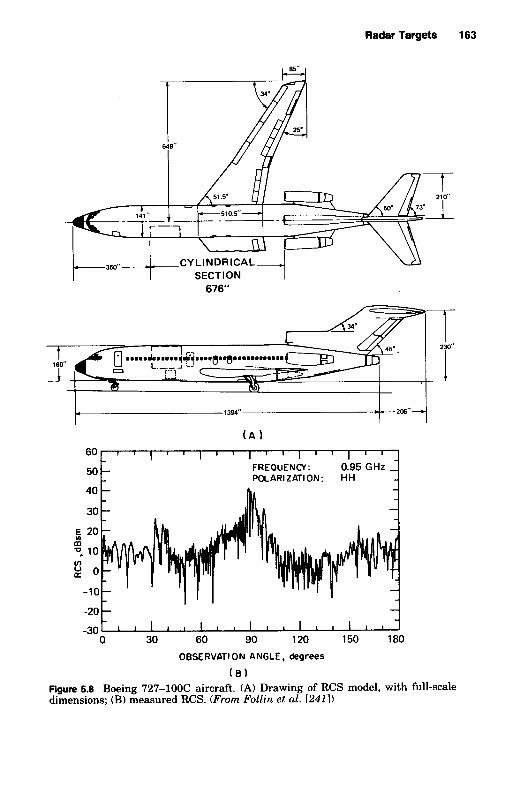
Radar Targets 163
676"
-20
-30
- - - L L I 1 I ' I ' I L ' I ' I ' I I
0 30 60 90 120 150 180
OBSERVATION ANGLE, degrees
-
(El) Figure 5.8 Boeing 727-1OOC aircraft. (A) Drawing of RCS model, with full-scale dimensions; (B) measured RCS. (From Follin et al. [2411)

164 Chapter Five
(A)
0 30 60 90 120 150 180 OBSERVATION ANGLE
(8)
Figure 5.9 Teledyne Ryan drone. (A) Drawing; (B) measured RCS. (From Follrn et al. [241])
aircraft, the drop in RCS is probably 6 to 8 dB when pulse durations drop from 1.0 ps to a few nanoseconds. Hence, surveillance radars tend to have longer pulses as opposed to tracking or identification appli- cations.
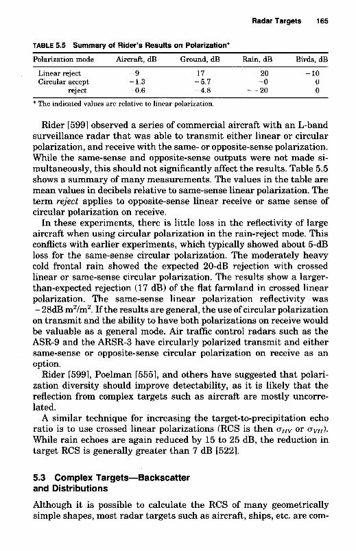
Radar Targets 165
TABLE 5.5 Summary of Rider’s Results on Polarization*
Polarization mode Aircraft, dB Ground, dB Rain, dB Birds, dB
Linear reject -9 - 17 ~ 20 - 10 Circular accept - 1.3 - 5.7 -0 0
reject - 0.6 - 4.8 --20 0
* The indicated values are relative to linear polarization.
Rider [599] observed a series of commercial aircraft with an L-band surveillance radar that was able to transmit either linear or circular polarization, and receive with the same- or opposite-sense polarization. While the same-sense and opposite-sense outputs were not made si- multaneously, this should not significantly affect the results. Table 5.5 shows a summary of many measurements. The values in the table are mean values in decibels relative to same-sense linear polarization. The term reject applies to opposite-sense linear receive or same sense of circular polarization on receive.
In these experiments, there is little loss in the reflectivity of large aircraft when using circular polarization in the rain-reject mode. This conflicts with earlier experiments, which typically showed about 5-dB loss for the same-sense circular polarization. The moderately heavy cold frontal rain showed the expected 20-dB rejection with crossed linear or same-sense circular polarization. The results show a larger- than-expected rejection (17 dB) of the flat farmland in crossed linear polarization. The same-sense linear polarization reflectivity was - 28dB m2/m2. If the results are general, the use of circular polarization on transmit and the ability to have both polarizations on receive would be valuable as a general mode. Air traffic control radars such as the ASR-9 and the ARSR-3 have circularly polarized transmit and either same-sense or opposite-sense circular polarization on receive as an option.
Rider [5991, Poelman [5551, and others have suggested that polari- zation diversity should improve detectability, as it is likely that the reflection from complex targets such as aircraft are mostly uncorre- lated.
A similar technique for increasing the target-to-precipitation echo ratio is to use crossed linear polarizations (RCS is then urn or uvH). While rain echoes are again reduced by 15 to 25 dB, the reduction in target RCS is generally greater than 7 dB 15221.
5.3 Complex Targets-Backscatter and Distributions
Although it is possible to calculate the RCS of many geometrically simple shapes, most radar targets such as aircraft, ships, etc. are com-

166 Chapter Five
plex. The RCS of complex targets can be computed in many cases by using the RCS of simple shapes. The most common procedure is to break the target into component parts and to combine them according to Eq. (5.3) [EO, 149, 7621. This approach is usually used to determine the average RCS over an aspect-angle change of several degrees. Re- alistic complex structures such as large aircraft may exhibit 10- to 15- dB RCS fluctuations for aspect changes of a fraction of a degree [3971. Since the precise target aspect is generally unknown and time variant, the RCS is best described in statistical terms.
The statistical distribution of the RCS is of great importance in predicting detectability. For fluctuating targets, the detection prob- ability of a single echo is roughly the probability that the target echo alone will cross a detection threshold; receiver noise primarily affects the false-alarm rate. This means that if the occurrence of a small RCS has a large probability, an unacceptably low detection probability can result for a given mean signal-to-noise ratio. A variety of RCS distri- bution models have been used; the choice depends on certain assump- tions about the nature of the target. Table 5.6 summarizes the most widely used statistical RCS models (see Chap. 31, describes their ap- plicability, and cites pertinent references.
Steady Target or Marcum model [461, 1131
The detection of a perfectly steady target echo in receiver noise was originally analyzed by Marcum. This nonfluctuating model is not re- alistic for real radar targets except in limited circumstances, such as when the target is a sphere or is motionless over the observation time.
Chi-square of degree 2m [368]
Specializations of the chi-square distribution encompass a large class of targets. The form of this distribution is given as item (2) in Table 5.6, in which 2m is the degree of freedom. As the degree becomes higher, fluctuations about the mean become more constrained, that is, the steady component becomes stronger. The ratio of the variance to the mean is equal to ml”. In the limit, as m becomes infinite, one has the steady-target case. Short-term statistics of aircraft RCS have been found to fall into various members of the chi-square family [5851.
Swerling cases 1 and 2 (chi-square of degree 2) [689, 2251
The statistics of Swerling cases 1 and 2 are most often referred to as the Rayleigh-power or exponential distributions. Swerling case 2 sta-

u)
5 .- u)
0
a '0
m
K
Q
I- 0
u) Q
'0
0
m 0
CI
c
P - s
- .- .- c
5 iii :
2 w
-I m
b .A
9- ad :,a>
h
2 M
e E &
m.z
Vz
e, $g
cs+-
ms
% "C
zjps: '
$2
5 *
sp
: h
UQ
m
0 35
3N
s.::a
v c
g g gzu.5
c0 a E
XM
b 0 a
=
Q,
?A 3 g 8 92 02: g 2
2~
4 y
o-
0)
m
-ez p
mo
a c
dm
8Q
)5
2?
Sm
om
gg
hg
~S
mm
Wg
.& u
?c" ~
cd L
i
;dk$s"dL 3
Gz
q Ob
Ai
>
s ZG
W
~A
OS
C~
Q
* iQ= 0 $
a,
x
un
..3
E E
~Z
cd PS
m m
M
uA
o) ,%
m
0 L
,.s
O'
CS
k cd
oa
b
c L,
0
g$
*&
-z
0-3," :"is% .I? c
.2 E
* g &$X
m
u
3 ? "
e
ms
Q.!?
%
h 3
g x 2
~3
~
&cJ-z$ g%m
"cr) 11
h~
~c
m
.$ 8
a
2b"zz
z.
%m
W
'h
E
g$
go
EE
m
a3 m
e
~~
.S
L2
'~
5
az
j$
,"
Ep
jp
gn
5
vn
~%
a
2 m
cd h
m A
Ts
bm
n a c
a.
~m
cd
acd
n,.j3
$3
2e: an
mu
m a
g h
sg
s
&~
A-
~D
J
* g$j E Wz
~
aQ
a2
a cO
3S
_h
U 9 i e
za
22
'-
Q
W
.- cd
- 5.2-
sk
~:
-~
~.
~~
8~
~.
~~
:~
~8
8%
68
~~
H~
dj
:~
~d
~
0
,bg
PE
: E
%O
Em
m+
22
E
mo
22
2%
a a
m "
2 8
e ol
Mu
13
3 &
g
a a
.%c
P=
gz
,z,i?
a
b
p:
H rn- 0
p: 9-
m
.3 c) 0
($2
z2
211%
I -
0
AI a
AI x
u)
h
.%
&
... H h
G
G
x I IH
I u
Q
22
3
!$
2b
I -
n
E a
;
a
n
AllH
2 2 g=:
m
I - Q 9
)
- !s
Q
8 O
El2
AIIH
4 K
H
- m
mi
i
*v
$
9 69
a
3
$A
5 3
%
b m
-u
p3 2.8 E
g ? a23
Q-
g$
-du
e?
8F
0 "0
%Q
mb
o
OQ
E's
8 g- ._
Q 8
-
u)
-
s$ u
u
"0 z VI
$32
MJ
e
m
MJ
~.
z
c m
'- .e
'i: .2 s '?a E'
h.u
AS
m
-e e 0
a-e
3s
gsm
:E
$30
0. 0 "1
EO
0--
- E!
?? z
l E
55 0
0
m *a
,$'s
)&
4
m
h
- h
h
3
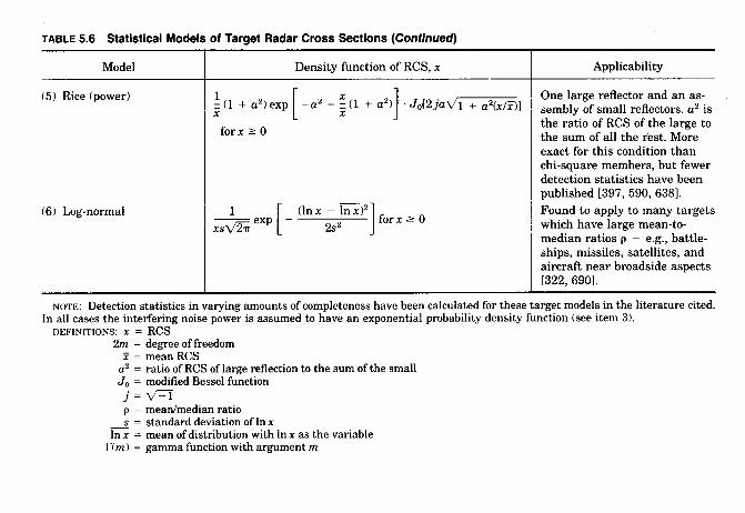
h
* m
m$
&a*
, .2 3
:xu
$8
c a
'G
9 W
5
ZC
JL
m &
$z
5s
z$
:$a g-:
x
5B
a*
j~
:n
+"
GC
,%
C
J8
5rn
Z
m-
m&
$
3 .8
%,,5
o)
h.2
2:g E E
W$
4
8 Z:,,A
c
nz
m Sa, '
a a
.e
u 8~
v) -
,?a:-$ z
472,
Ws
zz
mm
W
EE
m
.2E
$m
2;$
z2
3
,Z't;'t;5
.,"- M
OO
h
$c
a og
j2.2
2s
-- $ ,$
$8 g
$Z
;; 5 :-e%-
0 $
55
$*$
L
g$
s+.$g
0 82 0)
2E
WW
:,zz
5
n h ,*
g.rB
e.5
hl
r(
0
x h AI
ZH
! q 3
f3j 2
E
0
5"
C%-
g c
-u e
.- o$
+
N-
82
3
$3
I
13
D a
"5
ow
l.
- c
v)
2
HIIH
I'
N
H 2 '8
%
- d v 0
U
m
K
0)
+ 0
- cn 0
U
a-
- I
a
b -
?4 -
0
u AI
fx
c
-
-
r( If
g r(IIX
c
I" - .- m 0 5-
p
c
m
- -
.- cn-
v)
g - k
c W
9
2 2 v3
E
;I -
2 w
J
- rn
.:
2 5 2 26
.s: $2
ts
23
*
2: *o
Px
o) .%
Cm
E8
&
*
P .t: m
z -22 a
e
83
-
x
*-
oa
- ;;
2 ;t
'r
gs E
22 s
gs
Y
0
5; 28 x
z ii
52
4 5
G.
53
g 2
0 c.5
2b
%
B
oE
:.q's
.-$
g
25
z
3s
c.
?: -3! ;:
mW
Yo
c.
'; 't: 'S
.e
$: %
ge
P
u-*b
2
;%E
2 E E E
L E;:
E %
*
19 $ s
g
mo
0)
s W
3 % 2
2 .e
Yo
)
o) 2>
d
k-0
O
W
.e
*
2E
0:
&'C z
B
A0
h
a
hm
no
E:.g
&
av
cp
<
-~
.2
d
E &%
m
.- wq
&%
o)
O%
->
$c
.E
I mJ3mJE
'S &
V
2 11
/I II
II II
I1 II
II /I
II 5.2 x
Ei
Hm
uq
'l
am
x-
g
z v1 ."
;Z
g
8- k
zz
g
.I
ur
Z
c I

Radar Targets 169
tistics apply when the RCS pulse samples are independent on a pulse- to-pulse basis (rapidly fluctuating). Case 1 statistics apply when the samples are correlated within a pulse group but are independent on a scan-to-scan basis (slowly fading). The pulse-to-pulse independence case is not applicable to most radar targets because of their narrow Doppler spectra (see Sec. 5.8). This assumption may be valid when pulse-to-pulse frequency diversity is used (see Sec. 5.9). The Rayleigh model applies to a random assembly of scatterers, no one of which is dominant. It is the most widely used of all distribution functions for modeling large complex targets [lo, 63, 169, 4901. Experimental evi- dence suggests this model for complex targets such as large aircraft, whose aspects undergo large changes. However, it may not be appro- priate when applied to a target that presents a limited range of aspects, such as a simple target viewed over a short period of time [541, 5851.
Swerling cases 3 and 4 (chi-square of degree 4)
Case 4 statistics apply when there is pulse-to-pulse independence and case 3 statistics apply to scan-to-scan independence. Swerling assumed this model represented the class of targets having a large steady re- flector and a number of randomly oriented small reflectors, although he did not attempt to justify the assumption on a physical basis. The exact distribution that fits this assumption was given by Rice.
Rice distribution
When an assembly of scatterers includes a steady reflector whose return is significant compared with the sum of all the others, the density function has the form of the Rice distribution (see [397, p. 5601) given by item ( 5 ) of Table 5.6, where u2 is the ratio of the power from the large scatterers to the power from all the rest. When u2 + 0, this distribution converges to the Rayleigh density function, and when u2 + 30, it converges to the steady-target case. Scholefield 16381 compared the degree4 chi-square case (Swerling 3 and 4) with the Rice distri- bution with a2 = 1 (power from steady reflector equal to the power from the assembly). The detection statistics for the two agreed, except for small differences at the extremes of detection probability. The Rice distribution is an exact representation of the steady-plus-assembly reflector case.
Log-normal density function
The RCS distributions of some targets do not conform to any chi-square member. Some of these targets exhibit large values of RCS far more

170 Chapter Five
frequently than would any member of the chi-square class. Examples of this class of targets are satellites, missiles, and ships, which often have large mean-to-median RCS ratios.* The RCS of these targets can frequently be closely represented by the log-normal density function [item (6) of Table 5.61, which arises when the logarithm of a variate is normally distributed. Swerling derived procedures for approximating this function with chi-square members [6901. The log-normal function was also studied by Heidbreder and Mitchell [3221. They postulated that the high tails of this density function arose in practice from large specular returns at a relatively few aspect angles. For conservative estimates of system performance, one should neglect these tails and resort to the Rayleigh assumption.
Discrete scatterer models
The RCS of a complex target can often be expressed as the combination of a number of discrete scattering centers. For a target composed of N discrete scatterers whose returns combine in a random-phase fashion, the RCS distribution converges to the exponential distribution (Swer- ling 1 and 2) if N is large enough. If N is relatively small, the RCS will deviate from the exponential model as analyzed by Castella and Reilly [1141. If each discrete scatterer is of equal magnitude, the RCS distri- bution is a delta function for N = 1, a beta function for N = 2, and for N = 3 follows a complete elliptic integral of the first kind. For N > 3, an analytic expression has not been obtained except for N + 03,
in which case the exponential model applies. Results for various degrees of N obtained with Monte Carlo simulation show that with N = 10, the statistical model closely approximates the standard “many scat- terer” case. With N as few as 5, the distribution is still reasonably close to that case.
Summary of statistical modeling
1. Modeling is basically a coarse procedure. In no case should an assumed statistical model be used for very precise calculations of sys- tem performance (i.e., performance at very high or at very low detection probabilities).
2. If only one parameter is to be used to describe a complex target, it should be the median RCS. Detection statistics should then be cal- culated by using the Rayleigh model (Swerling cases l and 2) having the same median value. The choice between the pulse-to-pulse or the
* The mean-to-mean ratio for the Rayleigh function is 1.44, and for the degree-4 chi- square is 1.18.

Radar Targets 171
scan-to-scan independence assumption depends on the Doppler spec- trum width of the echoes and whether frequency diversity is used.
3. If the tails of the actual RCS distribution function are known to be much higher than those for the chi-square members, an upper bound on system performance may be established by using the statistics for the log-normal distribution function. These statistics have been ex- pressed in terms of the mean RCS and the mean-to-median ratio.
4. If the target is approaching the radar nose-on region, standard detection statistics should be used, and if a high detection probability is required before the target reaches a given range, cumulative detec- tion statistics should be used.
5.4 Measured Aircraft and Missile RCS Distributions
While it is possible to measure aircraft RCS at a given aspect, the precise aspect in flight is unknown and time variant. A plot of the aircraft return versus time appears as a noiselike function, even when the nominal aspect of the aircraft is constant. Because of the uncer- tainties about the aspect, the RCS is usually best described statistically. Ordinarily, one assumes a Rayleigh distribution; this model has been suggested by experiments on large aircraft undergoing several angular degrees of aspect change. Unfortunately, this model does not apply to all aircraft and to all radar detection and tracking problems. A good portion of the uncertainty lies in the observation time used to obtain the RCS distribution.
In one series of experiments by NRL, RCS distributions were obtained for a variety of aircraft [lo]. Flight paths were straight and level, and various aspect changes were observed by the radar. Data were recorded over 10-s intervals at P-, L-, S-, and X-bands. The Rayleigh model provided a good approximation to the distribution in many cases, al- though there were a large number of exceptions. The most consistent exceptions were for smaller aircraft and for all aircraft at broadside. Large, multiengine aircraft gave good Rayleigh approximations for as- pect changes of only 1 or 2". Small aircraft were often fit very poorly by this model, even when the aspect change was 8 to 9". In most cases, deviations from the Rayleigh distribution tended toward higher-order chi-square functions. In these cases the Rayleigh assumption would tend to provide conservative estimates of detection ranges for detection probabilities greater than 50 percent.
In tests conducted by J. Whybrew at the Applied Physics Laboratory, RCS distributions at C-band were plotted for a variety of conditions and were compared with chi-square functions [5851. In all but a few cases good fits were made to some chi-square function between the 10-

172 Chapter Five
and 90-percent points. For a small, two-engine Lear jet, chi-square approximations were obtained in the APL tests with degrees ranging from 1 to 37. About one-half the functions fell between degree 1.4 and 2.7. Occasionally, widely different distributions were obtained from one data segment to the next, even when the apparent azimuth aspects differed by only a degree or two. Figure 5.10 illustrates several mea- sured density functions. In (A) and (B) the nominal aspects were similar, although the precise aspect was unknown since the “crab” angle of the aircraft was unknown. Part (A) is approximated by the Rayleigh func- tions and part (B) by the chi-square function of degree 22. In both cases the run length was 2.0 s, although the results were similar when the run was extended to 8 s. Parts (C) and (D) show density functions measured over 1 s. Part (C) has the appearance of the Rayleigh function, whereas part (D) does not resemble any known function. These dis- tributions demonstrate the nonstationary character of the echoes.
The echoes from two Lear jets flying together approached the Ray- leigh density functions more frequently than did those of the single jet, as illustrated by Fig. 5.11A. The ordinate is the degree of freedom of a chi-square function that best fits the data. The abscissa is the data run length T times the bandwidth of the spectrum UT measured over the same data segment. Bandwidth here is defined as the standard deviation of the airframe power spectral density function measured about the mean Doppler frequency. This figure demonstrates that the two aircraft could be represented by the Rayleigh function with more confidence than could the single aircraft. This behavior is expected, since the Rayleigh model is approached as the degree of complexity of the target increases. Fig. 5.11B summarizes density functions mea- sured for other aircraft.
In general, as the product afT decreases, the estimated density func- tion is expected to tend toward a model of higher degree of freedom. For example, if the measurement interval is so short that all the re- ceived pulses have the same value, the measured density function will consist of a single value. This corresponds to a chi-square function having infinite degrees of freedom. Although the tendency is not obvious from the figure, where numerous data runs are presented, it does ap- pear in individual data segments that were broken into smaller in- tervals.
Table 5.7 lists some representative median RCS measurements for selected classes of targets and aspects. For most aircraft, the median RCS at nose aspect is smaller than that for other aspects, and this value can be used for conservative performance estimates. These are mostly measured with some interpolation. Some data are from scale models. No distinction is made in Table 5.7 between horizontal and

Radar Targets 173
Y U
W CHI-SQUARE OF DEGREE 2.7 K K 3 U U 0 U 0 > U z W
3 U W K U
z APPROXIMATE DENSITY FUNCTION:
0 47 UNITS
(A)
APPROXIMATE DENSITY FUNCTION: CHI-SQUARE OF DEGREE 22
W U z W
K K 3 U U 0 U 0 > U z W
3 U W (L U
104 UNITS RECEIVED POWER (linear scale) 0
(6) Figure 5.10 Probability density functions for small jet echoes. (A) Observation time 2 s, number of samples 624, aircraft aspect azimuth o", elevation 12", range 17.5 nmi; (B) observation time 2 s , number of samples 624, aircraft aspect azimuth lo", elevation 14", range 17.0 nmi;

- I I I 1 1 I I I I
APPROXIMATE DENSITY FUNCTION: CHI-SQUARE OF DEGREE 2 (RAYLEIGH) w
U L
Y LL LL 3 U U 0
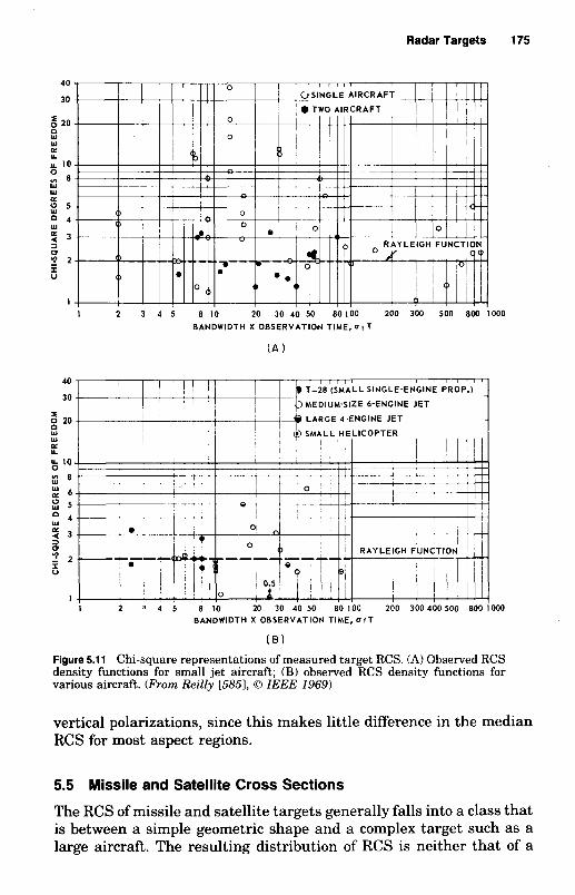
Radar Targets 175
40
30 TWO AIRCRAFT
a 20 n
a u IO a n 8
W W
U
0
W W E
W 0 5
: 4 4 3
2 2 0
V
I 1 2 3 4 5 8 10 20 30 40 50 80100 200 300 500 8W 1000
BANDWIDTH X OBSERVATION TIME, u f T
( A )
40
3 0
I 0 20 W
IL
W K
LL IO 0
I 8 : 6 s 5 O 4
4 3
2 2
W
0
I U
1 1 2 3 4 5 8 IO 20 30 40 SO 80100 200 300400500 8001OW
BANDWIDTH X OBSERVATION TIME, U f T
( 8 )
Figure 5.11 Chi-square representations of measured target RCS (A) Observed RCS density functions for small jet aircraft; (B) observed RCS density functions for various aircraft. (From Redly [5851, 0 IEEE 1969)
vertical polarizations, since this makes little difference in the median RCS for most aspect regions.
5.5 Missile and Satellite Cross Sections
The RCS of missile and satellite targets generally falls into a class that is between a simple geometric shape and a complex target such as a large aircraft. The resulting distribution of RCS is neither that of a

176 Chapter Five
TABLE 5.7 Targets-Median RCS, m2 Carrier frequency, GHz
1-2 3 5 10 17
Aircraft (Noseflail Avg.) Small propeller 2 3 2.5 Small jet (Lear) 1 1.5 1 1.2 T38-twin jet, F5 2 2-3 2 1-2/6* T39-Sabreliner 2.5 1018 9 F4, large fighter 5-815 P20110 4 4 737, DC9, MD80 10 10 10 10 10
Ryan drone 211
727, 707, DC8 type 2240115 40 30 30 DC-10 type, 747 70 70 70 70
Standing man (180 lb) 0.3 0.5 0.6 0.7 0.7 Automobiles 100 100 100 100 100 Ships-incoming ( x lo4 m')
4K tons 1.6 2.3 3.0 4.0 5.4 16K tons 13 18 24 32 43
Sea birds 0.002 0.001-0.004 0.004 Sparrow, starling, etc. 0.001 0.001 0.001 0.001 0.001
Birds
' Slash marks indicate different sets.
point reflector nor a random array of scatterers. This is pointed out by full-size X-band model measurements of a 54-in satellite* having spher- ical symmetry reported by Kennedy 13941. The cumulative distribution is shown in Fig. 5.12. Two sets of measurements are shown: a single frequency set, which shows a distribution that is more highly skewed than any of the Swerling models, and a frequency stepping set with each point being the average RCS from eight frequencies spread over 500 MHz. In both cases the mean-to-median ratio of RCS is about 10. Hence, the majority of RCS values are well below the uueruge. However, the median and the decibel average dBsm (the absolute geometric mean) are similar.
With frequency agility the probability of both large and small RCS values decreases (see Sec. 5.9). Gaheen, McDonough, and Tice [2551 compared the RCS distribution of the Tiros? and Nimbus satellites. These data are shown (Fig. 5.12) along with the unusual RCS distri- bution on a conical-shaped missile model. This model had a cone angle of 23.5", a length of 150 in, and a diameter of 53 in at the tail. Note that frequency agility substantially reduces the number of RCS values below 0.01 m2 for the missile target. On a single frequency, these data show that the median cross section of the cone-shaped missile is about
* Plus short stub antennas.
t The geometric cross-sectional area of the Tiros is about 3.4 m', or twice that of the 54-in satellite.

Radar Targets 177
99
98
95
< 3 90 2
Y BO
<
z I 70 SYMMETRICA
3 60 n
#,l y 50 2
2 40 P
30 Y
s 20 L
10
5
2
1 -25 -20 -15 -10 -5 0 5 10 15 20
RCS, d 6 m - SINGLE FREPUENCY ---- FREPUENCY AGILITY, 16 STEPS, 500 MHz TOTAL
Figure 5.12 Cumulative distribution of satellite RCS average for all aspects. (From the data of [255])
1 m2, while the 5-percent probability is about 20 dB less. Fig. 5.3 also suggests the log-normal distribution, which would appear as a straight line on this graph.
This satellite data should not be construed as being valid over a wide range of carrier frequencies. An indication of the frequency sensitivity of RCS of satellites is illustrated by a series of model measurements of the roughly 105-in Mercury space capsule reported by Mack and Gorr [4571. They show RCS values versus angle for simulated fre- quencies of 440 through 5600 MHz. Table 5.8 summarizes those data as percentiles exceeding a specified RCS. It can be seen that RCS values for the Mercury capsule do not have an obvious frequency dependence.
In the previous examples of satellite targets there was no attempt in the satellite design to reduce the RCS. However, in missile systems there is a considerable advantage in presenting a low RCS to a de- fending radar. For this reason there is a tendency to use radar-ab-

178 Chapter Five
TABLE 5.8 Percentage of Aspect Angles That a Specified RCS Is Exceeded for the Mercury Capsule, Vertical Polarity
Frequency, MHz cr 2 100 m2, % cr 2 10 m2, % u 2 1 m2, %
440 0 28 70 933 35 69 98
1184 8 28 62 2800 7 47 96 5600 2 13 60
sorbing materials (RAM) or a low-RCS shape such as a wedge or a cone-sphere. The RCS is small for a cone-sphere over a broad range of carrier frequencies when observed near the pointed end of the cone. The RCS of this object is the vector sum of the reflections from the tip, the joint between the cone and the sphere, and a “creeping wave” [653, 658,7611. A series of measurements and a theoretical curve are shown (Fig. 5.13), in which the nose-on cross section (in square wavelengths) is plotted as a function of the radius of the spherical portion (in wave- lengths). The important points to note about this idealized target are that, neglecting the oscillations, RCS is proportional to X2 and the size of the object itself has little effect if the pulse length is greater than the target length.
5.6 Marine Targets
The radar backscatter from a ship cannot be uniquely predicted due to interference resulting from the forward-scattered electromagnetic waves. As an approximation, the received power at the radar can be written [397, 7741
(5.6) PTGTGRX2Ut 16 sin4
pr = [ ( 4 ~ ) ~ R f ] [ (22tht)] where ut = radar cross section in absence of reflections
ha = antenna height h, = target height
The first term is the conventional free-space received power equation and the second term is a modifier that is periodic in elevation angle with a peak value of 16. This is the familiar lobing effect of surface radars that doubles the detection range at some elevations, but puts a null on targets that are situated on the surface of the water. There are several assumptions that must be explored before trying to evaluate the sin4 term in Eq. (5.6). The geometry can be illustrated by Fig. 5.14A. The modification of the field strength at the target is

-z ul
z1(QP
’N01133S
SS
O(13 M
31
1V
3S
Y3
W
179

CURVE h., ft
(A) 470
( I 1 21
IC) 470
(D) 60
A , cm TARGET REF
150 SYALL SHIP [7741
9 1 FREIGHTER [3971 10 DESTROYER I7741 3 2 40-ion TRAWLER I1741

Radar Targets 181
R, = p exp(j@), where p is the real part of the reflected amplitude and @ is the phase shift upon reflection (see Sec. 1.11).
It has been shown [774,6741 that for typical surface-radar calculation (target range Rt >> ha or h , and a flat surface with reflection coefficient of - 1) the relative phase of the reflected wave with respect to the direct wave is
4nh,ht D = - + a mt whereD = difference in phase between direct and reflected paths
(radians) @ = 7~ for flat smooth sea
Section 1.12 on forward scatter shows that a reflection coefficient of -1 can be expected at low microwave frequencies (A > 30 cm) and smooth seas. The relationship applies for grazing angles up to about 1” for both horizontal and vertical polarization. Assuming that the ship is a point reflector, making the small angle substitution in Eq. (5.6) yields
(5.7)
Thus, received power from a ship may fall off as fast as Rp8, even without including the horizon effect.* Experimental verification of this is shown in Fig. 5.14B, which illustrates relative power received as a function of range. The location on the ordinate is arbitrary. The R-’ dependence near the horizon is obvious on curveA for the 150-cm radar. The transition from the R dependence (free space) to the R-’ depen- dence for the higher-frequency radars occurs approximately at R = 4h,hJk and may be abrupt. Estimates of detection performance for various geometries and sea conditions can be obtained by using software such as EREPS [2071 or TSC’s Radar Workstation [5711. The difficult part of using the software is to enter a value for ht, the effective target height, and the RCS of the ship, ut. Values for sea reflectivity are included in the software packages or you can insert values from Chap. 7 . The following yields a good empirical fit for the vessel RCS in the absence of measured data.
The Naval Research Laboratory made carefully controlled measure- ments of the radar cross section of a number of naval vessels. Mea- surements were made at essentially grazing incidence at X-band, S- band, and L-band. An example is shown in Fig. 5.15, which gives the
* In Chap. 7 it is noted that the normalized backscatter from the sea itself (TO also
4nP&’&’R~t(h,ht)~ X2R:
P, =
falls off rapidly at low grazing angles.

1,000,000 / /
/ / . / r
/ /
/
/*: N E 100,000~
W ci // [L e ;'.. v) ;/ 9 -/
3
/ z b 10,000 7 * d
//* /
: ,/ /
1 1,ooob ' ' ' , , , a o I ' ' ' . a . . d ' ' '""l.l.

Radar Targets 183
expressed in terms of the ship’s displacement and the radar frequency. Such an expression for the 50th percentile is as follows:
(T = 52f1I2 D3I2
where u = cross section, m2 f = radar frequency, MHz
D = ship’s (full load) displacement, kilotons
Similar expressions can be obtained to describe other percentiles. This expression holds for the microwave band over which the measurements were made and over the range of ship sizes examined (approximately 2000 to 17,000 tons). The above relation was used to estimate the RCS of various Russian ships. The results are summarized in Table 5.9.
As a result of the almost inseparable effects of sea reflection and the
TABLE 5.9 Estimated Soviet Ship RCS at 9 GHz
Shiplclass Displacement, tons RCS, m2
Carriers: Kuril class 40,000 1.2 x lo6 Moskva class 18,000 3.7 x 10⁵
Sverdlov class 19,200 4.1 x 10⁵ Chapaev class 15,000 2.8 x 10⁴ Kirov class 9,060 1.3 x 10⁴ Kresta I1 class 7,500 1.0 x 10⁴ Kynda class 6,000 7.2 x 10⁴
Krivak and Kashin class 5,200 5.8 x 10⁴ Kanin and Krupny 4,600 4.9 x 10⁴ SAM Kotlin class 3,885 3.7 x 10⁴ Tallin class 4,300 4.3 x 10⁴
Kola class 1,900 1.2 x 10⁴ Riga class 1,600 9.9 x 10³ Mirka I and I1 class 1,100 5.6 x 10³ Petya I and I1 class 1,150 6.0 x 10³
Grisha class 750 3.2 x 10³ Poti class 650 3.2 x 10³ Kronstadt class 380 1.1 x 10³
Cruisers:
Destroyers:
Frigates:
Corvettes:
FPBs: Osa I and 11 class 200 510 Komar 80 110
SOURCE: From Skolnik in Eustace, H. F. (ed.), The Znternational Coun- termeasures Handbook, 3d ed., 1977-1978. Palo Alto: EW Communications, Inc., 1977, pp. 278-279.

184 Chapter Five
cross section of the ship itself, only the measurements of ship cross section in the R - 4 region are of general interest.
5.7 Miscellaneous Airborne Reflections and Clear Air Echoes
A modern high-power radar observes numerous reflections from various regions of the atmosphere. A radar that can detect a 1-m2 RCS target at 200 nmi will also detect a 10-4-m2 object at 20 nmi unless specific techniques are used to inhibit detection of slowly moving, low-RCS objects at near range. In addition to echoes from aircraft, missiles, and precipitation, there are a variety of reflections that are not as easily explained. This section summarizes a few of the backscatter properties of some of the “phenomena” that appear on radar displays. The use of the term phenomena is to emphasize that, while many of the reflections are from discrete objects such as birds or insects, there are also nu- merous echoes from atmospheric anomalies including clear air layers at the tropopause [231, breaking gravitational waves [3321, and ring echoes [671, p. 5531.
The term angel has been used for many years to describe the radar reflections from a location in the atmosphere that does not contain a known discrete target. Many of these angels are undoubtedly due to the presence of small birds and insects. Table 5.10 provides a summary of the RCS of birds and insects at several carrier frequencies [269,407, 381.
Because birds typically have dimensions comparable to a wavelength in the Mie region, the RCS is a strong and often oscillatory function
TABLE 5.10 Mean RCS of Birds and Insects*
Radar cross section, dBsm Size or Airspeed length knots UHF S- X-band
Duck 800 g 25-45 -13, -27 -30, -21* -21 Gull 600-750 g 15-30 -30, -21* Pigeon 30MOO g 25-45 -30 -26,* -21 -28, -2O* Grackle 130 g -40, -43 -25 - 28 Starling 75 g 20-42 - 30* - 31 Sparrow 25 g - 56 - 28 - 37 Hawkmoth 5 cm, 1.2 g 2.6 -74 - 50 - 39 Locust 2 x 0.4 cm -30, -40 Honeybee 1.3 x 0.6cm, 13 - 72 -40 to -49
Dragonfly 3 c m 1.6 -72 - 64 - 50 0.1 g
* Averages over various aspects except when indicated by an asterisk, which denotes a broadside measurement.

Radar Targets 185
of wavelength. This can be seen from the entries in the table in which the reported RCS at S-band (10 cm) is higher than at UHF (71 cm) or X-band (3.2 cm). It was also reported that the RCS distribution appears to follow a log-normal distribution with the mean-to-median ratio of about 2.5 for birds whose dimensions are greater than about four wave- lengths, and a smaller ratio for smaller birds.
The RCS of a number of insects was also measured [420,269]. Because these objects generally fall in the Rayleigh region, their RCS increases rapidly with increasing transmit frequency.
A single bird or insect is not a significant problem except when attempting to detect reduced cross section targets or projectiles. How- ever, the numbers of birds in a resolution cell can be quite high. Barry [381 gave estimates as high as 200,000 birds populating a 10-mi radius from an air traffic control radar (ASR). Over 700 angels (collections of birds) were observed on one ASR with normal settings for the radar. These are typically within 15 mi of an ASR. The average RCS of the angels was 0.28 m2 and varied from 0.005 to 2 m2. Ground speeds were 10 to 59 knots and maximum height was 5000 to 6000 ft. With ASR radar parameters, the average was about 3 detectable angels per square mile at 2 to 4 nmi and 0.3 at 6 to 8 nmi.
Airspeeds of birds (Table 5.10) can be significant. These are not directly additive to wind speeds, especially with migrating birds. Air- speeds of the birds themselves tend to drop with tail winds and increase in head winds. Other studies have shown that the median ground speed of migratory birds is about 50 knots and that the median height is about 1000 ft. Some birds flew as high as 4000 ft. The RCS of birds displays a modulation due to the wingbeat. Typical modulation rates of 2 to 5 Hz are measured under daylight; nighttime measurements involving larger birds show wingbeats of as much as 10 to 12 Hz.
Although many radar reflections can be attributed to birds, insects, precipitation, etc., a number of other echoes cannot be easily identified. Many of these can be attributed to fluctuations in the refractive index of the atmosphere. Radar reflections have been reported from the region of the tropopause [23, 3341. This is a layer of air at an altitude of 8 to 16 km that delineates the separation between the troposphere and the stratosphere and is the region near which clear air turbulence (CAT) is often found to occur. Since CAT has a considerable adverse effect on jet aircraft, the possibility of detecting it by radar is currently receiving considerable attention. Clear air echoes were reported virtually every day of one six-week operation with a set of three large, high-powered radars at UHF, S- and X-bands. Some of the time they appear as “braided structures’’ that are attributed to breaking gravitational waves [332]. In another set of experiments, regions that showed clear air echoes were simultaneously probed with an aircraft and were found

186 Chapter Five
Figure 5.16 The range-height display showing clear air convective cells. The abscissa is range out to 20 mi, the ordinate is altitude with the nearly horizontal line the 20,000- ft Marker Note also some layered echoes above the convective regions. (From Katz 13901)
to be turbulent [334]. An example of clear air echoes is shown in Fig. 5.16. An RHI display is shown with echoes that appear like braided structures (S-band radar). The sky was optically clear in these regions at the time of the photos.
There is also backscatter from the aurora in the polar regions, which is stronger at lower carrier frequencies. This is discussed briefly in Chap. 6.
Multifrequency radars can be used to distinguish between material particles, such as insects or clouds, and discontinuities in the atmo- sphere. It has been shown (see Chap. 6) that the reflectivity per unit volume q for particle diameters less than about 0.06A is given by'!'
9 = m5 A 4 IKJ'LD' (5.8)
where A is the wavelength and D is the droplet diameter. The value of
' In Chap 6 \rr is used instead of T for the normalized volume reflectivity The units of Ztr or T in this text are m'lm' or m '

Radar Targets 187
K = ~ 1:: I41 where n is the complex refractive index. The equation for the reflec- tivity of a refractively turbulent medium can be approximated by [3901
(5.9)
where (An)2 is the mean-square refractice index fluctuation and Le is related to the size of the turbulent eddies. The important difference between relations (5.8) and (5.9) is that echo particles like raindrops have a strong wavelength dependence while those from changes in refractivity are almost independent of wavelength. Thus, particulate matter or insects are seen primarily at the higher frequencies. Although the reflectivity q of the clear air echoes is only about lo-’5 m-’, they can be seen with high-powered radars at 10- to 20-km ranges.
There are many other reports of reflections from unidentified objects, many of which are caused by reflections resulting from anomalous propagation (ducting) in certain areas of the world. Air traffic control radars often develop tracks on atmospheric anomalies that do not ap- pear to have been caused by ducting. These are often referred to as “angels” or as “worms” if they can be tracked. A good overall description of atmospheric echoes in the absence of precipitation is given in Chap. 11 of Doviak and Zrinc [1871.
- rl ~ (A,,)! Le -2/3h - 113
-
5.8 Spectra of Radar Cross-section Fluctuations
The spectral width of the echoes from a complex target can have a considerable effect on the choice of radar processing technique and the specific parameters. In a Doppler tracking system (CW or pulse Dop- pler), it is desirable to reduce the Doppler filter bandwidth to the limits imposed by the fluctuations of the target echoes, the stability of the transmitter, and the Doppler shifts due to acceleration. Using this minimum Doppler bandwidth maximizes the signal-to-noise ratio and generally the signal-to-clutter ratio. To reduce the effect of target fading there should be additional postdetection (incoherent) integration of the outputs of the Doppler filters for a time duration greater than the correlation time of the target echoes.
Unfortunately, the relatively long correlation times of airborne tar- gets means that in a tracking radar, the duration of a target fade may cause excessive range and angle errors. In a surveillance radar, the target cross section may remain in a null for the entire time the beam illuminates the target. This means that excessively long processing

I
* x 5 Z
!k! '\ * \
I --'\ 5 /
- A 2 2
J *\ sx

Radar Targets 189
1.0 2.0
In
U K
z 4 W I
3.0 g U
W 0.75 I I 4.0 g z I- 0 :: z 6.0 E g 5 0.50 8.0 - 2
12.0 t: 5 20.0 I- 51
= I 3
O + 0 I-
W n :: 0 3
n
n E 4
z Z L W X -IU $ 0.25 2 3 0 W
E
~~ 0 2 5 10 SAMPLE 40 LENGTH, mr 160 640
Figure 5.18 Relative standard deviation of aircraft RCS (nose aspect, X-band). (After Edrington 12001)
motion occurs as the aircraft aspect changes. The resulting spectral width is proportional to the transmitted frequency. In a propeller air- craft, a second effect is caused by the amplitude modulation from the propellers. Returns from jet aircraft also contain modulation compo- nents at aspects that allow reflections from the interior of the engines. The spectral width from this component is not proportional to the transmit frequency but appears as amplitude modulation components about the airframe spectrum at multiples of the propeller rotation rate. The third effect is due to reflections from the rotating propeller or turbine blades themselves. At a given aspect the apparent center of reflection of a set of blades shifts back and forth in a periodic manner as the blades rotate. The radial component of this motion generates a spectrum typical of phase-modulation spectral energy. The phase mod- ulation from a turbine echo is similar to a single sideband modulation with spectral lines dominating on one side of the airframe line.
The width of the airframe spectrum is expected to follow the rela- tionship
Af = K ($) (s) (5.10)
The constant factor K is a proportionality factor. The factor LdX is a characteristic length of the target, such as wingspan or body length,

1.0
0.8
w 0 0.6-
-
- AIRFRAME D O P P L E R L I N E
I

Radar Targets 191
AIRFRAME SPECTRUM
( A ) COMPOSITE, 0.8 s
(B) PART 1, 0.0-0.2 I
0 s - - : f i o 0 . 0 5 ~ 0.09
ii TIJLIl o*IIIIl 0 3.15 DOPPLER FREQUENCY, kHz 3.67
(C) PART 2, 0.2-0.4 s
(L w z E ; 0.28
w o 2
(D) PART 3, 0.35-0.55 I
0
(E) PART4, 0.5-0.7 I
NOSE ASPECT-19O ELEVATION
Figure 5.20 C-band spectra of T-28 aircraft showing propeller modulation.
spectrum varied with the aspect. For the aspects in which the propeller spectrum was strong, its 3-dB width varied from 200 to 1000 Hz.
The percentage of energy contained in the propeller spectrum is also time variant. Figure 5.20 shows the spectrum of a small T-28 single- engine aircraft at nose aspect. These spectra are taken from unpub- lished experiments performed at the Applied Physics Laboratory. Part A shows the spectrum as measured over an 0.8-s interval. Parts B through E show how the energy was partitioned over successive 0.2-s segments. (Notice that the vertical scale for each plot is different.) In this series of spectra, the total power in the propeller spectrum is

1.0'
0.8 -
AIRFRAME SPECTRUM 0" 0.6 -
E
0.2

Radar Targets 193
TABLE 5.11 Spectral Line-Coherent Measurements
Percentage of Total Spectral Energy Outside of Main Airframe
% energy outside of airframe spectrum
Aircraft Minimum Average Maximum angle in av. Aspect No runs
T-28, small prop. aircraft 12 29 75 Nose 8
Medium multiengine jet 4 11 17 Nose 7
DC-8 or 707 size 17 28 38 Nose 3
Lear jet, small two-engine 0 22 59 0-30" 6
Large four-engine jet,
width is seen to be relatively insensitive to the particular type of air- craft. This tends to support an assertion made earlier that the length of target and its random component of motion are somewhat compen- sating.
One example of the airframe spectrum for a small T-28 propeller aircraft is illustrated in Fig. 5.22. In this example the target flew a constant-altitude radial path. Its radial velocity decreased in 0.8 s because it was at a close range (3.5 nmi). The spectrum resolution is 7 Hz in A and 3.5 Hz in B through E. In the lower four plots there is a Doppler shift of the dominant spectral line of about 50 Hz. Relative strengths are shown at the upper left of each figure. The complex composite spectrum A is now easily explained. The spectral line on the left of A is the result of the response during interval B. The noisy response during period C is of relatively low amplitude and does not contribute a single line. The strong clean line in D contributes the central line of A, and the moderate amplitude line of E appears on the right of A. Thus, what at first appeared to be a wide fluctuation spec- trum is probably due to target acceleration. This points out one of the difficulties in trying to relate coherent and incoherent spectrum mea- surements: acceleration results in spectral spreading in coherent, but not in incoherent, measurements. Another series of coherent spectrum measurements is shown in Fig. 5.23 for two small jets that were at- tempting to steadily maintain a wing-tip separation of 300 ft. Differ- ences in their instantaneous velocities are evident. Because coherent spectrum measurements include the effects of acceleration, the spec- trum widths so measured should be considered upper limits on the RCS fluctuation spectrum.
When the spectrum analysis is performed after envelope detection, it is no longer easy to separate the airframe spectrum from the other components. Part (B) of Table 5.12 summarizes some incoherent mea- surements made on jet aircraft. The spectrum width increases with the transmitted frequency and is roughly comparable to that for the

194 Chapter Five
(A) COMPOSITE, 0.8 s
( 6 ) PART 1, 0.0-0.2 I
m
im o.2'Al. 0 zA4 DOPPLER FREQUENCY, kHz 2A6
(C) PART 2, 0.2-0.4 5
g 0.44
(0 ) PART 3, 0.35-0.55 s
0
(E) PART4, 0.5-0.7 s NOSE ASPECT-35" ELEVATION
Figure 5.22 C-band power spectra of T-28 (propeller) aircraft.
airframe component of coherent measurements. It appears that the incoherent spectrum for jet aircraft is dominated by the airframe spec- trum. The time required for independent sampling may be estimated by using the 3-dB width of the spectrum. For the gaussian spectrum, the standard deviation and the 3-dB width are related by uf = 0.42 Af&,. Using this relationship, along with the results of Sec. 3.7, the independence time is estimated by TI = l/Af& This results in inde- pendence intervals rangingfrom 30 to 300 ms. Thus, unless polarization or frequency agility is used, the pulse-to-pulse independence assump- tion is not satisfied for most aircraft-detection radar problems.
The power spectrum of an aircraft or vehicle provides a signature of that class of target. Spectra from propeller or jet aircraft are easily

m
N
5 m
-,
a
m
h
2..
N
N
h
'y
m
0
- - -
0
d
5 .e
6 2 d
0
0
5
2
h
"! 2
7
- ~
, s G
E E
-
- I
I
s I
4 p1
s 0
U
-~
-3 I;
3- h
m
m
OD
-
7h
.E
2-
-
h g g
m
- *
0
Lt: m
a,
4 4
U
cr
0
a,
a
I
2 9 - -9
x 0
0
2
i2 a
2 ii
4
-
u c)
v! h
h
195

f n 8 * C
(A
a
3.
CI
CI
- z f g L
s I
E
2
u) H E 5 2
cy
7
v)
z A
w
m
- -
Q)
o*
6
e! E
c8
I44
sgssI4 22
E=
=&
Y
4
0
8 $5
*
&A? %
-
34
T Y
mea
CI),+
+V
*
*WD
Cr)n
)oa
W
1 g .5
oh
wv
, m
b 10
cow
5
B 22 y
$x
?
y?zzzz ,& B
4 32
ZP
-2$
i%
4N
rl 3 f
$2
v?cY
%$
$ 10101010~~
B
;T m
.$ P
B 4
Y
i! 2
31 E
E j-.
3 uu
rnrn
rnxu
2 I4
rnx
xb
b j
B .e
d
4 u 0
“M
h
f 4
3
?a .g
ig
s s
t- 10
n
2 1;
2 d
k
h
aw
l z
3-
2m
-I :fQz
4 .- a2
.-x gm
a’.aa 1
.? 22
a3g
d h
5;
2.gK K.g
3 a e 5
BA
h
a
5% 8
SE
E &
, .a.g 1
Q)
yy
g
AS
y G 5
%Z
la
ud
56
2 2
?P cM&
kE
rn 4
4r2 B
B
4?
”4
m
mw
mw
P-
m
e e 0
6
El m
i2
.- U
mm 4
0)
Y
8 I
E 4 m
U
A
E
--
-g
ge
E
22
lzz
cs
2
4
e! .2 m
d
a
B *
I
U
Yh
3
aaa aa 8
Y
23
El

Radar Targets 197
distinguished. In addition, each type of jet engine has a signature. These are often characterized by the jet engine modulation (JEM).
While there are few published results, some insight can be obtained by analysis and measurements on a helicopter reported by Fliss and Mensa [236]. They calculated the time history of a rotating blade such as a rotor, as illustrated in Fig. 5.24A. The simulated spectrum at different times corresponding to the position of the rotor is shown in Fig. 5.24B. Note the specular flash as the blade becomes perpendicular to the radar. The radial component of the tip is greatest at this time. Measured spectra on a rotating helicopter are shown in Fig. 5.25. The flash is quite clear, but the smaller tip signal is not apparent as in their other figures. Physical characteristics such as rotation rate, num- ber of blades, and blade length can be inferred with proper implemen- tation.
RADAR
-P < L / 2
X -L /2
( A )
MEAN TY
-:B v(0) = K J e x p (-J4 r X s i n O ) dX
W 0 3 b- J - a 5 a
FREOUENCY (6)
Figure 5.24 (A) Position and (B) simulated spectra of single rotor. (From Fliss and Mensa [2361, 0 IEEE, 1986)

198 Chapter Five
-22 dBV
-102
Figure 5.25 Measured helicopter spectra. (From Flcss and Mensa [236], 0 IEEE, 1986)
o nz B W 125Hz 5 0 M ) O H Z
5.9 Frequency-Agility Effects on Target Detection and Tracking
A frequency agility or diversity radar transmits several pulses on dif- ferent carrier frequencies during a single look at the target. The re- ceived signals are detected and either linearly integrated or otherwise combined with some logic technique. In detection and tracking radars frequency agility can
1. Deny enemies the possibility of concentrating all their jamming
2. Reduce the probability that a target will have an aspect angle that
3. Reduce range and angle tracking errors caused by finite target ex-
4. Allow improvement in the target signal-to-clutter fluctuations
power at a single carrier frequency (spot jamming)
gives a null in its RCS
tent (glint) and multipath effects
(S /C) for incoherent pulse radars
The first item has been mentioned in Chap. 1 and in Gustafson and As [2991. The second and third benefits result from the modification of the RCS distribution and are discussed in this section. The fourth benefit will become obvious after a discussion of the effects of multiple- frequency transmissions on clutter echoes. Chapter 3 showed that the most difficult targets to detect with high probability were those whose echoes fluctuated slowly. (Swerling cases 1 and 3.) If such a target presents a null in cross section on a given pulse, its aspect may not change significantly to increase the RCS for successive transmit pulses during a single scan. The echo from a complex target is the vector summation of the reflections from every scatterer on the target, and

-18
- 22
~ \I 85.70
200 Chapter Five
stationary target.* A target that is described as a Swerling case 1 for a single-frequency transmission becomes a case 2 target for a frequency agile radar, provided the frequency separation is sufficient. Similarly, a case 3 target becomes a case 4. If a high detection probability (Pd 2 0.9) is desired, the case 2 or 4 target requires considerably less energy than the case 1 or 3 target for multiple-phase transmissions per scan because the probability of making a threshold decision during a signal null is greatly reduced. The next paragraphs give some analysis and experimental results on how much frequency shift is needed to decor- relate the target echoes and how greatly the detectability is improved.
Since there is no unique description of a complex target, the decor- relation of target echoes with frequency shifting can be described only for some idealized cases. Examples are a volume filled with a large number of scatterers (rain, chaff, etc.) or a number of reflection points distributed along a line target. Theoretical and experimental verifi- cation of the correlation coefficient for volume scatterers is given in Chaps. 6 and 7. For uniformly distributed reflecting points along a line target of length L, Birkemeier and Wallace 1671 have shown that the correlation coefficient p of the square-law echoes is
(5.11) sin2[2.rrAf(L sin ~ Y C I
p(M' = [27rAf(L sin O)/c12
where Af = carrier frequency shift
c = velocity of light L sin 8 = projection of target length onto radial dimension
This equation assumes that the pulse length cd2 is greater than L sin 8. They also define a critical frequency shift Afc which yields the first zero of p(Af) and hence one definition of decorrelation
(5.12) C 150 MHz - - - - C -
hf, = 2L sin e 2Lo length in meters
Lo is defined as the effective radial extent of the scatterers. The term c/2Lo can be seen to be the inverse of the radial target extent in radar time. Since c = 3 x 10' d s , the critical frequency shift is 150 MHz divided by the effective target length. Ray [578], using different criteria, suggests that 45 MHdL,, is sufficient for decorrelation with p(Af) = 0.5. Gaheen, McDonough, and Tice [2551 suggest that 75 MHz/Lo is adequate (for a correlation coefficient of 0.4). Since most targets are
* The frequencies may be contiguous or separated by the interpulse period.

Radar Targets 201
not a large collection of linearly distributed scatterers, these values may not completely result in decorrelated returns from a target at all aspects. However, they should be sufficient to fill in the deep nulls. The correlation function versus frequency shift for the satellite target is shown for three 10" aspect sectors in Fig. 5.27 from Kennedy [394]. In sector 1, where the cross section is quite small (0.5 m2), there is considerable decorrelation of the received power with a frequency shift of c/4Lo. In sector 2, where the cross section is quite large (21 m2), there is little decorrelation. In this region decorrelation is not essential or even desired since the reflections will be strong at all frequencies. By averaging eight frequencies spaced over a 250-MHz band, the nulls that were below - 25 dB m2 were enhanced by 17 dB. Those that were between - 15 and - 25 dB m2 were enhanced by an average of 10 dB.
If the single-frequency target fluctuation model is known, the im- provement in detectability for N pulses can be determined from the appropriate Swerling curves 1461,2251. Without frequency agility and with integration times that are short compared with the correlation time of the target echoes, case 1 or case 3 should be used. If the frequency shift of the agility radar is sufficient to decorrelate the target echoes, case 2 or 4 for N pulses integrated should be used. The improvement in detectability is the difference in (SIN) between the two sets. For partially decorrelated target echoes, N should be replaced with the number of independent target echoes Ni. This will give pessimistic answers since the noise fluctuation is further reduced by N - Ni in- tegrations. The improvement in detectability is illustrated in Fig. 5.28 [2551 for the missile target studied by Kennedy and described in Sec. 5.5. The figure shows that the probability of the target echo exceeding any given small value x is improved drastically for 16 frequency in- crements, even for a total spread of 250 MHz. In this case Af = 16 MHz, which is less than Af/4L,,. Doubling the frequency spread gives only slight additional improvement because most of the gain comes from the first few independent samples.
Some experimental data have demonstrated the increase in detect- ability with frequency agility. The results of three sets of experiments on unidentified aircraft are summarized in Table 5.13. The first set at K, band [3781 gives the percentage of detections at various ranges for single frequency and for frequency stepping of 1 MHz per interpulse period. Both linear and logarithmic receivers were used. A somewhat unusual digital detection criterion makes it difficult to estimate the number of independent samples. The improvement in detectability was estimated from the observed detection range by
l4 range with frequency agility A(:) = ( range with single frequency

I \
-1 I
\ I I I I I I I
0
0
I 1
-;
- & d
- Q
s
\ \
c
Y
0'"
"
zce
c:p ip
: Z
UY
U
\ i$J
\ U
Q)
U
\ I
*K
U
I E::
I 2::
I 2c; "
ZK
FK
m
U
/ -
>Y
I I I
.- d - m
zo
g
3ltc
OZl
0)
I -
/I
P
w-
I/ $$;
, ,/'
,/'
-N
O
au, *
I I
I -
NN
I
NE E
E
n:
;
I I I I \\
I I I I I I
ON
0
I1 I1
I1 O
DD
- K
eK
0
00
ccc
uu
u
WY
Y -
mu,*
'I I
I/
I1
I E
Y'
.-
$3
g g
2
?E
2 s .s E
2
uc2 3 E 8
J0
9 5
s
2 .- U Q
- -
P 6 8
5
.- 6 -
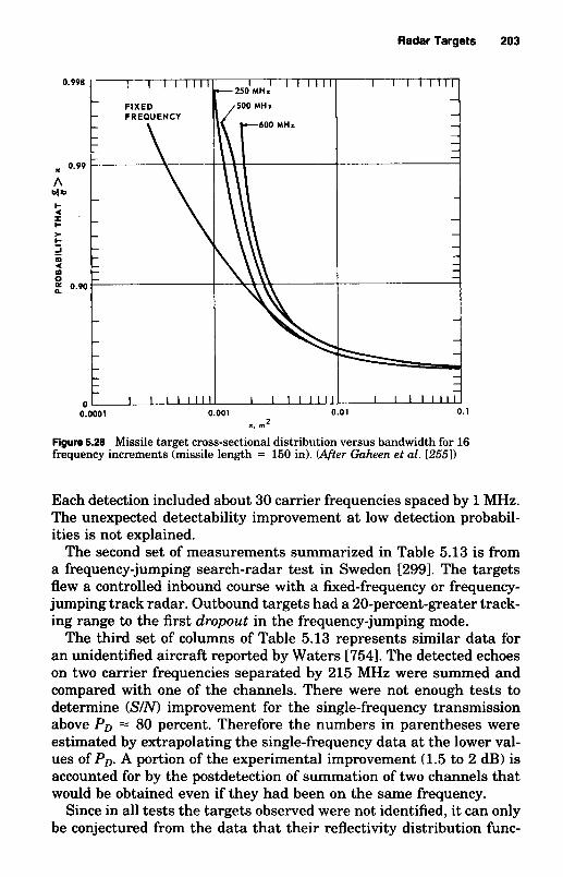
Radar Targets 203
0.990
= 0.99
A 01 4
I-
I c * c 1 m 4 m 0 E 0.90
0 0.0001 0.001 0.01 0.1
Figure 5.28 Missile target cross-sectional distribution versus bandwidth for 16 frequency increments (missile length = 150 in). (After G'uheen et al. [255])
I, m2
Each detection included about 30 carrier frequencies spaced by 1 MHz. The unexpected detectability improvement at low detection probabil- ities is not explained.
The second set of measurements summarized in Table 5.13 is from a frequency-jumping search-radar test in Sweden [2991. The targets flew a controlled inbound course with a fixed-frequency or frequency- jumping track radar. Outbound targets had a 20-percent-greater track- ing range to the first dropout in the frequency-jumping mode.
The third set of columns of Table 5.13 represents similar data for an unidentified aircraft reported by Waters [7541. The detected echoes on two carrier frequencies separated by 215 MHz were summed and compared with one of the channels. There were not enough tests to determine (SIN) improvement for the single-frequency transmission above PD = 80 percent. Therefore the numbers in parentheses were estimated by extrapolating the single-frequency data at the lower val- ues of Po. A portion of the experimental improvement (1.5 to 2 dB) is accounted for by the postdetection of summation of two channels that would be obtained even if they had been on the same frequency.
Since in all tests the targets observed were not identified, it can only be conjectured from the data that their reflectivity distribution func-

m .- 2
g Q
)
$2
83
g
e
2% Z
E
E 22
6s
s
m
m.9
ag
I
)+
c
W'5
2-3
.% f2$ Q
)
E E
B g
c&
.- E
$
2 0 gfi
?? $
f c
N$
$
cn .- 3
.- - - - m
C
- g
5 m
p.
al a
'Z;rd
U
Ee
"
$
c1
h
.- c cn
+a
E 4
3
* - .- - 8 9
c
al P N
$
6
+
zz
$
za
g
g
'?O$J
E w
cr) - g
"1
2
- 2s 4
m
*+
- c
a:? 4 g 32 2
4
8
f .g I
1) g.
= 3
2- g c 3
.!Ti gE
3
< *.2 h
d k 2
3.:
3 &
4
u)
4
0
3
E
Ii
c
C
.-
Q)m
m
W
8s
g3
4
m
204
. '%%
9L
oc
?"
.-- .t
-*
t-
hl
dd
u
!j * M
..
.
'.
.m2
0c
?%
p:
3 2 Y 6
.-
. . .t-
t-
mr
lo
*
..
.
e:
e
..
.
. 9
"g
p:
wo
..
tr:
..
e c 8 g
. .
w*
mm
..
b
..
&
Th
aiG
*h
lhlh
ldr
l- 2 2
f f 3 2! al
.- d
hl"
VT
0w
g :
.- * al
.-
-0
F c
qy
oL
-flwc
?c
'?
8 t-(D
*h
lh
lrlrlrl
a$
92 x
m
26
a)* a
m
0."
ala
&a
,N m
.
+*
2" 6 ?)
*oooooo
&"
tt WO
2
;2 m
Q)Q
)w
c-u
3m
- 2
2
- .. 'v)

I
MEASUREMENT - I - r 0.6 - a A L = 8.4m
0.4 - z- 0 F 0.2 - 0 z 3
- -4. -.
4
-
I I I I
I
MEASUREMENT - - -
A L = 15.2rn -
-- a

206 Chapter Five
the number and placement of the dominant reflectors on the target. In another paper, Gjessing, 12681 showed good agreement between theory and measurements on a 37.5-m cargo ship. He also showed that with his parameters, the echoes from sea clutter were mostly uncorrelated. He expanded on possibilities for target classification using Doppler, frequency agility, and polarization diversity as independent but com- plementary means of identifying an unknown target.
Figure 5.30 illustrates frequency correlation functions, p(Af), for tar- gets consisting of assemblies of discrete scatterers of varying number [1141. One extreme case with N = 2 shows an oscillatory correlation pattern; a limiting case is for N + m. When N is small, it is possible for p(Af) to achieve highly correlated values for sufficient frequency shift after a period of near-zero correlation. The frequency correlation pattern can provide information on the length of the target, as well as the radial separation of scattering centers. This information is a subset of what can be obtained in a coherent multifrequency system of the same bandwidth, but with a much simpler implementation (see Chap. 13).
Angle and range “glint” errors are also reduced with frequency agility, but it is more difficult to quantify the expected improvement. If the target can be represented by a line of scatterers perpendicular to the line of sight, there will be a time-correlated angle error signal for a single-frequency radar with the spectral energy of the error signal
0 0.20 0.40 0.60 0.80 1 .o A fUC
Figure 5.30 Frequency correlation functions for uniformly dis- tributed discrete scatterers of varying number along a length L. (From Castella and Redly, 1987 [114])

Radar Targets 207
concentrated near zero frequency.* Since the time constant of angle tracking loops is generally quite long, the angle error signals will follow the slowly varying phase front of the complex target echo. With several assumptions, as reported in [67, 4901, the spectrum of the angle error signals for a target of linearly distributed scatterers can be written
W , ( f ) = - 2 - - + - - - for f i 2 f m -
2fm rf2 ( f m 3f 3f2 f i f: f 3 )
= Oelsewhere
where 3 = mean-square value of perturbation signal U t ) f, = fon(L cos 0)/c fo = carrier frequency, Hz R = rotation rate of line target about its center (small angles
assumed) L cos e = L, = projection of target perpendicular to line of sight
The variance of U(t ) can be shown to be independent of R while the spectral width is proportional to R C671. Frequency agility essentially spreads the glint spectral energy outside the angle-servo bandwidth. Another way of viewing this effect is that frequency agility allows a number of independent samples of the angle of arrival to be averaged within the passband of the angle servos [2551. Methods of analysis of the reduction in angle error variance are given in [67, 5781. Under certain conditions the maximum reduction in the angle error variance due to glint can equal the number of frequencies transmitted. This assumes that the separation between adjacent frequencies is greater than clul , , where Lx is taken as the target projection perpendicular to the line of sight. Substantial glint reductions on both aircraft and ship targets have also been measured experimentally [2991. For the aircraft targets, the glint error signals up to 2 to 4 Hz were considerably reduced. With large ship targets the bearing errors were one-fourth to one-half as large with frequency-jumping as with single-frequency transmission. Range error fluctuations can also be reduced by frequency agility, which reduces the wander of the apparent centroid of reflection. For aircraft targets for which the length is comparable to the wingspan, the same amount of frequency shifting per pulse (=c/2Lo) improves detectability and reduces angle and range glint significantly.
This section has shown that in many cases frequency agility is de- sirable to modify target echoes and eliminate nulls in the RCS. It is
* Receiver noise is neglected in this discussion.

208 Chapter Five
shown in Secs. 6.6 and 7.6 that frequency agility can also decorrelate distributed-clutter echoes. By integrating these echoes, the RCS is made to approach its mean value while the variance of the clutter is reduced. This improves the signal-to-clutter ratio just as incoherent integration improves the signal-to-noise ratio.
5.10 Bistatic Radar Cross Section of Targets
A bistatic radar’s transmitting and receiving apertures are separated by a considerable distance. The major variation in a target’s bistatic cross section is due to the difference in the respective angles to the target, with range differences playing only a second-order role. There is relatively little data on the bistatic reflectivity of most targets of interest because the range of geometries is quite large relative to mono- static geometries, and because of experimental difficulties. Most bi- static RCS models are derived from available monostatic data.
From theoretical considerations, computer models, and reported ex- periments, we can define three regions for bistatic target RCS as a function of the bistatic angle, B.
1. A quasi-monostatic region where the bistatic angle is sufficiently small such that there is little shadowing of one portion of the target and any retroreflectors such as corner reflectors have the same RCS as the monostatic case. Crispin and Siege1 [1481 also restricted this condition to perfectly conducting and relatively smooth targets.
2. A bistatic region with larger angles such that there is some shad- owing. This would include conditions such as the reflections from the engines on the right side of an aircraft being shadowed by the fuselage when the receiver is viewing the aircraft from the left side.
3. The forward scatter or “forward-scatter enhancement region” near B = 180”.
Quasi-monostatic region
In the quasi-monostatic region, the monostatic-bistatzc equivalence the- orem is usually invoked. In this region the mean bistatic RCS is taken to be the mean monostatic RCS at the bisector angle. Monostatic RCS data or models are utilized while recognizing that there is considerable uncertainty. The equivalence theorem appears to be valid for small bistatic angles. The limits of “small” depend on the complexity of the target and the carrier wavelength. Consider the target to be receiving a plane wavefront from the transmitting antenna. It reradiates the energy as if the target were an irregular, but uniformly illuminated,

+ 5
0
m v -5.-
b' \
b" -10
-15
-k KANSAS U HELLENIC CHALLENGER
PHILLIPPEAN RIZAL
-- +
+ + A DELAWARE SUN -- + 8 .#
+A % A
e + 8 .
A a .- A t A
A A
A .-
+ i 1 I I I I I

210 Chapter Five
represents about as complex a target as will be encountered since the target size at X-band is over 1000 wavelengths. Willis [7781 suggests that this region be restricted to B < 5".
Bistatic region
In the region where shadowing and loss of retroreflectors are signifi- cant, the bistatic RCS is usually lower. The measurement on ships in Fig. 5.31 is one of the few data sets, but is probably representative of large complex targets. The calculated data on a 19-wavelength cylinder
35 55 75 95 115 135 ( A )
95 115 135 155 180
155
135
115
( E ) Figure 5.32 Calculated bistatic RCS, replotted as a function of bistatic angle p for a conducting cylinder (A) Near end-on; (B) 45" aspect; tC) broadside. (16 x 1.85 cm, 35 GHz, HH polarization). (From Ewe11 and Zehner 12141, 6) IEEE 1980)

Radar Targets 21 1
40 60 80 100 120 140
40 60 80 100 120 740
(C ) Figure 5.32 (Continued)
shown in Fig. 5.32 is an example of a simple but reasonably large target. If one reduces the backscatter from the nose, it could represent a small missile at L-band.
Without access to further data, one can only conjecture perhaps a 0.3-dB per degree falloff with bistatic angle from the ship data, with a maximum of perhaps 12 dB. In some target geometries, there will be an increase in RCS in this region. This will likely occur when the monostatic RCS is low as shown with the 45" aspect view of the cylinder. It is logical to predict that if radar-cross-section reduction techniques are used to reduce the "nose-on RCS" they will be less effective in the bistatic or forward-scatter regions.
Forward-scatter region
From an operational sense, the most important region for a bistatic radar is where the target is in a forward-scatter geometry. With the most common targets being aircraft, missiles, and ships in a nose-on aspect, there is a large specular reflection off the fuselage of an aircraft, the body of a missile, or the hull of a ship. In a near-nose aspect for the transmitter, the major forward reflections will be where 150 < B < 180". Siege1 1655, 6591 has shown that the maximum bistatic RCS in the forward-scatter region of a large, perfectly conducting body is 4.rrA'llx' where A is the projected area. Note that this is the product of the intercepted area A and the gain of an aperture having area A.
In the forward direction, the RCS falls off from the value at B = 180" depending on the size of the target. For a 3.2-wavelength sphere, the forward lobe is perhaps 2 lo", while for a 0.38-wavelength sphere,

0
f 9
.-
-
,Q
W
'W
,z
z
-c
'3
3
04
. -s;
z Y
:: 0) 'G
3.:
-A
i
00
,2
u
2 g
2
g"l 23: .!!!a
1,
11
11
1
* :-
00
00
~4
00
.9 .P
I7
79
rn
' w
rap 's3u w
rap 'sm sz
so
0-m
3
0
0
bod
r
nN
-
E 1 8. 4. P Q
Y
2 P P
Ly
-1
E U
2
L". It 0
0
s; t a *
0
00
00
~0
00
1
7-
79
r
n~
C
g~
~o
=O
Oo
I
77
9
wrap 'S3Y
0
wrap 'S3P
3 O
O
F
:$;E
4
ii c,
II II
B.2$ 4
21 2

Radar Targets 213
the lobe width is about 560". Observe that, in Fig. 5.32 where the incident aspect is 45", the monostatic RCS is relatively low as would be expected for a cylindrical target. Then note how large the RCS is in the forward region at 180" relative to the transmit energy. The lobe width is not shown, but is probably * 6". The values in this region are quite large relative to most monostatic aspects. The fall off from this region asB decreases is likely to be similar to the fall off from monostatic geometry.
Data from measurements and modeling at L-band are summarized in Chung-Chi Cha et al. [1161 for a missilelike shape that is 5 m long. Some results are shown in Fig. 5.33 with monostatic illumination and with a bistatic angle of 160". With nose illumination and a 160" bistatic angle, the RCS is measurably higher. From another figure, when the bistatic angle is increased to 170", the RCS is over 10 dB higher than the monostatic RCS. Figure 5.34 shows the results of the modeling technique versus carrier frequency for a bistatic angle of 10". Note the inverse RCS relationship with frequency in the 0.2- to 3.0-GHz region for this relatively sleek body.
I I I I O I I I I 1 1 1 1 I I
1 1 1 1 I I 1 1 1 1
20 l o o p RLOS + 10 - I I
+ HM * v v 0 -
5 -10-
y -20 - m 0
Iv)
I I l l I I I I l l I I
1 1 1 1 I I I I l l I I I I l l I I
I I I I l l I I I I 1 1 1 1 I I I I I 1 1 1 I I
-30 - 1 1 1 1 I I
-40 - :
-50 I , 0 0.01 0.1 0.3 0.5 1.0 3.0
--I_ FREQUENCY, GHz
MOMENT HIGH METHOD FREQUENCY
PREDICTION PREDICTION
Figure 5.34 Bistatic data across frequency (target length = 5 m; lower curve is fuselage alone). (From Chung-Chi Cha et al. 1116'1, I( IEEE 1988,

214 Chapter Five
Summary for large metallic targets
1. Use the equivalence theorem for B < 5" for targets that are large and complex. Use it for targets that are only a few wavelengths long to B = 10".
2. Use a value that decreases from the monostatic value at 5 - 10 < B < 90". The decrease from the forward-scatter region probably mirrors this.
3. The value near 180" is large and not easily estimated. If this ge- ometry is possible, calculations or measurements are required.
For a more complete treatment see the Willis chapter in the Radar Handbook [7781.
Chapter
6 Atmospheric Effects,
Weather and Chaff
F. E. Nathanson J. P. Reilly
Meteorological phenomena have two major effects on radar: the signals are attenuated by clouds, rain, snow, and the atmosphere itself; a relatively large signal is reflected from raindrops, hail, and snowflakes.* Attenuation becomes quite significant above X-band (9300 MHz ), but backscatter from snow and rainfall generally dominates the detection and tracking problem at frequencies down to L-band (1300 MHz). To compound the problem, the backscatter spectrum from precipitation and chaff is broadened because of wind shear, vertical fall rates, and air turbulence, all of which limit the ability of Doppler processors to separate targets from clutter on the basis of their relative velocities. The backscatter coefficient of chaff dipoles is shown to have much less dependence on the carrier frequency than precipitation echoes, but both have similar amplitude and spectral distributions. The equations and numerical values in this chapter apply to monostatic radars with linear polarization.
.j: For general references see NASA Publications 13611 12391 Atlas, “Advances in Radar Meteorology” 1251, Battan, Radar Meteorology 1481. and Doviak and Zrinc 11871.
21 5
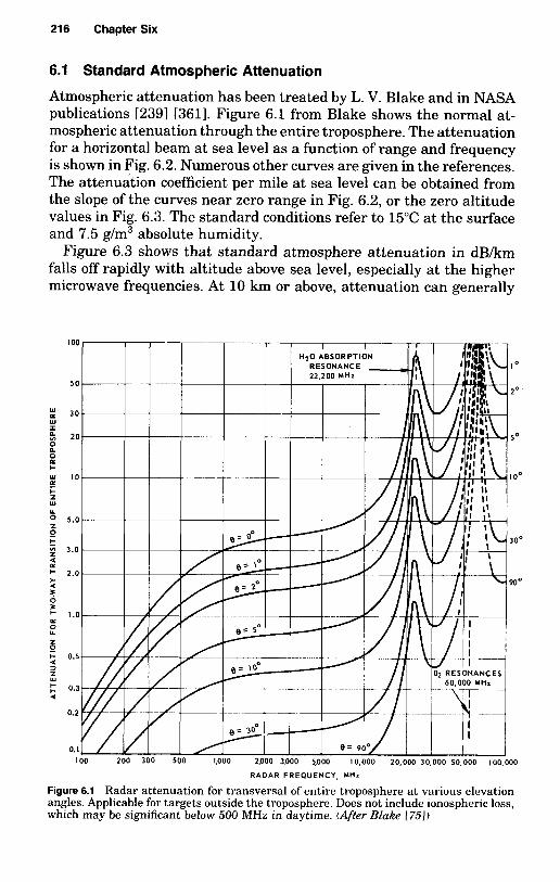
216 Chapter Six
6.1 Standard Atmospheric Attenuation
Atmospheric attenuation has been treated by L. V. Blake and in NASA publications 12391 13611. Figure 6.1 from Blake shows the normal at- mospheric attenuation through the entire troposphere. The attenuation for a horizontal beam at sea level as a function of range and frequency is shown in Fig. 6.2. Numerous other curves are given in the references. The attenuation coefficient per mile at sea level can be obtained from the slope of the curves near zero range in Fig. 6.2, or the zero altitude values in Fig. 6.3. The standard conditions refer to 15°C at the surface and 7.5 g/m3 absolute humidity.
Figure 6.3 shows that standard atmosphere attenuation in dB/km falls off rapidly with altitude above sea level, especially at the higher microwave frequencies. At 10 km or above, attenuation can generally
IO0
10
20 ' 5 0
k! 30
p 20 50 0"
w 10 100 I
I
0
I-
z Y
Y
0 5.0
0 t 30' 2 3.0 4
I- 2.0 > w o
r
+ 1.0
-
s
0 Y
z 9 I- 0.5 a
:: 0.3 4
0.2
z W
0. I 100 200 300 500 1,000 2,000 3.000 5,000 10,000 20,000 30,000 50,000 100.000
RADAR FREQUENCY, MHz
Figure 6.1 Radar attenuation for transversal of entire troposphere at various elevation angles. Applicable for targets outside the troposphere. Does not include ionospheric loss, which may be significant below 500 MHz in daytime. (After Bluke 1751)

C!
.0
oo00.
\
zHW
'AJN
3nO3H
:I H
YO
YH
o 0
0 0
0 0
8o
0 0
0 ,0
0 0
0,0
o 0
0."
..,"' -~
o
."
~-
a
...; ...
gp 'H
OI.LY
nH3.L.LY
A
YM
-OM
.L
\
8...o0M
oo"'
o0-00..,
....,
~No
~~
~oooOd:,0
Ec .
QI
o .'bc
~
W
~-~
~
C
~1-
O"'
.~-+
"Q
~
1- >
W
~"
QI
~
;.,C
~
1- ~
o O
o
N
1- S
-~
~C
o
Q
.~
C
~~
::!~Q
I+
"
~"'.~Q
Io
.t:.0
~"'o8~~~~~~C'!~
o ID
~G
I .,
..~~
"01-
ii:~

218 Chapter Six
0 10 20 30
ALTITUDE, krn
Figure 6.3 Variation of the total absorption coefficient in the standard atmosphere as a function of altitude for several frequencies. Includes oxygen and water vapor. (From Blake L751)
be neglected above 10-km altitude to at least 35 GHz. Values for higher carrier frequencies and other humidities can be found in Blood and Crane [781 and numerous other sources.
6.2 Precipitation Occurrence and Extent
Before exploring the impact of attenuation and reflectivity of meteo- rological scattterers, it is necessary to model their occurrence and ex- tent. As with other natural phenomena, there is extreme variability in time and geographic location, as well as altitude, season, and other factors.
The common rainfall descriptors are:
Type Rainfall rate, r in mm/h
Drizzle 0.25
Moderate rain 4.0 Heavy rain 16.0 Excessive rain >40.Q
Light rain 1.0

Atmospheric Effects, Weather and Chaff 219
The National Weather Service defines the following levels for me- teorological radars:
Level 1 1.52-6.09 rnmh Level 2 6.09-25.9 rnmh Level 3 25.9-53.1 rnmh Level 4 53.1-114.3 mmh Level 5 114.3-180.3 rnmh Level 6 180.3- rnmh
In earlier times, radar specifications often indicated merely an “all- weather” capability. Specifications for modern target detection radars generally should define widespread rainfall rate as well as a high rain- fall rate applying to a smaller area. In designing or evaluating a pro- posed system, one also requires an indication of the height profile of the rain and its spatial uniformity. For Doppler radars the wind velocity profile and local wind shear conditions are also required.
Statistical data on rainfall rate is summarized in Table 6.1 and Fig. 6.4. The table indicates that the probability of a rain exceeding 1 mm/h varies only from about 1.5 to 3.8 percent of the time from arid to wet areas. However, the probability of occurrence of greater than 20 mm/h varies by several hundred to one. It is shown in later chapters that design of air defense, air traffic control, or multimode airborne systems is quite different with anything near a 20-mm/h rainfall rate. It is also a question as to the “enemy’s’’ ability to operate in such an environment. Military and civil surveillance radars usually specify widespread 1- to 4-mm/h rain and sometimes a storm of perhaps 16
TABLE 6.1 Instantaneous Rainfall Probability in Various Locations in the World, %
Probability that indicated rainfall rate is exceeded, %
Light Moderate Heavy
Paris, France 1.6 0.74 0.22 0.001 Washington, D.C. 2.5 1.5 0.68 0.07 England (eastern) 2.4 1.5 0.65 0.004 Saigon, Vietnam 2.4 1.7 1.0 0.21 Turkey 1.5 0.7 0.25 0.01
1 2 4 20 mmh
Tokyo, Japan 3.2 2.0 1.2 0.24 Ceylon” 3.8 2.8 1.9 0.48 New Orleans 3.0 1.7 1.2 0.37 Worldwide average 1.6 1.0 0.47
’:’ Worst location noted. Maximum altitude for radar purposes 25,000 ft (7.5 km). Typical maximum altitude excluding thunderstorms 12,000 ft. NOTE: See also 197, 119, 3661.

m
(SlD
*Ja
W! *IJ
no
’0 33
VlN
33
M3
d S
n0
3N
VlN
VlS
NI
ii
220

- - - - - -

222 Chapter Six
(13611)
f E 100 E w'
z a LZ 50
I-
d
0 0.001 0.01 0.1 1 .o 10.0
PERCENT OF YEAR RAIN RATE EXCEEDED
Figure 6.7 Point rain rate distributions as a function of percent of year exceeded. (13611)

Atmospheric Effects, Weather and Chaff 223
varies considerably with geographic location. Europe has fewer heavy rains than southeast Asia, for example.
The height distribution of rain is also an important parameter when estimating attenuation and reflectivity. In general, rain reflectivity and attenuation decrease with height above the ground. One relationship for the falloff in intensity is rh, = exp( - 0.2h2) where r, is the surface rainfall rate and h is height in kilometers [5931. In a second model the constant is 0.036. A third model from Fordon [2421, for light to moderate summer mid-latitude rains, is illustrated in Fig. 6.8. Konrad [408] and Goldhirsh [275] made a number of measurements with well-instru- mented radars. While the individual measurements gave rather erratic height profiles, the averaged median height profiles for summer storms are illustrated in Fig. 6.9. These represent reflectivity rather than water content. (The meaning of dBZ is explained later.) The effective height of the thunderheads is a variable, but the reflectivity often increases in the 2- to 6-km level. However, in many cases a specification of rain extending uniformly to a 4-km height is adequate. In some cases a linear falloff to about 6 km is added.
0.0 0.0039 0.0078 0.0117 in./hr 0.0 0.1 0.2 0.3 mm/hr
0 1 2 3 4 5 6 7 8 9 10 11 mm/hr 0.039 0.078 0.117 0.156 0.195 0.234 0.273 0.312 0.351 0.394 0.433 In./hr
Figure 6.8 Estimated distribution of precipitation rate with height for summer rain in middle latitudes, for four values of estimated maximum updraft (specified in m/s by each curve). (From Fordon 12421)
PRECIPITATION RATE
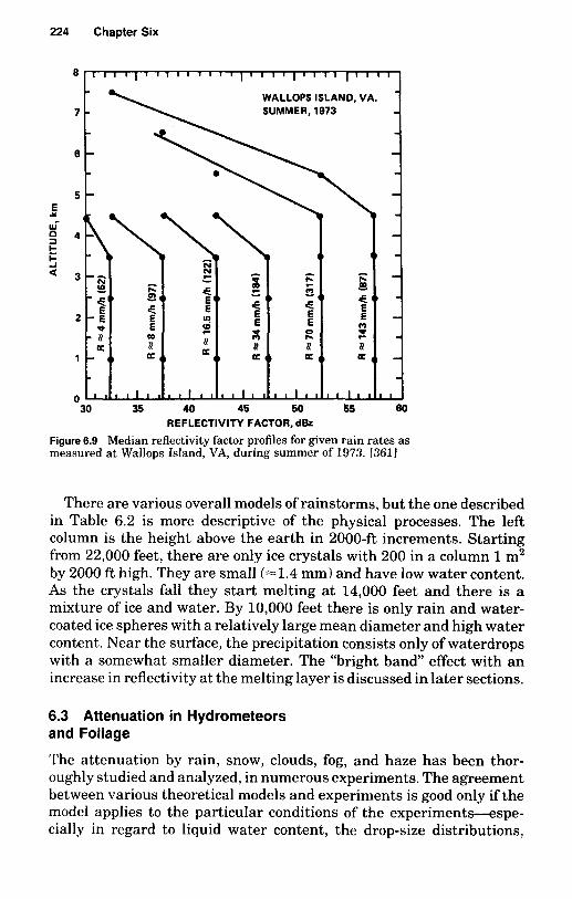
224 Chapter Six
0 - 1 1 1 1 1 , I 1 I I I , I , I , I f , , I 1 I 1 1 1 I I I - WALLOPS ISLAND, VA. SUMMER, 1973 -
-
- 5 -
- 4 1 -
- 30 35 40 45 50 65 Bo
REFLECTIVITY FACTOR, dBz
Figure 6.9 Median reflectivity factor profiles for given rain rates as measured at Wallops Island, VA, during summer of 1973. [361J
There are various overall models of rainstorms, but the one described in Table 6.2 is more descriptive of the physical processes. The left column is the height above the earth in 2000-ft increments. Starting from 22,000 feet, there are only ice crystals with 200 in a column 1 m2 by 2000 ft high. They are small (-1.4 mm) and have low water content. As the crystals fall they start melting at 14,000 feet and there is a mixture of ice and water. By 10,000 feet there is only rain and water- coated ice spheres with a relatively large mean diameter and high water content. Near the surface, the precipitation consists only of waterdrops with a somewhat smaller diameter. The “bright band” effect with an increase in reflectivity at the melting layer is discussed in later sections.
6.3 Attenuation in Hydrometeors and Foliage
The attenuation by rain, snow, clouds, fog, and haze has been thor- oughly studied and analyzed, in numerous experiments. The agreement between various theoretical models and experiments is good only if the model applies to the particular conditions of the experiments-espe- cially in regard to liquid water content, the drop-size distributions,

0
3 ?i +.
+.
.- I E > 0
'0
0 a - z .- C 2 3 2 W
-I
m
L *
m
S8
E y
qC
?'9
(9(9
m oooooo
- mi
rA U
EE
rlc
ue
4m
mm
3 9
2%
"1
oq
q
c =$
C
I
%N
24 zi
8 $2 V
YX
x~
z~
! B 8%
3; E
z~
~~
yy
~
2 3.p
22
00
00
00
E.2
c
u~
cu
mc
ur
l o
om
om
m
i
22
a
$ 2
%
gg
gg
gg
gg
32 g$
rlm
lom
mm
mm
ZII
E=: xd
l &a .5
G
%?J B
kZ
2%
d2
0 N
om
ww
cu
om
cD
*c
uo
8
2
ZmO N
cu
rl
rl
rl
rl
4
rng .%Oh 2
2
s
g$
- iiz
E %
$
OE
a2
ZB
%d
OL

226 Chapter Six
TABLE 6.3 Typical Characteristics of Hydrometeors
Typical Typical Density Diameter Drops Reflectivity base, top, liquid, droplets, Per z,,
m m g/m microns m3 dB
Haze 0 1500 .001 0.1 lo8 Fog (radiation) .04 10 2 x 10”
(advection) 0 50 .15 20 4 x 10’0
cumulus 500 1000 .50 20 1 O8 - 30 Fair weather
Stratus (heavy) 500 1500 .3 10 - 12 Cirrus High .17 170 14 Cumulus
Cumulonimbus 2.5 100 9 Rain (lmm/h) 0 4000 .06 310 26
Congestus 1600 2000 .a0 40
SOURCE: After Refs. 1720,266,5041.
temperature, and spatial uniformity of the path. Attenuation in rain and snow are the primary concern in the higher microwave regions with clouds, fog, and haze becoming important at 35 GHz and up. Radar is increasingly being used in various forms of sensing as the attenuation in the optical regions is frequently excessive for most missions. A gen- eral description of various forms of hydrometeors with typical para- meters is illustrated in Table 6.3. These are only representative cases- as fog can have a wide variety of visibilities; cumulus clouds come in various densities, etc. There is a wide range of drop sizes (the median or mode of the distributions shown here), number, and the density of the total liquid water. In later sections it is shown that the larger drop diameters dominate the reflectivity.
Attenuation in rain
The attenuation of electromagnetic waves in a uniform rain is usually significant above 2 GHz, and is proportional to the 2.3 to 2.8 power of frequency when the droplets are small compared with the wavelength. In this region the attenuation coefficient k is often expressed as
k = arb dB/km
where r is rainfall rate in millimeters per hour and a and 6 are constants that depend on many variables, including frequency, polarization, and temperature.
There have been numerous measurements programs with many of the early ones summarized by Medhurst [4711. His summary showed that the measured attenuation was higher than the theoretical work of Gunn and East 12981 especially at the lower rainfall rates. Since that time, it has been pointed out by Crane [1451 that the “point”

Atmospheric Effects, Weather and Chaff 227
100- ' ' ' ' " ' ' ' 1 ' ' ' 1 ' ' ' ' ' I ' ' ' ""'L
150 mm/h 50 -
20 -
E l o r f
6 9 kk 1r 5
o_ $ 0.2 - 5 E 0.1 I-
U 5 -
Q
c 2 -
: 0.5 1 c
- < -
0.05 -
0.02 -
0.01 1 I , I l l I I I I I I I , ,
1 2 5 IO 20 50 100 200 500 1000
FREQUENCY, GHz
Figure 6.10 Attenuation coefficient as a function of rain rate and frequency. (CCZR, 1986 [3611 [2391)
measurements tend to exceed the path average for low rainfall rates at lower precipitation levels. In addition, the humidity tends to be higher in rain. In the interest of standardization, it is suggested that the 1986 CCIR (International Telecommunications Union) model de- veloped for communication systems be used, as there are many studies in the past 20 years that went into that model. It is shown in Fig. 6.10 and detailed constants on Table 6.4. The subscripts H and Vcorrespond to horizontal and vertical polarization. The differences in these values lead to the elliptical polarization of attenuated signals described in the discussions on circular polarization in Chap. 5. In other, more detailed studies a values are lower and b values are higher for rainfall rates above about30 mm/h.
Attenuation in clouds
The attenuation in clouds varies greatly due to the extreme variation in densities. The basic relationship is

228 Chapter Six
TABLE 6.4 Specific Attentuation Coefficients'
Frequency, GHz aH a v b H bv
1 0.0000387 0.0000352 0.912 0.880 2 0.000154 0.000138 0.963 0.923 3 0.000650 0.000591 1.121 1.075 6 0.00175 0.00155 1.308 1.265 7 0.00301 0.00265 1.332 1.312 8 0.00454 0.00395 1.327 1.310
10 0.0101 0.00887 1.276 1.264 12 0.0188 0.0168 1.217 1.200 15 0.0367 0.0347 1.154 1.128 20 0.0751 0.0691 1.099 1.065 25 0.124 0.113 1.061 1.030 30 0.187 0.167 1.021 1.000 35 0.263 0.233 0.979 0.963 40 0.350 0.310 0.939 0.929 45 0.442 0.393 0.903 0.897 50 0.536 0.479 0.873 0.868 60 0.707 0.642 0.826 0.824 70 0.851 0.784 0.793 0.793 80 0.975 0.906 0.769 0.769 90 1.06 0.999 0.753 0.754
100 1.12 1.06 0.743 0.744 120 1.18 1.13 0.731 0.732 150 1.31 1.27 0.710 0.711 200 1.45 1.42 0.689 0.690 300 1.36 1.35 0.688 0.689 400 1.32 1.31 0.683 0.684
* Values for a and b at other frequencies can be obtained by interpolation using a logarithmic
SOURCE: Ref. [3611. scale for a and frequency and a linear scale for b.
A = k$ dB/km (one way) (6.2)
where k, is the attenuation coefficient given in Fig. 6.11 and D is the liquid water density in gm/m3 [681, p. 6-631.
The attenuation constant, A, is about 25 percent higher for saltwater clouds. Values of D generally fall in the range of 0.05 to 0.25 for strat- iform or layered clouds and 0.3 to 1.3 for dense stratocumulus clouds, and averages about 2.5 for cumulonimbus (rain) clouds. For water clouds, A varies approximately as f", and for ice clouds, the attenuation is 1 to 3 orders of magnitude less and varies as f.
Attenuation in snow
Attenuation in dry snow is about 20 to 50 times less than in melted drops with the same fall rate in millimeters per hour. However, when the snow is melting, the attenuation can be even higher than rain. In

Atmospheric Effects, Weather and Chaff 229
10 - - - - - - - 6 7
m I
0 50 100 150 Figure 6.11 Attenuation coefficient K, due to water droplets. (From CCZR 1982 Rpt. 721-1)
one model in a 0.3-km-thick melting layer, the attenuation was pre- dicted to be 0.54 dB at 13.6 GHz, 3.7 dB at 35 GHz, 6.75 dB at 94 GHz, and 8.5 dB at 140 GHz [5041.
Attenuation by fog, haze, and clouds
Attenuation by fog and haze is dependent on droplet size, density, and temperature. At millimeter wavelengths the drop-size distribution it- self is not critical. As with rain there is a wide variety of densities. Haze droplets are the smallest, with sizes from 0.01 to 3 microns, and thus do not cause significant attenuation even a t millimeter wave- lengths.
Radiation fog that forms over land has droplet diameters of 5 to 35 microns and densities of about 2 x 10"/m3. Advection fog that forms over water has droplets of 7 to 65 microns and an average diameter of 20 microns, but lower densities of 0.4 x 10" are observed. The ad- vection fog is the type usually described in the literature [595, 2861. A table of the typical forms is shown as Table 6.3.

230 Chapter Six
Richard [5951 summarized the attenuation measurements at 20°C. He gives a value of 0.12 dB/kdgm/m3 at 15 GHz, 0.55 at 35 GHz, 3.3 at 95 GHz and 7.0 at 150 GHz. An empirically derived relation for visibility (V) in kilometers as a function of liquid water content (MI in g/m3 was given as
V = 0.024 M p o 65 or M = (0.024/V)1 54
A relationship for fog attenuation coefficient A, (above 30 GHz), is [3611
Af = -1.347 + 11.152/f + .06f - .022T dB/km/g/m3
where f is the frequency in GHz and T is in degrees centigrade.
Attenuation by foliage
The radar detection of personnel and land vehicles involves the major problems of clutter echoes from the terrain and cultural features, the attenuation resulting from natural or man-made obstacles and wooded areas, and forward-scatter phenomena. If the radar has sufficient sen- sitivity, the detection range can be computed with the land clutter reflectivity values of Chap. 7 and the equations of Chap. 2. To determine sensitivity, the attenuation due to foliage must be determined.
The wide diversity in the types and density of foliage makes the estimate of attenuation highly variable. Early studies were summa- rized by Saxton and Lane [6331 at frequencies from 100 to 3000 MHz. They found that for either polarization the one-way attenuation by trees with leaves in that frequency region was given by
A = 0.25pdB/m (6.3)
where f i s the carrier frequency in GHz and y = 0.75. This relationship and more recent ones are shown in Fig. 6.12. Recent experiments at Georgia Tech Research Institute [152, 7771 confirmed the general de- pendence between 9 and 95 GHz, with a higher constant for summer conditions and dry foliage, and a lower constant for winter. However, the exponent, y was only about 0.3. Other results with a lower constant have been reported [239, pp. 5-191.
There is greater confusion about the effect of the depth of the foliage and the related frequency dependence. This is summarized in Ulaby 17201. The CCIR report adopted the following relationship for com- munication calculations where the antennas are close to a grove of trees:
A = 0.2f03d06 dB/m (6.4)

0.4 ~ 1 1 1 1 ' 1 i ' ' ' 1 ' 1 1 1 1 I I
POLARIZATIONS V
Z 0.3 - - 0 I-
z e 0.2- - 2 2 VERTICAL Z
-
0 - 1 1 1 1 1 1 1 I ' ' " ' ' ' 1 1 ' 1 ' " " 1 1 -

232 Chapter Six
While the phenomena are quite different, rain and chaff appear sta- tistically similar to a radar. The amplitude distributions are Rayleigh whether there are 10 or lo6 raindrops or chaff dipoles in the radar volume. Both are excellent tracers of the horizontal winds, and while the fall rate of rain is higher (up to 9.6 m/s for large drops), this primarily affects vertically pointing radars.
The backscatter from precipitation particles can be represented by a random assembly of scatterers, no one of which has a dominant effect on the sum. The RCS of the random assembly may be derived by assuming that the relative phase of each scatterer’s return is statis- tically independent of the others and is uniformly distributed between 0 and 27r. This is an example of the two-dimensional “random walk” problem in which each step is 6. This, in turn, leads to the well- known Rayleigh power relation.
The relation for the volume reflectivity of rain, where the droplets are small compared to the radar wavelength (in the Rayleigh region), is
Xu = q = T’ A - 4 IKI2 CD6 mP1 (6.5)
where A = the carrier wavelength. D = the droplet diameter. K = related to the complex refraction index and is a fairly
constant 0.9 over the microwave region for rain, and is about 0.2 for snow.
The units of Xu or q for target detection radars are m2 of equivalent radar cross section per m3 volume or m-’. At times q is given in other units and conversion must be made.*
While these units can be used for weather radars, the meteorological community uses Z for theoretical calculations of reflectivity, and 2, is often used for empirical or experimental data. The term 2 includes the wavelength dependency and is expressed in mm6/m3. It is usually ex- pressed in the form
Z = arb (6.6)
where r = rainfall rate in mmh.
The most representative relationship used by radar and radar mete- orology texts 1671, 25, 481 is
2 = 200r’.6 (temperate latitudes) mm6/m3 (6.7)
* The Xn merely states that the reflectivity is the vector sum of the reflected signals from each droplet.

Atmospheric Effects, Weather and Chaff 233
An alternate relationship, proposed by Atlas [251, is 2 = 214r1.39. Measurements of Florida rains have fitted the equation 2 = 286r1.43 and in Indonesia 2 - 311r1.44 [4941. The lower values of the exponent in other experiments [251 generally correspond to microwave frequen- cies above X-band with drop size large with respect to 0.1 A. Measure- ments at 35 GHz and higher place the exponent between 0.95 and 1.35; values for the constant term increase to almost 1000. Godard 12701 suggests an exponent of 1.2 at 35 GHz.
The 2 relationship is not in a useful form for radar system evaluation. A conversion factor to pulse radar received power, attributed to J. R. Probert-Jones [5631, is
'
1.1 x 10⁻²³ PtGtG,O+~ZL, X2R 2
(6.8) P, =
including the beam shape losses where in the units of the reference
Pt = transmitted pulse power, W.
P, = received pulse power, W.
Gt, G, = antenna gains, dimensionless.
e,+ = one-way, half-power antenna beamwidths, degrees.
R = range to clutter cell, nmi.
A = wavelength, cm.
r = effective pulse duration, ks.
2 = reflectivity, mm6/m3 (2 is not wavelength dependent at low
La = atmospheric and rain attenuation, two way (a negative value
frequencies in the Rayleigh region).
in dB when this loss term is in the numerator).
The ratio of returned power from a target to the returned power from the clutter can then be derived from the classical radar equation (see Chap. 2 for a clearer description of loss terms).
(6.9) Prain 8+rZR2
whereK = constant (primarily to keep units consistent, -200 de- pending on antenna pattern and assuming 3 dB of beam shape loss on both target and clutter); it also includes the refractive index for rain.
ut = target cross section, m2.
- - Ptar KA4ut -

234 Chapter Six
Since [ ( I T / ~ ) ~ $ T R ~ ] is the volume of the range cell (not in consistent units) and 2 is the parameter generally used by radar meteorologists, it has been found that a more useful form for the radar target-detection criterion, where receiver noise power is small when compared with clutter power, is
1010atLA4 (6.10) - RZ = UtL -
('iT/4)$e(CT/2)(S/C));a 284(n/4)+8(s/c)zT
where beam shape losses for the target and the rain are assumed equal.
(SIC) = the signal-to-clutter ratio for a given probability of detection (S/C is = 13 dB for a typical single-pulse surveillance radar with detection probability = 0.5 and false alarm probability = 1o-8).
e,$ = one-way, half-power antenna beamwidths, radians. c7/2 = effective pulse length, m.
ut = target cross section, m2. Za = backscatter coefficient, m2/m3, including wavelength effects.
L = processing losses appropriate to the rain backscatter case. T = pulse duration, s. A = wavelength, cm. R = target range, m, assuming that the rain fills the volume of the
range cell occupied by the target.
Table 6.5, derived from both theoretical and experimental data, gives Ca versus frequency and type of precipitation. Interpolation between
TABLE 6.5 Reflectivity of Uniform Rain, q or Pa m2/m3
Ztr, dB m - ' Transmit frequency, GHz
Z Radar band: S C X K, K;, W mm (dB) Type 3.0 5.6 9.3 15.0 35 95 140
- 12 Heavy stratus clouds -100 -85 -69 -62 14 Drizzle, 0.25 mm/h -102 -91 -81 -71 -58 -45" -50% 23 Light rain, 1 mm/h - 92 -81.5 -72 -62 -49 -43" -39'': 32 Moderate rain, 4 mm/h - 83 -72 -62 - 5 3 -41 -38" -38* 41 Heavy rain, 16 mm/h - 73 -62 - 5 3 -45 - 3 3 -35* -37*
'> Approximate N(Y~E: Recent experiments and theory have reduced the reflectivity at frequencies above 30
GHz relative to earlier predictions. Theoretical values at 35 and 95 GHz revised as per Crane and Burke and other considerations.

Atmospheric Effects, Weather and Chaff 235
10-2 p
BACKSCATTER MODELS
L 8 P LAWS 8 PARSONS I -- M-P MARSHALL-PALMER Rain Rare E -
------- --
---- ------
20 30 40 50 GO 70 80 90 100
FREQUENCY, GHz
Figure 6.13 Reflectivity versus frequency for rain. (Crane and Burke 11461)
radar bands on the table should be as X4 except for the highest fre- quencies and rainfall rates. Interpolation between the rainfall rates under the same restrictions should follow an r1.6 law.
Values for reflectivity in the millimeter wave region, developed by Crane [146], are shown in Fig. 6.13. It shows two curves based on the two common drop size distributions. Since drop-size distributions vary considerably with location, temperature, etc., the reflectivity is more variable in the millimeter wave region (35 GHz up). The peak and then fall in reflectivity is due to the droplet circumferences reaching and then exceeding the wavelength. Richard [5951 summarizes measure- ments in Florida rainstorms of the short, heavy shower type, and gives the following relationships for 2- to 100-mm/h rainfall rates. If average reflectivity from Eq. (6.6) is expressed in m- ' Frequency a b
9.4 GHz 1.0 x 10 x 1.52 35 2.2 x 10 6 1.05 70 1.4 x 10 4 0.59 95 8.9 x 10 R 0.57

236 Chapter Six
Note that the 70-GHz reflectivity is higher than both the 35 and 95 GHz for most of the rainfall-rate region. The 35- and 95-GHz data generally agree with Crane’s curves. There is considerable uncertainty in this data set, which is discussed in Currie, 1988 [153].
Fog reflectivity is generally not significant, but some relations can be found in Gossard and Strauch [286, 2881.
The 2 - r relationships reported for snow vary from 500r’ 6 for ice crystals to 2000r2.’ for wet snowflakes, where r is the rate, but now refers to the water content of the melted snow in millimetershour. In converting the 2 - F relationship to backscatter power, the substan- tially lower refractive index (about one-fifth) of ice and snow reduces the backscatter power by a factor of 5 for a given value of 2. Battan [48] indicates that snow causes about twice the backscatter of rain of the same water content at 1 mm/h and 3 times the backscatter at 3 mm/h. A single set of measurements by the author gave the same ( + 2 dB) backscatter at C-band for a uniform snow as would be cal- culated for a uniform l mm/h rain from Eqs. (6.7) and (6.8). The values of Xu for stratus clouds in Table 6.5 are useful only as models since there is no uniform description of clouds. A series of measurements of the reflectivity for clouds has been reported in the U.S.S.R. and is abstracted in Table 6.6 [543]. The mean value of reflectivity, the vari- ation, and the mode are given for several cloud types along with several vertical profiles. It should be noted that most of the values are higher than earlier estimates [6711. Reflectivity from rain clouds (Ns) is only about 3 dB below that of l-mm/h rain at the freezing level.
Reflections from clear air
So-called “radar angels” and “anomalous echoes” are observed by radar operators on an almost regular basis. Because of their generally small radar cross section, they are normally limited to relatively short ranges on aircraft surveillance radar. The operator of these radars usually learns to recognize and discriminate against clutter returns. On the other hand, the modern generation of radars is becoming more con- cerned with quick reaction, automatic detection, and data processing of small radar cross-section targets, such as missiles, mortar or artillery shells, bullets, and small ground vehicles. In these systems, the high cross-section target and human recognition discriminants against sky clutter no longer exist. Furthermore, the great expense of these systems makes it increasingly important in early radar design and testing phases to be aware of the data processing and false alarm problems imposed by the natural environment.
Even in air traffic surveillance, radar angels may in fact present a much greater problem than is generally recognized, since there is no

u) D a 0
0
- & a+ c.
c
u) .- .- a r
>
3 0
al d 3 3 c)
.- .- c E
w
A
m
4- e
ao
om
ou
3m
w-
Ne
I&
mu
jai&
nim
-&&
uj,
“C
-ac
oN
e
2 3 * ?
ZZ
m
2
(D
5
SE
W“
I
E u
3m
mm
oo
oo
oo
22
GJ :s
g5
;gg
gg
s’7
00
o
m
OC-
e
E *-
00
00
00
00
00
n
&?
“+
.lr(r(
00
00
0
IN
“4
c?
c?
c?
2 z
0
00
1
z 22 0
0
x I
s
00
00
0
2 6
.I
mzzzz
c%
(D
8g
5
NE
N
om
t-
00
-
&? IN
v?v?22 h
m
ow
ec
o
$2
69
g 55 (o
0
0
72
O
P
00
m
w
1-
NE
w
e
I s
00
00
0
6 %G%%8
&?
9 .E IN
2
88
88
-
G o
em
~
V
6
22% o
a
4 5 9
2E
zg
g
.i 4
22
$ .z E
9 m‘
k
a 7
ZZ-2 0
GSG
-c
o
.e
.- g $2
m
a
aE
ZE
g
nu
z
z 8
Z*-E
*- @
4si
--c ’C
I1.F
; m
.!qE
.-
mt:o
“M
E.%
IN
mg
-2
<
v
E *e
$$
?&
-33:gz
z 4-
m
Em
;s
.- *
mm
mw
z
tl. *
Ha
c-t-t-
m
rn 0
0
00
o
m
.- o
z
“E
O
aw
I j
00
00
0
WN
co
eO
o
c
*
z
-6.2 5$ $
E2
3
IN
2“ cn
&E

238 Chapter Six
way of knowing how many small planes have been mistaken for a flock of birds, and vice versa. Even after an accident has occurred, it is probably impossible to trace the underlying cause to this type of oc- currence.
Some years ago a Soviet MIG flown by a defecting pilot penetrated the U.S. air defenses and landed unhindered in Florida. This plane was spotted, briefly, on radar but went unreported. The radar operator was reported to have confessed that brief detections of this sort occur rather frequently. This is perhaps just a single example of an unrec- ognized but commonly occurring error. Surveillance radars in Florida often detect clear air echoes, and can track these echoes for minutes. The tracks have a “wiggly” character and are sometimes referred to as “worms.”
It seems clear that several distinct types of sky clutter must be considered to model a nominal echo environment. Depending on radar characteristics, operation, and location, any of these may prove to be the most important. The first, and usually most important, is the large cross-section, discrete, “dot angels.” They are generally attributed to birds and insects in the atmosphere, but may be due in part to other particles. They have grossly differing velocity, density, variation-in- activity, and wavelength characteristics. Actually, the small cross-sec- tion variety of discrete scatterers is more important in terms of a distributed phenomenon, since, in the cases of greatest concern, they occur in such density as to be unresolved by the radar resolution cell a t all but very short ranges. A distributed meteorological backscatter phenomenon is included as a second distinct type of sky clutter, at- tributed to turbulent layers. A major cause has been shown to be the inhomogeneities in refractive index that result from turbulence. The radar reflectivity is proportional to the turbulent structure constant of refractive index (Ct). This is a complex subject and evaluation of its occurrence impact is described in Gossard [2861, Strauch 12881, and Doviak and Zrinc [1871.
The difference between the frequency effects of particulate matter and refractive effects, is illustrated in Fig. 6.14. While values of C; exceeding Ca = 10 ~ l2 have been reported for thin layers, even 10 l4
or lo-’5 is not very common. The changes in refractive index are also responsible for various ducting conditions. Ducting often causes radar rays to curve downward, and land and sea clutter that is normally beyond the horizon is clearly seen on ground-based surveillance radars. Ducting over the ocean is common and is described in Chap. 7.
Auroral clutter
In the Arctic regions there is significant reflectivity from the aurora, especially a t low carrier frequencies. This clutter is primarily applicable

Atmospheric Effects, Weather and Chaff 239
PARTICULATE SCATTERERS
-
.- I E 6
BACKSCATTER
0.01 0.1 1 10
Figure 6.14 Backscattering cross section versus wave- length for particulate scatterers and for Bragg back- scatter. The refractive index structure parameter C i is a measure of the turbulent fluctuations in n if the im- portant scale ( U 2 ) lies within the inertial subrange of homogeneous isotropic turbulence. (From Gossard and Struuch [286, 2881. Elsevier Science Publishers, 1983)
A, m
to long-range radars since it exists as a layer at about 110 km above sea level. Reflectivity is highest a t VHF frequencies and reduces to about ZIJ = l o p 9 at 400 MHz and lop11 a t 1.3 GHz. There is a Doppler shift of several hundred d s .
6.5 Radar Precipitation Doppler Spectra
It is convenient to describe the Doppler spectra of radar signals re- turned from clouds or precipitation by four separate mechanisms (Atlas [25, p. 4051 Doviak [1871.
1. Wind shear: The change in wind speed with altitude results in a distribution of radial velocities over the vertical extent of the beam.

240 Chapter Six
2. Beam broadening: The finite width of the radar beam causes a spread of radial velocity components of the wind when the radar is looking crosswind. There is a similar but smaller component in the vertical plane.
3. Turbulence: Small-scale fluctuating currents of the wind cause a radial velocity distribution centered at the mean wind velocity.
4. Fall velocity distribution: A spread in fall velocities of the reflecting particles results in a spread of velocity components along the beam. The maximum fall rate is about 9.6 m/s in the absence of downdrafts.
A fifth mechanism may be considered in a system using a rotating or moving antenna (see Chap. 9). This mechanism is independent of the characteristics of the precipitation itself and is not discussed in this chapter. If we assume that these mechanisms are independent, then the variance of the Doppler velocity spectrum a: can be repre- sented as the sum of the variances of each contributing factor"
(6.10)
Although independence is not strictly satisfied, Eq. (6.11) nevertheless provides a useful approximation. The spectrum width is given in ve- locity units, d s ; for most radar frequencies the spectra can be converted to frequency units through the Doppler equation. In practice a single Doppler spectrum may not look gaussian, but may appear like those illustrated in Fig. 6.15.
Wind shear
Although wind shear (the change in wind velocity with altitude) has long been known to meteorologists, its effect on precipitation spectra
2 2 d = &ear + ubeam + uturb -k uFa11
* The power spectral density function of sea, land, or weather clutter is often described I341 by a gaussian spectrum having a stability or spectrum parameter a defined by
G( f ) = Go e dwi where G ( f ) is the spectral density function of the clutter, fo is the transmitted frequency, a is the stability parameter (dimensionless), and Go is a constant that depends on the received average power. A more convenient expression for the power spectrum is given in terms of the frequency spectrum variance a:
G ( f ) = G,,e r2/2$
Alternately, this equation can be expressed in terms of the velocity spectrum G(") = G o e , . o n , ~ y ,
The relationship between the spectrum variance and the parameter a is then
f; c2 a = - = %
2 4

Atmospheric Effects, Weather and Chaff 241
2000 ..mpl..
a s 2
I
Y -1
9 a z
VI U
W
-1
N - I U
Els :2
$ 2 2 a
YI
I-
-1 YI
Le
U s 2
0 DOPPLER FREQUENCY Hz 500 (C)
Figure 6.15 Sample power spectrum of rain echoes. (A) Range = 10 nmi; (B) range = 25 nmi; (C) range = 40 nmi.
is sometimes ignored. Wind shear can be the greatest factor contrib- uting to the Doppler spectrum spread of precipitation echoes in a long- range, ground-based radar. The change in wind velocity with height is a worldwide and year-round condition. An altitude of maximum wind velocity is always present although it experiences seasonal changes in height and intensity. The change in wind velocity with height can often be approximated by a constant gradient. A representation of the wind shear effect is shown in Fig. 6.16.
For elevation angles of a few degrees, the difference in radial com- ponents at the half-power points of the beam is
AVr z [Vi - Vzl
If we somewhat oversimplify and assume that the wind velocity gradient within the beam is constant, then for a gaussian antenna

242 Chapter Six
v,2 vro Vr I ANTENNA
DOPPLER VELOCITY - (A) (6)
Figure 6.16 Effects of wind shear on the Doppler spectrum. (A) Physical picture (side view); (B) velocity spectrum.
pattern this velocity distribution will have a standard deviation that is related to the half-power width by
ushear = 0.42 (AVr)
The difference between the normal wind shear and the small-scale gradients that are hazardous to aircraft is explained in Sec. 14.2. In terms of the wind speed gradient k this spectrum width is
ushear = 0.42 kR+z (6.12)
where k = the shear constant, i.e., velocity gradient, m/s/km, along the beam direction.
R = the slant range to clutter, km. +2 = two-way, half-power antenna elevation beamwidth, rad.
For radar calculations the value k == 5.7 m/s/km is suggested for pencil- beam radars in the United States, pointing in the direction consistent with that of the primary high-altitude winds. Although this value may give excessive estimates of the average wind velocity, it is consistent with average values of shear observed for 0.5- to 2-km altitude thickness layers. For an arbitrary radar azimuth, a shear constant k = 4.0 &sf km is more appropriate. There will be some direction in which the wind shear component is a minimum, although it may not be the crosswind at the beam center. Not only the wind speed but also the wind direction may change with height. As a result, in some instances the crosswind shear effect may be as great as the downwind effect. Figure 6.17 il-

Atmospheric Effects, Weather and Chaff 243
RANGE, nmi
Figure 6.17 Spectrum width due to wind shear (average over 360" of azimuth).
lustrates the spectrum width due to wind shear as a function of range. The shear constant assumed is 4.0 m/s/km, which is an average over 360" azimuth. Statistics for wind speed gradients in the Eastern United States are given in Fig. 6.18.
Although Eq. (6.11) seems to indicate that the spectrum width can increase indefinitely, in practice the value of ushear is limited to about 6 m/s for beamwidths of 2.5" or less. This is partly because precipitation is limited at some altitude ceiling, such as 15,000 or 20,000 ft [5011. Beside the spectrum reduction due to the effects of a weather ceiling, the value of ushear at longer ranges is also limited when a strong bright bund exists. Since the bright bund echoes are of small elevation extent that gives 5 to 10 dB greater intensity than the rain echoes that are above or below it, this layer dominates the total clutter power, and tends to place an upper limit on the width of the spectrum. (See Sec. 6.7.)
If the elevation extent of the beam is large (> 2 km), such as with a "fan" elevation beam, or when observing distant weather, a somewhat more sophisticated model is required. The horizontal velocity gradient over 1-km altitude intervals exceeds the slope of the data in Fig. 6.18 due to the higher local gradients over 1-km intervals. This has led to a model in which the variance U2,hea, increases with vertical extent rather than the standard deviation a,. This can be validated by looking

244 Chapter Six
WINTER 8-
-
WINTER d
-
0 10 20 30 40 50 60 70 80 WIND SPEED, rn/s
Figure 6.18 U.S. wind speeds in winter. (Northeastern U.S. winter data from Handbook of Geophysics t7271)
at both US. data and the measurements of Jansenn and Van Der Spek 13673 in the Netherlands. European winds and wind shear are some- what less than in the United States. Their data for light rains were shown to have a gradient more like 4 m/s/km at shorter ranges and a lower total gradient at greater than 20 km with a 4“ elevation beam. Their data show a more or less gaussian spectrum about 75 percent of the time with occasional double-peaked spectra.
There are other wind profile measurements that confirm a range of 4 to 7 m / s h for 1-km extents. For a world-wide model, Ushear = 4 d s/km is suggested for small elevation extents and u ~ ~ ~ ~ ~ , = 5 m/s/km as a limit for larger vertical extents.
There is a fair amount of confusion about the terms wind shear and turbulence as used here and in radar meteorology texts, and the term as used by the aviation industry. In any case, tests reported by Labitt [418] with both aircraft sensors and weather radars show a high cor- relation of radar-reported turbulence (spectral width) and the “tur- bulence” in the aircraft. This is discussed further in Sec. 14.2, “Meteorological Radar.”
Spectra caused by wind turbulence
Previous paragraphs have used the concept of a wind profile in terms of a mean velocity corresponding to a given altitude. Strictly speaking, because wind velocity is a nonstationary process, its mean cannot be defined without specifying the time over which the average is taken.

Atmospheric Effects, Weather and Chaff 245
Fluctuations about the mean are then called turbulence, an unpre- dictable variation that must be described statistically. (For purposes of this chapter, the averaging time shall be understood to be on the order of 1 s.)
A number of experiments using radar measurements have shown that the turbulence spectrum width is nearly independent of height, and an average value of the spectrum standard deviations for altitudes up to 1.5 km is u, = 1.0 m/s (although extreme values of 0.5 to 2.0 are also observed). For higher altitudes experiments indicate a lower value of uu = 0.6 m/s [397,614,615,675,436,5011. Additional data are given in Sec. 6.10 on chaff spectra.
Beam broadening
The spectrum component caused by beam broadening arises from the distribution of radial velocity components of a tangential wind blowing across a radar beam of nonzero width. The spectrum component will obviously have a zero mean and a standard deviation that may be derived in a manner analogous to the wind shear component.
(Tbeam = 0.42 V0e2 sin p (6.13)
where fI2 = the two-way, half-power antenna beamwidth in azimuth,
Vo = the wind velocity a t beam center or, in airborne radar, the
p = the azimuth angle relative to wind direction a t beam
rad.
net radial velocity of the aircraft and the wind.
center.
For most surface radar beamwidths (i.e., a few degrees) the beam- broadening component is quite small compared with the wind turbu- lence and wind shear components. For example, at a wind speed of 60 knots and a beamwidth of 2", the maximum broadening component is 0.5 m/s. To calculate the mean wind speed as a function of height, the gradient 4.0 d s k m is recommended with a minimum wind speed of 5 m/s at low altitudes.
Distribution of fall velocities
Because of the distribution of drop sizes in precipitation, a radar point- ing vertically will observe a Doppler spread resulting from a distri- bution of precipitation fall velocities.* Lhermitte [435, pp. 25-281 states that the standard deviation of fall velocities for rain is approximately
'I' Fall velocities versus drop size are found in Medhurst 14711 and are typically 4 to 6 d s for light rains.

246 Chapter Six
ufall = 1.0 m / s (vertical velocity component)
and is nearly independent of the rain intensity." At elevation angle + the spread of radial fall velocities is
ufall = 1.0 sin JI m /s
The mean fall velocity for heavier rains is -9 m/s. For elevation angles of a few degrees, this component is insignificant when compared with the wind shear and turbulence components. For snow, ufall << 1 m/s regardless of the elevation angle.
Summary of precipitation spectrum components
From the previous discussion, the precipitation spectrum width may be computed by
2 2 u u = (ushear + uturb + ugeam + @&11)1'2 (&SI
where ushear = 0.42 kR+z m / S (ushear i: 6.0). uturb = 1.0, m/s.
(Tbeam = 0.42 Vo O2 sin p, m/s. ufall = 1.0 sin +, m/s.
k = wind shear gradient, m/s/km (5.7 for along-wind
R = slant range, km.
p = azimuth relative to wind direction at beam center. + = elevation angle.
direction or 4.0 averaged over 360" azimuth).
02, +2 = horizontal and vertical two-way beamwidths, rad.
Vo = wind speed a t beam center, m/s .
Mean velocity
The mean velocity may be of major significance in the operation and clutter-rejection properties of a radar because of its contribution to the spectral spreading already discussed. The mean Doppler offset may also be an important design parameter in a pulse Doppler or MTI processor. Wind speed at the surface varies greatly from day to day, and also with geographic location and season. Despite the statistical variability of surface winds, there is a general trend for the average wind velocity to increase with altitude up to some maximum value.
'. There are often long tails on the low-frequency side of the Doppler spectrum due to the slow fall rate of the smaller drops.

Atmospheric Effects, Weather and Chaff 247
For general radar evaluation purposes, it is reasonable to use a model having a mean surface wind velocity V, and a maximum wind velocity V, a t an altitude h,.
Values for V,,, and h, vary with location and season. Figure 6.18 illustrated typical profiles applicable to the winter season in the North- eastern United States. Above 25 km, the wind profile increases from its minimum upper altitude value to 37 d s at an altitude of 40 km. A further example for the mid-Atlantic in January includes median winds of 15 d s at the surface, 20 d s a t 3 km, and 40 d s at 12 km. The same regicn in July would have similar winds aloft, but the mean surface wind would be closer to 10 d s [727].
In addition to the change of velocity, a change in wind direction with altitude will exist. This is a manifestation of the wind shear phenom- enon discussed earlier: It will result in a spectral spread when the radar resolution cell encompasses a large altitude extent. The variation in wind direction with altitude is termed a veering angle if the shift is clockwise, and a backing angle if it is counterclockwise. At latitudes above 20" N, all winds in the lower 1 km of the atmosphere typically have veering angles, and few examples of backing angles. Southerly surface winds veer more with height than do northerly winds. Above l-km altitude, northerly winds display backing angles, and southerly winds continue to veer with height. In the lower l-km "frictional layer" of the atmosphere, the average veering angle is 20 to 40", with extreme values as high as 90". At greater heights, winds either veer or back, but with approximately the same magnitude as in the frictional layer.
Experimental data
The previous discussion indicated that wind shear and wind turbulence are the primary contributors to the clutter spectrum of precipitation. At close ranges the turbulence effect should dominate (ut, -- 0.6 d s or 1.0 for altitudes less than 3 km); and, as range is increased, a point should be reached where the spectrum increases linearly with range because of the wind shear effect. This relationship was verified in a series of experiments with a 5.2-cm radar having a two-way, half-power beamwidth of 1.4" [5011. Fig. 6.19 summarizes measurements of the range dependence of u(, for this radar. The broadening effect with range is evident. The spectrum was found to be approximately centered at the radial wind speed component a t the beam center. The measured spectral widths on some occasions were found to exceed 5 m/s at short ranges. Since the vertical extent of the radar beam is only about 1.6 km a t 40 nmi, the square root relationship with elevation extent would also fit reasonably well. This condition was usually associated with very high wind shear gradients a t low altitudes. The behavior of ( J ~ on

5 -
4
3
\ 0' 2
ELEVATION ANGLE $45'
I I THEORY FOR k = 5.7 m/(sec)(km)
1
a m a " a .
k - //A THEORY FOR - a k = 4.0 m/(sec)(km)
(SHEAR GRADIENT)
5 .
A
$. 3 0
1
ELLvATioN'ANGLE - ' i o 0
a . a 0 :
" * 0
0 61 a 0
a . 0 m 0
1 Figure 6.20 Spectrum standard devia- tion for rain on November 28, 1966- a
a
AO <O unusually high shear a t low altitudes, IO - 20 30

Atmospheric Effects, Weather and Chaff 249
is improved if the clutter echoes can be processed in such a way that the ratio of the variance to the mean of the processed return can be reduced. This goal can be met if the echoes from successive pulses are statistically independent and are detected and summed (incoherent integration). Unfortunately, the echoes from precipitation remain cor- related for a number of milliseconds; however, the echoes can be made independent by shifting the carrier frequency from pulse to pulse by a frequency separation of at least the inverse of the pulse width.
This property of independence can be expressed by means of the frequency correlation coefficient which is defined as [463, 7481
p ( A f ) = - (6.14)
where Io is the square of the signal amplitude at frequency f o and I is the square of the amplitude at f o + A f . Many of the principles of frequency correlation for precipitation echoes follow the radar target characteristics discussed in Chap. 5. When the scattering volume con- tains many independent scatterers with more or less random positions, the normalized frequency correlation function of the echoes from mul- tifrequency rectangular pulses can be written [395, 2111
( Io) (I ) - ( I )2 1 2 - ( I ) 2
2 sin n d f
(6.15) p ( A f ) = ( nTAf ) where T = pulse duration.
A f = the transmit frequency change. p ( A f ) = the normalized correlation coefficient (correlation of the
echoes from two pulses transmitted closely in time but separated in frequency by the increment A f ).
The (sin' d x 2 ) function falls to zero at T A f = 1 and remains less than 0.05 for d f > 1, i.e., the clutter echoes are uncorrelated for frequency shifts greater than 117.
The result of an experiment to verify this relationship for rain is shown in Fig. 6.21 [501]. The frequency shift A f in all cases was 500 kHz, the pulses were approximately rectangular and of durations be- tween 0.4 and 3.2 ps, and the rainfall rate was high (20 mm/h). The elevation extent of the illuminated area was about 400 meters. The experimental results conform closely to the theory.
In conclusion, the signal-to-clutter ratio for spatially uniform clutter can be increased by frequency diversity and a postdetection integrator in the same way that the signal-to-receiver noise ratio is increased with postdetection integration. While it is shown in the next section
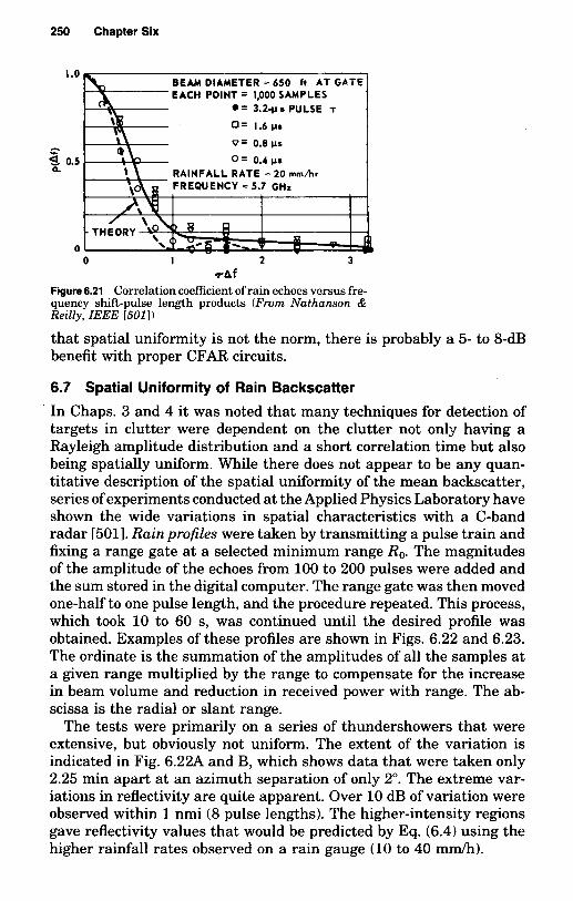
250 Chapter Six
1 .o
- - 2 0.5
0 0 I 2 3
.rAf Figure 6.21 Correlation coefficient of rain echoes versus fre- quency shift-pulse length products (From Nuthunson & Redly, IEEE [501])
that spatial uniformity is not the norm, there is probably a 5- to 8-dB benefit with proper CFAR circuits.
6.7 Spatial Uniformity of Rain Backscatter In Chaps. 3 and 4 it was noted that many techniques for detection of targets in clutter were dependent on the clutter not only having a Rayleigh amplitude distribution and a short correlation time but also being spatially uniform. While there does not appear to be any quan- titative description of the spatial uniformity of the mean backscatter, series of experiments conducted at the Applied Physics Laboratory have shown the wide variations in spatial characteristics with a C-band radar [5011. Rain profiles were taken by transmitting a pulse train and fixing a range gate at a selected minimum range Ro. The magnitudes of the amplitude of the echoes from 100 to 200 pulses were added and the sum stored in the digital computer. The range gate was then moved one-half to one pulse length, and the procedure repeated. This process, which took 10 to 60 s, was continued until the desired profile was obtained. Examples of these profiles are shown in Figs. 6.22 and 6.23. The ordinate is the summation of the amplitudes of all the samples at a given range multiplied by the range to compensate for the increase in beam volume and reduction in received power with range. The ab- scissa is the radial or slant range.
The tests were primarily on a series of thundershowers that were extensive, but obviously not uniform. The extent of the variation is indicated in Fig. 6.22A and B, which shows data that were taken only 2.25 min apart at an azimuth separation of only 2". The extreme var- iations in reflectivity are quite apparent. Over 10 dB of variation were observed within 1 nmi (8 pulse lengths). The higher-intensity regions gave reflectivity values that would be predicted by Eq. (6.4) using the higher rainfall rates observed on a rain gauge (10 to 40 mm/h).

.- E W'
(3
Z
4
E
c Z
4 :
UI
(~4
!un
JD=
~!I) 3an
iiidw
v ii
251
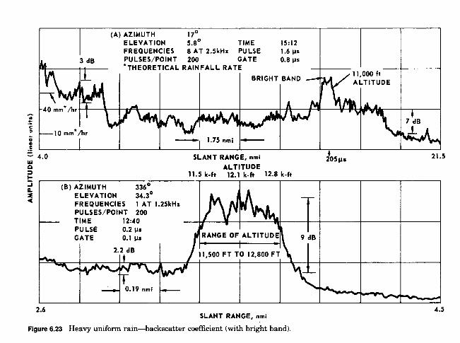
Y
*
- a L1 9
w'n
crz
E
2
4
.$
8 8
.E 8
53
d$
4 f 52 'E: (3
k
Y
0
.d
E !! 3 E 2 1 :
a !?!
d 1
0
WI
(w
~n
JD=YI)
3aniiid
wv
ii
252

Atmospheric Effects, Weather and Chaff 253
An example of what could be considered a uniform rain gave rather consistent recordings of 16 to 40 mndh for several hours. Radar profiles from this day are shown in Fig. 6.23. These two were chosen to illustrate the relatively uniform backscatter at lower altitudes and the apparent bright-band effect at the melting level.
With only a few exceptions the uniform rain appeared to be uniform at the lower elevation angles with about a +2-dB peak-to-peak vari- ation in backscatter coefficient over 1- to 2-nmi range intervals. The data in the figure and other data taken a t about the same time indicate that spatial nonuniformities of less than 1 nmi in extent exceed any uncertainties in the measurements.
Unfortunately, the wide disparity of measurements on different days precluded postulating any model for the gross uniformity of rain clutter. Changes in the mean backscatter may be larger than + l o dB in 10 nmi for showers, or as small as 2 1 dB for the more uniform rains.
Similar runs were made on the uniformity of a snowstorm. The mean backscatter was more uniform than for any of the rain measurements.
An attempt was made to estimate the spatial extent of the major nonuniformities by computing the spatial correlation function of the mean backscatter. The sum of the magnitudes of the backscatter from the pulses a t each range was corrected for the R-' dependence and inserted into an autocorrelation program. The range displacement where the normalized autocorrelation drops to one-half its value of zero lag is thus a measure of the range extent of the variations of the mean backscatter. While the statistical sample was too small for a rigorous analysis, the characteristic extent of the nonuniformities (where p = 0.5) was 0.6 to 1.4 nmi in the showers. This value was 2 to 3 nmi for the uniform rain, including the bright-band effect, and in a snow- storm the extent was 1.4 to 1.9 nmi at 3" elevation. Data for stratus clouds indicate correlation distances of about 7 nmi. [5041
To determine how to set a threshold for target detection in storms or showers does require some model. Figure 6.24 further illustrates the complexity of the modeling problem. It is essentially a plan view of a New England shower region. Note the very high-intensity cores with diameters of 1 to 2 km dropping 20 dB in a comparable distance.
Sekine et al. 16431 obtained spatial distributions for stormy conditions near Tokyo. The data fit the Weibull distribution quite well. The meas- ured shape parameter, c, varied between 1.25 and 2.0 with an average of about 1.7 where 2.0 corresponds to the Rayleigh distribution. Lower values of c correspond to longer tails on the distribution. This in turn requires a 2 parameter or distribution-free CFAR, as described in Sec. 4.8, to maintain a constant false alarm rate. Ward [7511 suggests mod- eling with the more complex K distribution, which also requires a sophisticated CFAR.

254 Chapter Six
CONTOURS 5dB APART
WEATHER RADAR DATA
2 4 JUL 1967 2052GMT
MILLSTONE HILL RADAR 1.4' EL, 275O- 290'AZ
AZIMUTH .degrees
I I I I I 0 10 20 30 40
TRANSVERSE DISTANCE AT 150 km, km
Figure 6.24 Weather radar map for New England showers. (From C U R , I986 L36l J)
Physical explanation of the bright band
The various physical factors that influence reflectivity changes in the bright band are: (1) the change in the dielectric constant from that of ice to that of water, (2) the change in the fall velocity of precipitation particles through the melting layer, (3) coalescence or the combining of individual snow crystals into snowflakes or clusters of crystal, (4) shape effects, or deviations from the spherical shape in melting snow, and (5) growth of precipitation particles.
The first two physical factors are the basic cause of the bright band. After the snow falls below the melting level it acquires a coating of water which effectively changes its dielectric constant and causes an increase in reflectivity by a factor of about 5. This makes a peak of reflectivity a t the bright band. By the time melting is completed, the fall velocity of the raindrops has increased to about 5 times that of the snowflakes. Due to the increased velocity the vertical spacing of the raindrops is 5 times as great as that of the snowflakes and hence the concentration of the number of raindrops becomes one-fifth that of the snow, thus tending to decrease the reflectivity. In the upper portion of the bright band, the increase in dielectric constant occurs without ap- preciable change in the fall velocity, while in the lower portion an increase in fall velocity occurs with little or no change in dielectric constant.
Coalescence is a more gradual process occurring both in the snow above the melting level and in the bright band. At low temperatures,

Atmospheric Effects, Weather and Chaff 255
TABLE 6.7 Average Echo-Intensity Changes Due to Physical Factors Above and Below the Bright Band (BB)
BB to rain below, Snow down to BB, Factor dB dB
Dielectric + 4 + 1 Fall velocity - 1.5 - 5.5 Coalescence or breakup t 3 - 1 Shape + 1.5 - 1.5
Total t 7 - 6.5 Growth 0 + 0.5
below about - 5"C, there is little tendency for coalescence to occur and snow mostly consists of single crystals. With increasing temperature, coalescence increases, possibly due to a greater cohesive property of the crystals. In the melting layer itself the snowflakes are frequently very large, sometimes as much as 3 to 4 in in diameter. Breakup of the large snowflakes into smaller raindrops may occur when melting is completed. Coalescence and breakup may be a highly variable factor.
In the melting layer, growth by condensation occurs due to the cooling effect of melting snow but in the absence of updrafts this effect is small and increases the reflectivity by about 12 percent. Table 6.7 shows estimated typical magnitudes of the various effects in the 2000-ft layers above and below the middle of the bright band (BB).
The bright-band thickness averages about 300 m, but can sometimes reach dimensions up to 1 km. The altitude of the bright band varies with latitude, climate, and season. An upper bright-band boundary may be assumed a t the altitude (h f ) of the 0" isotherm. Reflectivity above the 0" isotherm diminishes at a rate of about 6.5 dB/km, up to the altitude of the tropopause (hth The altitude of the 0" isotherm is approximately related to latitude, 4, according to hf = 4 km for latitudes up to about 36", and hf = [4 - 0.75 (4 - 36'11 km for latitudes above 36". The altitude of the tropopause, ht, is approximately related to latitude according to h, = 17 km for latitudes between 0 and 30", and h, = 9 km for latitudes between 30 and 90". Between 30 and 90", h, may be approximately determined by linear interpolation of height versus latitude.
6.8 Tropospheric Refraction Effects
Radio waves propagated through a medium with a varying index of refraction undergo both refractive bending and retardation of their velocity of propagation. These phenomena give rise to angle and range errors when a target is being tracked by a surface radar. The angular error is caused by the bending of the radar beam such that the wavefront
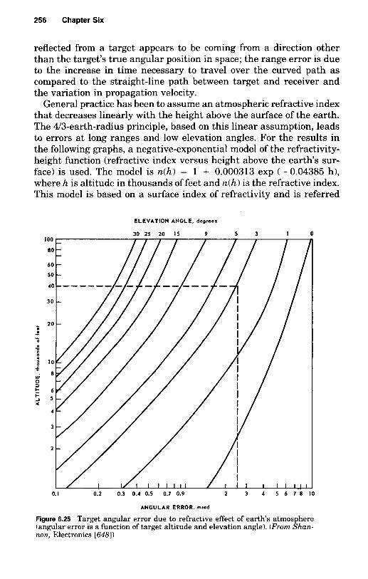
256 Chapter Six
reflected from a target appears to be coming from a direction other than the target’s true angular position in space; the range error is due to the increase in time necessary to travel over the curved path as compared to the straight-line path between target and receiver and the variation in propagation velocity.
General practice has been to assume an atmospheric refractive index that decreases linearly with the height above the surface of the earth. The 4/3-earth-radius principle, based on this linear assumption, leads to errors at long ranges and low elevation angles. For the results in the following graphs, a negative-exponential model of the refractivity- height function (refractive index versus height above the earth‘s sur- face) is used. The model is n(h) = 1 + 0.000313 exp ( - 0.04385 h), where h is altitude in thousands of feet and n(h) is the refractive index. This model is based on a surface index of refractivity and is referred
ELEVATION ANGLE, degrees
30 25 20 I5 9 5 3 I 0
80
60 - 50 -
- -
I 1 I I I I I l l 0.1 0.2 0.3 0.4 0.5 0.7 0.9 2 3 4 5 6 7 8 1 0
ANGULAR ERROR, mrod
Figure 6.25 Target angular error due to refractive effect of earth’s atmosphere (angular error is a function of target altitude and elevation angle). (From Shan- non, Electronics 16481)

Atmospheric Effects, Weather and Chaff 257
to as the CRPL (National Bureau of Standards, Central Radio Prop- agation Laboratory) exponential reference atmosphere. Other values of the equivalent earth radius are described in Chap. 1.
The CRPL reference atmosphere was used to calculate the tropo- spheric angular and range errors presented graphically in Figs. 6.25 and 6.26. The angular error is the angle between the apparent ray path
ELEVATION ANGLE, degrees
30 15 9 5 3 I 0 100 90 80
70
60
50
40
30
20
- 0 ... - -D c
; IO
I l i a n t A 6
$ 9
3 7
I-
5
4
3
2
1 100 200 300 0
RANGE ERROR, ft
Figure 6.26 Target range error due to refractive effect of earth's atmosphere (range error is a function of target altitude and elevation angle). (From Shannon, Electronics [6481)

258 Chapter Six
to the target from the radar and the straight-line path from the radar to the target. The range error is the apparent increased range of the target caused by the wavefront traveling a curved path instead of a straight-line one. The range error as a function of the total path length is shown in Fig. 6.26 for a one-way path. For a two-way path the errors must be doubled. A radar several thousand feet above sea level would have less error. The NRL radar coverage diagram based on the CRPL exponential reference atmosphere is reproduced from Blake [751 as Fig. 6.27. Experimental data on refractivity have been reported by Nichols [5071.
These range and elevation angle errors should be considered as known bias errors since their magnitudes are calculable. The uncer- tainty in their exact magnitudes (about 10 percent) from simplifying assumptions concerning the state of the atmosphere is partly from unknown bias errors and partly from “precision” errors. Contributing to the precision errors are the effects of irregularities in the troposphere. Barton [39, p. 4891 gives some rms values of the fluctuation of range and angle in the troposphere as follows (see also Millman [476, p. 317ffl):
Type of weather A range, ft A angle, mrad
Heavy cumulus 2.0 0.7 Scattered cumulus 0.5 0.3 Small scattered cumulus 0.1 0.15 Clear moist air 0.02 0.07 Clear normal air 0.005 0.03 Clear dry air 0.001 0.015
The above bias error models are limited to surface-to-air paths and do not take into account meteorological conditions at the time of the measurement. In meteorological radar investigations and for cases in which true geometric target trajectories to the highest attainable degree of accuracy are desired, the reference atmosphere should not be used without modification. At the minimum it should be corrected on the basis of a directly or indirectly measured value of the refractive index at the radar location.
The radio refractive index of air
A summary of the state of knowledge of this parameter appears in Bean [491. More recent data are in Blake [751, KO [4051, and the EREPS software 12071. Bean’s conclusions, with some paraphrasing, are as follows:

b
r5 ‘i~1
31
31
.1
Y
259

260 Chapter Six
1. The differences in determined values of the constants in the ex- pression for refractivity N (Bean’s Eq. 10) are small compared with the errors from using the formula; i.e., the errors in using ordinary meteorological measurements (e.g., radiosondes) mask the errors caused by using published values of the constants.
2. The refractive index is effectively nondispersive for frequencies be- low, for example, 50 GHz. (N.B., ionospheric effects, multipath ef- fects, and effects due to storm phenomena, which exhibit high coefficients of radiowave absorption, are not considered.)
3. The choice of atmospheric model for N depends on the location and application. World-wide statistics are given in the EREPS software.
4. The atmosphere, on the average, yields an exponential distribution of N with height.
Bean also indicates the divergence of a typical measured profile of Nfrom the often assumed 4/3 earth profile. From his graphs it is evident that the 4/3 earth model has about the correct slope in the first kilometer above the earth‘s surface but decreases much too rapidly above that height. It is also seen that the observed refractivity distribution is more nearly an exponential function of height than a linear function as assumed by the effective earth’s radius model. The exponential decrease of N with height is sufficiently regular to permit a first approximation of average N structure from surface conditions alone.
6.9 General Properties of Chaff
Fundamental relationships for chaff
Chuff (or window) is a form of electronic countermeasure that dates back to World War 11. Lightweight inexpensive metallic or metal-coated fibers have high radar reflectivity per pound when their length is near one-half wavelength of the radar they are trying to confuse. The con- fusion can take one of several forms: . A large cloud of dipoles dispersed in the atmosphere that shield
aircraft or missiles either in or near the cloud H A chaff “puff” that can emulate another aircraft or missile and cause
false detections . Packets of chaff that can also be used as track breakers in an attempt to force a track radar to track the chaff rather than the aircraft being tracked
The tactics of chaff use are complex but it is possible to model a basic chaff cloud and to detail its extent, reflectivity, and Doppler charac-

Atmospheric Effects, Weather and Chaff 261
teristics. Chaff a t frequencies below about 1 GHz is generally called “rope” and is either dispersed in small rolls or cut off a reel of wire or tape.
Chaff moves horizontally with the local winds as does rain. I t is an excellent tracer of the winds such that the velocity spectrum is the same as the wind spectrum in the horizontal plane. For horizontally oriented radar beams the Doppler characteristics are almost identical to rain. At one time the U.S.S.R. completely covered Czechoslovakia with chaff and kept it “refreshed” for several days.
The chaff dipoles are designed to resonate a t the frequencies of the radars that they are attempting to confuse. (Dipole length = one-half radar wavelength.) Often the dipoles in a package are cut to different lengths to cover an entire radar band or several radar bands. The maximum backscatter cross section of a single dipole occurs when the dipole is oriented parallel to the E plane of the incident radiation and perpendicular to the direction of propagation. This gives a maximum radar cross section
u , ~ = 0.857 h2
Schlesinger 16371 stated that if these dipoles are randomly oriented after dispersal into the atmosphere the overall cross section is ap- proximately
u = 0.18 A2N
where N is the total number of dipoles and u is the resultant radar cross section. Other calculations give a constant of 0.14, which gives a value closer to experiments. He further calculates that if they were all cut from old style aluminum foil 0.001-in thick, h/2 long, and 0.01-in wide the radar cross section is
u = 3000 W/f m2
where W is weight in pounds and f is transmit frequency in gigahertz. This would yield a 1000-m2 cross section for a single pound of narrow- band chaff a t 3 GHz. (See also Cassedy and Fainberg 11121 and Mack and Reiffen 14581.)
The bandwidth of the resonant-length chaff is only about 10 to 15 percent of the center frequency as illustrated in Fig. 6.28; and if it is desired to cover the desired frequency range from 1 to 10 GHz with the 10-percent bandwidth assumption, a 1.0-lb package of broadband foil chaff would give a 60-m2 radar cross section anywhere within the frequency range.
The modern form of chaff is aluminum-coated glass or mylar. At frequencies of 3 GHz or higher the diameter is about 0.001 inches. The
z 0 L 0.02
6? 0.12
% 0.10
W cn cn cn
0
n a K
0.006
0.004
’ I I ’
\ I I I
\ I I \ I
0.4 0.6 0.8 1.0 1.2 1.4 1.6 1.8 2.0 2.2 2.4 2 6 28

Atmospheric Effects, Weather and Chaff 263
I I I i t C l 1 I I / I I O lo4 - - -
- 0) V U a W I- W
w Lz - 3 0 v)
E W - Q v, W 1 0
-
-
2 lo3- - - -
a
-
% n
0 - a W m - 2 3 - z
LL 102 - - - - - - -
- -
10‘ I l 1 1 1 1 l
102 io3 1 o4 RESONANT FREQUENCY, MHr
Figure 6.29 Theoretical number of chaff dipoles required per square meter of RCS at resonant frequency. (Courtesy: Lundy Electronics [4541)
Modern chaff dispensers come in several varieties. In one form, di- poles are packaged into a plastic cylinder with a small explosive charge a t one end. In one variety, 750,000 X-band, 250,000 C-band, and 250,000 S-band dipoles are packaged into a 6-in-long cylinder that weighs only about 6 oz. This is about 3 million dipoles per pound, and costs only a few dollars per package.
In another form illustrated in Fig. 6.30, the dipoles of desired length are laid out on a roll that is about 1 ft in diameter and has a chaff weight of 50 lb. Six rolls are placed in an aircraft pod with a total of 300 pounds per pod. To dispense the chaff, the rolls are rotated, and air is rammed into the nose of the pod, blowing the chaff out the rear of the pod. The dispensing rate is controlled by the rotation rate of the rolls.
At lower frequencies “rope” is used instead of chaff, and is made of wire-long filaments that may be twisted fibers or foil. One type,

264 Chapter Six
CHAFF ROLL (6 EA 1
AIR DUCTS 16 EA 1
OR ALUMINUM FOIL) -
Figure 6.30 AN/ALE-38 chaff-dispensing system. (From Electronic Warfare, uol. 4, no 4, 1972 Courtesy Cardiff Publ. Co )
"stringball rope," is made of twisted fibers and is typically many meters long. It is characterized by its radar cross section per unit length. Although in a sense it is less efficient than dipoles, the h2 term in the RCS keeps the reflectivity at several hundred m2/lb.
Fall rates for dipoles are dependent on construction. For coated fi- berglass, it is less than 1 m/s.
Density of chaff
Obviously chaff can be dispensed at a wide variety of rates depending on the nature of the dispenser, the maximum chaff load of the aircraft, and the tactics. A typical system might be:
= Aircraft speed 600 knots or 10 nmi/min = Broadband chaff of 200 m2/lb (1 to 10 GHz) = Drop rate of 10 lb/min or 1 lb/nmi = Dispersion rate (horizontally) of 2.5 m/s (u").
At some time between 10 and 100 min, depending on the wind con- ditions, the chaff will be dispersed to about 1 nmi in a horizontal plane and some fraction of a nautical mile in elevation. A convenient as-

Atmospheric Effects, Weather and Chaff 265
sumption is that the chaff expands to a density of 1 lb/nmi3 and has a reflectivity density of Xu = 200 m2/nmi3. Since there are 6.36 km3 per nmi3, this converts to about Xu = 30 m2/km3. If the aircraft flies a 75-nmi "racetrack twice, with the second pass above or below the first by 1 nmi in elevation, the nominal cloud is 2 nmi by 2 nmi by 75 nmi in length. Three hundred pounds of chaff are dispersed in about 30 min.
The assumed density of chaff clouds is quite low, and the attenuation of electromagnetic waves is negligible. As a side issue, the U.S. and Canadian governments have made tests on the environmental impli- cations of chaff drops. They found no problem.
6.10 Spectra of Chaff Echoes
The Doppler spectrum of chaff return can be split into four components in the same manner as for precipitation:
1. Wind shear due to finite height of the radar beam 2. Beam broadening due to finite width of the beam 3. Turbulence 4. Fall velocity distribution of the dipoles
In the case of precipitation it was shown that the wind shear and beam-broadening effects were caused by the variations in the horizontal motion of the droplets within the radar beam. This motion of the rain was shown to follow the horizontal wind speed very closely. Experi- ments by Pilie' et al. [ti521 have also shown that there is very high correlation between horizontal wind and chaff velocities at altitudes of from 5000 to 10,000 ft. Similar experiments showed the same high correlation at from 24,000- to 35,000-ft altitudes. It can be concluded that the calculation of the first two effects (due to wind shear) for chaff should be identical to that described for rain in Sec. 6.5."
Because of the difficulty of separating the turbulent component from the shear components of the chaff spectrum, there is little information available on the spectrum of the chaff after dispersion. One fairly ex- tensive set of data was reported by Smirnova 16753 in 1965 in the U.S.S.R. Unfortunately his radar parameters were not included, but it was implied that the antenna beamwidths were about 0.7" and that the measurements were made looking almost exactly downwind. The altitudes observed were from about 1000 to 40,000 ft.
' The effects are identical if both the rain and chaff fill the radar beam. However, chaff does not usually have as much vertical extent.

266 Chapter Six
Several conclusions can be reached by interpreting the available information:
1. The turbulence component (Tturb above 12,000 ft varies between 0.35 and 1.2 m/s with an average of about 0.7 m / s or somewhat less than the assumed value of 1.0 m / s for precipitation.
2. Below 12,000 ft, readings as high as 2 m/s have been recorded, but an average value from 1000 to 12,000 ft is close to the 1.0 m/s used for precipitation. The larger values may be partially due to the vertical fall velocity distribution [6751.
3. An average of Smirnova's data on the turbulence velocity is included in Fig. 6.31. The lower-altitude tests (1500 to 13,000 ft) overlapped the high-altitude tests (8000 to 32,000 ft). Since there is not a sig- nificant correlation between wind velocity and turbulence it is as-
--T-- - T - - - T - ~ - - T - ~ LOW ALTITUDE TESTS (30-40' EL.)' * HIGHER ALTITUDE TESTS (<Zoo EL.)'
- - 5
MAX. VALUE
___. .--
GOLDSTEIN LOW WINOS
.___. .- _-- ___ - - - .. ___ .- I
- - _.___ - 0 2 4 6 8 10 12 14 16 18
WIND VELOCITY, m/r
Figure 6.31 Turbulence (r, of chaff versus wind velocity (After Srnirnoua 16751, Goldstem 1,3971. and Estes et (11 12101 ( 1985 IEEE)

Atmospheric Effects, Weather and Chaff 267
TABLE 6.8 Spectral Estimates for Mature Chaff
Run Chaff R, BW, (10, (T,.
number Radar type* km m / S m / S m / S
M1 X-band AGFICR 5 0.8 9.9 0.6 M2 X-band AGFICR 6 0.8 10.8 0.5 M3 X-band AGF/DC 6 0.8 - 1.2 0.3
M4 X-band AGFIDB 6 1.1 9.2 1.0 M5 X-band AGFICR 6 1.5 1.4 1.2 M6 X-band AGFICR 5 1.1 4.7 1.0 M7 X-band AGFICR 5 0.8 5.2 0.5 M8 X-band AGF/DC 8 1.0 6.3 0.6 M9 X-band AGFIDC 8 1.0 6.3 0.6 M10 X-band AGF/DC 8 1.0 4.8 0.6 M11 UHF ASIDB 13 1.5 3.9 1.1 M12 UHF AS/DB 9 1.5 4.1 1.2 M13 UHF ASIDB 12 1.5 3.3 1.2 M14 UHF AGF/CR 19 0.6 6.5 0.3 M15 UHF AGF/CR 31 0.6 8.5 0.3
4: Chaff type code:
Type Code Dipole material
Aluminum strips AS Aluminum-coated glass fibers AGF
Continuously dispensed, roll CR Discrete unit, box DB Discrete unit, cartridge DC
Dispensing method
SOURCE: Ref. 12101 0 IEEE, 1985.
sumed that the horizontal turbulence component is roughly constant a t 1.0 d s for low altitudes and at about 0.7 d s above 18,000 ft. These points are shown as arrows on the figure.
These data are only partially consistent with Goldstein’s data (a t A = 10 cm) from World War I1 13971; he estimated a standard deviation of 0.4 to 1.0 d s : * for low (< 10-knot) winds and 1.3 d s for 25-knot winds. Barlow’s [341 general value of 3.5 ft/s (= 1 d s ) agrees more closely. Since the 0.4 d s data point was for low winds and a different type of chaff, it can probably be disregarded. This leaves a range of ut. between 0.6 and 1.3 d s . Data from the more recent mature chaff measurements of Estes et al. 12101 a t both UHF and X-bands are included in Fig. 6.31 and shown in Table 6.8. The mean velocities varied between 1 and 11 d s . Measurements were taken within a few minutes of dispersal. The data tend to confirm the low values for the turbulence component. They also presented data a t 150 to 450 m behind the dis-
:j’ The 0.4 m/s curve is for chaff dispensed from a blimp; this chaff had different aero- dynamic properties than the chaff used to obtain the other values.

268 Chapter Six
pensing aircraft and found spectral widths (a,) about double those of the clouds away from the influence of the aircraft.
The final component of the chaff spectra is the Doppler spread due to the variation in fall velocity of the dipoles. Chaff dipoles fall more slowly than do the large raindrops that dominate the backscatter from precipitation; dipoles have typical terminal velocities of 0.7 d s as compared to about 6 d s for 1 mm/h rain. Theoretical and experimental studies of the fall velocity chaff were made by Jiusto and Eadie [370], including metallized nylon cylinders 0.0035 in in diameter and 0.6 in long. The experimental work was in a small altitude chamber without air turbulence. The measured median terminal fall rate was about 0.6 d s ; ufall would be = 1 d s . The variation in the fall rate of the nylon cylinders was only a few tenths of 1 d s . Thus, the range of vertical differential velocities is below 1 d s (- 0.5 d s ) at low altitudes. Further experimental data are available in Totty et al. [7061.
The measured spectra for chaff and rain are similar enough so that separate computations are not needed except for two factors:
1. If the vertical dispersion of chaff at high altitudes is small, there will be less shear effect.
2. Chaff has a higher fall velocity at high altitude (over 25,000 ft) and a low terminal velocity -0.7 d s ; rain, on the other hand, has a higher terminal velocity than its initial condition (clouds).
The general equation for the total variance of the velocity spectrum for chaff is then
2 2 d = ushear -k abeam -k Uturb -k ($all
where (+turb = 2.3 ft/s - 0.7 d s . ufall = sin + d s .
It is emphasized in the chapters on processing that the mean velocity of chaff (and rain) is also important in many signal-processing tech- niques, especially MTI, and that the spectra described here are centered at the mean radial velocity of the volume cell containing the chaff.

Chapter
7 Sea and Land
Backscatter
F. E. Nathanson J. P. Reilly
7.1 Backscatter from the Sea-Monostatic
Backscatter from the surface of the sea limits the performance of radar surveillance and missile guidance for airborne, shipboard, and coastal early warning and defense systems. The following three sections pro- vide models of the normalized radar power return from the sea as a function of frequency, polarization, grazing angle, and aspect with re- spect to the primary wind and sea condition. The statistics of these signals are given in Secs. 7.5, 7.6, and 7.7.
The general relationships between the wind and the surface condi- tions of the sea are given in Fig. 7.1. This figure defines sea state as well as would seem appropriate to subsequent discussions. Combined conditions a t any given time or place may vary considerably from this chart because of the wind history or geographical factors. Note that Beaufort sea state [item (2) in the table1 is not the same as the hydro- graphic sea state [item (6)l. The latter is appropriate for radar problems and is used in the following discussions.
269
Lt
JZ
E
I I
I I
1 3
I 1-
-.IL :-I
, y g ,
I 1-
:+ m
i I-:..{-: ' -
-0-
0 -1 -
P
0
~..-
-. -
-0
CJ
n-
Y
_n -
-0
::iL-
0
-0 __ -
n-
_0
__
_.
-
--10 0
,;: - ::
-E:-:-
0
-0
- -
-
.- :- *s
-E!! -
0
n
-0
0
-
--
n
n
n0
,I
--" --
0
-e
-.
- 0
-.. -
;Y
0
0
- _
__
. -
-
- n-
".I - --
- :--G
-
-
- - n_ o!! --
.- 0
__
ow .,
ZW
ea
-2:
-0
.-:- *;
-0
'I _9 --E
-
-E2 --
z:-"--" --- ;
- ---
nm
0
0
-4
-
0
__
-
0
n
--
-a
_W
Y
:: r
n
~
0
--
-:- 4
P.
--
-
rw -8
_. :a
.ig
-2; -- - ;
Y
Y
<. .e
-
tV
e 2:
-:--E-
2;
:t: -
:: I
-Y
w
I"
; -
- 0
--
- 0-
n-
- e.- nu
:----
J
-
22
0
0
Y.
=a
n
r3
y;
--- J
N
.O
:a
YY
-::
Ya
--
0
0
u
s: --
- --n-
Y
.I
b :;
Y
D
z 1 U
I
4L
- 2
4: r
1
2: e: :
--- -;: p
Y
'9 1
Y
I- .
:: E
:
:E u
0
;E f
E.
-5: r'
r g:
A
:f 3
;* o*
::
30
I
:4 :b
ze
Y*
___ -
4_
-:
0
c
0
-0
--- n
zn
- t
B
z
*=,
-8
w
:z x: 1
L of
2: k
5: :f
"U
o*
Y=
If
F' w
.
u1
*z
Y
J
=,-
eo
IW
:L
YO
0
0 .:
$ >
PI
,*
I
ZI
3
2
;
$E: 0
eI o
t
L
o
s
; :
sL
_:
5 2
ea
;; == g
i >
$
"Y
5
%
4 24
01
0.
*I;: 2
2 '
i; (0
4
25
r%
1
U
Y
g:: En
:z
Y
e
::;: ,"
y !
YY
Yt
.Y
3
2
ai
.,
::
i;
;
--
--
*-
-e
-
n_
-
I I:
-0
I--1-: 1 1:
I: 2
_n_
" v)
- -:-:
a n
Y.
9 s
--
B 5 z
-4
-
YU
.9
0
3 -=----
a
k
Le
.J
13
JY
Y
Y
-0
-2
-
J?
'. 0:
-0-
:z
v)
Yr
YZ
- Y
W
nw
ux
&
Y
h
_0
_.
s
t
- --
._
v)
Y
Y a I
'E J
2i 7.
gh
d J
$
--
%
* Y n
Y
0
--
-
c
v
cr) 0
-z
-
E z J
-D
-
Y
0
--- * J
ii
- --; !: ;; 5 --: ;: : b
2 o
E5
:
f 6
~ 8
2
5:
p
c.
26
g : E;
-$ t 2
p 61 ig
;
4 ; ;; 3; ;
5
IU
g;
Efl =5
4
i ;g
zgz; $
E ;; <;;g
:: 5
z; ;a,:
a *
>p
*:z
:
cfl 0
"U
u4
(;
I
t
:z: <::::
f ;:;I
::<E i
-A
m-
'z
*z
*
.*
0
$2
2 ;13;;
r $
n
u-g d
g$
;: ;
; ; ; :3
i:;&
5 i
! ii.
::
-
z
E:
-.
- n
-i
1:
.
-___n_
z
-I^
z ::
36
m
---
I- I
0
- 1;
:= :
r
2 ::
26 -
E ;t
2: :
2 0
.- -, <
w
I-
'0
I
- ?!
=1z. <.(o-
i sir
0
c. I-
f -
4 2
m
U
.- r
-

90 < n - x m
z 70 S
e W I-
Y LL 50
3 W
L 0
\

272 Chapter Seven
Climatic World Atlases, 1957. Table 7.1 gives the relative frequency of occurrence of wave heights in specific regions of the oceans.
Description of the sea surface. The quantitative interpretation of radar scatter from the sea requires an appreciation of certain prop- erties of ocean waves. A brief review is undertaken here of the ocean wave physics and characteristics. Also, common oceanographic no- menclature pertaining to ocean waves is defined and explained. Sea state. This term is used here to refer to the state of the sea, or roughness, as determined by the heights of the largest waves present. Numbers have been assigned to sea states by the International Ma- rines' Codes, and these are related to wave heights. They should not be confused with Beaufort (wind force) scale.
TABLE 7.1 Relative Frequency of Occurrence of Wave Heights in Specific Regions of the Oceans
Percentage of time-significant wave height (ft) from
Region 0-3 3-4 4-7 7-12 12-20 >20
North Atlantic between New- 20 20 20 15 10 15 foundland and England
Mid-equatorial Atlantic 20 30 25 15 5 5
South Atlantic a t latitude of 10 20 20 20 15 10
North Pacific between latitude 25 20 20 15 10 10
southern Argentina
of Oregon and southern coast of Alaska
East-equatorial Pacific 25 35 25 10 5 5
West wind belt of South Pacific 5 20 20 20 15 15 at latitude of southern Chile
North Indian Ocean during 55 25 10 5 0 0
North Indian Ocean during 15 15 25 20 15 10
Southern Indian Ocean be- 35 25 20 15 5 5
northeast monsoon season
southwest monsoon season
tween Madagascar and north- ern Australia
West wind belt of southern In- 10 20 20 20 15 15 dian Ocean between Cape of' Good Hope and southern Australia
Averages over all regions 22 23 80 15 9 9
sorwk:: Fiwii Long ct A. 14451.

Sea and Land Backscatter 273
Significant wave height. This term is a common maritime descriptor referring to the average of the heights-from crest to trough-of the one-third highest waves; it is denoted H1/3.
RMS wave (or roughness) height. This is a term describing root- mean-square height above the mean surface level-used in rough- surface scatter theories; it is denoted here by ah. While there is no exact general relationship between ‘Th and HI/3 , a common approx- imation frequently used for wind waves is Hi13 = 4 uh . Another approximation that is occasionally used is H1,3 = 2 . 8 3 ~ ~ . Average wave height. This is determined from rms wave height by ha = V% (Th. Also related to significant wave height by ha = 1.6 H1/3.
Length. The length or spatial period of a single ocean wave is the distance from one crest to another; it is denoted by L. Period. Unless denoted otherwise, this refers to the length of time it takes two successive crests of a single wave to pass one point. It is denoted by T. Spatial wavenumber. This is defined in terms of the length of an ocean wave as K = 2 d L . Temporal wavenumber. This is the radian wavenumber given in terms of the period by w = 2 d T . Fetch. This is the horizontal distance over which a nearly constant wind has been blowing. (It is also defined by its duration.)
Duration. This refers to the length of time during which a nearly constant wind has been blowing. Wind waves. This refers to a system of ocean waves that is being, or has very recently been, aroused by winds blowing locally above that area of the ocean. Wind waves result in a random appearing ocean height profile.
Fully developed seas. This is an equilibrium sea state condition reached after sufficient duration and fetch at a given wind speed. The estimated duration and fetch versus wind speed required to produce fully developed seas is provided in Fig. 7.1.
Swell. When wind waves move out of the area in which they were originally excited by the winds, or after winds have ceased to blow, these waves change their shape and settle down to what is known as swell. Swell appears less random and more nearly sinusoidal, of great length, and with great width along the crestlines. The usual period of swell is from 6 to 16 s. Swell can arise from storm areas thousands of miles distant and can increase radar reflectivity.

274 Chapter Seven
Deep-water waves. When the water is sufficiently deep that the effect of the bottom on the propagation characteristics of the waves can be neglected, they are called deep-water waves. Generally, if the depth is greater than one-half the length of a given wave, the deep- water approximation is valid. Except near beaches, ocean waves are deep-water waves, and this assumption is utilized throughout this book. Gravity waves. This term refers to waves in which the chief re- storing force upon the perturbed water mass is gravity. Waves whose lengths L are greater than 1.73 cm are gravity waves, since gravity waves are the essence of sea state. Capillary waves. This term refers to waves in which the chief re- storing force acting on the perturbed water mass is surface tension (less than 1.73 cm in length).
7.2 Empirical Sea Backscatter Models for Low Grazing Angles
For surface clutter (sea, land, or ice) the term vo is used to represent the normalized mean (or median) reflectivity from an area on the sur- face of the earth illuminated by a radar. In some references, the term (TO is used. The value is constant only for a given angle, carrier fre- quency, sea state, wind direction polarization, and even pulse length. To a first approximation the illuminated area is A = R02LIR for small grazing angles (91, narrow beamwidths and the peak antenna gain directed at the center of this clutter cell. R is the range from the radar to this cell, O2 is the two-way azimuth beamwidth, and LIR is the range resolution given by cd2 for noncoded pulses, or by the 3-dB resolution of a coded or compressed pulse. For better accuracy the effective pulse duration T' from Chap. 2 may be used. There is a t least a 3-dB standard deviation in almost all values of uo whether they are experimental or theoretical. This uncertainty is expanded in later sections.
The clutter cross section in a resolution cell can be approximated by
RCS I- RO~ARCT~ (7.1)
for small beamwidths and low grazing angles. Note that forward scatter is not explicitly taken into account, but is included in virtually all reported values of uo. The term is dimensionless and is called the normalized radar reflectivity and is most often presented as a mean value in decibels below 1-m2 reflectivity per square meter of illuminated area.
Tables 7.2 through 7.8 are models primarily compiled from experi- mental data with some extrapolation and interpolation between data points. There are averages of the decibel values of upwind. downwind,

Sea and Land Backscatter 275
TABLE 7.2 Normalized Mean Sea Backscatter Coefficient uo for Grazing Angle of 0.1"
Reflection coefficient in dB below 1 mVm2 at indicated carrier frequency, GHz
Sea UHF L S C X K" Ka state Pol. 0.5 GHz 1.25 3.0 5.6 9.3 17 35
0 V H 90" 87"
1 V 80" 72* 65:': H 80 75 71"
2 V 90t 87* 75* 67 56 H 95t 90* 75* 674: 59" 484:
3 V 88t 82" 754: 60" 51 47"
4 V 85t 78" 67" 58" 48 45 *
5 V 80" 70" 63j' 55" 44 42"
H 90t 82" 684' 69" 53"
H 74* 63" 60 48
H 70t 634: 58* 42"
H 6 V 56
* 5-dB error not unlikely. t 8-dB error not unlikely. NOTE: Monostatic radar, 0.5- to 10-ps pulse.
TABLE 7.3 Normalized Mean Sea Backscatter Coefficient uo for Grazing Angle of 0.3"
Reflection coefficient in dB below 1 m2/m2 at indicated carrier frequency
Sea UHF L S C X K" K, state Pol. 0.5 GHz 1.25 3.0 5.6 9.3 17 35
0 V 83 t 63" 55t H 834: 79 74'!'
1 V 784: 64"' 60 58 54"' 46t H 74 68 66:': 58
2 V 80 t 734: 62*' 55 52 52:': 43t 56" 533: H 78" 66:l: 60
3 V 78t 70" 58:': 504: 45 47:': 4o:k H 68': 60:': 50 46 42'1:
4 V 75t 65 57:!: 43 444: 38 H 551' 42 39:';
5 V
6 V 34
73t 64:': 52:!' 39 39 35"
37". .31:!:
r j 'p 44.'' 39 382: I I
H 64:"
H 46:': 34 37"'
., 5-dB error not unlikely. f 8-dB error not unlikely. NOTE: Monostatic radar, 0.5- to 1 0 - c ~ ~ pulse.

276 Chapter Seven
TABLE 7.4 Normalized Mean Sea Backscatter Coefficient uo for Grazing Angle of 1.0"
Reflection coefficient in dB below 1 m2/m2 at indicated carrier frequency
Sea UHF L S C X K, K J w state Pol. 0.5 GHz 1.25 3.0 5.6 9.3 17 35/94
0 V 68* 60* 60* 60* H 86 * 80* 75* 70* 60* 60* 60*
1 V 70* 65* 56 53 50 50* 48* H 84* 73* 66 56 51 48* 48*
2 V 63* 58* 53 47 44 42 40* H 82* 65* 55 48 46 41 38*
3 V 58* 54* 48 43 39 37 34 H 73* 60* 48 43 40 37 36
4 V 58* 45 42 39 37 35 32 H 63* 56* 45 39 36 34 34*
5 V 43 38 35 33 34 31 H 60* 50* 42 36 34 34
6 V 33 31* 32 H 41 32* 32
* 5-dB error not unlikely. NOTE: Monostatic radar, 0.5- to 10-ps pulse.
TABLE 7.5 Normalized Mean Sea Backscatter Coefficient uo for Grazing Angle of 3.0"
Reflection coefficient in dB below 1 m2/m2 at indicated carrier frequency
Sea UHF L S C X K, K J w state Pol. 0.5 GHz 1.25 3.0 5.6 9.3 17 35/94
0 V 60* <56* 50* 48* H 75* 72* 68" 63" <58* 53
1 V 60* 53* 52 49 45 41* 41 H 70* 62* 59 54 50 45* 43*
2 V 53 50 49 45 41 39 37 H 66* 59 53 48 43 38 40
3 V 43* 43* 43 40 38 36 34 H 61* 55* 46 42 39 35 37
4 V 38* 38 38 36 35 33 31 H 54* 48% 41 38 35 32* 32
5 V 40* 38 35 35 33 31" 30" H 53 46 40 36 33 30'
6 V 28 28 H 37 30 28
'i: 4-dB error not unlikely. NOTE: Monostatic radar, 0.5- to 10-ps pulse.

Sea and Land Backscatter 277
TABLE 7.6 Normalized Mean Sea Backscatter Coefficient u0 for Grazing Angle of 10"
Reflection coefficient in dB below 1 mYm' at indicated carrier frequency
Sea UHF L S C X K, Kdw state Pol. 0.5 GHz 1.25 3.0 5.6 9.3 17 35/94
0 V 45* 44* <47* <45* 44*
1 V 38 39 40 41 42 40 38
2 V 35" 37 38 39 36 34 33
3 V 34" 34 34 34 32 31 31 H 50 48 46 40 37 32 31
4 V 32* 31 31* 32 29 28 29 H 48* 45 40 36 34 29 29
H 60" <56"
H 56* 53 51
H 54% 53 51 48 43 37 36"
5 V 30 30 28 28 25 23 26* H 46 43 38 36 30 26 27*
6 V 30" 29 28 27" 22" 18'' H 44" 40" 37 35'' 27" 24''
': 4-dB error not unlikely. NOTE: Monostatic radar, 0.5- to 1 0 - p ~ pulse.
TABLE 7.7 Normalized Mean Sea Backscatter Coefficient u,, for Grazing Angle of 30"
Reflection coefficient in dB below 1 m2/m2 at indicated carrier frequency
Sea UHF L S C X K, K$w state Pol. 0.5 GHz 1.25 3.0 5.6 9.3 17 35/94
0 V 42* 42* 42* 37* 33" H 50" 50" 50" 48" 45"
1 V 38': 38" 40 42 36 312: 35" H 46" 48 44" 38"
2 V 30 31 322: 34 32 264: 30 H 42 41 40 42 38* 35'' 35"
3 V 28 30 29 28 26 23 23" H 40" 39 38 37 34 28 294:
4 V 28 28 27 25 24 22 22 H 38' 37 37 35 29 21 21
5 V 28 24" 23 22 22 18 204: H 35 343: 32 30 26 18 20"
6 V 252: 23" 22''' 2 1 :I: 17 15 H 33" 32" 30': 29" 21" 16
>' 5-dB error not unlikely. NOTI.:: Monostatic radar, 0.5- to 10-ps pulse.

278 Chapter Seven
TABLE 7.8 Normalized Mean Sea Backscatter Coefficient u0 for Grazing Angle of 60"
Reflection coefficient in dB below 1 mYm2 at indicated carrier frequency
Sea UHF L S C X K" K, state Pol. 0.5 GHz 1.25 3.0 5.6 9.3 17 35
0 V 32 33 34 26* 23 22* H 32 32 32 27:k 25* 22" 26*
1 V 23* 22 24 24 24 20* 24" H 22 24 25 26 24 20
2 V 20" 21 21 23 18 18* 19* H 22 21 21 22 23 18"
3 V 18* 18* 19 18* 16* 14 14* H 21 20 20 20 21 16* 16*
4 V 14" 15* 4 15" 6 1 5 * 3 14* 11 7 10
5 V 18* 15" 15 15 13* 11" 4 H 21* 18* 17 17 14 10*
6 V 18* 17j: 15" 14* 11* 10* H 20* 194: 178: 16' 12* 10
H 21* 18* /fi 17" s 16" 7 15* 12* // 12"
'i: 3-dB error not unlikely. NOTE: Monostatic radar, 0.5- to 10-ps pulse.
and crosswind where available. They are adjusted from incidence angle (from the vertical) or depression angle to the grazing angle +, which is the angle of the ray to the local horizontal of the radar cell (often called the clutter cell). Note that the remote sensing community uses incident angle rather than grazing angle. Median values were adjusted to mean values where practical. Occasionally data have been modified where the author believes it to be an error (such as with early NRL X-band data).
A smooth curve cannot be drawn through all the points and some data points deviate from a smooth fit. The reason for this presentation is that new data can be easily entered or modifications can be made. The original data set (1968) comprised about 25 references and was in the first printing of the first edition of this book (1969). This has often been used as a standard model. However, it was updated in later printings (after about 19741, but was not labeled as such. A few extra data points helped fill out the tables. Further revisions were distributed in 1983 and 1987 in short courses and government reports, but not published openly. Many helpful associates supplied data points from tests that were never published. This version (1990) is the result of about 60 experiments, but still contains many uncertainities especially at low carrier frequencies and low grazing angles.

Sea and Land Backscatter 279
The author now believes that two effects made the earlier low-grazing angle data higher than a true mean. First, the early data was generally from less sensitive radars and sometimes the experimenters reported only points a t which the echoes were above normal due to unknown increases in wind speed, wave heights, or ducting. Second, the frequent occurrence of ducting increases uo as was pointed out by Dyer [195, 1961, Eaves and Reedy [197, p. 3301, and Reilly and Dockery [5831. Propagation effects are discussed in Sec. 7.8. Changes in excess of 10 dB at 0.1-degree grazing are not uncommon.
If the tables are to be used to specify conditions for detection of low- flying aircraft, missiles, ships, periscopes, etc., the possibility that some of the entries may be biased on the high side would only lead to con- servative calculations of radar performance-these radars would en- counter ducting at least some of the time and must still detect the targets. Perhaps upwind values should be used for conservative spec- ifications. For remote sensing, global mean values may be more ap- propriate. The new tables reflect some lower values of uo a t low grazing angles as represented by newer experiments, but still may be biased higher by ducting conditions. Some values are still higher than models such as the one developed by Georgia Tech 13461. The tables do not sort the short pulse or spiky sea clutter problem, discussed later.
Some of the entries in the 35-GHz column also include the 94-GHz band. The few sets of data available at these frequencies either do not indicate a pattern as to which frequency has higher or lower values, or even a clear polarization difference (see Rivers [6101, Dyer [1961, and Wetzel in Skolnik [673, p. 13.121). At millimeter waves, higher wind speeds, especially a t low grazing angles, involve attentuation due to the spray that reduces the measured reflectivity. This could be part of the reason why Sittrop reported X-band reflectivity as being higher than the K,-band values for wind speeds in excess of 30 knots and 0.5- to 2-" grazing [668, 669,6701. This factor is in addition to assumptions about Bragg resonance.
The tables do not provide data at the HF frequencies (3 to 30 MHz) which are a highly specialized area of radar. HF reflectivity charac- teristics are complicated by the fact that the wavelength of the gravity waves is sometimes comparable to the electromagnetic wavelength. However, it appears clear that a t low grazing angles the reduction in uo going from 3 to 0.5 GHz does not continue to 0.05 GHz. It is not clear where uo increases again, but for grazing angles below lo", uo increases to a maximum of about -27 dB at low grazing angles for vertical polarization in the upwindldownwind direction. The physical process is complex and the Doppler spectrum is double peaked. For further information see Headrick in the Radar Handbook 16731 and [445, 301, 11, 121, 6811.

280 Chapter Seven
In general, the tabulated values table are for:
1. An average of the upwind, crosswind, and downwind values where available.
2. Pulse lengths in the 0.5- to 5-ps region, with echoes having ap- proximately Rayleigh distributions since they span multiple waves.
Data points not conforming to these assumptions have been crudely adjusted to conform. An asterisk is shown where data are questionable or where there is a severe conflict, leading to an expected error as indicated. Multipath factors are included.
The following ground rules have been observed and used for extrap- olation and interpolation, involving grazing angles up to 30”
1. For a given entry on the table, the return from vertical polarization will equal or exceed that from horizontal and the deviation will increase at lower sea states, lower depression angles, and lower transmit frequencies. The polarization differences do not appear to apply to high sea states and above 15 GHz.
2. The backscatter increases with grazing angle from 0 to 20” as O n , where n may be as high as 3 for low angles, low sea states, and low frequencies. The value of n decreases in the tables toward the lower right-hand corner (high frequencies and sea states), where it ap- proaches 0.
3. The backscatter coefficient at low grazing angles almost always increases with transmit frequency as f“‘ for horizontal polarization to at least 15 GHz where m may be as high as 3 below 2 GHz for a very low grazing angle (less than 1”) and seas below state 3. As the angle, sea state, or transmit frequency exceeds these values, the exponent drops toward 0.
4. The backscatter increases with sea state by as much as 10 dB/sea state for low seas and low frequencies, but reduces to a smaller change at higher sea states and frequencies. Earlier studies by NRL (1965-1970) indicates a “saturation” at about sea state 4 for C- and X-band, but more recent studies by NASA at K,-band and Raytheon (for General Dynamics) indicate that uo continues to increase sig- nificantly up to 30 to 40-ft wave heights.
5. Sea state 0 arbitrarily corresponds to a significant wave height less than 0.25 ft and winds less than 4 knots.
6. Ducting conditions often increase cro at low grazing angles (see Sec. 7.8).

Sea and Land Backscatter 281
7.3 Sea Clutter Near Vertical Incidence
The reflectivity at vertical incidence is of importance in remote-sensing and in airborne radars where the altitude line echo enters the sidelobes of a sensitive airborne radar. Reflectivity is quite high for calm seas at 0" incidence (90" grazing), since the radar is looking downward onto a mirror-like flat plate with some curvature due to the spherical nature of the ocean surface. Thus, like a flat metallic plate, the ocean surface will have a gain factor and uo will exceed unity. Unfortunately, the beamwidth of most measurement radars is relatively large and the earth's curvature must be taken into account. In addition, even 2 to 4" errors in knowing the vertical will yield significant errors. Thus, vertical incidence uo data varies from +10 to 26 dB for calm seas for either polarization. Values of + 15 to 20 dB for X- or K, band are appropriate for typical calm seas and small beamwidths. Note that with wave- lengths of 2 to 3 cm, the sea would have to be extremely calm to emulate a flat plate. However, tank measurements by Uliana et al. [7211 at 94 GHz yield uo as high as + 26 dB for light winds. For calm seas at lower carrier frequencies uo probably increases to above 20 dB until the carrier frequency is low enough that the waves penetrate the sea. Early measurements reported about + 16 dB at 400 MHz. See Daley [1581, Moore's and Wetzel's chapters in the Radar Handbook 16731 and the Ulaby et al. volumes [7201.
As the seas get rougher the surface is no longer like a mirror, and the reflected echoes will be deflected away from the vertical. The re- flectivity will drop 5 to 7 dB for sea state 5 a t x- or K, band for either polarization. As the incidence angle decreases from the vertical, a point is reached at which there is little dependence on roughness, polari- zation, or carrier frequency. This occurs at about 11 to 15" incidence angle and estimates average about uo = + 8 dB for narrow-beam radars from 1 to 15 GHz, with some lower values nearer to 0 dB reported in earlier experiments.
This high grazing angle (80 to 90") region is thus characterized by rougher seas directing energy away from the radar rather than toward it. There is a considerable base of data in the previously cited references and the large volume of NASA material based on the SEASAT program and airborne scatterometer flights. At depression angles of 60 to 70" the sea-state dependence reverses and for sea states of 4 or less, the magnitude of uo increases as sea state increases. Near vertical inci- dence, there is little dependence on wind or wave direction.
The region of grazing angles between 10 and 60" is often called the plateau region as there is only a mild angle dependence. With an elevated radar, the power density on the surface is proportional to the sine of the grazing angle. Many years ago a term y was introduced as

282 Chapter Seven
a reflectivity term (for land or sea) that is independent of grazing angle. It is called the constant y model; it represents a good fit to much of the data, and is still in use today.
go = y sin Y
It is a valid approximation for angle ranges 3" < Y < 60" but is some- times used beyond that. There is an extensive set of experiments at X- and K, band by Masuko [4641 with comparison to a considerable data base from the remote sensing world.
At the low angles, Barton [391 and others suggest that the sin Y relationship is valid to the critical angle Yc =h/4.rroh where uh is the rms surface deviation from the average height. Below Yc the propa- gation factor plays a dominant role, but the numerous theories do not fit the data well as ducting and shadowing play a major role for very low grazing angles.
7.4 Polarization and Wind-Direction Effects on Reflectivity
The polarization of the electromagnetic wave of the radar has a complex and not well understood effect on reflectivity. In a perhaps oversim- plified description, the reflecting parts of the wave structure react differently to horizontally and vertically polarized signals. For low to moderate grazing angles and lower sea states, the echo from vertically polarized radars is heavily dependent on the gravity wave, while the echoes from horizontally polarized radars are more dependent on the smaller (< 1.7 cm) capillary waves. The signals on each polarization are to a certain extent independent. It will be shown in later sections that the Doppler shift is higher for horizontal polarization. In addition, if the pulse length in distance units is less than or comparable to the distance between ocean waves (especially when looking upwind or downwind) the amplitude and spatial distributions depend on polari- zation. It has been shown that there is a degree of clustering of the echoes on the polarization sphere (see Chap. 5 ) . With a dual polarized radar this may lead to better discrimination of specific targets, but it is not clear that it is operationally significant in general target-detection radars.
For typical moderate- to long-pulse radars Tables 7.2 through 7.8 show that the mean reflectivity is somewhat higher on vertical than on horizontal polarizations. This is even more clear when looking a t results of specific experimenters such as Daley 1157,158,1591 and Long 14441 plus many papers in the remote-sensing world. Note that the ratio of vertically polarized echoes, denoted ufy, to horizontally polar-

20
0 aoVV'ooVH
aKH""Hv l a VALUES ::: +I%%!, I 15
m
o = P o =
= 10
0' P 0'
.v
5- -
1.5 TO 4.0° GRAZING ANGLES
++ 0 -6 5 -60 -55 -50 -45 -40 -35

284 Chapter Seven
Reflectivity versus wind direction
At most grazing angles (except near the vertical), the azimuth angle between the electromagnetic rays and the wind direction or ocean wave propagation direction is significant. At any given time there may be some difference between the instantaneous wind vector and the direc- tion of the average waves. The wave direction is dependent on the wind vector history and other factors. Radar observations in the upwind direction generally yield the highest backscatter. Backscatter from the downwind direction is somewhat lower and crosswind backscatter is the lowest. This can be explained by the angle of the surfaces of a breaking wave in which the reflecting slopes for an upwind look are the most vertical. A typical upwindcrosswind ratio is 6 dB, but higher values are possible [464]. The wind direction effect vanishes for very low grazing angles, diminishes at high sea states, and vanishes near vertical incidence. Some NRL data is shown in Fig. 7.4.
7.5 Spectrum of Sea Clutter Echoes
Relationship between sea clutter bandwidth and sea state for low grazing angles
The Doppler spectrum of sea backscatter is more complex than what was previously believed. One explanation for the frequency spread of signals returned from sea clutter is that the distribution of radial velocities of the scatterers causes a distribution of Doppler frequencies. These scatterers may be either individual wavelets, wind-blown spray and foam at higher sea states, gravity waves and swell, or any com- bination of these. When the spread of the velocity distribution increases, such as when the surface of the sea becomes more agitated, the clutter spectrum also broadens.
The width of the velocity spectrum uo may be related to the width of the Doppler spectrum C T ~ by the familiar expression
A (7.2)
where A is the transmitted wavelength. Spectrum measurements are expressed in velocity rather than frequency units so that the results of investigations a t various frequencies can be compared.
If the scattering mechanism is the same for all wavelengths, then multiplication of the Doppler spread by AI2 should make spectrum measurements (expressed in velocity units) a t different frequencies independent of frequency. Experimental observations from a number of different investigators are illustrated in Figs. 7.5 and 7.6. The carrier
uu = 5"f

zz
22
a E&
- a
a
%!&
E?=
?
N N
~Q
,
JJ=z O
IO
Xl
x >I “Q
,
>IAN
-I
ox
I
1
/ /I
J
ox
G?
//
2
E2
/I
OC
(D i
55
I I <I;
h.,
I1
/I
I /
I
zm
Nt
ox
+I-
’z
LO
/
wa
I
acr
>o
I a
&
02
a
a
oa
lL9
xz
aN
I
OF
wa
WN
WJ
>o
aa
a
a
aa
43:
O(0
x \
\
\\
\
X 4
oo
x
\ x
)
M
\/
\
0
/’ 0
I 0
10
II
II
II
II
I
Il
l I
II
II
I
~Q
)l
ot
01
ON
O
co
rn
2
++
++
+
II
II
I 0
r-
-0
lo
0
h
G 2 D E
-10
u
- *
% B
ro
e “
V-5
5 yz 4
$5
9 “0 3
o‘--z !
-*
:3
d
wn
.y
A3
cd
bo 2
-0
:z
z\
00 a 0
.d
U
..
L
U
U
0
g -cu
4 ‘2 s m
a cl
5 8
-2
3 .e 2 0
2 3 ?!

3,0
2.5
?
3- 2 2.0
5
s 1.9
U W
a W I-
-I U
I
LL 0
z
c 0
L 1.0 a
m m
-
? II
0.5
81-106 PIDGEON [546, 5501 m CIRCULAR POLARIZATION
#I A 14 / ’ - 1.2 A 15
A IO / . c
/ / - 1.0 9
3
I-
W
a
AI n
1 2 A / / ;:a 106 U
A16 / -0 .8 ; / 104A a A 1 1 3
4 - In In / 105
I 0
- 0.6 g 21 A
U 19 S A 2:: ’ p / % :::1,103 0 z
I- i
n / 9 2 A m A ~ 7 1:;; a
- 0.4 s 5 o A t 9 0 ; 4 L 37$2- - 0
87A a 9 1 96 36. / 88
A a 8 6 99 0 83 A
z 4 - 0.2 a ,I‘ 8:85 .
a ]E / 93 / 82
___ 0 5 IO L 15 20
D / 25O

Sea and Land Backscatter 287
4.5
4.0
3.5
< 5 3.0 (L I- U W
% (L 2.5 Y I- I- 3 A U
W 0 2.0
e
m g 1.5 0 L 0 I
z A
i 1.0 * z a
m
% 0.5 el
5 10 15 20 25 30 0
WIND SPEED, knots I 1 1 1 I 0 1 2 3 4 5 6
I I 0 0.3 1.3 2.7 5.3 10.0 16.0
HYDROGRAPHIC SEA STATE I I
SIGNIFICANT WAVE HEIGHT, h
Figure 7.6 Variation of bandwidth for envelope-detected sea clutter signals.
same trend. Since in theory the spectra of coherently detected and envelope-detected signals differ, the two analyses must be treated sep- arately. Tails of the distributions are discussed separately.
For purposes of this section a coherently detected signal may be thought of as one whose spectral properties are examined before en- velope detection. The spectrum bandwidth, when predetection analysis is used, is defined as the half-power width of the double-sided spectrum. Figure 7.5 shows an almost linear dependence of bandwidth on wind speed or sea state. Alternately, the spectrum width may be given in

288 Chapter Seven
terms of its standard deviation uu. For a hypothetical gaussian-shaped spectrum the relationship between the standard deviation and the half- power width AV is
(7.3) uu = 0.42 AV in velocity units
uf = 0.42 Af in frequency units, Hz
In this section, bandwidth Af for envelope-detected signals is defined as twice the width from the spectrum peak to the half-power point. A plot of postdetection spectrum bandwidth to corresponding values of wind speed is shown in Fig. 7.6. Although the scatter of points is larger than for the coherently detected signals, notice that for a given value of wind speed the envelope-detected bandwidth is larger than the co- herently detected bandwidth. If we accept the interpretation that the Doppler spectrum (predetection spectrum) is caused by the random motion of independent scatterers, then the video spectrum (postdetec- tion spectrum) is caused by the velocity difference distribution of the scatterers. Thus, the second central moments of the two spectra can be related; the variance of the video spectrum being twice that of the Doppler spectrum. This result can be arrived at by expressing the video spectrum as the convolution of the Doppler spectrum with itself.* The variances of the two spectrum representations are related by
(Jvideo 2 = 2uDoppler 2 (7.4)
When the Doppler spectrum is gaussian, the video spectrum is also gaussian. Therefore, the half-power width of the video spectrum should also be greater by the factor e. Comparing Figs. 7.5 and 7.6, we see that this relationship is indicated.
The data shown in Fig. 7.5 indicate that uu is about 10 percent of the wind velocity and the 3-dB width is about 25 percent of the wind velocity. Henry [3301, using a 50-m resolution pulse, reports similar values at X-band (vertical polarization) with two components in the main part of the spectrum and a much smaller third component near the wind speeds of 20 to 24 knots. The crosswind spectrum width is somewhat narrower.
Sittrop [6691 uses a somewhat more complex relationship for uu versus windspeed a t low grazing angles, but the data is in general agreement with Fig. 7.5. Both polarizations were measured. At X-band, the upwindkrosswind ratio of the bandwidth is higher than unity a t low winds but lower than unity a t winds above about 20 knots. At K, band there is a negligible ratio.
This result is for a square-law detection process See Davenport and Root 1163, pp. 251-2571.

SPECTRUM AFTER LONG OBSERVATION TIME

290 Chapter Seven
3. A swell component, a gravity wave component, a capillary wave component, and possibly a wind-driven-spray component. The spray may account for the tail in the spectrum reported by recent observers a t X-band and above.
These may be different with different polarizations. As an example, consider a long-term measurement in which the short-term internal turbulent motion spectral width is up Since the group is assumed to have slow motion as a body, the instantaneous spectrum slowly shifts the position of its peak value. Measurements made after a period of observation long enough to include these slow variations would have a variance equal to the sum of the variances for the instantaneous spectrum and the slow variation, i.e., the Doppler spectrum has the variance
uil = ui, + u; (7.5)
where uil is the variance of the Doppler spectrum for a long observation time, ui, is the variance of the instantaneous Doppler spectrum, and v i is the variance due to the group velocity for the total observation time. The variance of the video spectrum, however, is independent of vi, i.e., Eq. (7.5) still applies.
(7.6)
Eqs. (7.5) and (7.6) may be combined to relate the long-term Doppler spectrum and the video spectrum
(7.7)
2 uvideo = 2 d
Uvideo = @ (ail - uj)1'2
Mean value of Doppler shift
As implied in the discussion on the spectral width, there are numerous components that go into the mean value of the Doppler shift. Figure 7.8 illustrates that the mean velocity of the scatterers is related to the wind direction by a cosine factor. These measurements were made by Pidgeon with a 5.8-GHz surface radar. Note that there is a slightly lower-peak Doppler shift with the shorter pulse. A summary of Pid- geon's data a t other wind speeds is shown in Fig. 7.9. The grazing angles were 0.1 to 10". Note that the Doppler shift is significantly higher on horizontal polarization. Other data are 10 to 20 percent higher but confirm this trend.
Baker [28] notes the higher Doppler shift in the upwind/downwind direction for a surface X-band radar. He reports about a 3-m/s shift for H polarization, and about 2.5 rnls for V polarization for sea state 3 to
Sea and Land Backscatter 291
VERTICAL POLARIZATION 1.5
8 ndr WIND 1-m WAVES 1 .q
0.5 -
$ 0 I
HORIZONTAL POLARIZATION r-' 2.5 Y
I L.l
- 8 m/s WIND 1-m WAVE5
1.0-
PULSE LENGTH 0.1 vs
A 1.0W 0.5 -
Figure 7.8 Mean Doppler shift of sea echoes at various angles from the wind direction. (After Pid- ANGLE BETWEEN WIND-WAVE DIRECTION
PROPAGATION DIRECTION, degrees geon 15501)
4, but his waves were riding on an unknown velocity swell. For sea state 1, the average Doppler shift was 1 m/s for H polarization, and 0.7 m/s for Vpolarization. He used a short, 4.2-m pulse and his spectra are double peaked.
7.6 Spatial and Frequency Correlation of Sea Clutter
The spatial correlation of sea clutter is defined as the cross correlation between the signals returned from two separate patches of the sea in the radial dimension. The time interval separating the measurement of these two signals is assumed to be so small that there is negligible time decorrelation. At 5.7 GHz, Pidgeon [546] noted that the separation necessary to achieve independence was about the distance correspond- ing to a pulse length. Figure 7.10 illustrates the spatial correlation function versus radial displacement in units of pulse length. Included in Fig. 7.10 are spatial correlation functions replotted from several sources. The pulse length dependence is evident a t UHF, S-band, and C-band. Further measurements are required to determine better if the

wun m
0
v
l-4 0
i I
I I
In
-0 -.
a-
w
- 9
--N -
-
z --el
s -8 2 -
2
--$ p 2
2---
I
2
h
00
D
a
- 0
0
I- d
*
*N
z 0
.-
LL '..
0
c LL
k m
zs
cnk
EL
fi8
w
gF
5%
w
EX
I
0
aa
3y
"I
"I
d c
nl
-
. 0
0
IW
-
S/U
' lJ
lHS
YBlddOO 9
0 lN
BN
Od
W0
3 O
NlM
NW
OO
. ON
lMd
n
f UI
ii
292

Sea and Land Backscatter 293
___ AFTER ROSS, PALMER, FAKLEY [6211 PULSE WIDTH: 2 ~ s POLARIZATION: HORIZONTAL ANTENNA BEAMWIDTH: 4.6' HORIZONTAL PLANE
AFTER PIDGEON [5461 PULSE WIDTH: 0.1, 0.3, 1.0 us ( A V OF ALL THREE) POLARIZATION: HORIZONTAL AND VERTICAL ( A V OF BOTH) WAVE HEIGHT: 1.0 TO 2.5 f t
WIND SPEED: 6.5 TO 8.5 knots
PULSE WIDTH: 0 o . l W * AFTER PIDGEON [5511 POLARIZATION: HORIZONTAL AND VERTICAL
WAVE HEIGHT: 1.0 TO 8 ft 0 0.3 us 0.2-4.0" DEPRESSION
0 1.0 MS WIND SPEED: IO TO 40 knots
0 3.0 vs
0 0.4 ~
U
h = 55 Crn
0.2 I
0 0.4 0.8 1.2 1.6 2.0
RANGE DISPLACEMENT (FRACTION OF PULSE WIDTH)
Figure 7.10 Spatial correlation of radar sea return.
returns are partially decorrelated in range for very short pulses (< 0.1 ps) and narrow beamwidths, in which case the sea echo is resolved into individual waves (see Sec. 7.7).
In the measurement of the mean backscatter uo from the sea, the number of independent clutter samples determines the accuracy of the estimated mean value of the backscatter. It has been shown in Sec. 7.5 that the sea return from a given cell is correlated for a period of many milliseconds and that to achieve accuracies of about 1 dB in the

294 Chapter Seven
estimation of the mean requires measurement times in excess of 1 s for a stationary radar. Airborne radar measurements of clutter acquire the necessary independent samples averaging over space. Carrier fre- quency is a third dimension for averaging clutter returns.
The frequency correlation of clutter is also of great importance for the detection of low-flying aircraft or surface targets by a stationary radar. It is shown in Chap. 3 that incoherent integration can improve the detectability of target returns in the presence of sea clutter if the sea-clutter return is decorrelated from pulse to pulse.
Following the same approach as was described in Sec. 6.6 for pre- cipitation echoes, it has been shown by Goldstein [2781, Kerr [3971, and Wallace [744] that for a large collection of independent scatterers the correlation coefficient of the intensity of the radar echoes from a rec- tangular transmit pulse can be expressed as
2
(7.8) sin m A f
p = ( 'rrTAf ) where T = pulse duration
Af = transmit frequency change p = correlation coefficient
The correlation coefficient falls rapidly to zero at 'rAf = 1 and remains near zero for df 2 1.
The return from the sea for small beamwidths and pulse lengths does not contain as large a number of scatterers as does an extensive rain; however, it would appear to contain a sufficient number to cause partial independence when the frequency separation exceeds the in- verse of the pulse length. If the waves are resolved, the correlation function may take other forms, as described by Voles 17361.
An experimental program to determine the correlation coefficient of sea returns with frequency was performed by the Defense Research Laboratory of the University of Texas (Pidgeon [551, 5461). The ex- periments were performed primarily at C-band (5.7 GHz) with both horizontal and vertical polarization and with a 2.5", two-way beam- width.
Figure 7.11 is a composite of the correlation coefficient versus df for the data. The upper curve is for the infinite collection of small scatterers. The experimental points for TAf << 1 are less than unity due to the slight time decorrelation for the signals with small frequency separations. The solid-line data represent points taken a t about lo" grazing angle, wind speeds of 3 to 9 knots, and wave heights of 'I2 to 2'1, ft (Pidgeon 15461). The correlation coefficients a t TAf > 1 for pulse lengths of 0.1, 0.3, and 1.0 ps are all below 0.2, which indicates that

Sea and Land Backscatter 295
PULSE WIDTH T 0.2-4.0° DEPRESSION ANGLE 10-40-knot WINDS
0 0.1 us 1-84? WAVES
@ 0.3 ps
0 1.0 p*
0 3.0 us
e 10 us
1.0
a. I- z 0.8 w I! U W 0 0.6 U z 0 : 0.4 W IL e 0 x 0.2 v) 0
U a
0 0.01 0 1 1 .o IO
T A f
Figure 7.11 Frequency correlation of radar sea return a t C-band as a function of pulse length times frequency shift (vertical and horizontal polarizations). (After Pidgeon [546, 5511)
the return is essentially decorrelated. The individual points are from higher sea-state tests. Lind [4381 also showed decorrelation results.
Figure 7.12 shows only the data points for the 0.1-ps pulse trans- missions at lower sea states; this was done in order to determine whether the spiky clutter described in Sec. 7.7 is more correlated with frequency. Although the spread in the computed correlation coefficient is somewhat greater for horizontal polarization, the echoes seem de- correlated at T A f ? l; however, the mean backscatter power that is common to all frequencies for the 5-s computation period was subtracted before the correlation coefficient was computed." Thus an echo from an individual wave that persists for the entire measurement period would be taken out of the data, and sea-clutter spikes are often cor- related for 5 to 10 s. As in any attempt to describe the correlation
"The correlation process describes only deviations from the echo in the region of interest.

296 Chapter Seven
1.0 10.0 100.0
FREQUENCY O f FSET, MHz
Figure 7.12 Frequency correlation of radar sea return (pulse length = 0.1 (IS, C-band).
properties of a nonstationary process, care must be taken to ensure that the measurement is applicable to the type of radar processor that is under consideration. Typical reported data show 6- to 8-dB improve- ment with frequency agility and postdetection integration.
7.7 Short-Pulse Sea Clutter Echoes or Spikes
It is well known that the amplitude statistics of sea and land clutter deviate from the Rayleigh distribution for short pulses, narrow beam- widths, and low grazing angles. The tails of the distribution extend further from the mean value than would be expected from a large number of random scatterers. It is not difficult to visualize the reso- lution of ocean waves, since the individual waves often have a spatial period of over 200 ft (T = 0.4 ks). This is important in high-resolution or high-pulse compression ratio radar systems where a threshold de- tector is set at some arbitrary value above the mean value of the receiver noise or clutter. Numerous descriptions of spiky clutter have been reported, especially for horizontal polarization sea return. Partly be- cause of the difficulty of recording sea clutter echoes from short-pulse radars, it is difficult to confirm a specific power distribution function for short sea clutter echoes. The early measurements with an 8-ns, X- band, 0.9" beamwidth radar reported by Conlon [135] and Myers [4961 of NRL suggest a log-normal distribution. This distribution, which was introduced for certain targets (satellites, birds, etc. ), appears as a gaus- sian distribution when uo in decibels is plotted on probability paper. The ratio of the standard deviation to the mean value of uo is one parameter of interest since it is equal to unity for the Rayleigh distri- bution. Conlon's data show that value to be between 1.5 and 2.1 for

Sea and Land Backscatter 297
short-pulse, vertically polarized sea backscatter a t ranges of 450 to 2500 yards from a surface radar. The horizontally polarized echoes had a standard deviation-to-mean ratio of from 6.0 to in excess of 14.0 under the same conditions. In some data runs the echo that occurred 2 percent of the time exceeded the median echo by 20 dB. For vertical polarization this value was only 8 to 10 dB; and for a Rayleigh distribution, 7 dB would be expected. The more highly skewed distributions occurred at about sea state 2.
Measurements made by Pidgeon [5511 with a C-band surface radar cover the range of pulse lengths between 0.03 and 10.0 k s with a horizontal beamwidth of about 3". A-scope returns from the shorter pulse transmissions are shown in Fig. 7.13. The echoes were quite spiky with the effect being more pronounced with the 30-ns pulses.
An attempt to determine the change in distribution with pulse length is shown as Fig. 7.14. Since the complete distributions from Pidgeon's data are not available, only the ratio of the standard deviation to the mean is shown. An estimate of this parameter is also shown from the NRL data. This parameter is unity for a Rayleigh distribution. Pid- geon's tests were at C-band with a 2.5" beamwidth, and the NRL tests were at X-band with a 0.90 beamwidth. The lines drawn through the average values are merely to indicate the trend toward a highly skewed
- - - u c e f c e
%
n Q
5 - t W
n 5 3
!z J a - I W
I c
u
L
- 0
c)
-
t- RANGE, 5,000 ft 4 ( 6)
( A)
Figure 7 13 A scope returns from sea clutter a t C-band (sea state = 5, trace length ~
5000 ft. about 3 s between traces) (A) 30-ns pulse-detected video; ( B ) 100-ns pulse- bipolar video

298 Chapter Seven
20
K Y I- + IO
u 7 ORIZONTAL POLARIZATIO U
m 5
ib 4 6
5 4
I 3 0 I-
2 2 0 i 0 1.0 g 0.8
0 0.6
I-
Y
* 0.7
5 0.5 5 0.4
o 0.3 P
0.2 K 0.005 0.01 0.03 0.1 0.3 I .o 5.0
2.S0 BEAM, C BAND, 5s 1 - 2 IL
PULSE LENGTH, us
Figure 7.14 Distribution of short-pulse sea backscatter uo, standard-deviation-to-mean ratio.
distribution at short pulse lengths, especially with horizontal polari- zation.
In recent years many experiments to refine the sea spike distribution have been reported [7081, [6101, 17511, I281, [3301, [4471, and [1411. There is not a clear pattern at this time except that for radars looking for small aircraft, missiles, and ships above the sea at low grazing angles (< 6 to lo") there will be major problems due to sea spikes. The degree of the problem depends on the wind speed, radar pulse width, polarization, and to a lesser extent the carrier frequency. A useful pictorial from Hansen and Cavaleri [3081 is shown in Fig. 7.15. The surface radar was a t X-band and they observed a sea state 3. The abscissa is time and the ordinate is RCS in m2. The upper four traces are for vertical polarization. The spiky nature of the sea backscatter is obvious. Note that with a 10-to-1 reduction in pulse width there is less average clutter, but the peaks do not drop significantly from 10 ma. The lower four traces are for horizontal polarization. It can be visualized that the average RCS is lower for H than for V, but that the spikes, while fewer in number, are comparable in RCS. Thus while the product of (rO and the cell area drops with reduced pulse duration, the RCS of the spikes drops considerably less.
To determine the false alarm performance, it must be determined how far the threshold must be raised above the mean to achieve a given P,. The data of Bishop 168, 691 with a surface radar for 270- and 70-

10
5
N O E
d [L
(A)
10
5
(u
[L d o
-. (6)
Figure 7.15 Pulse-to-pulse amplitude of scatter for sea state 3, with pulse widths from 400 to 40 ns (scales 1 mL per division and 2 5 s per major division) (A) Vertical polarization, (B) horizonal polariLation (From Hansen and Caualeri 13081)
299

300 Chapter Seven
p.s pulses provide information to Pf = lO-5. At X-band for vertical polarization and 270-ps pulses the threshold must be 11 to 21 dB above the mean for vertical polarization and 17 to 22 dB above the mean for horizontal polarization. For 70-11s pulses the thresholds must be 12 to 18 dB for V and 21 to 22 dB for H . Compare these to the threshold values for receiver noise (-11 dB) given in Chap. 3.
Ryan [629] presents data for an X-band airborne radar observing sea clutter a t grazing angles of 0.3 to 2.0". One set of data provides infor- mation at Pfof l O - 3 and 1 O - 4 for 200-11s and 30-ns pulses a t horizontal polarization. For the 20041s pulse upwind the threshold is 10 dB at 2", 14 dB at lo, 13 dB at 0.5", and 12 dB at 0.3". For the 30-ns pulse the threshold was 20 dB at 2", 10 dB at lo, and 20 dB at 0.5". In contrast with the Hansen and Cavaleri data, there were many spikes of over 20 dBsm.
A number of empirical models for the statistical distribution of sea clutter have been considered at various times besides the "classical" Rayleigh power, including the Weibull, the log-normal, and the K- distributions. Each of these models represents an attempt to describe the often non-Rayleigh appearance of sea echo. Much of the confusion concerning models stems from a failure to distinguish between a tem- poral distribution applying to series of measurements a t a single res- olution cell, and a spatial distribution applying to samples from spatially distinct cells. The temporal distribution is often reasonably described as a Rayleigh power distribution if the cell contains even a few discrete scatterers. Even a single sea spike exhibits a fluctuating echo, despite the appearance of a single physical entity that endures some several seconds. However, if the short-term mean power in a resolution cell is sampled from one cell to another, the distribution of the means will itself be a statistical variable. This leads to the concept of a compound distribution, in which the mean of a Rayleigh distri- bution is itself a random variable. This arises from the fact that the sea is not truly homogeneous, especially at low grazing angles, but rather has reflectivity related to wave and swell patterns, wind pat- terns, shadowing from wave structures, and statistical variations of wave structure. The degree of heterogeneity depends on the size of the illuminated area, among other factors.
A model that is mathematically convenient is the Weibull distribu- tion; its density functionp(x) and cumulative distribution P(x 1 are given by the following two equations
l fa 1 /a
p(x) = e ax = (e) exp [ - In2 (E) ] (7.9)
P ( x ) = 1 - exp[ -1n 2 (2)1'aI (7.10)

Sea and Land Backscatter 301
where x, is the median value of reflectivity, and a is a slope parameter affecting the skewness of the distribution. The mean and median of a Weibull distribution are related by
x r(i + a) (7.11)
where z is the wide-area mean reflectivity across a large number of resolution cells (i.e., the parameter uo that has been treated elsewhere in this chapter), and r is the gamma function. As the a-parameter increases above unity, the distribution becomes increasingly skewed, and increasingly narrow as a is less than unity. With a = 0, a single- valued delta function is obtained. When a = 1, Eq. (7.9) is identical to the Rayleigh power form; with a = Vz, the Rayleigh voltage form is obtained. Sometimes the Weibull slope parameter is given in reciprocal form as c = l/a. The existence of two conventions is often a source of confusion. The Weibull distribution is plotted in Sec. 7.13.
7.8 Sea Clutter under Ducting Conditions*
Despite attempts to account for the relevant parameters in empirical models (for example, [583, 669, 670, 34611, calculated predictions of clutter power can deviate significantly from measurements and among various models. A significant source of variability may be traced to the atmospheric conditions that affect low-altitude radar propagation. The present discussion considers two models: one has been developed at the Georgia Institute ofTechnology [3461 (“GIT model); a second draws from the reflectivity data tabulated in this chapter, data from Barton [431, as well as features of the GIT model [“HYB” (hybrid) model]. A mathematical description of the GIT model is given at the end of this section; the HYB model is described in Ref. [5831.
Differences among various models are most apparent a t grazing an- gles $ below a few degrees. At small angles, reflectivity in the GIT model varies approximately as $; the relationship is closer to Q2 in the HYB model, as well as that of Sittrop [669,6701. A small grazing angle dependence of +4 is predicted from theoretical interference effects, a discussion of which may be found in references [583, 444, 5321. Some measurements conforming to a 4~~ law have been reported 13921. On the other hand, a $’ dependence is evident in various empirical models, including the HYB model. One hypothesis is that the measured data used to adjust empirical parameters in the GIT model were collected during standard, nonducting propagation conditions [5831. Measure- ments used in the HYB model are thought to reflect a more diverse
_ - - x, (In 2)”
’ Portions of this section have been adapted from 15831

302 Chapter Seven
set of conditions, including ducting. Considering the prevalence of duct- ing conditions in ocean propagation (see Sec. 1.101, this hypothesis appears reasonable.
The small-angle behavior in the foregoing discussion is expected below a transitional angle that is proportional to the ratio Alh,, where A is the radar wavelength, and he is the equivalent scattering height of the sea waves [444, 346, 6801. When average backscatter is plotted against range, one expects that beyond a transitional range, clutter ought to fall off as R-7 or R-5 for grazing angle relationships of 3r4 or +2, respectively. For ranges less than the transitional value, one expects an R - 3 dependency, assuming that u0 - JIP1 for angles above a few degrees.
The clutter power range laws in the foregoing description are ex- pected to occur in nonducting propagation conditions, such as the stan- dard Y3 earth atmosphere. However, significant deviations from these ideal range laws are often observed in experimental data. For example, range law exponents as low as - 4 have been observed in the region where -7 is expected under the standard atmosphere assumption [ 1951. Although clutter measurements have historically had many un- certainties with respect to the measurement conditions, the presence of ducting or near-ducting (super refraction) conditions is the probable cause of high clutter levels at longer ranges. Indeed, certain clutter reflectivity data presented by Dyer [1951, applying to a period when ducting was present, can be fitted to the grazing angle relationship +1.4. Measurements from the same area, but made later in the day when ducting was absent, provided a grazing angle fit of about +3.8.
At this point, it is useful to differentiate between the geometrical grazing angle that a straight line from the antenna makes with the surface tangent at a given range, and the angle that the incident energy makes with the same surface tangent a t that range. The former angle can be calculated from geometry and is the angle used in the grazing angle relationships already mentioned. The latter definition, however, is the one that should be used to drive empirical models of reflectivity. In standard atmosphere-type conditions, the two definitions agree when an adjustment is made to the earth radius used in the geometrical calculations. In more complicated refractive conditions, the direction of propagation a t the surface is substantially modified and cannot be determined from geometry alone. An example of this phenomenon has been demonstrated for evaporation ducts in Fig. 1.10. Thus, without independent knowledge of the propagation characteristics, one cannot deduce a grazing angle law from clutter power measurements based on the apparent range law.
Due to the sensitivity of clutter reflectivity to +, it is desirable to account for distortions of the grazing angle in some way. It is also reasonable to expect that sea returns will respond to the propagation

Sea and Land Backscatter 303
factor applicable to near-surface altitudes. Accordingly, a method that incorporates both grazing angle and propagation factor effects is de- sirable. One method is to assume that the GIT reflectivity calculations apply to a standard atmosphere condition [583], to remove the V3 earth propagation factor from the reflectivity values, and to substitute the propagation factor for the specific propagation condition of interest. This result is an adjusted reflectivity uop:
(7.12)
UOP(4JP) = Ub(*&J F;f(*& (7.13)
where uo(+) is the reflectivity determined from the GIT model evaluated at the grazing angle 4, and fi+) is the propagation factor for the 4/3 earth model, evaluated at a range corresponding to the grazing angle +. In Eq. (7.13), e(+P) is the propagation factor for ducted propagation, evaluated at a range where the grazing angle is +,,; the latter can be determined by optical ray-trace data, such as shown in Fig. 1.10. Beyond the limiting range, we assume that the grazing angle is equal to the asymptotic values noted at the limiting range. u,,(IJ+J accounts for variations in both the grazing angle and the propagation factor. There are a number of methods for determining the propagation factor. The method used here is based on the electromagnetic parabolic equation (EMPE) model, which provides a complete solution of a parabolic ap- proximation to the Helmholtz wave equation [184, 4051.
The propagation factor is customarily evaluated a t a specific height above the sea surface. An equivalent height for clutter is approximately 0.6ha, where ha is the average wave height [680, 4441. The reflectiv- ity calculation indicated by Eqs. (7.12) and (7.13) involves the ratio PJe, which causes the resulting answer to be relatively insensitive to the precise height that is assumed for the clutter. The calculation method indicated in the foregoing has been referred to as the reflectivity and propagation (REPROP) method.
Figures 7.16 and 7.17 illustrate reflectivity values that are generated by using the REPROP method. The antenna height is assumed to be 23 m, and the polarization is vertical. Each figure includes separate plots for average wave heights of ha = 0.25,1.25, and 2.5 m. The figures also list approximate sea states S. The results of the HYB model (upper curve), and the unmodified GIT model (lower curves labeled hd = 0) are included for comparison.
UO(*) ob(*) = - E(*)
Received clutter power
The rate of falloff of clutter power may be conveniently examined by calculating a normalized power (PC,,)

F -80 U u _I
:: -100- LT
-120 -20
- -
ha=1.25m
(S 2 4.0)
-
I , 1 , 1 1 1 1 4 I I I I 1 1 1
I I I I I I I I , I I I I I I I ~
- >
-
-60 - -
-80 - -
-loo - h = 2.5 rn -
( S E 5.7) -120 I I I I I I l I l I 1 1 I I I l l

Sea and Land Backscatter 305
1 10 100 RANGE krn
Figure 7.17 Reflectivity at 3 GHz calculated by reflectivity and propagation method. (From Reilly and Dockery, 1990 [5831)
The ratio given by Eq. (7.14) may be expressed alternatively as:
(7.15) uop(R, $d)
uop(ref) R31RLf
uop(ref) = the same variable corresponding to the reference
P A R ) =
where uop(R,$d) = the REPROP reflectivity determined at range R.
condition (‘Y3 earth and R = 10 km). RWf = the reference range (10 km).

306 Chapter Seven
I- I- 2 -40-
-
0- -
-40 - -
-80 - - f=9GHz
1 10 100 RANGE, km
Figure 7.18 Relative clutter power calculated by reflectivity and propagation method (ha = 1.25 [S = 4.01). (From Reilly and Dockery, 1990 15831)
Figure 7.18 illustrates the range dependence of P,, for the REPROP method at frequencies of 3 ,6 , and 9 GHz. Individual curves are shown for the 4/3 earth atmosphere and for duct heights of 2, 4, 10, 20, and 30 m. The oscillations that are seen at the higher frequencies and duct heights are due to multimode interference effects which arise because the larger ducts support more than one waveguide mode. The depths of the nulls are not accurately represented due to the relatively coarse range steps used in the calculations (20 steps per decade, equally spaced on a logarithmic scale). Calculations using the REPROP model have been compared with experimental S-band data [ 1831. The refractive conditions during these tests varied substantially with range, but the model performed quite well.

Sea and Land Backscatter 307
GIT reflectivity model
The following equations express the sea reflectivity model developed by the Georgia Institute of Technology [346]. Except for changes in notation, the equations are as given in the cited reference. The model is expected to be applicable during standard atmosphere propagation conditions.
A. Frequency range = 1 to 10 GHz
Reflectivity equations uo(H) = 10 log (3.9 x 1 O - 6 A+' 4 GaG,G,)
uO(H) - 1.051n(ha + 0.015) + 1.09ln(A) + 1.27 In (+ + 0.0001) + 9.70
ao(H) - 1.73 In (ha + 0.015) + 3.76 In ( A )
(3 to 10 GHz) 1 + 2.46 In (+ + 0.0001) + 22.2 (below 3 GHz)
where uO(H) and uo(V are the reflectivities evaluated at H and V polarizations, respectively.
Adjustment factors a4
Ga = - 1 + a4
G, = exp [0.2 cos +(l - 2.84XA + 0.015)p041
uo(V =
r Gw = [(1 + Vw/15.4) 1.94 V,
Definitions for adjustment factors
' = ( A + 0.015)04
a =
1.1
(14.4 A + 5.5) + ha A
B. Frequency range = 10 to 100 GHz
Reflectivity equations uo(H) = lOlog(5.78 x 10p6+0547G a G u G w )
ao(V) = uo(H) - 1.38 In (h,) + 3.43 In ( A ) + 1.31 In (+) + 18.55
Adjustment factors a4 G, = -
1 + a4

308 Chapter Seven
G, = exp [0.25 cos + (1 - 2.8IJJ) A-0.33l
Gw = [(l + VJ15.4)
Definitions for adjustment factors q = 1.93 K O . o 4
a =
T 1.94 V,
(14.4 A + 5.5) +ha h
C . Units and symbols ao(H), ao(V) = reflectivity for H and V polarization, dB . m2/m2
ha = average wave height, m (ha = 4.52 x l O - 3 V:5)
A = radar wavelength, m
IJJ = grazing angle, rad
V, = wind velocity, m/s
+ = look direction relative to wind direction, rad
7.9 Short-Range Clutter*
In a low-prf system (range unambiguous), reflections from ranges be- yond that of the target add to the total received. The relative amount of clutter power returned from distant ranges depends critically on the propagation conditions. Commonly encountered evaporation ducts, for instance, enhance clutter returns from ranges well beyond the “stan- dard atmosphere” horizon [5831.
In a high-prf system (Doppler unambiguous), the interpulse period may be shorter than the round-trip delay to the maximum required target-detection range, and clutter returned from ranges shorter than that of the target may fold onto the target’s reflection. Any pulse rep- etition interval shorter than the round-trip delay to the target is subject to short-range clutter interference. In such cases, antenna beam shape effects can have a major influence on the degree of clutter interference, and propagation effects are less important.
The effects of antenna design on short-range surface clutter have been analyzed in [5841. Some highlights of that study are mentioned here. In accordance with practice in many modern systems, the horizon
* Portions of this section have been adapted from 15841.

Sea and Land Backscatter 309
search function is assumed to be separate from a volume search func- tion. A single row of horizon search beams has been assumed.
Received surface clutter is given by an integral along a constant range contour (Fig. 7.19). The amount of clutter power from a given clutter element varies with the corresponding antenna coordinates in accordance with
P, ~c S f ? (a,0)f ,2(a,0)uo d0 (7.16)
where P, = received clutter power
boresight
defined such that fZ(0) = f X 0 ) = 1
a and 0 = azimuth and elevation angles with respect to antenna
f : and f : = antenna power pattern factors (transmit and receive),
uo = clutter reflectivity
For homogeneous surface clutter, uo is assumed to be constant over the equal-range contour, so that factor may be factored out of the integral sign. In that case it is convenient to describe an integrated antenna pattern as:
TI2
f ( a ) = j-,,2 f : (a,e)f;(a,e) de (7.17)
where it is assumed that the backlobes of the antenna pattern may be ignored. Equation (7.17) defines an effective antenna pattern for the integrated clutter along an equal-range contour corresponding to a depression angle a. This function replaces a conventional antenna pat-
RADARANTENNA LOCAL HORIZONTAL
CLUTTER ELEMENT
Figure 7.19 Geometric relationships for surface clutter.

310 Chapter Seven
tern factor requiring two angular variables, (Y and 0. Equation (7.17) may be expressed in normalized form as:
fc.1 fJ., = - f ( 0 )
(7.18)
By definition, f,(O) = 1. Clutter power follows the relationship
P, (x u o f n (a) (7.19)
This expression is convenient for clutter calculations inasmuch as only one angular variate is needed for the antenna pattern.
The clutter received from a particular range depends on the three- dimensional antenna pattern. Clearly, we can reduce sidelobes at the expense of widening the main beam by using appropriate illumination tapering functions. However, the optimum strategy for aperture illu- mination is not immediately apparent. Short-range clutter performance was investigated for various illumination strategies. Other assump- tions made with respect to radar parameters are: (1) single-row horizon search pattern, (2) constant horizon search time, (3) constant Pd for a horizon target, and (4) coherent integration within a beam. It is nec- essary to adjust the transmitted power in order to satisfy these as- sumptions when varying the antenna illumination function or “upspot” angle. The term upspot refers to the deviation from a horizontal ele- vation used in the horizon search process.
A number of antenna functions were considered in this study, as outlined in Table 7.9. The cases represented in the table involve vari- ations in the aperture illumination; the aperture size was held constant such that dlh = 39.3. The symbol “ U refers to uniform illumination; the symbol “T” refers to a Taylor-weighted pattern, with the designated sidelobe (SL) level. Mathematical expressions for the antenna patterns are given by Milligan [4751. The values listed under ATL refer to the amplitude taper loss as tabulated by Milligan; b2 is the 6-dB width of the two-way beam; b, refers to the 3-dB beamwidth of the transmit pattern (1.5” in this case). The last two columns of Table 7.9 list power factors that indicate the increase in transmitter power needed to main- tain the same horizon detectability as a system with uniform antenna illumination on both transmit and receive (case 0). As used here, de- tectability means detection probability as limited by receiver noise. With zero upspot angle, the power factor is given by the decibel sum of the ATL term, and a beamwidth factor 10 log b21b2,0, where b2,0 is the two-way beamwidth for case 0. The beamwidth adjustment accounts for the fact that coherent integration gain is inversely related to beam- width. With antenna upspot, the power factor includes the additional loss in SIN ratio resulting from the fact that a horizon target is no longer in the peak of the antenna pattern.

z II 4
3 .^
C
m C
.- CI
.- - - - al m >
= b .- g $
2
= c
C
u) c
E 0 cn = m .- - 2 P .- C u) 3
u)
-*
2
2
m C
C
al c 2 ? w
-J
m
*
9 P
q o
ao
mw
5 w
CD
mm
m z
t
II N
Q ZQ
5
d 'T 2
!5m
g
Oc
Jrl*
r-
p
1?(41 a
11 r
lr
lr
(@
l 3
3%
B %
4
4
99
o?
?cq
f3 0
al (II
La
.* - *
* c
-0
h
%" k?%
gzg .g 0
9"
E
5h
5
5 ,-lrl@
lm 2 i
9 .E 0
00
00
al
g (49'4'9 "2 2
J- 2
0 g 2 'ii
oo
ww
o k
22: B
?? rl-rl--
F
9 Q)
al
rd o
ow
wo
c '9
?f
n!
.g ..-. 0
a
*
r(,+
rl,-l
.e
m*
2 E r
E
%
3 m
mm
m
2 a
****
2 2
I/ II
II II ;
8 4
44
4 4
2 m
rnm
m 3
gg
01
'2 II
11 II 9
E
3D
GG
-G $
al C
$
*
4.2
3 b
-b-b
-b- 2 5 (II al
NC
Q*
2
mm
m *
*
44
4 .-
2 E mmm
$ L
3
a
o,-lh
lmrr
.n 2
0
9

312 Chapter Seven
An implicit assumption used in evaluating the influence of the an- tenna pattern on the target echo is that the effects of surface multipath do not vary greatly with changes in the antenna pattern and upspot. One condition justifying such an assumption is that the elevation (or depression) angles of direct and surface multipath rays do not differ greatly as compared with the antenna beamwidth. The assumption would also be applicable whenever the surface is sufficiently rough that the forward scatter reflection coefficient is small. With the stated as- sumption, the change in a horizon target's power would directly follow the antenna pattern along the horizon pointing direction.
Figure 7.20 illustrates relative clutter power as a function of range for each of the antenna illumination functions identified in Table 7.9. The vertical axis in Fig. 7.20 gives the decibel equivalent of a normalized CIN ratio:
(7.20) C - = k p n ( a ) ~ $ R p 3 N
where k includes the various terms in the radar range equation; P = power adjustment for constant horizon detectability as previously dis- cussed; and P = decibel value indicated by the two final columns in Table 7.9. The plots shown in Fig. 7.20 use k = lo3 and R is in kilo- meters. The upper part of Fig. 7.20 applies to an antenna pointing angle aligned along the local horizontal; the lower part of the figure applies to an elevation-pointing angle (upspot) of 0.75", which, in this example, is equal to the 3-dB beamwidth of the uniformly illuminated one-way pattern. The maximum clutter power without upspot occurs a t a range between 1 and 2 km. In a range-ambiguous search system, the clutter peak would represent the limitation on the achievable sig- nal-to-clutter ratio. Consequently, variations in radar operating pa- rameters leading to a reduction of the clutter peak would translate into corresponding signal-to-clutter gains. This statement is generally true, almost without regard to the range at which the clutter peak occurs.
As a general rule, the clutter peak with 0" upspot increases as we proceed from case 0 to case 4. With upspot added, the clutter peak is reduced significantly. Under case 0, the maximum clutter peak with upspot occurs at about 0.8 km, and is associated with the first sidelobe of the transmit pattern. With the upspot condition, case 1 has the minimum clutter peak among the five cases examined here. The case 1 antenna pattern is preferable from several points of view: it has the lowest clutter peak with upspot; it has sidelobes that are far superior to case 0; and it has the most narrow two-way beamwidth next to case 0.
Figure 7.21 displays the effects of upspot angle on the SIC ratio (upper

20 I I 1
-
- a n 2 -20
0 -30
- - . v) n
V
- -
-
-
n -60 - -
-70 - -
-80 I I
0 1 2 3

314 Chapter Seven
curve) and the SIN ratio (lower curve) for the case 1 illumination func- tion. It is assumed here that the target is situated on the horizon at the peak of the antenna beam, such that the SIN ratio versus upspot is defined by the antenna beam pattern. The clutter power is assumed to correspond to the peak of the profile displayed in the case 1 curves of Fig. 7.20. The upper curve shows that the SIC ratio continues to increase with upspot to a maximum angle of 0.9". At that point, the SIC ratio curve abruptly ceases to increase because the point of maximum clutter power shifts from the mainlobe to the first sidelobe. That effect can be understood by referring to Fig. 7.20. Under the upspot condition of 0.75", the peak clutter occurs from mainlobe returns a t a range of about 2.5 km; the clutter a t a range of 1 km due to the first sidelobe of the transmit pattern is slightly below that from the main beam. With a slight additional increase in upspot angle (> 0.9"), the mainlobe clutter falls below that from the first side, and the range of maximum clutter shifts abruptly from 2.5 to 1 km.
Figure 7.21 shows that the increase in SIC ratio with upspot angle occurs a t a much faster rate than the loss of SIN ratio. If one is willing to accept a modest loss in SIN ratio, a correspondingly larger benefit in SIC ratio can be gained. For example, a t an upspot angle of O.@, the SIN ratio loss is 3 dB, but the SIC gain is 10.4 dB. In order to recover the SIN ratio loss, it would be necessary to increase transmitter power by 3 dB, all other things being equal.
7.10 Backscatter from Various Terrain Types
The next sections describe the characteristics of surface clutter. In the detection of small, low-altitude aircraft, missiles, and surface targets, radar backscatter from various land and cultural features creates a more severe problem than does the backscatter from the seas. This is because land and cultural features generally have a higher reflectivity a t low grazing angles than does the sea surface. This effect is mitigated somewhat in the case of airborne targets, since the Doppler shift and spectrum width of land returns are small compared with those due to aircraft velocities. MTI techniques on stationary or slowly moving ra- dars can have high clutter rejection ratios for most land objects (Chap. 9). The discussion in the next sections applies primarily to monostatic target-detection radars.
It is difficult to give an adequate statistical distribution of the back- scatter characteristics of land for the following reasons:
1. The statistical nature of the return from a given area cannot be related to the type of land as easily as the relatively convenient use

Sea and Land Backscatter 315
99.99 99.5 99 95 90 80 70 60 50 40 30 20 15 10 5
0
- - N -10 E N' E I
g -20
t? u
+- E -30
u 8 -40
- LL LL
V
(L w t-
V m Y V
0.7" DEPRESSION, 9 3 GHz
2 -50
a m -60
- 70
,001 -01 .05 1 5 10 20 30 40 50 60 70 80 85 90 95
PERCENT OF TIME THAT CLUTTER IS GREATER THAN A GIVEN VALUE, P (-0.5" DEPRESSION ANGLE)
Figure 7.22 Land clutter backscatter distributions from surface radars.
of sea state descriptions. (Note that even the sea-state description a t any time is highly subjective.)
2. The land backscatter amplitude distribution at low grazing angles does not usually conform to the Rayleigh distribution because of the shadowing from hills, buildings, trees, etc. Even land that is con- sidered flat will roll by a degree or two.
3. The moisture content of the soil, or snow cover, can alter the back- scatter coefficient.
4. The derivation of a mean (u0) or median value (u,) differs between land and airborne measurements. The fixed radar sites essentially perform a time average of a given clutter cell while an airborne measurement performs a spatial average.
Figure 7.22 gives several cumulative distribution functions of uo from land-based radars.:': Two of the radars were operated at the Applied
.j_ The pattern factor effects are included in (r,,.

316 Chapter Seven
Physics Laboratory in Maryland for the detection of low-flying aircraft. Both of the profiles shown are for an azimuth angle where the clutter return extended for several miles. The terrain consisted of rolling coun- tryside with patches of 30-ft-high trees and a number of small houses. The approximate peak values of the time fluctuation were plotted rather than the temporal average. The third distribution is from a Swedish forest area [232] with a radar of similar parameters to the X-band radar at APL. While the maximum values of uo for these two areas are similar, the median values of the backscatter coefficient for the two APL radars differ by about 11 dB for the same terrain. This is undoubtedly due to the shadowing effect, which almost completely obscures close to 50 percent of the terrain. The median values from these two experiments would seem to indicate a strong frequency dependence, but that is not generally the case. The Swedish data in Fig. 7.22 from Linell [4411 do not have as marked a shadowing effect as do the APL data, probably because the radar used by Linell was located atop a 100-ft waterworks tower. The APL radars are approximately 50 ft above the local terrain. A fourth cumulative distribution is shown for a mountainous area.
The low-angle backscatter measurements reported by about 50 in- vestigators are crudely summarized in Tables 7.10 through 7.14. Var- ious general classifications of terrain are arranged on the chart in order of increasing backscatter coefficient at low depression angles. The val- ues of uo for each frequency are the average of horizontal and vertical polarizations unless otherwise stated. The values for uo are approxi- mate since some experimenters reported distributions from which uo had to be approximated. The results can be considered seasonal av- erages since the return from vegetation and forests varies by more than 9 dB, depending on the amount of foliage [2321. This same reference shows that the terrain backscatter was about 6 dB lower than the lowest seasonal average when there was a 4-in snow cover a t depression angles of about 1".
The term S in Tables 7.10 through 7.14 is an initial attempt to define the statistics of the backscatter coefficient for a pulse radar, where S is the dB difference between the median and the 84th percentile value of the cumulative distribution. Its significance is explained later. While not included in these tables, u, refers to the median value and (rS4
refers to the value of the backscatter coefficient that is not exceeded in 84 percent of the range cells. The difference between these values S has been found to be as high as 20 dB. The use of the mean rather than the median may be mathematically less satisfying, but in ob- serving experimental data the medians vary so dramatically depending on the siting, pulse duration masking, etc., that it is not clear how to average and construct a model. The median is less than noise in many data sets. The mean values are much better behaved. Thus, this model

U
a, c
.- 8 U .- C .- v)
.- c 5 2
s
c
LP
g
$
%
c
- h
& p
.a v-
0-
c
s m
o
o
vj b
II - 0)
- b
UI
2;
g$
p”
.s
9 E
m
0 .9
>.r_ >
=
.w
.- .- $3
z2
c U C
B
4
U
b rr“ 0
7
I-
rn w
4
2
av
,
9% -
M
bO +
$-
c
od
:A
3N
mm
d
d
co
rn
z&
-
-
a3
bO
t
d
m
N
m
3
mm
co
22
A
bO
&m
cD
0
$“I---- -
4-
*m
m
N
a
t
m
v, c
od
_
-
3 ““
3- b
O&
&Z
s
*m
e4
ml
ai
t
c 8 9 v,
22
g&
G&
m
m
e
.e
Y
a
--
q -
t$
2 a
v,
z
co
$1E
z
*m
Cv
c
.l
g
tm
*
9z
-
-- -
2 bO
55g
4-9
in
.5
*i 5
2-2 a
ES
d
-
2-
1
3-
.I
2
2 ‘-c
2
2
% 7 5.g
8. g
2
35
i 1
M
.sa ; $ 22
9 g:
8 &d
4 e .E:
i’ i-
VI
42
bo C
-3
a
I
E
3

.. t
h
=a
.v, v)
n
r-
A s
b
.g 9
- L .= 0
II cu x
- al: 00
c
z
a m
C
N
.- 2 0 b" * - .- > .- +. F
0 a
d 3 k P F 7
I- w
A
2 '0
C
K
m
mu
)
3%
a,! -
Gm
b"
22
mu
)
mm
_
-
53
ri
SAJ -
bo
o2
6G
&
rn"
3
hlu)
mm
-
_
9x
-J
-
2 g
zg
g 2
.g "Ox-
t
t
P Ct
u)
t
t%
gg
2
ai e
.e
* 8
u) :
q -
d
2 a
m
2 t%
gz
z2
6
-4-5
2%
2 bo562
s.2
rnrnhl
0
*
m
&
$2 -
v,
>A
-3
^.
"E $
E$
d2
2
2-
$
g 2
'9
g
g
- .s 2;
%
2z
2
- I
Oh
E
-a g
3
%E
L 3
M
E: .em
: 1
94
0
gx
2 2 $
e x
-4
-
Y
.e
5

b II al 0)
z 2 0)
C
b” 8 d - .- N
g = c
.- > .- CI
= U
C
m J
U
z 2 cv T
b
W
-I m
2
av
,
ti% -
AL
Zrn
“ b”
c c t
z2
2
co
w
Z&
-
5,-
4
b”
oo
cv
0
cvcvcv
cv
w
u
hX
2 -
0)
7
b”
g3
g
3 B ::
9
c 5
& 2 $.I
$a
0
4 -
b”g
gg
5 al e
s B v,
z q -
B
”og: t
$
zc
o
2 ro $2
-
&
2 gz-g
+-
a
0
*
-a
m
E
m
mm
cv
2
s
Y
3%
E$
$! 2 %
22
2
TT
k
mE
,
2 gt
-ak
-2
Gd‘?
P g ;$ 4
bp 6
hZ
3
U *
2
a
M
d -3
2-
B-
42
6
2
Zh
2

b 0
CI)
II - Q m
3 m
.- C N b b" 8 c * CI .- > .- - = U
!i & 2 I-
m 2 K
0
'c:
w
-I
aw
9%
?A
-
xm
bo
t
222
a,@
x&
-
ad
,-I
bo
mw
G
rlr
lr
l
Nw
3
x2
-
3 b
oz
ss
2
P '5 w
" "3 -
c t
6 &
I
bo
mw
w
rl
N3
rl
,-I
i
c - .- Y
w 8
4-3
U
q -
%
2 m
bm
mw
O
N+
+ 2'
Y
-o
w
E z
+-%
92
-
5 g
gg
2 2.5
-E 5
c)
0, 22
E$
d
o
5-
5 3
-
c 2
.-E
00
3: 2
2 $'? -
I O
&I
aE
2 -0
g
2
TJb
I 9
M
,sa
't: -$ 3
2
9 g
z
s 2 2
-fl i( .,-
6E
z
5
m
-5
.d

b 0 (D
It 0)
0
- $ .- m C
6 g 8 a" N
= c
.- > .- c = U
C
m -I
U
k 2 yc
W
-I
8 d 7
m
-0
ccc,
Y,
a?!4
(0"
-
b"
b0
$jrn
4
43
4
ao
w
ZA -
a+
3
b0255:
cu
m
U
hX
3 -
a, 1
b0
22
2
$I E
t
i-
g &
2 Y
,
h
.*
" "3 -
0
i-
b2
22
E: ai - .- 0
B Y
, 2
CnJ
-
%
bo
r-c
os
4
4
23
2 v)
$2 -
2 g
sm
-1- 4-
-a 0
0
-0
Y)
E & a
@J
42
2s
U
I
-i Q
*
W
$5
2
s
-1
$! E
'-
E
gs .-
3: z 7 3.z
z el a
g3
$
5
2 -$ 25 9
g: 3 z g
2 e
*I
-
c 2
- 1
- I i
M
.sa
3

322 Chapter Seven
better represents those areas where there is less masking and hence there is a land-clutter problem, especially for radars observing low grazing angles. If there is no value for S, the data appear to fit a Rayleigh distribution. In Secs. 7.7 and 7.13 there are equations and graphs for Weibull and log-normal distributions.
In a surface pulse radar with narrow beams and short pulse lengths (<1 ps), the value of u, + S should be used for low false-alarm prob- ability (< 10 - 2 ) systems; but, depending on the false-alarm criteria, u, + 2 s or u, + 3 s may be more appropriate." As the depression angle of the radar increases, the shadowing effect diminishes and the back- scatter conforms more closely to the Rayleigh distribution (see Sec. 7.7). When there is a vertical bar in a box it means that the distribution deviates considerably from the Rayleigh assumption. The following statements are tentative, but their general trends are indicative of low depression angles and homogeneous terrain:
1. The mean backscatter coefficient increases somewhat with fre- quency for most terrain types but usually not faster than linear with transmit frequency. The frequency effect on return from urban areas is quite small.
2. The mean backscatter coefficient increases about linearly with graz- ing angles from 1 to 10". In some cases a reduced value is found at 3 to 5".
3. There are polarization differences on individual measurements, but there is not a strong general effect. The tables represent an average.
4. In cultivated areas, soil moisture and snow cover have a strong effect.
5. As the pulse duration decreases from 1 ps, urn decreases and S increases, especially a t low grazing angles. The mean value, uo, changes very little.
In general the data base is good up to K, band for surface radars (IJJ < 2") and airborne radars (IJJ > 3") for low mountains, farmland, and wooded areas. There is sufficient data a t 1.3 to 15 GHz to provide good estimates of cities and deserts. In these cases, the uncertainty in know- ing the type of terrain probably exceeds the experimental errors (-3 dB). Data from 0 to 1.5" grazing is combined since it is extremely difficult to know true grazing angles, as almost all terrain rolls a degree or two. An illustration of the general trend versus frequency and angle is shown in Fig. 7.23. The data points in the tables are believed to be more accurate.
The available data a t K, band for deserts, farmland, and some wooded areas that show that reflectivity varies little with frequency for IJJ =
* v,,, would have to be derived from the graphs in Sec. 7.7 and 7.13.

-40
- 50
-
I I I I I

324 Chapter Seven
GHz with the higher values for refrozen snow and lower values as liquid water content increases. The values for 9 = 30" are about 5 dB higher and uo is approximately 0 dB for IJJ = 60 to 90". Data are included in Currie [1531 and Hayes [3191.
7.1 1 Composite Terrain at Low Grazing Angles
The description of land clutter return has been divided into types of terrain having backscatter coefficients that differ by a spread of about 15 dB between cities and cultivated land. If a surface radar is placed near a city a composite terrain return will be obtained. An example of this placement is shown in Fig. 7.24 [176]. The radar used to obtain these data was located near Huntsville, Alabama; the survey was made with an L-band radar using a 3-ps pulse and a 1.8" azimuth beamwidth. The figure was drawn for 241 of the returns from the strongest cells; the Huntsville city area gave the group of higher values of uo, and the hilly countryside showed another distribution centered around uo = - 40 dB. It appears from the report that over 2000 cells were observed, but that about 90 percent of the cells were masked by the terrain and hence gave negligible return. The median value urn cannot be deter- mined, and even the 84-percent value is probably indeterminate. Boothe [83] later fit this type of data to a Weibull distribution. The false alarm probability for a simple search radar, owing to clutter returns at this location, is determined by the relatively few large clutter cells unless a clutter mapping system is used to inhibit the returns from the city area. This is discussed in Chap. 14.
The histogram shown is appropriate only for the pulse length and beamwidth used. A decrease in either parameter will yield an even greater percentage of masked cells. The number of cells with substantial returns will increase, and the uo of those cells containing strong re- flectors will also increase. On the other hand, the percentage of cells with strong reflectors will decrease as the strong targets are resolved out.
Descriptive data on the increased shadowing effect at low depression angles and the seasonal variations of backscatter are included in the previously cited Swedish experiments 12321. Spatial distributions are available for depression angles of 0.4 to 5.0" (Table 7.15). At any given month, or for the all-season average, the median value of the back- scatter coefficient urn decreases very rapidly for decreasing depression angles. This is a stronger effect than would normally be expected for rough surfaces (especially for the pine and fir forest); however, the variable S increases rapidly with decreasing depression angle. Thus, the clutter power in a given direction is concentrated in the peak signals

v)
- - I
ln I
-,m
I.
n
w+
IZ
W
-4
E 3
IC
J
-J
l
-
4
w
-E
N
4
z
-3
a
0.
z
It
-
It
c;E
Ng
E
:$ B
02
n$
mm
W
IZ
E
=:
I
CW
g
*E
s I
gg
Pg
2 0
.0
J
i
42
5
W ‘
5 h
-4
0%
v
1-
I 8 E
v
rcl
I m
v)
IC
rz
2 d
- .o 0
co .o
w
N
01
?!
33
N3
tltlfl33
03
0 A
3N
3n
b3
tld
ii -
N -
UI
325

m
C c
.- E 5 n W
X
q '0
C
(D
d r
.- cn g
v)
;
E v)
In 7
b
m 2
27 2,,
-0.3
1
1 2
%
B i>
2 a
2 II
4 I
ll
I
I I
5.s
L@
3
m 3
25
$
%Z
333
Iv, 3
1
;%ng h
gs
wm
m
lb" N
m*
29
'C
g ?
Lo
" 2
z
.* %
X
wm3
(0
2.' m
-a
?
I -a
- %
/I
GS
et
-N
G .$!
Oh
'-
0
n
"Lo g
b" N
m*
c,
5-
93 z
g
p2
Il
l
El
I@
.a z +
8
.- 4
gs 3
g 333 gz
2 I
1 S
I1
LG
E 2
ww
w
g X
mw
~g I
ll
$
II
I,
-f
'4 2. ::
$E" 2? $!
I1
Il
l
a
wmm
;2
v1
c9 +
cis
00
3 .rl
5
4-
2 2
G%% Lo %
X
g 9
3
2: 2
3
?kc9
t-
E a ""v!
> v1
z *t-3
m
wo
om
- '- A
.*
gg
a
4 Y
@
%
2 mz20 33N 3
5 5
5
g 3
%
2 ;Pc,
b
2 N
md
' &
*T
l"u5
E
-
Y
n
a0
Lm
A
m 2
1;s *
dj? y
.- 86
Lo 9
s
811 ,
P-
00
5 @
t-
mw
U-
B
2% 2
0
-
* iz z $2 3
2 2: E
b" mmm
$8
E
$ i g7 11 ;zz
.z 0
25
rn
gm
%
?rg
0
00
6
EZ
l
E 8
es
22000 b"
mm
9m
I
II
I
V
00
3
33
L-
- Lo?
mo
m
9
Il
l
I
.9 2 a
m E
NZ
?Lo".
mo
2a
n
n

Sea and Land Backscatter 327
with negligible contribution from the shadowed areas. The use of cr, and S (in decibels) allows calculation for the total clutter power received by a system if the spatial distribution is log-normal or Weibull. The seasonal variation for the cultivated land backscatter is also interest- ing. A distinct minimum is shown for the snow cover in March and a peak return for the crops in August.
In a series of tests by the Naval Research Laboratory over various parts of the United States at from 5 to 9" depression angles, S was about 6 dB at 5", and 5 dB at 9" for either polarization at X-band [97, 1491. The value of urn was -21 to -29 dB except near the city of Nashville, where cr, increased to about - 12 dB.
Polarization effects
Polarization dependencies have been neglected in Tables 7.10 to 7.13 since an obvious trend cannot be found. For large terrain areas, the reflectivity on horizontal polarization is a few decibels lower for 4 = 1 and 3". This may be due to the preponderance of vertical scatterers (crops, trees, buildings) a t these angles. At 4 = lo", the echoes on horizontal polarization sometimes exceed vertical by about 2 dB, but this trend disappears a t 4 = 30". For remote sensing, the differences in polarization are significant for an area with a specific crop or group of trees or state of irrigation or azimuthal angle with respect to rows of crops. For target-detection radar models a clear pattern is not evi- dent. At this point other system considerations such as target cross sections, tracking, and rain rejection (with circular polarization) should dominate the choice of polarization.
There have been a number of efforts to determine if the use of crossed linear polarization (HV or V H ) can aid in detection. There is some evidence that polarization ratios (WIVH, etc.) can be of some assistance in detecting vehicles or aircraft if there are long integration times. However, attempts to use cross polarization are usually negated by the reduction in RCS of aircraft or vehicles by about 10 dB (see Chap. 5). The cross-polarized reflectivity (uVH or uHV) of fields, woods, villages is 5 to 15 dB lower than same sense reflectivity (crw or CTHH) . The use of the full polarization matrix or adaptive polarization shows more prom- ise, but it is too early to draw conclusions [7711.
A question often asked about land clutter is how much subclutter visibility or improvement factor is needed to detect a low-flying aircraft. The difficulty of giving a simple answer to this question is illustrated in Fig. 7.25, which shows what is essentially an A-scope trace of a surface radar. Here, however, the ordinate is the integrated amplitude of the clutter echoes from many transmitted pulses. The abscissa is range from the radar. The data were taken in Howard County, Mary-

E E
a
0
-
- D
- a e
- E -I -
- 3
an
iiidw
v
IOn
lIldW
V
3O
llllldW
V
urn
328

Sea and Land Backscatter 329
land with a 1 . 4 , two-way beamwidth, 10-kW C-band radar with vertical polarization. No STC was used. To obtain the traces, 10, 30, and 50 dB of attenuation were successively inserted ahead of the receiver. This allows determination of the effects of different amounts of clutter at- tenuation without having to construct a processor that actually dis- criminates between signal and clutter. In trace a, with 10 dB of attenuation, the system was saturated for most of the trace. There is effectively 30 dB of clutter attenuation in trace b and 50 dB in trace c. Thus, even with 30 to 50 dB of clutter attenuation, some land echoes are seen on the output display.
A second question of interest is how much is target detection im- proved if the pulse width is reduced or if pulse compression is used. The upper trace of Fig. 7.26 shows how the land clutter looks if the pulse length is 3.2 ps. The same region as in Fig. 7.25 was observed with 10 dB of attentuation prior to the receiver. It is virtually impossible to detect a target a t any time under these conditions. In b the pulse length was reduced to 0.8 ps with the same peak power and in c the pulse length is 0.2 ps. While the 16-to-1 reduction in the pulse length does not materially reduce the large reflectors, the chance of seeing a target between the high-clutter regions is considerably improved. Al- though the reflectivity in the location where these traces were taken is high, there is little masking. The cumulative distributions of (TO for the three pulse widths in this region are shown in Fig. 7.27. It can be seen on the lower right of the curves that the percentage masking is more pronounced for the shorter pulses and that the strong reflectors (water towers, etc.) give higher peak values of u0 with shorter pulses.
It can be concluded that land clutter echoes are rarely uniform in space, nor do they have a Rayleigh distribution, and that the relatively simple range equations for a clutter-limited radar in Chap. 2 must be used with care. A more reasonable detection criterion would be based on the percentage of the area of interest in which a low-flying target can be detected. This is the so-called intervisibility criterion.
7.12 Composite Terrain at Mid-Angles
The backscatter from composite terrain at 8 to 70" grazing angles does not have a strong shadowing effect and is less sensitive to polarization and transmit frequency. To a first approximation the angle dependence can be removed by using the parameter y, which is defined as
(TO
?=G where Jr is the grazing angle and y is usually expressed in dB(m2/m2). Numerous sources, for example 11851, have shown that y is almost

1
. _
-' ._
3a
niiid
wv
3an
iiidw
v u
p.
330

Sea and Land Backscatter 331
+20
7 + I 0
0 \\
m
08 z -10 E
0
+ V Y v)
g -20 0 K V n z 2 -30 n N W
J < I -40 0 z
-50
-60
- 70 0.1 0.5 I 2 5 10 2 0 30 50 70 80 90 95 98
PERCENTAGE OF TIME Oo EXCEEDS THE VALUE5 ON THE ORDINATE
Figure 7.27 Cumulative distribution of land cross section (io for high clutter azimuth
independent of Jl, neglecting backscatter from essentially smooth sur- faces such as deserts and roads. A convenient summary for all fre- quencies (400 to 35,000 MHz) and all polarizations for grazing angles of 6 to 70" is
ymax = - 3 dB
~m = Ymedian z - 14 dB
ymln = -29 dB
In this oversimplification, ymJx is a maximum of various experiments rather than a peak signal in time. Similarly, yll, and ymln are averages of the reported medians and minimum values. The maximum values are dominated by the echoes from urban areas. Above 65" grazing angle

332 Chapter Seven
ymL (and uo) increases rapidly to a value of 0 to 15 dB(mz/mz) at vertical incidence.
There are numerous reports" on the values of y and uo for various terrain types and frequencies, but the spread in the reported data precludes as detailed a summary as was given in the case of sea clutter. A heavily averaged (in decibels) chart of ym and ymax for several fre- quencies and gross terrain classifications is given in Table 7.16. It shows that for rough terrain (woods, hills, and cities) there is not an obvious frequency dependence; for roads and desert areas, y increases slightly less than linearly versus frequency. On the other hand there is a strong dependence on the type of terrain (roughness) especially a t the lower microwave frequencies. The value of ymax is an indication of the decibel average of the maximum values reported by each experiment rather than an indication of the maximum expected return.
Barton [39] accepts the overall median of - 14 dB, and suggests - 5 dB for mountains, - 10 dB for wooded hills, - 15 dB for farmland and -20 dB for flatland. These values are consistent with the table.
The trend with frequency shown on the table continues to 95 GHz. Currie 11521 gives data to indicate a y of -8 dB at 95 GHz for grass, crops, and deciduous trees. Thus, it is preferable to use some frequency correction for y rather than a single value. Since the overall averages cited were heavily based on X-band data, there should be a correction factor for general terrain (excluding deserts and cities) on a base fre- quency f o = 10 GHz. It is suggested that, when expressed in decibels
(9 y = yavg + 5 log
For example, yavg = - 14 dB, then y is calculated to be - 9 dB at 100 GHz and - 18.5 dB a t 1.3 GHz.
The references indicate no obvious polarization dependence. The spa- tial probability density functions seem to conform more closely to the Rayleigh law than they do for low grazing angles. The temporal dis- tribution functions result from a combination of a fixed and a fluctuating component, with the ratio depending on the terrain type.
Reflectivity at vertical incidence
As with sea clutter, land reflectivity is highest a t vertical incidence and falls off rapidly as the incidence angle departs from 90". Water areas may be + 15 dB; roadways and runways may be + 11 dB; sub-
' See 16, 57, 123, 142, 165, 175, 178, 209, 240, 289, 297, 368, 388, 387, 389, 391, 395, 444, 480, 531, 532, 587, 650, 6961

1 E N
' E
- g 2 %5
6 :s .- F
d E - Q
p
0
c.
z I1
9 3
- f C
.- a b
II 2-
Q)
K
ti g q 0 C
B
A
B en f P W
c: !I 3 I-
m
..
$
p=
Y.
.
?- .
.
k?% E
DJ
(D
Vm
.
2-
cU
dd
4
;t
-o
wm
:
$K
iZ
22
'
~o
oo
wm
$
44
,
2-
-+
$2
0- x
z
EC
9W
u)
Cr
)c
U
i-
-c
Ud
.+
4d
Q
)P
g c
g
ZN
OO
:In
N
h
$e
44
4
2 5
Ulz
8%
:: :
s 2
aw
:
m :*a
s
az
e
m 11
'T I v)
$W
.
Ec
U :u)
'A
g 2
-m
.
4 .
4
. +
m"
ao
mm
.
cU
:
$,
,A
.
171
h0
E g
gz .- +I
;
E $/ Ea
gg fq
p 3%
g*
2 2 3
%
2%
u
Et
-c
UC
UC
OC
DZ
i
-m
mm
rl
E *-
s I-
05
Pa
mc
Uw
V4
$2
ig
a cU
cU 4
4 4
PI
4O
, 2 .- o
E
&+
-z m
-l
cs
0,>
zg
.B
a- m
z
A0
O, > g Z .?
ncv
m S
QO
U*
+
&voBS

334 Chapter Seven
urban areas and cities near 0 dB. Ice is also about 0 dB. Where there are woods, vegetation, and grass there is two-way absorption and (TO
may drop to -10 dB at the higher frequencies. Skylab observations over the entire North American Continent (K, band, summer) show an average of + 3 dB. Moisture in the earth has more effect at lower carrier frequencies ([673] Chap. 12) as the waves penetrate the earth.
Frequency agility
As with precipitation and sea clutter there is a benefit to using fre- quency-agile transmission and postdetection processing if the cell con- tains distributed clutter. Surface-radar experiments of wooded terrain are illustrated in Fig. 7.28 [264, 5861. They show that sufficient de- correlation occurs for T A f between l and 2. This may not be the case if only 1 or 2 discrete scatterers dominate in a resolution cell. The decorrelation depends on whether the discrete is a point scatterer or a line scatterer that is not exactly perpendicular to the radar. It is sug- gested that T A f be at least 2 for satisfactory frequency-agility perfor- mance in land clutter.
7.13 Composite Terrain-Spatial and Temporal Distributions
In the design or evaluation of radars to detect and track targets in a land clutter background, there are two key distributions that determine
10
B +- 5 0 8
II - LL LL
8 0 6 z
g J w E 0 4 0 0
> V z w 3 0 2 s (L LL
0 0 5 1 0 15 2 0 2 5 30 3 5 40 0
PULSE WIDTH X FREQUENCY SHIFT PRODUCT, mf Figure 7.28 Frequency correlation function of land returns-wooded terrain, C-Band

Sea and Land Backscatter 335
design parameters and performance. The first is the amplitude and fluctuation properties of the echoes from a single resolution cell. If the cell contains many distributed scatterers, one amplitude distribution will be Rayleigh (exponential power distribution). The spectrum de- pends on the relative motion of the scatterers from pulse to pulse. If a portion of the scatterers do not move in the observation period, there will be a Rice distribution (see Chap. 31, which has a dc component as well as a fluctuating one. The form of the temporal distribution affects the design of CW, MTI, pulse Doppler, and MTD processors as described in Chaps. 9, 11, and 14. These temporal statistics are discussed later in this section.
The spatial distribution describes the variation of mean power across spatial resolution cells. Figures 7.25 and 7.26 illustrated this since the temporal fluctuation at each cell was heavily averaged before display. The spatial statistics affect where the target-detection threshold is to be set relative to some estimate of one or more parameters of the distribution. This is the CFAR problem of Chap. 4. If the distributions have a large tail as indicated by a large value of S (Tables 7.10, 7.11) for grazing angles of 0 to 3" the thresholds must be set quite high to avoid false alarms due to clutter.
Composite terrain distributions
Terrain echoes fluctuate over a very wide dynamic range, making it difficult to process signals within the linear range of a receiver. This is one of the reasons why the average RCS is difficult to accurately determine. The median RCS, on the other hand, is often easier to measure because receiver nonlinearities are less troublesome.
For an essentially homogeneous echoing area, uo and u, are expected to be equal within a few decibels. Distributions lie somewhere between the Rayleigh and the log-normal distributions. As has been considered the case for many years, it is a reasonable first approximation for land and sea echo to be assumed Rayleigh in character at higher grazing angles with moderately long pulses [444]. Depending on various radar parameters and the terrain, large amplitude peaks occur more often than is predicted by that distribution, but usually less often than is predicted by the log-normal distribution.
For a Rayleigh distribution,
10 log,, (2) = 1.6 dB.
In other words, if a distribution is perfectly Rayleigh in character, the average RCS exceeds the median by 1.6 dB. The Rayleigh distribution is shown as a member of the Weibull family in Fig. 7.29.

336 Chapter Seven
-
-
-
-
-
-50 -40 -30 -20 -10 0 10 20 30 10 LOG ( x / X ), dB
Figure 7.29 Weibull cumulative distribution functions normalized to mean values. Slope parameter a = 1 is the Rayleigh power function, and a = 0.5 is the Rayleigh voltage function.
Although the Rayleigh model is a reasonable one to use for moderately long pulses and relatively steep grazing angles, especially for homo- geneous terrain [444], it is often found that the distribution of land clutter possesses much longer tails than would be predicted by a Ray- leigh assumption. In an attempt to characterize experimental data, various other distributions have been used, the log-normal distribution being one of these. In the log-normal model, the decibel value of clutter power (or of reflectivity) is taken to be normally distributed. Just as with a standard normal function, the log-normal distribution is char- acterized by two parameters, such as the mean and standard deviation, or the mean and mean-to-median ratio. The standard deviation of the log-normal function is indicated as S when the random variable is

337Sea and Land Backscatter
expressed in decibel units: the mean j: S is coincident with the 16thand 84th cumulative percentiles.
For a log-normal distribution,
= 0.115 [82(dB)]
where [S2(dB)] is the variance and S(dB) is the standard deviation ofa distribution for which power levels are expressed in decibels. Thelog-normal distribution is illustrated in Fig. 7.30. If S is 7 dB, thethreshold must be 10 dB higher than for the Rayleigh at the 0.9999probability (Pr = 10-4).
For a gaussian distribution, two standard deviations centered aboutthe median contain 68 percent of the data points. For a Rayleigh dis-tribution, there are approximately 11 dE between these points (twostandard deviations).
Unfortunately, the log-normal distribution predicts extremely highvalues at the 10-5 and 10-6 probability points. If a radar cell is 0.1km in range and 1 km in azimuth the area is 105 m2. If 0"0 = -20 dBthe mean RCS is 30 dBsm. If S is 8 dB the RCS at p r = 0.9999 is 52
0 .,,0::: ". o
99.99
1!4L l,t{~V J!-'-I ,., ~ ~~ ~
3 1/ I ". ,11
/
~
1/8
~20
1'80
~1/11/1 99...u .
1/1aJ~
z~I1-1/11/1L.J-J
1/1L.J::3-J~>
lLO
1-ZL.JUIt:L.JQ.
RAYLEIGH "VOLTAGE
~
99 r95
80
50
20,/. ,
-tr- 1 gfL- ,0 ~,. ~"'
:1
10 -8 -6 -4 -2 0 2 4 6 8 10 12 14 16 18 20
10 LOG {x/il
I I I I I I I I I I I I I I I-2.5 -2.0 -1.5 -1.0 -0.5 0 0.5 1.0 1.5 2.0 2.5 3.0 3.5 4.0 4.5
LN (x/x)
Figure 7.30 Log normal cumulative distribution function, normalized to meanvalue. The parameter p is the mean-to-median ratio.

I
-
-
-
I

Sea and Land Backscatter 339
TABLE 7.17 Reflectivity of Large Discrete Land Echoes at a Rural Site
Temporal Temporal Type of scatterer Grazing angle, a median, dBsm peak, dBsm
Three autos 2.0 42 47 Metal roof building 3.5 43 45 House 3.5 44 46 Mobile home 4.0 42 46 30-ft hill 4.5 38 40 Rural building 4.5 40 41 Hospital 5.2 40 45 Mobile home 5.9 40 42 Metal-roof barn (40 ft) 6.7 43 49 Small-business district 10.5 42 48 3 metal sheds 11.2 42 44 House (aluminum siding) 11.4 41 44
angles from 10 experimenters plus measurements in the Netherlands.* Note the sharp increase S at the lower grazing angles. The solid lines were derived from a fit to other 10 sources of data, reduced by the author. An attempt to relate S to the cell area was unsuccessful.
Land-clutter discretes
The often cited tails of the spatial distributions of land areas sometimes result from natural formations but more often are from nearly vertical cultural features when seen by surface radars, aerostat radars, or long- range airborne surveillance radars. They consist of buildings, houses, powerlines, pylons, lighting poles, tracks, autos, billboards, etc. Even in less developed countries there are numerous structures made of corrugated metal, oil drums, old vehicles, ships, etc. McEvoy [4671 measured a number of these in western Massachusetts (rural with smaller towns) with an S-band, horizontally polarized radar with a 2" azimuth beamwidth and a 0.4-ps pulse. These are similar parameters to an air surveillance radar (ASR). A summary of the median reflectivity of the larger discretes is shown in Table 7.17 in dBsm. They exceed 40 dBsm and fluctuate to near 50 dBsm. The author has observed water towers in excess of 50 dBsm in similar surroundings. To see a 1-dBsm target in such a clutter background generally requires clutter atten- uation in excess of 55 dB.
The industry is now accepting a given density of discretes as part of a radar specification. Typical numbers include one 30-dBsm discrete
* See also: de Loor G . P., A. A. Jurriens, and H. Gravenstein, "The Radar Backscatter from Selected Agricultural Crops," IEEE Trans. vol. GE-12, no. 2, pp. 70-77, April 1974.

340 Chapter Seven
per nmi’ for an airport area, to perhaps 10/nmi’ in a moderately sized city. Lacomme [4191 suggests an average urban area of 0.8/nmi2 at 40 dBsm and 0.8/nmi2 for 50 dBsm. For a city he suggests 17/nmi2 at 40 dBsm and 0.3 nmi at 50 dBsm. These values appear to be modeled around an X-band radar with a 0.4 FS pulse.
A recent FAA specification [2061 for an L-band surveillance radar includes 500 autos of 10 dBsm in the coverage area plus 50 to 200 discretes in specified areas. Of these, 10 percent exceed 30 dBsm, 5 percent exceed 40 dBsm, 2 percent exceed 50 dBsm, and 1 percent exceed 60 dBsm.
Rigden [43, pp. 227-2321 made land measurements with a high- resolution (100 MHz), C-band surface radar, and reported that 18 per- cent of the clutter cells exceeded 1 dBsm and less than 1 percent exceeded 10 dBsm. At the 10-dBsm level the extent of each “point clutter” was l e k than 40 ns.
Spectrum of land clutter
The fluctuation spectrum of echoes is primarily from vegetated terrain and arises from the relative motion of the vegetation moving about in the wind. As the wind speed increases, the motion increases and the spectrum width is almost directly proportional to the transmitted fre- quency, at least in the 1- to 10-cm range of wavelengths. Figure 7.32 displays the spectrum width as a function of wind speed as determined from the data of many different sources. The transmitted wavelength varied from 1.25 to 9.2 cm. An estimated fit to the data is shown by the solid line. From the lower right corner, the dashed line represents the 90th percentile value for most data sets. Polarization does not seem to be a significant factor. The standard deviation of the clutter spectra (a,) in velocity units was determined by estimating the best fit to the gaussian shape, noting its standard deviation, and converting it to velocity units through the Doppler equation. The data of Fishbein et al. [2331 is included in Fig. 7.32. One data set is illustrated in Fig. 7.33, which shows large high-frequency tails in the power spectrum and approximated P ( f ) = 1/[1 + ( f l fc l3] . The relatively thorough U.S.S.R. Forest Measurements by Kapitanov et al. [3831 are also included in Fig. 7.32. Their measured spectra show tails with an exponent of 3.2 to 4.0 to about the - 40-dB level; the average is 3.7. In presenting these data, no distinction is made between those spectra resulting from co- herent and those from square-law detection. There is a steady (dc) component superimposed on these fluctuations. The ratio of the power in steady component (dc) to that in fluctuating component (ac) is also shown in Fig. 7‘32. This is the solid line decreasing from top right. The value can be used to fit the Rice distribution if desired. When calculating

Sea and Land Backscatter 341
- c 1.0
0’
E I
5” (L t B a cn LL 0 z 2 0.1 a > W 0
(L
z u)
n
5: 2
0.01
WIND VELOCITY, m / s L I I I I I I 1 2 5 10 15 20 30 40 50
WIND VELOCITY, knots
Figure 7.32 Spectrum width for land clutter, wooded terrain (fixed antenna). a2 is ratio of dc-to-ac component of signal. (Solid triangles are U.S.S.R. data [3831.)
MTI system performance, the dc and ac terms should be considered separately.
It is believed that the dc component is composed of the tree trunks reflections, large branches, and the surrounding terrain itself, while the ac component results from the leaves and smaller branches. As the wind increases, a greater proportion of the branches and trunks are set into motion. Even the relatively simple single MTI canceler will eliminate most of the dc component as long as the transmitter is stable and the dynamic range is not exceeded. The longer tails are more difficult to eliminate, and there may be little improvement from ad- ditional stages of MTI. If cancelations of greater than 30 dB are desired, the details of the spectral shape should be included in the analysis.
A case can be made for three contributions to the spectrum. A rel- atively strong dc component would be due to reflections from terrain, tree trunks, and for major tree branches. A fluctuating but smaller- amplitude component can be traced to smaller branches plus power lines etc. A third-higher frequency group would be from leaves, vehicles, vibrations, blower fans, wind-blown debris, moving people, birds, etc.

342 Chapter Seven
0-
-5 -
-10 -
m
d g -15-
D
--- EXP (-of ' ) ; a = 0 0 1 2 set' 8 W $ -20 - _I W n
-25 -
WIND SPEED 12 knots
-30 -
2 3 5 7 10 20 30 50 70 100 -35
FREQUENCY, Hz
Figure 7.33 Approximations of the clutter spectra obtained with an X-band radar. (From Fishbein et al. [2331)
As clutter rejection in the 60- to 80-dB range is being required, this third group needs better definition.
Simkins et al. [663] prepared three models for L-band surface radars that include both a dc component and a fluctuating one. He presents relationships for mountains, hills, and valleys. The broadest spectra are for the valleys, where an inverse f 3 relationship is suggested.
7.14 Bistatic Sea and Land Clutter
There are little data on bistatic land and sea clutter, some of which is included here. Since the primary usage of bistatic configurations is where the transmitter is on the surface and the receiver is a missile seeker more or less in the vertical plane above the transmitter, the primary concern is with a low-grazing-angle transmission and a some- what larger (but less than 90") receive grazing angle. Barton [461 has suggested the following approximation to the bistatic reflectivity:
(TO6 = [mot f i u or Z 9 1 ' 2 where (TO6 = bistatic reflectivity
uOt = monostatic reflectivity as seen by sensor at transmitter location
Sea and Land Backscatter 343
uOr = monostatic reflectivity as seen by sensor at receiver
E a n d c = two-way propagation factors from reflecting area to location
transmitter and receiver, respectively
Note that uOt and uOr are evaluated at their respective grazing angles. If (I is greater than a few degrees, the value of c approaches unity
and
uOb = (aot fl (T~,)~” for +,. > critical angle
If the constant gamma relationship holds,
uob = ye [(sin + t ) (sin +r)11’2
This implies that the bistatic reflectivity can be estimated from the reflectivity at the geometric mean of the transmit and receive angles.
This section indicates that, because of the definition of uo and its use in the radar equation, the bistatic value @ob may be higher than uo if +t >> +r at low grazing angles and uOb may be lower than uo if $t > 60”.
Consider that at least for the pulse-limited case, uo is defined as the reflectivity per unit surface area rather than in the plane perpendicular to the centerline of the radar beam. As such, the monostatic uo increases with + even for rough surfaces since the transmitter power density on the surface increases with 3rt. This led to the development of the term y where y sin $ = uo. For rough surfaces y is close to a constant for
Consider the diagram in Fig. 7.34. Assume that these ellipses are the “footprints” of a transmit and a receive beam of the same beam- width, and that the radar is pulse limited by a pulse of duration T . The longer ellipse A is from the lower + and the shorter ellipse B is from the higher +. Note that if the transmitter is higher and illuminates area B, and the receiver observes A, the power density on the surface will be higher than for the reverse case. Even assuming omnidirectional
3” < + < 60”.
LOW GRAZING ANGLES
RADAR d HIGH GRAZING ANGLES
Figure 7.34 Surface illumination.

344 Chapter Seven
scattering, uo will be greater when the transmit grazing angle is higher. This is true even if the radar cell is limited to cd2 in range extent. Thus, since uo (monostatic) increases with JI by its definition, uOb should be determined from the transmit angle up to near the specular region, as illustrated in Fig. 7.34.
The first conclusion is that one must not arbitrarily invoke reci- procity. Other tentative conclusions state that for vertical incidence transmitters (i.e. , geosynchronous or orbiting satellites) one cannot use JIt = 90" to obtain uOb since specular scattering dominates unless J I R is very close to 90". For 60" < J I R < 89", uo should be somewhere between uo for 60" and uo for 90".
Measured bistatic characteristics- sea and land
Experimental programs designed to study the bistatic sea cross section have been reported by Pidgeon [547, 5481 and Domville [1851. Both authors reached similar conclusions from their findings. A list of ex- periments is contained in Willis in the Radar Handbook [6731.
The bistatic cross section was measured from very small transmitter depression angles (0.2') to vertical incidence. The case in which the transmitter depression angle is less than 10" is of particular importance as illustrated in Fig. 7.35; Pidgeon found no cross-section dependence on receiver depression angles ranging from 10 to 90". Domville reports the same findings in similar situations for receiver depression angles ranging from 6 to 30". They found the cross section to be dependent on transmitter depression angle, and follows within the same order of magnitude the values predicted by monostatic models. Since the bistatic cross section almost agrees with monostatic models with the same depression angle, while the bistatic receiver angle is independently varied, Pidgeon concluded that the cross section depends only on the transmitter angle.
Polarization dependence was also studied with greater bistatic cross sections obtained with vertical polarization. Cross sections from crossed polarization were 10 to 15 dB lower than from vertical polarization for transmitter depression angles below 1". This difference was only 5 to 8 dB for transmitter angles greater than 3".
Ewe11 and Zehner [2141 reported bistatic sea clutter with an X-band, 0.2 IJ-S radar. The transmitter and receiver were on the surface and the azimuth angle was varied. Azimuthal bistatic RCS fell rapidly with similar results for both polarizations. The drop was about 5" db at 20"- 30" out of plane to about 20 db for 45" out of plane.
The British General Electric Co. studies of bistatic cross sections were classified into three main categories according to terrain type-

Sea and Land Backscatter 345
RECEIVER DEPRESSION ANGLE I O o ' ~ ' 9 0 ~ SEA WIND WIND
STATE VELOCITY DIRECTION
0 3 I O k n o t r DOWNWIND
A 2 20-30 knots CROSSING AND
0 1 5 knots CROSSING
CROSSING-DOWNWIND
RECEIVER POLARIZATION
TRANSMITTER POLARIZATION: VERTICAL
/;\ - VERTICAL - I - HORIZONTAL
0.2 0.3 0.4 0.5 0.6 0.7 0.8 0.9 1.0 2.0 3.0
TRANSMITTER DEPRESSION ANGLE yt, degrees
Figure 7.35 Bistatic cross section (C-band). (After Pidgeon L548l)
forest, urban, and rural. Forward reflection and backscatter measure- ment results were made at large and small receiver depression angles using a CW X-band radar. The large-angle backscatter measurements are similar to those of Blackwell and Rogers 1711. Forward reflection coefficients measurements were made using two aircraft. A CW trans- ponder was carried in one aircraft and served as the actual transmitter. The receiver and transmitter were carried 3 mi astern in another air- plane. Small-angle measurements were made by placing the trans- mitter 4 to 10 ft above the local terrain and flying the receiver over the transmitter along the illuminated track. The general intent of such

346 Chapter Seven
measurements was to obtain an overall picture covering a wide range of conditions. Much information from different sources was grouped into the three categories and included in the results.
Two important results are shown in Fig. 7.36. First, the bistatic cross section is shown to remain constant for receiver depression angles greater than 5". Domville also reported this conclusion for receiver angles between 6 and 40". No statistical variation with azimuth angle was reported. These facts support an isotropic scattering model for forest terrain. Note also the monostatic data collected by Goodyear and Philco. If all the RRE data were plotted according to transmitter de- pression angle, these points would group between 112 and 2". Note that the monostatic curves extrapolate to this point group. Since the curves indicate a strong transmitter angle dependence and little receiver angle dependence, monostatic measurements may be used as a good first approximation to bistatic situations.
Blackwell and Rogers [711 concluded their study on a dry coniferous forest with a vertically polarized CW X-band radar. The receiver was carried in one aircraft and was steered toward a transponder placed 20 ft above the ground. Runs were made at either 500 or 1000 ft. The transmitter, equipped with a wide-beam antenna, was carried in a second aircraft 2 mi astern the receiver. For receiver depression angles greater than 5", accuracy of 4 dB is reported; for less than 5", the illuminated ellipse about the transponder becomes extremely large, destroying terrain homogeneity and causing excessive shadowing. A summary for rural land is illustrated in Fig. 7.37 (replotted by Willis [673]). The conical shape about vertical incidence is general for all terrain types, but the extent of the ridge in the forward quadrant about the specular angle is indicative of the isotropic nature of the terrain.
Domville 11851 also made some measurements on a semidesert in Libya. The terrain surface was primarily sand and stones with plants 0.1 to 0.5 m high. A rainstorm did not alter the results. The transmitter, as in other tests, was only a few meters above the ground.
Virtually no change in bistatic reflectivity was noted for considerable changes in receiver angle. No data were given for the forward region, but with lower values for the bistatic angle, the reflectivity was -40 dB. With a single azimuth shift of 15", he reported a decrease of about 0.3 dB per degree of azimuth shift relative to the plane of incidence. Horizontal and vertical polarization yielded similar results, with cross polarization down by about 7 dB.
It was noted that with his system, a Land Rover exceeded the terrain echo by almost 10 dB. However, a herd of camels exceeded the clutter by only 5 dB. The number of humps was not recorded.
Lorti 14501 reported some additional tests including those by Johnson and Fey at 95 'GHz with both transmitter and receiver on the ground. The falloff rate versus azimuth angle was about 0.1 dB per degree.

f.
\I
@
@@
-
+.. \ I
m4
-
G G
GO
LLg I
U
G LL
I I .+
I I I
uz
oY)
ot
:t
I- k
< y
2 =
* I I
4%
4
%
2 I-IY
I-!Y
w
I
be x
2
%
2%
2
I I z: -
E=
4
.O
I <:
<: 5
I-
:I I
wY
E
t z
rS, 2
2
9 :I IY
* 9. E
l-
IYI-
+
;I1 I
5'
HO
-: o
4o
xb
@+
.. a
01
Z
E#
P
1-
$v
)O
-N
P(
Vv
)g
i
5 9, 5
33
33
33
33
31
-o
Y)
w z
IY
;O
G.
o>
;;
;;
;;<;
zv
) :; a
v)
v)
v)
ln
v)
v)
v)
v)
v)
v
vv
uv
vv
vu
%%
NZ
<
:ow
0
IY
:
ow
o
w
3
3
W
80
Z
n
3I-
3I-
Jt
JI-
-1
uv
u
v
@L
v4
+
\\ \
- In
IY
wz
w
z
v<
v
4
z
UIY
w
IY
0
VI
6
<
- z
zz
zz
zz
zz
=
I-W
*El 0
K
IY
IY
IY
IY
IY
KK
K %
LL
zE
EE
~
~w
~v
)v
)v
)v
)y
~
wL
E<
<=
h
p ,h
h h
\h >h p
p
+.
H +e O
PE
4
l-I-
I-I-
I-I-
I-+
+
ww
IY
z "
5
IIIIXIXIX >
z<
= O
vz
+o
.' 4x0
.O+
Y Pm 4
I I
1
l 0
v)
q: :
ggggggggg gQ@@: a
,
JJ
AA
JJ
JJ
J
..uu~uuuuuu
0
>
W
x* 00
Y
I I
I I
v)
N
0
N
v)
s1 ?
- v)
N
a C
n
x Z C .C
U
'g ti 2
;8
I.$
- - .I
0
N
M
C .I
N
E Q,
--
m
M
my
0
0
v)
-0
"
c w'
'g o
E
"Z
5 'i
25
IY "i
e&
J
z-
wo
a
C
2"
?
.:
$5
24
wc
1
v
.2
-I
*
<e
5
.2
8 g Z
Q,
.I
*
Y)
s
E g V
c1
c1
.I
s C
.- U
9 3 E 0
-
I I
t v)
m
0
m
m

348 Chapter Seven
-18 -19 FORWARD- +5 0 -8 -10 -13 -17 -17.5 -18.5 -20 SCATTER 180
170
160
150
140
SPECULAR RIDGE REGION
130
120
110 0 ? 0)
100 + 90 =
m
80\
B I STAT I C SCATTER REGION
7o SPECULAR RIDGE
60
ANGLE REGION 50
40
30
20
10
(ei t e p iaooi
LOW GRAZING-
0 / O 10 20 30 40 .50 60 70 80 90
MONOSTATIC 0, , degrees
( e , = e, ) Figure 7.37 X-band, vertically polarized bistatic reflectivity, ( ~ 0 , ~ in-plane (6 = 180"). (Data summary for rural land L185l)
Forward region
The best data on the forward region in land are again the data of Domville [1851. Figure 7.37 shows the specular ridge from the forward scatter where the.incident grazing angle is near zero and the receiver is near 180", to where both angles are 90". As in the case of man-made targets, the reflectivity is quite high.

Sea and Land Backscatter 349
In summary, there are angles at which the clutter backscatter is low relative to monostatic. The commonly encountered targets may or may not have high reflectivities at these angles, depending partially on whether there has been a deliberate attempt to reduce the monostatic RCS. See Willis in the Radar Handbook [6731 for their use in system analysis.

Chapter
8 Signal-Processing Concepts
and Waveform Design
The first seven chapters explored the concepts of detection, display, and target and clutter reflectivity that are common to many forms of radar processing. With proper interpretation these concepts are ap- plicable to the various waveforms and signal processors to be discussed in the following seven chapters.
This chapter includes some of the general principles of waveform and processor design. The choice of transmit waveform and of the corresponding receiver configurations involves two separable design problems. The waveform must be chosen to optimize performance in some total environment. The limitations are generally external to the radar though restrictions may be imposed by the type of transmitter or antenna. The currently accepted belief that there is no universal waveform is not surprising in light of the wide variety of waveforms used for electrical communication, a subject that has had over 100 years of intensive study. On the other hand, the inability to find a best waveform is not an excuse for failure to search for locally optimum waveforms for specific radar tasks and environments.
The design of the radar processors (the hardware) is somewhat sep- arable since there are generally two or more ways to design a near- optimum processor for a given waveform. Cost, complexity, and reli- ability rather than physical realizability are generally the bounds on
351

352 Chapter Eight
processor design. Practical signal processors with less than a 2-dB deviation from maximum efficiency have been constructed for virtually all waveforms.
This chapter introduces the subject of waveform design with the now standard range-Doppler ambiguity function description of Woodward [7791 that was derived in the early 1950s. The ambiguity function discussion in Sec. 8.3 contains only a summary of the results pertinent to the descriptions of the specific waveforms and processors of later chapters. Detailed descriptions of the general properties of various general waveform classes and their ambiguity functions can be found in many excellent references such as Siebert [6541, Skolnik [671], Cook and Bernfeld [136,641, Spafford [678, 6771, Fowle [2461, and Rihaczek [6021. A detailed tutorial definition and description of the radar am- biguity function and many of its properties can be found in Sinsky’s Chap. 7 of [94]. These expand the pioneering work of Woodward.
Despite their wide study, a knowledge of ambiguity functions has not generally been a substitute for learning specific waveforms and processors. This is primarily due to several limitations in the general descriptions of the ambiguity function. While with modern computers it is not difficult to derive the ambiguity function for a specific waveform, it is not generally possible to derive a specific waveform by starting with an ambiguity function. There are exceptions to this for a specific class of waveforms (i.e., FM, phase-coded waveforms, pulse trains). Also, the range dependence of various clutter and target echoes com- plicates the basic relationships of the foregoing references if the target and clutter are not a t the same distance from the radar. Finally, a thorough and bounded description of the target and clutter environ- ments is required for unique selection of appropriate waveforms. It is hoped that the descriptions of specific targets and clutter in Chaps. 5 , 6, and 7 in conjunction with an analytical description of the environ- ment (see Sec. 8.3) will remove some of this limitation.
8.1 Radar Requirements as We Approach the Year 2000
While the radar technology was advancing rapidly in the late 1970s and 1980s, several transients were injected into what had been a slow evolution in radar system requirements. Both designers and users long recognized that better reliability and maintainability were needed, and that these were achievable. It was also recognized that the development of jammers was advancing rapidly throughout the world, although at no greater pace than had been predicted in the early 1960s.
The first and most severe transient was the realization that reduced cross section or “STEALTH” aircraft and missiles would be flying in

Signal-Processing Concepts and Waveform Design 353
quantity in the mid-1990 era. The techniques of reducing radar cross section by shaping were well known 20 years ago in the radar com- munity and especially in the ballistic missile defense world. Radar- absorbing materials (RAM) were also widely available, but not practical for use on high-speed aircraft or missiles. Their importance did not influence the major procurements until about the time of President Carter’s announcement of the STEALTH aircraft. It is not known whether technology advances led to his announcement, or whether the funding then became available to develop the technology. In any case, the military radar procurements of the early 1990s are calling for radar target reflectivity (RCS) of 1 to 3 orders of magnitude smaller than those of today.
Another transient was the Falklands war, and the realization that even non-STEALTH missiles such as the Exocet could take advantage of the multipath null over water to elude radar detection. This mod- erately small target flying low over the ocean had an important effect on subsequent radar specifications.
Finally, the antiradiation missile (ARM), which passively homes on radar (or communication) emissions, was becoming an inventory item and not the “new” tactic that it was in Vietnam. These transients and the resulting changes in radar design are illustrated in Fig. 8.1.
The most straightforward radar improvement is the low-sidelobe antenna that is not included in the figure. For a small loss in gain, there is benefit in several areas. The logistics of placing an electronic jammer or an ARM consistently in the main beam of a radar is a difficult task. Thus, the tactical limitations require that the ARM operate in the sidelobe emissions of the threatened radar. In the ECM case, a 20- dB reduction in the average sidelobe level is equivalent to a factor of 100 reduction in the received jammer power. In the ARM case, the mathematics are not so trivial, since the task of the ARM signal pro- cessor is to detect the 100-times-lower radiation level in the presence of all the emitters in the frequency band. While it is well known that a 20-dB reduction in target cross section requires a 20-dB increase in radar power-aperture product or receiver sensitivity, it is not as well known what lengths must be taken to operate in an environment of clutter and false targets. The current generation of surveillance radar systems achieves satisfactory clutter improvement factors ( I ) of 45 to 55 dB for ground-based systems, and perhaps 10 to 20 dB more for airborne systems where there is no close-in clutter. The limitations of these systems include
1. Transmitter amplitude stability. 2. Transmitter phase stability. 3. Pulse width stability.

I RELIABILITY I 9 , I I I
r - - - - - - I I _ - _ _ - - _ _ -7.- -r--
I
1- - - - d. - -

Signal-Processing Concepts and Waveform Design 355
energy. The same 20-dB improvement must be made in the ability to reject clutter. In addition to specific waveforms and processors to achieve this, the transmitter stability must often improve by 20 dB.
The requirement for higher reliability (on the left of Fig. 8.1) is leading to solid-state transmitters. This often conflicts with the re- quirement for greater total energy, which is often easier to obtain from tubes at the higher microwave frequencies. In addition, solid-state transmitters like to work with high duty factors. In general, high duty factor is obtained by higher PRFs, which often require more complex signal processing also. For a monostatic radar, the antiradiation missile is best countered by low-probability-of-intercept (LPI) or reduced-prob- ability-of-intercept (RPI) waveforms wherein the energy is spread out in both time and frequency. This also leads to more sophisticated wave- forms. With monostatic radars, multiple receive beams are desirable, while they are almost mandatory with bistatic systems. Thus the new “threats” almost always drive to more sophisticated waveforms. Since the environments often vary, depending on where the radar is looking, multiple waveforms are common and multimade radars are becoming common. Thus, large digital memories and higher-speed processing circuitry are needed. Fortunately these tools are now available to the radar designer. The new signal processors are quite impressive.
All these advances need an advanced data-processing architecture to select the optimum waveform for a given environment and to re- configure the signal processor to match the waveform.
8.2 Matched Filters
In the earlier discussions of signal detectability and the corresponding radar range equations in Chaps. 1 through 4, it was emphasized that the signal-to-noise ratio should be maximized. The receiver transfer characteristic that achieves this end for white noise was derived by North [514] and is called the matched filter for the transmit waveform (see [714; 671, Sec. 9; 136, Chap. 21.
If the transmit waveform is represented by u(t) , its Fourier trans- form is
F ( w ) = 1: exp ( - jo t )u( t ) dt
If the receiver transfer function is H(o), the output signal of the receiver prior to envelope detection is
g ( t ) = 1’ lexp ( jot)IF(w)H(w) ~ l f (8.1)

356 Chapter Eight
Let g(to) be the maximum value of g( t ) . The power spectrum of the noise at the filter output is
(8.2) NO G(w) = - I H ( o ) ~ ~ 2
where Nd2 = the noise spectral density in wattshertz at the filter input. The factor one-half occurs because both negative and positive frequencies are used in the analysis, and the usual definition of noise density considers only positive frequencies. The average noise output power is then
N = No 1% I H ( W ) ~ ~ df
The energy of the input signal can be written
2 --I
E = 1% --r u2(t) dt = 11% IF(o)I2 df (8.3)
An optimum radar detector must maximize the ratio of peak signal power to mean noise power at its output.
(8.4) I) I /;-I F(o)H(w) exp (jot01 df
-- k(to)I2 - N Nor lH(c0)1~df
2 --x
The receiver transfer function, H(o), which maximizes this ratio, can be found by use of Schwarz’ inequality. The resulting filter is known as the matched filter.
Z X I /Iz x ( o ) ~ ( o ) dw I 5 1- x lr(w)I2 do 1% - -x ly(0)1~ do (8.5)
From this inequality, it follows immediately that
-<- Ig(to)l2 2E - N No
The maximum output signal-to-noise ratio occurs when the equality holds. The ratio is equal to unity only if
H(o) = KF*(o) exp ( -joto) (8.6)

Signal-Processing Concepts and Waveform Design 357
where the asterisk denotes the complex conjugate, to is the time delay to make the filter physically realizable, and K is a gain constant. As a result the peak signal-to-noise power ratio is
S 2~ 2(signalenergy) N No noise power density
It should be noted that S is the peak instantaneous signal power and N is the mean noise power. If the output signal is a pulse of sine wave, it is conventional to define the output signal-to-noise ratio as the mean signal power a t to divided by the mean noise power, so that for the optimum filter given by (8.6) we have SIN = E/No. Since there has been no specification of the waveform represented by u(t), the output signal-to-noise ratio is independent of the shape or complex modulation of the waveform as long as the noise is white. In later sections, it is shown that the optimum filter for detecting targets in strong clutter signals may not be the matched filter if the clutter location or spectrum is known. The impulse response function h(t) of the filter described by Eq. (8.6) is
_ - - _ - -
h(t) = Kzu"(t0 - t ) (8.7)
In other words, the impulse response is a delayed time image or time inverse of the input waveform multiplied by a simple gain constant. Since the output of a filter is the convolution of the input signal and the impulse response, the matched filter output go(t) can be ex- pressed as
TI2
g&) = A I f ( ~ ) f ( ~ + to - t ) dT T -TI2
Thus, in the absence of noise, the waveform is a time-shifted replica of the autocorrelation of the input signal.
If the interfering noise is gaussian and does not have a flat spectrum (is not white), but can be described by a power density spectrum N(o) , then the general optimum filter can be described by 1264, 1361.
(8.8)
Under these conditions the matched filter also maximizes the proba- bility of detection for a given false alarm rate.
The matched-filter output being the autocorrelation function of the transmit waveform is a general result. This indicates that the matched
KF*(w) exp ( - joto) N ( 0 ) H ~ ( w ) =

a
'in - 7 -
DELAY LINE
- +
LOW-PASS FILTER
. 0
e.
< DELAY LINE
t
e0 BAN D-P ASS
FILTER

Signal-Processing Concepts and Waveform Design 359
( 6 )
Figure 8.3 Filter responses for rectangular input pulse (sweep speed = 1 &cm, pulse length 4 ps) (A) Matched-filter IF response for strong slgnal ( IF = 3 16 MIIz), ( B ) matched-filter detected video for strong signal (Cour-tcJsy of S A Tuylor 16971)
Since pulsed radar signals are modulations of a n RF carrier, the single video pulse is not a sufficient representation of the signal unless a homodyne or I = Q system with two quadrature channels and two matched filters is implemented when the receiver conversion is made from RF or IF to video signals.
Unless quadrature channels are instrumented, the maximum de- tection efficiency is obtained with bandpass filters at RF or IF. The matched filter for a rectangular pulsed sinusoid is shown as Fig. 8.2B. The filter must have a high Q and the length of delay line must be exactly an odd half cycle of the period of the carrier. If T is large compared with a period of the carrier, the peak output of the filter will be within a few percent of the theoretical maximum 16131. It should

360 Chapter Eight
also be noted that the impulse responses of both of the IF and video filters are the time images of the waveforms to which they are matched.
An experimental result with the IF matched filter is shown in the top photo of Fig. 8.3. The SIN out of this filter was 0.9 dB (0.88 dB theoretical) higher than with a single-tuned bandpass filter having the optimum bandwidth of 0.417. The matched filter for a rectangular pulse is not as widely used as would be expected since the sin xlx response makes the receiver susceptible to out-of-band interference. A filter with a more rapid falloff has a loss of less than 0.5 dB. For similar reasons, trapezoidal rather than rectangular pulses are used to reduce inter- ference between radars.
I t should be noted that maximizing predetection SIN maximizes de- tectability in noise only if the system is linear (a square-law or higher- order detector will often increase the output SIN but will not enhance detectability [740, pp. 117; 3281. As stated previously, SIN in this book refers to a predetection power ratio unless stated otherwise.
The previous discussions showed that SIN in a matched filter receiver is independent of the transmitted waveform. Until about 1950, power amplifier transmitters were not generally available, and most trans- mitted waveforms were either CW or sine wave pulses. The advent of practical power amplifier chains led to an interest in the transmission of pulses with complex modulation and pulse compression systems. The primary object of pulse compression was to transmit high energy with a long pulse and simultaneously to obtain resolution corresponding to a short pulse.
8.3 The Radar Ambiguity Function
The study of radar waveforms would be quite simple if there were not a relative radial velocity between the radar, target, and the environ- mental interference (clutter). However, when there is a significant Dop- pler shift, the reflections from even a point target are no longer replicas of the transmitted waveform. As a result, when there is relative motion the output of the stationary target, or zero Doppler, matched filter is not the autocorrelation function of the transmit waveform. In addition, the response from a second target or clutter a t a slightly different range may appear a t the matched-filter output when the desired target re- sponse is a t its peak value. This overlap of signals occurs when the time extent of the waveform is greater than the differential time delay between the targets. As a result a special set of mathematical functions has evolved to allow interpretation of the output of a signal processor either when there is a target with a significant radial velocity or when multiple targets are present. These functions are called time-frequency autocorrelation functions or ambiguity functions and are based on the

Signal-Processing Concepts and Waveform Design 361
text by Woodward [7791. A concise definition of the radar ambiguity function, suggested by Sinsky [6661 and accepted by the IEEE [3561 resolves an inconsistency in the sign convention of this function. This revised convention is used in this edition.
The radar ambiguity function quantitatively describes the interfer- ence to a reference target caused by a range- and Doppler-shifted second target of equal cross section when using a matched-filter receiver as defined in (8.6). The radar ambiguity function is defined [921 as the response of the matched-filter radar receiver to a target displaced in range delay T and Doppler frequency u from a reference target. The response is measured at the instant in time when the reference target is at its maximum value.
The ambiguity function is therefore closely related to the matched- filtered output waveform. In fact it is simply the squared magnitude of the time-reversed matched-filter response. The matched-filtered out- put due to a Doppler-shifted echo is
g( t ) = I u(x)u*(x - t ) exp (j2.rrvx) cix (8.10)
The time-reversed matched-filter response, also referred to as the cor- relation function of u(x), is obtained from (8.10) by substituting - T
for t*
x , ( T , v ) = g( - ~ , u ) = u(x)u*(x + T ) exp (j27rvx) dx (8.11)
The radar ambiguity function is defined as the squared magnitude of this correlation function.
I (8.12)
In practice plots of the correlation function magnitude I X , ( T , V ) I are referred to as ambiguity diagrams (preferable as three-dimensional representations). In this notation T = 0 and u = 0 correspond to the time delay and Doppler displacement of the target of interest; i.e., the ambiguity diagram origin is centered on the target location in the range Doppler plane or range Doppler space.
For the case of matched-filter reception, the origin of the ambiguity function may be thought of as the output of the matched filter that is tuned in time delay and frequency shift to the signal reflected from an
2 *,L(T,V) = IXu(T,v)l
r All integrals without limits are assumed to have either infinite limits or for a t least the entire radar observation interval. Since there is no consistency in the notation for these functions, the symbols of many of the references have been altered to make this text more self-consistent. While the symbol + is often used for Doppler shift, it is used here for elevation angle, etc.

362 Chapter Eight
idealized point source target. In this case T becomes the time delay relative to the target position, and I, becomes the Doppler relative to the target Doppler [lSl. The filter responses far from the desired target location are undesirable if other targets or clutter may appear a t these locations. The ambiguity response at $,(T,O) is then the filter response to reflections at a different range but a t the same Doppler as the target a t the same point in time where the reference target is a t its maximum; i.e., T = 0. Also $JO,v) is the ambiguity response to a reflection at the same range as the target but with other Doppler shifts.
By the use of Parseval’s theorem, the ambiguity function can also be written
(8.13)
where F ( f ) is the Fourier transform of the wave form u(t). It is assumed that the received echoes are mixed with the transmit carrier frequency, and the only frequency variable of interest is the Doppler shift. An important inequality is
$ o ( T , V ) 5 $u(O, 0 ) (8.14)
that is, the ambiguity function is a maximum a t the origin. There are many other relationships in the literature that are important for specific studies [562, 6021. The following are general assumptions implied in the development of the ambiguity function and its application in this text 16781:
1. Point targets are assumed. This allows the usual convention of nor- malizing the peak signal power P,, to unity a t the origin of the ambiguity function
l 2 I x ~ , ( T , v ) ~ ~ = F( f - v)F*( f ) exp [ - j 2 ~ r f ~ ] d f I!
P, = * J O , 0 )
2. Target acceleration is assumed to be negligible.
(8.15) x
a << 7 T2
where a = target acceleration h = carrier wavelength
T,, = the signal duration
See Kelly and Wisner 13931 for extensions to accelerating targets.
3. Mismatch of the envelope of the target echo and the transmit wave- form due to high relative velocities is negligible or

Signal-Processing Concepts and Waveform Design 363
2u 1 - << - (8.16) c BTd
where u = the radial target velocity relative to the radar c = velocity of light
B = the signal bandwidth
(See Remley [5881 for the effect when this constraint is violated.)
4. All signals are narrow band such that the term Doppler shift is meaningful. This can be expressed as B << f o , where fo is the carrier frequency. Rihaczek [6021 shows that this is not a very severe re- striction.
5. There is a small percentage difference in the range from the radar to the various targets in the region of interest of the ambiguity diagram. This widely used simplification is a poor approximation for CW radar or pulse-train transmissions when the target of in- terest is distant from the radar and clutter or undesired targets are close to the radar. Analytic expressions to account for the range dependence are found in Chaps. 9, 10, and 11.
There are several other properties that simplify the use of the am- biguity function. It is convenient to normalize the signal u( t ) to unit energy
j l ~ ( t ) l ~ d t = 1 (8.17)
It is also useful to define a cross-ambiguity function ~ J ~ , ( T , U ) for use when the receiver filter is mismatched to the transmit waveform 1684, 683, 6781
I J J ~ J T , u ) = I x ~ ~ ~ , ( T , u ) ( ~ = u(t)u"'(t + T ) exp [ j2~rut ld t (8.18)
where the subscript u refers to the waveform properties and the sub- script u refers to the mismatched filter. Then, with point targets and the customary signal normalization
I1 l 2
/ [ $ f , ( T , v ) dTdv = [/*(,f ( 7 , ~ ) dTdv = 1 (8.19)
This important relation states that the total volume of the ambiguity function for all waveforms and filters is constant over the prescribed T and v space and must be less than unity over any finite region. Equation (8.19) is especially important in clutter and multiple-target

364 Chapter Eight
environments. The undesired portions of the ambiguity function (the range and Doppler ambiguities away from the origin) can be rearranged and hopefully placed in a region that is of little importance (i.e., a t Doppler frequencies that are higher than expected from any target of interest). It will be shown that this can be accomplished if the ap- proximate range and Doppler separation of targets and clutter are known.
Before expanding on the further properties of ambiguity functions for various waveforms, it seems worthwhile to pause and illustrate the derivation of the ambiguity function for a linear FM pulse (chirp). This particular derivation is an abstract of an analysis by P. J. Luke with a sign change to conform to the current standard.
Ambiguity function for linear FM pulse
Consider a signal represented in Woodward’s notation as follows:
s ( t ) = rect (:) expLj2.rr (fat + 1/2 kt211 (8.20)
where rect (2) = 1 if 121 < ‘/z = 0 if 121 > ‘/2
T’ is then the pulse length, and fo + k t is the instantaneous frequency. This can be rewritten in the form s ( t ) = u(t) e x p [ j 2 ~ @I, and u ( t ) =
rect(t/T’) exp[jdt21 is the complex envelope function. The time-frequency autocorrelation function is computed from Eq.
(8.11). As previously stated, it is customary to normalize the signal to unit energy. In the present case this is accomplished by dividing u( t ) by fl. Substituting in Eq. (8.111, one obtains
xu ( 7 , ~ ) = - 7 11% rect(:) rect (7) exp [ -j27r (KT - v)t l dt t + T e -jlrk&
(8.21)
For 0 5 T 5 T’ the limits of integration are - 7‘12 and ( ~ ‘ 1 2 ) - T , since the integrand is zero outside this range. Thus for 0 5 T 5 T’, one can obtain
s i n [ n ( k ~ - U H T ’ - 711 X ( T , V ) = &,”’ (8.22)
d k T - V ) T ’
For -7’ 5 T 5 0, the limits are --7’/2 - T and 7’12, and
s i n l d h - u) (T ’ - IT))] X ( T , V ) = eJ””’ rect ($) (8 .23)
T ( k T - V ) T ’

Signal-Processing Concepts and Waveform Design 365
which is valid for all T .
by setting u = 0; thus The time-autocorrelation function may be obtained from Eq. (8.23)
s in[dm’( l - I T ~ / T ’ ) ] nkm’
X ( T , o ) = rect ($1 (8.24)
The right side of Eq. (8.24) resembles the expression usually given for the compressed pulse ( s i n d m ’ ) / d m ’ which is actually the response of an ideal lossless delay equalizer. The differences are the factor rect (7/27’), which makes the true matched-filter output zero for 171 > T’ ,
and the argument of the sine function, which in Eq. (8.24) contains an additional factor (1 - I T [ / T ’ ) .
The zeros of Eq. (8.24) occur at those values of T for which KT(T’ - ) T I ) is an integer. Since this is a quadratic expression in T , the zeros are not uniformly spaced. The values of T for which Eq. (8.24) has zeros are given by
171 = ‘/z 7’ [I IT /‘2] (8.25)
where D = k ( T ‘ I 2 is the compression ratio. Note that the maximum integer n is less than or equal to one-fourth the compression ratio.
Simple pulse ambiguity function
The ambiguity function for a simple rectangular pulse is
sin%v(.r’ - ITI)] rect ( - 2;,) (8.26)
where T’ is the pulse duration. (This notation is used where pulse length might be confused with the time delay variable 7.) The function rect is the pulse function defined by Woodward [Eq. (8.2011. The ambiguity function is normalized so that +CO, 0 ) = 1.
The linear FM chirp pulse in which the frequency varies a t the rate k Hz/s has the normalized ambiguity function expressed in Eq. (8.23).
Comparison of Eqs. (8.23) and (8.26) shows that the only difference is that v in Eq. (8.26) is replaced by v - K T in Eq. (8.23). The result is that the surface represented by Eq. (8.23) may be obtained from that represented by Eq. (8.26) by translating every point ( 7 , ~ ) to the point (7, v - K T ) . Such a translation is a shear of the function parallel to the v axis (see Figs. 8.4 and 8.5). A cross section of the surface a t constant T is unaltered in shape or size but is shifted in the v direction by an
[ ( T V T ’ )2 $(T ,U) =

366 Chapter Eight
f = kT'
r
Figure 8.4 Ambiguity diagram for frequency-modulated pulse of sine wave.
amount proportional to T . On the other hand, a cross section of the simple pulse ambiguity function at constant v corresponds to a cross section of the FM ambiguity function along a line in the (T,u) plane having slope h with respect to the T axis. These two cross sections have the same shape and for any given T have the same amplitude but the second is stretched relative to the first by the factor m. A more detailed figure is shown in Chap. 13.
u V
T r
LONG PULSE SHORT PULSE
Figure 8.5 Two-dimensional ambiguity diagram for a single pulse of sine wave. (After Siebert, IRE 1654 1 )

Signal-Processing Concepts and Waveform Design 367
A top view of the ambiguity diagrams for the FM pulse of bandwidth B = k7’ and for the single pulse of duration T’ is shown in Figs. 8.4 and 8.5. The dark areas generally represent the regions where the ambiguity function is above an arbitrary level (say 3 dB). The hatched areas represent the regions where + ( T , v ) has a smaller but nonzero value. The hatched areas are often called the sidelobes of the ambiguity function.
Other waveforms
Ambiguity diagrams for many other common radar waveforms can be found in the literature [136; 677; 671, Sec. 101. The coherent pulse- train waveform is generated by sampling a sinusoidal carrier with N pulses of duration 7’. The interpulse period (constant in this case) is T, and the time duration of the train is T d as shown in Fig. 8.6A. The frequently illustrated ambiguity diagram for N = 5 is shown as Fig. 8.6B. The majority of volume of the ambiguity diagram can be seen to be distributed into a number of small area spikes that are periodic in range delay T and Doppler v. The hatched areas are called the Doppler ridges and are shown in more detail in Chap. 11. Note that there is a clear area of T - 27‘ between the ridges in the range dimension (as long as T >> 27’). If the undesired echoes can be placed in this region by choice of T and T’, they will not yield any response at the receiver output when the desired target is observed. The undesired echoes are then completely resolved from the target. The popularity of pulse-train or burst waveforms and pulse Doppler processors for multiple-target environments results from this interference-free region and the small area of the central lobe of the ambiguity function. It can be shown that there is no waveform that has a single isolated spike ambiguity diagram 15971.
Relation to accuracy
The area and shape of the central lobe of the ambiguity function are directly related to the accuracy that target-range (time-delay) or target- radial velocity (Doppler shift) can be measured. The relations for range accuracy when velocity is known or Doppler velocity accuracy when range is known were given in Sec. 1.8. It can be shown that for a given SIN the range uncertainty is proportional to the extent of the central lobe on the time axis and the Doppler uncertainty is proportional to the extent of the central lobe on the Doppler axis 1779, 671, 654, 2441. However, if both range and Doppler are unknown, there is a limit to the combined measurement of both. This is sometimes called the radar uncertainty relation. Rihaczek [568], based on the works of Gabor and Helstrom, showed that

368 Chapter Eight s I G T d I
(A)
U
r
(B)
Figure 8.6 Ambiguity diagram for a pulse-train consisting of five pulses. (A) Waveform; (B) ambiguity diagram for (A). (After Sieberl 16541)
2 2 p t, - (Y2 2 r2
(8.27) 1
UT = p( 2E/N0)1’2( 1 - cK2/p2t: )lr2
te(2E/No)1/2(1 - a 2 / p ‘ y ) ’ / 2
1 U” = (8.28)

Signal-Processing Concepts and Waveform Design 369
Combining the above relationships
OTO” 5 1 [1+$] (8.29)
where, as defined in Sec. 1.8, uT and uv are the rms range and Doppler uncertainties, p is the rms signal bandwidth, and t, is the effective time duration of the waveform.* The term a is a phase constant that measures the linear FM content of the signal [6031. A high FM content can be shown to increase the uncertainty in simultaneous measurement of range and velocity. Unless 2E/No or SIN is extremely large, it is difficult to tell where the target is on the diagonal ridge of the FM ambiguity function. The resolution measurement properties of the lin- ear FM waveform have been further clarified in a later paper by Rihaczek [6051.
If there is no linear FM as in a uniformly spaced single-frequency pulse train or other amplitude-modulated waveforms (a -- 01, the un- certainty decreases as the time-bandwidth product PT, is increased. As in clutter rejection or countermeasures immunity, the time-bandwidth product is a useful measurement of the quality of a waveform.
8.4 The Radar Environmental Diagram (With J. Patrick Reilly)
The ambiguity diagram has been used as a tool for evaluating the choice of waveform in specific environments. It has proven quite suc- cessful for suggesting specific waveforms for resolving multiple targets in range or range rate and in certain highly specific clutter environ- ments. With a surveillance radar system, which may simultaneously encounter several types of clutter with various spectral characteristics at unspecified locations, the ambiguity diagram alone is generally in- sufficient to make the choice of waveform. “In the extreme case, all signals (waveforms) are equally good (or bad) as long as they are not compared against a specific radar environment” [136, p. 701.
Chapters 6 and 7 have shown that different types of clutter have considerably different spectral, spatial, and amplitude distributions. Since the power reflected from land areas, sea surfaces, chaff, and precipitation often is far in excess of that from the target, it is necessary to choose the transmit waveform on the basis of these distributions. Fortunately, there are inevitably some bounds on the location, velocity,
* Fowle, Kelly, and Sheehan [244] derived similar relationships in terms of frequency- time correlation with somewhat different definitions for effective bandwidth and time duration. They also included a discussion of the effect of rotation of the axes of the ambiguity function on accuracy.
Pt,(W/NO)

370 Chapter Eight
and intensity of clutter. The environmental diagram shown in Fig. 8.7 is a pictorial representation of a “clutter threat”or “clutter model” [503]. It can also be used to help suggest the appropriate waveform for a particular class of radars. The diagram in this form is useful for an air traffic control or air defense surveillance radar located at a coastal site.
The limits on the radial velocity of various types of clutter are given on the ordinate, while the range extent is indicated along the abscissa. In this example the scale is broken to allow all four major types of clutter to be presented simultaneously. Land clutter is shown extending from the origin to 10 km in range to represent the radar horizon for the particular location. The vertical extent of the bar is the standard deviation of the velocity spectrum for land clutter echoes from a wooded area with a 20-knot surface wind.“ Density of the cross-hatching or shading can represent the reflectivity of the clutter of interest. Land clutter is shown as a solid bar to indicate that it generally has the highest reflectivity of any form of clutter seen by a surface-surveillance radar.
Sea clutter is modeled on the figure for a state 4 sea as a relatively intense type of clutter with a spectrum standard deviation of 1.0 d s . It is shown centered at 3.4 d s mean velocity. This is a reasonable value when looking directly into the wind or waves. On the other hand, the mean velocity may be zero when looking crosswind. The range of mean velocities &Vo is given by the vertical dashed line to indicate that the cross-hatched region can be centered anywhere between ? 3.4 m/s. The cross-hatching is more dense near the radar to show that the reflectivity near the radar is higher than at the lower grazing angles near the horizon. It becomes obvious that these models are derived on a statistical basis. Whoever specifies a clutter threat model essentially defines under what conditions the radar system must meet full spec- ifications. While there is a finite probability of sea state 7 occurring, it would be costly to expect full performance in that environment.
Figure 8.7 also models the clutter threat for a rainstorm that may occur 5 to 10 percent of the time. Mean velocities of 28 d s are not uncommon at moderate altitudes. As was the case for sea clutter, cross- wind values of the mean velocity of precipitation clutter drop to zero. The increase in the spectral width with range shows the combined effect of wind shear and the increasing vertical extent of the antenna beam at longer ranges. The standard deviation of the spectrum can be obtained from Chap. 6 when the beamwidth is known. Similarly, the mean radial velocity Vo can be approximated by a linear increase with the height of the beam center or with slant range.
The mean velocity of the trees V,, is obviously zero

- - - - - - - - - -
- - - - - - - - - - -
- - - -
d
*Z
b
=l
Fn L
G
371

372 Chapter Eight
Finally, a high-altitude chaff corridor is illustrated in the same for- mat. At all altitudes chaff moves at the velocity of the prevailing winds. Since the vertical extent of a chaff corridor is usually less than that of a rainstorm, the standard deviation of the spectrum usually has a lower value at long ranges than for rainstorms.
In all of the examples given, the spectral width has been expressed in meters per second and must be multiplied by 2/h to convert to Doppler frequency. The relationship between the physical motion of the clutter scatters and the spectral width has been found to conform to the Doppler equation throughout most of the microwave region of interest.
The cross-hatching for rain and chaff is shown in the figure to have lower density in the shear regions, indicating that the power spectral density of the echoes is lower for a gwen reflectivity than for signals with a narrow spectral width." It should be noted that normalized reflectivity per unit frequency rather than received power spectral den- sity is indicated by the cross-hatching.
Target-threat models can also be superimposed on this diagram, with the origin of the figure representing the radar location. This technique of presentation, sometimes called an R-V diagram, has been used to show the range and velocity bounds on a ballistic target with impact points near the radar site.
In its simplest form, the environmental diagram gives a pictorial description of the clutter and should aid the radar system designer by giving the numerical limits of the clutter characteristics for his design. If the carrier frequency is defined, the ordinate can be converted to hertz. If the radar performance in severe clutter is also desired (e.g., higher sea states, wind speeds, etc. 1 a second environmental diagram can be drawn.
Just as the ambiguity diagram is not a panacea for choosing wave- forms in a multiple-target environment, the environmental diagram does not suggest a unique waveform for maximum clutter rejection although it may suggest certain desirable characteristics of the wave- form or the processing technique. For example, if land echoes are the only clutter threat, a waveform and receiver response function with a notch or null a t zero velocity, such as one obtains with a moving target indicator (MTI), is obviously desirable. For other types of clutter the MTI (see Chap. 9) technique must be modified. It is well known that MTI systems designed for land use do not work very well on ships since the location of the MTI notch may be in error by the mean Doppler of
* This is important in CW or pulse Doppler systems that may have a Doppler filter bandwidth that is narrower than the clutter spectrum

Signal-Processing Concepts and Waveform Design 373
the sea clutter V, relative to ship’s motion. Clutter-locked systems, in which the ship’s (or aircraft’s) velocity and Vo are removed by com- pensating for the relative mean velocity of the clutter, have considerably improved the performance that can be obtained on moving platforms.
If rain and chaff are part of the clutter threat, the required width of the notch and the mean compensating frequency are often excessive especially a t the higher carrier frequencies; and other signal processing techniques must be used.
Since the axes of both the ambiguity and environmental diagrams can be drawn to the same scale, they can be superimposed to reveal range Doppler regions where clutter energy will be received. Preferably, the ambiguity diagram (AD) should be a transparent overlay, as its origin represents the expected target range and velocity. This location may occur over a large part of the environmental diagram (ED). The clutter outputs of a matched-filter receiver will then appear with the range Doppler characteristics defined by the intersections of the non- zero portions of the two diagrams. High clutter outputs will correspond to superposition of the dense areas on both diagrams, while the oc- currence of either one alone will not yield a clutter output. In evaluating a search system, the origin of the AD must be successively located on the ED at all target range and velocities within the specified threat model. An intersection of a high sidelobe on an AD with a low-density rainstorm is obviously less serious than an intersection with high- density (large (ro) land clutter.
The diagonal ridge on the AD for a linear FM search-radar waveform will obviously intersect with the rainstorm or chaff returns a t some locations. The clutter output is then proportional to the width of the ridge. Since the width of the ridge (say at the 3-dB points) is inversely proportional to the time-bandwidth product or pulse compression ratio, the clutter output is minimized for high compression ratios.
With a stationary radar and a CW waveform (Chap. lo) , there is no intersection of the narrow horizontal ambiguity ridge and the clutter regions on the ED for targets with radial velocities of greater than 2 40 d s . Thus, if target detection is not required in the Doppler region corresponding to less than +-40 d s , the theoretical clutter output of narrow-band Doppler receiver filters is zero. As a result, the theoretical clutter rejection of a CW radar system is infinite. In practice, however, while the receiver output contains no high Doppler frequency clutter, the front end of the receiver often becomes saturated since it receives all of the clutter energy. CW system performance is generally limited by transmitter noise on the clutter echo, spillover signals, and the intermodulation products of all the clutter signals. Some special prop- erties of ambiguity functions were addressed in the first edition I498 I .

374 Chapter Eight
8.5 Optimum Waveforms for Detection in Clutter
All of the waveforms discussed in Chaps. 9 through 14 are optimum for some particular clutter or ECM environment within the constraints of cost and complexity. The very short sinusoidal pulse waveform has a thin, vertical ridge ambiguity diagram. This thin ridge has a small common area with the distributed clutter regions of the environmental diagram. Similarly, a simple CW waveform may be the optimum for a surface radar if the targets of interest have a radial velocity in excess of 40 d s . The purpose of this section is to briefly refer to some of the numerous studies of optimization for clutter environments.
Optimization when the relative Doppler shift is zero or unknown
The design of optimum processors for detecting signals in clutter has been approached from several directions 117, 1, 136, 5351. Urkowitz [722; 671, Sec. 12.41 considered the form of the optimum receiver when the interference was entirely clutter and the target may have the same radial velocity as the clutter. For stationary clutter, the received power spectrum is identical to the power spectrum of the transmitted signal. That is, N ( w ) = [F(o)l2 = F(o)F"(o) . Then, from Eq. (8.8) and neglecting time delay the optimum clutter filter transfer function can be written
(8.30)
where F ( o ) is the Fourier transform of the received signal and K is a constant. Since this filter would have an infinitely wide total bandpass, the analysis emphasized the more practical band-limited case. In this latter case, the improvement I in signal-to-clutter ratio SIC was found to be proportional to the receiver bandwidth in the absence of receiver noise. In the usual case when noise is present, it has been shown by Manasse [4601, Rihaczek [6061, Brookner 1951, Urkowitz [7251, and others that increasing the signal bandwidth and using a matched filter is a better solution than merely increasing bandwidth when there is no Doppler separation of targets and clutter or when the separation is unknown.
In Manasse's study it was assumed that the clutter consisted of a large, randomly distributed ensemble of very small independent point scatterers. He showed that the transfer function of the optimum filter when noise is present is given by
K F ( W )
H, , , (W) = ~
(8.31) F"( f 1
(Nd2, + hlF(f)l2 H ( f ) =

Signal-Processing Concepts and Waveform Design 375
where Nd2 = the (additive) receiver noise spectral density k = aconstant
IF(f)J2 = the energy spectrum of the received signal
Manasse also showed that the single-pulse optimum signal-to-total interference ratio can be expressed as
l F ( f ) 1 2 df (8.32)
The constants A and k are determined by the nature of the target and clutter echoes and the geometry. Two important conclusions were drawn for the single pulse case from the relationship of Eq. (8.31).
1. When no clutter is present SMN + C) depends only on signal energy- to-noise density as shown by matched-filter theory.
2. When noise is negligible No = 0 or when clutter is dominant C >> N, (SIN + C),,t depends only on effective system bandwidth and does not depend on transmitted pulse energy (i.e., the Urkowitz [7221 result).
(") N + C = A2 1 N0/2 + klF(f)r2
It was also shown that when the spectrum of the pulse is flat as with a rectangular envelope linear FM or chirp pulse, a further improvement is obtained.
Rihaczek [6061 expanded the work of Urkowitz, Manasse, and others and showed that for negligible differential velocity between the target and clutter the matched filter is nearly the optimum filter whenever the clutter-to-noise ratio is less than 5. He also studied the case when there is a differential Doppler vo between target and clutter. In that case the bracketed term in the denominator of Eq. (8.32) is replaced by IF(f - vo)I2. The optimum waveform is then obtained when F ( f ) F ( f - vo) = 0 for F ( f ) # 0. This is essentially stating that the ambiguity function of the signal should have no volume at those portions of the time-frequency plane where the Doppler shift is vo.
Analytical and numerical results of this type were also obtained by Brookner [95] who emphasized that the existence of an optimum filter is dependent on the presence of nulls in the signal spectrum. A knowl- edge of the target-clutter Doppler is extremely important in taking advantage of the nulls. Westerfield, Prager, and Stewart [7671 pre- sented a study of waveform optimization for the noise-free case but where the target has a Doppler shift and the clutter has a spectral spread. Using the ambiguity function, they show that the spectrum of the transmit signal should either be much narrower or much wider than the clutter spectral spread.

376 Chapter Eight
This discussion has neglected the analyses of the multiple-target environment in the preceding references. The reduction of close-in (proximal) range or Doppler sidelobes of the ambiguity diagram for a given waveform is reserved for later chapters.
Optimization based on relative Doppler shift
The previous analyses emphasized the optimization for waveforms that were constrained to a single envelope and the target-to-clutter differ- ential was not known. There has also been a considerable effort in optimizing performance in clutter when there is known to be a signif- icant Doppler shift. The best known example is the MTI processor (Chap. 9) where a null in the spectrum of the received echo is placed a t the mean Doppler velocity of the clutter. It is shown that rejection of clutter signals having finite spectral width is improved as the number of cancellation stages is increased. Thus, the optimum waveform be- comes the coherent pulse burst or pulse train (Chap. ll), and the MTI processor is a clutter-rejection filter rather than a matched filter. How- ever, it will be shown that when target velocity is unknown, increasing the number of pulses (the total energy) does not improve the signal- to-noise ratio when the MTI processor alone is used. Thus, a further optimization is to cascade an MTI clutter-rejection filter with a matched filter for the pulse train (see Kroszezynski [416] and Kaiteris and Rubin 13801). This is now called the MTD (Chap. 14).
The optimization of pulse-train waveforms and processors has been studied in a number of excellent references [17, 171, 380, 589, 601, 626, 628, 6781.
Many of the specific cases are examined in Chaps. 11 and 14. How- ever, it is worthwhile a t this time to point out a pitfall in using the basic ambiguity function to compute the performance of a long pulse- train waveform in an extended clutter environment (i.e., uniform rain). This results from the general assumption given in Sec. 8.2 that the echo from a given scatter a t any location in the time-frequency plane of the ambiguity diagram yields the same power at the receiver. With this assumption the range dependence Pri - llR,, is neglected. It can be seen from the data in Chaps. 5 through 7 that the value of the exponent n is 4 for point targets, 2 for uniform volume scatterers and 3 to 4 for surface clutter. The range-law dependence can severely de- grade the performance obtained from long-duration waveforms when distant targets must compete with ambiguous close-in clutter.
While it would be nice to give a new set of guidelines for general waveform design when the environment is not well defined, I will suggest only two that have been inferred but not stated explicitly.

Signal-Processing Concepts and Waveform Design 377
1. The time duration of the waveform should be either very much greater than or much less than the time delay to the target when the target is a t a range where detection is mandatory.
2. The spectral spread of the transmit waveform should be either very much greater than that of the clutter or very much narrower than that of the clutter. However, the minimum spectral spread should not be much less than the spectral width of the target echo.
3. Complex environments are resulting in radars with multiple modes, preferably with adaptive selection of waveforms and filter shapes.
While much has been learned from Woodward’s ambiguity diagram, it seems fitting to close with a timely quotation by Woodward made about 14 years after his book was published 17801.
A Futility Theorem
There is continued speculation on the subject of ambiguity clearance. Like slums, ambiguity has a way of appearing on one place as fast as it is made to disappear in another. That it must be conserved is completely accepted but the thought remains that ambiguity might be segregated in some unwanted part of the t-f (time-frequency) plane where it will cease to be a practical embarrassment.
He then proceeded to dispose of “grandiose clearance schemes.”
8.6 Desirability of Range Doppler Ambiguity
It can be seen from the discussion in this chapter and in Chaps. 9 through 14 that there are common waveforms that yield a wide variety of ambiguity function shapes. The contours of the mainlobe (at 3 dB down from the peak) may be circular or elliptical with either large or small enclosed areas. The major axis of the elliptical shapes may be parallel to the range axis as with a CW transmission or parallel to the Doppler axis as with a short-pulse transmission. As was shown in Sec. 8.2, it may be a diagonal ridge with the rotation angle controlled by the change of carrier frequency per unit time. The contours of the mainlobe of the ambiguity function may also have relatively small area by displacing some of the total volume to other regions of the ambiguity plane. This may be achieved with pulse-train waveforms (Chap. 11) or noiselike phase-coded waveforms (Chap. 12). It is shown in later chap- ters that the relative location of the target and the clutter or false target regions on the ambiguity plane may be the dominant factor in the choice of waveform. This section points out some general hardware considerations that also affect the choice of waveform class and hence the ambiguity function shape.

370 Chapter Eight
The area of the ambiguity plane that is of interest for this discussion is a rectangle with dimensions determined by the maximum target range R, and the maximum target Doppler frequency ? fd, (assuming equal positive and negative maximum radial velocities). This may be called the range Doppler coverage area. Let the 3-dB contour of the central lobe of a thumbtack-type ambiguity function have a small area determined by 1/Td in Doppler where Td is the effective coherent trans- mission time and by cI2B in range where c is the velocity of light and B is the effective or rms transmission bandwidth. Then the number of range Doppler cells to be examined n for a target is approximately the ratio of the area of the target rectangle to the mainlobe rectangle of the ambiguity diagram of the waveform. With a consistent definition of T d and B this can be expressed as
(8.33)
This relation merely states that the use of thumbtack-type ambiguity functions with large time-bandwidth products BTd requires that many range Doppler cells be examined for the existence of a target. In most waveform-receiver combinations the range cells appear sequentially a t the receiver output. Thus, it is necessary to examine 2Tdfdnl Doppler channels per range cell to determine the presence of a target. For example if the waveform has a duration of 0.1 ms and the maximum target Doppler f dn , is ? 50 kHz, approximately 10 Doppler channels must be instrumented. If the required transmission bandwidth B for clutter reduction, target resolution, or accuracy is 2 MHz and the max- imum range coverage R, is 164 nmi (2R& = 2.0 ms), these Doppler channels must be examined for 4000 range cells.
In one sense this thumbtack ambiguity resulting from the use of a noiselike waveform is optimum if unambiguous target location in both range and velocity are required. However, the price of instrumenting the 10 Doppler channels per range gate may in some cases be exorbitant compared with the total radar cost. It is possible to reduce the hardware complexity if some ambiguity in target location in range and Doppler is permissible. For example, the transmission bandwidth requirement may be needed for clutter reduction only, and, from a system standpoint, exact determination of range or velocity is superfluous. In this case a waveform with a range Doppler ambiguity such as linear FM (chirp) may be adequate. The central lobe of the linear FM ambiguity function contains about 2TdB resolution cells although many of these are gen- erally outside the target range Doppler coverage. Then the output of the single channel FM matched filter can be said to contain simulta- neous observations of a larger portion of the range Doppler coverage than with a noiselike transmission.
4R~fdrn BTd c
n==

Signal-Processing Concepts and Waveform Design 379
1 . 0
w 0 0.9 3
J L
: 0 . 8
J z
VI Y 4 F 0 . 6
c 0.7
0 . 5
U I
0 0. I 0.2 0.3 0.4 AF Figure 8.8 Signal amplitude versus normalized Doppler shift for waveforms with different degrees o f range-Doppler coupling.
Various types of waveforms have different tolerance to Doppler shifts or range Doppler coupling factors [136, Chap. 9; 604, 5261. Some ex- amples are shown in Fig. 8.8. The ordinate is the moving-target echo amplitude at the output of the receiver normalized to the stationary- target output amplitude. The abscissa is the normalized Doppler shift (u lAf l . With the parameters of the foregoing example, the frequency deviation of the waveform A f is 2 MHz and the maximum Doppler shift is 50 kHz. Then the maximum normalized Doppler shift is defined as f , , , lA f or 0.025 in this case. The assumption for this figure is that there is only a single Doppler channel implemented to reduce hardware cost while accepting the loss in signal-to-noise ratio. If the reduction in amplitude is slight a t fdm, the hardware saving may be justified. The waveforms studied, the time-bandwidth product of the examples, and the references for the data in this text and elsewhere are
1. Linear FM or chirp T<IB = 100, Chap. 13 (1136, Chap. 91). 2. Frank polyphase code TdB = 100, Chap. 12 [1361. 3. Contiguous step FM Tc1B = 100, Chap. 13 [1361. 4. Nonlinear FM with Taylor spectrum weighting on transmit and
5, Nonlinear FM with Taylor spectrum weighting on transmit T,IB =
6. Binary phase code TCIB = 63, Chap. 12. 7. Linear FM with Taylor weighting on receive T,B = 50 [5261.
receive TdB = 50, Chap. 13 15261.
50 15261.

380 Chapter Eight
It can be seen from Fig. 8.8 that the linear FM waveform has the most tolerance to Doppler shift. At vlAf = 0.025 there is a negligible signal loss and the 10 Doppler channels need not be implemented. However, there is considerable ambiguity in the simultaneous deter- mination of range and velocity. This ambiguity is the price paid for a single-channel receiver. It can also be seen that the contiguous step FM (stepped chirp), the Frank polyphase codes, and the particular nonlinear FM on transmit and receive used in the example also yield less than 1-dB signal loss a t f d lA f = 0.025. The binary phase-code waveform with TB = 63 yields very poor performance at a normalized Doppler shift of 0.025 unless the appropriate Doppler channels are implemented. The curves of Fig. 8.8 are only appropriate for the time- bandwidths specified.
There is another factor to be considered when multiple targets may be encountered. The time (range) sidelobes increase when there is a significant Doppler shift. Waveform and receiver filter combinations that have small ambiguities on the range axis, [ /x(~,0)1 << /x(O,O)l] often have substantial ambiguity (sidelobes) for fil 2 'A. T(!. This can be seen from Fig. 8.9. The nonlinear FM transmit waveform E that had about a 2-dB signal loss a t vlhf = 0.025 has about -9-dB peak range sidelobes. On the other hand the linear FM waveform with Taylor weighting on receive maintains a - 33-dB range sidelobe level.
0
- 5
g -10
i > W -15
w g d - 2 0
0
z - 2 5
t W
W
E -30
-35
U - 0 .o . I 0 . 2 0 . 3 0 . 4 AF
Figure 8.9 Ratio of mainlobe to sidelobe peak of ambiguity function versus normalized Doppler shift for waveforms with high FM content. 1136, ii26l

Signal-Processing Concepts and Waveform Design 381
In a similar manner the pulse-train waveforms with their “bed of nails” ambiguity functions may have more than one peak in the range- Doppler coverage. The adverse effect of these ambiguous peaks with extended clutter is discussed in Chap. 11. When clutter is not a problem, the ambiguities in range or Doppler may be tolerable and result in simpler hardware. The parameters of many current pulse Doppler sys- tems deliberately have ambiguities in one coordinate of the ambiguity plane to achieve accuracy or resolution in the orthogonal coordinate.
The essential point of this section is that when ambiguities in the range Doppler coverage can be tolerated there may be considerable hardware savings. This is perhaps the primary reason for the contin- uing popularity of chirp systems in current radars. Alternately, am- biguity in certain regions of the range Doppler coverage can be traded for accuracy or resolution in range or Doppler as with pulse-train wave- forms.
8.7 Classes of Waveforms
In subsequent chapters the various waveforms and their properties are addressed. There are numerous options and the designer or eval- uator must determine which is appropriate to the task. The family of the widely used radar waveforms is summarized in Fig. 8.10 (polari-
+ - - + -
cw INTERRUPTED PHASE CODED FM/CW cw c w
NOPHASE CONTI NU I TY
PULSED (UNCODED)
COHERENT NONCOHERENT
+ + + - - + -
PULSED (INTRAPULSE
CODING1 I 1 I 1 I l l I 4 +CODECHIP LFM
PHASE CODED r ; l ~ ~ n f i i 6 6 . . . PULSED
(INTERPULSE CODING1 U
PHASE CODED HOPPED FREQUENCY
PULSED n n n n n n nnnnnnnnnnnnnnn LOW PRF MEDIUM PRF HIGH PRF
Figure 8.10 A partial listing of the family of radar waveforms (Courtesy of Technology Sercirte Corporation)

382 Chapter Eight
zation and impulse radars are not included). The first row is the con- tinuous wave or CW types. They are most appropriate where determining velocity is the major goal, such as in traffic radars where Doppler resolution of targets and clutter is critical and determining range is less critical, and in shorter-range systems. The pulsed wave- forms may be coded or uncoded. They may be coded within a pulse (pulse compresszon) or from pulse to pulse. Finally, the pulsed systems are typically denoted by low PRF where range is unambiguous but Doppler may be ambiguous; medium PRF where both range and Dop- pler are likely to be ambiguous; and high PRF where range is ambiguous but Doppler is not. Pulsed systems are obviously used where range resolution and accuracy are desired, and if high clutter rejection is desired, there is coherency from pulse to pulse.
The coherent pulse-train waveform is almost always required for surveillance radars where some ranging is desired and high clutter rejection (>35 dB) is necessary. Figure 8.11 illustrates terminology commonly used to describe pulse-train waveforms. While there is no standard, this terminology is utilized in almost all of this book and in many others. In newly designed systems it is common to implement 10 or more possible waveforms for ground-based surveillance and track- while-scan systems, while airborne fire control systems may have 25 or more.
- SUBPULSES
6 PULSEWIDTH PULSE REPETITION FREO (PRF) = f 1- -TIME PULSE REPETITION INTERVAL i DUTY FACTOR = r / T
(INTERPULSE PERIOD)
3J K/ N PULSES/LOOK
(PREDETECTION INTEGRATION)
- T I M E annnnnnllnnnn n n n n n (COHERENT PROCESSING DWELL)
- TIME
M LOOKS/ANTENNA DWELL (POSTDETECTION INTEGRATION)
7 LooK 2 < i--lmlllTTlT[llIl - .-__
- l L d h TIME I ~ A N T E N N A DWELL-/
Figure 8 11 Pulse train radar waveform terminology (Courtey of Technology Service Corporation)

Signal-Processing Concepts and Waveform Design 383
Classically, high PRF waveforms were used for airborne fire control. The systems worked well for closing intercepts with high Doppler. When there is a crossing target or tail chase, medium PRF appears to be the waveform of choice, with some sacrifice in maximum range. Low PRF has not been as successful due to inability to keep the clutter notches located at the surface clutter Doppler when implemented on a high speed platform that induces clutter spreading.
To evolve or evaluate a complex system it is necessary to examine the pulse-train properties and losses from Chaps. 9, 11, and 14 and also the coding within a pulse described in Chaps. 12 and 13.
8.8 Digital Representation of Signals
The understanding of digital signal processing is greatly enhanced if digitized signals are represented by complex numbers: in this repre- sentation, for example, a single-frequency sine wave signal is depicted as a rotating phasor. In addition to a certain mathematical convenience, however, there are practical equipment advantages to using complex signal representations. In terms of implementation, complex signals are derived by separating real signals into in-phase (I) and quadrature (Q) components. Some of the advantages which accrue from the use of I-& processing become apparent in subsequent sections.
Figure 8.12 shows the method by which I and Q channels are derived from a single-channel input signal. The signal is a single-frequency sine wave frequency wo + wl, with an amplitude A and an arbitrary phase angle Q0 at t = 0. In this example it is assumed that wo represents the I-F center frequency. An oscillator provides coherent I and Q ref- erence sources given by 2 cos mot and - 2 sin wot , respectively. After the signal is mixed with the I and Q reference sources, the products are low-pass filtered to retain the difference in frequency terms. This results in the signal being split into in-phase and quadrature compo- nents, which are given by
I = Acos(w,t + @o) Q = A sin (wit + Q0)
This pair of signals can then be thought of as a complex signal I + jQ. If the I and Q channels are now sampled and the analog samples converted to a sequence of digital numbers, xk in the 1 channel and Yk in the Q channel, the resultant sample pairs can be considered to be complex digital words Ah = xk + j y k = :Ah I exp ( jQk) . In this form, the successive sample pairs can be thought of as a sequence of digitized phasors with magnitudes f Ah f and successive phase angles @k. In the foregoing example of a single sine wave input signal

LOW PASS FILTER
LOW PASS FILTER
l ( t ) Q(t)
A I D CONVERTER
A I D CONVERTER

Signal-Processing Concepts and Waveform Design 385
I Figure 8.13 Rotating phasor representation of a complex digital signal.
amplitude spectra a t the input to the I and Q channel converters will be positioned at zero frequency as illustrated in Fig. 8.12.
In a signal channel processing system, shifting a signal spectrum down in frequency makes it impossible to separate positive and negative frequency components. This is the spectral foldover phenomenon. When both in-phase and quadrature channels are utilized, however, the spec- trum may be treated as if such spectral foldover does not occur. Al- though foldover does occur in each channel, the 90" phase relationship between the two channels makes it possible to recover the original undistorted spectrum if the channels are properly processed.
The lack of foldover is one of the advantages of I-& processing. As a practical matter, although two AiD converters are required for I-& processing, each can operate a t half the speed required in a single- channel processor. The sampling theorem requires that the AID in each channel sample the signal a t rate f s = 2fmax = B sampleds. (Note that one always wants to keep the maximum video frequency as low as possible in order to use the slowest speed and hence cheapest A/D possible.)
There is a small loss for not having continuous sampling. If one knew

15
14
13
12
11
2 10- - m L L 0
5 I 3 7 -
6 - z
4 -
-
-
-
-
-
9 -
8 -
TRW 5 -
3 -
I I I I I I I I I I 2 5 10 20 50 100 200 500 1,000 2,000 5,000

Chapter
9 Moving Target
Indicators (MTI)
J. Patrick Reilly
MTI systems comprise the most widely used class of radar processors for detecting moving targets in a background of clutter. Clutter is distinguished from receiver noise by its relatively narrow, low-fre- quency spectrum, which implies that these echoes are correlated from one sample to the next. Because of this property it is possible to reduce the effects of clutter with filters that reject energy a t clutter frequencies but pass the Doppler-shifted echoes from targets having higher veloc- ities than the clutter. A processar that distinguishes moving targets from clutter by virtue of the differences in their spectra is called a moving target indicator or simply MTI. The simplest MTI processor, the single delay-line canceler, subtracts two successive echoes from the same location; reflections from stationary objects cancel, while those from moving targets produce fluctuating signals. When an MTI pro- cessor is cascaded or combined with a pulse Doppler processor, it is usually referred to as a moving target detector (MTD). Principles of MTD processing are discussed in Chap. 14.
MTI processors built around delay-line cancelers have been used since World War 11. Early systems were primarily limited by system
387

388 Chapter Nine
instabilities such as oscillator incoherence. Subsequent equipment re- finements have in many cases shifted the main source of limitation from equipment instabilities to the characteristics of the clutter itself.
MTI canceler systems maximize signal-to-clutter ratios only for highly correlated interference. It should be understood that, to maxi- mize the signal-to-noise ratio, the radar system must also contain a matched filter for the individual pulses. It is also assumed that the clutter-to-noise ratio is large. It is meaningless to speak of clutter power being reduced to levels that are below the basic thermal noise limi- tation.
Several basic types of MTI processors have been implemented. One distinction between them is the type of information processed in the returned signals, that is, whether the phase, the amplitude, or both phase and amplitude are processed. Systems that use only phase or amplitude do not match the performance of those systems that use both phase and amplitude. Virtually all modern systems use quadra- ture channel processing, which is equivalent to amplitude and phase processing (see Sec. 9.3). Nevertheless, it is worth discussing other types of MTI processors since many of these are still in use.
9.1 MTI Configurations
Phase-processing MTI
The main elements of the phase-processing MTI system are illustrated in Fig. 9.1. Because the system must distinguish moving targets from stationary clutter by virtue of the target’s Doppler frequency, the phase coherence within the system itself must be held within close tolerances. This coherence is provided by a stable local oscillator (STALO) and a coherent oscillator (COHO) that establishes the intermediate fre- quency. The STALO translates the signal from the transmitted RF to an intermediate frequency. The COHO provides a reference signal for coherent detection of the received echo. In the simplest processor this phase-detected signal is processed in a delay-line canceler that forms the difference between two signals separated in time by the interpulse period. One branch of the canceler circuit in an analog system contains a bandpass equalizer, whose function is to match the frequency re- sponse of the delay-line branch. The operation of the MTI system when both signal and clutter are present is analyzed by considering their separate effects. This is a valid approach only if the system is linear. The addition of a limiter (shown as an option in Fig. 9.1) affects the signal-to-clutter ratios as discussed in Sec. 9.4.
Consider the operation of the canceler in response to an echo from a target a t a particular range Ro. The signal presented to the can- celer is

Moving Target Indicators (MTI) 389
E, = €(?)-E ( t t T)
Figure 9.1 Phase-processing MTI system.
E l = E sin (2Tfdt + cpo)
where cpo = the phase shift due to range = 4 ~ R d h (relative to that of the reference oscillator)
E = the amplitude of uncanceled signal fd = the Doppler frequency
The signal a t an interpulse period later is
E2 = E sin [2Tfd(t + llf,.) + cpO1
where llf,. = T i s the pulse repetition time. The signal output E,. from the canceler is
E, = E l ~ E2 = -2Esin - cos 2Tfd t + - + cpo (9.1)
One assumption implicit in this formulation is that each branch of the canceler has unity power gain. In later analyses this same as- sumption is made when considering clutter alone. No loss of generality is incurred when calculating signal-to-clutter ratios since the gain can- cels in the ratio, As Eq. (9.1) indicates, the difference voltage is a sine wave a t the Doppler frequency whose amplitude depends on the re- lationship between the Doppler frequency and the pulse repetition frequency. The solid line of Fig. 9.2 describes the gain of the canceler circuit as a function of Doppler frequency. In this figure So and S, represent the peak output and input signal power. Notice that certain
(3 [ ( 2 2 1

390 Chapter Nine
6 VI \ 0 ----So/Si FOR OTHERVALUESOF q0
Y)
I 2 4
E 2
4 II:
0 n
0 0 0.5 1.0 1.5 2.0
FREQUENCY R A T I O fd/f,
Figure 9.2 Power response of single-delay processor.
Doppler frequencies exist for which the output is zero. They occur whenever
fd blind = nfr n an integer (9.2)
The corresponding blind speeds are
A v d blind = 5 nfr n an integer (9.3)
As explained in Sec. 9.5, the signal power gain equals 2 when averaged uniformly over all values of fd/fp
The MTI systems under consideration are pulsed systems. Therefore, a target’s signal does not have the appearance of a continuous sinusoid at the Doppler frequency; rather the MTI output for a target echo can be considered to consist of a sample of the voltage E, [Eq. (9.111. The value of the difference signal depends on the phase cpo. As illustrated by the dashed curves of Fig. 9.2, blind phases exist in addition to the blind speeds. These phase nulls may be eliminated with quadrature processing. The loss resulting from blind phases is not as serious a problem as the loss caused by blind speeds if there are many transmit pulses per beamwidth. However, the loss associated with using only a single quadrature channel can be significant compared with dual-chan- ne1 performance [5051. For example, the penalty associated with single- channel operation without postdetection integration is 4.4 dB a t P d = 0.5, and 10.7 dB at P d = 0.9, with Pfa = 1O-6. This loss drops with integration-with a Swerling case 2 target, the loss is about 2.5 dB for two integrations, and drops slowly to 1.5 dB for infinite N; with a Swerling case 1 target, the loss can be estimated by assuming that the single-channel system has one-half the number of pulses as a dual- channel system [7641. The radar designer may be willing to accept the additional loss in order to conserve hardware.

Moving Target Indicators (MTI) 391
MODULATOR
Figure 9.3 Envelope-processing MTI system.
Amplitude-processing MTI
The amplitude-processing or, more correctly, envelope-processing MTI, diagrammed in Fig. 9.3, is one example of what is termed a noncoherent system in other literature. An advantage of this system is that the local oscillator need not be as stable as in other systems. A disadvantage of this system is, paradoxically, that clutter must be present in relatively large amounts to detect moving targets. This can be understood by referring to the phasor diagram of Fig. 9.4. This figure shows that the amplitude of the voltage E&) presented to the canceler varies because of the Doppler phase change of the target echo. The amplitude difference indicated in the figure is the output of a canceler circuit that takes
AMPLITUDE DIFFERENCE
Figure 9.4 Phasor diagram of signal and clutter. Ec (CLUTTER VOLTAGE)

392 Chapter Nine
successive amplitude differences. Of course, if no clutter were present, the envelope of the signal would remain constant on a pulse-to-pulse basis. Thus, the canceler output would consist only of receiver noise for targets in the absence of clutter.
The amplitude-processing MTI also possesses blind speeds and blind phases that depend on target range and Doppler frequency. Referring to the phasor diagram of Fig. 9.4, the resultant voltage amplitude may be expressed in terms of the signal and clutter amplitude by using the law of cosines
1 - E; + E,! - 2 E 3 , COS cp - - ( 3
( 3
E2 -
At a time later by the interpulse time, the target echo is assumed to have changed phase by the amount Acp, and the amplitude can be written
E; = E; + E,” - 2 E 3 , COS cp + -
where E,, E, = clutter and signal voltage, respectively El, E2 = magnitude of signal-plus-clutter voltage for the second
cp = average phase of the signal relative to the clutter pulse
Acp = relative phase change of signal during the interpulse period
If the detector prior to the canceler is a square-law device, the canceler circuit will form the difference between E: and E;. Thus, the signal output is given by
E,. = E? - E; = 4E$, (sin cp) sin - ( 3 and, since Acp = 2rfdIf,.
E,. = 4E$, sin- (sincp) (9.4) ( . ?) Equation (9.4) demonstrates that, just as in the phase-processing MTI system, both blind speeds and blind phases exist and that the power output for a target’s signal depends on the presence of clutter.
The performance of a noncoherent MTI will generally be significantly below that of a coherent quadrature processor, as noted in Sec. 9.4. Nevertheless, there may be valid reasons for implementing a nonco-

J. 90' SHIFT
PHASE DET. COHO PHASE DET.
AID I AID
I CLUTTER 1 _ _ _ _ _ _ _ _ _ _ _ &----------- 7 LOCK I I -------- J
DIGITAL MEMORY DIGITAL MEMORY
MTI FILTER MTI FILTER

394 Chapter Nine
are discussed presently, such as a digital implementation and a clutter- locking circuit. For the moment, ignore these new features and con- centrate on the quadrature aspect of the diagram.
The quadrature processor has two channels, identical with the ex- ception of a 90" phase shifter included in one channel. The output of the two channels would be as indicated by Eq. (9.11, except that the cosine multiplier indicated for one channel would be a sine term in the other channel. The two channel outputs are indicated as I (in-phase) and Q (quadrature); the vector sum calculated by (I2 + Q2)"2 would always result in the magnitude given by the initial term in Eq. (9.11, irrespective of the phase +o. Because of the similarity with vector arithmetic, the quadrature processor is sometimes referred to as a vector processor. The quadrature processor would have a frequency response indicated by the solid curve of Fig. 9.2.
Figure 9.5 shows the processor as using a square-law detector. One might prefer a linear-law detector to reduce dynamic range require- ments. In a digital system, a linear-law detector can be closely ap- proximated by the greater of 111 + !L21Ql, or IQl + 1/2111. Currently available digital processors can perform the square-law calculation on a single chip.
The availability of high-speed A/D converters makes a digital im- plementation of an MTI feasible in modern systems. The digital im- plementation allows significant flexibility in the design and operation of the MTI processor. For instance, it is easy to adapt the MTI filter characteristics to the environment and target. A digital system, how- ever, also imposes certain constraints on the maximum MTI perform- ance due to A/D quantization and dynamic range limitations. These issues are covered in Secs. 9.3 and 14.4.
Clutter-locking MTI
The presence of a mean velocity component of clutter can drastically affect MTI performance as demonstrated in a succeeding section. This mean velocity component can originate either from the average motion of the clutter itself or from the motion of the radar platform (as in a moving ship or aircraft). It is desirable to remove the average clutter frequency from the radar signal. One method for doing this uses the clutter-locking feature that is included in Fig. 9.5. An implementation of the technique is shown in Fig. 9.6. In this example, the average interpulse phase change is measured in a phase comparator and av- eraged over several range bins, thus providing an estimate of the av- erage clutter velocity. The average velocity is compensated for with a phase shifter placed in one branch of the canceler circuit. The response

UNCANCELLED SIGNAL
PHASE A
SHIFTER
-

396 Chapter Nine
q5-+1y3- CANCELED n RESIDUE STAGES
- - - (A)
T T T n STAGES
Z (SUMMING NETWORK) J . ;;;g;;D (B)
Figure 9.7 Multiple delay-line cancelers (A) Cascaded canceler sec- tions; (B) weighted summer
e) = 22n sin2i1 (F) (9.5)
This equation shows that the blind speeds are independent of the number of canceler stages. The signal power gain when averaged over all possible target Doppler frequencies for an n-stage canceler is
n
(2l1 = 2 = 3 d B
(2)2 = 6 = 7.8dB
(2)3 = 20 = 13dB (9.6)
n(n - 1) n(n -1xn - 2) 1 2 + . . . I i3 = l + n 2 + [ 2! j 2 + [ 3!
If combined phase and amplitude processing (vector or IF processing) were not used, the multiple canceler would experience a 3-dB loss in performance because of the blind phases, as explained for the single canceler.
One disadvantage of the cascaded-section canceler is that, because


398 Chapter Nine
Equation (9.8) is identical to Eq. (9.6) when binomial weights are used. When the weights in the two quadrature channels are equal, Eq. (9.8) indicates that the quadrature processor has 3 dB more gain than a single-channel processor. Similarly, the clutter power also has a 3-dB gain enhancement. The advantage of the two-channel system comes not strictly from power gain, but rather from the improvement in signal statistics a t the processor output, i.e., the elimination of blind phases.
Staggered PRF systems
The blind speeds inherent in the previously described MTI processors can pose serious limitations on target detection. The use of a varied pulse repetition frequency provides a technique for extending the first blind speed (see [247, 5381). For a system that has two repetition in- tervals available, T1 and T2, the three-pulse canceler may form the successive differences
E,. = [E(t) - E(t + Ti)] - [E(t + Ti) - E(t + TI + 7'211
This is equivalent to the weighted sum
E,. = E(t ) - 2E(t + TI) + E(t + Ti + 7'2) (9.9)
Using similar techniques, it is possible to process combinations of more than two pulses by forming their weighted sum, as in Fig. 9.7. When staggering is used weights other than binomial may be more desirable, as pointed out in Sec. 9.2.
Consider the two-period (three-pulse) system that has the ratio of interpulse spacing T11T2 = alb (a and b are integers). The first true blind speed occurs a t the frequency that satisfies the following equation:
(9.10) a b ( f d ) blind = 5 = E
As the stagger ratio TlIT2 is increased, the depth of the nulls between the blind speeds in the response characteristics is increased as shown in Fig. 9.9.
The improvement factor is traditionally used as an index of MTI performance. An alternate index might be formulated in terms of the percent of Doppler space exceeding some design value of I 14151. Such an index would be valuable for characterizing the improvements with PRF staggering. This is described in Sec. 14.4.

z 0
d
Il- rn - n
0
a
"Z
x
'3 J
E
2h
e
:&
z
*
4
II :s
<b
E
3
52
l-z
w.
l-
w
c)
W
c)
:in
2%
k
22 E
%
27
:?
"
E
B
?E
LL
UI
h
ul m
u 6 m
!3 3 2 2
0
0
0
e ii I
I I
I rn
z N
0
0
0
BP '3SN
OdS
3 I lV
N9
IS C
l37
1lV
WllO
N
399

400 Chapter Nine
9.2 Limitations on MTI Performance- Clutter Fluctuations
MTI improvement factor
This section introduces two quantities that provide a measure of MTI performance," clutter attenuation (CAI, and system improvement factor 1. Clutter attenuation is defined as the ratio of input clutter power C, to output clutter power Co.
(9.11)
The system improvement factor is defined as the signal-to-clutter ratio at the output of the MTI system compared with that a t the input, where the signal is understood as that averaged uniformly over all radial velocities, i.e.,
C. CO
CA = -..L
(9.12) I = - - WCO SlIC,
which can be expressed as -
(9.13)
The following paragraphs show how the improvement factor is limited by the environment, the system configuration, and the radar param- eters. These limitations are discussed individually and then, in Sec. 9.7, are related to the radar equations of Chap. 2.
Early MTI systems were limited primarily by the instabilities of the radar itself; however, subsequent developments in hardware have often shifted the main cause of limitation to the statistical properties of the clutter. The role of the clutter statistics can be appreciated from the following analysis.
SO I = - C A Si
Consider the residue signal from a single canceler
E,.(t) = E ( t ) - E(t + T )
where T = the interpulse time. Because of the noiselike appearance of clutter, it is not possible to predict the residue at any given time;
'!' MTI performance was at times measured in terms ofsuhclutter u i s ih l i t y . There does not appear to be a standardized definition of this term; consequently, it is not invoked as a measure of MTI performance.

Moving Target Indicators (MTI) 401
instead, the residue power must be averaged over the ensemble of canceled signals.
m) = [E(t) - E(t + T)I2
For stationary statistics this average is
m) = 2E”o - 2R(T) (9.14)
where R(T) = the autocorrelation function of the clutter evaluated a t T = T. The autocorrelation function may be expressed in terms of the normalized correlation function
R(7) p(7) = =
EL(t ) _ _ ~
By recognizing that E2(t)/Ext) = CA, Eq. (9.14) can be expressed as
(9.15) 1
2[1 - p(T)1 CA =
The improvement factor follows from Eq. (9.15)
(9.16) ’ - 1 - p(T)
This result shows that the improvement factor depends only on the correlation function of the clutter signal evaluated a t a single point- the interpulse time. A parallel development yields the expression for the double canceler
1 I -
(9.17) 1
4 1 1 - -p(T) + -p(2T) 3 3
1 2 =
The MTI improvement factor can be more generally expressed in terms of arbitrary parameters regarding the number of pulses processed, the weights, and tai-get Doppler. The following equation is an extension of the foregoing in terms of complex notation:
(9.18) (S,/S,) z = I1 I 1
C C Wk W,* p[(h - j )T l k - 1 j = 1
The numerator represents the signal gain as defined by Eq. (9.7) for a specific Doppler frequency, or by Eq. (9.8) if the signal gain is to be

402 Chapter Nine
averaged over all Doppler frequencies. The denominator represents the clutter gain (attenuation). It is easily verified that the general equation reduces to the specific forms of Eqs. (9.16) and (9.17) when applied to two- and three-pulse cancelers with binomial weights. The improve- ment factor defined by Eq. (9.18) is not restricted to MTI processors, but is equally valid for other coherent processors, including Doppler filter banks. For applications with multiple filters, the complex weights would be separately chosen for each filter, and the improvement factor would apply to that particular filter. In evaluating Eq. (9.181, use p(T) = p( - T ) , and p(0) = 1. Equation (9.18) readily accommodates the specification of a mean frequency component in the clutter spectrum. For a clutter process having a mean clutter frequency off,, the cor- relation coefficient is given by
(9.19) lZTfiT p(T) = po(T)e
where po( T ) = the correlation coefficient with zero mean Doppler. Equation (9.18) provides a general expression for the MTI improve-
ment factor. Applied expressions may be determined by specifying the MTI weights and the clutter correlation coefficients. It is customary to assume binomial weights-unless otherwise stated, that will be the assumption in this chapter. The correlation coefficients are customarily evaluated assuming a gaussian spectrum, which leads to a gaussian correlation function. However, a gaussian shape is not universally ac- cepted for clutter spectra (see Secs. 7.5, 7.13). Indeed, some experi- mental data for sea clutter indicate spectra with multiple peaks. Furthermore, spectra for rain clutter are sometimes thought to possess longer tails than the gaussian function would indicate. In that case, a gaussian assumption might lead to somewhat optimistic predictions of clutter performance. This subject has not been well documented. Unless otherwise stated, a gaussian assumption is used in this chapter. It does provide a reasonable fit to experimental data in some cases, and it is easy to manipulate mathematically. But the reader should be aware that other, more pessimistic, assumptions can be made. Assuming a gaussian spectrum and binomial MTI weights, the improvement factor can be expressed as" 15811
1 1 - exp[ - 2(27r(r,/Af,J21 cos 47r V&fr
3 3 - 4 exp[ - 2(27ru,, /Afrl21 cos 47r Vo/Afr + expl - 2(47rtr, /Afr)'1 cos BT Vo/Afr
I1 =
zz = (9.20)
When V,, = 0, the resulting expression is identical with that normally encountered in the literature

Moving Target Indicators (MTI) 403
where u1 = the standard deviation of clutter spectrum, m / s V, = the mean value of clutter spectrum, m / s
A = the radar wavelength, m f r = the pulse repetition frequency, s ~~ '
Expressions for higher-order cancelers are derived in [5811. At this point we may verify that the signal-to-noise ratio is not affected by the MTI processor. The improvement factor is evaluated for wideband noise from Eqs. (9.15) and (9.16) using p(T) = 0. The result is that the im- provement in signal-to-noise power is unity, i.e., the average signal- to-noise ratio is not improved over that of a single pulse.
For usable MTI operation (e.g., for I I > 10 dB) the arguments of the exponential and cosine functions in Eqs. (9.20) are much less than unity. Therefore, a good approximation may be obtained by taking the first two terms of the Taylor series for e --* and cos x, giving
A2f I 8.rr2(uz + Vg) I1 = (9.21)
The expression for the double canceler may be obtained by taking the first three terms of the Taylor series. For V, = 0, the result is
(9.22) A4f P I , = 1 2 8 ~ ~ ~ :
Evaluation of improvement factor
Figure 9.10 illustrates the improvement factor limitation for binomial canceler systems when V, = 0. These curves apply to either clutter- locking systems or those that receive clutter of zero mean Doppler. The reduction in improvement factor due to a nonzero mean clutter Doppler is illustrated in Fig. 9.11, which shows the loss (in decibels) from a system where V, = 0. The loss is seen to depend on the ratio Vo/u,."
Equation (9.20) can also be evaluated with values of uL, and Vo that correspond to the experimental values of clutter. For example, Fig. 9.12 shows the limitations on the single-canceler clutter improvement factor imposed by the spectrum of sea clutter as a function of sea state. Particular values of (T, and Vo may be obtained from the models of Chap. 7.1- It is evident that the presence of a mean Doppler component of sea clutter has a considerable effect on the improvement factor.
* Figure 9.11 accurately describes the loss in the linear regions of Fig. 9.10. The nonlinear regions are, of course, most unsatisfactory for MTI performance because of the poor improvement factor.
t The worst case values of V,, and ( J , for horizontal polarization a re shown. (See Reilly 15811 and Nathanson and Reilly 15031.)

404 Chapter Nine
: IS- 3 2 U
10- N = NUMBER OF DELAY LINES
oy = STANDARD DEVIATION OF SPECTRUM, m/s
A = WAVELENGTH, m '- f , = PULSE REPETITION FREQUENCY, I-'
10-3 2 3 4 s 10-2 2 3 4 s lo-' 2
o v / h f ,
Figure 9.10 Improvement factor for delay-line canceler as limited by clutter spectrum CV, = 0, binomial weighted MTI).
40
m m
I- z w I W
a P I -
V O ' Q "
(RATIO O F AVERAGE VELOCITY TO STANDARD DEVIATION O F VELOCITY SPECTRUM)
Figure 9.11 Reduction in improvement factor due to an average velocity com- ponent of the clutter spectrum ( N = number of delay lines, binomial weighted MTI).

Moving Target Indicators (MTI) 405
0 1 I 1 I I l l 1 0.1 0.2 0.4 0.6 0.8 1 2 3
STANDARD DEVIATION OF C L U T T E R SPECTRUM U,., m / ~
I I I I I I l l 1 0.5 1 2 3 4 5 6 7
APPROXIMATE HYDROGRAPHIC SEA STATE
Figure 9.12 Limitation of single-canceler improvement factor by sea clutter (horizontal polarization).
For most radars the clutter improvement factor for precipitation is a function of range. This is so because the spectrum width of precipi- tation clutter is a function of range (because of the wind shear effect described in Chap. 6 ) . Figure 9.13 illustrates an example of the im- provement factor limitation for precipitation clutter when clutter lock- ing is used. This figure represents the limitation when the radar is pointing in the up- or downwind direction, which is when the shear effect is most severe. Figure 9.14 shows the degradation that results when the mean velocity is not compensated for. These curves are drawn for a specific elevation angle since the shear-versus-range relationship is a function of angle and beamwidth.
Errors in estimating mean clutter velocity
The preceding section demonstrated that the mean velocity component of clutter can seriously degrade MTI performance. One system that

406 Chapter Nine
45
40
35
1 g 30 I- U 4 Y
c 25 z W
I u
g 20 P I
15
10
5
'5 6 7 8 9 1 0 15 20 30 40 50 60
RANGE TO CLUTTER, nm
Figure 9.13 Single-canceler improvement factor as limited by precipitation clutter (clutter-locked, radar looking up-/downwind, wind shear ( k ) = 5.7 dsedkm, typical of Eastern US.).
compensates for the mean velocity component is a clutter-locking sys- tem (Fig. 9.6) in which the mean clutter frequency is determined by averaging the phase differences between the returns from two pulses over several range intervals. Since the averaging process involves a finite number of samples, the mean velocity at the range of interest can only be estimated, i.e., the estimate of the mean will exhibit a statistical fluctuation.
The average Doppler frequency of a band-limited process may be estimated from interpulse phase differences through
N
(9.23) - 2.rr f =& A(Pc
where Acp = the interpluse phase difference T = the interpulse time N = the number of independent measures of A(P
Voles [7371 has demonstrated that interpulse phase differences provide rather poor estimates of the mean frequency, and a significant number

Moving Target Indicators (MTI) 407
6 9 10 IS 20 30 40 So 60
RANGE TO CLUTTER, nm
Figure 9.14 Single-canceler clutter improvement as limited by precipitation (noclutter locking, radar looking up-/downwind, elevation angle = 2°, two-way elevationbeamwidth = <!>2).
of samples may be needed to achieve acceptable accuracy. Figure 9.15illustrates the loss in single and double MTI cancelers due to averagingthe interpulse phase shift over a finite number of pulses. It is assumedthat N independent samples are obtained, such as by forming phasedifferences across N range bins, and that the spectral characteristicsare the same in each bin. The losses are expressed relative to a systemwith a gaussian spectrum having zero mean Doppler. As noted in thefigure, the number of samples needed to keep the loss within someprescribed limit is a function of the maximum improvement factorattained with a perfect estimate of the mean Doppler. To keep the losswithin some prescribed limit is a function of the maximum improvementfactor attained with a perfect estimate of the mean Doppler. To keepthe loss within one or two dB, some tens of range bins may be neededin the averaging process, the precise number depending on the orderof the canceler and the attainable improvement factor. Additional lossesassociated with including the target's signal in the average, or with amean Doppler that varies with range, can impose additional limitationsbeyond those represented in Fig. 9.15.
The technique of shifting by the average in Eq. (9.23) is not optimumwhen the clutter spectrum is multimodal, such as when more than one

408 Chapter Nine
- SINGLE CANCELER
--- DOUBLE CANCELER
10 I00
Figure 9.15 Clutter-locking loss in single and double MTI cancelers due to averaging the interpulse phase shift over N range cells. Curve parameters indicate improvement factor with perfect velocity compen- sation (From Voles [7371)
NUMBER OF CELLS AVERAGED, N
type of clutter is simultaneously present [203, 7341. Other techniques for clutter locking have been studied [733, 734, 735, 7371 including a digital implementation suitable for weather clutter environments [6511.
Limitations on staggered PRF systems
The blind speeds inherent in MTI operation pose a serious limitation to target detection. Section 9.1 described a staggered PRF system that increases the first blind speed. One disadvantage of the staggered PRF system is that, as the difference in interpulse times is increased, the clutter attenuation decreases (when the pulses are weighted binomi- ally). To illustrate this point, consider a three-pulse canceler using staggered PRF. The improvement factor for the staggered system I,s is derived in a manner parallel to that used to derive Eq. (9.171, result- ing in
1 (9.24)
2 1 3 3
I,s =
1 - - fp (T , ) + p(T2)l + -p(T, + T2)

Moving Target Indicators (MTI) 409
The improvement factor for the staggered system can be compared with that for a double-canceler system with interpulse time T = (Tl + T2)/2 by using Eq. (9.17) in the form
1
1 - -p[(T1 + T2)/2] + -p(T1 + T2) (9.25)
4 1 3 3
1 2 =
Equation (9.24) can be expressed in terms of the stagger ratio
(9.26) 1
1 - - [P(T, ) + p(kT1)I + 3 p[T1(1 + k)l 2 1 3
z, =
where k = T2/T1. Using the gaussian function for the spectrum of clutter, the auto-
correlation function is also gaussian and may be expanded into a Taylor series.*
Y2 T4
2aS sa4 p(T) = exp [SJ = 1 - - + - - * a
Using the first three Taylor series terms in Eqs. (9.25) and (9.26) results in the ratio
z2 - == - ~ 4 ~ : (1 - kY l6 [k. - (' 1:)4] (9.27) I,s 3T2(1 + kI2 + (1 + k)4
where T = (TI + T2)/2 k = TZ/Tl
Z2 = the improvement factor without staggering Z, = the improvement factor with staggering
Figure 9.16 illustrates this ratio with the abscissa in terms of Z2 rather than uYT2. This figure demonstrates that, as the stagger ratio departs from unity, the clutter attenuation is decreased toward the performance of the single canceler. While the losses associated with staggered wave- forms may be substantial when binomial weights are used, they may be largely recovered by using alternative weights, as discussed in the following.
'I' For a gaussian spectrum ir7 = 1/2~rir, = )c/4nir, . The first few terms of the Taylor series are adequate except for small cancellation ratios.

410 Chapter Nine
IO 20 30 , 40 50
IMPROVEMENT FACTOR WITH NO STAGGERING, dB
Figure 9.16 Improvement factor loss with staggered PRF system using binomial weights. (The period of the unstaggered canceler is the same as the average period of the staggered system.)
Alternative MTI weights
Binomial weights used in conventional MTI processors are not nec- essarily optimum. Optimum weighting schemes have been studied by several authors. Capon, for example, studied weights that maximize the average clutter improvement with unknown target-Doppler fre- quency [107]. The resulting weights are real quantities. The conven- tional processor with two pulses (W, = 1, W, = - 1) is already optimum. The solution for higher-order cancelers depends on the pulse-to-pulse clutter correlation. With highly correlated clutter, the optimum three- pulse canceler weights are nearly the binomial values [107, 416, 7401. By maximizing the improvement factor defined according to Eq. (9.121, we do not guarantee that Pd is also maximized. Nevertheless, for co- herent MTI processing, the weights that maximize either I or Pd are virtually identical [4121.
Ares studied the weights that optimize the improvement factor for a particular target Doppler frequency, where the interpulse periods are fixed [IS]. The resulting weights are complex, i.e., the pulses must be amplitude weighted and phase shifted. The exact weights depend on the target-Doppler frequency and on the clutter correlation coeffi-

Moving Target indicators (MTI) 41 1
cients. With this type of processor, and assuming a gaussian clutter correlation function, a three-pulse canceler may be improved by about 1.8 dB relative to a processor with binomial weights, and a four-pulse canceler by about 3 dB.
Ares also derived weights that are real and independent of the clutter correlation and target velocity. These weights are called maximally flat because of the shape of the ambiguity function, in which the first n - 2 derivatives are zero. If we consider the first of n weights equal to unity, the other weights are determined by solving the set of equations:
w1 = 1
w, + w3 + *. .w, = - 1
WZS, + w3s3 + * * * w,s, = 0 (9.28)
w, s2n-2 + w3 s3n-2 + * * * w, s n n - 2 = 0
where Si is the time delay between the first and ith pulses. For example, if the interpulse periods are T1, T2, . . . Tn-l, then S1 = 0, Sz = 2'1, S3 = TI + T2, etc. When no staggering is used, Tl = Tz . . . etc., and the solution reduces to the binomial weights. For three pulses with staggering, the maximally flat weights are:
w, = 1, w, = - T1 + T2 J 3 = E T1 T2
The maximally flat solution for four pulses is:
w1 = 1
w, = -
w3 =
(Ti + T,)(T1 + T2 + 7'3)
T,(T, + 7'3)
Ti(T1 + Tz + 7'3)
T2 T3
Ti(T1 + T,) w4 = - T3(T, + T3)
The signal response curve using these weights is only slightly altered from that using binomial weights. The main advantage is that the improvement factor losses caused by staggering (Fig. 9.16) can be re- covered. Thus, the velocity response function and the clutter notch may be shaped almost independently: the response function is determined

412 Chapter Nine
by the interpulse staggering; the clutter notch is determined by the weights.
9.3 Digital MTI Limitations
When a signal is quantized, its exact value is uncertain; that is, it appears as though additional quantization noise was added to the sys- tem. Clutter cannot be canceled to a level below this basic noise lim- itation. The abrupt clipping imposed on a signal as it exceeds the saturation level causes a signal distortion. This results in additional frequency components which pass through the MTI system. These two effects are analyzed separately in the following. Additional losses are associated with finite sampling in the range domain (see Chap. 4).
Quantization errors
Signal and clutter may not be analyzed separately in a nonlinear pro- cess such as quantization. The signal must be defined as the incre- mental increase in output power when a signal is present at the input compared to that when it is not. Using this definition, the signal-to- clutter ratio at the output of the digital MTI processor (Fig. 9.5) is
e o _ - [(El + c1 + E l ) - (E2 + c2 + E2)I2 - [(Cl + €3) - (C2 + €‘$)I2 - P C O [(CI + €3) - (C2 + €*)I2
(9.29)
where Ps0, Pco = output signal and clutter power, respectively El, E2 = input signal voltage for the first and second pulse C1, C2 = input clutter voltage for the first and second pulse
el , e:! = quantization errors when signal and clutter are
e3, e4 = quantization errors when only clutter is present present
This equation may be considerably simplified by making some as- sumptions concerning independence:
(El - E2)(C1 - C2) = (El - E2)(€1 - € 2 ) = (C, - C2)(€1 - € 2 )
Defining a: as the variance of the quantization error results in
= (C1 - C2)(€3 - €4) = 0
- (9.30) Ps0 - (E , - E2)2 - 2(€,€2 - €3€*)
(C, - c,? + 2tr: - 2E3Eq -
Pco

Moving Target Indicators (MTI) 413
Defining pt as the correlation coefficient of the quantization error for clutter alone and pw. as that when both clutter and signal are present, Eq. (9.30) becomes
(9.31) p,o- - E + 2u3p,(T) - p,(T)I 2{PlC - clcp + u: [ l - p,(T)I} P,o
whereE = (E1 - E2I2 P,, = the input clutter power T = the interpulse time
The improvement factor is obtained by dividing Eq. (9.31) by the input signal-to-clutter power ratio. Using the fact that the average signal gain for the single canceler is 2, the improvement factor is then
(9.32)
where p(T) is the correlation coefficient of the clutter signal. Eq. (9.32) illustrates that the quantization error correlation p,(T) has a quieting effect on the noise power caused by uz. However, except for clutter having an interpulse correlation coefficient unusually close to unity or for quantization levels approaching the rms value of the clutter signals, p,(T) is very small as illustrted by Fig. 9.17 [881. Neglecting the cor- relation factor pE,
I1 = (9.33)
This analysis may be extended to include the double canceler. The details are quite similar to the steps used to analyze the single canceler except that there are considerably more terms to contend with. The result is
1 + (u:/E2) [p,(T) - p,(T)I I1 =
1 - p(T) + (UyP6J [ l - p m 1
1 1 - p(T) + uyPLc
(9.34) I
3 3 Pl, u2 [4 3 3 1 ] ;:. u2 i4 1 E2 3 3
1 + t - [p,(T) - p,,(T)I - - [p,(2T) - p,,(2T)I
4 1 I2 =
1 - - p ( T ) + - p ( 2 T ) - -5 -p,(T) - -p , (2T) + -
Again, neglecting the quieting effects of the quantization correlation results in
(9.35) 1
4 1 3
I2 = 1 - 3 p ( T ) + - p(2T) + (u:/Pl,)

I]:
z
I- 4
I- z 3 c3
w 10-3
2
c!
4 l ow4
10-5
- L - - - - - - -
- - - - - - - -
I l l I l l

Moving Target Indicators (MTI) 415
50
_ _ _
40 I
U
RMS CLUTTER VOLTAGE SAT U R AT1 0 N VOLTAGE I-
I
I i
-I
0 2 3 4 5 6 7 8 9 IO
TOTAL NUMBER OF BITS Figure 9.18 Improvement factor limitation imposed by quantization errors (nonre- dundant zero)
(9.37)
where n is the number of bits (including sign bit) and E , is the sat- uration voltage of the digital register. Substituting into Eq. (9.361,
E: 12(2"-' - 1/2)2
u: =
(9.38)
This limitation on improvement factor, illustrated in Fig. 9.18, applies when the signal is less than E,,,. For greater signals, the effects of
PK I1 = I2 = 2 12(2"-' - 1/2Y
E n ,

416 Chapter Nine
clipping must be considered. For a given number of quantization levels, their spacing can be optimized for best canceler performance [7041. The optimum setting is a function of the input clutter power and the clutter correlation.
Losses due to clipping
Clipping occurs when the quantized signal exceeds the saturation level of the register, which results in a broadening of its spectrum and a narrowing of its correlation function. The value of the correlation co- efficient after clipping is desired since this quantity can be used to define MTI performance through Eqs. (9.16) and (9.17).
The expression for the nonlinear transformation of an autocorrelation function has been derived in a number of places, but it is difficult to evaluate for the most general case when both signal and clutter are present. However, when the signal-to-clutter ratio a t the input of the MTI processor approaches zero, the equations are greatly simplified. The expression for the correlation function of gaussian distributed noise alone is given by Van Vleck [7281:
Ro(n = p L ( n [ erf (+)I 2
2
+ 2 c - "(*) [ H,, J b ) exp( $11 (9.39) ~ n - 3 , 5 , n!
and the desired correlation coefficient is
Ro(T) p,(T) = -
Ro(0)
where p,(T), po(T) = input (before clipping) and output (after clipping) correlation coefficients
erf (3c) = the error function
Hn ( x ) = Hermite polynomial of degree n b = clipping level divided by rms clutter voltage
Two extreme cases are readily evaluated
p,(T) = p,(T) for b -+ x
2 . - (9.40) po(T) - sin ' [p , (nI for b + 0
Intermediate cases have been evaluated on a digital computer by in- cluding Hermite polynomials up to the degree 6000 in the summation. Results are presented in Fig. 9.19 in terms of the clutter improvement
T

(3
-
z n &
J
U
W a
e :# ?
g
&F
Ek
::
dz
-
lnc
-
st
ig
LU
0:
Ed
d
A
oc
L
'2
30
0
Ed
\
w
a
~a
z+
n
3
I,
I- - N
ul
'.&
3 E
? t
3
-E;z
G2
-Q
- L. h
* u
YE
o
*
g fi s g s
7:
o
v)
2
ZZ
EZ
0
0
?! 5
::
O
n
2 2 o
m
SP
'I t1
01
3V
j lN3
R3
hO
Hd
WI W
flWlX
IW
Y
rn .-
41 7

418 Chapter Nine
factor for the single and double canceler. These curves illustrate the improvement factor through the MTI canceler alone and do not show any additional losses in signal-to-clutter ratio which occur in the AID conversion process. When clipping is severe, two results are noteworthy: MTI performance is considerably degraded, and the difference in per- formance between the single and the double canceler is much smaller than that for a linear system.
One should interpret these results with caution. The improvement factor has been evaluated in terms of the improvement in output signal- to-clutter power ratio, and is not necessarily coincident with the gain in detectability. The distinction arises because the nonlinear process involves a modification of the statistical distribution of the clutter res- idues (see Sec. 9.4 for a further explanation of this distinction). Note that the statistical distribution for small clipping levels differs mark- edly from that for large clipping levels.
9.4 Noncoherent and Nonlinear Processes
MTI followed by postdetection integration
If there is more than one MTI output in each beam position, the quad- rature processor shown in Fig. 9.5 may be further refined with the addition of a postdetection integrator. In this case, successive residues represented by I' + Q2 (or some other power-law variant) would be summed at the MTI output. The combination of MTI filtering and postdetection integration has the property that when the clutter is highly turbulent, i.e., has small pulse-to-pulse correlation, the MTI performance is poor, but the postdetection integration process gives additional improvement. On the other hand, when the clutter is highly correlated, the MTI performance is good and the integration process is relatively ineffective. The performance of the combined processor may be understood by examining the correlation coefficient of the MTI residue:
R,(KT) = [E(t) - E(t + T)l[E(t + K T ) - E(t + T + K T ) ] (9.41)
where R,. = the correlation function (not normalized) of the MTI residue
f i t ) = the input clutter signal T = the interpulse period
By carrying out this operation and normalizing, the residue correlation coefficient p,. may be expressed in terms of the input clutter correlation P by:':
.+ This is essentially a special case of an analysis by Urkowitz 17241.

Moving Target Indicators (MTI) 419
2p(nT) - p l h + 1) 27 - pl(n ~ 1) TI 211 - p(T)I
(9.42)
When the residue signal is squared, the result is a signal having a dc component plus a fluctuating component. The correlation coefficient of the fluctuating component p,(kT) is given by [161, Chap. 121
p,(nT) =
p,(kT) = p?(kT) (9.43)
Recall from Chap. 3 that the reduction in noise variance with inte- gration of dependent samples may be evaluated in terms of the cor- relation coefficients of the samples. By using the expression for p\(hT) in conjunction with Eq. (3.101, one may determine the reduction in noise variance as expressed by the equivalent number of independent samples. The result for the MTI integration process previously de- scribed is (see also 13031):
(9.44)
The result of the MTI integration process is shown in Fig. 9.20. The solid lines show the reduction in clutter fluctuation power for a single canceler and for the integrator as a function of the standard deviation of a gaussian clutter spectrum. The gain for the combined processor is approximately given by their decibel sum. The combined processing gain for higher-order cancelers has also been evaluated in a manner similar to the preceding. The results are almost identical to those for the single canceler, except for the asymptotic behavior as ( ~ " l A f , -+ 1.
As the clutter correlation approaches zero (the right-hand axis of Fig. 9.20), it becomes equivalent to wideband receiver noise. The de- tectability improvement of a combined processor with uncorrelated inputs falls short of the gain that would be obtained with noncoherent integration of the same number of pulses; the loss ranges from 1 dB for a two-pulse canceler to 2.5 dB for a five-pulse canceler 17121. The loss occurs because the MTI residues are correlated, even though the input may be noiselike.
The results indicated by Fig. 9.20 are indicative of the potential gain in a combined MTI and postdetection processor, but may not exactly represent the gain in target detecLability because the statistical dis- tribution function of the target plus noise has not been accounted for.
IF limiting
Because of the extremely wide dynamic range of clutter power relative to receiver noise, some form ofclutter limiting will inevitably be present. The quantization process in a digital MTI requires clipping at a level
I ' N I
NI = N2 [ c {N - Ikl)p?(kT) k = ( N 1)

420 Chapter Nine
INPUT CLUTTER CORRELATION AT INTERPULSE TIME p(T) 0 9 0 1 0 9999 0 999 0 99
l o - 3 10-2 10 ‘ uv / a f , = +2f,
CLUTTER SPECTRUM WIDTH PARAMETER
Figure 9.20 Clutter performance improvement for MTI followed by postdetection integra- tion of N residues.
dictated by the digital dynamic range. Clipping was shown to result in significant losses relative to an ideal linear MTI system (Fig. 9.19). Another form of limiting takes place at the IF frequency prior to quad- rature detection (refer to Fig. 9.1). The difference between IF limiting and quadrature clipping is represented in Fig. 9.21 as a limit in the YQ domain. With IF limiting, the clutter vector is constrained to a circle; with quadrature clipping, the vector is confined to a square. In either case, the abrupt transition from a linear to a limited signal results in a broadening of the clutter spectrum, and consequently a reduction in the achievable improvement factor.
Ward and Shrader [750] evaluated the losses due to IF limiting using transformed clutter correlation coefficients, in a manner similar to the development described in Sec. 9.3 for quadrature clipping. Figure 9.22 illustrates the maximum improvement factor for different levels of limiting in two- and three-pulse cancelers using binomial weights. The variable a is the ratio of the limit voltage to the rms input clutter voltage. On this scale, a = 0 indicates “hard” limiting, and a = x indicates an ideal linear system. With hard limiting, much of the ad- vantage of higher-order cancelers is lost. As the limit level is allowed

7 I \A"' \,'
I

422 Chapter Nine
The losses associated with IF limiting (Fig. 9.22) are not as severe as those for quadrature clipping (Fig. 9.19). This result is due to the fact that clutter phase changes cause abrupt discontinuities with quad- rature clipping but not with IF limiting, as suggested by the vector limit diagram of Fig. 9.20. Therefore, the spectral spreading with IF limiting is less severe than with quadrature clipping. Consequently, a digital MTI system may perform better if a limiter is included a t IF, such that there is less clipping in the quantization process [7831.
The preceding analysis has used the conventional improvement fac- tor as an index of MTI performance. There is some intuitive appeal in the notion that the reduction in interference power is a meaningful index of performance. However, the use of a power-related index for nonlinear processes should be made with caution, as shown in the next section.
Performance index for nonlinear or noncoherent processes-amplitude- processing MTI
The improvement in signal-to-clutter power is customarily used as an index of MTI performance. For linear MTI processes, such as general weighted summer of Fig. 9.7, this directly translates into an equivalent improvement in target detectability. Such is not always the case when the clutter signal is subjected to a nonlinear or noncoherent transfor- mation prior to the MTI or filtering process. Although the power def- inition of Z is often more tractable mathematically for noncoherent processes [205, 4141, its relationship to detectability improvement is not alwqys apparent.
Two possible definitions of an improvement factor were suggested by Bath and Castella [471:
(9.45) CSdS,) - CSdCo) CCdC,) (S,IC,) ~~ - zpower =
(9.46) - (SilCi ID.1
(si/ci )D,n Idetection -
where So, S,, Co and C, refer to the signal and clutter power a t the output and input of the MTI processor, (S,/C,)D,I is the input SIC ratio needed to achieve some stated level of detection with one pulse, and (S,lC,)~.n is the input SIC ratio needed for the same level of detection after processing n pulses in an MTI filter. The first expression is the

Moving Target Indicators (MTI) 423
conventional definition of the MTI improvement factor, and is based only on a power ratio, without regard to detection performance. The second definition is based on detectability. When n samples of a gaus- sian clutter process are coherently combined in a general weighted summer (Fig. 9.71, the two definitions are the same. However, when the samples are first subjected to a nonlinear or noncoherent trans- formation, such as with the noncoherent MTI shown in Fig. 9.3, the two definitions can be very different.
The equality of the two definitions for a linear, coherent processor follows from the fact that a linear combination of gaussian samples remains gaussian, but with modified standard deviation. If a nonlin- earity or noncoherent transformation occurs prior to the MTI filtering process, the statistical distribution of residues becomes altered, and a simple power calculation does not necessarily correspond to the same detectability gain. The distinction can be very significant as illustrated in Fig. 9.23. The figure compares a two-pulse noncoherent amplitude MTI having a square-law envelope detector (as in Fig. 9.31, with a coherent MTI (as in Fig. 9.5). The two solid lines represent the im- provement factor calculated using a detectability criterion [Eq. (9.46)l. For a correlation coefficient of p = 0 (wideband noise), the noncoherent MTI performs below the coherent system by about 10 dB; for larger p where MTI filtering is effective, the difference is closer to 13 dB. The broken line indicates the improvement factor using a power ratio cal- culation for the noncoherent MTI according to Eq. (9.45). From the power ratio definition, one might conclude that the noncoherent pro-
40 I I I I I
m u. 30 rT 0 t- NONCOHERENT M II
-
POWER RATIO FOR
-
BREAK EVEN POINT
0 0.5 0.9 0.95 0.99 0.995 0.999 0.9995 0.9999 SUCCESSIVE PULSE CLUTTER CORRELATION COEFICIENT
Figure 9.23 Comparison of the improvement factors of two-pulse co- herent and noncoherent MTIs (PD = 0.5; P," = 10 ' averaged over all Dopplers). Solid lines apply to detectability definition of improvement factor; broken curve applies to power ratio definition. (From Bath & Castella 1471, C IEEE, 1984)

424 Chapter Nine
cessor is superior to the coherent processor for small values of p, and that it converges to the performance of the coherent processor for larger p. But from a detectability viewpoint, this conclusion would clearly be erroneous.
With a three-pulse canceler the detectability improvement for a square-law noncoherent processor is typically 20 dB below that for a coherent MTI; with a four-pulse canceler, the noncoherent MTI loss is about 25 dB. Bath and Castella also show that the performance of the noncoherent MTI depends on the power law of the detector and the input SIC ratio. The maximum attainable Pd with a linear-law detector is 0.66, even for large SIC ratios a t the radar input. With higher-order detector laws, P d approaching 1 .O is attainable with sufficiently large SIC ratios.
9.5 Ambiguous-Range Clutter
For radar processors employing multiple pulses in each beam position, a limitation on target detection may be imposed by clutter foldover, i.e., reflections from ranges other than that of the target itself. In a low PRF system (range unambiguous), reflections from ranges beyond the target add to the total clutter power interferences. The relative amount of clutter power returned from distant ranges depends critically on the propagation conditions. Commonly encountered evaporation ducts, for instance, enhance surface-clutter returns from ranges well beyond the “standard atmosphere” horizon [5831.
Returns from the first ambiguous range are customarily called sec- ond-time-around clutter; returns from the next interval are called third- time-around clutter, etc. Returns from ambiguous ranges can severely limit the achievable clutter improvement in environments where the clutter is extensive in range. This limitation results from the fact that ambiguous-range returns do not receive the full set of processor weights, thus seriously compromising the MTI rejection characteristic.
The effects of ambiguous-range clutter can be easily illustrated in a two-pulse MTI system. Consider the residue power from a reference range, Ro, at which a target’s detection must be tested.
m = {Eoft) - [Eo(t + T ) + E1(t)lj2 (9.47)
where E,.(t) = the residue signal, E,(t) and E,(t + T ) are the clutter returns from the first and second pulses at range R,; E l ( t ) is the second- time-around clutter from the first ambiguous range R1 = (Ro + rl l ) , r,, is the unambiguous range given by CTl2, and T is the interpulse in- terval. The bar over the expression indicates the statistical average. Equation (9.47) may be alternatively expressed as

Moving Target Indicators (MTI) 425
m = {[EO(t) - Eo(t + T)I2
- 2E, ( t ) [Eo(t) - Eo(t + 2'11 + R!(t)} (9.48)
The first term is the residue signal in the absence __ of second-time-around clutter. The middle term vanishes because E&, = 0 (the returns from ranges Ro and (Ro + r J are independent). Equation (9.48) may be conveniently expressed as
(9.49)
where k l = the ratio of clutter power at the target range to that a t the first ambiguous range, i.e.,
m = E [2 - 2 po(T) + k J
_ _ kl = E:IEE (9.50)
The clutter improvement factor is given by the ratio of signal gain to clutter gain (or reduction), expressed by
(9.51) I = = E:IEE
Following standard conventions, the signal gain term in the numerator is typically averaged over all Doppler frequencies. For the two-pulse canceler, S&3, = 2, and Eq. (9.51) may be expressed as
&IS,
I = 1 - po(T) + 2 (9.52)
where po(T) = the correlation coefficient of the returns from the target range. The limitation on the improvement factor imposed by the second- time-around clutter may be evaluated by assuming that the clutter is perfectly correlated a t the detection range, i.e., po(T) = 1, in which case
[ k 2 1 - I
(9.53)
For a three-pulse canceler, the returned signal includes contributions from both first and second ambiguous ranges. The residue power with binomial weights is given by
@ = {Eo(t) - 2 [Eo(t + T ) + E , ( t ) ]
2 - k l
I,,, =
+ [E,,(t + 27') + E,(t + 2') + E,(t)lJ2 (9.54)
With manipulations similar to those used for the two-pulse canceler analysis,

426 Chapter Nine
2 5 1 I-' (9.55) 1
I = 1 - -po(T) + -po(2T) - -kl pl(T) + -kl + -kz [ i 3 3 6 6
The first three terms in the brackets give the double-canceler improve- ment factor in the absence of clutter foldover; the additional terms are the contributions from first and second ambiguous interval clutter. The maximum improvement factor is again obtained for perfect correlation, i.e., p ( T ) = p(2T) = 1, so that
(9.56)
where k2 = f f / f $ , which represents the relative amount of clutter power reflected from the second ambiguous range (Ro + 2ru). If the first- interval clutter is dominant (k, >> k2), then, comparing Eqs. (9.53) and (9.56) shows that the binomial three-pulse canceler has a limitation that is better than the two-pulse canceler only by a factor of 3 (5 dB).
The limitation from clutter foldover in a general n-pulse processor with arbitrary weights, W,, is
6 I,, = ~
kl + k2 _ _
2 2
Imax = $ R [ko ($ wi) + kl (ij wi)
+ k2 ($ W L ) 2 + ... k,- 1 W: ] - l (9.57)
The first summation term in the foregoing expression represents the general signal gain in the numerator of Eq. (9.501, and the terms in brackets represent the denominator. By definition, ko = 1. Equation (9.57) is based on the assumption that p(T) = 1 for all T; consequently, the expression gives the maximum possible value of I .
Equation (9.57) suggests that only the clutter a t the unambiguous range Ro receives the benefit of all n weights. Subsequent ambiguous- range returns are processed with fewer of the weights and therefore receive relatively little cancellation. For example, the first weight W1 is absent from the returns at the first ambiguous range (Ro + ru), with the result that the cancellation of those returns is significantly com- promised.
The cancellation of ambiguous-range returns can be improved by using fill pulses, i.e., pulses that are transmitted but given zero weight in the receiver processor. The benefit of fill pulses can be illustrated in the three-pulse canceler, in which the weights are W1 = 0, W, = 1, W, = - 1. In this example, the first pulse is a fill pulse, and the other two are combined as in a two-pulse canceler. The maximum improve- ment factor according to Eq. (9.57) is:

Moving Target Indicators (MTI) 427
(9.58) 2 I,,, = - k2
This expression may be compared with Eq. (9.56), which is the cor- responding limitation of a three-pulse canceler without a fill pulse. Consider, for example, k l = lo-' ( - 2 0 dB), and k2 = lO-4 (-40 dB). The three-pulse canceler in this example would have a maximum im- provement factor of 27.7 dB, but with a fill pulse, the limitation would be 43.0 dB.
The limitation from ambiguous-range clutter is illustrated in the following for rain and for sea clutter under various conditions of evap- oration ducts.
In volume clutter that fills the radar beam, the returned power is inversely proportional to the square of range, such that
(9.59) R5 12, = (Ro + zru)2
From Eq. (9.58) the maximum improvement factor in a two-pulse can- celer is
(9.60) 2(Ro + rUl2 RE
Zmax =
It is interesting to note that beyond one-half the unambiguous range (Ro z- 0.5 T u ) , the maximum clutter improvement factor for the single canceler is only 12.5 dB.
Equation (9.60) is pessimistic in that it uses the assumption that the clutter completely fills the beam a t the first ambiguous range. If a maximum altitude for rain (or chaff) is assumed, the ambiguous range echoes only partially fill the beam. Equation (9.60) can then be re- written
2(Ro + rU)' (9.61)
R5 f l 1 Zmax =
where fll = the fraction of the beam volume that is filled by clutter at a range Ro + ru.
A similar expression for a three-pulse canceler without fill pulses can be expressed from Eq. (9.56) as
(9.62) I ' U1 Rg AF2 Rg [ (Ro + T - ~ , ) ~ (Ro + 2r,,Y + Imax = 6

-
10
PRECIPITATION LIMITED TO 15,000 ft
IS-NOTE: FOR LlKlTATlON IN SINGLE CANCELER, ..- ~ ~~~ ~ - - - - . - - - - - - ~ - SUBTRACT 5 d 6
I I LLL.1.. _.~_~_ -.-A.- .~~ .. -.I-..I_-l- I

> r l
2 150 t- z
w $ 2 a
30
0
I
120:; -
?I:: r, = 40 krn !
I

430 Chapter Nine
result that k2 = 0, regardless of the elevation angle. Thus, in this example, the three-pulse improvement factor limitation without filling [Eq. (9.5611 is 20.2 dB; but with single-pulse filling [Eq. (9.5811, is theoretically infinite, i.e., is limited by factors other than ambiguous range reflections.
The benefits of fill processing are realized only if the pulse train uses a constant interpulse interval so that ambiguous clutter is sampled at the same range on each successive receiver sample. If, however, in- terpulse staggering is used, the ambiguous ranges would not neces- sarily be the same on each sample. As a result, clutter beyond the unambiguous range would not receive the benefits of MTI cancellation.
These observations suggest the use of adaptive strategies if the radar system can alter its repetition interval and pulse weights. In an ideal system, the number of pulses, their weights, and the repetition interval would be adaptable to the magnitude and fluctuation spectrum of the clutter a t the target location, as well as the magnitude and character- istics of clutter a t distant ranges.
9.6 Airborne MTI
Airborne radars are sometimes used for long-range surveillance of air targets. In such systems, surface clutter may be a serious source of interference that often requires the use of some sort of MTI filtering. Airborne MTI (AMTI) systems pose special technical challenges and limitations that are generally not of concern in fixed or ship-borne radars. Figure 9.26 illustrates some features of an AMTI radar. An aircraft is assumed to have a platform velocity V,. The corresponding clutter Doppler velocity, V,, will depend on the scan angle coordinates according to
v, = v, cos 8 cos a (9.63)
where 8 and a are the azimuth and depression angles with respect to the velocity vector of the aircraft (level flight assumed). This leads to lines of constant Doppler frequency called isodops that form hyperbolas on the earth's surface (using a flat-earth analogy). For surveillance of distant targets, a = O", and V, varies as cos 8. Another feature em- phasized in the figure is that the illuminated areas on two successive pulses a t the same range and angle do not precisely overlap. These features impose unique requirements and limitations in the AMTI system.
One obvious requirement of the AMTI system is the need for clutter- locking measures to compensate for a significant Doppler offset. Such compensation must vary with the scan angle. One of the early clutter-

Moving Target Indicators (MTI) 431
16 -
a
I I I I I I I
2 4 6 8 1G 12 14 CROSS RANGE, km
Figure 9.26 Clutter characteristics seen by airborne ra- dar. Curves represent “isodops,” having constant mean Doppler frequency, expressed as a fraction of platform velocity, V,.A, andAz represent illuminated areas on two successive pulses a t same range and azimuth relative to platform. Distance scale applies to platform altitude of 6 km.
locking techniques became known as the TACCAR system (“time av- eraged clutter coherent airborne radar”), a description of which has been presented by Shrader [653]. Later methods for clutter locking are referred to in Secs. 9.1 and 9.2.
The isodop lines become more closely spaced as the scan angle varies from zero to 90”. Consequently, the spectral spread increases as the viewing direction moves toward broadside. The azimuth dependence of spectral spreading is roughly given by the derivative of Eq. (9.63) with respect to azimuth (assuming a = 0 for distant ranges). The velocity spread with respect to an antenna angular increment of d0 is thereby given by:
dV, = V, sin 0 d0 (9.64)
The equation suggests that the clutter velocity spread is a minimum when viewing straight ahead and is maximum a t broadside angles. An

432 Chapter Nine
BEAMWIDTH: 3' ROTATION: 12 rpm PULSE LENGTH: 0 . 7 5 p s PRF: 2 k H z WAVELENGTH: 3.2 cm SPEED: 250 Knots ALTITUDE: 20 kft
z + 0 5 U 0 z
+ 0 W
0
0
22
e
5 10 15 20 25
Figure 9.27 Contours of equal MTI improvement factor for Air- borne MTI. Contours are symmetric in all four quadrants. (Adapted from Dickey L178J)
RANGE FROM RADAR, nmi
explicit form for the clutter spectrum in an airborne radar is given in Sec. 10.5. It follows that, with perfect clutter locking, the achievable MTI improvement factor will be maximum a t zero azimuth and will decrease toward broadside azimuth angles. Figure 9.27 [1781 illustrates the theoretical performance of an AMTI at X-band. In this example, the clutter improvement I varies from 36 dB a t zero degrees to less than 12 dB at broadside.
The antenna sidelobes can impose a significant limitation in an AMTI. This statement can be appreciated with reference to Fig. 9.26, which suggests that the three-dimensional antenna pattern will en- counter Doppler frequencies from zero to the full platform velocity. often the Doppler spread will exceed the PRF, and will completely fill the target Doppler coverage. In such cases, the improvement factor limitation imposed by antenna sidelobes can be roughtly approximated as the ratio of integrated power in the antenna pattern to the integrated power in the sidelobes. Because of the relationship between the side- lobes and clutter Doppler, AMTI performance can be improved with antenna aperture weighting procedures [ 13 1.

Moving Target Indicators (MTI) 433
The effects of platform motion on AMTI performance depend on plat- form velocity, antenna depression and azimuth angles, antenna pat- tern, pulse width, wavelength, and altitude [178, 221, 264, 3251. One limitation arises from the fact that, for a constant range and azimuth with respect to the aircraft, the illuminated area is slightly displaced from one pulse to the next, resulting in a loss of correlation of the signal returned from the two pulses. For a shift only in range (applicable to 0" azimuth), the correlation of the I- or Q-channel signal versus range displacement for a uniform distribution of scatterers is
AR - nV,T (9.65) p(nT) = hR for 0 5 nV,T 5 AR
where AR = the ,range resolution. To illustrate the potential limitation, consider a system with an interpulse period of 2 ms, a range resolution of 75 m (T = 0.5 ps), and a platform velocity of 150 m/s (291 kn). Equation (9.65), along with Eqs. (9.16) and (9.171, indicates a limitation of 21.8 dB for a two-pulse canceler, and 23.5 dB for a three-pulse canceler. Even a modest range shift can impose a significant limitation on the AMTI. Its effects can be mitigated in a phased array or multiple- feed dish antenna by shifting its phase center between transmitted pulses. This configuration is called a displaced phase center antenna (DPCA) [673, Chap. 161.
9.7 System Limitations
The MTI improvement is limited by those factors that reduce the cor- relation of the clutter. In previous sections we examined the effects of decorrelation imposed by the fluctuating structure of the clutter scat- terers. Other sources of decorrelation can be traced to instabilities and motion of the radar itself. Several of the sources are considered in this section.
Phase errors
Phase instabilities in the demodulation process result in fluctuations in the clutter signal. The residue due to a phase change A(p at the IF frequency may be expressed by
E,. = El - E:!
= E COS (WIp? + cpo) - E COS IWIF( t + TI + ~ p o + Avl
where E = the magnitude of the uncanceled signal Acp = the phase error over the interpulse period

434 Chapter Nine
IF = the intermediate frequency T = the pulse repetition period
This equation may be reduced to
Aq 2 . ( Aq) 2 - _ Er E 2 sin - sin wIFt + qo + - E
The ensemble average of the magnitude of EYE2 is recognized as the reciprocal of the clutter attenuation factor. For small values, sin A q z Acp, which results in
-
(9.66)
Using Eq. (9.11), the improvement ratio as limited by phase instabil- ity is
_ - ~ - ' - l E r 1 2 - a(p2 for the single canceler CA 3
(9.67)
Equation (9.67) expresses the clutter improvement limitations due to phase instabilities that can arise from transmitter STALO or COHO variations in a single-canceler system.
A similar analysis of the double-canceler system requires some as- sumptions concerning the correlation of phase instabilities. The forms of the three pulses at the input of the double canceler are
2 ZI = 2
Acp limitation due to phase instability
El = E COS ( 0 1 F t + cpo)
E2 = E COS [01F( t + T ) + ~ p o + A ~ p l ]
E3 = E COS [ O I F ( ~ + 27') + cpo + Aq1 + A921
where Acpl, Acp2 = respective phase errors in radians during the first and second interpulse periods. The normalized residue is
1 /El - z z + Ed2 w - __ ~- - CA2 E2 E2
Two special cases of Er2 are of interest. In the first case, the phase errors from one pulse to the next are assumed equal (as in an oscillator with constant or slow drift). In this case the peak residue for small Acp gives
__ 1 IE,.2I2 __
(for Acp, = A q 2 ) ~ - ~ - - - ZAcp4 CA2 E2

Moving Target Indicators (MTI) 435
In the second case, the phase errors from one pulse to the next are assumed statistically independent, that is, A(plA(p2 = 0. In this case the peak residue is
1 CA2
~
~ = 2A(p2 for A(plA(p2 = 0
The improvement ratio limitation for the double canceler is
(9.68) limitation due to phase instability
(9.69) 1 6 Z2 = 7
A v
3 for Acpl inde- z2 = = ~~2 pendent of Aq2
forAcpl = A(p2
For phase errors that are only partially correlated, the solution for I2 lies between the values corresponding to Eqs. (9.68) and (9.69). An analysis of systematic instabilities is given by Barton [451.
Timing jitter
Timing jitter results in variations in the transmit interpulse time or in the receiver sampling time. The effects on MTI performance can be understood through the following approximate analysis. Consider two echoes returned from a stationary target where the interpulse delay time fluctuates about the nominal value T. The output of the canceler would consist of two spikes of width equal to the difference between the timing errors for the two pulses el and e2 as illustrated in Fig. 9.28. Prior to threshold detection, the pulses are assumed to be passed through a low-pass filter whose bandwidth is approximately 117 and rectified. The peak value of the residue out of such a filter is approx- imately
E ( E ~ - € 2 ) E,. = 7
where e l , e2 = the timing errors for the first and second pulses.
two pulses is The normalized residue power averaged over the ensemble for the
- 2 E : 2 ( ~ 1 - € 2 )
E2 7’ _ - -
which, for independent e l , e2, is

E l
I I
I I I E2 -

Moving Target Indicators (MTI) 437
(9.71)
where I& and IT& are the rms values of the transmitter and receiver sampling jitter respectively, and d is the rms value of the transmitted pulse (equal to 0.587 for a square pulse of width 7). It can be seen in this expression that the effects of transmitter and receiver sampling timing jitter are identical.
Another cause of cancellation residue that is quite similar to pulse position jitter results from variations in pulse width. Since a pulse width variation of 6 produces a single spike of the same width, the improvement factor can be immediately written by comparison with that for pulse jitter
d2 I = (UZl + IT:2)
(9.72) 7' limitation due to pulse us width variations 1 1 = 1 2 = -;i
where a; = the variance of the pulse width.
Amplitude instabilities
Another source of canceler residue can arise from pulse-to-pulse fluc- tuations in transmitted power or in signal gain. The residue from two pulses of different amplitudes is
E,. = AEl- A E 2
where AE1, aE2 = the voltage variations about a mean value for the two pulses. The normalized residue power is expressed in terms of the relative amplitude fluctuation as
- E; (AEl ~ AE2I2 E 2 E2
- -
which, for independent fluctuations, becomes
1 E: 2 4 - - - _ - - - CA1 E2 E2
-
for the single canceler
The normalized residue for the double canceler is -
EZ2 - (AEl - 2AE2 + AE,? E2 E2 - -
Again assuming independent fluctuations,

438 Chapter Nine
__ 1 E$ 6ug - - - - - - -
CA2 E2 E2 for the double canceler
The clutter improvement ratios follow from Eq. (9.13).
E2 ZI = I2 = 7
U E limitation due to amplitude fluctuation (9.73)
Antenna scanning limitations
It was shown in Sec. 9.6 that the translational motion of the antenna can impose a significant limitation on the achievable improvement factor because of the degradation of the pulse-to-pulse clutter corre- lation. Another important cause of clutter decorrelation is related to the angular motion of the antenna in a mechanically scanned system. Because of the antenna rotation, the radar does not receive echoes from the identical patch of scatterers from one pulse to the next, which causes a loss of correlation. Of course in an electronically scanned system, the antenna coordinates would remain fixed during an MTI dwell, and this limitation would not exist. The effects of antenna scanning can be analyzed by approximating a two-way antenna pattern as a gaussian function
(9.74)
where uH2 = the equivalent two-way standard deviation of the antenna power pattern (radians) and Go is the on-axis antenna power gain factor. The voltage of the echo from an elemental reflector would also have a gaussian time function as the antenna scans the patch of reflectors. The voltage from any individual scatterer would then vary with time as
(9.75)
G(0) = Go exp ( - 02/2u&)
E ( t ) = K exp ( - t2/2u2)
where u = fiuH2/a is the standard deviation of the time function (Y = the rotation rate of the antenna, radls K = a scaling factor
When many independent scatterers are present, numerous responses, each having the form of Eq. (9.75), are superimposed. The resulting spectrum retains the shape of the individual spectra, but the scaling factor K is increased.
The power spectral density function of the return is obtained by taking the squared magnitude of the Fourier transform of E ( t ) , which is

Moving Target Indicators (MTI) 439
G(o) = Go exp ( - w2/2ul",)
where CT, = ( a / 2 ~ , ~ ) , r a d s o = the radian frequency variable u, = the standard deviation of the spectrum, rads
The spectrum standard deviation due to scanning is expressed in hertz by dividing u, by 2 ~ r . Furthermore, the standard deviation of the an- tenna pattern uHZ may be replaced by an equivalent expression for the two-way, half-power azimuth beamwidth 02, which for a gaussian pat- tern is related by & = 2.36 uO2. The result of these substitutions is
(Y
CTs = ~ Hz (9.76) 5.35 02
where us is the spectrum width induced by antenna scanning, Hz, and 02 is the two-way horizontal beamwidth, rad.
The effect of the scanning spectrum spreading us can be more readily compared to that of clutter motion nu by converting us in Eq. (9.76) to equivalent velocity units through the Doppler equation
CUX
10.7 02 (J,s = ~ m / S (9.77)
with A in meters and a in rads . Figure 9.29 shows a, for various beamwidths and rates of scanning.
rz- '_* 30 0
z 0 4 - .f ; j n t 20.
2 - z - 4 :
I - * * E
I-; 3 u E *
I-7
- u { 10
% E W
n
I1! W
A 4 I (L
0 4n 0.8n 1 2n 1.6n 0 0 2 0
SCANNING R A T E a, r o d / s
Figure 9.29 Normalized spectrum width due to antenna scanning (two-way half-power horizontal beamwidth = 02).

440 Chapter Nine
To determine the MTI performance limitation caused by antenna scan- ning, the value of a, may be used along with Fig. 9.10 to obtain a value of the improvement factor. The result is nearly identical when the more realistic sin 8/8 pattern is assumed [295]. The limitation due to antenna scanning can be significant but can often be eliminated by using an electronically scanned antenna.
MTI system improvement factor
In the previous paragraphs we discussed factors that limit the clutter improvement ability of MTI radars. These individual limitations may be combined to give the system clutter improvement. To obtain the system improvement, recall that the clutter improvement is defined in terms of the residue power at the output of the canceler. If each source of residue power is independent, then the total residue power z is simply the sum of the separate causes E, that is
E = z + z + E + - - . E : l
Then, the total system improvement ratio IT may be calculated from
-
- - So E2 - so
Sl S,E?t IT = -CA = ~
It is evident from the preceding equation that the system improvement ratio can be determined from the individual ratios by
(9.78)
where IT is the total system improvement factor (power ratio) and ( I ) , is the improvement as limited by the ith cause.
To illustrate the relative importance of the various limitations, con- sider a radar that has the following parameters:
1 1 + ~ + - + ... 1 1 _ - - -
I T ( I ) , ( I ) , (I)c
A = 50 cm (transmitted wavelength) f,. = 0.6 kHz (pulse repetition frequency) T = 3 ps (pulse width)
'p2 = O2 = 1.5" (two-way vertical and horizontal beamwidth, re- spectively)
a = 0.41~ radls (antenna scanning rate-12 r/min) N = 2 (number of cascaded cancelers)
The type of cancellation scheme is a quadrature canceler. Assume the system instabilities are as follows:

Moving Target Indicators (MTI) 441
u, = 20 ns (timing jitter) uK = 15 ns (pulse-to-pulse width variation)
A q = 10 mrad (pulse-to-pulse independence) (rms phase in- stability at the canceler frequency)
uE/E = 0.005 (amplitude instability pulse-to-pulse variation)
Let the source of clutter be precipitation at 50 nmi and the wind shear gradient be 4 m/(s)(km) where + = 2" (elevation angle). The precipi- tation is assumed to exist up to 15,000-ft altitude. Table 9.1 lists the clutter improvement limitation due to each individual cause. The ad- ditional loss due to the mean velocity component is given when no clutter locking is used or, alternately, when clutter locking is provided on the basis of eight samples of interpulse phase change. The table shows that the overall system improvement is 13.8 dB when clutter locking is not used or 24.6 dB when it is used. In this example, the primary limitation is due to motion of the clutter.
TABLE 9.1 System Limitations for Example MTI
Source of limitation Z2, dB Determined by
I. Clutter motion 1. Spectrum width uu = (u:hear + 34
2. Antenna scanning (a, = 2.3 m / s ) 44 Zz from Fig. 9.10 a, from Fig. 9.38
3. Total (r, (Root sum square of 1 31.5 Zz from Fig. 9.10 and 2) = 4.7 d s
4. Additional loss due to mean V, from Chap. 6 velocity component Loss from Fig. 9.11 (a) No clutter locking (VU/(rr. = 3.2) V, from Chap. 6
Loss from Fig. 9.11 (b) With clutter locking (n = 8)
Loss from Fig. 9.15 5. Total limitation due to motion
(a ) No clutter locking 14.5 Item 3 less item 4a (b) With clutter locking 28.5 Item 3 less item 4b
ushear and aturh from Chap. 6 (r~u,~)' i ' = 4.2 d s
Loss = 17dB
Loss = 3 dB
11. Timing jitter 40 Eq. (9.67)
111. Pulse width variation 46 Eq. (9.69)
IV. Phase instability 45 Eq. (9.66)
V. Amplitude instability 46 Eq. (9.70)
VI. Second-time-around clutter - * Eq. (9.59)
VII. Total system improvement factor 1. No clutter locking 13.8 Eq. (9.75) items I-VI 2. With clutter locking 24.6 Eq. (9.75) items I-VI
% In this example, the radar beam is completely out of the clutter o f the first ambiguous range. Therefore, second-time-around clutter causes no limitation. (Altitude is determined with the aid o f a %, earth chart.)

442 Chapter Nine
Range equations for MTI systems
The clutter improvement factor describes the ability of the MTI system to improve the signal-to-clutter ratio; however, this factor may not always be directly used to compare the performance of two different systems since they could have the same clutter improvement even though one had a lower signal-to-clutter ratio to start with. The de- tection range in clutter, on the other hand, provides a basis for system evaluation and comparison. The following paragraphs develop expres- sions for the detection range for MTI radars.
MTI detection range for targets in volume clutter
Equation (9.21) approximated the clutter improvement factor for a single canceler. The values of uu and V, for precipitation may be related to range as discussed in Chap. 6. The following presents some of the environmental factors described in that section in a form that will be useful for the present discussion.
Chapter 6 showed that the spectrum variance for precipitation clutter u: is due primarily to the effects of wind shear and turbulence, that is, u% = uzhear can be approximated
Ushear z 0.42 kAh = 0.42 kR9, (9.79)
where Ah is the altitude spread of the radar beam, m; k is the component of wind velocity gradient in the direction of the radar beam, m/(s)(m) (for the up- or downwind case a typical value for the eastern United States is k = 5.7 m/(s)(km); 'p2 is the vertical half-power beamwidth- two-way path, rad; R is the range to clutter, m; and Ushear is in m/s. The clutter improvement factor may be related to range by combining Eqs. (9.21) and (9.79). For V, = 0 this is
(9.80)
Chapter 2 developed the expression for detection range in volume clutter. Assuming that the required signal-to-clutter ratio in the MTI system may be decreased by an amount equal to the clutter improve- ment factor,* the range equation becomest
A'f ," I1 =-
8 r 2 ( a $ b + 0.18 k2R'&)
* This assumption does not account for the effect that the velocity response charac- teristics of the canceler have on the detection probabilities. For a treatment of this topic, see Wainstein and Zubakov 1740, Sec. 421.
t The additional loss due to the mean velocity component V,, may be included in the loss factor L.

Moving Target Indicators (MTI) 443
(9.81)
where the value of II is given by Eq. (9.80), which suggests two special cases. In one case the shear effect is dominant (as when the radar looks up- or downwind at distant ranges); in the other case the turbulence effect is dominant (as when the radar looks crosswind or for short ranges).* For the shear-dominant case, Eq. (9.81) becomes
4(ln 2)uTLll R2 = ‘rr62(p2(CT/2)(s/C)cUL
2.8(ln2)A2f:uTL R4 = ‘rr3k28z(CT/2)(S/C)CUL
(ushear >> U k r d
(9.82) 2
This range equation is seen to depend on the product Af,.; (S/C) refers to the signal-to-clutter ratio at the input to the detector for a given Po.
In the turbulence-limited case Eq. (9.81) becomes
(In 2)A2fFu,L R2 =
2.rr3~2(p2(CT/2)(S/C)~u,u~ur~ (9.83)
2 ( u t u r b >> u&ear)
MTI detection range for targets in area clutter
Chapter 2 developed the expression for the detection range of targets in area clutter. Again assuming that the required signal-to-clutter ratio may be reduced by an amount equal to the clutter improvement ratio, the detection range expressions of Chap. 2 become
cp2R (9.84) tan + > - A2f?(sin +)uTL R2 = 27r302(p2(s/c)u()(u; + V,Z) CT/2
A2fZ(cos +)uTL (P2R
8.rr262(s/c)(c~/2)u~(u~ + vg) c7/2 R = tan + < - (9.85)
Equations (9.82) to (9.85) show that the power law of the single- canceler range equation may vary between 1 and 4, depending on the condition of clutter. The maximum range in precipitation or in sea clutter may be calculated in the crosswind case by using a zero mean clutter velocity, and in the up- or downwind case by using V, from
’ Another example of the turbulence-limited condition IS for a chaff cloud that has a small vertical extent.

444 Chapter Nine
Chap. 6. As a result, the range coverage for MTI systems can be de- scribed by a n elliptical pattern.
The previous range equations have been developed for the single- canceler system. The corresponding equations for the double-canceler can, using the clutter improvement factor 12, be developed in a similar manner.

IO Environmental Limitations
of CW Radars
The continuous wave (CW) radar is frequently used for detection and tracking of moving targets.” In its simplest form a single sinusoid is transmitted, and the received signals are mixed with the transmitted carrier frequency. The existence of moving targets is determined from the beat note or Doppler frequency shift f d .
(10.1)
where u is the radial velocity difference between the target and the radar (positive for closing geometries) and A is the carrier wavelength. The advantage of this technique is its simplicity.
As with virtually all radar waveforms, the angle of arrival of the target echoes can be determined with multiple receive apertures or with monopulse receivers. On the other hand, there is no target-range determination or resolution except with special geometries that occur with lunar or planetary observation radars. If range resolution is re-
2u f d = h
’ For geneid1 ic.ferc.ncr\ we h u n d e i \ in Skolnik 16731, Povejsil et al 15.571. and Vinitskiy 1731 I
445

446 Chapter Ten
quired, the transmit waveform must be modulated. Frequency mod- ulation is discussed in Sec. 10.2 and Chap. 13, and binary-phase modulation is discussed in Chap. 12.
Since the CW receiver responds to echoes from all ranges, it is gen- erally necessary to separate the leakage or spillover from the trans- mitter and signals from close-in clutter. This is usually accomplished by filtering out received signals a t the carrier frequency and at the Doppler frequency of the clutter. An alternate technique is to pulse the transmitter at a rate higher than twice the expected Doppler frequency. This technique is called interrupted CW or ICW to distinguish it from pulse Doppler or range-gated processors. ICW is discussed in Secs. 10.2 and 10.4, and pulse-Doppler processors are discussed in Chap. 11.
Rather than delve into the wide variety of CW or FM-CW receivers that are described in the literature (671, Chap. 3; 508; 7321, this chapter emphasizes the clutter limitations of CW radars. The equations and graphs of Secs. 10.3 through 10.5, combined with the clutter backscatter coefficients of Chaps. 6 and 7, should lead to quantitative computation of the detection performance of CW radars. It is shown that even if the spillover of the transmit signal into the receiver can be reduced to a tolerable level, clutter signals will exist that are far in excess of the minimum detectable signal (MDS).
10.1 Transmitter Spillover and Noise Limitations
Perhaps the primary design problem in CW radar is transmitterhe- ceiver isolation. Because both are operating simultaneously, the re- ceiver must reject the transmit signals and operate on the received ones. This direct coupling between the transmitter and receiver, var- iously called leakage, spillover, and feedthrough, can easily obscure target echoes. As an example, if the radar transmits 1 kW (60 dBm) of continuous power and the minimum detectable signal (MDS) is - 130 dBm, there must be in excess of 190 dB of isolation at the target Doppler frequency. About 20 to 40 dB of this can be obtained with ferrite cir- culators between the transmitter and receiver of a single-aperture sys- tem. If separate or polarized apertures can be utilized, 70 to 120 dB of isolation are obtainable.* When the geometry permits, such as in space tracking or planetary observation radars, the antennas can be widely separated or on opposite sides of a mountain to achieve even greater isolation. In addition to this isolation, additional rejection can be obtained with circuitry that samples the transmit signal and effec- tively subtracts a portion of it from the spillover signals. These spe-
-I Only 20 to 30 dB by polarization alone.

Environmental Limitations of CW Radars 447
cialized techniques can achieve additional isolation exceeding 60 dB [314; 5181.
Even with these techniques the spillover signal power can exceed the MDS by 90 dB and cause severe dynamic range problems in the receiver. The problem often does not arise from the spillover alone, but from the AM and FM noise sidebands of the transmitter leakage that appear in Doppler passband of the target. A high-quality CW trans- mitter may have AM noise sidebands that are 90 to 120 dB below the carrier in a 1-kHz bandwidth, and FM noise sidebands 70 to 95 dB below the carrier in the same bandwidth. These sidebands will either raise the MDS or appear as spurious false targets. Noise sideband limitations are discussed in [574; 271; 272; 314; 731, Chap. 21 and are only briefly summarized here. Transmitter noise will also appear on all clutter signals.
The permissible transmitter noise levels can in general be handled separately for AM and FM noise. However, there is no single parameter that can be specified that describes the transmitter stability require- ments. The simplest requirement to consider is that of spurious signals separated from the carrier frequency (or the main beam clutter fre- quency for an airborne radar) by at least a Doppler shift Afmm. These signals could be interpreted as a target. As might be expected, the lower the value of Afmln the more stringent are the transmitter stability requirements. For maximum sensitivity, the spurious signals in the Doppler filter of interest must be below the noise level in that filter. For example, if the spillover (or clutter) is 80 dB above the rms noise, a sideband rejection ratio requirement R of 86 dB on the AM and FM noise independently will ensure that, in the worst case of in-phase AM and FM components, the resultant signal will no more than equal the noise level [272]. First, consider the AM noise component. If M is the fractional amplitude modulation, there are two sidebands of amplitude 1/2M. The maximum allowable value of M for a given AM sideband rejection ratio RM is
M,,, = 2RE (10.2)
For noise sidebands due to frequency modulation, the relationship is not as simple. In most cases the modulating frequency f,, , is below Af,,,, and the higher-order sidebands must be calculated from the Bessel coefficients. Graphs are available in [272, Fig. 3.21 for calculating the maximum deviation for a given modulating frequency f , , , and sideband rejection ratio R. For single sinusoidal frequency modulation and a very small index of modulation
~- pc - ( .&%)2= 20log ( __ fm ) indB (10.3) P S B Afrrn, Afrms

448 Chapter Ten
where P, is the carrier and P S B is the total power in both sidebands. Afms is generally defined for a 1-kHz bandwidth as the rms deviation of a single sinusoidal frequency modulation at the center of a 1-kHz bandwidth that would equal the rms deviation of the total frequency modulation of the actual signal contained in the whole 1-kHz band 15741.
The configuration of the receive signal processor also influences the sensitivity of AM and FM noise if limiting is used to achieve a constant false-alarm rate (CFAR). Raduziner and Gillespie [5741 have shown that limiting at IF, prior to Doppler filtering, has a different effect on AM and FM noise on clutter echoes than does a synchronous detection or homodyne receiver followed by a high-pass filter, remodulation to IF, and then limiting before Doppler filtering. When clutter-limited, the homodyne system will tend to reduce the effect of FM components resulting from a single sinusoid or low-index complex frequency mod- ulation entering the receiver from stationary clutter echoes. (There is some controversy on this subject.)
10.2 CW, FM-CW, and ICW Transmissions
cw It was shown in Sec. 8.3 on the environmental diagram that the Doppler spectra of clutter echoes as seen by a stationary radar are often disjoint from the spectra of aircraft or missile echoes. As a result, there can be complete resolution of moving-target echoes from clutter. Thus, in the- ory the clutter rejection or improvement factor I is infinite. In practice, transmitter noise or receiver saturation is the limiting factor on target detectability. With an airborne CW radar the target spectrum may or may not overlap the clutter spectrum depending on the geometry and closing velocities as discussed in Sec. 10.6.
The detection range of a CW radar can be written from Eq. (2.6) as
(10.4) R4 = PT GTLTA~ L R L ~ LaLsvt
These terms are the same as those defined in Sec. 2.1 with the exception that the average transmit power PT is used rather than the peak power PT, and the Doppler filter or speedgate bandwidth b is used for the noise bandwidth. This equation is obtained by making use of the general theorem given in Chaps. 1 and 8, which states that detectability de- pends on the transmitted energy and not on the details of the transmit waveform (see also 1136, Chap. 6 I ). The only modification to Eq. (10.4) that is necessary for CW radar computations concerns the requirement
-
( 4rr )2KTs b(SIN)

Environmental Limitations of CW Radars 449
for a matched filter. For a sine-wave CW transmission and a stationary reflector, this would call for a zero-bandwidth receiver. In practice, the filter bandwidth b must encompass a t least the target spectral width due to fluctuation, target acceleration, antenna scanning modulation, time on target, and any frequency uncertainties in the receiver local oscillators, filters, etc. In current radars the filters generally have wider bandwidth than the absolute minimum, but there is a partial compen- sation for the loss in detectability with the use of postdetection filtering or integration. Typically, (SIN) for a CW radar must be at least 6 dB, rather than the 13-dB value required for detecting steady targets with pulse radars.
If the CW transmission is truncated at time Td as shown on Fig. lO.lA, a closer approximation can be made to a matched filter, but spillover and clutter problems are aggravated. The effect of truncation is to give all the spillover signals a sin2('.fdTd)/('.fdTd)2 spectrum. Even if the product of the Doppler shift and the dwell time fdTd is large, clutter signals that are often 50 to 100 dB above the target echo will have spectral components a t fd that are well above the noise in the filter bandwidth b. This effect is expanded on in Chap. 11 on pulse Doppler and burst waveforms.
FM-CW
While it is possible to truncate a CW transmission at a time T d and estimate range to some fraction of cTd/2, pulsed CW transmission for greater than 1 ms has found little application except for planetary observation radars. By far the most common technique for determining target range is to frequency modulate a continuous transmission (FM- CW). The modulation waveform may be a linear sawtooth, a triangle, or a simple sine wave. These modulations have the effect of broadening the spectrum of the transmit waveform and thus enhancing the ability to determine range.
If the modulation waveform is a linear sawtooth, the time-frequency relationships will be as in Fig. 10.2. A carrier frequency f o is modulated at a rate f o and transmitted. The echo from a target at range R will occur after a time Tl = 2R/c as shown in Fig. 10.2A. The received signal is mixed with the transmit signal and the difference or beat frequency fh is extracted. If the target is stationary,
(10.5) 2 R . fh = f r = fOTt = T f O
where f r is the beat frequency due only to the target range ([354, Sec. 3.31). The beat note has a constant frequency except near the turn-

450 Chapter Ten
7 TD 1
(A )
F T l
(B)
I- 't .-j 'b k", -f
( C )
I I + I + + I + I - I
I mm I
(D)
Figure 10.1 Waveforms for the general class of CW radar. (A) Continuous sine wave CW; (B) frequency modulated CW; (C) interrupted CW; (D) binary phase-coded CW.
around region of the sawtooth. If the carrier is modulated at a rate f i n with a frequency deviation Ah the range of a target can be determined from
(10.6) cfr Ro = - 4fInAf

> z
I- W
$3 f +fd
fr-fd mk!: * TIME

452 Chapter Ten
e, = ET sin 27rfot + - sin 27rf ,t (10.8)
the received signal from a target at range R, when mixed with the carrier frequency, will yield a difference frequency voltage waveform [671, p. 89; 5571
( 2f A f . 1
eb = KETE,[sin 27rf0T, + 7rAfTt cos(27rfmt - 7rfmTt)l (10.9)
where K = a constant of proportionality E,. = the received voltage from the target
T t f m << 1
The transmit and received waveforms are shown as Fig. 10.2C. If the argument of Eq. (10.9) is differentiated with respect to time,
the average beat frequency h over one-half a modulating cycle can be approximated by letting cos 7rfmTt = 1. Then [671, p. 901
- f r (10.10) Mfm Af f b - 7 -
The total spectrum of a carrier that is frequency modulated by a sine wave consists of a series of spectral lines that can be described by Bessel functions of the first kind and order 0, 1, 2, 3, etc. A reduction in spillover signals and close-in reflections can be obtained by the use of filters that pass only certain harmonics of the modulating frequency. For example, extraction of only those received frequencies near 3fm will result in considerable spillover rejection at a penalty of 4 to 10 dB in signal-to-receiver noise power. The detection of targets up to a given range can be optimized by proper choice of the modulating frequency f m and extraction of the receive signal components corresponding to the desired order of the Bessel function J,( f 1. It should be emphasized that frequency modulation will also smear the clutter spectrum over a wide range of frequencies. This may or may not be desirable depending on the total clutter power-to-signal ratio and the clutter location.
Target range can also be determined by phase modulation of the carrier. The most common waveform consists of simple binary phase modulation (0 to 180" phase shift) as illustrated in Fig. 10.1D. This technique is described in Chap. 12.
Interrupted CW (ICW)
When a single antenna must be used for both transmitting and re- ceiving, it is often impractical to achieve the desired isolation between the final transmitter stage and the receiver. To alleviate this problem

Environmental Limitations of CW Radars 453
and to eliminate the close-in clutter backscatter, the transmitter is often turned on or pulsed at a high rate for 10 to 60 percent of the total time. During this time 7, and for a short blanking period .rhthe receiver is switched off to eliminate transients, spillover, and close-in clutter. The remainder T , of the interpulse period is used for reception of the target echoes. The timing is shown diagrammatically in Fig. 10.1C. Then the interpulse period T can be written as
T = Tt + 76 + 7, (10.1 1)
then
& = " < I 7 d , = - < 1 Ti- d h = - < l 76
T T T
where d, and d, are the transmit and receive duty factors and d b is the blanking duty factor.
It is assumed that the receiver has a single range gate and that the PRF = 1IT is greater than twice the highest target-Doppler frequency. This type of transmission is often calledpulse Doppler in airborne radar systems but is referred to in this text as interrupted CW or ICW to distinguish it from the multiple range-gate systems discussed in Chap. 11 on pulse Doppler and burst waveforms.
Since the echo from a distant target with unknown range can enter the receiver no more than 100 d, percent of the time, there is an average loss in received signal power. This is generally referred to as eclipsing of the target echoes. One of the primary problems in the choice of an ICW waveform is to optimize the proportion of the interpulse period T devoted to T,, 76 , and 7,. Three types of optimization have been studied in which it is assumed that the target range is much greater than c TI2 :
1. The transmitter is peak-power-limited and it is desired to maximize the target signal-to-noise ratio SIN averaged over all possible target ranges for a given blanking time 76.
2. The transmitter is average-power-limited such that a large value of d, will necessitate a reduction in peak transmit power. The op- timization is again for maximum average SIN for a given blanking time Th.
3. The system sensitivity is limited by close-in clutter, and it is desir- able to increase 7 6 to blank out the close-in clutter. This optimization will maximize the signal-to-clutter ratio for a given amount of deg- radation in SIN.
The optimization of the average signal-to-noise ratio is not the

454 Chapter Ten
same as the optimization of detection probability [2711. If the target is eclipsed during any given observation time, the loss in detecta- bility is infinite. To alleviate this situation, the PRF is often switched between two or three values during the time the antenna moves one beamwidth.
Peak-power-limited case
For the peak-power-limited radar, Walcoff [7411 has shown that the average receive power from the target can be written
- 2 3
2 3
P, z - ‘T: + (1 - 27, - Tb)T? for Tt > 7, (10.12)
(10.13)
Assuming that the receiver noise during the period T , is the limiting factor on detectability, the receiver noise power N can be written
-- - ‘T: + (1 - 27t - Tb)T? for Tt < 7,
N = KTqbd, (10.14)
where K = Boltzmann’s constant T7 = system noise temperature as defined in Eq. (2.3)
d , = receiver duty ratio b = Doppler filter noise bandwidth
By calculating P and N for various values of T b , it was found that the optimum ratio of T,/T, was 1.67 for all values of db. The normalized signal-to-noise ratio is shown in Fig. 10.3 as a function of d , for several values of db. Since the minimum value of db is a function of the antenna, receiver layout, and spillover problems, it can generally be estimated prior to the choice of Tt and 7,. Once 76 can be approximated, the other terms can be determined by letting T t h , = 1.67.
Average-power-limited case
A second case of importance is when the transmitter average power is limited. This case also applies to preliminary design studies since trans- mitter cost for high-duty ratio systems is more dependent on average than peak power. Walcoff (7411 has also calculated the average return power for this case.
2 - 27: 7, P, = - f (1 - 27, - 7 6 ) - (10.15) Tt > 7,
37t 7 1

Environmental Limitations of CW Radars 455
0 0.1 0.2 0.3 0.4 0.5 0.6 0.7 0.8 0.9 1.0
TRANSMITTED DUTY CYCLE d,
Figure 10.3 Signal-to-noise ratio in the receiver gate as a function of duty cycle and receiver blanking time. Peak-power-limited case. (After Wulcoff L7411)
(10.16)
The receiver noise power is the same as expressed in Eq. (10.14). The optimization of S/N leads to T~ = 7,. for all values of 76. In this case there is less loss in SIN than for the peak-power-limited cases when 7 6 is large, since the peak power can be increased indefinitely as 76 iS increased. One method of selecting Tb is to draw graphs of clutter-to- signal power ratio PJP, versus range, shown in Figs. 10.5 through 10.7. From these graphs the location of the maximum clutter regions can be determined. Often ?b can be extended in order to gate out much of this clutter at the price of a moderate reduction in receiver duty factor.
2 3
z - T ; + (1 - 271 - Tb)Tt T t < 7,
Clutter-limited case
The clutter-limited case is difficult to evaluate in closed form. When the clutter is primarily the reflections from uniform rain close to the

456 Chapter Ten
radar, the blanking period (in distance units) must be at least equal to the extent of the antenna near field to significantly reduce the clutter power. Thus,
(10.17) 2 A
where D is the antenna diameter and A is the carrier wavelength. This is necessary since only one-half the clutter power is returned from the near field of a single-aperture CW system.
If the clutter is primarily due to sea or land clutter, the choice of Tb that maximizes SIC is strongly dependent on antenna height, main beam elevation angle, antenna sidelobes, and the potential use of a clutter fence.
10.3 Rain Clutter Power for Separate Transmit and Receive Antennas
This section considers the backscatter power from a uniform rain sur- rounding a two-aperture CW radar.* The radar has separate circular transmit and receive antennas that are collimated (parallel beams) on some distant target. It is assumed that the near fields (Fresnel regions) of the two antennas do not overlap and that the total backscatter from the rain is primarily due to the overlap of the far field patterns of the antennas as shown in Fig. 10.4. Further assumptions for this section are
1. The antennas have the same-sense linear polarization and uniform
2. Both apertures are large compared with a wavelength, and small
3. The rain is uniform everywhere. 4. Direct spillover and multiple scattering are negligible.
%>- D2
phase excitation.
angle approximations can be made.
Wild 17731 considered the total clutter power in the receiver for sep- arate, equal-diameter coplanar antennas. For uniformly illuminated apertures and neglecting attenuation, the relative backscatter power PRIPT can be approximated by
PR A% - = 0.022 - (10.18) uniform illumination PT a
* An analysis for a single-aperture CW system can be found in Nathanson, Radar Design Princzples, first edition (New York: McGraw-Hill, 1969).
Environmental Limitations of CW Radars 457
I - * P - D - 4
L c Y D - 1
Figure 10.4 Antenna beam geometry for separate apertures of equal diameter D.
where A = carrier wavelength, m Ca = volume reflectivity, m2/m3 a = center-to-center spacing in antenna diameters as
illustrated in Fig. 10.4, (Y 2 1
For uniform illumination (first sidelobe 17.5 dB down from the main- lobe), about 93 percent of the total power is from the overlapping regions of the main beams. The region where the mainlobe of one antenna intercepts the first sidelobe of the other contributes 4 percent. The remaining sidelobe contributions are about 3 percent.
The range dependence of the clutter is shown in Fig. 10.5. The or- dinate is the incremental relative backscatter and the abscissa is an arbitrary normalized range in units of the minimum range where the beams overlap rm.
(10.191
where D is the diameter of the uniformly illuminated apertures, and r,,l is slightly less than the transition range nro between the near and far fields.
Three curves are shown on the graph. Curve (A) is the contribution of the mainlobes, (B) includes the addition of the mainlobe to first sidelobe power, and (C) is the total power (in increments ofRlr,). From these curves the spectrum of the transmit FM noise which is received with the rain clutter can be derived. In addition curve (C) can be used
aD12 - aD2 3 . 8 h l ~ D 2.44h
r, -- -
458 Chapter Ten
1.0 .
0.8 * u) Z c E 0.6
a W t g 0.4 0 W
A N < 0.2 t e
0 v 'I' ' I I I I I 1 I I I 0 1 2 3 4 5 6 7 0 9 10 11
NORMALIZED RANGE (R/rm)
Figure 10.5 Range dependence of echo for two antenna CW radars in uniform rain. (A) Mainlobe contribution; (B) mainlobe plus first sidelobe; (C) total CW echo range power density. (Courtesy of Wild [773])
to estimate the total clutter power by integrating only for the range increments where the receiver is on.
At carrier frequencies above 10 GHz and rainfall rates above 16 mm/ h, the attenuation of the distant rain clutter signals may become sig- nificant. By expressing the two-way attenuation coefficient (from Chap. 6) in units of dBlr,,, Eq. (10.18) can be multiplied by an empirical attenuation factor to yield the relative backscatter for heavy rainfall
(10.20) A% pR = 0.022 (0.27)""h4 ~
P T a
where a is two-way rainfall attenuation in dBlr,,, and is valid for 0 5
a 5 3. Attenuation can be neglected for a 5 0.2 with less than 1-dB error unless the FM noise on distant clutter is important.
Wild [7731 also made hand calculations for amplitude-tapered ap- ertures with a [b + (1 - K2)"] distribution for b = 1/2, n = 2 where K is the radial distance from the center of the aperture [305, p. 661. This results in first sidelobes 26.5 dB below the peak gain. In this case 99 percent of the reflected power comes from the main beam intersec- tion. Neglecting attenuation, the relative rain backscatter power can be approximated for equally sized apertures.
pR - 0.023AZa P T a
(10.21) - tapered illumination

Environmental Limitations of CW Radars 459
A limited number of calculations were also made for unequal circular apertures with uniform illumination. With a few tenths of a decibel error, Eq. (10.18) can be modified as
(10.22) PR 0.056pAC0 PT a(2.7)’* _ - - unequal apertures
where N = the ratio of the larger aperture diameter to the smaller aperture diameter
Then 0 5 p. 5 1. Sidelobe contributions should yield only a slight increase in the relative backscatter.
The only widely reported experiments on the backscatter from two- antenna CW radars is the work of Kiely [4001. As with the single- aperture experiments, there is considerable disparity with the theory, even when the rainfall attenuation is estimated. The theory predicts higher relative backscatter than the experiments with the separated antennas.
10.4 Sea and Land Clutter Power for Surface Antennas
While the computation of the magnitude and spectrum of sea and land clutter echoes from an airborne antenna can be approximated by the relationships of Sec. 10.5, it is difficult to present simple relationships for the clutter echoes from a surface radar. This is a result of the clutter echoes being a highly sensitive function of the sidelobe structure of the antenna. One successful method of computation inserts the best esti- mate of the antenna pattern into a digital computer along with an analytic function for the clutter backscatter as a function of depression angle cro(Y). The clutter response from a large number of small areas on the surface is then integrated. The numerical results given in this section are the result of such a procedure. The emphasis is on the effect of beamwidth, sidelobe structure, and elevation of the centerline of the beam above the horizontal. The results are applicable to a CW, inter- rupted CW (ICW), or pulsed radar.
In order to give physical significance to the results, a number of assumptions have been made.
1. The target is in all cases a 5-m2 aircraft or missile a t 50 nmi from the radar.
2. The radar is vertically polarized at 60 ft above a flat earth and has an average CW power of 1 kW or an ICW peak power of 5 kW.
3. The frequencies of interest are C-band (A = 6 cm) or X-band (A = 3 cm).

460 Chapter Ten
4. The mean sea or land clutter reflectivity can be represented by u0(q) = y sin q for 0.001 < 9 < 0.1 rad where y is a constant, independent of Y. This gives a better approximation to the reflec- tivity than would a constant value for u0, although the values in Chap. 7 are even better. For the computations y = -28 dB, which roughly corresponds to the reflectivity from a sea state 3 at C-band, a sea state 2 a t X-band, or very flat terrain a t either band.
5. Forward-scatter effects have been neglected. This should not be a major factor a t C- or X-band
6 . Antenna spillover has been neglected. 7. The computation is performed in range increments of 1.2 ps (0.1
nmi) and in azimuth increments of 0.004 rad. Clutter a t azimuth angles beyond 20" did not influence the results.
8. Two basic antenna types are considered. The first is a small sym- metrical antenna with a 3" beamwidth with - 20-dB first sidelobes and -30 dB for the next few sidelobes. The second is a measured pattern of a higher-quality antenna with a 1.8" beamwidth a t C- band, - 30-dB first sidelobes, and the next sidelobes falling off rap- idly. This latter antenna pattern is scaled for X-band transmission and also for a 3.6" beamwidth.
Two systems are considered; the first is a pure CW system, and the second is an ICW system with 1.2-ks transmit time, 2.0-ps clutter decay time, and 1.8-ps receive time. The pulse repetition frequency is thus 200 kHz.
It may be well to collect the approximate equations for the return signals to get a feeling for effects such as transmit frequency. The clutter return can be written for main beam illumination (neglecting loss terms).
(10.23) PT GT G ~ A ~ ( u ~ A ) P, =
whereA = illuminated area
(4,irI3R,4
u0 = reflection coefficient = y sin q -- yh/R, (Secs. 7.2, 7.11) h = antenna height above the surface
R, = range to center of clutter element A = R , ~ ( c T / ~ ) for small 0 and low grazing angles 0 = two-way azimuth beamwidth, rad T = pulse duration or range-gate duration
but
Reducing the equation, one obtains
P,. = (10.24) PTGTGRA~Y~H(cTI~) main beam (47r?'Rp

Environmental Limitations of CW Radars 461
The return from a target of cross section ut and at range RT is
PT GT GRh'ut P, = ( 4 ~ r ) ~ R $
and the received clutter-to-signal ratio is 4 p ' i H , J - yhC7 RT
ps 2ut
By using y rather than uo the range term drops out of the equation for targets in the clutter. A small antenna height would seem to be advantageous, but it reduces the radar horizon and delays initial ac- quisition of targets.
The results to follow were computed using typical antenna patterns and calculated antenna gains at the target and clutter locations. Some typical results are presented in Fig. 10.6 and Table 10.1. Figure 10.6 illustrates the clutter-to-signal power ratio as a function of clutter range R, for the 1.8" beamwidth, high-quality circular antenna with elevation of the antenna centerline in milliradians as a parameter. The point at which the main beam hits the clutter is the "hump" at the center of the graph. The smaller hump at the left is due to the first-sidelobe clutter power. The total clutter power for a CW transmission (the area under the curves) is also indicated along with the beam elevation. It can be seen that elevating the beam reduces the clutter signal much faster than the target signal, although the signal-to-receiver noise power ratio is reduced. The total clutter signal for the ICW transmission is obtained by integrating a t only those delay times when the receiver is on (1.8 p s every 4.0 ps). In this case there is a 5.5-dB loss on the average in target signal from the CW case for 0" elevation due to the receive duty factor of 36 percent. Results with several other antenna configurations are shown in Table 10.1. The first column gives the antenna type and frequency. The second column is the beam elevation in milliradians (17 mrad = lo). The third column is the received clutter power P, for y = - 28 dB. This factor is important to determine if there is receiver saturation. For rough seas, add 10 dB to P, and P,lP,, and for typical wooded or hilly terrain, add 20 dB. The clutter-to-signal power is given for both the CW and ICW cases. The sensitivity loss column accounts for the reduced power density on the horizon as a result of elevating the beam and the 36-percent receiver duty factor of the ICW system.
It can be seen that a reduction of the beamwidth by a factor of 4 reduces the clutter-to-signal ratio by about 20 dB, and elevating the beam by about two-thirds of a beamwidth achieves a similar reduction. The ICW mode is advantageous only with the elevated beam with the nine-tenths beamwidth.

d m

Environmental Limitations of CW Radars 463
TABLE 10.1 at 50 nmi, y = -28
Clutter-to-Signal Ratios for Various Antennas for h = 20171, 5-m2 Target
CW transmission ICW transmission
Antenna size, Elevation Sensi- Sensi- frequency. :inqlc.. P,. P,.lP,, tivity PJP,, tivity
and beamis. 8 , 1 i 1 3 dBm dB loss, dB dB loss, dB
8-ft x-1. - 58 47 0 47 5.5
H r 0.9 - 85 28 7.5 22 13.0
8-ft C-l).z - 52 60 0
1.8" - 62 51
2-ft X-baEd - 58 73 0 High-quality 22 - 68 64 3.6" 44 - 85 53 7.5
82 2.5-ft X-band 0 Low-quality 3.0"
~-
- 37 - High-c; - 70 37
- High-qu;i - 58 54 -
- 79 41 7.5
-
- -
It can be seen from the values of total clutter power that considerable Doppler filtering is required even for the moderate environment that was assumed. The clutter problem does not vanish even if the centerline of the antenna beam is two to three beamwidths above the horizon. This is illustrated in Fig. 10.7 for the two antennas previously dis- cussed. The total clutter power exceeds the target echo, but the problem is far less severe for high-gain antennas with low sidelobes. These values can be compared with pulse system calculations in Chap. 7.
10.5 Clutter Spectrum for Airborne Radars
Since the primary purpose of a CW radar is the detection and tracking of targets on the basis of their velocity separation from clutter, it is useful to calculate the Doppler spectrum of these clutter echoes. If the radar is stationary, the relationships of Chaps. 6 and 7 should suffice, although it may be necessary to include a computation of the spectra of antenna sidelobe echoes. The Doppler spectrum at an airborne re- ceiver is dominated by the platform motion.
This section gives the equations to compute this spectrum by assum- ing that the antenna is circularly symmetrical with a beamwidth of less than 0.25 rad. In addition, the clutter is assumed to be homoge- neous with a negligible mean velocity compared with the platform motion. The analysis applies to a CW or ICW radar where the target and clutter are many times the unambiguous range.

0
a
0
v
0
N
s .* * 2
W - i
om
n
,-. ?2
m
A *
w9
D
*
;E
a
= k
>c
:
<W
2 g
.
RE
-2
B
o 2.9 o
E
-? *m
* k?
8.9 a
m
&$
22
I:! v
Tf
N
25
$
2
%$
e;'@? N
a0
m
a
om
+a
.- mn
- 2%
I ?
2
8P
" d,13 ,j
urn
-0
Sh
c
.2 c
0
N
0
0
N
0
v
0
rg
464

Environmental Limitations of CW Radars 465
Following the procedures of Farrell and Taylor [2211, the computation of the spectrum is divided into an antenna mainlobe computation and one or more sidelobe computations. They computed that, outside the first sidelobe, the sidelobe clutter spectrum is essentially flat. This occurs because there is no special correspondence between a particular sidelobe and a region on the surface of the earth. While this simplifying assumption is used in the equations of this section, Helgostam and Ronnerstam 13251 and Biernson and Jacobs 166, Fig. B.11 give more detailed spectral shapes for the first few sidelobes.
The geometry is shown in Fig. 10.8. The airborne radar at height h is moving at a velocity V in the Y-2 plane. The dive angle 5 arises in later discussions. The hyperbolas shown in the X-Y plane are the con- tours of constant Doppler or isodops. The Doppler frequency fd of the echoes from the center of the main beam is then [a211
(10.25) 61V cos A
f d = A
where V = the platform velocity, ft/s A = the RF wavelength A = the angle, rad, between the antenna axis and the radar
platform velocity vector if 0 < A < T
z
------ L _ _ _ _
NOTE: E L L I P T I C A L FIGURES ARE INTERSECTIOMS
OF CONSTANT ANTENNA GAIN CONES W I T H
THE GROUND.
Figure 10.8 Antenna geometry for airborne radar observing surface clut- ter. (After Farrell and Taylor, IEEE 1221 1)

466 Chapter Ten
If both V and A are in meters, the constant is equal to 2. The maximum spectral density in wattshertz at this center frequency, neglecting radar loss terms L, is
(1 0.26 1 1 0 - ' ~ ~ d ~ G ~ k % ~ Sin quo(*)
h2V sin A W A f d ) =
where d , = transmit duty factor (PTd = p for CW radar) Go = peak antenna gain (GT = GR) HI = one-way half-power beamwidth, rad 9 = depression angle from the horizontal
h = antenna height above surface, ft tro(Y) = normalized backscatter coefficient a t angle Y
The shape of the main beam clutter spectrum is
0.0387AAf W J f d * A f ) = Wm(fd) erfc [ vO1 sin A ] W/Hz (10.27)
where erfc = the complement of the error function.
These expressions were obtained [a211 assuming that
1. The earth is flat. Determination of uo(*) from Chap. 7 at the true grazing angle rather than the depression angle will make this a better approximation.
2. The antenna main beam has a gaussian shape. 3. The reflection coefficient uo is a constant over the main-beam illu-
minated area. 4. The range R to various points in the illuminated area is essentially
constant. 5. The angle from the velocity vector to the line of sight A is greater
than the angle from the center of the beam to the first null. If this is not the case, the spectrum of the clutter will most likely be disjoint from an inbound target.
The main beam clutter-to-signal power ratio can be calculated by dividing the product of Eq. (10.27) and the Doppler filter bandwidth b by the target echo power.
The sidelobe clutter-to-noise ratio was also derived by Farrell and Taylor I221 I. Assuming a flat Doppler spectrum in the sidelobe regions,
4.3 x 10'2PTdfG~g'X:'cro cos 6 - for c 5 45" (10.28) P,,
p , ph2V _ - -

Environmental Limitations of CW Radars 467
where P,, = the clutter power in the nth isodop or nth Doppler channel 6 = the dive angle from the horizontal of the aircraft or missile,
F = receiver noise figure, power ratio g = the normalized sidelobe power gain [if the sidelobes (one-
way) are 30 dB below the main beamg2 = 1O-6; also Gog is the absolute sidelobe gain]
positive downwards, rad
Clutter spectral densities for ICW transmission are given in [325, Figs. 2 and 31. MTI performance is described in Sec. 9.6.
Even if the target echo is well above the clutter, or if the clutter and target echo spectra are disjoint, there is always a possibility that a Doppler filter will “lock up’’ on the main beam clutter. This problem is often alleviated by looking at the highest Doppler frequencies first if only inbound targets are of interest. An alternate procedure is to de- termine the spectral width of the echo, since in general the clutter has a broader spectrum than the target. This latter method is sometimes called a coherency check.

I1 Pulse Doppler and
Burst Waveforms
11.1 Terminology and General Assumptions
It is now generally accepted that the use of a pulse-train waveform is virtually a necessity to detect small airborne targets in a land clutter background.*' The processing can take the form of the classical pulse Doppler described here, a sophisticated MTI (Chap. 91, or a moving target detector (MTD) (Chap. 14).
A pulse Doppler radar combines the range-discrimination capability of pulse radar with the frequency discrimination capability of CW radar by using a coherent pulse train, i.e., a train of pulses that are samples of a single unmodulated sine wave. For a fixed repetition rate, the spectrum consists of a set of lines with spacing equal to the repetition frequency. When a coherent pulse train is reflected by a moving object, the lines of the spectrum are Doppler frequency shifted a n amount proportional to the object's radial velocity. When a number of objects with different velocities are present, the resultant echo is a superpo-
':: For general references see Resnick 15891, Rihaczek 1606, 601, 6031, Galejs 12571, Morris 14871.
469

470 Chapter Eleven
sition of a corresponding number of pulse trains, each with its own Doppler shift. A range gate is used to select only those pulse trains coincident in time (within a pulse width) with the pulse-train echoes from the target. A narrow-band filter following the range gate often selects only a single spectral line corresponding to a particular Doppler shift, thus attenuating all those trains that pass the range gate but do not have the proper Doppler shift.
Burst waveforms may be considered a special case of pulse Doppler, with an implied range of 8 to 32 pulses per antenna beam position. This distinction is somewhat related to radar function, with the truly continuous transmission of pulses (pulse Doppler) being more appro- priate to tracking systems with long dwell times on the target. The burst waveforms are better suited to surveillance or acquisition sys- tems, as the parameters are chosen for compatibility with time re- strictions inherent in three-dimensional surveillance radars.
Therefore, the term pulse Doppler is used to describe systems with essentially continuous transmission of pulses, and the terms burst waveform or pulse train to describe transmissions of finite extent. A pulse Doppler receiver is considered one that extracts the energy in a single PRF line of the spectrum, while a comb filter receiver extracts the energy in all the spectral lines. With proper design, the performance of both types of receivers should be equivalent.
The use of the term burst waveform also implies removal of three restrictions generally attributed to pulse Doppler processes.
1. A burst waveform need not have all the pulses radiated at the same power level, and the processor may have amplitude or phase weight- ing on a pulse-by-pulse basis.
2. A processor for burst waveforms need not have a physical range gate but may have its gating defined by the time of arrival of the processor output a t a threshold.
3. A burst waveform need not have all the pulses on the same carrier frequency.*
In this section several assumptions are made about the waveform and the target being observed.
1. The target velocity is not high enough so that its echo passes out of the range gate during the coherent integration time.?
* The burst waveform with each pulse at a different carrier frequency or with only a
t If this is not the case, see Rihaczek 16041 who discusses the errors involved and few pulses per frequency is discussed in Chap. 13.
methods of compensation.

Pulse Doppler and Burst Waveforms 471
2. The target is not accelerating or decelerating by an amount sufficient to spread the Doppler echoes beyond the response of a single Doppler filter (see Chap. 5).
3. The carrier frequency is much greater than the spectral width of an individual pulse. This is not a general requirement.
4. The change in phase versus time due to target radial velocity is negligible during a single pulse.
It is to be noted that pulse Doppler in this book is also differentiated from multiple-pulse MTI or other multiple-pulse coherent systems that do not require that a range gate precede the Doppler filtering. It is also assumed that an attempt is made to make the receiver a matched filter to the pulse train. Deviations from these assumptions are handled as efficiency factors L, rather than by defining separate techniques.
The pulse Doppler waveform consists of a train of pulses that are constant-amplitude samples of a coherent carrier frequency. For con- venience in definitions, the minimum number of pulses N is 8 and the duty cycle low enough to separate this technique from interrupted CW, which has no range gating other than to prevent the receiver from saturating on the transmitted signal leakage or from close-in clutter returns (see Chap. 10).
The pulse Doppler technique shares many of the potential advantages of CW, pulse, and MTI systems, but suffers some of the limitations of each. Some of the advantages include:
1. The ability to measure range and velocity unambiguously over a predetermined region of the ambiguity plane in the presence of multiple targets
2. The ability to reject unwanted echoes in either Doppler or range domains or in both; higher surface-clutter rejection than other pro- cessors
3. Coherent rather than incoherent integration of the returns from many pulses with the attendant reduction in the required (SIN) or (SIC') per pulse
4. Less sensitivity than MTI systems to the mean velocity and spectral width of the unwanted clutter if the target velocity is separated from the center of the clutter spectrum by > UTd, where Td is the coherent integration time
5. Much greater spillover'" rejection and often greater close-in clutter rejection than with CW systems
* Leakage of signals directly from transmitter to receiver.

472 Chapter Eleven
The limitations cannot as easily be categorized but are intimately tied to the choice of such parameters as carrier frequency, PRF, pulse width, and filter bandwidth. The only truly general limitation is that pulse Doppler receiver circuitry is usually more complex than that found in pulse, CW, or simple MTI receiver systems. Pulse Doppler also requires a transmitter with a pulsed-power amplifier chain or a t least a pulsed transmitter in which the phase of each transmission is stored in some manner. This can be construed as a limitation of most coherent systems.
11.2 Range-Doppler Limitations
In the discussion on MTI systems, it was generally assumed that the interpulse period was greater than the required unambiguous range. If the resulting blind speeds presented a serious limitation, a staggered or dual PRF system was suggested. Ambiguous ranges were only con- sidered if second-time-around clutter echoes folded into the range in- terval of interest. In most current search radars the time per beam position has been sufficient to allow long interpulse periods and still retain three or more pulses per beam position. With the advent of large phased arrays with long detection ranges and narrow antenna beams, the time per beam position is considerably reduced. Since the pulse Doppler technique implies many pulses per beamwidth, the range- ambiguity problem becomes difficult to avoid. These are called medium or high PRF.
The ambiguity problem is more acute in search systems for air de- fense where the PRF and pulse length must be chosen to accommodate a broad span of target ranges and radial velocities. The carrier fre- quency and PRF determine the Doppler ambiguities (blind speeds) from the usual Doppler equation
2u 2ufo f d = T = c
wherehi = the Doppler frequency shift A = the transmit wavelength = c/fo u = the echo radial velocity
For an unambiguous velocity response it is required that
PRF 1 f d < T - G -

Pulse Doppler and Burst Waveforms 473
PULSE REPETITION FREQUENCY, s
4poO ZpOO 1,00010,000 400 200 1003,000
j
~I ~J
I'
~ib,
~~8O0
t100
500 ,
IS: ~~
~l I'J
1\1
300
I~"Oc~ 200
>-1-U9
> 100"'~0~
~ 'Otm
~ 50~z
1\.,"'
"I ,
~
1'!~
~30 ,~II"
20~
, I'~
5 6 8 10 20 30 40 50 60 80 100 200
UNAMBIGUOUS RANGE, nmi
Figure 11.1 Unambiguous velocity versus unambiguous range.
,00 400 500 700 WOO
where T = the interpulse period. For an unambiguous-range response,Rmax 5 (c/2)(T -T') where T' is the pulse duration.* The solution ofboth of these inequalities is shown in Fig. 11.1. The graph can be enteredat the desired maximum unambiguous velocity with a horizontal lineto the carrier-frequency line. The projection of this intersection to theabscissa gives the maximum unambiguous range and the related pulserepetition frequency. Alternately, the desired maximum range or PRF
", In this chapter T' is used for pulse length where it might be confused with the time
displacement variable T.

474 Chapter Eleven
can be entered on the abscissa to determine the unambiguous velocity. The example shows that for -+ 300-kn velocity coverage at S-band (3000 MHz), the unambiguous range is less than 27 nmi. For a finite number of pulses, the width of the spectral lines will slightly reduce these values.
It becomes obvious that for many short-wavelength applications, unambiguous operation is impractical and parameters should be chosen by careful study of the ambiguity diagram.
11.3 Ambiguity Diagrams for Single-Carrier Pulse Trains
The ambiguity function described in Chap. 8 has appeared in many forms. It has proven useful in interpreting the performance resulting from the transmission of finite pulse trains in either multiple-target or clutter environments. In studies of the ambiguity function or dia- gram, it must be emphasized that the peak of the function is centered at the range and Doppler of the target. Clutter and interference are then assumed to have the differential range and Doppler shifts.
Constant interpulse period
The uniform pulse train consisting of N rectangular pulses of duration T' and interpulse period T is the simplest and most widely used pulse Doppler waveform. Its great utility is based on the complete absence of time ambiguities in the region between the transmit pulses." The ambiguity diagram of this waveform for N = 9 is shown in Fig. 11.2 (see Resnick [589]). The central response is labeled +(O, 01, and the velocity response near the range axis where T = 0 is of the form for w = 2nv << 1/T
sin2(NwT/2) N 2 sin2(wT/2)
= Ix(0,w)l2 (11.1) *(O,O) --
The range response on the Doppler axis o = 0 is the square of the autocorrelation function of the individual rectangular pulses repeated at intervals of T. For a finite pulse train, the envelope of the range- ambiguity peaks of period T decreases as (N - IK112/N2, with K rep- resenting integer values of the interpulse period over - ( N - 1) 5 K 5 ( N - 1).
* If all the targets in the environment are located within the unambiguous range c(T - 27')/2 and are separated by at least 27', there can be infinite resolution of their echoes. See Chap. 8 for terminology.

c)
475

476 Chapter Eleven
TABLE 11.1 Uniform Pulse Spacing Without Weighting Function
Number of pulses
Ratio of Target Response to Doppler-Shifted Interference for
Average Doppler response, dB*
N O.l/T, 0.9IT 0.3/T, 0.71T 0.5/T
8 . . . . . . 19.1 21.0 12 15.4 22.5 24.6 16 16.5 24.7 27.0 20 18.1 27.3 29.0 24 20.2 29.0 30.6 32 23.0 31.5 33.1
+ The values in this table can be interpreted as the average improvement in clutter-to-signal ratio for point clutter at the target range but separated in Doppler frequency. This illustrates the interference rejection of the matched-filter receiver for a uniform pulse train.
Since the range response can be zero for a large portion of the un- ambiguous range if T ' / T is small, the primary regions of interest are the ridges parallel to the velocity axis. If the number of pulses is large, the sinusoidal sidelobes rapidly decrease from the values on the range axis and at multiples of UT. The Doppler response envelope is minimum at l/2T, where the peak sidelobe is roughly equal to 1/N times the peak in amplitude of 11N2 in power. Average values of the sidelobe power response at other regions along the Doppler axis are given in Table 11.1 for various values of N and at various percentages of the unam- biguous Doppler frequency.
Staggered pulse trains
Since in the time frequency plane of the ambiguity diagram the area between range ambiguities has identically zero sidelobes, the uniformly spaced pulse train provides maximum freedom from extended clutter echoes. When the target is relatively small and the clutter is widely distributed or the interfering targets are large, this would be the best burst waveform to use if N could be made sufficiently large. Amplitude and phase tapering can be used to reduce the Doppler sidelobes, and each individual pulse can be modulated to increase range resolution. These variations are discussed in later sections.
The main difficulty with the uniform pulse burst is that large range ambiguities will be close-in unless the PRF is low, and Doppler am- biguities will be close-in unless the PRF is high. The nonuniform burst provides maximum freedom from significant ambiguities and is most useful where the interfering targets are all of approximately the same cross section as the desired target. A small mainlobe volume of the ambiguity function is desirable, as in other pulse trains.
To construct a suitable waveform, the interpulse period should be varied so that a maximum number of time sidelobe locations are gen-

Pulse Doppler and Burst Waveforms 477
erated. This requires an almost uniform stagger in multiples of the pulse width. Time axis sidelobes in the autocorrelation function are not allowed to overlap, and hence no sidelobe has an amplitude greater than 1IN. The term magic stagger has been applied to this type of pulse train. In terms of the ambiguity surface +(T,o) for this type of waveform, Resnick [589, p. 291 has shown that
(11.2) N2 2 +(T, 0 ) for 171 2 T’
In other words, the central spike of the ambiguity function is a t least N2 greater than any zero Doppler time sidelobe in the region outside twice the pulse width. He also showed that this inequality holds for all Doppler. For the foregoing type of burst, when the number of pulses N exceeds a few dozen, it is desirable that the average PRF be high enough so that the first Doppler ambiguity a t fd = 1/T is a t a higher frequency than the highest Doppler frequency of interest to minimize Doppler ambiguities a t the target range. The ambiguity function for the Resnick-type waveform is shown in Fig. 11.3. The apparent peri- odicity for the Doppler response at zero range offset is somewhat mis- leading as is explained subsequently. Resnick also showed that
+(O, 0 )
(11.3) d o 1 KA + r’
lO(7, @ ) I 2 dT - = - i‘! -z K A - 7 ‘ 27r N2
where NT, w) = the signal correlation function [see Eq. (8.lO)l A = the minimum interpulse period K = integer used to define discrete periods of the ambiguity
surface
Since a sidelobe of the autocorrelation function is produced by each of the N pulses with the N - 1 other pulses, the total volume contained in these sidelobes is
for 171 > T’ (11.4)
and the remainder of the volume is along the Doppler axis within the strip (7’ 2 T 2 - 7‘).
Since the pulse train consists of small deviations from a uniform pulse train, the close-in spectrum (near the range axis) resembles the sin NXlsinX shape of the uniform pulse train. In that region, the clutter or interference rejection is comparable to the uniform pulse train. Thus, this waveform merits use where major range ambiguities cannot be tolerated, and the maximum expected target-Doppler velocities are
dw 1 ~ O ( T , w)I2 dT - = 1 - -
-1 r
i, !L 2Tr N

7
h
E: .I
2 % U
- 3 a
-u
-
s 3
0-
s E? -“
- h
-
3 2 E: 3
m
&I
e g 2 2 2 2 $2
6%
0 .y
.I
U
.e
U
c
am
L-9
:
ar:
a4
9: “3 e$ E
:Q
0.
?Z
sa ii2
470

Pulse Doppler and Burst Waveforms 479
within the first few ambiguous regions. This is illustrated in Fig. 11.4 for a 32-pulse train where A = 55 T‘ and total duration is 3346 T’. The abscissa is the normalized Doppler frequency in units of T,;’where T,, is the average interpulse period.
Nonuniformly spaced pulse trains having a moderately low sidelobe level will be generated when the sequence of interpulse spacings is
AI = A + r’[X + zql modulo (N - 1)
where i = 0, 1, 2, . . . , N - 2 N = the number of pulses in the train (N - 1 is a prime number)
X , q = positive integers such that N - 1 > q > 0 (choose q = (N - lY2, but not N/2 or (N - 21/21 and N - 1 > X 2 0.
The duration of the train will be
Td = (N - 1) [ A + T’ yy2)] The minimum interpulse spacing A, which i s also the distance to the first time sidelobe, can be as low as
N3” 7’ 4
A = -
and the duration-bandwidth product of the pulse burst can then be expected to be
Td N5I2 T,B = - z -
7‘ 4
For a pulse train with 32 pulses the maximum sidelobe level will be 30 dB down and the minimum TdB ;= 1450. It can be seen that, as the number of pulses becomes large (N > 1001, the length of the pulse train may become excessive. The duty factor may be lower than desired for target detectability or full transmitter utilization. Several of the Res- nick trains are illustrated in Table 11.2. Since the sidelobes are fairly high, this waveform is not widely used.
The second-order statistical properties of the target ensemble will undoubtedly limit the maximum duration of the waveform. Further, for the narrow-band approximation to be valid
- 1
TdB 5 [F] (11.5)
or for Mach-5 targets TdB f 90,000 (see also Remley [5881).

m
w
0
w
m
m
h
c
08
"
B
2
;kj- m
- e
'I- 8 6
2
;i
22
z
< *
2
3
=P
O
N
E*
z
c
G 2
00
N
2 2
m2
Q
0
N
!I 2
U
w1
Uh
-
h
a
X -
- .I
g +l
f s 2 cn ii
Or
?
0
m
0
q
0
m
0
2 N
0
BP 'I (" '0) x I
400

Pulse Doppler and Burst Waveforms 481
TABLE 11.2 Tabulation of TdS and Sequence of Spacings for Small Values of N
N TdB required Sequence
24 1* 1 34 3* 12
5 11* 3,1,5,2 6 17* 1,3,6,2,5 7$ 33t 4,7,5,8,6,3 8 35t 7,3,6,2,12,1,4 9 45t 2,8,14,1,4,7,6,3
4$ 6* 1,3,2
10 55t 1,5,4,13,3,8,7,12,2 12 85t 2,4,18,5,11,3,12,13,7,1,9 14 127t 5,23,10,3,8,1,18,7,17,15,14,2,4
* Optimum sequence (TJ3 minimum possible). t Extensive but not exhaustive search. $ Resnick L5891 and E. Paaske and V. G. Hansen, Note on
Incoherent Binary Sequences, ZEEE, vol. AES-4, pp. 128- 130, January, 1968.
11.4 Amplitude, Phase, and Pulse-Width Tapering of Finite Pulse Trains
The preceding sections on constant PRF and staggered pulse trains illustrated that the timing of the pulses in the waveform can be chosen to minimize the effects of localized clutter or interference. On the other hand, if there is extended clutter, the average improvement in the signal-to-clutter ratio (S/C) is limited to about the number of pulses in the waveform N . In both cases it was assumed that the transmitted pulses were constant in amplitude and width and the receiver consisted of a matched filter or set of filters.
It was implied (Chap. 8) that there are also optimum clutter filters that maximize the output S/C at a small penalty in the output SIN. An analogy to this optimization is the tapering of the transmit and receive apertures of a phased-array antenna wherein the angle side- lobes are reduced at the price of a small reduction in antenna gain and resolution.
One of the limiting factors in achieving clutter reduction by pulse Doppler techniques in narrow-beam rotating or phased-array radar systems is that the limited time allotted per beam position generally restricts the duration of the pulse train and hence the number of pulses. Since it is usually difficult to transmit a pulse train with pulses of varying amplitude, it seems best to consider the optimization of the receiver for the constant-amplitude, uniformly spaced pulse train of finite extent. As in all of this section, the effects of target acceleration are neglected, and the targets are assumed to approximate point re-

482 Chapter Eleven
flectors. The range law of the clutter echoes is not included until Sec. 11.8 and is discussed in Sec 7.9.
Taylor, cosine, Hamming, etc. amplitude weighting of the received pulse train can improve the signal-to-clutter ratio in many situations. It is shown that there are optimum complex (both amplitude and phase) weighting techniques that can yield even more improvement if the clutter range and Doppler are known approximately. With all these techniques, there is a slight penalty in signal-to-noise ratio SNR. A figure of merit for these receivers would be the efficiency L, for a given Doppler sidelobe reduction, defined as
output signal-to-noise of weighted processor output signal-to-noise of the matched filter
L, =
Both the efficiency and the sidelobe reduction can be made quite high if the unwanted reflectors or targets occupy a small region of the am- biguity plane. If they are less than a pulse length from the target range and are within the first Doppler ambiguity, the reduction in the Doppler sidelobes (compared with the uniform amplitude case of Table 11.1) at the target range can be substantial as shown in Fig. 11.5 for a train of only 21 pulses. The particular taper was based on the Hamming function [6991 and the loss in output SNR is only slightly over 1 dB while all Doppler sidelobes are down by 41 dB or more.
The Hamming function is an efficient taper and can be represented in discrete form by its weighting function amplitude 11711
] (11.6) d 2 n - N -1) [ (N-1 )
W ( n ) = K - (1 - K ) cos
where n = the number of the pulse in the train K = a constant (equal to 0.54)
There is no phase weighting in this type of taper. For K = 0.54, the theoretical peak sidelobe level is 42.8 dB below
the central peak with a 1.3-dB loss in peak signal-to-noise ratio. An approximation for the efficiency with weighting is
[ $ ...I2 LS = N (11.7)
N C A : 1
where A,, = the weighted amplitude of the Nth pulse. Other weighting functions are described in Sec. 11.6.

9
Ob
i$
$$
$
I I
I I
?!E 5
2
8P 'R
nM133dS
AllS
N30 bl3M
Od
UU
483
484 Chapter Eleven
If resolution of targets with nearly the same velocity is desired, there is the additional penalty of the widening of the central Doppler lobe by 40 to 50 percent. Taylor or Dolph-Chebyshev weighting functions [768, 6991 can then be used to minimize the degradation in Doppler resolution for a given sidelobe level. One limitation of the antenna-type tapers is that they optimize for clutter rejection only at the target range, whereas the clutter often extends into the ambiguous-range intervals. These antenna tapers are widely tabulated and usually do not involve phase weighting.
Significantly better efficiency and Doppler sidelobe rejection can be achieved for specific Doppler separations if the interference has a lim- ited range extent. A specific example would be the detection and track- ing of a reentry body where the echoes from the wake and tank fragments have comparable ranges and velocities but are not of interest. Descriptions of optimization procedures can be found in Stutt [684, 6831, Spafford [6781, and Rummler [626, 6281.
The value of these optimization techniques can be summarized as follows:
1. If the extent of the clutter in range and Doppler is small and its location in the ambiguity plane is approximately known, substantial S/C improvements can be achieved over the use of a matched filter. This is achieved with generally less than 1 to 1.5 dB loss in efficiency.
2. As the range extent of the clutter increases to one-half the length of the total waveform and the Doppler extent exceeds one-half the unambiguous velocity, the optimum receiver becomes less advan- tageous. The improvement I in SIC is limited to 5 to 16 dB over that of matched filters for pulse trains of 20 to 40 pulses.
3. If the range extent of the clutter is comparable to the length of the waveform, the optimization yields only 2.6 to 3.0 dB improvement above the matched filter 16261. An example of this is shown in the section on truncated pulse trains.
4. The penalties of using optimization rather than matched filtering are small if the estimate of the clutter location is poor.
5. Optimization degrades the Doppler resolution. This may or may not be a problem. The efficiency factors that are quoted here are de- pendent on the width and number of the Doppler filters that are actually implemented.
6. The advantages of optimization are obtained only with tight phase and amplitude tolerances. Rummler [626] stated that the results of the optimization (shown in Figs. 11.5 and 11.6) can be obtained only
Pulse Doppler and Burst Waveforms 485
0
m -D >. -1.0 U z W
U U U
- - w -2.0
2 I- U W
I- W
?,, -3.0 Figure 11.6 Detection efficiency -I versus relative suppression with
a 21-pulse train, clutter cloud distributed in Doppler from h, = s/6T to fii = -%T, in range (A) from n = -5 to n = 5; (B) from
o 5 I O 15 20 25 30 35 n = 0 t o n = 5. (AfterRummler -4.0
RELATIVE CLUTTER SUPPRESSION, dB 16261)
for an rms phase and amplitude uncertainty on each pulse of 1" and 0.2 dB, respectively.
An example that illustrates the loss in detection efficiency for a given clutter reduction as a result of the use of optimum waveforms in mod- erate clutter extents is contained in Fig. 11.6. Two clutter extents are shown for a clutter velocity spread of from 1/2T to 5/6T Hz. The ordinate is the efficiency L, as defined earlier, and the abscissa is the clutter suppression relative to that of a matched filter. For curve a, the range extent is 10 interpulse periods (five preceding and five following the target). For curve b the extent is five interpulse periods beyond the target (n = 0 to 5). It can be seen that even for moderately extensive clutter, significant relative improvement can be obtained with only 1 to 2 dB loss in efficiency. The zero range cut of the Doppler response for about a 1.7-dB loss in efficiency (and the clutter extent given for case a ) is sketched in Fig. 11.6.
A similar optimization is sketched in Fig. 11.7 from Spafford [6761. The clutter is assumed to extend throughout all the range ambiguities but was limited to between 0.275IT and 0.375IT in Doppler. The zero range cut of the ambiguity diagram $(O, 0)) is shown for the unweighted and optimum pulse trains. The loss in SNR with the optimum weighting is only about 0.1 dB. The zero range error cut is deceptive in that high rejection is shown in the desired Doppler region. However, the Doppler cuts a t the distal range ambiguities (where the clutter is also assumed to exist) degrade rapidly, and the overall improvement is only 2.85 dB better than the matched-filter receiver for range-extended clutter.
If the clutter extends throughout the 2N - 1 range ambiguities, Ares

486 Chapter Eleven
YY(0.0) 0
-10
m
w - -20 z 0 n
W K
7
WI
W -30
I- 4 -1 W
K -40
2
-50
0 -L-
O 0.1 0.2 0.3 0.4 0.5 ZTI
Figure 11.7 Power spectra a t target range for 32-pulse transmission. (After Spufford [6761)
[181 has shown that the use of a constant envelope burst and the optimum mismatched receiver yields a SIC improvement that is within 3 dB of the constant envelope burst and its matched filter.
In some situations, where it is necessary to use a burst of only a few pulses, the signal-to-clutter improvement for constant envelope burst is inadequate for the environment. If the transmitter chain is suffi- ciently linear, by weighting the amplitude of the pulses in the trans- mission as a function of time, an additional improvement may be obtained. This is especially useful in range-extended clutter since the clutter echoes from the distal range ambiguities then have relatively lower power at the input to the receiver.
With the aid of a computer and nonlinear optimization routines, Ares ll8l computed the improvement in signal-to-clutter ratio over that of a single pulse for bursts of from four to eight pulses. Some typical results are given in Fig. 11.8 for a weighted burst transmission and a matched-filter receiver. The clutter is assumed to be extended in range and have a spectral width of 2 percent of the unambiguous Doppler frequency. The optimization was for the case in which the mean velocity of the clutter is separated from that of the target by one-half the am- biguous velocity. Alternately, the clutter can be assumed to be sta- tionary and the target Doppler located at 1I2T. With the six-pulse transmission and a clutter spectral width of 10 percent, the improve- ment factor I is still 26 dB with 1I2T Doppler separation, while only 10.8 dB can be obtained with a uniform transmission and receiver-only optimization.
- PERCENTAGE OF UNAMBIGUOUS DOPPLER T

Pulse Doppler and Burst Waveforms 487
\ \\ 0 111/ 0.6 0.8 10
- 0 0.2 0 4 T NORMALIZED DOPPLER SHIFT
Figure 11.8 Improvement for N-pulse burst with weighted transmission and matched filter (clutter spectral width = 0.02/2'). (After Ares [I811
11.5 Block Diagrams for Pulse Doppler Receivers
There are many pulse Doppler receiver configurations for both search and tracking systems. The choice of configuration is based on the func- tion of the radar. Search radars usually require more sophisticated circuitry than tracking radars since a greater number of range gates

488 Chapter Eleven
and Doppler filters are needed to find the target. Discussions of the choice of carrier frequency are contained in the section on the ambiguity diagram and the section on clutter computations.
The discussion that follows assumes that both coherent range and Doppler processing are needed to reduce clutter as well as integrate the energy from many pulses.
Range gates and Doppler filters at IF
A block diagram of an early pulse Doppler receiver whose Doppler processing was accomplished with narrow-band IF filters is given in Fig. 11.9. Waveform parameters are shown at the top of the figure with the square pulses representing coherent samples of a constant fre- quency carrier. The received signals are mixed to a convenient first IF, filtered to approximately the inverse of the pulse width, and then mixed again to a second or third IF which is convenient for the final Doppler bandpass filtering, which occurs after range gating. The matched fil- tering for an individual pulse determines the design of the first band- pass filter and the range gate. In this section a matched filter implies optimization with respect to receiver noise unless called a clutter matched filter. This is discussed in the section on detection range com- putations and in Chap. 14.
The reason for using a multiple-conversion receiver is to simplify the filtering processes and remove the Doppler images. The spectrum of a continuous pulse train with interpulse period T and N approaching infinity is shown as the series of impulses centered about the carrier frequency fo on Fig. 11.10. The decrease in the height of the spectral lines away from fo results from multiplication by the spectrum of a single pulse in the train. If the pulse length is 1 p s and the interpulse period is 200 ks, there are about 400 significant lines in the spectrum.
The dotted lines in the figure represent the echoes from a point- source target approaching the radar a t a Doppler frequency of fd =
2uIh. The gaussian-shaped spectra near the transmit spectral lines represent clutter echoes with zero mean velocity but with finite width due to turbulent effects.
If the receiver is to coherently integrate many of the target-echo pulses, the doppler bandpass filter must have a width b <I< UT. In the example of a 5-kHz PRF, the bandwidth b would be about 100 Hz for 50-pulse coherent integration. If a single-conversion receiver were used at an IF of 500 kHz, the pulse-filter bandwidth (== 1 MHz) would become meaningless and the spectral lines and interference near the carrier frequency plus 1 MHz, 1.5 MHz, etc. would fold into the desired spectral region. With the double-conversion technique illustrated, the first IF could be about 60 MHz with a pulse-filter bandwidth of 1 MHz.

----- ----____
---------_
-_
-I
9 e, 9
?! *
m
II ii l-
l-
na
*
8
489

490

Pulse Doppler and Burst Waveforms 491
The number of range gates and Doppler filters is dependent on the prior knowledge of target location and radial velocity. In a tracking radar, only two range gates may be needed: an early and a late gate straddling the predicted range. Each of these gates could be followed by two or three Doppler filters straddling the predicted radial velocity. In an acquisition mode or for a search radar the number of range gates and velocity filters may fill the entire unambiguous range including all possible Doppler frequencies up to UT. Since the Doppler response is symmetrical around the PRF lines, the bank of filters may cover either the region between one pair of lines or may straddle a single line.
The minimum number of filters for all Doppler coverage is approx- imately equal to the number of pulses desired for coherent integration N, with the width of each filter b equal to lI(N,T) or UTd. Additional filters tend to reduce the loss when a target echo straddles two Doppler filters but does not give additional unambiguous information. If the filters are not perfectly rectangular, there is a loss of response in the crossover region between the filters. On the other hand, a rectangular bandpass filter is not a matched filter for a uniform pulse train.
After the Doppler filtering, the sinusoidal output of the filters is envelope or square-law detected and is often stored or integrated. The integration at this point is incoherent for all the pulses after the ef- fective time constant of the Doppler filter. The reduction in per-pulse (SIN) below that required for coherent integration of N, pulses can be approximated by determining NIN, and entering the appropriate curves of Marcum and Swerling [4611 (see Chap. 3). If the signal-to-noise ratio prior to the detector resulting from the coherent integration ofN, pulses is much greater than unity, the loss from incoherent integration is small.
Homodyne or zero-IF processor
Several limitations of the narrow-band IF filter configuration for pulse Doppler receivers have led to the zero-frequency IF (homodyne) con- figuration described in Sec. 8.8.
A basic block diagram of the homodyne pulse Doppler receiver is shown in Fig. 11.11. The one-step conversion from microwave RF to zero frequency is not necessary but can be accomplished with sufficient preamplification prior to the single sideband mixer. The mixers are of the single sideband type so as to attenuate the Doppler images and to provide the in-phase Z and quadrature Q components of the RF pulse signal. Using a signal representation basically that of Rice,
f ( t ) = Z cos ( w t ) + Q sin (wt )

h
.1
?! m m k e a a
B m - 1 a - z x
-3 g 6 2 4 0
r
r
l- -
x
w
t k
cn 0
ii
492

Pulse Doppler and Burst Waveforms 493
where w is the carrier frequency in radians. The mixer outputs are in quadrature (90" phase separation) and the phase and amplitude of each RF pulse are contained in the amplitude of the instantaneous I and Q components. These components are bipolar pulses where ( I2 + Q2)1'2 is the magnitude of the RF pulse. Tan - ' - (Q/I) is the phase angle of the RF pulse. These bipolar pulses then allow reconstruction of the Doppler signal. If the PRF is constant and is greater than the highest target Doppler, the Doppler frequency determination is unique. Oth- erwise the ambiguities in Doppler must be tolerated or resolved by other measurements such as range rate.
The transmit pulses are usually much shorter than a cycle of the Doppler, therefore the range gating follows a filter that is matched to the transmit pulse width. The determination of which range gate and Doppler filter contain the target signal (or if a signal exists) can be performed by several methods. The dc integration shown in Fig. 11.11 is one of the simplest to consider. If the Doppler prediction is exactly correct in one of the range-gateDoppler filter channels, all of the out- puts from the train of echo pulses in its I channel will have the same polarity, and those in the Q channel will also be unipolar." The I and Q integrators will simply add the returns from each pulse and after squaring and summing will yield the coherent summation of N, pulses. If the Doppler prediction in a channel is incorrect by much more than l /Td Hz, the pulses out of the mixer will vary in both amplitude and polarity during the pulse train. On account of the bipolarity, the output of this integrator will approach an infinitesimal percentage of the am- plitude in the correct Doppler as N approaches infinity if the integrator time constants also approach infinity. The residues in the incorrect range-Doppler channels are significant only if N, is small or if the samples are a t the ambiguous ranges or Dopplers. Since noise has random phase and amplitude, it will not integrate coherently. Sub- sequent sections place numerical bounds on the integration of noise and the clutter residues. In current designs this is all performed dig- itally.
Tapped delay-line and comb-filter processors
If the number of pulses to be coherently integrated is relatively small, a tapped delay-line implementation can be used. The portion of this configuration after the mixing processes is shown in Fig. 11.12. The delay lines are matched to the intervals between pulses with T, cor-
Both channels are necessary since it is possible for the signal to exist in only one channel

d .+
5-
A
T
>z
4
-
-
494

Pulse Doppler and Burst Waveforms 495
responding to the time between the transmission of the first and second pulses, etc. The time between the last two transmit pulses to be co- herently integrated is then given as T ( N - l ) . This manner of Doppler decoding can be used for a fixed nonuniform pulse train, with the special case of constant PRF resulting in equal lengths for all the delay lines.
The summing bus directly below the delay lines provides the zero- Doppler output if the delay lines are all an integral number of wave- lengths at the intermediate frequency. The time delays or phase shifters correspond to the radial distance the target moves between pulses. The arbitrary constant K is shown to indicate that the phase shifts must be adjusted to the individual spacings between pulses if the interpulse period is not constant. The conversion from time delay to phase shift must be made on the basis of target motion in carrier wavelengths. The value of + is often chosen such that N+ = 2.rr rad, which yields contiguous Doppler coverage with a 4-dB notch between Doppler filters for a uniform transmission. Smaller values of 6 will reduce the depth of the notch but will increase the response of a target in adjacent Doppler filters. The outputs of this processor have the bandwidth of the individual pulses. Coherent integration results from the vector voltage addition of the target echoes in the appropriate channel while noise adds powerwise.
What has been described is often called a Doppler matrix or phasing matrix. Its utility is limited by delay-line limitations and the require- ment for a large number of components for large number of pulses. One of its advantages is that there is no physical range gating, target range being determined by the time of appearance of echo pulses a t Doppler outputs. A zero range reference occurs when the first transmit pulse appears a t the output of delay line T I . Quartz delay lines have been used for this technique. A parallel configuration was common for quartz lines rather than the series of lines shown in Fig. 11.12.
If the number of pulses is large enough to achieve CFAR action, a limiter may be placed ahead of the delay lines. Then the normalized maximum output power is obtained from the coherent or voltage sum of N, pulses (g in power). The average noise power level is less than this value by a factor of N,, the number of pulses coherently integrated.
Since this configuration responds to any set of narrow-band signals associated with all the PRF lines (see Fig. 11.101, it is one of a class of comb filters. While it is functionally the same as a range-gated par- allel filter bank or a homodyne device it utilizes all the signal’s spectral components.
11.6 Fast Fourier Transform Processing
The processing described in the previous sections consisted of various implementations of taking the Fourier transform of the input signals.

496 Chapter Eleven
Since virtually all processing of pulse-train waveforms is currently performed digitally, and it is necessary to process the echo in each range gate for a number of transmitted pulses, the signal processor is forming the discrete Fourier transform (DFT) or something that is equivalent to it. A series of DFTs form the digital filter banks. DFTs can be computed for any number of pulses. The fast Fourier transform (FFT) algorithm is one implementation for rapidly forming near-op- tirnum digital filters for a uniform pulse train-processor. The Cooley- Tukey version illustrated in Fig. 11.13 (often called a bubble chart) is representative of a series of processors now being implemented. A mi- crowave version called the Butler matrix was used for radar beam- forming several years before it was suggested for computers. Examining the structure lends insight into the “pipeline” processor, which is one implementation that allows high-speed processing. Other implemen- tations are described in the next section.
For illustration, assume that there is a 16-pulse transmission with uniform time spacing, and that the 16 echoes from a range gate are not weighted and appear on the left as complex video (see Sec. 8.8). The echoes are numbered from 0 to 15 in binary form. Assume also that the processor is set such that the echoes from a stationary point target all have the same phase. The signals flow from left to right with the nodes (circles) representing operations. The number in the circle indicates phase rotation in sixteenths of 2 ~ r rad. Signals entering a node on a solid line are phase rotated and passed to the right. A phase rotation means a complex multiplication with a multiplicand of exp ( j 0 ) . Signals entering on a dashed line are not operated on but also pass to the right.
Observe that all 16 inputs appear a t the final node at the upper right corner without any phase shift. This is the zero Doppler channel output. The node at the center of the outputs on the right marked “1” corre- sponds to the first Doppler channel. The signal from the first pulse has all dashed lines to this output. The signal from the second pulse is phase shifted one-sixteenth of 27r as it enters the first Doppler channel output. Following the third input pulse, it is shifted 2d8 . The last input phase is shifted 15/16 x 2 7 ~ . Thus, the pulses receive a linear phase shift versus pulse number which corresponds to a linear phase shift versus time, which is a Doppler shift. This is easier to visualize if it is rec- ognized that the number of wavelengths from the radar to an inbound target is decreasing with time.
The pulses arrive at the second Doppler channel with twice the phase shift per input pulse number corresponding to twice the Doppler shift. The inputs to the fifteenth Doppler channel increase by 1s’/16 x 2 ~ r per pulse, giving a phase slope of 15 times the first Doppler channel. The 16 Doppler outputs respond to 16 different radial velocities. The de-

Pulse Doppler and Burst Waveforms 497
X
-__- - -- - - - - - -
Figure 11.13 Fast Fourier transform (2, = complex multipliers). Numbers in circles cor- respond to normalized complex phase rotations; i.e., 13 = (‘YI6) ( 2 ~ ) .
termination of which output port is which Doppler channel comes from reading the binary numbers on the left “backwards.”
With 16 inputs, there is no reason for any higher Doppler channel. The next output would be phase shifted l 6 I l s x 27~ = 0 degrees per pulse, which is identical to the zero-Doppler channel. This is the Dop- pler ambiguity a t the PRF. Faster targets will “fold over” into the 16 filters as long as the interpulse period is constant. In the FFT algorithm, the number of Doppler channels equals the number of input pulses. The algorithm is designed for binary numbers of pulses (2, 4, 8, 16, etc.). If there is not a binary number of pulses such as 15, “zero-padding” by adding a zero allows use of the FFT algorithms.
The key advantage of the FFT or similar algorithms is the reduction in the number of complex operations (complex multiply and add). For an FFT, it requires only slightly more than N log, N complex operations rather than fl operations with a discrete Fourier transform (DFT). In a DFT this means N2 complex multiplications and iV’ - N complex additions. A complex multiplication requires 4 conventional multipli- cations and 2 conventional additions. A complex addition requires 2

498 Chapter Eleven
conventional additions. For 16 pulses this is significant. With numerous pulses, the processing reduction is dramatic. At 64 pulses, 64 x 64 =
4096 operations, but 64 x 6 is only 384. Figure 11.14 implies withdrawing the inputs from a memory, op-
erating on them, and putting them back into memory as in a general- purpose computer. The faster and more common implementation is the “flowthrough” or “pipeline” processor illustrated in Fig. 11.14. Referring back to Fig. 11.13 it can be seen that the first stage or “pass” involves taking the first half of the inputs and operating on them with the second half of the inputs. Also note that nodes in the first set are either no input or inversion (180” phase shift). This is equivalent to the first stage shown in Fig. 11.14. The second stage in Fig. 11.13 involves operating in quarters of the number of inputs. In Fig. 11.14 another set of gates and adders directly processes the outputs of stage 1. In a similar manner, further processors are added in series. Since these operations are phase rotations of fractions of IT, complex multipliers and a sine-cosine table are required. There are log, N stages in this configuration.
The power of this pipeline processor is that Z-Q samples enter on the left and Doppler filter outputs exit on the right. While there is a latency in the output, the speed of processing is limited only by the speed of complex multiplication. With 25-MHz complex multipliers now avail- able, the available processing speed is quite high and is often limited by the A/D converters that precede the FFT processor. Range gates as short as 0.04 p s can thus be processed. With multiple range gates, there must be more processors or, if the pulses have longer duration, they can be time-multiplexed into a single processor. The Winograd Fourier transform reduces the number of multiplications to the order of N, while only slightly increasing the number of additions. Other algorithms are often used, especially with small numbers of pulses, but this illustration is representative.
The amplitude-versus-frequency response of two of these digital FFT filters is shown in Fig. 11.15. The solid line is the zero Doppler filter response. Since the assumption was that the pulse train was rectan- gular (unweighted) the Fourier transform has a sin d x shape with first sidelobes of 13.3 dB. The dashed curve labeled “uniform illumination filter response” is the shape of the first Doppler filter. With 16 pulses, its peak is at one-sixteenth the PRF. Note that the sidelobes have the opposite polarity of the zero Doppler filter. If the complex signals of the first Doppler filter are added to those of the zero Doppler filter by adding the respective I and Q values a new filter is formed halfway between the zero and first Doppler filters as illustrated. Since the sidelobes are in antiphase, they partially cancel, yielding a first sidelobe of the new filter a t -23 dB. All other sidelobes partially cancel. (The

I- 3
0
I- 3 0
7
w
1 W z cn
II m - i3 i3 2 x - 8 rr L
D
5 II
5 L
s; 2 a, V
R
d
wz
a, P
R
L
zx* c .
e
- E b,2
2; 5rr g: G
d
E ?
Z
Am
MQ,
IW
r
7
I1
5s
m
:- iiw
499

500 Chapter Eleven
1.0-
UNIFORM ILLUMINATION
F ILTER RESPONSE
COSINE WEIGHTED
F ILTER RESPONSE
-17.8 dB
-2.0 -1.0 0 1.0 2.0 3.0 4.0 5.0
Figure 11.15 Cosine weighting by summation of adjacent filters.
new filter has been normalized in the figure.) This operation can be shown to be equivalent to cosine weighting of the amplitude of the input pulses. This is, in effect, convolving the DFT output with the sequence [I, 11 which is equivalent to multiplying in the signal domain by the inverse DFT of [I, 11, which is the cosine window. There is a %-percent widening of the filter with the resultant loss in peak signal of about 1.0 dB. The unweighted filters cross a t the ~ 4-dB point yielding what is often called a Doppler cusping loss, since the target Doppler may be between the peaks of the filters. The cosine-weighted filters cross a t the -2.1-dB point. This partially compensates for the loss in peak signal and wider noise bandwidth of the weighted filters. Adding of adjacent filter outputs is often called windowing and is mathematically equivalent to amplitude weighting of inputs. The effect of other weight- ing options is illustrated in Table 11.3 where it is assumed that there are many input pulses. In this table H ( f h ) is the complex signal in the kth Doppler filter. For amplitude weighting, g ( t ) is the time function. For relatively good performance pulse Doppler implementations, the

v1
a, N
e b
,-I %
4
bb
9
d3
0
Q,
x
m
2
UY e-
B (
Om
m:
2 z
w
2m
ml
m
a C
zz
In w
e-
2 a
m
In
e
F9
W
(9
3
a
a, m
e-
Tr
rn 3
UY 1
d
CD w
r
lm
9
10
1
Q,
m
1
e- 3
N
m
e- Ln
2:
3
Y
,-I
a,
%+
rn Q
, m
l W
2 m
.22 a! Y-l
Ln -
Ln pE? 0
%
33
*
4.9
@
04
rA b
u" 1
3
p: 3
7
S
a
3
m a, c
m
Ua
2 %
'ST
CD m
l W
p: 7
3
x 3
9
u) C
0
0
C
LL
.. - .-
+ c
g +
is +
3
e
5 3
+e
vi
$ C
JZ
.- wl 8
2
+ a
m&
=
CD ss
M
.$ -
2 R
Q8
2
i
.5 g--
5 $11;
Q .s
'cr ;;
2 "! v
3 s-3 .?A
3
E q 00
2 II
E O
/I
't 7
g 3s- .- s
,\"
3s
: -
W
Sb
nW
a
i'
It 65 s -
u
3 8;
3 P-l
ci
Gc
6G
JG
+G
G
LCi
a
h
g 2 2
.e
+ e-
% '0
C
2?& -
i5 g a
g$
S3
-+
m
c .-
wl
C
8 -- 3
3 .? ,\" .;T
+ I
+
.- E
s8
+ s
bn
t
aa
.0
-I
u
m
$ '2 z E
5 .z m e
W
k.
k
e
g W
.f 2 0 c
:: 'c; 11

502 Chapter Eleven
TABLE 11.4 Dynamic Range of Digital Fourier Transforms, dB
Number of Time samples* bits at input 32 64 128 256 512
4 38 41 44 47 50 5 44 47 50 53 56 6 50 53 56 59 62 7 56 59 62 65 68 8 62 65 68 71 74 9 68 71 74 77 80
11 80 83 86 89 92 12 86 89 92 95 98
* Assumes that single sine wave fills A/D con- verter, and that the FFT has an unlimited num- ber of bits. If fluctuating clutter is the input signal, and receiver noise is considered, sub- tract 6 to 9 dB from the values in the table.
10 74 77 ao a3 86
Hamming function is popular (see Sec. 11.4). Other weighting functions such as the Blackman-Harris [1201 yield even lower sidelobes when the number of samples is large, but degrade significantly when N < 32. Digital filter architecture will be further discussed in Sec. 11.7.
As the signals pass through the various stages of an FFT or DFT, additional dynamic range must be provided to allow for the coherent (voltage) integration of targets while preserving the noise. The in- creased dynamic range at the output is illustrated in Table 11.4.
With a land-based surveillance radar, where surface clutter is a major problem, the zero Doppler channel can be eliminated, have a separate CFAR channel for large crossing targets, or have its output sent to a clutter map (see Sec. 14.1). In this type of radar the Doppler sidelobes should be as low as possible near zero Doppler. Special weighting func- tions or finite impulse response (FIR) filters are often used rather than an FFT implementation, especially if few pulses are transmitted per dwell. Note that in combining adjacent filters in an FFT, all the filters have nulls at zero Doppler. This aids in narrow-band land clutter re- jection.
11.7 Architecture for Pulse-Train Processors Mark A. Richards
As we have seen, signal processing for pulse-train waveforms empha- sizes Doppler filtering to separate targets from clutter. Depending on whether a few (perhaps two or three) or many (eight or more) pulses

Pulse Doppler and Burst Waveforms 503
are to be coherently integrated, a single-channel coherent MTI filter or a multichannel filter bank of bandpass filters might be used. Many systems cascade both. Furthermore, the bandpass filterbank can be implemented either as a collection of individual bandpass filters or indirectly with fast Fourier transform (FFT) processing, as shown in the previous section. While efficient (especially at larger numbers of pulses integrated), the FFT processor places some restrictions on the characteristics of the bandpass filters. Center frequencies must be reg- ularly spaced across the band, i.e., fk = KPRFIN, where N is the number of pulses processed. Also, the shape of each filter’s response (passband ripple, sidelobes, transition bandwidth) must be identical.
Once a Doppler filtering approach is chosen, it must be implemented in hardware, usually digital in modern systems. Processor architecture is the term used to describe the high-level organization of the imple- mentation. It includes consideration of fundamental algorithm choices, estimation of computational requirements, semiconductor technology, selection between single- and multiple- (e.g., pipeline) processor de- signs, wordlength requirements, memory sizing, interfaces, and control mechanisms. It does not include detailed logic or circuit designs. Pro- cessor architecture is often constrained by external considerations such as the need to interface to certain standard buses, to conform to overall system architectural standards, or to be programmed in particular computer languages.
Processor figures of merit
The most important computational characteristics of a signal processor are its throughput and latency. Both are measures of speed, which is the major design issue, but they are not the same. Nearly as important are the dynamic range and quantization noise of a processor, which are determined by its number representation, e.g., whether it uses fixed- point or floating point arithmetic.
Throughput is the rate at which a processor performs a function, such as an FFT, and is most often expressed in units such as MFLOPS (millions of floating point operations per second) or MOPS (millions of operations per second 1. Complex arithmetic equivalents such as MCFLOPS are sometimes used. MIPS (millions of instructions per second) are frequently used as well. For example, if a processor can complete a 16-point FFT every 100 IJ-S, its throughput is 10,000 16- point FFTs per second. The basic radix-2 implementation of one such FFT requires 128 real multiplies and 192 real additions [981. If floating- point arithmetic is used, the throughput of this example is then 3.2 MFLOPS.
Unfortunately, these terms are ambiguous and caution must be used

504 Chapter Eleven
in comparing competing claims. For instance, in the foregoing example, multiplies and additions were assumed to be of equal importance. This is often but not always the case, especially if the arithmetic is imple- mented in software. Also, in computing real multiplies and adds, it was assumed that a complex multiply requires four real multiplies and two real adds; but a complex multiply can be implemented with only three real multiplies a t the cost of five real additions [98].
There are other problems with the use of MIPS, which essentially measure processor clock speed and internal instruction pipelining. MIPS do not account for how many instruction cycles are required to complete an arithmetic operation. For multiplications, this is often more than one. MIPS are more appropriate for sizing control, input/ output, and sorting requirements than for arithmetic requirements. Finally, unrealistic peak burst FLOPS and MIPS rates, which ignore pipeline fill times or assume that all data is in a local high-speed cache memory, are often quoted.
Latency is the elapsed time from reading the first (or last) input word in a block of data to be processed into the signal processor until the first (or last) output result is available to be read out of the processor. The concept is illustrated in Fig. 11.16. Short latency times generally require high throughput, but the converse is not true. For example, a multiprocessor architecture with four computational units achieves the same throughput whether the units are arranged as a pipeline or in parallel, but the latency is four times longer for the pipeline. The essential difference is that the pipeline, once filled, processes four FFTs at once with one processor working on each at any given time, while the parallel structure applies all four processors to only one FFT at a time. Latency is frequently critical in certain fast-response jammers and ECM techniques. For filtering and detection processing of radar waveforms, it is generally not as important as throughput.
Processor number representation determines dynamic range and quantization noise. Processor dynamic range is the ratio of the largest to smallest nonzero representable numbers, while quantization noise
nn I--I
nnn /: nnnnnnn .uk
INPUT I , L
LATENCY LATENCY H OUTPUT
Figure 11.16 Definition of processor latency as the lag time between the input and output data streams.

Pulse Doppler and Burst Waveforms 505
refers to the noiselike error introduced when real numbers are quan- tized to one of a finite set of binary numbers. To see why these figures are important, consider a processor with a design goal of a 60-dB im- provement factor. If the signal processor's dynamic range is less than 60 dB, then either strong clutter signals must saturate the processor, causing nonlinear effects, or the desired small target signals are too small to be represented by a number other than zero. Alternately, if the signal-to-quantization-noise (SQNR) ratio is less than 60 dB, the target signals are lost in quantization noise.
For B bit fixed-point numbers, processor dynamic range is limited to about 6B - 6 dB,' while SQNR is about 6B - 1 dB 15251, although both formulas depend on details such as the choice of sign-magnitude or twos complement representation, or the A/D converter gain setting and signal statistics. Thus, an &bit processor of'fers only about 42-dB dynamic range and 47-dB SQNR, while a 16-bit processor can achieve figures in the 90-dB range. While that SQNR is probably adequate, the dynamic range is not. Although the instantaneous dynamic range in a given range cell may be well within 90 dB, when variations due to qualitative clutter differences and R4 losses over substantial range coverages are considered, the total dynamic range in many systems exceeds 100 dB. The signal dynamic range must then be reduced to match that of the receiver and signal processor with sensitivity time control.
It is also important to realize that signal amplitudes grow in many signal-processing operations. The output of a simple summation can be twice as large as the two signals summed. An N-point FFT can increase signal amplitude by a factor of N, which may be 16 or more, maybe much more. Thus, fixed-point processors require careful atten- tion to signal scaling to avoid overflow and maintain precision.
Many of these limitations are overcome with floating-point process- ing, which represents each sample by both a fixed point mantissa and an exponent. An increasingly popular floating-point format is the ANSI/ IEEE P754 32-bit standard. It uses a 24-bit sign-magnitude mantissa with an 8-bit exponent to achieve 150-dB SQNR with 1600-dB processor dynamic range, clearly more than adequate for virtually all Doppler processors. Floating-point arithmetic requires more complex hardware, and is therefore usually slower. However, as very large scale integration (VLSI) technology advances, floating-point DSP microprocessors are beginning to achieve speeds that make them usable in radar signal processors.
~- -
However. it IS sho#n in Chap 14 tha t clutter fluctuations limit the actual arhievable dvnamic range to approxiniatelv 6N 9 d B

506 Chapter Eleven
Architectures for digital filtering
The digital filters used for MTI processing are usually finite impulse response, or FIR, filters. FIR filters are aptly named for the fact that the output, when the input is a single nonzero number with all other input samples zero, is nonzero only for a fixed number of samples N equal to one more than the filter order; N may be anywhere from two to 10 in MTI processors. Equivalently, FIR filters have no feedback loops. They are useful for Doppler processing because they can be designed to have exactly linear phase response, even when coefficient quantization is taken into account [5251. Consequently, FIR filters need not distort the Doppler-induced phase shifts prior to FFT processing. Furthermore, linear phase FIR filters have symmetric impulse re- sponses, a fact that can be used to approximately halve the number of multiplies required to compute their outputs. While digital filters with feedback (called infinite impulse response, or IIR) can achieve greater frequency selectivity with less computation, they strongly distort the phase of the signal near their band edges and are thus unsuitable for coherent Doppler processing.
There are two basic approaches to FIR filter implementation. The first is the straightforward tapped delay line of Fig. 11.17. In this approach, the complex echo amplitude from successive pulses for a given range bin are passed through a delay line whose length equals the number of filter coefficients. Each sample is weighted by multipli- cation with its corresponding coefficient. For MTI filtering, the coeffi- cients will normally be real-valued. The products are summed to produce one output sample. Each input sample is next fed forward to the next delay stage, and the process repeated.
Tapped delay line filter throughput rates vary widely depending on the implementation technology selected. For example, the Texas In- struments TMS320C25 fixed-point general-purpose digital signal-pro- cessing (DSP) microprocessor can implement an N-tap FIR filter a t a rate of approximately 11/N megasamples per second [7001, while the
x( f l )
INPUT
OUTPUT
Figure 11.17 Tapped delay line implementation of a 4-tap (third-order) FIR digital filter.
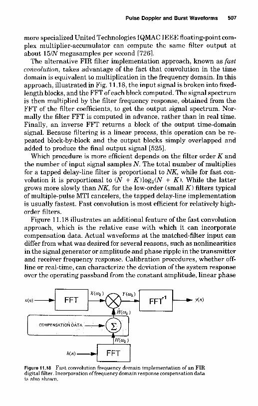
Pulse Doppler and Burst Waveforms 507
more specialized United Technologies IQMAC IEEE floating-point com- plex multiplier-accumulator can compute the same filter output a t about 15/N megasamples per second [7261.
The alternative FIR filter implementation approach, known as fast conuolution, takes advantage of the fact that convolution in the time domain is equivalent to multiplication in the frequency domain. In this approach, illustrated in Fig. 11.18, the input signal is broken into fixed- length blocks, and the FFT of each block computed. The signal spectrum is then multiplied by the filter frequency response, obtained from the FFT of the filter coefficients, to get the output signal spectrum. Nor- mally the filter FFT is computed in advance, rather than in real time. Finally, an inverse FFT returns a block of the output time-domain signal. Because filtering is a linear process, this operation can be re- peated block-by-block and the output blocks simply overlapped and added to produce the final output signal [5251.
Which procedure is more efficient depends on the filter order K and the number of input signal samples N. The total number of multiplies for a tapped delay-line filter is proportional to NK, while for fast con- volution it is proportional to (N + K)log2(N + K ) . While the latter grows more slowly than NK, for the low-order (small K ) filters typical of multiple-pulse MTI cancelers, the tapped delay-line implementation is usually fastest. Fast convolution is most efficient for relatively high- order filters.
Figure 11.18 illustrates an additional feature of the fast convolution approach, which is the relative ease with which it can incorporate compensation data. Actual waveforms a t the matched-filter input can differ from what was desired for several reasons, such as nonlinearities in the signal generator or amplitude and phase ripple in the transmitter and receiver frequency response. Calibration procedures, whether off- line or real-time, can characterize the deviation of the system response over the operating passband from the constant amplitude, linear phase
Y W
COMPENSATION DATA __c
Figure 11.18 Fast convolution frequency domain implementation of an FIR digital filter. Incorporation of frequency domain response compensation data is also shown.

508 Chapter Eleven
ideal. Since the error characterization is usually in the frequency do- main, compensation is most easily done in that domain. The fast con- volution structure lends itself readily to frequency domain compensation with minimal extra computation.
Architectures for fast Fourier transforms
The fast Fourier transform is really a growing collection of fast algo- rithms for computing the discrete Fourier transform (DFT). The best known is the Cooley-Tukey algorithm for signals of length N points, where N is constrained to be of the form RM for some radix R and integer M. This algorithm breaks the N-point DFT into repeated small elemental R-point DFTs. The example given in the previous section was a radix-2 Cooley-Tukey algorithm; radix 4 is also popular.
There are many other FFT algorithms, most described and compared succinctly by Burruss and Parks [981. The prime-factor and Winograd algorithms can be applied to signals whose length is a product of rel- atively prime numbers, N = N1Nz . . . N M . An example would be N = 2 x 5 x 7 = 70. While these are more efficient than the Cooley- Tukey algorithm in terms of multiplies per output point, they are rarely used in hardware because the structure of these algorithms has other disadvantages [5 ] . Most important are the lack of an “in-place” signal flow, a requirement for more than one type of elemental DFT block, and computational structures that vary with each stage. The first point has the effect of requiring extra memory in the FFT processor, the second implies multiple basic circuit designs, and the third makes it difficult to pipeline the FFT efficiently and complicates control and addressing circuitry.
Even for the Cooley-Tukey algorithm, there are at least five different high-level hardware architectures: the single processor, pipeline array, parallel array, parallel-pipeline array, and hypercube. We will concen- trate on the parallel-pipeline array and the single processor. Figure 11.19 illustrates the high-level architecture of these two implemen- tations. The box marked R indicates a processor that performs a single R-point FFT, or “butterfly.” If the FFT size N = Rw, then there will be M stages in the FFT with NIR butterflies in each stage. This single-butterfly processor might be an entire board of medium- and small-scale integrated circuits, a single custom very large scale inte- grated (VLSI) circuit, or a microprocessor specialized for digital signal processing.
The important characteristics of an FFT processor are the incre- mental time between completion of successive FFTs; the throughput in FFTs per second, which is the inverse of the incremental FFT time; the latency; the number of butterfly processors, or nodes, required; and

Pulse Doppler and Burst Waveforms 509
0 U T - J - q ~ ~ Fl lnc FFT time = N M T / R
MEhnRY IN No ofnodes=
(A)
Inc FFT time = NT/(RP/
OUT Throughput = RP/(NTj Latency = NMTIRP
OUT 1_J No of nodes = MP OUT
IN
(TOTAL OF M STAGES IN PIPELINE)
( B l
Figure 11.19 Two common FFT architectures and their performance. A box marked R denotes a single butterfly computation in radix R. (A) Single processor structure; (B) parallel-pipeline array.
the number of memories required. These characteristics are also shown in Fig. 11.19, with P the number of parallel nodes per pipeline stage and M the number of pipeline stages. T is the time required for a node to compute one butterfly. Generally, pipelining increases throughput but does not affect latency, while using parallel nodes improves both. The conventional pipeline of the previous section corresponds to P =
1. In that case, the throughput is increased by a factor M equal to the number of pipeline stages, but the latency is not reduced at all. In- creasing the number of nodes per stage, however, both further improves throughput and reduces latency. The disadvantage of multiple nodes per stage is that complex multiport memories are then required to supply all the nodes with inputs and receive their outputs simulta- neously.
As with digital filters, FFT times vary widely with the hardware used. The Texas Instruments TMS320C25 can complete a 256-point FFT in 1.408 ms [7001, while the United Technologies floating-point IQMAC requires 136.8 p s [7261. A circuit based on an experimental short-block floating-point VLSl radix4 butterfly circuit was capable of performing the same computation in 81.92 p s [4861.
In addition to the nodal computers, all FFT architectures require data memories, coefficient memories, and address generators. The data memories, included in Fig. 11.19, are usually “ping-ponged” and capable of supporting simultaneous read and write operations. If multiple nodes are used per stage, then multiple reads and writes must be accom- modated. Coefficient memories are usually read-only memories (ROMs)

510 Chapter Eleven
which store the cos(2.nnkIN) and s in(2~nklN) values required by the FFT algorithms so that they need not be continuously recomputed. Address generators are special counters that generate the addresses required to access and store both data and coefficients in the special bit-reversed orderings required by the algorithm. These devices offload the simple but high-speed address calculations from the main control processor, and are usually programmable via a few control pins for different DFT sizes. One address generator and coefficient ROM are usually required for each processing node.
An interesting recent development in FFT algorithms is the split- radix algorithm, which is an alternative to the Cooley-Tukey method for transform lengths which are powers of 2 [1901. While not as efficient as the Winograd in multiplies per output point, it is more efficient than the Cooley-Tukey algorithm when measured either by multiplies or by total multiplies and additions [5961. This makes it an excellent choice for software or single-node hardware FFT implementations, despite some extra programming complexity. However, it requires more but- terflies than the Cooley-Tukey algorithm and its structure does not permit completely efficient pipelining or parallelism. Consequently, it is not well suited to multiple-node parallel or pipeline implementations.
Sizing computational requirements
The first step in developing a processor architecture is to estimate requirements such as throughput, memory size, and latency. This is done by developing a detailed flow graph of the processing and using it along with the radar parameters to “walk through” the processing, estimating the loads a t each step. Figure 11.20 gives a simple example of the first level of such an analysis for the Doppler-processor section of a radar comprising a cascade of a three-pulse canceler and a 16- point FFT implemented with the conventional radix-2 algorithm. We assume a PRF of 5 kHz with processing of 200 50-m range cells, giving 10 km of total range coverage. Analog pulse compression, perhaps with a surface acoustic wave (SAW) device, precedes the analog-to-digital conversion, as does demodulation of the signal to baseband.
The 50-m range resolution implies a 3-MHz signal bandwidth, so the Nyquist sampling rate is also three megasamples per second. Since the receiver is coherent, the samples are complex, i.e., they have Z and Q components. The initial PRI buffer holds 1600 &bit words. This allows for 200 range cells of complex data for each of four pulses. Four pulses of data are stored at a time so that the three-pulse canceler that follows can be working on three rows of data, say numbers 1, 2, and 3, while a new fourth row is collected and stored. When the canceler finishes working through the 200 range bins, it shifts over one row, now op-

DATA RATE (COMPLEX, WORDLENGTH PULSE
MWORDS/SEC) (BITS)
3 0 6
PRI BUFFER 1600x8
V
\11/
1 .o 6
3-PULSE CANCELLER
1 0 6
FFT INPUT BUFFER 12,800X6
V 1 0 6
\(L
16.POINT FFT
1 0 12
FFT OUTPUT BUFFER 12,600~12
V
REAL MULTS REMARKS PER SECOND
. Range resolution = 50 m * PRF = 5 kHz * 200 range cells to store per PRI * Complex data doubles buner size * 4 pulses stored Io accommodate 3-pulse cameller . Dala rate slowed by spreading processing over PRI
. Finer symmetry, real coenlclentsgiveslwr real
.ZOO range hns liltered per PRI
.ZOO range bins tor each 01 16 pulses . size quadrupled lor "ping-pongng" and
4x10⁶ multiplies per inpul
mmpkex data
6x10⁶ . 126realmuhipliesperFFT . FFT on 200 range cells every 16 PRls E 3.2 ms - FFT imegratwn adds 4 bits lo wordleng(h
. same as lnprl builer excepl lor larger word Size

512 Chapter Eleven
half, while the output of the canceler begins refilling the first half. This process, similar to that used in the PRI buffer, is called “ping-ponging.” Estimates for the FFT computational rate and the output buffer sizing are outlined in Fig. 11.20 by similar reasoning.
Sizing is an iterative process. The next steps for the MTI section would probably be to expand the FFT structure, perhaps comparing alternatives such as pipelined or single-processor implementations, then to add in missing details such as coefficient memories and control requirements. For a first estimate, however, an analysis like that in Fig. 11.20 is usually reasonably accurate, especially if some design margin is factored in.
Architectural constraints
The designer rarely has full freedom in selecting an architecture. The signal processor is but one part of a larger system, and must conform to overall system constraints. For example, many military signal pro- cessors must meet very stringent special requirements for radiation hardness, electromagnetic emissions security, ruggedness, and built- in-test (BIT) capability. Radiation hardness requirements, in particu- lar, disqualify certain semiconductor processes from being used, elim- inating from consideration some microprocessors that might otherwise be chosen for an application.
Most signal processors are programmable to some degree. The soft- ware used to program the device is also frequently constrained. Using military systems as an example again, many require a processor to include a module that implements the military standard (MIL-STD) 1750A low-level computer instruction set. For high-level programming, specific languages such as JOVIAL or Ada are often specified. The lack of a validated Ada compiler can again disqualify some microprocessors from use.
Not all programming of electronic systems is necessarily done in standard assembly or high-level languages, however. So-called graph or block diagram languages 14251 are often used for programming mod- ular signal processors. In these languages, signal-processing algo- rithms are described by flow graphs in which operations such as summation of two signals or the FFT of a signal are indicated by blocks, and the input signal sources, output signal destinations, and order of operations are indicated by “wiring” the blocks together in the appro- priate sequence. Various vendor-specific software tools then “compile” the graph and translate it into real-time commands to route data to specific processor modules and to have those modules execute the ap- propriate functions.
Graph languages are an attempt to make it easier to implement

Pulse Doppler and Burst Waveforms 513
signal-processing algorithms efficiently on modular processors. An- other approach used in some very highly parallel architectures is to program them in special high-order languages such as OCCAM, which allow explicit specification of processes that can be executed in parallel. Yet another special case arises when the signal processing includes artificial intelligence or expert system concepts. Software for these types of systems is most often written in either LISP or PROLOG.
Military systems are not the only ones that enforce architectural constraints. Many commercial signal processors are modular in con- struction, using a backplane bus to transfer data and control signals between modules. New modules must therefore conform to the existing bus structure and communication protocols. Examples include the VME and Multibus I1 standards, which have developed as extensions of buses originally implemented around the popular Motorola 68000 and Intel 80x86 microprocessors, respectively. The others are newer concepts, developed to handle more complex systems and higher data rates.
Signal processors may be subject to other bus constraints as well. Many military processors must provide an interface to the MIL-STD 1553B serial bus. Virtually all processors, military or commercial, re- quire a common RS232 or RS422 serial port as well.
A good example of a more comprehensive set of system constraints is the complete avionics architectural concept known as PAVE PILLAR developed by the U.S. Air Force [5271, to which processors designed for the Advanced Tactical Fighter must conform. PAVE PILLAR in- cludes specification of a high-level signal processor architecture like that shown in Fig. 11.21. The key feature of the architecture is the modularity imposed by the requirement that the processor be built up from a small number of relatively generic modules (the “common signal processors” of the figure). Data communication between modules is handled by a high-speed reconfigurable switch, the “data exchange network,” which is itself built up from basic modules. Other modules
VIDEO
t--) DISTRIBUTION f-) 9 \NETWORK/
-,-\-+3- DATA NETWORKS AND CONTROL PROCESSORS (y:;:;;oNRGK;) uw - - Figure 11.21 The high-level architecture of a PAVE PILLAR signal pro- cessor. (After 15271)

514 Chapter Eleven
provide the interface to external sensors. The PAVE PILLAR concept specifies a core set of modules including, among others, a 125-MFLOP floating-point processor; a 3 MIPS MIL-STD 1750A CPU used for con- trol and general-purpose computing; a 1-Mword global memory and a 2-Mword nonvolatile memory, both with error detection and correction; interfaces to the MIL-STD 1553B serial bus, a 5OO-MbitIs sensor bus; a 24-channel, 25-Mwords data exchange network; and various utility modules such as timing generators and power supplies. Additional desirable modules for fixed-point arithmetic, sorting, FFTs, and so forth are also identified. The PAVE PILLAR architecture includes a com- prehensive treatment of built-in test and diagnosis a t the chip, board, and system levels.
11.8 Range Computations for Pulse Doppler Radar
The computation of detection range for a pulse Doppler search radar does not differ substantially from that of the simple pulse radar if the dependence on energy is kept in mind. The pulse radar range equation from Chap. 2 was given as
(11.8)
For a single transmit pulse and approximately a matched filter, the noise bandwidth BN = 117' where T' is the pulse width. Since a pulse Doppler system coherently integrates many (N,) pulses, it is almost sufficient to multiply the numerator of the range equation by N, if the transfer characteristic of the narrow-band filters following the range gate is such that they optimally integrate N, pulses, i.e., the narrow- band filter must also be matched to the total transmission time Td.
The simplest processor to consider is the tapped delay line (Fig. 11.12). In this configuration N, pulses are added voltagewise (@ in power), and N, noise samples are added with random phase (N, in power). The (SIN) required for a given probability of detection and false alarm probability is thus reduced by N, after allowance is made for the appropriate number of false alarm opportunities.
In any pulse Doppler system, the false alarm probability must be based on the product of the number of range gates ng and the number of Doppler filters K per range gate. The number of opportunities for false alarms is not necessarily greater than for a simple pulse radar since the number of independent samples a t the output of the filter is proportional to the filter bandwidth b. For a given velocity coverage, the filter bandwidth decreases as the number of Doppler filters in-
R4 = PTGTLTA, LRLPLJ, ~ u t
( 4 ~ )'KTS B N (SIN)

Pulse Doppler and Burst Waveforms 515
creases. Thus, in most cases the number of potential false alarms is independent of the number of Doppler filters.
Another version of the pulse Doppler range equation can be derived from the following relations:
(11.9) P
, - P d - T
where d, = transmit duty factor P = average transmit power P = pulse transmit power (average power during pulse)
Also
(1 1.10) - N C - T ‘Ne d, =
T(N, - 1) BNT(Nc - 1)
where T = average interpulse period Ne = number of coherently integrated pulses
Eliminating the duty factor from Eqs. (11.9) and (11.101,
(11.11)
A good approximation for the noise bandwidth of the matched Doppler filter is
P FT(N, - 1) BN N C
_ - -
1 - (11.12)
where Td = the coherent transmit time of pulse train. Then substituting for (Ne - 1 IT in Eq. (1 1.11 1 yields
1 T d (Ne - 1)T
b - - -
(11.13)
If Eq. (11.13) is then substituted in the range equation after the numerator has been multiplied by Ne to account for the coherent in- tegration, the alternate pulse Doppler range equation becomes
P P -=- BN bNc
(11.4)
It must be emphasized that (SIN) is the per-pulse signal-to-noise ratio in the Doppler filter for the desired probability of detection and false alarm probability.
R4 = ptGTLTAcRLPLaL,Lsut ( ~ T ~ ) ~ K T , ~ ( S I N )

516 Chapter Eleven
Deviations from ideal integration
The calculation of the efficiency factorl, for pulse Doppler must account for some potential added losses:
1. The deviation of the pulse matched filter from the optimum value. 2. The range gate being too narrow, too wide, or not centered on the
target return. This loss should not always be directly added to (1) since pulse “stretching” by the pulse matched filter partially com- pensates for minor errors in the range gating.
3. The Doppler matched-filter shape (or bandwidth) may deviate from the optimum.
4. The target response may straddle more than one Doppler filter or fall in the notches between them.
5. There may be a significant Doppler dispersion loss [588] if 2Tdu/~’c 2 1.
6. Doppler image noise may be folded onto the desired Doppler spec-
7. Phase- and time-delay errors reduce the sensitivity. 8. FM and AM transmitter noise imposed on nearby clutter may exceed
trum.
receiver noise (see Sec. 14.4).
The characteristics of the individual pulse and the Doppler filters deserve special attention. Analysis of the improvement obtained from coherent integration for various filter shapes has been reported by North [514], George and Zamanakos [2631, Galejs [2571, and others. For the case of a uniform pulse train of rectangular pulses and a uniform video comb filter with an idealized square passband, it has been shown 12631 that
Improvement = ( N J Y ) = 10 log (0.45 N,) in dB, if 7’ < _T (11.15)
The assumption here is that the input noise is white, and the rectan- gular Doppler filters cover the mainlobe of the (sinx/x)2 energy density spectrum (- 90 percent of the energy falls within the filter). The as- sumed filter bandwidth b = 2lN,T Hz is somewhat wider than the optimum.
By altering the gains of the “teeth’ of the comb filter to “match the amplitudes of the lines of the uniform pulse-train spectrum, an addi- tional improvement of 2.1 dB is obtained. If, in addition, each tooth of the filter is given a (sin x/x)‘ response, the North filter is obtained, the improvement of which is 4.3 dB greater than Eq. (11.15). The improve-
4

Pulse Doppler and Burst Waveforms 517
ment in this case ;= 0.8 dB greater than N,, presumably due to the assumptions of an overly wide bandpass for the single pulse and an idealized integrator.
Galejs [2571 has extended this analysis to physically realizable comb filters and to the case in which the pulse-train envelope is in a /sin x/xI form, which would result from an antenna beam scanning past a target. Using the same general assumptions as George, he obtained the (SIN) power improvements, above 10 log 0.45 N,, for practical filters and rectangular pulse trains. For rectangular pulses the improvement was 3.8, 1.7, and 1.8 dB for the optimum, cascaded delay line, and feedback filters, respectively. The exact values quoted here are for special cases. They should not be used without study of the detailed assumptions in the references, including the discussions on output sampling time.
11.9 Clutter Computations
Perhaps the most difficult part of predicting the performance of a pulse Doppler radar is the calculation of the rejection of extended clutter echoes.* The difficulty arises because the dominant clutter may not be a t the target location and may extend over a considerable portion of the ambiguity plane. The differing range dependencies of targets and clutter preclude the use of a single chart of equations. The general pulse Doppler range equation for uniform clutter is derived in this section with some indication of how simplifications can be made. It will be shown that in many cases the right members of the range equation can be factored into the range Ln clutter for a pulse radar and a clutter attenuation CA factor for the pulse Doppler.
The periodic character of the pulse-train spectrum causes Doppler ambiguities a t multiples of the repetition frequency. Thus, undesired targets (such as rain, chaff, sea or land clutter) may produce a large response at or near the Doppler frequency of the desired echo, thereby obscuring it. The use of a medium or high pulse repetition frequency to reduce the Doppler ambiguities is common in the design of pulse Doppler radars but aggravates the problem of range ambiguities. With a high PRF, echoes from many different ranges may be received si- multaneously so that even though the target might be in a clear region, clutter elsewhere along the antenna beam can cause interference. The peak echo power from clutter a t the output of the receiver range gate, neglecting antenna sidelobes, will be
' The majority of this section was prepared by Dr P J Luke, formerly of the Applied Physics Laboratory

518 Chapter Eleven
- P GAeL co j-!m,+)l4 ~u dV (1 1.16) R4 P, =
where G = antenna gain at beam center
(4.rrI2
A, = effective area of the receiving aperture
Co = clutter scattering cross-section density (usually expressed in square meters per cubic meter for volume clutter)
f ( 0 , +) = antenna amplitude pattern, which is a function of the angular coordinates 0,+ measured from the axis of the beam
Lu = attenuation factor due to the transmission medium (a function of range)
R = range to the volume element dV
L = transmitter and receiver loss factors combined
dV = R2 dfl d R d R = element of solid angle
For volume-extended clutter (e.g., rain, chaff) the integral with respect to the solid angle may be evaluated immediately, giving [563]
~ ( 0 , + ) 1 4 m = - .rrO1'l - - 0.57 01+1 I 8 In 2
where el and +1 are the one-way half-power beamwidths. The echo power from volume-extended clutter is then
(Za) (0.57 01+1) ?$ (11.17)
The integral with respect to R is taken over all ranges from which simultaneous or overlapping echoes are received.
Following the range gate, the signal is filtered by the Doppler filter, envelope detected, and compared with a threshold. In order to deter- mine the clutter energy at the detector input, we compute the spectral density of the clutter echo at the input to the filter and from that the clutter energy at the filter output. A similar computation yields the target-echo energy at the detector. The ratio of these two is the signal- to-clutter ratio for the particular range gate and Doppler filter being considered, which are the ones having the most target-echo energy.
Since the clutter return consists of echoes from many small reflectors distributed at random in space and, hence, with random phases, the spectral density for the clutter will be the sum of the spectral densities for the individual returns. The expected value of the resultant spectral density (with respect to both the spatial distribution and the frequency or velocity distribution) integrated over the filter bandwidth yields the mean clutter energy at the detector input.
- P G A , L P, = (4.rr)2

Pulse Doppler and Burst Waveforms 519
Constant interpulse period-clutter response
An echo consisting of a uniform train of N pulses with constant am- plitude a, and Doppler shift L relative to the filter center frequency has an energy spectral density
sin2[.rr(f - f,) NTI E L ( f ) = 2 a, ', l U , ( f - f , ) I 2 sin2[.rr(f - f , ) T ]
(11.18) I sin2[.rr(f + f,) NTI 1 2 2 {
+ 'UL(f + ')" sin2[.rr(f + L ) T ]
where T = the interpulse spacing T, = the pulse width of the echo after range gating (which may
truncate the pulse) TU(^) = the single-pulse spectrum (defined in this manner so that
U ( f ) is dimensionless, e.g., for a rectangular pulse U ( f ) = sin .rrfd.rrfT)
After truncation by. the range gate the echo from the ith reflector has a single-pulse spectrum T,U,(~) .
The frequencies f , are distributed over some interval which is usually small relative to the pulse-repetition frequency but may be greater than 1". Thus, the factor lU,(f t f,)I2/sin2 .rr(f t f,) T does not vary appreciably over this interval and may be given the constant value U,(f ? fC)'/sin2 ~ ( f ? f c ) T when averaging E,( f ) with respect to the dis- tribution of L. The frequency fc is an average with respect to the dis- tribution. Noting that the average of the factor sin2 n(f k LINT is '/2, the average spectral density is
Ec,(f) = i a f T i ? 1 { lWf - f C ) l 2 + l W f + f C ) l 2
2 sin2.rr(f - f c ) T 2 sin'df + f c ) T
This equation is valid only iff - fc > UNT. Since f , and fJ are inde- pendent, this is the spectral density for all the returns.
The total energy in the bandwidth of the filter is
' 2 Z l f r t b A l U , ( f ) l 2 df (11.19) ECL = i,"" E C , ( f ) df = 4 'L ', f , - b / 2 sin2.rrfT
where b = the filter bandwidth. Since b is small compared to lh,, U , ( f ) is essentially constant throughout the range of integration. Taking ( 1 7 , ( f ) 1 ~ evaluated at fc outside the integral and evaluating the remain- ing integral, noting that a:/2 is the peak pulse power, and summing over all reflectors, one obtains for the total clutter energy out of the filter

520 Chapter Eleven
P G A , L [(Xu)(0.57 0 1 W l [IT] L d d R [ lU(fc)12K T ] (11.20) Ec = [ (4ITY ]
where
i K = L ( sin rrbT IT COS ITbT - COS 2nfc T
The integral with respect to range is approximately
p + ~ r 2 - ( T g r 2 d R c - 3) E- La = r 2 % 9 2
2 k R; 2 k R k 2
where r = pulselength, re = rg - 713 if rg 2 r
rg = range-gate length Rk = range to the kth ambiguous range
If rg < r , interchange rg and r . Thus, finally one has for the total clutter energy
P T ~ ~ , ~ r - (Xu) (q) (0.57 O1+1) (2 ") IU(fJ2K (11.21)
(47~)' T k R; E, =
Target-echo response
The energy spectral density for a target echo consisting of a train of N pulses with amplitude a and Doppler shift fs relative to the filter center frequency is
sin2 IT ( f - f J N T E S ( f ) = 2 a2 r2 l u ( f - f S ) I 2 sin2 IT ( f - f s ) T
I sin2 IT ( f + f,) N T l {
+ l U ( f + f S ) l 2 sin2 IT ( f + f , ) T
If the range gate does not match the pulse (so that part of the pulse is eclipsed), r should be replaced by ET where 0 < E < 1. The signal energy out of the Doppler filter is then
f s i bI2
sin2 ITfNTdf (11.22)
The filter bandwidth b is generally much less than the PRF UT, and f , is less than b12. Otherwise the signal is in another filter, and one
1 hI2
E, = Io E , ( f ) d f = - a 2 r 2 ~ U ( f s ) 1 2 ~ 2 f? - hl2 sin2 rf T

Pulse Doppler and Burst Waveforms 521
should examine that filter. Therefore, sin (.rrfT) may be approximated by .rrfT.
The integral in Eq. (11.22) is then
df f<' ' I 2 sin2 TfNT fs' b'2 sin2 rrfNT J5 hl2 sin2 r f T d f = i ,-bl2 (,rrfT)2 (11.23)
NY m N n f 5 f 612) sin2 x ="I & = - r T rNlYf\-bl2) x2 T
where the function Y represents the fraction of the energy of a single line contained in the filter bandwidth. The signal energy is then
E, = PT(Yr$ L ($1 (J t L p R t ~ I U ( f # N Y
where Rt = target range Lp = pattern loss in case the target is not centered in the beam
With N pulses integrated, the coherent integration on the dwell time is Td = NT.
The ratio of signal energy to clutter energy at the output of the Doppler filter containing the target signal is thus
E. = [ mt 1 [ LP 1 [ (LJR:) ] [ I ~ ( ~ . ) I ~ N Y ] (11.24) E, (Zm) (CTe/2) 0.57 O1$1 c(LA/Rk2) IU(fc)l2 K
k
or, naming the factors,
E. = [echo power][pattern factorl[attenuationl[spectral factor] E,
For a duty ratio of T/T 5 0.01, the single-pulse envelope functions U(fs) and UCf,) differ by a small fraction of 1 percent (i.e., both signal and clutter are near the center of the single-pulse spectrum). Hence the ratio U( f , )2 to U(f,)' is essentially unity. The function Y is always < 1 but generally > 0.5.
A number of approximations can be made to make Eq. (11.24) more tractable. A reasonable average value for Y is about two-thirds, the gate length T~ = T , the atmospheric attenuation term La can be ne- glected, and L, = 0.57. Then Eq. (11.24) simplifies to
"-[ ( J t ] [ k 1 ] [E] (11.25) E, ( 2 ~ ) (CT/2) 81$1 R? c(Rt/Rk)2

522 Chapter Eleven
Clutter echoes only at the target
If the clutter is small in extent compared to the interpulse period (less than cT/2) and located only at the target, then the energy ratio is
sin nbT I] (11.26)
It should be noted that the first two brackets of Eq. (11.26) are the same as the equation for the simple pulse radar in volume clutter. Thus, the terms in the final bracket constitute the clutter attenuation or improvement factor for a train of N pulses using a close approxi- mation to a matched-filter receiver. The detection-range equation for clutter at the target range is then obtained by rewriting Eq. (11.26)
] [ 1 ( sinnbT I] (11.27)
N
"=[ ut E, (CUI (CT/2) 8141 ] [h] [: (cosnhT - cos2nfcT
N ut [ (%d (CT/2) 81$1 (SIC) n cos nbT - cos 2nfC T
R: =
Numerical values for the second bracket were given in Table 11.1.
Extended-clutter echoes
For clutter that extends quite close to the radar (uniform rain, etc.), the sum in the denominator of the third bracket of Eq. (11.25) is dom- inated by the term for the nearest ambiguous range R1 and the signal- to-clutter ratio is then
3- (Tt ] [z] [L,(Rt - Rl)l [g] (11.28)
where La (R, - R,) = the attenuation between the target and the first clutter region. The significance of this equation is that for volume clutter that is close to the radar at range R1, the signal-to-clutter ratio varies inversely as RP rather than as R? as in unambiguous pulse radars. The first ambiguous clutter range can be approximated by using the largest integer N1 which satisfies
E, - [ CU(CT/2) 81$1
(11.29) CT cT R 1 - R t - N 1 - > O if -<<-
The approximation breaks down if R1 is in the near zone of the antenna or if an STC circuit is used to reduce the near-in clutter.
For the intermediate case in which the clutter extends a t least several
[ (fIl 2 2

Pulse Doppler and Burst Waveforms 523
interpulse periods but not to the radar (the target may or may not be within the clutter), the sum in Eq. (11.25) may be approximated by
E k Ri2 -- [R, + (2Nl - 1) cT141 [R, + (2N2 - 1) cT/41 (1 1.30)
(N2 - N1 + 1)
where R, + N1 cT/2 = smallest ambiguous clutter range R, + N2 cT12 = largest ambiguous clutter range N2 - N1 + 1 = number of ambiguous ranges from which clutter
returns are simultaneously received
Both N1 and N2 may be negative as long as R, + (2N1 - 1) cT/4 is positive. If this term is near zero range, the approximation to obtain Eq. (11.30) is poor, and the system is most likely dominated by the first clutter echoes. In this case it will usually suffice to use Eq. (11.29).
Optimum value of filter bandwidth
In order to determine the optimum bandwidth for maximizing SIC, let b = XINT = XIT, for large N, where X is a constant factor. The last factor in Eq. (11.24) becomes
(11.31) NY
'[ T COS (TXIN) - COS 2rfc T 1 sin (TXIN)
Referring to Eq. (11.231, it is easily shown that the function Y is a monotonically increasing function of X which approaches the value 1 for X = N. For X decreasing, Y becomes asymptotic to X. Examination of the denominator of the foregoing expression shows it to be also a monotonic increasing function of X which, however, does not approach a constant value for large X but in fact increases indefinitely as XIN approaches 2fc T. At this point the approximations used to obtain Eq. (11.20) are no longer valid. For smallX the denominator is proportional to XIN.
The value of the fraction is thus proportional to 2\IL for small X and decreases as X increases. This suggests that the best bandwidth to use is the narrowest obtainable. This is true when clutter is the only in- terference to consider. In the presence of broadband noise, however, reduction of the bandwidth much below the reciprocal of the signal duration Td seriously degrades the signal-to-noise ratio. Also, if the target fluctuates rapidly or accelerates, little improvement in signal- to-noise ratio will be obtained by reducing the bandwidth below the spectral width of the fluctuations.

524 Chapter Eleven
The best bandwidth is then obtained by taking X to be of the order of 1, making the signal-to-clutter ratio proportional to M. The constant of proportionality depends on fc. If b is replaced by 1INT in the last bracket of Eqs. (11.27) through (11.311, this term can be written
sin abT )] = [A ( sin(a/N) )I (11.32)
N N
[: (cos abT - cos 2af,T 7~ cos(~IN - c 0 ~ 2 n f . T
If, in addition, N is a t least 30, sin(a1N) = TIN, cos alN = 1, and the bracketed term becomes
N2[1 - cos 2&TI = clutter attenuation (1 1.33)
As expected, the clutter attenuation term is maximized at fcT = I/2.
Then, for bT = 1lN and N large, the maximum clutter attenuation for a Doppler separation offcT -- '/2 (averaged over Dopplers in that region) can be approximated by
CA,,, = 2N2 near the optimum Doppler separation (11.34)
Alternately, for an average over all Doppler velocities (except for the ambiguous regions) the improvement factor I is N2. This analysis does not include effects of weighting described earlier and in Sec. 14.4.
11.10 Truncated Pulse Trains
The previous section on clutter computations emphasized that the close- in clutter a t range Ro is often the limiting factor in the performance of pulse Doppler systems in range-extended-clutter environments. For most detection criteria, the overall improvement factor I contains a term of the form RgR: for uniform volume clutter extended in range with a high PRF transmission. Thus, the overall improvement may be negligible for targets a t a range of many interpulse periods. The type of clutter that is of most concern in this description is assumed to be extended in range and separated from the target velocity but confined in Doppler extent. Rihaczek [601, 6031 and others have shown that a gniformly spaced pulse train is desirable since most of the energy under the ambiguity surface is concentrated in finite locations on the axes. The following discussion is based on uniform interpulse spacing of uniform amplitude pulses.
Single-burst pulse train
It can be seen from Eq. (11.30) that the summation of the clutter echoes from many ranges provides a limit to the signal-to-clutter ratio im-

Pulse Doppler and Burst Waveforms 525
provement in partially extended clutter. Ares [161 has shown that for a given target-to-clutter velocity ratio and interpulse period T there exists for each target range Rt a value of N that maximizes the signal- to-clutter ratio. This optimization exists only for clutter that extends for all the 2N - 1 ridges of the ambiguity diagram. The explanation for this optimization is that for small interpulse periods, the close-in clutter at range Ro is competing with target signals from distant ranges, and it is the echoes from the later transmitted pulses that constitute the greatest portion of the clutter entering the receiver. The optimum number of pulses found by Ares is
1 N z = - ( % ) fl cTl2 (11.35)
and the optimum clutter attenuation is CA,,, -- 2/3N, the improvement factor then being
(11.36)
It can be seen that the improvement factor increases with target range. The optimum Doppler velocity occurs a t approximately 1/2T, as expected. If the target range and Doppler frequency are approximately known, as in an acquisition or tracking radar, the optimum number of pulses and their spacing can be chosen. The target-detection range for uniform range extended clutter can then be written from Eq. (2.30).
2 =t IOpt Z= - N = 3 3 f l ( c T l 2 )
( 1 1.37)
It can be noted that the required (SIC) is only first-order dependent on target range and that both short pulse lengths and small interpulse periods are desired. Since a short interpulse period can only result from optimization with respect to a high Doppler frequency, the interpulse period term cTl2 in the denominator shows only the desirability of having a large velocity separation between the targets and the clutter.
If the interpulse period is not fixed by other considerations, a double optimization involving the period and the number of pulses can be performed. An example is given in Table 11.5. For a given range R, (in microseconds) and target Doppler frequency fd, the optimum number of pulses is shown. Also shown in the table is the length of the burst Td = 2 RJ3c and the Doppler resolution b in kHz.
The improvement factor for these same cases is shown in Table 11.6. The improvement factor is in decibels above the signal-to-clutter ratio
2LCLbt 3~(~ /4)81~1(CT’ /2 ) (CT/2) (s /c )~U
R o p t =

526 Chapter Eleven
TABLE 11.5 Optimum Number of Uniformly Spaced Pulses for Extended Clutter
Target Dwell Doppler No,, for Doppler frequency offset, kHz range time resolution Rt, PS Td, PS 6, kHz 4 5 8 10 12 15 20 25 30 35 40
400 231 4.33 2 2 4 5 6 7 9 12 14 16 18 500 289 3.46 2 3 5 6 7 9 12 14 17 20 23 600 346 2.89 3 4 6 7 8 10 14 17 21 24 28
700 404 2.48 3 4 7 8 10 12 16 20 24 28 32 800 462 2.17 4 5 7 9 11 14 18 23 28 32 37 900 517 1.94 4 5 8 10 12 16 21 26 31 36 42
1000 577 1.73 5 6 9 12 14 17 23 29 35 40 46 1100 635 1.58 5 6 10 13 15 19 25 32 38 44 51 1200 693 1.44 6 7 11 14 17 21 28 35 42 49 55
1300 751 1.33 6 8 12 15 18 23 30 38 45 53 60 1400 808 1.24 6 8 13 16 19 24 32 40 49 57 65 1600 923 1.08 7 9 15 18 22 28 37 46 55 65 74
that would result from a single pulse of the train, and it applies only to an extended-clutter situation. The values shown are slightly better than would be indicated by Eq. (11.36) for certain numbers of pulses (see also [3971).
Ares also considered receiver amplitude weighting of the truncated pulse train and showed that there was little additional improvement. The explanation for this is that the ambiguous clutter returns at other than the target range do not receive the symmetrical weighting that is necessary to reduce the Doppler sidelobes. Fig. 11.22 gives examples
TABLE 11.6 Optimum Improvement Factor, /,dB, for Uniformly Spaced Pulses and Extended Clutter
Target Doppler frequency offset, kHz range R,, p s 4 5 8 10 12 15 20 25 30 35 40
400 1.3 1.3 4.3 5.2 6.0 6.7 7.8 9.0 9.7 10.3 10.8 500 1.3 3.0 5.2 6.0 6.7 7.8 9.0 9.7 10.5 11.3 11.9 600 3.0 3.0 6.0 6.7 7.3 8.2 9.7 10.5 11.5 12.0 12.7
700 3.0 4.3 6.0 7.3 8.2 9.0 10.3 11.3 12.0 12.7 13.3 800 4.3 5.2 6.7 7.8 8.7 9.7 10.8 11.9 12.7 13.3 13.9 900 4.3 5.2 7.3 8.2 9.0 10.0 11.5 12.4 13.2 13.8 14.4
1000 5.2 6.0 7.8 9.0 9.7 10.5 11.9 12.9 13.7 14.3 14.9 1100 5.2 6.0 8.2 9.4 10.0 11.0 12.2 13.3 14.0 14.7 15.3 1200 6.0 6.7 8.7 9.7 10.5 11.5 12.7 13.7 14.5 15.1 15.6
1300 6.0 7.3 9.0 10.0 10.8 11.9 13.0 14.0 14.8 15.5 16.0 1400 6.0 7.3 9.4 10.3 11.0 12.0 13.3 14.2 15.1 15.8 16.4 1600 6.7 7.8 10.0 10.8 11.7 12.7 13.9 14.9 15.6 16.4 16.9

Pulse Doppler and Burst Waveforms 527
N = 6 , T= 2 3 . 5 P I
RAIN UNIFORM FROM 0 T O 3 5 , 0 0 0 11 TARGET AT OPTIMUM VELOCITY
3' ELEVATION BEAMWIDTH-CENTER AT I. 5'
2 4
2 2
20
g 18
l-
W 3 0 d B SIDE a W
> 16 0 w P I
t- 14
- CY W
I- 3 1
2 f 12
4 z 0 v)
I O
8
40 60 80 100 200
TARGET RANGE, nmi
Figure 11 2 2 Signal-to-clutter improvement versus target range for 16- pulse train and uniform rain. (From Ares [161)
[161 of the improvement obtained with a constant amplitude and a Taylor-tapered train of 16 pulses for various target ranges. It is drawn for the case of uniform rain clutter that has a narrow spectrum but is extended in range until the radar antenna beam reaches a 35,000-ft altitude. The improvement increases slowly from 40 to 100 nmi, and then, as the beam extends above the rain, the improvement increases more rapidly. The additional improvement resulting from tapering the received waveform is less than 3 dB at the optimum velocity and almost trivial a t other velocities, even with a 40-dB taper. Thus, significant improvement over the uniform case can occur only with complex weight- ing of the transmitted waveform as well as of the receiver waveform as discussed in Sec. 11.4.

528 Chapter Eleven
Geometric or burst programming
A pulse Doppler radar operating at high PRF will have blind ranges and close-in clutter problems if the transmit pulse train is not turned off immediately prior to and during the target-echo receive period.* By use of such a turn-off procedure, reduction of close-in clutter echoes can be achieved but a t the expense of reducing the total number of pulses on the target during the coherent integration time. A burst repetition frequencg, (BRF) is thus created that is a function of target range and the time allowed for nearby clutter to diminish to a tolerable level. This frequency is nominally equal to 1/(2T, - Ted) where Tt is the target echo time and Ted is the clutter decay time.
In the case of surface radars, it is often necessary to impose the requirement for a clutter decay time to prevent large clutter returns from regions much closer than the target range from entering the range gate, These returns may be from either the mainlobe or sidelobes of the antenna. For uniform clutter, increasing clutter decay time must be compromised with respect to the number of pulses transmitted. The functional relationship between target range, clutter decay, and the BRF is shown in Fig. 11.23. Here, the maximum percentage of pulses is taken to occur when transmit on and off times are equal; i.e., the clutter decay time is zero.
The adaptive control of the BRF in response to changes in target range and the range extent of the nearby clutter is termed geometric programming. Some experimental effects of using geometric program- ming are shown in the range profiles of Fig. 11.24. The equipment used was a high-PRF (150-kHz) digital implementation of a pulse Doppler radar. In all plots, the zero Doppler channel is displayed (normalized to the largest signal) to illustrate the land-clutter response. In Fig. 11.24A no geometric programming was used. This mode maintains maximum energy on the target (a water tower in this case) but suffers from ambiguous clutter folding onto the target range. Figure 11.24B shows the effect of geometric programming but without any clutter decay time, again allowing nearby clutter to fold onto the target region. In Fig. 11.24C local clutter has been removed by keeping the receiver off for an additional 12.8-ks interval after each burst. Since the system has a constant PRF, range ambiguities still occur beyond the target. In Fig. 11.24D a single-pulse transmission is shown for comparison. With this nonambiguous waveform, the return energy from the target is relatively low (no integration) and cannot yield any Doppler reso- lution.
The modulation of the transmit waveform with burst timing creates
I Material for this section courtesy of A Chwastyk
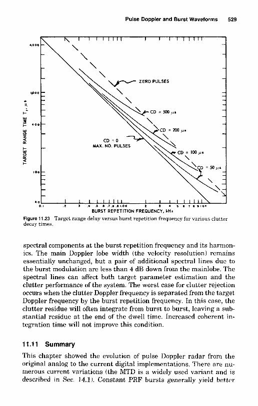
Pulse Doppler and Burst Waveforms 529
\ 1 ' ' ' I " ( 1 I I I I I I l l -
-
- -
lP00 - - * - - - -
- 3.
I- w I + 4 0 0 - - w - K
I- W
2 -
- - - -
8 2
100 -
- 0 1 . I 1 4 d 6 .I .a .a I . 0 K 1 3 4 S S ? 8 9 I O I
BURST REPETITION FREQUENCY, kHz
Figure 11.23 Target range delay versus burst repetition frequency for various clutter decay times.
spectral components at the burst repetition frequency and its harmon- ics. The main Doppler lobe width (the velocity resolution) remains essentially unchanged, but a pair of additional spectral lines due to the burst modulation are less than 4 dB down from the mainlobe. The spectral lines can affect both target parameter estimation and the clutter performance of the system. The worst case for clutter rejection occurs when the clutter Doppler frequency is separated from the target Doppler frequency by the burst repetition frequency. In this case, the clutter residue will often integrate from burst to burst, leaving a sub- stantial residue a t the end of the dwell time. Increased coherent in- tegration time will not improve this condition.
11.1 1 Summary
This chapter showed the evolution of pulse Doppler radar from the original analog to the current digital implementations. There are nu- merous current variations (the MTD is a widely used variant and is described in Sec. 14.1). Constant PRF bursts generally yield better

y _(C) I 130 PULSES , a 1 I - --4 -
B 1 0
E l N -
I
~- + I

Pulse Doppler and Burst Waveforms 531
mined on these filters alone and the result is subtracted from the stored inputs. The new inputs are then reprocessed in the pulse Doppler processor, and the result should have better overall signal-to-clutter ratios.
There can also be a phase code from pulse-to-pulse within a burst. This will allow determining in which range ambiguity the target exists. This is accomplished by parallel processors that decode assuming that the target is in the first, second, third ambiguity, etc. Another imple- mentation is applicable where it is known that undesired birds, ve- hicles, etc. can exist only within the first Doppler ambiguity (their Doppler is less than the PRF), and their range is less than the first ambiguous range. Polarization diversity is also being used for better target discrimination.
There is a steady trend toward using sophisticated software algo- rithms following pulse Doppler outputs to sort out the uncertainties in range and Doppler, especially in medium-PRF systems. In new sys- tems, especially in airborne multimode radars, the software costs in a total development program exceed the hardware costs.

12 Phase-Coding Techniques
Marvin N. Cohen Fred E. Nathanson
12.1 Principles of Phase Coding
The next two chapters elaborate on the two primary methods of ob- taining range resolution by means of pulse compression. This chapter expands on phase coding of a single-frequency carrier, while Chap. 13 emphasizes pulse coding by shifting the carrier frequency during the waveform. Since the compressed pulse is generally the output of a matched filter, the properties of the output waveforms (in the absence of a Doppler shift) can be discussed in terms of the autocorrelation function of the transmit signal. When there is a Doppler shift, the complete ambiguity function must be discussed. The various forms of phase coding (or phase modulation) provide an excellent basis for gen- eral studies of signal processing and can provide for an intuitive grasp of the significance of the ambiguity diagram.
While many of the concepts in this chapter are also applicable to amplitude coding, the emphasis is on the transmission of a constant- amplitude sinusoidal carrier that is divided into N equal segments, each of duration 7. The majority of the material deals with binary phase (biphase) coding, for which the phase of the sine wave in each segment
533

AMPLITUDE - I l l ,
I I I I I l l 1

Phase-Coding Techniques 535
step corresponds to a shift in ah+ , , , of one segment duration T . By describing the autocorrelation function only for discrete steps of T , the determination of its value for various codes will result in integer values approximating the triangular waveforms that result from an exact autocorrelation. The discrete procedure simplifies the calculation and drawing of the autocorrelation function on the time axis. The loss in accuracy is slight since the response of the system is theoretically linear except for the relatively minor nonlinearities that may be present in the hardwarelsoftware implementation of the matched filter.
The autocorrelation function is always a maximum at t = 0 and is equal to N. The values of the autocorrelation function away from the origin (that is, the range sidelobes of the waveform, which occur at T 5 t 5 (N - 1) T and (-N + 1) T 5 t 5 -7) on the time axis can be computed by numerous techniques, but can easily be visualized by setting up the following tables where, illustratively, the code consists of the first seven segments of Fig. 12.1. For a one-segment offset:
+ + + - - + - + + + - - + -
x1 = 1 1 - 1 1 - 1 - 1 = 0, the first sidelobe
The logic used in the foregoing example assumes that the occurrence of two pluses or two minuses (a match) gives unity and a plus and a minus equal -1. Thus, in this case, the value of the autocorrelation function at a one-segment offset is zero. Similarly, a two-segment offset would yield
+ + + - - + - + + + - - + -
x2 = 1 - 1 - 1 - 1 1 = - 1, the second sidelobe
These tables correspond to the computations performed in the tapped delay line given as Fig. 12.2. The incoming signal is clocked through the delay line at a rate of one chip per T , the multiplication of each chip with its corresponding filter weight is computed, and the sum of these results is computed and output. The entire compression of one occurrence of the code through the filter is given at the bottom of the figure. This corresponds to the compression of a single target through the system. Notice in Fig. 12.2 that the first tap of the filter is the last bit of the code, the second tap is the next-to-last code bit, etc. That is, the process of matched filtering real-valued signals requires that the filter be the time reversal of the signal. For complex signals, the matched filter is the time reversal of the complex conjugate of the signal.
Since such systems are essentially linear, the characteristics of the

536 Chapter Twelve
A I I I
4 1 - I ! I I
]e- T = 1%
(A)
TAPPED DELAY LINE
Hm
[TI MATCHED TO PULSE
(6)
13-- UI 0 2
W E
t+-T---v--T-@i ( C )
Figure 12.2 Binary phase-coded pulse compression.
compression for a single reflector can be utilized to predict the com- pression characteristics of the system when many reflectors are present. In particular, when various reflectors are in the scene, the output of the compression system will simply be a superposition of the outputs of the system in response to each of the reflectors.
The characteristics of such systems considered most important for the analysis of performance within the context of a radar system include

Phase-Coding Techniques 537
the peak sidelobe level (PSL), integrated sidelobe level (ISL) and loss in processing gain (LPG). For an N-bit code
PSL = 10 log [Max(x PYX :I
ISL = 10 log c x : / x ; Lo I and
LPG = 10 log ( X ~ / N ~ )
where x, = all the output-range sidelobes (e.g. all the amplitudes other
xo = amplitude of the peak of the compressed pulse (e.g., the than that corresponding to t = 0 in Fig. 12.2)
response in Fig. 12.2 at t = 0 )
As suggested in the figure, PSL is a measure of the largest sidelobe as compared with the peak of the compression, ISL is a measure of the total power in the sidelobes as compared with the peak of the com- pression, and LPG, appropriate when there is an intentional mismatch due to sidelobe suppression weighting (see Sec. 12.3) or due to hardware or Doppler mismatches between the transmitted code and received signal, is a measure of the loss in signal-to-noise ratio in the com- pression peak as compared with a matched-filter implementation.
12.2 The Barker, MPS, and Other Useful Biphase Codes
In multiple-target environments, it may be significant that the distri- bution of the time sidelobes of binary phase-coded words is different from that of linear FM pulse compression (Chap. 13). The time sidelobes of linear FM are maximum immediately adjacent to the mainlobe and decrease with distance from the main peak unless some unusual form of tapering is used. This is not generally true for phase codes. Depending on the class of phase code considered, the sidelobes may be fairly uni- form, or they may actually exhibit a tendency to be relatively low near the mainlobe. In addition, as seen in Sec. 12.4, mismatched filtering may be applied to sculpt the sidelobes in almost any desired way.
The general assumption to be made in this section, unless otherwise stated, is that the pulse lengths are short enough so that the radial velocity of the target does not cause a significant phase change during the length of the pulse. This limit can be expressed by
2uT 1 A 4
Tf,, = __ << - (12.2)

538 Chapter Twelve
or
A VT << - 8
where A = transmit wavelength LJ = target radial velocity T = NT = the pulse length
Violation of this inequality necessitates either a bank of Doppler matched filters or causes a loss in ( S / N ) or (S/C).
It is no coincidence that the example given in Fig. 12.2 exhibited sidelobes of magnitude 1 and 0 only. This was one example of a Barker code 1331. Barker codes are precisely those binary phase codes that have autocorrelation sidelobes only of magnitudes 1 and 0. As such, the Barker codes are the biphase codes with minimum possible peak sidelobe levels. All the known Barker codes, along with their autocor- relation PSL and ISL values, are given in Table 12.1. It has been shown that there are no other such codes of odd length and that there are no other such codes of even length less than 6084 [717, 7181. It is unlikely that any others exist at all, but despite excellent analyses of the problem as in [2541, this has not been proven.
These codes are only perfect in the time domain (unknown range, zero Doppler shift). As shown by Key et al. (see [246, p. lOSl), the output degrades rapidly in the presence of a Doppler shift. Figure 12.3 provides an ambiguity diagram of a 13-bit Barker code of duration T, where range is given in range bins and Doppler in hertz. Although the code response achieves a Doppler null a t UT, significant range sidelobes appear at higher Dopplers, and these can lead to false (ambiguous) returns even if a bank of matched filters is used for all possible Dopplers. That is, interference and clutter return from ranges and velocities other than the target can fold into the target cell and obscure the target return signal. On the other hand, with careful postprocessing, these
TABLE 12.1 The Known Barker Codes
Length of code Code elements PSL, db ISL, dB
1 + 2 + - , + + - 6.0 - 3.0 3 + + - - 9.5 - 6.5 4 + + - + , + + + - - 12.0 - 6.0 5 + + + - + - 14.0 - 8.0 7 + + + - - + - - 16.9 - 9.1
11 + + + - - - + - - + - - 20.8 - 10.8 13 + + + + + - - + + - + - + - 22.3 - 11.5

Phase-Coding Techniques 539
-12 -8 -4 0 4 8 12 RANGE BIN NUMBER
Figure 12.3 13-bit Barker ambiguity surface. (Courtesy o f J . M. Baden)
false returns can often be sorted out to provide a clear, unambiguous range Doppler map.
The limitation of a maximum length of 13 segments is a serious one, since it does not allow complete decoupling of average power from resolution, a principal aim of pulse compression systems.
The search for longer binary sequences with good sidelobe properties has taken many forms. One useful such effort has been the compilation of the minimum peak sidelobe (MPS) codes of lengths 14 through 48 [130]. The MPS codes are those binary sequences that attain the lowest PSL for a given length. The Barker codes are therefore MPS codes. In addition, for example, for length 14, the best peak sidelobe that can be achieved by the autocorrelation of biphase codes is 2, and for length 32, the best peak sidelobe that can be achieved is 3. Table 12.2 11301 summarizes the MPS codes of lengths 14 through 48. The first column of the table is code length and the third gives the minimum autocor- relation peak sidelobe that can be achieved. The second column gives the number of such distinct codes, where code reverses (reversing the order of the bits) and code inverses (inverting each bit) are not counted as distinct. Even though two codes may share the same PSL, they may still exhibit different ISLs. The best ISL among the MPS codes of each length is given in the fourth column, and a single example of such an MPS code is given in notation in the fifth column. Note that this table is not just a compilation of “relatively good codes for the given lengths, but that these codes are guaranteed to be the best (in terms of PSL) for each given length, since the technique utilized is equivalent to an exhaustive search of all possible sequences of that length.
Other approaches to finding binary sequences with good sidelobes

540 Chapter Twelve
TABLE 12.2 The Minimum Peak Sidelobe Biphase Codes Through Length 48
Length Number PSL ISL, dB (octal) Sample code
7 1 1 -9.12 047 8 16 2 - 6.02 227 9 20 2 - 5.28 327
10 10 2 - 5.85 0547 11 1 1 - 10.83 1107
12 32 2 -- 8.57 4657 13 1 1 - 11.49 12637 14 18 2 - 7.12 12203 15 26 2 - 6.89 14053 16 20 2 - 6.60 064167
17 8 2 - 6.55 073513 18 4 2 - 8.12 310365 19 2 2 - 6.88 1335617 20 6 2 - 7.21 1214033 21 6 2 -8.12 5535603
22 756 3 - 7.93 03466537 23 1021 3 - 7.50 161765 11 24 1716 3 - 9.03 31127743 25 2 2 -8.51 111240347 26 484 3 - 8.76 216005331 27 774 3 - 9.93 226735607 28 4 2 - 8.94 1074210455 29 56 1 3 - 8.31 2622500347 30 172 3 - 8.82 4305222017 31 502 3 - 8.56 05222306017
32 844 3 - 8.52 00171325314 33 278 3 - 9.30 31452454177 34 102 3 - 9.49 146377415125 35 222 3 - 8.79 000745525463 36 322 3 - 8.38 146122404076
37 110 3 - 8.44 0256411667636 38 34 3 - 9.19 0007415125146 39 60 3 - 8.06 1146502767474 40 114 3 ~ 8.70 02104367035132 41 30 3 - 8.75 03435224401544
42 8 3 - 9.41 04210756072264 43 24 3 - 8.29 000266253147034 44 30 3 - 7.98 017731662625327 45 8 3 -8.18 052741461555766 46 2 3 -8.12 0074031736662526
47 2 3 - 8.53 0151517641214610 48 18 3 - 7.87 0526554171447763
have been undertaken 1173, 396, 5761. Delong 11731 has discovered a number of these. By means of an extensive computer search, he has found binary codes of length 31, 45, 85, and 99 with peak sidelobe amplitudes of 3,4, 7, and 7, respectively. More recently, Kerdock I396 I

Phase-Coding Techniques 541
has built a dedicated computer and has successfully applied it to the search for good codes. In neither case ([1731 nor [3961) has any attempt been made to ascertain that the discovered codes are MPS, nor to compile a list of all codes of a given length with a given PSL, but long codes with excellent PSL values have been discovered this way. The characteristics of Legendre sequences have been exploited to generate a long list of good codes for prime lengths [5761. Table 12.3 abstracts some of the results of [1301, [3961, and [5761, and it includes some maximal length PN codes for comparisons.
Another, somewhat different approach to achieving longer codes (higher pulse compression ratios) is the process of code concatenation (or combination, both terms have been used in the literature). In this approach, one utilizes whatever codes are available and codes the trans- mit pulse a t two or more levels so that each segment of a code is again coded with another phase code. This has been called Barker-squared or combined Barker coding, when utilized with Barker codes. The prop- erties of such codes were calculated by Hollis [3431. He combined a Barker code of length 4 with the code of length 13 in two ways. When each bit of the 13-bit word was coded into 4 bits, the zero Doppler autocorrelation function of the waveform yielded four side peaks of amplitude 13 located at range offsets of ? 1, t 3 segments and 12
TABLE 12.3 Good Binary Phase Codes
Peak Code sidelobe PSL,
length value dB Source
13*,t,S 1 - 22.3 1331 28t,S 2 - 22.9 [130,3961 31w 4 - 17.8 [6971 29-48$ 3 - 19.7- - 24.1 [I301 51tS 3 - 24.6 [130,3961
63** 6 - 20.4 L6971 69t 4 - 24.7 [3961 88t 5 - 24.9 [3961 lOlt 6 - 24.5 L5761
9 ~ 23.0 16971
127t 7 - 25.2 15761 13 - 25.9 16971
317t 12 - 28.4 15761 19 - 28.6 16971 5 1 1 :I: 3:
577t 17 - 30.6 15761
1019t 24 - 32.6 15761 29 - 30.9 16971
127:':"
255"'
1 023 *:I:
:I. = Barker .> = Longest known code with given peak sidelobe $ : Minimum peak sidelobe code *:'!: = Maximum length PN code

542 Chapter Twelve
0
-5
- 10
8 -l5
2 -m
2 -25 P 4 -30
E -35
+. I- 3
W re
-40
-45
-50 -loo -75 -50 -25 0 25 50 75 loo
RANGE BIN NUMBER
Figure 12.4 25 x 5 concatenated code, matched filter.
peaks of amplitude 4. When each bit of the 4-bit word was coded into 13 bits, the same number of side peaks of amplitude greater than unity appeared, but the location of the side peaks of amplitude 13 occurred a t offsets of +- 13 and ’-+ 39 segments. The main peak of the autocor- relation function in both cases was 52. The first combination may be useful if the expected interference is considerably separated in range from the target. General properties of concatenated codes have been compiled by Cohen 11251.
Figure 12.4 gives the output of a 25 x 5 combined code autocorre- lation that provides a 125-to-1 compression ratio. As can be seen from the figure, the structure previously described, where the inner (the 21- bit) code’s sidelobes surround the main peak and the outer (the &bit) code’s sidelobes appear spaced by the length of the inner code, is evident. Such codes up to length 10,985 (a 5 x 13 x 13 x 13 combined Barker code) and mismatch filtering of their range sidelobes was studied in [129]. The sidelobe structures of such codes and special mismatch fil- tering for reduction of their range sidelobes are discussed further in Sec. 12.4.
When an unwanted target or small regions of clutter are separated by an appreciable portion of the pulse envelope, the linear FM” or chirp waveform is less susceptible to side-peak interference than many phase-
’ With a tapered receiver (see Chap 13)

Phase-Coding Techniques 543
coded words because of the falloff of the sidelobes as a function of the range from the peak inherent in such waveforms. On the other hand, there are certain binary phase-coded words that are desirable for re- solving closely spaced targets or observing missiles in the presence of tank fragments or decoys. There is no apparent method for finding these codes other than observation of a number of autocorrelation func- tions. For example, the code 4538 (octal) of length 255 with initial condition 21 has the following time sidelobes adjacent to (and sym- metrical about) the main peak:
0 , - l , O , - 1 , 0 , 1 , 0 , 1 , 2 , 1 , 2 , - 3 , - 2 , - 1 , 2 , 1 , 2
Thus, within eight segment lengths of the main peak, the ratio of the mainlobe to side-peak amplitude is 255 to 1 or 48 dB. A number of other codes have similar characteristics for six or seven segment offsets. To obtain this degree of discrimination the decoder must be highly linear and have a large dynamic range. As is seen in Sec. 12.4, specific mismatched filtering techniques can also be applied that provide ex- tremely clear (essentially 01, close-in sidelobe regions.
Periodic Barker sequences for N = 11 and 13 [1861, which are derived from the Barker codes described earlier, also have excellent sidelobes in the absence of Doppler shift. However, they degrade rapidly for targets of moderate velocity. Periodic codes with more than two pos- sibilities of phase per segment have also been reported [323, 2501. A detailed study of ternary codes was made by Tompkins [7031 where the coding includes t , - , and 0. The zero corresponds to the absence of a segment. Properties of ternary codes were tabulated up to N = 18 for those cases in which the periodic correlation for ni # 0 or N = 0 in the absence of a Doppler shift. In the regions off the range axis, the codes do not seem attractive.
12.3 Random and (Maximal-Length) Pseudorandom Codes
Another class of codes that may be used for generating large pulse compression ratios are those whose sequence of pluses and minuses are chosen in a random or essentially random manner. A random code is obtained when the sequence of pluses and minuses is determined by a random process, where the probability for each occurring is 0.5. A pseudorandom code results when a binary shift register with feedback is utilized for code generation.
For long random codes, the first null in the autocorrelation function tends to occur immediately before and after the compression peak. The power spectrum of such a random sequence, according to the Wiener-

544 Chapter Twelve
Khintchine theorem, is the Fourier transform of its autocorrelation function. The shape of the power spectrum is thus approximately equal to that of a single rectangular segment i
sin' (-rrfi) G(f) = (,rrf.)'
This type of power spectrum is shown in Fig. 12.5C for a 255-segment pseudorandom binary code whose starting point was varied from code to code. While not truly a random code, the first nulls appear at a frequency of 117 from the carrier, and the first sidelobes are about 13 dB below the peak. The code sequence shown in Fig. 12.5D was used to reverse the phase of the microwave carrier. These photos of the display of a microwave spectrum analyzer have a logarithmic amplitude scale (10 dB per division).
In some implementations of biphase coding, one may restrict the phase change to 90" rather than 180". This has the effect of reducing the spectral spread of the transmit waveform, which, in turn, can reduce RF interference between radars operating at closely spaced frequencies. Only minor changes are required in the receiver to accommodate such codings.
It has been shown [118] that the amplitude of the autocorrelation function ofN bit random sequences for offsets exceeding i falls between ~fr 0.667 CN with a 0.5 probability as N = =. The rms sidelobe level is about 0.7 v ' m . It is shown in later sections that by proper choice of code both the PSL and ISL can be held to a lower level and hence yield better clutter rejection. Before describing specific codes and their applications, it is worthwhile to state the properties of a long code in which the choice of the polarity of each segment is made randomly with equal probability [2811.
1. The numbers of pluses and minuses are approximately equal.
2. Consecutive segments of the same polarity (or runs) occur fre- quently. About half of these have a length of one; one-fourth have a length of two; one-eighth have a length of three; etc.
3. The value of the ambiguity function drops rapidly from the origin on both the time and Doppler axes. Thus, random coding constitutes a relatively simple implementation of a thumbtack ambiguity func- tion.
For random and pseudorandom codes, the sidelobes on the time axis are more easily controlled and analyzed than those on the Doppler axis, and thus the bulk of the following discussion emphasizes the properties for zero Doppler shift.
Another class of radar waveforms quite similar to random codes and

545

- 1 - 0 - 0 - 1
X 0 X 1 X2 x3 x4

Phase-Coding Techniques 547
ceived waveform. In a CW system, circular correlation occurs naturally even if the compressor is some variant of the tapped delay line shown earlier as Fig. 12.2. In Fig. 12.7, the result of passing a CW waveform through such a tapped delay line is represented. Note that because of the CW nature of the transmission (and hence the reception), the receive registers are always full with repetitions of the received waveform. This, by definition, represents the circular autocorrelation of the trans- mitted code. Circular autocorrelation may be represented mathemat- ically as
k - N
+(m) = C akakim (12.3)
where N is the (unrepeated) code length, ak for k = 1, . . . , N are the code elements, and ak + m = ah (modulo N). Note that the only difference between this equation and Eq. (12.1) is the definition of ah + m where k + m < 1 and 12 + m > N . In all that follows, we refer to this as circular or periodic correlation. In all other references to correlation, linear (aperiodic) is to be assumed.
While the periodic codes PN have greater application in communi- cations than in radar, they have several properties that make them useful in CW radar [4991. Perhaps the single most important such property is that the periodic autocorrelation function of a PN code has a constant value of minus unity on the time axis for the length of the period except a t the origin. The peak amplitude of the autocorrelation function has a height equal to the number of segments in the period. This important property of linear maximal-length sequences means that the rejection of undesired interference is proportional (in ampli- tude) to the length of one period of the sequence.
The following properties are attributable to pseudorandom sequences [280, 281, 1181. It may be of interest to note the similarities in some of these properties between the PN codes and the random codes, which were discussed earlier.
k = l
1. The number of segments of ones (1) in each period of the sequence is within one of the number of segments of zeros (0). This is some- times called the balance property.
2. In every period, half the runs have length 1, one-fourth have length 2, one-eighth have length 3, etc. (the run property).
3. The PN codes can be generated deterministically through the im- plementation of shift registers with feedback connections. The initial condition in the shift register determines the starting point of the code. The condition of all pluses is forbidden.
4. The last stage in the shift register must be connected to the feed- back circuit and there must be an even number of feedback taps.

4
.?= !I; + 3
0
::
+
-k
- (r - .-
T-
-
-0
l
E! ii 0
540

Phase-Coding Techniques 549
5. For maximal-length PN codes, each period has length 2" - 1. This is the longest possible period for an n-stage register.
6. In the absence of Doppler shift, the circular autocorrelation func- tion has two levels. Its amplitude at the origin ( t = 0) is equal to the length of a period N. For all offsets other than multiples of one period the magnitude of the function is unity. This can be written
N
x , = C akak + m k = l
(12.4)
7. There are 2N - 1 side peaks in the autocorrelation function and this function is symmetrical about the origin.
8. There are 2" - 1 different maximal-length codes that can be gen- erated from each n-bit shift register, they are simply shifts of each other derived by changing the seed utilized. The number of different n-bit shift registers that yield maximal-length codes (including mirror images) is given by 4d2" - l)/n [45, p. 29; 280, p. 241, where +(m) is Euler's phi function. If 2" - 1 is a prime number, the number of codes is (2" - 2)/n. If 2" - 1 is factorable into prime numbers denoted Pi, then the number of codes is
N if m = O , ? N , . . . , ? k N = { -1 otherwise
(12.5)
Each prime Pi is used in the foregoing computation only once even if it appears in the factorization more often.
9. The algebraic sum of all the autocorrelation functions for all the starting points of a given code is (2" - 1)' at the origin and [(N - k ) / N (2" - 1) for each segmznt k away from the origin in either direction [4991.
10. The ambiguity function of this waveform is symmetrical about both the time delay and Doppler shift axes.
The notation of 1, 0, 0, 1 in the shift register of Fig. 12.6 represents the initial condition being utilized, and it corresponds to the state of the individual binary elements (flip-flops, etc.) a t the start of the code- producing process, where 1 may be interpreted as no phase shift and 0 as requiring a phase shift. The time duration of the segments is determined by the clock generator frequency. The proper choice of the connection of the modulo 2 adder determines whether the sequence will be maximal length. The maximum length of a period will be 2" - 1, since if the initial condition of all zeros were to occur in the shift register, the subsequent stages would all remain zero. Adders with
442" - 1) - [2" - lI(P, - l)(Pa - l)(P3 - 1 ) . . . - n n(Pd(P&PJ. . .

550 Chapter Twelve
multiple feedback paths are also possible and the various allowable connections* are shown in the literature [204,280,63]. Other sequences with similar circular autocorrelation functions have been found, but they cannot be implemented with the convenient shift-and-add property of the binary shift register sequences [118, 2791.
To ensure that the output sequence from a shift register with feed- back is maximal length, the bits used in the feedback path of Fig. 12.6 must be determined by the 1 coefficients of primitive, irreducible po- lynominals modulo 2. An example for degree 5, length 31 can be written in binary notation as 100101. t The primitive, irreducible polynominal that this denotes is (see [697, 1181)
( 1 1 ~ 4 + (ob3 t (OV + (i)xl + ( i ~
The constant (last) 1 term in every such polynominal corresponds to the closing of the loop to the first bit in the register. The shift register corresponding to the preceding polynomials was shown diagrammati- cally in Fig. 12.6. An excellent compilation of the primitive, irreduc- ible polynomials modulo 2 can be found in the appendix of Peterson's book [5421.
A block diagram of a CW radar system with pseudorandom phase coding could look like Fig. 12.8 if the target range is known within a fraction of * T. A CW signal from the RF generator is reversed in phase according to the polarity of the shift register encoder. The 0 to 180" coded CW signal is then amplified and transmitted. Upon reception, the target echoes are mixed to a convenient IF and demodulated. If the time delay of the echo is exactly known, a CW signal appears at the narrow-band filters. Figure 12.8 also represents a top-level example of a limited-range decoder. Such decoder techniques are discussed in more detail in Sec. 12.6, along with range and Doppler tracking circuits. In particular, this is an example of active demodulation (correlation), which is quite similar to stretch processing (described in Section 13.7).
For general surveillance applications, aperiodic (linear) compressions are generally used, and these can be mechanized utilizing the same shift register-type compressor shown in Fig. 12.7 for periodic (circular) correlation of CW signals. PN codes are often chosen over randomly coded words for application because their generation and decoding can be easily mechanized and their sidelobe levels easily predicted. Also, they provide a rich source of good codes for arbitrary length Due to these properties, they have achieved great popularity for word lengths
As an example, if the modulo 2 adder were connected to the fourth and fifth stage
i It IS often written in octal notation as 458 The mirror image is also irreducible and of the shift register the output would not be maximum length
generates the reverse code

0
2v) yf5 3
I- 0
4
a LL eiL
on
wo
tc
o
a V
r! -
z 0
m
- IL
-if5 -
on:,
T3
o_ W
I- a
aI-
$ - O
Ik
4
:; u -
5 A
-
0" I- a 2 2
: &
:g
U
!g w
W
0
2
t - k
wn
I
I 0 a
J
5$
<
i
c)
al U C
JZ
J
ab
8 f?
I-:
X w
o
z C
JW
a
an
aa
9
> U .4
$5 $:
I-
F
-;E-
aa
a
=w
iLa
.a
tc 'E
k:
4
\<
~ e;
2 O
&
IL
g
ZB
:u
%
W
e '0
-I
I- a e
V
3
I-w;
f'"
0
kF0,
n '3 *:: r
w
Yg
f 'I-
.da ::
0
8: 3 (r
T I
, d =, I-
I -
t-
X 0
L
0
-m
m
w;
4
5 q
B
%.
98 ~
$+
o
n~
v)
Zk
gz 58

552 Chapter Twelve
of N = 31, 63, 127, 255. As we have seen, there are several maximal- length binary shift-register codes for each length 2" - 1, and there are 2" - 1 starting positions for each of these, thus providing a reasonable amount of pulse-to-pulse diversity when this is desirable. Also, within this multiplicity of codes, there are those that have minimum values of either the maximum peak value or rms (equivalently ISL) value of the side peaks. Use of these best maximal-length PN codes can yield desirable performance in both multiple-target and clutter environ- ments. Examples of the performance of such codes were given in Table 12.3.
A summary of maximum-length PN codes and their starting positions is given in Table 12.4 after Taylor [6971. The first column is the degree of the polynomial (number of register stages) and the code length. The second column is the polynomial in octal notation. The feedback con- ditions can be determined by drawing the shift-register diagram and superimposing the polynomial in binary form on the stages. The polynomial always has an extra one (one bit more than the number of stages), which refers to closing the loop to the first bit of the register. All of the 1 bits in the register are fed to logic circuitry in synchronism with the clock, and the resulting output is entered into the first bit of the shift register. The output for the particular case of Fig. 12.6 is taken from the first stage as shown. The third column lists the lowest peak sidelobe level that can be obtained when a suitable starting po- sition is used. These starting positions are tabulated in the fourth column in the decimal-equivalent form of the required binary state of the register. The fifth column shows the lowest rms sidelobe* amplitude of the codes, and the sixth column shows the decimal equivalent of the initial conditions in the register to achieve this level. In some cases there were too many pertinent starting conditions to list, and only the total number of these is shown.
After degree 8, only a portion of the code properties is available, and only the total number of maximal-length codes and the code with the lowest peak value are shown. None of the mirror images are shown; therefore, the total number of desirable codes is actually twice that contained in the table. Further information on longer codes can be obtained from Roth [6221 and Braasch and Erteza [851 or from tables of irreducible polynomials.
Roth's paper also contains an extensive table through degree 9 for determining the minimum number of modulo 2 adders and the cor-
A, The mean value of the residues of these codes is 0 3 . The values in the table are the rms deviations from this mean except for lengths 3 and 7.

Phase-Coding Techniques 553
TASLE 12.4 Maximal-Length Binary Code Properties
(number of stages) Polynomial, sidelobe conditions, sidelobe conditions, Degree Lowest peak Initialt Lowest rms Initial
and length octal amplitude decimal amplitude decimal
l ( 1 ) 003* 0 1 0 1 2 (3) 007* -1 12 0.707 12 3 (7 ) 013* -1 2 0.707 6
4 (15) 023* - 3 1,2,6 1.39 2,8
5 (31) 045* - 4 1.89 6,25 - 5 (9 conditions) 1.74 31
1.96 6
6 (63) 103* -6 2.62 32 -8 -9 (9 conditions) 2.81 35 - 10 (9 conditions) 2.38 7
7 (127) 203* -9 1,54 4.03 109 211* -9 9 3.90 38 235 -9 49 4.09 12 247 -9 104 4.23 24,104 253 - 10 54 4.17 36 277 - 10 14,20,73 4.15 50 313 - 9 99 4.04 113 357 - 9 15,50,78,90 4.18 122
8 (255) 435 - 13 67 5.97 135 453 - 14 (20 conditions) 5.98 254 455 - 14 124,190,236 6.10 246 515 - 14 54 6.08 218 537 - 13 90 5.91 90 543 - 14 (10 conditions) 6.02 197 607 - 14 (6 conditions) 6.02 15 717 - 14 124,249 5.92 156
9 (511) (24 codes) - 19 (1743 polynom) -8.0 10 (1023) (30 codes) - 29 (3023 polynom) 11 (2047) (88 codes) 12 (4095) (72 codes) 13 (8191) (315 codes)
SOURCE: After Taylor and MacArthur 13721. v Only single Mod-two adder required. + Mirror images not shown.
responding feedback connections for a given polynomial. The number of adders is minimized by using intermediate feedback connections.
It would be desirable if the low value of the circular autocorrelation function for pseudorandom sequences that was obtained on the time axis (except a t the origin) was also obtainable throughout the ambiguity plane. This would create a thumbtack ambiguity surface with a height (before normalization) ofN2 at the origin and a plateau of unity height

554 Chapter Twelve
extending in range for the length of the period and through the Doppler region. Unfortunately, this is not the case, and it has been shown that the squared magnitude of the ambiguity function for these sequences can be written as [204, 118, 2461."
ks 2
Ix(t>s)12 = 1 F akak trn (exp F) 1 = N 2 form = 0 (mod N),s = 0 = 0 form = 0 (mod N),s # 0 (12.6)
= 1
= N + 1 elsewhere
1 for m # (mod N),s = 0 mod 7
Nr
Mod N corresponds to the periodicity in time, t is time, and s is the Doppler shift. The region where the value is N + 1 is often called the plateau region. Persons 15401 has calculated the ambiguity function for a pseudorandom sequence of a length of seven segments. The central peak of height N 2 corresponds to the target response, and all range and Doppler shifts are measured from its location. The Doppler axis is completely free of ambiguities as long as the code contains many periods. The ambiguities along the range axis are unity height except a t the code period. The so-called plateau region consists of a series of ridges parallel to the range axis and at multiples of the rate of the periodic repetition.
If the length of the period is sufficient to place the major range ambiguities beyond a range where clutter or undesired targets can occur,? excellent clutter rejection can be obtained for smaller Doppler shifts. If, in addition, the period Nr is short such that the Doppler difference between desired and undesired targets is less than l/Nr, there will be virtually complete resolution of the desired target. If the radar parameters are such that both of these constraints cannot be met, there is a choice between competing against high-volume, ambig- uous-range spikes or the ridge parallel to the range axis a t a Doppler shift of 1/Nr. In many ways this waveform resembles a pulse Doppler waveform with period Nr.
If the integration time of the narrow-band Doppler filters in Fig. 12.8 is short, the values given for the regions other than the correlation period will fluctuate since the desirable properties of these codes apply only for long sequences. Chandler 11181 has placed some limits on this fluctuation.
' The segments a re all assumed to be contiguous phase modulations of a high carrier
t Or at any range if the clutter Doppler is sufficiently separated frequency

Phase-Coding Techniques 555
12.4 Sidelobe Suppression of Phase-Coded Words
In multiple-target environments where there are large undesired re- flectors (point clutter), or in distributed clutter it is often desirable that the time (range) sidelobes of the autocorrelation function of the binary phase-coded pulses be reduced to as low a level as possible. Otherwise the time sidelobes of one large target may appear as a smaller target a t another range, or the integrated sidelobes from extended targets or clutter may mask all the interesting structure in a scene. Key, Fowle, and Haggarty [212, 3981 seem to have been the first to demonstrate that weighting networks can be designed to reduce these sidelobes to an arbitrarily low level. Their approach consisted of a clever, albeit somewhat heuristic, method for deriving a set of linear equations whose solution provided an effective weighting network.
As an example they used the 13-bit perfect word (Barker code for N = 13) whose autocorrelation function has a spectrum
] (12.7)
It was shown that the desired part of the spectrum can be extracted from the signal received from a point target with negligible Doppler shift by a filter whose frequency characteristic is
sin (07’/2) sin (13 W T ‘ )
sin COT’ $(W) = (7’Y [ 1’ [ 12 f
WT’/2
13 12 + [sin ( 1 3 ~ ~ ’ ) / s i n 07’1
H ( w ) = (12.8)
For the Barker code they derived two weighting functions to approx- imate Eq. (12.81, the first of 13th order and the second of 25th order.
The 13th-order weighting network that eliminates the first six side- lobes is shown in Fig. 12.9; and the peak-to-residual sidelobe ratios are given in Table 12.5. Note that the weighting network is placed after the matched filter, necessitating two tapped delay lines in series (one for the matched filter and one for the weighting network). Thus, on the surface, this processing may seem equivalent to utilizing a single filter whose order (length) is 25 (13 + 13 - 1). In fact, since the delays utilized are all 27, the 13th-order filter is equivalent to a 26-bit filter in which every other bit is specified as 0. Thus, in terms of total delay through an equivalent single mismatched filter for the suppression of the 13-bit Barker code’s range sidelobes, the 13th-order filter shown is equivalent to a 37-bit (13 + (13 x 2 - 1) - 1) tapped delay line, and the 25th-order filter is equivalent to a 61-bit (13 + ( 2 5 x 2 - 1) - 1) tapped delay line.

556 Chapter Twelve
TOTAL OF 12 DELAY LINES OF 21 DELAY EACH A
I I
INPUT IS THE AUTOCORRELATION ------ ------ FUNCTION OFTHE 13-CODE SIGNAL
AMPLITUDE WEIGHTING CONSTANTS
w I SUMMING NETWORK
OUTPUT SIGNAL
Figure 12.9 Weighting network that controls amplitudes of the close-in sidelobes of the Barker 13 code. (After Fowle [246])
The weighting network causes only about a 0.25-dB loss in signal detectability for the higher-order network. The reduction in sidelobes to the -45.6-dB level, while impractical for older systems, may have some real application in current systems that are utilizing 10- and 12- bit A/D converters.
Other, more theoretical, techniques have been applied to this problem as well. Building on work initiated by Ackroyd and Ghani 121, Cohen et al. [127, 126, 1281 have continued to apply the theory of Wiener filtering to the problem of range sidelobe suppression for binary phase- coded autocorrelation functions. Implementing an optimal ISL tech- nique, it was shown that the PSL and ISL levels of the 13-bit Barker code can be optimally driven as close to zero as one desires (limited only by A/D quantization levels and other such system considerations) with the application of such mismatched filters. Figure 12.10 shows the performance of these filters as a function of filter length for the 13- bit Barker code. It may be of interest to note that maximum loss (LPG) is in all cases less than 0.21 dB. These filters have also been applied to the other Barker, the MPS, and some maximal-length PN codes with varying results that seem to be a function of code structure. Some codes, such as the Barkers, allow for excellent sidelobe suppression
TABLE 12.5 Sidelobe Reduction of a 13-segment Barker Code
Peak signal Peak signal Type of weighting function Residual peak sidelobes rms sidelobes
None 13 (22.3 dB) 25.3 dR 13th order 41.9 (32.4 dB) 25th order 189 (45.6 dB)

0
-5
-10
-15 m D J - -20 u)
-
-
- 0 . 0 . 0
- .ISL

2 -10:.
I - .
a - d -40-
< - 2 -10-
2 -20-
? -30-
I - .
E -
I
6 - ii -40- v V V

Phase-Coding Techniques 559
vides codes and mismatched filters of arbitrary length that give 0 sidelobes for periodic (circular) correlation. In the paper, actual codes and filters of lengths 3 through 32 are given, and the indication is that codes of all lengths can be found that have this property. Although the inherent loss can be severe for short codes, it approaches zero with increasing code length.
12.5 Polyphase-Coded Words
The Barker codes yield high autocorrelation peak-to-sidelobe ratios of N to 1 in amplitude, but they are known to exist only for lengths up to N = 13. Similarly, the MPS codes are known only through length 48. Other good codes are known, but principally for lengths less than 100 or so. The maximal-length PN codes and the technique ofcombining codes can be used for creating codes of arbitrarily long lengths. While the PN codes are easy to generate and decode, the ratio of amplitude of the central peak to largest side peak remains close to VN. The technique of combining codes leads to relatively high peak sidelobes, and even when mismatched filters are used to suppress these sidelobes, a penalty is paid for the code-filter mismatch. In cases in which the word length must be greater than N = 30 from accuracy, resolution, or automatic detection considerations, there are some additional good codes if the restriction of 0 to 180" phase shifting is removed (173, 250, 2491. Furthermore, and perhaps even more importantly, all the biphase codes share the common quality that they are quite sensitive to Doppler shift in that they exhibit thumbtacklike ambiguity functions, generally showing significant degradation in performance when the shift reaches or exceeds d 2 rad over the transmit pulse (that is, a Doppler frequency of 1/47').
For all these reasons cited, individuals have continued to search for and discover or invent innovative pulse compression codes. In this section three classes of polyphase codes are introduced and discussed: Frank, P4, and Welti codes. Bypolyphase coding we refer to modulation of the carrier with M discrete phases, where M is greater than 2 ( M = 2 is the biphase case). The Frank 12491 and Lewis and Kretschmer P4 14341 codes can be thought of as discrete approximations to linear FM (see Chap. 13). They exhibit better Doppler tolerance for broad range-Doppler coverage than do the biphase codes, and they exhibit relatively good sidelobe characteristics. A Welti code [7661 actually consists of a pair of polyphase codes whose autocorrelation sidelobes are equal in magnitude and opposite in sign. Thus, when an N-bit Welti code pair is transmitted, each code is compressed separately through its matched filter, and the compressed outputs are added. The result is an N-to-1 compression, 2N-to-processing gain, and range sidelobes

560 Chapter Twelve
that are uniformly zero. The Golay codes, mentioned earlier in Sec. 12.3 are, in fact, those Welti codes that happen to be biphase.
For what follows, let N represent the length of the code and M the number of phases to be utilized. In the case of Frank codes [2491 the length of the code is always N = @. These codes for M = 3 through 16 are shown in Table 12.6, in which the numbers correspond to phase shifts of 2 d M rad from an arbitrary phase reference. The codes for M = 3 found by Delong [1731 are labeled b and c. The code length can be the square of any integer, and the properties to be described have been verified up to M = 13. The generation of these codes is described in the reference.
The maximum sidelobe level is also shown in the table, and it can be seen that the amplitude ratio of the central peak N to the peak sidelobe is considerably greater than <N and approaches 3<N for M = 3 to 12. This may be important for surface radars that must cope with land clutter or in multiple-target environments, and it thus may
TABLE 12.6 Frank Codes for N = 9 to N = 256
Peak sidelobe 2T Code sequence in phase steps of -
M N amplitude M
3 9 1.0 (a) 0,0,0;0,1,2;0,2,1 (b) 0,1,1;2,1,2;1,1,0 (c) 0,0,2;
4 16 1.4 (a) 0,0,0,0;0,1,2,3;0,2,0,2;0,3,2,1
5 25 1.6 (a) 0,0,0,0,0;0,1,2,3,4;0,2,4;1,3;0,3,1,4,2;0,4,3,2,1
6 36 2.0 (a) 0,0,0,0,0,0;0,1,2,3,5;0,2,4,0,2,4;0,3,0,3,0,3;0,4,2,0,4,2;
7 49 2.25 (a) 0,0,0,0,0,0,0;0,1,2,3,4,5,6;0,2,4,6,1,3,5;0,3,6,2,5,1,4;
8 64 2.6 (a) 0,0,0,0,0,0,0,0;0,1,2,3,4,5,6,7;0,2,4,6,2,0,4,6;0,3,6,1,4,7,
2,0,0;1,0,1
0,5,4,3,2,1
0,4,1,5,2,6,3;0,5,3,1,6,4,2;0,6,5,3,2,1
2,5;0,4,0,4,0,4,0,4;0,5,2,74,1,6,3;0,6,4,2,0,6,4,2;0,7, 6,5,4,3,2,1
9 814 -2.8
10 100 -3.1
12 144 -3.9
16 256 -4.7
16” 256 28
16t 256 13
16$ 256 26
* Four-phase approximation to Frank code (rms sidelobes = 5.51). t Four-phase approximation to good binary codes (rms = 5.99). $ Four-phase approximation to linear FM (rms = 6.81). SOURCE: After Frank 12491, Delong 11731, and Queen 15691.

Phase-Coding Techniques 561
justify the additional expense of encoding and decoding into many phases. The important properties of Frank polyphase codes can be summarized as follows:
1. The autocorrelation function is symmetrical about t = 0. Each set of autocorrelation side peaks for t > TIN or t < TIN (negative offsets) is also symmetrical (for zero Doppler shift).
2. The autocorrelation function equals zero a t multiples ofM segments. 3. In all cases studied, the amplitude of the largest side peaks is the
vector sum ofM12 unit vectors (ifM is even) or (M + 1112 unit vectors (if M is odd), where the vectors are separated by angles of 2.nIM rad.
4. Starting points other than the illustrated sequence of all zeros (ex- cept for mirror images) seem to result in higher side-peak ampli- tudes.
5. In the presence of Doppler shift, the autocorrelation function de- grades at a much slower rate than for binary codes, but the peak shifts its position rapidly. For M = 4, a Doppler shift of M cycles (4 x 360") per sequence length will shift the main peak by four segment lengths, just as would be the case for a linear FM waveform (see Chaps. 8 and 13).
6. The codes have zero periodic correlation in the absence of Doppler shift [3231. That is,
x(m) = 0 form # 0, N, UV, etc.
and
x(m) = N - k form = kNandk <N.
Property number (5) implies that the ambiguity function is quite similar to a chirp or linear FM waveform, and in fact it can be seen that the code itself is a discrete approximation to linear FM. In par- ticular, consider the code for M = 8 in Table 12.6. After the initial sequence of zeros, the phase versus time is monotonically increasing (mod 2.n) for the first eight segments of the code. After that, the phase increases by 4.nlM, 6dM, 8 d M , etc., and the general phase variation approximates
de = at2
where t is time in units of the segment length and (Y is a constant. Since a second-order change of phase versus time is a linear frequency shift, the similarities to linear FM become obvious. This analogy be- tween Frank codes and linear FM is used to introduce Chap. 13.
As with linear FM, property (5) can be advantageous for single-pulse

562 Chapter Twelve
radars in the presence of Doppler shifts since there is little loss in sensitivity or clutter rejection as compared with biphase codes. On the other hand, a Doppler shift will be interpreted as a range error and the ambiguity diagram will have high diagonal ridges as in linear FM.
An important distinction between Frank codes and linear FM is that Frank codes exhibit distinct signal losses as the compressed peak moves in range as a function of Doppler shift. While linear FM signals exhibit this change smoothly with little or no loss, the discrete nature of the Frank code causes a 3- to 4-dB signal loss a t Doppler mismatches of odd-integer multiples of n rad per pulse. In addition, the PSL of the Frank code is degraded with high Doppler mismatches as well [433].
Also included in the table are some four-phase approximations to several pulse-compression waveforms that have desirable properties. Four-phase waveforms are receiving considerable interest since digital decoders are relatively easy to implement. While the four-phase ap- proximations to the Frank M = 16 waveforms do not have outstanding range sidelobe properties, Queen [5681 has shown that the peak range sidelobe is about 19 dB down from the peak and the rms sidelobes are about 33 dB down. The four-phase approximation to linear FM that was studied yields a peak range sidelobe that is 21 dB down from its peak compression.
Another set of codes that are discrete approximations to linear FM are the P4 codes [4341. The phase of the kth segment of a P4 code is given by
+k = (nk2/L) - nk
where L is the code length and k is'an integer, 0 5 k 5 L. As L gets large, the maximum subpulse-to-subpulse phase shift, which appears a t the beginning and end of the waveform, approaches 277 rad. That is, the transmitted P4 code is a 2-to-1 undersampled discrete approx- imation to linear FM. By matched filtering on receive, the transmit pulse is compressed, yielding peak sidelobes of -26 dB with respect to the peak. That the PSL is - 26 dB rather than the - 13 dB of linear FM is not happenstance; the undersampling rate of the P4 codes was chosen precisely to minimize PSL.
Fig. 12.12A, B, and C [la81 shows the compressed output of a 169- bit P4 code with no Doppler mismatch and with Doppler mismatches of approximately 95" and 190" per pulse, respectively. As can be seen from the figure, the response to Doppler mismatch is much more like that of linear FM than that of the biphase codes (the structure of which is significantly degraded at such shifts). However, a cusping loss very similar to that of the Frank codes is observed in C. Also, a broadening of the mainlobe is evident in both B and C. This broadening may be
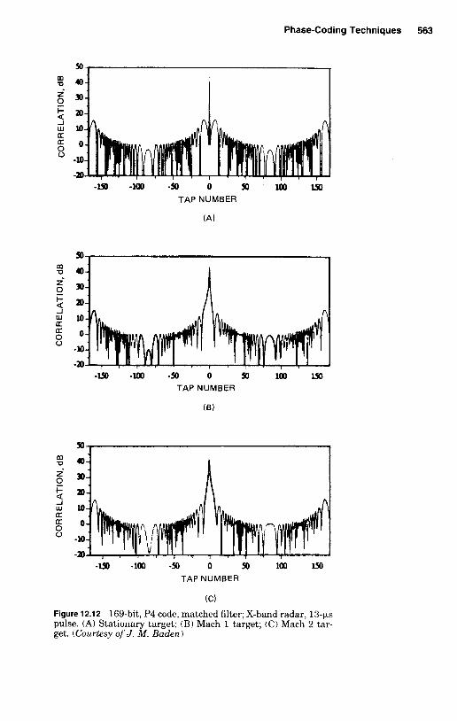
Phase-Coding Techniques 563
50
:a 230 0 : m
00
J
LT w l o
K O
-lo -20
TAP NUMBER
(A)
50
% o z- 30 g + m 4
5 0
w 10 IT
0 -lo
-m
TAP NUMBER
(6)
so % a 2- 30 2 $ 2 0
E o v -10
-m
J
LT w l o
-uD -la, -!a 0 50 la, w TAP NUMBER
(C)
Figure 12.12 169-bit, P4 code, matched filter; X-band radar, 13-ps pulse. (A) Stationary target; (B) Mach 1 target; ( C ) Mach 2 tar- get. (Courtesy o f J . M. Baden)

564 Chapter Twelve
interpreted either as an increase in the near-in sidelobes or as a coars- ening of the range resolution of the waveform.
The final class of codes discussed is the Welti codes [766l. These are four-phase (0 , 90, 180, and 270”) code pairs for which the sum of the individual autocorrelations leaves no range sidelobes. Being quater- nary, these are polyphase codes; however, unlike the Frank and P4 polyphase codes they are not approximations to linear FM. Rather, they behave much more like biphase codes in that they are extremely sensitive to Doppler mismatch. The Golay codes, discussed in Sec. 12.4, are precisely the subclass of Welti codes that happen to be biphase (no 90 or 270” shifts). Both the Welti and Golay codes are not only sensitive to Doppler shift, but their sidelobe canceling ability is extremely sen- sitive to any differentials between the two codes of a pair. That is, both a Doppler shift on both codes and minor differences between the Doppler or amplitude content of the two pulses of a pair can result in significant range sidelobes in the sum output.
12.6 Compression Techniques-All-Range Compressors
One of the advantages of the phase-coding technique is that a number of types of simple, efficient, and flexible compressors can be built. This flexibility is an important factor since the particular code can easily be changed from radar to radar or even from pulse to pulse in a single radar, as contrasted to other pulse compression techniques. In general, all the compressors in this section approximate matched-filter or cor- relation detectors, but they can just as well be implemented with a sidelobe-suppressing mismatched filter.
This discussion is divided into parts, with the functional breakdown indicated below:
Type General radar function Typical Doppler coverage
All-range compressors Analog Surveillance-short-coded words Limited Digital Surveillance-long-coded words Limited
Tracking-words or sequences Limited Cross correlators
Encoding techniques are not discussed except to state that it is ap- parent that encoding directly a t the microwave carrier frequency is by far the most satisfactory method for binary or four-phase encoding, Multiple, low-power diode crystal switches with good isolation are now available with switching speeds of a few nanoseconds. Microwave “magic tees” provide antiphase outputs, and “hybrids” provide 0 and 90” phase shifts over bandwidths in excess of 20 percent of the carrier

Phase-Coding Techniques 565
frequency. This type of encoder was used to generate the 0.1-ps-per- segment code of Fig. 12.4D. Digitally controlled phase shifters can also be quite effective.
If little prior information is available about the distance from the radar to the target, the receiver must be implemented to provide a matched filter for a large set of time delays. This is the typical sur- veillance or search configuration. The class of matched filters for which the filter’s output will reach its maximum value for any target range is called the all-range compressors. In the following discussion it is assumed that a phase-coded pulse is transmitted and the Doppler shift imposed on the pulse is negligible or at least known.
Analog compressors
Historically, the processing of phase-coded pulses was accomplished utilizing analog components such as lumped-parameter, glass, or crys- tal delay lines. More modern analog implementations utilize surface acoustic wave (SAW)-like devices to accomplish the tapped delay-line function at the RF or some intermediate (IF) frequency. While some one-of-a-kind programmable SAW devices-in which the codes and filters can be changed on a pulse-by-pulse basis-have been reported, none, or a t least very few, seem available off the shelf. Since one of the powerful features of phase codes is the ability to change the codes and filters rapidly to provide a measure of reduced susceptibility to outside and self-interference as well as intercept, the discussion on S A W devices is deferred to Chap. 13. Of some importance to mention here, however, is that one can, in general, achieve greater bandwidth with SAW devices than with digital compression techniques.* On the other hand, SAW devices are much more susceptible to degradations due to temperature and evidence very high insertion losses.
A different type of analog matched filter for decoding phase-coded words is shown in Fig. 12.13. This is the zero intermediate frequency (dc-IF) or homodyne configuration in which bipolar video is fed into each delay line. The local oscillator for the pair of mixers is a t the transmitted frequency fo , and the relative phases of this oscillator a t the mixers are in quadrature. The mixer outputs are thus the in-phase I and quadrature Q components of the echoes and contain no carrier frequency as such. In practice both mixers are constructed as a single- sideband mixer whereby the appropriate pair of outputs is obtained with only a single local oscillator input. Minor Doppler shifts (if known) can be added to the LO frequency to prevent degradation of the matched-filter output. Since the total signal may appear in either or
* Unless stepped frequencies are used.

566 Chapter Twelve
INVERTERS
PREAMPLIFIER I CHANNEL
T
INVERTERS
Figure 12.13 Bipolar video matched filter for phase-coded words.
both outputs and the resultant amplitude is e&) = (I2 + Q2)''", both channels are necessary to avoid an average 3-dB loss in signal-to-noise ratio. Another way of stating this is that since the phase of the target is unknown, the received signal may appear in the channel that was not constructed.
While this approach requires twice the number of delay-line ele- ments, it often requires less hardware than the compressors a t IF. This results from a combination of two effects. First, the delay-line band- width for the video waveform need be only one-half that of the bandpass waveform; second, no IF carrier need be passed through the lines.
The delay tolerances are also less critical for the dc-IF than for the RF or IF implementation. On the other hand, the physical realization of a wideband squaring and summing circuit, which is required for a dc-IF but not for an RF or IF implementation, is not trivial. Effective approximations and the emergence of new components that allow the full computation are described in the next subsection. A final point in favor of the dc-IF is that it lends itself to digital decoding or digital processing of the compressor outputs.
Digital compressors
When binary or quadrature (four-phase) codes are transmitted, a pair of shift registers can be used as a digital tapped delay-line pulse com- pressor. An all-range implementation of this form of digital pulse com- pression has been built for maximal length binary codes of up to 255 segments 1697) and is illustrated in Fig. 12.14. The shift-register en- coder is a t the upper left, and the I-& (homodyne) mixer is a t the lower

"l
W
0
40
W
W
-
2 z
nZ
0
:
Ln
0Z
'- I-
85
E;
:W
z
o$
;;: &
j WI
;
5;'- P 3
II
I-
3
a
:?iY I-
- 00
0
0
I- K
Z
3
3
y'
3
O
h
$
s .d
$ U
A
7 B z B f
2%
2: 3 E Y
nd
W
3
;5&
.d
F s E E
- si=
h
ul
R m
7L
RJ
- $2
.sms
2s
a
B
5%
?$
5
5
*-u
c
OU
iifi
W
0
567

568 Chapter Twelve
left of the diagram. The low-pass filters approximate matched filters for the segments of the code. The IF limiter is needed only to ease dynamic range problems and reduce the effect of impulse-type noise. The samplers are normally clocked a t the bit rate of the code, and only the polarity of the bits in each channel is shifted down the respective signal registers.
At the time of transmission, the encoded signal is stored in the code register with the polarity of each stage representing the polarity of the corresponding segment of the code. Several unique features of this compressor are worth noting. First, any binary code of length 255 can be transmitted and stored prior to reception of the received echoes. Thus, the code can be changed for each transmitted pulse if desired. In addition, any shorter maximal-length code can be stored if lower- range resolution is desired. Also, if only one code is to be used, the code register can be replaced by fixed wiring.
As the quantized target echoes propagate down the signal registers, their polarity is continuously matched with the stored code in the code register. The number of matches in the 255 gates between the signal and code register is continuously summed. When there is perfect align- ment of a target and the stored word, 255 matches should appear in the I or Q summer (or both). The summation of the agreements is combined in a greatest of circuit yielding the larger of 111 or IQI. This summation is fed to a threshold circuit where the threshold level is predetermined by the desired false alarm rate. Since there is broadband limiting prior to the compressor, the false alarm rate should be constant (CFAR) for noise, jamming, or other uncorrelated echoes. Target range is determined by stopping a counter when the threshold is exceeded.
The CFAR effect and an example of clutter reduction are shown in Fig. 12.15." At the upper left is the uncompressed (all pluses in the code) A-scope output from land-clutter echoes at the beginning of the trace. The backscatter from a localized rainstorm is a t the center of the trace. In all of the figures, the transmitted pulse length is the same and is about 3 percent of the illustrated trace length. As the number of bits in the code is increased, the compressor output decreases rapidly for the spatially uncorrelated rain clutter and with moderate rapidity for the partially correlated land-clutter echoes. As the number of bits in the code reaches 255, the clutter is reduced to the noise level, dem- onstrating the CFAR action. If a point target echo of sufficient energy were present, it would always reach the maximum output (equivalent
'I. See Chap. 4 for discussion of CFAR. In tha t chapter it was shown tha t the desired effect can be achieved only for large time-bandwidth products. With the configuration described here, the number of stages should be 2 63 when low false-alarm probabilities are desired.

Phase-Coding Techniques 569
(G) (H)
Figure 12.15 Detected video out of digital pulse compressor from rainstorm (100 ps/ cm). (A) Long pulse, no 4 code; (B) pulse compression = 3; ( C ) pulse compression = 7; (D) pulse compression = 15; (E) pulse compression = 31; (F) pulse compression = 63; ( G ) pulse compression = 127; (H) pulse compression = 255. (After Tuylor and MacArthur 16971)
to voltage addition) while distributed targets would be held to the noise level (equivalent to power addition).
There is some signal-processing loss in the digital processor illus- trated in Fig. 12.14. The combination of limiting and quantization causes about a 2-dB loss in efficiency. About 1 dB of this is the loss that is inherent in a CFAR processor. There is an additional fractional decibel loss for using the greatest of circuit. This loss is tabularized in

570 Chapter Twelve
TABLE 12.7 Signal-to-noise Penalty for Using Single Homodyne Channel or Sum of Magnitudes instead of Square-law Detector
A. Penalty, dB, for Rayleigh fluctuating targets* (case 1 or 2) as compared to (Iz + Qz)l’z
False alarm PO = 0.2 PO = 0.5 PO = 0.9 probability III I11 + IQI 111 III + IQI III 111 + IQI
10-1 1.6 0.2 3.4 0.2 9.1 0.2 10 - 2 2.2 0.3 3.6 0.3 9.9 0.4 10-4 2.4 0.4 4.0 0.4 10.5 0.5 10-6 2.5 0.5 4.4 0.6 10.7 0.6 l o - * 2.5 0.6 4.6 0.7 10.8 0.7
B. Signal-to-Noise penalty for steady target,* dB
False alarm probability, P D = 0.2 PO = 0.5 PO = 0.9
PN PI III + IQI I I I Dl + 181 I I I III + IQI lo-’ 1.6 0.15 2.4 0.15 10.4 0.25 10- 2 1.5 0.30 2.7 0.35 12.0 0.40 10-3 1.5 0.35 2.8 0.40 12.8 0.55 10-4 1.5 0.45 2.8 0.55 13.2 0.70 10-6 1.4 0.50 2.8 0.65 13.7 0.75
0.70 - 0.85 10-8 - 0.50 -
* Averaged over all possible values of target phase. Greatest of 111 or I Q i gives the same loss as I I I or I Q I .
Table 12.7. In addition there is about a 2.40-dB average range cusping loss if the full 255 code is used since the target echo may straddle adjacent bits in the registers. This loss is about 1.2 dB if the number of stages in the I and Q registers is twice the number of segments in the code [567]. The range cusping loss is discussed in Chap. 14.
Some advantages of this type of processor that were not mentioned previously include freedom froni adjustment and the inherent relia- bility of microelectronic digital circuitry. Also, the maximal-length code transmitted by one radar does not cause false targets to appear on another radar that uses a different code.
Since two signal registers are effectively four phase quantization levels, a similar configuration can be used to decode four-phase codes.
As in bipolar video processing, one of the principal bottlenecks in digital pulse compression has been the computation of the square root of the sum of the squares of the outputs of the I and Q channels. An excellent approximation to (I2 + Q2Y2 is to use the larger of 111 + 1/21Q1 or IQI + 1/21II with a simple logic circuit to decide which is larger.* An even simpler approximation is to use 111 + IQI or the larger of the
* This will reduce the loss in detectability to about 0.2 dB.

Phase-Coding Techniques 571
two. With this simplification the loss in detectability is less than 0.65 dB for Po = 0.5 and PN = l o p 6 for the steady- or fluctuating-target cases. Table 12.7 shows the losses compared with the sum of squares resulting from the various approximations. The losses are slightly dif- ferent for steady and fluctuating target models [452, 7401.
With the advent of fast, dedicated microprocessor chips such as the Plessey Pythagoras Processor, which is hard-wired to compute (I2 + Q2)1’2 given I and Q, there should be less need for the approximations already cited.
Modern technology has also made great strides in producing inte- grated hardware for the computation of the autocorrelation itself. In- tegrated circuit correlation chips have been introduced that can achieve throughput in the tens of MHz. Figure 12.16 is an example of a com- pressor configured utilizing Inmos A-100 signal processing chips 11311. A radar system utilizing such a processor could implement a simple pulse, Barker codes, a 5 x 21 (105-bit) combined Barker and MPS code for operational flexibility. The compressor in the figure can be recon- figured on a pulse-by-pulse basis to accommodate any of these wave- forms. The most stringent compression requirements come with utilization of the 105 to 1 pulse compression waveform. The filter im- plemented for the 105-bit waveform is the concatenation of a 59-bit optimal ISL mismatched filter for the 21-bit MPS component code and a 17-bit optimal ISL filter for the 5-bit component code. The 59-bit filter is implemented by the serial combination of the two processors shown in the upper left of the figure. The outputs from this stage of compression are stored in a 25-MHz random access memory (RAM) in preparation for the second and final stage of compression. The second stage is implemented by the parallel operation of five more A-100 processors, shown on the right-hand side of the figure. Each of these is loaded with the 17 coefficients necessary for compression of the 5-bit outer code. Compression is achieved by routing the outputs of the first stage se- quentially, one sample per processor, a t a 25-MHz rate, to the bank of five processors. In this way, the input to each processor occurs at a 5-MHz rate, with precisely the spacing between samples that is nec- essary to accomplish compression of the 5-bit outer code. Thus, one- fifth of the range bins are compressed in each of the five second-stage processors.
What has been described above is the compression of one (either the I or the Q) channel of this fully coherent system. The results of these operations are saved in RAM while the data from the other channel are routed through the same compressor configuration. When the I and the Q channels of all the range bins have been compressed, then the channels are combined as (I2 + Q21112 in software.
Figure 12.17 gives a simulation of the compression of a point target

h
g
a :
.- Y
G
6.
o
h0
V
d
2 'I: 2s 2G
=e E% uE : '5
s E
X
B
NQ)
-ln
.P c-
U-l
~
572

Phase-Coding Techniques 573
-200 -150 -100 -50 0 50 100 150 200 TAP NUMBER
Figure 12.17 Compressed return for 5 Y 21 concatenated code through a 17 x 59 mismatched filter.
through the processor. The pulse compression ratio is 105 to 1. The PSL and ISL are less than -30 and -20 dB., respectively. Although it may be difficult to discern in the figure, the structure of the 5-bit Barker code compression (through its 17-bit filter) is present as side- lobes separated by 21 bits, and each of these is surrounded by the structure of the compression of the 21-bit code.
Another implementation for the compression of biphase codes is the utilization of FFT microprocessor chips for the computation of what has come to be called fast convolution. Fast convolution consists of computing the Fourier transform of both the code and filter, multiplying the results, and then taking the inverse transform. This technique takes advantage of the fact that convolution in the time domain corresponds to multiplication in the frequency domain, as well as the efficiency of modern FFT computation. Some care must be taken in such an im- plementation, such as reordering the inputs (to compute correlation instead of convolution) and zero filling one or more of the FFTs to ensure that a linear (aperiodic) correlation rather than a circular (pe- riodic) correlation is computed. Nevertheless, fast convolution is often found to be more efficient than time domain correlations when the codes are, approximately, 64 to 128 bits or longer and the number of range bins to be compressed is not too large.

574 Chapter Twelve
VIDEO SAMPLER
TO I CORRELATORS CORRELATORS
T O THRESHOLD
Q CORRELATOR/ INTEGRATORS
T O TRANSMITTER
I G E & % ~ L R I BIPOLAR C O R R E L A T O R / I N T E G R A T O R
0 SIGNAL
ANALOG GATES
INTEGRATOR
t DUMP
GATE5 FROM SHIFT REGlSTER
Figure 12.10 Functional block diagram of range-gated correlator. (Courtesy o f M . Dauid- son)
12.7 Cross Correlators and Tracking Techniques
If the target range is approximately known, one or more cross corre- lators can be used to acquire and track the target echoes. The basic block diagram of a multiple correlator that is useful if Doppler shifts can be neglected or compensated for is shown in Fig. 12.18. It is illus- trated here in the I-Q configuration. The I and Q components of the signal appear a t a succession of correlator-integrators, each of which corresponds to a fixed range delay. To consider the action of a single correlator channel, it is simplest to assume that the code generator* is started at the instant that the bipolar received signal appears a t the
' The range delay to the target will be neglected temporarily

Phase-Coding Techniques 575
first correlator-integrator. The first stage of the shift register is either in the one or zero state corresponding to the first bit of the code, and energizes either the a o r b line to the correlator-integrator CII. As shown in the insert, this either passes directly or inverts the bipolar video signal while preserving its amplitude. At a subsequent time corre- sponding to the one-segment duration of the code, the second bit appears at the first stage of the shift register and the first CII. If there was an inversion in the code, the shift register energizes the opposite gate of the CIZ, and the signal applied to the integrator has the same polarity as the first bit. Thus, if the code is entirely aligned, the received voltage of all N bits is integrated. A similar integration process occurs for signals in the I channel. At the other integrators, cross correlations of the codes appear, and the polarities of the segments are almost random. At the end of the N segments the sidelobes appear on the other inte- grators. At the termination of the N-segment correlation code the levels in the integrators correspond to the sidelobes of the autocorrelation waveforms as discussed in previous sections. Obviously the integration continues if the code is repeated as a sequence both in the transmission and in the shift register. This circuit then becomes a compressor for a CWcode.
When this type of compressor is used for coded words, the range coverage can be increased indefinitely by running the code continuously into the shift register but dumping the integrators at the end of each sequence for each stage. In this case, each CII periodically observes many ranges each separated by NT. The video sampler must then be sequenced to yield the range-dependent signals (to the I2 + Q2 circuit) similar to those which would appear on a conventional range display. In any of these alternate configurations the various previously dis- cussed approximations can be made to I2 + Q2, or the exact output can be obtained with the Plessey Pythagoras Processor or a similar chip [5531.
In sum, the basic configuration and its variants represent an excellent example of a discrete matched filter since the integrators perform the filtering on bipolar video signals. Since this is a discrete operation, a loss in sensitivity (range cusping loss) occurs if there is a fractional segment length time mismatch between the shift-register code and the received signal.
The determination of coarse target range is merely the determination of which CIZ receives a signal that exceeds a preset threshold. If range is known to within approximately plus or minus one code segment, a simple fine-range tracker can be constructed with only two correlator- integrators. The range-delay circuit is set such that the target’s ex- pected range straddles the first two CII circuits. If the prediction is good, approximately one-half the voltage will be integrated on each

576 Chapter Twelve
circuit. For any small errors in estimation the voltage will be split proportionally. Thus, a range error signal can be derived from the ratio of the integrated voltages. This compressor is a version of an early-late gate or split gate range tracker. If short-coded pulses are used, the I and Q signals are gated into their respective integrators only for the predicted duration of the pulse envelope.
An alternate technique of deriving the range error signal is to invert the polarity of the I2 + Q2 output from the first CII and add it to the I2 + Q2 output of the second CII. The difference of these signals versus range error has the appearance of a range discriminator characteristic. Such a characteristic is shown in Fig. 12.19, curve a (neglecting the self-noise of the range sidelobes of the code). The difference signal can be filtered and used to vary the range-delay circuit with one polarity increasing the range-delay prediction and the other signal decreasing it for subsequent input signals. The amplitude of the difference signal when normalized to the total input signal power determines the amount of correction. The use of a limiting amplifier prior to the final mixer is one such form of normalization.
A somewhat simpler version of the range tracker for phase-coded waveforms is shown in Fig. 12.20. In this form the delayed code is used to switch the phase of the local oscillator (LO) signal to decode the received signals. The received signal is amplified (and sometimes lim- ited), divided into the early and late channels, mixed to dc, and inte- grated. A time delay of the order of the segment length is inserted to form the early channel. In alternate configurations, the delay may be placed in the appropriate LO line or may be obtained from the outputs of successive states of the shift register that forms the delayed-code generator. The shift regster outputs are used to switch a pair of phase- inverting switches in two separate LO lines similar to Fig. 12.13. This final variation is sometimes called the delay-lock tracking discriminator 1679, 1941.
A
DIFFERENCE OUTPUT
RANGE - ERROR
Figure 12.19 Early-late integrator difference output versus range error (unfiltered).

Phase-C
oding Techniques 577
ez 0
z
5a
oy
"%
a
zg
ea
w<
a-o
.Pc.
lz
ww
v-
w
-
(r
uo
578 Chapter Twelve
In all of these compressors, one channel is typically delayed by one- half to two segment lengths from the other, with the variations between them dependent on the nature and location of the delay element. The choice of the delay time* dK is a compromise between the error sen- sitivity of the range circuit, the pull-in range, and the efficiency or threshold level required for small signal-to-noise ratios [478]. If the delay time between early and late channels is less than T, the discrim- inator characteristic has a steeper slope as in curve b of Fig. 12.19, but a small pull-in range (- k 1.5~1.1- As the delay is increased, the range- error sensitivity decreases, but a greater pull-in range is achieved. Discussions of the optimum choice of parameters for the generalized radar split-gate tracking process are available in texts such as Barton [391 and Mityashev [479, Chap. 21, but descriptions for tracking of phase-coded signals are primarily limited to the communications field.
12.8 Phase-Coded Words-Noise and Clutter Performance
The performance of radar systems using phase-coded waveforms in the presence of noise, clutter, or undesired targets is not difficult to cal- culate for binary-coded words.
Phase-coded words-noise performance
In computing detection range, either of two methods gives a close ap- proximation to the correct answer for the matched-filter receiver com- peting with receiver or jamming noise.
1. In the denominator of the range equations, the noise bandwidth term BN can be made equal to the equivalent matched-filter band- width with the uncoded pulse.
2. The noise bandwidth term BN can be made equal to the matched- filter bandwidth of the segment length, and then the number of segments N must be placed in the numerator of the range equations to account for the coherent integration of the segments.
In both cases the required (SIN) for detection must be determined by using a desired false alarm number n', which is based on the number of segments in the observation range.
."K is a constant that is usually between one-half and two. t In practice, the matched filtering will smooth out these curves and extend them in
the range error direction.

Phase-Coding Techniques 579
The losses due to deviations from a matched-filter L, are not easy to
Limiting loss: If the signals are limited at RF or IF before decoding, the loss in detectability is approximately 1 dB if N is greater than about 63, for Po = 50 percent, PN = 1O-6 (see Chap. 4).
Quantization loss: If the compressor is all digital (see Sec. 12.5) and only 1 bit deep, as in the polarity-coincidence detector, the quanti- zation loss is approximately 1 dB for largeNin addition to the limiting loss (see I. Jacobs [3631). If there are two bits in both the I and Q channels, the total limiting and quantization loss reduces to 0.5 dB 15671. Range cusping loss: If there is a time mismatch between the stored waveform and the target echoes, there is a sampling or range cusping loss. If the time mismatch is one-half a segment length, the target signal in both of the adjacent range outputs is reduced by 6 dB. The average cusping loss is only about 2 to 3 dB and depends on the matched-filter bandwidth and on the type of postdetection filtering or integration. This loss is about 1.2 dB for two samples per 7.
Velocity compensation loss: If the target range changes by an ap- preciable portion of a carrier wavelength during the time duration of the entire pulse of N segments, the summation of the N segments does not yield N2 a t the matched-filter output. If there are no Doppler filters, the output is proportional to the voltage summation of the N segment vectors, each differing slightly in phase
e, - P!’~ - 2 cos [2.rrfd 7n + @I
formulate concisely. Some simple examples include:
N
(12.9) n = l
wherep, = power output f d = Doppler frequency 7 = segment duration 4 = phase to the target
As an example, for the case of a target with a radial velocity of 1000 ftls (Mach 1) at a carrier of 3 GHz, the Doppler frequency is about 6 kHz. If the segment length is 3.3 ps, the phase shift per segment is about 0.13 rad. If there are only 10 segments in the code, the loss in signal power is only about 2 dB. If the code length is 50 segments, the signal essentially disappears.
Phase-coded words-clutter performance
The performance of the phase-coded words in a distributed clutter environment can be estimated from the simple pulse radar equations

580 Chapter Twelve
€or clutter (given in Chap. 2) if the segment length is used to determine the resolution cell rather than the envelope of the transmitted pulse. The alternate forms and primary correction factors to these equations are now discussed.
In discrete clutter or in multiple-target environments, the radar cross section of the clutter can be used directly in computation of the signal- to-clutter ratio (S/C). In simplified form, predetection signal-to-clutter ratio is given by
S u,(CA) c u c
_ - -
where uc = the radar cross section of the undesired scatterers. The square of the ratio of the number of segments to the time-sidelobe peaks for the rms sidelobe level affects the clutter attenuation factor CA. For the Barker codes, this ratio is simply hf' for the peaks and uv2 for the rms sidelobe level. The choice of the peak sidelobe level or the rms sidelobe level must correspond to the choice to be used in the denominator of the clutter equations. Figure 12.21 shows that there is a 4- to 5-dB main peak-to-highest sidelobe advantage by using the PN codes with the lowest peaks. Polynomials and starting points corre- sponding to the better codes were given in Table 12.3.
In a distributed clutter environment where the range extent of the clutter is greater than the transmitted pulse length NT, the segment length (cd2 in distance units) is used to determine the resolution cell. A loss term must be entered to account for the time sidelobe contri- butions. Since there are 2N - 1 time sidelobes, the mean-square sidelobe value must be multiplied by 2N - 1 and compared to N" a t the peak.* (Note that this measure is very similar to ISL, as defined earlier.) A linear processor is assumed. Table 12.8 has been calculated (see [569]) from Table 12.7 to show this degradation for the maximal- length codes. This table was computed for discrete one-segment length offsets of the autocorrelation €unctions. A slightly different result would be obtained if correlation between adjacent sidelobes of the autocor- relation functions were included 1567 I . Several manual calculations have shown that the difference in compuation technique yields a minor error, and the degradation column in the table is slightly pessimistic. It can be seen that, for the better codes, the degradation is only about 1 dB and is almost independent of code length. An entry is shown €or
____ I It is assumed that the transmit pulse length i i small enough compared with the
target range to neglect the range-dependent tei ins

8
>Q
UO
-
* +-
P
3a
niiid
wv
3
na
is3~
LL
00
01
3
0
581
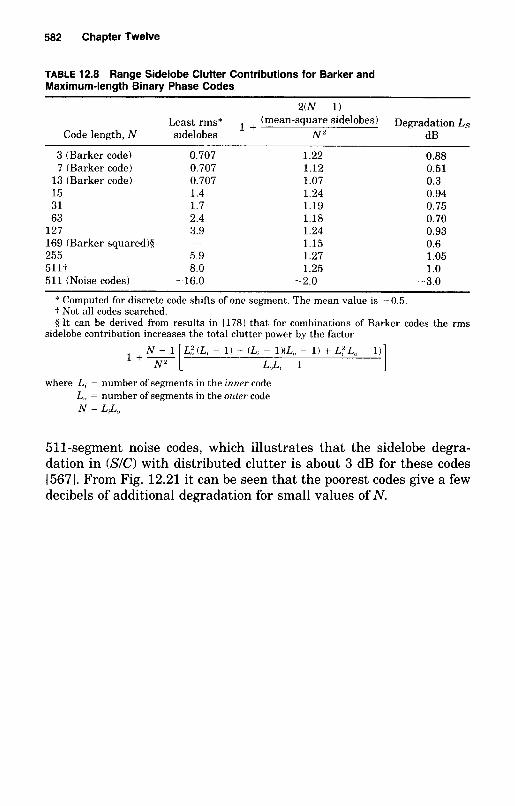
582 Chapter Twelve
TABLE 12.8 Range Sidelobe Clutter Contributions for Barker and Maximum-length Binary Phase Codes
2(N - 1) Least rms* 1 + (mean-square sidelobes) Degradation L~
Code length, N sidelobes NZ dB
3 (Barker code) 0.707 1.22 0.88 7 (Barker code) 0.707 1.12 0.51
13 (Barker code) 0.707 1.07 0.3 15 1.4 1.24 0.94 31 1.7 1.19 0.75 63 2.4 1.18 0.70
127 3.9 1.24 0.93 1.15 0.6 169 (Barker squared)$ -
255 5.9 1.27 1.05 5111. 8.0 1.25 1.0 511 (Noise codes) -16.0 -2.0 -3.0
I' Computed for discrete code shifts of one segment. The mean value is - 0.5. + Not all codes searched. 9 It can be derived from results in 11781 that for combinations of Barker codes the rms
sidelobe contribution increases the total clutter power by the factor
1 1 + NL [L:(L. - 1 ) + (L, - IKL,~ - 1) + L:L., ~ 1) NZ L,LL ~ 1
where L, = number of segments in the inner code L,, = number of segments in the outer code N = L,L,,
51 1-segment noise codes, which illustrates that the sidelobe degra- dation in (SKI with distributed clutter is about 3 dB for these codes [5671. From Fig. 12.21 it can be seen that the poorest codes give a few decibels of additional degradation for small values of N .

13 Frequency-Modu lated
Pu Ise Compression Waveforms
F.E. Nathanson M.N. Cohen
This chapter includes a discussion of the most widely used forms of pulse compression, those that fall into the general class of frequency modulation. Frequency-modulated (FM) waveforms can entail linear (LFM) or nonlinear (NLFM) modulation of the frequency of the transmit waveform. These modulations can be implemented either within a sin- gle coded pulse (intrapulse modulation) or on a pulse-to-pulse basis (interpulse modulation). Also, the frequency modulation may be achieved via either an analog (continuous) or a digital (discrete) process.
Since both frequency and phase modulation are forms of angle mod- ulation, the discussion begins with an example relating FM and phase- coded waveforms. In the rest of the discussion, the formulation, gen- eration, and processing of classical coded pulse LFM as well as more recently developed NLFM and interpulse waveforms are treated.
13.1 Multiplicity of Frequency-Modulation Techniques
It was shown in the chapter on signal processing concepts and waveform design that the basis of improved range resolution is some form of
583

584 Chapter Thirteen
-1.0 -0.8 -0.6 -0.4 - -0.2 0.0 0.2 0.4 0.6 0.8 1.0 NORMALIZED FREQUENCY
Figure 13.1 Spectra of the rows of a 64-segment Frank code.
modulation or coding within the envelope of the transmit pulse that widens the signal spectrum. While binary or 0-to-180" phase coding accomplishes this same end, it is not categorized as frequency modu- lation, and was therefore treated separately in Chap. 12.
It is interesting to note that the Frank polyphase codes (Sec. 12.5) are actually a phase approximation to a frequency code. If the Frank code for 64 segments is written as an 8 x 8 matrix with segments 1 through 8 making up the first row; segments 9 through 16, the second; etc., and the spectrum is calculated for each row, a series of spectra is obtained as shown in Fig. 13.1. Each row approximates a narrow-band carrier, and the movement of the carrier from row to row is linear, as can be seen from the figure. The total spectrum of the 64-segment pulse may be considered as that resulting from the sum of the spectra shown."
Two conclusions can be drawn from this figure. First, the more or less linear frequency variation versus time makes this waveform some- what ambiguous in the range Doppler plane of the ambiguity diagram. A single Doppler channel receiver is thus tolerant to greater Doppler shifts with this waveform than with a binary phase-coded waveform, though not as tolerant as FM. Second, the tapering of the spectrum envelope leads to low pulse compression time sidelobes. Typical values
' Details of the overall spectrum can be found in Cook and Bernfeld L711.

Frequency-Modulated Pulse Compression Waveforms 585
w
-540- ,
-630 -
-720 1 1 1 1 1 1 1 1 1 1 1 1 1 ~
1 2 3 4 5 6 7 8 9 1 0 1 1 1 2 1 3 1 4 1 5 1 6 SAMPLE NUMBER
Figure 13.2 The phase function of the P4 code.
for those sidelobes were shown in Chap. 12. The subject of range sidelobe reduction for FM waveforms is explored further in Sec. 13.9. Similarly, the phase function of the P4 codes (Sec. 12.51, as given in Fig. 13.2, can be seen to be a discrete approximation to quadratic phase, and quadratic phase is characteristic of LFM waveforms. Indeed, the P4 codes can be shown to be a 2-to-1 undersampled (both on transmit and receive) discrete representation of an LFM waveform, and so they share many of the properties of such a waveform [1281. Thus, the distinction in terminology between frequency and phase coding is pri- marily dependent on how the modulation is imposed on the waveform, rather than on the underlying strccture of the waveform.
While the generation of linear FM or chirp" waveforms has in the past been based on the use of passive dispersive delay lines, much of the description in this section is based on active generation of the desired waveform by the use of voltage-controlled oscillators (VCOs) and discrete frequency techniques. In the latter implementation of FM waveform generation, the transmit spectrum is formed by the sum- mation of a coherent series of short-duration RF pulse segments, each of which is selected from a comb of coherent frequencies. When passive generation techniques are discussed, surface acoustic wave (SAW) de- vices are emphasized. This departure from the conventional description of chirp systems [403] can be justified in a number of ways:
* A common term for linear FM radar signals coined by B.M. Oliver of the Bell Lab- oratories in 1951.

586 Chapter Thirteen
1. The description of the properties of chirp techniques is by far the best documented of the radar signal-processing techniques; and rather than repeat earlier analyses, the reader is referred to the excellent articles by the personnel of Bell Laboratories (Klauder and Price [403] and those of the Sperry Rand Corporation [64,136,5291. The original FM concepts are contained in patents that date back to 1940 and are described in these references.*
2. Modern technology has allowed the development of VCOs, digital synthesis techniques, and SAWS that permit much tighter control of important transmit waveform parameters, such as linearity with frequency and flat amplitude response, than do the more classical RF and IF dispersive delay techniques that have been employed in older systems.
3. It can be shown that virtually all the desired properties of linear FM are achievable by transmission of discrete frequency segments. These include the reduction of time sidelobes, the ability to improve target resolution and signal-to-clutter ratio, the ability to achieve greater detection range for a given peak transmitter power, and the capability of achieving automatic detection with a hard-limited re- ceiver 1664, 521, 767, 2601.
4. With discrete transmission of frequencies, it is possible to utilize an approximation to linear FM and accept the range Doppler ambiguity with perhaps slightly more hardware than is needed for analog techniques. However, accepting this penalty yields a more flexible means of waveform generation. For example, it is possible to scram- ble the ordering of the frequencies to eliminate the FM ambiguity and replace it with a thumbtacklike ambiguity function. This would eliminate the major range Doppler uncertainty but yield a general increase in the sidelobe level throughout the ambiguity plane.
5. It is shown that in an interpulse system, extremely high time-band- width products can be achieved via discrete frequency stepping, and that this can be accomplished by utilizing receiver components that have instantaneous narrow-band characteristics. Very high band- widths and time-bandwidth products can also be achieved in systems that utilize phase-locked VCO generation or digital frequency syn- thesis and upconversion generation techniques in the transmitter and active correlation (stretch) techniques in the receiver.
The summary of general characteristics of chirp-type signals and receivers given in Secs. 13.2 through 13.4 extends the ambiguity dia-
' Darlington's patent (No. 2,678,997) described chirp by means of linearly stepped frequencies as well as dispersive techniques.

Frequency-Modulated Pulse Compression Waveforms 587
gram discussion in the signal-processing section. It was noted there that a rectangular spectrum is generally desirable for maximizing clut- ter rejection 14601. In addition, a rectangular time function is the sim- plest to transmit with most types of transmitter power amplifiers. Sec. 13.3 contains a description of how both these goals can be achieved simultaneously.
13.2 Linear FM Pulses (Chirp)
By far the most widely implemented technique for pulse compression is the use of linear frequency modulation during the pulse. Many of the goals of waveform design can be attained with relatively simple dispersive devices. The desired transmission energy can often be ob- tained by the choice of the requisite pulse length, while the desired resolution can be independently specified by the frequency deviation. Improved performance over uncoded pulses is obtained in distributed clutter environments, and the receiver can be a constant false alarm rate device to cope with broadband noise interference.
Unfortunately, chirp is not a universally desirable waveform; hence the emphasis in previous sections on the multitude of other waveform modulations. The lack of unambiguous range and velocity resolution, discussed in the chapter on signal-processing concepts and waveform design, sometimes results in inadequate performance in sorting out targets, land and sea clutter echoes, decoys, and dense rain and chaff echoes. It would be in sharp contrast to the related field of communi- cations if a single waveform with a single relatively simple matched filter were adequate for all environments.
13.3 Generation and Decoding of FM Waveforms
In the design of a simple chirp system, the first parameter to be chosen is the duration of the pulse envelope, given the peak transmitter power. This determines the pulse energy and allows the prediction of the detectability of a given target model a t a given range. Second, the desired resolution determines the bandwidth of the transmission and therefore the performance in a distributed clutter environment.
One class of techniques for generating a long-duration FM signal is the so-called passive one illustrated in Fig. 13.3. An IF pulse of the approximate length of the desired compressed pulse is generated and inserted into a dispersive delay device. Since the compressed pulse for a linear FM waveform has a sin xlx time envelope, it can be shown that the input to a linear dispersive delay should have a time waveform 11361

S P F C T R U M
C- S H A P I N G - D I S P E R S I V E (3)
D E L A Y & D E T E C T O R -
F I L T E R
M I X E R A N D
S I D E B A N D M
I N V E R T E R L

Frequency-Modulated Pulse Compression Waveforms 589
After traversing the dispersive line the waveform is “up-mixed” (con- verted) to the desired carrier. Filtering out unwanted sidebands, the transmitted waveform can then be written as [641
T T f o r - - s t s - f&) = cos [ ( w o t ) + $1 2 2
where wo = the transmit carrier frequency. The generating waveform f , ( t ) can be obtained by passing a narrow pulse (radian bandwidth > Awl through a rectangular bandpass filter of width A w D n = A6 The filter must have a linear phase characteristic.
The dispersive delay devices were historically often composed of cas- caded all-pass networks 1136, 3711. More modern dispersive imple- mentations include dispersive ultrasonic delay lines [213, 1361, waveguide operated near cutoff [1831, optical devices, and, most re- cently, superconductive striplines 14551. For purposes of this discussion assume that the technique utilized has negligible attenuation over the bandwidth A f and a linear time delay versus frequency. The waveform at its output is shown diagrammatically in Fig. 13.3 as f i ( t ) , its fre- quency-versus-time characteristic as w&). It should be noted that there is often a certain amount of amplitude ripple versus time at the trans- mitter input. With the usual saturation in the transmitter, there will consequently be waveform distortion at the receiver output. However, this distortion has a small effect with large compression ratios.
The sideband modulator is used to convert the FM signal to the desired carrier frequency, and a time gate is usually employed to form the rectangular transmit waveform. Upon reception, the echo is mixed with a local oscillator that yields the sideband inverse to that utilized on transmission [ 5751. By this technique the frequency-versus-time characteristic is inverse with respect to the transmitted signal as il- lustrated by f 2 ( t ) and f3(t). This technique permits the use of identical dispersive delays in the transmit and receive lines. In practice, the received signal is often inserted in the same dispersive delay as was used for transmission, thus reducing hardware and tolerance require- ments.
The spectral shaping filter is used to reduce the - 13-dB time side- lobes to a tolerable level a t the cost of a slight reduction in signal-to- noise and signal-to-distributed-clutter ratios and at the further cost of an increase in compressed pulse width. In Sec. 13.9 various shaping filters and their characteristics are discussed. The detected waveform shown has a lsinxIxI form near its central lobe in the absence of spectral shaping. For a large compression ratio the waveform is similar to that shown in Fig. 13.9. The peak signal amplitude and, more importantly

590 Chapter Thirteen
0
-5
-10
-15 m U
3
3 0 E -30 0 t-
+' -20
e -25
4 -35
8 W oc @z -40
-45
-50
-55
-60 -8 -6 -4 -2 0 2 4 6 8
RANGE BIN NUMBER
(A)
-5-
-10-
m -15- U
-8 -6 -4 -2 0 2 4 6 8 RANGE BIN NUMBER
IB) Figure 13.4 Linear FM code with TB = 10 (A) Matched filter, (B) Hamming weighted filter

Frequency-Modulated Pulse Compression Waveforms 591
for pulse compression applications, its signal-to-noise ratio is increased by TAf, and the pulse width is reduced by approximately the same factor. That is, range resolution is given by A7 = C7/2 = c/(2 Af). For small time-bandwidth products, say TAf < 20, the output waveform deviates from the (sin x)/x in its sidelobe regions. Figure 13.4A shows the compressed output from such a system whose time-bandwidth prod- uct is 10. As can be seen in the figure, the first sidelobes are approx- imately 15 dB down from the peak. However, whereas a Hamming- weighted, large-time-bandwidth-product LFM waveform exhibits peak sidelobes on the order of -40 dB, the same weighting applied to the waveform of Fig. 13.4A results in peak side-lobes on the order of - 24 dB, as exhibited in Fig. 13.4B. The control of range sidelobes in the presence of Doppler mismatch is another potentially troublesome as- pect of small-time-bandwidth-product LFM waveforms.
An alternate chirp generation technique that utilizes active gener- ation of the FM waveform is to apply a sawtooth or ramp modulation waveform to a voltage-controlled oscillator or a square-law modulation to a phase-controlled oscillator [136, 641. Small variations in the mod- ulation function can be injected to compensate for distortions elsewhere in the system.
If target range is not known, a dispersive delay matched filter is usually used in the receiver. Other techniques for generating and com- pressing a linear FM waveform are discussed in Secs. 13.10 and 13.12, and an excellent summary of more classical dispersive devices is found in Cook and Bernfeld [136, Chaps. 12, 13, and 141. More recently, the move has been toward utilizing surface acoustic wave (SAW) devices, which typically operate a t IF. The theory underlying SAW operation has been known for some time, but it was not until the 1970s that the technology became sufficiently mature for widespread application. Ta- ble 13.1 summarizes the operating frequencies, compression ratios, and range side-lobe levels that have been reported in the open literature for various types of surface acoustic wave devices that have been re- alized for application (that is, that have been built utilizing standard manufacturing procedures). The insertion losses typically associated with such devices range from 25 to 50 dB. Careful custom construction can allow for devices that achieve dispersions to 150 ks, bandwidths in excess of 1 GHz, time-bandwidth products up to 10,000, and side- lobes approaching -40 dB [log]. In most of these cases slight varia- tions in pulse width can be traded for different peak sidelobe levels, but the sidelobe increase due to transmitter distortion (not included in the table) will generally preclude achieving peak sidelobe levels of bet- ter than -40 dB anyway. An example of the waveforms of a high- compression-ratio, passive linear FM system with sidelobe suppression is shown in Fig. 13.5. The peak sidelobes are -40 dB for the unit. A

592 Chapter Thirteen
TABLE 13.1 Characteristics of Typical SAW Devices
Compressed- Center pulse Peak
frequency, Bandwidth, Dispersion, width, sidelobe, MHz MHz )Ls w TB dB Remarks
30 6.3 13 0.22 60 27 Weighted FM* 60 6.5 6.7 0.22 30 33 Weighted FM* 60 10 100 0.175 571 30 Weighted FM'F 80 20 20 .05 364 12 LFMt
120 7.5 28.5 0.193 148 30 WeightedFM* 123 54 4 0.02 2700 12 LFMt 240 20 13.4 0.083 161 30 Weighted FM* 266 132 16 0.008 2000 12 LFMt 521 30 15 0.037 405 12 LFMt
1300 500 0.56 ,003 187 12 LFM*
* Interdigital transducer device (ITD). i Reflective array compressor (RAC).
new variation on SAW-like devices is the acoustic charge transport (ACT) and heterojunction acoustic charge transport (HACT) devices de- veloped in various laboratories around the country [6121.
If target range and range rate are approximately known, then pulse compression may be accomplished synchronously via correlation. That is, in a tracking system or in other systems in which the target position is known to within the resolution of the uncompressed pulse, a fre- quency ramp similar to the transmitter's may be used for decoding in the receiver via active correlation of the received signal with the trans- mitted modulation. Such a correlation receiver is intrinsically different from the compressive receivers discussed in the foregoing. This tech- nique, sometimes referred to as stretch, is discussed in more detail in Secs. 13.7 and 13.13.
13.4 Distortion Effects on Linear FM Signals
The effects of amplitude and phase distortion on pulse compression systems are best described by paired-echo analysis techniques (64,403, 1361 as follows in brief. In the frequency domain the distortion has been related to the transfer admittance of the system [4031
Y ( w ) = A(w) exp bB(w)l
The terms can be expanded into Fourier series of n terms
A(w) = a. + c a,L cos (new)
B ( w ) = bow + c 6 , sin (new)
n
n

Frequency-Modulated Pulse Compression Waveforms 593
(5)
Figure 13.5 Transmit and receive waveforms of disper- sive linear FM pulse-compression system. (A) Expanded pulse, transmit waveform, 30-MHz IF; ( B ) compressed pulse, 0.58 ps, ~ 40dB sidelobes, horizontal scale 1 ps/ cm. (Permission of Andersen Laboratories)
where for linear FM signals
c = complexconstant a,, cos (new) = amplitude distortion terms h,, sin (ncw) = phase distortion terms
The system is considered ideal when a,, = b,, = 0, or the distortion terms are zero.
For small phase deviations (--:25"). it is sufficient to consider only then = 1 term. Agraph of'the highest paired-range sidelobes for various peak phase and amplitude errors i s shown in Fig. 13.6 1403, 53, 519, 136 1. It i a11 tw w t 1 n thiit for 4, tJ tr r a i i g t h sidelobes, the amplitude

0.1
10
20
m
w ! 30 m
w Q - Y -- UI
W 4 4 0
< ? 40
z v1 - 0 5
0.2 0.4 0.6 0.8 1 2 4 6 8 1 0 20 40 -..._._...__ I I I 1- ______ + -.-. +-..4-~+---. ..- -.. - ~~ 1 . ~ ..-
-
~ __._____ ~~~-
-
L _ _ ~ ~ -
/ 0 d'
0 ', 0
~ __-...__ ~ _-__ . ... ____ ~._ . ~- / 0
- / ,0 '
z /
50
-
60 I I I 0.01 0.02 0.04 0.06
d'
-. .._.___. __
I I I I I
0.08 0.1 0.2 0.4 0.6 0.8 1 2 4

Frequency-Modulated Pulse Compression Waveforms 595
Figure 13.7 Typical compressed-pulse waveform (amplitude) for linear FM signal and random phase errors, TAF = 50. (A) 20" phase error (std. dev.); (B) 30" phase error; (C) 40" phase error.
that is, bl = K (voltage ripple ratio) (electrical length of device in degrees), or
= L (current ripple ratio)
Typical values for modern trasmitter components are given in Chap. 14.
13.5 Spectrum of a Comb of Frequencies
Consider the pulse waveform containing N equal-amplitude rectan- gular time segments of length t, each on a different frequency f,,. The envelope of this waveform is illustrated in Fig. 13.8A. The time origin will be taken as the midpoint of the first segment but otherwise con- forms to an analysis by O'Neill[5191. The waveform of the nth segment or subpulse is given by

f , f , f, f ri-1 f,
L _ _ - t
f, f, f , f, f, f a f, f, ---

Frequency-Modulated Pulse Compression Waveforms 597
the carrier term, the spectrum of the modulation of the entire pulse becomes
N sin r ( f 7 -n ) VCf) = A T 2 expj [2df~ - n)(l -n)l (13.4)
It is shown in later sections that the envelope of the compressed pulse out of the matched filter for this waveform has a sinxlx shape in the neighborhood of its mainlobe. The width of the compressed pulse at the 4-dB points is equal to TIN for uniform weighting of the fre- quencies. Since the transmit envelope has a duration of NT, the pulse compression ratio = N2. The matched-filter output waveform is illus- trated in Fig. 13.9 for N = 50. The oscilloscope gain is increased in the lower photograph to show the range-sidelobe details. The response of the scrambled-frequency waveform of Fig. 13.8B yields different outputs depending on the sequencing utilized. In general, random se- quencing of the frequencies results in a thumbtacklike ambiguity sur- face, destroying the range Doppler coupling generally associated with LFM. In Costas [143], ideal patterns for scrambled-frequency wave- forms are defined. These patterns are further investigated in [2821 and 12831 and have since come to be known as Costas Arrays. When they are utilized, not only is the range Doppler coupling destroyed, but the range and Doppler sidelobes vary from 1/N far from the peak response to 21N close to it, where N is the number of frequencies utilized.
It should be noted here that coherency is required in such a process to yield a high range resolution profile. That is, as noted earlier, the phases of the individual frequencies must be maintained between trans- mit and receive and the process must include compression on the IF signal or I and Q sampling of the received waveform. If, instead, one implements such a process by detecting the received signals [that is, by computing (I2 + Q2)”21 before compressing, then the result is the autocorelation of the range resolution profile, rather than the range resolution profile itself. While range resolution processing provides an absolute range map of the area of interest, the autocorrelation of the range resolution profile provides only the composite relative ranges between scatterers in the scene [202l.
The waveforms depicted in Figs. 13.8A and B represent intrapulse techniques, that is, FM coding techniques that are implemented on a single-pulse basis, much like most of the phase codes from Chap. 12. The waveform depicted in Fig. 13.8C introduces the possibility of im- plementing frequency modulation of the transmit waveform on an in- terpulse basis. The preceding analysis, which describes the charac- teristics of the intrapulse techniques, applies to this waveform as well; however, there are important differences between these classes of tech-
n = l d f 7 - n)
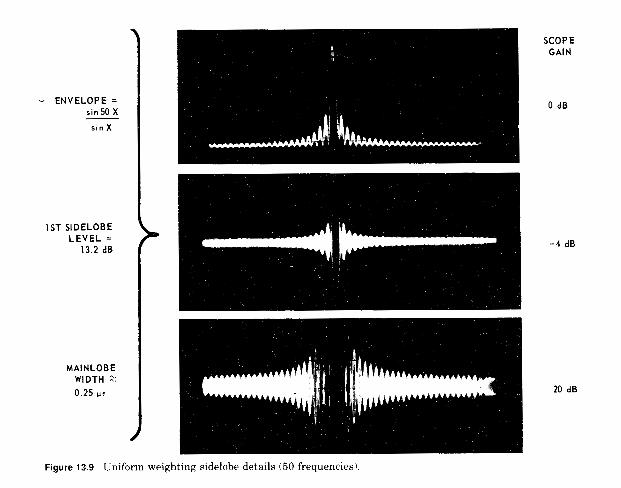
W
nZ
0
4
Z0
m
V
0
m
V
0
cu
i
c hr.
.- 1 R r E
ii rJl
598

Frequency-Modulated Pulse Compression Waveforms 599
niques in terms of waveform generation, operational applicability, and receiver characteristics. These differences are explored in Secs. 13.6 and 13.7.
13.6 Waveform Analysis for Discrete Frequencies
The rigorous analysis of discrete frequency pulse compression loses touch with physical significance unless some restrictive assumptions are made about the relations among the various parameters, such as the spacing between frequencies AL the subpulse or segment length T ,
and the phase of each of the subpulses &. Figure 13.10 is the time waveform of the envelope of the coherent summation of eight continuous sinusoidal carriers spaced by exactly Af in frequency. The bandwidth of the RF waveform is N A f and is assumed to be much less than the mean or carrier frequency f c . The spectrum is periodic in frequency, and, as would be expected, the time waveform is also periodic with a repetition period of U A f . A typical transmit time waveform is shown in Fig. 13.11. With an even number of frequencies, a center carrier frequency does not actually exist as any one of the individual frequen- cies.*
The necessary condition for compression of the energy is that all the phasors (shown on the figure as small arrows) achieve colinearity at some time during the period. This condition is shown under the first envelope peak a t time t = 2n/Af. This condition need not be made to occur on transmission as long as there are the appropriate phase ad- justments in each channel of a receiver such as shown in Fig. 13.12. As shown, the filters F, are placed inversely in time to the transmission frequencies f n . If the filter bandwidths are approximately 117, a nearly matched receiver is obtained. Since the bandwidth of each channel is only 1/N times the total signal bandwidth, these channels can be seen to be relatively narrow-band as compared with the overall bandwidth achieved. The phase and amplitude response to the received frequency segments is controlled in the individual channels. This eliminates the requirement for components having phase and amplitude linearity across the total transmission bandwidth. In this simplified diagram, the coherent summer is simply a voltage adder, which is then followed by an envelope detector. If the phases are not adjusted for colinear vector addition at some instant of time, the periodic time waveform appears noiselike. However, with the proper adjustment, the phasors can be made to peak up periodically for all time, providing the generated
* From an analytic signal representation point of view involving Hilbert transforms, there would be no need to limit the discussion to a narrow-band comb spectrum or to designate a specific carrier frequency.

>
qz V
z
wf
OQ
>f
+:
(u
w 1
1
It c
wz
K
O
LO
-
-
d I
.d
42
Q
)
a Q
)
- % a I [ :: 0 8 g T 5 2 x 0
>o
r
!!
c
ii rn 4%
600
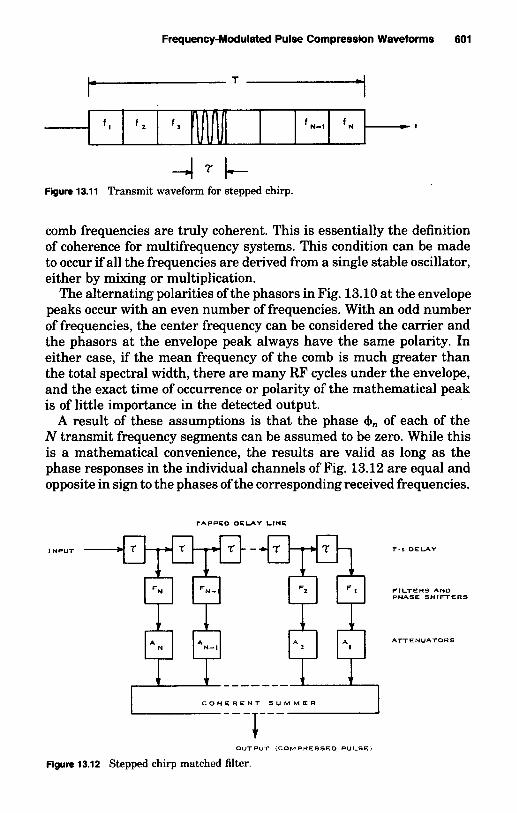
f , f , f , -

602 Chapter Thirteen
The following discussion is based on the pulse sequential transmis- sion of the frequencies, and the CW-derived periodic time waveform envelope previously discussed is not quite relevant. The envelope of the transmission on each frequency, which is referred to as the subpulse and which has a duration of 7, now determines what portion of that frequency is time selected for coherent summation with the other fre- quencies of the comb.
Figure 13.12 represents a compressive receiver for the discrete FM waveform and it can be implemented either at IF via analog processing utilizing a tapped delay line; dispersive devices like SAWS; or, at video- via digital processing, by first sampling the received waveforms at rates greater than or equal to l l u a n d then implementing the equivalent of digital tapped delay lines for each of the I and Q components of the signal or as a pipelined fast Fourier transform (FFT) processor. As discussed in Sec. 13.13, compressive receivers, in conjunction with any of the discrete intrapulse FM techniques, allow a fairly simple imple- mentation of all-range compression.
Before proceeding further it is desirable to make the assumption that the frequency spacing is equal to the inverse of the pulse length Af = lh, and the subpulse envelopes are rectangular. This has the desirable effect of keeping the mathematics reasonable, but, more importantly, it yields the best waveform properties for most practical situations. The validity of the preceding statement can be illustrated by consid- ering the matched-filter output when T A ~ # 1.
If TAf > 1, there are significant range ambiguities at time t = Il/Afl as seen from the autocorrelation function in Fig. 13.13. It can also be seen that when T A ~ = 1, the nulls of the autocorrelation function of the subpulse envelope tend to suppress these ambiguous peaks. When TAf < 1, the subpulse filters F, shown in Fig. 13.12 overlap, and the contribution of each channel to the coherent summation contains spu- rious signals. The details of the output waveform for TAf < 1 depend on the ordering of the frequencies in the pulse envelope.
Another way to motivate the choice TAf = 1 is to consider the cor- respondence between processor outputs and range cells. To this end, consider an interpulse stepped frequency waveform whose transmit pulse width is T , frequency step size is A L and total bandwidth is B = NW, where N is the number of pulses utilized. The transmit pulse determines a range gate of extent cd2, and one I and Q sample is collected from this range gate for each transmit frequency. These sam- ples are then loaded into an N point complex FFT to provide N complex output values. The total bandwidth utilized in this process is NM. The resulting resolution is therefore c / W A L It follows that, when TAf = 1, the range gate is resolved into N range cells, and each FFT output corresponds to precisely one of these cells. If the number of pulses ( N ) utilized is held constant and A f is increased so that TAf > 1, then the

Frequency-Modulated Pulse Compression Waveforms 603
eg (1)
- - - -1 Af N N Af -
Figure 13.13 Autocorrelation function of frequency-coded pulse.
total bandwidth is increased, and hence resolution cell size is decreased. But N finer resolution cells do not cover the specified range gate. Thus, in this case, only a portion of the range gate is resolved and, in fact, the reflectors in the unresolved portion fold into the resolved portion (hence the “ambiguous peaks” mentioned earlier). In this sense, the cells are not really resolved. Similarly, if the number of pulses utilized is held constant and Af is decreased so that df < 1 in the example, then the N coarser resolved cells over-cover the specified range gate. That is, certain resolution cells are represented by more than one FFT output, a redundancy that serves no useful purpose.
While in some special cases 7Af should be made different from unity (such as when the transmit pulse is assumed to have a gaussian rather than rectangular envelope [2023), the remainder of this section is lim- ited to discussions of systems with TAf = 1.
The transmitted waveform for a linearly stepped-frequency wave- form can be written
n - 1
n=O V(t) = c [ U ( t - n ~ ) - U ( t - En + 1]7)] COS (00 + nAW)t (13.5)
where oo = 2nf0, lowest frequency in the transmission comb
Aw = frequencyspacing = 2nAf
u(t) = unit step function = 1 , 7 2 0 { 0 , 7 < 0
N = number of frequencies in transmission The phase and time origin is taken to be the leading edge of the first
subpulse. It can be shown that the matched filter has an impulse response that can be written [7681
(13.6) h(t) = u( - t ) N- 1
= 2 [ U ( - t - n7) - U ( - t - [n 4- 1]7)]COS(O, + nAw)t n=O

604 Chapter Thirteen
If the matched-filter delays and filters are in the inverse order of transmission and the delay to the target is neglected,* the matched- filter output can be written
N-1
e&) = c A: expj(wo + nAw)t (13.7) n=O
in the region (N - l) t < t < Nt. With the assumption that Af = I/?, this becomes the only region of interest. Equation (13.7) is the finite sum Fourier series approximation to the matched-filter output, ne- glecting the detailed shape of the filters in each channel. An is the weighting function of the nth frequency segment, and is assumed equal to unity until Sec. 13.9. It follows that:
sin N(Aw/2)t (13.8)
To account for the autocorrelation of the rectangular segment en- velope as was illustrated in Fig. 13.8, Equation (13.8) should be mul- tiplied by the triangular function 7[1 - (lt1/7)] for It1 I 7, and zero elsewhere.
The term w, + [(N - 1) Ad21 is the mean frequency of the comb or carrier frequency and can be factored out. Thus, the second term de- termines the compressed pulse envelope. The nulls in the envelope occur when sin [N(Aw/2)tl = 0 or when
2 e&) = exp [ J '( w, + (N -1)Aw) t ] ( sin (Aw/2)t )
Am 2
N - t = + m n
where m = any integer. The first sidelobe peak is reduced from the mainlobe by 13.46 dB when N 2 50 and is 13.06 dB down for N = 8. This envelope has the sin (NX)/sin X shape and is similar to that il- lustrated in Fig. 13.13. At one-half the distance between the nulls, the linear envelope response is down by 4 dB and the width is
(13.9) 1 transmit envelope N 2 Compressed pulse(4 dB) = - =
N W -
The pulse compression ratio is then slightly greater than N2 with the customary definition of 3-dB pulse widths.
* That is, only differential delays with respect to target location are formulated.

Frequency-Modulated Pulse Compression Waveforms 605
Thus, the compressed-pulse matched-filter output for a stepped linear FM waveform has almost the same shape as that for a continuous linear FM waveform for large compression ratios.
13.7 Capabilities for Extreme Bandwidths and “Stretch” Techniques
In Secs. 13.1, 13.2, and 13.3 it was indicated that among the require- ments imposed on very wideband processors, many imply large time- bandwidth products. Phase-coding techniques are generally applicable to systems requiring, at most, 100 to 200 MHz of bandwidth due to limitations in the technological ability to A/D convert at much higher rates. Classical dispersive techniques for LFM waveforms can be uti- lized to achieve very wide bandwidths, but the devices utilized are often expensive, difficult to mass produce, and prone to performance deg- radation. However, modern ultrawide-bandwidth and very high time- bandwidth-product systems can generally be configured using one of three available techniques and can be built using reliable, mass- produced devices. Discrete frequency coding on either an intra- or interpulse basis provides two such techniques, and active correlation (stretch) processing provides a third. Each of these techniques is treated in the following discussion.
Three major factors favor the use of the discrete frequency tech- niques. The first is, for certain applications, the ability to eliminate the range Doppler ambiguity of linear FM. It will be seen that the matched-filter response, tapering effects, receiver sensitivities, etc., do not depend on the order in which the frequencies are transmitted. In simple terms, if the price is paid to implement matched filters for all expected target Dopplers, a thumbtack ambiguity function can be ob- tained (see Sec. 13.12). While there is an increase in the number of low-level residues, there is no range Doppler confusion between targets of comparable size. A related benefit to scrambling the frequencies is that the system does not respond to interfering FM-like signals gen- erated by other radars and will be less susceptible to repeater jammers if the sequencing of frequencies is made to change on a pulse-packet to pulse-packet basis.
The second and perhaps the most significant advantage of multiple- frequency channels is that the components in each channel need only have a bandwidth of 11N times the total processing bandwidth. This is illustrated in the waveform pictorial given in Fig. 13.11 and the receiver block diagram for the stepped-chirp frequency processor shown in Fig. 13.12. It is assumed that all subpulses or segments have the same amplitude upon transmission. The particular waveform shown in Fig. 13.11 is stepped linearly in frequency. After mixing to

606 Chapter Thirteen
the desired RF, the signal is transmitted, received, and mixed down to a convenient intermediate frequency to become the input of the matched filter of Fig. 13.12. In fact, if the stepped-frequency waveform is implemented on an interpulse basis, then the front end of the receiver can be kept instantaneously narrow-band by tuning it to the proper frequency for each transmission.
The third advantage of discrete systems is that channelization allows the capability for selective limiting in automatic detection or CFAR receivers. As was mentioned in Chap. 4, strong CW interference any- where in the total signal bandwidth can capture a limiting receiver for FM signals. This interference causes suppression of the target-echo signals and prevents the matched-filter output from crossing a preset threshold. In a channelized system, CW interference suppresses the target signal in only one of N channels, and the target signal power output is (N - 1)' times the output without the interference. If N is greater than about 10, target detection is not prevented with a fixed- threshold system for CW interference which is 20 to 30 dB above the per-channel echo signal power.
In summary, there is virtually no limit to step-frequency-processor time-bandwidth product capability. Many interpulse systems of this nature have been built with over a gigahertz of bandwidth and ex- tremely high time-bandwidth products. Specialized stepped-frequency instrumentation systems have been developed that achieve up to 10 GHz of bandwidth.
Another technique appropriate for achieving extremely high band- widths is through active generation and active correlational receiver processing, often referred to as stretch processing (after Caputi [ 109]), of intrapulse LFM signals.* Active correlation consists of multiplying returns by a replica of the transmitted waveform, filtering to extract the unmodulated waveform envelope, and then integrating the result- ing difference-frequency product across the pulse width to complete the matched-filtering operation. This multiply-and-integrate function must in general be performed for each combination of range gate and Doppler filter instrumented by the radar system.
LFM supports very efficient implementation of active correlation as illustrated in Fig. 13.14. The receiver output is mixed with an LFM signal of the same slope coefficient as the transmitted waveform. Hence, active-correlation multiplication is conducted at RF followed by low- pass filtering to extract the difference-frequency terms. Thereafter, the signal is split into I and Q components and digitized for further pro- cessing. ~_
* Much of the following discussion of stretch processing was adapted from material supplied by M. L. Belcher of Georgia Tech.

dZ
2 z 8
3a
nL
iidw
E
z 8 B
& i$ 0
s glj
@:g W
O?
81 0
22
kzzo gl 38: S
O
gB
g
b
8 %
<&
z
2%
os5
20
2
Gg 8
Z%O
88
58
w+ z
d;; m
zg
*3
s 24
i\p L
LL crl
8 m
mn
&w
z i5 Y 3
d
mm
nhw
1
G .e 5
11
%
z $
2
3 5
4
b W
P
kg
5 d
; g
2 $E
E a
28
a
,e gm
2 Y
Ef ?
p a Y
ci E *
x$
j
Y II
3 U
b>
3 E 5
P
E 51 El
8 -
g
s g
p
4:
a
?!
ii 0)

608 Chapter Thirteen
The return from each range bin within the selected range window (gate) thus corresponds to a pulsed tone at the output of the active difference mixer. The frequency of the tone corresponding to the ith range bin from the beginning of the range gate is given by T&, where 7, is the range delay from the first range bin to the ith range bin, and k is the frequency slope coefficient (that is, k = BIT, where B is the bandwidth and Tis the transmit pulse duration) of the waveform. Pulse compression is completed by performing a spectral analysis of the dif- ference-frequency output to transform the pulsed tones into corre- sponding frequency resolution cells. In practice, this spectral analysis is performed by digitizing the difference-frequency output and pro- cessing it through an FFT.
Define the range window as the range extent over which target re- turns will be processed. Then, the receive window duration, over which the receiver LFM sweep is implemented, is generally equal to the sum of the transmitted pulse width duration and 2RJC where Re is the larger of the range window spatial extent and the uncertainty in range. Let T, = 2RJC. As noted earlier for stepped-frequency FM, T, must be restricted to less than or equal to T, the transmit pulse width.
The Fourier transform relationship implies that LFM sidelobe sup- pression performance is sensitive to coherent modulation errors. Am- plitude or phase ripple across the uncompressed pulse is transformed into corresponding range sidelobes at the FFT output. These sidelobes are not significantly mitigated by the usual sidelobe-suppression weighting techniques.
LFM active correlation reduces computational throughput require- ments as compared with other digital compression techniques by per- forming multiplication within the receiver so that the signal processor must only implement integration (spectral analysis). Active correlation and FFT computation are performed just once for each specified range window, and each FFT output corresponds to the return from a specific range bin within the specified range window.
The required size of the FFT transform is given by
N = {d Te (T + Te)}r (13.10)
where { }r denotes that the number of data points must be rounded to an integer power of r, the FFT radix. The oversampling coefficient is given by a, transmit pulse duration by T, the chirp coefficient by k, and Te is defined as in the foregoing. Note that if Te << T, for example, T, = TIM for large M, then N = {BTli14)r. That is, if the pulse com- pression ratio is large and only a few range bins need to be compressed and range accuracy is also on the order of a few range bins, then the bandwidth of the receive signal, and thus the size of the required FFT,

Frequency-Modulated Pulse Compression Waveforms 609
is relatively small. On the other hand, if T, = T, then N -- {2BT),. In contrast, two FFTs of approximate length a BW(T + T,) are required to implement matched filtering via fast convolution (i.e., computation of the convolution of two waveforms via an FFT, multiplication, and inverse FFT of the result) if one were to implement an equivalent LFM waveform, digitize, and compress without utilizing an active deramp (stretch) process.
LFM pulse compression gain in decibels is nominally lolog (time- bandwidth product) less the sidelobe-suppression weighting and quan- tization losses. As indicated in Fig. 13.14, this gain is divided between the front-end mixing processing and the FFT within the signal pro- cessor. The number of bits used to represent the signal when converting into the digital domain must be sized to accommodate the signal-to- noise ratio anticipated at the output of the difference mixer and the desired sidelobe suppression.
Active-correlation LFM pulse compression is commonly used for both real-time and postprocessing wideband pulse compression require- ments. A number of significant extensions of LFM active-correlation process have been suggested and implemented. For example, special- ized techniques have been developed to accommodate the range-walk correlation required in SAR processing.
The stretch technique has been successfully implemented in the sat- ellite altimeters of SEASAT, GEOSAT, and TOPEX, and in the ALCOR long-range instrumentation radar. Implementation of stretch is also planned in several other systems proposed for the 1990s. The intent in the altimeters is precise ranging and wave-height determination over the ocean from an orbiting satellite. If the satellite orbit is known and the vertical distance to the mean sea surface is measured, the shape of the geoid can be accurately determined. The height of the ocean wave distorts the echo from the ocean surface.
The LFM systems implemented in SEASAT [3781 and some other similar systems used an LFM waveform with a bandwidth of 300 MHz and a time duration of approximately 3.3 ps. Since the orbit is known, there is relatively little uncertainty in the time delay to the sea surface and thus, stretch processing could effectively be applied. In SEASAT, a modified split-gate tracker was implemented with a 3-ns compressed pulse. The radar altimeter achieved 2 cm (0.14 ns) precision, and the range accuracy from an altitude of 600 km was subsequently measured as 8 cm (0.56 ns) in low to moderate sea states.
As wave height increases, the leading edge of the echo is smeared out in time. By matching the received leading edge to a series of tem- plates representing different wave heights, the wave height is esti- mated accurately and surface wind speed is derived from the wave height estimate.

610 Chapter Thirteen
In summary, ultrahigh bandwidths and time-bandwidth products can be achieved utilizing discrete as well as active-correlation, FM techniques. Discrete FM techniques can utilize extremely accurate and stable digital synthesizers to generate the required spectrum comb. Intrapulse discrete FM techniques can utilize channelized receivers or a wideband front end with relatively narrow-band IF and digital pro- cessing components. Interpulse discrete FM techniques require only a tunable receiver front end to achieve relatively narrow-band instan- taneous operation throughout the receiver. Active-correlation tech- niques can utilize tightly controlled VCOs or digital frequency synthesis techniques for signal generation and a wideband receiver front end. They allow for narrow band signal processing via the conversion of ultrahigh range (time) resolution requirements into ultrahigh fre- quency (tone) resolution requirements, which is much easier to achieve with modern signal-processing technology. The principal potential dif- ficulties one may encounter with each of these implementations in- cludes: (1) the need for a channelized receiver or finely tuned IF components for the intrapulse discrete FM approach, (2) the required time-on-target and the need for separate signal processors for each desired instrumented range swath for the interpulse FM approach, and (3) the need for a wideband receiver front end and the need for separate signal processors for each desired instrumented range swath with the active-correlation receiver processing approach.
13.8 Resolution Properties of Frequency- Coded Pulses
The virtues of wideband waveforms have been well explored analyti- cally, but it is always useful to show available experimental results. Figures 13.15 and 13.16 are typical outputs from two similar discrete frequency processors each with a coherent bandwidth of -80 MHz. These signal processors are described in Secs. 13.11 and 13.12. In one of the systems, the transmission consisted of eight frequency segments of 7 = 0.13-ps duration with 10-MHz frequency separation. In the second system, the subpulse length was 0.4 ps, and the frequency Af was 2.5 MHz. In each system there was also an incoherent output that was simply the summation of the detected envelopes on each frequency. The resolution of the incoherent channel was 0.13 p s in the first pro- cessor and 0.4 ps in the second. The compressed-pulse output of each system was = l/(NAf) = 12.5 ns in duration at the -4 dB points.
The resolution of the echoes from two 6-in metallic spheres is illus- trated in Fig. 13.15. They were suspended from a weather balloon 2000 yards from the radar. The A-scope photo was taken when they were 25 ft apart, but they were also resolved with less than 8-ft radial
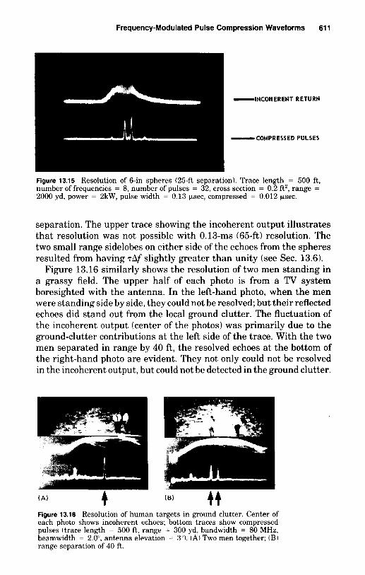
Frequency-Modulated Pulse Compression Waveforms 61 1
Figure 13.15 Resolution of 6-in spheres (25-ft separation). Trace length = 500 ft, number of frequencies = 8, number of pulses = 32, cross section = 0.2 ft2, range = 2000 yd, power = 2kW, pulse width = 0.13 psec, compressed = 0.012 psec.
separation. The upper trace showing the incoherent output illustrates that resolution was not possible with 0.13-ms (65-ft) resolution. The two small range sidelobes on either side of the echoes from the spheres resulted from having df slightly greater than unity (see Sec. 13.6).
Figure 13.16 similarly shows the resolution of two men standing in a grassy field. The upper half of each photo is from a TV system boresighted with the antenna. In the left-hand photo, when the men were standing side by side, they could not be resolved; but their reflected echoes did stand out from the local ground clutter. The fluctuation of the incoherent output (center of the photos) was primarily due to the ground-clutter contributions at the left side of the trace. With the two men separated in range by 40 ft, the resolved echoes at the bottom of the right-hand photo are evident. They not only could not be resolved in the incoherent output, but could not be detected in the ground clutter.
(A )
Figure 13.16 Resolution of human targets in ground clutter. Center of each photo shows incoherent echoes; bottom traces show compressed pulses (trace length = 500 ft, range = 300 yd, bandwidth = 80 MHz, beamwidth = 2.0". antenna elevation = 3"). (A) Two men together; ( B ) range separation of 40 ft.

612 Chapter Thirteen
While the improvement in target-to-clutter ratio was evident in the grassy areas, the echoes from the men did not stand out very well in a nearby wooded area unless they walked continuously in one direction.
The photos illustrate that high resolution, clutter reduction, and a constant-false-alarm-rate receiver can be achieved in practice as well as in theory. While these results were obtained with discrete frequency coding, they could also have been obtained with phase coding or linear FM.
13.9 Sidelobe Reduction
Just as we saw in Chap. 12 that the range (time) sidelobes of phase- coded waveforms could be improved over the matched-filter case by mismatching the transmit waveform and the receive processor, so can we develop and implement mismatch systems for sidelobe suppression of FM waveforms. Typically, one has a choice to impose an amplitude weighting in either the time or frequency domain in order to achieve sidelobe reduction, and this weighting may be applied to either the transmit or the receive waveform or both. In radar applications it is almost always desirable to operate the transmitter in saturation, so we generally apply the amplitude-weighting mismatches at the re- ceiver. For FM waveforms, the received signals represent the frequency- domain response of the target, and after processing we derive the time- (range-) domain response. Weighting prior to compression requires only a multiplication of the weighting function by the received waveform. Weighting after compression requires convolution of the weighting function by the received waveform. For these reasons, sidelobe reduc- tion for FM signals is usually achieved as an amplitude weighting prior to (or as part of) the compression process. The first sidelobe resulting from a uniformly weighted comb of frequencies was shown to be -13.5 dB below the mainlobe peak. The remaining sidelobes decay monoton- ically and symmetrically about the mainlobe. By amplitude weighting the frequencies, the sidelobes, in theory, may be reduced any desired amount.
In addition to the desirable sidelobe reduction, amplitude weighting of the frequencies has undesirable effects on the output waveform, including mainlobe widening and output signal-to-noise ratio degra- dation. These effects are measured as deviations from the sin (m)/ sink) envelope waveform, obtained from a- uniformly weighted fre- quency comb. The reason for the mainlobe broadening is deduced in- tuitively from the Fourier transform reciprocity relationship. When the spectral shape is made narrower, the time-domain waveform becomes broader and vice versa. A bell-shaped or tapered spectrum would then be expected to correspond to a wider time-domain waveform than would

Frequency-Modulated Pulse Compression Waveforms 613
a flat or unweighted spectrum of the same total frequency extent. Therefore, the resultant waveform in the time domain will be broader for an amplitude-weighted comb than for the uniformly weighted comb. Amplitude weighting may be introduced into a pulse compression radar either entirely at the receiver, or at both simultaneously. When the amplitude weighting is imposed equally on both the transmitted wave- form and on the corresponding gains of the receiver channels, the system is still considered matched. For a matched system, there will be no decrease in the signal-to-noise ratio due to weighting. However, when the amplitude weighting is introduced either at the transmitter or the receiver alone, the system is mismatched, with a resulting deg- radation in the signal-to-noise ratio.
Amplitude weighting at the receiver is accomplished in various ways, depending on the type of FM waveform employed. For discrete intra- pulse FM, it can be achieved by proper adjustment of the filter gains or by the insertion of the proper value attenuators in each of the parallel channels. It can be conveniently maintained, due to the accessibility of the components and the low power levels involved. For discrete interpulse FM, sidelobe reduction weighting can be simply introduced as a software or hardware multiply in the digital signal processor prior to transformation of the data. For stretch waveforms, the weighting can be applied after digitization of the correlated returns and before (or during) the subsequent FFT computation.
The frequency response of a matched filter is adjusted to maximize the output signal-to-noise ratio and requires that the amplitude re- sponse of the matched filter be equal to the amplitude spectrum of the input signal. The amount of mismatch is measured as a degradation from the optimum signal-to-noise ratio normally produced with a matched filter.
The loss in signal-to-noise ratio resulting from the use of weighting at the receiver alone is characterized by the loss factor L, given by [6991
2 [ jT w(t) dt ]
T I T 02(t ) dt (13.11) - - (SIN) weighted
(SIN) matched
where o(t) = the weighting function
transmitted waveform
L, =
- T = the processing time interval or the length of the
Equation (13.11) states that (SIN) is degraded by a factor L, times that obtained in the absence of matched weighting. For discrete-fre- quency amplitude weighting of an N-frequency radar, L, becomes

614 Chapter Thirteen
[$An]'
.[$..I L, = (13.12)
where An = the weighted amplitudes for the N . frequencies. The problem in selecting an appropriate amplitude-weighting func-
tion for a pulse compression system is to find what finite spectrum shape can produce a desired time waveform under some condition of optimization. A common criterion for optimization is to find a weighting function that provides a minimum mainlobe widening for a specified peak sidelobe level.
The amplitude-weighting functions that lower the sidelobes in the output time waveform all have a characteristic bell or tapered shape. When this function is applied to, for example, a comb of frequencies, the frequency in the center has the maximum amplitude, and all other frequencies have decreasing amplitudes symmetrically about the cen- ter. The output waveform for the more familiar functions, such as cosine and gaussian weighting, can be obtained from the Fourier transform relationship between the input and output of pulse compression sys- tems.
The sidelobe structure for a comb of frequencies, when weighted with a cosine-shaped taper, has been verified experimentally with a mul- tifrequency synthesizer called a DELRA (delay line range analyzer) [510, 7681. As used in the following figures, it simulates a 50-channel stepped-frequency generator and receiver. Figure 13.17A shows am- plitude versus frequency in 50 discrete steps for cosine weighting. In Fig. 13.17B, the compressed-pulse amplitude is shown with about - 22-dB first sidelobes as compared with the theoretical value of -23.6. Figure 13.17C shows the mainlobe region expanded in both di- mensions to show the rapid decay of the sidelobes.
Several other amplitude tapers have been used to obtain lower range sidelobes than can be achieved with cosine weighting. As another ex- ample, the sidelobe structure for Dolph-Chebyshev [171] tapering for 30-dB sidelobes was obtained on the synthesizer and is shown as Fig. 13.18B and C. DELRA was an analog device with a certain limit of accuracy. Thus, ideally, the sidelobes should be equal in amplitude, but this expected result is only approximated. The sidelobe structure for uniform weighting is illustrated as a reference at the top of the figures. While this taper is not practical for antennas or dispersive lines due to the large values required at the ends of the spectrum, there is no problem in approaching the theoretical limits for discrete frequency systems.
One other class of tapers, the Hamming functions, warrants special

Frequency-Modulated Pulse Compression Waveforms 615
( 6 ) 1ST SIDELOBE L E V E L = -22 dB (-23.6 dB THEORETICAL) MAIN LOBE WIDENING = 56%
kp T/2 s -----+I (C)
Figure 13.17 Sidelobe reduction with cosine amplitude weighting. ( A ) Cosine-weighted spectrum; ( B ) output compressed pulse; ( C ) expanded output.
consideration for pulse compression systems. The Hamming weighting function in continuous form is described in general terms by [6991
G(w) = + (1 - U ) C O S (T) for 0 < a < 1 (13.13)

m
n
0
m
s n
W
m
0
J
W a
In -
I1 . >
w I v)
5
m
616

Frequency-Modulated Pulse Compression Waveforms 617
Figure 13.19 Hamming function weighting sidelobe suppression (50 frequencies). (A) Hamming (sidelobe = -43dB); (B) scope gain (0 dB); (C) 25 dB. (After White and Ruuin [7691)
where the center" of the spectrum is assumed to occur a t o = 0. The resultant weighting function for the 50 discrete frequencies and a = 0.54 is shown in Fig. 13.19A. The distinguishing feature between this weighting function and the cosine function is that the amplitudes of the frequencies a t the edges of the spectrum are not zero. From Eq. (13.13) for w = ? W, the amplitude of the frequencies at the edges of the spectrum are equal to 0.08 (compared with a value of 1 at the center of the spectrum).
The output waveform shown in Fig. 13.19 may be described approx- imately by the Fourier integral used to find the envelope for Hamming weighting. The result for any value of a -is
'k In some references w = 0 is taken a t the edge of the spectrum. The amplitude at 2a ~ 1. This is often referred to as the the edge of the spectrum is a ~ (1 ~ a )
pedestal.

618 Chapter Thirteen
a sin Wt 1 - a e&) = - - + cos wt
2 wt 2W(1 - t2)
The theoretical maximum sidelobe level for a = 0.54 is -42.8 dB, which is beyond the dynamic range of the DELRA. The sidelobes were measured to be = 40 dB below the mainlobe peak. The mainlobe wid- ening over that for uniform weighing is 46 percent. The Hamming weighting function, due to its very low sidelobe level and comparatively low mainlobe widening, serves as a very effective method of amplitude weighting in practical pulse compression receivers.
Some of the properties of various weighting functions are summa- rized in Table 13.2 [699, 768, 1361. The Hamming class of weighting functions is characterized by the parameter a. The mainlobe broadening and processing loss are referenced to uniform weighting. The lobe decay function describes the rate of decrease of the sidelobes beyond the peak sidelobe. The theoretical and experimental values apply for N 2 40 frequencies, and some additional degradation is to be expected for smaller values of N [3051.
The time mismatch column is not directly applicable to short-du- ration stepped-frequency waveforms, but is pertinent to linear FM when there is a large Doppler shift. It is also significant in clutter computations for pulse Doppler waveforms. The value in the rows for 5- and 10-percent mismatch show the degradation when the weighting function is displaced from the received signal by that amount. The most significant effect is the increase in the range sidelobes. The column on processing loss can also be used for the loss in signal-to-clutter ratio for the case in which clutter has an extent greater than twice the transmit pulse length ([136, pp. 341-3431).
In order to maintain low range sidelobes, careful consideration must be given to the detailed bandpass characteristics of each channel [5191. In practice it has been possible to obtain -40-dB sidelobes by very careful adjustment of receivers employing 35 to 50 frequencies. In a practical operating system, - 35 to - 40 dB is a limit with most analog configurations. Tolerances are also given in Chap. 14.
13.1 0 Pulse Compression Decoders and Limiter Effects
In this section a matched-filter processor for a short, random stepped- frequency transmission is described. If the Doppler shift of the target echo is much less than l/Nt, a random ordering of frequencies can be used and only a single Doppler channel need be implemented in the receiver. With linear stepping of the frequencies, on the other hand, the tolerance to Doppler shift is much higher (see Fig. 8.8).

E 5 g g x U 0
al U
LL
0
a g
- (iD (R
g n i d E
v)
x 8 0
al - v- !!! m
4 3%
$
3 ?
3e
??
%?
?e
%e????
$2
2
rlrld
rlrlrlrlrlrlrlrld
rlrlrlrlrl
2c
iz t;' 3 6
"Q
?a
?Q
?"?
1?
"9
91
99
9?
?
3%
z-, 3
mm
Nw
Nr
lwb
*o
Om
*o
co
t-
*
rl OJ * m
m m
m m
m m
9 m
m + N
* m
M
.z 3 8%
or
lrlr
lr1
3r
lrlr
lor
lmr
lrl'r
lrl
9rn
??
k?
19
?""1
"
TF
E
2
*N
t-
W*
Wr
lO
O~
m
w
w
0
o*
I- d
8 %
t: ?
??
n
.2 w
'gg
i
oW
t-
Nm
am
mr
lo
mm
*r
l
o
aM
X_
; 4
rl
rl
rlrl
23 E
& 3 ~
~~
zz
zz
ff~;~
;flzl
gc
;
Y
E
t
.* $ 8 g
ooomooooooooooooo -
'28
~ ~
,
p 3 g
g
@! c)
s ssws sr! ES: 2
II
23
a:! 38
zz E
gg
wm
WW
co
aJ
8.;;
3 3
5 5 2 I1
II II
II I1 2 2
MZ
.- c 5
$E n
o
I3E
EE
AA
SB
'j; E E E a
a.- -
.gJ g .z 8
oa
aa
z-
zg
4
B 5
6
z U
zz
za
ao
E
Y
=a
%5
'36 P
g
4
rlr
l
-2
g
is
* O
NW
W
!3 2 2
.- 0
)
cc
a
z 3 f.$.$.$ee e 'r: 'E 'r: 'c: 'E:
+3k
t
-1-

620 Chapter Thirteen
The tapped delay-line pulse compression system of Fig. 13.20 is an expansion of Fig. 13.12. The transmit waveform is a contiguous se- quence of eight constant-amplitude, 0.1-ps pulses with a frequency spacing Af of 10 MHz. In a particular system of interest, the comb of frequencies was generated by modulating a carrier a t several gigahertz with an impulse-type function. This is represented by the signal gen- erator block. These frequencies are sampled with an eight-pole micro- wave diode switch, amplified, and then transmitted. The received target echoes are amplified in a low-noise traveling wave tube and then mixed to a convenient intermediate frequency. Since the spectral width is 80 MHz, an intermediate frequency IF centered at 567 MHz was chosen to allow about 14 carrier cycles to occur between the nulls of the com- pressed-pulse envelope. With a lower IF, detection of the 12.5-ns pulses would become more difficult. With a higher IF, the matched-filter delay- line losses would become excessive.
The signals are then injected into a tapped delay line consisting of eight sections of semirigid coaxial cable. Each section is 67 ft long (1.5 ns/ft delay), is quite stable, has only a 5-dB insertion loss, and coils onto a spool occupying the volume of about a 3-in cube. The delay-line taps are Stripline-type directional couplers with the coupling progres- sively tapered to account for the delay-line losses. At this point, there is no filtering other than the 100-MHz bandpass of the 567-MHz am- plifier. The individual channels are then amplified with either a linear or limiting amplifier whose gain is adjusted for the desired frequency taper. The 10-MHz filters are nominally the matched filters for the 0.1- ps segments. At this point each channel is divided into two outputs. The main output is the coherent summation of the eight segments that have been time aligned. The compressed pulse is then envelope detected and amplified in a wideband video detector. With uniform weighting the measured width of the pulse was close to the theoretical 12.5 ns.
The other eight signals out of the power dividers are detected and then amplified to form the incoherent summation of the eight 0.1-ps segments. This serves both as a reference channel and as a means to compare the detection statistics of complex target returns when si- multaneously processed coherently and incoherently. This type of sys- tem is easy to adjust and can be quite stable. The loss in peak signal power as a function of a phase error in one of the eight channels or of uncorrelated phase errors in all channels is shown in Fig. 13.21.
It is appropriate a t this point to discuss the effects of limiting on the compressed-pulse output. The purpose of using limiting amplifiers prior to the subpulse matched filters is to maintain a constant false alarm rate a t the detected matched-filter output and to limit the dynamic range of the output. The statistics of the limiting process were discussed in Chap. 4 on automatic detection by nonlinear, sequential, and adap-

w
P
e e
Ei %
Q
.* 8 s I
e Y 0 s - 3 a" x F R
- 1 R
.* - R
8 6 e ii v
0)
621

622 Chapter Thirteen
-. -. -. -. NORMALLY DISTRIBUTED PHASE ERRORS ( R M S VALUE) - A S 2 PHASE ERROR I N ONE OF EIGHT CHANNELS
U
O0 30' 60' 900 1200 1500 180. PHASE ERROR IN ONE CHANNEL
Figure 13.21 Relative signal power loss versus phase errors.
tive processes; however, there are some unique features of a limited receiver for frequency-coded signals which are worth noting here. If @ is greater than 64, the channel amplifiers of Fig. 13.20 can each have a hard-limiting characteristic with a bandwidth of slightly over 1 / ~ (10 MHz); and the coherent summed output signal will still yield desirable CFAR characteristics. Saturated coherent signals of power K out of the limiters will yield K A f 2 times this power at the coherent summation output. Random noise, rain, chaff, and most sea clutter echoes appear with random phase and have a relative summation out- put of KN. Thus s/", where N' is the noise power in the absence of signal, has a maximum value of N. While this value may be increased by making the bandwidth of the channel amplifiers wider than llt, as shown by Silber [6611, the immunity of the system to strong CW in- terference then decreases. Strong CW signals capture several of the overlapping channel limiters and suppress significant portions of the target echo.
When the factor of strong CW interference can be ignored, there are advantages in using a prelimiter bandwidth greater than llt, as illus- trated in Fig. 13.22. A 30-MHz IF signal out of a channel limiter is shown, along with the eight-frequency pulse-compressed output. The prelimiter bandwidth is 10 MHz for the 0.1-ks subpulse. The upper set of pictures was taken with the signals in each channel just at the limit level. The compressed-pulse output was square-law detected and typ-

-
(3
r I- - li -1
m n 0
W f
W
c
z -I m -u 0
W
z !z E -I m -u
'0
623

624 Chapter Thirteen
ical of the system at that time. In the center photos, the signal level was increased by 13 dB. The output of the limiter has a greater duration (7 > l/Af) due to the rise and fall portions of the subpulses receiving additional amplification, while the center portion of each subphase is held constant by the limiter. The detected compressed pulse shows that ambiguous outputs at & 0.1 p s from the peak are visible and could be confused with other targets.* With 26-dB limiting, the limiter output is doubled in extent and several peaks are apparent at the detector. Tapering to reduce these range sidelobes would be completely ineffec- tive. Some of the extraneous signal was also due to leakage through the transmit switches.
A similar system with 7 = 0.4 p s and a limiter bandwidth of 10 MHz does not exhibit this problem. As can be seen in Fig. 13.23, the com- pressed pulse is not altered and there is negligible increase in the range sidelobes for 55 dB of limiting. Since the prelimiter bandwidth is 4/7, there was a negligible lengthening of the pulses. The dynamic range of this particular system was in excess of 65 dB.
A somewhat surprising result was also obtained in the incoherent summation. With the prelimiter bandwidth of only 4 times the channel filter bandwidth, the dynamic range of the incoherent summation was marginally acceptable for visual target detection with the eight-channel system, and was more than adequate for automatic detection with a 32-channel system.
13.1 1 Nonlinear FM
To this point in our discussion, we have considered FM waveforms that utilize either linear frequency modulation, discrete approximations to linear frequency modulation, and scrambled stepped-frequency wave- forms that, although they are not in themselves linear, are derived from discrete approximations to linear FM waveforms. There is a whole other class of FM waveforms whose frequency functions are decidedly nonlinear with time.
These nonlinear FM (NLFM) waveforms are generally derived so that the spectral amplitude weightings used for sidelobe suppression in the receiver, as described in the foregoing, are instead approximated by a nonlinear time-frequency distribution characteristic that is shared by both the transmitted waveform and the receiver. That is, these waveforms are usually invented by deriving a frequency-time distri- bution whose square equals the product of alinear FM waveform with a chosen sidelobe-reduction weighting function. Such a frequency-
* It should be recalled that the coherent summation of the ungated comb frequencies has periodic peaks every 0.1 ps.

m
P
m
In
m
P
0
W z
c
- 0
2
--=f
a
+
625

626 Chapter Thirteen
modulation function was derived and realized utilizing a cascade of all-pass networks in [473] for cosine-squared-on-a-pedestal weighting. A frequency function whose compression approximates an LFM wave- form with Hamming weighting is given here as Fig. 13.24A, and the compression of the waveform through its matched filter is given in Fig. 13.24B. The compressed waveform contains peak sidelobes of approx- imately -38 dB, with practically no loss in resolution and signal-to- noise ratio, as compared with an LFM matched-filter implementation of the same bandwidth. Similar results, i.e., the ability to derive and implement NLFM waveforms that achieve sidelobe suppression with- out incurring the SNR and resolution degradations associated with mismatched filtering, have been reported in [3761 and [573]. Johnston [3761 reported that an NLFM spectrum of truncated gaussian shape was utilized to reduce the peak sidelobe level to - 46 dB, with negligible system losses, and showed that the derived NLFM waveform exhibited range Doppler characteristics very similar to those of the LFM wave- form. In [573], Taylor weighting of an LFM waveform is emulated via derivation of the appropriate NLFM waveform. The resulting matched system shows peak sidelobes down better than 35 dB, with negligible losses.
As one might expect, these NLFM techniques are also applicable to the other forms of FM- and LFM-derived phase codes. In particular, it is shown in [ 1761 that the equivalent of NLFM waveforms can be derived for a polyphase approximation to LFM, achieving -30 dB sidelobes with essentially no losses due to receiver mismatch.
The Doppler characteristics of these NLFM waveforms are also dis- cussed in the references given in the foregoing. In general, one can expect the NLFM waveforms to exhibit essentially the same range Doppler characteristics that LFM waveforms do for small Doppler shifts (see Fig. 8.8). As the Doppler shift increases, the response drops more rapidly than for linear FM. This can be used to advantage if the targets of interest have a limited range of radial velocities.
13.12 Ambiguity Diagrams for FM Waveforms
Ambiguity diagrams of FM waveforms can take many forms depending on the precise technique utilized. In this section we investigate the range Doppler response of LFM, stepped-frequency, and NLFM wave- forms through the study of their ambiguity diagrams. The diagrams for frequency-stepped waveforms are emphasized since they can be quite diverse because their response depends on both the ordering of the frequencies and the time spacing between the segments.
Fig. 13.25 provides the ambiguity diagram of an LFM waveform of

Frequency-Modulated Pulse Compression Waveforms 627
5 0 D -
M/T -
W T -
%/T - f
I I / ' I ' I ' I ' I ' I ' 32 64 9fi 128 160 192 224
SAMPLE NUMBER
(AI
-250 -200 -150 -100 -50 0 50 - 100 150 200 250 TAP NUMBER
(E)
Figure 13.24 (A) Nonlinear FM time-frequency function, TB = 128; (B) nonlinear FM, TB = 128.

628 Chapter Thirteen
m u - F. 3 - n F - 3
LT 0 -
P - 4 . w LT t c - 0 v -
-15 -10 -5 0 5 10 15 RANGE BIN NUMBER
(A)
-15 -10 -5 0 5 10 15 - RANGE BIN NUMBER
(6)
Figure13.25 LFM, TB = 128, ambiguity diagram. (A) Matched filtering; (B) Hamming weighting. (Courtesy J . M . Baden)

Frequency-Modulated Pulse Compression Waveforms 629
duration T and with a time-bandwidth product of 128. In the figure, range is given in range bins (that is, in multiples of cT/256), Doppler in hertz, and power in dB. Figure 13.25A gives the system response assuming matched filtering in the receiver and Fig. 13.25B gives the system response assuming Hamming weighting has been applied to the received signal for range sidelobe suppression. In both cases only the central 40 range bins are shown, for the sidelobes outside this region are quite low and thus of little consequence.
The ambiguity diagram for an NLFM waveform is given in Fig. 13.26A. The waveform utilized for the plot is the same as that utilized for Fig. 13.24; i.e., it represents an NLFM approximation to Hamming- weighted LFM waveform, with time-bandwidth product 128. Most strik- ing, and perhaps most important to notice, is the relative sensitivity of the sidelobe levels of this waveform as a function of Doppler mismatch as compared with Fig. 13.25B. This may be viewed more clearly in Fig. 13.26B, which represents the range response of the waveform when the Doppler mismatch is 5/T Hz.
The major contours of the stepped-frequency waveforms given in Fig. 13.8 are shown in Fig. 13.27. The frequency steps in all three cases areseparated by 1 / ~ . The diagram at the top is for an intrapulse stepped- frequency approximation to a linear FM pulse. The primary difference between this contour diagram and the chirp diagram of Fig. 13.25 is the result of the poor response of stepped FM to signals with a Doppler shift of 1/27. At this point the stepped compressed pulse is considerably reduced in amplitude from the value at the origin. This effect is not important for short pulses where ~ / N T >> fd.
The effect of scrambling the order of the frequencies within the pulse envelope is shown in the center diagram. The energy that appeared along the diagonal ridge at UT, 2/7, etc. is broken up and forms a pedestal of dimensions 117 by 7. There is also a lower spillover pedestal in the range dimension extending from 171 to PT~. This results from the far- out spectral components of each segment appearing in the wrong fre- quency channels. The lower-level pedestal is called secondary sidelobes if it occurs mostly along the range axis, or secondary ambiguities if it extends throughout the ambiguity plane [3481.
The contour diagram of a constant PRF linear stepped FM pulse train appears in Fig. 13.27C. Both the properties of linear FM and those of a pulse train are combined. As with all constant interpulse- period pulse trains, there are clear regions parallel to the Doppler axis. The major ambiguities appear at multiples of the pulse period T along a diagonal ridge. This is characteristic oflinear FM signals as opposed to the nonskewed, rectangular grid appearance of single-frequency pulse trains.
The variations possible with frequency-coded trains are almost in-

630 Chapter Thirteen
-15 -10 -5 0 5 10 15 RANGE BIN NUMBER
(A 1
-60 -50 -40 -30 -m -10 0 io 2p 30 40 M 60
( B )
RANGE BIN NUMBER
Figure 13.26 (A) Ambiguity diagram of nonlinear FM, TB = 128; (B) range response at 5/T Hz Doppler mismatch. (Courtesy J . M . Baderz)

Frequency-Modulated Pulse Compression Waveforms 631
DOPPLER
(A)
( C )
Figure 13.27 Ambiguity contours for discrete frequency waveforms. (A) Linear stepped FM; (B) scrambled pulse; (C) linear stepped FM pulse train.

632 Chapter Thirteen
BASEBAND I q/D
DIGITAL, A, 4
TO DISPLAY/ ~ ~ . Q + ~ . $ ~ @ - - ~ FFT t-) DOWNSTREAM
PROCESSING
t SIDELOBE
REDUCTION WEIGHING
Figure 13.28 Digital processing for a stepped frequency waveform.
finite in that the phase, frequency, and time of transmission of each pulse can be varied. The waveform can be tapered in time and frequency to reduce the sidelobes. Howard [3481 has studied the resultant vari- ations in the ambiguity diagram of numerous variations of interpulse timing. Several other specific examples are available in the literature [601, 1361.
13.1 3 Digital Decoders
Interpulse stepped-frequency waveforms are typically processsed as indicated in Fig. 13.28, where we assume N distinct frequencies are transmitted, and it is desired to compress over one transmit pulse footprint. The received RF waveform is downconverted and quadra- tured to yield I and Q signals at baseband. These values are then digitized, providing one I and one Q digital sample per transmit pulse. The resulting N I and Q samples are then weighted for sidelobe re- duction and transformed through an FFT. With some reordering, per- haps, the N FFT outputs then represent the compressed returns from the instrumented range swath. As noted in Sec. 13.7, stretch processors utilize the FFT in a very similar way.
The limiting factor in such decoders is often the time required to process the N-point Fourier transform. Typical performance values for modern processor-on-a-chip FFT devices seem to range between 250 ps and 1 ms per 1024-point complex FFT utilizing single chips, de- pending on the number of bits required. Many of these chips can be configured to perform in parallel, allowing the computation of 1024- point complex FFTs in as little as 50 ps.
An alternative processing configuration has been implemented for pulse compression in the Southwest Tethered Aerostat System L-88 Radar." In this implementation, an LFM or NLFM signal is transmitted
* Valuable notes on this system were provided by Dr. Larry Mertens (GE Company).

Frequency-Modulated Pulse Compression Waveforms 633
and digitized on receive. The digitized samples are reordered into an alternating stream of I and Q samples. These samples are Doppler filtered, pulse compressed, demodulated, and azimuth integrated. The pulse compression uses a correlation technique implemented on INMOS A-100 signal-processing chips. The chip is capable of correlating a string of 32 stored, 16-bit real numbers (a stored coefficient set) with an input signal at a throughput rate of 3.3 MHz for 16-bit number represen- tations. The chip is also capable of switching between two such sets of coefficients on a clock-by-clock basis [3601.
In the L-88 implementation, the received signal is fed into the A- 100 processor as an alternating sequence of 16-bit digitized I and Q samples of the received signal. The filter coefficients are represented to 12 bits of precision. The complex correlation is performed as shown in Fig. 13.29 and is similar to simple real correlation with the exception that the reference waveform coefficients are conjugated prior to the complex multiplication. The desired correlation terms are:
1 = z Ism x U c m + Qsm x Qcm
and
Q = z Qsm x Icm - Ism x Qcm
where the subscripts s and c refer to the input signal and reference waveform coefficients, respectively. The subscript rn identifies the time sequence.
MEMORY --Qsrn+~.~rm+l *Qrn, IrrnsQm-l v1srn-I ,...
a rn b BANKA INPUT BUS
CARRY FROM
+ [Tt*@ pq-@-+q-+@-e caq Funher to Stages - OJW'
PRIOR STAGES
-2 Rodud Tens When - Ism Q , q I,,I~, q - 'm Qcm+,
PrcduclTennsWhen Q,, Q,., Qsm Icm QmQ,
I IS lnpll
a IS lWI I I I I
( Q s m l m - l m Q m ) ( 'smIcm+QsmQcm)
1 a
Figure 13.29 L-88 pulse compression processor. (Courtesy ofDr. Larry Mertens [GE Com- pany])

634 Chapter Thirteen
Two correlators are required to produce the in-phase and the quad- rature outputs of the complex multiplier. Thus, 16 such processors are required to achieve the system’s time-bandwidth product of 250. Each chip time-multiplexes the complex multiplication by storing the com- plex coefficients in two memory banks and swapping banks every time a new I or Q is input. The correlation sums, computed as indicated in the figure, are accumulated over all the 250 terms as the values prop- agate down the chain of delays and adders.
Also of interest, perhaps, is the fact that after pulse compression is complete, the L-88 processor utilizes a Plessey PDSP 16330 (“Pytha- goras”) processing chip to convert the resulting I and Q data to am- plitude and phase and to detected video for further processing. Use of this chip eliminates the processing losses associated with the approx- imations that were discussed earlier (Sec. 12.5).

I4 Hybrid Processors,
Meteorological Radar, and System Performance
Analysis
14.1 The Moving Target Detector (MTD)
In the early 1970s the ground-based surveillance radars were bothered by ground clutter, birds, various forms of anomalous propagation, and weather. Air traffic control radars were capable with large commercial aircraft, but marginal in detecting and tracking the increasing general aviation fleet. MTI processors improved and numerous fixes were ap- plied to the radar output. There were still too many false alarms to implement automatic detection and tracking. It was a time of rapid advances in digital processors and memory, but poor communication between the digital community and the radar designers who had a primarily analog background. It was recognized that better clutter rejection could be obtained with a coherent pulse Doppler processor than with an MTI, and that high-clutter locations could be stored in a map with a digital memory.
M.I.T. Lincoln Laboratory brought together several of these concepts into the moving target detector (MTD) [493, 385, 2841.
635

e PULSES GENERALIZED
FILTERS TRANSVERSAL 4 MAGNITUDE]
RAIN AND WEATHER
LEVEL MEASUREMENT
I
ZERO CVELOCITY L MAGNITUDE C
FILTER - THRESHOLDING
I 1 GROUND
I OUTPUT
THRESHOLD - CLUTTER - RECURSIVE MEMORY
FILTER
CROSSING -

Hybrid Processors, Meteorological Radar, and System Performance Analysis
considerably different implementation. This is illustrated in Fig. 14.2 [284]. The block on the left is for a saturation-interference test to eliminate any range cell with strong interference.
The technical data package for the ARSR-4 described the desired capability and a typical configuration. Some of the goals were 12241 16633:
637
Range 160 nmi Capacity 550 aircraft Range accuracy Angle accuracy Rotation rate 5 t o 6 r p m AID converter Digital filter Range gates 1280 False-target reports Pulse duration 2 JLS Pulse-pulse phase 0.06" rms Pulse-pulse jitter 5-11s rms Instability residue Stalo noise (see Fig. 14.3) Processor dynamic range Improvement factor CFAR 13 range cells Clutter map seven-eighth feedback factor
1132-mi bias, 220-ft rms jitter 0.16" at SIN > 30 dB
12 bits I and Q, 1.3-MHz rate 8-point at 0 velocity, 7 at others
1 per scan at output
- 60 dB referenced to peak
66 dB to r m s noise 48 dB for 0.2 to 0.8 PRF
one-half-mil resolution 1 nmi by 1.4" azimuth
RECEIVER DIGITIZED SIGNALS
INTERFERENCE
TO CORRELATION INTERPOLATO
SURVEILLANCE
Figure 14.2 MTD I1 processor block diagram. (From Goodchild [284])

u Y ' -50-
W
0 z IL,
g -120 a a I
-130
-
I I I

Hybrid Processors, Meteorological Radar, and System Performance Analysis 639
20
% o
s -20 z W > ,Z -40 Q -J W U -60
- 80 0 0.2 0.4 0.6 0.8 1.0 0 0.2 0.4 0.6 0.8 1.0
( A ) (8)
0 0.2 0.4 0.6 0.8 1.0 ( C )
DOPPLER FREOUENCYIP. R. F. ASR-7
Figure 14.4 Nonzero velocity filter characteristics. (A) Filter 3; (B) filter 5; (C) filter 4. (From FAA [2061)
gain loss, 1-dB range-straddling loss, and 0.7-dB Doppler filter strad- dling loss [2841.
Clutter maps
It was shown in Chap. 7 that land clutter is rarely homogeneous, and there is frequently a 30- to 40-dB spread between the reflections from flat rural terrain and either mountains or man-made structures. The clutter-to-noise ratio of these structures may be 60 to 80 dB when observed by long-range surveillance radars. MTI, MTD, or pulse Dop- pler processors can eliminate most of this clutter, but there will gen- erally be a residue from the largest structures, surface vehicles, ships, rotating or vibrating objects, and flocksof birds. These residues occur at specific locations and may be isolated or clustered. Even though the density may be well less than l k m , the number in the surveillance area may be large.

IMPROVEMENT ASR-7IMTD I I FACToR
Hybrid Processors, Meteorological Radar, and System Performance Analysis
artifact. Thus, a few tens of residue reports in an area can dramatically degrade performance. This is not as large a problem in air traffic control systems, where commercial or general aviation either avoid, or at least stay only briefly in, high-clutter (urban?) areas. It is more of a problem in military or counterinterdiction systems, where a hostile pilot can make a good estimate of where the clutter regions exist. In addition it may be desirable to launch an attack missile along such a path, where radar performance is degraded.
The foregoing problem led to the development and production of clutter maps as another form of CFAR that is based more on spatial nonuniformities than on time fluctuations. It is implemented in a num- ber of systems in which the clutter-to-noise ratio exceeds the improve- ment factor. Prior to the clutter map era, IF limiters were often placed prior to the signal processors, providing an upper bound to the overall clutter suppression [3351.
The clutter map is a radar map, usually in polar coordinates, on which each clutter map cell is a pixel that represents the mean residue power of an area representing one or a few radar resolution cells. The residues are either fixed in space or are slowly moving. Thus ships, which are part of the clutter in an air traffic control system, may be the target in a vessel traffic control system. Obtaining the mean level of the residue is essential because, while the spatial locations may be fixed, there is a temporal fluctuation in the vast majority of the cells. In addition, the desired targets make a contribution to the map on each scan, and the averaging process over many scans minimizes their effect. Aircraft are not likely to stay in a single clutter map cell for many scans.
The most common implementation is to create a simple recursive or single-pole filter at each clutter map cell of the form. [673, Chap. 15; 511, 4271.
641
y I = (1 - w)y, 1 + wx,
where y L - 1 = the old clutter map amplitude y, = the updated clutter map value x, = the radar output on the current scan w = the weighting factor, usually y4, '18, or 'Il6
A target is detected when the new Val-ue x, exceeds Izy, - 1 where 12 is the threshold constant. This is essentially another form of CFAR with some loss based on the number of samples. The effective number of integrations can be expressed as qe = (2 - WYW. For w = '18, qe = 15. Shrader and Gregers Hansen developed a clutter map loss (partly

642 Chapter Fourteen
based on the work of Nitzberg) [6731. While not exactly linear, it can be approximated;
Clutter map loss (dB) = 5 fa/q, (14.1)
where fa = the magnitude of the exponent in the false alarm probability, and the loss is from about 0.4 to 2 dB. If the cell maps include several resolution cells qe is increased. The foregoing calculations are approx- imate since they assume that the residues are independent. One ob- servation is that current clutter maps at airports vary +4 dB over a three-month period. When observing the mountains to the west of a Denver site, the false alarm probability was as high at 0.45 in heavy clutter without the clutter map and dropped to 0.02 with the clutter map.
There is a problem with slowly moving clutter such as ships, bird flocks, vehicles, etc., which move from cell to cell during a scan. Sim- ilarly, if the radar is on a ship, all other clutter appears to move. Khoury and Hoyle [3991 describe a “spreading” technique. This is accomplished by letting the value in the clutter cells spread into adjacent cells at a selected rate. This requires a desired target to move more rapidly per scan. The result is a velocity response that can be tailored to the desired target’s minimum velocity. The clutter map stores echoes from moving targets, including weather, and the velocity discrimination has to be carefully controlled to detect slow-moving aircraft.
The clutter map approach does not work as well for airborne radar. In addition to clutter artifacts moving rapidly from cell to cell, the aspect angle of the artifacts relative to the radar will change, and a face of one building which is quite large at a specific angle to the radar may vanish, and the echo from another building may dramatically appear.
It is not clear whether frequency agility helps or hurts in developing clutter maps. It does increase the number of effective samples, but clutter artifacts appear on some frequencies and not others.
14.2 Meteorological Radar
The backscatter sections in Chap. 6 described the reflections from pre- cipitation as a clutter to a target-detection radar. In meteorological or weather radar this “clutter” is the target and the reflections from land are the clutter. While weather radars have been widely utilized since the 1950s, the signal processing and displays were unsophisticated and indicated only gross precipitation patterns with warning capabilities only when highly skilled operators were watching the displays. In the 1970s, the addition of digital postdetection integrators and digitally

Hybrid Processors, Meteorological Radar, and System Performance Analysis 643
refreshed memories removed much of the “speckled or “mottled look on the displays. This was closely followed by color displays that gave a much better indication of the intensity of the precipitation. These were backfitted to the 1950s era WSR-57 National Weather Service radars.
In the 1960s it was shown that Doppler radar could yield added information on the horizontal velocity of the precipitation and, more importantly, indicate the turbulence and/or wind shear in a radar res- olution cell (see Nathanson and Reilly [5011). Special-purpose digital circuits were developed to cure certain problems. One of the problems was that land clutter was often misinterpreted as weather echoes, especially when there were ducting conditions. It was called an anom- alous propagation indicator (API) and was based on measuring the relative fluctuation in a number of pulses [3731. If the relative fluc- tuation was less than a selected value, those radar cells were inhibited. It is also used in the newest systems.
Experiments in the 1970s related the radar observations to potential hazardous weather [187], and tornado warning time could be increased from. about 2 min with a reflectively-only radar to about 20 min with a high-resolution Doppler radar. While experimental Doppler radars were common in the late 1970s and early 1980s, the cost of replacing the National Weather Service radars with new digital Doppler radar delayed the development into the mid 1980s. The system that evolved was called NEXRAD and the radar designated the WSR-88D [3241. About 160 systems are being deployed in the early 1990s for both civil and military uses. The impetus for the development was a combination of the damage and loss of life due to severe storms in the United States plus the growing realization that many aircraft disasters were weather related. About 650 people were killed in numerous U.S. aircraft, weather-related accidents betweer, the mid-1960s and the late 1980s. Most of these are now attributed to microbursts near air terminals. These local phenomena are discussed later.
Several design tradeoffs are necessary to combine the unambiguous, long-range weather-detection goals of a national weather radar net- work, and the higher PRFs required for Doppler radars to meet sam- pling requirements for unambiguous Doppler measurements. This is compounded by the requirements for accuracy of measurement of mean radar reflectivity (Z , ) , mean radial velocity (VJ, and mean spectral width (uu).
To achieve reflectivity accuracies of about 1 dB requires averaging (integrating) numerous (> 30) independent measurements, as de- scribed in Doviak and Zrnic [187, Chap. 61. This is compatible with the low PRF required for long-range detection, but not compatible with Doppler measurements. Doppler measurements require samples while

644 Chapter Fourteen
the echoes are still correlated, or, stated in other terms, the sampling rate must be well above the inverse of the spectral width. Thus, while there are ways to do simultaneous reflectivity and Doppler measure- ments, it is simpler and less prone to range or Doppler foldover problems to sequentially transmit a low-PRF "reflectivity mode" followed by a higher-PRF "Doppler mode." Unfortunately, this takes considerable time for narrow-beam, pencil-beam radars. In NEXRAD the reflectivity mode uses PRFs as low as 318 Hz, while the Doppler mode has PRFs to 1304 Hz. These and other parameters of the WSR-88D are shown in Table 14.1 from Heiss et al. [3241. The time to scan preselected volumes is about 5 to 6 min due to the high resolution goals. This is too long a scan period for timely microburst alerts.
The velocity gradients of interest and the desire for high resolution in severe storm areas led to choice of a 28-ft antenna with a beamwidth of about 1" and range resolution cells of about 0.25 km. A large dish was selected for cost considerations. In early trade studies, the rapid data acquisition properties of phased-array or stacked-beam antennas were considered, but projected costs were excessive. Sidelobes in the elevation plane are specified to be quite low to minimize ground clutter. Echoes from adjacent range cells are often averaged in weather radars to reduce fluctuation and improve accuracy. Thus, the selected radar resolution in the reflectivity mode is often much finer than that required by the user. The slight loss in detectability is more than compensated for by improved accuracy.
The weather radars have MTI circuits to reduce the ground clutter
TABLE 14.1 NEXRAD, WSR-88D Characteristics
Radome diameter 39 ft (12 m) paraboloid RF loss-two-way 0.3 dB at 2800 MHz Pedestal Elevation over azimuth Steerability Azimuth: 360" Elevation: - 1.0 to 45.0" Rotational rate-maximum Azimuth: 36" s 1 Elevation: 36" s 1
Antenna polarization Circular Reflector diameter 28 ft (8.5 m) Gain (at 2800 MHz) 45.5 dB Beamwidth 0.95" First sidelobe level 29 dB Transmitter frequency Peak power 750 kW Pulse widths (nominal) rf duty cycle 0.0021 maximum PRFs
Receiver dynamic range 95 dB Noise temperature 450°K - Bandwidth, 3 dB 0.79 MHz
2700 MHz to 3000 MHz
1.57 JLS and 4.5 ps
Short pulse: 318 to 1304 HZ Long pulse: 318 to 452 Hz
SOURCE: Mlcrowaue Journal 13241

Hybrid Processors, Meteorological Radar, and System Performance Analysis 645
that would indicate higher rainfall rates if not eliminated. The ground clutter would also bias the velocity measurements. However, the MTI notch does eliminate some weather with low radial velocity.
Ground clutter rejection is achieved by a five-pole, infinite impulse response (IIR) filter and achieves over 50-dB clutter rejection (see Chap. 11). To achieve this, the transmitter and receiver were designed to have a phase noise-to-carrier ratio of - 54 dB (integrated over the Nyquist co-interval).
The received echoes are linearly integrated to obtain an accurate measure of radar reflectivity. Specified sensitivity is -8 dB 2, at 50 km and typical sensitivity is 0.01 mm/h rainfall at this range. Doppler shift is estimated by a pulse pair processor (described later in this section). The standard deviation of the velocity estimate is less than 1 d s for SIN > 8 dB with an input spectral width of 4 d s . The spectral width is estimated from the autocorrelation function evaluated at a lag equal to the interpulse period (see Chap. 9). The standard deviation of the width estimate is less than 1 m/s at SIN > 10 dB for spectral widths of 4 d s .
In operational tests in August, 1989, severe storms were detected with 91-percent probability relative to a national average of 58 percent for prior systems. The false alarm rate was 21 percent compared with a previous 57 percent. Raw radar outputs are converted to products before dissemination over a national network. Displays are 640 x 512 pixels, with magnification and storage capabilities.
Long-range (>200 nmi) ground-based weather radars are generally at S-band (3 GHz) to achieve penetration (low attenuation) during heavy rains, even though the reflectivity is about 10 dB higher at C-band (5.5 GHz).
Microburst detection radars
In the early 1980s, microbursts were identified as the cause of most of the aircraft accidents, rather than the gust fronts that had been pre- viously blamed. Microbursts are short-lived phenomena with an av- erage lifetime of 10 min. They are produced by relatively innocuous convective clouds (dry microbursts) as well as by thunderstorms (wet microbursts) [2241. The primary problem is the approach-and-depar- ture corridor to about 3 mi from the ends of the runways. A typical microburst structure is shown in Fig. 14.6. In 1987 tests at Denver, nearly 500 microbursts were recorded. They have also been found to be prevalent near Brisbane in Australia.-
The FAA Terminal Doppler Weather Radar (TDWR) Systems Re- quirement statement specifies that a wind shear is reportable if it produces a runway-oriented wind speed rate of change of 20 kn per

646 Chapter Fourteen
- LIII)
(PEAK WIND INTENSITY)
Figure 14.6 Microburst structure. (From FAA [224])
nautical mile over a distance of 0.5 to 4 nmi. The probability of detection must be 90 percent with a false report probability of less than 10 percent.
The electromagnetic spectrum, especially near airports, is over- crowded at S-band with the ASR terminal radar family and N E W both being at that band. Since the TDWR is primarily for shorter ranges, C-band was chosen for the carrier frequency. The transmit power re- quirements are lower, but there is a problem with Doppler ambiguities. The desired velocity coverage is +- 40 m/s, but the unambiguous Doppler is only ? 22 m/s at the maximum PRF of 1672 Hz. To allow for de- aliasing, several PRF from 1066 Hz to the maximum are utilized. A low PRF allows reflectivity data to 460 km. While volume scan is re- peated at 5-min intervals, the lowest elevation angles are revisited each minute for microburst detection. About 50 radars are in production at Raytheon 14721.
In other respects TDWR is functionally similar to NEXRAD. The major parameters are shown in Table 14.2. Clutter filtering is per- formed with four-pole equal-ripple elliptic filters with a flat passband. The digital implementation uses 12-bit A/D converters, and has a land clutter suppression goal of 55 dB.
Since microbursts are physically small, point moving targets such as aircraft, automobiles, air terminal vehicles, and birds must be elim- inated before detections are declared. Point target algorithms have been tested and are being improved. The key to success is simple timely warnings transmitted to pilots with few false alarms.
Airborne weather radars
Since pilots have to make the final decision as to whether to land or “pull off,” it is desirable to have the microburst detection radar capa-

Hybrid Processors, Meteorologlcal Radar, and System Performance Analysis
TABLE 14.2 TDWR Performance Parameters
Operating frequency 5.6-5.65 GHz Instrumented range Doppler mode 89 km
System clutter suppression 55 dB
Antenna (25 ft) Gain 50 dB
647
Reflectivity 460 km
Beamwidth 0.55" Pencil beam Sidelobes-near-in -27 dB Sidelobes-beyond 5" -40 dB Beam positioning accuracy 0.05"
Transmitter Peak power 250 kW Average power 550 W
PRF 2000 Hz max Pulse length 1.1 ps ( -6 dB)
Receiver Dynamic range 129 dB STC 26 dB AGC 42 dB Line a ri t y 61 dB
Noise figure 2.3 dB
Signal processor Clutter filters 4-Pole elliptic
Reliability MTBF 550 hrs Inherent availability 0.99967
Clutter canceller Infinite impulse response design Notch half-widths 0.5 to 4 d s (0 to 8 kn) Reflectivity bias 0 to 1 dB (on 4 d s width) Minimum usable velocity 0 to 4 d s (0 to 8 kn) Range sampling 0.25 km (0.13 nmi) Velocity calculation Pulse pair processing
1 d s (2 kn) Number of pulses averaged 40 to 200 Range increment 0.25 km (0.13 nmi) Reflectivity calculation Linear power average Estimate accuracy (nominal) 1 dB Number of pulses averaged Range increment
SOURCE: Microwave Journal [4721
Estimate accuracy (nominal)
6 to 64 1 km (0.54 nmi)
bility in the aircraft itself. Since there is limited space (about 0.8 m diameter) in the nose of an aircraft, the radar must also have a long- range weather-detection capability. This presents a difficult tradeoff as the beamwidth of NEXRAD is about 1.0" and 0.55" for TDWR, To achieve comparable resolution would require going to 35 GHz, where the attenuation in range is quite high and it would be difficult to avoid both range and Doppler ambiguities.
The starting point is the current airborne weather radars that are either at C- or X-band. The C-band systems have less attenuation in

648 Chapter Fourteen
heavy rain. They are currently being implemented with limited Doppler capability. In level flight, the radar beam can be slightly elevated to minimize ground clutter. In the terminal approach, the glide slope is about 3", and the radar must look down at the land clutter, automobiles entering and leaving the terminal area, and other vehicles on taxiways, etc. At these angles, the clutter background is considerably higher than for surface radars. In addition, the antenna diameter is limited to about 30 in, precluding beamwidths narrower than 2.5 to 3.0". Land clutter rejection is made more difficult because of the spectral broadening due to the high aircraft velocities and moderate beamwidths.
The goals for the next generation of airborne weather radars are much broader to justify the added cost and complexity. Studies and experiments are underway at NASA, Langley, VA. and at various con- tractors [2121.
The NASA, Langley program is emphasizing the airborne microburst detection and warning problem. That problem is separated into two subareas: the high reflectivity or "wet" microburst with reflectivity of 20-35 dBZ, and the low reflectivity or "dry" microburst with reflectivity of 0 to 10 dBZ. Obviously both 15- to 20-dB greater sensitivity and clutter rejection are required by the dry microburst. Stable transmitters with 10 to 15 dB more power are being considered. While the ground clutter spectrum is quite narrow, the spectra of the vehicles occupy the same Doppler region as the microbursts. The microbursts have to be selected by algorithms that sort on the basis of spatial Doppler patterns as opposed to the point moving target characteristics of surface vehicles. Microbursts are approximately circular with a diameter of 1 to 4 km at the surface.
Table 14.3 shows an abstract of overall goals for an airborne sensor system that might include optical, as well as radar, sensors. Note that
TABLE 14.3 Goals for Airborne Weather Sensor
Rangdtime Velocities Angle, etc.
t 90" Az 3" Res. Long-range weather
Microburst detection 3-10 km/15-40 s 2 50 dsec 2 30" Az detection 200-300 nmi clutter suppression
clutter suppression 100-300 m resolution
Ground mapping 0.5" resolution
Runway imaging 0.5 km High data rate
Wake vortex 2 30"
Clean air turbulence 180 s
detection 10-20 s clutter suppression

Hybrid Processors, Meteorological Radar, and System Performance Analysis
the goals include a mapping capability as a navigation aid, and a high- resolution terminal imaging capability as a landing aid. The detection of wake from other aircraft, especially on parallel runways, and clear air turbulence (CAT) requires a much more sensitive radar or, more likely, a laser radar.
If microburst detection, without the need for long-range weather detection were the only requirement, the improved sensitivity and an- gular resolution of a 16- or 35-GHz radar would be a possible solution for many of the goals. Meeting most of the goals likely requires either two radar frequencies or an X-band radar and an optical sensor.
649
The pulse-pair processor
In most target-detection radars that transmit a uniform pulse train, either a matched-filter processor or an MTI filter is used for the signal processor. The matched filter is usually some form of discrete Fourier transform (DFT). The signal level in each discrete filter is tested against a threshold level established by comparing with the signal levels in the adjacent range cells and Doppler filters. If the Doppler of the target is desired, the signal levels in adjacent filters are compared. In weather radar the goals are slightly different. The desired measurements are the power of the echo, the mean radial velocity, and the velocity var- iance. In weather radars these are computed directly from the auto- correlation function for the Oth, first, and second lag expressed here as Ro, R1, Rz. If the power spectrum is symmetrical, and a gaussian- shaped spectrum is assumed, one set of algorithms is [4181:
Power or intensity, 0th moment
dBZ = 10 log (kJRoJ) (14.2)
(The noise power should be subtracted from Rd Mean radial velocity or first moment
V = k/4~rT tan-' [Zm(Rl)/R&Rl)1 (14.3)
Velocity variance or second moment
U: = A2/24n2 T 2 Zm(JR11/JR2[) (14.4)
where A = the radar wavelength T = the interpulse period k = a constant from the radar parameters
These turn out to be maximum entropy estimators. The estimates are unbiased if the spectrum is symmetrical, but that condition is not

650 Chapter Fourteen
necessary for good estimates. Doviak and ZrniC [1871 give slightly dif- ferent algorithms and an error analysis for various assumptions about the nature of the weather spectrum. The error of these estimates is in some cases less than that obtained from DFT analyses, but degrades when the spectral width becomes an appreciable fraction of the inverse of the interpulse period. The normalized velocity error is shown in Fig. 14.7. The primary virtue is the simplicity of the pulse pair processor (PPP) relative to DFT or FFT implementations. The computation of the autocorrelation function is a simple product of pair of adjacent time samples when the signals are represented in VQ form. Where detect- ability is not the main criterion, it is an appropriate choice. It is used in both NEXRAD and TDWR.
Space-based meteorological radar
In the 10 to 15 years after 1992, the ground-based meteorological radar field will be dominated by NEXRAD, TDWR, and their derivatives. They will give good short-term predictions where they are densely deployed. The next advance will be satellite-based radars to extend the capabilities of the passive (optical and microwave) radiometric of the
NORMALIZED SPECTRUM WIDTH, rYn
Figure 14.7 Standard deviations of the mean frequency estimate (autocovariance processing). Spectrum width is normalized to the Nyquist interval 2u,. Note a gradual increase between 0 and 0.2 and an exponential rise thereafter. (Courtesy Academic Press 11871)

Hybrid Processors, Meteorological Radar, and System Performance Analysis 651
Defense Meteorological Satellite Programs (DMSP) and the NOAA sat- ellites in the United States.
There are several limitations of passive sensors in meeting the pri- mary current goals of determining cloud bottoms, cloud tops, and the altitude of the melting layer. These are required for global weather modeling, longer-term weather prediction, and ground-based military systems that need to estimate visibility for optical instruments. These new requirements are not well served by ground-based radars whose definition is primarily in the horizontal plane.
Space-based meteorological radars (SBMR) have been studied since the early 1970s [673, Chap. 22, 1051. Since the range for low-orbit satellites will be 600 to 1000 km the sensitivity and resolution must be drastically better than for surface systems, which only have 25 to 40 percent of these ranges. In addition, the goal is to see clouds that have 30-dB lower reflectivity than light rains. All this must be accom- plished with a total weight and power consumption of a small fraction of ground-based systems.
The studies of the 1970s pointed out that one of the most severe problems is to separate the echoes from clouds and light rain from the dramatically higher echoes from land and oceans. This requires large antennas with narrow beamwidths and low sidelobes. The sidelobe requirement is quite critical, since to obtain the required swath (cou- erage area) means observing low-altitude precipitation at slant angles where these echoes cannot be resolved in time from the ground echoes in the sidelobes just below the precipitation of interest.
The early studies showed that antenna sizes must be 300 to 1000 wavelengths and that carrier frequencies must be 10 GHz or greater. Fortunately, the space-based radar does not have to look through the precipitation for more than a few kilometers, and the millimeter wave radar is practical if the attenuation can be accounted for. In the 1970s the antenna designs were either not practical or too costly.
By the late 1980s, space-band meteorological radar became feasible as a result of relatively large apertures placed into orbit and signifi- cantly lower receiver noise temperatures a t 10 GHz and higher. Several designs evolved for possible launch in the mid- to late 1990s.
Table 14.4 illustrates the two-way attenuation y and backscattering coefficient q for hydrometeors from 14 to 140 GHz. Note the dramatic increase in reflectivity and attenuation with increasing carrier fre- quency. The melting layer has quite high attenuation, but is only about 0.3 km thick. The proposed systems fell into two areas. The first was to monitor tropical rains under the NASA TRMM program. It was originally proposed as a two-carrier frequency system at roughly 13.6 and 35 GHz. The two frequencies were felt to be necessary to calibrate

652
C/)
GI
"f8.oQ:CI
C.;:GI
=IVU(/)
"CCIVCO:;~CGI
=c(~~...W-Im~
..s<0~ Na10~ Na""ao Nso~
10OO
Oc-1
0 00
ICt)r--1Q
...C'I
cc'""'""oooI
I I
"j' I
OQ
OQ
t-O)O
oC'i~
o
I I C()""~
101O""t')t')C
()CD
I I
I I
I
Q)100Q
)O~
~~
~
ICQ
t-~a.~
~C
QC
QC
O~
I I
I I
I
II"JlI"JaJ~O
c-icxj.'..:~1:'1
IQ)Q
)t--C'j
MM
M(Q
~
I I
I I
I
.j"Q: I
.01
~
bO
0)Q
I ~
=
0)
5- ~
~
~~
fI
e ~
"'
b .~
~
~
ooo

Hybrid Processors, Meteorological Radar, and System Performance Analysis
the uncertainty in the attenuation. Later designs led to a single-fre- quency system at 24 GHz due to cost considerations.
Another study for the Air Force E041 evaluated other approaches with the goal of measuring the tops and bottoms of stratus clouds (0.3 @m3 water content). Frequency tradeoffs and system designs were iterated for best overall performance. The bands at 13.6 and 140 GHz were eliminated fairly quickly due to the physically large antennas and large transmitters at the low frequency and excess attenuation encountered at the highest frequency. The appropriate meteorological radar equation can be written in several forms: [lo51 [6731
653
- K P,7D2F Md3 P, = A4R2
where attenuation is neglected and K = constant P, = average receive power Pt = peak transmit power 7 = effective pulse duration (see Chap. 2)
D = antenna diameter F = beam shape and filling factors
M = liquid water content d = droplet diameter A = carrier wavelength R = range (related to altitude)
Also in another form
- 1018PtGTGR C T IKI2 z in MKS units 512 (2 In 2) R2A2
P, =
where G = peak gain (gaussian shape) c = velocity of light
2 = reflectivity in nm6/m3 (Chap. 6) K 2 = 0.93 for rain, 0.2 for ice
The frequency tradeoff showed that 35 GHz was slightly superior to 94 GHz. This is illustrated in Table 14.5. Note that they would be comparable if only clouds without a melting layer were present. This tradeoff assumed that the state of the art was used for transmitter antenna design. With the large apertures required, tolerances would limit antenna dimensions to 500 to 700 A.
Another interesting result was that the performance was almost independent of radar configuration. A dish or planar array was com- pared with a long linear-array system and a synthetic aperture (SAR)

054 Chapter Fourteen
TABLE 14.5 Relative Merits of 35 and 94 GHz
Parameter 35 GHz 94 GHz
Peak transmit power +6 dB Aperture area +6 dB Losses + 1.8 dB System noise temperature + 2 dB Cloud penetration +1 dB 2, clouds (light rain)
Melting layer penetration
+16 dB (5-10 dB)
+ 3 dB Total + 19.8 dB +16 dB
configuration. The SAR was comparable only when a very small swath (< 100 km) was acceptable. Small swaths have little value in global monitoring. The dish was selected as the best option until at least the year 2000. The phased array is heavier, more costly, and probably more “lossy” at millimeter wavelengths.
The parameters of the cloud-sensing radar called ALLRAD are shown in Table 14.6 based on components available in 1990 [5041. It was shown in the study that adding a lower-frequency radar was heavy and only useful for heavier rains. It was also shown that calibration up to about 30-mm/h rainfall rate could be obtained with simple radiometers and by utilizing the reduced backscatter from land or ocean areas to esti- mate attenuation. A comparison of this cloud radar and the TRMM system which needs only to observe rain is shown in Table 14.7. The difference is the reflectivity of clouds versus light rain.
Other proposed systems were described by Cantafio and Kovalcik E1051 including TRAMAR, a dual-frequency system at 9.7 and 24 GHz,
TABLE 14.6 RadarlRadlometer parameters
Frequenc y-radar 35.6 GHz Frequency-radiometer 36.6-37.6 GHz Antenna diameter 4.1 m Beamwidth (one-way) 0.16 degrees First sidelobes 31 dB Gains (40% efficiency) 59.7 dB Number Transmitters 2 Peak power/XMIT 6.2 kW Average power/XMIT 150 W Pulse repetition frequency 7 kHZ Pulse duration 3.3 Micro Losses (approximate) 7 dB System noise temperature 500 Beg K Rotation rate 17 rpm Nadir angles 10-25 degrees Horizontal resolution (rain) -2 kM

Hybrid Processors, Meteorological Radar, and System Petformance Analysis
TABLE 14.7 Rough Comparison of TRMM and ALLRAD
655
Parameter TRMM ALLRAD SIN diff.
Gain (dB) 47.7 59.7 24.4 dB Peak power (kW) 0.57 6.2 10 dB
Pulse duration 1.67 3.75 7 dB
Frequency (GHz) 13.8 35.6 8.2 dB Noise figure (dB) 2.5 2.5 0 dB Relative total -34 dB PRF and integration area roughly comparable. TRMM parameters from 1989 Radar Met. Conf.
Loss diff (dB) 0 - 2.5 -2.5 dB
Beamwidth (deg) 0.71 0.16 -13 dB
with a beamwidth as narrow as 0.1" at 24 GHz. They also summarize another concept called LORRA with beamwidths in the azimuth plane of less than 0.05" at 35 GHz. These have advanced antennas with electronic scan in one plane.
Another design problem for SBMR is in the transmitter area. Average power requirements are in excess of 100 W, but resolving low-lying cloud bottoms from the earth's surface limits pulse durations to a few ps. In many systems, this would immediately suggest pulse compres- sion. However, with the typical geometries for weather operation, the ground echo exceeds the cloud echo by 50 to 60 dB, and, thus, the near- in range sidelobes of the pulse compression system must be reduced to a comparable level. It is unlikely that this level has been met in airborne or satellite systems. If the requirement is only to see very light rain, pulse compression may be practical.
Orbiting satellites will have a limited swath, but coverage can exceed 800 km. Multiple satellites are required for global coverage, but no- where near the number of ground-based systems. In addition, the sat- ellite will provide radar coverage over the oceans that is not currently available.
Eliminating the requirement for multiple satellites in orbit would require the use of a satellite in a geosynchronous orbit. Unfortunately, a monostatic configuration at the 36,000-km range is currently im- practical as the relatively large meteorological systems such as NE- have only 1/50 of that range. One possible alternative is a bistatic configuration with the transmitter in geosynchronous orbit and multiple receive-only radar systems on the ground or on aircraft. The direct signal received from the satellite is cross correlated with the bistatic echoes from precipitation (Nathanson in [24 pp. D341-3501).
The signals impinging at a passive receiver, resulting from illumi- nation from a geosynchronous satellite, will yield more or less constant reflective power at reasonable range from a ground station. While the power intensity at a ground receiver falls off inversely as the square

656 Chapter Fourteen
of the range from the receiver, the beam volume increases directly as the square of the range from the receiver. (The angular resolution degrades with increasing range.) There is no need for STC.
The power and aperture sizes are not great due to the volume-search mission of a meteorological radar. Since at any point on the earth’s surface it is desired to scan a preselected area (or volume), there is not a significant difference whether that area is scanned with a short, intense beam for a short period of time, or the received power is in- tegrated over a long period of time. Basically, the criterion for an area search is the energy incident on that area in the desired period. It is more efficient to have the satellite illuminate an area of 400 to 700 km in diameter at one time rather than flood the entire country with a lower power density; since this requires only a 1- to 2-m aperture at 12 GHz, there is no severe demand on satellite state of the art. Average levels required to detect light rains near the ground are approximately 200 W radiated from the satellite. This is well within the envelope of what has been accomplished at geosynchronous altitudes. Due to the geometry involved, it is necessary only to scan the satellite beam by t 3” in one plane and k 1V2” in the other plane to cover the United States. This scanning can be accomplished either mechanically, since it is rather slow, or electronically, using multiple feeds or frequency- scanning techniques.
The 12 to 14-GHz carrier frequency was suggested because there are current communication satellite transmitters with scanning arrays op- erating in that band. The beams from the satellite would periodically scan the surface or concentrate on areas with impending severe weather. The higher carrier frequency is acceptable because although the attenuation coefficient is higher, only one-way horizontal attenu- ation is involved.
When the technique was proposed (1981), 2- to 4-mm/h rain detection was practical. With new technology, especially low-noise HEMT re- ceivers (see Chap. 2), light-rain detection (< 1 mm/h) is currently prac- tical. Receive antennas of the size of current airborne weather radars (30 in) are adequate.
14.3 Aerostat Surveillance Radars
From the 1970s there have been a few radars attached to aerostats tethered as high as 15,000 ft above sea level. This deployment allows coverage against low-flying aircraft to ranges of 160 to 200 nmi. These surveillance radars are used for military defense and civil purposes such as drug interdiction, and to counter possible smuggling and ter- rorism.
The United States and other countries are deploying various radars along their borders, coastlines, and islands. These include lightweight

Hybrid Processors, Meteorological Radar, and System Performance Analysis 657
versions of surveillance radars with simplified air traffic control sys- tems, for example, large Customs/Coast Guard aerostat radars by GE which are called L88 (partly based on FPS/117 “SEEK IGLOO tech- nology), and large Customs/Coast Guard aerostat radars by TCOW Westinghouse, which are generally called LASS and are installed as Cariball or Sowrball (these are derivatives of the Marine Corps TPS/ 63). The LASS system is shown in Fig. 14.8. There are also a few older Air Force aerostat radars, and some smaller ones called SASS. The SASS systems are based on Westinghouse X-band airborne Doppler radars.
The aerostat radars are primarily designed to detect and track air- craft; to enable them to have long-range coverage they are deployed at 10,000 to 15,000 ft above sea level. With these geometries they also see numerous vehicles, boats, and ships. The larger systems use L-band, have relatively large lightweight antennas, and transmit sev- eral hundred kilowatts of peak power. They can remain at altitude for several days, and all power for the radar is brought up through the tether. A significant advantage is that the motion is quite low, and velocity compensation is not needed as in airborne radars. The smaller aerostats (SASS) are flown at several thousand feet and can be tethered from ships. Typical radar ranges are of the order of 50 nmi.
The large aerostats use fixed- or staggered-pulse, low-PRF MTI and pulse compression. The digital pulse compressor was outlined in Chap. 13. The clutter rejection is high (60 to 65 dB) as they look down at the land at steeper angles than do surface radars.
In some areas they are used for small boat tracking. Maritime chan- nels have been designed to be in parallel with, but not interfering with, the air target channels on the aerostats. These are, in general, designed for radial velocities of about 10 to 70 kn.
The current trackers are basically track-while-scan systems. On each radar scan (about 12 s), the range to the target is measured, as is the centroid of the “run length or “hits” in azimuth. These are stored for several scans in a digital target extractor (DTE), and a velocity vector is derived from the change in target position from scan to scan. Tracking is accomplished in a similar manner to air traffic control systems.
14.4 Performance Estimation for Coherent Pulse Radars* This section describes the numerous limitations on the actual perfor- mance of a coherent pulse radar or a radar mode whose primary purpose is to discriminate a small target in the presence of clutter. The emphasis is on pulse train waveforms that are processed by a moving target
* Portions of this section were developed under an Internal Georgia Tech STGC Pro- gram.

658 Chapter Fourteen
Figure 14.8 Large Aerostat Surveillance System (LASS). (Courtesy Westinghouse Ucfi.ri.sc Center)
Hybrid Processors, Meteorological Radar, and System Performance Analysis 659
indicator (MTI), a pulse Doppler processor (PD), or a moving target detector (MTD), which is roughly a combination of an MTI and a PD. The individual pulses may be coded and introduce other limitations, but that should not alter the following analyses. It is also assumed that the pulse train is coherent, that an attempt has been made to keep the amplitudes of the pulses constant or following some prescribed amplitude taper, and that an attempt has been made to have the relative phases approach what would have been obtained had one sam- pled a perfectly stable oscillator.
Since the goal is to determine performance, it is necessary to have a reference. The almost universal reference is the performance of the radar if it transmits a single pulse of the pulse train and a matched filter is implemented in the receiver. The equations for performance in receiver noise, jamming, and clutter are widely available. The ad- ditional clutter performance obtained by the multiple pulses is ex- pressed by an improvement factor I which combines the benefits from the multiple pulses (and the appropriate processor) with the limitations of nature and the hardware implementation.
There are several terms to describe radar performance in a clutter environment. The oldest term is subclutter visibility (SCV), whose def- inition is given in an IEEE standard as 13561:
subclutter visibility (radar). The ratio by which the target echo power may be weaker than the incident clutter echo power and still be detected with specified detection and false alarm probabilities. Target and clutter powers are measured on a single pulse return and all target velocities are assumed equally likely. This term combines the performance of the signal processor and the
various circuits in the detection process. The numerical value varies with the selected detection and false alarm probabilities. While it may be a useful measure of overall performance of a particular system, it does not lend itself to comparative analysis of radar waveforms and signal processors without a rather complicated detection simulation or analysis. SCV is also dependent on the fluctuation model of the target.
In most stages of radar design or analysis, it seems appropriate to partition the process of waveform and processor evaluation from the detection, CFAR, and thresholding system. In testing, it is also simpler to measure ratios of clutter into and out of the signal processor. The subsequent discussions attempt to discuss processing and detection separately.
The improvement factor is currently formally defined only for MTI processing, but it is often used for pulse Doppler systems. The IEEE Standard definition [3561 is:
MTZ improvement factor (radar MTI). The signal-to-clutter ratio at the output of the system divided by the signal-to-clutter ratio at the input of the system, averaged uniformly over all target radial velocities of interest. See also: clutter attenuation, moving target indication.

660 Chapter Fourteen
The system is meant to include the clutter filter, but not the post- detection integration process. The input to the radar can be at RF, IF, or even bipolar video as long as these components are all linear. The improvement factor can be expressed as:
I = (C,/C,) (S,[fl/S,)
where C, and C, = the powers of the clutter echoes at the input and
S, and So = the powers of the target echoes a t the input and output, respectively
output, respectively.
The term S,[fI/S, is to normalize I to the average target gain. If one makes the assumption that the potential range of all target Dopplers can be much higher than the PRF, and thus all Dopplers are equally likely, then the bar over the term represents the average over all Dopplers. There is still some ambiguity as to whether to average I over possible Dopplers in absolute units or in decibels. Since noise also has the property that all frequencies are equally likely, the ratio of the signals equals the noise gain of the filter and
I = (C,/C,, (NOIN,)
This definition has several limitations primarily related to the range of target velocities that is desired or specified. For example, targets up to 50 kn may not be of any interest. More importantly, the velocity response of a bank or Doppler filters might be quite complex with different sensitivities a t different velocities. The simple definition also implies linear processing and optimum utilization of the dynamic range. Finally, the use of I does not directly relate to detectability as the amplitude distribution and power spectrum of the residues of an MTI filter are not noiselike.
To make the improvement factor a more general term that is appli- cable to a number of Doppler processors, we define I ( f ) as the improve- ment factor obtained over a range of possible target Dopplers. Its definition is similar to Ward's [7471 and Ludloff et al. [4511, and is discussed later in this section.
The computation of the performance of a processor for a pulse train waveform is best performed on a computer with some combination of algorithms for computing each limitation, and perhaps a Monte Carlo simulation to evaluate detection and false alarm probabilities. The following outlines the major contributors that limit performance in a clutter environment.
An illustration of the major sources is shown in Fig. 14.9. The signals entering the receiver include the target echo, the clutter echoes, receiver

1. TRANSMIT AMPLITUDE NOISE'
3. PULSE WIDTH NOISE MIXER
5. PULSE STAGGER ( f)
2. TRANSMIT 4 NOISE PRE-AMP
4. PULSE JITTER NOISE I F-AM P
c PULSE
MATCHED FILTER
1-0 DETECTOR
1. TRANSMIT AMPLITUDE NOISE 2. TRANSMIT + NOISE 3. PULSE WIDTH NOISE 4. PULSE JITTER NOISE 5. PULSE STAGGER (f)
6. MISMATCHED FILTER LOSS
7. 1-0 IMBALANCE
SAMPLE AND
HOLD
AID CONVERT
c c
4 c
MTI FIR FFT
COMBINE DETECT
AND CFAR
8. RANGE STRADDLING LOSS
9. OUANTIZATION LOSS IO. SATURATION LOSS
11. TRANSFER FUNCTION ( f) 12. INHERENT CLUTTER (f ) 13. SCANNING MODULATION
14. SOUARE LAW DETECTION
15. CFAR LOSS: APPROXIMATION
INSUFFICIENT SAMPLES
POSTDETECTION INTEGRATOR 16. IMPERFECT INTEGRATOR
I

662 Chapter Fourteen
Referring again to Fig. 14.9, there is a loss if one does not use a “matched filter” (see Blake’s Cb term in [741) for the individual pulses plus another matched filter for the pulse train. The individual pulses may also be coded and thus there are two losses for not using ideal filters. These are not expanded on here since they have a minor effect on calculating I, and since, at this point, we are assuming that the processor is linear, the errors could just as easily be assigned to the “Combine Detect and CFAR” box.
The “sample and hold circuits may have instabilities, which are best added elsewhere, but there is a significant loss in that the samples may not occur at the peak of the target echo out of the matched filter. This range-straddling loss cannot be computed independently of the matched-filter loss, as a mismatched filter generally tends to extend the target waveform in time. This tends to counteract the range-strad- dling loss. Also, the target appears in two range gates and there is a probability of detecting the target in either or both gates. Some de- signers oversample to reduce the loss, at the price of more hardware.
The quantization loss of an A/D converter is a noiselike limitation to the improvement factor. The saturation loss is much more compli- cated as nonlinear processes are involved. These processes are sensitive to the relation of the dynamic range of the input to the number of bits in the A/D, the ratio of the noise power to the level of the least significant bit, and even the amplitude distribution of the targets and clutter. This is all part of the dynamic range limitation.
Consider a radar with an analog-to-digital converter with a limited number of bits, and the problem of where to set the rms noise and the clutter in the dynamic range. 1. If the noise level is set much below the least significant bit, there
is a loss in detectability even in the absence of clutter. This is quantization noise and also affects performance in clutter. Losses decrease as the input is increased to allow accurate quantization of small signals.
2. With noise occupying more of the dynamic range of the A/D, the ratio of clutter to noise that occurs before the clutter saturates is reduced. The clutter cells that saturate create saturation noise that reduces the maximum obtainable improvement factor. Thus, putting the signals higher in the dynamic range increases the saturation loss for a given level of clutter. Saturation noise can often be modeled as white noise, although doing so is not entirely valid.
3. Clutter, like noise, fluctuates and thus its mean level must be well below the maximum so that the peaks do not saturate. This varies for different clutter-fluctuation models.
4. The actual level of the clutter varies from site to site and from one direction to another.

1 . 6 ~ 1 0 - ~ -
0 2 0.8
0.4
-
-
I I 1 I 1 *
1.6~10-~
1.2
-
K =SATURATION LEV/RMS VOLTAGE
-
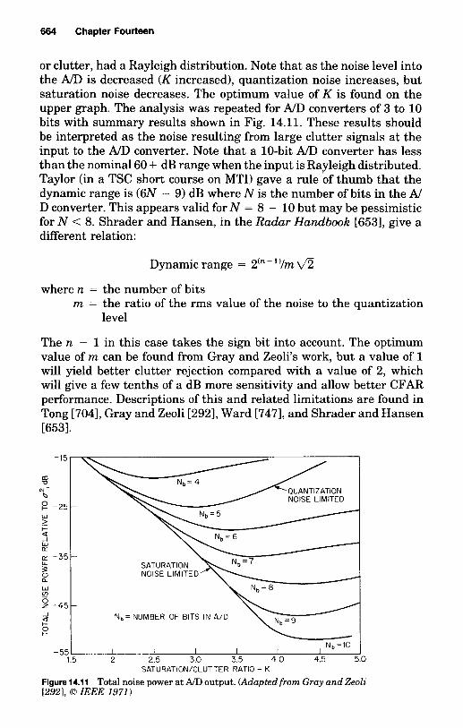
664 Chapter Fourteen
or clutter, had a Rayleigh distribution. Note that as the noise level into the A/D is decreased (K increased), quantization noise increases, but saturation noise decreases. The optimum value of K is found on the upper graph. The analysis was repeated for A/D converters of 3 to 10 bits with summary results shown in Fig. 14.11. These results should be interpreted as the noise resulting from large clutter signals at the input to the A/D converter. Note that a 10-bit A/D converter has less than the nominal 60 + dB range when the input is Rayleigh distributed. Taylor (in a TSC short course on MTI) gave a rule of thumb that the dynamic range is (6N - 9) dB where N is the number of bits in the A/ D converter. This appears valid for N = 8 - 10 but may be pessimistic for N < 8. Shrader and Hansen, in the Radar Handbook 16531, give a different relation:
Dynamic range = 2'" - "Im .\/z
where n = the number of bits m = the ratio of the rms value of the noise to the quantization
level
The n - 1 in this case takes the sign bit into account. The optimum value of m can be found from Gray and Zeoli's work, but a value of 1 will yield better clutter rejection compared with a value of 2, which will give a few tenths of a dB more sensitivity and allow better CFAR performance. Descriptions of this and related limitations are found in Tong [7041, Gray and Zeoli [2921, Ward [7471, and Shrader and Hansen 16531.
NOISE LIMITED
W
n -35- W
v, 0 Z -45 _J
-
Nb = NUMBER OF BITS IN A/D a 6 t-
Nb=10 - 55 I I I I I
1.5 2 2.5 3.0 3.5 4.0 4.5 5.0
Figure 14.1 1 Total noise power at A/D output. (Adapted from Gray and Zeoli 12921, 0 IEEE 1971)
SATURATION/CLUTTER RATIO = K

Hybrid Processors, Meteorological Radar, and System Performance Analysis 665
The box labeled “MIT, FIR, F F T is to represent the pulse train processor. It is here that the Doppler spectrum of the target and clutter have a major effect, and the ultimate performance of the system is defined. The term MTD (moving target detector) is not included here since it includes clutter maps, etc. that are not directly part of the pulse train processor. Items (ll), (121, and (13) are to indicate that the ultimate performance is still limited by the inherent clutter spectrum, which is taken to include wind-blown effects, the variation in clutter Doppler of the scatterers in various parts of the radar beam, plus the uncompensated components due to platform motion and radial motions of the clutter. For MTI, the limitation on improvement factor is de- scribed in Chap. 9 and also in Chap. 15 of the second edition of the Radar Handbook 16731.
There are target velocities, near blind or dim speeds, at which de- tection is poor or impossible. These are losses if the system is required to detect targets a t these velocities. The allocation of these losses is described later.
The scanning modulation of a rotating antenna broadens the inherent clutter spectrum. The transfer function item is to represent the limi- tations (or benefits) of this block. In a digital processor there are always some additional losses due to quantization and roundoff. There is in- variably a Doppler cusping loss due to a target Doppler straddling two adjacent filters in a similar manner to the range-straddling loss. At this point the losses from Doppler cusping are excluded from this box. It may be appropriate to define the term ultimate performance to de- scribe the performance of the chosen filter without external hardware limitations.
Following the filter block is the “Combine Detect and CFAR block.” At this point there are usually I and Q signals for each pulse from each range gate for an MIT-like processor or from each Doppler filter for each range gate for a batch of pulses for pulse-Doppler-like processors. The I and Q signals are either squared and added to constitute a square- law detector or added by one of several algorithms to approximate a linear detector. There is a small loss in the latter process, but it is usually the preferred approach. These outputs are usually fed to a constant false alarm rate (CFAR) circuit before or after integration, and then to a threshold circuit that establishes the false alarm rate. The CFAR circuit attempts to estimate the mean and some other pa- rameter of the input signals. There are several losses in this process; the first loss results from the CFAR only using a finite number of samples to estimate these parameters. It can be defined as:
CFAR loss. The additional amount that the detection threshold must be raised due to the finite number of samples used to estimate the mean of the distribution plus quantization losses in the estimation. There is an additional loss if the distribution is assumed to be non-Rayleigh, and an attempt is made to estimate

666 Chapter Fourteen
the second parameter as well. This part of the loss can often be neglected if pessimistic estimates are made for the distribution loss, defined later.
The second loss term relates to the uncertainty in knowing which statistical distribution best fits the radar samples. (This is not really a loss in the usual sense of the word.) If the noise or clutter samples are Rayleigh with a constant mean value (in space) and are independent in time, as receiver noise, the distribution is known with only an es- timate of the mean value. Otherwise there is a distribution loss. It can be defined as:
Distribution loss. The additional amount that the detection threshold must be raised (or lowered) due to the tails of the clutter distribution exceeding those of the Rayleigh distribution.
CFAR losses were described in Chap. 4. Finally, there is some loss if the postdetection integration is not linear, as is obtained with a recursive integrator. If the inputs are from a rotating antenna, the weighting function and the time constant of the integrator must be matched to the antenna pattern.
Losses attributable to the clutter source
The clutter echo as it enters the radar has first- and second-order statistical properties that limit complete elimination by a filter. The clutter has a mean Doppler component that is related to the winds except in the case of ground clutter. The shift in the clutter spectrum is generally unknown, but can often be estimated by averaging the phase shift from a number of pair of echoes. Similarly, the radar plat- form may be moving and shift the clutter spectrum. The power spectrum has a width due to environmental considerations, in addition, the finite beamwidth of the radar allows it to simultaneously observe scatterers at different locations with differing velocities (see Chaps. 5, 6, and 7). This inherent clutter spectrum is broadened by the moving platform plus the scanning modulation of a rotating antenna. Additionally, the clutter spectrum may be broadened by staggered pulse transmissions as in a staggered-pulse MTI. It may also be appropriate to include the time jitter of the transmitter at this point, since it has a similar effect to pulse stagger.
Simulation block diagram
It appears appropriate to illustrate and organize the error sources of Fig. 14.9 by the simulation block diagram of Fig. 14.12. The target echo, the receiver noise, clutter, and jamming are assumed to be ad-

GENERATOR
TARGET FLUCTUATION TARGET EXTENT
GENERATOR
5. PULSE STAGGER 12. INHERENT CLUTTER
COMPLEX MULTIPLIER
13. SCANNING MODULATION
/ 1. TRANSMIT AMPL. NOISE - 9. QUANTIZATION AND
SATURATION NOISE
MTI FIR FFT
7. 1-0 IMBALANCE
11. TRANSFER FUNCTION
I POSTDETECTlON I 14. SQUARE-LAW DETECT INTEGRATE INTEGRATION.
LOOK-UP
DOPPLER CUSPING
I 15. CFAR LOSSES
I

668 Chapter Fourteen
values of e are obtained by expanding the individual error sources in a Taylor series.
For simulation purposes, the clutter generator might include the velocity offset of the spectrum and a widening due to the other factors. The clutter generator should be derived from the same source as the target generator. The effect of the wider spectrum can be seen at the output of the “MTI, FIR, or F F T filter in the simulation or the spectral width limitation can be individually calculated for simple MTI systems described in Chap. 9. The intent of this diagram is that the filters are assumed to be perfect. These portions of Fig. 14.12 account for the environmental limitations, those of the transmitter and receiver, and of the signal-processing subsystem. At this point, the signal-to-noise, signal-to-jamming, and signal-to-clutter ratios may be calculated. It is not absolutely necessary to make assumptions about the spatial dis- tribution of the clutter at this time. Spectrum analysis would indicate the nature of the limitations in uniform clutter. However, the detec- tibility and false alarm probability of the system are not yet available, since the distributions of the target and the sum of noise, jamming, and clutter are unknown as well as their temporal and spatial corre- lations. The target and clutter distributions have a major effect on the saturation noise component, and should be included in the target and clutter generators. Parameters are suggested in Chaps. 6 and 7.
The I-Q combine, CFAR, integration, and detection block
In the absence of system errors or saturation, the foregoing portions of the simulation are all linear. In this block, the detection process is the first nonlinear operation. A square-law detector is considered op- timum, but it is usually approximated by various algorithms, many of which approximate a linear detector. The loss is a few tenths of a decibel. The constant false alarm rate (CFAR) circuit estimates the total in- terference level in time (range) and often additionally in Doppler in the vicinity of the target echo. The detection curves of Marcum and Swerling and the others assume that there is exact estimation of the mean value of the noise background.
As stated previously, there are losses in estimation of the statistics of this interference. The spatial statistics, including temporal corre- lation of the processors, must be included at the input to have valid results. CFAR circuits can be before or after postdetection integration or both. Postdetection integration can take several forms and be linear or recursive. There is some loss that can be calculated or that show up in the simulation. There is at least one, and often several, thresholds in the detection process. For example, in an rn-out-of-n detector, there

Hybrid Processors, Meteorological Radar, and System Performance Analysis
is an initial threshold to decide if a single pulse echo is large enough and then a second determination if rn of these threshold crossings ap- peared in the last n transmissions (at a given range). The thresholds are set to establish the false alarm probability (Pfa), and the detections are counted. These topics were discussed in Chap. 4, and clutter maps were discussed in Sec. 14.1.
In a simulation, this block can be run separately and operate on stored outputs of the filter block. Thus the diagram of Fig. 14.2 implies that a radar simulation can be split into several subsimulations.
1. A target, noise, jamming, and clutter generator whose outputs are summed into the input of a complex multiplier
2. An error generator, where the individual error sources are approx- imated and added to form an error modulation
3. A signal-processing filter subsystem simulation 4. A combiner, CFAR, and detection subsystem simulation
There should be several advantages to running the subsimulations sequentially.
1. They can be run on a smaller computer with only the results stored from step to step.
2. The simulations up to the combine/CFAR can be run for a single range gate with and without the target. Other range gates can be subsequently run as along as the distributions are maintained and the spatial and temporal correlations are properly programmed.
669
3. The subsimulation outputs should be more easily understood. 4. The tasks can be divided among several personnel. 5. Partial results will be available sooner.
Improvement factor as a function of target velocity
As was stated earlier, the improvement factor for an MTI, pulse Dop- pler, or MTD processor can only be truly evaluated for a target at a specific radial velocity. Each of the processors has velocity regions that are believed to be clutter (the stopband) and the corresponding outputs are attenuated. Since realizable filters cannot have a square velocity response for a finite number of pulses transmitted, there is a loss on targets at a slightly higher velocity. There is also a loss on both sides of all the PRF lines for fixed PRF systems, and losses in “batch trans- missions at different PRFs. With most surveillance systems having a limited number of pulses per beam, the losses are significant.

670 Chapter Fourteen
There are several ways of describing the loss. Rivers [6111 (private communication) calculates the percentage loss as a fraction of the PRF, and describes this as “wasted bandwidth. He assumes that in addition to the loss due to the stopband for clutter, the velocity region from the -3-dB point of the adjacent target filter to the velocity at which the filter sidelobes are sufficiently low is wasted. Thus, there is a velocity region that is the sum of the stopband plus the waste bandwidth, at which detection is unlikely. He performed calculations for Dolph-Che- bychev filters with varying sidelobe levels.
For design sidelobe levels of 70 dB, the wasted bandwidth was 46, 33, 25, and 13 percent for 8, 12, 16, and 32 pulses. These percentages are in addition to the stopband percentage. Thus, for systems trying to achieve high clutter-rejection levels, using 12 pulses or less per beam is quite inefficient. The alternative of increasing the number of pulses without increasing the total time could be equally damaging if it in- troduces range-ambiguous clutter. The use of two or more shorter bursts at different PRFs does not present an obvious cure if the total time available is insufficient. Going to higher PRFs to obtain more pulses per burst is highly desirable if it does not introduce or aggravate the range-ambiguous clutter problem. With this approach, a value for de- tectability versus target radial velocity is determined for the passband, and the waste-plus-stopband percentage is stated separately.
A related approach for MTI processors is described by Kretschmer, 1986 [4151. He shows how the improvement factor increases as the number of pulses is increased, but that the percentage of the Doppler bandwidth at which targets are detected (“visible space”) decreases with increasing pulses. An example for clutter centered at zero Doppler and with binomial weights for the MTI is illustrated in Fig. 14.13. If it is required that I ( f ) is within 3 dB of I , 68 percent of the targets are visible with a two-pulse canceler, but only about 44 percent are visible with a five-pulse canceler. This limitation is alleviated by using stag- gered-pulse MTI with the appropriate weighting.
These methods are most useful in evaluating initial designs, making tentative choices of the PRF for a single burst, the number of PRFs in a beam, and the value for each PRF; and the system choices of carrier frequency and time per beam position. For evaluating a tentative set of designs, a more analytical evaluation of target detection versus ve- locity or a simulation is required.
Another approach is probably best described by Ludloff et al. 1981 [4511 and expanded on by Taylor [6941 [6731, who describe a Doppler- dependent signal-to-interference ratio, which is called Z(fd) , or simply Z ( f ) when there is no ambiguity. The common expression for the overall improvement factor of a radar system is generally expressed as

Hybrid Processors, Meteorological Radar, and System Performance Analysis 671
10
0
-10
m -20 '0
M
1. 5 Y
- 30
- 40
- 50
- 60 0.0 0.2 0.4 0.6 0.8 1.0
FREQUENCYIPRF Figure 14.13 Target Doppler visibility space. (From Kretchmer [415])
1 1 1 1 - - - + - = - . . . I -II 1 2 1 3
where the Z, = the individual limitations, which are usually contained in an improvement factor budget. For this equation to be properly interpreted, either the individual terms must be Doppler independent or they must all be interpreted at each target velocity of interest. The latter approach is quite complicated, and thus most analysts divide the terms into frequency-dependent ones and those that appear as white noise. Unfortunately, some of the ones that are assumed to be white noise, such as A/D limitations (discussed earlier) and transmitter noise, do have a Doppler dependence as described in Echard and Watt [1981.
At this point it is useful to point out the major limitation in the use of I when evaluating a radar system. The foregoing definition assumes that the clutter-to-noise ratio at an MTI or Doppler filter output is well above unity, and that the dynamic range is adequate to contain the

672 Chapter Fourteen
maximum clutter peaks and have noise alone be adequately described by the least significant bits.
To circumvent this limitation, the term signal-to-interference-ratio improvement, IsIR is defined, but is denoted I i . It must include the frequency-dependent terms. To try to partition into individual terms that can be calculated, the approach of Ludloff et al. [4511 is followed. He defines dynamic range as
D = Ci,max/Nin
where Ci, max = the maximum clutter amplitude admissible for clut- ter processing, divided by 2. Then D is 3 dB less than the processor input dynamic range, usually defined as (2" - 1)/2m, where n is the number of bits including sign, and m is the value of the system noise given in increments of the A/D converter. For n = 10 and m = 1, D is about 54 dB, which agrees well with Gray and Zeoli's value of 53 dB. Their value assumes that it is possible optimally to set the clutter- saturation ratio at a particular radar site. This is not inconsistent with Taylor, who would reduce the fluctuating clutter-to-A/D-saturation ra- tio a bit more. His rule of thumb would be 60 - 9 = 51 dB as a practical value.
With noise alone, there is an improvement in SIN due to the SIN gain of a multipulse canceler or pulse train processor. This is denoted IN. Then, in the absence of other limitations, the SIR improvement is DIN. The more pulses that are transmitted, the greater is the potential improvement factor.
To summarize Ludloff s development
1 1 1 1 + - + - II DIN IC IC,E
_ - - -
where IC is the frequency-dependent signal-to-clutter improvement, and the last term is the signal-to-equipment-noise ratio at filter output to signal-to-clutter ratio at the filter input. It is the equipment noise limitation.
To illustrate these limitations, Ludloff et al. [4511 present a case of an 8-pulse waveform in a ground-clutter environment. A matched filter for each pulse is assumed, along with an optimum maximum likelihood processor that coherently processes the 8 pulses. For each Doppler there is a transversal filter, centered at the target Doppler, whose filter weights are derived from the maximum-likelihood-ratio test of statis- tics. The sidelobes of the illustrated filter are quite low at the Doppler of the land clutter at the expense of poorer sidelobes in the passband of the filter bank. The envelope of all of the optimum filters, and the filter shape does equal the 59-dB dynamic range maximum that was

Hybrid Processors, Meteorological Radar, and System Performance Analysis 673
assumed. In a real system, with a finite number of filters, there will be other limitations.
Specific limitations on clutter-rejection performance
This section is an expansion of each of the individual limitations on the overall clutter-rejection capability of pulse-train processors. It is assumed that each of the individual limitations does not limit the improvement factor below 30 dB. In many cases the simplified ex- pressions assume a flat spectrum of the error signals. References are given for more exact computations.
Transmitters
The transmitter is becoming the limiting device in systems requiring improvement factors greater than 50 dB, assuming that the A/D con- verter and number of bits in the processor are adequate. The trans- mitter is defined here to include the modulator, power supplies, and the waveform synthesizer, as well as the master oscillator and the transmit device itself. An essential point to consider is that the trans- mitter noises are all contained in the reflections from clutter. They are also contained in the target echo, but this is generally not significant unless there is another relatively large target being processed simul- taneously with a small one, such as when a radar is looking for a small missile launched from a large ship.
In the frequency domain, the spectrum of the normalized transmitter error sources can be represented by:
SJf, = k - z f - 2 + k - 1 f - l + ko + K , f
where the first term is the so-called flicker noise and the ko term is the white noise. These terms usually dominate unless there is a spectral line, usually at a power supply frequency or one or more of its har- monics. It is also possible, but not very likely, to have an f 2 term. Examples of typical devices are shown in Fig. 14.14. These were pre- sumably obtained with stable power supplies.
The effect on radar performance is not a simple calculation as phase, frequency, and amplitude errors must be considered. The limits due to local oscillator shifts are often range dependent. The frequency-de- pendent terms must be multiplied by the MTI response, and in pulse Doppler systems the components of S,,Cf) appear differently in the various Doppler filters. A summary of the effects on MTI is given by Shrader and Hansen [6531 in Table 14.8 where they assume that the peak-to-peak values of the instabilities occur on a pulse-to-pulse basis.

60
\\ \ .
\ I . \,A
7-k

Hybrid Processors, Meteorological Radar, and System Performance Analysis
TABLE 14.8 Instability Limitations [673]
675
Pulse-to-pulse instability Limit on improvement factor
Transmitter frequency
STALO or COHO frequency
Transmitter phase shift
COHO locking
Pulse timing
Pulse width
I = 20 log [l/(?r A ~ T ) ]
I = 20 log [1/(2?r AfT)]
I = 20 log (1/A+)
I = 20 log ( M A + )
I = 20 log [ ~ / ( V ? , A t f i ) l
I = 20 log [ ~ / ( h P W f i ) ]
Pulse amplitude I = 20 log (NU)
A/D jitter
A/D jitter with pulse compression following A/D I = 20 log [ T ( J a T ) ]
I = 20 log [T/(JBT)]
where Af = interpulse frequency change
T = transmitted pulse length
T = transmission time to and from target
A+ = interpulse phase change
At = time jitter
J = A/D sampling time jitter
BT = time-bandwidth product of pulse compression system (BT = unity for uncoded pulses)
APW = pulse-width jitter
A = pulse amplitude, V
AA = interpulse amplitude change
obtain the clutter "residue." Alternately, Table 14.9 and other sources can be used as inputs to Table 14.8 for MTI systems, or more elaborate calculations for pulse Doppler systems.
I/Q-channel gain/phase imbalance
The imbalances in gain or phase in the I and Q channels create an image response in addition to the desired signal. A useful approxi- mation for small errors is that the image power is ta,/2I2, where a, is the amplitude imbalance. For 30-dB image power, the gain imbalance must be less than 0.53 dB. The image power from phase imbalance is (ad2I2, where ua is the rms phase imbalance. Phase imbalance must be held to 3.6" to maintain image power below -30 dB. This is illus- trated in Fig. 14.15 for a simulated 3-percent gain imbalance with an FFT processor with 128 samples. Figure 14.16 shows a similar image response when there is a 3" nonorthogonality between I and Q. An

* ga
gs
d
ei
-
g 0
r+ g
g
v-l
rt
md
5
5 3
s:
y*
z
32
2 s:
g+
+g
,+
0,
.?
a5
0
II II
It tI
It II
tl b
M
as
w
z2
3 E
5
2 b
U
2
22
2
U
so
u
se
g
7 gcn L
.+
3; c
2d
F
OL
.
k M
3
oz
L.
6"
VQ
e
@
&
g ,a
e g
g2
2
5 .9 z
%
b
4E
a
2 2
22
2
U
a8
h'
I1 II
It II
I1 I1
It
1
8;
2 m
ad
?,
m
8 E
a
I z
;+
P
-
5 'i .z 2
%g
s
8 9
2 40)
82
Z
c-(
oh
m
.* A
%$
%
$ o&
0% n
0
$2
ww
O
Q ;g
*IN
2
I-llco
g 0
9
8
c 3 .5 .2
b
21%
37
2 s64
am
L
.c
Ul
h q
L5
+$
e
5 -8
5
&4
Fr g3 E 4,11 61
4,
4,
ul4,
$
0
0
00
0 08 :e
q
h
&g
8"" 0-8
*
h
Qrl O
h
*v
-l a Iq
p y
m > 2"
c .$
00
11 II
I1 II
I[ I1
It It
8p
d" 8le 8 3 e c 0 LL m
0
r
4.0 .- - 5
m Gj
52
.
c c
zg
F 2
s22; *
Od
;
g
a
2 u1 -1
2
zz
$j
4
UF
r E2
g a
g Z
8E
2Vcr"V
9
2i F c
8.
'C 2
7
g $
3
m
E
E
I-
676
E r- * 8 8 B
.9 ?? I
9
z!
'El
'El
x
- 3 - B * g B g ! 2 9 *
Y
.e
2 2 %j
sg
%
!=
m k
.e
SA
3
J!
'
6
Ev
$
0
.$ f %
28
p
6
w 2
62
4
k?
a

Hybrid Processors, Meteorological Radar, and System Performance Analysis 677
40
30
20 DESIRED RESPONSE
10
0 35.5 dB
-10
IMAGE
-20
-30
-40
Figure 14.15 FFT response with 3-percent gain imbalance. (Cour- tesy of J . Scheer)
40
30
20
10
30.5 dB 0
IMAGE -10
-20
-30
-40 100 500 900
Figure 14.16 FFT response with 3" nonorthogonality. (Courtesy of J . Scheer)

W -I
-10
- \dB \ D E G R E T
- -

Hybrid Processors, Meteorological Radar, and System Performance Analysis
square the errors and calculate an overall improvement factor. This may yield pessimistic results, as an I-& imbalance may not be additive with some correlated clutter residue or spurious tralrsmitter signal at some other Doppler frequency. In the absence of a full simulation, it is probably best to identify the three or four major contributors and analyze their effect in the Doppler domain.
679

Bibliography and References
1. Abramowitz, W., Analytical Signal Processing Techniques in a Reverberation- limited Environment, Grumman Res. Dept. Rept., RE-262, June 1966 (AD485861).*
2. Ackroyd, M., and F. Ghani, “Optimum Mismatched Filters for Sidelobe Sup- pression,” IEEE Trans. AES, vol. 9, pp. 214-218, Mar. 1973.
3. Adams, W. B., “Phased Array Radar Performance with Wideband Signals,”EAS- CONProc., IEEE, Washington, DC, Oct. 1967; IEEE Trans., vol. AES-3, no. 6, pp. 257-271, Nov. 1967.
4. Advanced Radar Systems, AGARD Conference Proceedings No. 66, AGARD- CP-66-70, 1970 (AD715485).
5. AGARD Conference Proceedings No. 197, New Devices, Techniques and Systems in Radar, The Hague, Netherlands. June 14-17, 1976.
6. Airborne Overland Radar Techniques and Testing Study, sec. V., Ground Clutter Model, Illinois Institute of Technology Research Institute, Sept. 1965.
7. Albanese, K., “Pseudorandom Code Waveform Design for CW Radar,” IEEE Trans. AES, vol. 15, no. 1, pp. 67-75, Jan. 1979.
8. Alekseev, G. V. et al., “Surfaces and Distributions of Reflected Signals in the Meter and Decimeter Wavelength Ranges,” Soviet Radio Physics, vol. 15, no. 2, pp. 200-210, Feb. 1972.
9. Altshuler, Edward E., “A Simple Expression for Estimating Attenuation by Fog at Millimeter Wavelengths,” IEEE Trans., vol. A€-32, no. 7, pp. 757-758, July 1984.
10. Ament, W. S., F. C. MacDonald, H. J . Passerini, and R. 0. Shrewbridge, “Quan- titative Measurements of Radar Echoes from Aircraft,” series of 16 Naval Re- search Laboratory reports on RCS measurements made between October 1950 and June 1960.
11. Ament, W. S., J . A. Burkett, F. C. MacDonald, and D. L. Ringwalt, Characteris- tics of Radar Sea Clutter: Observations at 220 Mc, Naval Res. Lab., Rept. 5218, Washington, DC, Nov. 19, 1958.
12. Anderson, John R., and David Karp, “Evaluation of the MTD in a High-Clutter Environment,” IEEE 1980 Inter. Radar Confer., pp. 219-224, Washington, DC, April 1980.
13. Andrews, G. A., “Platform Motion Compensation for AMTI Radar,” EASCON ’76 Record, pp. 64A-64H, Washington, DC, Sept. 26-29, 1976.
14. Annett, M. E., Engineering Report on Analysis of ASW Flight Data, Philco Rept.
15. Ares, M., The Performance of Burst Waveforms in Extended Clutter, Gen. Elec. H-1084, July 1952 (AD5707).
Heavy Military Electron. Dept., Syracuse, NY, Jan. 12, 1965.
* AD numbers in parentheses refer to NTIC listings.
681

682 Bibliography and References
16. Ares, M., The Performance of Some Uniformly Spaced Burst Waveforms in Ex- tended Clutter, Gen. Elec. Heavy Military Electron. Dept. Rept. R65EMH3, Syracuse, NY, Jan. 12, 1965.
17. Ares, M., Optimum Burst Waveforms for Detection of Targets in Uniform Range- extended Clutter, Gen. Elec. Heavy Military Electron. Dept. Rept. R66EMH16, Syracuse, NY (See also 16351 pp. 293-296.), March 1966. Also ZEEE Trans., vol. AES23, no. 1, pp. 138-141, Jan. 1967.
18. Ares, M., Some Anticlutter Waveforms Suitable for Phased Array Radars, Gen. Elec. Heavy Military Electron. Dept. Rept. R66EMH8, Syracuse, NY, Nov. 1965.
19. Ares, M., Postdetection Combining of Multiple Frequency Channel Radar Sig- nals, Gen. Elec. Heavy Military Electron. Dept. Rept. R67EMH20, Syracuse, NY, June 27, 1967.
20. Armendariz, Manuel, and L. J . Rider, Wind Shear for Small Thickness Layers, Atmos. Sci. Lab., ECOM-5040, White Sands Missile Range, NM, Mar. 1966 (AD482329).
21. Aronoff, E., and N. M. Greenblatt, “Medium PRF Radar Design and Perfor- mance,” Radars, vol. 7, pp. 53-67, Artech House, Inc., Dedham, MA, 1978.
22. Ashby, R. M., V. Josephson, and S. Sydoriak, Signal Threshold Studies, Naval Res. Lab. Rept. R-3007, Dec. 1, 1946.
23. Atlas, David, K. R. Hardy, and T. G. Konrad, “Radar Detection of the Tropopause and Clear Air Turbulence,” Proc. 12th Radar Meteorol. Conf., Norman, OK, Oct. 19, 1966.
24. Atlas, David, and Otto W. Thiele (ed.), Precipitation Measurements from Space, NASA Workshop Report, NASA, Goddard Space Flight Center, Greenbelt, MD, Oct. 1981.
25. Atlas, David, “Advances in Radar Meteorology,” in Landsberg (ed.), Advances in Geophysics, vol. 10, Academic Press, Inc., New York, 1964.
26. Baars, Ernst Peter, and Helmut Essen, “Millimeter-Wave Backscatter Mea- surements on Snow-Covered Terrain,” ZEEE Trans. on Geoscience and Remote Sensing, vol. 26, no. 3, pp. 282-299, May 1988.
27. Baden, J . M., and M. N. Cohen, “Optimal Peak Sidelobe Filters for Biphase Pulse Compression,” Proc. 1990 Inter. Radar Confer., Washington, DC, May 1990.
28. Baker, C. J., “Coherent and Polarization Properties of High Resolution Radar Sea Echo,” Proc. of the 1989 Inter. Symposium on Noise and Clutter Rejection in Radars and Zmaging Sensors, pp. 54-59, Tokyo, 1989.
29. Baker, C. H., Man and Radar Displays, Pergamon Press, Inc. and The Macmillan Co., New York, 1962.
30. Bakulev, P. A. and Stepin, V. M., “Features of Signal Processing in Modern Surveillance Radars (A Review),” Zzvestiya VUZ. Radioelektronika, vol. 29, no. 4, 1986 (English translation).
31. Balch, H. T., J . C. Dale, T. W. Eddy, and R. M. Lauver, “Estimation of the Mean of a Stationary Random Process by Periodic Sampling,” Bell Systems Tech. J., vol. 45, no. 5, pp. 733-741, MayJune 1966.
32. Bardash, M., “Ambiguities in Radar Signal Measurements of Extended Targets,” RCA Damp Tech. Monograph, DTM-62-18, Moorestown, NJ, Oct. 1962.
33. Barker, R. H., Group Synchronizing of Binary Digital Systems, Communication Theory, Academic Press, Inc., New York, 1953. (Papers read at a symposium on Applications of Communication Theory held a t the Institution of Electrical En- gineers, London, Sept. 22-26, 1952.)
34. Barlow, E. J., “Doppler Radar,”Proc. IRE, vol. 37, no. 4, pp. 340-355, Apr. 1949. 35. Barrett, C. R., “Adaptive Threshold and Automatic Detection Techniques,” in
J . L. Eaves and E. K. Reedy (eds.), Principles of Modern Radar, Van Nostrand Reinhold Company, New York, 1987.
36. Barrick, D. E., Radar Signal Spectrum Distortions Produced by Volume and Surface Distributed Scatterers, USNCNSRI Spring Meeting, April 9-12, 1968, National Academy of Sciences, Washington, D.C.
37. Barrick, Remote Sensing of the Troposphere, V. E., Derr, NOM, Aug. 15,1972. 38. Barry, J . R. et al., Angel Clutter and the ASR Air Traffic Control Radar, vol. 1
Study Results, APL’JHU Technical Report MSO-F-195, AD775 258, Feb. 1973.

Bibliography and References 683
39. Barton, David K., Modern Radar System Analysis, Artech House, Norwood, MA, 1988.
40. Barton, D. K., “Radar System Performance Charts,” IEEE Trans., vol. MIL-9, nos. 3-4, pp. 255-263, July-Oct. 1965.
41. Barton, D. K., and W. M. Hall, “Antenna Pattern Loss Factors for Scanning Radars,” Proc. IEEE (Corr.). vol. 53, no. 9, pp. 1257, 1258, Sept. 1965.
42. Barton, D. K., “Radar Equations for Jamming and Clutter,” EASCON Proc., IEEE Washington, DC, Oct. 1967; IEEE Trans., vol. AES-3, no. 6, pp. 340-355, Nov. 1967.
43. Barton, David K., Radar Clutter, Radars Vol. 5, Artech House, Inc., Dedham, MA, 1975.
44. Barton, D. K., Detectability Factor and Integration Loss, Raytheon Co. Intern. Memo. DKB-66, Wayland, MA, Aug. 6, 1965.
45. Barton, D. K., Radar System Analysis, Prentice-Hall, Inc., Englewood Cliffs, NJ, 1964.
46. Barton, David K., “Land Clutter Models for Radar Design and Analysis,” Proc. IEEE, vol. 73, no. 2, pp. 197-204, Feb. 1985.
47. Bath, W. G., and F. R. Castella, “Detection Performance of a Noncoherent MTI,” Proc. IEEE, National Radar Conf., pp. 74-78, Mar. 1984.
48. Battan, L. J., Radar Meteorology, University of Chicago Press, Chicago, 1959. Also Radar Observations of the Atmosphere, University of Chicago Press, 1973.
49. Bean, B. R., “The Radio Refractive Index of Air,” Proc. IRE, vol. 50, pp. 260- 273, Mar. 1962.
50. Beard, C. I., Behavior of Non-Rayleigh Statistics of Microwave Forward Scatter from a Random Water Surface, Boeing Res. Lab. Rept. DI-82-0587, Seattle, WA, Dec. 1966.
51. Beard, C. I., I. Katz, and L. M. Spetner, “Phenomenological Vector Model of Microwave Reflection from the Ocean,” IRE Trans., vol. AP-4, no. 2, Apr. 1956.
52. Beard, C. I., and I. Katz, “The Dependence of Microwave Radio Signal Spectra on Ocean Roughness and Wave Spectra,” IRE Trans., vol. AP-5, no. 2, pp. 183- 191, Apr. 1957.
53. Beard, C. I., “Coherent and Incoherent Scattering of Microwaves from the Ocean,” IRE Trans., vol. AP-9, no. 5, pp. 470-483, Sept. 1961.
54. Beasley, E. W., “Effect of Surface Reflections on Rain Cancellation in Radars Using Circular Polarization,” Proc. IEEE (Letters), vol. 54, no. 12, Dec. 1966.
55. Bechtel, M. E., and H. W. Prensen, “Errors in R-meter Measurements of the Velocity Spread of Meteorological Targets Resulting from Radar Frequency In- stabilities,” 12th Conf. Radar Meteorol., Norman, OK, Oct. 17-20, 1966.
56. Beckmann, P., “Shadowing of Random Rough Surfaces,” IEEE-PGAP, vol. AP- 13, pp. 384-388, May 1965.
57. Beckmann, P., and A. Spizzichino, The Scattering of Electromagnetic Waves from Rough Surfaces, The Macmillan Co., New York, 1963.
58. Bell, J., “Propagation Measurements a t 3.6 and 11 Gds over a Line of Sight Path,”Proc. IEE, vol. 114, no. 5, pp. 545-549, May 1967.
59. Bello, P., and W. Higgins, “Effect of Hard Limiting on the Probabilities of In- correct Dismissal and False Alarm at the Output of an Envelope Detector,” IRE Trans. IT, pp. 60-66, Apr. 1961.
60. Benham, Fredrick C., et al., Pulse Pair Estimation of Doppler Spectrum Pa- rameters, Air Force Cambridge Research Laboratories Final Report, AFCRL 72-0222, Mar. 30, 1972.
61. Bennett, W. R., “Spectra of Quantized Signals,” Bell System Tech. J., vol. 27, July 1948.
62. Bennett, John R., Ian G. Cumming, and Robert A. Deane, “The Digital Processing of Seasat Synthetic Aperture Radar Data,” IEEE 1980 Inter. Radar Confer., pp. 168-175, Washington, DC, Apr. 1980.
63. Berkowitz, R. S. (ed.), Modern Radar-Analysis, Evaluation and System Design, John Wiley & Sons, Inc., New York, 1965.
64. Bernfeld, M., C. E. Cook, J . Paolillo, and C. A. Palmieri, “Matched Filtering Pulse Compresion and Waveform Design” (four parts), Microwave J., pt. 1, pp.

684 Bibliography and References
56-64, Oct. 1964; pt. 2, pp. 81-90, Nov. 1964; pt. 3, pp. 70-76, Dec. 1964; pt. 4, pp. 73-81, Jan. 1965.
65. Bickel, H. J., “Spectrum Analysis with Delay-line Filters,” 1959 WESCON Conu. Rec., pt. 8, pp. 59-67, IRE, 1959.
66. Biernson, G., and I. Jacobs, “Clutter Spectra for an Airborne CW Doppler Radar,” Trans. 1959 Symp. Radar Return, pp. 377-438, May 11-12, 1959.
67. Birkemeier, W. P., and N. D. Wallace, “Radar Tracking Accuracy Improvement by means of Pulse-to-Pulse Frequency Modulation,”AIEE Trans. Commun. Elec- tron., vol. 81, pp. 571-575, Jan. 1963.
68. Bishop, Geffry, Amplitude Distribution Characteristics of X-Band Radar Sea Clutter and Small Surface Targets, Royal Radar Establishment Memo No. 2348, 1970.
69. Bishop, G., “Radar Sea Clutter,” in Determination and Use of Radar Scattering Characteristics, AGARD Lecture Series No. 59, 1973; also “Amplitude Distri- bution Characteristics of X-Band Radar Sea Clutter and Small Surface Targets,” Royal Signals and Radar Establishment, Malvern, RRE Memorandum No. 2348, 1970.
70. Blackband, W. T., Radar Techniques for Detection, Tracking, and Navigation, 8th Symp. AGARD Avionics Panel, AGARDograph 100, Gordon and Breach, New York, 1966.
71. Blackwell, F., and W. Rogers, Some Measurements of Bistatic Terrain Reflection Coefficient of a Forest Area at X-Band, Royal Radar Establishment, Ministry of Aviation, Malvern Worcs, England, Memo No. 2157, Jan. 1965.
72. Blake, S., “OS-CFAR Theory for Multiple Targets and Nonuniform Clutter,” IEEE Trans. AES, vol. 24, no. 6, pp. 785-790, Nov. 1988.
73. Blake, L. V., “Recent Advances in Basic Radar Range Calculation Technique,” IRE Trans., vol. MIL-5, no. 2, pp. 154-164, Apr. 1961.
74. Blake, L. V., Radar Range-Performance Analysis, Lexington Books, 1980 (also Artech House, 1986).
75. Blake, L. V., A Guide to Basic Pulse-radar Maximum-range Calculation Part 1-Equations, Definitions, and Aids to Calculation, Naval Res. Lab. Rept. 5868, Dec. 23, 1969. [Also Radio Ray (Radar) Range-height-angle charts, Naval Res. Lab. Rept. 6650, Jan. 22, 1968.1
76. Blake, L. V., RadarRadio Tropospheric Absorption and Noise Temperature, Naval Research Laboratory Report 7461, Oct. 30, 1972.
77. Blevis, B. C., R. M. Dohoo, and K. S. McCormick, “Measurements of Rainfall Attenuation at 8 and 15 GHz,” ZEEE Trans., vol. AP-15, no. 3, pp. 394-403, May 1967.
78. Blood, David W., and Robert K. Crane, “Atmospheric Absorption Loss Algorithm for Radar and Communication Slant Paths,” IGARSS ’85, ZEEE Geoscience and Remote Sensing Society and USNCIURSI-Commission F, Oct. 7-9, 1985.
79. Bodnar, Richard A,, and Richard M. Smith, “Ambiguity Functions for Quadratic Phase-Coded Pulse Trains,” IEEE Trans. AES, vol. 20, no. 2, pp. 141-157, Mar. 1984.
80. Bogotch, S. E., and C. E. Cook, “The Effect of Limiting on the Detectability of Partially-time-coincident Pulse Compression Signals,” IEEE Trans., vol. MIL- 9, no. 1, pp. 17-24, Jan. 1965.
81. Bogush, Alfred, J., Jr., Radar and the Atmosphere, Artech House, Norwood, MA, 1989.
82. Bongianni, W. L., and J . B. Harrington, “Ultrawide Bandwidth Pulse Compres- sion in YIG,” Proc. IEEE, vol. 54, no. 8, pp. 1074-1075, Aug. 1966.
83. Boothe, R. R., The Weibull Distribution Applied to the Ground Clutter Back- scatter Coefficient, USAMC Report RE-TR-69-15, June 1969.
84. Boring, J . G., E. R. Flynt, M. W. Long, and V. R. Widerquist, Final Report Project No. 157-96, Sea Return Study, Georgia Inst. Tech. Eng. Exp. Sta. Rept., Aug. 1, 1957 (AD246180).
85. Braasch, R. H., and A. Erteza, “A Recursion for Determining Feedback Formulas for Maximal Length Linear Pseudo-random Sequences,” Proc. IEEE (Letters), vol. 54, no. 7, pp. 999-1000, July 1966.

Bibliography and References 685
86. Bracalante, E. M., C. L. Britt, and W. R. Jones, “Airborne Doppler Radar De- tection of Low Altitude Windshear,” AZMNASAIAFWAL Sensors and Mea- surement Technology Conference, AIAA-88-4657, Atlanta, GA, Sept. 7-9, 1988.
87. Breckhovskikh, L. M., Waves in Layered Media, Chap. 5, Academic Press, New York, 1980.
88. Brennan, L. E., and I. S. Reed, “Quantization Noise in Digital Moving Target Indication Systems,” IEEE Trans., vol. AES-2, no. 6, pp. 655-658, Nov. 1966.
89. Brennan, L. E., and F. S. Hill, Jr., “A Two-step Sequential Procedure for Im- proving the Cumulative probability of Detection in Radars,” IEEE Trans., vol. MIL-9, no. 3 4 , pp. 278-287, July-Oct. 1965.
90. Britt, C. 0. et al., Back Scattering Cross-sections at 4.3 Millimeter Wavelengths of Moderate Sea Surfaces, Univ. Texas Rept. 95 [NONR 375(01)1, Nov. 8, 1957.
91. Brookner, E., “Cumulative Probability of Detection,” in E. Brookner (ed.), Radar Technology, Artech House, Dedham, MA, 1977.
92. Brookner, E., Radar Technology, Artech House, Inc., Dedham, MA, 1977 (Chap. 7, Sinsky, A. I., “Waveform Selection and Processing”).
93. Brookner, Eli, “Trends in Radar Signal Processing,”Microwave Journal, pp. 20- 39, Oct. 1982.
94. Brookner, Eli (ed.), Aspects ofModern Radar, Artech House, Norwood, MA, 1988. 95. Brookner, E., Signal Processing and Synthesis for Optimum Clutter Rejection,
Raytheon Space Inform., Syst. Rept. FR-65-343, presented at the International Conference on Microwave, Circuits, and Information Theory, Tokyo, Sept. 1964, Oct. 30, 1964; revised May 1, 1965.
96. Buhring, Walter, “Coherent Signal Processing in a Frequency Agile Jittered Pulse Radar,” IEEE 1980 Inter. Radar Confer., pp. 17-1-17-6, Washington, DC, Apr. 1980.
97. Burroughs, H. H., Rain Intensity-Time Distributions, Naval Ordnance Lab. Rept. 729, Corona, CA, June 15,1967 (AD654709).
98. Burruss, C. S., and T. W. Parks, DFTIFFT and Convolution Algorithms: Theory and Implementation, John Wiley & Sons, Inc., New York, 1985.
99. Bussgang, J . J., P. Nesbeda, and H. Safran, ‘‘ A Unified Analysis of Range Performance of CW, Pulse and Pulse Doppler Radar,” Proc. IRE, vol. 47, no. 10,
100. Bussgang, J. J., and D. Middleton, “Optimum Sequential Detection of Signals in Noise,” IRE Trans. IT-1, pp. 5-18, Dec. 1955.
101. Cahn, C. R., “ANote on Signal-to-Noise Ratio in Bandpass Limiters,” IRE Trans. IT, pp. 39-43, Jan. 1961.
102. Camp, W. W., A Short Description of Alcor, Massachusetts Institute of Tech- nology Lincoln Laboratory, Project Rept. RDT-13 (Radar Discrimination Tech- nology), July 20, 1967.
103. Campbell, J. P., “Back-scattering Characteristics of Land and Sea at X-band,” Aeronautical Electron. 1958 Natl. Conf. Proc., pp. 12-14, Dayton, Ohio, May 1968.
104. Campbell, C. K., “Applications of Surface Acoustic Wave and Shallow Bulk Acous- tic Wave Devices,” Proc. IEEE, vol. 77, no. 10, pp. 1453-1484, Oct. 10, 1989.
105. Cantafio, Leopold, and Edward Kovalcik, “Space-Based Radar Antennas for Weather Observation Missions,” Microwave Journal, pp. 131-148, Jan. 1990.
106. Capon, J., “High-speed Fourier Analysis with Recirculating Delay-line Hetero- dyner Feedback Loops,” IRE Trans. Instr., vol. 1-10, no. 1, pp. 32-73, June 1, 1961.
107. Capon, J., “Optimum Weighting Functions for the Detection of Sampled Signals in Noise,” IEEE Trans. Inform. Theory, Apr. 1964.
108. Capon, J., “On the Properties of an Active Time-variable Network: The Coherent Memory Filter,” Proc. Symp. Active Networks Feedback Systems, pp. 561-581, Polytechnic Institute of Brooklyn, Apr. 19-20, 1960.
109. Caputi, W. J., “Stretch: A Time Transformation Technique,” IEEE Trans. U S , vol. 7, no. 2, pp. 269-278, Mar. 1971.
110. Carey, Thomas J., John C. Lovell, and Thomas L. Grisell, “Low-Noise Synthesizer Design,” Hewlett-Packard Journal, vol. 38, no. 11, pp. 34-38, Dec. 1987.
pp. 1753-1762, Oct. 1959.

686 Bibliography and References
111. Cartledge, L., and R. M. ODonnell, Description and Performance Evaluation of the Moving Target Detector, Project Report ATC-69, Lincoln Laboratory, MIT, Mar. 8, 1977.
112. Cassedy, E. S., and J . Fainberg, “Back-scattering Cross Sections of Cylindrical Wires of Finite Conductivity,” IRE Trans. Antennas Propagation, vol. AP-8, no. 1, pp. 1-7, Jan. 1960.
113. Castella, F. C., “Optimisation of a Generalized Square-law Detector,” ZEE Proc., vol. 130, pt. F, no. 5, pp. 405408, 1983.
114. Castella, F. R., and J . P. Reilly, “Radar Detection Statistics for Discrete Scatterer Target Models with Frequency Agile Illumination,” ZEE Inter. Radar Conf., London, pp. 370-374, Oct. 1987.
115. Celliers, A. F., “Autocorrelation Determines the Coherency of Injection-Locked Pulsed Systems,” Microwave Journal, pp. 163-165, Jan. 1989.
116. Cha, Chung-Chi, J. Michels, and E. Starczewski, “An RCS Analysis of Generic Airborne Vehicles Dependence on Frequency and Bistatic Angle,” Proc. 1988 ZEEE National Radar Confer., 88CH2572-6, pp. 214-219.
117. Chadwick, R B., and R. G. Strauch, “Processing of FM-CW Doppler Radar Signals from Distributed Targets,” ZEEE Trans. AES, vol. 15, no. 1, pp. 185-188, Jan. 1979.
118. Chandler, J . P., An Introduction to Pseudo-Noise Modulation, Harry Diamond Lab. Rept. TM-64-4, HDL-16100, Washington, DC, Jan. 30, 1964 (AD479308).
119. Cheston, T. C., and J . Frank, “Antenna Arrays,” in M. I. Skolnik (ed.), Radar Handbook, Chap. 11, McGraw-Hill Book Co., New York, 1990.
120. Churchill, F. E., “Sidelobe Levels of Weighting Functions with a Platform when the Number of Samples ( N ) is Small,” Proc. ZEEE, vol. 72, no. 12, Dec. 1984.
121. Clark, N. D., Nielson, G. Hagn, and L. Rorden, An Investigation of the Back- scatter of High Frequency Radio Waves from Land, Sea, Water, and Ice, Stan- ford Res. Inst. Proj. 2090, May 1960.
122. Clarke, A. S., Target Noise Reduction by Pulse-to-Pulse Frequency Shifting (Non- Coherent Processing), Hughes Aircraft Co. Aerospace Group Rept. TM893, Cul- ver City, Cal., Nov. 1967.
123. Clutter Data Appendixes, vol. 11, Evaluation of Airborne Overland Radar Tech- niques and Testing, Airborne Instrument Laboratories, RTD-TR-65, Sept. 1965 (AD487604).
124. Cochran, W. T. et al., “What is the Fast Fourier Transform?”Proc. IEEE, vol. 55, no. 10, pp. 1664-1674, Oct. 1967.
125. Cohen, M., “Pulse Compression in Radar Systems,” Chapter 15, in J . L. Eaves and E. K. Reedy (eds.), Principles of Modern Radar, Van Nostrand Reinhold, New York, 1987.
126. Cohen, M., and Cohen, P., “Near Perfect Biphase Codes and Optimal Filtering of Their Range Sidelobes,” Proc. 18th European Microwave Confer., Stockholm, Sweden, Sept. 1988.
127. Cohen, M., and J . Baden, Pulse Compression Coding Study, Georgia Tech In- ternal Technical Memo, Project A-3366, Jan. 1983.
128. Cohen, M. N., and J . M. Baden, Unpublished Technical Notes, Dec. 1989. 129. Cohen, M., Binary Phase-Coded Pulse Compression, Internal Report No. 293-
R-0021, Norden Systems, Norwalk, CT, 1979. 130. Cohen, M. N., M. R. Fox, and J. M. Baden, “Minimum Peak Sidelobe Pulse
Compression Codes,” Proc. 1990 Inter. Radar Confer., Washington, DC, May 1990.
131. Cohen, M., Binary Pulse Compression, Standard Elektrik Lorenz, Final Tech- nical Report, Dec. 1988.
132. Cole, E. L., M. J. Hodges, R. G. Oliver, and A. C. Sullivan, “Novel Accuracy and Resolution Algorithms for the Third Generation MTD,” ZEEE 1986 National Radar Confer., 86CH2270-7, pp. 4 1 4 7 , 1986.
133. Coleman, S. D., and G. R. Hetrich, “Ground Clutter and Its Calculation for Airborne Pulse Doppler Radar,” Proc. 5th Natl. Conv. Military Electron., pp. 409415, Washington, DC, 1961.
134. Colin, J. M., “Radar Design for Detection in Clutter,” ZEEE 1980 Inter. Radar Confer., pp. 317-321, Washington, DC, Apr. 1980.

Bibliography and References 687
135. Conlon, J. R., High Resolution Radar, Part 11-Sea Clutter Measurements, Naval Res. Lab. Rept. NRL-4951, Washington, DC, Aug. 29, 1957.
136. Cook, C. E., and M. Bernfeld, Radar Signals-An Zntroduction to Theory and Applications, Academic Press, Inc., New York, Mar. 1967.
137. Cooley, J. W., and J. W. Tukey, “An Algorithm for the Machine Calculation of Complex Fourier Series,” Mathematics Computation, vol. 19, pp. 297-301, Apr. 1965.
138. Cope, R., “Tackle Noise Variations at Video,” Electronic Design, no. 20, pp. 54- 56, Sept. 26, 1968.
139. Corriher, H. A., Jr., and B. 0. Pyron, Abstracts on Radar Reflectivity of Sea Targets, Georgia Inst. Tech. Eng. Exp. Sta. Proj. A914, vol. 1, Atlanta, GA, Dec. 15,1966 (AD813955L).
140. Corriher, H. A., Jr. et al., A Bibliography of Radar Reflection Characteristics, vol. 7, ECOM-03759-F, Georgia Institute of Technology, Apr. 14, 1967 (AD820157).
141. Corsini, G. et al., “First Experimental Results Relevant to the Mediterranean Sea-Clutter,’’ Proc. 1989 Inter. Symposium on Noise and Clutter Rejection in Radars and Imaging Sensors, pp. 3 7 4 1 , Tokyo, 1989.
142. Cosgriff, R. L., W. H. Peake, and R. C. Taylor, Terrain Scattering, Properties for Sensor System Design Terrain Handbook 11, Ohio State University Antenna Laboratory, May 1960.
143. Costas, J. P., “A Study of a Class of Detection Waveforms Having Nearly Ideal Ambiguity Properties,” Proc. ZEEE, vol. 72, no. 8, pp. 996-1009, Aug. 1984.
144. Cox, Charles, “The Relation of Backscattered Radiation to Wind-Stress at the Sea Surface,” Intern. Symp. Electromagnetic Sensing Earth Satellites, Miami Beach, FL, Nov. 1965.
145. Crane, R. K., and D. W. Blood, “Handbook for the Estimation of Microwave Propagation Effects-Link Calculations for Earth-Space Paths,” ERT Doc. NO. P-7376-TRI, prepared under NASA Contract NAS5-25341,1979.
146. Crane, R. K., and H. K. Burke, The Evaluation of Models for Atmospheric At- tenuation and Backscatter Characteristic Estimation at 95 GHZ, Environmental Research and Technology Doc. No. P-3606, Feb. 1978.
147. Crawford, A. B., and D. C. Hogg, “Measurement of Atmospheric Attenuation at Millimeter Wavelengths,” Bell Telephone Monograph 2646, vol. 35, pp. 907-916, July 1956.
148. Crispin, J. W., Jr., and K. M. Siege1 (eds.), Methods of Radar Cross Section Analysis, pp. 154-184, Academic Press, New York, 1968.
149. Crispin, J. W., and A. L. Maffett, “Radar Cross Section Estimation for Simple Shapes,” Proc. ZEEE, volo. 53, no. 8, pp. 833-848, Aug. 1965.
150. Crispin, J. W., Jr. et al., A Theoretical Method for the Calculation of Radar Cross Section of Aircraft and Missiles, University of Michigan Radiation Lab. Report
151. Croney, J., “Improved Radar Visibility of Small Targets in Sea Clutter, Radio Electron. Engr., pp. 135-148, Sept. 1966 (also A.S.W.E. Lab. Note XRA-65-1, Portsmouth, England, June 1, 1965).
152. Currie, Nicholas, C., and Charles E. Brown, Principles and Applications of Mil- limeter-Wave Radar, Artech House, Norwood, MA, 1987.
153. Currie, Nicholas C. (ed.), Radar Reflectivity Measurement: Techniques & Ap- plications, Artech House, Norwood, MA, 1989. Also see: Currie, N.C. et al., “Millimeter-Wave Measurements and Analysis of Snow-Covered Ground,” ZEEE Trans. on Geoscience and Remote Sensing, vol. 26, no. 3, May 1988.
154. Curry, G. R., A Study of Radar Clutter in Tradex, M.I.T./Lincoln Lab., Group Rept. 1964-29, May 25, 1964 (also IRE Trans., vol. MIL 9, no. 1, pp, 39-44, Jan. 1965).
155. Daley, J. C., Sea Clutter Measurements at X and C Band, Naval Res. Lab. Letter Rept. 5720-18A.JCD, Aug. 17, 1966.
156. Daley, J . C., Airborne Radar Backscatter Study at Four Frequencies, Naval Res. Lab. Letter Rept. 5270-20A.JCD, Aug. 23, 1966.
2591-1-H, July 1959.

688 Bibliography and References
157. Daley, J . C., W. T. Davis, and N. R. Mills, Radar Sea Return in High Sea States, NRL Report 7142, Naval Research Laboratory, Washington, DC, Sept. 25,1970.
158. Daley, J. C. et al., Radar Sea Return-Joss 11, NRL Report 7534, Naval Research Laboratory, Washington, DC, Feb. 21, 1973.
159. Daley, J . C. et al., Radar Sea Return-Joss I, NRL Report 7268, Naval Research Laboratory, Washington, DC, May 11, 1971.
160. Dana, Roger A,, Dennis Moraitis, and Richard D. Wilmot, “Utilization of Radar Clutter Correlation Characteristics for Automatic MTI Video Selection,” ZEEE 1980 Inter. Radar Confer., pp. 305-316, Washington, DC, Apr. 1980.
161. Davenport, W. B., Jr., and W. L. Root, Introduction to the Theory of Random Signals and Noise, McGraw-Hill Book Co., New York, 1958.
162. Davenport, W. B., Jr., “Signal-to-Noise Ratios in Band-pass Limiters,” J . Appl. Phys., vol. 24, no. 6, pp. 720-727, June 1953.
163. Davenport, W. B., Jr., and W. L. Root, An Introduction to the Theory of Random Signals and Noise, IEEE Press, New York, 1987.
164. Davidson, M., Dolph-Tschebycheff Amplitude Tapering Factors for Waveforms, Appl. Phys. Lab. Intern. Memo, TWC-3465, Apr. 1962.
165. Davies, H., “The Reflection of Electromagnetic Waves from a Rough Surface,” Proc. ZEE, pt. 4, vol. 101, pp. 209-214, Jan. 15, 1954 (also Oxford University Inst. Monograph no. 90).
166. Davies, H., and G. G. MacFarlane, “Radar Echoes from the Sea Surface at Centimeter Wave-lengths,” Proc. Phys. SOC. London, vol. 58, 1946.
167. Davis, D. E. N., and R. A. Bromley, “Measurements on Aircraft Echoes Using Wideband Pulse-Compression Radar,” Proc. ZEEE, vol. 116, no. 8, pp. 1293- 1296, Aug. 1969.
168. Dawe, Byron, R., “A Radar Cross Section Model for Icebergs,”ZEEE Inter. Radar Confer., Arlington, VA, May 6-9, 1985.
169. Delano, R. H., “A Theory of Target Glint or Angular Scintillation in Radar Tracking,”Proc. IRE, vol. 41, no. 8, pp. 1778-1784, Dec. 1953.
170. Delay Devices for Pulse Compression Radar, ZEE Conf. Publ. 20, Feb. 21, 1966. 171. Deley, G. W., Width Modulated Pulse-Doppler Waveforms for Clutter Rejection,
Def. Res. Corp., Tech. Memo. 364, June 1966 (AD647195). 172. Delisle, G. Y., M. Lecours, G. Gonthier, G. Ratte, and C. Deschenes, “RCS of
Projectiles-Analytical and Experimental Results,” Proc. ZEEE 1986 National Radar Confer., pp. 83-88, 1986.
173. Delong, D. F., Jr., Experimental Autocorrelation of Binary Codes, M.I.T./Lincoln Lab. Rept. 47G-0006, Oct. 24, 1960 (AD245803).
174. Demin, I. D., The Effect of Sea Roughness on Radar Visibility of Small Ships, Leningrad-Central Naval Sei.-Res. Inst. Navigation Commun., no. 20, issue 79 (translation), Air Force Systems Command/Foreign Technology Division, pp. 56- 63, Aug. 8, 1966 (AD643974).
175. Di Toro, J . A,, Clutter Model for AEW Radar Design, U S . Naval Air Development Center Rept. NADC-AE-6638, Johnsville, PA, Nov. 29, 1966 (AD644567).
176. Di Vito, A. et al., “Synthesis and Evaluation of Phase Codes for Pulse Com- pression Radar,” Rivista Technica Selenia, vol. 9, no. 2, pp. 12-24, 1985.
177. Di Vito, A,, G. Galati, and D. Iovino, “A Comparison of Variance Reduction Techniques for Radar Simulation,” Inter. Confer.-Radar 87, London, UK, 19- 21 Oct. 1987.
178. Dickey, F. R., Jr., “Theoretical Performance of Airborne Moving Target Indi- cators,” IRE Trans., vol. ANE-8, pp. 12-23, June 1953.
179. DiFranco, J. V., and W. L. Rubin, RadarDetection, Prentice-Hall, Inc., Englewood Cliffs, NJ, 1968.
180. Dike, G., R. Wallenberg, and J . Potenza, “Inverse SAR and its Application to Aircraft Classification,” ZEEE 1980 Inter. Radar Confer., pp. 161-167, Wash- ington, DC, Apr. 1980.
181. Dillard, George M. and John T. Rickard, “Performance of an MTI Followed by Incoherent Integration for Nonfluctuating Signals,” ZEEE 1980 Inter. Radar Confer., pp. 194-199, Washington, D.C., Apr. 1980.

Bibliography and References 689
182. Dillard, G. A. and R. A. Dillard, “Radar Automatic Detection,” Microuraue Jour- nal, vol. 28, no. 6, pp. 125-130, June 1985.
183. Dockery, G. D., “A Method for Modelling Sea Surface Clutter in Complicated Propagation Environments,” Proc. IEE, Part F., vol. 137, no. 2, pp. 73-79, 1990.
184. Dockery, G. D., “Modeling Electromagnetic Wave Propagation in the Troposphere Using the Parabolic EquationTIEEE Trans. Ant. Prop., vol. 36, no. 10, pp. 1464- 1470,1988.
185. Domville, A. R., The Bistatic Reflection from Land and Sea of X-band Radio Waves, Part 1 and 2, GEC-AEI (Electronics) Ltd., Stanmore, Middlesex, England, Memos No. SLM. 1802,2116, July 1967, July 1968, and Supplement July 1969.
186. Douce, J. L., Barker Sequences, Electronics (Letters), p. 159 (British), School of Engineering ScienceAJniv. of Wanvick Coventry, Worcester, Apr. 1966.
187. Doviak, Richard J., and Dusan S. Zrnic, Doppler Radar and Weather Obserua- tions, Academic Press, Inc., Orlando, FL, 1984.
188. Doviak, Richard J . and Dusan S. Zrnic, “Siting of Doppler Weather Radars to Shield Ground Targets,” IEEE Trans. Weather on Antennas and Propagation,
189. Drury, W. H., Improved MTI Radar Signal Processor, Project Report ATC-39, Lincoln Laboratory, M.I.T., Apr. 3, 1975.
190. Duhamel, P., and H. Hollmann, “Split-Radix FFT Algorithm,” Electr. Lett., vol. 20, no. 1, pp. 14-16, Jan. 5, 1985.
191. Dukeman, Mordechai, and Amnon Hammer, “Weighting Effects on Costas Array Ambiguity Function,” Inter. Radar Confer., pp. 168-173, Paris, 1989.
192. Dunn-Rogers, Juliet, “Sea CAS-Sea Clutter Acquisition System,” Proc. 1989 Inter. Symposium on Noise and Clutter Rejection in Radars and Imaging Sensors, pp. 27, IEICE, 1989.
193. Durlach, N. I., Influence of the Earth’s Surface on Radar, M.I.T./Lincoln Lab. Tech. Rept. 373, Jan. 18, 1965 (AD627635).
194. Dye, R. A., “Performance of the Delay-lock Tracking Discriminator with Binary Signals,” 1965 IEEE Conf., vol. MILE-Con 9, pp. 151-158, Sept. 1965.
195. Dyer, F. B., M. J . Gary, and G. W. Ewell, “Some Comments on the Character- ization of Radar Sea Return,” Proc. 1974 Inter. IEEE Symp. Ant. and Prop., pp. 323-326, Atlanta, 1974.
196. Dyer, F. B., N. C. Currie, and M. S. Applegate, “Radar Backscatter from Land, Sea, Rain, and Snow at Millimeter Wavelengths,”Radar 77, pp. 559-562, London.
197. Eaves, Jerry L., and Edward K. Reedy (eds.), Principles of Modern Radar, Van Nostrand Reinhold Company, New York, 1987.
198. Echard, J . D. and M. L. Watt, The Quantization Noise Spectrum of a Sinusoid in Colored Noise, Submitted for Publication ZEEE Trans. on Acoustics, Speech, and Signal Processing, Georgia Tech. Research Institute, Atlanta, GA, 1990.
199. Edgar, A. K., E. J. Dodsworth, and M. P. Warden, “The Design of a Modern Surveillance Radar,” Inter. Confer. on Radar-Present and Future, IEE Confer- ence Publication No. 105, pp. 8-13, Oct. 23-25 1973.
200. Edrington, T. S., Fluctuation of CW Radar Echoes from Aircraft, Def. Res. Lab. Univ. Texas DRL-448, Apr. 1960.
201. Edrington, T. S., “The Amplitude Statistics of Aircraft Radar Echoes,” ZEEE Trans., vol. MIL-9, no. 1, pp. 10-16, Jan. 1965.
202. Einstein, T. H., Generation of High Resolution Radar Range Profiles and Range Profile Auto-Correlation Functions Using Stepped Frequency Pulse Trains, Project Report ‘IT-54, M.I.T. Lincoln Laboratory, Oct. 1984.
203. Ekstrom, J., “MTI Clutter Locking for Arbitrary Clutter Spectral Shapes,” IEEE Trans., vol. AES-10, no. 6, pp. 872-874, Nov. 1974.
204. Elspas, B., A Radar System Based on Statistical Estimation and Resolution Considerations, Appl. Electron. Lab. Stanford Univ. Tech. Rept. 361-1, Aug. 1, 1955 (AD207896).
205. Emerson, R. C., Some Pulsed Doppler MTI and AMTI Techniques, The Rand Corporation, Rept. R-274, March 1954. Reprinted in: D. C. Schleher, MTI Radar, Artech House, 1978.
VO~. A€-33, pp. 685-689, July 1985.

690 Bibliography and References
206. En Route Moving Target Detector Technical Data Package, 1980. Federal Avi- ation Administration, also FAf-E-2763, App. A, Jan. 86, Washington, DC.
207. H. V. Hitney, A. E. Barrios and G. E. Lindem, EREPS, A refractive index pre- diction software package, available from Code 543 NOSC San Diego, CA 92152, 1988. Rev. 20, Feb. 1990.
208. Erickson, C. W. Clutter Cancelling in Autocorrelation Functions by Binary Se- quence Pairing, U.S. Navy Electron. Lab. Rept. 1047, San Diego, Cal., June 13, 1961 (AD01401).
209. Ericson, L. O., “Terrain Return Measurements with an Airborne X-band Radar Station,” Proc. Sixth ConF Swedish Natl. Comm. Sci. Radio, March 13, 1963, Research Institute of National Defense, Stockholm, 1963.
210. Estes, Wilmot J., Robert H. Flake, and Claud C. Pinson, “Spectral Characteristics of Radar Echoes From Aircraft Dispensed Chaff,” IEEE Trans. AES, vol. 21, no. 7, pp. 8-18, Jan. 1985.
211. Evans, G. C., “Influence of Ground Reflections on Radar Tracking Accuracy,” Proc. IEE, vol. 113, no. 8, pp. 1281-1286, Aug. 1966.
212. Evans, James E., and Daniel Hynek, “Clutter Rejection in Doppler Weather Radars Used for Airport Wind Shear Detection,” Proc. 1989 Inter. Symp. on Noise and Clutter Rejection in Radars and Imaging Sensors, 1989.
213. Eveleth, J. H., “A Survey of Ultrasonic Delay Lines Operating Below 100 MHz,” Proc. IEEE, vol. 53, no. 10, pp. 1406-1428, Oct. 1965.
214. Ewell, G. W. and S. P. Zehner “Bistatic Radar Cross Section of Ship Targets,” IEEE Journal of Oceanic Engineering, vol. OE-5, no. 4, pp. 211-215, Oct. 1980. See also; George W. Ewell and Stephen P. Zehner, “Bistatic Sea Clutter Return Near Grazing Incidence,” IEE Inter. Radar Confer., pp. 188-192, London, 1982.
215. Fante, Ronald L., “A Model for Target Detection with Over-The-Horizon Radar,” IEEE Trans. AES, vol. 26, no. 1, pp. 68-87, Jan. 1990.
216. Farina, A,, and F. A. Studer, Radar Data Processing, vol. 11, Research Studies Press Ltd., 1986.
217. Farina, A,, and F. A. Studer, Radar Data Processing, vol. I, Research Studies Press Ltd., 1985.
218. Farina, A. and F. A. Studer, “A Review of CFAR Detection Techniques in Radar Systems,” Microwave Journal, vol. 29, no. 9, pp. 115-128, Sept. 1986.
219. Farina, Alfonso, F. Scannapieco, and F. Vinelli, “Target Detection and Classi- fication with Very High Range Resolution Radar,” International Radar Confer., pp. 20-25, Paris, 1989.
220. Farina, A., A. Russo, F. A. Studer, “Coherent Radar Detection in Log-Normal Clutter,” IEE Proc., vol. 133, Part F, no. 1, pp. 39-54, Feb. 1986.
221. Farrell, J . L., and R. L. Taylor, “Doppler Radar Clutter,”IRE Trans., vol. ANE- 11, no. 3, pp. 162-172, Sept. 1964.
222. Farrell, E. B., “Plotting Experimental Data on Normal or Log-normal Probability Paper,” Industrial Quality Control, vol. 15, no. 1, July 1958.
223. Fay, F. A,, J. Clarke and R. S. Peters, “Weibull Distribution Applied to Sea Clutter,” IEE Inter. Radar Confer., London, 1977.
224. Federal Aviation Administration Terminal Doppler Weather Radar Operational Demonstration, Fact Sheet, July 1, 1988.
225. Fehlner, L. F., Marcum’s and Swerling’s Data on Target Detection by a Pulsed Radar, Appl. Phys. LabJJohns Hopkins Univ. Rept. TG-451, Silver Spring, MD, July 1962 (also supplement TG-451A, Sept. 1964).
226. Fenwick, R. B., and G. H. Barry, “Step-by-Step to a Linear Frequency Sweep,” Electronics, pp. 66-70, July 16, 1965.
227. Fine, T., “On the Estimation of the Mean of a Random Process,” Proc. IEEE, vol. 53, no. 2, pp. 187-188, Feb. 1965.
228. Finn, H. M., “A New Approach to Sequential Detection in Phased Array Radar Systems,”Proc. IEEENatl. Winter Conv. Military Electron., vol. 2, pp. 34,1963.
229. Finn, H. M., “Adaptive Detection in Clutter,” Proc. NEC, vol. 22, p. 562, 1966 (also see RCA APTM-1140-47, Dec. 1, 1966 and “Adaptive Detection with Reg- ulated Error Probabilities,” RCA Rev., vol. 28, no. 4, Dec. 1967).
230. Finn, H. M. and R. S. Johnson, “Adaptive Detection Mode with Threshold Control

Bibliography and References 691
as a Function of Spatially Sampled Clutter-Level Estimates,” RCA Review, vol. 29, no. 3, Sept. 1968.
231. Finn, H. M., and R. S. Johnson, “Efficient Sequential Detection in the Presence of Strong Localized Signal Interference,” RCA Reu., Sept. 1966.
232. Fiscella, B., and P. P. Lombardini, “Oceanographic Use of a Coastal X Band Incoherent Radar,” IEEE 1980 Inter. Radar Confer., pp. 51-55, Washington, DC, Apr. 1980.
233. Fishbein, W., S. W. Graveline, and 0. E. Rittenbach, Clutter Attenuation Anal- ysis, USAEXOM, Tech. Rept. ECOM-2808, Fort Monmouth, NJ, Mar. 1967. Also
234. Fitts, R. E., The Strategy of Electromagnetic Conflict, Peninsula Publishing, Los Altos, CA, 1980.
235. Flesher, G. T., and G. I. Cohn, “The General Theory of Comb Filters,”Proc. NEC, pp. 282-295, Chicago, 1958.
236. Fliss, G. G., and D. L. Mensa, “Instrumentation for RCS Measurements of Mod- ulation Spectra of Arcraft Blades,” ZEEE 1986 National Radar Confer., IEEE 86CH2270-7, 1986.
237. Fliss, G., and D. Mensa, Spectral Signatures of Rotating Structures (private communication).
238. Flock, Warren L., “Propagation Effects on Satellite Systems at Frequencies Below 10 GHz,” NASA Reference Publication 1108, 1983.
239. Flock, Warren L., “Propagation Effects on Satellite Systems at Frequencies Below 10 GHz,” 2d ed., NASA Reference Publication 1108(02), Dec. 1987.
240. Floyd, W. L., and T. J. Lund, “Scatterometer Program,” Proc. 1966 Aerospace Electron. Systems Conu. Rec. (supplement to IEEE Trans. Aerospace Electron Sys.), vol. AES-2, no. 6, Nov. 1966.
241. Follin, J. W., Jr., F. C. Paddison, and A. L. Maffett, “Statistics of Radar Cross Section Scintillations,” Electromagnetics, 4, pp. 139-164, 1984.
242. Fordon, W. A., “Environmental Factors Influencing Radar System Design,” Sym- posium on Radar Techniques and Systems, New Delhi, India, May 1970.
243. Fossi, M. e t al., “Experimental Results on a Double Polarization Radar,” Inter. Confer. on Radar, pp. 519-524, Paris, May 21-24,1984.
244. Fowle, E. N., E. J . Kelly, and J . A. Sheehan, Accuracy and Resolution, Unpub- lished notes a t M.I.T./Lincoln Laboratory, June 1961.
245. Fowle, E. N., E. J. Kelly, and J. A. Sheehan, “Radar System Performance in a Dense-target Environment,” IRE Nut. Conu. Rec., pt. 4, pp. 136-145, 1961.
246. Fowle, E. N., The Design of Radar Signals, Mitre Corporation, SR-98, Bedford, MA, Nov. 1, 1963 (AD617711).
247. Fowler, C. A,, A. P. Uzzo Jr., and A. E. Ruvin, “Signal Processing Techniques for Surveillance Radar Sets,” IRE Trans., vol. MIL-5, no. 2, pp. 103-108, April 1961.
248. Francois, Robert E., Jr., “Geometric Radar Coverage Predictions Using Digital Terrain Elevation Data,” IEEE 1980 Inter. Radar Confer., pp. 322-329, Wash- ington, DC, April 1980.
249. Frank, R. L., “Polyphase Codes with Good Nonperiodic Correlation,” IEEE Trans., vol. IT-9, pp. 43-45, Jan. 1963.
250. Frank, R. L., and S. A. Zadoff, “Phase Shift Pulse Codes with Good Periodic Correlation Properties,” IRE Trans., vol. IT-8, pp. 381-382, Oct. 1962.
251. Freedman, Avraham, and Nadav Levanon, “Staggered Costas Signals,” IEEE Trans. AES, vol. 22, no. 6, pp. 695-701, Nov. 1986.
252. Freni, A., D. Giuli, M. Gherardelli, S. Minuti, T. A. Seliga, and K. Aydin, “Rainfall- Clutter Discrimination in Dual Linear Polarization Radars,” Radar Meteorology Conference Preprints, American Meteorological Society, Boston, MA, 1989.
253. G. D. Dockery, and G. C. Konstanzer, “Recent Advances in Prediction of Tro- pospheric Propagation Using the Parabolic Equation,”Johns Hopkins APL Tech. Digest, vol. 4, no. 8, pp. 404-412, 1988.
254. Gabbay, S., Properties of Even-Length Barker Codes and Specific Polyphase Codes with Barker Type Autocorrelation Functions,” NRL Report 8586, Naval Research Laboratory, Washington, DC, July 1982.
1635, pp. 331-3541.

692 Bibliography and References
255. Gaheen, A. F., J . McDonough, and D. P. Tice, Frequency Diversity Radar Study, vol. 1, Experimental Verification of Frequency and Polarization Diversity on the Statistics of the Radar Cross Section of Satellite Targets, Westinghouse Electric Corp., Baltimore, MD, Feb. 11, 1966 (AD480358).
256. Galati, G., and M. Orsini, “Doppler-Tolerant Digital Pulse Compression with Minimized Hardware,” Inter. Radar Confer., pp. 22-25, Paris, 1989.
257. Galejs, J. “Enhancement of Pulse Train Signals by Comb Filters,” IRE Trans. Inform. Theory, vol. ITA, no. 3, pp. 114-125, Sept. 1958.
258. Gallagher, J . M., H. Krason, and W. Todd, Multifrequency Clutter Study, Ray- theon Co. Missile Sys. Div. BR-3289, Bedford, MA, March 5, 1965.
259. Gandhi, P. P. and Kassam, S. A., “Analysis of CFAR Processors in Nonhomo- geneous Background,” IEEE Trans. AES, vol. 24, pp. 427-445, July 4, 1988.
260. Garbacz, R. J . and D. L. Moffett, “An Experimental Study of Bistatic Scattering from some Small, Absorber-coated Metal Spheres,” Proc. IRE, vol. 49, pp. 1184- 1192, July 1961.
261. Gardner, R. E., Doppler Spectral Characteristics of Aircraft Radar Targets a t S-band, Naval Res. Lab. Rept. 5656, Aug. 3, 1961.
262. Gent, H., I. M. Hunter, and N. P. Robinson, “Polarization of Radar Echoes, Including Aircraft Precipitation and Terrain,” Proc. ZEE, vol. 110, no. 12, pp. 2139-2148, Dec. 1963.
263. George, S. F., and A. S. Zamanakos, “Comb Filters for Pulsed Radar Use,” Proc. IRE, vol. 42, no. 7, pp. 1159-1165, July 1954.
264. George, T. S., “Fluctuations of Ground Clutter Return in Airborne Radar Equip- ment,”Proc. IEE (British), vol. 99, pt. 4, no. 2, pp. 92-98, April 1952.
265. Gill, W. J., “A Comparison of Binary Delay-lock Tracking-loop Implementations,” IEEE Trans., vol. AES-2, no. 4, pp. 415424, July 1966.
266. Giuli, D., “Polarization Diversity in Radars,” Proc. IEEE, vol. 74, no. 2, pp. 245- 269, Feb. 1986.
267. Gjessing, Dag J., and Jens Hjelmstad, “Artificial Perception. Characterization and Recognition of Objects and Scattering Surfaces Based on Electromagnetic Waves. Target Adaptive Matched Illumination Radar (TAMIR),” International Confer. on Radar, Paris, May 24-28, 1989.
268. Gjessing, Dag J., “Target Recognition by an Adaptive Radar,” International Confer. on Radar, Paris, May 21-24, 1984. Also Gjessing, D. T., J . Hjelmstad, and T. Lund, “A Multifrequency Adaptive Radar for Detection and Identification of Objects: Results on Preliminary Experiments on Aircraft Against a Sea-Clutter Background,” IEEE Trans. on Antennas and Propagation, vol. 30, no. 3, pp. 351- 65, May 1982.
269. Glover, K. M., D. R. Hardy, C. R. Landry, and T. Konrad, “Radar Characteristics of Known Insects in Free Flight,” Proc. 12th Radar Meteorol. Conc, Norman. OK, Oct. 19, 1966 (also Science, vol. 154, no. 967, 1966).
270. Godard, S., Properties of Attenuation of Radiowaves in the 0.86-cm Band by Rain, translated from J. Rech. Atmos. (J . Atmos. Res.), vol. 2, no. 4, pp. 121-
271. Goetz, L. P., and J. D. Albright, “Airborne Pulse-Doppler Radar,” IRE Trans., vol. MIL-5, no. 2, pp. 116-126, Apr. 1954.
272. Goetz, L. P., and W. A. Skillman, “Master Oscillator Requirements for Coherent Radar Sets,” IEEE-NASA Symp. Short Term Frequency Stability, NASA SP-80, pp. 19-27, NOV. 23, 1964.
273. Golay, M., Complementary Series, vol. 7, no. 2, pp. 82-87, Apr. 1961. 274. Goldhirsh, J., and I. Katz, “Useful Experimental Results for Earth Satellite Rain
Attenuation Modeling,” IEEE Trans. Ant. Prop., vol. 27, no. 3, pp. 413415,1979. 275. Goldhirsh, Julius, “Rain Cell Size Statistics as a Function of Rain Rate for
Attenuation Modeling,”ZEEE Trans. Ant. Prop., vol. 31, no. 5, pp. 799-800, Sept. 1983.
276. Goldman, H., and Bar-David, I., “Analysis and Application of the Excision CFAR Detector,” IEE Proc., vol. 135, pt F, no. 6, pp. 563-575, Dec. 1988.
277. Goldstein, G. B., “False-Alarm Regulation in Log-Normal and Weibull Clutter,” IEEE Trans. AES, vol. 9, no. 1, pp. 84-92, Jan. 1973.

Bibliography and References 693
278. Goldstein, H., “Frequency Dependence of the Properties of Sea Echo,”Phys. Rev., vol. 70, Dec. 1 and 15, 1956. (See also [2111.)
279. Golomb, S. W., and R. A. Scholtz, “Generalized Barker Sequences,”IEEE Trans. Inform. Theory, vol. IT-11, no. 4, pp. 533-537, Oct. 1965.
280. Golomb, S. W. et ai., Digital Communications, Prentice-Hall, Inc., Englewood Cliffs, NJ, 1964.
281. Golomb, S. W., Sequences with Randomness Properties, MR-6193-K, Contract Req. no. 639498, Glenn L. Martin Co., June 14, 1955.
282. Golomb, S. W., “Algebraic Constructions for Costas Arrays,” Journal of Com- binatorial Theory, series A 37, 13-21 (1984).
283. Golomb, S. W., and H. Taylor, “Construction and Properties of Costas Arrays,” Proc. IEEE, vol. 72, pp. 1143-1163, Sept. 1984.
284. Goodchild, W., Moving Target DetectodAirport Surveillance Radar (ASR-7) Field Evaluation, Federal Aviation Administration Technical Center Final Report, Rept. DOT/FAA/RD-81/57, Aug. 1981.
285. Gordon, William B., and Jon D. Wilson, Rain Clutter Statistics, Naval Research Laboratory Report 8639, Washington, DC, Sept. 30, 1982.
286. Gossard, E. E., and R. G. Strauch, Radar Observation of Clean Air and Clouds (Development in Atmospheric Science 14-Series), Elsevier Science Publishing Company, Inc., New York, NY, 1983.
287. Gossard, E. E., “The Height Distribution of Refractive Index Structure Parameter in an Atmosphere Being Modified by Spatial Transition at Its Lower Boundary,” Rad. Sci, vol. 13, no. 3, pp 489-500, 1978.
288. Gossard, Earl E., Richard G. Strauch, Radar Applications in Cloud and Clear- Air Studies, NOAA Technical Memorandum ERL WPG87, Boulder, CO, Nov. 1981.
289. Grant, C. R., and B. S. Yaplee, “Backscattering from Water and Land at Cen- timeter and Millimeter Wavelengths,” Proc. IRE, vol. 45, no. 7, July 1957.
290. Grasso, G., and P. F. Guarguaglini, “Clutter Residues of a Coherent MTI Radar Receiver,” IEEE Trans. Aero. Elect. Sys., vol. A E S 5 , no. 2, pp. 195-204, 1969.
291. Graves, C. D., “Radar Polarization Scattering Matrix,” Proc. IRE, vol. 44, no. 2, pp. 248-252, Feb. 1956.
292. Gray, G., and G. Zeoli, “Quantization and Saturation Noise Due to A/D Con- version,” IEEE Trans. AES, pp. 222-223, Jan. 1971.
293. Gray, Glenn A. and Fred E. Nathanson, “Digital Processing of Radar Signals,” IEEE EASCON Proc., pp. 208-215, 1971.
294. Green, B. A,, Jr., “Radar Detection Probability with Logarithmic Detectors,”IRE Trans., vol. ITA, no. 1, pp. 50-52, Mar. 1958.
295. Grisetti, R. S., M. M. Santa, and G. M. Kirkpatrick, “Effect of Internal Fluctuation and Scanning on Clutter Attenuation in MTI Radar,” IRE Trans.-Aeronautical Navigational Electron., pp. 3 7 4 1 , Mar. 1955.
296. Guinard, N. W., and J . C. Daley, “An Experimental Study of a Sea Clutter Model,” Proc. IEEE, vol. 58, no. 4, Apr. 1970.
297. Guinard, N. W., J . T. Ransone, Jr., M. B. Laing, and L. E. Hearton, NRL Terrain Clutter Study, Phase I, Naval Res. Lab. Rept. 6487, May 10, 1967 (AD653447).
298. Gunn, K. L. S., and T. W. R. East, “The Microwave Properties of Precipitation Particles,” Quart. J . Roy. Meteorol. Soc., vol. 80, pp. 522-545, Oct. 1954.
299. Gustafson, B. G., and B. 0. As, “System Properties of Jumping-frequency Ra- dars,” Phillips Telecommun. Rev., vol. 25, no. 1, pp. 70-76, July 1964. (See also Lind, G., “Reduction of Radar Tracking Errors with Frequency Agility,” IEEE Trans., vol. A E M , no. 3, pp. 410416, May 1968.)
300. Hadad, J . D., “Basic Relation Between the Frequency Stability Specification and the Application,” IEE-NASA Symp. Short Term Frequency Stability, NASA SP- 80, Nov. 23, 1964.
301. Hagn, G., Investigation of Direct Backscatter of High Frequency Radio Waves from Land, Sea Water, and Ice, Stanford Res. Final Rept. 2, NONR 2917-(OO), Menlo Park, CA, May 1962.
302. Hall, W. M., General Radar Equation, in “Space Aeronautics R&D Handbook, 1962-1963 (also unpublished Appendix A).
694 Bibliography and References
303. Hall, W. M., and H. R. Ward, “Signal to Noise Loss in Moving Target Indicators,” Proc. IEEE (Letters), vol. 56, no. 2, pp. 233-234, Feb. 1968.
304. Hammond, D. L., and R. E. Morden, “Signal Processing Techniques for a Lunar Radar System,” Suppl. IEEE Trans. Aerospace Electron. Sys., vol. A E S 2 , no.
305. Hansen, R. C. (ed.), Microwave Scanning Antennas, vol. I, Academic Press, Inc., New York, 1964.
306. Hansen, V. Gregers, “Simple Expressions for Determining Radar Detection Thresholds,” IEEE Trans. AES, vol. 18, no. 4, pp. 510-512, July 1982.
307. Hansen, V. Gregers, Optimum Pulse Doppler Search Radar Processing and Prac- tical Approximations, Raytheon Co. Rept., Wayland, Mass., 1978.
308. Hansen, V. G., “Studies of Logarithmic Radar Receiver Using Pulse-length Dis- crimination,” ZEEE Trans., vol. A E S l , no. 3, pp. 246-253, Dec. 1965.
309. Hansen, V. Gregers, and David Michelson, “A Comparison of the Performance Against Clutter of Optimum, Pulsed Doppler and MTI Processors,” IEEE 1980 Inter. Radar Confer., pp. 211-218, Washington, DC, Apr. 1980.
310. Hansen, V. G., “Comments on ‘Performance Data for a Double-Threshold De- tection Radar,’ ” IEEE Trans. AES, vol. 7, no. 3, p. 561, May 1971.
311. Hansen, V. G., and Ward, H. R., “Detection Performance of the Cell Averaging LoglCFAR Receiver,” IEEE Trans. AES, vol. 8, no. 5, pp. 64&652, Sept. 1972.
312. Hansen, V. G., and J . H. Sawyers, “Detectability Loss Due to ‘Greatest of‘ Se- lection in a Cell-Averaging CFAR,” IEEE Trans. AES, vol. 16, no. 1, pp. 115- 118, Jan. 1980.
313. Harkness, L. L., Personal Communication, Georgia Tech Research Institute, Atlanta, GA, Feb. 1988.
314. Harmer, J . D., and W. S. O’Hare, “Some Advances in CW Radar Techniques,” IRE Nut. Conv. MIL Electron., pp. 311-323, 1961.
315. Harrington, J . V., “An Analysis of the Detection of Repeated Signals in Noise by Binary Integration,” IRE Trans, vol. IT-1, no. 1, pp. 1-9, Mar. 1955.
316. Harrison, A., “Methods of Distinguishing Sea Targets from Clutter on a Civil Marine Radar,” Radio Electron, Engr., vol. 27, pp. 261-275, Apr. 1964.
317. Harrold, T. W., “Attenuation of 8.6-mm Wavelength Radiation in Rain,” Proc. IEE, vol. 114, no. 2, pp. 201-203, Feb. 1967.
318. Hayes, R. D. et al., “Reflectivity and Emissivity of Snow and Ground at MM Waves,” 1980 IEEE International Radar Confer., pp. 67-72, Washington, DC.
319. Hayes, R. D., N. C. Currie, and J . A. Scheer, “Reflectivity and Emissivity of Snow and Ground at MM Waves,” IEEE 1980 Inter. Radar Confer., pp. 67-72, Wash- ington, DC, Apr. 1980.
320. Hayes, R. D., and F. B. Dyer, Land Clutter Characteristics for Computer Modeling of Fire Control Radar Systems, Technical Report Number 1, EES/GIT Project A-1485 under Contract No. DAAA-25-73-C-0256, May 15, 1973.
321. Heffner, R. W., “A Backscatter-Multipath Model for Ground Wave Pulse Com- munications Systems,” 1964 IEEE Intern. Conv. Rec., vol. 6, no. 10, 1964.
322. Heidbreder, G. R., and R. L. Mitchell, “Detection Probabilities for Log-normally Distributed Signals,” IEEE Trans., vol. AES-3, no. 1, pp. 5-13, Jan. 1967.
323. Heimiller, R. C., “Phase Shift Pulse Codes with Good Periodic Correlation Prop- erties,” IRE Trans., vol. IT-7, pp. 254-257, Oct. 1961.
324. Heiss, William H., Dale Sirmans, and David L. McGrew, “NEXRAD-Next Gen- eration Weather Radar (WSR-88D),” Microwave Journal, Jan. 1990.
325. Helgostam, L. F., and B. Ronnerstam, “Ground Clutter Calculation for Airborne Doppler Radars,” IEEE Trans., vol. MIL-9, nos. 3 and 4, pp. 294-297, July- Oct. 1965.
326. Helmken, Henry H., and Matthew J. Vanderhill, ‘Very Low Grazing Angle Radar Backscatter from the Ocean Surface,” IEEE 1990 Inter. Radar Conf, Washing- ton, DC, May 1990.
327. Helstrom, C. W., “Performance of Receiver with Linear Detectors,” IEEE Trans., vol. AES26 , no. 2, pp. 210-217, Mar. 1990. Analysis of Two-stage Signal De- tection System, Westinghouse Res. Lab. Rept. 412 FF 512-R2, Pittsburgh, PA, Apr. 1960.
6, pp. 395-399, NOV. 1966.

Bibliography and References 695
328. Helstrom, C. W. , An Introduction to Sequential Detection in Radar, Westing- house Res. Lab. Rept. 412 FF 512-R1, R2, Pittsburgh, Penn., March 1960. (Also see “A Range Sampled Sequential Detection System,” IRE PGIT, vol. IT-8, pp. 4 3 4 7 , Jan. 1962.
329. Hendry, A. and G. C. McCormick, “Deterioration of Circular-polarization Clutter Cancellation in Anisotropic Precipitation Media,” Electronics Letters, vol. 10, no. 10, May 16, 1974.
330. Henry, Jean Philippe, “Amplitude and Spectral Characterization of Radar Sea Clutter,” International Radar Confer., pp. 126-137, Paris, 1989.
311. Hewlett-Packard Journal, Dec. 1987. 332. Hicks, J. J., and J . K. Angell, “Radar Observations of Braided Structures in the
Visually Clear Atmosphere,” J . Appl. Meteorol., Feb. 1968. 333. Hicks, B. L. et al., Sea Clutter Spectrum Studies Using Airborne Coherent Radar
111, Control Sys. Lab.l[Jniv. Illinois Rept. R 105, May 1958. 334. Hicks, J . J., I. Katz, C. R. Landry, and K. R. Hardy, “Clear Air Turbulence:
Simultaneous Observations by Radar and Aircraft,” Science, vol. 157, no. 3790, pp. 808, 809, Aug. 18, 1967.
335. Higgins, William F., and Aditya K. Kamal, “Clutter-Rejection Degradation Due to Limiting,” Proc. 1989 Inter. Symposium on Noise and Clutter Rejection in Radars and Imaging Sensors, pp. 281-286, IEICE, Tokyo, 1989.
336. Hill, R. T., Performance Characteristics of Radar Phased Arrays, Assoc. Senior Engs.-Bureau Ships 3rd Ann. Tech. Symp., Mar. 25, 1966.
337. Hill, J . E., “Antenna Polarization,” Watkins-Johnson Co., Tech-Notes, vol. 6, no.
338. Hilst, G. R., Analysis of the Audio-frequency Fluctuations in Radar Storm Echoes: A Key to the Relative Velocities of the Precipitation Particles, M.I.T. Dept. Meteorol. Weather Radar Res. Tech. Rept. 9, pt. A, Nov, 1, 1949 (AD128649).
339. Hitney, H. V., A. E. Barrios, and G. E. Lindem, “Engineer’s Refractive Effects Prediction System (EREPS),” Users Manual, Naval Ocean Systems Center, Code 543, San Diego, CA, July 1988 (AD 203443).
340. Hoffman, L. A,, H. J . Winthroub, and W. A. Garber, “Propagation Observations at 3.2 Millimeters,” Proc. IEEE, vol. 54, no. 4, pp. 449454, Apr. 1966.
341. Hoffman, J., Relativistic and Classical Doppler Electronic Tracking Accuracies, AIAA Space Flight Testing Conf., Cocoa Beach, FL, Mar. 18, 1963.
342. Holliday, E. M., W. E. Wood, D. E. Powell, and C. E. Basham, L-band Clutter Measurements, U.S. Army Missile Command Rept. RE-TR-65-1, Redstone Ar- senal, AL, Nov. 1964 (AD461590).
343. Hollis, E., “Comparison of Combined Barker Codes for Coded Radar Use,”ZEEE Trans. Aerospace Electron. Sys., vol. A E S 3 , no. 1, pp. 141-143, Jan. 1967.
344. Hollis, E. E., “Predicting the Truncated Autocorrelation Functions of Combined Barker Sequences of any Length without Use of a Computer,”ZEEE Trans., vol. AES3, no. 2, pp. 368-369, Mar. 1967.
345. Hoover, R. M., and R. J . Urick, “Sea Clutter in Radar and Sonar,” IRE Conu. Rec., 1957, pt. 9, p. 17, Nov. 1957.
346. Horst, M. M., F. B. Dyer, and M. T. Tuley, “Radar Sea Clutter Model,” Inter. Confer. on Ant. and Prop., IEE Conf. Pub. No. 169, Pts. 1 and 2, London, 1978. (See also R. N. Trebits and B. Perry, Multifrequency Radar Sea Backscatter Data Reduction, Georgia Institute of Technology, Final Technical Report, GIT/ EESA-2717, June 1981Sept. 1982.)
347. Houghton, E. W., Radar Echoing Areas of Birds, RRE Memorandum No. 2557, Malvern, England, July, 1969.
348. Howard, T. B., “Application of Some Linear FM Results to Frequency-Diversity Waveforms,” RCA Reu., vol. 26, no. 1, pp. 75-105.
349. Hsiao, J . K., “On the Optimization of MTI Clutter Rejection,”ZEEE Trans. AES, vol. AES-10, pp. 622-629. Sept. 1974.
350. Hsiao, James K., “Phased Array Sidelobe Level, Gain, Beamwidth, and Error Tolerance,”Znternational Confer. on Radar, pp. 304-308, Paris, May 21-24,1984.
351. Hudson, Brian H., and Nicholas C. Currie, “Millimeter Wave Reflectivity of Paved Runway Surfaces,” ZEEE Southcon, 1989.
4, pp. 2-15, JUly-AUg. 1979.

696 Bibliography and References
352. Hughes, P. K. 11, “A High-Resolution Radar Detection Strategy,” IEEE Trans. AES, vol. 19, no. 5, pp. 663-667, Sept. 1983.
353. Hughes, Charles J., “Performance of Digital Signal Processors for MTI and Hard- Limited Radar Detection,” Proc. 1984 International Symposium on Noise and Clutter Rejection, in Radars and Imaging Sensors, Moorestown, NJ, 1984.
354. Hunter, I. M., and T. B. A. Senior, “Experimental Studies of Sea-surface Effects on Low-angle Radars,” Proc. IEE, vol. 113, no. 11, pp. 1731-1740, Nov. 1966.
355. Hynes, R., and R. E. Gardner, “Doppler Spectra of S-band and X-band Signals,” IEEE Eastcon Proc., Washington, DC, Oct. 16-18,1967; IEEE Trans., vol. AES- 3, no. 6, pp. 356-365, Nov. 1967.
356. IEEE Std 686-1982, IEEE Standard Radar Definitions, New York, NY 10017, USA, Oct. 15, 1982.
357. IEEE Std 521-1984, IEEE Standard Letter Designations for Radar-Frequency Bands, New York, NY 10017, Nov. 30, 1984.
358. IEEE Std. 100-1977, IEEE Standard Dictionary of Electrical and Electronics Terms, 2nd ed., Wiley-Interscience. (See also IEEE Standard Radar Definitions 1982.)
359. Ignatova, R. V., V. A. Petrushevskii, and E. Sal’man, “Radar Echo Characteristics of Clouds” (translation), American Meteorological Society, 1965.
360. Inmos A-100 Tech. Note, July 1986, and the Digital Signal Processing Handbook, Inmos, Colorado Springs, CO, July 1989.
361. Ippolito, Louis, J., “Propagation Effects Handbook for Satellite Systems Design,” 4th ed., NASA Reference Publication 1082(04), Feb. 1989.
362. Jacob, J . S., “Graphical Comparison of a Doppler-shift Advantage for Three Pulse- compression Techniques,” 1965 IEEE Conf., MIL-E-CON 9, pp. 182-187, Sept. 1965.
363. Jacobs, I., “The Effects of Video Clipping on the Performance of an Active Satellite PSK Communication System,” IEEE Trans. Commun. Tech., pp. 195-201, June 1965.
364. Jacobus, R. W., A Linear FM 1OOO:l Pulse Compression System, Tech. Docu- mentary Rept. ESD-TDR-63-237, Mitre Corp., Bedford, MA, July 1963 (AD41 1637).
365. Jakeman, E., and P. N. Pusey, “Statistics of Non-Rayleigh Microwave Sea Echo,” IEE Inter. Radar Confer., London, 1977.
366. James, W. J., The Effect of the Weather in Eastern England on the Performance of X-band Ground Radars, Royal Radar Establishment Tech. Note, no. 655, July 1961.
367. Janssen, Louis, H., and Gerard A. Van Der Spek, “The Shape of Doppler Spectra from Precipitation,” IEEE Trans. AES, vol. 21, no. 2, pp. 208-219, Mar. 1985.
368. Janza, F. J., R. K. Moore, B. D. Warner, and A. R. Edison, Radar Cross Sections of Terrain Near-vertical Incidence at 415 Mc, 3800 Mc and Extension ofAnalysis to X-band, Univ. New Mexico Eng. Expt. Sta. Tech. Rept. EE-21, May 1959.
369. Jeske, H., “Die Ausbreitung elektromagnetischer Wellen im cm- bis m-Band uber dem Meer unter besonderer Berucksichtigung der meteorologicschen Be- dingungen in der maritimen Grenzschicht,” Hamberger Geophysikalische Ein- zelschrzften, De Gruyter, Hamburg, 1965.
370. Jiusto, J. E., and W. J. Eadie, “Terminal Fall Velocity of Radar Chaff,” J . Ge- ophysical Res., vol. 68, no. 9, pp. 2858-2861, May l , 1963.
371. Johnson, C. M., S. P. Schlesinger, J. C. Wiltse, and C. W. Smith, Sea Scattering Measurements in the Region from 9.6 to 38 kMc, Johns Hopkins Univ. Radiation Lab. Tech. Rept. 27, Sept. 1955 (AD605545).
372. Johnson, C. M., S. P. Schlesinger, and J. C. Wiltse, “Backscattering Character- istics of the Sea in the Region from 10 to 50 kMc,” Proc. IRE, vol. 45, no. 2, pp. 220-228, Feb. 1957.
373. Johnson, C. M., S. P. Schlesinger, and J . C. Wiltse, “Backscattering Character- istics of the Sea in the Region from 10 to 60 kMc,” Johns Hopkins Univ. Radiation Lab. Tech. Rept. 35, May 1956.
374. Johnson, G. N. et al., “An Analysis of Techniques for Dealing with Anomalous

Bibliography and References 697
Propagation,” Preprint volume, 16th Radar Meteorology Conf, Houston, Texas, April 22-24, 1975; Amer. Meteor. SOC., pp. 374-377, Boston MA.
375. Johnson, Nicolas, “Cumulative Detection Probability for Swerling 111 and IV Targets,” Proc. ZEEE (Letters), vol. 54, no. 11, pp. 1583, 1584, Nov. 1966.
376. Johnston, A,, “Improvements to a Pulse Compression Radar Matched Filter,” The Radio and Electronic Engineer, vol. 53, no. 4, pp. 13%140, Apr. 1983.
377. Jones, J. J., “Hard Limiting of Two Signals in Random Noise,”ZEEE Trans., vol. IT-9, pp. 34-42, Jan. 1963.
378. Jonsen, G. L., On the Improvement of Detection Range Using Frequency Agile Techniques, Boeing Airplane Co. Transport Div. Doc. D6-6835, Apr. 1964.
379. KA Radar Weather Performance Data and Analysis, Emerson Elec.-Electron. Space Div. Rept. 1840, St. Louis, Dec. 9, 1964.
380. Kaiteris, C. P., and W. L. Rubin, “Radar Waveform Design for Detecting Targets in Clutter,” Proc. IEE, vol. 114, no. 6, pp. 696-702, June 1967.
381. Kaiteris, C., and W. L. Rubin, “A Noncoherent Signal Design Technique for Achieving a Low Residue Ambiguity Function,” ZEEE Trans. (Corr), vol. AES 2, no. 4, pp. 46-71, July 1966.
382. Kalmykov, A. I., and V. V. Pustovoytenko, “On the Polarization Features of Radio Signals Scattered from the Sea Surface at Small Grazing Angles,” Journal of Geophysical Research, vol. 81, no. 12, pp. 1960-1964, Apr. 20, 1976.
383. Kapitanov, V. A,, U. V. Mel’nichuk, and A. A. Chernikov, “Spectra of Radar Signals Reflected from Forests a t Centimeter Waves,” Radio Engineering and Electronic Physics, vol. 18, Scripta Technica, Sept. 1973.
384. Kaplan, E. L., “Signal-Detection Studies with Applications,” Bell Sys. Tech. J. , vol. 34;Mar. 1955.
385. Karp, D., and J . R. Anderson, Moving Target Detector (Mod 11) Summary Report, FAA Project Report FAA-RD-80-77, Lincoln Labaratory, Nov. 3, 1981.
386. Katz, I., “A Polychromatic Radar,” 12th Radar Meteorol. Conf., American Me- teorological Society, Norman, OK, Oct. 1966.
387. Katz, Isadore, ‘Vave Length Dependence of the Radar Reflectivity of the Earth and the Moon,” J. Geophysical Res., vol. 71, no. 2, pp. 361-366, Jan. 15, 1966.
388. Katz, Isadore, and L. M. Spetner, “Two Statistical Models for Radar Terrain Return,”ZRE Trans., vol. Ala, no. 3, pp. 242-246, May 1960.
389. Katz, Isadore, “Radar Reflectivity of the Earth’s Surface,” APL Tech. Digest, vol. 2 , no. 3, pp. 10-17, Jan.-Feb. 1963.
390. Katz, Isadore, “Probing the Clear Atmosphere with Radar,” APL Tech. Digest, vol. 6, no. 1, pp. 2-8, Sept.-Oct. 1966.
391. Katz, Isadore, Radar Backscattering from Terrain at X-band, Appl. Phys. Lab./ Johns Hopkins Univ. Rept. C L 0 4 0 0 2 , Silver Spring, MD, June 5, 1963.
392. Katzin, M. “On the Mechanisms of Radar Sea Clutter,” Proc. IRE, vol. 45, no. 1, pp. 44-54, 1957.
393. Kelly, E. J., and Wishner, “Matched Filter Theory for High Velocity Accelerating Targets,” ZEEE Trans., vol. MIL 9, pp. 56-59, Jan. 1965.
394. Kennedy, R. W., The Spatial and Spectral Characteristics of the Radar Cross Section of Satellite-type Targets, Air Force Avionics Lab. Tech. Rept. AFAG TR-66-17, Research and Technology Division, Air Force Systems Command, Wright-Patterson AFB, OH, Mar. 1966.
395. Kennett, Rosemary G., and Fuk K. Li, “Seasat Over-Land Scatterometer Data, Part I: Global Overview of the K,-Band Backscatter Coefficients,” ZEEE Trans. on Geoscience and Remote Sensing, vol. 27, no. 5, pp. 592-605, Sept. 1989.
396. Kerdock, A. M., R. Mayer, and D. Bass, “Longest Binary Pulse Compression Codes with Given Peak Sidelobe Levels,” Proc. ZEEE, vol. 74, no. 2, Letters, p. 366, Feb. 1986.
397. Kerr, D. E. (ed.), Propagation ofshort Radio Waves, M.I.T. Radiation Laboratory Series, no. 13, McGraw-Hill Book Co., New York, 1951.
398. Key, E. L., E. N. Fowle, and R. C. Haggarty, A Method of Sidelobe Suppression in Phase-coded Pulse Compression Systems, M.I,T./Lincoln Lab. Tech. Rept. 209, Aug. 28, 1959.

698 Bibliography and References
399. Khoury, E. N., and J . S. Hoyle, “Clutter Maps: Design and Performance,” Re- printed from Proc. IEEE Nut. Radar Confer., March 13-14, 1984.
400. Kiely, D. G., “Rain Clutter Measurements with CW Radar Systems Operating in the 8mm Wavelength Band,” Proc. ZEE (British), vol. 101, pt. 3, no. 70, pp. 101-108, March 1954.
401. Kiss, Charles J., Hyperbolic-FM (CHYF’E), US Army Missile Command, Red- stone Arsenal, Alabama, Tech. Rept. RE-73-32, Oct. 1, 1973.
402. Klauder, J. R., “The Design ofRadar Signals Having Both High Range Resolution and High Velocity Resolution,” Bell System Tech. J . , vol. 39, pp. 808ff, July 1960.
403. Klauder, J . R., A. C. Price, S. Darlington, and W. J . Albersheim, “The Theory and Design of Chirp Radars,” Bell System Tech. J . , vol. 39, no. 4, pp. 745-808, July 1960.
404. Klein, Albert M., and Masaaki T. Fujita, “Detection Performance of Hard-Limited Phase Coded Signals,” IEEE Trans. AES, vol. 15, no. 6, pp. 795-802, Nov. 1979.
405. KO, H. W., J . W. Sari, and J . P. Skura, “Anomalous Microwave Propagation Through Atmospheric Ducts,” The Johns Hopkins APL Tech. Dig., vol. 4, no. 2,
406. Kohlenstein, L. C., Effect of Quantization and Limiting on Signal-to-Noise Ratio and System Linearity, Appl. Phys. Lab. Intern. Memo. TWI-3-028, March 1964 (not generally available).
407. Konrad, T. G., J. J. Hicks, and E. B. Dobson, “Radar Characteristics of Known Single Birds in Flight,” Science, vol. 159, no. 3812, pp. 274-280, Jan. 19, 1968.
408. Konrad, T. G., Statistical Models of Summer Rain Showers Derived from Fine- Scale Radar Observations, The Johns Hopkins University-Applied Physics Lab- oratory Report, APUJHU-CP 056, Apr. 1977.
409. Kovaly, J. J. et al., Sea Clutter Studies Using Airborne Coherent Radar, Univ. Illinois Control Sys. Lab. Rept. 37, June 26, 1953.
410. Krason, H., and G. Randig, “Terrain Backscattering Characteristics at Low Grazing Angles for X and S Band,” Proc. ZEEE (Letters) (special issue on com- puters), vol. 54, no. 12, Dec. 1966.
pp. 12-16, 1983.
411. Kraus, J. D., Antennas, McGraw-Hill Book Co., New York, 1950. 412. Kretschmer, F. F., “MTI Weightings,” IEEE Trans. Aero. Elect. Sys., vol. AES-
10, pp. 153-156, Jan. 1974. 413. Kretschmer, Frank F., Jr., and Karl Gerlach, Radar Waveforms Derived from
Orthogonal Matrices, Naval Research Laboratory, Rept. 9080, Washington, DC, Feb. 14, 1989.
414. Kretschmer, F. F., C. L. Lin, and B. L. Lewis, “A Comparison of Noncoherent and Coherent MTI Improvement Factors,” IEEE Trans. Aero. Elect. Sys., vol. AES-19, no. 3, pp. 398-404, 1983.
415. Kretschmer, Frank F., Jr., “MTI Target Visibility,” IEEE Trans. AES, vol. 22, no. 2, pp. 216-218, Mar. 1986.
416. Kroszezynski, J., “On the Optimum MTI Reception,” IEEE Trans., vol. IT-11, no. 3, pp. 451-452, July 1965.
417. Kunegel, Jacques, “The TVD 900: A Modern Signal Processing Applied to Primary Civilian ATC Radar,” International Radar Confer., Paris, pp. 23G240, 1989.
418. Labitt, Melvin, Coordinated Radar and Aircraft Observations of Turbulence, Federal Aviation Administration Project Report, FAA-RD-81-44, May 26,1981.
419. Lacomme, Philippe, “Ground Clutter Modeling,” Inter. Radar Confer 1989., Paris, France, Apr. 24-28, 1989.
420. LaGrone, A., A. Deam, and G. Walker, Radio Sci., J. Res. 68D, 895 (1964). (See also: Hajovsky, R. G., A. P. Deam, and A. H. LaGrone, “Radar Reflections from Insects in the Lower Atmosphere,” ZEEE Trans. Antennas and Propagation, vol. 14, pp. 224-227, Mar. 1966.)
421. Lammers, Uve H. W., Dallas T. Hayes, and Richard A. Marr, “Millimeter-Wave Multipath Measurements on Snow Cover,” IEEE Trans. on Geoscience and Re- mote Sensing, vol. 26, no. 3, pp. 259-267, May 1988.
422. Lane, P. E., and R. L. Robb, Sea Clutter Measurements a t S and X Band, A.S.R.E. Tech. Note NX 55-6, Portsmouth, Hants, England, Aug. 19, 1955 (AD302300).

Bibliography and References 699
423. Lane, T. L., C. R. Scheer, and N. C. Currie, “An Overview of MMW Radar Reflectivity,” Proc. of the 1988 IEEE Inter. Radar Confer., Ann Arbor, MI, April 20-21, 1988.
424. Lawson, J. L., and G. E. Uhlenbeck, Threshold Signals, M.I.T. Radiation Lab. Series, no. 24, McGraw-Hill Book Co., New York, 1950.
425. Lee, E. A. et al., “Gabriel: A Design Environment for DSP,” IEEE Trans. Acous- tics, Speech, & Sig. Proc., vol. 37, no. 11, pp. 1751-1762, Nov. 1989.
426. Lee, Y. W., Statistical Theory of Communications, John Wiley & Sons, Inc., New York, Sept. 1964.
427. Lepere, G., and C. Bruno, “Programmed Processing for Air Traffic Control Ra- dars: Implementation of an MTD Type System,” International Confer. on Radar, Paris, pp. 479-484, May 21-24, 1984.
428. Lerner, R. M., R. Price, and R. Manasse, “Loss of Detectability in Band-pass Limiters,” IRE Trans., vol. IT-4, pp. 34-38, Mar. 1958.
429. Lerner, R. M., “A Matched Filter Detection System for Complicated Doppler Shifted Signals,”ZRE Trans. Inform. Theory, vol. IT-6, pp. 373-385, June 1960.
430. Levanon, N., “Detection Loss Due to Interfering Targets in Ordered Statistics CFAR,”ZEEE Trans. AES, vol. 24, no. 6, pp. 678-681, Nov. 1988.
431. Levine, Daniel, Radargrammetry, McGraw-Hill Book Co., New York, 1960. 432. Lewis, E. O., B. W. Currie, and S. Haykin, “Effect of Polarization on the Marine
Radar Detection of Icebergs,” IEEE Inter. Radar Confer., Arlington, VA, May 6-9, 1985.
433. Lewis, Bernard L., Frank F. Kretchmer, Jr., Wesley W. Shelton, Aspects of Radar Signal Processing, Artech House, Norwood, MA, 1986.
434. Lewis, B., and F. Kretchmer, “Linear Frequency Modulation Derived Polyphase Pulse Compression Codes,” Aerospace and Electronic Systems, vol. 18, no. 5, pp. 637-641, Sept. 1982.
435. Lhermitte, R. M., Motions of Scatterers and the Variance of the Mean Intensity of Weather Radar Signals, Sperry Rand Res. Center Program 38310, SRRC- RR-63-57, Atmospheric Physics Department, Sudbury MA, Nov. 1963.
436. Lhermitte, R. M., “Weather Echoes in Doppler and Conventional Radars,” Proc. 10th Weather Radar Conf, Apr. 1965.
437. Lieber, Robert in E. H. Ehling (ed.), Range Instrumentation, Chap. 3, Prentice- Hall, Inc., Englewood Cliffs, NJ, 1967.
438. Lind, G., “Measurement of Sea Clutter with Frequency Agdity Radar,” Philips Telecommunication Review, vol. 29, no. 1, Apr. 1970.
439. Linder, R. A., and G. H. Kutz, “Digital Moving Target Indicators,”IEEE Trans. (Suppl.), vol. AES-3, no. 6, pp. 374-385, Nov. 1967.
440. Lindgren, B. W., Statistical Theory, The Macmillan Co., New York, 1962. 441. Linell, T., “An Experimental Investigation ofthe Amplitude Distribution of Radar
Terrain Return,” 6th Conf. Swedish Natl. Comm. Sci. Radio, Research Institute of National Defense, Stockholm, Mar. 13, 1963.
442. Liu, Bede, “Effect of Timing Jitter on Performance of MTI Filters,” IEEE Trans. AES, vol. 25, no. 3, pp. 335-342, May 1989.
443. Locke, A. S., Guidance, pp. 100-101, D. Van Nostrand Co., Inc., 1955. 444. Long, M. W., Radar Reflectivity of Land and Sea, Artech House Inc., 1983. 445. Long, M. W., R. D. Wetherington, J. L. Edwards, and A. B. Abeling, Wavelength
Dependence of Sea Echo, Georgia Inst. Tech. Final Rept. Proj. A-840, July 15, 1965 (AD477905).
446. Long, M. W., “A Radar Model for Land and Sea,” Prepared for Proc. of the Open Symposium of URSI, La Baule, France, 28 Apri l4 May, 1977.
447. Long, Maurice W., “Polarization and Statistical Properties of Clutter,” Proc. 1984 Inter. Symposium on Noise and Clutter Rejection in Radars and Imaging Sensors,
448. Long, M. W., “Backscattering for Circular Polarization,” Electron. Letters, vol. 2, p. 341, Sept. 1966.
449. Long, M. W., “On the Polarization and the Wavelength Dependence of Sea Echo,” IEEE Trans., vol. AP-13, pp. 749-754, Sept. 1965. (See also “Polarization and Sea Echo,” Electron. Letters, Feb. 1967.)
pp. 25-31, Tokyo, 1984.

700 Bibliography and References
450. Lorti, Daniel C., Bistatic Radar Terrain and Sea Clutter Phenomenology, Xon- tech, Inc. Report XTI-30518-82, Van Nuys, CA, Sept. 30, 1982.
451. Ludloff, A. e t al., “Doppler Processing Waveform Design and Performance Meas- ures for Some Pulsed Doppler and MTD Radars,” Ortung and Nauigation, W. Germany, Mar. 1981 and Jan. 1982.
452. Luke, P. J., Detection of I Channel Only and of I and Q, Appl. Phys. Lab./Johns Hopkins Univ. Intern. Memo MRT-7006, Oct. 5, 1967.
453. Luke, P. J., Rain Clutter for CW Radar, Appl. Phys. Lab./Johns Hopkins Univ. Intern. Memo. MRT-0-0004, Silver Spring, MD, Nov. 5, 1965.
454. Lundy Technical Center, Design of Chaff Units, TM-65RD-38, July 1, 1965. 455. Lynch et al., “Multigigahertz-bandwidth Linear-frequency Modulated Filters
Using a Superconductive Stripline,” Applied Physics Letters, vol. 43, no. 3,
456. Macdonald, F. C., “Correlation of Radar Sea Clutter on Vertical and Horizon- tal Polarizations with Wave Height and Slope,” Proc. IRE, vol. 43, no. 14.2, 1955.
457. Mack, R. B., and B. B. Gorr, Measured Radar Backscatter Cross Sections of the Project Mercury Capsule, Air Force Cambridge Res. Lab. Rept. AFCRL 38, Bed- ford, Mass., Feb. 1961.
458. Mack, C. L., Jr., and B. Reiffen, “RF Characteristics of Thin Dipoles,” P m . ZEEE, vol. 52, no. 5, pp. 533-542, May 1964.
459. Mallett, J . D., and L. E. Brennan, “Cumulative Probability for Targets Ap- proaching a Uniformly Scanning Search Radar,” Proc. ZEEE, vol. 51, pp. 59f% 601, Apr. 1963.
460. Manasse, R., The Use of Pulse Coding to Discriminate against Clutter, M.I.T./ Lincoln Lab. Group Rept. 312-12 (rev. l), June 7, 1961.
461. Marcum, J. I., and P. Swerling, “Studies of Target Detection by Pulsed Radar,” IRE Trans., vol. IT-6, no. 2, pp. 59-267, Apr. 1960 (from Rand Corp. Res. Memos RM 753, RM 754, July 1948).
462. Maron, D. A., “Frequency-Jumped Burst Waveforms with Stretch Processing,” Proc. of the 1990 Inter. Raclar Conf, Washington, DC, May 1990.
463. Marshall, J. S., and Walter Hitschfeld, “Interpretation of the Fluctuating Echo from Randomly Distributed Scatters,” Can. J . Phys., vol. 31, pts. 1 and 2, pp.
464. Masuko, Harunobu et al., “Measurement of Microwave Backscattering Signa- tures of the Ocean Surface Using X Band and K, Band Airborne Scatterometers,” Journal of Geophysical Research, vol. 91, no. C11, pp. 13,065-13,083, Nov. 15, 1986.
465. Max, J., “Quantizing for Minimum Distortion,”ZRE Trans., vol. IT-6, no. 1, pp.
466. MB Associates (article), Electronic Warfare, vol. 4, no. 4, 1972. 467. McEvoy, W. J., Discrete Clutter Measurements Program: Operations in Western
Massachusetts, The Mitre Corp., Bedford, Mass. ESD-TR-72-132, MTR-2074, AD 742297, Mar. 1972.
468. McGinn, J. W., and E. W. Pike, “A Study of Sea Clutter Spectra,” Proc. Symp. Statistical Methods Radio Wave Propugation, UCLA, June 18-20, 1958, Per- gamon Press, Inc., New York, 1960.
469. McLane, P. J., L. L. Campbell, and M. F. Meisiya,”Performance of MTI Circuits Due to Amplitude Limiting,” ZEEE Trans. Aero. Elect. Sys., vol. AES-12, no. 4, pp. 519422,1976.
470. Mead, James B., and Robert E. McIntosh, “Observations of Clouds and Fog with a 1.4 mm Wavelength Radar,“ PZERS 1989 Proc., Abstracts, Boston, MA, July 25-26, 1989.
471. Medhurst, R. G., “Rainfall Attenuation of Centimeter Waves: Comparison of Theory and Measurement,” ZEEE Trans., vol. AP-13, no. 4, pp. 550-564, July, 1965.
472. Menske, R. A,, “Detection Probability for a System with Instantaneous Automatic Gain Control,” 1965 ZEEE Conf. Military Electron, vol. MIL-E-CON 9, pp. 28- 31, Sept. 1965.
pp. 319-321, Aug. 1983.
962-994.
962-994.

Bibliography and References 701
473. Michelson, M., W. W. Shrader, and J . G. Wieler, “Terminal Doppler Weather
474. Millett, R. E., “A Matched Filter Pulse Compression System Using a Non-Linear
475. Milligan, T. A. Modern Antenna Design, McGraw-Hill Book Co., New York, 1985. 476. Millman, Jacob, and Herbert Taub, Pulse and Digital Circuits, McGraw-Hill
Book Co., New York, 1956. 477. Millman, George H., and Gary R. Nelson, “Surface Wave HF Radar for Over-
the-Horizon Detection,” IEEE 1980 Inter. Radar Confer., Washington, DC, Apr.
478. Mitchell, R. L., “Importance Sampling Applied to Simulation of False Alarm Statistics,” ZEEE Trans. AES, vol. 17, no. 1, pp. 15-24, Jan. 1981.
479. Mityashev, B. N., The Determination of the Time Position of Pulses in the Presence of Noise, translated by Scripta Technica, Inc., D. L. Jones (ed.), Mac- Donald, London, 1965.
480. Mooney, D., and G. Ralston, “Performance in Clutter of Airborne Pulse, MTI, CW Doppler and Pulse Doppler Radar,” IRE Intern. Conu. Rec., 1961.
481. Moore, J. D. and N. B. Lawrence, “Comparison of Two CFAR Methods Used with Square Law Detection of Swerling 1 Targets,” 1980 ZEEE International Radar Confer., pp. 403-409, 1980.
482. Moore, R. K., “Radar Scatterometry-An Active Remote Sensing Tool,” Proc. 4th Symp. Remote Sensing Environment, Apr. 12, 13, and 14, 1966, University of Michigan 4864-11-x, pp. 339-374, June 1966.
483. Moore, R. K., and W. J . Pierson, Measuring Sea State and Estimating Surface Winds from a Polar Orbiting Satellite, Center for Research in Engineering Sci- ence/University of Kansas and the Department of Meteorology and Oceanog- raphy/New York University, Nov. 1965.
484. Moore, R. K. et al., “A Radar Clutter Model: Average Scattering Coefficients of Land, Snow, and Ice,”ZEEE Trans. AES, vol. 16, no. 6, pp. 783-799, Nov. 1980.
485. Morchin, William C., Airborne Early Warning Radar, Artech House, Nonvood, MA, 1990.
486. Morris, C. E. et al., A CMOS/SOS Digital Signal Processing Chip for Front-end Sensor Processing, Digest of Papers, 1987 Government Microcircuit Applications Conference, pp. 305-308, Oct. 1987.
487. Morris, G. V., Airborne Pulsed Doppler Radar, Artech House, Nonvood, MA, 1988.
488. Moser, R., and J . Stover, “Generation of Pseudo-Random Sequences for Spread Spectrum Systems,” Microwave Journal, pp. 287-295, May 1985.
489. Muchmore, R. B., “Reply to Comments by Leon Peters and F. C. Weiner,” IRE Trans. Antennas Propagation, vol. AI-9, pp. 112-113, Jan. 1961.
490. Muchmore, R. B., “Aircraft Scintillation Spectra,” IRE Trans., vol. AF-8, pp. 201-212, Mar. 1960.
491. Muehe, C. E., “Moving Target Detector, An Improved Signal Processor,” 31st Technical Meeting of the Avionics Panel, AGARD, pp. 14-18, The Hague, Neth- erlands, June 1976.
492. Muehe, C. E. et al., “New Techniques Applied to Air Traffic Control Radars,” Proc. ZEEE, vol. 62, no. 6, pp. 716-723, June 1974.
493. Muehe, C. E., “Digital Signal Processor for Air Traffic Control Radars,” NEREM 1974, Boston MA, Oct. 29-31, 1974.
494. Mueller, E. A,, and A. L. Sims, Investigation of the Quantitative Determination Precipitation by Radar Echo Measurements, Illinois State Water Survey, Tech. Rept. ECOM-00032-F, Urbana, IL, Dec. 1966 (AD645218).
495. Myers, G. F., High-resolution Radar, Part 4, Sea Clutter Analysis, Naval Res. Lab. Rept. 5191, Washington, DC, Oct. 21, 1958.
496. Myers, G. F., High-resolution Radar, Part 3, Sea Clutter Analysis, Naval Res. Lab. Rept. 4952, Washington, DC, Oct. 21, 1958.
497. Nathanson, F. E., and J . P. Reilly, “Frequency Agility for Radar Target Detection and Tracking,” APL Technical Digest, pp. 2-8, July-Aug. 1970.
Radar,” Microwave Journal, vol. 33, no. 2, pp. 139-148, Feb. 1990.
FM Waveform,” ZEEE Trans. AES, vol. 6, no. 1, pp. 73-78, Jan. 1970.
1980, pp. 106-112.
702 Bibliography and References
498. Nathanson, Fred E., Radar Design Principles, 1st ed., McGraw-Hill Book Co., New York, 1969.
499. Nathanson, F. E., “Time Sidelobes in a Combined Phase-coded and Pulse-Doppler System,”Proc. IEEE (Corr.), vol. 53, no. 11, pp. 1775-1776, Nov. 1965.
500. Nathanson, Fred E., and Paul L. Smith Jr . , A Modified Coefficient for the Weather Radar Equation, Preprints of the 15th Radar Meteorolog,y Conference, Cham- paign-Urbana, Illinois: published by AMs, Boston, MA, pp. 228-230, Oct. 10- 12, 1972.
501. Nathanson, F. E., and J . P. Reilly, “Radar Precipitation Echoes,” IEEE Trans., vol. AEW, no. 4, pp. 505-514, July 1968; Also, Radar Precipitation Echoes- Experiments on Temporal, Spatial and Frequency Correlation, Appl. Phys. Lab./ Johns Hopkins Univ. Rept. TG-899, April 1967.
502. Nathanson, Fred E., “Adaptive Circular Polarization,” IEEE Inter. Radar Confer., pp. 221-225, 1975.
503. Nathanson, F. E., and J. P. Reilly, “Clutter Statistics that Affect Radar Per- formance Analysis,” EASCON Proc. (supplement to IEEE Trans.), vol. AES-3, no. 6, pp. 386-398, Nov. 1967.
504. Nathanson, F. E., et al., Radar Sounder, AFGGTR-88-0300, Air Force Geo- physics Lab, Hanscom, AFB, Sept. 1988.
505. Nathanson, F. E., and P. J. Luke, “Loss from Approximations to Square-Law Detectors in Quadrature Systems with Post-Detection Integration,” IEEE Trans. AES, pp. 75-77, Jan. 1972.
506. Nathanson, F. E., and M. Davidson, “A Coherent Frequency Waveform Synthe- sizer,”Proc. IEEE (Corr.), vol. 51, no. 12, pp. 1173-1774. Dec. 1963.
507. Neuf, Don and Steve Spohrer, “Conventional and New Applications for the Quad- rature IF Microwave Mixer,” Microwave Journal, pp. 1-8, Jan. 1983.
508. Nichols, D. E. T., Determination of the Total Refraction of 3.6 cm Wavelength Radiation Passing through the Atmosphere, Royal Aircraft Establishment, RT 66191, June 1966 (AD807747).
509. Nilssen, 0. K., “New Methods of Range Measuring Doppler Radar,” IRE Trans., vol. AN’E-9, no. 4, pp. 255-265, Dec. 1962.
510. Nitzberg, R., “Analysis of the Arithmetic Mean CFAR Normalizer for Fluctuating Targets,” IEEE Trans. AES, vol. 14, no. 1, pp. 44-47, Jan. 1978.
511. Nitzberg, R., “Clutter Map CFAR Analysis,” IEEE Trans. AES, vol. 22, no. 4, pp. 419-421, July 1986.
512. Nohara, T. J., S. Haykin, B. W. Currie, and C. Krasnor, “Towards the Improved Detection of Small Ice Targets in K-Distributed Sea Clutter,” Proc. 1989 Inter. Symposium on Noise and Clutter Rejection in Radars and Imaging Sensors, pp. 66-71. IEICE, 1989.
513. Nolen, J . C., J . Schneider, and J . Lacis, Statistics of Radar Detection, Bendix Corporation, Bendix Radio Division, Baltimore, Feb. 1966.
514. North, D. O., “An Analysis of the Factors which Determine Signal Noise Dis- crimination in Pulsed Carrier Systems,” Proc. IEEE, vol. 51, no. 7, pp. 1016- 1027, July 1963.
515. Novak, L. M., “Radar Target Detection and Map-Matching Algorithm Studies,” IEEE Trans. AES, vol. 16, no. 5, pp. 620-625, Sept. 1980.
516. OClock, George D., Jr., “Improved Matched Filters Sharpen Spread Spectrum,” Microwaves & RF, pp. 125-129, Sept. 1985.
517. O’Donnell, R. M. et al., Advanced Signal Processing for Airport Surveillance Radars, EASCON 1974, Washington, DC, Oct. 1974.
518. OHara, F. J., and G. M. Moore, “A High Performance CW Receiver Using Feedthru Nulling,” Microwave J., vol. 6, no. 9, pp. 63-71, Sept. 1963.
519. ONeill, H. J., A Wideband Stepped Frequency Pulse Compression System,” Appl. Electron. Lab. G.E.C. (Electron) LTD Rept. SLR 398, Stanmore, Middlesex, En- gland, Oct. 1966.
520. OSullivan, Michael R., Kim M. Harrington, and Robert L. Nevin, “Sidelobe Blanking Systems Performance for Swerling Targets,” International Radar Con- fer., pp. 569-577, Paris, Apr. 1989.

Bibliography and References 703
521. Ohman, G. P., “Getting High Range Resolution with Pulse Compression Radar,” Electronics, vol. 33, no. 41, pp. 53-57, Oct. 7, 1960.
522. Olin, I. D., and F. E., “Queen, Dynamic Measurement of Radar Cross Section,” Proc. IEEE, vol. 53, no. 8, pp. 954-961, Aug. 1965.
523. Olsen, R. L., D. V. Rogers, and D. B. Hodge, “The aRh Relation in the Calculation of Rain Attenuation,” IEEE Trans. Ant. Prop., vol. 26, pp. 318-329, 1978.
524. Onstott, Robert G., Richard K. Moore, and W. F. Weeks, “Surface-Based Scat- terometer Results of Arctic Sea Ice,” IEEE Trans. on Geoscience Electronics, vol. 17, no. 3, pp. 78-85, July 1979. (See also Robert G. Onstott and Denise J. Gineris, Synthetic Aperture Radar Imagery of Airports and Surrounding Areas, NASA Contractor Report 4275, DOT/FAAID%89/14, Contract NAS1-18465, Feb. 1990; Robert G. Onstott and Denise J . Gineris, Synthetic Aperture Radar Imagery of Airports and Surrounding Areas, NASA Contractor Report 4280 DOTIFAAIDS 89/15, Contract NAS1-18465, Mar. 1990.)
525. Oppenheim, A. V., and R. W. Schafer, Digital Signal Processing, Prentice-Hall, Englewood Cliffs, NJ, 1975.
526. Optimum Waveform Study for Coherent Pulse Radar, Final Report on Contract NOnr4649(00)(X), Radio Corporation ofAmerica, Moorestown, NJ, Feb. 28,1965 (AD641391).
527. Ostgaard et al., Architecture Specification for PAVE PILLAR Avionics, US Air Force Wright Aeronautical Laboratories report AFWALTR-87-1114, Wright- Patterson Air Force Base, OH, Jan. 1987. DTIC Report no. AD-A188 722.
528. Paddison, F. C. et al. “Large Bistatic Angle Radar Cross Section of a Right Circular Cyclinder,” Electromagnetics, vol. 5, pp. 63-77, 1985.
529. Palmieri, C. A,, Radar Waveform Design, Sperry Eng. Rev. (Radar), pt. 1, Winter, 1962, pp. 32-43.
530. Passarelli, Richard E., Jr., and Dusan S. Zrnic, “An Expression for Phase Noise,” Preprints 24th Radar Meteorology Symposium, FL, American Meteorological Society, 1989.
531. Peake, W. H., “Theory of Radar Return from Rough Terrain,” 1959 IRE Con- vention Record, vol. 7, pp. 27-41, 1959.
532. Peake, W. H., The Interaction of Electromagnetic Waves with Some Natural Surfaces, Ohio State Univ. Rept. 898-2, May 30, 1959.
533. Peake, W. H., and S. T. Cost, The Bistatic Echo Area of Terrain at 10 GHz, WESCON 1968, Session 22.
534. Peake, W. H., “Theory of Radar Return from Terrain,” IRE Natl. Conv. Rec., pt. 1, pp. 27-41, Antenna Laboratory, Ohio State University, 1959.
535. Pedersen, C., Detectability of Radar Echoes in Noise and Clutter Interference, Columbia Univ. Tech. Rept. T-2/318 CU-28-65-AF-1478-ERL, Sept. 30, 1965.
536. Peebles, P. Z., Jr., and G. H. Stevens, “A Technique for the Generation of Highly Linear FM Pulse Radar Signals,” IEEE Trans., vol. MIL.-9, no. 1, pp. 32-38, Jan. 1965.
537. Peebles, Peyton, Z., Jr., “Bistatic Radar Cross Sections of Chaff,” IEEE Trans. AES, vol. 20, no. 2, Mar. 1984, pp. 133-134.
538. Perlman, S. E., “Staggered Rep Rate Fills Radar Blind Spots,” Electronics, vol. 31, no. 47, pp. 82-85, Nov. 21, 1958.
539. Perry, James L., “Modern Radar Clutter Suppression Techniques. A Comparison of Theoretical and Measured Results,” International Conf. on Radar Parts, pp. 485-491, May 21-24, 1984.
540. Persons, C. E., “Ambiguity Function of Pseudo-random Sequences,” Proc. IEEE (Corr.), vol. 54, no. 12, pp. 1946-1947, Dec. 1966
541. Peters, L., and F. C. Weimer, “Concerning the Assumption of Random Distri- bution of Scatterers as a Model of an Aircraft for Tracking Radars,” IRE Trans. Antennas Propagation, vol. AP-9, pp. 110-111, Jan. 1961.
542. Peterson, E., and E. Weldon, Error Correcting Codes, Second edition, M.I.T. Press, Cambridge, MA, 1972, Appendix C.
543. Petrushevskii, V. A., R. V. Ignatova, and E. Sal’man, Radar Echo Characteristics of Clouds (translation), American Meteorological Society, 1965 (AD630675).

704 Bibliography and References
544. Pham, Kim Khanh, “Improvement of Visibility in Ground Clutter,”Znter. Confer. on Radar 1989, Paris, April 24-28, 1989.
545. Philippides, C., Degradation of a Pulse Compression System due to Random Phase Errors, Appl. Phys. Lab./Johns Hopkins Univ. Rept. TG-843, Aug. 1966.
546. Pidgeon, V. W., “Time, Frequency, and Spatial Correlation of Radar Sea Return,” Space Sys. Planetary Geol. Geophys., American Astronautical Society, May 1967.
547. Pidgeon, V. W., “Bistatic Cross Section of the Sea for a Beaufort 5 Sea,” Space Sys. Planetary Geol. Geophys., American Astronautical Society, May 1967.
548. Pidgeon, V. W., “Bistatic Cross Section of the Sea,” ZEEE Trans., vol. AP-14, no. 3, pp. 405-406, May 1966.
549. Pidgeon, V. W., “Radar Land Clutter for Small Grazing Angles at X and L Band,” Space Sys. Planetary Geol. Geophys., American Astronautical Society, May 1967.
550. Pidgeon, V. W., “The Doppler Dependence of Radar Sea Return,” J. Geophys. Res., Feb. 15, 1968.
551. Pidgeon, V. W., Private Communication, Applied Physics Laboratory/Johns Hop- kins University.
552. Pilie, R. J., J. E. Jiusto, and R. R. Rogers, “Wind Velocity Measurement with Doppler Radar,” Proc. 10th Weather Radar Conf, American Meteorological So- ciety, Washington, DC, Apr. 1963.
553. Plessey, “PDSP 16330-Pythagoras Processor,” Plessey Semiconductors, October 1987.
554. Plessey HP Series of Microwave Absorbing Material-Data Sheet, Plessey Mi- crowave Materials, San Diego, CA, 92138, 1979.
555. Poleman, A. J., “Cross Correlation of Orthogonally Polarized Backscatter,”ZEEE AES, vol. 12, no. 6, pp. 674-682 (also Poleman, A. J., ZEEE Trans. AES, vol. 11, pp. 66W362, 1975).
556. Potts, B., Memorandum on the Average Radar Echo Area of Orbiting Satellites, Antenna Lab. Ohio State Univ. Rept. 1116-7, Columbus, OH, June 23, 1961 (AD264033).
557. Povejsil, D. J., R. S. Raven, and P. Waterman, Airborne Radar, D. Van Nostrand Co., Inc., Princeton, NJ, 1961.
558. Predrag, R., and A. Zejak, “Sidelobe Suppression In Phase-Coded Pulse Com- pression Radars by LS and MX Filtering,” Proc. 1990 Inter. Radar Confer., Washington, DC, May 1990, to appear.
559. Prengaman, R. J., R. E. Thurber, and W. G. Bath, “A Retrospective Detection Algorithm for Extraction of Weak Targets in Clutter and Interference Environ- ments,” ZEEE Inter. Radar Confer., pp. 341-345, 1985.
560. Presley, J. A., “The Censored Mean-Level Detector for Multiple Target Envi- ronments,” ORINCON Corporation, Final Report, Contract No. N66001-83-C- 0324, Naval Sea Systems Command, 1984.
561. Preston, G. W., “The Search Efficiency of the Probability Ratio Sequential Search Radar,”ZRE Intern, Conv. Rec., vol. 8, pt. 4, pp. 116-124, 1960.
562. Price, R., and E. M. Hofstetter, “Bounds on the Volume and Height Distributions of the Ambiguity Function,” ZEEE Trans. Inform. Theory, vol. IT-11, no. 2, pp. 207-214, Apr. 1965.
563. Probert-Jones, J . R., “The Radar Equation in Meteorology,” Quart. J. Roy. Me- teorol. SOC., vol. 88, pp. 485-495, 1962.
564. Proc. 13th Radar Meteorol. Conf., McGill University, Montreal, July 1968. 565. Proc. ZEEE (Radar Reflectivity Issue), vol. 53, no. 8, Aug. 1965. 566. Prosser, A. G., and W. G. Bath, “Macroscopic Spatial-Temporal Correlation Prop-
erties of Radar Clutter,” ZEEE 1986 National Radar Confer., IEEE 86CH2270- 7, 1986.
567. Queen, J. L., Private Communication on detection losses in noise and clutter to Applied Physics Laboratory/Johns Hopkins University.
568. Queen, J. L., 4-Phase Code Correlation Functions, Appl. Phys. Lab. Intern. Memo
569. Queen, J. L., Effect of Time Sidelobes on Clutter Response of Zero-180” Phase MRT-00425, July 18, 1967.
Codes, Appl. Phys. Lab. Intern. Memo. MRT-0-057, May 23, 1967.

Bibliography and References 705
570. Radar Cross Section Measurement Systems, System Planning Corporation Bro-
571. Radar Workstation. A radar performance calculation software package sold by
572. RADARCON 90 Proc., Adelaide, Australia, Apr. 18, 1990. 573. Radio Corporation of America, Optimum Waveform Study for Coherent Pulse
Doppler, Moorestown, NJ, Final Tech Rept. for Office of Naval Research Contract No. NOnr 4649(00) (X), Feb. 1965.
574. Raduziner, D. M., and N. R. Gillespie, “Coherent Radar EM Noise Limitations,” IEEE-NASA Symp. Short-term Frequency Stability, NASA SP-80, pp. 29-38, Greenbelt, MD, Nov. 23-24, 1964.
575. Ramp, H. O., and E. R. Wingrove, “Principles ofpulse Compression,”IRE Trans., vol. MIL-5, pp. 108-116, Apr. 1961.
576. Rao, K. V., and V. U. Reddy, “Biphase Sequence Generation with Low Sidelobe Autocorrelation Function,” ZEEE Trans. AES, vol. 22, no. 2, pp. 12&132, Mar. 1986.
577. Rappaport, S. S., “On Optimum Dynamic Range Centering,”Proc. IEEE (Letters), vol. 54, no. 8, pp. 1067-1068, Aug. 1966.
578. Ray, Howard, “Improving Radar Range and Angle Detection with Frequency Agility,” Proc. 11th Ann. East Coast Conf. Aerospace Navigational Electron., pp. 1.3.6-1 to 1.3.6-7, IEEE, Baltimore, MD, Oct. 21-23, 1964.
579. Rebkopf, H. L., Flight Test Data on Radar Reflection from Terrain, Defense Documentation Center, Defense Supply Agency, Cameron Station, Alexandria, VA, Doc. No. D-16740, Contract No. AF 33(038) 19589, May 18,1956 (AD93657).
580. Reid, W. S., K. D. Tschetter, and R. M. Johnson, “Analysis of a Rank-Based Radar Detection System Operating on Real Data,” Record of the ZEEE 1985 Inter. Radar Confer., pp. 435-441, Arlington, VA, May 6-9, 1985.
581. Reilly, J. P., Clutter Reduction by Delay Line Cancellers, masters thesis, George Washington University, Washington, DC, Feb. 1967.
582. Reilly, J . P., “Clutter Rejection Limitations in Ambiguous Range Clutter,” Proc. ZEEE Inter. Radar Confer.-l990, Arlington, VA, May 1990.
583. Reilly, J . P., and G. D. Dockery, “Influence of Evaporation Ducts on Radar Sea Return,” Proc. IEE, pt F, vol. 137, no. 2, pp. 80-88, 1990.
584. Reilly, J . P., “Short-Range Radar Sea Clutter in Horizon Search Systems: An- tenna Pattern Effects,” in press.
585. Reilly, J . P., “On the Statistical Representation of Targets for Detection Stud- ies,” IEEE Trans. AES, vol. 5, no. 3, pp. 560-561, 1969.
586. Reiss, A., W. S. Whitlock, and M. H. A. Smith, Land and Precipitation Clutter Measurements a t C Band, A.S.W.E. Laboratory NoteXRE4&lO, Portsdown, June 1968.
587. Reitz, E. A., Radar Terrain Return Study, Final Report, Measurements of Ter- rain Backscattering Coefficients with an Airbonie X-Band Radar, Goodyear Cor- poration, GERA-463, Sept. 30, 1959.
588. Remley, W. R., “Doppler Dispersion Effects in Matched Filter Detection and Resolution,”Proc. ZEEE, vol. 54, no. 1, pp. 33-39, Jan. 1966.
589. Resnick, J. B., High Resolution Waveforms Suitable for a Multiple Target En- vironment, masters thesis, Massachusetts Institute of Technology, June 1962.
591. Rice, S. O., in N. Wax (ed.), Mathematical Analysis of Random Noise (selected papers on noise and stochastic processes), Dover Publications, Inc., New York, 1954.
592. Rice, S. O., “Statistical Properties of a Sine Wave plus Random Noise,” Bell System Tech. J. , vol. 27, pp. 109-157, Jan. 1948.
593. Rice, S. O., “Mathematical Analysis of Random Noise,” Bell System Tech. J., vols. 23 and 24, pp. 282-332; 45-156, 1945.
590. Rice, P. et al., Transmission Loss Predictions for Tropospheric Communication Circuits, Natl. Bureau Std. Tech. Note 101, vols. 1 and 2, 1965.
594. Richard, Victor W., John E. Kammerer, and Richard G. Reitz, US Army Ballistic
chures, Arlington, VA, Sept. 1988.
Technology Service Corporation, Silver Spring, Md. 20910.

706 Bibliography and References
Research Laboratory Memorandum Report, ARBRLMR-2800, Aberdeen Prov- ing Ground, MD, Dec. 1977.
595. Richard, Victor W., John E. Kammerer, and H. Bruce Wallace, “Rain Backscatter Measurements at Millimeter Wavelengths,” IEEE Trans. on Geoscience and Remote Sensing, vol. 26, no. 3, pp. 244-252, May 1988.
596. Richards, M. A., “On the Hardware Implementation of the Split-Radix FFT,” ZEEE Trans. Acoustics, Speech, & Sig. Proc., vol. 36, no. 10, pp. 1575-1581, Oct. 1988.
597. Richman, D., Resolution of Multiple Targets in Clutter, Inst. Defense Analyses Res. Paper P-158 IDA/HQ 66-5086, June 1966, revised Apr., 1967 (AD652578).
598. Rickard, J . T. and Dillard, G. M., “Adaptive Detection AIgorithms for Multiple- Target Situations,” IEEE Trans. AES, vol. 13, no. 4, pp. 338-343, July 1977.
599. Rider, G. C., “A Polarization Approach to the Clutter Problem,” 1977Inter. Radar Confer. Proc., pp. 130-134, London, 1977.
600. Riggs, R. F., “The Angular Accuracy of Monopulse Radar in the Presence of Clutter,” Proc. NEC, vol. 22, 1966.
601. Rihaczek, A. W., “Radar Resolution Properties of Pulse Trains,” Proc. ZEEE, vol. 52, pp. 153-164, Feb. 1964.
602. Rihaczek, A. W., High Resolution Radar, McGraw-Hill Book Company, New York, 1969.
603. Rihaczek, A. W., “Radar Signal Design for Target Resolution,” Proc. ZEEE, vol. 53, pp. 116-128, Feb. 1965.
604. Rihaczek, A. W., “Doppler-tolerant Signal Waveforms,” Proc. IEEE, vol. 54, no. 6, pp. 849-857, June 1966.
605. Rihaczek, A. W., Measurement Properties of the Chirp Signal, Space Sys. Div. Air Force Sys. Command Rept. TDR-469 (5230-43)2, SSD-TR-65-115, Aero- space Corporation, El Segundo, CA, AFO4(695H69, Aug. 1965.
606. Rihaczek, A. W., “Optimum Filters for Signal Detection in Clutter,”ZEEE Trans. AES, vol. AES-1, no. 3, pp. 297-299, Dec. 1965.
607. Riley, Joseph R., “Radar Cross Section of Insects,” Proc. IEEE, vol. 73, no. 2, Feb. 1985.
608. Ritcey, J . A., “Performance of Max-Mean Level Detector with and Without Cen- soring,” IEEE Trans. AES, vol. 25, no. 2, pp. 213-222, Mar. 1989.
609. Ritcey, J . A,, “Performance Analysis of the Censored Mean-Level Detector,”ZEEE Trans. AES, vol. 22, no. 4, pp. 443454, July 1986.
610. Rivers, Wayne, Low-Angle Radar Sea Return at 3-MM Wavelength, Georgia Institute of Technology, Final Report A-1268, Atlanta, Georgia, Nov. 15, 1970.
61 1. Rivers, Wayne, Wasted Bandwidth of Doppler Filters, Private Communication, Apr. 18, 1986.
612. Robinson, H. L., “SAW Markets in North America,” Microwave Journal, vol. 32, no. 12, pp. 26-43, Dec. 1989.
613. Rochefort, J. S., “Matched Filters for Detecting Pulsed Signals in Noise,” IRE Natl. Conu. Rec., vol. 2, pp. 30-34, 1954.
614. Rogers, R. R., and B. R. Tripp, “Some Radar Measurements of Turbulence in Snow,” J. Appl. Meteorol., pp. 603-610, Oct. 1961.
615. Rogers, R. R., “Radar Measurement of Gustiness,”Proc. 6th Weather Radar Conf, pp. 96-106, American Meteorological Society, Boston.
616. Rohling, H., “Radar CFAR Thresholding in Clutter and Multiple Target Situ- ations,” IEEE Trans. AES, vol. 19, no. 4, pp. 60-21, July 1983.
617. Rohling, H., and Plagge, W., “Mismatched Filter Design for Periodical Binary Phased Signals,” IEEE Trans. AES, vol. 25, no. 6, pp. 890-897, Nov. 1989.
618. Rohling, H., “New CFAR-Processor Based on an Ordered Statistic,” Record of IEEE 1985 International Radar Confer., pp. 271-275, Arlington, VA, May 6-9, 1985.
619. Roll, R. G., Use of the Autocorrelation Function of the Inphase and Quadrature Power from a Turbulent Process . . . ,” Appl. Phys. Lab./Johns Hopkins Univ. Rept. BPD 65U-14, Silver Spring, MD, Nov. 10, 1965.
620. Root, W. L., “Remarks, Mostly Historical, on Signal Detection and Signal Pa- rameter Estimation,” Proc. IEEE, vol. 75, no. l l , pp. 1446-1457, Nov. 1975.

Bibliography and References 707
621. Ross, A. W., D. C. Fakley, and L. R. Palmer, Sea-Clutter Investigations, Ad- miralty Signal and Radar Establishment, England, R4/50/15, Sept. 7, 1950.
622. Roth, H. H., “Linear Binary Shift Register Circuits Utilizing a Minimum Number of MOD-2 Adders,” ZEEE Trans. Inform. Theory, vol. IT-11, no. 2, pp. 215-220, Apr. 1965.
623. Rubin, W. L., and S. K. Kamen, “SIN Ratios in a Two-channel Band-Pass Limiter,” Proc. ZEEE, pp. 389-390, Feb. 1963.
624. Rubin, W. L., and C. P. Kaiteris, “Some Results Concerning Radar Waveform Design for Detecting Targets in Clutter,” Proc. ZEEE (Letters), vol. 54, no. 11, pp. 1609-1610, Dec. 1966.
625. Rummler, W. D., Accuracy of Spectral Width Estimators Using Pulse Pair Wave- forms, Tech. Memo MM-68-4121-14, Oct. 29,1968, Bell Telephone Laboratories, Whipppany, NJ.
626. Rummler, W. D., “Clutter Suppression by Complex Weighting of Coherent Pulse Trains,“ ZEEE Trans., vol. AES-2, no. 6, pp. 689-699, Nov. 1966.
627. Rummler, W. D., Two-Pulse Spectral Measurements, Tech. Memo MM-68-4121- 15, Nov. 7, 1968, Bell Telephone Laboratories, Whippany, NJ.
628. Rummler, W. D., “A Technique for Improving the Clutter Performance of Co- herent Pulse Train Signals,” ZEEE Trans., vol. AES-3, no. 6, pp. 898-907, Nov. 1967.
629. Ryan, Joseph, “Sea Clutter Measurements at X-band,” Inter. Conf. on Radar, pp. 488493, Paris, Apr. 24-28, 1989.
630. Sakamoto, J. et al., “Coded Pulse Radar System,” J. Faculty Eng. Univ. Tokyo, vol. 27, no. 1, pp. 119-181, 1964.
631. Sander, J., “Rain Attenuation of Millimeter Waves at Lambda = 5.77, 3.3, and 2mm,”ZEEE Trans., vol. AP-23, no. 2, Mar. 1975.
632. Sangston, K. J., Coherent Detection of Radar Targets in K-Distributed, Corre- lated Clutter, NRL Report 9130, Naval Research Laboratory, Washington, DC, Aug. 5, 1988.
633. Saxton, J. A., ‘YHF and UHF Reception, Effects of Trees and Other Obstacles,” Wireless World, pp. 229-232, May 1955.
634. Schelling, Burrows, and Ferrell, “Ultra-short-wave Propagation,” Proc. IRE, vol. 21, pp. 440-442, 458-461, March 3, 1933.
635. Schleher, D. Curtis, Ph.D. (ed.), MTZ Radar, Artech House, Inc., Dedham, MA, 1978.
636. Schleher, D. C., “MTI Detection Performance in Rayleigh and Log-Normal Clut- ter,” 1980 ZEEE Inter. Radar Confer., pp. 299-304, Washington, DC, 1980.
637. Schlesinger, R. J., Principles of Electronic Warfare, Prentice-Hall Space Tech- nology Series, Prentice-Hall, Inc., Englewood Cliffs, NJ, 1961.
638. Scholefield, P. H. R., “Statistical Aspects of Ideal Radar Targets,” Proc. ZEEE, vol. 55, no. 4, pp. 587-590, April 1967.
639. Schwartz, M., “A Coincidence Procedure for Signal Detection,” IRE Trans., vol. IT-2, no. 4, pp. 135-139, Dec. 1956.
640. Schwartz, Mischa, Information Transmission Modulation and Noise, McGraw- Hill Book Co., New York, 1959.
641. Scoggins, J. R., and M. Susko, FPS-16 RadadJimsphere Wind Data Measured at the Eastern Test Range, AGRO-Astrodynamics Laboratory, NASA TM X53290, July 9, 1965.
642. Sekine, M. et al., “Suppression of Weibull-Distributed Weather Clutter,” ZEEE 1980 Inter. Radar Confer., pp. 294-298, Washington, DC, Apr. 1980.
643. Sekine, M. et al., “On Weibull-Distributed Weather Clutter,” ZEEE Trans. AES, vol. 15, no. 6, pp. 824-828, Nov. 1979.
644. Sekine, Matsuo et al., “MTI Processing and Weibull-Distributed Ground Clutter,” ZEEE Trans. AES, vol. 18, no. 4, pp. 799-830, Nov. 1982.
645. Sekine, M. et al., Veibull-Distributed Ground Clutter,” IEEE Trans. AES, vol. 17, no. 4, pp. 596-598, July 1981.
646. Senior, T. B. A,, “A Survey of Analytical Techniques for Cross-section Estima- tion,’’ Proc. ZEEE, vol. 53, no. 8, pp. 822-833, Aug. 1965.
647. Sevy, J. L., “The Effect of Hard Limiting an Angle-modulated Signal Plus Noise,”

708 Bibliography and References
ZEEE Trans., vol. AES-4, no. 1, pp. 24-30, Jan. 1968. (See also pp. 125-128.) 648. Shannon, Electronics, vol. 35, no. 49, pp. 52-56, Dec. 1962. 649. Sherman, Samuel M., “Comparison of Pure and Doppler-Coupled Range Mea-
surements,”ZEEE 1980Znter. Radar Confer., pp. 421-426, Washington, DC, Apr. 1980.
650. Shenvood, E. M., and E. E. Ginston, “Reflection Coefficients of Irregular Terrain at 10 cm,” Proc. IRE (Corr.), vol. 43, no. 7, pp. 877-878, July 1955.
651. Short, R. D., “An Adaptive MTI for Weather Clutter Suppression,”ZEEE Trans. Aero. Elect. Sys., vol. AES-18, no. 5, pp. 552-562, 1982.
652. Shrader, William W., and Thomas A. Weil, “Lens-Effect Loss for Distributed Targets,” ZEEE Trans. AES, vol, 23, no. 4, pp. 594-595, July 1987.
653. Shrader, W., “MTI Radar,” in M. I. Skolnik (ed.), Radar Handbook, Chap. 17, McGraw-Hill Book Co., New York, 1970.
654. Siebert, W. McC., “A Radar Detection Philosophy,” IRE Trans., vol. IT-2, no. 3, pp. 204-221, Sept. 1956.
655. Siegel, K. M. et al., “Radar Calculation of Simple Shapes-Bistatic,” Methods of Radar Cross Section Analysis, Chap. 5, Academic Press, New York, 1968.
656. Siegel, K. M. “Far Field Scattering from Bodies of Revolution,” Appl. Sci. Res., sec. B., vol. 7, pp. 293-328, 1958.
657. Siegel, A. D., and J. J. Wilcox, Radar Sea Clutter Doppler Characteristics, System Planning Corp. Report 1327 to USAF RADC, Jan. 22, 1990.
658. Siegel, K. M., “Low Frequency Radar Cross-section,” Proc. ZEEE, vol. 51, pp. 231-233, Jan. 1963.
659. Siegel, K. M. et al., “Bistatic Radar Cross Sections of Surfaces of Revolution,” Journal of Applied Physics, vol. 26, no. 3, pp. 297-305, Mar. 1955.
660. Siggia, Alan, “Processing Phase-Coded Radar Signals with Adaptive Digital Fil- ters,” 21st Radar Meteorology Confer., pp. 163-166, Edmonton, Canada, Amer- ican Meteorological Society, Boston, MA.
661. Silber, D., “Probabilities of Detection and False Alarm for a Coherent Detector with Amplitude Limiting of Arbitrary Hardness,” 1966 ZEEE Intern. Conu. Rec., pt. 7, pp. 107-123, Apr. 1966.
662. Silver, S., Microwave Antenna Theory and Design, M.I.T. Radiation Laboratory Series, vol. 12, chap. 6, McGraw-Hill Book Co., New York, 1949.
663. Simkins, William L., Vincent C. Vannicola, and James P. Ryan, Seek Igloo Radar Clutter Study, RADC-TR-77-338, Rome Air Development Center, Griffiss Air Force Base, New York, Oct. 1977 (Also updated in FAA-E-2763 Specification, Appendix A; Jan. 1986.)
664. Simon, L. H., An Analysis of Frequency Step Pulse Compression, RCA-Radar Sys. Memo., Moorestown, N.J., Apr. 12, 1961.
665. Sims, A. L., E. A. Mueller, and G. E. Stout, Investigation of the Quantitative Determination of Point and Areal Precipitation by Radar Echo Measurements, Illinois State Water Survey Interim Rept. 1, Oct. 1, 1964-Mar, 31, 1965 (AD623409).
666. Sinsky, A. I., and Wang, C. P., “Standardization of the Definition of the Radar Ambiguity Functions,” ZEEE Trans. AES, pp. 532-533, July 1974.
667. Sinsky, A. I., Private Communication on Wide Bandwidth Signals in Phase Steered Arrays, 1967.
668. Sittrop, H., X and %-Band Radar Backscatter Characteristics of Sea-clutter,” Physics Lab TNO, Rept. No. PHL 1975-08, The Netherlands, Apr. 1975.
669. Sittrop, H., “On the Sea-Clutter Dependency on Windspeed,” ZEEE Inter. Radar Confer., Radar 77, pp. 110-114, London, 1977.
670. Sittrop, H., “Characteristics of Clutter and Targets at X- and &-Band,”AGARD Confer. Proc., No. 197 Conference on New Devices, Techniques, and Systems in Radar, The Hague, The Netherlands, pp. 28.1-28.27, June 1977b.
671. Skolnik, Merrill I., Introduction to Radar Systems, McGraw-Hill Book Co., New York, 1980.
672. Skolnik, Merrill I., Radar Information from the Partial Derivatives of the Echo Signal Phase from a Point Scatterer, Naval Res. Lab. Rept. 6148, Feb. 17,1988.
673. Skolnik, Merrill I., Radar Handbook, McGraw-Hill, New York, 1990.

Bibliography and References 709
674. Skolnik, M. I., Introduction to Radar Systems, McGraw-Hill Book Co., New York, 1962 (revised 1980).
675. Smirnova, G. A., Experiments in Radar Measurement of Clear Sky-Turbulence with the Aid of Passive Reflectors, translated from Tsentr. Aerologicheskaya Observatoriya, Trudy (Central Aerological Observatory Trans.), no. 57, pp. 72- 76, Appl. Phys. LaWJohns Hopkins Univ. Trans. 1462, Silver Spring, MD, 1965.
676. Spafford, L. J., Optimum Radar Receive Waveforms in the Presence of Clutter, Gen. Elec. Heavy Military Electron. Dept. Rept. R65EMH14, Syracuse, NY, June 3, 1965.
677. Spafford, L. J., Ambiguity Function Catalog of Uniformly Spaced Envelope Re- current Pulse Trains, Gen. Elec. Heavy Military Electron. Dept. Rept. R66EMH51, Syracuse, NY, Nov. 1966.
678. Spafford, L. J., Optimum Radar Signal Processing in Clutter, Gen. Elec. Heavy Military Electron. Dept. Rept. RG7EMH16, Syracuse, NY, June 1967 (also Ph.D. thesis Polytechnic Institute of Brooklyn, June 1967, and IEEE Trans., vol. IT- 14, no. 2, pp. 734-743, Sept. 1968).
679. Spilker, J . J., Jr., “Delay Lock Tracking of Binary Signals,” ZEEE Trans, vol. SET-9, pp. 1-8, Mar. 1963.
680. Steben, J. O., and H. Urkowitz, “An Improved Model for Simulating Radar Sea Return, Including Sea Spikes,” Proc. IRE Radar ’87 Conference, pp. 466-470, London, Oct. 19-21, 1987.
681. Steele, J. G., “Backscatter of 16 Mds Radio Waves from Land and Sea,”Austral. J. Phys., vol. 18, pp. 317-327, Aug. 1965. (See also Proc. ZEEE, vol. 55, no. 9, pp. 1583-1590, Sept. 1967.)
682. Stewart, Dorothy A., Wind Shear and Baroclinity in Cross Sections along 8WW, US. Army Missile Command Rept. RR-TR-67-4, Redstone Arsenal, AL, Feb. 1967 (AD652256).
683. Stutt, C. A., A Mismatch Filter Approach to Clutter Discrimination, GE Res. Lab Memo., Schenectady, NY, Dec. 1964.
684. Stutt, C. A., Integral Equation for Optimum Mismatched Filter for Suppressing Sidelobes Over a Designated Region of the 7-A Plane, GE Res. Lab. Memo., Schenectady, NY, Dec. 1964.
685. Stutt, C. A., and L. J. Spafford, “A ‘Best’ Mismatched Filter Response for Radar Clutter Discrimination,” ZEEE Trans., vol. ITA, no. 2, March 1968.
686. Stutt, C. A., Preliminary Report on Ground-wave-radar Sea Clutter, Lincoln Lab. Tech. Rept. 134, Sept. 21, 1956.
687. Suresh Babu, B. N., and C. M. Sorrentino, “Analog-To-Digital Converter Effects On Airborne Radar Performance,” Proc. 1989 ZEEE National Radar Confer., pp. 5-1, Dallas, TX, March 29-30, 1989.
688. Swartzlander, Earl E., Jr., “Spectrum Analysis and the Unconventional But- terfly,” Defense Science and Engineering, pp. 66-75, Oct. 1985.
689. Swerling, P., Probability of Detection for Fluctuating Targets, Rand Corporation, RM-1217, Mar. 17, 1954.
690. Swerling, P., Probability of Detection for Some Additional Fluctuating Target Cases, Aerospace Corp. Rept. TOR-699 (9990)-14, El Segundo, CA, Mar. 1966.
691. Swerling, P., Radar Target Signatures, Intensive Lecture Series, Technology Service Corporation, Santa Monica, CA, Aug. 26-30, 1968.
692. Tamir, T., “On Radio Wave Propagation in Forest Environments,” ZEEE Trans., vol. AP-15, no. 6, pp. 806-817, Nov. 1967.
693. Taylor, J . W., G. Brunins, “Design of a New Airport Surveillance Radar (ASR- 9),” Proc. ZEEE, vol. 73, no. 2, pp. 284-289, Feb. 1985.
694. Taylor, J . W., Jr., “Sacrifices in Radar Clutter Suppression Due to Compromises in Implementation of Digital Doppler Filters,” ZEE Znternational Radar Confer., pp. 46-50, London, 1982.
695. Taylor, John W., Jr., and Herman J . Blinchikoff, “Quadriphase Code-A Radar Pulse Compression Signal with Unique Characteristics,” ZEEE Trans. AES, vol. 24, no. 2, pp. 15&170, March 1988.
696. Taylor, R. C., “Terrain Measurements at X-, Ku-Band,” IRE Natl. Conv. Rec., on Antennas and Propagation, vol. 7, pt. 1, pp. 2741, 1959.

710 Bibliography and References
697. Taylor, S. A., and J. L. MacArthur, Digital Pulse Compression Radar Receiver, Appl. Phys. Lab. Tech. Digest, vol. 6, no. 4, pp. 2-10, 1967.
698. Taylor, J . W., Jr., and H. J . Blinchikoff, “Quadriphase Code-A Radar Pulse Compression Signal with Unique Characteristics,” ZEEE Trans. AES, vol. 24, no. 2, pp. 156-170, Mar. 1988.
699. Temes, C. L., “Sidelobe Suppression in a Range-channel Pulse Compression Radar,” IRE Trans., vol. MIL-6, no. 2, pp. 162-169, Apr. 1962.
700. Texas Instruments Special Report, vol. 5, no. 1, Oct. 1989. Published by Military Products Division, Texas Instruments.
701. Thomas, J. B., “Nonparametric Detection,” Proc. IEEE, vol. 58, no. 5, pp. 623- 631, May 1970.
702. Tolbert, C. W. et al., Back Scattering Cross Sections of Water Droplets, Rain, and Foliage at 4.3 Millimeter Radio Wavelengths, Univ. Texas Elec. Eng. Res. Lab. Rept. 91, Apr. 30, 1957 (AD200368).
703. Tompkins, D. N., Codes with Zero Correlation, Hughes Aircraft Tech. Memo. 651, June 1960.
704. Tong, P. S., “Quantization Requirements in Digital MTI,” IEEE Trans. AES, vol. 13, no. 5, pp. 512621, Sept. 1977.
705. Tong, P. S. and P. E. Steichen, “Performance of CFAR Devices in ECM Envi- ronments,” DDRE Radar ECCM Symposium (1976), reprinted in S. L. Johnston (ed.), Radar ECCM, Artech House, Dedham, MA, 1979.
706. Totty, R. E. e t al., Investigation of Chaff Communications at 4,650 MHz, Tech. Rept. ECOM-0202-3, Radiation Inc., Melbourne, FL, Aug. 1967 (AD664124).
707. Trizna, Dennis B., “Open Ocean Radar Sea Scatter Measurements,” ZEEE Inter. Radar Confer., Arlington, VA, May 6-9, 1985.
708. Trizna, Dennis B., Measurement and Interpretation of North Atlantic Ocean Marine Radar Sea Scatter, NRL Report 9099, Naval Research Laboratory, Wash- ington, DC, May 31, 1988.
709. Trizna, Dennis B., “Results of a Marine Radar Sea Scatter Experiment for Non- Equilibrium Seas,”Proc. of the 1989 IEEENational Radar Confer., Dallas, Texas, Mar. 29-30, 1989.
710. Trunk, G. V., “Range Resolution of Targets Using Automatic Detectors,” ZEEE Trans. AES, vol. 14, no. 5, pp. 750-755, Sept. 1978.
711. Trunk, G. V., “Detection of Targets in Non-Rayleigh Sea Clutter,” Eascon-71, IEEE, 1971.
712. Trunk, G. V., MTI Integration Loss, Naval Laboratory, Washington DC, Rept. 8132, July 1977.
713. Trunk, G. V., W. B. Gordon, and B. H. Cantrell, “False Alarm Control Using Doppler Estimation,” IEEE Trans, AES, vol. 26, no. 1, pp. 146-153, Jan. 1990.
714. Turin, G. L., “An Introduction to Matched Filters,” IRE Trans., vol. IT-6, pp. 311-329, June 1960.
715. Turin, G. L., A Review of Correlation, Matched-filter and Signal Coding Tech- niques with Emphasis on Radar Applications, Hughes Aircraft Sys. Devel. Lab. Tech. Memo. 559, vol. 1, Apr. 1957.
716. Turnbull, Donald H., Radar Enhancement of Small Aircraft in the Air Traffic Control System, FAA Report FAA-RD-75-98, Washington, DC, Sept. 1975.
717. Turyn, R., “On Barker Codes of Even Length,” Proc. IEEE (Corr.), vol. 51, p. 1256, Sept. 1963.
718. Turyn, R., Optimum Codes Study, ContractAF19(604)-5473, Sylvania Electronic Systems Final Report, Jan. 1960.
719. Ulaby, F. T., M. W. Whitt, and M. C. Dobson, Polarimetric Radar Detection of Point Targets in a Forest Environment, Report No. 024825-1-F, Radiation Lab- oratory, The University of Michigan, Ann Arbor, Apr. 1988.
720. Ulaby, Fawwaz T., Richard K. Moore, and Adrian K. Fung, Microwave Remote Sensing-Active and Passive, vol. 1-1981, vol. 2-1982, vol 3-1986, Addison- Wesley, Reading MA.
721. Uliana, E. A. et al., “95 GHz Short Pulse Radar,” ZGARSS ’89, Vancouver, Canada, IEEE no. 89 CH2768-0 (Supplement), July 1989.

Bibliography and References 71 1
722. Urkowitz, H., “Filters for Detection of Small Radar Signals in Clutter,” J . Appl. Phys., vol. 24, no. 8, pp. 1024-1031, Aug. 1953.
723. Urkowitz, H., “Analysis and Synthesis of Delay Line Periodic Filters,” IRE Trans., vol. CT-4, pp. 41-53, June 1957.
724. Urkowitz, H., “Analysis of Periodic Filters with Stationary Random Inputs,” IRE Trans., vol. CT-6, no. 4, pp. 33C334, Dec. 1959.
725. Urkowitz, H., Some Properties and Effects of Reverberation in Acoustic Sur- veillance, Gen. Atronics Corp. Rept. 1594-2041-2, Feb. 1967.
726. UT69532 ZQMAC Applications Handbook, United Technologies Microelectronics Center, Colorado Springs, CO, Aug. 1989.
727. Valley, S. L., (ed.), Handbook of Geophysics and Space Environments, McGraw- Hill Book Co., New York, Apr. 1965.
728. Van Trees, H. L., “Optimum Signal Design and Processing for Reverberation- limited Environments,” IEEE Trans., vol. MIL-9, pp. 212-229, July-Oct. 1965.
729. Van Vleck, J . H., and D. Middleton, “The Spectrum of Clipped Noise,” Proc. IEEE, vol. 54, no. 1, Jan. 1966 (reprint from 1943 report).
730. Vaughn, Charles, R., “Birds and Insects as Radar Targets: A Review,” Proc. ZEEE, vol. 73, no. 2, Feb. 1985.
731. Vinitskiy, A. S., Principles of Continuous Wave Radar, translated from the Rus- sian (Leningrad, 19611, English translation OTS-64-21507, Feb. 6, 1964.
732. Vogei, M., Uber das Statistische Verhalten der Radarechoes von Flugzeugen, Wiss. Ges. Tuftfart E. V. Berlin, Jan. 1962.
733. Voles, R., “Effects of Noise in Clutter-locking MTI Systems,” Proc. IEEE (Lon- don), vol. 122, no. 7, pp. 689-692, 1975.
734. Voles, R., “MTI Clutter Locking When the Spectrum is Asymmetric,” Proc. ZEEE (London), pp. 1169-1172, Nov. 1975.
735. Voles, R., “New Techniques for MTI Clutter Locking,” IEEE International Radar Conference, London, Oct. 1973.
736. Voles, R., “Frequency Correlation of Clutter,” Proc. IEEE (Letters), vol. 54, no. 6, pp. 881-882, June 1966.
737. Voles, R., “The Losses Due to the Error in Estimating the Velocity in Clutter- locking MTI Systems,” IEEE Trans. Aero. Elect. Sys., pp. 950-951, Nov. 1973.
738. Waddell, M. C., Air Battle Analyzer Handbook, Applied Physics Laboratory/ Johns Hopkins University, TG421, Silver Spring, MD, Apr. 1963.
739. Wagner, T. C.,Analytical Transients, John Wiley & Sons, Inc., New York, 1959. 740. Wainstein, L. A., and V. D. Zubakov, Extraction of Signals from Noise (translation
from Russian edited by R. A. Silverman), Prentice-Hall, Inc., Englewood Cliffs, NJ, 1962.
741. Walcoff, P., Duty Cycle Optimization for a High PRF Radar, Radar Comm., Dev. Engr. Tech. Memo. 39, Westinghouse Air Arm, Baltimore, Feb. 25, 1964.
742. Wald, A., Sequential Analysis, John Wiley & Sons, Inc., New York. 743. Walker, J. F., “Performance Data for a Double-Threshold Detection Radar,” IEEE
Trans. U S , vol. 7, no. 1, pp. 142-146, Jan. 1971. 744. Wallace, P. R., “Interpretation of the Fluctuating Echo from Randomly Distrib-
uted Scatterers,” Can. J . Phys., vol. 31, pt. 2, pp. 995-1009, Sept. 1952. 745. Wallin, Christina, “Experimental Investigation of Correlation Between Fading
and Glint for Ship Targets,” International Radar Confer., pp. 511-516, Paris, 1989.
746. Wang, H., and L. Cai, “On Adaptive Implementation of Optimum MTI in Severely Nonhomogeneous Environments,” ZEEE 1990 Inter. Radar Confer, Washington, DC, May 1990.
747. Ward, H. R., “Clutter Filter Performance Measures,” IEEE 1980 Inter. Radar Confer., pp. 231-239, Washington, DC, May 1980.
748. Ward, H. R., “Dynamic Range Centering for Minimum Probability of Excluding a Rayleigh Distributed Signal,” Proc. IEEE (Letters), vol. 54, no. 1, pp. 59-60, Jan. 1966.
749. Ward, H. R., and S. S. Rappaport, “Radar Dynamic Range Centering for Log- Normal Target Statistics,” Proc. IEEE, Dec. 1970.
750. Ward, H. R., and W. W. Shrader, “MTI Performance Degradation Caused by

712 Bibliography and References
Limiting,” IEEE EASCON Rec., vol. 6 a C 3 AES, pp. 16S174, Sept. 1968. 751. Ward, Keith D., “Application of the K Distribution to Radar Clutter-AReview,”
Proc. 1989 Inter. Symposium on Noise and Clutter Rejection in Radars and Imaging Sensors, pp. 15-21, IEICE, Tokyo, 1989.
752. Ward, R., and W. W. Shrader, “MTI Performance Degradation Caused by Lim- iting,” Proc. EASCON ’68, pp. 16S171, Washington, DC, Sept. 9-11, 1968.
753. Warden, M. P., An Experimental Study of Some Clutter Characteristics, AGARD Conf. 66, 1970, AD 715485.
754. Waters, P. L., “Frequency Diversity Performance of a Ground Surveillance Ra- dar,’’ Proc. IEE (Letters), vol. 1, no. 10, pp. 282-283, Dec. 1965.
755. Watts, S., and D. C. Wicks, “Empirical Models for Detection Prediction in K- Distribution Radar Sea Clutter,” IEEE 1990 Intern. Radar Confer., Washington DC, May 1990.
756. Watts, S. and D. C. Wicks, “Empirical Models for Detection Prediction in K- Distribution Radar Sea Clutter,” ZEEE 1990 Inter. Radar Conf., Washington, DC, May 1990.
757. Webb, Richard C., “If Signal Sampling Improves Receiver Detection Accuracy,” Microwave & RF, pp. 99-103, Mar. 1989.
758. Weber, P. and S. Haykin, “Ordered Statistic CFAR Processing for Two-Parameter Distributions with Variable Skewness,” IEEE Trans. AES, vol. 21, no. 6, pp. 819-821, Nov. 1985.
759. Weber, P., S. Haykin, and R. Gray, “Airborne Pulse-Doppler Radar: False-Alarm Control,” ZEEE Proc., vol. 134, pt F, no. 2, pp. 127-134, Apr. 1987.
760. Weil, Thomas A,, “Transmitters,” in M. I. Skolnik (ed.), Radar Handbook, Mc- Graw-Hill Book Co., New York, 1990.
761. Weiner, S. D., A Model of Radar Scattering from the Cone Sphere, M.I.T./Lincoln Lab. Tech. Note 1966-47, Lexington, MA, Oct. 20, 1966 (AD646853).
762. Weinstock, W., Target Cross Section Models for Radar Systems Analysis, doctoral dissertation, University of Pennsylvania, PA, 1964.
763. Weiss, M., “Analysis of Some Modified Cell-Averaging CFAR Processors in Mul- tiple-Target Situations,”ZEEE Trans. AES, vol. 18, no. l , pp. 102-114, Jan. 1982.
764. Weiss, M. and I. Gertner, “Loss in Single-channel MTI with Post-detection In- tegration,” IEEE Trans., vol. AES18, no. 2, pp. 205-207, 1982.
765. Weissberger, M., and J . Hauber, Modeling the Increase in Loss Caused by Prop- agation through a Grove of Trees, North American Radio Science Meeting, Que- bec, June 1980.
766. Welti, G., “Quaternary Codes for Pulsed Radar,” IRE Trans. on Information Theory, vol. 7, pp. 82-87, June 1960.
767. Westerfield, E. C., R. H. Prager, and J . L. Stewart, “Processing Gains Against Reverberation (Clutter) Using Matched Filters,” IRE Trans. Inform. Theory, vol. IT-6, pp. 342-348, June 1960.
768. White, D. M., Synthesis of Pulse Compression Waveforms with Weighted Finite Frequency Combs, Appl. Phys. Lab. Rept., TG-934, Aug. 1967.
769. White, W. O., and A. E. Ruvin, “Recent Advances in the Synthesis of Comb Filters,”ZRE Nut. Conu. Rec., vol. 5, pt. 2, pp. 186-199, 1957.
770. Whitlock, A., M. Shepherd, and A. L. C. Quigley, Some Measurements of the Effects of Frequency Agdity on Aircraft Radar Returns, AGARD Conf. 66,1970 (AD715485).
771. Wicks, Michael C. et al., “Polarization Radar Processing Technology,” IEEE 1990 Inter. Radar Confer., Arlington, VA, May 1990.
772. Widrow, B., “Statistical Analysis of Amplitude Quantized Sampled-data Sys- tems,”AZEE Trans., vol. 79, pp. 555-568, Jan. 1961.
773. Wild, T. A., Private Communication on Calculated Return from Total Rainfall in a Collimated Bistatic Radar to Applied Physics Laboratory.
774. Wilkes, M. V., and J . A. Ramsay, “A Theory of the Performance of Radar on Ship Targets,” Proc. Cambridge Phil. Soc., vol. 43, pp. 202-231, 1947.
775. Williams, P. D. L., H. D. Crump, and K. Curtis, “Experimental Study of Radar Cross Section of Maritime Targets,” ZEEE Journal of Electronic Circuits and Systems, 1978, vol. 2, no. 4, pp. 121-135, 1978.

Bibliography and References 713
776. Williams, P. D. L., M. Phil., “Medium Fading of Radar Targets a t Sea with Special Reference to Operation at 3 cm and 10 cm,” ZEE Proc., vol. 127, pt. F, no. 3., pp. 212-224, June 1980.
777. Williamson, F. R. et al., “Design Criteria for a Microwave Intervisibility Mea- surement System,” ZEEE Inter. Radar Confer., Arlington, VA, May 6-9, 1985.
778. Willis, N. J. “Bistatic Radar” Lecture Notes In Technology Service Corp. Intensivt Short Course, Dec. 1988. (See also Skolnik, Radar Handbook, 1990, Chap. 25, and Bistatic Radar, Artech House, 1990.)
779. Woodward, P. M., Probability and Information Theory, with Applications to Radar, Pergamon Press, Ltd., London, McGraw-Hill Book Company, New York, 1953.
780. Woodward, P. M., Radar Ambiguity Analysis, RRE Tech. Note 731, Royal Radar Establishment, Malvern Worcs, England, Feb. 1967 (AD653404).
781. Worley, R., “Optimum Thresholds for Binary Integration,”ZEEE Trans., vol. IT- 14, no. 2, pp. 349-352, Mar. 1968.
782. Young, C. A,, Signal-to-Noise Ratios, Appl. Phys. Lab./Johns Hopkins Univ. Intern. Memo. MRD-0-013, Silver Spring, MD, Nov. 9, 1965 (not generally available).
783. Zeoli, Gene W., “IF Versis Video Limiting for Two-Channel Coherent Signal Processors,” ZEEE Trans. Inform. Theory, vol. IT-17, no. 5, pp. 579-586, Sept. 1971.
784. Zierler, N., “Linear Recurring Sequences,” J. SOC. Znd. and Appl. Math, vol. 7, no. 1, pp. 3 1 4 8 , Mar. 1959.
785. Zoraster, Steven, “Minimum Peak Range Sidelobe Filters for Binary Phase- Coded Waveforms,” PEEE Trans. AES, vol. 16, Jan. 1980.

Index
Accuracy of measurements, 25-26 Adaptive circular polarization, 159 Adaptive threshold techniques, 129-142 Aerostat radars, 656-657 Airborne radar, clutter spectrum,
Aircraft echoes, 160-165, 171-176 airframe component, 190-196 bandwidth of echoes, 172 cross section, 160 Autocorrelation: missile RCS, 162-165 spectrum width, 187-197
Atmospheric refraction, 33-41, 302 Attenuation of microwaves, 216, 224-231
by clouds, 227-228, 652 fog and haze, 229-230 foliageltrees, 230-231
by snow, 228-229 Aurora backscatter, 186 Auroral clutter, 238
463-467 by rain, 226-227
circular (periodic), 547, 548 linear (aperiodic), 534, 547
Autocorrelation function, 79
Backscatter (see Cross section;
Backscatter coefficients of rain, clouds,
Band-pass limiters (see Limiters)
AM and FM noise, 31-33, 446-448,
Ambiguity function, 360-369 673-675
for coherent pulsc trains, 368 and environmental diagram, 369-373 for frequency-coded trains, 631 for linear frequency modulation, 366,
for phase codes, 539, 544, 549 for single-carrier pulse trains, 308
Ambiguous range clutter, 308 in MTI systems, 424-430
Amplitude weighting, 501 AMTI, 430-433 Analog-to-digital converters, 386,
Angels, 184-187 Bistatic radar: Angle errors (see Glint) Anomolous propagation indicator (MI),
Antenna:
Reflectivity)
and snow, 231-238
626-632 Barker codes, 538-539 Barker squared codes, 541 periodic Barker codes, 543
Beacon equations, 64 Beaufort scale, 269-272 Binary phase coding (see Phase codes) Binomial weights in MTI, 395 Birds, echoes from, 184-185
662-665,678 Biphase coding, 533-555
clutter, 342-349 range equations, 65-67
643 target, RCS, 208-213 Blind speedphases in MTI, 390, 392-393,
Bright band, 254-255 Burst waveforms (see Pulse Doppler
bandwidth limit, 29 396, 398 beamwidth, 7, 27 gain or aperture, 8, 28 transientlike effects, 30 radar)
Approaching target, 101-104 Area scattering equations, 71-75 Array antennas, 26-31 ARSR-4, 637 Chaff, 260-268 Atmospheric attenuation, 216-218
Capillary waves, 274 Cells, definition, 78
density of, 264-265
715

716 Index
Chaff (Cont.):
Characteristic length of targets, 189 Chirp (see Linear frequency modulation) Chi-square distribution, 166-169
Circular polarization, 153-161, 165 Clear-air echoes, 184, 186, 236-239 Clipping in MTI processors, 416 Clouds, 234-239 Cumulative detection, 99-101
attenuation by, 227-228, 652 Clutter equations:
Cross section (RCS), statistical models spectra of, 265-265 (Cont.):
discrete scatterer, 170 log-normal, 179, 296-300, 337, 339 Marcum, 80-87, 166 Rice, 169 Swerling cases, 80-87, 166, 169, 175 Weibull, 300
of aircraft echoes, 175
turbine modulation, 192
Detectibility factor vs. number of pulses,
Digital integrators, 98-99 Digital MTI processors, 412-416
arca clutter coefficient for, 71-75 88-98 volume clutter detection ranges, 67-71
Clutter improvement factor (see Improve-
Clutter locking in MTI processors, 394 Clutter map, 636, 639, 642 Coherent integration, 78
Compound, distribution, 300 Concatenated codes, 541-542
compressor for, 571-573 Constant false alarm rate (CFAR), 12S142 Continuous-wave (CW) radar: 619
ment ractor) clipping losses, 416 quantization errors, 412
Digital pulse-train processors, 502-514 Digital representation of signals,
Digital target extractor (DTE), 640, 657 Displaced phase center antenna, 433 Distribution loss, 666 Dolph-Chebyshev weighting, 614, 616,
Coincidence detection, 58 383-386
bistatic, 456-459 Doppler shift, 6 FM-CW, 448-452 interrupted (ICW), 452-456 Ducting, 38-41 noise sidebands, 446-448
circular (periodic), 547, 548 linear (aperiodic), 534, 547
Correlation functions, 79 temporal, 88-98 in MTI, 421
Correlation time, 95-98 of aircraft echoes, 195 MTI residues, 418-419
aircraft, 160-165, 171-178 aurora, 186 Environmental diagram, 369-373 birds and insect.s, 184-187 bistatic, 208ff corner reflector, 150 definition, 147 effects on targets, 198-208 fluctuations, 187-198 frequency agility, 176 distribution) isotropic reflector, 148 luneburg lens, 151 Fall velocity: missiles and satellites, 175-178 optical region, 148-150 polarization effects (see Polarization) propeller echoes, 190-193 number, 81-83 raindrops, 231-236, 651-654 Rayleigh region, 149-152 ship targets, 180-184 simple shapes, 147-153 statistical models, 165-175, 188
Doppler spectra of precipitation, 235-248
and MTI performance, 428 Coridation: and sea clutter, 301-307
Dwell time, 382,469-531 Dynamic range, 662-663, 670, 672, 673
in Fourier transform, 502
of radar receivers, 109-111, 664 of Rayleigh signals, 142
Cross section (RCS): Eclipsing factor, 452-456 EMPE model, 303
Environmental factors, 16 Equivalent independent sampling, 95-98 Evaporation ducts, 38-41
and MTI performance, 428 and sea clutter, 301-307
Exponential distribution (see Rayleigh
of chaff, 264 of rain and snow, 240-247
False alarm control, 143-146
Fast convolution, 573 Fast Fourier transform, 495-502 Fill pulses, 426-430 FIR filters, 506-512 Fluctuating targets, losses in detection,
chi-square, 85-87, 166 85-95

Index 717
Forward scatter, 41-47, 212, 348 413 carth propagation, 21-24, 33-41 Frank codes, 560-562, 584 Frequency agility, 198-208
discrete reflector model, 206 frequency bands, 16-21 and land clutter, 334 and precipitation, 248-250 and satellite targets, 176, 199, 202 and sca cluttcr, 294-296 sca echo, 294-296
Land clutter (Cont.): spatial distribution, 335-336 spectra, 340-342 vertical incidence, 332
Latency, 11 LFM (see Linear frequency modulation) Limiters, 110-120
in MTI, 419 in pulse compression, 116 in pulse Doppler, 116 small signal suppression, 114
Frequency coding (see Pulse comprcssion) I<’rcqucncy correlation, 294-296
Frequency-modulated CW (FM-CW),
Linear detector, 83-85 Linear frequency modulation (chirp),
ambiguity function of, 626-629
digital processing of, 608, 632-634 generation and compression of, 585-592 and limiters, 618-624 low time-bandwidth product, 590-591 range Doppler coupling, 585, 628-629 sidelobe reduction in, 612-618 stepped, 595-605, 610-612, 629, 631 stretch processing, 605-610 weighting loss, 613-614
for bird echoes, 185 of land echoes, 337-338 of sea echoes, 296-301
(Sec also Frequency agility) 583-585, 587-595
448-452 approximation of, 584-585
Gamma, 282
Clint and frequency agility, 206-207 Golay codes, 558 Good binary phase codes, 540-541 Grazing angle, 33-37 Grouiid clutter (see Land clutter)
Hamming weighting, 501, 614, 617, 619
Improvement factor (I):
(See also Rcflectivity)
Log-normal distribution, 326-331
in digital MTI, 400, 416, 422, 425-429,
vs. Doppler, 660, 669-673 gain and phase imbalance, 675-678 in pulse Doppler, 659-666 transmitters, 673-676
434-441 of targets, 169 Loss terms, definition of, 50-52 Low altitude detection, 21-24 Low noise receivers, 56
Independent sampling, of clutter, 88-98, Marcum target model, 166 195 Marine targets, 178-183
Insects, radar cross section, 184-187 Matched filter, 355-360 Integrated sidelobes, 12 detectability, 355-360 Integration, 78 Interrupted CW (ICW), 4 4 8 4 4 9 Intervisibility criterion, 329 airborne, 646-649 Isodops, 430
Jamming equations, 60-64
for linear FM, 364-365 Meteorological radar, 642-656
equation, 232-236, 653, 654 pulse-pair processor, 649-650 spaced based, 650-656
bistatic, 66 terminal Doppler, 645-646 burn-through, 62 stand-off, 62-63 volume search, 63
Microburst detection radars, 645-649 Mie (resonance) region, 148 Minimum detectable signal, 53 Minimum peak sidelobe codes (MPS),
Mismatch filter, with phase coded pulses,
Moving target detector (MTD), 387,
Moving target indicator (MTI):
K distributions, 300 539-540
Land clutter: 555-559
discretes, 338-339 635-642 bistatic, 342-349
distribution of, 315, 334-339 low-angle, 314-327 airborne, 430-433 polarization effects, 327-329 pulse width effects, 329
ambiguous range clutter, 424-430 amplitude (envelope) processing, 391,
reflectivity of, high-angle, 329-333 421-424

718 Index
Moving targct indicator (MTI) (Cont.): Phase codes (Cont.): amplitude instability, 437 P4, 562-564 antenna motion, 438-440 hinoniial weights, 395, 410 blind speediphase, 390, 392-393, 396,
clipping, 416 clutter attenuation, 400 clutter-locking system, 394 complex weights, 397, 401 Polarization: digital, 412-416 adaptive, 159 feedback, 397 followed by integration, 418-419 IF limiting, 419 improvement factor definition, 400,
and mean clutter velocity, 401,
multiple canceler, 395, 397 noncoherent, 391, 418 nonlinear, 416, 418-424 reflectivity) optimum processing, 410-412 phase errors, 433-434 quadrature channel, 393-394 quantization errors, 412 microwaves) rangc equations, 442-444 staggered PRF, 398, 408-411 target response, 397 timing jitter, 435 vector-processing, 393-394, 396
periodic Barker, 543 pseudorandom, 545-554 random, 543-545
398 Welti, 564 Phase instabilities in MTI, 433-434 Pipeline processor, 498-514 PN codes (see Pseudorandom codes)
and land clutter, 322, 327-329 scattering matrix, 153-154 and sea clutter, 290-291 of target echoes, 160-165
422-423 and weather rejection, 155-158
405-408 Postdetection integration (see Noncoherent integration)
Polyphase codes, 559-564
Precipitation (see Clouds; Rain; Snow
Probability density function, 80 Propagation factor, and sea echo, 303 Propagation losses (see Attenuation of
Propagation over ocean, 38-41 Propeller modulation, 190 Pseudorandom codes, 545-554
ambiguity function of, 554 compressor for, 566-569 generation of, 546, 549-553 properties of, 548, 549
phase-coding techniques, 533-582
losses, 579, 613-614, 618-624
for aperiodic biphase codes, 534-536
for linear frequency modulation, 589,
for nonlinear FM, 591-592 for periodic biphase codes, 547-548 for PN codes, 566-568 for stepped frequency, 601-602,
for stretch waveforms, 606-609 for tracking, 574-577
architecture for processors, 502-514 block diagrams for receivers, 487-514
fast Fourier transform (FFT), 495-514 pipeline processors, 498, 506-512
MTD, 635-642 Multipath, 41-47 Multiple targets, 172 Pulse compression:
NEXRAD, 643-645 frequency-coding techniques, 583-634 Noise, 55 Noise figure, 55-56 Noncoherent (postdetection) integration,
Pulse compression processors:
87-88 for combined codes, 571-573 of MTI residues, 418-419
Nonlinear FM, 624-629 591-592
Optical region, 148-152 Optimum scan time, 101-104 Optimum waveforms in clutter, 374-377 Optimum weighting in MTI, 410-412 620-624
P4 Codes, 562-564 Performance estimation, 657-679
coherent pulse radars, 514-524 Phase codes, 534-537
Barker, 538-539 clutter computations, 517-523
Pulse Doppler radar:
Barker squared, 541 concatenated, 541-542
Frank, 560-562 pulse trains, 474-481 Golay, 558 range computation, 514-517 Good, 540-541 weighting functions, 501
minimum peak sidelobe, 539-540 mismatch filtering of, 555-559
Pulse length dependence: land clutter, 322, 329-330

Index 719
Pulse lcnglh dcpendcnce (Cont.):. sca clutter, 291-293, 296-300
l'u lsc-pa i i.-pi'occssoi., G49--650 Pulsc trains (see l'ulse Doppler radar)
Quadrature channels, 383-386, 498-502 Quantization losscs, 662-664
Sea clutter models, 274-284 bistatic reflectivity, 342-346 ducting conditions, 301-308 for surface antennas, 459-463 frequency correlation, 291-296 frequency dependence, 280 Georgia Tech model, 307 mean doppler, 290-291 polarization effects, 282 pulse width effects (see Sea spikes) short range, 274ff, 308-314 sidelobe effects, 309 spatial correlation, 296-301 spectra, 284-290 statistical distribution, 300 wind direction, 284
coiwlation of, 413 MTl limitations, 414
Radar absorbing materials, 178 Radar block diagram, 2 Radar cross section (see Cross section) Radar equation, 5-9, 49-60 Radio frequency interference, 10 Radio refractive index, 21-24, 33-41 Rain: Sea spikes, 296-301
vs. altitude, 223-226 extent, 221 definition, 270 rates, 218-224 occurrence probability, 271-272
cancellation, 159 Second-time echoes, 15 in CW radar, 456-459 frequency correlation, 248-250 polarization effects, 156-159, 165 spectra, 239-248 Short pulse effects: uniformity, 250-255
Random codes, 543-545 Range cusping loss, 666-667 Sidelobes: Range Doppler coupling, 377-381 Range sidelobes, 535-537
Rayleigh distribution, 166-171 Sidelobe suppression:
Sea state, 270-274
Rain clutter, 231-236 Sea targets, 178-184
Sensitivity time control (STC), 109-111 Sequential detection, 120-123 Shadowing by land, 314-315
on land clutter, 327-329,339-340 on sea clutter, 296-301
losses in S/C, 501 in pulse trains, 481-487, 500-502 reduction (see Weighting functions)
in biphase pulse compression,
in FM pulse compression, 612-618
suppression of, 555-559, 612-618
dynamic range of signals, 142-143 of land clutter, 322, 336 of sea clutter, 280 target models, 166, 171
555-559
Signal-to-noise ratio, definition, 57
Small signal suppression, 113-120 Snow reflectivity, 323-324
clear air turbulence, 186-187 Spatial uniformity of clutter: Georgia Tech model, 307-308 land, 314-328 ice and snow, 323-324 rain and snow, 250-255 land, 316-322 sea reflections, 291-293 sea, 274ff, 301-304 Spectrum: (See ulso Cross section; Sea clutter
Rayleigh region, 149-152 Simulation, 666-669 Rayleigh scattering, 152, 232 RCS (see Cross section) Reflectivity: Space radar, 650-657
airframe, 188-193 antenna scanning, 438-439
Refraction, 33-41, 258-260 instantaneous, 284-285 tropospheric, 255-258 of polyphase codes, 584
Refractive index, 258-260 propeller, 190-192, 197 Repeater, 64 Resolution, 10, 360-368 Resonance region, 152-153 575-578 Rice distribution, 316, 340
Sampling (see Correlation time; Indepen-
models; Land clutter)
Spillover in CW radar, 446448,456-459 Split-gate track with phase coding,
Staggered PRF in MTI, 398,408-411 Staggered pulse trains, 476-481 Standard atmosphere, 33-37, 302 Stepped frequency waveforms, 595-605, dent sampling)
SAW devices, 12, 13 610412,629-631

720 Index
Stretch processing, 605-610 Subclutter visibility, 659 Surface acoustic wave (SAW) devices,
Swerling target models, 166-169
TACCAR, 431 Tapering (see Wejghting functions) Tapped delay line processor, 493-495,
536, 548, 555-559 Targets (see Cross section) Taylor weighting, 619 Terrain backscatter (see Land clutter) Track-before-detect, 123-129 in MTI, 411 Tracking errors:
due to troposphere, 255-258 Transients in antennas, 29-31 Transmitters, 31-33, 673-676 Transmitter noise, stability, 31-33, 673-676 Tropospheric reaction effects, 255-260 Turbine modulation, 192
Upspot for low targets, 309-314
Visible space, 670-671 Volume clutter, 67-71
Wasted bandwidth, 670 Wave height, 272-273 Waveforms:
565, 591-592 choice of, 381-383 optimum, 374-377
Weather radar, 643-647 Weibull distribution, 300, 324-336
Weighting functions: land, 315, 324, 336-338
cosine, 600, 614-615 Dolph-Chebyshev, 614, 616, 619 Hamming, 501, 614, 617, 619 losses, 501
in pulse Doppler, 498-502 optimal ISL, 556-5518. 573 optimal PSL, 557-558 optimal tracking, 557-558 Taylor, 619
Welti codes, 564 Winds, 239-248, 271-274
speed statistics, 271 turbulence, 244-248, 642-650 velocity measurement, 642-650
Wind shear, effect of, on MTI, 442 Window functions, 498-502