Imaging mesoscale upper ocean dynamics using syntheticaperture radar and optical data

Vladimir Kudryavtsev,1,2,3 Alexander Myasoedov,1,2 Bertrand Chapron,4

Johnny A. Johannessen,5,6 and Fabrice Collard7

Received 11 August 2011; revised 17 January 2012; accepted 29 February 2012; published 19 April 2012.

[1] A synergetic approach for quantitative analysis of high-resolution ocean syntheticaperture radar (SAR) and imaging spectrometer data, including the infrared (IR) channels,is suggested. This approach first clearly demonstrates that sea surface roughness anomaliesderived from Sun glitter imagery compare very well to SAR roughness anomalies.As further revealed using these fine-resolution (�1 km) observations, the derivedroughness anomaly fields are spatially correlated with sharp gradients of the sea surfacetemperature (SST) field. To quantitatively interpret SAR and optical (in visible and IRranges) images, equations are derived to relate the “surface roughness” signatures to theupper ocean flow characteristics. As developed, a direct link between surface observationsand divergence of the sea surface current field is anticipated. From these satelliteobservations, intense cross-frontal dynamics and vertical motions are then found to occurnear sharp horizontal gradients of the SST field. As a plausible mechanism, it is suggestedthat interactions of the wind-driven upper layer with the quasi-geostrophic current field(via Ekman advective and mixing mechanisms) result in the generation of secondaryageostrophic circulation, producing convergence and divergence of the surface currents.The proposed synergetic approach combining SST, Sun glitter brightness, and radarbackscatter anomalies, possibly augmented by other satellite data (e.g., altimetry,scatterometry, ocean color), can thus provide consistent and quantitative determinationof the location and intensity of the surface current convergence/divergence(upwelling/downwelling). This, in turn, establishes an important step toward advancesin the quantitative interpretation of the upper ocean dynamics from theirtwo-dimensional satellite surface expressions.

Citation: Kudryavtsev, V., A. Myasoedov, B. Chapron, J. A. Johannessen, and F. Collard (2012), Imaging mesoscale upperocean dynamics using synthetic aperture radar and optical data, J. Geophys. Res., 117, C04029, doi:10.1029/2011JC007492.

1. Introduction

[2] Satellite optical imagery provides regular observationsof the ocean color and the sea surface temperature (SST)field, offering fascinating expressions of surface patterns atdifferent scales from hundreds of kilometers down to about1 km resolution. These observations often reveal the rich-ness, complexity, and mesoscale to submesoscale heteroge-neity of the upper ocean dynamics and the interaction withbiological processes.

[3] Based on very different principles, imaging radars,better known as synthetic aperture radars (SARs), also oftenprovide spectacular manifestations of mesoscale and sub-mesoscale ocean surface signatures. In such cases, the imagecontrasts are associated with the ocean surface roughnessvariations linked to changes in the near-surface winds,waves, and currents, as well as the presence of surfacecontaminants. As a key aspect, current shears and ageos-trophic motions have the potential to affect the short-scalesurface wave energy very locally, resulting in enhanced orsuppressed radar-detectable roughness changes [see, e.g.,Marmorino et al., 1994; Johannessen et al., 1996; Jansenet al., 1998; Kudryavtsev et al., 2005; Johannessen et al.,2005]. Practical forward radar imaging models of surfacecurrent features in the presence of varying surface windforcing have been previously developed to advance thequantitative interpretation of the high-resolution radar obser-vations [Alpers and Hennings, 1984; Romeiser and Alpers,1997; Kudryavtsev et al., 2005]. Though the ability of SARto detect surface phenomena is restricted to “favorable” lowto moderate wind speed conditions, the high spatial reso-lution, wide coverage, SAR imaging capabilities make it a

1Nansen International Environmental and Remote Sensing Center,St. Petersburg, Russia.

2Also at Russian State Hydrometeorological University, St. Petersburg,Russia.

3Also at Marine Hydrophysical Institute, Sevastopol, Ukraine.4Institute Francais de Recherche pour l’Exploitation de la Mer,

Plouzané, France.5Nansen Environmental and Remote Sensing Center, Bergen, Norway.6Also at Geophysical Institute, University of Bergen, Bergen, Norway.7Direction of Radar Applications, CLS, Plouzané, France.

Copyright 2012 by the American Geophysical Union.0148-0227/12/2011JC007492

JOURNAL OF GEOPHYSICAL RESEARCH, VOL. 117, C04029, doi:10.1029/2011JC007492, 2012

C04029 1 of 13

powerful instrument to investigate various oceanic phenom-ena, e.g., internal waves, mesoscale surface current featuresincluding filaments, meandering fronts and eddies, as well asbiogenic and oil slicks [e.g., Gasparovic et al., 1988;

Lyzenga and Bennett, 1988; Johannessen et al., 1996; Bealet al., 1997; Espedal et al., 1998; Gade et al., 1998].[4] A more consistent use of high-resolution satellite

imagery in the visible, infrared, and microwave bands cantherefore strengthen the opportunity to advance toward anintegrated analysis tool for better quantitative retrieval of theupper ocean dynamics. As illustrated in Figure 1, forinstance, it is revealed that coincident images of SST patternsand sea surface SAR roughness features expressed in termsof wind speed contain expressions of sharp SST changesalmost precisely colocated with elongated features of bright/dark SAR wind speed anomalies (see also Lin et al. [2002] asan example of synergetic analysis of SAR backscatter, oceancolor (Chl a) and SST in the upwelling region).[5] To gain confidence in such interpretations, our present

objective is to further introduce the potential use of an oftenneglected quantitative contemporaneous source of informa-tion. Under favorable imaging geometry near the Sun glitterarea, reflected sunlight radiations measured by satelliteimaging spectrometers (e.g., by the Moderate ResolutionImaging Spectroradiometer (MODIS) or Medium Resolu-tion Imaging Spectroradiometer (MERIS) instrument) rep-resent the major part of the outgoing radiation. Sun glitterpossesses valuable quantitative information on statisticalproperties of the short wind waves [Cox and Munk, 1954].Spatial variations of these properties caused by variablewind, surface slicks, and surface currents can thereforebecome visible in the Sun glitter areas as measurable con-trasts of the sea surface brightness signals [see, e.g., Munket al., 2000; Jackson, 2007; Hennings et al., 1994; Huet al., 2009]. Recently, a new method has been developedto exploit the Sun glitter signatures of ocean phenomena interms of variations of the sea surface roughness meansquared slope (MSS) [Kudryavtsev et al., 2012]. Potentially,the MSS retrievals from optical sensors can thus be consid-ered complementary to the SAR derived normalized radarcross section (NRCS) anomalies and be used to constrain thequantitative interpretations of mesoscale and submesoscalesurface phenomena expressed in infrared, color, and radarbackscatter satellite images.[6] The main goal of the present study is thus to assess and

demonstrate the high degree of correspondence betweendetected contrasts from satellite SAR and multispectraloptical observations and to suggest an advanced approachfor the investigation of surface manifestation of the meso-scale upper ocean dynamics. In section 2 we present the datafollowed by a discussion of the common physics behind thesimilarity in the Sun glitter MSS and SAR NRCS expres-sions of the mesoscale features. A quantitative retrieval ofthe surface current properties, based on the use of the SSTimage, is presented in section 3, followed by an analysis anddiscussion of the relation between the divergence of surfacecurrent fields and the observed NRCS and the MSSanomalies and the radar imaging model simulation results.The summary and conclusion are then presented in section 4.

2. SAR and Sun Glitter Signaturesof the Surface Currents

2.1. Observations

[7] The study strongly capitalizes on the synergy ofMODIS and SAR imagery of the Agulhas current area

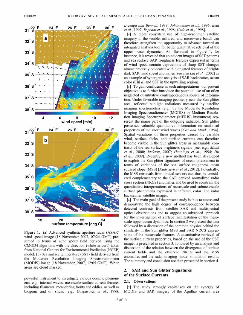
Figure 1. (a) Advanced synthetic aperture radar (ASAR)wind speed image (18 November 2007, 07:24 GMT) pre-sented in terms of wind speed field derived using theCMOD4 algorithm with the direction (white arrows) takenfrom National Centers for Environmental Prediction (NCEP)model. (b) Sea surface temperature (SST) field derived fromthe Moderate Resolution Imaging Spectroradiometer(MODIS) image (18 November, 2007, 12:05 GMT). Whiteareas are cloud masked.

KUDRYAVTSEV ET AL.: MESOSCALE UPPER OCEAN DYNAMICS C04029C04029

2 of 13

acquired 5 h apart on 18 November 2007. The greater AgulhasCurrent regime is highly dynamic and characterized by a widerange of mesoscale and submesoscale processes and featuresincluding meanders, fronts, filaments, and eddies. The region,

moreover, is also often favorable for Sun glitter analysis basedon the MODIS data. Figure 1 displays the wind field derivedfrom the Envisat advanced SAR (ASAR) wide-swath imageacquired on 18 November 2007, 07:24 GMT, using theCMOD4 transfer function [Stoffelen and Anderson, 1997]with a prescribed wind field direction taken from the NationalCenters for Environmental Prediction (NCEP) model, and theSST field derived from the MODIS image (acquired less than5 h apart on 12:05 GMT) using a standard retrieval algorithm.The wind speed varies from 4 m/s to 13 m/s, but a variety ofdistinct features presumably caused by the oceanic mesoscalevariability, including meandering fronts and eddies, are alsorevealed, in particular bounded by 34�–35.5�N and 26�–30�E.These features are also clearly expressed in the SST field.Thus, both the SST and SAR fields apparently possess surfacesignatures of the same mesoscale upper ocean dynamicphenomena.[8] The original Aqua MODIS image in the red channel

(645 nm) at 250 m resolution is shown in Figure 2a andclearly reveals both the Sun glitter and the presence of cloudsThe Sun glitter has a “strip-like structure” typical for theMODIS imagery. A surface brightness feature to the right ofthe Sun glitter (marked by the arrow) is also visible, that maybe interpreted as surface manifestation of the ocean currents.By decomposing the original brightness on the smoothedbrightness �B (averaging scale 30� 30 km2) and its variations~B , the remarkable details of the latter feature become moredistinct as revealed by the presence of the 80 km in diameteranticyclonic (rotating anticlockwise) shaped eddy shown inFigure 2b. The full description of the method for the retrievalof such anomalies in the Sun glitter brightness variationsassociated with changes in the mean square slope of the seasurface is given by Kudryavtsev et al. [2012].[9] The sea surface mean square slope (MSS) contrasts

derived from these Sun glitter brightness variations are

defined as Ks ¼ s2 � s20

� �=s20, where s

20 is the MSS averaged

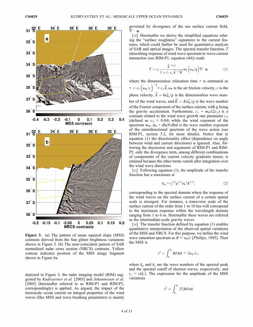
over the 30 km � 30 km window. The pattern of the MSScontrasts (see Figure 3a) is even further magnified, in com-parison to the brightness variation pattern, and clearly displayexpressions of linear frontal features, meanders, and eddieswith widths ranging from 1 to 10 km. The contrasts reachingup to �20% are “statistically uniform” over the observedarea, except in local areas adjacent to the clouds where theSun glitter brightness is “contaminated” by the cloud sha-dows, and thus not applicable for the retrieval algorithm.[10] The SAR NRCS contrasts shown in Figure 3b, Ks ¼s0 � s0ð Þ=s0, are defined using a similar moving average toobtain the variations of the NRCS relative to the meanbackscatter s0 with a spatial resolution of 30 � 30 km2.The qualitative comparison between the two contrast fieldsevidently reveals a significant relationship. Consistent withJohannessen et al. [2005], who suggested that the SARexpressions of the mesoscale features result from the shortwave modulations by the surface current divergence field,the similarity between the MSS and NRCS features thuspresumes that the MSS anomalies field also traces the sur-face current divergence field.

2.2. Physics of Similarity Between MSS and NRCS

[11] In order to further investigate and quantify theagreement between the MSS and SAR NRCS contrasts

Figure 2. (a) Aqua MODIS image in the red channel with a250 m resolution of the Agulhas Current area (acquired on18 November 2007, 12:05) marking a distinct strip-like struc-ture of the Sun glitter area which is typical for the MODISSun glitter imagery. White arrow indicates a brightness fea-ture corresponding to the surface manifestation of the oceancurrent. (b) The corresponding Sun glitter brightness varia-tions (~B ¼ B� �B) depicting a variety of “small-scale” sur-face features. Brightness of the image and its variations aregiven in conventional units. White areas are the clouds mask,and South Africa is marked in brown.

KUDRYAVTSEV ET AL.: MESOSCALE UPPER OCEAN DYNAMICS C04029C04029

3 of 13

depicted in Figure 3, the radar imaging model (RIM) sug-gested by Kudryavtsev et al. [2005] and Johannessen et al.[2005] (hereinafter referred to as RIM-P1 and RIM-P2,correspondingly) is applied. As argued, the impact of themesoscale ocean current on integral properties of the windwaves (like MSS and wave breaking parameters) is mainly

governed by divergence of the sea surface current field,r ⋅ u.[12] Hereinafter we derive the simplified equations relat-

ing the “surface roughness” signatures to the current fea-tures, which could further be used for quantitative analysisof SAR and optical images. The spectral transfer function, T(describing response of wind wave spectrum to wave-currentinteraction (see RIM-P1, equation (44)) reads

T ¼ ct

⌢k�3=2

1þ i � ct⌢k �2⌢K

mk u*=g� �

r � u; ð1Þ

where the dimensionless relaxation time t is estimated as

t ¼ ct u*=c� ��2

≡ ct⌢k, u* is the air friction velocity, c is the

phase velocity,⌢k ¼ ku2*=g is the dimensionless wave num-

ber of the wind waves, and⌢K ¼ Ku2*=g is the wave number

of the Fourier component of the surface current, with g beingthe gravity acceleration. Furthermore, ct = m*/(2cb) is aconstant related to the wind wave growth rate parameter cb(defined as cb ≈ 0.04) while the wind exponent of thespectrum m*, mk = dlnN/dlnk is the wave number exponentof the omnidirectional spectrum of the wave action (seeRIM-P1, section 3.2, for more details). Notice that inequation (1) the directionality effect (dependence on anglebetween wind and current directions) is ignored. Also, fol-lowing the discussion and arguments of RIM-P1 and RIM-P2, only the divergence term, among different combinationsof components of the current velocity gradients tensor, isretained because the other terms vanish after integration overthe wind wave directions.[13] Following equation (1), the amplitude of the transfer

function has a maximum at

km ≈ c1=2t g1=2u�1* K1=2; ð2Þ

corresponding to the spectral domain where the response ofthe wind waves on the surface current of a certain spatialscale is strongest. For instance, a transverse scale of thesurface current of the order from 1 to 10 km will correspondto the maximum response within the wavelength domainranging from 1 to 6 m. Hereinafter these waves are referredas the intermediate-scale gravity waves.[14] The transfer function defined by equation (1) enables

quantitative interpretation of the observed spatial variationsof the MSS and NRCS. For this purpose, we define the windwave saturation spectrum as B∝ u*/c [Phillips, 1985]. Thenthe MSS is

s2 ¼Z kp

kc

Bd lnk ∝ 2u*=cc;

where kp and kc are the wave numbers of the spectral peakand the spectral cutoff of shortest waves, respectively, andcc = c(kc). The expression for the amplitude of the MSSvariations

~s2 ¼Z kp

kc

Tj jBd lnk

Figure 3. (a) The pattern of mean squared slope (MSS)contrasts derived from the Sun glitter brightness variationsshown in Figure 2. (b) The near-coincident pattern of SARnormalized radar cross section (NRCS) contrasts. Yellowcontour indicates position of the MSS image fragmentshown in Figure 6a.

KUDRYAVTSEV ET AL.: MESOSCALE UPPER OCEAN DYNAMICS C04029C04029

4 of 13

with the use of equation (1) is then approximately equal to

~s2 ∝ mkc1=2t gKð Þ�1=2r � u: ð3Þ

Thus the expression for the MSS contrasts reads

~s2=s2 ∝ mkc1=2t u�1

* kcKð Þ�1=2r � u ð4Þ

and demonstrates that the MSS contrasts also get largerwhen the wind speed reduces. It also follows that the MSScontrasts are proportional to the magnitude of the currentvelocity drop over divergence zone and inversely propor-tional to the square root of its transverse scale.[15] Notice that equation (4) describes the MSS variations

caused by the direct interaction of intermediate-scale waveswith the surface current (resulting from the action of thestraining mechanism). Due to the relatively short relaxationtime, the shorter wind waves do not “directly feel” themesoscale current (since equation (1) approaches zero atlarge

⌢k ). However, as suggested in RIM, the mechanical

disturbances of the sea surface by wave breaking serve as anadditional energy input (along with wind forcing) to shorterwind waves. Therefore modulation of the small-scaleroughness can be caused by the enhancement/suppression ofbreaking of the intermediate-scale waves on the mesoscalecurrents. This mechanism provides additional contribution(proportional to wave breaking modulations) to the MSSanomalies expressed by equation (4).[16] Let us now consider response of the NRCS of the sea

surface in the presence of mesoscale currents. As discussedby Kudryavtsev et al. [2003, 2005] and further analyzedrecently by Mouche et al. [2007] and Guérin et al. [2010],the NRCS of the sea surface, s0

p, can be represented as thesum of a polarized composite Bragg-scattering term, sbr

p , anda scalar contribution, swb, associated with the longer wavesor steeper singular events, which both depend on the fractionof the sea surface covered by breaking waves, q, i.e.,swb = s0wbq, where s0wb is a NRCS of the breaking zone.Using this decomposition, the NRCS of the sea surface reads

s p0 ¼ s p

br þ s0wbq: ð5Þ

[17] Although the Bragg scattering dominates the NRCSvariations, the effect of the wave breaking is also important,especially at large incidence angles and HH polarization(see, e.g., RIM-P1, Figure 3). The term sbr

p is proportional tothe wave saturation spectrum B at the Bragg wave numberkbr: sbr

p = pGp2 sin�4qB(kbr), where Gp

2 is the geometricscattering coefficient. The Bragg waves are characterized bysmall spatial relaxation scale (of order 1 m) as comparedwith the surface current scales, and thus they do not interactdirectly with the mesoscale surface current (i.e., equation (1)in this range vanishes). However, as argued by RIM-P1, themechanical disturbances of the surface by the breakingwaves serve as an additional (to the wind input) energysource for shorter waves, and therefore we represent thewave spectrum as a sum: B = B0 +DBwb, where B0 is a windforced part and DBwb is a contribution of mechanical dis-turbances of the sea surface by breaking waves to the shortwave spectrum. The latter term is proportional to the inten-sity of wave breaking events characterized here by the

fraction of the sea surface q: i.e., DBwb ∝ q. Partial contri-bution of the surface disturbances by wave breaking to fullwave spectrum, pwb = DBwb/B, is strongly dependent onwave direction: at upwind directions pwb is of order 0.1, butat crosswind directions (where wind forcing vanishes) itsvalue attains pwb = 1 (see, e.g., RIM-P1, Figure 1). Thusmodulation of wave breaking on a mesoscale current mayaffect the NRCS via (1) their direct impact on radar back-scatter (term s0wbq in equation (5)) and (2) mechanicalgeneration of short surface waves providing the Braggscattering (term sbr

p in equation (5)).[18] Thus, following model (5), spatial variations of the

NRCS, ~s p0 , caused by modulations of the wave breaking, ~q,

are defined as

~sp0=s

p0 ¼ 1� P p

wb

� �pwb þ P p

wb

� �~q=q; ð6Þ

where Pwbp (8, q) = swb/s0

p is partial contribution of wavebreaking to the total NRCS, which is dependent on incidenceangle, q, and radar look direction, 8. As follows from (6),the field of the NRCS contrasts is similar to the field ofwave breaking anomalies. However, the magnitude of thetransfer coefficient (terms in the square bracket) dependson radar look direction relative to the wind vector. Atcrosswind radar look direction (where we recall that pwb = 1)the NRCS contrasts follow the wave breaking contrasts,while at upwind directions the NRCS contrasts are weaker(with reduction factor depending on incidence angle andpolarization).[19] An analysis similar to MSS can be done for the esti-

mation of the response of the wave breaking to the meso-scale currents (see RIM-P1, section 3.4, for more details).The fraction of the sea surface covered by breaking waves isdefined through the length of the breaking wavefronts L(k)as q ∝

RL(k)dk. Assuming that the wave breaking dissipa-

tion is proportional to the wind energy input, the quantity qcan be expressed as

q ∝Z kp

kb

bBd lnk ∝ u*=cb� �3

;

where b is the wind wave growth rate, kb is the wave numberof the shortest breaking waves, and cb = c(kb). The length ofthe breaking fronts is a strong nonlinear function of thesaturation spectrum. For the adopted B ∝ u*/c, the quantityL(k) is a cubic function of B. Therefore, the spatial varia-tions of q in the presence of the mesoscale currents isdefined as

~q ∝ 3

Z kp

kb

TbBd lnk;

and with the use of equation (1) it can be expressed as

~q ∝ ctmk ln kb=kmð Þ u*gr � u: ð7Þ

[20] Modulation of the fraction of the sea surface coveredby breaking waves is provided by the breaking in the “shortwave” interval ct

1/2u*K/g1/2 ≡ km < k < kb, i.e., in the interval

from the shortest breaking waves (with k = kb) to the waves

KUDRYAVTSEV ET AL.: MESOSCALE UPPER OCEAN DYNAMICS C04029C04029

5 of 13

possessing maximal response to the impact of the currentdefined by equation (2). The expression for the wind wavebreaking contrasts then reads

~q

q∝ ctmk ln kb=kmð Þ g

u2*kbw�1b r � u: ð8Þ

[21] As well as the MSS contrasts, the wave breakingvariations follow the surface current divergence field. Sincemk < 0, the enhancement of the wave breaking (as well as theMSS contrasts) takes place in the zones of surface currentconvergence, where r ⋅ u < 0. However, contrary to theMSS contrasts, the wave breaking contrasts decrease fasterwith increasing wind.[22] Referring to equation (6) (with equation (8)) and

equation (4), we thus conclude that both the expressions ofthe NRCS and the MSS contrasts trace the surface currentdivergence field, so that positive/negative contrasts corre-spond to convergence/divergence of the surface currents.However, we notice that the most favorable conditions forSAR imagery of the surface mesoscale currents take placewhen radar look direction is collinear with the crosswinddirection.[23] It is also important to emphasize that for optical

spectrometers, the measurements are proportional to the seasurface slope probability density function (PDF). Accordingto Cox and Munk [1954], the slope variances under low tomoderate wind conditions (from 3 to 10 m/s) are relativelyweak, with the standard deviation s of order s ∝ 0.1 � 0.2.Away from the specular point at incidence angles of about10�–20�, the PDF therefore rapidly drops and the slopevariations become more dependent on the higher-order sta-tistical moments, e.g., on the skewness and the kurtosis.Both these properties are associated with wave breaking,particularly small-scale breaking [Chapron et al., 2000,2002]. Therefore, in the area away from the specular point,the PDF shape and the Sun glitter brightness are stronglydependent on the fraction of the sea surface, q, covered bythe steepest events. Correspondingly, the Sun glitter bright-ness features in such areas should also be determined by thewave breaking contrasts defined by equation (6).[24] Thus both the Sun glitter features (independent on

how far they are from the specular point) and the NRCSfeatures can quantitatively trace the divergence of themesoscale to submesoscale surface current field. Conse-quently, the sea surface signatures manifested in Figure 3can certainly be considered as a tracer of the surface cur-rent divergence field.

3. Mesoscale Current Features Derived From SSTand Their Relation to SAR and MSS Anomalies

[25] Comparing the sea roughness MSS and NRCS fea-tures (shown in Figure 3) with the SST patterns (shown inFigure 1), the very good qualitative agreement is striking.The main surface roughness changes coincide with localSST fronts. In general, this observation is not surprising, asocean frontal areas are known for their intense cross-frontaldynamics and vertical motions (upwelling/downwelling). Inthis context, a model framework for the diagnostic calcula-tions of the surface current field from the snapshot of the

SST field can be used to give additional experimental evi-dences for the relation of the sea surface roughness anoma-lies to the current divergence field.

3.1. Quasi-Geostrophic and Ageostrophic CirculationsReconstructed From the SST Field

[26] Advective influence of the Ekman transport and dia-batic mixing in the Ekman layer can be considered as one ofthe main mechanisms generating the ageostrophic secondarycirculation (ASC) in the vicinity of oceanic fronts [Klein andHua, 1990; Garrett and Loder, 1981; Thompson, 2000;Nagai et al., 2006]. Another mechanism was also recentlydiscussed by McWilliams et al. [2009], analogous to self-induced frontogenesis to accelerate and sharpen temperaturegradients from its related initial ageostrophic secondary cir-culation. Detailed consideration of all possible mechanismsis certainly beyond the scope of the present study. However,in order to interpret the coincident SST frontal features andthe sea surface roughness anomalies, we restrict our analysisto the model framework based on the generation of the ASCby the Ekman forcing only. In so doing, we assume that thetotal oceanic current field can be represented as a sum of thequasi-geostrophic current (QGC), U, the wind drift currentue (which can also include the inertial current), and the ASCfield, ua, resulting from both the interaction of the Ekmanflow with the QGC and the diabatic mixing in the Ekmanlayer. Thus the total current field is expressed asu = U + ue + ua.[27] To the first order of the Rossby number the governing

equations describing the dynamics of the ASC current field(see Klein and Hua [1990], Garrett and Loder [1981],Thompson [2000], and Nagai et al. [2006] for more details)reads

ueb∂U1=∂xb � fua2 ¼ nt∂2U1=∂x23ueb∂U2=∂xb þ fua1 ¼ nt∂2U2=∂x23

; ð9Þ

where nt is the turbulent eddy viscosity assumed constantover the depth (inside the upper mixed Ekman layer), f is theCoriolis parameter, and b = 1, 2. In equation (9), the spatialscale of the wind field variability largely exceeds thecross-front spatial scale. Hence, taking into account the“thermal wind” balance equation, ∂U1/∂x3 = (g/ f )∂r/∂x2,∂U2/∂x3 = �(g/f )∂r/∂x1, and the equation for the ocean stater = r0(1 � aT), the solution of equation (9) expressed interms of the ASC reads

ua1 ¼ �f �1ueb∂U2

∂xbþ ntga=f 2� � ∂

∂x3∂T∂x1

�

ua2 ¼ f �1ueb∂U1

∂xbþ ntga=f 2� � ∂

∂x3∂T∂x2

� ; ð10Þ

where g is the gravity acceleration and a is the thermalexpansion coefficient. The first term in equation (10)describes the generation of the ASC due to the advectiveinteraction of the Ekman flow with the QGC (the mechanismsuggested by Klein and Hua [1990]), while the second termaccounts for the generation of the ASC due to the frictionaleffect in the Ekman layer (the mechanism suggested by

KUDRYAVTSEV ET AL.: MESOSCALE UPPER OCEAN DYNAMICS C04029C04029

6 of 13

Garrett and Loder [1981]). Both of these mechanisms wouldinduce ocean current divergence in the vicinity of the ther-mal front as straightforwardly following from equation (10),

r � u ¼ �f �1ueb∂∂xb

W þ ntga=f 2� � ∂

∂x3DT ; ð11Þ

where Wz = ∂U2/∂x1 � ∂U1/∂x2 ≡ Dy is the vorticity of theQGC, y is the stream function of the QG flow, andDT is theLaplacian of the water temperature. A balance of the left-hand side (LHS) of equation (11) with the first term in theRHS represents the solution obtained by Klein and Hua[1990] for the Ekman advective mechanism, while a bal-ance with the second term in the RHS of equation (11)represents the solution suggested by Garrett and Loder[1981] for diabatic mixing mechanism of the ASC genera-tion. Thus equation (11) can be considered as a generalizedsolution combining both mechanisms of the ASC generationdue to the interaction of QGC with the Ekman layer.[28] For simplicity, hereinafter the wind-driven currents

are assumed to be the sum of classical Ekman currentvelocity uek = [t2/(fh), � t1/(fh)] and the inertial currentui(t), i.e.,

ue ¼ t2= f hð Þ;�t1= f hð Þ½ � þ ui tð Þ; ð12Þwhere t = v*

2[cos 8w, sin 8w], v* is the friction velocity inthe water, 8w is the directions of the wind velocity vector,h = (nt/ f )1/2 is the Ekman layer depth, and the inertialvelocity ui(t) can be prescribed following the time variabilityof the wind velocity. The turbulent eddy viscosity nt can beassessed following similarity between the marine and theatmospheric Ekman (planetary) boundary layers. For thestably stratified boundary layer the eddy viscosity isnt = gkv*L, where g ≈ 0.2 is a constant, k ≈ 0.4 is theKarman constant, and L is the Obukhov length scale [see,e.g., Brown, 1982]. By expressing L through the Brunt-Väisälä frequency for the upper ocean as L = v*

3/(kvtN2), the

eddy viscosity reads

nt ¼ g1=2v2*=N ; ð13aÞ

and the Ekman layer depth can thus be expressed as

h ¼ g1=4v*=ffiffiffiffiffifN

p: ð13bÞ

The estimates of h for, e.g., 10 m/s wind speed and f = 10�4

are h ≈ 28 m if the Prandtl ratio N/f = 10 and h ≈ 90 m ifN/f = 1.[29] In order to define the sea surface current divergence

(produced by ASC according to equation (11)), we need tointroduce the QGC field. At mesoscales (10–500 km) andsubmesoscales (1–10 km), ocean dynamics is often that of astably stratified rapidly rotating flow, with horizontalvelocities, on average, much larger than vertical velocities.The motion is thus quasi two-dimensional and can beinvestigated in the frameworks of different approximations.Based on the surface quasi-geostrophic (SQG) dynamics[Held et al., 1995; Lapeyre and Klein, 2006], Isern-Fontanetet al. [2008] presented a practical approach for the recon-struction of the current velocity field at scales between30 and 300 km from the snapshot of an SST image. Con-sidering the SQG dynamics, the stream function of the QGC

y k; zð Þ and the SST field T s kð Þ in the Fourier space arelinked by the following relation:

y k; zð Þ ¼ gaT s kð Þfnbk

exp n0kzð Þ; ð14Þ

where n = N/f is the Prandtl ratio for the Brunt-Vàisala fre-quencies N0 and Nb determining, respectively, the large-scaleand mesoscale properties of the flow. Defining the QGCvelocity through the stream function y as U ¼ �ikyy ; ikxy

� �(or in physical space as U = (�∂y /∂x2, ∂y/∂x1)) we can thendetermine the ASC field through equation (10).[30] In the Fourier space, the components of the ASC

defined by equation (10) with equation (14), supple-mented with estimations of the Ekman layer depth fromequation (13b) and the eddy viscosity coefficient fromequation (13a), are expressed through the SST as

bua1 ; bua2� �¼ a

g1=4n1=2b

� gv*f 2

s � sin 8w � 8ð Þ þ ig3=4n1=2b

v*K

fj j� �

� K1;K2ð ÞT s; ð15Þ

where s = sign( f ), i is the imaginary unit, 8 is the directionof the wave number vector K, and as before g = 0.2. Thesecond term in the bracket indicates the significance of theratio of the mixing mechanism relative to the advectiveterm. If we assume that nb = 10 and f = 10�4 s�1, then thisratio is approximately equal 0.1 for a wind speed 10 m/sand K = 2p/104 rad/m. In contrast, the ratio is approaching 1for the shorter scale, e.g., K = 2p/103 rad/m. The efficiencyof this mixing mechanism increases both with a shorteningof the QGC scales and an increasing wind speed. Hence, atlow to moderate wind speeds and the current scale of orderK ∝ 10�3 rad/m or less, the Ekman transport mechanism(which in the general case includes also the inertial currents)dominates the ASC generation. From equation (15), thedivergence of the surface current in the Fourier spacedr � u ¼ iKb buab reads

dr � u ¼ ia

g1=4n1=2b

� gv*f 2

s � sin 8w � 8ð Þ þ ig3=4n1=2b

v*K

fj j� �

K2T s:

ð16Þ

Thus this equation directly links the divergence of the sur-face current to the SST field.[31] The SST field available from the MODIS data (see

Figure 1b) and the SAR wind field (see Figure 1a) are thenused as input parameters to determine the surface currentvelocity field. In order to remove the large-scale SST vari-ability, the spectral components with K < 2p/100 rad/km werefiltered out. The spectral transform of the QG stream functionwas determined from equation (14), assuming nb = n0 = 50. Asapplied, the standard deviation of the derived surface QGvelocities is then found equal to about 1 m/s. Use of theseconstants also helps to match the SAR derived surface velocity[Chapron et al., 2005; Johannessen et al., 2008] from therange Doppler measurements (not shown here). The back-ground Ekman current, equations (12), (13a), and (13b), andASC, equation (10), are calculated for the “mean observed”SAR southerly wind speed of 7 m/s.

KUDRYAVTSEV ET AL.: MESOSCALE UPPER OCEAN DYNAMICS C04029C04029

7 of 13

[32] The vorticity of the QGC field and the surface currentdivergence derived from the observed SST field are shownin Figure 4. The QGC vorticity field exhibits a variety ofmesoscale patterns and the existence of a “main jet” repre-senting the Agulhas Current. In comparison to the surfacecurrent divergence, one reveals that the convergence/diver-gence patterns trace the gradients of the QGC vorticity field,which in turn is similar to the SST Laplacian field.

3.2. Relation of Reconstructed Divergence Field to SARand MSS Anomalies

[33] Looking closer at the fragment of the SAR imageshown in Figure 5a (it corresponds to the area above 36�S ofthe SAR image shown Figure 3) where the wind field was

Figure 4. (a) The vorticity of the surface quasi-geostrophiccurrent (QGC) derived from the SST shown in Figure 1bwith the use of equation (14). (b) The surface current diver-gence field, r ⋅ u, attributed to secondary ageostrophic cir-culation resulting from interaction of Ekman forcing(advective and mixing mechanisms) with QGC (seeequations (11) and (16)). Note that the divergence field isinverted (i.e., field of �r ⋅ u is shown), and thus bright lin-ear features correspond to the convergence zones and darkfeatures correspond to the divergence zones.

Figure 5. (a) A fragment of the SAR NRCS contrasts fieldshown in Figure 3 and (b) the corresponding fragment of thesurface current divergence field shown in Figure 4. Brightareas in Figure 5b correspond to the current convergence,and dark areas correspond to the current divergence (seeFigure 4 for more details).

KUDRYAVTSEV ET AL.: MESOSCALE UPPER OCEAN DYNAMICS C04029C04029

8 of 13

presumably uniform, the SAR image contrasts can be treatedas surface manifestation of the oceanic mesoscale dynamics.The corresponding field of the surface current divergence isshown in Figure 5b.[34] A visual inspection of Figure 5 shows that field of the

NRCS contrasts and the divergence field (recall that there isa 5 h time interval between the SAR and MODIS acquisi-tions) have a very similar texture. Overall, the bright NRCScontrasts correspond to the current convergence while thedark contrasts represent the divergence zones. This obser-vation, moreover, can be considered as experimental evi-dence of the model finding reported by RIM-P1 and RIM-P2and simplified in equations (4), (8) with (6). On the otherhand, if one believes that the relation between the NRCSanomalies and the current divergence exists, the apparentgood agreement between SAR anomalies and the expectedsurface current divergence field would indicate that the

approach used for the reconstruction of the QGC and theASC works properly and provides plausible estimations ofthe surface current field.[35] A similar conclusion can be made with respect to the

fragment of the MSS contrasts field shown in Figure 6a(enlarged fragment of the MSS field shown in Figure 3).The divergence field shown in Figure 6b was calculated forthe local northerly wind. (Recall that the wind directionin this case is opposite to the one used before in calculations ofthe divergence field shown in Figure 4b). From equation (16)it follows that the wind direction affects the sign of r ⋅ u,which explains the difference between Figure 6b and thecorresponding fragment shown in Figure 4b. The choice ofthe wind direction in this case is suggested by the local winddirection as predicted by NCEP model (see Figure 1) andprovides the “proper” sign of the divergence. Notice also thatNCEP model predicts calm conditions over the observed

Figure 6. (a) Fragment of the MSS contrasts field, shown in Figure 3 (its position is indicated with yel-low contour). (b) Field of the surface current divergence. The manifest difference between fields of surfacecurrent divergence shown in Figure 6b and in the corresponding area in Figure 4b is explained by the factthat r ⋅ u shown here was calculated for the local northerly wind, while r ⋅ u shown in Figure 4b in thisarea was calculated for the southerly wind (see text for more explanation). Bright areas correspond to thecurrent convergence, and dark areas correspond to the current divergence (see Figure 4b for more details).

KUDRYAVTSEV ET AL.: MESOSCALE UPPER OCEAN DYNAMICS C04029C04029

9 of 13

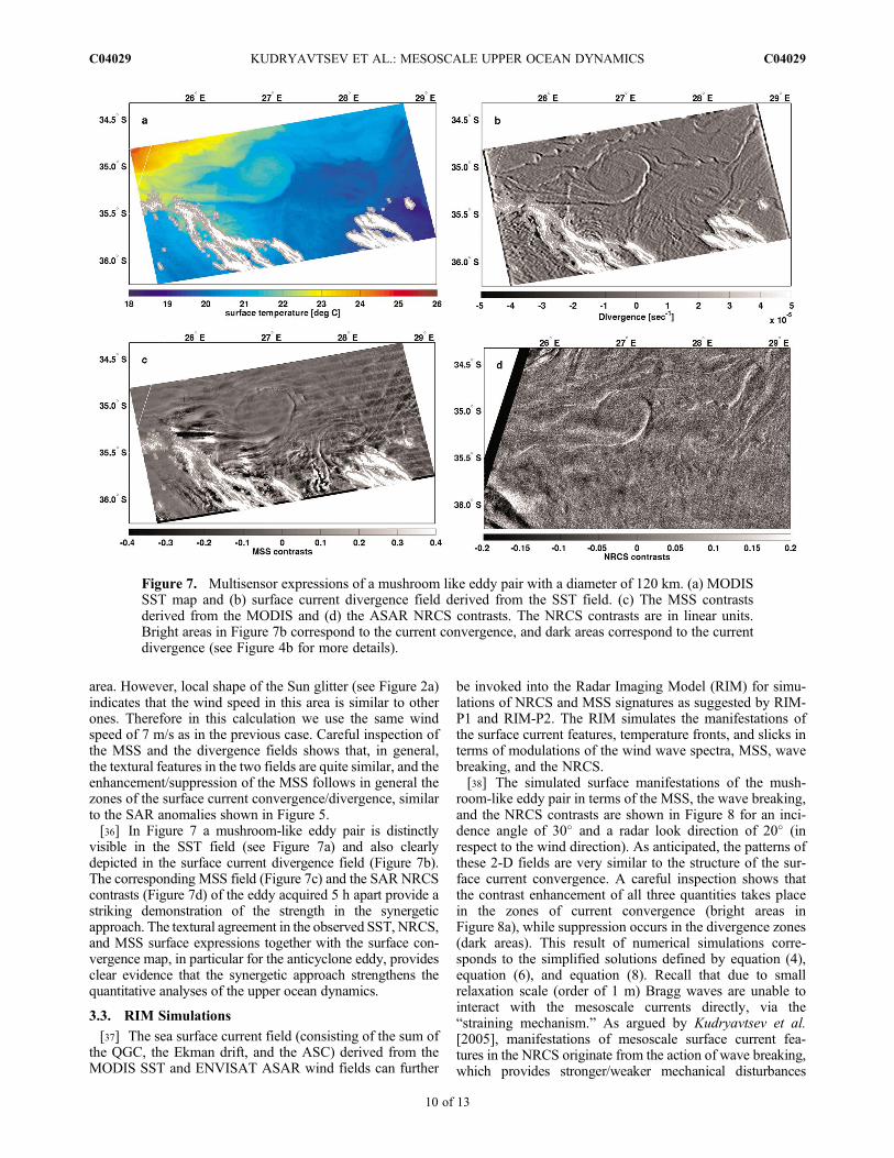
area. However, local shape of the Sun glitter (see Figure 2a)indicates that the wind speed in this area is similar to otherones. Therefore in this calculation we use the same windspeed of 7 m/s as in the previous case. Careful inspection ofthe MSS and the divergence fields shows that, in general,the textural features in the two fields are quite similar, and theenhancement/suppression of the MSS follows in general thezones of the surface current convergence/divergence, similarto the SAR anomalies shown in Figure 5.[36] In Figure 7 a mushroom-like eddy pair is distinctly

visible in the SST field (see Figure 7a) and also clearlydepicted in the surface current divergence field (Figure 7b).The corresponding MSS field (Figure 7c) and the SAR NRCScontrasts (Figure 7d) of the eddy acquired 5 h apart provide astriking demonstration of the strength in the synergeticapproach. The textural agreement in the observed SST, NRCS,and MSS surface expressions together with the surface con-vergence map, in particular for the anticyclone eddy, providesclear evidence that the synergetic approach strengthens thequantitative analyses of the upper ocean dynamics.

3.3. RIM Simulations

[37] The sea surface current field (consisting of the sum ofthe QGC, the Ekman drift, and the ASC) derived from theMODIS SST and ENVISAT ASAR wind fields can further

be invoked into the Radar Imaging Model (RIM) for simu-lations of NRCS and MSS signatures as suggested by RIM-P1 and RIM-P2. The RIM simulates the manifestations ofthe surface current features, temperature fronts, and slicks interms of modulations of the wind wave spectra, MSS, wavebreaking, and the NRCS.[38] The simulated surface manifestations of the mush-

room-like eddy pair in terms of the MSS, the wave breaking,and the NRCS contrasts are shown in Figure 8 for an inci-dence angle of 30� and a radar look direction of 20� (inrespect to the wind direction). As anticipated, the patterns ofthese 2-D fields are very similar to the structure of the sur-face current convergence. A careful inspection shows thatthe contrast enhancement of all three quantities takes placein the zones of current convergence (bright areas inFigure 8a), while suppression occurs in the divergence zones(dark areas). This result of numerical simulations corre-sponds to the simplified solutions defined by equation (4),equation (6), and equation (8). Recall that due to smallrelaxation scale (order of 1 m) Bragg waves are unable tointeract with the mesoscale currents directly, via the“straining mechanism.” As argued by Kudryavtsev et al.[2005], manifestations of mesoscale surface current fea-tures in the NRCS originate from the action of wave breaking,which provides stronger/weaker mechanical disturbances

Figure 7. Multisensor expressions of a mushroom like eddy pair with a diameter of 120 km. (a) MODISSST map and (b) surface current divergence field derived from the SST field. (c) The MSS contrastsderived from the MODIS and (d) the ASAR NRCS contrasts. The NRCS contrasts are in linear units.Bright areas in Figure 7b correspond to the current convergence, and dark areas correspond to the currentdivergence (see Figure 4b for more details).

KUDRYAVTSEV ET AL.: MESOSCALE UPPER OCEAN DYNAMICS C04029C04029

10 of 13

of the surface in the convergent/divergent zones. Thesemechanical disturbances lead to the local enhancement/suppression of the Bragg waves and hence the modulation ofthe radar backscattering. Comparing the fields of simulatedNRCS and MSS contrasts with the observations shown inFigure 7, one may notice that the magnitudes of the modelcontrasts are consistent with the observed values. Since RIMwas extensively tested against available data (see RIM-P1), thisfact presumes that the reconstructed field of the surface currentdivergence may be considered as close to the “real” field. It isworth noting that the simulations of the NRCS contrasts for thesame eddy pair without accounting for the impact of wavebreaking on both the NRCS and Bragg waves modulations(a “standard” relaxation model) gives NRCS contrasts 4 ordersof magnitude less than that shown in Figure 8.[39] Comparison of the numerical RIM simulations

(shown in Figure 8) with the simplified relations expressedin equation (4) and equation (8) provides an opportunity toassess the proportionality constants for further use of thesimplified solutions in practical applications. We arrived at

~s2

s2¼ � cs

u* kcKð Þ1=2r � u

~q

q0¼ �cq ln

u*kb

g1=2K1=2

� g

u2*kbw�1b r � u

ð17Þ

with cs = 180 and cq = 470 at kc = (g/g)1/2 and kb = kR/10(g is the surface tension, kR is radar wave number).[40] All in all, the analysis of SAR and the MSS signatures

of the subscale and mesoscale upper ocean dynamics showthat they have a distinct textural similarity with the surfacecurrent divergence field, with contrasts of about the samemagnitude, although slight differences in the details of thecontrast patterns can be found. This is presumably resultingfrom (1) a shortcoming in the reconstruction of the surfacecurrent and the divergence field from the MODIS derivedSST snapshot; (2) uncertainties in the local wind field, winddrift, Ekman current, and inertial currents estimates; and(3) temporal evolution of the mesoscale features in the near5 h time interval between the ASAR and MODIS acquisi-tions. Nevertheless, the overall agreement is very promisingand clearly demonstrates the feasibility of retrieving quan-titative estimates of the upper layer dynamics from themultisensor surface expressions of mesoscale features.

4. Conclusion

[41] Hitherto the complete quantitative understanding ofthe SAR imaging of surface roughness modulations inducedby the surface current divergence and convergence fieldhas been insufficient. In this study a new synergeticapproach for quantitative analysis of SAR and imaging

Figure 8. (a) Divergence of the surface current derived from the SST field (see Figure 7a). Bright/darkareas correspond to the current convergence/divergence. The remaining plots are RIM simulations ofthe surface manifestations of the mushroom-like eddy pair presented in the form of the contrasts in the(b) MSS, (c) wave breaking, and (d) NRCS.

KUDRYAVTSEV ET AL.: MESOSCALE UPPER OCEAN DYNAMICS C04029C04029

11 of 13

spectrometer data, including the infrared channels, has beenpresented and applied.[42] Notably, this synergetic approach clearly demon-

strates that the sea surface mean square slope (MSS)anomalies derived from the Sun glitter imagery (formed byfull range of waves, from capillaries to energy containingwaves) compare very well to SAR NRCS anomalies. Bothfields are then found to spatially correspond to frontal areaspresenting large SST gradients. Since typical frontal regioncould consist of an along-front jet with intense cross-frontaldynamics and vertical motion, such results were alreadyexpected following RIM-P1 and RIM-P2 results.[43] Building on the assumption that the upper ocean cir-

culation is quasi two-dimensional, the surface quasi-geostrophic current (QGC) field is reconstructed fromsnapshot of band-pass-filtered satellite infrared SST data,following the surface quasi-geostrophic (SQG) dynamics.As this resulting QGC field is nondivergent, its directinteraction with the wind waves results in weak surfacemanifestation of mesoscale current features, as alreadyshown by RIM-P1 and RIM-P2. More likely, it is the pos-sible interaction of the wind-driven upper layer motion withthe QGC field (via Ekman advective and mixing mechan-isms, as suggested by Klein and Hua [1990] and Garrett andLoder, 1981]) that can result in the generation of a suffi-ciently strong ageostrophic surface current, producing largesurface convergence and divergence. Under the proposedassumption, intense cross-frontal dynamics occur near sharphorizontal gradients of the vorticity of the QGC, as well asstrong vertical gradients of the QGC velocity.[44] Accordingly, one may consider the observed striking

agreement and correspondence between roughness anoma-lies and SST gradients as “experimental evidence” of the factthat the impact of the surface current divergence on the shortwind waves constitutes the governing mechanism leading tomanifestation of mesoscale surface current features in theform of the “surface roughness” anomalies. On the otherhand, the correlation between the surface roughnessanomalies and the model surface current divergence stronglysuggests that the model framework for the reconstruction ofthe mesoscale surface current is quite reliable.[45] The surface current field derived from MODIS SST

and SAR wind data was also used as the input parameters forthe RIM forward simulations and clearly documents that theobserved anomalies in the SAR NRCS, as well as anomaliesof the MSS derived from the MODIS data, represent thesurface expressions of the ocean current convergence/divergence areas along meandering fronts and eddies.[46] In summary, the proposed synergetic approach com-

bining SST, Sun glitter brightness, and SAR data, possiblyaugmented by other external sources of lower-resolutioninformation (e.g., altimeter and scatterometer), providesconsistent and quantitative determination of the location andintensity of the surface current convergence/divergence(upwelling/downwelling). This, in turn, establishes animportant and promising step toward advances in the quan-titative interpretation and understandings of the upper oceandynamics from their 2-D satellite surface expressions.

[47] Acknowledgments. Core support for this study was provided bythe joint CNES-EUMETSAT funded OSTST project Ocean3D and theANR funded REDHOTS project. ENVISAT ASAR data were providedby ESA through the study contract 18709/05/I-LG. Support of Russian

Federation government grants 11.G34.31.0078 for the Russian Sate Hydro-meteorological University and the Federal Programme under contractN14.740.11.0201 are gratefully acknowledged.

ReferencesAlpers, W., and I. Hennings (1984), A theory of the imaging mechanismof underwater bottom topography by real and synthetic aperture radar,J. Geophys. Res., 89(C6), 10,529–10,546, doi:10.1029/JC089iC06p10529.

Beal, R., V. Kudryavtsev, D. Thompson, S. Grodsky, D. Tilley, V. Dulov,and H. Graber (1997), The influence of the marine atmospheric boundarylayer on ERS-1 synthetic aperture radar imagery of the Gulf Stream,J. Geophys. Res., 102(C3), 5799–5814, doi:10.1029/96JC03109.

Brown, R. (1982), On two-layer models and the similarity functions for thePBL, Boundary Layer Meteorol., 24, 451–463, doi:10.1007/BF00120733.

Chapron, B., V. Kerbaol, D. Vandemark, and T. Elfouhaily (2000), Impor-tance of peakedness in sea surface slope measurements and applications,J. Geophys. Res., 105, 17,195–17,202, doi:10.1029/2000JC900079.

Chapron B., D. Vandemark, and T. Elfouhaily (2002), On the skewness ofthe sea slope probability distribution, in Gas Transfer at Water Surfaces,Geophys. Monogr. Ser., vol. 127, edited by M. A. Donelan et al.,pp. 59–63, AGU, Washington, D. C.

Chapron, B., F. Collard, and F. Ardhum (2005), Direct measurementsof ocean surface velocity from space: Interpretation and validation,J. Geophys. Res., 110, C07008, doi:10.1029/2004JC002809.

Cox, C., and W. Munk (1954), Measurement of the roughness of the seasurface from photographs of the Sun’s glitter, J. Opt. Soc. Am., 44,838–850, doi:10.1364/JOSA.44.000838.

Espedal, H. A., O. M. Johannessen, J. A. Johannessen, E. Dano, D. R.Lyzenga, and J. C. Knulst (1998), COASTWATCH’95: ERS 1/2 SARdetection of natural film on the ocean surface, J. Geophys. Res., 103(C11),24,969–24,982, doi:10.1029/98JC01660.

Gade, M., W. Alpers, H. Huehnerfuss, H. Masuko, and T. Kobayashi(1998), Imaging of biogenic and anthropogenic ocean surface films bythe multifrequency/multipolarization SIR-C/X-SAR, J. Geophys. Res.,103(C9), 18,851–18,866, doi:10.1029/97JC01915.

Garrett, C. J. R., and J. W. Loder (1981), Dynamical aspects of shallow seafronts, Philos. Trans. R. Soc. London A, 302, 563–581, doi:10.1098/rsta.1981.0183.

Gasparovic, R. F., J. A. Apel, and E. S. Kasischke (1988), An overview ofthe SAR internal wave signature experiment, J. Geophys. Res., 93(C10),12,304–12,316, doi:10.1029/JC093iC10p12304.

Guérin, C.-A., G. Sorian, and B. Chapron (2010), The weighted curvatureapproximation in scattering from sea surfaces, Waves Random ComplexMedia, 20(3), 364–384, doi:10.1080/17455030903563824.

Held, I. M., R. T. Pierrehumbert, S. T. Garner, and K. L. Swanson (1995),Surface quasi-geostrophic dynamics, J. Fluid Mech., 282, 1–20,doi:10.1017/S0022112095000012.

Hennings, I., J. Matthews, and M. Metzner (1994), Sun glitter radiance andradar cross-section modulations of the sea bed, J. Geophys. Res., 99(C8),16,303–16,326, doi:10.1029/93JC02777.

Hu, C., X. Li, W. G. Pichel, and F. E. Muller-Karger (2009), Detectionof natural oil slicks in the NW Gulf of Mexico using MODIS imagery,Geophys. Res. Lett., 36, L01604, doi:10.1029/2008GL036119.

Isern-Fontanet, J., G. Lapeyre, P. Klein, B. Chapron, and M. W. Hecht(2008), Three-dimensional reconstruction of oceanic mesoscale currentsfrom surface information, J. Geophys. Res., 113, C09005, doi:10.1029/2007JC004692.

Jackson, C. (2007), Internal wave detection using the Moderate ResolutionImaging Spectroradiometer (MODIS), J. Geophys. Res., 112, C11012,doi:10.1029/2007JC004220.

Jansen, R., C. Shen, S. Chubb, A. Cooper, and T. Evans (1998), Subsurface,surface, and radar modeling of a Gulf Stream current convergence,J. Geophys. Res., 103(C9), 18,723–18,743, doi:10.1029/98JC01195.

Johannessen, J. A., R. Shuchman, G. Digranes, D. Lyzenga,W.Wackerman,O. Johannessen, and P.Vachon (1996), Coastal ocean fronts and eddies imagedwith ERS-1 synthetic aperture radar, J. Geophys. Res., 101, 6651–6667,doi:10.1029/95JC02962.

Johannessen, J. A., V. Kudryavtsev, D. Akimov, T. Eldevik, N. Winther,and B. Chapron (2005), On radar imaging of current features: 2. Mesoscaleeddy and current front detection, J. Geophys. Res., 110, C07017,doi:10.1029/2004JC002802.

Johannessen, J. A., B. Chapron, F. Collard, V. Kudryavtsev, A. Mouche,D. Akimov, and K.-F. Dagestad (2008), Direct ocean surface velocitymeasurements from space: Improved quantitative interpretation of Envi-sat ASAR observations, Geophys. Res. Lett., 35, L22608, doi:10.1029/2008GL035709.

Klein, P., and B. Hua (1990), The mesoscale variability of the sea surfacetemperature: An analytical and numerical model, J. Mar. Res., 48, 729–763.

KUDRYAVTSEV ET AL.: MESOSCALE UPPER OCEAN DYNAMICS C04029C04029

12 of 13

Kudryavtsev, V., D. Hauser, G. Caudal, and B. Chapron, (2003), A semi-empirical model of the normalized radar cross-section of the sea surface:1. Background model, J. Geophys. Res., 108(C3), 8054, doi:10.1029/2001JC001003.

Kudryavtsev, V., D. Akimov, J. A. Johannessen, and B. Chapron (2005),On radar imaging of current features: 1. Model and comparison with obser-vations, J. Geophys. Res., 110, C07016, doi:10.1029/2004JC002505.

Kudryavtsev, V., A. Myasoedov, B. Chapron, J. Johannessen, and F. Collard(2012), Joint sun-glitter and radar imagery of surface slicks, Remote Sens.Environ., in press.

Lapeyre, G., and P. Klein (2006), Dynamics of the upper oceanic layers interms of surface quasigeostrophy theory, J. Phys. Oceanogr., 36, 165–176,doi:10.1175/JPO2840.1.

Lin, I.-I., L.-S. Wen, K.-K. Liu, W.-T. Tsai, and A. K. Liu (2002), Evidenceand quantification of the correlation between radar backscatter and oceancolour supported by simultaneously acquired in situ sea truth, Geophys.Res. Lett., 29(10), 1464, doi:10.1029/2001GL014039.

Lyzenga, D. R., and J. R. Bennett (1988), Full-spectrum modeling of syn-thetic aperture radar internal wave signature, J. Geophys. Res., 93(C10),12,345–12,354, doi:10.1029/JC093iC10p12345.

Marmorino, G. O., R. W. Jansen, G. R. Valenzuela, C. L. Trump, J. S. Lee,and J. A. C. Kaiser (1994), Gulf Stream surface convergence imaged bysynthetic aperture radar, J. Geophys. Res., 99, 18,315–18,328, doi:10.1029/94JC01643.

McWilliams, J. C., F. Colas, and M. J. Molemaker (2009), Cold filamentaryintensification and oceanic surface convergence lines, Geophys. Res.Lett., 36, L18602, doi:10.1029/2009GL039402.

Mouche, A. A., B. Chapron, N. Reul, D. Hauser, and Y. Quilfen (2007),Importance of the sea surface curvature to interpret the normalized radarcross section, J. Geophys. Res., 112, C10002, doi:10.1029/2006JC004010.

Munk, W., L. Armi, K. Fischer, and F. Zachariasen (2000), Spirals on thesea, Proc. R. Soc. A, 456, 1217–1280.

Nagai, T., A. Tandon, and D. L. Rudnick (2006), Two-dimensional ageo-strophic secondary circulation at ocean fronts due to vertical mixing andlarge-scale deformation, J. Geophys. Res., 111, C09038, doi:10.1029/2005JC002964.

Phillips, O. M. (1985), Spectral and statistical properties of the equilibriumrange in wind-generated gravity waves, J. Fluid Mech., 156, 505–531,doi:10.1017/S0022112085002221.

Romeiser, R., and W. Alpers (1997), An improved composite surface modelfor the radar backscattering cross section of the ocean surface: 2. Modelresponse to surface roughness variations and the radar imaging of under-water bottom topography, J. Geophys. Res., 102(C11), 25,251–25,267,doi:10.1029/97JC00191.

Stoffelen, A., and D. Anderson (1997), Scatterometer data interpretation:Estimation and validation of the transfer function CMOD4, J. Geophys.Res., 102(C3), 5767–5780, doi:10.1029/96JC02860.

Thompson, L. (2000), Ekman layers and two-dimensional frontogenesis inthe upper ocean, J. Geophys. Res., 105, 6437–6451, doi:10.1029/1999JC900336.

B. Chapron, Institute Francais de Recherche pour l’Exploitation de laMer, F-29280 Plouzané, France.F. Collard, Direction of Radar Applications, CLS, 115, rue Claude

Chappe, F-29280 Plouzané, France.J. A. Johannessen, Nansen Environmental and Remote Sensing Center,

Thormohlensgate 47, Bergen N-5006, Norway.V. Kudryavtsev and A. Myasoedov, Nansen International Environmental

and Remote Sensing Center, 7, 14th Line, Office 49, St. Petersburg 199034,Russia.

KUDRYAVTSEV ET AL.: MESOSCALE UPPER OCEAN DYNAMICS C04029C04029

13 of 13