Strategy Choice in Transit Networks

Achille FONZONE a, Jan-Dirk SCHMÖCKERb, Fumitaka KURAUCHI c,

Seham M. HASSAN d

a School of Engineering and Built Environment, Napier University,

United Kingdom a E-mail: a.fonzone@napier.ac.uk b Graduate School of Engineering, Kyoto University, Japan

b E-mail: schmoecker@trans.kuciv.kyoto-u.ac.jp

c Department of Civil Engineering, Gifu University, Japan

c E-mail: kurauchi@gifu-u.ac.jp

d Graduate School of Engineering, Gifu University, Japan

d E-mail: sehassan2007@yahoo.com Abstract: Public transport passengers are assumed to choose routes that minimise

the expected travel times. In networks with high-frequency services this requires

the adoption of hyperpaths. An experimental validation of the hyperpath model

has been carried out through a web-based survey. Findings of previous work on

the survey are compared with a new cluster analysis of travellers’ behaviour as

reported by respondents in the stated preference section of the survey. Results

show that the behaviour usually assumed in transit models is not the most

common approach to route choice in transit network. Implications for transit

assignment models are discussed.

Keywords: Passenger Behaviour, Transit Asssignment, Hyperpaths, Web survey,

Cluster Analysis

1. INTRODUCTION

It is generally assumed that on transit networks travellers try to minimise their expected

travel time consisting of waiting time, on-board time as well as potentially other factors such

as fare, crowding or seat availability by selecting a hyperpath. A hyperpath can be defined as a

set of attractive lines identified by the passenger for each stop, each of which might be the

optimal one from the stop, depending on lines arrival time, frequency, cost etc. In networks

with few uncertainties, e.g. regular arrival times, low congestion, this set of services will be

smaller as passengers can better estimate whether it is advantageous to let slow services pass

in order to wait for the faster service that might arrive soon. This behavioural assumption has

led to a fairly large set of literature.

A passenger at a stop frequently has a choice between a number of lines which will get

him directly or indirectly to his destination. The lines may differ in their attractiveness,

perhaps due to the travel time to the destination, the number of changes, the probability of

seat availability, etc. A dilemma frequently faced is whether to take the next vehicle arriving

or to wait for a more attractive line, i.e. a line with shorter travel time. Often the choice is

determined by the first vehicle to arrive. This family of issues is referred to as the common

lines problem. Lampkin and Saalmans (1967) assumed that the passenger at the stop ignores

lines that are obviously “bad” and chooses the first vehicle to arrive from among the other

routes. This introduces the notion of a strategy, which consists of a choice set of attractive

lines and a selection rule. Further Chriqui and Robillard (1975) presented a probabilistic

framework for studying the common lines problem. The passenger at a stop selects the sub-set

of lines which minimises his expected travel time on the assumption that he selects the next

vehicle serving a line within that sub-set.

Spiess and Florian (1989) combined the common lines problem and the equilibrium

assignment problem in a linear programming framework. Passengers choose a set of routes to

minimise their expected travel times provided they always board the first vehicle to arrive

which serves one of their chosen routes. To find the solution, a non-linear mixed integer

program with a total travel time objective plus flow conservation and non-negativity

constraints was first formulated and converted into a linear program.

The approach of Spiess and Florian (1989) was given a graph theoretic framework by Nguyen

and Pallottino (1988), who introduced the concept of hyperpaths. A hyperpath connecting an

origin to a destination includes all the elemental paths that could be used by a passenger, and

thus encapsulates his strategy. Costs consist of link travel costs and node delay costs. The

share of traffic on each link leaving any node in a hyperpath is proportional to the respective

service frequencies on those links, so the distribution of traffic across the elemental paths can

be calculated sequentially.

So far, the development of transit assignment models considering the hyperpath choice

has been reviewed. The implicit assumption on the above models is the equal weight on

in-vehicle and waiting time, and there is no additional burden in transferring the line. These

assumptions are, however, apparently inadequate and much research has analysed the value of

time of public transport in-vehicle time, waiting time, walking time and so on (Wardman,

2004).

Based on the above background, we conducted a survey to better understand the

behaviour of passengers and which factors influence their strategy choice. Our research

questions are: Do all travellers choose the same hyperpath or can significant differences be

observed? Are previous transit experiences and socio demographic characteristics

significantly influencing factors? Are there possibly even cultural differences between

passengers in different countries as maybe anecdotally claimed? To answer these questions we

conducted a web-based survey which involved respondents from 25 countries. A full

presentation of the survey and first analyses can be found in Fonzone et al. (2010) and

Schmöcker et al. (2012). In this paper, together with a summary of the previous conclusions,

we present a further analysis of the survey which aims at identifying different routing

strategies in transit networks and at establishing the existence of relationships with demand

characteristics.

The paper is organised as follows: In Section 2 we provide a description of the survey

and in particular of the questionnaire and the sample. In Section 3 we report the main results

of the two mentioned works dealing with the same survey, as they are useful for a correct

interpretation of results of this paper. Section 4 describes a cluster analysis singling out

demand segments captured by the survey and route choice strategies adopted by respondents.

Moreover the relationship between demand and strategy choices is investigated. Section 6

concludes the paper by discussing implications and further work.

2. SURVEY

2.1 General Description

In order to reach a large number of people in geographically distant places, and to allow

for sufficient time for respondents to answer the numerous and not always simple questions, a

web-based survey was developed. Potential respondents have been contacted principally by

email. The main, but not exclusive, distribution channels were mailing lists of engineering

students and transport specialists. Responses were collected between November 2009 and

January 2010.

The questionnaire is made up of three sections and 36 questions, as described in Table 1.

“Personal information” concerned age, gender, working status as well as place where

respondents live and study. In the section “Actual behaviour” (referred to as RP – Revealed

Preference experiment in the following) respondents were asked to consider a trip by public

transport they frequently make. Then firstly characteristics of these trips were asked for such

as time duration, public transport means used or whether the trip requires interchanging.

Respondents were further asked to answer questions on the information sources they use to

plan the trip and potentially inform themselves about alternatives. To understand route choice

flexibility in particular respondents were further asked to state whether they do consider

alternative routes by varying for example their departure station or route choice from their

departure or an interchange station. The third part of the questionnaire on “Hypothetical route

choice scenarios” includes 8 Stated Preference (SP) experiment questions. Participants were

asked to select a route choice strategy in a simplified network making use of information

about headways or waiting times and travel times. 6 of the 8 questions were intended to

investigate how transit users deal with hyperpath choice, the other 2 to test the attitude

towards reliability of the service.

Table 1. Structure of the questionnaire

Section Subsection Question

numbers

Type of question

Total Text entry

Multiple choice, single answer

Multiple choice, multiple answers

Matrix Table

Personal

information Q1-6 3 2 0 1 6

Actual

behaviour

Trip

characteristic

s

Q7-16 4 4 1 1 10

Available

information Q17-20 0 3 1 0 4

Choice

flexibility Q21-28 0 4 4 0 8

Hypothetical

route choice

scenarios

(Route choice

strategy) Q29-Q34 0 5 0 1 8

(Reliability) Q35-36 0 2 0 0 2

Total 7 20 6 3 36

2.2 Sample

The survey was completed by 597 respondents.38% of the respondents are women with

a mean age of 29.6 years; and 90% are less than 42 years old. The male component of the

sample has a mean age of 31.4 years and a 90th percentile of the age distribution equal to 48.0

years (Figure 1a). The vast majority of respondents are either students or employees (Figure

1b).

(a)

(b)

Figure 1. (a) Age distribution per gender, (b) Occupational category

Participants come from 106 different work/study cities, which have been taken as

reference to determine respondent’s country and when geographical aspects are considered in

the following; the 10 most represented cities are listed in Table 2.

Table 2. 10 most represented cities

City Country Overall

percentage Cumulative percentage

Percent within the country

London UK 24.9 24.9 79.8 Roma Italy 13.4 38.3 60.7 Tokyo Japan 7.4 45.7 54.1

Karlsruhe Germany 4.9 50.5 58.7 Taranto Italy 4.5 55.1 25.0 Wuhan China 4.3 59.4 46.2

Berkeley USA 2.5 61.9 25.0 Graz Austria 2.3 64.3 81.3

Kyoto Japan 2.3 66.6 17.6 New York USA 2.0 68.6 19.6

Replies arrive from 25 countries (namely Australia, Austria, Belgium, Canada, Chile,

China, Czech, Denmark, France, Germany, Holland, Iran, Israel, Italy, Japan, Mexico,

Netherlands, New Zealand, Norway, Portugal, Spain, Sweden, Switzerland, UK, USA), with

the six original target countries covering 90.5% of the sample. UK and Italy are more

represented than other target countries (Figure 2). Respondents can be considered expert

transit users: 70.0% travel by public transport 2-3 times a week or more.

Figure 2. Country of origin of the respondents

The sample is clearly biased as to age, gender, and occupation of respondents. The

choice of the web as platform for the survey could have brought forward a bias towards lower

values in the age distribution. The gender split could have been influenced by the choice of

the mailing lists addressed to distribute the survey: Most of them are in the engineering field,

where, in some places, the male workforce is still predominant. Also the very low number of

not employed, self employed and retired people is probably due to the way in which the

survey was publicised. The lack of knowledge about the socio-demographics characteristics

of public transport users in geographically and socially distant contexts such as those

surveyed prevents from evaluating the representativeness of the sample, which in any case is

extremely small compared to the whole population of the public transport users. However

because of the exploratory nature of the survey it is deemed that even a sample not completely

representative from the demographic point of view can grant useful results. This is somehow

equivalent to assume that the behavioural characteristics we are interested in are not affected

by demographics; consequently they have been not included in the models interpreting choice

flexibility.

The high proportion of transit users is probably another bias of our sample, but it is

intentional because our rationale is that, if even “experts” do not consider complex route

choice strategies, occasional public transport users will even less. Travel behaviour and

experience are strictly related, and both depend on the features of the transport system with

which the user is familiar: e.g., it is reasonable to expect the travellers whose experience is

limited to low frequency services or to systems with few overlapping lines to be less prone to

consider multiple path alternatives in their decision making process, even though they are

familiar with public transport. This can be an issue when people are aggregated at a world

level: Combining respondents with different experiences, without any kind of sample

selection, might give rise to biased and difficult to interpret results. On the other side such a

large geographic scale is helpful to capture behaviour invariants, if they exist, which is one

aim of the present paper.

3. PREVIOUS STUDIES

3.1 Basic Structure

This study continues the work of Fonzone et al (2010) and Kurauchi et al (2012a) in

which the results of RP and SP sections respectively are analysed in relation to the

characteristic of the demand class of the respondents. Demand classes are defined in terms of

respondent’s personal characteristics and trip characteristics. Although our sample is clearly

biased towards the young, male expert public transport users in a few selected countries, we

believe that some important observations are made.

To support the conclusions of this paper, the main findings of the previous analyses are

summarised here. The reader is referred to the original works for a comprehensive description

of questions and answers and for details on the analysis.

3.1 Basic Structure

We observe that trip itineraries are not fixed in most cases supporting the argument to

model route choice as a “hyperpath” and not as choice of a single alternative. However, the

tendency to consider more lines at a given stop is not so pronounced; this is equivalent to say

that the attractive choice sets at stops tend to be made up of just a single line. It might be

rather the stop or platform choice of passengers that should be modelled as a hyperpath.

Moreover the most frequent kind of change concerns the departure stop/station, whose choice

is often ignored by models. This can be interpreted as an indication that usually transit

network representations are assumed which are not consistent with travellers’ mental maps. A

greater consideration of the importance of anchor points in transit modelling seems to be

endorsed by the results of the survey.

Very few respondents have explicit knowledge about service timetables and frequencies

at all the transfer points of their reported trips, even though these are usual trips and only

rarely entail more than two changes. However, this does not prevent people from modifying

their itineraries quite often. Therefore the alternatives actually considered by public transport

users might be different from those derived from the assumption of perfect information and

crucially depending on complexity of the network and on the effects of learning by repetition

(reinforcement). A possibly counterintuitive hint on the role of reinforcement in the way

transit users deal with network representation comes from the relation between the existence

of the attitude to change and the information. One would expect that more information

provides the traveller with a larger set of options. Instead analysis of a set of logistic models

seems to indicate that the travellers with more information on service departure times have a

weaker attitude to change. The results further suggest that those who (perceive to) have an

adequate knowledge of the network (and so do not use any information sources) are those

most likely to change their route. Taking these results together, one might conclude that

information and day-to-day learning tends to lead to a rather fixed, simpler route set

considered by travellers. However such result cannot be considered conclusive both because

in our analysis different specifications of the models bring about considerably different results,

and because the argument could be reversed by saying that less information is needed when

systems are simpler.

A lack of explicit and/or implicitly accumulated knowledge can be compensated by

relying on information sources, but the information systems in use at the moment do not

foster rational adaptive behaviour, because they often only consider only a partial and

deterministic network. Most information systems do not assist travellers in the calculation of

shortest paths/hyperpaths (timetables and displays), or they provide travellers with

suggestions on alternative single paths – which assume no variance in service times or

frequencies – and cannot be updated according to the real time conditions (on line journey

planners at home).

The models built to explain the existence of an attitude to change show that it correlates

in a significant way to the intrinsic characteristics of the trip (duration on average, expected

and feared excess travel, minimum number of changes) and to the meaning of the trip itself to

the traveller (purpose and importance of punctuality). A positive effect on the existence of the

attitude is proved for the expected excess trip time, the minimum number of changes and,

with some caveats, the relevance of on-time arrivals. Such findings contradict the assumption

usually underpinning transit modelling that the travel behaviour is irrespective of the trip

characteristics (e.g. in determining a hyperpath a line is added to a choice set even if this

causes a very small reduction of expected travel time in an already short trip) and supports the

development of models considering expectations, regret, fuzzy decision criteria and multiclass

users.

The minimum number of changes is an indicator of the complexity of a trip and it is

reasonable to assume that its positive influence onto the attitude to change is due mainly to

the fact that more compulsory changes mean more chances of not compulsory changes. But

given that the investigated dimensions of changes include also type of changes not related to

intermediate stops (i.e. changing departure point and changing an already boarded line), the

finding can admit also another explanation: The existence of “dynamic” travellers, who

become "fitter to changes" because of "training". It is a suggestive hypothesis worth being

tested, which does not contrast with the widely accepted idea that changes are associated with

costs, because it has to do with an attitude which can be more or less exerted depending on

the characteristics of the system used by a traveller.

The link between vehicle overcrowding and higher frequency of change is expected and calls

for the introduction of seat availability information in route choice and assignment models. As

with other tentative conclusions in this analysis one might however qualify this argument by

the observation that the most crowded cities in our sample are also the ones with the highest

number of route options.

3.2 Stated Behaviour (Kurauchi et al., 2012a)

Hyperpath selection is formulated as a discrete choice model and the relative weights

for in-vehicle time, waiting time and the number of transfers are estimated. We especially

focus on the difference of the weights among different user groups. Table 3 summarises

estimation result of cross-nested model considering individual attributes. Regarding age we

find that subdividing those over 60 into more groups is not significant, possibly due to our

low sample size for this population group. Our results confirm that people living in China

seem to behave differently. They do not seem to care much about the travel time, but dislike

transfers. This may be because the public transportation facilities in China are designed

without considering transferring enough. Regarding the experience of crowded train, contrary

to our expectation, people who sometimes fail to board put higher weight on travel time,

waiting time, but lower weight on the number of transfers. We further find that respondents

who experience uncertain travel times have higher on-board and weighting time values but

value the number of transfers comparatively less. This is according to our expectations as

these passengers might “become easier nervous” if waiting times and on-board travel times

are longer.

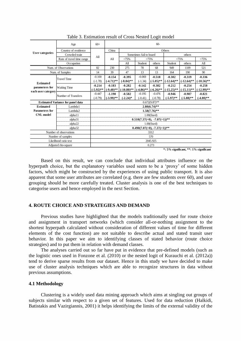
Table 3. Estimation result of Cross Nested Logit model

Based on this result, we can conclude that individual attributes influence on the

hyperpath choice, but the explanatory variables used seem to be a ‘proxy’ of some hidden

factors, which might be constructed by the experiences of using public transport. It is also

apparent that some user attributes are correlated (e.g. there are few students over 60), and user

grouping should be more carefully treated. Cluster analysis is one of the best techniques to

categorise users and hence employed in the next Section.

4. ROUTE CHOICE AND STRATEGIES AND DEMAND

Previous studies have highlighted that the models traditionally used for route choice

and assignment in transport networks (which consider all-or-nothing assignment to the

shortest hyperpath calculated without consideration of different values of time for different

elements of the cost function) are not suitable to describe actual and stated transit user

behavior. In this paper we aim to identifying classes of stated behavior (route choice

strategies) and to put them in relation with demand classes.

The analyses carried out so far have put in evidence that pre-defined models (such as

the logistic ones used in Fonzone et al. (2010) or the nested logit of Kurauchi et al. (2012a))

tend to derive sparse results from our dataset. Hence in this study we have decided to make

use of cluster analysis techniques which are able to recognize structures in data without

previous assumptions.

4.1 Methodology

Clustering is a widely used data mining approach which aims at singling out groups of

subjects similar with respect to a given set of features. Used for data reduction (Halkidi,

Batistakis and Vazirgiannis, 2001) it helps identifying the limits of the external validity of the

Age 60+

Country of residence China

Crowded train

Rate of travel time range <75% >75%

Occupation All Student others Student others All

82 230 275 78 68 949 1109 521

14 39 47 13 13 164 190 90

Travel Time-0.100

(-1.78)

-0.154

(-4.71)**

-0.395

(-8.84)**

-0.069

(-1.34)

-0.518

(-5.05)**

-0.302

(-12.64)**

-0.319

(-12.64)**

-0.336

(-10.56)**

Waiting Time-0.214

(-5.92)**

-0.183

(-9.40)**

-0.282

(-10.80)**

-0.142

(-4.86)**

-0.382

(-6.26)**

-0.212

(-15.25)**

-0.254

(-15.11)**

-0.258

(-12.99)**

Number of Transfers-0.447

(-0.79)

-1.190

(-3.99)**

-0.582

(-2.24)*

-0.195

(-0.41)

-0.476

(-0.78)

-0.946

(-5.97)**

-0.987

(-5.88)**

-0.821

(-4.00)**

Lambda1

Lambda2

alpha11

alpha31

alpha22

alpha32

Num. of Samples

*: 5% significant, **: 1% significant

<75%

60-

All

Others

All

Sometimes fail to board others

>75%

0.273Adjusted rho-square

Estimated

parameters for

each user category

User categories

Num. of Observations

1.00(fixed)

0.490(7.07(=0), -7.37(=1))**

3312

570

2045.925

0.672(9.87)**

2.80(6.74)**

1.58(7.76)**

1.00(fixed)

0.510(7.37(=0), -7.07(=1))**

Estimated Variance for panel data

Estimated

Parameters for

CNL model

Number of observations

Number of samples

Likelihood ratio test

results drawn from a non-randomly chosen sample. Moreover it can be useful to identify

behavioural patterns in an explorative study.

We base the analysis of the attitude of transit users towards hyperpath-based route

choice on a double clustering. Firstly responses are grouped according to the personal

characteristics of respondents and to the characteristics of the reported trips. This allows

characterising the segments of demand for public transport trips that our web-based survey

was able to capture (the results of this first clustering are referred to as “demand” clusters). A

second clustering concerns the answers to 5 questions (Q29, Q31-33) of the stated preference

section of the questionnaire (“behaviour” clusters). From this a clearer understanding comes

of the different approaches to route choice in transit networks. Finally demand and behaviour

clusters are compared to check whether different demand segments adopt different decision

making processes.

Since our dataset includes categorical variables, the SPSS TwoStep procedure is used

which is generally deemed suitable to deal with non-interval variables. The number of clusters

in this procedure is normally decided on the basis of the Bayes Information Criterion or of the

Akaike’s Information Criterion. The former tends to underestimate the “correct” number of

clusters whereas the latter tends to overestimate it (Mooi and Sarstedt, 2011). The Silhouette

coefficient is provided as measure of goodness-of-fit. However, it has to be noted that the

cluster model selection based on the information criteria makes use of a heuristic method.

Moreover the Silhouette coefficient is a geometrical-based validity measure; such kind of

indicators provide useful information only if specific assumptions as to the shape of clusters

hold. To overcome these problems, an approach can be taken to cluster validation based on

the stability of solution. Kuncheva and Vetrov (2006) provide a clear discussion of the issue,

Bel Mufti and BelMufti, Bertrand and ElMoubarki (2005) can be consulted for references to

seminal works. We select the optimal model taking into account both the default SPSS

measures and a stability analysis. Details on model selection are given in the Appendix.

4.2 Demand Clusters

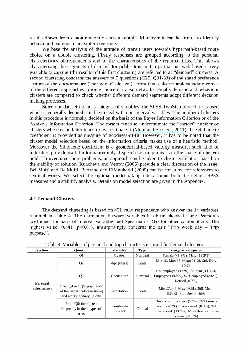
The demand clustering is based on 431 valid respondents who answer the 14 variables

reported in Table 4. The correlation between variables has been checked using Pearson’s

coefficient for pairs of interval variables and Spearman’s Rho for other combinations. The

highest value, 0.641 (p<0.01), unsurprisingly concerns the pair ”Trip week day – Trip

purpose”.

Table 4. Variables of personal and trip characteristics used for demand clusters Section Question Variable Type Range or categories

Personal

information

Q1 Gender Nominal Female (41.8%), Male (58.2%)

Q2 Age (years) Scale Min 15, Max 66, Mean 31.28, Std. Dev.

10.24

Q3 Occupation Nominal

Not employed (1.6%), Student (44.8%),

Employee (49.9%), Self-employed (3.0%),

Retired (0.7%)

From Q4 and Q5: population

of the largest between living

and working/studying city

Population Scale Min 27,065, Max 19,612,368, Mean

6.60E6, Std. Dev. 6.16E6

From Q6: the highest

frequency in the 4 types of

trips

Familiarity

with PT Ordinal

Once a month or less (7.2%), 2-3 times a

month (9.0%), Once a week (8.8%), 2-3

times a week (13.7%), More than 2-3 times

a week (61.3%)

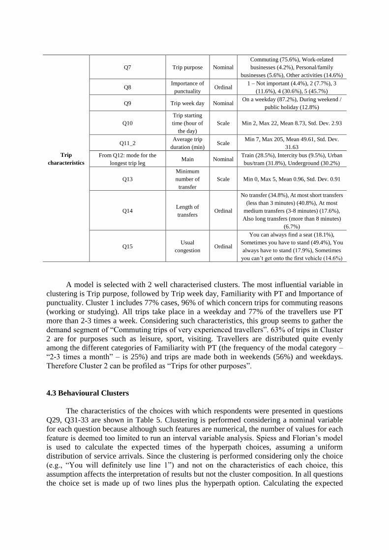
Trip

characteristics

Q7 Trip purpose Nominal

Commuting (75.6%), Work-related

businesses (4.2%), Personal/family

businesses (5.6%), Other activities (14.6%)

Q8 Importance of

punctuality Ordinal

1 – Not important (4.4%), 2 (7.7%), 3

(11.6%), 4 (30.6%), 5 (45.7%)

Q9 Trip week day Nominal On a weekday (87.2%), During weekend /

public holiday (12.8%)

Q10

Trip starting

time (hour of

the day)

Scale Min 2, Max 22, Mean 8.73, Std. Dev. 2.93

Q11_2 Average trip

duration (min) Scale

Min 7, Max 205, Mean 49.61, Std. Dev.

31.63

From Q12: mode for the

longest trip leg Main Nominal

Train (28.5%), Intercity bus (9.5%), Urban

bus/tram (31.8%), Underground (30.2%)

Q13

Minimum

number of

transfer

Scale Min 0, Max 5, Mean 0.96, Std. Dev. 0.91

Q14 Length of

transfers Ordinal

No transfer (34.8%), At most short transfers

(less than 3 minutes) (40.8%), At most

medium transfers (3-8 minutes) (17.6%),

Also long transfers (more than 8 minutes)

(6.7%)

Q15 Usual

congestion Ordinal

You can always find a seat (18.1%),

Sometimes you have to stand (49.4%), You

always have to stand (17.9%), Sometimes

you can’t get onto the first vehicle (14.6%)

A model is selected with 2 well characterised clusters. The most influential variable in

clustering is Trip purpose, followed by Trip week day, Familiarity with PT and Importance of

punctuality. Cluster 1 includes 77% cases, 96% of which concern trips for commuting reasons

(working or studying). All trips take place in a weekday and 77% of the travellers use PT

more than 2-3 times a week. Considering such characteristics, this group seems to gather the

demand segment of “Commuting trips of very experienced travellers”. 63% of trips in Cluster

2 are for purposes such as leisure, sport, visiting. Travellers are distributed quite evenly

among the different categories of Familiarity with PT (the frequency of the modal category –

“2-3 times a month” – is 25%) and trips are made both in weekends (56%) and weekdays.

Therefore Cluster 2 can be profiled as “Trips for other purposes”.

4.3 Behavioural Clusters

The characteristics of the choices with which respondents were presented in questions

Q29, Q31-33 are shown in Table 5. Clustering is performed considering a nominal variable

for each question because although such features are numerical, the number of values for each

feature is deemed too limited to run an interval variable analysis. Spiess and Florian’s model

is used to calculate the expected times of the hyperpath choices, assuming a uniform

distribution of service arrivals. Since the clustering is performed considering only the choice

(e.g., “You will definitely use line 1”) and not on the characteristics of each choice, this

assumption affects the interpretation of results but not the cluster composition. In all questions

the choice set is made up of two lines plus the hyperpath option. Calculating the expected

travel time with Spiess and Florian’s method, the hyperpath option is the fastest in every

question.

Table 5. Characteristics of the variables in the SP questions used for behaviour clusters Question

(Variable) Option

On-board time

(min)

Waiting time

(min)

Total travel

time (min)

Transfers

(number)

Q29

(Nchoice1)

Line 1 (3.2%) 10 15 25 0

Line 2*

(12.2%) 14 5 19 0

The first

arriving

(84.3%)

13 3.75 16.75 0

Q31 – first

section

(Nchoice2)

Line 1 (7.1%) 10 15 25 0

Line 2* (6.5%) 14 10 24 0

The first

arriving

(86.4%)

12.4 6 18.4 0

Q31 – second

section

(Nchoice3)

Line 3*

(46.3%) 10 15 25 0

Line 4 (4.6%) 20 10 30 0

The first

arriving

(49.1%)

16 6 22 0

Q32

(Nchoice4)

Line 1 (10.7%) 10 20 30 1

Line 3*

(53.3%) 20 6 26 0

The first

arriving

(35.9%)

16.25 7.5 23.75 1

Q33

(Nchoice5)

Line 1 (29.1%) 12 16 28 0

Line 3*

(18.7%) 16 8 24 1

The first

arriving

(52.2%)

15.2 6.4 21.6 1

Q34

(Nchoice6)

Line 1 (5.7%) 10 30 40 1

Line 3*

(30.8%) 15 20 35 1

The first

arriving

(63.5%)

13 18 31 1

* Shortest single path

In this case the 6 cluster model has been chosen shown in Figure 3. The analysis is

based on 523 cases. Profiles of the 6 clusters are also reported in Figure 3, in the row

“Description”.

Figure 3. 6 cluster model of strategy choice

Interestingly only 15.3% of respondents choose always the hyperpath alternative, to

which the Spiess and Florian’s model would assign the whole demand.

4.4 Association between Strategy Choice and Demand

In order to understand whether some user groups are more likely to adopt a given

choice strategy we evaluate the association between the behaviour and demand clusters using

the chi-square test. We also investigate the relationships between strategies and single

demand-related variables which have been found relevant in the previous analyses of the

survey or in another studies concerning route choice. The association of the choices in each

SP question and the demand clusters is also studied. Table 6 lists the performed tests and the

resulting significance values.

Table 5. Chi-square test on strategy choice Behavioural

choice

User/trip

characteristic

Categories Number

of cases

Significance

(asymptotic,

2-tails)

Behaviour

cluster

Demand cluster See Figure 3 394 0.44

Gender Male, Female 523 0.10

Age ≤29-,30-49, ≥50 523 0.04

Occupation Student, Employee, Other 523 0.03

Importance of Not important to important: 1-2, 3, 4-5 of the original 520 0.84

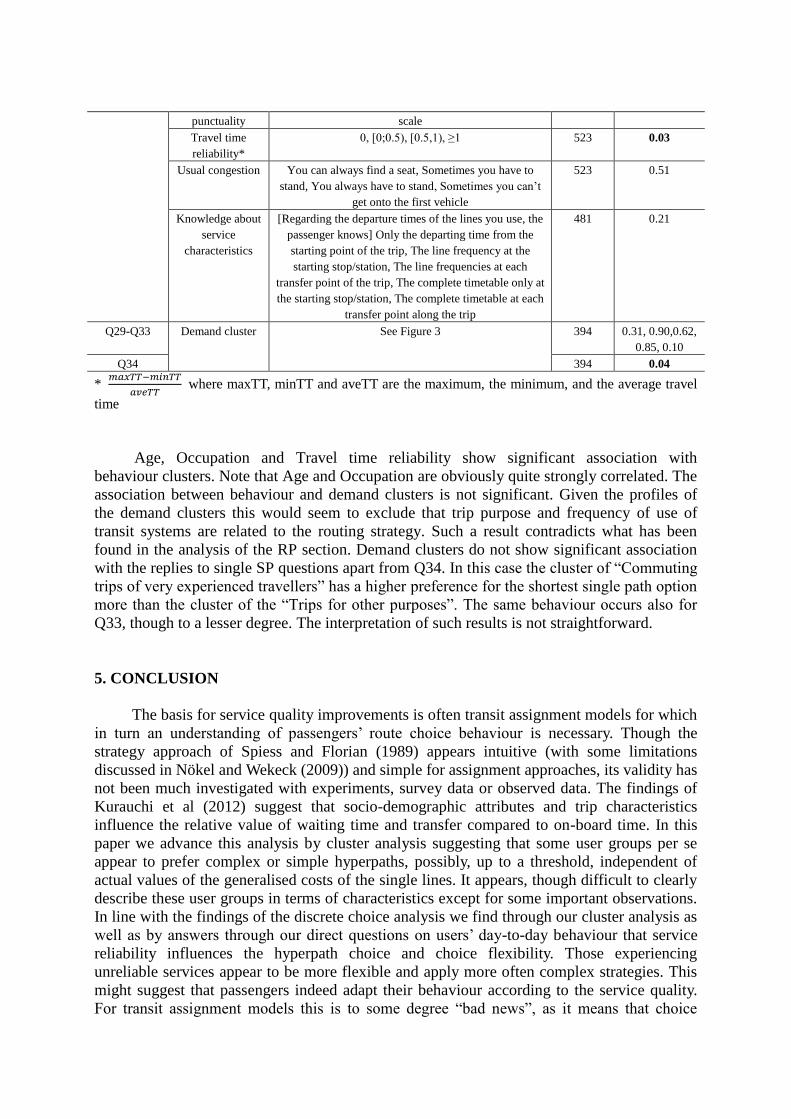
punctuality scale

Travel time

reliability*

0, [0;0.5), [0.5,1), ≥1 523 0.03

Usual congestion You can always find a seat, Sometimes you have to

stand, You always have to stand, Sometimes you can’t

get onto the first vehicle

523 0.51

Knowledge about

service

characteristics

[Regarding the departure times of the lines you use, the

passenger knows] Only the departing time from the

starting point of the trip, The line frequency at the

starting stop/station, The line frequencies at each

transfer point of the trip, The complete timetable only at

the starting stop/station, The complete timetable at each

transfer point along the trip

481 0.21

Q29-Q33 Demand cluster See Figure 3 394 0.31, 0.90,0.62,

0.85, 0.10

Q34 394 0.04

* 𝑚𝑎𝑥𝑇𝑇−𝑚𝑖𝑛𝑇𝑇

𝑎𝑣𝑒𝑇𝑇 where maxTT, minTT and aveTT are the maximum, the minimum, and the average travel

time

Age, Occupation and Travel time reliability show significant association with

behaviour clusters. Note that Age and Occupation are obviously quite strongly correlated. The

association between behaviour and demand clusters is not significant. Given the profiles of

the demand clusters this would seem to exclude that trip purpose and frequency of use of

transit systems are related to the routing strategy. Such a result contradicts what has been

found in the analysis of the RP section. Demand clusters do not show significant association

with the replies to single SP questions apart from Q34. In this case the cluster of “Commuting

trips of very experienced travellers” has a higher preference for the shortest single path option

more than the cluster of the “Trips for other purposes”. The same behaviour occurs also for

Q33, though to a lesser degree. The interpretation of such results is not straightforward.

5. CONCLUSION

The basis for service quality improvements is often transit assignment models for which

in turn an understanding of passengers’ route choice behaviour is necessary. Though the

strategy approach of Spiess and Florian (1989) appears intuitive (with some limitations

discussed in Nökel and Wekeck (2009)) and simple for assignment approaches, its validity has

not been much investigated with experiments, survey data or observed data. The findings of

Kurauchi et al (2012) suggest that socio-demographic attributes and trip characteristics

influence the relative value of waiting time and transfer compared to on-board time. In this

paper we advance this analysis by cluster analysis suggesting that some user groups per se

appear to prefer complex or simple hyperpaths, possibly, up to a threshold, independent of

actual values of the generalised costs of the single lines. It appears, though difficult to clearly

describe these user groups in terms of characteristics except for some important observations.

In line with the findings of the discrete choice analysis we find through our cluster analysis as

well as by answers through our direct questions on users’ day-to-day behaviour that service

reliability influences the hyperpath choice and choice flexibility. Those experiencing

unreliable services appear to be more flexible and apply more often complex strategies. This

might suggest that passengers indeed adapt their behaviour according to the service quality.

For transit assignment models this is to some degree “bad news”, as it means that choice

parameters should, ideally, be city specific. Furthermore, we find that age and occupation

influence the hyperpath choice. Students choose less often complex hyperpaths, which

Kurauchi et al. (2012a) explain with a lower value of waiting time. The implication of this is

that the weight of values of waiting time and transfer penalties should depend on age and

occupation.

A problem of asking respondents which strategy they would choose in hypothetical

choice scenarios clearly is the level of abstraction from their daily experiences. We therefore

included in our survey some additional questions regarding their choice flexibility on their

most frequent transit trip. These results suggest that our scenario observations might

overestimate choice flexibility. Habits might play a more important role than assumed in

models or many users might not “optimise” their route choice in terms of total travel time if

they could gain only a few minutes. Together with previous observations, this again could

suggest that threshold models are appropriate for transit assignment where passengers stick to

a single shortest route unless a different route is significantly better or unless a fairly major

disruption appears. A second important finding from our questions on daily behaviour is that

passengers appear to be as flexible in their stop and transfer point choice as in their line

choice. This has direct implications for transit assignment models as in most cases the

hyperpath choice is limited to line choice only.

In further work our findings should be confirmed with an extended survey reducing the

biases in our sample towards young, highly educated males. Our findings further might

suggest that our hypothetical scenarios are partly to abstract for some respondents.

Time-series smart card data that include data on line choice as well as boarding and alighting

points could be a way to advance the analysis. Kurauchi et al. (2012b) discuss an approach for

this with an analysis of Oyster card data.

ACKNOWLEDGMENTS

We would like to thank Dr Hiroshi Shimamoto (Kyoto University), Professor Michael

G. H. Bell (Imperial College London) and several members of the COST action 1004 for

some valuable discussions which have influenced this research. This research has further been

supported by “Grant-in-Aid for Challenging Exploratory Research”, No. 2365312,

(2011-2012) from The Ministry of Education, Culture, Sports, Science and Technology of

Japan.

APPENDIX – Details of cluster analysis

Stability analysis method

Solving a cluster problem means to identify correctly the number of clusters and the

assignment of objects to clusters. Our approach to evaluating the goodness of a cluster model

is based on the consideration that, if a model is correctly specified i.e. if the correct number of

clusters is assumed, two objects belonging to the same “true” cluster should be assigned to the

same “estimated” cluster whatever subset of the original set of objects is used in the clustering

process. In other words a good model is a model that provides stable solutions when

perturbations are introduced in input data. To test the stability of solutions we adopt the

following procedure

1. Specify the model setting the number of clusters n

2. Randomly split the sample in two disjoint subsamples S1 and S2 almost of the same size

3. Build a n cluster model of S1 using the SPSS TwoStep procedure, say 𝑇

4. Using the cluster distribution in 𝑇 as dependent variable, build a Classification Tree

and use it to predict a clustering of S1, say 𝑇 , and S2, say

𝑇

4.1. Evaluate the Misclassification Risk (MR) associated to the tree

5. Build a n cluster model of S2 using the SPSS TwoStep procedure, say 𝑇

6. Compare 𝑇 with

𝑇 using the Adjusted Rand Index (ARI)

7. Repeat steps from 2to 6 for 5 times in total

Once a model has been specified (step 1), clustering can be interpreted as the

application of classification rules to allocate objects to clusters. These rules are not known

when clustering is performed and can be recognised only at the end of the clustering process.

Profiling is making such rules explicit. Our procedure checks (step 6) whether the application

to S2 (step 4) of the rules identified using S1 (step 3) gives rise to the same clustering

originated by the direct application of the clustering algorithm to S2 (step 5). In other words,

S2 is used to validate the model provided by S1.

The similarity of the two clustering of S2 is measured by ARI. The original Rand index

(Rand, 1971) is a measure of the similarity of two partitions of a set 𝒪 of 𝑟 objects: Let 𝒫

and 𝒬 two partitions of 𝒪, 𝑎 the number of objects which are in the same set both in 𝒫

and in 𝒬, and 𝑏 the number of objects which are in different sets both in 𝒫 and in 𝒬. The

Rand index is the ratio 𝑎+𝑏

(𝑟2). ARI has been proposed by Hubert and Arabie (1985) to correct

the fact that the expected value of the Rand index of two random partitions is not constant.

ARI ranges between 0 and 1. In cluster analysis Rand index and ARI are frequently used as

measure of external validity of a clustering when correct clusters are known a priori (Milligan

and Cooper, 1986). In our procedure the clusters of S2 generated by the rules underpinning

𝑇 are assumed correct and compared with those generated by applying the SPSS TwoStep

(i.e. 𝑇 ).

In evaluating the results of such comparison, it has to be considered that the rules

defining 𝑇 can be derived only in an approximate way by using the Classification Tree

technique (step 4). MR (step 4.1), the percentage of cases correctly classified by a tree, is

interpreted as an indicator of the Classification Tree algorithm capacity to identify such rules.

If MR in 4.1 is high (i.e. if 𝑇 and

𝑇 are different), 𝑇 might not coincide with the

clustering of S2 induced by the (unknown) rules giving rise to 𝑇 and the value of ARI in

6 might be due just to the bad performance of the Classification Tree technique.

5 iterations of the procedure (step 7) are performed to account for the randomness in

defining S1 and S2 (step 2).

Demand clusters

For the demand-related variables the SPSS heuristic strongly suggests a 2 cluster model

using either information criteria, BIC and AIC (results as to the former are shown in Figure

4a). Reader are referred to the SPSS manual (PASW Statistics 18, 2010) for details

concerning the heuristic. The 2 cluster model shows the highest Silhouette index; however the

value is quite low in absolute terms (0.1790, Figure 4b). Kaufman and Rousseeuw (1990)

suggest that an acceptable clustering should have a Silhouette greater than 0.2000. SPSS

evaluates the Silhouette index by averaging over all cases the ratio 𝑑𝑜𝑐−min𝑑𝑐 𝑑𝑑𝑐

𝑚𝑎𝑥{𝑑𝑜𝑐,min𝑑𝑐 𝑑𝑑𝑐} where

𝑑𝑜𝑐 is the Euclidean distance of a case from the centroid of its own cluster, 𝑑𝑑𝑐 that between

the case and the centroid of a different cluster. Therefore high Silhouette values characterize

clusterings with cohesive and separated clusters. However cases can occur in which clusters

are well distinguished but not cohesive or separated (see for instance fig.1 in (Lange et al.,

2004)). Since no knowledge on cluster shape is available prior to clustering, we consider the

Silhouette index only as one of the indicators of the relative goodness-of-fit of different

models. In the stability analysis models have been evaluated with a number of clusters

ranging from 2 to 6. The Classification Tree technique fails in detecting the rules

underpinning 𝑇 for the models with number of clusters higher than 4 (Figure 4c).

Therefore for such models ARI cannot be considered reliable. Among the models with lower

number of clusters, that with 2 clusters is clearly the most stable one (Figure 4d). ARI is

also reasonably good in absolute terms. In conclusion, the 2 cluster model is chosen for the

demand variables. Note that the clustering reported in the main text is calculated using all

available data.

(a)

(b)

(c)

(d)

Figure 4. Performance indicators in clustering demand variables - (a) BIC measures, (c)

Silhouette index, (c) Misclassification Risk, (d) Adjusted Rand Index

Behaviour clusters

In the case of the behaviour clusters, SPSS supports the choice of the 4 cluster model

with both AIC and BIC (Figure 5a). However the 4 cluster model performs only slightly

better than the 6 cluster one. The Silhouette index are in the range of “fair” models (0.2000 –

0.5000) for all the models. The Silhouette of the 6 cluster model is slightly better than that of

the 4 cluster one (Figure 5b). Also in the case of behaviour clusters MR (as expected) tends to

increase with the number of clusters, with the exclusion of the 2 cluster model for which the

0.0000

0.0500

0.1000

0.1500

0.2000

2 clu 3 clu 4 clu 5 clu 6 clu

Model

Silhouette

0.0000

0.2000

0.4000

0.6000

2 clu 3 clu 4 clu 5 clu 6 clu

MR

95% CI upper limit

95% CI lower limit

average

0.0000

0.2000

0.4000

0.6000

0.8000

1.0000

2 clu 3 clu 4 clu 5 clu 6 clu

Model

ARI

95% CI upper limit

95% CI lower limit

average

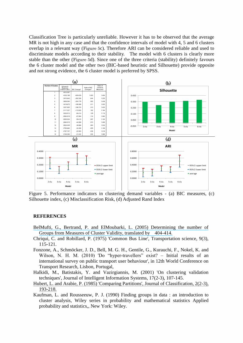
Classification Tree is particularly unreliable. However it has to be observed that the average

MR is not high in any case and that the confidence intervals of model with 4, 5 and 6 clusters

overlap in a relevant way (Figure 5c). Therefore ARI can be considered reliable and used to

discriminate models according to their stability. The model with 6 clusters is clearly more

stable than the other (Figure 5d). Since one of the three criteria (stability) definitely favours

the 6 cluster model and the other two (BIC-based heuristic and Silhouette) provide opposite

and not strong evidence, the 6 cluster model is preferred by SPSS.

(a)

(b)

(c)

(d)

Figure 5. Performance indicators in clustering demand variables - (a) BIC measures, (c)

Silhouette index, (c) Misclassification Risk, (d) Adjusted Rand Index

REFERENCES

BelMufti, G., Bertrand, P. and ElMoubarki, L. (2005) Determining the number of

Groups from Measures of Cluster Validity, translated by 404-414.

Chriqui, C. and Robillard, P. (1975) 'Common Bus Line', Transportation science, 9(3),

115-121.

Fonzone, A., Schmöcker, J. D., Bell, M. G. H., Gentile, G., Kurauchi, F., Nokel, K. and

Wilson, N. H. M. (2010) 'Do “hyper-travellers” exist? – Initial results of an

international survey on public transport user behaviour', in 12th World Conference on

Transport Research, Lisbon, Portugal,

Halkidi, M., Batistakis, Y. and Vazirgiannis, M. (2001) 'On clustering validation

techniques', Journal of Intelligent Information Systems, 17(2-3), 107-145.

Hubert, L. and Arabie, P. (1985) 'Comparing Partitions', Journal of Classification, 2(2-3),

193-218.

Kaufman, L. and Rousseeuw, P. J. (1990) Finding groups in data : an introduction to

cluster analysis, Wiley series in probability and mathematical statistics Applied

probability and statistics,, New York: Wiley.

-0.050

0.050

0.150

0.250

0.350

0.450

2 clu 3 clu 4 clu 5 clu 6 clu

Model

Silhouette

0.0000

0.1000

0.2000

0.3000

0.4000

2 clu 3 clu 4 clu 5 clu 6 clu

Model

MR

95% CI upper limit

95% CI lower limit

average

0.0000

0.2000

0.4000

0.6000

0.8000

2 clu 3 clu 4 clu 5 clu 6 clu

Model

ARI

95% CI upper limit

95% CI lower limit

average

Kuncheva, L. I. and Vetrov, D. P. (2006) 'Evaluation of stability of k-means cluster

ensembles with respect to random initialization', Ieee Transactions on Pattern

Analysis and Machine Intelligence, 28(11), 1798-1808.

Kurauchi, F., Schmöcker, J. D., Fonzone, A., Hemdan, S. M. H., Shimamoto, H. and

Bell, M. G. H. (2012a) 'Estimation of Weights of Times and transfers for Hyperpath

Travellers', in Proceedings of TRB 91st Annual Meeting, Washington, D.C.,

Kurauchi, F., Schmöcker, J. D., Shimamoto, H. and Hemdan, S. M. H. (2012b)

'Empirical Analysis on Passengers’ Hyperpath Construction by Smart Card Data', in

12th Conference on Advanced Systems for Public Transport (CASPT), Santiago,

Chile,

Lampkin, W. and Saalmans, P. D. (1967) 'The Design of Routes; Service Frequencies

and Schedules of a Municipal Bus Undertaking: A Case Study', Operational Research

Quarterly, 18(4), 375-397.

Lange, T., Volker, R., Braun, M. L. and Buhmann, J. M. (2004) 'Stability-Based

Validation of Clustering Solutions', Neural Computation, 16(6), 1299-1323.

Milligan, G. W. and Cooper, M. C. (1986) 'A Study of the Comparability of External

Criteria for Hierarchical Cluster-Analysis', Multivariate Behavioral Research, 21(4),

441-458.

Mooi, E. and Sarstedt, M. (2011) A Concise Guide to Market Research, Berlin

Heidelberg: Springer-Verlag.

Nguyen, S. and Pallottino, S. (1988) 'Equilibrium traffic assignment for large scale

transit networks', European journal of operational research, 37(2), 176-186.

Nokel, K. and Wekeck, S. (2009) 'Boarding and alighting in frequency-based transit

assignment', in TRB 99th Annual Meeting, Washington,

PASW Statistics 18 (2010) Algorithms, on-line help.

Rand, W. M. (1971) 'Objective Criteria for Evaluation of Clustering Methods', Journal of

the American Statistical Association, 66(336), 846-&.

Spiess, H. and Florian, M. (1989) 'Optimal strategies. A new assignment model for

transit networks', Transportation research. Part B, Methodological, 23B(2), 83-102.

Wardman, M. R. (2004) 'Public transport values of time', Transport Policy, 11, 363-377.