Double-blind test program for astrometric planet detection with Gaia
33
arXiv:0802.0515v1 [astro-ph] 4 Feb 2008 Astronomy & Astrophysics manuscript no. dbt˙gaia˙revised˙2 c ESO 2008 February 6, 2008 Double-blind test program for astrometric planet detection with Gaia S. Casertano 1 , M. G. Lattanzi 2 , A. Sozzetti 2,3 , A. Spagna 2 , S. Jancart 4 , R. Morbidelli 2 , R. Pannunzio 2 , D. Pourbaix 4 , and D. Queloz 5 1 Space Telescope Science Institute, 3700 San Martin Drive, Baltimore, MD 21218, USA 2 INAF - Osservatorio Astronomico di Torino, via Osservatorio 20, 10025 Pino Torinese, Italy 3 Harvard-Smithsonian Center for Astrophysics, 60 Garden Street, Cambridge, MA 02138, USA 4 Institut d’Astronomie et d’Astrophysique, Universit´ e Libre de Bruxelles, CP. 226, Boulevard du Triomphe, 1050 Bruxelles, Belgium 5 Observatoire de Gen` eve, 51 Ch. de Maillettes, 1290 Sauveny, Switzerland Received ......; accepted ...... ABSTRACT Aims. The scope of this paper is twofold. First, it describes the simulation scenarios and the results of a large-scale, double-blind test campaign carried out to estimate the potential of Gaia for detecting and measuring planetary systems. The identified capabilities are then put in context by highlighting the unique contribution that the Gaia exoplanet discoveries will be able to bring to the science of extrasolar planets in the next decade. Methods. We use detailed simulations of the Gaia observations of synthetic planetary systems and develop and utilize independent software codes in double-blind mode to analyze the data, including statistical tools for planet detection and different algorithms for single and multiple Keplerian orbit fitting that use no a priori knowledge of the true orbital parameters of the systems. Results. 1) Planets with astrometric signatures α ≃ 3 times the assumed single-measurement error σ ψ and period P ≤ 5 yr can be detected reliably and consistently, with a very small number of false positives. 2) At twice the detection limit, uncertainties in orbital parameters and masses are typically 15% − 20%. 3) Over 70% of two-planet systems with well-separated periods in the range 0.2 ≤ P ≤ 9 yr, astrometric signal-to-noise ratio 2 ≤ α/σ ψ ≤ 50, and eccentricity e ≤ 0.6 are correctly identified. 4) Favorable orbital configurations (both planets with P ≤ 4 yr and α/σ ψ ≥ 10, redundancy over a factor of 2 in the number of observations) have orbital elements measured to better than 10% accuracy > 90% of the time, and the value of the mutual inclination angle i rel determined with uncertainties ≤ 10 ◦ . 5) Finally, nominal uncertainties obtained from the fitting procedures are a good estimate of the actual errors in the orbit reconstruction. Extrapolating from the present-day statistical properties of the exoplanet sample, the results imply that a Gaia with σ ψ = 8 μas, in its unbiased and complete magnitude-limited census of planetary systems, will discover and measure several thousands of giant planets out to 3-4 AUs from stars within 200 pc, and will characterize hundreds of multiple-planet systems, including meaningful coplanarity tests. Finally, we put Gaia’s planet discovery potential into context, identifying several areas of planetary-system science (statistical properties and correlations, comparisons with predictions from theoretical models of formation and evolution, interpretation of direct detections) in which Gaia can be expected, on the basis of our results, to have a relevant impact, when combined with data coming from other ongoing and future planet search programs. Key words. planetary systems – astrometry – methods: data analysis – methods: numerical – methods: statistical – stars: statistics 1. Introduction The continuously increasing catalog of extrasolar planets is to- day surpassing the threshold of 270 planets announced 1 . Most of the nearby (d 200 − 300 pc) exoplanet candidates have been detected around F-G-K-M dwarfs by long-term, high-precision (1 − 5ms −1 ) Doppler search programs (e.g., Butler et al. 2006, and references therein; Udry et al. 2007, and references therein). Over a dozen of these are ‘hot Jupiters’ with orbital periods P ≃ 1 − 20 days discovered to cross the disk of their relatively bright (V < 13) parent stars thanks to high-cadence, milli-mag photometric measurements 2 . An additional dozen or so extra- Send offprint requests to: A. Sozzetti, e-mail: [email protected] 1 See, for example, Jean Schneider’s Extrasolar Planet Encyclopedia at http://exoplanet.eu/ 2 For a review, see Charbonneau et al. 2007, and ref- erences therein. For an updated list, see for example ob- swww.unige.ch/ pont/TRANSITS.htm, and references therein solar planets have been found residing at d > 300 pc, thanks to both transit photometry (e.g., Konacki et al. 2003, 2005; Bouchy et al. 2004; Pont et al. 2004, 2007; Udalski et al. 2007; Collier Cameron et al. 2006; Mandushev et al. 2007; Kov´ acs et al. 2007; Bakos et al. 2007) as well as microlensing surveys in the Galactic bulge (e.g., Bond et al. 2004; Udalski et al. 2005; Gould et al. 2006; Bealieu et al. 2006). The sample of nearby exoplanets and their host stars is amenable to follow-up studies with a variety of indirect and direct techniques, such as high-resolution (visible-light and in- frared) imaging and stellar spectroscopy, and photometric tran- sit timing (for a review, see for example Charbonneau et al. 2007, and references therein). Milli-arcsecond (mas) astrome- try for bright planet hosts within 200-300 pc provides precise distance estimates thanks to Hipparcos parallaxes (Perryman et al. 1997). However, despite a few important successes (Benedict et al. 2002, 2006; McArthur et al. 2004; Bean et al. 2007), as- trometric measurements with mas precision have so far proved of limited utility when employed as either a follow-up tool or
Transcript of Double-blind test program for astrometric planet detection with Gaia

arX
iv:0
802.
0515
v1 [
astr
o-ph
] 4
Feb
200
8Astronomy & Astrophysicsmanuscript no. dbt˙gaia˙revised˙2 c© ESO 2008February 6, 2008
Double-blind test program for astrometric planet detectio n withGaia
S. Casertano1, M. G. Lattanzi2, A. Sozzetti2,3, A. Spagna2, S. Jancart4, R. Morbidelli2, R. Pannunzio2, D. Pourbaix4,and D. Queloz5
1 Space Telescope Science Institute, 3700 San Martin Drive, Baltimore, MD 21218, USA2 INAF - Osservatorio Astronomico di Torino, via Osservatorio 20, 10025 Pino Torinese, Italy3 Harvard-Smithsonian Center for Astrophysics, 60 Garden Street, Cambridge, MA 02138, USA4 Institut d’Astronomie et d’Astrophysique, Universite Libre de Bruxelles, CP. 226, Boulevard du Triomphe, 1050 Bruxelles, Belgium5 Observatoire de Geneve, 51 Ch. de Maillettes, 1290 Sauveny, Switzerland
Received ......; accepted ......
ABSTRACT
Aims. The scope of this paper is twofold. First, it describes the simulation scenarios and the results of a large-scale, double-blind testcampaign carried out to estimate the potential of Gaia for detecting and measuring planetary systems. The identified capabilities arethen put in context by highlighting the unique contributionthat the Gaia exoplanet discoveries will be able to bring to the science ofextrasolar planets in the next decade.Methods. We use detailed simulations of the Gaia observations of synthetic planetary systems and develop and utilize independentsoftware codes in double-blind mode to analyze the data, including statistical tools for planet detection and different algorithms forsingle and multiple Keplerian orbit fitting that use no a priori knowledge of the true orbital parameters of the systems.Results. 1) Planets with astrometric signaturesα ≃ 3 times the assumed single-measurement errorσψ and periodP ≤ 5 yr canbe detected reliably and consistently, with a very small number of false positives. 2) At twice the detection limit, uncertainties inorbital parameters and masses are typically 15%− 20%. 3) Over 70% of two-planet systems with well-separated periods in the range0.2 ≤ P ≤ 9 yr, astrometric signal-to-noise ratio 2≤ α/σψ ≤ 50, and eccentricitye ≤ 0.6 are correctly identified. 4) Favorable orbitalconfigurations (both planets withP ≤ 4 yr andα/σψ ≥ 10, redundancy over a factor of 2 in the number of observations) have orbitalelements measured to better than 10% accuracy> 90% of the time, and the value of the mutual inclination angleirel determined withuncertainties≤ 10
. 5) Finally, nominal uncertainties obtained from the fitting procedures are a good estimate of the actual errorsin the orbit reconstruction. Extrapolating from the present-day statistical properties of the exoplanet sample, the results imply thata Gaia withσψ = 8 µas, in its unbiased and complete magnitude-limited census of planetary systems, will discover and measureseveral thousands of giant planets out to 3-4 AUs from stars within 200 pc, and will characterize hundreds of multiple-planet systems,including meaningful coplanarity tests. Finally, we put Gaia’s planet discovery potential into context, identifyingseveral areas ofplanetary-system science (statistical properties and correlations, comparisons with predictions from theoreticalmodels of formationand evolution, interpretation of direct detections) in which Gaia can be expected, on the basis of our results, to have a relevant impact,when combined with data coming from other ongoing and futureplanet search programs.
Key words. planetary systems – astrometry – methods: data analysis – methods: numerical – methods: statistical – stars: statistics
1. Introduction
The continuously increasing catalog of extrasolar planetsis to-day surpassing the threshold of 270 planets announced1. Mostof the nearby (d . 200−300 pc) exoplanet candidates have beendetected around F-G-K-M dwarfs by long-term, high-precision(1− 5 m s−1) Doppler search programs (e.g., Butler et al. 2006,and references therein; Udry et al. 2007, and references therein).Over a dozen of these are ‘hot Jupiters’ with orbital periodsP ≃ 1 − 20 days discovered to cross the disk of their relativelybright (V < 13) parent stars thanks to high-cadence, milli-magphotometric measurements2. An additional dozen or so extra-
Send offprint requests to: A. Sozzetti,e-mail:[email protected]
1 See, for example, Jean Schneider’s Extrasolar Planet Encyclopediaat http://exoplanet.eu/
2 For a review, see Charbonneau et al. 2007, and ref-erences therein. For an updated list, see for example ob-swww.unige.ch/ pont/TRANSITS.htm, and references therein
solar planets have been found residing atd > 300 pc, thanks toboth transit photometry (e.g., Konacki et al. 2003, 2005; Bouchyet al. 2004; Pont et al. 2004, 2007; Udalski et al. 2007; CollierCameron et al. 2006; Mandushev et al. 2007; Kovacs et al. 2007;Bakos et al. 2007) as well as microlensing surveys in the Galacticbulge (e.g., Bond et al. 2004; Udalski et al. 2005; Gould et al.2006; Bealieu et al. 2006).
The sample of nearby exoplanets and their host stars isamenable to follow-up studies with a variety of indirect anddirect techniques, such as high-resolution (visible-light and in-frared) imaging and stellar spectroscopy, and photometrictran-sit timing (for a review, see for example Charbonneau et al.2007, and references therein). Milli-arcsecond (mas) astrome-try for bright planet hosts within 200-300 pc provides precisedistance estimates thanks to Hipparcos parallaxes (Perryman etal. 1997). However, despite a few important successes (Benedictet al. 2002, 2006; McArthur et al. 2004; Bean et al. 2007), as-trometric measurements with mas precision have so far provedof limited utility when employed as either a follow-up tool or

2 S. Casertano et al.: DBT Campaign for Planet Detection withGaia
to independently search for planetary mass companions orbitingnearby stars (for a review, see for example Sozzetti 2005, andreferences therein).
In several past exploratory works (Casertano et al. 1996;Casertano & Sozzetti 1999; Lattanzi et al. 1997, 2000a, 2000b,2002; Sozzetti et al 2001, 2002, 2003a, 2003b), we have shownin some detail what space-borne astrometric observatorieswithmicro-arcsecond (µas)-level precision, such as Gaia (Perrymanet al. 2001) and SIM PlanetQuest (Unwin et al. 2007), canachieve in terms of search, detection and measurement of ex-trasolar planets of mass ranging from Jupiter-like to Earth-like.In those studies we adopted a qualitatively correct description ofthe measurements that each mission will carry out, and we es-timated detection probabilities and orbital parameters using re-alistic, non-linear least-square fits to those measurements. ForGaia, we used the then-current scanning law and error model;for SIM, we included reference stars, as well as the target, andadopted realistic observational overheads and signal-to-noise es-timates as provided by the SIM Project. Other, more recent stud-ies (Ford & Tremaine 2003; Ford 2004, 2006; Catanzarite et al.2006) have focused on evaluating the potential of astrometricplanet searches with SIM, revisiting and essentially confirmingthe findings of our previous works.
Although valid and useful, the studies currently availableneed updating and improving. In the specific case of planet de-tection and measurement with Gaia, we have thus far largely ne-glected the difficult problem of selecting adequate starting val-ues for the non-linear fits, using perturbed starting valuesin-stead. The study of multiple-planet systems, and in particularthe determination of whether the planets are coplanar—withinsuitable tolerances—is incomplete. The characteristics of Gaiahave changed, in some ways substantially, since our last workon the subject (Sozzetti et al 2003a). Last but not least, in orderto render the analysis truly independent from the simulations,these studies should be carried out in double-blind mode.
We present here a substantial program of double-blind testsfor planet detection with Gaia (preliminary findings were re-cently presented by Lattanzi et al. (2005)). The results expectedfrom this study include: a) an improved, more realistic assess-ment of the detectability and measurability of single and mul-tiple planets under a variety of conditions, parametrized by thesensitivity of Gaia; b) an assessment of the impact of Gaia incritical areas of planet research, in dependence on its expectedcapabilities; and c) the establishment of several Centers with ahigh level of readiness for the analysis of Gaia observations rel-evant to the study of exoplanets.
This paper is arranged as follows. In Section 2 we de-scribe our simulation setup and clearly state the working as-sumptions adopted (the relaxation of some of which might havea non-negligible impact on Gaia’s planet-hunting capabilities).In Section 3 we present the bulk of the results obtained duringour extensive campaign of double-blind tests. Section 4 attemptsto put Gaia’s potential for planet detection and measurementin context, by identifying several areas of planetary science inwhich Gaia can be expected, on the basis of our results, to havea dominant impact, and by delineating a small number of recom-mended research programs that can be conducted successfullyby the mission as planned. In section 5 we summarize our find-ings and provide concluding remarks.
2. Protocol definition and simulation setup
2.1. Double-blind tests protocol
For the purpose of this study, we have devised a specific proto-col for the double-blind tests campaign. Initially, three groups ofparticipants are identified: 1) theSimulators define and generatethe simulated observations, assuming specific characteristics ofthe Gaia satellite; simulators also define the type of results thatare expected for each set of simulations; 2) theSolvers receivethe simulated data and produce “solutions”—as defined by thesimulators; solvers define the criteria they adopt in answeringthe questions posed by the simulators; 3) theEvaluators receiveboth the “truth”—i.e., the input parameters—from the simula-tors and the solutions from the solvers, compare the two, anddraw a set of conclusions on the process.
A sequence of tasks, each with well-defined goals and timescales, has been established. Each task requires a separateset ofsimulations, and is carried out in several steps:
1. Simulation: The Simulators make the required set of simula-tions available to the Solvers, together with a clear definitionof the required solutions.
2. Clarification: A short period after the simulations are madeavailable in which the Solvers request any necessary clari-fication on the simulations themselves and on the requiredsolutions; after the clarification period, there is no contactbetween Simulators and Solvers until the Discussion step.
3. Delivery: On a specified deadline, the Simulators delivertheinput parameters for the simulations to the Evaluator, and theSolvers deliver their solutions together with a clear explana-tion of the criteria they used—e.g., the statistical meaningof “detection”, or how uncertainties on estimated parameterswere defined.
4. Evaluation: The Evaluators compare input parameters andsolutions and carry out any statistical tests they find useful,both to establish the quality of the solutions and to interprettheir results in terms of the capabilities of Gaia, if applicable.
5. Discussion: The Evaluators publicize their initial results. Allparticipants are given access to input parameters and all solu-tions, and the Evaluators’ results are discussed and modifiedas needed.
2.2. Observing scenario
The simulations were provided by the group at the TorinoObservatory. The simulations were made available via WWW asplain text files. A detailed description of the code for the simu-lation of Gaia astrometric observations can be found in our pre-vious exploratory works (Lattanzi et al. 2000a; Sozzetti etal.2001). We summarize here its main features.
Each simulation consists of a time series of observations(with a nominal mission lifetime set to 5 years) of a sampleof stars with given (catalog) low-accuracy astrometric param-eters (positions, proper motions, and parallax). Each observa-tion consists of a one-dimensional coordinate in the along-scandirection of the instantaneous great circle followed by Gaia atthat instant. The initially unperturbed photocenter position of astar is computed on the basis of its five astrometric parameters,which are drawn from simple distributions, not resembling anyspecific galaxy model. The distribution of two-dimensionalpo-sitions is random, uniform. The distribution of proper motions isGaussian, with dispersion equal to a value of transverse veloc-ity VT = 15 km sec−1, typical of the solar neighborhood. Thephotocenter position can then be corrected for the gravitational

S. Casertano et al.: DBT Campaign for Planet Detection with Gaia 3
perturbation of one or more planetary mass companions. TheKeplerian motion of each orbiting planet is described via the fullset of seven orbital elements. For simplicity, all experiments de-scribed here were produced assuming stellar massM⋆ = 1 M⊙.The resulting astrometric signature (in arcsec) is then expressedasα = (Mp/M⋆)× (ap/d), whereMp is the planet mass,ap is theplanet orbital semi-major axis andd is the distance to the system(in units of M⊙, AU, and pc, respectively). Simulated observa-tions are generated by adding the appropriate astrometric noise,as described in the next section.
Finally, the Gaia scanning law has been updated to the mostrecent expectations (precession angle around the Sun directionξ = 50
, precession speed of the satellite’s spin axisvp = 5.22
rev yr−1, spin axis rotation speedvr = 60 arcsec s−1), whichresult in fewer observations and possibly less ability to disen-tangle near-degenerate solutions than with the original scanninglaw (e.g., Lindegren & de Bruijne 2005). Each star is observedon averageNobs = 43 times3; note that the simplest star+planetsolution has 12 parameters, and therefore the redundancy oftheinformation is not very high.
2.3. Assumptions and caveats
The simulated data described above indicate that a number ofworking assumptions have been made. In particular, a variety ofphysical effects that can affect stellar positions have not been in-cluded, and a number of instrumental as well as astrophysicalnoise sources have not been considered (for a detailed review,see for example Sozzetti 2005). Our main simplifying assump-tions are summarized below.
1) the position of a star at a given time is described in Euclideanspace. A general relativistic formulation of Gaia-like globalastrometric observations, which has been the subject of sev-eral studies in the recent past (Klioner & Kopeikin 1992; deFelice et al. 1998, 2001, 2004; Vecchiato et al. 2003; Klioner2003, 2004), has not been taken into account;
2) we assume that the reconstruction and calibration of individ-ual great circles have been carried out, with nominal zeroerrors (i.e., knowledge of the spacecraft attitude is assumedperfect). We refer the reader to e.g. Sozzetti (2005), andreferences therein, for a summary of issues related to thecomplex problem of accurately calibrating out attitude errors(due to, e.g., particle radiation, thermal drifts, and spacecraftjitter) in space-borne astrometric measurements;
3) the abscissa is only affected by random errors, and no sys-tematic effects are considered (e.g., zero-point errors, chro-maticity, radiation damage, etc...). A simple Gaussian mea-surement error model is implemented, with standard devia-tionσψ = 8 µas, which applies to bright targets (V < 13). Inthis context, the projected end-of-mission accuracy on astro-metric parameters is 4µas. Recently, Gaia has successfullypassed the Preliminary Design Review and entered phaseC/D of the mission development. ESA has selected EADS-Astrium as Prime Contractor for the realization of the satel-lite. Scanning law and astrometric section of the selectedpayload, the only of relevance here, remain largely consistentwith the assumptions adopted in our simulations. However,very recent estimates of the error budget indicate a possible
3 We define as elementary observation the successive crossingof thetwo fields-of-view of the satellite, separated by the basic angle γ =106.5
.
degradation of 35%− 40% (i.e.,∼ 11 µas) in the single-measurement precision, corresponding to a typical final ac-curacy of 5− 5.5 µas for objects in the above magnituderange, with some dependence on spectral type (red objectsperforming closer to specifications). We will address in thediscussion section the possible impact of such performancedegradation on Gaia’s planet-hunting capabilities;
4) light aberration, light deflection, and other apparent effects(e.g., perspective acceleration) are considered as perfectlyremoved from the observed along-scan measurements;
5) when multi-component systems are generated around a tar-get, the resulting astrometric signal is the superpositionoftwo strictly non-interacting Keplerian orbits. It is recognizedthat gravitational interactions among planets can result insignificant deviations from purely Keplerian motion (such asthe case of the GJ 876 planetary system, e.g. Laughlin et al.2005). However, most of the multiple-planet systems discov-ered to-date by radial-velocity techniques can be well mod-eled by planets on independent Keplerian orbits, at least fortime-scales comparable to Gaia’s expected mission duration;
6) a number of potentially important sources of ‘astrophysi-cal’ noise, due to the environment or intrinsic to the target,have not been included in the simulations. In particular, wehave not considered a) the dynamical effect induced by long-period stellar companions to the targets, b) the possible shiftsin the stellar photocenter due to the presence of circumstel-lar disks with embedded planets (Rice et al. 2003a; Takeuchiet al. 2005), and c) variations in the apparent stellar positionproduced by surface temperature inhomogeneities, such asspots and flares (e.g, Sozzetti 2005, and references therein;Eriksson & Lindegren 2007).
The geometric model of the measurement process is de-scribed in detail in the Appendix.
3. Results
The double-blind test campaign encompassed a set of experi-ments that were necessary to establish a reliable estimate of theplanet search and measurement capabilities of Gaia under real-istic analysis procedures, albeit in the presence of an idealizedmeasurement process. In particular, a number of different taskswere designed, such that the participating groups would be ablea) to analyze data produced by a nominal satellite, without takinginto account the imperfections due to measurement biases, non-Gaussian error distributions, imperfections in the spheresolu-tion, and so on; b) to convert any Gaussian error model for Gaiameasurements into expected detection probability—includingcompleteness and false positives—and accuracy in orbital pa-rameters that can be achieved within the mission; c) to assessto what extent, and with what reliability, coplanarity of multipleplanets can be determined, and how the presence of a planet candegrade the orbital solution for another.
We broke down the work plan into three tests: T1, T2, andT3, whose main results are presented below. To facilitate read-ing, we have chosen to provide the summaries of the results con-cerning each of the three tests at the beginning of the correspond-ing sub-sections.
3.1. Test T1: Planet detection
Test T1 is designed primarily to establish the reliability and com-pleteness of planet detections for single-planet systems based onsimulated data, with fulla priori understanding of their noise

4 S. Casertano et al.: DBT Campaign for Planet Detection withGaia
Fig. 1. Left: Distribution of period and signature for the planets missed by Solver A’s broad criterion (A1). If more than one planetis present, the one with the largest signature is plotted. Right: distribution of period and signature for the planets missed by criterionB1.
Fig. 2. Inclination and eccentricity of the planets simulated forthe T1 experiment. Black dots are planets withα < 15 µas andP < 6 yr not detected by the A1 criterion.
characteristics. Simulated data were prepared for 100,000stars.Of these, 45,202 have no planets, 49,870 one, 3878 two, and1050 have three planets. The astrometric signature of each planetranges from 0.8 to 80µas (0.1 ≤ α/σψ ≤ 10), the periodPfrom 0.2 to 12 years, while eccentricities are drawn from a ran-dom distribution within the range 0.0 ≤ e ≤ 0.9. All other or-bital elements (inclinationi, longitude of pericenterω, pericenterepochτ, and position angle of the nodesΩ) were distributed ran-domly as follows: 1
≤ i ≤ 90
, 0ω ≤ 360
, 0 ≤ τ ≤ P, and
0 ≤ Ω ≤ 180. For systems with multiple planets, there was no
specific relationship between periods, phases, or amplitudes ofthe planetary signatures. The distribution of planetary signatureswas unknown to the solvers.
On this dataset, solvers were asked to carry out two tests.Test T1 consisted of identifying the likely planet detections,based on a single-star analysis and criteria of the Solvers’ownchoosing. Test T1b gave the opportunity to the solvers to im-prove on their planet detection on the basis of an orbital fit,i.e.,using the knowledge that the deviations from a single-star modelwere in fact expected to have the signature of a star-planet sys-tem. Two Solvers participated in this step and provided com-pletely independent solutions. Solver A attempted to improvethe quality of planet detection using orbital fits, in the spirit ofthe T1b test; Solver B was satisfied with the quality of the de-tection achieved from the statistical properties of the residuals tothe single-star fit. Although the solvers used different detectioncriteria and post-processing analysis, both ultimately achievedgood (and comparable) detection quality, indicating that the pro-cedures they used are robust and consistent. In particular,the T1experiment has shown that, at least for the cases under consid-eration, detection tests (e.g.,χ2 or F2) based on deviations fromthe single-star astrometric solution perform as well as canbe ex-pected. Planets down to astrometric signatureα ≃ 2σψ can bedetected reliably and consistently, with a very small number offalse positives. Even better, the choice of the detection thresholdis an effective way to distinguish between highly reliable andmarginal candidates. Under the assumptions of this test, whichis based on an idealized, perfectly known noise model, poten-tial planet-bearing stars can be identified and screened reliably.Refinements of the detection criteria based on additional consid-erations, e.g., the quality of the orbital fit, can potentially makean improvement in the fitting procedure. However, the perfor-mance of a straightχ2 or F2 test is already extremely good; suchtests, if properly applied, can yield candidates with the expectedrange of sensitivity and with a powerful discrimination againstfalse positives.

S. Casertano et al.: DBT Campaign for Planet Detection with Gaia 5
Fig. 3. Left: same as Figure 2, but here the results are expressed in terms of inclination angle and number of observations. Right:same as Figure 2, in thee-Nobs plane.
3.1.1. First-pass detection
Both solvers approach test T1 on the basis of the quality of thesingle-star, five-parameter solution for the astrometric measure-ments.
Solver A adopts two criteria to identify candidate planets,one broad, aimed at detecting as many candidates as reasonable,and one strict, designed to reduce the number of false positives.Specifically, Solver A usesP(χ2), the probability that the ob-servedχ2 of the single-star solution is as bad or worse than thevalue observed in the presence of pure measurement errors, andP(F), the F-test probability on the same fit. A large value ofχ2
or of theF statistic can readily arise if the deviations due to thepresence of a planet are much larger than the expected measure-ment errors, and thus a low value ofP(χ2) and P(F) signifieslikely planet (and unlikely false positive).
The broad criterion, A1, requires only thatP(χ2) < 0.05,and favors completeness over reliability: many more marginalcandidates are included, but false positives will be more numer-ous. The strict criterion, A2, requires bothP(χ2) < 0.0001 andP(F) < 0.0001, and favors reliability over completeness: candi-dates satisfying this criterion have a small probability ofbeingfalse positives, but many marginal cases will be missed.
Criterion A1 identifies 44,914 candidates, of which 42,810are indeed planets and 2,104 are false positives, close to the 5%expected from the criterion. On the other hand, 11,988 plan-ets are missed by this criterion. Typically, the planets missedhave signature smaller than 15µas or period longer than 5 years(Figure 1, left panel), high eccentricity and/or close to edge-onorbits (Figure 2), and relatively small numbers of observations(Nobs< 40, Figure 3). The performance of this and other criteriadiscussed here is summarized in Table 1.
Criterion A2 yields only 28,655 detections, withno falsepositives, but misses 26,143 planets—only half of the true plan-ets are found. Because of the more demanding criteria, planetswith signature up to 30µas can be missed by this criterion, re-gardless of period. Nonetheless, the dramatic drop in falsepos-itives is very important, and would probably favor the strictercriterion.
A further refinement of Solver A’s search criterion is dis-cussed below. However, it is worth noting that a criterion basedpurely onP(χ2) < 0.0001, without theP(F) requirement, woulddetect 34,918 planets, only 4 of which are false positives, andmiss 19,880—a substantially better performance at the costof amodest number of false positives.
Solver B adopts a similar method, using specifically theF2indicator (see the Hipparcos Catalogue, vol. 1, p. 112), whichis expected to follow a normal distribution with mean 0 anddispersion 1. His criterion, B1, requires|F2| > 3, which inessence is a 3-sigma criterion. With this criterion, SolverB iden-tifies 37,643 correctly as having a planet (or more), while 17,155are missed and 106 (0.2% of the no-star sample) are false pos-itives. Similarly to A1, the missed planets mostly have signa-ture smaller than 20µas or period longer than 5 years (Figure 1,right panel), The overall distribution is similar to that ofplanetsmissed by A1, although more marginal cases are excluded—andfewer false positives are included.
Criterion B1 appears to be preferable to A1, which finds5,000 more planets at the cost of nearly 2,000 false positives.If a 0.2% incidence of false positives is considered acceptable,the performance is also better than that of A2, with nearly 9,000more planets found at a modest cost in false positives. However,the simpleP(χ2) < 0.0001 criterion finds nearly as many planets,with a much smaller fraction of false positives. In practice, thechoice between these criteria would depend on the specific ap-plication and sample properties. For example, for the simulateddata studied here, a fine-tunedP(χ2) test, e.g., with thresholdset at 0.001 (C1), would find 37,714 valid candidates (about asmany as B1 and 2,000 fewer than A4, discussed below) and only68 false positives.
3.1.2. Refining the detection criteria
Realizing that his strict criterion (which requires bothP(χ2) <0.0001 andP(F) < 0.0001) may be too stringent, while the sim-ple P(χ2) < 0.05 criterion is expected to allow too many falsepositives, Solver A attempts a detection refinement based onthequality of the orbital fit, in the spirit of the T1b test.

6 S. Casertano et al.: DBT Campaign for Planet Detection withGaia
Table 1. Summary of detection probability
Name Criterion Detections MissedTotal True False
A1 P(χ2) < 0.05 44 914 42 810 2 104 11 988A2 P(χ2) < 0.0001, P(F) < 0.0001 28 655 28 655 0 26 143A3 P(χ2) < 0.0001 or 40 196 39 630 566 15 168
P(χ2) < 0.05, P(χ2)orbital > 0.2A4 P(χ2) < 0.0001 or 39 957 39 768 189 15 030
P(χ2) < 0.05, P(∆χ2) < 0.001B1 |F2| > 3 37 749 37 643 106 17 155C1 P(χ2) < 0.001 37 782 37 714 68 17 084
For the purpose of this test, Solver A considers the“marginal” candidates with 0.0001 < P(χ2) < 0.05; of these,2,100 are in fact false positives, while 7,892 have a real planet. Inthis case, there are 34,918 non-marginal detections—thosewithP(χ2) < 0.0001—of which only 4 are false detections.
The first refinement (A3) is based on the quality of the orbitalfit: a marginal candidate passes if theχ2 statistics of the residualsafter the orbital fit improves toP(χ2) > 0.2 (a minimum factor4 improvement). A total of 5,274 marginal candidates pass thistest; of these, 11% are false detections. Of the marginal candi-dates that do not pass the refinement, 33% are false positives.Thus, this orbital refinement does improve the probability thatthe candidate is real, and can in fact increase the sample of pos-sible candidates (see Table 1).
The second refinement for the marginal candidates (A4) isbased on the likelihood ratio test applied to the two fits, with orwithout the planet. For a candidate to pass, the fit with the planetis required to improve theχ2 with a probability better than 0.001,i.e., P(∆χ2) < 0.001. Of the 5,035 stars that pass, 96% do infact have a planet; only 185 are false positives. The likelihoodratio improvement appears to perform significantly better thanthe simpler test based on the newχ2 probability (see Table 1).
The refined criteria, especially A4, do improve substantiallyon A1, bringing its performance in line with that of B1. A4 findsabout 2,000 more candidates than B1, but 83 more false posi-tives. B1 is simpler to apply, and the expected distributionof theF2 statistic is well-defined in the case of stars without planets;this makes it possible to clearly label those candidates that aremost likely to be false positives, and therefore to derive sampleswith different levels of confidence for different purposes. On theother hand, A4 offers the potential to detect more stars, includ-ing potentially some stars with relatively small signatures but agood orbital fit, without an excessive increase in the numberoffalse positives. Neither approach offers the freedom from falsedetections of A2, which however comes at the cost of fewer can-didates.
It may be worthwhile considering orbital fit criteria as ameans to improve the detection statistics for a more tightlyse-lected initial sample. For example, one could consider a likeli-hood ratio threshold that depends on the originalP(χ2), so thatmore marginal candidates (with a greater probability of beingfalse positives) are held to a stricter likelihood ratio requirement.Conceivably, such requirements could achieve a better combi-nation of sensitivity and reliability than straightχ2 or F2 tests.However, their investigation is beyond the scope of this analysis;a new set of tests would be needed to assess such techniques intrue double-blind fashion.
3.2. Test T2: Single-planet orbit determination
The T2 experiment is designed primarily to establish the accu-racy of the orbital determination for single planets with solidlydetected signatures, under the assumption that the noise charac-teristics of the data are fully understood. Solvers knew that eachstar had one planet, but did not know the distribution of signa-tures and periods. The T2 test determines how well the orbitalparameters of a single planet can be measured for a variety ofsignature significance, period, inclination, and other parameters.Simulated data were prepared for 50,000 stars, each with exactlyone planet with signatures ranging between 16µas (astrometricsignal-to-noiseα/σψ = 2) and 1.6 mas (α/σψ = 200) and peri-ods between 0.2 and 12 years; all other orbital parameters wererandomly distributed with the same prescriptions of Test T1.
Each solver was asked to carry out a full orbital reconstruc-tion analysis for each star, beginning from the period search andincluding error estimates for each of the orbital parameters. Asfor the T1 test, two solvers, A and B, participated in this test,each with their independently developed numerical code. Thefirst, obvious conclusion is that both solvers achieve very goodresults, recovering very solidly the orbital parameters ofthe vastmajority of ‘good’ cases - those with high astrometric signatureand period shorter than the mission duration. In addition, theirresults are extremely consistent, indicating the robustness of theprocedures they developed and of the overall approach.
Both Solvers run their respective pipelines, consisting ofde-tection, initial parameter determination, and orbital reconstruc-tion, on each of the 50,000 simulated time series provided bythe Simulators. They have no a priori knowledge of the orbitalproperties of each planet, although they do know that each staris expected to have one and only one planet.
In both cases, solvers use the equivalent of a least-squaresalgorithm to fit the astrometric data for each planet; they need tosolve for the star’s basic astrometric information (position, par-allax, proper motion), for which only low-accuracy catalogpa-rameters are provided, as well as for the parameters of the reflexmotion. Solver B provides orbital solutions expressed in termsof P, e, τ, and the four Thiele-Innes parametersA, B, F,G (e.g.,Green 1985). He provides also estimated uncertainties for eachparameter and the full covariance matrix. Solver A also providesP, e, andτ, but instead of the Thiele-Innes parameters, he returnsa, i,Ω, andω. He computes formal errors for each parameter, butnot the covariance matrix.
Solver B reports no solution for 521 stars, about 1% of thetotal. Solver A reports a solution for all stars, but 69 are invalidas the estimated error in the orbital parameters is undefined; weexclude these objects from further consideration. In addition, afew tens of objects have very large errors, and may not be mean-ingful. It is important to note that for both solvers the numberof such cases is very small, and—as they are identified during

S. Casertano et al.: DBT Campaign for Planet Detection with Gaia 7
Fig. 6. Distribution of estimated periods and their errors for or-bits with signature larger than 0.4 mas as a function of true pe-riod. The lines with error bars show the median and interquar-tile range for the period estimated by Solver A (solid) and B(dashed). The lines without error bars represent the medianesti-mated errors from the fitting procedure for Solver A (solid) andB (dashed).
the solution process—they present no risk of contaminatingthesearch for planets; they simply reflect the limitations of the ob-servations.
3.2.1. Retrieving orbital parameters
The orbital period is perhaps the most important of the orbitalparameters, and generally the most critical in terms of obtain-ing an orbital solution that is close to the truth. Period search isusually a delicate process, and aliasing, especially for relativelysparsely sampled orbits, can be a serious concern. Therefore theevaluation of the solutions starts with the orbital period.In sum-mary, the period is retrieved with very good accuracy and smallbias for true periods ranging from 0.3 to 6 years. A small fractionof very short and very long periods are aliased to very differentperiods; these cannot be readily identified by simply inspectingthe estimated errors. Long periods are systematically underesti-mated; this trend is predictable on the basis of simulations, andthe amount of bias is comparable to the estimated period error.
Figure 4 shows the quality of the match between the true pe-riod and the solution by Solver B (Solution 1) and by Solver A(Solution 2). For the 20,411 stars with true period shorter than5 years, both solvers recover over 98% with a fractional error inthe period of 10% or smaller (20,054 for Solver A, 20,158 forSolver A). This includes a few cases (45 for Solver A, 27 forSolver B) for which no valid solution is returned. Almost allthecases with poor period determination have either very smallsig-natures or periods shorter than 3 months, for which aliasingcanoccur with the relatively sparse sampling of the Gaia scanninglaw. Such cases are rare, no more than 2% of all short-periodplanets, but are not readily identified by the nominal error in theperiod. Short-period solutions will probably need to be lookedat more carefully to eliminate the possibility of aliasing in thesolution.
While fidelity is extremely good for planets with true periodranging from a few months to the mission lifetime, the quality
of the solution degrades quickly for periods longer than themis-sion duration. Visually, it is clear that - for given amplitude ofthe perturbation - the ability to recover the planet’s period withmodest errors starts degrading at periods of about 6 years. Notealso that for very long true periods, the fitted period is system-atically shorter than the truth; at 10 years, the typical recoveredperiod is substantially shorter, about 7 years, with a very largedispersion. In a small number of cases (418 for Solver A, 150for Solver B), a very small period is fitted to a long period ob-ject (resulting in the small cloud of points near theP = 0 axis inboth panels of Figure 4), indicating that the fit has aliased into acompletely different range.
Figure 5 shows the error in the period, as estimated by eachSolver, as a function of true period. As in the period difference,the estimated error also increases greatly with increasingperiod,and in fact the estimated uncertainties are comparable withtheerror in the fitted period shown in Figure 4.
The comparison between error in fitted period and estimatederror is shown in a more quantitative way in Figure 6. The curvesand error bars illustrate the median and quartiles of the fittedperiod distribution in bins of true period, solid for SolverA anddotted for Solver B; the thin diagonal dashed line corresponds toexact solutions. As it can be clearly seen, the period solution isvery good, without indication of significant bias, up to about 6years, beyond which the solution underestimates the period. Themedian estimated errors (lower curves) match the interquartilerange reasonably well.
Figure 7 shows how the period accuracy varies with signa-ture for periods around 1, 3, 5, and 6 years. In each case, largersignatures mean a stronger astrometric signal, and thus better ac-curacy; the distribution of errors matches well the estimate fromthe solution itself. In each panel, the blue dots (scale to the left)represent the difference between fitted and true period as func-tion of true signature in the stated period range, and the reddots(scale to the right) show the error as estimated by the solverforthat particular orbit. The solid lines and points representthe me-dian values for a 0.2 mas bin in signature; the error bars for theperiod error show the range between the first and third quartilein each bin. Panels to the left refer to solutions by Solver A,tothe right by Solver B. In each panel and for each signature bin,the median estimated error (red triangles) is very close to thedifference between median and quartile error for the same set ofsolutions, indicating that the estimated errors are a good guide tothe true errors. The median of the difference between fitted andtrue period (blue squares) is generally small, showing thatthereis very little bias in the period estimate.
The other orbital parameters are similarly well estimated forthe vast majority of ”good” orbital solutions, excluding thosewith low signature and long period. For example, Figure 8 com-pares the eccentricity fitted by the two Solvers with the truevaluefor all stars with period shorter than 5 years and signature largerthan 0.4 mas, which corresponds to the top 75% in signature.Similarly, Figure 9 shows the true and fitted (by Solver B) val-ues of the Thiele-Innes parameters A and B for the same cases.Clearly both sets of parameters represent high quality orbital fits.Other orbital parameters follow similar patterns.
Finally, it is worth mentioning how subtle differences in theorbital solutions carried out by the two solvers can be seen ifone focuses on regimes of relatively low astrometric signal. Weshow for example in Figure 10 the comparison between the dis-tributions of fittedP ande for Solver A and Solver B in cases of5 < α/σψ < 10 and 3< α/σψ < 5, and restricting ourselves togood solutions for whichP is within 10% of the true value ande differs from the true value by no more than 0.1. On the one

8 S. Casertano et al.: DBT Campaign for Planet Detection withGaia
Fig. 4. Distribution of fitted period as a function of true period forSolver A (left) and B (right).
Fig. 5. Distribution of estimated error in the period as a function of true period for Solver A (left) and B (right).
hand, from the Figure it is clear how both solvers identify andmeasure precisely orbital periods for virtually the same stars; aKolmogorov-Smirnov (K-S) test gives a probability that thetwodistributions are the same of 0.15 and 0.98 for the two regimesof signal strength investigated. On the other hand, the distribu-tions of well-measured eccentricities are significantly different,with a the K-S test giving a probability of the null hypothesis of0.04 and 0.005, respectively. The most obvious feature is the in-crease in the number of very large eccentricity values (e & 0.6)correctly identified by Solver A with respect to Solver B. Inparticular, in the range 3< α/σψ < 5 Solver A measures ac-curately the eccentricity for some 23% more stars than SolverB. A possible explanation for this discrepancy maybe found inthe different approaches the two solvers adopt to reach the con-figuration of initial starting guesses for the parameters intheorbital fits. Both solvers tackle this issue implementing a two-tiered strategy consisting of a combined global+local minimiza-
tion procedure. Solver A uses a methodology similar to that de-scribed in Konacki et al. (2002), in which a Fourier expansionof the Keplerian motion is used to derive initial guesses of thefull set of orbital elements, subsequently utilized in a local non-linear least-squares analysis. Instead, Solver B adopts a schemein which a guess toP is obtained using a period-search tech-nique (e.g. Horne & Baliunas 1986), and then an exploration ofthe (e, τ)-space is carried out to derive the linear parametersA,B, F, andG as the unique minimizer ofχ2 when e, P, andτare fixed (e.g., Pourbaix 2002). However, for highly non-linearfitting procedures with a large number of model parameters thestatistical properties of the solutions are not at all trivial (and sig-nificantly differ from those of linear models). A serious study ofdifferences in the fitting procedures adopted by the two Solverswould require, for example, an in-depth analysis of the relativeagreement between a variety of statistical indicators of the qual-

S. Casertano et al.: DBT Campaign for Planet Detection with Gaia 9
Fig. 7. Error in period as a function of astrometric signature for different period ranges and for both solvers. The dots show thedifference between fitted and true period (blue, left axis) and the estimated uncertainty from the solution (red, right axis). Shown onthe left panels are the solutions by Solver A, and on the rightthose by Solver B. Heavy dots represent the median values, binned inastrometric signature; error bars represent the interquartile range.
ity and robustness of the fits. Such a study lies beyond the scopeof this work, and we leave it for future investigations.
3.2.2. Estimated and actual errors
A more quantitative analysis of the fitted parameters can be car-ried out by comparing the distribution of differences betweentrue and fitted parameters with the errors estimated as part of thesolution process. The distribution of differences can be used todetermine the actual uncertainties in the fit, which in the idealcase would match the uncertainties estimated by the fit. In re-ality, this is not a perfect process; the estimated uncertainties
are based on noisy data, and therefore tend to be biased towardssmaller values when the noise produces an apparently largersig-nal. Nonetheless, a general agreement between estimated and ac-tual errors is to be expected for a good fitting process.
The results presented in this Section demonstrate that bothSolvers are not only capable of recovering the expected signalfor the overwhelming majority of the simulated orbits undertheconditions of the T2 test (as shown in the previous Section),butalso that error estimates are generally accurate, with the overalldistribution of the difference between fitted and true parametersvery close to the solution results. Some discrepancies—a bias ofup to 2 sigma in estimated period and a mismatch of up to a fac-

10 S. Casertano et al.: DBT Campaign for Planet Detection with Gaia
Fig. 8. Fitted vs. true orbital eccentricity for Solver A (left) andSolver B (right). Included are the orbits with signature larger than0.4 mas—approximately 75% of the cases studied—and period shorter than 5 years.
Fig. 9. Fitted vs. true values of the Thiele-Innes parameters A and B, according to the solution by Solver B. As in Figure 8, includedare orbits withα > 0.4 mas andP > 5 yr.
tor 2 in estimated errors—do occur under special circumstances,such as very short and very long periods. These discrepancies,small in the economy of this test, can be evaluated and cor-rected for by a more thorough understanding of the estimationprocess and its error estimates. An incorrect solution is returnedfor about 2% of the planets. Such cases are not identified fromtheir formal error estimates, and will need to be addressed by amore aggressive understanding of possible aliasing in orbital pa-rameter space. Simulations and solutions show conclusively thatcorrect solutions with accurate error estimates can be obtainedfor about 98% of the simulated planets.
Indeed, the estimated and actual errors do match with goodaccuracy under most conditions. An indication can be seen inFigure 6, where we show that the typical difference between trueand fitted period, as estimated from the interquartile range, isvery close to the median estimated uncertainty for diverse valuesof orbital period and amplitude.
A more quantitative—and challenging—test can be carriedout by studying the distribution of differences in the parameterscompared with their predicted errors. Since predicted errors canin principle depend on the amplitude of the signature, period,times of observation, and other orbit details, we define thescaleddifference as the difference between the fitted and the true valueof an orbital parameter, divided by its estimated uncertainty forthat same case. If the errors are predicted correctly and followa Gaussian distribution, this quantity will also be distributednormally with zero mean and unit dispersion. Discrepanciesbe-tween predicted and actual errors will show up as distortions inthis distribution.
The expectation of a good error distribution should hold pri-marily for the cases with good signal and solid orbit reconstruc-tion, for which the true and the reconstructed orbits are close.We therefore focus on planets withP < 5 years andα > 0.4mas, about 20,000 cases.

S. Casertano et al.: DBT Campaign for Planet Detection with Gaia 11
Fig. 10. Top left and right: distributions of well-measured values of P ande for the two Solvers in the case of 5< α/σψ < 10.Bottom left and right: the same, but for the case of 3< α/σψ < 5.
Figure 11 shows a definite distortion of the overall scaleddifference in period for both Solver B (blue) and Solver A (red);the width of the distribution is similar to the predicted value(dashed), but the peak is shifted towards positive values (i.e.,the fitted value of the period is statistically biased towards pos-itive errors, or longer periods). The difference is small, about0.5-sigma, but it is nonetheless statistically significantbecauseof the large number of simulations used.
The difference in period appears to be a function of the pe-riod itself. When considering planets with different periods, itappears that the period difference decreases for longer periods,and vanishes at∼ 5 years. This appears clearly in Figure 12,where the median and interquartile scaled period difference is
binned as a function of period for both solutions. Periods shorterthan 5 years are overestimated, while longer periods are under-estimated. The difference remains comparable to the estimatederror (one sigma), except for periods around 1 year and shorterwhich are overestimated by up to 2 sigma. We remind the readerthat this is in part a result of the errors being very small; the typ-ical period error at 1 year is 0.005 years (see Figure 7), so asafraction of the period itself, this bias is typically less than a per-cent. Nonetheless, the fact that the difference is systematic andpresent in both solutions suggests that there is a conceptual issueworth of further analysis.
We next consider the distribution of linear parameters, us-ing the Thiele-InnesB parameter in the Solver B solution as an

12 S. Casertano et al.: DBT Campaign for Planet Detection with Gaia
Fig. 12. Scaled period differences for Solver A (left) and Solver B (right), for all orbits with signature larger than 0.4 mas. The curveand error bar represent the median and quartiles in 1-year bins in true period.
Fig. 13. Distribution of scaled difference in the Thiele-Innes parameterB for the Solver B solution. The left panel shows all datapoints; the right panel only the planets with signature larger than 0.4 mas and period shorter than 5 years. The dashed curve in eachplot is a reference Gaussian with zero mean and unit dispersion.
example. The overall distribution of scaled errors is, not surpris-ingly, unbiased in the mean, and is comparable in width to theexpected distribution (Figure 13, left panel). However, the ob-served distribution does differ from the nominal Gaussian, bothfor small and for large errors. The core of the distribution ap-pears narrower than the Gaussian, indicating that errors may beoverestimated for part of the distribution; on the other hand, theelevated tails—and the 2% of solutions that fall outside the5-sigma range of the histogram—indicate that errors are underes-timated for some objects.
A closer analysis shows that the narrow peak is due primarilyto planets with small signatures (< 0.4 mas) and periods shorterthan 5 years, while the tails are largely due to long-period plan-ets. Figure 13, right panel, shows that the distribution of scaleddifferences forB for all planets with signature larger than 0.4
mas and period shorter than 5 years is very close to Gaussian,although about 2% of outliers remain.
3.3. Test T3: Multiple-planet solutions and coplanarity
The T3 experiment is designed primarily to determine how wellmultiple-planet systems can be identified and solved for, aswellas how well the mutual inclination angle of pairs of planetaryorbits can be measured. In addition, the accuracy of multiple-planet solutions will be compared with that of single-planet so-lutions for systems with similar properties. The noise character-istics of the data are assumed to be fully understood.
Each solver was asked to carry out a full orbital reconstruc-tion analysis for each star, beginning from the period search andincluding error estimates for each of the orbital parameters. As
S. Casertano et al.: DBT Campaign for Planet Detection with Gaia 13
Fig. 11. Histogram of scaled period differences for planets withperiod between 1 and 5 years and signature larger than 0.4 mas.The red histogram is for Solver A, blue for Solver B. The dashedlines represent a Gaussian distribution with zero mean and unitdispersion.
for the T1 and T2 tests, two solvers, Solver A and Solver B,participated in this test, each with their independently developednumerical code.
Simulated data were prepared for 3,000 stars, in two sepa-rate experiments (T3a and T3b). In the two cases, respectively310 and 307 objects had one planet, while the remaining 2690and 2693 had two planets. In both experiments, astrometric sig-natures ranged betweenα = 16µas (astrometric signal-to-noiseα/σψ ≃ 2) andα = 400µas (α/σψ ≃ 50). The first planet wasalways generated with a mass Mp = 1 MJ, and withP uniformly,randomly distributed between 0.2 and 9 years. The second planetwas constrained to haveP at least a factor 2 shorter or longerthan the first planet, and its corresponding mass was assignedas to produce an astrometric signal falling in the above men-tioned range. The orbital eccentricity was randomly distributed,but limited to the ranges 0.1 ≤ e ≤ 0.6 and 0.0 ≤ e ≤ 0.6 in theT3a and T3b experiments, respectively. In the first experiment,no constraints were placed on the value of the mutual inclina-tion angleirel between pairs of planetary orbits. In the secondexperiment, it was constrained to beirel ≤ 10
.
Both Solvers run their respective pipelines, consisting ofde-tection, initial parameter determination, and orbital reconstruc-tion, on each of the 3,000 simulated time series provided by theSimulators. They have no a priori knowledge of the orbital prop-erties of each planet, nor they know whether a star has none, one,or more planets.
In both cases, solvers use the equivalent of a least-squaresalgorithm to fit the astrometric data for each planet; they needto solve for the star’s basic astrometric information (position,parallax, proper motion), for which only low-accuracy catalogparameters are provided, as well as for the parameters of there-
flex motion, for each detected companion. For all planets fittedfor, Solver B provides the results in the form of periodP, ec-centricitye, epoch of pericenter passageT , and the Thiele-InnesparametersA, B, F,G. He provides also estimated uncertaintiesfor each parameter. Solver A also provides period, eccentricity,and pericenter passage, but instead of the Thiele-Innes parame-ters, he returns semi-major axisa, inclinationi, position angle ofthe ascending nodeΩ, and longitude of pericenterω. Like SolverB, he computes formal errors for each parameter.
In summary, the results presented in Sec. 3.3 demonstratethat the expected signal can be recovered for over 70% of thesimulated orbits under the conditions of the T3 test (for everytwo-planet system, periods shorter than 9 years and differing byat least a factor of two, 2≤ α/σψ ≤ 50, moderate eccentric-ities). Favorable orbital configurations (both planets with peri-ods≤ 4 years, both astrometric signals at least ten times largerthan the nominal single-measurement error, and redundancyofover a factor two in the number of data points with respect tothe number of fitted parameters) have periods measured to betterthan 10% accuracy> 90% of the time, and comparable resultshold for other orbital elements. A modest degradation of up to10% (slightly different for different parameters) is observed inthe fraction of correct solutions with respect to the single-planetsolutions of the T2 test. The useful range of periods for accu-rate orbit reconstruction is reduced by about 30% with respectto the single-planet case. The overall results are mostly insensi-tive to the mutual inclination of pairs of planetary orbits.Over80% of favorable configurations haveirel measured to better than10, with only mild dependencies on its actual value, or on the
inclination angle with respect to the line of sight of the planets.Error estimates are generally accurate, particularly for fitted pa-rameters such as the orbital period, while (propagated) formaluncertainties on the mutual inclination angle seem to oftenun-derestimate the true errors. Finally, it is worth mentioning how,as already shown by radial-velocity surveys, long-term astro-metric monitoring, even with lower per-measurement precision,would be very beneficial for improving on the determination ofmultiple-planet system orbits and mutual alignment, thanks tothe increasingly higher redundancy in the number of observa-tions with respect to the number of estimated model parametersin the solutions.
3.3.1. Overall quality of the solutions
For both experiments, Solver A reports solutions for all stars.Solver A initially carries out an orbital solution for a singleplanet orbiting each star. He then performs aχ2-test on the post-fit observation residuals, at the 99.73% confidence level. Thisallows one to provide an initial assessment of the detectabilityof the signal of a second planet in the system, as a function ofitsproperties.
For the first experiment, a total of 509 objects haveP(χ2) ≥0.0027, thus are classified as systems with only one planet. Ofthese, 289 out of 310 simulated ones are truly star+planet sys-tems. Of the remaining 220 objects orbited by 2 planets butfor which a single planet solution appears satisfactory, the over-whelming majority of the cases (93%) are constituted by systemsin which at least one planet hasP exceeding the time-span ofthe observations (T = 5 yr), and often times the inner planet hasP ≃ T . In virtually all cases, the fitted value of the period is closeto that of the inner planet, or it’s intermediate between that of theinner and that of the outer planet. In the 7% of cases in whichboth planets haveP ≤ 5 yr, one of the astrometric signatures is

14 S. Casertano et al.: DBT Campaign for Planet Detection with Gaia
always close to the detection limit (α/σψ ≤ 3). Essentially iden-tical results hold for the second experiment. A more thorough in-vestigation of the behavior of false detections and of the realm ofdegradation of detection efficiency in presence of a second planetis beyond the scope of this report, and it will require much largersample sizes. Finally, Solver A performs a two-planet solutionon all stars. In both experiments, essentially the same fractionof systems with two planets (≈ 73%) passes theχ2-test on thepost-fit residuals, at the 99.73% level. For the remaining 27% ofcases in which a two-planet solution is not satisfactory withinthe predefined statistical tolerances, Solver A does not attemptto fit for a three-planet configuration.
From the results reported by Solver B for the T3b exper-iment, 24 stars have no solution (in 85% of the cases objectswith less than 25 observations). For the remaining 2976 objects,Solver B fits at least two planets, and a 3-planet orbital solu-tion is reported for 43% of the sample. Overall,∼ 56% of thesystems are correctly identified by Solver B as having only twoplanets, with post-fitP(χ2) ≥ 0.05. The T3a experiment yieldedvery similar results.
Overall, only∼ 40% of the two-planet systems simulatedhave a good solution according to both Solvers. Simply basedon the post-fitχ2 test, the two fitting algorithms thus performdifferently in a measurable fashion, unlike the T2 test case, inwhich the performance of the two codes for single-planet orbitalfits was essentially identical.
The next steps are to focus on good (P(χ2) ≥ 0.0027 forSolver A, P(χ2) ≥ 0.05 for Solver B) two-planet solutions re-ported by the Solvers when the simulated systems are truly com-posed of two planets, and investigate a) how well solvers ac-tually recover the orbital parameters of the planets, b) howthequality of multiple-planet solutions compares with that ofsingle-planet fits for planets with comparable properties, and c) howaccurately the actual value of the mutual inclination angleirel isrecovered in the case of quasi-coplanar and randomly orientedpairs of planetary orbits.
3.3.2. Multiple-Keplerian orbit reconstruction
The relative performances of Solver A’s and B’s algorithms inaccurately recovering the orbital parameters in the case oftwo-planet systems are quantified using the results for the orbital pe-riod of the two planets. This is the most important of the orbitalparameters, and the most critical in terms of obtaining an orbitalsolution that is close to the truth. As already noted above, wefind that the overall performance in multiple-planet orbit recon-struction does not depend significantly on the relative alignmentof the orbits, so that we present here results from the T3b exper-iment, i.e. the quasi-coplanar orbits case.
The first noticeable result are the large differences in the dis-tributions of orbital parameters for the two Solvers. Figure 14shows, compared to the true simulated ones (solid histograms),the recovered distributions of orbital periods of the first and sec-ond planet. In the upper four panels, the results for all stars (ex-cluding objects with only one planet, but for Solver B includingthose for which three planets are fitted) are presented for bothSolvers. In panels five and six, Solver B’s results are shown onlyfor stars with good two-planet solutions, while in the last twopanels Solver B’s distributions of periods of the second andthirdplanet are presented, for the sample of stars with three-planet or-bital solutions.
On the one hand, for Solver A’s solutions (panels 1 and 2)the most obvious feature observed is the fact that in a significantnumber of orbital solutions the periods are swapped (roughly
30% of the cases, averaging over all periods), i.e. the first planetidentified in the data is the second generated in the simulations,and vice-versa. This result is easily understood, as, giventhesimulation setup, the dominant signal (identified by, for exam-ple, a better sampled period, or a larger astrometric signature) isnot necessarily the one of the first planet generated. Otherwise,Solver A’s solutions appear to recover reasonably well the trueunderlying distributions.
On the other hand, for Solver B’s solutions no obvious pat-tern of this kind can be found. Instead, over 1/3 of the peri-ods identified as dominant is within 0.5 years, and no periodsgreater than 5 years are identified (panel 3). The former featureis in common to the solutions for the second planet (panel 4).When only two-planet solutions (with good post-fitP(χ2)) areconsidered (panels 5 and 6), the recovered distributions still looklargely different from those obtained by Solver A and from thetrue ones. Finally, as it appears clear by comparing panels 7and8, and 5 and 6, the vast majority of short-period period orbitsfitted for the second planet (∼ 90%), and∼ 50% of those forthe first planet, seems to be the undesired consequence of three-planet fits, with a correspondingly very large number of longperiods found for the third planet.
Such differences translate in a lower percentage of correctlyidentified two-planet systems by Solver B (even when the post-fit χ2-test is satisfactory). In fact, in Figure 15 we show the dis-tributions of true periods for the first and second planet com-pared to the fitted distributions when the value of the periodfallswithin 10% of the simulated one. In order to compare results be-tween the two Solvers in almost identical conditions, for SolverA only stars with post-fitP(χ2) ≥ 0.05 are included, while forSolver B only two-planet solutions are considered (all havingP(χ2) ≥ 0.05). Overall, Solver B’s algorithm performs about40% worse than Solver A’s (for the first and second planet re-spectively, 554 and 807 stars satisfy the above constraintsforSolver B, while for Solver A the equivalent numbers are 993and 1223). This difference increases to over a factor of two ifSolver A’s P(χ2) ≥ 0.0027 criterion is adopted. The number ofstars with both periods simultaneously satisfying the above con-ditions is also lower for Solver B, by some 15%. It is true thatabout 10% of the stars for which Solver B performs three-planetfits actually have the orbital period of the first and second planetfitted falling within the above-mentioned criteria, thus helpingto somewhat reduce the observed discrepancy in performance.However, we will only focus on Solver A’s∼ 70% of good two-planet orbital solutions (at the 99.73% confidence level), atotalof 1912 and 1900 stars for the T3a and T3b tests, respectively.Focusing on Solver A’s cleaner, and larger, sample of good or-bital solutions allows one to effectively undertake the compar-ison between the T2 and T3 tests, by using stellar samples forwhich orbital solutions have comparable quality.
3.3.3. Comparison with test T2
We use orbital period and eccentricity as proxies to understandthe behavior of the two-planet orbital solutions, and comparethem with analogous results obtained in the T2 experiment. Theproperties of good two-planet solutions should thus be easier tounderstand.
For the T3b case (quasi-coplanar orbits), the four panels ofFigure 16 show, as a function of the value of the true orbital pe-riod, the fraction of stars with good orbital solutions for whichthe periods of both planets are recovered by Solver A with afractional uncertainty∆P/P ≤ 10% (where∆P is the differencebetween fitted and true period value). For comparison, analogous

S. Casertano et al.: DBT Campaign for Planet Detection with Gaia 15
Fig. 14. Distribution of orbital periods in the multiple-planet solutions (dashed and dashed-dotted lines), compared with thetrue underlyingdistributions (solid lines). Top two panels: results for planet 1 and 2 obtained by Solver A (all stars). Panels 3 and 4: the same for Solver B,including stars with both two and three planets found. Panels 5 and 6: the same for Solver B, but excluding stars with threeplanets fitted. Bottomtwo panels: the true distribution of the second planet compared with the same distributions for planet two and three obtained by Solver B in thesample of three-planet orbital fits.
16 S. Casertano et al.: DBT Campaign for Planet Detection with Gaia
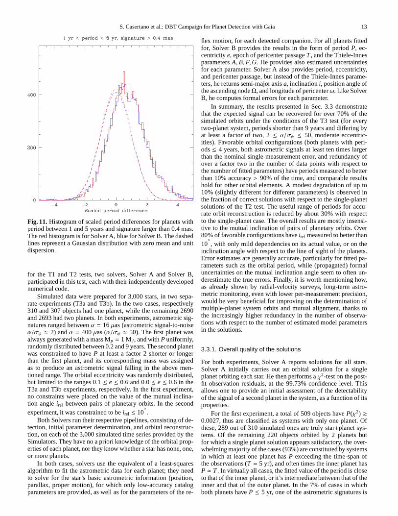
Fig. 15. True distributions for planet 1 and 2 (solid histogram) compared with the same distributions derived by Solver A (top twopanels) and Solver B (bottom two panels) when the fitted values of the periods lie within 10% of the simulated values.
results from the T2 experiment are over-plotted, after constrain-ing orbital periods, eccentricities, and astrometric signals to liein the same ranges of the T3b experiment (P ≤ 9 yr,e ≤ 0.6, andα ≤ 400µas).
Overall, the quality of the solutions degrades quickly alreadyfor periods≥ 2 years, and the fraction of systems with both or-bital periods recovered to within 10% of the true value is at least5%-10% lower than the single-planet case. For configurations inwhich both planets haveP ≤ 5 yr, α/σψ ≥ 10, and for whicha numberNoss ≥ 45 of observations are carried out over the 5-yr simulated mission lifetime (bottom right panel), the situation
improves significantly. Over 90% of all orbital configurationshave both periods measured to better than 10%, and the 5%-10%deficit with respect to the T2 experiment applies for periodsinthe range 0.2 ≤ P ≤ 4 yr, for both planets in the systems. A verysimilar behavior is observed (but not shown) in the T3a experi-ment, in which no constraints are put on the mutual inclinationangles.
Formal errors from the fitting procedure appear to match theactual errors reasonably well. To determine more quantitativelyhow good an approximation the estimated errors are for the trueones, we utilize the same metric adopted in the T2 experiment,

S. Casertano et al.: DBT Campaign for Planet Detection with Gaia 17
Fig. 16. Fraction of systems with good orbital solutions (P(χ2) ≥ 0.0027) in the T3b experiment for which both orbital periods arerecovered by Solver A with a fractional uncertainty≤ 10%, as a function of period (0.5-yr bins). For comparison, the same resultsare displayed for the T2 test. Top left: all stars. Top right:systems with both periods≤ 5 yr. Bottom left: systems with both periods≤ 5 yr, and withα/σψ ≥ 10. Bottom right: systems with both periods≤ 5 yr,α/σψ ≥ 10, and withNoss≥ 45.
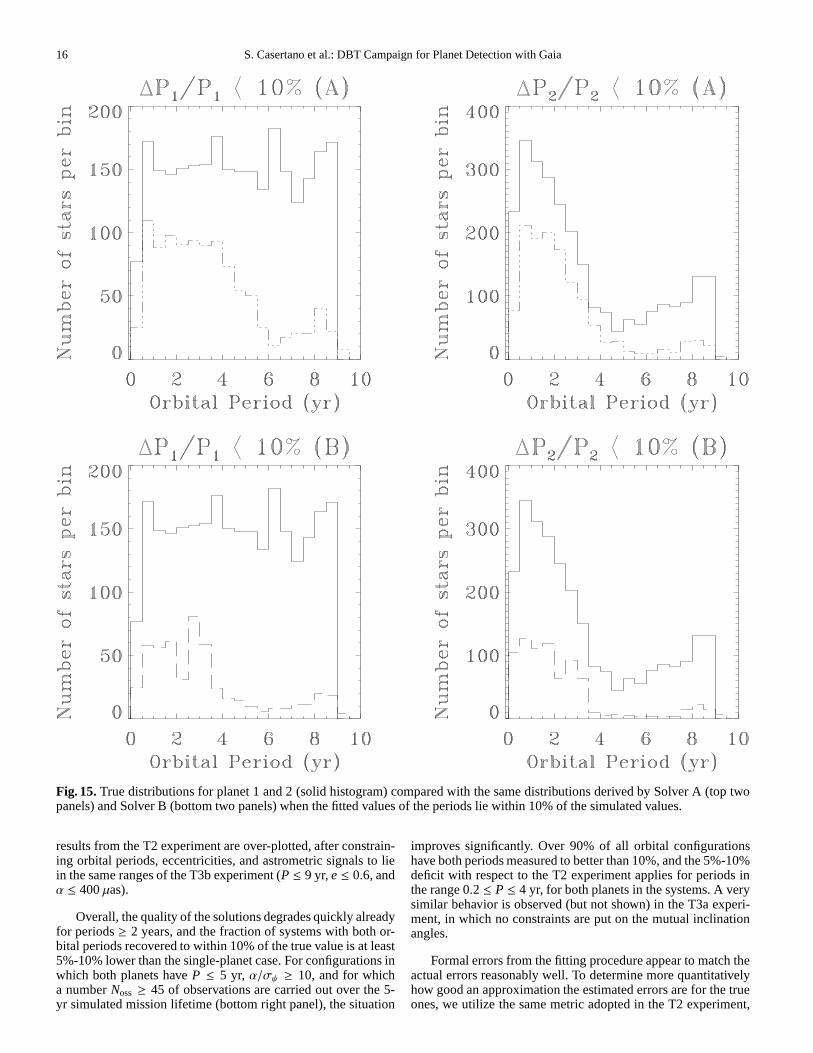
i.e. the scaled difference∆Pj/σPj ( j = 1, 2) defined as the ratiobetween the fitted and the true value of the orbital period of thej-th planet and its corresponding formal uncertainty. We limitourselves to the sample of stars for which Solver A obtains goodsolutions (99.73% confidence level), and for which orbital pe-riods are recovered to within 10% accuracy. Figure 17 showsthat, for both planets, and in both the T3a and T3b experiment,the distributions of scaled period differences are quite close tothe predicted value (a Gaussian with zero mean and unit disper-sion). A small shift in the peak of the∆P/σP distribution for thesecond planet in the T3b test might be present, but its statisticalsignificance is low. Elevated tails, however, indicate thata non-negligible fraction of objects have underestimated periods (7%of the objects lie above the 3-σ, and 2% above the 5-σ thresholdout of the scale of the plot in Figure 17).
Finally, the two panels of Figure 18 show results for the ec-centricities of both planets in the systems. Displayed are the frac-tions of systems with good orbital solutions for which the fittedvalues ofe are within 0.05 of the true value, the left panel dis-playing results from the full sample with good orbital solutions,and the right after applying the above-mentioned constraints onperiods, astrometric signal, and number of observations. Overall,for both planets a degradation of∼ 20% between the single-planet and the two-planet solutions is observed, independentlyof the actual value ofe. Favorable configurations havee deter-mined within 0.05 of the true value about 80% of the time, withadegradation of∼ 10% with respect to the single-planet solutionsof the T2 test, in line with what is found for the orbital periods.The modest degradation of∼ 5%− 10% in the fraction of well-measured periods and eccentricities with respect to the result ofthe T2 test is likely due to the increased number of parameters
18 S. Casertano et al.: DBT Campaign for Planet Detection with Gaia
Fig. 18. Left: Fraction of systems with good orbital solutions (P(χ2) ≥ 0.0027) in the T3b experiment for which both eccentricitiesare determined within 0.05 of the true values. For comparison, analogous results for the T2 test sample are displayed. Left: all stars.Right: systems with both periods≤ 5 yr, withα/σψ ≥ 10, and withNoss≥ 45.
Fig. 17. Histogram of scaled period differences∆P/σP for goodtwo-planet fits (P(χ2) ≥ 0.0027) with periods accurate to betterthan 10% for the T3a (green solid and dashed lines) and T3b(red solid and dashed lines) experiments. The dotted curvesarereference Gaussians with zero mean and unit dispersion.
in the two-planet fits (19 vs. 12 in the single-planet solutions),given the same number of observations. Other orbital parame-ters follow similar patterns. And again, essentially identical re-sults are obtained for the T3a test, demonstrating that the rela-tive alignment between pairs of planetary orbits does not seemto play a significant role in terms of the ability of Solver A’salgorithm to reconstruct with good accuracy the orbits of bothplanets, under favorable conditions.
3.3.4. Coplanarity measurements
The mutual inclinationirel of two orbits is defined as the anglebetween the two orbital planes, and is given by the formula:
cosirel = cosiin cosiout + siniin siniout cos(Ωout− Ωin), (1)
whereiin andiout, Ωin andΩout are the inclinations and linesof nodes of the inner and outer planet, respectively. The value ofirel is thus a trigonometric function ofi andΩ of both planets,and the latter two are in turn derived as non-linear combinationsof the four Thiele-Innes elements, which are the actual parame-ters fitted for in the orbital solutions. It is thus conceivable thatany uncertainties in the determination of the linear parameters inthe two-planet solutions might propagate in a non-trivial manneronto the derived value ofirel, and consequently a value of mu-tual inclination angle close to the truth might be more difficult toobtain.
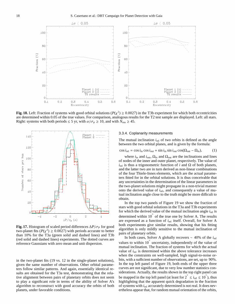
In the top two panels of Figure 19 we show the fraction ofstars with good orbital solutions in the T3a and T3b experimentsfor which the derived value of the mutual inclination angleirel isdetermined within 10
of the true one by Solver A. The results
are expressed as a function ofirel itself. Overall, for Solver Aboth experiments give similar results, showing that his fittingalgorithm is only mildly sensitive to the mutual inclination ofpairs of planetary orbits.
In both cases, Solver A globally recovers∼ 40% of theirel
values to within 10
uncertainty, independently of the value ofmutual inclination. The fraction of systems for which the actualvalue ofirel is determined within the above tolerance increaseswhen the constraints on well-sampled, high signal-to-noise or-bits, with a sufficient number of observations, are set, up to 90%.In the top left panel of Figure 19, both ends of the upper threecurves are not significant, due to very low number statisticscon-siderations. Actually, the results shown in the top right panel canbe mapped in the top left panel (at least for 2
≤ irel ≤ 10
), thus
highlighting that the apparent quick degradation in the fractionof systems withirel accurately determined is not real. It does nev-ertheless appear that, for random mutual orientation of theorbits,
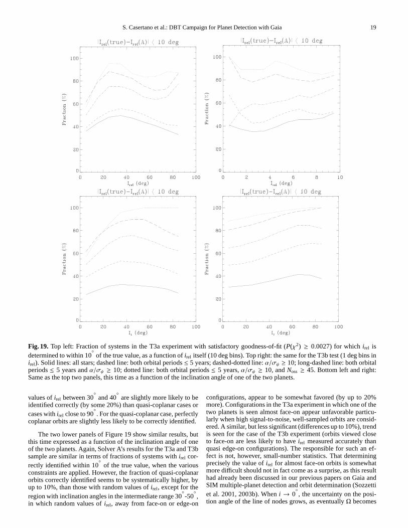
S. Casertano et al.: DBT Campaign for Planet Detection with Gaia 19
Fig. 19. Top left: Fraction of systems in the T3a experiment with satisfactory goodness-of-fit (P(χ2) ≥ 0.0027) for whichirel isdetermined to within 10
of the true value, as a function ofirel itself (10 deg bins). Top right: the same for the T3b test (1 deg bins in
irel). Solid lines: all stars; dashed line: both orbital periods≤ 5 years; dashed-dotted line:α/σψ ≥ 10; long-dashed line: both orbitalperiods≤ 5 years andα/σψ ≥ 10; dotted line: both orbital periods≤ 5 years,α/σψ ≥ 10, andNoss ≥ 45. Bottom left and right:Same as the top two panels, this time as a function of the inclination angle of one of the two planets.
values ofirel between 30
and 40
are slightly more likely to beidentified correctly (by some 20%) than quasi-coplanar cases orcases withirel close to 90
. For the quasi-coplanar case, perfectly
coplanar orbits are slightly less likely to be correctly identified.
The two lower panels of Figure 19 show similar results, butthis time expressed as a function of the inclination angle ofoneof the two planets. Again, Solver A’s results for the T3a and T3bsample are similar in terms of fractions of systems withirel cor-rectly identified within 10
of the true value, when the various
constraints are applied. However, the fraction of quasi-coplanarorbits correctly identified seems to be systematically higher, byup to 10%, than those with random values ofirel, except for theregion with inclination angles in the intermediate range 30
-50,
in which random values ofirel, away from face-on or edge-on
configurations, appear to be somewhat favored (by up to 20%more). Configurations in the T3a experiment in which one of thetwo planets is seen almost face-on appear unfavorable particu-larly when high signal-to-noise, well-sampled orbits are consid-ered. A similar, but less significant (differences up to 10%), trendis seen for the case of the T3b experiment (orbits viewed closeto face-on are less likely to haveirel measured accurately thanquasi edge-on configurations). The responsible for such an ef-fect is not, however, small-number statistics. That determiningprecisely the value ofirel for almost face-on orbits is somewhatmore difficult should not in fact come as a surprise, as this resulthad already been discussed in our previous papers on Gaia andSIM multiple-planet detection and orbit determination (Sozzettiet al. 2001, 2003b). Wheni → 0
, the uncertainty on the posi-
tion angle of the line of nodes grows, as eventuallyΩ becomes

20 S. Casertano et al.: DBT Campaign for Planet Detection with Gaia
Fig. 20. Top left and right: Same as the two upper panels of Figure 19, but for the formal uncertainties onirel as calculated bypropagating the formal errors on the Thiele-Innes elementsfrom the covariance matrix of the solutions. Bottom left andright: Sameas the two lower panels of Figure 19, but for the formal uncertainties onirel calculated as for the top two panels.
undefined fori = 0. If one of the two planetary orbits is close
to face-on, butirel is large, then the incorrect identification ofΩis reflected in a poorer determination ofirel. The effect is less se-vere if the two orbits are quasi-coplanar, because in this case, asi → 0
for both planets, the term depending onΩ in equation 1
becomes very small, and ultimately an accurate knowledge ofΩ
is not required.
Finally, in Figure 20 we show the behavior of the nominaluncertainties onirel obtained by propagating the formal errorson the Thiele-Innes elements from the covariance matrix of thesolutions. The results are plotted as a function ofirel (upper pan-els) andi of one of the two planets (lower panels). The nominaluncertainties appear to follow rather closely the actual errors. Wenote, however, that in several cases formal errors seem to under-estimate the real ones. This effect is highlighted by systemati-cally higher fractions of objects with low values of the nominal
errors with respect to the real ones. This mild trend is observedfor all values ofirel andi, and in both experiments.
3.4. Directions for future work
Several complex issues have been left aside in the preliminaryanalyses carried out for all experiments of the double-blind testsprogram, such as correlations between orbital parameters andtheir errors, more thorough investigations of how well formalerrors map the real ones, or in-depth studies of the conditionsin which two-planet orbital fits are more likely to fail (e.g., dueto covariance between proper motion solutions and long-periodorbits). These topics will require rather sophisticated approachesand a more aggressive understanding of correlations and aliasingin orbital parameter space, and significantly larger samplesizes.
Another area of potential improvement concerns the possi-bility to explore alternative methods for orbit fitting to improve

S. Casertano et al.: DBT Campaign for Planet Detection with Gaia 21
on the interpretaton of the observations and ultimately theinfer-ences concerning the overall population of planets. One possiblevenue could be the evaluation of the applicability of Bayesianmodel selection, based on Markov chain Monte Carlo algorithms(e.g., Ford & Gregory 2007), to simulated Gaia data, in ordertogauge their potential for accurate characterization of orbital pa-rameters and their uncertainties.
The understanding of the technical specifications of the Gaiasatellite and its astrometric instrument will develop further withtime, therefore some of the simplifying assumptions in our sim-ulations will be progressively relaxed and a more realisticer-ror model (e.g., including zero-point uncertainties, calibrationserrors, chromaticity effects, attitude error) and a realistic errordistribution forψ, including bias and magnitude terms, adopted.
Finally, there is margin for adding more realism to our ref-erence model of planetary systems, by considering actual distri-butions of orbital parameters and masses, and up-to-date valuesof planetary frequencies. We will include some degree of mu-tual dynamical interactions in representative cases of planetarysystems, and evaluate in detail the impact of possible sources ofastrometric noise that might pollute and/or mimic planetary sig-natures (e.g., binarity of the parent star, stellar spots, and proto-planetary disks, whose impact can be seen in terms of additionaldynamical perturbations as well as contamination by scatteredlight).
4. Discussion: Gaia in context
The striking properties revealed by the observational dataon ex-trasolar planets (for a review, see e.g. Udry et al. 2007) reflectthe complexities inherent in the processes of planet formationand evolution. The comparison between theory and observationhas shown that several difficult problems are limiting at presentour ability to elucidate in a unified manner all the various phases.Rather, one often resorts to attempt to investigate separately lim-ited aspects of the physics of planet formation and evolution us-ing a ‘compartmentalized’ approach.
However, improvements are being made toward the defini-tion of more robust theories capable of simultaneously explain-ing a large range of the observed properties of extrasolar planets,as well as of making new, testable predictions. To this end, helpfrom future data obtained with a variety of techniques will proveinvaluable. In light of the results of the double-blind tests cam-paign presented in the previous sections, we focus here on thepotential of high-precision global astrometry with Gaia, as com-pared to other planet detection methods, to help answer severaloutstanding questions in the science of planetary systems.
4.1. Gaia discovery space
We show in Figure 21 a summary of the results presented in theprevious sections, in terms of the minimum astrometric signa-ture required for detection and measurement of orbital parame-ters and masses with Gaia, as a function of the orbital periodofthe companion, and averaging over all other orbital parameters.
The curves in Figure 21 correspond, respectively, to iso-probability contours for 95% efficiency (virtual completeness)in detection at the 99.73% confidence level, 50% probabilityofmeasuring the companion mass to better than 15% accuracy, andfor the same likelihood of measuring eccentricities with uncer-tainties lower than 0.1 and the inclination angle of the orbitalplane to better than 10
accuracy. All curves are polynomial fits
to the actual iso-probability curves, with extrapolationsfor val-
ues ofP < 0.2 yr andP > 12 yr, i.e. out of the period rangecovered by our simulations. For comparison, the minimum as-trometric signatures (assuming sini = 1) and orbital periods ofthe present-day planet sample are overplotted. The plot, whichclosely resembles those presented in our earlier works (Lattanziet al. 2000a; Sozzetti et al. 2002) indicates that Gaia wouldde-tect∼ 55% of the extrasolar planets presently known (the exactfraction depending on the actual value of sini), and for> 50%of these it would be capable of accurately measuring orbitalpa-rameters and actual masses.
However, ongoing and planned surveys for planets with avariety of techniques are being designed to embrace the three-fold goal of 1) following-up and improving on the characteri-zation of the presently known extrasolar planet sample, 2) tar-geting more carefully defined and selected stellar samples,and3) covering new areas of the planet discovery space, with theultimate expectation of eventually reaching the capability to dis-cover Earth-sized planets in the Habitable Zone (e.g., Kastinget al. 1993) of nearby stars. Indeed, by the time Gaia flies vari-ous other observatories will be operational, gathering additionalinformation on the already known extrasolar planets sampleand producing a wealth of new discoveries. For example, bothground-based as well as space-borne instrumentation for astro-metric planet searches is being developed, such as VLTI/PRIMA(Delplancke et al. 2006) and SIM PlanetQuest, with targetedsingle-measurement precision comparable to, if not higherthan,Gaia’s. Then, the most effective way to proceed in order to gaugethe relative importance of the Gaia global astrometric survey isnot by looking at its discovery potentialper se, but rather in con-nection with outstanding questions to be addressed and answeredin the science of planetary systems, thus helping to discriminatebetween proposed models of planet formation and evolution.
By doing so, one immediately realizes that Gaia’s mostunique contribution will likely reside in the unbiased and com-plete magnitude limited census of stars of all ages, spectral types,and metallicity in the solar neighborhood that could be screenedfor new planets, rather than on the additional insight its mea-surements might give onalready discovered planets. In order toquantify our statement, we convert the results in Figure 21 in theequivalent range of companion masses and semi-major axes thatcould be detected and measured orbiting a star of given mass andat a distance from the Sun. For illustration, we show in Figure 22Gaia’s discovery space in theMp−a plane for 3σ detection (with95% probability) and for accurately measuring> 50% of thetime orbital elements and masses of planets orbiting a 1-M⊙ starat 200 pc, and a 0.5-M⊙ M dwarf at 25 pc (objects withV < 13,for which Gaia’s highest astrometric precision can be achieved).From the Figure, one would then conclude that Gaia could dis-cover and measure massive giant planets (Mp & 2− 3 MJ) with1 < a < 4 AU orbiting solar-type stars as far as the nearest star-forming regions, as well as explore the domain of Saturn-massplanets with similar orbital semi-major axes around late-typestars within 30-40 pc. Particularly for the latter case, theGaiasensitivity nicely complements at wider separations the area ofthe discovery space covered by ground-based transit photometryand decade-long Doppler surveys (see caption for details).
4.1.1. How many planets will Gaia find?
To better gauge the Gaia potential for planet discovery, we up-date the early results of Lattanzi et al. (2000b), and re-computethe number of possible planetary systems within Gaia’s graspusing estimates of the stellar content in the solar neighborhoodand our present-day understanding of the giant planet frequency

22 S. Casertano et al.: DBT Campaign for Planet Detection with Gaia
Fig. 21. Boundaries of secure (≃ 3σ, for σ = 8 µas) detection and accurate mass and orbital parameters determination with Gaiacompared to the known extrasolar planets (data from http://exoplanet.eu), which are plotted for the minimum case: orbit viewededge-on, true mass equals radial velocity minimum mass, andastrometric signature minimum. Lines of different shape representthe minimum astrometric signature for 95% probability of a 3σ detection (solid line), the minimum astrometric signatureneededto determine at least 50% of the time the mass of a planet with better than 15% accuracy (dash-dotted line), the eccentricity withuncertainties< 0.1 (short-dashed line), and the inclination angle with uncertainties< 10
(long-dashed line), respectively. The true
astrometric signature, which is proportional to the true mass, will be generally higher, much higher in some cases, withthe effectthat more reliable detections and orbital fits will be possible.
Table 2. Number of giant planets detected and measured byGaia.
∆d N⋆ ∆a ∆Mp Nd Nm
(pc) (AU) (MJ)
0-50 ∼10 000 1.0 - 4.0 1.0 - 13.0 ∼ 1400 ∼ 700
50-100 ∼51 000 1.0 - 4.0 1.5 - 13.0 ∼ 2500 ∼ 1750
100-150 ∼114 000 1.5 - 3.8 2.0 - 13.0∼ 2600 ∼ 1300
150-200 ∼295 000 1.4 - 3.4 3.0 - 13.0∼ 2150 ∼ 1050
distribution fp. For the former, we use the Besancon model ofstellar population synthesis (Bienayme et al. 1987; Robin&Creze 1986), constrained toV < 13, and for spectral types ear-lier than K5. According to this Galaxy model, we should expectN⋆ ∼ 15 000,∼ 61 000,∼ 175 000, and∼ 470 000 stars withinradii of 50 pc, 100 pc, 150 pc, and 200 pc, respectively (seeFigure 23). Forfp, we take the Tabachnik & Tremaine (2002)approach, and use a power-law functional form to integrate adifferential fraction within an arbitrary range ofMp andP:
d fp = CMβpPγdMpdP (2)
We find the normalizationC by using the Tabachnik &Tremaine (2002) values for the exponents (β = −1.1, γ =−0.73), which still provide a good description for the observed

S. Casertano et al.: DBT Campaign for Planet Detection with Gaia 23
Fig. 22. Gaia discovery space for planets of given mass and orbital radius compared to the present-day sensitivity of other indirectdetection methods, namely Doppler spectroscopy and transit photometry. Red curves of different styles have the same meaning asin Figure 21 assuming a 1-M⊙ G dwarf primary at 200 pc, while the blue curves are for a 0.5-M⊙ M dwarf at 25 pc. The radialvelocity curve (pink line) is for detection at the 3σRV level, assumingσRV = 3 m s−1, M⋆ = 1M⊙, and 10-yr survey duration. Fortransit photometry (green curve), the assumptions of Gaudiet al. (2005) are used, i.e.σV = 5 milli-mag, S/N = 9, M⋆ = 1 M⊙,R⋆ = 1 R⊙, uniform and dense (> 1000 datapoints) sampling. Black dots indicate the inventory of exoplanets as of September 2007.Transiting systems are shown as light-blue filled pentagons. Jupiter and Saturn are also shown as red pentagons.
mass and period distributions of exoplanets (see for exampleButler et al. 2006), and by imposing that the fraction of planetswith 1 ≤ Mp ≤ 15MJ and 2≤ P ≤ 3000 d equals the observed7% for F-G-K normal stars with−0.5 ≤[Fe/H]≤ 0.5 (Marcy etal. 2005).
An estimate of the number of giant planets at a given dis-tanced (in pc) whose astrometric signal could be detected byGaia with 3σ confidence 95% of the time is then given byNd ∼ 0.95× fp × N⋆, whereN⋆ is computed within a sphereof radiusd centered on the Sun for given limiting magnitudeand spectral type, while the value offp is calculated integrat-ing over a specific range of masses and periods. The number ofplanets for which, say, masses will be determined at least 50%of the time with an accuracy of better than 15% will instead be:Nm ∼ 0.50× Nd. The results are summarized in Table 2. Onethen realizes that, based on our present knowledge of giant plan-ets frequencies (Mp > 1 − 3MJ), integrated over a wide rangeof spectral types and metallicities, Gaia could then find∼ 8 000
such objects, and accurately measure masses and orbital param-eters for∼ 4000 of them.
4.1.2. How many multiple-planet systems will Gaia find?
As of December 2007, 24 planet-bearing stars are orbited bymore than one planet, corresponding to∼ 12% of the total sam-ple of RV-detected systems4. However, many systems known tohost one exoplanet show more distant, long-period, sub-stellarcompanions with highly significant but incomplete orbits (withinferred semi-major axis typically beyond 5 AU). Recent anal-yses of these long-term trends (Wright et al. 2007) indicatethat∼ 30% of known exoplanet systems show significant evidence of
4 Johnson et al. (2007) and Setiawan et al. (2008) report possiblemultiple companions around GJ 317 and HD 47536. We elect not toinclude them as their orbits are either only loosely constrained or notyet statistically very significant

24 S. Casertano et al.: DBT Campaign for Planet Detection with Gaia
multiplicity. Considering that the mass distribution of planets in-creases steeply toward lower masses (e.g., Marcy et al. 2005), in-completeness must be considerable between 1.0 and 0.1 Jupiter-masses. Thus, the actual occurrence of multiple planets amongstars having one known planet is likely considerably greater than30%.
We report in Table 3 the relevant parameters of the multiple-planet systems with well-measured orbits known to-date, or-dered by increasing distance of the system from the Sun. Theexpected values of the astrometric signature (αmin) are computedassuming perfectly edge-on, coplanar configurations (sini j = 1,for j = 1, . . . , np). The single-measurement precision isσψ = 8µas for all stars. Of these systems,∼ 50% have more than onecomponent withαmin > 3σψ, ∼ 40% have components withαmin > 3σψ as well asP < 5 − 6 yr, and some 16% have bothαmin > 10σψ as well asP < 5 − 6 yr. Extrapolating from thenumbers obtained in the previous Section and the ones above,one then infers that of the∼ 8000 new planetary systems dis-covered by Gaia,∼ 1000 would have multiplicity greater thanone, and∼ 400− 500 could have orbital parameters and massesmeasured to better than 15%− 20% accuracy.

S. Casertano et al.: DBT Campaign for Planet Detection with Gaia 25
Table 3. List of relevant parameters for known planetary systems.
Planet d M⋆ Mp sini a α(pc) (M⊙) (MJ) (AU) (µas)
GJ 876b 4.72 0.32 1.93 0.21 265.6GJ 876c 0.56 0.13 48.0GJ 876d 0.02 0.02 0.2GJ 581b 6.26 0.31 0.05 0.04 1.0GJ 581c 0.02 0.07 0.6GJ 581d 0.02 0.25 3.1HD 69830b 12.60 0.86 0.03 0.08 0.2HD 69830c 0.04 0.19 0.7HD 69830d 0.06 0.63 3.455 Cncb 13.40 1.03 0.78 0.11 6.755 Cncc 0.22 0.24 3.955 Cncd 3.92 5.26 1534.055 Cnce 0.05 0.04 0.1υ Andb 13.47 1.27 0.69 0.06 2.4υ Andc 1.98 0.83 95.1υ Andd 3.95 2.51 575.347 Umab 13.97 1.03 2.60 2.11 376.747 Umac 1.34 7.73 347.5HD 160691b 15.30 1.08 1.67 1.50 153.0HD 160691c 3.10 4.17 781.1HD 160691d 0.04 0.09 0.2HD 160691e 0.52 0.92 29.1HD 190360c 15.89 1.04 0.06 0.13 0.5HD 190360b 1.50 3.92 365.7HD 128311b 16.60 0.80 2.18 1.10 174.8HD 128311c 3.21 1.76 415.1HD 82943b 27.46 1.18 1.75 1.19 64.7HD 82943c 2.01 0.75 46.6HD 37124c 33.00 0.91 0.68 3.19 75.0HD 37124b 0.61 0.53 11.1HD 37124d 0.60 1.64 33.8HD 11964b 33.98 1.13 0.11 0.23 0.7HD 11964c 0.70 3.17 58.0HD 169830b 36.32 1.40 2.88 0.81 46.0HD 169830c 4.04 3.60 285.4HD 217107b 37.00 1.02 1.33 0.07 2.6HD 217107c 2.50 4.41 292.3HD 12661b 37.16 1.07 2.30 0.83 47.6HD 12661c 1.57 2.56 101.0HD 168443b 37.88 1.06 8.02 0.30 59.8HD 168443c 18.10 3.91 1314.1HD 38529b 42.43 1.39 0.78 0.13 1.7HD 38529c 12.70 3.68 789.4HD 155358b 42.70 0.87 0.89 0.63 15.1HD 155358c 0.50 1.22 16.6HD 202206b 46.34 1.13 17.40 0.83 273.0HD 202206c 2.44 2.55 117.9HIP 14810b 52.90 0.99 3.84 0.07 5.1HIP 14810c 0.76 0.41 5.9HD 74156b 64.56 1.05 1.88 0.29 8.0HD 74156d 0.4 1.04 6.1HD 74156c 8.03 3.85 456.1HD 108874c 68.50 1.00 1.02 2.68 39.9HD 108874b 1.36 1.05 20.9HD 73526b 99.00 1.02 2.90 0.66 18.6HD 73526c 2.50 1.05 25.5
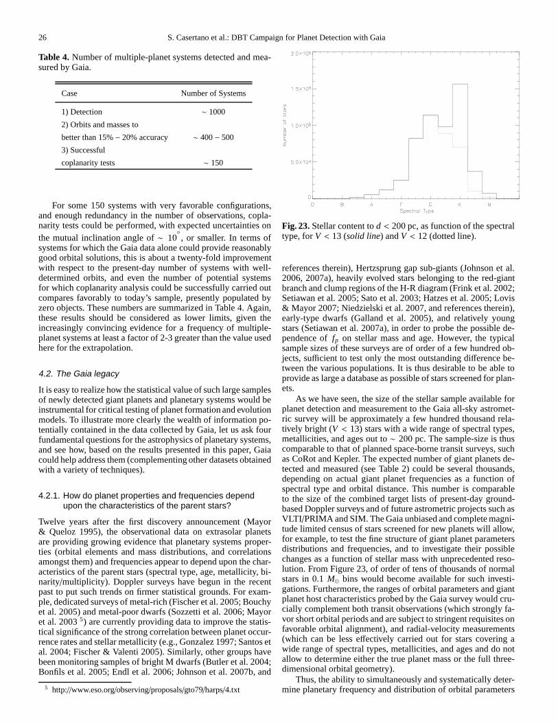
26 S. Casertano et al.: DBT Campaign for Planet Detection with Gaia
Table 4. Number of multiple-planet systems detected and mea-sured by Gaia.
Case Number of Systems
1) Detection ∼ 1000
2) Orbits and masses to
better than 15%− 20% accuracy ∼ 400− 500
3) Successful
coplanarity tests ∼ 150
For some 150 systems with very favorable configurations,and enough redundancy in the number of observations, copla-narity tests could be performed, with expected uncertainties onthe mutual inclination angle of∼ 10
, or smaller. In terms of
systems for which the Gaia data alone could provide reasonablygood orbital solutions, this is about a twenty-fold improvementwith respect to the present-day number of systems with well-determined orbits, and even the number of potential systemsfor which coplanarity analysis could be successfully carried outcompares favorably to today’s sample, presently populatedbyzero objects. These numbers are summarized in Table 4. Again,these results should be considered as lower limits, given theincreasingly convincing evidence for a frequency of multiple-planet systems at least a factor of 2-3 greater than the valueusedhere for the extrapolation.
4.2. The Gaia legacy
It is easy to realize how the statistical value of such large samplesof newly detected giant planets and planetary systems wouldbeinstrumental for critical testing of planet formation and evolutionmodels. To illustrate more clearly the wealth of information po-tentially contained in the data collected by Gaia, let us askfourfundamental questions for the astrophysics of planetary systems,and see how, based on the results presented in this paper, Gaiacould help address them (complementing other datasets obtainedwith a variety of techniques).
4.2.1. How do planet properties and frequencies dependupon the characteristics of the parent stars?
Twelve years after the first discovery announcement (Mayor& Queloz 1995), the observational data on extrasolar planetsare providing growing evidence that planetary systems proper-ties (orbital elements and mass distributions, and correlationsamongst them) and frequencies appear to depend upon the char-acteristics of the parent stars (spectral type, age, metallicity, bi-narity/multiplicity). Doppler surveys have begun in the recentpast to put such trends on firmer statistical grounds. For exam-ple, dedicated surveys of metal-rich (Fischer et al. 2005; Bouchyet al. 2005) and metal-poor dwarfs (Sozzetti et al. 2006; Mayoret al. 20035) are currently providing data to improve the statis-tical significance of the strong correlation between planetoccur-rence rates and stellar metallicity (e.g., Gonzalez 1997; Santos etal. 2004; Fischer & Valenti 2005). Similarly, other groups havebeen monitoring samples of bright M dwarfs (Butler et al. 2004;Bonfils et al. 2005; Endl et al. 2006; Johnson et al. 2007b, and
5 http://www.eso.org/observing/proposals/gto79/harps/4.txt
Fig. 23. Stellar content tod < 200 pc, as function of the spectraltype, forV < 13 (solid line) andV < 12 (dotted line).
references therein), Hertzsprung gap sub-giants (Johnsonet al.2006, 2007a), heavily evolved stars belonging to the red-giantbranch and clump regions of the H-R diagram (Frink et al. 2002;Setiawan et al. 2005; Sato et al. 2003; Hatzes et al. 2005; Lovis& Mayor 2007; Niedzielski et al. 2007, and references therein),early-type dwarfs (Galland et al. 2005), and relatively youngstars (Setiawan et al. 2007a), in order to probe the possiblede-pendence offp on stellar mass and age. However, the typicalsample sizes of these surveys are of order of a few hundred ob-jects, sufficient to test only the most outstanding difference be-tween the various populations. It is thus desirable to be able toprovide as large a database as possible of stars screened forplan-ets.
As we have seen, the size of the stellar sample available forplanet detection and measurement to the Gaia all-sky astromet-ric survey will be approximately a few hundred thousand rela-tively bright (V < 13) stars with a wide range of spectral types,metallicities, and ages out to∼ 200 pc. The sample-size is thuscomparable to that of planned space-borne transit surveys,suchas CoRot and Kepler. The expected number of giant planets de-tected and measured (see Table 2) could be several thousands,depending on actual giant planet frequencies as a function ofspectral type and orbital distance. This number is comparableto the size of the combined target lists of present-day ground-based Doppler surveys and of future astrometric projects such asVLTI /PRIMA and SIM. The Gaia unbiased and complete magni-tude limited census of stars screened for new planets will allow,for example, to test the fine structure of giant planet parametersdistributions and frequencies, and to investigate their possiblechanges as a function of stellar mass with unprecedented reso-lution. From Figure 23, of order of tens of thousands of normalstars in 0.1M⊙ bins would become available for such investi-gations. Furthermore, the ranges of orbital parameters andgiantplanet host characteristics probed by the Gaia survey wouldcru-cially complement both transit observations (which strongly fa-vor short orbital periods and are subject to stringent requisites onfavorable orbital alignment), and radial-velocity measurements(which can be less effectively carried out for stars covering awide range of spectral types, metallicities, and ages and donotallow to determine either the true planet mass or the full three-dimensional orbital geometry).
Thus, the ability to simultaneously and systematically deter-mine planetary frequency and distribution of orbital parameters

S. Casertano et al.: DBT Campaign for Planet Detection with Gaia 27
for the stellar mix in the solar neighborhood without any poten-tial biases induced by the choice of specific selection criteria fortarget lists, stems out as a fundamental contribution that Gaiawill uniquely provide, the only limitations being those intrinsicto the mission, i.e., to the actual sensitivity of the Gaia measure-ments to planetary perturbations, which in this paper we havequantitatively gauged.
4.2.2. What is the preferred method of gas giant planetformation?
Fig. 24. Stellar distribution in the solar neighborhood (d < 200pc) as function metallicity, forV < 13 (solid line) andV < 12(dotted line).
The two main competing models of giant-planet formationby core accretion (e.g., Pollack et al. 1996. For a review seeLissauer & Stevenson 2007) anddisk instability (e.g., Boss 2001.For a review see Durisen et al. 2007) make very different predic-tions regarding formation time-scales (Mayer et al. 2002; Alibertet al. 2005; Boss 2006), planet properties (Armitage et al. 2002;Kornet & Wolf 2006; Ida & Lin 2004a, 2005, 2008; Rice et al.2003b), and frequencies as a function of host star characteris-tics (Laughlin et al. 2004; Ida & Lin 2004b, 2005, 2008; Kornetet al. 2005, 2006; Rice et al. 2003b; Boss 2000, 2002, 2006).Furthermore, correlations between orbital elements and masses,and possibly between the former and some of the host star char-acteristics (metallicity, mass) might reflect the outcome of a vari-ety of migration processes and their possible dependence onen-vironment (Livio & Pringle 2003; Ida & Lin 2004a, 2008; Boss2005; Burkert & Ida 2007). Some of these predictions could betested on firm statistical grounds by extending planet surveys tolarge samples of stars that are not readily accessible to Dopplersurveys.
For example, Galaxy models (Bienayme et al. 1987; Robin& Creze 1986) predict∼ 4000 F–G–K dwarfs and sub-dwarfsto 200 pc, brighter thanV = 13 mag, and with metallicity[Fe/H] < −1.0 (see Figure 24). The entire population will bescreened by Gaia for giant planets on wide orbits thus comple-menting the shorter-period ground-based spectroscopic surveys(e.g., Sozzetti et al. 2006), which are also limited in the samplesizes due to the intrinsic faintness and weakness of the spectrallines of the targets. These data combined would allow for im-proved understanding of the behavior of the probability of planetformation in the low-metallicity regime, by direct comparison
between large samples of metal-poor and metal-rich stars, in turnputting stringent constraints on the proposed planet formationmodels and helping to better the role of stellar metallicityin themigration scenarios for gas giant planets.
Table 5. The closest (≤ 200 pc) star forming regions and youngstellar kinematic groups.
Name Distance (pc) Age (Myr)
Hercules-Lyra 15-40 100AB Doradus 20-50 30-50Subgroup B4 20-50 80-100β Pictoris 30-50 8-15Tucana-Horologium 50-60 8-50TW Hya 50 3-50MBM 12 60-110 3-10η Chamaeleontis 90-150 8-10η Carinæ 100 8MBM 20 110-160 3-10Pleaides 125 75-100 Ophiuchi 125-150 1-2Taurus-Auriga 135 1-2Corona Austrina 140 1-2Lupus 140 1-2o Velorum 160 30ϑ Carinæ 160 30Scorpio-Centaurus 160-180 2-20α Persei 175 85Serpens 200 5-10
Furthermore, within the useful (for Gaia) distance horizonof ∼ 200 pc, hundreds of relatively bright (V < 13− 14) youngstars can be found in some twenty or so nearby star-forming re-gions and young associations (see Table 5 for a list of youngassociations, open clusters, and moving groups in the age range∼ 1 − 100 Myr in the solar neighborhood, with ages in the ap-proximate range 1-100 Myr. The data, ordered by increasing dis-tance from the Sun, are from Zuckermann & Song (2004, andreferences therein) and Lopez-Santiago et al. (2006, and refer-ences therein)). All these stars will be observed by Gaia withenough astrometric precision to detect the presence of massivegiant planets (Mp & 2 MJ) orbiting at 2-4 AU. The possibil-ity to determine the epoch of giant planet formation in the pro-toplanetary disk would provide the definitive observational testto distinguish between the proposed theoretical models. Thesedata would uniquely complement near- and mid-infrared imag-ing surveys (e.g., Burrows 2005, and references therein) for di-rect detection of young, bright, wide-separation (a > 30− 100AU) giant planets, such as JWST.
4.2.3. How do dynamical interactions affect the architectureof planetary systems?
The highly eccentric orbits of planetary systems have been ex-plained so far calling into question a variety of dynamical mech-anisms, such as interactions between a planet and the gaseousdisk, planet-planet resonant interactions, close encounters be-tween planets, secular interactions with a companion star (seefor example Ford & Rasio 2007, and references therein). Someof these eccentricity excitation mechanisms can give rise tovery different orbital architectures, including significantly non-coplanar orbits (Thommes & Lissauer 2003). An effective way to
28 S. Casertano et al.: DBT Campaign for Planet Detection with Gaia
understand their relative roles would involve measuring the mu-tual inclination angle between pairs of planetary orbits. Studiesaddressing the long-term dynamical stability issue for multiple-planet systems (presently divided in three broad classes ofhi-erarchical, secularly interacting and resonantly interacting sys-tems. See for example Kiseleva-Eggleton et al. 2002; Ji et al.2003 and references therein; Correia et al. 2005; Barnes & Quinn2004; Gozdziewski & Konacki 2004 and references therein),as well as the possibility of formation and survival of terres-trial planets in the Habitable Zone of the parent star (Menou&Tabachnik 2003; Jones et al. 2005 and references therein), wouldalso greatly benefit from knowledge of the mutual inclination an-gle between planetary orbits.
The only way to provide meaningful estimates of the fullthree-dimensional geometry ofany planetary system (withoutrestrictions on the orbital alignment with respect to the line ofsight) is through direct estimates of the mutual inclinations an-gles using high-precision astrometry. We have shown here how,extrapolating from today’s knowledge of the frequency and ar-chitectures of multiple-planet systems, Gaia could detectandmeasure several hundred such systems, and perform a significantcoplanarity analysis in a few hundred cases (see Table 4). Thesedata, combined with those available from Doppler measure-ments and transit photometry and transit timing (e.g., MiraldaEscude 2002; Holman & Murray 2005; Agol et al. 2005), wouldthen allow to put studies of the dynamical evolution of planetarysystems on firmer grounds.
4.2.4. What are the phase functions and light curves of gasgiant planets?
The combination of high-cadence, milli-mag photometric and1-5 m s−1 precision radial-velocity measurements of transit-ing planet systems provides the fundamental observationaldata(planetary mass, radius, density, and gravity) needed for amean-ingful comparison with structural models of hot Jupiters (e.g.,Burrows 2005, and references therein). The special geometryof a transiting planet also permits a number of follow-up stud-ies, which in particular have enabled direct observation oftheirtransmission spectra and emitted radiation (Charbonneau et al.2007, and references therein). These data provide the first obser-vational constraints on atmospheric models of these extrasolargas giants (Burrows 2005, and references therein).
The next logical step, the direct detection of extrasolar gi-ant planets using high-contrast imaging instruments, requiresthat their dim light be separated from under the glare of theirbright parent stars. Several theoretical studies (Hubbardet al.2002; Baraffe et al. 2003; Sudarsky et al. 2005; Dyudina et al.2005; Burrows et al. 2004, 2007) have discussed exoplanet ap-parent brightness in reflected host star light (expressed inunitsof the planet/host star flux ratio log(Fpl/Fstar) as functions oforbit geometry, orbital phase, cloud cover, cloud composition,mass and age. In particular, orbit and orientation of an extraso-lar planet play a crucially important role in its flux at the Earthand in its interpretation, with strong dependence on eccentric-ity and inclination (Burrows et al. 2004). Depending upone andi, log(Fpl/Fstar) can be essentially constant (in case ofe ≃ 0.0,
i ≃ 0, for example), or vary by over an order of magnitude (in
case ofe ≃ 0.6, i ≃ 90
for example) along the orbit of an ex-oplanet, and this can induce significant changes in the chemicalcomposition of its atmosphere (e.g., from cloudy to cloud-free).As for the knowledge of the actual mass of the planet, particu-larly at young ages theory predicts changes in intrinsic luminos-
ity by a factor of nearly 100 can occur between objects in themass range 1MJ . Mp . 5 MJ. The few wide-separation sub-stellar companions detected to-date by means of direct imag-ing techniques (Chauvin et al. 2005a, 2005b; Neuhauser et al.2005; Biller et al. 2006), have planetary-mass solutions withintheir error bars, but these mass estimates rely upon so far poorlycalibrated theoretical mass-luminosity relationships, thus theiractual nature (planets or brown dwarfs) remains highly uncer-tain. It is then clear how accurate knowledge of all orbital pa-rameters and actual mass are essential for understanding thethermophysical conditions on a planet and determining its vis-ibility. Recently, the first prediction of epoch and location ofmaximum brightness was derived for the giant planet orbitingǫ Eridani using HST/FGS astrometry in combination with high-precision radial-velocities (Benedict et al. 2006). As of today,there are some 20 RV-detected exoplanets withMp sini > 1 MJ ,P > 1 yr and projected separations> 0.1 arcsec (the typicalsize of the Inner Working Angle of coronagraphic instrumentspresently under study) for which Gaia could provide informa-tion on where and when to observe, and presumably several tensmore will be discovered in the next several years by Dopplersurveys and by Gaia itself. Gaia’s ability to accurately measureorbital parameters (including inclination) and actual mass of aplanet through high-precision astrometric measurements wouldthen provide important supplementary data to aid in the interpre-tation of direct detections of exoplanets.
4.2.5. How common are the terrestrial planets?
With the advent of the new generation of ultra-high precisionspectrographs such as HARPS (e.g., Pepe et al. 2004), radial-velocity programs achieving. 1 m s−1 measurement precisionhave begun detecting around nearby M dwarfs close-in planetswith Mp sini ≃ 5− 10 M⊕ (Rivera et al. 2005; Lovis et al. 2006;Udry et al. 2007), so-called ‘super-Earths’, likely to be mostly‘rocky’ in composition. One of them, GJ 581d (Udry et al. 2007),may orbit within the Habitable Zone of the parent star, depend-ing on the assumed exoplanet atmosphere (Selsis et al. 2007;vonBloh et al. 2007). The announcement of the discovery of a short-period habitable terrestrial planet around a low-mass starmightwell be just around the corner. However, the strongest statisticalconstraints (including bona-fide detections) on the frequency ofEarth-sized habitable planets orbiting Sun-like stars will likelycome from currently operating and upcoming space-borne ob-servatories devoted to ultra-high precision transit photometry,such as CoRot (Baglin et al. 2002) and Kepler (Borucki et al.2003), and very high-precision narrow-angle astrometry, such asSIM (Beichman et al., 2007, and references therein).
The next challenging step will be to directly detect and char-acterize terrestrial, habitable planets orbiting stars very close(d . 25 pc) to our Sun, searching for elements in their at-mospheres that can be interpreted as ‘bio-markers’ (Hitchcok& Lovelock 1967; Des Marais et al. 2002; Seager et al. 2005;Tinetti et al. 2007; Kaltenegger et al. 2007), implying the likelyexistence of a complex biology on the surface. Imaging terres-trial planets is presently the primary science goal of the coro-nagraphic and interferometric configurations of the TerrestrialPlanet Finder (TPF-C & TPF-I) and Darwin missions (Beichmanet al. 2007, and references therein). Ultimately, the final list oftargets will be formulated taking into account constraintscom-ing from the knowledge offp in the terrestrial mass regime,potential stellar host characteristics (spectral type, binarity, sur-face activity), and environment. In this respect, Gaia astrometryof all nearby stars, including the large numbers of M dwarfs,

S. Casertano et al.: DBT Campaign for Planet Detection with Gaia 29
within 25 pc from the Sun will be an essential ingredient in or-der to provide Darwin/TPF with a comprehensive database ofF-G-K-M stars with and without detected giant planets orbit-ing out to several AUs from which to choose additional targetsbased on the presence or absence of Jupiter signposts (Sozzetti etal. 2003b). Such measurements will uniquely complement ongo-ing and planned radial-velocity programs and exo-zodiacaldustemission observations from the ground with Keck-I, LBTI, andVLTI.
5. Summary and conclusions
We have presented results from an extensive program of double-blind tests for planet detection and measurement with Gaia.Themain findings obtained in this study include: a) an improved,more realistic assessment of the detectability and measurabil-ity of single and multiple planets under a variety of conditions,parametrized by the sensitivity of Gaia, and b) an assessment ofthe impact of Gaia in critical areas of planet research, in depen-dence on its expected capabilities.
Overall, the results of our earlier works (Lattanzi et al.2000a; Sozzetti et al. 2001, 2003a) are essentially confirmed,with a fundamental improvement due to the successful devel-opment of independent orbital fitting algorithms applicable toreal-life data that do not utilize any a priori knowledge of the or-bital parameters of the planets. In particular, the resultsof the T1test (planet detection) indicate that planets down to astrometricsignaturesα ≃ 25µas, corresponding to∼ 3 times the assumedsingle-measurement error, can be detected reliably and consis-tently, with a very small number of false positives (dependingon the specific choice of the threshold for detection).
The results of the T2 test (single-planet orbital solutions) in-dicate that: 1) orbital periods can be retrieved with very good ac-curacy (better than 10%) and small bias in the range 0.3 . P . 6yrs, and in this period range the other orbital parameters andthe planet mass are similarly well estimated. The quality ofthesolutions degrades quickly for periods longer than the missionduration, and in particularly the fitted value ofP is systemat-ically underestimated; 2) uncertainties in orbit parameters arewell understood; 3) nominal uncertainties obtained from the fit-ting procedure are a good estimate of the actual errors in theor-bit reconstruction. Modest discrepancies between estimated andactual errors arise only for planets with extremely good signal(errors are overestimated) and for planets with very long period(errors are underestimated); such discrepancies are of interestmainly for a detailed numerical analysis, but they do not touchsignificantly the assessment of Gaia’s ability to find planets andour preparedness for the analysis of perturbation data.
The results of the T3 test (multiple-planet orbital solutions)indicate that 1) over 70% of the simulated orbits under theconditions of the T3 test (for every two-planet system, periodsshorter than 9 years and differing by at least a factor of two,2 ≤ α/σψ ≤ 50, e ≤ 0.6) are correctly identified; 2) favorableorbital configurations (both planet with periods≤ 4 yr and as-trometric signal-to-noise ratioα/σψ ≥ 10, redundancy of over afactor of 2 in the number of observations) have periods measuredto better than 10% accuracy> 90% of the time, and compara-ble results hold for other orbital elements; 3) for these favorablecases, only a modest degradation of up to 10% in the fractionof well-measured orbits is observed with respect to single-planetsolutions with comparable properties; 4) the overall results aremostly insensitive to the mutual inclination of pairs of planetaryorbits; 5) over 80% of the favorable configurations haveirel mea-
sured to better than 10
accuracy, with only mild dependencieson its actual value, or on the inclination angle with respectto theline of sight of the planets; 6) error estimates are generally ac-curate, particularly for fitted parameters, while modest discrep-ancies (errors are systematically underestimated) arise betweenformal and actual errors onirel.
Then, we attempted to put Gaia’s potential for planet detec-tion and measurement in context, by identifying several areas ofplanetary science in which Gaia can be expected, on the basisof our results, to have a dominant impact, and by delineatinga number of recommended research programs that can be con-ducted successfully by the mission as planned. In conclusion,Gaia’s main strength continues to be the unbiased and completemagnitude limited census of stars of all ages, spectral types, andmetallicity in the solar neighborhood that will be screenedfornew planets, which translates into the ability to measure actualmasses and orbital parameters for possibly thousands of plane-tary systems.
The Gaia data have the potential to a) significantly refineour understanding of the statistical properties of extrasolar plan-ets: the predicted database of several thousand extrasolarplanetswith well-measured properties will allow for example to test thefine structure of giant planet parameters distributions andfre-quencies, and to investigate their possible changes as a functionof stellar mass with unprecedented resolution; b) help cruciallytest theoretical models of gas giant planet formation and migra-tion: for example, specific predictions on formation time-scalesand the role of varying metal content in the protoplanetary diskwill be probed with unprecedented statistics thanks to the thou-sands of metal-poor stars and hundreds of young stars screenedfor giant planets out to a few AUs ; c) improve our comprehen-sion of the role of dynamical interactions in the early as wellas long-term evolution of planetary systems: for example, themeasurement of orbital parameters for hundreds of multiple-planet systems, including meaningful coplanarity tests will al-low to discriminate between various proposed mechanisms foreccentricity excitation; d) aid in the understanding of direct de-tections of giant extrasolar planets: for example, actual mass es-timates and full orbital geometry determination (including incli-nation angles) for suitable systems will inform direct imagingsurveys about where and when to point, in order to estimate op-timal visibility, and will help in the modeling and interpretationof giant giant planets’ phase functions and light curves; e)pro-vide important supplementary data for the optimization of theselection of targets for Darwin/TPF: for example, all F-G-K-Mstars within the useful volume (∼ 25 pc) will be screened forJupiter- and Saturn-sized planets out to several AUs, and thesedata will help to probe the long-term dynamical stability oftheirHabitable Zones, where terrestrial planets may have formed, andmaybe found.
We conclude by providing a word of caution, in light of thepossible degradations in the expected Gaia astrometric precisionon bright stars (V < 13). Indeed, refinements in the overall Gaiaerror model (which includes centroiding as well as systematicuncertainties due to a variety of calibration errors) are still pos-sible, and a better understanding of some of the many effects thatneed to be taken into account may help reduce the present-dayend-of-mission scientific contingency margin of∼ 20% whichis included to account for discrepancies that may occur betweenthe simplified error-budget assessment performed now and thetrue performances on real data. However, if ultimately a degrada-tion of 35%−40% in the single-measurement precision on brightstars were to be confirmed, the Gaia science case for exoplanetswould be affected to some degree of relevance. For example, by

30 S. Casertano et al.: DBT Campaign for Planet Detection with Gaia
Table 6. Number of single- and multiple-planet systems detectedand measured by Gaia as a function ofσψ.
σψa (µas) N⋆
b Ndc Nm
d Nd,multe Nm,mult
f Ncoplg
8 500 000 8 000 4 000 1 000 500 15912 148 148 2 370 1 185 296 148 4716 62 500 1 000 500 125 62 1924 18 519 296 148 37 18 540 4 000 64 32 8 4 180 500 8 4 1 0 0
a Single-measurement precisionb Number of stars within the useful distance, assumed to scalewith
the cube of the radius (in pc) of a sphere centered around the Sunc Number of single-planet systems detectedd Number of single-planet systems whose astrometric orbits are mea-
sured to better than 15% accuracye Number of multiple-planet systems detectedf Number of multiple-planet systems with orbits measured to better
than 15%-20% accuracyg number of multiple-planet systems for which successful coplanarity
tests (withirel known to better than 10
accuracy) can be carried out.
simply scaling with the value of the astrometric signal neededfor detection and measurement of the orbital parameters to 15%-20% (α/σψ ∼ 3 − 5, see Figure 21), asσψ increases the sametype of system (same stellar mass, same planet mass, same or-bital period) would be characterized at increasingly shorter dis-tances. A comparison between numbers of detectable and mea-surable single- and multiple-planet systems as a function of in-creasing Gaia single-measurement error is presented in Table 6.Assuming that the number of objects scales with the cube of theradius (in pc) of a sphere centered around the Sun (with no dis-tinction of spectral types), ifσψ degrades from 8µas to 12µas(closer to the present-day estimate) then this would correspondto a reduction of a factor∼ 2 in the distance limit and in a cor-responding decrease in the number of stars available for investi-gation from∼ 5 × 10⁵ to ∼ 1.5× 10⁵. If σψ were to worsen bya factor 2, the number of stars available for planet detection andmeasurement (∼ 6×10⁴) would be reduced by about an order ofmagnitude. Accordingly, the expected numbers of giant planetsdetected and measured would decrease from∼ 4000 to∼ 1200and∼ 500, respectively, and the number of multiple systemsfor which coplanarity could be established would diminish from∼ 160 to∼ 50 and∼ 20, respectively. We conclude that a factor 2degradation in astrometric precision would severely impact mostof Gaia exoplanet science case. We are aware that, instead ofus-ing simple scaling laws, one should provide more quantitativestatements based on new simulations. However, this activity willnecessarily be tied to further developments of the understand-ing of the technical specifications of Gaia and its instruments,and of its observation and data analysis process; therefore, weplan to revisit these issues as needed in the future, depending onthe actual evolution of the knowledge of the Gaia measurementprocess.
Acknowledgements. We are indebted to an anonymous referee for a very care-ful, critical reading of the manuscript, and many useful comments and sugges-tions which helped to greatly improve it. This research has made use of NASA’sAstrophysics Data System Abstract Service and of the SIMBADdatabase, op-erated at CDS, Strasbourg, France. M.G.L. acknowledges support from STScIthrough the Institute’s Visitor Program for 2007. We gratefully acknowledgeINAF (P. Vettolani, Projects Department) for its continuedsupport of the Italianparticipation to the Gaia mission.
References
Agol, E., Steffen, J., Sari, R., & Clarkson, W. 2005, MNRAS, 359, 567Alibert, Y., Mordasini, C., Benz, W., & Winisdoerffer, C. 2005, A&A, 434, 343Armitage, P. J., Livio, M., Lubow, S. H., & Pringle, J. E. 2002, MNRAS, 334,
248Bakos, G.A., et al. 2007, ApJ, 671, L173Baglin, A., et al. 2002, in Radial and Nonradial Pulsations as Probes of Stellar
Physics, eds. C. Aerts, T. R. Bedding, & J. Christensen-Dalsgaard, ASPConf. Ser., 259, 626
Baraffe, I., Chabrier, G., Allard, F., Hauschildt, P.H. 2003, A&A,402, 701Barnes, R., & Quinn, T. 2004, ApJ, 611, 494Bean, J. L., et al. 2007, AJ, 134, 749Beaulieu, J.-Ph., et al. 2006, Nature, 439, 437Beichman, C. A., Fridlund, M., Traub, W. A., Stapelfeldt, K.R., Quirrenbach,
A., & Seager, S. 2007, in Protostars and Planets V, B. Reipurth, D. Jewitt,and K. Keil (eds.), University of Arizona Press, Tucson, 915
Benedict, G. F., et al. 2002, ApJ, 581, L115Benedict, G. F., et al., 2006, AJ, 132, 2206Bienayme, O., Robin, A. C., & Creze, M. 1987, A&A, 180, 94Biller, B. A., Kasper, M., Close, L. M., Brandner, W., & Kellner, S. 2006, ApJ,
641, L141Bond, I., et al., 2004, ApJ, 606, L155Bonfils, X., et al. 2005, A&A, 443, L15Borucki, W. J., et al. 2003, in Future EUV/UV and Visible Space Astrophysics
Missions and Instrumentation, eds. J. C. Blades & O. H. W. Siegmund, Proc.SPIE, 4854, 129
Boss, A. P. 2000, ApJ, 536, L101Boss, A. P. 2001, ApJ, 563, 367Boss, A. P. 2002, ApJ, 567, L149Boss, A. P. 2005, ApJ, 629, 535Boss, A. P. 2006, ApJ, 643, 501Bouchy, F., Pont, F., Santos, N. C., Melo, C., Mayor, M., Queloz, D., & Udry, S.
2004, A&A, 421, L13Bouchy, F., et al. 2005, A&A, 444, L15Burkert, A., & Ida, S. 2007,ApJ, 660, 845Burrows, A., Sudarsky, D., & Hubeny, I. 2004, ApJ, 609, 407Burrows, A. 2005, Nature, 433, 261Burrows, A., Budaj, J., & Hubeny, I. 2007, ApJ, accepted (arXiv:0709.4080)Butler, R. P., Vogt, S. S., Marcy, G. W., Fischer, D. A., Wright, J. T., Henry, G.
W., Laughlin, G., & Lissauer, J. J. 2004, ApJ, 617, 580Butler, R. P., et al. 2006, ApJ, 646, 505Casertano, S., Lattanzi, M. G., Perryman, M. A. C., & Spagna,A. 1996, Ap&SS,
241, 89Casertano, S., & Sozzetti, A. 1999, in in Working on the Fringe: Optical and IR
Interferometry from Ground and Space, ed. S. Unwin & R. Stachnik, ASPConf. Ser. 194, 171
Catanzarite, J., Shao, M., Tanner, A., Unwin, S., & Yu, J. 2006, PASP, 118, 1319Charbonneau, D., Brown, T. M., Burrows, A., & Laughlin, G. 2007, in Protostars
and Planets V, B. Reipurth, D. Jewitt, and K. Keil (eds.), University ofArizona Press, Tucson, 701
Chauvin, G., et al. 2005a, A&A, 438, L25Chauvin, G., et al. 2005b, A&A, 438, L29Collier Cameron, A., et al. 2006, MNRAS, 375, 95Correia, A. C. M., Udry, S., Mayor, M., Laskar, J., Naef, D., Pepe, F., Queloz,
D., & Santos, N. C. 2005, A&A, 440, 751de Felice, F., Lattanzi, M. G., Vecchiato, A., & Bernacca, P.L. 1998, A&A, 332,
1133de Felice, F., Bucciarelli, B., Lattanzi, M. G., & Vecchiato, A. 2001, A&A, 373,
336de Felice, F., Crosta, M. T., Vecchiato, A., Lattanzi, M. G.,& Bucciarelli, B.
2004, ApJ, 607, 580Delplancke, F., et al. 2006, in Advances in Stellar Interferometry, eds. J.D.
Monnier, M. Scholler, & W.C. Danchi, Proc. SPIE, 6268, 27Des Marais, D. J., et al. 2002, Astrobiology, 2, 153Durisen, R. H., Boss, A. P., Mayer, L., Nelson, A. F., Quinn, T., & Rice, W. K.
M. 2007, in Protostars and Planets V, B. Reipurth, D. Jewitt,and K. Keil(eds.), University of Arizona Press, Tucson, 607
Dyudina, U. A., Sackett, P. D., Bayliss, D. D. R., Seager, S.,Porco, C. C.,Throop, H. B., & Dones, L. 2005, ApJ, 618, 973
Endl, M., Cochran, W. D., Kurster, M., Paulson, D. B., Wittenmyer, R. A.,MacQueen, P. J., & Tull, R. G. 2006, ApJ, 649, 436
Eriksson, U., & Lindegren, L. 2007, A&A, 476, 1389ESA 1997, The Hipparcos and Tycho Catalogues, ESA SP-1200Fischer, D. A., & Valenti, J. 2005, ApJ, 622, 1102Fischer, D. A., et al. 2005, ApJ, 620, 481Ford, E. B., & Tremaine, S. 2003, PASP, 115, 1171Ford, E. B. 2004, PASP, 116, 1083

S. Casertano et al.: DBT Campaign for Planet Detection with Gaia 31
Ford, E. B. 2006, PASP, 118, 364Ford, E. B., & Gregory, P. C. 2007, in Statistical Challengesin Modern
Astronomy IV, G.J. Babu and E.D. Feigelson (eds.), ASP Conf.Ser., 371,189
Ford, E. B., & Rasio, F. A. 2007, ApJ, submitted (astro-ph/0703163)Frink, S., Mitchell, D. S., Quirrenbach, A., Fischer, D. A.,Marcy, G. W., &
Butler, R. P. 2002, ApJ, 576, 478Galland, F., Lagrange, A.-M., Udry, S., Chelli, A., Pepe, F., Beuzit, J.-L., &
Mayor, M. 2005, A&A, 444, L21Gaudi, B. S., Seager, S., & Mallen-Ornelas, G. 2005, ApJ, 623, 472Gonzalez G., 1997, MNRAS, 285, 403Gould, A., et al. 2006, ApJ, 644, L37Gozdziewski, K., & Konacki, M. 2004, ApJ, 610, 1093Green, R. M. 1985, Spherical Astronomy, Cambridge University PressHatzes, A. P., Guenther, E. W., Endl, M., Cochran, W. D., Dllinger, M. P., &
Bedalov, A. 2005, A&A, 437, 743Hitchcock, D. R., & Lovelock, J. E. 1967, Icarus, 7, 149Holman, M. J., & Murray, N. W. 2005, Science, 307, 1288Horne, J. H., & Baliunas, S. L. 1986, ApJ, 302, 757Hubbard, W. B., Burrows, A., & Lunine, J. I. 2002, ARA&A, 40, 103Ida, S., & Lin, D. N. C. 2004a, ApJ, 604, 388Ida, S., & Lin, D. N. C. 2004b, ApJ, 616, 567Ida, S., & Lin, D. N. C. 2005, ApJ, 626, 1045Ida, S., & Lin, D. N. C. 2008, ApJ, 673, 487Johnson, J. A., Marcy, G. W., Fischer, D. A., Henry, G. W., Wright, J. T.,
Isaacson, H., & McCarthy, C. 2006, ApJ, 652, 1724Johnson, J. A., et al. 2007a, ApJ, 655, 785Johnson, J. A., Butler, R. P., Marcy, G. W., Fischer, D. A., Vogt, S. S., Wright, J.
T., & Peek, K. M. G. 2007b, ApJ, 670, 833Ji, J., Liu, L., Kinoshita, H., Zhou, J., Nakai, H., & Li, G. 2003, ApJ, 591, L57Jones, B. W., Underwood, D. R., & Sleep, P. N. 2005, ApJ, 622, 1091Kaltenegger, L., Traub, W. A., & Jucks, K. W. 2007, ApJ, 658, 598Kasting, J. F., Whitmire, D. P., & Reynolds, R. T. 1993, Icarus, 101, 108Kiseleva-Eggleton, L., Bois, E., Rambaux, N., & Dvorak, R. 2002, ApJ, 578,
L145Klioner, S. A., & Kopeikin, S. M. 1992, AJ, 104, 897Klioner, S. A. 2003, AJ, 125, 1580Klioner, S. A. 2004, Phys. Rev. D, 69, No. 124001Konacki, M., Maciejewski, A. J., & Wolszczan, A. 2002, ApJ, 567, 566Konacki, M., Torres, G., Jha, S., & Sasselov, D. D. 2003, Nature, 421, 507Konacki, M., Torres, G., Sasselov, D. D., & Jha, S. 2005, ApJ,624, 372Kornet, K., & Wolf, S. 2005, A&A, 454, 989Kornet, K., Bodenheimer, P., Rozyczka, M., & Stepinski, T.F. 2005, A&A, 430,
1133Kornet, K., Bodenheimer, P., & Rozyczka, M. 2006, A&A, 458,661Kovacs, G., et al. 2007, ApJ, 670, L41Lattanzi, M. G., Spagna, A., Sozzetti, A., & Casertano, S. 1997, in Proc. of the
ESA Symposium ‘Hipparcos - Venice ’97’, ESA SP-402, 755Lattanzi, M. G., Spagna, A., Sozzetti, A., & Casertano, S. 2000a, MNRAS, 317,
211Lattanzi, M. G., Sozzetti, A., & Spagna, A. 2000b, in From Extra-solar Planets to
Cosmology: The VLT Opening Symposium, ed. J. Bergeron & A. Renzini(Berlin: Springer-Verlag), 479
Lattanzi, M. G., Casertano, S., Sozzetti, A., & Spagna, A. 2002, in GAIA: AEuropean Space Project, eds. O. Bienayme & C. Turon, EAS PublicationsSeries (EDP Sciences), 2, 207
Lattanzi, M. G., Casertano, S., Jancart, S., Morbidelli, R., Pannunzio, R.,Pourbaix, D., Sozzetti, A., & Spagna, A. 2005, in The Three-DimensionalUniverse with Gaia, eds. C. Turon, K.S. O’Flaherty, & M.A.C.Perryman,ESA SP-576, 251
Laughlin, G., Bodenheimer, P., & Adams, F. C. 2004, ApJ, 612,L73Laughlin, G., Butler, R. P., Fischer, D. A., Marcy, G. W., Vogt, S. S., & Wolf, A.
S. 2005, ApJ, 622, 1182Lindegren, L., & de Bruijne, J. H. J. 2005, in Astrometry in the Age of the Next
Generation of Large Telescopes, ASP Conf. Ser. 338, 25Lissauer, J. J., & Stevenson, D. J. 2007, in Protostars and Planets V, B. Reipurth,
D. Jewitt, and K. Keil (eds.), University of Arizona Press, Tucson, 591Livio, M., & Pringle, J. E. 2003, MNRAS, 346, L42Lovis, C., et al. 2006, Nature, 441, 305Lovis, C., & Mayor, M. 2007, A&A, 472, 657Lopez-Santiago, J., Montes, D., Crespo-Chacon, I., & Fernandez-Figueroa, M.
J. 2006, ApJ, 643, 1160Mandushev, G., et al. 2007, ApJ, 667, L195Marcy, G. W., Butler, R. P., Fischer, D. A., Vogt, S. S., Wright, J. T., Tinney,
C. G., & Jones, H. R. A 2005, Progress of Theoretical Physics Supplement,158, 24
Mayer L., Quinn T., Wadsley J., & Stadel J., 2002, Science, 298, 1756Mayor, M., & Queloz, D. 1995, Nature, 378, 355
McArthur, B. E., et al. 2004, ApJ, 614, L81Menou, C., & Tabachnik, S. 2003, ApJ, 583, 473Miralda-Escude, J. 2002, ApJ, 564, 1019Neuhauser, R., Guenther, E. W., Wuchterl, G., Mugrauer, M., Bedalov, A., &
Hauschildt, P. H. 2005, A&A, 435, L13Niedzielski, A., et al. 2007, ApJ, 669, 1354Pepe, F., et al. 2004, A&A, 423, 385Perryman, M. A. C., et al. 1997, A&A, 323, L49Perryman, M. A. C., et al. 2001, A&A, 369, 339Pollack, J. B., Hubickyj, O., Bodenheimer, P., Lissauer, J.J., Podolack, M., &
Greenzweig, Y. 1996, Icarus, 124, 62Pont, F., Bouchy, F., Queloz, D., Santos, N. C, Melo, C., Mayor, M., & Udry, S.
2004, A&A, 426, L15Pont, F., et al. 2007, A&A, submitted (arXiv:0710.5278)Pourbaix, D. 2002, A&A, 385, 686Rice, W. K. M., Armitage, P. J., Bate, M. R., & Bonnell, I. A. 2003a, MNRAS,
338, 227Rice, W. K. M., Armitage, P. J., Bonnell, I. A., Bate, M. R., Jeffers, S. V., & Vine,
S. G. 2003b, MNRAS, 346, L36Rivera, E., Lissauer, J. J., Butler, R. P., Marcy, G. W., Vogt, S. S., Fischer, D. A.,
Brown, T., Laughlin, G., & Henry, G. W. 2005, ApJ, 634, 625Robin, A. C., & Creze, M. 1986, A&A, 157, 71Santos, N. C., Israelian, G., & Mayor, M. 2004, A&A, 415, 1153Sato, B., et al. 2003, ApJ, 597, L157Seager, S., Turner, E. L., Schafer, J., & Ford, E. B. 2005, Astrobiology, 5, 372Selsis, F., Kasting, J. F., Levrard, B., Paillet, J., Ribas,I., & Delfosse, X. 2007,
A&A, 476, 1373Setiawan, J., Rodmann, J., da Silva, L., Hatzes, A. P., Pasquini, L., von der Luhe,
O., de Medeiros, J. R., Dollinger, M. P., & Girardi, L. 2005,A&A, 437, L31Setiawan, J., Weise, P., Henning, Th., Launhardt, R., Mller, A., & Rodmann, J.
2007a, ApJ, 660, L145Setiawan, J., et al. 2008, in Proceedings of the ESO Workshop“Precision
Spectroscopy in Astrophysics”, eds. L. Pasquini, M. Romaniello, N.C.Santos, & A. Correia, 201
Sozzetti, A., Casertano, S., Lattanzi, M. G., & Spagna A. 2001, A&A, 373, L21Sozzetti, A., Casertano, S., Brown, R. A., & Lattanzi, M. G. 2002, PASP, 114,
1173Sozzetti, A., Casertano, S., Lattanzi, M. G., & Spagna A. 2003a, in Towards
Other Earths: DARWIN/TPF and the Search for Extrasolar TerrestrialPlanets, eds. M. Fridlund & T. Henning, ESA SP-539, 605
Sozzetti, A., Casertano, S., Brown, R. A., & Lattanzi, M. G. 2003b, PASP, 115,1072
Sozzetti, A. 2005, PASP, 117, 1021Sozzetti, A., Torres, G., Latham, D. W., Carney, B. W., Stefanik, R. P., Boss, A.
P., Laird, J. B., & Korzennik, S. G. 2006, ApJ, 649, 428Sudarsky, D., Burrows, A., Hubeny, I., & Li, A. 2005, ApJ, 627, 520Tabachnik, S., & Tremaine, S. 2002, MNRAS, 335, 151Takeuchi, T., Velusamy, T., & Lin, D. N. C. 2005, ApJ, 618, 987Tinetti, G., Rashby, S., & Yung, Y. L. 2007, ApJ, 644, L129Thommes, E. W., & Lissauer, J. J. 2003, ApJ, 597,566Udalski, A., et al. 2005, ApJ, 628, L109Udalski, A., et al. 2007, A&A, submitted (arXiv:0711.3978)Udry, S., et al., 2007, A&A, 469, L43Unwin, S. C., et al. 2007, PASP, submitted (arXiv:0708.3953)Vecchiato, A., Lattanzi, M. G., Bucciarelli, B., Crosta, M., de Felice, F., & Gai,
M. 2003, A&A, 399, 337von Bloh, W., Bounama, C., Cuntz, M., & Franck, S. 2007, A&A, 476, 1365Wright, J. T., et al. 2007, ApJ, 657, 533Zuckerman, B., & Song, I. 2004, ARA&A, 42, 685

32 S. Casertano et al.: DBT Campaign for Planet Detection with Gaia
Appendix A: The Simulated Model
The code for the generation of synthetic Gaia observations of planetary systems is run by the Simulators group.We start by generating spheres ofN targets. Each target’s two-dimensional position is described in the ecliptic reference frame
via a set of two coordinatesλb andβb, called here barycentric coordinates. We linearly update the barycentric position as a functionof time, accounting for the (secular) effects of proper motion (two components,µλ andµβ), the (periodic) effect of the parallaxπ, and the (Keplerian) gravitational perturbations inducedon the parent star by one or more orbiting planets (mutual interactionsbetween planets are presently not taken into account). The model of motion can thus be expressed as follows:
xecl = x0ecl+ xπ,µecl +
np∑
j=1
xK,jecl (A.1)
Where:
x0ecl =
cosβb cosλbcosβb sinλb
sinβb
is the initial position vector of the system barycenter. Thevarious perturbative effects are initially defined in the tangent plane. Theparallax and proper motion terms are contribute as:
xπ,µ =
µλt + πFλ
µβt + πFβ
0
Where the parallax factors are defined utilizing the classicformulation by Green (1985):
Fλ = − sin(λb − λ⊙)
Fβ = − sinβb sin(λb − λ⊙)
andλ⊙ is the sun’s longitude at the given timet. The term describing the Keplerian motion of the j-th planetin the tangent plane is:
xK,j =
xK,jyK,j0
=
j cosϑjj sinϑj
0
,
wherej is the separation andϑj the position angle. The two coordinates xK,j and yK,j are functions of the 7 orbital elements:
xK,j = aj(1− ej cosEj)(cos(νj + ωj) cosΩj − sin(νj + ωj) sinΩj cosij) (A.2)
yK,j = aj(1− ej cosEj)(cos(νj + ωj) sinΩj + sin(νj + ωj) cosΩj cosij), (A.3)
whereij is the inclination of the orbital plane,ωj is the longitude of the pericenter,Ωj is the position angle of the line of nodes,ejis the eccentricity,aj is the apparent semi-major axis of the star’s orbit around the system barycenter, i.e. theastrometric signature.For what concerns Ej , the eccentric anomaly, is the solution to Kepler’s Equation:
Ej − ej sinEj = Mj , (A.4)
with the mean anomaly Mj , expressed in terms of the orbital periodPj and the epoch of the pericenter passageτj :
Mj =2πPj
(t − τj) (A.5)
Finally, the true anomalyνj is a function of the eccentricity and the eccentric anomaly:
νj = 2 arctan
(
1+ ej
1− ej
)1/2
tanEj/2
(A.6)
We then rotate on the ecliptic reference frame by means of thetransformation matrix:
R(λb, βb) =
− sinλb − sinβb cosλb cosβb cosλbcosλb − sinβb sinλb cosβb sinλb
0 cosβb sinβb
The other two vectors in Eq. A.1 are thus defined as:
xK,jecl = R(λb, βb) · xK,j
=
− sinλbj cosϑj − sinβb cosλbj sinϑjcosλbj cosϑj − sinβb sinλbj sinϑj
cosβbj sinϑj
S. Casertano et al.: DBT Campaign for Planet Detection with Gaia 33
xπ,µecl = R(λb, βb) · xπ,µ
=
− sinλbµλt + πFλ − sinβb cosλbµβt + πFβ
cosλbµλt + πFλ − sinβb sinλbµβt + πFβ
cosβbµβt + πFβ
This allows us to write Eq. A.1 in the form:
xecl
yecl
zecl
=
cosβb cosλb − sinλbj cosϑj − sinβb cosλb∑np
j=1 j sinϑj
− sinλbµλt + πFλ − sinβb cosλbµβt + πFβ
cosβb sinλb + cosλb∑np
j=1 j cosϑj − sinβb sinλb∑np
j=1 j sinϑj
+ cosλbµλt + πFλ − sinβb sinλbµβt + πFβ
sinβb + cosβb∑np
j=1 j sinϑj + cosβbµβt + πFβ
Finally, a rotation to the local reference frame defined by the Instantaneous Great Circles is made by means of the transformationmatrix (e.g., ESA 1997):
xIGC = R(λp, βp) · xecl, (A.7)
where:
R(λp, βp) =
− sinλp cosλp 0− sinβp cosλp − sinβp sinλp cosβpcosβp cosλp cosβp sinλp sinβp
andλp, βp are the coordinates of the pole of the IGC at any given time. The resulting vector can be expressed in terms of the twoangular coordinatesψ andη:
xIGC =
xIGCyIGCzIGC
=
cosψ cosηcosη sinψ
sinη
By now expanding in Taylor Series to first order the IGC cartesian position vector of each target, it is possible to derive aset oflinearized equations of condition expressing only the observed abscissaψ as a function of all astrometric parameters and orbitalelements. We formally have:
δxIGC =
n∑
m=1
∂xIGC
∂amdam (A.8)
The n unknownsam represent positions, proper motions, parallax, and the 7⋆ np orbital elements (if the star is not single). Nowconsider that:
δxIGC = δ(xIGC, yIGC, zIGC) = (δ(cosψ cosη), δ(sinψ cosη), δ sinη)
= (− sinψ cosηdψ − sinη cosψdη, cosψ cosηdψ − sinη sinψdη, cosηdη)
= (− sinψ cosηdψ, cosψ cosηdψ, 0)
+(− sinη cosψdη,− sinη sinψdη, cosηdη)
= cosη(− sinψ, cosψ, 0)dψ + (− sinη cosψ,− sinη sinψ, cosη)dη
= cosηdψeψ + dηeη
whereeη andeψ constitute the pair of orthogonal unit vectors in the directions parallel toψ andη, as defined in the tangent plane.We then have:
cosηdψeψ + dηeη =n
∑
m=1
∂xIGC
∂amdam (A.9)
By taking the scalar product witheψ, we obtain the following scalar expression:
cosηdψ = (− sinψ)n
∑
m=1
∂xIGC
∂amdam + (cosψ)
n∑
m=1
∂yIGC
∂amdam (A.10)
If we now define:
cam = (− sinψ)∂xIGC
∂am+ (cosψ)
∂yIGC
∂am, (A.11)
then the linearized condition equation takes the form:
cosηdψ =n
∑
m=1
camdam = F(λ, β, µλ, µβ, π, aj, Pj , τj , ωj ,Ωj , ej , ij), j = 1, . . . , nP (A.12)
For each given target, there will be as many equations of thisform as the number of observation epochs. The quantity dψ = ψobs−ψcatis defined as the difference between the observed and catalog abscissa.