Stochastic evolution of rationality

JEAN-CLAUDE FALMAGNE and JEAN-PAUL DOIGNON

STOCHASTIC EVOLUTION OF RATIONALITY

ABSTRACT. Following up on previous results by Falmagne, this paper investi-gates possible mechanisms explaining how preference relations are created andhow they evolve over time. We postulate a preference relation which is initiallyempty and becomes increasingly intricate under the influence of a random envi-ronment delivering discrete tokens of information concerning the alternatives.The framework is that of a class of real-time stochastic processes having inter-linked Markov and Poisson components. Specifically, the occurence of the tokensis governed by a Poisson process, while the succession of preference relations isa Markov process. In an example case, the preference relations are the variouspossible semiorders on the set of alternatives. Asymptotic results are obtained inthe form of the limit probabilities of any semiorder. The arguments extend to amuch more general situation including interval orders, biorders and partial orders.The results provide (up to a small number of parameters) complete quantitativepredictions for panel data of a standard type, in which the same sample of subjectshas been asked to compare the alternatives a number of times.

KEY WORDS: Biorder, semiorder, Poisson process, Markov chain, random walk

INTRODUCTION

Presumably, a subject or consumer first confronted with a choice sit-uation, be it the selection of a car or that of a political candidate to anelective office, initially knows little about the available alternatives.It is tempting to suppose that the mental structure underlying themanifest choices of a subject evolve over time, from some initial-ly naive state where the subject is indifferent to all the alternativesinto a sophisticated state where this mental structure can be repre-sented by an intricate relation such as a linear order or a semiorder(in the sense of Luce, 1956). In a recent paper (Falmagne, 1993)hereafter referred to as the source paper, we proposed a stochastictheory describing such an evolution, focusing on the case of linearorders. The purpose of the present paper is to apply the same ideasto the case of other types of preference relations, such as semiorders,interval orders or partial orders. (The present paper is self contained,however.) The basic concepts at the core of this work are recalledinformally below.

Theory and Decision 43: 107–138, 1997.c 1997 Kluwer Academic Publishers. Printed in the Netherlands.

108 JEAN-CLAUDE FALMAGNE AND JEAN-PAUL DOIGNON

We assume a naive state that can be represented by the emp-ty relation. The transformations taking place over time result fromthe probabilistic occurence of quantum items of information, called‘tokens’, which are delivered to the subject by the medium at randomtimes. Tokens can arise as a result of a conversation with a neighbor,or features of a TV program presenting a debate on the comparativemerits of the alternatives, or the viewing of a poster (to name buta few possibilities). Note that the occurences of these token eventsare not necessarily meant to be observable, or controllable by theexperimenter: there are too many possible tokens, and their effect onan individual is not easily assessed. A telling analogy with statisticalmechanics was given in the source paper. The status of the tokensresembles that of the particles whose combined effect is postulat-ed, for instance, in the derivation of the Boltzmann distribution orthe Bose–Einstein distribution. The existence of the particles canbe ascertained, but these chance manifestations play no role in thecomputation of the results. In the source paper, these tokens wereformalized as ordered pairs (x,y) of alternatives. In the most impor-tant case, the occurence of a token (x,y) (with x 6= y) signals that ‘xis preferable to y’. The occurence of a token may result in a modifi-cation of some edge of the graph of the preference relation. Generalaxioms were given, casting the theory as a Markov process having asa state space the collection of all preference relations. In other words,the state of the Markov process is the current preference relation ofthe subject. The occurence of the tokens is governed by a Poissonprocess. A special case of the axioms was analyzed in the sourcepaper which entails the existence of a unique ergodic set composedof all the linear orders on the set of alternatives. Asymptotic resultswere formulated and proved. In particular, an explicit formula forthe asymptotic probabilities of all the linear orders was obtained.In other words, the axioms guarantee the asymptotic existence of arandom utility model in the sense of Block and Marschak (1960).This theory provides explicit predictions–up to a small number ofparameters–of data consisting of successive rankings of the alterna-tives in a set by the same subjects at any arbitrarily chosen timest1, � � �, tn. Other types of sequential data (such as binary choices orapproval voting) could also be predicted and were discussed in thesource paper.

STOCHASTIC EVOLUTION OF RATIONALITY 109

The present paper is devoted to a different class of preferencerelations, which includes as special cases the (strict) semiorders,the interval orders, the biorders and the partial orders. We take thesemiorders as our leading example. The semiorders are interestingfor two reasons. For one, the concept of an ‘order with a threshold’has been a concern of economists and other behavioral scientistsfor a long time. In experimental psychology, the name of Fechn-er (1860 / 1966) comes to mind, with his many followers. But thereferences in the economics literature are also numerous (for sur-veys, see Fishburn, 1970, 1985; Roberts, 1970; and Suppes, Krantz,Luce and Tversky, 1989). The second reason is both conceptual andtechnical. A key concept of our approach is that the transformationof an initially naive state into an articulate relation results from theaccumulated effects of token events over time. Two relevant tech-nical features of semiorders are that the empty relation itself is asemiorder, and more importantly, that any semiorder can be trans-formed into another semiorder (on the same set) simply by eitheradding or removing a single pair (see Doignon and Falmagne, 1997and Theorem 3 below), an operation which, in our theory, is inducedby the occurence of a single token. It turns out that these two fea-tures of the semiorders hold for various types of relations, which alsoinclude the partial orders, the interval orders and the biorders (butnot, obviously, the linear orders). This means that the results givenhere will be applicable to many other cases of relations. As in thesource paper, the axioms given here will lead to specific predictionsregarding the asymptotic probabilities of all the relations in any sub-class deemed suitable for a particular empirical setup. This result isapplicable to panel data of a standard type, in which the same sampleof subjects have been asked to compare the alternatives a number oftimes. A discussion on the applicability of this theory to such datawill be given, including detailed statistical considerations.

Two notable differences between this theory and that of the sourcepaper must be pointed out. One concerns the tokens. In the theorydescribed here, the feasible tokens are of two types: positive or neg-ative. Accordingly these tokens are, represented by ‘signed’ orderedpairs of distinct elements. For convenience of notation, we alwayswrite xy for the (ordered) pair (x; y). A positive token is symbolizedby a pair xy signalling that ‘alternative x is preferable to alternative


y’. A negative token is denoted as fxy, which conveys the messagethat ‘x is not preferable to y ’. In both cases, we suppose that x 6= y.The theory will specify how the occurence of a positive token mayresult in the possible addition of the corresponding pair to the prefer-ence relation, and how a negative token may determine the removalof such a pair. In the source paper, no distinction was made betweena positive token xy and a negative token fyx. The introduction of thenegative tokens is a generalization which, on the one hand, rendersthe theory more symmetrical, making some of the results easier tograsp, and on the other hand, opens the possibility of capturing somerevealing aspects of the distribution of the tokens. For instance, ahigh density of the negative tokens could reflect a case of ‘negativecampaigning’ or ‘negative advertising.’ According to the theory, thiswould result in a high proportion of the subjects being in the emptystate or near it, i.e. uninterested or uncommitted.

The second difference from the source paper was implicit in theoutline of the theory given above. We suppose here that the subjectis, in a technical sense, rational from the start and remains rationalthrough all the transformations induced by the occurences of thetokens. In the case of the semiorders, the initially empty state is astrict semiorder because all the defining conditions are vacuouslysatisfied. The occurences of the tokens will transform this emptysemiorder into other semiorders, and may gradually become quiteelaborate. At no time, however, will the state of the subject leave theset of all semiorders. A similar scheme would apply in all the othercases of the theory. By contrast, it was assumed in the source paperthat the ergodic set (i.e. the set of all linear orders) was reachableonly after some meandering in the set of all relations on the set ofalternatives.

It is not the aim of this theory, in its present status, to providea full theoretical account of all the phenomena that can arise whensubjects repeatedly express preferences in real time. This paper dealswith a special case in which the subjects are sampled from a rela-tively homogeneous population, and develop preferences over timeaccording to the same stochastic mechanisms. We believe, however,that this special case is the potential cornerstone of a more compre-hensive theory that would be able to account for all or most of theeffects described in the literature (see e.g. Converse, 1964, 1970;


Feldman, 1989). A number of possible extensions of this theory arediscussed in the paper, which should evoke how such a more generaltheory could be constructed.

Our second section recalls standard concepts on preference rela-tions, and summarizes some results recently obtained by Doignonand Falmagne (1997) in preparation for the theory expounded here.The stochastic aspects of the theory are developed next, and a numberof theoretical results are stated and proved. In passing, we proposea variety of extensions of the so-called Feigin and Cohen distribu-tion (Feigin and Cohen, 1978). The applicability of the theory is thenexamined from a statistical viewpoint. The paper ends with a generaldiscussion of this approach.

WELL GRADED FAMILIES OF PREFERENCE RELATIONS

DEFINITION 1. Let X and Y be two basic finite sets, with Y notnecessarily distinct or disjoint from X . As indicated, we alwayswrite xy to denote a pair (x; y). A pair xy such that x 6= y is calleddisparate. For any relation R from X to Y , that is R � X � Y , wedenote by �R = (X�Y ) nR the complement of R (w.r.t.X�Y ). Moregenerally, the complement of a subsetR of a basic setE is �R = EnR:As is customary, we write R�1 = fxyjyRxg for the converse ofa relation R. The (relative) product of relations R1; R2; . . . ; Rk isdenoted as R1R2 � � �Rk: (Thus, RS = fxyj9z; xRz ^ zSyg, etc.)We will always designate by I the identity relation on the set X [Y ,that is I = fxxjx 2 X [ Y g.

Consider the following three axioms for a relation R from X to Y .For all x; z 2 X and y; w 2 Y ,

(B) if xRy and zRw; then xRw or zRy; (i.e. R �R�1R � R)

(S) if xRy and yRz; then wRz or xRw; (i.e.RR �R�1 � R)(I) :(xRx): (i.e. R \ I = ;)

A compact formulation of each axiom in relative product notationis given in parentheses. With regard to Axiom (S), notice for furtherreference that RR �R�1 � R is equivalent to �R�1RR � R. Supposefirst that X = Y: Condition (I) together with either Condition (B) orCondition (S) imply thatR is transitive. The relationR is an interval


order on X iff it satisfies Axioms (I) and (B). It is a semiorder iff itsatisfies Axioms (I), (B) and (S). Both interval orders and semiordersare strict partial orders (i.e. they are irreflexive and transitive). Thefollowing generalization of interval orders is also of interest. Abiorder between X and Y is any relation R � X � Y satisfyingCondition (B), this time for X and Y possibly distinct or disjoint.Thus, an interval order is nothing but an irreflexive biorder betweena set and itself.

We begin by focusing on the semiorders. The concept of a semi-order is often attributed to Luce (1956) and occupies a prominentplace in ordinal measurement theory. The interest of semiorders liesin part in their numerical representation, which formalizes the ideaof a ‘preference with a threshold’. For example, if R is a semiorderon a finite set X , we can assert the existence of a function f on Xsatisfying, for all x; y 2 X

xRy , f(x) > f(y) + 1

(Suppes and Zinnes, 1963; Suppes et al., 1989.) The relation �R\ �R�1

is called the indifference relation of R. Clearly, the indifferencerelation of a semiorder is reflexive and symmetric, but not necessarilytransitive.

We say that x covers y (for the semiorder R) if x(RnRR)y (that is,if xRy and there is no z such that xRz and zRy). The set of coveringpairs forms the Hasse diagram ofR. Notice in passing that the emptyrelation onX is vacuously a semiorder, with the indifference relationX �X .

A remarkable property of semiorders is the following: if R is asemiorder onX , we can always create another semiorder on the sameset by adding or removing some pair. This is illustrated in Figure 1.At the center of the figure, we have a representation of the semiorderR = fyx; xw; yw; yzgon the setX = fx; y; z; wg. The semiorderRat the center of Figure 1 is represented by its Hasse diagram and thecorresponding indifference relation by the dotted lines. (The loopsare omitted.) The same conventions apply to the representation ofthe two other semiorders in Figure 1, and will be used throughout.

Removing a pair from a semiorder does not always generate asemiorder, however. Three forbidden cases are pictured in Figure 2.(The irrelevant edges are omitted in this figure. We suppose that the


Figure 1. Two examples of semiorders obtained from the semiorder R at thecenter of the figure. The semiorder on the left is obtained by removing the pairyx. The semiorder on the right results from adding the pair xz. For each of thethree semiorders, the solid lines represent the Hasse diagram and the dotted linesrepresent the corresponding indifference relation, omitting the loops.

Figure 2. The three forbidden situations in which removing the pair xy froma semiorder would not yield a semiorder. Note that the representation is notcomplete: only the relevant edges of the Hasse diagram are indicated in each case.

three represented graphs are parts of the Hasse diagrams of threeunspecified semiorders. Note that some vertices may coincide.) Forexample, removing xy from the semiorder of Case A to manufacturethe relation R0 = Rnfxyg would yield the situation

wR0y; xR0z; :(wR0z); :(xR0y);

a contradiction of Condition (B) in the definition of a semiorder inDefinition 1.

It is easy to see that removing the pair xy in Case B or in CaseC would yield contradictions of Condition (S). By gathering thosepairs xy whose removal from a semiorderR yield another semiorder,we define a new relation RI � R; formally

RI = Rn(R �R�1R [ RR �R�1[ �R�1RR):(1)


Figure 3. The three forbidden situations in which adding the pairxy to a semiorderwould not yield a semiorder. The conventions are as in Figure 2.

The interpretation of the three sets removed by the union in theparenthesis of (1) should be clear from Figure 2 and the Axiomsdefining a semiorder. For example, the product R �R�1R correspondsto Axiom (B) and Case A of Figure 1; we cannot remove from Ra pair xy belonging to R �R�1R since this would yield a relationR0 = Rnfxyg that would not satisfy R0 �R0�1R0 � R0. The two otherproducts removed fromR correspond to Axiom (S) and Cases B andC of Figure 2. (Remember that RR �R�1 � R and �R�1RR � R aretwo equivalent versions of Axiom (S).)

The situation concerning a possible addition of a disparate pairxy to a semiorder is symmetrical. Such an addition generates asemiorder except in three cases, which are illustrated by Figure 3.For example, adding xy to the semiorder in Case A’ to manufacturethe semiorder R’ would yield a violation of Condition (B) (seeFigure 3), namely

xR0y; wR0z; :(wR0y); :(xR0z):

Similarly adding xy in either Case B’ or Case C’ would createviolations of Condition (S). Notice the symmetry between the threecases A, B and C of Figure 2 and the corresponding cases of Figure3: any dotted line in Figure 2 is transformed into a solid line in Figure3 and vice versa. All the cases in which the addition of a pair xy toa semiorder R would yield another semiorder are captured by therelation RO defined below:

RO = �Rn(I [ �RR�1 �R [ R�1 �R �R [ �R �RR�1):(2)

Examining the union in right member of Equation (2) should leadthe reader to parsing the exact relationships between each of the four


Figure 4. The 3-semiohedron for the set f1,2,3g. The directed edges and the �ijs refer to a random walk to be described later in this paper.

sets removed, Axioms (I), (B) and (S), and the three Case A’, B’ andC’ of Figure 2.

To sum up, the situation for the semiorders is thus as follows.For any semiorderR, we can always manufacture another semiorderon the same set either by removing a pair from RI , or by addingto R a pair from RO. Notice that RI may be empty (if R = ;).Similarly RO may be empty (when R is a linear order–regarded


as a strict semiorder). But RI [RO is never empty. Moreover, it canbe shown (and will be stated formally later in this paper, cf. Theorem3) that any two semiorders R and S can be linked by a sequenceof semiorders R = R0; R1; . . . ; Rk = S such that for 1 � i � k,we have either Ri = Ri�1 [ fxyg or Ri = Ri�1nfxyg for somepair xy. The number k is exactly the number of pairs by which Rand S differ, namely k = j(RnS) [ (SnR)j. Let S be the familyof all the semiorders on a particular finite set X . The graph havingthe elements of S as vertices, and the pairs (R; S) such that eitherS = R[fxyg orS = Rnfxyg as edges, will be called a semiohedronor more precisely an m-semiohedron if X contains m elements. Apicture of a 3-semiohedron for the set X = f1, 2, 3g is given inFigure 4. Note that there are 19 semiorders (in fact, partial orders)on a set of three elements.

The term ‘semiohedron’ extends in a natural way a terminologyused for linear orders. In combinatorics, the graph of all permutations(or linear orders) on a finite set is sometimes called a permutohedron.The edges of this graph are the pairs of permutations (�; �0) suchthat there is a transposition of adjacent values transforming � into�0 (see e.g. Guilbaud and Rosenstiehl, 1963; Berge, 1968; FeldmanHogaasen, 1969; Le Conte de Poly-Barbut, 1990; references can befound in Bjorner, 1984.)

To avoid repetitions, we postpone a formal statement of these gen-eral results for semiorders, since the situation that we just describedactually holds for many types of relations which includes not onlythe semiorders but also the partial orders, the biorders and the inter-val orders. In the rest of this section, which sets the stage for thestochastic theory at the focus of this paper, we summarize somerecent results of Doignon and Falmagne (1997).

DEFINITION 2. A standard distance d on the family of all subsetsof a set E is obtained by defining d(R; S) = j(RnS) [ (SnR)j forany two subsets R and S. A collection F of subsets of E is wellgraded when, for any R and S in F at distance k, there alwaysexist sets R = F0; F1; . . . ; Fk = S in F such that d(Fi�1; Fi) =1,for i = 1; . . . ; k. This definition applies here to specific families ofrelations regarded as sets of pairs. Well graded families of sets havealso been investigated in the context of knowledge spaces, whichare combinatoric structures playing a role in the design of efficient


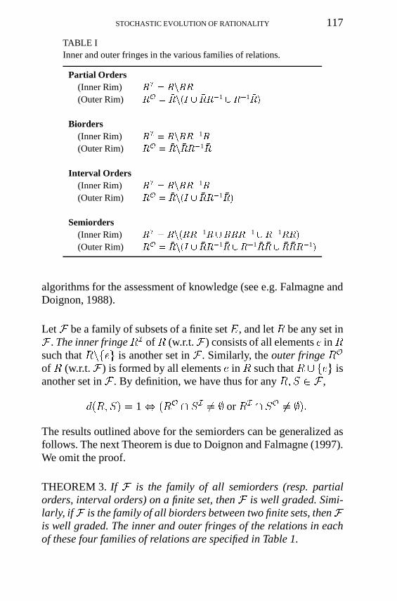
TABLE IInner and outer fringes in the various families of relations.

Partial Orders(Inner Rim) RI = RnRR

(Outer Rim) RO = �Rn(I [ �RR�1 [ R�1 �R)

Biorders(Inner Rim) RI = RnR �R�1R

(Outer Rim) RO = �Rn �RR�1 �R

Interval Orders(Inner Rim) RI = RnR �R�1R

(Outer Rim) RO = �Rn(I [ �RR�1 �R)

Semiorders(Inner Rim) RI = Rn(R �R�1R [ RR �R�1 [ �R�1RR)

(Outer Rim) RO = �Rn(I [ �RR�1 �R [ R�1 �R �R [ �R �RR�1)

algorithms for the assessment of knowledge (see e.g. Falmagne andDoignon, 1988).

Let F be a family of subsets of a finite set E, and let R be any set inF . The inner fringeRI of R (w.r.t.F ) consists of all elements e in Rsuch that Rnfeg is another set in F . Similarly, the outer fringe RO

of R (w.r.t. F ) is formed by all elements e in R such that R [ feg isanother set in F . By definition, we have thus for any R; S 2 F ,

d(R; S) = 1 , (RO\ SI 6= ; or RI

\ SO 6= ;):

The results outlined above for the semiorders can be generalized asfollows. The next Theorem is due to Doignon and Falmagne (1997).We omit the proof.

THEOREM 3. If F is the family of all semiorders (resp. partialorders, interval orders) on a finite set, then F is well graded. Simi-larly, ifF is the family of all biorders between two finite sets, thenFis well graded. The inner and outer fringes of the relations in eachof these four families of relations are specified in Table 1.


BASIC CONCEPTS OF THE THEORY

In keeping with our introductory comments, we suppose that thesubject is initially naive. In order words, the preference relation attime t = 0 is the empty set. We also assume that at some randomtimes t1; t2; . . . ; tn; . . . quantum tokens of information on the alterna-tives and their relationships are delivered by the environment. Thesetokens can be ‘positive’ or ‘negative.’ A positive token conveys amessage such as ‘x is preferable to y’, while a negative token maycarry the meaning that ‘x is not preferable to y’. These two types oftokens are denoted by xy and fxy, respectively (with x 6= y).

We suppose that these positive and negative tokens are deliveredin random fashion by the environment through various means whichare not monitored or controlled by the observer, such as TV commer-cials or programs, newspaper articles or adds, posters, conversations,etc. To represent these phenomena, we postulate the existence of aprobabilistic mechanism with two components. One concerns thetimes of occurence of the tokens, which is assumed to be ruled bya renewal counting process (specifically, a homogeneous Poissonprocess, but this assumption is only critical for part of the predic-tions). The other concerns the nature of the occuring tokens, whichis governed by a probability distribution on the set of all tokens, thisdistribution being characteristic of the environment. The occurenceof a token can affect the current preference relation R—the state ofthe subject—only by adding a single disparate pair toR, or removingsuch a pair from it. A formal statement of the theory is given in thenext definition and in the ensuing list of axioms. Comments followthe definition.

DEFINITION 4. Let X be the finite set of alternatives, and let Sbe a well graded family of (binary) relations on X , containing theempty relation. Examples are the semiorders, the partial orders andthe interval orders. To avoid trivialities, we suppose that jXj > 1.We denote the set of all tokens by

T = T+ [ T�

with

T+ = f� j� = xy for x; y 2 X; x 6= yg;

T� = f� j� = fxy for x; y 2 X; x 6= yg:


A token is called positive or negative depending whether it belongsto T+ or T�.

The preference relations in S are called states. A state may bemodified by the occurence of a token. The arrivals of the tokens attimes t1; t2; . . . ; tn; . . . are governed by a stochastic process. Thesetransitions are specified by the operation � : (R; �) 7! R�� mappingS � T into S, defined by

R � � =

8><>:R [ fxyg if � = xy 2 RO \ T+;Rnfxyg if � = fxy 2 T�and xy 2 RI ;R in all other cases.

(3)

Thus,R � � is the state resulting from the occurence of the token� for an individual previously in stateR. Since, with probability one,the initial state is the empty relation, the occurence of a token willalways result in transforming any relation R in S into some relationR’in S, which may be identical to R. In the case of the semiorder,for example, the token xy transforms the initial state ;, which isvacuously a semiorder, into the semiorder fxyg.

An exemplary sequence of tokens occuring at times t1; . . . ; tn; . . .and their effects on the states, in the case of the semiorders, ispictured by Figure 5. Notice that the token wz presented at time t2

is ignored, because wz is not in the outer fringe of the current statefxyg, regarded as a semiorder. However, if the set of states S hadbeen the set of all partial orders on X , then the occurence of wz attime t2 would have resulted in the partial order fxy; wzg : indeedwz is in the outer fringe of fxyg regarded as a partial order.

We now turn to the probabilistic aspects of the theory. For termi-nology and basic concepts, see Parzen (1962) and Kemeny and Snell(1960). We assume that there exists a positive probability distribution

� : T ! [0; 1] : � 7! ��

on the collection T of tokens. Thus, �� > 0 for any � 2 T , andP�2T �� = 1. The theory will be stated in terms of three collections

of random variables. For any t > 0,

St specifies the state of the individual at time t,Nt indicates the number of tokens arising in the half open interval

of time ]0, t], and


Figure 5. Exemplary sequence of tokens occuring at times t1; t2; . . . ; t5; . . . Thestates are semiorders represented by their Hasse diagrams.

Tt means the last token presented before or at time t; we set Tt = 0if no tokens were presented, that is, if Nt = 0.

We shall also use the random variable

Nt;t+� = Nt+� � Nt

specifying the number of tokens arising in the half-open interval]t; t + �]. Thus, St takes its values in the set S of states; Nt andNt;t+� are nonnegative integers, and Tt 2 T [ f0g. The randomvariable Nt will turn out to be the ‘counting random variable’ of aPoisson process regulating the number of Poisson events occuringin the interval ]0, t].

The three axioms [I], [T] and [L] below define a stochastic process(Nt;Tt; St)t>0 up to the parameters �� ’s (� 2 T ) and one parameter� pertaining to the intensity of the Poisson process.


AXIOM 5. [I] (Initial state). Initially, the state of the individual isthe empty relation. The subject remains in state? until the realizationof the first token. That is, for any t > 0

P(St = ?jN0;t = 0) = 1:

The remaining axioms specify the process recursively. The nota-tion Et stands for any arbitrarily chosen history of the process beforetime t > 0, and E0 denotes the empty history.[T] (Occurence of the tokens). The occurence of the tokens is gov-erned by a homogeneous Poisson process of intensity �. When aPoisson event is realized, the token � occurs with probability �� ,regardless of past events. Thus, for any nonnegative integer k, anyreal numbers t � 0 and � > 0, and any history Et,

P(Nt;t+� = k) =(��)ke��

k!(4)

P(Tt+� = � jNt;t+� = 1; Et) = P(Tt+� = � jNt;t+� = 1) = �� :(5)

[L] (Learning). If R is the state at time t, and a single token � occursbetween times t and t+ �, then the state at time t+ � will be R � �regardless of past events before time t, with the operation � definedas in Equation (3). Formally:

P(St+� = SjTt+� = �;Nt;t+� = 1; St = R; Et)

= P(St+� = SjTt+� = �;Nt;t+� = 1; St = R)

=

(1 if S = R � �;0 otherwise.

The stochastic process defined by Axioms [I], [T], and [L] willbe called the stochastic rationality theory. The special case of thistheory in which the set of states S contains all the semiorders on thefinite set X will be referred to as the stochastic semiorder model. Asimilar terminology will be adopted in the cases of the partial ordersand the interval orders. It is easy to check that–in view of Theorem3–essentially the same axioms would apply in a situation in whichthe set of states contains all the biorders between two finite sets. Thiscase will be labelled the stochastic biorder model.


REMARKS 6. (a) Axiom [L], together with Equation (3) definingthe operation �, forms the core of the theory, and formalize twosimple ideas. One is that the individual is endowed with rationalityin the guise of some well graded family of relations, of which thesemiorders, the partial orders etc. are prime examples. The other isthat the mental structure formalized by the states are rather rigid.They can be altered only minimally at any time. Specifically, thefeasible minimal changes are represented either by the addition ofa single disparate pair to the state, or by the removal of such a pairfrom the state.

(b) Some objections can be levelled against these axioms. Inthe case of a political election, for example, the Poisson processand the probability distribution on the set of tokens reflect the timecourse and the content of the political campaigning. It is unrealistic tosuppose that the only difference between the voters is attributed to thechance occurence of the tokens, the distribution of which is supposedto be the same for all. (The voters read different newspapers, watchdifferent TV programs, have different neighbors and co-workers.) Another objection concerns the homogeneity of the Poisson process. Itwould seem natural to suppose that the intensity of the campaigningchanges in the course of the campaign, with perhaps a peak on theeve of the election. However serious, the objections bear only onsuperficial aspects of the theory. Relatively minor alterations of theaxioms are easy to conceive and to implement, which would takecare of these and some other shortcomings. We shall come back tothese issues in a later section of this paper. In the mean time, thereader should keep in mind that some key asymptotic results do notspecifically depend upon the assumption of a homogeneous Poissonprocess, and would also hold in the much more general setting of anarbitrary renewal process (see in particular Theorem 10).

(c) Finally, we mention that generalizations of this theory areeasily conceivable, in which the elements of the basic wellgradedfamily S are not (necessarily) binary relations, but n-ary relationsor even arbitrary sets. With an appropriately redefined set T oftokens, the developments would remain essentially the same. (Sucha generalization is given in Falmagne, 1997.)


RESULTS

We begin by introducing a useful device.

DEFINITION 7. For a given realization of the Poisson process attimes t1; . . . ; tn; . . ., we partition the time axis into the segments

]0; t1[; [t1; t2[; . . . ; [tn; tn+1[; . . .(6)

such that Nt = 0 for t < t1;Nt = 1 for t1 � t < t2; and in generalNt = n for tn � t < tn+1. Fixing the sequence (tn), and definingS�n = Stn , we obtain a discrete parameter process (S�n) with statespace, S. The process (S�n) will be called the discrete companionof (St). Even though this discrete parameter process is implicitlyindexed by the particular sequence (6) of times of occurence ofPoisson events, in some important sense it does not depend on it.In fact, the situation is that described in the Theorem below, whichfollows immediately from the definitions.

THEOREM 8. The discrete companion (S�n) of (St) is a homoge-neous Markov chain, with state space S and transition probabilitiesdefined, for any distinct R, S in S, with t1; t2; . . . ; tn; tn+1; . . ., as in(6), by

p�R;S = P(S�n+1 = SjS�n = R) = P(Stn+1 = SjStn = R)

=

�� if S = R � �;0 otherwise,

a result which does not depend upon the sequence (tn) associatedwith a particular realization of the Poisson process.

Notice that

P(St+� = SjSt = R)

=1Xk=0

P(St+� = SjNt;t+� = k; St = R)P(Nt;t+� = kjSt = R)

=1Xk=0

P(S�n+k = SjS�n = R)P(Nt;t+� = k):

Writing

p�R;S(k) = P(S�n+k = SjS�n = R)(7)

for the k-step transition probability of the Markov chain (S�n), andusing Equation (4), we obtain the following result:


THEOREM 9. The stochastic process (St) is a homogeneous Markovprocess, with transition probability function

pR;S(�) = P(St+� = SjSt = R)

=1Xk=0

p�R;S(k)(��)ke��

k!:(8)

(Thus, pR;S(�) is the probability of a transition from stateR to stateSin � units of time.) Important aspects of the Markov process (St) canbe investigated via a study of the Markov chain (S�n). In particular,we can use Equation (8) to predict the role of the passage of timeon the evolution of the preference relations. It turns out that theasymptotic probabilities of the states in the Markov chain (S�n) andin the Markov process (St) exist and coincide. The next Theoremspecifies these asymptotic probabilities. We use the notation for anyrelation R 2 S:

R = R [ I = �RnI:(9)

(Notice that ^R = R.)

THEOREM 10. The homogeneous Markov chain (S�n) is irreducibleand aperiodic. In this case, the asymptotic probabilities of the statesexist and form the unique stationary distribution of the Markov chain(S�n). We obtain for any R 2 S:

pR = limt!1

P(St = R) = limn!1

P(S�n = R)

=

Qxy2R �xy �

Qzw2R � ezwP

S2S

Qst2S �st �

Quv2S � euv :(10)

We postpone the proof of this theorem for a moment. Consideringthe structure of S as a well graded family of states, it makes senseto describe the Markov chain (S�n) as a random walk on S.

An example of such a random walk forX =f1, 2, 3gwas presentedin Figure 4. In this situation, there are exactly five different typesof semiorders, as can be seen from the figure. We write S3 for thecollection of all 19 semiorders on X = f1, 2, 3g, and we denote thesemiorders in S3 by �;�0 etc. Setting

K =X�02S3

Yij2�

�ijY

lk2 b�0

�elk;


Equation (10) becomes for these five cases, with distinct i; j; k 2f1, 2, 3g and with obvious notation for the asymptotic probabilitiespR:

p[i�j�k] =1K�ij�eji�ik�eki�jk�ekj;

p[i�j;i�k] =1K�ij�eji�ik�eki�ejk�ekj;

p[j�k;i�k] =1K�ik�eki�jk�ekj�eij�eji

p[i�j] =1K�ij�eji�eik�eki�jk�kj;

p[;] =1K�eij�eji�eik�eki�ejk�ekj:(11)

In the proof of Theorem 10, we use the following well-known result.

LEMMA 11. Let (mR;S)R;S2S be the transition matrix of a regularMarkov chain on a finite set S, and let � : R 7! �R be a probabilitydistribution on S. Suppose that

8R; S 2 S; �R �mR;S = �S �mS;R:

Then � is the unique stationary distribution of the Markov chain.

It suffices to show that �R =P

S2S �S �mS;R for all R 2 S. Weleave to the reader to check the algebra.

Proof (of Theorem 10) 12. The Markov chain (S�n) is irreduciblebecause: (i) S is well graded, and (ii) �� > 0 for any token � . Togeth-er, (i) and (ii) mean that any two states of the Markov chain commu-nicate. To prove that the irreducible Markov chain (S�n) is aperiodic,it suffices to show that p�R;R > 0 for some state R. Since S containsthe empty relation and jXj > 1, there is a state R containing somedisparate pair xy. (For example, we can take R = ; � xy). Wenecessarily have R � xy = R, with p�R;R � �xy > 0. We concludethat the Markov chain (S�n) has a unique stationary distribution.


It remains to show that the stationary distribution is that given byEquation (10). We use Lemma 11, and prove that for any R; S 2 S,writing K for the denominator in (10),

1K

�Qxy2R �xy �

Qzw2R � ~zw

�p�R;S

= 1K

�Qxy2S �xy �

Qzw2S � ~zw

�p�S;R:

(12)

In the Markov chain (S�n), the one-step transition probabilities betweenstate R and state S are given by

p�R;S = �st ^ p�S;R = � ~st if SnR = fstg; for some st 2 X (Case 1)p�R;S = � ~st ^ p�S;R = �st if RnS = fstg; for some st 2 X; (Case 2)p�R;S = p�R;S = 0 if d(R; S) > 1: (Case 3):

In Case 3, the two members of Equation (12) vanish, and it is easy tocheck that in each of Cases 1 and 2, the factors in the two membersof (12) are identical. We leave the verification to the reader.

REMARK 13. (a) Note that the result of Theorem 10 would holdunder much more general hypotheses on the process governing thedelivery of the tokens. The assumption of homogeneity of the Pois-son process plays no useful role in establishing the result. In fact,a much more general class of renewal counting processes can beassumed.

(b) A special case of the probability distribution p : R 7! pRdefined by (10) on the well graded family S is conceptually close toa distribution on a set of linear orders proposed by Mallows (1957,see also Feigin and Cohen, 1978). Fix a particular relation R0 2 S

and define

�� =

8>>>><>>>>:

� if 9 xy = � 2 T+ \ R0;� if 9 xy = � 2 T+ \ R0;� if 9 fxy = � 2 T�with xy 2 R0;� if 9 fxy = � 2 T�with xy 2 R0:

(13)

Replacing the �’s in Equation (10) by the values given by (13), weobtain

pR�jR\R0j � �jR\R0j � �jR\R0j � �jR\R0jP

S2S

��jS\R0j � �jS\R0j � �jS\R0j � �S\R0j

� :


After setting � = � and � = �, this reduces to

pR =�d(R;R0) � �d(R;R0)PS2S �

d(S;R0) � �d(S;R0):(14)

Notice that with m = jXj, we have d(R; S)+ d(R; S) = m(m� 1)for any two relations R; S 2 S. Dividing the numerator and thedenominator of (14) by �m(m�1), we obtain

pR =(�=�)d(R;R0)PS2S(�=�

d(S;R0));(15)

which is similar to Feigin and Cohen’s distribution for linear orders,but applies here to any well-graded family of relations. (The mean-ing of the exponent is different in the two cases though.) The twoparameters of this distribution are thus the distinguished relation R0

and the ratio �=� > 0.

Using Theorem 10 and Theorem 9, an explicit expression can beobtained for the asymptotic joint probability of observing the statesR and S at time t and time t+ �, respectively.

THEOREM 14. Writing, as before, p�R;S(k) for the k-step transitionprobability between the states R and S in the random walk on S, wehave successively

limt!1

P(St = R; St+�=S)= limt!1

[P(St)=R)P(St+�=SjSt=R)]

= pR � pR;S(�)

=

Qxy2R �xy �

Qzw2R � ~zwP

W2S

Qst2W �st �

Quv2W � ~uv

1Xk=0

p�R;S(k)(��)ke��

k!(16)

The proof is straightforward.

APPLICATION TO THE SEMIORDERS

We apply these results in a case in which S is the set of all semiorderson a finite set X . The Markov chain (S�n) is then a random walk on


the semiohedron associated with X . In addition, we suppose that theempirical situation justifies the simplifying assumption

�xy = � eyx(17)

for all disparate pairs xy. The example of the 3-semiohedron wasdisplayed in Figure 4, for the set X = f1, 2, 3g. Only the centrifugaltransitions are indicated in Figure 4 (the center being the emptysemiorder). The opposite transition can be obtained by reversing thearrows in Figure 4, and replacing any transition probability �ij by�ji. As before, we denote a typical semiorder by �, and we write �for the set of all disparate pairs which are also indifferent w. r. t. �.That is

x � y () (:(x � y) ^ :(y � x) ^ x 6= y):

Similar conventions and notations apply to other semiorders appear-ing in the discussion or in the formulas. Those will be denoted�0;� ", etc. Specializing Theorems 10 and 14, we obtain:

THEOREM 15. Suppose that S contains all the semiorders on afinite set X containing at least two elements, and that Equation (17)holds for any disparate pair xy. As an application of Theorem 10,we obtain for the asymptotic probability of any semiorder �:

p� = limt!1

P(St =�)

=

Qxy2� �

2xy

Qzw2� �zwP

�002S

Qxy2�00 �2

xy

Qzw2�00 �zw

(18)

Similarly, using Theorem 14, the asymptotic probability of a jointoccurence of state � at time t and state �0 at time t + � is given bythe formula:

limt!1

P(St = �; St+� =�0) = lim

t!1

[P(St =�)P(St+� =�0jSt =�)]

= p�p�;�0(�)

=

Qxy2� �

2xy

Qzw2� �zwP

�002S

Qxy2�00 �2

xy

Qzw2�00 �zw

1Xk=0

p��;�0(k)

(��)ke��

k!(19)

The proof is immediate. A conspicuous difference between thepair of Equations (10), (16) and the pair (18), (19), respectively, lies


in the squares appearing in the denominators and the numerators ofthe latter two equations. These squares result from the simplifyingassumption �xy = � eyx in (17): each product �xy� exy in (10) has beenreplaced by �2

xy.

REMARKS ON STATISTICAL TESTING. In principle, this theorycan be applied and tested using standard statistical techniques. Anexample is analyzed here for the semiorder model discussed above,in which a chi-square method is used, based on Equation (19). (Weassume thus that �xy = � eyx for every disparate pair xy.) Suppose that2000 potential voters have been asked, on two occasions, to rate ona scale of 0 to 100 three major candidates in a presidential election.(There are many examples of data of this type.) For concreteness,suppose that the first survey was made on April 14th, and the secondon June 30 of the same election year. Thus, the interval betweenthe two surveys is 77 days. Each of the 2000 subjects has giventwo ratings of the three candidates. It is reasonable to only retainthe ordinal information contained in these ratings. Accordingly weconvert any rating r into a semiorder � by the formula

x � y =) r(x) > r(y) + C

in which the constant C is to be determined empirically. This recod-ing results in assigning a pair (�;�0) of semiorders to each subject.Let N(�;�0) be the number of subjects being assigned the pair ofsemiorders (�;�0); we have thus:

P�;�02S N(�;�0) = 2000. We

suppose that at the time of the first survey, all subjects were alreadyfully exposed to the pros and cons regarding each of the three can-didates. This means that asymptotic results can be used in the formof Equation (18).

A statistical test can be derived from the chi-square statistic

X�;�02S

�N(�;�0)� 2000�

�p� � p�;�0(77)

��22000� [p� � p�;�0(77)]

(20)

with p� as in (18) and

p�;�0(77) =1Xk=0

p��;�0(k)

(�77)ke��77

k!:(21)

We use Equation (8) with � = 77. Note that six parameters areused: there are six parameters �xy (these six having sum 1), plus the


intensity parameter � of the Poisson process. Since we have 192 �

1 = 360 data points (independent response frequencies associatedto the 192 pairs of semiorders), the chi-square statistic in (20) has360� 6 = 354 degrees of freedom. The parameters �xy, and � canbe estimated for example by minimizing (20) using an optimizingroutine such as PRAXIS (cf. Powel, 1964; Brent, 1074). In practicethe series in (19) can be replaced by a finite sum, and the individualPoisson probabilities can be replaced by a standard approximation,such as

(77�)ke�77�

k!� (2�)�

12

Z g+(�;k)

g�(�;k)

e�12u

2du

with

g+(�; k) = (k � 77�+ 12)(77�)

12

g�(�; k) = (k � 77�� 12)(77�)

12

(cf. Johnson and Kotz, 1969). Moreover, if q is a large enoughpositive integer, we get

p��;�0(q) � p�

�0 =

Qxy2�0 �xy

Qzw2�0 �zwP

�002S

Qst2�00 �st

Quv2�00 �uv

It follows that (21) can be rewritten in the form of the approximation

p�;�0(77) �q�1Xk=0

p��;�0(k)[�(g+(�; k))� �(g�(�; k))]

+p��0

1Xk=q

(�77)ke��77

k!

in which � stands for the distribution function of a standard normalrandom variable, and the tail of the Poisson distribution in the lastterm can itself be replaced by an approximation such as that proposedby Peizer and Pratt (1968), for example.

In the application of such a test, the number of degrees of free-dom may be smaller than 354, since some grouping of the cells maybe necessary for the convergence of the chi-square statistic. Nev-ertheless, in view of the large number of subjects, the number ofdegrees of freedom will remain large, allowing the use of the normal


approximation to the chi-square to evaluate the goodness of fit. It thefit is satisfactory, the estimated values of the parameters �xy and �provide a quantitative assessment of the campaign. In principle, theparameters may also be used to predict the voters behavior at somelater time.

It must be emphasized that the potential applications of the theoryare by no means limited to the asymptotic predictions discussed inthis section. Admittedly, an application in a non-asymptotic casewould be computationally more difficult. In principle however, suchan application is feasible.

VARIATIONS OF THE THEORY

A number of limitations of this theory were alluded to earlier, whichwe now address. In some situations, the assumptions of the theoryshould be altered, depending on some features of the alternatives, thesubjects or the situation. A few examples are given below, which willevoke other possibilities. For concreteness, these examples are for-mulated in the framework of the semiorder model with the assump-tion �xy = � eyx considered in the last section. Extensions to othercases should be obvious.

ASSESSING THE EFFECT OF A MAJOR EVENT. A variation ofthe application described in the preceding section arises in a slightlydifferent situation. We still have three candidates campaigning for apolitical office. Suppose, however, that the researcher is especiallyinterested in assessing in detail the effect of an important mediaevent such as a debate between the candidates, and that the firstrating was obtained just before the debate, and the second one weeklater. Equation (19) can still be used, but with some modifications.The �xy’s entering in the expression of p� in the equation mustbe regarded as reflecting the probabilities of the tokens before thedebate. A different set of parameters �0xy must be postulated forthe expression of the transition probabilities p�

�;�0(k), since thesetransitions may have been at least in part induced by the debate.In the same vein, the intensity parameter � of the Poisson processshould also reflect the effect of the debate. Moreover, we should set� = 7 (days). If a reasonable fit is obtained, a comparison between


the estimated values of the � and the �’ parameters may provide aquantitative assessment of the effect of the debate. The numbers ofdegrees of freedom in the chi-square statistic is of course decreasedby five points, since five additional parameters have been used topredict the data.

Recalling Remark 13(a) we point out that this prediction does notdepend on the assumption that the delivery of the tokens before thedebate is governed by a homogeneous Poisson process. As indicatedby Equation (19), a homogeneous Poisson process is explicitly usedin the computation of the effect of the debate, in the form of the seriesin that equation. This assumption of homogeneity is not shocking,since it only concerns a short period of seven days. As for the otherfactor in that equation, representing the asymptotic probability of thesemiorder�, a general class of renewal counting processes could bepostulated which would yield the same expression.

FEATURES OF THE ALTERNATIVES. In some situations, thealternatives can be described by features which may play a role inthe predictions. In the political example discussed above, it maybe useful to know that candidate x is a woman in favor of ‘freechoice’, since this may be relevant to the subjects’ preferences.Several elaborations of the theory can be conceived to handle suchcases, and two are sketched here. In both cases, we assume thatthe set of alternatives can be represented as a Cartesian productX = X1 � X2. (Thus, (x1; x2) may represent a woman favoring‘free choice’, while (y1; y2) represents a male candidate advocatingthe ‘pro-life’ option.)

We first consider the possibility that this Cartesian product struc-ture is affecting the delivery of the tokens, which we typically writeas (x1x2; y1y2). A concept of ‘independence of the factors’ could beformalized by a multiplicative decomposition of the token probabil-ities according to the formula:

�x1x2;y1y2 = �(1)x1y1�(2)x2y2

:(22)

for any token (x1x2; y1y2). No change in the axioms of theory wouldbe required, but the number of parameters would decrease substan-tially. A drawback of this formula however, is that the interpretationof the parameters �(i)xiyi(i = 1; 2) in terms of the token events is notclear. A more drastic reformulation would arise from assuming that


the collection of tokens contains ‘single issue’ tokens xy 2 Xi�Xi

for i = 1, 2). The effect of such tokens on the current relation wouldhave to be formalized. In other words, a set of rules could be postulat-ed that amount to redefining the operation � used in the formulationof Axiom [L].

The Cartesian product structure of the tokens could also affect thenature of the preference relation itself, in the sense that the semiordercould reflect a combined effect of the factors. For example, wecould investigate well graded families of ‘conjoint’ semiorders �,satisfying an additive representation

(x1; x2) � (y1; y2)() f1(x1) + f2(x2) > f1(y1) + f2(y2) + C;

where f1 and f2 are real valued functions. (See Luce, 1973, 1978, forsome results regarding such a representation.) We shall not includesuch developments in this paper.

NON-HOMOGENEOUS POISSON PROCESS. The assumptionthat the time of delivery of the tokens is governed by a homogeneousPoisson process can easily be generalized to a much broader class ofrenewal counting processes. An example of how such a process canarise and how predictions can be made was mentioned, but a moresystematic approach can be taken. In a typical election, the intensityof the flow of messages directed to the potential voters increasesover time, with a peak on the eve before the election. A simpleadaption of the theory would consist in replacing the homogeneityassumption of the Poisson process by another, in which the intensityparameter � of the Poisson process increases over time, possiblyexponentially. The asymptotic probabilities of the semiorders givenin Equation (18) would not change, but some computation wouldbe more complicate, such as that involved in the series of Equation(19).

INDIVIDUAL DIFFERENCES. The more serious limitation of thetheory as it is stated here lies in the assumption that all subjects areembedded in the same medium and the only difference between themis to be attributed to the chance events associated with the delivery ofthe tokens. This is at best an approximation. There are two distinctcriticisms here. One concerns the process governing the deliveryof the tokens which, for a sufficiently diverse population, should


not be assumed to be identical for all subjects. The other criticismwould argue against the assumption that all subjects are alike in theirreactions to the tokens. In this regard, note that the theory does notquite state that all subjects react to the tokens the same way sincethe effect of a token depends upon the current preference relation(the state of the subject). Nevertheless, one may wish to have somemechanisms in the theory that would explicitly model individualdifferences concerning both the exposure to the tokens, and theireffects on the subjects.

Both of these criticisms are blunted in a situation in which thesubjects belong to a reasonably homogeneous class, or can be par-tioned into a number of such classes by objective criteria. In the lastcase, the theory can be applied to each class separately. The estimat-ed values of the parameters �� and � can be compared and analyzed,possibly revealing interesting differences between the classes.

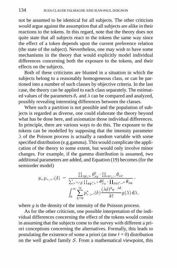
When such a partition is not possible and the population of sub-jects is regarded as diverse, one could elaborate the theory beyondwhat has be done here, and axiomatize those individual differences.In principle, there are various ways to do this. The exposure to thetokens can be modelled by supposing that the intensity parameter� of the Poisson process is actually a random variable with somespecified distribution (e.g.gamma). This would complicate the appli-cation of the theory to some extent, but would only involve minorchanges. For example, if the gamma distribution is assumed, twoadditional parameters are added, and Equation (19) becomes (for thesemiorder model)

p�p�;�0(�) =

Qxy2� �

2xy �

Qzw2� �zwP

�002S

Qxy2�00 �2

xy �Q

zw2�00 �zw�

Z1

0

1Xk=0

p��;�0(k)

(��)ke��

k!g(�) d�;

where g is the density of the intensity of the Poisson process.As for the other criticism, one possible interpretation of the indi-

vidual differences concerning the effect of the tokens would consistin assuming that the subjects come to the survey with different a pri-ori conceptions concerning the alternatives. Formally, this leads topostulating the existence of some a priori (at time t = 0) distributionon the well graded family S. From a mathematical viewpoint, this


modification is a rather trivial one, since Axiom [I] also assumessuch a distribution, but with a mass concentrated on the empty pref-erence relation. Some reflection will convince the reader that, withthis modification, the stochastic process has still the well gradedfamily S as a unique ergodic set. (All the states communicate.) Onecould also suppose that a voter ‘filters’ the flow of tokens deliveredby the environment according to some preconceptions. (The stateof a voter insensitive to women’s issues may be less likely to beaffected by a positive token xy, in which x represents a woman andy a man.) The cases of voters totally impervious to the tokens andresponding either idiosyncratically, or randomly, can be regarded asextreme forms of such filters. In general, the theory can be elaboratedso as to give a formal status to such filters.

As suggested by the above examples, there are a various ways ofincorporating individual differences within the theory, if the situationrequires such developments. Needless to say, the elaborations of thetheory evoked in this section were only meant as illustrations ofsome possibilities.

SUMMARY AND DISCUSSION

We have presented a theory purporting to explain how rationalitycould evolve from a naive state portrayed by the empty relation, to asophisticated state represented by a semiorder or some other kind oforder relation. This evolution was formalized by a stochastic processwith three interlinked parts. One is a Poisson process governing thetimes t1; t2; . . . ; tn; . . . of occurence of quantum events of informa-tion, called tokens, which are delivered by the medium. The secondis a probability distribution on the collection of all possible tokens,which regulates the nature of the quantum event occuring at timetn. Any token is formalized by some pair xy of distinct alternatives,bearing a positive or negative tag. The occurence of a positive tokenxy signals a quantum superiority of x over y, while the correspond-ing negative token fxy indicates the absence of such a superiority. Thelast part of the stochastic process is a Markov process describing thechanges of states occuring in the subject as a result of the occurenceof particular tokens. The state space of the Maskov process is the setof all relations in a well graded family S of relations on the set X


of alternatives, assumed to contain the empty relation. Examples ofwell graded families include the partial orders, the semiorders, thebiorders and the interval orders. The succession of states forms anirreducible Markov chain on S. Asymptotic and sequential predic-tions were derived, which were applied in a special case involvingthe semiorders. The theory is capable of very strong predictions. Forinstance, on the basis of panel type data collected at time t1 and t2, anexact prediction can be made concerning the probability distributionon the set of preference relations at any later time t3.

The axioms governing the transitions of the Markov process(which coincide with the changes of state of the subject), whileapparently technical, were in fact inspired by simple and reason-able ideas. At first, when the preference relation is empty or lean,the subject’s state is easily modified. Most tokens affect the statein a straightforward manner, by adding to or deleting from the cur-rent preference relation the pair corresponding to the token, therebyproducing a new relation in the same well graded family and thuspreserving rationality. These early tokens contribute to the subject’sawareness of the alternatives, and influence the relative situations ofthese alternatives in the cognitive structure of the subject. Over time,however, an increasingly sophisticated state may be achieved whichis endowed with a corresponding amount of rigidity. Few tokens arethen capable of modifying the state. In fact, the current state canonly be affected by tokens concerning pairs xy of alternatives whichare in some sense contiguous with respect to the subject’s currentpreference relation. Accordingly, the addition or the removal of sucha pair would only involve a minimal change of the current relation.Reflecting on the basic mechanism of this theory, we see that it ispartly exogenous, in that the tokens are delivered by the environ-ment, and partly endogenous, in that the effect of the tokens dependupon the subject’s state. This dual nature seems unavoidable.

An obvious alternative to the discrete theory described here wouldbe a continuous analogue in which the effects on a subject of exter-nal events concerning the options would be formalized in terms ofinformative ‘stuff’ of variable magnitude. Such a direction can cer-tainly be taken and may lead to workable predictions in the spirit ofthose obtained here. However, our experience with such dichotomies(quantity of ‘stuff’ vs volley of tokens) suggest that distinguishing


between the two types of theorization on the basis of data may beelusive.

ACKNOWLEDGEMENTS

This work was supported by NSF grant SPR–930–7423 to J.-Cl.Falmagne at University of California, Irvine. We are grateful to BillBatchelder, Dina Blok, Art DeVany, Bernie Grofman and MichelRegenwetter and especially Greg Engl for their reactions to earlierpresentations of this material. The second author thanks the Institutefor Mathematical Behavioral Sciences for its hospitality in July andAugust 1994.

REFERENCES

Berge, Cl: 1968, ‘Principes de Combinatoire’ (translated as: Principles of Combi-natorics. New York: Academic Press, 1971), Dunod, Paris.

Bjorner, A: 1984, ‘Ordering of Coxeter Groups’, Contemporary Mathematics 34,175–195.

Block, H.D. and Marschak, J: 1960, Random Orderings and Probabilistic Theo-ries of Responses; in ‘Contributions to Probability and Statistics’, I. Olkin, S.Ghurye, W. Hoeffding, W. Madow, and H. Mann (Eds.), Stanford UniversityPress, Stanford.

Brent, R.P: 1974, ‘Algorithms for Minimization Without Derivatives’, (2nd. ed.)Prentice Hall, Englewood Cliffs.

Converse, P.E.: 1964, ‘The Nature of Belief Systems in Mass Publics,’ in Ideologyand Discontent D.E. Apter (Ed.), Free Press, New York.

Converse, P.E.: 1970, ‘Attitudes and Non-Attitudes: Contination of a Dialogue’,in The Quantitative Analysis of Social Problems, E.R. Tufte (Ed.), AddisonWesley, Reading Mass.

Doignon, J.-P. and Falmagne, J.-C1.: 1997, ‘Well Graded Families of Relations’,Discrete Mathematics, 173 (1-3), 35–44.

Falmagne, J.-Cl.: 1996, ‘A Stochastic Theory for the Emergence and the Evolutionof Preference Relations’, Mathematical Social Sciences 31, 63–84.

Falmagne, J.-Cl.: 1997, ‘Stochastic Token Theory’, Journal of Mathematical Psy-chology, 41.

Falmagne, J.-Cl. and Doignon, J.-P.: 1988, ‘A Markovian Procedure for Assessingthe State of a System’, Journal of Mathematical Psychology 3, 232–258.

Fechner, G. T.: 1860, ‘Elemente der Psychophysik’ [translated as Elements ofPsychophysics Vol. 1. New York: Holt Rinehart and Winston, 1966], Druck undVerlag von Breitkops Hartel, Leipzig.

Feigin, P. D. and Cohen, A.: 1978, ‘On a Model for the Cocordance BetweenJudges’, Journal of the Royal Statistical Society B 40, 203–213.

Feldman, S.: 1989 ‘Measuring Issue Prefereces: The Problems of Response Insta-bility’ in Political Analysis J.A. Stimson (Ed.), Annual Publication of theMethodology Section of the American Political Science Association, The Uni-versity of Michigan Press, Ann Arbor.


Feldman Hogaasen, J.: 1969, ‘Ordres Partiels et Permutohedre’, Mathematiqueset Sciences Humaines 18, 27–38.

Fishburn, P.: 1970, ‘Intransitive Indifference in Preference Theory: A Survey’,Operations Research 28, 207–228.

Fishburn, P.: 1985, Interval Orders and Interval Graphs, Wiley, New York.Guilbaud, G. Th. and Rosenstiehl, P.: 1963, ‘Analyse Algebriqe d’un Scrutin’,

Mathematiques et Sciences Humaines 3, 9–33.Johnson, N.L. and Kotz, S.: 1969, Distributions in Statistics Discrete Distributions.

Houghton Mifflin, New York.Kemeny, J.G. and Snell, L.: 1960, Finite Markov Chains, Van Nostrand, Princeton.Le Conte de Poly-Barbut, Cl.: 1990, ‘Le Diagramme du Treillis Permutohedre

est Intersection des Diagrammes de Deux Produits Directs d’Ordres Totaux’,Mathematiques, Informatique et Sciences Humaines 112, 49–53.

Luce, R.D.: 1956 ‘Semiorders and a Theory of Utility Discrimination’, Econo-metrica 24, 178–191.

Luce, R.D.: 1973, ‘Three Axiom Systems for Additive Semiordered Structures’,SIAM Journal of Applied Mathematics 25 (1) 41–53.

Luce, R.D.: 1978, ‘Lexicographic Tradeoff Structures’, Theory and Decision 9187–193.

Mallows, C.L.: 1957, ‘Non-null Ranking Models’, Biometrika 44, 114–130.Parzen, E.: 1962, Stochastic Processes, Holden-Day, San Francisco.Peizer, D.B. and Pratt, J.W.: 1968, ‘A Normal Approximation for Binomial F. Beta

and Other Common Related Tail probabilities’, Journal of American StatisticsAssociation 63, 1417–1456.

Powel, M.J.D.: 1964, ‘An Efficient Method for Finding the Minimum of a Functionin Several Variables Without Calculating Derivatives’, Computer Journal 7,155–162.

Roberts, F.: 1970, ‘On Nontransitive Indifference’, Journal of Mathematical Psy-chology 7, 243-258.

Scott, D. and Suppes, P.: 1958, ‘Foundational Aspects of Theories of Measure-ment’, Journal of Symbolic Logic 23, 113–128.

Suppes, P., Krantz, D.K., Luce, R.D., and Tversky, A.: 1989, Foundations ofMeasurement, Vol. 2: Geometrical, Threshold, and Probabilistic Representa-tions,’Academic Press, New York.

Suppes, P. and Zinnes, J.L.: 1963, ‘Basic Measurement Theory’, in Handbookof Mathematical Psychology. Vol. 1. pp. 1–76, R.D. Luce, R.R. Bush and E.Galanter (Eds.), Wiley, New York.

School of Social SciencesUniversity of CaliforniaIrvine, CA 92717 U.S.A.and Universite Libre de BruxellesBrussels, Belgium

Stochastic evolution of rationality

Documents

Transcript of Stochastic evolution of rationality