QAPL 2006

Stochastic Ambient Calculus

Maria G. Vigliotti 1,2 Peter G. Harrison3

Imperial College,London,

UK

Abstract

Mobile Ambients (MA) have acquired a fundamental role in modelling mobility in systemswith mobile code and mobile devices, and in computation overadministrative domains.We present the stochastic version of Mobile Ambients, called Stochastic Mobile Ambients(SMA), where we extendMA with time and probabilities. Inspired by previous models,PEPA andSπ, we enhance the prefix of the capabilities with arate and the ambient witha linear function that operates on the rates of processes executing inside it.The linearfunctions associated with ambients represent the delays that govern particular administrat-ive domains. We derive performance measures from the labelled transition semantics asin standard models. We also define a strong Markov bisimulation in the style of reductionsemantics known as barbed bisimulation. We argue that performance measures are of vitalimportance in designing any kind of distributed system, andthatSMA can be useful in thedesign of the complicated mobile systems.

Key words: Stochastic process algebra, mobility, Markov models.

1 Introduction

Realistic models of distributed, mobile systems include performance measures andquantitative assessments of uncertainty. Performance evaluation is crucial in orderto quantify the behaviour of complex interactive systems with respect to users’quality of service (QoS) constraints [12]. Process algebra is a suitable formalismfor concurrent complex systems, though in its classical development, takes intoaccount only qualitative behaviour; see, for instance,CCS, ACP, CSP. The mainadvantage of process algebra is the compositionality of thedescription of complexsystems: the behaviour of the entire system is derived by thebehaviours of itscomponents.

1 This work has been supported by the EPSRC grant PROFORMA grant GR\ 5451402 Email: mgv98@doc.ic.ac.uk3 Email: pgh@doc.ipc.ac.uk

This paper is electronically published inElectronic Notes in Theoretical Computer Science

URL: www.elsevier.nl/locate/entcs

Vigliotti and Harrison

In the last twenty years, a lot of effort has been made to endowdescriptionsgiven in a process algebraic setting with performance metrics, in order to obtainformal specifications of complex systems. Some stochastic process algebras havebeen proposedPEPA [13], IMC [3], EMPA [1], Sπ [24]. Yet, those models arebased on classical style concurrent languages. In this paper we are concerned withextending stochastic process algebra with more recent generation of calculi. Themain motivation for this work is the attempt to enhance with time and probabilit-ies formal semantics models for networking. Similar work has been carried out byDi Pierro, Hankin and Wiklicky [23] and De Nicola, Latella and Massink [20] forthe process calculus KLAIM. We consider in this paper MobileAmbients (MA).The basic idea underpinningMA is that any kind of computation on the Internet,from accessing web-pages to routing packets, is about crossing physical or virtualboundaries and gaining access to administrative domains.MA aims to representlocations, mobility and administrative domains - conceptsthat were not directlymodelled in previous classical calculi such asCCS, or CSP. The main advantageof MA is the simple underlying, unifying concept ofambient. Ambients are meantto represent administrative domains; they have a tree structure, possibly containingsub-ambients. The notion of access and mobility is capturedby the operational se-mantics, where processes equipped with the appropriate capability can freely enteror exit an ambient.

In the community of programming languages,MA has become very popular[6,7,21,8,29] and different dialects have been proposed, like Safe Ambients [15],Safe Ambients with Passwords [16], Boxed Ambient [4], Robust Ambients [10],and the Push and Pull Ambient Calculus [22], to name but a few. Whilst the qual-itative aspects of computation - equivalence checking, absence of deadlock, non-interference via type systems - are widely studied inMA and its dialects, quantit-ative aspects of computation have been largely neglected sofar.

We believe that sinceMA models mobile distributed computation quite well,adding time and probabilities (i.e. stochastic quantities) to it can be a real benefitto the aim of modelling real life applications.

In this paper we present an extension ofMA with continuous time delays andprobabilities, where the underlying model is Markovian. This implies that, in ourstochastic process algebra, each action is delayed by an amount of time sampledfrom a negative exponential distribution, which yields indirectly, through a racecondition, the probabilities of the choices of the next action to be performed. Wecall this calculus Stochastic Mobile Ambients (SMA). To defineSMA we proceedas in previous models [13,24,12], but we makeparticular and uniqueuse of theprimitive ambient. We augment the prefix of the capabilitieswith a rate λ, i.e.in (n, λ), out (n, λ), open (n, λ), and each ambient with a linear functionf that in-fluences the rate of the computation, i.e.n[P ]f . This means that we can regardeach ambient as running at a particular speed. As in standard(PEPA [13], andSπ [24]), the rates of the prefixes are the only information necessary for specify-ing completely the (random) delay of processes, this sampled from the negativeexponential distribution. The function associated with the ambients influences the

2

Vigliotti and Harrison

delay which governs that particular administrative domain. Thus, when ambientmigrates, its delay is influenced by the the function that governs the parent ambi-ent. This carries a deep meaning in terms of capturing the semantics of distributedsystems. Having localities that run at different speeds is the semantic differencebetween simple concurrent systems and distributed ones. This lies in the fact that,the same process at different localities behaves in different ways.

We also contribute to the paper with the definition ofstochastic strong bisim-ulation [3,13]. The bisimulation defined in this paper is different from standardstochastic bisimulation defined in on labelled transition systems . In ambient calcu-lus in general, purely labelled bisimulation is problematic. Any labelled transition

system has to be second-order, i.e.PP ′

−→P ′′, where the labelP ′ is not a simple ac-tion but a process. It is known from the literature on processalgebra that with thiskind of labelled transition system, it is difficult to define bisimulation [28,27]. TheAmbient calculus is no exception. Thebarbed bisimulation[19], however, takesinto account only reductions via synchronisation, and use aspecial predicate thatentails the point of view of an observer. InCCS it has been proved that labelledand barbed bisimulations are equivalent [19]. In this paper, we define a stochasticstrong bisimulation on top of the barbed one, and we will see that this relation doesyield some interesting laws unique toMA.

The paper is organised as follows: in Section2 we review essential propertiesof Markov processes; in Section3 we present the Stochastic Mobile Ambients: thesyntax and labelled transition system semantics; in Section 4 we show how theMarkov model can be derived; in Section5 we present an application of our work;in Section6 we introduce our notion of strong Markovian bisimulation; the paperconcludes in Section7.

2 Markov Model

2.1 Preliminaries

We first give the basic definitions required for the Markov process that will providethe underlying quantitative model for the Stochastic Mobile Ambients. We do notintroduce the elementary notions of probability theory; the interested reader is re-ferred to [26,11,9] instead. We reserve the capital lettersX, Y, Z to indicaterandomvariables, which are real-valued functions (possibly real vector-valued functions)on some spaceS (in our case, a set of processes), e.g.X : S → IR. We useF, Gfor probability distribution functions.

Definition 2.1 A negative exponential random variableX with rate(or parameter)λ has probability distribution functionF defined by

F (t) ≡ Pr(X ≤ t)def=

1 − e−λt t ≥ 0

0 t < 0

3

Vigliotti and Harrison

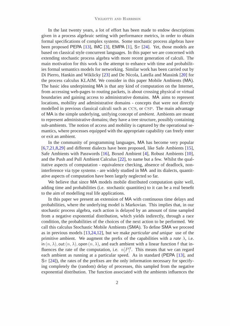
A stochastic processis a family of random variables{X(t) : t ∈ T} whereX(t) takes values in (i.e. has as range) a setS⊂ IRd called itsstate space. Thestate space can be discrete (e.g. integers) or continuous, normally the real num-bers, or (d-fold) product space thereof. The setT is usually interpreted as the time(integer or real). In this paper, we consider non-negative continuous time only.A Markov Process is a stochastic process in which the probabilistic future beha-viour (‘evolution’ of the system) depends only on the current state. In other words,stochastically, the past history of the process does not influence its future behaviour.

Definition 2.2 Consider the state spaceSdef= {si : i ∈ IN}. The family of random

variables{X(t), t > 0} is a Continuous Time Markov Chain (CTMC) with statespaceS if, for all n ∈ IN and for each sequence of time instancest1 < t2 < . . . <tn−1 < tn, we have :

Pr(X(tn) = sn|X(t1) = s1, . . . , X(tn−1) = sn−1) =

Pr(X(tn) = sn|X(tn−1) = sn−1)

The above Markov property is also calledmemoryless, in the sense that theprobability of being in statesn at timetn depends only on the system’s state (sn−1 inthe definition) just after the most recent transition (at time tn−1). It can be formallyproved, that the only continuous distribution that enjoys the memoryless propertyis the exponential one [26,11].

Another well-known property of the exponential distribution is that it is closedunder the minimum operation over a set of random variables. This fact is not truefor the maximum. Moreover, by the memoryless property, the probability that agiven task with exponential duration completes first out of aset of such tasks is theconstant proportional to its rate [26,11].

Proposition 2.3 For 1 ≤ i ≤ n, let Xi be pairwise independent exponentiallydistributed random variables with ratesλi. Then

(i) The random variablemin1≤i≤n(Xi) is exponentially distributed with rate∑n

i=1 λi.

(ii) Pr(min1≤j≤n(Xj) = Xi) = λiPn

j=1λj

.

The importance of continuous time processes is related to the ability of mod-elling systems where changes of state can occur at arbitrarymoments, and wherethe intervals between those changes can be of arbitrary length. In computing, thiscan be interpreted as arrival of jobs at servers, transactions between web-servicesor connection between different mobile devices.

The Markov model is particularly simple to handle from an analytical pointof view, due to the memoryless property. In fact, the memoryless property tellsus that “the future is independent of the past” i.e. the fact that an event has nothappened yet, tells us nothing about how much longer it will take before it doeshappen. The time that a system spends in a certain state is called its sojourntime and, in the Markov model, this sojourn time is exponentiallydistributed inevery state. Moreover, the ratesλi of all the exponential sojourn times in states

4

Vigliotti and Harrison

i fully characterise the stochastic behaviour of the system.A CTMC is indeedcompletely characterised by its generator matrixQ and its initial state distribution.The entries of the generator matrixQ = (qij) specify the transition rates: we writeqij ≥ 0 to denote the rate of transiting from statesi to statesj, if i 6= j; thediagonal entries of the matrix are chosen so as to make all rows sum to zero, i.e.

qiidef= −

∑

j 6=i qij . In everyCTMC there is an embedded Discrete Time MarkovChain,DTMC, which can be obtained by considering only the instants at which thesystem changes state. We writepi,j to mean the probability of moving from statesi

to statesj at a transition instant. Thus,

pij =qij

∑

k 6=i qik

In the next sections we introduce the basic for Stochastic Mobile Ambients. Weshall see, later. that the processes define the state space for aCTMC. Also we shallshow how to specify the generator matrix along with some analytical measures.

3 Stochastic Mobile Ambients

3.1 The syntax

MA inherits a few operators from previous process calculi suchas CCS and theπ-calculus[18]. The new primitives are theambientand a special form of guardthat goes under the name ofcapability. In this section we present theSMA whichdiffers from standardMA in the following ways: we use recursion instead of rep-lication, the capabilities are enhanced with a rateλ, local sum is introduced andthe ambient operator is enhanced with a linear function. In the appendix AppendixA we describe the standard ambient calculus. In this paper wedo not consider thecommunication primitives as in the original calculus [7] for simplicity. The resultsin this paper would not be changed by considering the full calculus. We assumethe existence of a set of namesN and that the metavariablesa, n, m, . . . range overthis set.

Definition 3.1 The set ofprocess termsof MA Pr, is given by the following syn-tax:

P, Q ::= 0 nil

|∑

i∈IMi.Pi local sum

| n[P ]f stochastic ambient

| P | Q composition

| (νn)P restriction

| (fixA = P ) recursion

| A identifier

5

Vigliotti and Harrison

whereM stands for thecapabilitiesdefined by the following grammar:

M, N ::= in (n, λ) enter capability

| out (n, λ) exit capability

| open (n, λ) open capability

M Capabilitiescan be viewed of as terms that enable the ambients to performsome actions. An ambient gains ability to go inside another ambient whosename isn with in (n, λ) capability. An ambient gains ability to leave a parentambient whose name isn with the out (n, λ) capability. An ambient namedncan be dissolved by the means of theopen (n, λ) capability.

The intuition behind the the capabilitiesin (n, λ), out (n, λ) andopen (n, λ)is that the action enabled in the ambients are exponentiallydistributed with apossible rateλ. We refer to a possible rate because such rates may be influencedby the ambient where they are located.

0 Nil represents the inactive process, the process that does not reduce.∑

i∈IMi.Pi Local sumrepresents a process that could choose to behave as anyprocess in the formMi.Pi, for i ∈ I. We call it local sum (or choice) becauseit is not a generalised choice among processes, for instancen[P ]f + m[Q]f isnot possible. The choice represents a race condition on the processes, wherethe fastest one will succeed. The probability of choosing one of the state in thechoice is given by Lemma2.3(ii).

n[P ]f Stochastic ambientis composed of three parts:n is the name of the ambient,P is the active process inside andf is a linear function on real numbers,f : IR →IR. The square brackets aroundP indicate the perimeter of the ambient. If theambient moves, everything inside moves with it.

The functionf is a particular feature present inSMA only. It governs thegeneral rate of computation of a particular ambient. We havechosen a linearfunction for consistency with the computation of the generator matrix ofCTMC.However, any more general function on reals could have been considered.

Representing that a program at different localities runs atdifferent speedsmakes the semantic difference between simple concurrent systems and distrib-uted ones. For example,open (n, λ).P | n[0]f

′

can be interpreted as the failureof the servern, where such a failure happens with rateλ. However, assuming thatthis event was happening inside a bigger local network calledNet[open (n, λ).P |n[0]f

′

]f then the rate of failure of the servern insideNet is not longerλ but f(λ).We writen [P ] if the functionf is either not relevant or is the identity.

P | Q Parallel compositionmeans thatP andQ are running in parallel and canexecute independently from each other, or else co-operate over certain actions.Different fromPEPA andSπ, cooperation always requires a passive component,making the rate of the action concerned in that co-operationquite simple, sinceit coincides with the corresponding rate in the active component.

6

Vigliotti and Harrison

(νa)P Restrictionof the namen, makes the name private and unique toP . Noother process can use this name for interacting withP . Restriction is a binder andP is its scope. Given a processP , there is a natural notion offree names(fn(P ))andbound names(bn(P )). We omit the definitions which are straightforward.

(fixA = P ) Recursionmodels infinite behaviour. We writeP{A/Q} to indicatethat every occurence of the identifierA has been substituted by the processQ inP .

Where no confusion is possible, we will use the shorthandM instead ofM.0,andn [ ] instead ofn [0]. Moreover we will write(νn1 . . . nk)P instead of(νn1). . . (νnk)P .

3.2 Semantics ofSMA

We present here a labelled transition system which defines the semantics of theStochastic Mobile Ambients calculus. The original mobile ambients has a se-mantics given in terms of reduction semantics. These two semantics are equivalent.We present here the labelled semantics because makes proofseasier.

Due to the nature of the Mobile Ambients, in order to specify the computationalsteps that represent one ambient moving into another, or an ambient moving outsideanother, processes are put on the labels of the transition rules. This kind of labelledtransition system is called asecond order labelled transition system. The set offirst order labelsAct1 is defined as

Act1def= {exitn, entern, open n, open n : ∀n ∈ N}.

The set of second order labelsAct2 is defined as

Act2def= {in n(P ), in n(P ), out n(P ), (k)in n(P ), (k)out n(P ) : ∀n, k ∈ N , P ∈ Pr}.

The set of actionsAct is definedActdef= Act1 ∪ Act2 ∪ {τ}. For the second or-

der labels, we sometime writeα(Q) where the meta-variableα ranges over the{in n, in n, out n, (k)in n, (k)out n} andQ over the processes that appear in the la-bel. We naturally extend the notion of free names to labelsα written fn(α) in

the following way: fn(exitn) = fn(entern) = fn(open n) = fn(open n)def= {n};

fn(in n) = fn(in n) = fn(out n)def= {n} and fn((k)in n) = fn(in n) − {k} and

fn((k)out n)def= fn((k)out n) − {k}.

With the notationP αr

P ′ we mean that a processP performs an actionαwith rater and then evolves inP ′, whereα ranges overAct. The rate could beeither a positive real number or could be⊤, which means that the component ispassive, and the rate of the transition is dictated by the co-operating process. Weshall see in the labelled transition semantics that only ambients enjoy passive rates.

Definition 3.2 A labelled transition system−→ Pr ×Act× IR∪{⊤}×Pr written

7

Vigliotti and Harrison

enter in (n, r).P enternr

P out (n, r).P exitnr

P exit

open open (n, r).P opennr

PMi.Pi

αi

riPi

∑

i∈IMi.Piαi

riPi

sum

in

P enternr

P ′

m[P ]f in n(m[P ′]f)r

0

P exitnr

P ′

m[P ]f outn(m[P ′]f)r

0out

entered n[P ]f in n(A)⊤

n[A | P ]f n[P ]f openn⊤

P opened

res 1

P αr

P ′

(νk)P αr(νk)P

P α(Q)r

P ′

(νk)P (k) α(Q)r

P ′res 2

k 6∈ fn(α) k 6∈ fn(α), k ∈ fn(Q)

P{A/(fixA = P )} αr

P ′

(fixA = P ) αr

P ′rec

P αr

P ′ bn(α) ∩ fn(Q) = ∅

P | Q αr

P ′ | Qpar

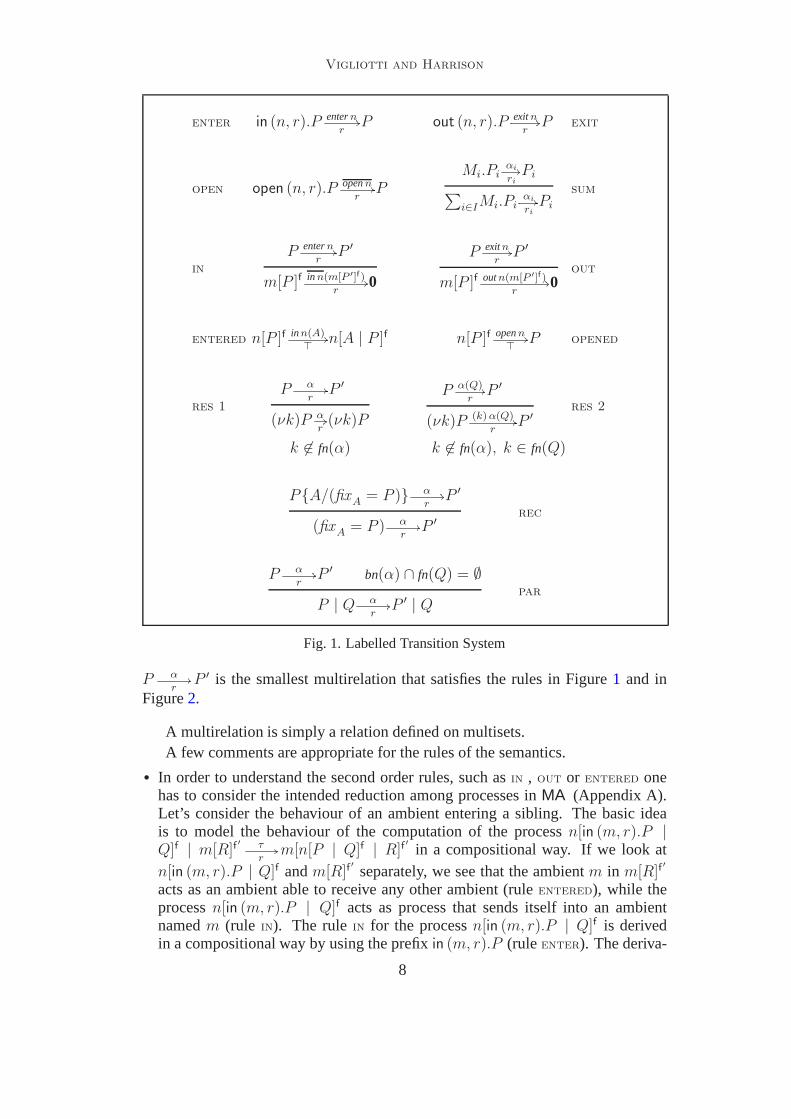
Fig. 1. Labelled Transition System

P αr

P ′ is the smallest multirelation that satisfies the rules in Figure 1 and inFigure2.

A multirelation is simply a relation defined on multisets.A few comments are appropriate for the rules of the semantics.

• In order to understand the second order rules, such asin , out or entered onehas to consider the intended reduction among processes inMA (Appendix A).Let’s consider the behaviour of an ambient entering a sibling. The basic ideais to model the behaviour of the computation of the processn[in (m, r).P |Q]f | m[R]f

′ τr

m[n[P | Q]f | R]f′

in a compositional way. If we look atn[in (m, r).P | Q]f andm[R]f

′

separately, we see that the ambientm in m[R]f′

acts as an ambient able to receive any other ambient (ruleentered), while theprocessn[in (m, r).P | Q]f acts as process that sends itself into an ambientnamedm (rule in). The rulein for the processn[in (m, r).P | Q]f is derivedin a compositional way by using the prefixin (m, r).P (ruleenter). The deriva-

8

Vigliotti and Harrison

P in n(P ′)r

P ′′ Q in n(P ′)⊤

Q′

P | Q τrP ′′ | Q′

comm in

P (k) in n(P ′)r

P ′′ Q in n(P ′)⊤

Q′ k /∈ fn(Q)

P | Q τ

r(νk)(P ′′ | Q′)

comm in∗

P outn(P ′)r

P ′′

n[P ]ff(r)τ P ′ | n[P ′′]f

comm out

P (k) outn(P ′)r

P ′′ k 6= n

n[P ]ff(r)τ (νk)(P ′ | n[P ′′]f)

comm out∗

P opennr

P ′ Q openn⊤

Q′

P | Q τrP ′ | Q′

comm open

P τr

P ′

n[P ]ff(r)τ n[P ′]f

amb

Fig. 2. Labelled Transition System for internal actions

tion tree for the rule above, using our labelled transition system is the following:

in (m, r).P entermr

Ppar

in (m, r).P | Q entermr

P | Qin

m[in (n, r).P | Q]f in n(m[P | Q]f)r

0entered

m[R]f′ in n(m[P | Q]f)

⊤m[m[P | Q]f | R]f

′

comm in

m[in (n, r).P | Q]f | m[R]f′ τ

r0 | m[m[P | Q]f | R]f

′

A similar explanation holds for the rule were a child-ambient exit the parent-ambient. The rules for parallel composition, recursion, choice and restriction arestandard.

• In the ruleamb becomes clear how the surrounding ambient of a process influ-ences the original rate.

• The rulesentered andopened proceed as passive actions, indicated by the rate⊤ under the arrow. The concept of passive actions, taken fromPEPA [13]. It isquite natural to think that an ambient is passive in the co-operation, when opened,entered or exit - by another agent. InPEPA passive actions induce an order that

9

Vigliotti and Harrison

helps in case choice among passive components. InSMA, such an order is notnecessary, since choice is local, i.e.n[P ]f + m[P ]f

′

is not a term of the syntax.• The rulescomm in, comm in

∗, comm out, comm out∗, comm open, par and

entered have a symmetric rule that has been omitted.

4 The underlying Markov model

In this section, we present a method to derive a Markov model from a StochasticMobile Ambient specification. The basic idea is that the state space of the underly-ing Markov model is given by the set of derivatives of the specification’s execution,i.e. of theτ actions. This is different fromPEPA andSπ, where the derivatives ofvisible actions can also be part of the state space of the model. The entries of thegenerator matrix are the sums of rates associated to a process to the same derivativevia τ action. Informally, assume an enumeration the state space of a processP ,then ifPi, Pj are two derivative ofP such thatPi λ

τ Pj . The entry of the generatormatrix qij is defined as follows:

q(Pi, Pj)def=

∑

Piτλ

Pj

λ.

With the generator matrix and the initial distribution, or equivalently the initial stateof the process, the Markov process is completely characterised.

Definition 4.1 If Pλτ P ′, thenP ′ is a (one step) derivative ofP . More generally if

P1 λ1

τ1 . . .λn

τn Pn, n ≥ 1, thenPn is a derivative ofP .

Notice that the previous definition is different from a standard labelled transitionsystem such asPEPA. We consider onlyτ actions, instead of any possible action.The set of derivatives of a process, which can be thought of asthe state space of theunderlying Markov model, is defined as follows.

Definition 4.2 The derivatives of a Stochastic Ambient Calculus processP , writtends(P ) is the smallest set of processes such that

• P ∈ ds(P );• if Pi ∈ ds(P ) andPi λ

τ Pj for someλ ∈ IR, thenPj ∈ ds(P ).

Let P ∈ Pr. P hasfinite branching if admits only a finite set of states.

Theorem 4.3 LetP be a finite Stochastic Mobile Ambient process and let ds(P ) beits set of derivatives. Then, the stochastic process{X(t) | t > 0}, whereX(0) = PandX(t) = Pj ∈ ds(P ), is a continuous time Markov chain with state space ds(P ).

The proof of this result is similar to [13].

10

Vigliotti and Harrison

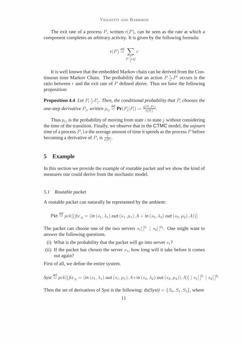
The exit rate of a processP , written r(P ), can be seen as the rate at which acomponent completes an arbitrary activity. It is given by the following formula:

r(P )def=

∑

Pτr

Q

r

It is well known that the embedded Markov chain can be derivedfrom the Con-tinuous time Markov Chain. The probability that an actionP τ

rP ′ occurs is the

ratio betweenr and the exit rate ofP defined above. Thus we have the followingproposition:

Proposition 4.4 LetPiτrPj. Then, the conditional probability thatPi chooses the

one-step derivativePj , writtenpijdef= Pr(Pj|Pi) =

q(Pi,Pj)

r(Pi).

Thuspij is the probability of moving from statei to statej without consideringthe time of the transition. Finally, we observe that in theCTMC model, thesojourntimeof a processP , i.e the average amount of time it spends as the processP beforebecoming a derivative ofP , is 1

r(P ).

5 Example

In this section we provide the example of routable packet andwe show the kind ofmeasures one could derive from the stochastic model.

5.1 Routable packet

A routable packet can naturally be represented by the ambient:

Pktdef= pck[(fixA = (in (s1, λ1).out (s1, µ1).A + in (s2, λ2).out (s2, µ2).A))]

The packet can choose one of the two serverss1[ ]f1 | s2[ ]

f2 . One might want toanswer the following questions.

(i) What is the probability that the packet will go into server s1?

(ii) If the packet has chosen the servers1, how long will it take before it comesout again?

First of all, we define the entire system.

Systdef= pck[(fixA = (in (s1, λ1).out (s1, µ1).A+in (s2, λ2).out (s2, µ2)).A)] | s1[ ]

f1 | s2[ ]f2

Then the set of derivatives ofSystis the following:ds(Syst)= {S0, S1, S2}, where

11

Vigliotti and Harrison

S0 = pck[(fixA = (in (s1, λ1).out (s1, µ1).A + in (s2, λ2).out (s2, µ2).A))] | s1[ ]f1 | s2[ ]

f2

S1 = s1[pck[out (s1, µ1).(fixA = (in (s1, λ1).out (s1, µ1).A + in (s2, λ2).out (s2, µ2).A))]]f1

| s2[ ]f2

S2 = s1[ ]f1 |

s2[pck[out (s2, µ2).(fixA = (in (s1, λ1).out (s1, µ1).A + in (s2, λ2).out (s2, µ2).A))]]f2

We derive the generator matrix as described in Section4 and obtain:

Q =

−(λ1 + λ2) λ1 λ2

f1(µ1) −f1(µ1) 0

f2(µ2) 0 −f2(µ2)

We note that the underlying state space of this process is irreducible, in the sensethat any node is reachable from the other. It is well known, this process eventuallyapproaches a stable behaviour. For question(1), by Proposition 4.4, the answer isp01 = λ1

λ1+λ2

since the exit rater(S0) = (λ1 + λ2). For question (2), the answer ist1 = 1

f1(µ1)by the observation at the end of the previous paragraph.

6 Strong Bisimulation

In this section we provide a definition of strong Markovian bisimulation. Bisim-ulation and bisimilarity are commonly defined in standard process algebras suchCCS[18,17]. Strong bisimulation is an equivalence relation that associates pro-cesses that can perform similar actions and find themselves in bisimilar states again.Strong bisimulation has been adapted in stochastic processalgebra [13,3], by takinginto account the frequency of the actions as well. Roughly speaking when consid-ering the quantitative behaviour, the basic idea is that in bisimilar states, actions areequivalent if they also happen at the same frequency. This isdefined by imposingthat processes move to bisimilar states with the same exit rate. In previous workon stochastic process algebra, Markovian strong bisimulation is defined in termsof a labelled transition system. It is widely known that in second order, labelledtransition systems, such as the one forSMA where processes occur in the labels,bisimulation has to deal carefully with the interplay between restriction and higherorder labels [27,28]. For this reason, our definition of strong Markovian bisimula-tion is a bit different with respect to the definition given inPEPA and IMC. Weused in this setting a variation of contextual bisimulation[14,30] adapted to thestochastic setting. We claim that this is the first time such adefinition is given.Contextual bisimulation uses the notion ofbarb, which is an observational predic-ate, and contexts in order to discriminate bisimilar processes.

12

Vigliotti and Harrison

Definition 6.1 A processP exhibits an ambient namedn, writtenP ↓ n if:

n[P ]f ↓ n

P ↓ n

P | Q ↓ n

P ↓ n

Q | P ↓ n

P ↓ n m 6= n

(νm)P ↓ n

P ↓ n

(fixA = P ) ↓ n

Definition 6.2 [Process context] The process contextC is given by the syntax:

C ::= [·] | C|P | P | C | n[C]f | (νn)C | M.C

C[Q] denotes the result of filling the hole[·] in the contextC with processQ.

Definition 6.3 An equivalence relationS : Pr ×Pr is astrong Markovian bisimu-lation if for all P, Q ∈ Pr, P S Q implies that for all equivalence classesE in Pr/S

and namesn ∈ N :

(i) if P ↓ n thenQ ↓ n;

(ii) γ•(P, E) = γ•(Q, E).

whereγ• : Pr × 2Pr → IR

γ•(P, E) =∑

{| λ : C[P ]λτ R, ∀R ∈ E, ∀C contexts |}.

Two processesP, Q are called strongly Markovian bisimilar, writtenP ∼M Q, iffor some Markovian strong bisimulationS , (P, Q) ∈ S .

The notation{| . . . |} stands for a multi-set. As usual, the strong Markovianbisimilarity is the largest strong Markovian bisimulation. Moreover this relationis preserved by all contexts by definition. In the next proposition we show somesignificant bisimilar processes.

Proposition 6.4 (i) P | Q ∼M Q | P .

(ii) P | 0 ∼M P .

(iii) (P | Q) | R ∼M P | (Q | R).

(iv) M.P + N.Q ∼M N.Q + M.P .

(v) M.P + 0 ∼M M.P .

(vi) in (n, λ).P + in (n, µ).P ∼M in (n, λ + µ).P .

(vii) open (n, λ).P + open (n, µ).P ∼M open (n, λ + µ).P .

(viii) out (n, λ).P + out (n, µ).P ∼M out (n, λ + µ).P .

(ix) (νn)n[in (q, λ)]f ∼M (νn)n[in (q, λ′)]f′

if f(λ) = f ′(λ′).

(x) (νn)n[out (q, λ)]f ∼M (νn)n[out (q, λ′)]f′

if f(λ) = f ′(λ′).

13

Vigliotti and Harrison

It is important to note that (10) and (11) are peculiar to theSMA world and arenot found in other process algebras.

7 Conclusions

We have presented the Stochastic Ambient Calculus, which isa stochastic exten-sion of mobile ambients with performance measures, whose underlying model isMarkovian. The restriction to the Markovian model is simple, mathematically tract-able and powerful. Other, more general action-delay distributions are also possible,but numerically less practical.

In the present version, we have not included anything about steady state distri-butions in aCTMC as this has been dealt inPEPA andSπ. However, it could behandled here in a similar way. As future research is concerned, it would be interest-ing to extend the ambient logic [7] in similar fashion to the work done by Latella,De Nicola, Katoen and Massink [25] for the modal logic associated to the KLAIMlanguage.

8 Acknowledgements

We would like to thank Gethin Norman for pointing out that recursion must be usedinstead of replication inSMA. We would like to thank Jeremy Bradley for manyuseful discussions and the rest of the AESOP research group at Imperial College.We also thank the anonymous referees for very useful comments.

Appendix A

Mobile AmbientsMA aims to represent, in a general way, computation over theInternet. The main advantage ofMA is the simple underlying, unifying concept ofambient. Ambients are meant to represent bounded places for computation suchas concrete locations, concrete domains, abstract domains, or laptop computers.Ambients move into and out of other ambients bringing along moving code, staticprocesses and possibly other ambients.

In the following paragraph, that has been inspired by [5,7], we will try to outlinethe main features of the concept of ambient. InMA ambients are represented asfollows:

• An ambient defines a perimeter, a boundary, that establisheswhat is inside theambient and what is outside the ambient.

• An ambient has aname.• Ambients can move around: they enter or exit other ambients.• An ambient is a collection oflocal agents, i.e. processes, which run directly

inside the ambient.n [P ] is the syntax for an ambient whose name isn with therunning processP inside.

14

Vigliotti and Harrison

• An ambient may have other ambients inside, creating a hierarchy of nested am-bients, which could be represented as a tree. Each sub-ambient has its own nameand behaves as an independent ambient.

• An ambient moves with all the sub-ambients and processes inside.

We shall assume the existence of a set of namesN , the metavariablesn, m, z, s, . . .range over the this set.

Definition 8.1 The set of process terms of MA is given by the following syntax:

P, Q ::= 0 | P | Q | (νn)P | n [P ] | M.P | !P

whereM stands for thecapabilitiesdefined by the following grammar:

M ::= in n | out n | open n

Nil, written0, represents the inactive process, the process that does notreduce.Ambient, writtenn [P ], is composed of two parts (it is a binary operator):n is thename of the ambient,P is the active process inside. The square brackets aroundP indicate the perimeter of the ambient. If the ambient moves,everything insidemoves with it.Parallel composition, writtenP | Q means thatP andQ are runningin parallel and can compute independently from each other.Restriction, written(νn)P , of the namen, makes the name private and unique toP . No other processcan use this name for interacting withP . Restriction is a binder andP is its scope.Given a processP , there is a natural notion offree names(fn(P )) andbound names(bn(P )). Replication, written !P , simulates recursion by spinning off copies ofP . Action prefixwrittenM.P , represents a process whereP is enabled only if theprefix M has been consumed. Capabilities can be thought of as terms that enablethe ambients to perform some actions. An ambient gains the ability to go insideanother ambient whose name isn with the in n capability. An ambient gains theability to leave a parent ambient whose name isn with the out n capability. Anambient namedn can be dissolved by the means of theopen n capability.

Operational semantics defines interaction among terms. Themeaning of thecomputation is given by the basic movement that ambients areable to make: en-tering an ambient, exiting an ambient and dissolving an ambient. Graphically thesteps of computation are shown below.

Entering an ambient The following diagram shows the reduction for the ambientnamedr, that has the ability to move into the siblingn.

r in n.P | Q | n R −→ n r P | Q | R

Exit from an ambient The following diagram shows the reduction for the ambi-

15

Vigliotti and Harrison

ent namedr, that has the ability to move out of the parentn.

n r outn.P | Q | R −→ r P | Q | n R

Opening an ambient The following diagram shows the reduction for the ambientnamedn, that can be dissolved by a process holding the right capability.

open n.P | n R −→ P | R

Formally, steps of computation are represented by areduction relationwhichis defined below.Structural congruence, ≡, (as it appears in the rulered cong

below), formally introduces structural rearrangements ofterms. Structurally equi-valent terms have the same semantics. This relation is developed from the metaphorpresent in the ‘Chemical Abstract Machine’ [2].

Thestructural congruence relationis the smallest congruence overMA termsthat satisfies the following equations:

P | 0 ≡ P

P | Q ≡ Q | P

(P | Q) | R ≡ P | (Q | R)

(νy)0 ≡ 0

(νm)(νn)P ≡ (νn)(νm)P

(νn)(P | Q) ≡ P | (νn)Q if n /∈ fn(P )

(νm)n [P ] ≡ n [(νm)P ] if n 6= m

!P ≡ P |!P

!0 ≡ 0

Definition 8.2 Thereduction relationis the smallest binary relation overMA termssatisfying the following set of rules:

m [in n.P | Q] | n [R] −→ n [m [P | Q] | R] red in

n [m [out n.P | Q] | R] −→ m [P | Q] | n [R] red out

open n.Q | n [R] −→ Q | R red open

P −→ P ′

red par

P | R −→ P ′ | R

P −→ P ′

red restr

(νn)P −→ (νn)P ′

16

Vigliotti and Harrison

P −→ P ′

red amb

n [P ] −→ n [P ′]

P ≡ P ′ −→ Q′ ≡ Qred cong

P −→ Q

Finally the observational predicate express what can be observed during com-putation. In the case ofMA the name of a top level ambient has been chosentraditionally as basic observation.

A processP exhibits a barbn, written asP ↓ n, if and only ifP ≡ (νp1 . . . pn)(n [P ′] |P ′′), for someP ′, P ′′ andn /∈ {p1 . . . pn}.

References

[1] M. Bernardo and R. Gorrieri. Extended Markovian ProcessAlgebra. InProceedingsof CONCUR’96, volume 1119 ofLNCS. Springer-Verlag, 1996.

[2] G. Berry and G. Boudol. Chemical Abstract Machine. InProceedings of the 17thACM Symposium on Principles of Programming Languages, pages 81–94. ACM,1990.

[3] E. Brinksma and H. Hermanns. Process Algebra and Markov Chains. InProceedingsof FMPA 2000, volume 2090 ofLNCS, pages 183–231. Springer-Verlag, 2001.

[4] M. Bugliesi, G. Castagna, and S. Crafa. Boxed ambients. In Proceedings ofTACAS’01, volume 2215 ofLNCS, pages 38–63. Springer-Verlag, 2001.

[5] L. Cardelli. Abstraction for Mobile Computation. In J. Vitek and C. Jensen,editors,Proceedings of Secure Internet Programming: Security Issues for Mobile andDistributed Objects, volume 1603 ofLNCS, pages 51–94. Springer-Verlag, 1999.

[6] L. Cardelli and A.D. Gordon. Types for Mobile Ambients. In Proceedings of the26th ACM Symposium on Principles of Programming Languages, pages 79–92. ACM,January 1999.

[7] L. Cardelli and A.D. Gordon. Anytime, Anywhere. Modal Logic for MobileAmbients. InProceedings of the 27th ACM Symposium on Principles of ProgrammingLanguages, pages 365–377, 2000.

[8] W. Charatonik, A.D. Gordon, and J. Talbot. Finite control ambients. InProceedingsof ESOP’02, volume 2305 ofLNCS, pages 295–313. Springer-Verlag, 2002.

[9] W. Feller. An Introduction to Probability Theory and its Applications. Wiley andSons, 1968.

[10] L. Guan, Y. Yang, and J. You. Making ambients more robust. In Proceedings ofInternational Conference on Software: Theory and Practice, pages 377–384, 2000.Beijing, China.

[11] P.G. Harrison and N.M. Patel.Performance Modelling and Communication Networksand Computer Architectures. Addison-Wesley, 1992.

17

Vigliotti and Harrison

[12] U. Herzog. Stochastic Process Algebra Benefits for Performance EvaluationChallenges. InProceedings of CONCUR’98, volume 1466 ofLNCS, pages 366–372.Springer-Verlag, 1998.

[13] J. Hillston. A Compositional Approach to Perfomance Modelling. PhD thesis,Department of Computer Science, Edinburgh, 1994.

[14] K. Honda and N. Yoshida. On the Reduction-based ProcessSemantics.TheoreticalComputer Science, 151:437–486, 1995.

[15] F. Levi and D. Sangiorgi. Controlling Interference forAmbients. InProceedings of28th ACM Symposium on Principles of Programming Languages, 2000.

[16] M. Merro and M. Hennessy. Bisimulation Congruences in Safe Ambients. InProceedings of the 29th ACM Symposium on Principles of Programming Languages,pages 71–80. ACM, 2002.

[17] R. Milner. Communication and Concurrency. Prentice-Hall International, 1989.

[18] R. Milner. Communicating and Mobile Systems: theπ-calculus. CambridgeUniversity Press, 1999.

[19] R. Milner and D. Sangiorgi. Barbed Bisimulation. InProceedings of the 19thInternational Colloquium on Automata, Languages and Programming, volume 623of LNCS, 1992.

[20] Rocco De Nicola, Diego Latella, and Mieke Massink. Formal modelling andquantitative analysis of KLAIM-based mobile systems. InSAC, pages 428–435, 2005.

[21] H.R. Nielsen and F. Nielsen. Validating the firewalls inmobile ambients. InProceedings of CONCUR’99, LNCS, pages 463–477, 1999.

[22] I.C.C. Phillips and M.G. Vigliotti. On the Reduction Semantics for the Push and Pullambient calculus. InProceedings of IFIP International Conference on TheoreticalComputer Science, volume 1872, pages 550–562, August 2002.

[23] Alessandra Di Pierro, Chris Hankin, and Herbert Wiklicky. Continuous-timeprobabilistic KLAIM. volume 128, pages 27–38, 2005.

[24] C. Priami. Stochasticπ-Calculus.The Computer Journal, 38(7):579–589, 1995.

[25] Diego Latella, Rocco De Nicola, Joost-Pieter Katoen and Mieke Massink. Towardsa logic for performance and mobility. InWorkshop on Quantitative Aspects ofProgramming Languages., 2005. To appear.

[26] S. M. Ross.Introduction to probability models. Academic Press, Inc, 1985.

[27] D. Sangiorgi.Expressing Mobility in Process Algebra: First-Order and Higher-OrderParadigms. PhD thesis, University of Edinburgh, 1993.

[28] B. Thomsen.Calculi for Higher Order Communicating Systems. PhD thesis, ImperialCollege, 1990.

18

Vigliotti and Harrison

[29] M.G. Vigliotti. Semantics and expressiveness of the Ambient Calculus. Technicalreport, Imperial College, 2001. Ph.D. Transfer Report.

[30] M.G. Vigliotti. Reduction Semantics for Ambient Calculi. PhD thesis, ImperialCollege, 2004.

19