Laboratoire de l’Informatique du Parallélisme

École Normale Supérieure de LyonUnité Mixte de Recherche CNRS-INRIA-ENS LYON-UCBL no 5668

Understanding untyped λµµ calculus

Pierre LescanneSilvia Likavec

November 2004

Research Report No RR2004-50

École Normale Supérieure de Lyon46 Allée d’Italie, 69364 Lyon Cedex 07, France

Téléphone : +33(0)4.72.72.80.37Télécopieur : +33(0)4.72.72.80.80

Adresse électronique :lip@ens-lyon.fr

Understanding untyped λµµ calculus

Pierre LescanneSilvia Likavec

November 2004

Abstract

We prove the confluence of λµµT and λµµQ, two well-behaved subcalculi ofthe λµµ calculus, closed under call-by-name and call-by-value reduction, re-spectively. Moreover, we give the interpretation of λµµT in the category ofnegated domains, and the interpretation of λµµQ in the Kleisli category. Tothe best of our knowledge this is the first interpretation of untyped λµµ calculus.

Keywords: Continuation semantics, classical logic, categories, type theory

Resume

On prouve la confluence de λµµT et λµµQ, deux sous-calculs de λµµ dotes debonnes proprietes et clos par reduction en appel par nom et en appel par valeur,respectivement. De plus, on donne l’interpretation de λµµT dans la categoriedes “domaines nies” et l’interpretation de λµµQ dans la categorie de Kleisli. Anotre connaissance, cela constitue la premiere interpetation non typee du λµµcalcul.

Mots-cles: semantique par continuation, logique classique, categories,theorie des types

1 Introduction

When interpreting calculi that embody a notion of control, it is convenient to start from contin-uation semantics that enables to explicitly refer to continuations, the semantic constructs thatrepresent evaluation contexts.

The method of continuations was first introduced in [21] in order to formalize flow control inprogramming languages. Continuation-passing-style (cps) translations were introduced by Fisherand Reynolds in [6] and [17] for call-by-value lambda calculus, whereas a call-by-name variant wasintroduced by Plotkin in [16]. Moggi gave a semantic version of call-by-value cps translation inhis study of notions of computation in [14]. Lafont [10] introduced cps translation of call-by-nameλC calculus [4], [5] to a fragment of lambda calculus that corresponds to the ¬,∧-fragment ofintuistionistic logic.

Categorical semantics for both call-by-name and call-by-value versions of Parigot’s λµ calculus[15] with disjunction types was given by Selinger in [20]. The two variants of λµ calculus areshown to be isomorphic in the presence of product and disjunction types. Hofmann and Stre-icher presented categorical continuation models for call-by-name λµ calculus in [9] and showed thecompleteness. Lengrand gave categorical semantics for typed λµµ calculus and λξ calculus (impli-cational fragment of the classical sequent calculus LK) in [13]. First attempt to give denotationalsemantics for pure (untyped) λµ calculus is presented in Laurent [12] by defining a type systemwith intersection and union types.

Although the original λµµ calculus of [2] has a system of simple types based on the sequentcalculus, the untyped version is a Turing-complete language for computation with explicit repre-sentation of control, as well as code. In this work we try to give a meaning to untyped λµµ calculusand understand its behaviour. We interpret its variant closed under call-by-name reduction in thecategory of negated domains, and the variant closed under call-by-value reduction in the Kleislicategory. As far as we know, this is the first interpretation of untyped λµµ calculus. We also provethe confluence of both versions.

The paper is organized as follows. In Section 2 we recall the syntax and the reduction rulesof λµµ calculus, and its two well-behaved subcalculi λµµT and λµµQ. In Section 3 we prove theconfluence for λµµT and λµµQ. Section 4 gives an account of negated categories where we interpretλµµT calculus. In Section 5 we present the basic notions of Kleisli triple and Kleisli category andinterpret λµµQ calculus. Finally, we give the improved interpretation of λµµT calculus. Weconclude in Section 6.

2 Overview of λµµ calculus

2.1 Intuition and syntax

λµµ calculus was introduced by Curien and Herbelin in [2], giving a Curry-Howard correspondencefor classical logic. The terms of λµµ represent derivations in a sequent calculus proof system andreduction reflects the process of cut-elimination.

The untyped version of the calculus can be seen as the foundation of a functional programminglanguage with explicit notion of control and was further studied by Dougherty, Ghilezan andLescanne in [7] and [3].

The basic syntactic entities are given by the following, where v ranges over the set CalleR ofcallers, e ranges over the set CalleE of callees and c ranges over the set Capsule of capsules:

v ::= x | λx.v | µα.c e ::= α | v • e | µx.c c ::= 〈v ‖ e〉

There are two kinds of variables in the calculus: the set Varv of caller variables (denoted by x, y, . . .)and the set Vare, of callee variables (denoted by α, β, . . .). The caller variables can be bound byλ abstraction and µ abstraction, whereas the callee variables can be bound by µ abstraction. Thesets of free caller and callee variables, Fvv and Fve, are defined as usual, respecting Barendregt’sconvention.

1

Capsules are the place where callers and callees interact. A caller can either get the data fromthe callee or it can ask the callee to take place as one of its internal callee variables. A callee canask a caller to take place as one of its internal caller variables. The components can be nested andmore processes can be active at the same time.

In [2], the basic constructs are called commands, terms, and contexts. The present names forthe syntactic constructs of the calculus were chosen by Ghilezan and Lescanne in [7], since theyreflect better the symmetry of the calculus. Also, it should be possible to use the notion “term”to refer to all the expressions of the calculus, not just to a subset of terms. Finally, commandsdefinitely do not denote commands. We use this new terminology in our work.

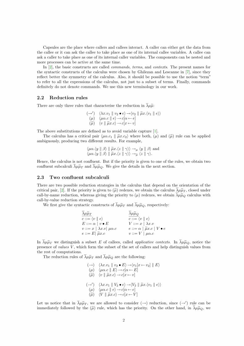
2.2 Reduction rules

There are only three rules that characterise the reduction in λµµ:

(→′) 〈λx.v1 ‖ v2 • e〉→〈v2 ‖ µx.〈v1 ‖ e〉〉(µ) 〈µα.c ‖ e〉→ c[α← e](µ) 〈v ‖ µx.c〉→ c[x← v]

The above substitutions are defined as to avoid variable capture [1].The calculus has a critical pair 〈µα.c1 ‖ µx.c2〉 where both, (µ) and (µ) rule can be applied

ambiguously, producing two different results. For example,

〈µα.〈y ‖ β〉 ‖ µx.〈z ‖ γ〉〉 →µ 〈y ‖ β〉 and〈µα.〈y ‖ β〉 ‖ µx.〈z ‖ γ〉〉 →µ 〈z ‖ γ〉.

Hence, the calculus is not confluent. But if the priority is given to one of the rules, we obtain twoconfluent subcalculi λµµT and λµµQ. We give the details in the next section.

2.3 Two confluent subcalculi

There are two possible reduction strategies in the calculus that depend on the orientation of thecritical pair, [2]. If the priority is given to (µ) redexes, we obtain the calculus λµµT , closed undercall-by-name reduction, whereas giving the priority to (µ) redexes, we obtain λµµQ calculus withcall-by-value reduction strategy.

We first give the syntactic constructs of λµµT and λµµQ, respectively:

λµµT λµµQ

c ::= 〈v ‖ e〉 c ::= 〈v ‖ e〉E ::= α | v • E V ::= x | λx.vv ::= x | λx.v| µα.c e ::= α | µx.c | V • ee ::= E| µx.c v ::= V | µα.c

In λµµT we distinguish a subset E of callees, called applicative contexts. In λµµQ, notice thepresence of values V , which form the subset of the set of callers and help distinguish values fromthe rest of computations.

The reduction rules of λµµT and λµµQ are the following:

(→) 〈λx.v1 ‖ v2 • E〉→〈v1[x← v2] ‖ E〉(µ) 〈µα.c ‖ E〉→ c[α←E](µ) 〈v ‖ µx.c〉→ c[x← v]

(→′) 〈λx.v1 ‖ V2 • e〉→〈V2 ‖ µx.〈v1 ‖ e〉〉(µ) 〈µα.c ‖ e〉→ c[α← e](µ) 〈V ‖ µx.c〉→ c[x←V ]

Let us notice that in λµµT , we are allowed to consider (→) reduction, since (→′) rule can beimmediately followed by the (µ) rule, which has the priority. On the other hand, in λµµQ, we

2

have to use the rule (→′), since the priority is given to (µ) rule. A different choice would beto consider only the (→′) rule for both subcalculi, but we think this choice makes explicit thepriorities of the rules in each subcalculus.

3 Confluence

Since in the next sections we work with two confluent subcalculi of λµµ, we first prove the conflu-ence for each of them. We adopt the technique of parallel reductions given by Takahashi in [24].This approach consists of simultaneously reducing all the redexes existing in a term.

We give the proof only for λµµT , since the proof for λµµQ is obtained by a straightforwardmodification of the proof for λµµT . We denote the union of the three reduction relations for λµµT

by →n and its reflexive and transitive closure by →→n.First, we define the notion of parallel reduction⇒n for λµµT . We will see that→→n is a reflexive

and transitive closure of ⇒n, so in order to prove the confluence of →→n, it is enough to prove thediamond property for ⇒n. The diamond property follows from the stronger “Star property” for⇒n.

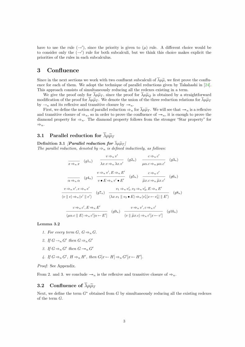
3.1 Parallel reduction for λµµT

Definition 3.1 [Parallel reduction for λµµT ]The parallel reduction, denoted by ⇒n is defined inductively, as follows:

x⇒n x(g1n)

v⇒n v′

λx.v⇒n λx.v′(g2n)

c⇒n c′

µα.c⇒n µα.c′(g3n)

α⇒n α(g4n)

v⇒n v′, E⇒n E′

v • E⇒n v′ • E′(g5n)

c⇒n c′

µx.c⇒n µx.c′(g6n)

v⇒n v′, e⇒n e′

〈v ‖ e〉⇒n〈v′ ‖ e′〉(g7n)

v1⇒n v′1, v2⇒n v′2, E⇒n E′

〈λx.v1 ‖ v2 • E〉⇒n〈v′1[x← v′2] ‖ E′〉(g8n)

c⇒n c′, E⇒n E′

〈µα.c ‖ E〉⇒n c′[α←E′](g9n)

v⇒n v′, c⇒n c′

〈v ‖ µx.c〉⇒n c′[x← v′](g10n)

Lemma 3.2

1. For every term G, G⇒n G.

2. If G→n G′ then G⇒n G′

3. If G⇒n G′ then G→→n G′

4. If G⇒n G′, H⇒n H ′, then G[x←H]⇒n G′[x←H ′].

Proof: See Appendix.

From 2. and 3. we conclude →→n is the reflexive and transitive closure of ⇒n.

3.2 Confluence of λµµT

Next, we define the term G∗ obtained from G by simultaneously reducing all the existing redexesof the term G.

3

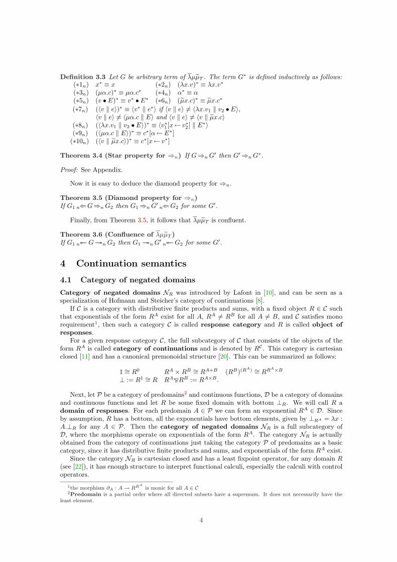
Definition 3.3 Let G be arbitrary term of λµµT . The term G∗ is defined inductively as follows:(∗1n) x∗ ≡ x (∗2n) (λx.v)∗ ≡ λx.v∗

(∗3n) (µα.c)∗ ≡ µα.c∗ (∗4n) α∗ ≡ α(∗5n) (v • E)∗ ≡ v∗ • E∗ (∗6n) (µx.c)∗ ≡ µx.c∗

(∗7n) (〈v ‖ e〉)∗ ≡ 〈v∗ ‖ e∗〉 if 〈v ‖ e〉 6= 〈λx.v1 ‖ v2 • E〉,〈v ‖ e〉 6= 〈µα.c ‖ E〉 and 〈v ‖ e〉 6= 〈v ‖ µx.c〉

(∗8n) (〈λx.v1 ‖ v2 • E〉)∗ ≡ 〈v∗1 [x← v∗2 ] ‖ E∗〉(∗9n) (〈µα.c ‖ E〉)∗ ≡ c∗[α←E∗]

(∗10n) (〈v ‖ µx.c〉)∗ ≡ c∗[x← v∗]

Theorem 3.4 (Star property for ⇒n) If G⇒n G′ then G′⇒n G∗.

Proof: See Appendix.

Now it is easy to deduce the diamond property for ⇒n.

Theorem 3.5 (Diamond property for ⇒n)If G1 n⇐G⇒n G2 then G1⇒n G′ n⇐G2 for some G′.

Finally, from Theorem 3.5, it follows that λµµT is confluent.

Theorem 3.6 (Confluence of λµµT )If G1 n←←G→→n G2 then G1→→n G′ n←←G2 for some G′.

4 Continuation semantics

4.1 Category of negated domains

Category of negated domains NR was introduced by Lafont in [10], and can be seen as aspecialization of Hofmann and Steicher’s category of continuations [8].

If C is a category with distributive finite products and sums, with a fixed object R ∈ C suchthat exponentials of the form RA exist for all A, RA 6= RB for all A 6= B, and C satisfies monorequirement1, then such a category C is called response category and R is called object ofresponses.

For a given response category C, the full subcategory of C that consists of the objects of theform RA is called category of continuations and is denoted by RC . This category is cartesianclosed [11] and has a canonical premonoidal structure [20]. This can be summarized as follows:

1 ∼= R0 RA ×RB ∼= RA+B (RB)(RA) ∼= RRA×B

⊥ := R1 ∼= R RAORB := RA×B .

Next, let P be a category of predomains2 and continuous functions, D be a category of domainsand continuous functions and let R be some fixed domain with bottom ⊥R. We will call R adomain of responses. For each predomain A ∈ P we can form an exponential RA ∈ D. Sinceby assumption, R has a bottom, all the exponentials have bottom elements, given by ⊥RA = λx :A.⊥R for any A ∈ P. Then the category of negated domains NR is a full subcategory ofD, where the morphisms operate on exponentials of the form RA. The category NR is actuallyobtained from the category of continuations just taking the category P of predomains as a basiccategory, since it has distributive finite products and sums, and exponentials of the form RA exist.

Since the category NR is cartesian closed and has a least fixpoint operator, for any domain R(see [22]), it has enough structure to interpret functional calculi, especially the calculi with controloperators.

1the morphism ∂A : A → RRAis monic for all A ∈ C

2Predomain is a partial order where all directed subsets have a supremum. It does not necessarily have theleast element.

4

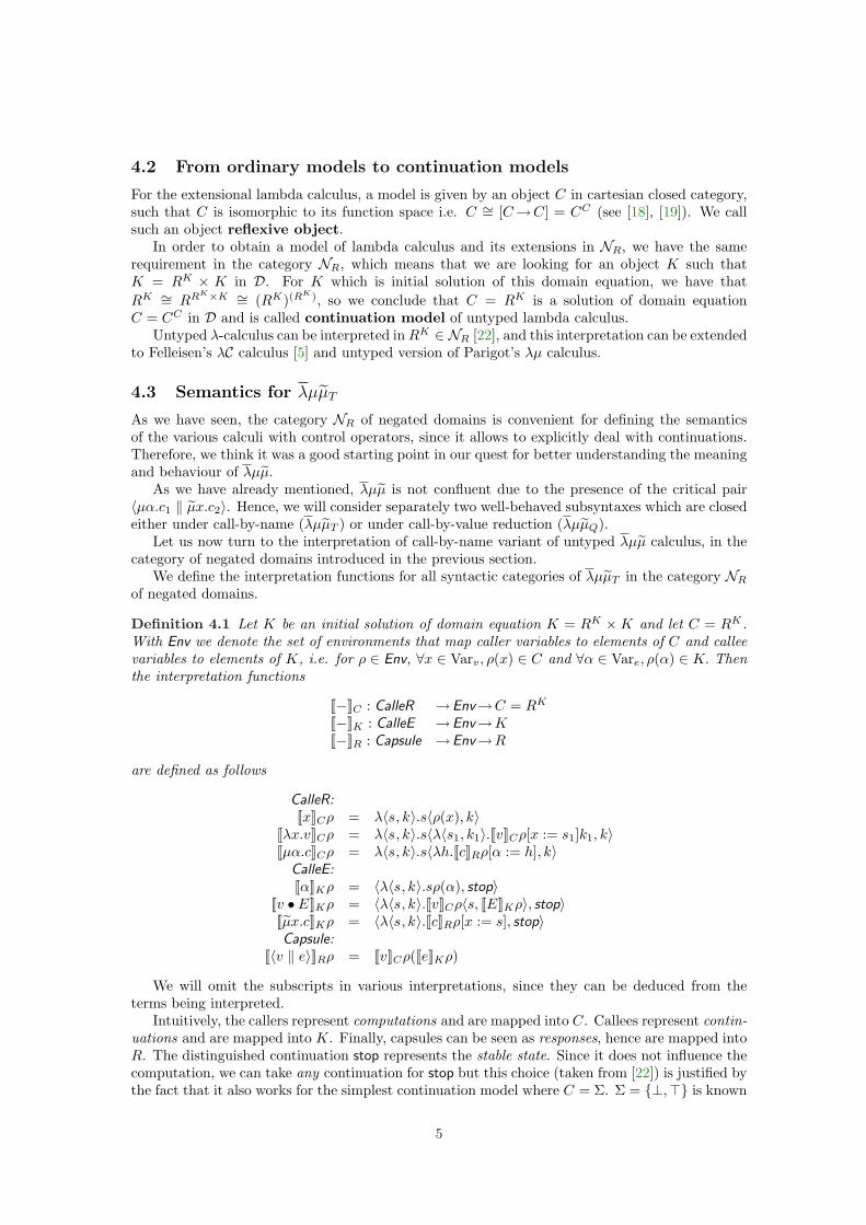
4.2 From ordinary models to continuation models

For the extensional lambda calculus, a model is given by an object C in cartesian closed category,such that C is isomorphic to its function space i.e. C ∼= [C→C] = CC (see [18], [19]). We callsuch an object reflexive object.

In order to obtain a model of lambda calculus and its extensions in NR, we have the samerequirement in the category NR, which means that we are looking for an object K such thatK = RK × K in D. For K which is initial solution of this domain equation, we have thatRK ∼= RRK×K ∼= (RK)(R

K), so we conclude that C = RK is a solution of domain equationC = CC in D and is called continuation model of untyped lambda calculus.

Untyped λ-calculus can be interpreted in RK ∈ NR [22], and this interpretation can be extendedto Felleisen’s λC calculus [5] and untyped version of Parigot’s λµ calculus.

4.3 Semantics for λµµT

As we have seen, the category NR of negated domains is convenient for defining the semanticsof the various calculi with control operators, since it allows to explicitly deal with continuations.Therefore, we think it was a good starting point in our quest for better understanding the meaningand behaviour of λµµ.

As we have already mentioned, λµµ is not confluent due to the presence of the critical pair〈µα.c1 ‖ µx.c2〉. Hence, we will consider separately two well-behaved subsyntaxes which are closedeither under call-by-name (λµµT ) or under call-by-value reduction (λµµQ).

Let us now turn to the interpretation of call-by-name variant of untyped λµµ calculus, in thecategory of negated domains introduced in the previous section.

We define the interpretation functions for all syntactic categories of λµµT in the category NR

of negated domains.

Definition 4.1 Let K be an initial solution of domain equation K = RK ×K and let C = RK .With Env we denote the set of environments that map caller variables to elements of C and calleevariables to elements of K, i.e. for ρ ∈ Env, ∀x ∈ Varv, ρ(x) ∈ C and ∀α ∈ Vare, ρ(α) ∈ K. Thenthe interpretation functions

[[−]]C : CalleR →Env→C = RK

[[−]]K : CalleE →Env→K[[−]]R : Capsule →Env→R

are defined as follows

CalleR:[[x]]Cρ = λ〈s, k〉.s〈ρ(x), k〉

[[λx.v]]Cρ = λ〈s, k〉.s〈λ〈s1, k1〉.[[v]]Cρ[x := s1]k1, k〉[[µα.c]]Cρ = λ〈s, k〉.s〈λh.[[c]]Rρ[α := h], k〉

CalleE:[[α]]Kρ = 〈λ〈s, k〉.sρ(α), stop〉

[[v • E]]Kρ = 〈λ〈s, k〉.[[v]]Cρ〈s, [[E]]Kρ〉, stop〉[[µx.c]]Kρ = 〈λ〈s, k〉.[[c]]Rρ[x := s], stop〉Capsule:

[[〈v ‖ e〉]]Rρ = [[v]]Cρ([[e]]Kρ)

We will omit the subscripts in various interpretations, since they can be deduced from theterms being interpreted.

Intuitively, the callers represent computations and are mapped into C. Callees represent contin-uations and are mapped into K. Finally, capsules can be seen as responses, hence are mapped intoR. The distinguished continuation stop represents the stable state. Since it does not influence thecomputation, we can take any continuation for stop but this choice (taken from [22]) is justified bythe fact that it also works for the simplest continuation model where C = Σ. Σ = {⊥,>} is known

5

as Sierpinski space, where it is only possible to observe termination (represented by ⊥) and diver-gence (represented by >). It is the greatest element of K and is defined as stop = 〈λk.>R, stop〉,where k ∈ K and >R is the greatest element of the domain R.

Let us now give some explanations for the given interpretations. First of all, since K ∼= RK×K,continuations are of the form 〈s, k〉, where s ∈ C and k ∈ K. Therefore we can see continuations aslists of denotations which correspond to denotational versions of call-by-name evaluation contexts.

Callers are interpreted as functions that map continuations to responses. This reflects the factthat a caller can either get data from a callee or ask it to take place of one of its internal calleevariables. Hence, callers expect callees as arguments. The double abstraction over callees comesfrom the necessity to trigger the computation in (µ) rule. It actually enables applying the currentevaluation context to a computation and continuing the computation.

Since a callee can ask a caller to take the place of one of its internal caller variables, it has afunctional part that can be applied to a caller (the first part of the pair). The second componentof the pair is stop, since during the computation, a new evaluation context is provided by thecaller.

Finally, in the case of capsules, the interpretation of the caller is applied to the interpretationof the callee, thus producing an element in R.

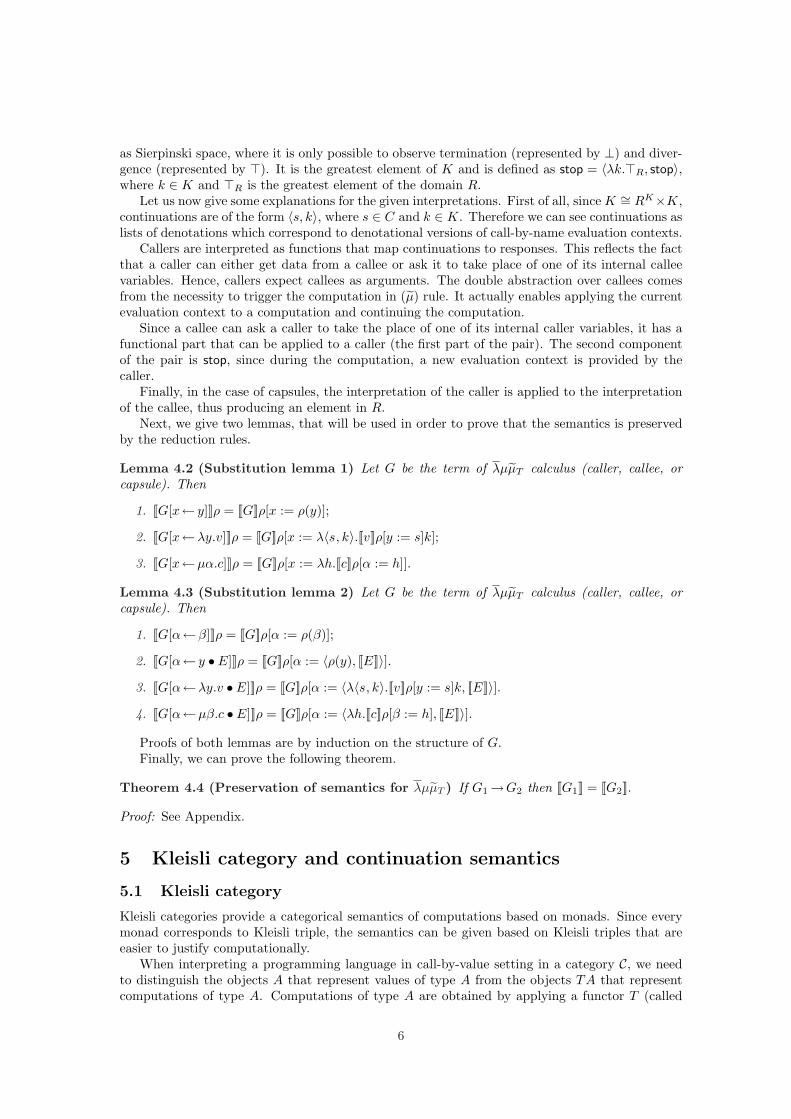
Next, we give two lemmas, that will be used in order to prove that the semantics is preservedby the reduction rules.

Lemma 4.2 (Substitution lemma 1) Let G be the term of λµµT calculus (caller, callee, orcapsule). Then

1. [[G[x← y]]]ρ = [[G]]ρ[x := ρ(y)];

2. [[G[x←λy.v]]]ρ = [[G]]ρ[x := λ〈s, k〉.[[v]]ρ[y := s]k];

3. [[G[x←µα.c]]]ρ = [[G]]ρ[x := λh.[[c]]ρ[α := h]].

Lemma 4.3 (Substitution lemma 2) Let G be the term of λµµT calculus (caller, callee, orcapsule). Then

1. [[G[α←β]]]ρ = [[G]]ρ[α := ρ(β)];

2. [[G[α← y • E]]]ρ = [[G]]ρ[α := 〈ρ(y), [[E]]〉].3. [[G[α←λy.v • E]]]ρ = [[G]]ρ[α := 〈λ〈s, k〉.[[v]]ρ[y := s]k, [[E]]〉].4. [[G[α←µβ.c • E]]]ρ = [[G]]ρ[α := 〈λh.[[c]]ρ[β := h], [[E]]〉].

Proofs of both lemmas are by induction on the structure of G.Finally, we can prove the following theorem.

Theorem 4.4 (Preservation of semantics for λµµT ) If G1→G2 then [[G1]] = [[G2]].

Proof: See Appendix.

5 Kleisli category and continuation semantics

5.1 Kleisli category

Kleisli categories provide a categorical semantics of computations based on monads. Since everymonad corresponds to Kleisli triple, the semantics can be given based on Kleisli triples that areeasier to justify computationally.

When interpreting a programming language in call-by-value setting in a category C, we needto distinguish the objects A that represent values of type A from the objects TA that representcomputations of type A. Computations of type A are obtained by applying a functor T (called

6

notion of computation in [14]) to A. There are certain conditions that T has to satisfy and itturns out that T needs to be a Kleisli triple, whereas programs form the Kleisli category for sucha triple.

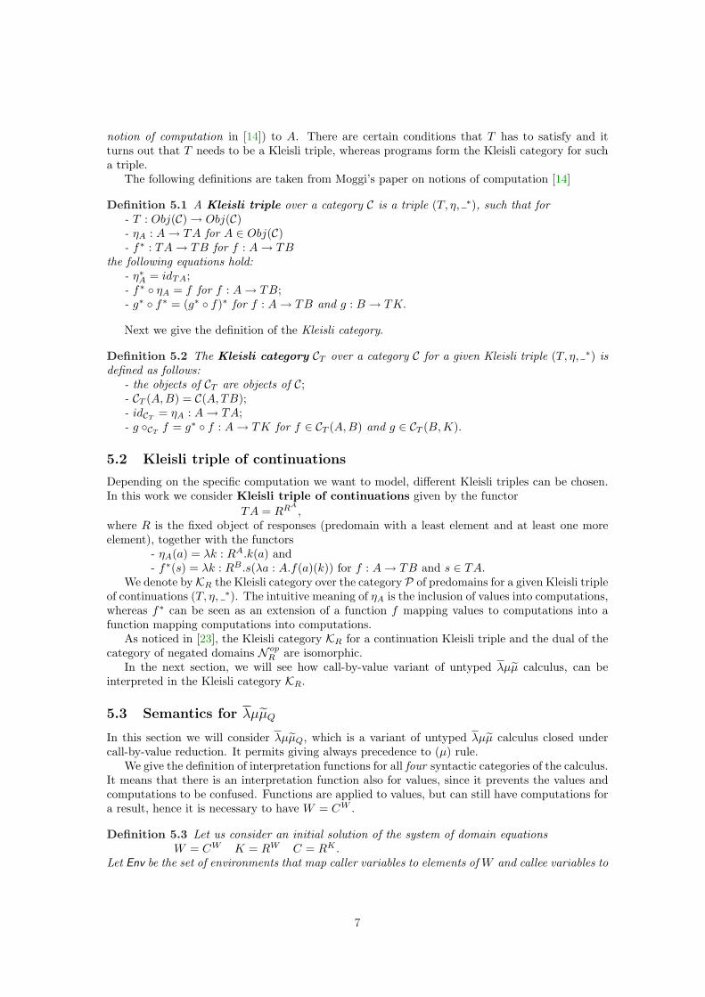
The following definitions are taken from Moggi’s paper on notions of computation [14]

Definition 5.1 A Kleisli triple over a category C is a triple (T, η, ∗), such that for- T : Obj(C) → Obj(C)- ηA : A → TA for A ∈ Obj(C)- f∗ : TA → TB for f : A → TB

the following equations hold:- η∗A = idTA;- f∗ ◦ ηA = f for f : A → TB;- g∗ ◦ f∗ = (g∗ ◦ f)∗ for f : A → TB and g : B → TK.

Next we give the definition of the Kleisli category.

Definition 5.2 The Kleisli category CT over a category C for a given Kleisli triple (T, η, ∗) isdefined as follows:

- the objects of CT are objects of C;- CT (A,B) = C(A, TB);- idCT

= ηA : A → TA;- g ◦CT

f = g∗ ◦ f : A → TK for f ∈ CT (A,B) and g ∈ CT (B, K).

5.2 Kleisli triple of continuations

Depending on the specific computation we want to model, different Kleisli triples can be chosen.In this work we consider Kleisli triple of continuations given by the functor

TA = RRA

,where R is the fixed object of responses (predomain with a least element and at least one moreelement), together with the functors

- ηA(a) = λk : RA.k(a) and- f∗(s) = λk : RB .s(λa : A.f(a)(k)) for f : A → TB and s ∈ TA.

We denote byKR the Kleisli category over the category P of predomains for a given Kleisli tripleof continuations (T, η, ∗). The intuitive meaning of ηA is the inclusion of values into computations,whereas f∗ can be seen as an extension of a function f mapping values to computations into afunction mapping computations into computations.

As noticed in [23], the Kleisli category KR for a continuation Kleisli triple and the dual of thecategory of negated domains N op

R are isomorphic.In the next section, we will see how call-by-value variant of untyped λµµ calculus, can be

interpreted in the Kleisli category KR.

5.3 Semantics for λµµQ

In this section we will consider λµµQ, which is a variant of untyped λµµ calculus closed undercall-by-value reduction. It permits giving always precedence to (µ) rule.

We give the definition of interpretation functions for all four syntactic categories of the calculus.It means that there is an interpretation function also for values, since it prevents the values andcomputations to be confused. Functions are applied to values, but can still have computations fora result, hence it is necessary to have W = CW .

Definition 5.3 Let us consider an initial solution of the system of domain equationsW = CW K = RW C = RK .

Let Env be the set of environments that map caller variables to elements of W and callee variables to

7

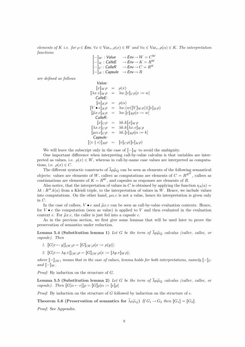
elements of K i.e. for ρ ∈ Env, ∀x ∈ Varv, ρ(x) ∈ W and ∀α ∈ Vare, ρ(α) ∈ K. The interpretationfunctions

[[−]]W : Value →Env→W = CW

[[−]]K : CalleE →Env→K = RW

[[−]]C : CalleR →Env→C = RK

[[−]]R : Capsule →Env→R

are defined as followsValue:[[x]]W ρ = ρ(x)

[[λx.v]]W ρ = λw.[[v]]Cρ[x := w]CalleE:[[α]]Kρ = ρ(α)

[[V • e]]Kρ = λw.(w([[V ]]W ρ))([[e]]Kρ)[[µx.c]]Kρ = λw.[[c]]Rρ[x := w]

CalleR:[[x]]Cρ = λk.k[[x]]W ρ

[[λx.v]]Cρ = λk.k[[λx.v]]W ρ[[µα.c]]Cρ = λk.[[c]]Rρ[α := k]Capsule:

[[〈v ‖ e〉]]Rρ = [[v]]Cρ([[e]]Kρ)

We will leave the subscript only in the case of [[−]]W to avoid the ambiguity.One important difference when interpreting call-by-value calculus is that variables are inter-

preted as values, i.e. ρ(x) ∈ W , whereas in call-by-name case values are interpreted as computa-tions, i.e. ρ(x) ∈ C.

The different syntactic constructs of λµµQ can be seen as elements of the following semanticalobjects: values are elements of W , callers as computations are elements of C = RRW

, callees ascontinuations are elements of K = RW , and capsules as responses are elements of R.

Also notice, that the interpretation of values in C is obtained by applying the function ηA(a) =λk : RA.k(a) from a Kleisli triple, to the interpretation of values in W . Hence, we include valuesinto computations. On the other hand, µα.c is not a value, hence its interpretation is given onlyin C.

In the case of callees, V • e and µx.c can be seen as call-by-value evaluation contexts. Hence,for V • e the computation (seen as value) is applied to V and then evaluated in the evaluationcontext e. For µx.c, the caller is just fed into a capsule c.

As in the previous section, we first give some lemmas that will be used later to prove thepreservation of semantics under reduction.

Lemma 5.4 (Substitution lemma 1) Let G be the term of λµµQ calculus (caller, callee, orcapsule). Then

1. [[G[x← y]]](W )ρ = [[G]](W )ρ[x := ρ(y)];

2. [[G[x←λy.v]]](W )ρ = [[G]](W )ρ[x := [[λy.v]]W ρ];

where [[−]](W ) means that in the case of values, lemma holds for both interpretations, namely [[−]]Cand [[−]]W .

Proof: By induction on the structure of G.

Lemma 5.5 (Substitution lemma 2) Let G be the term of λµµQ calculus (caller, callee, orcapsule). Then [[G[α← e]]]ρ = [[G]]ρ[α := [[e]]ρ]

Proof: By induction on the structure of G followed by induction on the structure of e.

Theorem 5.6 (Preservation of semantics for λµµQ) If G1→G2 then [[G1]] = [[G2]].

Proof: See Appendix.

8

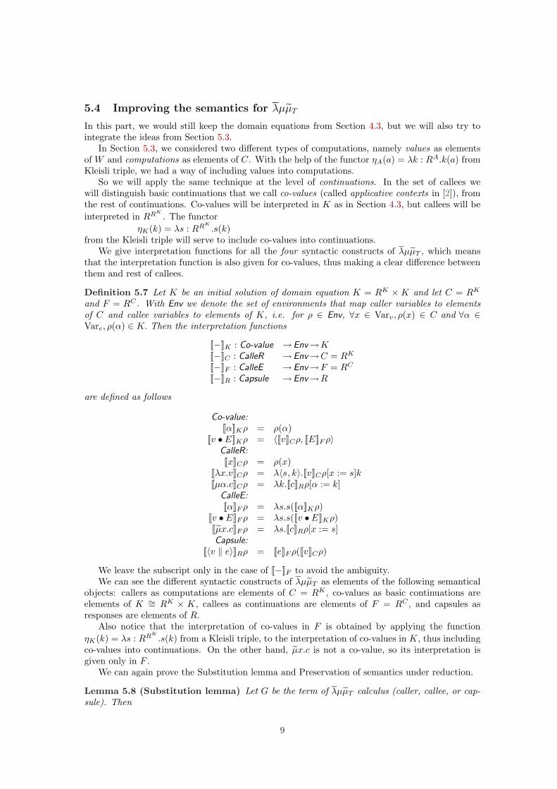
5.4 Improving the semantics for λµµT

In this part, we would still keep the domain equations from Section 4.3, but we will also try tointegrate the ideas from Section 5.3.

In Section 5.3, we considered two different types of computations, namely values as elementsof W and computations as elements of C. With the help of the functor ηA(a) = λk : RA.k(a) fromKleisli triple, we had a way of including values into computations.

So we will apply the same technique at the level of continuations. In the set of callees wewill distinguish basic continuations that we call co-values (called applicative contexts in [2]), fromthe rest of continuations. Co-values will be interpreted in K as in Section 4.3, but callees will beinterpreted in RRK

. The functorηK(k) = λs : RRK

.s(k)from the Kleisli triple will serve to include co-values into continuations.

We give interpretation functions for all the four syntactic constructs of λµµT , which meansthat the interpretation function is also given for co-values, thus making a clear difference betweenthem and rest of callees.

Definition 5.7 Let K be an initial solution of domain equation K = RK ×K and let C = RK

and F = RC . With Env we denote the set of environments that map caller variables to elementsof C and callee variables to elements of K, i.e. for ρ ∈ Env, ∀x ∈ Varv, ρ(x) ∈ C and ∀α ∈Vare, ρ(α) ∈ K. Then the interpretation functions

[[−]]K : Co-value →Env→K[[−]]C : CalleR →Env→C = RK

[[−]]F : CalleE →Env→F = RC

[[−]]R : Capsule →Env→R

are defined as follows

Co-value:[[α]]Kρ = ρ(α)

[[v • E]]Kρ = 〈[[v]]Cρ, [[E]]F ρ〉CalleR:[[x]]Cρ = ρ(x)

[[λx.v]]Cρ = λ〈s, k〉.[[v]]Cρ[x := s]k[[µα.c]]Cρ = λk.[[c]]Rρ[α := k]

CalleE:[[α]]F ρ = λs.s([[α]]Kρ)

[[v • E]]F ρ = λs.s([[v • E]]Kρ)[[µx.c]]F ρ = λs.[[c]]Rρ[x := s]Capsule:

[[〈v ‖ e〉]]Rρ = [[e]]F ρ([[v]]Cρ)

We leave the subscript only in the case of [[−]]F to avoid the ambiguity.We can see the different syntactic constructs of λµµT as elements of the following semantical

objects: callers as computations are elements of C = RK , co-values as basic continuations areelements of K ∼= RK × K, callees as continuations are elements of F = RC , and capsules asresponses are elements of R.

Also notice that the interpretation of co-values in F is obtained by applying the functionηK(k) = λs : RRK

.s(k) from a Kleisli triple, to the interpretation of co-values in K, thus includingco-values into continuations. On the other hand, µx.c is not a co-value, so its interpretation isgiven only in F .

We can again prove the Substitution lemma and Preservation of semantics under reduction.

Lemma 5.8 (Substitution lemma) Let G be the term of λµµT calculus (caller, callee, or cap-sule). Then

9

1. [[G[x← v]]]ρ = [[G]]ρ[x := [[v]]ρ];

2. [[G[α←E]]](K)ρ = [[G]](K)ρ[x := [[E]]Kρ]

where [[−]](K) means that lemma holds for both interpretations, [[−]]F and [[−]]K .

Theorem 5.9 (Preservation of semantics for λµµT ) If G1→G2 then [[G1]] = [[G2]].

Proof: See Appendix.

6 Conclusions and future work

As a step towards better understanding of denotational semantics of λµµ calculus, we interpretedits untyped call-by-name (λµµT ) and call-by-value (λµµQ) versions, which permits us to exploitλµµ as a programming language. Continuation semantics of λµµT is given by the interpretationin the category of negated domains of [22], whereas λµµQ is interpreted in Moggi’s Kleisli categoryover predomains for the continuation monad [14]. Using computational monads, we also give animproved interpretation for λµµT . As a first research direction it would be interesting to betterunderstand the correspondence between these interpretations.

Another important contribution of this work is the proof of confluence for both versions ofλµµ.

We would like to extend the present work to the complete symmetric calculus of [2] and findthe interpretation for all the constructs of that calculus, including e • v and βλ.e. It seems thatthis is not a trivial task, and that we need better understanding of the behaviour of these terms.

Another interesting direction to follow would be to interpret the typed λµµ calculus in Selinger’scontrol (co-control) categories [20], for both call-by-name and call-by-value variant of the calculus,similar to the ones given in [13], but giving different interpretations for types (closer to the onesgiven in [8]).

Finally, thorough analysis of semantics of the calculus typed using intersection and union types[3] is foreseen.

References

[1] H. P. Barendregt. The Lambda Calculus: its Syntax and Semantics. North-Holland, Amster-dam, revised edition, 1984.

[2] P.-L. Curien and H. Herbelin. The Duality of Computation. In Proc. 5th ACM SIGPLANInternational Conference on Functional Programming (ICFC’00), pages 233–243. ACM Press,2000.

[3] D. Dougherty, S. Ghilezan, and P. Lescanne. Characterizing strong normalization in a lan-guage with control operators. In Proc. 6th ACM-SIGPLAN International Conference onPrinciples and Practice of Declarative Programming PPDP’04, 2004.

[4] M. Felleisen, D. P. Friedman, E. Kohlbecker, and B. F. Duba. A syntactic theory of sequentialcontrol. Theoretical Computer Science, 52(3):205–237, 1987.

[5] M. Felleisen and R. Hieb. The revised report on the syntactic theories of sequential controland state. Theoretical Computer Science, 103(2):235–271, 1992.

[6] M. Fischer. Lambda calculus schemata. In Proc. ACM Conference on Proving AssertionsAbout Programs ’72, pages 104–109. ACM Press, 1972.

[7] S. Ghilezan and P. Lescanne. Classical proofs, typed processes and intersection types. InInternational Workshop TYPES’03 (Selected Papers), volume 3085 of LNCS, pages 226–241.Springer-Verlag, 2004.

10

[8] M. Hofmann and Th. Streicher. Continuation models are universal for lambda-mu-calculus. InProc. 11th IEEE Annual Symposium on Logic in Computer Science LICS ’97, pages 387–397.IEEE Computer Society Press, 1997.

[9] M. Hofmann and Th. Streicher. Completeness of continuation models for λµ-calculus. Infor-mation and Computation, 179(2):332 – 355, 2002.

[10] Y. Lafont. Negation versus implication. Draft, 1991.

[11] Y. Lafont, B. Reus, and Th. Streicher. Continuation semantics or expressing implication bynegation. Technical Report 93-21. University of Munich, 1993.

[12] O. Laurent. On the denotational semantics of the pure lambda-mu calculus. Manuscript,2004.

[13] S. Lengrand. Call-by-value, call-by-name, and strong normalization for the classical sequentcalculus. In B. Gramlich and S. Lucas, editors, Electronic Notes in Theoretical ComputerScience, volume 86. Elsevier, 2003.

[14] E. Moggi. Notions of computations and monads. Information and Computation, 93(1), 1991.

[15] M. Parigot. λµ-calculus: An algorithmic interpretation of classical natural deduction. InProc. International Conference on Logic Programming and Automated Reasoning, LPAR’92,volume 624 of LNCS, pages 190–201. Springer Verlag, 1992.

[16] G. D. Plotkin. Call-by-name, call-by-value and the λ-calculus. Theoretical Computer Science,1:125–159, 1975.

[17] J. C. Reynolds. Definitional interpreters for higher-order programming languages. In Proc.ACM Annual Conference, pages 717–740. ACM Press, 1972.

[18] D. S. Scott. Continuous lattices. In F.W.Lawvere, editor, Toposes, Algebraic Geometry andLogic, volume 274 of Lecture Notes in Mathematics, pages 97–136. Springer-Verlag, 1972.

[19] D. S. Scott. Domains for denotational semantics. In M. Nielsen and E. M. Schmidt, editors,Automata, Languages and Programming, volume 140 of Lecture Notes in Computer Science,pages 577–613. Springer-Verlag, 1982.

[20] P. Selinger. Control categories and duality: on the categorical semantics of the lambda-mucalculus. Mathematical Structures in Computer Science, 11:207–260, 2001.

[21] C. Strachey and C.P. Wadsworth. Continuations: A mathematical semantics for handling fulljumps. Oxford University Computing Laboratory Technical Monograph PRG-11, 1974.

[22] Th. Streicher and B. Reus. Classical logic, continuation semantics and abstract machines.Journal of Functional Programming, 8(6):543–572, 1998.

[23] Th. Streicher and B. Reus. Continuation semantics: Abstract machines and control operators.Unpublished manuscript, 1998.

[24] M. Takahashi. Parallel reduction in λ-calculus. Information and Computation, 118:120–127,1995.

A Appendix

Proof of Lemma 3.2

1. By induction on the structure of G. Base cases are the rules (g1n) and (g4n) from Definition3.1. For any other term of the calculus, we apply the induction hypothesis to the immediatesubterms of G (rules (g2n), (g3n), (g5n)− (g7n)). 2

11

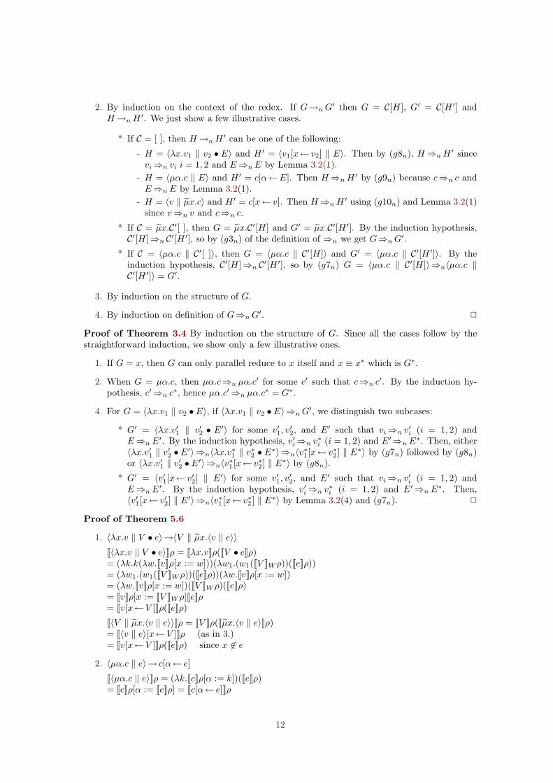
2. By induction on the context of the redex. If G→n G′ then G = C[H], G′ = C[H ′] andH→n H ′. We just show a few illustrative cases.

* If C = [ ], then H→n H ′ can be one of the following:

- H = 〈λx.v1 ‖ v2 • E〉 and H ′ = 〈v1[x← v2] ‖ E〉. Then by (g8n), H⇒n H ′ sincevi⇒n vi i = 1, 2 and E⇒n E by Lemma 3.2(1).

- H = 〈µα.c ‖ E〉 and H ′ = c[α←E]. Then H⇒n H ′ by (g9n) because c⇒n c andE⇒n E by Lemma 3.2(1).

- H = 〈v ‖ µx.c〉 and H ′ = c[x← v]. Then H⇒n H ′ using (g10n) and Lemma 3.2(1)since v⇒n v and c⇒n c.

* If C = µx.C′[ ], then G = µx.C′[H] and G′ = µx.C′[H ′]. By the induction hypothesis,C′[H]⇒n C′[H ′], so by (g3n) of the definition of ⇒n we get G⇒n G′.

* If C = 〈µα.c ‖ C′[ ]〉, then G = 〈µα.c ‖ C′[H]〉 and G′ = 〈µα.c ‖ C′[H ′]〉. By theinduction hypothesis, C′[H]⇒n C′[H ′], so by (g7n) G = 〈µα.c ‖ C′[H]〉⇒n〈µα.c ‖C′[H ′]〉 = G′.

3. By induction on the structure of G.

4. By induction on definition of G⇒n G′. 2

Proof of Theorem 3.4 By induction on the structure of G. Since all the cases follow by thestraightforward induction, we show only a few illustrative ones.

1. If G = x, then G can only parallel reduce to x itself and x ≡ x∗ which is G∗.

2. When G = µα.c, then µα.c⇒n µα.c′ for some c′ such that c⇒n c′. By the induction hy-pothesis, c′⇒n c∗, hence µα.c′⇒n µα.c∗ = G∗.

4. For G = 〈λx.v1 ‖ v2 • E〉, if 〈λx.v1 ‖ v2 • E〉⇒n G′, we distinguish two subcases:

* G′ = 〈λx.v′1 ‖ v′2 • E′〉 for some v′1, v′2, and E′ such that vi⇒n v′i (i = 1, 2) and

E⇒n E′. By the induction hypothesis, v′i⇒n v∗i (i = 1, 2) and E′⇒n E∗. Then, either〈λx.v′1 ‖ v′2 • E′〉⇒n〈λx.v∗1 ‖ v∗2 • E∗〉⇒n〈v∗1 [x← v∗2 ] ‖ E∗〉 by (g7n) followed by (g8n)or 〈λx.v′1 ‖ v′2 • E′〉⇒n〈v∗1 [x← v∗2 ] ‖ E∗〉 by (g8n).

* G′ = 〈v′1[x← v′2] ‖ E′〉 for some v′1, v′2, and E′ such that vi⇒n v′i (i = 1, 2) and

E⇒n E′. By the induction hypothesis, v′i⇒n v∗i (i = 1, 2) and E′⇒n E∗. Then,〈v′1[x← v′2] ‖ E′〉⇒n〈v∗1 [x← v∗2 ] ‖ E∗〉 by Lemma 3.2(4) and (g7n). 2

Proof of Theorem 5.6

1. 〈λx.v ‖ V • e〉→〈V ‖ µx.〈v ‖ e〉〉[[〈λx.v ‖ V • e〉]]ρ = [[λx.v]]ρ([[V • e]]ρ)= (λk.k(λw.[[v]]ρ[x := w]))(λw1.(w1([[V ]]W ρ))([[e]]ρ))= (λw1.(w1([[V ]]W ρ))([[e]]ρ))(λw.[[v]]ρ[x := w])= (λw.[[v]]ρ[x := w])([[V ]]W ρ)([[e]]ρ)= [[v]]ρ[x := [[V ]]W ρ][[e]]ρ= [[v[x←V ]]]ρ([[e]]ρ)

[[〈V ‖ µx.〈v ‖ e〉〉]]ρ = [[V ]]ρ([[µx.〈v ‖ e〉]]ρ)= [[〈v ‖ e〉[x←V ]]]ρ (as in 3.)= [[v[x←V ]]]ρ([[e]]ρ) since x 6∈ e

2. 〈µα.c ‖ e〉→ c[α← e]

[[〈µα.c ‖ e〉]]ρ = (λk.[[c]]ρ[α := k])([[e]]ρ)= [[c]]ρ[α := [[e]]ρ] = [[c[α← e]]]ρ

12

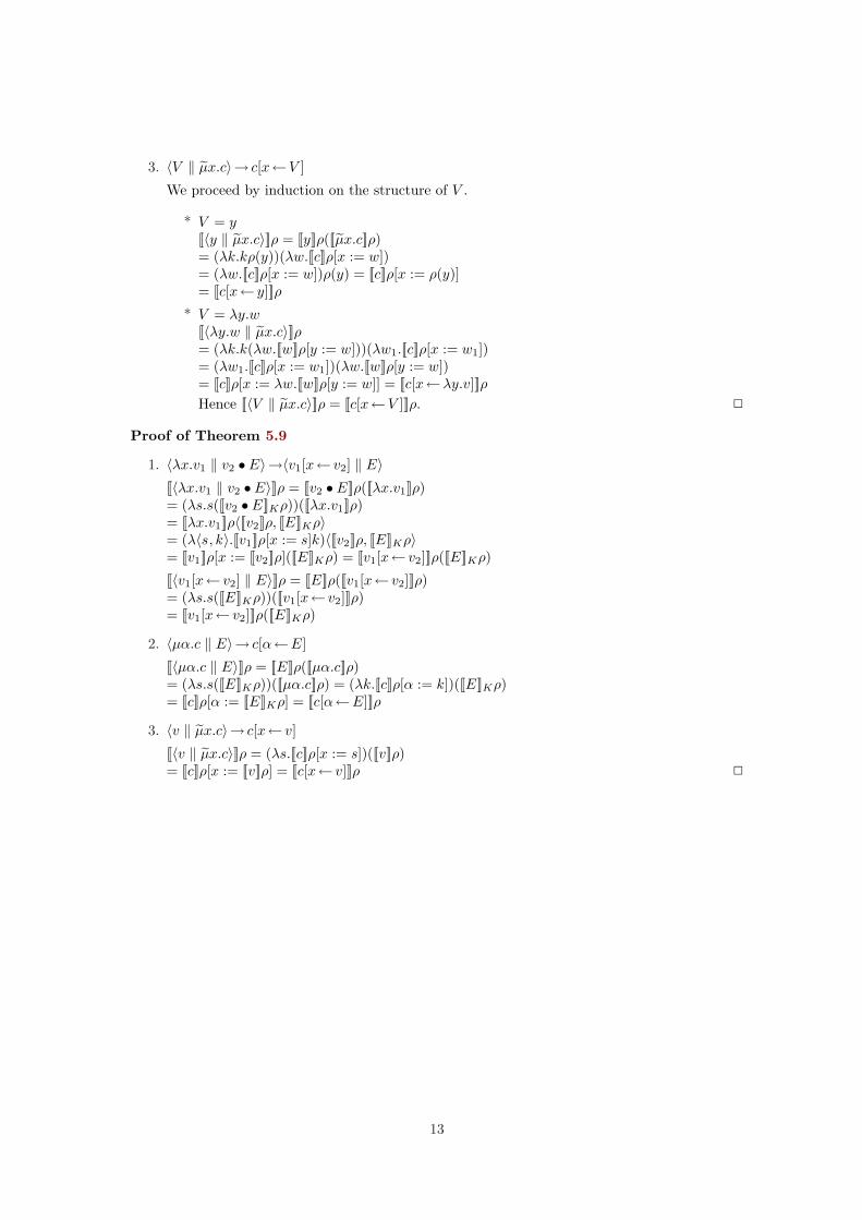
3. 〈V ‖ µx.c〉→ c[x←V ]

We proceed by induction on the structure of V .

* V = y[[〈y ‖ µx.c〉]]ρ = [[y]]ρ([[µx.c]]ρ)= (λk.kρ(y))(λw.[[c]]ρ[x := w])= (λw.[[c]]ρ[x := w])ρ(y) = [[c]]ρ[x := ρ(y)]= [[c[x← y]]]ρ

* V = λy.w[[〈λy.w ‖ µx.c〉]]ρ= (λk.k(λw.[[w]]ρ[y := w]))(λw1.[[c]]ρ[x := w1])= (λw1.[[c]]ρ[x := w1])(λw.[[w]]ρ[y := w])= [[c]]ρ[x := λw.[[w]]ρ[y := w]] = [[c[x←λy.v]]]ρHence [[〈V ‖ µx.c〉]]ρ = [[c[x←V ]]]ρ. 2

Proof of Theorem 5.9

1. 〈λx.v1 ‖ v2 • E〉→〈v1[x← v2] ‖ E〉[[〈λx.v1 ‖ v2 • E〉]]ρ = [[v2 • E]]ρ([[λx.v1]]ρ)= (λs.s([[v2 • E]]Kρ))([[λx.v1]]ρ)= [[λx.v1]]ρ〈[[v2]]ρ, [[E]]Kρ〉= (λ〈s, k〉.[[v1]]ρ[x := s]k)〈[[v2]]ρ, [[E]]Kρ〉= [[v1]]ρ[x := [[v2]]ρ]([[E]]Kρ) = [[v1[x← v2]]]ρ([[E]]Kρ)

[[〈v1[x← v2] ‖ E〉]]ρ = [[E]]ρ([[v1[x← v2]]]ρ)= (λs.s([[E]]Kρ))([[v1[x← v2]]]ρ)= [[v1[x← v2]]]ρ([[E]]Kρ)

2. 〈µα.c ‖ E〉→ c[α←E]

[[〈µα.c ‖ E〉]]ρ = [[E]]ρ([[µα.c]]ρ)= (λs.s([[E]]Kρ))([[µα.c]]ρ) = (λk.[[c]]ρ[α := k])([[E]]Kρ)= [[c]]ρ[α := [[E]]Kρ] = [[c[α←E]]]ρ

3. 〈v ‖ µx.c〉→ c[x← v]

[[〈v ‖ µx.c〉]]ρ = (λs.[[c]]ρ[x := s])([[v]]ρ)= [[c]]ρ[x := [[v]]ρ] = [[c[x← v]]]ρ 2

13