MTH4101 Calculus II

Carl MurraySchool of Mathematical Sciences

Queen Mary University of LondonSpring 2011

Lecture Notes

1

1 Complex Numbers

1.1 Introduction

We have already met several types of numbers.

Natural numbers (or positive integers) (N)::

N = {0, 1, 2, 3, . . . }

If m and n are positive integers then

m+ n = p and mn = q

are also positive integers (i.e. the system is closed under addition and multipli-cation). This allows us to solve equations like 3 + n = 7 but not equations like7 + n = 3.

Integers (Z):Negative integers (and zero) allow us to solve equations like 7 + n = 3.

Z = {. . . ,−3,−2,−1, 0, 1, 2, 3, . . . }

So we can solve equations like m + n = p to find the third integer when we knowthe other two.

But what about equations like mn = q?

Rationals (Q):Rational numbers can be expressed as the ratio of two integers. The set of rationalsis denoted by Q.

So if we know m and q we can find n = q/m (provided m 6= 0).

Reals (R):Not all numbers can be expressed as the ratio of two integers. Consider the lengthof the hypotenuse of the triangle formed by two sides of a square and the diagonal(below).

By Pythagoras’ theorem, h2 = 11 + 12 = 2. The solution is h =√

2 and thisbelongs to the set of real numbers, R but not Z or Q.

2

Figure 1: The diagonal of a square of unit radius

Therefore, in Z, we can solve equations like

x+ a = 0 (1)

where a ∈ Z.

In Q, we can solve equations like

ax+ b = 0 (2)

where a, b ∈ Q (and a 6= 0).

In R, we can solve equations like (1) and (2) as well as equations which arequadratic, such as

ax2 + bx+ c = 0 (3)

provided a 6= 0 and b2 − 4ac ≥ 0.

The solution of (3) is

x =−b±

√b2 − 4ac

2a(4)

But what do we do if b2 − 4ac < 0? For this we need to invent a new set ofnumbers, C, the set of complex numbers.

3

1.2 Complex Numbers

The complex number, z, is defined in terms of an ordered pair of real numbers,(x, y), and the imaginary number

i =√−1

such thatz = x+ iy

where x is the real part and y is the imaginary part.

We can writex = Re(z) y = Im(z) .

(Note that x and y are both real numbers.)

Example:

Solve the equation x2 − 2x+ 2 = 0.

Using the formula for the solution of the quadratic with a = 1, b = −2 and c = 2we have

x =2±√

4− 8

2=

2±√−4

2=

2±√

(4)(−1)

2.

Hence the solution is

x = 1± 1

2

√4√−1 = 1± i .

A consequence of the definition of i is that powers of i may be expressed in termsof ±1 and i. For example,

i2 = −1

i3 = i2i = (−i)i = −ii4 = (i2)2 = (−1)(−1) = 1 etc.

4

Figure 2: Representing a complex number in the Argand diagram

Also

i−1 =1

i=

1

i· ii

=i

i2=

i

−1= −i

i−2 =1

i2= −1

i−3 =1

i3=

1

i2i=

1

(−1)i= −1 · 1

i= i etc.

Since a complex number is defined in terms of an ordered pair of real numbers(x, y), it follows that every complex number can be represented by one point in aplane. The converse is also true. In fact, there is a 1-1 correspondence betweenthe set C and the points in a plane. This gives rise to the Argand diagram (above)where x and y lie along the real and imaginary axes, respectively. The Arganddiagram repesents z = x+ iy both as a point P (x, y) and as a vector ~OP .

From polar coordinates:

x = r cos θ y = r sin θ

and soz = x+ iy = r(cos θ + i sin θ) .

5

Note: The expression cos θ + i sin θ is sometimes written as cis θ.

The quantity r (i.e. the length of the line joining O and P in the Argand diagram)is called the absolute value or the modulus of the complex number z. The modulusof z is written as |z| or mod z. Note that |z| is always positive and is zero onlywhen z = 0.

The angle θ (i.e. the angle the line OP makes with the x or real axis) is called theargument of z. It is written as arg z. However, θ is not unique because the anglesθ + 2kπ (where k is zero or any integer) are also arguments of the same complexnumber. We define the principal argument of a complex number to be that valueof θ which satisfies

−π < θ ≤ π .

From the Argand diagram:

|z| = r =√x2 + y2

andsin θ =

y√x2 + y2

cos θ =x√

x2 + y2

for all θ. Hencetan θ =

y

xand θ = tan−1 y

x

Example:

If z = 2 + 3i find |z| and arg z.

|z| = r =√

22 + 32 =√

13

sin θ =3√13, cos θ =

2√13

Hence

tan θ =sin θ

cos θ=

3

2; arg z = θ = tan−1(3/2) ≈ 56.31◦ .

6

x

y

x iy+

x

y

x iy−

Figure 3: Taking the complex conjugate corresponds to a reflection in the x axisin the Argand diagram

If z = x+ iy is a complex number then the complex conjugate, z, is defined to be

z = x− iy .

Therefore finding the complex conjugate of a complex number is equivalent tochanging the sign of the imaginary component.

Since |x− iy| =√x2 + (−y)2 =

√x2 + y2, it follows that

|z| = |z| .

Using the Argand diagram we can illustrate the effect of taking the complex con-jugate of a complex number.

It is clear that z is the mirror image of z in the real (i.e. x) axis.

1.3 Operations with Complex Numbers

Let z1 = x1 + iy1 and z2 = x2 + iy2 be two complex numbers. The sum of z1 andz2 is defined as

z1 + z2 = (x1 + iy1) + (x2 + iy2) = (x1 + x2) + i(y1 + y2) .

7

In other words, we add the real parts and we add the imaginary parts.

Hence, for any three complex numbers z1, z2 and z3, we have

z1 + z2 = z2 + z1 (commutative)

z1 + (z2 + z3) = (z1 + z2) + z3 (associative) .

Note also that if z = x+ iy then

z + z = 2x and z − z = 2iy .

We can use the Argand diagram to obtain a geometric interpretation of the additionof two complex numbers. Consider z3 = z1 + z2 = (x1 + x2) + i(y1 + y2). If weconsider the corresponding Argand diagram we see that the resulting complexnumber, z3 is obtained by completing the parallelogram with sides OP and OQ.This gives the point S(z3) and the parallelogram OPSQ.

There is a similar interpretation for the subtraction of two complex numbers.

Let z1 = x1 + iy1 and z2 = x2 + iy2 be two complex numbers. The product of z1

and z2 is defined as

z1z2 = (x1 + iy1)(x2 + iy2)

= (x1x2 − y1y2) + i(x1y2 + x2y1) using i2 = −1

Hence, for any three complex numbers z1, z2 and z3, we have

z1z2 = z2z1 (commutative)

z1(z2z3) = (z1z2)z3 (associative) .

Alsozz = (x+ iy)(x− iy) = x2 + y2 = r2 = |z|2

and since |z| is always positive,

|z| =√zz

Note: The fact that zz = |z|2, a positive, real quantity means that when acomplex number is present in a denominator of a quotient, it can be removed by

8

x

y

O

P z

Q z

S z

xx x

( )

( )

( )

1

2

3

12 3

Figure 4: Adding two complex numbers in the Argand diagram

multiplying top and bottom by the complex conjugate of the denominator. Wewill make use of this property later on.

Similarly,|zn| =

√znzn = (zz)n/2 = |z|n

Likewise|z1z2|2 = z1z2z1z2 = z1z1 · z2z2 = |z1|2|z2|2

and since all the absolute values (i.e. the moduli) have to be positive, this gives

|z1z2| = |z1||z2| .

Note that

z1z2 = r1r2(cos θ1 + i sin θ1)(cos θ2 + i sin θ2)

= r1r2(cos θ1 cos θ2 − sin θ1 sin θ2 + i sin θ1 cos θ2 + i cos θ1 sin θ2)

= r1r2 {cos(θ1 + θ2) + i sin(θ1 + θ2)}

This has a geometrical interpretation in the context of the Argand diagram (seebelow). The result of multiplying z1 and z2 is a complex number with modulus(absolute value) |z1z2| = r1r2 and an argument arg (z1z2) = θ1 + θ2.

9

Figure 5: The multiplication of two complex numbers

There is a similar interpretation for the division of two complex numbers. It caneasily be shown that

z2

z1

=r2r1{cos(θ2 − θ1) + i sin(θ2 − θ1)} .

Therefore the result of dividing z2 by z1 is a complex number with modulus|z2/z1| = r2/r1 and an argument arg (z2/z1) = θ2 − θ1.

Example:

If z1 = −3 + 5i and z2 = 2− 3i find the complex numbers (a) z1 + z2, (b) z1 − z2,(c) z1z2 and (d) z1/z2 .

(a) z1 + z2 = −3 + 5i+ 2− 3i = −1 + 2i

(b) z1 − z2 = −3 + 5i− (2− 3i) = −5 + 8i

(c) z1z2 = (−3 + 5i)(2− 3i) = (−3 · 2 + 5 · 3) + i(5 · 2 + 3 · 3) = 9 + 19i

(d)z1

z2

=−3 + 5i

2− 3i=

(−3 + 5i)

(2− 3i)· (2 + 3i)

(2 + 3i)=−21 + i

13(using complex conjugate)

Note that |z1| =√

32 + 52 =√

34, |z2| =√

22 + 32 =√

13 and |z1z2| =√

92 + 192 =√442 =

√34 · 13 =

√34√

13. Hence this confirms our previous result that|z1z2| = |z1||z2|.

10

An important point to note about equations involving complex numbers is thatthere are really two equations: one where we can equate the real components andone where we can equate the imaginary components.

Example:

If z1 = 5 + a+ 3i and z2 = 4− (2 + b)i where a, b ∈ R, find a and b when z1 = z2.

If z1 = z2 then5 + a+ 3i = 4− (2 + b)i .

Equating the real parts gives 5 + a = 4; hence a = −1 .

Equating the imaginary parts gives 3 = −(2 + b); hence b = −5 .

Note: If z1 = z2 then Re(z1) = Re(z2) and Im(z1) = Im(z2).

1.4 Loci and Regions

A locus (the plural is “loci”) is a curve or other figure formed by all the pointssatisfying a particular equation. The use of modules and arguments can define locior regions in the Argand diagram.

Example:

Describe the locus of the point defined by |z| = 5.

If we use z = x + iy then |z| =√x2 + y2 = r = 5 since x2 + y2 = 52. The curve

described by the equation x2 + y2 = 52 is a circle, radius 5 units, centred on theorigin.

11

Example:

Describe the locus of the point defined by arg z = π/4.

If we use z = x+ iy then arg z = tan−1(y/x) = π/4. Hence

y

x= tan

π

4= 1 and hence y = x (x > 0) .

This is the equation of a line from the origin making an angle π/4 with the x-axis.

Example:

Describe the locus of the point defined by |z − 1| = 1.

If we use z = x+ iy then z − 1 = x− 1 + iy. Hence

|z − 1| =√

(x− 1)2 + y2 = 1 and hence (x− 1)2 + y2 = 1 .

This is the equation of a circle, radius 1, centred on x = 1, y = 0.

Example:

Describe the region defined by |z − 1| ≤ 1.

We have already shown (above) that the locus of |z − 1| = 1 is a circle, radius 1,centred on x = 1, y = 0. Hence, the region defined by |z − 1| ≤ 1 has to be theinterior of this circle.

Example:

Describe the locus of the point defined by |z| = 2|z − 1|.

If we use z = x+ iy then |z|2 = 4|z − 1|2. Hence

x2 + y2 = 4((x− 1)2 + y2) = 4(x2 + y2 + 1− 2x) .

12

Therefore3x2 + 3y2 − 8x+ 4 = 0 .

Dividing through by 3 and adding 16/9 to each side gives

x2 − 8

3x+

16

9+ y2 =

16

9− 4

3=

4

9

which can be written as (x− 4

3

)2

+ y2 =

(2

3

)2

.

This is the equation of a circle, radius 2/3, centred on x = 4/3, y = 0.

Example:

Describe the locus of the point defined by arg (z − a) = π/4.

If we use z = x+ iy then z − a = x− a+ iy and

arg (z − a) =π

4= tan−1

(y

x− a

).

Hencey

x− a= tan

π

4= 1 and hence y = x− a .

This is the equation of a straight line, gradient 1, crossing the x axis at x = a.

Example:

Describe the region defined by |z| ≤ |z − 1|.

If we use z = x + iy then |z| =√x2 + y2 and |z − 1| =

√(x− 1)2 + y2. So, for

|z| ≤ |z − 1|, we have |z|2 ≤ |z − 1|2. Hence

x2 + y2 ≤ (x− 1)2 + y2 = x2 − 2x+ 1 + y2 .

This gives 2x ≤ 1 and so the region is given by x ≤ 12

. This is the region to theleft of the vertical line through x = 1/2.

13

-10 -5 0 5 10-10

-5

0

5

10

-3 -2 -1 0 1 2 3-3

-2

-1

0

1

2

3

-3 -2 -1 0 1 2 3-3

-2

-1

0

1

2

3

-3 -2 -1 0 1 2 3-3

-2

-1

0

1

2

3

-3 -2 -1 0 1 2 3-3

-2

-1

0

1

2

3

-3 -2 -1 0 1 2 3-3

-2

-1

0

1

2

3

z z z

z z z z z

= = − =

− ≤ = − ≤ −

5 4 1 1

1 1 2 1 1

arg /π

Figure 6: Diagrams illustrating some of the solutions to the examples above

14

1.5 Trigonometric Functions and Hyperbolic Functions

Later in the course we will see that the power series

∞∑r=0

arxr = a0 + a1x+ a2x

2 + . . . (5)

(where the ar are real constants and x is real) converges if |x| < R, where R is theradius of convergence defined by

R = limr→∞

∣∣∣∣ arar+1

∣∣∣∣ .If we replace x by a complex number z in (5) the power series will again convergeprovided |z| < R. The functions expx, sinx, cosx can all be represented as powerseries in x; each has an equivalent series in z.

ez = 1 + z +z2

2!+z3

3!+z4

4!+ · · · (6)

sin z = z − z3

3!+z5

5!− z7

7!+ · · · (7)

cos z = 1− z2

2!+z4

4!− z6

6!+ · · · . (8)

These series in z converge for 0 ≤ |z| <∞.

Now put z = iθ in (6), where θ is any real number. We have:

eiθ = 1 + iθ +i2θ2

2!+i3θ3

3!+i4θ4

4!+ · · ·

= 1 + iθ − θ2

2!− iθ3

3!+θ4

4!+ · · ·

=

(1− θ2

2!+θ4

4!+ · · ·

)+ i

(θ − θ3

3!+ · · ·

)= cos θ + i sin θ (using (7) and (8)) .

This is Euler’s relation. But, as we showed above, we can also write z as z =r(cos θ + i sin θ). Hence

z = r eiθ

or, more generally,z = r ei(θ+2kπ)

15

Figure 7: Argand diagrams for eiθ = cos θ + i sin θ (a) as a vector and (b) as apoint.

where k is any integer.

Replacing θ by −θ in Euler’s relation gives

e−iθ = cos θ − i sin θ .

Hence

cos θ =eiθ + e−iθ

2(9)

and

sin θ =eiθ − e−iθ

2i(10)

Example:

Write z = (4 + 3i)eiπ/3 in the form u+ iv where u and v are real numbers.

From Euler’s relation,

eiπ/3 = cosπ

3+ i sin

π

3=

1

2+ i

√3

2.

16

Hence

z = (4 + 3i)

(1

2+ i

√3

2

)=

1

2(4 + 3i)(1 + i

√3) =

(4− 3

√3

2

)+ i

(3 + 4

√3

2

).

Note that

eiπ/2 = cosπ

2+ i sin

π

2= i

eiπ = cos π + i sin π = −1

e3iπ/2 = cos3π

2+ i sin

3π

2= −i

e2iπ = cos 2π + i sin 2π = 1

In general, for any integer n,

enπi = cosnπ + i sinnπ = (−1)n

e2nπi = cos 2nπ + i sin 2nπ = 1

Note: If we writez = r ei(θ+2πk)

then we can define the natural logarithm of z as

ln z = ln(r ei(θ+2πk)

)= ln r + i(θ + 2πk) = ln

√x2 + y2 + i

(tan−1 y

x+ 2πk

).

In (9) and (10) we defined cos and sin in terms of a complex exponential. Here wedefine two basic hyperbolic functions, cosh and sinh:

coshx =ex + e−x

2(pronounced “cosh”)

sinhx =ex − e−x

2(pronounced “shine”)

(These should be compared with our previous expressions for cos θ = 12(eiθ + e−iθ)

and sin θ = 12i

(eiθ − e−iθ).)

17

We can also define several additional hyperbolic functions:

tanhx =sinhx

coshx=ex − e−x

ex + e−x(pronounced “than”)

cothx =1

tanhx=ex + e−x

ex − e−x(pronounced “coth”)

sechx =1

coshx=

2

ex + e−x(pronounced “shec”)

cosechx =1

sinhx=

2

ex − e−x(pronounced “coshec”)

There are also several hyperbolic identities similar to the trigonometric ones. Forexample,

cosh2 x− sinh2 x = 1

sinh 2x = 2 sinhx coshx

cosh 2x = cosh2 x+ sinh2 x .

1.6 De Moivre’s Theorem

Consider the set of n complex numbers,

z1 = r1(cos θ1 + i sin θ1)

z2 = r2(cos θ2 + i sin θ2)...

zn = rn(cos θn + i sin θn)

We have already shown that

z1z2 = r1r2 (cos(θ1 + θ2) + i sin(θ1 + θ2)) .

Hence,z1z2z3 = r1r2r3 (cos(θ1 + θ2 + θ3) + i sin(θ1 + θ2 + θ3)) .

This can be generalised so that

z1z2 . . . zn = r1r2 . . . rn (cos(θ1 + θ2 + · · ·+ θn) + i sin(θ1 + θ2 + · · ·+ θn)) .

Now set r1 = r2 = · · · = rn = 1 and θ1 = θ2 = · · · θn = θ. This gives

zn = (cos θ + i sin θ)n = cosnθ + i sinnθ

18

where n is any positive integer. This results is known as de Moivre’s theorem. Theresult is also valid for n < 0 and n = p/q (i.e. where n is a negative integer andwhere n is a rational number).

For example,

(cos θ + i sin θ)−m =1

(cos θ + i sin θ)m=

1

cosmθ + i sinmθ

= (cosmθ + i sinmθ)−1 = cosmθ − i sinmθ

= cos(−mθ) + i sin(−mθ)

which proves the relation.

We now consider several applications of de Moivre’s theorem.

1.6.1 Expansion of cosnθ, sinn θ, cosnθ and sinnθ

Let z = cos θ + i sin θ. Then

1

z= cos θ − i sin θ .

Hence

z +1

z= 2 cos θ

z − 1

z= 2i sin θ .

By de Moivre’s theorem,

zn = (cos θ + i sin θ)n = cosnθ + i sinnθ1

zn= (cos θ + i sin θ)−n = cosnθ − i sinnθ

and so

zn +1

zn= 2 cosnθ

zn − 1

zn= 2i sinnθ .

19

Example:

Find expressions for cos6 θ and sin5 θ in terms of cosines and sines of multipleangles, respectively.

We have

2 cos θ = z +1

z

and so

26 cos6 θ =

(z +

1

z

)6

= z6 + 6z5 · 1

z+ 15z4 · 1

z2+ 20z3 · 1

z3+ 15z2 · 1

z4+ 6z · 1

z5+

1

z6

=

(z6 +

1

z6

)+ 6

(z4 +

1

z4

)+ 15

(z2 +

1

z2

)+ 20

= 2 cos 6θ + 12 cos 4θ + 30 cos 2θ + 20 .

Hence

cos6 θ =1

32(cos 6θ + 6 cos 4θ + 15 cos 2θ + 10) .

Similarly,

25i5 sin5 θ =

(z − 1

z

)5

=

(z5 − 1

z5

)− 5

(z3 − 1

z3

)+ 10

(z − 1

z

)and so

25i sin5 θ = 2i sin 5θ − 10i sin 3θ + 20i sin θ

giving

sin5 θ =1

16(sin 5θ − 5 sin 3θ + 10 sin θ) .

The converse problem can also be solved using de Moivre’s theorem.

Example:

Express cos 6θ and sin 6θ in terms of powers of cos θ and sin θ.

20

By de Moivre’s theorem,

cos 6θ + i sin θ = (cos θ + i sin θ)6

= cos6 θ + 6i cos5 θ sin θ + 15i2 cos4 θ sin2 θ + 20i3 cos3 θ sin3 θ

+15i4 cos2 θ sin4 θ + 6i5 cos θ sin5 θ + i6 sin6 θ

= cos6 θ + 6i cos5 θ sin θ − 15 cos4 θ sin2 θ − 20i cos3 θ sin3 θ

+15 cos2 θ sin4 θ + 6i cos θ sin5 θ − sin6 θ .

Remember that we essentially have two equations, one for the real parts and onefor the imaginary parts. This gives

Re(cos 6θ + i sin 6θ) = cos 6θ = cos6 θ − 15 cos4 θ sin2 θ + 15 cos2 θ sin4 θ − sin6 θ

and

Im(cos 6θ + i sin 6θ) = sin 6θ = 6 cos5 θ sin θ − 20 cos3 θ sin3 θ + 6 cos θ sin5 θ .

Note that we can simplify these expressions further using the fact that sin2 θ +cos2 θ = 1.

1.6.2 Roots of complex numbers and solution of equations

We can use de Moivre’s theorem to find the complex roots of numbers.

Example:

Find the n complex roots of the equation zn− 1 = 0 where n is a positive integer.

Remember that we can write unity (the number 1) in a number of ways:

1 = e2πki = cos 2πk + i sin 2πk

where k is any integer (or zero). de Moivre’s theorem now gives

z = 11/n = (cos 2πk + i sin 2πk)1/n = cos2πk

n+ i sin

2πk

n

21

which, letting k = 0, 1, 2, . . . , (n− 1), has n distinct values z1, z2, . . . , zn.

For example, when n = 6 the six roots of z6 − 1 = 0 are the six values of

z = cos2πk

6+ i sin

2πk

6

obtained by putting k = 0, 1, 2, 3, 4, 5. Taking each in turn gives

(k = 0) z1 = cos 0 + i sin 0 = 1

(k = 1) z2 = cosπ

3+ i sin

π

3=

1

2+ i

√3

2

(k = 2) z3 = cos2π

3+ i sin

2π

3= −1

2+ i

√3

2(k = 3) z4 = cos π + i sin π = −1

(k = 4) z5 = cos4π

3+ i sin

4π

3= −1

2− i√

3

2

(k = 5) z6 = cos5π

3+ i sin

5π

3=

1

2− i√

3

2.

Note that in the Argand diagram these roots are located on a circle of radius 1 atangular separations of π/3. Also note that no new roots are obtained by givingk any other values. (E.g. Setting k = 6 just reproduces the rot corresponding tok = 0.)

Figure 8 shows the location of the cube roots of the general complex numberz = r eiθ and the fourth roots of z = −16.

Example:

Find the solutions of the equation z4 − 1 = i√

3.

z4 = 1 + i√

3 = 2

(1

2+ i

√3

2

)= 2

{cos(π

3+ 2πk

)+ i sin

(π3

+ 2πk)}

22

(a) (b)

Figure 8: (a) The three cube roots of z = r eiθ and (b) the four fourth roots ofz = −16.

Hence, by de Moivre’s theorem,

z = 21/4

{cos

(π

12+πk

2

)+ i sin

(π

12+πk

2

)}where k = 0, 1, 2, 3. The four roots are:

(k = 0) z1 = 21/4(

cosπ

12+ i sin

π

12

)(k = 1) z2 = 21/4

(cos

7π

12+ i sin

7π

12

)(k = 2) z3 = 21/4

(cos

13π

12+ i sin

13π

12

)= −z1

(k = 3) z4 = 21/4

(cos

19π

12+ i sin

19π

12

)= −z2

Note that in the Argand diagram these roots are located on a circle of radius 21/4

at angular separations of π/2.

Note: The principal root is the one closest to the positive x-axis.

23

Example:

Find all the values of (1 + i)i.

Let z = (1 + i)i. Then

ln z = i ln(1 + i) = i ln(√

2 ei(π/4+2kπ))

= i(

ln√

2 + i(π

4+ 2kπ

))= i ln

√2−

(π4

+ 2kπ)

= −(π

4+ 2kπ

)+ i ln

√2 .

Hence

z = e−(π/4+2kπ)ei ln√

2 = e−(π/4+2kπ){

cos(ln√

2) + i sin(ln√

2)}.

1.6.3 Evaluation of integrals

Consider the integral ∫eax cos bx dx .

We can writeeax cos bx = Re

(e(a+ib)x

)Hence∫

eax cos bx dx = Re

(∫e(a+ib)xdx

)= Re

(1

a+ ib· e(a+ib)x

)= Re

(1

a+ ib· a− iba− ib

· eax [cos bx+ i sin bx]

)= Re

(a− iba2 + b2

· eax [cos bx+ i sin bx]

)=

1

a2 + b2· eax Re (a cos bx+ b sin bx− ib cos bx+ ia sin bx)

=eax

a2 + b2· (a cos bx+ b sin bx)

24

An alternative way to do this question is to use integration by parts (twice!):

I =

∫eax cos bx dx =

=eax sin bx

b−∫

sin bx

b· a eax dx

=eax sin bx

b− a

b

∫eax sin bx dx

=eax sin bx

b− a

b

(−e

ax cos bx

b−∫

(− cos bx)

b· a eax dx

)=

eax sin bx

b+a

b· e

ax cos bx

b− a2

b2

∫eax cos bx dx

=eax sin bx

b+a

b2· eax cos bx− a2

b2· I .

This gives us an equation in I which we can solve to find I. Gathering the termsin I gives

I

(1 +

a2

b2

)=eax sin bx

b+a

b2· eax cos bx

and hence

I =b2

a2 + b2

(eax sin bx

b+a

b2· eax cos bx

)=

eax

a2 + b2· (a cos bx+ b sin bx)

as before.

2 Partial Derivatives

2.1 Functions of Several Variables

Consider the following functions:

V = V (r, h) = πr2h (volume of cylinder, radius r, height h)

M = M(r, ρ) =4

3πr3ρ (mass of sphere, radius r, density ρ)

Each is a function of two variables. In the case of V , for example, the quantities rand h are the input variables and V is the output variable (independent variables→ dependent variable).

25

Figure 9: Example domains and ranges for function of two variables

Figure 10: The domain of f(x, y) =√y − x2 consists of the shaded region and its

bounding parabola y = x2

If f is a function of two independent variables, x and y, the domain of f is a regionin the x-y plane.

Example: Describe the domain of the function f(x, y) =√y − x2.

Since f is defined only where y − x2 ≥ 0, the domain is the closed unboundedregion show in Fig. 10. The parabola y = x2 is the boundary of the domain. Thepoints above the parabola make up the domain’s interior.

26

Figure 11: Three of the parabolas that go to make up the surface defined byz = x2 + y2, and the resulting paraboloid.

There are two ways to visualise a function f(x, y):

1. Sketch the surface z = f(x, y) in space.

2. Draw and label curves in the domain on which f has a constant value.

As an example we will consider the function

f(x, y) = x2 + y2 .

To visualise the surface, consider the nature of f for a fixed value of y, y = asay. In this case z = x2 + a2 and z = z(x). The equation z = x2 + a2 defines aparabola in the plane y = a, perpendicular to the y-axis. Each different value of agives a different parabola. For example, for y = a = 0 we have z = x2. Thereforethe required surface is made up of parabolas and forms a paraboloid as shown inFig. 11.

Examples of other surfaces are shown in Figure 12.

Alternatively we can consider the curves where f has a constant value. The curvesdefined by f(x, y) = x2 + y2 = constant are a set of circles. The set of points in

27

Figure 12: The three dimensional surfaces defined by the functions (a) f(x, y) =x2 + y2, (b) f(x, y) = −x2− y2, (c) f(x, y) = x2 + y2 + 5 and (d) f(x, y) = y2−x2.

28

-10 -5 5 10

-10

-5

5

10

x y2 2 100+ =

x y2 2 25+ =

x

y

Figure 13: Examples of two curves defined by f(x, y) = x2 + y2 = constant.

the plane where a function f(x, y) has a constant value f(x, y) = c is called a levelcurve of f . This is illustrated in Figure 13 for the function f(x, y) = x2 + y2.

Example: Graph the function f(x, y) = 100− x2 − y2 and plot the level curvesf(x, y) = 0, f(x, y) = 51 and f(x, y) = 75 in the domain of f in the plane.

The domain is the entire x-y plane and the range is the set of real numbers ≤ 100.The graph is the paraboloid given by z = 100− x2 − y2 (see Fig. 14)

When f(x, y) = 0, we have 100− x2 − y2 = 0 or x2 + y2 = 100. This correspondsto a circle of radius 10.

When f(x, y) = 51, we have 100− x2− y2 = 51 or x2 + y2 = 49. This correspondsto a circle of radius 7.

When f(x, y) = 75, we have 100− x2− y2 = 75 or x2 + y2 = 25. This correspondsto a circle of radius 5.

29

Figure 14: The graph and selected level curves of the function f(x, y) = 100 −x2 − y2.

The curve in space in which the plane z = c cuts a surface z = f(x, y) is called thecontour curve f(x, y) = c. For example, Fig. 15 shows the contour curve producedwhere the plane z = 75 intersects the surface z = f(x, y) = 100− x2 − y2.

2.2 Limits and Continuity in Higher Dimensions

For functions of one variable we say that f(x) approaches the limit L as x → awhenever

limx→a

f(x) = L .

Therefore as x approaches a, so f(x) approaches L. The limits are the same asx→ a from both directions.

For functions of one variable we say that f(x) is continuous at x = a wheneverlimx→a f(x) exists, f(a) is defined and the limit L equals f(a). Therefore

continuity of the function f(x) at x = a ⇒ limx→a

f(x) = f(a) .

30

Figure 15: A plane z = c parallel to the x-y plane intersecting a surface z = f(x, y)produces a contour curve.

31

Figure 16: Definition of the limit of a function of two variables

How do we extend the concepts of limits and continuity to functions of two vari-ables?

The definition of the limit of a function of two variables is given in Fig. 16.

This definition leads to the following properties:

If L, M and k are real numbers and

lim(x,y)→(x0,y0)

f(x, y) = L and lim(x,y)→(x0,y0)

g(x, y) = M

then

1. lim(x,y)→(x0,y0)

(f(x, y) + g(x, y)) = L+M

2. lim(x,y)→(x0,y0)

(f(x, y)− g(x, y)) = L−M

3. lim(x,y)→(x0,y0)

(f(x, y) · g(x, y)) = L ·M

4. lim(x,y)→(x0,y0)

(kf(x, y)) = kL

5. lim(x,y)→(x0,y0)

f(x, y)

g(x, y)=

L

M

6. If r and s are integers with no common factors, and s 6= 0, then

lim(x,y)→(x0,y0)

(f(x, y))r/s = Lr/s provided Lr/s is a real number.

For polynomials and rational functions the limit as (x, y) → (x0, y0) can be cal-

32

culated by evaluating the function at (x0, y0) (provided the rational function isdefined at (x0, y0)).

For example,

lim(x,y)→(0,1)

x− xy + 3

x2y + 5xy − y3=

0− (0)(1) + 3

(0)2(1) + 5(0)(1)− (1)3= −3 .

Example: Find

lim(x,y)→(0,0)

x2 − xy√x−√y

.

There is a problem with just setting x = y = 0 because√x−√y → 0 as (x, y)→

(0, 0). However, we can write

lim(x,y)→(0,0)

x2 − xy√x−√y

= lim(x,y)→(0,0)

x2 − xy√x−√y

·(√x+√y)

√x+√y

= lim(x,y)→(0,0)

x(x− y)(√x+√y)

(x− y)

= lim(x,y)→(0,0)

x(√x+√y) = 0 .

Now we use limits to define continuity for a function of two variables (see Fig. 17).

The Two-Path Test for Nonexistence of a Limit states that if a function f(x, y)has different limits along two different paths as (x, y)→ (x0, y0), then

lim(x,y)→(x0,y0)

f(x, y)

does not exist.

Figure 18 illustrates this concept for paths approaching a point in radial andtangential directions.

33

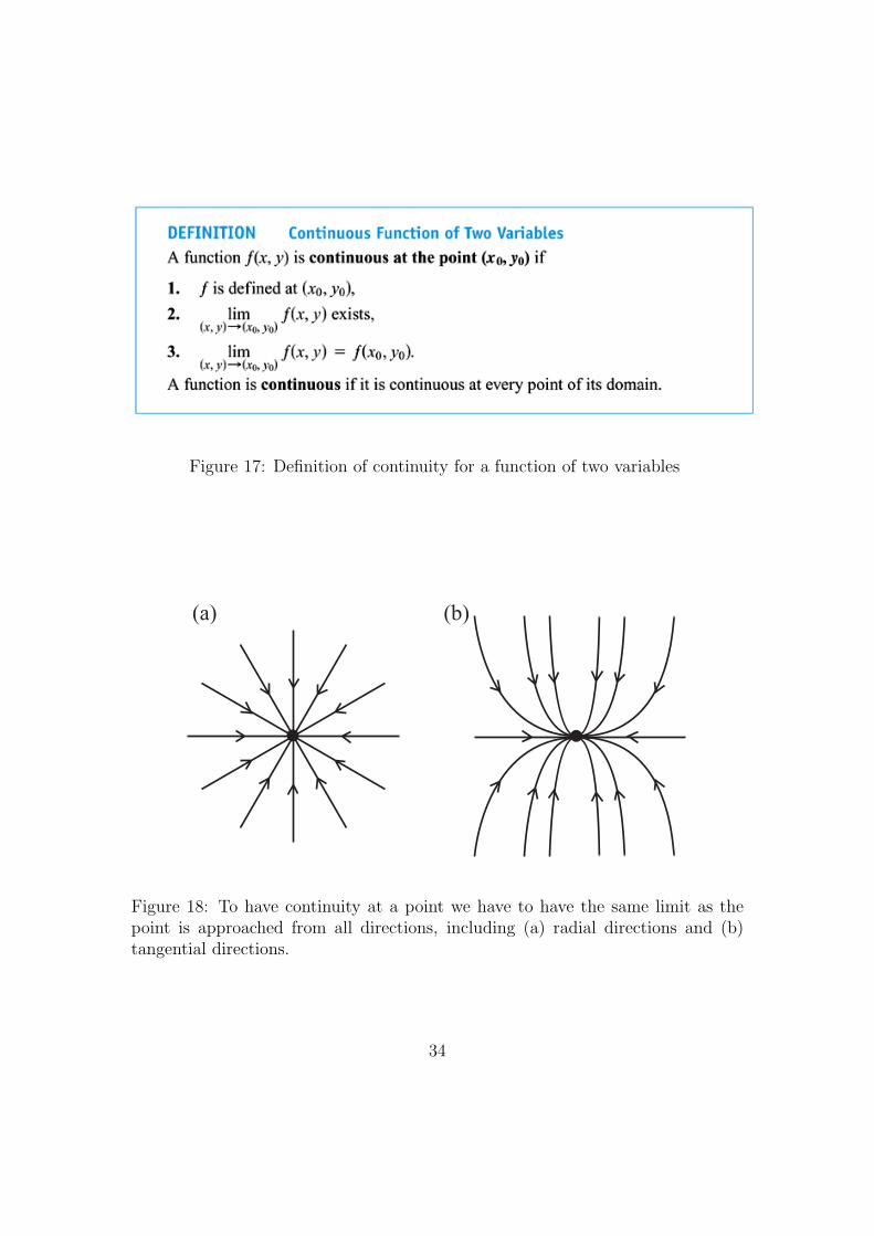
Figure 17: Definition of continuity for a function of two variables

(a) (b)

Figure 18: To have continuity at a point we have to have the same limit as thepoint is approached from all directions, including (a) radial directions and (b)tangential directions.

34

Example: Show that the function

f(x, y) =2x2y

x4 + y2

has no limit as (x, y)→ (0, 0).

We cannot use substitution as it leads to 0/0. However, we can consider whathappens as we approach (0, 0) along a family of different curves. Remember, thechoice of curves is up to us as the Two-Path Test does not specify what the pathshould be. Consider the family of parabolas given by y = kx2 (x 6= 0). Along thecurves the function is

f(x, y)|y=kx2 =2x2y

x4 + y2

∣∣∣∣y=kx2

=2x2(kx2)

x4 + (kx2)2=

2kx4

x4 + k2x4=

2k

1 + k2.

Therefore, as we approach (0, 0) along any curve y = kx2, we have

lim(x,y)→(0,0)

f(x, y) = lim(x,y)→(0,0)

[f(x, y)|y=kx2

]=

2k

1 + k2.

Therefore the actual limit will depend on which path of approach we take (i.e. whichparabola we are on which is determined by the value of k). Therefore, by the Two-Path Test there is no limit as (x, y)→ (0, 0).

Sometimes it is more useful to use polar coordinates.

Example: Determine the continuity of the function defined by

f(x, y) =

{ 2xyx2+y2

if (x, y) 6= (0, 0)

0 if (x, y) = (0, 0)

In polar coordinates, i.e. x = r cos θ, y = r sin θ, the function can be written as

f =2r2 cos θ sin θ

r2(cos2 θ + sin2 θ)= sin 2θ

provided we are not at the origin (i.e. provided r = 0). Therefore, as r → 0, f 6→ 0in all directions. For example, along θ = π/4, f = sin 2θ = sinπ/2 = 1 everywherealong the line. Therefore the function is not continuous.

35

2.3 Partial Derivatives

For functions of one variable, y = f(x), the derivative at a point is the gradient ofthe tangent to the curve at that point. For functions of two variables, z = f(x, y),an infinite number of tangents exist at a point.

However, if we fix y = y0 in f(x, y) and let x vary, then f(x, y0) depends only onx. This leads to the following definition:

The partial derivative of f(x, y) with respect to x at the point (x0, y0) is

∂f

∂x

∣∣∣∣(x0,y0)

= limh→0

f(x0 + h, y0)− f(x0, y0)

h= fx

provided the limit exists.

There is a similar definition for the partial derivative with respect to y:

The partial derivative of f(x, y) with respect to y at the point (x0, y0) is

∂f

∂y

∣∣∣∣(x0,y0)

= limh→0

f(x0, y0 + h)− f(x0, y0 + h)

h= fy

provided the limit exists.

We can extend this to three (or more) dimensions,

For example, if f(x, y) = x2 + y2 then fx = 2x, fy = 2y.

For example, if f(x, y, z) = xy2z3 then fx = y2z3, fy = 2xyz3, fz = 3xy2z2.

Note how we treat the other variables as constants when we do partial differenti-ation.

Example: Find ∂f/∂x and ∂f/∂y at the point (4,−5) for the function f(x, y) =x2 + 3xy + y − 1.

36

∂f

∂x=

∂

∂x(x2 + 3xy + y − 1) = 2x+ 3y

∂f

∂y=

∂

∂y(x2 + 3xy + y − 1) = 3x+ 1 .

At the point (4,−5) we have

∂f

∂x= −7 ,

∂f

∂y= 13 .

Example: Find ∂z/∂x if the equation yz − ln z = x+ y defines z = z(x, y).

∂

∂x(yz − ln z) =

∂

∂x(x+ y) .

Hence

y∂z

∂x− 1

z

∂z

∂x= 1 + 0 .

This gives (y − 1

z

)∂z

∂x= 1 ; ⇒ ∂z

∂x=

z

yz − 1.

We can also obtain higher order derivatives.

Example: If f(x, y) = x cos y + y ex, find

fxx =∂2f

∂x2, fyx =

∂2f

∂y∂x, fyy =

∂2f

∂y2and fxy =

∂2f

∂x∂y.

The first step is to find the first partial derivatives:

∂f

∂x= cos y + y ex

∂f

∂y= −x sin y + ex .

37

Now we take the partial derivatives of the first partial derivatives. This gives:

∂2f

∂x2= y ex

∂2f

∂y∂x= − sin y + ex

∂2f

∂x∂y= − sin y + ex

∂2f

∂y2= −x cos y .

The Mixed Derivatives Theorem states that if f(x, y) and its partial derivativesfx, fy, fxy and fyx are defined throughout an open region containing a point (a, b)and are all continuous at (a, b) then

fxy(a, b) = fyx(a, b) .

The theorem can be extended to higher orders, provided the derivatives are con-tinuous.

Example: Find fyxyz if f(x, y, z) = 1− 2xy2z + x2y.

Reversing the order we get

fy = −4xyz + x2 , fyx = −4yz + 2x , fyxy = −4z , fyxyz = −4 .

The definition of a differential function is given in Figure 19.

If fx and fy are continuous throughout an open region R, then f is differentiableat every point of R.

If a function f(x, y) is differentiable at a point (x0, y0) then f is continuous at(x0, y0).

38

Figure 19: The definition of a differentiable function.

2.4 The Chain Rule

If w = f(x, y) has continuous partial derivatives fx and fy and if x = x(t), y = y(t)are differentiable functions of t then w = f(x(t), y(t)) is a differentiable functionof t and

dw

dt=∂f

∂x

dx

dt+∂f

∂y

dy

dt.

This is the Chain Rule. We can easily extend it to functions of three variables:

dw

dt=∂f

∂x

dx

dt+∂f

∂y

dy

dt+∂f

∂z

dz

dt

where f = f(x, y, z).

We can use tree diagrams to illustrate the application of the Chain Rule (seeFig. 20).

If w = f(x, y) where x = g(r, s) and y = h(r, s) then

∂w

∂r=∂w

∂x

∂x

∂r+∂w

∂y

∂y

∂rand

∂w

∂s=∂w

∂x

∂x

∂s+∂w

∂y

∂y

∂s.

Also, if w = f(x) and x = g(r, s) then

∂w

∂r=

dw

dx

∂x

∂rand

∂w

∂s=

dw

dx

∂x

∂s.

39

(a) (b)

Figure 20: Tree diagrams are used to remember the Chain Rule. (a) To find dw/dt,start at w and read down each route to t, multiplying derivatives along the way;then add the products. (b) For functions of three variables there are three routesfrom w to t instead of two, but finding dw/dt is still the same: read down eachroute, multiplying derivatives along the way; then add.

Example: Use the Chain Rule to find the derivative of w = xy with respect tot along the path x = cos t, y = sin t.

dw

dt=∂w

∂x

dx

dt+∂w

∂y

dy

dt= y(− sin t) + (cos t)x = − sin2 t+ cos2 t = cos 2t .

Note that we could have done this more directly by noting that

w = xy = cos t sin t =1

2sin 2t ;

dw

dt=

1

2· 2 cos 2t = cos 2t .

Example: Express ∂w/∂r and ∂w/∂s in terms of r and s if

w = x+ 2y + z2 , x =r

s, y = r2 + ln s , z = 2r .

We have

∂w

∂r=

∂w

∂x

∂x

∂r+∂w

∂y

∂y

∂r+∂w

∂z

∂z

∂r

= (1)

(1

s

)+ (2)(2r) + (2z)(2) =

1

s+ 12r

40

and

∂w

∂s=

∂w

∂x

∂x

∂s+∂w

∂y

∂y

∂s+∂w

∂z

∂z

∂s

= (1)

(−rs2

)+ (2)

(1

s

)+ (2z)(0) =

2

s− r

s2.

Suppose that F (x, y) is differentiable and that F (x, y) = 0 defines y as a differen-tiable function of x. Then at any point where Fy 6= 0,

dy

dx= −Fx

Fy.

This is the Formula for Implicit Differentiation.

Example: Find dy/dx if y2 − x2 − sinxy = 0.

F (x, y) = y2 − x2 − sinxy

⇒ dy

dx= −Fx

Fy= −(−2x− y cosxy)

(2y − x cosxy)=

2x+ y cosxy

2y − x cosxy.

2.5 Directional Derivatives and Gradient Vectors

The derivative of a function at a point in a particular direction is called the di-rectional derivative and is defined in Fig. 21. The directional derivative is alsodenoted by (Duf)P0

. This is the derivative of f at the point P0 in the direction ofthe unit vector u.

We can develop a more efficient formula for the directional derivative by consideringthe line

x = x0 + su1 , y = y0 + su2

through the point P0(x, y), parameterised with the arc length parameter s increas-

41

Figure 21: The definition of the directional derivative.

Figure 22: The definition of the gradient vector.

ing in the direction of the unit vector u = u1i + u2j. Then(df

ds

)u,P0

=

(∂f

∂x

)P0

dx

ds+

(∂f

∂y

)P0

dy

ds(via the Chain Rule)

=

(∂f

∂x

)P0

u1 +

(∂f

∂y

)P0

u2

=

[(∂f

∂x

)P0

i +

(∂f

∂y

)P0

j

]· [u1i + u2j]

which is the scalar product of the gradient of f at P0 with the direction of thevector u.

This leads to the definition of the gradient vector shown in Fig. 22. The expression∇f is called “grad f”, “gradient of f” or “del f”.

42

If we write

∇ ≡ i∂

∂x+ j

∂

∂y

we can think of ∇ as a vector differential operator operating on a scalar functionand returning a vector quantity.

We can now write the directional derivative using the gradient:

If f(x, y) is differentiable in an open region containing P0(x0, y0) then(df

ds

)u,P0

= (∇f)P0· u .

This is the scalar product of the grad f at P0 and u.

Example: Find the derivative of f(x, y) = x ey + cos(xy) at the point (2, 0) inthe direction of v = 3i− 4j.

The unit vector is

u =v

|v|=

v√32 + 42

=3

5i− 4

5j .

Now

fx(2, 0) = (ey − y sin(xy))(2,0) = e0 − 0 = 1

fx(2, 0) = (xey − x sin(xy))(2,0) = 2e0 − 2 · 0 = 2 .

Hence∇f |(2,0) = fx(2, 0)i + fy(2, 0)j = i + 2j

and so

(Duf)|(2,0) = ∇f |(2,0) · u = (i + 2j) ·(

3

5i− 4

5j

)=

3

5− 8

5= −1 .

Note that:Duf = ∇f · u = |∇f | cos θ

where θ is the angle between the vectors ∇f and u. This implies the following:

43

• f increases most rapidly when cos θ = 1 (i.e. u is parallel to ∇f)

• f decreases most rapidly when cos θ = −1 (i.e. u is in opposite direction to∇f)

• f has zero change when cos θ = 0 (i.e. u is orthogonal to ∇f).

The gradient has the following properties:

∇(kf) = k∇f for any number k

∇(f + g) = ∇f +∇g∇(f − g) = ∇f −∇g∇(fg) = f ∇g + g∇f

∇(f

g

)=

g∇f − f ∇gg2

At every point (x0, y0) in the domain of a differentiable function f(x, y) the gradientof f is normal to the level curve through (x0, y0). This is illustrated in Fig. 23.A tangent line is always normal to the gradient. Therefore the equation of thetangent through a point P (x0, y0) is

fx(x0, y0)(x− x0) + fy(x0, y0)(y − y0) = 0 .

Example: Find the equation for the tangent to the ellipse

x2

4+ y2 = 2

at the point (−2, 1).

The ellipse is a level curve of the function

f(x, y) =x2

4+ y2 .

The gradient of f at (−2, 1) is

∇f |(−2,1) =(x

2i + 2yj

)(−2,1)

= −i + 2j

and hence the tangent to the line at this point is

(−1)(x+ 2) + (2)(y − 1) = 0 which simplifies to x− 2y = −4 .

This is illustrated in Fig. 24.

44

Figure 23: The gradient of a differentiable function of two variables is alwaysnormal to the function’s level curve through that point.

Figure 24: The tangent to the ellipse can be found by treating the ellipse as a levelcurve of the function f(x, y) = (x2/4) + y2.

45

Figure 25: The definitions of the tangent plane and the normal line.

2.6 Tangent Planes and Differentials

The definitions of the tangent plane and the normal line are shown in Fig. 25.

Therefore the equation of the tangent plane is

fx(P0)(x− x0) + fy(P0)(y − y0) + fz(P0)(z − z0) = 0

and the equation of the normal line is

x = x0 + fx(P0)t , y = y0 + fy(P0)t , z = z0 + fz(P0)t .

Example: Find the tangent plane and normal line of the surface

f(x, y, z) = x2 + y2 + z − 9 = 0

(a circular paraboloid) at the point P0(1, 2, 4) (see Fig. 26).

∇f |P0= (2x i + 2y j + k)(1,2,4) = 2 i + 4 j + k

where at the point P0 we have fx(P0) = 2, fy(P0) = 4 and fz(P0) = 1. Thereforethe equation of the tangent plane is

2(x− 1) + 4(y − 2) + (z − 4) = 0

which simplifies to2x+ 4y + z = 14 .

46

Figure 26: The tangent plane and normal line to the surface x2 + y2 + z − 9 = 0at P0(1, 2, 4).

47

The normal line to the surface at P0 is

x = 1 + 2t , y = 2 + 4t , z = 4 + t .

Example: The surfaces

f(x, y, z) = x2 + y2− 2 = 0 (cylinder) and g(x, y, z) = x+ z− 4 = 0 (plane)

meet in an ellipse E. Find parametric equations for the line tangent to E at thepoint P0(1, 1, 3) (see Fig. 27).

The tangent line is orthogonal to both ∇f and ∇g at P0 and hence is parallel tothe vector v = ∇f ×∇g. Hence

∇f |(1,1,3) = (2xi + 2yj)(1,1,3) = 2i + 2j

∇g|(1,1,3) = (i + k)(1,1,3) = i + k .

Hence

v = (2i + 2j)× (i + k) =

∣∣∣∣∣∣i j k2 2 01 0 1

∣∣∣∣∣∣ = 2i− 2j− 2k .

Therefore the equation of the tangent line is

x = 1 + 2t , y = 1− 2t , z = 3− 2t .

The estimated change, df , in the value of a function f when we move a smalldistance ds from a point P0 in a direction u is

df =(∇f |P0

· u)ds .

Example: Estimate how much the value of f(x, y, z) = y sinx+ 2yz will changeif the point P (x, y, z) moves 0.1 units from P0(0, 1, 0) towards P1(2, 2,−2).

48

Figure 27: The cylinder f(x, y, z) = x2 + y2 − 2 = 0 and the p;lane g(x, y, z) =x+ z − 4 = 0 intersect in an ellipse.

49

Figure 28: The definitions of the linearisation and standard linear approximationof a function f(x, y).

First we need to find a vector describing the displacement. We have

~P0P1 = ~P1 − ~P0 = (2, 2,−2)− (0, 1, 0) = 2i + j− 2k .

Hence the unit vector in this direction is

u =~P0P1∣∣∣ ~P0P1

∣∣∣ =~P0P1√

22 + 12 + 22=

2

3i +

1

3j− 2

3k .

Also∇f |(0,1,0) = ((y cosx)i + (sinx+ 2z)j + 2yk)(0,1,0) = i + 2k .

Therefore

∇f |P0· u = (i + 2k) ·

(2

3i +

1

3j− 2

3k

)=

2

3− 4

3= −2

3.

Hence

df =(∇f |P0

· u)ds =

(−2

3

)(0.1) ≈ −0.067 units .

Figure 28 gives the definitions of the linearisation and standard linear approxima-tion of a function f(x, y). Linearisation is illustrated in Fig. 29.

50

Figure 29: If f is differentiable at (x0, y0), then the value of f at any point (x, y)nearby is approximately f(x0, y0) + fx(x0, y0)∆x+ fy(x0, y0)∆y.

Example: Find the linearisation of

f(x, y) = x2 − xy +1

2y2 + 3

at the point (3, 2).

We first evaluate f , fx and fy at the point (x0, y0) = (3, 2):

f(3, 2) =

(x2 − xy +

1

2y2 + 3

)(3,2)

= 8

fx(3, 2) =∂

∂x

(x2 − xy +

1

2y2 + 3

)(3,2)

= (2x− y)(3,2) = 4

fy(3, 2) =∂

∂y

(x2 − xy +

1

2y2 + 3

)(3,2)

= (−x+ y)(3,2) = −1

giving

L(x, y) = f(x0, y0) + fx(x0, y0)(x− x0) + fy(x0, y0)(y − y0)

= 8 + (4)(x− 3) + (−1)(y − 2) = 4x− y − 2 .

Hence the linearisation of f at (3, 2) is L(x, y) = 4x− y − 2.

51

If f has continuous first and second partial derivatives throughout an open setcontaining a rectangle R centred at (x0, y0) and if M is any upper bound for thevalues of |fxx|, |fyy| and fxy| on R, then the error E(x, y) incurred in replacingf(x, y) on R by its linearisation satisfies the inequality

|E(x, y)| ≤ 1

2M (|x− xo|+ |y − y0|)2 .

Example: Find an upper bound for the error in the linear approximation of

f(x, y) = x2 − xy +1

2y2 + 3

over the rectangle R defined by |x− 3| ≤ 0.1, |y − 2| ≤ 0.1 near (3, 2).

This is the same function investigated in the previous example. We have

|fxx| = |2| = 2 , |fxy| = | − 1| = 1 , |fyy = |1| = 1 .

The largest absolute value of the second partial derivatives is 2 and so we takeM = 2 in the expression for the error. This gives

|E(x, y)| ≤ 1

2· 2 · (|x− 3|+ |y − 2|)2 = (|x− 3|+ |y − 2|)2 .

Hence|E(x, y)| ≤ (0.1 + 0.1)2 = 0.04 .

Figure 30 contains the definition of the total differential of a function f .

Example: The volume V = πr2h of a cylinder is to be calculated from measuredvalues of r (the radius) and h (the height). Suppose that r is measured with anerror of no more than 2% and h with an error of no more than 0.5%. Estimatethe resulting possible percentage error in the calculation of V .

52

Figure 30: The definition of the total differential.

dV = Vr dr + Vh dh = 2πrh dr + πr2 dh

and sodV

V=

2πrh dr + πr2 dh

πr2h=

2 dr

r+dh

h.

Hence ∣∣∣∣dVV∣∣∣∣ =

∣∣∣∣2drr +dh

h

∣∣∣∣ ≤ ∣∣∣∣2drr∣∣∣∣+

∣∣∣∣dhh∣∣∣∣ ≤ 2(0.02) + 0.005 = 0.045 .

Therefore the error is no more than 4.5%.

2.7 Extreme Values and Saddle Points

When we investigated extreme values for functions of one variable we looked forpoints where the graph had a horizontal tangent line. For functions of two variableswe look for points where the surface defined by z = f(x, y) has a horizontal tangentplane. This leads to the definition of local maxima, local minima, critical pointsand saddle points (see Fig. 31).

Local maxima correspond to “mountain peaks” on the surface z = f(x, y) andlocal minima correspond to “valley bottoms” (see Fig. 32). From the definitioncritical points are locations where both fx and fy are zero or where one or bothof fx and fy do not exist. Therefore local maxima and minima are critical pointsbut critical points can also include saddle points (see the definition). An exampleof a saddle point is the origin in the surface shown in Fig. 33. (See also Fig. 12d.).

53

Figure 31: The definitions of local maximum, local minimum, critical point andsaddle point for a function f(x, y).

54

Figure 32: A local maximum corresponds to a “mountain peak” and a local mini-mum to a “valley low”.

Therefore, finding critical points of a function is not sufficient to identify the typeof critical point (local maximum, local minimum or saddle point). To do this weneed to make use of second partial derivatives.

Theorem: The Second Derivative Test for Local Extreme Values

Suppose that f(x, y) and its first and second partial derivatives are continuousthroughout a disk centred at (a, b) and that fx(a, b) = fy(a, b) = 0. Then:

1. f has a local maximum at (a, b) if fxx < 0 and fxxfyy − f 2xy > 0 at (a, b)

2. f has a local minimum at (a, b) if fxx > 0 and fxxfyy − f 2xy > 0 at (a, b)

3. f has a saddle point at (a, b) if fxxfyy − f 2xy < 0 at (a, b)

4. The test is inconclusive at (a, b) if fxxfyy − f 2xy = 0 at (a, b). In this case we

must find some other way to determine the behaviour of f at (a, b).

55

Figure 33: The origin is a saddle point of the function f(x, y) = y2 − x2. Thereare no local extreme values.

The quantity

fxxfyy − f 2xy =

∣∣∣∣ fxx fxyfxy fyy

∣∣∣∣is called the discriminant or Hessian of the function f .

Example: Find the local extreme values of f(x, y) = xy− x2− y2− 2x− 2y+ 4and determine the nature of each.

At extreme values fx and fy are zero. This gives the two simultaneous equations

fx = y − 2x− 2 = 0 ; fy = x− 2y − 2 = 0 .

The solution of these equations is x = y = −2. Hence (−2,−2) is the only pointwhere f may take an extreme value. Now take the second derivatives:

fxx = −2 < 0 , fyy = −2 , fxy = 1 .

At the point (−2, 2),

fxxfyy − f 2xy = (−2)(−2)− 12 = 3 > 0 .

56

So fxx < 0 and fxxfyy − f 2xy > 0. Therefore f has a local maximum at (−2,−2).

The value of f at this point is f(−2,−2) = 8.

Example: Find the local extreme values of f(x, y) = xy.

fx = y = 0 and fy = x = 0 at extreme values. Therefore the origin (0, 0) is apossible extreme value.

Taking second derivatives, fxx = 0, fyy = 0 and fxy = 1. Hence fxxfyy − f 2xy =

−1 < 0. Therefore f(x, y) has a saddle point at (0, 0). Hence f(x, y) = xy has nolocal extreme values.

2.8 Lagrange Multipliers

Suppose that f(x, y, z) and g(x, y, z) are differentiable and∇g 6= 0 when g(x, y, z) =0. To find the local maximum and minimum values of f subject to the constraintg(x, y, z) = 0, we need to find the values of x, y, z and λ that simultaneouslysatisfy the equations

∇f = λ∇g and g(x, y, z) = 0 .

This is the Method of Lagrange Multipliers. For functions of two variables thecondition is similar but without the variable z. We will see how the method worksby considering two examples.

Example: Find the greatest and smallest values that the function f(x, y) = xytakes on the ellipse

x2

8+y2

2= 1 .

(see Fig. 34).

57

Figure 34: The ellipse defined by x2/8 + y2/2 = 1.

We need to find the extreme values of f(x, y) = xy subject to the constraint

g(x, y) =x2

8+y2

2− 1 = 0 .

First, find the values of x, y and λ for which

∇f = λ∇g and g(x, y) = 0 .

∇f = fxi + fyj = yi + xj

∇g = gxi + gyj =x

4i + yj .

Hence

yi + xj =λ

4xi + λyj .

Comparing components gives

y =λ

4x , x = λy .

Therefore

y =λ

4(λy) =

λ2

4y .

Hence y = 0 or λ = ±2 and there are two cases to consider.

58

Figure 35: When subjected to the constraint g(x, y) = x2/8 + y2/2 − 1 = 0 thefunction f(x, y) = xy takes on extreme values at the four points (±2,±1). Theseare the points on the ellipse when ∇f (red) is a scalar multiple of ∇g (blue).

1. If y = 0, then x = y = 0. But (0, 0) does not lie on the ellipse. hence y 6= 0.

2. If y 6= 0, then λ = ±2 and x = ±2y. Substituting in g(x, y) = 0 gives

(±2y)2

8+y2

2= 1 ⇒ 4y2 + 4y2 = 8 ⇒ y = ±1 .

Therefore f(x, y) has its extreme values on the ellipse at the four points (±2, 1),(±2,−1). The extreme values are xy = 2 and xy = −2.

Example: Find the maximum and minimum values of the function f(x, y) =3x+ 4y on the circle x2 + y2 = 1.

f(x, y) = 3x+ 4y , g(x, y) = x2 + y2 − 1 .

59

The Lagrange multiplier condition states that ∇f = λ∇g and hence

3i + 4j = 2λxi + 2λj ⇒ x =3

2λ, y =

2

λ(λ 6= 0) .

Therefore x and y have the same sign.

The condition g(x, y) = 0 gives

x2 + y2 − 1 = 0

and this gives (3

2λ

)2

+

(2

λ

)2

− 1 = 0 .

This gives9

4λ2+

4

λ2= 1 ⇒ 9 + 16 = 4λ2 ⇒ λ = ±5

2.

Hence

x =3

2λ= ±3

5, y =

2

λ= ±4

5.

Therefore the function f(x, y) = 3x+4y has extreme values at (x, y) = ±(3/5, 4/5).

3 Multiple Integrals

3.1 Double Integrals

Consider a function f(x, y) defined on a rectangular region R : a ≤ x ≤ b, c ≤y ≤ d (see Fig. 37).

The area of a small rectangle with sides ∆xk and ∆yk is

∆Ak = ∆xk ∆yk .

At each point the function has a particular value, e.g. f(xk, yk). As in Section 2on Partial Derivatives, we can consider this as defining the height z at the point(i.e. z = f(x, y)).

60

Figure 36: The function f(x, y) = 3x + 4y takes on its largest value on the unitcircle g(x, y) = x2 + y2−1 = 0 at the point (3/5, 4/5) and its smallest value at thepoint (−3/5,−4/5). At each of these points, ∇f is a scalar multiple of ∇g. Thefigure shows the gradient at the first point.

61

Figure 37: Rectangular grid partitioning the region R into small rectangles of area∆Ak = ∆xk ∆yk.

Figure 38: Approximating solids with rectangular boxes leads us to define thevolumes of more general solids as double integrals. The volume of the solid shownhere is the double integral of f(x, y) over the base region R.

62

Figure 39: As n increases, the Riemann sum approximations approach the totalvolume of the solid shown in Fig. 38.

The product f(xk, yk) ∆Ak is the volume of a solid with base area ∆Ak and heightf(xk, yk) (see Fig. 38).

The Riemann sum, Sn, of these solids over R is

Sn =n∑k=1

f(xk, yk) ∆Ak .

Now consider what happens as ∆Ak → 0 (as n → ∞). When the limit of thesesums exists the function f is said to be integrable and the limit is called the doubleintegral of f over R written as∫

R

∫f(x, y) dA or

∫R

∫f(x, y) dx dy

Also, the volume of the portion of the solid directly above the base ∆Ak isf(xk, yk) ∆Ak. Hence the total volume above the region R is

Volume = limn→∞

Sn =

∫R

∫f(x, y) dA

where ∆Ak → 0 as n→∞. Figure 39 shows how the Riemann sum approximationsof the volume become more accurate as the number n of boxes increases.

Consider the calculation of the volume under the plane z = 4 − x − y over therectangular region R : 0 ≤ x ≤ 2 and 0 ≤ y ≤ 1 in the x-y plane.

63

Figure 40: To obtain the cross-sectional area A(x), we hold x fixed and integratewith respect to y.

First consider a slice perpendicular to the x-axis (see Fig. 40). The volume underthe plane is ∫ x=2

x=0

A(x) dx (11)

where A(x) is the cross-sectional area at x. For each value of x we may calculateA(x) as the integral

A(x) =

∫ y=1

y=0

(4− x− y) dy (12)

which is the area under the curve z = 4−x− y in the plane of the corss-section atx. In calculating A(x), x is held fixed and the integration takes place with respectto y.

64

Combining (11) and (12) we have

Volume =

∫ x=2

x=0

A(x) dx

=

∫ x=2

x=0

(∫ y=1

y=0

(4− x− y) dy

)dx

=

∫ x=2

x=0

[4y − xy − y2

2

]y=1

y=0

dx =

∫ x=2

x=0

(7

2− x)

dx

=

[7

2x− x2

2

]2

0

=

(7

2· 2− 22

2

)− (0− 0) = 5 .

We can write

Volume =

∫ 2

0

∫ 1

0

(4− x− y) dy dx .

This is an iterated or repeated integral. The expression states that we can get thevolume under the plane by (i) integrating 4− x− y with respect to y from y = 0to y = 1, holding x fixed, and then (ii) integrating the resulting expression in xfrom x = 0 to x = 2. In other words, first do the dy integral and then do the dxintegral.

Now consider the plane perpendicular to the y-axis (see Fig. 41). We have

A(y) =

∫ x=2

x=0

(4− x− y) dx =

[4x− x2

2− xy

]x=2

x=0

= 6− 2y .

The volume is then

Volume =

∫ y=1

y=0

A(y) dy =

∫ y=1

y=0

(6− 2y) dy =[6y − y2

]10

= 5

as before.

This leads to the Fubini’s Theorem (First Form) (see Fig. 42).

Example: Calculate∫∫

Rf(x, y) dA for

f(x, y) = 1− 6x2y where R : 0 ≤ x ≤ 2, −1 ≤ y ≤ 1 .

65

Figure 41: To obtain the cross-sectional area A(y), we hold y fixed and integratewith respect to x.

Figure 42: The statement of the First Form of Fubini’s Theorem.

66

∫R

∫f(x, y) dA =

∫ 1

−1

∫ 2

0

(1− 6x2y) dx dy =

∫ 1

−1

[x− 2x3y

]x=2

x=0dy

=

∫ 1

−1

(2− 16y) dy =[2y − 8y2

]1−1

= (−6)− (−10) = 4 .

Alternatively, we could reverse the order:∫R

∫f(x, y) dA =

∫ 2

0

∫ 1

−1

(1− 6x2y) dy dx =

∫ 2

0

[y − 3x2y2

]y=1

y=−1dx

=

∫ 2

0

[(1− 3x2)− (−1− 3x2)

]dx =

∫ 2

0

2 dx = [2x]20 = 4

as before.

Example: Calculate the volume V under z = f(x, y) = x2y with base R whereR is the rectangle 1 ≤ x ≤ 2, −3 ≤ y ≤ 4.

V =

∫R

∫x2y dA =

∫ x=2

x=1

(∫ y=4

y=−3

x2y dy

)dx

=

∫ x=2

x=1

[x2y2

2

]y=4

y=−3

dx =

∫ x=2

x=1

7x2

2dx =

[7x3

6

]x=2

x=1

=49

6.

Changing the order gives:

V =

∫R

∫x2y dA =

∫ y=4

y=−3

(∫ x=2

x=1

x2y dx

)dy

=

∫ y=4

y=−3

[x3y

3

]x=2

x=1

dy =

∫ y=4

y=−3

7y

3dy =

[7y2

6

]y=4

y=−3

=49

6

as before.

In this last example we could have separated the integrand into its x and y parts:

V =

∫ x=2

x=1

(∫ y=4

y=−3

x2y dy

)dx =

(∫ x=2

x=1

x2 dx

)(∫ y=4

y=−3

y dy

)=

7

3· 7

2=

49

6.

67

Figure 43: The statement of the Stronger Form of Fubini’s Theorem.

More generally, if f(x, y) = g(x)h(y), (i.e. the function is separable) and the regionis rectangular then∫

R

∫g(x)h(x) dA =

∫ x=b

x=a

(∫ y=d

y=c

g(x)h(y) dy

)dx

=

(∫ x=b

x=a

g(x) dx

)(∫ y=d

y=c

h(y) dy

).

Now consider the case where the region R is not rectangular. We can make use ofa stronger form of Fubini’s Theorem (see Fig. 43).

Example: Find the value of∫∫

R(3− x− y) dA where R is the region defined by

0 ≤ x ≤ 1, x = 1 and y = x.

The region of integration in the x-y plane and the volume defined by z = 3−x−yis shown in Fig. 44(a). In order to do the double integral we will first consider theapproach where we fix the value of x and do the y integral (see Fig. 44(b)). We

68

Figure 44: (a) Prism with a triangular base in the xy-plane. The volume of thisprism is defined as a double integral over R. To evaluate it as an iterated integral,we may (b) integrate first with respect to y and then with respect to x, or (c)integrate first with respect to x and then with respect to y.

69

have∫R

∫(3− x− y) dA =

∫ x=1

x=0

∫ y=x

y=0

(3− x− y) dy dx =

∫ 1

0

[3y − xy − y2

2

]y=xy=0

dx

=

∫ 1

0

(3x− 3x2

2

)dx =

[3x2

2− x3

2

]1

0

= 1 .

We can also change the order of the integration where we fix the value of y anddo the x integral (see Fig. 44(c)). We have∫R

∫(3− x− y) dA =

∫ y=1

y=0

∫ x=1

x=y

(3− x− y) dx dy =

∫ 1

0

[3x− x2

2− xy

]x=1

x=y

dy

=

∫ 1

0

((3− 1

2− y)−(

3y − y2

2− y2

))dy

=

∫ 1

0

(5

2− 4y +

3

2y2

)dy =

[5

2y − 2y2 +

y3

2

]y=1

y=0

= 1 .

In some cases the order of integration can be crucial to solving the problem.

Example: Calculate∫∫

R(sinx)/x dA where R is the triangle in the x-y plane

bounded by the x-axis, the line y = x and the line x = 1.

The region of integration is shown in Fig. 45.

Taking vertical strips (i.e. keeping x fixed and allowing y to vary) gives∫ 1

0

(∫ x

0

sinx

xdy

)dx =

∫ 1

0

[y

sinx

x

]y=xy=0

dx =

∫ 1

0

sinx dx

= [− cosx]10 = − cos 1 + cos 0 = 1− cos 1 .

However, if we reverse the order of integration we get∫ 1

0

∫ 1

y

sinx

xdx dy

70

Figure 45: The region of integration defined by the x-axis, the line y = x and theline x = 1.

and∫

(sinx)/x dx cannot be expressed in terms of elementary functions makingthe integral difficult to do.

A key part of the process of double (and multiple) integration over a region is tofind the limits of the integration. We can illustrate the procedure by consideringthe double integral of a function over the region R given by the intersection of theline x+ y = 1 with the circle x2 + y2 = 1 (see Fig. 46).

1. The first step (Fig. 46(a)) is to sketch the region of integration and label itsboundary curves.

2. The second step (Fig. 46(b)) is to find the y-limits of integration. Imaginea vertical line through the region, R, and mark the points where it entersand leaves R. In this case such a line would enter at y = 1− x and leave aty =√

1− x2.

3. The third step (Fig. 46(c)) is to find the x-limits of integration. Choose thex-limits that include all vertical lines through R. In this case lower limit isx = 0 and the upper limit is x = 1.

71

Figure 46: Steps in finding the limits of integration in double integrals. (a) Sketch.(b) Find the y-limits of integration. (c) Find the x-limits of integration. (d)Reverse the order of integration if necessary.

4. The fourthstep (Fig. 46(d)), which may not be necessary, is to consider re-versing the order of integration. If we were to reverse the order of integration,the x-limits would be from x = 1− y to x =

√1− y2 and then the y-limits

would be from y = 0 to y = 1.

Example: Sketch the region of integration for the integral∫ 2

0

∫ 2x

x2

(4x+ 2) dy dx

72

Figure 47: An example of how to changing the order of integration changes thelimits on the integrals.

and write an equivalent integral with the order of integration reversed. Evaluatethe integral.

As written, the order of integration would imply that we do the y-integral first,from y = x2 to y + 2x, followed by the x-integral from x = 0 to x = 2. However,we are told to reverse the order of integration. This means we do the x-integrationfirst, from x = y/2 to x =

√y, followed by the y-integral from y = 0 to y = 4 (see

Fig. 47). In other words,∫ 2

0

∫ 2x

x2

(4x+ 2) dy dx =

∫ 4

0

∫ √yy/2

(4x+ 2) dx dy

We can evaluate the integral using either ordering so let us revert to the original:∫ 2

0

∫ 2x

x2

(4x+ 2) dy dx =

∫ 2

0

[4xy + 2y]2xx2 dx =

∫ 2

0

(8x2 + 4x− 4x3 − 2x2

)dx

=

∫ 2

0

(−4x3 + 6x2 + 4x

)dx =

[−x4 + 2x3 + 2x2

]20

= −16 + 16 + 8 = 8 .

73

y

xx = 1y = 0

y = 2x

y = 0

y

xx = 1

y = 2

y = 0

x = y/2

y = 0

x = 1

(a) (b)

Figure 48: The triangular region bounded by y = 0, x = 1 and y = 2x, with (a)vertical strips for fixed x and varying y, and (b) horizontal strips for fixed y andvarying x.

Double integrals have the following properties:∫R

∫c f(x, y) dA = c

∫R

∫f(x, y) dA for any number c∫

R

∫(f(x, y)± g(x, y)) dA =

∫R

∫f(x, y) dA±

∫R

∫g(x, y) dA∫

R

∫f(x, y) dA ≥ 0 if f(x, y) ≥ 0 on R∫

R

∫f(x, y) dA ≥

∫R

∫g(x, y) dA if f(x, y) ≥ g(x, y) on R∫

R

∫f(x, y) dA =

∫R1

∫f(x, y) dA+

∫R2

∫f(x, y) dA

if R = R1 ∪R2

Example: Find∫∫

Rf(x, y) dA for the triangular region bounded by y = 0, x = 1

and y = 2x for f(x, y) = x2y2.

The region and the two possibilities for the order of integration are shown inFig. 48.

74

-a a

a

0

y

x -

-

a a

a

0

y

x

y = +√a2-x2

x = √a2-y2

fixed x

x =+√a2-y2

(a) (b)

Figure 49: The semi-circular region bounded by x2 + y2 = a2 and y ≥ 0, with (a)vertical strips for fixed x and varying y, and (b) horizontal strips for fixed y andvarying x.

First consider the order where we fix x and vary y giving us vertical strips for thefirst integration (Fig. 48(a)). We have∫

R

∫f(x, y) dA =

∫ x=1

x=0

(∫ y=2x

y=0

x2y2 dy

)dx =

∫ x=1

x=0

[x2y3

3

]y=2x

y=0

dx

=

∫ x=1

x=0

8x5

3dx =

[8x6

18

]x=1

x=0

=4

9.

Alternatively, if we fix y and vary x we have horizontal strips for the first integra-tion (Fig. 48(b)). This gives∫

R

∫f(x, y) dA =

∫ y=2

y=0

(∫ x=1

x=y/2

x2y2 dx

)dy =

∫ y=2

y=0

[x3y2

3

]x=1

x=y/2

dy

=

∫ y=2

y=0

(y2

3− y5

24

)dy =

[y3

9− y6

6 · 24

]y=2

y=0

=4

9.

Note that this example is not separable because it is a non-rectangular region(i.e. the limits on the x and y integrals now depend on the region of integration).

Now consider the region R inside the semi-circle defined by x2 +y2 = a2 and y ≥ 0.The region and the two possible strips that could be taken are shown in Fig. 49.

If we fix x then the vertical strips have y-limits given by

0 ≤ y ≤ +√a2 − x2

75

as in Fig. 49(a). We can then allow x to vary within the limits −a ≤ x ≤ a sothat the whole region is covered. Hence∫ ∫

R

f(x, y) dA =

∫ x=+a

x=−a

(∫ y=+√a2−x2

y=0

f(x, y) dy

)dx .

Alternatively, if we fix y then the horizontal strips have x-limits given by

−√a2 − y2 ≤ x ≤ +

√a2 − y2

as in Fig. 49(b). We can then allow y to vary within the limits 0 ≤ y ≤ a so thatthe whole region is covered. Hence∫ ∫

R

f(x, y) dA =

∫ y=a

y=0

(∫ x=+√a2−y2

x=−√a2−y2

f(x, y) dx

)dy .

Note that we will obtain the same answer in each case. In practice we need to usethe way that provides the simpler integration.

Example: Find the region R for the double integration∫ x=2a

x=0

∫ y=√

6a2−x2

y=√ax

2xy dy dx

and hence evaluate the integral.

In the second integral the limits of y are

√ax ≤ y ≤

√6a2 − x2 .

Therefore the lower limit defines a parabola, y2 = ax, while the upper limit definesa circle, x2 + y2 = 6a2 (the circle’s radius is

√6a). These two curves intersect at

6a2 − x2 = ax ⇒ x2 + ax− 6a2 = 0 ⇒ x = 2a .

We are now in a position to draw the two curves. These are shown in Fig. 50.

76

y

x

y = √ax

y = √6a2-x2

x = 2ax = 0

Figure 50: The region bounded by the curve y =√x and the curve y =

√6a2 − x2,

with vertical strips for fixed x and varying y.

Therefore the integral can be written as∫ x=2a

x=0

∫ √6a2−x2

y=√ax

2xy dy dx =

∫ x=2a

x=0

[xy2]y=√6a2−x2

y=√ax

dx

=

∫ x=2a

x=0

(6a2x− ax2 − x3

)dx

=

[3a2x2 − ax3

3− x4

4

]x=2a

x=0

=16

3a4 .

In this case it is actually possible to do the integration using horizontal stripskeeping y fixed for the first integration. However, the integration would have tobe done in two parts. In the first part the limit for x are 0 ≤ x ≤ y2/a with ygoing from 0 to

√2a. In the second part the limits are 0 ≤ x ≤

√6a2 − y2 with y

going from√

2a to√

6a.

There are always two ways to do a double integral; choose the simpler because theother may be impossible!

Double integrals can also be calculated over unbounded regions.

77

Example: Evaluate the integral∫∞

0

∫∞0x e−(x+2y)dx dy.

We have∫ ∞0

∫ ∞0

x e−(x+2y)dx dy =

∫ ∞0

∫ ∞0

e−2yx e−xdx dy

(integrate by parts with u = x, dv = e−xdx)

=

∫ ∞0

e−2y

{[−x e−x

]∞0−∫ ∞

0

(−e−x

)dx

}dy

=

∫ ∞0

e−2y((0− 0) +

[−e−x

]∞0

)dy

=

[−1

2e−2y

]∞0

= 0−(−1

2

)=

1

2.

3.2 Area

The area, A, of a closed, bounded plane region R is given by

A =

∫R

∫dA .

This is equivalent to calculating∫∫

Rf(x, y) dA with f(x, y) = 1.

Example: Find the area of the region R bounded by y = x and y = x2 in thefirst quadrant.

The diagram of the region of integration is shown in Fig. 51. Taking vertical strips,the area A is given by

A =

∫ 1

0

∫ x

x2

dy dx =

∫ 1

0

[y]xx2 dx

=

∫ 1

0

(x− x2) dx =

[x2

2− x3

3

]1

0

=1

6.

78

Figure 51: The region bounded by the curve y = x and the curve y = x2.

Example: Find the area of the region R enclosed by the parabola y = x2 andthe line y = x+ 2.

The region of integration is shown in Fig. 52.

Determining the points of intersection is essential to determining the limits on theintegrations. We can find the points by setting x2 = x+2 which gives x2−x−2 =(x + 1)(x − 2) = 0, giving x = −1 and x = 2. The corresponding values of y arey = 1 and y = 4. So the points of intersection are (−1, 1) and (2, 4).

If we use vertical strips (i.e. fix x and vary y) for the first integral we will not haveto split up the region of integration. From the diagram we see that the lower andupper limits for the first integration are therefore y = x2 and y = x+2. This gives

A =

∫ 2

−1

∫ x+2

x2

dy dx =

∫ 2

−1

[y]x+2x2 dx

=

∫ 2

−1

(x+ 2− x2

)dx =

[x2

2+ 2x− x3

3

]2

−1

=9

2.

79

Figure 52: Calculating the area of the region bounded by the line y = x+2 and thecurve y = x2 takes (a) two double integrals if the first integration is with respectto x, but (b) only one if the first integration is with respect to y.

Double integrals can also be used to find the average value of functions over differ-ent regions. The average value of the function f(x, y) over the region R is definedto be

〈f〉 =1

area of R

∫R

∫f(x, y) dA .

Example: Find the average value of f(x, y) = x cosxy over the rectangle R :0 ≤ x ≤ π, 0 ≤ y ≤ 1.

The area of the region R is just π, the product of the length of the two sides ofthe rectangle. We just need to find

∫∫Rf(x, y) dA and then divide by π.∫ π

0

∫ 1

0

x cosxy dy dx =

∫ π

0

[sinxy]y=1y=0 dx

=

∫ π

0

(sinx− 0) dx = [− cosx]π0 = 1 + 1 = 2 .

Hence 〈f〉 = 2/π.

80

3.3 Change of Variables in Double Integrals

For functions of one variable it is often useful to integrate by a change of variable,e.g. x = x(u). The rule is to replace x by x(u) and dx by (dx/du)du and thenalter the x-limits to the u-limits. This is integration by substitution. This gives

I =

∫ x=b

x=a

f(x) dx =

∫ u=u2

u=u1

f(x(u))dx

dudu

where the limits u1 and u2 correspond to the limits a and b such that a = x(u1)and b = x(u2).

This procedure is fine if x(u) increases with u. If x(u) is a decreasing function ofu the u-limits are then reversed and therefore we have a change of sign:

I =

∫ x=b

x=a

f(x) dx = −∫ u=u2

u=u1

f(x(u))dx

dudu .

But dx/du < 0 in this case, so we can combine both cases in one formula:∫ x=b

x=a

f(x) dx =

∫ u=u2

u=u1

f(x(u))

∣∣∣∣dxdu

∣∣∣∣ du .

Note that on the right-hand side of this equation the function f(x) is expressed asf(x(u)). Also, the right-hand side of the equation includes a magnification factor|dx/du|, multiplying the du; this comes from transforming from dx to du.

For functions of two variables one would similarly expect that the change in vari-ables

x = x(u, v), y = y(u, v)

(for example, for polar coordinates u = r and v = θ) would result in a change inthe area by a magnification factor M such that

dx dy = M du dv .

As an example consider a linear change of coordinates:

x = x(u, v) = au+ bv, y = y(u, v) = cu+ dv

or (xy

)=

(a bc d

)(uv

)(13)

81

u

v

e1

e2

(u=0,v=1)

(u=1,v=0)

(u=1,v=1)

x

y

(b, d)

(a, c)

(a+b, c+d)

e1

e2 P

(a) (b)

Figure 53: (a) The unit square in the (u, v) coordinate system. (b) The trans-formed unit square in the (x, y) coordinate system.

where a, b, c and d are constants.

Now write M for the transformation matrix composed of a, b, c and d and recallthat a unit square in (u, v) variables has sides(

uv

)=

(10

)= e1,

(uc

)=

(01

)= e2

as shown in Fig. 53(a).

Now, to see what happens to this unit square under the transformation M, justapply M. This gives

M e1 = e′1 =

(a bc d

)(10

)=

(ac

)M e2 = e′2 =

(a bc d

)(01

)=

(bd

)where (a, c) and (b, d) represent the coordinates of the new corners in the (x, y)plane (see Fig. 53(b)).

Therefore, under the transformation M we find

unit square in (u, v) based on e1, e2 → parallelogram in (x, y) based on e′1, e′2 .

Note from the matrix and the diagram that the point (1, 1) in (u, v) transforms tothe point (a+ b, c+ d) in (x, y).

82

x

y

P

b a

a

c c

d

d

c c

b

b

b

R

R

T1

T1

T2

T2

Figure 54: Individual areas in the transformed unit square.

Now consider the area of the parallelogram P (see Fig. 54). We have

Area P = [Total area of rectangle]

− [Area of 2 pairs of equal triangles T1 and T2]

− [Area of 2 rectangles R] .

Therefore,

Area P = (a+ b)(c+ d)− 2 · 1

2ac− 2 · 1

2bd− 2bc

= ad− bc = det

(a bc d

)= det M

Since the unit square (area) gets multiplied by a factor of det M, a small rectangleof sides δu and δv, with area δu δv also gets multiplied by the same factor det M.Hence, replacing u and v in Eq. (13) by δu and δv gives the corresponding changesδx and δy as (

δxδy

)=

(a bc d

)(δuδv

)or,

δx = a δu+ b δv, δy = c δu+ d δv, .

83

Therefore, for a linear change of variables:

(Rectangular area du dv in (u, v) plane)

→(“Parallelogram” area, i.e. (det M)δu δv in (x, y) plane) .

Now let us consider a nonlinear change of coordinates. We take the transformationto have the following form:

x = x(u, v), y = y(u, v)

where, neglecting small errors, the increments in x and y are given by

δx =∂x

∂uδu+

∂x

∂vδv

δy =∂y

∂uδu+

∂y

∂vδv

or, in matrix form, (δxδy

)=

(∂x/∂u ∂x/∂v∂y/∂u ∂y/∂v

)(δuδv

).

The Jacobian matrix is defined to be

M

(x, y

u, v

)≡(∂x/∂u ∂x/∂v∂y/∂u ∂y/∂v

)and the Jacobian determinant is defined to be

∂(x, y)

∂(u, v)≡ det M

(x, y

u, v

).

So, for a nonlinear change of variables:

(Rectangular area du dv in (u, v) plane )

→(Parallelogram area, i.e. (det M)δu δv in (x, y) plane) .

This is illustrated in Fig. 55.

84

uu

u

v

v

u+δu

u+δu

v+δvv+δvv

x

y(a) (b)

RR'

Figure 55: The transformation of the rectangular area R in the (u, v) plane to thearea R′ in the (x, y) plane.

Therefore, the required formula for double integrals under a change of variables is:∫ ∫R

f(x, y) dx dy =

∫ ∫R′f(x(u, v), y(u, v))

∣∣∣∣∂(x, y)

∂(u, v)

∣∣∣∣ du dv

where ∣∣∣∣∂(x, y)

∂(u, v)

∣∣∣∣ = |det M|

can be thought of as the magnification factor.

Note that the factor ∣∣∣∣∂(x, y)

∂(u, v)

∣∣∣∣is |det M|, the absolute value of the determinant of the matrix M. Note that wetake the modulus as in the one variable case.

Note that

dx dy →∣∣∣∣∂(x, y)

∂(u, v)

∣∣∣∣ du dv

is the analogue of

dx→∣∣∣∣dxdu

∣∣∣∣ du .

This should help when trying to remember the formula,

∂(x, y)

∂(u, v)=

∣∣∣∣∂x/∂u ∂x/∂v∂y/∂u ∂y/∂v

∣∣∣∣ .85

In matrix notation, vertical lines on either side of a matrix denote the determinant.However, vertical lines on either side of an expression also denote the absolutevalue. For example, if we let

A =

(a bc d

)then

det A =

∣∣∣∣a bc d

∣∣∣∣ = ad− bc

and|det A| = |ad− bc| .

Example: Evaluate the integral

I =

∫ ∫R

(x2 + y2) dx dy

where R is a circle x2 + y2 = a2, by changing to polar coordinates.

In polar coordinates we have

x = r cos θ, y = r sin θ .

Therefore, taking u = r and v = θ, we can write the Jacobian matrix as

M =

(∂x/∂r ∂x/∂θ∂y/∂r ∂y/∂θ

)=

(cos θ −r sin θsin θ r cos θ

)and the Jacobian determinant is

det M =∂(x, y)

∂(r, θ)=

∣∣∣∣cos θ −r sin θsin θ r cos θ

∣∣∣∣ = r(cos2 θ + sin2 θ

)= r

which is always positive and so we do not need to take the absolute value. Theoriginal area R and the transformed area R′ are shown in Fig. 56. Note that thecircle in the (x, y) plane transforms into a rectangle in the (r, θ) plane. Note thathere R is the region given by x2 + y2 ≤ a2 and R′ is the region given by 0 ≤ r ≤ a,0 ≤ θ ≤ 2π.

Therefore

I =

∫ ∫R

(x2 + y2) dx dy =

∫ ∫R′

(r2)

(r) dr dθ

86

ra

θ

x

y(a) (b)

R R'

0

2π

a

Figure 56: The transformation of the circular area R in the (x, y) plane to therectangular area R′ in the (r, θ) plane.

where the r2 on the right-hand integral comes from the transformed x2+y2 and ther dr dθ is from the transformed dx dy with r coming from the Jacobian determinantdet M. Hence

I =

∫ r=a

r=0

∫ θ=2π

θ=0

r3 dθ dr =

(∫ r=a

r=0

r3 dr

)(∫ θ=2π

θ=0

dθ

)=πa4

2

where we note that the integral is separable.

Example: Find the area enclosed by the lemniscate r2 = 4 cos 2θ.

The curve is shown in Fig. 57. The symmetry of the curve about the x- and y-axesmeans that we only need to calculate the shaded area and multiply it by 4.

Note that r = 0 when θ = π/4, 3π/4, 5π/4, 7π/4 and that r = 2 when θ = 0, π.The total area is

A = 4

∫ π/4

0

∫ √4 cos 2θ

0

r dr dθ since dx dy = r dr dθ)

= 4

∫ π/4

0

[r2

2

]r=√4 cos 2θ

r=0

dθ = 4

∫ π/4

0

2 cos 2θ dθ

= [4 sin 2θ]π/40 = 4 .

87

Figure 57: To integrate over the shaded region, we run r from 0 to√

4 cos 2θ andθ from 0 to π/4.

Example: Evaluate the double integral∫ 4

0

∫ x=y/2+1

x=y/2

2x− y2

dx dy

by applying the transformation u = (2x − y)/2, v = y/2 and integrating over anappropriate region of the x-y plane.

We can write x and y in terms of u and v as x = u+ v and y = 2v. The Jacobianof the transformation is

J(u, v) =

∣∣∣∣∂(x, y)

∂(u, v)

∣∣∣∣ =

∣∣∣∣∂x/∂u ∂x/∂v∂y/∂u ∂y/∂v

∣∣∣∣=

∣∣∣∣∂(u+ v)/∂u ∂(u+ v)/∂v∂(2v)/∂u ∂(2v)/∂v

∣∣∣∣ =

∣∣∣∣1 10 2

∣∣∣∣ = 2 .

Note that:∂(x, y)

∂(u, v)=

(∂(u, v)

∂(x, y)

)−1

. (14)

88

Figure 58: The equations x = u + v and y = 2v transform G into R. Reversingthe transformation by the equations u = (2x − y)/2 and v = y/2 transforms Rinto G.

This can be useful in solving some problems.

Example: Evaluate the integral

I =

∫ ∫R

1 · dx dy

(i.e. the area of the region R) where R is enclosed by y2 = x, y2 = 2x, xy = 1 andxy = 2.

The region R bounded by the curves is shown in Fig. 59.

To solve the integral consider the change of variables defined by

u = y2/x, v = xy .

Then we can write the four bounding curves as

y2 = x⇔ u = 1, y2 = 2x⇔ u = 2, xy = 1⇔ v = 1, xy = 2⇔ v = 2 .

So the region becomes a square (the region R′ in Fig. 59(b)).

Now, for the Jacobian determinant it is easier to use Eq. (14). So, to calculate∂(x, y)/∂(u, v) we first calculate ∂(u, v)/∂(x, y) and then take the inverse. Using

89

100

2

1

2 y2=2x

y2=x

xy=2

xy=1

R

00

R'

u

v

u=1

v=1

v=2

u=2

(a) (b)

x

y

Figure 59: The transformation of (a) the area R in the (x, y) plane bounded bythe curves y2 = x, y2 = 2x, xy = 2 and xy = 1 to (b) the square R′ in the (u, v)plane bounded by u = 1, u = 2, v = 1 and v = 2.

u = y2/x and v = xy we have

∂(u, v)

∂(x, y)=

∣∣∣∣∂u/∂x ∂u/∂y∂v/∂x ∂v/∂y

∣∣∣∣ =

∣∣∣∣−y2/x2 2y/xy x

∣∣∣∣ = −3y2

x= −3u .

Therefore, using Eq. (14),

∂(x, y)

∂(u, v)=

(∂(u, v)

∂(x, y)

)−1

= − 1

3u.

Hence

I =

∫ ∫R

1 · dx dy =

∫ ∫R′

1 ·∣∣∣∣∂(x, y)

∂(u, v)

∣∣∣∣ du dv

=

∫ ∫R′

∣∣∣∣− 1

3u

∣∣∣∣ du dv =1

3

∫ u=2

u=1

∫ v=2

v=1

1

udv du

=1

3

∫ u=2

u=1

[vu

]v=2

v=1du

=1

3

∫ u=2

u=1

1

udu =

1

3[lnu]u=2

u=1 =ln 2

3

90

Example: Evaluate the integral∫ ∞−∞

e−x2/2dx .

If we call this integral I, we can write

I2 =

(∫ ∞−∞

e−x2/2dx

)(∫ ∞−∞

e−y2/2dy

)=

∫ ∞−∞

∫ ∞−∞

e−(x2+y2)/2dx dy .

Now transform to polar coordinates with the limits 0 ≤ r < ∞ and −π ≤ θ ≤ π.This gives

I2 =

∫ π

−π

∫ ∞0

e−r2/2

∣∣∣∣∂(x, y)

∂(r, θ)

∣∣∣∣ dr dθ =

∫ π

−π

∫ ∞0

r e−r2/2 dr dθ

=

∫ π

−π

[−e−r2/2

]∞0

dθ =

∫ π

−π((0)− (−1)) dθ =

∫ π

−πdθ = 2π .

Hence I =√

2π.

Note that the probability density function for a normal (or Gaussian) distributionis

ϕ(x) =1

σ√

2πe−(x−µ)2/(2σ2)

for mean µ and standard deviation σ. If we write t = (x − µ)/σ (i.e. express thedisplacement from the mean in terms of the standard deviation) then the totalprobability is

P =1

σ√

2π

∫ ∞−∞

e−(x−µ)2/(2σ2)dx =1

σ√

2π

∫ ∞−∞

e−t2/2σ dt

=1√2π

∫ ∞−∞

e−t2/2σ dt = 1 . (by our previous result)

In fact, more generally, the error function, erf z, is defined as

erf z =2√π

∫ z

0

e−t2

dt .

91

3.4 Triple Integrals

Triple integrals are integrations where the region of integration is a volume. Thebasic concepts are similar to those we introduced for two-dimensional (double)integrals, but now we have

limδx,δy,δz→0

(∑f(x, y, z) δx δy δz

)where δV = δx δy δz are now small volumes (see Fig. 60(a)).

The limit as the size of the volume element δV → 0 is written as∫ ∫ ∫V

f(x, y, z) dx dy dz =

∫ ∫ ∫V

f(x, y, z) dV

where V is the three–dimensional region being integrated over.

The integrals are, as in the two-dimensional case, evaluated by repeated integrationwhere we integrate over one variable at a time. For example, we could start byintegrating over z first (see Fig. 60(b)).

The procedure is as follows.

1 Fix (x, y) and integrate over the allowed values of z in the region V . Thez-integral limits are the small, filled circles at the bottom and the top of thedashed line with, say, z = z1(x, y) at the bottom and z = z2(x, y) at the topas shown in Fig. 60(b). Therefore we are summing vertically over the boxesshown in Fig. 60(b).

2 This result depends on the choice of (x, y) and is defined in the region R ofthe (x, y) plane which is the projection of V on to this plane as shown inFig. 60(c). This now defines the region over which we must do the x and yintegrations.

Now we can take the double integral of the result of the z-integration over theregion R in the (x, y) plane (see Fig. 60(d)).

Therefore∫ ∫ ∫V

f(x, y, z) dV =

∫ x=b

x=a

∫ y=y2(x)

y=y1(x)

∫ z=z2(x,y)

z=z1(x,y)

f(x, y, z) dz dy dx .

92

Figure 60: (a) The volume of integration, V , and the volume element δV =δx δy δz. (b) The lower (z = z1) and upper (z = z2) limits on z for the firstintegration over the volume of integration, V ; this leads to a stack of volumeelements from z = z1 to z = z2. (c) The projection of the volume V on to the(x, y) plane defines the region R over which we must do the x and y integrations.(d) The region R in the (x, y) plane over which we must do the x and y integrations.

93

y

z

x

1

1

1 y

z

x

1

1

1

(a) (b)

Figure 61: The volume formed by the intersection of the planes x = 0, y = 0,z = 0 and x + y + z = 1. (a) The lower and upper bounds on z (at each end ofthe dashed line) for fixed x and y. (b) Vertical strips from the (x, y) plane to thetetrahedron plane defined by z = 1 − x − y as well as strips in the (x, y) plane(z = 0).

Consider the evaluation of the integral∫ ∫ ∫T

f(x, y, z) dV

over the tetrahedron T bounded by the planes x = 0, y = 0, z = 0 and x+y+z = 1.

Note that the plane x + y + z = 1 passes through x = 1 (putting y = z = 0) andsimilarly through y = 1 and z = 1. The relevant planes are shown in Fig. 61.

Now evidently for fixed (x, y) the z-limits are the heavy dots corresponding toz = 0 at the bottom and z = 1− x− y at the top. This gives our z-limits.

The projection R of T on to the (x, y) plane is the triangle on which the tetrahedronrests, i.e. the triangle given by x = 0, y = 0 and x + y = 1 (obtained by settingz = 0). So

I =

∫ x=1

x=0

∫ y=1−x

y=0

∫ z=1−x−y

z=0

f(x, y, z) dz dy dx .

For example, if f(x, y, z) = 1 then

I =

∫ ∫ ∫T

1 · dV =

∫ ∫ ∫T

dV = volume of T .

94

Therefore, in this case

I =

∫ x=1

x=0

∫ y=1−x

y=0

∫ z=1−x−y

z=0

1 dz dy dx =

∫ x=1

x=0

∫ y=1−x

y=0

[z]z=1−x−yz=0 dy dx

=

∫ x=1

x=0

∫ y=1−x

y=0

(1− x− y) dy dx =

∫ x=1

x=0

[y − xy − y2

2

]y=1−x

y=0

dx

=

∫ x=1

x=0

(1− x)2

2dx =

1

6

and this is the volume of the tetrahedron.

We can “picture”∫∫∫

Vf dV as a “four-dimensional” volume, but it is easier to

think of f(x, y, z) as a mass density (i.e. mass per unit volume), so that∫ ∫ ∫V

f dV = total mass of V .

Example: Find the volume V of the region D enclosed by the surfaces z =x2 + 3y2 and z = 8− x2 − y2.

Where the surfaces intersect x2 + 3y2 = 8− x2 − y2 and so at the intersection wehave

x2 + 2y2 = 4, z > 0 .

This is illustrated in Fig. 62.

The boundary of the region R (the projection of D on to the x-y plane) is anellipse with equation x2 + 2y2 = 4. We now have all the information necessary to

95

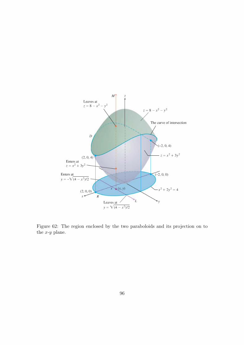
Figure 62: The region enclosed by the two paraboloids and its projection on tothe x-y plane.

96

do the integral. We have

V =

∫ ∫ ∫D

dz dy dx =

∫ 2

−2

∫ √(4−x2)/2

−√

(4−x2)/2

∫ 8−x2−y2

x2+3y2dz dy dx

=

∫ 2

−2

∫ √(4−x2)/2

−√

(4−x2)/2

((8− x2 − y2)− (x2 + 3y2)

)dy dx

=

∫ 2

−2

∫ √(4−x2)/2

−√

(4−x2)/2

(8− 2x2 − 4y2

)dy dx

=

∫ 2

−2

[(8− 2x2)y − 4

3y3

]√(4−x2)/2

−√

(4−x2)/2

dx

=

∫ 2

−2

{((8− 2x2)

√(4− x2)

2− 4

3

(4− x2

2

)3/2)

−

((8− 2x2)

√(4− x2)

2− 4

3

(4− x2

2

)3/2)}

dx

=

∫ 2

−2

(2(8− 2x2)

√(4− x2)

2− 8

3

(4− x2

2

)3/2)

dx

=

∫ 2

−2

(8

(4− x2

2

)3/2

− 8

3

(4− x2

2

)3/2)

dx

=4√

2

3

∫ 2

−2

(4− x2

)3/2dx [since (8− 8/3)/(23/2) = 4

√2/3]

=4√

2

3

∫ π/2

−π/243/2

(cos2 θ

)3/2 · 2 cos θ dθ [using subst. x = 2 sin θ]

=4√

2

3· 16

∫ π/2

−π/2cos4 θ dθ =

4√

2

3· 16

∫ π/2

−π/2

1

8(3 + 4 cos 2θ + cos 4θ) dθ

=4√

2

3· 2[3θ + 2 sin 2θ +

1

4sin 4θ

]π/2−π/2

=4√

2

3· 2 · 3

(π2

+π

2

)= 8√

2π .

Triple integrals can also be used to find the average value of a function over avolume. For example, the function F (x, y, z) defined over a volume D has an

97

Figure 63: The cube defined by the planes x = 2, y = 2 and z = 2.

average value

〈F (x, y, z)〉 =1

volume of D

∫ ∫ ∫D

F (x, y, z) dV

Example: Find the average value of F (x, y, z) = xyz over the cube bounded bythe planes x = 2, y = 2 and z = 2 in the first octant.

The solid of integration is shown in Fig. 63.

The volume of the cube is 23 = 8. The integral is∫ 2

0

∫ 2

0

∫ 2

0

xyz dx dy dz =

∫ 2

0

∫ 2

0

[x2

2yz

]2

0

dy dz

=

∫ 2

0

∫ 2

0

2yz dy dz =

∫ 2

0

[y2z]20

dz

=

∫ 2

0

4z dz =[2z2]20

= 8 .

98

Therefore the average value of F (x, y, z) = xyz over the cube is

〈F (x, y, z)〉 =1

volume of cube

∫ ∫ ∫cube

xyz dV =1

8· 8 = 1 .

3.5 Change of Variables in Triple Integrals

Changing variables in triple integrals is similar to the procedure used for doubleintegrals. Suppose

x = x(u, v, w), y = y(u, v, w), z = z(u, v, w) .

We define the Jacobian matrix for change of variables from (x, y, z) to (u, v, w) tobe

M

(x, y, z

u, v, w

)=

∂x/∂u ∂x/∂v ∂x/∂w∂y/∂u ∂y/∂v ∂y/∂w∂z/∂u ∂z/∂v ∂z/∂w

.

We can also define the Jacobian determinant

∂(x, y, z)

∂(u, v, w)≡ det M

such that the transformation for volume is

dx dy dz =

∣∣∣∣ ∂(x, y, z)

∂(u, v, w)

∣∣∣∣ du dv dw .

As before, for reversible transformations ∂(x, y, z)/∂(u, v, w) 6= 0 and we have

∂(x, y, z)

∂(u, v, w)=

(∂(u, v, w)

∂(x, y, z)

)−1

.

The integral under the change of variables becomes∫ ∫ ∫V

f(x, y, z) dx dy dz =∫ ∫ ∫V ′f(x(u, v, w), y(u, v, w), z(u, v, w))

∣∣∣∣ ∂(x, y, z)

∂(u, v, w)

∣∣∣∣ du dv dw

where V ′ is the transformed volume in (u, v, w) coordinates.

99

y

z

P

O

P'

r

x

φ

θ

Figure 64: The spherical polar coordinate system (r, θ, φ) for a point P in relationto the cartesian coordinate system (x, y, z).

Example: Find an expression for dx dy dz for the coordinate transformationfrom cartesian coordinates to spherical polar coordinates given by

x = x(r, θ, φ) = r sin θ cosφ

y = y(r, θ, φ) = r sin θ sinφ

z = z(r, θ, φ) = r cos θ .

The relationship between the coordinate systems is shown in Fig. 64. Note thatOP ′ = r sin θ.

Let u = r, v = θ and w = φ. Then

∂(x, y, z)

∂(u, v, w)=

∂(x, y, z)

∂(r, θ, φ)

=

∣∣∣∣∣∣sin θ cosφ r cos θ cosφ −r sin θ sinφsin θ sinφ r cos θ sinφ r sin θ cosφ

cos θ −r sin θ 0

∣∣∣∣∣∣= r2 sin θ .

100

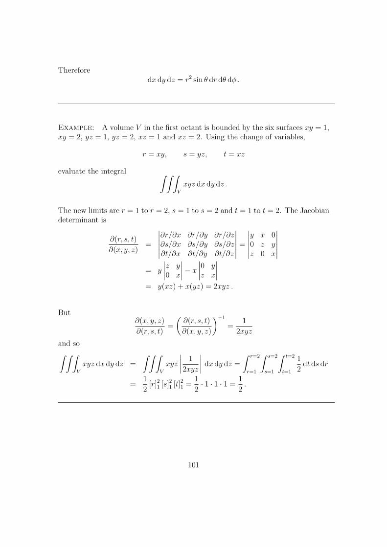
Thereforedx dy dz = r2 sin θ dr dθ dφ .

Example: A volume V in the first octant is bounded by the six surfaces xy = 1,xy = 2, yz = 1, yz = 2, xz = 1 and xz = 2. Using the change of variables,

r = xy, s = yz, t = xz

evaluate the integral ∫ ∫ ∫V

xyz dx dy dz .

The new limits are r = 1 to r = 2, s = 1 to s = 2 and t = 1 to t = 2. The Jacobiandeterminant is

∂(r, s, t)

∂(x, y, z)=

∣∣∣∣∣∣∂r/∂x ∂r/∂y ∂r/∂z∂s/∂x ∂s/∂y ∂s/∂z∂t/∂x ∂t/∂y ∂t/∂z

∣∣∣∣∣∣ =

∣∣∣∣∣∣y x 00 z yz 0 x

∣∣∣∣∣∣= y

∣∣∣∣z y0 x

∣∣∣∣− x ∣∣∣∣0 yz x

∣∣∣∣= y(xz) + x(yz) = 2xyz .

But∂(x, y, z)

∂(r, s, t)=

(∂(r, s, t)

∂(x, y, z)

)−1

=1

2xyz

and so∫ ∫ ∫V

xyz dx dy dz =

∫ ∫ ∫V

xyz

∣∣∣∣ 1

2xyz

∣∣∣∣ dx dy dz =

∫ r=2

r=1

∫ s=2

s=1

∫ t=2

t=1

1

2dt ds dr

=1

2[r]21 [s]21 [t]21 =

1

2· 1 · 1 · 1 =

1

2.

101

Figure 65: The definition of an infinite sequence.

4 Infinite Sequences and Series

4.1 Sequences

A sequence is a list of numbers in a given order:

a1, a2, a3, . . . , an, . . . .

Each of the a1, a2, etc. represents a number; these are therms of the sequence. Forexample

2, 4, 6, 8, . . . , 2n, . . .

has first term a1 = 2, second term a2 = 4 and nth term an = 2n. The integer n iscalled the index of an and denotes where an occurs on the list.

We can consider the sequence

a1, a2, a3, . . . , an, . . .

as a function that sends 1 to a1, 2 to a2, etc. and in general sends the positiveinteger n to the nth term an. The definition of an infinite sequence is shown inFig. 65.

Sequences can be described by rules or by listing terms. For example,

an =√n {an} =

{√1,√

2,√

3, . . . ,√n, . . .

}bn = (−1)n+1(1/n) {bn} =

{1,−1

2,1

3,−1

4, . . . , (−1)n+1 1

n, . . .

}cn = (n− 1)/n {cn} =

{0,

1

2,2

3,3

4, . . . ,

n− 1

n, . . .

}dn = (−1)n+1 {dn} =

{1,−1, 1,−1, . . . , (−1)n+1, . . .

}102

Figure 66: Sequences can be represented as points on the real line or as pointsin the plane where the horizontal axis n is the index number of the term and thevertical axis an is its value.

Sequences can be illustrated graphically either as points on a real axis or as thegraph of a function defining the sequence. This is illustrated in Fig. 66.

Consider the following sequences:{1,

1

2,1

3,1

4, . . . ,

1

n, . . .

}terms approach 0 as n gets large{

0,1

2,2

3,3

4, . . . , 1− 1

n, . . .

}terms approach 1 as n gets large{√

1,√

2,√

3,√

4, . . . ,√n, . . .

}terms get larger than any number as n increases{

1,−1, 1,−1, . . . , (−1)n+1, . . .}

terms oscillate between 1 and −1,

never converging to a single value

This leads to the definition of convergence, divergence and a limit shown in Fig. 67.

The concept of a limit is illustrated in Fig. 68. Here an → L if y = L is a horizontalasymptote of the sequence of points {(n, an)}.

103

Figure 67: The definition of convergence, divergence and a limit.

Figure 68: an → L if y = L is a horizontal asymptote of the sequence of points{(n, an)}. In this figure, all the an’s after aN lie within ε of L.

104

We will now consider two examples of the application of the definitions.

(1) We want to prove that:

limn→∞

1

n= 0.

Let ε > 0 be given. We need an integer N such that for all n,

n > N, ⇒∣∣∣∣ 1n − 0

∣∣∣∣ < ε .

This condition will be satisfied provided 1/n < ε, which means n > 1/ε. Thereforeif N is any integer greater than 1/ε, the implication will hold for all n > N . Hencelimn→∞(1/n) = 0. For example, suppose we take ε = 0.01 then the condition isjust n > 100.

(2) We want to prove that the sequence{1,−1, 1,−1, . . . , (−1)n+1, . . .

}diverges.

Assume that the sequence converges to some number L. Choose ε = 12

in thedefinition of the limit and so all terms an of the sequence with n larger than someN must lie within ε = 1

2of L. Since 1 is in every term in the sequence, 1 must lie

within ε of L. Hence

|L− 1| < 1

2or

1

2< L <

3

2.

Then −1 is also in every other term and so we must have

|L− (−1)| < 1

2or − 3

2< L < −1

2.

However, both conditions cannot be satisfied simultaneously. Therefore no suchlimit exists and so the sequence diverges.

The definition of a sequence that diverges to infinity, or diverges to negative infinityis given in Fig. 69. The sum, difference, product, constant multiple and quotientrules for sequences are given in Fig. 70.

We can use these rules to help us to calculate limits of sequences.

Example: Find limn→∞(n− 1)/n.

limn→∞

(n− 1

n

)= lim

n→∞

(1− 1

n

)= lim

n→∞1− lim

n→∞

1

n= 1− 0 = 1 .

105

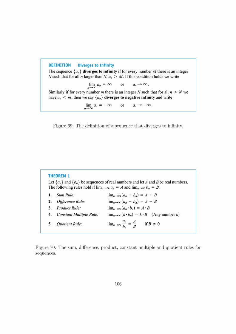
Figure 69: The definition of a sequence that diverges to infinity.

Figure 70: The sum, difference, product, constant multiple and quotient rules forsequences.

106

Figure 71: The Sandwich Theorem for Sequences.

Example: Find limn→∞ 5/n2.

limn→∞

5

n2= 5 · lim

n→∞

1

n· limn→∞

1

n= 5 · 0 · 0 = 0 .

The Sandwich Theorem for Sequences (see Fig. 71) provides another method forfinding the limits of sequences. Note that if |bn| ≤ cn and cn → 0 as n→∞, thenbn → 0 also, because −cn ≤ bn ≤ cn.

Example: Find limn→∞(sinn)/n.

By the properties of the sine function we must have −1 ≤ sinn ≤ 1 for all n.Therefore

− 1

n≤ sinn

n≤ 1

n⇒ lim

n→∞

sinn

n→ 0

because limn→∞(−1/n) = limn→∞(1/n) = 0 and the use of the Sandwich Theorem.

Example: Find limn→∞ 1/2n.

1/2n must always lie between 0 and 1/n (e.g. 12< 1, 1

4< 1

2, 1

8< 1

3, 1

16< 1

4, . . . ).

Therefore

0 ≤ 1

2n≤ 1

n⇒ lim

n→∞

1

2n→ 0 .

107

Figure 72: The Continuous Function Theorem for Sequences.

Figure 73: A theorem making the formal connection between limn→∞ an andlimx→∞ f(x).

The Continuous Function Theorem for Sequences (see Fig. 72) can be used todetermine the limits of sequences.

Example: Determine the limit of the sequence{

21/n}

as n→∞.

We already know that the sequence{

1n

}converges to 0 as n→∞. Let an = 1/n,

f(x) = 2x and L = 0 in the continuous function theorem for sequences. This gives

21/n = f(1/n)→ f(L) = 20 = 1 as n→∞ .

Hence the sequence{

21/n}

converges to 1.

We can also make use of l’Hopital’s Rule to find the limits of sequences. To do sowe need to make use of the theorem shown in Fig. 73.

108

Example: Show that limn→∞ ((lnn)/√n) = 0.

limn→∞

lnn√n

= limn→∞

1/n

(1/2)n−1/2(using l’Hopital’s Rule)

= limn→∞

2 · n1/2

n= 2 lim

n→∞

1

n1/2= 0 .

Example: Does the sequence whose nth term is an = ((n+1)/(n−1))n converge?If so, find limn→∞ an.

If we just take the straightforward limit we get 1∞. Typically with questions ofthis type we take the logarithm. This gives:

ln an = ln

(n+ 1

n− 1

)n= n ln

(n+ 1

n− 1

).

Hence

limn→∞

ln an = limn→∞

n ln

(n+ 1

n− 1

)= lim

n→∞

ln(n+1n−1

)1/n

= limn→∞

n−1n+1· (n−1)−(n+1)

(n−1)2

−1/n2(using l’Hopital’s Rule)

= limn→∞

−2/(n2 − 1)

−1/n2= lim

n→∞

2n2

n2 − 1= 2 .

This implies limn→∞ ln an = 2 and since f(x) = ex is continuous we have

an = eln an → e2 as n→∞ .

Therefore the sequence {an} converges to e2.

Figure 74 gives some common results for the limits of sequences. The first re-sult can be proved using l’Hopital’s rule. The second and third results can beproved using logarithms and applying the theorem given in Fig. 73. Proofs of theremaining results are given in Appendix 3 of Thomas.

109

Figure 74: Some limits that frequently arise.

Example: Show that limn→∞n√n2 = 1.

limn→∞

n√n2 = lim

n→∞n2/n = lim

n→∞

(n1/n

)2= (1)2 = 1 .

Example: Show that limn→∞ n sin(1/n) = 1.

limn→∞

n sin

(1

n

)= lim

n→∞

sin(1/n)

(1/n)= lim

n→∞

(−1/n2) cos(1/n)

(−1/n2)(using l’Hopital’s Rule)

= limn→∞

cos

(1

n

)= 1 .

Figure 75 contains the definition of a nondecreasing sequence; this is a sequencewhere each term is at least as large as its predecessor. Examples of nondecreasingsequences are the sequence of natural numbers, {1, 2, 3, . . . , n, . . . } and constantsequences such as {3, 3, 3, . . . }.

Figure 76 has the definitions of sequences that are bounded from above, an upperbound, and the least upper bound.

110

Figure 75: The definition of a nondecreasing sequence.

Figure 76: The definition of bounded from above, upper bound and least upperbound.

From these definitions we can state that the sequence of natural numbers given by,{1, 2, 3, . . . , n, . . . }, has no upper bound and that the sequence

{12, 2

3, 3

4, . . . , n

n+1, . . .

}is bounded from above by M = 1.

This leads on to the Nondecreasing Sequence Theorem given in Fig. 77. Thisimplies that a nondecreasing sequence converges when it is bounded from aboveand it diverges to infinity if it is not bounded from above.

Figure 77: The Nondecreasing Sequence Theorem.

111

Figure 78: The definitions of an infinite series, the nth term in a series, partialsums, converges, sum and diverges.

4.2 Infinite series

An infinite series is the sum of an infinite sequence of numbers

a1 + a2 + a3 + · · ·+ an + · · · .

Figure 78 gives the definitions of an infinite series, the nth term in a series, partialsums, converges, sum and diverges.

A geometric series has the form

a+ ar + ar2 + · · ·+ arn−1 + · · · =∞∑n=1

arn−1 =∞∑n=0

arn

112

where a and r are fixed real numbers and a 6= 0. The quantity r is called the ratioof the geometric series and can be positive or negative.

In the special case where r = 1 the nth partial sum is

sn = a+ a · 1 + a · 12 + · · ·+ a · 1n−1 = na

and the series diverges because limn→∞ sn = ±∞ depending on the sign of a. Ifr = −1 the series diverges because either sn = 0 or sn = 0 depending on the valueof n.

Now consider the case of a geometric series with |r| 6= 1. We have

sn = a+ ar + ar2 + · · ·+ arn−1

⇒ rsn = ar + ar2 + · · ·+ arn−1 + arn

⇒ sn − rsn = a− arn or sn(1− r) = a(1− rn)

⇒ sn =a(1− rn)

1− r(r 6= 1) .

Therefore, if |r| < 1 then rn → 0 as n→∞ and hence sn → a/(1− r). If |r| > 1then |rn| → ∞ and the series diverges. So we have

∞∑n=1

arn−1 =a

1− rfor |r| < 1

and the geometric series converges.

For example,

1

9+

1

27+

1

81· · · =

∞∑n=1

1

9

(1

3

)n−1

=(1/9)

1− (1/3)=

1

6(a = 1/9, r = 1/3)

and

5− 5

4+

5

16− 5

64+ · · · =

∞∑n=0

(−1)n5

4n=

5

1 + (1/4)= 4 (a = 5, r = −1/4) .

Example: Find the sum of the series∑∞

n=1 1/((n(n+ 1)).

113

Note that we can use partial fractions to write

1

n(n+ 1)=

1

n− 1

n+ 1.

Hence the sum of the first k terms is

k∑n=1

1

n(n+ 1)=

k∑n=1

(1

n− 1

n+ 1

)and so the kth partial sum is

sk =

(1

1− 1

2

)+

(1

2− 1

3

)+

(1

3− 1

4

)+ · · ·+

(1

k− 1

k + 1

)=

1

1+

(−1

2+

1

2

)+

(−1

3+

1

3

)+ · · ·+

(−1

k+

1

k

)− 1

k + 1

Hence sk → 1 as k →∞ and so the series converges giving

∞∑n=1

1

n(n+ 1)= 1 .

Suppose the series∑∞

n=1 an converges to a sum S and the nth partial sum of theseries is sn = a1 + a2 + · · · + an. When n is large, both sn and sn−1 are close toS and therefore their difference, an, is close to zero. Using the Difference Rule forsequences we have

an = sn − sn−1 → S − S = 0 as n→∞ .

Hence, if∑∞

n=1 an converges, then an → 0. This is stated in Fig. 79. Note thatthe converse of this is false: If an → 0 this does not imply that the series

∑∞n=1 an

converges. This, in turn, leads to the nth-Term Test for Divergence shown inFig. 80. For example, we can apply the nth Term Test in the following cases:

∞∑n=1

n2 diverges because n2 →∞

∞∑n=1

n+ 1

ndiverges because

n+ 1

n→ 1

∞∑n=1

(−1)n+1 diverges because limn→∞

(−1)n+1 does not exist

∞∑n=1

−n2n+ 5

diverges because limn→∞

−n2n+ 5

= −1

26= 0 .

114

Figure 79: Property of the general term in a convergent series.

Figure 80: Statement of the nth Term Test for Divergence.

Consider the unusual case of a series where an → 0 but the series itself diverges.The series is

1 +1

2+

1

2+

1

4+

1

4+

1

4+

1

4+ · · ·+ 1

2n+

1

2n+ · · ·+ 1

2n+ · · ·

where there are two terms of 1/2, four terms of 1/4, ..., 2n terms of 1/2n, etc. Inthis case each grouping of terms adds up to 1 so the partial sums must increasewithout bound and so the series diverges, even though the terms of the series forma sequence that converges to 0.

If we have two convergent series, we can add them term by term, subtract themterm by term, or multiply them by constants to make new convergent series. Thisis stated formally in Fig. 81.

Example: Find∑∞

n=1(3n−1 − 1)/6n−1 .

∞∑n=1

3n−1 − 1

6n−1=

∞∑n=1

(1

2n−1− 1

6n−1

)=∞∑n=1

1

2n−1−∞∑n=1

1

6n−1

=1

1− (1/2)− 1

1− (1/6)(two geometric series)

= 2− 6

5=

4

5.

115

Figure 81: The Sum, Difference and Constant Multiple Rules for convergent series.

We can add a finite number of terms or delete a finite number of terms withoutaltering the convergence or divergence of a series but if the series is convergentthis will usually alter the sum. Consider the series,

∞∑n=1

an = a1 + a2 + · · ·+ ak−1 +∞∑n=k

an .

If∑∞

n=1 an converges, then∑∞

n=k an converges for any k > 1. Conversely, if∑∞n=k an converges for any k > 1, then

∑∞n=1 an converges.

Note that re-indexing a series (e.g. changing the starting value of the index) doesnot alter its convergence, provided the order of the terms is preserved.

4.3 The Integral Test

For a given series,∑an we want to know: (1) Does it converge? (2) If it converges,

what is its sum?

A corollary of the Nondecreasing Sequence Theorem (see Fig. 77) is that the series∑∞n=1 an of non-negative terms converges if and only if its partial sums are bounded

from above.

Consider the harmonic series:

∞∑n=1

1

n= 1 +

1

2+

1

3+ · · ·+ 1

n+ · · · .

116

Figure 82: The sum of the areas of the rectangles under the graph of f(x) = 1/x2

is less than the area under the graph.

This series is actually divergent even though the nth term, 1/n → 0 as n → ∞.However, the series has no upper bound for its partial sums. We can see this bywriting the series as

1 +1

2+

(1

3+

1

4

)+

(1

5+

1

6+

1

7+

1

8

)+

(1

9+

1

10+ · · ·+ 1

16

)+ · · · .

Now 13

+ 14> 2

4= 1

2, 1

5+ 1

6+ 1

7+ 1

8> 4

8= 1

2, 1

9+ 1

10+ · · · + 1

16> 8

16= 1

2and

so on. Therefore the sum of the 2n terms ending with 1/2n+1 is > 2n/2n+1 = 1/2.Therefore the sequence of partial sums is not bounded from above, and so theharmonic series diverges.

Now consider the series,

∞∑n=1

1

n2= 1 +

1

4+

1

9+

1

16+ · · ·+ 1

n2+ · · ·

Does it converge or diverge? To answer this question we will consider a newapproach involving the use of integration. What we need to do is compare series∑∞

n=1 1/n2 with the integral∫ x

11/x2 dx (see Fig. 82). From Fig. 82,

117

Figure 83: The Integral Test.

sn =1

12+

1

22+

1

32+ · · ·+ 1

n2

= f(1) + f(2) + f(3) · · ·+ f(n)

< f(1) +

∫ n

1

1

x2dx

< 1 +

∫ ∞1

1

x2dx

Therefore

sn < 1 +

∫ ∞1

1

x2dx = 1 +

[−1

x

]∞1

= 2 .

Thus sn < 2 for all n and the partial sums are bounded from above (by 2) andtherefore the series converges. (In fact, the sum of the series is π2/6.) Note thatthe series and the integral need not have the same value in the convergent case.

The approach we have just taken leads us to the Integral Test (see Fig. 83). Wewill consider the proof for the case N = 1 and we start with the asumption that fis a decreasing function with f(n) = an for every n. In Fig. 84(a) the areas of therectangles a1, a2, . . . , an enclose more area than that under the curve y = f(x)between x = 1 and x = n+ 1. Therefore we can write∫ n+1

1

f(x) dx ≤ a1 + a2 + · · ·+ an .

Now consider the rectangles as shown in Fig. 84(b). If we ignore the first rectanglewe can write

a2 + a3 + · · ·+ an ≤∫ n

1

f(x) dx

or, adding the area a1 to each side gives

a1 + a2 + a3 + · · ·+ an ≤ a1 +

∫ n

1

f(x) dx

118

Figure 84: Subject to the conditions of the Integral Test, the series∑∞

n=1 an andthe integral

∫∞1f(x) dx both converge or both diverge.

119

Combining the two inequalities gives∫ n+1

1

f(x) dx ≤ a1 + a2 + · · ·+ an ≤ a1 +

∫ n

1

f(x) dx .

These inequalities will hold as n→∞.

Therefore, if∫ n

1f(x) dx is finite, the right-hand part of the inequality shows that∑

an is also finite. Similarly, if∫ n

1f(x) dx is infinite, then

∑an is infinite by the

left-hand part of the inequality.

The Integral Test can be used to show that the p-series,∑∞

n=1 1/np converges ifp > 1, and diverges if p ≤ 1 (see Thomas for proof).

Example: Show that the series∑∞

n=1 1/(n2 + 1) converges by the integral test.

The function f(x) = 1/(x2 + 1) is positive, continuous and decreasing for x ≥ 1.Also ∫ ∞

1

1

x2 + 1dx = lim

b→∞

[tan−1 x

]b1

= limb→∞

[tan−1 b− tan−1 1

]=

π

2− π

4=π

4

and so the series converges (but we do not know its sum).

4.4 The Ratio Test

Let∑an be a series with positive terms and suppose that

limn→∞

an+1

an= ρ .

Then:

(a) The series converges if ρ < 1.

120

(b) The series diverges if ρ > 1 or ρ is infinite.

(c) The test is inconclusive if ρ = 1.

This is the Ratio Test. Proofs of the above results are given in Thomas.

The two series we looked at in the last section are good examples of cases whereρ = 1 and the test is inconclusive.∑ 1

n:

an+1

an=

1/(n+ 1)

1/n=

n

n+ 1→ 1

∑ 1

n2:

an+1

an=

1/(n+ 1)2

1/n2=

(n

n+ 1

)2

→ 12 = 1 .

In each case ρ = 1 (i.e. the test is inconclusive) and yet we know that∑

1/ndiverges whereas

∑1/n2 converges.

Example: Use the Ratio Test to investigate the convergence of the followingseries:

(a)∞∑n=1

2n + 5

3n, (b)

∞∑n=1

(2n)!

(n!)2, (c)

∞∑n=1

n!

nn.

(a)

an =2n + 5

3n; an+1 =

2n+1 + 5

3n+1;

⇒ an+1

an=

(2n+1 + 5)/3n+1

(2n + 5)/3n=

1

3· 2n+1 + 5

2n + 5=

1

3

(2 + 5 · 2−n

1 + 5 · 2−n

)⇒ an+1

an→ 1

3· 2

1=

2

3< 1 as n→∞ and the series converges.

(b)

an =(2n)!

(n!)2; an+1 =

(2(n+ 1)!)

((n+ 1)!)2;

⇒ an+1

an=

(2n+ 2)!

(n+ 1)!(n+ 1)!· n!n!

(2n)!=

(2n+ 2)(2n+ 1)

(n+ 1)(n+ 1)

=4n+ 2

n+ 1=

4 + 2/n

1 + 1/n→ 4 > 1 and the series diverges.

121

Figure 85: The definition of power series about x = 0 and x = a.

(c)

an =n!

nn; an+1 =

(n+ 1)!

(n+ 1)n+1;

⇒ an+1

an=

(n+ 1)!nn

(n+ 1)n+1n!=

(n+ 1)nn

(n+ 1)n(n+ 1)

=nn

(n+ 1)n=

(n

n+ 1

)n=

(1

1 + 1/n

)n→ 1

and we cannot determine the convergence or the divergence.

4.5 Power Series

A power series is an infinite series in powers of some variable, usually x. Suchseries can be added, subtracted, multiplied, differentiated and integrated to givenew power series. Power series about x = 0 and x = a are defined in Fig. 85.

Consider the case where the coefficients in (1) in Fig. 85 are all unity.:

∞∑n=0

cnxn =

∞∑n=0

xn = 1 + x+ x2 + · · ·+ xn + · · · .

This is just a geometric series with first term 1 and ratio x. We know from the

122

Figure 86: The graphs of f(x) = 1/(1− x) and four of its polynomial approxima-tions.

properties of geometric series that it converges to 1/(1− x) for |x| < 1. Hence

1

1− x= 1 + x+ x2 + · · ·+ xn + · · · , −1 < x < 1 .

We can think of the right-hand side of this equation a sequence of partial sumswhich are polynomials Pn(x) that approximate the function on the left.

f(x) =1

1− x; P0(x) = 1 (horizontal line)

P1(x) = 1 + x (straight line, slope 1)

P2(x) = 1 + x+ x2 (quadratic curve [parabloa])...

etc.

The successive polynomials are illustrated in Fig. 86.

Now consider the power series

1− 1

2(x− 2) +

1

4(x− 2)2 + · · ·+

(−1

2

)n(x− 2)n + · · · .

This matches the form of (2) in Fig. 85 with a = 2, cn = (−1/2)n. This isa geometric series with the first term 1 and ratio r = −(x − 2)/2. This series

123

Figure 87: The graphs of f(x) = 2/x and its first three polynomial approximations.

converges for |(x− 2)/2| < 1 or 0 < x < 4. The sum is

1

1− r=

1

1 + (x− 2)/2=

2

x.

Hence

2

x= 1− (x− 2)

2+

(x− 2)2

4− · · ·+

(−1

2

)2

(x− 2)n + · · · , 0 < x < 4 .

Again we can consider the series as a sequence of partial sums which are polyno-mials Pn(x) that approximate 2/x:

f(x) =2

x; P0(x) = 1

P1(x) = 1− 1

2(x− 2) = 2− x

2

P2(x) = 1− 1

2(x− 2) +

1

4(x− 2)2 = 3− 3x

2+x2

4...

etc.

The successive polynomials are illustrated in Fig. 87.

A series∑an converges absolutely if the corresponding series of absolute values,∑

|an|, converges. The Convergence Theorem for Power Series is shown in Fig. 88and a corollary to it in Fig. 89.

124

Figure 88: The Convergence Theorem for Power Series.

Figure 89: A corollary to the Convergence Theorem for Power Series.

A series that converges but does not converge absolutely, converges conditionally.

Here R is called the radius of convergence and the interval of radius R centred atx = a is called the interval of convergence.

When studying the convergence of power series such as these, alternating seriesfrequently arise. Here we can make use of an additional test. The AlternatingSeries Test states that the series

∞∑n=1

(−1)n+1un = u1 − u2 + u3 −+u4 − u5 + · · ·

converges if all three of the following conditions hold: (i) The un are all positive,(ii) un ≥ un+1 for all n ≥ N , for some integer N and (iii) un → 0 as n→∞.

We can test a power series for convergence using several methods:

125

1. Use a test such as the ratio test to find the interval where the series converges.

2. If the interval of absolute convergnec is finite, test for convergence or diver-gence at each endpoint using a test such as the integral test.

3. If the interval of convergence is a − R < x < a + R, the series diverges for|x− a| > R.

Example: Use the ratio test to determine the convergence of

∞∑n=1

(−1)n−1 x2n−1

2n− 1= x− x3

3+x5

5− · · · .

We have ∣∣∣∣un+1

un

∣∣∣∣ =2n− 1

2n+ 1x2 → x2 .

Therefore the series converges absolutely for x2 < 1 and diverges for x2 > 1. Atx = 1 the series is 1− 1

3+ 1

5− 1

7+ · · · which can be shown to converge. The series

also converges at x = −1.

Let

f(x) =∞∑n=0

cn(x− a)n

converge for a−R < x < a+R with R > 0. It can be shown that such a functionhas derivatives of all orders inside the interval of convergence. This means that

f ′(x) =∞∑n=1

ncn(x− a)n−1

f ′′(x) =∞∑n=2

n(n− 1)cn(x− a)n−2 , etc.

Each derived series converges at every interior point of the interval of convergenceof the initial series. Furthermore

∞∑n=0

cn(x− a)n+1

n+ 1

126

also converges in the same intervals and hence∫f(x) dx =

∞∑n=0

cn(x− a)n+1

n+ 1+ C .

For example,

f(x) =1

1− x= 1 + x+ x2 + · · ·+ xn + · · ·

=∞∑n=0

xn , −1 < x < 1

f ′(x) =1

(1− x)2= 1 + 2x+ 3x2 + · · ·+ nxn−1 + · · ·

=∞∑n=1

nxn−1 , −1 < x < 1

f ′′(x) =2

(1− x)3= 2 + 6x+ 12x2 + · · ·+ n(n− 1)xn−2 + · · ·

=∞∑n=2

n(n− 1)xn−2 , −1 < x < 1 .

Example: Identify the function with the power series

f(x) = x− x3

3+x5

5− · · · , −1 ≤ x ≤ 1 .

We havef ′(x) = 1− x2 + x4 − x6 + · · · , −1 < x < 1 .

This is a geometric series (first term 1 and ratio −x2) and so we can use the formulafor the sum of such a series to write

f ′(x) =1

1− (−x2)=

1

1 + x2

and hence ∫f ′(x) dx =

∫dx

1 + x2= tan−1 x+ C .

The original series for f(x) is zero when x = 0 and so C = 0. Hence

f(x) = x− x3

3+x5

5− · · · = tan−1 x .

127

4.6 Taylor and Maclaurin Series

Consider the function f(x) represented as a power series:

f(x) =∞∑n=0

an(x− a)n = a0 + a1(x− a) + · · ·+ an(x− a)n + · · ·

with a positive radius of convergence, R. We have

f ′(x) = a1 + 2a2(x− a) + · · ·+ nan(x− a)n−1 + · · ·f ′′(x) = 1 · 2a2 + 2 · 3a3(x− a) + · · ·+ n(n− 1)an(x− a)n−2 + · · ·

...

f (n)(x) = n! an + a sum of terms with (x− a) as a factor.

Therefore

f ′(a) = a1 , f′′(a) = 1 · 2a2 , f

′′′(a) = 1 · 2 · 3a3 , . . . , f(n)(a) = n! an .

This gives us a formula for the coefficients in the power series:

an =f (n)(a)

n!.

It also suggest that if f has a series representation then it must be

f(x) = f(a) + f ′(a)(x− a) +f ′′(a)

2!(x− a)2 + · · ·+ f (n)(a)

n!(x− a)n + · · · .

This leads us to the definition of the Taylor Series and the Maclaurin Series givenin Fig. 90.

Example: Find the Taylor series generated by f(x) = 1/x at x = 2. Where, ifanywhere, does the series converge to 1/x?

f(x) = x−1 ; f(2) = 2−1 =1

2

f ′(x) = −x−2 ; f ′(2) = − 1

22

f ′′(x) = 2!x−3 ;f ′′(2)

2!= 2−3 =

1

23

...

f (n)(x) = (−1)nn!x−(n+1) ;f (n)(2)

n!=

(−1)n

2n+1.

128

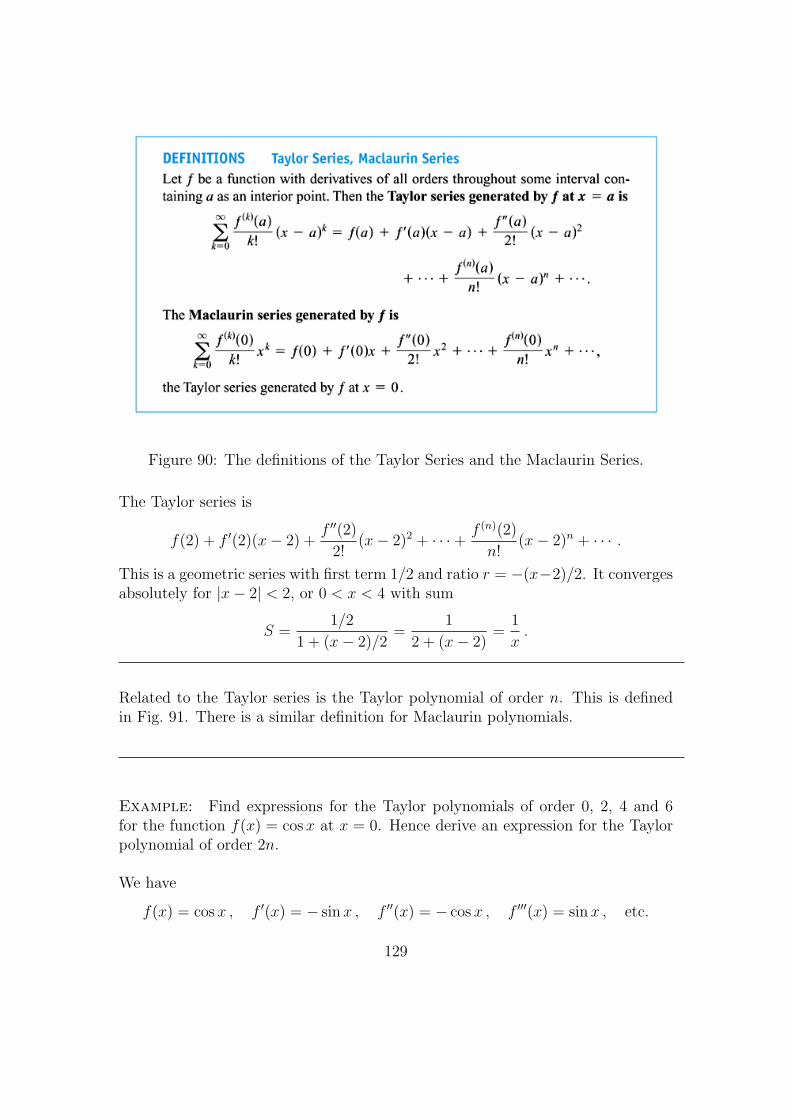
Figure 90: The definitions of the Taylor Series and the Maclaurin Series.

The Taylor series is

f(2) + f ′(2)(x− 2) +f ′′(2)

2!(x− 2)2 + · · ·+ f (n)(2)

n!(x− 2)n + · · · .

This is a geometric series with first term 1/2 and ratio r = −(x−2)/2. It convergesabsolutely for |x− 2| < 2, or 0 < x < 4 with sum

S =1/2

1 + (x− 2)/2=

1

2 + (x− 2)=

1

x.

Related to the Taylor series is the Taylor polynomial of order n. This is definedin Fig. 91. There is a similar definition for Maclaurin polynomials.

Example: Find expressions for the Taylor polynomials of order 0, 2, 4 and 6for the function f(x) = cosx at x = 0. Hence derive an expression for the Taylorpolynomial of order 2n.

We have

f(x) = cos x , f ′(x) = − sinx , f ′′(x) = − cosx , f ′′′(x) = sin x , etc.

129

Figure 91: The definition of the Taylor polynomial of order n.

Hencef (2n)(x) = (−1)n cosx , f (2n+1)(x) = (−1)n+1 sinx .

At x = 0, the cosines are 1 and the sines are 0, so

f (2n)(0) = (−1)n , f (2n+1)(0) = 0 .

Therefore the Taylor series for f(x) = cos x about x = 0 is

f(0) + f ′(0)x+f ′′(0)

2!x2 + · · ·+ f (2n)(0)

n!xn + · · ·

= 1 + 0 · x− 1 · x2

2!+ 0 · x

3

3!+ 1 · x

4

4!+ · · ·+ (−1)n

x2n

(2n)!+ · · · .

Therefore the first four Taylor polynomials of f(x) = cos x about x = 0 are

P0(x) = 1

P2(x) = 1− x2

2!

P4(x) = 1− x2

2!+x4

4!

P6(x) = 1− x2

2!+x4

4!− x6

6!

and the Taylor polynomial of order 2n is

P2n(x) = P2n+1(x) = 1− x2

2!+x4

4!− · · ·+ (−1)n

x2n

(2n)!.

130

Figure 92: The Taylor polynomials for cosx converge to cosx as n→∞. We candeduce the behaviour of cosx arbitrarily far away solely from knowing the valuesof the cosine and its derivatives at x = 0.

Figure 92 shows how successive Taylor polynomials provide better and better ap-proximations to the function as n→∞.

Below we give the Taylor series expansions for a variety of functions about x = 0(for ex, sin x, cosx, cosh x and sinhx) and x = 1 (for lnx and

√x). These can all

be derived using the methods in this section. Some of these were already given inSection 1.5 above.

Taylor series about x = 0:

ex = 1 + x+x2

2!+x3

3!+x4

4!+ · · ·

sinx = x− x3

3!+x5

5!− x7

7!+ · · ·

cosx = 1− x2

2!+x4

4!− x6

6!+ · · ·

coshx = 1 +x2

2!+x4

4!+x6

6!+ · · ·

sinhx = x+x3

3!+x5

5!+x7

7!+ · · · .

131

Figure 93: The statement of Taylor’s formula.

Taylor series about x = 1:

lnx = (x− 1)− 1

2(x− 1)2 +

1

3(x− 1)3 − 1

4(x− 1)4 + · · ·

√x = 1 +

1

2(x− 1)− 1

8(x− 1)2 +

1

16(x− 1)3 − · · · .

4.7 Convergence of Taylor Series and Error Estimates

There are still two unanswered questions about Taylor series:

1. When does a Taylor series converge to the function that generated it?

2. How accurately do a function’s Taylor polynomials approximate the functionon a given interval.

To answer these questions we need to make use of Taylor’s formula (see Fig. 93).The quantity Rn(x) in Taylor’s Formula is called the remainder of order n or theerror term for the approximation of f by Pn(x) over I. If Rn(x) → 0 as n → ∞for all x ∈ I, we say that the Taylor series converges to f on I and we write

f(x) =∞∑k=0

f (k)(a)

k!(x− a)k .

132

Figure 94: The statement of the Remainder Estimation Theorem.

Finally we can use the Remainder Estimation Theorem (Fig. 94) to provide anestimate of the error.

Example: Show that the Taylor series for sinx at x = 0 converges for all x.

We havef(x) = sinx , f ′(x) = cos x , f ′′(x) = − sinx , . . .

and, in general,

f (2k)(x) = (−1)k sinx , f (2k+1)(x) = (−1)k cosx

Therefore, evaluating at x = 0 gives f (2k)(0) = 0 and f (2k+1)(0) = (−1)k. Hencethe Taylor series for sin x at x = 0 is

sinx = x− x3

3!+x5

5!− · · ·+ (−1)kx2k+1

(2k + 1)!+R2k+1(x) .

Applying the Remainder Estimation Theorem with M = 1 gives

|R2k+1(x)| ≤ 1 · |x|2k+2

(2k + 2)!→ 0 as k →∞ for all x.

Therefore R2k+1(x) → 0 and the Maclaurin series for sinx converges to sin x forevery x.

133

Example: Calculate e with an error of less than 10−6.

We have:

ex = 1 + x+x2

2!+x3

3!+x4

4!+ · · · .

Therefore

e = 1 + 1 +1

2!+ · · ·+ 1

n!+Rn(1)

with

Rn(1) =ec · 1

(n+ 1)!

for some c between 0 and 1. Let us assume we know that e < 3. Hence

1

(n+ 1)!< Rn(1) <

3

(n+ 1)!

because 1 < ec < 3 for 0 < c < 1. By experiment we find 1/9! > 10−6 while3/10! < 10−6. Thus n+ 1 should be at least 10 or n should be at least 9. Hence

e = 1 + 1 +1

2+

1

3!+ · · ·+ 1

9!≈ 2.718282 .

4.8 Applications of Power Series

4.8.1 Binomial series

The Taylor series generated by f(x) = (1 + x)m where m is a constant is

f(x) = 1 +mx+m(m− 1)

2!x2 +

m(m− 1)(m− 2)

3!x3 + · · ·

+m(m− 1)(m− 2) . . . (m− k + 1)

k!xk + · · · .

This is called the binomial series and it converges absolutely for |x| < 1.

If m is an integer ≥ 0, the series stops after (m + 1) terms because coefficientsfrom k = m+1 onwards are zero. If m is not a positive integer the series is infiniteand converges for |x| < 1.

134

So, for −1 < x < 1, we have

(1 + x)m = 1 +∞∑k=1

(mk

)xk

where (m1

)= m,

(m2

)=m(m− 1)

2!, . . .(

mk

)=m(m− 1)(m− 2) . . . (m− k + 1)

k!for k ≥ 3.

Note that in the case where m = −1,(−11

)= −1 ,

(−12

)= 1 and

(−1k

)= (−1)k .

For example,

x

1 + x2= x(1 + x2)−1

= x

(1− x2 +

(−1)(−2)

2!x4 +

(−1)(−2)(−3)

3!x6 + · · ·

)= x(1− x2 + x4 − x6 + · · · )= x− x3 + x5 − x7 + · · · .

4.8.2 Series solutions of differential equations

As an example, consider the differential equation

y′′ + x2y = 0 .

We can assume a power series solution:

y = a0 + a1x+ a2x2 + · · ·+ anx

n + · · ·⇒ y′′ = 2a2 + 3 · 2 a3x+ · · ·+ n(n− 1)anx

n−2 + · · ·and x2y = a0x

2 + a1x3 + · · ·+ anx

n+2 + · · · .

Subsitiuting in the differential equation gives

y′′ + x2y = 2a2 + 6a3x+ (12a4 + a0)x2 + · · ·+ (n(n− 1)an + an−4)x

n−2

= 0 if the series satisfies the differential equation.

135

Equating the coefficients gives

2a2 = 0 , 6a3 = 0 , 12a4 + a0 = 0 , . . . ,

n(n− 1)an + an−4 = 0 ; an =−an−4

n(n− 1).

When x = 0, y = a0 and hence a0 = y(0).

Also, when x = 0, y′ = a1 and hence a1 = y′(0).

Furthermore a2 = 0, a3 = 0 and hence a6 = 0, a7 = 0, a10 = 0 and a11 = 0.

We also have

a4 =−a0

4 · 3, a8 =

−a4

8 · 7=

a0

3 · 4 · 7 · 8, etc.

and

a5 =−a1

5 · 4, a9 =

−a5

9 · 8=

a1

4 · 5 · 8 · 9, etc.

Therefore our series solution is now

y = a0

(1− x4

3 · 4+

x8

3 · 4 · 7 · 8− · · ·

)+ a1

(x− x5

4 · 5+

x9

4 · 5 · 8 · 9− · · ·

).

Note that there are two constants, a0 and a1, in the solution as this is a secondorder differential equation.

4.8.3 Evaluation of non-elementary integrals

We can use the term-by-term integration property of power series to allow us todo non-elementary integrals.

Example: Express∫

sinx2 dx as a power series.

Recall that

sinx = x− x3

3!+x5

5!− · · ·

Hence

sinx2 = x2 − x6

3!+x10

5!− · · ·

136

and so ∫sinx2 dx = C +

x3

3− x7

7 · 3!+

x11

11 · 5!− · · · .

where C is a constant of integration.

4.8.4 Evaluating indeterminate forms

Power series are also useful in evaluating indeterminate forms.

Example: Find

limx→0

(1

sinx− 1

x

).

We can write

1

sinx− 1

x=

x− sinx

x sinx=x−

(x− x3

3!+ x5

5!− · · ·

)x ·(x− x3

3!+ x5

5!− · · ·

)=

x3(

13!− x2

5!+ · · ·

)x2(1− x2

3!+ · · ·

) = x

(13!− x2

5!+ · · ·

)(1− x2

3!+ · · ·

) .

Hence

limx→0

(1

sinx− 1

x

)= lim

x→0

x(

13!− x2

5!+ · · ·

)(1− x2

3!+ · · ·

) = 0 .

Note that since 1/ sinx− 1/x ≈ x · (1/3!) = x/6, we can write cosec x ≈ (1/x) +(x/6).

137