ADVANCED PLACEMENT CALCULUS AB
11
ADVANCED PLACEMENT STATISTICS COURSE SYLLABUS OVERVIEW Advanced Placement Statistics introduces students to the major concepts and tools for collecting, analyzing, and drawing conclusions from data through four broad themes: (1) exploring data, (2) sampling and experimentation, (3) anticipating patterns and, (4) statistical inference. Collaboration between the students, parents, and classroom teacher will go in effect to produce a calendar for extended sessions. A minimum of five (5) sessions, including a mock exam, are required in order to cover all objectives necessary to help be successful on the exam. TEACHING STRATEGIES It is understood that the prerequisites for Advanced Placement Statistics expose student the TI-83 or 84 calculators. Most students own the TI-83 plus, TI-84, or the TI-89. Other students are encouraged to purchase the TI-84 or TI-89. In addition to the calculator, students will have the opportunity to see a set of interactive statistical applets and software including Fathom. Students will also learn the strategy and not just the skills. At various concepts special problems will be assigned to help give students experience using a representative statistics package and writing statistics narratives. Students must be able to speak statistically and convey data within context. It is my belief that students can successfully present information verbally in comfortable settings. Students are seated in pods from three (3) to six (6) students each creating open opportunities for collaborative work. All tests are formatted like the Advanced Placement exam. This allows the students to become familiar with what to expect. Students are also expected to remediate and correct all tests if necessary. Test corrections, if necessary, are mandatory and will be 5% of the final grade. All test corrections must be completed within two weeks of the date of return. CLASSROOM MECHANICS Attendance: Please refer to the Weaver Academy attendance policy. Make-Up Work: Any work that is missed due to an absence must be completed within 3 school days of the absence. Tutorials: Any student that earns a “C” or lower on any progress report is required to attend tutorial for AP Statistics. Please refer to your individual teacher for tutorial availability. WE are here to help each student succeed. WE will do whatever WE can to ensure that your child gets as much assistance with their education as possible. Schedule─ Tuesdays: 4:05-5:00pm, other times by appointment only.
-
Upload
khangminh22 -
Category
Documents
-
view
4 -
download
0
Transcript of ADVANCED PLACEMENT CALCULUS AB

ADVANCED PLACEMENT STATISTICS COURSE SYLLABUS
OVERVIEW
Advanced Placement Statistics introduces students to the major concepts and tools for collecting, analyzing, and drawing conclusions from data through four broad themes: (1) exploring data, (2) sampling and experimentation, (3) anticipating patterns and, (4) statistical inference. Collaboration between the students, parents, and classroom teacher will go in effect to produce a calendar for extended sessions. A minimum of five (5) sessions, including a mock exam, are required in order to cover all objectives necessary to help be successful on the exam.
TEACHING STRATEGIES
It is understood that the prerequisites for Advanced Placement Statistics expose student the TI-83 or 84 calculators. Most students own the TI-83 plus, TI-84, or the TI-89. Other students are encouraged to purchase the TI-84 or TI-89. In addition to the calculator, students will have the opportunity to see a set of interactive statistical applets and software including Fathom. Students will also learn the strategy and not just the skills. At various concepts special problems will be assigned to help give students experience using a representative statistics package and writing statistics narratives. Students must be able to speak statistically and convey data within context. It is my belief that students can successfully present information verbally in comfortable settings. Students are seated in pods from three (3) to six (6) students each creating open opportunities for collaborative work. All tests are formatted like the Advanced Placement exam. This allows the students to become familiar with what to expect. Students are also expected to remediate and correct all tests if necessary. Test corrections, if necessary, are mandatory and will be 5% of the final grade. All test corrections must be completed within two weeks of the date of return.
CLASSROOM MECHANICS
Attendance: Please refer to the Weaver Academy attendance policy.
Make-Up Work: Any work that is missed due to an absence must be completed within 3 school days of the absence.
Tutorials: Any student that earns a “C” or lower on any progress report is required to attend tutorial for AP Statistics. Please refer to your individual teacher for tutorial availability. WE are here to help each student succeed. WE will do whatever WE can to ensure that your child gets as much assistance with their education as possible.
Schedule─ Tuesdays: 4:05-5:00pm, other times by appointment only.

Course Assessment: We will use a variety of assessment tools throughout the course. Each quarter’s average will be calculated using the following percentages:
Remediation 5% Projects 10% Quizzes 35% Tests 50%
A test will be given at the end of each unit. Cumulative tests will also be given periodically throughout the course. Test corrections are calculated in the Remediation score.
Late Work: No late work will be accepted with the exception of absences. Students are only allowed to turn in late work if they are absent the day the work is assigned.
Grading Scale: 90 – 100 A 60 – 69 D 80 – 89 B 0 – 59 F 70 – 79 C **Normal rounding rules will apply**
Your final grade in this course will be comprised of your Quarter 3 and Quarter 4 averages (80%) and the End of Course Exam (20%).
Emergency Procedures: During a fire drill please walk orderly out the double doors to the parking lot across from the mobile units. If a fire drill occurs during lunch please find your third period teacher in the appointed area. During a tornado drill please walk orderly out the double doors to the north wing or the main building. We will enter from the garage or the Auto Shop. During lockdown please find a place on the floor as far as possible from the door/windows and keep quiet to be able to hear all directions from the teacher. If lockdown occurs during lunch, please go to the nearest faculty/staff location.
Honor Pledge: I will abide by the Weaver Honor Code. I will not give or receive unpermitted assistance in the preparation of any work or assessment that is to be used by the instructor as the basis of grading. WE expect every student to keep a copy of this syllabus in their notebook so we can refer to it when necessary. If you have any questions regarding the items discussed in this syllabus, please ask immediately.
CONTACT INFORMATION: Ms. Nina Sumpter P. 336.370.8282ex1743 Voicemail#: 206863 Email: [email protected]
Texting App: Remind- Enter this number 81010, Text this message @589apstats Or email [email protected] (subject line can be blank)

Pacing Guide (Tentative Schedule-follows the online book edition) An overview of the course will be given the first day.
Unit Name Description Objectives Covered
Unit 3: Anticipating Patterns Days (approximately) Block—6 Yearlong—11
Chapter 5: Probability What are the chances? 5.1 Introduction, The Idea of Probability,
Myths about Randomness
5.1 Simulation
5.2 Probability Models, Basic Rules of
Probability
5.2 Two-Way Tables and Probability, Venn
Diagrams and Probability
5.3 What is Conditional Probability?,
Conditional Probability and Independence,
Tree Diagrams and the General Multiplication
Rule
5.3 Independence: A Special Multiplication
Rule, Calculating Conditional Probabilities
o Interpret probability as a long-run
relative frequency.
o Use simulation to model chance
behavior.
o Describe a probability model for a
chance process.
o Use basic probability rules, including the
complement rule and the addition rule
for mutually exclusive events.
o Use a Venn diagram to model a chance
process involving two events.
o Use the general addition rule to calculate
P(AB)
o When appropriate, use a tree diagram to
describe chance behavior.
o Use the general multiplication rule to
solve probability questions.
o Determine whether two events are
independent.
o Find the probability that an event occurs
using a two-way table.
o When appropriate, use the multiplication
rule for independent events to compute
probabilities.
o Compute conditional probabilities.
Unit 1: Exploring Data Days (approximately) Block—6 Yearlong—11
Chapter 1: Exploring Data 1.1 Bar Graphs and Pie Charts, Graphs: Good
and Bad
1.1 Two-Way Tables and Marginal
Distributions, Relationships Between
Categorical Variables: Conditional
Distributions, Organizing a Statistical Problem
1.2 Dotplots, Describing Shape, Comparing
Distributions, Stemplots
1.2 Histograms, Using Histograms Wisely
1.3 Measuring Center: Mean and Median,
Comparing Mean and Median, Measuring
Spread: IQR, Identifying Outliers
1.3 Five Number Summary and Boxplots,
Measuring Spread: Standard Deviation,
Choosing Measures of Center and Spread
o Identify the individuals and variables in
a set of data.
o Classify variables as categorical or
quantitative. Identify units of
measurement for a quantitative variable.
o Make a bar graph of the distribution of a
categorical variable or, in general, to
compare related quantities.
o Recognize when a pie chart can and
cannot be used.
o Identify what makes some graphs
deceptive.
o From a two-way table of counts, answer
questions involving marginal and
conditional distributions.
o Describe the relationship between two
categorical variables by computing
appropriate conditional distributions.
o Construct bar graphs to display the
relationship between two categorical
variables.
o Make a dotplot or stemplot to display
small sets of data.
o Describe the overall pattern (shape,
center, and spread) of a distribution and
identify any major departures from the
pattern (like outliers).
o Identify the shape of a distribution from
a dotplot, stemplot, or histogram as
roughly symmetric or skewed. Identify
the number of modes.
o Make a histogram with a reasonable
choice of classes.
o Identify the shape of a distribution from
a dotplot, stemplot, or histogram as
roughly symmetric or skewed. Identify
the number of modes.
o Interpret histograms.
o Calculate and interpret measures of
center (mean, median)
o Calculate and interpret measures of
spread (IQR)
o Identify outliers using the 1.5 IQR
rule.
o Make a boxplot.
o Calculate and interpret measures of
spread (standard deviation)
o Select appropriate measures of center
and spread
o Use appropriate graphs and numerical
summaries to compare distributions of
quantitative variables.
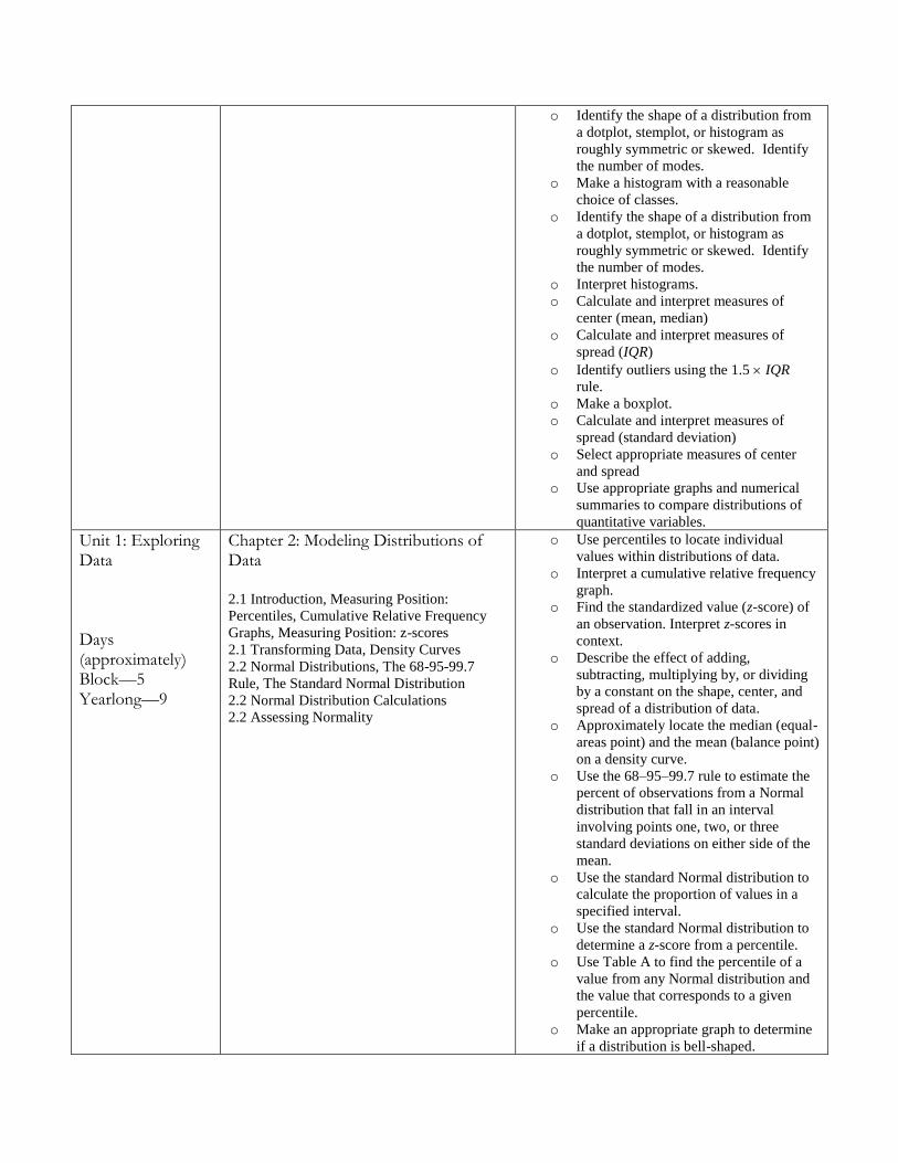
Unit 1: Exploring Data Days (approximately) Block—5 Yearlong—9
Chapter 2: Modeling Distributions of Data 2.1 Introduction, Measuring Position:
Percentiles, Cumulative Relative Frequency
Graphs, Measuring Position: z-scores
2.1 Transforming Data, Density Curves
2.2 Normal Distributions, The 68-95-99.7
Rule, The Standard Normal Distribution
2.2 Normal Distribution Calculations
2.2 Assessing Normality
o Use percentiles to locate individual
values within distributions of data.
o Interpret a cumulative relative frequency
graph.
o Find the standardized value (z-score) of
an observation. Interpret z-scores in
context.
o Describe the effect of adding,
subtracting, multiplying by, or dividing
by a constant on the shape, center, and
spread of a distribution of data.
o Approximately locate the median (equal-
areas point) and the mean (balance point)
on a density curve.
o Use the 68–95–99.7 rule to estimate the
percent of observations from a Normal
distribution that fall in an interval
involving points one, two, or three
standard deviations on either side of the
mean.
o Use the standard Normal distribution to
calculate the proportion of values in a
specified interval.
o Use the standard Normal distribution to
determine a z-score from a percentile.
o Use Table A to find the percentile of a
value from any Normal distribution and
the value that corresponds to a given
percentile.
o Make an appropriate graph to determine
if a distribution is bell-shaped.

o Use the 68-95-99.7 rule to assess
Normality of a data set.
o Interpret a Normal probability plot
Unit 1: Exploring Data Days (approximately) Block—6 Yearlong—10
Chapter 3: Describing Relationships 3.1 Explanatory and response variables
3.1 Displaying relationships: scatterplots
3.1 Interpreting scatterplots
3.1 Measuring linear association: correlation
3.1 Facts about correlation
3.2 Least-squares regression
3.2 Interpreting a regression line
3.2 Prediction
3.2 Residuals and the least-squares regression
line
3.2 Calculating the equation of the least-
squares regression line
3.2 How well the line fits the data: residual
plots
3.2 How well the line fits the data: the role of
r2 in regression
3.2 Interpreting computer regression output
3.2 Correlation and regression wisdom
o Describe why it is important to
investigate relationships between
variables.
o Identify explanatory and response
variables in situations where one
variable helps to explain or influences
the other.
o Make a scatterplot to display the
relationship between two quantitative
variables.
o Describe the direction, form, and
strength of the overall pattern of a
scatterplot.
o Recognize outliers in a scatterplot.
o Know the basic properties of correlation.
o Calculate and interpret correlation.
o Explain how the correlation r is
influenced by extreme observations.
o Interpret the slope and y intercept of a
least-squares regression line.
o Use the least-squares regression line to
predict y for a given x.
o Explain the dangers of extrapolation.
o Calculate and interpret residuals.
o Explain the concept of least squares.
o Use technology to find a least-squares
regression line.
o Find the slope and intercept of the least-
squares regression line from the means
and standard deviations of x and y and
their correlation.
o Construct and interpret residual plots to
assess if a linear model is appropriate.
o Use the standard deviation of the
residuals to assess how well the line fits
the data.
o Use r2 to assess how well the line fits the
data.
o Identify the equation of a least-squares
regression line from computer output.
o Explain why association doesn’t imply
causation.
o Recognize how the slope, y intercept,
standard deviation of the residuals, and
r2 are influenced by extreme
observations.

Unit 3: Anticipating Patterns Days (approximately) Block—6 Yearlong—11
Chapter 6: Random Variables 6.1 Standard Deviation (and Variance) of a
Discrete Random Variable, Continuous
Random Variables
6.2 Linear Transformations
6.2 Combining Random Variables, Combining
Normal Random Variables
6.3 Binomial Settings and Binomial Random
Variables, Binomial Probabilities
6.3 Mean and Standard Deviation of a
Binomial Distribution, Binomial Distributions
in Statistical Sampling
6.3 Geometric Random Variables
o Use a probability distribution to answer
questions about possible values of a random
variable.
o Calculate the mean of a discrete random
variable.
o Interpret the mean of a random variable.
o Calculate the standard deviation of a discrete
random variable.
o Interpret the standard deviation of a random
variable.
o Describe the effects of transforming a
random variable by adding or subtracting a
constant and multiplying or dividing by a
constant.
o Find the mean and standard deviation of the
sum or difference of independent random
variables.
o Determine whether two random variables are
independent.
o Find probabilities involving the sum or
difference of independent Normal random
variables.
o Determine whether the conditions for a
binomial random variable are met.
o Compute and interpret probabilities involving
binomial distributions.
o Calculate the mean and standard deviation of
a binomial random variable. Interpret these
values in context.
o Find probabilities involving geometric
random variables.
Unit 3: Anticipating Patterns Days (approximately) Block—5 Yearlong—10
Chapter 7: Sampling Distributions 7.1 Parameters and Statistics
7.1 Sampling Variability, Describing Sampling
Distributions
7.2 The Sampling Distribution of p̂ , Using
the Normal Approximation for p̂ ,
7.3 The Sampling Distribution of x : Mean
and Standard Deviation, Sampling from a
Normal Population
7.3 The Central Limit Theorem
o Distinguish between a parameter and a
statistic.
o Understand the definition of a sampling
distribution.
o Distinguish between population distribution,
sampling distribution, and the distribution of
sample data.
o Determine whether a statistic is an unbiased
estimator of a population parameter.
o Understand the relationship between sample
size and the variability of an estimator.
o Find the mean and standard deviation of the
sampling distribution of a sample proportion
p̂ for an SRS of size n from a population
having proportion p of successes.
o Check whether the 10% and Normal
conditions are met in a given setting.
o Use Normal approximation to calculate
probabilities involving p̂ .
o Use the sampling distribution of p̂ to

evaluate a claim about a population
proportion.
o Find the mean and standard deviation of the
sampling distribution of a sample mean x
from an SRS of size n.
o Calculate probabilities involving a sample
mean x when the population distribution is
Normal.
o Explain how the shape of the sampling
distribution of x is related to the shape of
the population distribution.
o Use the central limit theorem to help find
probabilities involving a sample mean x .
Unit 2: Sampling and Experimentation Days (approximately) Block—8 Yearlong—14
Chapter 4: Designing Studies 4.1 Introduction, Sampling and Surveys, How
to Sample Badly, How to Sample Well:
Random Samples
4.1 Other Sampling Methods
4.1 Inference for Sampling, Sample Surveys:
What Can Go Wrong?
4.2 Observational Studies vs. Experiments,
The Language of Experiments, How to
Experiment Badly
4.2 How to Experiment Well, Three Principles
of Experimental Design
4.2 Experiments: What Can Go Wrong?
Inference for Experiments
4.2 Blocking, Matched Pairs Design
4.3 Scope of Inference, the Challenges of
Establishing Causation
4.2 Class Experiments
or
4.3 Data Ethics* (*optional topic)
o Identify the population and sample in a
sample survey.
o Identify voluntary response samples and
convenience samples. Explain how these bad
sampling methods can lead to bias.
o Describe how to use Table D to select a
simple random sample (SRS).
o Distinguish a simple random sample from a
stratified random sample or cluster sample.
Give advantages and disadvantages of each
sampling method.
o Explain how undercoverage, nonresponse,
and question wording can lead to bias in a
sample survey.
o Distinguish between an observational study
and an experiment.
o Explain how a lurking variable in an
observational study can lead to confounding.
o Identify the experimental units or subjects,
explanatory variables (factors), treatments,
and response variables in an experiment.
o Describe a completely randomized design for
an experiment.
o Explain why random assignment is an
important experimental design principle.
o Describe how to avoid the placebo effect in
an experiment.
o Explain the meaning and the purpose of
blinding in an experiment.
o Explain in context what “statistically
significant” means.
o Distinguish between a completely
randomized design and a randomized block
design.
o Know when a matched pairs experimental
design is appropriate and how to implement
such a design.
o Determine the scope of inference for a
statistical study.
o Evaluate whether a statistical study has been
carried out in an ethical manner.

Unit 4: Statistical Inference Days (approximately) Block—5 Yearlong—10
Chapter 8: Estimating with Confidence 8.1 Using Confidence Intervals Wisely, 8.2
Conditions for Estimating p, Constructing a
Confidence Interval for p
8.2 Putting It All Together: The Four-Step
Process, Choosing the Sample Size
8.3 When Is Known: The One-Sample z
Interval for a Population Mean, When Is
Unknown: The t Distributions, Constructing a
Confidence Interval for
8.3 Using t Procedures Wisely
o Interpret a confidence level.
o Interpret a confidence interval in context.
o Understand that a confidence interval gives
a range of plausible values for the
parameter.
o Understand why each of the three inference
conditions—Random, Normal, and
Independent—is important.
o Explain how practical issues like
nonresponse, undercoverage, and response
bias can affect the interpretation of a
confidence interval.
o Construct and interpret a confidence interval
for a population proportion.
o Determine critical values for calculating a
confidence interval using a table or your
calculator.
o Carry out the steps in constructing a
confidence interval for a population
proportion: define the parameter; check
conditions; perform calculations; interpret
results in context.
o Determine the sample size required to obtain
a level C confidence interval for a
population proportion with a specified
margin of error.
o Understand how the margin of error of a
confidence interval changes with the sample
size and the level of confidence C.
o Understand why each of the three inference
conditions—Random, Normal, and
Independent—is important.
o Construct and interpret a confidence interval
for a population mean.
o Determine the sample size required to obtain
a level C confidence interval for a
population mean with a specified margin of
error.
o Carry out the steps in constructing a
confidence interval for a population mean:
define the parameter; check conditions;
perform calculations; interpret results in
context.
o Understand why each of the three inference
conditions—Random, Normal, and
Independent—is important.
o Determine sample statistics from a
confidence interval.

Unit 4: Statistical Inference Days (approximately) Block—6 Yearlong—11
Chapter 9: Testing a Claim 9.1 Type I and Type II Errors, Planning
Studies: The Power of a Statistical Test
9.2 Carrying Out a Significance Test, The
One-Sample z Test for a Proportion
9.2 Two-Sided Tests, Why Confidence
Intervals Give More Information
9.3 Carrying Out a Significance Test for ,
The One Sample t Test, Two-Sided Tests and
Confidence Intervals
9.3 Inference for Means: Paired Data, Using
Tests Wisely
o State correct hypotheses for a significance
test about a population proportion or mean.
o Interpret P-values in context.
o Interpret a Type I error and a Type II error
in context, and give the consequences of
each.
o Understand the relationship between the
significance level of a test, P(Type II error),
and power.
o Check conditions for carrying out a test
about a population proportion.
o If conditions are met, conduct a significance
test about a population proportion.
o Use a confidence interval to draw a
conclusion for a two-sided test about a
population proportion.
o Check conditions for carrying out a test
about a population mean.
o If conditions are met, conduct a one-sample
t test about a population mean .
o Use a confidence interval to draw a
conclusion for a two-sided test about a
population mean.
o Recognize paired data and use one-sample t
procedures to perform significance tests for
such data.
Unit 4: Statistical Inference Days (approximately) Block—6 Yearlong—11
Chapter 10: Comparing Two Populations or Groups 10.1 Confidence Intervals for p1 – p2
10.1 Significance Tests for p1 – p2, Inference
for Experiments
10.2 Activity: Does Polyester Decay?, The
Sampling Distribution of a Difference Between
Two Means
10.2 The Two-Sample t-Statistic, Confidence
Intervals for 1 2
10.2 Significance Tests for 1 2
, Using
Two-Sample t Procedures Wisely
o Describe the characteristics of the sampling
distribution of 1 2ˆ ˆp p
o Calculate probabilities using the sampling
distribution of 1 2ˆ ˆp p
o Determine whether the conditions for
performing inference are met.
o Construct and interpret a confidence interval
to compare two proportions.
o Perform a significance test to compare two
proportions.
o Interpret the results of inference procedures
in a randomized experiment.
o Describe the characteristics of the sampling
distribution of 1 2x x
o Calculate probabilities using the sampling
distribution of 1 2x x
o Determine whether the conditions for
performing inference are met.
o Use two-sample t procedures to compare
two means based on summary statistics.
o Use two-sample t procedures to compare
two means from raw data.
o Interpret standard computer output for two-
sample t procedures.
o Perform a significance test to compare two
means.
o Check conditions for using two-sample t
procedures in a randomized experiment.
o Interpret the results of inference procedures
in a randomized experiment.
o Determine the proper inference procedure to
use in a given setting.
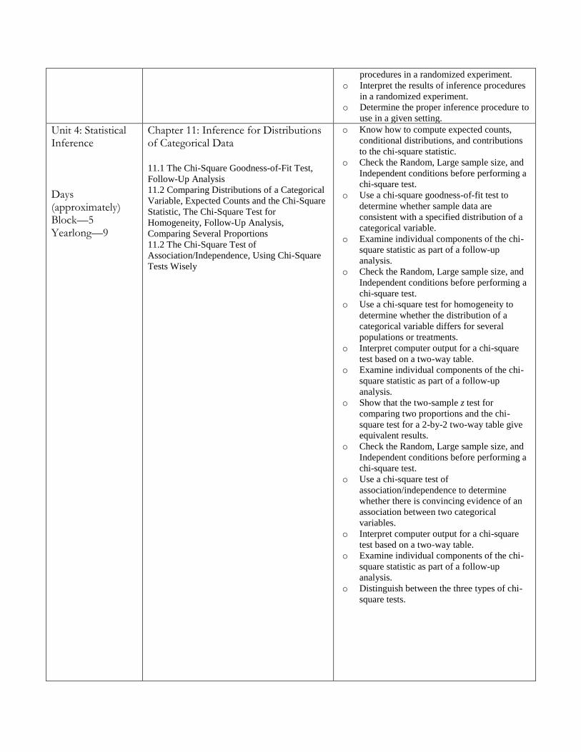
Unit 4: Statistical Inference Days (approximately) Block—5 Yearlong—9
Chapter 11: Inference for Distributions of Categorical Data 11.1 The Chi-Square Goodness-of-Fit Test,
Follow-Up Analysis
11.2 Comparing Distributions of a Categorical
Variable, Expected Counts and the Chi-Square
Statistic, The Chi-Square Test for
Homogeneity, Follow-Up Analysis,
Comparing Several Proportions
11.2 The Chi-Square Test of
Association/Independence, Using Chi-Square
Tests Wisely
o Know how to compute expected counts,
conditional distributions, and contributions
to the chi-square statistic.
o Check the Random, Large sample size, and
Independent conditions before performing a
chi-square test.
o Use a chi-square goodness-of-fit test to
determine whether sample data are
consistent with a specified distribution of a
categorical variable.
o Examine individual components of the chi-
square statistic as part of a follow-up
analysis.
o Check the Random, Large sample size, and
Independent conditions before performing a
chi-square test.
o Use a chi-square test for homogeneity to
determine whether the distribution of a
categorical variable differs for several
populations or treatments.
o Interpret computer output for a chi-square
test based on a two-way table.
o Examine individual components of the chi-
square statistic as part of a follow-up
analysis.
o Show that the two-sample z test for
comparing two proportions and the chi-
square test for a 2-by-2 two-way table give
equivalent results.
o Check the Random, Large sample size, and
Independent conditions before performing a
chi-square test.
o Use a chi-square test of
association/independence to determine
whether there is convincing evidence of an
association between two categorical
variables.
o Interpret computer output for a chi-square
test based on a two-way table.
o Examine individual components of the chi-
square statistic as part of a follow-up
analysis.
o Distinguish between the three types of chi-
square tests.

Unit 4: Statistical Inference Days (approximately) Block—5 Yearlong—10
Chapter 12: More About Regression 12.1 The Sampling Distribution of b,
Conditions for Regression Inference
12.1 Estimating Parameters, Constructing a
Confidence Interval for the Slope
12.1 Performing a Significance Test for the
Slope
12.2 Transforming with Powers and Roots
12.2 Transforming with Logarithms
o Check conditions for performing inference
about the slope of the population
regression line.
o Interpret computer output from a least-
squares regression analysis.
o Construct and interpret a confidence interval
for the slope of the population regression
line.
o Perform a significance test about the slope
of a population regression line.
o Use transformations involving powers and
roots to achieve linearity for a relationship
between two variables.
o Make predictions from a least-squares
regression line involving transformed data.
o Use transformations involving logarithms to
achieve linearity for a relationship between
two variables.
o Make predictions from a least-squares
regression line involving transformed data.
o Determine which of several transformations
does a better job of producing a linear
relationship.
MAJOR ASSIGNMENTS
• CRITICAL STATISTICAL ANALYSES These assignments provide students the opportunity to find an article in print or electronic form that is based on a statistical procedure. Students use the tools they have learned in class to analyze the information in the article, and then write a critical report in their findings.
• RELEASED FREE RESPONSE QUESTIONS Certain questions will be assigned from 1993-current tests for students to complete as homework, class work, a quiz, or as part of a unit or cumulative test.
• FINAL PROJECT A team approach to designing and conducting a statistical study, with an extensive set of scoring rubrics.
• CHAPTER PROJECTS Students will complete certain chapter projects as a hands-on approach to learning concepts.
• UNIT TESTS There are four unit test and up to four cumulative AP test.
• CHAPTER QUIZZES Students will take multiple quizzes per chapter in a variety of forms including but not limited to vocabulary, reading, matching, case studies, released free response questions, etc. There will be one cumulative quiz per chapter.
MAJOR TEXT Yates, Daniel S., Moore, David S., and Starnes, Daren S. The Practice of Statistics, 4th ed. New York: W.H. Freeman, 2011 (online edition)