CLP 3 – Multivariable Calculus
391
-
Upload
khangminh22 -
Category
Documents
-
view
2 -
download
0
Transcript of CLP 3 – Multivariable Calculus
CLP-3 MULTIVARIABLE CALCULUS
Joel FELDMAN Andrew RECHNITZER Elyse YEAGER
THIS DOCUMENT WAS TYPESET ON TUESDAY 31ST AUGUST, 2021.
§§ Legal stuff
• Copyright c© 2017–2021 Joel Feldman, Andrew Rechnitzer and Elyse Yeager.
• This work is licensed under the Creative Commons Attribution-NonCommercial-ShareAlike 4.0 International License. You can view a copy of the license athttp://creativecommons.org/licenses/by-nc-sa/4.0/.
• Links to the source files can be found at the text webpage
2
CONTENTS
1 Vectors and Geometry in Two and Three Dimensions 11.1 Points . . . . . . . . . . . . . . . . . . . . . . . . . . . . . . . . . . . . . . . . . 11.2 Vectors . . . . . . . . . . . . . . . . . . . . . . . . . . . . . . . . . . . . . . . . 6
1.2.1 Addition of Vectors and Multiplication of a Vector by a Scalar . . . . 91.2.2 The Dot Product . . . . . . . . . . . . . . . . . . . . . . . . . . . . . . 141.2.3 (Optional) Using Dot Products to Resolve Forces — The Pendulum . 191.2.4 (Optional) Areas of Parallelograms . . . . . . . . . . . . . . . . . . . . 231.2.5 The Cross Product . . . . . . . . . . . . . . . . . . . . . . . . . . . . . 251.2.6 (Optional) Some Vector Identities . . . . . . . . . . . . . . . . . . . . . 341.2.7 (Optional) Application of Cross Products to Rotational Motion . . . 361.2.8 (Optional) Application of Cross Products to Rotating Reference Frames 37
1.3 Equations of Lines in 2d . . . . . . . . . . . . . . . . . . . . . . . . . . . . . . 401.4 Equations of Planes in 3d . . . . . . . . . . . . . . . . . . . . . . . . . . . . . . 431.5 Equations of Lines in 3d . . . . . . . . . . . . . . . . . . . . . . . . . . . . . . 491.6 Curves and their Tangent Vectors . . . . . . . . . . . . . . . . . . . . . . . . . 56
1.6.1 Derivatives and Tangent Vectors . . . . . . . . . . . . . . . . . . . . . 621.7 Sketching Surfaces in 3d . . . . . . . . . . . . . . . . . . . . . . . . . . . . . . 70
1.7.1 Level Curves and Surfaces . . . . . . . . . . . . . . . . . . . . . . . . . 791.8 Cylinders . . . . . . . . . . . . . . . . . . . . . . . . . . . . . . . . . . . . . . . 841.9 Quadric Surfaces . . . . . . . . . . . . . . . . . . . . . . . . . . . . . . . . . . 85
2 Partial Derivatives 872.1 Limits . . . . . . . . . . . . . . . . . . . . . . . . . . . . . . . . . . . . . . . . . 87
2.1.1 Optional — A Nasty Limit That Doesn’t Exist . . . . . . . . . . . . . 942.2 Partial Derivatives . . . . . . . . . . . . . . . . . . . . . . . . . . . . . . . . . 972.3 Higher Order Derivatives . . . . . . . . . . . . . . . . . . . . . . . . . . . . . 110
2.3.1 Optional — The Proof of Theorem 2.3.4 . . . . . . . . . . . . . . . . . 112
2.3.2 Optional — An Example of B2 fBxBy (x0, y0) ‰ B2 f
ByBx (x0, y0) . . . . . . . . . 1152.4 The Chain Rule . . . . . . . . . . . . . . . . . . . . . . . . . . . . . . . . . . . 116
2.4.1 Memory Aids for the Chain Rule . . . . . . . . . . . . . . . . . . . . . 1172.4.2 Chain Rule Examples . . . . . . . . . . . . . . . . . . . . . . . . . . . 120
i
CONTENTS CONTENTS
2.4.3 Review of the Proof of ddt f (x(t)) = d f
dx (x(t)) dxdt (t) . . . . . . . . . . . 125
2.4.4 Proof of Theorem 2.4.1 . . . . . . . . . . . . . . . . . . . . . . . . . . . 1252.5 Tangent Planes and Normal Lines . . . . . . . . . . . . . . . . . . . . . . . . 127
2.5.1 Surfaces of the Form z = f (x, y). . . . . . . . . . . . . . . . . . . . . . 1282.5.2 Surfaces of the Form G(x, y, z) = 0. . . . . . . . . . . . . . . . . . . . . 134
2.6 Linear Approximations and Error . . . . . . . . . . . . . . . . . . . . . . . . . 1472.6.1 Quadratic Approximation and Error Bounds . . . . . . . . . . . . . . 1552.6.2 Optional — Taylor Polynomials . . . . . . . . . . . . . . . . . . . . . . 160
2.7 Directional Derivatives and the Gradient . . . . . . . . . . . . . . . . . . . . 1622.8 Optional — Solving the Wave Equation . . . . . . . . . . . . . . . . . . . . . 172
2.8.1 Really Optional — Derivation of the Wave Equation . . . . . . . . . . 1762.9 Maximum and Minimum Values . . . . . . . . . . . . . . . . . . . . . . . . . 179
2.9.1 Absolute Minima and Maxima . . . . . . . . . . . . . . . . . . . . . . 2022.10 Lagrange Multipliers . . . . . . . . . . . . . . . . . . . . . . . . . . . . . . . . 212
2.10.1 (Optional) An Example with Two Lagrange Multipliers . . . . . . . . 220
3 Multiple Integrals 2253.1 Double Integrals . . . . . . . . . . . . . . . . . . . . . . . . . . . . . . . . . . . 225
3.1.1 Vertical Slices . . . . . . . . . . . . . . . . . . . . . . . . . . . . . . . . 2253.1.2 Horizontal Slices . . . . . . . . . . . . . . . . . . . . . . . . . . . . . . 2293.1.3 Volumes . . . . . . . . . . . . . . . . . . . . . . . . . . . . . . . . . . . 2383.1.4 Examples . . . . . . . . . . . . . . . . . . . . . . . . . . . . . . . . . . 2393.1.5 Optional — More about the Definition of
ťR f (x, y) dxdy . . . . . . 254
3.1.6 Even and Odd Functions . . . . . . . . . . . . . . . . . . . . . . . . . 2593.2 Double Integrals in Polar Coordinates . . . . . . . . . . . . . . . . . . . . . . 270
3.2.1 Polar Coordinates . . . . . . . . . . . . . . . . . . . . . . . . . . . . . . 2703.2.2 Polar Curves . . . . . . . . . . . . . . . . . . . . . . . . . . . . . . . . 2723.2.3 Integrals in Polar Coordinates . . . . . . . . . . . . . . . . . . . . . . . 2773.2.4 Optional— Error Control for the Polar Area Formula . . . . . . . . . 291
3.3 Applications of Double Integrals . . . . . . . . . . . . . . . . . . . . . . . . . 2933.4 Surface Area . . . . . . . . . . . . . . . . . . . . . . . . . . . . . . . . . . . . . 3083.5 Triple Integrals . . . . . . . . . . . . . . . . . . . . . . . . . . . . . . . . . . . 3163.6 Triple Integrals in Cylindrical Coordinates . . . . . . . . . . . . . . . . . . . . 324
3.6.1 Cylindrical Coordinates . . . . . . . . . . . . . . . . . . . . . . . . . . 3243.6.2 The Volume Element in Cylindrical Coordinates . . . . . . . . . . . . 3263.6.3 Sample Integrals in Cylindrical Coordinates . . . . . . . . . . . . . . 327
3.7 Triple Integrals in Spherical Coordinates . . . . . . . . . . . . . . . . . . . . . 3343.7.1 Spherical Coordinates . . . . . . . . . . . . . . . . . . . . . . . . . . . 3343.7.2 The Volume Element in Spherical Coordinates . . . . . . . . . . . . . 3353.7.3 Sample Integrals in Spherical Coordinates . . . . . . . . . . . . . . . 339
3.8 Optional— Integrals in General Coordinates . . . . . . . . . . . . . . . . . . 3463.8.1 Optional — Dropping Higher Order Terms in du, dv . . . . . . . . . 355
A Trigonometry 357A.1 Trigonometry — Graphs . . . . . . . . . . . . . . . . . . . . . . . . . . . . . . 357A.2 Trigonometry — Special Triangles . . . . . . . . . . . . . . . . . . . . . . . . 357A.3 Trigonometry — Simple Identities . . . . . . . . . . . . . . . . . . . . . . . . 358
ii
CONTENTS CONTENTS
A.4 Trigonometry — Add and Subtract Angles . . . . . . . . . . . . . . . . . . . 359A.5 Inverse Trigonometric Functions . . . . . . . . . . . . . . . . . . . . . . . . . 360
B Powers and Logarithms 362B.1 Powers . . . . . . . . . . . . . . . . . . . . . . . . . . . . . . . . . . . . . . . . 362B.2 Logarithms . . . . . . . . . . . . . . . . . . . . . . . . . . . . . . . . . . . . . . 363
C Table of Derivatives 365
D Table of Integrals 367
E Table of Taylor Expansions 369
F 3d Coordinate Systems 371F.1 Cartesian Coordinates . . . . . . . . . . . . . . . . . . . . . . . . . . . . . . . 371F.2 Cylindrical Coordinates . . . . . . . . . . . . . . . . . . . . . . . . . . . . . . 372F.3 Spherical Coordinates . . . . . . . . . . . . . . . . . . . . . . . . . . . . . . . 373
G ISO Coordinate System Notation 376G.1 Polar Coordinates . . . . . . . . . . . . . . . . . . . . . . . . . . . . . . . . . . 376G.2 Cylindrical Coordinates . . . . . . . . . . . . . . . . . . . . . . . . . . . . . . 378G.3 Spherical Coordinates . . . . . . . . . . . . . . . . . . . . . . . . . . . . . . . 379
H Conic Sections and Quadric Surfaces 382
iii
CONTENTS CONTENTS
iv
VECTORS AND GEOMETRY INTWO AND THREE DIMENSIONS
Chapter 1
Before we get started doing calculus in two and three dimensions we need to brush upon some basic geometry, that we will use a lot. We are already familiar with the Cartesianplane1, but we’ll start from the beginning.
1.1IJ Points
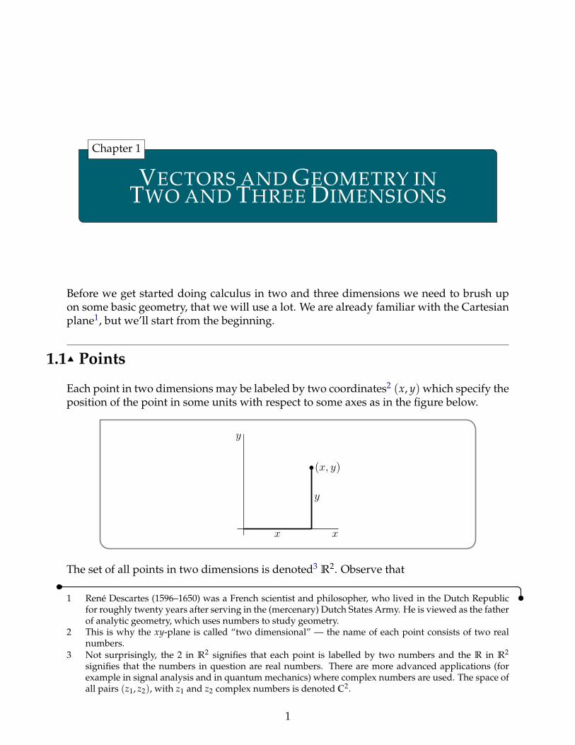
Each point in two dimensions may be labeled by two coordinates2 (x, y) which specify theposition of the point in some units with respect to some axes as in the figure below.
x
y
x
y
(x, y)
The set of all points in two dimensions is denoted3 R2. Observe that
1 Rene Descartes (1596–1650) was a French scientist and philosopher, who lived in the Dutch Republicfor roughly twenty years after serving in the (mercenary) Dutch States Army. He is viewed as the fatherof analytic geometry, which uses numbers to study geometry.
2 This is why the xy-plane is called “two dimensional” — the name of each point consists of two realnumbers.
3 Not surprisingly, the 2 in R2 signifies that each point is labelled by two numbers and the R in R2
signifies that the numbers in question are real numbers. There are more advanced applications (forexample in signal analysis and in quantum mechanics) where complex numbers are used. The space ofall pairs (z1, z2), with z1 and z2 complex numbers is denoted C2.
1
VECTORS AND GEOMETRY 1.1 POINTS
• the distance from the point (x, y) to the x-axis is |y|• if y ą 0, then (x, y) is above the x-axis and if y ă 0, then (x, y) is below the x-axis• the distance from the point (x, y) to the y-axis is |x|• if x ą 0, then (x, y) is the right of the y-axis and if x ă 0, then (x, y) is to the left of
the y-axis• the distance from the point (x, y) to the origin (0, 0) is
ax2 + y2
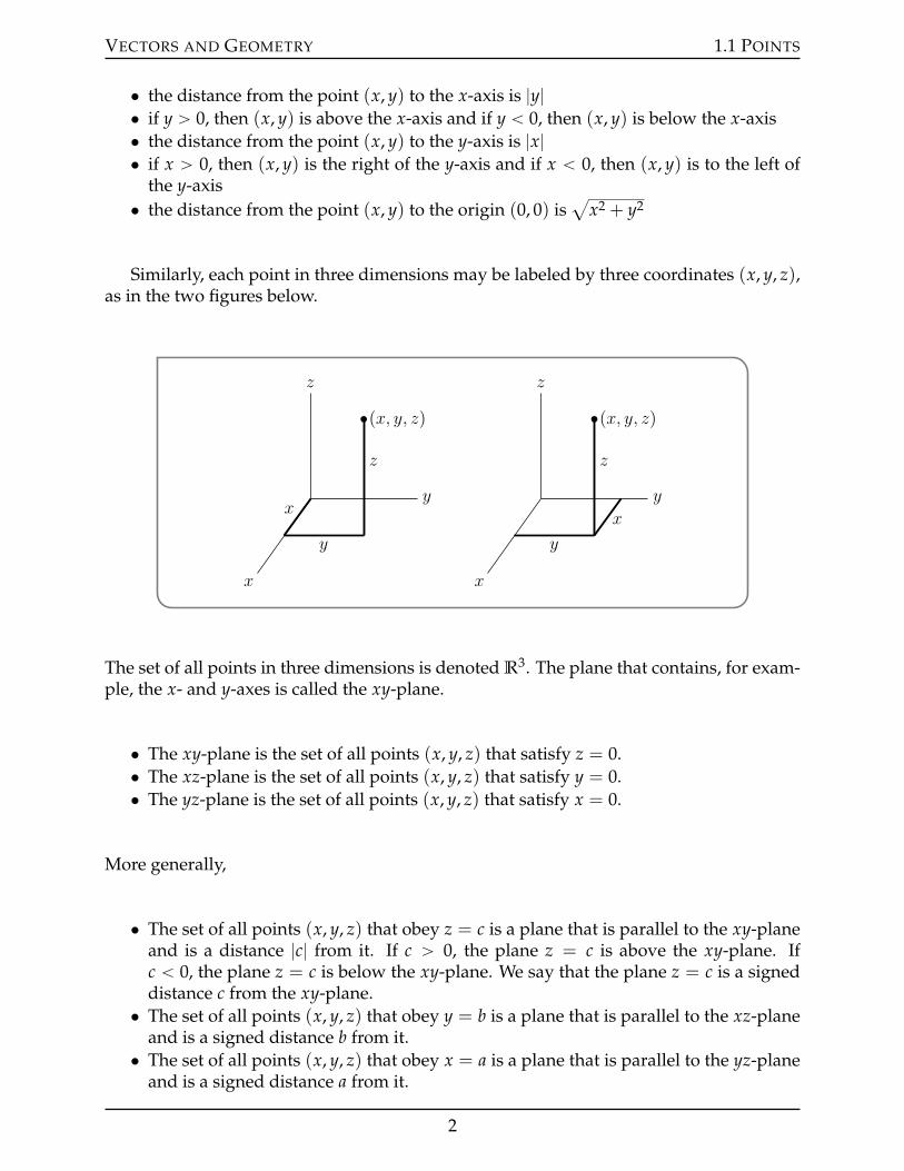
Similarly, each point in three dimensions may be labeled by three coordinates (x, y, z),as in the two figures below.
(x, y, z)
x
y
z
x
y
z
(x, y, z)
x
y
z
x
y
z
The set of all points in three dimensions is denoted R3. The plane that contains, for exam-ple, the x- and y-axes is called the xy-plane.
• The xy-plane is the set of all points (x, y, z) that satisfy z = 0.• The xz-plane is the set of all points (x, y, z) that satisfy y = 0.• The yz-plane is the set of all points (x, y, z) that satisfy x = 0.
More generally,
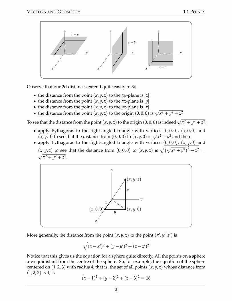
• The set of all points (x, y, z) that obey z = c is a plane that is parallel to the xy-planeand is a distance |c| from it. If c ą 0, the plane z = c is above the xy-plane. Ifc ă 0, the plane z = c is below the xy-plane. We say that the plane z = c is a signeddistance c from the xy-plane.• The set of all points (x, y, z) that obey y = b is a plane that is parallel to the xz-plane
and is a signed distance b from it.• The set of all points (x, y, z) that obey x = a is a plane that is parallel to the yz-plane
and is a signed distance a from it.
2
VECTORS AND GEOMETRY 1.1 POINTS
z “ c
x
y
z
y “ b
x
y
z
x “ ax
y
z
Observe that our 2d distances extend quite easily to 3d.
• the distance from the point (x, y, z) to the xy-plane is |z|• the distance from the point (x, y, z) to the xz-plane is |y|• the distance from the point (x, y, z) to the yz-plane is |x|• the distance from the point (x, y, z) to the origin (0, 0, 0) is
ax2 + y2 + z2
To see that the distance from the point (x, y, z) to the origin (0, 0, 0) is indeeda
x2 + y2 + z2,
• apply Pythagoras to the right-angled triangle with vertices (0, 0, 0), (x, 0, 0) and(x, y, 0) to see that the distance from (0, 0, 0) to (x, y, 0) is
ax2 + y2 and then
• apply Pythagoras to the right-angled triangle with vertices (0, 0, 0), (x, y, 0) and
(x, y, z) to see that the distance from (0, 0, 0) to (x, y, z) isb(a
x2 + y2)2
+ z2 =ax2 + y2 + z2.
px, 0, 0q px, y, 0q
px, y, zq
x
y
z
x
y
z
More generally, the distance from the point (x, y, z) to the point (x1, y1, z1) isb(x´ x1)2 + (y´ y1)2 + (z´ z1)2
Notice that this gives us the equation for a sphere quite directly. All the points on a sphereare equidistant from the centre of the sphere. So, for example, the equation of the spherecentered on (1, 2, 3) with radius 4, that is, the set of all points (x, y, z) whose distance from(1, 2, 3) is 4, is
(x´ 1)2 + (y´ 2)2 + (z´ 3)2 = 16
3
VECTORS AND GEOMETRY 1.1 POINTS
Here is an example in which we sketch a region in the xy-plane that is specified usinginequalities.
Example 1.1.1
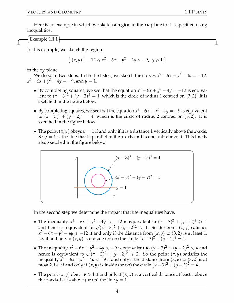
In this example, we sketch the region (x, y)
ˇ ´ 12 ď x2 ´ 6x + y2 ´ 4y ď ´9, y ě 1(
in the xy-plane.We do so in two steps. In the first step, we sketch the curves x2 ´ 6x + y2 ´ 4y = ´12,
x2 ´ 6x + y2 ´ 4y = ´9, and y = 1.
• By completing squares, we see that the equation x2 ´ 6x + y2 ´ 4y = ´12 is equiva-lent to (x ´ 3)2 + (y´ 2)2 = 1, which is the circle of radius 1 centred on (3, 2). It issketched in the figure below.
• By completing squares, we see that the equation x2´ 6x+ y2´ 4y = ´9 is equivalentto (x ´ 3)2 + (y ´ 2)2 = 4, which is the circle of radius 2 centred on (3, 2). It issketched in the figure below.
• The point (x, y) obeys y = 1 if and only if it is a distance 1 vertically above the x-axis.So y = 1 is the line that is parallel to the x-axis and is one unit above it. This line isalso sketched in the figure below.
px ´ 3q2 ` py ´ 2q2 “ 1
px ´ 3q2 ` py ´ 2q2 “ 4
y “ 1
x
y
In the second step we determine the impact that the inequalities have.
• The inequality x2 ´ 6x + y2 ´ 4y ě ´12 is equivalent to (x ´ 3)2 + (y ´ 2)2 ě 1and hence is equivalent to
a(x´ 3)2 + (y´ 2)2 ě 1. So the point (x, y) satisfies
x2 ´ 6x + y2 ´ 4y ě ´12 if and only if the distance from (x, y) to (3, 2) is at least 1,i.e. if and only if (x, y) is outside (or on) the circle (x´ 3)2 + (y´ 2)2 = 1.
• The inequality x2 ´ 6x + y2 ´ 4y ď ´9 is equivalent to (x ´ 3)2 + (y´ 2)2 ď 4 andhence is equivalent to
a(x´ 3)2 + (y´ 2)2 ď 2. So the point (x, y) satisfies the
inequality x2 ´ 6x + y2 ´ 4y ď ´9 if and only if the distance from (x, y) to (3, 2) is atmost 2, i.e. if and only if (x, y) is inside (or on) the circle (x´ 3)2 + (y´ 2)2 = 4.
• The point (x, y) obeys y ě 1 if and only if (x, y) is a vertical distance at least 1 abovethe x-axis, i.e. is above (or on) the line y = 1.
4
VECTORS AND GEOMETRY 1.1 POINTS
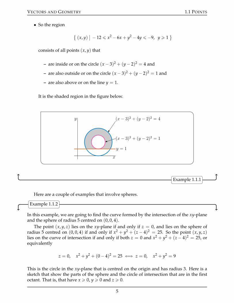
• So the region
(x, y)
ˇ ´ 12 ď x2 ´ 6x + y2 ´ 4y ď ´9, y ě 1(
consists of all points (x, y) that
– are inside or on the circle (x´ 3)2 + (y´ 2)2 = 4 and
– are also outside or on the circle (x´ 3)2 + (y´ 2)2 = 1 and
– are also above or on the line y = 1.
It is the shaded region in the figure below.
px ´ 3q2 ` py ´ 2q2 “ 1
px ´ 3q2 ` py ´ 2q2 “ 4
y “ 1
x
y
Example 1.1.1
Here are a couple of examples that involve spheres.
Example 1.1.2
In this example, we are going to find the curve formed by the intersection of the xy-planeand the sphere of radius 5 centred on (0, 0, 4).
The point (x, y, z) lies on the xy-plane if and only if z = 0, and lies on the sphere ofradius 5 centred on (0, 0, 4) if and only if x2 + y2 + (z ´ 4)2 = 25. So the point (x, y, z)lies on the curve of intersection if and only if both z = 0 and x2 + y2 + (z´ 4)2 = 25, orequivalently
z = 0, x2 + y2 + (0´ 4)2 = 25 ðñ z = 0, x2 + y2 = 9
This is the circle in the xy-plane that is centred on the origin and has radius 3. Here is asketch that show the parts of the sphere and the circle of intersection that are in the firstoctant. That is, that have x ě 0, y ě 0 and z ě 0.
5

VECTORS AND GEOMETRY 1.2 VECTORS
z
y
x
Example 1.1.2
Example 1.1.3
In this example, we are going to find all points (x, y, z) for which the distance from (x, y, z)to (9,´12, 15) is twice the distance from (x, y, z) to the origin (0, 0, 0).
The distance from (x, y, z) to (9,´12, 15) isa(x´ 9)2 + (y + 12)2 + (z´ 15)2. The dis-
tance from (x, y, z) to (0, 0, 0) isa
x2 + y2 + z2. So we want to find all points (x, y, z) forwhich b
(x´ 9)2 + (y + 12)2 + (z´ 15)2 = 2b
x2 + y2 + z2
Squaring both sides of this equation gives
x2 ´ 18x + 81 + y2 + 24y + 144 + z2 ´ 30z + 225 = 4(x2 + y2 + z2)
Collecting up terms gives
3x2 + 18x + 3y2 ´ 24y + 3z2 + 30z = 450 and then, dividing by 3,
x2 + 6x + y2 ´ 8y + z2 + 10z = 150 and then, completing squares,
x2 + 6x + 9 + y2 ´ 8y + 16 + z2 + 10z + 25 = 200 or
(x + 3)2 + (y´ 4)2 + (z + 5)2 = 200
This is the sphere of radius 10?
2 centred on (´3, 4,´5).Example 1.1.3
1.2IJ Vectors
In many of our applications in 2d and 3d, we will encounter quantities that have both amagnitude (like a distance) and also a direction. Such quantities are called vectors. That is,a vector is a quantity which has both a direction and a magnitude, like a velocity. If you aremoving, the magnitude (length) of your velocity vector is your speed (distance travelled
6
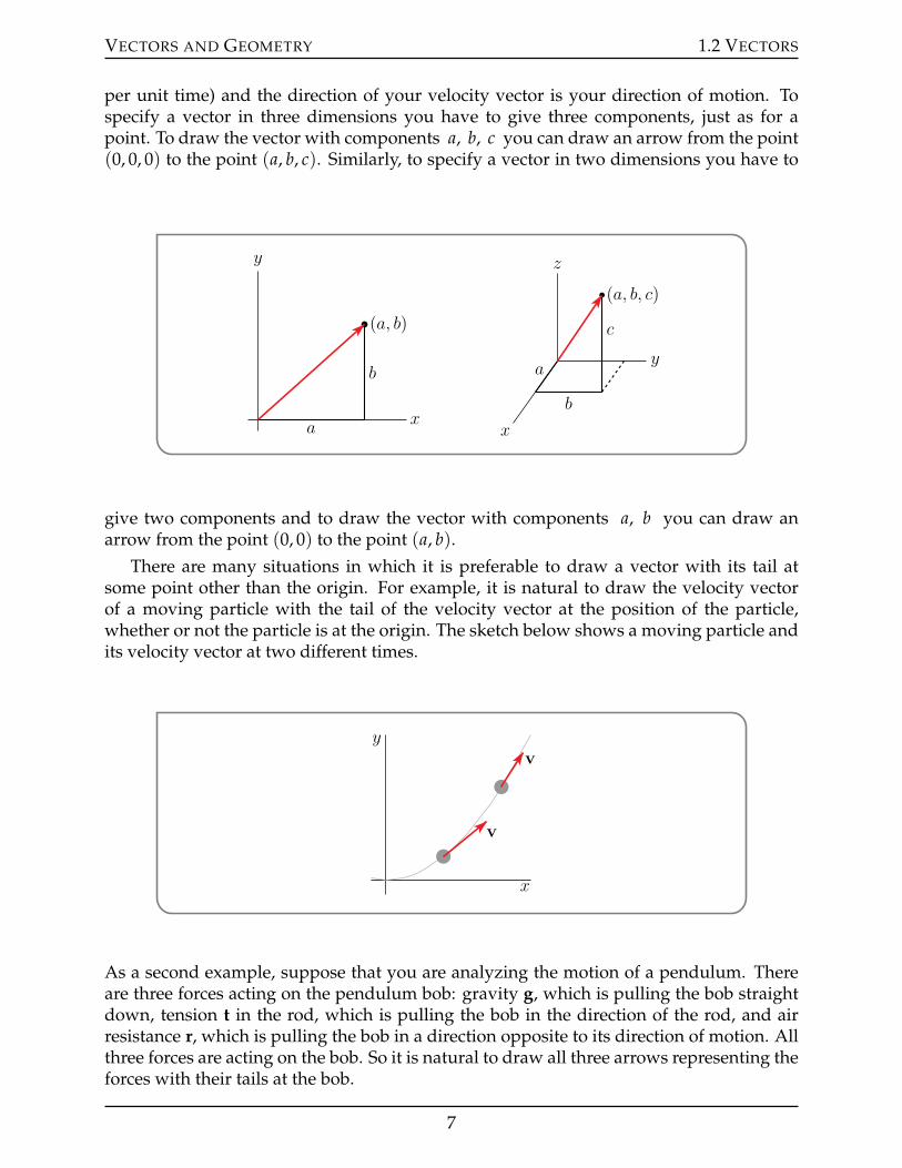
VECTORS AND GEOMETRY 1.2 VECTORS
per unit time) and the direction of your velocity vector is your direction of motion. Tospecify a vector in three dimensions you have to give three components, just as for apoint. To draw the vector with components a, b, c you can draw an arrow from the point(0, 0, 0) to the point (a, b, c). Similarly, to specify a vector in two dimensions you have to
x
y
a
b
(a, b)
pa, b, cq
a
b
c
x
y
z
give two components and to draw the vector with components a, b you can draw anarrow from the point (0, 0) to the point (a, b).
There are many situations in which it is preferable to draw a vector with its tail atsome point other than the origin. For example, it is natural to draw the velocity vectorof a moving particle with the tail of the velocity vector at the position of the particle,whether or not the particle is at the origin. The sketch below shows a moving particle andits velocity vector at two different times.
v
v
x
y
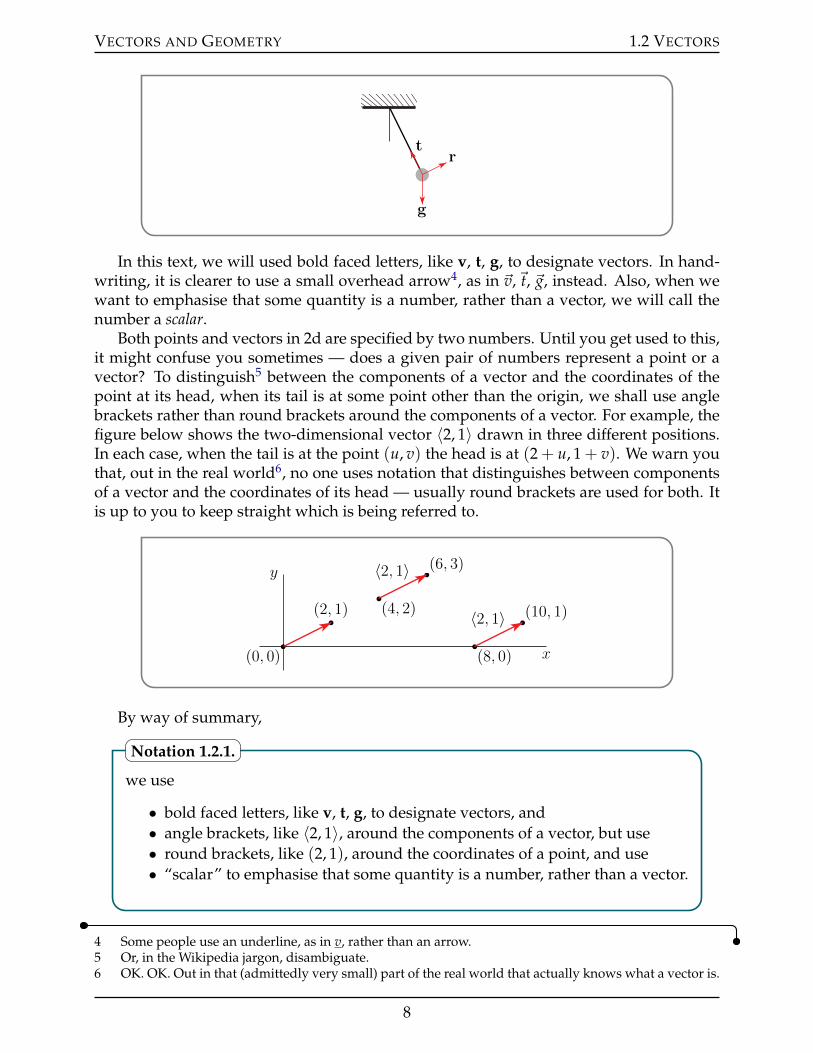
As a second example, suppose that you are analyzing the motion of a pendulum. Thereare three forces acting on the pendulum bob: gravity g, which is pulling the bob straightdown, tension t in the rod, which is pulling the bob in the direction of the rod, and airresistance r, which is pulling the bob in a direction opposite to its direction of motion. Allthree forces are acting on the bob. So it is natural to draw all three arrows representing theforces with their tails at the bob.
7
VECTORS AND GEOMETRY 1.2 VECTORS
g
tr
In this text, we will used bold faced letters, like v, t, g, to designate vectors. In hand-writing, it is clearer to use a small overhead arrow4, as in ~v,~t, ~g, instead. Also, when wewant to emphasise that some quantity is a number, rather than a vector, we will call thenumber a scalar.
Both points and vectors in 2d are specified by two numbers. Until you get used to this,it might confuse you sometimes — does a given pair of numbers represent a point or avector? To distinguish5 between the components of a vector and the coordinates of thepoint at its head, when its tail is at some point other than the origin, we shall use anglebrackets rather than round brackets around the components of a vector. For example, thefigure below shows the two-dimensional vector 〈2, 1〉 drawn in three different positions.In each case, when the tail is at the point (u, v) the head is at (2 + u, 1 + v). We warn youthat, out in the real world6, no one uses notation that distinguishes between componentsof a vector and the coordinates of its head — usually round brackets are used for both. Itis up to you to keep straight which is being referred to.
x
y
(0, 0)
(2, 1)
(8, 0)
(10, 1)(4, 2)
(6, 3)〈2, 1〉
〈2, 1〉
By way of summary,
we use
• bold faced letters, like v, t, g, to designate vectors, and• angle brackets, like 〈2, 1〉, around the components of a vector, but use• round brackets, like (2, 1), around the coordinates of a point, and use• “scalar” to emphasise that some quantity is a number, rather than a vector.
Notation 1.2.1.
4 Some people use an underline, as in v, rather than an arrow.5 Or, in the Wikipedia jargon, disambiguate.6 OK. OK. Out in that (admittedly very small) part of the real world that actually knows what a vector is.
8
VECTORS AND GEOMETRY 1.2 VECTORS
1.2.1 §§ Addition of Vectors and Multiplication of a Vector by a Scalar
Just as we have done many times in the CLP texts, when we define a new type of object,we want to understand how it interacts with the basic operations of addition and multipli-cation. Vectors are no different, and we shall shortly see a natural way to define additionof vectors. Multiplication will be more subtle, and we shall start with multiplication of avector by a number (rather than with multiplication of a vector by another vector).
By way of motivation for the definitions of addition and multiplication by a number,imagine that we are out for a walk on the xy-plane.
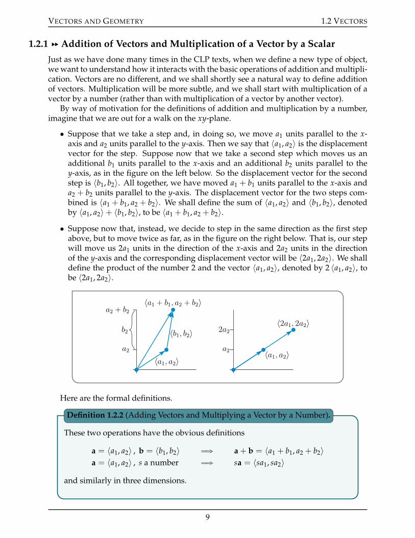
• Suppose that we take a step and, in doing so, we move a1 units parallel to the x-axis and a2 units parallel to the y-axis. Then we say that 〈a1, a2〉 is the displacementvector for the step. Suppose now that we take a second step which moves us anadditional b1 units parallel to the x-axis and an additional b2 units parallel to they-axis, as in the figure on the left below. So the displacement vector for the secondstep is 〈b1, b2〉. All together, we have moved a1 + b1 units parallel to the x-axis anda2 + b2 units parallel to the y-axis. The displacement vector for the two steps com-bined is 〈a1 + b1, a2 + b2〉. We shall define the sum of 〈a1, a2〉 and 〈b1, b2〉, denotedby 〈a1, a2〉+ 〈b1, b2〉, to be 〈a1 + b1, a2 + b2〉.• Suppose now that, instead, we decide to step in the same direction as the first step
above, but to move twice as far, as in the figure on the right below. That is, our stepwill move us 2a1 units in the direction of the x-axis and 2a2 units in the directionof the y-axis and the corresponding displacement vector will be 〈2a1, 2a2〉. We shalldefine the product of the number 2 and the vector 〈a1, a2〉, denoted by 2 〈a1, a2〉, tobe 〈2a1, 2a2〉.
a2
a2 ` b2
b2
〈a1, a2〉
〈b1, b2〉
〈a1 ` b1, a2 ` b2〉
a2
2a2
〈a1, a2〉
〈2a1, 2a2〉
Here are the formal definitions.
These two operations have the obvious definitions
a = 〈a1, a2〉 , b = 〈b1, b2〉 ùñ a + b = 〈a1 + b1, a2 + b2〉a = 〈a1, a2〉 , s a number ùñ sa = 〈sa1, sa2〉
and similarly in three dimensions.
Definition 1.2.2 (Adding Vectors and Multiplying a Vector by a Number).
9
VECTORS AND GEOMETRY 1.2 VECTORS
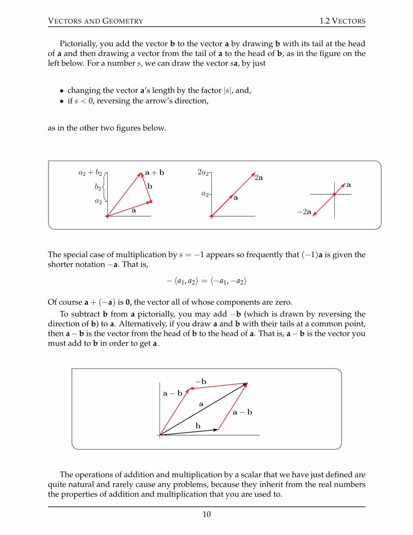
Pictorially, you add the vector b to the vector a by drawing b with its tail at the headof a and then drawing a vector from the tail of a to the head of b, as in the figure on theleft below. For a number s, we can draw the vector sa, by just
• changing the vector a’s length by the factor |s|, and,• if s ă 0, reversing the arrow’s direction,
as in the other two figures below.
a2
a2 ` b2
b2
a
b
a ` b
a2
2a2
a
2aa
´2a
The special case of multiplication by s = ´1 appears so frequently that (´1)a is given theshorter notation ´a. That is,
´ 〈a1, a2〉 = 〈´a1,´a2〉
Of course a + (´a) is 0, the vector all of whose components are zero.To subtract b from a pictorially, you may add ´b (which is drawn by reversing the
direction of b) to a. Alternatively, if you draw a and b with their tails at a common point,then a´ b is the vector from the head of b to the head of a. That is, a´ b is the vector youmust add to b in order to get a.
a− ba
b
−b
a− b
The operations of addition and multiplication by a scalar that we have just defined arequite natural and rarely cause any problems, because they inherit from the real numbersthe properties of addition and multiplication that you are used to.
10
VECTORS AND GEOMETRY 1.2 VECTORS
Let a, b and c be vectors and s and t be scalars. Then
(1) a + b = b + a (2) a + (b + c) = (a + b) + c(3) a + 0 = a (4) a + (´a) = 0(5) s(a + b) = sa + sb (6) (s + t)a = sa + ta(7) (st)a = s(ta) (8) 1a = a
Theorem 1.2.3 (Properties of Addition and Scalar Multiplication).
We have just been introduced to many definitions. Let’s see some of them in action.
Example 1.2.4
For example, ifa = 〈1, 2, 3〉 b = 〈3, 2, 1〉 c = 〈1, 0, 1〉
then
2a = 2 〈1, 2, 3〉 = 〈2, 4, 6〉´b = ´ 〈3, 2, 1〉 = 〈´3,´2,´1〉3c = 3 〈1, 0, 1〉 = 〈3, 0, 3〉
and
2a´ b + 3c = 〈2, 4, 6〉+ 〈´3,´2,´1〉+ 〈3, 0, 3〉= 〈2´ 3 + 3 , 4´ 2 + 0 , 6´ 1 + 3〉= 〈2, 2, 8〉
Example 1.2.4
Two vectors a and b
• are said to be parallel if a = s b for some nonzero real number s and
• are said to have the same direction if a = s b for some number s ą 0.
Definition 1.2.5.
There are some vectors that occur sufficiently commonly that they are given specialnames. One is the vector 0. Some others are the “standard basis vectors”.
11
VECTORS AND GEOMETRY 1.2 VECTORS
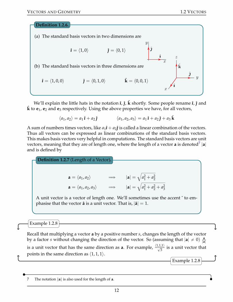
(a) The standard basis vectors in two dimensions are
ııı = 〈1, 0〉 = 〈0, 1〉
x
y
ııı
(b) The standard basis vectors in three dimensions are
ııı = 〈1, 0, 0〉 = 〈0, 1, 0〉 k = 〈0, 0, 1〉x
y
z
ııı
k
Definition 1.2.6.
We’ll explain the little hats in the notation ııı, , k shortly. Some people rename ııı, andk to e1, e2 and e3 respectively. Using the above properties we have, for all vectors,
〈a1, a2〉 = a1 ııı + a2 〈a1, a2, a3〉 = a1 ııı + a2 + a3 k
A sum of numbers times vectors, like a1ııı+ a2 is called a linear combination of the vectors.Thus all vectors can be expressed as linear combinations of the standard basis vectors.This makes basis vectors very helpful in computations. The standard basis vectors are unitvectors, meaning that they are of length one, where the length of a vector a is denoted7 |a|and is defined by
a = 〈a1, a2〉 ùñ |a| =b
a21 + a2
2
a = 〈a1, a2, a3〉 ùñ |a| =b
a21 + a2
2 + a23
A unit vector is a vector of length one. We’ll sometimes use the accent ˆ to em-phasise that the vector a is a unit vector. That is, |a| = 1.
Definition 1.2.7 (Length of a Vector).
Example 1.2.8
Recall that multiplying a vector a by a positive number s, changes the length of the vectorby a factor s without changing the direction of the vector. So (assuming that |a| ‰ 0) a
|a|
is a unit vector that has the same direction as a. For example, 〈1,1,1〉?
3is a unit vector that
points in the same direction as 〈1, 1, 1〉.Example 1.2.8
7 The notation a is also used for the length of a.
12
VECTORS AND GEOMETRY 1.2 VECTORS
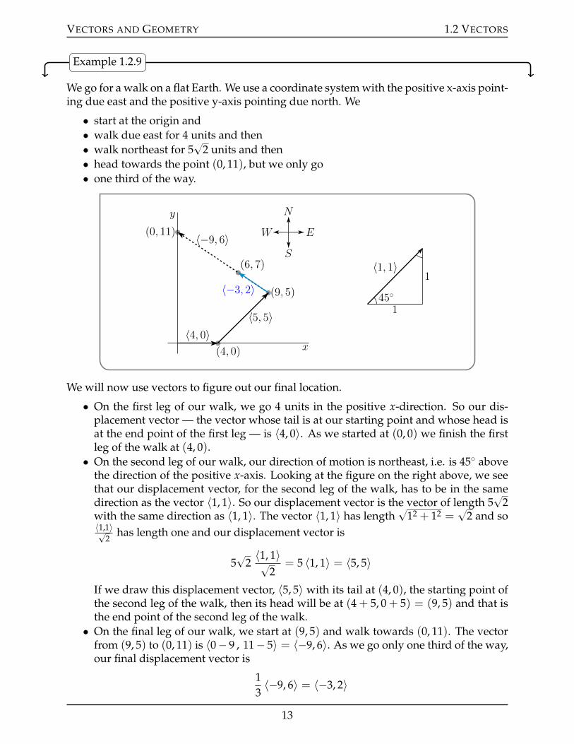
Example 1.2.9
We go for a walk on a flat Earth. We use a coordinate system with the positive x-axis point-ing due east and the positive y-axis pointing due north. We
• start at the origin and• walk due east for 4 units and then• walk northeast for 5
?2 units and then
• head towards the point (0, 11), but we only go• one third of the way.
p4, 0q
p9, 5q
p6, 7q
p0, 11q
x
y
E
N
W
S
〈4, 0〉〈5, 5〉
〈´9, 6〉
〈´3, 2〉45˝
1
1〈1, 1〉
We will now use vectors to figure out our final location.
• On the first leg of our walk, we go 4 units in the positive x-direction. So our dis-placement vector — the vector whose tail is at our starting point and whose head isat the end point of the first leg — is 〈4, 0〉. As we started at (0, 0) we finish the firstleg of the walk at (4, 0).• On the second leg of our walk, our direction of motion is northeast, i.e. is 45˝ above
the direction of the positive x-axis. Looking at the figure on the right above, we seethat our displacement vector, for the second leg of the walk, has to be in the samedirection as the vector 〈1, 1〉. So our displacement vector is the vector of length 5
?2
with the same direction as 〈1, 1〉. The vector 〈1, 1〉 has length?
12 + 12 =?
2 and so〈1,1〉?
2has length one and our displacement vector is
5?
2〈1, 1〉?
2= 5 〈1, 1〉 = 〈5, 5〉
If we draw this displacement vector, 〈5, 5〉 with its tail at (4, 0), the starting point ofthe second leg of the walk, then its head will be at (4 + 5, 0 + 5) = (9, 5) and that isthe end point of the second leg of the walk.• On the final leg of our walk, we start at (9, 5) and walk towards (0, 11). The vector
from (9, 5) to (0, 11) is 〈0´ 9 , 11´ 5〉 = 〈´9, 6〉. As we go only one third of the way,our final displacement vector is
13〈´9, 6〉 = 〈´3, 2〉
13
VECTORS AND GEOMETRY 1.2 VECTORS
If we draw this displacement vector with its tail at (9, 5), the starting point of thefinal leg, then its head will be at (9´ 3, 5 + 2) = (6, 7) and that is the end point ofthe final leg of the walk, and our final location.
Example 1.2.9
1.2.2 §§ The Dot Product
Let’s get back to the arithmetic operations of addition and multiplication. We will be usingboth scalars and vectors. So, for each operation there are three possibilities that we needto explore:
• “scalar plus scalar”, “scalar plus vector” and “vector plus vector”• “scalar times scalar”, “scalar times vector” and “vector times vector”
We have been using “scalar plus scalar” and “scalar times scalar” since childhood. “vectorplus vector” and “scalar times vector” were just defined above. There is no sensible wayto define “scalar plus vector”, so we won’t. This leaves “vector times vector”. There areactually two widely used such products. The first is the dot product, which is the topic ofthis section, and which is used to easily determine the angle θ (or more precisely, cos θ)between two vectors. We’ll get to the second, the cross product, later.
Here is preview of what we will do in this dot product subsection §1.2.2. We are goingto give two formulae for the dot product, a ¨ b, of the pair of vectors a = 〈a1, a2, a3〉 andb = 〈b1, b2, b3〉.
• The first formula is a ¨b = a1b1 + a2b2 + a3b3. We will take it as our official definitionof a ¨ b. This formula provides us with an easy way to compute dot products.
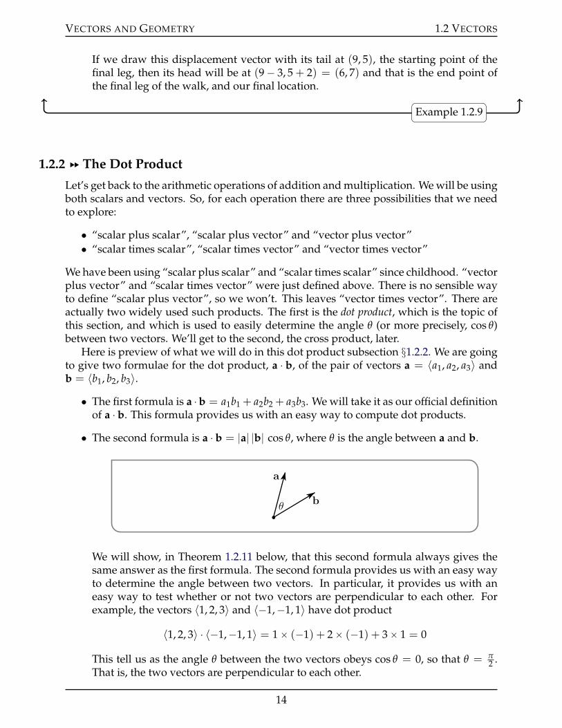
• The second formula is a ¨ b = |a| |b| cos θ, where θ is the angle between a and b.
a
bθ
We will show, in Theorem 1.2.11 below, that this second formula always gives thesame answer as the first formula. The second formula provides us with an easy wayto determine the angle between two vectors. In particular, it provides us with aneasy way to test whether or not two vectors are perpendicular to each other. Forexample, the vectors 〈1, 2, 3〉 and 〈´1,´1, 1〉 have dot product
〈1, 2, 3〉 ¨ 〈´1,´1, 1〉 = 1ˆ (´1) + 2ˆ (´1) + 3ˆ 1 = 0
This tell us as the angle θ between the two vectors obeys cos θ = 0, so that θ = π2 .
That is, the two vectors are perpendicular to each other.
14
VECTORS AND GEOMETRY 1.2 VECTORS
After we give our official definition of the dot product in Definition 1.2.10, and give theimportant properties of the dot product, including the formula a ¨ b = |a| |b| cos θ, inTheorem 1.2.11, we’ll give some examples. Finally, to see the dot product in action, we’lldefine what it means to project one vector on another vector and give an example.
The dot product of the vectors a and b is denoted a ¨ b and is defined by
a = 〈a1, a2〉 , b = 〈b1, b2〉 ùñ a ¨ b = a1b1 + a2b2
a = 〈a1, a2, a3〉 , b = 〈b1, b2, b3〉 ùñ a ¨ b = a1b1 + a2b2 + a3b3
in two and three dimensions respectively.
Definition 1.2.10 (Dot Product).
The properties of the dot product are as follows:
Let a, b and c be vectors and let s be a scalar. Then
(0) a, b are vectors and a ¨ b is a scalar
(1) a ¨ a = |a|2(2) a ¨ b = b ¨ a(3) a ¨ (b + c) = a ¨ b + a ¨ c, (a + b) ¨ c = a ¨ c + b ¨ c(4) (sa) ¨ b = s(a ¨ b)(5) 0 ¨ a = 0(6) a ¨ b = |a| |b| cos θ where θ is the angle between a and b(7) a ¨ b = 0 ðñ a = 0 or b = 0 or a K b
Theorem 1.2.11 (Properties of the Dot Product).
Proof. Properties 0 through 5 are almost immediate consequences of the definition. Forexample, for property 3 (which is called the distributive law) in dimension 2,
a ¨ (b + c) = 〈a1, a2〉 ¨ 〈b1 + c1, b2 + c2〉= a1(b1 + c1) + a2(b2 + c2) = a1b1 + a1c1 + a2b2 + a2c2
a ¨ b + a ¨ c = 〈a1, a2〉 ¨ 〈b1, b2〉+ 〈a1, a2〉 ¨ 〈c1, c2〉= a1b1 + a2b2 + a1c1 + a2c2
Property 6 is sufficiently important that it is often used as the definition of dot product.It is not at all an obvious consequence of the definition. To verify it, we just write |a´ b|2in two different ways. The first expresses |a´ b|2 in terms of a ¨ b. It is
|a´ b|2 1= (a´ b ) ¨ (a´ b )
3= a ¨ a´ a ¨ b´ b ¨ a + b ¨ b1,2= |a|2 + |b|2 ´ 2a ¨ b
15
VECTORS AND GEOMETRY 1.2 VECTORS
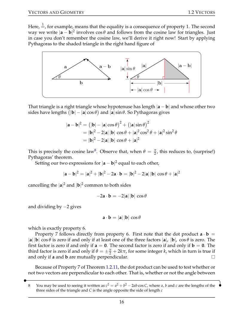
Here, 1=, for example, means that the equality is a consequence of property 1. The second
way we write |a ´ b|2 involves cos θ and follows from the cosine law for triangles. Justin case you don’t remember the cosine law, we’ll derive it right now! Start by applyingPythagoras to the shaded triangle in the right hand figure of
bθ
a a ´ b
|b||a| cos θ
|a| sin θθ
|a| |a ´ b|
That triangle is a right triangle whose hypotenuse has length |a´ b| and whose other twosides have lengths
(|b| ´ |a| cos θ)
and |a| sin θ. So Pythagoras gives
|a´ b|2 =(|b| ´ |a| cos θ
)2+(|a| sin θ
)2
= |b|2 ´ 2|a| |b| cos θ + |a|2 cos2 θ + |a|2 sin2 θ
= |b|2 ´ 2|a| |b| cos θ + |a|2
This is precisely the cosine law8. Observe that, when θ = π2 , this reduces to, (surprise!)
Pythagoras’ theorem.Setting our two expressions for |a´ b|2 equal to each other,
|a´ b|2 = |a|2 + |b|2 ´ 2a ¨ b = |b|2 ´ 2|a| |b| cos θ + |a|2
cancelling the |a|2 and |b|2 common to both sides
´2a ¨ b = ´2|a| |b| cos θ
and dividing by ´2 gives
a ¨ b = |a| |b| cos θ
which is exactly property 6.Property 7 follows directly from property 6. First note that the dot product a ¨ b =
|a| |b| cos θ is zero if and only if at least one of the three factors |a|, |b|, cos θ is zero. Thefirst factor is zero if and only if a = 0. The second factor is zero if and only if b = 0. Thethird factor is zero if and only if θ = ˘π
2 + 2kπ, for some integer k, which in turn is true ifand only if a and b are mutually perpendicular.
Because of Property 7 of Theorem 1.2.11, the dot product can be used to test whether ornot two vectors are perpendicular to each other. That is, whether or not the angle between
8 You may be used to seeing it written as c2 = a2 + b2 ´ 2ab cos C, where a, b and c are the lengths of thethree sides of the triangle and C is the angle opposite the side of length c
16
VECTORS AND GEOMETRY 1.2 VECTORS
the two vectors is 90˝. Another name9 for “perpendicular” is “orthogonal”. Testing fororthogonality is one of the main uses of the dot product.
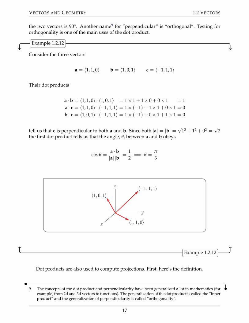
Example 1.2.12
Consider the three vectors
a = 〈1, 1, 0〉 b = 〈1, 0, 1〉 c = 〈´1, 1, 1〉
Their dot products
a ¨ b = 〈1, 1, 0〉 ¨ 〈1, 0, 1〉 = 1ˆ 1 + 1ˆ 0 + 0ˆ 1 = 1a ¨ c = 〈1, 1, 0〉 ¨ 〈´1, 1, 1〉 = 1ˆ (´1) + 1ˆ 1 + 0ˆ 1 = 0b ¨ c = 〈1, 0, 1〉 ¨ 〈´1, 1, 1〉 = 1ˆ (´1) + 0ˆ 1 + 1ˆ 1 = 0
tell us that c is perpendicular to both a and b. Since both |a| = |b| = ?12 + 12 + 02 =
?2
the first dot product tells us that the angle, θ, between a and b obeys
cos θ =a ¨ b|a| |b| =
12ùñ θ =
π
3
z
y
x 〈1, 1, 0〉
〈1, 0, 1〉〈´1, 1, 1〉
Example 1.2.12
Dot products are also used to compute projections. First, here’s the definition.
9 The concepts of the dot product and perpendicularity have been generalized a lot in mathematics (forexample, from 2d and 3d vectors to functions). The generalization of the dot product is called the “innerproduct” and the generalization of perpendicularity is called “orthogonality”.
17
VECTORS AND GEOMETRY 1.2 VECTORS
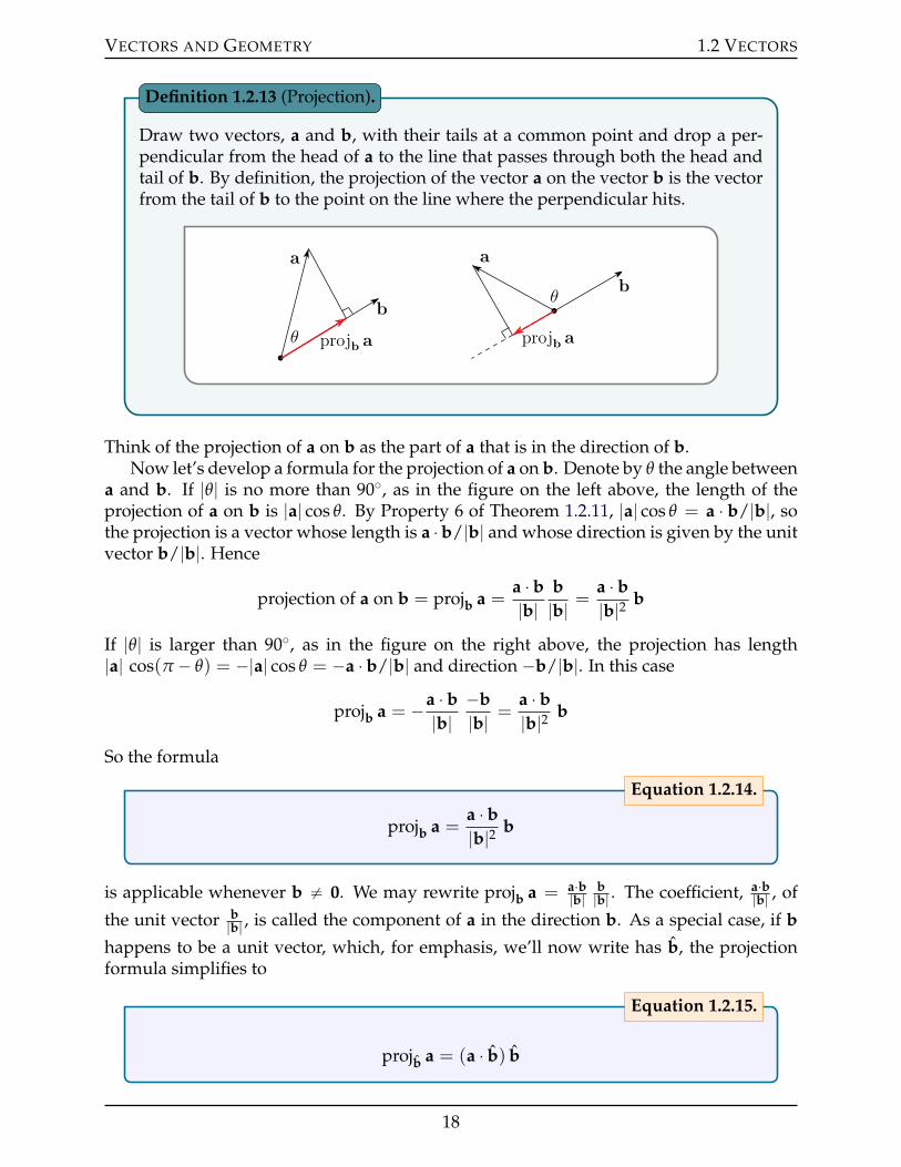
Draw two vectors, a and b, with their tails at a common point and drop a per-pendicular from the head of a to the line that passes through both the head andtail of b. By definition, the projection of the vector a on the vector b is the vectorfrom the tail of b to the point on the line where the perpendicular hits.
a
b
projb aθ
a
b
projb a
θ
Definition 1.2.13 (Projection).
Think of the projection of a on b as the part of a that is in the direction of b.Now let’s develop a formula for the projection of a on b. Denote by θ the angle between
a and b. If |θ| is no more than 90˝, as in the figure on the left above, the length of theprojection of a on b is |a| cos θ. By Property 6 of Theorem 1.2.11, |a| cos θ = a ¨ b/|b|, sothe projection is a vector whose length is a ¨b/|b| and whose direction is given by the unitvector b/|b|. Hence
projection of a on b = projb a =a ¨ b|b|
b|b| =
a ¨ b|b|2 b
If |θ| is larger than 90˝, as in the figure on the right above, the projection has length|a| cos(π ´ θ) = ´|a| cos θ = ´a ¨ b/|b| and direction ´b/|b|. In this case
projb a = ´a ¨ b|b|
´b|b| =
a ¨ b|b|2 b
So the formula
projb a =a ¨ b|b|2 b
Equation 1.2.14.
is applicable whenever b ‰ 0. We may rewrite projb a = a¨b|b|
b|b| . The coefficient, a¨b
|b| , of
the unit vector b|b| , is called the component of a in the direction b. As a special case, if b
happens to be a unit vector, which, for emphasis, we’ll now write has b, the projectionformula simplifies to
projb a = (a ¨ b) b
Equation 1.2.15.
18
VECTORS AND GEOMETRY 1.2 VECTORS
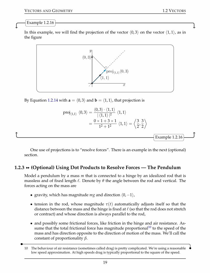
Example 1.2.16
In this example, we will find the projection of the vector 〈0, 3〉 on the vector 〈1, 1〉, as inthe figure
x
y
〈0, 3〉
〈1, 1〉proj〈1,1〉〈0, 3〉
By Equation 1.2.14 with a = 〈0, 3〉 and b = 〈1, 1〉, that projection is
proj〈1,1〉 〈0, 3〉 = 〈0, 3〉 ¨ 〈1, 1〉| 〈1, 1〉 |2 〈1, 1〉
=0ˆ 1 + 3ˆ 1
12 + 12 〈1, 1〉 =⟨
32
,32
⟩
Example 1.2.16
One use of projections is to “resolve forces”. There is an example in the next (optional)section.
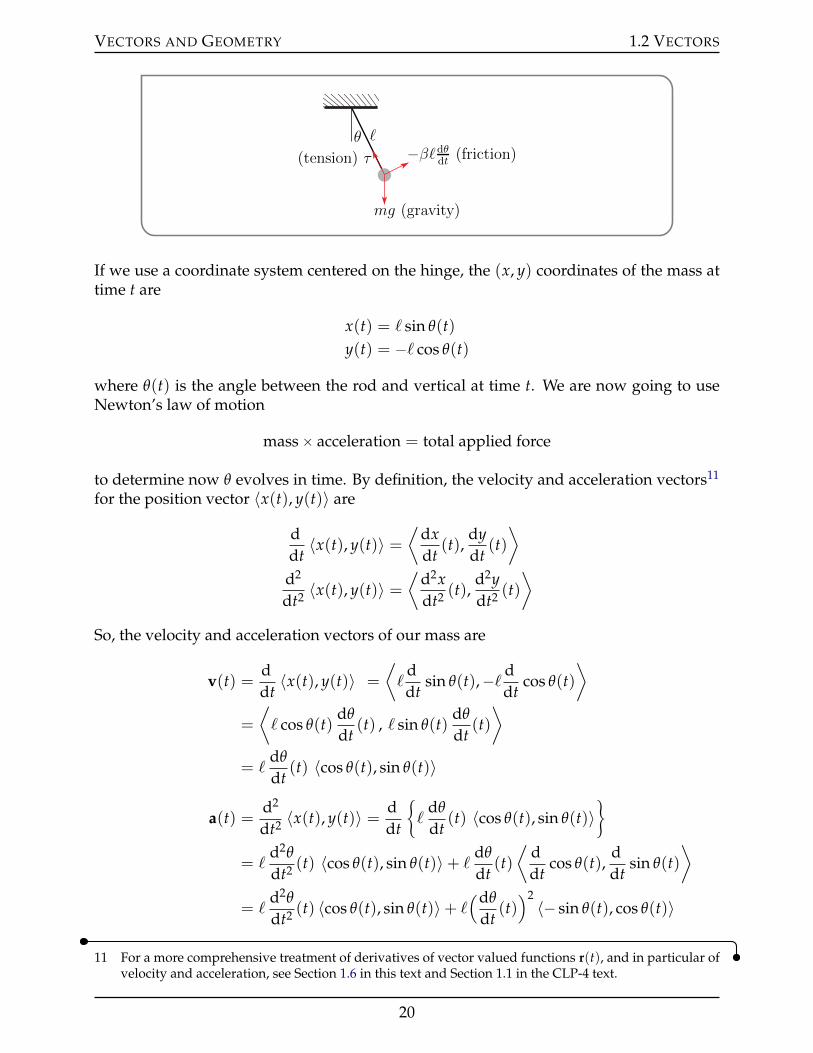
1.2.3 §§ (Optional) Using Dot Products to Resolve Forces — The Pendulum
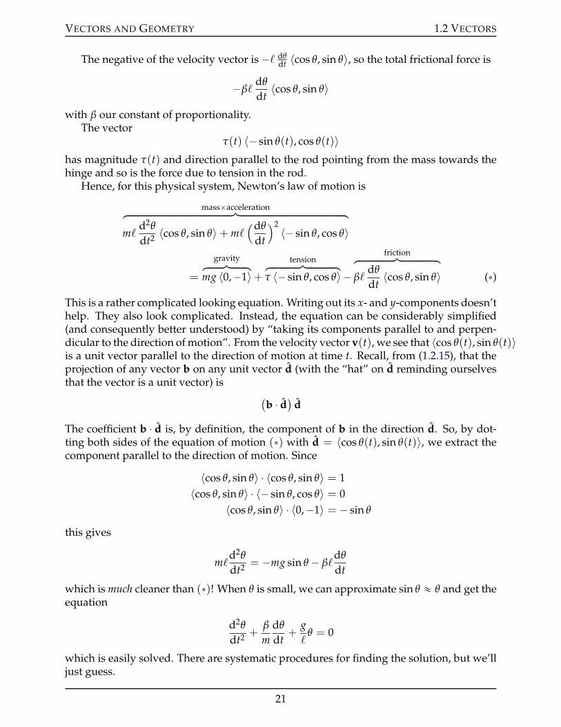
Model a pendulum by a mass m that is connected to a hinge by an idealized rod that ismassless and of fixed length `. Denote by θ the angle between the rod and vertical. Theforces acting on the mass are
• gravity, which has magnitude mg and direction 〈0,´1〉,
• tension in the rod, whose magnitude τ(t) automatically adjusts itself so that thedistance between the mass and the hinge is fixed at ` (so that the rod does not stretchor contract) and whose direction is always parallel to the rod,
• and possibly some frictional forces, like friction in the hinge and air resistance. As-sume that the total frictional force has magnitude proportional10 to the speed of themass and has direction opposite to the direction of motion of the mass. We’ll call theconstant of proportionality β.
10 The behaviour of air resistance (sometimes called drag) is pretty complicated. We’re using a reasonablelow speed approximation. At high speeds drag is typically proportional to the square of the speed.
19
VECTORS AND GEOMETRY 1.2 VECTORS
θ ℓ
mg (gravity)
(tension) τ ´βℓdθdt
(friction)
If we use a coordinate system centered on the hinge, the (x, y) coordinates of the mass attime t are
x(t) = ` sin θ(t)y(t) = ´` cos θ(t)
where θ(t) is the angle between the rod and vertical at time t. We are now going to useNewton’s law of motion
massˆ acceleration = total applied force
to determine now θ evolves in time. By definition, the velocity and acceleration vectors11
for the position vector 〈x(t), y(t)〉 are
ddt〈x(t), y(t)〉 =
⟨dxdt
(t),dydt
(t)⟩
d2
dt2 〈x(t), y(t)〉 =⟨
d2xdt2 (t),
d2ydt2 (t)
⟩
So, the velocity and acceleration vectors of our mass are
v(t) =ddt〈x(t), y(t)〉 =
⟨`
ddt
sin θ(t),´` ddt
cos θ(t)⟩
=
⟨` cos θ(t)
dθ
dt(t) , ` sin θ(t)
dθ
dt(t)⟩
= `dθ
dt(t) 〈cos θ(t), sin θ(t)〉
a(t) =d2
dt2 〈x(t), y(t)〉 = ddt
"`
dθ
dt(t) 〈cos θ(t), sin θ(t)〉
*
= `d2θ
dt2 (t) 〈cos θ(t), sin θ(t)〉+ `dθ
dt(t)⟨
ddt
cos θ(t),ddt
sin θ(t)⟩
= `d2θ
dt2 (t) 〈cos θ(t), sin θ(t)〉+ `(dθ
dt(t))2〈´ sin θ(t), cos θ(t)〉
11 For a more comprehensive treatment of derivatives of vector valued functions r(t), and in particular ofvelocity and acceleration, see Section 1.6 in this text and Section 1.1 in the CLP-4 text.
20
VECTORS AND GEOMETRY 1.2 VECTORS
The negative of the velocity vector is ´` dθdt 〈cos θ, sin θ〉, so the total frictional force is
´β`dθ
dt〈cos θ, sin θ〉
with β our constant of proportionality.The vector
τ(t) 〈´ sin θ(t), cos θ(t)〉has magnitude τ(t) and direction parallel to the rod pointing from the mass towards thehinge and so is the force due to tension in the rod.
Hence, for this physical system, Newton’s law of motion is
massˆaccelerationhkkkkkkkkkkkkkkkkkkkkkkkkkkkkkkkkikkkkkkkkkkkkkkkkkkkkkkkkkkkkkkkkj
m`d2θ
dt2 〈cos θ, sin θ〉+ m`(dθ
dt
)2〈´ sin θ, cos θ〉
=
gravityhkkkkkikkkkkjmg 〈0,´1〉+
tensionhkkkkkkkkkikkkkkkkkkjτ 〈´ sin θ, cos θ〉´
frictionhkkkkkkkkkkikkkkkkkkkkj
β`dθ
dt〈cos θ, sin θ〉 (˚)
This is a rather complicated looking equation. Writing out its x- and y-components doesn’thelp. They also look complicated. Instead, the equation can be considerably simplified(and consequently better understood) by “taking its components parallel to and perpen-dicular to the direction of motion”. From the velocity vector v(t), we see that 〈cos θ(t), sin θ(t)〉is a unit vector parallel to the direction of motion at time t. Recall, from (1.2.15), that theprojection of any vector b on any unit vector d (with the “hat” on d reminding ourselvesthat the vector is a unit vector) is
(b ¨ d) d
The coefficient b ¨ d is, by definition, the component of b in the direction d. So, by dot-ting both sides of the equation of motion (˚) with d = 〈cos θ(t), sin θ(t)〉, we extract thecomponent parallel to the direction of motion. Since
〈cos θ, sin θ〉 ¨ 〈cos θ, sin θ〉 = 1〈cos θ, sin θ〉 ¨ 〈´ sin θ, cos θ〉 = 0
〈cos θ, sin θ〉 ¨ 〈0,´1〉 = ´ sin θ
this gives
m`d2θ
dt2 = ´mg sin θ ´ β`dθ
dt
which is much cleaner than (˚)! When θ is small, we can approximate sin θ « θ and get theequation
d2θ
dt2 +β
mdθ
dt+
g`
θ = 0
which is easily solved. There are systematic procedures for finding the solution, but we’lljust guess.
21
VECTORS AND GEOMETRY 1.2 VECTORS
When there is no friction (so that β = 0), we would expect the pendulum to just oscil-late. So it is natural to guess
θ(t) = A sin(ωt´ δ)
which is an oscillation with (unknown) amplitude A, frequency ω (radians per unit time)and phase δ. Substituting this guess into the left hand side, θ2 + g
` θ, yields
´Aω2 sin(ωt´ δ) + A g` sin(ωt´ δ)
which is zero if ω =a
g/`. So θ(t) = A sin(ωt´ δ) is a solution for any amplitude Aand phase δ, provided the frequency ω =
ag/`.
When there is some, but not too much, friction, so that β ą 0 is relatively small, wewould expect “oscillation with decaying amplitude”. So we guess
θ(t) = Ae´γt sin(ωt´ δ)
for some constant decay rate γ, to be determined. With this guess,
θ(t) = Ae´γt sin(ωt´ δ)
θ1(t) = ´ γAe´γt sin(ωt´ δ) + ωAe´γtcos(ωt´ δ)
θ2(t) = (γ2 ´ω2)Ae´γtsin(ωt´ δ)´ 2γωAe´γt cos(ωt´ δ)
and the left hand side
d2θ
dt2 +β
mdθ
dt+
g`
θ
=
[γ2 ´ω2 ´ β
mγ +
g`
]Ae´γt sin(ωt´ δ) +
[´2γω +
β
mω
]Ae´γt cos(ωt´ δ)
vanishes if γ2 ´ω2 ´ βm γ + g
` = 0 and ´2γω + βm ω = 0. The second equation tells us the
decay rate γ = β2m and then the first tells us the frequency
ω =
bγ2 ´ β
m γ + g` =
cg` ´ β2
4m2
When there is a lot of friction (namely when β2
4m2 ą g` , so that the frequency ω is not a real
number), we would expect damping without oscillation and so would guess θ(t) = Ae´γt.You can determine the allowed values of γ by substituting this guess in.
To extract the components perpendicular to the direction of motion, we dot with 〈´ sin θ, cos θ〉rather than 〈cos θ, sin θ〉. Note that, because 〈´ sin θ, cos θ〉 ¨ 〈cos θ, sin θ〉 = 0, the vector〈´ sin θ, cos θ〉 really is perpendicular to the direction of motion. Since
〈´ sin θ, cos θ〉 ¨ 〈cos θ, sin θ〉 = 0〈´ sin θ, cos θ〉 ¨ 〈´ sin θ, cosθ〉 = 1
〈´ sin θ, cos θ〉 ¨ 〈0,´1〉 = ´ cos θ
dotting both sides of the equation of motion (˚) with 〈´ sin θ, cos θ〉 gives
m`(dθ
dt
)2= ´mg cos θ + τ
This equation just determines the tension τ = m`(dθ
dt)2
+ mg cos θ in the rod, once youknow θ(t).
22

VECTORS AND GEOMETRY 1.2 VECTORS
1.2.4 §§ (Optional) Areas of Parallelograms
A parallelogram is naturally determined by the two vectors that define its sides. We’llnow develop a formula for the area of a parallelogram in terms of these two vectors.
Construct a parallelogram as follows. Pick two vectors 〈a, b〉 and 〈c, d〉. Draw themwith their tails at a common point. Then draw 〈a, b〉 a second time with its tail at thehead of 〈c, d〉 and draw 〈c, d〉 a second time with its tail at the head of 〈a, b〉. If the com-mon point is the origin, you get a picture like the figure below. Any parallelogram can
pa ` c, b ` dq
pa, bq
pc, dq
a c
d
b
c a
b
d
be constructed like this if you pick the common point and two vectors appropriately.Let’s compute the area of the parallelogram. The area of the large rectangle with ver-tices (0, 0), (0, b + d), (a + c, 0) and (a + c, b + d) is (a + c)(b + d). The parallelogram wewant can be extracted from the large rectangle by deleting the two small rectangles (eachof area bc), and the two lightly shaded triangles (each of area 1
2 cd), and the two darklyshaded triangles (each of area 1
2 ab). So the desired
area = (a + c)(b + d)´ (2ˆ bc)´ (2ˆ 12 cd)´ (2ˆ 1
2 ab)= ad´ bc
In the above figure, we have implicitly assumed that a, b, c, d ě 0 and d/c ě b/a. Inwords, we have assumed that both vectors 〈a, b〉 , 〈c, d〉 lie in the first quadrant and that〈c, d〉 lies above 〈a, b〉. By simply interchanging a Ø c and b Ø d in the picture andthroughout the argument, we see that when a, b, c, d ě 0 and b/a ě d/c, so that thevector 〈c, d〉 lies below 〈a, b〉, the area of the parallelogram is bc´ ad. In fact, all cases arecovered by the formula
area of parallelogram with sides 〈a, b〉 and 〈c, d〉 = |ad´ bc|
Equation 1.2.17.
Given two vectors 〈a, b〉 and 〈c, d〉, the expression ad´ bc is generally written
det[
a bc d
]= ad´ bc
23
VECTORS AND GEOMETRY 1.2 VECTORS
and is called the determinant of the matrix12
[a bc d
]
with rows 〈a, b〉 and 〈c, d〉. The determinant of a 2ˆ 2 matrix is the product of the diagonalentries minus the product of the off-diagonal entries.
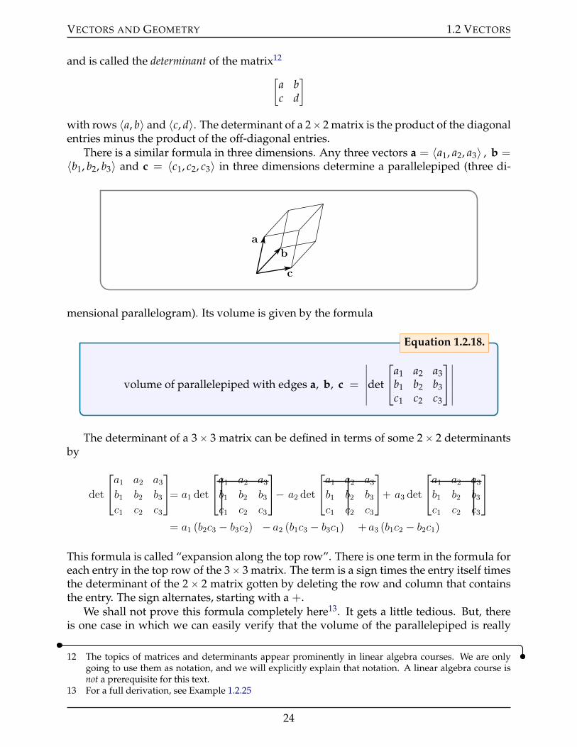
There is a similar formula in three dimensions. Any three vectors a = 〈a1, a2, a3〉 , b =〈b1, b2, b3〉 and c = 〈c1, c2, c3〉 in three dimensions determine a parallelepiped (three di-
a
b
c
mensional parallelogram). Its volume is given by the formula
volume of parallelepiped with edges a, b, c =
ˇˇˇdet
a1 a2 a3b1 b2 b3c1 c2 c3
ˇˇˇ
Equation 1.2.18.
The determinant of a 3ˆ 3 matrix can be defined in terms of some 2ˆ 2 determinantsby
det
a1 a2 a3b1 b2 b3c1 c2 c3
= a1 det
a1 a2 a3b1 b2 b3c1 c2 c3
− a2 det
a1 a2 a3b1 b2 b3c1 c2 c3
+ a3 det
a1 a2 a3b1 b2 b3c1 c2 c3
= a1 (b2c3 − b3c2) − a2 (b1c3 − b3c1) + a3 (b1c2 − b2c1)
This formula is called “expansion along the top row”. There is one term in the formula foreach entry in the top row of the 3ˆ 3 matrix. The term is a sign times the entry itself timesthe determinant of the 2ˆ 2 matrix gotten by deleting the row and column that containsthe entry. The sign alternates, starting with a +.
We shall not prove this formula completely here13. It gets a little tedious. But, thereis one case in which we can easily verify that the volume of the parallelepiped is really
12 The topics of matrices and determinants appear prominently in linear algebra courses. We are onlygoing to use them as notation, and we will explicitly explain that notation. A linear algebra course isnot a prerequisite for this text.
13 For a full derivation, see Example 1.2.25
24
VECTORS AND GEOMETRY 1.2 VECTORS
given by the absolute value of the claimed determinant. If the vectors b and c happen tolie in the xy plane, so that b3 = c3 = 0, then
det
a1 a2 a3b1 b2 0c1 c2 0
= a1(b20´ 0c2)´ a2(b10´ 0c1) + a3(b1c2 ´ b2c1)
= a3(b1c2 ´ b2c1)
The first factor, a3, is the z-coordinate of the one vector not contained in the xy-plane. Itis (up to a sign) the height of the parallelepiped. The second factor is, up to a sign, thearea of the parallelogram determined by b and c. This parallelogram forms the base ofthe parallelepiped. The product is indeed, up to a sign, the volume of the parallelepiped.That the formula is true in general is a consequence of the fact (that we will not prove)that the value of a determinant does not change when one rotates the coordinate systemand that one can always rotate our coordinate axes around so that b and c both lie in thexy-plane.
1.2.5 §§ The Cross Product
We have already seen two different products involving vectors — the multiplication ofa vector by a scalar and the dot product of two vectors. The dot product of two vectorsyields a scalar. We now introduce another product of two vectors, called the cross product.The cross product of two vectors will give a vector. There are applications which have twovectors as inputs and produce one vector as an output, and which are related to the crossproduct. Here is a very brief mention of two such applications. We will look at them inmuch more detail later.
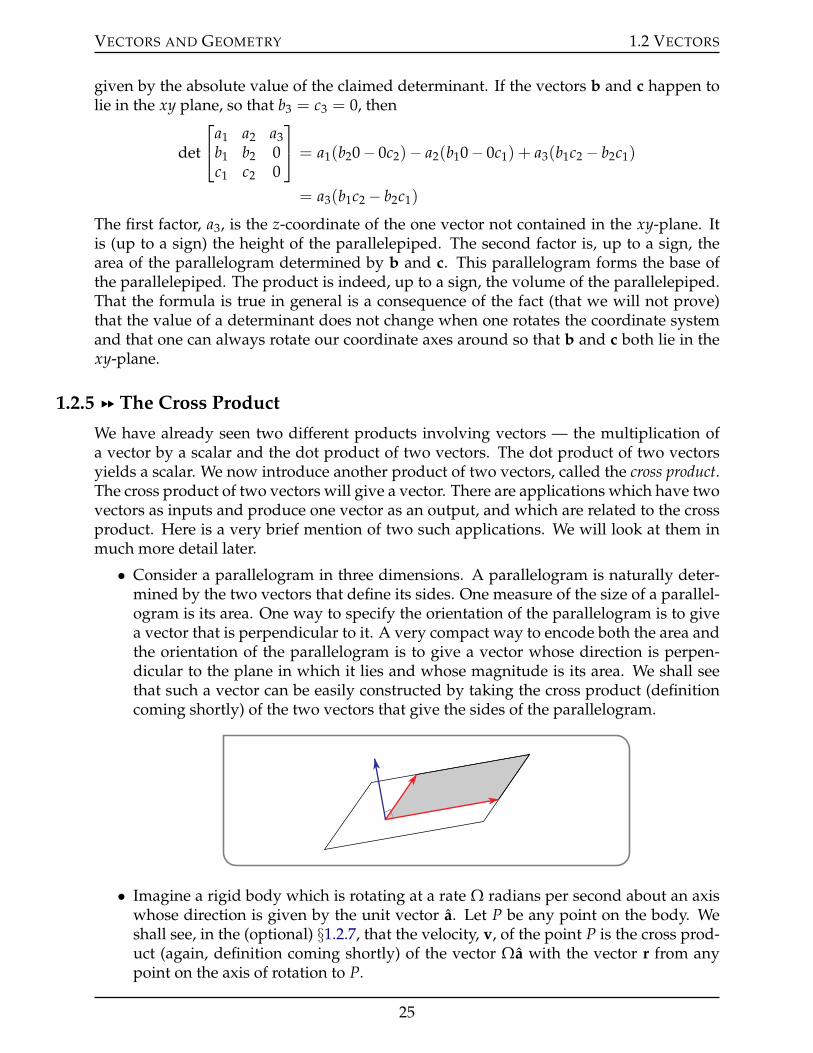
• Consider a parallelogram in three dimensions. A parallelogram is naturally deter-mined by the two vectors that define its sides. One measure of the size of a parallel-ogram is its area. One way to specify the orientation of the parallelogram is to givea vector that is perpendicular to it. A very compact way to encode both the area andthe orientation of the parallelogram is to give a vector whose direction is perpen-dicular to the plane in which it lies and whose magnitude is its area. We shall seethat such a vector can be easily constructed by taking the cross product (definitioncoming shortly) of the two vectors that give the sides of the parallelogram.
• Imagine a rigid body which is rotating at a rate Ω radians per second about an axiswhose direction is given by the unit vector a. Let P be any point on the body. Weshall see, in the (optional) §1.2.7, that the velocity, v, of the point P is the cross prod-uct (again, definition coming shortly) of the vector Ωa with the vector r from anypoint on the axis of rotation to P.
25
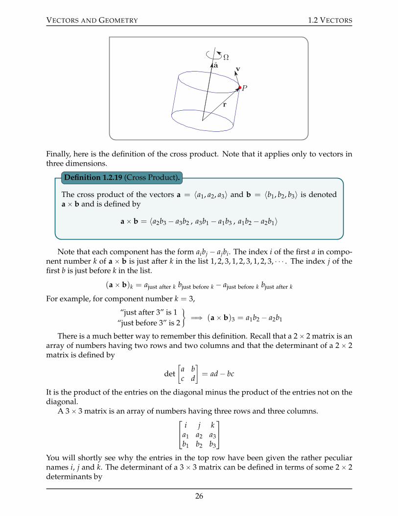
VECTORS AND GEOMETRY 1.2 VECTORS
P
r
vaΩ
Finally, here is the definition of the cross product. Note that it applies only to vectors inthree dimensions.
The cross product of the vectors a = 〈a1, a2, a3〉 and b = 〈b1, b2, b3〉 is denotedaˆ b and is defined by
aˆ b = 〈a2b3 ´ a3b2 , a3b1 ´ a1b3 , a1b2 ´ a2b1〉
Definition 1.2.19 (Cross Product).
Note that each component has the form aibj ´ ajbi. The index i of the first a in compo-nent number k of aˆ b is just after k in the list 1, 2, 3, 1, 2, 3, 1, 2, 3, ¨ ¨ ¨ . The index j of thefirst b is just before k in the list.
(aˆ b)k = ajust after k bjust before k ´ ajust before k bjust after k
For example, for component number k = 3,
“just after 3” is 1“just before 3” is 2
*ùñ (aˆ b)3 = a1b2 ´ a2b1
There is a much better way to remember this definition. Recall that a 2ˆ 2 matrix is anarray of numbers having two rows and two columns and that the determinant of a 2ˆ 2matrix is defined by
det[
a bc d
]= ad´ bc
It is the product of the entries on the diagonal minus the product of the entries not on thediagonal.
A 3ˆ 3 matrix is an array of numbers having three rows and three columns.
i j ka1 a2 a3b1 b2 b3
You will shortly see why the entries in the top row have been given the rather peculiarnames i, j and k. The determinant of a 3ˆ 3 matrix can be defined in terms of some 2ˆ 2determinants by
26
VECTORS AND GEOMETRY 1.2 VECTORS
det
i j k
a1 a2 a3b1 b2 b3
= i det
i j k
a1 a2 a3b1 b2 b3
− j det
i j k
a1 a2 a3b1 b2 b3
+ k det
i j k
a1 a2 a3b1 b2 b3
= i (a2b3 − a3b2) − j (a1b3 − a3b1) + k (a1b2 − a2b1)
This formula is called “expansion of the determinant along the top row”. There is oneterm in the formula for each entry in the top row. The term is a sign times the entry itselftimes the determinant of the 2 ˆ 2 matrix gotten by deleting the row and column thatcontains the entry. The sign alternates, starting with a +. If we now replace i by ııı, j by and k by k, we get exactly the formula for aˆ b of Definition 1.2.19. That is the reason forthe peculiar choice of names for the matrix entries. So
aˆ b = det
ııı ka1 a2 a3b1 b2 b3
= ııı(a2b3 ´ a3b2)´ (a1b3 ´ a3b1) + k(a1b2 ´ a2b1)
is a mnemonic device for remembering the definition of a ˆ b. It is also good from thepoint of view of evaluating aˆ b. Here are several examples in which we use the deter-minant mnemonic device to evaluate cross products.
Example 1.2.20
In this example, we’ll use the mnemonic device to compute two very simple cross prod-ucts. First
ııı ˆ “ det
»–ııı k1 0 00 1 0
fifl“ ııı det
»–ııı k1 0 00 1 0
fifl ´ det
»–ııı k1 0 00 1 0
fifl ` kdet
»–ııı k1 0 00 1 0
fifl
“ ııı p0 ˆ 0 ´ 0 ˆ 1q ´ p1 ˆ 0 ´ 0 ˆ 0q ` k p1 ˆ 1 ´ 0 ˆ 0q “ k
Second
ˆ ııı “ det
»–ııı k0 1 01 0 0
fifl“ ııı det
»–ııı k0 1 01 0 0
fifl ´ det
»–ııı k0 1 01 0 0
fifl ` kdet
»–ııı k0 1 01 0 0
fifl
“ ııı p1 ˆ 0 ´ 0 ˆ 0q ´ p0 ˆ 0 ´ 0 ˆ 1q ` k p0 ˆ 0 ´ 1 ˆ 1q “ ´k
Note that, unlike most (or maybe even all) products that you have seen before, ıııˆ is notthe same as ˆ ııı!
Example 1.2.20
Example 1.2.21
In this example, we’ll use the mnemonic device to compute two more complicated crossproducts. Let a = 〈1, 2, 3〉 and b = 〈1,´1, 2〉. First
27
VECTORS AND GEOMETRY 1.2 VECTORS
a ˆ b “ det
»–ııı k1 2 31 ´1 2
fifl“ ıııdet
»–ııı k1 2 31 ´1 2
fifl ´ det
»–ııı k1 2 31 ´1 2
fifl` k det
»–ııı k1 2 31 ´1 2
fifl
“ ııı t2 ˆ 2 ´ 3 ˆ p´1qu ´ t1 ˆ 2 ´ 3 ˆ 1u` k t1 ˆ p´1q ´ 2 ˆ 1u“ 7 ııı ` ´ 3 k
Second
b ˆ a “ det
»–ııı k1 ´1 21 2 3
fifl“ ıııdet
»–ııı k1 ´1 21 2 3
fifl ´ det
»–ııı k1 ´1 21 2 3
fifl` k det
»–ııı k1 ´1 21 2 3
fifl
“ ııı tp´1q ˆ 3 ´ 2 ˆ 2u ´ t1 ˆ 3 ´ 2 ˆ 1u` k t1 ˆ 2 ´ p´1q ˆ 1u“ ´7 ııı ´ ` 3 k
Here are some important observations.
• The vectors aˆ b and bˆ a are not the same! In fact bˆ a = ´aˆ b. We shall see inTheorem 1.2.23 below that this was not a fluke.
• The vector a ˆ b has dot product zero with both a and b. So the vector a ˆ b isprependicular to both a and b. We shall see in Theorem 1.2.23 below that this wasalso not a fluke.
Example 1.2.21
Example 1.2.22
Yet again we use the mnemonic device to compute a more complicated cross product. Thistime let a = 〈3, 2, 1〉 and b = 〈6, 4, 2〉. Then
a ˆ b “ det
»–ııı k3 2 16 4 2
fifl“ ııı det
»–ııı k3 2 16 4 2
fifl ´ det
»–ııı k3 2 16 4 2
fifl ` kdet
»–ııı k3 2 16 4 2
fifl
“ ııı p2 ˆ 2 ´ 1 ˆ 4q ´ p3 ˆ 2 ´ 1 ˆ 6q ` k p3 ˆ 4 ´ 2 ˆ 6q “ 0
We shall see in Theorem 1.2.23 below that it is not a fluke that the cross product is 0. It isa consequence of the fact that a and b = 2a are parallel.
Example 1.2.22
We now move on to learning about the properties of the cross product. Our first prop-erties lead up to a more intuitive geometric definition of aˆ b, which is better for inter-preting aˆ b. These properties of the cross product, which state that aˆ b is a vector andthen determine its direction and length, are as follows. We will collect these properties,and a few others, into a theorem shortly.
(0) a, b are vectors in three dimensions and aˆ b is a vector in three dimensions.
28
VECTORS AND GEOMETRY 1.2 VECTORS
(1) aˆ b is perpendicular to both a and b.
Proof : To check that a and aˆ b are perpendicular, one just has to check that the dotproduct a ¨ (aˆ b) = 0. The six terms in
a ¨ (aˆ b) = a1(a2b3 ´ a3b2) + a2(a3b1 ´ a1b3) + a3(a1b2 ´ a2b1)
cancel pairwise. The computation showing that b ¨ (aˆ b) = 0 is similar.
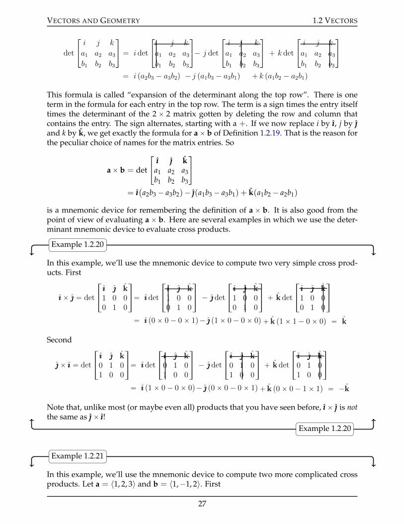
(2) |aˆ b| = |a| |b| sin θ where 0 ď θ ď π is the angle between a and b
= the area of the parallelogram with sides a and ba
a
b b
θ
Proof : The formula |aˆ b| = |a| |b| sin θ is gotten by verifying that
|aˆ b|2 =(aˆ b
) ¨ (aˆ b)
= (a2b3 ´ a3b2)2 + (a3b1 ´ a1b3)
2 + (a1b2 ´ a2b1)2
= a22b2
3 ´ 2a2b3a3b2 + a23b2
2 + a23b2
1 ´ 2a3b1a1b3 + a21b2
3
+ a21b2
2 ´ 2a1b2a2b1 + a22b2
1
is equal to
|a|2 |b|2 sin2 θ = |a|2|b|2(1´ cos2 θ)
= |a|2|b|2 ´ (a ¨ b)2
=(a2
1 + a22 + a2
3)(
b21 + b2
2 + b23)´ (a1b1 + a2b2 + a3b3
)2
= a21b2
2 + a21b2
3 + a22b2
1 + a22b2
3 + a23b2
1 + a23b2
2
´ (2a1b1a2b2 + 2a1b1a3b3 + 2a2b2a3b3)
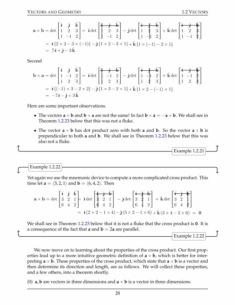
To see that |a| |b| sin θ is the area of the parallelogram with sides a and b, just recallthat the area of any parallelogram is given by the length of its base times its height.Think of a as the base of the parallelogram. Then |a| is the length of the base and|b| sin θ is the height.
a
a
b b
θ
These properties almost determine aˆ b. Property 1 forces the vector aˆ b to lie on theline perpendicular to the plane containing a and b. There are precisely two vectors on thisline that have the length given by property 2. In the left hand figure of
29
VECTORS AND GEOMETRY 1.2 VECTORS
a
b
c
d a
b
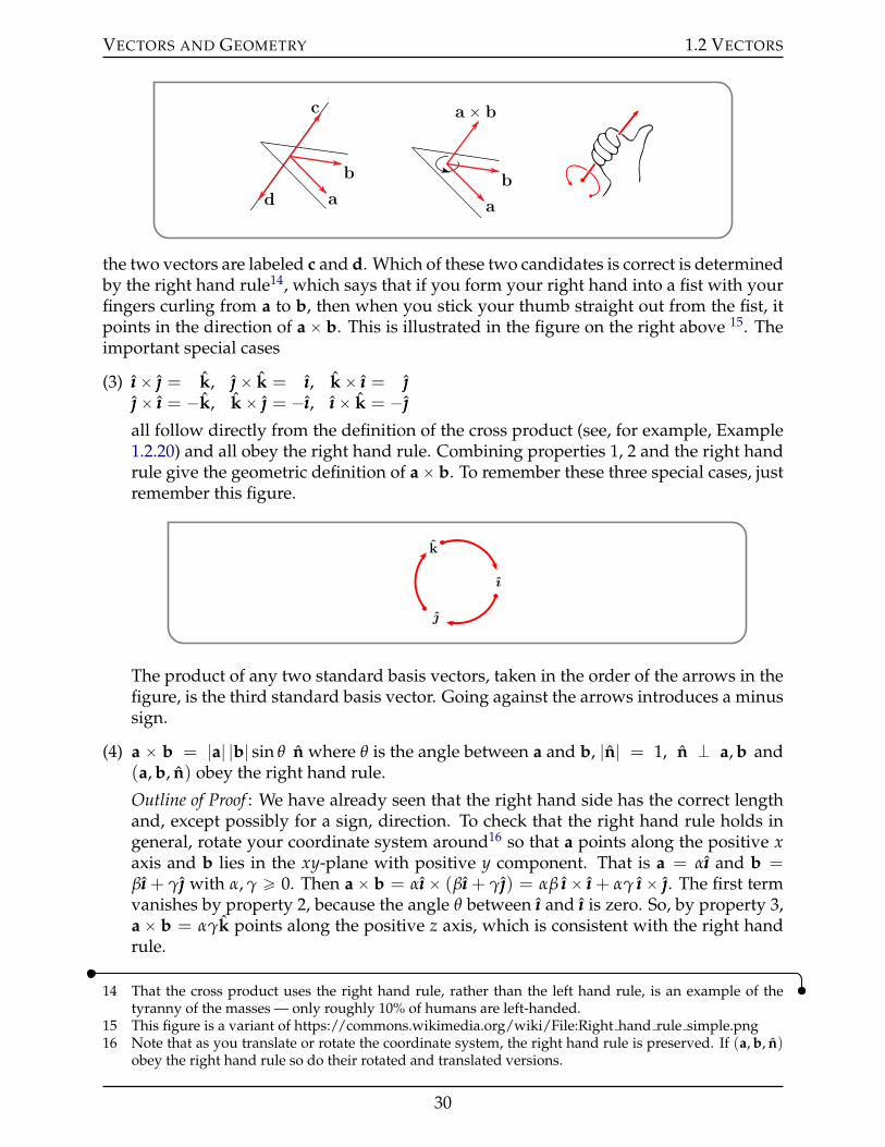
a ˆ b
the two vectors are labeled c and d. Which of these two candidates is correct is determinedby the right hand rule14, which says that if you form your right hand into a fist with yourfingers curling from a to b, then when you stick your thumb straight out from the fist, itpoints in the direction of aˆ b. This is illustrated in the figure on the right above 15. Theimportant special cases
(3) ıııˆ = k, ˆ k = ııı, kˆ ııı = ˆ ııı = ´k, kˆ = ´ııı, ıııˆ k = ´
all follow directly from the definition of the cross product (see, for example, Example1.2.20) and all obey the right hand rule. Combining properties 1, 2 and the right handrule give the geometric definition of aˆ b. To remember these three special cases, justremember this figure.
The product of any two standard basis vectors, taken in the order of the arrows in thefigure, is the third standard basis vector. Going against the arrows introduces a minussign.
(4) a ˆ b = |a| |b| sin θ n where θ is the angle between a and b, |n| = 1, n K a, b and(a, b, n) obey the right hand rule.
Outline of Proof : We have already seen that the right hand side has the correct lengthand, except possibly for a sign, direction. To check that the right hand rule holds ingeneral, rotate your coordinate system around16 so that a points along the positive xaxis and b lies in the xy-plane with positive y component. That is a = αııı and b =βııı + γ with α, γ ě 0. Then aˆ b = αıııˆ (βııı + γ) = αβ ıııˆ ııı + αγ ıııˆ . The first termvanishes by property 2, because the angle θ between ııı and ııı is zero. So, by property 3,aˆ b = αγk points along the positive z axis, which is consistent with the right handrule.
14 That the cross product uses the right hand rule, rather than the left hand rule, is an example of thetyranny of the masses — only roughly 10% of humans are left-handed.
15 This figure is a variant of https://commons.wikimedia.org/wiki/File:Right hand rule simple.png16 Note that as you translate or rotate the coordinate system, the right hand rule is preserved. If (a, b, n)
obey the right hand rule so do their rotated and translated versions.
30
VECTORS AND GEOMETRY 1.2 VECTORS
The analog of property 7 of the dot product (which says that a ¨ b is zero if and only ifa = 0 or b = 0 or a K b) follows immediately from property 2.
(5) aˆ b = 0 ðñ a = 0 or b = 0 or a ‖ b
The remaining properties are all tools for helping do computations with cross products.Here is a theorem which summarizes the properties of the cross product. We have alreadyseen the first five. The other properties are all tools for helping do computations withcross products.
(0) a, b are vectors in three dimensions and aˆb is a vector in three dimensions.
(1) aˆ b is perpendicular to both a and b.
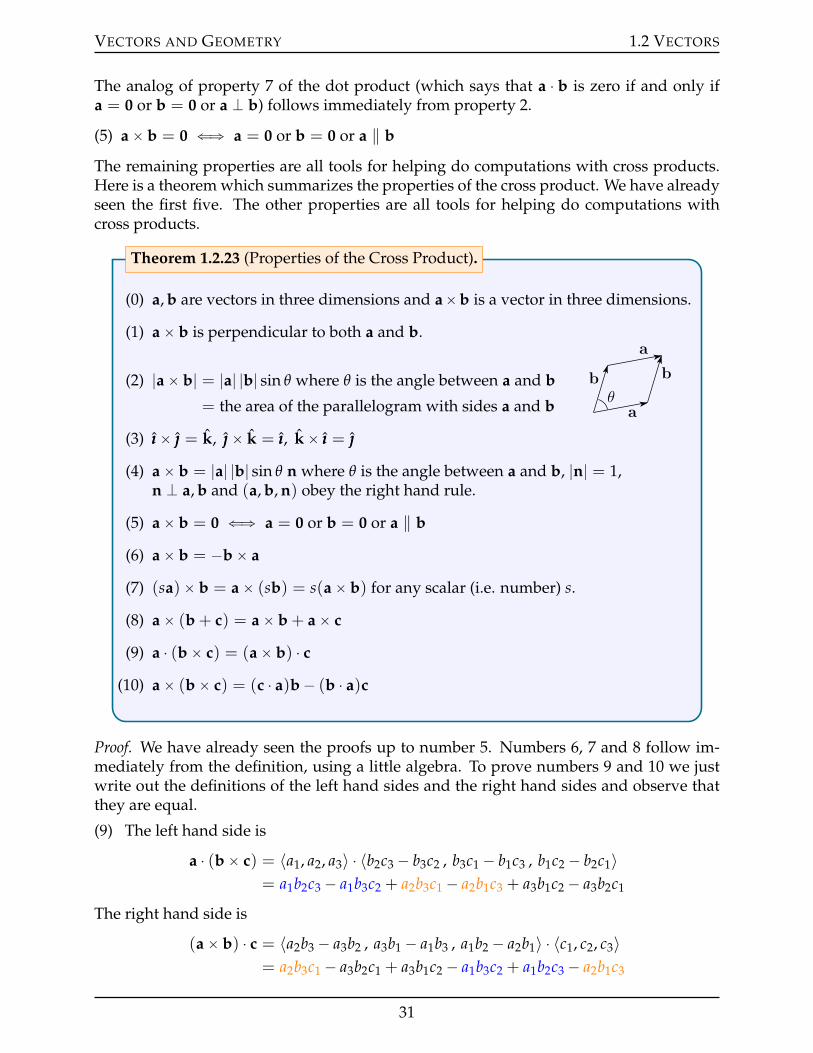
(2) |aˆ b| = |a| |b| sin θ where θ is the angle between a and b
= the area of the parallelogram with sides a and b a
a
b b
θ
(3) ıııˆ = k, ˆ k = ııı, kˆ ııı =
(4) aˆ b = |a| |b| sin θ n where θ is the angle between a and b, |n| = 1,n K a, b and (a, b, n) obey the right hand rule.
(5) aˆ b = 0 ðñ a = 0 or b = 0 or a ‖ b
(6) aˆ b = ´bˆ a
(7) (sa)ˆ b = aˆ (sb) = s(aˆ b) for any scalar (i.e. number) s.
(8) aˆ (b + c) = aˆ b + aˆ c
(9) a ¨ (bˆ c) = (aˆ b) ¨ c(10) aˆ (bˆ c) = (c ¨ a)b´ (b ¨ a)c
Theorem 1.2.23 (Properties of the Cross Product).
Proof. We have already seen the proofs up to number 5. Numbers 6, 7 and 8 follow im-mediately from the definition, using a little algebra. To prove numbers 9 and 10 we justwrite out the definitions of the left hand sides and the right hand sides and observe thatthey are equal.
(9) The left hand side is
a ¨ (bˆ c) = 〈a1, a2, a3〉 ¨ 〈b2c3 ´ b3c2 , b3c1 ´ b1c3 , b1c2 ´ b2c1〉= a1b2c3 ´ a1b3c2 + a2b3c1 ´ a2b1c3 + a3b1c2 ´ a3b2c1
The right hand side is
(aˆ b) ¨ c = 〈a2b3 ´ a3b2 , a3b1 ´ a1b3 , a1b2 ´ a2b1〉 ¨ 〈c1, c2, c3〉= a2b3c1 ´ a3b2c1 + a3b1c2 ´ a1b3c2 + a1b2c3 ´ a2b1c3
31
VECTORS AND GEOMETRY 1.2 VECTORS
The left and right hand sides are the same.
(10) We will give the straightforward, but slightly tedious, computations in (the optional)§1.2.6.
Take particular care with properties 6 and 10. They are counterintuitive and area frequent source of errors. In particular, for general vectors a, b, c, the crossproduct is neither commutative nor associative, meaning that
aˆ b ‰ bˆ aaˆ (bˆ c) ‰ (aˆ b)ˆ c
For example
ıııˆ (ıııˆ ) = ıııˆ k = ´kˆ ııı = ´
(ıııˆ ııı)ˆ = 0ˆ = 0
Warning 1.2.24.
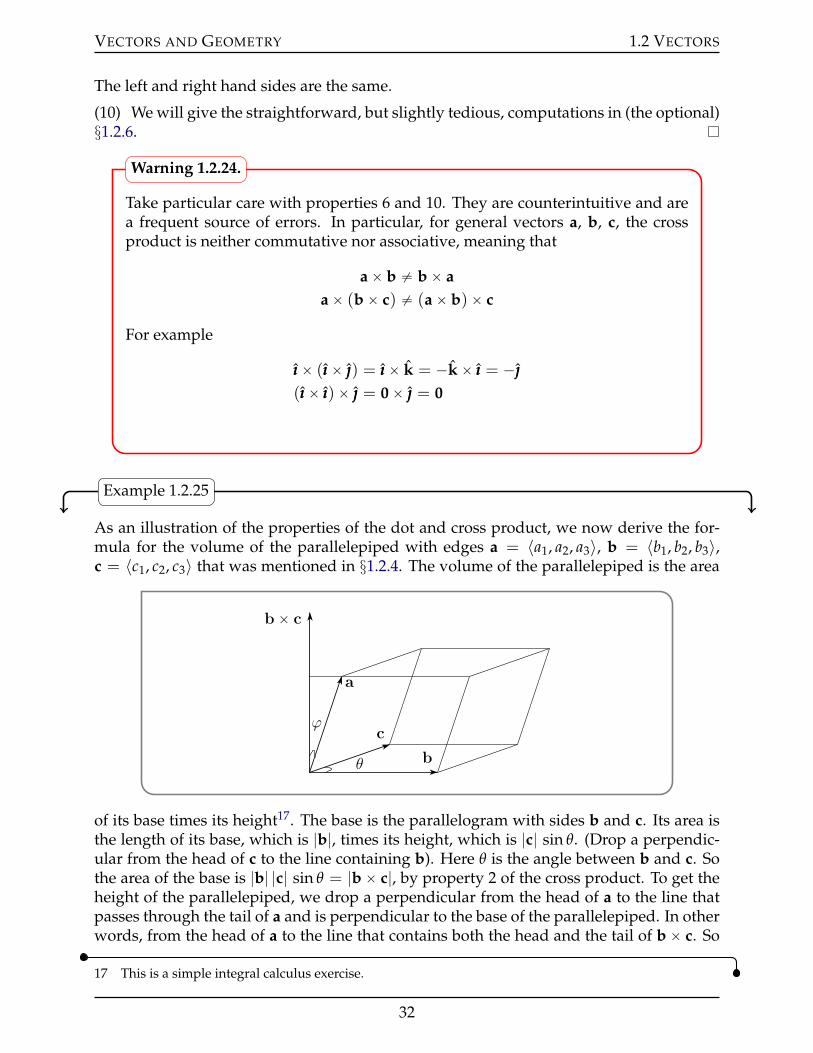
Example 1.2.25
As an illustration of the properties of the dot and cross product, we now derive the for-mula for the volume of the parallelepiped with edges a = 〈a1, a2, a3〉, b = 〈b1, b2, b3〉,c = 〈c1, c2, c3〉 that was mentioned in §1.2.4. The volume of the parallelepiped is the area
a
c
b
b ˆ c
θ
ϕ
of its base times its height17. The base is the parallelogram with sides b and c. Its area isthe length of its base, which is |b|, times its height, which is |c| sin θ. (Drop a perpendic-ular from the head of c to the line containing b). Here θ is the angle between b and c. Sothe area of the base is |b| |c| sin θ = |bˆ c|, by property 2 of the cross product. To get theheight of the parallelepiped, we drop a perpendicular from the head of a to the line thatpasses through the tail of a and is perpendicular to the base of the parallelepiped. In otherwords, from the head of a to the line that contains both the head and the tail of bˆ c. So
17 This is a simple integral calculus exercise.
32
VECTORS AND GEOMETRY 1.2 VECTORS
the height of the parallelepiped is |a| | cos ϕ|. (The absolute values have been included be-cause if the angle between bˆ c and a happens to be greater than 90˝, the cos ϕ producedby taking the dot product of a and (bˆ c) will be negative.) All together
volume of parallelepiped = (area of base) (height)= |bˆ c| |a| | cos ϕ|=
ˇa ¨ (bˆ c)
ˇ
= |a1(bˆ c)1 + a2(bˆ c)2 + a3(bˆ c)3|=
ˇˇa1 det
[b2 b3c2 c3
]´ a2 det
[b1 b3c1 c3
]+ a3 det
[b1 b2c1 c2
]ˇˇ
=
ˇˇˇdet
a1 a2 a3b1 b2 b3c1 c2 c3
ˇˇˇ
Example 1.2.25
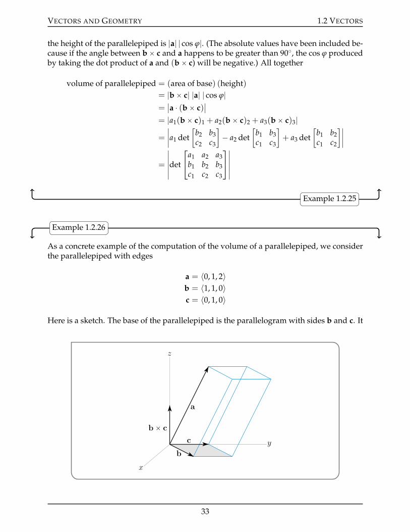
Example 1.2.26
As a concrete example of the computation of the volume of a parallelepiped, we considerthe parallelepiped with edges
a = 〈0, 1, 2〉b = 〈1, 1, 0〉c = 〈0, 1, 0〉
Here is a sketch. The base of the parallelepiped is the parallelogram with sides b and c. It
x
y
z
a
b
c
b ˆ c
33
VECTORS AND GEOMETRY 1.2 VECTORS
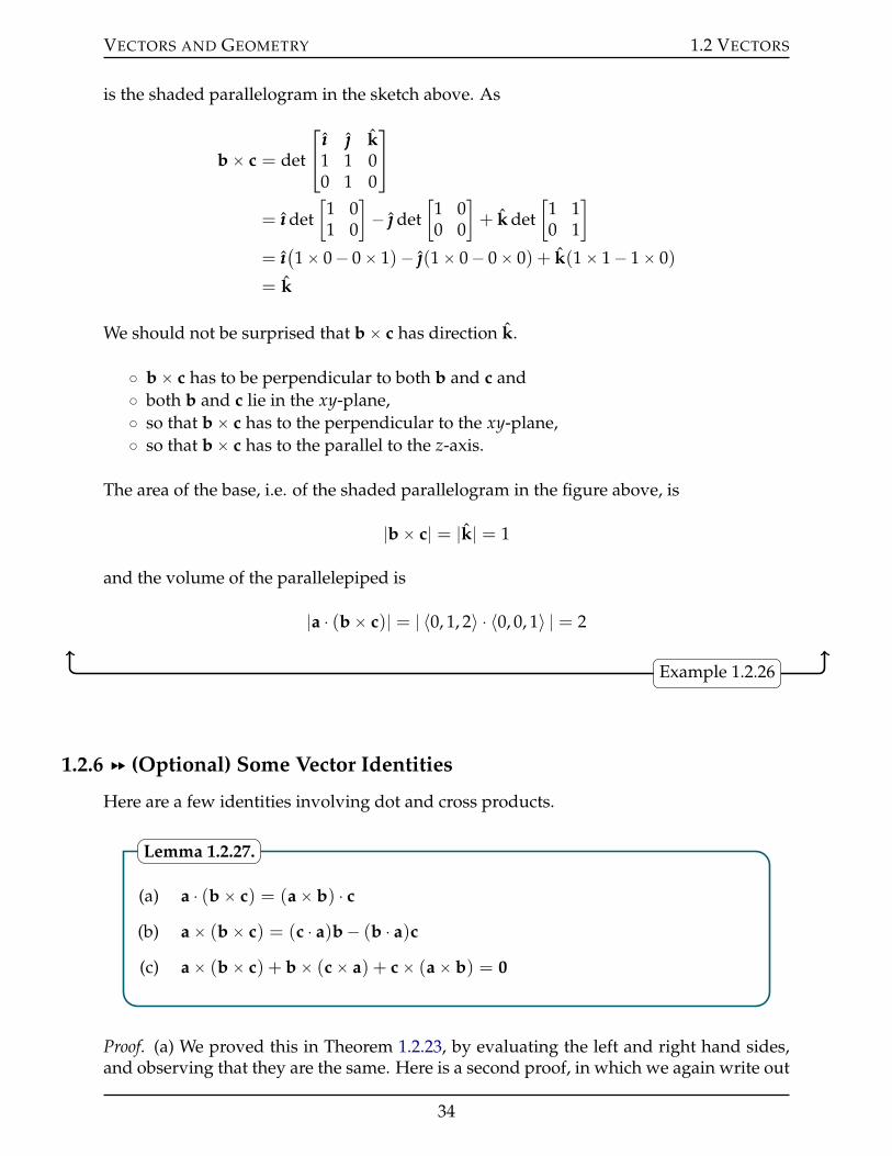
is the shaded parallelogram in the sketch above. As
bˆ c = det
ııı k1 1 00 1 0
= ııı det[
1 01 0
]´ det
[1 00 0
]+ k det
[1 10 1
]
= ııı(1ˆ 0´ 0ˆ 1)´ (1ˆ 0´ 0ˆ 0) + k(1ˆ 1´ 1ˆ 0)
= k
We should not be surprised that bˆ c has direction k.
˝ bˆ c has to be perpendicular to both b and c and˝ both b and c lie in the xy-plane,˝ so that bˆ c has to the perpendicular to the xy-plane,˝ so that bˆ c has to the parallel to the z-axis.
The area of the base, i.e. of the shaded parallelogram in the figure above, is
|bˆ c| = |k| = 1
and the volume of the parallelepiped is
|a ¨ (bˆ c)| = | 〈0, 1, 2〉 ¨ 〈0, 0, 1〉 | = 2
Example 1.2.26
1.2.6 §§ (Optional) Some Vector Identities
Here are a few identities involving dot and cross products.
(a) a ¨ (bˆ c) = (aˆ b) ¨ c(b) aˆ (bˆ c) = (c ¨ a)b´ (b ¨ a)c(c) aˆ (bˆ c) + bˆ (cˆ a) + cˆ (aˆ b) = 0
Lemma 1.2.27.
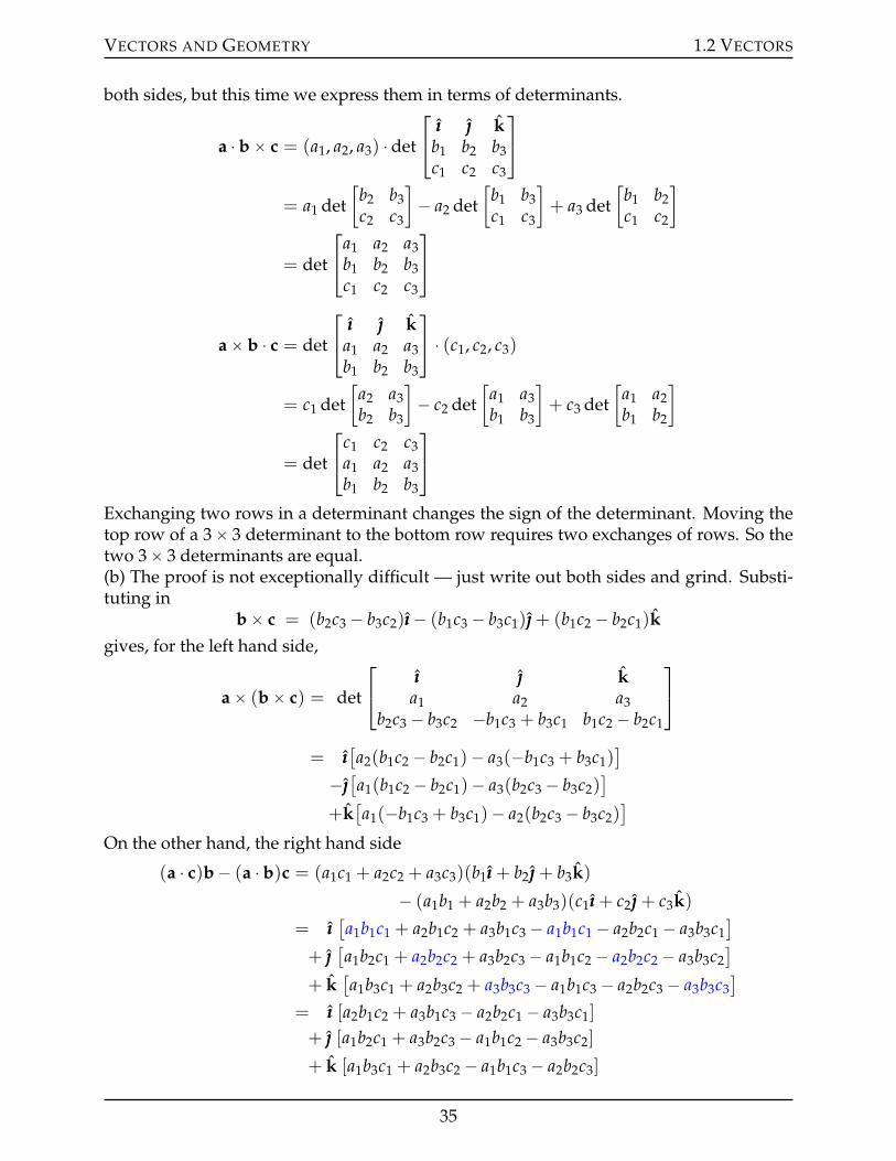
Proof. (a) We proved this in Theorem 1.2.23, by evaluating the left and right hand sides,and observing that they are the same. Here is a second proof, in which we again write out
34
VECTORS AND GEOMETRY 1.2 VECTORS
both sides, but this time we express them in terms of determinants.
a ¨ bˆ c = (a1, a2, a3) ¨ det
ııı kb1 b2 b3c1 c2 c3
= a1 det[
b2 b3c2 c3
]´ a2 det
[b1 b3c1 c3
]+ a3 det
[b1 b2c1 c2
]
= det
a1 a2 a3b1 b2 b3c1 c2 c3
aˆ b ¨ c = det
ııı ka1 a2 a3b1 b2 b3
¨ (c1, c2, c3)
= c1 det[
a2 a3b2 b3
]´ c2 det
[a1 a3b1 b3
]+ c3 det
[a1 a2b1 b2
]
= det
c1 c2 c3a1 a2 a3b1 b2 b3
Exchanging two rows in a determinant changes the sign of the determinant. Moving thetop row of a 3ˆ 3 determinant to the bottom row requires two exchanges of rows. So thetwo 3ˆ 3 determinants are equal.(b) The proof is not exceptionally difficult — just write out both sides and grind. Substi-tuting in
bˆ c = (b2c3 ´ b3c2)ııı´ (b1c3 ´ b3c1) + (b1c2 ´ b2c1)kgives, for the left hand side,
aˆ (bˆ c) = det
ııı ka1 a2 a3
b2c3 ´ b3c2 ´b1c3 + b3c1 b1c2 ´ b2c1
= ııı[a2(b1c2 ´ b2c1)´ a3(´b1c3 + b3c1)
]
´[a1(b1c2 ´ b2c1)´ a3(b2c3 ´ b3c2)
]
+k[a1(´b1c3 + b3c1)´ a2(b2c3 ´ b3c2)
]
On the other hand, the right hand side
(a ¨ c)b´ (a ¨ b)c = (a1c1 + a2c2 + a3c3)(b1ııı + b2 + b3k)
´ (a1b1 + a2b2 + a3b3)(c1ııı + c2 + c3k)
= ııı[a1b1c1 + a2b1c2 + a3b1c3 ´ a1b1c1 ´ a2b2c1 ´ a3b3c1
]
+ [a1b2c1 + a2b2c2 + a3b2c3 ´ a1b1c2 ´ a2b2c2 ´ a3b3c2
]
+ k[a1b3c1 + a2b3c2 + a3b3c3 ´ a1b1c3 ´ a2b2c3 ´ a3b3c3
]
= ııı [a2b1c2 + a3b1c3 ´ a2b2c1 ´ a3b3c1]
+ [a1b2c1 + a3b2c3 ´ a1b1c2 ´ a3b3c2]
+ k [a1b3c1 + a2b3c2 ´ a1b1c3 ´ a2b2c3]
35

VECTORS AND GEOMETRY 1.2 VECTORS
The last formula that we had for the left hand side is the same as the last formula we hadfor the right hand side. Oof! This is a little tedious to do by hand. But any computeralgebra system will do it for you in a flash.(c) We just apply part (b) three times
aˆ (bˆ c) + bˆ (cˆ a) + cˆ (aˆ b)= (c ¨ a)b´ (b ¨ a)c + (a ¨ b)c´ (c ¨ b)a + (b ¨ c)a´ (a ¨ c)b= 0
1.2.7 §§ (Optional) Application of Cross Products to Rotational Motion
In most computations involving rotational motion, the cross product shows up in oneform or another. This is one of the main applications of the cross product. Consider, forexample, a rigid body which is rotating at a constant rate of Ω radians per second aboutan axis whose direction is given by the unit vector a. Let P be any point on the body. Let’sfigure out its velocity. Pick any point on the axis of rotation and designate it as the originof our coordinate system. Denote by r the vector from the origin to the point P. Let θdenote the angle between a and r. As time progresses the point P sweeps out a circle ofradius R = |r | sin θ.
P
r
v
0
a
θ
Ω
In one second P travels along an arc that subtends an angle of Ω radians, which is thefraction Ω
2π of a full circle. The length of this arc is Ω2π ˆ 2πR = ΩR = Ω|r | sin θ so P
travels the distance Ω|r | sin θ in one second and its speed, which is also the length of itsvelocity vector, is Ω|r | sin θ.
Now we just need to figure out the direction of the velocity vector. That is, the directionof motion of the point P. Imagine that both a and r lie in the plane of a piece of paper,as in the figure above. Then v points either straight into or straight out of the page andconsequently is perpendicular to both a and r. To distinguish between the “into the page”and “out of the page” cases, let’s impose the conventions that Ω ą 0 and the axis ofrotation a is chosen to obey the right hand rule, meaning that if the thumb of your righthand is pointing in the direction a, then your fingers are pointing in the direction of motionof the rigid body. Under these conventions, the velocity vector v obeys
36
VECTORS AND GEOMETRY 1.2 VECTORS
• |v| = Ω|r||a| sin θ
• v K a, r
• (a, r, v) obey the right hand rule
That is, v is exactly Ωa ˆ r. It is conventional to define the “angular velocity” of a rigidbody to be vector Ω = Ωa. That is, the vector with length given by the rate of rotationand direction given by the axis of rotation of the rigid body. In particular, the bigger therate of rotation, the longer the angular velocity vector. In terms of this angular velocityvector, the velocity of the point P is
v = Ωˆ r
1.2.8 §§ (Optional) Application of Cross Products to Rotating Reference Frames
Imagine a moving particle that is being tracked by two observers.
(a) One observer is fixed (out in space) and measures the position of the particle to be(X(t), Y(t), Z(t)
).
(b) The other observer is tied to a merry-go-round (the Earth) and measures the positionof the particle to be
(x(t), y(t), z(t)
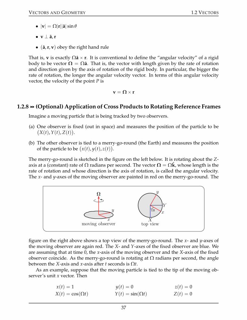
).
The merry-go-round is sketched in the figure on the left below. It is rotating about the Z-axis at a (constant) rate of Ω radians per second. The vector Ω = Ωk, whose length is therate of rotation and whose direction is the axis of rotation, is called the angular velocity.The x- and y-axes of the moving observer are painted in red on the merry-go-round. The
Ω
x
y
moving observer
Ωt x
y
top viewX
Y
figure on the right above shows a top view of the merry-go-round. The x- and y-axes ofthe moving observer are again red. The X- and Y-axes of the fixed observer are blue. Weare assuming that at time 0, the x-axis of the moving observer and the X-axis of the fixedobserver coincide. As the merry-go-round is rotating at Ω radians per second, the anglebetween the X-axis and x-axis after t seconds is Ωt.
As an example, suppose that the moving particle is tied to the tip of the moving ob-server’s unit x vector. Then
x(t) = 1 y(t) = 0 z(t) = 0X(t) = cos(Ωt) Y(t) = sin(Ωt) Z(t) = 0
37
VECTORS AND GEOMETRY 1.2 VECTORS
or, if we write r(t) =(x(t), y(t), z(t)
)and R(t) =
(X(t), Y(t), Z(t)
), then
r(t) = (1 , 0 , 0) R(t) =(
cos(Ωt) , sin(Ωt) , 0)
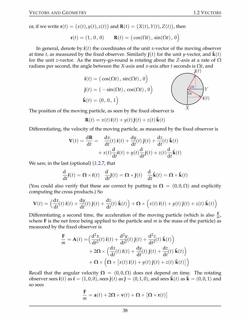
In general, denote by ııı(t) the coordinates of the unit x-vector of the moving observerat time t, as measured by the fixed observer. Similarly (t) for the unit y-vector, and k(t)for the unit z-vector. As the merry-go-round is rotating about the Z-axis at a rate of Ωradians per second, the angle between the X-axis and x-axis after t seconds is Ωt, and
ııı(t) =(
cos(Ωt) , sin(Ωt) , 0)
(t) =(´ sin(Ωt) , cos(Ωt) , 0
)Ωt
Ωt
ıııptq
ptq
X
Y
k(t) =(0 , 0 , 1
)
The position of the moving particle, as seen by the fixed observer is
R(t) = x(t) ııı(t) + y(t) (t) + z(t) k(t)
Differentiating, the velocity of the moving particle, as measured by the fixed observer is
V(t) =dRdt
=dxdt(t) ııı(t) +
dydt(t) (t) +
dzdt(t) k(t)
+ x(t)ddt
ııı(t) + y(t)ddt
(t) + z(t)ddt
k(t)
We saw, in the last (optional) §1.2.7, that
ddt
ııı(t) = Ωˆ ııı(t)ddt
(t) = Ωˆ (t)ddt
k(t) = Ωˆ k(t)
(You could also verify that these are correct by putting in Ω = (0, 0, Ω) and explicitlycomputing the cross products.) So
V(t) =(dx
dt(t) ııı(t) +
dydt(t) (t) +
dzdt(t) k(t)
)+ Ωˆ
(x(t) ııı(t) + y(t) (t) + z(t) k(t)
)
Differentiating a second time, the acceleration of the moving particle (which is also Fm ,
where F is the net force being applied to the particle and m is the mass of the particle) asmeasured by the fixed observer is
Fm
= A(t) =(d2x
dt2(t) ııı(t) +d2ydt2(t) (t) +
d2zdt2(t) k(t)
)
+ 2Ωˆ(dx
dt(t) ııı(t) +
dydt(t) (t) +
dzdt(t) k(t)
)
+ Ωˆ(
Ωˆ [x(t) ııı(t) + y(t) (t) + z(t) k(t)])
Recall that the angular velocity Ω = (0, 0, Ω) does not depend on time. The rotatingobserver sees ııı(t) as ııı = (1, 0, 0), sees (t) as = (0, 1, 0), and sees k(t) as k = (0, 0, 1) andso sees
Fm
= a(t) + 2Ωˆ v(t) + Ωˆ [Ωˆ r(t)]
38

VECTORS AND GEOMETRY 1.2 VECTORS
where, as usual,
v(t) =ddt
r(t) =(dx
dt(t) ,
dydt
(t) ,dzdt
(t))
a(t) =d2
dt2 r(t) =(d2x
dt2 (t) ,d2ydt2 (t) ,
d2zdt2 (t)
)
So the acceleration of the particle seen by the moving observer is
a(t) =Fm´ 2Ωˆ v(t)´Ωˆ [Ωˆ r(t)
]
Here
• F is the sum of all external forces acting on the moving particle,• Fcor = ´2Ωˆ v(t) is called the Coriolis force and• ´Ωˆ [Ωˆ r(t)
]is called the centrifugal force.
As an example, suppose that you are the moving particle and that you are at the edgeof the merry-go-round. Let’s say t = 0 and you are at ııı. Then F is the friction that thesurface of the merry-go-round applies to the soles of your shoes. If you are just standingthere, v(t) = 0, so that Fcor = 0, and the friction F exactly cancels the centrifugal force´Ωˆ [Ωˆ r(t)
]so that you remain at ııı(t). Assume that Ω ą 0. Now suppose that you
start walking around the edge of the merry-go-round. Then, at t = 0, r = ııı and
• if you walk in the direction of rotation (with speed one), as in the figure on the leftbelow, v = and the Coriolis force Fcor = ´2Ωkˆ = 2Ω ııı tries to push you off ofthe merry-go-round, while• if you walk opposite to the direction of rotation (with speed one), as in the figure on
the right below, v = ´ so that the Coriolis force Fcor = ´2Ωkˆ (´) = ´2Ω ııı triesto pull you into the centre of the merry-go-round.
Ω
vFcor
Ω
v
Fcor
On a rotating ball, such as the Earth, the Coriolis force deflects wind to the right (coun-terclockwise) in the northern hemisphere and to the left (clockwise) is the southern hemi-sphere. In particular, hurricanes/cyclones/typhoons rotate counterclockwise in the north-ern hemisphere and clockwise in the southern hemisphere. On the other hand, when itcomes to water draining out of, for example, a toilet, Coriolis force effects are dominatedby other factors like asymmetry of the toilet.
39
VECTORS AND GEOMETRY 1.3 EQUATIONS OF LINES IN 2D
1.3IJ Equations of Lines in 2d
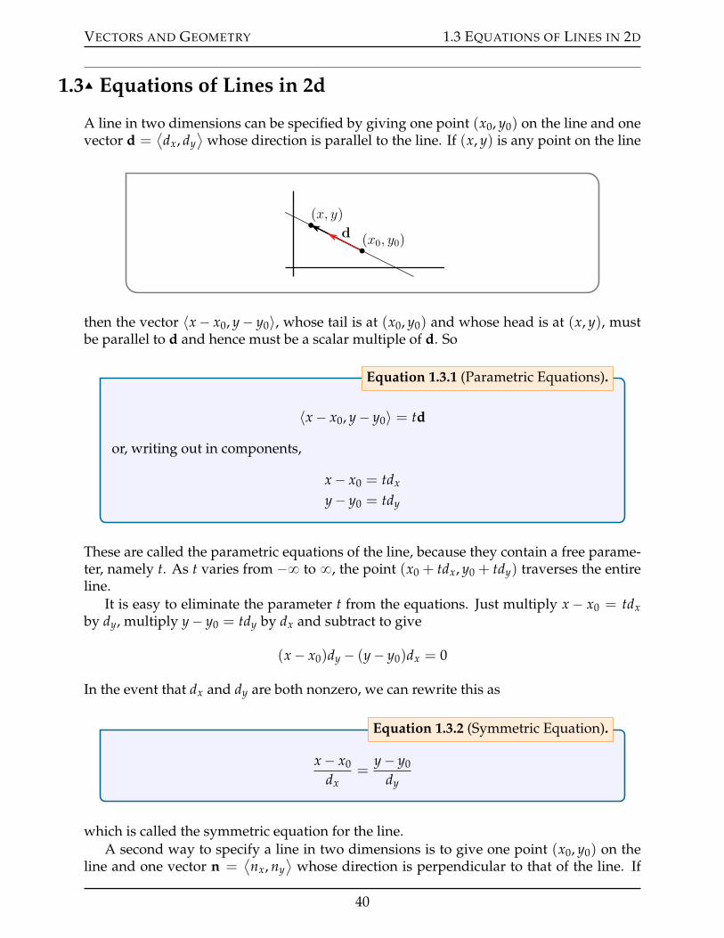
A line in two dimensions can be specified by giving one point (x0, y0) on the line and onevector d =
⟨dx, dy
⟩whose direction is parallel to the line. If (x, y) is any point on the line
(x0, y0)
(x, y)
d
then the vector 〈x´ x0, y´ y0〉, whose tail is at (x0, y0) and whose head is at (x, y), mustbe parallel to d and hence must be a scalar multiple of d. So
〈x´ x0, y´ y0〉 = td
or, writing out in components,
x´ x0 = tdx
y´ y0 = tdy
Equation 1.3.1 (Parametric Equations).
These are called the parametric equations of the line, because they contain a free parame-ter, namely t. As t varies from ´8 to 8, the point (x0 + tdx, y0 + tdy) traverses the entireline.
It is easy to eliminate the parameter t from the equations. Just multiply x ´ x0 = tdxby dy, multiply y´ y0 = tdy by dx and subtract to give
(x´ x0)dy ´ (y´ y0)dx = 0
In the event that dx and dy are both nonzero, we can rewrite this as
x´ x0
dx=
y´ y0
dy
Equation 1.3.2 (Symmetric Equation).
which is called the symmetric equation for the line.A second way to specify a line in two dimensions is to give one point (x0, y0) on the
line and one vector n =⟨nx, ny
⟩whose direction is perpendicular to that of the line. If
40
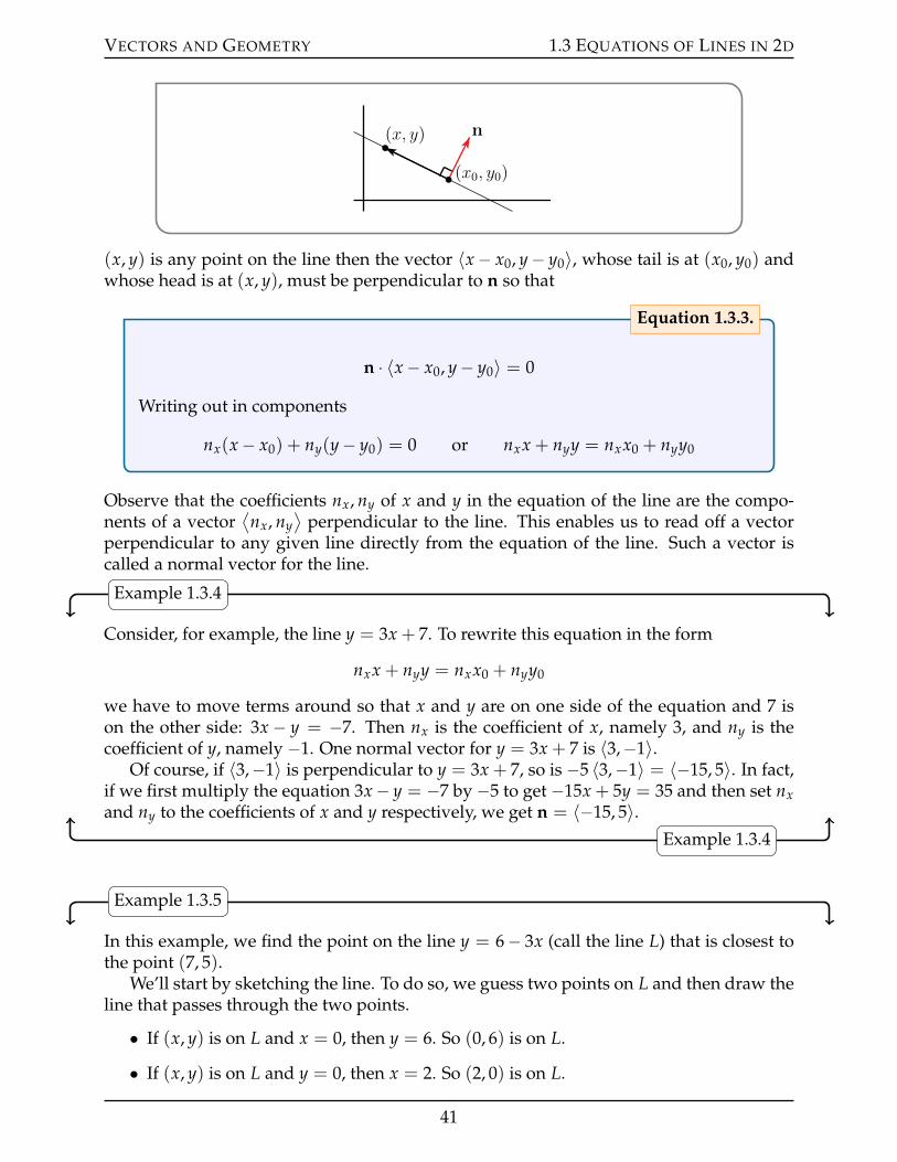
VECTORS AND GEOMETRY 1.3 EQUATIONS OF LINES IN 2D
(x0, y0)
(x, y) n
(x, y) is any point on the line then the vector 〈x´ x0, y´ y0〉, whose tail is at (x0, y0) andwhose head is at (x, y), must be perpendicular to n so that
n ¨ 〈x´ x0, y´ y0〉 = 0
Writing out in components
nx(x´ x0) + ny(y´ y0) = 0 or nxx + nyy = nxx0 + nyy0
Equation 1.3.3.
Observe that the coefficients nx, ny of x and y in the equation of the line are the compo-nents of a vector
⟨nx, ny
⟩perpendicular to the line. This enables us to read off a vector
perpendicular to any given line directly from the equation of the line. Such a vector iscalled a normal vector for the line.
Example 1.3.4
Consider, for example, the line y = 3x + 7. To rewrite this equation in the form
nxx + nyy = nxx0 + nyy0
we have to move terms around so that x and y are on one side of the equation and 7 ison the other side: 3x ´ y = ´7. Then nx is the coefficient of x, namely 3, and ny is thecoefficient of y, namely ´1. One normal vector for y = 3x + 7 is 〈3,´1〉.
Of course, if 〈3,´1〉 is perpendicular to y = 3x + 7, so is ´5 〈3,´1〉 = 〈´15, 5〉. In fact,if we first multiply the equation 3x´ y = ´7 by ´5 to get ´15x + 5y = 35 and then set nxand ny to the coefficients of x and y respectively, we get n = 〈´15, 5〉.
Example 1.3.4
Example 1.3.5
In this example, we find the point on the line y = 6´ 3x (call the line L) that is closest tothe point (7, 5).
We’ll start by sketching the line. To do so, we guess two points on L and then draw theline that passes through the two points.
• If (x, y) is on L and x = 0, then y = 6. So (0, 6) is on L.
• If (x, y) is on L and y = 0, then x = 2. So (2, 0) is on L.
41
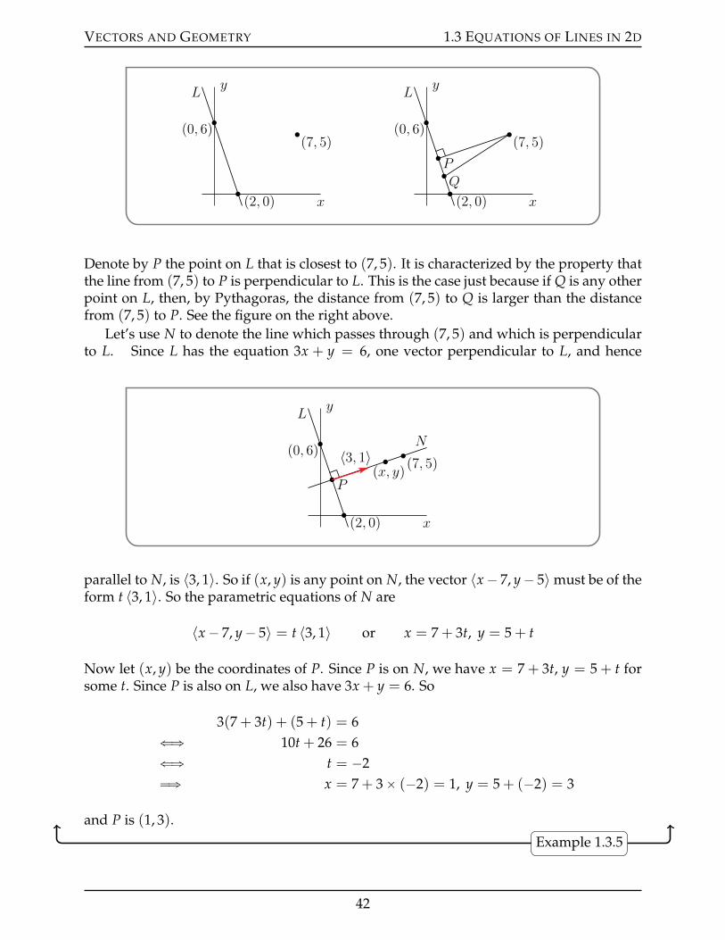
VECTORS AND GEOMETRY 1.3 EQUATIONS OF LINES IN 2D
L
p0, 6q
p2, 0q
p7, 5q
x
yL
p0, 6q
p2, 0q
p7, 5qP
Q
x
y
Denote by P the point on L that is closest to (7, 5). It is characterized by the property thatthe line from (7, 5) to P is perpendicular to L. This is the case just because if Q is any otherpoint on L, then, by Pythagoras, the distance from (7, 5) to Q is larger than the distancefrom (7, 5) to P. See the figure on the right above.
Let’s use N to denote the line which passes through (7, 5) and which is perpendicularto L. Since L has the equation 3x + y = 6, one vector perpendicular to L, and hence
L
(0, 6)
(2, 0)
(7, 5)
P
N
(x, y)〈3, 1〉
x
y
parallel to N, is 〈3, 1〉. So if (x, y) is any point on N, the vector 〈x´ 7, y´ 5〉must be of theform t 〈3, 1〉. So the parametric equations of N are
〈x´ 7, y´ 5〉 = t 〈3, 1〉 or x = 7 + 3t, y = 5 + t
Now let (x, y) be the coordinates of P. Since P is on N, we have x = 7 + 3t, y = 5 + t forsome t. Since P is also on L, we also have 3x + y = 6. So
3(7 + 3t) + (5 + t) = 6ðñ 10t + 26 = 6ðñ t = ´2ùñ x = 7 + 3ˆ (´2) = 1, y = 5 + (´2) = 3
and P is (1, 3).
Example 1.3.5
42
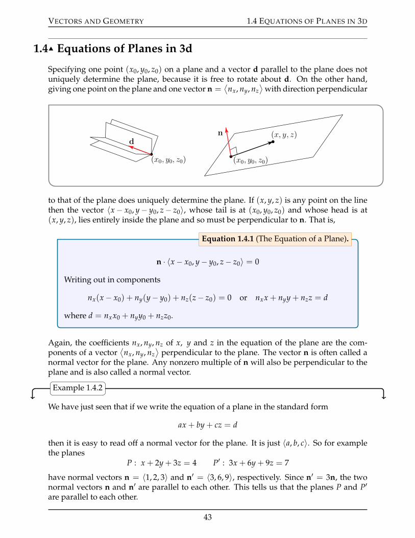
VECTORS AND GEOMETRY 1.4 EQUATIONS OF PLANES IN 3D
1.4IJ Equations of Planes in 3d
Specifying one point (x0, y0, z0) on a plane and a vector d parallel to the plane does notuniquely determine the plane, because it is free to rotate about d. On the other hand,giving one point on the plane and one vector n =
⟨nx, ny, nz
⟩with direction perpendicular
(x0, y0, z0)
d
(x0, y0, z0)
(x, y, z)n
to that of the plane does uniquely determine the plane. If (x, y, z) is any point on the linethen the vector 〈x´ x0, y´ y0, z´ z0〉, whose tail is at (x0, y0, z0) and whose head is at(x, y, z), lies entirely inside the plane and so must be perpendicular to n. That is,
n ¨ 〈x´ x0, y´ y0, z´ z0〉 = 0
Writing out in components
nx(x´ x0) + ny(y´ y0) + nz(z´ z0) = 0 or nxx + nyy + nzz = d
where d = nxx0 + nyy0 + nzz0.
Equation 1.4.1 (The Equation of a Plane).
Again, the coefficients nx, ny, nz of x, y and z in the equation of the plane are the com-ponents of a vector
⟨nx, ny, nz
⟩perpendicular to the plane. The vector n is often called a
normal vector for the plane. Any nonzero multiple of n will also be perpendicular to theplane and is also called a normal vector.
Example 1.4.2
We have just seen that if we write the equation of a plane in the standard form
ax + by + cz = d
then it is easy to read off a normal vector for the plane. It is just 〈a, b, c〉. So for examplethe planes
P : x + 2y + 3z = 4 P1 : 3x + 6y + 9z = 7
have normal vectors n = 〈1, 2, 3〉 and n1 = 〈3, 6, 9〉, respectively. Since n1 = 3n, the twonormal vectors n and n1 are parallel to each other. This tells us that the planes P and P1
are parallel to each other.
43
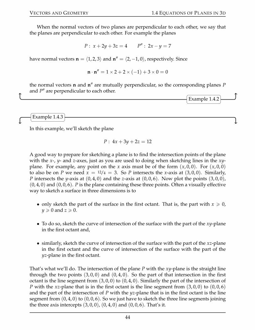
VECTORS AND GEOMETRY 1.4 EQUATIONS OF PLANES IN 3D
When the normal vectors of two planes are perpendicular to each other, we say thatthe planes are perpendicular to each other. For example the planes
P : x + 2y + 3z = 4 P2 : 2x´ y = 7
have normal vectors n = 〈1, 2, 3〉 and n2 = 〈2,´1, 0〉, respectively. Since
n ¨ n2 = 1ˆ 2 + 2ˆ (´1) + 3ˆ 0 = 0
the normal vectors n and n2 are mutually perpendicular, so the corresponding planes Pand P2 are perpendicular to each other.
Example 1.4.2
Example 1.4.3
In this example, we’ll sketch the plane
P : 4x + 3y + 2z = 12
A good way to prepare for sketching a plane is to find the intersection points of the planewith the x-, y- and z-axes, just as you are used to doing when sketching lines in the xy-plane. For example, any point on the x axis must be of the form (x, 0, 0). For (x, 0, 0)to also be on P we need x = 12/4 = 3. So P intersects the x-axis at (3, 0, 0). Similarly,P intersects the y-axis at (0, 4, 0) and the z-axis at (0, 0, 6). Now plot the points (3, 0, 0),(0, 4, 0) and (0, 0, 6). P is the plane containing these three points. Often a visually effectiveway to sketch a surface in three dimensions is to
• only sketch the part of the surface in the first octant. That is, the part with x ě 0,y ě 0 and z ě 0.
• To do so, sketch the curve of intersection of the surface with the part of the xy-planein the first octant and,
• similarly, sketch the curve of intersection of the surface with the part of the xz-planein the first octant and the curve of intersection of the surface with the part of theyz-plane in the first octant.
That’s what we’ll do. The intersection of the plane P with the xy-plane is the straight linethrough the two points (3, 0, 0) and (0, 4, 0). So the part of that intersection in the firstoctant is the line segment from (3, 0, 0) to (0, 4, 0). Similarly the part of the intersection ofP with the xz-plane that is in the first octant is the line segment from (3, 0, 0) to (0, 0, 6)and the part of the intersection of P with the yz-plane that is in the first octant is the linesegment from (0, 4, 0) to (0, 0, 6). So we just have to sketch the three line segments joiningthe three axis intercepts (3, 0, 0), (0, 4, 0) and (0, 0, 6). That’s it.
44
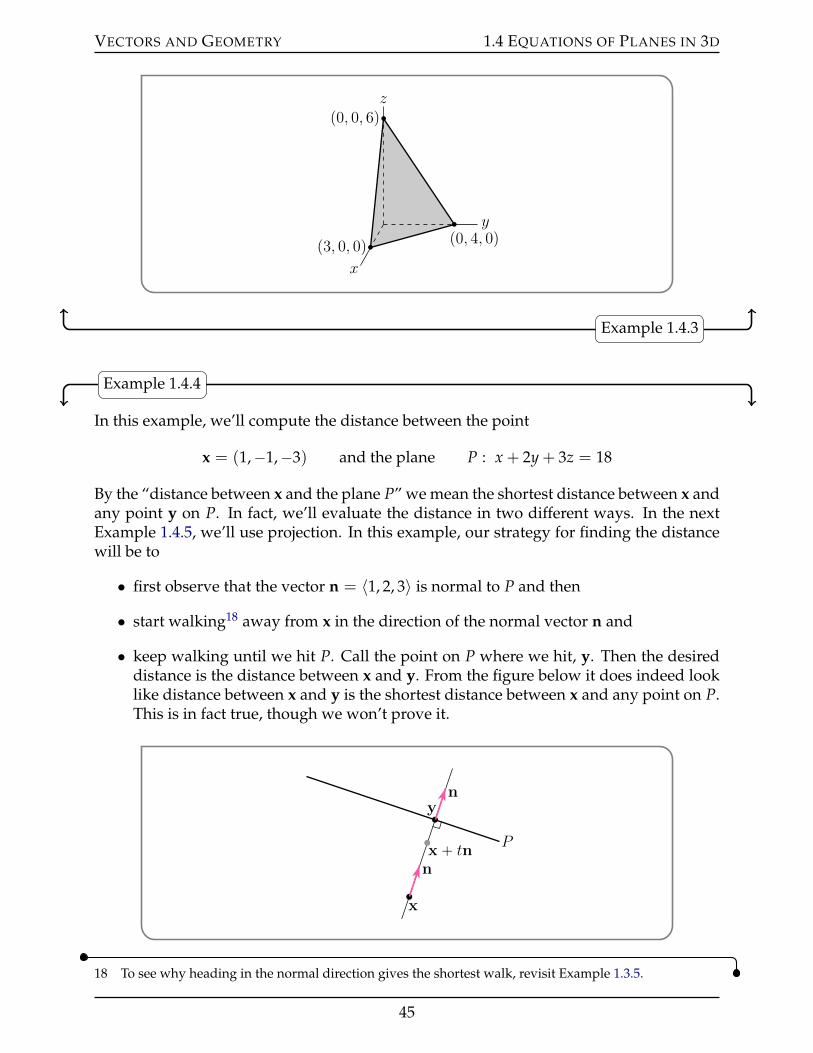
VECTORS AND GEOMETRY 1.4 EQUATIONS OF PLANES IN 3D
z
y
x
p3, 0, 0q p0, 4, 0q
p0, 0, 6q
Example 1.4.3
Example 1.4.4
In this example, we’ll compute the distance between the point
x = (1,´1,´3) and the plane P : x + 2y + 3z = 18
By the “distance between x and the plane P” we mean the shortest distance between x andany point y on P. In fact, we’ll evaluate the distance in two different ways. In the nextExample 1.4.5, we’ll use projection. In this example, our strategy for finding the distancewill be to
• first observe that the vector n = 〈1, 2, 3〉 is normal to P and then
• start walking18 away from x in the direction of the normal vector n and
• keep walking until we hit P. Call the point on P where we hit, y. Then the desireddistance is the distance between x and y. From the figure below it does indeed looklike distance between x and y is the shortest distance between x and any point on P.This is in fact true, though we won’t prove it.
P
x
y
n
n
x ` tn
18 To see why heading in the normal direction gives the shortest walk, revisit Example 1.3.5.
45
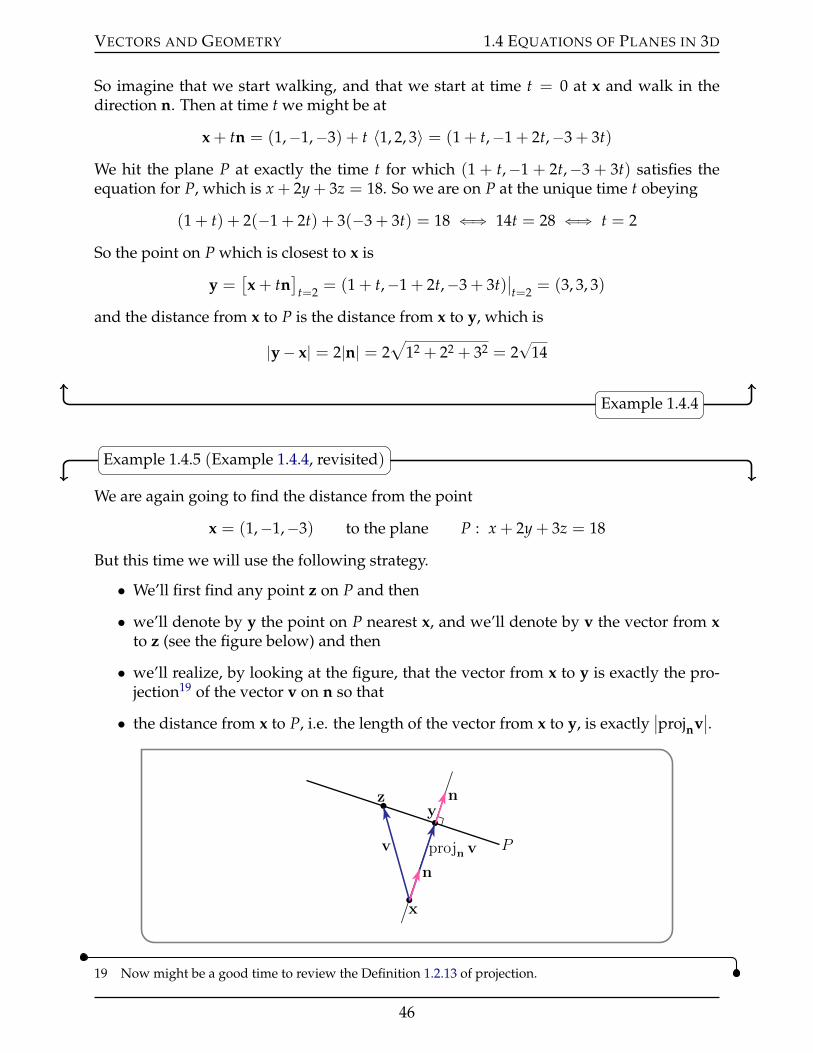
VECTORS AND GEOMETRY 1.4 EQUATIONS OF PLANES IN 3D
So imagine that we start walking, and that we start at time t = 0 at x and walk in thedirection n. Then at time t we might be at
x + tn = (1,´1,´3) + t 〈1, 2, 3〉 = (1 + t,´1 + 2t,´3 + 3t)
We hit the plane P at exactly the time t for which (1 + t,´1 + 2t,´3 + 3t) satisfies theequation for P, which is x + 2y + 3z = 18. So we are on P at the unique time t obeying
(1 + t) + 2(´1 + 2t) + 3(´3 + 3t) = 18 ðñ 14t = 28 ðñ t = 2
So the point on P which is closest to x is
y =[x + tn
]t=2 = (1 + t,´1 + 2t,´3 + 3t)
ˇt=2 = (3, 3, 3)
and the distance from x to P is the distance from x to y, which is
|y´ x| = 2|n| = 2a
12 + 22 + 32 = 2?
14
Example 1.4.4
Example 1.4.5 (Example 1.4.4, revisited)
We are again going to find the distance from the point
x = (1,´1,´3) to the plane P : x + 2y + 3z = 18
But this time we will use the following strategy.
• We’ll first find any point z on P and then
• we’ll denote by y the point on P nearest x, and we’ll denote by v the vector from xto z (see the figure below) and then
• we’ll realize, by looking at the figure, that the vector from x to y is exactly the pro-jection19 of the vector v on n so that
• the distance from x to P, i.e. the length of the vector from x to y, is exactlyˇprojnv
ˇ.
x
yz
projn vv P
n
n
19 Now might be a good time to review the Definition 1.2.13 of projection.
46
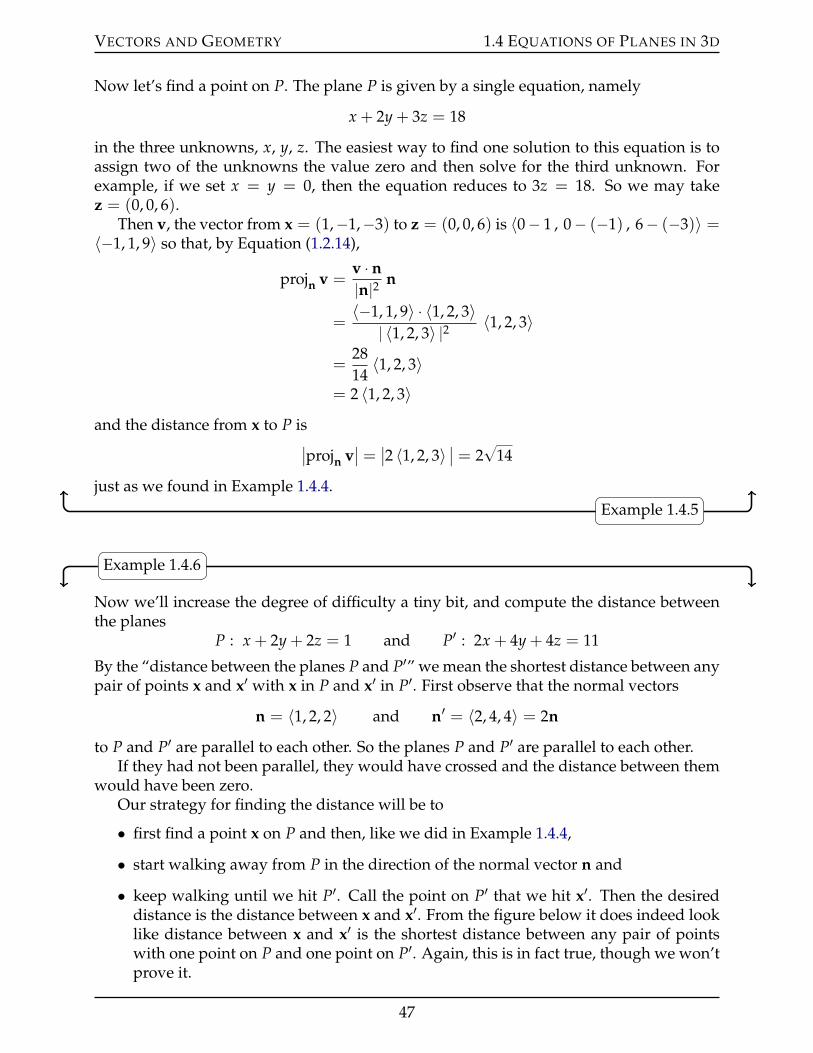
VECTORS AND GEOMETRY 1.4 EQUATIONS OF PLANES IN 3D
Now let’s find a point on P. The plane P is given by a single equation, namely
x + 2y + 3z = 18
in the three unknowns, x, y, z. The easiest way to find one solution to this equation is toassign two of the unknowns the value zero and then solve for the third unknown. Forexample, if we set x = y = 0, then the equation reduces to 3z = 18. So we may takez = (0, 0, 6).
Then v, the vector from x = (1,´1,´3) to z = (0, 0, 6) is 〈0´ 1 , 0´ (´1) , 6´ (´3)〉 =〈´1, 1, 9〉 so that, by Equation (1.2.14),
projn v =v ¨ n|n|2 n
=〈´1, 1, 9〉 ¨ 〈1, 2, 3〉
| 〈1, 2, 3〉 |2 〈1, 2, 3〉
=2814〈1, 2, 3〉
= 2 〈1, 2, 3〉and the distance from x to P is
ˇprojn v
ˇ=
ˇ2 〈1, 2, 3〉
ˇ= 2
?14
just as we found in Example 1.4.4.Example 1.4.5
Example 1.4.6
Now we’ll increase the degree of difficulty a tiny bit, and compute the distance betweenthe planes
P : x + 2y + 2z = 1 and P1 : 2x + 4y + 4z = 11
By the “distance between the planes P and P1” we mean the shortest distance between anypair of points x and x1 with x in P and x1 in P1. First observe that the normal vectors
n = 〈1, 2, 2〉 and n1 = 〈2, 4, 4〉 = 2n
to P and P1 are parallel to each other. So the planes P and P1 are parallel to each other.If they had not been parallel, they would have crossed and the distance between them
would have been zero.Our strategy for finding the distance will be to
• first find a point x on P and then, like we did in Example 1.4.4,
• start walking away from P in the direction of the normal vector n and
• keep walking until we hit P1. Call the point on P1 that we hit x1. Then the desireddistance is the distance between x and x1. From the figure below it does indeed looklike distance between x and x1 is the shortest distance between any pair of pointswith one point on P and one point on P1. Again, this is in fact true, though we won’tprove it.
47
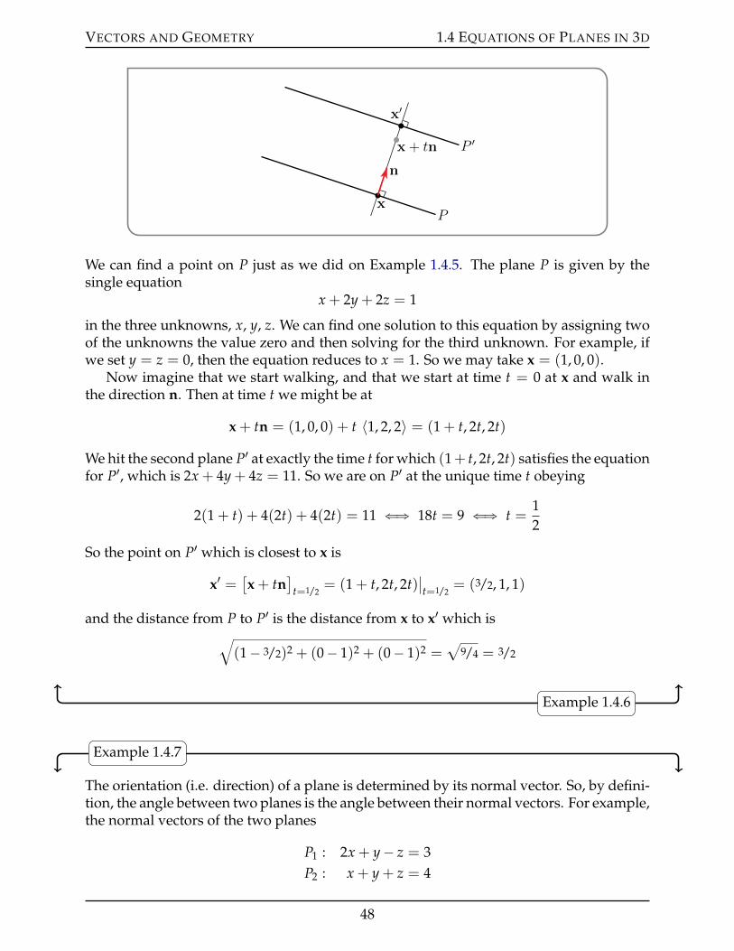
VECTORS AND GEOMETRY 1.4 EQUATIONS OF PLANES IN 3D
P
P ′
x
x′
n
x + tn
We can find a point on P just as we did on Example 1.4.5. The plane P is given by thesingle equation
x + 2y + 2z = 1
in the three unknowns, x, y, z. We can find one solution to this equation by assigning twoof the unknowns the value zero and then solving for the third unknown. For example, ifwe set y = z = 0, then the equation reduces to x = 1. So we may take x = (1, 0, 0).
Now imagine that we start walking, and that we start at time t = 0 at x and walk inthe direction n. Then at time t we might be at
x + tn = (1, 0, 0) + t 〈1, 2, 2〉 = (1 + t, 2t, 2t)
We hit the second plane P1 at exactly the time t for which (1+ t, 2t, 2t) satisfies the equationfor P1, which is 2x + 4y + 4z = 11. So we are on P1 at the unique time t obeying
2(1 + t) + 4(2t) + 4(2t) = 11 ðñ 18t = 9 ðñ t =12
So the point on P1 which is closest to x is
x1 =[x + tn
]t=1/2
= (1 + t, 2t, 2t)ˇt=1/2
= (3/2, 1, 1)
and the distance from P to P1 is the distance from x to x1 which isb(1´ 3/2)2 + (0´ 1)2 + (0´ 1)2 =
a9/4 = 3/2
Example 1.4.6
Example 1.4.7
The orientation (i.e. direction) of a plane is determined by its normal vector. So, by defini-tion, the angle between two planes is the angle between their normal vectors. For example,the normal vectors of the two planes
P1 : 2x + y´ z = 3P2 : x + y + z = 4
48
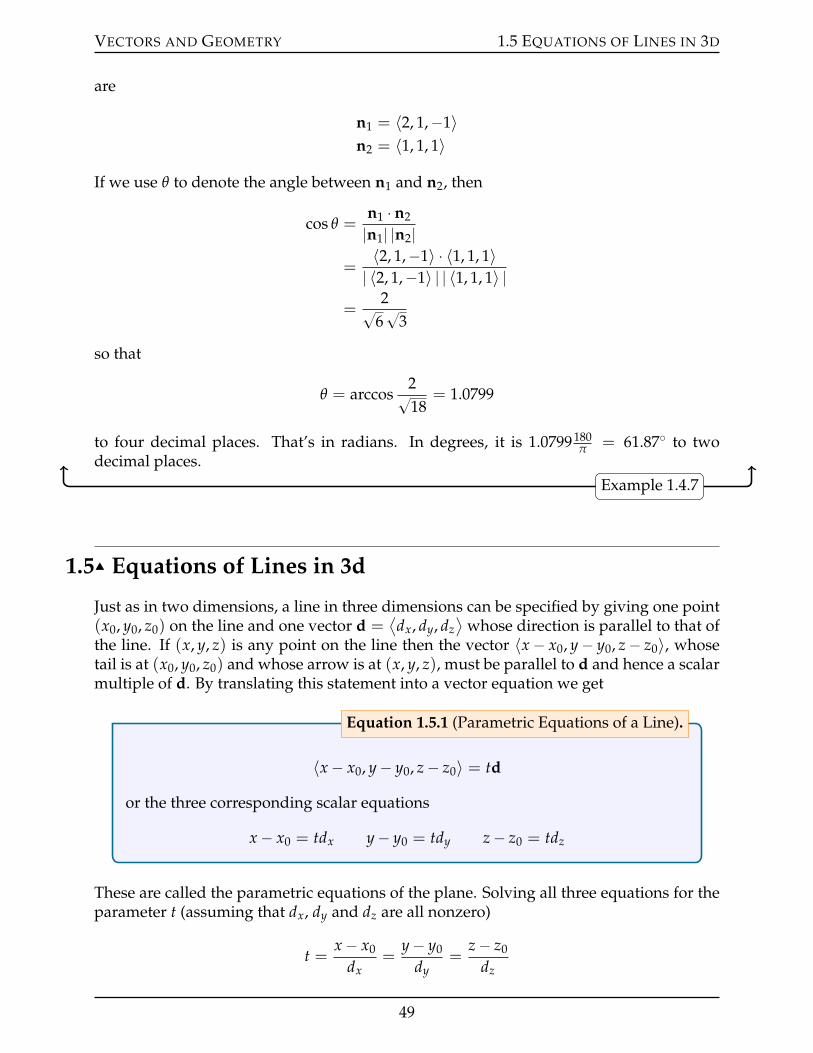
VECTORS AND GEOMETRY 1.5 EQUATIONS OF LINES IN 3D
are
n1 = 〈2, 1,´1〉n2 = 〈1, 1, 1〉
If we use θ to denote the angle between n1 and n2, then
cos θ =n1 ¨ n2
|n1| |n2|=〈2, 1,´1〉 ¨ 〈1, 1, 1〉| 〈2, 1,´1〉 | | 〈1, 1, 1〉 |
=2?
6?
3
so that
θ = arccos2?18
= 1.0799
to four decimal places. That’s in radians. In degrees, it is 1.0799180π = 61.87˝ to two
decimal places.Example 1.4.7
1.5IJ Equations of Lines in 3d
Just as in two dimensions, a line in three dimensions can be specified by giving one point(x0, y0, z0) on the line and one vector d =
⟨dx, dy, dz
⟩whose direction is parallel to that of
the line. If (x, y, z) is any point on the line then the vector 〈x´ x0, y´ y0, z´ z0〉, whosetail is at (x0, y0, z0) and whose arrow is at (x, y, z), must be parallel to d and hence a scalarmultiple of d. By translating this statement into a vector equation we get
〈x´ x0, y´ y0, z´ z0〉 = td
or the three corresponding scalar equations
x´ x0 = tdx y´ y0 = tdy z´ z0 = tdz
Equation 1.5.1 (Parametric Equations of a Line).
These are called the parametric equations of the plane. Solving all three equations for theparameter t (assuming that dx, dy and dz are all nonzero)
t =x´ x0
dx=
y´ y0
dy=
z´ z0
dz
49
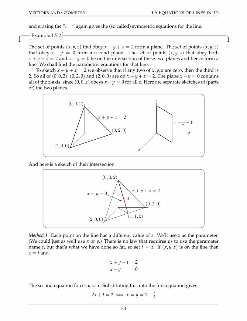
VECTORS AND GEOMETRY 1.5 EQUATIONS OF LINES IN 3D
and erasing the “t =” again gives the (so called) symmetric equations for the line.
Example 1.5.2
The set of points (x, y, z) that obey x + y + z = 2 form a plane. The set of points (x, y, z)that obey x ´ y = 0 form a second plane. The set of points (x, y, z) that obey bothx + y + z = 2 and x´ y = 0 lie on the intersection of these two planes and hence form aline. We shall find the parametric equations for that line.
To sketch x + y + z = 2 we observe that if any two of x, y, z are zero, then the third is2. So all of (0, 0, 2), (0, 2, 0) and (2, 0, 0) are on x + y + z = 2. The plane x´ y = 0 containsall of the z-axis, since (0, 0, z) obeys x´ y = 0 for all z. Here are separate sketches of (partsof) the two planes.
p0, 2, 0q
p0, 0, 2q
p2, 0, 0q
x ` y ` z “ 2
z
y
x
x ´ y “ 0
And here is a sketch of their intersection
p0, 2, 0q
p0, 0, 2q
p2, 0, 0q p1, 1, 0q
x ` y ` z “ 2x ´ y “ 0
d
Method 1. Each point on the line has a different value of z. We’ll use z as the parameter.(We could just as well use x or y.) There is no law that requires us to use the parametername t, but that’s what we have done so far, so set t = z. If (x, y, z) is on the line thenz = t and
x + y + t = 2x´ y = 0
The second equation forces y = x. Substituting this into the first equation gives
2x + t = 2 ùñ x = y = 1´ t2
50
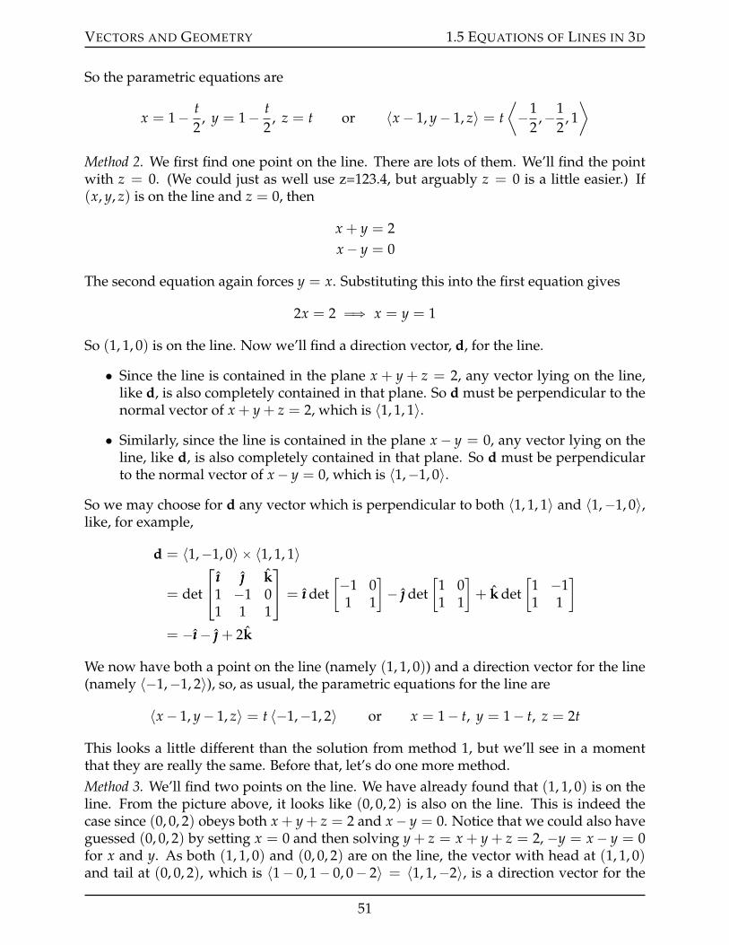
VECTORS AND GEOMETRY 1.5 EQUATIONS OF LINES IN 3D
So the parametric equations are
x = 1´ t2
, y = 1´ t2
, z = t or 〈x´ 1, y´ 1, z〉 = t⟨´1
2,´1
2, 1⟩
Method 2. We first find one point on the line. There are lots of them. We’ll find the pointwith z = 0. (We could just as well use z=123.4, but arguably z = 0 is a little easier.) If(x, y, z) is on the line and z = 0, then
x + y = 2x´ y = 0
The second equation again forces y = x. Substituting this into the first equation gives
2x = 2 ùñ x = y = 1
So (1, 1, 0) is on the line. Now we’ll find a direction vector, d, for the line.
• Since the line is contained in the plane x + y + z = 2, any vector lying on the line,like d, is also completely contained in that plane. So d must be perpendicular to thenormal vector of x + y + z = 2, which is 〈1, 1, 1〉.
• Similarly, since the line is contained in the plane x ´ y = 0, any vector lying on theline, like d, is also completely contained in that plane. So d must be perpendicularto the normal vector of x´ y = 0, which is 〈1,´1, 0〉.
So we may choose for d any vector which is perpendicular to both 〈1, 1, 1〉 and 〈1,´1, 0〉,like, for example,
d = 〈1,´1, 0〉ˆ 〈1, 1, 1〉
= det
ııı k1 ´1 01 1 1
= ııı det
[´1 01 1
]´ det
[1 01 1
]+ k det
[1 ´11 1
]
= ´ııı´ + 2k
We now have both a point on the line (namely (1, 1, 0)) and a direction vector for the line(namely 〈´1,´1, 2〉), so, as usual, the parametric equations for the line are
〈x´ 1, y´ 1, z〉 = t 〈´1,´1, 2〉 or x = 1´ t, y = 1´ t, z = 2t
This looks a little different than the solution from method 1, but we’ll see in a momentthat they are really the same. Before that, let’s do one more method.Method 3. We’ll find two points on the line. We have already found that (1, 1, 0) is on theline. From the picture above, it looks like (0, 0, 2) is also on the line. This is indeed thecase since (0, 0, 2) obeys both x + y + z = 2 and x´ y = 0. Notice that we could also haveguessed (0, 0, 2) by setting x = 0 and then solving y + z = x + y + z = 2, ´y = x´ y = 0for x and y. As both (1, 1, 0) and (0, 0, 2) are on the line, the vector with head at (1, 1, 0)and tail at (0, 0, 2), which is 〈1´ 0, 1´ 0, 0´ 2〉 = 〈1, 1,´2〉, is a direction vector for the
51

VECTORS AND GEOMETRY 1.5 EQUATIONS OF LINES IN 3D
line. As (0, 0, 2) is a point on the line and 〈1, 1,´2〉 is a direction vector for the line, theparametric equations for the line are
〈x´ 0, y´ 0, z´ 2〉 = t 〈1, 1,´2〉 or x = t, y = t, z = 2´ 2t
This also looks similar, but not quite identical, to our previous answers. Time for a com-parison.Comparing the answers. The parametric equations given by the three methods are different.That’s just because we have really used different parameters in the three methods, eventhough we have called the parameter t in each case. To clarify the relation between thethree answers, rename the parameter of method 1 to t1, the parameter of method 2 to t2and the parameter of method 3 to t3. The parametric equations then become
Method 1: x = 1´ t1
2y = 1´ t1
2z = t1
Method 2: x = 1´ t2 y = 1´ t2 z = 2t2
Method 3: x = t3 y = t3 z = 2´ 2t3
Substituting t1 = 2t2 into the Method 1 equations gives the Method 2 equations, andsubstituting t3 = 1´ t2 into the Method 3 equations gives the Method 2 equations. So allthree really give the same line, just parametrized a little differently.
Example 1.5.2
A line in three dimensions has infinitely many normal vectors.For example, the line
〈x´ 1, y´ 1, z〉 = t 〈1, 2,´2〉has direction vector 〈1, 2,´2〉. Any vector perpendicular to 〈1, 2,´2〉 is perpen-dicular to the line. The vector 〈n1, n2, n3〉 is perpendicular to 〈1, 2,´2〉 if and onlyif
0 = 〈1, 2,´2〉 ¨ 〈n1, n2, n3〉 = n1 + 2n2 ´ 2n3
There is whole plane of 〈n1, n2, n3〉’s obeying this condition, of which 〈2,´1, 0〉,〈0, 1, 1〉 and 〈2, 0, 1〉 are only three examples.
Warning 1.5.3.
The next two examples illustrate two different methods for finding the distance be-tween a point and a line.
Example 1.5.4
In this example, we find the distance between the point (2, 3,´1) and the line
L : 〈x´ 1, y´ 2, z´ 3〉 = t 〈1, 1, 2〉 or, equivalently, x = 1 + t, y = 2 + t, z = 3 + 2t
52
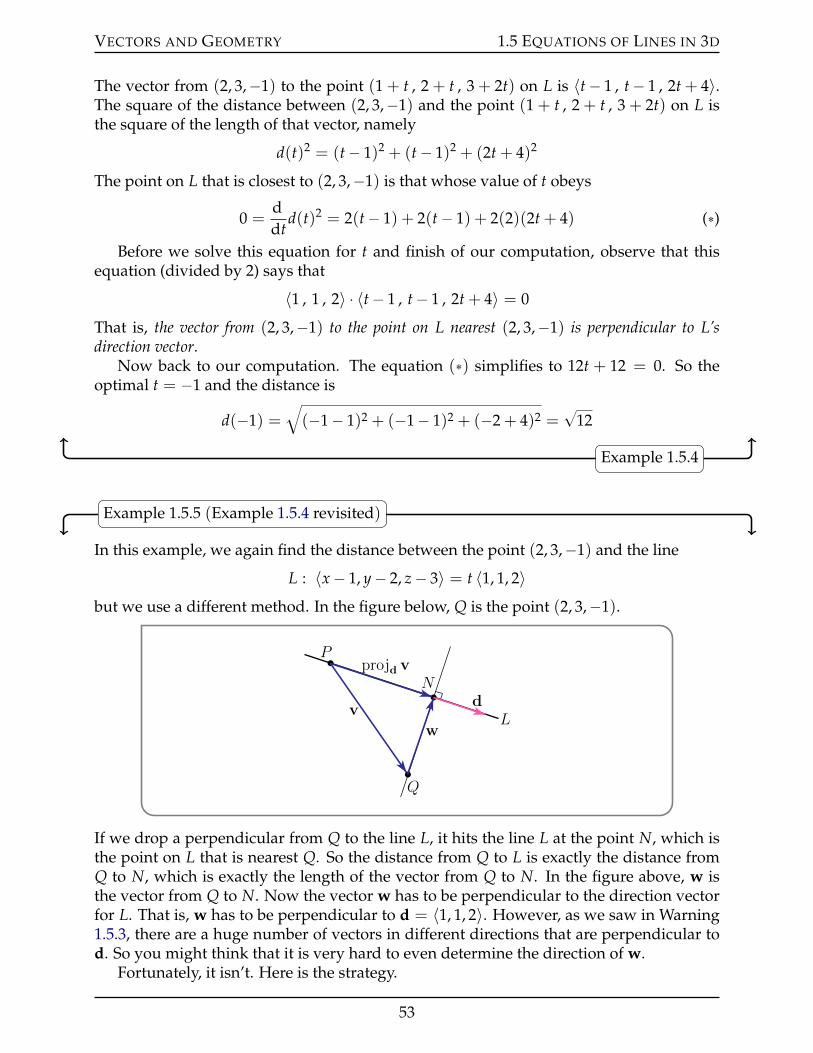
VECTORS AND GEOMETRY 1.5 EQUATIONS OF LINES IN 3D
The vector from (2, 3,´1) to the point (1 + t , 2 + t , 3 + 2t) on L is 〈t´ 1 , t´ 1 , 2t + 4〉.The square of the distance between (2, 3,´1) and the point (1 + t , 2 + t , 3 + 2t) on L isthe square of the length of that vector, namely
d(t)2 = (t´ 1)2 + (t´ 1)2 + (2t + 4)2
The point on L that is closest to (2, 3,´1) is that whose value of t obeys
0 =ddt
d(t)2 = 2(t´ 1) + 2(t´ 1) + 2(2)(2t + 4) (˚)Before we solve this equation for t and finish of our computation, observe that this
equation (divided by 2) says that
〈1 , 1 , 2〉 ¨ 〈t´ 1 , t´ 1 , 2t + 4〉 = 0
That is, the vector from (2, 3,´1) to the point on L nearest (2, 3,´1) is perpendicular to L’sdirection vector.
Now back to our computation. The equation (˚) simplifies to 12t + 12 = 0. So theoptimal t = ´1 and the distance is
d(´1) =b(´1´ 1)2 + (´1´ 1)2 + (´2 + 4)2 =
?12
Example 1.5.4
Example 1.5.5 (Example 1.5.4 revisited)
In this example, we again find the distance between the point (2, 3,´1) and the line
L : 〈x´ 1, y´ 2, z´ 3〉 = t 〈1, 1, 2〉but we use a different method. In the figure below, Q is the point (2, 3,´1).
Q
N
Pprojd v
v
w
dL
If we drop a perpendicular from Q to the line L, it hits the line L at the point N, which isthe point on L that is nearest Q. So the distance from Q to L is exactly the distance fromQ to N, which is exactly the length of the vector from Q to N. In the figure above, w isthe vector from Q to N. Now the vector w has to be perpendicular to the direction vectorfor L. That is, w has to be perpendicular to d = 〈1, 1, 2〉. However, as we saw in Warning1.5.3, there are a huge number of vectors in different directions that are perpendicular tod. So you might think that it is very hard to even determine the direction of w.
Fortunately, it isn’t. Here is the strategy.
53

VECTORS AND GEOMETRY 1.5 EQUATIONS OF LINES IN 3D
• Pick any point on L and call it P.• It is very easy to find the vector from P to N — it is just the projection of the vector
from P to Q (called v in the figure above) on d.• Once we know projd v, we will be able to compute
w = projd v´ v
• and then the distance from Q to the line L is just |w|.Here is the computation. We’ll choose P to be the point on L that has t = 0, which is(1, 2, 3). So the vector from P = (1, 2, 3) to Q = (2, 3,´1) is
v = 〈2´ 1, 3´ 2,´1´ 3〉 = 〈1, 1,´4〉
The projection of v = 〈1, 1,´4〉 on d = 〈1, 1, 2〉 is
projd v =〈1, 1,´4〉 ¨ 〈1, 1, 2〉
| 〈1, 1, 2〉 |2 〈1, 1, 2〉 = ´66〈1, 1, 2〉 = 〈´1,´1,´2〉
and thenw = projd v´ v = 〈´1,´1,´2〉´ 〈1, 1,´4〉 = 〈´2,´2, 2〉
and finally the distance from Q to the line L is
|w| = | 〈´2,´2, 2〉 | = |2 〈´1,´1, 1〉 | = 2?
3
Example 1.5.5
The next two (optional) examples illustrate two different methods for finding the dis-tance between two lines.
Example 1.5.6 (Optional)
In this example, we find the distance between the lines
L : 〈x´ 1, y´ 2, z´ 3〉 = t 〈1, 0,´1〉L1 : 〈x´ 1, y´ 2, z´ 1〉 = t 〈1,´2, 1〉
We can rewrite the equations of the lines as
L : x = 1 + t, y = 2, z = 3´ tL1 : x = 1 + t, y = 2´ 2t, z = 1 + t
Of course the value of t in the parametric equation for L need not be the same as the valueof t in the parametric equation for L1. So let us denote by x(s) = (1 + s , 2 , 3´ s) andy(t) = (1 + t , 2´ 2t , 1 + t) the points on L and L1, respectively, that are closest together.Note that the vector from x(s) to y(t) is 〈t´ s , ´2t , ´2 + s + t〉. Then, in particular,
• x(s) is the point on L that is closest to the point y(t), and• y(t) is the point on L1 that is closest to the point x(s).
54
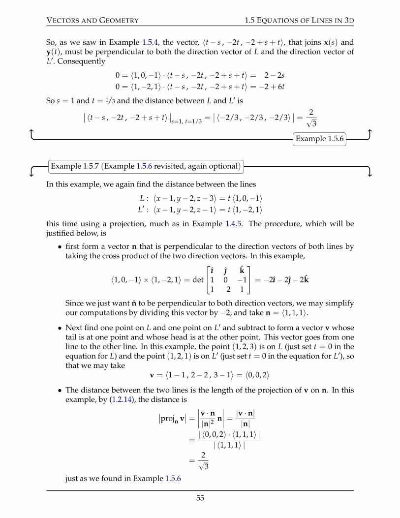
VECTORS AND GEOMETRY 1.5 EQUATIONS OF LINES IN 3D
So, as we saw in Example 1.5.4, the vector, 〈t´ s , ´2t , ´2 + s + t〉, that joins x(s) andy(t), must be perpendicular to both the direction vector of L and the direction vector ofL1. Consequently
0 = 〈1, 0,´1〉 ¨ 〈t´ s , ´2t , ´2 + s + t〉 = 2´ 2s0 = 〈1,´2, 1〉 ¨ 〈t´ s , ´2t , ´2 + s + t〉 = ´2 + 6t
So s = 1 and t = 1/3 and the distance between L and L1 isˇ〈t´ s , ´2t , ´2 + s + t〉
ˇs=1, t=1/3 =
ˇ〈´2/3 , ´2/3 , ´2/3〉
ˇ=
2?3
Example 1.5.6
Example 1.5.7 (Example 1.5.6 revisited, again optional)
In this example, we again find the distance between the lines
L : 〈x´ 1, y´ 2, z´ 3〉 = t 〈1, 0,´1〉L1 : 〈x´ 1, y´ 2, z´ 1〉 = t 〈1,´2, 1〉
this time using a projection, much as in Example 1.4.5. The procedure, which will bejustified below, is
• first form a vector n that is perpendicular to the direction vectors of both lines bytaking the cross product of the two direction vectors. In this example,
〈1, 0,´1〉ˆ 〈1,´2, 1〉 = det
ııı k1 0 ´11 ´2 1
= ´2ııı´ 2´ 2k
Since we just want n to be perpendicular to both direction vectors, we may simplifyour computations by dividing this vector by ´2, and take n = 〈1, 1, 1〉.• Next find one point on L and one point on L1 and subtract to form a vector v whose
tail is at one point and whose head is at the other point. This vector goes from oneline to the other line. In this example, the point (1, 2, 3) is on L (just set t = 0 in theequation for L) and the point (1, 2, 1) is on L1 (just set t = 0 in the equation for L1), sothat we may take
v = 〈1´ 1 , 2´ 2 , 3´ 1〉 = 〈0, 0, 2〉• The distance between the two lines is the length of the projection of v on n. In this
example, by (1.2.14), the distance is
ˇprojn v
ˇ=
ˇˇv ¨ n|n|2 n
ˇˇ = |v ¨ n|
|n|=| 〈0, 0, 2〉 ¨ 〈1, 1, 1〉 |
| 〈1, 1, 1〉 |=
2?3
just as we found in Example 1.5.6
55
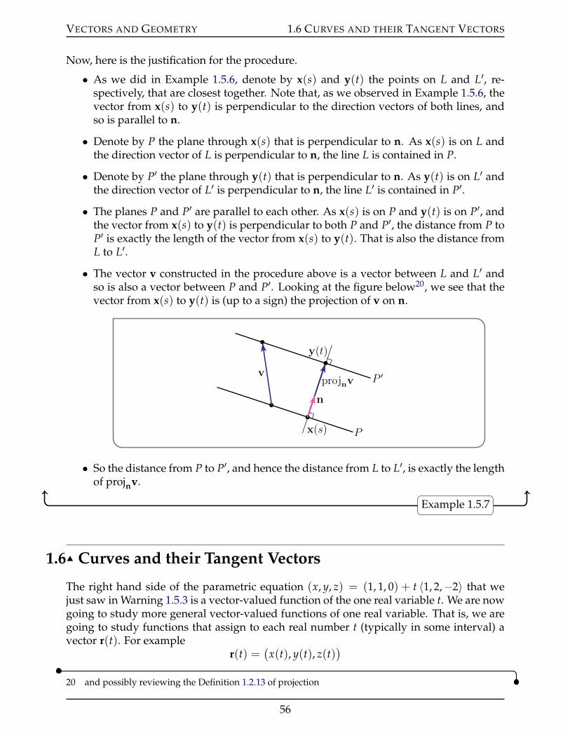
VECTORS AND GEOMETRY 1.6 CURVES AND THEIR TANGENT VECTORS
Now, here is the justification for the procedure.
• As we did in Example 1.5.6, denote by x(s) and y(t) the points on L and L1, re-spectively, that are closest together. Note that, as we observed in Example 1.5.6, thevector from x(s) to y(t) is perpendicular to the direction vectors of both lines, andso is parallel to n.
• Denote by P the plane through x(s) that is perpendicular to n. As x(s) is on L andthe direction vector of L is perpendicular to n, the line L is contained in P.
• Denote by P1 the plane through y(t) that is perpendicular to n. As y(t) is on L1 andthe direction vector of L1 is perpendicular to n, the line L1 is contained in P1.
• The planes P and P1 are parallel to each other. As x(s) is on P and y(t) is on P1, andthe vector from x(s) to y(t) is perpendicular to both P and P1, the distance from P toP1 is exactly the length of the vector from x(s) to y(t). That is also the distance fromL to L1.
• The vector v constructed in the procedure above is a vector between L and L1 andso is also a vector between P and P1. Looking at the figure below20, we see that thevector from x(s) to y(t) is (up to a sign) the projection of v on n.
projnv
P
P 1
xpsq
yptq
n
v
• So the distance from P to P1, and hence the distance from L to L1, is exactly the lengthof projnv.
Example 1.5.7
1.6IJ Curves and their Tangent Vectors
The right hand side of the parametric equation (x, y, z) = (1, 1, 0) + t 〈1, 2,´2〉 that wejust saw in Warning 1.5.3 is a vector-valued function of the one real variable t. We are nowgoing to study more general vector-valued functions of one real variable. That is, we aregoing to study functions that assign to each real number t (typically in some interval) avector r(t). For example
r(t) =(x(t), y(t), z(t)
)
20 and possibly reviewing the Definition 1.2.13 of projection
56
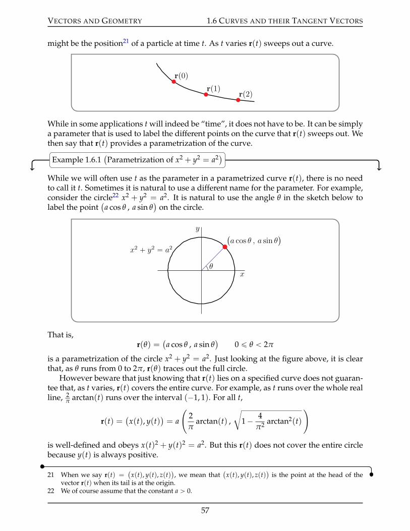
VECTORS AND GEOMETRY 1.6 CURVES AND THEIR TANGENT VECTORS
might be the position21 of a particle at time t. As t varies r(t) sweeps out a curve.
r(0)
r(1)r(2)
While in some applications t will indeed be “time”, it does not have to be. It can be simplya parameter that is used to label the different points on the curve that r(t) sweeps out. Wethen say that r(t) provides a parametrization of the curve.
Example 1.6.1(Parametrization of x2 + y2 = a2)
While we will often use t as the parameter in a parametrized curve r(t), there is no needto call it t. Sometimes it is natural to use a different name for the parameter. For example,consider the circle22 x2 + y2 = a2. It is natural to use the angle θ in the sketch below tolabel the point
(a cos θ , a sin θ
)on the circle.
x
y
x2 ` y2 “ a2
`a cos θ , a sin θ
˘
θ
That is,r(θ) =
(a cos θ , a sin θ
)0 ď θ ă 2π
is a parametrization of the circle x2 + y2 = a2. Just looking at the figure above, it is clearthat, as θ runs from 0 to 2π, r(θ) traces out the full circle.
However beware that just knowing that r(t) lies on a specified curve does not guaran-tee that, as t varies, r(t) covers the entire curve. For example, as t runs over the whole realline, 2
π arctan(t) runs over the interval (´1, 1). For all t,
r(t) =(x(t), y(t)
)= a
(2π
arctan(t) ,
c1´ 4
π2 arctan2(t)
)
is well-defined and obeys x(t)2 + y(t)2 = a2. But this r(t) does not cover the entire circlebecause y(t) is always positive.
21 When we say r(t) =(
x(t), y(t), z(t)), we mean that
(x(t), y(t), z(t)
)is the point at the head of the
vector r(t) when its tail is at the origin.22 We of course assume that the constant a ą 0.
57
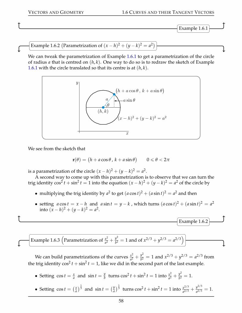
VECTORS AND GEOMETRY 1.6 CURVES AND THEIR TANGENT VECTORS
Example 1.6.1
Example 1.6.2(Parametrization of (x´ h)2 + (y´ k)2 = a2)
We can tweak the parametrization of Example 1.6.1 to get a parametrization of the circleof radius a that is centred on (h, k). One way to do so is to redraw the sketch of Example1.6.1 with the circle translated so that its centre is at (h, k).
x
y
px ´ hq2 ` py ´ kq2 “ a2
a sin θa
ph, kq
`h ` a cos θ , k ` a sin θ
˘
θ
We see from the sketch that
r(θ) =(h + a cos θ , k + a sin θ
)0 ď θ ă 2π
is a parametrization of the circle (x´ h)2 + (y´ k)2 = a2.A second way to come up with this parametrization is to observe that we can turn the
trig identity cos2 t + sin2 t = 1 into the equation (x´ h)2 + (y´ k)2 = a2 of the circle by
• multiplying the trig identity by a2 to get (a cos t)2 + (a sin t)2 = a2 and then
• setting a cos t = x ´ h and a sin t = y´ k , which turns (a cos t)2 + (a sin t)2 = a2
into (x´ h)2 + (y´ k)2 = a2.
Example 1.6.2
Example 1.6.3(
Parametrization of x2
a2 +y2
b2 = 1 and of x2/3 + y2/3 = a2/3)
We can build parametrizations of the curves x2
a2 +y2
b2 = 1 and x2/3 + y2/3 = a2/3 fromthe trig identity cos2 t + sin2 t = 1, like we did in the second part of the last example.
• Setting cos t = xa and sin t = y
b turns cos2 t + sin2 t = 1 into x2
a2 +y2
b2 = 1.
• Setting cos t =( x
a) 1
3 and sin t =( y
a) 1
3 turns cos2 t + sin2 t = 1 into x2/3
a2/3 +y2/3
a2/3 = 1.
58
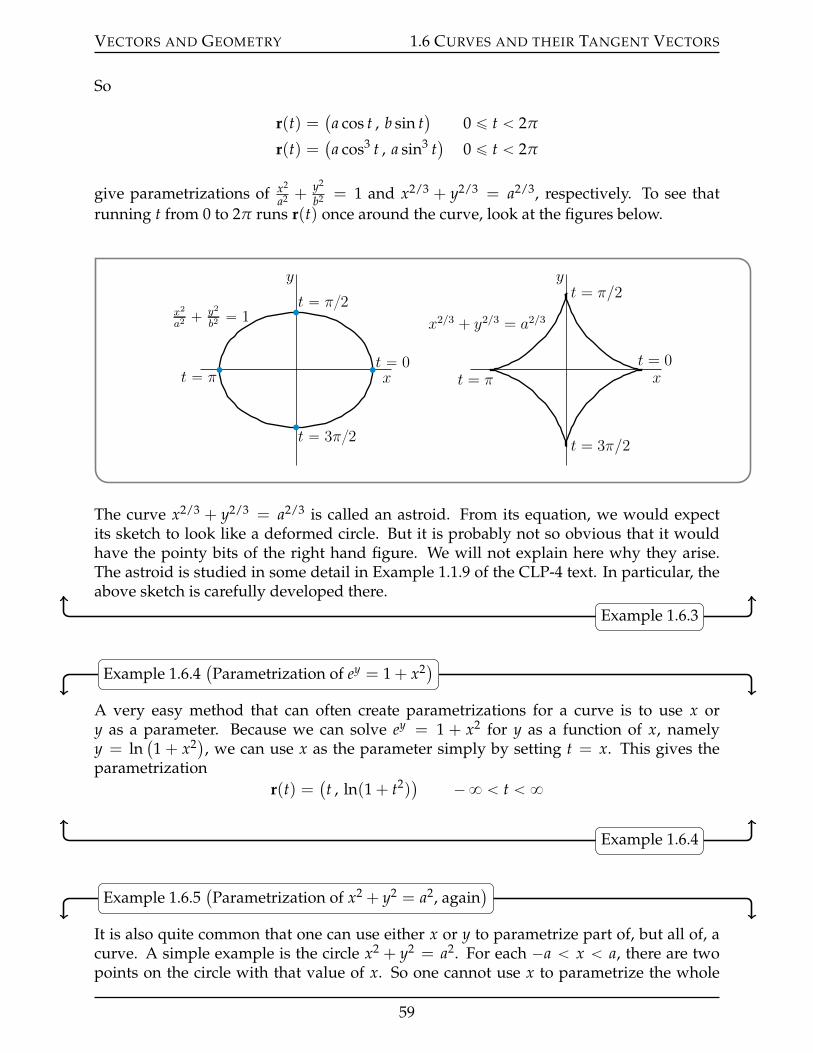
VECTORS AND GEOMETRY 1.6 CURVES AND THEIR TANGENT VECTORS
So
r(t) =(a cos t , b sin t
)0 ď t ă 2π
r(t) =(a cos3 t , a sin3 t
)0 ď t ă 2π
give parametrizations of x2
a2 + y2
b2 = 1 and x2/3 + y2/3 = a2/3, respectively. To see thatrunning t from 0 to 2π runs r(t) once around the curve, look at the figures below.
x
y
x2
a2` y2
b2“ 1
t “ 0t “ π
t “ π2
t “ 3π2
x
y
x2/3 + y2/3 = a2/3
t = 0t = π
t = π/2
t = 3π/2
The curve x2/3 + y2/3 = a2/3 is called an astroid. From its equation, we would expectits sketch to look like a deformed circle. But it is probably not so obvious that it wouldhave the pointy bits of the right hand figure. We will not explain here why they arise.The astroid is studied in some detail in Example 1.1.9 of the CLP-4 text. In particular, theabove sketch is carefully developed there.
Example 1.6.3
Example 1.6.4(Parametrization of ey = 1 + x2)
A very easy method that can often create parametrizations for a curve is to use x ory as a parameter. Because we can solve ey = 1 + x2 for y as a function of x, namelyy = ln
(1 + x2), we can use x as the parameter simply by setting t = x. This gives the
parametrizationr(t) =
(t , ln(1 + t2)
) ´8 ă t ă 8
Example 1.6.4
Example 1.6.5(Parametrization of x2 + y2 = a2, again
)
It is also quite common that one can use either x or y to parametrize part of, but all of, acurve. A simple example is the circle x2 + y2 = a2. For each ´a ă x ă a, there are twopoints on the circle with that value of x. So one cannot use x to parametrize the whole
59
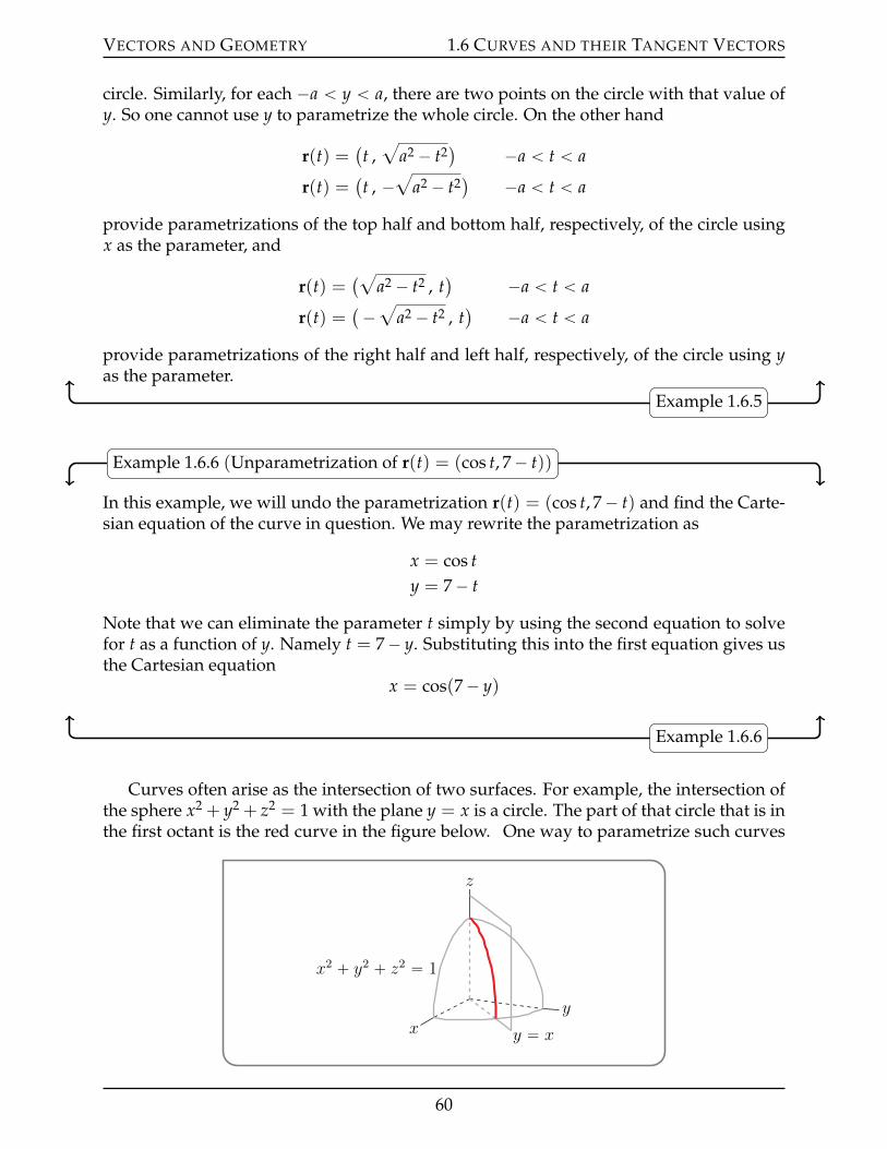
VECTORS AND GEOMETRY 1.6 CURVES AND THEIR TANGENT VECTORS
circle. Similarly, for each ´a ă y ă a, there are two points on the circle with that value ofy. So one cannot use y to parametrize the whole circle. On the other hand
r(t) =(t ,
aa2 ´ t2
) ´a ă t ă a
r(t) =(t , ´
aa2 ´ t2
) ´a ă t ă a
provide parametrizations of the top half and bottom half, respectively, of the circle usingx as the parameter, and
r(t) =(a
a2 ´ t2 , t) ´a ă t ă a
r(t) =(´
aa2 ´ t2 , t
) ´a ă t ă a
provide parametrizations of the right half and left half, respectively, of the circle using yas the parameter.
Example 1.6.5
Example 1.6.6 (Unparametrization of r(t) = (cos t, 7´ t))
In this example, we will undo the parametrization r(t) = (cos t, 7´ t) and find the Carte-sian equation of the curve in question. We may rewrite the parametrization as
x = cos ty = 7´ t
Note that we can eliminate the parameter t simply by using the second equation to solvefor t as a function of y. Namely t = 7´ y. Substituting this into the first equation gives usthe Cartesian equation
x = cos(7´ y)
Example 1.6.6
Curves often arise as the intersection of two surfaces. For example, the intersection ofthe sphere x2 + y2 + z2 = 1 with the plane y = x is a circle. The part of that circle that is inthe first octant is the red curve in the figure below. One way to parametrize such curves
z
yx y “ x
x2 ` y2 ` z2 “ 1
60
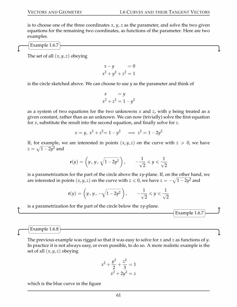
VECTORS AND GEOMETRY 1.6 CURVES AND THEIR TANGENT VECTORS
is to choose one of the three coordinates x, y, z as the parameter, and solve the two givenequations for the remaining two coordinates, as functions of the parameter. Here are twoexamples.
Example 1.6.7
The set of all (x, y, z) obeying
x´ y = 0
x2 + y2 + z2 = 1
is the circle sketched above. We can choose to use y as the parameter and think of
x = y
x2 + z2 = 1´ y2
as a system of two equations for the two unknowns x and z, with y being treated as agiven constant, rather than as an unknown. We can now (trivially) solve the first equationfor x, substitute the result into the second equation, and finally solve for z.
x = y, x2 + z2= 1´ y2 ùñ z2 = 1´ 2y2
If, for example, we are interested in points (x, y, z) on the curve with z ě 0, we havez =
a1´ 2y2 and
r(y) =(
y , y ,b
1´ 2y2)
, ´ 1?2ď y ď 1?
2
is a parametrization for the part of the circle above the xy-plane. If, on the other hand, weare interested in points (x, y, z) on the curve with z ď 0, we have z = ´a1´ 2y2 and
r(y) =(
y , y , ´b
1´ 2y2)
, ´ 1?2ď y ď 1?
2
is a parametrization for the part of the circle below the xy-plane.Example 1.6.7
Example 1.6.8
The previous example was rigged so that it was easy to solve for x and z as functions of y.In practice it is not always easy, or even possible, to do so. A more realistic example is theset of all (x, y, z) obeying
x2 +y2
2+
z2
3= 1
x2 + 2y2 = z
which is the blue curve in the figure
61
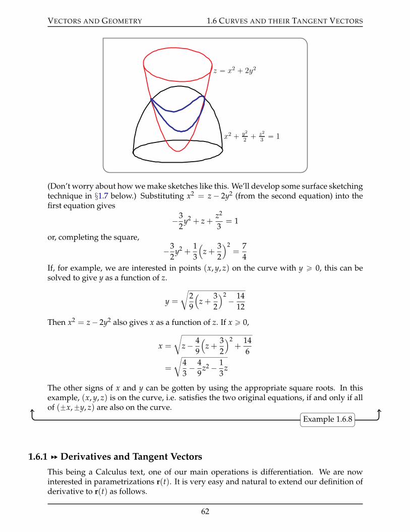
VECTORS AND GEOMETRY 1.6 CURVES AND THEIR TANGENT VECTORS
x2 ` y2
2` z2
3“ 1
z “ x2 ` 2y2
(Don’t worry about how we make sketches like this. We’ll develop some surface sketchingtechnique in §1.7 below.) Substituting x2 = z ´ 2y2 (from the second equation) into thefirst equation gives
´32
y2 + z +z2
3= 1
or, completing the square,
´32
y2 +13
(z +
32
)2=
74
If, for example, we are interested in points (x, y, z) on the curve with y ě 0, this can besolved to give y as a function of z.
y =
c29
(z +
32
)2´ 14
12
Then x2 = z´ 2y2 also gives x as a function of z. If x ě 0,
x =
cz´ 4
9
(z +
32
)2+
146
=
c43´ 4
9z2 ´ 1
3z
The other signs of x and y can be gotten by using the appropriate square roots. In thisexample, (x, y, z) is on the curve, i.e. satisfies the two original equations, if and only if allof (˘x,˘y, z) are also on the curve.
Example 1.6.8
1.6.1 §§ Derivatives and Tangent Vectors
This being a Calculus text, one of our main operations is differentiation. We are nowinterested in parametrizations r(t). It is very easy and natural to extend our definition ofderivative to r(t) as follows.
62
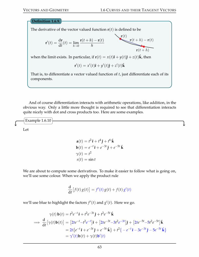
VECTORS AND GEOMETRY 1.6 CURVES AND THEIR TANGENT VECTORS
The derivative of the vector valued function r(t) is defined to be
r1(t) =drdt
(t) = limhÑ0
r(t + h)´ r(t)h
rptq
rpt ` hq
rpt ` hq ´ rptq
when the limit exists. In particular, if r(t) = x(t)ııı + y(t) + z(t)k, then
r1(t) = x1(t)ııı + y1(t) + z1(t)k
That is, to differentiate a vector valued function of t, just differentiate each of itscomponents.
Definition 1.6.9.
And of course differentiation interacts with arithmetic operations, like addition, in theobvious way. Only a little more thought is required to see that differentiation interactsquite nicely with dot and cross products too. Here are some examples.
Example 1.6.10
Let
a(t) = t2 ııı + t4 + t6 k
b(t) = e´t ııı + e´3t + e´5t k
γ(t) = t2
s(t) = sin t
We are about to compute some derivatives. To make it easier to follow what is going on,we’ll use some colour. When we apply the product rule
ddt[
f (t) g(t)]= f 1(t) g(t) + f (t) g1(t)
we’ll use blue to highlight the factors f 1(t) and g1(t). Here we go.
γ(t) b(t) = t2e´t ııı + t2e´3t + t2e´5t k
ùñ ddt[γ(t)b(t)
]=[2te´t´t2e´t]ııı +
[2te´3t´3t2e´3t] +
[2te´5t´5t2e´5t]k
= 2t
e´t ııı + e´3t + e´5t k(+ t2 ´ e´t ııı´ 3e´3t ´ 5e´5t k
(
= γ1(t)b(t) + γ(t)b1(t)
63
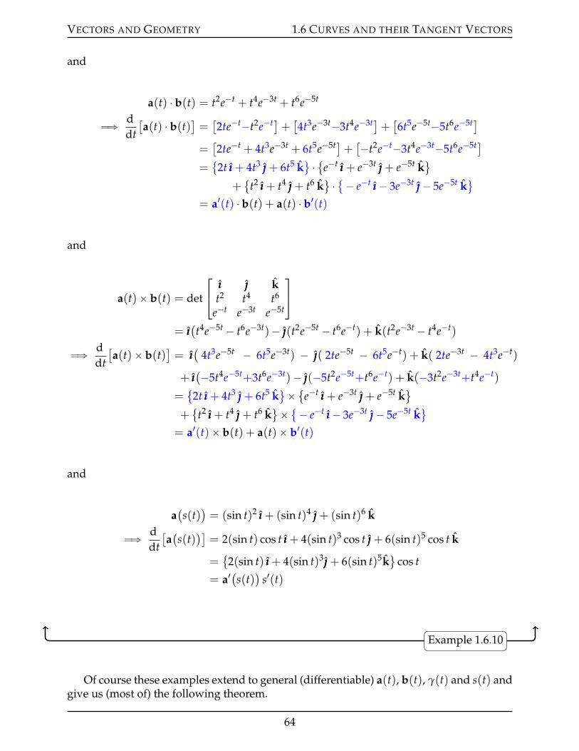
VECTORS AND GEOMETRY 1.6 CURVES AND THEIR TANGENT VECTORS
and
a(t) ¨ b(t) = t2e´t + t4e´3t + t6e´5t
ùñ ddt[a(t) ¨ b(t)] = [2te´t´t2e´t]+
[4t3e´3t´3t4e´3t]+
[6t5e´5t´5t6e´5t]
=[2te´t + 4t3e´3t + 6t5e´5t]+
[´t2e´t´3t4e´3t´5t6e´5t]
=
2t ııı + 4t3 + 6t5 k( ¨ e´t ııı + e´3t + e´5t k
(
+
t2 ııı + t4 + t6 k( ¨ ´ e´t ııı´ 3e´3t ´ 5e´5t k
(
= a1(t) ¨ b(t) + a(t) ¨ b1(t)
and
a(t)ˆ b(t) = det
ııı kt2 t4 t6
e´t e´3t e´5t
= ııı(t4e´5t ´ t6e´3t)´ (t2e´5t ´ t6e´t) + k(t2e´3t ´ t4e´t)
ùñ ddt[a(t)ˆ b(t)
]= ııı
(4t3e´5t ´ 6t5e´3t) ´ ( 2te´5t ´ 6t5e´t) + k( 2te´3t ´ 4t3e´t)
+ ııı(´5t4e´5t+3t6e´3t)´ (´5t2e´5t+t6e´t) + k(´3t2e´3t+t4e´t)
=
2t ııı + 4t3 + 6t5 k(ˆ
e´t ııı + e´3t + e´5t k(
+
t2 ııı + t4 + t6 k(ˆ ´ e´t ııı´ 3e´3t ´ 5e´5t k
(
= a1(t)ˆ b(t) + a(t)ˆ b1(t)
and
a(s(t)
)= (sin t)2 ııı + (sin t)4 + (sin t)6 k
ùñ ddt[a(s(t)
)]= 2(sin t) cos t ııı + 4(sin t)3 cos t + 6(sin t)5 cos t k
=
2(sin t) ııı + 4(sin t)3 + 6(sin t)5k(
cos t
= a1(s(t)
)s1(t)
Example 1.6.10
Of course these examples extend to general (differentiable) a(t), b(t), γ(t) and s(t) andgive us (most of) the following theorem.
64
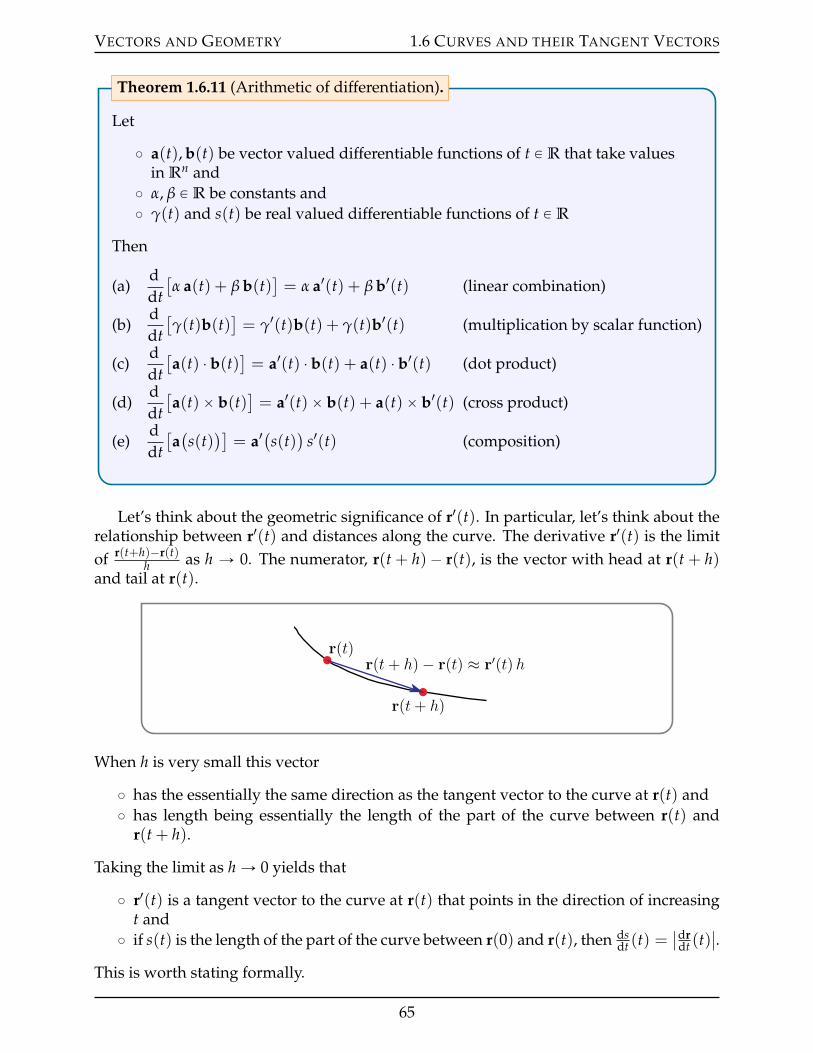
VECTORS AND GEOMETRY 1.6 CURVES AND THEIR TANGENT VECTORS
Let
˝ a(t), b(t) be vector valued differentiable functions of t P R that take valuesin Rn and
˝ α, β P R be constants and˝ γ(t) and s(t) be real valued differentiable functions of t P R
Then
(a)ddt[α a(t) + β b(t)
]= α a1(t) + β b1(t) (linear combination)
(b)ddt[γ(t)b(t)
]= γ1(t)b(t) + γ(t)b1(t) (multiplication by scalar function)
(c)ddt[a(t) ¨ b(t)] = a1(t) ¨ b(t) + a(t) ¨ b1(t) (dot product)
(d)ddt[a(t)ˆ b(t)
]= a1(t)ˆ b(t) + a(t)ˆ b1(t) (cross product)
(e)ddt[a(s(t)
)]= a1
(s(t)
)s1(t) (composition)
Theorem 1.6.11 (Arithmetic of differentiation).
Let’s think about the geometric significance of r1(t). In particular, let’s think about therelationship between r1(t) and distances along the curve. The derivative r1(t) is the limitof r(t+h)´r(t)
h as h Ñ 0. The numerator, r(t + h)´ r(t), is the vector with head at r(t + h)and tail at r(t).
r(t)
r(t+ h)
r(t+ h)− r(t) ≈ r′(t) h
When h is very small this vector
˝ has the essentially the same direction as the tangent vector to the curve at r(t) and˝ has length being essentially the length of the part of the curve between r(t) and
r(t + h).
Taking the limit as h Ñ 0 yields that
˝ r1(t) is a tangent vector to the curve at r(t) that points in the direction of increasingt and
˝ if s(t) is the length of the part of the curve between r(0) and r(t), then dsdt (t) =
ˇdrdt (t)
ˇ.
This is worth stating formally.
65
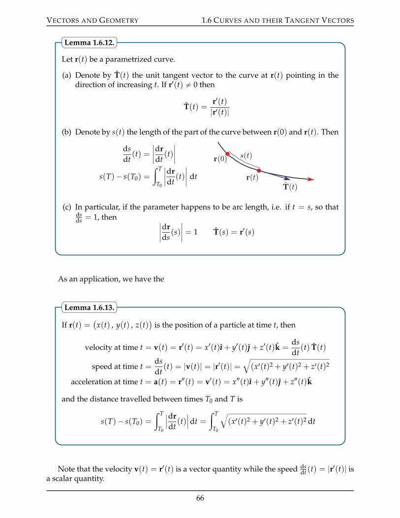
VECTORS AND GEOMETRY 1.6 CURVES AND THEIR TANGENT VECTORS
Let r(t) be a parametrized curve.
(a) Denote by T(t) the unit tangent vector to the curve at r(t) pointing in thedirection of increasing t. If r1(t) ‰ 0 then
T(t) =r1(t)|r1(t)|
(b) Denote by s(t) the length of the part of the curve between r(0) and r(t). Then
dsdt
(t) =ˇˇdrdt
(t)ˇˇ
s(T)´ s(T0) =
ż T
T0
ˇˇdrdt
(t)ˇˇ dt
rp0q
rptqTptq
sptq
(c) In particular, if the parameter happens to be arc length, i.e. if t = s, so thatdsds = 1, then ˇ
ˇdrds
(s)ˇˇ = 1 T(s) = r1(s)
Lemma 1.6.12.
As an application, we have the
If r(t) =(x(t) , y(t) , z(t)
)is the position of a particle at time t, then
velocity at time t = v(t) = r1(t) = x1(t)ııı + y1(t) + z1(t)k =dsdt
(t) T(t)
speed at time t =dsdt
(t) = |v(t)| = |r1(t)| =b(x1(t)2 + y1(t)2 + z1(t)2
acceleration at time t = a(t) = r2(t) = v1(t) = x2(t)ııı + y2(t) + z2(t)k
and the distance travelled between times T0 and T is
s(T)´ s(T0) =
ż T
T0
ˇˇdrdt
(t)ˇˇdt =
ż T
T0
b(x1(t)2 + y1(t)2 + z1(t)2 dt
Lemma 1.6.13.
Note that the velocity v(t) = r1(t) is a vector quantity while the speed dsdt (t) = |r1(t)| is
a scalar quantity.
66
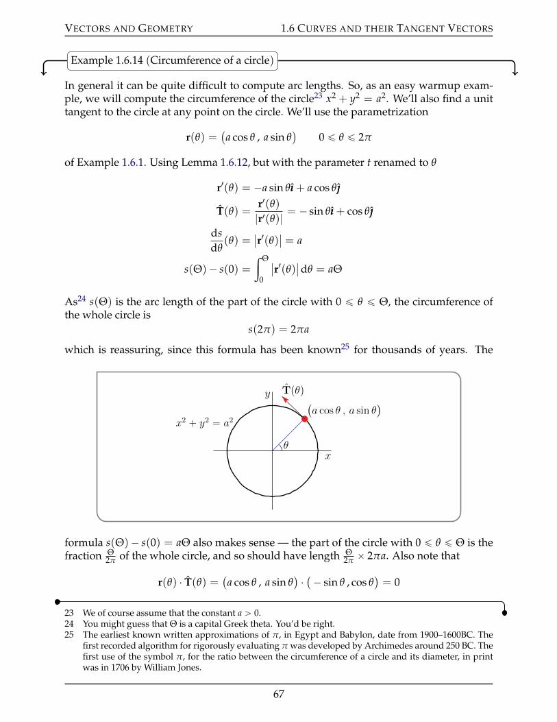
VECTORS AND GEOMETRY 1.6 CURVES AND THEIR TANGENT VECTORS
Example 1.6.14 (Circumference of a circle)
In general it can be quite difficult to compute arc lengths. So, as an easy warmup exam-ple, we will compute the circumference of the circle23 x2 + y2 = a2. We’ll also find a unittangent to the circle at any point on the circle. We’ll use the parametrization
r(θ) =(a cos θ , a sin θ
)0 ď θ ď 2π
of Example 1.6.1. Using Lemma 1.6.12, but with the parameter t renamed to θ
r1(θ) = ´a sin θııı + a cos θ
T(θ) =r1(θ)|r1(θ)| = ´ sin θııı + cos θ
dsdθ
(θ) =ˇr1(θ)
ˇ= a
s(Θ)´ s(0) =ż Θ
0
ˇr1(θ)
ˇdθ = aΘ
As24 s(Θ) is the arc length of the part of the circle with 0 ď θ ď Θ, the circumference ofthe whole circle is
s(2π) = 2πa
which is reassuring, since this formula has been known25 for thousands of years. The
x
y
x2 ` y2 “ a2
`a cos θ , a sin θ
˘
θ
Tpθq
formula s(Θ)´ s(0) = aΘ also makes sense — the part of the circle with 0 ď θ ď Θ is thefraction Θ
2π of the whole circle, and so should have length Θ2π ˆ 2πa. Also note that
r(θ) ¨ T(θ) = (a cos θ , a sin θ) ¨ (´ sin θ , cos θ
)= 0
23 We of course assume that the constant a ą 0.24 You might guess that Θ is a capital Greek theta. You’d be right.25 The earliest known written approximations of π, in Egypt and Babylon, date from 1900–1600BC. The
first recorded algorithm for rigorously evaluating π was developed by Archimedes around 250 BC. Thefirst use of the symbol π, for the ratio between the circumference of a circle and its diameter, in printwas in 1706 by William Jones.
67
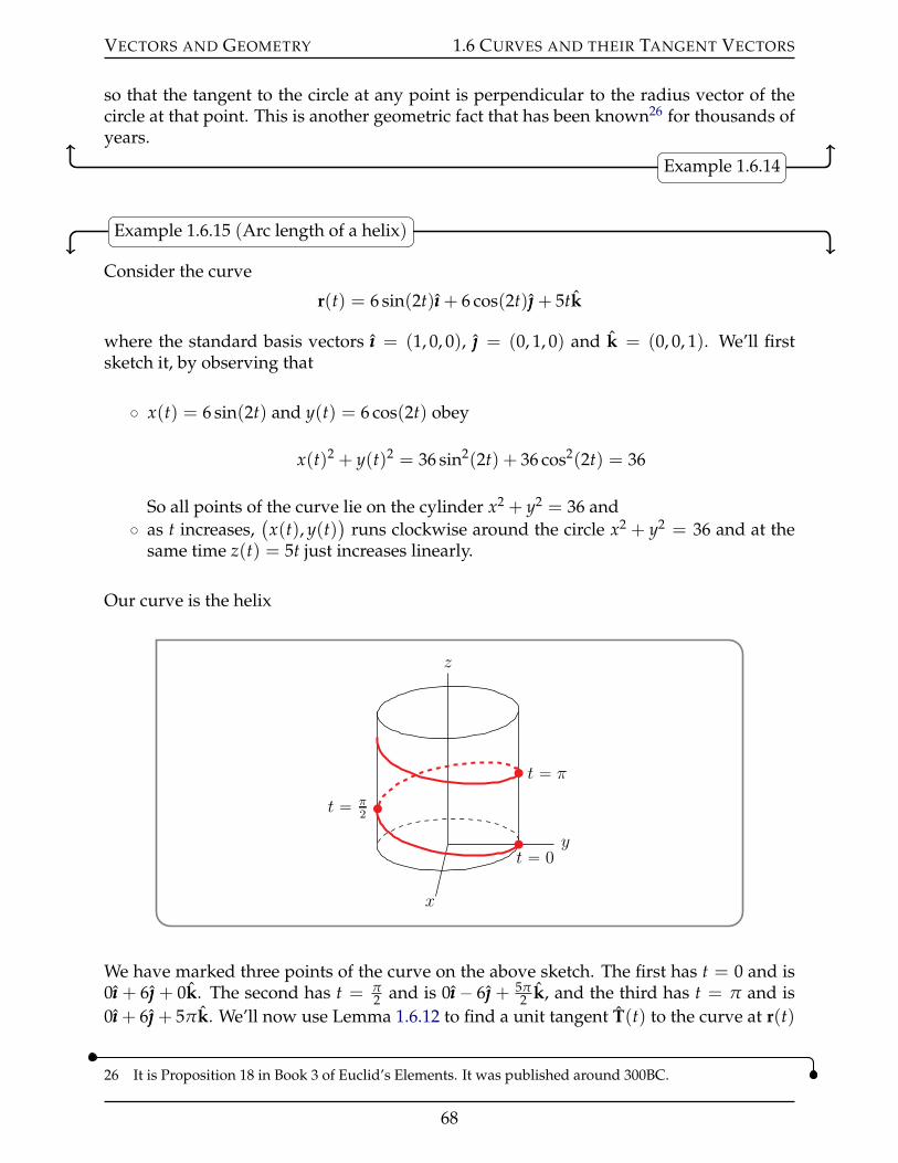
VECTORS AND GEOMETRY 1.6 CURVES AND THEIR TANGENT VECTORS
so that the tangent to the circle at any point is perpendicular to the radius vector of thecircle at that point. This is another geometric fact that has been known26 for thousands ofyears.
Example 1.6.14
Example 1.6.15 (Arc length of a helix)
Consider the curve
r(t) = 6 sin(2t)ııı + 6 cos(2t) + 5tk
where the standard basis vectors ııı = (1, 0, 0), = (0, 1, 0) and k = (0, 0, 1). We’ll firstsketch it, by observing that
˝ x(t) = 6 sin(2t) and y(t) = 6 cos(2t) obey
x(t)2 + y(t)2 = 36 sin2(2t) + 36 cos2(2t) = 36
So all points of the curve lie on the cylinder x2 + y2 = 36 and˝ as t increases,
(x(t), y(t)
)runs clockwise around the circle x2 + y2 = 36 and at the
same time z(t) = 5t just increases linearly.
Our curve is the helix
y
z
x
t “ 0
t “ π2
t “ π
We have marked three points of the curve on the above sketch. The first has t = 0 and is0ııı + 6 + 0k. The second has t = π
2 and is 0ııı´ 6 + 5π2 k, and the third has t = π and is
0ııı + 6 + 5πk. We’ll now use Lemma 1.6.12 to find a unit tangent T(t) to the curve at r(t)
26 It is Proposition 18 in Book 3 of Euclid’s Elements. It was published around 300BC.
68
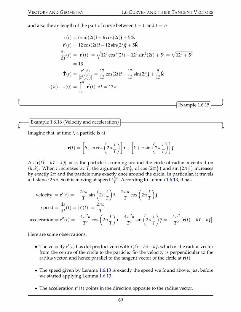
VECTORS AND GEOMETRY 1.6 CURVES AND THEIR TANGENT VECTORS
and also the arclength of the part of curve between t = 0 and t = π.
r(t) = 6 sin(2t)ııı + 6 cos(2t) + 5tk
r1(t) = 12 cos(2t)ııı´ 12 sin(2t) + 5kdsdt
(t) =ˇr1(t)
ˇ=
b122 cos2(2t) + 122 sin2(2t) + 52 =
a122 + 52
= 13
T(t) =r1(t)|r1(t))| =
1213
cos(2t)ııı´ 1213
sin(2t) +5
13k
s(π)´ s(0) =ż π
0
ˇr1(t)
ˇdt = 13π
Example 1.6.15
Example 1.6.16 (Velocity and acceleration)
Imagine that, at time t, a particle is at
r(t) =[
h + a cos(
2πtT
)]ııı +[
k + a sin(
2πtT
)]
As |r(t) ´ h ııı ´ k | = a, the particle is running around the circle of radius a centred on(h, k). When t increases by T, the argument, 2π t
T , of cos(2π t
T)
and sin(2π t
T)
increasesby exactly 2π and the particle runs exactly once around the circle. In particular, it travelsa distance 2πa. So it is moving at speed 2πa
T . According to Lemma 1.6.13, it has
velocity = r1(t) = ´2πaT
sin(
2πtT
)ııı +
2πaT
cos(
2πtT
)
speed =dsdt
(t) = |r1(t)| = 2πaT
acceleration = r2(t) = ´4π2aT2 cos
(2π
tT
)ııı´ 4π2a
T2 sin(
2πtT
) = ´4π2
T2
[r(t)´ h ııı´ k
]
Here are some observations.
• The velocity r1(t) has dot product zero with r(t)´ h ııı´ k , which is the radius vectorfrom the centre of the circle to the particle. So the velocity is perpendicular to theradius vector, and hence parallel to the tangent vector of the circle at r(t).
• The speed given by Lemma 1.6.13 is exactly the speed we found above, just beforewe started applying Lemma 1.6.13.
• The acceleration r2(t) points in the direction opposite to the radius vector.
69
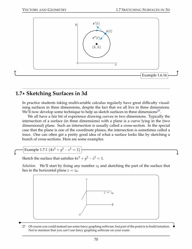
VECTORS AND GEOMETRY 1.7 SKETCHING SURFACES IN 3D
x
y
rptqr1ptq
r2ptq
ph, kq
Example 1.6.16
1.7IJ Sketching Surfaces in 3d
In practice students taking multivariable calculus regularly have great difficulty visual-ising surfaces in three dimensions, despite the fact that we all live in three dimensions.We’ll now develop some technique to help us sketch surfaces in three dimensions27.
We all have a fair bit of experience drawing curves in two dimensions. Typically theintersection of a surface (in three dimensions) with a plane is a curve lying in the (twodimensional) plane. Such an intersection is usually called a cross-section. In the specialcase that the plane is one of the coordinate planes, the intersection is sometimes called atrace. One can often get a pretty good idea of what a surface looks like by sketching abunch of cross-sections. Here are some examples.
Example 1.7.1(4x2 + y2 ´ z2 = 1
)
Sketch the surface that satisfies 4x2 + y2 ´ z2 = 1.
Solution. We’ll start by fixing any number z0 and sketching the part of the surface thatlies in the horizontal plane z = z0.
z
y
x
z “ z0
27 Of course you could instead use some fancy graphing software, but part of the point is to build intuition.Not to mention that you can’t use fancy graphing software on your exam.
70
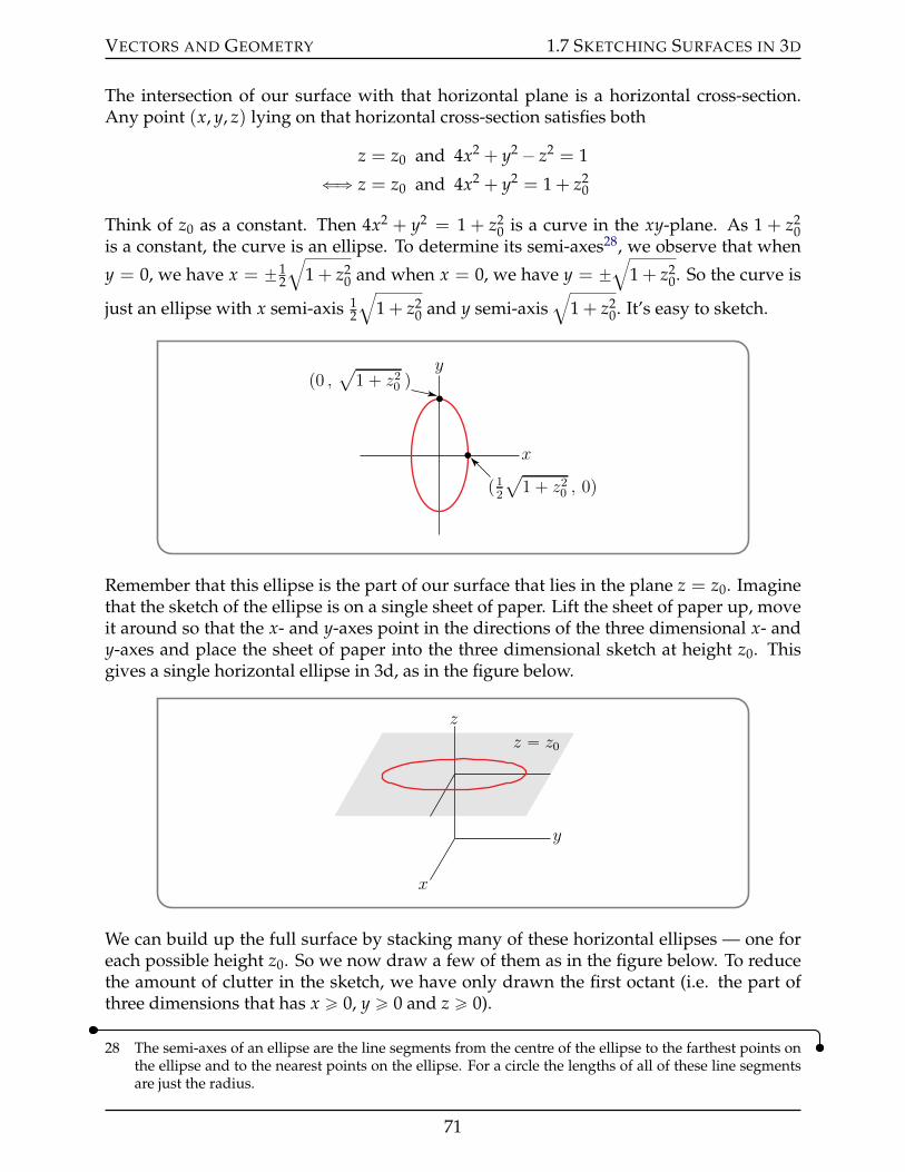
VECTORS AND GEOMETRY 1.7 SKETCHING SURFACES IN 3D
The intersection of our surface with that horizontal plane is a horizontal cross-section.Any point (x, y, z) lying on that horizontal cross-section satisfies both
z = z0 and 4x2 + y2 ´ z2 = 1
ðñ z = z0 and 4x2 + y2 = 1 + z20
Think of z0 as a constant. Then 4x2 + y2 = 1 + z20 is a curve in the xy-plane. As 1 + z2
0is a constant, the curve is an ellipse. To determine its semi-axes28, we observe that when
y = 0, we have x = ˘12
b1 + z2
0 and when x = 0, we have y = ˘b
1 + z20. So the curve is
just an ellipse with x semi-axis 12
b1 + z2
0 and y semi-axisb
1 + z20. It’s easy to sketch.
x
y
(12
√1 + z20 , 0)
(0 ,√
1 + z20 )
Remember that this ellipse is the part of our surface that lies in the plane z = z0. Imaginethat the sketch of the ellipse is on a single sheet of paper. Lift the sheet of paper up, moveit around so that the x- and y-axes point in the directions of the three dimensional x- andy-axes and place the sheet of paper into the three dimensional sketch at height z0. Thisgives a single horizontal ellipse in 3d, as in the figure below.
z
y
x
z “ z0
We can build up the full surface by stacking many of these horizontal ellipses — one foreach possible height z0. So we now draw a few of them as in the figure below. To reducethe amount of clutter in the sketch, we have only drawn the first octant (i.e. the part ofthree dimensions that has x ě 0, y ě 0 and z ě 0).
28 The semi-axes of an ellipse are the line segments from the centre of the ellipse to the farthest points onthe ellipse and to the nearest points on the ellipse. For a circle the lengths of all of these line segmentsare just the radius.
71
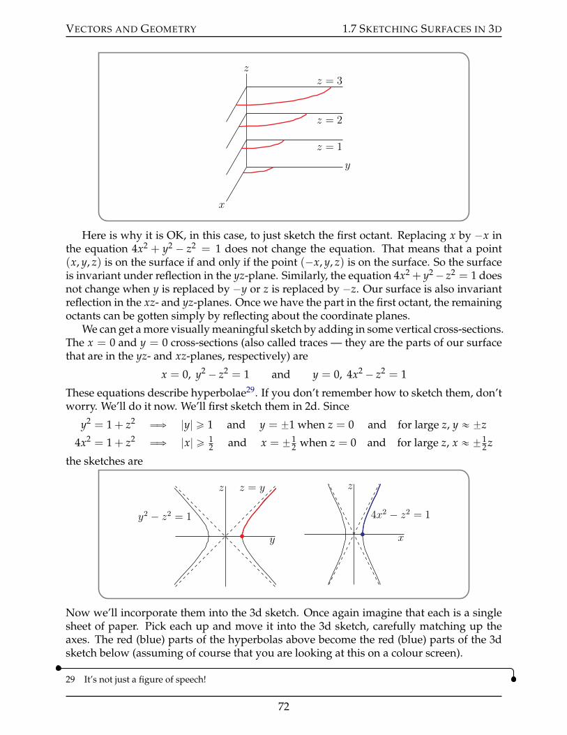
VECTORS AND GEOMETRY 1.7 SKETCHING SURFACES IN 3D
z
y
x
z = 1
z = 2
z = 3
Here is why it is OK, in this case, to just sketch the first octant. Replacing x by ´x inthe equation 4x2 + y2 ´ z2 = 1 does not change the equation. That means that a point(x, y, z) is on the surface if and only if the point (´x, y, z) is on the surface. So the surfaceis invariant under reflection in the yz-plane. Similarly, the equation 4x2 + y2´ z2 = 1 doesnot change when y is replaced by ´y or z is replaced by ´z. Our surface is also invariantreflection in the xz- and yz-planes. Once we have the part in the first octant, the remainingoctants can be gotten simply by reflecting about the coordinate planes.
We can get a more visually meaningful sketch by adding in some vertical cross-sections.The x = 0 and y = 0 cross-sections (also called traces — they are the parts of our surfacethat are in the yz- and xz-planes, respectively) are
x = 0, y2 ´ z2 = 1 and y = 0, 4x2 ´ z2 = 1
These equations describe hyperbolae29. If you don’t remember how to sketch them, don’tworry. We’ll do it now. We’ll first sketch them in 2d. Since
y2 = 1 + z2 ùñ |y| ě 1 and y = ˘1 when z = 0 and for large z, y « ˘z
4x2 = 1 + z2 ùñ |x| ě 12 and x = ˘1
2 when z = 0 and for large z, x « ˘12 z
the sketches are
y
z z = y
y2 − z2 = 1
x
z
4x2 − z2 = 1
Now we’ll incorporate them into the 3d sketch. Once again imagine that each is a singlesheet of paper. Pick each up and move it into the 3d sketch, carefully matching up theaxes. The red (blue) parts of the hyperbolas above become the red (blue) parts of the 3dsketch below (assuming of course that you are looking at this on a colour screen).
29 It’s not just a figure of speech!
72
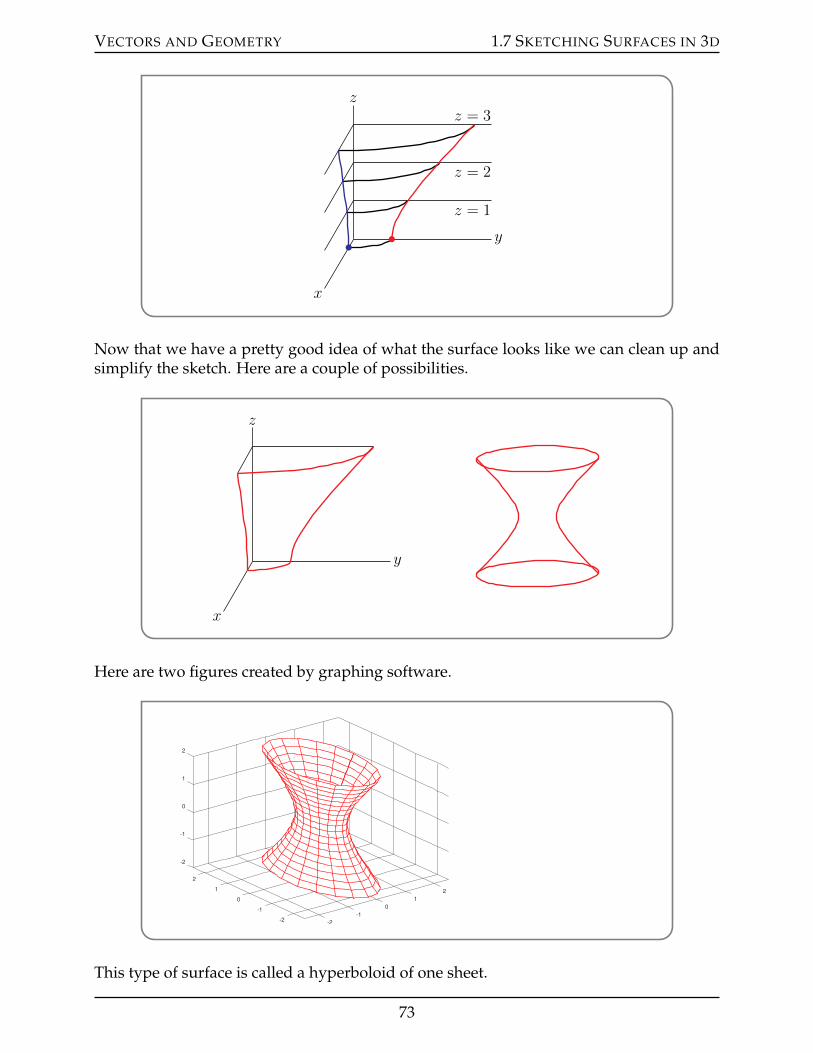
VECTORS AND GEOMETRY 1.7 SKETCHING SURFACES IN 3D
z
y
x
z = 1
z = 2
z = 3
Now that we have a pretty good idea of what the surface looks like we can clean up andsimplify the sketch. Here are a couple of possibilities.
z
y
x
Here are two figures created by graphing software.
-2
-1
0
1
2
2
1
-1
0-1
0
1
-2-2
2
This type of surface is called a hyperboloid of one sheet.
73
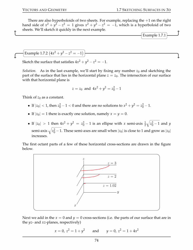
VECTORS AND GEOMETRY 1.7 SKETCHING SURFACES IN 3D
There are also hyperboloids of two sheets. For example, replacing the +1 on the righthand side of x2 + y2 ´ z2 = 1 gives x2 + y2 ´ z2 = ´1, which is a hyperboloid of twosheets. We’ll sketch it quickly in the next example.
Example 1.7.1
Example 1.7.2(4x2 + y2 ´ z2 = ´1
)
Sketch the surface that satisfies 4x2 + y2 ´ z2 = ´1.
Solution. As in the last example, we’ll start by fixing any number z0 and sketching thepart of the surface that lies in the horizontal plane z = z0. The intersection of our surfacewith that horizontal plane is
z = z0 and 4x2 + y2 = z20 ´ 1
Think of z0 as a constant.
• If |z0| ă 1, then z20 ´ 1 ă 0 and there are no solutions to x2 + y2 = z2
0 ´ 1.
• If |z0| = 1 there is exactly one solution, namely x = y = 0.
• If |z0| ą 1 then 4x2 + y2 = z20 ´ 1 is an ellipse with x semi-axis 1
2
bz2
0 ´ 1 and y
semi-axisb
z20 ´ 1. These semi-axes are small when |z0| is close to 1 and grow as |z0|
increases.
The first octant parts of a few of these horizontal cross-sections are drawn in the figurebelow.
z
y
x
z “ 1.02
z “ 2
z “ 3
Next we add in the x = 0 and y = 0 cross-sections (i.e. the parts of our surface that are inthe yz- and xz-planes, respectively)
x = 0, z2 = 1 + y2 and y = 0, z2 = 1 + 4x2
74
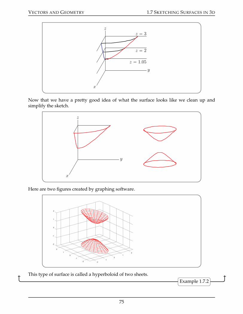
VECTORS AND GEOMETRY 1.7 SKETCHING SURFACES IN 3D
z
y
x
z “ 1.05
z “ 2
z “ 3
Now that we have a pretty good idea of what the surface looks like we clean up andsimplify the sketch.
z
y
x
Here are two figures created by graphing software.
-2
-1
0
1
2
2
1
0
-1
-2-2
-1
0
1
2
This type of surface is called a hyperboloid of two sheets.Example 1.7.2
75
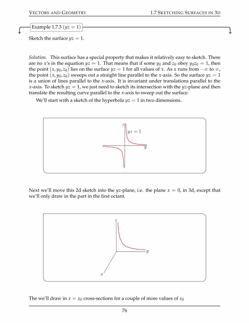
VECTORS AND GEOMETRY 1.7 SKETCHING SURFACES IN 3D
Example 1.7.3 (yz = 1)
Sketch the surface yz = 1.
Solution. This surface has a special property that makes it relatively easy to sketch. Thereare no x’s in the equation yz = 1. That means that if some y0 and z0 obey y0z0 = 1, thenthe point (x, y0, z0) lies on the surface yz = 1 for all values of x. As x runs from ´8 to 8,the point (x, y0, z0) sweeps out a straight line parallel to the x-axis. So the surface yz = 1is a union of lines parallel to the x-axis. It is invariant under translations parallel to thex-axis. To sketch yz = 1, we just need to sketch its intersection with the yz-plane and thentranslate the resulting curve parallel to the x-axis to sweep out the surface.
We’ll start with a sketch of the hyperbola yz = 1 in two dimensions.
y
z
yz = 1
Next we’ll move this 2d sketch into the yz-plane, i.e. the plane x = 0, in 3d, except thatwe’ll only draw in the part in the first octant.
z
y
x
The we’ll draw in x = x0 cross-sections for a couple of more values of x0
76
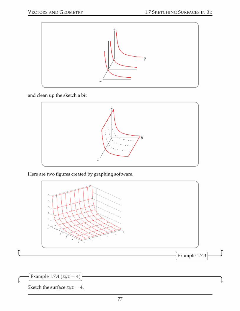
VECTORS AND GEOMETRY 1.7 SKETCHING SURFACES IN 3D
z
y
x
and clean up the sketch a bit
z
y
x
Here are two figures created by graphing software.
0
1
2
3
4
5
0
1
5
4
3
2
0
1
2
3
4
5
Example 1.7.3
Example 1.7.4 (xyz = 4)
Sketch the surface xyz = 4.
77
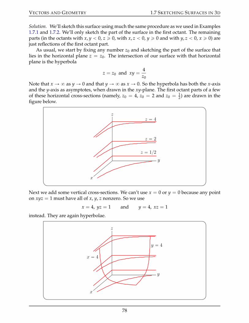
VECTORS AND GEOMETRY 1.7 SKETCHING SURFACES IN 3D
Solution. We’ll sketch this surface using much the same procedure as we used in Examples1.7.1 and 1.7.2. We’ll only sketch the part of the surface in the first octant. The remainingparts (in the octants with x, y ă 0, z ě 0, with x, z ă 0, y ě 0 and with y, z ă 0, x ě 0) arejust reflections of the first octant part.
As usual, we start by fixing any number z0 and sketching the part of the surface thatlies in the horizontal plane z = z0. The intersection of our surface with that horizontalplane is the hyperbola
z = z0 and xy =4z0
Note that x Ñ 8 as y Ñ 0 and that y Ñ 8 as x Ñ 0. So the hyperbola has both the x-axisand the y-axis as asymptotes, when drawn in the xy-plane. The first octant parts of a fewof these horizontal cross-sections (namely, z0 = 4, z0 = 2 and z0 = 1
2 ) are drawn in thefigure below.
z
y
x
z “ 12
z “ 2
z “ 4
Next we add some vertical cross-sections. We can’t use x = 0 or y = 0 because any pointon xyz = 1 must have all of x, y, z nonzero. So we use
x = 4, yz = 1 and y = 4, xz = 1
instead. They are again hyperbolae.
z
y
x
x “ 4
y “ 4
78
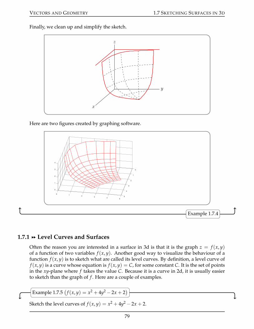
VECTORS AND GEOMETRY 1.7 SKETCHING SURFACES IN 3D
Finally, we clean up and simplify the sketch.
z
y
x
Here are two figures created by graphing software.
0
1
2
3
4
0
1
2
01
2
4
3
34
5
5
Example 1.7.4
1.7.1 §§ Level Curves and Surfaces
Often the reason you are interested in a surface in 3d is that it is the graph z = f (x, y)of a function of two variables f (x, y). Another good way to visualize the behaviour of afunction f (x, y) is to sketch what are called its level curves. By definition, a level curve off (x, y) is a curve whose equation is f (x, y) = C, for some constant C. It is the set of pointsin the xy-plane where f takes the value C. Because it is a curve in 2d, it is usually easierto sketch than the graph of f . Here are a couple of examples.
Example 1.7.5(
f (x, y) = x2 + 4y2 ´ 2x + 2)
Sketch the level curves of f (x, y) = x2 + 4y2 ´ 2x + 2.
79
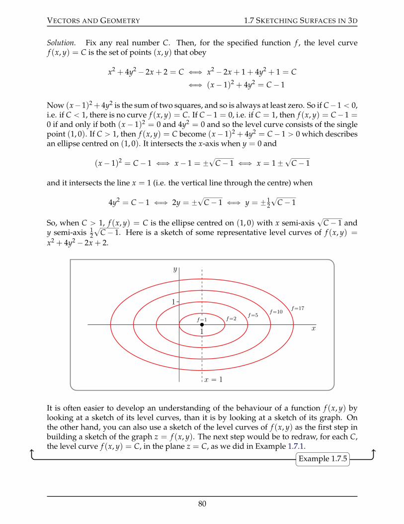
VECTORS AND GEOMETRY 1.7 SKETCHING SURFACES IN 3D
Solution. Fix any real number C. Then, for the specified function f , the level curvef (x, y) = C is the set of points (x, y) that obey
x2 + 4y2 ´ 2x + 2 = C ðñ x2 ´ 2x + 1 + 4y2 + 1 = C
ðñ (x´ 1)2 + 4y2 = C´ 1
Now (x´1)2 + 4y2 is the sum of two squares, and so is always at least zero. So if C´1 ă 0,i.e. if C ă 1, there is no curve f (x, y) = C. If C´ 1 = 0, i.e. if C = 1, then f (x, y) = C´ 1 =0 if and only if both (x´ 1)2 = 0 and 4y2 = 0 and so the level curve consists of the singlepoint (1, 0). If C ą 1, then f (x, y) = C become (x´ 1)2 + 4y2 = C´ 1 ą 0 which describesan ellipse centred on (1, 0). It intersects the x-axis when y = 0 and
(x´ 1)2 = C´ 1 ðñ x´ 1 = ˘?C´ 1 ðñ x = 1˘?C´ 1
and it intersects the line x = 1 (i.e. the vertical line through the centre) when
4y2 = C´ 1 ðñ 2y = ˘?C´ 1 ðñ y = ˘12
?C´ 1
So, when C ą 1, f (x, y) = C is the ellipse centred on (1, 0) with x semi-axis?
C´ 1 andy semi-axis 1
2
?C´ 1. Here is a sketch of some representative level curves of f (x, y) =
x2 + 4y2 ´ 2x + 2.
x
y
x “ 1
1
1
f“1 f“2f“5
f“10f“17
It is often easier to develop an understanding of the behaviour of a function f (x, y) bylooking at a sketch of its level curves, than it is by looking at a sketch of its graph. Onthe other hand, you can also use a sketch of the level curves of f (x, y) as the first step inbuilding a sketch of the graph z = f (x, y). The next step would be to redraw, for each C,the level curve f (x, y) = C, in the plane z = C, as we did in Example 1.7.1.
Example 1.7.5
80
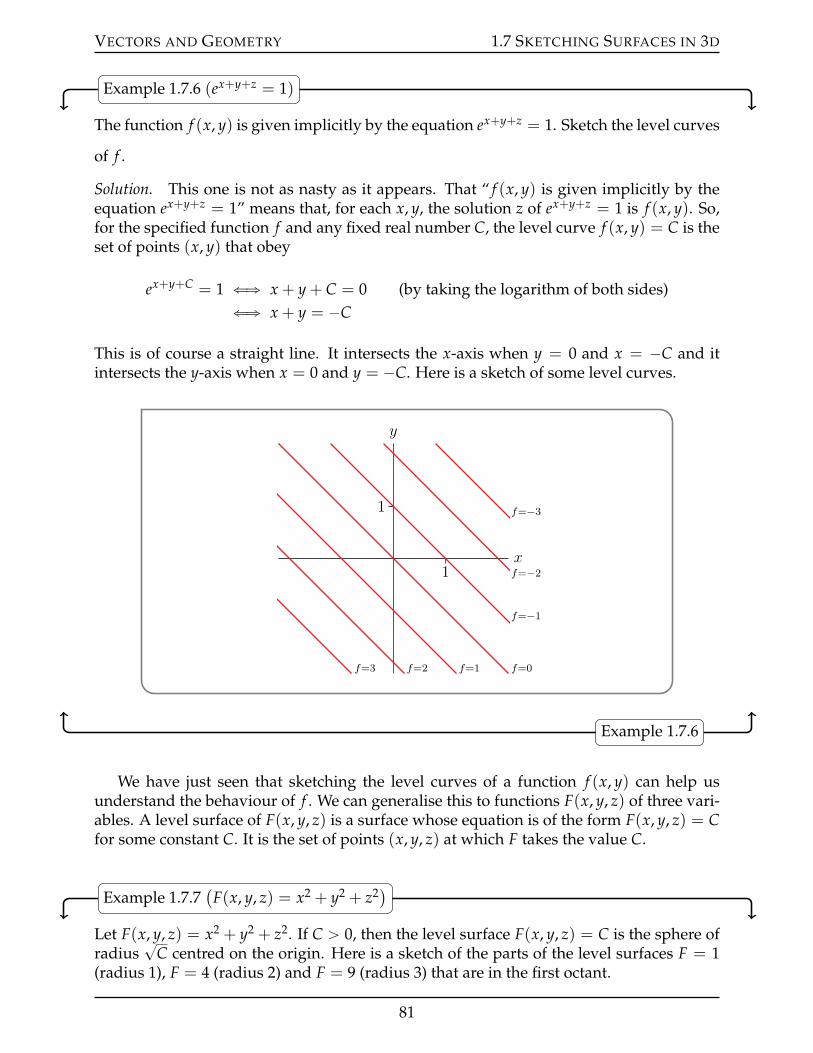
VECTORS AND GEOMETRY 1.7 SKETCHING SURFACES IN 3D
Example 1.7.6 (ex+y+z = 1)
The function f (x, y) is given implicitly by the equation ex+y+z = 1. Sketch the level curves
of f .
Solution. This one is not as nasty as it appears. That “ f (x, y) is given implicitly by theequation ex+y+z = 1” means that, for each x, y, the solution z of ex+y+z = 1 is f (x, y). So,for the specified function f and any fixed real number C, the level curve f (x, y) = C is theset of points (x, y) that obey
ex+y+C = 1 ðñ x + y + C = 0 (by taking the logarithm of both sides)ðñ x + y = ´C
This is of course a straight line. It intersects the x-axis when y = 0 and x = ´C and itintersects the y-axis when x = 0 and y = ´C. Here is a sketch of some level curves.
x
y
1
1
f=0f=1
f=−1
f=2
f=−2
f=3
f=−3
Example 1.7.6
We have just seen that sketching the level curves of a function f (x, y) can help usunderstand the behaviour of f . We can generalise this to functions F(x, y, z) of three vari-ables. A level surface of F(x, y, z) is a surface whose equation is of the form F(x, y, z) = Cfor some constant C. It is the set of points (x, y, z) at which F takes the value C.
Example 1.7.7(
F(x, y, z) = x2 + y2 + z2)
Let F(x, y, z) = x2 + y2 + z2. If C ą 0, then the level surface F(x, y, z) = C is the sphere ofradius
?C centred on the origin. Here is a sketch of the parts of the level surfaces F = 1
(radius 1), F = 4 (radius 2) and F = 9 (radius 3) that are in the first octant.
81
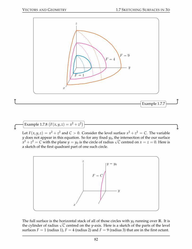
VECTORS AND GEOMETRY 1.7 SKETCHING SURFACES IN 3D
z
y
x
F “ 9
F “ 1
F “ 4
Example 1.7.7
Example 1.7.8(
F(x, y, z) = x2 + z2)
Let F(x, y, z) = x2 + z2 and C ą 0. Consider the level surface x2 + z2 = C. The variabley does not appear in this equation. So for any fixed y0, the intersection of the our surfacex2 + z2 = C with the plane y = y0 is the circle of radius
?C centred on x = z = 0. Here is
a sketch of the first quadrant part of one such circle.
z
y
x
F “ C
y “ y0
The full surface is the horizontal stack of all of those circles with y0 running over R. It isthe cylinder of radius
?C centred on the y-axis. Here is a sketch of the parts of the level
surfaces F = 1 (radius 1), F = 4 (radius 2) and F = 9 (radius 3) that are in the first octant.
82
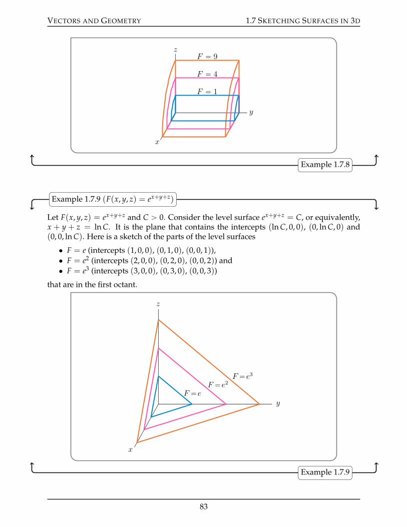
VECTORS AND GEOMETRY 1.7 SKETCHING SURFACES IN 3D
z
y
x
F “ 9
F “ 4
F “ 1
Example 1.7.8
Example 1.7.9 (F(x, y, z) = ex+y+z)
Let F(x, y, z) = ex+y+z and C ą 0. Consider the level surface ex+y+z = C, or equivalently,x + y + z = ln C. It is the plane that contains the intercepts (ln C, 0, 0), (0, ln C, 0) and(0, 0, ln C). Here is a sketch of the parts of the level surfaces
• F = e (intercepts (1, 0, 0), (0, 1, 0), (0, 0, 1)),• F = e2 (intercepts (2, 0, 0), (0, 2, 0), (0, 0, 2)) and• F = e3 (intercepts (3, 0, 0), (0, 3, 0), (0, 0, 3))
that are in the first octant.
z
y
x
F “e3
F “eF “e2
Example 1.7.9
83
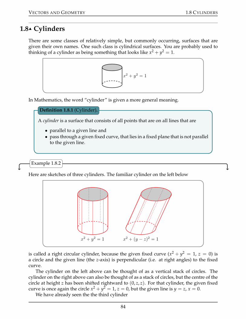
VECTORS AND GEOMETRY 1.8 CYLINDERS
1.8IJ Cylinders
There are some classes of relatively simple, but commonly occurring, surfaces that aregiven their own names. One such class is cylindrical surfaces. You are probably used tothinking of a cylinder as being something that looks like x2 + y2 = 1.
x2 ` y2 “ 1
In Mathematics, the word “cylinder” is given a more general meaning.
A cylinder is a surface that consists of all points that are on all lines that are
• parallel to a given line and• pass through a given fixed curve, that lies in a fixed plane that is not parallel
to the given line.
Definition 1.8.1 (Cylinder).
Example 1.8.2
Here are sketches of three cylinders. The familiar cylinder on the left below
x2 ` y2 “ 1 x2 ` py ´ zq2 “ 1
is called a right circular cylinder, because the given fixed curve (x2 + y2 = 1, z = 0) isa circle and the given line (the z-axis) is perpendicular (i.e. at right angles) to the fixedcurve.
The cylinder on the left above can be thought of as a vertical stack of circles. Thecylinder on the right above can also be thought of as a stack of circles, but the centre of thecircle at height z has been shifted rightward to (0, z, z). For that cylinder, the given fixedcurve is once again the circle x2 + y2 = 1, z = 0, but the given line is y = z, x = 0.
We have already seen the the third cylinder
84
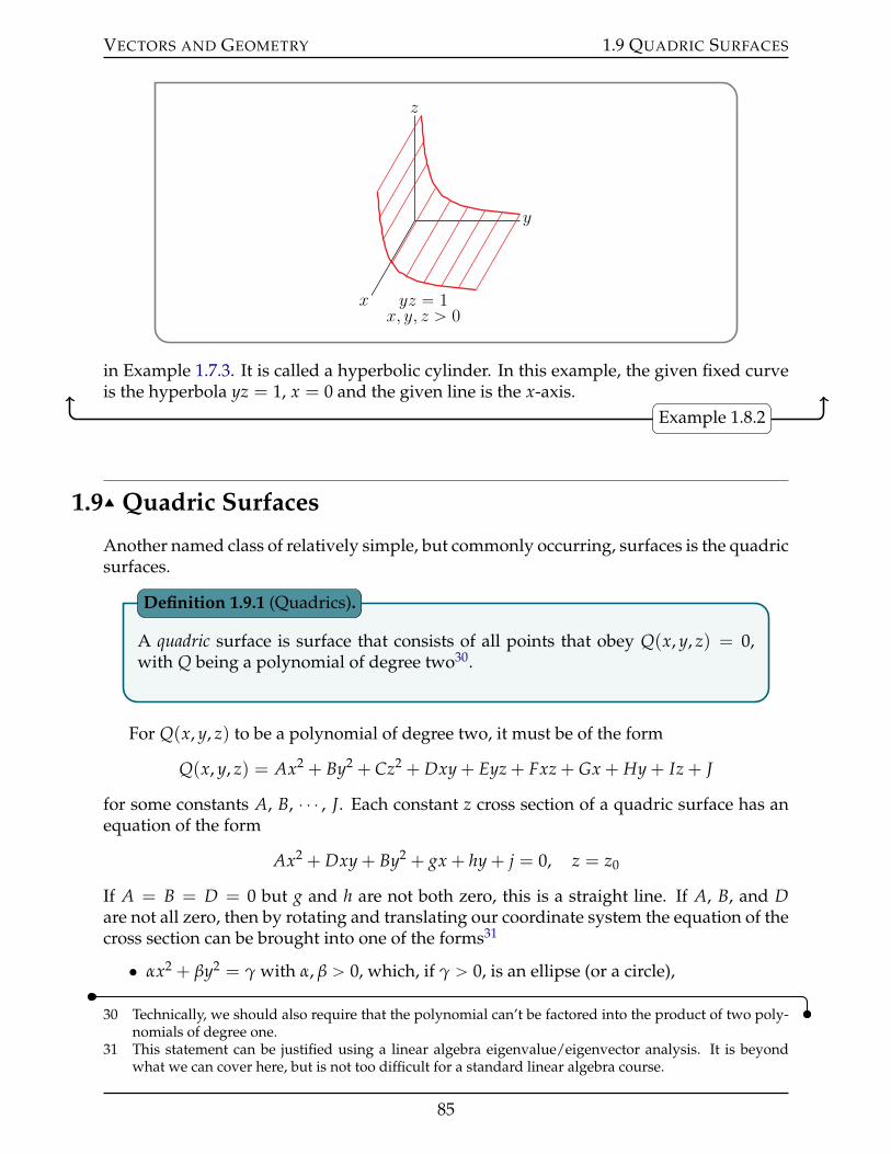
VECTORS AND GEOMETRY 1.9 QUADRIC SURFACES
z
y
x yz “ 1x, y, z ą 0
in Example 1.7.3. It is called a hyperbolic cylinder. In this example, the given fixed curveis the hyperbola yz = 1, x = 0 and the given line is the x-axis.
Example 1.8.2
1.9IJ Quadric Surfaces
Another named class of relatively simple, but commonly occurring, surfaces is the quadricsurfaces.
A quadric surface is surface that consists of all points that obey Q(x, y, z) = 0,with Q being a polynomial of degree two30.
Definition 1.9.1 (Quadrics).
For Q(x, y, z) to be a polynomial of degree two, it must be of the form
Q(x, y, z) = Ax2 + By2 + Cz2 + Dxy + Eyz + Fxz + Gx + Hy + Iz + J
for some constants A, B, ¨ ¨ ¨ , J. Each constant z cross section of a quadric surface has anequation of the form
Ax2 + Dxy + By2 + gx + hy + j = 0, z = z0
If A = B = D = 0 but g and h are not both zero, this is a straight line. If A, B, and Dare not all zero, then by rotating and translating our coordinate system the equation of thecross section can be brought into one of the forms31
• αx2 + βy2 = γ with α, β ą 0, which, if γ ą 0, is an ellipse (or a circle),
30 Technically, we should also require that the polynomial can’t be factored into the product of two poly-nomials of degree one.
31 This statement can be justified using a linear algebra eigenvalue/eigenvector analysis. It is beyondwhat we can cover here, but is not too difficult for a standard linear algebra course.
85
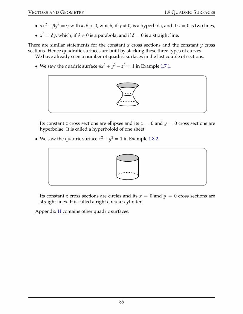
VECTORS AND GEOMETRY 1.9 QUADRIC SURFACES
• αx2´ βy2 = γ with α, β ą 0, which, if γ ‰ 0, is a hyperbola, and if γ = 0 is two lines,
• x2 = δy, which, if δ ‰ 0 is a parabola, and if δ = 0 is a straight line.
There are similar statements for the constant x cross sections and the constant y crosssections. Hence quadratic surfaces are built by stacking these three types of curves.
We have already seen a number of quadric surfaces in the last couple of sections.
• We saw the quadric surface 4x2 + y2 ´ z2 = 1 in Example 1.7.1.
Its constant z cross sections are ellipses and its x = 0 and y = 0 cross sections arehyperbolae. It is called a hyperboloid of one sheet.
• We saw the quadric surface x2 + y2 = 1 in Example 1.8.2.
Its constant z cross sections are circles and its x = 0 and y = 0 cross sections arestraight lines. It is called a right circular cylinder.
Appendix H contains other quadric surfaces.
86
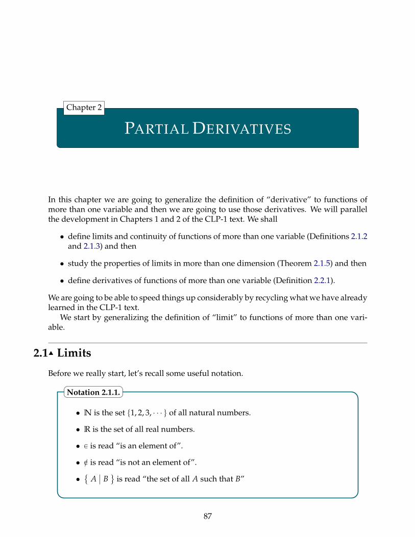
PARTIAL DERIVATIVES
Chapter 2
In this chapter we are going to generalize the definition of “derivative” to functions ofmore than one variable and then we are going to use those derivatives. We will parallelthe development in Chapters 1 and 2 of the CLP-1 text. We shall
• define limits and continuity of functions of more than one variable (Definitions 2.1.2and 2.1.3) and then
• study the properties of limits in more than one dimension (Theorem 2.1.5) and then
• define derivatives of functions of more than one variable (Definition 2.2.1).
We are going to be able to speed things up considerably by recycling what we have alreadylearned in the CLP-1 text.
We start by generalizing the definition of “limit” to functions of more than one vari-able.
2.1IJ Limits
Before we really start, let’s recall some useful notation.
• N is the set t1, 2, 3, ¨ ¨ ¨ u of all natural numbers.
• R is the set of all real numbers.
• P is read “is an element of”.
• R is read “is not an element of”.
•
Aˇ
B(
is read “the set of all A such that B”
Notation 2.1.1.
87
PARTIAL DERIVATIVES 2.1 LIMITS
• If S is a set and T is a subset of S, then SzT is
x P Sˇ
x R T(
, the set S withthe elements of T removed. In particular, if S is a set and a is an element ofS, then Sztau =
x P Sˇ
x ‰ a(
is the set S with the element a removed.
• If n is a natural number, Rn is used for both the set of n-component vectors〈x1, x2, ¨ ¨ ¨ , xn〉 and the set of points (x1, x2, ¨ ¨ ¨ , xn) with n coordinates.
• If S and T are sets, then f : S Ñ T means that f is a function which assignsto each element of S an element of T. The set S is called the domain of f .
• [a, b] =
x P Rˇ
a ď x ď b(
(a, b] =
x P Rˇ
a ă x ď b(
[a, b) =
x P Rˇ
a ď x ă b(
(a, b) =
x P Rˇ
a ă x ă b(
Notation 2.1.1 (continued).
The definition of the limit of a function of more than one variable looks just like thedefinition1 of the limit of a function of one variable. Very roughly speaking
limxÑa
f (x) = L
if f (x) approaches L whenever x approaches a. Here is a more careful definition of limit.
Let
˝ m and n be natural numbers2
˝ a P Rm
˝ the function f (x) be defined for all x near3 a and take values in Rn
˝ L P Rn
We write
limxÑa
f (x) = L
if4 the value of the function f (x) is sure to be arbitrarily close to L whenever thevalue of x is close enough to a, without5 being exactly a.
Definition 2.1.2 (Limit).
1 Definition 1.3.3 in the CLP-1 text.2 In this text, we will interested in m, n P
1, 2, 3
(, but the definition works for all natural numbers m, n.
3 To be precise, there is a number r ą 0 such that f (x) is defined for all x obeying |x´ a| ă r.4 There is a precise, formal version of this definition that looks just like Definition 1.7.1 of the CLP-1 text.5 You may find the condition “without being exactly a” a little strange, but there is a good reason for it,
which we have already seen in Calculus I. In the definition f 1(x) = limxÑa
f (x)´ f (a)x´a , the function whose
limit is being taken, namely f (x)´ f (a)x´a , is not defined at all at x = a. This will again happen when we
define derivatives of functions of more than one variable.
88
PARTIAL DERIVATIVES 2.1 LIMITS
Now that we have extended the definition of limit, we can extend the definition of conti-nuity.
Let
˝ m and n be natural numbers˝ a P Rm
˝ the function f (x) be defined for all x near a and take values in Rn
(a) The function f is continuous at a point a if
limxÑa
f (x) = f (a)
(b) The function f is continuous on a set D if it is continuous at every point of D.
Definition 2.1.3 (Continuity).
Here are a few very simple examples. There will be some more substantial exampleslater — after, as we did in the CLP-1 text, we build some tools that can be used to buildcomplicated limits from simpler ones.
Example 2.1.4
(a) If f (x, y) is the constant function which always takes the value L, then
lim(x,y)Ñ(a,b)
f (x, y) = L
(b) If f : R2 Ñ R2 is defined by f (x, y) = (x, y), then
lim(x,y)Ñ(a,b)
f (x, y) = (a, b)
(c) By definition, as (x, y) approaches (a, b), x approaches a and y approaches b, so that iff : R2 Ñ R is defined by f (x, y) = x, then
lim(x,y)Ñ(a,b)
f (x, y) = a
Similarly, if g : R2 Ñ R is defined by g(x, y) = y, then
lim(x,y)Ñ(a,b)
g(x, y) = b
Example 2.1.4
89
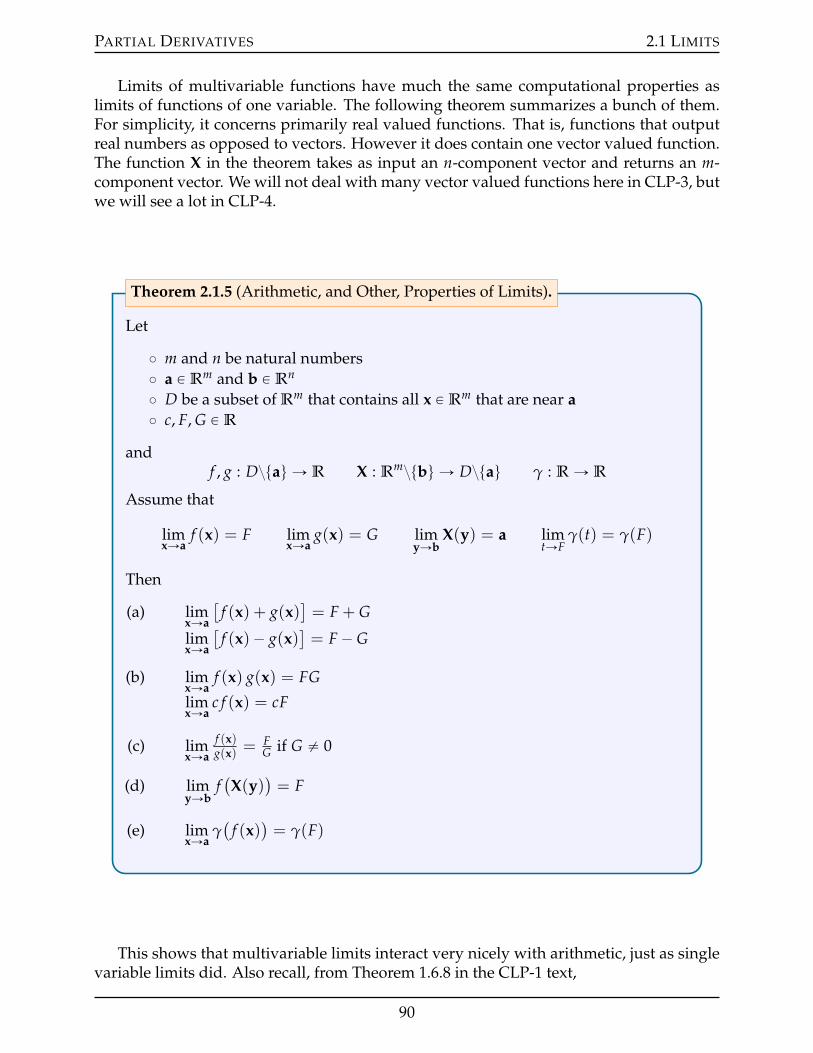
PARTIAL DERIVATIVES 2.1 LIMITS
Limits of multivariable functions have much the same computational properties aslimits of functions of one variable. The following theorem summarizes a bunch of them.For simplicity, it concerns primarily real valued functions. That is, functions that outputreal numbers as opposed to vectors. However it does contain one vector valued function.The function X in the theorem takes as input an n-component vector and returns an m-component vector. We will not deal with many vector valued functions here in CLP-3, butwe will see a lot in CLP-4.
Let
˝ m and n be natural numbers˝ a P Rm and b P Rn
˝ D be a subset of Rm that contains all x P Rm that are near a˝ c, F, G P R
andf , g : Dztau Ñ R X : Rmztbu Ñ Dztau γ : R Ñ R
Assume that
limxÑa
f (x) = F limxÑa
g(x) = G limyÑb
X(y) = a limtÑF
γ(t) = γ(F)
Then
(a) limxÑa
[f (x) + g(x)
]= F + G
limxÑa
[f (x)´ g(x)
]= F´ G
(b) limxÑa
f (x) g(x) = FG
limxÑa
c f (x) = cF
(c) limxÑa
f (x)g(x) =
FG if G ‰ 0
(d) limyÑb
f(X(y)
)= F
(e) limxÑa
γ(
f (x))= γ(F)
Theorem 2.1.5 (Arithmetic, and Other, Properties of Limits).
This shows that multivariable limits interact very nicely with arithmetic, just as singlevariable limits did. Also recall, from Theorem 1.6.8 in the CLP-1 text,
90
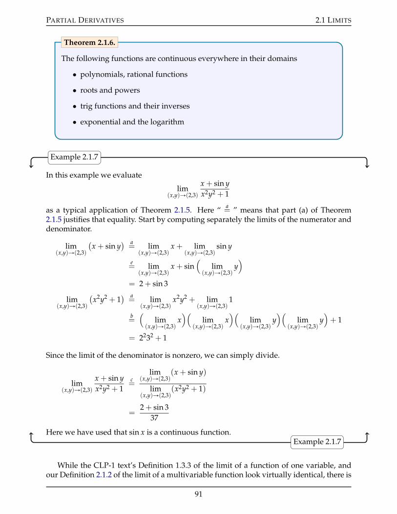
PARTIAL DERIVATIVES 2.1 LIMITS
The following functions are continuous everywhere in their domains
• polynomials, rational functions
• roots and powers
• trig functions and their inverses
• exponential and the logarithm
Theorem 2.1.6.
Example 2.1.7
In this example we evaluate
lim(x,y)Ñ(2,3)
x + sin yx2y2 + 1
as a typical application of Theorem 2.1.5. Here “ a= ” means that part (a) of Theorem
2.1.5 justifies that equality. Start by computing separately the limits of the numerator anddenominator.
lim(x,y)Ñ(2,3)
(x + sin y
) a= lim
(x,y)Ñ(2,3)x + lim
(x,y)Ñ(2,3)sin y
e= lim
(x,y)Ñ(2,3)x + sin
(lim
(x,y)Ñ(2,3)y)
= 2 + sin 3
lim(x,y)Ñ(2,3)
(x2y2 + 1
) a= lim
(x,y)Ñ(2,3)x2y2 + lim
(x,y)Ñ(2,3)1
b=(
lim(x,y)Ñ(2,3)
x)(
lim(x,y)Ñ(2,3)
x)(
lim(x,y)Ñ(2,3)
y)(
lim(x,y)Ñ(2,3)
y)+ 1
= 2232 + 1
Since the limit of the denominator is nonzero, we can simply divide.
lim(x,y)Ñ(2,3)
x + sin yx2y2 + 1
c=
lim(x,y)Ñ(2,3)
(x + sin y)
lim(x,y)Ñ(2,3)
(x2y2 + 1)
=2 + sin 3
37
Here we have used that sin x is a continuous function.Example 2.1.7
While the CLP-1 text’s Definition 1.3.3 of the limit of a function of one variable, andour Definition 2.1.2 of the limit of a multivariable function look virtually identical, there is
91
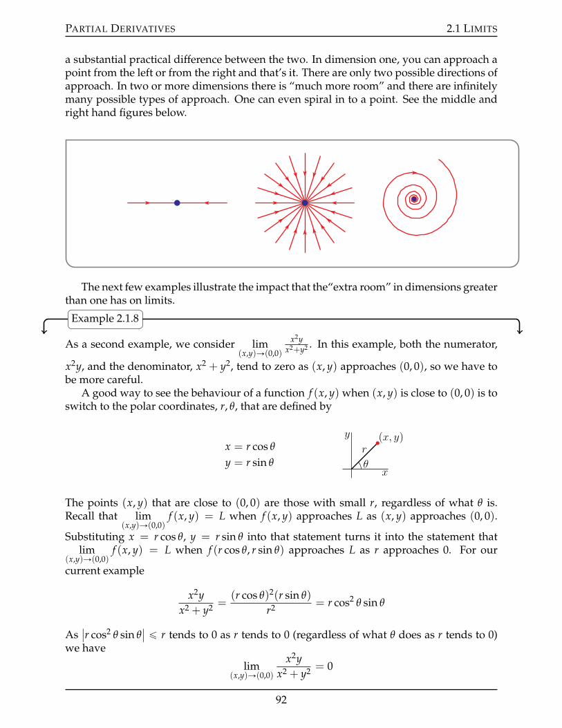
PARTIAL DERIVATIVES 2.1 LIMITS
a substantial practical difference between the two. In dimension one, you can approach apoint from the left or from the right and that’s it. There are only two possible directions ofapproach. In two or more dimensions there is “much more room” and there are infinitelymany possible types of approach. One can even spiral in to a point. See the middle andright hand figures below.
The next few examples illustrate the impact that the“extra room” in dimensions greaterthan one has on limits.
Example 2.1.8
As a second example, we consider lim(x,y)Ñ(0,0)
x2yx2+y2 . In this example, both the numerator,
x2y, and the denominator, x2 + y2, tend to zero as (x, y) approaches (0, 0), so we have tobe more careful.
A good way to see the behaviour of a function f (x, y) when (x, y) is close to (0, 0) is toswitch to the polar coordinates, r, θ, that are defined by
x = r cos θ
x
y px, yqr
θy = r sin θ
The points (x, y) that are close to (0, 0) are those with small r, regardless of what θ is.Recall that lim
(x,y)Ñ(0,0)f (x, y) = L when f (x, y) approaches L as (x, y) approaches (0, 0).
Substituting x = r cos θ, y = r sin θ into that statement turns it into the statement thatlim
(x,y)Ñ(0,0)f (x, y) = L when f (r cos θ, r sin θ) approaches L as r approaches 0. For our
current example
x2yx2 + y2 =
(r cos θ)2(r sin θ)
r2 = r cos2 θ sin θ
Asˇr cos2 θ sin θ
ˇ ď r tends to 0 as r tends to 0 (regardless of what θ does as r tends to 0)we have
lim(x,y)Ñ(0,0)
x2yx2 + y2 = 0
92

PARTIAL DERIVATIVES 2.1 LIMITS
Example 2.1.8
Example 2.1.9
As a third example, we consider lim(x,y)Ñ(0,0)
x2´y2
x2+y2 . Once again, the best way to see the be-
haviour of f (x, y) = x2´y2
x2+y2 for (x, y) close to (0, 0) is to switch to polar coordinates.
f (x, y) =x2 ´ y2
x2 + y2 =(r cos θ)2 ´ (r sin θ)2
r2 = cos2 θ ´ sin2 θ = cos(2θ)
Note that, this time, f is independent of r but does depend on θ. Here is a greatly magni-fied sketch of a number of level curves for f (x, y).
f“cosp90˝q“0
f“cosp0q“1
f“cosp30˝q“?32
f“cosp60˝q“12
f“cosp135˝q“´1?2
f“cosp180˝q“´1
r “ 10´137
Observe that
˝ as (x, y) approaches (0, 0) along the ray with 2θ = 30˝, f (x, y) approaches the value?
32 (and in fact f (x, y) takes the value cos(30˝) =
?3
2 at every point of that ray)
˝ as (x, y) approaches (0, 0) along the ray with 2θ = 60˝, f (x, y) approaches the value12 (and in fact f (x, y) takes the value cos(60˝) = 1
2 at every point of that ray)
˝ as (x, y) approaches (0, 0) along the ray with 2θ = 90˝, f (x, y) approaches the value0 (and in fact f (x, y) takes the value cos(90˝) = 0 at every point of that ray)
˝ and so on
So there is not single number L such that f (x, y) approaches L as r = |(x, y)| Ñ 0, no
matter what the direction of approach is. The limit lim(x,y)Ñ(0,0)
x2´y2
x2+y2 does not exist.
Here is another way to come to the same conclusion.
˝ Pick any really small positive number. We’ll use 10´137 as an example.
˝ Pick any real number F between ´1 and 1. We’ll use F =?
32 as an example.
93
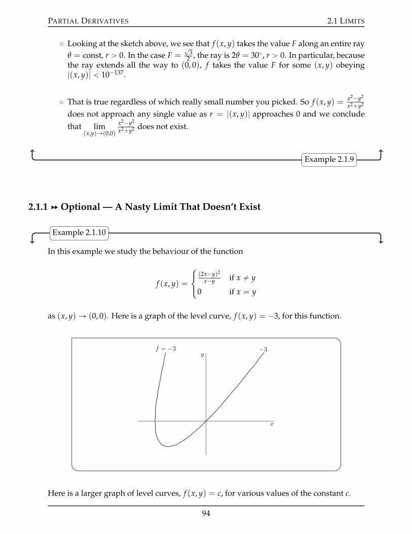
PARTIAL DERIVATIVES 2.1 LIMITS
˝ Looking at the sketch above, we see that f (x, y) takes the value F along an entire rayθ = const, r ą 0. In the case F =
?3
2 , the ray is 2θ = 30˝, r ą 0. In particular, becausethe ray extends all the way to (0, 0), f takes the value F for some (x, y) obeying|(x, y)| ă 10´137.
˝ That is true regardless of which really small number you picked. So f (x, y) = x2´y2
x2+y2
does not approach any single value as r = |(x, y)| approaches 0 and we conclude
that lim(x,y)Ñ(0,0)
x2´y2
x2+y2 does not exist.
Example 2.1.9
2.1.1 §§ Optional — A Nasty Limit That Doesn’t Exist
Example 2.1.10
In this example we study the behaviour of the function
f (x, y) =
$&%
(2x´y)2
x´y if x ‰ y
0 if x = y
as (x, y)Ñ (0, 0). Here is a graph of the level curve, f (x, y) = ´3, for this function.
y
x
´3f “ ´3
Here is a larger graph of level curves, f (x, y) = c, for various values of the constant c.
94
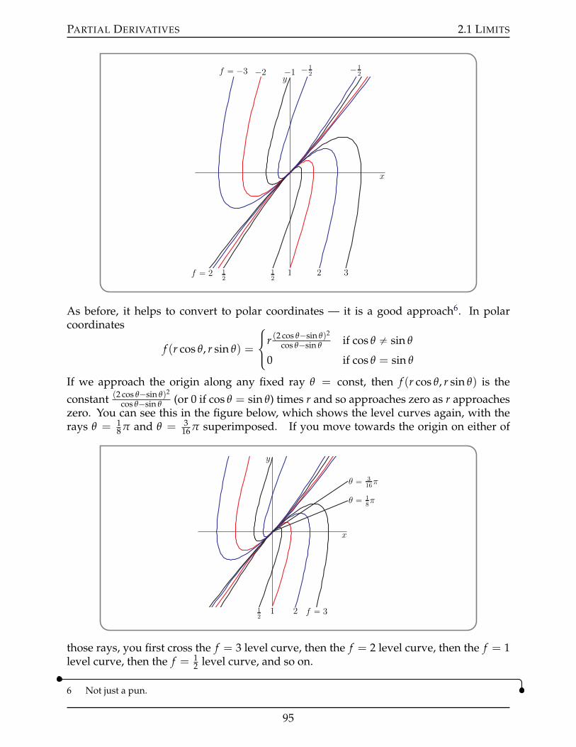
PARTIAL DERIVATIVES 2.1 LIMITS
y
x
1
´1
2f “ 2
´2
3
f “ ´3
12
12
´12
´12
As before, it helps to convert to polar coordinates — it is a good approach6. In polarcoordinates
f (r cos θ, r sin θ) =
$&%
r (2 cos θ´sin θ)2
cos θ´sin θ if cos θ ‰ sin θ
0 if cos θ = sin θ
If we approach the origin along any fixed ray θ = const, then f (r cos θ, r sin θ) is the
constant (2 cos θ´sin θ)2
cos θ´sin θ (or 0 if cos θ = sin θ) times r and so approaches zero as r approacheszero. You can see this in the figure below, which shows the level curves again, with therays θ = 1
8 π and θ = 316 π superimposed. If you move towards the origin on either of
y
x
1 2 f “ 312
θ “ 316π
θ “ 18π
those rays, you first cross the f = 3 level curve, then the f = 2 level curve, then the f = 1level curve, then the f = 1
2 level curve, and so on.
6 Not just a pun.
95
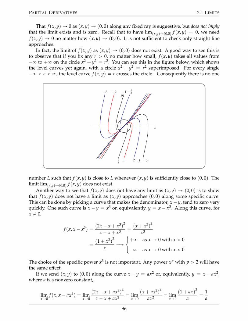
PARTIAL DERIVATIVES 2.1 LIMITS
That f (x, y) Ñ 0 as (x, y) Ñ (0, 0) along any fixed ray is suggestive, but does not implythat the limit exists and is zero. Recall that to have lim(x,y)Ñ(0,0) f (x, y) = 0, we needf (x, y) Ñ 0 no matter how (x, y) Ñ (0, 0). It is not sufficient to check only straight lineapproaches.
In fact, the limit of f (x, y) as (x, y) Ñ (0, 0) does not exist. A good way to see this isto observe that if you fix any r ą 0, no matter how small, f (x, y) takes all values from´8 to +8 on the circle x2 + y2 = r2. You can see this in the figure below, which showsthe level curves yet again, with a circle x2 + y2 = r2 superimposed. For every single´8 ă c ă 8, the level curve f (x, y) = c crosses the circle. Consequently there is no one
y
x
1
´1
2
´2
f “ 3
´3
12
´12
number L such that f (x, y) is close to L whenever (x, y) is sufficiently close to (0, 0). Thelimit lim(x,y)Ñ(0,0) f (x, y) does not exist.
Another way to see that f (x, y) does not have any limit as (x, y) Ñ (0, 0) is to showthat f (x, y) does not have a limit as (x, y) approaches (0, 0) along some specific curve.This can be done by picking a curve that makes the denominator, x´ y, tend to zero veryquickly. One such curve is x ´ y = x3 or, equivalently, y = x ´ x3. Along this curve, forx ‰ 0,
f (x, x´ x3) =(2x´ x + x3)
2
x´ x + x3 =(x + x3)
2
x3
=(1 + x2)
2
xÝÑ
$&%+8 as x Ñ 0 with x ą 0
´8 as x Ñ 0 with x ă 0
The choice of the specific power x3 is not important. Any power xp with p ą 2 will havethe same effect.
If we send (x, y) to (0, 0) along the curve x ´ y = ax2 or, equivalently, y = x ´ ax2,where a is a nonzero constant,
limxÑ0
f (x, x´ ax2) = limxÑ0
(2x´ x + ax2)2
x´ x + ax2 = limxÑ0
(x + ax2)2
ax2 = limxÑ0
(1 + ax)2
a=
1a
96
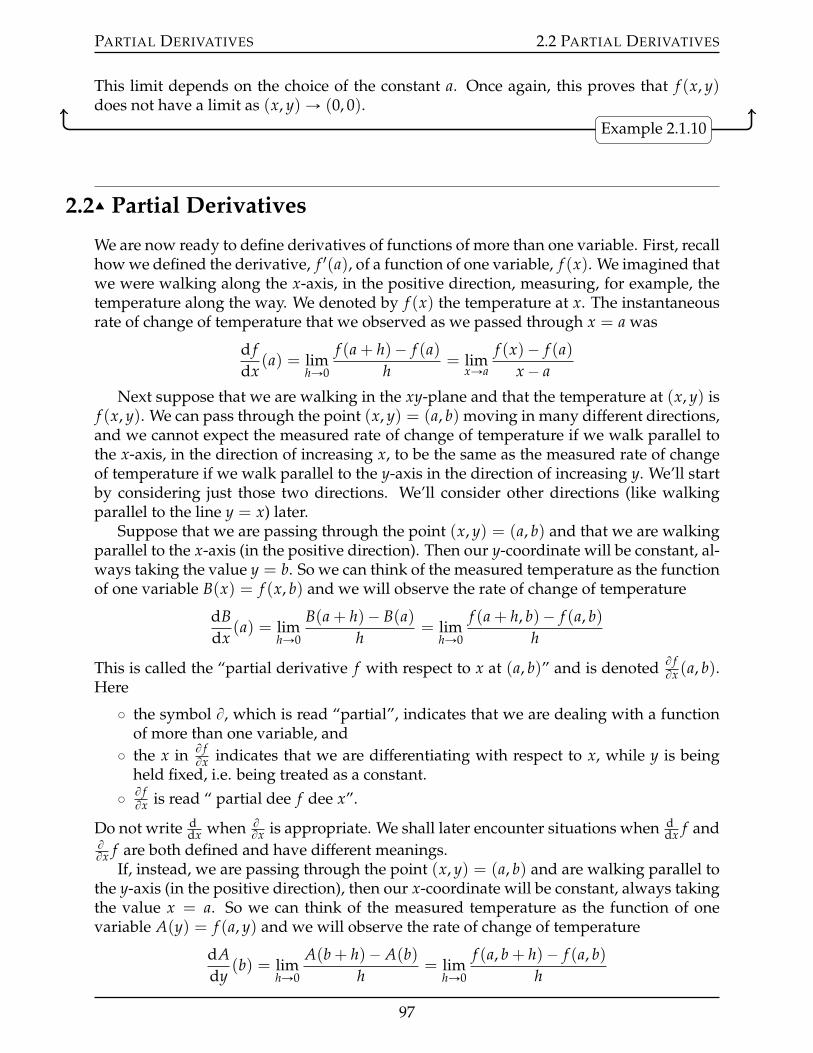
PARTIAL DERIVATIVES 2.2 PARTIAL DERIVATIVES
This limit depends on the choice of the constant a. Once again, this proves that f (x, y)does not have a limit as (x, y)Ñ (0, 0).
Example 2.1.10
2.2IJ Partial Derivatives
We are now ready to define derivatives of functions of more than one variable. First, recallhow we defined the derivative, f 1(a), of a function of one variable, f (x). We imagined thatwe were walking along the x-axis, in the positive direction, measuring, for example, thetemperature along the way. We denoted by f (x) the temperature at x. The instantaneousrate of change of temperature that we observed as we passed through x = a was
d fdx
(a) = limhÑ0
f (a + h)´ f (a)h
= limxÑa
f (x)´ f (a)x´ a
Next suppose that we are walking in the xy-plane and that the temperature at (x, y) isf (x, y). We can pass through the point (x, y) = (a, b) moving in many different directions,and we cannot expect the measured rate of change of temperature if we walk parallel tothe x-axis, in the direction of increasing x, to be the same as the measured rate of changeof temperature if we walk parallel to the y-axis in the direction of increasing y. We’ll startby considering just those two directions. We’ll consider other directions (like walkingparallel to the line y = x) later.
Suppose that we are passing through the point (x, y) = (a, b) and that we are walkingparallel to the x-axis (in the positive direction). Then our y-coordinate will be constant, al-ways taking the value y = b. So we can think of the measured temperature as the functionof one variable B(x) = f (x, b) and we will observe the rate of change of temperature
dBdx
(a) = limhÑ0
B(a + h)´ B(a)h
= limhÑ0
f (a + h, b)´ f (a, b)h
This is called the “partial derivative f with respect to x at (a, b)” and is denoted B fBx (a, b).
Here
˝ the symbol B, which is read “partial”, indicates that we are dealing with a functionof more than one variable, and
˝ the x in B fBx indicates that we are differentiating with respect to x, while y is being
held fixed, i.e. being treated as a constant.˝ B fBx is read “ partial dee f dee x”.
Do not write ddx when B
Bx is appropriate. We shall later encounter situations when ddx f and
BBx f are both defined and have different meanings.
If, instead, we are passing through the point (x, y) = (a, b) and are walking parallel tothe y-axis (in the positive direction), then our x-coordinate will be constant, always takingthe value x = a. So we can think of the measured temperature as the function of onevariable A(y) = f (a, y) and we will observe the rate of change of temperature
dAdy
(b) = limhÑ0
A(b + h)´ A(b)h
= limhÑ0
f (a, b + h)´ f (a, b)h
97
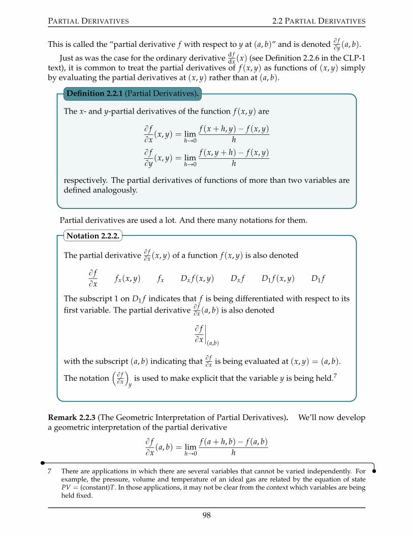
PARTIAL DERIVATIVES 2.2 PARTIAL DERIVATIVES
This is called the “partial derivative f with respect to y at (a, b)” and is denoted B fBy (a, b).
Just as was the case for the ordinary derivative d fdx (x) (see Definition 2.2.6 in the CLP-1
text), it is common to treat the partial derivatives of f (x, y) as functions of (x, y) simplyby evaluating the partial derivatives at (x, y) rather than at (a, b).
The x- and y-partial derivatives of the function f (x, y) are
B fBx
(x, y) = limhÑ0
f (x + h, y)´ f (x, y)h
B fBy
(x, y) = limhÑ0
f (x, y + h)´ f (x, y)h
respectively. The partial derivatives of functions of more than two variables aredefined analogously.
Definition 2.2.1 (Partial Derivatives).
Partial derivatives are used a lot. And there many notations for them.
The partial derivative B fBx (x, y) of a function f (x, y) is also denoted
B fBx
fx(x, y) fx Dx f (x, y) Dx f D1 f (x, y) D1 f
The subscript 1 on D1 f indicates that f is being differentiated with respect to itsfirst variable. The partial derivative B f
Bx (a, b) is also denoted
B fBx
ˇˇ(a,b)
with the subscript (a, b) indicating that B fBx is being evaluated at (x, y) = (a, b).
The notation(B fBx
)y
is used to make explicit that the variable y is being held.7
Notation 2.2.2.
Remark 2.2.3 (The Geometric Interpretation of Partial Derivatives). We’ll now developa geometric interpretation of the partial derivative
B fBx
(a, b) = limhÑ0
f (a + h, b)´ f (a, b)h
7 There are applications in which there are several variables that cannot be varied independently. Forexample, the pressure, volume and temperature of an ideal gas are related by the equation of statePV = (constant)T. In those applications, it may not be clear from the context which variables are beingheld fixed.
98
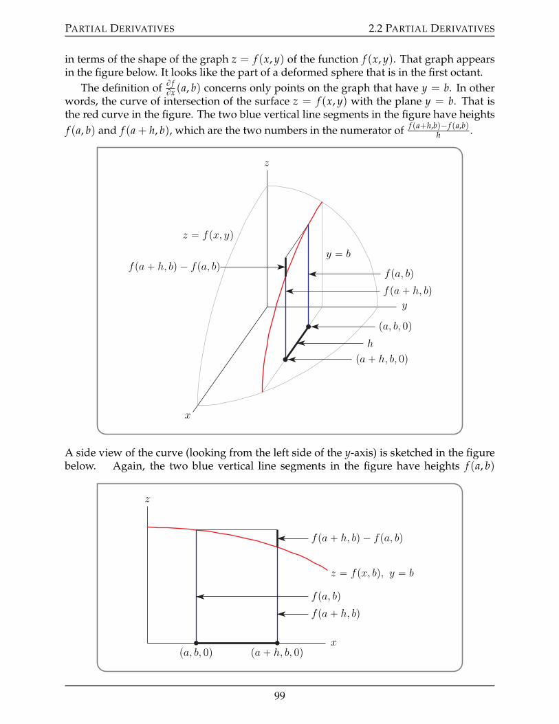
PARTIAL DERIVATIVES 2.2 PARTIAL DERIVATIVES
in terms of the shape of the graph z = f (x, y) of the function f (x, y). That graph appearsin the figure below. It looks like the part of a deformed sphere that is in the first octant.
The definition of B fBx (a, b) concerns only points on the graph that have y = b. In other
words, the curve of intersection of the surface z = f (x, y) with the plane y = b. That isthe red curve in the figure. The two blue vertical line segments in the figure have heightsf (a, b) and f (a + h, b), which are the two numbers in the numerator of f (a+h,b)´ f (a,b)
h .
z
y
x
z “ fpx, yqy “ b
h
fpa, bqfpa ` h, bq
pa, b, 0q
pa ` h, b, 0q
fpa ` h, bq ´ fpa, bq
A side view of the curve (looking from the left side of the y-axis) is sketched in the figurebelow. Again, the two blue vertical line segments in the figure have heights f (a, b)
z
x
z “ fpx, bq, y “ b
fpa, bqfpa ` h, bq
pa, b, 0q pa ` h, b, 0q
fpa ` h, bq ´ fpa, bq
99
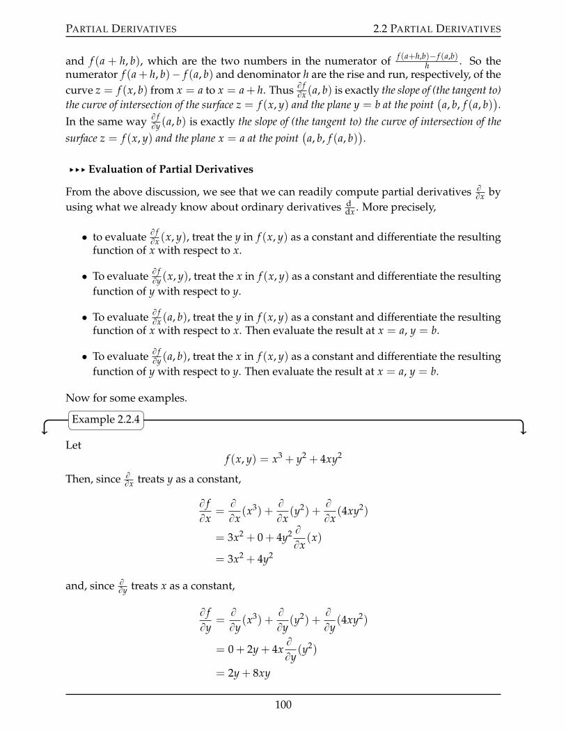
PARTIAL DERIVATIVES 2.2 PARTIAL DERIVATIVES
and f (a + h, b), which are the two numbers in the numerator of f (a+h,b)´ f (a,b)h . So the
numerator f (a + h, b)´ f (a, b) and denominator h are the rise and run, respectively, of thecurve z = f (x, b) from x = a to x = a+ h. Thus B f
Bx (a, b) is exactly the slope of (the tangent to)the curve of intersection of the surface z = f (x, y) and the plane y = b at the point
(a, b, f (a, b)
).
In the same way B fBy (a, b) is exactly the slope of (the tangent to) the curve of intersection of the
surface z = f (x, y) and the plane x = a at the point(a, b, f (a, b)
).
§§§ Evaluation of Partial Derivatives
From the above discussion, we see that we can readily compute partial derivatives BBx by
using what we already know about ordinary derivatives ddx . More precisely,
• to evaluate B fBx (x, y), treat the y in f (x, y) as a constant and differentiate the resulting
function of x with respect to x.
• To evaluate B fBy (x, y), treat the x in f (x, y) as a constant and differentiate the resulting
function of y with respect to y.
• To evaluate B fBx (a, b), treat the y in f (x, y) as a constant and differentiate the resulting
function of x with respect to x. Then evaluate the result at x = a, y = b.
• To evaluate B fBy (a, b), treat the x in f (x, y) as a constant and differentiate the resulting
function of y with respect to y. Then evaluate the result at x = a, y = b.
Now for some examples.
Example 2.2.4
Letf (x, y) = x3 + y2 + 4xy2
Then, since BBx treats y as a constant,
B fBx
=BBx
(x3) +BBx
(y2) +BBx
(4xy2)
= 3x2 + 0 + 4y2 BBx
(x)
= 3x2 + 4y2
and, since BBy treats x as a constant,
B fBy
=BBy
(x3) +BBy
(y2) +BBy
(4xy2)
= 0 + 2y + 4xBBy
(y2)
= 2y + 8xy
100
PARTIAL DERIVATIVES 2.2 PARTIAL DERIVATIVES
In particular, at (x, y) = (1, 0) these partial derivatives take the values
B fBx
(1, 0) = 3(1)2 + 4(0)2 = 3
B fBy
(1, 0) = 2(0) + 8(1)(0) = 0
Example 2.2.4
Example 2.2.5
Letf (x, y) = y cos x + xexy
Then, since BBx treats y as a constant, B
Bx eyx = yeyx and
B fBx
(x, y) = yBBx
(cos x) + exy BBx
(x) + xBBx(exy) (by the product rule)
= ´y sin x + exy + xyexy
B fBy
(x, y) = cos xBBy
(y) + xBBy(exy)
= cos x + x2exy
Example 2.2.5
Let’s move up to a function of four variables. Things generalize in a quite straight forwardway.
Example 2.2.6
Letf (x, y, z, t) = x sin(y + 2z) + t2e3y ln z
Then
B fBx
(x, y, z, t) = sin(y + 2z)
B fBy
(x, y, z, t) = x cos(y + 2z) + 3t2e3y ln z
B fBz
(x, y, z, t) = 2x cos(y + 2z) + t2e3y/z
B fBt
(x, y, z, t) = 2te3y ln z
Example 2.2.6
Now here is a more complicated example — our function takes a special value at (0, 0).To compute derivatives there we revert to the definition.
101
PARTIAL DERIVATIVES 2.2 PARTIAL DERIVATIVES
Example 2.2.7
Set
f (x, y) =
# cos x´cos yx´y if x ‰ y
0 if x = y
If b ‰ a, then for all (x, y) sufficiently close to (a, b), f (x, y) = cos x´cos yx´y and we can
compute the partial derivatives of f at (a, b) using the familiar rules of differentiation.However that is not the case for (a, b) = (0, 0). To evaluate fx(0, 0), we need to set y = 0and find the derivative of
f (x, 0) =
#cos x´1
x if x ‰ 00 if x = 0
with respect to x at x = 0. As we cannot use the usual differentiation rules, we evaluatethe derivative8 by applying the definition
fx(0, 0) = limhÑ0
f (h, 0)´ f (0, 0)h
= limhÑ0
cos h´1h ´ 0
h(Recall that h ‰ 0 in the limit.)
= limhÑ0
cos h´ 1h2
= limhÑ0
´ sin h2h
(By l’Hopital’s rule.)
= limhÑ0
´ cos h2
(By l’Hopital again.)
= ´12
We could also evaluate the limit of cos h´1h2 by substituting in the Taylor expansion
cos h = 1´ h2
2+
h4
4!´ ¨ ¨ ¨
We can also use Taylor expansions to understand the behaviour of f (x, y) for (x, y) near(0, 0). For x ‰ y,
cos x´ cos yx´ y
=
[1´ x2
2! +x4
4! ´ ¨ ¨ ¨]´[1´ y2
2! +y4
4! ´ ¨ ¨ ¨]
x´ y
=´ x2´y2
2! + x4´y4
4! ´ ¨ ¨ ¨x´ y
= ´ 12!
x2 ´ y2
x´ y+
14!
x4 ´ y4
x´ y´ ¨ ¨ ¨
= ´x + y2!
+x3 + x2y + xy2 + y3
4!´ ¨ ¨ ¨
8 It is also possible to evaluate the derivative by using the technique of the optional §2.15 in the CLP-1text.
102
PARTIAL DERIVATIVES 2.2 PARTIAL DERIVATIVES
So for (x, y) near (0, 0),
f (x, y) «#´ x+y
2 if x ‰ y0 if x = y
So it sure looks like (and in fact it is true that)
• f (x, y) is continuous at (0, 0) and
• f (x, y) is not continuous at (a, a) for small a ‰ 0 and
• fx(0, 0) = fy(0, 0) = ´12
Example 2.2.7
Example 2.2.8
Again set
f (x, y) =
# cos x´cos yx´y if x ‰ y
0 if x = y
We’ll now compute fy(x, y) for all (x, y).
The case y ‰ x: When y ‰ x,
fy(x, y) =BBy
cos x´ cos yx´ y
=(x´ y) B
By (cos x´ cos y)´ (cos x´ cos y) BBy (x´ y)
(x´ y)2 by the quotient rule
=(x´ y) sin y + cos x´ cos y
(x´ y)2
The case y = x: When y = x,
fy(x, y) = limhÑ0
f (x, y + h)´ f (x, y)h
= limhÑ0
f (x, x + h)´ f (x, x)h
= limhÑ0
cos x´cos(x+h)x´(x+h) ´ 0
h(Recall that h ‰ 0 in the limit.)
= limhÑ0
cos(x + h)´ cos xh2
Now we apply L’Hopital’s rule, remembering that, in this limit, x is a constant and h isthe variable — so we differentiate with respect to h.
fy(x, y) = limhÑ0
´ sin(x + h)2h
103
PARTIAL DERIVATIVES 2.2 PARTIAL DERIVATIVES
Note that if x is not an integer multiple of π, then the numerator ´ sin(x + h) does nottend to zero as h tends to zero, and the limit giving fy(x, y) does not exist. On the otherhand, if x is an integer multiple of π, both the numerator and denominator tend to zeroas h tends to zero, and we can apply L’Hopital’s rule a second time. Then
fy(x, y) = limhÑ0
´ cos(x + h)2
= ´cos x2
The conclusion:
fy(x, y) =
$’’&’’%
(x´y) sin y+cos x´cos y(x´y)2 if x ‰ y
´ cos x2 if x = y with x an integer multiple of π
DNE if x = y with x not an integer multiple of π
Example 2.2.8
Example 2.2.9 (Optional — A Little Weirdness)
In this example, we will see that the function
f (x, y) =
#x2
x´y if x ‰ y
0 if x = y
is not continuous at (0, 0) and yet has both partial derivatives fx(0, 0) and fy(0, 0) perfectlywell defined. We’ll also see how that is possible. First let’s compute the partial derivatives.By definition,
fx(0, 0) = limhÑ0
f (0 + h, 0)´ f (0, 0)h
= limhÑ0
hhkkikkjh2
h´0 ´ 0h
= limhÑ0
1
= 1
fy(0, 0) = limhÑ0
f (0, 0 + h)´ f (0, 0)h
= limhÑ0
02
0´h ´ 0h
= limhÑ0
0
= 0
So the first order partial derivatives fx(0, 0) and fy(0, 0) are perfectly well defined.To see that, nonetheless, f (x, y) is not continuous at (0, 0), we take the limit of f (x, y)
as (x, y) approaches (0, 0) along the curve y = x´ x3. The limit is
limxÑ0
f(x, x´ x3) = lim
xÑ0
x2
x´ (x´ x3)= lim
xÑ0
1x
which does not exist. Indeed as x approoaches 0 through positive numbers, 1x approaches
+8, and as x approoaches 0 through negative numbers, 1x approaches ´8.
104
PARTIAL DERIVATIVES 2.2 PARTIAL DERIVATIVES
So how is this possible? The answer is that fx(0, 0) only involves values of f (x, y)with y = 0. As f (x, 0) = x, for all values of x, we have that f (x, 0) is a continuous, andindeed a differentiable, function. Similarly, fy(0, 0) only involves values of f (x, y) withx = 0. As f (0, y) = 0, for all values of y, we have that f (0, y) is a continuous, and indeeda differentiable, function. On the other hand, the bad behaviour of f (x, y) for (x, y) near(0, 0) only happens for x and y both nonzero.
Example 2.2.9
Our next example uses implicit differentiation.
Example 2.2.10
The equationz5 + y2ez + e2x = 0
implicitly determines z as a function of x and y. That is, the function z(x, y) obeys
z(x, y)5 + y2ez(x,y) + e2x = 0
For example, when x = y = 0, the equation reduces to
z(0, 0)5 = ´1
which forces9 z(0, 0) = ´1. Let’s find the partial derivative BzBx (0, 0).
We are not going to be able to explicitly solve the equation for z(x, y). All we know isthat
z(x, y)5 + y2ez(x,y) + e2x = 0
for all x and y. We can turn this into an equation for BzBx (0, 0) by differentiating10 the whole
equation with respect to x, giving
5z(x, y)4 BzBx
(x, y) + y2ez(x,y) BzBx
(x, y) + 2e2x = 0
and then setting x = y = 0, giving
5z(0, 0)4 BzBx
(0, 0) + 2 = 0
As we already know that z(0, 0) = ´1,
BzBx
(0, 0) = ´ 25z(0, 0)4 = ´2
5
9 The only real number z which obeys z5 = ´1 is z = ´1. However there are four other complex numberswhich also obey z5 = ´1.
10 You should have already seen this technique, called implicit differentiation, in your first Calculuscourse. It is covered in Section 2.11 in the CLP-1 text.
105
PARTIAL DERIVATIVES 2.2 PARTIAL DERIVATIVES
Example 2.2.10
Next we have a partial derivative disguised as a limit.
Example 2.2.11
In this example we are going to evaluate the limit
limzÑ0
(x + y + z)3 ´ (x + y)3
(x + y)z
The critical observation is that, in taking the limit z Ñ 0, x and y are fixed. They do notchange as z is getting smaller and smaller. Furthermore this limit is exactly of the formof the limits in the Definition 2.2.1 of partial derivative, disguised by some obfuscatingchanges of notation.
Set
f (x, y, z) =(x + y + z)3
(x + y)
Then
limzÑ0
(x + y + z)3 ´ (x + y)3
(x + y)z= lim
zÑ0
f (x, y, z)´ f (x, y, 0)z
= limhÑ0
f (x, y, 0 + h)´ f (x, y, 0)h
=B fBz
(x, y, 0)
=
[ BBz
(x + y + z)3
x + y
]
z=0
Recalling that BBz treats x and y as constants, we are evaluating the derivative of a function
of the form (const+z)3
const . So
limzÑ0
(x + y + z)3 ´ (x + y)3
(x + y)z= 3
(x + y + z)2
x + y
ˇˇz=0
= 3(x + y)
Example 2.2.11
The next example highlights a potentially dangerous difference between ordinary andpartial derivatives.
Example 2.2.12
In this example we are going to see that, in contrast to the ordinary derivative case, BrBx is
not, in general, the same as(BxBr)´1.
Recall that Cartesian and polar coordinates11 (for (x, y) ‰ (0, 0) and r ą 0) are related
11 If you are not familiar with polar coordinates, don’t worry about it. There will be an introduction tothem in §3.2.1.
106
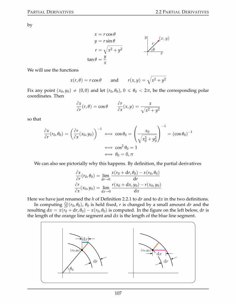
PARTIAL DERIVATIVES 2.2 PARTIAL DERIVATIVES
by
x = r cos θ
x
y px, yqr
θ
y = r sin θ
r =b
x2 + y2
tan θ =yx
We will use the functions
x(r, θ) = r cos θ and r(x, y) =b
x2 + y2
Fix any point (x0, y0) ‰ (0, 0) and let (r0, θ0), 0 ď θ0 ă 2π, be the corresponding polarcoordinates. Then
BxBr
(r, θ) = cos θBrBx
(x, y) =xa
x2 + y2
so that
BxBr
(r0, θ0) =
( BrBx
(x0, y0)
)´1
ðñ cos θ0 =
x0b
x20 + y2
0
´1
= (cos θ0)´1
ðñ cos2 θ0 = 1ðñ θ0 = 0, π
We can also see pictorially why this happens. By definition, the partial derivatives
BxBr
(r0, θ0) = limdrÑ0
x(r0 + dr, θ0)´ x(r0, θ0)
drBrBx
(x0, y0) = limdxÑ0
r(x0 + dx, y0)´ r(x0, y0)
dx
Here we have just renamed the h of Definition 2.2.1 to dr and to dx in the two definitions.In computing Bx
Br (r0, θ0), θ0 is held fixed, r is changed by a small amount dr and theresulting dx = x(r0 + dr, θ0)´ x(r0, θ0) is computed. In the figure on the left below, dr isthe length of the orange line segment and dx is the length of the blue line segment.
dr
θ0
dx
px0,y0q
dr
dxpx0,y0q
107
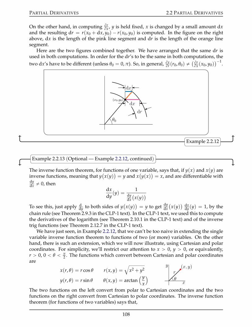
PARTIAL DERIVATIVES 2.2 PARTIAL DERIVATIVES
On the other hand, in computing BrBx , y is held fixed, x is changed by a small amount dx
and the resulting dr = r(x0 + dx, y0) ´ r(x0, y0) is computed. In the figure on the rightabove, dx is the length of the pink line segment and dr is the length of the orange linesegment.
Here are the two figures combined together. We have arranged that the same dr isused in both computations. In order for the dr’s to be the same in both computations, thetwo dx’s have to be different (unless θ0 = 0, π). So, in general, Bx
Br (r0, θ0) ‰(BrBx (x0, y0)
)´1.
dr
θ0
dx
dxpx0,y0q
Example 2.2.12
Example 2.2.13 (Optional — Example 2.2.12, continued)
The inverse function theorem, for functions of one variable, says that, if y(x) and x(y) areinverse functions, meaning that y
(x(y)
)= y and x
(y(x)
)= x, and are differentiable with
dydx ‰ 0, then
dxdy
(y) =1
dydx(x(y)
)
To see this, just apply ddy to both sides of y
(x(y)
)= y to get dy
dx(x(y)
) dxdy (y) = 1, by the
chain rule (see Theorem 2.9.3 in the CLP-1 text). In the CLP-1 text, we used this to computethe derivatives of the logarithm (see Theorem 2.10.1 in the CLP-1 text) and of the inversetrig functions (see Theorem 2.12.7 in the CLP-1 text).
We have just seen, in Example 2.2.12, that we can’t be too naive in extending the singlevariable inverse function theorem to functions of two (or more) variables. On the otherhand, there is such an extension, which we will now illustrate, using Cartesian and polarcoordinates. For simplicity, we’ll restrict our attention to x ą 0, y ą 0, or equivalently,r ą 0, 0 ă θ ă π
2 . The functions which convert between Cartesian and polar coordinatesare
x(r, θ) = r cos θ r(x, y) =b
x2 + y2
x
y px, yqr
θy(r, θ) = r sin θ θ(x, y) = arctan(y
x
)
The two functions on the left convert from polar to Cartesian coordinates and the twofunctions on the right convert from Cartesian to polar coordinates. The inverse functiontheorem (for functions of two variables) says that,
108
PARTIAL DERIVATIVES 2.2 PARTIAL DERIVATIVES
• if you form the first order partial derivatives of the left hand functions into the matrix[BxBr (r, θ) Bx
Bθ (r, θ)ByBr (r, θ) By
Bθ (r, θ)
]=
[cos θ ´r sin θ
sin θ r cos θ
]
• and you form the first order partial derivatives of the right hand functions into thematrix
[BrBx (x, y) Br
By (x, y)BθBx (x, y) Bθ
By (x, y)
]=
x?x2+y2
y?x2+y2
´y
x2
1+(yx )
2
1x
1+(yx )
2
=
x?x2+y2
y?x2+y2
´yx2+y2
xx2+y2
• and if you evaluate the second matrix at x = x(r, θ), y = y(r, θ),[BrBx(x(r, θ), y(r, θ)
)BrBy(x(r, θ), y(r, θ)
)
BθBx(x(r, θ), y(r, θ)
)BθBy(x(r, θ), y(r, θ)
)]=
[cos θ sin θ
´ sin θr
cos θr
]
• and if you multiply12 the two matrices together[BrBx(x(r, θ), y(r, θ)
)BrBy(x(r, θ), y(r, θ)
)
BθBx(x(r, θ), y(r, θ)
)BθBy(x(r, θ), y(r, θ)
)] [
BxBr (r, θ) Bx
Bθ (r, θ)ByBr (r, θ) By
Bθ (r, θ)
]
=
[cos θ sin θ
´ sin θr
cos θr
] [cos θ ´r sin θ
sin θ r cos θ
]
=
[(cos θ)(cos θ) + (sin θ)(sin θ) (cos θ)(´r sin θ) + (sin θ)(r cos θ)
(´ sin θr )(cos θ) + ( cos θ
r )(sin θ) (´ sin θr )(´r sin θ) + ( cos θ
r )(r cos θ)
]
• then the result is the identity matrix[
1 00 1
]
and indeed it is!
This two variable version of the inverse function theorem can be derived by applying thederivatives B
Br and BBθ to the equations
r(x(r, θ), y(r, θ)
)= r
θ(x(r, θ), y(r, θ)
)= θ
and using the two variable version of the chain rule, which we will see in §2.4.Example 2.2.13
12 Matrix multiplication is usually covered in courses on linear algebra, which you may or may not havetaken. That’s why this example is optional.
109
PARTIAL DERIVATIVES 2.3 HIGHER ORDER DERIVATIVES
2.3IJ Higher Order Derivatives
You have already observed, in your first Calculus course, that if f (x) is a function of x,then its derivative, d f
dx (x), is also a function of x, and can be differentiated to give the
second order derivative d2 fdx2 (x), which can in turn be differentiated yet again to give the
third order derivative, f (3)(x), and so on.We can do the same for functions of more than one variable. If f (x, y) is a function of x
and y, then both of its partial derivatives, B fBx (x, y) and B f
By (x, y) are also functions of x andy. They can both be differentiated with respect to x and they can both be differentiatedwith respect to y. So there are four possible second order derivatives. Here they are,together with various alternate notations.
BBx
(B fBx
)(x, y) =
B2 fBx2 (x, y) = fxx(x, y)
BBy
(B fBx
)(x, y) =
B2 fByBx
(x, y)= fxy(x, y)
BBx
(B fBy
)(x, y) =
B2 fBxBy
(x, y)= fyx(x, y)
BBy
(B fBy
)(x, y) =
B2 fBy2 (x, y) = fyy(x, y)
In B2 fBy Bx = B2
By Bx f , the derivative closest to f , in this case BBx , is applied first.
In fxy, the derivative with respect to the variable closest to f , in this case x, is applied first.
Example 2.3.1
Let f (x, y) = emy cos(nx). Then
fx = ´nemy sin(nx) fy = memy cos(nx)
fxx = ´n2emy cos(nx) fyx = ´mnemy sin(nx)
fxy = ´mnemy sin(nx) fyy = m2emy cos(nx)
Example 2.3.1
Example 2.3.2
Let f (x, y) = eαx+βy. Then
fx = αeαx+βy fy = βeαx+βy
fxx = α2eαx+βy fyx = βαeαx+βy
fxy = αβeαx+βy fyy = β2eαx+βy
110
PARTIAL DERIVATIVES 2.3 HIGHER ORDER DERIVATIVES
More generally, for any integers m, n ě 0,
Bm+n fBxm Byn = αmβneαx+βy
Example 2.3.2
Example 2.3.3
If f (x1, x2, x3, x4) = x41 x3
2 x23 x4, then
B4 fBx1 Bx2 Bx3 Bx4
=B3
Bx1 Bx2 Bx3
(x4
1 x32 x2
3
)
=B2
Bx1 Bx2
(2 x4
1 x32 x3
)
=BBx1
(6 x4
1 x22 x3
)
= 24 x31 x2
2 x3
and
B4 fBx4 Bx3 Bx2 Bx1
=B3
Bx4 Bx3 Bx2
(4x3
1 x32 x2
3 x4
)
=B2
Bx4 Bx3
(12 x3
1 x22 x2
3 x4
)
=BBx4
(24 x3
1 x22 x3 x4
)
= 24 x31 x2
2 x3
Example 2.3.3
Notice that in Example 2.3.1,
fxy = fyx = ´mnemy sin(nx)
and in Example 2.3.2fxy = fyx = αβeαx+βy
and in Example 2.3.3
B4 fBx1 Bx2 Bx3 Bx4
=B4 f
Bx4 Bx3 Bx2 Bx1= 24 x3
1 x22 x3
In all of these examples, it didn’t matter what order we took the derivatives in. The fol-lowing theorem13 shows that this was no accident.
13 The history of this important theorem is pretty convoluted. See “A note on the history of mixed partialderivatives” by Thomas James Higgins which was published in Scripta Mathematica 7 (1940), 59-62.
111
PARTIAL DERIVATIVES 2.3 HIGHER ORDER DERIVATIVES
If the partial derivatives B2 fBxBy and B2 f
ByBx exist and are continuous at (x0, y0), then
B2 fBxBy
(x0, y0) =B2 fByBx
(x0, y0)
Theorem 2.3.4 (Clairaut’s Theorem14 or Schwarz’s Theorem15).
2.3.1 §§ Optional — The Proof of Theorem 2.3.4
§§§ Outline
Here is an outline of the proof of Theorem 2.3.4. The (numbered) details are in the subsec-tion below. Fix real numbers x0 and y0 and define
F(h, k) =1hk[
f (x0 + h, y0 + k)´ f (x0, y0 + k)´ f (x0 + h, y0) + f (x0, y0)]
We define F(h, k) in this way because both partial derivatives B2 fBxBy (x0, y0) and B2 f
ByBx (x0, y0)
are limits of F(h, k) as h, k Ñ 0. Precisely, we show in item (1) in the details below that
BByB fBx
(x0, y0) = limkÑ0
limhÑ0
F(h, k)
BBxB fBy
(x0, y0) = limhÑ0
limkÑ0
F(h, k)
Note that the two right hand sides here are identical except for the order in which thelimits are taken.
Now, by the mean value theorem (four times),
F(h, k)(2)=
1h
[B fBy
(x0 + h, y0 + θ1k)´ B fBy
(x0, y0 + θ1k)]
(3)=BBxB fBy
(x0 + θ2h, y0 + θ1k)
F(h, k)(4)=
1k
[B fBx
(x0 + θ3h, y0 + k)´ B fBx
(x0 + θ3h, y0)
]
(5)=BByB fBx
(x0 + θ3h, y0 + θ4k)
for some numbers 0 ă θ1, θ2, θ3, θ4 ă 1. All of the numbers θ1, θ2, θ3, θ4 depend on x0, y0, h, k.Hence B
BxB fBy
(x0 + θ2h, y0 + θ1k) =BByB fBx
(x0 + θ3h, y0 + θ4k)
14 Alexis Clairaut (1713–1765) was a French mathematician, astronomer, and geophysicist.15 Hermann Schwarz (1843–1921) was a German mathematician.
112
PARTIAL DERIVATIVES 2.3 HIGHER ORDER DERIVATIVES
for all h and k. Taking the limit (h, k) Ñ (0, 0) and using the assumed continuity of bothpartial derivatives at (x0, y0) gives
lim(h,k)Ñ(0,0)
F(h, k) =BBxB fBy
(x0, y0) =BByB fBx
(x0, y0)
as desired. To complete the proof we just have to justify the details (1), (2), (3), (4) and (5).
§§§ The Details
(1) By definition,
BByB fBx
(x0, y0) = limkÑ0
1k
[B fBx
(x0, y0 + k)´ B fBx
(x0, y0)
]
= limkÑ0
1k
[limhÑ0
f (x0 + h, y0 + k)´ f (x0, y0 + k)h
´ limhÑ0
f (x0 + h, y0)´ f (x0, y0)
h
]
= limkÑ0
limhÑ0
f (x0 + h, y0 + k)´ f (x0, y0 + k)´ f (x0 + h, y0) + f (x0, y0)
hk= lim
kÑ0limhÑ0
F(h, k)
Similarly,
BBxB fBy
(x0, y0) = limhÑ0
1h
[B fBy
(x0 + h, y0)´ B fBy
(x0, y0)
]
= limhÑ0
1h
[limkÑ0
f (x0 + h, y0 + k)´ f (x0 + h, y0)
k´ lim
kÑ0
f (x0, y0 + k)´ f (x0, y0)
k
]
= limhÑ0
limkÑ0
f (x0 + h, y0 + k)´ f (x0 + h, y0)´ f (x0, y0 + k) + f (x0, y0)
hk= lim
hÑ0limkÑ0
F(h, k)
(2) The mean value theorem (Theorem 2.13.4 in the CLP-1 text) says that, for any differ-entiable function ϕ(x),
• the slope of the line joining the points(x0, ϕ(x0)
)and
(x0 + k, ϕ(x0 + k)
)on the
graph of ϕ
is the same as
• the slope of the tangent to the graph at some point between x0 and x0 + k.
That is, there is some 0 ă θ1 ă 1 such that
ϕ(x0 + k)´ ϕ(x0)
k=
dϕ
dx(x0 + θ1k)
113
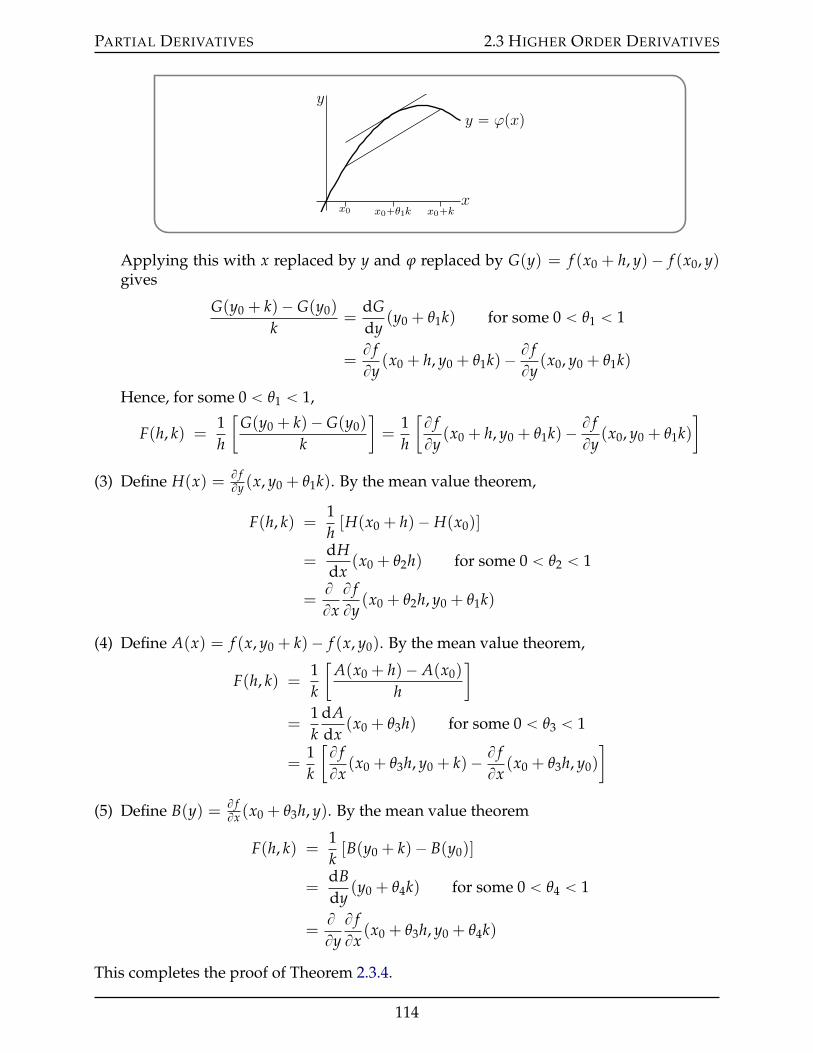
PARTIAL DERIVATIVES 2.3 HIGHER ORDER DERIVATIVES
x
y
y “ ϕpxq
x0 x0`kx0`θ1k
Applying this with x replaced by y and ϕ replaced by G(y) = f (x0 + h, y)´ f (x0, y)gives
G(y0 + k)´ G(y0)
k=
dGdy
(y0 + θ1k) for some 0 ă θ1 ă 1
=B fBy
(x0 + h, y0 + θ1k)´ B fBy
(x0, y0 + θ1k)
Hence, for some 0 ă θ1 ă 1,
F(h, k) =1h
[G(y0 + k)´ G(y0)
k
]=
1h
[B fBy
(x0 + h, y0 + θ1k)´ B fBy
(x0, y0 + θ1k)]
(3) Define H(x) = B fBy (x, y0 + θ1k). By the mean value theorem,
F(h, k) =1h[H(x0 + h)´ H(x0)]
=dHdx
(x0 + θ2h) for some 0 ă θ2 ă 1
=BBxB fBy
(x0 + θ2h, y0 + θ1k)
(4) Define A(x) = f (x, y0 + k)´ f (x, y0). By the mean value theorem,
F(h, k) =1k
[A(x0 + h)´ A(x0)
h
]
=1k
dAdx
(x0 + θ3h) for some 0 ă θ3 ă 1
=1k
[B fBx
(x0 + θ3h, y0 + k)´ B fBx
(x0 + θ3h, y0)
]
(5) Define B(y) = B fBx (x0 + θ3h, y). By the mean value theorem
F(h, k) =1k[B(y0 + k)´ B(y0)]
=dBdy
(y0 + θ4k) for some 0 ă θ4 ă 1
=BByB fBx
(x0 + θ3h, y0 + θ4k)
This completes the proof of Theorem 2.3.4.
114
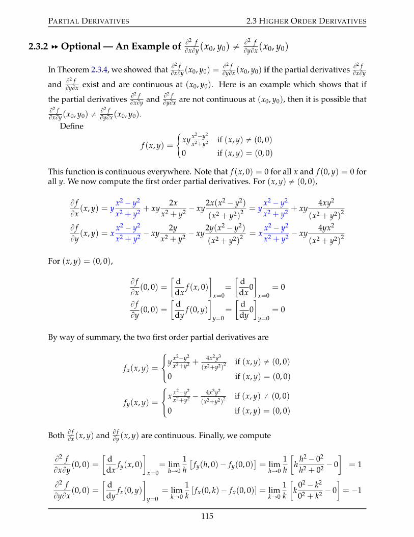
PARTIAL DERIVATIVES 2.3 HIGHER ORDER DERIVATIVES
2.3.2 §§ Optional — An Example of B2 fBxBy(x0, y0) ‰ B2 f
ByBx(x0, y0)
In Theorem 2.3.4, we showed that B2 fBxBy (x0, y0) =
B2 fByBx (x0, y0) if the partial derivatives B2 f
BxBy
and B2 fByBx exist and are continuous at (x0, y0). Here is an example which shows that if
the partial derivatives B2 fBxBy and B2 f
ByBx are not continuous at (x0, y0), then it is possible thatB2 fBxBy (x0, y0) ‰ B2 f
ByBx (x0, y0).Define
f (x, y) =
#xy x2´y2
x2+y2 if (x, y) ‰ (0, 0)
0 if (x, y) = (0, 0)
This function is continuous everywhere. Note that f (x, 0) = 0 for all x and f (0, y) = 0 forall y. We now compute the first order partial derivatives. For (x, y) ‰ (0, 0),
B fBx
(x, y) = yx2 ´ y2
x2 + y2 + xy2x
x2 + y2 ´ xy2x(x2 ´ y2)
(x2 + y2)2 = yx2 ´ y2
x2 + y2 + xy4xy2
(x2 + y2)2
B fBy
(x, y) = xx2 ´ y2
x2 + y2 ´ xy2y
x2 + y2 ´ xy2y(x2 ´ y2)
(x2 + y2)2 = xx2 ´ y2
x2 + y2 ´ xy4yx2
(x2 + y2)2
For (x, y) = (0, 0),
B fBx
(0, 0) =[
ddx
f (x, 0)]
x=0=
[ddx
0]
x=0= 0
B fBy
(0, 0) =[
ddy
f (0, y)]
y=0=
[ddy
0]
y=0= 0
By way of summary, the two first order partial derivatives are
fx(x, y) =
$&%
y x2´y2
x2+y2 +4x2y3
(x2+y2)2 if (x, y) ‰ (0, 0)
0 if (x, y) = (0, 0)
fy(x, y) =
$&%
x x2´y2
x2+y2 ´ 4x3y2
(x2+y2)2 if (x, y) ‰ (0, 0)
0 if (x, y) = (0, 0)
Both B fBx (x, y) and B f
By (x, y) are continuous. Finally, we compute
B2 fBxBy
(0, 0) =[
ddx
fy(x, 0)]
x=0= lim
hÑ0
1h[
fy(h, 0)´ fy(0, 0)]= lim
hÑ0
1h
[h
h2 ´ 02
h2 + 02 ´ 0]
= 1
B2 fByBx
(0, 0) =[
ddy
fx(0, y)]
y=0= lim
kÑ0
1k[ fx(0, k)´ fx(0, 0)] = lim
kÑ0
1k
[k
02 ´ k2
02 + k2 ´ 0]= ´1
115
PARTIAL DERIVATIVES 2.4 THE CHAIN RULE
2.4IJ The Chain Rule
You already routinely use the one dimensional chain rule
ddt
f(x(t)
)=
d fdx(x(t)
) dxdt
(t)
in doing computations likeddt
sin(t2) = cos(t2) 2t
In this example, f (x) = sin(x) and x(t) = t2.We now generalize the chain rule to functions of more than one variable. For con-
creteness, we concentrate on the case in which all functions are functions of two variables.That is, we find the partial derivatives BF
Bs and BFBt of a function F(s, t) that is defined as a
compositionF(s, t) = f
(x(s, t) , y(s, t)
)
We are using the name F for the new function F(s, t) as a reminder that it is closely relatedto, though not the same as, the function f (x, y). The partial derivative BF
Bs is the rate ofchange of F when s is varied with t held constant. When s is varied, both the x-argument,x(s, t), and the y-argument, y(s, t), in f
(x(s, t) , y(s, t)
)vary. Consequently, the chain rule
for f(x(s, t) , y(s, t)
)is a sum of two terms — one resulting from the variation of the x-
argument and the other resulting from the variation of the y-argument.
Assume that all first order partial derivatives of f (x, y), x(s, t) and y(s, t) existand are continuous. Then the same is true for F(s, t) = f
(x(s, t) , y(s, t)
)and
BFBs
(s, t) =B fBx(x(s, t) , y(s, t)
) BxBs
(s, t) +B fBy(x(s, t) , y(s, t)
) ByBs
(s, t)
BFBt
(s, t) =B fBx(x(s, t) , y(s, t)
) BxBt
(s, t) +B fBy(x(s, t) , y(s, t)
) ByBt
(s, t)
Theorem 2.4.1 (The Chain Rule).
We will give the proof of this theorem in §2.4.4, below. It is common to state this chainrule as
BFBs
=B fBxBxBs
+B fByByBs
BFBt
=B fBxBxBt
+B fByByBt
That is, it is common to suppress the function arguments. But you should make sure thatyou understand what the arguments are before doing so.
Theorem 2.4.1 is given for the case that F is the composition of a function of two vari-ables, f (x, y), with two functions, x(s, t) and y(s, t), of two variables each. There is nothingmagical about the number two. There are obvious variants for any numbers of variables.For example,
116
PARTIAL DERIVATIVES 2.4 THE CHAIN RULE
if F(t) = f(x(t), y(t), z(t)
), then
dFdt
(t) =B fBx(x(t) , y(t) , z(t)
) dxdt
(t) +B fBy(x(t) , y(t) , z(t)
) dydt
(t)
+B fBz(x(t) , y(t) , z(t)
) dzdt
(t)
Equation 2.4.2.
and
if F(s, t) = f(x(s, t)
), then
BFBt
(s, t) =d fdx(x(s, t)
) BxBt
(s, t)
Equation 2.4.3.
There will be a large number of examples shortly. First, here is a memory aid.
2.4.1 §§ Memory Aids for the Chain Rule
We recommend strongly that you use the following procedure, without leaving out anysteps, the first couple of dozen times that you use the chain rule.
Step 1 List explicitly all the functions involved and specify the arguments of each func-tion. Ensure that all different functions have different names. Invent new names forsome of the functions if necessary. In the case of the chain rule in Theorem 2.4.1, thelist would be
f (x, y) x(s, t) y(s, t) F(s, t) = f(x(s, t), y(s, t)
)
While the functions f and F are closely related, they are not the same. One is afunction of x and y while the other is a function of s and t.
Step 2 Write down the templateBFBs
=B fBs
Note that
• The function F appears once in the numerator on the left. The function f , fromwhich F is constructed by a change of variables, appears once in the numeratoron the right.• The variable in the denominator on the left appears once in the denominator on
the right.
Step 3 Fill in the blanks with every variable that makes sense. In particular, since f is afunction of x and y, it may only be differentiated with respect to x and y. So we addtogether two copies of our template — one for x and one for y:
BFBs
=B fBxBxBs
+B fByByBs
117
PARTIAL DERIVATIVES 2.4 THE CHAIN RULE
Note that x and y are functions of s so that the derivatives BxBs and By
Bs make sense.The first term, B f
BxBxBs , arises from the variation of x with respect to s and the second
term, B fByByBs , arises from the variation of y with respect to s.
Step 4 Put in the functional dependence explicitly. Fortunately, there is only one func-tional dependence that makes sense. The left hand side is a function of s and t.Hence the right hand side must also be a function of s and t. As f is a function of xand y, this is achieved by evaluating f at x = x(s, t) and y = y(s, t).
BFBs
(s, t) =B fBx(x(s, t), y(s, t)
)BxBs
(s, t) +B fBy(x(s, t), y(s, t)
)ByBs
(s, t)
If you fail to put in the arguments, or at least if you fail to remember what the argu-ments are, you may forget that B f
Bx and B fBy depend on s and t. Then, if you have to
compute a second derivative of F, you will probably fail to differentiate the factorsB fBx(x(s, t), y(s, t)
)and B f
By(x(s, t), y(s, t)
).
To help remember the formulae of Theorem 2.4.1, it is sometimes also useful to pretendthat our variables are physical quantities with f , F having units of grams, x, y having unitsof meters and s, t having units of seconds. Note that
• the left hand side, BFBs , has units grams per second.
• Each term on the right hand side contains the partial derivative of f with respectto a different independent variable. That independent variable appears once in thedenominator and once in the numerator, so that its units (in this case meters) cancelout. Thus both of the terms B f
BxBxBs and B f
ByByBs on the right hand side also have the units
grams per second.
• Hence both sides of the equation have the same units.
Here is a pictorial procedure that uses a tree diagram to help remember the chain ruleBBs f(x(s, t), y(s, t)
)= B f
BxBxBs +
B fByByBs . As in the figure on the left below,
˝ write, on the top row, “ f ”.˝ Write, on the middle row, each of the variables that the function f (x, y) depends on,
namely“x” and “y”.˝ Write, on the bottom row,
– below x, each of the variables that the function x(s, t) depends on, namely “s”and “t”, and
– below y, each of the variables that the function y(s, t) depends on, namely “s”and “t”.
˝ Draw a line joining each function with each of the variables that it depends on.˝ Then, as in the figure on the right below, write beside each line, the partial derivative
of the function at the top of the line with respect to the variable at the bottom of theline.
118
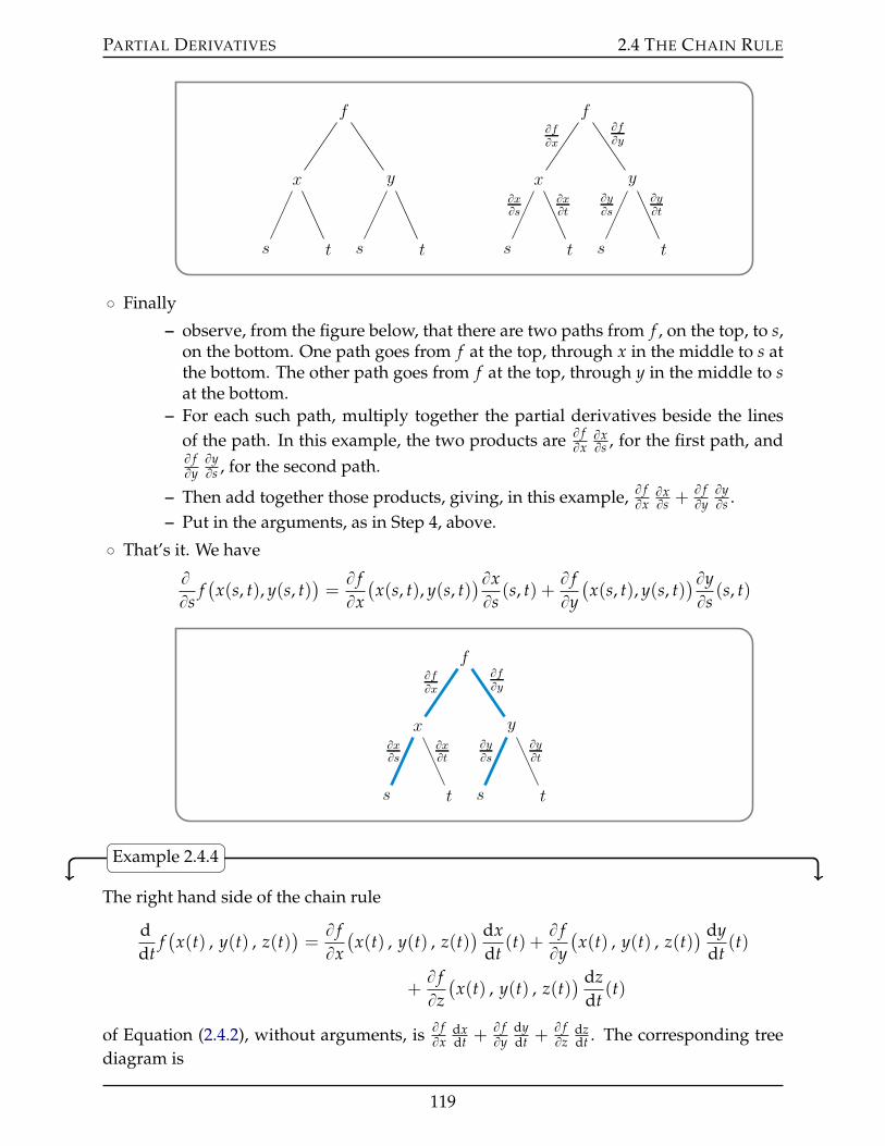
PARTIAL DERIVATIVES 2.4 THE CHAIN RULE
f
x y
s t s t
f
x y
s t s t
BfBx
BfBy
BxBt
ByBt
BxBs
ByBs
˝ Finally
– observe, from the figure below, that there are two paths from f , on the top, to s,on the bottom. One path goes from f at the top, through x in the middle to s atthe bottom. The other path goes from f at the top, through y in the middle to sat the bottom.
– For each such path, multiply together the partial derivatives beside the linesof the path. In this example, the two products are B f
BxBxBs , for the first path, and
B fByByBs , for the second path.
– Then add together those products, giving, in this example, B fBxBxBs +
B fByByBs .
– Put in the arguments, as in Step 4, above.
˝ That’s it. We have
BBs
f(x(s, t), y(s, t)
)=B fBx(x(s, t), y(s, t)
)BxBs
(s, t) +B fBy(x(s, t), y(s, t)
)ByBs
(s, t)
f
x y
s t s t
BfBx
BfBy
BxBs
ByBs
BxBt
ByBt
Example 2.4.4
The right hand side of the chain rule
ddt
f(x(t) , y(t) , z(t)
)=B fBx(x(t) , y(t) , z(t)
) dxdt
(t) +B fBy(x(t) , y(t) , z(t)
) dydt
(t)
+B fBz(x(t) , y(t) , z(t)
) dzdt
(t)
of Equation (2.4.2), without arguments, is B fBx
dxdt +
B fBy
dydt +
B fBz
dzdt . The corresponding tree
diagram is
119
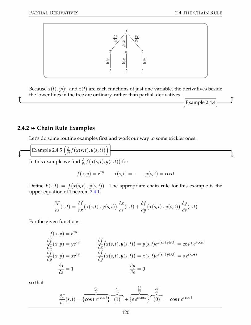
PARTIAL DERIVATIVES 2.4 THE CHAIN RULE
f
x y z
t t t
BfBx Bf
By
BfBz
dxdt
dydt
dzdt
Because x(t), y(t) and z(t) are each functions of just one variable, the derivatives besidethe lower lines in the tree are ordinary, rather than partial, derivatives.
Example 2.4.4
2.4.2 §§ Chain Rule Examples
Let’s do some routine examples first and work our way to some trickier ones.
Example 2.4.5(BBs f(x(s, t), y(s, t)
))
In this example we find BBs f(x(s, t), y(s, t)
)for
f (x, y) = exy x(s, t) = s y(s, t) = cos t
Define F(s, t) = f(x(s, t) , y(s, t)
). The appropriate chain rule for this example is the
upper equation of Theorem 2.4.1.
BFBs
(s, t) =B fBx(x(s, t) , y(s, t)
) BxBs
(s, t) +B fBy(x(s, t) , y(s, t)
) ByBs
(s, t)
For the given functions
f (x, y) = exy
B fBx
(x, y) = yexy B fBx(x(s, t), y(s, t)
)= y(s, t)ex(s,t) y(s,t) = cos t es cos t
B fBy
(x, y) = xexy B fBy(x(s, t), y(s, t)
)= x(s, t)ex(s,t) y(s,t) = s es cos t
BxBs
= 1ByBs
= 0
so that
BFBs
(s, t) =
B fBxhkkkkkkikkkkkkj
cos t es cos t(BxBshkkikkj(1) +
B fByhkkkkikkkkj
s es cos t(ByBshkkikkj(0) = cos t es cos t
120
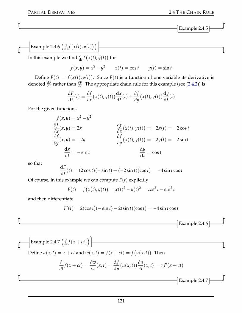
PARTIAL DERIVATIVES 2.4 THE CHAIN RULE
Example 2.4.5
Example 2.4.6(
ddt f(x(t), y(t)
))
In this example we find ddt f(x(t), y(t)
)for
f (x, y) = x2 ´ y2 x(t) = cos t y(t) = sin t
Define F(t) = f(x(t), y(t)
). Since F(t) is a function of one variable its derivative is
denoted dFdt rather than BF
Bt . The appropriate chain rule for this example (see (2.4.2)) is
dFdt
(t) =B fBx(x(t), y(t)
)dxdt
(t) +B fBy(x(t), y(t)
)dydt
(t)
For the given functions
f (x, y) = x2 ´ y2
B fBx
(x, y) = 2xB fBx(x(t), y(t)
)= 2x(t) = 2 cos t
B fBy
(x, y) = ´2yB fBy(x(t), y(t)
)= ´2y(t) = ´2 sin t
dxdt
= ´ sin tdydt
= cos t
so thatdFdt
(t) = (2 cos t)(´ sin t) + (´2 sin t)(cos t) = ´4 sin t cos t
Of course, in this example we can compute F(t) explicitly
F(t) = f(x(t), y(t)
)= x(t)2 ´ y(t)2 = cos2 t´ sin2 t
and then differentiate
F1(t) = 2(cos t)(´ sin t)´ 2(sin t)(cos t) = ´4 sin t cos t
Example 2.4.6
Example 2.4.7(BBt f (x + ct)
)
Define u(x, t) = x + ct and w(x, t) = f (x + ct) = f(u(x, t)
). Then
BBt
f (x + ct) =BwBt
(x, t) =d fdu(u(x, t)
)BuBt
(x, t) = c f 1(x + ct)
Example 2.4.7
121
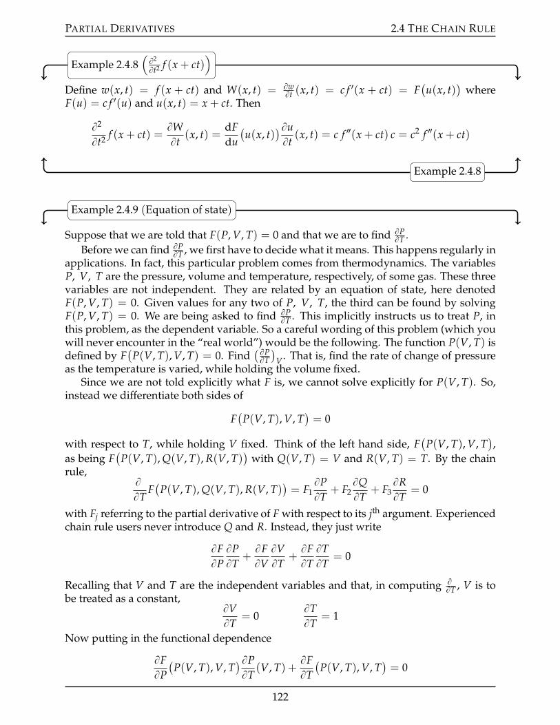
PARTIAL DERIVATIVES 2.4 THE CHAIN RULE
Example 2.4.8(B2
Bt2 f (x + ct))
Define w(x, t) = f (x + ct) and W(x, t) = BwBt (x, t) = c f 1(x + ct) = F
(u(x, t)
)where
F(u) = c f 1(u) and u(x, t) = x + ct. Then
B2
Bt2 f (x + ct) =BWBt
(x, t) =dFdu(u(x, t)
)BuBt
(x, t) = c f 2(x + ct) c = c2 f 2(x + ct)
Example 2.4.8
Example 2.4.9 (Equation of state)
Suppose that we are told that F(P, V, T) = 0 and that we are to find BPBT .
Before we can find BPBT , we first have to decide what it means. This happens regularly in
applications. In fact, this particular problem comes from thermodynamics. The variablesP, V, T are the pressure, volume and temperature, respectively, of some gas. These threevariables are not independent. They are related by an equation of state, here denotedF(P, V, T) = 0. Given values for any two of P, V, T, the third can be found by solvingF(P, V, T) = 0. We are being asked to find BP
BT . This implicitly instructs us to treat P, inthis problem, as the dependent variable. So a careful wording of this problem (which youwill never encounter in the “real world”) would be the following. The function P(V, T) isdefined by F
(P(V, T), V, T) = 0. Find
(BPBT)
V . That is, find the rate of change of pressureas the temperature is varied, while holding the volume fixed.
Since we are not told explicitly what F is, we cannot solve explicitly for P(V, T). So,instead we differentiate both sides of
F(
P(V, T), V, T)= 0
with respect to T, while holding V fixed. Think of the left hand side, F(
P(V, T), V, T),
as being F(
P(V, T), Q(V, T), R(V, T))
with Q(V, T) = V and R(V, T) = T. By the chainrule,
BBT
F(
P(V, T), Q(V, T), R(V, T))= F1
BPBT
+ F2BQBT
+ F3BRBT
= 0
with Fj referring to the partial derivative of F with respect to its jth argument. Experiencedchain rule users never introduce Q and R. Instead, they just write
BFBPBPBT
+BFBVBVBT
+BFBTBTBT
= 0
Recalling that V and T are the independent variables and that, in computing BBT , V is to
be treated as a constant,BVBT
= 0BTBT
= 1
Now putting in the functional dependence
BFBP(
P(V, T), V, T)BPBT
(V, T) +BFBT(
P(V, T), V, T)= 0
122
PARTIAL DERIVATIVES 2.4 THE CHAIN RULE
and solvingBPBT
(V, T) = ´BFBT(
P(V, T), V, T)
BFBP(
P(V, T), V, T)
Example 2.4.9
Example 2.4.10
Suppose that f (x, y) = 0 and that we are to find d2ydx2 .
Once again, x and y are not independent variables. Given a value for either x or y, the
other is determined by solving f (x, y) = 0. Since we are asked to find d2ydx2 , it is y that is
to be viewed as a function of x, rather than the other way around. So f (x, y) = 0 reallymeans that, in this problem, f
(x, y(x)
)= 0 for all x. Differentiating both sides of this
equation with respect to x,
f(x, y(x)
)= 0 for all x
ùñ ddx
f(x, y(x)
)= 0
Note that ddx f(x, y(x)
)is not the same as fx
(x, y(x)
). The former is, by definition, the
rate of change with respect to x of g(x) = f(x, y(x)
). Precisely,
dgdx
= lim∆xÑ0
g(x + ∆x)´ g(x)∆x
= lim∆xÑ0
f(x + ∆x , y(x + ∆x)
)´ f(x , y(x)
)
∆x(˚)
On the other hand, by definition,
fx(x, y) = lim∆xÑ0
f (x + ∆x, y)´ f (x, y)∆x
ùñ fx(x, y(x)
)= lim
∆xÑ0
f(x + ∆x , y(x)
)´ f(x , y(x)
)
∆x(˚˚)
The right hand sides of (˚) and (˚˚) are not the same. In dgdx , as ∆x varies the value of y
that is substituted into the first f (¨ ¨ ¨ ) on the right hand side, namely y(x + ∆x), changesas ∆x changes. That is, we are computing the rate of change of f along the (curved) pathy = y(x). In (˚˚), the corresponding value of y is y(x) and is independent of ∆x. That is,we are computing the rate of change of f along a horizontal straight line. As a concreteexample, suppose that f (x, y) = x + y. Then, 0 = f
(x , y(x)
)= x + y(x) gives y(x) = ´x
so thatddx
f(x, y(x)
)=
ddx
f (x,´x) =ddx
[x + (´x)] =ddx
0 = 0
But f (x, y) = x + y implies that fx(x, y) = 1 for all x and y so that
fx(x, y(x)) = fx(x, y)ˇˇy=´x
= 1ˇˇy=´x
= 1
123
PARTIAL DERIVATIVES 2.4 THE CHAIN RULE
Now back to
f(x, y(x)
)= 0 for all x
ùñ ddx
f(x, y(x)
)= 0
ùñ fx(x, y(x)
)dxdx
+ fy(x, y(x)
)dydx
(x) = 0 by the chain rule
ùñ dydx
(x) = ´ fx(x, y(x)
)
fy(x, y(x)
)
ùñ d2ydx2 (x) = ´ d
dx
[fx(x, y(x)
)
fy(x, y(x)
)]
= ´ fy(x, y(x)
) ddx [ fx
(x, y(x)
)]´ fx
(x, y(x)
) ddx [ fy
(x, y(x)
)]
fy(x, y(x)
)2 (:)
by the quotient rule. Now it suffices to substitute in ddx[
fx(x, y(x)
)]and d
dx[
fy(x, y(x)
)].
For the former apply the chain rule to h(x) = u(x, y(x)
)with u(x, y) = fx
(x, y).
ddx[
fx(x, y(x)
)]=
dhdx
(x)
= ux(x, y(x)
)dxdx
+ uy(x, y(x)
)dydx
(x)
= fxx(x, y(x)
)dxdx
+ fxy(x, y(x)
)dydx
(x)
= fxx(x, y(x)
)´ fxy(x, y(x)
)[
fx(x, y(x)
)
fy(x, y(x)
)]
Substituting this and
ddx[
fy(x, y(x)
)]= fyx
(x, y(x)
)dxdx
+ fyy(x, y(x)
)dydx
(x)
= fyx(x, y(x)
)´ fyy(x, y(x)
)[
fx(x, y(x)
)
fy(x, y(x)
)]
into the right hand side of (:) gives the final answer.
d2ydx2 (x) = ´
fy fxx ´ fy fxyfxfy´ fx fyx + fx fyy
fxfy
f 2y
= ´ f 2y fxx ´ 2 fx fy fxy + f 2
x fyy
f 3y
with all of fx, fy, fxx, fxy, fyy having arguments(x , y(x)
).
Example 2.4.10
We now move on to the proof of Theorem 2.4.1. To give you an idea of how the proofwill go, we first review the proof of the familiar one dimensional chain rule.
124
PARTIAL DERIVATIVES 2.4 THE CHAIN RULE
2.4.3 §§ Review of the Proof of ddt f(
x(t))= d f
dx
(x(t)
) dxdt (t)
As a warm up, let’s review the proof of the one dimensional chain rule
ddt
f(x(t)
)=
d fdx(x(t)
) dxdt
(t)
assuming that dxdt exists and that d f
dx is continuous. We wish to find the derivative of F(t) =f(x(t)
). By definition
F1(t) = limhÑ0
F(t + h)´ F(t)h
= limhÑ0
f(x(t + h)
)´ f(x(t)
)
h
Notice that the numerator is the difference of f (x) evaluated at two nearby values ofx, namely x1 = x(t + h) and x0 = x(t). The mean value theorem is a good tool forstudying the difference in the values of f (x) at two nearby points. Recall that the meanvalue theorem says that, for any given x0 and x1, there exists an (in general unknown) cbetween them so that
f (x1)´ f (x0) = f 1(c) (x1 ´ x0)
For this proof, we choose x0 = x(t) and x1 = x(t + h). The the mean value theorem tellsus that there exists a ch so that
f(x(t + h)
)´ f(x(t)
)= f (x1)´ f (x0) = f 1(ch)
[x(t + h)´ x(t)
]
We have put the subscript h on ch to emphasise that ch, which is between x0 = x(t) andx1 = x(t + h), may depend on h. Now since ch is trapped between x(t) and x(t + h) andsince x(t + h) Ñ x(t) as h Ñ 0, we have that ch must also tend to x(t) as h Ñ 0. Pluggingthis into the definition of F1(t),
F1(t) = limhÑ0
f(x(t + h)
)´ f(x(t)
)
h
= limhÑ0
f 1(ch)[x(t + h)´ x(t)
]
h
= limhÑ0
f 1(ch) limhÑ0
x(t + h)´ x(t)h
= f 1(x(t)
)x1(t)
as desired.
2.4.4 §§ Proof of Theorem 2.4.1
We’ll now prove the formula for BBs f(x(s, t) , y(s, t)
)that is given in Theorem 2.4.1. The
proof uses the same ideas as the proof of the one variable chain rule, that we have justreviewed.
125
PARTIAL DERIVATIVES 2.4 THE CHAIN RULE
We wish to find the partial derivative with respect to s of F(s, t) = f(x(s, t) , y(s, t)
).
By definition
BFBs
(s, t) = limhÑ0
F(s + h, t)´ F(s, t)h
= limhÑ0
f(x(s + h, t) , y(s + h, t)
)´ f(x(s, t) , y(s, t)
)
h
The numerator is the difference of f (x, y) evaluated at two nearby values of (x, y), namely(x1, y1) =
(x(s+ h, t) , y(s+ h, t)
)and (x0, y0) =
(x(s, t) , y(s, t)
). In going from (x0, y0) to
(x1, y1), both the x and y-coordinates change. By adding and subtracting we can separatethe change in the x-coordinate from the change in the y-coordinate.
f (x1, y1)´ f (x0, y0) =
f (x1, y1)´ f (x0, y1)(+
f (x0, y1)´ f (x0, y0)(
The first half,
f (x1, y1)´ f (x0, y1)(
, has the same y argument in both terms and so is thedifference of the function of one variable g(x) = f (x, y1) (viewing y1 just as a constant)evaluated at the two nearby values, x0, x1, of x. Consequently, we can make use of themean value theorem as we did in §2.4.3 above. There is a cx,h between x0 = x(s, t) andx1 = x(s + h, t) such that
f (x1, y1)´ f (x0, y1) = g(x1)´ g(x0) = g1(cx,h)[x1 ´ x0] =B fBx
(cx,h , y1) [x1 ´ x0]
=B fBx(cx,h , y(s + h, t)
) [x(s + h, t)´ x(s, t)
]
We have introduced the two subscripts in cx,h to remind ourselves that it may depend onh and that it lies between the two x-values x0 and x1.
Similarly, the second half,
f (x0, y1) ´ f (x0, y0)(
, is the difference of the function ofone variable h(y) = f (x0, y) (viewing x0 just as a constant) evaluated at the two nearbyvalues, y0, y1, of y. So, by the mean value theorem,
f (x0, y1)´ f (x0, y0) = h(y1)´ h(y0) = h1(cy,h)[y1 ´ y0] =B fBy
(x0, cy,h) [y1 ´ y0]
=B fBy(x(s, t) , cy,h
) [y(s + h, t)´ y(s, t)
]
for some (unknown) cy,h between y0 = y(s, t) and y1 = y(s + h, t). Again, the two sub-scripts in cy,h remind ourselves that it may depend on h and that it lies between the twoy-values y0 and y1. So, noting that, as h tends to zero, cx,h, which is trapped betweenx(s, t) and x(s + h, t), must tend to x(s, t), and cy,h, which is trapped between y(s, t) and
126
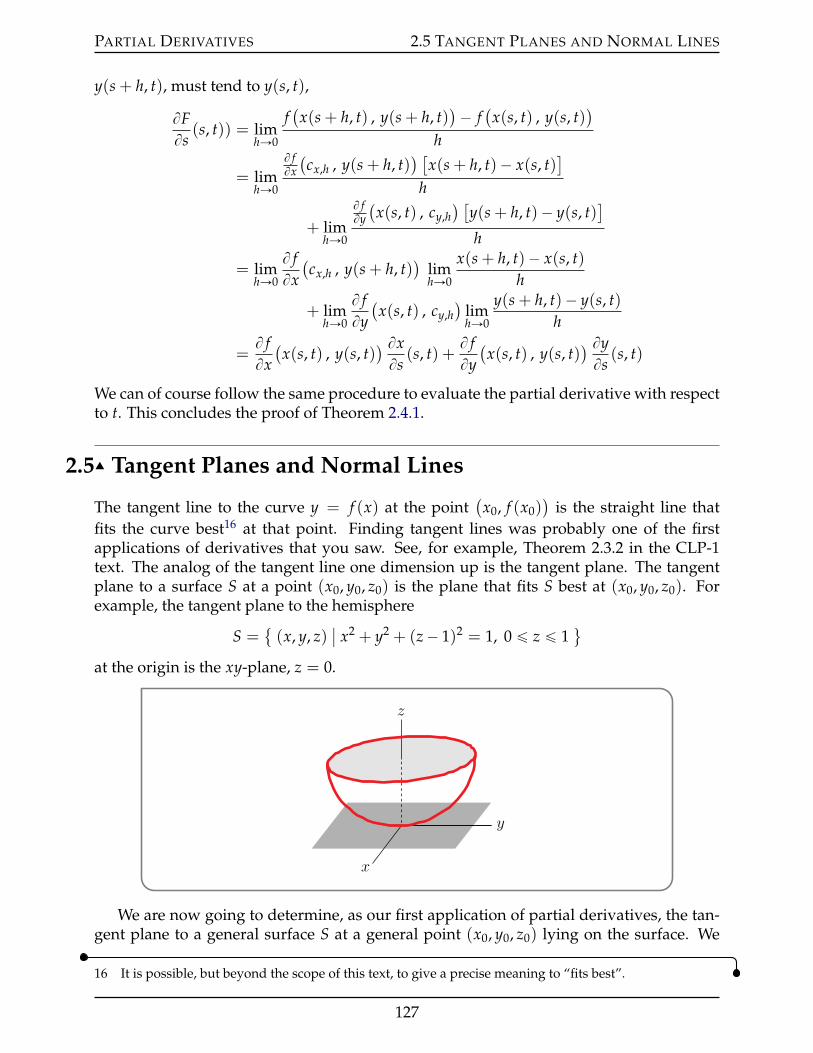
PARTIAL DERIVATIVES 2.5 TANGENT PLANES AND NORMAL LINES
y(s + h, t), must tend to y(s, t),
BFBs
(s, t)) = limhÑ0
f(x(s + h, t) , y(s + h, t)
)´ f(x(s, t) , y(s, t)
)
h
= limhÑ0
B fBx(cx,h , y(s + h, t)
) [x(s + h, t)´ x(s, t)
]
h
+ limhÑ0
B fBy(x(s, t) , cy,h
) [y(s + h, t)´ y(s, t)
]
h
= limhÑ0
B fBx(cx,h , y(s + h, t)
)limhÑ0
x(s + h, t)´ x(s, t)h
+ limhÑ0
B fBy(x(s, t) , cy,h
)limhÑ0
y(s + h, t)´ y(s, t)h
=B fBx(x(s, t) , y(s, t)
) BxBs
(s, t) +B fBy(x(s, t) , y(s, t)
) ByBs
(s, t)
We can of course follow the same procedure to evaluate the partial derivative with respectto t. This concludes the proof of Theorem 2.4.1.
2.5IJ Tangent Planes and Normal Lines
The tangent line to the curve y = f (x) at the point(x0, f (x0)
)is the straight line that
fits the curve best16 at that point. Finding tangent lines was probably one of the firstapplications of derivatives that you saw. See, for example, Theorem 2.3.2 in the CLP-1text. The analog of the tangent line one dimension up is the tangent plane. The tangentplane to a surface S at a point (x0, y0, z0) is the plane that fits S best at (x0, y0, z0). Forexample, the tangent plane to the hemisphere
S = (x, y, z)
ˇx2 + y2 + (z´ 1)2 = 1, 0 ď z ď 1
(
at the origin is the xy-plane, z = 0.
z
y
x
We are now going to determine, as our first application of partial derivatives, the tan-gent plane to a general surface S at a general point (x0, y0, z0) lying on the surface. We
16 It is possible, but beyond the scope of this text, to give a precise meaning to “fits best”.
127
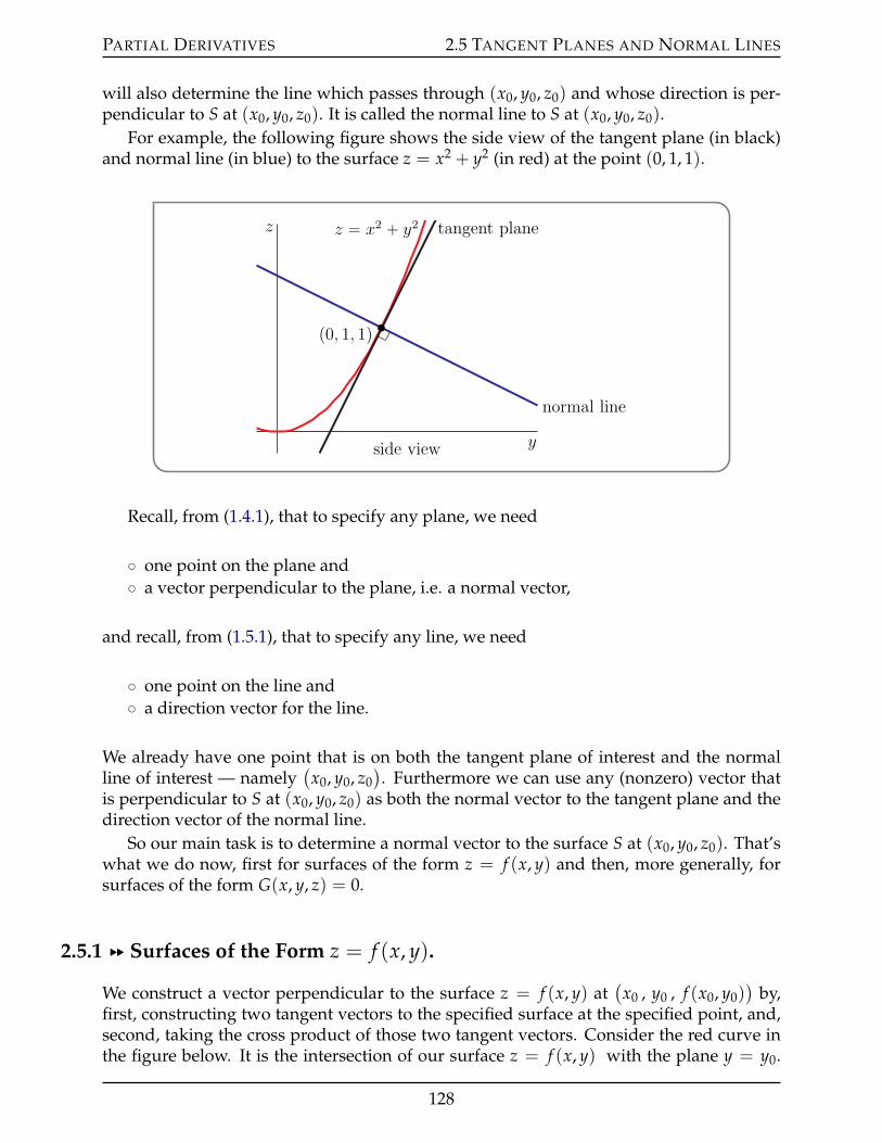
PARTIAL DERIVATIVES 2.5 TANGENT PLANES AND NORMAL LINES
will also determine the line which passes through (x0, y0, z0) and whose direction is per-pendicular to S at (x0, y0, z0). It is called the normal line to S at (x0, y0, z0).
For example, the following figure shows the side view of the tangent plane (in black)and normal line (in blue) to the surface z = x2 + y2 (in red) at the point (0, 1, 1).
y
z z “ x2 ` y2 tangent plane
normal line
p0, 1, 1q
side view
Recall, from (1.4.1), that to specify any plane, we need
˝ one point on the plane and˝ a vector perpendicular to the plane, i.e. a normal vector,
and recall, from (1.5.1), that to specify any line, we need
˝ one point on the line and˝ a direction vector for the line.
We already have one point that is on both the tangent plane of interest and the normalline of interest — namely
(x0, y0, z0
). Furthermore we can use any (nonzero) vector that
is perpendicular to S at (x0, y0, z0) as both the normal vector to the tangent plane and thedirection vector of the normal line.
So our main task is to determine a normal vector to the surface S at (x0, y0, z0). That’swhat we do now, first for surfaces of the form z = f (x, y) and then, more generally, forsurfaces of the form G(x, y, z) = 0.
2.5.1 §§ Surfaces of the Form z = f (x, y).
We construct a vector perpendicular to the surface z = f (x, y) at(x0 , y0 , f (x0, y0)
)by,
first, constructing two tangent vectors to the specified surface at the specified point, and,second, taking the cross product of those two tangent vectors. Consider the red curve inthe figure below. It is the intersection of our surface z = f (x, y) with the plane y = y0.
128
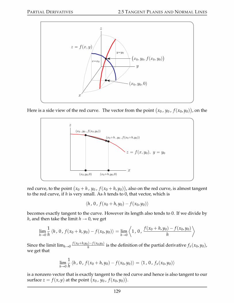
PARTIAL DERIVATIVES 2.5 TANGENT PLANES AND NORMAL LINES
z
y
x
z “ fpx, yqy“y0
x“x0
`x0, y0, fpx0, y0q
˘
px0, y0, 0q
Here is a side view of the red curve. The vector from the point(x0 , y0 , f (x0, y0)
), on the
z
x
z “ fpx, y0q, y “ y0
px0 , y0 , fpx0,y0qqpx0`h , y0 , fpx0`h,y0qq
px0,y0,0q px0`h,y0,0q
red curve, to the point(x0 + h , y0 , f (x0 + h, y0)
), also on the red curve, is almost tangent
to the red curve, if h is very small. As h tends to 0, that vector, which is
〈h , 0 , f (x0 + h, y0)´ f (x0, y0)〉
becomes exactly tangent to the curve. However its length also tends to 0. If we divide byh, and then take the limit h Ñ 0, we get
limhÑ0
1h〈h , 0 , f (x0 + h, y0)´ f (x0, y0)〉 = lim
hÑ0
⟨1 , 0 ,
f (x0 + h, y0)´ f (x0, y0)
h
⟩
Since the limit limhÑ0f (x0+h,y0)´ f (x0,y0)
h is the definition of the partial derivative fx(x0, y0),we get that
limhÑ0
1h〈h , 0 , f (x0 + h, y0)´ f (x0, y0)〉 = 〈1 , 0 , fx(x0, y0)〉
is a nonzero vector that is exactly tangent to the red curve and hence is also tangent to oursurface z = f (x, y) at the point
(x0 , y0 , f (x0, y0)
).
129
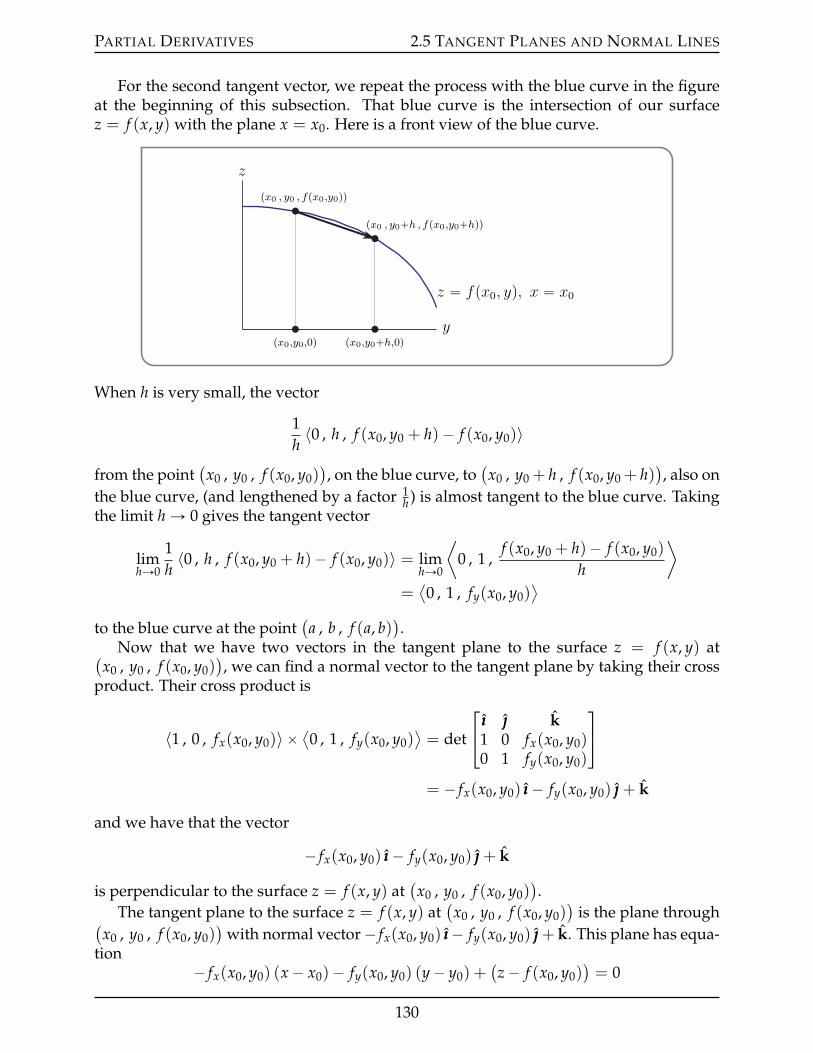
PARTIAL DERIVATIVES 2.5 TANGENT PLANES AND NORMAL LINES
For the second tangent vector, we repeat the process with the blue curve in the figureat the beginning of this subsection. That blue curve is the intersection of our surfacez = f (x, y) with the plane x = x0. Here is a front view of the blue curve.
z
y
z “ fpx0, yq, x “ x0
px0 , y0 , fpx0,y0qq
px0 , y0`h , fpx0,y0`hqq
px0,y0,0q px0,y0`h,0q
When h is very small, the vector
1h〈0 , h , f (x0, y0 + h)´ f (x0, y0)〉
from the point(x0 , y0 , f (x0, y0)
), on the blue curve, to
(x0 , y0 + h , f (x0, y0 + h)
), also on
the blue curve, (and lengthened by a factor 1h ) is almost tangent to the blue curve. Taking
the limit h Ñ 0 gives the tangent vector
limhÑ0
1h〈0 , h , f (x0, y0 + h)´ f (x0, y0)〉 = lim
hÑ0
⟨0 , 1 ,
f (x0, y0 + h)´ f (x0, y0)
h
⟩
=⟨0 , 1 , fy(x0, y0)
⟩
to the blue curve at the point(a , b , f (a, b)
).
Now that we have two vectors in the tangent plane to the surface z = f (x, y) at(x0 , y0 , f (x0, y0)
), we can find a normal vector to the tangent plane by taking their cross
product. Their cross product is
〈1 , 0 , fx(x0, y0)〉ˆ⟨0 , 1 , fy(x0, y0)
⟩= det
ııı k1 0 fx(x0, y0)0 1 fy(x0, y0)
= ´ fx(x0, y0) ııı´ fy(x0, y0) + k
and we have that the vector
´ fx(x0, y0) ııı´ fy(x0, y0) + k
is perpendicular to the surface z = f (x, y) at(x0 , y0 , f (x0, y0)
).
The tangent plane to the surface z = f (x, y) at(x0 , y0 , f (x0, y0)
)is the plane through(
x0 , y0 , f (x0, y0))
with normal vector´ fx(x0, y0) ııı´ fy(x0, y0) + k. This plane has equa-tion
´ fx(x0, y0) (x´ x0)´ fy(x0, y0) (y´ y0) +(z´ f (x0, y0)
)= 0
130
PARTIAL DERIVATIVES 2.5 TANGENT PLANES AND NORMAL LINES
or, after a little rearrangement,
z = f (x0, y0) + fx(x0, y0) (x´ x0) + fy(x0, y0) (y´ y0)
Now that we have the normal vector, finding the equation of the normal line to the surfacez = f (x, y) at the point
(x0 , y0 , f (x0, y0)
)is straightforward. Writing it in parametric
form,〈x, y, z〉 = 〈x0, y0, f (x0, y0)〉+ t
⟨´ fx(x0, y0) , ´ fy(x0, y0) , 1⟩
By way of summary
(a) The vector´ fx(x0, y0) ııı´ fy(x0, y0) + k
is normal to the surface z = f (x, y) at(x0 , y0 , f (x0, y0)
).
(b) The equation of the tangent plane to the surface z = f (x, y) at the point(x0 , y0 , f (x0, y0)
)may be written as
z = f (x0, y0) + fx(x0, y0) (x´ x0) + fy(x0, y0) (y´ y0)
(c) The parametric equation of the normal line to the surface z = f (x, y) at thepoint
(x0 , y0 , f (x0, y0)
)is
〈x, y, z〉 = 〈x0, y0, f (x0, y0)〉+ t⟨´ fx(x0, y0) , ´ fy(x0, y0) , 1
⟩
or, writing it component by component,
x = x0 ´ t fx(x0, y0) y = y0 ´ t fy(x0, y0) z = f (x0, y0) + t
Theorem 2.5.1 (Tangent Plane and Normal Line).
Example 2.5.2
As a warm-up example, we’ll find the tangent plane and normal line to the surface z =x2 + y2 at the point (1, 0, 1). To do so, we just apply Theorem 2.5.1 with x0 = 1, y0 = 0 and
f (x, y) = x2 + y2 f (1, 0) = 1fx(x, y) = 2x fx(1, 0) = 2fy(x, y) = 2y fy(1, 0) = 0
So the tangent plane is
z = f (x0, y0) + fx(x0, y0) (x´ x0) + fy(x0, y0) (y´ y0) = 1 + 2(x´ 1) + 0(y´ 0)= ´1 + 2x
and the normal line is
〈x, y, z〉 = 〈x0, y0, f (x0, y0)〉+ t⟨´ fx(x0, y0) , ´ fy(x0, y0) , 1
⟩= 〈1, 0, 1〉+ t 〈´2 , 0 , 1〉
= 〈1´ 2t , 0 , 1 + t〉
131
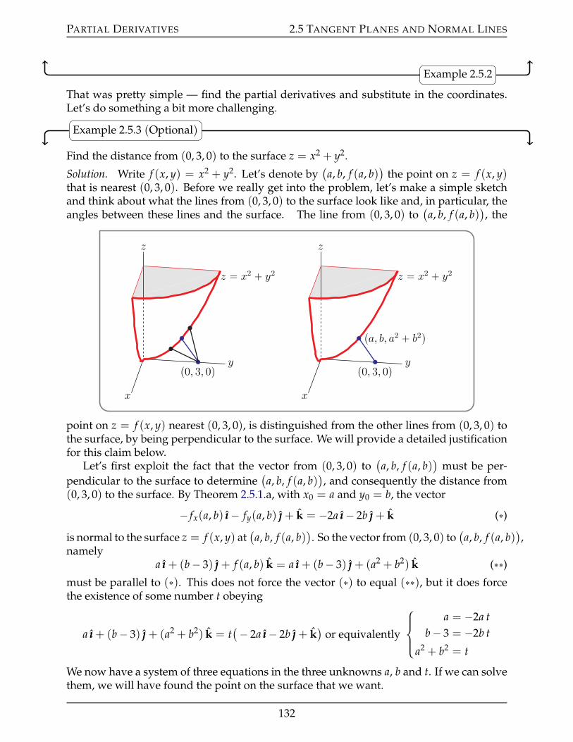
PARTIAL DERIVATIVES 2.5 TANGENT PLANES AND NORMAL LINES
Example 2.5.2
That was pretty simple — find the partial derivatives and substitute in the coordinates.Let’s do something a bit more challenging.
Example 2.5.3 (Optional)
Find the distance from (0, 3, 0) to the surface z = x2 + y2.
Solution. Write f (x, y) = x2 + y2. Let’s denote by(a, b, f (a, b)
)the point on z = f (x, y)
that is nearest (0, 3, 0). Before we really get into the problem, let’s make a simple sketchand think about what the lines from (0, 3, 0) to the surface look like and, in particular, theangles between these lines and the surface. The line from (0, 3, 0) to
(a, b, f (a, b)
), the
z
y
x
z “ x2 ` y2
p0, 3, 0q
z
y
x
z “ x2 ` y2
p0, 3, 0q
pa, b, a2 ` b2q
point on z = f (x, y) nearest (0, 3, 0), is distinguished from the other lines from (0, 3, 0) tothe surface, by being perpendicular to the surface. We will provide a detailed justificationfor this claim below.
Let’s first exploit the fact that the vector from (0, 3, 0) to(a, b, f (a, b)
)must be per-
pendicular to the surface to determine(a, b, f (a, b)
), and consequently the distance from
(0, 3, 0) to the surface. By Theorem 2.5.1.a, with x0 = a and y0 = b, the vector
´ fx(a, b) ııı´ fy(a, b) + k = ´2a ııı´ 2b + k (˚)is normal to the surface z = f (x, y) at
(a, b, f (a, b)
). So the vector from (0, 3, 0) to
(a, b, f (a, b)
),
namelya ııı + (b´ 3) + f (a, b) k = a ııı + (b´ 3) + (a2 + b2) k (˚˚)
must be parallel to (˚). This does not force the vector (˚) to equal (˚˚), but it does forcethe existence of some number t obeying
a ııı + (b´ 3) + (a2 + b2) k = t(´ 2a ııı´ 2b + k
)or equivalently
$’&’%
a = ´2a tb´ 3 = ´2b t
a2 + b2 = t
We now have a system of three equations in the three unknowns a, b and t. If we can solvethem, we will have found the point on the surface that we want.
132
PARTIAL DERIVATIVES 2.5 TANGENT PLANES AND NORMAL LINES
• The first equation is a(1 + 2t) = 0 so that either a = 0 or t = ´12 .
• The third equation forces t ě 0, so a = 0, and the last equation reduces to t = b2.
• Substituting this into the middle equation gives
b´ 3 = ´2b3 or equivalently 2b3 + b´ 3 = 0
In general, cubic equations are very hard to solve17. But, in this case, we can guess onesolution18, namely b = 1. So (b ´ 1) must be a factor of 2b3 + b ´ 3 and a little divisionthen gives us
0 = 2b3 + b´ 3 = (b´ 1)(2b2 + 2b + 3)
We can now find the roots of the quadratic factor by using the high school formula
´2˘a22 ´ 4(2)(3)
4
Since 22 ´ 4(2)(3) ă 0, the factor 2b2 + 2b + 3 has no real roots. So the only real solutionto the cubic equation 2b3 + b´ 3 = 0 is b = 1.
In summary,
• a = 0, b = 1 and
• the point on z = x2 + y2 nearest (0, 3, 0) is (0, 1, 1) and
• the distance from (0, 3, 0) to z = x2 + y2 is the distance from (0, 3, 0) to (0, 1, 1),which is
a(´2)2 + 12 =
?5.
Finally back to the claim that, because(a, b, f (a, b)
)is the point on z = f (x, y) that is
nearest19 (0, 3, 0), the vector from (0, 3, 0) to(a, b, f (a, b)
)must be perpendicular to the
surface z = f (x, y) at(a, b, f (a, b)
). Note that the square of the distance from (0, 3, 0) to a
general point(x, y, f (x, y)
)on z = f (x, y) is
D(x, y) = x2 + (y´ 3)2 + f (x, y)2
If x = a, y = b minimizes D(x, y) then, in particular,
17 The method for solving cubics was developed in the 15th century by del Ferro, Cardano and Ferrari(Cardano’s student). Ferrari then went on to discover a formula for the roots of a quartic. Both thecubic and quartic formulae are extremely cumbersome, and no such formula exists for polynomials ofdegree 5 and higher. This is the famous Abel-Ruffini theorem.
18 See Appendix A.16 in the CLP-2 text. There it is shown that any integer root of a polynomial withinteger coefficients must divide the constant term exactly. So in this case only ˘1 and ˘3 could beinteger roots. So it is good to check to see if any of these are solutions before moving on to moresophisticated techniques.
19 Note that we are assuming that(a, b, f (a, b)
)is the point on the surface that is nearest (0, 3, 0). That
there exists such a point is intuitively obvious from a sketch of the surface. The mathematical proofthat there exists such a point is beyond the scope of this text.
133
PARTIAL DERIVATIVES 2.5 TANGENT PLANES AND NORMAL LINES
• restricting our attention to the slice y = b of the surface, x = a minimizes g(x) =D(x, b) = x2 + (b´ 3)2 + f (x, b)2 so that
0 = g1(a) =BBx
[x2 + (b´ 3)2 + f (x, b)2
]ˇˇx=a
= 2a + 2 f (a, b) fx(a, b)
= 2 〈a , b´ 3 , f (a, b)〉 ¨ 〈1 , 0 , fx(a, b)〉
and
• restricting our attention to the slice x = a of the surface, y = b minimizes h(y) =D(a, y) = a2 + (y´ 3)2 + f (a, y)2 so that
0 = h1(b) =BBy
[a2 + (y´ 3)2 + f (a, y)2
]ˇˇy=b
= 2(b´ 3) + 2 f (a, b) fy(a, b)
= 2 〈a , b´ 3 , f (a, b)〉 ¨ ⟨0 , 1 , fy(a, b)⟩
We have expressed the final right hand sides of both of the above bullets as the dot productof the vector 〈a , b´ 3 , f (a, b)〉 with something because
˝ 〈a , b´ 3 , f (a, b)〉 is the vector from (0, 3, 0) to the point (a , b , f (a, b))
on the surfaceand
˝ the vanishing of the dot product of two vectors implies that the two vectors areperpendicular.
Thus, that
〈a , b´ 3 , f (a, b)〉 ¨ 〈1 , 0 , fx(a, b)〉 = 〈a , b´ 3 , f (a, b)〉 ¨ ⟨0 , 1 , fy(a, b)⟩= 0
tells us that the vector 〈a , b´ 3 , f (a, b)〉 from (0, 3, 0) to(a, b, f (a, b)
)is perpendicular
to both 〈1 , 0 , fx(a, b)〉 and⟨0 , 1 , fy(a, b)
⟩and hence is parallel to their cross product
〈1 , 0 , fx(a, b)〉ˆ ⟨0 , 1 , fy(a, b)⟩, which we already know is a normal vector to the surface
z = f (x, y) at(a, b, f (a, b)
).
This shows that the point on the surface that minimises the distance to (0, 3, 0) is joinedto (0, 3, 0) by a line that is parallel to the normal vector — just as we required.
Example 2.5.3
2.5.2 §§ Surfaces of the Form G(x, y, z) = 0.
We now use a little trickery to construct a vector perpendicular to the surface G(x, y, z) = 0at the point
(x0 , y0 , z0
). Imagine that you are walking on the surface and that at time 0
you are at the point(x0 , y0 , z0
). Let r(t) =
(x(t) , y(t) , z(t)
)denote your position at
time t. Because you are walking along the surface, we know that r(t) always lies on the
134
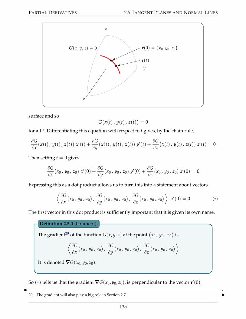
PARTIAL DERIVATIVES 2.5 TANGENT PLANES AND NORMAL LINES
z
y
x
Gpx, y, zq “ 0 rp0q “ `x0, y0, z0
˘
rptq
surface and soG(x(t) , y(t) , z(t)
)= 0
for all t. Differentiating this equation with respect to t gives, by the chain rule,
BGBx(x(t) , y(t) , z(t)
)x1(t) +
BGBy(x(t) , y(t) , z(t)
)y1(t) +
BGBz(x(t) , y(t) , z(t)
)z1(t) = 0
Then setting t = 0 gives
BGBx(x0 , y0 , z0
)x1(0) +
BGBy(x0 , y0 , z0
)y1(0) +
BGBz(x0 , y0 , z0
)z1(0) = 0
Expressing this as a dot product allows us to turn this into a statement about vectors.⟨BGBx(x0 , y0 , z0
),BGBy(x0 , y0 , z0
),BGBz(x0 , y0 , z0
)⟩ ¨ r1(0) = 0 (˚)
The first vector in this dot product is sufficiently important that it is given its own name.
The gradient20 of the function G(x, y, z) at the point(x0 , y0 , z0
)is
⟨BGBx(x0 , y0 , z0
),BGBy(x0 , y0 , z0
),BGBz(x0 , y0 , z0
)⟩
It is denoted∇∇∇G(x0, y0, z0).
Definition 2.5.4 (Gradient).
So (˚) tells us that the gradient∇∇∇G(x0, y0, z0), is perpendicular to the vector r1(0).
20 The gradient will also play a big role in Section 2.7.
135
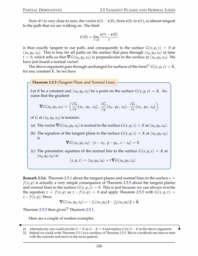
PARTIAL DERIVATIVES 2.5 TANGENT PLANES AND NORMAL LINES
Now if t is very close to zero, the vector r(t)´ r(0), from r(0) to r(t), is almost tangentto the path that we are walking on. The limit
r1(0) = limtÑ0
r(t)´ r(0)t
is thus exactly tangent to our path, and consequently to the surface G(x, y, z) = 0 at(x0, y0, z0). This is true for all paths on the surface that pass through (x0, y0, z0) at timet = 0, which tells us that∇∇∇G(x0, y0, z0) is perpendicular to the surface at (x0, y0, z0). Wehave just found a normal vector!
The above argument goes through unchanged for surfaces of the form21 G(x, y, z) = K,for any constant K. So we have
Let K be a constant and (x0, y0, z0) be a point on the surface G(x, y, z) = K. As-sume that the gradient
∇∇∇G(x0, y0, z0) =
⟨BGBx(x0 , y0 , z0
),BGBy(x0 , y0 , z0
),BGBz(x0 , y0 , z0
)⟩
of G at (x0, y0, z0) is nonzero.
(a) The vector∇∇∇G(x0, y0, z0) is normal to the surface G(x, y, z) = K at (x0, y0, z0).
(b) The equation of the tangent plane to the surface G(x, y, z) = K at (x0, y0, z0)is
∇∇∇G(x0, y0, z0) ¨ 〈x´ x0 , y´ y0 , z´ z0〉 = 0
(c) The parametric equation of the normal line to the surface G(x, y, z) = K at(x0, y0, z0) is
〈x, y, z〉 = 〈x0, y0, z0〉+ t∇∇∇G(x0, y0, z0)
Theorem 2.5.5 (Tangent Plane and Normal Line).
Remark 2.5.6. Theorem 2.5.1 about the tangent planes and normal lines to the surface z =f (x, y) is actually a very simple consequence of Theorem 2.5.5 about the tangent planesand normal lines to the surface G(x, y, z) = 0. This is just because we can always rewritethe equation z = f (x, y) as z ´ f (x, y) = 0 and apply Theorem 2.5.5 with G(x, y, z) =z´ f (x, y). Since
∇∇∇G(x0, y0, z0) = ´ fx(x0, y0) ııı´ fy(x0, y0) + k
Theorem 2.5.5 then gives22 Theorem 2.5.1.
Here are a couple of routine examples.
21 Alternatively, one could rewrite G = K as G´ K = 0 and replace G by G´ K in the above argument.22 Indeed we could write Theorem 2.5.1 as a corollary of Theorem 2.5.5. But in a textbook one tries to start
with the concrete and move to the more general.
136
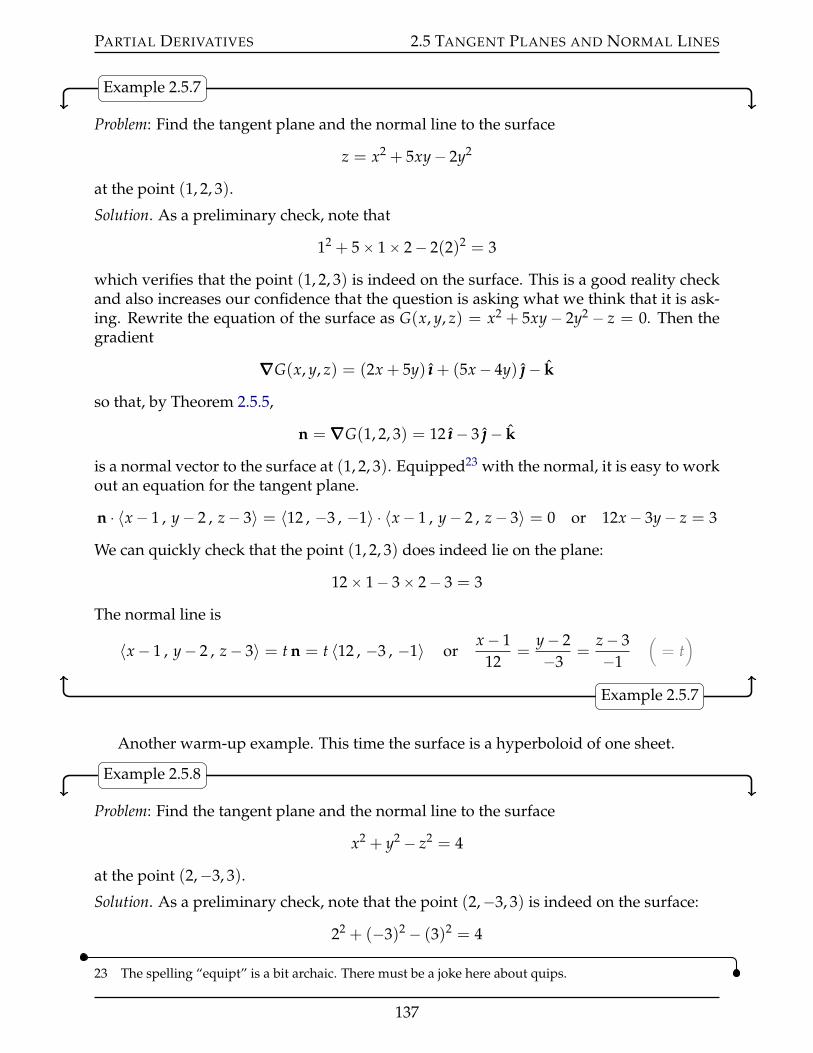
PARTIAL DERIVATIVES 2.5 TANGENT PLANES AND NORMAL LINES
Example 2.5.7
Problem: Find the tangent plane and the normal line to the surface
z = x2 + 5xy´ 2y2
at the point (1, 2, 3).
Solution. As a preliminary check, note that
12 + 5ˆ 1ˆ 2´ 2(2)2 = 3
which verifies that the point (1, 2, 3) is indeed on the surface. This is a good reality checkand also increases our confidence that the question is asking what we think that it is ask-ing. Rewrite the equation of the surface as G(x, y, z) = x2 + 5xy´ 2y2 ´ z = 0. Then thegradient
∇∇∇G(x, y, z) = (2x + 5y) ııı + (5x´ 4y) ´ k
so that, by Theorem 2.5.5,
n =∇∇∇G(1, 2, 3) = 12 ııı´ 3 ´ k
is a normal vector to the surface at (1, 2, 3). Equipped23 with the normal, it is easy to workout an equation for the tangent plane.
n ¨ 〈x´ 1 , y´ 2 , z´ 3〉 = 〈12 , ´3 , ´1〉 ¨ 〈x´ 1 , y´ 2 , z´ 3〉 = 0 or 12x´ 3y´ z = 3
We can quickly check that the point (1, 2, 3) does indeed lie on the plane:
12ˆ 1´ 3ˆ 2´ 3 = 3
The normal line is
〈x´ 1 , y´ 2 , z´ 3〉 = t n = t 〈12 , ´3 , ´1〉 orx´ 1
12=
y´ 2´3
=z´ 3´1
(= t)
Example 2.5.7
Another warm-up example. This time the surface is a hyperboloid of one sheet.
Example 2.5.8
Problem: Find the tangent plane and the normal line to the surface
x2 + y2 ´ z2 = 4
at the point (2,´3, 3).
Solution. As a preliminary check, note that the point (2,´3, 3) is indeed on the surface:
22 + (´3)2 ´ (3)2 = 4
23 The spelling “equipt” is a bit archaic. There must be a joke here about quips.
137
PARTIAL DERIVATIVES 2.5 TANGENT PLANES AND NORMAL LINES
The equation of the surface is G(x, y, z) = x2 + y2 ´ z2 = 4. Then the gradient of G is
∇∇∇G(x, y, z) = 2x ııı + 2y ´ 2z k
so that, at (2,´3, 3),
∇∇∇G(2,´3, 3) = 4 ııı´ 6 ´ 6 k
and so, by Theorem 2.5.5,
n =12(4 ııı´ 6 ´ 6 k
)= 2 ııı´ 3 ´ 3 k
is a normal vector to the surface at (2,´3, 3). The tangent plane is
n ¨ 〈x´ 2 , y + 3 , z´ 3〉 = 〈2 , ´3 , ´3〉 ¨ 〈x´ 2 , y + 3 , z´ 3〉 = 0 or 2x´ 3y´ 3z = 4
Again, as a check, we can verify that our point (2,´3, 3) is indeed on the plane:
2ˆ 2´ 3ˆ (´3)´ 3ˆ 3 = 4
The normal line is
〈x´ 2 , y + 3 , z´ 3〉 = t n = t 〈2 , ´3 , ´3〉 orx´ 2
2=
y + 3´3
=z´ 3´3
(= t)
Example 2.5.8
138
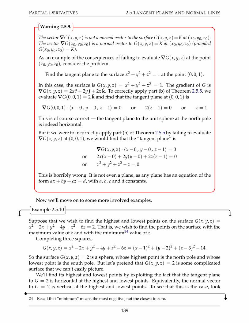
PARTIAL DERIVATIVES 2.5 TANGENT PLANES AND NORMAL LINES
The vector∇∇∇G(x, y, z) is not a normal vector to the surface G(x, y, z)=K at (x0, y0, z0).The vector∇∇∇G(x0, y0, z0) is a normal vector to G(x, y, z) = K at (x0, y0, z0) (providedG(x0, y0, z0) = K).
As an example of the consequences of failing to evaluate∇∇∇G(x, y, z) at the point(x0, y0, z0), consider the problem
Find the tangent plane to the surface x2 + y2 + z2 = 1 at the point (0, 0, 1).
In this case, the surface is G(x, y, z) = x2 + y2 + z2 = 1. The gradient of G is∇∇∇G(x, y, z) = 2x ııı + 2y + 2z k. To correctly apply part (b) of Theorem 2.5.5, weevaluate∇∇∇G(0, 0, 1) = 2 k and find that the tangent plane at (0, 0, 1) is
∇∇∇G(0, 0, 1) ¨ 〈x´ 0 , y´ 0 , z´ 1〉 = 0 or 2(z´ 1) = 0 or z = 1
This is of course correct — the tangent plane to the unit sphere at the north poleis indeed horizontal.
But if we were to incorrectly apply part (b) of Theorem 2.5.5 by failing to evaluate∇∇∇G(x, y, z) at (0, 0, 1), we would find that the “tangent plane” is
∇∇∇G(x, y, z) ¨ 〈x´ 0 , y´ 0 , z´ 1〉 = 0or 2x(x´ 0) + 2y(y´ 0) + 2z(z´ 1) = 0
or x2 + y2 + z2 ´ z = 0
This is horribly wrong. It is not even a plane, as any plane has an equation of theform ax + by + cz = d, with a, b, c and d constants.
Warning 2.5.9.
Now we’ll move on to some more involved examples.
Example 2.5.10
Suppose that we wish to find the highest and lowest points on the surface G(x, y, z) =x2´ 2x + y2´ 4y + z2´ 6z = 2. That is, we wish to find the points on the surface with themaximum value of z and with the minimum24 value of z.
Completing three squares,
G(x, y, z) = x2 ´ 2x + y2 ´ 4y + z2 ´ 6z = (x´ 1)2 + (y´ 2)2 + (z´ 3)2 ´ 14.
So the surface G(x, y, z) = 2 is a sphere, whose highest point is the north pole and whoselowest point is the south pole. But let’s pretend that G(x, y, z) = 2 is some complicatedsurface that we can’t easily picture.
We’ll find its highest and lowest points by exploiting the fact that the tangent planeto G = 2 is horizontal at the highest and lowest points. Equivalently, the normal vectorto G = 2 is vertical at the highest and lowest points. To see that this is the case, look
24 Recall that “minimum” means the most negative, not the closest to zero.
139
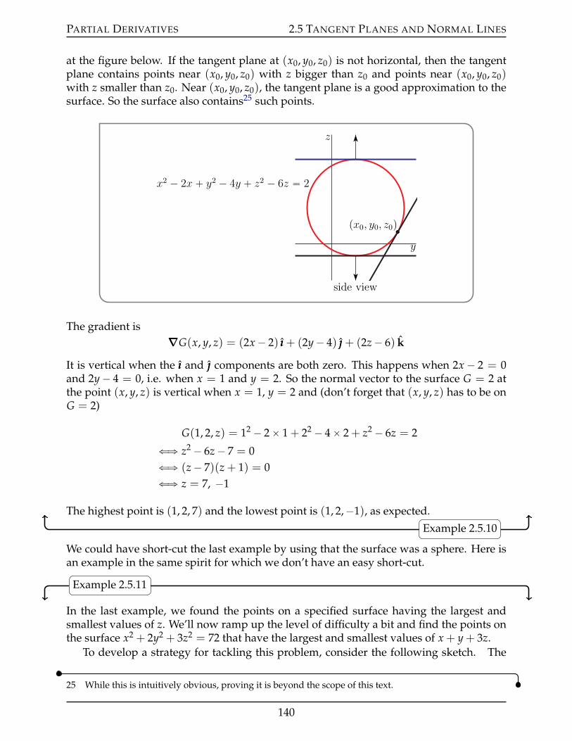
PARTIAL DERIVATIVES 2.5 TANGENT PLANES AND NORMAL LINES
at the figure below. If the tangent plane at (x0, y0, z0) is not horizontal, then the tangentplane contains points near (x0, y0, z0) with z bigger than z0 and points near (x0, y0, z0)with z smaller than z0. Near (x0, y0, z0), the tangent plane is a good approximation to thesurface. So the surface also contains25 such points.
y
z
x2 ´ 2x ` y2 ´ 4y ` z2 ´ 6z “ 2
px0, y0, z0q
side view
The gradient is∇∇∇G(x, y, z) = (2x´ 2) ııı + (2y´ 4) + (2z´ 6) k
It is vertical when the ııı and components are both zero. This happens when 2x ´ 2 = 0and 2y´ 4 = 0, i.e. when x = 1 and y = 2. So the normal vector to the surface G = 2 atthe point (x, y, z) is vertical when x = 1, y = 2 and (don’t forget that (x, y, z) has to be onG = 2)
G(1, 2, z) = 12 ´ 2ˆ 1 + 22 ´ 4ˆ 2 + z2 ´ 6z = 2
ðñ z2 ´ 6z´ 7 = 0ðñ (z´ 7)(z + 1) = 0ðñ z = 7, ´1
The highest point is (1, 2, 7) and the lowest point is (1, 2,´1), as expected.
Example 2.5.10
We could have short-cut the last example by using that the surface was a sphere. Here isan example in the same spirit for which we don’t have an easy short-cut.
Example 2.5.11
In the last example, we found the points on a specified surface having the largest andsmallest values of z. We’ll now ramp up the level of difficulty a bit and find the points onthe surface x2 + 2y2 + 3z2 = 72 that have the largest and smallest values of x + y + 3z.
To develop a strategy for tackling this problem, consider the following sketch. The
25 While this is intuitively obvious, proving it is beyond the scope of this text.
140
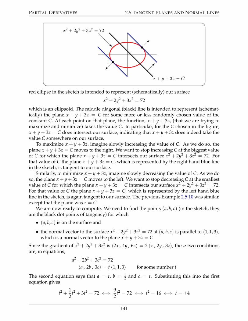
PARTIAL DERIVATIVES 2.5 TANGENT PLANES AND NORMAL LINES
x ` y ` 3z “ C
x2 ` 2y2 ` 3z2 “ 72
red ellipse in the sketch is intended to represent (schematically) our surface
x2 + 2y2 + 3z2 = 72
which is an ellipsoid. The middle diagonal (black) line is intended to represent (schemat-ically) the plane x + y + 3z = C for some more or less randomly chosen value of theconstant C. At each point on that plane, the function, x + y + 3z, (that we are trying tomaximize and minimize) takes the value C. In particular, for the C chosen in the figure,x + y + 3z = C does intersect our surface, indicating that x + y + 3z does indeed take thevalue C somewhere on our surface.
To maximize x + y + 3z, imagine slowly increasing the value of C. As we do so, theplane x + y+ 3z = C moves to the right. We want to stop increasing C at the biggest valueof C for which the plane x + y + 3z = C intersects our surface x2 + 2y2 + 3z2 = 72. Forthat value of C the plane x + y + 3z = C, which is represented by the right hand blue linein the sketch, is tangent to our surface.
Similarly, to minimize x + y + 3z, imagine slowly decreasing the value of C. As we doso, the plane x+ y+ 3z = C moves to the left. We want to stop decreasing C at the smallestvalue of C for which the plane x + y + 3z = C intersects our surface x2 + 2y2 + 3z2 = 72.For that value of C the plane x + y + 3z = C, which is represented by the left hand blueline in the sketch, is again tangent to our surface. The previous Example 2.5.10 was similar,except that the plane was z = C.
We are now ready to compute. We need to find the points (a, b, c) (in the sketch, theyare the black dot points of tangency) for which
• (a, b, c) is on the surface and
• the normal vector to the surface x2 + 2y2 + 3z2 = 72 at (a, b, c) is parallel to 〈1, 1, 3〉,which is a normal vector to the plane x + y + 3z = C
Since the gradient of x2 + 2y2 + 3z2 is 〈2x , 4y , 6z〉 = 2 〈x , 2y , 3z〉, these two conditionsare, in equations,
a2 + 2b2 + 3c2 = 72〈a , 2b , 3c〉 = t 〈1, 1, 3〉 for some number t
The second equation says that a = t, b = t2 and c = t. Substituting this into the first
equation gives
t2 +12
t2 + 3t2 = 72 ðñ 92
t2 = 72 ðñ t2 = 16 ðñ t = ˘4
141
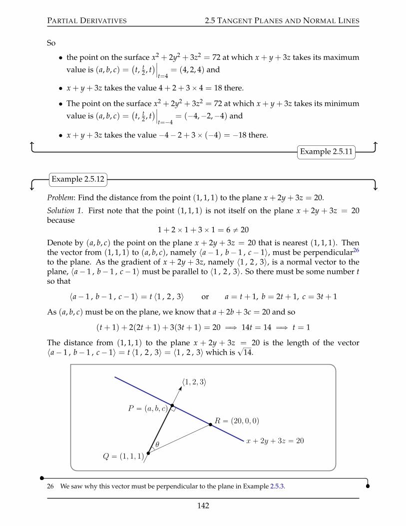
PARTIAL DERIVATIVES 2.5 TANGENT PLANES AND NORMAL LINES
So
• the point on the surface x2 + 2y2 + 3z2 = 72 at which x + y + 3z takes its maximum
value is (a, b, c) =(t, t
2 , t)ˇˇt=4
= (4, 2, 4) and
• x + y + 3z takes the value 4 + 2 + 3ˆ 4 = 18 there.
• The point on the surface x2 + 2y2 + 3z2 = 72 at which x + y + 3z takes its minimum
value is (a, b, c) =(t, t
2 , t)ˇˇt=´4
= (´4,´2,´4) and
• x + y + 3z takes the value ´4´ 2 + 3ˆ (´4) = ´18 there.
Example 2.5.11
Example 2.5.12
Problem: Find the distance from the point (1, 1, 1) to the plane x + 2y + 3z = 20.
Solution 1. First note that the point (1, 1, 1) is not itself on the plane x + 2y + 3z = 20because
1 + 2ˆ 1 + 3ˆ 1 = 6 ‰ 20
Denote by (a, b, c) the point on the plane x + 2y + 3z = 20 that is nearest (1, 1, 1). Thenthe vector from (1, 1, 1) to (a, b, c), namely 〈a´ 1 , b´ 1 , c´ 1〉, must be perpendicular26
to the plane. As the gradient of x + 2y + 3z, namely 〈1 , 2 , 3〉, is a normal vector to theplane, 〈a´ 1 , b´ 1 , c´ 1〉 must be parallel to 〈1 , 2 , 3〉. So there must be some number tso that
〈a´ 1 , b´ 1 , c´ 1〉 = t 〈1 , 2 , 3〉 or a = t + 1, b = 2t + 1, c = 3t + 1
As (a, b, c) must be on the plane, we know that a + 2b + 3c = 20 and so
(t + 1) + 2(2t + 1) + 3(3t + 1) = 20 ùñ 14t = 14 ùñ t = 1
The distance from (1, 1, 1) to the plane x + 2y + 3z = 20 is the length of the vector〈a´ 1 , b´ 1 , c´ 1〉 = t 〈1 , 2 , 3〉 = 〈1 , 2 , 3〉 which is
?14.
x ` 2y ` 3z “ 20
P “ pa, b, cq
Q “ p1, 1, 1q
R “ p20, 0, 0q
〈1, 2, 3〉
θ
26 We saw why this vector must be perpendicular to the plane in Example 2.5.3.
142

PARTIAL DERIVATIVES 2.5 TANGENT PLANES AND NORMAL LINES
Solution 2. Denote by P = (a, b, c) the point on the plane x + 2y + 3z = 20 that is nearestthe point Q = (1, 1, 1). Pick any other point on the plane and call it R. For example(x, y, z) = (20, 0, 0) obeys x + 2y + 3z = 20 and so R = (20, 0, 0) is a point on the plane.
The triangle PQR is right angled. Denote by θ the angle between the hypotenuse QRand the side QP. The distance from Q = (1, 1, 1) to the plane is the length of the linesegment QP, which is
distance = |QP| = |QR| cos θ
Now, the dot product between the vector from Q to R, which is 〈19,´1,´1〉, with thevector 〈1, 2, 3〉, which is normal to the plane and hence parallel to the side QP is
〈19,´1,´1〉 ¨ 〈1, 2, 3〉 = 14
= | 〈19,´1,´1〉 | | 〈1, 2, 3〉 | cos θ = |QR|?
14 cos θ
so that, finally,
distance = |QR| cos θ =14?14
=?
14
Example 2.5.12
Example 2.5.13
Problem: Let F(x, y, z) = 0 and G(x, y, z) = 0 be two surfaces. These two surfaces intersectalong a curve. Find a tangent vector to this curve at the point (x0, y0, z0).
Solution. Call the tangent vector T. Then T has to be
˝ tangent to the surface F(x, y, z) = 0 at (x0, y0, z0) and˝ tangent to the surface G(x, y, z) = 0 at (x0, y0, z0).
Consequently T has to be
˝ perpendicular to the vector∇∇∇F(x0, y0, z0), which is normal to F(x, y, z) = 0 at (x0, y0, z0),and at the same time has to be
˝ perpendicular to the vector ∇∇∇G(x0, y0, z0), which is normal to G(x, y, z) = 0 at(x0, y0, z0).
Recall that an easy way to construct a vector that is perpendicular to two other vectors isto take their cross product. So we take
T =∇∇∇F(x0, y0, z0)ˆ∇∇∇G(x0, y0, z0) = det
ııı kFx Fy FzGx Gy Gz
=(
FyGz ´ FzGy)
ııı +(
FzGx ´ FxGz)
+(
FxGy ´ FyGx)
k
where all partial derivatives are evaluated at (x, y, z) = (x0, y0, z0).
143
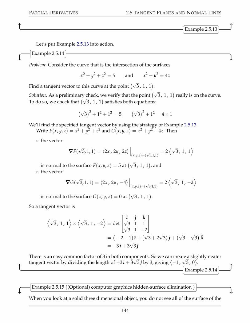
PARTIAL DERIVATIVES 2.5 TANGENT PLANES AND NORMAL LINES
Example 2.5.13
Let’s put Example 2.5.13 into action.
Example 2.5.14
Problem: Consider the curve that is the intersection of the surfaces
x2 + y2 + z2 = 5 and x2 + y2 = 4z
Find a tangent vector to this curve at the point(?
3 , 1 , 1).
Solution. As a preliminary check, we verify that the point(?
3 , 1 , 1)
really is on the curve.To do so, we check that
(?3 , 1 , 1
)satisfies both equations:
(?3)2
+ 12 + 12 = 5(?
3)2
+ 12 = 4ˆ 1
We’ll find the specified tangent vector by using the strategy of Example 2.5.13.Write F(x, y, z) = x2 + y2 + z2 and G(x, y, z) = x2 + y2 ´ 4z. Then
˝ the vector
∇∇∇F(?
3, 1, 1) = 〈2x , 2y , 2z〉ˇˇ(x,y,z)=(
?3,1,1)
= 2⟨?
3 , 1 , 1⟩
is normal to the surface F(x, y, z) = 5 at(?
3 , 1 , 1), and
˝ the vector
∇∇∇G(?
3, 1, 1) = 〈2x , 2y , ´4〉ˇˇ(x,y,z)=(
?3,1,1)
= 2⟨?
3 , 1 , ´2⟩
is normal to the surface G(x, y, z) = 0 at(?
3 , 1 , 1).
So a tangent vector is
⟨?3 , 1 , 1
⟩ˆ⟨?
3 , 1 , ´2⟩= det
ııı k?3 1 1?3 1 ´2
=(´ 2´ 1
)ııı +(?
3 + 2?
3)
+(?
3´?3)
k
= ´3 ııı + 3?
3
There is an easy common factor of 3 in both components. So we can create a slightly neatertangent vector by dividing the length of ´3 ııı + 3
?3 by 3, giving
⟨´1 ,?
3 , 0⟩.
Example 2.5.14
Example 2.5.15 ((Optional) computer graphics hidden-surface elimination )
When you look at a solid three dimensional object, you do not see all of the surface of the
144
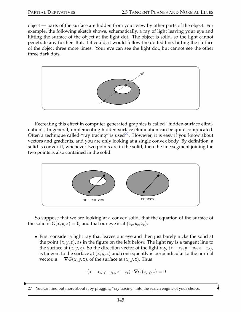
PARTIAL DERIVATIVES 2.5 TANGENT PLANES AND NORMAL LINES
object — parts of the surface are hidden from your view by other parts of the object. Forexample, the following sketch shows, schematically, a ray of light leaving your eye andhitting the surface of the object at the light dot. The object is solid, so the light cannotpenetrate any further. But, if it could, it would follow the dotted line, hitting the surfaceof the object three more times. Your eye can see the light dot, but cannot see the otherthree dark dots.
Recreating this effect in computer generated graphics is called “hidden-surface elimi-nation”. In general, implementing hidden-surface elimination can be quite complicated.Often a technique called “ray tracing” is used27. However, it is easy if you know aboutvectors and gradients, and you are only looking at a single convex body. By definition, asolid is convex if, whenever two points are in the solid, then the line segment joining thetwo points is also contained in the solid.
not convex convex
So suppose that we are looking at a convex solid, that the equation of the surface ofthe solid is G(x, y, z) = 0, and that our eye is at (xe, ye, ze).
• First consider a light ray that leaves our eye and then just barely nicks the solid atthe point (x, y, z), as in the figure on the left below. The light ray is a tangent line tothe surface at (x, y, z). So the direction vector of the light ray, 〈x´ xe, y´ ye, z´ ze〉,is tangent to the surface at (x, y, z) and consequently is perpendicular to the normalvector, n =∇∇∇G(x, y, z), of the surface at (x, y, z). Thus
〈x´ xe, y´ ye, z´ ze〉 ¨∇∇∇G(x, y, z) = 0
27 You can find out more about it by plugging “ray tracing” into the search engine of your choice.
145
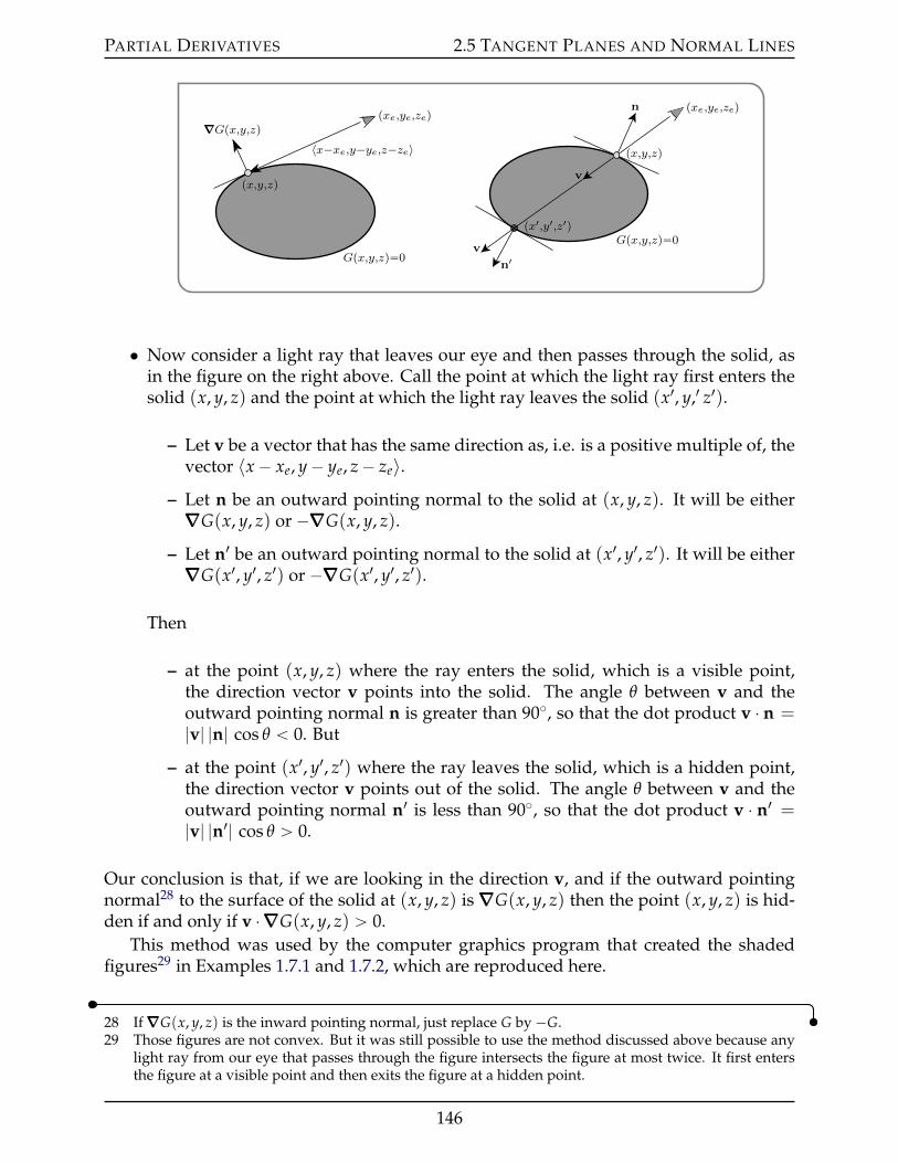
PARTIAL DERIVATIVES 2.5 TANGENT PLANES AND NORMAL LINES
Gpx,y,zq“0
pxe,ye,zeq
〈x´xe,y´ye,z´ze〉∇∇∇Gpx,y,zq
px,y,zq
Gpx,y,zq“0
v
n
px,y,zq
pxe,ye,zeq
px1,y1,z1qv
n1
• Now consider a light ray that leaves our eye and then passes through the solid, asin the figure on the right above. Call the point at which the light ray first enters thesolid (x, y, z) and the point at which the light ray leaves the solid (x1, y,1 z1).
– Let v be a vector that has the same direction as, i.e. is a positive multiple of, thevector 〈x´ xe, y´ ye, z´ ze〉.
– Let n be an outward pointing normal to the solid at (x, y, z). It will be either∇∇∇G(x, y, z) or ´∇∇∇G(x, y, z).
– Let n1 be an outward pointing normal to the solid at (x1, y1, z1). It will be either∇∇∇G(x1, y1, z1) or ´∇∇∇G(x1, y1, z1).
Then
– at the point (x, y, z) where the ray enters the solid, which is a visible point,the direction vector v points into the solid. The angle θ between v and theoutward pointing normal n is greater than 90˝, so that the dot product v ¨ n =|v| |n| cos θ ă 0. But
– at the point (x1, y1, z1) where the ray leaves the solid, which is a hidden point,the direction vector v points out of the solid. The angle θ between v and theoutward pointing normal n1 is less than 90˝, so that the dot product v ¨ n1 =|v| |n1| cos θ ą 0.
Our conclusion is that, if we are looking in the direction v, and if the outward pointingnormal28 to the surface of the solid at (x, y, z) is∇∇∇G(x, y, z) then the point (x, y, z) is hid-den if and only if v ¨∇∇∇G(x, y, z) ą 0.
This method was used by the computer graphics program that created the shadedfigures29 in Examples 1.7.1 and 1.7.2, which are reproduced here.
28 If∇∇∇G(x, y, z) is the inward pointing normal, just replace G by ´G.29 Those figures are not convex. But it was still possible to use the method discussed above because any
light ray from our eye that passes through the figure intersects the figure at most twice. It first entersthe figure at a visible point and then exits the figure at a hidden point.
146
PARTIAL DERIVATIVES 2.6 LINEAR APPROXIMATIONS AND ERROR
Example 2.5.15
Tangent planes, in addition to being geometric objects, provide a simple but powerfultool for approximating functions of two variables near a specified point. We saw some-thing very similar in the CLP-1 text where we approximated functions of one variable bytheir tangent lines. This brings us to our next topic — approximating functions.
2.6IJ Linear Approximations and Error
A frequently used, and effective, strategy for building an understanding of the behaviourof a complicated function near a point is to approximate it by a simple function. Thefollowing suite of such approximations is standard fare in Calculus I courses. See, forexample, §3.4 in the CLP-1 text.
g(t0 + ∆t) « g(t0) constant approximationg(t0 + ∆t) « g(t0) + g1(t0)∆t linear, or tangent line, approximation
g(t0 + ∆t) « g(t0) + g1(t0)∆t + 12 g2(t0)∆t2 quadratic approximation
More generally, for any natural number n, the approximation
g(t0 + ∆t) « g(t0) + g1(t0)∆t + 12 g2(t0)∆t2 + ¨ ¨ ¨+ 1
n! g(n)(t0)∆tn
is known as the Taylor polynomial of degree n. You may have also found a formula forthe error introduced in making this approximation. The error En(∆t) is defined by
g(t0 + ∆t) = g(t0) + g1(t0)∆t + 12! g
2(t0)∆t2 + ¨ ¨ ¨+ 1n! g
(n)(t0)∆tn + En(∆t)
and obeys30
En(∆t) = 1(n+1)! g
(n+1)(t0 + c∆t)∆tn+1
for some (unknown) 0 ď c ď 1.It is a simple matter to use these one dimensional approximations to generate the anal-
ogous multidimensional approximations. To introduce the ideas, we’ll generate the linearapproximation to a function, f (x, y), of two variables, near the point (x0, y0). Define
g(t) = f(x0 + t ∆x , y0 + t ∆y
)
30 You may have seen it written as En(x) = 1(n+1)! g(n+1)(c)(x´ a)n+1
147
PARTIAL DERIVATIVES 2.6 LINEAR APPROXIMATIONS AND ERROR
We have defined g(t) so that
g(0) = f(x0 , y0
)and g(1) = f
(x0 + ∆x , y0 + ∆y
)
Consequently, setting t0 = 0 and ∆t = 1,
f(x0 + ∆x , y0 + ∆y
)= g(1) = g(t0 + ∆t)« g(t0) + g1(t0)∆t= g(0) + g1(0)
We can now compute g1(0) using the multivariable chain rule of (2.4.2):
g1(t) =B fBx(x0 + t ∆x , y0 + t ∆y
)∆x +
B fBy(x0 + t ∆x , y0 + t ∆y
)∆y
so that,
f(x0 + ∆x , y0 + ∆y
) « f(x0 , y0
)+B fBx(x0 , y0
)∆x +
B fBy(x0 , y0
)∆y
Equation 2.6.1.
Of course exactly the same procedure works for functions of three or more variables. Inparticular
f(x0 + ∆x , y0 + ∆y , z0 + ∆z
)
« f(x0 , y0 , z0
)+B fBx(x0 , y0 , z0
)∆x +
B fBy(x0 , y0 , z0
)∆y +
B fBz(x0 , y0 , z0
)∆z
Equation 2.6.2.
While these linear approximations are quite simple, they tend to be pretty decent provided∆x and ∆y are small. See the optional §2.6.1 for a more precise statement.
Remark 2.6.3. Applying (2.6.1), with ∆x = x´ x0 and ∆y = y´ y0. gives
f(x , y
) « f(x0 , y0
)+B fBx(x0 , y0
)(x´ x0) +
B fBy(x0 , y0
)(y´ y0)
Looking at part (b) of Theorem 2.5.1, we see that this just says that the tangent plane tothe surface z = f (x, y) at the point
(x0 , y0 , f (x0, y0)
)remains close to the surface when
(x, y) is close to (x0, y0).
Example 2.6.4
Letf (x, y) =
bx2 + y2
148
PARTIAL DERIVATIVES 2.6 LINEAR APPROXIMATIONS AND ERROR
Then
B fBx
(x, y) =12
2xax2 + y2
fx(x0, y0) =x0b
x20 + y2
0
B fBy
(x, y) =12
2yax2 + y2
fy(x0, y0) =y0b
x20 + y2
0
so that the linear approximation to f (x, y) at (x0, y0) is
f(x0 + ∆x , y0 + ∆y
) « f(x0 , y0
)+ fx
(x0 , y0
)∆x + fy
(x0 , y0
)∆y
=b
x20 + y2
0 +x0b
x20 + y2
0
∆x +y0b
x20 + y2
0
∆y
Example 2.6.4
People often write ∆ f for the change f(x0 +∆x , y0 +∆y
)´ f(x0 , y0
)in the value
of f . Then the linear approximation (2.6.1) becomes
∆ f « B fBx(x0 , y0
)∆x +
B fBy(x0 , y0
)∆y
If they want to emphasize that that ∆x, ∆y and ∆ f are really small (they mayeven say “infinitesimal”), they’ll write31 dx, dy and d f instead. In this notation
d f « B fBx(x0 , y0
)dx +
B fBy(x0 , y0
)dy
Notation 2.6.5.
Suppose that we wish to approximate a quantity Q and that the approximationturns out to be Q + ∆Q. Then
• the absolute error in the approximation is |∆Q| and
• the relative error in the approximation isˇˇ∆Q
Q
ˇˇ and
• the percentage error in the approximation is 100ˇˇ∆Q
Q
ˇˇ
Definition 2.6.6.
31 Don’t take the notation dx or the terminology “infinitesimal” too seriously. It is just intended to signal“very small”.
149
PARTIAL DERIVATIVES 2.6 LINEAR APPROXIMATIONS AND ERROR
In Example 3.4.5 of the CLP-1 text we found an approximate value for the number?4.1 by using a linear approximation to the single variable function f (x) =
?x. We can
make similar use of linear approximations to multivariable functions.
Example 2.6.7
Problem: Find an approximate value for (0.998)3
1.003 .
Solution: Set f (x, y) =x3
y. We are to find (approximately) f (0.998 , 1.003). We can easily
find
f (1, 1) =13
1= 1
and sinceB fBx
=3x2
yand
B fBy
= ´x3
y2
we can also easily find
B fBx
(1, 1) = 312
1= 3
B fBy
(1, 1) = 113
12 = ´1
So, setting ∆x = ´0.002 and ∆y = 0.003, we have
0.9983
1.003= f (0.998 , 1.003) = f (1 + ∆x , 1 + ∆y) « f
(1, 1)+B fBx(1, 1)
∆x +B fBy(1, 1)
∆y
« 1 + 3(´0.002)´ 1(0.003) = 0.991
By way of comparison, the exact answer is 0.9910389 to seven decimal places.
Example 2.6.7
Example 2.6.8
Problem: Find an approximate value for (4.2)1/2 + (26.7)1/3 + (256.4)1/4.
Solution: Set f (x, y, z) = x1/2 + y1/3 + z1/4. We are to find (approximately) f (4.2 , 26.7 , 256.4).We can easily find
f (4, 27, 256) = (4)1/2 + (27)1/3 + (256)1/4 = 2 + 3 + 4 = 9
and sinceB fBx
=1
2x1/2B fBy
=1
3y2/3B fBz
=1
4z3/4
150
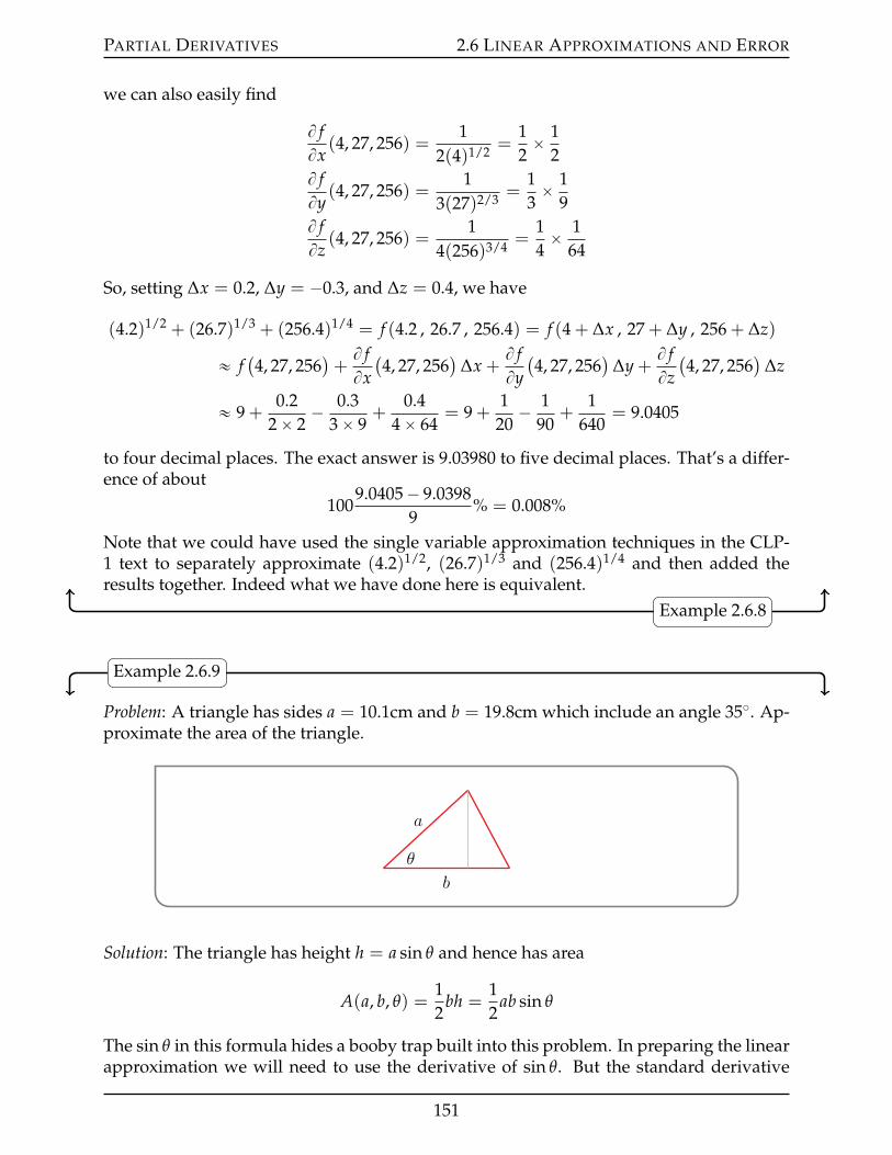
PARTIAL DERIVATIVES 2.6 LINEAR APPROXIMATIONS AND ERROR
we can also easily find
B fBx
(4, 27, 256) =1
2(4)1/2 =12ˆ 1
2B fBy
(4, 27, 256) =1
3(27)2/3 =13ˆ 1
9B fBz
(4, 27, 256) =1
4(256)3/4 =14ˆ 1
64
So, setting ∆x = 0.2, ∆y = ´0.3, and ∆z = 0.4, we have
(4.2)1/2 + (26.7)1/3 + (256.4)1/4 = f (4.2 , 26.7 , 256.4) = f (4 + ∆x , 27 + ∆y , 256 + ∆z)
« f(4, 27, 256
)+B fBx(4, 27, 256
)∆x +
B fBy(4, 27, 256
)∆y +
B fBz(4, 27, 256
)∆z
« 9 +0.2
2ˆ 2´ 0.3
3ˆ 9+
0.44ˆ 64
= 9 +1
20´ 1
90+
1640
= 9.0405
to four decimal places. The exact answer is 9.03980 to five decimal places. That’s a differ-ence of about
1009.0405´ 9.0398
9% = 0.008%
Note that we could have used the single variable approximation techniques in the CLP-1 text to separately approximate (4.2)1/2, (26.7)1/3 and (256.4)1/4 and then added theresults together. Indeed what we have done here is equivalent.
Example 2.6.8
Example 2.6.9
Problem: A triangle has sides a = 10.1cm and b = 19.8cm which include an angle 35˝. Ap-proximate the area of the triangle.
θ
b
a
Solution: The triangle has height h = a sin θ and hence has area
A(a, b, θ) =12
bh =12
ab sin θ
The sin θ in this formula hides a booby trap built into this problem. In preparing the linearapproximation we will need to use the derivative of sin θ. But the standard derivative
151
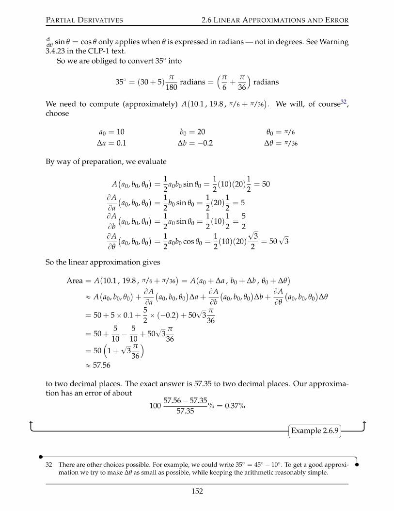
PARTIAL DERIVATIVES 2.6 LINEAR APPROXIMATIONS AND ERROR
ddθ sin θ = cos θ only applies when θ is expressed in radians — not in degrees. See Warning3.4.23 in the CLP-1 text.
So we are obliged to convert 35˝ into
35˝ = (30 + 5)π
180radians =
(π
6+
π
36
)radians
We need to compute (approximately) A(10.1 , 19.8 , π/6 + π/36). We will, of course32,
choose
a0 = 10 b0 = 20 θ0 = π/6
∆a = 0.1 ∆b = ´0.2 ∆θ = π/36
By way of preparation, we evaluate
A(a0, b0, θ0
)=
12
a0b0 sin θ0 =12(10)(20)
12= 50
BABa(a0, b0, θ0
)=
12
b0 sin θ0 =12(20)
12= 5
BABb(a0, b0, θ0
)=
12
a0 sin θ0 =12(10)
12=
52
BABθ
(a0, b0, θ0
)=
12
a0b0 cos θ0 =12(10)(20)
?3
2= 50
?3
So the linear approximation gives
Area = A(10.1 , 19.8 , π/6 + π/36)= A(a0 + ∆a , b0 + ∆b , θ0 + ∆θ
)
« A(a0, b0, θ0
)+BABa(a0, b0, θ0
)∆a +
BABb(a0, b0, θ0
)∆b +
BABθ
(a0, b0, θ0
)∆θ
= 50 + 5ˆ 0.1 +52ˆ (´0.2) + 50
?3
π
36
= 50 +5
10´ 5
10+ 50
?3
π
36= 50
(1 +
?3
π
36
)
« 57.56
to two decimal places. The exact answer is 57.35 to two decimal places. Our approxima-tion has an error of about
10057.56´ 57.35
57.35% = 0.37%
Example 2.6.9
32 There are other choices possible. For example, we could write 35˝ = 45˝ ´ 10˝. To get a good approxi-mation we try to make ∆θ as small as possible, while keeping the arithmetic reasonably simple.
152
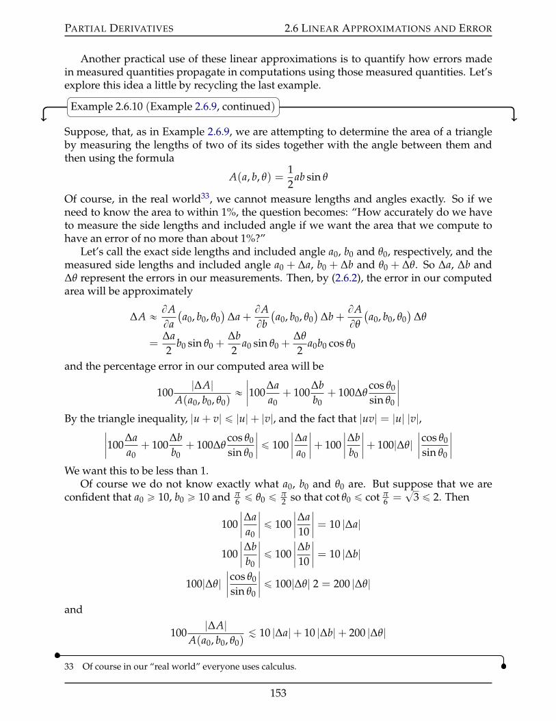
PARTIAL DERIVATIVES 2.6 LINEAR APPROXIMATIONS AND ERROR
Another practical use of these linear approximations is to quantify how errors madein measured quantities propagate in computations using those measured quantities. Let’sexplore this idea a little by recycling the last example.
Example 2.6.10 (Example 2.6.9, continued)
Suppose, that, as in Example 2.6.9, we are attempting to determine the area of a triangleby measuring the lengths of two of its sides together with the angle between them andthen using the formula
A(a, b, θ) =12
ab sin θ
Of course, in the real world33, we cannot measure lengths and angles exactly. So if weneed to know the area to within 1%, the question becomes: “How accurately do we haveto measure the side lengths and included angle if we want the area that we compute tohave an error of no more than about 1%?”
Let’s call the exact side lengths and included angle a0, b0 and θ0, respectively, and themeasured side lengths and included angle a0 + ∆a, b0 + ∆b and θ0 + ∆θ. So ∆a, ∆b and∆θ represent the errors in our measurements. Then, by (2.6.2), the error in our computedarea will be approximately
∆A « BABa(a0, b0, θ0
)∆a +
BABb(a0, b0, θ0
)∆b +
BABθ
(a0, b0, θ0
)∆θ
=∆a2
b0 sin θ0 +∆b2
a0 sin θ0 +∆θ
2a0b0 cos θ0
and the percentage error in our computed area will be
100|∆A|
A(a0, b0, θ0)«ˇˇ100
∆aa0
+ 100∆bb0
+ 100∆θcos θ0
sin θ0
ˇˇ
By the triangle inequality, |u + v| ď |u|+ |v|, and the fact that |uv| = |u| |v|,ˇˇ100
∆aa0
+ 100∆bb0
+ 100∆θcos θ0
sin θ0
ˇˇ ď 100
ˇˇ∆a
a0
ˇˇ+ 100
ˇˇ∆b
b0
ˇˇ+ 100|∆θ|
ˇˇcos θ0
sin θ0
ˇˇ
We want this to be less than 1.Of course we do not know exactly what a0, b0 and θ0 are. But suppose that we are
confident that a0 ě 10, b0 ě 10 and π6 ď θ0 ď π
2 so that cot θ0 ď cot π6 =
?3 ď 2. Then
100ˇˇ∆a
a0
ˇˇ ď 100
ˇˇ∆a10
ˇˇ = 10 |∆a|
100ˇˇ∆b
b0
ˇˇ ď 100
ˇˇ∆b10
ˇˇ = 10 |∆b|
100|∆θ|ˇˇcos θ0
sin θ0
ˇˇ ď 100|∆θ| 2 = 200 |∆θ|
and
100|∆A|
A(a0, b0, θ0)À 10 |∆a|+ 10 |∆b|+ 200 |∆θ|
33 Of course in our “real world” everyone uses calculus.
153
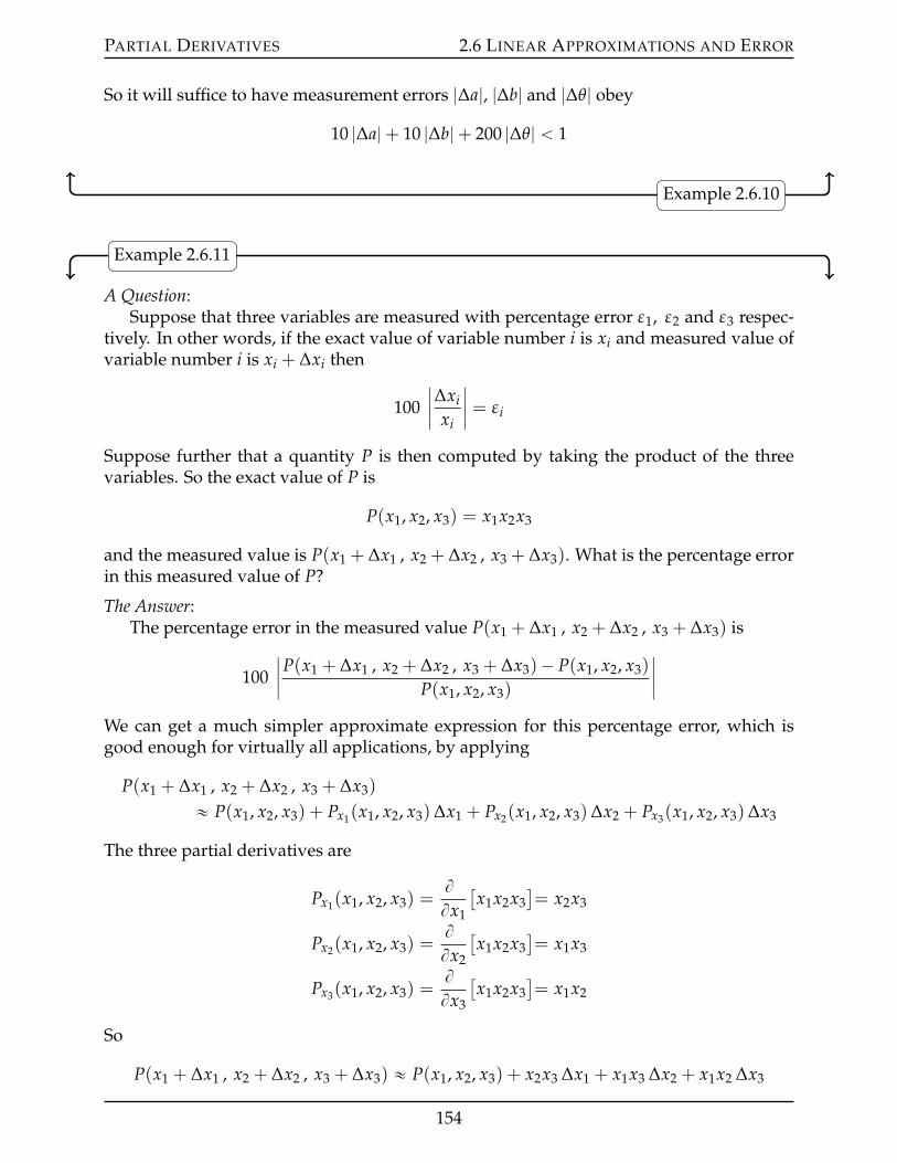
PARTIAL DERIVATIVES 2.6 LINEAR APPROXIMATIONS AND ERROR
So it will suffice to have measurement errors |∆a|, |∆b| and |∆θ| obey
10 |∆a|+ 10 |∆b|+ 200 |∆θ| ă 1
Example 2.6.10
Example 2.6.11
A Question:Suppose that three variables are measured with percentage error ε1, ε2 and ε3 respec-
tively. In other words, if the exact value of variable number i is xi and measured value ofvariable number i is xi + ∆xi then
100ˇˇ∆xi
xi
ˇˇ = εi
Suppose further that a quantity P is then computed by taking the product of the threevariables. So the exact value of P is
P(x1, x2, x3) = x1x2x3
and the measured value is P(x1 + ∆x1 , x2 + ∆x2 , x3 + ∆x3). What is the percentage errorin this measured value of P?
The Answer:The percentage error in the measured value P(x1 + ∆x1 , x2 + ∆x2 , x3 + ∆x3) is
100ˇˇP(x1 + ∆x1 , x2 + ∆x2 , x3 + ∆x3)´ P(x1, x2, x3)
P(x1, x2, x3)
ˇˇ
We can get a much simpler approximate expression for this percentage error, which isgood enough for virtually all applications, by applying
P(x1 + ∆x1 , x2 + ∆x2 , x3 + ∆x3)
« P(x1, x2, x3) + Px1(x1, x2, x3)∆x1 + Px2(x1, x2, x3)∆x2 + Px3(x1, x2, x3)∆x3
The three partial derivatives are
Px1(x1, x2, x3) =BBx1
[x1x2x3
]= x2x3
Px2(x1, x2, x3) =BBx2
[x1x2x3
]= x1x3
Px3(x1, x2, x3) =BBx3
[x1x2x3
]= x1x2
So
P(x1 + ∆x1 , x2 + ∆x2 , x3 + ∆x3) « P(x1, x2, x3) + x2x3 ∆x1 + x1x3 ∆x2 + x1x2 ∆x3
154
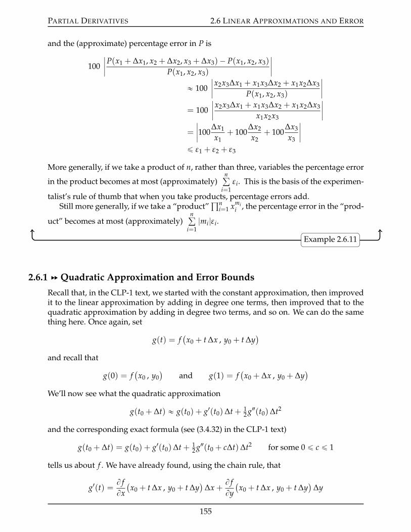
PARTIAL DERIVATIVES 2.6 LINEAR APPROXIMATIONS AND ERROR
and the (approximate) percentage error in P is
100ˇˇP(x1 + ∆x1, x2 + ∆x2, x3 + ∆x3)´ P(x1, x2, x3)
P(x1, x2, x3)
ˇˇ
« 100ˇˇx2x3∆x1 + x1x3∆x2 + x1x2∆x3
P(x1, x2, x3)
ˇˇ
= 100ˇˇx2x3∆x1 + x1x3∆x2 + x1x2∆x3
x1x2x3
ˇˇ
=
ˇˇ100
∆x1
x1+ 100
∆x2
x2+ 100
∆x3
x3
ˇˇ
ď ε1 + ε2 + ε3
More generally, if we take a product of n, rather than three, variables the percentage error
in the product becomes at most (approximately)nř
i=1εi. This is the basis of the experimen-
talist’s rule of thumb that when you take products, percentage errors add.Still more generally, if we take a “product”
śni=1 xmi
i , the percentage error in the “prod-
uct” becomes at most (approximately)nř
i=1|mi|εi.
Example 2.6.11
2.6.1 §§ Quadratic Approximation and Error Bounds
Recall that, in the CLP-1 text, we started with the constant approximation, then improvedit to the linear approximation by adding in degree one terms, then improved that to thequadratic approximation by adding in degree two terms, and so on. We can do the samething here. Once again, set
g(t) = f(x0 + t ∆x , y0 + t ∆y
)
and recall that
g(0) = f(x0 , y0
)and g(1) = f
(x0 + ∆x , y0 + ∆y
)
We’ll now see what the quadratic approximation
g(t0 + ∆t) « g(t0) + g1(t0)∆t + 12 g2(t0)∆t2
and the corresponding exact formula (see (3.4.32) in the CLP-1 text)
g(t0 + ∆t) = g(t0) + g1(t0)∆t + 12 g2(t0 + c∆t)∆t2 for some 0 ď c ď 1
tells us about f . We have already found, using the chain rule, that
g1(t) =B fBx(x0 + t ∆x , y0 + t ∆y
)∆x +
B fBy(x0 + t ∆x , y0 + t ∆y
)∆y
155
PARTIAL DERIVATIVES 2.6 LINEAR APPROXIMATIONS AND ERROR
We now need to evaluate g2(t). Temporarily write f1 = B fBx and f2 = B f
By so that
g1(t) = f1(x0 + t ∆x , y0 + t ∆y
)∆x + f2
(x0 + t ∆x , y0 + t ∆y
)∆y
Then we have, again using the chain rule,
ddt[
f1(x0 + t ∆x , y0 + t ∆y
)]=B f1
Bx(x0 + t ∆x , y0 + t ∆y
)∆x +
B f1
By(x0 + t ∆x , y0 + t ∆y
)∆y
=B2 fBx2
(x0 + t ∆x , y0 + t ∆y
)∆x +
B2 fByBx
(x0 + t ∆x , y0 + t ∆y
)∆y (˚)
and
ddt[
f2(x0 + t ∆x , y0 + t ∆y
)]=B f2
Bx(x0 + t ∆x , y0 + t ∆y
)∆x +
B f2
By(x0 + t ∆x , y0 + t ∆y
)∆y
=B2 fBxBy
(x0 + t ∆x , y0 + t ∆y
)∆x +
B2 fBy2
(x0 + t ∆x , y0 + t ∆y
)∆y (˚˚)
Adding ∆x times (˚) to ∆y times (˚˚) and recalling that B2 fByBx = B2 f
BxBy , gives
g2(t) =B2 fBx2
(x0 + t ∆x , y0 + t ∆y
)∆x2 + 2
B2 fBxBy
(x0 + t ∆x , y0 + t ∆y
)∆x∆y
+B2 fBy2
(x0 + t ∆x , y0 + t ∆y
)∆y2
Now setting t0 = 0 and ∆t = 1, the quadratic approximation
f(x0 + ∆x , y0 + ∆y
)= g(1) « g(0) + g1(0) + 1
2 g2(0)
is
f(x0 + ∆x , y0 + ∆y
) « f(x0 , y0
)+B fBx(x0 , y0
)∆x +
B fBy(x0 , y0
)∆y
+12
"B2 fBx2
(x0, y0
)∆x2 + 2
B2 fBxBy
(x0, y0
)∆x∆y +
B2 fBy2
(x0, y0
)∆y2
*
Equation 2.6.12.
and the corresponding exact formula
f(x0 + ∆x , y0 + ∆y
)= g(1) = g(0) + g1(0) + 1
2 g2(c)
is
156
PARTIAL DERIVATIVES 2.6 LINEAR APPROXIMATIONS AND ERROR
f(x0 + ∆x , y0 + ∆y
)= f
(x0 , y0
)+B fBx(x0 , y0
)∆x +
B fBy(x0 , y0
)∆y
+12
"B2 fBx2
(r(c)
)∆x2 + 2
B2 fBxBy
(r(c)
)∆x∆y +
B2 fBy2
(r(c)
)∆y2
*
where r(c) =(x0 + c ∆x , y0 + c ∆y
)and c is some (unknown) number satisfying
0 ď c ď 1.
Equation 2.6.13.
If we can bound the second derivativesˇˇB2 fBx2
(r(c)
)ˇˇ ,ˇˇ B2 fBxBy
(r(c)
)ˇˇ ,ˇˇB2 fBy2
(r(c)
)ˇˇ ď M
we can massage (2.6.13) into the formˇˇ f(x0 + ∆x , y0 + ∆y
)´!
f(x0 , y0
)+B fBx(x0 , y0
)∆x +
B fBy(x0 , y0
)∆y
)ˇˇ
ď M2(|∆x|2 + 2|∆x| |∆y|+ |∆y|2)
Equation 2.6.14.
Why might we want to do this? The left hand side of (2.6.14) is exactly the error in thelinear approximation (2.6.1). So the right hand side is a rigorous bound on the error in thelinear approximation.
Example 2.6.15 (Example 2.6.7, continued)
Suppose that we approximate (0.998)3
1.003 as in Example 2.6.7 and we want a rigorous boundon the approximation. We can get such a rigorous bound by applying (2.6.13). Set
f (x, y) =x3
y
and
x0 = 1 ∆x = ´0.002 y0 = 1 ∆y = 0.003
Then the exact answer is f(x0 + ∆x , y0 + ∆y
)and the approximate answer is f
(x0 , y0
)+
B fBx(x0 , y0
)∆x+ B f
By(x0 , y0
)∆y, so that, by (2.6.13), the error in the approximation is exactly
12
ˇˇB2 fBx2
(r(c)
)∆x2 + 2
B2 fBxBy
(r(c)
)∆x∆y +
B2 fBy2
(r(c)
)∆y2
ˇˇ
157
PARTIAL DERIVATIVES 2.6 LINEAR APPROXIMATIONS AND ERROR
with r(c) =(1´ 0.002c , 1 + 0.0003c
)for some, unknown, 0 ď c ď 1. For our function f
f (x, y) =x3
yB fBx
(x, y) =3x2
yB fBy
(x, y) = ´x3
y2
B2 fBx2 (x, y) =
6xy
B2 fBxBy
(x, y) = ´3x2
y2B2 fBy2 (x, y) =
2x3
y3
We don’t know what r(c) =(1´ 0.002c , 1 + 0.0003c
)is. But we know that 0 ď c ď 1, so
we definitely know that the x component of r(c) is smaller that 1 and the y component ofr(c) is bigger than 1. So
ˇˇB2 fBx2
(r(c)
)ˇˇ ď 6ˇˇ B2 fBxBy
(r(c)
)ˇˇ ď 3ˇˇB2 fBy2
(r(c)
)ˇˇ ď 2
and
error ď 12
[6∆x2 + 2ˆ 3|∆x ∆y|+ 2∆y2
]
ď 3(0.002)2 + 3(0.002)(0.003) + (0.003)2
= 0.000039
By way of comparison, the exact error is 0.0000389, to seven decimal places.
Example 2.6.15
Example 2.6.16
In this example, we find the quadratic approximation of f (x, y) =a
1 + 4x2 + y2 at(x0, y0) = (1, 2) and use it to compute approximately f (1.1 , 2.05). We know that we willneed all partial derivatives up to order 2, so we first compute them and evaluate them at(x0, y0) = (1, 2).
f (x, y) =b
1 + 4x2 + y2 f (x0, y0) = 3
fx(x, y) =4xa
1 + 4x2 + y2fx(x0, y0) =
43
fy(x, y) =ya
1 + 4x2 + y2fy(x0, y0) =
23
fxx(x, y) =4a
1 + 4x2 + y2´ 16x2
[1 + 4x2 + y2]3/2 fxx(x0, y0) =43´ 16
27=
2027
fxy(x, y) = ´ 4xy[1 + 4x2 + y2]3/2 fxy(x0, y0) = ´ 8
27
fyy(x, y) =1a
1 + 4x2 + y2´ y2
[1 + 4x2 + y2]3/2 fyy(x0, y0) =13´ 4
27=
527
158
PARTIAL DERIVATIVES 2.6 LINEAR APPROXIMATIONS AND ERROR
We now just substitute them into (2.6.12) to get that the quadratic approximation to fabout (x0, y0) is
f(x0 + ∆x , y0 + ∆y
) « f (x0, y0) + fx(x0, y0)∆x + fy(x0, y0)∆y
+12
[fxx(x0, y0)∆x2 + 2 fxy(x0, y0)∆x∆y + fyy(x0, y0)∆y2
]
= 3 +43
∆x +23
∆y +1027
∆x2 ´ 827
∆x∆y +5
54∆y2
In particular, with ∆x = 0.1 and ∆y = 0.05,
f (1.1 , 2.05) « 3 +43(0.1) +
23(0.05) +
1027
(0.01)´ 827
(0.005) +554
(0.0025) = 3.1691
The actual value, to four decimal places, is 3.1690. The percentage error is about 0.004%.Example 2.6.16
Example 2.6.17
In this example, we find the quadratic approximation of f (x, y) = e2x sin(3y) about (x0, y0) =(0, 0) in two different ways.
The first way uses the canned formula (2.6.12). We compute all partial derivatives upto order 2 at (x0, y0).
f (x, y) = e2x sin(3y) f (x0, y0) = 0
fx(x, y) = 2e2x sin(3y) fx(x0, y0) = 0
fy(x, y) = 3e2x cos(3y) fy(x0, y0) = 3
fxx(x, y) = 4e2x sin(3y) fxx(x0, y0) = 0
fxy(x, y) = 6e2x cos(3y) fxy(x0, y0) = 6
fyy(x, y) = ´9e2x sin(3y) fyy(x0, y0) = 0
So the quadratic approximation to f about (0, 0) is
f(x , y
) « f (x, y) + fx(x, y)x + fy(0, 0)y +12
[fxx(0, 0)x2 + 2 fxy(0, 0)xy + fyy(0, 0)y2
]
= 3y + 6xy
That’s pretty simple — just compute a bunch of partial derivatives and substitute into theformula (2.6.12).
But there is also a sneakier, and often computationally more efficient, method to getthe same result. It exploits the single variable Taylor expansions
ex = 1 + x +12!
x2 + ¨ ¨ ¨
sin y = y´ 13!
y3 + ¨ ¨ ¨
159
PARTIAL DERIVATIVES 2.6 LINEAR APPROXIMATIONS AND ERROR
Replacing x by 2x in the first and y by 3y in the second and multiplying the two together,keeping track only of terms of degree at most two, gives
f (x, y) = e2x sin(3y)
=[1 + (2x) +
12!(2x)2 + ¨ ¨ ¨
][(3y)´ 1
3!(3y)3 + ¨ ¨ ¨
]
=[1 + 2x + 2x2 + ¨ ¨ ¨
][3y´ 9
2y3 + ¨ ¨ ¨
]
= 3y + 6xy + 6x2y + ¨ ¨ ¨ ´ 92
y3 ´ 9xy3 ´ 9x2y3 + ¨ ¨ ¨= 3y + 6xy + ¨ ¨ ¨
just as in the first computation.
Example 2.6.17
2.6.2 §§ Optional — Taylor Polynomials
We have just found linear and quadratic approximations to the function f (x, y), for (x, y)near the point (x0, y0). In CLP-1, we found not only linear and quadratic approximations,but in fact a whole hierarchy of approximations. For each integer n ě 0, the nth degreeTaylor polynomial for f (x) about x = a was defined, in Definition 3.4.11 of the CLP-1 text,to be
nÿ
k=0
1k!
f (k)(a) ¨ (x´ a)k
We’ll now define, and find, the Taylor polynomial of degree n for the function f (x, y)about (x, y) = (x0, y0). It is going to be a polynomial of degree n in ∆x and ∆y. The mostgeneral such polynomial is
Tn(∆x, ∆y) =ÿ
`,mě0`+mďn
a`,m (∆x)`(∆y)m
with all of the coefficients a`,m being constants. The specific coefficients for the Taylorpolynomial are determined by the requirement that all partial derivatives of Tn(∆x, ∆y) at∆x = ∆y = 0 are the same as the corresponding partial derivatives of f
(x0 +∆x , y0 +∆y
)
at ∆x = ∆y = 0.By way of preparation for our computation of the derivatives of Tn(∆x, ∆y), consider
ddt
t4 = 4t3 d2
dt2 t4 = (4)(3)t2 d3
dt3 t4 = (4)(3)(2)t
d4
dt4 t4 = (4)(3)(2)(1) = 4!d5
dt5 t4 = 0d6
dt6 t4 = 0
160
PARTIAL DERIVATIVES 2.6 LINEAR APPROXIMATIONS AND ERROR
and
ddt
t4ˇˇt=0
= 0d2
dt2 t4ˇˇt=0
= 0d3
dt3 t4ˇˇt=0
= 0
d4
dt4 t4ˇˇt=0
= 4!d5
dt5 t4ˇˇt=0
= 0d6
dt6 t4ˇˇt=0
= 0
More generally, for any natural numbers p, m,
dp
dtp tm =
#m(m´ 1) ¨ ¨ ¨ (m´ p + 1)tm´p if p ď m0 if p ą m
so thatdp
dtp tmˇˇt=0
=
#m! if p = m0 if p ‰ m
Consequently
Bp
B(∆x)pBq
B(∆y)q (∆x)`(∆y)mˇˇ∆x=∆y=0
=
#`! m! if p = ` and q = m0 if p ‰ ` or q ‰ m
and
Bp+q Tn
B(∆x)p B(∆y)q (0, 0) =ÿ
`,mě0`+mďn
a`,mBp
B(∆x)pBq
B(∆y)q (∆x)`(∆y)mˇˇ∆x=∆y=0
=
#p! q! ap,q if p + q ď n0 if p + q ą n
Our requirement that the derivatives of f and Tn match is the requirement that, for allp + q ď n,
Bp+q Tn
B(∆x)p B(∆y)q (0, 0) =Bp+q
B(∆x)p B(∆y)q f(x0 + ∆x , y0 + ∆y
)ˇˇ∆x=∆y=0
=Bp+q fBxp Byq (x0, y0)
This requirement gives
p! q! ap,q =Bp+q fBxp Byq (x0, y0)
So the Taylor polynomial of degree n for the function f (x, y) about (x, y) = (x0, y0) is theright hand side of
f(x0 + ∆x , y0 + ∆y
) «ÿ
`,mě0`+mďn
1`! m!
B`+m fBx` Bym (x0, y0) (∆x)`(∆y)m
Equation 2.6.18.
161
PARTIAL DERIVATIVES 2.7 DIRECTIONAL DERIVATIVES AND THE GRADIENT
This is for functions, f (x, y), of two variables. There are natural extensions of thisfor functions of any (finite) number of variables. For example, the Taylor polynomial ofdegree n for a function, f (x, y, z), of three variables is the right hand side of
f(x0 + ∆x , y0 + ∆y , z0 + ∆z
) «ÿ
k,`,mě0k+`+mďn
1k! `! m!
Bk+`+m fBxk By` Bzm (x0, y0, z0) (∆x)k(∆y)`(∆z)m
2.7IJ Directional Derivatives and the Gradient
The principal interpretation of d fdx (a) is the rate of change of f (x), per unit change of
x, at x = a. The natural analog of this interpretation for multivariable functions is thedirectional derivative, which we now introduce through a question.
§§§ A Question
Suppose that you are standing at (a, b) near a campfire. The temperature you feel at (x, y)is f (x, y). You start to move with velocity v = 〈v1, v2〉. What rate of change of temperaturedo you feel?
§§§ The Answer
Let’s set the beginning of time, t = 0, to the time at which you leave (a, b). Then
˝ at time 0 you are at (a, b) and feel the temperature f (a, b) and˝ at time t you are at (a + v1t , b + v2t) and feel the temperature f (a + v1t , b + v2t). So˝ the change in temperature between time 0 and time t is f (a + v1t , b + v2t)´ f (a, b),˝ the average rate of change of temperature, per unit time, between time 0 and time t
is f (a+v1t , b+v2t)´ f (a,b)t and the
˝ instantaneous rate of change of temperature per unit time as you leave (a, b) islimtÑ0
f (a+v1t , b+v2t)´ f (a,b)t .
Concentrate on the t dependence in this limit by writing f (a + v1t , b + v2t) = g(t). Then
limtÑ0
f (a + v1t , b + v2t)´ f (a, b)t
= limtÑ0
g(t)´ g(0)t
=dgdt
(0)
=ddt[
f (a + v1t , b + v2t)]ˇˇt=0
By the chain rule, we can write the right hand side in terms of partial derivatives of f .
ddt[
f (a + v1t , b + v2t)]= fx(a + v1t , b + v2t) v1 + fy(a + v1t , b + v2t) v2
162
PARTIAL DERIVATIVES 2.7 DIRECTIONAL DERIVATIVES AND THE GRADIENT
So, the instantaneous rate of change per unit time as you leave (a, b) is
limtÑ0
f (a + v1t , b + v2t)´ f (a, b)t
=[
fx(a + v1t , b + v2t) v1 + fy(a + v1t , b + v2t) v2]ˇˇt=0
= fx(a, b) v1 + fy(a, b) v2
=⟨
fx(a, b) , fy(a, b)⟩ ¨ 〈v1, v2〉
Notice that we have expressed the rate of change as the dot product of the velocity vectorwith a vector of partial derivatives of f . We have seen such a vector of partial derivativesof f before; in Definition 2.5.4, we defined the gradient of the three variable functionG(x, y, z) at the point
(x0 , y0 , z0
)to be
⟨Gx(x0 , y0 , z0
), Gy
(x0 , y0 , z0
), Gz
(x0 , y0 , z0
)⟩.
Here we see the natural two dimensional analog.
The vector⟨
fx(a, b) , fy(a, b)⟩
is denoted ∇∇∇ f (a, b) and is called “the gradient ofthe function f at the point (a, b)”.
Definition 2.7.1.
In general, the gradient of f is a vector with one component for each variable of f . The jth
component is the partial derivative of f with respect to the jth variable.Now because the dot product∇∇∇ f (a, b) ¨v appears frequently, we introduce some handy
notation.
Given any vector v = 〈v1, v2〉, the expression⟨
fx(a, b), fy(a, b)⟩ ¨ 〈v1, v2〉 =∇∇∇ f (a, b) ¨ v
is denoted Dv f (a, b).
Notation 2.7.2.
Armed with this useful notation we can answer our question very succinctly.
The rate of change of f per unit time as you leave (a, b) moving with velocity vis
Dv f (a, b) =∇∇∇ f (a, b) ¨ v
Equation 2.7.3.
We can compute the rate of change of temperature per unit distance (as opposed toper unit time) in a similar way. The change in temperature between time 0 and time t isf (a + v1t, b + v2t)´ f (a, b). Between time 0 and time t, you have travelled a distance |v|t.So the instantaneous rate of change of temperature per unit distance as you leave (a, b) is
limtÑ0
f (a + v1t, b + v2t)´ f (a, b)t|v|
This is exactly 1|v| times lim
tÑ0
f (a+v1t,b+v2t)´ f (a,b)t which we computed above to be Dv f (a, b).
So
163
PARTIAL DERIVATIVES 2.7 DIRECTIONAL DERIVATIVES AND THE GRADIENT
Given any nonzero vector v, the rate of change of f per unit distance as you leave(a, b) moving in direction v is
∇∇∇ f (a, b) ¨ v|v| = Dv/|v| f (a, b)
Equation 2.7.4.
Dv/|v| f (a, b) is called the directional derivative of the function f (x, y) at the point(a, b) in the direction34 v.
Definition 2.7.5.
§§§ The Implications
We have just seen that the instantaneous rate of change of f per unit distance as we leave(a, b) moving in direction v is a dot product, which we can write as
∇∇∇ f (a, b) ¨ v|v| = |∇∇∇ f (a, b)| cos θ
where θ is the angle between the gradient vector∇∇∇ f (a, b) and the direction vector v. Writ-ing it in this way allows us to make some useful observations. Since cos θ is always be-tween ´1 and +1
• the direction of maximum rate of increase is that having θ = 0. So to get maximumrate of increase per unit distance, as you leave (a, b), you should move in the samedirection as the gradient ∇∇∇ f (a, b). Then the rate of increase per unit distance is|∇∇∇ f (a, b)|.
• The direction of minimum (i.e. most negative) rate of increase is that having θ =180˝. To get minimum rate of increase per unit distance you should move in thedirection opposite∇∇∇ f (a, b). Then the rate of increase per unit distance is´|∇∇∇ f (a, b)|.
• The directions giving zero rate of increase are those perpendicular to ∇∇∇ f (a, b). Ifyou move in a direction perpendicular to∇∇∇ f (a, b), then f (x, y) remains constant asyou leave (a, b). At that instant, you are moving so that f (x, y) remains constant andconsequently you are moving along the level curve f (x, y) = f (a, b). So ∇∇∇ f (a, b)is perpendicular to the level curve f (x, y) = f (a, b) at (a, b). The correspondingstatement in three dimensions is that∇∇∇F(a, b, c) is perpendicular to the level surfaceF(x, y, z) = F(a, b, c) at (a, b, c). Hence a good way to find a vector normal to the sur-face F(x, y, z) = F(a, b, c) at the point (a, b, c) is to compute the gradient∇∇∇F(a, b, c).This is precisely what we saw back in Theorem 2.5.5.
34 Some people require direction vectors to have unit length. We don’t.
164
PARTIAL DERIVATIVES 2.7 DIRECTIONAL DERIVATIVES AND THE GRADIENT
Now that we have defined the directional derivative, here are some examples.
Example 2.7.6
Problem: Find the directional derivative of the function f (x, y) = ex+y2at the point (0, 1)
in the direction ´ııı + .
Solution. To compute the directional derivative, we need the gradient. To compute thegradient, we need some partial derivatives. So we start with the partial derivatives of f at(0, 1):
fx(0, 1) = ex+y2ˇˇ x=0
y=1
= e
fy(0, 1) = 2yex+y2ˇˇ x=0
y=1
= 2e
So the gradient of f at (0, 1) is
∇∇∇ f (0, 1) = fx(0, 1) ııı + fy(0, 1) = e ııı + 2e
and the direction derivative in the direction ´ııı + is
D ´ııı+|´ııı+|
f (0, 1) =∇∇∇ f (0, 1) ¨ ´ııı +
| ´ ııı + | =(e ııı + 2e
) ¨ ´ııı + ?2
=e?2
Example 2.7.6
Example 2.7.7
Problem: Find the directional derivative of the function w(x, y, z) = xyz + ln(xz) at thepoint (1, 3, 1) in the direction 〈1 , 0 , 1〉. In what directions is the directional derivativezero?
Solution. First, the partial derivatives of w at (1, 3, 1) are
wx(1, 3, 1) =[
yz +1x
] ˇˇ(1,3,1)
= 3ˆ 1 +11= 4
wy(1, 3, 1) = xzˇˇ(1,3,1)
= 1ˆ 1 = 1
wz(1, 3, 1) =[
xy +1z
] ˇˇ(1,3,1)
= 1ˆ 3 +11= 4
so the gradient of w at (1, 3, 1) is
∇∇∇w(1, 3, 1) =⟨wx(1, 3, 1) , wy(1, 3, 1) , wz(1, 3, 1)
⟩= 〈4 , 1 , 4〉
and the direction derivative in the direction 〈1 , 0 , 1〉 is
D 〈1 , 0 , 1〉|〈1 , 0 , 1〉|
w(1, 3, 1) =∇∇∇w(1, 3, 1) ¨ 〈1 , 0 , 1〉| 〈1 , 0 , 1〉 | = 〈4 , 1 , 4〉 ¨ 〈1 , 0 , 1〉?
2=
8?2= 4
?2
165
PARTIAL DERIVATIVES 2.7 DIRECTIONAL DERIVATIVES AND THE GRADIENT
The directional derivative of w at (1, 3, 1) in the direction t ‰ 0 is zero if and only if
0 = D t|t|
w(1, 3, 1) =∇∇∇w(1, 3, 1) ¨ t|t| = 〈4 , 1 , 4〉 ¨ t
|t|which is the case if and only if t is perpendicular to 〈4 , 1 , 4〉. So if we walk in the directionof any vector in the plane, 4x + y + 4z = 0 (which has normal vector 〈4 , 1 , 4〉) then thedirectional derivative is zero.
Example 2.7.7
Example 2.7.8
Letf (x, y) = 5´ x2 ´ 2y2 (a, b) =
(´ 1,´1)
In this example, we’ll explore the behaviour of the function f (x, y) near the point (a, b).Note that for any fixed f0 ă 5, f (x, y) = f0 is the ellipse x2 + 2y2 = 5´ f0. So the graph
z = f (x, y) consists of a bunch of horizontal ellipses stacked one on top of each other.
• Since the ellipse x2 + 2y2 = 5´ f0 has x-semi-axisa
5´ f0 and y-semi-axisb
5´ f02 ,
– the ellipses start with a point on the z axis when f0 = 5 and
– increase in size as f0 decreases.
• The part of the graph z = f (x, y) in the first octant is sketched in the top figurebelow.
• Several level curves, f (x, y) = f0, are sketched in the bottom figure below.
• The gradient vector
∇∇∇ f (a, b) = 〈´2x,´4y〉ˇ(´1,´1) = 〈2, 4〉 = 2 〈1, 2〉
at (´1,´1) is also illustrated in the bottom sketch.
We have that, at (a, b) = (´1,´1),
˝ the unit vector giving the direction of maximum rate of increase is the unit vector inthe direction of the gradient vector 2 〈1, 2〉, which is 1?
5〈1, 2〉. The maximum rate of
increase is | 〈2, 4〉 | = 2?
5.
˝ The unit vector giving the direction of minimum rate of increase is ´ 1?5〈1, 2〉 and
that minimum rate is ´| 〈2, 4〉 | = ´2?
5.
˝ The directions giving zero rate of increase are perpendicular to∇∇∇ f (a, b). One vectorperpendicular35 to 〈1, 2〉 is 〈2,´1〉. So the unit vectors giving the direction of zerorate of increase are the ˘ 1?
5(2,´1). These are the directions of the tangent vector at
(a, b) to the level curve of f through (a, b), which is the curve f (x, y) = f (a, b).
35 Check this by taking the dot product of 〈1, 2〉 and 〈2,´1〉.
166
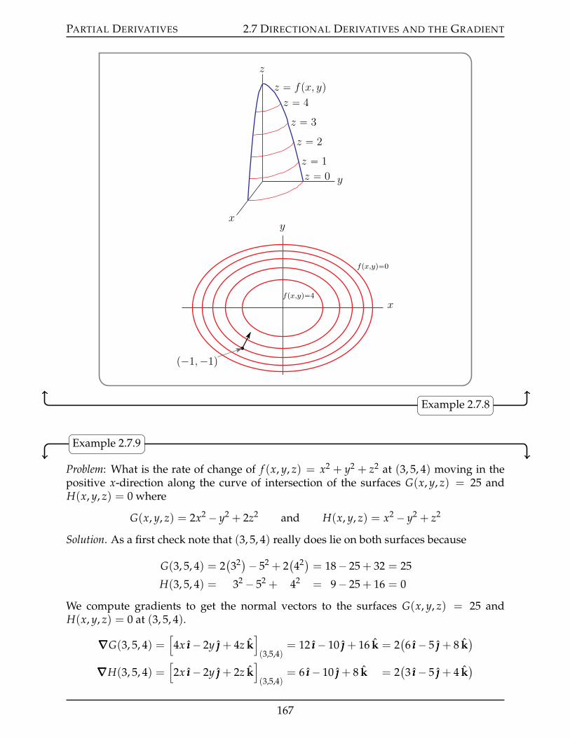
PARTIAL DERIVATIVES 2.7 DIRECTIONAL DERIVATIVES AND THE GRADIENT
z
y
x
z “ 4
z “ fpx, yq
z “ 3
z “ 2
z “ 1
z “ 0
x
y
fpx,yq“4
fpx,yq“0
p´1,´1q
Example 2.7.8
Example 2.7.9
Problem: What is the rate of change of f (x, y, z) = x2 + y2 + z2 at (3, 5, 4) moving in thepositive x-direction along the curve of intersection of the surfaces G(x, y, z) = 25 andH(x, y, z) = 0 where
G(x, y, z) = 2x2 ´ y2 + 2z2 and H(x, y, z) = x2 ´ y2 + z2
Solution. As a first check note that (3, 5, 4) really does lie on both surfaces because
G(3, 5, 4) = 2(32)´ 52 + 2
(42) = 18´ 25 + 32 = 25
H(3, 5, 4) = 32 ´ 52 + 42 = 9´ 25 + 16 = 0
We compute gradients to get the normal vectors to the surfaces G(x, y, z) = 25 andH(x, y, z) = 0 at (3, 5, 4).
∇∇∇G(3, 5, 4) =[4x ııı´ 2y + 4z k
](3,5,4)
= 12 ııı´ 10 + 16 k = 2(6 ııı´ 5 + 8 k
)
∇∇∇H(3, 5, 4) =[2x ııı´ 2y + 2z k
](3,5,4)
= 6 ııı´ 10 + 8 k = 2(3 ııı´ 5 + 4 k
)
167
PARTIAL DERIVATIVES 2.7 DIRECTIONAL DERIVATIVES AND THE GRADIENT
The direction of interest is tangent to the curve of intersection. So the direction of interestis tangent to both surfaces and hence is perpendicular to both gradients. Consequentlyone tangent vector to the curve at (3, 5, 4) is
∇∇∇G(3, 5, 4) ˆ∇∇∇H(3, 5, 4) = 4(6 ııı´ 5 + 8 k
)ˆ (3 ııı´ 5 + 4 k)
= 4 det
ııı k6 ´5 83 ´5 4
= 4(20 ııı´ 15 k
)= 20
(4 ııı´ 3 k
)
and the unit tangent vector to the curve at (3, 5, 4) that has positive x component is
4 ııı´ 3 k|4 ııı´ 3 k| =
45
ııı´ 35
k
The desired rate of change is
D 45 ııı´ 3
5 k f (3, 5, 4) =∇∇∇ f (3, 5, 4) ¨(
45
ııı´ 35
k)=
[2x ııı+2y +2z k](x,y,z)=(3,5,4)hkkkkkkkkkikkkkkkkkkj(6 ııı + 10 + 8 k
) ¨(
45
ııı´ 35
k)
= 0
Actually, we could have known that the rate of change would be zero.
• Any point (x, y, z) on the curve obeys both y2 = x2 + z2 and 2x2 ´ y2 + 2z2 = 25.
• Substituting y2 = x2 + z2 into 2x2 ´ y2 + 2z2 = 25 gives x2 + z2 = 25.
• So, at any point on the curve, x2 + z2 = 25 and y2 = x2 + z2 = 25 so that x2 + y2 + z2 =50.
• That is, f (x, y, z) = x2 + y2 + z2 takes the value 50 at every point of the curve.
• So of course the rate of change of f along the curve is 0.
Example 2.7.9
Let’s change things up a little. In the next example, we are told the rates of changein two different directions. From this we are to determine the rate of change in a thirddirection.
Example 2.7.10
Problem: The rate of change of a given function f (x, y) at the point P0 = (1, 2) in the direc-tion towards P1 = (2, 3) is 2
?2 and in the direction towards P2 = (1, 0) is ´3. What is the
rate of change of f at P0 towards the origin P3 = (0, 0)?
Solution. We can easily determine the rate of change of f at the point P0 in any directiononce we know the gradient∇∇∇ f (1, 2) = a ııı + b . So we will first use the two given rates ofchange to determine a and b, and then we determine the rate of change towards (0, 0).
168
PARTIAL DERIVATIVES 2.7 DIRECTIONAL DERIVATIVES AND THE GRADIENT
The two rates of change that we are given are those in the directions of the vectors
ÝÝÑP0P1 = 〈1, 1〉 ÝÝÑP0P2 = 〈0,´2〉
As you might guess, the notationÝÑPQ means the vector whose tail is at P and whose head
is at Q. So the given rates of change tell us that
2?
2 = D 〈1,1〉|〈1,1〉|
f (1, 2) =∇∇∇ f (1, 2) ¨ 〈1, 1〉| 〈1, 1〉 | = 〈a, b〉 ¨ 〈1, 1〉?
2=
a?2+
b?2
´3 = D 〈0,´2〉|〈0,´2〉|
f (1, 2) =∇∇∇ f (1, 2) ¨ 〈0,´2〉| 〈0,´2〉 | = 〈a, b〉 ¨ 〈0,´2〉
2= ´b
These two lines give us two linear equations in the two unknowns a and b. The secondequation directly gives us b = 3. Substituting b = 3 into the first equation gives
a?2+
3?2= 2
?2 ùñ a + 3 = 4 ùñ a = 1
A direction vector from P0 = (1, 2) towards P3 = (0, 0) is
ÝÝÑP0P3 = 〈´1,´2〉
and the rate of change (per unit distance) in that direction is
D 〈´1,´2〉|〈´1,´2〉|
f (1, 2) =∇∇∇ f (1, 2) ¨ 〈´1,´2〉| 〈´1,´2〉 | = 〈a, b〉 ¨ 〈´1,´2〉?
5= 〈1, 3〉 ¨ 〈´1,´2〉?
5= ´ 7?
5
Example 2.7.10
Example 2.7.11 (Optional)
Problem: Find all points (a, b, c) for which the spheres (x ´ a)2 + (y ´ b)2 + (z ´ c)2 = 1and x2 + y2 + z2 = 1 intersect orthogonally. That is, the tangent planes to the two spheresare to be perpendicular at each point of intersection.
Solution. Let (x0, y0, z0) be a point of intersection. That is
(x0 ´ a)2 + (y0 ´ b)2 + (z0 ´ c)2 = 1
x20 + y2
0 + z20 = 1
A normal vector to G(x, y, z) = (x´ a)2 + (y´ b)2 + (z´ c)2 = 1 at (x0, y0, z0) is
N =∇∇∇G(x0, y0, z0) = 〈2(x0 ´ a) , 2(y0 ´ b) , 2(z0 ´ c)〉
A normal vector to g(x, y, z) = x2 + y2 + z2 = 1 at (x0, y0, z0) is
n =∇∇∇g(x0, y0, z0) = 〈2x0 , 2y0 , 2z0〉
169
PARTIAL DERIVATIVES 2.7 DIRECTIONAL DERIVATIVES AND THE GRADIENT
The two tangent planes are perpendicular if and only if N and n are perpendicular, whichis the case if and only if
0 = N ¨ n = 4x0(x0 ´ a) + 4y0(y0 ´ b) + 4z0(z0 ´ c)
or, dividing the equation by 4,
x0(x0 ´ a) + y0(y0 ´ b) + z0(z0 ´ c) = 0
Let’s pause to take stock. We need to find all (a, b, c)’s such that the statement
(x0, y0, z0) is a point of intersection of the two spheres (S1)
implies the statement
the normal vectors N and n are perpendicular (S2)
In equations, we need to find all (a, b, c)’s such that the statement
(x0, y0, z0) obeys x20 + y2
0 + z20 = 1 and (x0 ´ a)2 + (y0 ´ b)2 + (z0 ´ c)2 = 1 (S1)
implies the statement
(x0, y0, z0) obeys x0(x0 ´ a) + y0(y0 ´ b) + z0(z0 ´ c) = 0 (S2)
Now if we expand (S2) then we can, with a little care, massage it into something that looksmore like (S1).
x0(x0 ´ a) + y0(y0 ´ b) + z0(z0 ´ c) = x20 + y2
0 + z20 ´ ax0 ´ by0 ´ cz0
=12
![x2
0 + y20 + z2
0]+[(x0 ´ a)2 + (y0 ´ b)2 + (z0 ´ c)2]´ a2 ´ b2 ´ c2
)
If (S1) is true, then[x2
0 + y20 + z2
0]= 1 and
[(x0 ´ a)2 + (y0 ´ b)2 + (z0 ´ c)2] = 1 so that
x0(x0 ´ a) + y0(y0 ´ b) + z0(z0 ´ c) =12
!1 + 1 ´ a2 ´ b2 ´ c2
)
and statement (S2) is true if and only if
a2 + b2 + c2 = 2
Our conclusion is that the set of allowed points (a, b, c) is the sphere of radius?
2centred on the origin.
Example 2.7.11
Example 2.7.12 (Optional — The gradient in polar coordinates)
Question: What is the gradient of a function in polar coordinates?
Answer. As was the case in Examples 2.4.9 and 2.4.10, figuring out what the question isasking is half the battle. By Definition 2.5.4, the gradient of a function g(x, y) is the vector
170
PARTIAL DERIVATIVES 2.7 DIRECTIONAL DERIVATIVES AND THE GRADIENT
⟨gx(x, y), gy(x, y)
⟩. In this question we are told that we are given some function f (r, θ)
of the polar coordinates36 r and θ. We are supposed to convert this function to Cartesiancoordinates.
This means that we are to consider the function
g(x, y) = f(r(x, y), θ(x, y)
)
with
r(x, y) =b
x2 + y2
θ(x, y) = arctanyx
Then we are to compute the gradient of g(x, y) and express the answer in terms of r andθ. By the chain rule,
BgBx
=B fBrBrBx
+B fBθ
Bθ
Bx
=B fBr
12
2xax2 + y2
+B fBθ
´y/x2
1 + (y/x)2
=B fBr
xax2 + y2
´ B fBθ
yx2 + y2
=B fBr
r cos θ
r´ B fBθ
r sin θ
r2
since x = r cos θ and y = r sin θ
=B fBr
cos θ ´ B fBθ
sin θ
rSimilarly
BgBy
=B fBrBrBy
+B fBθ
Bθ
By
=B fBr
12
2yax2 + y2
+B fBθ
1/x1 + (y/x)2
=B fBr
yax2 + y2
+B fBθ
xx2 + y2
=B fBr
sin θ +B fBθ
cos θ
rSo ⟨
gx, gy⟩= fr 〈cos θ, sin θ〉+ fθ
r〈´ sin θ, cos θ〉
or, with all the arguments written explicitly,⟨
gx(x, y), gy(x, y)⟩= fr
(r(x, y), θ(x, y)
)〈cos θ(x, y) , sin θ(x, y)〉
+1
r(x, y)fθ
(r(x, y), θ(x, y)
)〈´ sin θ(x, y) , cos θ(x, y)〉
36 Polar coordinates were defined in Example 2.1.8.
171
PARTIAL DERIVATIVES 2.8 OPTIONAL — SOLVING THE WAVE EQUATION
Example 2.7.12
2.8IJ Optional — Solving the Wave Equation
Many phenomena are modelled by equations that relate the rates of change of variousquantities. As rates of change are given by derivatives the resulting equations containderivatives and so are called differential equations. We saw a number of such differentialequations in §2.4 of the CLP-1 text.
In this section we consider
B2wBx2 (x, t)´ 1
c2B2wBt2 (x, t) = 0
This is an extremely important37partial differential equation called the “wave equation”(in one spatial dimension) that is used in modelling water waves, sound waves, seismicwaves, light waves and so on. The reason that we are looking at it here is that we can usewhat we have just learned to see that its solutions are waves travelling with speed c.
To start, we’ll use gradients and the chain rule to find the solution of the slightly sim-pler equation
BwBx
(x, t)´ 1cBwBt
(x, t) = 0
By way of motivation for what will follow, note that
• we can rewrite the above equation as⟨
1 , ´1c
⟩¨∇∇∇w(x, t) = 0
• This equation tells that the gradient of any solution w(x, t) must always be perpen-dicular to the constant vector
⟨1 , ´1
c⟩.
• A vector 〈a, b〉 is perpendicular to⟨1 , ´1
c⟩
if and only if
〈a, b〉 ¨⟨
1 , ´1c
⟩= 0 ðñ a´ b
c= 0 ðñ b = ac ðñ 〈a, b〉 = a 〈1, c〉
That is, a vector is perpendicular to⟨1 , ´1
c⟩
if and only if it is parallel to 〈1, c〉.
• Thus the gradient of any solution w(x, t) must always be parallel to the constantvector 〈1 , c〉.
• Recall that one of our implications following Definition 2.7.5 is that the gradient ofw(x, t) must always be perpendicular to the level curves of w.
37 If you plug “wave equation” into your favourite search engine you will get more than a million hits.
172
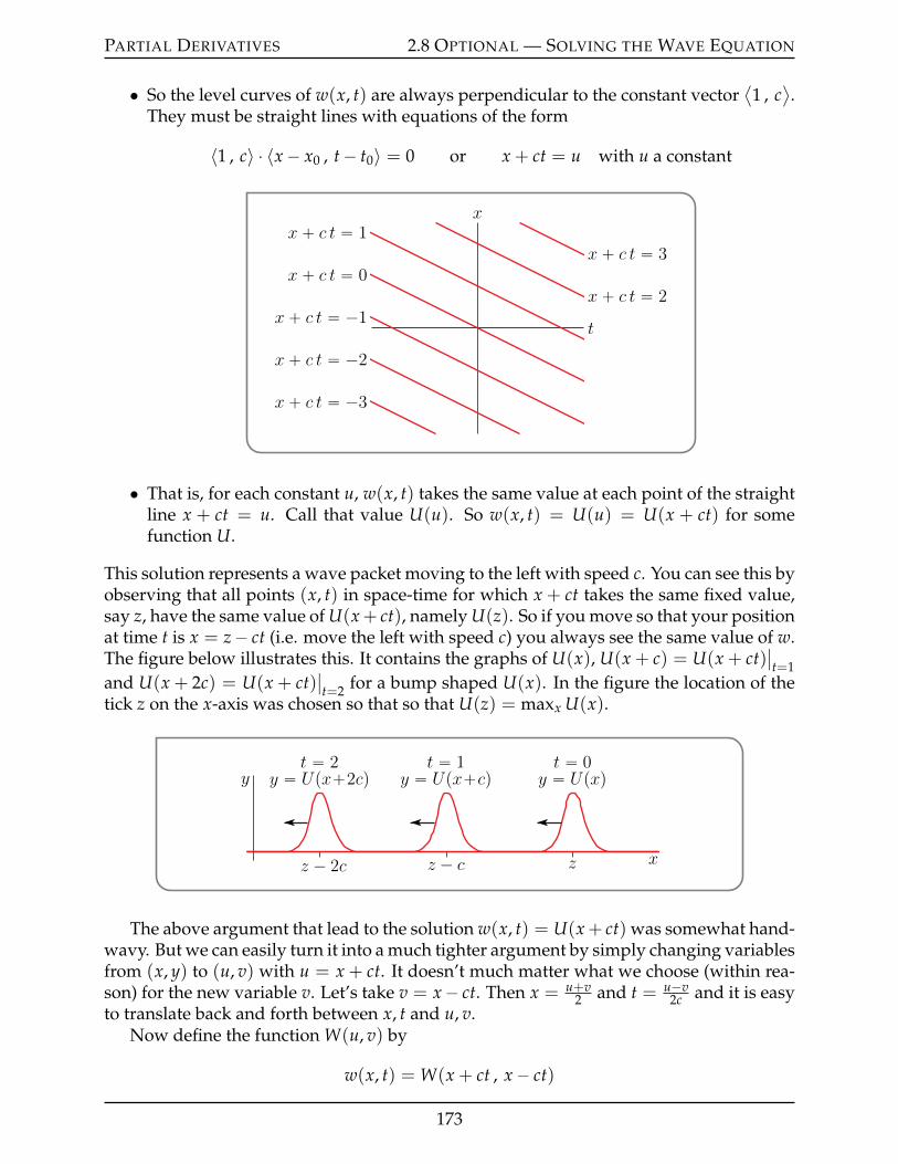
PARTIAL DERIVATIVES 2.8 OPTIONAL — SOLVING THE WAVE EQUATION
• So the level curves of w(x, t) are always perpendicular to the constant vector⟨1 , c
⟩.
They must be straight lines with equations of the form
〈1 , c〉 ¨ 〈x´ x0 , t´ t0〉 = 0 or x + ct = u with u a constant
t
x
x ` c t “ 0
x ` c t “ 1
x ` c t “ ´1
x ` c t “ ´2
x ` c t “ ´3
x ` c t “ 2
x ` c t “ 3
• That is, for each constant u, w(x, t) takes the same value at each point of the straightline x + ct = u. Call that value U(u). So w(x, t) = U(u) = U(x + ct) for somefunction U.
This solution represents a wave packet moving to the left with speed c. You can see this byobserving that all points (x, t) in space-time for which x + ct takes the same fixed value,say z, have the same value of U(x+ ct), namely U(z). So if you move so that your positionat time t is x = z´ ct (i.e. move the left with speed c) you always see the same value of w.The figure below illustrates this. It contains the graphs of U(x), U(x + c) = U(x + ct)
ˇt=1
and U(x + 2c) = U(x + ct)ˇt=2 for a bump shaped U(x). In the figure the location of the
tick z on the x-axis was chosen so that so that U(z) = maxx U(x).
x
y
z ´ 2c
y “ Upx`2cqt “ 2
z ´ c
y “ Upx`cqt “ 1
z
y “ Upxqt “ 0
The above argument that lead to the solution w(x, t) = U(x + ct) was somewhat hand-wavy. But we can easily turn it into a much tighter argument by simply changing variablesfrom (x, y) to (u, v) with u = x + ct. It doesn’t much matter what we choose (within rea-son) for the new variable v. Let’s take v = x´ ct. Then x = u+v
2 and t = u´v2c and it is easy
to translate back and forth between x, t and u, v.Now define the function W(u, v) by
w(x, t) = W(x + ct , x´ ct)
173
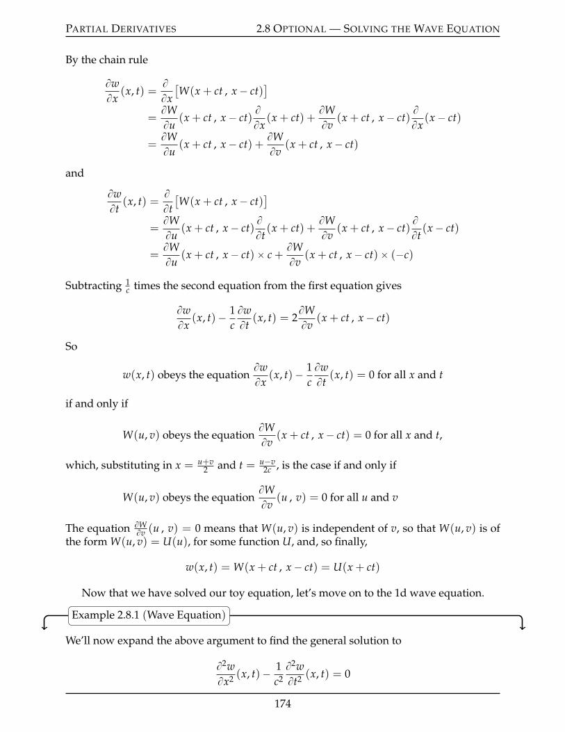
PARTIAL DERIVATIVES 2.8 OPTIONAL — SOLVING THE WAVE EQUATION
By the chain rule
BwBx
(x, t) =BBx[W(x + ct , x´ ct)
]
=BWBu
(x + ct , x´ ct)BBx
(x + ct) +BWBv
(x + ct , x´ ct)BBx
(x´ ct)
=BWBu
(x + ct , x´ ct) +BWBv
(x + ct , x´ ct)
and
BwBt
(x, t) =BBt[W(x + ct , x´ ct)
]
=BWBu
(x + ct , x´ ct)BBt(x + ct) +
BWBv
(x + ct , x´ ct)BBt(x´ ct)
=BWBu
(x + ct , x´ ct)ˆ c +BWBv
(x + ct , x´ ct)ˆ (´c)
Subtracting 1c times the second equation from the first equation gives
BwBx
(x, t)´ 1cBwBt
(x, t) = 2BWBv
(x + ct , x´ ct)
So
w(x, t) obeys the equationBwBx
(x, t)´ 1cBwBt
(x, t) = 0 for all x and t
if and only if
W(u, v) obeys the equationBWBv
(x + ct , x´ ct) = 0 for all x and t,
which, substituting in x = u+v2 and t = u´v
2c , is the case if and only if
W(u, v) obeys the equationBWBv
(u , v) = 0 for all u and v
The equation BWBv (u , v) = 0 means that W(u, v) is independent of v, so that W(u, v) is of
the form W(u, v) = U(u), for some function U, and, so finally,
w(x, t) = W(x + ct , x´ ct) = U(x + ct)
Now that we have solved our toy equation, let’s move on to the 1d wave equation.
Example 2.8.1 (Wave Equation)
We’ll now expand the above argument to find the general solution to
B2wBx2 (x, t)´ 1
c2B2wBt2 (x, t) = 0
174
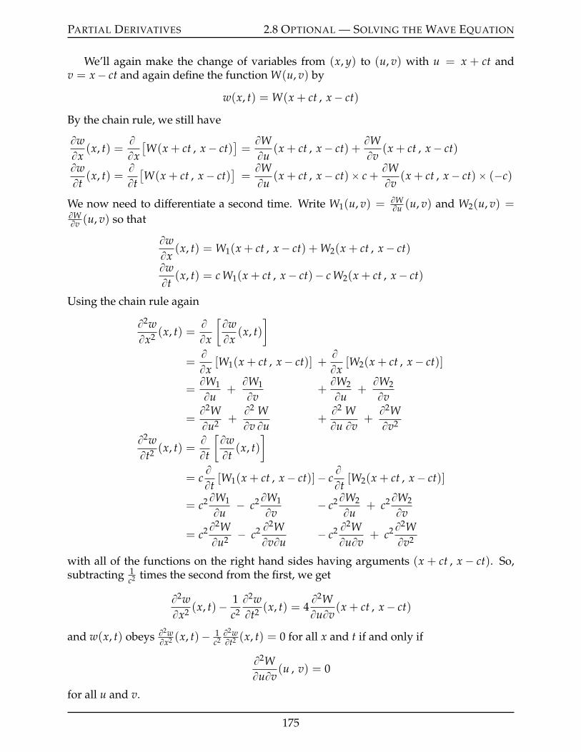
PARTIAL DERIVATIVES 2.8 OPTIONAL — SOLVING THE WAVE EQUATION
We’ll again make the change of variables from (x, y) to (u, v) with u = x + ct andv = x´ ct and again define the function W(u, v) by
w(x, t) = W(x + ct , x´ ct)
By the chain rule, we still have
BwBx
(x, t) =BBx[W(x + ct , x´ ct)
]=BWBu
(x + ct , x´ ct) +BWBv
(x + ct , x´ ct)
BwBt
(x, t) =BBt[W(x + ct , x´ ct)
]=BWBu
(x + ct , x´ ct)ˆ c +BWBv
(x + ct , x´ ct)ˆ (´c)
We now need to differentiate a second time. Write W1(u, v) = BWBu (u, v) and W2(u, v) =
BWBv (u, v) so that
BwBx
(x, t) = W1(x + ct , x´ ct) + W2(x + ct , x´ ct)
BwBt
(x, t) = c W1(x + ct , x´ ct)´ c W2(x + ct , x´ ct)
Using the chain rule again
B2wBx2 (x, t) =
BBx
[BwBx
(x, t)]
=BBx
[W1(x + ct , x´ ct)] +BBx
[W2(x + ct , x´ ct)]
=BW1
Bu+BW1
Bv+BW2
Bu+BW2
Bv
=B2WBu2 +
B2 WBv Bu
+B2 WBu Bv
+B2WBv2
B2wBt2 (x, t) =
BBt
[BwBt
(x, t)]
= cBBt
[W1(x + ct , x´ ct)]´ cBBt
[W2(x + ct , x´ ct)]
= c2BW1
Bu´ c2BW1
Bv´ c2BW2
Bu+ c2BW2
Bv
= c2B2WBu2 ´ c2 B2W
BvBu´ c2 B2W
BuBv+ c2B2W
Bv2
with all of the functions on the right hand sides having arguments (x + ct , x ´ ct). So,subtracting 1
c2 times the second from the first, we get
B2wBx2 (x, t)´ 1
c2B2wBt2 (x, t) = 4
B2WBuBv
(x + ct , x´ ct)
and w(x, t) obeys B2wBx2 (x, t)´ 1
c2B2wBt2 (x, t) = 0 for all x and t if and only if
B2WBuBv
(u , v) = 0
for all u and v.
175
PARTIAL DERIVATIVES 2.8 OPTIONAL — SOLVING THE WAVE EQUATION
• This tells us that the u-derivative of BWBv is zero, so that BW
Bv is independent of u. Thatis BW
Bv (u, v) = rV(v) for some function V. The reason that we have called it rV insteadof V with become evident shortly.
• Recall that to apply BBv , you treat u as a constant and differentiate with respect to v.
• So BWBv (u, v) = rV(v) says that, when u is thought of as a constant, W is an antideriva-
tive of rV.
• That is, W(u, v) =ş
V(v)dv + U, with U being an arbitrary constant. As u is beingthought of as a constant, U is allowed to depend on u.
So, denoting by V any antiderivative of V, we can write our solution in a very neat form.
W(u, v) = U(u) + V(v)
and the function we want is38
w(x, t) = W(x + ct , x´ ct) = U(x + ct) + V(x´ ct)
As we saw above U(x + ct) represents a wave packet moving to the left with speed c.Similarly, V(x´ ct) represents a wave packet moving to the right with speed c.
Notice that w(x, t) = U(x + ct) + V(x ´ ct) is a solution regardless of what U and Vare. The differential equation cannot tell us what U and V are. To determine them, weneed more information about the system — usually in the form of initial conditions, likew(x, 0) = ¨ ¨ ¨ and Bw
Bt (x, 0) = ¨ ¨ ¨ . General techniques for solving partial differential equa-tions lie beyond this text — but definitely require a good understanding of multivariablecalculus. A good reason to keep on reading!
Example 2.8.1
2.8.1 §§ Really Optional — Derivation of the Wave Equation
In this section we derive the wave equation
B2wBx2 (x, t)´ 1
c2B2wBt2 (x, t) = 0
in one application. To be precise, we apply Newton’s law to an elastic string, and concludethat small amplitude transverse vibrations of the string obey the wave equation.
Here is a sketch of a tiny element of the string.
38 This is known as d’Alembert’s form of the solution. It is named after Jean le Rond d’Alembert, 1717–1783, who was a French mathematician, physicist, philosopher and music theorist.
176
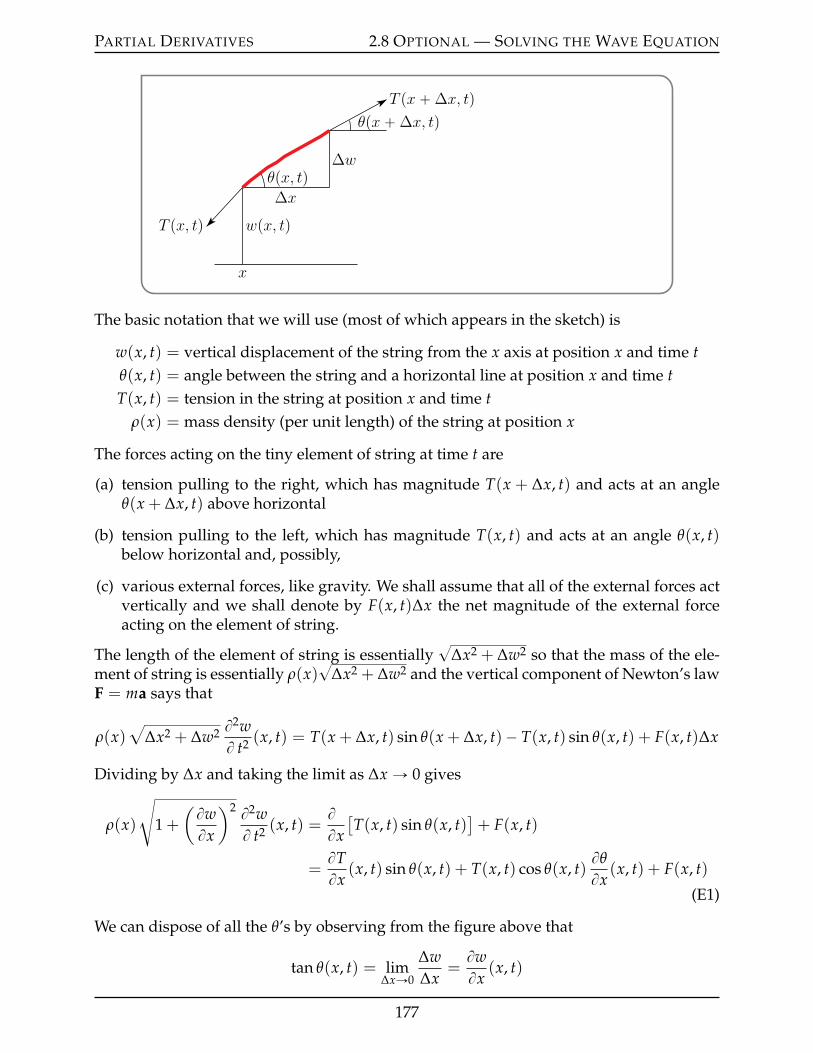
PARTIAL DERIVATIVES 2.8 OPTIONAL — SOLVING THE WAVE EQUATION
wpx, tq∆x
∆w
x
T px ` ∆x, tq
T px, tq
θpx ` ∆x, tq
θpx, tq
The basic notation that we will use (most of which appears in the sketch) is
w(x, t) = vertical displacement of the string from the x axis at position x and time tθ(x, t) = angle between the string and a horizontal line at position x and time tT(x, t) = tension in the string at position x and time t
ρ(x) = mass density (per unit length) of the string at position x
The forces acting on the tiny element of string at time t are
(a) tension pulling to the right, which has magnitude T(x + ∆x, t) and acts at an angleθ(x + ∆x, t) above horizontal
(b) tension pulling to the left, which has magnitude T(x, t) and acts at an angle θ(x, t)below horizontal and, possibly,
(c) various external forces, like gravity. We shall assume that all of the external forces actvertically and we shall denote by F(x, t)∆x the net magnitude of the external forceacting on the element of string.
The length of the element of string is essentially?
∆x2 + ∆w2 so that the mass of the ele-ment of string is essentially ρ(x)
?∆x2 + ∆w2 and the vertical component of Newton’s law
F = ma says that
ρ(x)a
∆x2 + ∆w2 B2wB t2 (x, t) = T(x + ∆x, t) sin θ(x + ∆x, t)´ T(x, t) sin θ(x, t) + F(x, t)∆x
Dividing by ∆x and taking the limit as ∆x Ñ 0 gives
ρ(x)
d1 +
(BwBx
)2 B2wB t2 (x, t) =
BBx[T(x, t) sin θ(x, t)
]+ F(x, t)
=BTBx
(x, t) sin θ(x, t) + T(x, t) cos θ(x, t)Bθ
Bx(x, t) + F(x, t)
(E1)
We can dispose of all the θ’s by observing from the figure above that
tan θ(x, t) = lim∆xÑ0
∆w∆x
=BwBx
(x, t)
177
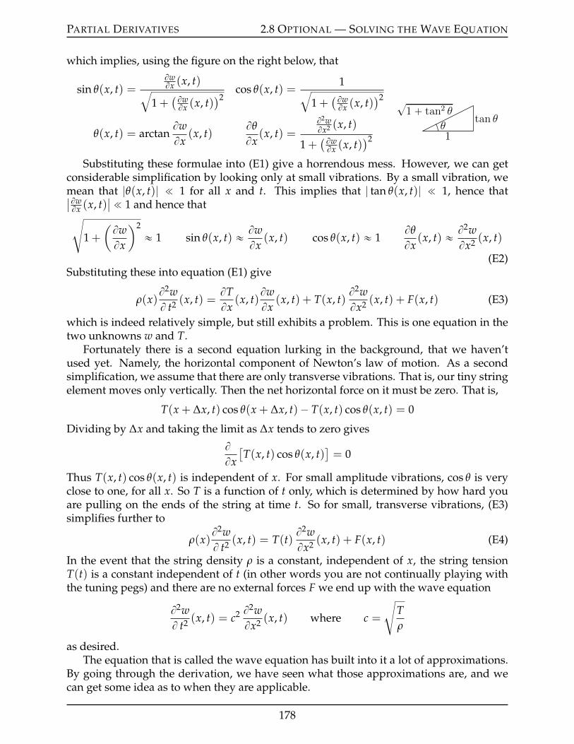
PARTIAL DERIVATIVES 2.8 OPTIONAL — SOLVING THE WAVE EQUATION
which implies, using the figure on the right below, that
sin θ(x, t) =BwBx (x, t)b
1 +(BwBx (x, t)
)2cos θ(x, t) =
1b1 +
(BwBx (x, t)
)2
θtan θ
1
?1 ` tan2 θ
θ(x, t) = arctanBwBx
(x, t)Bθ
Bx(x, t) =
B2wBx2 (x, t)
1 +(BwBx (x, t)
)2
Substituting these formulae into (E1) give a horrendous mess. However, we can getconsiderable simplification by looking only at small vibrations. By a small vibration, wemean that |θ(x, t)| ! 1 for all x and t. This implies that | tan θ(x, t)| ! 1, hence thatˇBwBx (x, t)
ˇ ! 1 and hence thatd
1 +(BwBx
)2
« 1 sin θ(x, t) « BwBx
(x, t) cos θ(x, t) « 1Bθ
Bx(x, t) « B
2wBx2 (x, t)
(E2)Substituting these into equation (E1) give
ρ(x)B2wB t2 (x, t) =
BTBx
(x, t)BwBx
(x, t) + T(x, t)B2wBx2 (x, t) + F(x, t) (E3)
which is indeed relatively simple, but still exhibits a problem. This is one equation in thetwo unknowns w and T.
Fortunately there is a second equation lurking in the background, that we haven’tused yet. Namely, the horizontal component of Newton’s law of motion. As a secondsimplification, we assume that there are only transverse vibrations. That is, our tiny stringelement moves only vertically. Then the net horizontal force on it must be zero. That is,
T(x + ∆x, t) cos θ(x + ∆x, t)´ T(x, t) cos θ(x, t) = 0
Dividing by ∆x and taking the limit as ∆x tends to zero gives
BBx[T(x, t) cos θ(x, t)
]= 0
Thus T(x, t) cos θ(x, t) is independent of x. For small amplitude vibrations, cos θ is veryclose to one, for all x. So T is a function of t only, which is determined by how hard youare pulling on the ends of the string at time t. So for small, transverse vibrations, (E3)simplifies further to
ρ(x)B2wB t2 (x, t) = T(t)
B2wBx2 (x, t) + F(x, t) (E4)
In the event that the string density ρ is a constant, independent of x, the string tensionT(t) is a constant independent of t (in other words you are not continually playing withthe tuning pegs) and there are no external forces F we end up with the wave equation
B2wB t2 (x, t) = c2 B2w
Bx2 (x, t) where c =
dTρ
as desired.The equation that is called the wave equation has built into it a lot of approximations.
By going through the derivation, we have seen what those approximations are, and wecan get some idea as to when they are applicable.
178
PARTIAL DERIVATIVES 2.9 MAXIMUM AND MINIMUM VALUES
2.9IJ Maximum and Minimum Values
One of the core topics in single variable calculus courses is finding the maxima and min-ima of functions of one variable. We’ll now extend that discussion to functions of morethan one variable39. Rather than leaping into the deep end, we’ll not be too ambitiousand concentrate on functions of two variables. That being said, many of the techniqueswork more generally. To start, we have the following natural extensions to some familiardefinitions.
Let the function f (x, y) be defined for all (x, y) in some subset R of R2. Let (a, b)be a point in R.
• (a, b) is a local maximum of f (x, y) if f (x, y) ď f (a, b) for all (x, y) close to(a, b). More precisely, (a, b) is a local maximum of f (x, y) if there is an r ą 0such that f (x, y) ď f (a, b) for all points (x, y) within a distance r of (a, b).
• (a, b) is a local minimum of f (x, y) if f (x, y) ě f (a, b) for all (x, y) close to(a, b).
• Local maximum and minimum values are also called extremal values.
• (a, b) is an absolute maximum or global maximum of f (x, y) if f (x, y) ď f (a, b)for all (x, y) in R.
• (a, b) is an absolute minimum or global minimum of f (x, y) if f (x, y) ě f (a, b)for all (x, y) in R.
Definition 2.9.1.
§§ Local Maxima and Minima
One of the first things you did when you were developing the techniques used to find themaximum and minimum values of f (x) was ask yourself40
Suppose that the largest value of f (x) is f (a). What does that tell us about a?
After a little thought you answered
If the largest value of f (x) is f (a) and f is differentiable at a, then f 1(a) = 0.
39 Life is not (always) one-dimensional and sometimes we have to embrace it.40 Or perhaps your instructor asked you.
179
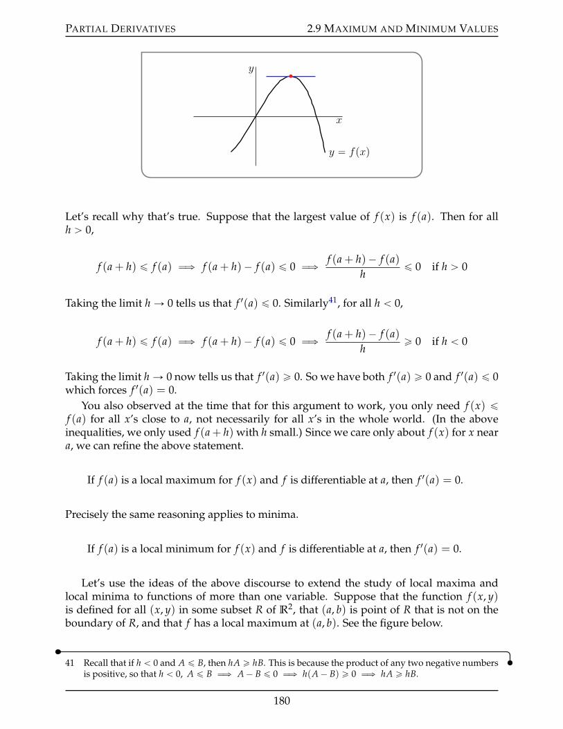
PARTIAL DERIVATIVES 2.9 MAXIMUM AND MINIMUM VALUES
x
y
y “ fpxq
Let’s recall why that’s true. Suppose that the largest value of f (x) is f (a). Then for allh ą 0,
f (a + h) ď f (a) ùñ f (a + h)´ f (a) ď 0 ùñ f (a + h)´ f (a)h
ď 0 if h ą 0
Taking the limit h Ñ 0 tells us that f 1(a) ď 0. Similarly41, for all h ă 0,
f (a + h) ď f (a) ùñ f (a + h)´ f (a) ď 0 ùñ f (a + h)´ f (a)h
ě 0 if h ă 0
Taking the limit h Ñ 0 now tells us that f 1(a) ě 0. So we have both f 1(a) ě 0 and f 1(a) ď 0which forces f 1(a) = 0.
You also observed at the time that for this argument to work, you only need f (x) ďf (a) for all x’s close to a, not necessarily for all x’s in the whole world. (In the aboveinequalities, we only used f (a + h) with h small.) Since we care only about f (x) for x neara, we can refine the above statement.
If f (a) is a local maximum for f (x) and f is differentiable at a, then f 1(a) = 0.
Precisely the same reasoning applies to minima.
If f (a) is a local minimum for f (x) and f is differentiable at a, then f 1(a) = 0.
Let’s use the ideas of the above discourse to extend the study of local maxima andlocal minima to functions of more than one variable. Suppose that the function f (x, y)is defined for all (x, y) in some subset R of R2, that (a, b) is point of R that is not on theboundary of R, and that f has a local maximum at (a, b). See the figure below.
41 Recall that if h ă 0 and A ď B, then hA ě hB. This is because the product of any two negative numbersis positive, so that h ă 0, A ď B ùñ A´ B ď 0 ùñ h(A´ B) ě 0 ùñ hA ě hB.
180
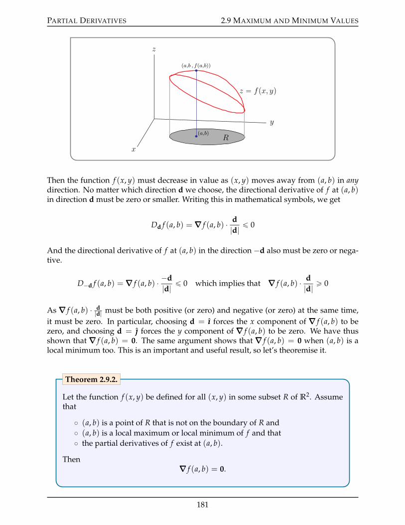
PARTIAL DERIVATIVES 2.9 MAXIMUM AND MINIMUM VALUES
z
y
x
R
pa,b , fpa,bqq
pa,bq
z “ fpx, yq
Then the function f (x, y) must decrease in value as (x, y) moves away from (a, b) in anydirection. No matter which direction d we choose, the directional derivative of f at (a, b)in direction d must be zero or smaller. Writing this in mathematical symbols, we get
Dd f (a, b) =∇∇∇ f (a, b) ¨ d|d| ď 0
And the directional derivative of f at (a, b) in the direction ´d also must be zero or nega-tive.
D´d f (a, b) =∇∇∇ f (a, b) ¨ ´d|d| ď 0 which implies that ∇∇∇ f (a, b) ¨ d
|d| ě 0
As ∇∇∇ f (a, b) ¨ d|d| must be both positive (or zero) and negative (or zero) at the same time,
it must be zero. In particular, choosing d = ııı forces the x component of ∇∇∇ f (a, b) to bezero, and choosing d = forces the y component of ∇∇∇ f (a, b) to be zero. We have thusshown that ∇∇∇ f (a, b) = 0. The same argument shows that ∇∇∇ f (a, b) = 0 when (a, b) is alocal minimum too. This is an important and useful result, so let’s theoremise it.
Let the function f (x, y) be defined for all (x, y) in some subset R of R2. Assumethat
˝ (a, b) is a point of R that is not on the boundary of R and˝ (a, b) is a local maximum or local minimum of f and that˝ the partial derivatives of f exist at (a, b).
Then∇∇∇ f (a, b) = 0.
Theorem 2.9.2.
181
PARTIAL DERIVATIVES 2.9 MAXIMUM AND MINIMUM VALUES
Let f (x, y) be a function and let (a, b) be a point in its domain. Then
• if ∇∇∇ f (a, b) exists and is zero we call (a, b) a critical point (or a stationarypoint) of the function, and
• if∇∇∇ f (a, b) does not exist then we call (a, b) a singular point of the function.
Definition 2.9.3.
Note that some people (and texts) combine both of these cases and call (a, b) acritical point when either the gradient is zero or does not exist.
Warning 2.9.4.
Theorem 2.9.2 tells us that every local maximum or minimum (in the interiorof the domain of a function whose partial derivatives exist) is a critical point.Beware that it does not42 tell us that every critical point is either a local maximumor a local minimum.
Warning 2.9.5.
In fact, we shall see later43, in Examples 2.9.13 and 2.9.15, critical points that are neitherlocal maxima nor a local minima. None-the-less, Theorem 2.9.2 is very useful becauseoften functions have only a small number of critical points. To find local maxima andminima of such functions, we only need to consider its critical and singular points. We’llreturn later to the question of how to tell if a critical point is a local maximum, localminimum or neither. For now, we’ll just practice finding critical points.
Example 2.9.6(
f (x, y) = x2 ´ 2xy + 2y2 + 2x´ 6y + 12)
Find all critical points of f (x, y) = x2 ´ 2xy + 2y2 + 2x´ 6y + 12.
Solution. To find the critical points, we need to find the gradient. To find the gradient weneed to find the first order partial derivatives. So, as a preliminary calculation, we findthe two first order partial derivatives of f (x, y).
fx(x, y) = 2x´ 2y + 2fy(x, y) = ´2x + 4y´ 6
So the critical points are the solutions of the pair of equations
2x´ 2y + 2 = 0 ´ 2x + 4y´ 6 = 0
42 A very common error of logic that people make is “Affirming the consequent”. “If P then Q” is true,does not imply that “If Q then P” is true . The statement “If he is Shakespeare then he is dead” is true.But concluding from “That man is dead” that “He must be Shakespeare” is just silly.
43 And you also saw, for example in Example 3.6.4 of the CLP-1 text, that critical points that are alsoinflection points are neither local maxima nor local minima.
182
PARTIAL DERIVATIVES 2.9 MAXIMUM AND MINIMUM VALUES
or equivalently (dividing by two and moving the constants to the right hand side)
x´ y = ´1 (E1)´x + 2y = 3 (E2)
This is a system of two equations in two unknowns (x and y). One strategy for solving asystem like this is to
• First use one of the equations to solve for one of the unknowns in terms of the otherunknown. For example, (E1) tells us that y = x + 1. This expresses y in terms of x.We say that we have solved for y in terms of x.
• Then substitute the result, y = x + 1 in our case, into the other equation, (E2). In ourcase, this gives
´x + 2(x + 1) = 3 ðñ x + 2 = 3 ðñ x = 1
• We have now found that x = 1, y = x+ 1 = 2 is the only solution. So the only criticalpoint is (1, 2). Of course it only takes a moment to verify that∇∇∇ f (1, 2) = 〈0, 0〉. It isa good idea to do this as a simple check of our work.
An alternative strategy for solving a system of two equations in two unknowns, like (E1)and (E2), is to
• add equations (E1) and (E2) together. This gives
(E1) + (E2) : (1´ 1)x + (´1 + 2)y = ´1 + 3 ðñ y = 2
The point here is that adding equations (E1) and (E2) together eliminates the un-known x, leaving us with one equation in the unknown y, which is easily solved.For other systems of equations you might have to multiply the equations by somenumbers before adding them together.
• We now know that y = 2. Substituting it into (E1) gives us
x´ 2 = ´1 ùñ x = 1
• Once again (thankfully) we have found that the only critical point is (1, 2).
Example 2.9.6
This was pretty easy because we only had to solve linear equations, which in turn was aconsequence of the fact that f (x, y) was a polynomial of degree two. Here is an examplewith some slightly more challenging algebra.
183
PARTIAL DERIVATIVES 2.9 MAXIMUM AND MINIMUM VALUES
Example 2.9.7(
f (x, y) = 2x3 ´ 6xy + y2 + 4y)
Find all critical points of f (x, y) = 2x3 ´ 6xy + y2 + 4y.
Solution. As in the last example, we need to find where the gradient is zero, and to findthe gradient we need the first order partial derivatives.
fx = 6x2 ´ 6y fy = ´6x + 2y + 4
So the critical points are the solutions of
6x2 ´ 6y = 0 ´ 6x + 2y + 4 = 0
We can rewrite the first equation as y = x2, which expresses y as a function of x. We canthen substitute y = x2 into the second equation, giving
´6x + 2y + 4 = 0 ðñ ´6x + 2x2 + 4 = 0 ðñ x2 ´ 3x + 2 = 0 ðñ (x´ 1)(x´ 2) = 0ðñ x = 1 or 2
When x = 1, y = 12 = 1 and when x = 2, y = 22 = 4. So, there are two critical points:(1, 1), (2, 4).
Alternatively, we could have also used the second equation to write y = 3x ´ 2, andthen substituted that into the first equation to get
6x2 ´ 6(3x´ 2) = 0 ðñ x2 ´ 3x + 2 = 0
just as above.Example 2.9.7
And here is an example for which the algebra requires a bit more thought.
Example 2.9.8 ( f (x, y) = xy(5x + y´ 15))
Find all critical points of f (x, y) = xy(5x + y´ 15).
Solution. The first order partial derivatives of f (x, y) = xy(5x + y´ 15) are
fx(x, y) = y(5x + y´ 15) + xy(5) = y(5x + y´ 15) + y(5x) = y(10x + y´ 15)fy(x, y) = x(5x + y´ 15) + xy(1) = x(5x + y´ 15) + x(y) = x(5x + 2y´ 15)
The critical points are the solutions of fx(x, y) = fy(x, y) = 0. That is, we need to find allx, y that satisfy the pair of equations
y(10x + y´ 15) = 0 (E1)x(5x + 2y´ 15) = 0 (E2)
The first equation, y(10x + y ´ 15) = 0, is satisfied if at least one of the two factors y,(10x + y´ 15) is zero. So the first equation is satisfied if at least one of the two equations
y = 0 (E1a)10x + y = 15 (E1b)
184
PARTIAL DERIVATIVES 2.9 MAXIMUM AND MINIMUM VALUES
is satisfied. The second equation, x(5x + 2y´ 15) = 0, is satisfied if at least one of the twofactors x, (5x + 2y ´ 15) is zero. So the second equation is satisfied if at least one of thetwo equations
x = 0 (E2a)5x + 2y = 15 (E2b)
is satisfied.So both critical point equations (E1) and (E2) are satisfied if and only if at least one
of (E1a), (E1b) is satisfied and in addition at least one of (E2a), (E2b) is satisfied. So bothcritical point equations (E1) and (E2) are satisfied if and only if at least one of the followingfour possibilities hold.
• (E1a) and (E2a) are satisfied if and only if x = y = 0
• (E1a) and (E2b) are satisfied if and only if y = 0, 5x + 2y = 15 ðñ y = 0, 5x = 15
• (E1b) and (E2a) are satisfied if and only if 10x + y = 15, x = 0 ðñ y = 15, x = 0
• (E1b) and (E2b) are satisfied if and only if 10x+ y = 15, 5x+ 2y = 15. We can use, forexample, the second of these equations to solve for x in terms of y: x = 1
5(15´ 2y).When we substitute this into the first equation we get 2(15´ 2y) + y = 15, which wecan solve for y. This gives ´3y = 15´ 30 or y = 5 and then x = 1
5(15´ 2ˆ 5) = 1.
In conclusion, the critical points are (0, 0), (3, 0), (0, 15) and (1, 5).A more compact way to write what we have just done is
fx(x, y) = 0 and fy(x, y) = 0ðñ y(10x + y´ 15) = 0 and x(5x + 2y´ 15) = 0
ðñ y = 0 or 10x + y = 15
(and
x = 0 or 5x + 2y = 15
(
ðñ y = 0, x = 0
(or
y = 0, 5x + 2y = 15
(or
10x + y = 15, x = 0
(or
10x + y = 15, 5x + 2y = 15(
ðñ x = y = 0
(or
y = 0, x = 3
(or
x = 0, y = 15
(or
x = 1, y = 5
(
Example 2.9.8
Let’s try a more practical example — something from the real world. Well, a mathe-matician’s “real world”. The interested reader should search-engine their way to a dis-cussion of “idealisation”, “game theory” “Cournot models” and “Bertrand models”. Butdon’t spend too long there. A discussion of breweries is about to take place.
Example 2.9.9
In a certain community, there are two breweries in competition44, so that sales of each neg-atively affect the profits of the other. If brewery A produces x litres of beer per month and
44 We have both types of music here — country and western.
185
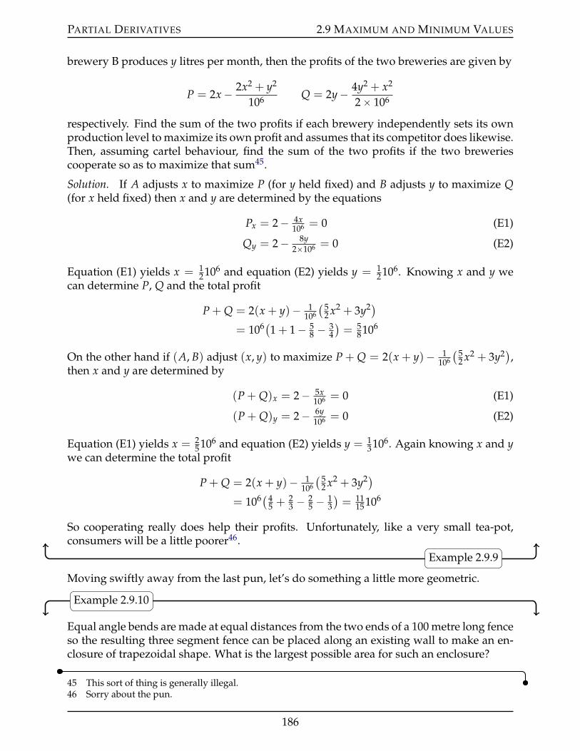
PARTIAL DERIVATIVES 2.9 MAXIMUM AND MINIMUM VALUES
brewery B produces y litres per month, then the profits of the two breweries are given by
P = 2x´ 2x2 + y2
106 Q = 2y´ 4y2 + x2
2ˆ 106
respectively. Find the sum of the two profits if each brewery independently sets its ownproduction level to maximize its own profit and assumes that its competitor does likewise.Then, assuming cartel behaviour, find the sum of the two profits if the two breweriescooperate so as to maximize that sum45.
Solution. If A adjusts x to maximize P (for y held fixed) and B adjusts y to maximize Q(for x held fixed) then x and y are determined by the equations
Px = 2´ 4x106 = 0 (E1)
Qy = 2´ 8y2ˆ106 = 0 (E2)
Equation (E1) yields x = 12106 and equation (E2) yields y = 1
2106. Knowing x and y wecan determine P, Q and the total profit
P + Q = 2(x + y)´ 1106
(52 x2 + 3y2)
= 106(1 + 1´ 58 ´ 3
4
)= 5
8106
On the other hand if (A, B) adjust (x, y) to maximize P + Q = 2(x + y)´ 1106
(52 x2 + 3y2),
then x and y are determined by
(P + Q)x = 2´ 5x106 = 0 (E1)
(P + Q)y = 2´ 6y106 = 0 (E2)
Equation (E1) yields x = 25106 and equation (E2) yields y = 1
3106. Again knowing x and ywe can determine the total profit
P + Q = 2(x + y)´ 1106
(52 x2 + 3y2)
= 106(45 +
23 ´ 2
5 ´ 13
)= 11
15106
So cooperating really does help their profits. Unfortunately, like a very small tea-pot,consumers will be a little poorer46.
Example 2.9.9
Moving swiftly away from the last pun, let’s do something a little more geometric.
Example 2.9.10
Equal angle bends are made at equal distances from the two ends of a 100 metre long fenceso the resulting three segment fence can be placed along an existing wall to make an en-closure of trapezoidal shape. What is the largest possible area for such an enclosure?
45 This sort of thing is generally illegal.46 Sorry about the pun.
186
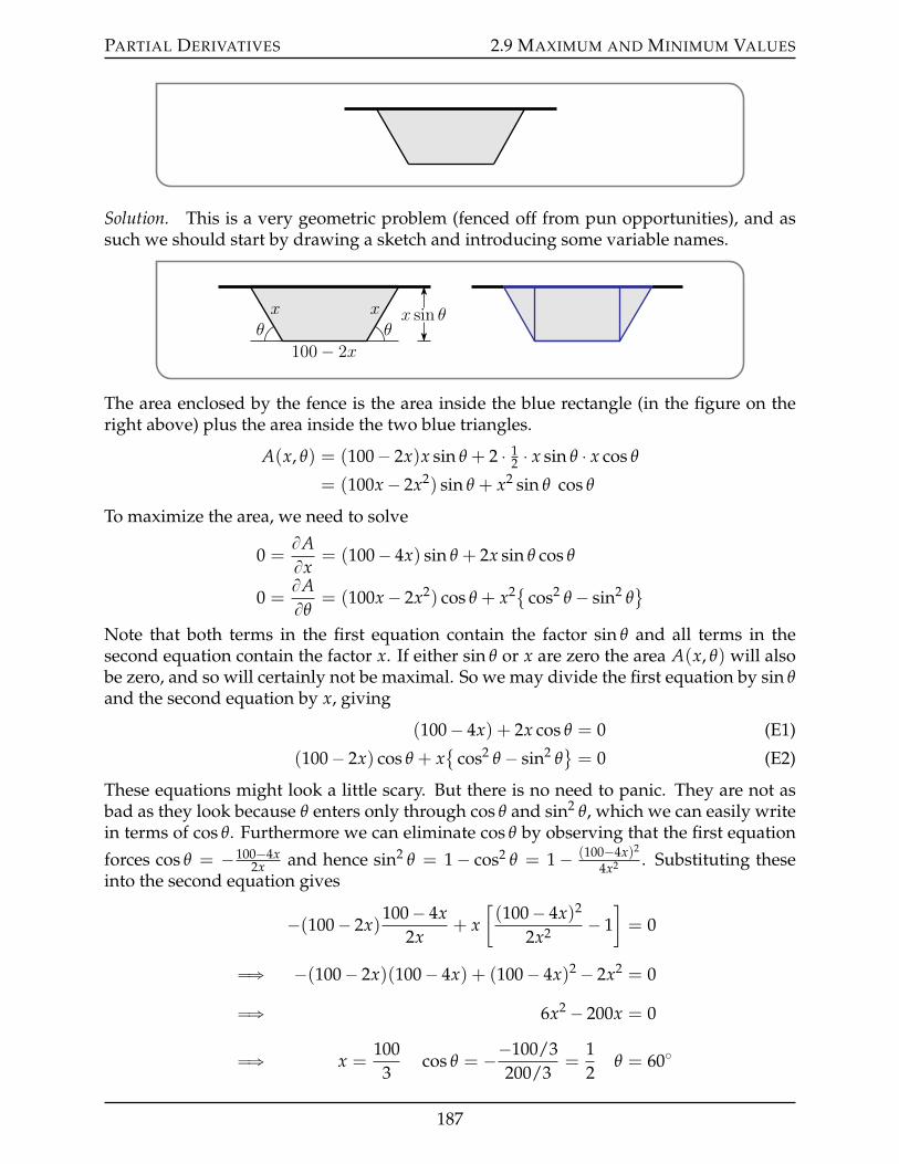
PARTIAL DERIVATIVES 2.9 MAXIMUM AND MINIMUM VALUES
Solution. This is a very geometric problem (fenced off from pun opportunities), and assuch we should start by drawing a sketch and introducing some variable names.
x sin θx x
100 ´ 2xθθ
The area enclosed by the fence is the area inside the blue rectangle (in the figure on theright above) plus the area inside the two blue triangles.
A(x, θ) = (100´ 2x)x sin θ + 2 ¨ 12 ¨ x sin θ ¨ x cos θ
= (100x´ 2x2) sin θ + x2 sin θ cos θ
To maximize the area, we need to solve
0 =BABx
= (100´ 4x) sin θ + 2x sin θ cos θ
0 =BABθ
= (100x´ 2x2) cos θ + x2 cos2 θ ´ sin2 θ(
Note that both terms in the first equation contain the factor sin θ and all terms in thesecond equation contain the factor x. If either sin θ or x are zero the area A(x, θ) will alsobe zero, and so will certainly not be maximal. So we may divide the first equation by sin θand the second equation by x, giving
(100´ 4x) + 2x cos θ = 0 (E1)
(100´ 2x) cos θ + x
cos2 θ ´ sin2 θ(= 0 (E2)
These equations might look a little scary. But there is no need to panic. They are not asbad as they look because θ enters only through cos θ and sin2 θ, which we can easily writein terms of cos θ. Furthermore we can eliminate cos θ by observing that the first equation
forces cos θ = ´100´4x2x and hence sin2 θ = 1´ cos2 θ = 1´ (100´4x)2
4x2 . Substituting theseinto the second equation gives
´(100´ 2x)100´ 4x
2x+ x
[(100´ 4x)2
2x2 ´ 1]= 0
ùñ ´(100´ 2x)(100´ 4x) + (100´ 4x)2 ´ 2x2 = 0
ùñ 6x2 ´ 200x = 0
ùñ x =100
3cos θ = ´´100/3
200/3=
12
θ = 60˝
187
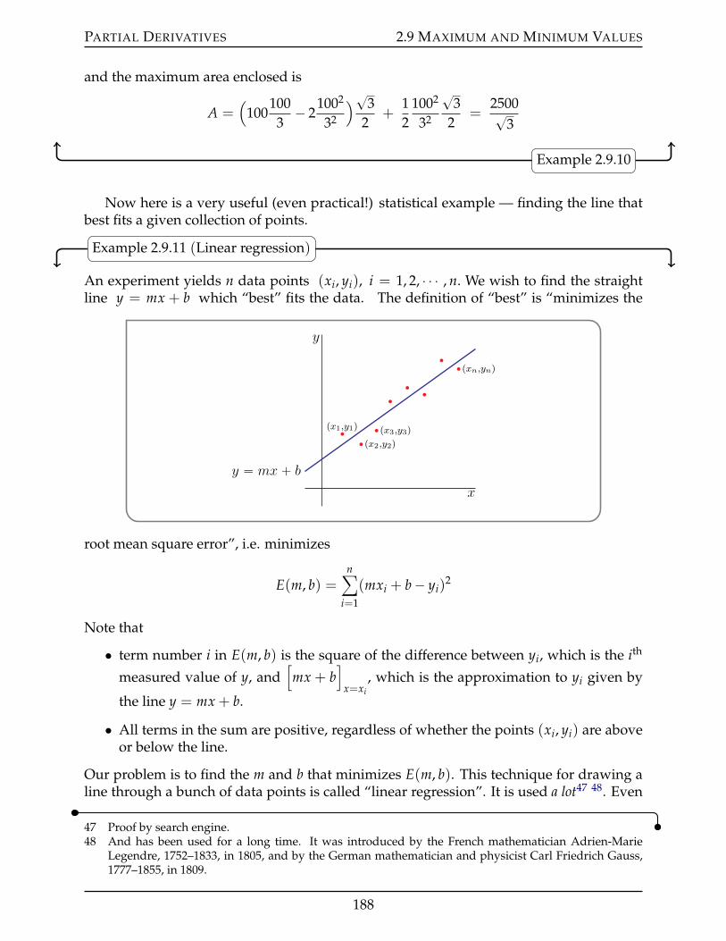
PARTIAL DERIVATIVES 2.9 MAXIMUM AND MINIMUM VALUES
and the maximum area enclosed is
A =(
1001003´ 2
1002
32
)?32
+12
1002
32
?3
2=
2500?3
Example 2.9.10
Now here is a very useful (even practical!) statistical example — finding the line thatbest fits a given collection of points.
Example 2.9.11 (Linear regression)
An experiment yields n data points (xi, yi), i = 1, 2, ¨ ¨ ¨ , n. We wish to find the straightline y = mx + b which “best” fits the data. The definition of “best” is “minimizes the
x
y
px1,y1qpx2,y2q
px3,y3q
pxn,ynq
y “ mx ` b
root mean square error”, i.e. minimizes
E(m, b) =nÿ
i=1
(mxi + b´ yi)2
Note that
• term number i in E(m, b) is the square of the difference between yi, which is the ith
measured value of y, and[mx + b
]x=xi
, which is the approximation to yi given by
the line y = mx + b.
• All terms in the sum are positive, regardless of whether the points (xi, yi) are aboveor below the line.
Our problem is to find the m and b that minimizes E(m, b). This technique for drawing aline through a bunch of data points is called “linear regression”. It is used a lot47 48. Even
47 Proof by search engine.48 And has been used for a long time. It was introduced by the French mathematician Adrien-Marie
Legendre, 1752–1833, in 1805, and by the German mathematician and physicist Carl Friedrich Gauss,1777–1855, in 1809.
188
PARTIAL DERIVATIVES 2.9 MAXIMUM AND MINIMUM VALUES
in the real world — and not just the real world that you find in mathematics problems.The actual real world that involves jobs.
Solution. We wish to choose m and b so as to minimize E(m, b). So we need to determinewhere the partial derivatives of E are zero.
0 =BEBm
=nÿ
i=1
2(mxi + b´ yi)xi = m[ nř
i=12x2
i
]+ b[ nř
i=12xi
]´[ nř
i=12xiyi
]
0 =BEBb
=nÿ
i=1
2(mxi + b´ yi) = m[ nř
i=12xi
]+ b[ nř
i=12]´[ nř
i=12yi
]
There are a lot of symbols here. But remember that all of the xi’s and yi’s are given con-stants. They come from, for example, experimental data. The only unknowns are m andb. To emphasize this, and to save some writing, define the constants
Sx =nř
i=1xi Sy =
nři=1
yi Sx2 =nř
i=1x2
i Sxy =nř
i=1xiyi
The equations which determine the critical points are (after dividing by two)
Sx2 m + Sx b = Sxy (E1)Sx m + n b = Sy (E2)
These are two linear equations on the unknowns m and b. They may be solved in any ofthe usual ways. One is to use (E2) to solve for b in terms of m
b =1n(Sy ´ Sxm
)(E3)
and then substitute this into (E1) to get the equation
Sx2 m +1n
Sx(Sy ´ Sxm
)= Sxy ùñ (
nSx2 ´ S2x)m = nSxy ´ SxSy
for m. We can then solve this equation for m and substitute back into (E3) to get b. Thisgives
m =nSxy ´ SxSy
nSx2 ´ S2x
b =Sy
nnSx2 ´ S2
xnSx2 ´ S2
x´ Sx
nnSxy ´ SxSy
nSx2 ´ S2x
=nSySx2 ´ nSxSxy
n(nSx2 ´ S2x)
= ´SxSxy ´ SySx2
nSx2 ´ S2x
Another way to solve the system of equations is
n(E1)´ Sx(E2) :[nSx2 ´ S2
x
]m = nSxy ´ SxSy
´Sx(E1) + Sx2(E2) :[nSx2 ´ S2
x
]b = ´SxSxy + SySx2
which gives the same solution.
189

PARTIAL DERIVATIVES 2.9 MAXIMUM AND MINIMUM VALUES
So given a bunch of data points, it only takes a quick bit of arithmetic — no calculusrequired — to apply the above formulae and so to find the best fitting line. Of course whileyou don’t need any calculus to apply the formulae, you do need calculus to understandwhere they came from. The same technique can be extended to other types of curve fittingproblems. For example, polynomial regression.
Example 2.9.11
§§ The Second Derivative Test
Now let’s start thinking about how to tell if a critical point is a local minimum or max-imum. Remember what happens for functions of one variable. Suppose that x = a isa critical point of the function f (x). Any (sufficiently smooth) function is well approxi-mated, when x is close to a, by the first few terms of its Taylor expansion
f (x) = f (a) + f 1(a) (x´ a) + 12 f 2(a) (x´ a)2 + 1
3! f (3)(a) (x´ a)3 + ¨ ¨ ¨As a is a critical point, we know that f 1(a) = 0 and
f (x) = f (a) + 12 f 2(a) (x´ a)2 + 1
3! f (3)(a) (x´ a)3 + ¨ ¨ ¨
If f 2(a) ‰ 0, f (x) is going to look a lot like f (a) + 12 f 2(a) (x´ a)2 when x is really close to
a. In particular
• if f 2(a) ą 0, then we will have f (x) ą f (a) when x is close to (but not equal to) a, sothat a will be a local minimum and
• if f 2(a) ă 0, then we will have f (x) ă f (a) when x is close to (but not equal to) a, sothat a will be a local maximum, but
• if f 2(a) = 0, then we cannot draw any conclusions without more work.
A similar, but messier, analysis is possible for functions of two variables. Here are somesimple quadratic examples that provide a warmup for that messier analysis.
Example 2.9.12(
f (x, y) = x2 + 3xy + 3y2 ´ 6x´ 3y´ 6)
Consider f (x, y) = x2 + 3xy + 3y2 ´ 6x´ 3y´ 6. The gradient of f is
∇∇∇ f (x, y) =(2x + 3y´ 6
)ııı +(3x + 6y´ 3
)
So (x, y) is a critical point of f if and only if
2x + 3y = 6 (E1)3x + 6y = 3 (E2)
Multiplying the first equation by 2 and subtracting the second equation gives
x = 9 (2(E1) - (E2))
190
PARTIAL DERIVATIVES 2.9 MAXIMUM AND MINIMUM VALUES
Then substituting x = 9 back into the first equation gives
2ˆ 9 + 3y = 6 ùñ y = ´4
So f (x, y) has precisely one critical point, namely (9 , ´4).Now let’s try to determine if f (x, y) has a local minimum, or a local maximum, or
neither, at (9,´4). A good way to determine the behaviour of f (x, y) for (x, y) near (9,´4)is to make the change of variables49
x = 9 + ∆x y = ´4 + ∆y
and study the behaviour of f for ∆x and ∆y near zero.
f(9 + ∆x , ´4 + ∆y
)= (9 + ∆x)2 + 3(9 + ∆x)(´4 + ∆y) + 3(´4 + ∆y)2
´ 6(9 + ∆x)´ 3(´4 + ∆y)´ 6
= (∆x)2 + 3∆x ∆y + 3(∆y)2 ´ 27
And a good way to study the sign of quadratic expressions like (∆x)2 + 3∆x ∆y+ 3(∆y)2 isto complete the square. So far you have probably just completed the square for quadraticexpressions that involve only a single variable. For example
x2 + 3x + 3 =
(x +
32
)2
´ 94+ 3
When there are two variables around, like ∆x and ∆y, you can just pretend that one ofthem is a constant and complete the square as before. For example, if you pretend that ∆yis a constant,
(∆x)2 + 3∆x ∆y + 3(∆y)2 =
(∆x +
32
∆y)2
+
(3´ 9
4
)(∆y)2
=
(∆x +
32
∆y)2
+34(∆y)2
To this point, we have expressed
f(9 + ∆x , ´4 + ∆y
)=
(∆x +
32
∆y)2
+34(∆y)2 ´ 27
As the smallest values of(∆x + 3
2 ∆y)2
and 34(∆y)2 are both zero, we have that
f (x, y) = f(9 + ∆x , ´4 + ∆y
) ě ´27 = f (9,´4)
for all (x, y) so that (9,´4) is both a local minimum and a global minimum for f .Example 2.9.12
49 This is equivalent to translating the graph so that the critical point lies at (0, 0).
191
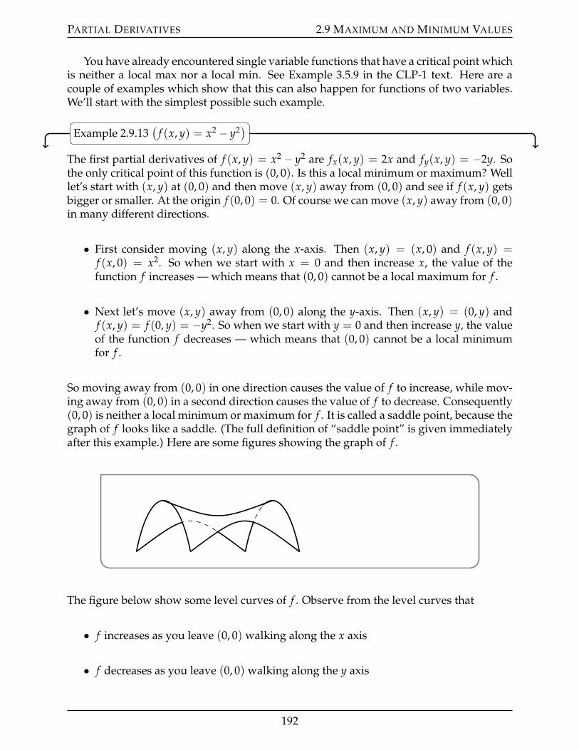
PARTIAL DERIVATIVES 2.9 MAXIMUM AND MINIMUM VALUES
You have already encountered single variable functions that have a critical point whichis neither a local max nor a local min. See Example 3.5.9 in the CLP-1 text. Here are acouple of examples which show that this can also happen for functions of two variables.We’ll start with the simplest possible such example.
Example 2.9.13(
f (x, y) = x2 ´ y2)
The first partial derivatives of f (x, y) = x2 ´ y2 are fx(x, y) = 2x and fy(x, y) = ´2y. Sothe only critical point of this function is (0, 0). Is this a local minimum or maximum? Welllet’s start with (x, y) at (0, 0) and then move (x, y) away from (0, 0) and see if f (x, y) getsbigger or smaller. At the origin f (0, 0) = 0. Of course we can move (x, y) away from (0, 0)in many different directions.
• First consider moving (x, y) along the x-axis. Then (x, y) = (x, 0) and f (x, y) =f (x, 0) = x2. So when we start with x = 0 and then increase x, the value of thefunction f increases — which means that (0, 0) cannot be a local maximum for f .
• Next let’s move (x, y) away from (0, 0) along the y-axis. Then (x, y) = (0, y) andf (x, y) = f (0, y) = ´y2. So when we start with y = 0 and then increase y, the valueof the function f decreases — which means that (0, 0) cannot be a local minimumfor f .
So moving away from (0, 0) in one direction causes the value of f to increase, while mov-ing away from (0, 0) in a second direction causes the value of f to decrease. Consequently(0, 0) is neither a local minimum or maximum for f . It is called a saddle point, because thegraph of f looks like a saddle. (The full definition of “saddle point” is given immediatelyafter this example.) Here are some figures showing the graph of f .
The figure below show some level curves of f . Observe from the level curves that
• f increases as you leave (0, 0) walking along the x axis
• f decreases as you leave (0, 0) walking along the y axis
192
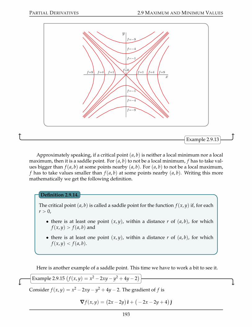
PARTIAL DERIVATIVES 2.9 MAXIMUM AND MINIMUM VALUES
x
y
f=0f=1f=1
f=−1
f=−1
f=4f=4
f=−4
f=−4
f=9f=9
f=−9
f=−9
Example 2.9.13
Approximately speaking, if a critical point (a, b) is neither a local minimum nor a localmaximum, then it is a saddle point. For (a, b) to not be a local minimum, f has to take val-ues bigger than f (a, b) at some points nearby (a, b). For (a, b) to not be a local maximum,f has to take values smaller than f (a, b) at some points nearby (a, b). Writing this moremathematically we get the following definition.
The critical point (a, b) is called a saddle point for the function f (x, y) if, for eachr ą 0,
• there is at least one point (x, y), within a distance r of (a, b), for whichf (x, y) ą f (a, b) and
• there is at least one point (x, y), within a distance r of (a, b), for whichf (x, y) ă f (a, b).
Definition 2.9.14.
Here is another example of a saddle point. This time we have to work a bit to see it.
Example 2.9.15(
f (x, y) = x2 ´ 2xy´ y2 + 4y´ 2)
Consider f (x, y) = x2 ´ 2xy´ y2 + 4y´ 2. The gradient of f is
∇∇∇ f (x, y) =(2x´ 2y
)ııı +(´ 2x´ 2y + 4
)
193
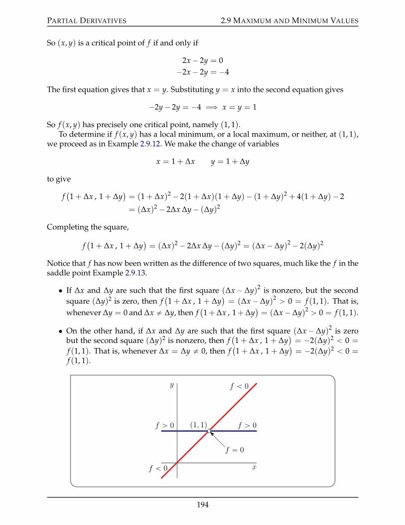
PARTIAL DERIVATIVES 2.9 MAXIMUM AND MINIMUM VALUES
So (x, y) is a critical point of f if and only if
2x´ 2y = 0´2x´ 2y = ´4
The first equation gives that x = y. Substituting y = x into the second equation gives
´2y´ 2y = ´4 ùñ x = y = 1
So f (x, y) has precisely one critical point, namely (1, 1).To determine if f (x, y) has a local minimum, or a local maximum, or neither, at (1, 1),
we proceed as in Example 2.9.12. We make the change of variables
x = 1 + ∆x y = 1 + ∆y
to give
f(1 + ∆x , 1 + ∆y
)= (1 + ∆x)2 ´ 2(1 + ∆x)(1 + ∆y)´ (1 + ∆y)2 + 4(1 + ∆y)´ 2
= (∆x)2 ´ 2∆x ∆y´ (∆y)2
Completing the square,
f(1 + ∆x , 1 + ∆y
)= (∆x)2 ´ 2∆x ∆y´ (∆y)2 = (∆x´ ∆y)2 ´ 2(∆y)2
Notice that f has now been written as the difference of two squares, much like the f in thesaddle point Example 2.9.13.
• If ∆x and ∆y are such that the first square (∆x´ ∆y)2 is nonzero, but the secondsquare (∆y)2 is zero, then f
(1 + ∆x , 1 + ∆y
)= (∆x´ ∆y)2 ą 0 = f (1, 1). That is,
whenever ∆y = 0 and ∆x ‰ ∆y, then f(1+∆x , 1+∆y
)= (∆x´ ∆y)2 ą 0 = f (1, 1).
• On the other hand, if ∆x and ∆y are such that the first square (∆x´ ∆y)2 is zerobut the second square (∆y)2 is nonzero, then f
(1 + ∆x , 1 + ∆y
)= ´2(∆y)2 ă 0 =
f (1, 1). That is, whenever ∆x = ∆y ‰ 0, then f(1 + ∆x , 1 + ∆y
)= ´2(∆y)2 ă 0 =
f (1, 1).
f “ 0
f ă 0
f ă 0
f ą 0f ą 0
x
y
p1, 1q
194
PARTIAL DERIVATIVES 2.9 MAXIMUM AND MINIMUM VALUES
So
• f (x, y) ą f (1, 1) at all points on the blue line in the figure above, and
• f (x, y) ă f (1, 1) at all point on the red line.
We conclude that (1, 1) is the only critical point for f (x, y), and furthermore that it is asaddle point.
Example 2.9.15
The above three examples show that we can find all critical points of quadratic func-tions of two variables. We can also classify each critical point as either a minimum, amaximum or a saddle point.
Of course not every function is quadratic. But by using the quadratic approximation(2.6.12) we can apply the same ideas much more generally. Suppose that (a, b) is a criticalpoint of some function f (x, y). For ∆x and ∆y small, the quadratic approximation (2.6.12)gives
f(a + ∆x , b + ∆y
) « f(a , b
)+ fx
(a , b
)∆x + fy
(a , b
)∆y
+12
!fxx(a, b)
∆x2 + 2 fxy(a, b)
∆x∆y + fyy(a, b)
∆y2)
= f(a , b
)+
12
!fxx(a, b)
∆x2 + 2 fxy(a, b)
∆x∆y + fyy(a, b)
∆y2)
(˚)
since (a, b) is a critical point so that fx(a, b) = fy(a, b) = 0. Then using the technique ofExamples 2.9.12 and 2.9.15, we get50 (details below)
Let r ą 0 and assume that all second order derivatives of the function f (x, y) arecontinuous at all points (x, y) that are within a distance r of (a, b). Assume thatfx(a, b) = fy(a, b) = 0. Define
D(x, y) = fxx(x, y) fyy(x, y)´ fxy(x, y)2
It is called the discriminant of f . Then
• if D(a, b) ą 0 and fxx(a, b) ą 0, then f (x, y) has a local minimum at (a, b),
• if D(a, b) ą 0 and fxx(a, b) ă 0, then f (x, y) has a local maximum at (a, b),
• if D(a, b) ă 0, then f (x, y) has a saddle point at (a, b), but
• if D(a, b) = 0, then we cannot draw any conclusions without more work.
Theorem 2.9.16 (Second Derivative Test).
50 There are analogous results in higher dimensions that are accessible to people who have learned somelinear algebra. They are derived by diagonalizing the matrix of second derivatives, which is called theHessian matrix.
195
PARTIAL DERIVATIVES 2.9 MAXIMUM AND MINIMUM VALUES
“Proof”. We are putting quotation marks around the word “Proof”, because we are not go-ing to justify the fact that it suffices to analyse the quadratic approximation in equation (˚).Let’s temporarily suppress the arguments (a, b). If fxx(a, b) ‰ 0, then by completing thesquare we can write
fxx ∆x2 + 2 fxy ∆x∆y + fyy ∆y2 = fxx
(∆x +
fxy
fxx∆y)2
+
(fyy ´
f 2xy
fxx
)∆y2
=1
fxx
!(fxx ∆x + fxy ∆y
)2+(
fxx fyy ´ f 2xy)
∆y2)
Similarly, if fyy(a, b) ‰ 0,
fxx ∆x2 + 2 fxy ∆x∆y + fyy ∆y2 =1
fyy
!(fxy ∆x + fyy ∆y
)2+(
fxx fyy ´ f 2xy)
∆x2)
Note that this algebra breaks down if fxx(a, b) = fyy(a, b) = 0. We’ll deal with that caseshortly. More importantly, note that
• if(
fxx fyy ´ f 2xy) ą 0 then both fxx and fyy must be nonzero and of the same sign and
furthermore, whenever ∆x or ∆y are nonzero,!(
fxx ∆x + fxy ∆y)2
+(
fxx fyy ´ f 2xy)
∆y2)ą 0 and
!(fxy ∆x + fyy ∆y
)2+(
fxx fyy ´ f 2xy)
∆x2)ą 0
so that, recalling (˚),
– if fxx(a, b) ą 0, then (a, b) is a local minimum and
– if fxx(a, b) ă 0, then (a, b) is a local maximum.
• If(
fxx fyy ´ f 2xy) ă 0 and fxx is nonzero then
!(fxx ∆x + fxy ∆y
)2+(
fxx fyy ´ f 2xy)
∆y2)
is strictly positive whenever ∆x ‰ 0, ∆y = 0 and is strictly negative wheneverfxx ∆x + fxy ∆y = 0, ∆y ‰ 0, so that (a, b) is a saddle point. Similarly, (a, b) is also asaddle point if
(fxx fyy ´ f 2
xy) ă 0 and fyy is nonzero.
• Finally, if fxy ‰ 0 and fxx = fyy = 0, then
fxx ∆x2 + 2 fxy ∆x ∆y + fyy ∆y2 = 2 fxy ∆x ∆y
is strictly positive for one sign of ∆x ∆y and is strictly negative for the other sign of∆x ∆y. So (a, b) is again a saddle point.
196
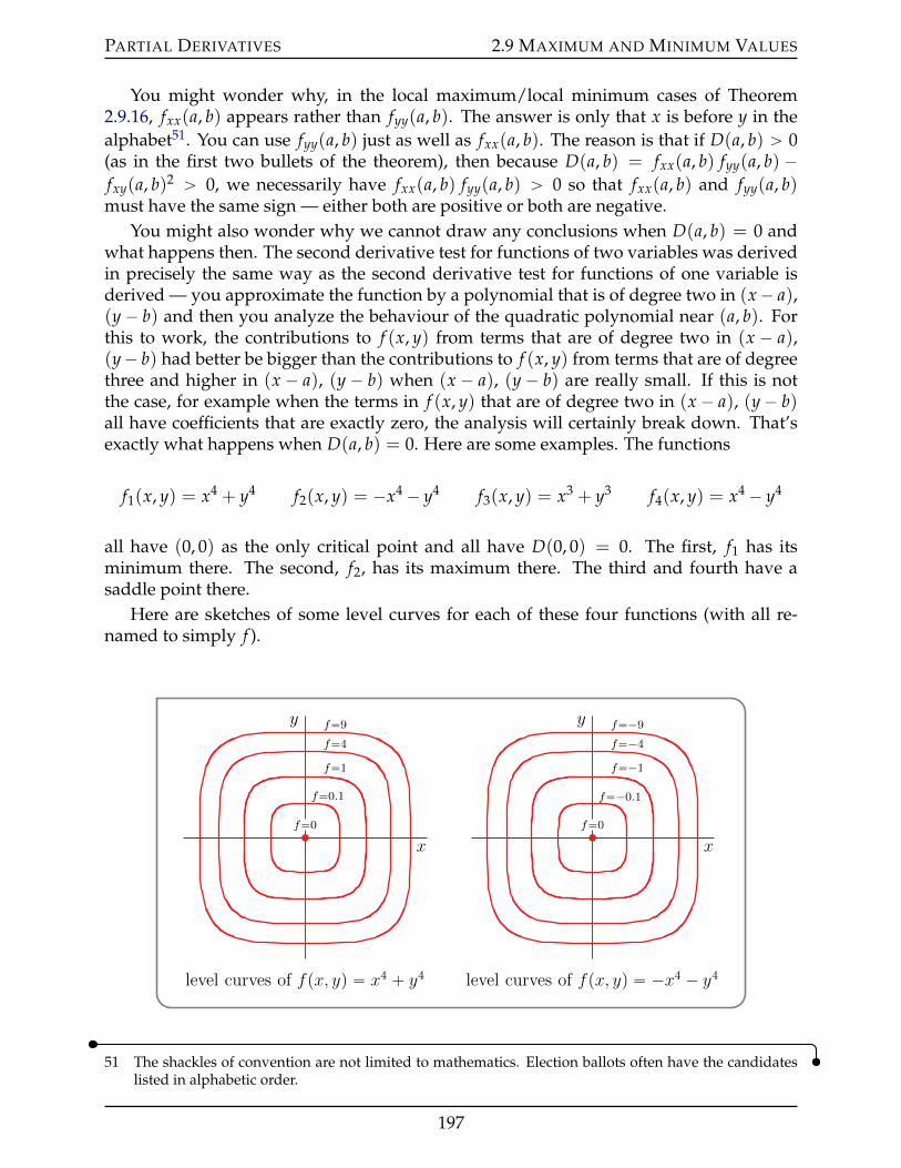
PARTIAL DERIVATIVES 2.9 MAXIMUM AND MINIMUM VALUES
You might wonder why, in the local maximum/local minimum cases of Theorem2.9.16, fxx(a, b) appears rather than fyy(a, b). The answer is only that x is before y in thealphabet51. You can use fyy(a, b) just as well as fxx(a, b). The reason is that if D(a, b) ą 0(as in the first two bullets of the theorem), then because D(a, b) = fxx(a, b) fyy(a, b) ´fxy(a, b)2 ą 0, we necessarily have fxx(a, b) fyy(a, b) ą 0 so that fxx(a, b) and fyy(a, b)must have the same sign — either both are positive or both are negative.
You might also wonder why we cannot draw any conclusions when D(a, b) = 0 andwhat happens then. The second derivative test for functions of two variables was derivedin precisely the same way as the second derivative test for functions of one variable isderived — you approximate the function by a polynomial that is of degree two in (x´ a),(y´ b) and then you analyze the behaviour of the quadratic polynomial near (a, b). Forthis to work, the contributions to f (x, y) from terms that are of degree two in (x ´ a),(y´ b) had better be bigger than the contributions to f (x, y) from terms that are of degreethree and higher in (x ´ a), (y ´ b) when (x ´ a), (y ´ b) are really small. If this is notthe case, for example when the terms in f (x, y) that are of degree two in (x ´ a), (y´ b)all have coefficients that are exactly zero, the analysis will certainly break down. That’sexactly what happens when D(a, b) = 0. Here are some examples. The functions
f1(x, y) = x4 + y4 f2(x, y) = ´x4 ´ y4 f3(x, y) = x3 + y3 f4(x, y) = x4 ´ y4
all have (0, 0) as the only critical point and all have D(0, 0) = 0. The first, f1 has itsminimum there. The second, f2, has its maximum there. The third and fourth have asaddle point there.
Here are sketches of some level curves for each of these four functions (with all re-named to simply f ).
x
y
f“0
f“0.1
f“1
f“4
f“9
level curves of fpx, yq “ x4 ` y4
x
y
f“0
f“´0.1
f“´1
f“´4
f“´9
level curves of fpx, yq “ ´x4 ´ y4
51 The shackles of convention are not limited to mathematics. Election ballots often have the candidateslisted in alphabetic order.
197
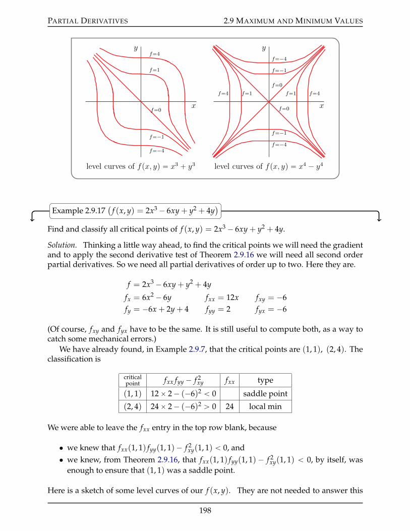
PARTIAL DERIVATIVES 2.9 MAXIMUM AND MINIMUM VALUES
x
y
f“0
f“1
f“´1
f“4
f“´4
level curves of fpx, yq “ x3 ` y3
x
y
f“0
f“0
f“1f“1
f“´1
f“´1
f“4f“4
f“´4
f“´4
level curves of fpx, yq “ x4 ´ y4
Example 2.9.17(
f (x, y) = 2x3 ´ 6xy + y2 + 4y)
Find and classify all critical points of f (x, y) = 2x3 ´ 6xy + y2 + 4y.
Solution. Thinking a little way ahead, to find the critical points we will need the gradientand to apply the second derivative test of Theorem 2.9.16 we will need all second orderpartial derivatives. So we need all partial derivatives of order up to two. Here they are.
f = 2x3 ´ 6xy + y2 + 4y
fx = 6x2 ´ 6y fxx = 12x fxy = ´6fy = ´6x + 2y + 4 fyy = 2 fyx = ´6
(Of course, fxy and fyx have to be the same. It is still useful to compute both, as a way tocatch some mechanical errors.)
We have already found, in Example 2.9.7, that the critical points are (1, 1), (2, 4). Theclassification is
criticalpoint fxx fyy ´ f 2
xy fxx type
(1, 1) 12ˆ 2´ (´6)2 ă 0 saddle point
(2, 4) 24ˆ 2´ (´6)2 ą 0 24 local min
We were able to leave the fxx entry in the top row blank, because
• we knew that fxx(1, 1) fyy(1, 1)´ f 2xy(1, 1) ă 0, and
• we knew, from Theorem 2.9.16, that fxx(1, 1) fyy(1, 1) ´ f 2xy(1, 1) ă 0, by itself, was
enough to ensure that (1, 1) was a saddle point.
Here is a sketch of some level curves of our f (x, y). They are not needed to answer this
198
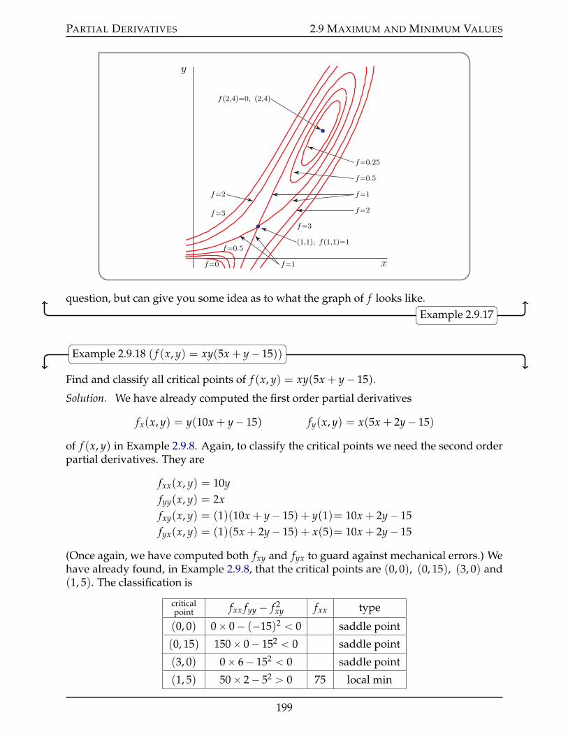
PARTIAL DERIVATIVES 2.9 MAXIMUM AND MINIMUM VALUES
x
y
p1,1q, fp1,1q“1
fp2,4q“0, p2,4q
f“0
f“0.25
f“0.5
f“0.5
f“1
f“1
f“2
f“2
f“3
f“3
question, but can give you some idea as to what the graph of f looks like.Example 2.9.17
Example 2.9.18 ( f (x, y) = xy(5x + y´ 15))
Find and classify all critical points of f (x, y) = xy(5x + y´ 15).
Solution. We have already computed the first order partial derivatives
fx(x, y) = y(10x + y´ 15) fy(x, y) = x(5x + 2y´ 15)
of f (x, y) in Example 2.9.8. Again, to classify the critical points we need the second orderpartial derivatives. They are
fxx(x, y) = 10yfyy(x, y) = 2xfxy(x, y) = (1)(10x + y´ 15) + y(1)= 10x + 2y´ 15fyx(x, y) = (1)(5x + 2y´ 15) + x(5)= 10x + 2y´ 15
(Once again, we have computed both fxy and fyx to guard against mechanical errors.) Wehave already found, in Example 2.9.8, that the critical points are (0, 0), (0, 15), (3, 0) and(1, 5). The classification is
criticalpoint fxx fyy ´ f 2
xy fxx type
(0, 0) 0ˆ 0´ (´15)2 ă 0 saddle point
(0, 15) 150ˆ 0´ 152 ă 0 saddle point
(3, 0) 0ˆ 6´ 152 ă 0 saddle point
(1, 5) 50ˆ 2´ 52 ą 0 75 local min
199
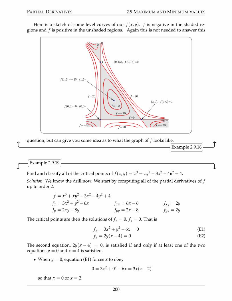
PARTIAL DERIVATIVES 2.9 MAXIMUM AND MINIMUM VALUES
Here is a sketch of some level curves of our f (x, y). f is negative in the shaded re-gions and f is positive in the unshaded regions. Again this is not needed to answer this
x
y
p3,0q, fp3,0q“0
fp0,0q“0, p0,0q
p0,15q, fp0,15q“0
fp1,5q“´25, p1,5q
f“0
f“´10
f“´20
f“´20f“´20f“20
f“20f“20
question, but can give you some idea as to what the graph of f looks like.Example 2.9.18
Example 2.9.19
Find and classify all of the critical points of f (x, y) = x3 + xy2 ´ 3x2 ´ 4y2 + 4.
Solution. We know the drill now. We start by computing all of the partial derivatives of fup to order 2.
f = x3 + xy2 ´ 3x2 ´ 4y2 + 4
fx = 3x2 + y2 ´ 6x fxx = 6x´ 6 fxy = 2yfy = 2xy´ 8y fyy = 2x´ 8 fyx = 2y
The critical points are then the solutions of fx = 0, fy = 0. That is
fx = 3x2 + y2 ´ 6x = 0 (E1)fy = 2y(x´ 4) = 0 (E2)
The second equation, 2y(x ´ 4) = 0, is satisfied if and only if at least one of the twoequations y = 0 and x = 4 is satisfied.
• When y = 0, equation (E1) forces x to obey
0 = 3x2 + 02 ´ 6x = 3x(x´ 2)
so that x = 0 or x = 2.
200
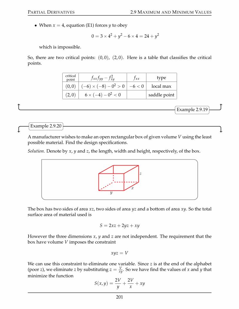
PARTIAL DERIVATIVES 2.9 MAXIMUM AND MINIMUM VALUES
• When x = 4, equation (E1) forces y to obey
0 = 3ˆ 42 + y2 ´ 6ˆ 4 = 24 + y2
which is impossible.
So, there are two critical points: (0, 0), (2, 0). Here is a table that classifies the criticalpoints.
criticalpoint fxx fyy ´ f 2
xy fxx type
(0, 0) (´6)ˆ (´8)´ 02 ą 0 ´6 ă 0 local max
(2, 0) 6ˆ (´4)´ 02 ă 0 saddle point
Example 2.9.19
Example 2.9.20
A manufacturer wishes to make an open rectangular box of given volume V using the leastpossible material. Find the design specifications.
Solution. Denote by x, y and z, the length, width and height, respectively, of the box.
yx
z
The box has two sides of area xz, two sides of area yz and a bottom of area xy. So the totalsurface area of material used is
S = 2xz + 2yz + xy
However the three dimensions x, y and z are not independent. The requirement that thebox have volume V imposes the constraint
xyz = V
We can use this constraint to eliminate one variable. Since z is at the end of the alphabet(poor z), we eliminate z by substituting z = V
xy . So we have find the values of x and y thatminimize the function
S(x, y) =2Vy
+2Vx
+ xy
201
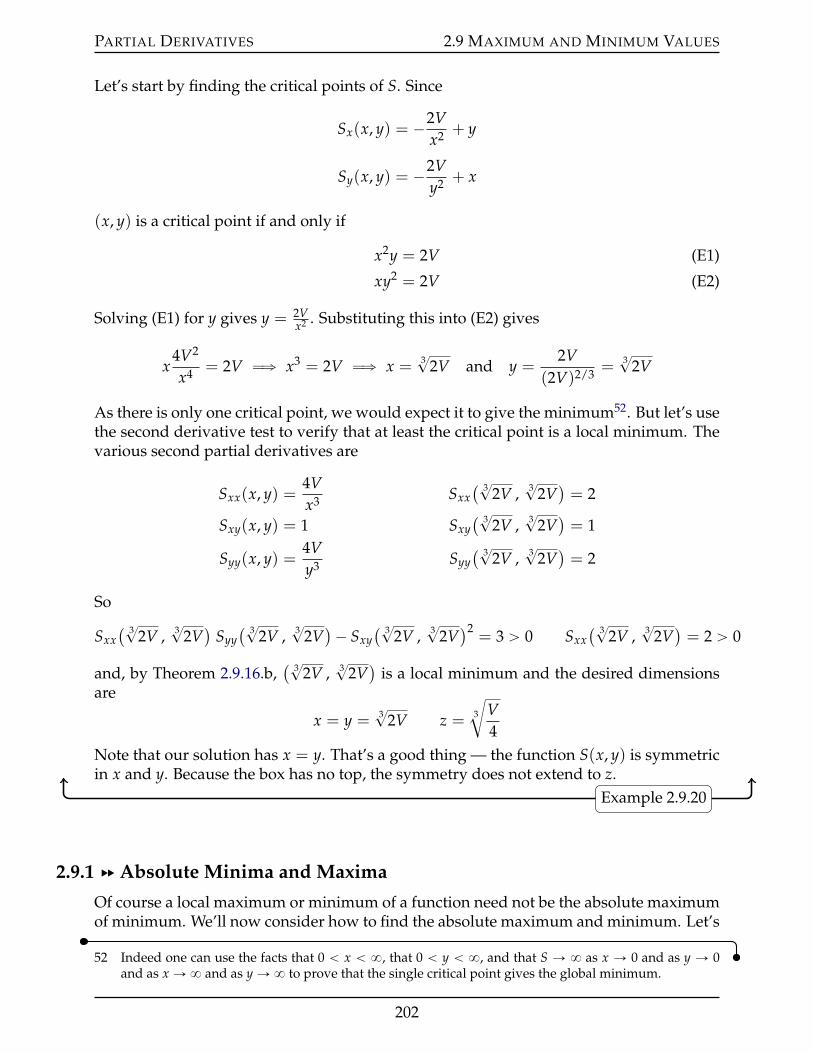
PARTIAL DERIVATIVES 2.9 MAXIMUM AND MINIMUM VALUES
Let’s start by finding the critical points of S. Since
Sx(x, y) = ´2Vx2 + y
Sy(x, y) = ´2Vy2 + x
(x, y) is a critical point if and only if
x2y = 2V (E1)
xy2 = 2V (E2)
Solving (E1) for y gives y = 2Vx2 . Substituting this into (E2) gives
x4V2
x4 = 2V ùñ x3 = 2V ùñ x =3?
2V and y =2V
(2V)2/3 =3?
2V
As there is only one critical point, we would expect it to give the minimum52. But let’s usethe second derivative test to verify that at least the critical point is a local minimum. Thevarious second partial derivatives are
Sxx(x, y) =4Vx3 Sxx
( 3?
2V , 3?
2V)= 2
Sxy(x, y) = 1 Sxy( 3?
2V , 3?
2V)= 1
Syy(x, y) =4Vy3 Syy
( 3?
2V , 3?
2V)= 2
So
Sxx( 3?
2V , 3?
2V)
Syy( 3?
2V , 3?
2V)´ Sxy
( 3?
2V , 3?
2V)2
= 3 ą 0 Sxx( 3?
2V , 3?
2V)= 2 ą 0
and, by Theorem 2.9.16.b,( 3?
2V , 3?
2V)
is a local minimum and the desired dimensionsare
x = y =3?
2V z =3
cV4
Note that our solution has x = y. That’s a good thing — the function S(x, y) is symmetricin x and y. Because the box has no top, the symmetry does not extend to z.
Example 2.9.20
2.9.1 §§ Absolute Minima and Maxima
Of course a local maximum or minimum of a function need not be the absolute maximumof minimum. We’ll now consider how to find the absolute maximum and minimum. Let’s
52 Indeed one can use the facts that 0 ă x ă 8, that 0 ă y ă 8, and that S Ñ 8 as x Ñ 0 and as y Ñ 0and as x Ñ8 and as y Ñ8 to prove that the single critical point gives the global minimum.
202
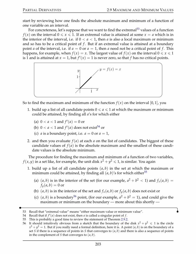
PARTIAL DERIVATIVES 2.9 MAXIMUM AND MINIMUM VALUES
start by reviewing how one finds the absolute maximum and minimum of a function ofone variable on an interval.
For concreteness, let’s suppose that we want to find the extremal53 values of a functionf (x) on the interval 0 ď x ď 1. If an extremal value is attained at some x = a which is inthe interior of the interval, i.e. if 0 ă a ă 1, then a is also a local maximum or minimumand so has to be a critical point of f . But if an extremal value is attained at a boundarypoint a of the interval, i.e. if a = 0 or a = 1, then a need not be a critical point of f . Thishappens, for example, when f (x) = x. The largest value of f (x) on the interval 0 ď x ď 1is 1 and is attained at x = 1, but f 1(x) = 1 is never zero, so that f has no critical points.
x
y y = f(x) = x
1
1
So to find the maximum and minimum of the function f (x) on the interval [0, 1], you
1. build up a list of all candidate points 0 ď a ď 1 at which the maximum or minimumcould be attained, by finding all a’s for which either
(a) 0 ă a ă 1 and f 1(a) = 0 or
(b) 0 ă a ă 1 and f 1(a) does not exist54 or
(c) a is a boundary point, i.e. a = 0 or a = 1,
2. and then you evaluate f (a) at each a on the list of candidates. The biggest of thesecandidate values of f (a) is the absolute maximum and the smallest of these candi-date values is the absolute minimum.
The procedure for finding the maximum and minimum of a function of two variables,f (x, y) in a set like, for example, the unit disk x2 + y2 ď 1, is similar. You again
1. build up a list of all candidate points (a, b) in the set at which the maximum orminimum could be attained, by finding all (a, b)’s for which either55
(a) (a, b) is in the interior of the set (for our example, a2 + b2 ă 1) and fx(a, b) =fy(a, b) = 0 or
(b) (a, b) is in the interior of the set and fx(a, b) or fy(a, b) does not exist or
(c) (a, b) is a boundary56 point, (for our example, a2 + b2 = 1), and could give themaximum or minimum on the boundary — more about this shortly —
53 Recall that “extremal value” means “either maximum value or minimum value”.54 Recall that if f 1(a) does not exist, then a is called a singular point of f .55 This is probably a good time to review the statement of Theorem 2.9.2.56 It should intuitively obvious from a sketch that the boundary of the disk x2 + y2 ď 1 is the circle
x2 + y2 = 1. But if you really need a formal definition, here it is. A point (a, b) is on the boundary of aset S if there is a sequence of points in S that converges to (a, b) and there is also a sequence of pointsin the complement of S that converges to (a, b).
203
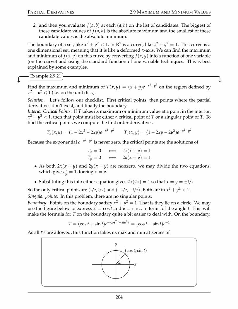
PARTIAL DERIVATIVES 2.9 MAXIMUM AND MINIMUM VALUES
2. and then you evaluate f (a, b) at each (a, b) on the list of candidates. The biggest ofthese candidate values of f (a, b) is the absolute maximum and the smallest of thesecandidate values is the absolute minimum.
The boundary of a set, like x2 + y2 ď 1, in R2 is a curve, like x2 + y2 = 1. This curve is aone dimensional set, meaning that it is like a deformed x-axis. We can find the maximumand minimum of f (x, y) on this curve by converting f (x, y) into a function of one variable(on the curve) and using the standard function of one variable techniques. This is bestexplained by some examples.
Example 2.9.21
Find the maximum and minimum of T(x, y) = (x + y)e´x2´y2on the region defined by
x2 + y2 ď 1 (i.e. on the unit disk).
Solution. Let’s follow our checklist. First critical points, then points where the partialderivatives don’t exist, and finally the boundary.Interior Critical Points: If T takes its maximum or minimum value at a point in the interior,x2 + y2 ă 1, then that point must be either a critical point of T or a singular point of T. Tofind the critical points we compute the first order derivatives.
Tx(x, y) = (1´ 2x2 ´ 2xy)e´x2´y2Ty(x, y) = (1´ 2xy´ 2y2)e´x2´y2
Because the exponential e´x2´y2is never zero, the critical points are the solutions of
Tx = 0 ðñ 2x(x + y) = 1Ty = 0 ðñ 2y(x + y) = 1
• As both 2x(x + y) and 2y(x + y) are nonzero, we may divide the two equations,which gives x
y = 1, forcing x = y.
• Substituting this into either equation gives 2x(2x) = 1 so that x = y = ˘1/2.
So the only critical points are (1/2, 1/2) and (´1/2,´1/2). Both are in x2 + y2 ă 1.Singular points: In this problem, there are no singular points.Boundary: Points on the boundary satisfy x2 + y2 = 1. That is they lie on a circle. We mayuse the figure below to express x = cos t and y = sin t, in terms of the angle t. This willmake the formula for T on the boundary quite a bit easier to deal with. On the boundary,
T = (cos t + sin t)e´ cos2 t´sin2 t = (cos t + sin t)e´1
As all t’s are allowed, this function takes its max and min at zeroes of
x
y
(cos t, sin t)
t1
204
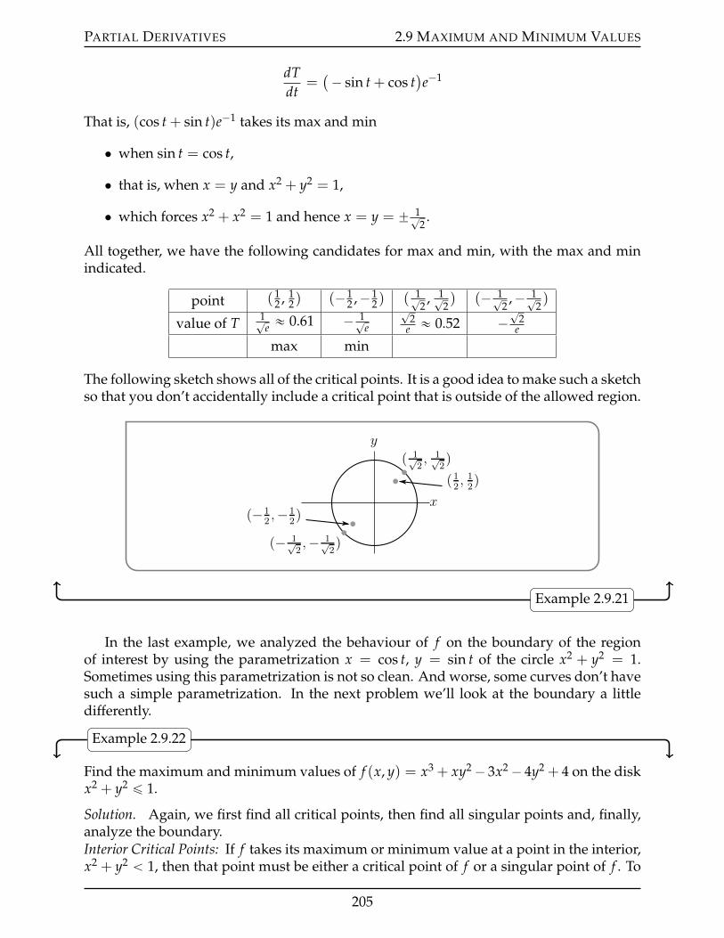
PARTIAL DERIVATIVES 2.9 MAXIMUM AND MINIMUM VALUES
dTdt
=(´ sin t + cos t
)e´1
That is, (cos t + sin t)e´1 takes its max and min
• when sin t = cos t,
• that is, when x = y and x2 + y2 = 1,
• which forces x2 + x2 = 1 and hence x = y = ˘ 1?2.
All together, we have the following candidates for max and min, with the max and minindicated.
point (12 , 1
2) (´12 ,´1
2) ( 1?2, 1?
2) (´ 1?
2,´ 1?
2)
value of T 1?e « 0.61 ´ 1?
e
?2
e « 0.52 ´?
2e
max min
The following sketch shows all of the critical points. It is a good idea to make such a sketchso that you don’t accidentally include a critical point that is outside of the allowed region.
x
y
(12, 12)
(−12,−1
2)
( 1√2, 1√
2)
(− 1√2,− 1√
2)
Example 2.9.21
In the last example, we analyzed the behaviour of f on the boundary of the regionof interest by using the parametrization x = cos t, y = sin t of the circle x2 + y2 = 1.Sometimes using this parametrization is not so clean. And worse, some curves don’t havesuch a simple parametrization. In the next problem we’ll look at the boundary a littledifferently.
Example 2.9.22
Find the maximum and minimum values of f (x, y) = x3 + xy2´ 3x2´ 4y2 + 4 on the diskx2 + y2 ď 1.
Solution. Again, we first find all critical points, then find all singular points and, finally,analyze the boundary.Interior Critical Points: If f takes its maximum or minimum value at a point in the interior,x2 + y2 ă 1, then that point must be either a critical point of f or a singular point of f . To
205
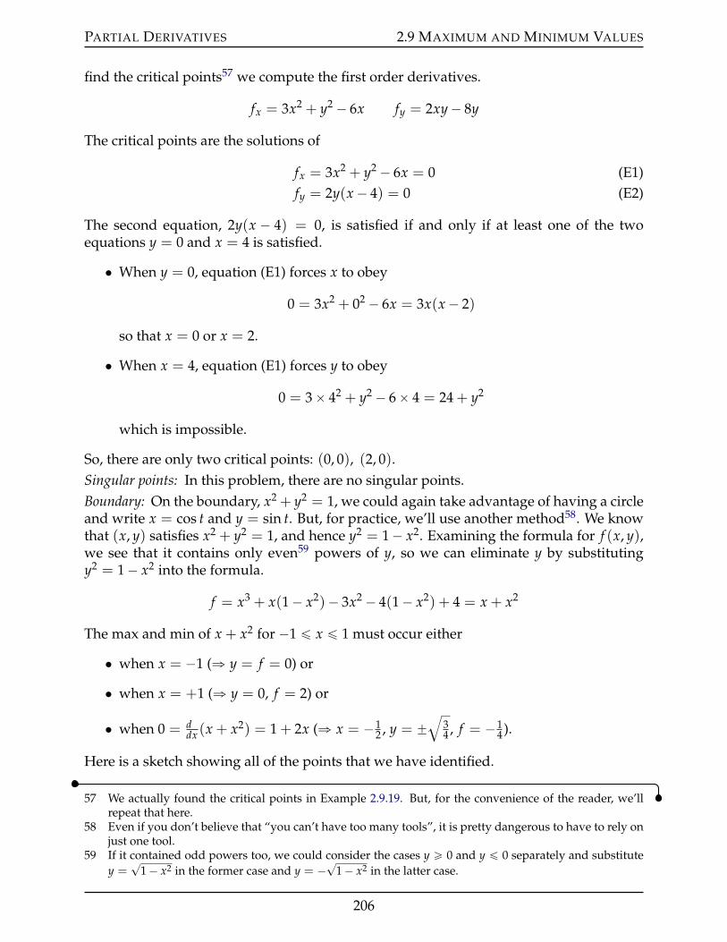
PARTIAL DERIVATIVES 2.9 MAXIMUM AND MINIMUM VALUES
find the critical points57 we compute the first order derivatives.
fx = 3x2 + y2 ´ 6x fy = 2xy´ 8y
The critical points are the solutions of
fx = 3x2 + y2 ´ 6x = 0 (E1)fy = 2y(x´ 4) = 0 (E2)
The second equation, 2y(x ´ 4) = 0, is satisfied if and only if at least one of the twoequations y = 0 and x = 4 is satisfied.
• When y = 0, equation (E1) forces x to obey
0 = 3x2 + 02 ´ 6x = 3x(x´ 2)
so that x = 0 or x = 2.
• When x = 4, equation (E1) forces y to obey
0 = 3ˆ 42 + y2 ´ 6ˆ 4 = 24 + y2
which is impossible.
So, there are only two critical points: (0, 0), (2, 0).Singular points: In this problem, there are no singular points.Boundary: On the boundary, x2 + y2 = 1, we could again take advantage of having a circleand write x = cos t and y = sin t. But, for practice, we’ll use another method58. We knowthat (x, y) satisfies x2 + y2 = 1, and hence y2 = 1´ x2. Examining the formula for f (x, y),we see that it contains only even59 powers of y, so we can eliminate y by substitutingy2 = 1´ x2 into the formula.
f = x3 + x(1´ x2)´ 3x2 ´ 4(1´ x2) + 4 = x + x2
The max and min of x + x2 for ´1 ď x ď 1 must occur either
• when x = ´1 (ñ y = f = 0) or
• when x = +1 (ñ y = 0, f = 2) or
• when 0 = ddx (x + x2) = 1 + 2x (ñ x = ´1
2 , y = ˘b
34 , f = ´1
4 ).
Here is a sketch showing all of the points that we have identified.
57 We actually found the critical points in Example 2.9.19. But, for the convenience of the reader, we’llrepeat that here.
58 Even if you don’t believe that “you can’t have too many tools”, it is pretty dangerous to have to rely onjust one tool.
59 If it contained odd powers too, we could consider the cases y ě 0 and y ď 0 separately and substitutey =
?1´ x2 in the former case and y = ´
?1´ x2 in the latter case.
206
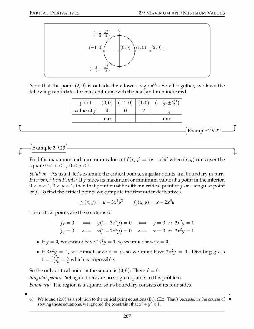
PARTIAL DERIVATIVES 2.9 MAXIMUM AND MINIMUM VALUES
x
y
(0, 0) (2, 0)(1, 0)(−1, 0)
(−12,√32)
(−12,−
√32)
Note that the point (2, 0) is outside the allowed region60. So all together, we have thefollowing candidates for max and min, with the max and min indicated.
point (0, 0) (´1, 0) (1, 0)(´ 1
2 ,˘?
32
)
value of f 4 0 2 ´14
max min
Example 2.9.22
Example 2.9.23
Find the maximum and minimum values of f (x, y) = xy´ x3y2 when (x, y) runs over thesquare 0 ď x ď 1, 0 ď y ď 1.
Solution. As usual, let’s examine the critical points, singular points and boundary in turn.Interior Critical Points: If f takes its maximum or minimum value at a point in the interior,0 ă x ă 1, 0 ă y ă 1, then that point must be either a critical point of f or a singular pointof f . To find the critical points we compute the first order derivatives.
fx(x, y) = y´ 3x2y2 fy(x, y) = x´ 2x3y
The critical points are the solutions of
fx = 0 ðñ y(1´ 3x2y) = 0 ðñ y = 0 or 3x2y = 1
fy = 0 ðñ x(1´ 2x2y) = 0 ðñ x = 0 or 2x2y = 1
• If y = 0, we cannot have 2x2y = 1, so we must have x = 0.
• If 3x2y = 1, we cannot have x = 0, so we must have 2x2y = 1. Dividing gives
1 = 3x2y2x2y = 3
2 which is impossible.
So the only critical point in the square is (0, 0). There f = 0.Singular points: Yet again there are no singular points in this problem.Boundary: The region is a square, so its boundary consists of its four sides.
60 We found (2, 0) as a solution to the critical point equations (E1), (E2). That’s because, in the course ofsolving those equations, we ignored the constraint that x2 + y2 ď 1.
207
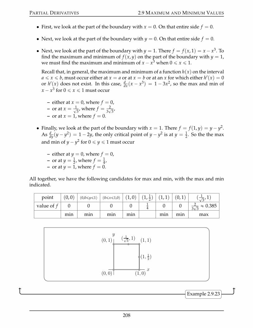
PARTIAL DERIVATIVES 2.9 MAXIMUM AND MINIMUM VALUES
• First, we look at the part of the boundary with x = 0. On that entire side f = 0.
• Next, we look at the part of the boundary with y = 0. On that entire side f = 0.
• Next, we look at the part of the boundary with y = 1. There f = f (x, 1) = x´ x3. Tofind the maximum and minimum of f (x, y) on the part of the boundary with y = 1,we must find the maximum and minimum of x´ x3 when 0 ď x ď 1.
Recall that, in general, the maximum and minimum of a function h(x) on the intervala ď x ď b, must occur either at x = a or at x = b or at an x for which either h1(x) = 0or h1(x) does not exist. In this case, d
dx (x ´ x3) = 1´ 3x2, so the max and min ofx´ x3 for 0 ď x ď 1 must occur
– either at x = 0, where f = 0,– or at x = 1?
3, where f = 2
3?
3,
– or at x = 1, where f = 0.
• Finally, we look at the part of the boundary with x = 1. There f = f (1, y) = y´ y2.As d
dy (y´ y2) = 1´ 2y, the only critical point of y´ y2 is at y = 12 . So the the max
and min of y´ y2 for 0 ď y ď 1 must occur
– either at y = 0, where f = 0,– or at y = 1
2 , where f = 14 ,
– or at y = 1, where f = 0.
All together, we have the following candidates for max and min, with the max and minindicated.
point (0, 0) (0,0ďyď1) (0ďxď1,0) (1, 0) (1, 12) (1, 1) (0, 1) ( 1?
3, 1)
value of f 0 0 0 0 14 0 0 2
3?
3« 0.385
min min min min min min max
x
y
(0, 0) (1, 0)
(1, 1)
(1, 12)
(0, 1) ( 1√3, 1)
Example 2.9.23
208
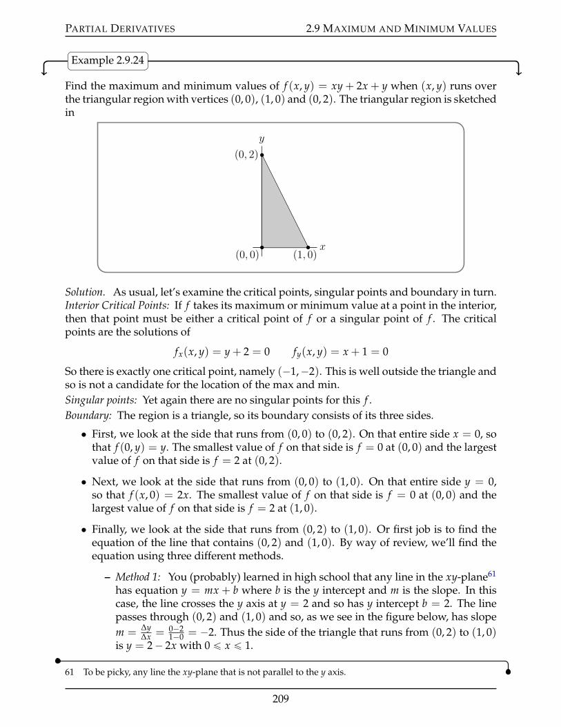
PARTIAL DERIVATIVES 2.9 MAXIMUM AND MINIMUM VALUES
Example 2.9.24
Find the maximum and minimum values of f (x, y) = xy + 2x + y when (x, y) runs overthe triangular region with vertices (0, 0), (1, 0) and (0, 2). The triangular region is sketchedin
x
y
p0, 0q p1, 0q
p0, 2q
Solution. As usual, let’s examine the critical points, singular points and boundary in turn.Interior Critical Points: If f takes its maximum or minimum value at a point in the interior,then that point must be either a critical point of f or a singular point of f . The criticalpoints are the solutions of
fx(x, y) = y + 2 = 0 fy(x, y) = x + 1 = 0
So there is exactly one critical point, namely (´1,´2). This is well outside the triangle andso is not a candidate for the location of the max and min.Singular points: Yet again there are no singular points for this f .Boundary: The region is a triangle, so its boundary consists of its three sides.
• First, we look at the side that runs from (0, 0) to (0, 2). On that entire side x = 0, sothat f (0, y) = y. The smallest value of f on that side is f = 0 at (0, 0) and the largestvalue of f on that side is f = 2 at (0, 2).
• Next, we look at the side that runs from (0, 0) to (1, 0). On that entire side y = 0,so that f (x, 0) = 2x. The smallest value of f on that side is f = 0 at (0, 0) and thelargest value of f on that side is f = 2 at (1, 0).
• Finally, we look at the side that runs from (0, 2) to (1, 0). Or first job is to find theequation of the line that contains (0, 2) and (1, 0). By way of review, we’ll find theequation using three different methods.
– Method 1: You (probably) learned in high school that any line in the xy-plane61
has equation y = mx + b where b is the y intercept and m is the slope. In thiscase, the line crosses the y axis at y = 2 and so has y intercept b = 2. The linepasses through (0, 2) and (1, 0) and so, as we see in the figure below, has slopem = ∆y
∆x = 0´21´0 = ´2. Thus the side of the triangle that runs from (0, 2) to (1, 0)
is y = 2´ 2x with 0 ď x ď 1.
61 To be picky, any line the xy-plane that is not parallel to the y axis.
209
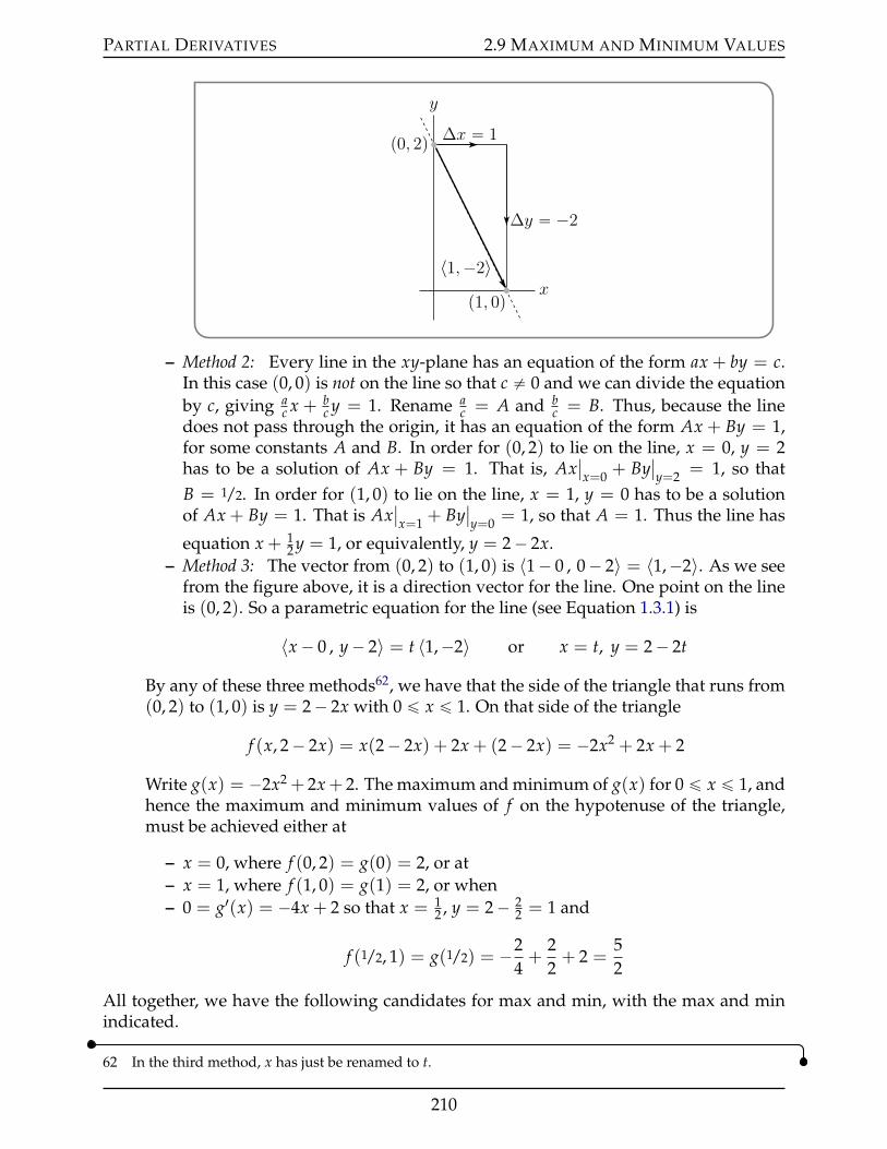
PARTIAL DERIVATIVES 2.9 MAXIMUM AND MINIMUM VALUES
x
y
p1, 0q
p0, 2q
〈1,´2〉
∆x “ 1
∆y “ ´2
– Method 2: Every line in the xy-plane has an equation of the form ax + by = c.In this case (0, 0) is not on the line so that c ‰ 0 and we can divide the equationby c, giving a
c x + bc y = 1. Rename a
c = A and bc = B. Thus, because the line
does not pass through the origin, it has an equation of the form Ax + By = 1,for some constants A and B. In order for (0, 2) to lie on the line, x = 0, y = 2has to be a solution of Ax + By = 1. That is, Ax
ˇx=0 + By
ˇy=2 = 1, so that
B = 1/2. In order for (1, 0) to lie on the line, x = 1, y = 0 has to be a solutionof Ax + By = 1. That is Ax
ˇx=1 + By
ˇy=0 = 1, so that A = 1. Thus the line has
equation x + 12 y = 1, or equivalently, y = 2´ 2x.
– Method 3: The vector from (0, 2) to (1, 0) is 〈1´ 0 , 0´ 2〉 = 〈1,´2〉. As we seefrom the figure above, it is a direction vector for the line. One point on the lineis (0, 2). So a parametric equation for the line (see Equation 1.3.1) is
〈x´ 0 , y´ 2〉 = t 〈1,´2〉 or x = t, y = 2´ 2t
By any of these three methods62, we have that the side of the triangle that runs from(0, 2) to (1, 0) is y = 2´ 2x with 0 ď x ď 1. On that side of the triangle
f (x, 2´ 2x) = x(2´ 2x) + 2x + (2´ 2x) = ´2x2 + 2x + 2
Write g(x) = ´2x2 + 2x + 2. The maximum and minimum of g(x) for 0 ď x ď 1, andhence the maximum and minimum values of f on the hypotenuse of the triangle,must be achieved either at
– x = 0, where f (0, 2) = g(0) = 2, or at– x = 1, where f (1, 0) = g(1) = 2, or when– 0 = g1(x) = ´4x + 2 so that x = 1
2 , y = 2´ 22 = 1 and
f (1/2, 1) = g(1/2) = ´24+
22+ 2 =
52
All together, we have the following candidates for max and min, with the max and minindicated.
62 In the third method, x has just be renamed to t.
210
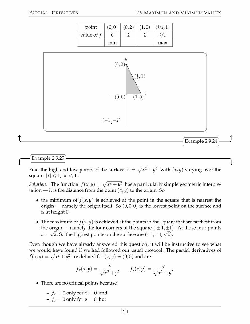
PARTIAL DERIVATIVES 2.9 MAXIMUM AND MINIMUM VALUES
point (0, 0) (0, 2) (1, 0) (1/2, 1)
value of f 0 2 2 5/2
min max
x
y
p0, 0q p1, 0q
p0, 2q
p´1,´2q
p12, 1q
Example 2.9.24
Example 2.9.25
Find the high and low points of the surface z =a
x2 + y2 with (x, y) varying over thesquare |x| ď 1, |y| ď 1 .
Solution. The function f (x, y) =a
x2 + y2 has a particularly simple geometric interpre-tation — it is the distance from the point (x, y) to the origin. So
• the minimum of f (x, y) is achieved at the point in the square that is nearest theorigin — namely the origin itself. So (0, 0, 0) is the lowest point on the surface andis at height 0.
• The maximum of f (x, y) is achieved at the points in the square that are farthest fromthe origin — namely the four corners of the square
(˘ 1,˘1). At those four points
z =?
2. So the highest points on the surface are (˘1,˘1,?
2).
Even though we have already answered this question, it will be instructive to see whatwe would have found if we had followed our usual protocol. The partial derivatives off (x, y) =
ax2 + y2 are defined for (x, y) ‰ (0, 0) and are
fx(x, y) =xa
x2 + y2fy(x, y) =
yax2 + y2
• There are no critical points because
– fx = 0 only for x = 0, and– fy = 0 only for y = 0, but
211
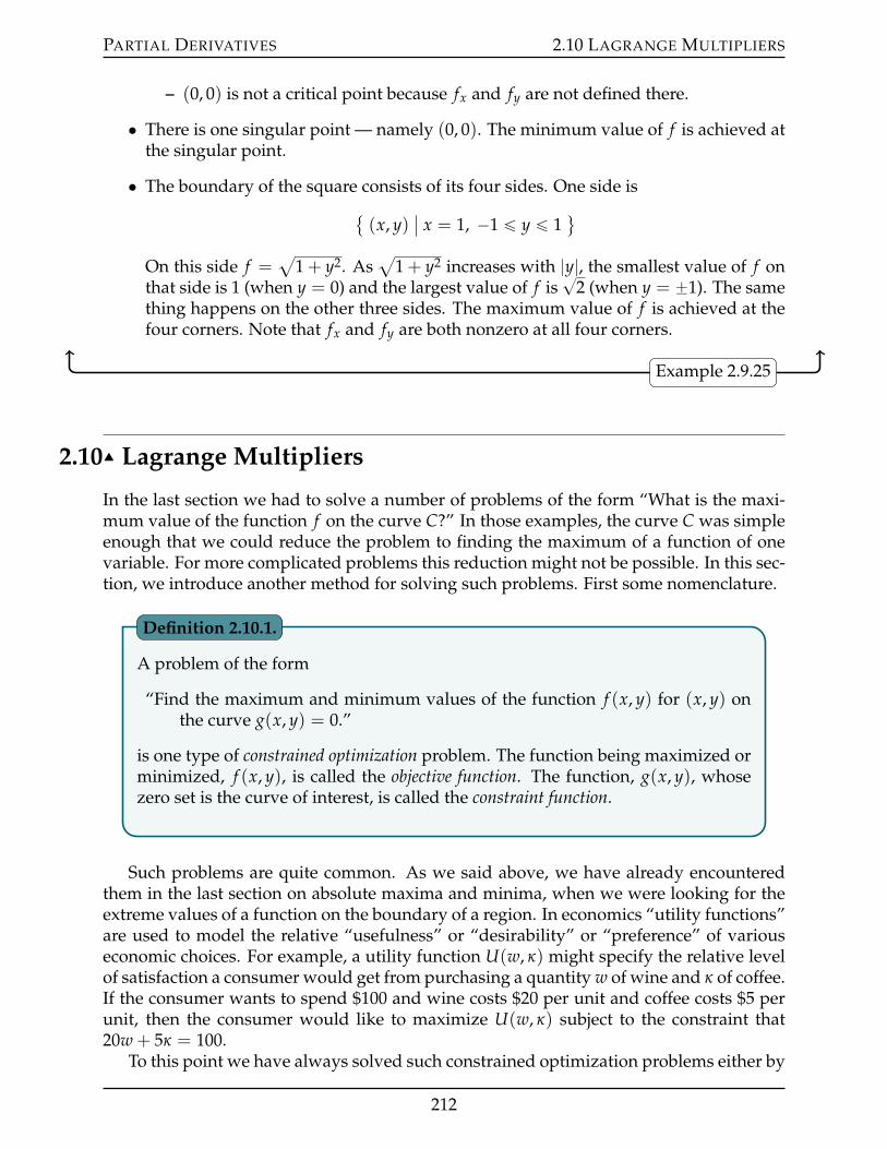
PARTIAL DERIVATIVES 2.10 LAGRANGE MULTIPLIERS
– (0, 0) is not a critical point because fx and fy are not defined there.
• There is one singular point — namely (0, 0). The minimum value of f is achieved atthe singular point.
• The boundary of the square consists of its four sides. One side is (x, y)
ˇx = 1, ´1 ď y ď 1
(
On this side f =a
1 + y2. Asa
1 + y2 increases with |y|, the smallest value of f onthat side is 1 (when y = 0) and the largest value of f is
?2 (when y = ˘1). The same
thing happens on the other three sides. The maximum value of f is achieved at thefour corners. Note that fx and fy are both nonzero at all four corners.
Example 2.9.25
2.10IJ Lagrange Multipliers
In the last section we had to solve a number of problems of the form “What is the maxi-mum value of the function f on the curve C?” In those examples, the curve C was simpleenough that we could reduce the problem to finding the maximum of a function of onevariable. For more complicated problems this reduction might not be possible. In this sec-tion, we introduce another method for solving such problems. First some nomenclature.
A problem of the form
“Find the maximum and minimum values of the function f (x, y) for (x, y) onthe curve g(x, y) = 0.”
is one type of constrained optimization problem. The function being maximized orminimized, f (x, y), is called the objective function. The function, g(x, y), whosezero set is the curve of interest, is called the constraint function.
Definition 2.10.1.
Such problems are quite common. As we said above, we have already encounteredthem in the last section on absolute maxima and minima, when we were looking for theextreme values of a function on the boundary of a region. In economics “utility functions”are used to model the relative “usefulness” or “desirability” or “preference” of variouseconomic choices. For example, a utility function U(w, κ) might specify the relative levelof satisfaction a consumer would get from purchasing a quantity w of wine and κ of coffee.If the consumer wants to spend $100 and wine costs $20 per unit and coffee costs $5 perunit, then the consumer would like to maximize U(w, κ) subject to the constraint that20w + 5κ = 100.
To this point we have always solved such constrained optimization problems either by
212
PARTIAL DERIVATIVES 2.10 LAGRANGE MULTIPLIERS
• solving g(x, y) = 0 for y as a function of x (or for x as a function of y) or by
• parametrizing the curve g(x, y) = 0. This means writing all points of the curve in theform
(x(t), y(t)
)for some functions x(t) and y(t). For example we used x(t) = cos t,
y(t) = sin t as a parametrization of the circle x2 + y2 = 1 in Example 2.9.21.
However quite often the function g(x, y) is so complicated that one cannot explicitly solveg(x, y) = 0 for y as a function of x or for x as a function of y and one also cannot explicitlyparametrize g(x, y) = 0. Or sometimes you can, for example, solve g(x, y) = 0 for y asa function of x, but the resulting solution is so complicated that it is really hard, or evenvirtually impossible, to work with. Direct attacks become even harder in higher dimen-sions when, for example, we wish to optimize a function f (x, y, z) subject to a constraintg(x, y, z) = 0.
There is another procedure called the method of “Lagrange63 multipliers” that comesto our rescue in these scenarios. Here is the three dimensional version of the method.There are obvious analogs is other dimensions.
Let f (x, y, z) and g(x, y, z) have continuous first partial derivatives in a regionof R3 that contains the surface S given by the equation g(x, y, z) = 0. Furtherassume that∇∇∇g(x, y, z) ‰ 0 on S.
If f , restricted to the surface S, has a local extreme value at the point (a, b, c) onS, then there is a real number λ such that
∇∇∇ f (a, b, c) = λ∇∇∇g(a, b, c)
that is
fx(a, b, c) = λ gx(a, b, c)fy(a, b, c) = λ gy(a, b, c)fz(a, b, c) = λ gz(a, b, c)
The number λ is called a Lagrange multiplier.
Theorem 2.10.2 (Lagrange Multipliers).
Proof. Suppose that (a, b, c) is a point of S and that f (x, y, z) ě f (a, b, c) for all points(x, y, z) on S that are close to (a, b, c). That is (a, b, c) is a local minimum for f on S. Ofcourse the argument for a local maximum is virtually identical.
Imagine that we go for a walk on S, with the time t running, say, from t = ´1 to t = +1and that at time t = 0 we happen to be exactly at (a, b, c). Let’s say that our position is(
x(t), y(t), z(t))
at time t. Write
F(t) = f(x(t), y(t), z(t)
)
63 Joseph-Louis Lagrange was actually born Giuseppe Lodovico Lagrangia in Turin, Italy in 1736. Hemoved to Berlin in 1766 and then to Paris in 1786. He eventually acquired French citizenship and thenthe French claimed he was a French mathematician, while the Italians continued to claim that he wasan Italian mathematician.
213
PARTIAL DERIVATIVES 2.10 LAGRANGE MULTIPLIERS
So F(t) is the value of f that we see on our walk at time t. Then for all t close to 0,(x(t), y(t), z(t)
)is close to
(x(0), y(0), z(0)
)= (a, b, c) so that
F(0) = f(x(0), y(0), z(0)
)= f (a, b, c) ď f
(x(t), y(t), z(t)
)= F(t)
for all t close to zero. So F(t) has a local minimum at t = 0 and consequently F1(0) = 0.By the chain rule, Theorem 2.4.1,
F1(0) =ddt
f(x(t), y(t), z(t)
)ˇˇt=0
= fx(a, b, c
)x1(0) + fy
(a, b, c
)y1(0) + fz
(a, b, c
)z1(0) = 0 (˚)
We may rewrite this as a dot product:
0 = F1(0) =∇∇∇ f (a, b, c) ¨ ⟨x1(0) , y1(0) , z1(0)⟩
ùñ ∇∇∇ f (a, b, c) K ⟨x1(0) , y1(0) , z1(0)⟩
This is true for all paths on S that pass through (a, b, c) at time 0. In particular it is true forall vectors 〈x1(0) , y1(0) , z1(0)〉 that are tangent to S at (a, b, c). So∇∇∇ f (a, b, c) is perpendic-ular to S at (a, b, c).
But we already know, by Theorem 2.5.5.a, that∇∇∇g(a, b, c) is also perpendicular to S at(a, b, c). So∇∇∇ f (a, b, c) and∇∇∇g(a, b, c) have to be parallel vectors. That is,
∇∇∇ f (a, b, c) = λ∇∇∇g(a, b, c)
for some number λ. That’s the Lagrange multiplier rule of our theorem.
So to find the maximum and minimum values of f (x, y, z) on a surface g(x, y, z) = 0,assuming that both the objective function f (x, y, z) and constraint function g(x, y, z) havecontinuous first partial derivatives and that∇∇∇g(x, y, z) ‰ 0, you
1. build up a list of candidate points (x, y, z) by finding all solutions to the equations
fx(x, y, z) = λ gx(x, y, z)fy(x, y, z) = λ gy(x, y, z)fz(x, y, z) = λ gz(x, y, z)g(x, y, z) = 0
Note that there are four equations and four unknowns, namely x, y, z and λ.
2. Then you evaluate f (x, y, z) at each (x, y, z) on the list of candidates. The biggest ofthese candidate values is the absolute maximum and the smallest of these candidatevalues is the absolute minimum.
Another way to write the system of equations in the first step is
Lx(a, b, c, λ) = Ly(a, b, c, λ) = Lz(a, b, c, λ) = Lλ(a, b, c, λ) = 0
214
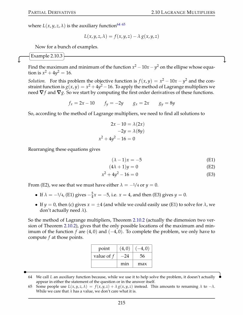
PARTIAL DERIVATIVES 2.10 LAGRANGE MULTIPLIERS
where L(x, y, z, λ) is the auxiliary function64 65
L(x, y, z, λ) = f (x, y, z)´ λ g(x, y, z)
Now for a bunch of examples.
Example 2.10.3
Find the maximum and minimum of the function x2´ 10x´ y2 on the ellipse whose equa-tion is x2 + 4y2 = 16.
Solution. For this problem the objective function is f (x, y) = x2 ´ 10x ´ y2 and the con-straint function is g(x, y) = x2 + 4y2´16. To apply the method of Lagrange multipliers weneed∇∇∇ f and∇∇∇g. So we start by computing the first order derivatives of these functions.
fx = 2x´ 10 fy = ´2y gx = 2x gy = 8y
So, according to the method of Lagrange multipliers, we need to find all solutions to
2x´ 10 = λ(2x)´2y = λ(8y)
x2 + 4y2 ´ 16 = 0
Rearranging these equations gives
(λ´ 1)x = ´5 (E1)(4λ + 1)y = 0 (E2)
x2 + 4y2 ´ 16 = 0 (E3)
From (E2), we see that we must have either λ = ´1/4 or y = 0.
• If λ = ´1/4, (E1) gives ´54 x = ´5, i.e. x = 4, and then (E3) gives y = 0.
• If y = 0, then (c) gives x = ˘4 (and while we could easily use (E1) to solve for λ, wedon’t actually need λ).
So the method of Lagrange multipliers, Theorem 2.10.2 (actually the dimension two ver-sion of Theorem 2.10.2), gives that the only possible locations of the maximum and min-imum of the function f are (4, 0) and (´4, 0). To complete the problem, we only have tocompute f at those points.
point (4, 0) (´4, 0)
value of f ´24 56
min max
64 We call L an auxiliary function because, while we use it to help solve the problem, it doesn’t actuallyappear in either the statement of the question or in the answer itself.
65 Some people use L(x, y, z, λ) = f (x, y, z) + λ g(x, y, z) instead. This amounts to renaming λ to ´λ.While we care that λ has a value, we don’t care what it is.
215
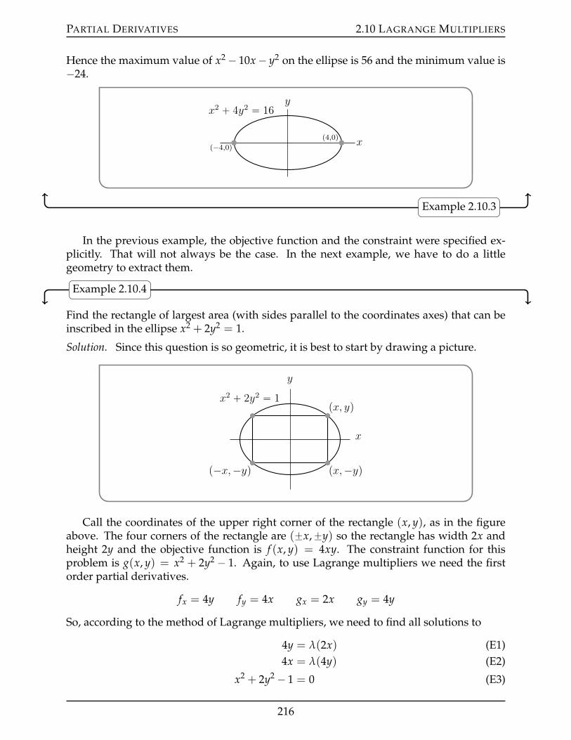
PARTIAL DERIVATIVES 2.10 LAGRANGE MULTIPLIERS
Hence the maximum value of x2 ´ 10x´ y2 on the ellipse is 56 and the minimum value is´24.
x
yx2 ` 4y2 “ 16
p´4,0qp4,0q
Example 2.10.3
In the previous example, the objective function and the constraint were specified ex-plicitly. That will not always be the case. In the next example, we have to do a littlegeometry to extract them.
Example 2.10.4
Find the rectangle of largest area (with sides parallel to the coordinates axes) that can beinscribed in the ellipse x2 + 2y2 = 1.
Solution. Since this question is so geometric, it is best to start by drawing a picture.
x
y
px, yq
px,´yqp´x,´yq
x2 ` 2y2 “ 1
Call the coordinates of the upper right corner of the rectangle (x, y), as in the figureabove. The four corners of the rectangle are (˘x,˘y) so the rectangle has width 2x andheight 2y and the objective function is f (x, y) = 4xy. The constraint function for thisproblem is g(x, y) = x2 + 2y2 ´ 1. Again, to use Lagrange multipliers we need the firstorder partial derivatives.
fx = 4y fy = 4x gx = 2x gy = 4y
So, according to the method of Lagrange multipliers, we need to find all solutions to
4y = λ(2x) (E1)4x = λ(4y) (E2)
x2 + 2y2 ´ 1 = 0 (E3)
216
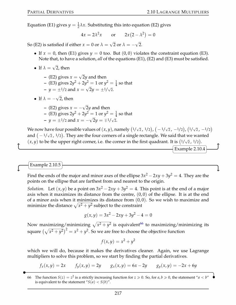
PARTIAL DERIVATIVES 2.10 LAGRANGE MULTIPLIERS
Equation (E1) gives y = 12 λx. Substituting this into equation (E2) gives
4x = 2λ2x or 2x(2´ λ2) = 0
So (E2) is satisfied if either x = 0 or λ =?
2 or λ = ´?2.
• If x = 0, then (E1) gives y = 0 too. But (0, 0) violates the constraint equation (E3).Note that, to have a solution, all of the equations (E1), (E2) and (E3) must be satisfied.
• If λ =?
2, then
– (E2) gives x =?
2y and then– (E3) gives 2y2 + 2y2 = 1 or y2 = 1
4 so that– y = ˘1/2 and x =
?2y = ˘1/
?2.
• If λ = ´?2, then
– (E2) gives x = ´?2y and then– (E3) gives 2y2 + 2y2 = 1 or y2 = 1
4 so that– y = ˘1/2 and x = ´?2y = ¯1/
?2.
We now have four possible values of (x, y), namely(
1/?
2 , 1/2),(´ 1/
?2 , ´1/2
),(
1/?
2 , ´1/2)
and(´ 1/
?2 , 1/2
). They are the four corners of a single rectangle. We said that we wanted
(x, y) to be the upper right corner, i.e. the corner in the first quadrant. It is(
1/?
2 , 1/2).
Example 2.10.4
Example 2.10.5
Find the ends of the major and minor axes of the ellipse 3x2´ 2xy + 3y2 = 4. They are thepoints on the ellipse that are farthest from and nearest to the origin.
Solution. Let (x, y) be a point on 3x2 ´ 2xy + 3y2 = 4. This point is at the end of a majoraxis when it maximizes its distance from the centre, (0, 0) of the ellipse. It is at the endof a minor axis when it minimizes its distance from (0, 0). So we wish to maximize andminimize the distance
ax2 + y2 subject to the constraint
g(x, y) = 3x2 ´ 2xy + 3y2 ´ 4 = 0
Now maximizing/minimizinga
x2 + y2 is equivalent66 to maximizing/minimizing itssquare
(ax2 + y2
)2= x2 + y2. So we are free to choose the objective function
f (x, y) = x2 + y2
which we will do, because it makes the derivatives cleaner. Again, we use Lagrangemultipliers to solve this problem, so we start by finding the partial derivatives.
fx(x, y) = 2x fy(x, y) = 2y gx(x, y) = 6x´ 2y gy(x, y) = ´2x + 6y
66 The function S(z) = z2 is a strictly increasing function for z ě 0. So, for a, b ě 0, the statement “a ă b”is equivalent to the statement “S(a) ă S(b)”.
217
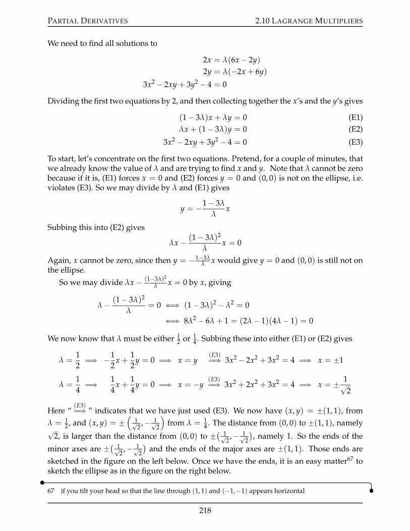
PARTIAL DERIVATIVES 2.10 LAGRANGE MULTIPLIERS
We need to find all solutions to
2x = λ(6x´ 2y)2y = λ(´2x + 6y)
3x2 ´ 2xy + 3y2 ´ 4 = 0
Dividing the first two equations by 2, and then collecting together the x’s and the y’s gives
(1´ 3λ)x + λy = 0 (E1)λx + (1´ 3λ)y = 0 (E2)
3x2 ´ 2xy + 3y2 ´ 4 = 0 (E3)
To start, let’s concentrate on the first two equations. Pretend, for a couple of minutes, thatwe already know the value of λ and are trying to find x and y. Note that λ cannot be zerobecause if it is, (E1) forces x = 0 and (E2) forces y = 0 and (0, 0) is not on the ellipse, i.e.violates (E3). So we may divide by λ and (E1) gives
y = ´1´ 3λ
λx
Subbing this into (E2) gives
λx´ (1´ 3λ)2
λx = 0
Again, x cannot be zero, since then y = ´1´3λλ x would give y = 0 and (0, 0) is still not on
the ellipse.
So we may divide λx´ (1´3λ)2
λ x = 0 by x, giving
λ´ (1´ 3λ)2
λ= 0 ðñ (1´ 3λ)2 ´ λ2 = 0
ðñ 8λ2 ´ 6λ + 1 = (2λ´ 1)(4λ´ 1) = 0
We now know that λ must be either 12 or 1
4 . Subbing these into either (E1) or (E2) gives
λ =12ùñ ´1
2x +
12
y = 0 ùñ x = y(E3)ùñ 3x2 ´ 2x2 + 3x2 = 4 ùñ x = ˘1
λ =14ùñ 1
4x +
14
y = 0 ùñ x = ´y(E3)ùñ 3x2 + 2x2 + 3x2 = 4 ùñ x = ˘ 1?
2
Here “(E3)ùñ ” indicates that we have just used (E3). We now have (x, y) = ˘(1, 1), from
λ = 12 , and (x, y) = ˘
(1?2,´ 1?
2
)from λ = 1
4 . The distance from (0, 0) to ˘(1, 1), namely?2, is larger than the distance from (0, 0) to ˘( 1?
2,´ 1?
2
), namely 1. So the ends of the
minor axes are ˘( 1?2,´ 1?
2
)and the ends of the major axes are ˘(1, 1). Those ends are
sketched in the figure on the left below. Once we have the ends, it is an easy matter67 tosketch the ellipse as in the figure on the right below.
67 if you tilt your head so that the line through (1, 1) and (´1,´1) appears horizontal
218
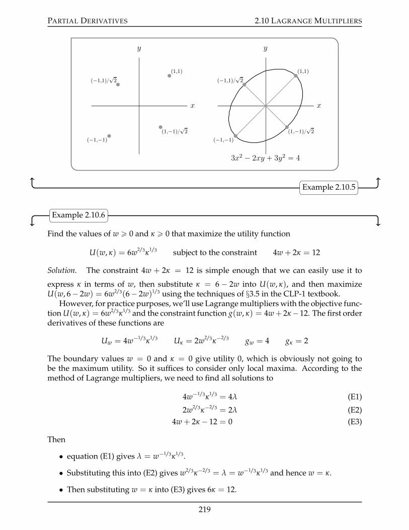
PARTIAL DERIVATIVES 2.10 LAGRANGE MULTIPLIERS
x
y
p1,1q
p´1,´1qp1,´1q?
2
p´1,1q?2
x
y
p1,1q
p´1,´1qp1,´1q?
2
p´1,1q?2
3x2 ´ 2xy ` 3y2 “ 4
Example 2.10.5
Example 2.10.6
Find the values of w ě 0 and κ ě 0 that maximize the utility function
U(w, κ) = 6w2/3κ1/3 subject to the constraint 4w + 2κ = 12
Solution. The constraint 4w + 2κ = 12 is simple enough that we can easily use it to
express κ in terms of w, then substitute κ = 6 ´ 2w into U(w, κ), and then maximizeU(w, 6´ 2w) = 6w2/3(6´ 2w)1/3 using the techniques of §3.5 in the CLP-1 textbook.
However, for practice purposes, we’ll use Lagrange multipliers with the objective func-tion U(w, κ) = 6w2/3κ1/3 and the constraint function g(w, κ) = 4w+ 2κ´12. The first orderderivatives of these functions are
Uw = 4w´1/3κ1/3 Uκ = 2w2/3κ´
2/3 gw = 4 gκ = 2
The boundary values w = 0 and κ = 0 give utility 0, which is obviously not going tobe the maximum utility. So it suffices to consider only local maxima. According to themethod of Lagrange multipliers, we need to find all solutions to
4w´1/3κ1/3 = 4λ (E1)
2w2/3κ´2/3 = 2λ (E2)
4w + 2κ ´ 12 = 0 (E3)
Then
• equation (E1) gives λ = w´1/3κ1/3.
• Substituting this into (E2) gives w2/3κ´2/3 = λ = w´1/3κ1/3 and hence w = κ.
• Then substituting w = κ into (E3) gives 6κ = 12.
219
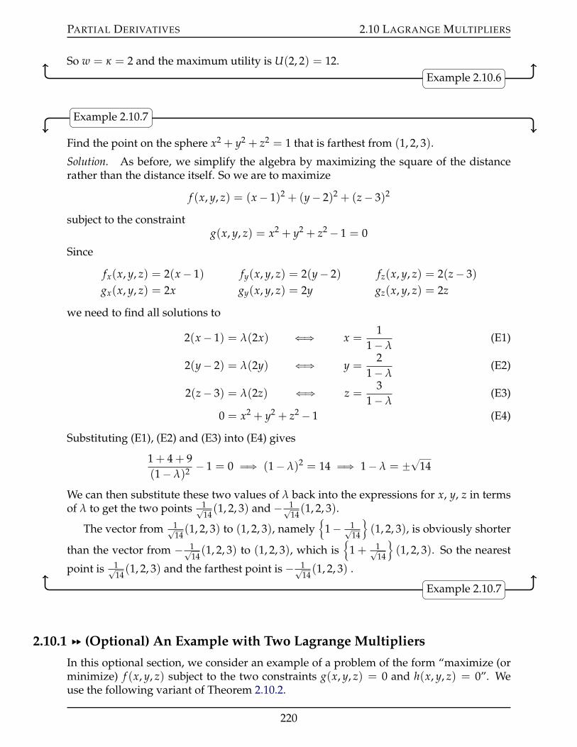
PARTIAL DERIVATIVES 2.10 LAGRANGE MULTIPLIERS
So w = κ = 2 and the maximum utility is U(2, 2) = 12.Example 2.10.6
Example 2.10.7
Find the point on the sphere x2 + y2 + z2 = 1 that is farthest from (1, 2, 3).
Solution. As before, we simplify the algebra by maximizing the square of the distancerather than the distance itself. So we are to maximize
f (x, y, z) = (x´ 1)2 + (y´ 2)2 + (z´ 3)2
subject to the constraintg(x, y, z) = x2 + y2 + z2 ´ 1 = 0
Since
fx(x, y, z) = 2(x´ 1) fy(x, y, z) = 2(y´ 2) fz(x, y, z) = 2(z´ 3)gx(x, y, z) = 2x gy(x, y, z) = 2y gz(x, y, z) = 2z
we need to find all solutions to
2(x´ 1) = λ(2x) ðñ x =1
1´ λ(E1)
2(y´ 2) = λ(2y) ðñ y =2
1´ λ(E2)
2(z´ 3) = λ(2z) ðñ z =3
1´ λ(E3)
0 = x2 + y2 + z2 ´ 1 (E4)
Substituting (E1), (E2) and (E3) into (E4) gives
1 + 4 + 9(1´ λ)2 ´ 1 = 0 ùñ (1´ λ)2 = 14 ùñ 1´ λ = ˘
?14
We can then substitute these two values of λ back into the expressions for x, y, z in termsof λ to get the two points 1?
14(1, 2, 3) and ´ 1?
14(1, 2, 3).
The vector from 1?14(1, 2, 3) to (1, 2, 3), namely
!1´ 1?
14
)(1, 2, 3), is obviously shorter
than the vector from ´ 1?14(1, 2, 3) to (1, 2, 3), which is
!1 + 1?
14
)(1, 2, 3). So the nearest
point is 1?14(1, 2, 3) and the farthest point is ´ 1?
14(1, 2, 3) .
Example 2.10.7
2.10.1 §§ (Optional) An Example with Two Lagrange Multipliers
In this optional section, we consider an example of a problem of the form “maximize (orminimize) f (x, y, z) subject to the two constraints g(x, y, z) = 0 and h(x, y, z) = 0”. Weuse the following variant of Theorem 2.10.2.
220
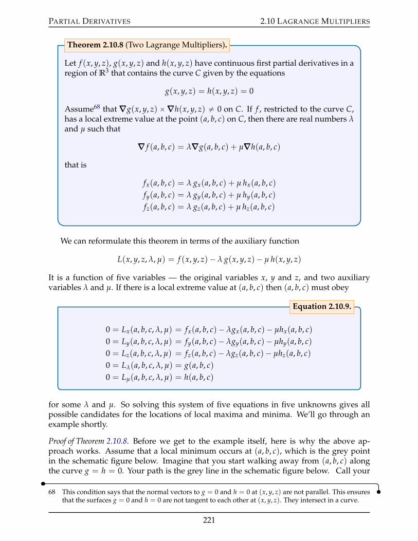
PARTIAL DERIVATIVES 2.10 LAGRANGE MULTIPLIERS
Let f (x, y, z), g(x, y, z) and h(x, y, z) have continuous first partial derivatives in aregion of R3 that contains the curve C given by the equations
g(x, y, z) = h(x, y, z) = 0
Assume68 that ∇∇∇g(x, y, z)ˆ∇∇∇h(x, y, z) ‰ 0 on C. If f , restricted to the curve C,has a local extreme value at the point (a, b, c) on C, then there are real numbers λand µ such that
∇∇∇ f (a, b, c) = λ∇∇∇g(a, b, c) + µ∇∇∇h(a, b, c)
that is
fx(a, b, c) = λ gx(a, b, c) + µ hx(a, b, c)fy(a, b, c) = λ gy(a, b, c) + µ hy(a, b, c)fz(a, b, c) = λ gz(a, b, c) + µ hz(a, b, c)
Theorem 2.10.8 (Two Lagrange Multipliers).
We can reformulate this theorem in terms of the auxiliary function
L(x, y, z, λ, µ) = f (x, y, z)´ λ g(x, y, z)´ µ h(x, y, z)
It is a function of five variables — the original variables x, y and z, and two auxiliaryvariables λ and µ. If there is a local extreme value at (a, b, c) then (a, b, c) must obey
0 = Lx(a, b, c, λ, µ) = fx(a, b, c)´ λgx(a, b, c)´ µhx(a, b, c)0 = Ly(a, b, c, λ, µ) = fy(a, b, c)´ λgy(a, b, c)´ µhy(a, b, c)0 = Lz(a, b, c, λ, µ) = fz(a, b, c)´ λgz(a, b, c)´ µhz(a, b, c)0 = Lλ(a, b, c, λ, µ) = g(a, b, c)0 = Lµ(a, b, c, λ, µ) = h(a, b, c)
Equation 2.10.9.
for some λ and µ. So solving this system of five equations in five unknowns gives allpossible candidates for the locations of local maxima and minima. We’ll go through anexample shortly.
Proof of Theorem 2.10.8. Before we get to the example itself, here is why the above ap-proach works. Assume that a local minimum occurs at (a, b, c), which is the grey pointin the schematic figure below. Imagine that you start walking away from (a, b, c) alongthe curve g = h = 0. Your path is the grey line in the schematic figure below. Call your
68 This condition says that the normal vectors to g = 0 and h = 0 at (x, y, z) are not parallel. This ensuresthat the surfaces g = 0 and h = 0 are not tangent to each other at (x, y, z). They intersect in a curve.
221
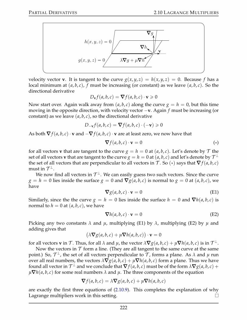
PARTIAL DERIVATIVES 2.10 LAGRANGE MULTIPLIERS
gpx, y, zq “ 0
hpx, y, zq “ 0
∇∇∇g
∇∇∇h
λ∇∇∇g ` µ∇∇∇h
v
velocity vector v. It is tangent to the curve g(x, y, z) = h(x, y, z) = 0. Because f has alocal minimum at (a, b, c), f must be increasing (or constant) as we leave (a, b, c). So thedirectional derivative
Dv f (a, b, c) =∇∇∇ f (a, b, c) ¨ v ě 0
Now start over. Again walk away from (a, b, c) along the curve g = h = 0, but this timemoving in the opposite direction, with velocity vector ´v. Again f must be increasing (orconstant) as we leave (a, b, c), so the directional derivative
D´v f (a, b, c) =∇∇∇ f (a, b, c) ¨ (´v) ě 0
As both∇∇∇ f (a, b, c) ¨ v and ´∇∇∇ f (a, b, c) ¨ v are at least zero, we now have that
∇∇∇ f (a, b, c) ¨ v = 0 (˚)for all vectors v that are tangent to the curve g = h = 0 at (a, b, c). Let’s denote by T theset of all vectors v that are tangent to the curve g = h = 0 at (a, b, c) and let’s denote by T Kthe set of all vectors that are perpendicular to all vectors in T . So (˚) says that∇∇∇ f (a, b, c)must in T K.
We now find all vectors in T K. We can easily guess two such vectors. Since the curveg = h = 0 lies inside the surface g = 0 and ∇∇∇g(a, b, c) is normal to g = 0 at (a, b, c), wehave
∇∇∇g(a, b, c) ¨ v = 0 (E1)
Similarly, since the the curve g = h = 0 lies inside the surface h = 0 and ∇∇∇h(a, b, c) isnormal to h = 0 at (a, b, c), we have
∇∇∇h(a, b, c) ¨ v = 0 (E2)
Picking any two constants λ and µ, multiplying (E1) by λ, multiplying (E2) by µ andadding gives that (
λ∇∇∇g(a, b, c) + µ∇∇∇h(a, b, c)) ¨ v = 0
for all vectors v in T . Thus, for all λ and µ, the vector λ∇∇∇g(a, b, c) + µ∇∇∇h(a, b, c) is in T K.Now the vectors in T form a line. (They are all tangent to the same curve at the same
point.) So, T K, the set of all vectors perpendicular to T , forms a plane. As λ and µ runover all real numbers, the vectors λ∇∇∇g(a, b, c) + µ∇∇∇h(a, b, c) form a plane. Thus we havefound all vector in T K and we conclude that∇∇∇ f (a, b, c) must be of the form λ∇∇∇g(a, b, c) +µ∇∇∇h(a, b, c) for some real numbers λ and µ. The three components of the equation
∇∇∇ f (a, b, c) = λ∇∇∇g(a, b, c) + µ∇∇∇h(a, b, c)
are exactly the first three equations of (2.10.9). This completes the explanation of whyLagrange multipliers work in this setting.
222
PARTIAL DERIVATIVES 2.10 LAGRANGE MULTIPLIERS
Example 2.10.10
Find the distance from the origin to the curve that is the intersection of the two surfaces
z2 = x2 + y2 x´ 2z = 3
Solution. Yet again, we simplify the algebra by maximizing the square of the distancerather than the distance itself. So we are to maximize
f (x, y, z) = x2 + y2 + z2
subject to the constraints
0 = g(x, y, z) = x2 + y2 ´ z2 0 = h(x, y, z) = x´ 2z´ 3
Since
fx = 2x fy = 2y fz = 2zgx = 2x gy = 2y gz = ´2zhx = 1 hy = 0 hz = ´2
the method of Lagrange multipliers requires us to find all solutions to
2x = λ(2x) + µ(1) (E1)2y = λ(2y) + µ(0) ðñ (1´ λ)y = 0 (E2)2z = λ(´2z) + µ(´2) (E3)
z2 = x2 + y2 (E4)x´ 2z = 3 (E5)
Since equation (E2) factors so nicely we start there. It tells us that either y = 0 or λ = 1.
Case λ = 1: When λ = 1 the remaining equations reduce to
0 = µ (E1)0 = 4z + 2µ (E3)
z2 = x2 + y2 (E4)x´ 2z = 3 (E5)
So
• equation (E1) gives µ = 0.• Then substituting µ = 0 into (E3) gives z = 0.• Then substituting z = 0 into (E5) gives x = 3.• Then substituting z = 0 and x = 3 into (E4) gives 0 = 9 + y2, which is impossible,
since 9 + y2 ě 9 ą 0 for all y.
223
PARTIAL DERIVATIVES 2.10 LAGRANGE MULTIPLIERS
So we can’t have λ = 1.
Case y = 0: When y = 0 the remaining equations reduce to
2(1´ λ)x = µ (E1)(1 + λ)z = ´µ (E3)
z2 = x2 (E4)x´ 2z = 3 (E5)
These don’t clean up quite so nicely as in the λ = 1 case. But at least equation (E4) tells usthat z = ˘x. So we have to consider those two possibilities.
Subcase y = 0, z = x: When y = 0 and z = x, the remaining equations reduce to
2(1´ λ)x = µ (E1)(1 + λ)x = ´µ (E3)
´x = 3 (E5)
So equation (E5) now tells us that x = ´3 so that (x, y, z) = (´3, 0,´3). (We don’t reallycare what λ and µ are. But as they obey ´6(1´ λ) = µ, ´3(1 + λ) = ´µ we have, addingthe two equations together
´9 + 3λ = 0 ùñ λ = 3
and then, subbing into either equation, µ = 12.)
Subcase y = 0, z = ´x: When y = 0 and z = ´x, the remaining equations reduce to
2(1´ λ)x = µ (E1)(1 + λ)x = µ (E3)
3x = 3 (E5)
So equation (E5) now tells us that x = 1 so that (x, y, z) = (1, 0,´1). (Again, we don’treally care what λ and µ are. But as they obey 2(1 ´ λ) = µ, (1 + λ) = µ we have,subtracting the second equation from the first,
1´ 3λ = 0 ùñ λ =13
and then, subbing into either equation, µ = 43 .)
Conclusion: We have two candidates for the location of the max and min, namely(´3, 0,´3) and (1, 0,´1). The first is a distance 3
?2 from the origin, giving the maxi-
mum, and the second is a distance?
2 from the origin, giving the minimum. In particular,the distance is
?2.
Example 2.10.10
224
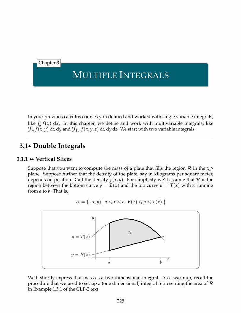
MULTIPLE INTEGRALS
Chapter 3
In your previous calculus courses you defined and worked with single variable integrals,like
şba f (x) dx. In this chapter, we define and work with multivariable integrals, likeť
R f (x, y) dx dy andţ
V f (x, y, z) dx dy dz. We start with two variable integrals.
3.1IJ Double Integrals
3.1.1 §§ Vertical Slices
Suppose that you want to compute the mass of a plate that fills the region R in the xy-plane. Suppose further that the density of the plate, say in kilograms per square meter,depends on position. Call the density f (x, y). For simplicity we’ll assume that R is theregion between the bottom curve y = B(x) and the top curve y = T(x) with x runningfrom a to b. That is,
R = (x, y)
ˇa ď x ď b, B(x) ď y ď T(x)
(
x
y
y “ T pxq
y “ Bpxqa b
R
We’ll shortly express that mass as a two dimensional integral. As a warmup, recall theprocedure that we used to set up a (one dimensional) integral representing the area of Rin Example 1.5.1 of the CLP-2 text.
225
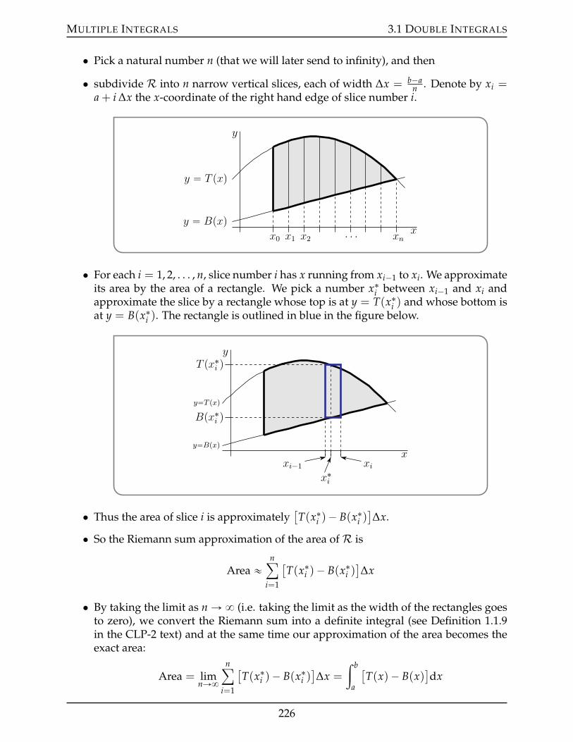
MULTIPLE INTEGRALS 3.1 DOUBLE INTEGRALS
• Pick a natural number n (that we will later send to infinity), and then
• subdivide R into n narrow vertical slices, each of width ∆x = b´an . Denote by xi =
a + i ∆x the x-coordinate of the right hand edge of slice number i.
x
y
y “ T pxq
y “ Bpxqx0 x1 x2 ¨ ¨ ¨ xn
• For each i = 1, 2, . . . , n, slice number i has x running from xi´1 to xi. We approximateits area by the area of a rectangle. We pick a number x˚i between xi´1 and xi andapproximate the slice by a rectangle whose top is at y = T(x˚i ) and whose bottom isat y = B(x˚i ). The rectangle is outlined in blue in the figure below.
x
y
xi´1 xi
xi
Bpxi q
T pxi q
y“T pxq
y“Bpxq
• Thus the area of slice i is approximately[T(x˚i )´ B(x˚i )
]∆x.
• So the Riemann sum approximation of the area ofR is
Area «nÿ
i=1
[T(x˚i )´ B(x˚i )
]∆x
• By taking the limit as n Ñ 8 (i.e. taking the limit as the width of the rectangles goesto zero), we convert the Riemann sum into a definite integral (see Definition 1.1.9in the CLP-2 text) and at the same time our approximation of the area becomes theexact area:
Area = limnÑ8
nÿ
i=1
[T(x˚i )´ B(x˚i )
]∆x =
ż b
a
[T(x)´ B(x)
]dx
226
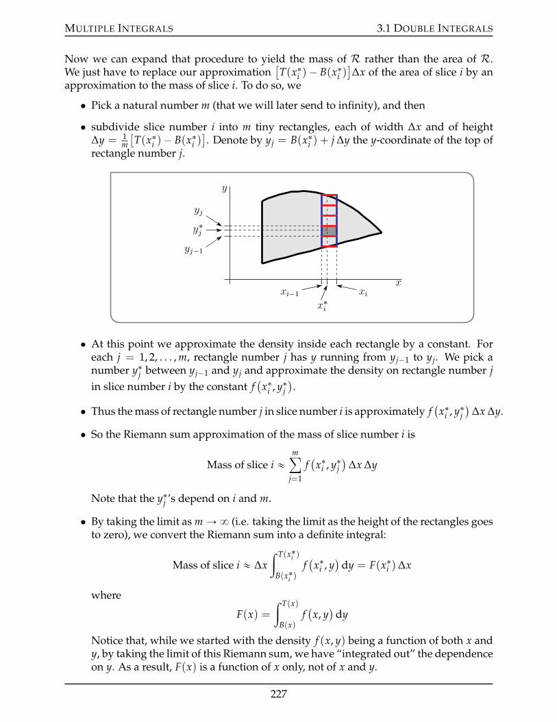
MULTIPLE INTEGRALS 3.1 DOUBLE INTEGRALS
Now we can expand that procedure to yield the mass of R rather than the area of R.We just have to replace our approximation
[T(x˚i )´ B(x˚i )
]∆x of the area of slice i by an
approximation to the mass of slice i. To do so, we
• Pick a natural number m (that we will later send to infinity), and then
• subdivide slice number i into m tiny rectangles, each of width ∆x and of height∆y = 1
m[T(x˚i )´ B(x˚i )
]. Denote by yj = B(x˚i ) + j ∆y the y-coordinate of the top of
rectangle number j.
x
y
xi´1 xi
xi
yj´1
yj
yj
• At this point we approximate the density inside each rectangle by a constant. Foreach j = 1, 2, . . . , m, rectangle number j has y running from yj´1 to yj. We pick anumber y˚j between yj´1 and yj and approximate the density on rectangle number jin slice number i by the constant f
(x˚i , y˚j
).
• Thus the mass of rectangle number j in slice number i is approximately f(x˚i , y˚j
)∆x ∆y.
• So the Riemann sum approximation of the mass of slice number i is
Mass of slice i «mÿ
j=1
f(x˚i , y˚j
)∆x ∆y
Note that the y˚j ’s depend on i and m.
• By taking the limit as m Ñ 8 (i.e. taking the limit as the height of the rectangles goesto zero), we convert the Riemann sum into a definite integral:
Mass of slice i « ∆xż T(x˚i )
B(x˚i )f(x˚i , y
)dy = F(x˚i )∆x
where
F(x) =ż T(x)
B(x)f(x, y)
dy
Notice that, while we started with the density f (x, y) being a function of both x andy, by taking the limit of this Riemann sum, we have “integrated out” the dependenceon y. As a result, F(x) is a function of x only, not of x and y.
227
MULTIPLE INTEGRALS 3.1 DOUBLE INTEGRALS
• Finally taking the limit as n Ñ 8 (i.e. taking the limit as the slice width goes to zero),we get
Mass = limnÑ8
nÿ
i=1
∆xż T(x˚i )
B(x˚i )f(x˚i , y
)dy = lim
nÑ8
nÿ
i=1
F(x˚i )∆x
Now we are back in familiar 1-variable territory. The sumnř
i=1F(x˚i )∆x is a Riemann
sum approximation to the integralşb
a F(x)dx. So
Mass =
ż b
aF(x)dx =
ż b
a
[ż T(x)
B(x)f(x, y)
dy
]dx
This is our first double integral. There are a couple of different standard notations for thisintegral.
ij
R
f(x, y)
dx dy =
ż b
a
[ż T(x)
B(x)f(x, y)
dy
]dx
=
ż b
a
ż T(x)
B(x)f(x, y)
dy dx =
ż b
adx
ż T(x)
B(x)dy f
(x, y)
The last three integrals here are called iterated integrals, for obvious reasons.
Notation 3.1.1.
Note that
• to evaluate the integralż b
a
ż T(x)
B(x)f(x, y)
dy dx,
– first evaluate the inside integralşT(x)
B(x) f(x, y)
dy using the inside limits of in-tegration, and by treating x as a constant and using standard single variableintegration techniques, such as those in the CLP-2 text. The result of the insideintegral is a function of x only. Call it F(x).
– Then evaluate the outside integralşb
a F(x)dx, whose integrand is the answerto the inside integral. Again, this integral is evaluated using standard singlevariable integration techniques.
• To evaluate the integralż b
adx
ż T(x)
B(x)dy f
(x, y),
– first evaluate the inside integralşT(x)
B(x) dy f(x, y)
using the limits of integration
that are directly beside the dy. Indeed the dy is written directly besideşT(x)
B(x) to
228
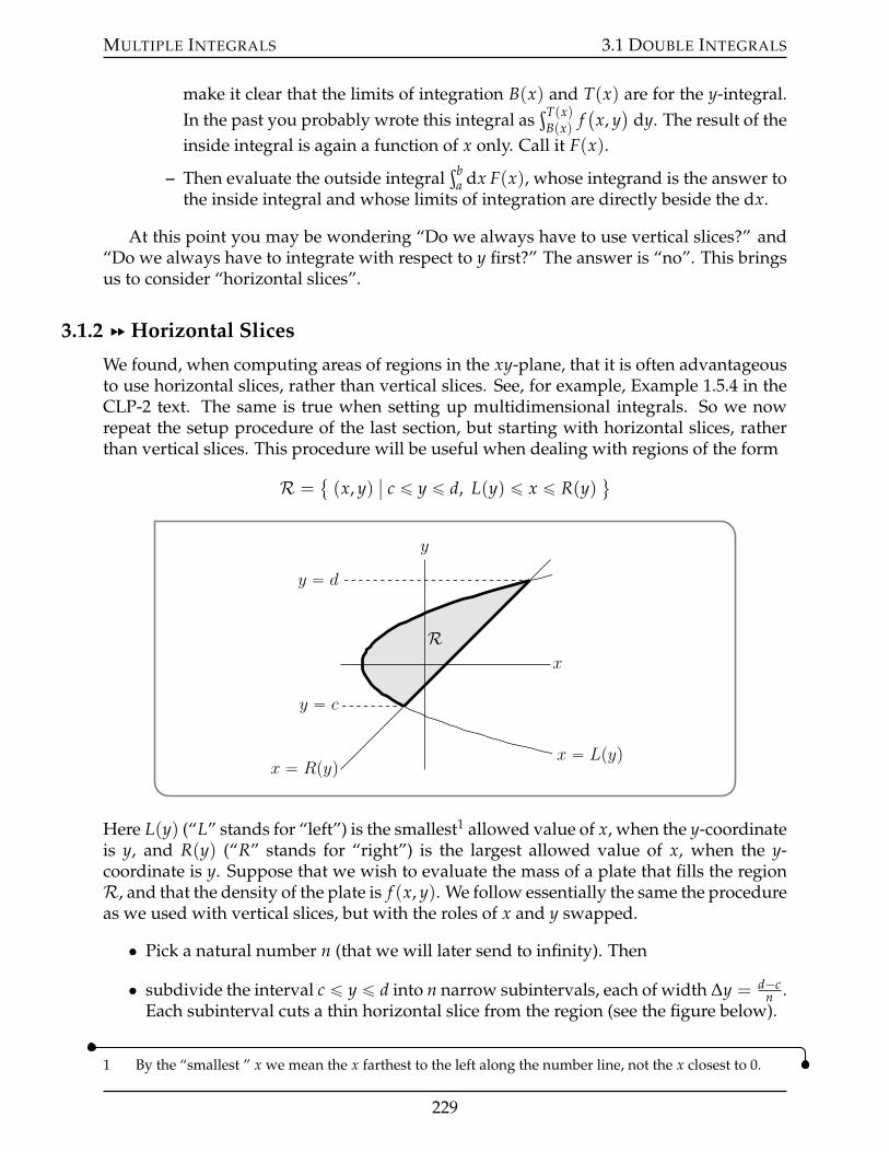
MULTIPLE INTEGRALS 3.1 DOUBLE INTEGRALS
make it clear that the limits of integration B(x) and T(x) are for the y-integral.In the past you probably wrote this integral as
şT(x)B(x) f
(x, y)
dy. The result of theinside integral is again a function of x only. Call it F(x).
– Then evaluate the outside integralşb
a dx F(x), whose integrand is the answer tothe inside integral and whose limits of integration are directly beside the dx.
At this point you may be wondering “Do we always have to use vertical slices?” and“Do we always have to integrate with respect to y first?” The answer is “no”. This bringsus to consider “horizontal slices”.
3.1.2 §§ Horizontal Slices
We found, when computing areas of regions in the xy-plane, that it is often advantageousto use horizontal slices, rather than vertical slices. See, for example, Example 1.5.4 in theCLP-2 text. The same is true when setting up multidimensional integrals. So we nowrepeat the setup procedure of the last section, but starting with horizontal slices, ratherthan vertical slices. This procedure will be useful when dealing with regions of the form
R = (x, y)
ˇc ď y ď d, L(y) ď x ď R(y)
(
x
y
x “ Lpyqx “ Rpyq
y “ d
y “ c
R
Here L(y) (“L” stands for “left”) is the smallest1 allowed value of x, when the y-coordinateis y, and R(y) (“R” stands for “right”) is the largest allowed value of x, when the y-coordinate is y. Suppose that we wish to evaluate the mass of a plate that fills the regionR, and that the density of the plate is f (x, y). We follow essentially the same the procedureas we used with vertical slices, but with the roles of x and y swapped.
• Pick a natural number n (that we will later send to infinity). Then
• subdivide the interval c ď y ď d into n narrow subintervals, each of width ∆y = d´cn .
Each subinterval cuts a thin horizontal slice from the region (see the figure below).
1 By the “smallest ” x we mean the x farthest to the left along the number line, not the x closest to 0.
229
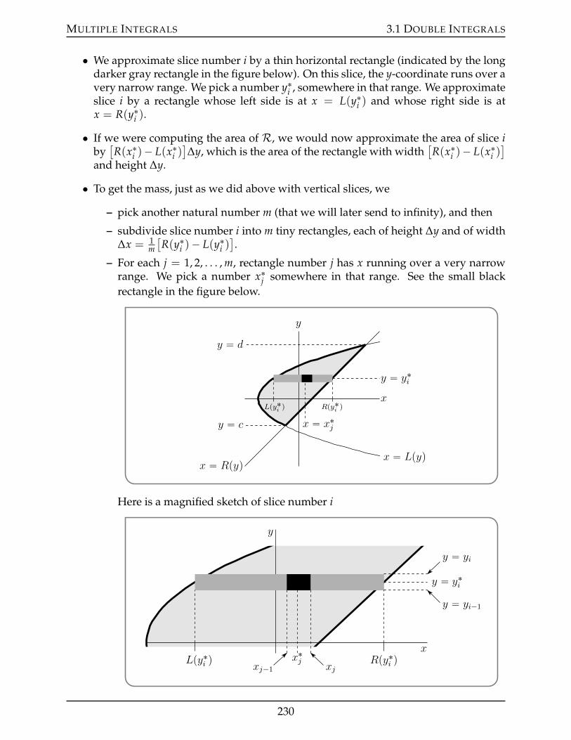
MULTIPLE INTEGRALS 3.1 DOUBLE INTEGRALS
• We approximate slice number i by a thin horizontal rectangle (indicated by the longdarker gray rectangle in the figure below). On this slice, the y-coordinate runs over avery narrow range. We pick a number y˚i , somewhere in that range. We approximateslice i by a rectangle whose left side is at x = L(y˚i ) and whose right side is atx = R(y˚i ).
• If we were computing the area of R, we would now approximate the area of slice iby[R(x˚i )´ L(x˚i )
]∆y, which is the area of the rectangle with width
[R(x˚i )´ L(x˚i )
]
and height ∆y.
• To get the mass, just as we did above with vertical slices, we
– pick another natural number m (that we will later send to infinity), and then
– subdivide slice number i into m tiny rectangles, each of height ∆y and of width∆x = 1
m[R(y˚i )´ L(y˚i )
].
– For each j = 1, 2, . . . , m, rectangle number j has x running over a very narrowrange. We pick a number x˚j somewhere in that range. See the small blackrectangle in the figure below.
x
y
x “ Lpyqx “ Rpyq
x “ xj
y “ yi
y “ d
y “ c
Lpy˚i q Rpy˚
i q
Here is a magnified sketch of slice number i
x
y
xjxj´1 xj
y “ yi
y “ yi´1
y “ yi
Lpyi q Rpyi q
230
MULTIPLE INTEGRALS 3.1 DOUBLE INTEGRALS
– On rectangle number j in slice number i, we approximate the density by f(x˚j , y˚i
),
giving us that the mass of rectangle number j in slice number i is approximatelyf(x˚j , y˚i
)∆x ∆y.
– So the Riemann sum approximation of the mass of (horizontal) slice number iis
Mass of slice i «mÿ
j=1
f(x˚j , y˚i
)∆x ∆y
– By taking the limit as m Ñ 8 (i.e. taking the limit as the width of the rectanglesgoes to zero), we convert the Riemann sum into a definite integral:
Mass of slice i « ∆yż R(y˚i )
L(y˚i )f(x, y˚i
)dx = F(y˚i )∆y
where
F(y) =ż R(y)
L(y)f(x, y)
dx
Observe that, as x has been integrated out, F(y) is a function of y only, not of xand y.
• Finally taking the limit as n Ñ 8 (i.e. taking the limit as the slice width goes to zero),we get
Mass = limnÑ8
nÿ
i=1
∆yż R(y˚i )
L(y˚i )f(x, y˚i
)dx = lim
nÑ8
nÿ
i=1
F(y˚i )∆y
Nownř
i=1F(y˚i )∆y is a Riemann sum approximation to the integral
şdc F(y)dy. So
Mass =
ż d
cF(y)dy =
ż d
c
[ż R(y)
L(y)f(x, y)
dx
]dy
The standard notations of Notation 3.1.1 also apply to this integral.
ij
R
f(x, y)
dx dy =
ż d
c
[ż R(y)
L(y)f(x, y)
dx
]dy
=
ż d
c
ż R(y)
L(y)f(x, y)
dx dy =
ż d
cdy
ż R(y)
L(y)dx f
(x, y)
Notation 3.1.2.
Note that
231
MULTIPLE INTEGRALS 3.1 DOUBLE INTEGRALS
• to evaluate the integralż d
c
ż R(y)
L(y)f(x, y)
dx dy,
– first evaluate the inside integralşR(y)
L(y) f(x, y)
dx using the inside limits of inte-gration. The result of the inside integral is a function of y only. Call it F(y).
– Then evaluate the outside integralşd
c F(y)dy, whose integrand is the answer tothe inside integral.
• To evaluate the integralż d
cdy
ż R(y)
L(y)dx f
(x, y),
– first evaluate the inside integralşR(y)
L(y) dx f(x, y)
using the limits of integration
that are directly beside the dx. Again, the dx is written directly besideşR(y)
L(y) tomake it clear that the limits of integration L(y) and R(y) are for the x-integral.In the past you probably wrote this integral as
şR(y)L(y) f
(x, y)
dx. The result of theinside integral is again a function of y only. Call it F(y).
– Then evaluate the outside integralşd
c dy F(y), whose integrand is the answer tothe inside integral and whose limits of integration are directly beside the dy.
By way of summary, we now have two integral representations for the mass of regionsin the xy-plane.
Let R be a region in the xy-plane and let the function f (x, y) be defined andcontinuous onR.
(a) If
R = (x, y)
ˇa ď x ď b, B(x) ď y ď T(x)
(
with B(x) and T(x) being continuous, and if the mass density inR is f (x, y),then the mass ofR isż b
a
[ż T(x)
B(x)f(x, y)
dy
]dx =
ż b
a
ż T(x)
B(x)f(x, y)
dy dx =
ż b
adx
ż T(x)
B(x)dy f
(x, y)
(b) IfR =
(x, y)
ˇc ď y ď d, L(y) ď x ď R(y)
(
with L(y) and R(y) being continuous, and if the mass density inR is f (x, y),then the mass ofR isż d
c
[ż R(y)
L(y)f(x, y)
dx
]dy =
ż d
c
ż R(y)
L(y)f(x, y)
dx dy =
ż d
cdy
ż R(y)
L(y)dx f
(x, y)
Theorem 3.1.3.
232
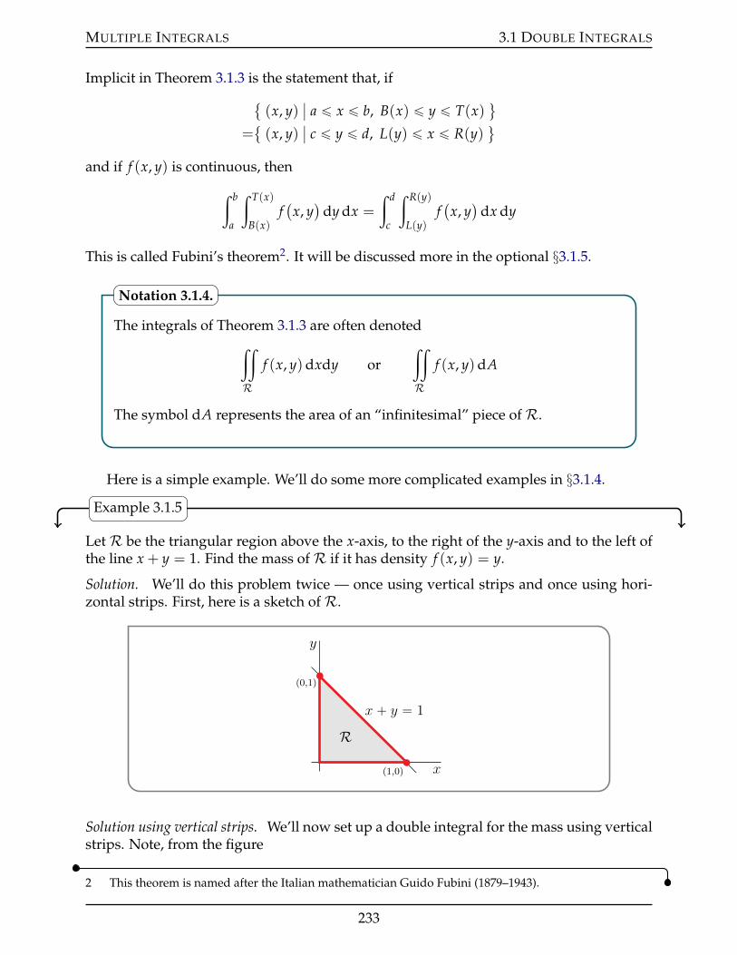
MULTIPLE INTEGRALS 3.1 DOUBLE INTEGRALS
Implicit in Theorem 3.1.3 is the statement that, if (x, y)
ˇa ď x ď b, B(x) ď y ď T(x)
(
= (x, y)
ˇc ď y ď d, L(y) ď x ď R(y)
(
and if f (x, y) is continuous, then
ż b
a
ż T(x)
B(x)f(x, y)
dy dx =
ż d
c
ż R(y)
L(y)f(x, y)
dx dy
This is called Fubini’s theorem2. It will be discussed more in the optional §3.1.5.
The integrals of Theorem 3.1.3 are often denotedij
R
f (x, y)dxdy orij
R
f (x, y)dA
The symbol dA represents the area of an “infinitesimal” piece ofR.
Notation 3.1.4.
Here is a simple example. We’ll do some more complicated examples in §3.1.4.
Example 3.1.5
Let R be the triangular region above the x-axis, to the right of the y-axis and to the left ofthe line x + y = 1. Find the mass ofR if it has density f (x, y) = y.
Solution. We’ll do this problem twice — once using vertical strips and once using hori-zontal strips. First, here is a sketch ofR.
x
y
x ` y “ 1
R
p1,0q
p0,1q
Solution using vertical strips. We’ll now set up a double integral for the mass using verticalstrips. Note, from the figure
2 This theorem is named after the Italian mathematician Guido Fubini (1879–1943).
233
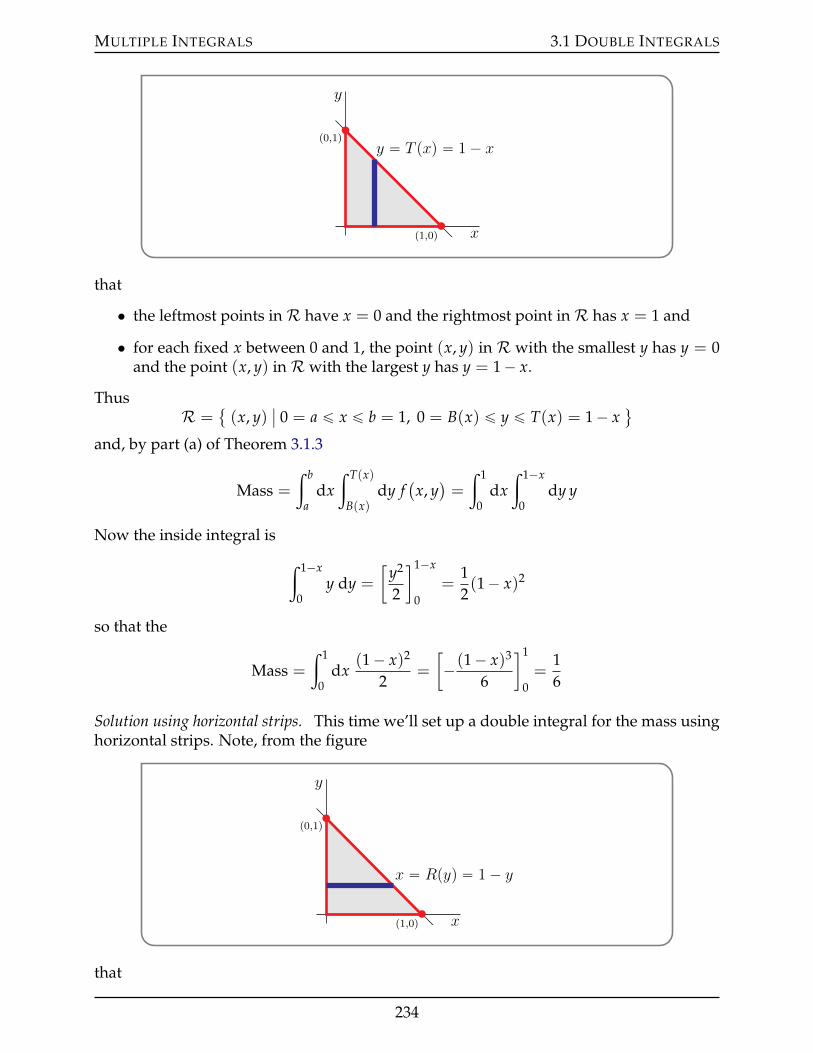
MULTIPLE INTEGRALS 3.1 DOUBLE INTEGRALS
x
y
y “ T pxq “ 1 ´ x
p1,0q
p0,1q
that
• the leftmost points inR have x = 0 and the rightmost point inR has x = 1 and
• for each fixed x between 0 and 1, the point (x, y) in R with the smallest y has y = 0and the point (x, y) inR with the largest y has y = 1´ x.
ThusR =
(x, y)
ˇ0 = a ď x ď b = 1, 0 = B(x) ď y ď T(x) = 1´ x
(
and, by part (a) of Theorem 3.1.3
Mass =
ż b
adx
ż T(x)
B(x)dy f
(x, y)=
ż 1
0dx
ż 1´x
0dy y
Now the inside integral is
ż 1´x
0y dy =
[y2
2
]1´x
0=
12(1´ x)2
so that the
Mass =
ż 1
0dx
(1´ x)2
2=
[´(1´ x)3
6
]1
0=
16
Solution using horizontal strips. This time we’ll set up a double integral for the mass usinghorizontal strips. Note, from the figure
x
y
x “ Rpyq “ 1 ´ y
p1,0q
p0,1q
that
234
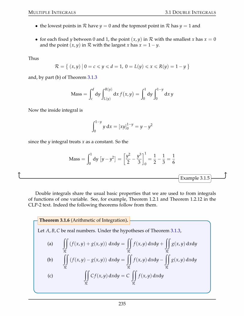
MULTIPLE INTEGRALS 3.1 DOUBLE INTEGRALS
• the lowest points inR have y = 0 and the topmost point inR has y = 1 and
• for each fixed y between 0 and 1, the point (x, y) in R with the smallest x has x = 0and the point (x, y) inR with the largest x has x = 1´ y.
Thus
R = (x, y)
ˇ0 = c ď y ď d = 1, 0 = L(y) ď x ď R(y) = 1´ y
(
and, by part (b) of Theorem 3.1.3
Mass =
ż d
cdy
ż R(y)
L(y)dx f
(x, y)=
ż 1
0dy
ż 1´y
0dx y
Now the inside integral is
ż 1´y
0y dx = [xy]1´y
0 = y´ y2
since the y integral treats x as a constant. So the
Mass =
ż 1
0dy[y´ y2] =
[y2
2´ y3
3
]1
0=
12´ 1
3=
16
Example 3.1.5
Double integrals share the usual basic properties that we are used to from integralsof functions of one variable. See, for example, Theorem 1.2.1 and Theorem 1.2.12 in theCLP-2 text. Indeed the following theorems follow from them.
Let A, B, C be real numbers. Under the hypotheses of Theorem 3.1.3,
(a)ij
R
( f (x, y) + g(x, y)) dxdy =
ij
R
f (x, y)dxdy +
ij
R
g(x, y)dxdy
(b)ij
R
( f (x, y)´ g(x, y)) dxdy =
ij
R
f (x, y)dxdy´ij
R
g(x, y)dxdy
(c)ij
R
C f (x, y)dxdy = Cij
R
f (x, y)dxdy
Theorem 3.1.6 (Arithmetic of Integration).
235
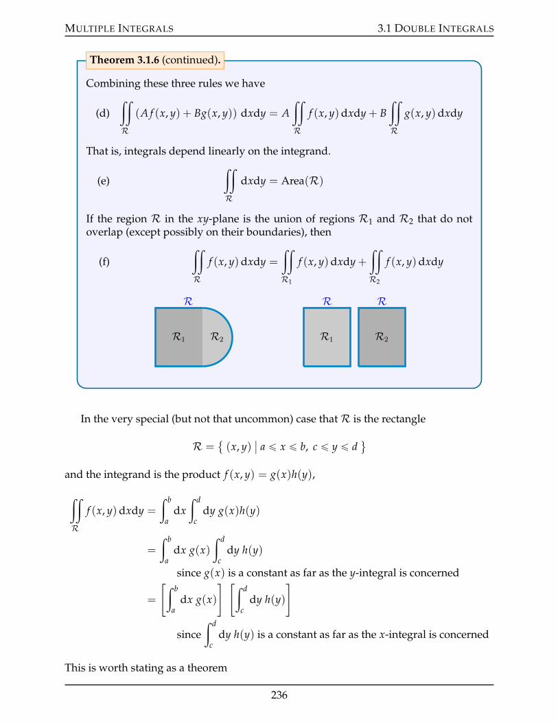
MULTIPLE INTEGRALS 3.1 DOUBLE INTEGRALS
Combining these three rules we have
(d)ij
R
(A f (x, y) + Bg(x, y)) dxdy = Aij
R
f (x, y)dxdy + Bij
R
g(x, y)dxdy
That is, integrals depend linearly on the integrand.
(e)ij
R
dxdy = Area(R)
If the region R in the xy-plane is the union of regions R1 and R2 that do notoverlap (except possibly on their boundaries), then
(f)ij
R
f (x, y)dxdy =
ij
R1
f (x, y)dxdy +
ij
R2
f (x, y)dxdy
R1 R2
R
R1 R2
R R
Theorem 3.1.6 (continued).
In the very special (but not that uncommon) case thatR is the rectangle
R = (x, y)
ˇa ď x ď b, c ď y ď d
(
and the integrand is the product f (x, y) = g(x)h(y),
ij
R
f (x, y)dxdy =
ż b
adx
ż d
cdy g(x)h(y)
=
ż b
adx g(x)
ż d
cdy h(y)
since g(x) is a constant as far as the y-integral is concerned
=
[ż b
adx g(x)
] [ż d
cdy h(y)
]
sinceż d
cdy h(y) is a constant as far as the x-integral is concerned
This is worth stating as a theorem
236
MULTIPLE INTEGRALS 3.1 DOUBLE INTEGRALS
If the domain of integration
R = (x, y)
ˇa ď x ď b, c ď y ď d
(
is a rectangle and the integrand is the product f (x, y) = g(x)h(y), then
ij
R
f (x, y)dxdy =
[ż b
adx g(x)
] [ż d
cdy h(y)
]
Theorem 3.1.7.
Just as was the case for single variable integrals, sometimes we don’t actually need toknow the value of a double integral exactly. We are instead interested in bounds on itsvalue. The following theorem provides some simple tools for generating such bounds.They are the multivariable analogs of the single variable tools in Theorem 1.2.12 of theCLP-2 text.
Under the hypotheses of Theorem 3.1.3,
(a) If f (x, y) ě 0 for all (x, y) inR, thenij
R
f (x, y)dxdy ě 0
(b) If there are constants m and M such that m ď f (x, y) ď M for all (x, y) in R,then
m Area(R) ďij
R
f (x, y)dxdy ď M Area(R)
(c) If f (x, y) ď g(x, y) for all (x, y) inR, thenij
R
f (x, y)dxdy ďij
R
g(x, y)dxdy
(d) We haveˇˇˇij
R
f (x, y)dxdy
ˇˇˇ ď
ij
R
| f (x, y)|dxdy
Theorem 3.1.8 (Inequalities for Integrals).
237
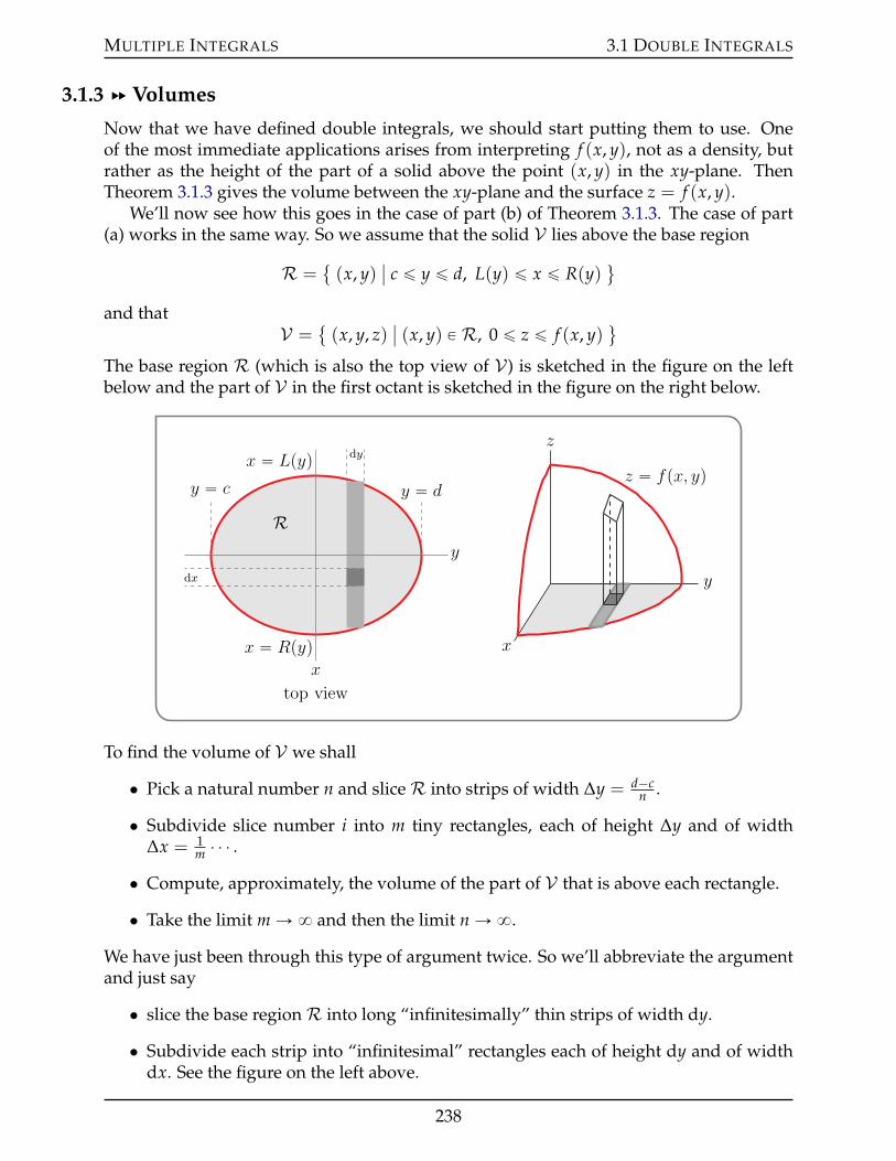
MULTIPLE INTEGRALS 3.1 DOUBLE INTEGRALS
3.1.3 §§ Volumes
Now that we have defined double integrals, we should start putting them to use. Oneof the most immediate applications arises from interpreting f (x, y), not as a density, butrather as the height of the part of a solid above the point (x, y) in the xy-plane. ThenTheorem 3.1.3 gives the volume between the xy-plane and the surface z = f (x, y).
We’ll now see how this goes in the case of part (b) of Theorem 3.1.3. The case of part(a) works in the same way. So we assume that the solid V lies above the base region
R = (x, y)
ˇc ď y ď d, L(y) ď x ď R(y)
(
and thatV =
(x, y, z)
ˇ(x, y) P R, 0 ď z ď f (x, y)
(
The base region R (which is also the top view of V) is sketched in the figure on the leftbelow and the part of V in the first octant is sketched in the figure on the right below.
y
x
top view
x “ Lpyq
x “ Rpyq
dx
dy
y “ dy “ c
R
z
y
x
z “ fpx, yq
To find the volume of V we shall
• Pick a natural number n and sliceR into strips of width ∆y = d´cn .
• Subdivide slice number i into m tiny rectangles, each of height ∆y and of width∆x = 1
m ¨ ¨ ¨ .• Compute, approximately, the volume of the part of V that is above each rectangle.
• Take the limit m Ñ 8 and then the limit n Ñ 8.
We have just been through this type of argument twice. So we’ll abbreviate the argumentand just say
• slice the base regionR into long “infinitesimally” thin strips of width dy.
• Subdivide each strip into “infinitesimal” rectangles each of height dy and of widthdx. See the figure on the left above.
238
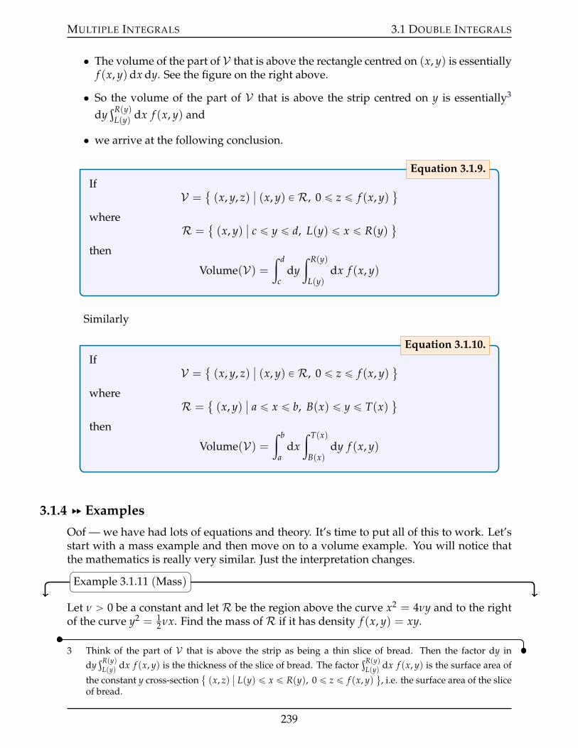
MULTIPLE INTEGRALS 3.1 DOUBLE INTEGRALS
• The volume of the part of V that is above the rectangle centred on (x, y) is essentiallyf (x, y)dx dy. See the figure on the right above.
• So the volume of the part of V that is above the strip centred on y is essentially3
dyşR(y)
L(y) dx f (x, y) and
• we arrive at the following conclusion.
IfV =
(x, y, z)
ˇ(x, y) P R, 0 ď z ď f (x, y)
(
whereR =
(x, y)
ˇc ď y ď d, L(y) ď x ď R(y)
(
then
Volume(V) =ż d
cdy
ż R(y)
L(y)dx f (x, y)
Equation 3.1.9.
Similarly
IfV =
(x, y, z)
ˇ(x, y) P R, 0 ď z ď f (x, y)
(
whereR =
(x, y)
ˇa ď x ď b, B(x) ď y ď T(x)
(
then
Volume(V) =ż b
adx
ż T(x)
B(x)dy f (x, y)
Equation 3.1.10.
3.1.4 §§ Examples
Oof — we have had lots of equations and theory. It’s time to put all of this to work. Let’sstart with a mass example and then move on to a volume example. You will notice thatthe mathematics is really very similar. Just the interpretation changes.
Example 3.1.11 (Mass)
Let ν ą 0 be a constant and let R be the region above the curve x2 = 4νy and to the rightof the curve y2 = 1
2 νx. Find the mass ofR if it has density f (x, y) = xy.
3 Think of the part of V that is above the strip as being a thin slice of bread. Then the factor dy indy
şR(y)L(y) dx f (x, y) is the thickness of the slice of bread. The factor
şR(y)L(y) dx f (x, y) is the surface area of
the constant y cross-section (x, z)
ˇL(y) ď x ď R(y), 0 ď z ď f (x, y)
(, i.e. the surface area of the slice
of bread.
239
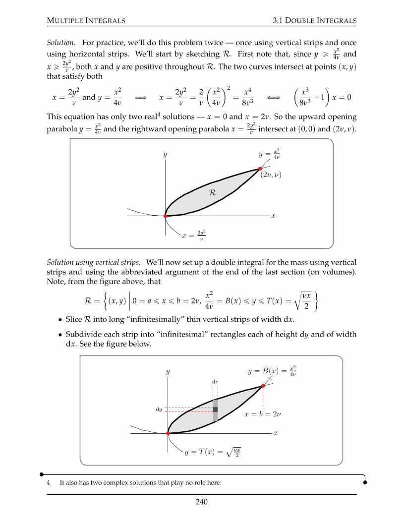
MULTIPLE INTEGRALS 3.1 DOUBLE INTEGRALS
Solution. For practice, we’ll do this problem twice — once using vertical strips and onceusing horizontal strips. We’ll start by sketching R. First note that, since y ě x2
4ν and
x ě 2y2
ν , both x and y are positive throughout R. The two curves intersect at points (x, y)that satisfy both
x =2y2
νand y =
x2
4νùñ x =
2y2
ν=
2ν
(x2
4ν
)2
=x4
8ν3 ðñ(
x3
8ν3 ´ 1)
x = 0
This equation has only two real4 solutions — x = 0 and x = 2ν. So the upward opening
parabola y = x2
4ν and the rightward opening parabola x = 2y2
ν intersect at (0, 0) and (2ν, ν).
x
y y “ x2
4ν
x “ 2y2
ν
p2ν, νq
R
Solution using vertical strips. We’ll now set up a double integral for the mass using verticalstrips and using the abbreviated argument of the end of the last section (on volumes).Note, from the figure above, that
R =
"(x, y)
ˇˇ 0 = a ď x ď b = 2ν,
x2
4ν= B(x) ď y ď T(x) =
cνx2
*
• SliceR into long “infinitesimally” thin vertical strips of width dx.
• Subdivide each strip into “infinitesimal” rectangles each of height dy and of widthdx. See the figure below.
dx
dy
x
y y “ Bpxq “ x2
4ν
y “ T pxq “ aνx2
x “ b “ 2ν
4 It also has two complex solutions that play no role here.
240
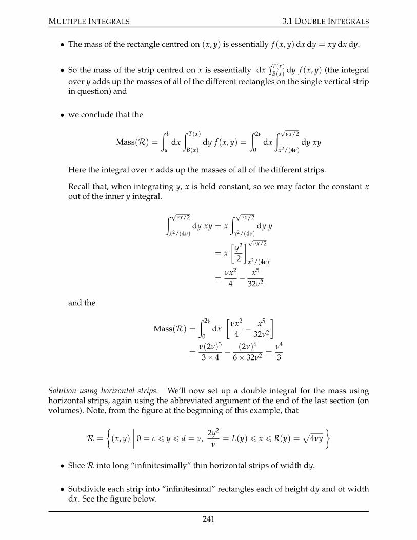
MULTIPLE INTEGRALS 3.1 DOUBLE INTEGRALS
• The mass of the rectangle centred on (x, y) is essentially f (x, y)dx dy = xy dx dy.
• So the mass of the strip centred on x is essentially dxşT(x)
B(x) dy f (x, y) (the integralover y adds up the masses of all of the different rectangles on the single vertical stripin question) and
• we conclude that the
Mass(R) =ż b
adx
ż T(x)
B(x)dy f (x, y) =
ż 2ν
0dx
ż ?νx/2
x2/(4ν)dy xy
Here the integral over x adds up the masses of all of the different strips.
Recall that, when integrating y, x is held constant, so we may factor the constant xout of the inner y integral.
ż ?νx/2
x2/(4ν)dy xy = x
ż ?νx/2
x2/(4ν)dy y
= x[
y2
2
]?νx/2
x2/(4ν)
=νx2
4´ x5
32ν2
and the
Mass(R) =ż 2ν
0dx
[νx2
4´ x5
32ν2
]
=ν(2ν)3
3ˆ 4´ (2ν)6
6ˆ 32ν2 =ν4
3
Solution using horizontal strips. We’ll now set up a double integral for the mass usinghorizontal strips, again using the abbreviated argument of the end of the last section (onvolumes). Note, from the figure at the beginning of this example, that
R =
"(x, y)
ˇˇ 0 = c ď y ď d = ν,
2y2
ν= L(y) ď x ď R(y) =
a4νy
*
• SliceR into long “infinitesimally” thin horizontal strips of width dy.
• Subdivide each strip into “infinitesimal” rectangles each of height dy and of widthdx. See the figure below.
241
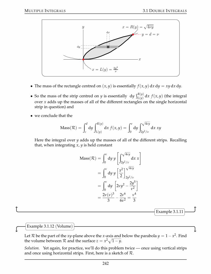
MULTIPLE INTEGRALS 3.1 DOUBLE INTEGRALS
dx
dy
x
y x “ Rpyq “ ?4νy
x “ Lpyq “ 2y2
ν
y “ d “ ν
• The mass of the rectangle centred on (x, y) is essentially f (x, y)dx dy = xy dx dy.
• So the mass of the strip centred on y is essentially dyşR(y)
L(y) dx f (x, y) (the integralover x adds up the masses of all of the different rectangles on the single horizontalstrip in question) and
• we conclude that the
Mass(R) =ż d
cdy
ż R(y)
L(y)dx f (x, y) =
ż ν
0dy
ż ?4νy
2y2/νdx xy
Here the integral over y adds up the masses of all of the different strips. Recallingthat, when integrating x, y is held constant
Mass(R) =ż ν
0dy y
[ż ?4νy
2y2/νdx x
]
=
ż ν
0dy y
[x2
2
]?4νy
2y2/ν
=
ż ν
0dy[
2νy2 ´ 2y5
ν2
]
=2ν(ν)3
3´ 2ν6
6ν2 =ν4
3
Example 3.1.11
Example 3.1.12 (Volume)
LetR be the part of the xy-plane above the x-axis and below the parabola y = 1´ x2. Findthe volume betweenR and the surface z = x2a1´ y.
Solution. Yet again, for practice, we’ll do this problem twice — once using vertical stripsand once using horizontal strips. First, here is a sketch ofR.
242
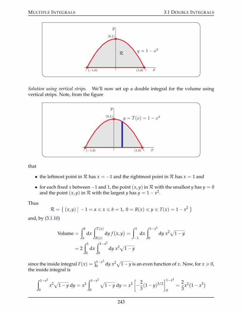
MULTIPLE INTEGRALS 3.1 DOUBLE INTEGRALS
x
y
y “ 1 ´ x2
R
p´1,0q p1,0q
p0,1q
Solution using vertical strips. We’ll now set up a double integral for the volume usingvertical strips. Note, from the figure
x
y
y “ T pxq “ 1 ´ x2
p´1,0q p1,0q
p0,1q
that
• the leftmost point inR has x = ´1 and the rightmost point inR has x = 1 and
• for each fixed x between´1 and 1, the point (x, y) inRwith the smallest y has y = 0and the point (x, y) inR with the largest y has y = 1´ x2.
ThusR =
(x, y)
ˇ ´ 1 = a ď x ď b = 1, 0 = B(x) ď y ď T(x) = 1´ x2 (
and, by (3.1.10)
Volume =
ż b
adx
ż T(x)
B(x)dy f
(x, y)=
ż 1
´1dx
ż 1´x2
0dy x2a1´ y
= 2ż 1
0dx
ż 1´x2
0dy x2a1´ y
since the inside integral F(x) =ş1´x2
0 dy x2a1´ y is an even function of x. Now, for x ě 0,the inside integral is
ż 1´x2
0x2a1´ y dy = x2
ż 1´x2
0
a1´ y dy = x2
[´2
3(1´ y)3/2
]1´x2
0=
23
x2(1´ x3)
243
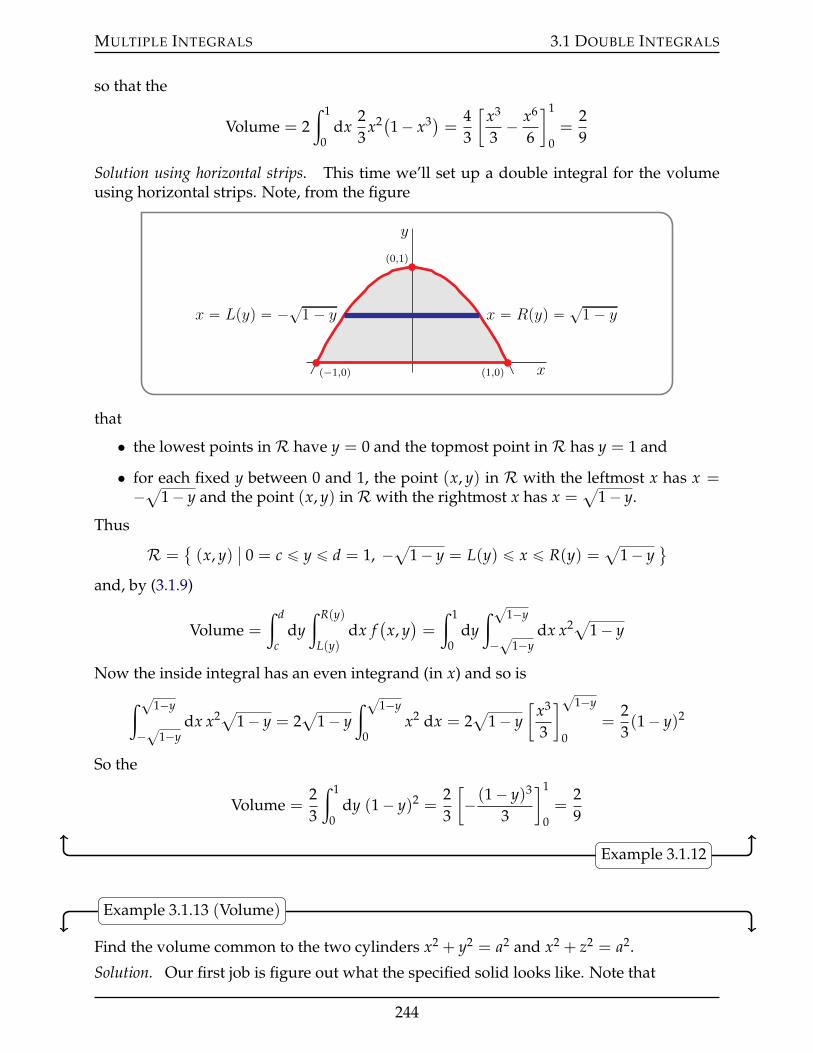
MULTIPLE INTEGRALS 3.1 DOUBLE INTEGRALS
so that the
Volume = 2ż 1
0dx
23
x2(1´ x3) = 43
[x3
3´ x6
6
]1
0=
29
Solution using horizontal strips. This time we’ll set up a double integral for the volumeusing horizontal strips. Note, from the figure
x
y
x “ Lpyq “ ´?1 ´ y x “ Rpyq “ ?
1 ´ y
p´1,0q p1,0q
p0,1q
that
• the lowest points inR have y = 0 and the topmost point inR has y = 1 and
• for each fixed y between 0 and 1, the point (x, y) in R with the leftmost x has x =´a1´ y and the point (x, y) inR with the rightmost x has x =
a1´ y.
Thus
R = (x, y)
ˇ0 = c ď y ď d = 1, ´a1´ y = L(y) ď x ď R(y) =
a1´ y
(
and, by (3.1.9)
Volume =
ż d
cdy
ż R(y)
L(y)dx f
(x, y)=
ż 1
0dy
ż ?1´y
´?
1´ydx x2a1´ y
Now the inside integral has an even integrand (in x) and so is
ż ?1´y
´?
1´ydx x2a1´ y = 2
a1´ y
ż ?1´y
0x2 dx = 2
a1´ y
[x3
3
]?1´y
0=
23(1´ y)2
So the
Volume =23
ż 1
0dy (1´ y)2 =
23
[´(1´ y)3
3
]1
0=
29
Example 3.1.12
Example 3.1.13 (Volume)
Find the volume common to the two cylinders x2 + y2 = a2 and x2 + z2 = a2.
Solution. Our first job is figure out what the specified solid looks like. Note that
244
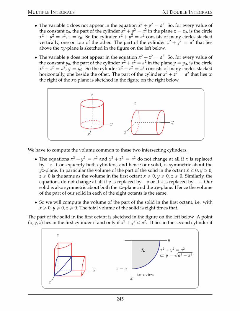
MULTIPLE INTEGRALS 3.1 DOUBLE INTEGRALS
• The variable z does not appear in the equation x2 + y2 = a2. So, for every value ofthe constant z0, the part of the cylinder x2 + y2 = a2 in the plane z = z0, is the circlex2 + y2 = a2, z = z0. So the cylinder x2 + y2 = a2 consists of many circles stackedvertically, one on top of the other. The part of the cylinder x2 + y2 = a2 that liesabove the xy-plane is sketched in the figure on the left below.
• The variable y does not appear in the equation x2 + z2 = a2. So, for every value ofthe constant y0, the part of the cylinder x2 + z2 = a2 in the plane y = y0, is the circlex2 + z2 = a2, y = y0. So the cylinder x2 + z2 = a2 consists of many circles stackedhorizontally, one beside the other. The part of the cylinder x2 + z2 = a2 that lies tothe right of the xz-plane is sketched in the figure on the right below.
y
z
x
y
z
x
We have to compute the volume common to these two intersecting cylinders.
• The equations x2 + y2 = a2 and x2 + z2 = a2 do not change at all if x is replacedby ´x. Consequently both cylinders, and hence our solid, is symmetric about theyz-plane. In particular the volume of the part of the solid in the octant x ď 0, y ě 0,z ě 0 is the same as the volume in the first octant x ě 0, y ě 0, z ě 0. Similarly, theequations do not change at all if y is replaced by ´y or if z is replaced by ´z. Oursolid is also symmetric about both the xz-plane and the xy-plane. Hence the volumeof the part of our solid in each of the eight octants is the same.
• So we will compute the volume of the part of the solid in the first octant, i.e. withx ě 0, y ě 0, z ě 0. The total volume of the solid is eight times that.
The part of the solid in the first octant is sketched in the figure on the left below. A point(x, y, z) lies in the first cylinder if and only if x2 + y2 ď a2. It lies in the second cylinder if
y
z
x
y
xtop view
x “ a
R x2 ` y2 “ a2
or y “ ?a2 ´ x2
245
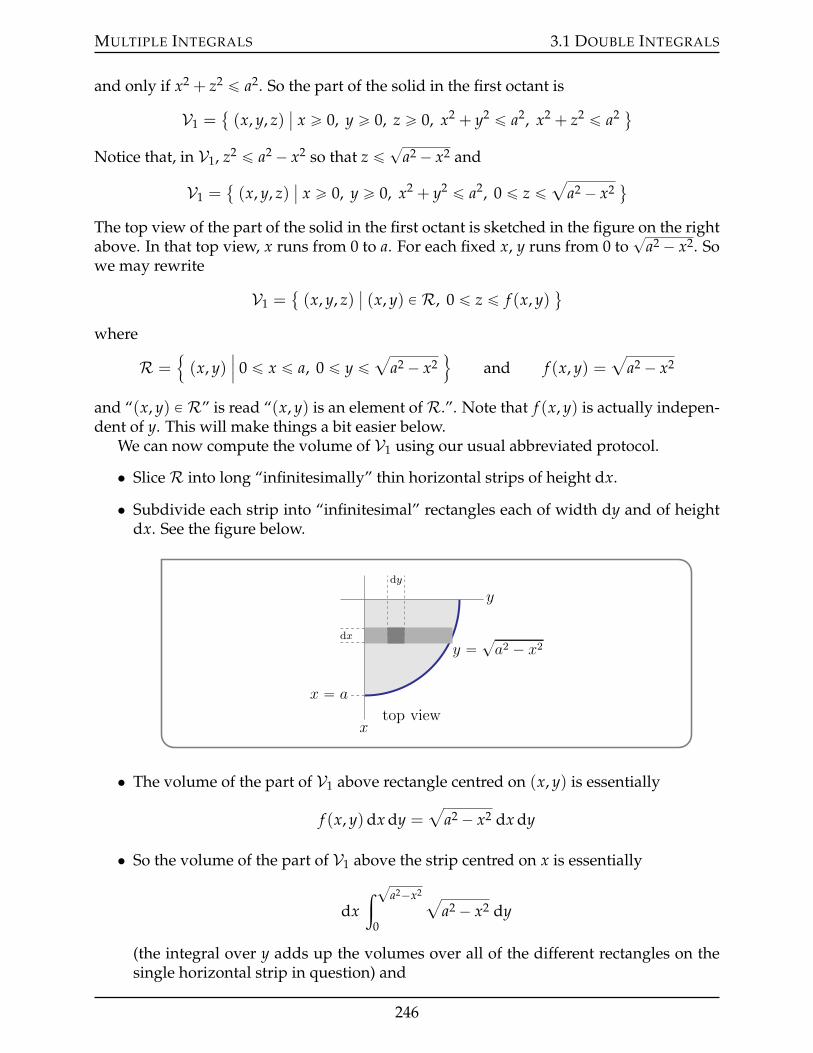
MULTIPLE INTEGRALS 3.1 DOUBLE INTEGRALS
and only if x2 + z2 ď a2. So the part of the solid in the first octant is
V1 = (x, y, z)
ˇx ě 0, y ě 0, z ě 0, x2 + y2 ď a2, x2 + z2 ď a2 (
Notice that, in V1, z2 ď a2 ´ x2 so that z ď ?a2 ´ x2 and
V1 = (x, y, z)
ˇx ě 0, y ě 0, x2 + y2 ď a2, 0 ď z ď
aa2 ´ x2
(
The top view of the part of the solid in the first octant is sketched in the figure on the rightabove. In that top view, x runs from 0 to a. For each fixed x, y runs from 0 to
?a2 ´ x2. So
we may rewrite
V1 = (x, y, z)
ˇ(x, y) P R, 0 ď z ď f (x, y)
(
where
R =!(x, y)
ˇˇ 0 ď x ď a, 0 ď y ď
aa2 ´ x2
)and f (x, y) =
aa2 ´ x2
and “(x, y) P R” is read “(x, y) is an element ofR.”. Note that f (x, y) is actually indepen-dent of y. This will make things a bit easier below.
We can now compute the volume of V1 using our usual abbreviated protocol.
• SliceR into long “infinitesimally” thin horizontal strips of height dx.
• Subdivide each strip into “infinitesimal” rectangles each of width dy and of heightdx. See the figure below.
y
xtop view
dx
dy
x “ a
y “ ?a2 ´ x2
• The volume of the part of V1 above rectangle centred on (x, y) is essentially
f (x, y)dx dy =a
a2 ´ x2 dx dy
• So the volume of the part of V1 above the strip centred on x is essentially
dxż ?a2´x2
0
aa2 ´ x2 dy
(the integral over y adds up the volumes over all of the different rectangles on thesingle horizontal strip in question) and
246
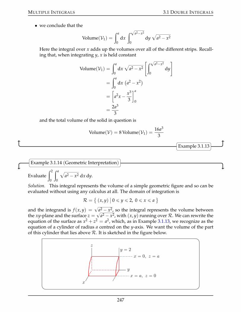
MULTIPLE INTEGRALS 3.1 DOUBLE INTEGRALS
• we conclude that the
Volume(V1) =
ż a
0dx
ż ?a2´x2
0dy
aa2 ´ x2
Here the integral over x adds up the volumes over all of the different strips. Recall-ing that, when integrating y, x is held constant
Volume(V1) =
ż a
0dx
aa2 ´ x2
[ż ?a2´x2
0dy
]
=
ż a
0dx(a2 ´ x2)
=
[a2x´ x3
3
]a
0
=2a3
3and the total volume of the solid in question is
Volume(V) = 8 Volume(V1) =16a3
3
Example 3.1.13
Example 3.1.14 (Geometric Interpretation)
Evaluateż 2
0
ż a
0
aa2 ´ x2 dx dy.
Solution. This integral represents the volume of a simple geometric figure and so can beevaluated without using any calculus at all. The domain of integration is
R = (x, y)
ˇ0 ď y ď 2, 0 ď x ď a
(
and the integrand is f (x, y) =?
a2 ´ x2, so the integral represents the volume betweenthe xy-plane and the surface z =
?a2 ´ x2, with (x, y) running overR. We can rewrite the
equation of the surface as x2 + z2 = a2, which, as in Example 3.1.13, we recognize as theequation of a cylinder of radius a centred on the y-axis. We want the volume of the partof this cylinder that lies aboveR. It is sketched in the figure below.
y
z
x
x “ 0, z “ a
x “ a, z “ 0
y “ 2
247
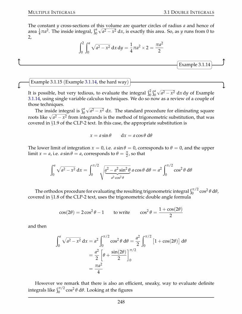
MULTIPLE INTEGRALS 3.1 DOUBLE INTEGRALS
The constant y cross-sections of this volume are quarter circles of radius a and hence ofarea 1
4 πa2. The inside integral,şa
0
?a2 ´ x2 dx, is exactly this area. So, as y runs from 0 to
2,ż 2
0
ż a
0
aa2 ´ x2 dx dy =
14
πa2 ˆ 2 =πa2
2
Example 3.1.14
Example 3.1.15 (Example 3.1.14, the hard way)
It is possible, but very tedious, to evaluate the integralş2
0şa
0
?a2 ´ x2 dx dy of Example
3.1.14, using single variable calculus techniques. We do so now as a review of a couple ofthose techniques.
The inside integral isşa
0
?a2 ´ x2 dx. The standard procedure for eliminating square
roots like?
a2 ´ x2 from integrands is the method of trigonometric substitution, that wascovered in §1.9 of the CLP-2 text. In this case, the appropriate substitution is
x = a sin θ dx = a cos θ dθ
The lower limit of integration x = 0, i.e. a sin θ = 0, corresponds to θ = 0, and the upperlimit x = a, i.e. a sin θ = a, corresponds to θ = π
2 , so that
ż a
0
aa2 ´ x2 dx =
ż π/2
0
da2 ´ a2 sin2 θloooooomoooooon
a2 cos2 θ
a cos θ dθ = a2ż π/2
0cos2 θ dθ
The orthodox procedure for evaluating the resulting trigonometric integralşπ/2
0 cos2 θ dθ,covered in §1.8 of the CLP-2 text, uses the trigonometric double angle formula
cos(2θ) = 2 cos2 θ ´ 1 to write cos2 θ =1 + cos(2θ)
2
and then
ż a
0
aa2 ´ x2 dx = a2
ż π/2
0cos2 θ dθ =
a2
2
ż π/2
0
[1 + cos(2θ)
]dθ
=a2
2
[θ +
sin(2θ)
2
]π/2
0
=πa2
4
However we remark that there is also an efficient, sneaky, way to evaluate definiteintegrals like
şπ/20 cos2 θ dθ. Looking at the figures
248
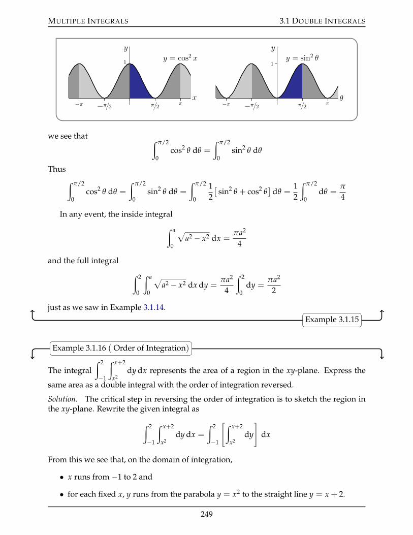
MULTIPLE INTEGRALS 3.1 DOUBLE INTEGRALS
y
x´π ´π2 ππ2
1y “ cos2 x
y
θ´π ´π2 ππ2
1y “ sin2 θ
we see that ż π/2
0cos2 θ dθ =
ż π/2
0sin2 θ dθ
Thusż π/2
0cos2 θ dθ =
ż π/2
0sin2 θ dθ =
ż π/2
0
12[
sin2 θ + cos2 θ]
dθ =12
ż π/2
0dθ =
π
4
In any event, the inside integral
ż a
0
aa2 ´ x2 dx =
πa2
4
and the full integral
ż 2
0
ż a
0
aa2 ´ x2 dx dy =
πa2
4
ż 2
0dy =
πa2
2
just as we saw in Example 3.1.14.Example 3.1.15
Example 3.1.16 ( Order of Integration)
The integralż 2
´1
ż x+2
x2dy dx represents the area of a region in the xy-plane. Express the
same area as a double integral with the order of integration reversed.
Solution. The critical step in reversing the order of integration is to sketch the region inthe xy-plane. Rewrite the given integral as
ż 2
´1
ż x+2
x2dy dx =
ż 2
´1
[ż x+2
x2dy
]dx
From this we see that, on the domain of integration,
• x runs from ´1 to 2 and
• for each fixed x, y runs from the parabola y = x2 to the straight line y = x + 2.
249
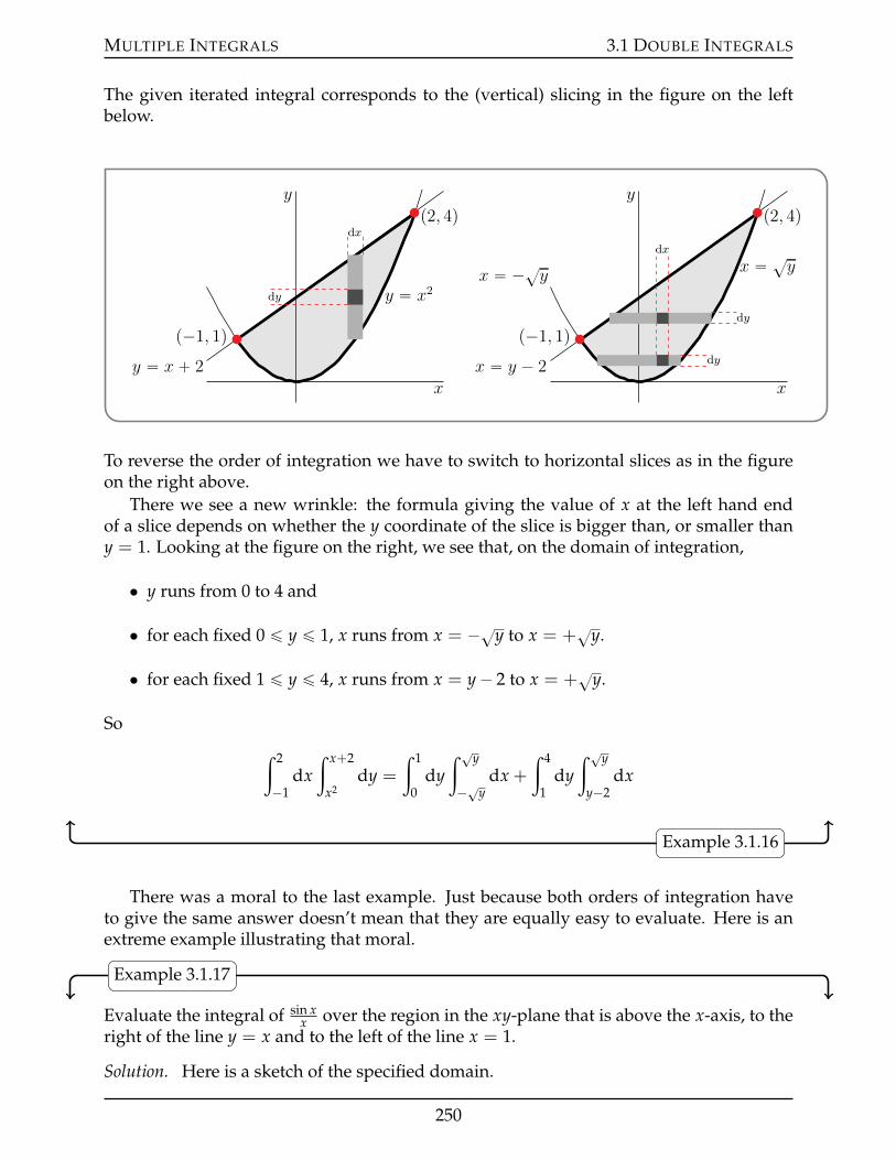
MULTIPLE INTEGRALS 3.1 DOUBLE INTEGRALS
The given iterated integral corresponds to the (vertical) slicing in the figure on the leftbelow.
p2, 4q
p´1, 1q
dx
dy
x
y
y “ x2
y “ x ` 2
p2, 4q
p´1, 1q
dx
dy
dy
x
y
x “ ?y
x “ y ´ 2
x “ ´?y
To reverse the order of integration we have to switch to horizontal slices as in the figureon the right above.
There we see a new wrinkle: the formula giving the value of x at the left hand endof a slice depends on whether the y coordinate of the slice is bigger than, or smaller thany = 1. Looking at the figure on the right, we see that, on the domain of integration,
• y runs from 0 to 4 and
• for each fixed 0 ď y ď 1, x runs from x = ´?y to x = +?y.
• for each fixed 1 ď y ď 4, x runs from x = y´ 2 to x = +?y.
So
ż 2
´1dx
ż x+2
x2dy =
ż 1
0dy
ż ?y
´?y
dx +
ż 4
1dy
ż ?y
y´2dx
Example 3.1.16
There was a moral to the last example. Just because both orders of integration haveto give the same answer doesn’t mean that they are equally easy to evaluate. Here is anextreme example illustrating that moral.
Example 3.1.17
Evaluate the integral of sin xx over the region in the xy-plane that is above the x-axis, to the
right of the line y = x and to the left of the line x = 1.
Solution. Here is a sketch of the specified domain.
250
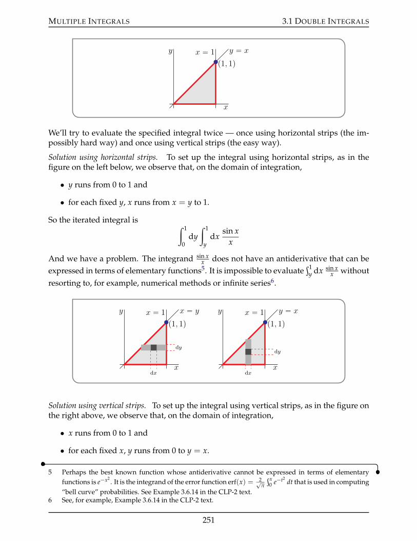
MULTIPLE INTEGRALS 3.1 DOUBLE INTEGRALS
p1, 1q
x
y y “ xx “ 1
We’ll try to evaluate the specified integral twice — once using horizontal strips (the im-possibly hard way) and once using vertical strips (the easy way).
Solution using horizontal strips. To set up the integral using horizontal strips, as in thefigure on the left below, we observe that, on the domain of integration,
• y runs from 0 to 1 and
• for each fixed y, x runs from x = y to 1.
So the iterated integral is ż 1
0dy
ż 1
ydx
sin xx
And we have a problem. The integrand sin xx does not have an antiderivative that can be
expressed in terms of elementary functions5. It is impossible to evaluateş1
y dx sin xx without
resorting to, for example, numerical methods or infinite series6.
p1, 1q
dx
dy
x
y x “ yx “ 1
p1, 1q
dx
dy
x
y y “ xx “ 1
Solution using vertical strips. To set up the integral using vertical strips, as in the figure onthe right above, we observe that, on the domain of integration,
• x runs from 0 to 1 and
• for each fixed x, y runs from 0 to y = x.
5 Perhaps the best known function whose antiderivative cannot be expressed in terms of elementaryfunctions is e´x2
. It is the integrand of the error function erf(x) = 2?π
şx0 e´t2
dt that is used in computing“bell curve” probabilities. See Example 3.6.14 in the CLP-2 text.
6 See, for example, Example 3.6.14 in the CLP-2 text.
251
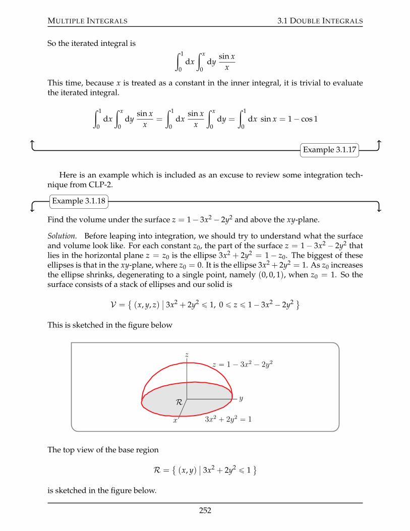
MULTIPLE INTEGRALS 3.1 DOUBLE INTEGRALS
So the iterated integral isż 1
0dx
ż x
0dy
sin xx
This time, because x is treated as a constant in the inner integral, it is trivial to evaluatethe iterated integral.
ż 1
0dx
ż x
0dy
sin xx
=
ż 1
0dx
sin xx
ż x
0dy =
ż 1
0dx sin x = 1´ cos 1
Example 3.1.17
Here is an example which is included as an excuse to review some integration tech-nique from CLP-2.
Example 3.1.18
Find the volume under the surface z = 1´ 3x2 ´ 2y2 and above the xy-plane.
Solution. Before leaping into integration, we should try to understand what the surfaceand volume look like. For each constant z0, the part of the surface z = 1´ 3x2 ´ 2y2 thatlies in the horizontal plane z = z0 is the ellipse 3x2 + 2y2 = 1´ z0. The biggest of theseellipses is that in the xy-plane, where z0 = 0. It is the ellipse 3x2 + 2y2 = 1. As z0 increasesthe ellipse shrinks, degenerating to a single point, namely (0, 0, 1), when z0 = 1. So thesurface consists of a stack of ellipses and our solid is
V = (x, y, z)
ˇ3x2 + 2y2 ď 1, 0 ď z ď 1´ 3x2 ´ 2y2 (
This is sketched in the figure below
z
y
x
z “ 1 ´ 3x2 ´ 2y2
3x2 ` 2y2 “ 1
R
The top view of the base region
R = (x, y)
ˇ3x2 + 2y2 ď 1
(
is sketched in the figure below.
252

MULTIPLE INTEGRALS 3.1 DOUBLE INTEGRALS
y
x
top view
x “ ´b
1´2y2
3
x “b
1´2y2
3
dx
dy
y “ 1?2y “ ´1?
2
R
Considering that the x-dependence in z = 1´ 3x2 ´ 2y2 is almost identical to the y-dependence in z = 1´ 3x2 ´ 2y2 (only the coefficients 2 and 3 are interchanged), usingvertical slices is likely to lead to exactly the same level of difficulty as using horizontalslices. So we’ll just pick one — say vertical slices.
The fattest part of R is on the y-axis. The intersection points of the ellipse with they-axis have x = 0 and y obeying 3(0)2 + 2y2 = 1 or y = ˘1/
?2. So inR, ´1/
?2 ď y ď 1/
?2
and, for each such y, 3x2 ď 1´ 2y2 or ´b
1´2y2
3 ď x ďb
1´2y2
3 . So using vertical strips asin the figure above
Volume(V) =ij
R
(1´ 3x2 ´ 2y2)dx dy
=
ż 1/?
2
´1/?
2
dyż b
1´2y23
´
b1´2y2
3
dx(1´ 3x2 ´ 2y2)
= 4ż 1/
?2
0dy
ż b1´2y2
3
0dx(1´ 3x2 ´ 2y2)
= 4ż 1/
?2
0dy[(1´ 2y2)x´ x3
]b
1´2y23
0
= 4ż 1/
?2
0dy
c1´ 2y2
3
[(1´ 2y2)´ 1´ 2y2
3
]
= 8ż 1/
?2
0dy[
1´ 2y2
3
]3/2
To evaluate this integral, we use the trig substitution7 2y2 = sin2 θ, or
y =sin θ?
2dy =
cos θ?2
dθ
7 See §1.9 in the CLP-2 text for a general discussion of trigonometric substitution.
253
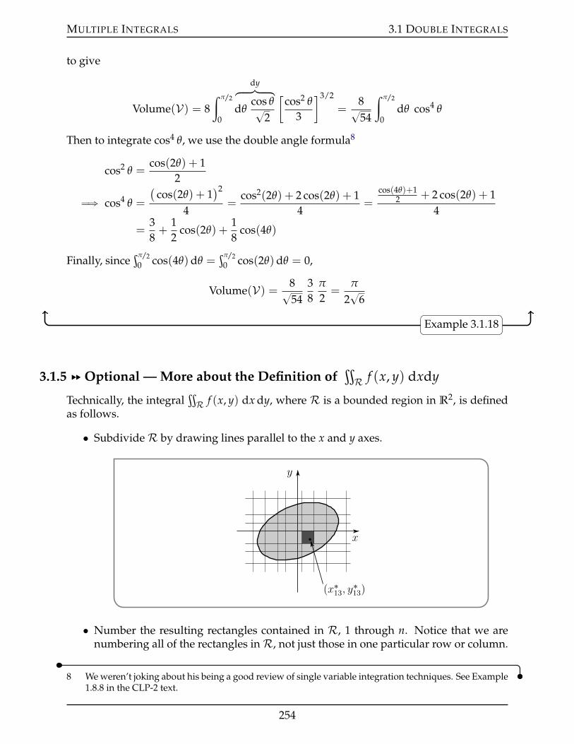
MULTIPLE INTEGRALS 3.1 DOUBLE INTEGRALS
to give
Volume(V) = 8ż π/2
0
dyhkkkikkkj
dθcos θ?
2
[cos2 θ
3
]3/2
=8?54
ż π/2
0dθ cos4 θ
Then to integrate cos4 θ, we use the double angle formula8
cos2 θ =cos(2θ) + 1
2
ùñ cos4 θ =
(cos(2θ) + 1
)2
4=
cos2(2θ) + 2 cos(2θ) + 14
=cos(4θ)+1
2 + 2 cos(2θ) + 14
=38+
12
cos(2θ) +18
cos(4θ)
Finally, sinceşπ/2
0 cos(4θ)dθ =şπ/2
0 cos(2θ)dθ = 0,
Volume(V) = 8?54
38
π
2=
π
2?
6
Example 3.1.18
3.1.5 §§ Optional — More about the Definition ofťR f (x, y) dxdy
Technically, the integralťR f (x, y) dx dy, where R is a bounded region in R2, is defined
as follows.
• SubdivideR by drawing lines parallel to the x and y axes.
x
y
px13, y13q
• Number the resulting rectangles contained in R, 1 through n. Notice that we arenumbering all of the rectangles inR, not just those in one particular row or column.
8 We weren’t joking about his being a good review of single variable integration techniques. See Example1.8.8 in the CLP-2 text.
254
MULTIPLE INTEGRALS 3.1 DOUBLE INTEGRALS
• Denote by ∆Ai the area of rectangle #i.
• Select an arbitrary point (x˚i , y˚i ) in rectangle #i.
• Form the sumnř
i=1f (x˚i , y˚i )∆Ai. Again note that the sum runs over all of the rectan-
gles inR, not just those in one particular row or column.
Now repeat this construction over and over again, using finer and finer grids. If, as thesize9 of the rectangles approaches zero, this sum approaches a unique limit (independentof the choice of parallel lines and of points (x˚i , y˚i )), then we define
ij
R
f (x, y) dx dy = limnÿ
i=1
f (x˚i , y˚i )∆Ai
If f (x, y) is continuous in a regionR described by
a ď x ď bB(x) ď y ď T(x)
for continuous functions B(x), T(x), then
ij
R
f (x, y) dx dy andż b
adx[ ż T(x)
B(x)dy f (x, y)
]
both exist and are equal. Similarly, ifR is described by
c ď y ď dL(y) ď x ď R(y)
for continuous functions L(y), R(y), then
ij
R
f (x, y) dx dy andż d
cdy[ ż R(y)
L(y)dx f (x, y)
]
both exist and are equal.
Theorem 3.1.19.
The proof of this theorem is not particularly difficult, but is still beyond the scope ofthis text. The main ideas in the proof can already be seen in section 1.1.6 of the CLP-2 text.An important consequence of this theorem is
9 For example, let pi be the perimeter of rectangle number i and require that max1ďiďn pi tends to zero.This way both the heights and widths of all rectangles also tend to zero.
255
MULTIPLE INTEGRALS 3.1 DOUBLE INTEGRALS
If f (x, y) is continuous in a regionR described by both#
a ď x ď bB(x) ď y ď T(x)
+and
#c ď y ď d
L(y) ď x ď R(y)
+
for continuous functions B(x), T(x), L(y), R(y), then both
ż b
adx[ ż T(x)
B(x)dy f (x, y)
]and
ż d
cdy[ ż R(y)
L(y)dx f (x, y)
]
exist and are equal.
Theorem 3.1.20 (Fubini).
The hypotheses of both of these theorems can be relaxed a bit, but not too much. Forexample, if
R = (x, y)
ˇ0 ď x ď 1, 0 ď y ď 1
(f (x, y) =
#1 if x, y are both rational numbers0 otherwise
then the integralťR f (x, y) dx dy does not exist. This is easy to see. If all of the x˚i ’s and
y˚i ’s are chosen to be rational numbers, then
nÿ
i=1
f (x˚i , y˚i )∆Ai =nÿ
i=1
∆Ai = Area(R)
But if we choose all the x˚i ’s and y˚i ’s to be irrational numbers, then
nÿ
i=1
f (x˚i , y˚i )∆Ai =nÿ
i=1
0 ∆Ai = 0
So the limit ofnř
i=1f (x˚i , y˚i )∆Ai, as the maximum diagonal of the rectangles approaches
zero, depends on the choice of points (x˚i , y˚i ). So the integralťR f (x, y) dx dy does not
exist.Here is an even more pathological10 example.
Example 3.1.21
In this example, we relax exactly one of the hypotheses of Fubini’s Theorem, namely thecontinuity of f , and construct an example in which both of the integrals in Fubini’s The-orem exist, but are not equal. In fact, we choose R =
(x, y)
ˇ0 ď x ď 1, 0 ď y ď 1
(
and we use a function f (x, y) that is continuous on R, except at exactly one point — theorigin.
10 For mathematicians, “pathological” is a synonym for “cool”.
256
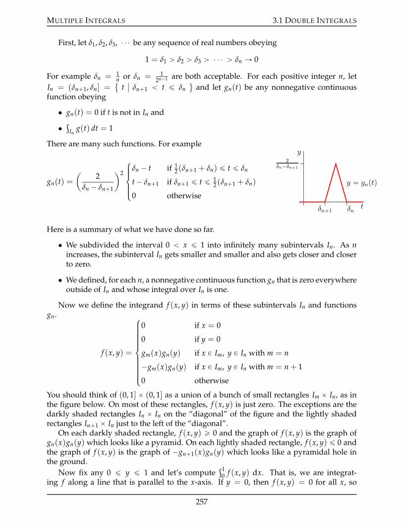
MULTIPLE INTEGRALS 3.1 DOUBLE INTEGRALS
First, let δ1, δ2, δ3, ¨ ¨ ¨ be any sequence of real numbers obeying
1 = δ1 ą δ2 ą δ3 ą ¨ ¨ ¨ ą δn Ñ 0
For example δn = 1n or δn = 1
2n´1 are both acceptable. For each positive integer n, letIn = (δn+1, δn] =
tˇ
δn+1 ă t ď δn(
and let gn(t) be any nonnegative continuousfunction obeying
• gn(t) = 0 if t is not in In and
•ş
Ing(t) dt = 1
There are many such functions. For example
gn(t) =(
2δn ´ δn+1
)2
$’’&’’%
δn ´ t if 12(δn+1 + δn) ď t ď δn
t´ δn+1 if δn+1 ď t ď 12(δn+1 + δn)
0 otherwiset
y
δn`1 δn
2δn´δn`1
y “ gnptq
Here is a summary of what we have done so far.
• We subdivided the interval 0 ă x ď 1 into infinitely many subintervals In. As nincreases, the subinterval In gets smaller and smaller and also gets closer and closerto zero.
• We defined, for each n, a nonnegative continuous function gn that is zero everywhereoutside of In and whose integral over In is one.
Now we define the integrand f (x, y) in terms of these subintervals In and functionsgn.
f (x, y) =
$’’’’’’’’&’’’’’’’’%
0 if x = 0
0 if y = 0
gm(x)gn(y) if x P Im, y P In with m = n
´gm(x)gn(y) if x P Im, y P In with m = n + 1
0 otherwise
You should think of (0, 1]ˆ (0, 1] as a union of a bunch of small rectangles Im ˆ In, as inthe figure below. On most of these rectangles, f (x, y) is just zero. The exceptions are thedarkly shaded rectangles In ˆ In on the “diagonal” of the figure and the lightly shadedrectangles In+1 ˆ In just to the left of the “diagonal”.
On each darkly shaded rectangle, f (x, y) ě 0 and the graph of f (x, y) is the graph ofgn(x)gn(y) which looks like a pyramid. On each lightly shaded rectangle, f (x, y) ď 0 andthe graph of f (x, y) is the graph of ´gn+1(x)gn(y) which looks like a pyramidal hole inthe ground.
Now fix any 0 ď y ď 1 and let’s computeş1
0 f (x, y) dx. That is, we are integrat-ing f along a line that is parallel to the x-axis. If y = 0, then f (x, y) = 0 for all x, so
257
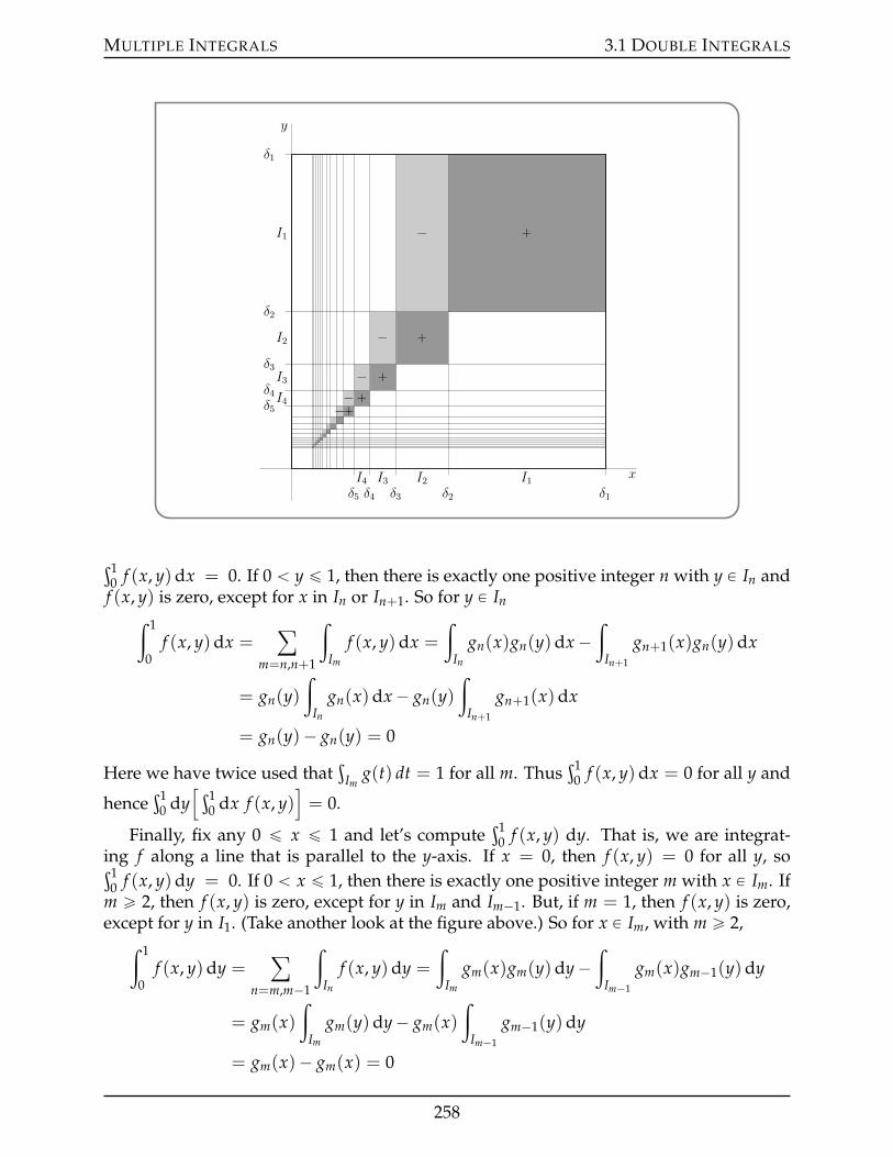
MULTIPLE INTEGRALS 3.1 DOUBLE INTEGRALS
δ1
δ1
δ2
δ2
δ3
δ3
δ4
δ4
δ5
δ5
I1
I1
I2
I2
I3
I3
I4
I4
`´
`´
`´`´
`
x
y
ş10 f (x, y)dx = 0. If 0 ă y ď 1, then there is exactly one positive integer n with y P In andf (x, y) is zero, except for x in In or In+1. So for y P In
ż 1
0f (x, y)dx =
ÿ
m=n,n+1
ż
Im
f (x, y)dx =
ż
In
gn(x)gn(y)dx´ż
In+1
gn+1(x)gn(y)dx
= gn(y)ż
In
gn(x)dx´ gn(y)ż
In+1
gn+1(x)dx
= gn(y)´ gn(y) = 0
Here we have twice used thatş
Img(t) dt = 1 for all m. Thus
ş10 f (x, y)dx = 0 for all y and
henceş1
0 dy[ ş1
0 dx f (x, y)]= 0.
Finally, fix any 0 ď x ď 1 and let’s computeş1
0 f (x, y) dy. That is, we are integrat-ing f along a line that is parallel to the y-axis. If x = 0, then f (x, y) = 0 for all y, soş1
0 f (x, y)dy = 0. If 0 ă x ď 1, then there is exactly one positive integer m with x P Im. Ifm ě 2, then f (x, y) is zero, except for y in Im and Im´1. But, if m = 1, then f (x, y) is zero,except for y in I1. (Take another look at the figure above.) So for x P Im, with m ě 2,
ż 1
0f (x, y)dy =
ÿ
n=m,m´1
ż
In
f (x, y)dy =
ż
Im
gm(x)gm(y)dy´ż
Im´1
gm(x)gm´1(y)dy
= gm(x)ż
Im
gm(y)dy´ gm(x)ż
Im´1
gm´1(y)dy
= gm(x)´ gm(x) = 0
258
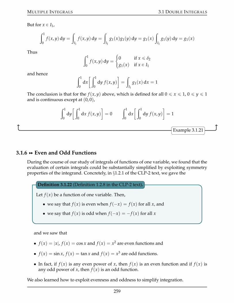
MULTIPLE INTEGRALS 3.1 DOUBLE INTEGRALS
But for x P I1,
ż 1
0f (x, y)dy =
ż
I1
f (x, y)dy =
ż
I1
g1(x)g1(y)dy = g1(x)ż
I1
g1(y)dy = g1(x)
Thus ż 1
0f (x, y)dy =
#0 if x ď δ2
g1(x) if x P I1
and hence ż 1
0dx[ ż 1
0dy f (x, y)
]=
ż
I1
g1(x)dx = 1
The conclusion is that for the f (x, y) above, which is defined for all 0 ď x ď 1, 0 ď y ď 1and is continuous except at (0, 0),
ż 1
0dy[ ż 1
0dx f (x, y)
]= 0
ż 1
0dx[ ż 1
0dy f (x, y)
]= 1
Example 3.1.21
3.1.6 §§ Even and Odd Functions
During the course of our study of integrals of functions of one variable, we found that theevaluation of certain integrals could be substantially simplified by exploiting symmetryproperties of the integrand. Concretely, in §1.2.1 of the CLP-2 text, we gave the
Let f (x) be a function of one variable. Then,
• we say that f (x) is even when f (´x) = f (x) for all x, and
• we say that f (x) is odd when f (´x) = ´ f (x) for all x
Definition 3.1.22 (Definition 1.2.8 in the CLP-2 text).
and we saw that
• f (x) = |x|, f (x) = cos x and f (x) = x2 are even functions and
• f (x) = sin x, f (x) = tan x and f (x) = x3 are odd functions.
• In fact, if f (x) is any even power of x, then f (x) is an even function and if f (x) isany odd power of x, then f (x) is an odd function.
We also learned how to exploit evenness and oddness to simplify integration.
259
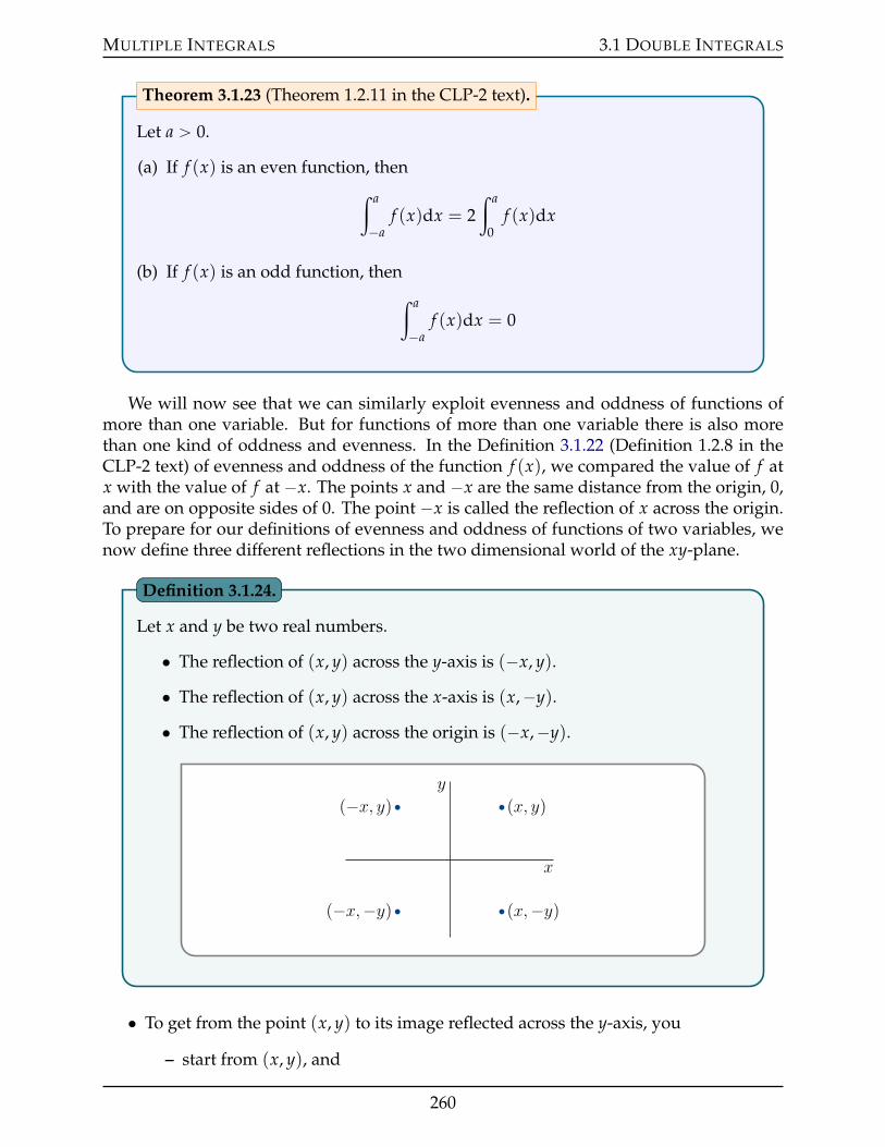
MULTIPLE INTEGRALS 3.1 DOUBLE INTEGRALS
Let a ą 0.
(a) If f (x) is an even function, thenż a
´af (x)dx = 2
ż a
0f (x)dx
(b) If f (x) is an odd function, thenż a
´af (x)dx = 0
Theorem 3.1.23 (Theorem 1.2.11 in the CLP-2 text).
We will now see that we can similarly exploit evenness and oddness of functions ofmore than one variable. But for functions of more than one variable there is also morethan one kind of oddness and evenness. In the Definition 3.1.22 (Definition 1.2.8 in theCLP-2 text) of evenness and oddness of the function f (x), we compared the value of f atx with the value of f at ´x. The points x and ´x are the same distance from the origin, 0,and are on opposite sides of 0. The point ´x is called the reflection of x across the origin.To prepare for our definitions of evenness and oddness of functions of two variables, wenow define three different reflections in the two dimensional world of the xy-plane.
Let x and y be two real numbers.
• The reflection of (x, y) across the y-axis is (´x, y).
• The reflection of (x, y) across the x-axis is (x,´y).
• The reflection of (x, y) across the origin is (´x,´y).
x
y
px, yqp´x, yq
px,´yqp´x,´yq
Definition 3.1.24.
• To get from the point (x, y) to its image reflected across the y-axis, you
– start from (x, y), and
260
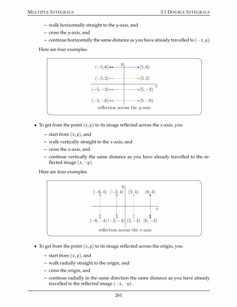
MULTIPLE INTEGRALS 3.1 DOUBLE INTEGRALS
– walk horizontally straight to the y-axis, and
– cross the y-axis, and
– continue horizontally the same distance as you have already travelled to (´x, y).
Here are four examples.
p5, 6qp´5, 6q
p5, 2qp´5, 2q
p5,´2qp´5,´2q
p5,´6qp´5,´6q
x
y
reflection across the y-axis
• To get from the point (x, y) to its image reflected across the x-axis, you
– start from (x, y), and
– walk vertically straight to the x-axis, and
– cross the x-axis, and
– continue vertically the same distance as you have already travelled to the re-flected image (x,´y).
Here are four examples.
p6, 4q
p6,´4q
p2, 4q
p2,´4q
p´2, 4q
p´2,´4q
p´6, 4q
p´6,´4q
x
y
reflection across the x-axis
• To get from the point (x, y) to its image reflected across the origin, you
– start from (x, y), and
– walk radially straight to the origin, and
– cross the origin, and
– continue radially in the same direction the same distance as you have alreadytravelled to the reflected image (´x,´y).
261
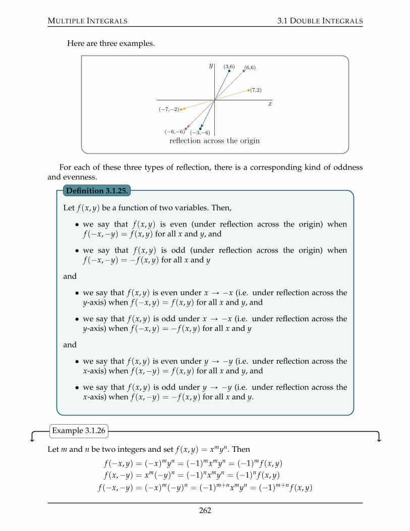
MULTIPLE INTEGRALS 3.1 DOUBLE INTEGRALS
Here are three examples.
p3,6q
p´3,´6q
p6,6q
p´6,´6q
p7,2q
p´7,´2qx
y
reflection across the origin
For each of these three types of reflection, there is a corresponding kind of oddnessand evenness.
Let f (x, y) be a function of two variables. Then,
• we say that f (x, y) is even (under reflection across the origin) whenf (´x,´y) = f (x, y) for all x and y, and
• we say that f (x, y) is odd (under reflection across the origin) whenf (´x,´y) = ´ f (x, y) for all x and y
and
• we say that f (x, y) is even under x Ñ ´x (i.e. under reflection across they-axis) when f (´x, y) = f (x, y) for all x and y, and
• we say that f (x, y) is odd under x Ñ ´x (i.e. under reflection across they-axis) when f (´x, y) = ´ f (x, y) for all x and y
and
• we say that f (x, y) is even under y Ñ ´y (i.e. under reflection across thex-axis) when f (x,´y) = f (x, y) for all x and y, and
• we say that f (x, y) is odd under y Ñ ´y (i.e. under reflection across thex-axis) when f (x,´y) = ´ f (x, y) for all x and y.
Definition 3.1.25.
Example 3.1.26
Let m and n be two integers and set f (x, y) = xmyn. Then
f (´x, y) = (´x)myn = (´1)mxmyn = (´1)m f (x, y)f (x,´y) = xm(´y)n = (´1)nxmyn = (´1)n f (x, y)
f (´x,´y) = (´x)m(´y)n = (´1)m+nxmyn = (´1)m+n f (x, y)
262
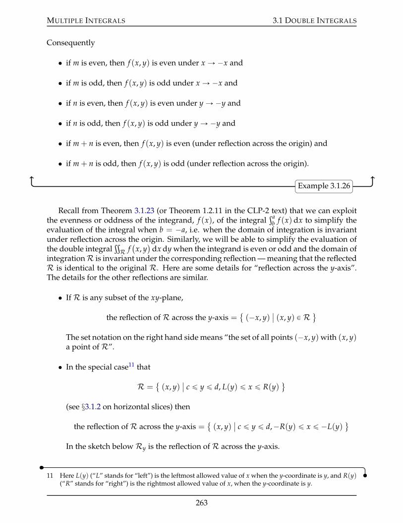
MULTIPLE INTEGRALS 3.1 DOUBLE INTEGRALS
Consequently
• if m is even, then f (x, y) is even under x Ñ ´x and
• if m is odd, then f (x, y) is odd under x Ñ ´x and
• if n is even, then f (x, y) is even under y Ñ ´y and
• if n is odd, then f (x, y) is odd under y Ñ ´y and
• if m + n is even, then f (x, y) is even (under reflection across the origin) and
• if m + n is odd, then f (x, y) is odd (under reflection across the origin).
Example 3.1.26
Recall from Theorem 3.1.23 (or Theorem 1.2.11 in the CLP-2 text) that we can exploitthe evenness or oddness of the integrand, f (x), of the integral
şab f (x)dx to simplify the
evaluation of the integral when b = ´a, i.e. when the domain of integration is invariantunder reflection across the origin. Similarly, we will be able to simplify the evaluation ofthe double integral
ťR f(x, y)
dx dy when the integrand is even or odd and the domain ofintegrationR is invariant under the corresponding reflection — meaning that the reflectedR is identical to the original R. Here are some details for “reflection across the y-axis”.The details for the other reflections are similar.
• IfR is any subset of the xy-plane,
the reflection ofR across the y-axis = (´x, y)
ˇ(x, y) P R (
The set notation on the right hand side means “the set of all points (´x, y) with (x, y)a point ofR”.
• In the special case11 that
R = (x, y)
ˇc ď y ď d, L(y) ď x ď R(y)
(
(see §3.1.2 on horizontal slices) then
the reflection ofR across the y-axis = (x, y)
ˇc ď y ď d,´R(y) ď x ď ´L(y)
(
In the sketch belowRy is the reflection ofR across the y-axis.
11 Here L(y) (“L” stands for “left”) is the leftmost allowed value of x when the y-coordinate is y, and R(y)(“R” stands for “right”) is the rightmost allowed value of x, when the y-coordinate is y.
263
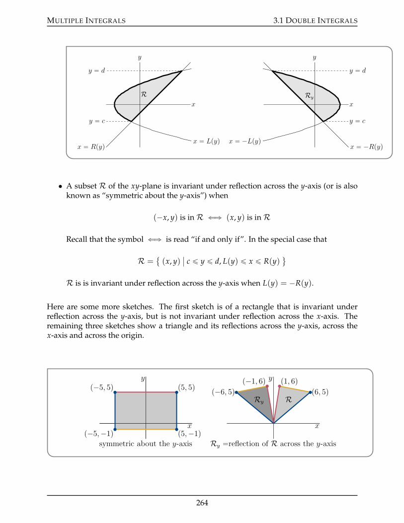
MULTIPLE INTEGRALS 3.1 DOUBLE INTEGRALS
x
y
x “ Lpyqx “ Rpyq
y “ d
y “ c
Rx
y
x “ ´Lpyqx “ ´Rpyq
y “ d
y “ c
Ry
• A subset R of the xy-plane is invariant under reflection across the y-axis (or is alsoknown as “symmetric about the y-axis”) when
(´x, y) is inR ðñ (x, y) is inR
Recall that the symbol ðñ is read “if and only if”. In the special case that
R = (x, y)
ˇc ď y ď d, L(y) ď x ď R(y)
(
R is is invariant under reflection across the y-axis when L(y) = ´R(y).
Here are some more sketches. The first sketch is of a rectangle that is invariant underreflection across the y-axis, but is not invariant under reflection across the x-axis. Theremaining three sketches show a triangle and its reflections across the y-axis, across thex-axis and across the origin.
p5, 5q
p5,´1q
p´5, 5q
p´5,´1qx
y
symmetric about the y-axis
RRy
p1, 6qp´1, 6qp6, 5qp´6, 5q
x
y
Ry “reflection of R across the y-axis
264
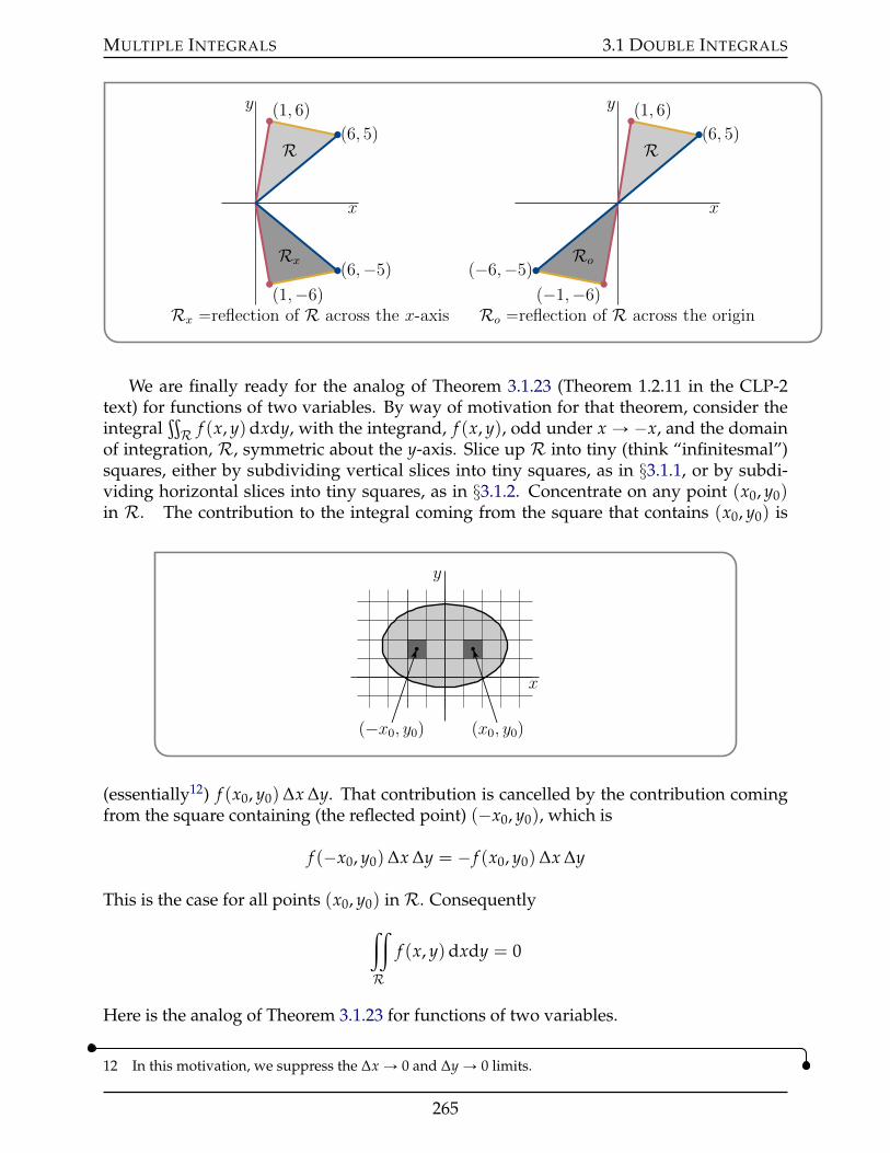
MULTIPLE INTEGRALS 3.1 DOUBLE INTEGRALS
R
Rx
p1, 6q
p1,´6q
p6, 5q
p6,´5q
x
y
Rx “reflection of R across the x-axis
R
Ro
p1, 6q
p´1,´6q
p6, 5q
p´6,´5q
x
y
Ro “reflection of R across the origin
We are finally ready for the analog of Theorem 3.1.23 (Theorem 1.2.11 in the CLP-2text) for functions of two variables. By way of motivation for that theorem, consider theintegral
ťR f (x, y)dxdy, with the integrand, f (x, y), odd under x Ñ ´x, and the domain
of integration, R, symmetric about the y-axis. Slice up R into tiny (think “infinitesmal”)squares, either by subdividing vertical slices into tiny squares, as in §3.1.1, or by subdi-viding horizontal slices into tiny squares, as in §3.1.2. Concentrate on any point (x0, y0)in R. The contribution to the integral coming from the square that contains (x0, y0) is
x
y
px0, y0qp´x0, y0q
(essentially12) f (x0, y0)∆x ∆y. That contribution is cancelled by the contribution comingfrom the square containing (the reflected point) (´x0, y0), which is
f (´x0, y0)∆x ∆y = ´ f (x0, y0)∆x ∆y
This is the case for all points (x0, y0) inR. Consequently
ij
R
f (x, y)dxdy = 0
Here is the analog of Theorem 3.1.23 for functions of two variables.
12 In this motivation, we suppress the ∆x Ñ 0 and ∆y Ñ 0 limits.
265
MULTIPLE INTEGRALS 3.1 DOUBLE INTEGRALS
(a) LetR be a subset of the xy-plane that is symmetric about the y-axis. If f (x, y)is odd under x Ñ ´x, then
ij
R
f (x, y)dxdy = 0
Denote by R+ the set of all points in R that have x ě 0. If f (x, y) is evenunder x Ñ ´x, then
ij
R
f (x, y)dxdy = 2ij
R+
f (x, y)dxdy
(b) LetR be a subset of the xy-plane that is symmetric about the x-axis. If f (x, y)is odd under y Ñ ´y, then
ij
R
f (x, y)dxdy = 0
Denote by R+ the set of all points in R that have y ě 0. If f (x, y) is evenunder y Ñ ´y, then
ij
R
f (x, y)dxdy = 2ij
R+
f (x, y)dxdy
(c) LetR be a subset of the xy-plane that is invariant under reflection across theorigin. If f (x, y) is odd (under reflection across the origin), then
ij
R
f (x, y)dxdy = 0
Denote by R+ either the set of all points in R that have x ě 0 or the set ofall points in R that have y ě 0. If f (x, y) is even (under reflection across theorigin), then
ij
R
f (x, y)dxdy = 2ij
R+
f (x, y)dxdy
Theorem 3.1.27 (2d Even and Odd).
Proof. We will give only the proof for part (a) in the special case that
R = (x, y)
ˇc ď y ď d, L(y) ď x ď R(y)
(
In part (a), we are assuming that R is symmetric about the y-axis, so that L(y) = ´R(y).
266
MULTIPLE INTEGRALS 3.1 DOUBLE INTEGRALS
So, using horizontal strips, as described in §3.1.2,
ij
R
f (x, y)dxdy =
ż d
cdy
ż R(y)
´R(y)dx f (x, y)
Fix any c ď y ď d.
• If f (x, y) is odd under x Ñ ´x, then f (´x, y) = ´ f (x, y) for all ´R(y) ď x ď R(y)and ż R(y)
´R(y)dx f (x, y) = 0
by part (b) of Theorem 3.1.23 (Theorem 1.2.11 in the CLP-2 text).
• If f (x, y) is even under x Ñ ´x, then f (´x, y) = f (x, y) for all ´R(y) ď x ď R(y)and ż R(y)
´R(y)dx f (x, y) = 2
ż R(y)
0dx f (x, y)
by part (a) of Theorem 3.1.23.
As the statements of the two bullets are true for each fixed c ď y ď d, we have that
• if f (x, y) is odd under x Ñ ´x, then
ij
R
f (x, y)dxdy =
ż d
cdy
ż R(y)
´R(y)dx f (x, y) =
ż d
cdy 0
= 0
• and if f (x, y) is even under x Ñ ´x, then
ij
R
f (x, y)dxdy =
ż d
cdy
ż R(y)
´R(y)dx f (x, y) =
ż d
cdy 2
ż R(y)
0dx f (x, y)
= 2ij
R+
f (x, y)dxdy
The proof of part (a) whenR is not of the formR = (x, y)
ˇc ď y ď d, L(y) ď x ď R(y)
(
(for example ifR has holes in it) is most easily done using the change of variables x = ´u,y = v in Theorem 3.8.3, which is part of the optional §3.8.
The proof of part (b) is similar to the proof of part (a).The proof of part (c) is most easily done using the change of variables x = ´u, y = ´v
in Theorem 3.8.3, which is part of the optional §3.8.
Example 3.1.28
Evaluate the integralťR ex sin(y + y3)dxdy over the triangular regionR in the sketch
267
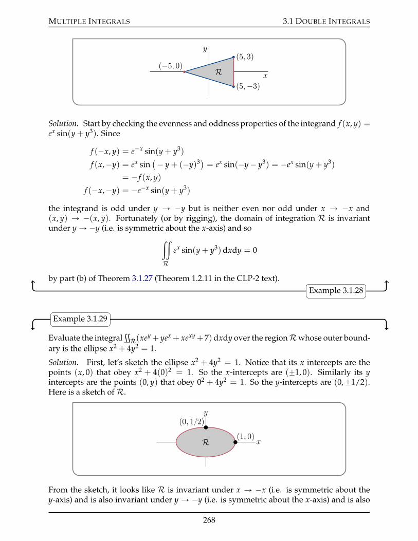
MULTIPLE INTEGRALS 3.1 DOUBLE INTEGRALS
x
y
Rp5, 3q
p5,´3q
p´5, 0q
Solution. Start by checking the evenness and oddness properties of the integrand f (x, y) =ex sin(y + y3). Since
f (´x, y) = e´x sin(y + y3)
f (x,´y) = ex sin(´ y + (´y)3) = ex sin(´y´ y3) = ´ex sin(y + y3)
= ´ f (x, y)
f (´x,´y) = ´e´x sin(y + y3)
the integrand is odd under y Ñ ´y but is neither even nor odd under x Ñ ´x and(x, y) Ñ ´(x, y). Fortunately (or by rigging), the domain of integration R is invariantunder y Ñ ´y (i.e. is symmetric about the x-axis) and so
ij
R
ex sin(y + y3)dxdy = 0
by part (b) of Theorem 3.1.27 (Theorem 1.2.11 in the CLP-2 text).Example 3.1.28
Example 3.1.29
Evaluate the integralťR(xey + yex + xexy + 7)dxdy over the regionRwhose outer bound-
ary is the ellipse x2 + 4y2 = 1.
Solution. First, let’s sketch the ellipse x2 + 4y2 = 1. Notice that its x intercepts are thepoints (x, 0) that obey x2 + 4(0)2 = 1. So the x-intercepts are (˘1, 0). Similarly its yintercepts are the points (0, y) that obey 02 + 4y2 = 1. So the y-intercepts are (0,˘1/2).Here is a sketch ofR.
x
y
R p1, 0qp0, 12q
From the sketch, it looks like R is invariant under x Ñ ´x (i.e. is symmetric about they-axis) and is also invariant under y Ñ ´y (i.e. is symmetric about the x-axis) and is also
268

MULTIPLE INTEGRALS 3.1 DOUBLE INTEGRALS
invariant under (x, y) Ñ ´(x, y). It is easy to check analytically that this is indeed thecase. The point (x, y) is in R if and only if it is inside x2 + 4y2 = 1. That is the case if andonly if x2 + 4y2 ď 1. Since
(´x)2 + 4y2 = x2 + (´4y)2 = (´x)2 + 4(´y)2 = x2 + 4y2
we have
(x, y) is inR ðñ (´x, y) is inRðñ (x,´y) is inRðñ (´x,´y) is inR
Now let’s check the evenness and oddness properties of the integrand.
f (x, y) = xey + yex + xexy + 7
f (´x, y) = ´xey + ye´x ´ xe´xy + 7
f (x,´y) = xe´y ´ yex + xe´xy + 7
f (´x,´y) = ´xe´y ´ ye´x ´ xexy + 7
So f (x, y) is neither even nor odd under any of x Ñ ´x, y Ñ ´y, and (x, y) Ñ ´(x, y).BUT, look at the four terms of f (x, y) separately.
• The first term of f (x, y), namely xey, is odd under x Ñ ´x.
• The second term of f (x, y), namely yex, is odd under y Ñ ´y.
• The third term of f (x, y), namely xexy, is odd under (x, y)Ñ ´(x, y).
• The fourth term of f (x, y), namely 7, is even under all of x Ñ ´x, y Ñ ´y, and(x, y)Ñ ´(x, y).
So, by parts (a), (b) and (c) of Theorem 3.1.27, in order,
ij
R
(xey + yex + xexy + 7)dxdy =
ij
R
xey dxdy +
ij
R
yex dxdy +
ij
R
xexy dxdy + 7ij
R
dxdy
= 0 + 0 + 0 + 7 Area(R)
Since R is an ellipse with semi-major axis a = 1 and semi-minor axis b = 12 , it has area
πab = 12 π and ij
R
(xey + yex + xexy + 7)dxdy = 72 π
Example 3.1.29
269
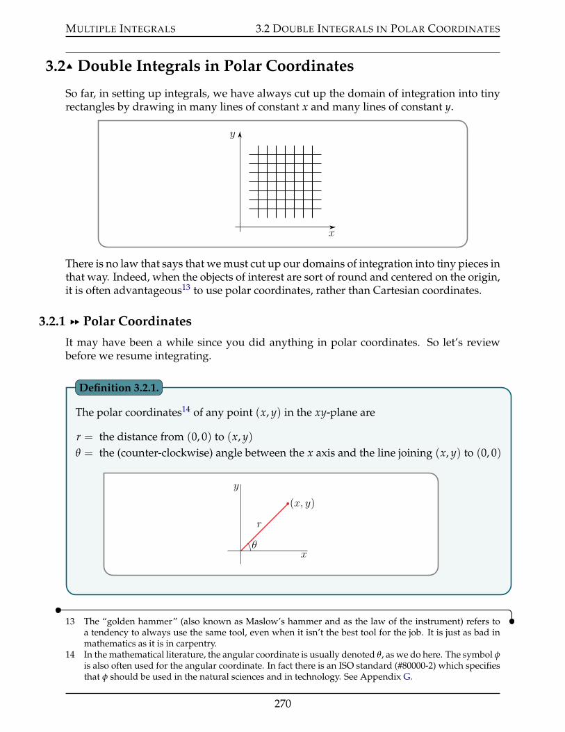
MULTIPLE INTEGRALS 3.2 DOUBLE INTEGRALS IN POLAR COORDINATES
3.2IJ Double Integrals in Polar Coordinates
So far, in setting up integrals, we have always cut up the domain of integration into tinyrectangles by drawing in many lines of constant x and many lines of constant y.
x
y
There is no law that says that we must cut up our domains of integration into tiny pieces inthat way. Indeed, when the objects of interest are sort of round and centered on the origin,it is often advantageous13 to use polar coordinates, rather than Cartesian coordinates.
3.2.1 §§ Polar Coordinates
It may have been a while since you did anything in polar coordinates. So let’s reviewbefore we resume integrating.
The polar coordinates14 of any point (x, y) in the xy-plane are
r = the distance from (0, 0) to (x, y)θ = the (counter-clockwise) angle between the x axis and the line joining (x, y) to (0, 0)
r
px, yq
x
y
θ
Definition 3.2.1.
13 The “golden hammer” (also known as Maslow’s hammer and as the law of the instrument) refers toa tendency to always use the same tool, even when it isn’t the best tool for the job. It is just as bad inmathematics as it is in carpentry.
14 In the mathematical literature, the angular coordinate is usually denoted θ, as we do here. The symbol φis also often used for the angular coordinate. In fact there is an ISO standard (#80000-2) which specifiesthat φ should be used in the natural sciences and in technology. See Appendix G.
270

MULTIPLE INTEGRALS 3.2 DOUBLE INTEGRALS IN POLAR COORDINATES
Cartesian and polar coordinates are related, via a quick bit of trigonometry, by
x = r cos θ y = r sin θ
r =b
x2 + y2 θ = arctanyx
Equation 3.2.2.
The following two figures show a number of lines of constant θ, on the left, and curvesof constant r, on the right.
x
y
lines of constant θ
x
y
curves of constant r
Note that the polar angle θ is only defined up to integer multiples of 2π. For example,the point (1, 0) on the x-axis could have θ = 0, but could also have θ = 2π or θ = 4π. It issometimes convenient to assign θ negative values. When θ ă 0, the counter-clockwise15
angle θ refers to the clockwise angle |θ|. For example, the point (0,´1) on the negativey-axis can have θ = ´π
2 and can also have θ = 3π2 .
x
y
r “ 1, θ “ ´π2, θ “ 3π2
3π2π2
It is also sometimes convenient to extend the above definitions by saying that x =r cos θ and y = r sin θ even when r is negative. For example, the following figure shows(x, y) for r = 1, θ = π/4 and for r = ´1, θ = π/4. Both points lie on the line through
15 or anti-clockwise or widdershins. Yes, widdershins is a real word, though the Oxford English Dic-tionary lists its frequency of usage as between 0.01 and 0.1 times per million words. Of course both“counter-clockwise” and “anti-clockwise” assume that your clock is not a sundial in the southern hemi-sphere.
271
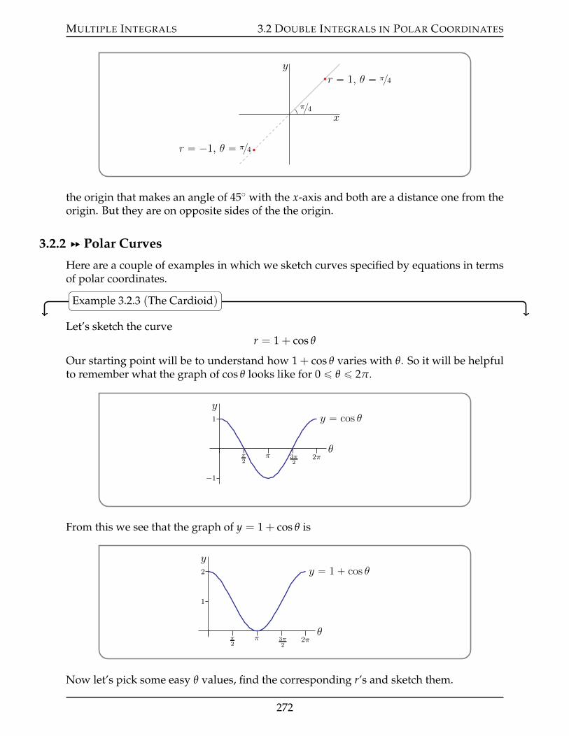
MULTIPLE INTEGRALS 3.2 DOUBLE INTEGRALS IN POLAR COORDINATES
r “ 1, θ “ π4
r “ ´1, θ “ π4
x
y
π4
the origin that makes an angle of 45˝ with the x-axis and both are a distance one from theorigin. But they are on opposite sides of the the origin.
3.2.2 §§ Polar Curves
Here are a couple of examples in which we sketch curves specified by equations in termsof polar coordinates.
Example 3.2.3 (The Cardioid)
Let’s sketch the curver = 1 + cos θ
Our starting point will be to understand how 1 + cos θ varies with θ. So it will be helpfulto remember what the graph of cos θ looks like for 0 ď θ ď 2π.
y
θπ2
3π2
π 2π
1
´1
y “ cos θ
From this we see that the graph of y = 1 + cos θ is
y
θπ2
3π2
π 2π
1
2 y “ 1 ` cos θ
Now let’s pick some easy θ values, find the corresponding r’s and sketch them.
272
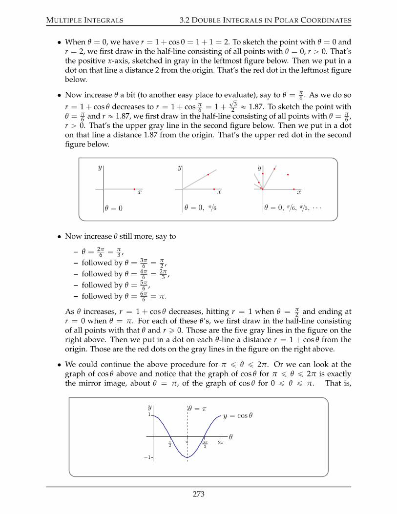
MULTIPLE INTEGRALS 3.2 DOUBLE INTEGRALS IN POLAR COORDINATES
• When θ = 0, we have r = 1 + cos 0 = 1 + 1 = 2. To sketch the point with θ = 0 andr = 2, we first draw in the half-line consisting of all points with θ = 0, r ą 0. That’sthe positive x-axis, sketched in gray in the leftmost figure below. Then we put in adot on that line a distance 2 from the origin. That’s the red dot in the leftmost figurebelow.
• Now increase θ a bit (to another easy place to evaluate), say to θ = π6 . As we do so
r = 1 + cos θ decreases to r = 1 + cos π6 = 1 +
?3
2 « 1.87. To sketch the point withθ = π
6 and r « 1.87, we first draw in the half-line consisting of all points with θ = π6 ,
r ą 0. That’s the upper gray line in the second figure below. Then we put in a doton that line a distance 1.87 from the origin. That’s the upper red dot in the secondfigure below.
x
y
θ “ 0
x
y
θ “ 0, π6x
y
θ “ 0, π6, π3, ¨ ¨ ¨
• Now increase θ still more, say to
– θ = 2π6 = π
3 ,– followed by θ = 3π
6 = π2 ,
– followed by θ = 4π6 = 2π
3 ,– followed by θ = 5π
6 ,– followed by θ = 6π
6 = π.
As θ increases, r = 1 + cos θ decreases, hitting r = 1 when θ = π2 and ending at
r = 0 when θ = π. For each of these θ’s, we first draw in the half-line consistingof all points with that θ and r ě 0. Those are the five gray lines in the figure on theright above. Then we put in a dot on each θ-line a distance r = 1 + cos θ from theorigin. Those are the red dots on the gray lines in the figure on the right above.
• We could continue the above procedure for π ď θ ď 2π. Or we can look at thegraph of cos θ above and notice that the graph of cos θ for π ď θ ď 2π is exactlythe mirror image, about θ = π, of the graph of cos θ for 0 ď θ ď π. That is,
y
θπ2
3π2
π 2π
1
´1
θ “ πy “ cos θ
273
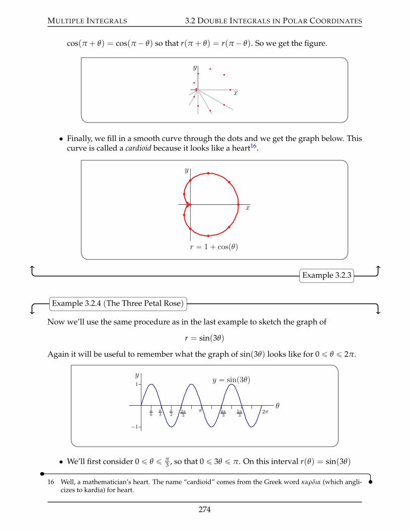
MULTIPLE INTEGRALS 3.2 DOUBLE INTEGRALS IN POLAR COORDINATES
cos(π + θ) = cos(π ´ θ) so that r(π + θ) = r(π ´ θ). So we get the figure.
x
y
• Finally, we fill in a smooth curve through the dots and we get the graph below. Thiscurve is called a cardioid because it looks like a heart16.
x
y
r “ 1 ` cospθq
Example 3.2.3
Example 3.2.4 (The Three Petal Rose)
Now we’ll use the same procedure as in the last example to sketch the graph of
r = sin(3θ)
Again it will be useful to remember what the graph of sin(3θ) looks like for 0 ď θ ď 2π.
y
θπ6
π3
π2
2π3
π 4π3
5π3
2π
1
´1
y “ sinp3θq
• We’ll first consider 0 ď θ ď π3 , so that 0 ď 3θ ď π. On this interval r(θ) = sin(3θ)
16 Well, a mathematician’s heart. The name “cardioid” comes from the Greek word καρδια (which angli-cizes to kardia) for heart.
274
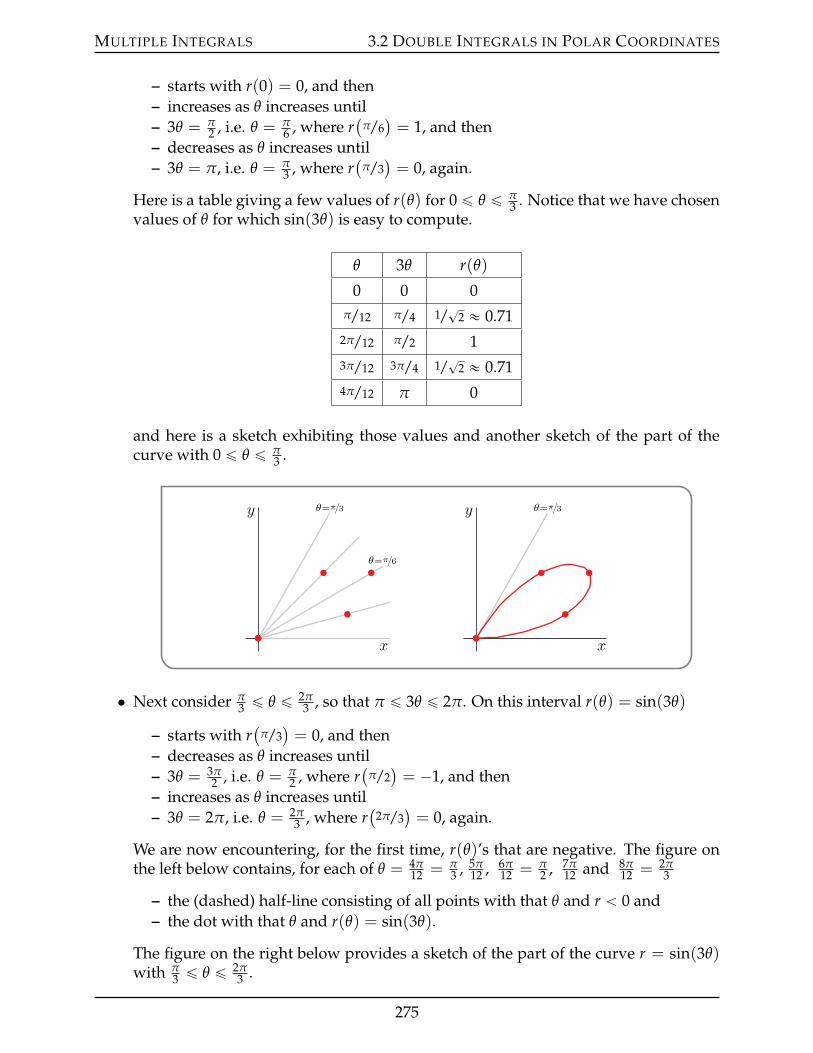
MULTIPLE INTEGRALS 3.2 DOUBLE INTEGRALS IN POLAR COORDINATES
– starts with r(0) = 0, and then– increases as θ increases until– 3θ = π
2 , i.e. θ = π6 , where r
(π/6)= 1, and then
– decreases as θ increases until– 3θ = π, i.e. θ = π
3 , where r(
π/3)= 0, again.
Here is a table giving a few values of r(θ) for 0 ď θ ď π3 . Notice that we have chosen
values of θ for which sin(3θ) is easy to compute.
θ 3θ r(θ)
0 0 0π/12 π/4 1/
?2 « 0.71
2π/12 π/2 13π/12 3π/4 1/
?2 « 0.71
4π/12 π 0
and here is a sketch exhibiting those values and another sketch of the part of thecurve with 0 ď θ ď π
3 .
x
y θ“π3
θ“π6
x
y θ“π3
• Next consider π3 ď θ ď 2π
3 , so that π ď 3θ ď 2π. On this interval r(θ) = sin(3θ)
– starts with r(
π/3)= 0, and then
– decreases as θ increases until– 3θ = 3π
2 , i.e. θ = π2 , where r
(π/2)= ´1, and then
– increases as θ increases until– 3θ = 2π, i.e. θ = 2π
3 , where r(
2π/3)= 0, again.
We are now encountering, for the first time, r(θ)’s that are negative. The figure onthe left below contains, for each of θ = 4π
12 = π3 , 5π
12 , 6π12 = π
2 , 7π12 and 8π
12 = 2π3
– the (dashed) half-line consisting of all points with that θ and r ă 0 and– the dot with that θ and r(θ) = sin(3θ).
The figure on the right below provides a sketch of the part of the curve r = sin(3θ)with π
3 ď θ ď 2π3 .
275
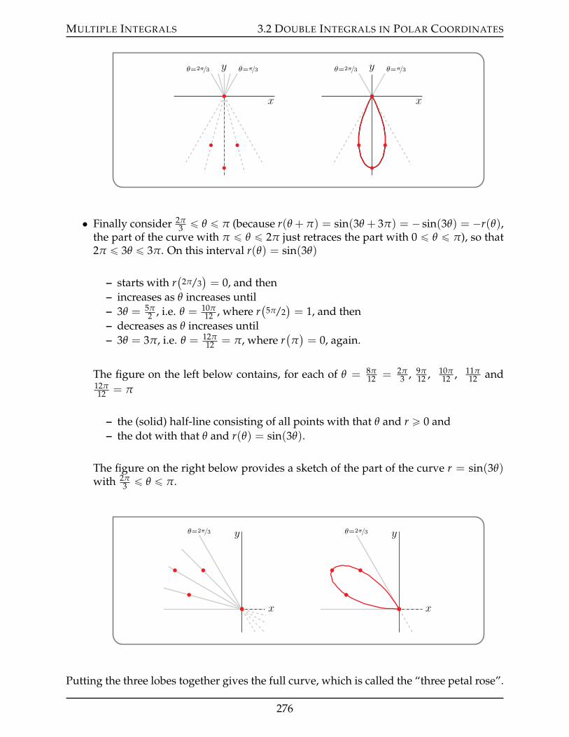
MULTIPLE INTEGRALS 3.2 DOUBLE INTEGRALS IN POLAR COORDINATES
x
y θ“π3θ“2π3
x
y θ“π3θ“2π3
• Finally consider 2π3 ď θ ď π (because r(θ + π) = sin(3θ + 3π) = ´ sin(3θ) = ´r(θ),
the part of the curve with π ď θ ď 2π just retraces the part with 0 ď θ ď π), so that2π ď 3θ ď 3π. On this interval r(θ) = sin(3θ)
– starts with r(
2π/3)= 0, and then
– increases as θ increases until– 3θ = 5π
2 , i.e. θ = 10π12 , where r
(5π/2
)= 1, and then
– decreases as θ increases until– 3θ = 3π, i.e. θ = 12π
12 = π, where r(π)= 0, again.
The figure on the left below contains, for each of θ = 8π12 = 2π
3 , 9π12 , 10π
12 , 11π12 and
12π12 = π
– the (solid) half-line consisting of all points with that θ and r ě 0 and– the dot with that θ and r(θ) = sin(3θ).
The figure on the right below provides a sketch of the part of the curve r = sin(3θ)with 2π
3 ď θ ď π.
x
yθ“2π3
x
yθ“2π3
Putting the three lobes together gives the full curve, which is called the “three petal rose”.
276
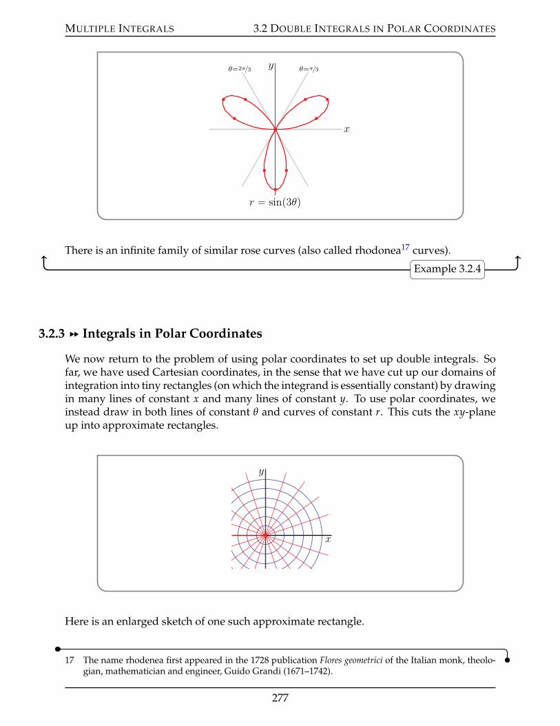
MULTIPLE INTEGRALS 3.2 DOUBLE INTEGRALS IN POLAR COORDINATES
x
y
r “ sinp3θq
θ“2π3 θ“π3
There is an infinite family of similar rose curves (also called rhodonea17 curves).
Example 3.2.4
3.2.3 §§ Integrals in Polar Coordinates
We now return to the problem of using polar coordinates to set up double integrals. Sofar, we have used Cartesian coordinates, in the sense that we have cut up our domains ofintegration into tiny rectangles (on which the integrand is essentially constant) by drawingin many lines of constant x and many lines of constant y. To use polar coordinates, weinstead draw in both lines of constant θ and curves of constant r. This cuts the xy-planeup into approximate rectangles.
x
y
Here is an enlarged sketch of one such approximate rectangle.
17 The name rhodenea first appeared in the 1728 publication Flores geometrici of the Italian monk, theolo-gian, mathematician and engineer, Guido Grandi (1671–1742).
277
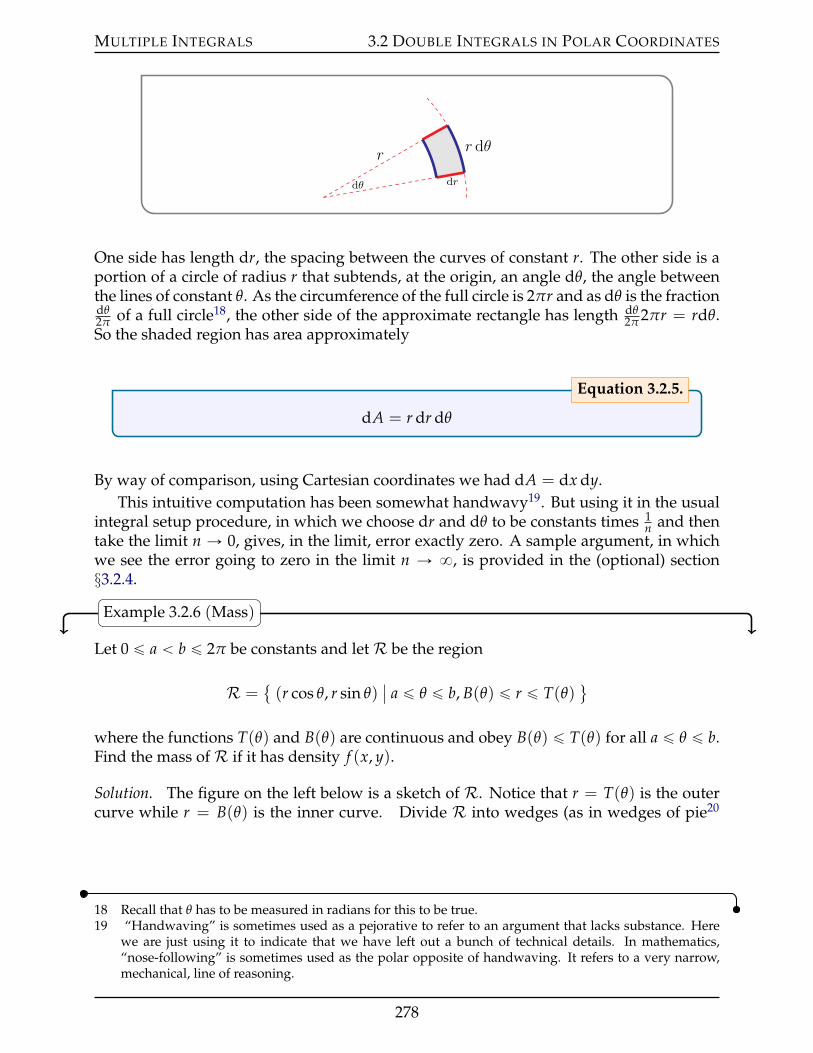
MULTIPLE INTEGRALS 3.2 DOUBLE INTEGRALS IN POLAR COORDINATES
dθ dr
rr dθ
One side has length dr, the spacing between the curves of constant r. The other side is aportion of a circle of radius r that subtends, at the origin, an angle dθ, the angle betweenthe lines of constant θ. As the circumference of the full circle is 2πr and as dθ is the fractiondθ2π of a full circle18, the other side of the approximate rectangle has length dθ
2π 2πr = rdθ.So the shaded region has area approximately
dA = r dr dθ
Equation 3.2.5.
By way of comparison, using Cartesian coordinates we had dA = dx dy.This intuitive computation has been somewhat handwavy19. But using it in the usual
integral setup procedure, in which we choose dr and dθ to be constants times 1n and then
take the limit n Ñ 0, gives, in the limit, error exactly zero. A sample argument, in whichwe see the error going to zero in the limit n Ñ 8, is provided in the (optional) section§3.2.4.
Example 3.2.6 (Mass)
Let 0 ď a ă b ď 2π be constants and letR be the region
R = (r cos θ, r sin θ)
ˇa ď θ ď b, B(θ) ď r ď T(θ)
(
where the functions T(θ) and B(θ) are continuous and obey B(θ) ď T(θ) for all a ď θ ď b.Find the mass ofR if it has density f (x, y).
Solution. The figure on the left below is a sketch of R. Notice that r = T(θ) is the outercurve while r = B(θ) is the inner curve. Divide R into wedges (as in wedges of pie20
18 Recall that θ has to be measured in radians for this to be true.19 “Handwaving” is sometimes used as a pejorative to refer to an argument that lacks substance. Here
we are just using it to indicate that we have left out a bunch of technical details. In mathematics,“nose-following” is sometimes used as the polar opposite of handwaving. It refers to a very narrow,mechanical, line of reasoning.
278
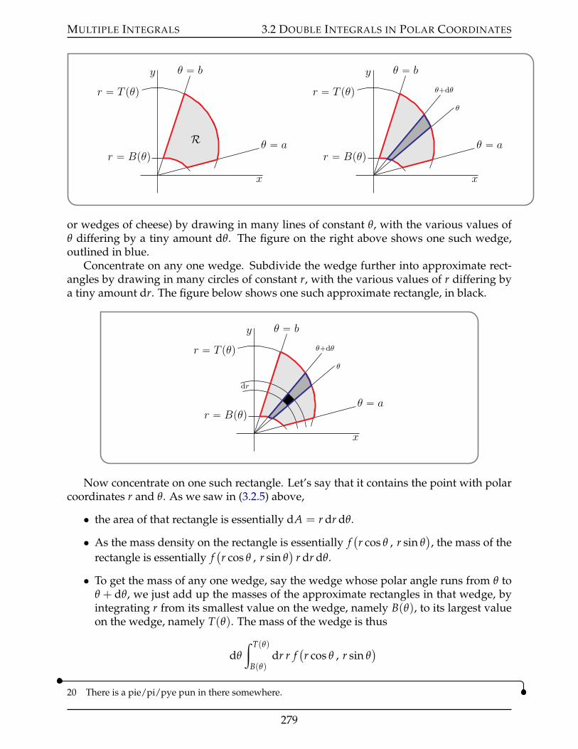
MULTIPLE INTEGRALS 3.2 DOUBLE INTEGRALS IN POLAR COORDINATES
x
y
θ “ a
θ “ b
r “ T pθq
r “ BpθqR
x
y
θ “ a
θ “ b
θ
θ`dθr “ T pθq
r “ Bpθq
or wedges of cheese) by drawing in many lines of constant θ, with the various values ofθ differing by a tiny amount dθ. The figure on the right above shows one such wedge,outlined in blue.
Concentrate on any one wedge. Subdivide the wedge further into approximate rect-angles by drawing in many circles of constant r, with the various values of r differing bya tiny amount dr. The figure below shows one such approximate rectangle, in black.
x
y
θ “ a
θ “ b
θ
θ`dθr “ T pθq
r “ Bpθq
dr
Now concentrate on one such rectangle. Let’s say that it contains the point with polarcoordinates r and θ. As we saw in (3.2.5) above,
• the area of that rectangle is essentially dA = r dr dθ.
• As the mass density on the rectangle is essentially f(r cos θ , r sin θ
), the mass of the
rectangle is essentially f(r cos θ , r sin θ
)r dr dθ.
• To get the mass of any one wedge, say the wedge whose polar angle runs from θ toθ + dθ, we just add up the masses of the approximate rectangles in that wedge, byintegrating r from its smallest value on the wedge, namely B(θ), to its largest valueon the wedge, namely T(θ). The mass of the wedge is thus
dθ
ż T(θ)
B(θ)dr r f
(r cos θ , r sin θ
)
20 There is a pie/pi/pye pun in there somewhere.
279
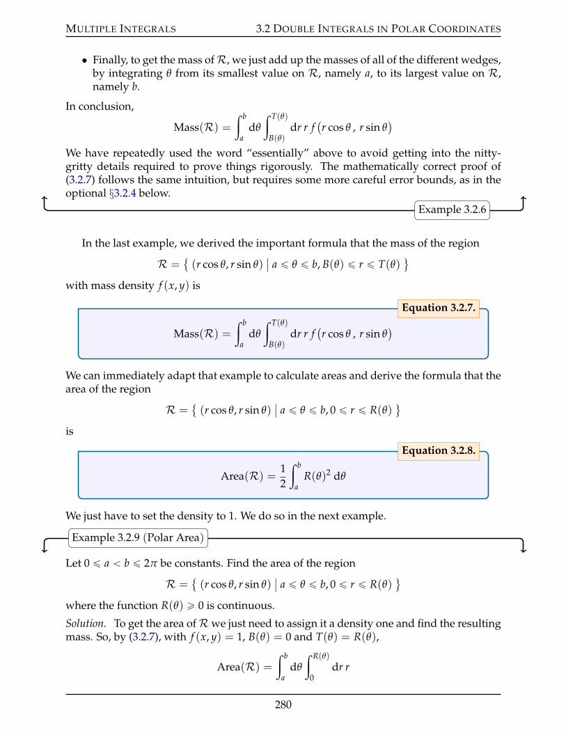
MULTIPLE INTEGRALS 3.2 DOUBLE INTEGRALS IN POLAR COORDINATES
• Finally, to get the mass ofR, we just add up the masses of all of the different wedges,by integrating θ from its smallest value on R, namely a, to its largest value on R,namely b.
In conclusion,
Mass(R) =ż b
adθ
ż T(θ)
B(θ)dr r f
(r cos θ , r sin θ
)
We have repeatedly used the word “essentially” above to avoid getting into the nitty-gritty details required to prove things rigorously. The mathematically correct proof of(3.2.7) follows the same intuition, but requires some more careful error bounds, as in theoptional §3.2.4 below.
Example 3.2.6
In the last example, we derived the important formula that the mass of the region
R = (r cos θ, r sin θ)
ˇa ď θ ď b, B(θ) ď r ď T(θ)
(
with mass density f (x, y) is
Mass(R) =ż b
adθ
ż T(θ)
B(θ)dr r f
(r cos θ , r sin θ
)Equation 3.2.7.
We can immediately adapt that example to calculate areas and derive the formula that thearea of the region
R = (r cos θ, r sin θ)
ˇa ď θ ď b, 0 ď r ď R(θ)
(
is
Area(R) = 12
ż b
aR(θ)2 dθ
Equation 3.2.8.
We just have to set the density to 1. We do so in the next example.
Example 3.2.9 (Polar Area)
Let 0 ď a ă b ď 2π be constants. Find the area of the region
R = (r cos θ, r sin θ)
ˇa ď θ ď b, 0 ď r ď R(θ)
(
where the function R(θ) ě 0 is continuous.
Solution. To get the area ofRwe just need to assign it a density one and find the resultingmass. So, by (3.2.7), with f (x, y) = 1, B(θ) = 0 and T(θ) = R(θ),
Area(R) =ż b
adθ
ż R(θ)
0dr r
280
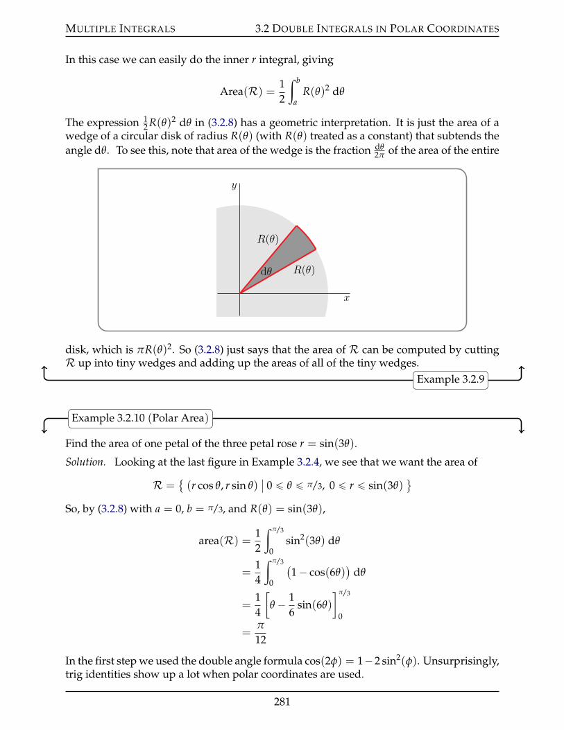
MULTIPLE INTEGRALS 3.2 DOUBLE INTEGRALS IN POLAR COORDINATES
In this case we can easily do the inner r integral, giving
Area(R) = 12
ż b
aR(θ)2 dθ
The expression 12 R(θ)2 dθ in (3.2.8) has a geometric interpretation. It is just the area of a
wedge of a circular disk of radius R(θ) (with R(θ) treated as a constant) that subtends theangle dθ. To see this, note that area of the wedge is the fraction dθ
2π of the area of the entire
x
y
Rpθq
Rpθq
dθ
disk, which is πR(θ)2. So (3.2.8) just says that the area of R can be computed by cuttingR up into tiny wedges and adding up the areas of all of the tiny wedges.
Example 3.2.9
Example 3.2.10 (Polar Area)
Find the area of one petal of the three petal rose r = sin(3θ).
Solution. Looking at the last figure in Example 3.2.4, we see that we want the area of
R = (r cos θ, r sin θ)
ˇ0 ď θ ď π/3, 0 ď r ď sin(3θ)
(
So, by (3.2.8) with a = 0, b = π/3, and R(θ) = sin(3θ),
area(R) = 12
ż π/3
0sin2(3θ) dθ
=14
ż π/3
0
(1´ cos(6θ)
)dθ
=14
[θ ´ 1
6sin(6θ)
]π/3
0
=π
12
In the first step we used the double angle formula cos(2φ) = 1´2 sin2(φ). Unsurprisingly,trig identities show up a lot when polar coordinates are used.
281
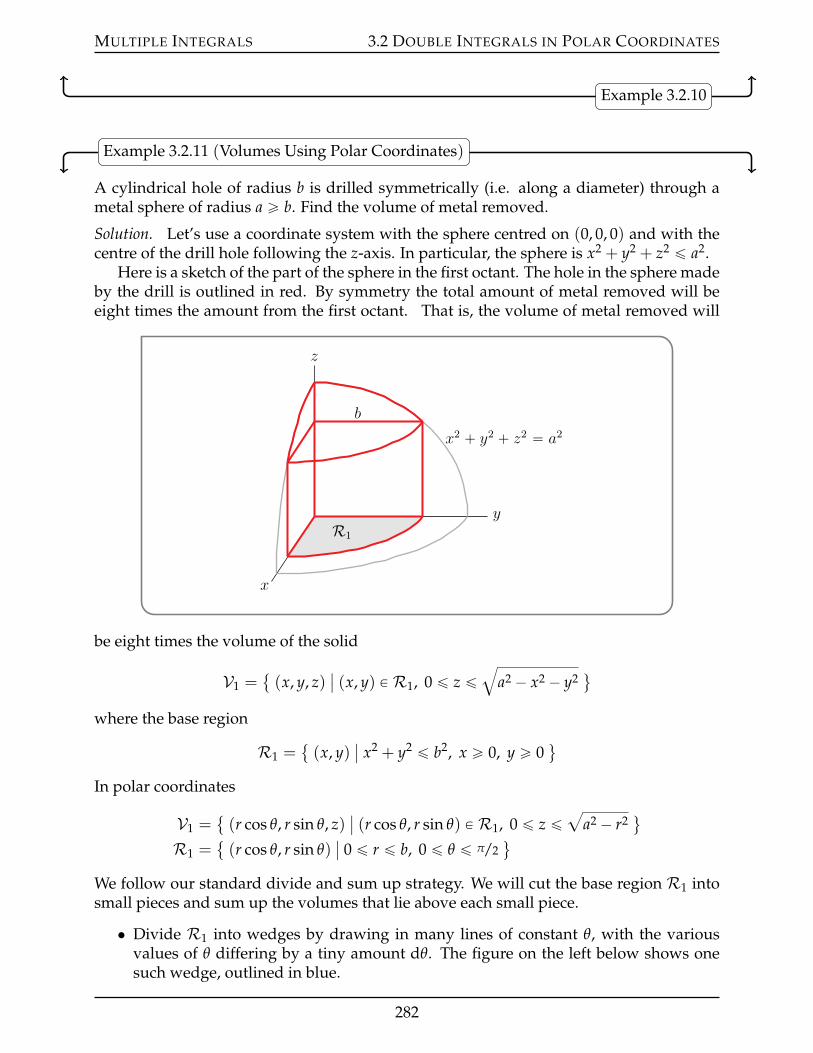
MULTIPLE INTEGRALS 3.2 DOUBLE INTEGRALS IN POLAR COORDINATES
Example 3.2.10
Example 3.2.11 (Volumes Using Polar Coordinates)
A cylindrical hole of radius b is drilled symmetrically (i.e. along a diameter) through ametal sphere of radius a ě b. Find the volume of metal removed.
Solution. Let’s use a coordinate system with the sphere centred on (0, 0, 0) and with thecentre of the drill hole following the z-axis. In particular, the sphere is x2 + y2 + z2 ď a2.
Here is a sketch of the part of the sphere in the first octant. The hole in the sphere madeby the drill is outlined in red. By symmetry the total amount of metal removed will beeight times the amount from the first octant. That is, the volume of metal removed will
z
y
x
b
R1
x2 ` y2 ` z2 “ a2
be eight times the volume of the solid
V1 = (x, y, z)
ˇ(x, y) P R1, 0 ď z ď
ba2 ´ x2 ´ y2
(
where the base region
R1 = (x, y)
ˇx2 + y2 ď b2, x ě 0, y ě 0
(
In polar coordinates
V1 = (r cos θ, r sin θ, z)
ˇ(r cos θ, r sin θ) P R1, 0 ď z ď
aa2 ´ r2
(
R1 = (r cos θ, r sin θ)
ˇ0 ď r ď b, 0 ď θ ď π/2
(
We follow our standard divide and sum up strategy. We will cut the base region R1 intosmall pieces and sum up the volumes that lie above each small piece.
• Divide R1 into wedges by drawing in many lines of constant θ, with the variousvalues of θ differing by a tiny amount dθ. The figure on the left below shows onesuch wedge, outlined in blue.
282
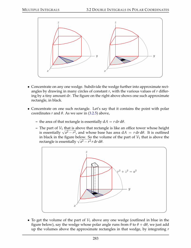
MULTIPLE INTEGRALS 3.2 DOUBLE INTEGRALS IN POLAR COORDINATES
z
y
x
z
y
x
• Concentrate on any one wedge. Subdivide the wedge further into approximate rect-angles by drawing in many circles of constant r, with the various values of r differ-ing by a tiny amount dr. The figure on the right above shows one such approximaterectangle, in black.
• Concentrate on one such rectangle. Let’s say that it contains the point with polarcoordinates r and θ. As we saw in (3.2.5) above,
– the area of that rectangle is essentially dA = r dr dθ.
– The part of V1 that is above that rectangle is like an office tower whose heightis essentially
?a2 ´ r2, and whose base has area dA = r dr dθ. It is outlined
in black in the figure below. So the volume of the part of V1 that is above therectangle is essentially
?a2 ´ r2 r dr dθ.
z
y
x
r2 ` z2 “ a2
• To get the volume of the part of V1 above any one wedge (outlined in blue in thefigure below), say the wedge whose polar angle runs from θ to θ + dθ, we just addup the volumes above the approximate rectangles in that wedge, by integrating r
283
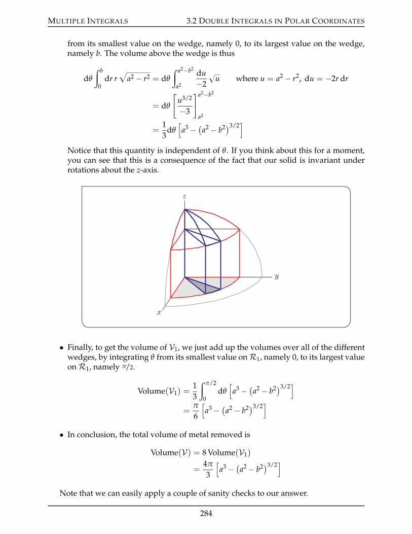
MULTIPLE INTEGRALS 3.2 DOUBLE INTEGRALS IN POLAR COORDINATES
from its smallest value on the wedge, namely 0, to its largest value on the wedge,namely b. The volume above the wedge is thus
dθ
ż b
0dr r
aa2 ´ r2 = dθ
ż a2´b2
a2
du´2
?u where u = a2 ´ r2, du = ´2r dr
= dθ
[u3/2
´3
]a2´b2
a2
=13
dθ[
a3 ´ (a2 ´ b2)3/2]
Notice that this quantity is independent of θ. If you think about this for a moment,you can see that this is a consequence of the fact that our solid is invariant underrotations about the z-axis.
z
y
x
• Finally, to get the volume of V1, we just add up the volumes over all of the differentwedges, by integrating θ from its smallest value onR1, namely 0, to its largest valueonR1, namely π/2.
Volume(V1) =13
ż π/2
0dθ[
a3 ´ (a2 ´ b2)3/2]
=π
6
[a3 ´ (a2 ´ b2)3/2
]
• In conclusion, the total volume of metal removed is
Volume(V) = 8 Volume(V1)
=4π
3
[a3 ´ (a2 ´ b2)3/2
]
Note that we can easily apply a couple of sanity checks to our answer.
284

MULTIPLE INTEGRALS 3.2 DOUBLE INTEGRALS IN POLAR COORDINATES
• If the radius of the drill bit b = 0, no metal is removed at all. So the total volumeremoved should be zero. Our answer does indeed give 0 in this case.
• If the radius of the drill bit b = a, the radius of the sphere, then the entire spheredisappears. So the total volume removed should be the volume of a sphere of radiusa. Our answer does indeed give 4
3 πa3 in this case.
• If the radius, a, of the sphere and the radius, b, of the drill bit are measured in unitsof meters, then the remaining volume 4π
3
[a3 ´ (a2 ´ b2)3/2
], has units meters3, as it
should.
Example 3.2.11
The previous two problems were given to us (or nearly given to us) in polar coor-dinates. We’ll now get a little practice converting integrals into polar coordinates, andrecognising when it is helpful to do so.
Example 3.2.12 (Changing to Polar Coordinates)
Convert the integralş1
0şx
0 ya
x2 + y2 dy dx to polar coordinates and evaluate the result.
Solution. First recall that in polar coordinates x = r cos θ, y = r sin θ and dx dy = dA =r dr dθ so that the integrand (and dA)
yb
x2 + y2 dy dx = (r sin θ) r r dr dθ = r3 sin θ dr dθ
is very simple. So whether or not this integral will be easy to evaluate using polar coordi-nates will be largely determined by the domain of integration.
So our main task is to sketch the domain of integration. To prepare for the sketch, notethat in the integral
ż 1
0
ż x
0yb
x2 + y2 dy dx =
ż 1
0dx[ż x
0dy y
bx2 + y2
]
• the variable x runs from 0 to 1 and
• for each fixed 0 ď x ď 1, y runs from 0 to x.
So the domain of integration is
D = (x, y)
ˇ0 ď x ď 1, 0 ď y ď x
(
which is sketched in the figure on the left below. It is a right angled triangle.
x
y y “ x
Dx “ 1
x
y θ “ π4
r “ 1cos θ
285
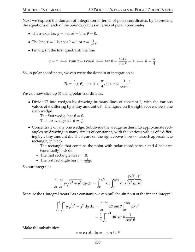
MULTIPLE INTEGRALS 3.2 DOUBLE INTEGRALS IN POLAR COORDINATES
Next we express the domain of integration in terms of polar coordinates, by expressingthe equations of each of the boundary lines in terms of polar coordinates.
• The x-axis, i.e. y = r sin θ = 0, is θ = 0.
• The line x = 1 is r cos θ = 1 or r = 1cos θ .
• Finally, (in the first quadrant) the line
y = x ðñ r sin θ = r cos θ ðñ tan θ =sin θ
cos θ= 1 ðñ θ =
π
4
So, in polar coordinates, we can write the domain of integration as
R =!(r, θ)
ˇˇ 0 ď θ ď π
4, 0 ď r ď 1
cos θ
)
We can now slice upR using polar coordinates.
• Divide R into wedges by drawing in many lines of constant θ, with the variousvalues of θ differing by a tiny amount dθ. The figure on the right above shows onesuch wedge.
– The first wedge has θ = 0.– The last wedge has θ = π
4 .
• Concentrate on any one wedge. Subdivide the wedge further into approximate rect-angles by drawing in many circles of constant r, with the various values of r differ-ing by a tiny amount dr. The figure on the right above shows one such approximaterectangle, in black.
– The rectangle that contains the point with polar coordinates r and θ has area(essentially) r dr dθ.
– The first rectangle has r = 0.– The last rectangle has r = 1
cos θ .
So our integral is
ż 1
0
ż x
0yb
x2 + y2 dy dx =
ż π/4
0dθ
ż 1cos θ
0dr r
y?
x2+y2hkkkikkkj(r2 sin θ)
Because the r-integral treats θ as a constant, we can pull the sin θ out of the inner r-integral.
ż 1
0
ż x
0yb
x2 + y2 dy dx =
ż π/4
0dθ sin θ
ż 1cos θ
0dr r3
=14
ż π/4
0dθ sin θ
1cos4 θ
Make the substitutionu = cos θ, du = ´ sin θ dθ
286
MULTIPLE INTEGRALS 3.2 DOUBLE INTEGRALS IN POLAR COORDINATES
When θ = 0, u = cos θ = 1 and when θ = π4 , u = cos θ = 1?
2. So
ż 1
0
ż x
0yb
x2 + y2 dy dx =14
ż 1/?
2
1(´du)
1u4
= ´14
[u´3
´3
]1/?
2
1=
112
[2?
2´ 1]
Example 3.2.12
Example 3.2.13 (Changing to Polar Coordinates)
Evaluateż 8
0e´x2
dx.
Solution. This is actually a trick question. In fact it is a famous trick question21. Theintegrand e´x2
does not have an antiderivative that can be expressed in terms of elemen-tary functions22. So we cannot evaluate this integral using the usual Calculus II methods.However we can evaluate it’s square
[ż 8
0e´x2
dx]2
=
ż 8
0e´x2
dxż 8
0e´y2
dy =
ż 8
0dx
ż 8
0dy e´x2´y2
precisely because this double integral can be easily evaluated just by changing to polarcoordinates! The domain of integration is the first quadrant
(x, y)
ˇx ě 0, y ě 0
(. In
polar coordinates, dxdy = r drdθ and the first quadrant is
(r cos θ , r sin θ)
ˇr ě 0, 0 ď θ ď π/2
(
So
[ż 8
0e´x2
dx]2
=
ż 8
0dx
ż 8
0dy e´x2´y2
=
ż π/2
0dθ
ż 8
0dr r e´r2
As r runs all the way to +8, this is an improper integral, so we should be a little bit
21 The solution is attributed to the French Mathematician Simeon Denis Poisson (1781–840) and was pub-lished in the textbook Cours d’Analyse de l’ecole polytechnique by Jacob Karl Franz Sturm (1803–1855).
22 On the other hand it is the core of the function erf(z) = 2?π
şz0 e´t2
dt, which gives Gaussian (i.e. bellcurve) probabilities. “erf” stands for “error function”.
287
MULTIPLE INTEGRALS 3.2 DOUBLE INTEGRALS IN POLAR COORDINATES
careful.
[ż 8
0e´x2
dx]2
= limRÑ8
ż π/2
0dθ
ż R
0dr r e´r2
= limRÑ8
ż π/2
0dθ
ż R2
0
du2
e´u where u = r2, du = 2r dr
= limRÑ8
ż π/2
0dθ
[´e´u
2
]R2
0
= limRÑ8
π
2
[12´ e´R2
2
]
=π
4
and so we get the famous result
ż 8
0e´x2
dx =
?π
2
Example 3.2.13
Example 3.2.14
Find the area of the region that is inside the circle r = 4 cos θ and to the left of the linex = 1.
Solution. First, let’s check that r = 4 cos θ really is a circle and figure out what circle it is.To do so, we’ll convert the equation r = 4 cos θ into Cartesian coordinates. Multiplyingboth sides by r gives
r2 = 4r cos θ ðñ x2 + y2 = 4x ðñ (x´ 2)2 + y2 = 4
So r = 4 cos θ is the circle of radius 2 centred on (2, 0). We’ll also need the intersectionpoint(s) of x = r cos θ = 1 and r = 4 cos θ. At such an intersection point
r cos θ = 1, r = 4 cos θ ùñ 1cos θ
= 4 cos θ
ùñ cos2 θ =14
ùñ cos θ =12
since r cos θ = 1 ą 0
ùñ θ = ˘π
3
Here is a sketch of the region of interest, which we’ll callR.
288
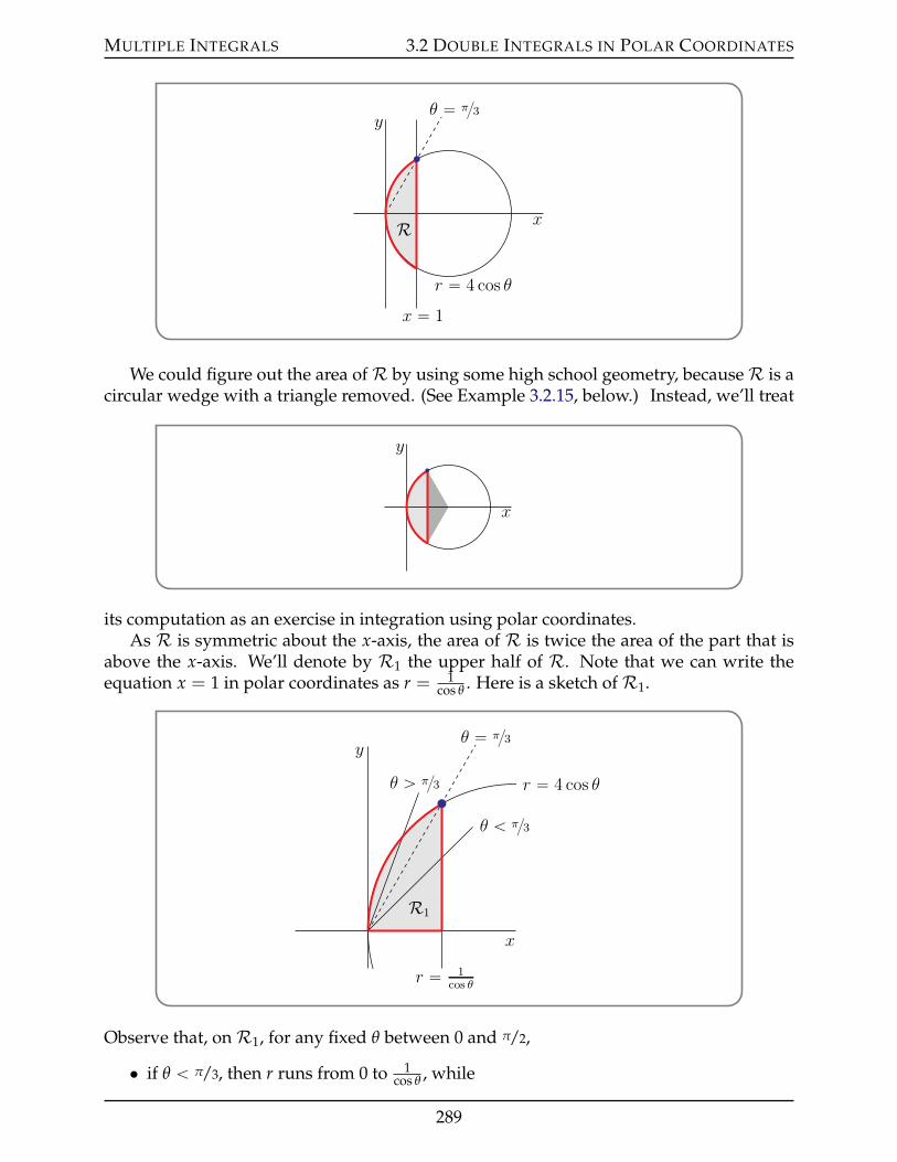
MULTIPLE INTEGRALS 3.2 DOUBLE INTEGRALS IN POLAR COORDINATES
x
y
r “ 4 cos θ
R
x “ 1
θ “ π3
We could figure out the area ofR by using some high school geometry, becauseR is acircular wedge with a triangle removed. (See Example 3.2.15, below.) Instead, we’ll treat
x
y
its computation as an exercise in integration using polar coordinates.As R is symmetric about the x-axis, the area of R is twice the area of the part that is
above the x-axis. We’ll denote by R1 the upper half of R. Note that we can write theequation x = 1 in polar coordinates as r = 1
cos θ . Here is a sketch ofR1.
x
y
θ ą π3
θ ă π3
r “ 4 cos θ
R1
r “ 1cos θ
θ “ π3
Observe that, onR1, for any fixed θ between 0 and π/2,
• if θ ă π/3, then r runs from 0 to 1cos θ , while
289
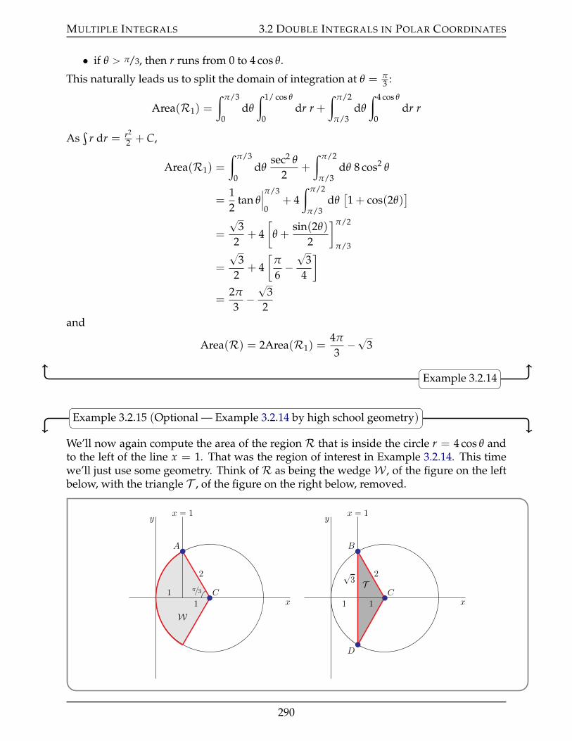
MULTIPLE INTEGRALS 3.2 DOUBLE INTEGRALS IN POLAR COORDINATES
• if θ ą π/3, then r runs from 0 to 4 cos θ.
This naturally leads us to split the domain of integration at θ = π3 :
Area(R1) =
ż π/3
0dθ
ż 1/ cos θ
0dr r +
ż π/2
π/3dθ
ż 4 cos θ
0dr r
Asş
r dr = r2
2 + C,
Area(R1) =
ż π/3
0dθ
sec2 θ
2+
ż π/2
π/3dθ 8 cos2 θ
=12
tan θˇˇπ/3
0+ 4
ż π/2
π/3dθ[1 + cos(2θ)
]
=
?3
2+ 4
[θ +
sin(2θ)
2
]π/2
π/3
=
?3
2+ 4
[π
6´?
34
]
=2π
3´?
32
and
Area(R) = 2Area(R1) =4π
3´?3
Example 3.2.14
Example 3.2.15 (Optional — Example 3.2.14 by high school geometry)
We’ll now again compute the area of the region R that is inside the circle r = 4 cos θ andto the left of the line x = 1. That was the region of interest in Example 3.2.14. This timewe’ll just use some geometry. Think of R as being the wedgeW , of the figure on the leftbelow, with the triangle T , of the figure on the right below, removed.
Wx
y
π3
x “ 1
A
C11
2T
x
yx “ 1
B
D
C1 1
2?3
290
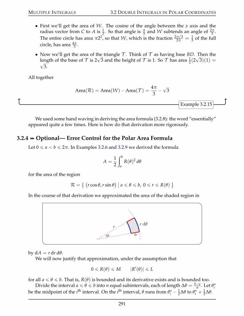
MULTIPLE INTEGRALS 3.2 DOUBLE INTEGRALS IN POLAR COORDINATES
• First we’ll get the area of W . The cosine of the angle between the x axis and theradius vector from C to A is 1
2 . So that angle is π3 and W subtends an angle of 2π
3 .The entire circle has area π22, so that W , which is the fraction 2π/3
2π = 13 of the full
circle, has area 4π3 .
• Now we’ll get the area of the triangle T . Think of T as having base BD. Then thelength of the base of T is 2
?3 and the height of T is 1. So T has area 1
2(2?
3)(1) =?3.
All together
Area(R) = Area(W)´Area(T ) = 4π
3´?3
Example 3.2.15
We used some hand waving in deriving the area formula (3.2.8): the word “essentially”appeared quite a few times. Here is how do that derivation more rigorously.
3.2.4 §§ Optional— Error Control for the Polar Area Formula
Let 0 ď a ă b ď 2π. In Examples 3.2.6 and 3.2.9 we derived the formula
A =12
ż b
aR(θ)2 dθ
for the area of the region
R = (
r cos θ, r sin θ) ˇ
a ď θ ď b, 0 ď r ď R(θ)(
In the course of that derivation we approximated the area of the shaded region in
dθ dr
rr dθ
by dA = r dr dθ.We will now justify that approximation, under the assumption that
0 ď R(θ) ď M |R1(θ)| ď L
for all a ď θ ď b. That is, R(θ) is bounded and its derivative exists and is bounded too.Divide the interval a ď θ ď b into n equal subintervals, each of length ∆θ = b´a
n . Let θ˚ibe the midpoint of the ith interval. On the ith interval, θ runs from θ˚i ´ 1
2 ∆θ to θ˚i +12 ∆θ.
291
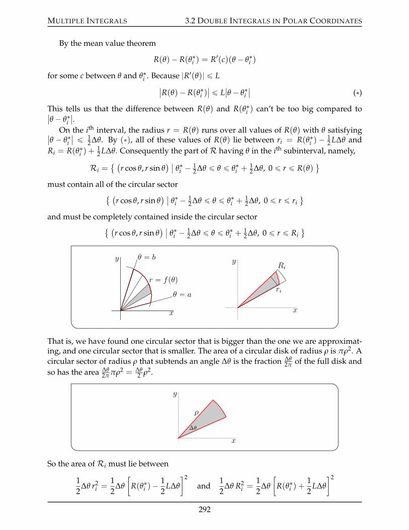
MULTIPLE INTEGRALS 3.2 DOUBLE INTEGRALS IN POLAR COORDINATES
By the mean value theorem
R(θ)´ R(θ˚i ) = R1(c)(θ ´ θ˚i )
for some c between θ and θ˚i . Because |R1(θ)| ď LˇR(θ)´ R(θ˚i )
ˇ ď Lˇθ ´ θ˚i
ˇ(˚)
This tells us that the difference between R(θ) and R(θ˚i ) can’t be too big compared toˇθ ´ θ˚i
ˇ.
On the ith interval, the radius r = R(θ) runs over all values of R(θ) with θ satisfyingˇθ ´ θ˚i
ˇ ď 12 ∆θ. By (˚), all of these values of R(θ) lie between ri = R(θ˚i ) ´ 1
2 L∆θ andRi = R(θ˚i ) +
12 L∆θ. Consequently the part ofR having θ in the ith subinterval, namely,
Ri = (
r cos θ, r sin θ) ˇ
θ˚i ´ 12 ∆θ ď θ ď θ˚i +
12 ∆θ, 0 ď r ď R(θ)
(
must contain all of the circular sector (
r cos θ, r sin θ) ˇ
θ˚i ´ 12 ∆θ ď θ ď θ˚i +
12 ∆θ, 0 ď r ď ri
(
and must be completely contained inside the circular sector (
r cos θ, r sin θ) ˇ
θ˚i ´ 12 ∆θ ď θ ď θ˚i +
12 ∆θ, 0 ď r ď Ri
(
x
y
θ “ a
θ “ b
r “ fpθq
x
y
ri
Ri
That is, we have found one circular sector that is bigger than the one we are approximat-ing, and one circular sector that is smaller. The area of a circular disk of radius ρ is πρ2. Acircular sector of radius ρ that subtends an angle ∆θ is the fraction ∆θ
2π of the full disk andso has the area ∆θ
2π πρ2 = ∆θ2 ρ2.
x
y
ρ
∆θ
So the area ofRi must lie between
12
∆θ r2i =
12
∆θ
[R(θ˚i )´
12
L∆θ
]2
and12
∆θ R2i =
12
∆θ
[R(θ˚i ) +
12
L∆θ
]2
292
MULTIPLE INTEGRALS 3.3 APPLICATIONS OF DOUBLE INTEGRALS
Observe that [R(θ˚i )˘
12
L∆θ
]2
= R(θ˚i )2 ˘ LR(θ˚i )∆θ +
14
L2∆θ2
implies that, since 0 ď R(θ) ď M,
R(θ˚i )2 ´ LM∆θ +
14
L2∆θ2 ď[
R(θ˚i )˘12
L∆θ
]2
ď R(θ˚i )2 + LM∆θ +
14
L2∆θ2
Hence (multiplying by ∆θ2 to turn them into areas)
12
R(θ˚i )2∆θ ´ 1
2LM∆θ2 +
18
L2∆θ3 ď Area(Ri) ď 12
R(θ˚i )2∆θ +
12
LM∆θ2 +18
L2∆θ3
and the total area A obeys the bounds
nÿ
i=1
[12
R(θ˚i )2∆θ ´ 1
2LM∆θ2 +
18
L2∆θ3]ď Aď
nÿ
i=1
[12
R(θ˚i )2∆θ +
12
LM∆θ2 +18
L2∆θ3]
12
nÿ
i=1
R(θ˚i )2∆θ ´ 1
2nLM∆θ2 +
18
nL2∆θ3 ď Aďnÿ
i=1
12
R(θ˚i )2∆θ +
12
nLM∆θ2 +18
nL2∆θ3
Since ∆θ = b´an ,
12
nÿ
i=1
R(θ˚i )2∆θ´ LM
2(b´a)2
n+
L2
8(b´a)3
n2 ď A ď 12
nÿ
i=1
R(θ˚i )2∆θ+
LM2
(b´a)2
n+
L2
8(b´a)3
n2
Now take the limit as n Ñ 8. Since
limnÑ8
[12
nÿ
i=1
R(θ˚i )2∆θ ˘ LM
2(b´ a)2
n+
L2
8(b´ a)3
n2
]
=12
ż b
aR(θ)2 dθ ˘ lim
nÑ8
LM2
(b´ a)2
n+ lim
nÑ8
L2
8(b´ a)3
n2
=12
ż b
aR(θ)2 dθ (since L, M, a and b are all constants)
we have that
A =12
ż b
aR(θ)2 dθ
exactly, as desired.
3.3IJ Applications of Double Integrals
Double integrals are useful for more than just computing areas and volumes. Here are afew other applications that lead to double integrals.
293

MULTIPLE INTEGRALS 3.3 APPLICATIONS OF DOUBLE INTEGRALS
§§§ Averages
In Section 2.2 of the CLP-2 text, we defined the average value of a function of one vari-able. We’ll now extend that discussion to functions of two variables. First, we recall thedefinition of the average of a finite set of numbers.
The average (mean) of a set of n numbers f1, f2, ¨ ¨ ¨ , fn is
f = 〈 f 〉 = f1 + f2 + ¨ ¨ ¨+ fn
n
The notations f and 〈 f 〉 are both commonly used to represent the average.
Definition 3.3.1.
Now suppose that we want to take the average of a function f (x, y) with (x, y) runningcontinuously over some region R in the xy-plane. A natural approach to defining whatwe mean by the average value of f overR is to
• First fix any natural number n.
• Subdivide the region R into tiny (approximate) squares each of width ∆x = 1n and
height ∆y = 1n . This can be done by, for example, subdividing vertical strips into
tiny squares, like in Example 3.1.11.
• Name the squares (in any fixed order) R1, R2, ¨ ¨ ¨ , RN, where N is the total numberof squares.
• Select, for each 1 ď i ď N, one point in square number i and call it (x˚i , y˚i ). So(x˚i , y˚i ) P Ri.
• The average value of f at the selected points is
1N
Nÿ
i=1
f (x˚i , y˚i ) =řN
i=1 f (x˚i , y˚i )řNi=1 1
=
řNi=1 f (x˚i , y˚i )∆x ∆y
řNi=1 ∆x ∆y
We have transformed the average into a ratio of Riemann sums.
Once we have the Riemann sums it is clear what to do next. Taking the limit n Ñ 8, we
get exactlyťR f (x,y)dx dyťR dx dy . That’s why we define
294
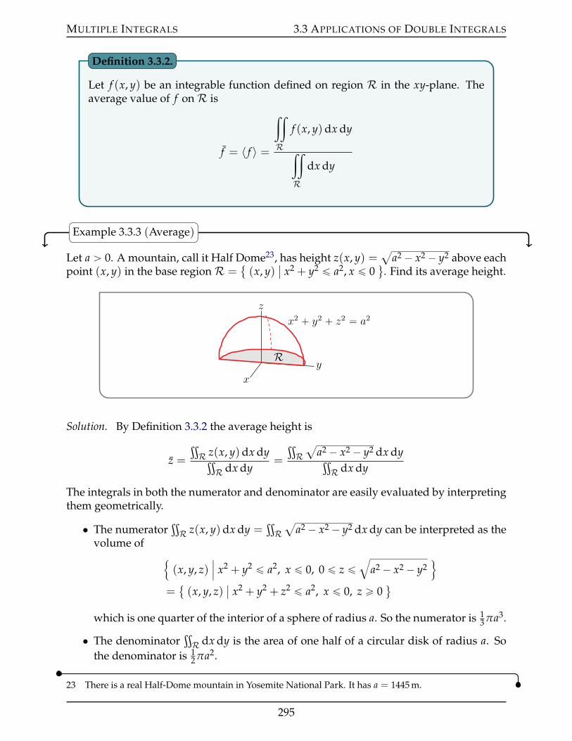
MULTIPLE INTEGRALS 3.3 APPLICATIONS OF DOUBLE INTEGRALS
Let f (x, y) be an integrable function defined on region R in the xy-plane. Theaverage value of f onR is
f = 〈 f 〉 =
ij
R
f (x, y)dx dy
ij
R
dx dy
Definition 3.3.2.
Example 3.3.3 (Average)
Let a ą 0. A mountain, call it Half Dome23, has height z(x, y) =a
a2 ´ x2 ´ y2 above eachpoint (x, y) in the base regionR =
(x, y)
ˇx2 + y2 ď a2, x ď 0
(. Find its average height.
z
y
x
x2 ` y2 ` z2 “ a2
R
Solution. By Definition 3.3.2 the average height is
z =
ťR z(x, y)dx dyťR dx dy
=
ťRa
a2 ´ x2 ´ y2 dx dyťR dx dy
The integrals in both the numerator and denominator are easily evaluated by interpretingthem geometrically.
• The numeratorťR z(x, y)dx dy =
ťRa
a2 ´ x2 ´ y2 dx dy can be interpreted as thevolume of
!(x, y, z)
ˇˇ x2 + y2 ď a2, x ď 0, 0 ď z ď
ba2 ´ x2 ´ y2
)
= (x, y, z)
ˇx2 + y2 + z2 ď a2, x ď 0, z ě 0
(
which is one quarter of the interior of a sphere of radius a. So the numerator is 13 πa3.
• The denominatorťR dx dy is the area of one half of a circular disk of radius a. So
the denominator is 12 πa2.
23 There is a real Half-Dome mountain in Yosemite National Park. It has a = 1445 m.
295
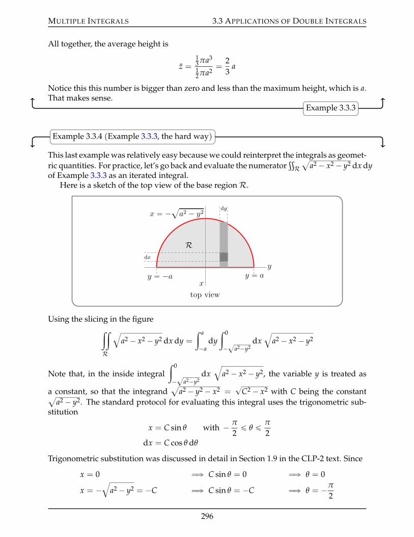
MULTIPLE INTEGRALS 3.3 APPLICATIONS OF DOUBLE INTEGRALS
All together, the average height is
z =13 πa3
12 πa2
=23
a
Notice this this number is bigger than zero and less than the maximum height, which is a.That makes sense.
Example 3.3.3
Example 3.3.4 (Example 3.3.3, the hard way)
This last example was relatively easy because we could reinterpret the integrals as geomet-ric quantities. For practice, let’s go back and evaluate the numerator
ťRa
a2 ´ x2 ´ y2 dx dyof Example 3.3.3 as an iterated integral.
Here is a sketch of the top view of the base regionR.
y
x
top view
x “ ´aa2 ´ y2
dx
dy
y “ ay “ ´a
R
Using the slicing in the figureij
R
ba2 ´ x2 ´ y2 dx dy =
ż a
´ady
ż 0
´?
a2´y2dx
ba2 ´ x2 ´ y2
Note that, in the inside integralż 0
´?
a2´y2dx
ba2 ´ x2 ´ y2, the variable y is treated as
a constant, so that the integranda
a2 ´ y2 ´ x2 =?
C2 ´ x2 with C being the constantaa2 ´ y2. The standard protocol for evaluating this integral uses the trigonometric sub-
stitution
x = C sin θ with ´ π
2ď θ ď π
2dx = C cos θ dθ
Trigonometric substitution was discussed in detail in Section 1.9 in the CLP-2 text. Since
x = 0 ùñ C sin θ = 0 ùñ θ = 0
x = ´b
a2 ´ y2 = ´C ùñ C sin θ = ´C ùñ θ = ´π
2
296
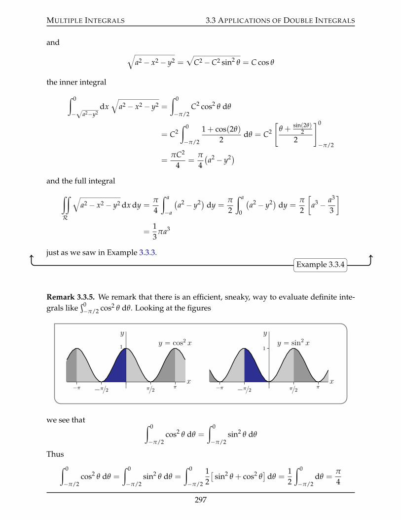
MULTIPLE INTEGRALS 3.3 APPLICATIONS OF DOUBLE INTEGRALS
andb
a2 ´ x2 ´ y2 =a
C2 ´ C2 sin2 θ = C cos θ
the inner integral
ż 0
´?
a2´y2dx
ba2 ´ x2 ´ y2 =
ż 0
´π/2C2 cos2 θ dθ
= C2ż 0
´π/2
1 + cos(2θ)
2dθ = C2
[θ + sin(2θ)
22
]0
´π/2
=πC2
4=
π
4(a2 ´ y2)
and the full integral
ij
R
ba2 ´ x2 ´ y2 dx dy =
π
4
ż a
´a
(a2 ´ y2) dy =
π
2
ż a
0
(a2 ´ y2) dy =
π
2
[a3 ´ a3
3
]
=13
πa3
just as we saw in Example 3.3.3.Example 3.3.4
Remark 3.3.5. We remark that there is an efficient, sneaky, way to evaluate definite inte-grals like
ş0´π/2 cos2 θ dθ. Looking at the figures
y
x´π ´π2 ππ2
1y “ cos2 x
y
x´π ´π2 ππ2
1y “ sin2 x
we see that ż 0
´π/2cos2 θ dθ =
ż 0
´π/2sin2 θ dθ
Thusż 0
´π/2cos2 θ dθ =
ż 0
´π/2sin2 θ dθ =
ż 0
´π/2
12[
sin2 θ + cos2 θ]
dθ =12
ż 0
´π/2dθ =
π
4
297
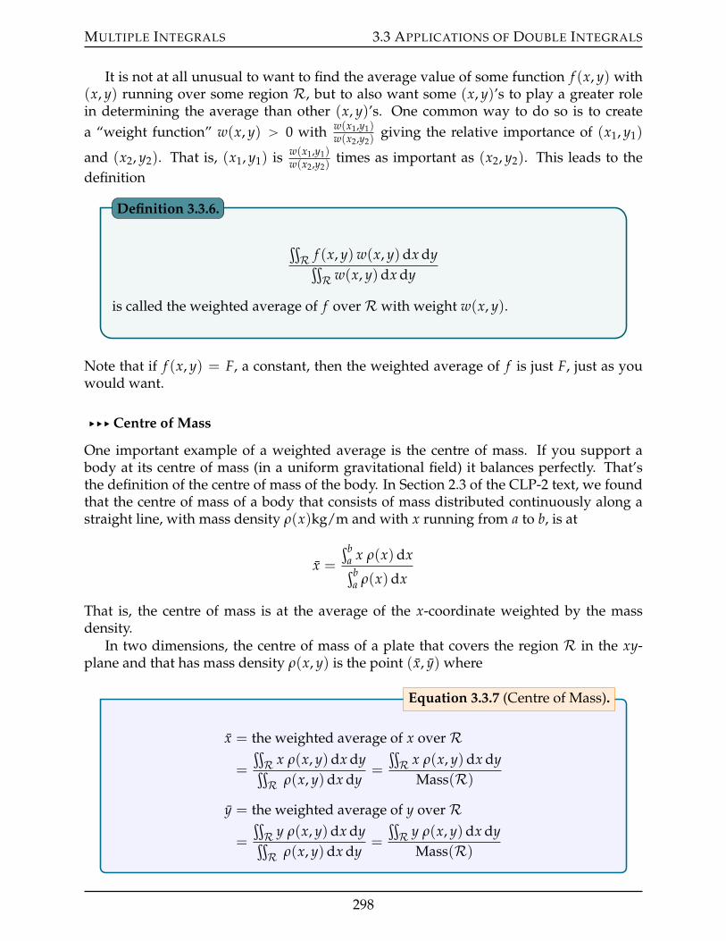
MULTIPLE INTEGRALS 3.3 APPLICATIONS OF DOUBLE INTEGRALS
It is not at all unusual to want to find the average value of some function f (x, y) with(x, y) running over some region R, but to also want some (x, y)’s to play a greater rolein determining the average than other (x, y)’s. One common way to do so is to createa “weight function” w(x, y) ą 0 with w(x1,y1)
w(x2,y2)giving the relative importance of (x1, y1)
and (x2, y2). That is, (x1, y1) is w(x1,y1)w(x2,y2)
times as important as (x2, y2). This leads to thedefinition
ťR f (x, y)w(x, y)dx dyťR w(x, y)dx dy
is called the weighted average of f overR with weight w(x, y).
Definition 3.3.6.
Note that if f (x, y) = F, a constant, then the weighted average of f is just F, just as youwould want.
§§§ Centre of Mass
One important example of a weighted average is the centre of mass. If you support abody at its centre of mass (in a uniform gravitational field) it balances perfectly. That’sthe definition of the centre of mass of the body. In Section 2.3 of the CLP-2 text, we foundthat the centre of mass of a body that consists of mass distributed continuously along astraight line, with mass density ρ(x)kg/m and with x running from a to b, is at
x =
şba x ρ(x)dxşb
a ρ(x)dx
That is, the centre of mass is at the average of the x-coordinate weighted by the massdensity.
In two dimensions, the centre of mass of a plate that covers the region R in the xy-plane and that has mass density ρ(x, y) is the point (x, y) where
x = the weighted average of x overR
=
ťR x ρ(x, y)dx dyťR ρ(x, y)dx dy
=
ťR x ρ(x, y)dx dy
Mass(R)
y = the weighted average of y overR
=
ťR y ρ(x, y)dx dyťR ρ(x, y)dx dy
=
ťR y ρ(x, y)dx dy
Mass(R)
Equation 3.3.7 (Centre of Mass).
298
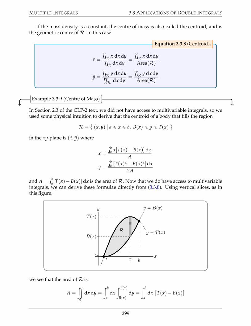
MULTIPLE INTEGRALS 3.3 APPLICATIONS OF DOUBLE INTEGRALS
If the mass density is a constant, the centre of mass is also called the centroid, and isthe geometric centre ofR. In this case
x =
ťR x dx dyťR dx dy
=
ťR x dx dy
Area(R)
y =
ťR y dx dyťR dx dy
=
ťR y dx dy
Area(R)
Equation 3.3.8 (Centroid).
Example 3.3.9 (Centre of Mass)
In Section 2.3 of the CLP-2 text, we did not have access to multivariable integrals, so weused some physical intuition to derive that the centroid of a body that fills the region
R = (x, y)
ˇa ď x ď b, B(x) ď y ď T(x)
(
in the xy-plane is (x, y) where
x =
şba x[T(x)´ B(x)]dx
A
y =
şba [T(x)2 ´ B(x)2]dx
2A
and A =şb
a [T(x)´ B(x)]dx is the area ofR. Now that we do have access to multivariableintegrals, we can derive these formulae directly from (3.3.8). Using vertical slices, as inthis figure,
x b
T pxq
Bpxq
x
y
y “ T pxq
y “ Bpxq
a
R
we see that the area ofR is
A =
ij
R
dx dy =
ż b
adx
ż T(x)
B(x)dy =
ż b
adx[T(x)´ B(x)
]
299

MULTIPLE INTEGRALS 3.3 APPLICATIONS OF DOUBLE INTEGRALS
and that (3.3.8) gives
x =1A
ij
R
x dx dy =1A
ż b
adx
ż T(x)
B(x)dy x =
1A
ż b
adx x
[T(x)´ B(x)
]
y =1A
ij
R
y dx dy =1A
ż b
adx
ż T(x)
B(x)dy y =
1A
ż b
adx
[T(x)2
2´ B(x)2
2
]
just as desired.Example 3.3.9
We’ll start with a simple mechanical example.
Example 3.3.10 (Quarter Circle)
In Example 2.3.4 of the CLP-2 text, we found the centroid of the quarter circular disk
D = (x, y)
ˇx ě 0, y ě 0, x2 + y2 ď r2 (
by using the formulae of the last example. We’ll now find it again using (3.3.8).Since the area of D is 1
4 πr2, we have
x =
ťD x dx dy
14 πr2
y =
ťD y dx dy
14 πr2
We’ll evaluateť
D x dx dy by using horizontal slices, as in the figure on the left below.
x
y
x “ ar2 ´ y2p0, rq
x
y
y “ ?r2 ´ x2
pr, 0q
Looking at that figure, we see that
• y runs from 0 to r and
• for each y in that range, x runs from 0 toa
r2 ´ y2.
So
ij
D
x dx dy =
ż r
0dy
ż ?r2´y2
0dx x =
ż r
0dy[
x2
2
]?r2´y2
0=
12
ż r
0dy[r2 ´ y2]
=12
[r3 ´ r3
3
]=
r3
3
300
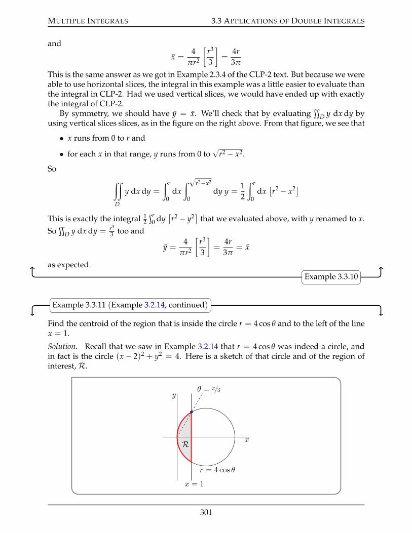
MULTIPLE INTEGRALS 3.3 APPLICATIONS OF DOUBLE INTEGRALS
and
x =4
πr2
[r3
3
]=
4r3π
This is the same answer as we got in Example 2.3.4 of the CLP-2 text. But because we wereable to use horizontal slices, the integral in this example was a little easier to evaluate thanthe integral in CLP-2. Had we used vertical slices, we would have ended up with exactlythe integral of CLP-2.
By symmetry, we should have y = x. We’ll check that by evaluatingť
D y dx dy byusing vertical slices slices, as in the figure on the right above. From that figure, we see that
• x runs from 0 to r and
• for each x in that range, y runs from 0 to?
r2 ´ x2.
Soij
D
y dx dy =
ż r
0dx
ż ?r2´x2
0dy y =
12
ż r
0dx[r2 ´ x2]
This is exactly the integral 12
şr0 dy
[r2 ´ y2] that we evaluated above, with y renamed to x.
Soť
D y dx dy = r3
3 too and
y =4
πr2
[r3
3
]=
4r3π
= x
as expected.Example 3.3.10
Example 3.3.11 (Example 3.2.14, continued)
Find the centroid of the region that is inside the circle r = 4 cos θ and to the left of the linex = 1.
Solution. Recall that we saw in Example 3.2.14 that r = 4 cos θ was indeed a circle, andin fact is the circle (x ´ 2)2 + y2 = 4. Here is a sketch of that circle and of the region ofinterest,R.
x
y
r “ 4 cos θ
R
x “ 1
θ “ π3
301
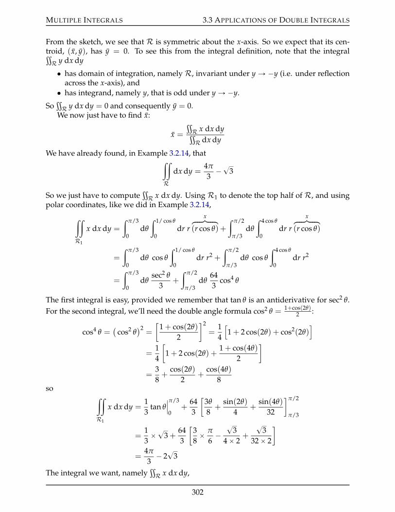
MULTIPLE INTEGRALS 3.3 APPLICATIONS OF DOUBLE INTEGRALS
From the sketch, we see that R is symmetric about the x-axis. So we expect that its cen-troid, (x, y), has y = 0. To see this from the integral definition, note that the integralťR y dx dy
• has domain of integration, namely R, invariant under y Ñ ´y (i.e. under reflectionacross the x-axis), and• has integrand, namely y, that is odd under y Ñ ´y.
SoťR y dx dy = 0 and consequently y = 0.
We now just have to find x:
x =
ťR x dx dyťR dx dy
We have already found, in Example 3.2.14, thatij
R
dx dy =4π
3´?3
So we just have to computeťR x dx dy. Using R1 to denote the top half of R, and using
polar coordinates, like we did in Example 3.2.14,
ij
R1
x dx dy =
ż π/3
0dθ
ż 1/ cos θ
0dr r
xhkkkikkkj(r cos θ) +
ż π/2
π/3dθ
ż 4 cos θ
0dr r
xhkkkikkkj(r cos θ)
=
ż π/3
0dθ cos θ
ż 1/ cos θ
0dr r2 +
ż π/2
π/3dθ cos θ
ż 4 cos θ
0dr r2
=
ż π/3
0dθ
sec2 θ
3+
ż π/2
π/3dθ
643
cos4 θ
The first integral is easy, provided we remember that tan θ is an antiderivative for sec2 θ.For the second integral, we’ll need the double angle formula cos2 θ = 1+cos(2θ)
2 :
cos4 θ =(
cos2 θ)2
=
[1 + cos(2θ)
2
]2
=14
[1 + 2 cos(2θ) + cos2(2θ)
]
=14
[1 + 2 cos(2θ) +
1 + cos(4θ)
2
]
=38+
cos(2θ)
2+
cos(4θ)
8so
ij
R1
x dx dy =13
tan θˇˇπ/3
0+
643
[3θ
8+
sin(2θ)
4+
sin(4θ)
32
]π/2
π/3
=13ˆ?3 +
643
[38ˆ π
6´?
34ˆ 2
+
?3
32ˆ 2
]
=4π
3´ 2?
3
The integral we want, namelyťR x dx dy,
302
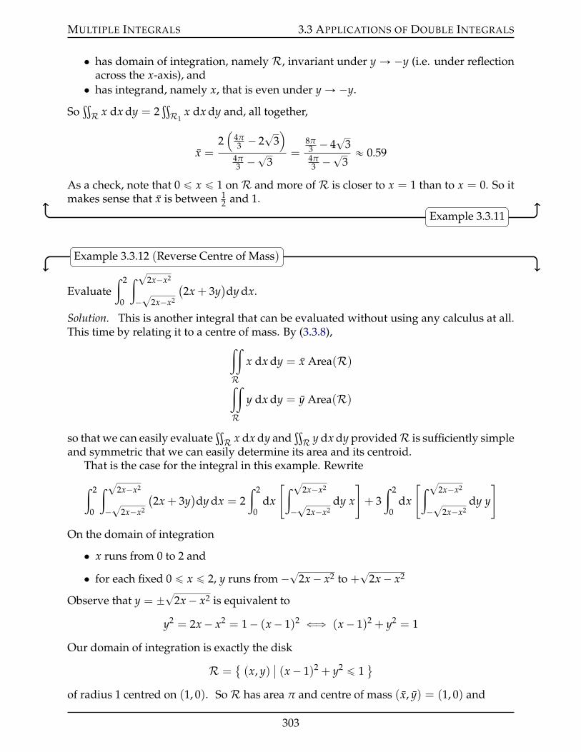
MULTIPLE INTEGRALS 3.3 APPLICATIONS OF DOUBLE INTEGRALS
• has domain of integration, namely R, invariant under y Ñ ´y (i.e. under reflectionacross the x-axis), and• has integrand, namely x, that is even under y Ñ ´y.
SoťR x dx dy = 2
ťR1
x dx dy and, all together,
x =2(
4π3 ´ 2
?3)
4π3 ´
?3
=8π3 ´ 4
?3
4π3 ´
?3« 0.59
As a check, note that 0 ď x ď 1 on R and more of R is closer to x = 1 than to x = 0. So itmakes sense that x is between 1
2 and 1.
Example 3.3.11
Example 3.3.12 (Reverse Centre of Mass)
Evaluateż 2
0
ż ?2x´x2
´?
2x´x2
(2x + 3y
)dy dx.
Solution. This is another integral that can be evaluated without using any calculus at all.This time by relating it to a centre of mass. By (3.3.8),
ij
R
x dx dy = x Area(R)ij
R
y dx dy = y Area(R)
so that we can easily evaluateťR x dx dy and
ťR y dx dy providedR is sufficiently simple
and symmetric that we can easily determine its area and its centroid.That is the case for the integral in this example. Rewrite
ż 2
0
ż ?2x´x2
´?
2x´x2
(2x + 3y
)dy dx = 2
ż 2
0dx
[ż ?2x´x2
´?
2x´x2dy x
]+ 3
ż 2
0dx
[ż ?2x´x2
´?
2x´x2dy y
]
On the domain of integration
• x runs from 0 to 2 and
• for each fixed 0 ď x ď 2, y runs from ´?2x´ x2 to +?
2x´ x2
Observe that y = ˘?2x´ x2 is equivalent to
y2 = 2x´ x2 = 1´ (x´ 1)2 ðñ (x´ 1)2 + y2 = 1
Our domain of integration is exactly the disk
R = (x, y)
ˇ(x´ 1)2 + y2 ď 1
(
of radius 1 centred on (1, 0). SoR has area π and centre of mass (x, y) = (1, 0) and
303
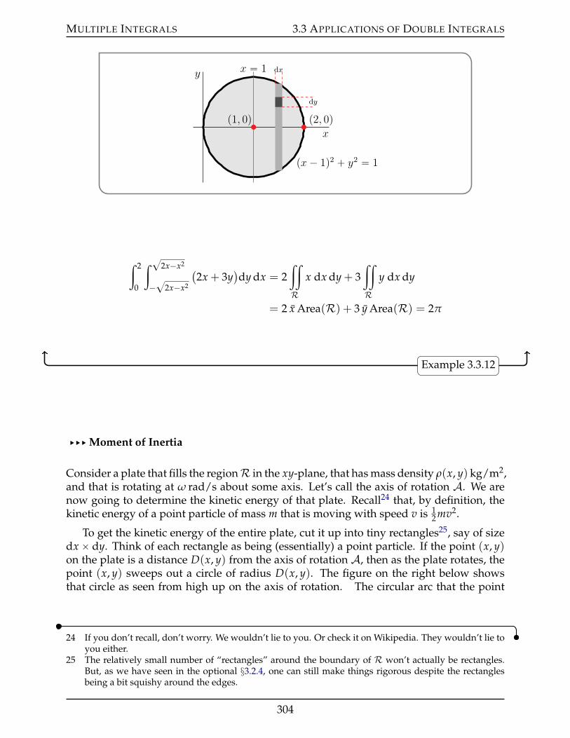
MULTIPLE INTEGRALS 3.3 APPLICATIONS OF DOUBLE INTEGRALS
p1, 0q p2, 0q
dx
dy
x “ 1
x
y
px ´ 1q2 ` y2 “ 1
ż 2
0
ż ?2x´x2
´?
2x´x2
(2x + 3y
)dy dx = 2
ij
R
x dx dy + 3ij
R
y dx dy
= 2 x Area(R) + 3 y Area(R) = 2π
Example 3.3.12
§§§ Moment of Inertia
Consider a plate that fills the regionR in the xy-plane, that has mass density ρ(x, y) kg/m2,and that is rotating at ω rad/s about some axis. Let’s call the axis of rotation A. We arenow going to determine the kinetic energy of that plate. Recall24 that, by definition, thekinetic energy of a point particle of mass m that is moving with speed v is 1
2 mv2.
To get the kinetic energy of the entire plate, cut it up into tiny rectangles25, say of sizedx ˆ dy. Think of each rectangle as being (essentially) a point particle. If the point (x, y)on the plate is a distance D(x, y) from the axis of rotation A, then as the plate rotates, thepoint (x, y) sweeps out a circle of radius D(x, y). The figure on the right below showsthat circle as seen from high up on the axis of rotation. The circular arc that the point
24 If you don’t recall, don’t worry. We wouldn’t lie to you. Or check it on Wikipedia. They wouldn’t lie toyou either.
25 The relatively small number of “rectangles” around the boundary of R won’t actually be rectangles.But, as we have seen in the optional §3.2.4, one can still make things rigorous despite the rectanglesbeing a bit squishy around the edges.
304
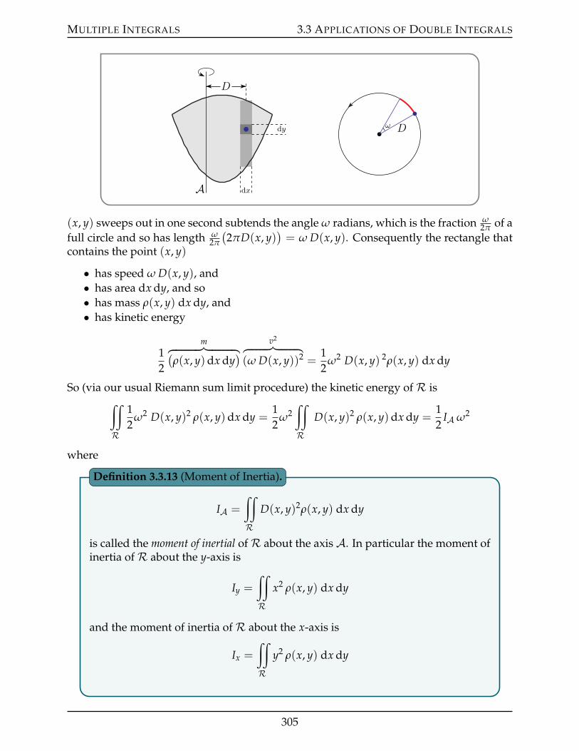
MULTIPLE INTEGRALS 3.3 APPLICATIONS OF DOUBLE INTEGRALS
dx
dy
D
A
ω D
(x, y) sweeps out in one second subtends the angle ω radians, which is the fraction ω2π of a
full circle and so has length ω2π
(2πD(x, y)
)= ω D(x, y). Consequently the rectangle that
contains the point (x, y)
• has speed ω D(x, y), and• has area dx dy, and so• has mass ρ(x, y) dx dy, and• has kinetic energy
12
mhkkkkkkkkikkkkkkkkj(ρ(x, y)dx dy
)v2hkkkkkkikkkkkkj
(ω D(x, y))2 =12
ω2 D(x, y) 2ρ(x, y) dx dy
So (via our usual Riemann sum limit procedure) the kinetic energy ofR isij
R
12
ω2 D(x, y)2 ρ(x, y)dx dy =12
ω2ij
R
D(x, y)2 ρ(x, y)dx dy =12
IA ω2
where
IA =
ij
R
D(x, y)2ρ(x, y) dx dy
is called the moment of inertial ofR about the axis A. In particular the moment ofinertia ofR about the y-axis is
Iy =
ij
R
x2 ρ(x, y) dx dy
and the moment of inertia ofR about the x-axis is
Ix =
ij
R
y2 ρ(x, y) dx dy
Definition 3.3.13 (Moment of Inertia).
305
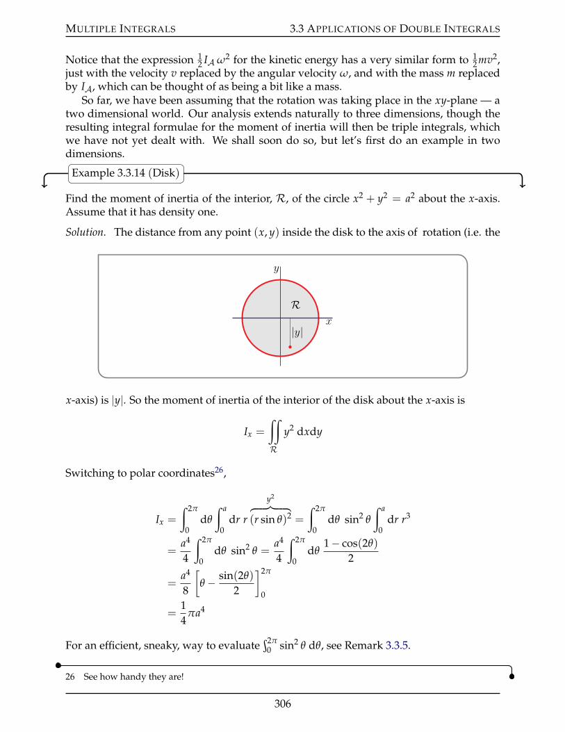
MULTIPLE INTEGRALS 3.3 APPLICATIONS OF DOUBLE INTEGRALS
Notice that the expression 12 IA ω2 for the kinetic energy has a very similar form to 1
2 mv2,just with the velocity v replaced by the angular velocity ω, and with the mass m replacedby IA, which can be thought of as being a bit like a mass.
So far, we have been assuming that the rotation was taking place in the xy-plane — atwo dimensional world. Our analysis extends naturally to three dimensions, though theresulting integral formulae for the moment of inertia will then be triple integrals, whichwe have not yet dealt with. We shall soon do so, but let’s first do an example in twodimensions.
Example 3.3.14 (Disk)
Find the moment of inertia of the interior, R, of the circle x2 + y2 = a2 about the x-axis.Assume that it has density one.
Solution. The distance from any point (x, y) inside the disk to the axis of rotation (i.e. the
R
y
|y|x
x-axis) is |y|. So the moment of inertia of the interior of the disk about the x-axis is
Ix =
ij
R
y2 dxdy
Switching to polar coordinates26,
Ix =
ż 2π
0dθ
ż a
0dr r
y2hkkkikkkj(r sin θ)2 =
ż 2π
0dθ sin2 θ
ż a
0dr r3
=a4
4
ż 2π
0dθ sin2 θ =
a4
4
ż 2π
0dθ
1´ cos(2θ)
2
=a4
8
[θ ´ sin(2θ)
2
]2π
0
=14
πa4
For an efficient, sneaky, way to evaluateş2π
0 sin2 θ dθ, see Remark 3.3.5.
26 See how handy they are!
306
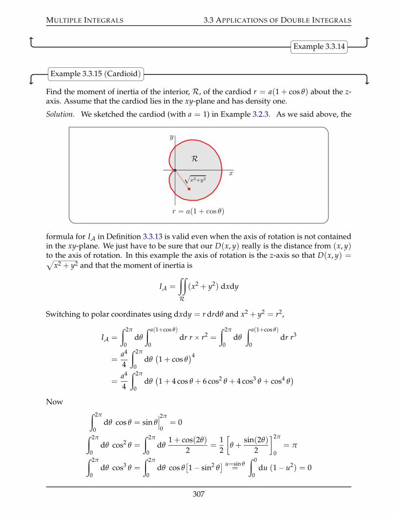
MULTIPLE INTEGRALS 3.3 APPLICATIONS OF DOUBLE INTEGRALS
Example 3.3.14
Example 3.3.15 (Cardioid)
Find the moment of inertia of the interior, R, of the cardiod r = a(1 + cos θ) about the z-axis. Assume that the cardiod lies in the xy-plane and has density one.
Solution. We sketched the cardiod (with a = 1) in Example 3.2.3. As we said above, the
Rx
y
?x2`y2
r “ ap1 ` cos θq
formula for IA in Definition 3.3.13 is valid even when the axis of rotation is not containedin the xy-plane. We just have to be sure that our D(x, y) really is the distance from (x, y)to the axis of rotation. In this example the axis of rotation is the z-axis so that D(x, y) =a
x2 + y2 and that the moment of inertia is
IA =
ij
R
(x2 + y2) dxdy
Switching to polar coordinates using dxdy = r drdθ and x2 + y2 = r2,
IA =
ż 2π
0dθ
ż a(1+cos θ)
0dr rˆ r2 =
ż 2π
0dθ
ż a(1+cos θ)
0dr r3
=a4
4
ż 2π
0dθ(1 + cos θ
)4
=a4
4
ż 2π
0dθ(1 + 4 cos θ + 6 cos2 θ + 4 cos3 θ + cos4 θ
)
Nowż 2π
0dθ cos θ = sin θ
ˇˇ2π
0= 0
ż 2π
0dθ cos2 θ =
ż 2π
0dθ
1 + cos(2θ)
2=
12
[θ +
sin(2θ)
2
]2π
0= π
ż 2π
0dθ cos3 θ =
ż 2π
0dθ cos θ
[1´ sin2 θ
] u=sin θ=
ż 0
0du (1´ u2) = 0
307
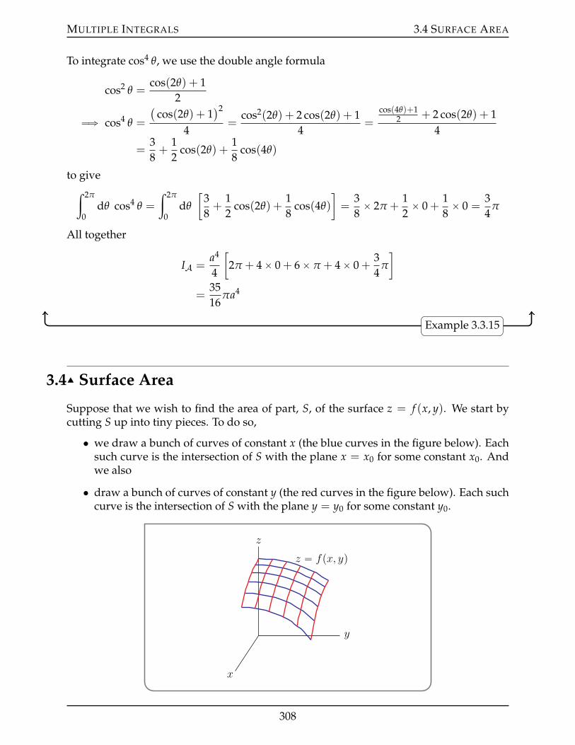
MULTIPLE INTEGRALS 3.4 SURFACE AREA
To integrate cos4 θ, we use the double angle formula
cos2 θ =cos(2θ) + 1
2
ùñ cos4 θ =
(cos(2θ) + 1
)2
4=
cos2(2θ) + 2 cos(2θ) + 14
=cos(4θ)+1
2 + 2 cos(2θ) + 14
=38+
12
cos(2θ) +18
cos(4θ)
to giveż 2π
0dθ cos4 θ =
ż 2π
0dθ
[38+
12
cos(2θ) +18
cos(4θ)
]=
38ˆ 2π +
12ˆ 0 +
18ˆ 0 =
34
π
All together
IA =a4
4
[2π + 4ˆ 0 + 6ˆ π + 4ˆ 0 +
34
π
]
=3516
πa4
Example 3.3.15
3.4IJ Surface Area
Suppose that we wish to find the area of part, S, of the surface z = f (x, y). We start bycutting S up into tiny pieces. To do so,
• we draw a bunch of curves of constant x (the blue curves in the figure below). Eachsuch curve is the intersection of S with the plane x = x0 for some constant x0. Andwe also
• draw a bunch of curves of constant y (the red curves in the figure below). Each suchcurve is the intersection of S with the plane y = y0 for some constant y0.
z
y
x
z “ fpx, yq
308
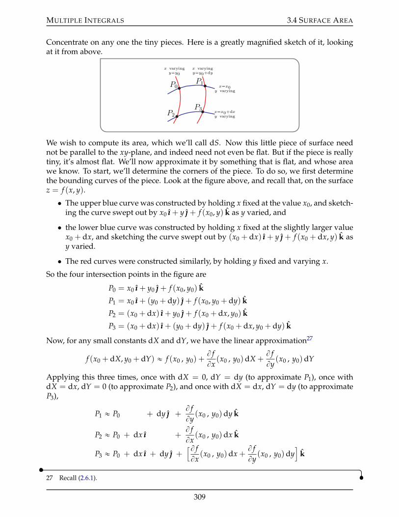
MULTIPLE INTEGRALS 3.4 SURFACE AREA
Concentrate on any one the tiny pieces. Here is a greatly magnified sketch of it, lookingat it from above.
P2
P3
P1P0
x“x0`dxy varying
x“x0y varying
x varyingy“y0`dy
x varyingy“y0
We wish to compute its area, which we’ll call dS. Now this little piece of surface neednot be parallel to the xy-plane, and indeed need not even be flat. But if the piece is reallytiny, it’s almost flat. We’ll now approximate it by something that is flat, and whose areawe know. To start, we’ll determine the corners of the piece. To do so, we first determinethe bounding curves of the piece. Look at the figure above, and recall that, on the surfacez = f (x, y).
• The upper blue curve was constructed by holding x fixed at the value x0, and sketch-ing the curve swept out by x0 ııı + y + f (x0, y) k as y varied, and
• the lower blue curve was constructed by holding x fixed at the slightly larger valuex0 + dx, and sketching the curve swept out by (x0 + dx) ııı + y + f (x0 + dx, y) k asy varied.
• The red curves were constructed similarly, by holding y fixed and varying x.
So the four intersection points in the figure are
P0 = x0 ııı + y0 + f (x0, y0) k
P1 = x0 ııı + (y0 + dy) + f (x0, y0 + dy) k
P2 = (x0 + dx) ııı + y0 + f (x0 + dx, y0) k
P3 = (x0 + dx) ııı + (y0 + dy) + f (x0 + dx, y0 + dy) k
Now, for any small constants dX and dY, we have the linear approximation27
f (x0 + dX, y0 + dY) « f (x0 , y0) +B fBx
(x0 , y0)dX +B fBy
(x0 , y0)dY
Applying this three times, once with dX = 0, dY = dy (to approximate P1), once withdX = dx, dY = 0 (to approximate P2), and once with dX = dx, dY = dy (to approximateP3),
P1 « P0 + dy +B fBy
(x0 , y0)dy k
P2 « P0 + dx ııı +B fBx
(x0 , y0)dx k
P3 « P0 + dx ııı + dy +[B fBx
(x0 , y0)dx +B fBy
(x0 , y0)dy]
k
27 Recall (2.6.1).
309
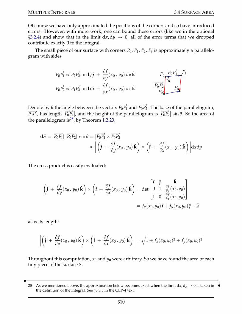
MULTIPLE INTEGRALS 3.4 SURFACE AREA
Of course we have only approximated the positions of the corners and so have introducederrors. However, with more work, one can bound those errors (like we in the optional§3.2.4) and show that in the limit dx, dy Ñ 0, all of the error terms that we droppedcontribute exactly 0 to the integral.
The small piece of our surface with corners P0, P1, P2, P3 is approximately a parallelo-gram with sides
ÝÝÑP0P1 « ÝÝÑP2P3 « dy +B fBy
(x0 , y0)dy k
ÝÝÑP0P2 « ÝÝÑP1P3 « dx ııı +B fBx
(x0 , y0)dx kP2
P3
P1P0
θ
ÝÝÝÑP0P1
ÝÝÝÑP0P2
Denote by θ the angle between the vectors ÝÝÑP0P1 and ÝÝÑP0P2. The base of the parallelogram,ÝÝÑP0P1, has lengthˇÝÝÑP0P1
ˇ, and the height of the parallelogram is
ˇÝÝÑP0P2ˇ
sin θ. So the area ofthe parallelogram is28, by Theorem 1.2.23,
dS = |ÝÝÑP0P1| |ÝÝÑP0P2| sin θ =ˇÝÝÑP0P1 ˆÝÝÑP0P2
ˇ
«ˇˇ(
+B fBy
(x0 , y0) k)ˆ(
ııı +B fBx
(x0 , y0) k) ˇˇdxdy
The cross product is easily evaluated:
( +
B fBy
(x0 , y0) k)ˆ(
ııı +B fBx
(x0 , y0) k)= det
ııı k0 1 B f
By (x0, y0)
1 0 B fBx (x0, y0)
= fx(x0, y0) ııı + fy(x0, y0) ´ k
as is its length:
ˇˇ(
+B fBy
(x0 , y0) k)ˆ(
ııı +B fBx
(x0 , y0) k)ˇˇ =
b1 + fx(x0, y0)2 + fy(x0, y0)2
Throughout this computation, x0 and y0 were arbitrary. So we have found the area of eachtiny piece of the surface S.
28 As we mentioned above, the approximation below becomes exact when the limit dx, dy Ñ 0 is taken inthe definition of the integral. See §3.3.5 in the CLP-4 text.
310
MULTIPLE INTEGRALS 3.4 SURFACE AREA
For the surface z = f (x, y),
dS =b
1 + fx(x, y)2 + fy(x, y)2 dxdy
Similarly, for the surface x = g(y, z),
dS =b
1 + gy(y, z)2 + gz(y, z)2 dydz
and for the surface y = h(x, z),
dS =b
1 + hx(x, z)2 + hz(x, z)2 dxdz
Equation 3.4.1.
Consequently, we have
(a) The area of the part of the surface z = f (x, y) with (x, y) running over theregion D in the xy-plane is
ij
D
b1 + fx(x, y)2 + fy(x, y)2 dxdy
(b) The area of the part of the surface x = g(y, z) with (y, z) running over theregion D in the yz-plane is
ij
D
b1 + gy(y, z)2 + gz(y, z)2 dydz
(c) The area of the part of the surface y = h(x, z) with (x, z) running over theregion D in the xz-plane is
ij
D
b1 + hx(x, z)2 + hz(x, z)2 dxdz
Theorem 3.4.2.
Example 3.4.3 (Area of a cone)
As a first example, we compute the area of the part of the cone
z =b
x2 + y2
with 0 ď z ď a or, equivalently, with x2 + y2 ď a2.
311
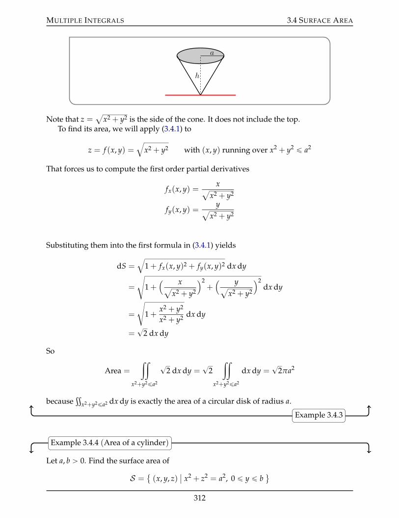
MULTIPLE INTEGRALS 3.4 SURFACE AREA
h
a
Note that z =a
x2 + y2 is the side of the cone. It does not include the top.To find its area, we will apply (3.4.1) to
z = f (x, y) =b
x2 + y2 with (x, y) running over x2 + y2 ď a2
That forces us to compute the first order partial derivatives
fx(x, y) =xa
x2 + y2
fy(x, y) =ya
x2 + y2
Substituting them into the first formula in (3.4.1) yields
dS =b
1 + fx(x, y)2 + fy(x, y)2 dx dy
=
d1 +
( xax2 + y2
)2+( ya
x2 + y2
)2dx dy
=
d1 +
x2 + y2
x2 + y2 dx dy
=?
2 dx dy
So
Area =
ij
x2+y2ďa2
?2 dx dy =
?2
ij
x2+y2ďa2
dx dy =?
2πa2
becauseť
x2+y2ďa2 dx dy is exactly the area of a circular disk of radius a.
Example 3.4.3
Example 3.4.4 (Area of a cylinder)
Let a, b ą 0. Find the surface area of
S = (x, y, z)
ˇx2 + z2 = a2, 0 ď y ď b
(
312
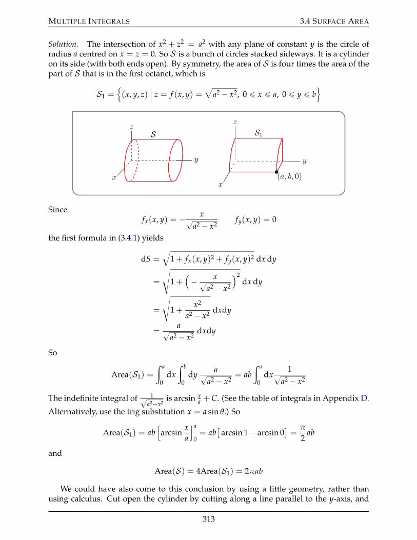
MULTIPLE INTEGRALS 3.4 SURFACE AREA
Solution. The intersection of x2 + z2 = a2 with any plane of constant y is the circle ofradius a centred on x = z = 0. So S is a bunch of circles stacked sideways. It is a cylinderon its side (with both ends open). By symmetry, the area of S is four times the area of thepart of S that is in the first octanct, which is
S1 =!(x, y, z)
ˇˇ z = f (x, y) =
aa2 ´ x2, 0 ď x ď a, 0 ď y ď b
)
y
z
x
S
y
z
x
S1
pa, b, 0q
Sincefx(x, y) = ´ x?
a2 ´ x2fy(x, y) = 0
the first formula in (3.4.1) yields
dS =b
1 + fx(x, y)2 + fy(x, y)2 dx dy
=
d1 +
(´ x?
a2 ´ x2
)2dx dy
=
d1 +
x2
a2 ´ x2 dxdy
=a?
a2 ´ x2dxdy
So
Area(S1) =
ż a
0dx
ż b
0dy
a?a2 ´ x2
= abż a
0dx
1?a2 ´ x2
The indefinite integral of 1?a2´x2
is arcsin xa + C. (See the table of integrals in Appendix D.
Alternatively, use the trig substitution x = a sin θ.) So
Area(S1) = ab[arcsin
xa
]a
0= ab
[arcsin 1´ arcsin 0
]=
π
2ab
and
Area(S) = 4Area(S1) = 2πab
We could have also come to this conclusion by using a little geometry, rather thanusing calculus. Cut open the cylinder by cutting along a line parallel to the y-axis, and
313
MULTIPLE INTEGRALS 3.4 SURFACE AREA
then flatten out the cylinder. This gives a rectangle. One side of the rectangle is just acircle of radius a, straightened out. So the rectangle has sides of lengths 2πa and b and hasarea 2πab.
Example 3.4.4
Example 3.4.5 (Area of a hemisphere)
This time we compute the surface area of the hemisphere
x2 + y2 + z2 = a2 z ě 0
(with a ą 0). You probably know, from high school, that the answer is 12 ˆ 4πa2 = 2πa2.
But you have probably not seen a derivation29 of this answer. Note that, since x2 + y2 =a2 ´ z2 on the hemisphere, the set of (x, y)’s for which there is a z with (x, y, z) on thehemisphere is exactly
(x, y) P R2
ˇx2 + y2 ď a2 (. So the hemisphere is
S =!(x, y, z)
ˇˇ z =
ba2 ´ x2 ´ y2, x2 + y2 ď a2
)
We will compute the area of S by applying (3.4.1) to
z = f (x, y) =b
a2 ´ x2 ´ y2 with (x, y) running over x2 + y2 ď a2
The first formula in (3.4.1) yields
dS =b
1 + fx(x, y)2 + fy(x, y)2 dxdy
=
d1 +
( ´xaa2 ´ x2 ´ y2
)2+( ´ya
a2 ´ x2 ´ y2
)2dxdy
=
d1 +
x2 + y2
a2 ´ x2 ´ y2 dxdy
=
da2
a2 ´ x2 ´ y2 dxdy
So the area isť
x2+y2ďa2a?
a2´x2´y2 dxdy. To evaluate this integral, we switch to polar
29 There is a pun hidden here, because you can (with a little thought) also get the surface area by differen-tiating the volume with respect to the radius.
314
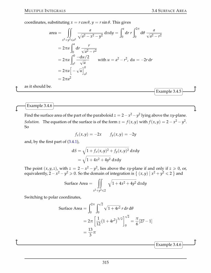
MULTIPLE INTEGRALS 3.4 SURFACE AREA
coordinates, substituting x = r cos θ, y = r sin θ. This gives
area =
ij
x2+y2ďa2
aaa2 ´ x2 ´ y2
dxdy =
ż a
0dr r
ż 2π
0dθ
a?a2 ´ r2
= 2πaż a
0dr
r?a2 ´ r2
= 2πaż 0
a2
´du/2?u
with u = a2 ´ r2, du = ´2r dr
= 2πa[´?u
]0
a2
= 2πa2
as it should be.Example 3.4.5
Example 3.4.6
Find the surface area of the part of the paraboloid z = 2´ x2´ y2 lying above the xy-plane.
Solution. The equation of the surface is of the form z = f (x, y) with f (x, y) = 2´ x2 ´ y2.So
fx(x, y) = ´2x fy(x, y) = ´2y
and, by the first part of (3.4.1),
dS =b
1 + fx(x, y)2 + fy(x, y)2 dxdy
=b
1 + 4x2 + 4y2 dxdy
The point (x, y, z), with z = 2´ x2 ´ y2, lies above the xy-plane if and only if z ě 0, or,equivalently, 2´ x2 ´ y2 ě 0. So the domain of integration is
(x, y)
ˇx2 + y2 ď 2
(and
Surface Area =
ij
x2+y2ď2
b1 + 4x2 + 4y2 dxdy
Switching to polar coordinates,
Surface Area =
ż 2π
0
ż ?2
0
a1 + 4r2 r dr dθ
= 2π
[1
12(1 + 4r2)3/2
]?2
0=
π
6[27´ 1]
=133
π
Example 3.4.6
315
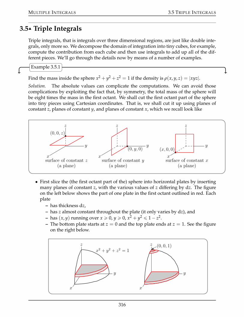
MULTIPLE INTEGRALS 3.5 TRIPLE INTEGRALS
3.5IJ Triple Integrals
Triple integrals, that is integrals over three dimensional regions, are just like double inte-grals, only more so. We decompose the domain of integration into tiny cubes, for example,compute the contribution from each cube and then use integrals to add up all of the dif-ferent pieces. We’ll go through the details now by means of a number of examples.
Example 3.5.1
Find the mass inside the sphere x2 + y2 + z2 = 1 if the density is ρ(x, y, z) = |xyz|.Solution. The absolute values can complicate the computations. We can avoid thosecomplications by exploiting the fact that, by symmetry, the total mass of the sphere willbe eight times the mass in the first octant. We shall cut the first octant part of the sphereinto tiny pieces using Cartesian coordinates. That is, we shall cut it up using planes ofconstant z, planes of constant y, and planes of constant x, which we recall look like
y
z
x
p0, 0, zq
surface of constant z(a plane)
y
z
x
p0, y, 0q
surface of constant y(a plane)
y
z
x
px, 0, 0q
surface of constant x(a plane)
• First slice the (the first octant part of the) sphere into horizontal plates by insertingmany planes of constant z, with the various values of z differing by dz. The figureon the left below shows the part of one plate in the first octant outlined in red. Eachplate
– has thickness dz,– has z almost constant throughout the plate (it only varies by dz), and– has (x, y) running over x ě 0, y ě 0, x2 + y2 ď 1´ z2.– The bottom plate starts at z = 0 and the top plate ends at z = 1. See the figure
on the right below.
z
y
x
x2 ` y2 ` z2 “ 1
z
y
x
p0, 0, 1q
316
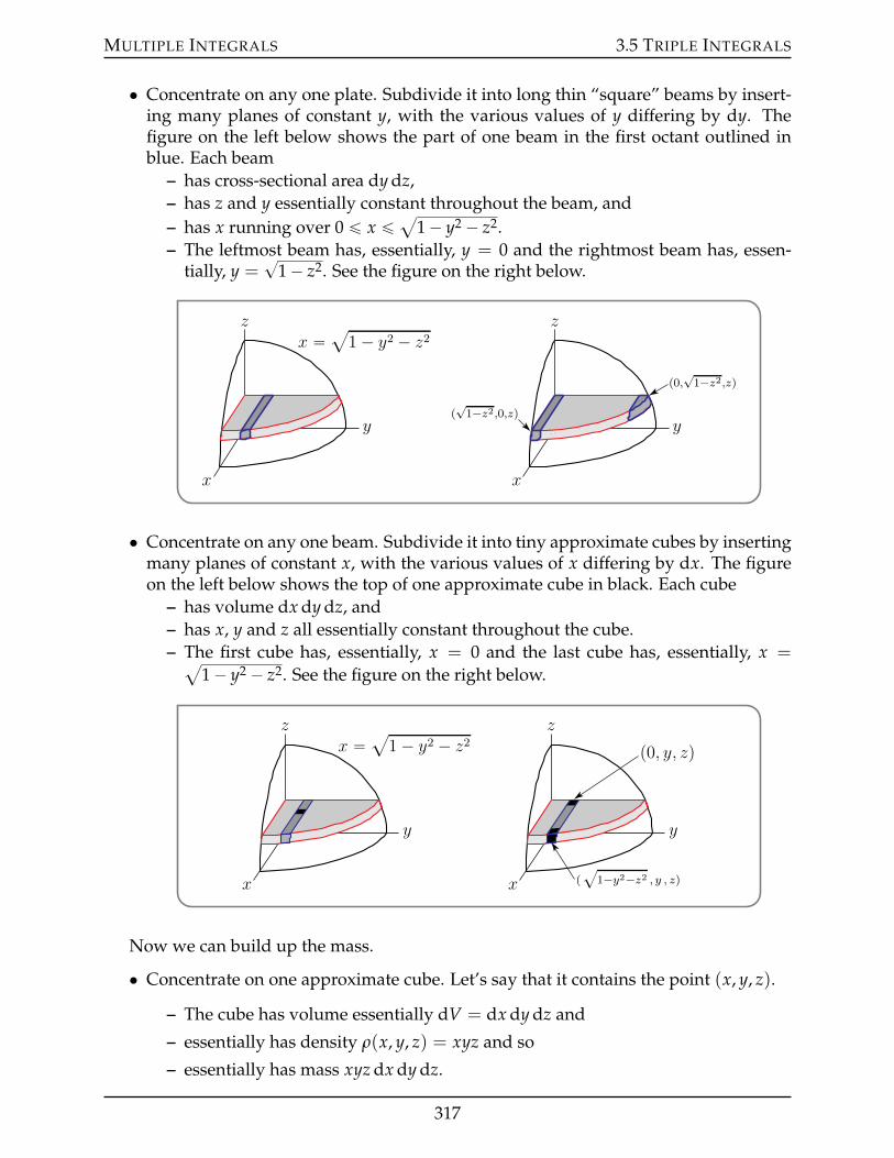
MULTIPLE INTEGRALS 3.5 TRIPLE INTEGRALS
• Concentrate on any one plate. Subdivide it into long thin “square” beams by insert-ing many planes of constant y, with the various values of y differing by dy. Thefigure on the left below shows the part of one beam in the first octant outlined inblue. Each beam
– has cross-sectional area dy dz,– has z and y essentially constant throughout the beam, and– has x running over 0 ď x ďa
1´ y2 ´ z2.– The leftmost beam has, essentially, y = 0 and the rightmost beam has, essen-
tially, y =?
1´ z2. See the figure on the right below.
z
y
x
x “ a1 ´ y2 ´ z2
z
y
x
p0,?1´z2,zq
p?1´z2,0,zq
• Concentrate on any one beam. Subdivide it into tiny approximate cubes by insertingmany planes of constant x, with the various values of x differing by dx. The figureon the left below shows the top of one approximate cube in black. Each cube
– has volume dx dy dz, and– has x, y and z all essentially constant throughout the cube.– The first cube has, essentially, x = 0 and the last cube has, essentially, x =a
1´ y2 ´ z2. See the figure on the right below.
z
y
x
x “ a1 ´ y2 ´ z2
z
y
x
p0, y, zq
p?
1´y2´z2 , y , zq
Now we can build up the mass.
• Concentrate on one approximate cube. Let’s say that it contains the point (x, y, z).
– The cube has volume essentially dV = dx dy dz and
– essentially has density ρ(x, y, z) = xyz and so
– essentially has mass xyz dx dy dz.
317
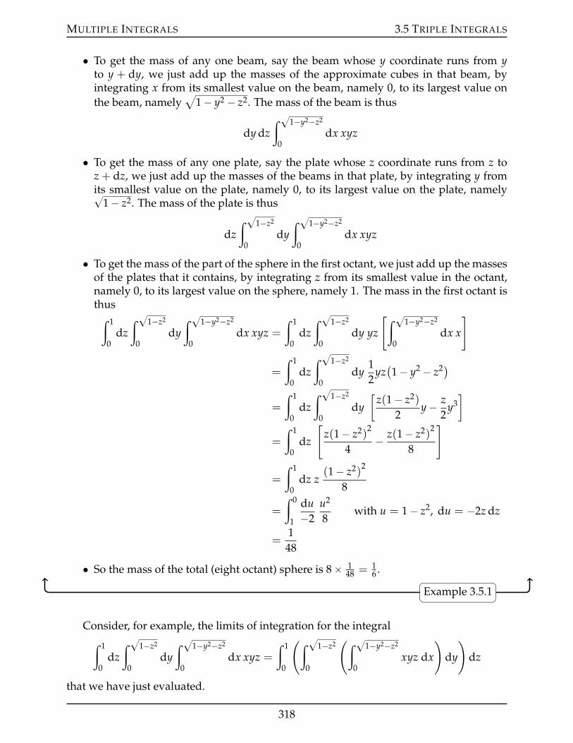
MULTIPLE INTEGRALS 3.5 TRIPLE INTEGRALS
• To get the mass of any one beam, say the beam whose y coordinate runs from yto y + dy, we just add up the masses of the approximate cubes in that beam, byintegrating x from its smallest value on the beam, namely 0, to its largest value onthe beam, namely
a1´ y2 ´ z2. The mass of the beam is thus
dy dzż ?1´y2´z2
0dx xyz
• To get the mass of any one plate, say the plate whose z coordinate runs from z toz + dz, we just add up the masses of the beams in that plate, by integrating y fromits smallest value on the plate, namely 0, to its largest value on the plate, namely?
1´ z2. The mass of the plate is thus
dzż ?1´z2
0dy
ż ?1´y2´z2
0dx xyz
• To get the mass of the part of the sphere in the first octant, we just add up the massesof the plates that it contains, by integrating z from its smallest value in the octant,namely 0, to its largest value on the sphere, namely 1. The mass in the first octant isthusż 1
0dz
ż ?1´z2
0dy
ż ?1´y2´z2
0dx xyz =
ż 1
0dz
ż ?1´z2
0dy yz
[ż ?1´y2´z2
0dx x
]
=
ż 1
0dz
ż ?1´z2
0dy
12
yz(1´ y2 ´ z2)
=
ż 1
0dz
ż ?1´z2
0dy[
z(1´ z2)
2y´ z
2y3]
=
ż 1
0dz
[z(1´ z2)
2
4´ z(1´ z2)
2
8
]
=
ż 1
0dz z
(1´ z2)2
8
=
ż 0
1
du´2
u2
8with u = 1´ z2, du = ´2z dz
=1
48
• So the mass of the total (eight octant) sphere is 8ˆ 148 = 1
6 .
Example 3.5.1
Consider, for example, the limits of integration for the integralż 1
0dz
ż ?1´z2
0dy
ż ?1´y2´z2
0dx xyz =
ż 1
0
(ż ?1´z2
0
(ż ?1´y2´z2
0xyz dx
)dy
)dz
that we have just evaluated.
318
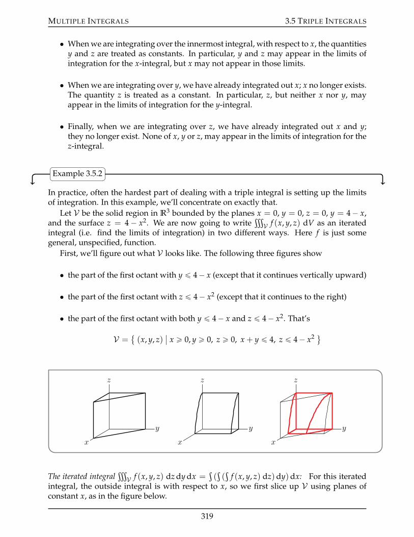
MULTIPLE INTEGRALS 3.5 TRIPLE INTEGRALS
• When we are integrating over the innermost integral, with respect to x, the quantitiesy and z are treated as constants. In particular, y and z may appear in the limits ofintegration for the x-integral, but x may not appear in those limits.
• When we are integrating over y, we have already integrated out x; x no longer exists.The quantity z is treated as a constant. In particular, z, but neither x nor y, mayappear in the limits of integration for the y-integral.
• Finally, when we are integrating over z, we have already integrated out x and y;they no longer exist. None of x, y or z, may appear in the limits of integration for thez-integral.
Example 3.5.2
In practice, often the hardest part of dealing with a triple integral is setting up the limitsof integration. In this example, we’ll concentrate on exactly that.
Let V be the solid region in R3 bounded by the planes x = 0, y = 0, z = 0, y = 4´ x,and the surface z = 4´ x2. We are now going to write
ţV f (x, y, z) dV as an iterated
integral (i.e. find the limits of integration) in two different ways. Here f is just somegeneral, unspecified, function.
First, we’ll figure out what V looks like. The following three figures show
• the part of the first octant with y ď 4´ x (except that it continues vertically upward)
• the part of the first octant with z ď 4´ x2 (except that it continues to the right)
• the part of the first octant with both y ď 4´ x and z ď 4´ x2. That’s
V = (x, y, z)
ˇx ě 0, y ě 0, z ě 0, x + y ď 4, z ď 4´ x2 (
z
y
x
z
y
x
z
y
x
The iterated integralţV f (x, y, z) dz dy dx =
ş(ş(ş
f (x, y, z) dz)dy)dx: For this iteratedintegral, the outside integral is with respect to x, so we first slice up V using planes ofconstant x, as in the figure below.
319
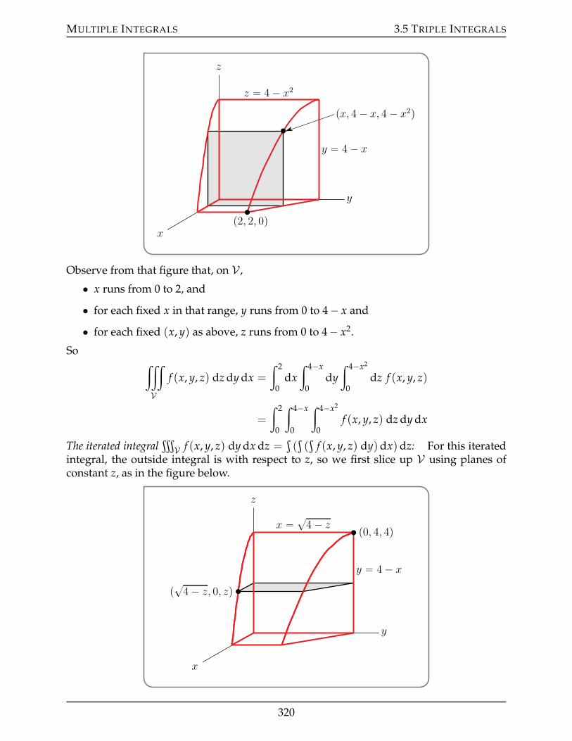
MULTIPLE INTEGRALS 3.5 TRIPLE INTEGRALS
z
y
xp2, 2, 0q
px, 4 ´ x, 4 ´ x2q
y “ 4 ´ x
z “ 4 ´ x2
Observe from that figure that, on V ,
• x runs from 0 to 2, and
• for each fixed x in that range, y runs from 0 to 4´ x and
• for each fixed (x, y) as above, z runs from 0 to 4´ x2.
So¡
V
f (x, y, z) dz dy dx =
ż 2
0dx
ż 4´x
0dy
ż 4´x2
0dz f (x, y, z)
=
ż 2
0
ż 4´x
0
ż 4´x2
0f (x, y, z) dz dy dx
The iterated integralţV f (x, y, z) dy dx dz =
ş(ş(ş
f (x, y, z) dy)dx)dz: For this iteratedintegral, the outside integral is with respect to z, so we first slice up V using planes ofconstant z, as in the figure below.
z
y
x
p0, 4, 4q
p?4 ´ z, 0, zq
y “ 4 ´ x
x “ ?4 ´ z
320
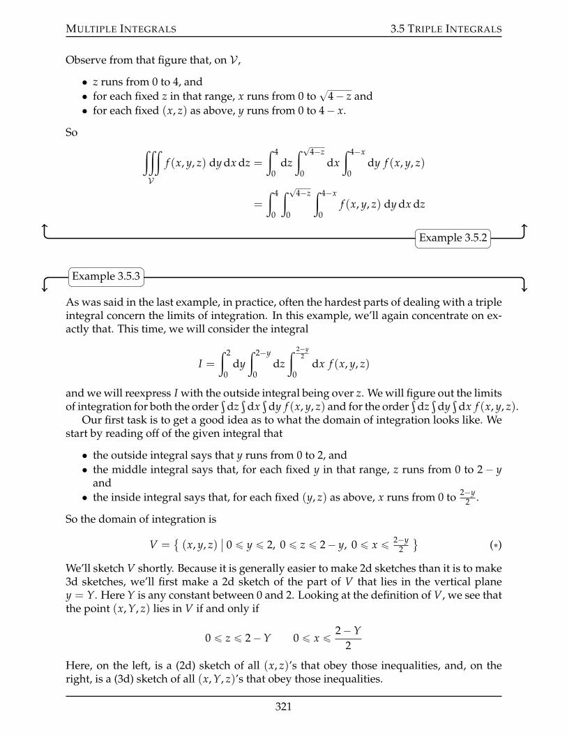
MULTIPLE INTEGRALS 3.5 TRIPLE INTEGRALS
Observe from that figure that, on V ,
• z runs from 0 to 4, and• for each fixed z in that range, x runs from 0 to
?4´ z and
• for each fixed (x, z) as above, y runs from 0 to 4´ x.
So¡
V
f (x, y, z) dy dx dz =
ż 4
0dz
ż ?4´z
0dx
ż 4´x
0dy f (x, y, z)
=
ż 4
0
ż ?4´z
0
ż 4´x
0f (x, y, z) dy dx dz
Example 3.5.2
Example 3.5.3
As was said in the last example, in practice, often the hardest parts of dealing with a tripleintegral concern the limits of integration. In this example, we’ll again concentrate on ex-actly that. This time, we will consider the integral
I =ż 2
0dy
ż 2´y
0dz
ż 2´y2
0dx f (x, y, z)
and we will reexpress I with the outside integral being over z. We will figure out the limitsof integration for both the order
şdz
şdx
şdy f (x, y, z) and for the order
şdz
şdy
şdx f (x, y, z).
Our first task is to get a good idea as to what the domain of integration looks like. Westart by reading off of the given integral that
• the outside integral says that y runs from 0 to 2, and• the middle integral says that, for each fixed y in that range, z runs from 0 to 2´ y
and• the inside integral says that, for each fixed (y, z) as above, x runs from 0 to 2´y
2 .
So the domain of integration is
V = (x, y, z)
ˇ0 ď y ď 2, 0 ď z ď 2´ y, 0 ď x ď 2´y
2
((˚)
We’ll sketch V shortly. Because it is generally easier to make 2d sketches than it is to make3d sketches, we’ll first make a 2d sketch of the part of V that lies in the vertical planey = Y. Here Y is any constant between 0 and 2. Looking at the definition of V, we see thatthe point (x, Y, z) lies in V if and only if
0 ď z ď 2´Y 0 ď x ď 2´Y2
Here, on the left, is a (2d) sketch of all (x, z)’s that obey those inequalities, and, on theright, is a (3d) sketch of all (x, Y, z)’s that obey those inequalities.
321
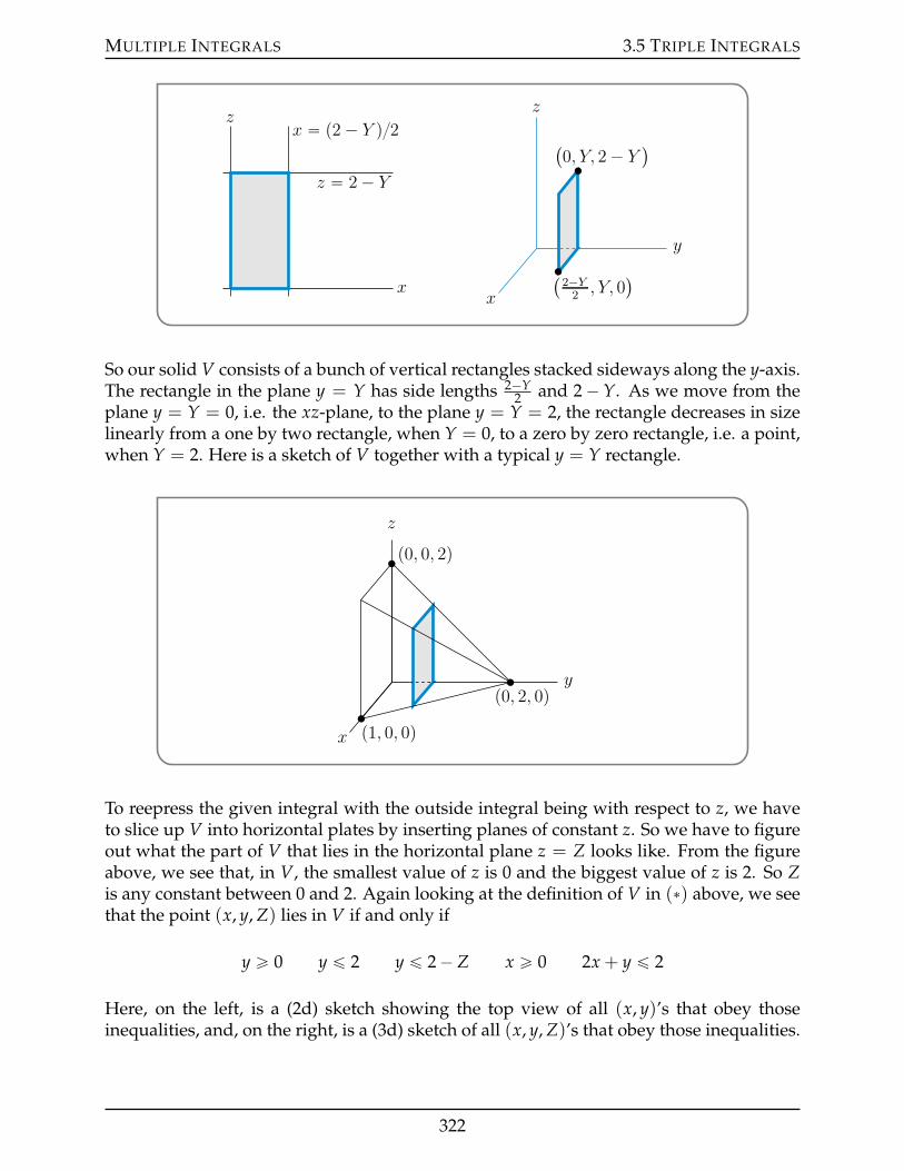
MULTIPLE INTEGRALS 3.5 TRIPLE INTEGRALS
x
z
z “ 2 ´ Y
x “ p2 ´ Y q2
`2´Y2
, Y, 0˘
`0, Y, 2 ´ Y
˘
z
y
x
So our solid V consists of a bunch of vertical rectangles stacked sideways along the y-axis.The rectangle in the plane y = Y has side lengths 2´Y
2 and 2´ Y. As we move from theplane y = Y = 0, i.e. the xz-plane, to the plane y = Y = 2, the rectangle decreases in sizelinearly from a one by two rectangle, when Y = 0, to a zero by zero rectangle, i.e. a point,when Y = 2. Here is a sketch of V together with a typical y = Y rectangle.
p1, 0, 0q
p0, 0, 2q
p0, 2, 0q
z
y
x
To reepress the given integral with the outside integral being with respect to z, we haveto slice up V into horizontal plates by inserting planes of constant z. So we have to figureout what the part of V that lies in the horizontal plane z = Z looks like. From the figureabove, we see that, in V, the smallest value of z is 0 and the biggest value of z is 2. So Zis any constant between 0 and 2. Again looking at the definition of V in (˚) above, we seethat the point (x, y, Z) lies in V if and only if
y ě 0 y ď 2 y ď 2´ Z x ě 0 2x + y ď 2
Here, on the left, is a (2d) sketch showing the top view of all (x, y)’s that obey thoseinequalities, and, on the right, is a (3d) sketch of all (x, y, Z)’s that obey those inequalities.
322
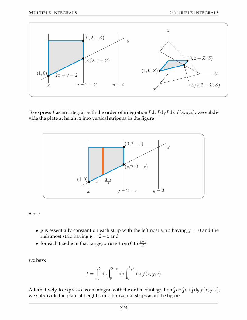
MULTIPLE INTEGRALS 3.5 TRIPLE INTEGRALS
y
x y “ 2
2x ` y “ 2
y “ 2 ´ Z
p1, 0q
pZ2, 2 ´ Zq
p0, 2 ´ Zq
p1, 0, Zq
p0, 2 ´ Z,Zq
pZ2, 2 ´ Z,Zq
z
y
x
To express I as an integral with the order of integrationş
dzş
dyş
dx f (x, y, z), we subdi-vide the plate at height z into vertical strips as in the figure
y
x y “ 2
x “ 2´y2
y “ 2 ´ z
p1, 0q
pz2, 2 ´ zq
p0, 2 ´ zq
Since
• y is essentially constant on each strip with the leftmost strip having y = 0 and therightmost strip having y = 2´ z and• for each fixed y in that range, x runs from 0 to 2´y
2
we have
I =ż 2
0dz
ż 2´z
0dy
ż 2´y2
0dx f (x, y, z)
Alternatively, to express I as an integral with the order of integrationş
dzş
dxş
dy f (x, y, z),we subdivide the plate at height z into horizontal strips as in the figure
323
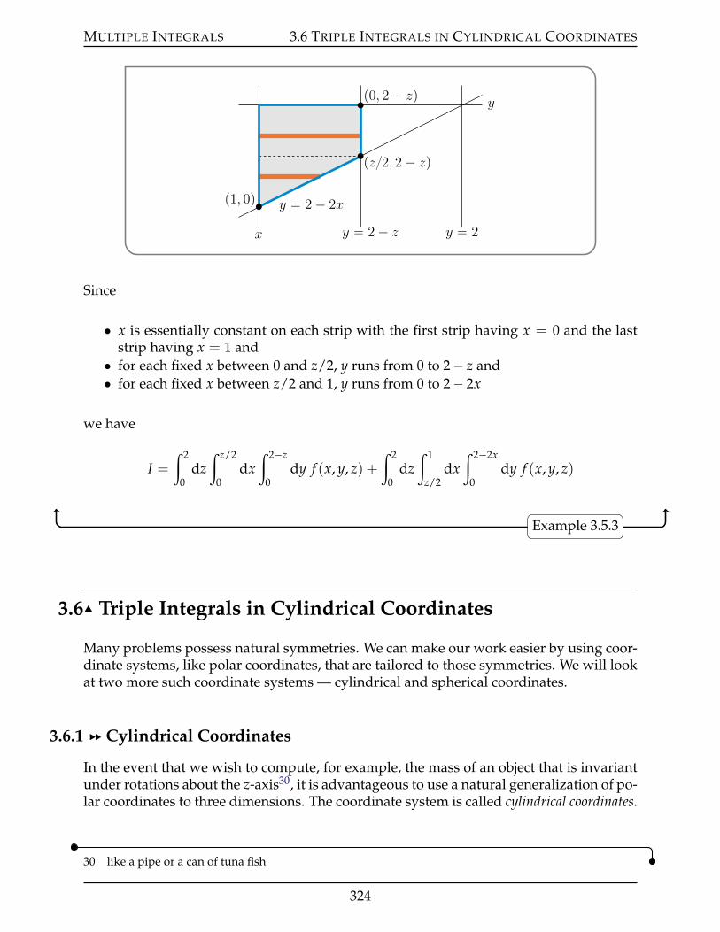
MULTIPLE INTEGRALS 3.6 TRIPLE INTEGRALS IN CYLINDRICAL COORDINATES
y
x y “ 2
y “ 2 ´ 2x
y “ 2 ´ z
p1, 0q
pz2, 2 ´ zq
p0, 2 ´ zq
Since
• x is essentially constant on each strip with the first strip having x = 0 and the laststrip having x = 1 and• for each fixed x between 0 and z/2, y runs from 0 to 2´ z and• for each fixed x between z/2 and 1, y runs from 0 to 2´ 2x
we have
I =ż 2
0dz
ż z/2
0dx
ż 2´z
0dy f (x, y, z) +
ż 2
0dz
ż 1
z/2dx
ż 2´2x
0dy f (x, y, z)
Example 3.5.3
3.6IJ Triple Integrals in Cylindrical Coordinates
Many problems possess natural symmetries. We can make our work easier by using coor-dinate systems, like polar coordinates, that are tailored to those symmetries. We will lookat two more such coordinate systems — cylindrical and spherical coordinates.
3.6.1 §§ Cylindrical Coordinates
In the event that we wish to compute, for example, the mass of an object that is invariantunder rotations about the z-axis30, it is advantageous to use a natural generalization of po-lar coordinates to three dimensions. The coordinate system is called cylindrical coordinates.
30 like a pipe or a can of tuna fish
324
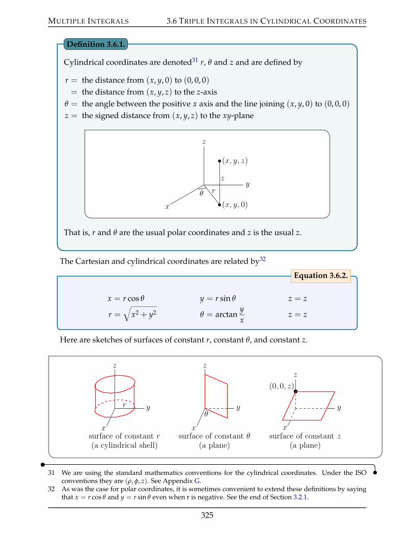
MULTIPLE INTEGRALS 3.6 TRIPLE INTEGRALS IN CYLINDRICAL COORDINATES
Cylindrical coordinates are denoted31 r, θ and z and are defined by
r = the distance from (x, y, 0) to (0, 0, 0)= the distance from (x, y, z) to the z-axis
θ = the angle between the positive x axis and the line joining (x, y, 0) to (0, 0, 0)z = the signed distance from (x, y, z) to the xy-plane
px, y, zq
px, y, 0q
y
z
x
z
rθ
That is, r and θ are the usual polar coordinates and z is the usual z.
Definition 3.6.1.
The Cartesian and cylindrical coordinates are related by32
x = r cos θ y = r sin θ z = z
r =b
x2 + y2 θ = arctanyx
z = z
Equation 3.6.2.
Here are sketches of surfaces of constant r, constant θ, and constant z.
y
z
x
r
surface of constant r(a cylindrical shell)
y
z
x
θ
surface of constant θ(a plane)
y
z
x
p0, 0, zq
surface of constant z(a plane)
31 We are using the standard mathematics conventions for the cylindrical coordinates. Under the ISOconventions they are (ρ, φ, z). See Appendix G.
32 As was the case for polar coordinates, it is sometimes convenient to extend these definitions by sayingthat x = r cos θ and y = r sin θ even when r is negative. See the end of Section 3.2.1.
325
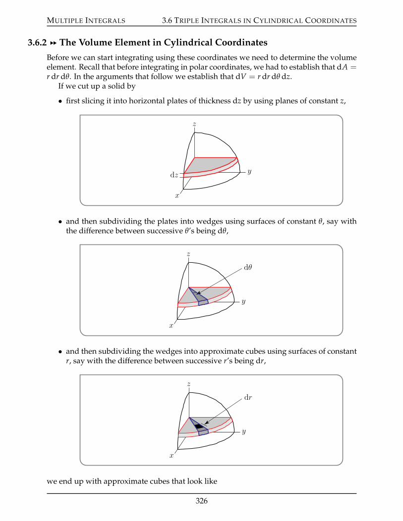
MULTIPLE INTEGRALS 3.6 TRIPLE INTEGRALS IN CYLINDRICAL COORDINATES
3.6.2 §§ The Volume Element in Cylindrical Coordinates
Before we can start integrating using these coordinates we need to determine the volumeelement. Recall that before integrating in polar coordinates, we had to establish that dA =r dr dθ. In the arguments that follow we establish that dV = r dr dθ dz.
If we cut up a solid by
• first slicing it into horizontal plates of thickness dz by using planes of constant z,
z
y
x
dz
• and then subdividing the plates into wedges using surfaces of constant θ, say withthe difference between successive θ’s being dθ,
z
y
x
dθ
• and then subdividing the wedges into approximate cubes using surfaces of constantr, say with the difference between successive r’s being dr,
z
y
x
dr
we end up with approximate cubes that look like
326
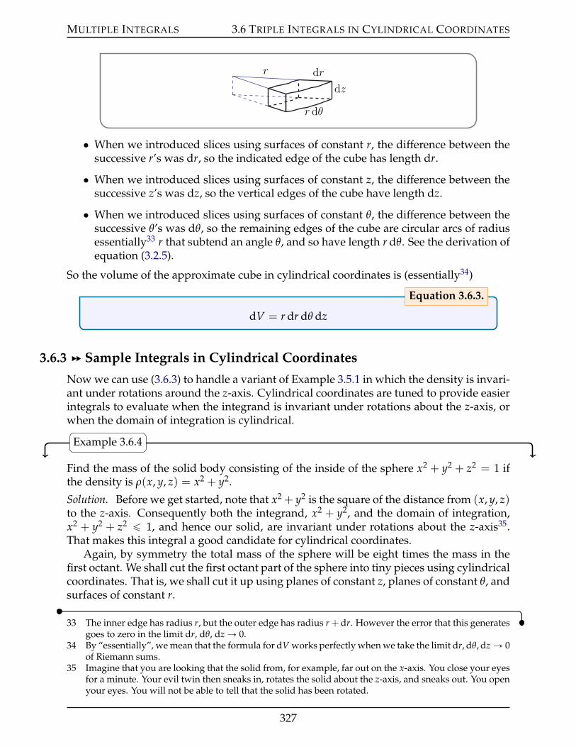
MULTIPLE INTEGRALS 3.6 TRIPLE INTEGRALS IN CYLINDRICAL COORDINATES
r dr
dz
r dθ
• When we introduced slices using surfaces of constant r, the difference between thesuccessive r’s was dr, so the indicated edge of the cube has length dr.
• When we introduced slices using surfaces of constant z, the difference between thesuccessive z’s was dz, so the vertical edges of the cube have length dz.
• When we introduced slices using surfaces of constant θ, the difference between thesuccessive θ’s was dθ, so the remaining edges of the cube are circular arcs of radiusessentially33 r that subtend an angle θ, and so have length r dθ. See the derivation ofequation (3.2.5).
So the volume of the approximate cube in cylindrical coordinates is (essentially34)
dV = r dr dθ dz
Equation 3.6.3.
3.6.3 §§ Sample Integrals in Cylindrical Coordinates
Now we can use (3.6.3) to handle a variant of Example 3.5.1 in which the density is invari-ant under rotations around the z-axis. Cylindrical coordinates are tuned to provide easierintegrals to evaluate when the integrand is invariant under rotations about the z-axis, orwhen the domain of integration is cylindrical.
Example 3.6.4
Find the mass of the solid body consisting of the inside of the sphere x2 + y2 + z2 = 1 ifthe density is ρ(x, y, z) = x2 + y2.
Solution. Before we get started, note that x2 + y2 is the square of the distance from (x, y, z)to the z-axis. Consequently both the integrand, x2 + y2, and the domain of integration,x2 + y2 + z2 ď 1, and hence our solid, are invariant under rotations about the z-axis35.That makes this integral a good candidate for cylindrical coordinates.
Again, by symmetry the total mass of the sphere will be eight times the mass in thefirst octant. We shall cut the first octant part of the sphere into tiny pieces using cylindricalcoordinates. That is, we shall cut it up using planes of constant z, planes of constant θ, andsurfaces of constant r.
33 The inner edge has radius r, but the outer edge has radius r + dr. However the error that this generatesgoes to zero in the limit dr, dθ, dz Ñ 0.
34 By “essentially”, we mean that the formula for dV works perfectly when we take the limit dr, dθ, dz Ñ 0of Riemann sums.
35 Imagine that you are looking that the solid from, for example, far out on the x-axis. You close your eyesfor a minute. Your evil twin then sneaks in, rotates the solid about the z-axis, and sneaks out. You openyour eyes. You will not be able to tell that the solid has been rotated.
327
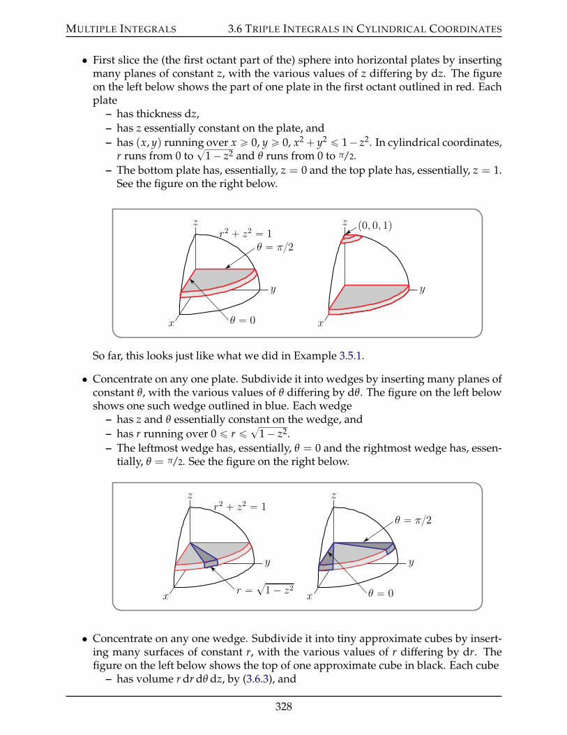
MULTIPLE INTEGRALS 3.6 TRIPLE INTEGRALS IN CYLINDRICAL COORDINATES
• First slice the (the first octant part of the) sphere into horizontal plates by insertingmany planes of constant z, with the various values of z differing by dz. The figureon the left below shows the part of one plate in the first octant outlined in red. Eachplate
– has thickness dz,– has z essentially constant on the plate, and– has (x, y) running over x ě 0, y ě 0, x2 + y2 ď 1´ z2. In cylindrical coordinates,
r runs from 0 to?
1´ z2 and θ runs from 0 to π/2.– The bottom plate has, essentially, z = 0 and the top plate has, essentially, z = 1.
See the figure on the right below.
z
y
x
r2 ` z2 “ 1θ “ π2
θ “ 0
z
y
x
p0, 0, 1q
So far, this looks just like what we did in Example 3.5.1.
• Concentrate on any one plate. Subdivide it into wedges by inserting many planes ofconstant θ, with the various values of θ differing by dθ. The figure on the left belowshows one such wedge outlined in blue. Each wedge
– has z and θ essentially constant on the wedge, and– has r running over 0 ď r ď ?1´ z2.– The leftmost wedge has, essentially, θ = 0 and the rightmost wedge has, essen-
tially, θ = π/2. See the figure on the right below.
z
y
x
r2 ` z2 “ 1
r “ ?1 ´ z2
z
y
x
θ “ π2
θ “ 0
• Concentrate on any one wedge. Subdivide it into tiny approximate cubes by insert-ing many surfaces of constant r, with the various values of r differing by dr. Thefigure on the left below shows the top of one approximate cube in black. Each cube
– has volume r dr dθ dz, by (3.6.3), and
328
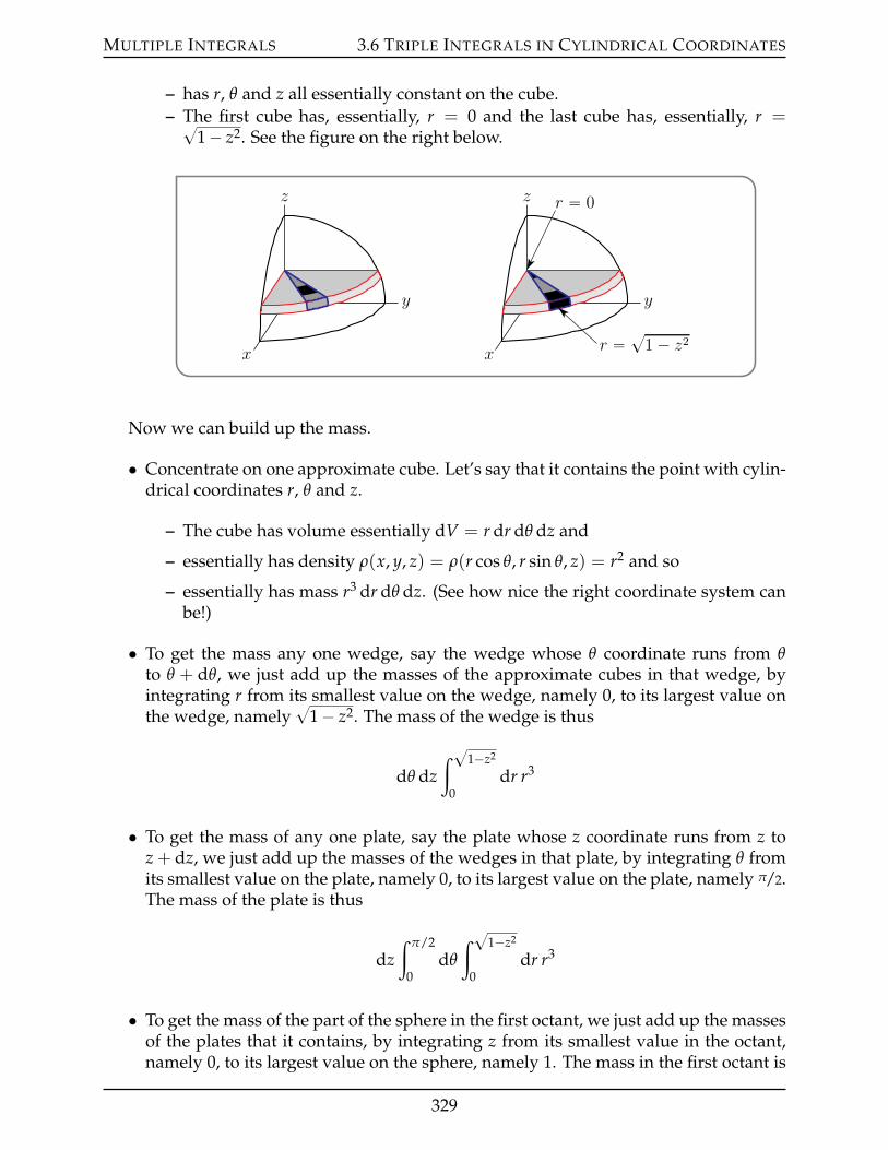
MULTIPLE INTEGRALS 3.6 TRIPLE INTEGRALS IN CYLINDRICAL COORDINATES
– has r, θ and z all essentially constant on the cube.– The first cube has, essentially, r = 0 and the last cube has, essentially, r =?
1´ z2. See the figure on the right below.
z
y
x
z
y
xr “ ?
1 ´ z2
r “ 0
Now we can build up the mass.
• Concentrate on one approximate cube. Let’s say that it contains the point with cylin-drical coordinates r, θ and z.
– The cube has volume essentially dV = r dr dθ dz and
– essentially has density ρ(x, y, z) = ρ(r cos θ, r sin θ, z) = r2 and so
– essentially has mass r3 dr dθ dz. (See how nice the right coordinate system canbe!)
• To get the mass any one wedge, say the wedge whose θ coordinate runs from θto θ + dθ, we just add up the masses of the approximate cubes in that wedge, byintegrating r from its smallest value on the wedge, namely 0, to its largest value onthe wedge, namely
?1´ z2. The mass of the wedge is thus
dθ dzż ?1´z2
0dr r3
• To get the mass of any one plate, say the plate whose z coordinate runs from z toz + dz, we just add up the masses of the wedges in that plate, by integrating θ fromits smallest value on the plate, namely 0, to its largest value on the plate, namely π/2.The mass of the plate is thus
dzż π/2
0dθ
ż ?1´z2
0dr r3
• To get the mass of the part of the sphere in the first octant, we just add up the massesof the plates that it contains, by integrating z from its smallest value in the octant,namely 0, to its largest value on the sphere, namely 1. The mass in the first octant is
329
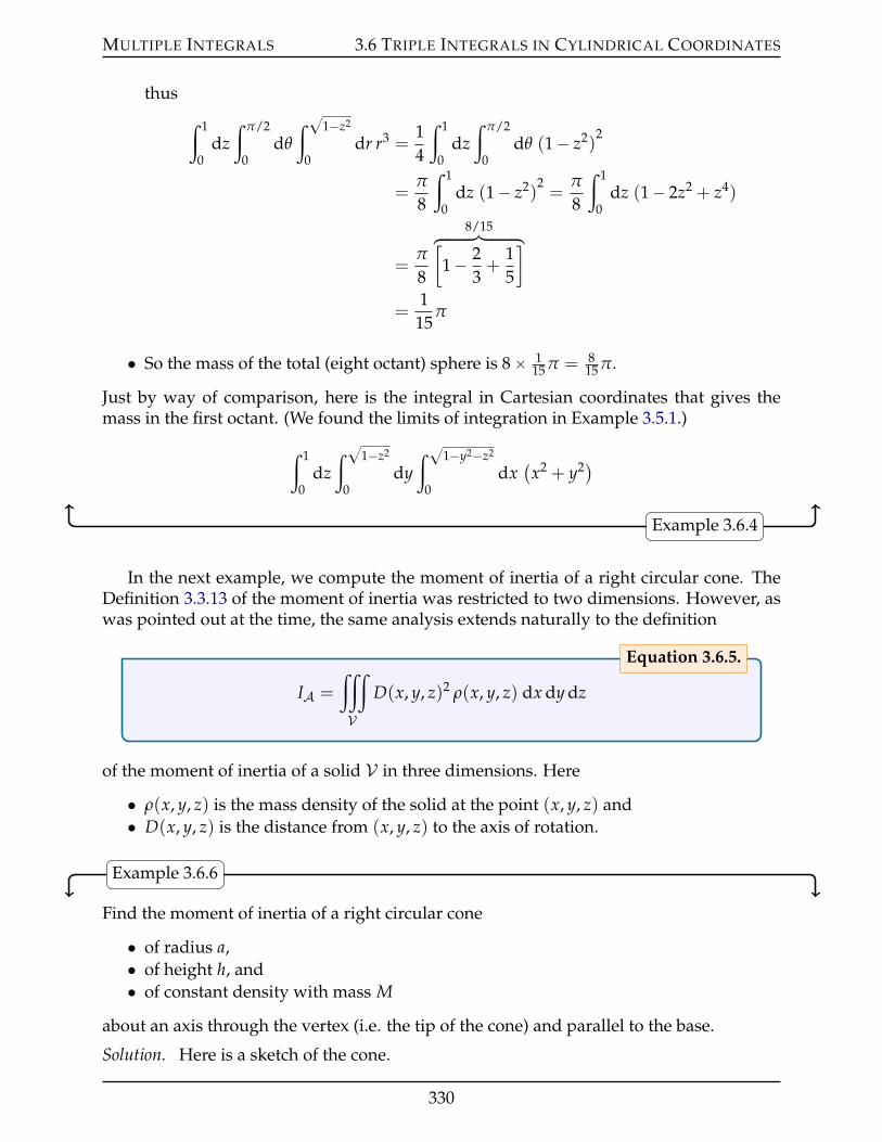
MULTIPLE INTEGRALS 3.6 TRIPLE INTEGRALS IN CYLINDRICAL COORDINATES
thus
ż 1
0dz
ż π/2
0dθ
ż ?1´z2
0dr r3 =
14
ż 1
0dz
ż π/2
0dθ (1´ z2)
2
=π
8
ż 1
0dz (1´ z2)
2=
π
8
ż 1
0dz (1´ 2z2 + z4)
=π
8
8/15hkkkkkkikkkkkkj[1´ 2
3+
15
]
=1
15π
• So the mass of the total (eight octant) sphere is 8ˆ 115 π = 8
15 π.
Just by way of comparison, here is the integral in Cartesian coordinates that gives themass in the first octant. (We found the limits of integration in Example 3.5.1.)
ż 1
0dz
ż ?1´z2
0dy
ż ?1´y2´z2
0dx(x2 + y2)
Example 3.6.4
In the next example, we compute the moment of inertia of a right circular cone. TheDefinition 3.3.13 of the moment of inertia was restricted to two dimensions. However, aswas pointed out at the time, the same analysis extends naturally to the definition
IA =
¡
V
D(x, y, z)2 ρ(x, y, z) dx dy dz
Equation 3.6.5.
of the moment of inertia of a solid V in three dimensions. Here
• ρ(x, y, z) is the mass density of the solid at the point (x, y, z) and• D(x, y, z) is the distance from (x, y, z) to the axis of rotation.
Example 3.6.6
Find the moment of inertia of a right circular cone
• of radius a,• of height h, and• of constant density with mass M
about an axis through the vertex (i.e. the tip of the cone) and parallel to the base.
Solution. Here is a sketch of the cone.
330
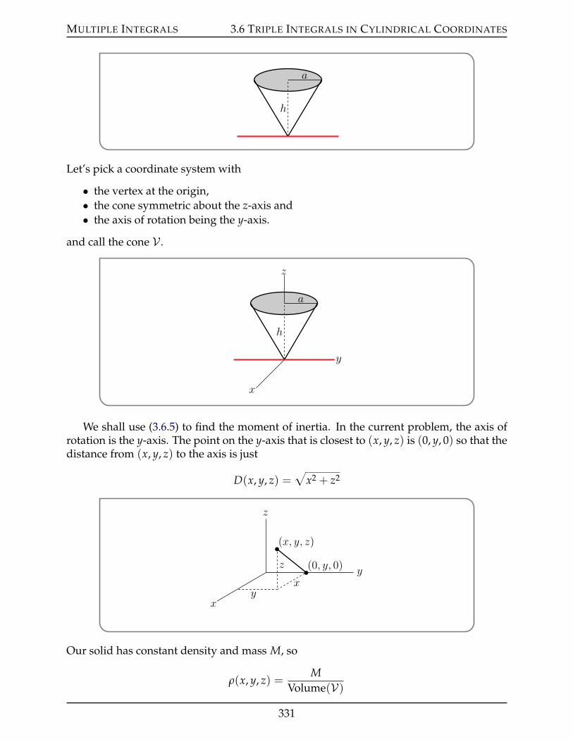
MULTIPLE INTEGRALS 3.6 TRIPLE INTEGRALS IN CYLINDRICAL COORDINATES
h
a
Let’s pick a coordinate system with
• the vertex at the origin,• the cone symmetric about the z-axis and• the axis of rotation being the y-axis.
and call the cone V .
h
a
z
y
x
We shall use (3.6.5) to find the moment of inertia. In the current problem, the axis ofrotation is the y-axis. The point on the y-axis that is closest to (x, y, z) is (0, y, 0) so that thedistance from (x, y, z) to the axis is just
D(x, y, z) =a
x2 + z2
y
z
x
px, y, zqp0, y, 0q
xy
z
Our solid has constant density and mass M, so
ρ(x, y, z) =M
Volume(V)
331
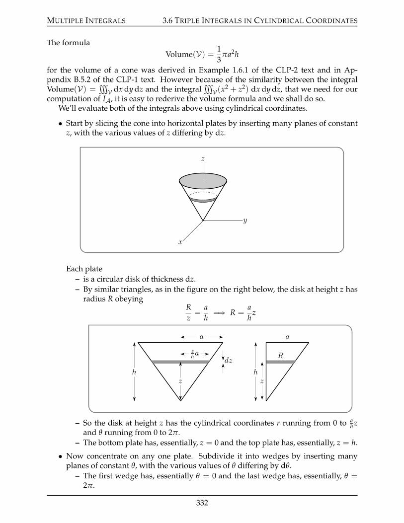
MULTIPLE INTEGRALS 3.6 TRIPLE INTEGRALS IN CYLINDRICAL COORDINATES
The formulaVolume(V) = 1
3πa2h
for the volume of a cone was derived in Example 1.6.1 of the CLP-2 text and in Ap-pendix B.5.2 of the CLP-1 text. However because of the similarity between the integralVolume(V) =
ţV dx dy dz and the integral
ţV (x2 + z2) dx dy dz, that we need for our
computation of IA, it is easy to rederive the volume formula and we shall do so.We’ll evaluate both of the integrals above using cylindrical coordinates.
• Start by slicing the cone into horizontal plates by inserting many planes of constantz, with the various values of z differing by dz.
z
y
x
Each plate– is a circular disk of thickness dz.– By similar triangles, as in the figure on the right below, the disk at height z has
radius R obeyingRz=
ahùñ R =
ah
z
dz
zh
a
zha
zh
a
R
– So the disk at height z has the cylindrical coordinates r running from 0 to ah z
and θ running from 0 to 2π.– The bottom plate has, essentially, z = 0 and the top plate has, essentially, z = h.
• Now concentrate on any one plate. Subdivide it into wedges by inserting manyplanes of constant θ, with the various values of θ differing by dθ.
– The first wedge has, essentially θ = 0 and the last wedge has, essentially, θ =2π.
332
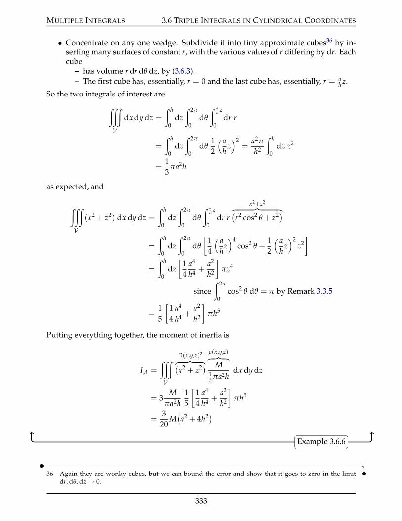
MULTIPLE INTEGRALS 3.6 TRIPLE INTEGRALS IN CYLINDRICAL COORDINATES
• Concentrate on any one wedge. Subdivide it into tiny approximate cubes36 by in-serting many surfaces of constant r, with the various values of r differing by dr. Eachcube
– has volume r dr dθ dz, by (3.6.3).– The first cube has, essentially, r = 0 and the last cube has, essentially, r = a
h z.
So the two integrals of interest are
¡
V
dx dy dz =
ż h
0dz
ż 2π
0dθ
ż ah z
0dr r
=
ż h
0dz
ż 2π
0dθ
12
( ah
z)2
=a2π
h2
ż h
0dz z2
=13
πa2h
as expected, and
¡
V
(x2 + z2) dx dy dz =
ż h
0dz
ż 2π
0dθ
ż ah z
0dr r
x2+z2hkkkkkkkkikkkkkkkkj(r2 cos2 θ + z2)
=
ż h
0dz
ż 2π
0dθ
[14
( ah
z)4
cos2 θ +12
( ah
z)2
z2]
=
ż h
0dz[
14
a4
h4 +a2
h2
]πz4
sinceż 2π
0cos2 θ dθ = π by Remark 3.3.5
=15
[14
a4
h4 +a2
h2
]πh5
Putting everything together, the moment of inertia is
IA =
¡
V
D(x,y,z)2hkkkkikkkkj(x2 + z2)
ρ(x,y,z)hkkikkjM
13 πa2h
dx dy dz
= 3M
πa2h15
[14
a4
h4 +a2
h2
]πh5
=3
20M(a2 + 4h2)
Example 3.6.6
36 Again they are wonky cubes, but we can bound the error and show that it goes to zero in the limitdr, dθ, dz Ñ 0.
333
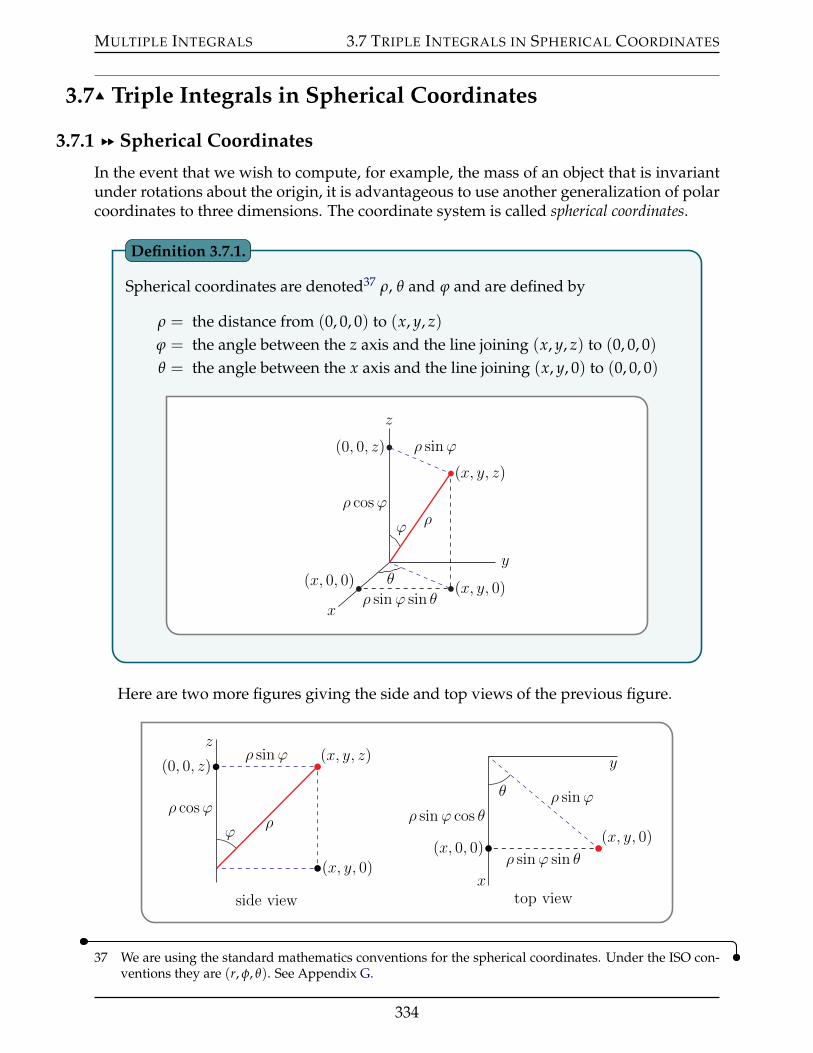
MULTIPLE INTEGRALS 3.7 TRIPLE INTEGRALS IN SPHERICAL COORDINATES
3.7IJ Triple Integrals in Spherical Coordinates
3.7.1 §§ Spherical Coordinates
In the event that we wish to compute, for example, the mass of an object that is invariantunder rotations about the origin, it is advantageous to use another generalization of polarcoordinates to three dimensions. The coordinate system is called spherical coordinates.
Spherical coordinates are denoted37 ρ, θ and ϕ and are defined by
ρ = the distance from (0, 0, 0) to (x, y, z)ϕ = the angle between the z axis and the line joining (x, y, z) to (0, 0, 0)θ = the angle between the x axis and the line joining (x, y, 0) to (0, 0, 0)
z
y
x
p0, 0, zq
px, y, 0qpx, 0, 0q θ
ϕ
px, y, zq
ρ
ρ sinϕ
ρ cosϕ
ρ sinϕ sin θ
Definition 3.7.1.
Here are two more figures giving the side and top views of the previous figure.
z
p0, 0, zq
ρ cosϕ
px, y, 0qside view
ρ sinϕ
ϕρ
px, y, zq y
x
px, 0, 0q
top view
ρ sinϕ sin θ
ρ sinϕ cos θρ sinϕθ
px, y, 0q
37 We are using the standard mathematics conventions for the spherical coordinates. Under the ISO con-ventions they are (r, φ, θ). See Appendix G.
334
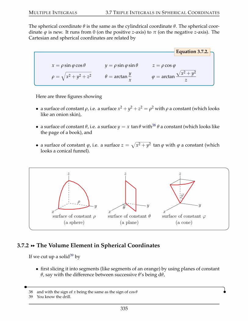
MULTIPLE INTEGRALS 3.7 TRIPLE INTEGRALS IN SPHERICAL COORDINATES
The spherical coordinate θ is the same as the cylindrical coordinate θ. The spherical coor-dinate ϕ is new. It runs from 0 (on the positive z-axis) to π (on the negative z-axis). TheCartesian and spherical coordinates are related by
x = ρ sin ϕ cos θ y = ρ sin ϕ sin θ z = ρ cos ϕ
ρ =b
x2 + y2 + z2 θ = arctanyx
ϕ = arctan
ax2 + y2
z
Equation 3.7.2.
Here are three figures showing
• a surface of constant ρ, i.e. a surface x2 + y2 + z2 = ρ2 with ρ a constant (which lookslike an onion skin),
• a surface of constant θ, i.e. a surface y = x tan θ with38 θ a constant (which looks likethe page of a book), and
• a surface of constant ϕ, i.e. a surface z =a
x2 + y2 tan ϕ with ϕ a constant (whichlooks a conical funnel).
z
yx
ρ
surface of constant ρ
(a sphere)
z
y
xθ
surface of constant θ
(a plane)
z
y
x
ϕ
surface of constant ϕ
(a cone)
3.7.2 §§ The Volume Element in Spherical Coordinates
If we cut up a solid39 by
• first slicing it into segments (like segments of an orange) by using planes of constantθ, say with the difference between successive θ’s being dθ,
38 and with the sign of x being the same as the sign of cos θ39 You know the drill.
335
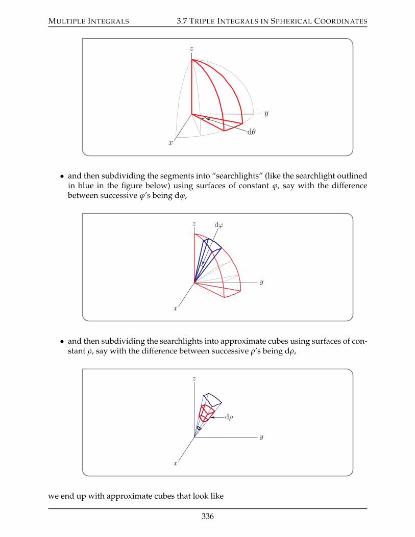
MULTIPLE INTEGRALS 3.7 TRIPLE INTEGRALS IN SPHERICAL COORDINATES
z
y
x
dθ
• and then subdividing the segments into “searchlights” (like the searchlight outlinedin blue in the figure below) using surfaces of constant ϕ, say with the differencebetween successive ϕ’s being dϕ,
z
y
x
dϕ
• and then subdividing the searchlights into approximate cubes using surfaces of con-stant ρ, say with the difference between successive ρ’s being dρ,
z
y
x
dρ
we end up with approximate cubes that look like
336
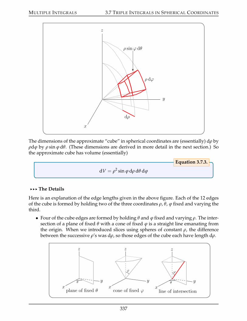
MULTIPLE INTEGRALS 3.7 TRIPLE INTEGRALS IN SPHERICAL COORDINATES
z
y
x
dρ
ρ dϕ
ρ sinϕ dθ
The dimensions of the approximate “cube” in spherical coordinates are (essentially) dρ byρdϕ by ρ sin ϕ dθ. (These dimensions are derived in more detail in the next section.) Sothe approximate cube has volume (essentially)
dV = ρ2 sin ϕ dρ dθ dϕ
Equation 3.7.3.
§§§ The Details
Here is an explanation of the edge lengths given in the above figure. Each of the 12 edgesof the cube is formed by holding two of the three coordinates ρ, θ, ϕ fixed and varying thethird.
• Four of the cube edges are formed by holding θ and ϕ fixed and varying ρ. The inter-section of a plane of fixed θ with a cone of fixed ϕ is a straight line emanating fromthe origin. When we introduced slices using spheres of constant ρ, the differencebetween the successive ρ’s was dρ, so those edges of the cube each have length dρ.
z
y
xθ
plane of fixed θ
z
y
x
ϕ
cone of fixed ϕ
z
y
xθ
ϕ
line of intersection
337
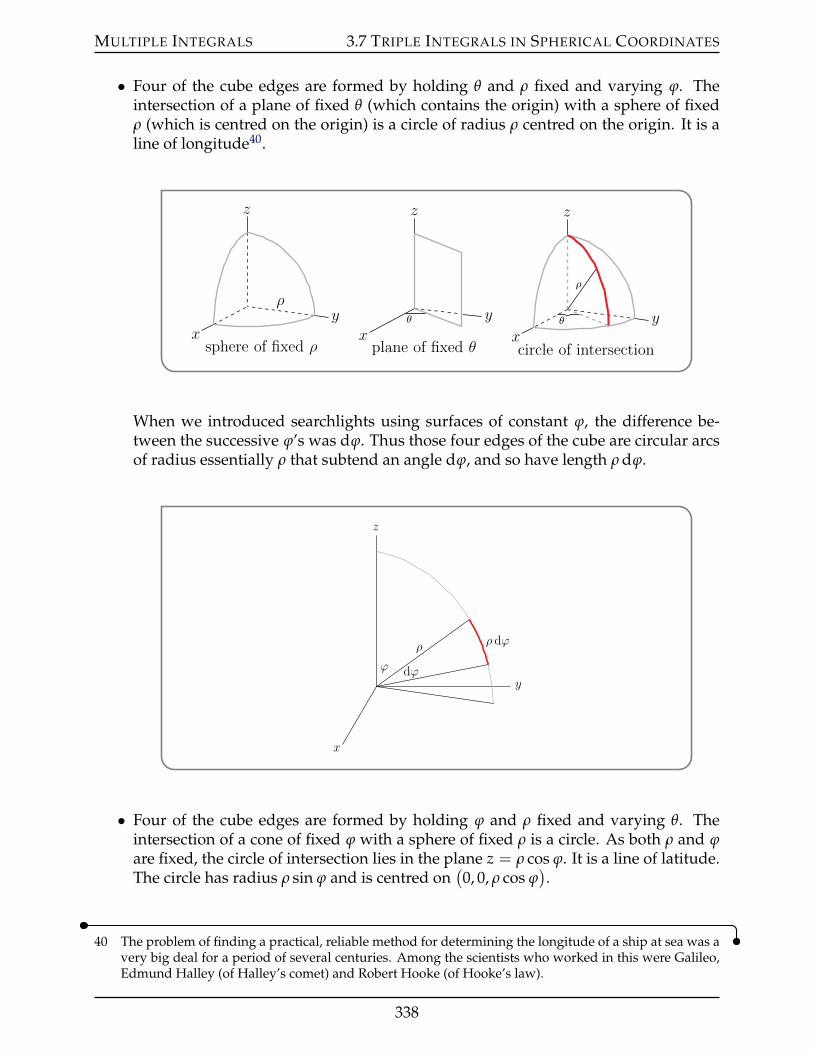
MULTIPLE INTEGRALS 3.7 TRIPLE INTEGRALS IN SPHERICAL COORDINATES
• Four of the cube edges are formed by holding θ and ρ fixed and varying ϕ. Theintersection of a plane of fixed θ (which contains the origin) with a sphere of fixedρ (which is centred on the origin) is a circle of radius ρ centred on the origin. It is aline of longitude40.
z
yx
ρ
sphere of fixed ρ
z
y
xθ
plane of fixed θ
z
yx
ρ
θ
circle of intersection
When we introduced searchlights using surfaces of constant ϕ, the difference be-tween the successive ϕ’s was dϕ. Thus those four edges of the cube are circular arcsof radius essentially ρ that subtend an angle dϕ, and so have length ρ dϕ.
z
y
x
ρ ρ dϕ
ϕ dϕ
• Four of the cube edges are formed by holding ϕ and ρ fixed and varying θ. Theintersection of a cone of fixed ϕ with a sphere of fixed ρ is a circle. As both ρ and ϕare fixed, the circle of intersection lies in the plane z = ρ cos ϕ. It is a line of latitude.The circle has radius ρ sin ϕ and is centred on
(0, 0, ρ cos ϕ
).
40 The problem of finding a practical, reliable method for determining the longitude of a ship at sea was avery big deal for a period of several centuries. Among the scientists who worked in this were Galileo,Edmund Halley (of Halley’s comet) and Robert Hooke (of Hooke’s law).
338
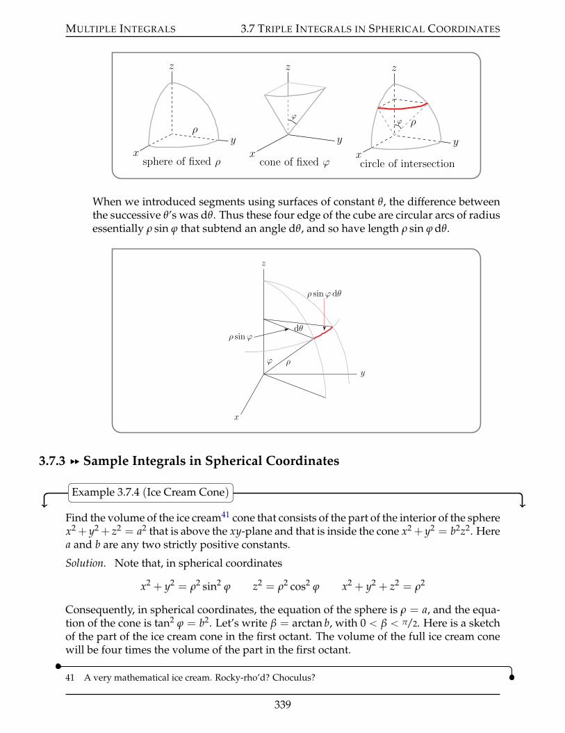
MULTIPLE INTEGRALS 3.7 TRIPLE INTEGRALS IN SPHERICAL COORDINATES
z
yx
ρ
sphere of fixed ρ
z
y
x
ϕ
cone of fixed ϕ
z
yx
ϕ ρ
circle of intersection
When we introduced segments using surfaces of constant θ, the difference betweenthe successive θ’s was dθ. Thus these four edge of the cube are circular arcs of radiusessentially ρ sin ϕ that subtend an angle dθ, and so have length ρ sin ϕ dθ.
z
y
x
ρ sinϕ
ϕ ρ
dθ
ρ sinϕ dθ
3.7.3 §§ Sample Integrals in Spherical Coordinates
Example 3.7.4 (Ice Cream Cone)
Find the volume of the ice cream41 cone that consists of the part of the interior of the spherex2 + y2 + z2 = a2 that is above the xy-plane and that is inside the cone x2 + y2 = b2z2. Herea and b are any two strictly positive constants.
Solution. Note that, in spherical coordinates
x2 + y2 = ρ2 sin2 ϕ z2 = ρ2 cos2 ϕ x2 + y2 + z2 = ρ2
Consequently, in spherical coordinates, the equation of the sphere is ρ = a, and the equa-tion of the cone is tan2 ϕ = b2. Let’s write β = arctan b, with 0 ă β ă π/2. Here is a sketchof the part of the ice cream cone in the first octant. The volume of the full ice cream conewill be four times the volume of the part in the first octant.
41 A very mathematical ice cream. Rocky-rho’d? Choculus?
339
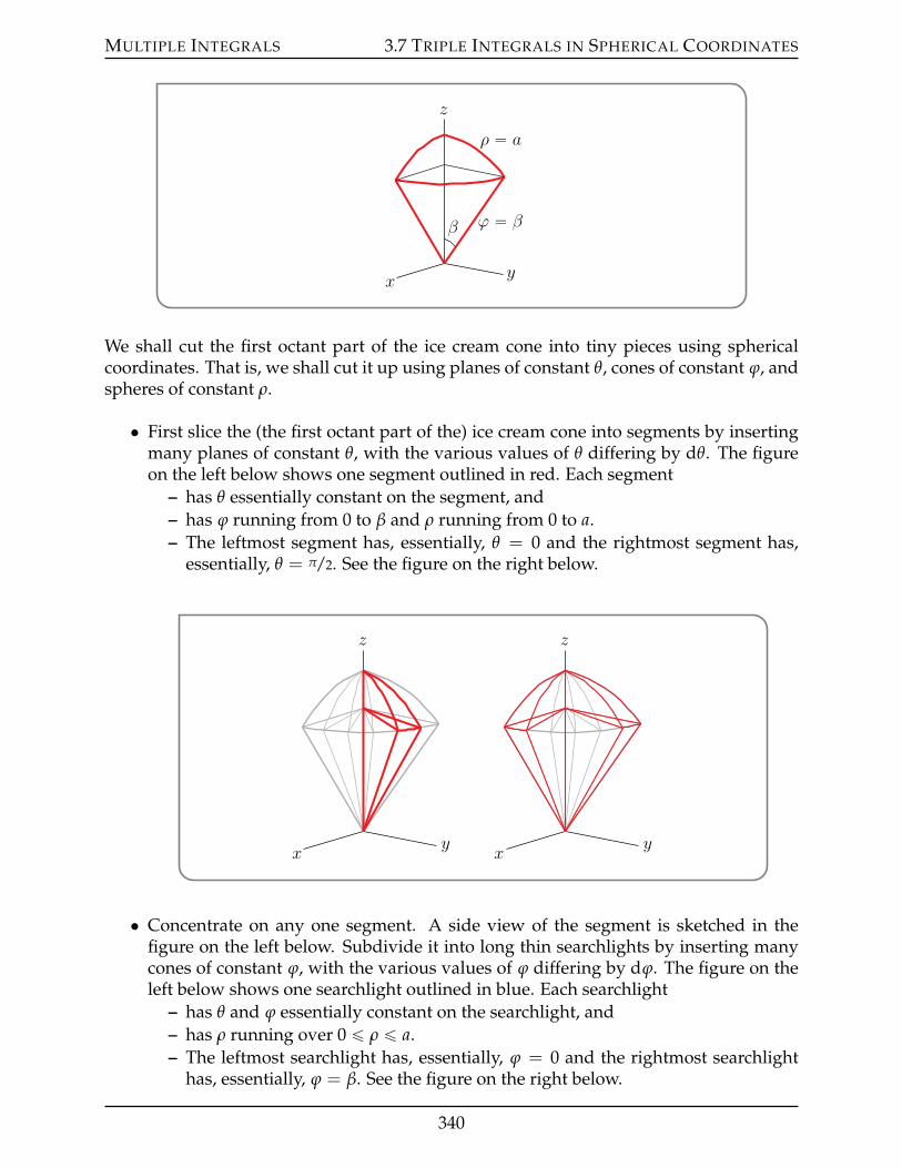
MULTIPLE INTEGRALS 3.7 TRIPLE INTEGRALS IN SPHERICAL COORDINATES
z
yx
β ϕ “ β
ρ “ a
We shall cut the first octant part of the ice cream cone into tiny pieces using sphericalcoordinates. That is, we shall cut it up using planes of constant θ, cones of constant ϕ, andspheres of constant ρ.
• First slice the (the first octant part of the) ice cream cone into segments by insertingmany planes of constant θ, with the various values of θ differing by dθ. The figureon the left below shows one segment outlined in red. Each segment
– has θ essentially constant on the segment, and– has ϕ running from 0 to β and ρ running from 0 to a.– The leftmost segment has, essentially, θ = 0 and the rightmost segment has,
essentially, θ = π/2. See the figure on the right below.
z
yx
z
yx
• Concentrate on any one segment. A side view of the segment is sketched in thefigure on the left below. Subdivide it into long thin searchlights by inserting manycones of constant ϕ, with the various values of ϕ differing by dϕ. The figure on theleft below shows one searchlight outlined in blue. Each searchlight
– has θ and ϕ essentially constant on the searchlight, and– has ρ running over 0 ď ρ ď a.– The leftmost searchlight has, essentially, ϕ = 0 and the rightmost searchlight
has, essentially, ϕ = β. See the figure on the right below.
340
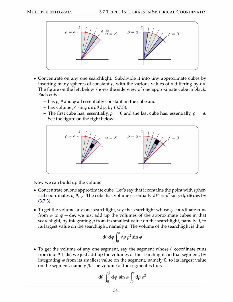
MULTIPLE INTEGRALS 3.7 TRIPLE INTEGRALS IN SPHERICAL COORDINATES
z
ϕ “ β
ϕϕ`dϕρ “ a
z
ϕ “ βρ “ a
• Concentrate on any one searchlight. Subdivide it into tiny approximate cubes byinserting many spheres of constant ρ, with the various values of ρ differing by dρ.The figure on the left below shows the side view of one approximate cube in black.Each cube
– has ρ, θ and ϕ all essentially constant on the cube and– has volume ρ2 sin ϕ dρ dθ dϕ, by (3.7.3).– The first cube has, essentially, ρ = 0 and the last cube has, essentially, ρ = a.
See the figure on the right below.
z
ϕ “ βρ “ az
ϕ “ βρ “ a
Now we can build up the volume.
• Concentrate on one approximate cube. Let’s say that it contains the point with spher-ical coordinates ρ, θ, ϕ. The cube has volume essentially dV = ρ2 sin ϕ dρ dθ dϕ, by(3.7.3).
• To get the volume any one searchlight, say the searchlight whose ϕ coordinate runsfrom ϕ to ϕ + dϕ, we just add up the volumes of the approximate cubes in thatsearchlight, by integrating ρ from its smallest value on the searchlight, namely 0, toits largest value on the searchlight, namely a. The volume of the searchlight is thus
dθ dϕ
ż a
0dρ ρ2 sin ϕ
• To get the volume of any one segment, say the segment whose θ coordinate runsfrom θ to θ + dθ, we just add up the volumes of the searchlights in that segment, byintegrating ϕ from its smallest value on the segment, namely 0, to its largest valueon the segment, namely β. The volume of the segment is thus
dθ
ż β
0dϕ sin ϕ
ż a
0dρ ρ2
341
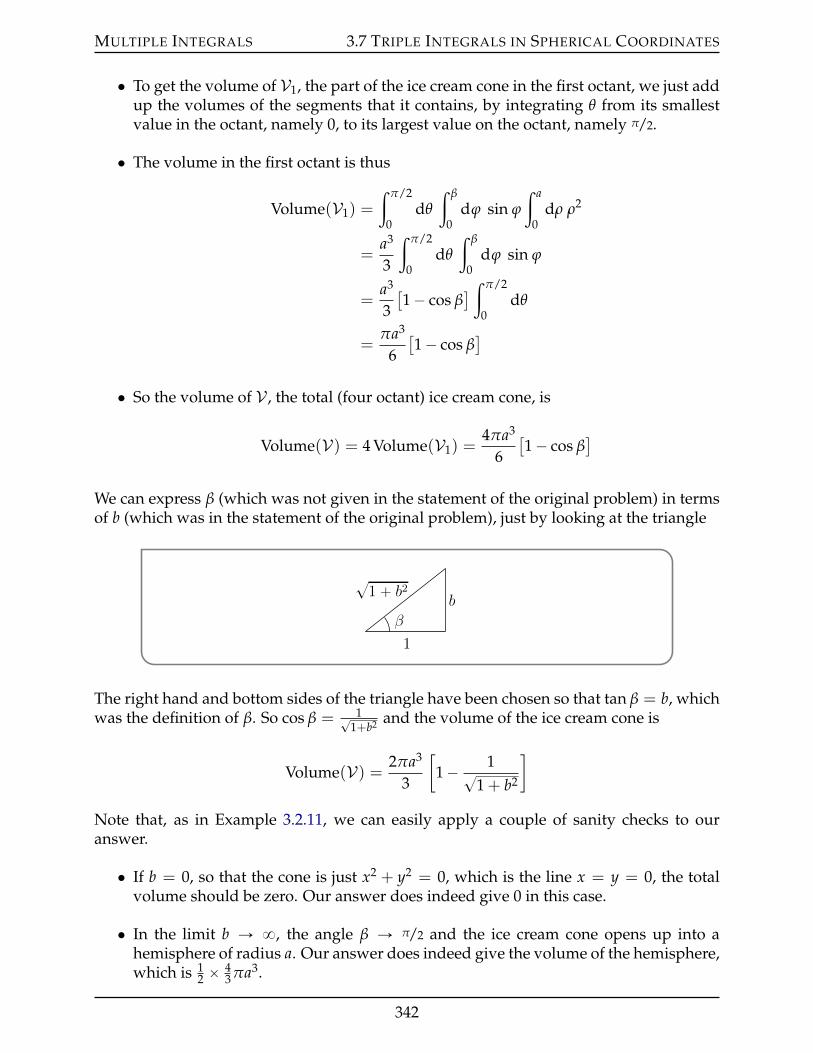
MULTIPLE INTEGRALS 3.7 TRIPLE INTEGRALS IN SPHERICAL COORDINATES
• To get the volume of V1, the part of the ice cream cone in the first octant, we just addup the volumes of the segments that it contains, by integrating θ from its smallestvalue in the octant, namely 0, to its largest value on the octant, namely π/2.
• The volume in the first octant is thus
Volume(V1) =
ż π/2
0dθ
ż β
0dϕ sin ϕ
ż a
0dρ ρ2
=a3
3
ż π/2
0dθ
ż β
0dϕ sin ϕ
=a3
3[1´ cos β
] ż π/2
0dθ
=πa3
6[1´ cos β
]
• So the volume of V , the total (four octant) ice cream cone, is
Volume(V) = 4 Volume(V1) =4πa3
6[1´ cos β
]
We can express β (which was not given in the statement of the original problem) in termsof b (which was in the statement of the original problem), just by looking at the triangle
β
1
b
?1 ` b2
The right hand and bottom sides of the triangle have been chosen so that tan β = b, whichwas the definition of β. So cos β = 1?
1+b2 and the volume of the ice cream cone is
Volume(V) = 2πa3
3
[1´ 1?
1 + b2
]
Note that, as in Example 3.2.11, we can easily apply a couple of sanity checks to ouranswer.
• If b = 0, so that the cone is just x2 + y2 = 0, which is the line x = y = 0, the totalvolume should be zero. Our answer does indeed give 0 in this case.
• In the limit b Ñ 8, the angle β Ñ π/2 and the ice cream cone opens up into ahemisphere of radius a. Our answer does indeed give the volume of the hemisphere,which is 1
2 ˆ 43 πa3.
342
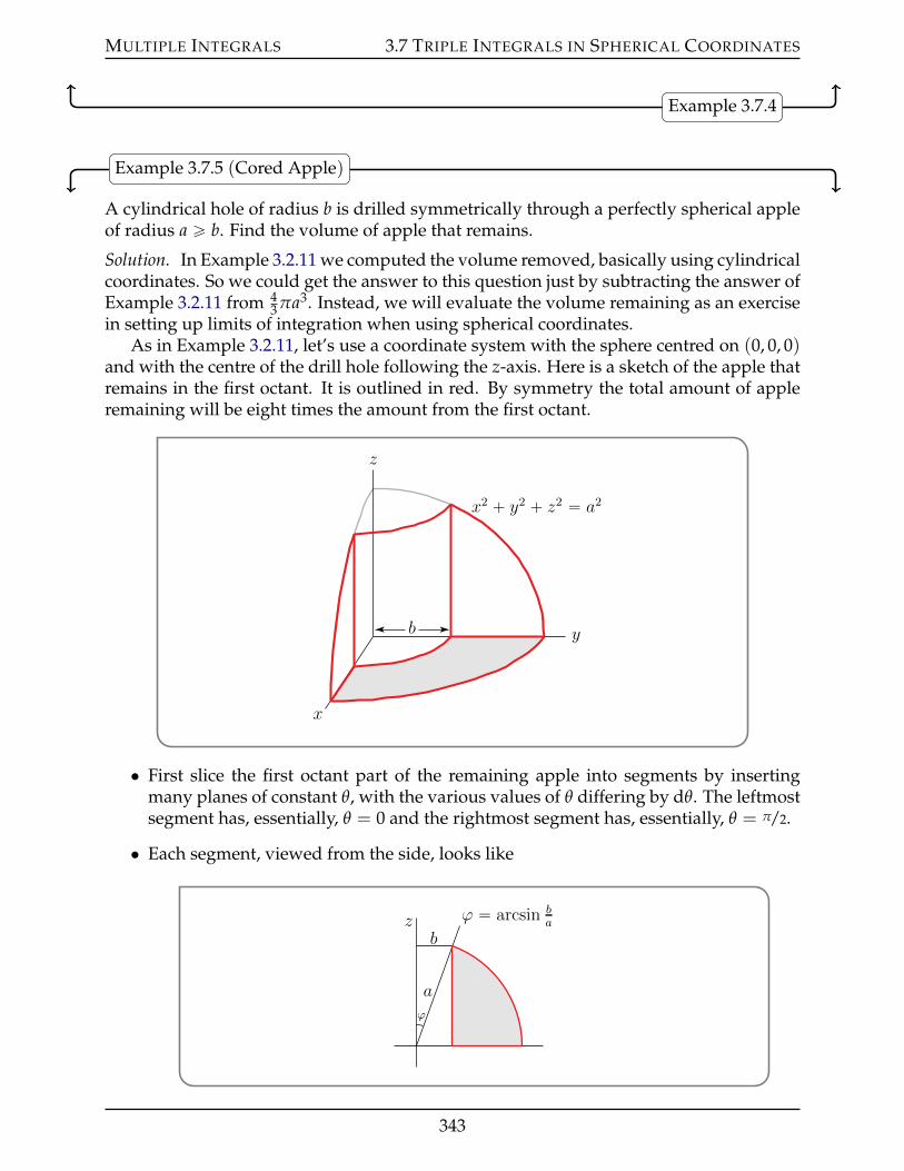
MULTIPLE INTEGRALS 3.7 TRIPLE INTEGRALS IN SPHERICAL COORDINATES
Example 3.7.4
Example 3.7.5 (Cored Apple)
A cylindrical hole of radius b is drilled symmetrically through a perfectly spherical appleof radius a ě b. Find the volume of apple that remains.
Solution. In Example 3.2.11 we computed the volume removed, basically using cylindricalcoordinates. So we could get the answer to this question just by subtracting the answer ofExample 3.2.11 from 4
3 πa3. Instead, we will evaluate the volume remaining as an exercisein setting up limits of integration when using spherical coordinates.
As in Example 3.2.11, let’s use a coordinate system with the sphere centred on (0, 0, 0)and with the centre of the drill hole following the z-axis. Here is a sketch of the apple thatremains in the first octant. It is outlined in red. By symmetry the total amount of appleremaining will be eight times the amount from the first octant.
z
y
x
b
x2 ` y2 ` z2 “ a2
• First slice the first octant part of the remaining apple into segments by insertingmany planes of constant θ, with the various values of θ differing by dθ. The leftmostsegment has, essentially, θ = 0 and the rightmost segment has, essentially, θ = π/2.
• Each segment, viewed from the side, looks like
z ϕ “ arcsin ba
a
b
ϕ
343
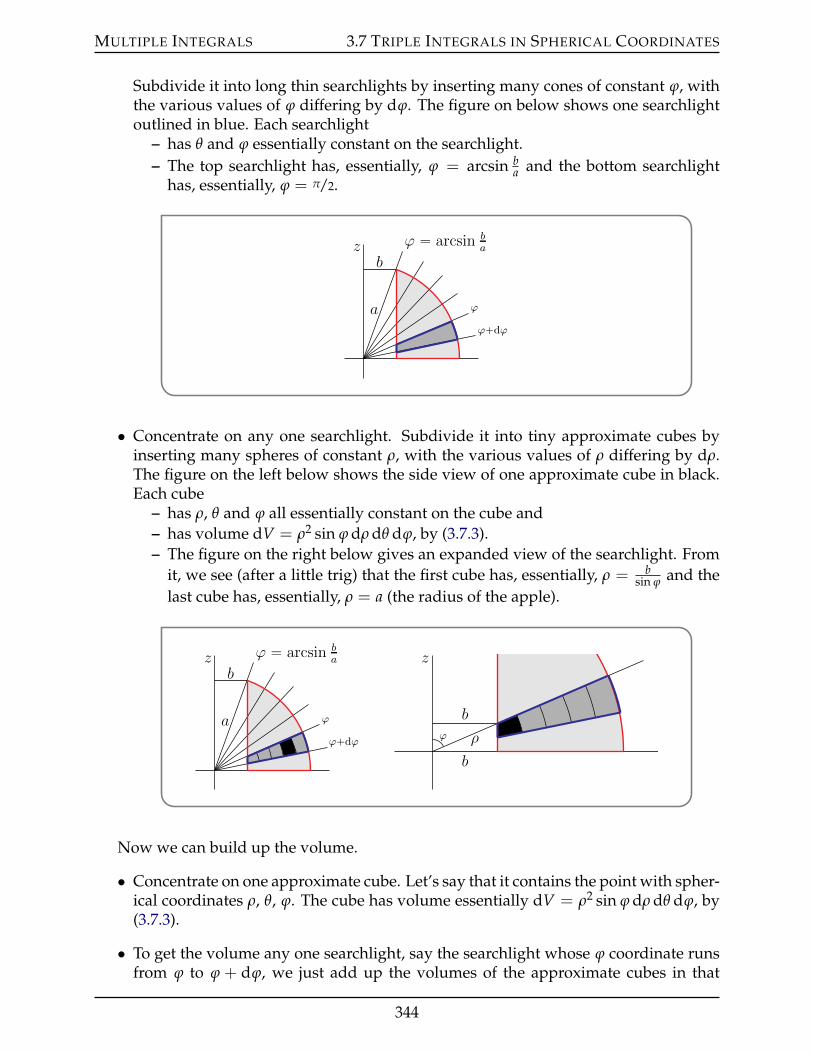
MULTIPLE INTEGRALS 3.7 TRIPLE INTEGRALS IN SPHERICAL COORDINATES
Subdivide it into long thin searchlights by inserting many cones of constant ϕ, withthe various values of ϕ differing by dϕ. The figure on below shows one searchlightoutlined in blue. Each searchlight
– has θ and ϕ essentially constant on the searchlight.– The top searchlight has, essentially, ϕ = arcsin b
a and the bottom searchlighthas, essentially, ϕ = π/2.
z ϕ “ arcsin ba
ϕ
ϕ`dϕ
a
b
• Concentrate on any one searchlight. Subdivide it into tiny approximate cubes byinserting many spheres of constant ρ, with the various values of ρ differing by dρ.The figure on the left below shows the side view of one approximate cube in black.Each cube
– has ρ, θ and ϕ all essentially constant on the cube and– has volume dV = ρ2 sin ϕ dρ dθ dϕ, by (3.7.3).– The figure on the right below gives an expanded view of the searchlight. From
it, we see (after a little trig) that the first cube has, essentially, ρ = bsin ϕ and the
last cube has, essentially, ρ = a (the radius of the apple).
z ϕ “ arcsin ba
ϕ
ϕ`dϕ
a
bz
ϕ
b
ρ
b
Now we can build up the volume.
• Concentrate on one approximate cube. Let’s say that it contains the point with spher-ical coordinates ρ, θ, ϕ. The cube has volume essentially dV = ρ2 sin ϕ dρ dθ dϕ, by(3.7.3).
• To get the volume any one searchlight, say the searchlight whose ϕ coordinate runsfrom ϕ to ϕ + dϕ, we just add up the volumes of the approximate cubes in that
344
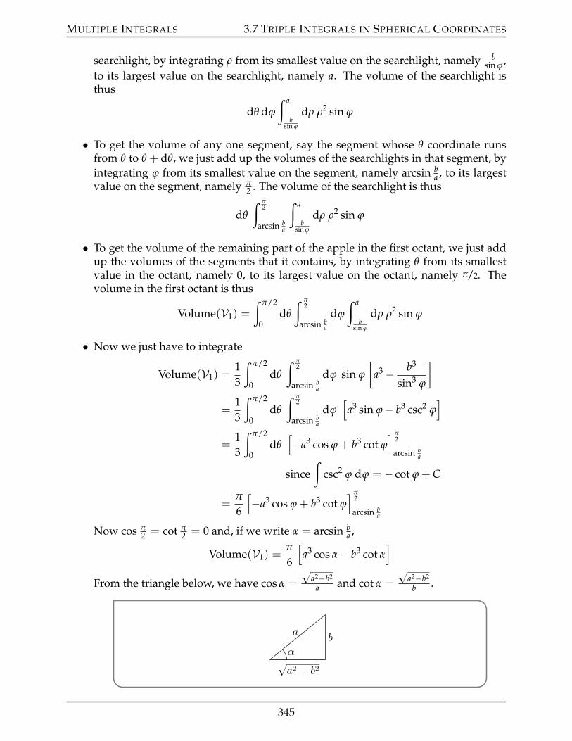
MULTIPLE INTEGRALS 3.7 TRIPLE INTEGRALS IN SPHERICAL COORDINATES
searchlight, by integrating ρ from its smallest value on the searchlight, namely bsin ϕ ,
to its largest value on the searchlight, namely a. The volume of the searchlight isthus
dθ dϕ
ż a
bsin ϕ
dρ ρ2 sin ϕ
• To get the volume of any one segment, say the segment whose θ coordinate runsfrom θ to θ + dθ, we just add up the volumes of the searchlights in that segment, byintegrating ϕ from its smallest value on the segment, namely arcsin b
a , to its largestvalue on the segment, namely π
2 . The volume of the searchlight is thus
dθ
ż π2
arcsin ba
ż a
bsin ϕ
dρ ρ2 sin ϕ
• To get the volume of the remaining part of the apple in the first octant, we just addup the volumes of the segments that it contains, by integrating θ from its smallestvalue in the octant, namely 0, to its largest value on the octant, namely π/2. Thevolume in the first octant is thus
Volume(V1) =
ż π/2
0dθ
ż π2
arcsin ba
dϕ
ż a
bsin ϕ
dρ ρ2 sin ϕ
• Now we just have to integrate
Volume(V1) =13
ż π/2
0dθ
ż π2
arcsin ba
dϕ sin ϕ
[a3 ´ b3
sin3 ϕ
]
=13
ż π/2
0dθ
ż π2
arcsin ba
dϕ[
a3 sin ϕ´ b3 csc2 ϕ]
=13
ż π/2
0dθ[´a3 cos ϕ + b3 cot ϕ
] π2
arcsin ba
sinceż
csc2 ϕ dϕ = ´ cot ϕ + C
=π
6
[´a3 cos ϕ + b3 cot ϕ
] π2
arcsin ba
Now cos π2 = cot π
2 = 0 and, if we write α = arcsin ba ,
Volume(V1) =π
6
[a3 cos α´ b3 cot α
]
From the triangle below, we have cos α =?
a2´b2
a and cot α =?
a2´b2
b .
α?a2 ´ b2
ba
345
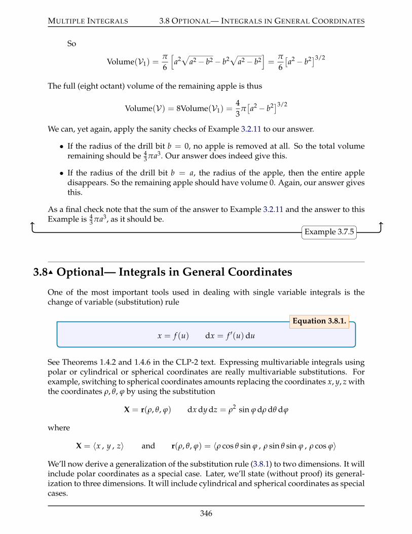
MULTIPLE INTEGRALS 3.8 OPTIONAL— INTEGRALS IN GENERAL COORDINATES
So
Volume(V1) =π
6
[a2a
a2 ´ b2 ´ b2a
a2 ´ b2]=
π
6[a2 ´ b2]3/2
The full (eight octant) volume of the remaining apple is thus
Volume(V) = 8Volume(V1) =43
π[a2 ´ b2]3/2
We can, yet again, apply the sanity checks of Example 3.2.11 to our answer.
• If the radius of the drill bit b = 0, no apple is removed at all. So the total volumeremaining should be 4
3 πa3. Our answer does indeed give this.
• If the radius of the drill bit b = a, the radius of the apple, then the entire appledisappears. So the remaining apple should have volume 0. Again, our answer givesthis.
As a final check note that the sum of the answer to Example 3.2.11 and the answer to thisExample is 4
3 πa3, as it should be.
Example 3.7.5
3.8IJ Optional— Integrals in General Coordinates
One of the most important tools used in dealing with single variable integrals is thechange of variable (substitution) rule
x = f (u) dx = f 1(u)du
Equation 3.8.1.
See Theorems 1.4.2 and 1.4.6 in the CLP-2 text. Expressing multivariable integrals usingpolar or cylindrical or spherical coordinates are really multivariable substitutions. Forexample, switching to spherical coordinates amounts replacing the coordinates x, y, z withthe coordinates ρ, θ, ϕ by using the substitution
X = r(ρ, θ, ϕ) dx dy dz = ρ2 sin ϕ dρ dθ dϕ
where
X = 〈x , y , z〉 and r(ρ, θ, ϕ) = 〈ρ cos θ sin ϕ , ρ sin θ sin ϕ , ρ cos ϕ〉
We’ll now derive a generalization of the substitution rule (3.8.1) to two dimensions. It willinclude polar coordinates as a special case. Later, we’ll state (without proof) its general-ization to three dimensions. It will include cylindrical and spherical coordinates as specialcases.
346
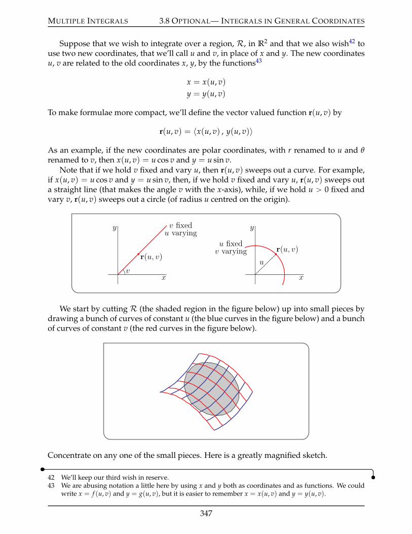
MULTIPLE INTEGRALS 3.8 OPTIONAL— INTEGRALS IN GENERAL COORDINATES
Suppose that we wish to integrate over a region, R, in R2 and that we also wish42 touse two new coordinates, that we’ll call u and v, in place of x and y. The new coordinatesu, v are related to the old coordinates x, y, by the functions43
x = x(u, v)y = y(u, v)
To make formulae more compact, we’ll define the vector valued function r(u, v) by
r(u, v) = 〈x(u, v) , y(u, v)〉
As an example, if the new coordinates are polar coordinates, with r renamed to u and θrenamed to v, then x(u, v) = u cos v and y = u sin v.
Note that if we hold v fixed and vary u, then r(u, v) sweeps out a curve. For example,if x(u, v) = u cos v and y = u sin v, then, if we hold v fixed and vary u, r(u, v) sweeps outa straight line (that makes the angle v with the x-axis), while, if we hold u ą 0 fixed andvary v, r(u, v) sweeps out a circle (of radius u centred on the origin).
rpu, vq
v fixedu varying
x
y
v
rpu, vqu fixedv varying
x
y
u
We start by cutting R (the shaded region in the figure below) up into small pieces bydrawing a bunch of curves of constant u (the blue curves in the figure below) and a bunchof curves of constant v (the red curves in the figure below).
Concentrate on any one of the small pieces. Here is a greatly magnified sketch.
42 We’ll keep our third wish in reserve.43 We are abusing notation a little here by using x and y both as coordinates and as functions. We could
write x = f (u, v) and y = g(u, v), but it is easier to remember x = x(u, v) and y = y(u, v).
347
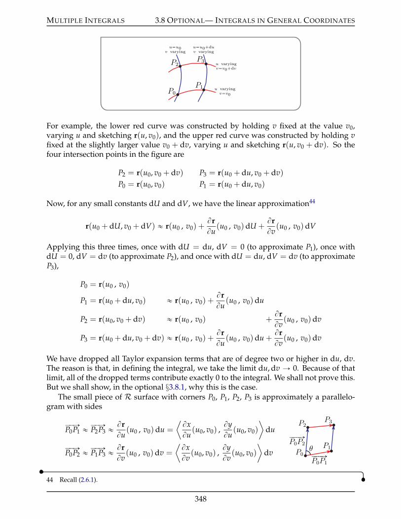
MULTIPLE INTEGRALS 3.8 OPTIONAL— INTEGRALS IN GENERAL COORDINATES
P0
P1
P3P2
u varyingv“v0
u varyingv“v0`dv
u“u0`duv varying
u“u0v varying
For example, the lower red curve was constructed by holding v fixed at the value v0,varying u and sketching r(u, v0), and the upper red curve was constructed by holding vfixed at the slightly larger value v0 + dv, varying u and sketching r(u, v0 + dv). So thefour intersection points in the figure are
P2 = r(u0, v0 + dv) P3 = r(u0 + du, v0 + dv)P0 = r(u0, v0) P1 = r(u0 + du, v0)
Now, for any small constants dU and dV, we have the linear approximation44
r(u0 + dU, v0 + dV) « r(u0 , v0) +BrBu
(u0 , v0)dU +BrBv
(u0 , v0)dV
Applying this three times, once with dU = du, dV = 0 (to approximate P1), once withdU = 0, dV = dv (to approximate P2), and once with dU = du, dV = dv (to approximateP3),
P0 = r(u0 , v0)
P1 = r(u0 + du, v0) « r(u0 , v0) +BrBu
(u0 , v0)du
P2 = r(u0, v0 + dv) « r(u0 , v0) +BrBv
(u0 , v0)dv
P3 = r(u0 + du, v0 + dv) « r(u0 , v0) +BrBu
(u0 , v0)du +BrBv
(u0 , v0)dv
We have dropped all Taylor expansion terms that are of degree two or higher in du, dv.The reason is that, in defining the integral, we take the limit du, dv Ñ 0. Because of thatlimit, all of the dropped terms contribute exactly 0 to the integral. We shall not prove this.But we shall show, in the optional §3.8.1, why this is the case.
The small piece of R surface with corners P0, P1, P2, P3 is approximately a parallelo-gram with sides
ÝÝÑP0P1 « ÝÝÑP2P3 « BrBu
(u0 , v0)du =
⟨BxBu
(u0, v0) ,ByBu
(u0, v0)
⟩du
ÝÝÑP0P2 « ÝÝÑP1P3 « BrBv
(u0 , v0)dv =
⟨BxBv
(u0, v0) ,ByBv
(u0, v0)
⟩dv P0
P1
P3P2
θÝÝÝÑP0P1
ÝÝÝÑP0P2
44 Recall (2.6.1).
348
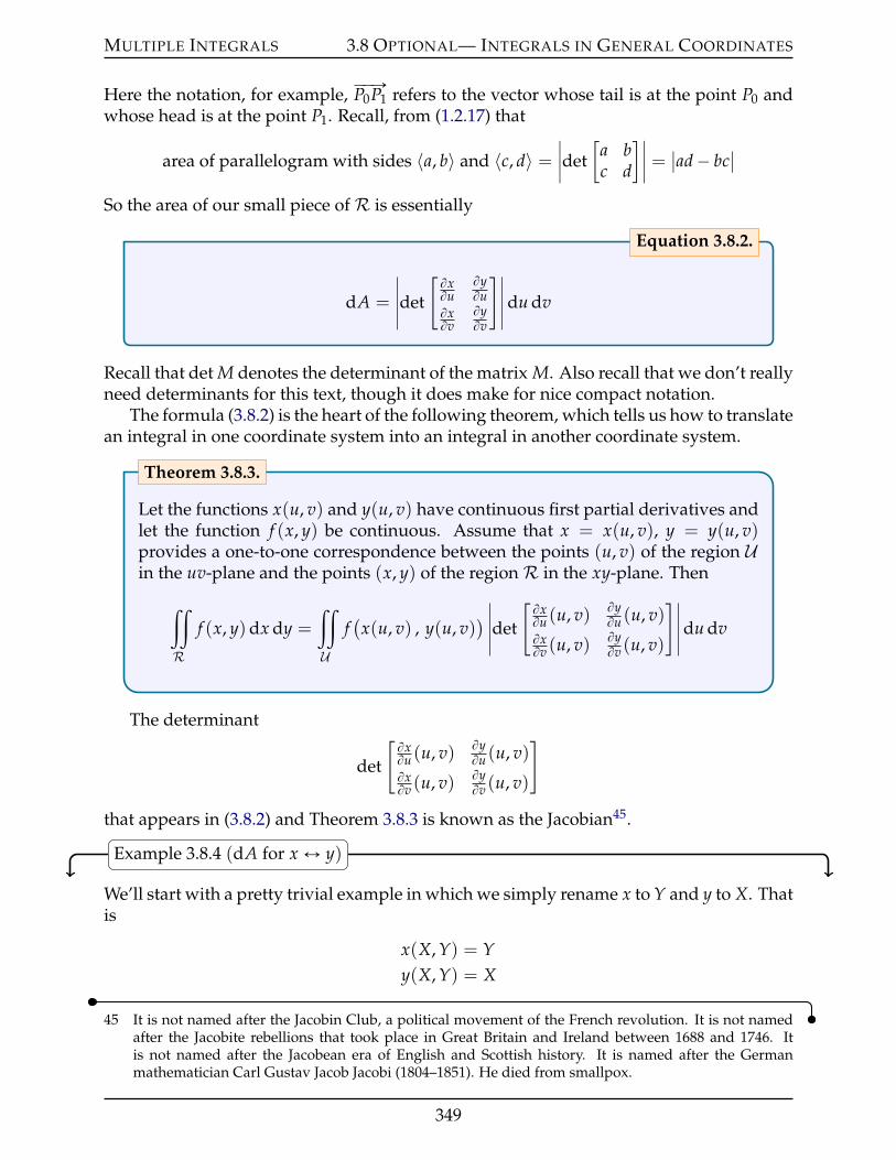
MULTIPLE INTEGRALS 3.8 OPTIONAL— INTEGRALS IN GENERAL COORDINATES
Here the notation, for example, ÝÝÑP0P1 refers to the vector whose tail is at the point P0 andwhose head is at the point P1. Recall, from (1.2.17) that
area of parallelogram with sides 〈a, b〉 and 〈c, d〉 =ˇˇdet
[a bc d
]ˇˇ =
ˇad´ bc
ˇ
So the area of our small piece ofR is essentially
dA =
ˇˇˇdet
[BxBu
ByBu
BxBv
ByBv
]ˇˇˇdu dv
Equation 3.8.2.
Recall that det M denotes the determinant of the matrix M. Also recall that we don’t reallyneed determinants for this text, though it does make for nice compact notation.
The formula (3.8.2) is the heart of the following theorem, which tells us how to translatean integral in one coordinate system into an integral in another coordinate system.
Let the functions x(u, v) and y(u, v) have continuous first partial derivatives andlet the function f (x, y) be continuous. Assume that x = x(u, v), y = y(u, v)provides a one-to-one correspondence between the points (u, v) of the region Uin the uv-plane and the points (x, y) of the regionR in the xy-plane. Then
ij
R
f (x, y)dx dy =
ij
U
f(x(u, v) , y(u, v)
)ˇˇˇdet
[BxBu (u, v) By
Bu (u, v)BxBv (u, v) By
Bv (u, v)
]ˇˇˇdu dv
Theorem 3.8.3.
The determinant
det
[BxBu (u, v) By
Bu (u, v)BxBv (u, v) By
Bv (u, v)
]
that appears in (3.8.2) and Theorem 3.8.3 is known as the Jacobian45.
Example 3.8.4 (dA for x Ø y)
We’ll start with a pretty trivial example in which we simply rename x to Y and y to X. Thatis
x(X, Y) = Yy(X, Y) = X
45 It is not named after the Jacobin Club, a political movement of the French revolution. It is not namedafter the Jacobite rebellions that took place in Great Britain and Ireland between 1688 and 1746. Itis not named after the Jacobean era of English and Scottish history. It is named after the Germanmathematician Carl Gustav Jacob Jacobi (1804–1851). He died from smallpox.
349
MULTIPLE INTEGRALS 3.8 OPTIONAL— INTEGRALS IN GENERAL COORDINATES
SinceBxBX
= 0ByBX
= 1
BxBY
= 1ByBY
= 0
(3.8.2), but with u renamed to X and v renamed to Y, gives
dA =
ˇˇˇdet
[0 11 0
]ˇˇˇdX dY = dX dY
which should really not be a shock.Example 3.8.4
Example 3.8.5 (dA for Polar Coordinates)
Polar coordinates have
x(r, θ) = r cos θ
y(r, θ) = r sin θ
SinceBxBr
= cos θByBr
= sin θ
BxBθ
= ´r sin θByBθ
= r cos θ
(3.8.2), but with u renamed to r and v renamed to θ, gives
dA =
ˇˇˇdet
[cos θ sin θ
´r sin θ r cos θ
]ˇˇˇdrdθ =
(r cos2 θ + r sin2 θ
)drdθ
= r dr dθ
which is exactly what we found in (3.2.5).Example 3.8.5
Example 3.8.6 (dA for Parabolic Coordinates)
Parabolic46 coordinates are defined by
x(u, v) =u2 ´ v2
2y(u, v) = uv
46 The name comes from the fact that both the curves of constant u and the curves of constant v areparabolas.
350
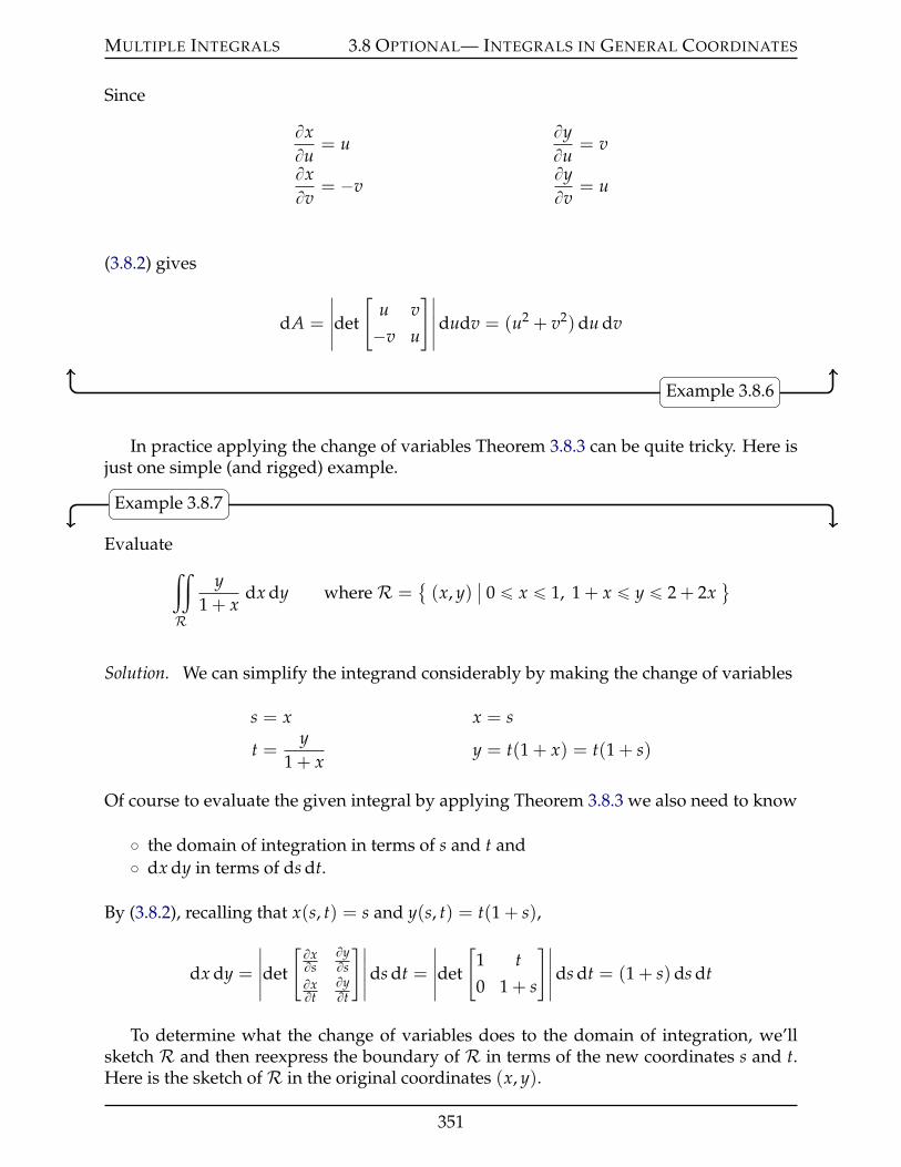
MULTIPLE INTEGRALS 3.8 OPTIONAL— INTEGRALS IN GENERAL COORDINATES
Since
BxBu
= uByBu
= v
BxBv
= ´vByBv
= u
(3.8.2) gives
dA =
ˇˇˇdet
[u v´v u
]ˇˇˇdudv = (u2 + v2)du dv
Example 3.8.6
In practice applying the change of variables Theorem 3.8.3 can be quite tricky. Here isjust one simple (and rigged) example.
Example 3.8.7
Evaluateij
R
y1 + x
dx dy whereR = (x, y)
ˇ0 ď x ď 1, 1 + x ď y ď 2 + 2x
(
Solution. We can simplify the integrand considerably by making the change of variables
s = x x = s
t =y
1 + xy = t(1 + x) = t(1 + s)
Of course to evaluate the given integral by applying Theorem 3.8.3 we also need to know
˝ the domain of integration in terms of s and t and˝ dx dy in terms of ds dt.
By (3.8.2), recalling that x(s, t) = s and y(s, t) = t(1 + s),
dx dy =
ˇˇˇdet
[BxBs
ByBs
BxBt
ByBt
]ˇˇˇds dt =
ˇˇˇdet
[1 t0 1 + s
]ˇˇˇds dt = (1 + s)ds dt
To determine what the change of variables does to the domain of integration, we’llsketch R and then reexpress the boundary of R in terms of the new coordinates s and t.Here is the sketch ofR in the original coordinates (x, y).
351
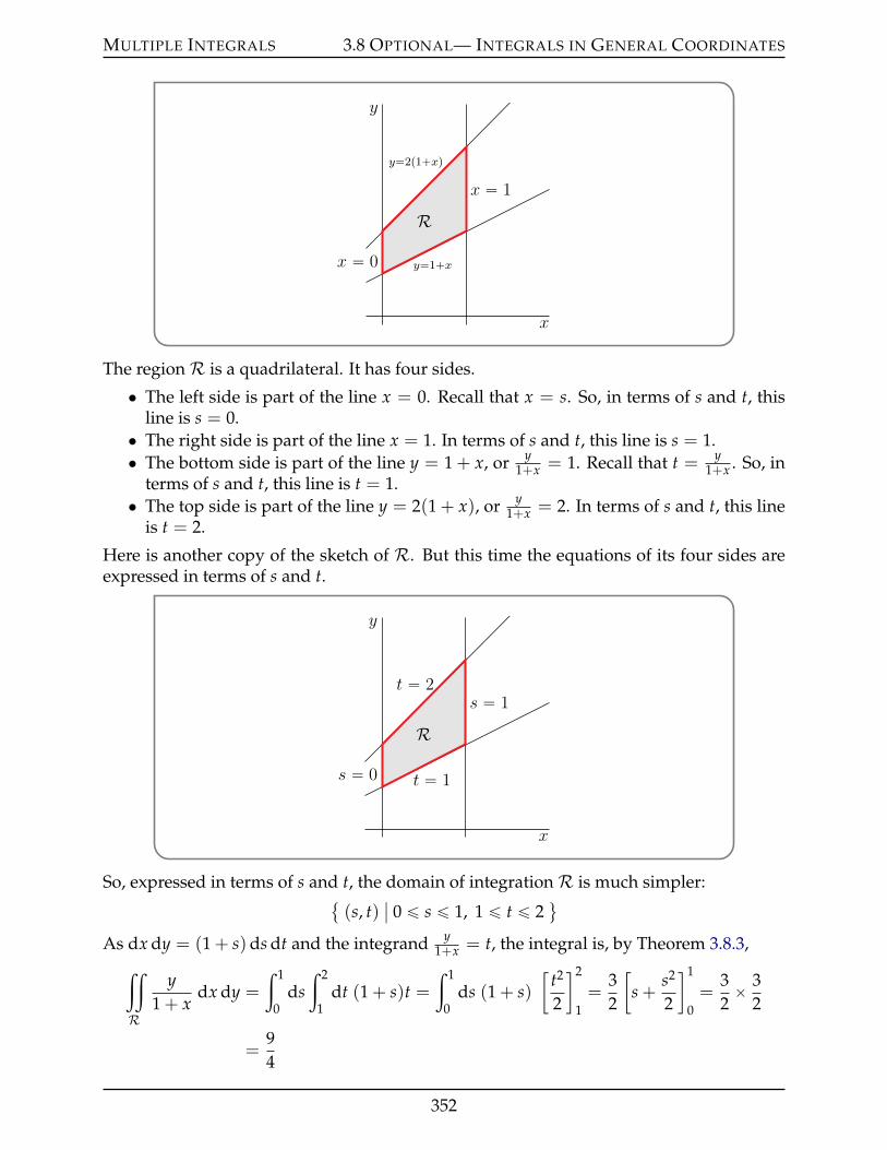
MULTIPLE INTEGRALS 3.8 OPTIONAL— INTEGRALS IN GENERAL COORDINATES
x
y
y“2p1`xq
y“1`x
x “ 1
x “ 0
R
The regionR is a quadrilateral. It has four sides.
• The left side is part of the line x = 0. Recall that x = s. So, in terms of s and t, thisline is s = 0.• The right side is part of the line x = 1. In terms of s and t, this line is s = 1.• The bottom side is part of the line y = 1 + x, or y
1+x = 1. Recall that t = y1+x . So, in
terms of s and t, this line is t = 1.• The top side is part of the line y = 2(1 + x), or y
1+x = 2. In terms of s and t, this lineis t = 2.
Here is another copy of the sketch of R. But this time the equations of its four sides areexpressed in terms of s and t.
x
y
t “ 2
t “ 1
s “ 1
s “ 0
R
So, expressed in terms of s and t, the domain of integrationR is much simpler: (s, t)
ˇ0 ď s ď 1, 1 ď t ď 2
(
As dx dy = (1 + s)ds dt and the integrand y1+x = t, the integral is, by Theorem 3.8.3,
ij
R
y1 + x
dx dy =
ż 1
0ds
ż 2
1dt (1 + s)t =
ż 1
0ds (1 + s)
[t2
2
]2
1=
32
[s +
s2
2
]1
0=
32ˆ 3
2
=94
352
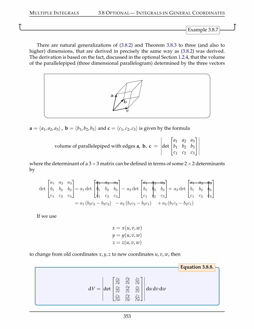
MULTIPLE INTEGRALS 3.8 OPTIONAL— INTEGRALS IN GENERAL COORDINATES
Example 3.8.7
There are natural generalizations of (3.8.2) and Theorem 3.8.3 to three (and also tohigher) dimensions, that are derived in precisely the same way as (3.8.2) was derived.The derivation is based on the fact, discussed in the optional Section 1.2.4, that the volumeof the parallelepiped (three dimensional parallelogram) determined by the three vectors
a
b
c
a = 〈a1, a2, a3〉 , b = 〈b1, b2, b3〉 and c = 〈c1, c2, c3〉 is given by the formula
volume of parallelepiped with edges a, b, c =
ˇˇˇdet
a1 a2 a3b1 b2 b3c1 c2 c3
ˇˇˇ
where the determinant of a 3ˆ3 matrix can be defined in terms of some 2ˆ2 determinantsby
det
a1 a2 a3b1 b2 b3c1 c2 c3
= a1 det
a1 a2 a3b1 b2 b3c1 c2 c3
− a2 det
a1 a2 a3b1 b2 b3c1 c2 c3
+ a3 det
a1 a2 a3b1 b2 b3c1 c2 c3
= a1 (b2c3 − b3c2) − a2 (b1c3 − b3c1) + a3 (b1c2 − b2c1)
If we use
x = x(u, v, w)
y = y(u, v, w)
z = z(u, v, w)
to change from old coordinates x, y, z to new coordinates u, v, w, then
dV =
ˇˇˇˇdet
BxBu
ByBu
BzBu
BxBv
ByBv
BzBv
BxBw
ByBw
BzBw
ˇˇˇˇdu dv dw
Equation 3.8.8.
353
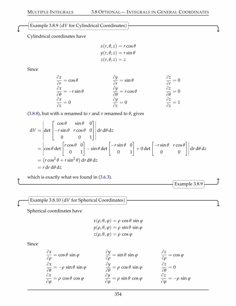
MULTIPLE INTEGRALS 3.8 OPTIONAL— INTEGRALS IN GENERAL COORDINATES
Example 3.8.9 (dV for Cylindrical Coordinates)
Cylindrical coordinates have
x(r, θ, z) = r cos θ
y(r, θ, z) = r sin θ
z(r, θ, z) = z
Since
BxBr
= cos θByBr
= sin θBzBr
= 0
BxBθ
= ´r sin θByBθ
= r cos θBzBθ
= 0
BxBz
= 0ByBz
= 0BzBz
= 1
(3.8.8), but with u renamed to r and v renamed to θ, gives
dV =
ˇˇˇˇdet
cos θ sin θ 0´r sin θ r cos θ 0
0 0 1
ˇˇˇˇdr dθ dz
=
ˇˇˇcos θ det
[r cos θ 0
0 1
]´ sin θ det
[´r sin θ 0
0 1
]+ 0 det
[´r sin θ r cos θ
0 0
]ˇˇˇdr dθ dz
=(r cos2 θ + r sin2 θ
)dr dθ dz
= r dr dθ dz
which is exactly what we found in (3.6.3).Example 3.8.9
Example 3.8.10 (dV for Spherical Coordinates)
Spherical coordinates have
x(ρ, θ, ϕ) = ρ cos θ sin ϕ
y(ρ, θ, ϕ) = ρ sin θ sin ϕ
z(ρ, θ, ϕ) = ρ cos ϕ
Since
BxBρ
= cos θ sin ϕByBρ
= sin θ sin ϕBzBρ
= cos ϕ
BxBθ
= ´ρ sin θ sin ϕByBθ
= ρ cos θ sin ϕBzBθ
= 0
BxBϕ
= ρ cos θ cos ϕByBϕ
= ρ sin θ cos ϕBzBϕ
= ´ρ sin ϕ
354
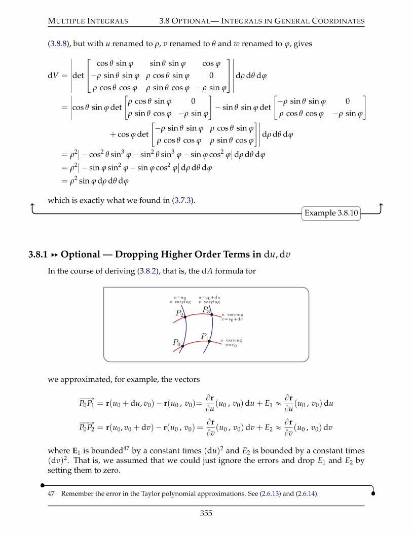
MULTIPLE INTEGRALS 3.8 OPTIONAL— INTEGRALS IN GENERAL COORDINATES
(3.8.8), but with u renamed to ρ, v renamed to θ and w renamed to ϕ, gives
dV =
ˇˇˇˇdet
cos θ sin ϕ sin θ sin ϕ cos ϕ
´ρ sin θ sin ϕ ρ cos θ sin ϕ 0ρ cos θ cos ϕ ρ sin θ cos ϕ ´ρ sin ϕ
ˇˇˇˇdρ dθ dϕ
=
ˇˇˇcos θ sin ϕ det
[ρ cos θ sin ϕ 0ρ sin θ cos ϕ ´ρ sin ϕ
]´ sin θ sin ϕ det
[´ρ sin θ sin ϕ 0ρ cos θ cos ϕ ´ρ sin ϕ
]
+ cos ϕ det
[´ρ sin θ sin ϕ ρ cos θ sin ϕ
ρ cos θ cos ϕ ρ sin θ cos ϕ
]ˇˇˇdρ dθ dϕ
= ρ2 ˇ´ cos2 θ sin3 ϕ´ sin2 θ sin3 ϕ´ sin ϕ cos2 ϕˇdρ dθ dϕ
= ρ2 ˇ´ sin ϕ sin2 ϕ´ sin ϕ cos2 ϕˇdρ dθ dϕ
= ρ2 sin ϕ dρ dθ dϕ
which is exactly what we found in (3.7.3).
Example 3.8.10
3.8.1 §§ Optional — Dropping Higher Order Terms in du, dv
In the course of deriving (3.8.2), that is, the dA formula for
P0
P1
P3P2
u varyingv“v0
u varyingv“v0`dv
u“u0`duv varying
u“u0v varying
we approximated, for example, the vectors
ÝÝÑP0P1 = r(u0 + du, v0)´ r(u0 , v0)=BrBu
(u0 , v0)du + E1 « BrBu
(u0 , v0)du
ÝÝÑP0P2 = r(u0, v0 + dv)´ r(u0 , v0) =BrBv
(u0 , v0)dv + E2 « BrBv
(u0 , v0)dv
where E1 is bounded47 by a constant times (du)2 and E2 is bounded by a constant times(dv)2. That is, we assumed that we could just ignore the errors and drop E1 and E2 bysetting them to zero.
47 Remember the error in the Taylor polynomial approximations. See (2.6.13) and (2.6.14).
355
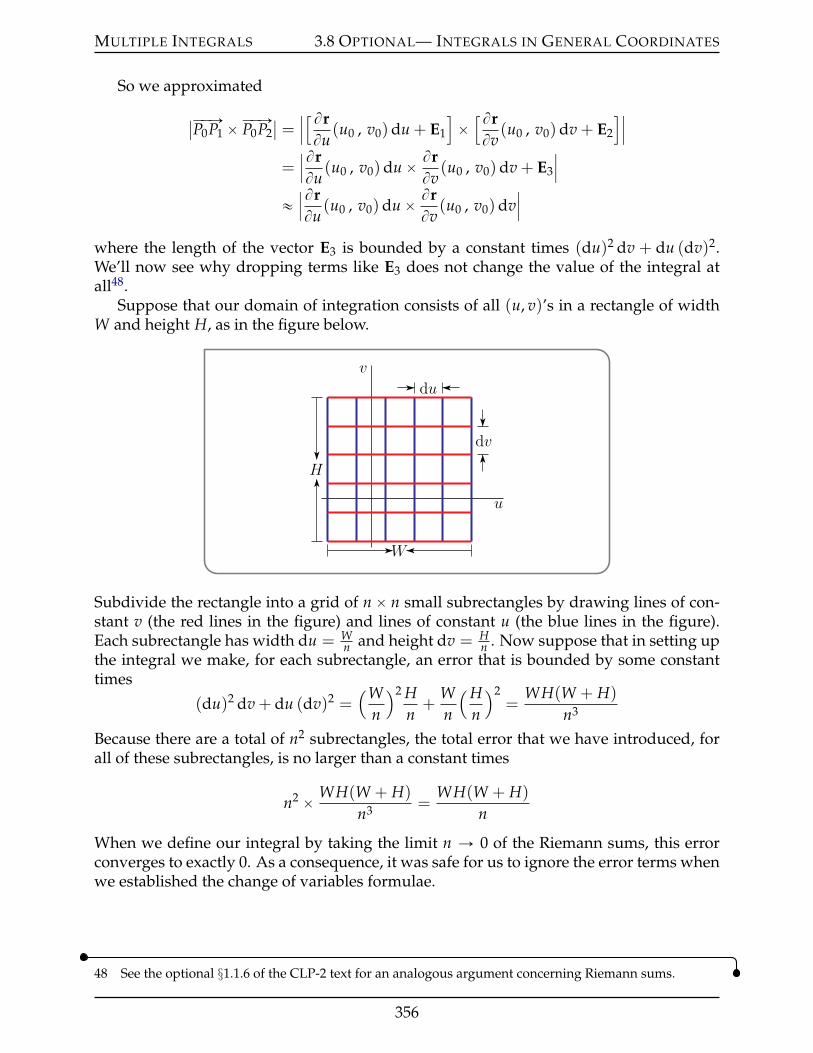
MULTIPLE INTEGRALS 3.8 OPTIONAL— INTEGRALS IN GENERAL COORDINATES
So we approximated
ˇÝÝÑP0P1 ˆÝÝÑP0P2ˇ=
ˇˇ[ BrBu
(u0 , v0)du + E1
]ˆ[BrBv
(u0 , v0)dv + E2
]ˇˇ
=ˇˇBrBu
(u0 , v0)duˆ BrBv
(u0 , v0)dv + E3
ˇˇ
«ˇˇBrBu
(u0 , v0)duˆ BrBv
(u0 , v0)dvˇˇ
where the length of the vector E3 is bounded by a constant times (du)2 dv + du (dv)2.We’ll now see why dropping terms like E3 does not change the value of the integral atall48.
Suppose that our domain of integration consists of all (u, v)’s in a rectangle of widthW and height H, as in the figure below.
u
v
du
W
dv
H
Subdivide the rectangle into a grid of nˆ n small subrectangles by drawing lines of con-stant v (the red lines in the figure) and lines of constant u (the blue lines in the figure).Each subrectangle has width du = W
n and height dv = Hn . Now suppose that in setting up
the integral we make, for each subrectangle, an error that is bounded by some constanttimes
(du)2 dv + du (dv)2 =(W
n
)2 Hn+
Wn
(Hn
)2=
WH(W + H)
n3
Because there are a total of n2 subrectangles, the total error that we have introduced, forall of these subrectangles, is no larger than a constant times
n2 ˆ WH(W + H)
n3 =WH(W + H)
n
When we define our integral by taking the limit n Ñ 0 of the Riemann sums, this errorconverges to exactly 0. As a consequence, it was safe for us to ignore the error terms whenwe established the change of variables formulae.
48 See the optional §1.1.6 of the CLP-2 text for an analogous argument concerning Riemann sums.
356
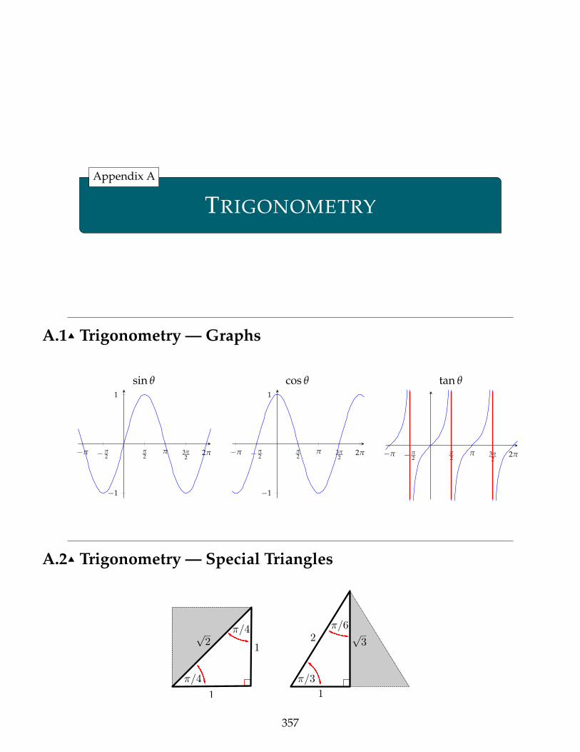
TRIGONOMETRY
Appendix A
A.1IJ Trigonometry — Graphs
sin θ cos θ tan θ
´π ´ π2
π2
π 3π2
2π
´1
1
´π ´ π2
π2
π 3π2
2π
´1
1
´π ´ π2
π2
π 3π2
2π
A.2IJ Trigonometry — Special Triangles
357
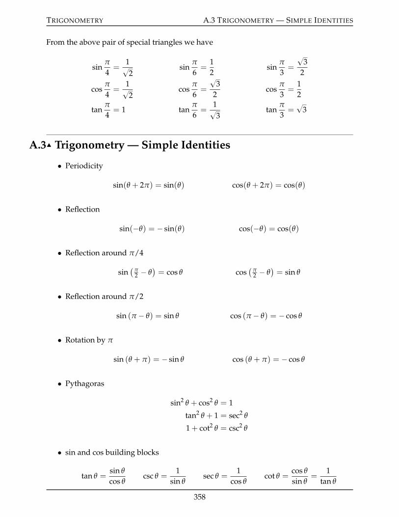
TRIGONOMETRY A.3 TRIGONOMETRY — SIMPLE IDENTITIES
From the above pair of special triangles we have
sinπ
4=
1?2
sinπ
6=
12
sinπ
3=
?3
2
cosπ
4=
1?2
cosπ
6=
?3
2cos
π
3=
12
tanπ
4= 1 tan
π
6=
1?3
tanπ
3=?
3
A.3IJ Trigonometry — Simple Identities
• Periodicity
sin(θ + 2π) = sin(θ) cos(θ + 2π) = cos(θ)
• Reflection
sin(´θ) = ´ sin(θ) cos(´θ) = cos(θ)
• Reflection around π/4
sin(
π2 ´ θ
)= cos θ cos
(π2 ´ θ
)= sin θ
• Reflection around π/2
sin (π ´ θ) = sin θ cos (π ´ θ) = ´ cos θ
• Rotation by π
sin (θ + π) = ´ sin θ cos (θ + π) = ´ cos θ
• Pythagoras
sin2 θ + cos2 θ = 1
tan2 θ + 1 = sec2 θ
1 + cot2 θ = csc2 θ
• sin and cos building blocks
tan θ =sin θ
cos θcsc θ =
1sin θ
sec θ =1
cos θcot θ =
cos θ
sin θ=
1tan θ
358
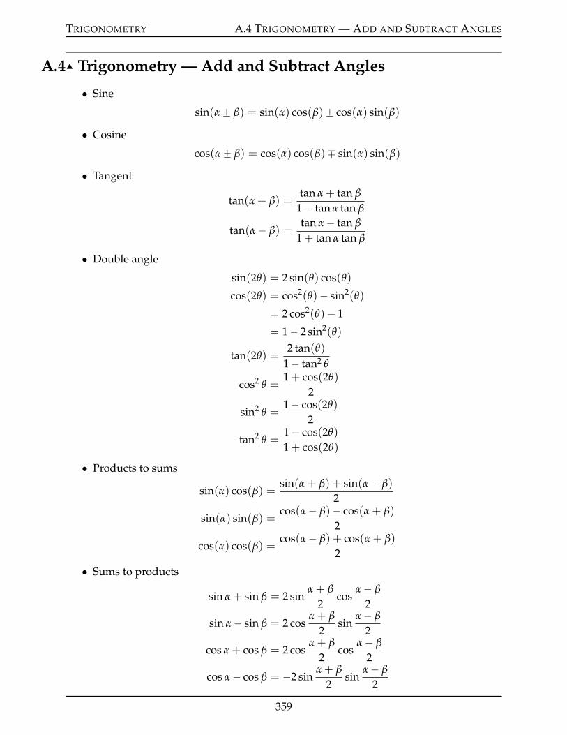
TRIGONOMETRY A.4 TRIGONOMETRY — ADD AND SUBTRACT ANGLES
A.4IJ Trigonometry — Add and Subtract Angles
• Sine
sin(α˘ β) = sin(α) cos(β)˘ cos(α) sin(β)
• Cosine
cos(α˘ β) = cos(α) cos(β)¯ sin(α) sin(β)
• Tangent
tan(α + β) =tan α + tan β
1´ tan α tan β
tan(α´ β) =tan α´ tan β
1 + tan α tan β
• Double angle
sin(2θ) = 2 sin(θ) cos(θ)
cos(2θ) = cos2(θ)´ sin2(θ)
= 2 cos2(θ)´ 1
= 1´ 2 sin2(θ)
tan(2θ) =2 tan(θ)
1´ tan2 θ
cos2 θ =1 + cos(2θ)
2
sin2 θ =1´ cos(2θ)
2
tan2 θ =1´ cos(2θ)
1 + cos(2θ)
• Products to sums
sin(α) cos(β) =sin(α + β) + sin(α´ β)
2
sin(α) sin(β) =cos(α´ β)´ cos(α + β)
2
cos(α) cos(β) =cos(α´ β) + cos(α + β)
2
• Sums to products
sin α + sin β = 2 sinα + β
2cos
α´ β
2
sin α´ sin β = 2 cosα + β
2sin
α´ β
2
cos α + cos β = 2 cosα + β
2cos
α´ β
2
cos α´ cos β = ´2 sinα + β
2sin
α´ β
2
359
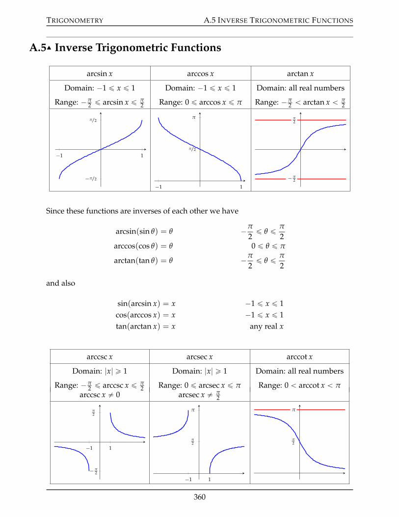
TRIGONOMETRY A.5 INVERSE TRIGONOMETRIC FUNCTIONS
A.5IJ Inverse Trigonometric Functions
arcsin x arccos x arctan x
Domain: ´1 ď x ď 1 Domain: ´1 ď x ď 1 Domain: all real numbers
Range: ´π2 ď arcsin x ď π
2 Range: 0 ď arccos x ď π Range: ´π2 ă arctan x ă π
2
´1 1
´π/2
π/2
´1 1
π/2
π
´ π2
π2
Since these functions are inverses of each other we have
arcsin(sin θ) = θ ´π
2ď θ ď π
2arccos(cos θ) = θ 0 ď θ ď π
arctan(tan θ) = θ ´π
2ď θ ď π
2
and also
sin(arcsin x) = x ´1 ď x ď 1cos(arccos x) = x ´1 ď x ď 1tan(arctan x) = x any real x
arccsc x arcsec x arccot x
Domain: |x| ě 1 Domain: |x| ě 1 Domain: all real numbers
Range: ´π2 ď arccsc x ď π
2 Range: 0 ď arcsec x ď π Range: 0 ă arccot x ă πarccsc x ‰ 0 arcsec x ‰ π
2
´1 1
´ π2
π2
´1 1
π2
π
π2
π
360
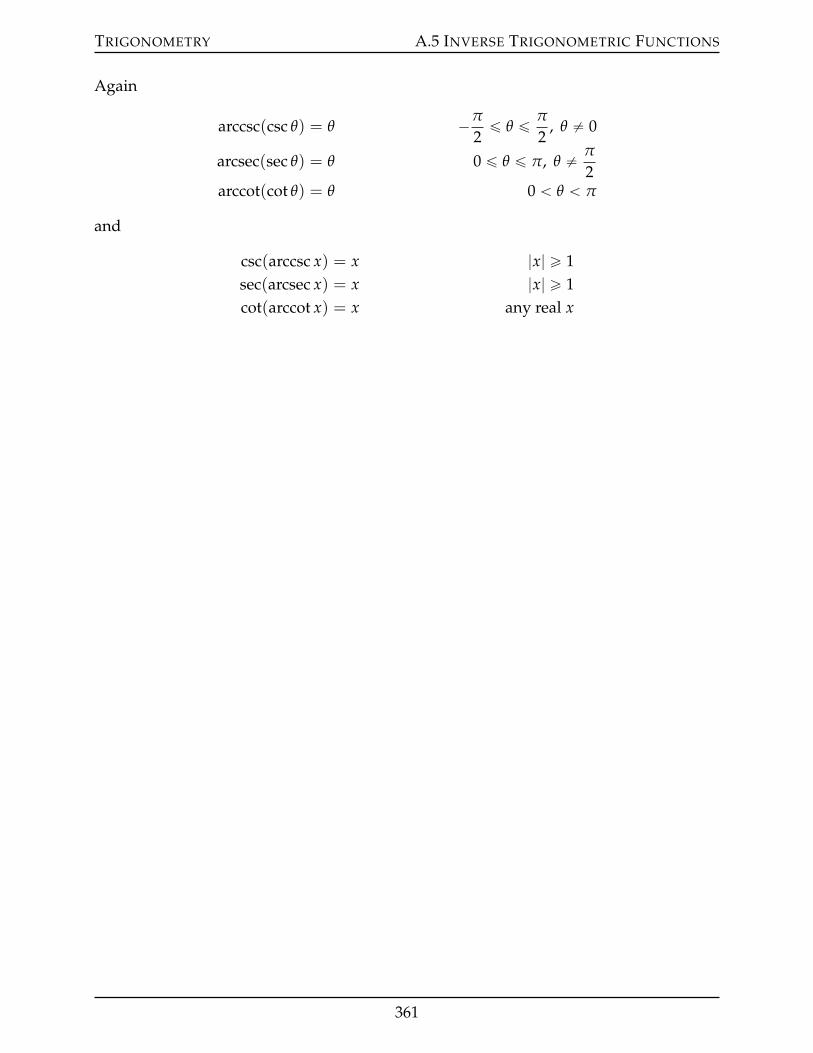
TRIGONOMETRY A.5 INVERSE TRIGONOMETRIC FUNCTIONS
Again
arccsc(csc θ) = θ ´π
2ď θ ď π
2, θ ‰ 0
arcsec(sec θ) = θ 0 ď θ ď π, θ ‰ π
2arccot(cot θ) = θ 0 ă θ ă π
and
csc(arccsc x) = x |x| ě 1sec(arcsec x) = x |x| ě 1cot(arccot x) = x any real x
361
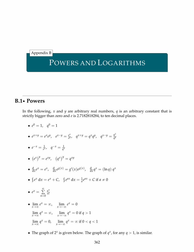
POWERS AND LOGARITHMS
Appendix B
B.1IJ Powers
In the following, x and y are arbitrary real numbers, q is an arbitrary constant that isstrictly bigger than zero and e is 2.7182818284, to ten decimal places.
• e0 = 1, q0 = 1
• ex+y = exey, ex´y = ex
ey , qx+y = qxqy, qx´y = qx
qy
• e´x = 1ex , q´x = 1
qx
•(ex)y
= exy,(qx)y
= qxy
• ddx ex = ex, d
dx eg(x) = g1(x)eg(x), ddx qx = (ln q) qx
•ş
ex dx = ex + C,ş
eax dx = 1a eax + C if a ‰ 0
• ex =8ř
n=0
xn
n!
• limxÑ8
ex = 8, limxÑ´8
ex = 0
limxÑ8
qx = 8, limxÑ´8
qx = 0 if q ą 1
limxÑ8
qx = 0, limxÑ´8
qx = 8 if 0 ă q ă 1
• The graph of 2x is given below. The graph of qx, for any q ą 1, is similar.
362
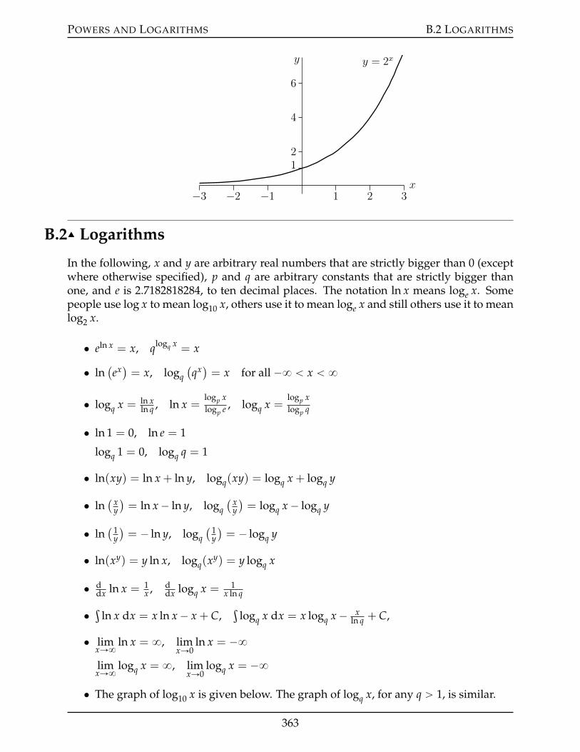
POWERS AND LOGARITHMS B.2 LOGARITHMS
x
y
1 2 3−1−2−3
12
4
6
y = 2x
B.2IJ Logarithms
In the following, x and y are arbitrary real numbers that are strictly bigger than 0 (exceptwhere otherwise specified), p and q are arbitrary constants that are strictly bigger thanone, and e is 2.7182818284, to ten decimal places. The notation ln x means loge x. Somepeople use log x to mean log10 x, others use it to mean loge x and still others use it to meanlog2 x.
• eln x = x, qlogq x = x
• ln(ex) = x, logq
(qx) = x for all ´8 ă x ă 8
• logq x = ln xln q , ln x =
logp xlogp e , logq x =
logp xlogp q
• ln 1 = 0, ln e = 1
logq 1 = 0, logq q = 1
• ln(xy) = ln x + ln y, logq(xy) = logq x + logq y
• ln( x
y)= ln x´ ln y, logq
( xy)= logq x´ logq y
• ln( 1
y)= ´ ln y, logq
( 1y)= ´ logq y
• ln(xy) = y ln x, logq(xy) = y logq x
• ddx ln x = 1
x , ddx logq x = 1
x ln q
•ş
ln x dx = x ln x´ x + C,ş
logq x dx = x logq x´ xln q + C,
• limxÑ8
ln x = 8, limxÑ0
ln x = ´8limxÑ8
logq x = 8, limxÑ0
logq x = ´8
• The graph of log10 x is given below. The graph of logq x, for any q ą 1, is similar.
363
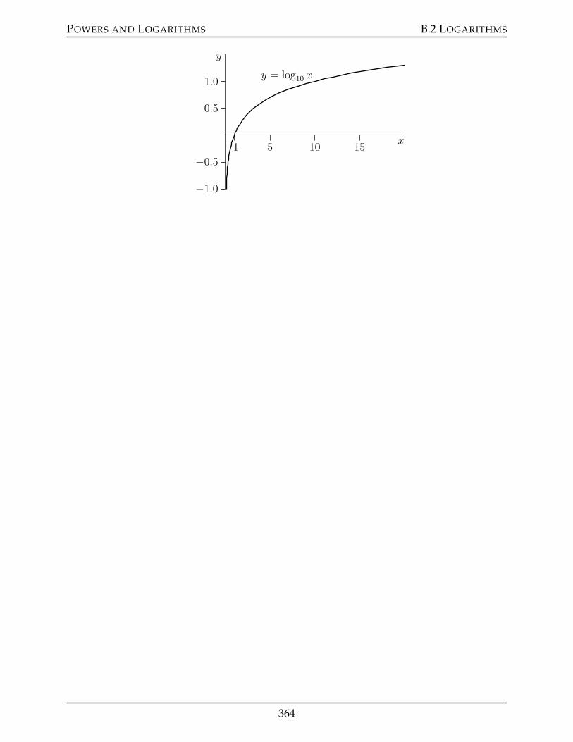
POWERS AND LOGARITHMS B.2 LOGARITHMS
x
y
1 5 10 15
0.5
1.0
−0.5
−1.0
y = log10 x
364
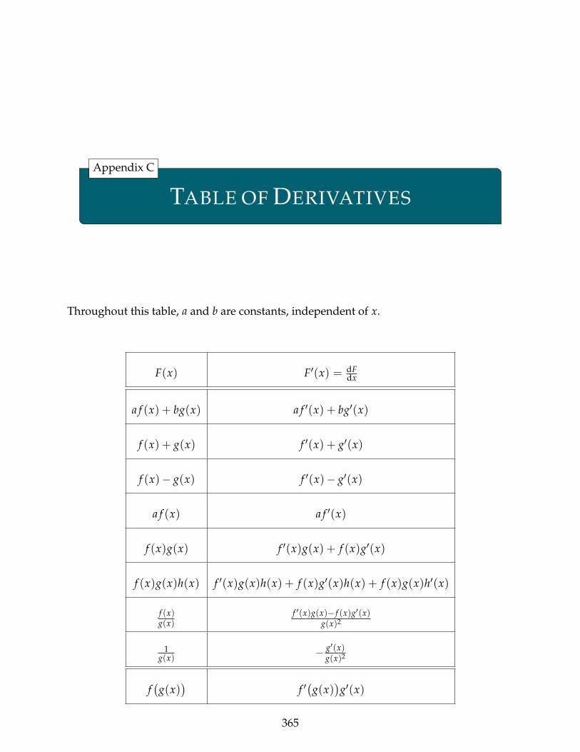
TABLE OF DERIVATIVES
Appendix C
Throughout this table, a and b are constants, independent of x.
F(x) F1(x) = dFdx
a f (x) + bg(x) a f 1(x) + bg1(x)
f (x) + g(x) f 1(x) + g1(x)
f (x)´ g(x) f 1(x)´ g1(x)
a f (x) a f 1(x)
f (x)g(x) f 1(x)g(x) + f (x)g1(x)
f (x)g(x)h(x) f 1(x)g(x)h(x) + f (x)g1(x)h(x) + f (x)g(x)h1(x)
f (x)g(x)
f 1(x)g(x)´ f (x)g1(x)g(x)2
1g(x) ´ g1(x)
g(x)2
f(
g(x))
f 1(
g(x))
g1(x)
365
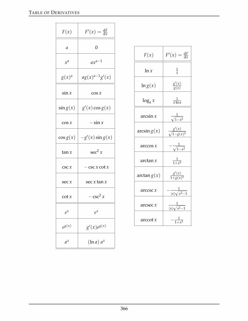
TABLE OF DERIVATIVES
F(x) F1(x) = dFdx
a 0
xa axa´1
g(x)a ag(x)a´1g1(x)
sin x cos x
sin g(x) g1(x) cos g(x)
cos x ´ sin x
cos g(x) ´g1(x) sin g(x)
tan x sec2 x
csc x ´ csc x cot x
sec x sec x tan x
cot x ´ csc2 x
ex ex
eg(x) g1(x)eg(x)
ax (ln a) ax
F(x) F1(x) = dFdx
ln x 1x
ln g(x) g1(x)g(x)
loga x 1x ln a
arcsin x 1?1´x2
arcsin g(x) g1(x)?1´g(x)2
arccos x ´ 1?1´x2
arctan x 11+x2
arctan g(x) g1(x)1+g(x)2
arccsc x ´ 1|x|?
x2´1
arcsec x 1|x|?
x2´1
arccot x ´ 11+x2
366
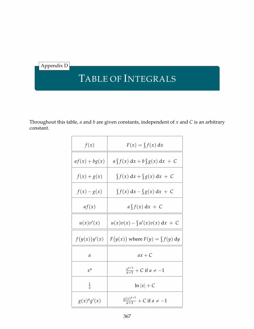
TABLE OF INTEGRALS
Appendix D
Throughout this table, a and b are given constants, independent of x and C is an arbitraryconstant.
f (x) F(x) =ş
f (x) dx
a f (x) + bg(x) aş
f (x) dx + bş
g(x) dx + C
f (x) + g(x)ş
f (x) dx +ş
g(x) dx + C
f (x)´ g(x)ş
f (x) dx´ şg(x) dx + C
a f (x) aş
f (x) dx + C
u(x)v1(x) u(x)v(x)´ şu1(x)v(x) dx + C
f(y(x)
)y1(x) F
(y(x)
)where F(y) =
şf (y) dy
a ax + C
xa xa+1
a+1 + C if a ‰ ´1
1x ln |x|+ C
g(x)ag1(x) g(x)a+1
a+1 + C if a ‰ ´1
367
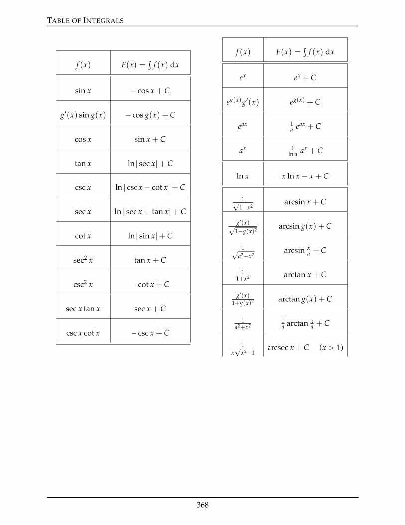
TABLE OF INTEGRALS
f (x) F(x) =ş
f (x) dx
sin x ´ cos x + C
g1(x) sin g(x) ´ cos g(x) + C
cos x sin x + C
tan x ln | sec x|+ C
csc x ln | csc x´ cot x|+ C
sec x ln | sec x + tan x|+ C
cot x ln | sin x|+ C
sec2 x tan x + C
csc2 x ´ cot x + C
sec x tan x sec x + C
csc x cot x ´ csc x + C
f (x) F(x) =ş
f (x) dx
ex ex + C
eg(x)g1(x) eg(x) + C
eax 1a eax + C
ax 1ln a ax + C
ln x x ln x´ x + C
1?1´x2
arcsin x + C
g1(x)?1´g(x)2 arcsin g(x) + C
1?a2´x2
arcsin xa + C
11+x2 arctan x + C
g1(x)1+g(x)2 arctan g(x) + C
1a2+x2
1a arctan x
a + C
1x?
x2´1arcsec x + C (x ą 1)
368
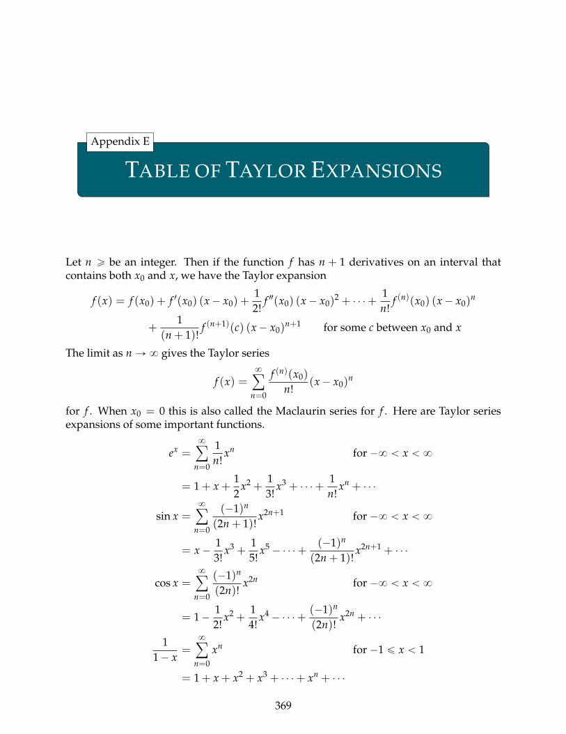
TABLE OF TAYLOR EXPANSIONS
Appendix E
Let n ě be an integer. Then if the function f has n + 1 derivatives on an interval thatcontains both x0 and x, we have the Taylor expansion
f (x) = f (x0) + f 1(x0) (x´ x0) +12!
f 2(x0) (x´ x0)2 + ¨ ¨ ¨+ 1
n!f (n)(x0) (x´ x0)
n
+1
(n + 1)!f (n+1)(c) (x´ x0)
n+1 for some c between x0 and x
The limit as n Ñ 8 gives the Taylor series
f (x) =8ÿ
n=0
f (n)(x0)
n!(x´ x0)
n
for f . When x0 = 0 this is also called the Maclaurin series for f . Here are Taylor seriesexpansions of some important functions.
ex =8ÿ
n=0
1n!
xn for ´8 ă x ă 8
= 1 + x +12
x2 +13!
x3 + ¨ ¨ ¨+ 1n!
xn + ¨ ¨ ¨
sin x =8ÿ
n=0
(´1)n
(2n + 1)!x2n+1 for ´8 ă x ă 8
= x´ 13!
x3 +15!
x5 ´ ¨ ¨ ¨+ (´1)n
(2n + 1)!x2n+1 + ¨ ¨ ¨
cos x =8ÿ
n=0
(´1)n
(2n)!x2n for ´8 ă x ă 8
= 1´ 12!
x2 +14!
x4 ´ ¨ ¨ ¨+ (´1)n
(2n)!x2n + ¨ ¨ ¨
11´ x
=8ÿ
n=0
xn for ´1 ď x ă 1
= 1 + x + x2 + x3 + ¨ ¨ ¨+ xn + ¨ ¨ ¨
369
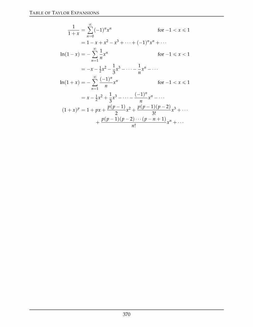
TABLE OF TAYLOR EXPANSIONS
11 + x
=8ÿ
n=0
(´1)nxn for ´1 ă x ď 1
= 1´ x + x2 ´ x3 + ¨ ¨ ¨+ (´1)nxn + ¨ ¨ ¨
ln(1´ x) = ´8ÿ
n=1
1n
xn for ´1 ď x ă 1
= ´x´ 12 x2 ´ 1
3x3 ´ ¨ ¨ ¨ ´ 1
nxn ´ ¨ ¨ ¨
ln(1 + x) = ´8ÿ
n=1
(´1)n
nxn for ´1 ă x ď 1
= x´ 12 x2 +
13
x3 ´ ¨ ¨ ¨ ´ (´1)n
nxn ´ ¨ ¨ ¨
(1 + x)p = 1 + px +p(p´ 1)
2x2 +
p(p´ 1)(p´ 2)3!
x3 + ¨ ¨ ¨
+p(p´ 1)(p´ 2) ¨ ¨ ¨ (p´ n + 1)
n!xn + ¨ ¨ ¨
370
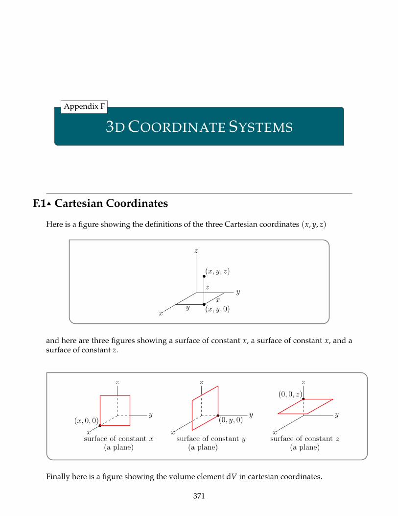
3D COORDINATE SYSTEMS
Appendix F
F.1IJ Cartesian Coordinates
Here is a figure showing the definitions of the three Cartesian coordinates (x, y, z)
y
z
x
px, y, zq
px, y, 0qx
y
z
and here are three figures showing a surface of constant x, a surface of constant x, and asurface of constant z.
y
z
x
px, 0, 0q
surface of constant x(a plane)
y
z
x
p0, y, 0q
surface of constant y(a plane)
y
z
x
p0, 0, zq
surface of constant z(a plane)
Finally here is a figure showing the volume element dV in cartesian coordinates.
371
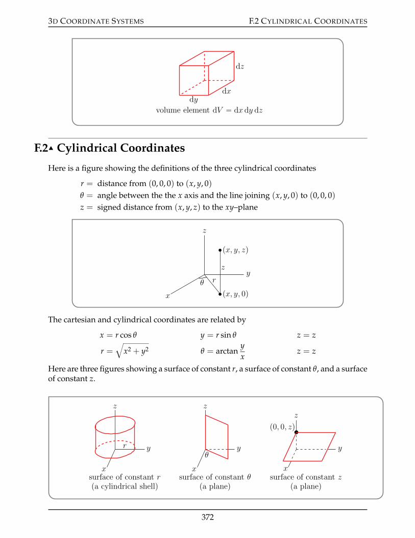
3D COORDINATE SYSTEMS F.2 CYLINDRICAL COORDINATES
dxdy
dz
volume element dV “ dx dy dz
F.2IJ Cylindrical Coordinates
Here is a figure showing the definitions of the three cylindrical coordinates
r = distance from (0, 0, 0) to (x, y, 0)θ = angle between the the x axis and the line joining (x, y, 0) to (0, 0, 0)z = signed distance from (x, y, z) to the xy–plane
px, y, zq
px, y, 0q
y
z
x
z
rθ
The cartesian and cylindrical coordinates are related by
x = r cos θ y = r sin θ z = z
r =b
x2 + y2 θ = arctanyx
z = z
Here are three figures showing a surface of constant r, a surface of constant θ, and a surfaceof constant z.
y
z
x
r
surface of constant r(a cylindrical shell)
y
z
x
θ
surface of constant θ(a plane)
y
z
x
p0, 0, zq
surface of constant z(a plane)
372
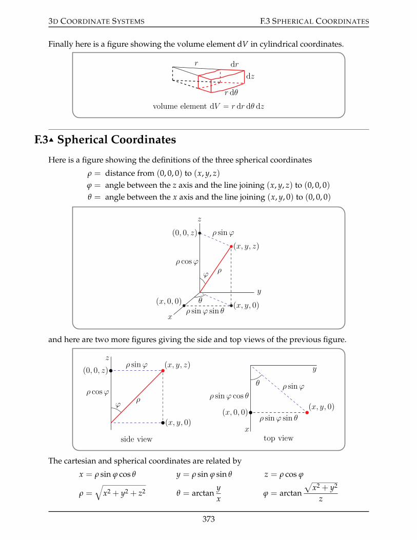
3D COORDINATE SYSTEMS F.3 SPHERICAL COORDINATES
Finally here is a figure showing the volume element dV in cylindrical coordinates.
r dr
dz
r dθ
volume element dV “ r dr dθ dz
F.3IJ Spherical Coordinates
Here is a figure showing the definitions of the three spherical coordinates
ρ = distance from (0, 0, 0) to (x, y, z)ϕ = angle between the z axis and the line joining (x, y, z) to (0, 0, 0)θ = angle between the x axis and the line joining (x, y, 0) to (0, 0, 0)
z
y
x
p0, 0, zq
px, y, 0qpx, 0, 0q θ
ϕ
px, y, zq
ρ
ρ sinϕ
ρ cosϕ
ρ sinϕ sin θ
and here are two more figures giving the side and top views of the previous figure.
z
p0, 0, zq
ρ cosϕ
px, y, 0qside view
ρ sinϕ
ϕρ
px, y, zq y
x
px, 0, 0q
top view
ρ sinϕ sin θ
ρ sinϕ cos θρ sinϕθ
px, y, 0q
The cartesian and spherical coordinates are related by
x = ρ sin ϕ cos θ y = ρ sin ϕ sin θ z = ρ cos ϕ
ρ =b
x2 + y2 + z2 θ = arctanyx
ϕ = arctan
ax2 + y2
z
373
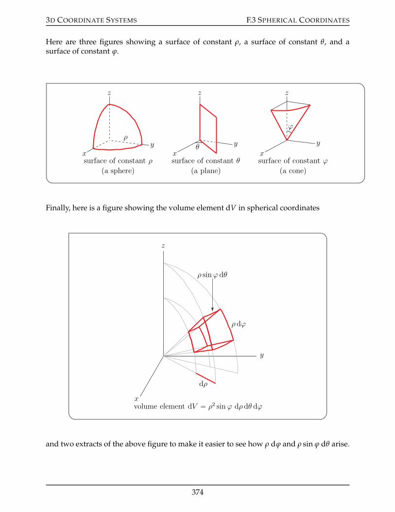
3D COORDINATE SYSTEMS F.3 SPHERICAL COORDINATES
Here are three figures showing a surface of constant ρ, a surface of constant θ, and asurface of constant ϕ.
z
yx
ρ
surface of constant ρ
(a sphere)
z
y
xθ
surface of constant θ
(a plane)
z
y
x
ϕ
surface of constant ϕ
(a cone)
Finally, here is a figure showing the volume element dV in spherical coordinates
z
y
x
dρ
ρ dϕ
ρ sinϕ dθ
volume element dV “ ρ2 sinϕ dρ dθ dϕ
and two extracts of the above figure to make it easier to see how ρ dϕ and ρ sin ϕ dθ arise.
374
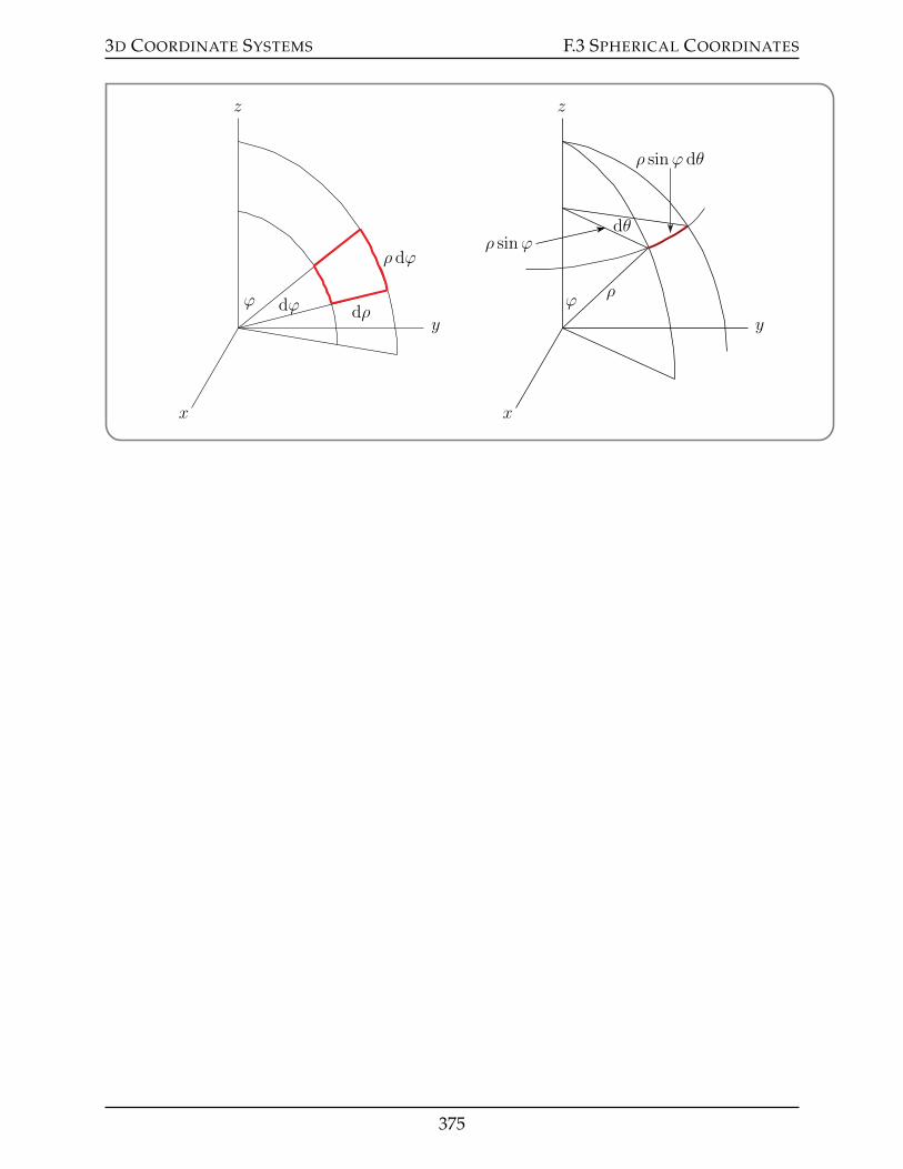
3D COORDINATE SYSTEMS F.3 SPHERICAL COORDINATES
z
y
x
ρ dϕ
ϕ dϕ dρ
z
y
x
ρ sinϕ
ϕρ
dθ
ρ sinϕ dθ
375
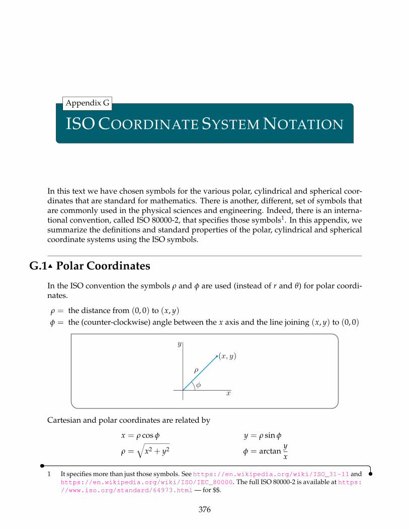
ISO COORDINATE SYSTEM NOTATION
Appendix G
In this text we have chosen symbols for the various polar, cylindrical and spherical coor-dinates that are standard for mathematics. There is another, different, set of symbols thatare commonly used in the physical sciences and engineering. Indeed, there is an interna-tional convention, called ISO 80000-2, that specifies those symbols1. In this appendix, wesummarize the definitions and standard properties of the polar, cylindrical and sphericalcoordinate systems using the ISO symbols.
G.1IJ Polar Coordinates
In the ISO convention the symbols ρ and φ are used (instead of r and θ) for polar coordi-nates.
ρ = the distance from (0, 0) to (x, y)φ = the (counter-clockwise) angle between the x axis and the line joining (x, y) to (0, 0)
ρ
px, yq
x
y
φ
Cartesian and polar coordinates are related by
x = ρ cos φ y = ρ sin φ
ρ =b
x2 + y2 φ = arctanyx
1 It specifies more than just those symbols. See https://en.wikipedia.org/wiki/ISO_31-11 andhttps://en.wikipedia.org/wiki/ISO/IEC_80000. The full ISO 80000-2 is available at https://www.iso.org/standard/64973.html — for $$.
376
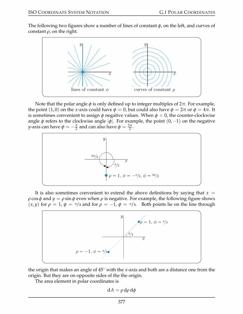
ISO COORDINATE SYSTEM NOTATION G.1 POLAR COORDINATES
The following two figures show a number of lines of constant φ, on the left, and curves ofconstant ρ, on the right.
x
y
lines of constant φ
x
y
curves of constant ρ
Note that the polar angle φ is only defined up to integer multiples of 2π. For example,the point (1, 0) on the x-axis could have φ = 0, but could also have φ = 2π or φ = 4π. Itis sometimes convenient to assign φ negative values. When φ ă 0, the counter-clockwiseangle φ refers to the clockwise angle |φ|. For example, the point (0,´1) on the negativey-axis can have φ = ´π
2 and can also have φ = 3π2 .
x
y
ρ “ 1, φ “ ´π2, φ “ 3π2
3π2π2
It is also sometimes convenient to extend the above definitions by saying that x =ρ cos φ and y = ρ sin φ even when ρ is negative. For example, the following figure shows(x, y) for ρ = 1, φ = π/4 and for ρ = ´1, φ = π/4. Both points lie on the line through
ρ “ 1, φ “ π4
ρ “ ´1, φ “ π4
x
y
π4
the origin that makes an angle of 45˝ with the x-axis and both are a distance one from theorigin. But they are on opposite sides of the the origin.
The area element in polar coordinates is
dA = ρ dρ dφ
377
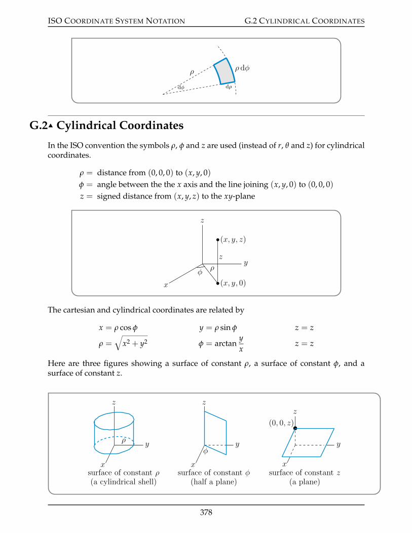
ISO COORDINATE SYSTEM NOTATION G.2 CYLINDRICAL COORDINATES
dφ dρ
ρ ρ dφ
G.2IJ Cylindrical Coordinates
In the ISO convention the symbols ρ, φ and z are used (instead of r, θ and z) for cylindricalcoordinates.
ρ = distance from (0, 0, 0) to (x, y, 0)φ = angle between the the x axis and the line joining (x, y, 0) to (0, 0, 0)z = signed distance from (x, y, z) to the xy-plane
px, y, zq
px, y, 0q
y
z
x
z
ρφ
The cartesian and cylindrical coordinates are related by
x = ρ cos φ y = ρ sin φ z = z
ρ =b
x2 + y2 φ = arctanyx
z = z
Here are three figures showing a surface of constant ρ, a surface of constant φ, and asurface of constant z.
y
z
x
ρ
surface of constant ρ(a cylindrical shell)
y
z
x
φ
surface of constant φ(half a plane)
y
z
x
p0, 0, zq
surface of constant z(a plane)
378
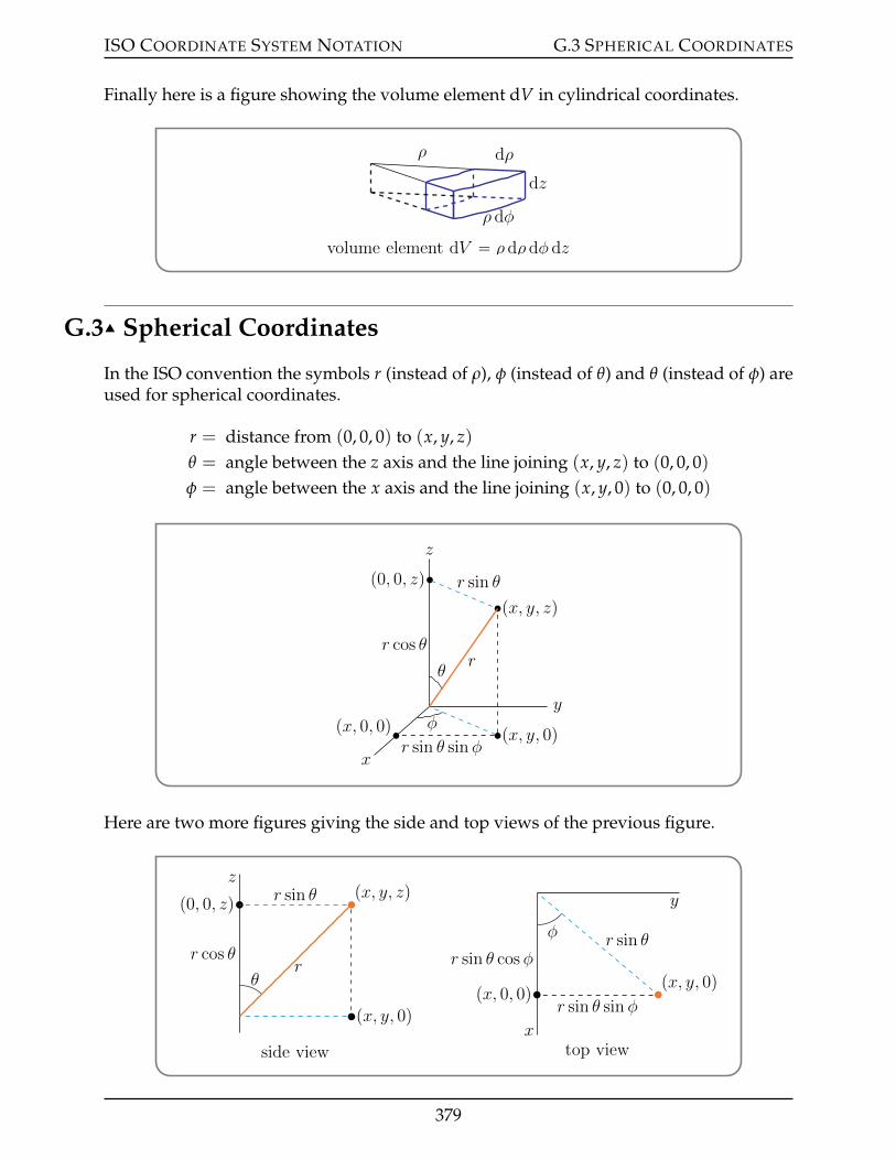
ISO COORDINATE SYSTEM NOTATION G.3 SPHERICAL COORDINATES
Finally here is a figure showing the volume element dV in cylindrical coordinates.
ρ dρ
dz
ρ dφ
volume element dV “ ρ dρ dφ dz
G.3IJ Spherical Coordinates
In the ISO convention the symbols r (instead of ρ), φ (instead of θ) and θ (instead of φ) areused for spherical coordinates.
r = distance from (0, 0, 0) to (x, y, z)θ = angle between the z axis and the line joining (x, y, z) to (0, 0, 0)φ = angle between the x axis and the line joining (x, y, 0) to (0, 0, 0)
z
y
x
p0, 0, zq
px, y, 0qpx, 0, 0q φ
θ
px, y, zq
r
r sin θ
r cos θ
r sin θ sinφ
Here are two more figures giving the side and top views of the previous figure.
z
p0, 0, zq
r cos θ
px, y, 0qside view
r sin θ
θr
px, y, zq y
x
px, 0, 0q
top view
r sin θ sin φ
r sin θ cosφr sin θφ
px, y, 0q
379

ISO COORDINATE SYSTEM NOTATION G.3 SPHERICAL COORDINATES
The cartesian and spherical coordinates are related by
x = r sin θ cos φ y = r sin θ sin φ z = r cos θ
r =b
x2 + y2 + z2 φ = arctanyx
θ = arctan
ax2 + y2
z
Here are three figures showing a surface of constant r, a surface of constant φ, and asurface of constant θ.
z
yx
r
surface of constant r
(a sphere)
z
y
xφ
surface of constant φ
(half a plane)
z
y
x
θ
surface of constant θ
(a cone)
Finally, here is a figure showing the volume element dV in spherical coordinates
z
y
x
dr
r dθ
r sin θ dφ
volume element dV “ r2 sin θ dr dθ dφ
and two extracts of the above figure to make it easier to see how r dθ and r sin θ dφ arise.
380
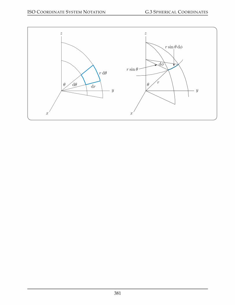
ISO COORDINATE SYSTEM NOTATION G.3 SPHERICAL COORDINATES
z
y
x
r dθ
θ dθ dr
z
y
x
r sin θ
θr
dφ
r sin θ dφ
381
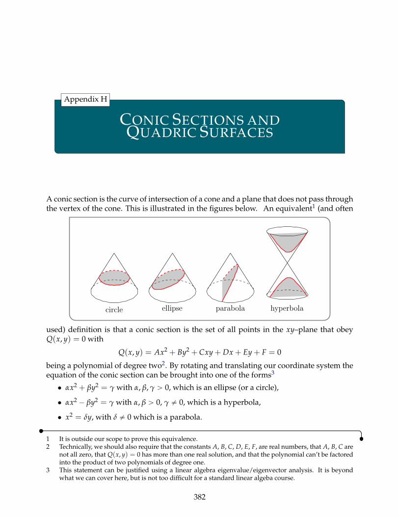
CONIC SECTIONS ANDQUADRIC SURFACES
Appendix H
A conic section is the curve of intersection of a cone and a plane that does not pass throughthe vertex of the cone. This is illustrated in the figures below. An equivalent1 (and often
circle ellipse parabola hyperbola
used) definition is that a conic section is the set of all points in the xy–plane that obeyQ(x, y) = 0 with
Q(x, y) = Ax2 + By2 + Cxy + Dx + Ey + F = 0
being a polynomial of degree two2. By rotating and translating our coordinate system theequation of the conic section can be brought into one of the forms3
• αx2 + βy2 = γ with α, β, γ ą 0, which is an ellipse (or a circle),
• αx2 ´ βy2 = γ with α, β ą 0, γ ‰ 0, which is a hyperbola,
• x2 = δy, with δ ‰ 0 which is a parabola.
1 It is outside our scope to prove this equivalence.2 Technically, we should also require that the constants A, B, C, D, E, F, are real numbers, that A, B, C are
not all zero, that Q(x, y) = 0 has more than one real solution, and that the polynomial can’t be factoredinto the product of two polynomials of degree one.
3 This statement can be justified using a linear algebra eigenvalue/eigenvector analysis. It is beyondwhat we can cover here, but is not too difficult for a standard linear algeba course.
382
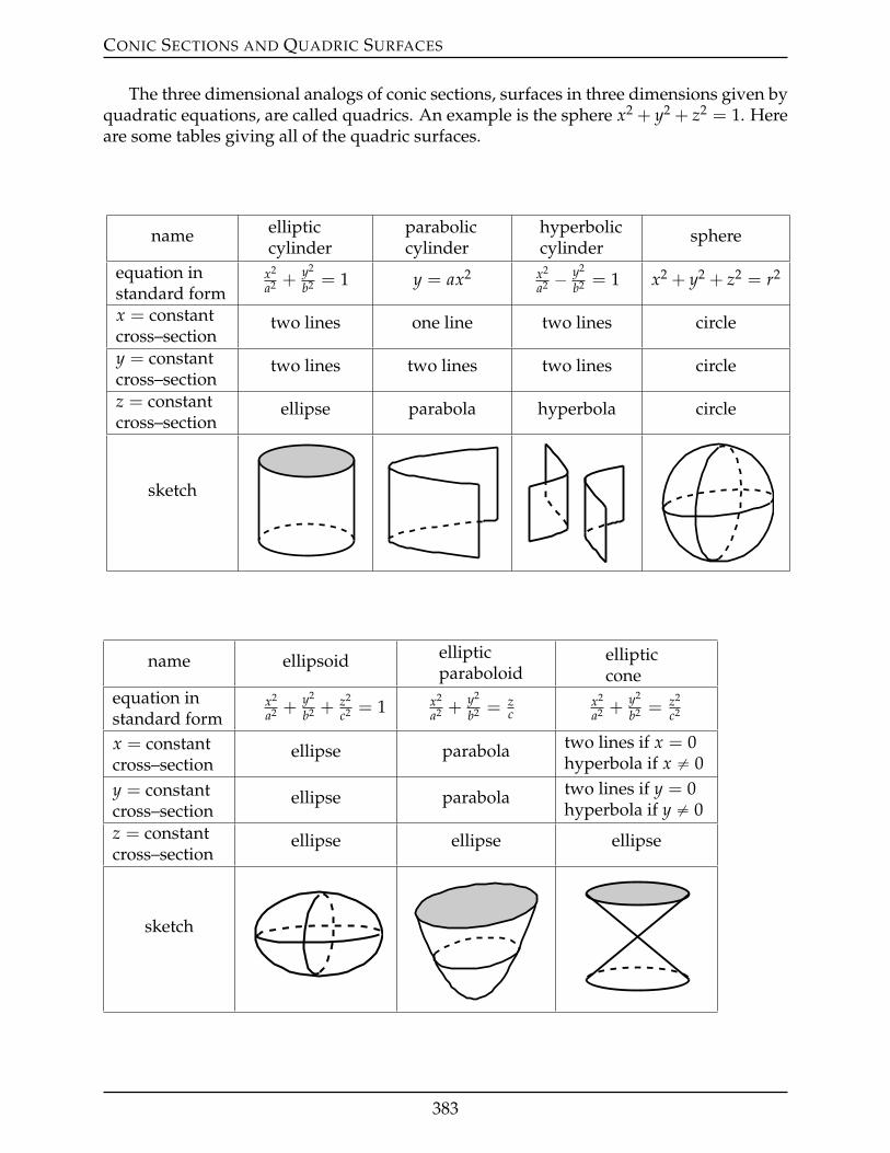
CONIC SECTIONS AND QUADRIC SURFACES
The three dimensional analogs of conic sections, surfaces in three dimensions given byquadratic equations, are called quadrics. An example is the sphere x2 + y2 + z2 = 1. Hereare some tables giving all of the quadric surfaces.
name ellipticcylinder
paraboliccylinder
hyperboliccylinder
sphere
equation instandard form
x2
a2 +y2
b2 = 1 y = ax2 x2
a2 ´ y2
b2 = 1 x2 + y2 + z2 = r2
x = constantcross–section
two lines one line two lines circle
y = constantcross–section
two lines two lines two lines circle
z = constantcross–section
ellipse parabola hyperbola circle
sketch
name ellipsoid ellipticparaboloid
ellipticcone
equation instandard form
x2
a2 +y2
b2 +z2
c2 = 1 x2
a2 +y2
b2 = zc
x2
a2 +y2
b2 = z2
c2
x = constantcross–section
ellipse parabola two lines if x = 0hyperbola if x ‰ 0
y = constantcross–section
ellipse parabola two lines if y = 0hyperbola if y ‰ 0
z = constantcross–section
ellipse ellipse ellipse
sketch
383
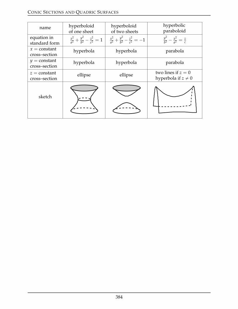
CONIC SECTIONS AND QUADRIC SURFACES
name hyperboloidof one sheet
hyperboloidof two sheets
hyperbolicparaboloid
equation instandard form
x2
a2 +y2
b2 ´ z2
c2 = 1 x2
a2 +y2
b2 ´ z2
c2 = ´1 y2
b2 ´ x2
a2 = zc
x = constantcross–section
hyperbola hyperbola parabola
y = constantcross–section
hyperbola hyperbola parabola
z = constantcross–section
ellipse ellipse two lines if z = 0hyperbola if z ‰ 0
sketch
384