Calculus IB: Lecture 01
710
Calculus IB: Lecture 01 Luo Luo Department of Mathematics, HKUST http://luoluo.people.ust.hk/ Luo Luo (HKUST) MATH 1013 1 / 24
-
Upload
khangminh22 -
Category
Documents
-
view
3 -
download
0
Transcript of Calculus IB: Lecture 01

Calculus IB: Lecture 01
Luo Luo
Department of Mathematics, HKUST
http://luoluo.people.ust.hk/
Luo Luo (HKUST) MATH 1013 1 / 24
Outline
1 Course Overview
2 Sets and Intervals
3 Solving Inequalities
4 Absolute Value
Luo Luo (HKUST) MATH 1013 2 / 24

Outline
1 Course Overview
2 Sets and Intervals
3 Solving Inequalities
4 Absolute Value
Luo Luo (HKUST) MATH 1013 3 / 24
Why Calculus is Important?
Calculus is used in everywhere
mathematics,
physical science,
computer science,
statistics,
engineering,
economics,
......
Engineering would be almost impossible without calculus today.
I believe an understanding of calculus is never wasted.
Luo Luo (HKUST) MATH 1013 3 / 24

Course Overview
Topics in single variable calculus
1 functions and graphs
2 limits of functions and continuity
3 derivatives and their applications
4 indefinite and definite integrals
Intended learning outcomes
1 develop basic computational skills in calculus
2 express quantitative relationships by the language of functions
3 apply calculus in modeling and solving real-world problems
Luo Luo (HKUST) MATH 1013 4 / 24

Assessment Scheme and Resources
Percentage of coursework and examination
1 25% by online homework (https://www.classviva.org)
2 no midterm exam
3 75% by final exam
Recommended reading:
1 Jishan Hu, Weiping Li and Yueping Wu. “Calculus for scientists andengineers with MATLAB”.
2 James Stewart. “Single variable calculus: Early transcendentals”.Cengage Learning, 2015.
Luo Luo (HKUST) MATH 1013 5 / 24

Outline
1 Course Overview
2 Sets and Intervals
3 Solving Inequalities
4 Absolute Value
Luo Luo (HKUST) MATH 1013 6 / 24

Notations of Sets
A set is a well-defined collection of distinct elements.
1 We can list all elements: e.g., the expression {2, 5, 7} means a setconsisting of three numbers: 2, 5 and 7.
2 Capital letters are often used to denote a set; e.g., A = {2, 5, 7},where 2, 5, 7 are called the elements of the set A.
3 The set of all real numbers is often denoted by the symbol R.
4 The set of all integer is often denoted by the symbol Z.
5 We use {x : P(x)} to denote the set which is consisted of allelements x satisfying the description P(x).
Luo Luo (HKUST) MATH 1013 6 / 24
Notations of Sets
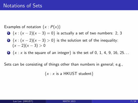
Examples of notation {x : P(x)}1 {x : (x − 2)(x − 3) = 0} is actually a set of two numbers: 2, 3
2 {x : (x − 2)(x − 3) > 0} is the solution set of the inequality:(x − 2)(x − 3) > 0
3 {x : x is the square of an integer} is the set of 0, 1, 4, 9, 16, 25. . .
Sets can be consisting of things other than numbers in general; e.g.,
{x : x is a HKUST student}
Luo Luo (HKUST) MATH 1013 7 / 24

Notations of Intervals
Infinity, denoted by ∞, represents something that is larger than any realnumber. Similarly, we use −∞ to represent negative infinity that is smallerthan any real number.
An interval is a set of real numbers that contains all real numbers lyingbetween any two endpoints.
1 An endpoint could be a real number, infinity or negative infinity.
2 What is “between”?
Luo Luo (HKUST) MATH 1013 8 / 24

Notations of Intervals
Let a and b be two real numbers. We define different classes of interval asfollows.
Open Intervals Closed Intervals
(a, b) = {x : a < x < b} [a, b] = {x : a ≤ x ≤ b}(−∞, a) = {x : x < a} (−∞, a] = {x : x ≤ a}(a,∞) = {x : x > a} [a,∞) = {x : x ≥ a}
Half Open Half Closed Intervals
[a, b) = {x : a ≤ x < b}(a, b] = {x : a < x ≤ b}
The interval (−∞,∞) formed by all real numbers, that is R = (−∞,∞),which is considered as both open and closed.
The interval [a, b] = (a, b) = [a, b) = (a, b] = (a, a) = [a, a) = (a, a]contains nothing when a > b. We call it empty set, denoted by ∅ or {}.
Luo Luo (HKUST) MATH 1013 9 / 24
Basic Operations on Sets
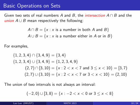
Given two sets of real numbers A and B, the intersection A ∩ B and theunion A ∪ B mean respectively the following:
A ∩ B = {x : x is a number in both A and B}A ∪ B = {x : x is a number either in A or in B}
For examples,
{1, 2, 3, 4} ∩ {3, 4, 9} = {3, 4}{1, 2, 3, 4} ∪ {3, 4, 9} = {1, 2, 3, 4, 9}
(2, 7) ∩ [3, 10) = {x : 2 < x < 7 and 3 ≤ x < 10} = [3, 7)
(2, 7) ∪ (3, 10) = {x : 2 < x < 7 or 3 < x < 10} = (2, 10)
The union of two intervals is not always an interval:
(−2, 0) ∪ [3, 8) = {x : −2 < x < 0 or 3 ≤ x < 8}
Luo Luo (HKUST) MATH 1013 10 / 24

Outline
1 Course Overview
2 Sets and Intervals
3 Solving Inequalities
4 Absolute Value
Luo Luo (HKUST) MATH 1013 11 / 24
Solving Inequalities
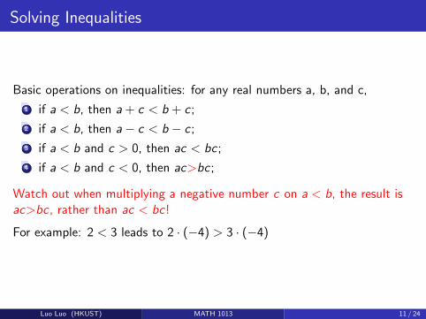
Basic operations on inequalities: for any real numbers a, b, and c,
1 if a < b, then a + c < b + c ;
2 if a < b, then a− c < b − c ;
3 if a < b and c > 0, then ac < bc;
4 if a < b and c < 0, then ac>bc;
Watch out when multiplying a negative number c on a < b, the result isac>bc, rather than ac < bc!
For example: 2 < 3 leads to 2 · (−4) > 3 · (−4)
Luo Luo (HKUST) MATH 1013 11 / 24
Solving Inequalities
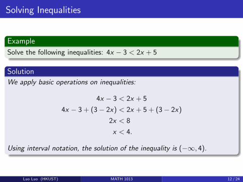
Example
Solve the following inequalities: 4x − 3 < 2x + 5
Solution
We apply basic operations on inequalities:
4x − 3 < 2x + 5
4x − 3 + (3− 2x) < 2x + 5 + (3− 2x)
2x < 8
x < 4.
Using interval notation, the solution of the inequality is (−∞, 4).
Luo Luo (HKUST) MATH 1013 12 / 24
Solving Inequalities
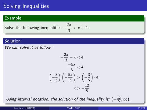
Example
Solve the following inequalities −2x
3< x + 4.
Solution
We can solve it as follow:
−2x
3− x < 4
−5x
3< 4(
−3
5
)(−5x
3
)>
(−3
5
)· 4
x > −12
5
Using interval notation, the solution of the inequality is: (−125 ,∞).
Luo Luo (HKUST) MATH 1013 13 / 24

Solving Inequalities
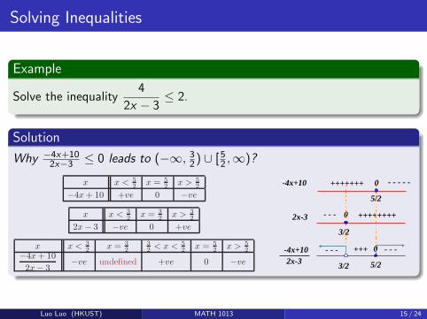
Example
Solve the inequality4
2x − 3≤ 2.
If you multiply 2x − 3 to both sides of the inequality, it is not clear howthe inequality is changed since 2x − 3 may or may not be positive.
Solution
We have
4
2x − 3− 2 ≤ 0⇐⇒ 4
2x − 3− 2(2x − 3)
2x − 3≤ 0
⇐⇒ −4x + 10
2x − 3≤ 0.
The solution of the inequality is x < 32 or x ≥ 5
2 . Using interval notation,the solution is: (−∞, 32) ∪ [52 ,∞).
Luo Luo (HKUST) MATH 1013 14 / 24
Solving Inequalities
Example
Solve the inequality4
2x − 3≤ 2.
Solution
Why −4x+102x−3 ≤ 0 leads to (−∞, 32) ∪ [52 ,∞)?
3. if a < b and c > 0, then ac < bc ;
4. if a < b and c < 0, then ac > bc ; (e.g., 2 < 3, and 2 · (−4) > 3 · (−4).)Watch out when multiplying a negative number to both sides of an inequality, or dividing both sides
of an inequality by a negative number!
Example 1 Solve the following inequalities: (i) 4x− 3 < 2x+ 5; (ii) −2x
3< x+ 4.
(i) Direct approach:4x− 3 < 2x+ 5
4x− 3 + (3 − 2x) < 2x+ 5 + (3− 2x)
2x < 8
x < 4
Using interval notation, the solution of the in-
equality is: (−∞, 4).
Another approach: by working with the equation
4x− 3 = 2x+ 5⇐⇒ 2x = 8⇐⇒ x = 4
we have that x = 4 divides the real line into two
disjoint open intervals (−∞, 4), and (4,∞). Just
by putting in numbers in each interval, it is easy
to check that (−∞, 4) is the solution of 4x − 3 <
2x+ 5.
(ii) −2x
3− x < 4
−5x
3< 4
(
− 3
5
)(
− 5x
3
)
>(
− 3
5
)
· 4
x > −12
5
Using interval notation, the solution of the in-
equality is: (− 125 ,∞)
Now, try solving the equation − 2x3 = x + 4,
and then figure out the solution of the inequality
− 2x3 < x+ 4.
Example 2 Solve the inequality4
2x− 3≤ 2.
Note that if you multiply 2x − 3 to both sides of the inequality, it is not clear how the inequality is
changed since 2x− 3 may or may not be positive.
4
2x− 3− 2 ≤ 0⇐⇒ 4
2x− 3− 2(2x− 3)
2x− 3≤ 0
−4x+ 10
2x− 3≤ 0
The solution of the inequality is: x < 32 or x ≥ 5
2 .
Using interval notation, the solution is: (−∞, 32 ) ∪ [ 52 ,+∞).
Why? The basic idea is to check when the factors −4x+ 10 and 2x− 3 are positive, or negative.
x x < 52 x = 5
2 x > 52
−4x+ 10 +ve 0 −ve
x x < 32 x = 3
2 x > 32
2x− 3 −ve 0 +ve
x x < 32 x = 3
232 < x < 5
2 x = 52 x > 5
2−4x+ 10
2x− 3−ve undefined +ve 0 −ve
5/2
3/2
3/2 5/2
-4x+10
-4x+10
2x-3
2x-3
+++++++
+++
++++++++
- - - - -
- - -
- - - - - -
0
0
0
Hence the solution, x < 32 or x ≥ 5
2 , can be seen easily from these sign tables of−4x+ 10
2x− 3, or sign lines.
An alternative approach is to first work with the equation
4
2x− 3= 2⇐⇒ 2x− 3 = 2⇐⇒ x =
5
2
2
Luo Luo (HKUST) MATH 1013 15 / 24
Solving Inequalities
Exercise
Solve the inequality(x − 2)(x − 5)
(x + 2)(x − 8)≥ 0.
Hint: There are four numbers 2, 5,−2 and 8 divide the real line into fivedisjoint open intervals. We can do the sign checking for each of theseintervals.
Luo Luo (HKUST) MATH 1013 16 / 24

Outline
1 Course Overview
2 Sets and Intervals
3 Solving Inequalities
4 Absolute Value
Luo Luo (HKUST) MATH 1013 17 / 24

Absolute Value
The absolute value of a real number x , denoted by |x |, is defined by
|x | =
{x if x ≥ 0,
−x if x < 0.
For example, |5| = 5, and | − 5| = −(−5) = 5. Similarly,
|x − y | =
{x − y if x ≥ y ,
y − x if x < y .
The value of |x − y | can also be seen as the distance between the numbersx and y on the real line.
x y
|x-y| = y - x
xy
|x-y| = x - y
Luo Luo (HKUST) MATH 1013 17 / 24

Absolute Value
No matter what a mathematical expression �, we have
|�| =
{� if � ≥ 0,
−� if � < 0.
Note also that for any positive real number k , we have
1 |�| < k ⇐⇒ − k < � < k
2 |�| > k ⇐⇒ � < −k or � > k
Example
The equation |2x − 5| = 3 simply means 2x − 5 = 3 or 2x − 5 = −3, thatis x = 4 or x = 1.
Luo Luo (HKUST) MATH 1013 18 / 24
Equations or Inequalities Involving Absolute Values
Example
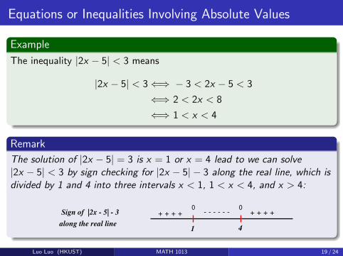
The inequality |2x − 5| < 3 means
|2x − 5| < 3⇐⇒ − 3 < 2x − 5 < 3
⇐⇒ 2 < 2x < 8
⇐⇒ 1 < x < 4
Remark
The solution of |2x − 5| = 3 is x = 1 or x = 4 lead to we can solve|2x − 5| < 3 by sign checking for |2x − 5| − 3 along the real line, which isdivided by 1 and 4 into three intervals x < 1, 1 < x < 4, and x > 4:
Sign of |2x - 5| - 3
along the real line1 4
00+ + + ++ + + + - - - - - -
Luo Luo (HKUST) MATH 1013 19 / 24

Equations or Inequalities Involving Absolute Values
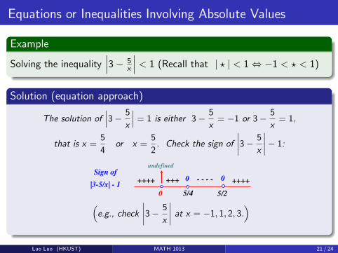
Example
Solving the inequality∣∣∣3− 5
x
∣∣∣ < 1 (Recall that | ? | < 1⇔ −1 < ? < 1)
Solution (inequality approach)
−1 < 3− 5
x< 1⇐⇒ −1 <
3x − 5
x< 1
0 < 1 +3x − 5
xand
3x − 5
x− 1 < 0
0 <4x − 5
xand
2x − 5
x< 0(
x < 0 or x >5
4
)and 0 < x <
5
2
i.e.,5
4< x <
5
2
Luo Luo (HKUST) MATH 1013 20 / 24
Equations or Inequalities Involving Absolute Values
Example
Solving the inequality∣∣∣3− 5
x
∣∣∣ < 1 (Recall that | ? | < 1⇔ −1 < ? < 1)
Solution (equation approach)
The solution of∣∣∣3− 5
x
∣∣∣ = 1 is either 3− 5
x= −1 or 3− 5
x= 1,
that is x =5
4or x =
5
2. Check the sign of
∣∣∣∣3− 5
x
∣∣∣∣− 1:
5/25/40|3-5/x| - 1
Sign of00
undefined
++++- - - -++++ +++
(e.g., check
∣∣∣∣3− 5
x
∣∣∣∣ at x = −1, 1, 2, 3.)
Luo Luo (HKUST) MATH 1013 21 / 24
Equations or Inequalities Involving Absolute Values
Some Exercises
Find the solution of the inequality
1
∣∣2x − 5∣∣ ≥ 3
2
∣∣∣3− 5
x
∣∣∣ ≥ 1
3 |x − 1|+ |x − 3| < 4 (a harder one!)
Luo Luo (HKUST) MATH 1013 22 / 24

Some Basic Properties of Absolute Values
Some Properties of Absolute Values:
1 | − x | = |x |
2 |xy | = |x ||y |
3
∣∣∣xy
∣∣∣ =|x ||y |
, where y 6= 0
4 |x + y | ≤ |x |+ |y | (triangle inequality)
where equality holds if and only if x , y are of the same sign (equivalentlyab > 0), or one of them is 0.
Luo Luo (HKUST) MATH 1013 23 / 24

The Proof of Triangle Inequality
Why |x + y | ≤ |x |+ |y | holds?
Proof.
It follows easily from
|x + y |2 = (x + y)2 = x2 + 2xy + y 2
= |x |2 + 2xy + |y |2
≤ |x |2 + 2|x ||y |+ |x |2 = (|x |+ |y |)2
|x + y | ≤ |x |+ |y |
where equality holds if and only if xy = |xy |, equivalently, xy ≥ 0.
Luo Luo (HKUST) MATH 1013 24 / 24

Calculus IB: Lecture 02
Luo Luo
Department of Mathematics, HKUST
http://luoluo.people.ust.hk/
Luo Luo (HKUST) MATH 1013 1 / 40

Outline
1 What is a Function?
2 Some Elementary Function
3 Basic Operations: Sum, Product, Quotient and Composition
4 Functions with Certain Special Properties
5 Transformations of Graphs
Luo Luo (HKUST) MATH 1013 2 / 40
Outline
1 What is a Function?
2 Some Elementary Function
3 Basic Operations: Sum, Product, Quotient and Composition
4 Functions with Certain Special Properties
5 Transformations of Graphs
Luo Luo (HKUST) MATH 1013 3 / 40

What is a Function?
A function f is a rule that assigns to each element x in a set Dexactly one element in a set E , which is denoted by f (x) and calledthe function value of f at x .
The set D is called the domain of f and the set E is called thecodomain of f .
A function f with domain D and codomain E is usually denoted byf : D −→ E .
We can think of a function f : D −→ E as an input-output machinewhich produces a unique output value f (x) in the codomain E for anygiven input value x taken from the domain D.
By considering the set of all function values of f , we have the rangeof the function: range of f = {f (x) : x is in the domain D}.
Note that the range of a function f : D −→ E may not be the wholecodomain E . f is said to be onto or surjective if E = range of f .Luo Luo (HKUST) MATH 1013 3 / 40
What is a Function?
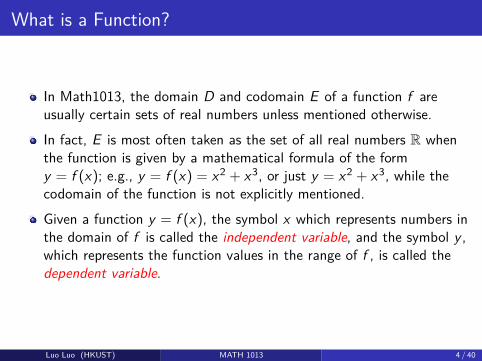
In Math1013, the domain D and codomain E of a function f areusually certain sets of real numbers unless mentioned otherwise.
In fact, E is most often taken as the set of all real numbers R whenthe function is given by a mathematical formula of the formy = f (x); e.g., y = f (x) = x2 + x3, or just y = x2 + x3, while thecodomain of the function is not explicitly mentioned.
Given a function y = f (x), the symbol x which represents numbers inthe domain of f is called the independent variable, and the symbol y ,which represents the function values in the range of f , is called thedependent variable.
Luo Luo (HKUST) MATH 1013 4 / 40

Graph of a Function
The graph of a function f : D −→ E is just the set of ordered pairs ofnumbers
graph of f = {(x , f (x)) : x is a number in D}
which can be geometrically plotted as a set of coordinate points in thexy -plane, if the function f is not too complicated.
Vertical line test for the graph of a functionThe graph of any function f should intersect every vertical line atmost once (since for any number c in the domain of f , only onefunction value f (c) is assigned).Conversely, any set of points in the xy -plane passing this test can beused to defined a function graphically.
Luo Luo (HKUST) MATH 1013 5 / 40
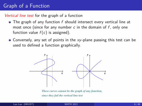
Graph of a FunctionVertical line test for the graph of a function
The graph of any function f should intersect every vertical line atmost once (since for any number c in the domain of f , only onefunction value f (c) is assigned).
Conversely, any set of points in the xy -plane passing this test can beused to defined a function graphically.
x
y
x
y
These curves cannot be the graph of any function,
since they fail the vertical line test
Luo Luo (HKUST) MATH 1013 6 / 40
What is a Function?
A function is usually used to relate two quantities, namely, to indicate howthe value of a quantity (in the domain) determines uniquely the value ofanother quantity (in the codomain).
A function can be described in the following ways:1 verbally; (by a description in words)2 numerically; (by a table of function values, often partially)3 visually; (by a graph)4 by an explicit formula.
Luo Luo (HKUST) MATH 1013 7 / 40

Some basic examples of functions
ExampleConsider a domain D = {1, 2, 4, 7}, and the codomain R which is the setof all real numbers. Let the rule of the function f : D −→ R, whichassigns function values to numbers in D, be defined explicitly by setting
f (1) = 1, f (2) = 3, f (4) = 1, f (7) = 6.
The graph of f is obviously the set of four ordered pairs of numbers{(1, 1), (2, 3), (4, 1), (7, 6)}, which can also be described in terms of asimple table of function values, or a figure of four points in the xy -plane:
x 1 2 4 7f (x) 1 3 1 6
or←→2
4
6
2 4 6
x
y
Luo Luo (HKUST) MATH 1013 8 / 40

Some basic examples of functions
Describing a function f by a complete table of function values, or acomplete geometric graph, is not always feasible.
Especially when the domain D of f has too many numbers; e.g., what ifdomain D contains infinitely many numbers?
Luo Luo (HKUST) MATH 1013 9 / 40

Some basic examples of functions
ExampleConsider the function f : R −→ R where the rule for assigning functionvalues is defined by the following mathematical formula f (x) = 2x .It is then easy to figure out any function value you want, e.g.,
f (2) = 2 · 2 = 4, f (21) = 2 · 21 = 42, f (−3) = 2 · (−3) = −6
However, it is obviously impossible to show a complete table of functionvalues, as there are infinitely many real numbers.
This function is simple enoughto sketch: a straight line in thexy -plane through the origin withslope 2.
x
y
y = 2x
Luo Luo (HKUST) MATH 1013 10 / 40
Some basic examples of functions
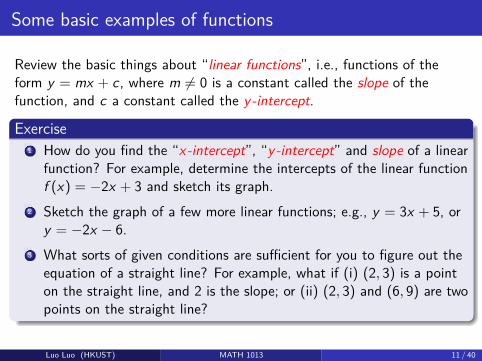
Review the basic things about “linear functions”, i.e., functions of theform y = mx + c, where m 6= 0 is a constant called the slope of thefunction, and c a constant called the y-intercept.
Exercise1 How do you find the “x-intercept”, “y-intercept” and slope of a linear
function? For example, determine the intercepts of the linear functionf (x) = −2x + 3 and sketch its graph.
2 Sketch the graph of a few more linear functions; e.g., y = 3x + 5, ory = −2x − 6.
3 What sorts of given conditions are sufficient for you to figure out theequation of a straight line? For example, what if (i) (2, 3) is a pointon the straight line, and 2 is the slope; or (ii) (2, 3) and (6, 9) are twopoints on the straight line?
Luo Luo (HKUST) MATH 1013 11 / 40
Some basic examples of functions
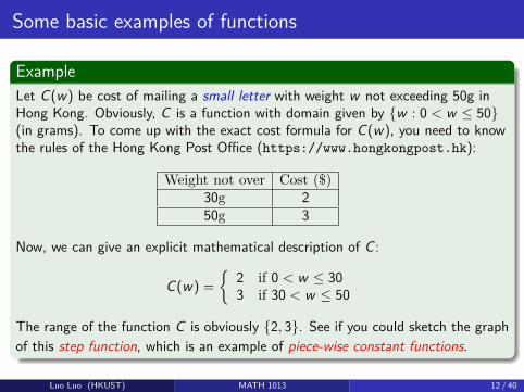
ExampleLet C(w) be cost of mailing a small letter with weight w not exceeding 50g inHong Kong. Obviously, C is a function with domain given by {w : 0 < w ≤ 50}(in grams). To come up with the exact cost formula for C(w), you need to knowthe rules of the Hong Kong Post Office (https://www.hongkongpost.hk):
Weight not over Cost ($)30g 250g 3
Now, we can give an explicit mathematical description of C :
C(w) ={
2 if 0 < w ≤ 303 if 30 < w ≤ 50
The range of the function C is obviously {2, 3}. See if you could sketch the graphof this step function, which is an example of piece-wise constant functions.
Luo Luo (HKUST) MATH 1013 12 / 40

Some basic examples of functions
ExampleThe absolute value function, denoted by f (x) = |x |, is given by thefollowing case by case formula:
y
x
y = |x|f (x) =
{x if x ≥ 0−x if x < 0
f (x) = |x | is an example of what people call piecewise linear functions.The domain of f is the set of all real numbers, and the range is the set ofall non-negative real numbers.
Luo Luo (HKUST) MATH 1013 13 / 40

Some basic examples of functions
Exercise1 Sketch the graph of f (x) = |2x − 4|, which is another example of a
piece-wise linear function.2 Sketch the graph of the function (“unit step function”)
y = uc(t) ={
0 if t < c1 if t ≥ c
where c is some fixed constant.3 Sketch the graph of the function y = 3u2(t)− 2u4(t); and then use
piece-wise defined formula to describe the function.
Luo Luo (HKUST) MATH 1013 14 / 40

Some basic examples of functions
Example (real wold)Let’s just take the domain D to be an appropriate set of real numbers in eachcontext below, and codomain E = R the set of all real numbers. All units are SIunits when applicable.
numbers in D represent function values in E representside length area of the square with given side length
temperature in Celsius same temperature in Fahrenheit
These functions above can be described more clearly by mathematical formulas ifsuitable symbols are introduced to denote the quantities involved.
numbers in D represent function values in E representx = side length A = area of the square...
C = temperature in Celsius F = same temperature in Fahrenheit
A = x2 (area of a square), F = 95C + 32 (unit conversion)
Luo Luo (HKUST) MATH 1013 15 / 40

Some basic examples of functions
RemarkSome domains of above functions are restricted to a certain range ofvalues limited by physical restrictions.
1 For the area function, we have D = {x : x ≥ 0}.2 The minimum temperature is taken as -273.15 on the Celsius scale.
It is important to understand the “practical domain” of a function in anymodeling application, i.e., possible inputs of the function limited by theassumptions of the model, instead of just the “natural domain” of thefunction, i.e., where the formula makes sense mathematically.
Luo Luo (HKUST) MATH 1013 16 / 40

Outline
1 What is a Function?
2 Some Elementary Function
3 Basic Operations: Sum, Product, Quotient and Composition
4 Functions with Certain Special Properties
5 Transformations of Graphs
Luo Luo (HKUST) MATH 1013 17 / 40
Some Elementary Functions
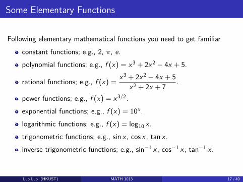
Following elementary mathematical functions you need to get familiar
constant functions; e.g., 2, π, e.
polynomial functions; e.g., f (x) = x3 + 2x2 − 4x + 5.
rational functions; e.g., f (x) = x3 + 2x2 − 4x + 5x2 + 2x + 7 .
power functions; e.g., f (x) = x3/2.
exponential functions; e.g., f (x) = 10x .
logarithmic functions; e.g., f (x) = log10 x .
trigonometric functions; e.g., sin x , cos x , tan x .
inverse trigonometric functions; e.g., sin−1 x , cos−1 x , tan−1 x .
Luo Luo (HKUST) MATH 1013 17 / 40

Outline
1 What is a Function?
2 Some Elementary Function
3 Basic Operations: Sum, Product, Quotient and Composition
4 Functions with Certain Special Properties
5 Transformations of Graphs
Luo Luo (HKUST) MATH 1013 18 / 40

Basic Operations: Sum, Product and Quotient
Given real-valued functions f and g , we can define new functions f + g(sum), fg (product), and f
g (quotient) simply by setting following rules:
(f + g)(x) = f (x) + g(x)
(fg)(x) = f (x)g(x)
( fg)
(x) = f (x)g(x)
as long as both function values, f (x) and g(x), are well-defined, and thecorresponding arithmetic operations on them are valid.
However, we need to be careful with the domains of these functions.
Luo Luo (HKUST) MATH 1013 18 / 40
Basic Operations: Sum, Product and Quotient
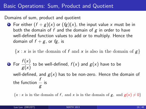
Domains of sum, product and quotient1 For either (f + g)(x) or (fg)(x), the input value x must be in
both the domain of f and the domain of g in order to havewell-defined function values to add or to multiply. Hence thedomain of f + g , or fg , is
{x : x is is the domain of f and x is also in the domain of g}
2 For f (x)g(x) to be well-defined, f (x) and g(x) have to be
well-defined, and g(x) has to be non-zero. Hence the domain ofthe function f
g is
{x : x is in the domain of f , and x is in the domain of g , and g(x) 6= 0}
Luo Luo (HKUST) MATH 1013 19 / 40
Basic Operations: Composition
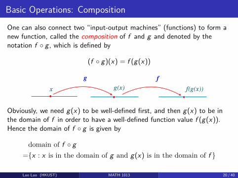
One can also connect two “input-output machines” (functions) to form anew function, called the composition of f and g and denoted by thenotation f ◦ g , which is defined by
(f ◦ g)(x) = f (g(x))
x f(g(x))
g f
g(x)
Obviously, we need g(x) to be well-defined first, and then g(x) to be inthe domain of f in order to have a well-defined function value f (g(x)).Hence the domain of f ◦ g is given by
domain of f ◦ g={x : x is in the domain of g and g(x) is in the domain of f }
Luo Luo (HKUST) MATH 1013 20 / 40
Basic Operations: Composition
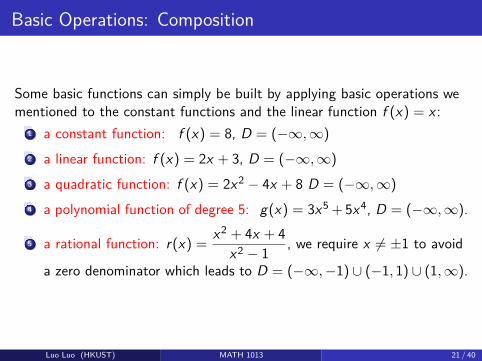
Some basic functions can simply be built by applying basic operations wementioned to the constant functions and the linear function f (x) = x :
1 a constant function: f (x) = 8, D = (−∞,∞)2 a linear function: f (x) = 2x + 3, D = (−∞,∞)3 a quadratic function: f (x) = 2x2 − 4x + 8 D = (−∞,∞)4 a polynomial function of degree 5: g(x) = 3x5 + 5x4, D = (−∞,∞).
5 a rational function: r(x) = x2 + 4x + 4x2 − 1 , we require x 6= ±1 to avoid
a zero denominator which leads to D = (−∞,−1) ∪ (−1, 1) ∪ (1,∞).
Luo Luo (HKUST) MATH 1013 21 / 40

Polynomial Function and Rational Function
1 A polynomial function of degree n is a function of the form
p(x) = anxn + an−1xn−1 + · · ·+ a1x + a0,
where, and a0, . . . , an are some constants.2 A rational function is the quotient of two polynomials, i.e., a function
of the form
R(x) = anxn + an−1xn−1 + · · ·+ a1x + a0bmxm + bm−1xm−1 + · · ·+ b1x + b0
where n, m are non-negative integers, and a0, . . . , an, b0, . . . , bn aresome constants with an 6= 0 and bm 6= 0.
Luo Luo (HKUST) MATH 1013 22 / 40
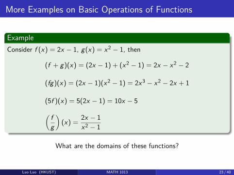
More Examples on Basic Operations of Functions
ExampleConsider f (x) = 2x − 1, g(x) = x2 − 1, then
(f + g)(x) = (2x − 1) + (x2 − 1) = 2x − x2 − 2
(fg)(x) = (2x − 1)(x2 − 1) = 2x3 − x2 − 2x + 1
(5f )(x) = 5(2x − 1) = 10x − 5( f
g
)(x) = 2x − 1
x2 − 1
What are the domains of these functions?
Luo Luo (HKUST) MATH 1013 23 / 40

Examples on Composition Operation
ExampleSuppose f (x) = 2x − 1, g(x) = x2 − 1 as above. Then
(f ◦ g)(x) = f (g(x))= f (x2 − 1)= 2(x2 − 1)− 1= 2x2 − 3
(Note that f (F) = 2F− 1)
(g ◦ f )(x) = g(f (x))= g(2x − 1)= (2x − 1)2 − 1= 4x2 − 4x
(Note that g(F) = F2 − 1)
Note that in general, f ◦ g and g ◦ f are not the same function.
Luo Luo (HKUST) MATH 1013 24 / 40
Examples on Composition Operation
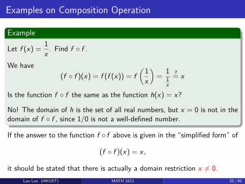
Example
Let f (x) = 1x . Find f ◦ f .
We have(f ◦ f )(x) = f (f (x)) = f
(1x
)= 1
1x
?= x
Is the function f ◦ f the same as the function h(x) = x?
No! The domain of h is the set of all real numbers, but x = 0 is not in thedomain of f ◦ f , since 1/0 is not a well-defined number.
If the answer to the function f ◦ f above is given in the “simplified form” of
(f ◦ f )(x) = x ,
it should be stated that there is actually a domain restriction x 6= 0.Luo Luo (HKUST) MATH 1013 25 / 40
Examples on Composition Operation
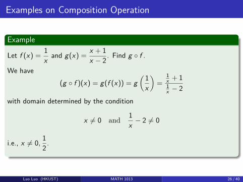
Example
Let f (x) = 1x and g(x) = x + 1
x − 2. Find g ◦ f .
We have(g ◦ f )(x) = g(f (x)) = g
(1x
)=
1x + 11x − 2
with domain determined by the condition
x 6= 0 and 1x − 2 6= 0
i.e., x 6= 0, 12.
Luo Luo (HKUST) MATH 1013 26 / 40
Examples on Composition Operation
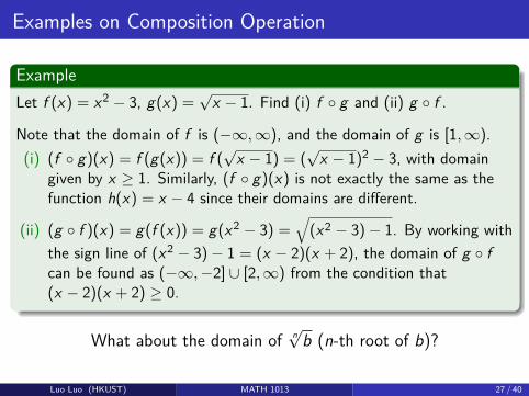
ExampleLet f (x) = x2 − 3, g(x) =
√x − 1. Find (i) f ◦ g and (ii) g ◦ f .
Note that the domain of f is (−∞,∞), and the domain of g is [1,∞).(i) (f ◦ g)(x) = f (g(x)) = f (
√x − 1) = (
√x − 1)2 − 3, with domain
given by x ≥ 1. Similarly, (f ◦ g)(x) is not exactly the same as thefunction h(x) = x − 4 since their domains are different.
(ii) (g ◦ f )(x) = g(f (x)) = g(x2 − 3) =√
(x2 − 3)− 1. By working withthe sign line of (x2 − 3)− 1 = (x − 2)(x + 2), the domain of g ◦ fcan be found as (−∞,−2] ∪ [2,∞) from the condition that(x − 2)(x + 2) ≥ 0.
What about the domain of n√
b (n-th root of b)?
Luo Luo (HKUST) MATH 1013 27 / 40

More discussion on n√
b
1 For any positive even number n, the radical expression n√b denotesthe positive root of the equation xn = b. For example, 4√16 = 2 since24 = 16. No real root exists if b is negative, e.g., 4√−16 does notexist as a real number since x4 ≥ 0 > −16 for any real number x , i.e.,x4 = −16 has no real solution.
2 For any positive odd number n, the equation xn = b has a unique realroot for any given real number b, which is also denoted by n√b. Forexamples, 3√8 = 2 since 23 = 8, and 3√−8 = −2 since (−2)3 = −8.
3 Recall that a radical expression can also be expressed in terms ofexponent notation; e.g., n
√x = x 1
n for any positive integer n. Therelation between the power function y = xn and the n-th rootfunction y = n
√x will be discussed in more detail later when we deal
with the concept of inverse function.
Luo Luo (HKUST) MATH 1013 28 / 40
More Discussion on Composition Operation
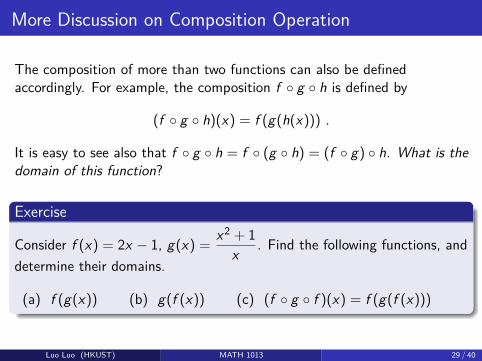
The composition of more than two functions can also be definedaccordingly. For example, the composition f ◦ g ◦ h is defined by
(f ◦ g ◦ h)(x) = f (g(h(x))) .
It is easy to see also that f ◦ g ◦ h = f ◦ (g ◦ h) = (f ◦ g) ◦ h. What is thedomain of this function?
Exercise
Consider f (x) = 2x − 1, g(x) = x2 + 1x . Find the following functions, and
determine their domains.
(a) f (g(x)) (b) g(f (x)) (c) (f ◦ g ◦ f )(x) = f (g(f (x)))
Luo Luo (HKUST) MATH 1013 29 / 40
Outline
1 What is a Function?
2 Some Elementary Function
3 Basic Operations: Sum, Product, Quotient and Composition
4 Functions with Certain Special Properties
5 Transformations of Graphs
Luo Luo (HKUST) MATH 1013 30 / 40
Even and Odd Functions
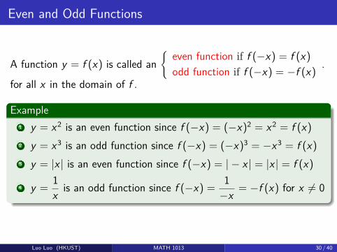
A function y = f (x) is called an{
even function if f (−x) = f (x)odd function if f (−x) = −f (x) .
for all x in the domain of f .
Example1 y = x2 is an even function since f (−x) = (−x)2 = x2 = f (x)2 y = x3 is an odd function since f (−x) = (−x)3 = −x3 = f (x)3 y = |x | is an even function since f (−x) = | − x | = |x | = f (x)
4 y = 1x is an odd function since f (−x) = 1
−x = −f (x) for x 6= 0
Luo Luo (HKUST) MATH 1013 30 / 40

Even and Odd Functions
(1)y = x2 is an even function (2)y = x3 is an odd function
0
5
10
15
20
25
-4 -2 0 2 4
x
y
y = x2
-x x
y = x2
-100
-50
0
50
100
-4 -2 0 2 4
x
y
x
-x
x3
-x3
the graph of an even the graph of an oddfunction is symmetric with function is symmetric with
respect to the y -axis respect to the origin(graph remains unchanged after (graph remains unchanged after
reflection about y-axis) rotation of 180 degrees about origin)
Luo Luo (HKUST) MATH 1013 31 / 40
Even and Odd Functions
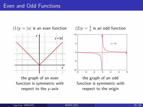
(1)y = |x | is an even function (2)y = 1x is an odd function
y = |x|
x
y
-10
-5
0
5
10
-6 -4 -2 0 2 4 6
x
y
y = 1/x
the graph of an even the graph of an oddfunction is symmetric with function is symmetric with
respect to the y -axis respect to the origin
Luo Luo (HKUST) MATH 1013 32 / 40

Periodic FunctionsA function f (x) is periodic if there is a number T 6= 0 such thatf (x + T ) = f (x) for all x in the domain. The smallest such T > 0, if itexists, is called the (fundamental) period of the periodic function.Note that a periodic function may has no (fundamental) period, why?
The graph of a periodic function does not change, if it is shifted to the left(or right), by a distance equal to an integral multiple of the period.
Any function f defined on the interval [a, b) can be extended to a periodicfunction defined on the entire real line: keep shifting the graph by adistance of b − a.
y = f(x)
a b a b
Luo Luo (HKUST) MATH 1013 33 / 40
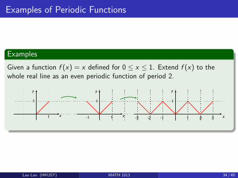
Examples of Periodic Functions
ExamplesGiven a function f (x) = x defined for 0 ≤ x ≤ 1. Extend f (x) to thewhole real line as an even periodic function of period 2.
1
1
y
x1 -1-1
1 1
y y
x1 x2-2 3-3
Luo Luo (HKUST) MATH 1013 34 / 40
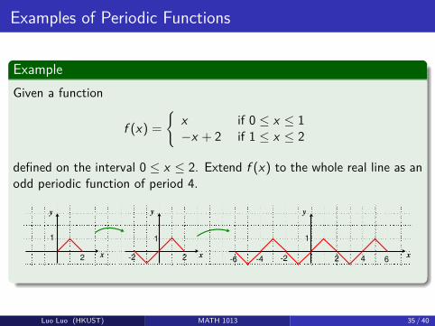
Examples of Periodic Functions
ExampleGiven a function
f (x) ={
x if 0 ≤ x ≤ 1−x + 2 if 1 ≤ x ≤ 2
defined on the interval 0 ≤ x ≤ 2. Extend f (x) to the whole real line as anodd periodic function of period 4.
2
1
y
x
1 1
y y
x x2-2 4-42-2 6-6
Luo Luo (HKUST) MATH 1013 35 / 40
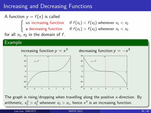
Increasing and Decreasing FunctionsA function y = f (x) is called{
an increasing function if f (x1) < f (x2) whenever x1 < x2
a decreasing function if f (x1) > f (x2) whenever x1 < x2
for all x1, x2 in the domain of f .
Exampleincreasing function:y = x3 decreasing function:y = −x3
-30
-20
-10
0
10
20
30
-3 -2 -1 0 1 2 3
x
y
y = x3
-30
-20
-10
0
10
20
30
-3 -2 -1 0 1 2 3
x
y
y = -x3
The graph is rising/dropping when travelling along the positive x -direction. Byarithmetic, x3
2 > x31 whenever x2 > x1, hence x3 is an increasing function.
Luo Luo (HKUST) MATH 1013 36 / 40
Outline
1 What is a Function?
2 Some Elementary Function
3 Basic Operations: Sum, Product, Quotient and Composition
4 Functions with Certain Special Properties
5 Transformations of Graphs
Luo Luo (HKUST) MATH 1013 37 / 40

Transformations of Graphs
1 Graph of y = f (x) + k:{upward shifting of the graph of f by k units if k > 0downward shifting of the graph of f by k units if k < 0
2 Graph of y = f (x + k):{shifting the graph of f to the right by |k| > 0 units if k < 0shifting the graph of f to the left by k units if k > 0
3 Graph of y = −f (x): reflecting the graph of f across the x -axis.4 Graph of y = f (−x): reflecting the graph of f across the y -axis.5 Graph of y = kf (x), where k > 0:{
stretching the graph of f in y -direction by a factor of k if k > 1compressing the graph of f in y -direction by a factor of k if 0 < k < 1
6 Graph of y = f (kx), where k > 0:{compressing the graph of f in x -direction by a factor of k if k > 1stretching the graph of f in x -direction by a factor of k if 0 < k < 1
Luo Luo (HKUST) MATH 1013 37 / 40
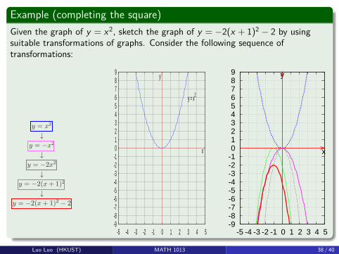
Example (completing the square)Given the graph of y = x2, sketch the graph of y = −2(x + 1)2 − 2 by usingsuitable transformations of graphs. Consider the following sequence oftransformations:
Transformations of Graphs
As long as you are familiar with the graphing process, it is pretty easy to see how the graph of a function
y = f(x) is related to the graphs of y = f(x) + k, y = f(x + k), y = kf(x) and y = f(kx) for some fixed
constant k.
(i) Graph of y = f(x) + k:
{
upward shifting of the graph of f by k units if k > 0
Downward shifting of the graph of f by k units if k < 0
(ii) Graph of y = f(x+ k):
{
Shifting the graph of f to the right by |k| > 0 units if k < 0
Shifting the graph of f to the left by k units if k > 0
(iii) Graph of y = −f(x): Reflecting the graph of f across the x-axis.
(iv) Graph of y = f(−x): Reflecting the graph of f across the y-axis.
(v) Graph of y = kf(x), where k > 0:
{
Stretching the graph of f in y-direction by a factor of k if k > 1
Compressing the graph of f in y-direction by a factor of k if 0 < k < 1
(vi) Graph of y = f(kx), where k > 0:
{
Compressing the graph of f in x-direction by a factor of k if k > 1
Stretching the graph of f in x-direction by a factor of k if 0 < k < 1
Example 10 Given the graph of y = x2, sketch the graph of y = −2(x + 1)2 − 2 by using suitable
transformations of graphs.
Consider the following sequence of transformations:
-9-8-7-6-5-4-3-2-1 0 1 2 3 4 5 6 7 8 9
-5 -4 -3 -2 -1 0 1 2 3 4 5
x
y
y = x2
-9-8-7-6-5-4-3-2-1 0 1 2 3 4 5 6 7 8 9
-5 -4 -3 -2 -1 0 1 2 3 4 5
x
y
y = x2
↓y = −x2
↓y = −2x2
↓y = −2(x+ 1)2
↓y = −2(x+ 1)2 − 2
Remark. (Completing The Square)
A quadratic polynomial y = ax2 + bx+ c, where a 6= 0, can be written as
y = a(
x+b
2a
)2
+ c− b2
4a
Thus the vertex of its graph is given by the coordinate point (− b2a , c− b
4a ), which is the lowest point on the
graph if a > 0, and highest point on the graph if a < 0.
The graph is symmetric with respect to the vertical line x = − b2a , the axis of symmetry.
14
Luo Luo (HKUST) MATH 1013 38 / 40
Examples of Transformations of Graphs
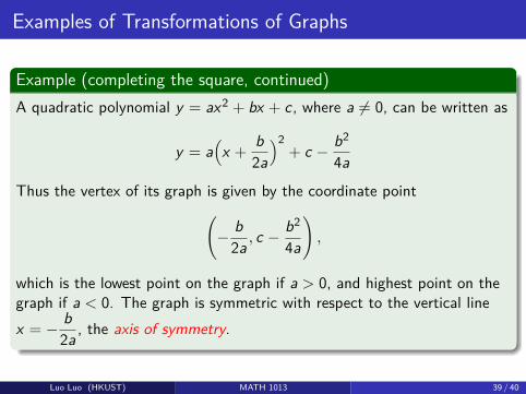
Example (completing the square, continued)A quadratic polynomial y = ax2 + bx + c, where a 6= 0, can be written as
y = a(x + b
2a)2
+ c − b2
4a
Thus the vertex of its graph is given by the coordinate point(− b
2a , c −b2
4a
),
which is the lowest point on the graph if a > 0, and highest point on thegraph if a < 0. The graph is symmetric with respect to the vertical linex = − b
2a , the axis of symmetry.
Luo Luo (HKUST) MATH 1013 39 / 40

Examples of Transformations of Graphs
ExampleConsider the function defined by f (x) =
√x . Compare the graph of
y = f (x) with the graphs of y = 3f (x),y = 13 f (x), y = f (3x) and
y = f( x
3):
3f (x)←→ f (x)←→ 13 f (x) f (3x)←→ f (x)←→ f ( x
3 )
-1
0
1
2
3
4
5
6
7
-1 0 1 2 3 4 5
x
y
y = 3x1/2
y = x1/2
y = x1/2
/3
stretch
compress
-1
0
1
2
3
4
5
-1 0 1 2 3 4 5
x
y
y = (3x)1/2
y = x1/2
compress
y = (x/3)1/2
stretch
y = 3√
x , y =√
x , y = 13√
x y =√
3x , y =√
x , y =√ x
3
Luo Luo (HKUST) MATH 1013 40 / 40

Calculus IB: Lecture 03
Luo Luo
Department of Mathematics, HKUST
http://luoluo.people.ust.hk/
Luo Luo (HKUST) MATH 1013 1 / 39

Outline
1 One-to-One Functions
2 Power Functions
3 Inverse Functions
4 Exponential and Logarithmic Functions
5 Radian Measure of an Angle
6 Sine and Cosine Functions
Luo Luo (HKUST) MATH 1013 2 / 39

Outline
1 One-to-One Functions
2 Power Functions
3 Inverse Functions
4 Exponential and Logarithmic Functions
5 Radian Measure of an Angle
6 Sine and Cosine Functions
Luo Luo (HKUST) MATH 1013 3 / 39

One-to-One Functions
1 Recall that for any x in the domain of a function f , only one functionvalue f (x) can be assigned to x .
2 However, it is possible that two different numbers x1 6= x2 in thedomain of f have the same function value, i.e. f (x1) = f (x2).
3 By ruling out above possibility, we have the concept of a one-to-onefunction: A function f is said to be one-to-one if f (x1) 6= f (x2) forany two numbers x1 6= x2 in the domain of f .
4 In other words, f (x) never takes on the same function value twice ormore times when x runs through the domain of f ; or equivalently, theequation
f (x) = b
has exactly one solution for any b in the range of f . In particular, f isa one-to-one function if x1 = x2 whenever f (x1) = f (x2).
Luo Luo (HKUST) MATH 1013 3 / 39
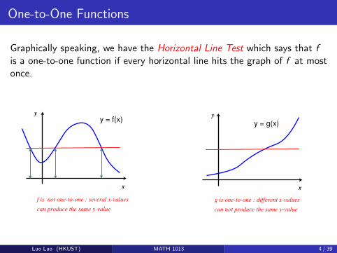
One-to-One Functions
Graphically speaking, we have the Horizontal Line Test which says that fis a one-to-one function if every horizontal line hits the graph of f at mostonce.
y y
x x
f is not one-to-one : several x-values
can produce the same y-value
g is one-to-one : different x-values
can not produce the same y-value
y = f(x)y = g(x)
Luo Luo (HKUST) MATH 1013 4 / 39

Examples of One-to-One Functions
Example
Let f be defined by f (x) = x2. It is obviously that f takes on everypositive number b 6= 0 exactly two times, since x2 = b has exactly tworoots x = ±
√b for any b > 0; e.g.,
f (2) = 22 = 4 = (−2)2 = f (−2) .
f is thus not a one-to-one function.
However, if the domain of f (x) = x2 is restricted to 0 ≤ x <∞, thefunction f is then one-to-one, since x2 = b has exactly one non-negativesolution
√b.
Luo Luo (HKUST) MATH 1013 5 / 39

Increasing (Decreasing) Functions are One-to-One
1 If f is an increasing function with domain D a set of real numbers, thenf (x1) < f (x2) for any number x1, x2 in the domain D such that x1 < x2.Hence f (x1) 6= f (x2) for any x1 6= x2.
2 Similarly, the decreasing functions are also one-to-one functions.
3 For any positive integer n, the power function y = x2n+1 is an increasingfunction with domain −∞ < x <∞. Similarly, the power function y = x2n
is an increasing function when the domain is restricted to 0 ≤ x <∞.
Example 4. Increasing functions, or decreasing functions, are always one-to-one.
For example, if f is an increasing function with domain D a set of real numbers, then f(x1) < f(x2) for
any number x1, x2 in the domain D such that x1 < x2. Hence f(x1) 6= f(x2) for any x1 6= x2.
For example, for any positive integer n, the power function y = x2n+1 is an increasing function with
domain −∞ < x < ∞. Similarly, the power function y = x2n is an increasing function when the domain is
restricted to 0 ≤ x <∞.
−2 −1 1 2
−3
−2
−1
1
2
3
x
y
y=x3
y=x5
−1 1 2 3
−1
1
2
3
4
5
x
y
y=x2
y=x4
y=x6
Example 5. y = |x| is not a one-to-one function.
Just note that | − 2| = 2 = |2|, while 2 6= −2.
Example 6. f(x) =1
xis a one-to-one function.
Obviously, if f(x1) =1
x1=
1
x2= f(x2), we must have x1 = x2. However, f is neither an increasing nor
a decreasing function.
−4 −3 −2 −1 1 2 3 4−1
1
2
3
4
5
6
7
x
y
y=2
y=|x|
−4 −3 −2 −1 1 2 3 4
−4
−2
2
4
x
y
y=2
y= 1x
−4 −3 −2 −1 1 2 3 4
−4
−2
2
4
x
y
y= 1x2
y= 1x
y= 1x3
Remark Note that for any positive integer n, the function1
xncan also be expressed in the form of power
function as1
xn= x−n. The following exponent laws for integer powers (or exponents) then follow easily.
(i) x0 = 1 ((By convention) (ii) xn+m = xnxm (iii) xn−m =xn
xm
(iv) (xn)m = xnm (v) (xy)n = xnyn (vi)(x
y
)n
=xn
yn
where n, m are any integers. For example, if n,m are positive integers with n < m, then
xnxm = (x · x · · · · · x︸ ︷︷ ︸
n many factors
) · ( x · x · · · · · x︸ ︷︷ ︸
m many factors
) = x · x · · · · · x︸ ︷︷ ︸
n + m many factors
= xn+m
xn
xm=
n many factors︷ ︸︸ ︷x · x · · · · · xx · x · · · · · x︸ ︷︷ ︸
m many factors
=1
x · x · · · · · x︸ ︷︷ ︸
m − n many factors
=1
xm−n= xn−m
Note that these exponent laws hold also for exponents which are real numbers. However, it would be harder
to see what x√2 means.
17
Luo Luo (HKUST) MATH 1013 6 / 39

Outline
1 One-to-One Functions
2 Power Functions
3 Inverse Functions
4 Exponential and Logarithmic Functions
5 Radian Measure of an Angle
6 Sine and Cosine Functions
Luo Luo (HKUST) MATH 1013 7 / 39

Power Functions
Note that for any positive integer n, the function1
xncan also be expressed
in the form of power function as1
xn= x−n.
The exponent laws for integer powers (or exponents) then follow easily:
(i) x0 = 1 (by convention) (ii) xn+m = xnxm (iii) xn−m =xn
xm
(iv) (xn)m = xnm (v) (xy)n = xnyn (vi)(xy
)n=
xn
yn
where n, m are any integers.
Luo Luo (HKUST) MATH 1013 7 / 39

Power Functions
For example, if n,m are positive integers with n < m, then
xnxm = (x · x · · · · · x︸ ︷︷ ︸n many factors
) · ( x · x · · · · · x︸ ︷︷ ︸m many factors
) = x · x · · · · · x︸ ︷︷ ︸n +m many factors
= xn+m
xn
xm=
n many factors︷ ︸︸ ︷x · x · · · · · xx · x · · · · · x︸ ︷︷ ︸m many factors
=1
x · x · · · · · x︸ ︷︷ ︸m − n many factors
=1
xm−n= xn−m
Note that these exponent laws hold also for exponents which are realnumbers. However, it would be harder to see what xp means when p is airrational number (such as p =
√2).
Luo Luo (HKUST) MATH 1013 8 / 39
Outline
1 One-to-One Functions
2 Power Functions
3 Inverse Functions
4 Exponential and Logarithmic Functions
5 Radian Measure of an Angle
6 Sine and Cosine Functions
Luo Luo (HKUST) MATH 1013 9 / 39

Inverse Functions Arising from One-to-One Functions
Consider the linear relationy = 2x + 3
between x and y , where y is considered as a function of x , can berewritten as
x =y − 3
2
Hence x can then be considered as a function of y .
The same process can be applied to any one-to-one functions.
Luo Luo (HKUST) MATH 1013 9 / 39
Inverse Functions Arising from One-to-One Functions
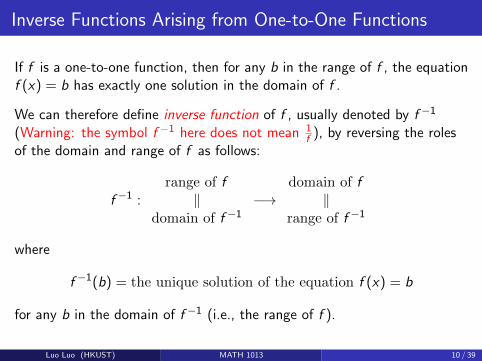
If f is a one-to-one function, then for any b in the range of f , the equationf (x) = b has exactly one solution in the domain of f .
We can therefore define inverse function of f , usually denoted by f −1
(Warning: the symbol f −1 here does not mean 1f ), by reversing the roles
of the domain and range of f as follows:
f −1 :range of f‖
domain of f −1−→
domain of f‖
range of f −1
where
f −1(b) = the unique solution of the equation f (x) = b
for any b in the domain of f −1 (i.e., the range of f ).
Luo Luo (HKUST) MATH 1013 10 / 39
Inverse Functions and Arrow Diagram
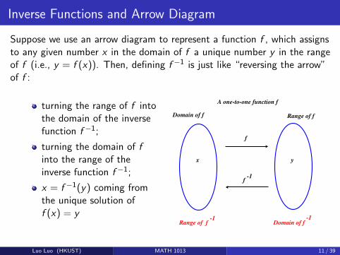
Suppose we use an arrow diagram to represent a function f , which assignsto any given number x in the domain of f a unique number y in the rangeof f (i.e., y = f (x)). Then, defining f −1 is just like “reversing the arrow”of f :
turning the range of f intothe domain of the inversefunction f −1;
turning the domain of finto the range of theinverse function f −1;
x = f −1(y) coming fromthe unique solution off (x) = y
A one-to-one function f
f
yx
f-1
Domain of f Range of f
Domain of f -1
Range of f-1
Luo Luo (HKUST) MATH 1013 11 / 39
Inverse Functions and Arrow Diagram
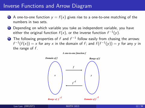
1 A one-to-one function y = f (x) gives rise to a one-to-one matching of thenumbers in two sets.
2 Depending on which variable you take as independent variable, you haveeither the original function f (x), or the inverse function f −1(y).
3 The following properties of f and f −1 follow easily from chasing the arrows:f −1(f (x)) = x for any x in the domain of f ; and f (f −1(y)) = y for any y inthe range of f .
A one-to-one function f
f
yx
f-1
Domain of f Range of f
Domain of f -1
Range of f-1
Luo Luo (HKUST) MATH 1013 12 / 39
Examples of Inverse Functions
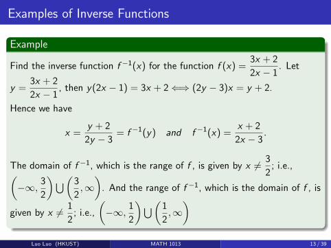
Example
Find the inverse function f −1(x) for the function f (x) =3x + 2
2x − 1. Let
y =3x + 2
2x − 1, then y(2x − 1) = 3x + 2⇐⇒ (2y − 3)x = y + 2.
Hence we have
x =y + 2
2y − 3= f −1(y) and f −1(x) =
x + 2
2x − 3.
The domain of f −1, which is the range of f , is given by x 6= 3
2; i.e.,(
−∞, 3
2
)⋃(3
2,∞)
. And the range of f −1, which is the domain of f , is
given by x 6= 1
2; i.e.,
(−∞, 1
2
)⋃(1
2,∞)
Luo Luo (HKUST) MATH 1013 13 / 39

Graphs of Inverse Functions
It is interesting that the graph of x = f −1(y) is the same as the graph ofy = f (x), except that the y -axis is now viewed as the domain axis.
In particular, the graph of the inverse function y = f −1(x) can beobtained by reflecting the graph of the one-to-one function y = f (x)across the line y = x , or simply by renaming the x-axis as the y -axis, andy -axis as the x-axis.
xx
x
x
y
y
yy
y = f (x) x = f (y) -1
y = x y = x
Reflecting range into domain Renaming the axes
yy = f (x)
-1
x
Luo Luo (HKUST) MATH 1013 14 / 39

Graphs of Inverse Functions
Example
For any integer n ≥ 2, the n-th root function n√x is defined as follows:
n√x =
{the inverse function of y = xn with domain [0,∞) if n is even
the inverse function of y = xn if n is odd
V
P
P =2
Vvs V =
2
P
The graph of the inverse function y = f−1(x) can therefore be obtained by reflecting the graph of the
one-to-one function y = f(x) across the line y = x, or simply by renaming the x-axis as the y-axis, and
y-axis as the x-axis.
xx
x
x
y
y
yy
y = f (x) x = f (y) -1
y = x y = x
Reflecting range into domain Renaming the axes
y y = f (x) -1
x
Example 10. For any integer n ≥ 2, the n-th root function n√x is defined as follows:
n√x =
the inverse function of y = xn with domain restricted to [0,∞) if n is even
the inverse function of y = xn if n is odd
1 2 3 4 5
−1
1
2
3
4
x
y
y=√x
y=x2
−4 −3 −2 −1 1 2 3 4 5
−4
−3
−2
−1
1
2
3
4
5
x
y
y= 3√x
y=x3
In particular, the domain of an n-th root function is given as follows.
domain of n√x is given by:
{[0,∞) if n is even
(−∞,∞) if n is odd
Using exponent notation, an n-th root function can be written as n√x = x
1n .
More generally, a power function of the form xnm , where n is an integer and m is a positive integer, is
defined by
xnm = m
√xn .
Exercise. Extend the law of exponents to rational powers. For example, why do we have x12+
13 = x
12x
13 ?
(Hint: What is (x1/2x1/3)6?)
20
Luo Luo (HKUST) MATH 1013 15 / 39
Root Functions and Power Functions
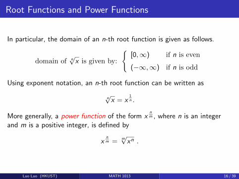
In particular, the domain of an n-th root function is given as follows.
domain of n√x is given by:
{[0,∞) if n is even
(−∞,∞) if n is odd
Using exponent notation, an n-th root function can be written as
n√x = x
1n .
More generally, a power function of the form xnm , where n is an integer
and m is a positive integer, is defined by
xnm =
m√xn .
Luo Luo (HKUST) MATH 1013 16 / 39

Outline
1 One-to-One Functions
2 Power Functions
3 Inverse Functions
4 Exponential and Logarithmic Functions
5 Radian Measure of an Angle
6 Sine and Cosine Functions
Luo Luo (HKUST) MATH 1013 17 / 39
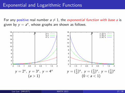
Exponential and Logarithmic Functions
For any positive real number a 6= 1, the exponential function with base a isgiven by y = ax , whose graphs are shown as follows.
0
2
4
6
8
10
12
14
16
18
-2 -1.5 -1 -0.5 0 0.5 1 1.5 2
y 2**x3**x4**x
0
2
4
6
8
10
12
14
16
18
-2 -1.5 -1 -0.5 0 0.5 1 1.5 2
y (1./2)**x(1./3)**x(1./4)**x
y = 2x , y = 3x , y = 4x y = (12)x , y = (13)x , y = (14)x
(a > 1) (0 < a < 1)
Luo Luo (HKUST) MATH 1013 17 / 39
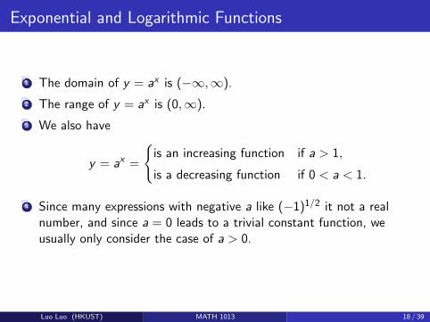
Exponential and Logarithmic Functions
1 The domain of y = ax is (−∞,∞).
2 The range of y = ax is (0,∞).
3 We also have
y = ax =
{is an increasing function if a > 1,
is a decreasing function if 0 < a < 1.
4 Since many expressions with negative a like (−1)1/2 it not a realnumber, and since a = 0 leads to a trivial constant function, weusually only consider the case of a > 0.
Luo Luo (HKUST) MATH 1013 18 / 39
Exponential and Logarithmic Functions
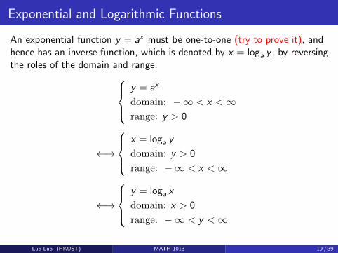
An exponential function y = ax must be one-to-one (try to prove it), andhence has an inverse function, which is denoted by x = loga y , by reversingthe roles of the domain and range:
y = ax
domain: −∞ < x <∞range: y > 0
←→
x = loga y
domain: y > 0
range: −∞ < x <∞
←→
y = loga x
domain: x > 0
range: −∞ < y <∞
Luo Luo (HKUST) MATH 1013 19 / 39

Example (take a = 10 and see what happens)
y = 10x
y x −3 −2 −1 0 c =? 1 2 b =?y 0.001 0.01 0.1 1 8 10 100 100
x x = log10(y)
The graph of the exponential function with base 10, y = 10x , gives you the
graphs of the common logarithmic function y = log10 x at the same time.
-1.5
-1
-0.5
0
0.5
1
-1 0 1 2 3 4 5 6
y
x
y = log10x
Note that to find the value of b = log10 100 is just a problem of solving the
equation 10b = 100 = 102, and hence obviously b = 2 = log10 100.
It is not so easy to find the exact value of c = log10 8 though, which means
10c = 8. A rough estimate is 12 < c < 1 since 101/2 < 8 = 10c < 101.
Luo Luo (HKUST) MATH 1013 20 / 39
Properties of Exponential and Logarithmic Functions
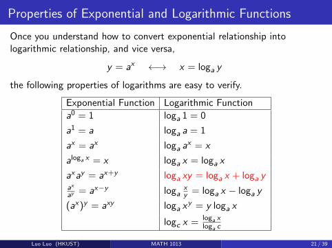
Once you understand how to convert exponential relationship intologarithmic relationship, and vice versa,
y = ax ←→ x = loga y
the following properties of logarithms are easy to verify.
Exponential Function Logarithmic Function
a0 = 1 loga 1 = 0
a1 = a loga a = 1
ax = ax loga ax = x
aloga x = x loga x = loga x
axay = ax+y loga xy = loga x + loga yax
ay = ax−y logaxy = loga x − loga y
(ax)y = axy loga xy = y loga x
logc x = loga xloga c
Luo Luo (HKUST) MATH 1013 21 / 39

Properties of Exponential and Logarithmic Functions
Verify the property loga(xy) = loga x + loga y
Let C = loga x , and D = loga y . Hence we have aC = x and aD = y .What if you multiplying the two together?
aCaD = xy ⇐⇒ aC+D = xy
Now, convert it to:
loga(xy) = C + D = loga x + loga y
All other properties in the table above can be checked by similararguments. (Exercise!)
Luo Luo (HKUST) MATH 1013 22 / 39

The Natural Exponential/Logarithmic Function
The exponential/logarithmic function with a special base e ≈ 2.7182 . . .
y = ex , y = loge x , ln x
is called the natural exponential/logarithmic function. Note that all otherexponential function can be expressed in term of the natural exponentialfunction, since
ax = e ln ax
= ex ln a .
For example, 3x = ex ln 3.
Luo Luo (HKUST) MATH 1013 23 / 39
The Natural Exponential/Logarithmic Function
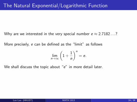
Why are we interested in the very special number e ≈ 2.7182 . . .?
More precisely, e can be defined as the “limit” as follows
limn→∞
(1 +
1
n
)n
= e.
We shall discuss the topic about “e” in more detail later.
Luo Luo (HKUST) MATH 1013 24 / 39
More Examples on Using Exp-Log
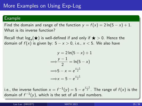
Example
Find the domain and range of the function y = f (x) = 2 ln(5− x) + 1.What is its inverse function?
Recall that loga(F) is well-defined if and only if F > 0. Hence thedomain of f (x) is given by: 5− x > 0, i.e., x < 5. We also have
y = 2 ln(5− x) + 1
=⇒y − 1
2= ln(5− x)
=⇒5− x = ey−12
=⇒x = 5− ey−12
i.e., the inverse function x = f −1(y) = 5− ey−12 . The range of f (x) is the
domain of f −1(y), which is the set of all real numbers.
Luo Luo (HKUST) MATH 1013 25 / 39

More Examples on Using Exp-Log
Example
Solve the following equations: (a) 24(1− e−t/2) = 16; (b) 22x−3 = 3x+1
24(1− e−t/2) = 16 22x−3 = 3x+1
1− e−t/2 =16
24=
2
3ln 22x−3 = ln 3x+1
e−t/2 =1
3(2x − 3) ln 2 = (x + 1) ln 3
− t
2= ln
1
3(2 ln 2− ln 3)x = ln 3 + 3 ln 2
t = −2 ln1
3= ln 9 (≈ 2.1792) x =
ln 3 + 3 ln 2
2 ln 2− ln 3
Luo Luo (HKUST) MATH 1013 26 / 39

Hyperbolic Functions
The hyperbolic functions are defined and denoted by
sinh x =ex − e−x
2, cosh x =
ex + e−x
2, tanh x =
sinh x
cosh x=
ex − e−x
ex + e−x
Please verify the following identities:
cosh2 x − sinh2 x = 1
sinh(x + y) = sinh x cosh y + cosh x sinh y
cosh(x + y) = cosh x cosh y + sinh x sinh y
Hyperbolic functions have some similar properties to trigonometricfunctions.
Luo Luo (HKUST) MATH 1013 27 / 39

Outline
1 One-to-One Functions
2 Power Functions
3 Inverse Functions
4 Exponential and Logarithmic Functions
5 Radian Measure of an Angle
6 Sine and Cosine Functions
Luo Luo (HKUST) MATH 1013 28 / 39

Radian Measure of an Angle
If the point (1, 0) starts to travel along the unit circle centered at the(0, 0) through a distance θ in counterclockwise direction, the anglesubtended by the corresponding circular arc is said to be a positive anglewith radian measure θ.Angles obtained by clockwise rotations are considered as negative angles.
positive angle
negative angle
(1,0)
t
Directed angle : angle can be assigned a +ve or -ve sign
Luo Luo (HKUST) MATH 1013 28 / 39
Radian Measure of an Angle
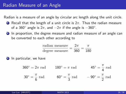
Radian is a measure of an angle by circular arc length along the unit circle.
1 Recall that the length of a unit circle is 2π. Thus the radian measureof a 360◦ angle is 2π, and −2π if the angle is −360◦.
2 In proportion, the degree measure and radian measure of an angle canbe converted to each other according to
radian measure
degree measure=
2π
360=
π
180
3 In particular, we have
360◦ = 2π rad 180◦ = π rad 45◦ =π
4rad
30◦ =π
6rad 60◦ =
π
3rad − 90◦ =
π
2rad
Luo Luo (HKUST) MATH 1013 29 / 39

Radian Measure of an Angle
Since the length and area of a circle of radius r are 2πr and πr2, the arclength and area of a circular section subtended by an angle θ in radianscan be determined according to the following proportion:
circular sector area
circle area=
θ
2π=
circular arc length
circle length
circular sector area
πr2=
θ
2π=
circular arc length
2πr
Math1013 Calculus IB
Week 3-4: Trigonometric Functions and Their Inverse Functions
Radian Measure Of An Angle
If the coordinate point (0, 1) starts to travel along the unit circle centered at the origin (0, 0) through a
distance θ in counterclockwise direction, the angle subtended by the corresponding circular arc is said to be
a positive angle with radian measure θ. Angles obtained by clockwise rotation are considered as negative
angles.
positive angle
negative angle
(1,0)
θ
Directed angle : angle can be assigned a +ve or -ve sign
In other words, radian is a measure of an angle by circular arc length along the unit circle.
• The length of a unit circle is 2π, hence the radian measure of a 360◦ angle is 2π.
• In proportion, the degree measure and radian measure of an angle can be converted to each other
according todegree measure
radian measure=
360
2π=
180
π
In particular,
360◦ = 2π rad., 180◦ = π rad., 45◦ =π
4rad.,
30◦ =π
6rad., 60◦ =
π
3rad., −90◦ = −π
2rad.
• Since the length and area of a circle of radius r are 2πr and πr2 respectively, the arc length and area
of a circular section subtended by an angle θ in radians can be determined according to the following
proportion:
circular sector area
circle area=
θ
2π=
circular arc length
circle length
circular sector area
πr2=
θ
2π=
circular arc length
2πr r A
B
O
θ
and hence we have the following:
Circular sector OAB: Area = 12r
2θ
Arc length = rθ
where θ is measured in radians.
25
and hence we have
circular sector area =1
2r2θ and circular arc length = rθ
where θ is measured in radians, NOT degrees.
Luo Luo (HKUST) MATH 1013 30 / 39
Radian Measure of an Angle
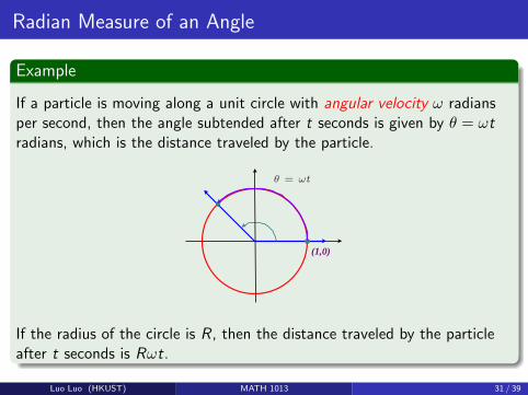
Example
If a particle is moving along a unit circle with angular velocity ω radiansper second, then the angle subtended after t seconds is given by θ = ωtradians, which is the distance traveled by the particle.
Example 1.
(i) The degree measure d of an angle of 2 radians is:
d
2=
180
π⇐⇒ d =
(360
π
)◦
(ii) The radian measure θ of an angle of 72◦ is:
72
θ=
180
π⇐⇒ θ =
72π
180=
2π
5(in radians.)
The arc length and area of a circular section with angle 72◦ and radius 4 are therefore
area =1
2· 42 · 2π
5=
16π
5(sq. unit)
arc length = 4 · 2π5
=8π
5(unit)
Example 2. If a particle is moving along a unit circle with angular velocity ω radians per second, then the
angle subtended after t seconds is given by θ = ωt radians, which is the distance traveled by the particle.
(1,0)
θ = ωt
If the radius of the circle is R, then the distance traveled by the particle after t seconds is Rωt (unit).
Sine and Cosine Functions
When a point originally at (0, 1) moves along the unit circle through an angle of θ radians, the coordinates
of the position (x, y) reached by the point depend on the value of θ, i.e., they are functions of θ, which are
denoted by
x = sin θ
and
y = cos θ
(x, y)
(1, 0) x x
y
y
1 domain: (−∞,∞), or −∞ < θ <∞
range: [−1, 1], or − 1 ≤ sin θ, cos θ ≤ 1
As the point is moving along the circle, its coordinates are oscillating between −1 and 1, and it is then
easy to see the shape of the graphs of x = sin θ and y = cos θ from the geometry of the circle, as well as
some basic properties of these two functions.
−2π −π π 2π
−2
−1
1
2x = sin θx
θ
−2π −π π 2π
−2
−1
1
2y = cos θy
θ
26
If the radius of the circle is R, then the distance traveled by the particleafter t seconds is Rωt.
Luo Luo (HKUST) MATH 1013 31 / 39
Outline
1 One-to-One Functions
2 Power Functions
3 Inverse Functions
4 Exponential and Logarithmic Functions
5 Radian Measure of an Angle
6 Sine and Cosine Functions
Luo Luo (HKUST) MATH 1013 32 / 39

Sine and Cosine Functions
When a point originally at (0, 1) moves along the unit circle through anangle of θ radians, the coordinates of the position (x , y) reached by thepoint depend on the value of θ, i.e., they are functions of θ:
y = sin θ and x = cos θ, where θ ∈ (−∞,+∞) and x , y ∈ [−1, 1].
Example 1.
(i) The degree measure d of an angle of 2 radians is:
d
2=
180
π⇐⇒ d =
(360
π
)◦
(ii) The radian measure θ of an angle of 72◦ is:
72
θ=
180
π⇐⇒ θ =
72π
180=
2π
5(in radians.)
The arc length and area of a circular section with angle 72◦ and radius 4 are therefore
area =1
2· 42 · 2π
5=
16π
5(sq. unit)
arc length = 4 · 2π5
=8π
5(unit)
Example 2. If a particle is moving along a unit circle with angular velocity ω radians per second, then the
angle subtended after t seconds is given by θ = ωt radians, which is the distance traveled by the particle.
(1,0)
θ = ωt
If the radius of the circle is R, then the distance traveled by the particle after t seconds is Rωt (unit).
Sine and Cosine Functions
When a point originally at (0, 1) moves along the unit circle through an angle of θ radians, the coordinates
of the position (x, y) reached by the point depend on the value of θ, i.e., they are functions of θ, which are
denoted by
x = sin θ
and
y = cos θ
(x, y)
(1, 0) x x
y
y
1 domain: (−∞,∞), or −∞ < θ <∞
range: [−1, 1], or − 1 ≤ sin θ, cos θ ≤ 1
As the point is moving along the circle, its coordinates are oscillating between −1 and 1, and it is then
easy to see the shape of the graphs of x = sin θ and y = cos θ from the geometry of the circle, as well as
some basic properties of these two functions.
−2π −π π 2π
−2
−1
1
2x = sin θx
θ
−2π −π π 2π
−2
−1
1
2y = cos θy
θ
26
Luo Luo (HKUST) MATH 1013 32 / 39
Sine and Cosine Functions
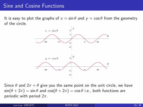
It is easy to plot the graphs of x = sin θ and y = cos θ from the geometryof the circle.
Example 1.
(i) The degree measure d of an angle of 2 radians is:
d
2=
180
π⇐⇒ d =
(360
π
)◦
(ii) The radian measure θ of an angle of 72◦ is:
72
θ=
180
π⇐⇒ θ =
72π
180=
2π
5(in radians.)
The arc length and area of a circular section with angle 72◦ and radius 4 are therefore
area =1
2· 42 · 2π
5=
16π
5(sq. unit)
arc length = 4 · 2π5
=8π
5(unit)
Example 2. If a particle is moving along a unit circle with angular velocity ω radians per second, then the
angle subtended after t seconds is given by θ = ωt radians, which is the distance traveled by the particle.
(1,0)
θ = ωt
If the radius of the circle is R, then the distance traveled by the particle after t seconds is Rωt (unit).
Sine and Cosine Functions
When a point originally at (0, 1) moves along the unit circle through an angle of θ radians, the coordinates
of the position (x, y) reached by the point depend on the value of θ, i.e., they are functions of θ, which are
denoted by
x = sin θ
and
y = cos θ
(x, y)
(1, 0) x x
y
y
1 domain: (−∞,∞), or −∞ < θ <∞
range: [−1, 1], or − 1 ≤ sin θ, cos θ ≤ 1
As the point is moving along the circle, its coordinates are oscillating between −1 and 1, and it is then
easy to see the shape of the graphs of x = sin θ and y = cos θ from the geometry of the circle, as well as
some basic properties of these two functions.
−2π −π π 2π
−2
−1
1
2x = sin θx
θ
−2π −π π 2π
−2
−1
1
2y = cos θy
θ
26
Since θ and 2π + θ give you the same point on the unit circle, we havesin(θ + 2π) = sin θ and cos(θ + 2π) = cos θ i.e., both functions areperiodic with period 2π.
Luo Luo (HKUST) MATH 1013 33 / 39

Some Function Values of sin θ and cos θ
θ 0 π6
π4
π3
π2
2π3
3π4
5π6 π
sin θ 0 12
√22
√32 1
√32
√22
12 0
cos θ 1√32
√22
12 0 −1
2 −√22
√32 −1
• Since θ and 2π + θ give you the same point on the unit circle, we have
sin(θ + 2π) = sin θ, and cos(θ + 2π) = cos θ
i.e., both functions are periodic with period 2π.
• Some function values of sin θ and cos θ can be found from special triangles as given in the following
table:
θ 0 π6
π4
π3
π2
2π2
3π4
5π6 π
sin θ 0 12
√22
√32 1
√32
√22
12 0
cos θ 1√32
√22
12 0 − 1
2 −√22
√32 −1
π4
π4
π3
π3
√2
2
√2
2
111 √3
2
π6
1
2
1
2
Moreover,
(i) sin θ = 0 if and only if θ = nπ for some integer n.
(Points on the unit circle with zero y-coordinates are (±1, 0).)(ii) cos θ = 0 if and only if θ = (2n+ 1)
π
2= (n+ 1
2 )π. for some integer n.
(Points on the unit circle with zero x-coordinates are (0,±1).)
• Note that we have the following identities:
(i) sin2 θ + cos2 θ = 1 (Pythagoras Theorem!)
(ii) cos θ = sin(θ + π2 ) (Graph shifting!)
(iii) sin θ = cos(θ − π2 ) (Graph shifting!)
• Since the angles θ and −θ put two points on the unit circle symmetric with respect to the x-axis, and
θ + π gives a point antipodal to that of θ, it is easy to see that
sin(−θ) = − sin θ; i.e., sin θ is an odd function
cos(−θ) = cos θ; i.e., cos θ is an even function
sin(θ + π) = − sin θ;
cos(θ + π) = − cos θ;
θ
−θ
θ+π
(cos θ,sin θ)
(cos θ,− sin θ)
(− cos θ,− sin θ)
Work out the following identities by studying points on the unit circle given by the angles θ, π2 − θ and
π − θ.
sin(π − θ) = sin θ sin(π/2− θ) = cos θ
cos(π − θ) = − cos θ cos(π/2− θ) = sin θ
π−θ
−θ−θ
π2 −θ
• If (x, y) is a point on the circle of radius R, with equation x2 + y2 = R2, we have by proportion that
x = R cos θ, y = R sin θ .
27
sin θ = 0 if and only if θ = nπ for some integer n. (points on the unitcircle with zero y -coordinates are (±1, 0))
cos θ = 0 if and only if θ = (2n + 1)π2 = (n + 12)π for some integer n.
(points on the unit circle with zero x-coordinates are (0,±1))
Luo Luo (HKUST) MATH 1013 34 / 39

Properties of Sine and Cosine
Note that we have the following identities:
1 sin2 θ + cos2 θ = 1 (Pythagoras Theorem)
2 cos θ = sin(θ + π
2
)(graph shifting)
3 sin θ = cos(θ − π
2
)(graph shifting)
Example 1.
(i) The degree measure d of an angle of 2 radians is:
d
2=
180
π⇐⇒ d =
(360
π
)◦
(ii) The radian measure θ of an angle of 72◦ is:
72
θ=
180
π⇐⇒ θ =
72π
180=
2π
5(in radians.)
The arc length and area of a circular section with angle 72◦ and radius 4 are therefore
area =1
2· 42 · 2π
5=
16π
5(sq. unit)
arc length = 4 · 2π5
=8π
5(unit)
Example 2. If a particle is moving along a unit circle with angular velocity ω radians per second, then the
angle subtended after t seconds is given by θ = ωt radians, which is the distance traveled by the particle.
(1,0)
θ = ωt
If the radius of the circle is R, then the distance traveled by the particle after t seconds is Rωt (unit).
Sine and Cosine Functions
When a point originally at (0, 1) moves along the unit circle through an angle of θ radians, the coordinates
of the position (x, y) reached by the point depend on the value of θ, i.e., they are functions of θ, which are
denoted by
x = sin θ
and
y = cos θ
(x, y)
(1, 0) x x
y
y
1 domain: (−∞,∞), or −∞ < θ <∞
range: [−1, 1], or − 1 ≤ sin θ, cos θ ≤ 1
As the point is moving along the circle, its coordinates are oscillating between −1 and 1, and it is then
easy to see the shape of the graphs of x = sin θ and y = cos θ from the geometry of the circle, as well as
some basic properties of these two functions.
−2π −π π 2π
−2
−1
1
2x = sin θx
θ
−2π −π π 2π
−2
−1
1
2y = cos θy
θ
26
Luo Luo (HKUST) MATH 1013 35 / 39
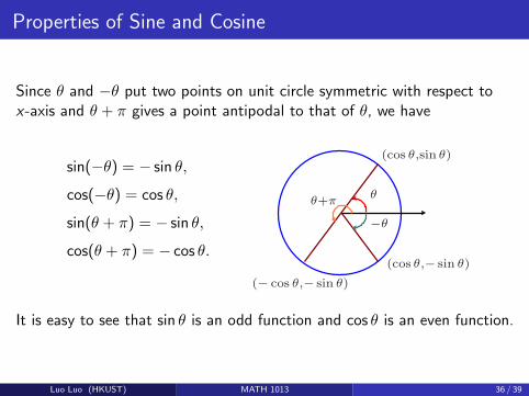
Properties of Sine and Cosine
Since θ and −θ put two points on unit circle symmetric with respect tox-axis and θ + π gives a point antipodal to that of θ, we have
sin(−θ) = − sin θ,
cos(−θ) = cos θ,
sin(θ + π) = − sin θ,
cos(θ + π) = − cos θ.
• Since θ and 2π + θ give you the same point on the unit circle, we have
sin(θ + 2π) = sin θ, and cos(θ + 2π) = cos θ
i.e., both functions are periodic with period 2π.
• Some function values of sin θ and cos θ can be found from special triangles as given in the following
table:
θ 0 π6
π4
π3
π2
2π2
3π4
5π6 π
sin θ 0 12
√22
√32 1
√32
√22
12 0
cos θ 1√32
√22
12 0 − 1
2 −√22
√32 −1
π4
π4
π3
π3
√2
2
√2
2
111 √3
2
π6
1
2
1
2
Moreover,
(i) sin θ = 0 if and only if θ = nπ for some integer n.
(Points on the unit circle with zero y-coordinates are (±1, 0).)(ii) cos θ = 0 if and only if θ = (2n+ 1)
π
2= (n+ 1
2 )π. for some integer n.
(Points on the unit circle with zero x-coordinates are (0,±1).)
• Note that we have the following identities:
(i) sin2 θ + cos2 θ = 1 (Pythagoras Theorem!)
(ii) cos θ = sin(θ + π2 ) (Graph shifting!)
(iii) sin θ = cos(θ − π2 ) (Graph shifting!)
• Since the angles θ and −θ put two points on the unit circle symmetric with respect to the x-axis, and
θ + π gives a point antipodal to that of θ, it is easy to see that
sin(−θ) = − sin θ; i.e., sin θ is an odd function
cos(−θ) = cos θ; i.e., cos θ is an even function
sin(θ + π) = − sin θ;
cos(θ + π) = − cos θ;
θ
−θ
θ+π
(cos θ,sin θ)
(cos θ,− sin θ)
(− cos θ,− sin θ)
Work out the following identities by studying points on the unit circle given by the angles θ, π2 − θ and
π − θ.
sin(π − θ) = sin θ sin(π/2− θ) = cos θ
cos(π − θ) = − cos θ cos(π/2− θ) = sin θ
π−θ
−θ−θ
π2 −θ
• If (x, y) is a point on the circle of radius R, with equation x2 + y2 = R2, we have by proportion that
x = R cos θ, y = R sin θ .
27
It is easy to see that sin θ is an odd function and cos θ is an even function.
Luo Luo (HKUST) MATH 1013 36 / 39
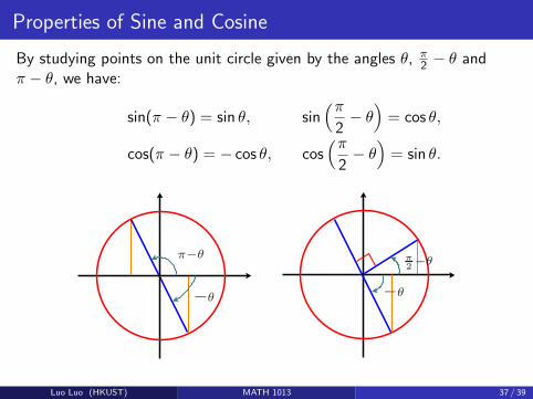
Properties of Sine and Cosine
By studying points on the unit circle given by the angles θ, π2 − θ and
π − θ, we have:
sin(π − θ) = sin θ, sin(π
2− θ)
= cos θ,
cos(π − θ) = − cos θ, cos(π
2− θ)
= sin θ.
• Since θ and 2π + θ give you the same point on the unit circle, we have
sin(θ + 2π) = sin θ, and cos(θ + 2π) = cos θ
i.e., both functions are periodic with period 2π.
• Some function values of sin θ and cos θ can be found from special triangles as given in the following
table:
θ 0 π6
π4
π3
π2
2π2
3π4
5π6 π
sin θ 0 12
√22
√32 1
√32
√22
12 0
cos θ 1√32
√22
12 0 − 1
2 −√22
√32 −1
π4
π4
π3
π3
√2
2
√2
2
111 √3
2
π6
1
2
1
2
Moreover,
(i) sin θ = 0 if and only if θ = nπ for some integer n.
(Points on the unit circle with zero y-coordinates are (±1, 0).)(ii) cos θ = 0 if and only if θ = (2n+ 1)
π
2= (n+ 1
2 )π. for some integer n.
(Points on the unit circle with zero x-coordinates are (0,±1).)
• Note that we have the following identities:
(i) sin2 θ + cos2 θ = 1 (Pythagoras Theorem!)
(ii) cos θ = sin(θ + π2 ) (Graph shifting!)
(iii) sin θ = cos(θ − π2 ) (Graph shifting!)
• Since the angles θ and −θ put two points on the unit circle symmetric with respect to the x-axis, and
θ + π gives a point antipodal to that of θ, it is easy to see that
sin(−θ) = − sin θ; i.e., sin θ is an odd function
cos(−θ) = cos θ; i.e., cos θ is an even function
sin(θ + π) = − sin θ;
cos(θ + π) = − cos θ;
θ
−θ
θ+π
(cos θ,sin θ)
(cos θ,− sin θ)
(− cos θ,− sin θ)
Work out the following identities by studying points on the unit circle given by the angles θ, π2 − θ and
π − θ.
sin(π − θ) = sin θ sin(π/2− θ) = cos θ
cos(π − θ) = − cos θ cos(π/2− θ) = sin θ
π−θ
−θ−θ
π2 −θ
• If (x, y) is a point on the circle of radius R, with equation x2 + y2 = R2, we have by proportion that
x = R cos θ, y = R sin θ .
27
Luo Luo (HKUST) MATH 1013 37 / 39
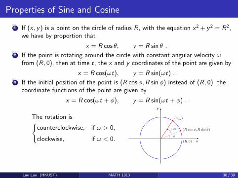
Properties of Sine and Cosine
1 If (x , y) is a point on the circle of radius R, with the equation x2 + y2 = R2,we have by proportion that
x = R cos θ, y = R sin θ .
2 If the point is rotating around the circle with constant angular velocity ωfrom (R, 0), then at time t, the x and y coordinates of the point are given by
x = R cos(ωt), y = R sin(ωt) .
3 If the initial position of the point is (R cosφ,R sinφ) instead of (R, 0), thecoordinate functions of the point are given by
x = R cos(ωt + φ), y = R sin(ωt + φ) .
The rotation is{counterclockwise, if ω > 0,
clockwise, if ω < 0.
If the point is rotating around the circle with constant angular
velocity ω, then at time t, the x and y coordinates of the point
are given by
x = R cosωt, y = R sinωt .
If the initial position of the point is the point (R cosφ,R sinφ)
instead of (R, 0), the coordinate functions of the particle are
given by
x = R cos(ωt+ φ), y = R sin(ωt+ φ) .
x
y
ωt
φ
(x,y)
(R,0)
(R cosφ,R sinφ)
The rotation is counterclockwise if ω > 0, and clockwise if ω < 0.
It is clear that these functions are periodic with period2π
|ω| . They are often used in describing certain
periodic oscillation motion of a particle, namely, simple harmonic motion.
R is called the amplitude, − φω the phase shift and ωt+ φ the phase or phase angle of the oscillation.
The graphs of these functions can be easily found by performing suitable transformations on the graph
of the sine or cosine function.
t
y
R
− φω − φ
ω+ 2πω
y=R sin(ωt+φ)
Exercise. Sketch the graph of the function x = 3 cos(2t+ π4 ).
More Trigonometric Functions
Four other trigonometric functions, namely, tan θ (tangent), cot θ (cotangent), csc θ (cosecant), and sec θ
(secant) are defined by
tan θ =sin θ
cos θ,
domain = {θ : cos θ 6= 0}range: (−∞,∞)
cot θ =cos θ
sin θ,
domain = {θ : sin θ 6= 0}range: (−∞,∞)
csc θ =1
sin θ,
domain = {θ : sin θ 6= 0}range: (−∞,−1] ∪ [1,∞)
sec θ =1
cos θ,
domain = {θ : cos θ 6= 0}range: (−∞,−1] ∪ [1,∞)
• tan θ is a periodic function with period π:
tan(θ + π) = tan θ
The domain of tan θ is θ 6= nπ + π/2, where n = 0,±1,±2,±3, · · · , and the range is (−∞,∞).
28
Luo Luo (HKUST) MATH 1013 38 / 39

Properties of Sine and Cosine
1 It is clear that functions x = R cos(ωt + φ) and y = R sin(ωt + φ) areperiodic with period 2π/|ω|.
2 Such functions are often used in describing certain periodic oscillationmotion, namely, simple harmonic motion. R is called the amplitude,−φ/ω the phase shift and ωt + φ the phase or phase angle.
3 The graphs of these functions can be easily found by performingsuitable transformations on the graph of the sine or cosine function.
If the point is rotating around the circle with constant angular
velocity ω, then at time t, the x and y coordinates of the point
are given by
x = R cosωt, y = R sinωt .
If the initial position of the point is the point (R cosφ,R sinφ)
instead of (R, 0), the coordinate functions of the particle are
given by
x = R cos(ωt+ φ), y = R sin(ωt+ φ) .
x
y
ωt
φ
(x,y)
(R,0)
(R cosφ,R sinφ)
The rotation is counterclockwise if ω > 0, and clockwise if ω < 0.
It is clear that these functions are periodic with period2π
|ω| . They are often used in describing certain
periodic oscillation motion of a particle, namely, simple harmonic motion.
R is called the amplitude, − φω the phase shift and ωt+ φ the phase or phase angle of the oscillation.
The graphs of these functions can be easily found by performing suitable transformations on the graph
of the sine or cosine function.
t
y
R
− φω − φ
ω+ 2πω
y=R sin(ωt+φ)
Exercise. Sketch the graph of the function x = 3 cos(2t+ π4 ).
More Trigonometric Functions
Four other trigonometric functions, namely, tan θ (tangent), cot θ (cotangent), csc θ (cosecant), and sec θ
(secant) are defined by
tan θ =sin θ
cos θ,
domain = {θ : cos θ 6= 0}range: (−∞,∞)
cot θ =cos θ
sin θ,
domain = {θ : sin θ 6= 0}range: (−∞,∞)
csc θ =1
sin θ,
domain = {θ : sin θ 6= 0}range: (−∞,−1] ∪ [1,∞)
sec θ =1
cos θ,
domain = {θ : cos θ 6= 0}range: (−∞,−1] ∪ [1,∞)
• tan θ is a periodic function with period π:
tan(θ + π) = tan θ
The domain of tan θ is θ 6= nπ + π/2, where n = 0,±1,±2,±3, · · · , and the range is (−∞,∞).
28
Luo Luo (HKUST) MATH 1013 39 / 39

Calculus IB: Lecture 04
Luo Luo
Department of Mathematics, HKUST
http://luoluo.people.ust.hk/
Luo Luo (HKUST) MATH 1013 1 / 32
Outline
1 More Trigonometric Functions
2 Inverse Trigonometric Functions
3 The Slope of a Tangent Line
4 Limit and Natural Logarithmic Function
Luo Luo (HKUST) MATH 1013 2 / 32
Outline
1 More Trigonometric Functions
2 Inverse Trigonometric Functions
3 The Slope of a Tangent Line
4 Limit and Natural Logarithmic Function
Luo Luo (HKUST) MATH 1013 3 / 32

More Trigonometric Functions
Four other trigonometric functions, namely, tan θ (tangent), cot θ(cotangent), csc θ (cosecant), and sec θ (secant) are defined by
tan θ =sin θ
cos θ
domain: {θ : cos θ 6= 0}range: (−∞,∞)
cot θ =cos θ
sin θ
domain: {θ : sin θ 6= 0}range: (−∞,∞)
csc θ =1
sin θ
domain: {θ : sin θ 6= 0}range: (−∞,−1] ∪ [1,∞)
sec θ =1
cos θ
domain: {θ : cos θ 6= 0}range: (−∞,−1] ∪ [1,∞)
Luo Luo (HKUST) MATH 1013 3 / 32
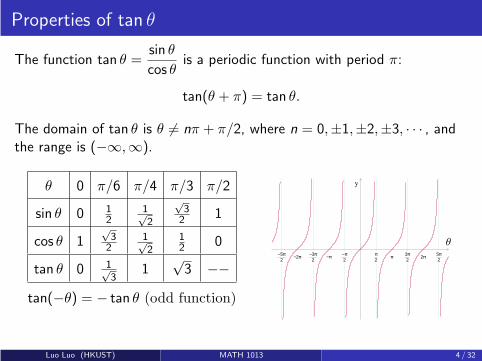
Properties of tan θ
The function tan θ =sin θ
cos θis a periodic function with period π:
tan(θ + π) = tan θ.
The domain of tan θ is θ 6= nπ + π/2, where n = 0,±1,±2,±3, · · · , andthe range is (−∞,∞).
θ 0 π/6 π/4 π/3 π/2
sin θ 0 12
1√2
√32 1
cos θ 1√32
1√2
12 0
tan θ 0 1√3
1√3 −−
tan(−θ) = − tan θ (odd function)
−5π2 −2π −3π
2 −π −π2
π2 π 3π
2 2π 5π2
y
θ
Luo Luo (HKUST) MATH 1013 4 / 32
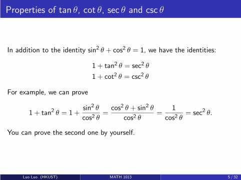
Properties of tan θ, cot θ, sec θ and csc θ
In addition to the identity sin2 θ + cos2 θ = 1, we have the identities:
1 + tan2 θ = sec2 θ
1 + cot2 θ = csc2 θ
For example, we can prove
1 + tan2 θ = 1 +sin2 θ
cos2 θ=
cos2 θ + sin2 θ
cos2 θ=
1
cos2 θ= sec2 θ.
You can prove the second one by yourself.
Luo Luo (HKUST) MATH 1013 5 / 32

Graphs of csc θ and sec θ
−5π2 −2π −3π
2 −π −π2
π2 π 3π
2 2π 5π2
y
θ−5π2 −2π −3π
2 −π −π2
π2 π 3π
2 2π 5π2
y
θ
y = csc θ = 1sin θ y = sec θ = 1
cos θ
period = 2π period = 2π
domain θ 6= nπ domain θ 6= nπ + π2
where n = 0,±1,±2, · · · where n = 0,±1,±2, · · ·range x ≤ −1 or x ≥ 1 range x ≤ −1 or x ≥ 1
Luo Luo (HKUST) MATH 1013 6 / 32
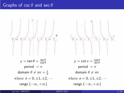
Graphs of csc θ and sec θ
−5π2 −2π −3π
2 −π −π2
π2 π 3π
2 2π 5π2
y
θ
y = tan θ = sin θcos θ y = cot x = cos θ
sin θ
period = π period = π
domain θ 6= nπ + π2 domain θ 6= nπ
where n = 0,±1,±2, · · · where n = 0,±1,±2, · · ·range (−∞,+∞) range (−∞,+∞)
Luo Luo (HKUST) MATH 1013 7 / 32

Trigonometric Identities: Angle Addition and Subtraction
sin(α+ β) = sinα cosβ + sinβ cosα
sin(α− β) = sinα cosβ − sinβ cosα
cos(α+ β) = cosα cosβ − sinα sinβ
cos(α− β) = cosα cosβ + sinα sinβ
tan(α+ β) =tanα+ tanβ
1− tanα tanβ
tan(α− β) =tanα− tanβ
1 + tanα tanβ
sin 2α = 2 sinα cosα
cos 2α = 2 cos2 α− 1 = 1− 2 sin2 α
Luo Luo (HKUST) MATH 1013 8 / 32

Trigonometric Identities: Product to Sum/Sum to Product
sinα cosβ =1
2[sin(α+ β) + sin(α− β)]
cosα sinβ =1
2[sin(α+ β)− sin(α− β)]
cosα cosβ =1
2[cos(α+ β) + cos(α− β)]
sinα sinβ =1
2[cos(α+ β)− cos(α− β)]
sinα+ sinβ = 2 sinα+ β
2cos
α− β
2
sinα− sinβ = 2 cosα+ β
2sin
α− β
2
cosα+ cosβ = 2 cosα+ β
2cos
α− β
2
cosα− cosβ = −2 sinα+ β
2sin
α− β
2
Luo Luo (HKUST) MATH 1013 9 / 32

Trigonometric Identities
All these formulas can be derived from one identity
cos(α+ β) = cosα cosβ − sinβ sinα
For examples,
cos(α− β) = cos(α+ (−β))
= cosα cos(−β)− sinα sin(−β)
= cosα cosβ + sinβ sinα
sin(α− β)
= cos((π
2− α
)
+ β)
=cos(π
2− α
)
cosβ − sin(π
2− α
)
sinβ
=sinα cosβ − sinβ cosα
Luo Luo (HKUST) MATH 1013 10 / 32
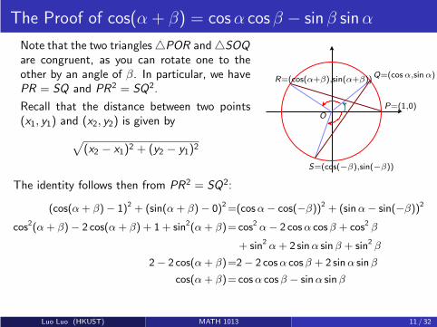
The Proof of cos(α + β) = cosα cos β − sin β sinα
Note that the two triangles△POR and△SOQ
are congruent, as you can rotate one to theother by an angle of β. In particular, we havePR = SQ and PR2 = SQ2.
Recall that the distance between two points(x1, y1) and (x2, y2) is given by
√
(x2 − x1)2 + (y2 − y1)2
Q=(cosα,sinα)R=(cos(α+β),sin(α+β))
P=(1,0)O
S=(cos(−β),sin(−β))
The identity follows then from PR2 = SQ2:
(cos(α+ β)− 1)2 + (sin(α+ β)− 0)2=(cosα− cos(−β))2 + (sinα− sin(−β))2
cos2(α+ β)− 2 cos(α+ β) + 1 + sin2(α+ β)= cos2 α− 2 cosα cosβ + cos2 β
+ sin2 α+ 2 sinα sinβ + sin2 β
2− 2 cos(α+ β)=2− 2 cosα cosβ + 2 sinα sinβ
cos(α+ β)= cosα cosβ − sinα sinβ
Luo Luo (HKUST) MATH 1013 11 / 32
Some Exercises
1 Work out the triple angle formulas for sin 3α, cos 3α.
Hint: sin 3α = sin(α+ 2α)
2 Can you rewrite functions like y = a sinωt + b cosωt into the formy = R sin(ωt + C ) for some constants R , ω, C? For example, since
sinπ
4= cos
π
4=
1√2, we have
y = sin t + cos t =√2(sin t cos
π
4+ cos t sin
π
4) =
√2 sin(t +
π
4) .
Hint: consider
a sinωt+b cosωt =√
a2 + b2[
a√a2 + b2
sinωt +b√
a2 + b2cosωt
]
which can be rewritten as R sin(ωt + C ), or R cos(ωt + C ) forsuitable choice of C .
Luo Luo (HKUST) MATH 1013 12 / 32
Outline
1 More Trigonometric Functions
2 Inverse Trigonometric Functions
3 The Slope of a Tangent Line
4 Limit and Natural Logarithmic Function
Luo Luo (HKUST) MATH 1013 13 / 32
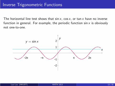
Inverse Trigonometric Functions
The horizontal line test shows that sin x , cos x , or tan x have no inversefunction in general. For example, the periodic function sin x is obviouslynot one-to-one.
−2π −π π 2π
−2
−1
1
2y = sin xy
x
Luo Luo (HKUST) MATH 1013 13 / 32

Inverse Trigonometric Functions
However, after restricting the domain to [−π2 ,
π2 ], the function y = sin x is
one-to-one, and hence has an inverse function.
−2π −π π 2π
−2
−1
1
2y = sin x , x ∈ [−π2 ,
π2 ]
y
x
The inverse function of y = sin x , with x restricted to the interval [−π2 ,
π2 ],
is denoted by y = sin−1 x or y = arcsin x .
Luo Luo (HKUST) MATH 1013 14 / 32
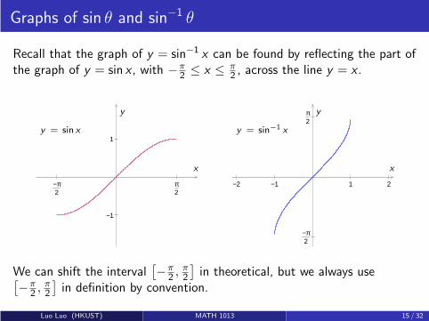
Graphs of sin θ and sin−1 θ
Recall that the graph of y = sin−1 x can be found by reflecting the part ofthe graph of y = sin x , with −π
2 ≤ x ≤ π2 , across the line y = x .
−π2
π2
−1
1y = sin x
y
x
−2 −1 1 2
−π2
π2
y = sin−1 x
y
x
We can shift the interval[
−π2 ,
π2
]
in theoretical, but we always use[
−π2 ,
π2
]
in definition by convention.
Luo Luo (HKUST) MATH 1013 15 / 32

Graphs of cos θ and cos−1 θ
The inverse trigonometric functions cos−1 x can also be defined byinverting the functions cos x with domain restricted to 0 ≤ x ≤ π.
π2 π
−1
1 y = cos x
y
x
−2 −1 1 2
π2
π
y = cos−1 x
y
x
Luo Luo (HKUST) MATH 1013 16 / 32
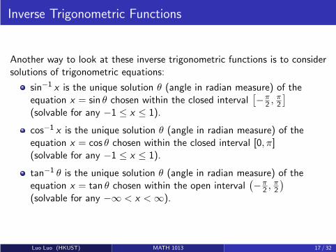
Inverse Trigonometric Functions
Another way to look at these inverse trigonometric functions is to considersolutions of trigonometric equations:
sin−1 x is the unique solution θ (angle in radian measure) of theequation x = sin θ chosen within the closed interval
[
−π2 ,
π2
]
(solvable for any −1 ≤ x ≤ 1).
cos−1 x is the unique solution θ (angle in radian measure) of theequation x = cos θ chosen within the closed interval [0, π](solvable for any −1 ≤ x ≤ 1).
tan−1 θ is the unique solution θ (angle in radian measure) of theequation x = tan θ chosen within the open interval
(
−π2 ,
π2
)
(solvable for any −∞ < x < ∞).
Luo Luo (HKUST) MATH 1013 17 / 32

Graphical View of Solving Trigonometric Equations
1 1
1
1
1
x
x
xxx
x
−π2 ≤ θ = sin−1 x ≤ π
2−1 ≤ x ≤ 1
0 ≤ θ = cos−1 x ≤ π2
−1 ≤ x ≤ 1
−π2 ≤ θ = tan−1 x ≤ π
2−∞ < x < ∞
θ
θθθ
θ
θ
Luo Luo (HKUST) MATH 1013 18 / 32
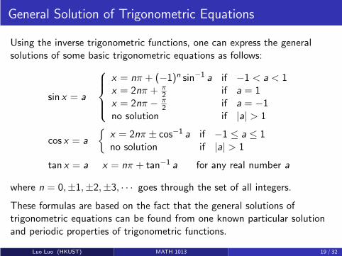
General Solution of Trigonometric Equations
Using the inverse trigonometric functions, one can express the generalsolutions of some basic trigonometric equations as follows:
sin x = a
x = nπ + (−1)n sin−1 a if −1 < a < 1x = 2nπ + π
2 if a = 1x = 2nπ − π
2 if a = −1no solution if |a| > 1
cos x = a
{
x = 2nπ ± cos−1 a if −1 ≤ a ≤ 1no solution if |a| > 1
tan x = a x = nπ + tan−1 a for any real number a
where n = 0,±1,±2,±3, · · · goes through the set of all integers.
These formulas are based on the fact that the general solutions oftrigonometric equations can be found from one known particular solutionand periodic properties of trigonometric functions.
Luo Luo (HKUST) MATH 1013 19 / 32
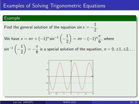
Examples of Solving Trigonometric Equations
Example
Find the general solution of the equation sin x = −1
2.
We have x = nπ + (−1)n sin−1
(
−1
2
)
= nπ − (−1)nπ
6, where
sin−1
(
−1
2
)
= −π
6is a special solution of the equation, n = 0,±1,±2, . . .
-1
-0.5
0
0.5
1
-3π -2π -π 0 π 2π 3π
Luo Luo (HKUST) MATH 1013 20 / 32

Examples of Solving Trigonometric Equations
We can also consider the unit circle:
Adding integer multiples of the periods to generate all solutions:
x =
2nπ + sin−1(
−12
)
2nπ + π − sin−1(
−12
)
n = 0,±1,±2, . . .
⇐⇒{
x = nπ + (−1)n sin−1(
−12
)
n = 0,±1,±2, . . .
Luo Luo (HKUST) MATH 1013 21 / 32

Outline
1 More Trigonometric Functions
2 Inverse Trigonometric Functions
3 The Slope of a Tangent Line
4 Limit and Natural Logarithmic Function
Luo Luo (HKUST) MATH 1013 22 / 32

The Slope of a Tangent Line
In geometry, the tangent line to a curve at a given point is the straight linethat “just touches” the curve at that point.
The secant line of a curve is a line that intersects the curve at a minimumof two distinct points.
Recall that the slope of a straight line passing through two distinct points(x1, y1), (x2, y2) is given by
m =y2 − y1
x2 − x1
Let’s consider the function y = f (x) = x2. How to find the slope mtan ofthe tangent line to the graph of f at the point (1, 1)?
Luo Luo (HKUST) MATH 1013 22 / 32
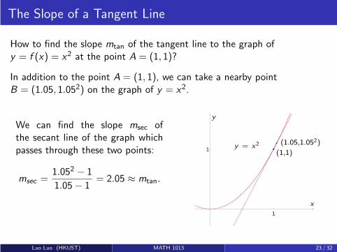
The Slope of a Tangent Line
How to find the slope mtan of the tangent line to the graph ofy = f (x) = x2 at the point A = (1, 1)?
In addition to the point A = (1, 1), we can take a nearby pointB = (1.05, 1.052) on the graph of y = x2.
We can find the slope msec ofthe secant line of the graph whichpasses through these two points:
msec =1.052 − 1
1.05− 1= 2.05 ≈ mtan.
1
1 y = x2
(1,1)
(1.05,1.052)
x
y
Luo Luo (HKUST) MATH 1013 23 / 32

The Slope of a Tangent Line
We can get better and better approximation of the slope mtan by lookingat slope of secant line through (1, 1) and another point (1 + h, (1 + h)2)on the graph, when h is chosen to be closer and closer to 0:
h 0.05 0.005 0.0005 0.00005
msec 2.05 2.005 2.0005 2.00005
In general, for any h 6= 0, we have
msec =(1 + h)2 − 1
(1 + h)− 1=
2h + h2
h= 2 + h
Note that as h → 0 (“as h 6= 0 is approaching 0”), msec is approaching thenumber 2, which gives us the slope of the tangent line mtan = 2.
Luo Luo (HKUST) MATH 1013 24 / 32
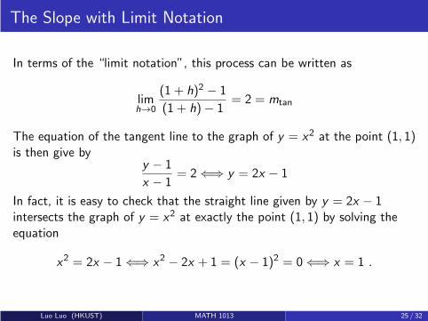
The Slope with Limit Notation
In terms of the “limit notation”, this process can be written as
limh→0
(1 + h)2 − 1
(1 + h)− 1= 2 = mtan
The equation of the tangent line to the graph of y = x2 at the point (1, 1)is then give by
y − 1
x − 1= 2 ⇐⇒ y = 2x − 1
In fact, it is easy to check that the straight line given by y = 2x − 1intersects the graph of y = x2 at exactly the point (1, 1) by solving theequation
x2 = 2x − 1 ⇐⇒ x2 − 2x + 1 = (x − 1)2 = 0 ⇐⇒ x = 1 .
Luo Luo (HKUST) MATH 1013 25 / 32

Example (tangent line problem of cubic function)
Find the equation of the tangent line to the curve defined by the equation y = x3
at the point (2, 8).
Consider the slope of the secant line passing through the point (2, 8) and anearby point (2 + h, (2 + h)3) on the curve. Then
msec =(2 + h)3 − 8
(2 + h)− 2=
12h + 6h2 + h3
h= 12 + 6h + h2 −→ 12 as h → 0
Using the limit notation, we have
limh→0
(2 + h)3 − 8
(2 + h)− 2= lim
h→0
12h + 6h2 + h3
h= lim
h→0(12 + 6h + h2) = 12
Hence the slope of the tangent line is 12, and the equation of the tangent line tothe graph of y = x3 at (2, 8) is
y − 8
x − 2= 12 ⇐⇒ y = 12x − 16
Luo Luo (HKUST) MATH 1013 26 / 32

Outline
1 More Trigonometric Functions
2 Inverse Trigonometric Functions
3 The Slope of a Tangent Line
4 Limit and Natural Logarithmic Function
Luo Luo (HKUST) MATH 1013 27 / 32

Why y = ex , y = loge x , ln x with e ≈ 2.7182?
One condition that determines the number e, which is the base of the
natural logarithmic function, is that the slope of the tangent line to thegraph of the natural logarithmic function y = loge x = ln x at (1, 0) is 1.
−1 1 2 3 4 5 6 7
−2
2
4
x
y
y = ln x
y = x−1
Luo Luo (HKUST) MATH 1013 27 / 32
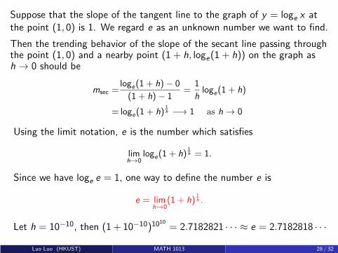
Suppose that the slope of the tangent line to the graph of y = loge x atthe point (1, 0) is 1. We regard e as an unknown number we want to find.
Then the trending behavior of the slope of the secant line passing throughthe point (1, 0) and a nearby point (1 + h, loge(1 + h)) on the graph ash → 0 should be
msec =loge(1 + h)− 0
(1 + h)− 1=
1
hloge(1 + h)
= loge(1 + h)1h −→ 1 as h → 0
Using the limit notation, e is the number which satisfies
limh→0
loge(1 + h)1h = 1.
Since we have loge e = 1, one way to define the number e is
e = limh→0
(1 + h)1h .
Let h = 10−10, then (1 + 10−10)1010= 2.7182821 · · · ≈ e = 2.7182818 · · ·
Luo Luo (HKUST) MATH 1013 28 / 32

Tangent Line Problem of Exponential Function
Find the slope of the tangent line to the graph of the natural exponentialfunction y = ex at the point (0, 1).
Just recall that the graph of y = ex can be found by reflecting the graph of itsinverse function y = ln x across the line y = x .
The tangent line to the graph of y = ln xat the point (1, 0) will be reflected to thetangent line to the graph of y = ex at thepoint (0, 1).
It is easy to see that the slope of this tangentline to y = ex is also 1.
Using two nearby points (0, 1), (h, eh) onthe graph of y = ex , and the slope of thesecant line passing through them, we have
limh→0
eh − 1
h= 1.
−1 1 2 3 4 5 6 7
−2
2
4
x
y
y = ln x
y = ex
y = x−1
y = x+1
Luo Luo (HKUST) MATH 1013 29 / 32
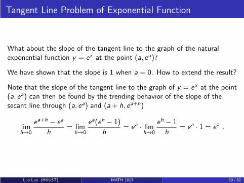
Tangent Line Problem of Exponential Function
What about the slope of the tangent line to the graph of the naturalexponential function y = ex at the point (a, ea)?
We have shown that the slope is 1 when a = 0. How to extend the result?
Note that the slope of the tangent line to the graph of y = ex at the point(a, ea) can then be found by the trending behavior of the slope of thesecant line through (a, ea) and (a+ h, ea+h)
limh→0
ea+h − ea
h= lim
h→0
ea(eh − 1)
h= ea · lim
h→0
eh − 1
h= ea · 1 = ea .
Luo Luo (HKUST) MATH 1013 30 / 32

Tangent Line Problem of Sine Function
Find the slope of the tangent line to the graph of the function y = sin x atthe point (0, 0).
By considering the slope of the secant line through the points (0, 0) and(h, sin h), the slope of the tangent line to the graph of the functiony = sin x at the point (0, 0) is given by
limh→0
sin h − sin 0
h= lim
h→0
sin h
h
By calculating a few function values of sin hh
as h → 0, it is reasonable to
guess that limh→0
sin h
h= 1.
x 0.1 0.01 0.001 0.0001sin h/h 0.998334166 0.999983333 0.999999833 0.999999998
The slope of the tangent line to the graph of y = sin x at the origin (0, 0)is then equal to 1. The equation of the tangent line is y = x .
Luo Luo (HKUST) MATH 1013 31 / 32

Tangent Line Problem of Sine Function
A precise explanation for
limh→0
sin h
h= 1
would require more understanding on the limits of function values. Weshall look at this limit again later.
Luo Luo (HKUST) MATH 1013 32 / 32

Calculus IB: Lecture 05
Luo Luo
Department of Mathematics, HKUST
http://luoluo.people.ust.hk/
Luo Luo (HKUST) MATH 1013 1 / 19
Outline
1 Limit Definition of Derivative
2 Limits of Function Values (Precise Definition)
Luo Luo (HKUST) MATH 1013 2 / 19
Outline
1 Limit Definition of Derivative
2 Limits of Function Values (Precise Definition)
Luo Luo (HKUST) MATH 1013 3 / 19
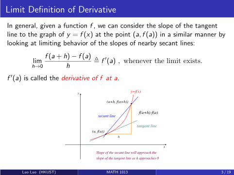
Limit Definition of Derivative
In general, given a function f , we can consider the slope of the tangentline to the graph of y = f (x) at the point (a, f (a)) in a similar manner bylooking at limiting behavior of the slopes of nearby secant lines:
limh→0
f (a+ h)− f (a)
h, f ′(a) , whenever the limit exists.
f ′(a) is called the derivative of f at a.
(a, f(a))
(a+h, f(a+h))
f(a+h)-f(a)
h
y
x
y=f(x)
tangent line
secant line
Slope of the secant line will approach the
slope of the tangent line as h approaches 0
Luo Luo (HKUST) MATH 1013 3 / 19
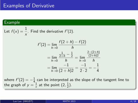
Examples of Derivative
Example
Let f (x) =1
x. Find the derivative f ′(2).
f ′(2) = limh→0
f (2 + h)− f (2)
h
= limh→0
12+h
− 12
h= lim
h→0
2−(2+h)(2+h)2
h
= limh→0
−1
(2 + h)2=
−1
2 · 2= −
1
4
where f ′(2) = −14 can be interpreted as the slope of the tangent line to
the graph of y = 1xat the point (2, 12).
Luo Luo (HKUST) MATH 1013 4 / 19
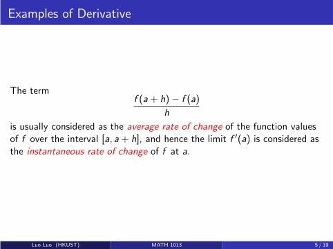
Examples of Derivative
The termf (a+ h)− f (a)
h
is usually considered as the average rate of change of the function valuesof f over the interval [a, a+ h], and hence the limit f ′(a) is considered asthe instantaneous rate of change of f at a.
Luo Luo (HKUST) MATH 1013 5 / 19

Examples of Derivative
Example
Let s(t) = t2 (in meters) be the position of a particle moving along thes-axis at time t (in seconds).
Consider that t = 2.05, then the average rate of change
(1 + 0.05)2 − 1
0.05= 2.05 (m/s)
is the usual average velocity of the particle on the time interval [1, 1.05].
The instantaneous rate of change of s = t2 at t = 1 is called theinstantaneous velocity of the particle at time t = 1:
s ′(1) = limh→0
(1 + h)2 − 1
h= lim
h→0
h(2 + h)
h= lim
h→02 + h = 2 (m/s)
Luo Luo (HKUST) MATH 1013 6 / 19

Outline
1 Limit Definition of Derivative
2 Limits of Function Values (Precise Definition)
Luo Luo (HKUST) MATH 1013 7 / 19

Limits of Function Values (Precise Definition)
This section is beyond the requirement of MATH 1013. It will
NOT been contained in our homework or exam.
Intuitively speaking, given real numbers c and L, the expression
limx→c
f (x) = L
means that f (x) becomes arbitrarily close to L as x approaches c .
What is “arbitrarily close”? What is “approaches”?
The exact definition of limx→c
f (x) is still missing!
Luo Luo (HKUST) MATH 1013 7 / 19
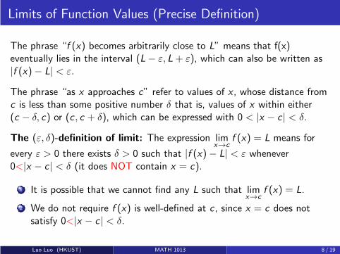
Limits of Function Values (Precise Definition)
The phrase “f (x) becomes arbitrarily close to L” means that f(x)eventually lies in the interval (L− ε, L+ ε), which can also be written as|f (x)− L| < ε.
The phrase “as x approaches c” refer to values of x , whose distance fromc is less than some positive number δ that is, values of x within either(c − δ, c) or (c , c + δ), which can be expressed with 0 < |x − c | < δ.
The (ε, δ)-definition of limit: The expression limx→c
f (x) = L means for
every ε > 0 there exists δ > 0 such that |f (x)− L| < ε whenever0<|x − c | < δ (it does NOT contain x = c).
1 It is possible that we cannot find any L such that limx→c
f (x) = L.
2 We do not require f (x) is well-defined at c , since x = c does notsatisfy 0<|x − c | < δ.
Luo Luo (HKUST) MATH 1013 8 / 19

Example: Show that limx→2
x2 = 4 by the (ε, δ)-definition.
Let ε > 0 be given; we want to show i.e., |x2 − 4| < ε. How do we find δsuch that any x satisfies |x − 2| < δ, we are guaranteed that |x2 − 4| < ε?
Note that |x2 − 4| = |x − 2| · |x + 2|, hence we consider (suppose x 6= −2)
|x2 − 4| < ε ⇐⇒ |x − 2| · |x + 2| < ε ⇐⇒ |x − 2| <ε
|x + 2|
We cannot set δ = ε/|x + 2|, because given ε > 0, δ must be a constantvalue which is independent on x (δ can depends on ε).
Luo Luo (HKUST) MATH 1013 9 / 19
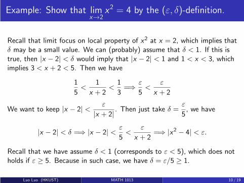
Example: Show that limx→2
x2 = 4 by the (ε, δ)-definition.
Recall that limit focus on local property of x2 at x = 2, which implies thatδ may be a small value. We can (probably) assume that δ < 1. If this istrue, then |x − 2| < δ would imply that |x − 2| < 1 and 1 < x < 3, whichimplies 3 < x + 2 < 5. Then we have
1
5<
1
x + 2<
1
3=⇒
ε
5<
ε
x + 2
We want to keep |x − 2| <ε
|x + 2|. Then just take δ =
ε
5, we have
|x − 2| < δ =⇒ |x − 2| <ε
5<
ε
x + 2=⇒ |x2 − 4| < ε.
Recall that we have assume δ < 1 (corresponds to ε < 5), which does notholds if ε ≥ 5. Because in such case, we have δ = ε/5 ≥ 1.
Luo Luo (HKUST) MATH 1013 10 / 19

Example: Show that limx→2
x2 = 4 by the (ε, δ)-definition.
When ε ≥ 5, we can just let δ = 1. Similar to previous analysis for any|x − 2| < δ = 1, we have −1 < x − 2 < 1 and 3 < x + 2 < 5, hence
|x2 − 4| = |x − 2| · |x + 2| < 1 · 5 = 5 ≤ ε −→ |x2 − 4| < ε.
In summary, for every ε > 0, there exists δ = min(ε
5, 1)
> 0 such that
|x2 − 4| < ε whenever 0 < |x − 2| < δ. Based on the (ε, δ)-definition oflimit, we can conclude that
limx→2
x2 = 4.
Luo Luo (HKUST) MATH 1013 11 / 19

Limits of Function Values
We have provide the precise definition of
limx→c
f (x) = L
when c and L are real numbers.
Recall the endpoints of intervals are not limited to real number. Forexample, we can define (−∞, 1], (3,∞), (−∞,∞) . . .
What about infinity in limits?
Luo Luo (HKUST) MATH 1013 12 / 19

Finite Limit at Infinity
Let f (x) = 1x. Then f (x) becomes arbitrarily close to 0 as x is arbitrary
large. We can writelimx→∞
f (x) = 0.
−4 −3 −2 −1 1 2 3 4
−4
−3
−2
−1
1
2
3
4
x
y
y = 1x
Luo Luo (HKUST) MATH 1013 13 / 19

Finite Limit at Infinity
More general, given function f (x) and real number L, the expression
limx→∞
f (x) = L
means for every ε > 0 there exists N > 0 such that |f (x)− L| < εwhenever x > N.
Similarly, given function f (x) and real number L, the expression
limx→−∞
f (x) = L
means for every ε > 0 there exists N < 0 such that |f (x)− L| < εwhenever x < N.
Luo Luo (HKUST) MATH 1013 14 / 19
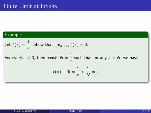
Finite Limit at Infinity
Example
Let f (x) =1
x. Show that limx→∞ f (x) = 0.
For every ε > 0, there exists N =1
εsuch that for any x > N, we have
|f (x)− 0| =1
x<
1
N= ε.
Luo Luo (HKUST) MATH 1013 15 / 19
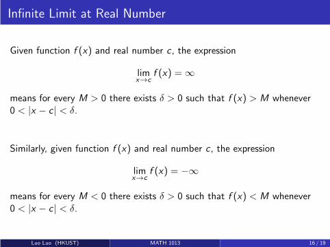
Infinite Limit at Real Number
Given function f (x) and real number c , the expression
limx→c
f (x) = ∞
means for every M > 0 there exists δ > 0 such that f (x) > M whenever0 < |x − c | < δ.
Similarly, given function f (x) and real number c , the expression
limx→c
f (x) = −∞
means for every M < 0 there exists δ > 0 such that f (x) < M whenever0 < |x − c | < δ.
Luo Luo (HKUST) MATH 1013 16 / 19
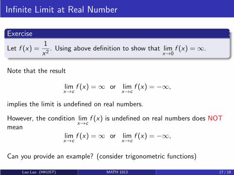
Infinite Limit at Real Number
Exercise
Let f (x) =1
x2. Using above definition to show that lim
x→0f (x) = ∞.
Note that the result
limx→c
f (x) = ∞ or limx→c
f (x) = −∞,
implies the limit is undefined on real numbers.
However, the condition limx→c
f (x) is undefined on real numbers does NOTmean
limx→c
f (x) = ∞ or limx→c
f (x) = −∞,
Can you provide an example? (consider trigonometric functions)
Luo Luo (HKUST) MATH 1013 17 / 19

Infinite Limit at Infinity
Given function f (x), the expression
limx→∞
f (x) = ∞
means for every M > 0 there exists N > 0 such that f (x) > M wheneverx > N.
Similarly, we can also give the definitions of
1 limx→∞
f (x) = −∞,
2 limx→−∞
f (x) = ∞,
3 limx→−∞
f (x) = −∞.
Luo Luo (HKUST) MATH 1013 18 / 19

The (ε, δ)-Definition
We can use (ε, δ)-definition to define a lot of things in calculus such aslimit, continuity, derivative and integral.
This section is NOT contained in the requirement of MATH 1013.
You can ignore this topic if you think it is difficult.
The (ε, δ)-definition is important to a deeper understanding of calculus.You can read a book of mathematical analysis if you are interested in it,but we will not talk about this topic in our course anymore.
Luo Luo (HKUST) MATH 1013 19 / 19

Calculus IB: Lecture 06
Luo Luo
Department of Mathematics, HKUST
http://luoluo.people.ust.hk/
Luo Luo (HKUST) MATH 1013 1 / 33

Outline
1 Limits of Function Values (Intuitive Understanding)
2 Asymptotes and Limits at Infinity
3 Basic Techniques in Limit Computation
Luo Luo (HKUST) MATH 1013 2 / 33

Outline
1 Limits of Function Values (Intuitive Understanding)
2 Asymptotes and Limits at Infinity
3 Basic Techniques in Limit Computation
Luo Luo (HKUST) MATH 1013 3 / 33

Limits of Function Values (Intuitive Understanding)
Come back the requirement of MATH 1013!
An important point to keep in mind is that finding limx→a
f (x) is NOT the
same as finding the function value f (a).
1 limx→a
f (x) may exist even if f (x) is undefined at x = a
2 limx→a
f (x) may not exists even if f (x) is well-defined at x = a
Luo Luo (HKUST) MATH 1013 3 / 33
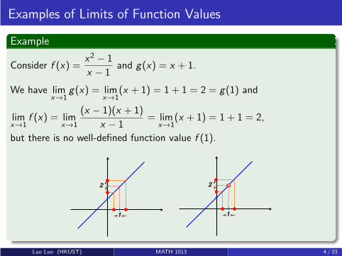
Examples of Limits of Function Values
Example
Consider f (x) =x2 − 1
x − 1and g(x) = x + 1.
We have limx→1
g(x) = limx→1
(x + 1) = 1 + 1 = 2 = g(1) and
limx→1
f (x) = limx→1
(x − 1)(x + 1)
x − 1= lim
x→1(x + 1) = 1 + 1 = 2,
but there is no well-defined function value f (1).
1
2
1
2
Luo Luo (HKUST) MATH 1013 4 / 33

Finding Limits by Graphs
Graphically speaking, finding limits of function values is like riding alongthe graph (hollow circle means the function value is undefined at thispoint).
2 4 6−2−4−6
2
4
6
−2
−4
−6
f (0) is well-defined, and limx→0
f (x) = f (0).
limx→4
f (x) = 6, while f (4) is not well-defined.
Luo Luo (HKUST) MATH 1013 5 / 33

2 4 6−2−4−6
2
4
6
−2
−4
−6
f (−3) = 3, but the left-hand limit is
limx→−3−
f (x) = 1 6= f (−3)
and the right-hand limit is
limx→−3+
f (x) = 5 6= f (−3)
x → −3− means that x is approaching −3 from the left (i.e. x < −3)
x → −3+ means that x is approaching −3 from the right (i.e. x > −3).
Luo Luo (HKUST) MATH 1013 6 / 33
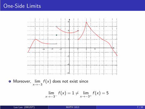
One-Side Limits
2 4 6−2−4−6
2
4
6
−2
−4
−6
Moreover, limx→−3
f (x) does not exist since
limx→−3−
f (x) = 1 6= limx→−3+
f (x) = 5
Luo Luo (HKUST) MATH 1013 7 / 33

One-Side Limits
2 4 6−2−4−6
2
4
6
−2
−4
−6
What happens as x → 2−, or x → 2+?
We have limx→2−
f (x) = 4 = f (2), but limx→2+
f (x) = 2 6= f (2) = 4.
The (two-sided) limit limx→2
f (x) does not exist!
Luo Luo (HKUST) MATH 1013 8 / 33
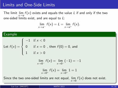
Limits and One-Side Limits
The limit limx→a
f (x) exists and equals the value L if and only if the two
one-sided limits exist, and are equal to L:
limx→a−
f (x) = L = limx→a+
f (x).
Example
Let f (x) =
−1 if x < 0
0 if x = 0
1 if x > 0
, then f (0) = 0, and
limx→0−
f (x) = limx→0−
(−1) = −1
limx→0+
f (x) = limx→0+
1 = 1
Since the two one-sided limits are not equal, limx→0
f (x) does not exist.
Luo Luo (HKUST) MATH 1013 9 / 33
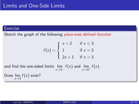
Limits and One-Side Limits
Exercise
Sketch the graph of the following piece-wise defined function
f (x) =
x + 2 if x < 3
1 if x = 3
2x + 1 if x > 3
and find the one-sided limits limx→3−
f (x) and limx→3+
f (x).
Does limx→3
f (x) exist?
Luo Luo (HKUST) MATH 1013 10 / 33
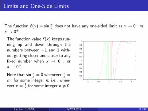
Limits and One-Side Limits
The function f (x) = sin π
xdoes not have any one-sided limit as x → 0− or
x → 0+ .
-1
-0.8
-0.6
-0.4
-0.2
0
0.2
0.4
0.6
0.8
1
-1 -0.5 0 0.5 1
The function value f (x) keeps run-ning up and down through thenumbers between −1 and 1 with-out getting closer and closer to anyfixed number when x → 0−, orx → 0+.
Note that sin π
x= 0 whenever π
x=
nπ for some integer n; i.e., when-ever x = 1
nfor some integer n 6= 0.
Luo Luo (HKUST) MATH 1013 11 / 33
Outline
1 Limits of Function Values (Intuitive Understanding)
2 Asymptotes and Limits at Infinity
3 Basic Techniques in Limit Computation
Luo Luo (HKUST) MATH 1013 12 / 33
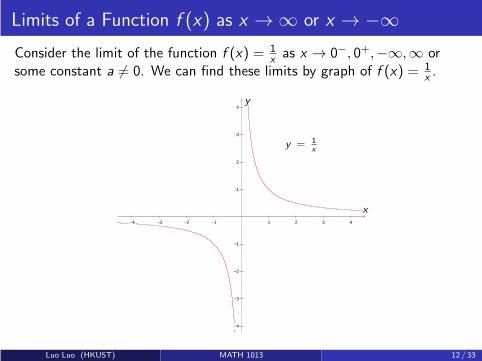
Limits of a Function f (x) as x → ∞ or x → −∞Consider the limit of the function f (x) = 1
xas x → 0−, 0+,−∞,∞ or
some constant a 6= 0. We can find these limits by graph of f (x) = 1x.
−4 −3 −2 −1 1 2 3 4
−4
−3
−2
−1
1
2
3
4
x
y
y = 1x
Luo Luo (HKUST) MATH 1013 12 / 33

Limits of a Function f (x) as x → ∞ or x → −∞
(a) limx→0+
1
x= +∞ (b) lim
x→0−
1
x= −∞ (c) lim
x→+∞
1
x= 0
(d) limx→−∞
1
x= 0 (e) lim
x→a
1
x=
1
afor all real number a 6= 0
−4 −3 −2 −1 1 2 3 4
−4
−3
−2
−1
1
2
3
4
x
y
y = 1x
Luo Luo (HKUST) MATH 1013 13 / 33

Horizontal Asymptote and Vertical Asymptote
The line y = 0 (x-axis) is called a horizontal asymptote of the functionf (x) = 1
x. The line x = 0 (y -axis) is called a vertical asymptote of this
function.
−4 −3 −2 −1 1 2 3 4
−4
−3
−2
−1
1
2
3
4
x
y
y = 1x
Luo Luo (HKUST) MATH 1013 14 / 33

Horizontal Asymptote and Vertical Asymptote
In general, we may consider the limiting behavior of f (x) as x → ∞ orx → −∞, or consider some one-sided limits to see if f (x) is approaching∞ or −∞ as x → a+ or a → a−.
1 y = L is a horizontal asymptote of the function f (x) if eitherlimx→∞
f (x) = L or limx→−∞
f (x) = L.
2 x = b is a vertical asymptote of the function f (x) if at least one ofthe following holds:
1 limx→b−
f (x) = ∞
2 limx→b−
f (x) = −∞
3 limx→b+
f (x) = ∞
4 limx→b+
f (x) = −∞
Luo Luo (HKUST) MATH 1013 15 / 33

Horizontal Asymptote and Vertical Asymptote
Note that f has two different horizontal asymptotes y = L1 and y = L2 if
limx→∞
f (x) = L1 6= limx→−∞
f (x) = L2
In any case, a function can have at most two horizontal asymptotes.
Luo Luo (HKUST) MATH 1013 16 / 33
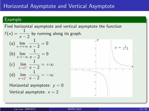
Horizontal Asymptote and Vertical Asymptote
Example
Find horizontal asymptote and vertical asymptote the function
f (x) =1
x − 2by running along its graph.
(a) limx→+∞
1
x − 2= 0
(b) limx→−∞
1
x − 2= 0
(c) limx→2+
1
x − 2= +∞
(d) limx→2−
1
x − 2= −∞
Horizontal asymptote: y = 0
Vertical asymptote: x = 2
−3 −2 −1 1 2 3 4 5
−4
−3
−2
−1
1
2
3
4
x
y
y = 1x−2
Luo Luo (HKUST) MATH 1013 17 / 33

Horizontal Asymptote and Vertical Asymptote
Example
Find horizontal asymptote and vertical asymptote the function
f (x) =x − 1
x= 1− 1
xby running along its graph.
(a) limx→+∞
x − 1
x= 1
(b) limx→−∞
x − 1
x= 1
(c) limx→0+
x − 1
x= −∞
(d) limx→0−
x − 1
x= +∞
Horizontal asymptote: y = 1
Vertical asymptote: x = 0
−4 −3 −2 −1 1 2 3 4
−4
−3
−2
−1
1
2
3
4
x
y
y = x−1x
y =1
Luo Luo (HKUST) MATH 1013 18 / 33
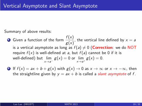
Vertical Asymptote and Slant Asymptote
Summary of above results:
1 Given a function of the formf (x)
g(x), the vertical line defined by x = a
is a vertical asymptote as long as f (a) 6= 0 (Correction: we do NOTrequire f (x) is well-defined at a, but f (a) cannot be 0 if it iswell-defined) but lim
x→a−g(x) = 0 or lim
x→a+g(x) = 0.
2 If f (x) = ax + b + g(x) with g(x) → 0 as x → ∞ or x → −∞, thenthe straightline given by y = ax + b is called a slant asymptote of f .
Luo Luo (HKUST) MATH 1013 19 / 33
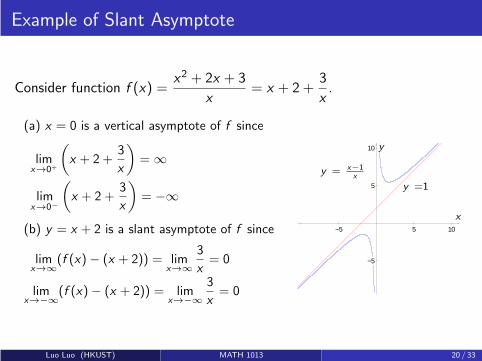
Example of Slant Asymptote
Consider function f (x) =x2 + 2x + 3
x= x + 2 +
3
x.
(a) x = 0 is a vertical asymptote of f since
limx→0+
(
x + 2 +3
x
)
= ∞
limx→0−
(
x + 2 +3
x
)
= −∞
(b) y = x + 2 is a slant asymptote of f since
limx→∞
(f (x)− (x + 2)) = limx→∞
3
x= 0
limx→−∞
(f (x)− (x + 2)) = limx→−∞
3
x= 0
−5 5 10
−5
5
10
x
y
y = x−1x
y =1
Luo Luo (HKUST) MATH 1013 20 / 33

Exercise of Slant Asymptote
Exercise
Show that y = −x and y = x are two slant asymptotes of the functionf (x) =
√1 + x2.
Hint: Consider the values of
limx→∞
(
√
1 + x2 − x)
= limx→∞
(
(√1 + x2 − x)(
√1 + x2 + x)√
1 + x2 + x
)
and
limx→−∞
(
√
1 + x2 + x)
= limx→−∞
(
(√1 + x2 + x)(
√1 + x2 − x)√
1 + x2 − x
)
.
Luo Luo (HKUST) MATH 1013 21 / 33

Examples of Multiple Vertical Asymptotes
Consider the function f (x) = tan(x), we have
limx→a+
tan(x) = −∞ and limx→a−
tan(x) = ∞,
where a =π
2+ nπ for any integer n.
−5π2 −2π −3π
2 −π −π2
π2 π 3π
2 2π 5π2
y
x
Hence x =π
2+ nπ with any integer n is a vertical asymptote and there are
infinite asymptotes in total.
Luo Luo (HKUST) MATH 1013 22 / 33

Examples of Multiple Horizontal Asymptotes
Consider the function f (x) = tan−1(x), we have
limx→∞
tan(x) =π
2and lim
x→−∞
tan(x) = −π
2.
−3 −2 −1 1 2 3 4
−π
−π2
π2
π x
y=tan−1 x
x
Hence y =π
2and y = −π
2are two horizontal asymptotes.
Luo Luo (HKUST) MATH 1013 23 / 33

Examples of Multiple Slant Asymptotes
Consider the function f (x) = x + tan−1(x), we have
limx→∞
(
f (x)− x − π
2
)
= 0 and limx→−∞
(
f (x)− x +π
2
)
= 0.
-5 -4 -3 -2 -1 0 1 2 3 4 5-5
-4
-3
-2
-1
0
1
2
3
4
5
y=x+tan-1(x)
Hence y = x − π
2and y = x +
π
2are two slant asymptotes.
Luo Luo (HKUST) MATH 1013 24 / 33

Outline
1 Limits of Function Values (Intuitive Understanding)
2 Asymptotes and Limits at Infinity
3 Basic Techniques in Limit Computation
Luo Luo (HKUST) MATH 1013 25 / 33

Some Useful Limit Laws
Suppose that limx→a
f (x) and limx→a
g(x) exists on real numbers, then we have:
1 limx→a
[cf (x)] = c limx→a
f (x) for any constant c
2 limx→a
[f (x) + g(x)] = limx→a
f (x) + limx→a
g(x)
3 limx→a
[f (x)− g(x)] = limx→a
f (x)− limx→a
g(x)
4 limx→a
[f (x)g(x)] = limx→a
f (x) · limx→a
g(x)
5 limx→a
f (x)
g(x)=
limx→a
f (x)
limx→a
g(x)if lim
x→ag(x) 6= 0
6 limx→a
[f (x)]p =(
limx→a
f (x))p
for any rational exponent p when
( limx→a
f (x))p exists.
Luo Luo (HKUST) MATH 1013 25 / 33

Some Useful Limit Laws
All of these rules can be proved by precise definition of limit, which isbased on (ε, δ) language.
The following things are undefined:
∞∞ ,
0
0, 0 · ∞ and ∞−∞.
Luo Luo (HKUST) MATH 1013 26 / 33

Some Useful Limit Laws
Let f (x) =1
x2and g(x) = − 1
x2. What is lim
x→a[f (x) + g(x)]?
The definition of f (x) and g(x) means
f (x) + g(x) =
{
0, x 6= 0,
undefined, x = 0.
Then we have limx→0+
[f (x) + g(x)] = limx→0−
[f (x) + g(x)] = 0 and
limx→0
[f (x) + g(x)] = 0.
However, we have
limx→0
f (x) = limx→0
1
x2= ∞ and lim
x→0g(x) = lim
x→0− 1
x2= −∞.
Since ∞+ (−∞) is undefined, we can NOT say ∞+ (−∞) = 0
Luo Luo (HKUST) MATH 1013 27 / 33
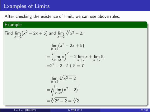
Examples of Limits
After checking the existence of limit, we can use above rules.
Example
Find limx→2
(x2 − 2x + 5) and limx→2
3√
x2 − 2.
limx→2
(x2 − 2x + 5)
=(
limx→2
x)2
− 2 limx→2
x + limx→2
5
=22 − 2 · 2 + 5 = 7
limx→2
3√
x2 − 2
= 3
√
limx→2
(x2 − 2)
=3√
22 − 2 =3√2
Luo Luo (HKUST) MATH 1013 28 / 33
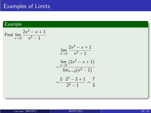
Examples of Limits
Example
Find limx→2
2x2 − x + 1
x2 − 1.
limx→2
2x2 − x + 1
x2 − 1
=limx→2
(
2x2 − x + 1)
limx→2(x2 − 1)
=2 · 22 − 2 + 1
22 − 1=
7
3
Luo Luo (HKUST) MATH 1013 29 / 33

Examples of Limits
Several algebraic tricks, mostly about factor canceling, are often needed inorder to find limits of the form 0
0 or ∞
∞.
Example
Find the limit limx→2
x2 − 4
x − 2.
(
0
0-type limit
)
Note that if we directly substitute x = 2 into the expression, we will getsome undefined expression 0
0 . This suggests that (x − 2) is a factor ofboth the numerator and the denominator. After factoring, we have
limx→2
x2 − 4
x − 2= lim
x→2
(x − 2)(x + 2)
x − 2= lim
x→2(x + 2) = 2 + 2 = 4
Note that for x → 2, we do not need to consider x = 2.
Luo Luo (HKUST) MATH 1013 30 / 33
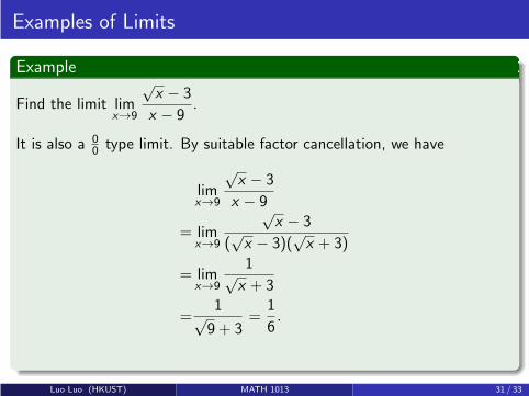
Examples of Limits
Example
Find the limit limx→9
√x − 3
x − 9.
It is also a 00 type limit. By suitable factor cancellation, we have
limx→9
√x − 3
x − 9
= limx→9
√x − 3
(√x − 3)(
√x + 3)
= limx→9
1√x + 3
=1√9 + 3
=1
6.
Luo Luo (HKUST) MATH 1013 31 / 33
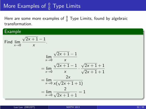
More Examples of 00 Type Limits
Here are some more examples of 00 Type Limits, found by algebraic
transformation.
Example
Find limx→0
√2x + 1− 1
x.
limx→0
√2x + 1− 1
x
= limx→0
√2x + 1− 1
x·√2x + 1 + 1√2x + 1 + 1
= limx→0
2x
x(√2x + 1 + 1)
= limx→0
2√2x + 1 + 1
= 1
Luo Luo (HKUST) MATH 1013 32 / 33
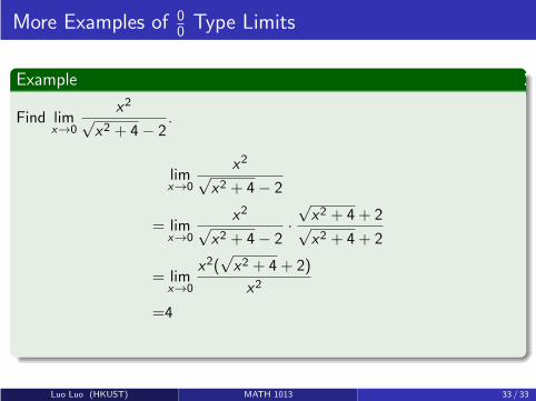
More Examples of 00 Type Limits
Example
Find limx→0
x2√x2 + 4− 2
.
limx→0
x2√x2 + 4− 2
= limx→0
x2√x2 + 4− 2
·√x2 + 4 + 2√x2 + 4 + 2
= limx→0
x2(√x2 + 4 + 2)
x2
=4
Luo Luo (HKUST) MATH 1013 33 / 33

Calculus IB: Lecture 07
Luo Luo
Department of Mathematics, HKUST
http://luoluo.people.ust.hk/
Luo Luo (HKUST) MATH 1013 1 / 30
Outline
1 Basic Techniques in Limit Computation (Cont’d)
2 Extended Real Number System
3 Squeeze Theorem
Luo Luo (HKUST) MATH 1013 2 / 30
Outline
1 Basic Techniques in Limit Computation (Cont’d)
2 Extended Real Number System
3 Squeeze Theorem
Luo Luo (HKUST) MATH 1013 3 / 30

Examples of ∞∞ Type Limits
Example
Find the limit limx→+∞
2x2 − x + 3
3x2 + x − 1.
We need to understand the behavior of the function 1xas x → +∞:
limx→+∞
2x2 − x + 3
3x2 + x − 1= lim
x→+∞
x2(2− 1x+ 3
x2)
x2(3 + 1x− 1
x2)
= limx→+∞
2− 1x+ 3
x2
3 + 1x− 1
x2
=2− 0 + 3 · 03 + 0− 0
=2
3,
where we use the fact
limx→+∞
1
x= 0, lim
x→+∞
1
x2= lim
x→+∞
1
x· limx→+∞
1
x= 0 · 0 = 0.
Luo Luo (HKUST) MATH 1013 3 / 30
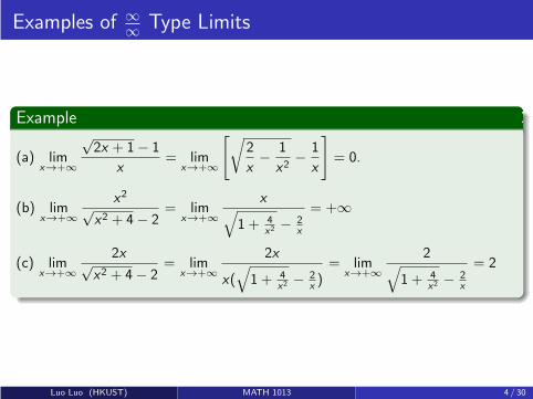
Examples of ∞∞ Type Limits
Example
(a) limx→+∞
√2x + 1− 1
x= lim
x→+∞
[
√
2
x− 1
x2− 1
x
]
= 0.
(b) limx→+∞
x2√x2 + 4− 2
= limx→+∞
x√
1 + 4x2 − 2
x
= +∞
(c) limx→+∞
2x√x2 + 4− 2
= limx→+∞
2x
x(√
1 + 4x2 − 2
x)= lim
x→+∞
2√
1 + 4x2 − 2
x
= 2
Luo Luo (HKUST) MATH 1013 4 / 30
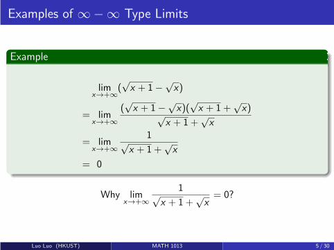
Examples of ∞−∞ Type Limits
Example
limx→+∞
(√x + 1−
√x)
= limx→+∞
(√x + 1−√
x)(√x + 1 +
√x)√
x + 1 +√x
= limx→+∞
1√x + 1 +
√x
= 0
Why limx→+∞
1√x + 1 +
√x= 0?
Luo Luo (HKUST) MATH 1013 5 / 30
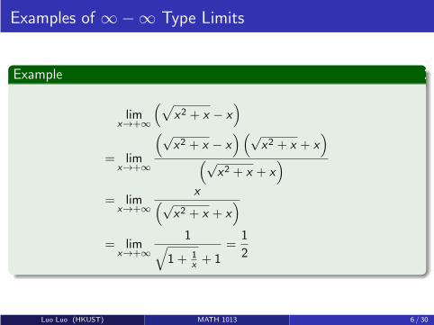
Examples of ∞−∞ Type Limits
Example
limx→+∞
(
√
x2 + x − x)
= limx→+∞
(√x2 + x − x
)(√x2 + x + x
)
(√x2 + x + x
)
= limx→+∞
x(√
x2 + x + x)
= limx→+∞
1√
1 + 1x+ 1
=1
2
Luo Luo (HKUST) MATH 1013 6 / 30

Examples of ∞−∞ Type Limits
When computing limits of the form
limx→∞
(f (x)− g(x)),
where both f and g are approaching ∞ as x is approaching ∞, one isactually looking at the trending behaviour of the gap between the graph off and g , i.e., how
f (x)− g(x)
behaves as x → ∞.
Luo Luo (HKUST) MATH 1013 7 / 30

Examples of ∞−∞ Type Limits
Example
Find one-sided limits: limx→1−
x2 − x + 1
x2 − 1and lim
x→1+
x2 − x + 1
x2 − 1. We have
limx→1−
x2 − x + 1
x2 − 1= lim
x→1−
x2 − x + 1
x + 1· 1
x − 1=
1
2· (−∞) = −∞
and
limx→1+
x2 − x + 1
x2 − 1= lim
x→1+
x2 − x + 1
x + 1· 1
x − 1=
1
2· ∞ = ∞
Hence x = 1 is a vertical asymptote of the functionx2 − x + 1
x2 − 1.
Luo Luo (HKUST) MATH 1013 8 / 30
Outline
1 Basic Techniques in Limit Computation (Cont’d)
2 Extended Real Number System
3 Squeeze Theorem
Luo Luo (HKUST) MATH 1013 9 / 30

Limit Laws with Infinity
We define the arithmetic operations as follows
c · ∞ = ∞ · c = ∞ for real number c > 0.
Based on above notations, we can generalize
limx→a
[f (x)g(x)] = limx→a
f (x) · limx→a
g(x)
to the case that one of limx→a
f (x) and limx→a
g(x) is ∞.
Formally speaking, the notation ∞ · c means we have
limx→a
[f (x)g(x)] = ∞
when limx→a
f (x) = ∞ and limx→a
g(x) = c > 0.
Luo Luo (HKUST) MATH 1013 9 / 30

The Proof of ∞ · c = ∞
Proof: The limit limx→a
f (x) = ∞ means for any M0 > 0, there exists δ0 > 0
such that f (x) > M0 whenever 0 < |x − a| < δ0. Hence, for every M > 0,let M0 =
2Mc, there exists δ0 > 0 such that
|f (x)| = f (x) >2M
c
whenever 0 < |x − a| < δ0.
The limit limx→a
g(x) = c means for every ε1 > 0 there exists δ1 > 0 such
that |g(x)− c | < ε1 whenever 0 < |x − a| < δ1. Let ε1 =c2 , there exist
δ1 > 0 such that we have
−c
2< g(x)− c <
c
2=⇒ c
2< g(x) <
3c
2=⇒ |g(x)| > c
2
whenever 0 < |x − a| < δ1.
Luo Luo (HKUST) MATH 1013 10 / 30
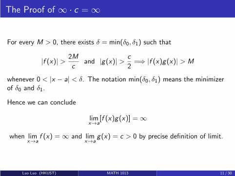
The Proof of ∞ · c = ∞
For every M > 0, there exists δ = min(δ0, δ1) such that
|f (x)| > 2M
cand |g(x)| > c
2=⇒ |f (x)g(x)| > M
whenever 0 < |x − a| < δ. The notation min(δ0, δ1) means the minimizerof δ0 and δ1.
Hence we can conclude
limx→a
[f (x)g(x)] = ∞
when limx→a
f (x) = ∞ and limx→a
g(x) = c > 0 by precise definition of limit.
Luo Luo (HKUST) MATH 1013 11 / 30
Extended Real Number System
We introduce extended real number system to address the calculationcontains the ∞ and −∞. It is useful in describing the algebra on infinitiesand the various limiting behaviors in calculus.
Recall that R = (−∞,∞) presents the set of all real number.
The extended real number system is denoted by R or [−∞,+∞] orR ∪ {−∞,+∞}.
Here, “+∞” is equivalent to “∞” and “−(−∞)”.
Luo Luo (HKUST) MATH 1013 12 / 30

Arithmetic Operations on R
a+∞ = +∞+ a = +∞, a 6= −∞
a−∞ = −∞+ a = −∞, a 6= +∞
a · (+∞) = +∞ · a = +∞, a ∈ (0,+∞]
a · (−∞) = −∞ · a = −∞, a ∈ (0,+∞]
a · (+∞) = +∞ · a = −∞, a ∈ [−∞, 0)
a · (−∞) = −∞ · a = +∞, a ∈ [−∞, 0)
Luo Luo (HKUST) MATH 1013 13 / 30

Arithmetic Operations on R
a
+∞ =a
−∞ = 0, a ∈ R
+∞a
= +∞, a ∈ (0,+∞)
−∞a
= −∞, a ∈ (0,+∞)
+∞a
= −∞, a ∈ (−∞, 0)
−∞a
= +∞, a ∈ (−∞, 0)
Luo Luo (HKUST) MATH 1013 14 / 30
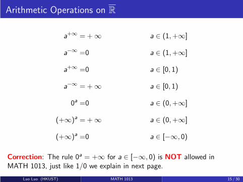
Arithmetic Operations on R
a+∞ =+∞ a ∈ (1,+∞]
a−∞ =0 a ∈ (1,+∞]
a+∞ =0 a ∈ [0, 1)
a−∞ =+∞ a ∈ [0, 1)
0a =0 a ∈ (0,+∞]
(+∞)a =+∞ a ∈ (0,+∞]
(+∞)a =0 a ∈ [−∞, 0)
Correction: The rule 0a = +∞ for a ∈ [−∞, 0) is NOT allowed inMATH 1013, just like 1/0 we explain in next page.
Luo Luo (HKUST) MATH 1013 15 / 30
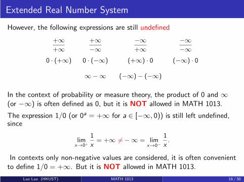
Extended Real Number System
However, the following expressions are still undefined
+∞+∞
+∞−∞
−∞+∞
−∞−∞
0 · (+∞) 0 · (−∞) (+∞) · 0 (−∞) · 0
∞−∞ (−∞)− (−∞)
In the context of probability or measure theory, the product of 0 and ∞(or −∞) is often defined as 0, but it is NOT allowed in MATH 1013.
The expression 1/0 (or 0a = +∞ for a ∈ [−∞, 0)) is still left undefined,since
limx→0+
1
x= +∞ 6=−∞ = lim
x→0−
1
x.
In contexts only non-negative values are considered, it is often convenientto define 1/0 = +∞. But it is NOT allowed in MATH 1013.
Luo Luo (HKUST) MATH 1013 16 / 30
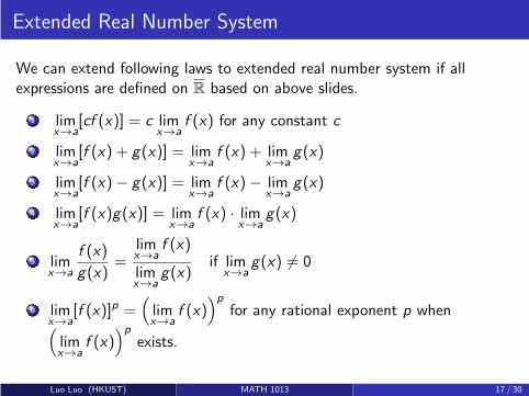
Extended Real Number System
We can extend following laws to extended real number system if allexpressions are defined on R based on above slides.
1 limx→a
[cf (x)] = c limx→a
f (x) for any constant c
2 limx→a
[f (x) + g(x)] = limx→a
f (x) + limx→a
g(x)
3 limx→a
[f (x)− g(x)] = limx→a
f (x)− limx→a
g(x)
4 limx→a
[f (x)g(x)] = limx→a
f (x) · limx→a
g(x)
5 limx→a
f (x)
g(x)=
limx→a
f (x)
limx→a
g(x)if lim
x→ag(x) 6= 0
6 limx→a
[f (x)]p =(
limx→a
f (x))p
for any rational exponent p when(
limx→a
f (x))p
exists.
Luo Luo (HKUST) MATH 1013 17 / 30
Exercise
Find (i) limx→−1−
x2 − x + 1
x2 − 1, (ii) lim
x→−1+
x2 − x + 1
x2 − 1. Can you find all
vertical asymptotes of the functionx2 − x + 1
x2 − 1? and any horizontal
asymptotes?
Exercise
Compute the limit (a) limx→0+
(
1√x− 1
x
)
, (b) limx→2
√
x2 − 5x + 6
x2 − 4.
Exercise
Compute the limit (a) limx→e2
(ln x)3 − 8
(ln x)2 − 4, (b) lim
x→0
1 + sin x
cos2 x.
Luo Luo (HKUST) MATH 1013 18 / 30

Outline
1 Basic Techniques in Limit Computation (Cont’d)
2 Extended Real Number System
3 Squeeze Theorem
Luo Luo (HKUST) MATH 1013 19 / 30

Squeeze Theorem
Squeeze Theorem (or Sandwich Theorem)
Let I be an interval having the point a. Let g , f , and h be functionsdefined on I , except possibly at a itself. Suppose that for every x in I
NOT equal to a, we have If g(x) ≤ f (x) ≤ h(x) for all x near a, exceptperhaps when x = a, then
limx→a
g(x) ≤ limx→a
f (x) ≤ limx→a
h(x)
whenever these limits exist. (The same is true for one-sided limits.)
Exercise
Try to prove squeeze theorem by (ε, δ)-definition.
Note that we only require g(x) ≤ f (x) ≤ h(x) holds locally.
Luo Luo (HKUST) MATH 1013 19 / 30
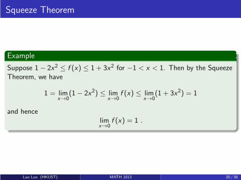
Squeeze Theorem
Example
Suppose 1− 2x2 ≤ f (x) ≤ 1 + 3x2 for −1 < x < 1. Then by the SqueezeTheorem, we have
1 = limx→0
(1− 2x2) ≤ limx→0
f (x) ≤ limx→0
(1 + 3x2) = 1
and hencelimx→0
f (x) = 1 .
Luo Luo (HKUST) MATH 1013 20 / 30

Squeeze Theorem
Example
Show that limx→0
x sin1
x= 0 by applying the Squeeze Theorem:
−|x | ≤ x sin1
x≤ |x |
0 = − limx→0
|x | ≤ limx→0
x sin1
x≤ lim
x→0|x | = 0 .
-0.2
-0.1
0
0.1
0.2
-0.2 -0.1 0 0.1 0.2
Luo Luo (HKUST) MATH 1013 21 / 30
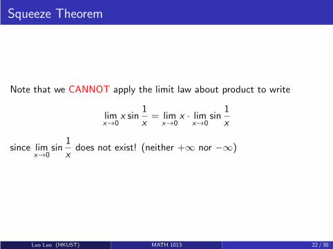
Squeeze Theorem
Note that we CANNOT apply the limit law about product to write
limx→0
x sin1
x= lim
x→0x · lim
x→0sin
1
x
since limx→0
sin1
xdoes not exist! (neither +∞ nor −∞)
Luo Luo (HKUST) MATH 1013 22 / 30
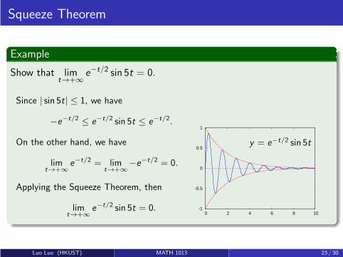
Squeeze Theorem
Example
Show that limt→+∞
e−t/2 sin 5t = 0.
Since | sin 5t| ≤ 1, we have
−e−t/2 ≤ e−t/2 sin 5t ≤ e−t/2.
On the other hand, we have
limt→+∞
e−t/2 = limt→+∞
−e−t/2 = 0.
Applying the Squeeze Theorem, then
limt→+∞
e−t/2 sin 5t = 0. -1
-0.5
0
0.5
1
0 2 4 6 8 10
y = e−t/2 sin 5t
Luo Luo (HKUST) MATH 1013 23 / 30

Examples of Squeeze Theorem
In Lecture 04, we guessed
limθ→0
sin θ
θ= 1
by calculating several points of θ near 0:
θ 0.1 0.01 0.001 0.0001
sin θ/θ 0.998334166 0.999983333 0.999999833 0.999999998
Now, we can prove it by Squeeze Theorem.
Luo Luo (HKUST) MATH 1013 24 / 30
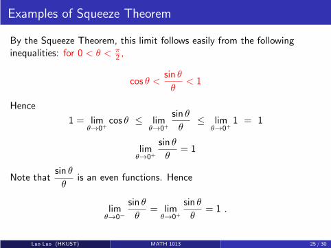
Examples of Squeeze Theorem
By the Squeeze Theorem, this limit follows easily from the followinginequalities: for 0 < θ < π
2 ,
cos θ <sin θ
θ< 1
Hence
1 = limθ→0+
cos θ ≤ limθ→0+
sin θ
θ≤ lim
θ→0+1 = 1
limθ→0+
sin θ
θ= 1
Note thatsin θ
θis an even functions. Hence
limθ→0−
sin θ
θ= lim
θ→0+
sin θ
θ= 1 .
Luo Luo (HKUST) MATH 1013 25 / 30
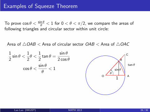
Examples of Squeeze Theorem
To prove cos θ < sin θθ < 1 for 0 < θ < π/2, we compare the areas of
following triangles and circular sector within unit circle:
Area of △OAB < Area of circular sector OAB < Area of △OAC
1
2sin θ <
1
2θ <
1
2tan θ =
sin θ
2 cos θ
cos θ <sin θ
θ< 1
O A
B
C
θsin θ
tan θ
1
Luo Luo (HKUST) MATH 1013 26 / 30
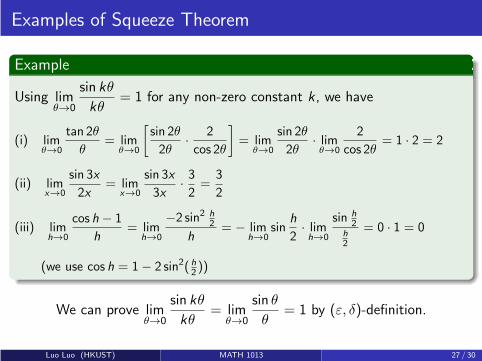
Examples of Squeeze Theorem
Example
Using limθ→0
sin kθ
kθ= 1 for any non-zero constant k , we have
(i) limθ→0
tan 2θ
θ= lim
θ→0
[
sin 2θ
2θ· 2
cos 2θ
]
= limθ→0
sin 2θ
2θ· limθ→0
2
cos 2θ= 1 · 2 = 2
(ii) limx→0
sin 3x
2x= lim
x→0
sin 3x
3x· 32=
3
2
(iii) limh→0
cos h − 1
h= lim
h→0
−2 sin2 h2
h= − lim
h→0sin
h
2· limh→0
sin h2
h2
= 0 · 1 = 0
(we use cos h = 1− 2 sin2( h2 ))
We can prove limθ→0
sin kθ
kθ= lim
θ→0
sin θ
θ= 1 by (ε, δ)-definition.
Luo Luo (HKUST) MATH 1013 27 / 30
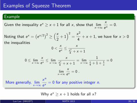
Examples of Squeeze Theorem
Example
Given the inequality ex ≥ x + 1 for all x , show that limx→∞
x
ex= 0.
Noting that ex =(
ex/2)2 ≥
(x
2+ 1
)2=
x2
4+ x + 1, we have for x > 0
the inequalities
0 <x
ex≤ x
x2
4 + x + 1
0 ≤ limx→∞
x
ex≤ lim
x→∞
xx2
4 + x + 1= lim
x→∞
1x4 + 1 + 1
x
= 0
limx→∞
x
ex= 0 .
More generally, limx→∞
xn
ex= 0 for any positive integer n.
Why ex ≥ x + 1 holds for all x?
Luo Luo (HKUST) MATH 1013 28 / 30
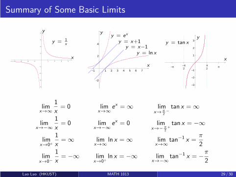
Summary of Some Basic Limits
−4 −3 −2 −1 1 2 3 4
−4
−3
−2
−1
1
2
3
4
x
y
y = 1x
−1 1 2 3 4 5 6 7
−2
2
4
x
y
y = ln x
y = ex
y = x−1y = x+1
−π −π2
π2 π
−3
−2
−1
1
2
3y = tan x
y
x
limx→∞
1
x= 0 lim
x→∞
ex = ∞ limx→π
2−
tan x = ∞
limx→−∞
1
x= 0 lim
x→−∞
ex = 0 limx→−
π
2+tan x = −∞
limx→0+
1
x= ∞ lim
x→∞
ln x = ∞ limx→∞
tan−1 x =π
2
limx→0−
1
x= −∞ lim
x→0+ln x = −∞ lim
x→−∞
tan−1 x = −π
2
Luo Luo (HKUST) MATH 1013 29 / 30
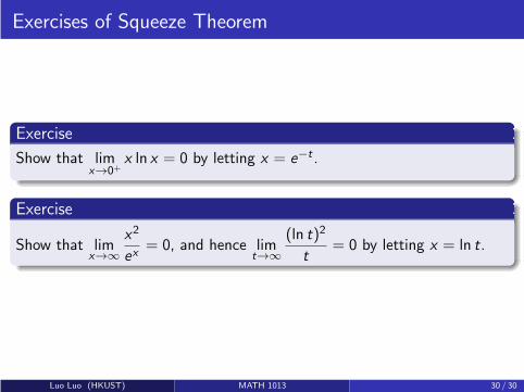
Exercises of Squeeze Theorem
Exercise
Show that limx→0+
x ln x = 0 by letting x = e−t .
Exercise
Show that limx→∞
x2
ex= 0, and hence lim
t→∞
(ln t)2
t= 0 by letting x = ln t.
Luo Luo (HKUST) MATH 1013 30 / 30

Calculus IB: Lecture 08
Luo Luo
Department of Mathematics, HKUST
http://luoluo.people.ust.hk/
Luo Luo (HKUST) MATH 1013 1 / 30
Outline
1 Continuity of Functions
2 Intermediate Value Theorem
3 Derivatives of Basic Functions
4 Non-Differentiability
Luo Luo (HKUST) MATH 1013 2 / 30

Outline
1 Continuity of Functions
2 Intermediate Value Theorem
3 Derivatives of Basic Functions
4 Non-Differentiability
Luo Luo (HKUST) MATH 1013 3 / 30

Continuity of Functions
We have seen that even when f (c), limx→c−
f (x) and limx→c+
f (x) all exist, it is
still possible that they are not equal.
When they are all well-defined and equal on real numbers (we do notconsider ∞ or −∞), we say that the function is continuous at x = c .
Roughly speaking, this is a mathematical way to say that no “suddenjump” on the graph will occur when passing through x = c .
2 4 6−2−4−6
2
4
6
−2
−4
−6
Luo Luo (HKUST) MATH 1013 3 / 30
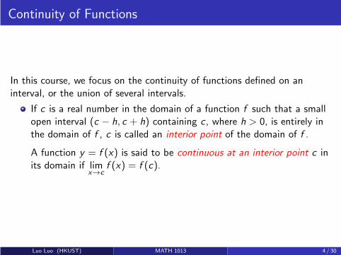
Continuity of Functions
In this course, we focus on the continuity of functions defined on aninterval, or the union of several intervals.
If c is a real number in the domain of a function f such that a smallopen interval (c − h, c + h) containing c , where h > 0, is entirely inthe domain of f , c is called an interior point of the domain of f .
A function y = f (x) is said to be continuous at an interior point c inits domain if lim
x→cf (x) = f (c).
Luo Luo (HKUST) MATH 1013 4 / 30
Continuity of Functions
If a is a number in the domain of of f which is not an interior point,then the continuity condition lim
x→af (x) = f (a) should be understood
as f (x) is getting closer and closer to f (a) as x in the domain of f isgetting closer to closer to a.
In particular, x → a should be understood as x → a+ is a is a “leftendpoint” of the domain. Similarly, x → a should be understood asx → b− if b is a “right endpoint” of the domain.
Luo Luo (HKUST) MATH 1013 5 / 30
Continuity of Functions
Sometimes, d is called a point of discontinuity of a function f if thecondition
limx→a
f (x) = f (d)
is not satisfied, i.e., either
f (d) is not well-defined;
or or the limit does not exist at all;
or f (d) is well-defined but not equal to the well-defined limitlimx→a
f (x).
According to this definition, every point not in the domain of f couldbe considered as a point of discontinuity of the function, which issometime confusing.
Luo Luo (HKUST) MATH 1013 6 / 30

Continuity of Functions
Example
It is easy to see where the functions are continuous/discontinuous:
1 3 5 2 -2 24
(i) (ii) (iii)
(i) Point of discontinuity: x = 1, 3, or 6. (Continuous at every point in thedomain except x = 1, 3.)
(ii) Point of discontinuity: x = 1, 2, 3, or 4. (Continuous at every point inthe domain except x = 1, 2, 3.)
(iii) Continuous at every point in the domain of the function.
(checking across which point the graph breaks into “separate pieces”).
Luo Luo (HKUST) MATH 1013 7 / 30
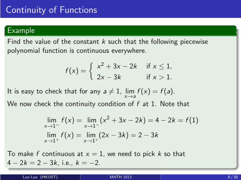
Continuity of Functions
Example
Find the value of the constant k such that the following piecewisepolynomial function is continuous everywhere.
f (x) =
{
x2 + 3x − 2k if x ≤ 1,
2x − 3k if x > 1.
It is easy to check that for any a 6= 1, limx→a
f (x) = f (a).
We now check the continuity condition of f at 1. Note that
limx→1−
f (x) = limx→1−
(x2 + 3x − 2k) = 4− 2k = f (1)
limx→1+
f (x) = limx→1+
(2x − 3k) = 2− 3k
To make f continuous at x = 1, we need to pick k so that4− 2k = 2− 3k , i.e., k = −2.
Luo Luo (HKUST) MATH 1013 8 / 30

Continuity of Functions
Example
Find the value of the constant k such that the following piecewisepolynomial function is continuous everywhere.
f (x) =
{
x2 + 3x − 2k if x ≤ 1,
2x − 3k if x > 1.
It is easy to check that for any a 6= 1, limx→a
f (x) = f (a).
We now check the continuity condition of f at 1. Note that
limx→1−
f (x) = limx→1−
(x2 + 3x − 2k) = 4− 2k = f (1)
limx→1+
f (x) = limx→1+
(2x − 3k) = 2− 3k
To make f continuous at x = 1, we need to pick k so that4− 2k = 2− 3k , i.e., k = −2.
Luo Luo (HKUST) MATH 1013 9 / 30

Properties of Continuous Functions
Sums, differences, products of continuous functions are continuous.
In particular, polynomial functions are continuous on the entire realline. Recall here that a polynomial function of degree n is a functionof the form
f (x) = axn + an−1xn−1 + · · ·+ a1x + a0
where a0, a1, . . . , an are real numbers, and n is a non-negative integer.
Luo Luo (HKUST) MATH 1013 10 / 30
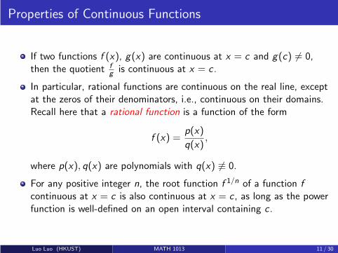
Properties of Continuous Functions
If two functions f (x), g(x) are continuous at x = c and g(c) 6= 0,then the quotient f
gis continuous at x = c .
In particular, rational functions are continuous on the real line, exceptat the zeros of their denominators, i.e., continuous on their domains.Recall here that a rational function is a function of the form
f (x) =p(x)
q(x),
where p(x), q(x) are polynomials with q(x) 6≡ 0.
For any positive integer n, the root function f 1/n of a function f
continuous at x = c is also continuous at x = c , as long as the powerfunction is well-defined on an open interval containing c .
Luo Luo (HKUST) MATH 1013 11 / 30

Properties of Continuous Functions
These properties are straightforward consequences of the limit laws.
For example, if f and g are continuous at a, then
limx→a
f (x) = f (a), limx→a
g(x) = g(a)
and hence
limx→a
(f + g)(x)
= limx→a
(f (x) + g(x))
= limx→a
f (x) + limx→a
g(x)
=f (a) + g(a) = (f + g)(a)
i.e., the function f + g is also continuous at a.
Luo Luo (HKUST) MATH 1013 12 / 30
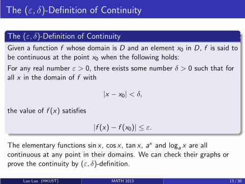
The (ε, δ)-Definition of Continuity
The (ε, δ)-Definition of Continuity
Given a function f whose domain is D and an element x0 in D, f is said tobe continuous at the point x0 when the following holds:
For any real number ε > 0, there exists some number δ > 0 such that forall x in the domain of f with
|x − x0| < δ,
the value of f (x) satisfies
|f (x)− f (x0)| ≤ ε.
The elementary functions sin x , cos x , tan x , ax and loga x are allcontinuous at any point in their domains. We can check their graphs orprove the continuity by (ε, δ)-definition.
Luo Luo (HKUST) MATH 1013 13 / 30
Properties of Continuous Functions
Note also that if f is continuous at c and g is continuous at f (c),then the composition of the two functions g ◦ f is continuous at c .
In fact, as x → c , f (x) → f (c) by the continuity of f at c , and henceg(f (x)) → g(f (c)) by the continuity of g at f (c).
Exercise
By drawing graphs, find some examples of f and g so that g ◦ f iscontinuous at c , while
g is not continuous at f (c);
or f is not continuous at c .
Luo Luo (HKUST) MATH 1013 14 / 30
Outline
1 Continuity of Functions
2 Intermediate Value Theorem
3 Derivatives of Basic Functions
4 Non-Differentiability
Luo Luo (HKUST) MATH 1013 15 / 30

Intermediate Value Theorem
Theorem (Intermediate Value Theorem)
Suppose the function y = f (x) is continuous on a closed interval [a, b] andlet w be a real number between f (a) and f (b), where f (a) 6= f (b). Thenthere must be a number c in (a, b) such that f (c) = w.
y
x
a b
w
c
f(a)
f(b)
In other words, the equation f (x) = w must have at least one root in theinterval (a, b). The Intermediate Value Theorem is very useful in locatingroots of equations.
Luo Luo (HKUST) MATH 1013 15 / 30
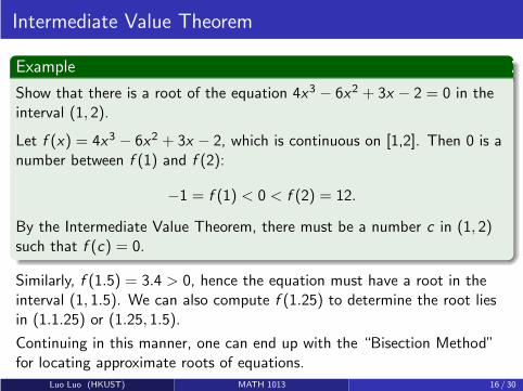
Intermediate Value Theorem
Example
Show that there is a root of the equation 4x3 − 6x2 + 3x − 2 = 0 in theinterval (1, 2).
Let f (x) = 4x3 − 6x2 + 3x − 2, which is continuous on [1,2]. Then 0 is anumber between f (1) and f (2):
−1 = f (1) < 0 < f (2) = 12.
By the Intermediate Value Theorem, there must be a number c in (1, 2)such that f (c) = 0.
Similarly, f (1.5) = 3.4 > 0, hence the equation must have a root in theinterval (1, 1.5). We can also compute f (1.25) to determine the root liesin (1.1.25) or (1.25, 1.5).
Continuing in this manner, one can end up with the “Bisection Method”for locating approximate roots of equations.
Luo Luo (HKUST) MATH 1013 16 / 30

Intermediate Value Theorem
By the Intermediate Value Theorem, the problem of solving an inequalityof the form f (x) < 0 for any continuous function f is essentially the sameas solving f (x) = 0.
Once the zeros or undefined point of f (x) are all located, it is just amatter of sign checking for f (x) in various intervals in order to solve theinequality f (x) < 0 or f (x) > 0.
Luo Luo (HKUST) MATH 1013 17 / 30

Intermediate Value Theorem
For example, the roots and undefined points of
(x + 3)(2x − 5)
x + 2= 0
are x = −3, 52 and −2 respectively, which divide the real line into fourdisjoint open intervals:
(−∞,−3), (−3,−2),
(
−2,5
2
)
,
(
5
2,∞
)
.
Note that (x+3)(2x−5)x+2 cannot change sign in each of these intervals, since
no other root is possible. By putting in some x values in these intervals, itis easy to see that
f (x)
< 0 if x < −3 or − 2 < x <5
2
> 0 if − 3 < x < −2 or x >5
2
Luo Luo (HKUST) MATH 1013 18 / 30
Outline
1 Continuity of Functions
2 Intermediate Value Theorem
3 Derivatives of Basic Functions
4 Non-Differentiability
Luo Luo (HKUST) MATH 1013 19 / 30
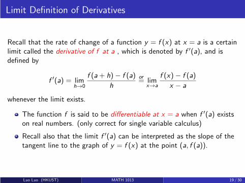
Limit Definition of Derivatives
Recall that the rate of change of a function y = f (x) at x = a is a certainlimit called the derivative of f at a , which is denoted by f ′(a), and isdefined by
f ′(a) = limh→0
f (a+ h)− f (a)
h
or= lim
x→a
f (x)− f (a)
x − a
whenever the limit exists.
The function f is said to be differentiable at x = a when f ′(a) existson real numbers. (only correct for single variable calculus)
Recall also that the limit f ′(a) can be interpreted as the slope of thetangent line to the graph of y = f (x) at the point (a, f (a)).
Luo Luo (HKUST) MATH 1013 19 / 30

Limit Definition of Derivatives
If we want to measure how fast the function value y = f (x) changes as xvaries, we consider the derivative function f ′(x), which is defined asfollows:
f ′(x) = limh→0
f (x + h)− f (x)
h
whenever the limit exists. Geometrically speaking, f ′ is the slope functionof f .
(x,f(x))
(x+h,f(x+h))
f(x+h)-f(x)
h
y
x
y=f(x)
tangent line
secant line
Slope of secant line will approach the
slope of the tangent line as h approaches 0.
Luo Luo (HKUST) MATH 1013 20 / 30

Limit Definition of Derivatives
Some other often used notations to denote the derivative f ′(x) of thefunction y = f (x) are as follows:
df
dx,
dy
dx, y ′, and
df
dx
∣
∣
∣
∣
x=a
=dy
dx
∣
∣
∣
∣
x=a
= y ′(a) = f ′(a).
The process of finding the derivative of a given function is calleddifferentiation.
When computing derivatives by using the limit definition of derivative, it issometimes called differentiating by the first principle.
Luo Luo (HKUST) MATH 1013 21 / 30
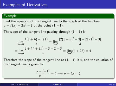
Examples of Derivatives
Example
Find the equation of the tangent line to the graph of the functiony = f (x) = 2x2 − 3 at the point (1,−1).
The slope of the tangent line passing through (1,−1) is
limh→0
f (1 + h)− f (1)
h= lim
h→0
[2(1 + h)2 − 3]− [2 · 12 − 3]
h
= limh→0
2 + 4h + 2h2 − 3− 2 + 3
h= lim
h→0(4 + 2h) = 4
Therefore the slope of the tangent line at (1,−1) is 4, and the equation ofthe tangent line is given by
y − (−1)
x − 1= 4 =⇒ y = 4x − 5
Luo Luo (HKUST) MATH 1013 22 / 30
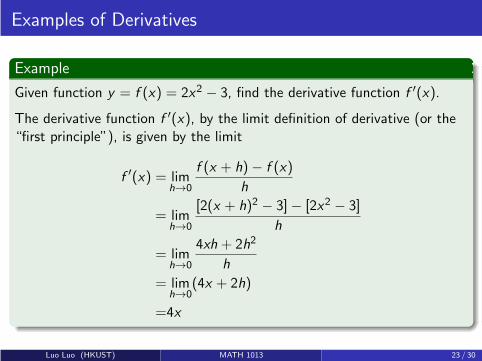
Examples of Derivatives
Example
Given function y = f (x) = 2x2 − 3, find the derivative function f ′(x).
The derivative function f ′(x), by the limit definition of derivative (or the“first principle”), is given by the limit
f ′(x) = limh→0
f (x + h)− f (x)
h
= limh→0
[2(x + h)2 − 3]− [2x2 − 3]
h
= limh→0
4xh + 2h2
h
= limh→0
(4x + 2h)
=4x
Luo Luo (HKUST) MATH 1013 23 / 30
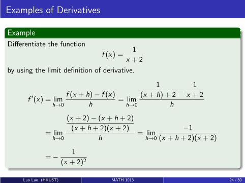
Examples of Derivatives
Example
Differentiate the function
f (x) =1
x + 2
by using the limit definition of derivative.
f ′(x) = limh→0
f (x + h)− f (x)
h= lim
h→0
1
(x + h) + 2− 1
x + 2
h
= limh→0
(x + 2)− (x + h + 2)
(x + h + 2)(x + 2)
h= lim
h→0
−1
(x + h + 2)(x + 2)
=− 1
(x + 2)2
Luo Luo (HKUST) MATH 1013 24 / 30
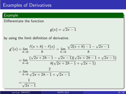
Examples of Derivatives
Example
Differentiate the function
g(x) =√2x − 1
by using the limit definition of derivative.
g ′(x) = limh→0
f (x + h)− f (x)
h= lim
h→0
√
2(x + h)− 1−√2x − 1
h
= limh→0
(√2x + 2h − 1−
√2x − 1)(
√2x + 2h − 1 +
√2x − 1)
h(√2x + 2h − 1 +
√2x − 1)
= limh→0
2√2x + 2h − 1 +
√2x − 1
=1√
2x − 1
Luo Luo (HKUST) MATH 1013 25 / 30

Differentiable and Continuous
Theorem
If f is differentiable at a point x = a, then f is continuous at x = a.
Proof.
We have
limx→a
f (x)− f (a) = limx→a
(f (x)− f (a))
= limx→a
[
f (x)− f (a)
x − a· (x − a)
]
= limx→a
f (x)− f (a)
x − a· limx→a
(x − a)
=f ′(a) · 0 = 0
That is, limx→a
f (x) = f (a) and hence the function is continuous at a.
Luo Luo (HKUST) MATH 1013 26 / 30

Outline
1 Continuity of Functions
2 Intermediate Value Theorem
3 Derivatives of Basic Functions
4 Non-Differentiability
Luo Luo (HKUST) MATH 1013 27 / 30
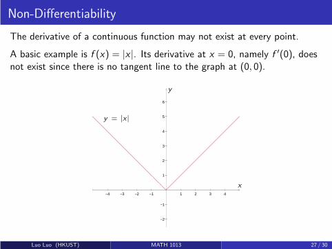
Non-Differentiability
The derivative of a continuous function may not exist at every point.
A basic example is f (x) = |x |. Its derivative at x = 0, namely f ′(0), doesnot exist since there is no tangent line to the graph at (0, 0).
−4 −3 −2 −1 1 2 3 4
−2
−1
1
2
3
4
5
6
y = |x |
x
y
Luo Luo (HKUST) MATH 1013 27 / 30
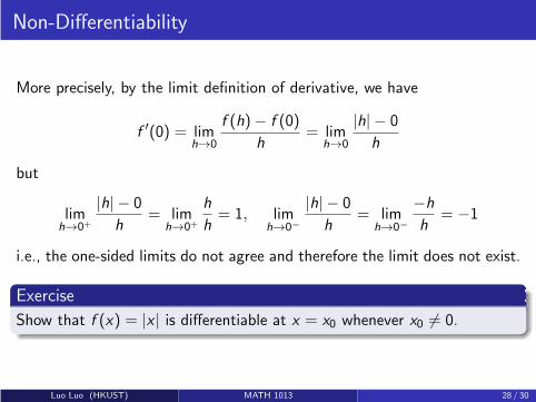
Non-Differentiability
More precisely, by the limit definition of derivative, we have
f ′(0) = limh→0
f (h)− f (0)
h= lim
h→0
|h| − 0
h
but
limh→0+
|h| − 0
h= lim
h→0+
h
h= 1, lim
h→0−
|h| − 0
h= lim
h→0−
−h
h= −1
i.e., the one-sided limits do not agree and therefore the limit does not exist.
Exercise
Show that f (x) = |x | is differentiable at x = x0 whenever x0 6= 0.
Luo Luo (HKUST) MATH 1013 28 / 30
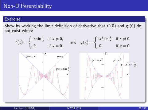
Non-Differentiability
Exercise
Show by working the limit definition of derivative that f ′(0) and g ′(0) donot exist where
f (x) =
{
x sin 1x
if x 6= 0,
0 if x = 0.and g(x) =
{
x2 sin 1x
if x 6= 0,
0 if x = 0.
−0.2 0.2
−0.2
0.2
y=x sin 1x
y=−x y=x
x
y
−0.10 −0.05 0.05 0.10
−0.005
0.005 y=x2 sin 1x
y=−x2 y=x2
x
y
Luo Luo (HKUST) MATH 1013 29 / 30

Weierstrass Function
The Weierstrass function is an example of a real-valued function that iscontinuous everywhere but differentiable nowhere.
In Weierstrass’s original paper, the function was defined as follows:
f (x) =∞∑
n=0
an cos(bnπx),
where 0 < a < 1, b is a positive odd integer and ab > 1 + 32π.
-3 -2 -1 0 1 2 3
-3
-2
-1
0
1
2
3 a=0.7, b=9
-2 -1.5 -1 -0.5 0 0.5 1 1.5 2-2
-1.5
-1
-0.5
0
0.5
1
1.5
2
a=0.4, b=15
Luo Luo (HKUST) MATH 1013 30 / 30

Calculus IB: Lecture 09
Luo Luo
Department of Mathematics, HKUST
http://luoluo.people.ust.hk/
Luo Luo (HKUST) MATH 1013 1 / 25

Outline
1 Basic Formulas of Derivatives
2 Rules of Differentiation
3 The Chain Rule
Luo Luo (HKUST) MATH 1013 2 / 25

Outline
1 Basic Formulas of Derivatives
2 Rules of Differentiation
3 The Chain Rule
Luo Luo (HKUST) MATH 1013 3 / 25
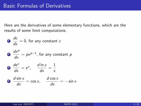
Basic Formulas of Derivatives
Here are the derivatives of some elementary functions, which are theresults of some limit computations.
1dc
dx= 0, for any constant c
2dxp
dx= pxp−1, for any constant p
3dex
dx= ex ,
d ln x
dx=
1
x
4d sin x
dx= cos x ,
d cos x
dx= − sin x
Luo Luo (HKUST) MATH 1013 3 / 25

Basic Formulas of Derivatives: dxp
dx = pxp−1
In the case of p is a non-negative integer, we have
dxp
dx= lim
h→0
(x + h)p − xp
h
= limh→0
[(x + h)− x ][(x + h)p−1 + (x + h)n−2x + · · ·+ xp−1
]h
= limh→0
h[(x + h)p−1 + (x + h)n−2x + · · ·+ xp−1
]h
= limh→0
[(x + h)p−1 + (x + h)n−2x + · · ·+ xp−1
]= lim
h→0
[xp−1 + xp−2x + · · ·+ xp−1︸ ︷︷ ︸
p terms
]=pxp−1
What about p is not a non-negative integer?
Luo Luo (HKUST) MATH 1013 4 / 25
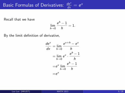
Basic Formulas of Derivatives: dex
dx = ex
Recall that we have
limh→0
eh − 1
h= 1.
By the limit definition of derivative,
dex
dx= lim
h→0
ex+h − ex
h
= limh→0
ex · eh − 1
h
=ex limh→0
eh − 1
h
=ex
Luo Luo (HKUST) MATH 1013 5 / 25

Basic Formulas of Derivatives: d ln xdx = 1
x
Recall that we haveln x = loge x
ande = lim
h→0(1 + h)
1h .
Using the definition of derivative, we have
d ln x
dx= lim
h→0
ln(x + h)− ln x
h
= limh→0
1
hln
(x + h
x
)= lim
h→0ln
(1 +
h
x
) 1h
.
Luo Luo (HKUST) MATH 1013 6 / 25

Basic Formulas of Derivatives: d ln xdx = 1
x
Let y =h
xand h→ 0 means y → 0, then
limh→0
ln
(1 +
h
x
) 1h
= limy→0
ln (1 + y)1xy
= limy→0
ln[(1 + y)
1y
] 1x
= limy→0
1
xln (1 + y)
1y
=1
xlimy→0
ln (1 + y)1y
=1
xln
(limy→0
(1 + y)1y
)
Luo Luo (HKUST) MATH 1013 7 / 25

Basic Formulas of Derivatives: d ln xdx = 1
x
The last step is based on the following theorem.
Theorem
Suppose function f satisfies limy→x0
f (y) = u0 and function g is continuous
at u0, then the composition function (g ◦ f )(y) = g(f (y)) holds that
limy→y0
(g ◦ f )(y) = limu→u0
g(u) = g(u0).
Let g(u) = ln u and f (y) = (1 + y)1y , we have
limy→0
ln (1 + y)1y = ln
(limy→0
(1 + y)1y
)= ln e = 1,
since g(u) = ln u is continuous on its domain. Hence, we haved ln x
dx=
1
x.
Luo Luo (HKUST) MATH 1013 8 / 25
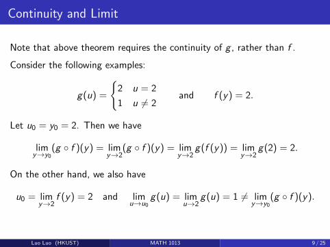
Continuity and Limit
Note that above theorem requires the continuity of g , rather than f .
Consider the following examples:
g(u) =
{2 u = 2
1 u 6= 2and f (y) = 2.
Let u0 = y0 = 2. Then we have
limy→y0
(g ◦ f )(y) = limy→2
(g ◦ f )(y) = limy→2
g(f (y)) = limy→2
g(2) = 2.
On the other hand, we also have
u0 = limy→2
f (y) = 2 and limu→u0
g(u) = limu→2
g(u) = 1 6= limy→y0
(g ◦ f )(y).
Luo Luo (HKUST) MATH 1013 9 / 25

Outline
1 Basic Formulas of Derivatives
2 Rules of Differentiation
3 The Chain Rule
Luo Luo (HKUST) MATH 1013 10 / 25
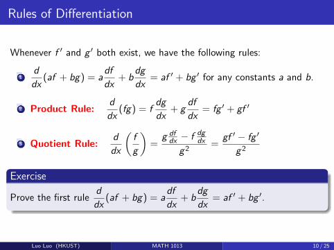
Rules of Differentiation
Whenever f ′ and g ′ both exist, we have the following rules:
1d
dx(af + bg) = a
df
dx+ b
dg
dx= af ′ + bg ′ for any constants a and b.
2 Product Rule:d
dx(fg) = f
dg
dx+ g
df
dx= fg ′ + gf ′
3 Quotient Rule:d
dx
(f
g
)=
g dfdx − f dg
dx
g2=
gf ′ − fg ′
g2
Exercise
Prove the first ruled
dx(af + bg) = a
df
dx+ b
dg
dx= af ′ + bg ′.
Luo Luo (HKUST) MATH 1013 10 / 25

The Proof of Product Rule
We prove this rule by the limit definition of derivative:
(fg)′(x)
= limh→0
f (x + h)g(x + h)− f (x)g(x)
h
= limh→0
(f (x + h)g(x + h)− f (x + h)g(x)) + (f (x + h)g(x)− f (x)g(x))
h
= limh→0
f (x + h)(g(x + h)− g(x))
h+ lim
h→0
g(x)(f (x + h)− f (x))
h
= limh→0
f (x + h) · limh→0
g(x + h)− g(x)
h+ g(x) · lim
h→0
f (x + h)− f (x)
h
=f (x)g ′(x) + g(x)f ′(x)
where we use limh→0
f (x + h) = f (x) since a function is continuous at any
point where f ′ exists.
Luo Luo (HKUST) MATH 1013 11 / 25
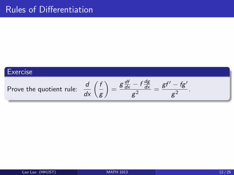
Rules of Differentiation
Exercise
Prove the quotient rule:d
dx
(f
g
)=
g dfdx − f dg
dx
g2=
gf ′ − fg ′
g2.
Luo Luo (HKUST) MATH 1013 12 / 25
Outline
1 Basic Formulas of Derivatives
2 Rules of Differentiation
3 The Chain Rule
Luo Luo (HKUST) MATH 1013 13 / 25

The Chain Rule
Let F is compositions of two functions f and g :
F (x) = (f ◦ g)(x) = f (g(x)),
such that
1 g is a differentiable at x (the derivative g ′(x) exists),
2 and f is a is differentiable at g(x) (the derivative f ′(g(x)) exists);
then y = F (x) = (f ◦ g)(x) is differentiable at x , and its derivative is
F ′(x) = f ′(g(x)) · g ′(x).
Luo Luo (HKUST) MATH 1013 13 / 25

The Proof of Chain Rule
There is one idea for the proof
F ′(x) = limh→0
f (g(x + h))− f (g(x))
h
= limh→0
[f (g(x + h))− f (g(x))
g(x + h)− g(x)· g(x + h)− g(x)
h
]
= limh→0
f (g(x + h))− f (g(x))
g(x + h)− g(x)︸ ︷︷ ︸slope of f at g(x)
· limh→0
g(x + h)− g(x)
h︸ ︷︷ ︸slope of g(x) at x
=f ′(g(x)) · g ′(x) How to proof this equality?
The remain is to show that
limh→0
f (g(x + h))− f (g(x))
g(x + h)− g(x)= f ′(g(x)).
Luo Luo (HKUST) MATH 1013 14 / 25

The Proof of Chain Rule
Recall the (ε, δ)-definition of limit.
Definition
The expression limh→0
w(x) = L means for every ε > 0 there exists δ > 0
such that |w(h)− L| < ε whenever 0 < |h| < δ.
We must find δ > 0 such that w(h) is well defined whenever
0 < |h| < δ.
However, the function
w(h) =f (g(x + h))− f (g(x))
g(x + h)− g(x)
is not well defined when g(x + h)− g(x) = 0.
Luo Luo (HKUST) MATH 1013 15 / 25

The Proof of Chain Rule
For constant function such that g(x) = a, it is obviously
w(h) =f (g(x + h))− f (g(x))
g(x + h)− g(x)
is undefined.
In such case, we have
F (x) = f (g(x)) = f (a),
which is also a constant function, so that F ′(x) = 0.
If g(x) is any differentiable but not constant function, is it true that wecan always find a constant δ > 0 such that w(h) is well defined wheneverh in (−δ, 0) ∪ (0, δ) (that is 0 < |h| < δ)?
Luo Luo (HKUST) MATH 1013 16 / 25
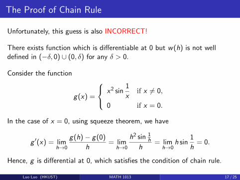
The Proof of Chain Rule
Unfortunately, this guess is also INCORRECT!
There exists function which is differentiable at 0 but w(h) is not welldefined in (−δ, 0) ∪ (0, δ) for any δ > 0.
Consider the function
g(x) =
x2 sin1
xif x 6= 0,
0 if x = 0.
In the case of x = 0, using squeeze theorem, we have
g ′(x) = limh→0
g(h)− g(0)
h= lim
h→0
h2 sin 1h
h= lim
h→0h sin
1
h= 0.
Hence, g is differential at 0, which satisfies the condition of chain rule.
Luo Luo (HKUST) MATH 1013 17 / 25
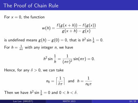
The Proof of Chain Rule
For x = 0, the function
w(h) =f (g(x + h))− f (g(x))
g(x + h)− g(x)
is undefined means g(h)− g(0) = 0, that is h2 sin 1h = 0.
For h = 1nπ with any integer n, we have
h2 sin1
h=
1
(nπ)2sin(nπ) = 0.
Hence, for any δ > 0, we can take
n0 =⌈ 1
δπ
⌉and h =
1
n0π
Then we have h2 sin 1h = 0 and 0 < h < δ.
Luo Luo (HKUST) MATH 1013 18 / 25

The Proof of Chain Rule
The idea on Page 18 does NOT work!
F ′(x) = limh→0
f (g(x + h))− f (g(x))
h
= limh→0
[f (g(x + h))− f (g(x))
g(x + h)− g(x)· g(x + h)− g(x)
h
]
= limh→0
f (g(x + h))− f (g(x))
g(x + h)− g(x)︸ ︷︷ ︸This term may be undefined!
· limh→0
g(x + h)− g(x)
h︸ ︷︷ ︸slope of g(x) at x
=f ′(g(x)) · g ′(x) This step is WRONG!!!
Luo Luo (HKUST) MATH 1013 19 / 25
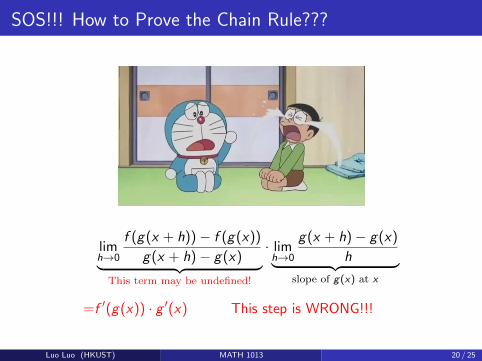
SOS!!! How to Prove the Chain Rule???
limh→0
f (g(x + h))− f (g(x))
g(x + h)− g(x)︸ ︷︷ ︸This term may be undefined!
· limh→0
g(x + h)− g(x)
h︸ ︷︷ ︸slope of g(x) at x
=f ′(g(x)) · g ′(x) This step is WRONG!!!
Luo Luo (HKUST) MATH 1013 20 / 25

SOS!!! How to Prove the Chain Rule??????
We can replace the term
limh→0
f (g(x + h))− f (g(x))
g(x + h)− g(x)
by something which is well-defined!
Luo Luo (HKUST) MATH 1013 21 / 25
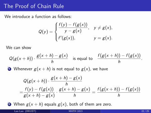
The Proof of Chain Rule
We introduce a function as follows:
Q(y) =
f (y)− f (g(x))
y − g(x), y 6= g(x),
f ′(g(x)), y = g(x).
We can show
Q(g(x + h)) · g(x + h)− g(x)
his equal to
f (g(x + h))− f (g(x))
h.
1 Whenever g(x + h) is not equal to g(x), we have
Q(g(x + h)) · g(x + h)− g(x)
h
=f (y)− f (g(x))
g(x + h)− g(x)· g(x + h)− g(x)
h=
f (g(x + h))− f (g(x))
h
2 When g(x + h) equals g(x), both of them are zero.
Luo Luo (HKUST) MATH 1013 22 / 25

The Proof of Chain Rule
We have
F ′(x) = limh→0
f (g(x + h))− f (g(x))
h
= limh→0
(Q(g(x + h)) · g(x + h)− g(x)
h
)
= limh→0
Q(g(x + h)) · limh→0
g(x + h)− g(x)
h︸ ︷︷ ︸g ′(x)
Since both g and Q are continuous, we have
limh→0
Q(g(x + h)) = Q
(limh→0
g(x + h)
)= Q (g(x)) = f ′(g(x)).
Luo Luo (HKUST) MATH 1013 23 / 25
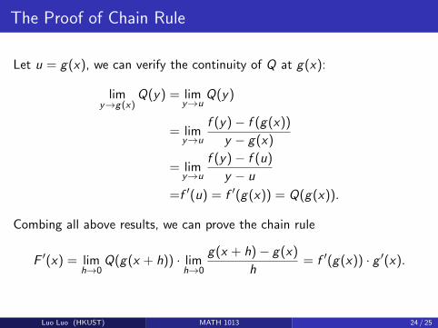
The Proof of Chain Rule
Let u = g(x), we can verify the continuity of Q at g(x):
limy→g(x)
Q(y) = limy→u
Q(y)
= limy→u
f (y)− f (g(x))
y − g(x)
= limy→u
f (y)− f (u)
y − u
=f ′(u) = f ′(g(x)) = Q(g(x)).
Combing all above results, we can prove the chain rule
F ′(x) = limh→0
Q(g(x + h)) · limh→0
g(x + h)− g(x)
h= f ′(g(x)) · g ′(x).
Luo Luo (HKUST) MATH 1013 24 / 25

Examples of Chain Rule
Now, we can showdxp
dx= pxp−1 for any constant exponent p.
Proof.
The definition of ln means xp = e ln xp
= ep ln x , then
dxp
dx=d(ep ln x
)dx
=deu
du· d (p ln x)
dxChain rule with f (u) = eu and g(x) = p ln x
=eu · p · d ln x
dxUsing
deu
du= eu and
d ln x
x=
1
x
=xp · p · 1
xUsing
d ln x
x=
1
x
=pxp−1
Luo Luo (HKUST) MATH 1013 25 / 25

Calculus IB: Lecture 10
Luo Luo
Department of Mathematics, HKUST
http://luoluo.people.ust.hk/
Luo Luo (HKUST) MATH 1013 1 / 28

Outline
1 Derivatives of Trigonometric Functions
2 Derivatives of Inverse Functions
3 Implicit Differentiation
Luo Luo (HKUST) MATH 1013 2 / 28
Outline
1 Derivatives of Trigonometric Functions
2 Derivatives of Inverse Functions
3 Implicit Differentiation
Luo Luo (HKUST) MATH 1013 3 / 28
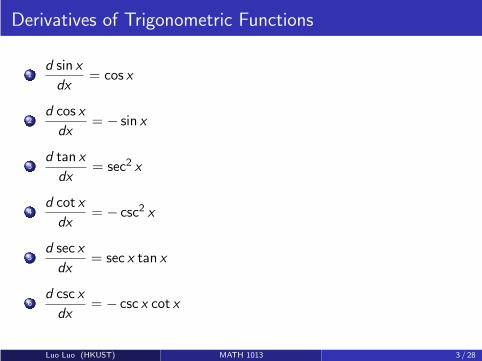
Derivatives of Trigonometric Functions
1d sin x
dx= cos x
2d cos x
dx= − sin x
3d tan x
dx= sec2 x
4d cot x
dx= − csc2 x
5d sec x
dx= sec x tan x
6d csc x
dx= − csc x cot x
Luo Luo (HKUST) MATH 1013 3 / 28

Derivatives of sin x
Using the identities (Lecture-L04)
sinα− sinβ = 2 cosα+ β
2sin
α− β
2
with α = x + h and β = x , we have
d sin x
dx= lim
h→0
sin(x + h)− sin x
h
= limh→0
2 cos(
x + h2
)
sin(
h2
)
h
= limh→0
cos
(
x +h
2
)
· limh→0
sin(
h2
)
h2
=cos
(
limh→0
(
x +h
2
))
· limt→0
sin t
tlet t =
h
2
= cos x · 1 = cos x .
Luo Luo (HKUST) MATH 1013 4 / 28

Derivatives of cos x
Using the identities (Lecture-L04)
cosα− cosβ = −2 sinα+ β
2sin
α− β
2
with α = x + h and β = x , we have
d cos x
dx= lim
h→0
cos(x + h)− cos x
h
= limh→0
−2 sin(
x + h2
)
sin(
h2
)
h
=− limh→0
sin
(
x +h
2
)
· limh→0
sin(
h2
)
h2
=− sin
(
limh→0
(
x +h
2
))
· limt→0
sin t
tlet t =
h
2
=− sin x · 1 = − sin x .
Luo Luo (HKUST) MATH 1013 5 / 28

Derivatives of tan x
By usingd sin x
dx= cos x ,
d cos x
dx= − sin x and quotient rule we have
d tan x
dx=
d
dx
sin x
cos x
=cos x
d sin x
dx− sin x
d cos x
dxcos2 x
=cos2 x + sin2 x
cos2 x
=1
cos2 x= sec2 x .
Luo Luo (HKUST) MATH 1013 6 / 28
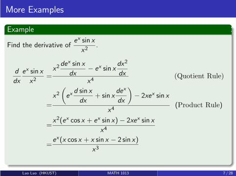
More Examples
Example
Find the derivative ofex sin x
x2.
d
dx
ex sin x
x2=x2
dex sin x
dx− ex sin x
dx2
dxx4
(Quotient Rule)
=
x2(
exd sin x
dx+ sin x
dex
dx
)
− 2xex sin x
x4(Product Rule)
=x2(ex cos x + ex sin x)− 2xex sin x
x4
=ex(x cos x + x sin x − 2 sin x)
x3
Luo Luo (HKUST) MATH 1013 7 / 28

Exercise of Derivatives
Exercise
Show that
1d cot x
dx= − csc2 x ,
2d sec x
dx= sec x tan x ,
3d csc x
dx= − csc x cot x .
Luo Luo (HKUST) MATH 1013 8 / 28

More Examples
Example
Differentiate y = (3x4 − 2x2 + 1)3.
Let u = 3x4 − 2x2 + 1, then y = u3,dy
du= 3u2, and
du
dx= 3 · 4x4−1 − 2 · 2x2−1 + 0 = 12x3 − 4x .
Hence by the chain rule,
dy
dx=dy
du· dudx
=3u2 · (12x3 − 4x)
=3(3x4 − 2x2 + 1)2(12x4 − 4x).
Luo Luo (HKUST) MATH 1013 9 / 28

More Examples
Example
Differentiate y =
(
x
1 + x
)13
.
Let u =x
1 + x, then y = 3
√u = u
13 . We have
dy
du=
1
3u
13−1 =
1
3u−
23 ,
du
dx=
(1 + x) · dxdx
− xd(1+x)
dx
(1 + x)2=
1
(1 + x)2.
By the chain rule, we obtain
dy
dx=
dy
du· dudx
=1
3
(
x
1 + x
)
−23 1
(1 + x)2=
1
3x−
23 (1 + x)−
43
Luo Luo (HKUST) MATH 1013 10 / 28

More Examples
Exercise
Define y = (1 + x2) sin(2x2 + ex2) + esin ln x . Show that
dy
dx=2x sin(2x2 + ex
2) + (1 + x2) cos(2x2 + ex
2)(4x + 2xex
2)
+1
xesin ln x cos ln x .
Luo Luo (HKUST) MATH 1013 11 / 28

Outline
1 Derivatives of Trigonometric Functions
2 Derivatives of Inverse Functions
3 Implicit Differentiation
Luo Luo (HKUST) MATH 1013 12 / 28

Derivatives of Inverse Functions
Theorem (Derivatives of Inverse Function)
Suppose f is a differentiable and has inverse function f −1 over an interval
I and x is a point in I such that x = f (a) and f ′(a) 6= 0, then f −1 is
differentiable at x and its derivative is
(
f −1)′
(x) =1
f ′(a)=
1
f ′(f −1(x)).
Proof.
The definition of inverse function means f (f −1(x)) = x . We can regardf (f −1(x)) as composition of f and f −1 and use chain rule to obtain
(
f ◦ f −1)′
(x) = 1 =⇒ f ′(f −1(x)) ·(
f −1)′
(x) = 1 =⇒(
f −1)′
(x) =1
f ′(f −1(x))
Luo Luo (HKUST) MATH 1013 12 / 28

Derivatives of Inverse Functions
Exercise
By reflection across the line y = x , the tangent line to the graph ofy = f −1(x) at the point (x , f −1(x)) is reflected to the tangent line to thegraph of y = f (x) at (f −1(x), x). Try to explain
(
f −1)′
(x) =1
f ′(f −1(x))
in geometric view.
x x+h
y = f −1(x)
y = f (x)y
Luo Luo (HKUST) MATH 1013 13 / 28

Derivatives of Inverse Functions
Example
Let y = ln x = f −1(x) where f (x) = ex .
Then f ′(x) = ex , and
(f −1)′(x) =1
f ′(f −1(x))=
1
e ln x=
1
x
which meansd ln x
dx=
1
xwe have proved before.
Luo Luo (HKUST) MATH 1013 14 / 28
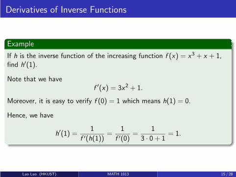
Derivatives of Inverse Functions
Example
If h is the inverse function of the increasing function f (x) = x3 + x + 1,find h′(1).
Note that we havef ′(x) = 3x2 + 1.
Moreover, it is easy to verify f (0) = 1 which means h(1) = 0.
Hence, we have
h′(1) =1
f ′(h(1))=
1
f ′(0)=
1
3 · 0 + 1= 1.
Luo Luo (HKUST) MATH 1013 15 / 28

Derivatives of Inverse Functions
Example
Find the derivative of tan−1 x .
Define f (x) = tan x with domain −π/2 < x < π/2. Then we have
f −1(x) = tan−1 x and f ′(x) = sec2 x .
Hence, we have
(f −1)′(x) =1
f ′(f −1(x))=
1
sec2(tan−1 x)=
1
1 + tan2(tan−1(x))=
1
1 + x2,
where we use the identity (consider that u = tan−1 x)
1
sec2 u=
cos2 u
sin2 u + cos2 u=
1sin2 ucos2 u + 1
=1
tan2 u + 1
In other words, we haved tan−1 x
dx=
1
1 + x2.
Luo Luo (HKUST) MATH 1013 16 / 28
Outline
1 Derivatives of Trigonometric Functions
2 Derivatives of Inverse Functions
3 Implicit Differentiation
Luo Luo (HKUST) MATH 1013 17 / 28

Implicit Differentiation
Sometimes, a function y = f (x) can be defined implicitly by an equationof x and y of the form
F (x , y) = 0.
For example, the unit circle can be defined as
x2 + y2 = 1.
By solving the equation, we obtain two functions
y =√
1− x2 with y ′ =dy
dx= − x√
1− x2
and
y = −√
1− x2 with y ′ =dy
dx=
x√1− x2
.
Luo Luo (HKUST) MATH 1013 17 / 28

The Implicit Function Theorem (beyond the requirement)
Graphically, we can observe x2 + y2 = 1 fails the familiar vertical line test,but it could pass the vertical line test locally.
Most of points on the circle we can choose a small neighborhood whereour curve satisfies the vertical line test (determines y as a function of x).
-1 -0.5 0 0.5 1
-1
-0.5
0
0.5
1
Luo Luo (HKUST) MATH 1013 18 / 28
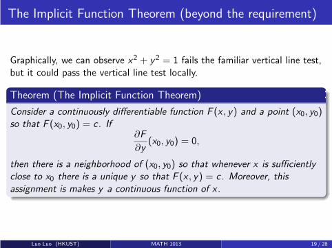
The Implicit Function Theorem (beyond the requirement)
Graphically, we can observe x2 + y2 = 1 fails the familiar vertical line test,but it could pass the vertical line test locally.
Theorem (The Implicit Function Theorem)
Consider a continuously differentiable function F (x , y) and a point (x0, y0)so that F (x0, y0) = c. If
∂F
∂y(x0, y0) = 0,
then there is a neighborhood of (x0, y0) so that whenever x is sufficiently
close to x0 there is a unique y so that F (x , y) = c. Moreover, this
assignment is makes y a continuous function of x.
Luo Luo (HKUST) MATH 1013 19 / 28

Implicit Differentiation
In general, it is difficult or impossible to find the explicit expression ofy = f (x) by F (x , y), but we can express y ′ = f ′(x) by x and y .
We desire to find f ′(x) directly from the implicit form F (x , y) = 0 withoutsolving y = f (x).
Implicit differentiation can be done as follows:
F (x , y) = 0ddx
both sides
−→ an equation to solve fordy
dx
Luo Luo (HKUST) MATH 1013 20 / 28
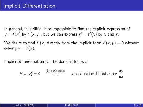
Implicit Differentiation
In general, it is difficult or impossible to find the explicit expression ofy = f (x) by F (x , y), but we can express y ′ = f ′(x) by x and y .
We desire to find f ′(x) directly from the implicit form F (x , y) = 0 withoutsolving y = f (x).
Implicit differentiation can be done as follows:
F (x , y) = 0ddx
both sides
−→ an equation to solve fordy
dx
Luo Luo (HKUST) MATH 1013 21 / 28

Implicit Differentiation
Example
Find the derivative of function y = f (x) from the equation of unit circle.
We take the differentiation on both sides of the equation:
x2 + y2 = 1 =⇒dx2
dx+
dy2
dx=
d1
dx
=⇒2x +dy2
dy· dydx
= 0
=⇒2x + 2y · y ′ = 0
=⇒y ′ = −x
y.
We can obtain a unique expression for the slope of the tangent line of unitcircle at point (x , y) without the expression of y = f (x).
Luo Luo (HKUST) MATH 1013 22 / 28

Implicit Differentiation
Example
Find the derivative of function y = f (x) from equation sin(xy) = x2 + y .
We take the differentiation on both sides of the equation:
sin(xy) = x2 + y =⇒d sin(xy)
dx=
dx2
dx+
dy
dx
=⇒ cos(xy) · dxydx
= 2x +dy
dx
=⇒ cos(xy) ·(
x · dydx
+dx
dx· y
)
= 2x +dy
dx
=⇒y ′ =dy
dx=
y cos(xy)− 2x
1− x cos(xy).
It is impossible to find explicit expression for y = f (x) for this example.
Luo Luo (HKUST) MATH 1013 23 / 28

Implicit Differentiation
Example
Find the derivative of y = 3√2− 2x2.
The function can defined by equation 2x2 + y3 = 2.
Just differentiate both sides as functions of x to get
d2x2
dx+
dy3
dx=
d2
dx=⇒ 4x + 3y2
dy
dx= 0,
Then we havedy
dx= − 4x
3y2= −4
3x(2− 2x2)−
23 .
Luo Luo (HKUST) MATH 1013 24 / 28

Derivative of Inverse Trigonometric Function
Example
Find derivatives of y = sin−1 x .
We have x = sin y with −π2 ≤ y ≤ π
2 and
x = sin y =⇒dx
dx=
d sin y
dx
=⇒1 =d sin y
dy· dydx
=⇒1 = cos y · dydx
Since sin2 y + cos2 y = 1 and cos y ≥ 0 whenever −π2 ≤ y ≤ π
2 , we have
dy
dx=
1
cos y=
1√
1− sin2 y=
1√1− x2
.
Luo Luo (HKUST) MATH 1013 25 / 28

Derivative of Inverse Trigonometric Function
Exercise
Find derivatives of
cos−1 x , cot−1 x , csc−1 x and sec−1 x .
by implicit differentiation.
Luo Luo (HKUST) MATH 1013 26 / 28

Chain Rule Version of Basic Derivative Formulas
The following chain rule versions of basic derivative formulas areconvenient to use for calculation of derivatives.
d�p
dx= p�p−1 · d�
dx
de�
dx= e� · d�
dx
d ln�
dx=
1
�· d�dx
d sin�
dx= cos� · d�
dx
d cos�
dx= − sin� · d�
dx
d tan�
dx= sec2� · d�
dx
d sec�
dx= sec� · tan� · d�
dx
d sin−1�
dx=
1√1−�2
· d�dx
d tan−1�
dx=
1
1 +�2· d�dx
Luo Luo (HKUST) MATH 1013 27 / 28
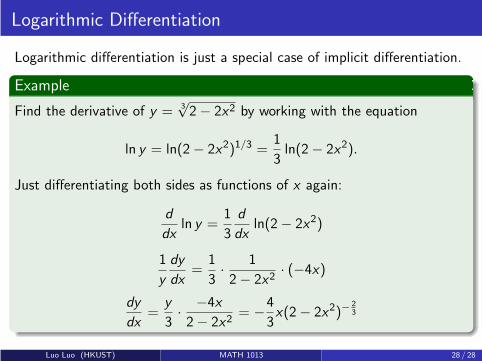
Logarithmic Differentiation
Logarithmic differentiation is just a special case of implicit differentiation.
Example
Find the derivative of y = 3√2− 2x2 by working with the equation
ln y = ln(2− 2x2)1/3 =1
3ln(2− 2x2).
Just differentiating both sides as functions of x again:
d
dxln y =
1
3
d
dxln(2− 2x2)
1
y
dy
dx=
1
3· 1
2− 2x2· (−4x)
dy
dx=
y
3· −4x
2− 2x2= −4
3x(2− 2x2)−
23
Luo Luo (HKUST) MATH 1013 28 / 28

Calculus IB: Lecture 11
Luo Luo
Department of Mathematics, HKUST
http://luoluo.people.ust.hk/
Luo Luo (HKUST) MATH 1013 1 / 18

Outline
1 Rates of Changes
2 Higher Order Derivatives
Luo Luo (HKUST) MATH 1013 2 / 18

Outline
1 Rates of Changes
2 Higher Order Derivatives
Luo Luo (HKUST) MATH 1013 3 / 18
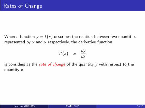
Rates of Change
When a function y = f (x) describes the relation between two quantitiesrepresented by x and y respectively, the derivative function
f ′(x) ordy
dx
is considers as the rate of change of the quantity y with respect to thequantity x .
Luo Luo (HKUST) MATH 1013 3 / 18

Related Rates
The main idea about related rates is essentially the following.
Given some quantities
q1 = q1(t)q2 = q2(t)...qn = qn(t)
which are all functions of t,
where t may represent time or some other quantity,
if there is an equation relating all these quantities, then
d
dtof both sides of the relation
gives−→ an equation relating the rates of changesdq1
dt,dq2
dt, . . . ,
dqn
dt
Luo Luo (HKUST) MATH 1013 4 / 18

Examples of Related Rates
Example (cone container)
Water is flowing into a cone container at a rate of 2m3/min. Suppose theshape of the cone container satisfies
base radius
height=
r
h=
1
2.
How fast is the water level rising (speed of h increasing) when the waterin the container is 3m in depth?
Luo Luo (HKUST) MATH 1013 5 / 18

Example (cone container)
At time t, volume of water with depth h is V =1
3πr2h and r =
h
2.
We also know thatdV
dt= 2m3/min. The question is find
dh
dt
∣
∣
∣
∣
h=3
.
Here the equation relating V and h, both are functions of t, is
V =π
3
(
h
2
)2
h =π
12h3
Taking the derivatives of both sides with respect to t,the chain rule means
dV
dt=
π
4h2 ·
dh
dt
When h = 3m, we have
2 =π
4(3)2 ·
dh
dt
∣
∣
∣
∣
h=3
=⇒dh
dt
∣
∣
∣
∣
h=3
=8
9πm/min
Luo Luo (HKUST) MATH 1013 6 / 18

Examples of Related Rates
Example (ladder and wall)
A ladder of 5m long is leaning again the wall. If the bottom of the ladderis pulled away from the wall at a rate of 1m/min, how fast is the top of theladder dropping when the bottom of the ladder is 3m away from the wall?
x
y
Luo Luo (HKUST) MATH 1013 7 / 18
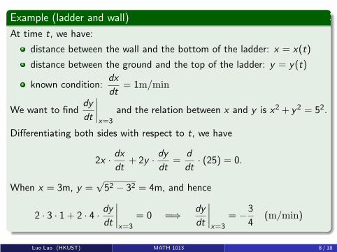
Example (ladder and wall)
At time t, we have:
distance between the wall and the bottom of the ladder: x = x(t)
distance between the ground and the top of the ladder: y = y(t)
known condition:dx
dt= 1m/min
We want to finddy
dt
∣
∣
∣
∣
x=3
and the relation between x and y is x2 + y2 = 52.
Differentiating both sides with respect to t, we have
2x ·dx
dt+ 2y ·
dy
dt=
d
dt· (25) = 0.
When x = 3m, y =√52 − 32 = 4m, and hence
2 · 3 · 1 + 2 · 4 ·dy
dt
∣
∣
∣
∣
x=3
= 0 =⇒dy
dt
∣
∣
∣
∣
x=3
= −3
4(m/min)
Luo Luo (HKUST) MATH 1013 8 / 18

Examples of Related Rates
Example (walking man)
A man starts walking along a straight line at a velocity of 1.5m/s. A light beam6m from the road is tracking the man. How fast is the angle of the beam turningwhen the man is 9m away from the starting point?
x
6m θ
At time t, we have:
distance travelled by the man : x = x(t)
turning angle of the light beam: θ = θ(t)
known condition:dx
dt= 1.5 m/s
We want to finddθ
dt
∣
∣
∣
∣
x=9
.
Luo Luo (HKUST) MATH 1013 9 / 18

Examples of Related Rates
Example (walking man)
The relation between x and θ is: tan θ =x
6.
Differentiating both sides with respect to t, we have
sec2 θ ·dθ
dt=
1
6
dx
dt
When x = 9m, sec θ =√92+62
6 =√1176 m, and hence
117
36·dθ
dt
∣
∣
∣
∣
x=9
=1
6· 1.5 =⇒
dθ
dt
∣
∣
∣
∣
x=9
=9
117(rad/s).
Luo Luo (HKUST) MATH 1013 10 / 18

Examples of Related Rates
Example (travelling along the curve)
A particle is travelling along the graph of the function y = x2 such that thevelocity of the particle in x-direction is 1m/s. How fast is the distance betweenthe particle and the origin increasing when x = 2m?
(x, y)sAt time t, we have:
x coordinate of the particle: x = x(t)
y coordinate of the particle: y = y(t)
distance between the particle and the origin: s = s(t)
known condition:dx
dt= 1 m/s
Luo Luo (HKUST) MATH 1013 11 / 18

Example (travelling along the curve)
We want to findds
dt
∣
∣
∣
∣
x=2
. Relations of the quantities:
{
y = x2
s2 = x2 + y2
d/dt−→
dy
dt= 2x
dx
dt
2sds
dt= 2x
dx
dt+ 2y
dy
dt
When x = 2m, y = 4m, s =√22 + 42 =
√20m and
dy
dt
∣
∣
∣
∣
x=2
= 2 · 2 · 1 = 4
2√20 ·
ds
dt
∣
∣
∣
∣
x=2
= 2 · 2 · 1 + 2 · 4 ·dy
dt
∣
∣
∣
∣
x=2
= 4 + 8 · 4
Henceds
dt
∣
∣
∣
∣
x=2
=18√20
m/s.
Luo Luo (HKUST) MATH 1013 12 / 18
Outline
1 Rates of Changes
2 Higher Order Derivatives
Luo Luo (HKUST) MATH 1013 13 / 18

Second Order Derivative (or Second Derivative)
If s = s(t) is the position function of a particle moving along a linerepresented by the x axis, then
dx
dt= velocity function = v(t)
dv
dt= acceleration function = a(t)
In particular, if m is the mass of the particle, and F is the force acting onthe particle, Newton’s Second Law F = ma can be expressed as
F = mdv
dt= m
d2s
dt2
where the second derivative means “the derivative of the derivative”:
s ′′(t) =d2s
dt2means=
d
dt
(
ds
dt
)
.
Luo Luo (HKUST) MATH 1013 13 / 18

Example
The Hooke’s Law for spring-mass system, which says that the spring forceacting on a mass attached to the spring is proportional to the displacementof the mass from its equilibrium position, can be expressed as
md2s
dt2= −kx
where k is the spring constant, and x is the displacement of the mass fromits equilibrium position (spring is unstretched).
Luo Luo (HKUST) MATH 1013 14 / 18
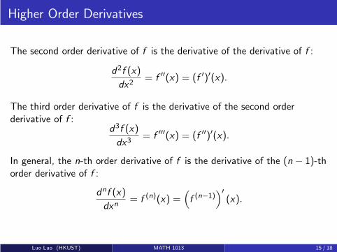
Higher Order Derivatives
The second order derivative of f is the derivative of the derivative of f :
d2f (x)
dx2= f ′′(x) = (f ′)′(x).
The third order derivative of f is the derivative of the second orderderivative of f :
d3f (x)
dx3= f ′′′(x) = (f ′′)′(x).
In general, the n-th order derivative of f is the derivative of the (n − 1)-thorder derivative of f :
dnf (x)
dxn= f (n)(x) =
(
f (n−1))′
(x).
Luo Luo (HKUST) MATH 1013 15 / 18
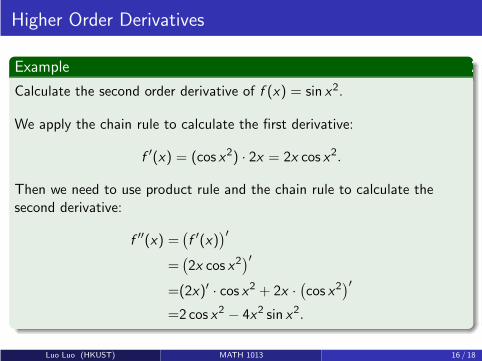
Higher Order Derivatives
Example
Calculate the second order derivative of f (x) = sin x2.
We apply the chain rule to calculate the first derivative:
f ′(x) = (cos x2) · 2x = 2x cos x2.
Then we need to use product rule and the chain rule to calculate thesecond derivative:
f ′′(x) =(
f ′(x))′
=(
2x cos x2)′
=(2x)′ · cos x2 + 2x ·(
cos x2)′
=2 cos x2 − 4x2 sin x2.
Luo Luo (HKUST) MATH 1013 16 / 18

Higher Order Derivatives
Example
For any polynomial Pn(x) of degree n, show that P(k)n (x) = 0 for any
integer k > n.
Sinced
dx(xm)′ = mxm−1, we have
dk
dxk(xm) = 0 if k > m.
Hence, if k > n, we have
dk
dxkPn(x)
=dk
dxk(a0 + a1x + · · ·+ anx
n)
=a0 ·dk
dxk(1) + a1 ·
dk
dxk(x) + · · ·+ an ·
dk
dxk(xn)
=0 + 0 + · · ·+ 0 = 0.
Luo Luo (HKUST) MATH 1013 17 / 18

Higher Order Derivatives
Exercise
For any polynomial Pn(x) of degree n and positive integer k ≤ n, find
P(k)n (x).
Exercise
Let the function y = f (x) defined implicitly by equation x2 + y2 = 1. Useimplicit differentiation to show that
d2y
dx2= −
1
y3.
Luo Luo (HKUST) MATH 1013 18 / 18

Calculus IB: Lecture 12
Luo Luo
Department of Mathematics, HKUST
http://luoluo.people.ust.hk/
Luo Luo (HKUST) MATH 1013 1 / 32

Outline
1 Extreme Values of Functions
2 The Mean Value Theorem
3 Using 1st and 2nd Derivatives in Graphing
Luo Luo (HKUST) MATH 1013 2 / 32

Outline
1 Extreme Values of Functions
2 The Mean Value Theorem
3 Using 1st and 2nd Derivatives in Graphing
Luo Luo (HKUST) MATH 1013 3 / 32
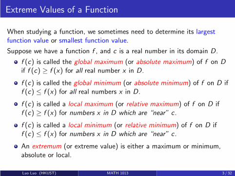
Extreme Values of a Function
When studying a function, we sometimes need to determine its largestfunction value or smallest function value.
Suppose we have a function f , and c is a real number in its domain D.
f (c) is called the global maximum (or absolute maximum) of f on D
if f (c) ≥ f (x) for all real number x in D.
f (c) is called the global minimum (or absolute minimum) of f on D iff (c) ≤ f (x) for all real numbers x in D.
f (c) is called a local maximum (or relative maximum) of f on D iff (c) ≥ f (x) for numbers x in D which are “near” c .
f (c) is called a local minimum (or relative minimum) of f on D iff (c) ≤ f (x) for numbers x in D which are “near” c .
An extremum (or extreme value) is either a maximum or minimum,absolute or local.
Luo Luo (HKUST) MATH 1013 3 / 32

Extreme Values of Functions
Precise definition of local maximum: Suppose we have a function f ,and c is a number in its domain D. f (c) is called a local maximum (orrelative maximum) of f on D if there exists an δ > 0 such we havef (c) ≥ f (x) whenever |x − c | < δ holds for any x in domain D.
Precise definition of local minimum: Suppose we have a function f ,and c is a number in its domain D. f (c) is called a local minimum (orrelative minimum) of f on D if there exists an δ > 0 such we havef (c) ≤ f (x) whenever |x − c | < δ holds for any x in domain D.
Note also that any global maximum (global minimum respectively) isautomatically a local maximum (local minimum respectively).
Luo Luo (HKUST) MATH 1013 4 / 32

Extreme Values of Functions
Here is a simple graph of y = f (x) defined on a closed interval [a, b] toillustrate the usage of these terms above:
x
y
a b
y = f (x)
m
M
c d e
The global maximum is reached at two points, M = f (c) = f (d), and theglobal minimum is reached at one point, m = f (e).
In addition, there are three other local maximum, and four other localminimum.
Luo Luo (HKUST) MATH 1013 5 / 32

Extreme Values of Functions
A function may not have maximum or minimum though. Just look at thegraph below:
x
y
a b
You may run along the graph toget closer and closer to the two“holes” (y -values), but can neverreach those heights as any functionvalue.
This is obviously due to the exis-tence of points of discontinuity.
We are more interested in extreme values of continuous functions.
Luo Luo (HKUST) MATH 1013 6 / 32
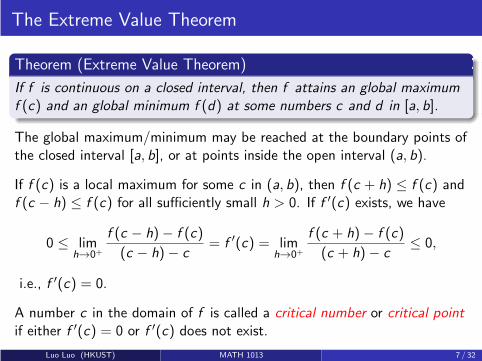
The Extreme Value Theorem
Theorem (Extreme Value Theorem)
If f is continuous on a closed interval, then f attains an global maximum
f (c) and an global minimum f (d) at some numbers c and d in [a, b].
The global maximum/minimum may be reached at the boundary points ofthe closed interval [a, b], or at points inside the open interval (a, b).
If f (c) is a local maximum for some c in (a, b), then f (c + h) ≤ f (c) andf (c − h) ≤ f (c) for all sufficiently small h > 0. If f ′(c) exists, we have
0 ≤ limh→0+
f (c − h)− f (c)
(c − h)− c= f ′(c) = lim
h→0+
f (c + h)− f (c)
(c + h)− c≤ 0,
i.e., f ′(c) = 0.
A number c in the domain of f is called a critical number or critical pointif either f ′(c) = 0 or f ′(c) does not exist.
Luo Luo (HKUST) MATH 1013 7 / 32
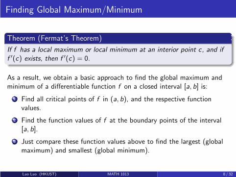
Finding Global Maximum/Minimum
Theorem (Fermat’s Theorem)
If f has a local maximum or local minimum at an interior point c, and if
f ′(c) exists, then f ′(c) = 0.
As a result, we obtain a basic approach to find the global maximum andminimum of a differentiable function f on a closed interval [a, b] is:
1 Find all critical points of f in (a, b), and the respective functionvalues.
2 Find the function values of f at the boundary points of the interval[a, b].
3 Just compare these function values above to find the largest (globalmaximum) and smallest (global minimum).
Luo Luo (HKUST) MATH 1013 8 / 32

Example
Find global maximum/minimum of function f (x) = x3 on interval [−2, 3].
We can verify 0 is unique critical point of f since
f ′(x) = 3x2 = 0 ⇐⇒ x = 0.
A straightforward comparison of function values leads to
f (−2) = −8,
f (0) = 0,
f (3) = 27.
-10
-5
0
5
10
-3 -2 -1 0 1 2 3
x
y
y = x3
Hence f (−2) = −8 global minimum and f (3) = 27 is global maximum,but f (0) = 0 is neither local maximum value nor local minimum value.
Luo Luo (HKUST) MATH 1013 9 / 32

Finding Global Maximum/Minimum
Example
Find the absolute maximum and minimum values of f (x) = 3x(4− ln x)on the interval
[
1, e5]
.
We desire to find the critical point of f by its derivative:
f ′(x) = 3(4− ln x) + 3x(−1
x) = 9− 3 ln x (Product Rule)
f ′(x) = 0 ⇐⇒ ln x = 3 ⇐⇒ x = e3
At the only critical point x = e3: f (e3) = 3e3(4− ln e3) = 3e3.
At the endpoints of the interval [1, e5]:
f (1) = 3(4− ln 1) = 12, f (e5) = 3e5(4− ln e5) = −3e5.
Then, the global maximum is 3e3, and the global minimum is −3e5.
Luo Luo (HKUST) MATH 1013 10 / 32

Example
Find the absolute maximum and minimum values of f (x) = x23 on the
interval [−8, 4].
The derivative of f is
f ′(x) =2
3x
23−1 =
2
3x−
13 =
2
3x−13
,
which can never be 0. 0
1
2
3
4
-8 -6 -4 -2 0 2 4
However, x = 0 is a critical point since f ′(0) does not exist. Hence, thispoint also should be taken into consideration.
Compare function values at the critical point and endpoints:
f (0) = 0, f (−8) = (−8)23 = 4, f (4) = 4
23 =
3√16.
The absolute maximum value is 4, and the absolute minimum value is 0.
Luo Luo (HKUST) MATH 1013 11 / 32

Outline
1 Extreme Values of Functions
2 The Mean Value Theorem
3 Using 1st and 2nd Derivatives in Graphing
Luo Luo (HKUST) MATH 1013 12 / 32

Rolle’s Theorem
Combining the extreme value theorem and Fermat’s theorem, it is easy toconclude Rolle’s theorem.
Theorem (Extreme Value Theorem)
If f is continuous on a closed interval, then f attains an global maximum
f (c) and an global minimum f (d) at some numbers c and d in [a, b].
Theorem (Fermat’s Theorem)
If f has a local maximum or local minimum at an interior point c, and if
f ′(c) exists, then f ′(c) = 0.
Theorem (Rolle’s Theorem)
If f is continuous on the closed interval [a, b] and differentiable on the
open interval (a, b), and f (a) = f (b) and a < b, then f ′(c) = 0 for some
number c ∈ (a, b).
Luo Luo (HKUST) MATH 1013 12 / 32

Rolle’s Theorem
Theorem (Rolle’s Theorem)
If f is continuous on the closed interval [a, b] and differentiable on the
open interval (a, b), f (a) = f (b) and a < b, then f ′(c) = 0 for some
number c ∈ (a, b).
Proof.
The idea is pretty simple: either f (x) = f (a) = f (b) for all x in [a, b], andthus f ′(x) = 0 for all x in (a, b), or a maximum is reached at some c in(a, b) by the extreme value theorem so that f ′(c) = 0 by the Fermat’stheorem.
Luo Luo (HKUST) MATH 1013 13 / 32

Theorem (Mean Value Theorem)
If f is continuous on the closed interval [a, b] and differentiable on the
open interval (a, b), then
f (b)− f (a)
b − a= f ′(c)
for some c ∈ (a, b), or equivalently f (b)− f (a) = f ′(c)(b − a).
a b
y
x
y = f(x)
c
slope of tangent line
slope of secant line
f '(c)
f(b) - f(a)
b - a
Luo Luo (HKUST) MATH 1013 14 / 32

Mean Value Theorem
The proof of mean value theorem is based on the gap between the graphof f and the secant line joining the endpoints of the graph
h(x) = f (x)−[
f (a) +f (b)− f (a)
b − a(x − a)
]
a b
y
x
y = f(x)
c
slope of tangent line
slope of secant line
f '(c)
f(b) - f(a)
b - a
Luo Luo (HKUST) MATH 1013 15 / 32

Mean Value Theorem
The proof of mean value theorem is based on the gap between the graphof f and the secant line joining the endpoints of the graph
h(x) = f (x)−[
f (a) +f (b)− f (a)
b − a(x − a)
]
It is easy to verify h(a) = h(b) = 0, then h(x) satisfies the conditions ofRolle’s theorem. Hence, there exists some c in (a, b) such that h′(c) = 0:
h′(c) = f ′(c)−[
0 +f (b)− f (a)
b − a
]
= 0
=⇒f ′(c) =f (b)− f (a)
b − aor f (b)− f (a) = f ′(c)(b − a)
Luo Luo (HKUST) MATH 1013 16 / 32

Mean Value Theorem
Here are some consequences of the mean value theorem:
If f ′ = 0 on the whole interval (a, b), then f is a constant function onthe interval. (for any a < x1 < x2 < b, we havef (x2)− f (x1) = f ′(c)(x2 − x1) = 0, i.e., f (x1) = f (x2))
If f ′(x) > 0 for all x in an interval (a, b), then f (x) is an increasingfunction on (a, b). (for any a < x1 < x2 < b, we havef (x2)− f (x1) = f ′(c)(x2 − x1), for some c between x1 and x2, i.e.,f (x2) > f (x1) since f ′(c) > 0)
If f ′(x) < 0 for all x in an interval (a, b), then f (x) is an decreasingfunction on (a, b).
Luo Luo (HKUST) MATH 1013 17 / 32

Another Mean Value Theorem
Exercise
If f is twice differentiable on (a, b) and continuous on [a, b], then
f (b)− f (a)− f ′(a)(b − a) =f ′′(c)
2(b − a)2
for some c ∈ (a, b).
Hint: Consider
h(x) = f (x)− f (a)− f ′(a)(x − a)− f (b)− f (a)− f ′(a)(b − a)
(b − a)2(x − a)2
h′(x) = f ′(x)− f ′(a)− 2 · f (b)− f (a)− f ′(a)(b − a)
(b − a)2(x − a)
What if you now apply the Rolle’s Theorem? What is h′′(x)?
Luo Luo (HKUST) MATH 1013 18 / 32

Outline
1 Extreme Values of Functions
2 The Mean Value Theorem
3 Using 1st and 2nd Derivatives in Graphing
Luo Luo (HKUST) MATH 1013 19 / 32

Using 1st and 2nd Derivatives in Graphing
A lot about function y = f (x) can be found by f ′(x) and f ′′(x).
f (x)
f ′(x)
Critical Points : f ′(x) = 0 (or undefined)
Intervals of Increase/Decrease (± sign of f ′(x))
1st Derivative Test for Local Extrema
(i.e., look at the sign line of f ′.)
f ′′(x)
Convex/Concave Intervals (±sign of f ′′(x))
Inflection Points - where concavity changes.
2nd Derivative Test for Local Extrema
Luo Luo (HKUST) MATH 1013 19 / 32

First Derivative Test
c c
+ + + + + + + +- - - - - - - - 00
increasing increasingdecreasing decreasing
f(c) is a local maximum f(c) is a local minimum
Sign of f'(x) across a critical point c with f'(c)=0
f (c) is neither a local maximum nor a local minimum if the sign of f ′ doesnot change across c .
Luo Luo (HKUST) MATH 1013 20 / 32

Second Derivative Test
Second order derivative test
f ′(c) = 0 and
{
f ′′(c) < 0, then f (c) is a local maximum.
f ′′(c) > 0, then f (c) is a local minimum.
This follows from the limit definition of derivative and the 1st derivativetest. If f ′(c) = 0 and f ′′(c) > 0, then we have
limh→0
f ′(c + h)− f ′(c)
h= lim
h→0
f ′(c + h)− 0
h= f ′′(c) > 0
which means when h is very close to 0,f ′(c + h)
h≈ f ′′(c) >
1
2f ′′(c) > 0.
Hence if h > 0, we have f ′(c + h) > h2 f
′′(c) > 0; and if h < 0, we have
f ′(c + h) < h2 f
′′(c) < 0. Thus f (c) is a local minimum by the 1stderivative test.
Luo Luo (HKUST) MATH 1013 21 / 32

Second Derivative Test
How to obtainf ′(c + h)
h≈ f ′′(c) >
1
2f ′′(c) > 0 from the limit?
The formal description: there exists δ > 0 such that for any 0 < |h| < δ,we have
f ′(c + h)
h> 0.
Try to prove it by (ε, δ)-definition of limit and local minimum/maximum.
Luo Luo (HKUST) MATH 1013 22 / 32

Second Derivative Test
Please note that
f ′(c) = 0 and f ′′(c) ≥ 0 does not mean f (c) is a local minimum
f ′(c) = 0 and f ′′(c) ≤ 0 does not mean f (c) is a local maximum
−2 −1 1 2
−3
−2
−1
1
2
3
x
y
y=x3y=x5
f (0) is neither local minimum nor local maximum
Luo Luo (HKUST) MATH 1013 23 / 32

Second Derivative Test
Suppose f , f ′ and f ′′ are well defined on (a, b) and c in (a, b). Note thatsufficient condition and necessary condition of local extrema are different.
f ′(c) = 0 and f ′′(c) > 0 mean f (c) is a local minimum
f (c) is a local minimum means f ′(c) = 0 and f ′′(c) ≥ 0
f ′(c) = 0 and f ′′(c) < 0 mean f (c) is a local maximum
f (c) is a local maximum means f ′(c) = 0 and f ′′(c) ≤ 0
Luo Luo (HKUST) MATH 1013 24 / 32

Second Derivative Test
Exercise
Under conditions in last page, prove f (c) is a local minimum meansf ′(c) = 0 and f ′′(c) ≥ 0.
Hint: If f (c) is a local minimum for c in (a, b), then first derivative testmeans f ′(c) = 0. Hence, we only need to show f ′′(c) ≥ 0. We supposef ′′(c) < 0, then the exercise on page 18 will lead to contradiction.
The result f ′′(c) ≥ 0 cannot be improved to f ′′(c) > 0. We just needconsider constant function f (x) = c . Every f (x) are local minimum ormaximum and f ′(x) = 0, but f ′′(0) = 0 is not strictly greater than 0.
Luo Luo (HKUST) MATH 1013 25 / 32

Endpoints and Local Minimum/Maximum
If f (x) is differentiable on (a, b) and continuous on [a, b], can we concludethe endpoints f (a) (or f (b)) must be a local minimum or local maximum?
x
y
a b
y = f (x)
m
M
c d e
It is incorrect!
Luo Luo (HKUST) MATH 1013 26 / 32
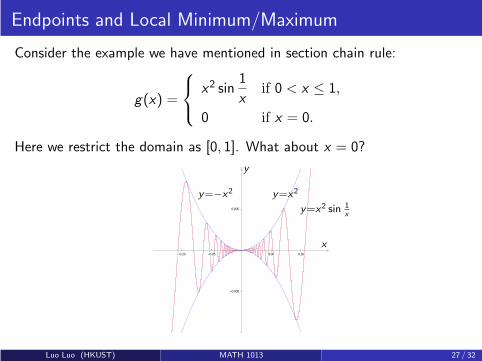
Endpoints and Local Minimum/Maximum
Consider the example we have mentioned in section chain rule:
g(x) =
x2 sin1
xif 0 < x ≤ 1,
0 if x = 0.
Here we restrict the domain as [0, 1]. What about x = 0?
−0.10 −0.05 0.05 0.10
−0.005
0.005 y=x2 sin 1x
y=−x2 y=x2
x
y
Luo Luo (HKUST) MATH 1013 27 / 32

Endpoints and Local Minimum/Maximum
Note that g(0) is neither local minimum or local maximum of
g(x) =
x2 sin1
xif 0 < x ≤ 1,
0 if x = 0.
Luo Luo (HKUST) MATH 1013 28 / 32

Examples: f (x) = x3 − 2x2 + x − 1
Find the intervals of increase/decrease, and local extrema of the functionf (x) = x3 − 2x2 + x − 1.
By differentiating the function, we have
f ′(x) = 3x2 − 4x + 1 = (3x − 1)(x − 1).
The critical points can be found by solving the equation f ′(x) = 0:
(3x − 1)(x − 1) = 0 ⇐⇒ x =1
3, or x = 1.
Let’s check the sign of f ′(x) in intervals x < 13 ,
13 < x < 1, and x > 1:
f(x) increasing increasingdecreasing
+ + + + + + + + + + + +- - - - - - - -
13
00
1
By the first derivative test, we have
f
(
1
3
)
= −23
27is a local maximum and f (1) = −1 is a local minimum.
Luo Luo (HKUST) MATH 1013 29 / 32
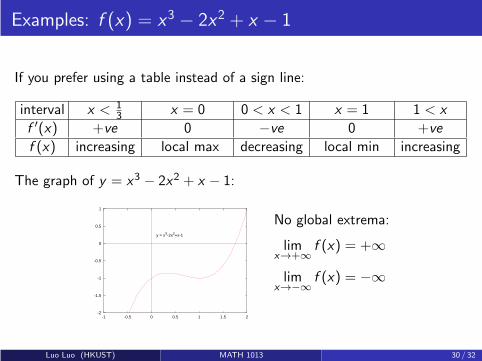
Examples: f (x) = x3 − 2x2 + x − 1
If you prefer using a table instead of a sign line:
interval x < 13 x = 0 0 < x < 1 x = 1 1 < x
f ′(x) +ve 0 −ve 0 +ve
f (x) increasing local max decreasing local min increasing
The graph of y = x3 − 2x2 + x − 1:
-2
-1.5
-1
-0.5
0
0.5
1
-1 -0.5 0 0.5 1 1.5 2
y = x3-2x2+x-1
No global extrema:
limx→+∞
f (x) = +∞
limx→−∞
f (x) = −∞
Luo Luo (HKUST) MATH 1013 30 / 32
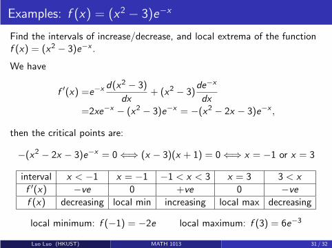
Examples: f (x) = (x2 − 3)e−x
Find the intervals of increase/decrease, and local extrema of the functionf (x) = (x2 − 3)e−x .
We have
f ′(x) =e−x d(x2 − 3)
dx+ (x2 − 3)
de−x
dx
=2xe−x − (x2 − 3)e−x = −(x2 − 2x − 3)e−x ,
then the critical points are:
−(x2 − 2x − 3)e−x = 0 ⇐⇒ (x − 3)(x + 1) = 0 ⇐⇒ x = −1 or x = 3
interval x < −1 x = −1 −1 < x < 3 x = 3 3 < x
f ′(x) −ve 0 +ve 0 −ve
f (x) decreasing local min increasing local max decreasing
local minimum: f (−1) = −2e local maximum: f (3) = 6e−3
Luo Luo (HKUST) MATH 1013 31 / 32
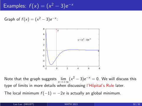
Examples: f (x) = (x2 − 3)e−x
Graph of f (x) = (x2 − 3)e−x :
-6
-4
-2
0
2
4
6
8
-2 0 2 4 6 8
x
y
y = (x2 - 3)e-x
Note that the graph suggests limx→+∞
(x2 − 3)e−x = 0. We will discuss this
type of limits in more details when discussing l’Hopital’s Rule later.
The local minimum f (−1) = −2e is actually an global minimum.
Luo Luo (HKUST) MATH 1013 32 / 32

Calculus IB: Lecture 13
Luo Luo
Department of Mathematics, HKUST
http://luoluo.people.ust.hk/
Luo Luo (HKUST) MATH 1013 1 / 16

Outline
1 Convexity/Concavity and 2nd Derivatives
2 Graph Sketching
Luo Luo (HKUST) MATH 1013 2 / 16
Outline
1 Convexity/Concavity and 2nd Derivatives
2 Graph Sketching
Luo Luo (HKUST) MATH 1013 3 / 16

Convexity/Concavity and 2nd Derivatives
What does the graph of y = f (x) on an interval mean by the sign of f ′′?
f ′′ > 0 =⇒ f ′ is increasing (the slope of tangent line is increasing)=⇒ f is concave up (or strictly convex)
f ′′ < 0 =⇒ f ′ is decreasing (the slope of tangent line is decreasing).=⇒ f is concave down (or strictly concave)
y
x
y = f(x)
concave down
concave up
f ''(x)<0
f ''(x)>0
Inflection Point
(Concavity changes across inflection point)
Sign of f ''(x) changes across an inflection point.
c c
++++ - - - - - - - - - - ++++or
slope decreasing
slope increasing
Luo Luo (HKUST) MATH 1013 3 / 16
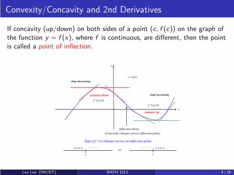
Convexity/Concavity and 2nd Derivatives
If concavity (up/down) on both sides of a point (c , f (c)) on the graph ofthe function y = f (x), where f is continuous, are different, then the pointis called a point of inflection.
y
x
y = f(x)
concave down
concave up
f ''(x)<0
f ''(x)>0
Inflection Point
(Concavity changes across inflection point)
Sign of f ''(x) changes across an inflection point.
c c
++++ - - - - - - - - - - ++++or
slope decreasing
slope increasing
Luo Luo (HKUST) MATH 1013 4 / 16

Convexity/Concavity and 2nd Derivatives
The convexity of f on an interval:
f ′′ ≥ 0 =⇒ f is convex
f ′′ > 0 =⇒ f is strictly convex (concave up)
f ′′ ≥ c for some c > 0 =⇒ f is strongly convex
The concavity of f on an interval:
f ′′ ≤ 0 =⇒ f is concave
f ′′ < 0 =⇒ f is strictly concave (concave down)
f ′′ ≤ c for some c < 0 =⇒ f is strongly concave
The linear function is both convex and concave. Since we have f ′′(x) = 0for f (x) = ax + b.
Luo Luo (HKUST) MATH 1013 5 / 16

Convexity/Concavity and 2nd Derivatives
A strictly convex function may NOT be a strongly convex function.
Consider the function f (x) = ex defined on (−∞,∞), we have
f ′(x) = ex , f ′′(x) = ex and limx→−∞
f ′′(x) = 0.
Since f ′′(x) > 0, the function f (x) is strictly convex on (−∞,∞).
However, for any c > 0, there exists M such that f ′′(x) < c for anyx < M. Hence, f (x) is not strongly convex.
Luo Luo (HKUST) MATH 1013 6 / 16
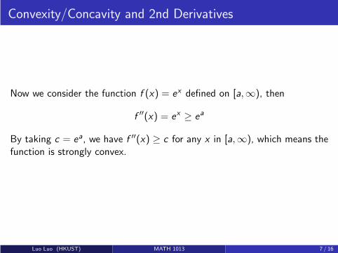
Convexity/Concavity and 2nd Derivatives
Now we consider the function f (x) = ex defined on [a,∞), then
f ′′(x) = ex ≥ ea
By taking c = ea, we have f ′′(x) ≥ c for any x in [a,∞), which means thefunction is strongly convex.
Luo Luo (HKUST) MATH 1013 7 / 16

Convex/Concave Functions
We can also define of convexity/concavity for non-differentiable functions.
−4 −3 −2 −1 1 2 3 4
−2
−1
1
2
3
4
5
6
f (x)=|x |
x
y
A real-valued function defined on an interval is called convex (concave) ifthe line segment between any two points on the graph of the function liesabove (below) the graph between the two points.
Luo Luo (HKUST) MATH 1013 8 / 16
Outline
1 Convexity/Concavity and 2nd Derivatives
2 Graph Sketching
Luo Luo (HKUST) MATH 1013 9 / 16
Graph Sketching
Roughly speaking, 1st/2nd derivatives of a function f , together with somelimits (asymptotes), symmetric properties, and intercepts, can helpdetermine the shape of the graph of f pretty well.
We can also use software (e.g. MATLAB) to plot the figure of a function(not allowed in final exam).
Luo Luo (HKUST) MATH 1013 9 / 16

Graph Sketching
The following strategies can be used in final exam:
1 Identify the domain of f , and any symmetry property of the graph:e.g., even, odd function?,. . . .
2 Identify the asymptotes, either vertical or horizontal.
3 Compute the first and second derivative : f ′, f ′′.
4 Determine the critical points (where is f ′(x) = 0, or f ′(x) does notexist), and interval of increase/decrease (i.e., where does f havepositive rate of change f ′(x) > 0, or negative rate of changef ′(x) < 0), by looking at the sign line of f ′.
5 Determine the concavity of the graph by the sign line of f ′′, andindicate the inflection points.
6 Plot a suitable number of points, especially the x and/or y intercept,local max/min points, inflection points.
Luo Luo (HKUST) MATH 1013 10 / 16

Graph Sketching: Example
Sketch the graph of the following function
y = f (x) =x2 − 3
x3.
The domain is x 6= 0. Note that x = 0 is a vertical asymptote since
limx→0+
x2 − 3
x3= −∞, lim
x→0−
x2 − 3
x3= ∞.
and y = 0 is a horizontal asymptote since
limx→∞
x2 − 3
x3= 0 = lim
x→−∞
x2 − 3
x3
The function is an odd since f (−x) = −f (x).
The x-intercept is x = ±√3, since f (±
√3) = 0.
Luo Luo (HKUST) MATH 1013 11 / 16
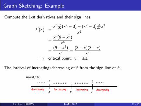
Graph Sketching: Example
Compute the 1-st derivatives and their sign lines:
f ′(x) =x3 d
dx(x2 − 3)− (x2 − 3) d
dxx3
x6
=x2(9− x2)
x6
=(9− x2)
x4=
(3− x)(3 + x)
x4
=⇒ critical point: x = ±3.
The interval of increasing/decreasing of f from the sign line of f ′:
-3 0 3
sign of f '(x)
- - - - - - - - - - + + + + + + + + + + + +0 0
increasing increasingdecreasing decreasing
Luo Luo (HKUST) MATH 1013 12 / 16

Graph Sketching: Example
Compute the 2-st derivatives and their sign lines:
f ′′(x) =x4(−2x)− (9− x2)(4x3)
x8
=2(x2 − 18)
x5
=2(x − 3
√2)(x + 3
√2)
x5
=⇒ Inflection points:(
3√2, f (3
√2))
and(
−3√2, f (−3
√2))
.
The concavity of f can be found easily from the sign line of f ′′:
0
sign of f ''(x)
- - - - - - - - - - - - - - + + + + + + + + + + + +0 0
concave down downup up−3
√
2 3√
2
Luo Luo (HKUST) MATH 1013 13 / 16
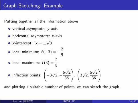
Graph Sketching: Example
Putting together all the information above
vertical asymptote: y -axis
horizontal asymptote: x-axis
x-intercept: x = ±√3
local minimum: f (−3) = −2
9
local maximum: f (3) =2
9
inflection points:
(
−3√2,−5
√2
36
)
,
(
3√2,
5√2
36
)
and plotting a suitable number of points, we can sketch the graph.
Luo Luo (HKUST) MATH 1013 14 / 16
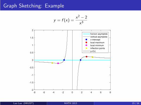
Graph Sketching: Example
y = f (x) =x2 − 2
x3
-8 -6 -4 -2 0 2 4 6 8-2
-1.5
-1
-0.5
0
0.5
1
1.5
2
horizon asymptote
vertical asymptote
x-intercept
local maximum
local minimum
inflection points
y=f(x)
Luo Luo (HKUST) MATH 1013 15 / 16

Graph Sketching by MATLAB
Luo Luo (HKUST) MATH 1013 16 / 16

Calculus IB: Lecture 14
Luo Luo
Department of Mathematics, HKUST
http://luoluo.people.ust.hk/
Luo Luo (HKUST) MATH 1013 1 / 41

Outline
1 Optimization Problems
2 Characterization of Convexity/Concavity
3 Properties of Convex Functions
Luo Luo (HKUST) MATH 1013 2 / 41

Outline
1 Optimization Problems
2 Characterization of Convexity/Concavity
3 Properties of Convex Functions
Luo Luo (HKUST) MATH 1013 3 / 41

Optimization Problems
Mathematical optimization (alternatively spelled optimisation) is theselection of a best element (with regard to some criterion) from some setof available alternatives.
Optimization problems of sorts arise in all quantitative disciplines fromcomputer science and engineering to operations research and economics,and the development of solution methods has been of interest inmathematics for centuries.
In the simplest case, an optimization problem consists of finding themaximum or minimum of a certain function to meet certain purpose,depending on the requirement of the problem.
Luo Luo (HKUST) MATH 1013 3 / 41
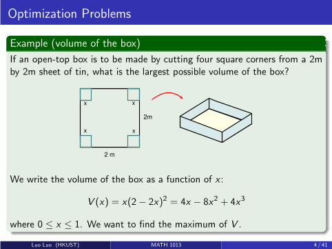
Optimization Problems
Example (volume of the box)
If an open-top box is to be made by cutting four square corners from a 2mby 2m sheet of tin, what is the largest possible volume of the box?
2 m
2m
xx
x x
We write the volume of the box as a function of x :
V (x) = x(2− 2x)2 = 4x − 8x2 + 4x3
where 0 ≤ x ≤ 1. We want to find the maximum of V .
Luo Luo (HKUST) MATH 1013 4 / 41

Optimization Problems
Example (volume of the box)
We first find the critical point of V (x) = 4x − 8x2 + 4x3:
dV
dx= 4− 16x + 12x2 = 0 ⇐⇒ x = 1 or x =
1
3.
By comparing the function values at critical points and endpoints
V (1) = 0, V (0) = 0, V
(
1
3
)
=16
27,
the maximum volume is16
27m3, which reached by cutting
1
3m.
Luo Luo (HKUST) MATH 1013 5 / 41
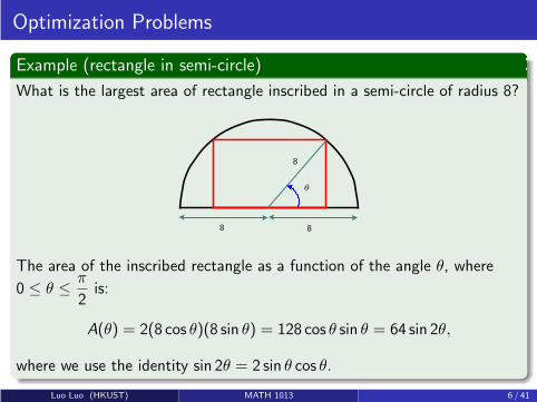
Optimization Problems
Example (rectangle in semi-circle)
What is the largest area of rectangle inscribed in a semi-circle of radius 8?
8
8
8
θ
The area of the inscribed rectangle as a function of the angle θ, where
0 ≤ θ ≤ π
2is:
A(θ) = 2(8 cos θ)(8 sin θ) = 128 cos θ sin θ = 64 sin 2θ,
where we use the identity sin 2θ = 2 sin θ cos θ.
Luo Luo (HKUST) MATH 1013 6 / 41

Optimization Problems
Example (rectangle in semi-circle)
We first find the critical point of A(θ) = 64 sin 2θ:
A′(θ) = 128 cos 2θ = 0 ⇐⇒ 2θ =π
2⇐⇒ θ =
π
4.
By comparing the function values at critical points and endpoints
A(0) = 0 = A(π
2
)
, A(π
4
)
= 64,
the maximum area is 64, which reached when θ =π
4and the rectangle is a
square of base length 2 ·(
8 cos π4
)
= 8√2.
Luo Luo (HKUST) MATH 1013 7 / 41
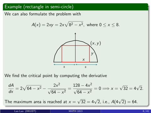
Example (rectangle in semi-circle)
We can also formulate the problem with
A(x) = 2xy = 2x√
82 − x2, where 0 ≤ x ≤ 8.
x
y
(x , y)
8 8
We find the critical point by computing the derivative
dA
dx= 2
√
64− x2 − 2x2√64− x2
=128− 4x2√64− x2
= 0 =⇒ x =√32 = 4
√2.
The maximum area is reached at x =√32 = 4
√2, i.e., A(4
√2) = 64.
Luo Luo (HKUST) MATH 1013 8 / 41

Optimization Problems
Example (Snell’s Law)
The ground surfaces on two sides of a certain boundary line are made ofdifferent materials.A man can run with speed v1 m/s on the side of location P which a mfrom the line, and v2 m/s on the side of location Q which is b m from theline.Running along a straight path on either side, how should he choose thecross-boundary point R in order to reach location Q as soon as possible?
P
O R S
Q
x
a
bL
Luo Luo (HKUST) MATH 1013 9 / 41

Optimization Problems
Example (Snell’s Law)
Let OR = x , OS = L, then RS = L− x . The time to reach Q is thefunction as follows:
T (x) =
√x2 + a2
v1+
√
(L− x)2 + b2
v2, where 0 ≤ x ≤ L.
We want to select x in [0, L] to minimize T (x).
P
O R S
Q
x
a
bL
Luo Luo (HKUST) MATH 1013 10 / 41
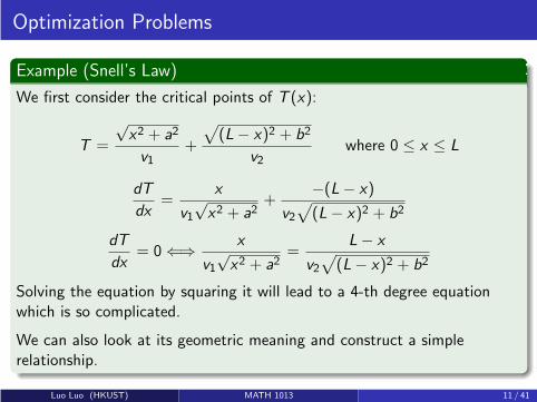
Optimization Problems
Example (Snell’s Law)
We first consider the critical points of T (x):
T =
√x2 + a2
v1+
√
(L− x)2 + b2
v2where 0 ≤ x ≤ L
dT
dx=
x
v1√x2 + a2
+−(L− x)
v2√
(L− x)2 + b2
dT
dx= 0 ⇐⇒ x
v1√x2 + a2
=L− x
v2√
(L− x)2 + b2
Solving the equation by squaring it will lead to a 4-th degree equationwhich is so complicated.
We can also look at its geometric meaning and construct a simplerelationship.
Luo Luo (HKUST) MATH 1013 11 / 41

Optimization Problems
Example (Snell’s Law)
Let ∠OPR = α, ∠RQS = β. Then we can simplify the condition ofT ′(x) = 0 as follows:
x
v1√x2 + a2
=L− x
v2√
(L− x)2 + b2⇐⇒ 1
v1· ORPR
=1
v2· RSQR
⇐⇒ 1
v1· sinα =
1
v2· sinβ ⇐⇒ sinα
sinβ=
v1
v2
P
O R S
Q
x
a
bL
Luo Luo (HKUST) MATH 1013 12 / 41

Optimization Problems
Example (Snell’s Law)
Let ∠OPR = α, ∠RQS = β. Hence, the condition of T ′(x) = 0 can bewritten as
sinα
sinβ=
v1
v2.
P
O R S
Q
x
a
bL
Can we conclude the x leads to T ′(x) = 0 is a minimizer?
Luo Luo (HKUST) MATH 1013 13 / 41
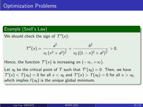
Optimization Problems
Example (Snell’s Law)
We should check the sign of T ′′(x):
T ′′(x) =a2
v1 (x2 + a2)32
+b2
v2 ((L− x)2 + a2)32
> 0.
Hence, the function T ′(x) is increasing on (−∞,+∞).
Let x0 be the critical point of T such that T ′(x0) = 0. Then, we haveT ′(x) < T (x0) = 0 for all x < x0 and T ′(x) > T (x0) = 0 for all x > x0,which implies f (x0) is the unique global minimum.
Luo Luo (HKUST) MATH 1013 14 / 41
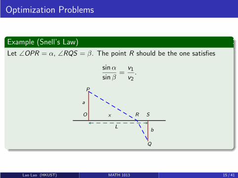
Optimization Problems
Example (Snell’s Law)
Let ∠OPR = α, ∠RQS = β. The point R should be the one satisfies
sinα
sinβ=
v1
v2.
P
O R S
Q
x
a
bL
Luo Luo (HKUST) MATH 1013 15 / 41

Optimization Problems
Example (Snell’s Law)
Let ∠OPR = α, ∠RQS = β. In optics, Snell’s law says if a light passingthrough boundary OS between two different isotropic media (such aswater, glass, or air) from P with directions PR , its trace satisfies
sinα
sinβ=
v1
v2.
P
O R S
Q
x
a
bL
Luo Luo (HKUST) MATH 1013 16 / 41

Optimization Problems
Example (maximizing the profit)
Suppose c(x) = x3 − 6x2 + 15x is the cost of producing x thousands ofunits of a product, and r(x) = 8x the revenue of selling x thousands ofunits of the product.
Then p(x) = r(x)− c(x) is the profit of selling x thousands of units of theproduct. Find the production level which maximizes the profit.
-10
0
10
20
30
40
0 1 2 3 4 5
Revenuer(x) = 8x cost
c(x) = x3 - 6x
2 + 15x
x
profit p(x) = r(x) - c(x)
y
Luo Luo (HKUST) MATH 1013 17 / 41
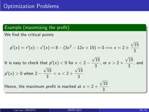
Optimization Problems
Example (maximizing the profit)
We find the critical points
p′(x) = r ′(x)− c ′(x) = 8− (3x2 − 12x + 15) = 0 =⇒ x = 2±√15
3
It is easy to check that p′(x) < 0 for x < 2−√15
3, or x > 2 +
√15
3, and
p′(x) > 0 when 2−√15
3< x < 2 +
√15
3.
Hence, the maximum profit is reached at x = 2 +
√15
3.
Luo Luo (HKUST) MATH 1013 18 / 41

Optimization Problems
Example (maximizing the profit)
At x = 2−√15
3, the profit is a local minimum (local maximum loss).
Hence, you will be fired if you select x = 2−√15
3.
-10
0
10
20
30
40
0 1 2 3 4 5
Revenuer(x) = 8x cost
c(x) = x3 - 6x
2 + 15x
x
profit p(x) = r(x) - c(x)
y
‘Luo Luo (HKUST) MATH 1013 19 / 41

Closed Form Expression
For all above examples, we can provide the closed from expression for thesolution of the optimization problems.
A closed-form expression is an expression expressed using a finite numberof standard operations. It may contain
constants, variables
certain “well-known” operations (e.g., +−×÷)
elementary functions (e.g., n-th root, exponent, logarithm,trigonometric functions, and inverse trigonometric functions)
It usually does not contain limit, differentiation, or integration (will beintroduced in last 2 or 3 weeks).
The set of operations and functions admitted in a closed-form expressionmay vary with author and context.
Luo Luo (HKUST) MATH 1013 20 / 41
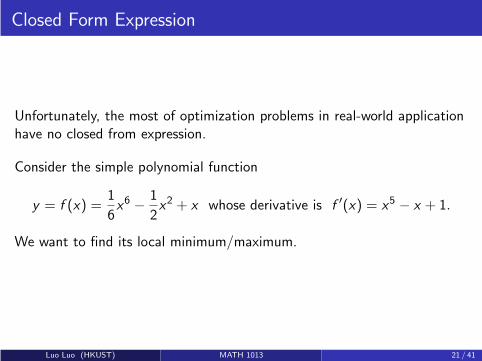
Closed Form Expression
Unfortunately, the most of optimization problems in real-world applicationhave no closed from expression.
Consider the simple polynomial function
y = f (x) =1
6x6 − 1
2x2 + x whose derivative is f ′(x) = x5 − x + 1.
We want to find its local minimum/maximum.
Luo Luo (HKUST) MATH 1013 21 / 41
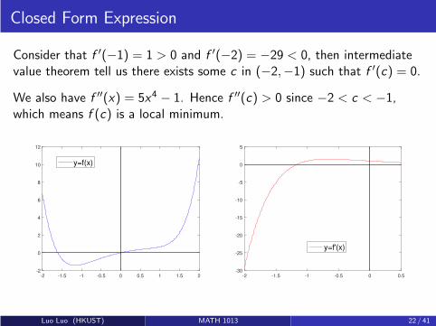
Closed Form Expression
Consider that f ′(−1) = 1 > 0 and f ′(−2) = −29 < 0, then intermediatevalue theorem tell us there exists some c in (−2,−1) such that f ′(c) = 0.
We also have f ′′(x) = 5x4 − 1. Hence f ′′(c) > 0 since −2 < c < −1,which means f (c) is a local minimum.
-2 -1.5 -1 -0.5 0 0.5 1 1.5 2-2
0
2
4
6
8
10
12
y=f(x)
-2 -1.5 -1 -0.5 0 0.5-30
-25
-20
-15
-10
-5
0
5
y=f'(x)
Luo Luo (HKUST) MATH 1013 22 / 41
Closed Form Expression
The Abel-Ruffini theorem (first asserted in 1799 and completely proved in1824) shows that there is no closed form expression for the solution of
x5 − x + 1 = 0.
We can use iterative methods to generate a sequence of improvingapproximate solutions.
For optimization problems, one class of popular functions we are interestedin is convex/concave function.
Luo Luo (HKUST) MATH 1013 23 / 41

Outline
1 Optimization Problems
2 Characterization of Convexity/Concavity
3 Properties of Convex Functions
Luo Luo (HKUST) MATH 1013 24 / 41
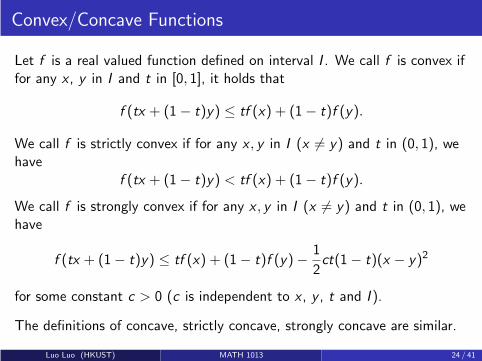
Convex/Concave Functions
Let f is a real valued function defined on interval I . We call f is convex iffor any x , y in I and t in [0, 1], it holds that
f (tx + (1− t)y) ≤ tf (x) + (1− t)f (y).
We call f is strictly convex if for any x , y in I (x 6= y) and t in (0, 1), wehave
f (tx + (1− t)y) < tf (x) + (1− t)f (y).
We call f is strongly convex if for any x , y in I (x 6= y) and t in (0, 1), wehave
f (tx + (1− t)y) ≤ tf (x) + (1− t)f (y)− 1
2ct(1− t)(x − y)2
for some constant c > 0 (c is independent to x , y , t and I ).
The definitions of concave, strictly concave, strongly concave are similar.
Luo Luo (HKUST) MATH 1013 24 / 41

1st/2nd Order Condition
Theorem (1st/2nd order condition)
Suppose function f is twice differentiable over an open interval I . Then,
the following statements are equivalent:
(a) f is convex.
(b) f (y) ≥ f (x) + f ′(x)(y − x), for all x and y in I .
(c) f ′′(x) ≥ 0, for all x in I .
We say (b) is first-order condition and (b) is second order condition.
We prove this theorem by showing:
(a) =⇒ (b)
(b) =⇒ (a)
(b) =⇒ (c)
(c) =⇒ (b)
Luo Luo (HKUST) MATH 1013 25 / 41

f is convex =⇒ f (y) ≥ f (x) + f ′(x)(y − x)
For any t ∈ [0, 1] and x , y in I , the convexity of f means
f (ty + (1− t)x) ≤ tf (y) + (1− t)f (x)
Since ty + (1− t)x = x + t(y − x), we have
f (x + t(y − x)) ≤ tf (y) + (1− t)f (x)
=⇒f (x + t(y − x))− f (x) ≤ t(f (y)− f (x)).
If x = y , then
f (y) ≥ f (x) + f ′(x)(y − x) ⇐⇒ f (x) ≥ f (x).
If t = 0, then
f (ty + (1− t)x) ≤ tf (y) + (1− t)f (x) =⇒ f (x) ≤ f (x).
If t = 1, then
f (ty + (1− t)x) ≤ tf (y) + (1− t)f (x) =⇒ f (y) ≤ f (y).
Luo Luo (HKUST) MATH 1013 26 / 41
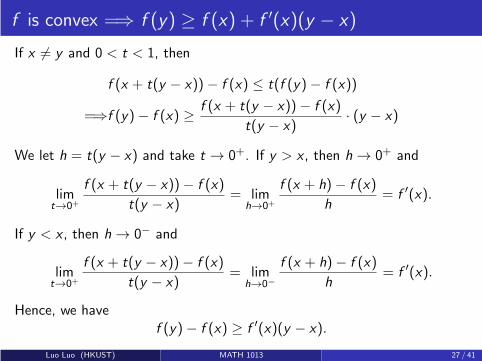
f is convex =⇒ f (y) ≥ f (x) + f ′(x)(y − x)
If x 6= y and 0 < t < 1, then
f (x + t(y − x))− f (x) ≤ t(f (y)− f (x))
=⇒f (y)− f (x) ≥ f (x + t(y − x))− f (x)
t(y − x)· (y − x)
We let h = t(y − x) and take t → 0+. If y > x , then h → 0+ and
limt→0+
f (x + t(y − x))− f (x)
t(y − x)= lim
h→0+
f (x + h)− f (x)
h= f ′(x).
If y < x , then h → 0− and
limt→0+
f (x + t(y − x))− f (x)
t(y − x)= lim
h→0−
f (x + h)− f (x)
h= f ′(x).
Hence, we havef (y)− f (x) ≥ f ′(x)(y − x).
Luo Luo (HKUST) MATH 1013 27 / 41
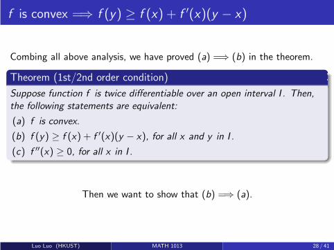
f is convex =⇒ f (y) ≥ f (x) + f ′(x)(y − x)
Combing all above analysis, we have proved (a) =⇒ (b) in the theorem.
Theorem (1st/2nd order condition)
Suppose function f is twice differentiable over an open interval I . Then,
the following statements are equivalent:
(a) f is convex.
(b) f (y) ≥ f (x) + f ′(x)(y − x), for all x and y in I .
(c) f ′′(x) ≥ 0, for all x in I .
Then we want to show that (b) =⇒ (a).
Luo Luo (HKUST) MATH 1013 28 / 41
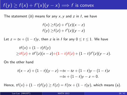
f (y) ≥ f (x) + f ′(x)(y − x) =⇒ f is convex
The statement (b) means for any x , y and z in I , we have
f (x) ≥f (z) + f ′(z)(x − z)
f (y) ≥f (z) + f ′(z)(y − z)
Let z = tx + (1− t)y , then z is in I for any 0 ≤ t ≤ 1. We have
tf (x) + (1− t)f (y)
≥tf (z) + tf ′(z)(x − z)+(1− t)f (z) + (1− t)f ′(z)(y − z).
On the other hand
t(x − z) + (1− t)(y − z) =tx − tz + (1− t)y − (1− t)z
=tx + (1− t)y − z = 0.
Hence, tf (x) + (1− t)f (y) ≥ f (z) = f (tx + (1− t)y), which means (a).
Luo Luo (HKUST) MATH 1013 29 / 41
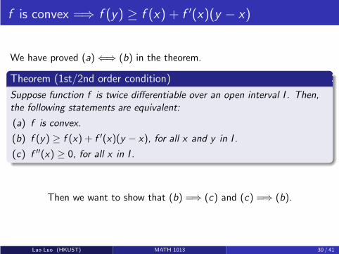
f is convex =⇒ f (y) ≥ f (x) + f ′(x)(y − x)
We have proved (a) ⇐⇒ (b) in the theorem.
Theorem (1st/2nd order condition)
Suppose function f is twice differentiable over an open interval I . Then,
the following statements are equivalent:
(a) f is convex.
(b) f (y) ≥ f (x) + f ′(x)(y − x), for all x and y in I .
(c) f ′′(x) ≥ 0, for all x in I .
Then we want to show that (b) =⇒ (c) and (c) =⇒ (b).
Luo Luo (HKUST) MATH 1013 30 / 41
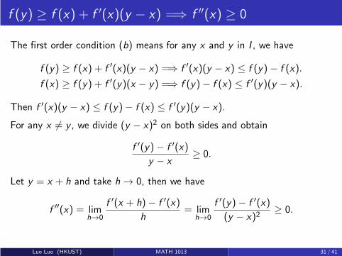
f (y) ≥ f (x) + f ′(x)(y − x) =⇒ f ′′(x) ≥ 0
The first order condition (b) means for any x and y in I , we have
f (y) ≥ f (x) + f ′(x)(y − x) =⇒ f ′(x)(y − x) ≤ f (y)− f (x).
f (x) ≥ f (y) + f ′(y)(x − y) =⇒ f (y)− f (x) ≤ f ′(y)(y − x).
Then f ′(x)(y − x) ≤ f (y)− f (x) ≤ f ′(y)(y − x).
For any x 6= y , we divide (y − x)2 on both sides and obtain
f ′(y)− f ′(x)
y − x≥ 0.
Let y = x + h and take h → 0, then we have
f ′′(x) = limh→0
f ′(x + h)− f ′(x)
h= lim
h→0
f ′(y)− f ′(x)
(y − x)2≥ 0.
Luo Luo (HKUST) MATH 1013 31 / 41
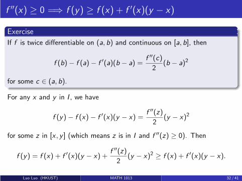
f ′′(x) ≥ 0 =⇒ f (y) ≥ f (x) + f ′(x)(y − x)
Exercise
If f is twice differentiable on (a, b) and continuous on [a, b], then
f (b)− f (a)− f ′(a)(b − a) =f ′′(c)
2(b − a)2
for some c ∈ (a, b).
For any x and y in I , we have
f (y)− f (x)− f ′(x)(y − x) =f ′′(z)
2(y − x)2
for some z in [x , y ] (which means z is in I and f ′′(z) ≥ 0). Then
f (y) = f (x) + f ′(x)(y − x) +f ′′(z)
2(y − x)2 ≥ f (x) + f ′(x)(y − x).
Luo Luo (HKUST) MATH 1013 32 / 41
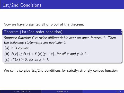
1st/2nd Conditions
Now we have presented all of proof of the theorem.
Theorem (1st/2nd order condition)
Suppose function f is twice differentiable over an open interval I . Then,
the following statements are equivalent:
(a) f is convex.
(b) f (y) ≥ f (x) + f ′(x)(y − x), for all x and y in I .
(c) f ′′(x) ≥ 0, for all x in I .
We can also give 1st/2nd conditions for strictly/strongly convex function.
Luo Luo (HKUST) MATH 1013 33 / 41

1st/2nd Conditions
Now we have presented all of proof of the theorem.
Theorem (1st/2nd order condition)
Suppose function f is twice differentiable over an open interval I . Then,
the following statements are equivalent:
(a) f is convex.
(b) f (y) ≥ f (x) + f ′(x)(y − x), for all x and y in I .
(c) f ′′(x) ≥ 0, for all x in I .
We can also give 1st/2nd conditions for strictly/strongly convex function.
Luo Luo (HKUST) MATH 1013 34 / 41

1st/2nd Conditions
Now we have presented all of proof of the theorem.
Theorem (1st/2nd order condition)
Suppose function f is twice differentiable over an open interval I . Then,
the following statements are equivalent:
(a) f is convex.
(b) f (y) ≥ f (x) + f ′(x)(y − x), for all x and y in I .
(c) f ′′(x) ≥ 0, for all x in I .
We can also give 1st/2nd conditions for strictly/strongly convex function.
Luo Luo (HKUST) MATH 1013 35 / 41

Outline
1 Optimization Problems
2 Characterization of Convexity/Concavity
3 Properties of Convex Functions
Luo Luo (HKUST) MATH 1013 36 / 41
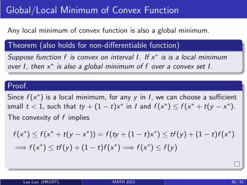
Global/Local Minimum of Convex Function
Any local minimum of convex function is also a global minimum.
Theorem (also holds for non-differentiable function)
Suppose function f is convex on interval I . If x∗ is is a local minimum
over I , then x∗ is also a global minimum of f over a convex set I .
Proof.
Since f (x∗) is a local minimum, for any y in I , we can choose a sufficientsmall t < 1, such that ty + (1− t)x∗ in I and f (x∗) ≤ f (x∗ + t(y − x∗).
The convexity of f implies
f (x∗) ≤ f (x∗ + t(y − x∗)) = f (ty + (1− t)x∗) ≤ tf (y) + (1− t)f (x∗)
=⇒ f (x∗) ≤ tf (y) + (1− t)f (x∗) =⇒ f (x∗) ≤ f (y)
Luo Luo (HKUST) MATH 1013 36 / 41
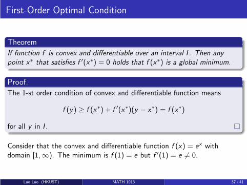
First-Order Optimal Condition
Theorem
If function f is convex and differentiable over an interval I . Then any
point x∗ that satisfies f ′(x∗) = 0 holds that f (x∗) is a global minimum.
Proof.
The 1-st order condition of convex and differentiable function means
f (y) ≥ f (x∗) + f ′(x∗)(y − x∗) = f (x∗)
for all y in I .
Consider that the convex and differentiable function f (x) = ex withdomain [1,∞). The minimum is f (1) = e but f ′(1) = e 6= 0.
Luo Luo (HKUST) MATH 1013 37 / 41

First-Order Optimal Condition
We desire to establish an equivalent condition for global minimum ofconvex and differentiable function.
A good strategy is relaxing the condition of f ′(x∗) = 0 to
f ′(x∗)(y − x∗) ≥ 0
holds for all y in I .
Luo Luo (HKUST) MATH 1013 38 / 41

First-Order Optimal Condition
Theorem (sufficient condition)
If function f is convex and differentiable over an interval I . Then any
point x∗ that satisfies
f ′(x∗)(y − x∗) ≥ 0
for all y in I holds that f (x∗) is a global minimum.
Theorem (necessary condition)
If function f is convex and differentiable over an interval I . Then for any
point x∗ such that f (x∗) is a global minimum, we have
f ′(x∗)(y − x∗) ≥ 0
for all y in I .
Luo Luo (HKUST) MATH 1013 39 / 41

Proof (necessary condition).
Let x∗ in I and f (x∗) is a global minimum. Suppose y in I such that
f ′(x∗)(y − x∗) < 0.
There must hold that y 6= x∗. Let t > 0, h = t(y − x∗). Taking t → 0+, then
limt→0+
f (x∗ + t(y − x∗))− f (x∗)
t
=(y − x∗) · limt→0+
f (x∗ + t(y − x∗))− f (x∗)
t(y − x∗)
=(y − x∗) · limh→0
f (x∗ + h)− f (x∗)
h= f ′(x∗)(y − x∗) < 0.
For sufficient small t, we have f (x∗ + t(y − x∗)− f (x∗) < 0 for x∗ + t(y − x∗) inI , which contradicts to x∗ is global minimum. Hence, we must have
f ′(x∗)(y − x∗) ≥ 0
and the convexity means f (y) ≥ f (x∗) + f ′(x∗)(y − x∗) ≥ f (x∗).
Luo Luo (HKUST) MATH 1013 40 / 41
First-Order Optimal Condition
Note that the equivalent condition
f ′(x∗)(y − x∗) ≥ 0,
only depends on the function value and the derivative of f .
Hence, it works for any convex and differentiable even if f ′ is notdifferentiable (f ′′ may not exist).
Luo Luo (HKUST) MATH 1013 41 / 41

Calculus IB: Lecture 15
Luo Luo
Department of Mathematics, HKUST
http://luoluo.people.ust.hk/
Luo Luo (HKUST) MATH 1013 1 / 22

Outline
1 Geometric View of Convex Function
2 Global/Local Minimum of Convex Function
3 Linear Approximation
Luo Luo (HKUST) MATH 1013 2 / 22

Outline
1 Geometric View of Convex Function
2 Global/Local Minimum of Convex Function
3 Linear Approximation
Luo Luo (HKUST) MATH 1013 3 / 22
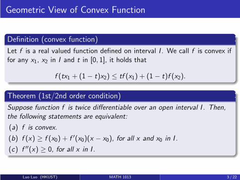
Geometric View of Convex Function
Definition (convex function)
Let f is a real valued function defined on interval I . We call f is convex iffor any x1, x2 in I and t in [0, 1], it holds that
f (tx1 + (1− t)x2) ≤ tf (x1) + (1− t)f (x2).
Theorem (1st/2nd order condition)
Suppose function f is twice differentiable over an open interval I . Then,
the following statements are equivalent:
(a) f is convex.
(b) f (x) ≥ f (x0) + f ′(x0)(x − x0), for all x and x0 in I .
(c) f ′′(x) ≥ 0, for all x in I .
Luo Luo (HKUST) MATH 1013 3 / 22

Geometric View of Convex Function
Let f (x) be a convex function and define the linear function (x1 6= x2)
g(x) =f (x2)− f (x1)
x2 − x1(x − x1) + f (x1).
Then we have g(x1) = f (x1), g(x2) = f (x2) and g(x) ≥ f (x) for any x1 ≤ x ≤ x2.
-1 -0.8 -0.6 -0.4 -0.2 0 0.2 0.4 0.6 0.8 10
0.1
0.2
0.3
0.4
0.5
0.6
0.7
0.8
0.9
1
P(x1, f(x
1))
Q(x2, f(x
2))
R(x1, 0) S(x
2, 0)
y=f(x)
y=g(x)
Luo Luo (HKUST) MATH 1013 4 / 22
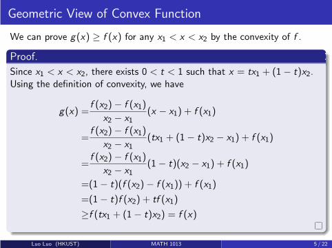
Geometric View of Convex Function
We can prove g(x) ≥ f (x) for any x1 < x < x2 by the convexity of f .
Proof.
Since x1 < x < x2, there exists 0 < t < 1 such that x = tx1 + (1− t)x2.Using the definition of convexity, we have
g(x) =f (x2)− f (x1)
x2 − x1(x − x1) + f (x1)
=f (x2)− f (x1)
x2 − x1(tx1 + (1− t)x2 − x1) + f (x1)
=f (x2)− f (x1)
x2 − x1(1− t)(x2 − x1) + f (x1)
=(1− t)(f (x2)− f (x1)) + f (x1)
=(1− t)f (x2) + tf (x1)
≥f (tx1 + (1− t)x2) = f (x)
Luo Luo (HKUST) MATH 1013 5 / 22
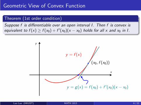
Geometric View of Convex Function
Theorem (1st order condition)
Suppose f is differentiable over an open interval I . Then f is convex is
equivalent to f (x) ≥ f (x0) + f ′(x0)(x − x0) holds for all x and x0 in I .
x
y
y = f (x)
y = g(x) = f (x0) + f ′(x0)(x − x0)
(x0, f (x0))
Luo Luo (HKUST) MATH 1013 6 / 22
Outline
1 Geometric View of Convex Function
2 Global/Local Minimum of Convex Function
3 Linear Approximation
Luo Luo (HKUST) MATH 1013 7 / 22
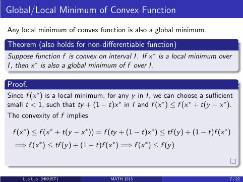
Global/Local Minimum of Convex Function
Any local minimum of convex function is also a global minimum.
Theorem (also holds for non-differentiable function)
Suppose function f is convex on interval I . If x∗ is a local minimum over
I , then x∗ is also a global minimum of f over I .
Proof.
Since f (x∗) is a local minimum, for any y in I , we can choose a sufficientsmall t < 1, such that ty + (1− t)x∗ in I and f (x∗) ≤ f (x∗ + t(y − x∗).
The convexity of f implies
f (x∗) ≤ f (x∗ + t(y − x∗)) = f (ty + (1− t)x∗) ≤ tf (y) + (1− t)f (x∗)
=⇒ f (x∗) ≤ tf (y) + (1− t)f (x∗) =⇒ f (x∗) ≤ f (y)
Luo Luo (HKUST) MATH 1013 7 / 22
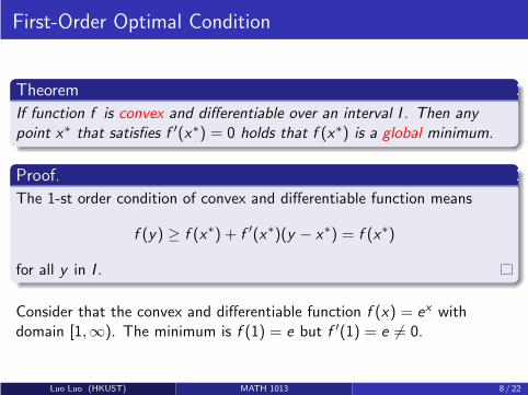
First-Order Optimal Condition
Theorem
If function f is convex and differentiable over an interval I . Then any
point x∗ that satisfies f ′(x∗) = 0 holds that f (x∗) is a global minimum.
Proof.
The 1-st order condition of convex and differentiable function means
f (y) ≥ f (x∗) + f ′(x∗)(y − x∗) = f (x∗)
for all y in I .
Consider that the convex and differentiable function f (x) = ex withdomain [1,∞). The minimum is f (1) = e but f ′(1) = e 6= 0.
Luo Luo (HKUST) MATH 1013 8 / 22

First-Order Optimal Condition
We desire to establish an equivalent condition for global minimum ofconvex and differentiable function.
A good strategy is relaxing the condition of f ′(x∗) = 0 to
f ′(x∗)(y − x∗) ≥ 0
holds for all y in I .
Luo Luo (HKUST) MATH 1013 9 / 22

First-Order Optimal Condition
Theorem (sufficient condition)
If function f is convex and differentiable over an interval I . Then any
point x∗ that satisfies
f ′(x∗)(y − x∗) ≥ 0
for all y in I holds that f (x∗) is a global minimum.
Theorem (necessary condition)
If function f is convex and differentiable over an interval I . Then for any
point x∗ such that f (x∗) is a global minimum, we have
f ′(x∗)(y − x∗) ≥ 0
for all y in I .
Luo Luo (HKUST) MATH 1013 10 / 22
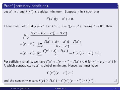
Proof (necessary condition).
Let x∗ in I and f (x∗) is a global minimum. Suppose y in I such that
f ′(x∗)(y − x∗) < 0.
There must hold that y 6= x∗. Let t > 0, h = t(y − x∗). Taking t → 0+, then
limt→0+
f (x∗ + t(y − x∗))− f (x∗)
t
=(y − x∗) · limt→0+
f (x∗ + t(y − x∗))− f (x∗)
t(y − x∗)
=(y − x∗) · limh→0
f (x∗ + h)− f (x∗)
h= f ′(x∗)(y − x∗) < 0.
For sufficient small t, we have f (x∗ + t(y − x∗)− f (x∗) < 0 for x∗ + t(y − x∗) inI , which contradicts to x∗ is global minimum. Hence, we must have
f ′(x∗)(y − x∗) ≥ 0
and the convexity means f (y) ≥ f (x∗) + f ′(x∗)(y − x∗) ≥ f (x∗).
Luo Luo (HKUST) MATH 1013 11 / 22
First-Order Optimal Condition
Note that the optimal condition
f ′(x∗)(y − x∗) ≥ 0,
only depends on the function value and the derivative of f .
Hence, it works even if f ′ is not differentiable (f ′′ does not exist).
Luo Luo (HKUST) MATH 1013 12 / 22
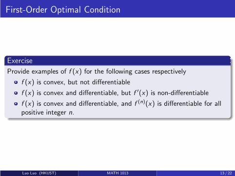
First-Order Optimal Condition
Exercise
Provide examples of f (x) for the following cases respectively
f (x) is convex, but not differentiable
f (x) is convex and differentiable, but f ′(x) is non-differentiable
f (x) is convex and differentiable, and f (n)(x) is differentiable for allpositive integer n.
Luo Luo (HKUST) MATH 1013 13 / 22
Outline
1 Geometric View of Convex Function
2 Global/Local Minimum of Convex Function
3 Linear Approximation
Luo Luo (HKUST) MATH 1013 14 / 22

Linear Approximation
Recall that the slope of the tangent line to the graph of y = f (x) at x = a
is the derivative
f ′(a) = limh→0
f (a+ h)− f (a)
h
Therefore the equation of the tangent line to the graph of y = f (x) at thepoint (a, f (a)) is determined by the slope condition
y = f (a) + f ′(a)(x − a).
Letting x = a+ h, we have
f ′(a) ≈ f (a+ h)− f (a)
h=
f (x)− f (a)
x − awhen h = x − a ≈ 0
i.e., f (x) ≈ f (a) + f ′(a)(x − a) , when x ≈ a. In other words,
tangent lineapproximates−→ graph of y = f (x) near the point (a, f (a))
Luo Luo (HKUST) MATH 1013 14 / 22

Linear Approximation
The tangent line approximation at x = a, or linear approximation at x = a, orlinearization at x = a, of a function y = f (x) (differentiable at x = a) is that weare using the tangent line equation (or the corresponding linear function) toapproximate the given function.
y = f (x)≈←− Tangent Line Equation : y = f (a) + f ′(a)(x − a)
=⇒ f (x) ≈ f (a) + f ′(a)(x − a) for x − a ≈ 0
(a, f(a))
(a+h, f(a+h))
f(a+h)-f(a)
h=x-a
y
x
y=f(x)
tangent line
secant line
Tangent line approximates the graph of
y = f(x) as h approaches 0.
Luo Luo (HKUST) MATH 1013 15 / 22
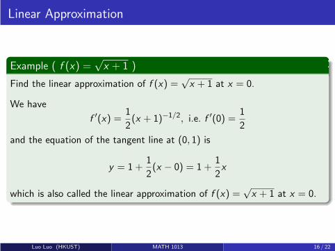
Linear Approximation
Example ( f (x) =√x + 1 )
Find the linear approximation of f (x) =√x + 1 at x = 0.
We have
f ′(x) =1
2(x + 1)−1/2
, i.e. f ′(0) =1
2
and the equation of the tangent line at (0, 1) is
y = 1 +1
2(x − 0) = 1 +
1
2x
which is also called the linear approximation of f (x) =√x + 1 at x = 0.
Luo Luo (HKUST) MATH 1013 16 / 22
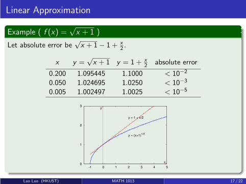
Linear Approximation
Example ( f (x) =√x + 1 )
Let absolute error be√x + 1− 1 + x
2 .
x y =√x + 1 y = 1 + x
2 absolute error
0.200 1.095445 1.1000 < 10−2
0.050 1.024695 1.0250 < 10−3
0.005 1.002497 1.0025 < 10−5
0
1
2
3
-1 0 1 2 3 4 5
y = (x+1)1/2
x
y
y = 1 + x/2
Luo Luo (HKUST) MATH 1013 17 / 22

Linear Approximation
Example ( 3√8.5)
Find an approximate value of 3√8.5 by the linear approximation of a
suitable function.
Let f (x) = 3√x = x1/3, with f ′(x) = 1
3x−2/3.
The linear approximation at x = 8 is:
f (x) ≈ f (8) + f ′(8)(x − 8) = 2 +1
12(x − 8) =
x
12+
4
3
Thus
f (8.5) ≈ 8.5
12+
4
3=
245
120= 2.04167.
Note that 3√8.5 = 2.04093 from a calculator.
Luo Luo (HKUST) MATH 1013 18 / 22
Differential of the Function
The tangent line approximation at x is
f (x +∆x) ≈ f (x) + f ′(x)∆x ,
where ∆x denotes some increment in x (which could be negative).
Then we use ∆y or ∆f to denote the change in the function values
∆y = ∆f = f (x +∆x)− f (x).
and the linear approximation be expressed as
∆f ≈ f ′(x)∆x .
Note that f ′(x)∆x is the change of y -value along the tangent line!
Luo Luo (HKUST) MATH 1013 19 / 22

Differential of the Function
y
x
better approximation
for smaller h
approximation error
h=∆x=dx
dy=f ′(x)dx
slope =f ′(x)
(x+h,f (x+h))
(x ,f (x))
f (x+h)−f (x)
y=f (x)
The notation of differentials df = f ′(x)dx is obtained by expressing ∆x asdx , and dy = df = f ′(x)dx can be used as an approximation of
∆y = f (x +∆x)− f (x).
Luo Luo (HKUST) MATH 1013 20 / 22

Linear Approximation
Example (area of a circle)
Approximate the increase in the area of a circle when the radius isincreased from 10m to 10.1m.
The area of the circle is A(r) = πr2, then dA = A′(r)dr = 2πrdr .
For r = 10m and dr = 0.1m, we have dA = 2π(10)0.1 = 2πm2, whichapproximates the change in area ∆A.
The approximate area at r = 10.1 m is:
A ≈ A(10) + dA = 100π + 2π = 102πm2.
The exact area at r = 10.1m is A = π(10.1)2 = π(10)2 +∆A. Theabsolute error of the estimate is
|π(10.1)2 − 102π| = 102.01π − 102π = 0.01 = |∆A− dy |m2
Luo Luo (HKUST) MATH 1013 21 / 22

Linear Approximation of Convex Function
Given a differentiable function y = f (x) defined on an open interval I , its linearapproximation is
f (x) ≈ f (a) + f ′(a)(x − a).
We additionally suppose f is convex, then the first-order condition means
f (x) ≥ f (a) + f ′(a)(x − a).
Hence, the linear approximation provides a lower bound of convex function.
(a, f(a))
(a+h, f(a+h))
f(a+h)-f(a)
h=x-a
y
x
y=f(x)
tangent line
secant line
Tangent line approximates the graph of
y = f(x) as h approaches 0.
Luo Luo (HKUST) MATH 1013 22 / 22

Calculus IB: Lecture 16
Luo Luo
Department of Mathematics, HKUST
http://luoluo.people.ust.hk/
Luo Luo (HKUST) MATH 1013 1 / 32
Outline
1 L’Hopital’s Rule
2 Common Mistakes when Using L’Hopital’s Rule
3 Convex Optimization
Luo Luo (HKUST) MATH 1013 2 / 32

Outline
1 L’Hopital’s Rule
2 Common Mistakes when Using L’Hopital’s Rule
3 Convex Optimization
Luo Luo (HKUST) MATH 1013 3 / 32

L’Hopital’s Rule
One may use derivatives to help compute limits of the0
0-type or
∞∞ -type,
which is essentially what L’Hopital’s rule does.
The rule is named after the 17th-century French mathematician Guillaumede L’Hopital, however, the theorem was first introduced in 1694 by theSwiss mathematician Johann Bernoulli.
Johann Bernoulli (1667–1748) Guillaume de L’Hopital (1661–1704)
Luo Luo (HKUST) MATH 1013 3 / 32
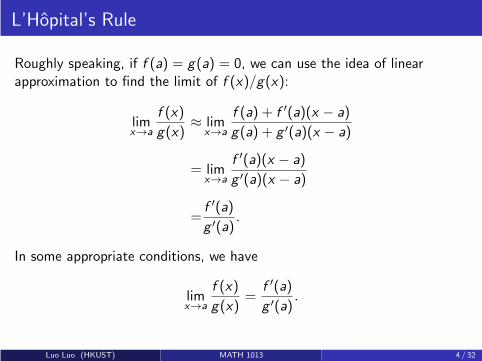
L’Hopital’s Rule
Roughly speaking, if f (a) = g(a) = 0, we can use the idea of linearapproximation to find the limit of f (x)/g(x):
limx→a
f (x)
g(x)≈ lim
x→a
f (a) + f ′(a)(x − a)
g(a) + g ′(a)(x − a)
= limx→a
f ′(a)(x − a)
g ′(a)(x − a)
=f ′(a)
g ′(a).
In some appropriate conditions, we have
limx→a
f (x)
g(x)=
f ′(a)
g ′(a).
Luo Luo (HKUST) MATH 1013 4 / 32

Baby L’Hopital’s Rule
Theorem (Baby L’Hopital’s Rule, 00-type)
Let f (x) and g(x) be continuous functions on an interval containingx = a, with f (a) = g(a) = 0. Suppose that f and g are differentiable, andf ′ and g ′ are continuous. Finally, suppose that g ′(a) 6= 0. Then
limx→a
f (x)
g(x)= lim
x→a
f ′(x)
g ′(x)=
f ′(a)
g ′(a).
We also have
limx→a+
f (x)
g(x)= lim
x→a+
f ′(x)
g ′(x)and lim
x→a−
f (x)
g(x)= lim
x→a−
f ′(x)
g ′(x).
Luo Luo (HKUST) MATH 1013 5 / 32
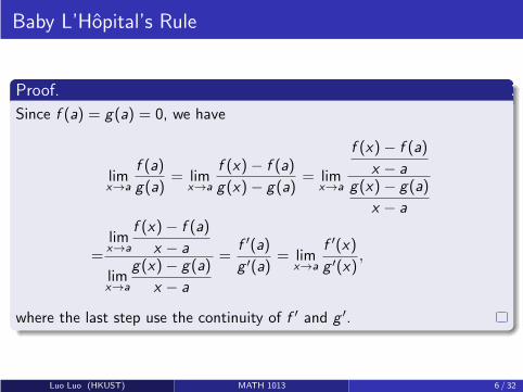
Baby L’Hopital’s Rule
Proof.
Since f (a) = g(a) = 0, we have
limx→a
f (a)
g(a)= lim
x→a
f (x)− f (a)
g(x)− g(a)= lim
x→a
f (x)− f (a)
x − ag(x)− g(a)
x − a
=limx→a
f (x)− f (a)
x − a
limx→a
g(x)− g(a)
x − a
=f ′(a)
g ′(a)= lim
x→a
f ′(x)
g ′(x),
where the last step use the continuity of f ′ and g ′.
Luo Luo (HKUST) MATH 1013 6 / 32

Macho L’Hopital’s Rule
Theorem (Macho L’Hopital’s Rule, one-side)
Suppose that f and g are continuous on a closed interval [a, b], and aredifferentiable on the open interval (a, b). Suppose that g ′(x) is never zero
on (a, b) and limx→a+
f ′(x)
g ′(x)exists, and that lim
x→a+f (x) = lim
x→a+g(x) = 0.
Then
limx→a+
f (x)
g(x)= lim
x→a+
f ′(x)
g ′(x).
This theorem doesn’t require anything about g ′(a), just about how g ′
behaves to the right of a.
The conclusion relates limit of f (x)/g(x) to another one-side limit off (x)′/g(x)′, and not to the value of f ′(a)/g ′(a).
Luo Luo (HKUST) MATH 1013 7 / 32

Macho L’Hopital’s Rule
Exercise/Tutorial
Prove Macho L’Hopital’s rule.
Hint: Although we do not suppose what is f (a) and g(a), we can define
F (x) =
{
0 x = a
f (x) x > aand G (x) =
{
0 x = a
g(x) x > a.
Then try to prove the following theorem and apply it.
Theorem (cauchy’s mean value theorem)
If F (x) and G (x) are continuous on [a, b] and differentiable on (a, b), thenthere is a point c in (a, b) such that
(F (b)− F (a))G ′(c) = (G (b)− G (a))F ′(c).
(when G (x) = x, this is the same as the usual mean value theorem)
Luo Luo (HKUST) MATH 1013 8 / 32

General form of L’Hopital’s Rule
The previous versions apply to forms of type∞∞ as well as
0
0, and apply to
limits as x → ∞ or x → −∞ as well as to limits x → a+ or x → a−. In allof these cases, the rule is:
limf (x)
g(x)= lim
f ′(x)
g ′(x).
baby form macho form general form
Luo Luo (HKUST) MATH 1013 9 / 32
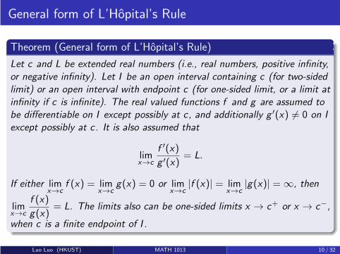
General form of L’Hopital’s Rule
Theorem (General form of L’Hopital’s Rule)
Let c and L be extended real numbers (i.e., real numbers, positive infinity,or negative infinity). Let I be an open interval containing c (for two-sidedlimit) or an open interval with endpoint c (for one-sided limit, or a limit atinfinity if c is infinite). The real valued functions f and g are assumed tobe differentiable on I except possibly at c, and additionally g ′(x) 6= 0 on Iexcept possibly at c. It is also assumed that
limx→c
f ′(x)
g ′(x)= L.
If either limx→c
f (x) = limx→c
g(x) = 0 or limx→c
|f (x)| = limx→c
|g(x)| = ∞, then
limx→c
f (x)
g(x)= L. The limits also can be one-sided limits x → c+ or x → c−,
when c is a finite endpoint of I .
Luo Luo (HKUST) MATH 1013 10 / 32

Examples of L’Hopital’s Rule
Example ( 00-type )
limx→0
sin x
x= lim
x→0
d sin x
dxdx
dx
= limx→0
cos x
1= cos 0 = 1.
However, this computation is somewhat stupid, because we have used
d sin x
dx= cos x .
We can directly obtain the result by the definition of derivative
limx→0
sin x
x= lim
x→0
sin x − sin 0
x − 0=
d sin x
dx
∣∣∣x=0
= cos 0 = 1.
Luo Luo (HKUST) MATH 1013 11 / 32
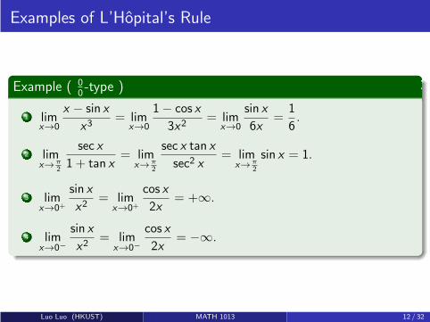
Examples of L’Hopital’s Rule
Example ( 00-type )
1 limx→0
x − sin x
x3= lim
x→0
1− cos x
3x2= lim
x→0
sin x
6x=
1
6.
2 limx→
π
2
sec x
1 + tan x= lim
x→π
2
sec x tan x
sec2 x= lim
x→π
2
sin x = 1.
3 limx→0+
sin x
x2= lim
x→0+
cos x
2x= +∞.
4 limx→0−
sin x
x2= lim
x→0−
cos x
2x= −∞.
Luo Luo (HKUST) MATH 1013 12 / 32

Examples of L’Hopital’s Rule
Example ( 00-type )
1 limx→2
x2 − 4
x3 − 8= lim
x→2
d
dx(x2 − 4)
d
dx(x3 − 8)
= limx→2
2x
3x2=
2 · 23 · 22 =
1
3
2 limx→0
x√3x + 4− 2
= limx→0
dx
dxd [(3x + 4)1/2 − 2]
dx
= limx→0
132(3x + 4)−1/2
= limx→0
2
3(3x + 4)1/2 =
4
3
Luo Luo (HKUST) MATH 1013 13 / 32
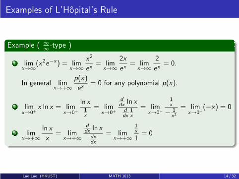
Examples of L’Hopital’s Rule
Example ( ∞
∞-type )
1 limx→∞
(x2e−x) = limx→∞
x2
ex= lim
x→∞
2x
ex= lim
x→∞
2
ex= 0.
In general limx→+∞
p(x)
ex= 0 for any polynomial p(x).
2 limx→0+
x ln x = limx→0+
ln x1x
= limx→0+
d
dxln x
d
dx
1x
= limx→0+
1x
− 1x2
= limx→0+
(−x) = 0
3 limx→+∞
ln x
x= lim
x→+∞
d
dxln xdx
dx
= limx→+∞
1x
1= 0
Luo Luo (HKUST) MATH 1013 14 / 32
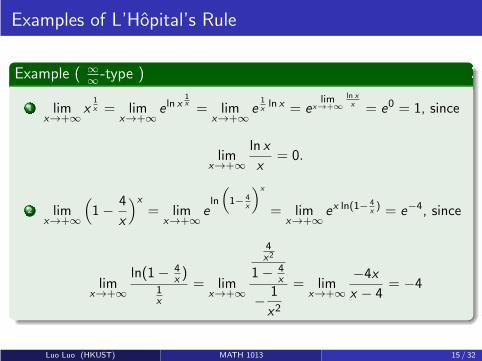
Examples of L’Hopital’s Rule
Example ( ∞
∞-type )
1 limx→+∞
x1x = lim
x→+∞
e ln x1x = lim
x→+∞
e1xln x = e
limx→+∞
ln x
x = e0 = 1, since
limx→+∞
ln x
x= 0.
2 limx→+∞
(
1− 4
x
)x
= limx→+∞
eln
(
1− 4x
)x
= limx→+∞
ex ln(1− 4x) = e−4, since
limx→+∞
ln(1− 4x)
1x
= limx→+∞
4x2
1− 4x
− 1
x2
= limx→+∞
−4x
x − 4= −4
Luo Luo (HKUST) MATH 1013 15 / 32

Outline
1 L’Hopital’s Rule
2 Common Mistakes when Using L’Hopital’s Rule
3 Convex Optimization
Luo Luo (HKUST) MATH 1013 16 / 32
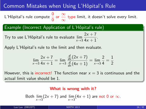
Common Mistakes when Using L’Hopital’s Rule
L’Hopital’s rule compute0
0or
∞∞ type limit, it doesn’t solve every limit.
Example (Incorrect Application of L’Hopital’s rule)
Try to use L’Hopital’s rule to evaluate limx→3
2x + 7
4x + 1.
Apply L’Hopital’s rule to the limit and then evaluate.
limx→3
2x + 7
4x + 1= lim
x→3
d
dx(2x + 7)
d
dx(4x + 1)
= limx→3
2
4=
1
2
However, this is incorrect! The function near x = 3 is continuous and theactual limit value should be 1.
What is wrong with it?
Both limx→3
(2x + 7) and limx→3
(4x + 1) are not 0 or ∞.
Luo Luo (HKUST) MATH 1013 16 / 32
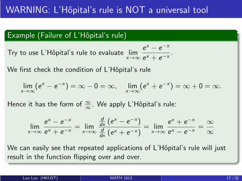
WARNING: L’Hopital’s rule is NOT a universal tool
Example (Failure of L’Hopital’s rule)
Try to use L’Hopital’s rule to evaluate limx→∞
ex − e−x
ex + e−x.
We first check the condition of L’Hopital’s rule
limx→∞
(ex − e−x) = ∞− 0 = ∞, limx→∞
(ex + e−x) = ∞+ 0 = ∞.
Hence it has the form of ∞
∞. We apply L’Hopital’s rule:
limx→∞
ex − e−x
ex + e−x= lim
x→∞
d
dx(ex − e−x)
d
dx(ex + e−x)
= limx→∞
ex + e−x
ex − e−x=
∞∞
We can easily see that repeated applications of L’Hopital’s rule will justresult in the function flipping over and over.
Luo Luo (HKUST) MATH 1013 17 / 32

WARNING: L’Hopital’s rule is NOT a universal tool
Example (Failure of L’Hopital’s rule)
It is easy to evaluate limx→∞
ex − e−x
ex + e−xby simplifying step at first.
We just need to multiplye−x
e−xas follows:
limx→∞
ex − e−x
ex + e−x= lim
x→∞
(ex − e−x)
(ex + e−x)· e
−x
e−x= lim
x→∞
1− e−2x
1 + e−2x=
1− 0
1 + 0= 1.
Luo Luo (HKUST) MATH 1013 18 / 32
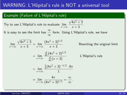
WARNING: L’Hopital’s rule is NOT a universal tool
Example (Failure of L’Hopital’s rule)
Try to use L’Hopital’s rule to evaluate limx→∞
√4x2 + 3
x + 3.
It is easy to see the limit has∞∞ form. Using L’Hopital’s rule, we have
limx→∞
√4x2 + 3
x + 3= lim
x→∞
(4x2 + 3)1/2
x + 3Rewriting the original limit
= limx→∞
d
dx(4x2 + 3)1/2
d
dx(x + 3)
L’Hopital’s rule
= limx→∞
12 (4x
2 + 3)−1/2 · 8x1
= limx→∞
4x
(4x2 + 3)1/2=
∞∞ .
Luo Luo (HKUST) MATH 1013 19 / 32
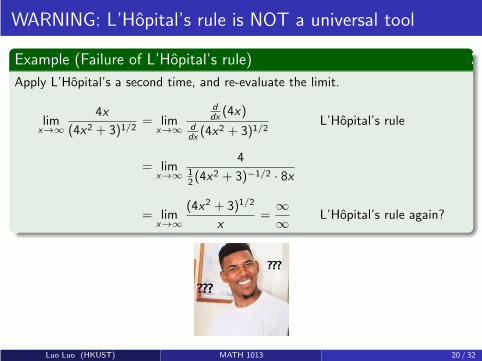
WARNING: L’Hopital’s rule is NOT a universal tool
Example (Failure of L’Hopital’s rule)
Apply L’Hopital’s a second time, and re-evaluate the limit.
limx→∞
4x
(4x2 + 3)1/2= lim
x→∞
d
dx(4x)
d
dx(4x2 + 3)1/2
L’Hopital’s rule
= limx→∞
412 (4x
2 + 3)−1/2 · 8x
= limx→∞
(4x2 + 3)1/2
x=
∞∞ L’Hopital’s rule again?
Luo Luo (HKUST) MATH 1013 20 / 32

WARNING: L’Hopital’s rule is NOT a universal tool
Example (Failure of L’Hopital’s rule)
· · · = limx→∞
(4x2 + 3)1/2
x= lim
x→∞
d
dx(4x2 + 3)1/2
d
dx(x)
= limx→∞
12 (4x
2 + 3)−1/2 · 8x1
= limx→∞
4x
(4x2 + 3)1/2
This is exactly the function we got at the start of last page! No matter how manytimes we try using L’Hopital’s’s rule, it will never yield a limit value. The processwill just keep cycling around and around.
Luo Luo (HKUST) MATH 1013 21 / 32

WARNING: L’Hopital’s rule is NOT a universal tool
L’Hopital’s rule guarantees that
limx→a
f (x)
g(x)= lim
x→a
f ′(x)
g ′(x)︸ ︷︷ ︸
if the limits exist, the limits are equal.
However, it does not guarantee the second limit can be evaluated.
Most of the time the second (or third, or fourth, or ...) limits we get fromthe rule have a simpler form and the new limit is more easily evaluated.But as this example shows, that isn’t always the case.
Instead of repeating L’Hopital’s rule, it is important (even critical) tosimplify the function at each stage.
Luo Luo (HKUST) MATH 1013 22 / 32

WARNING: L’Hopital’s rule is NOT a universal tool
Example (Failure of L’Hopital’s rule)
Factor the x2 out of the square-root:
limx→∞
√4x2 + 3
x + 3= lim
x→∞
√
x2(4 + 3
x2
)
x + 3= lim
x→∞
√x2 ·
√
4 + 3x2
x + 3
= limx→∞
|x | ·√
4 + 3x2
x + 3= lim
x→∞
x ·√
4 + 3x2
x + 3
Since x → ∞, we replace |x | with just x . Factor the x out of the denominator:
limx→∞
x ·√
4 + 3x2
x + 3= lim
x→∞
x ·√
4 + 3x2
x(1 + 3
x
) = limx→∞
√
4 + 3x2
1 + 3x
=lim
x→∞
√
4 + 3x2
limx→∞
(1 + 3x)
= 4.
Luo Luo (HKUST) MATH 1013 23 / 32
L’Hopital’s Rule
1 L’Hopital’s rule help us compute limits of the0
0or
∞∞ -type
2 L’Hopital’s rule is not a universal tool.
3 We must check the form of limit before applying L’Hopital’s rule.
4 Sometimes, simplifying the expression is more useful.
Luo Luo (HKUST) MATH 1013 24 / 32
Outline
1 L’Hopital’s Rule
2 Common Mistakes when Using L’Hopital’s Rule
3 Convex Optimization
Luo Luo (HKUST) MATH 1013 25 / 32

Convex Optimization
We study how to find the minimum of a convex function f .
This section is beyond the requirement of MATH 1013. It will NOTbeen contained in our homework or exam, however, it is very helpfulto understand the concepts of convex function, linear approximation,optimization problem and Newton methods (next week).
Luo Luo (HKUST) MATH 1013 25 / 32
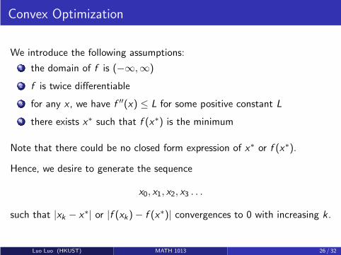
Convex Optimization
We introduce the following assumptions:
1 the domain of f is (−∞,∞)
2 f is twice differentiable
3 for any x , we have f ′′(x) ≤ L for some positive constant L
4 there exists x∗ such that f (x∗) is the minimum
Note that there could be no closed form expression of x∗ or f (x∗).
Hence, we desire to generate the sequence
x0, x1, x2, x3 . . .
such that |xk − x∗| or |f (xk)− f (x∗)| convergences to 0 with increasing k .
Luo Luo (HKUST) MATH 1013 26 / 32

Convex Optimization
Exercise
If f is twice differentiable on (a, b) and continuous on [a, b], then
f (b)− f (a)− f ′(a)(b − a) =f ′′(c)
2(b − a)2
for some c ∈ (a, b).
Let a = xk and b = x 6= xk , then there exists c such that
f (x) =f (xk) + f ′(xk)(x − xk) +f ′′(c)
2(x − xk)
2
≤f (xk) + f ′(xk)(x − xk) +L
2(x − xk)
2
Luo Luo (HKUST) MATH 1013 27 / 32
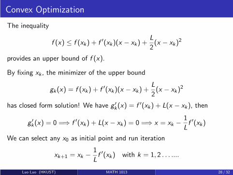
Convex Optimization
The inequality
f (x) ≤ f (xk) + f ′(xk)(x − xk) +L
2(x − xk)
2
provides an upper bound of f (x).
By fixing xk , the minimizer of the upper bound
gk(x) = f (xk) + f ′(xk)(x − xk) +L
2(x − xk)
2
has closed form solution! We have g ′
k(x) = f ′(xk) + L(x − xk), then
g ′
k(x) = 0 =⇒ f ′(xk) + L(x − xk) = 0 =⇒ x = xk −1
Lf ′(xk)
We can select any x0 as initial point and run iteration
xk+1 = xk −1
Lf ′(xk) with k = 1, 2 . . . ....
Luo Luo (HKUST) MATH 1013 28 / 32

Convex Optimization
For any initial point x0, the iteration scheme
xk+1 = xk −1
Lf ′(xk) with k = 1, 2 . . . ....
satisfies
f (xk)− f (x∗) ≤ |x0 − x∗|2Lk
.
Since |x0 − x∗| and L are independent to k , we have
limk→∞
|x0 − x∗|2Lk
= 0.
Hence, f (xk) convergences to f (x∗).
Luo Luo (HKUST) MATH 1013 29 / 32

Convex Optimization
If we additionally suppose f is strongly convex with constant c .
Then for any initial point x0, the iteration scheme
xk+1 = xk −1
Lf ′(xk) with k = 1, 2 . . . ....
satisfies
f (xk)− f (x∗) ≤(
1− c
L
)k
(f (x0)− f (x∗)).
In fact, we can prove c ≤ L which means
limk→∞
(
1− c
L
)k
(f (x0)− f (x∗)) = 0.
Hence, f (xk) convergences to f (x∗).
Luo Luo (HKUST) MATH 1013 30 / 32

Convex Optimization
By comparing the convergence result
f (xk)− f (x∗) ≤ |x0 − x∗|2Lk
for convex f
and
f (xk)− f (x∗) ≤(
1− c
L
)k
(f (x0)− f (x∗)) for strongly convex f ,
we have
limk→∞
(
1− c
L
)k
(f (x0)− f (x∗))
|x0 − x∗|2Lk
= 0.
Luo Luo (HKUST) MATH 1013 31 / 32

Convex Optimization
The iteration
xk+1 = xk −1
Lf ′(xk) with k = 1, 2 . . . ....
is called gradient descent, which is the most popular method to find theminimum of a convex function.
A convex function on a closed interval I must have a maximum on theendpoint of I .
Luo Luo (HKUST) MATH 1013 32 / 32

Calculus IB: Lecture 17
Luo Luo
Department of Mathematics, HKUST
http://luoluo.people.ust.hk/
Luo Luo (HKUST) MATH 1013 1 / 29

Outline
1 Newton’s Method: Algorithm
2 Newton’s Method: Convergence Analysis
3 Newton’s Method: Application in Convex Optimization
Luo Luo (HKUST) MATH 1013 2 / 29

Outline
1 Newton’s Method: Algorithm
2 Newton’s Method: Convergence Analysis
3 Newton’s Method: Application in Convex Optimization
Luo Luo (HKUST) MATH 1013 3 / 29

Newton’s Method
Newton’s method, also known as the Newton–Raphson method, namedafter Isaac Newton and Joseph Raphson (who can provide a picture/photoof Raphson?), is a root-finding algorithm.
Sir Isaac Newton (1642-1726), the greatest scientist of all time.
Luo Luo (HKUST) MATH 1013 3 / 29
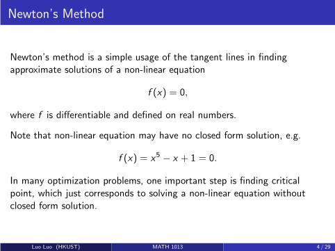
Newton’s Method
Newton’s method is a simple usage of the tangent lines in findingapproximate solutions of a non-linear equation
f (x) = 0,
where f is differentiable and defined on real numbers.
Note that non-linear equation may have no closed form solution, e.g.
f (x) = x5 − x + 1 = 0.
In many optimization problems, one important step is finding criticalpoint, which just corresponds to solving a non-linear equation withoutclosed form solution.
Luo Luo (HKUST) MATH 1013 4 / 29

Newton’s Method
The Newton’s method generates sequence
x0, x1, x2, x3 . . .
such that f (xk) converges to 0 with increasing k .
The basic idea is applying linear approximation on f (x) at given xk
f (x) ≈ f (xk) + f ′(xk)(x − xk).
Then we solve the linear equation
f (xk) + f ′(xk)(x − xk) = 0
is an approximation of solving f (x) = 0.
Luo Luo (HKUST) MATH 1013 5 / 29
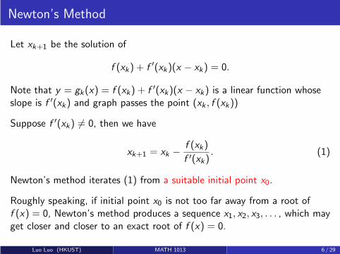
Newton’s Method
Let xk+1 be the solution of
f (xk) + f ′(xk)(x − xk) = 0.
Note that y = gk(x) = f (xk) + f ′(xk)(x − xk) is a linear function whoseslope is f ′(xk) and graph passes the point (xk , f (xk))
Suppose f ′(xk) 6= 0, then we have
xk+1 = xk −f (xk)
f ′(xk). (1)
Newton’s method iterates (1) from a suitable initial point x0.
Roughly speaking, if initial point x0 is not too far away from a root off (x) = 0, Newton’s method produces a sequence x1, x2, x3, . . . , which mayget closer and closer to an exact root of f (x) = 0.
Luo Luo (HKUST) MATH 1013 6 / 29
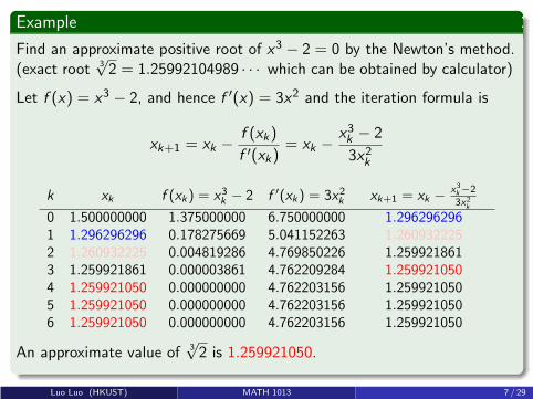
Example
Find an approximate positive root of x3 − 2 = 0 by the Newton’s method.(exact root 3
√2 = 1.25992104989 · · · which can be obtained by calculator)
Let f (x) = x3 − 2, and hence f ′(x) = 3x2 and the iteration formula is
xk+1 = xk −f (xk)
f ′(xk)= xk −
x3k− 2
3x2k
k xk f (xk) = x3k− 2 f ′(xk) = 3x2
kxk+1 = xk − x
3k−2
3x2k
0 1.500000000 1.375000000 6.750000000 1.2962962961 1.296296296 0.178275669 5.041152263 1.2609322252 1.260932225 0.004819286 4.769850226 1.2599218613 1.259921861 0.000003861 4.762209284 1.2599210504 1.259921050 0.000000000 4.762203156 1.2599210505 1.259921050 0.000000000 4.762203156 1.2599210506 1.259921050 0.000000000 4.762203156 1.259921050
An approximate value of 3√2 is 1.259921050.
Luo Luo (HKUST) MATH 1013 7 / 29

Newton’s Method
Convergence behavior of xk and f (xk) with iterations:
0 1 2 3 4 5 6
0
0.5
1
1.5
Luo Luo (HKUST) MATH 1013 8 / 29
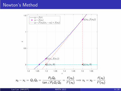
Newton’s Method
1.2 1.25 1.3 1.35 1.4 1.45 1.5 1.55
0
0.5
1
1.5
x0 − x1 = Q1Q0 =P0Q0
tan∠P0Q1Q0=
f (x0)
f ′(x0)=⇒ x1 = x0 −
f (x0)
f ′(x0)
Luo Luo (HKUST) MATH 1013 9 / 29
Newton’s Method
Exercise
Find an approximate value of the root of the equation
cos x − x = 0
by the Newton’s Method (using calculator or MATLAB).
Luo Luo (HKUST) MATH 1013 10 / 29
Outline
1 Newton’s Method: Algorithm
2 Newton’s Method: Convergence Analysis
3 Newton’s Method: Application in Convex Optimization
Luo Luo (HKUST) MATH 1013 11 / 29

Convergence Analysis
Above example show that Newton’s method
xk+1 = xk −f (xk)
f ′(xk).
produces a sequencex1, x2, x3, . . .
which converge to the solution x∗ such that f (x∗) = 0.
We impose the following assumptions to further analysis
1 the function f is differentiable
2 there exists positive µ such that |f ′(x)| ≥ µ for all x
3 there exists positive C such that |f ′′(x)| ≤ C for all x
4 the initial point is NOT far away form x∗
(We typically suppose f ′(x) is C -Lipschitz continuous, rather than |f ′′(x)| ≤ C ,but the related analysis needs some techniques beyond MATH 1013.)
Luo Luo (HKUST) MATH 1013 11 / 29
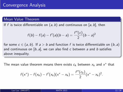
Convergence Analysis
Mean Value Theorem
If f is twice differentiable on (a, b) and continuous on [a, b], then
f (b)− f (a)− f ′(a)(b − a) =f ′′(c)
2(b − a)2
for some c ∈ (a, b). If a > b and function f is twice differentiable on (b, a)and continuous on [b, a], we can also find c between a and b satisfiesabove inequality.
The mean value theorem means there exists ck between xk and x∗ that
f (x∗)− f (xk)− f ′(xk)(x∗ − xk) =
f ′′(ck)
2(x∗ − xk)
2.
Luo Luo (HKUST) MATH 1013 12 / 29

Convergence Analysis
Using the iteration of Newton’s Method
xk+1 = xk −f (xk)
f ′(xk).
and the result from mean value theorem
f (x∗)− f (xk)− f ′(xk)(x∗ − xk) =
f ′′(ck)
2(x∗ − xk)
2,
we have
|xk+1 − x∗| =∣
∣
∣
∣
xk −f (xk)
f ′(xk)− x∗
∣
∣
∣
∣
=1
|f ′(xk)|∣
∣f ′(xk) · (xk − x∗)− (f (xk)− f (x∗))∣
∣
=1
|f ′(xk)|
∣
∣
∣
∣
f ′′(ck)
2(x∗ − xk)
2
∣
∣
∣
∣
=|f ′′(ck)|2|f ′(xk)|
|xk − x∗|2
Luo Luo (HKUST) MATH 1013 13 / 29
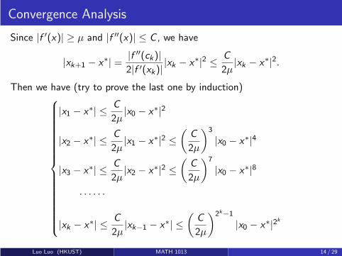
Convergence Analysis
Since |f ′(x)| ≥ µ and |f ′′(x)| ≤ C , we have
|xk+1 − x∗| = |f ′′(ck)|2|f ′(xk)|
|xk − x∗|2 ≤ C
2µ|xk − x∗|2.
Then we have (try to prove the last one by induction)
|x1 − x∗| ≤ C
2µ|x0 − x∗|2
|x2 − x∗| ≤ C
2µ|x1 − x∗|2 ≤
(
C
2µ
)3
|x0 − x∗|4
|x3 − x∗| ≤ C
2µ|x2 − x∗|2 ≤
(
C
2µ
)7
|x0 − x∗|8
· · · · · ·
|xk − x∗| ≤ C
2µ|xk−1 − x∗| ≤
(
C
2µ
)2k−1
|x0 − x∗|2k
Luo Luo (HKUST) MATH 1013 14 / 29
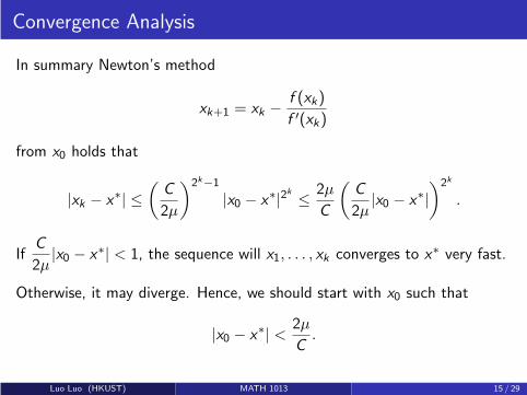
Convergence Analysis
In summary Newton’s method
xk+1 = xk −f (xk)
f ′(xk)
from x0 holds that
|xk − x∗| ≤(
C
2µ
)2k−1
|x0 − x∗|2k ≤ 2µ
C
(
C
2µ|x0 − x∗|
)2k
.
IfC
2µ|x0 − x∗| < 1, the sequence will x1, . . . , xk converges to x∗ very fast.
Otherwise, it may diverge. Hence, we should start with x0 such that
|x0 − x∗| < 2µ
C.
Luo Luo (HKUST) MATH 1013 15 / 29
Outline
1 Newton’s Method: Algorithm
2 Newton’s Method: Convergence Analysis
3 Newton’s Method: Application in Convex Optimization
Luo Luo (HKUST) MATH 1013 16 / 29
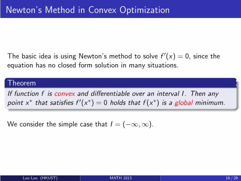
Newton’s Method in Convex Optimization
The basic idea is using Newton’s method to solve f ′(x) = 0, since theequation has no closed form solution in many situations.
Theorem
If function f is convex and differentiable over an interval I . Then any
point x∗ that satisfies f ′(x∗) = 0 holds that f (x∗) is a global minimum.
We consider the simple case that I = (−∞,∞).
Luo Luo (HKUST) MATH 1013 16 / 29

Newton’s Method in Convex Optimization
Impose previous assumption on f ′:
1 the function f ′ differentiable
2 there exists positive µ such that |f ′′(x)| ≥ µ for all x
3 there exists positive C such that |f ′′′(x)| ≤ C for all x
4 the initial point x0 satisfies |x0 − x∗| < 2µC
In the view of convex optimization:
1 the function f is twice differentiable
2 the function f is strongly convex with factor µ > 0, i.e. f ′′(x) ≥ µ.
3 there exists positive C such that |f ′′′(x)| ≤ C for all x
4 the initial point x0 satisfies |x0 − x∗| < 2µC
The third one typically can be replaced by “there exists C > 0 such thatfor any x1 and x2, we have |f ′′(x1)− f ′′(x2)| ≤ C |x1 − x2|”.
Luo Luo (HKUST) MATH 1013 17 / 29
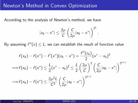
Newton’s Method in Convex Optimization
According to the analysis of Newton’s method, we have
|xk − x∗| ≤ 2µ
C
(
C
2µ|x0 − x∗|
)2k
.
By assuming f ′′(x) ≤ L, we can establish the result of function value
f (xk)− f (x∗)− f ′(x∗)(xk − x∗) =f ′′(ck)
2(x∗ − xk)
2
=⇒f (xk)− f (x∗) ≤ L
2(x∗ − xk)
2 ≤ L
2
(
2µ
C
)2(C
2µ|x0 − x∗|
)2k+1
=⇒f (xk)− f (x∗) ≤ 2µ2L
C 2
(
C
2µ|x0 − x∗|
)2k+1
Luo Luo (HKUST) MATH 1013 18 / 29
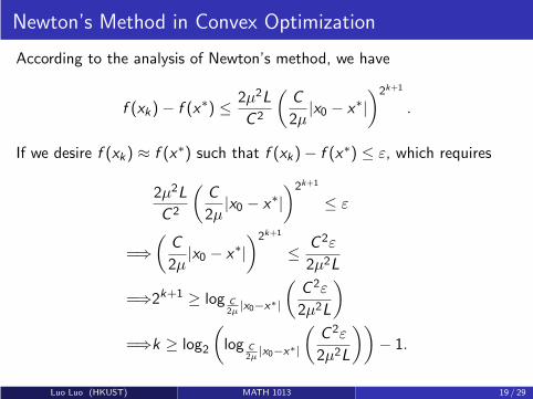
Newton’s Method in Convex Optimization
According to the analysis of Newton’s method, we have
f (xk)− f (x∗) ≤ 2µ2L
C 2
(
C
2µ|x0 − x∗|
)2k+1
.
If we desire f (xk) ≈ f (x∗) such that f (xk)− f (x∗) ≤ ε, which requires
2µ2L
C 2
(
C
2µ|x0 − x∗|
)2k+1
≤ ε
=⇒(
C
2µ|x0 − x∗|
)2k+1
≤ C 2ε
2µ2L
=⇒2k+1 ≥ log C
2µ|x0−x∗|
(
C 2ε
2µ2L
)
=⇒k ≥ log2
(
log C
2µ|x0−x∗|
(
C 2ε
2µ2L
))
− 1.
Luo Luo (HKUST) MATH 1013 19 / 29
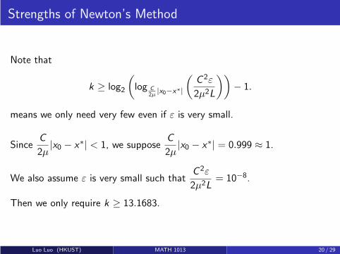
Strengths of Newton’s Method
Note that
k ≥ log2
(
log C
2µ|x0−x∗|
(
C 2ε
2µ2L
))
− 1.
means we only need very few even if ε is very small.
SinceC
2µ|x0 − x∗| < 1, we suppose
C
2µ|x0 − x∗| = 0.999 ≈ 1.
We also assume ε is very small such thatC 2ε
2µ2L= 10−8.
Then we only require k ≥ 13.1683.
Luo Luo (HKUST) MATH 1013 20 / 29
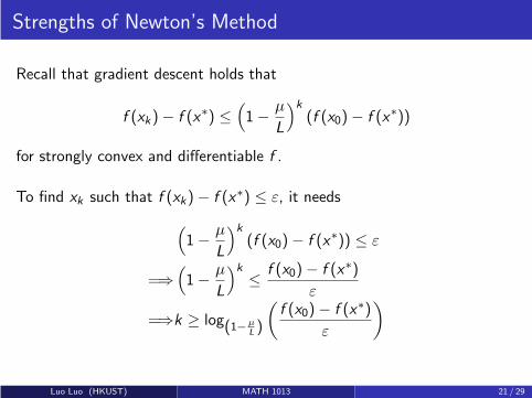
Strengths of Newton’s Method
Recall that gradient descent holds that
f (xk)− f (x∗) ≤(
1− µ
L
)k
(f (x0)− f (x∗))
for strongly convex and differentiable f .
To find xk such that f (xk)− f (x∗) ≤ ε, it needs
(
1− µ
L
)k
(f (x0)− f (x∗)) ≤ ε
=⇒(
1− µ
L
)k
≤ f (x0)− f (x∗)
ε
=⇒k ≥ log(1−µ
L)
(
f (x0)− f (x∗)
ε
)
Luo Luo (HKUST) MATH 1013 21 / 29

Strengths of Newton’s Method
If it is desired a very very accuracy approximation, we only interested inhow ε affects k since ε is much smaller than other terms.
Then gradient descent needs
k ≥ logC1(C2ε)
and Newton’s method needs
k ≥ log2(
logC3(C4ε)
)
.
We have (try to show that by L’Hopital’s rule as an exercise)
limε→0+
log2(
logC3(C4ε)
)
logC1(C2ε)
= 0.
Luo Luo (HKUST) MATH 1013 22 / 29
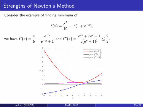
Strengths of Newton’s Method
Consider the example of finding minimum of
f (x) =x2
10+ ln(1 + e−x),
we have f ′(x) =x
5− e−x
e−x + 1and f ′′(x) =
e2x + 7e2 + 1
5(ex + 1)2≤ 9
2.
-5 -4 -3 -2 -1 0 1 2 3 4 5
-2
-1
0
1
2
3
4
5
6
7
8
Luo Luo (HKUST) MATH 1013 23 / 29
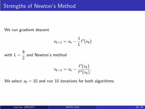
Strengths of Newton’s Method
We run gradient descent
xk+1 = xk −1
Lf ′(xk)
with L =9
2and Newton’s method
xk+1 = xk −f ′(xk)
f ′′(xk).
We select x0 = 10 and run 10 iterations for both algorithms.
Luo Luo (HKUST) MATH 1013 24 / 29

Strengths of Newton’s Method
The convergence behavior of f (x) and ln |f ′(x)|. In theoretical, |f ′(x)|should tend to 0 which leads to ln |f ′(x)| → −∞, but the computercannot present too small magnitude of a real number if it is not 0.
0 2 4 6 8 10
number of iterations
0
10
20
30
40
50
60
70
80
Gradient Descent
Newton's Method
0 2 4 6 8 10
number of iterations
-40
-30
-20
-10
0
10
Gradient Descent
Newton's Method
Luo Luo (HKUST) MATH 1013 25 / 29
Weakness of Newton’s Method
The initial point x0 of Newton’s method should be near x∗:
C
2µ|x0 − x∗| < 1.
Unfortunately, there is no good strategy to select x0 for general f since wedo not know what is x∗ at first.
In other words, the convergence of Newton’s method is local, not global.
On the other hand, gradient descent could converge to the optimalsolution with any initial point x0 (global convergence).
Luo Luo (HKUST) MATH 1013 26 / 29

Weakness of Newton’s Method
Newton’s method depends on the twice differentiability while gradientdescent only requires first differentiability.
Newton’s method works only if f ′′(xk) 6= 0 which is unnecessary forgradient descent.
If f has many input variables, the computational cost of Newton’s methodis much more expensive than gradient descent.
Luo Luo (HKUST) MATH 1013 27 / 29

Weakness of Newton’s Method
Consider using Newton’s method to solve
f (x) = x2 − 5 = 0.
If we let x0 = 0, then f ′(x0) = 2x0 = 0 and the update
x1 = x0 −f (x0)
f ′(x0)is undefined.
Luo Luo (HKUST) MATH 1013 28 / 29
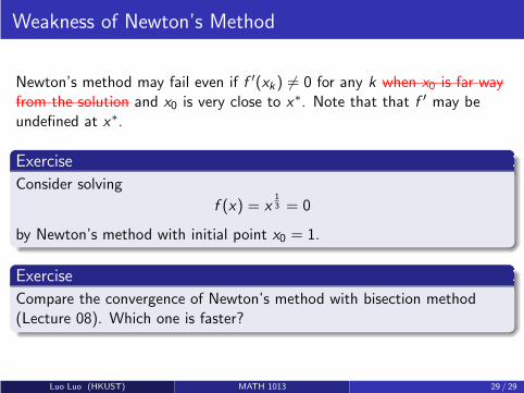
Weakness of Newton’s Method
Newton’s method may fail even if f ′(xk) 6= 0 for any k when x0 is far wayfrom the solution and x0 is very close to x∗. Note that that f ′ may beundefined at x∗.
Exercise
Consider solving
f (x) = x13 = 0
by Newton’s method with initial point x0 = 1.
Exercise
Compare the convergence of Newton’s method with bisection method(Lecture 08). Which one is faster?
Luo Luo (HKUST) MATH 1013 29 / 29

Calculus IB: Lecture 18
Luo Luo
Department of Mathematics, HKUST
http://luoluo.people.ust.hk/
Luo Luo (HKUST) MATH 1013 1 / 33
Outline
1 Antiderivatives/Indefinite Integral
2 The Substitution Rule
3 Integration by Parts
Luo Luo (HKUST) MATH 1013 2 / 33
Outline
1 Antiderivatives/Indefinite Integral
2 The Substitution Rule
3 Integration by Parts
Luo Luo (HKUST) MATH 1013 3 / 33
Antiderivatives
1 Differentiation problem: Given a function f −→ finddf
dx.
2 Reversing the process: Given a function f −→ find a function F
such that F ′ = f .
3 This can also be considered as a question of solving the “differentialequation”
d
dx(which function) = f (x) .
4 Any function F satisfying F ′ = f is called an antiderivative (or aprimitive function) of f .
Luo Luo (HKUST) MATH 1013 3 / 33
Antiderivatives
1 Any function F satisfying F ′ = f is called an antiderivative (or aprimitive function) of f .
2 Obviously, if F is an antiderivative of f , then so is F + C for any
constant C , sincedC
dx= 0.
3 Note that if F and G are two antiderivatives of f on an open interval,then we have
(F − G )′ = F ′ − G ′ = f − f = 0 .
By the mean value theorem, F − G must then be a constant functionon the interval; i.e., G (x)− F (x) = C for some constant C .
Luo Luo (HKUST) MATH 1013 4 / 33
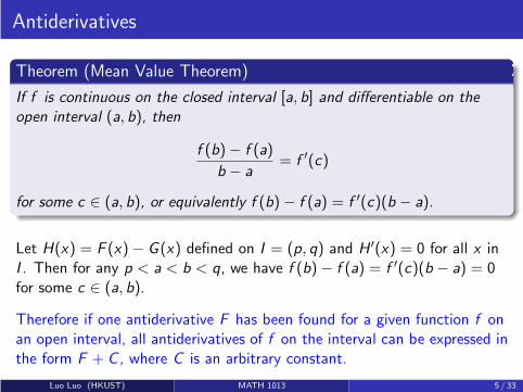
Antiderivatives
Theorem (Mean Value Theorem)
If f is continuous on the closed interval [a, b] and differentiable on the
open interval (a, b), then
f (b)− f (a)
b − a= f ′(c)
for some c ∈ (a, b), or equivalently f (b)− f (a) = f ′(c)(b − a).
Let H(x) = F (x)− G (x) defined on I = (p, q) and H ′(x) = 0 for all x inI . Then for any p < a < b < q, we have f (b)− f (a) = f ′(c)(b − a) = 0for some c ∈ (a, b).
Therefore if one antiderivative F has been found for a given function f onan open interval, all antiderivatives of f on the interval can be expressed inthe form F + C , where C is an arbitrary constant.
Luo Luo (HKUST) MATH 1013 5 / 33

Antiderivatives
Example
Let f (x) = 3x2. Solve the antiderivative problem:d
dx(?) = 3x2.
Knowing thatdx3
dx= 3x2,
the antiderivatives of 3x2 are given by x3 + C , where C is an arbitraryconstant.
Luo Luo (HKUST) MATH 1013 6 / 33

Antiderivatives
Example
Let g(x) = 2 cos x . Solve the antiderivative problem:d
dx(?) = 2 cos x .
Sinced sin x
dx= cos x ,
it easy to see thatd(2 sin x)
dx= 2 cos x .
Hence the antiderivatives of 2 cos x are given by 2 sin x + C , where C is anarbitrary constant.
Luo Luo (HKUST) MATH 1013 7 / 33

Antiderivatives
Example
Let h(x) = x + e2x . Solve the antiderivative problem:d
dx(?) = x + e2x
Sincedx2
dx= 2x and
de2x
dx= 2e2x ,
we haved
dx
(1
2x2 +
1
2e2x
)
= x + e2x .
Hence, the antiderivatives of h(x) = x + e2x are given by
(
1
2x2 +
1
2e2x
)
+ C .
Luo Luo (HKUST) MATH 1013 8 / 33

Indefinite Integral
The indefinite integral notation
∫
f (x)dx
is nothing but a new dress of the antiderivatives! The function f (x)appearing in an indefinite integral is usually called the integrand.
Luo Luo (HKUST) MATH 1013 9 / 33
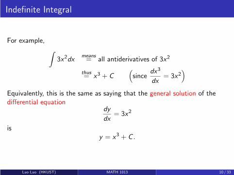
Indefinite Integral
For example,
∫
3x2dxmeans= all antiderivatives of 3x2
thus= x3 + C
(
sincedx3
dx= 3x2
)
Equivalently, this is the same as saying that the general solution of thedifferential equation
dy
dx= 3x2
isy = x3 + C .
Luo Luo (HKUST) MATH 1013 10 / 33

Indefinite Integral
Example
Show that
∫
(2x + 1)ex2+xdx = ex
2+x + C .
This is just another way to say
d
dx(ex
2+x) = ex2+x · d(x
2 + x)
dx= (2x + 1)ex
2+x .
(2x + 1)ex2+x
is the derivative of
ex2+x
vs⇐⇒ex
2+x
is an antiderivative of
(2x + 1)ex2+x
Luo Luo (HKUST) MATH 1013 11 / 33

Indefinite Integral
In fact, we have∫
f (x)dx = F (x) + C ⇐⇒ dF
dx= f (x).
In particular,d
dx
∫
f (x)dx = f (x),
and∫
f ′(x)dx = f (x) + C .
Luo Luo (HKUST) MATH 1013 12 / 33

Indefinite Integral
d
dx
1
p + 1xp+1 = xp
p 6=−1⇐⇒∫
xpdx =1
p + 1xp+1 + C
d
dxex = ex ⇐⇒
∫
exdx = ex + C
d
dxln |x | = 1
x⇐⇒
∫
1
xdx = ln |x |+ C
d
dxsin x = cos x ⇐⇒
∫
cos xdx = sin x + C
d
dx[− cos x ] = sin x ⇐⇒
∫
sin xdx = − cos x + C
d
dxtan x = sec2 x ⇐⇒
∫
sec2 xdx = tan x + C
...
Luo Luo (HKUST) MATH 1013 13 / 33
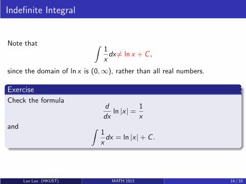
Indefinite Integral
Note that∫
1
xdx 6= ln x + C ,
since the domain of ln x is (0,∞), rather than all real numbers.
Exercise
Check the formulad
dxln |x | = 1
x
and∫
1
xdx = ln |x |+ C .
Luo Luo (HKUST) MATH 1013 14 / 33
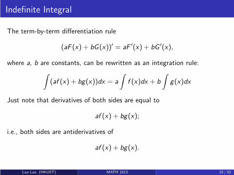
Indefinite Integral
The term-by-term differentiation rule
(aF (x) + bG (x))′ = aF ′(x) + bG ′(x),
where a, b are constants, can be rewritten as an integration rule:
∫
(af (x) + bg(x))dx = a
∫
f (x)dx + b
∫
g(x)dx
Just note that derivatives of both sides are equal to
af (x) + bg(x);
i.e., both sides are antiderivatives of
af (x) + bg(x).
Luo Luo (HKUST) MATH 1013 15 / 33

Indefinite Integral
Example
1
∫
(
3x4 − 2x3)
dx = 3
∫
x4dx − 2
∫
x3dx =3
5x5 − 1
2x4 + C
2
∫(
x5 − ex +1
x
)
dx =
∫
x5dx −∫
exdx +
∫
1
xdx
=1
6x6 − ex + ln |x |+ C
3
∫
(
3 sin x − 2 sec2 x + 3ex)
dx = −3 cos x − 2 tan x + 3ex + C
Luo Luo (HKUST) MATH 1013 16 / 33
Outline
1 Antiderivatives/Indefinite Integral
2 The Substitution Rule
3 Integration by Parts
Luo Luo (HKUST) MATH 1013 17 / 33
The Substitution Rule
So far, most of our integrals could be found directly, up to some algebraicmanipulations.
When an integral looks complicated, without an obvious antiderivative,quite often we need to make it simpler by using a suitable “substitution”.
Luo Luo (HKUST) MATH 1013 17 / 33

The Substitution Rule
If you knowd
dxsin x2 = 2x cos x2,
then it is of course straightforward to write∫
2x cos x2dx = sin x2 + C .
What if you don’t know the derivative?
Let u = x2, so thatdu
dx= 2x .
Now, by formally writing du = 2xdx and putting everything into theoriginal integral, we have
∫
2x cos x2dx =
∫
cos udueasy= sin u + C = sin x2 + C
Luo Luo (HKUST) MATH 1013 18 / 33
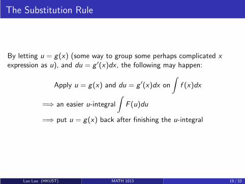
The Substitution Rule
By letting u = g(x) (some way to group some perhaps complicated x
expression as u), and du = g ′(x)dx , the following may happen:
Apply u = g(x) and du = g ′(x)dx on
∫
f (x)dx
=⇒ an easier u-integral
∫
F (u)du
=⇒ put u = g(x) back after finishing the u-integral
Luo Luo (HKUST) MATH 1013 19 / 33
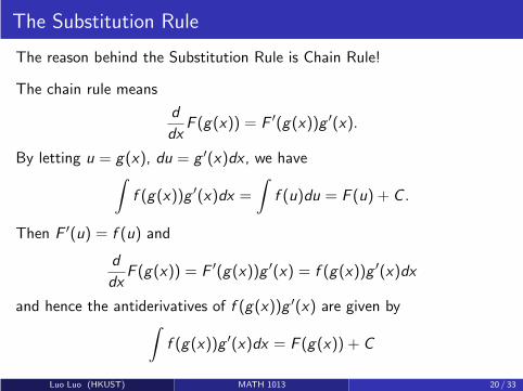
The Substitution Rule
The reason behind the Substitution Rule is Chain Rule!
The chain rule means
d
dxF (g(x)) = F ′(g(x))g ′(x).
By letting u = g(x), du = g ′(x)dx , we have∫
f (g(x))g ′(x)dx =
∫
f (u)du = F (u) + C .
Then F ′(u) = f (u) and
d
dxF (g(x)) = F ′(g(x))g ′(x) = f (g(x))g ′(x)dx
and hence the antiderivatives of f (g(x))g ′(x) are given by∫
f (g(x))g ′(x)dx = F (g(x)) + C
Luo Luo (HKUST) MATH 1013 20 / 33

The Substitution Rule
Theorem
If u = g(x) is a differentiable function whose range is an interval I , and
f (x) is continuous on I , then
∫
f (g(x))g ′(x)dx =
∫
f (u)du.
Luo Luo (HKUST) MATH 1013 21 / 33
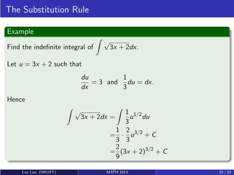
The Substitution Rule
Example
Find the indefinite integral of
∫ √3x + 2dx .
Let u = 3x + 2 such that
du
dx= 3 and
1
3du = dx .
Hence∫ √
3x + 2dx =
∫
1
3u1/2du
=1
3· 23u3/2 + C
=2
9(3x + 2)3/2 + C
Luo Luo (HKUST) MATH 1013 22 / 33

The Substitution Rule
Example
Find the indefinite integral of
∫
sin(5x + 2)dx .
Let u = 5x + 2 such that
du
dx= 5 and
1
5du = dx .
Hence∫
sin(5x + 2)dx =
∫
1
5sin udu
=− 1
5cos u + C
=− 1
5cos(5x + 2) + C
Luo Luo (HKUST) MATH 1013 23 / 33
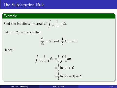
The Substitution Rule
Example
Find the indefinite integral of
∫
1
2x + 1dx .
Let u = 2x + 1 such that
du
dx= 2 and
1
2du = dx .
Hence∫
1
2x + 1dx =
1
2
∫
1
udu
=1
2ln |u|+ C
=1
2ln |2x + 1|+ C
Luo Luo (HKUST) MATH 1013 24 / 33
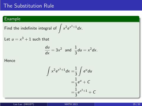
The Substitution Rule
Example
Find the indefinite integral of
∫
x2ex3+1dx .
Let u = x3 + 1 such that
du
dx= 3x2 and
1
3du = x2dx .
Hence∫
x2ex3+1dx =
1
3
∫
eudu
=1
3eu + C
=1
3ex
3+1 + C
Luo Luo (HKUST) MATH 1013 25 / 33
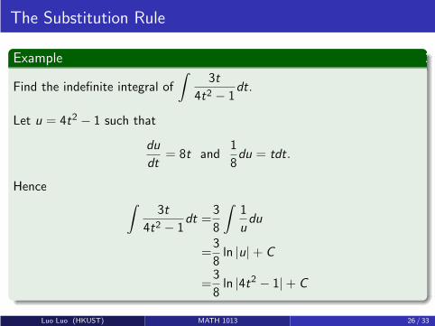
The Substitution Rule
Example
Find the indefinite integral of
∫
3t
4t2 − 1dt.
Let u = 4t2 − 1 such that
du
dt= 8t and
1
8du = tdt.
Hence∫
3t
4t2 − 1dt =
3
8
∫
1
udu
=3
8ln |u|+ C
=3
8ln |4t2 − 1|+ C
Luo Luo (HKUST) MATH 1013 26 / 33

The Substitution Rule
Exercise
Find the following indefinite integral
1
∫
x√x2 + 1
dx
2
∫
sec xdx (hint: let u = sec x + tan x)
3
∫
sin3 θdθ
4
∫
cos3 θdθ
5
∫
xe6x2dx
Luo Luo (HKUST) MATH 1013 27 / 33
Outline
1 Antiderivatives/Indefinite Integral
2 The Substitution Rule
3 Integration by Parts
Luo Luo (HKUST) MATH 1013 28 / 33
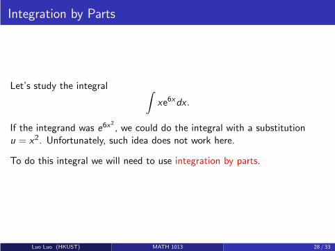
Integration by Parts
Let’s study the integral∫
xe6xdx .
If the integrand was e6x2, we could do the integral with a substitution
u = x2. Unfortunately, such idea does not work here.
To do this integral we will need to use integration by parts.
Luo Luo (HKUST) MATH 1013 28 / 33

Integration by Parts
We’ll start with the product rule of derivative
[f (x)g(x)]′ = f ′(x)g(x) + f (x)g ′(x)
Now integrate both sides of this formula
f (x)g(x) =
∫
[f (x)g(x)]′ dx
=
∫
[
f ′(x)g(x) + f (x)g ′(x)]
dx
=
∫
f ′(x)g(x)dx +
∫
f (x)g ′(x)dx
Substituting u = f (x), v = g(x), du = f ′(x)dx and dv = g ′(x)dx , then
∫
udv = uv −∫
vdu
Luo Luo (HKUST) MATH 1013 29 / 33

Integration by Parts
The following formula is called integration by parts
∫
udv = uv −∫
vdu
To use this formula, we will need to identify u and dv , then compute
∫
vdu
Luo Luo (HKUST) MATH 1013 30 / 33

Integration by Parts
Example
Find the indefinite integral of
∫
xe6xdx .
Let u = x and dv = e6xdx , then du = dx and
v =
∫
e6xdx =1
6e6x
Using integration by parts, we have
∫
xe6xdx =
∫
udv = uv −∫
vdu
=x
6e6x −
∫
1
6e6xdx =
x
6e6x − 1
36e6x + C
Luo Luo (HKUST) MATH 1013 31 / 33
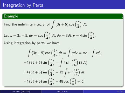
Integration by Parts
Example
Find the indefinite integral of
∫
(3t + 5) cos( t
4
)
dt.
Let u = 3t + 5, dv = cos( t
4
)
dt, du = 3dt, v = 4 sin( t
4
)
.
Using integration by parts, we have
∫
(3t + 5) cos( t
4
)
dt =
∫
udv = uv −∫
vdu
=4 (3t + 5) sin( t
4
)
−∫
4 sin( t
4
)
(3dt)
=4 (3t + 5) sin( t
4
)
− 12
∫
sin( t
4
)
dt
=4 (3t + 5) sin( t
4
)
+ 48 cos( t
4
)
+ C
Luo Luo (HKUST) MATH 1013 32 / 33
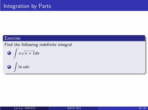
Integration by Parts
Exercise
Find the following indefinite integral
1
∫
x√x + 1dx
2
∫
ln xdx
Luo Luo (HKUST) MATH 1013 33 / 33

Calculus IB: Lecture 19
Luo Luo
Department of Mathematics, HKUST
http://luoluo.people.ust.hk/
Luo Luo (HKUST) MATH 1013 1 / 28

Outline
1 Initial Value Problems
2 Area under Curve
3 Riemann Sums and Definite Integrals
Luo Luo (HKUST) MATH 1013 2 / 28

Outline
1 Initial Value Problems
2 Area under Curve
3 Riemann Sums and Definite Integrals
Luo Luo (HKUST) MATH 1013 3 / 28
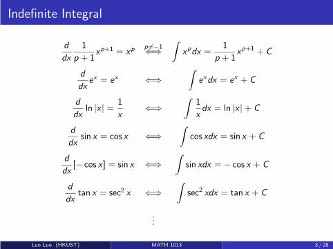
Indefinite Integral
d
dx
1
p + 1xp+1 = xp
p 6=−1⇐⇒
∫
xpdx =1
p + 1xp+1 + C
d
dxex = ex ⇐⇒
∫
exdx = ex + C
d
dxln |x | =
1
x⇐⇒
∫1
xdx = ln |x |+ C
d
dxsin x = cos x ⇐⇒
∫
cos xdx = sin x + C
d
dx[− cos x ] = sin x ⇐⇒
∫
sin xdx = − cos x + C
d
dxtan x = sec2 x ⇐⇒
∫
sec2 xdx = tan x + C
...
Luo Luo (HKUST) MATH 1013 3 / 28

Initial Value Problems
The constant C appearing in
∫
f (x)dx = F (x) + C
may be determined uniquely if further condition is imposed on the value ofthe antiderivative at a specific x0.
Such a value of the antiderivative is usually called an initial value.
No simple result can summarize which types of further condition couldlead to uniqueness. This topic is contained in other course, e.g “OrdinaryDifferential Equations”.
Luo Luo (HKUST) MATH 1013 4 / 28
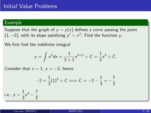
Initial Value Problems
Example
Suppose that the graph of y = y(x) defines a curve passing the point(1,−2), with its slope satisfying y ′ = x2. Find the function y .
We first find the indefinite integral
y =
∫
x2dx =1
2 + 1x2+1 + C =
1
3x3 + C .
Consider that x = 1, y = −2, hence
−2 =1
3(1)3 + C ⇐⇒ C = −2−
1
3= −
7
3
i.e., y =1
3x3 −
7
3.
Luo Luo (HKUST) MATH 1013 5 / 28

Initial Value Problems
Example
The acceleration of a falling particle near the surface of the earth isapproximately g = 9.8m/s2. If v(t) is the velocity of the particle, and theinitial value at t = 0 is v(0) = v0, find v(t).
The initial value problem is:dv
dt= −g , and v(0) = v0. We have
v(t) = −
∫
gdt = −gt + C .
Putting in t = 0, we have v0 = −9.8(0) + C = C i.e., v(t) = −gt + v0.
Luo Luo (HKUST) MATH 1013 6 / 28
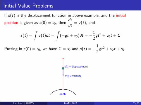
Initial Value Problems
If s(t) is the displacement function in above example, and the initial
position is given as s(0) = s0, thends
dt= v(t), and
s(t) =
∫
v(t)dt =
∫
(−gt + v0)dt = −1
2gt2 + v0t + C
Putting in s(0) = s0, we have C = s0 and s(t) = −1
2gt2 + v0t + s0.
earth
s(t) = displacement
v(t) = velocity
Luo Luo (HKUST) MATH 1013 7 / 28
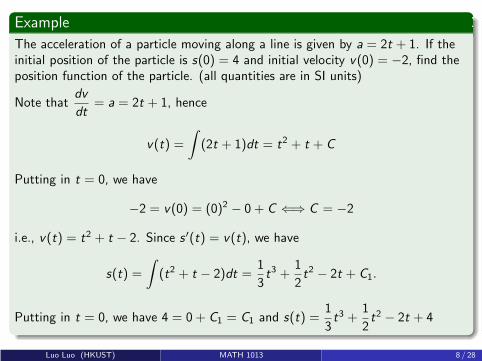
Example
The acceleration of a particle moving along a line is given by a = 2t + 1. If theinitial position of the particle is s(0) = 4 and initial velocity v(0) = −2, find theposition function of the particle. (all quantities are in SI units)
Note thatdv
dt= a = 2t + 1, hence
v(t) =
∫
(2t + 1)dt = t2 + t + C
Putting in t = 0, we have
−2 = v(0) = (0)2 − 0 + C ⇐⇒ C = −2
i.e., v(t) = t2 + t − 2. Since s ′(t) = v(t), we have
s(t) =
∫
(t2 + t − 2)dt =1
3t3 +
1
2t2 − 2t + C1.
Putting in t = 0, we have 4 = 0 + C1 = C1 and s(t) =1
3t3 +
1
2t2 − 2t + 4
Luo Luo (HKUST) MATH 1013 8 / 28
Outline
1 Initial Value Problems
2 Area under Curve
3 Riemann Sums and Definite Integrals
Luo Luo (HKUST) MATH 1013 9 / 28

Area Under a Graph By Squeezing
The idea of definite integral is basically from a combination of theapproximation of area by rectangles and limit taking.
Let’s start with a simple example to illustrate how the area under thegraph of a function can be squeezed out by using rectangularapproximations of the region.
Luo Luo (HKUST) MATH 1013 9 / 28

Area Under y = 1− x2 over [0, 1]
Problem: Finding the area A under the graph of y = 1− x2 over theinterval [0, 1].
Although it is not immediately clear what the area A is, it is extremelyeasy to estimate the area A roughly by using just a few rectangles.
00
11
11
Luo Luo (HKUST) MATH 1013 10 / 28

Area Under y = 1− x2 over [0, 1]
1 Divide the interval [0, 1] into 4 subintervals of the same length.
2 Use rectangles based on these subintervals, with heights equal to functionsvalues at the left or right endpoints of the subintervals, to estimate the area.
3 The area A is then squeezed between sums of rectangular areas:
A >(1− (0.25)2) · 0.25 + (1− (0.5)2) · 0.25 + (1− (0.75)2) · 0.25 = 0.53125
A <(1− 02) · 0.25 + (1− (0.25)2) · 0.25
+ (1− (0.5)2) · 0.25 + (1− (0.75)2) · 0.25 = 0.78125
00
11
11
Luo Luo (HKUST) MATH 1013 11 / 28
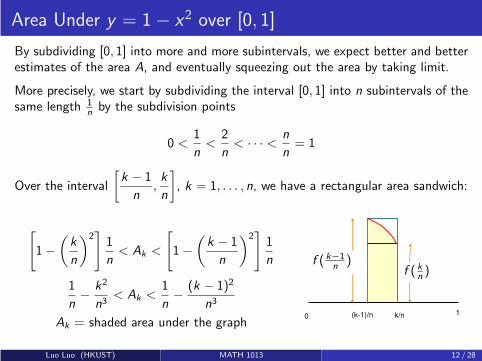
Area Under y = 1− x2 over [0, 1]
By subdividing [0, 1] into more and more subintervals, we expect better and betterestimates of the area A, and eventually squeezing out the area by taking limit.
More precisely, we start by subdividing the interval [0, 1] into n subintervals of thesame length 1
nby the subdivision points
0 <1
n<
2
n< · · · <
n
n= 1
Over the interval
[k − 1
n,k
n
]
, k = 1, . . . , n, we have a rectangular area sandwich:
0 1k/n(k-1)/n
f ( k−1n
)f ( k
n)
[
1−
(k
n
)2]
1
n< Ak <
[
1−
(k − 1
n
)2]
1
n
1
n−
k2
n3< Ak <
1
n−
(k − 1)2
n3
Ak = shaded area under the graph
Luo Luo (HKUST) MATH 1013 12 / 28
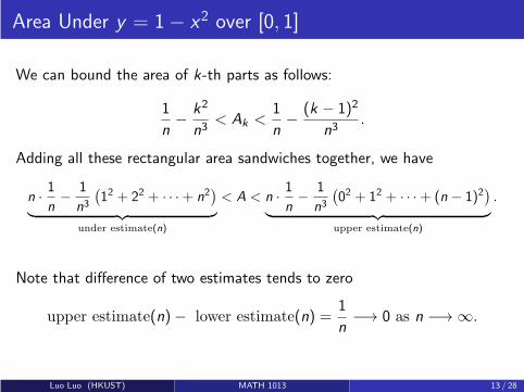
Area Under y = 1− x2 over [0, 1]
We can bound the area of k-th parts as follows:
1
n−
k2
n3< Ak <
1
n−
(k − 1)2
n3.
Adding all these rectangular area sandwiches together, we have
n ·1
n−
1
n3
(12 + 22 + · · ·+ n2
)
︸ ︷︷ ︸
under estimate(n)
< A < n ·1
n−
1
n3
(02 + 12 + · · ·+ (n − 1)2
)
︸ ︷︷ ︸
upper estimate(n)
.
Note that difference of two estimates tends to zero
upper estimate(n)− lower estimate(n) =1
n−→ 0 as n −→ ∞.
Luo Luo (HKUST) MATH 1013 13 / 28
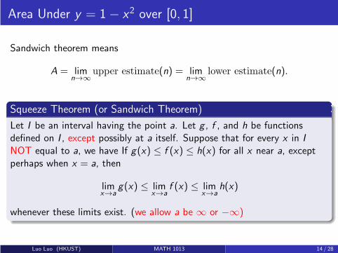
Area Under y = 1− x2 over [0, 1]
Sandwich theorem means
A = limn→∞
upper estimate(n) = limn→∞
lower estimate(n).
Squeeze Theorem (or Sandwich Theorem)
Let I be an interval having the point a. Let g , f , and h be functionsdefined on I , except possibly at a itself. Suppose that for every x in I
NOT equal to a, we have If g(x) ≤ f (x) ≤ h(x) for all x near a, exceptperhaps when x = a, then
limx→a
g(x) ≤ limx→a
f (x) ≤ limx→a
h(x)
whenever these limits exist. (we allow a be ∞ or −∞)
Luo Luo (HKUST) MATH 1013 14 / 28
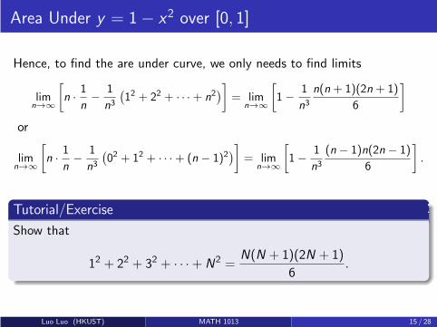
Area Under y = 1− x2 over [0, 1]
Hence, to find the are under curve, we only needs to find limits
limn→∞
[
n ·1
n−
1
n3
(12 + 22 + · · ·+ n2
)]
= limn→∞
[
1−1
n3n(n + 1)(2n + 1)
6
]
or
limn→∞
[
n ·1
n−
1
n3
(02 + 12 + · · ·+ (n − 1)2
)]
= limn→∞
[
1−1
n3(n − 1)n(2n − 1)
6
]
.
Tutorial/Exercise
Show that
12 + 22 + 32 + · · ·+ N2 =N(N + 1)(2N + 1)
6.
Luo Luo (HKUST) MATH 1013 15 / 28
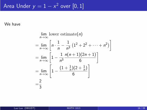
Area Under y = 1− x2 over [0, 1]
We have
limn→∞
lower estimate(n)
= limn→∞
[
n ·1
n−
1
n3
(12 + 22 + · · ·+ n2
)]
= limn→∞
[
1−1
n3n(n + 1)(2n + 1)
6
]
= limn→∞
[
1−(1 + 1
n)(2 + 1
n)
6
]
=2
3
Luo Luo (HKUST) MATH 1013 16 / 28

Area Under y = 1− x2 over [0, 1]
Similarly,
limn→∞
upper estimate(n)
= limn→∞
[
n ·1
n−
1
n3
(02 + 12 + · · ·+ (n − 1)2
)]
= limn→∞
[
1−1
n3(n − 1)n(2n − 1)
6
]
= limn→∞
[
1−(1− 1
n)(2− 1
n)
6
]
=2
3
Hence, the area under the graph of y = 1− x2 over [0, 1] is2
3.
Luo Luo (HKUST) MATH 1013 17 / 28
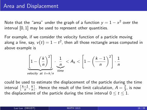
Area and Displacement
Note that the “area” under the graph of a function y = 1− x2 over theinterval [0, 1] may be used to represent other quantities.
For example, if we consider the velocity function of a particle movingalong a line, say, v(t) = 1− t2, then all those rectangle areas computed inabove example is
[
1−
(k
n
)2]
︸ ︷︷ ︸
velocity at t=k/n
·1
n︸︷︷︸
time
< Ak <
[
1−
(k − 1
n
)2]
·1
n
could be used to estimate the displacement of the particle during the timeinterval
[k−1n
, kn
]. Hence the result of the limit calculation, A = 2
3 , is nowthe displacement of the particle during the time interval 0 ≤ t ≤ 1.
Luo Luo (HKUST) MATH 1013 18 / 28
Outline
1 Initial Value Problems
2 Area under Curve
3 Riemann Sums and Definite Integrals
Luo Luo (HKUST) MATH 1013 19 / 28
Riemann Sums
The process in computing area in above example can obviously be appliedto any continuous function f on the interval [a, b].
The so called Riemann sum of a continuous function f (x) on an interval[a, b] with respect to a subdivision of the interval into n subintervals bythe points
a = x0 < x1 < x2 < · · · < xn = b
is a straightforward generalization of rectangular approximation of area.
Luo Luo (HKUST) MATH 1013 19 / 28

Riemann Sums
More precisely, denote the length of the i-th subinterval [xi−1, xi ] by ∆xi ,and choose for each a point ci in the subinterval [xi−1, xi ] for eachi = 1, 2, . . . , n. The corresponding Riemann sum is defined by:
Sn = f (c1)∆x1 + f (c2)∆x2 + · · ·+ f (cn)∆xn =n∑
i=1
f (ci )∆xi
1 If ci = xi−1 for all i , then Sn is called a left (left point) Riemann sum.
2 If ci = xi for all i , then Sn is called a right Riemann (right point) sum.
3 If ci = (xi−1 + xi )/2 for all i , then Sn is called a middle (middlepoint) Riemann sum.
For specific function, Riemann sums converge as the partition “gets finerand finer” (n gets larger and larger).
Luo Luo (HKUST) MATH 1013 20 / 28

Riemann Sums and Signed Area
If you look at the graph of the function, a Riemann sum is just arectangular approximation of the signed area (+ve/-ve area) between thegraph and the x-axis, based on the chosen points xi ’s and ci ’s.
x
y
y = f(x)
areas under the x-axis are given negative sign
areas above the x-axis are given positive sign
a b
Luo Luo (HKUST) MATH 1013 21 / 28
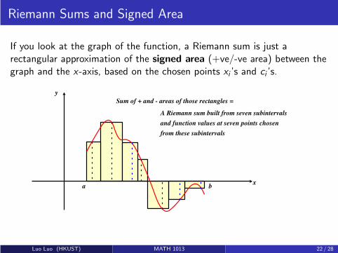
Riemann Sums and Signed Area
If you look at the graph of the function, a Riemann sum is just arectangular approximation of the signed area (+ve/-ve area) between thegraph and the x-axis, based on the chosen points xi ’s and ci ’s.
x
y
a b
A Riemann sum built from seven subintervals
and function values at seven points chosen
from these subintervals
Sum of + and - areas of those rectangles =
Luo Luo (HKUST) MATH 1013 22 / 28
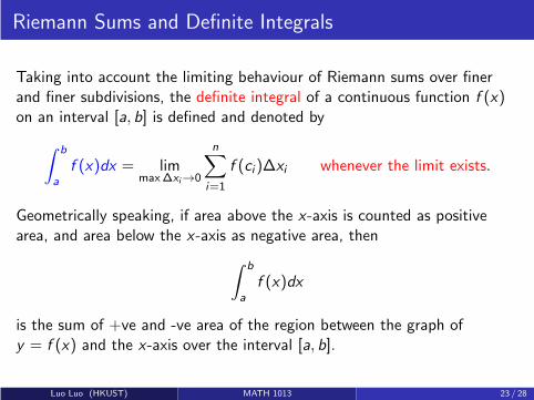
Riemann Sums and Definite Integrals
Taking into account the limiting behaviour of Riemann sums over finerand finer subdivisions, the definite integral of a continuous function f (x)on an interval [a, b] is defined and denoted by
∫ b
a
f (x)dx = limmax∆xi→0
n∑
i=1
f (ci )∆xi whenever the limit exists.
Geometrically speaking, if area above the x-axis is counted as positivearea, and area below the x-axis as negative area, then
∫ b
a
f (x)dx
is the sum of +ve and -ve area of the region between the graph ofy = f (x) and the x-axis over the interval [a, b].
Luo Luo (HKUST) MATH 1013 23 / 28

Riemann Sums and Definite Integrals
Just recall that the “rectangular areas” in the Riemann sum could actuallymean certain quantity other than area, e.g., displacement.The actually meaning of a definite integral
∫ b
a
f (x)dx
in application relies on the meaning on the product f (ci )∆xi , i.e., the unitfrom “unit of the y -axis” times “unit of the x-axis”.
Luo Luo (HKUST) MATH 1013 24 / 28
Riemann Sums and Definite Integrals
The summation notation, or the sigma notation, is often used to expressthe sum of a number of terms indexed by integers:
a1 + a2 + · · ·+ an =
n∑
k=1
ak
For example:n∑
k=1
k2 = 12 + 22 + 32 + · · ·+ n2.
A basic property of the summation notation is: for any constants A, B ,
n∑
k=1
[Aak + Bbk ] = A
n∑
k=1
ak + B
n∑
k=1
bk .
Luo Luo (HKUST) MATH 1013 25 / 28
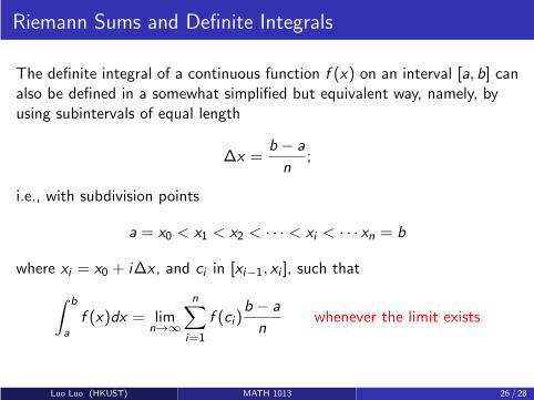
Riemann Sums and Definite Integrals
The definite integral of a continuous function f (x) on an interval [a, b] canalso be defined in a somewhat simplified but equivalent way, namely, byusing subintervals of equal length
∆x =b − a
n;
i.e., with subdivision points
a = x0 < x1 < x2 < · · · < xi < · · · xn = b
where xi = x0 + i∆x , and ci in [xi−1, xi ], such that
∫ b
a
f (x)dx = limn→∞
n∑
i=1
f (ci )b − a
nwhenever the limit exists
Luo Luo (HKUST) MATH 1013 26 / 28
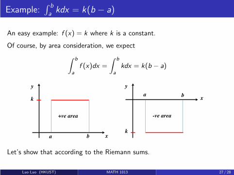
Example:∫ b
akdx = k(b − a)
An easy example: f (x) = k where k is a constant.
Of course, by area consideration, we expect
∫ b
a
f (x)dx =
∫ b
a
kdx = k(b − a)
y
x
k
a b
+ve area
y
x
k
a b
-ve area
Let’s show that according to the Riemann sums.
Luo Luo (HKUST) MATH 1013 27 / 28
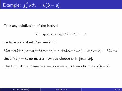
Example:∫ b
akdx = k(b − a)
Take any subdivision of the interval
a = x0 < x1 < x2 < · · · < xn = b
we have a constant Riemann sum
k(x1−x0)+k(x2−x1)+k(x3−x2)+· · ·+k(xn−xn−1) = k(xn−x0) = k(b−a)
since f (ci ) = k , no matter how you choose ci in [xi−1, xi ].
The limit of the Riemann sums as n → ∞ is then obviously k(b − a).
Luo Luo (HKUST) MATH 1013 28 / 28
Calculus IB: Lecture 20
Luo Luo
Department of Mathematics, HKUST
http://luoluo.people.ust.hk/
Luo Luo (HKUST) MATH 1013 1 / 33

Outline
1 More Examples of Definite Integrals
2 Fundamental Theorem of Calculus
Luo Luo (HKUST) MATH 1013 2 / 33

Outline
1 More Examples of Definite Integrals
2 Fundamental Theorem of Calculus
Luo Luo (HKUST) MATH 1013 3 / 33
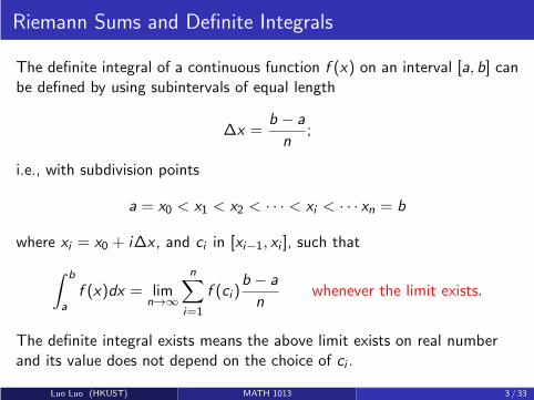
Riemann Sums and Definite Integrals
The definite integral of a continuous function f (x) on an interval [a, b] canbe defined by using subintervals of equal length
∆x =b − a
n;
i.e., with subdivision points
a = x0 < x1 < x2 < · · · < xi < · · · xn = b
where xi = x0 + i∆x , and ci in [xi−1, xi ], such that
∫
b
a
f (x)dx = limn→∞
n∑
i=1
f (ci )b − a
nwhenever the limit exists.
The definite integral exists means the above limit exists on real numberand its value does not depend on the choice of ci .
Luo Luo (HKUST) MATH 1013 3 / 33

Riemann Sums and Definite Integrals
In this section, we suppose all of definite integrals exist if we use notation
∫
b
a
f (x)dx .
The existence of definite integral is not required in our course. We willgive a brief sketch for this topic in next week.
Luo Luo (HKUST) MATH 1013 4 / 33

Example:∫ 1
0 xdx = 12
Consider the partition of [0, 1] into n subintervals by the subdivision points
0 <1
n<
2
n<
3
n< · · · < n
n= 1.
We have the left-endpoint Riemann sum is
0 · 1n+
1
n· 1n+
2
n· 1n+ · · ·+ n − 1
n· 1n
=1
n2· [0 + 1 + 2 + 3 + · · ·+ (n − 1)]
=1
n2· (n − 1)n
2=
1− 1n
2
which tends to the limit1
2as n → +∞.
Luo Luo (HKUST) MATH 1013 5 / 33
Example:∫ 1
0 xdx = 12
Similarly, we have the right-endpoint Riemann sum is
1
n· 1n+
2
n· 1n+ · · ·+ n
n· 1n
=1
n2· [1 + 2 + 3 + · · ·+ n]
=1
n2· n(n + 1)
2=
1 + 1n
2
which also tends to the limit1
2as n → +∞.
Luo Luo (HKUST) MATH 1013 6 / 33

Example:∫ 1
0 xdx = 12
Note that any other Riemann sum
Sn =1
n[c1 + c2 + · · ·+ cn]
with respect to the partition of the interval above, and ci in[
i−1n, i
n
]
, issqueezed between the left-endpoint and right-endpoint Riemann sums
1
2
(
1− 1
n
)
≤ Sn ≤ 1
2
(
1 +1
n
)
since the thin rectangular area with height f (ci ) = ci over the subinterval[
i−1n, i
n
]
is squeezed by
1
n· i − 1
n≤ 1
n· ci ≤
1
n· in.
Luo Luo (HKUST) MATH 1013 7 / 33

Example:∫ 1
0 xdx = 12
Summing over the thin rectangular areas
1
n· i − 1
n≤ 1
n· ci ≤
1
n· in,
We have
limn→∞
1
2
(
1− 1
n
)
≤ limn→∞
1
n[c1 + c2 + · · ·+ cn] ≤ lim
n→∞
1
2
(
1 +1
n
)
,
then∫ 1
0xdx = lim
n→∞
1
n[c1 + c2 + · · ·+ cn] =
1
2.
Luo Luo (HKUST) MATH 1013 8 / 33
Example:∫ 1
0 xdx = 12
If we let x be time and velocity of a partical is be v = f (x) = x , then thedefinite integral (corresponds to the area under the curve)
∫ 1
0f (x)dx =
1
2
is the displacement from time 0 to 1.
y
x1
1
y = x
Luo Luo (HKUST) MATH 1013 9 / 33

Example:∫ 1
0 exdx
Find the value of the definite integral
∫ 1
0exdx
by working with left-endpoint Riemann sums.
We consider the subdivision points are: 0,1
n,2
n,. . . ,
k
n, . . . ,
n
n= 1.
Computing the function values at 0,1
n,2
n,. . . ,
n − 1
n, the left-endpoint
Riemann sum Sn is
Sn =1
n
[
e0 + e1n + e
2n + · · ·+ e
n−1n
]
=1
n
[
1 + e1n +
(
e1n
)2+ · · ·+
(
e1n
)n−1]
Luo Luo (HKUST) MATH 1013 10 / 33
Example:∫ 1
0 exdx
The left-endpoint Riemann sum Sn is
Sn =1
n
[
e0 + e1n + e
2n + · · ·+ e
n−1n
]
=1
n
[
1 + e1n +
(
e1n
)2+ · · ·+
(
e1n
)n−1]
Using the formula 1 + t + t2 + · · ·+ tn−1 = tn−1
t−1 for any t 6= 1, we have
∫ 1
0exdx = lim
n→∞
Sn = limn→∞
1
n
(
e1n
)n
− 1
e1n − 1
=e − 1
limn→∞
e1n − 11n
= e − 1
where we use the result limn→∞
e1n − 11n
= 1.
Luo Luo (HKUST) MATH 1013 11 / 33

Example:∫ 1
0 exdx
Then we check the limit limn→∞
e1n − 11n
= 1.
Let x =1
n, then n → ∞ means x → 0 and we have
limn→∞
e1n − 11n
= limx→0
ex − 1
x= lim
x→0
ex
1= 1,
where we use L’Hopital’s rule (check the conditions!).
Luo Luo (HKUST) MATH 1013 12 / 33

Example: Area of a Circle = πr 2
In geometry, the area enclosed by a circle of radius r is πr2. How toexplain this result in the view of Riemann sums/definite integral?
Luo Luo (HKUST) MATH 1013 13 / 33

Example: Area of a Circle = πr 2
Based on the symmetric property of circle, we only needs to consider theright-top part of the circle.
We start by subdividing the interval [0, 1] into n subintervals of the samelength 1
nby the subdivision points
0 <1
n<
2
n< · · · < n
n= 1
Luo Luo (HKUST) MATH 1013 14 / 33
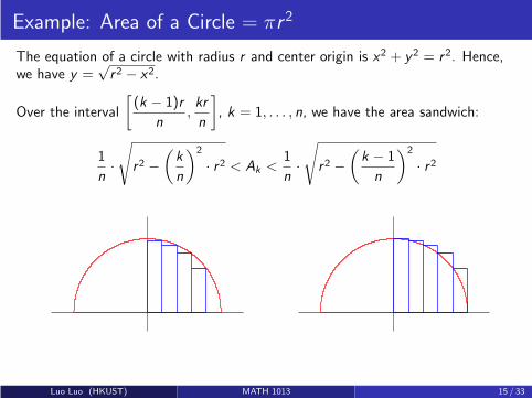
Example: Area of a Circle = πr 2
The equation of a circle with radius r and center origin is x2 + y2 = r2. Hence,we have y =
√r2 − x2.
Over the interval
[
(k − 1)r
n,kr
n
]
, k = 1, . . . , n, we have the area sandwich:
1
n·
√
r2 −(
k
n
)2
· r2 < Ak <1
n·
√
r2 −(
k − 1
n
)2
· r2
Luo Luo (HKUST) MATH 1013 15 / 33
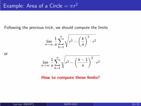
Example: Area of a Circle = πr 2
Following the previous trick, we should compute the limits
limn→∞
1
n
n∑
k=1
√
r2 −(
k
n
)2
· r2
or
limn→∞
1
n
n∑
k=1
√
r2 −(
k − 1
n
)2
· r2
How to compute these limits?
Luo Luo (HKUST) MATH 1013 16 / 33
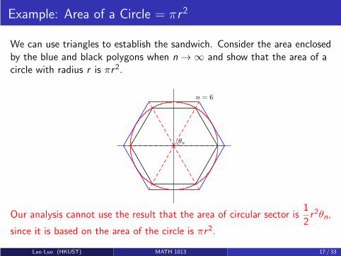
Example: Area of a Circle = πr 2
We can use triangles to establish the sandwich. Consider the area enclosedby the blue and black polygons when n → ∞ and show that the area of acircle with radius r is πr2.
Our analysis cannot use the result that the area of circular sector is1
2r2θn,
since it is based on the area of the circle is πr2.
Luo Luo (HKUST) MATH 1013 17 / 33

Example: Area of a Circle = πr 2
Area of the circle = n · Area(Sector OPMQ)
Area(△OPQ) < Area(Sector OPMQ) < Area(△ORS)
Luo Luo (HKUST) MATH 1013 18 / 33
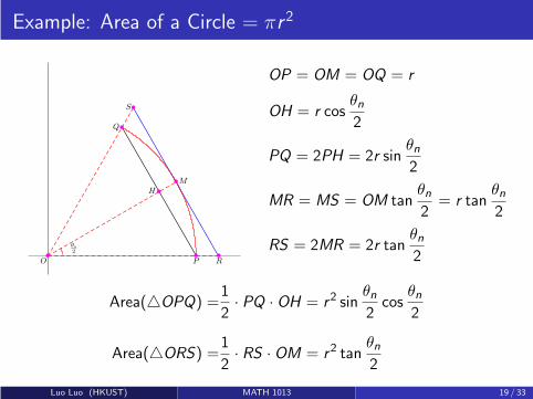
Example: Area of a Circle = πr 2
OP = OM = OQ = r
OH = r cosθn2
PQ = 2PH = 2r sinθn2
MR = MS = OM tanθn2
= r tanθn2
RS = 2MR = 2r tanθn2
Area(△OPQ) =1
2· PQ · OH = r2 sin
θn2cos
θn2
Area(△ORS) =1
2· RS · OM = r2 tan
θn2
Luo Luo (HKUST) MATH 1013 19 / 33

Example: Area of a Circle = πr 2
Let Ak = Area(Sector OPMQ), then the area of the circle is
S =n
∑
k=1
Ak = A1 + A2, . . . ,An.
Hence, we have
r2 sinθn2cos
θn2
< Ak < r2 tanθn2
and
n · r2 sin θn2cos
θn2
< S < n · r2 tan θn2.
Taking n → ∞, we can obtain S =1
2πr2 by sandwich theorem.
Luo Luo (HKUST) MATH 1013 20 / 33

Example: Area of a Circle = πr 2
Let x =π
n→ 0+. Since θn =
2π
n, we have
limn→∞
n · r2 · sin θn2
· cos θn2
= limn→∞
n · r2 · sin π
n· cos π
n
= limn→∞
πr2 ·sin π
n
πn
· cos πn
=πr2 · limn→∞
cosπ
n· limn→∞
sin πn
πn
=πr2 · limx→0+
cos x · limx→0
sin x
x
=πr2
Luo Luo (HKUST) MATH 1013 21 / 33

Example: Area of a Circle = πr 2
Since x =π
n→ 0+ and θn =
2π
n, we have
limn→∞
n · r2 · tan θn2
= limn→∞
n · r2 ·sin π
n
cos πn
= limx→0
r2 · πx· sin xcos x
=πr2 · limx→0+
sin x
x· limx→0+
cos x
=πr2
Hence, the sandwich theorem means S = πr2.
Luo Luo (HKUST) MATH 1013 22 / 33
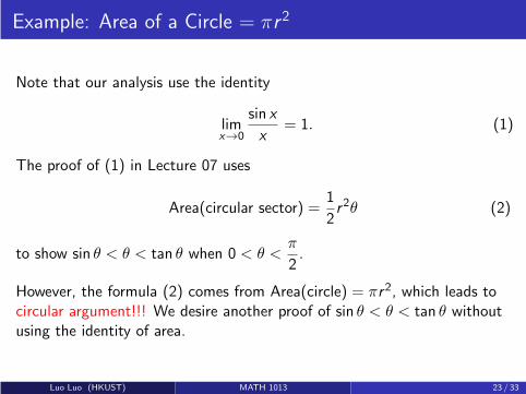
Example: Area of a Circle = πr 2
Note that our analysis use the identity
limx→0
sin x
x= 1. (1)
The proof of (1) in Lecture 07 uses
Area(circular sector) =1
2r2θ (2)
to show sin θ < θ < tan θ when 0 < θ <π
2.
However, the formula (2) comes from Area(circle) = πr2, which leads tocircular argument!!! We desire another proof of sin θ < θ < tan θ withoutusing the identity of area.
Luo Luo (HKUST) MATH 1013 23 / 33

Show sin θ < θ without Area
Let θ = ∠AOC be the corresponding angle of the sector and the lengths ofOC and OA is the radius r . Then the length of arc AC is rθ.
The shortest distance from point C to line AO is CE = r sin θ, where CE isorthogonal to OA. Another path from point C to line OA is arc CA, whichis longer than CE because it is not the shortest path. So we have
r sin θ < rθ =⇒ sin θ < θ.
Luo Luo (HKUST) MATH 1013 24 / 33
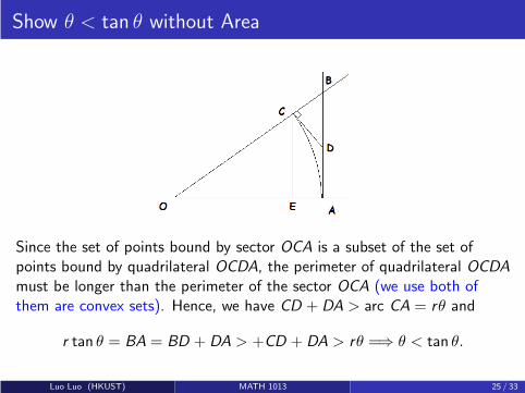
Show θ < tan θ without Area
Since the set of points bound by sector OCA is a subset of the set ofpoints bound by quadrilateral OCDA, the perimeter of quadrilateral OCDAmust be longer than the perimeter of the sector OCA (we use both ofthem are convex sets). Hence, we have CD + DA > arc CA = rθ and
r tan θ = BA = BD + DA > +CD + DA > rθ =⇒ θ < tan θ.
Luo Luo (HKUST) MATH 1013 25 / 33
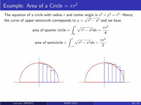
Example: Area of a Circle = πr 2
The equation of a circle with radius r and center origin is x2 + y2 = r2. Hence,
the curve of upper semicircle corresponds to y =√r2 − x2 and we have
area of quarter circle =
∫
r
0
√
r2 − x2dx =πr2
4
area of semicircle =
∫
r
−r
√
r2 − x2dx =πr2
2
Luo Luo (HKUST) MATH 1013 26 / 33

Outline
1 More Examples of Definite Integrals
2 Fundamental Theorem of Calculus
Luo Luo (HKUST) MATH 1013 27 / 33

Fundamental Theorem of Calculus
Calculating definite integrals by the original limit definition based onRiemann sums is very difficult in general.
We have seen that it is so complicated even if we only want to derive thearea formula of a circle.
Sometimes, there is an easier way compute definite integrals in general.
Luo Luo (HKUST) MATH 1013 27 / 33

Fundamental Theorem of Calculus
Theorem (Fundamental Theorem of Calculus)
Let f be a continuous function on the closed interval [a, b]. If F (x) is anantiderivative of f , i.e., F ′(x) = f (x), then
∫
b
a
f (x)dx = F (b)− F (a),
which is often denoted as F (x)∣
∣
b
aor
[
F (x)]b
a.
In other words, whenever you can find∫
f (x)dx = F (x) + C ,
it is just one step further to find the corresponding definite integral:∫
b
a
f (x)dx = F (b)− F (a).
Luo Luo (HKUST) MATH 1013 28 / 33
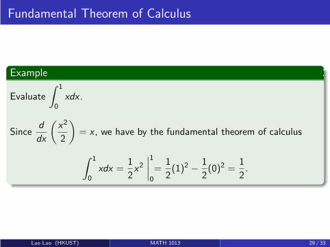
Fundamental Theorem of Calculus
Example
Evaluate
∫ 1
0xdx .
Sinced
dx
(
x2
2
)
= x , we have by the fundamental theorem of calculus
∫ 1
0xdx =
1
2x2
∣
∣
∣
∣
1
0
=1
2(1)2 − 1
2(0)2 =
1
2.
Luo Luo (HKUST) MATH 1013 29 / 33
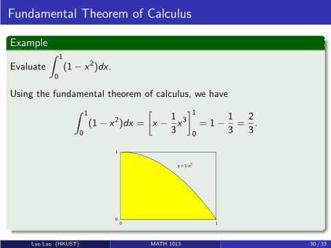
Fundamental Theorem of Calculus
Example
Evaluate
∫ 1
0(1− x2)dx .
Using the fundamental theorem of calculus, we have
∫ 1
0(1− x2)dx =
[
x − 1
3x3]1
0
= 1− 1
3=
2
3.
0
1
0 1
y = 1-x2
Luo Luo (HKUST) MATH 1013 30 / 33
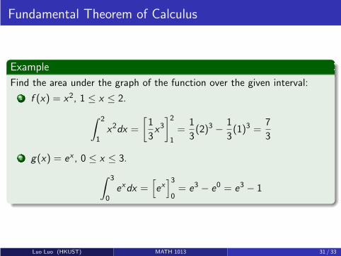
Fundamental Theorem of Calculus
Example
Find the area under the graph of the function over the given interval:
1 f (x) = x2, 1 ≤ x ≤ 2.
∫ 2
1x2dx =
[
1
3x3]2
1
=1
3(2)3 − 1
3(1)3 =
7
3
2 g(x) = ex , 0 ≤ x ≤ 3.
∫ 3
0exdx =
[
ex]3
0= e3 − e0 = e3 − 1
Luo Luo (HKUST) MATH 1013 31 / 33

Fundamental Theorem of Calculus
Example
Find the area under the graph of the function over the given interval:
1 h(x) = sin x , 0 ≤ x ≤ π.
∫ π
0sin xdx =
[
− cos x]π
0= [− cos(π)]− [− cos 0] = 2
2 u(x) = cos x , 0 ≤ x ≤ π/2.
∫ π/2
0cos xdx =
[
sin x]π/2
0= sin
π
2− sin 0 = 1
Luo Luo (HKUST) MATH 1013 32 / 33
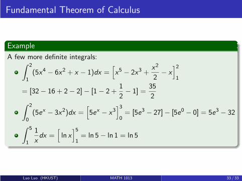
Fundamental Theorem of Calculus
Example
A few more definite integrals:∫ 2
1(5x4 − 6x2 + x − 1)dx =
[
x5 − 2x3 +x2
2− x
]2
1
= [32− 16 + 2− 2]− [1− 2 +1
2− 1] =
35
2∫ 2
0(5ex − 3x2)dx =
[
5ex − x3]3
0= [5e3 − 27]− [5e0 − 0] = 5e3 − 32
∫ 5
1
1
xdx =
[
ln x]5
1= ln 5− ln 1 = ln 5
Luo Luo (HKUST) MATH 1013 33 / 33

Calculus IB: Lecture 21
Luo Luo
Department of Mathematics, HKUST
http://luoluo.people.ust.hk/
Luo Luo (HKUST) MATH 1013 1 / 30
Outline
1 The Proof of Fundamental Theorem of Calculus
2 Integrability and Properties of Definite Integral
3 Taylor Series
Luo Luo (HKUST) MATH 1013 2 / 30
Outline
1 The Proof of Fundamental Theorem of Calculus
2 Integrability and Properties of Definite Integral
3 Taylor Series
Luo Luo (HKUST) MATH 1013 3 / 30

Fundamental Theorem of Calculus
Theorem (Fundamental Theorem of Calculus)
Let f be a continuous function on the closed interval [a, b]. If F (x) is anantiderivative of f , i.e., F ′(x) = f (x), then
∫
b
a
f (x)dx = F (b)− F (a),
which is often denoted as F (x)∣
∣
b
aor
[
F (x)]b
a.
In other words, whenever you can find∫
f (x)dx = F (x) + C ,
it is just one step further to find the corresponding definite integral:∫
b
a
f (x)dx = F (b)− F (a).
Luo Luo (HKUST) MATH 1013 3 / 30

The Proof of Fundamental Theorem of Calculus
Partition the interval [a, b] with n subintervals of equal lengthb − a
n.
By the mean value theorem Theorem, there exists x∗ in [xi−1, xi ] such that
F (xi )− F (xi−1) = F ′(x∗i )(xi − xi−1) = f (x∗i ) ·b − a
n
Then, we take the Riemann sum of the function f on [a, b]:
n∑
i=1
f (x∗i ) ·b − a
n=
n∑
i=1
(F (xi )− F (xi−1)) = F (xn)−F (x0) = F (b)−F (a).
Thus by the definition of definite integral, we have
∫
b
a
f (x)dx = limn→∞
n∑
i=1
f (x∗i ) ·b − a
n= F (b)− F (a).
Luo Luo (HKUST) MATH 1013 4 / 30

Example of Fundamental Theorem of Calculus
Example
Find the definite integral
∫ 2
−1
1
x2dx
Since
(
−1
x
)
′
=1
x2, we use fundamental theorem of calculus to obatin
∫ 2
−1
1
x2dx =
(
−1
x
)
∣
∣
∣
∣
∣
2
−1
= −1
2− 1 = −3
2
Luo Luo (HKUST) MATH 1013 5 / 30

Example of Fundamental Theorem of Calculus
-4 -3 -2 -1 0 1 2 3 4
0
5
10
15
20
The definite integral
∫ 2
−1
1
x2dx can NOT be negative!!!
Luo Luo (HKUST) MATH 1013 6 / 30

Outline
1 The Proof of Fundamental Theorem of Calculus
2 Integrability and Properties of Definite Integral
3 Taylor Series
Luo Luo (HKUST) MATH 1013 7 / 30
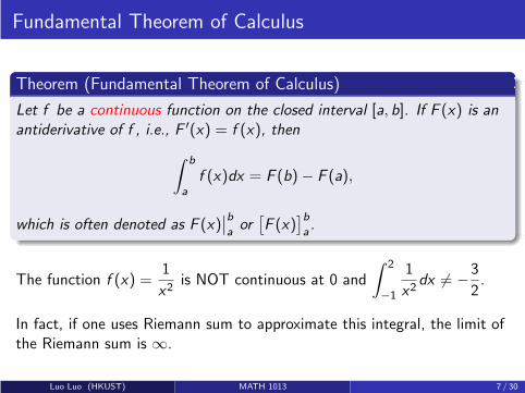
Fundamental Theorem of Calculus
Theorem (Fundamental Theorem of Calculus)
Let f be a continuous function on the closed interval [a, b]. If F (x) is anantiderivative of f , i.e., F ′(x) = f (x), then
∫
b
a
f (x)dx = F (b)− F (a),
which is often denoted as F (x)∣
∣
b
aor
[
F (x)]b
a.
The function f (x) =1
x2is NOT continuous at 0 and
∫ 2
−1
1
x2dx 6= −3
2.
In fact, if one uses Riemann sum to approximate this integral, the limit ofthe Riemann sum is ∞.
Luo Luo (HKUST) MATH 1013 7 / 30

Riemann Sums and Integrability
The definite integral of a continuous function f (x) on an interval [a, b] can bedefined by using subintervals of equal length
∆x =b − a
n;
i.e., with subdivision points a = x0 < x1 < x2 < · · · < xi < · · · xn = b, wherexi = x0 + i∆x , and ci in [xi−1, xi ].
If the limit of Riemann sum
limn→∞
n∑
i=1
f (ci ) ·∆
exists on real numbers, we say the function f is Riemann integrable if the limit ofthe Riemann sum exists and has a unique limit L. The limit is called the definiteintegral of f from a to b, denoted by
∫
b
a
f (x)dx = limn→∞
n∑
i=1
f (ci ) ·∆ = L
Luo Luo (HKUST) MATH 1013 8 / 30

Integrable Functions
Theorem (sufficient condition)
If f is continuous on on [a, b], then f must be (Riemann) integrable.
Theorem (sufficient condition+)
If f is continuous over [a, b] or bounded on [a, b] with a finite number ofdiscontinuous points, then f is integrable on [a, b].
Theorem (necessary condition)
If f is (Riemann) integrable on [a, b], then f must be bounded on [a, b].
Luo Luo (HKUST) MATH 1013 9 / 30

Integrable Functions
Example
The function
f (x) =
{
x2 0 ≤ x < 1
2 1 ≤ x ≤ 2
is integrable om [0, 2].
0 0.5 1 1.5 2
0
0.5
1
1.5
2
2.5
Luo Luo (HKUST) MATH 1013 10 / 30

Integrable Functions
The definite integral of
f (x) =
{
x2 0 ≤ x < 1
2 1 ≤ x ≤ 2
on [0, 2] is
∫ 2
0f (x)dx = lim
t→1−
∫
t
0f (x)dx +
∫ 2
1f (x)dx
Luo Luo (HKUST) MATH 1013 11 / 30

Non-Integrable Functions
Theorem (necessary condition)
If f is (Riemann) integrable on [a, b], then f must be bounded on [a, b].
Example
The function f (x) =1
x2is unbounded on [−1, 2].
Even if M > 0 is sufficient large, we have xM =1√
M + 1in [−1, 2]
such that f (xM) = M + 1 > M.
Luo Luo (HKUST) MATH 1013 12 / 30

Non-Integrable Functions
Theorem (sufficient condition+)
If f is continuous over [a, b] or bounded on [a, b] with a finite number ofdiscontinuous points, then f is integrable on [a, b].
Example (Dirichlet Function)
Dirichlet function is defined as follows
D(x) =
{
1 if x is a rational number,
0 if x is not a rational number.
Dirichlet function is nowhere continuous (in other words, there are infinitenumber of discontinuous points) and not (Riemann) integrable on any[a, b] when a < b.
Luo Luo (HKUST) MATH 1013 13 / 30

Non-Integrable Functions
Consider the behavior of Dirichlet function
D(x) =
{
1 if x is a rational number,
0 if x is a irrational number.
on interval [a, b], where a < b.
Let a = 0 and b = 1. given rational number 0.123, we can constructinfinite irrational numbers
0.123x1x2x3 . . . xn . . .
Since each xi can be select from 0, 1, . . . , 9, we can think
#rational numbers
#irrational numbers≈ lim
n→∞
(
1
10
)n
= 0
Intuitively, rationals number in [0, 1] is much less than irrational number.
Luo Luo (HKUST) MATH 1013 14 / 30
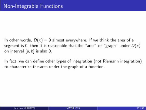
Non-Integrable Functions
In other words, D(x) = 0 almost everywhere. If we think the area of asegment is 0, then it is reasonable that the “area” of “graph” under D(x)on interval [a, b] is also 0.
In fact, we can define other types of integration (not Riemann integration)to characterize the area under the graph of a function.
Luo Luo (HKUST) MATH 1013 15 / 30
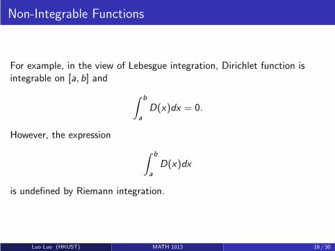
Non-Integrable Functions
For example, in the view of Lebesgue integration, Dirichlet function isintegrable on [a, b] and
∫
b
a
D(x)dx = 0.
However, the expression
∫
b
a
D(x)dx
is undefined by Riemann integration.
Luo Luo (HKUST) MATH 1013 16 / 30
Integrable Functions
In homework and exam of MATH 1013, “integrable” always refers
to Riemann integrable.
Luo Luo (HKUST) MATH 1013 17 / 30

Some Properties of Integrable Functions
Let f and g are integrable on closed interval [a, b], then
1 for any constants A, B , we have
∫
b
a
[Af (x) + Bg(x)]dx = A
∫
b
a
f (x)dx + B
∫
b
a
f (x)dx
2 for any constants a ≤ b ≤ c , we have
∫
c
a
f (x)dx =
∫
b
a
f (x)dx +
∫
c
b
f (x)dx
3 if f (x) ≥ g(x) on [a, b], then
∫
b
a
f (x)dx ≥∫
b
a
g(x)dx
4 if a > b, we define
∫
a
b
f (x)dx = −∫
b
a
f (x)dx in conventional.
Luo Luo (HKUST) MATH 1013 18 / 30
Outline
1 The Proof of Fundamental Theorem of Calculus
2 Integrability and Properties of Definite Integral
3 Taylor Series
Luo Luo (HKUST) MATH 1013 19 / 30

Integral Sandwiches for sin x and cos x
Consider that cos x ≤ 1 and sin x < x . Then for any x ≥ 0,
cos x ≤ 1 =⇒∫
x
0cos tdt ≤
∫
x
01dt ⇐⇒ sin t
∣
∣
∣
∣
x
0
≤ t
∣
∣
∣
∣
x
0
sin x ≤ x =⇒∫
x
0sin tdt ≤
∫
x
0tdt ⇐⇒ − cos t
∣
∣
∣
∣
x
0
≤ x2
2
1− x2
2≤ cos x =⇒
∫
x
0
(
1− t2
2
)
dt ≤∫
x
0cos tdt = sin x
x − x3
3!≤ sin x =⇒
∫
x
0
(
t − t3
3!
)
dt ≤∫
x
0sin tdt = − cos x + 1
· · · · · · =⇒ · · · · · ·
Exclamation mark “!” means factorial, that is, k! = 1 · 2 · · · · k for anypositive integer k . We define 0! = 1 in conventional.
Luo Luo (HKUST) MATH 1013 19 / 30
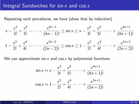
Integral Sandwiches for sin x and cos x
Repeating such procedures, we have (show that by induction)
x − x3
3!+
x5
5!− · · · − x4n−1
(4n − 1)!≤ sin x ≤ x − x3
3!+
x5
5!− · · ·+ x4n+1
(4n + 1)!
1− x2
2!+
x4
4!− · · · − x2n−2
(2n − 2)!≤ cos x ≤ 1− x2
2!+
x4
4!− · · ·+ x2n+2
(2n + 2)!
We can approximate sin x and cos x by polynomial functions
sin x ≈ x − x3
3!+
x5
5!− · · ·+ x4n+1
(4n + 1)!
cos x ≈ 1− x2
2!+
x4
4!− · · ·+ x2n+2
(2n + 2)!
Luo Luo (HKUST) MATH 1013 20 / 30

Integral Sandwiches for sin x and cos x
We can use the polynomial
p(x) = x − x3
3!+
x5
5!− x7
7!
to estimate the function value of sin x , then we have
p(x) ≤ sin x ≤ x − x3
3!+
x5
5!− x7
7!+
x9
9!=⇒ sin x − p(x) ≤ x9
9!
If we restrict x on[
0,π
4
]
, the above inequalities implies
0 ≤ sin x − p(x) ≤ x9
9!≤
(π4 )9
9!= 3.13× 10⁻⁷
Luo Luo (HKUST) MATH 1013 21 / 30
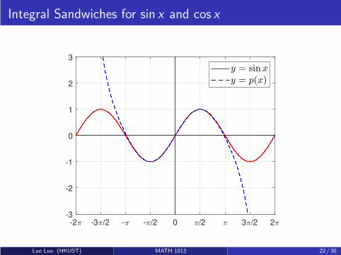
Integral Sandwiches for sin x and cos x
-2 -3 /2 - - /2 0 /2 3 /2 2
-3
-2
-1
0
1
2
3
Luo Luo (HKUST) MATH 1013 22 / 30
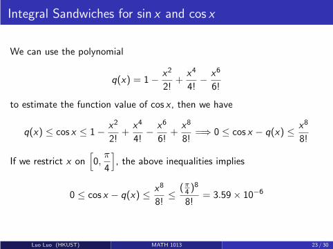
Integral Sandwiches for sin x and cos x
We can use the polynomial
q(x) = 1− x2
2!+
x4
4!− x6
6!
to estimate the function value of cos x , then we have
q(x) ≤ cos x ≤ 1− x2
2!+
x4
4!− x6
6!+
x8
8!=⇒ 0 ≤ cos x − q(x) ≤ x8
8!
If we restrict x on[
0,π
4
]
, the above inequalities implies
0 ≤ cos x − q(x) ≤ x8
8!≤
(π4 )8
8!= 3.59× 10⁻⁶
Luo Luo (HKUST) MATH 1013 23 / 30
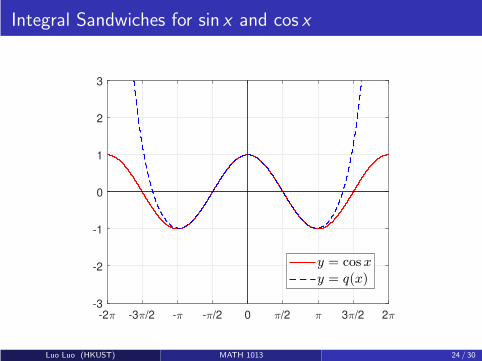
Integral Sandwiches for sin x and cos x
-2 -3 /2 - - /2 0 /2 3 /2 2
-3
-2
-1
0
1
2
3
Luo Luo (HKUST) MATH 1013 24 / 30
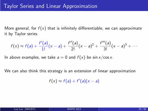
Taylor Series and Linear Approximation
More general, for f (x) that is infinitely differentiable, we can approximateit by Taylor series
f (x) ≈ f (a) +f ′(a)
1!(x − a) +
f ′′(a)
2!(x − a)2 +
f ′′′(a)
3!(x − a)3 + · · ·
In above examples, we take a = 0 and f (x) be sin x/cos x .
We can also think this strategy is an extension of linear approximation
f (x) ≈ f (a) + f ′(a)(x − a)
Luo Luo (HKUST) MATH 1013 25 / 30

Taylor Series and Optimization
Let a = xk , we have
f (x) ≈ f (xk) + f ′(xk)(x − xk) +f ′′(xk)
2(x − xk)
2 +f ′′′(xk)
3!(x − xk)
3 + · · ·
The iteration of gradient descent is
xk+1 =xk −1
Lf ′(xk)
= argminx
[
f (xk) + f ′(xk)(x − xk) +L
2(x − xk)
2
]
Recall that we suppose f ′′(x) ≤ L for positive L in the analysis of convexoptimization, which means the update is optimizing and upper bound offirst three terms in Taylor series.
Luo Luo (HKUST) MATH 1013 26 / 30

Taylor Series and Optimization
It is easy to check
xk+1 =xk −1
Lf ′(xk)
= argminx
[
f (xk) + f ′(xk)(x − xk) +L
2(x − xk)
2.
]
We define
g(x) = f (xk) + f ′(xk)(x − xk) +L
2(x − xk)
2,
then g ′′(x) = L > 0 and g ′(x) = f ′(xk) + L(x − xk).
Hence, g(x) is convex and xk+1 is its unique critical point (minimizer).
Luo Luo (HKUST) MATH 1013 27 / 30
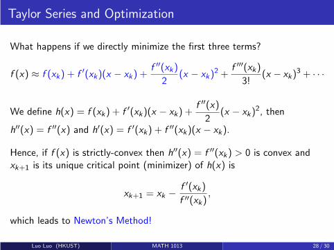
Taylor Series and Optimization
What happens if we directly minimize the first three terms?
f (x) ≈ f (xk) + f ′(xk)(x − xk) +f ′′(xk)
2(x − xk)
2 +f ′′′(xk)
3!(x − xk)
3 + · · ·
We define h(x) = f (xk) + f ′(xk)(x − xk) +f ′′(x)
2(x − xk)
2, then
h′′(x) = f ′′(x) and h′(x) = f ′(xk) + f ′′(xk)(x − xk).
Hence, if f (x) is strictly-convex then h′′(x) = f ′′(xk) > 0 is convex andxk+1 is its unique critical point (minimizer) of h(x) is
xk+1 = xk −f ′(xk)
f ′′(xk),
which leads to Newton’s Method!
Luo Luo (HKUST) MATH 1013 28 / 30
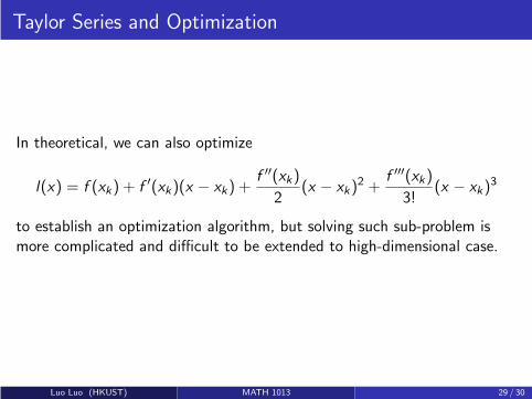
Taylor Series and Optimization
In theoretical, we can also optimize
l(x) = f (xk) + f ′(xk)(x − xk) +f ′′(xk)
2(x − xk)
2 +f ′′′(xk)
3!(x − xk)
3
to establish an optimization algorithm, but solving such sub-problem ismore complicated and difficult to be extended to high-dimensional case.
Luo Luo (HKUST) MATH 1013 29 / 30
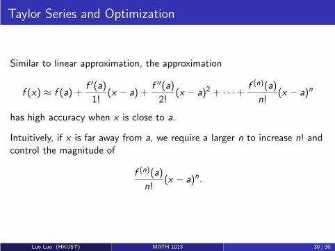
Taylor Series and Optimization
Similar to linear approximation, the approximation
f (x) ≈ f (a) +f ′(a)
1!(x − a) +
f ′′(a)
2!(x − a)2 + · · ·+ f (n)(a)
n!(x − a)n
has high accuracy when x is close to a.
Intuitively, if x is far away from a, we require a larger n to increase n! andcontrol the magnitude of
f (n)(a)
n!(x − a)n.
Luo Luo (HKUST) MATH 1013 30 / 30

Calculus IB: Lecture 22
Luo Luo
Department of Mathematics, HKUST
http://luoluo.people.ust.hk/
Luo Luo (HKUST) MATH 1013 1 / 26
Outline
1 Fundamental Theorem of Calculus (v2)
2 Net Change Theorem
3 Substitution Rules in Definite Integral
Luo Luo (HKUST) MATH 1013 2 / 26

Outline
1 Fundamental Theorem of Calculus (v2)
2 Net Change Theorem
3 Substitution Rules in Definite Integral
Luo Luo (HKUST) MATH 1013 3 / 26
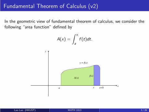
Fundamental Theorem of Calculus (v2)
In the geometric view of fundamental theorem of calculus, we consider thefollowing “area function” defined by
A(x) =
∫ x
a
f (t)dt.
x
y
y = f(x)
a x x+h
A(x)f(x)
Luo Luo (HKUST) MATH 1013 3 / 26

Fundamental Theorem of Calculus (v2)
In the geometric view of fundamental theorem of calculus, we consider thefollowing “area function” defined by
A(x) =
∫ x
a
f (t)dt.
Then we study the derivative of A(x).
x
y
y = f(x)
a x x+h
A(x)f(x)
Luo Luo (HKUST) MATH 1013 4 / 26
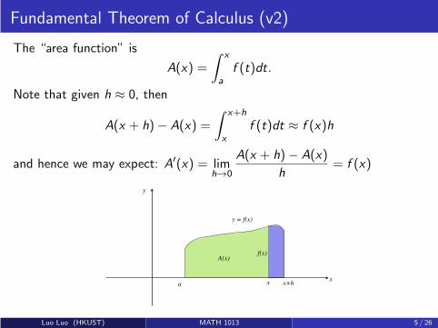
Fundamental Theorem of Calculus (v2)
The “area function” is
A(x) =
∫ x
a
f (t)dt.
Note that given h ≈ 0, then
A(x + h)− A(x) =
∫ x+h
x
f (t)dt ≈ f (x)h
and hence we may expect: A′(x) = limh→0
A(x + h)− A(x)
h= f (x)
x
y
y = f(x)
a x x+h
A(x)f(x)
Luo Luo (HKUST) MATH 1013 5 / 26

Fundamental Theorem of Calculus (v2)
To be precise, just consider the “area sandwich” for h > 0:
minx≤t≤x+h
f (t)h ≤ A(x + h)− A(x) ≤ maxx≤t≤x+h
f (t)h
As f is continuous on [a, b], we have by taking limits
f (x) = limh→0+
minx≤t≤x+h
f (t)
≤ limh→0+
A(x + h)− A(x)
h
≤ limh→0+
maxx≤t≤x+h
f (t) = f (x)
For h < 0, we consider the interval [x + h, x ] and end up with
limh→0−
A(x + h)− A(x)
h= f (x)
Luo Luo (HKUST) MATH 1013 6 / 26

Fundamental Theorem of Calculus (v2)
In other word, A′(x) = f (x) and hence the area function A(x) is anantiderivative of f (x). Rewrite this as a theorem, we have:
Theorem (Fundamental Theorem of Calculus v2)
Let f be a continuous function on the interval [a, b]. Then
d
dx
∫ x
a
f (t)dt = f (x).
Luo Luo (HKUST) MATH 1013 7 / 26

Fundamental Theorem of Calculus (v2)
Recall that the antiderivative of f can be expressed as∫
f (x)dx = F (x) + C ,
and there must be a constant C such that (fundamental theorem of calculus v2)∫ x
a
f (t)dt = F (x) + C
Putting in x = a, we have
0 =
∫ a
a
f (t)dt = F (a) + C ⇐⇒ C = −F (a)
Therefore we have∫ x
a
f (t)dt = F (x)− F (a)
which corresponds to previous version of fundamental theorem of calculus∫ b
a
f (t)dt = F (b)− F (a)
Luo Luo (HKUST) MATH 1013 8 / 26

Fundamental Theorem of Calculus (v2)
Example
Let y =
∫ x2
1sin 3tdt, find
dy
dx
Let u = x2 and use chain rule, then
dy
dx=
(
d
du
∫ u
1sin 3tdt
)
· dudx
=(sin 3u) · dudx
= (sin 3x2) · dx2
dx= 2x sin 3x2
Exercise
Instead of using the fundamental theorem of calculus directly, try to usethe limit definition of derivative to find derivatives above.
Luo Luo (HKUST) MATH 1013 9 / 26

Outline
1 Fundamental Theorem of Calculus (v2)
2 Net Change Theorem
3 Substitution Rules in Definite Integral
Luo Luo (HKUST) MATH 1013 10 / 26

Net Change Theorem
Just by rewriting the fundamental theorem of calculus
∫ b
a
f (x)dx = F (b)− F (a)
where F ′(x) = f (x) into another form, we have net change theorem
∫ b
a
F ′(x)dx = F (b)− F (a)
since F (b)− F (a) is the change in y = F (x) when x changes from a to b.
Luo Luo (HKUST) MATH 1013 10 / 26
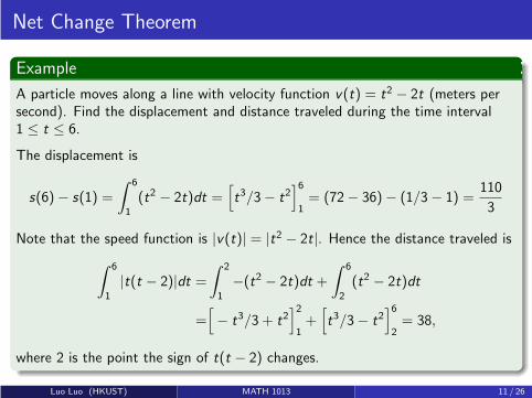
Net Change Theorem
Example
A particle moves along a line with velocity function v(t) = t2 − 2t (meters persecond). Find the displacement and distance traveled during the time interval1 ≤ t ≤ 6.
The displacement is
s(6)− s(1) =
∫ 6
1
(t2 − 2t)dt =[
t3/3− t2]6
1= (72− 36)− (1/3− 1) =
110
3
Note that the speed function is |v(t)| = |t2 − 2t|. Hence the distance traveled is
∫ 6
1
|t(t − 2)|dt =∫ 2
1
−(t2 − 2t)dt +
∫ 6
2
(t2 − 2t)dt
=[
− t3/3 + t2]2
1+[
t3/3− t2]6
2= 38,
where 2 is the point the sign of t(t − 2) changes.
Luo Luo (HKUST) MATH 1013 11 / 26
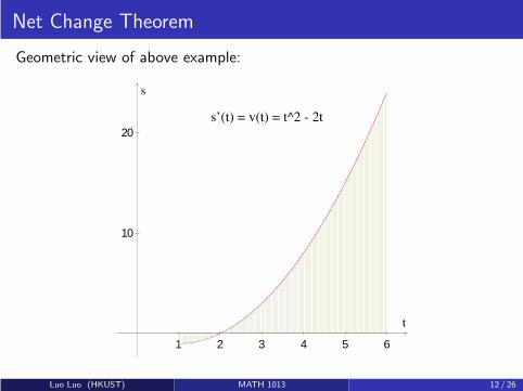
Net Change Theorem
Geometric view of above example:
1 2 3 4 5 6
10
20
t
s
s’(t) = v(t) = t^2 - 2t
Luo Luo (HKUST) MATH 1013 12 / 26

Example
Suppose a volcano spewed out solid materials is of the rate r(t) at which aregiven in the following table.
t(in seconds) 0 1 2 3 4 5 6r(t)(tones per second) 2 10 24 36 46 54 60
(a) Give upper and lower estimates for the total quantity Q(6) of eruptedmaterials after 6 seconds.
(b) Use the Midpoint Rule (Midpoint Riemann Sum) to estimate Q(6).
(a) Using the table,
2 + 10 + 24 + 36 + 46 + 54 <
∫ 6
0
r(t)dt < 10 + 24 + 36 + 46 + 54 + 60
172 < Q(6) < 230 (tones)
(b) Using three subintervals of length 2, with subdivision points 0 < 2 < 4 < 6,we have midpoints 1, 3, 5 and hence
Q(6) ≈ 2(10 + 36 + 54) = 200 (tones)
Luo Luo (HKUST) MATH 1013 13 / 26

Outline
1 Fundamental Theorem of Calculus (v2)
2 Net Change Theorem
3 Substitution Rules in Definite Integral
Luo Luo (HKUST) MATH 1013 14 / 26
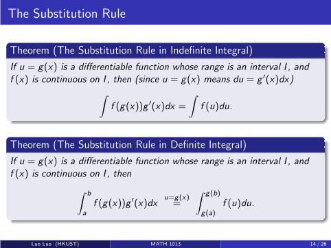
The Substitution Rule
Theorem (The Substitution Rule in Indefinite Integral)
If u = g(x) is a differentiable function whose range is an interval I , andf (x) is continuous on I , then (since u = g(x) means du = g ′(x)dx)
∫
f (g(x))g ′(x)dx =
∫
f (u)du.
Theorem (The Substitution Rule in Definite Integral)
If u = g(x) is a differentiable function whose range is an interval I , andf (x) is continuous on I , then
∫ b
a
f (g(x))g ′(x)dxu=g(x)=
∫ g(b)
g(a)f (u)du.
Luo Luo (HKUST) MATH 1013 14 / 26
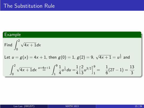
The Substitution Rule
Example
Find
∫ 2
0
√4x + 1dx
Let u = g(x) = 4x + 1, then g(0) = 1, g(2) = 9,√4x + 1 = u
12 and
∫ 2
0
√4x + 1dx
u=4x+1=
∫ 9
1
1
4u
12 du =
1
4
[2
3u3/2
]9
1=
1
6(27− 1) =
13
3
Luo Luo (HKUST) MATH 1013 15 / 26

Example
Find
∫ π
2
0sin3 x cos4 xdx
We hope the expression only depends on cos x or sin x :
∫ π
2
0sin3 x cos4 xdx =
∫ π
2
0sin2 x cos4 x (sin x dx)
=
∫ π
2
0(1− cos2 x) cos4 x (−d cos x)
Let u = g(x) = cos x , then g(0) = cos 0 = 1, g(1) = sin π2 = 0 and
∫ π
2
0sin3 x cos4 xdx = −
∫ g(π2)
g(0)(1− u2)u4du
=−[
t5
5− t7
7
]0
1
= −[
0−(
1
5− 1
7
)]
=2
35
Luo Luo (HKUST) MATH 1013 16 / 26
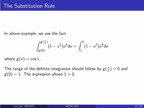
The Substitution Rule
In above example, we use the fact
∫ g(π2)
g(0)(1− u2)u4du =
∫ 0
1(1− u2)u4du
where g(x) = cos x .
The range of the definite integration should follow by g(π2 ) = 0 andg(0) = 1. The expression allows 1 > 0.
Luo Luo (HKUST) MATH 1013 17 / 26
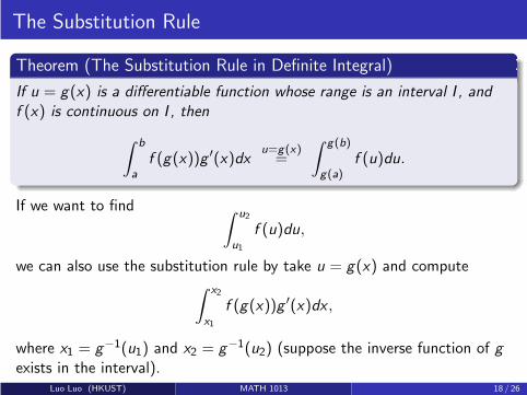
The Substitution Rule
Theorem (The Substitution Rule in Definite Integral)
If u = g(x) is a differentiable function whose range is an interval I , andf (x) is continuous on I , then
∫ b
a
f (g(x))g ′(x)dxu=g(x)=
∫ g(b)
g(a)f (u)du.
If we want to find∫ u2
u1
f (u)du,
we can also use the substitution rule by take u = g(x) and compute∫ x2
x1
f (g(x))g ′(x)dx ,
where x1 = g−1(u1) and x2 = g−1(u2) (suppose the inverse function of gexists in the interval).
Luo Luo (HKUST) MATH 1013 18 / 26

The Substitution Rule
The expression∫ x2
x1
f (g(x))g ′(x)dx
looks more complicated than
∫ u2
u1
f (u)du.
However, such substitution could be very useful in some specific problem.
Luo Luo (HKUST) MATH 1013 19 / 26
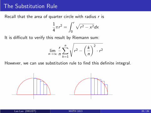
The Substitution Rule
Recall that the area of quarter circle with radius r is
1
4πr2 =
∫ r
0
√
r2 − x2dx
It is difficult to verify this result by Riemann sum:
limn→∞
r
n
n∑
k=1
√
r2 −(
k
n
)2
· r2
However, we can use substitution rule to find this definite integral.
Luo Luo (HKUST) MATH 1013 20 / 26

The Substitution Rule
Let x = r sin θ. Since the function sin θ is a one-to-one function in [0, π
2 ] andr sin 0 = 0, r sin π
2 = r , we have
∫ r
0
√
r2 − x2dx =
∫ π
2
0
√
r2 − r2 sin2 θ d(r sin θ)
=
∫ π
2
0
√
r2 − r2 sin2 θ · r cos θdθ
=r2∫ π
2
0
√
1− sin2 θ cos θdθ
=r2∫ π
2
0
cos2 θdθ
=r2∫ π
2
0
1 + cos 2θ
2dθ
=r2[
θ
2+
sin 2θ
4
]π
2
0
= r2[
π
4+
sinπ
4−(
0 +sin 0
4
)]
=1
4πr2
Luo Luo (HKUST) MATH 1013 21 / 26
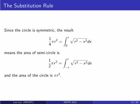
The Substitution Rule
Since the circle is symmetric, the result
1
4πr2 =
∫ r
0
√
r2 − x2dx
means the area of semi-circle is
1
2πr2 =
∫ r
−r
√
r2 − x2dx
and the area of the circle is πr2.
Luo Luo (HKUST) MATH 1013 22 / 26
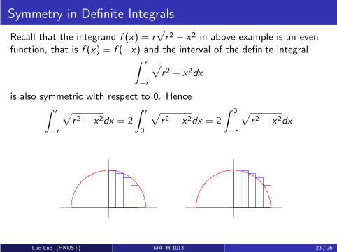
Symmetry in Definite Integrals
Recall that the integrand f (x) = r√r2 − x2 in above example is an even
function, that is f (x) = f (−x) and the interval of the definite integral∫ r
−r
√
r2 − x2dx
is also symmetric with respect to 0. Hence∫ r
−r
√
r2 − x2dx = 2
∫ r
0
√
r2 − x2dx = 2
∫ 0
−r
√
r2 − x2dx
Luo Luo (HKUST) MATH 1013 23 / 26
Symmetry in Definite Integrals
Consider a “difficult” problem
∫ 1
−1
tan x
1 + 3x2 + 5x4 + 7x6=?
Applying Riemann sum is very complicated.
Using fundamental theorem of calculus is also very difficult.
Is this problem real “difficult”?
Luo Luo (HKUST) MATH 1013 24 / 26

Symmetry in Definite Integrals
We define
f (x) =tan x
1 + 3x2 + 5x4 + 7x6.
In fact, f (x) is an odd function, that is
f (x) = −f (−x).
Recall that definite integral is the signed area between the graph of thefunction and the x-axis.
Odd function means the graph is symmetric with respect to origin.
Since the range [−1, 1] also is symmetric and f (x) is well defined on it, wemust have
∫ 1
−1f (x)dx = 0
Luo Luo (HKUST) MATH 1013 25 / 26

Symmetry in Definite Integrals
Since the signed areas are canceled, we must have∫ 1
−1f (x)dx =
∫ 1
−1
tan x
1 + 3x2 + 5x4 + 7x6dx = 0.
-1 -0.5 0 0.5 1
-0.3
-0.2
-0.1
0
0.1
0.2
0.3
Luo Luo (HKUST) MATH 1013 26 / 26