Calculus of Residues

Chapter 21

Calculus of Residues

One of the most powerful tools made available by complex analysis is thetheory of residues, which makes possible the routine evaluation of certain realdefinite integrals that are impossible to calculate otherwise. Example 20.2.6showed a situation in which an integral was related to expansion coefficientsof Laurent series. Here we will develop a systematic way of evaluating bothreal and complex integrals using the same idea.

Recall that a singular point z0 of f(z) is a point at which f fails to beanalytic. If, in addition, there is some neighborhood of z0 in which f isanalytic at every point (except, of course, at z0 itself), then z0 is called anisolated singularity of f . All singularities we have encountered so far have isolated singularitybeen isolated singularities. Although singularities that are not isolated alsoexist, we shall not discuss them in this book.

21.1 The Residue

Let z0 be an isolated singularity of f . Then there exists an r > 0 such that,within the “annular” region 0 < |z − z0| < r, the function f has the Laurentexpansion1

f(z) =∞!

n=−∞an(z − z0)n ≡

∞!

n=0

an(z − z0)n +b1

z − z0+

b2

(z − z0)2+ · · · ,

where

an =1

2πi

"

C

f(ξ) dξ

(ξ − z0)n+1and bn =

12πi

"

Cf(ξ)(ξ − z0)n−1 dξ.

In particular,

b1 =1

2πi

"

Cf(ξ) dξ, (21.1)

1We are using bn for a−n.

526 Calculus of Residues

where C is any simple closed contour around z0, traversed in the positivesense, on and interior to which f is analytic except at the point z0 itself.residue defined

Box 21.1.1. The complex number b1, which is 12πi times the integral of

f(z) along the contour, is called the residue of f at the isolated singularpoint z0.

It is important to note that the residue is independent of the contour C aslong as z0 is the only isolated singular point within C.

Example 21.1.1. We want to evaluate the integral!

Csin z dz/(z − π/2)3 where

C is any simple closed contour having z = π/2 as an interior point.To evaluate the integral we expand around z = π/2 and use Equation (21.1).

We note that

sin z = cos"z − π

2

#=

∞$

n=0

(−1)n (z − π/2)2n

(2n)!= 1 − (z − π/2)2

2+ · · ·

sosin z

(z − π/2)3=

1(z − π/2)3

− 12

%1

z − π/2

&+ · · · .

It follows that b1 = − 12 ; therefore,

!C

sin z dz/(z − π/2)3 = 2πib1 = −iπ. !Example 21.1.2. The integral

!C

cos z dz/z2, where C is the circle |z| = 1, iszero because

cos zz2

=1z2

∞$

n=0

(−1)n z2n

(2n)!=

1z2

− 12

+z2

4!+ · · ·

yields b1 = 0 (no 1/z term in the Laurent expansion). Therefore, by Equation (21.1)the integral must vanish.

When C is the circle |z| = 2,!

Cez dz/(z − 1)3 = iπe because

ez = eez−1 = e∞$

n=0

(z − 1)n

n!= e

'1 + (z − 1) +

(z − 1)2

2!+ · · ·

(

andez

(z − 1)3= e

'1

(z − 1)3+

1(z − 1)2

+12

%1

z − 1

&+ · · ·

(.

Thus, b1 = e/2, and the integral is 2πib1 = iπe. !

We use the notation Res[f(z0)] to denote the residue of f at the isolatedsingular point z0. Equation (21.1) can then be written as

)

Cf(z) dz = 2πi Res[f(z0)].

What if there are several isolated singular points within the simple closedcontour C? Let Ck be the positively traversed circle around zk shown inFigure 21.1. Then the Cauchy–Goursat theorem yields

0 =)

C′f(z) dz =

)

circlesf(z) dz +

)

parallellines

f(z) dz +)

Cf(z) dz,

21.1 The Residue 527

z1

z2

zm

C1

C2

Cm

Figure 21.1: Singularities are avoided by going around them.

where C′ is the union of all contours inside which union there are no singu-larities. The contributions of the parallel lines cancel out, and we obtain

!

Cf(z) dz = −

m"

k=1

!

Ck

f(z) dz =m"

k=1

2πi Res[f(zk)],

where in the last step the definition of residue at zk has been used. The minussign disappears in the final result because the sense of Ck, while positive forthe shaded region of Figure 21.1, is negative for the interior of Ck becausethis interior is to our right as we traverse Ck in the direction indicated. Wethus have

Theorem 21.1.3. (The Residue Theorem). Let C be a positively inte-grated simple closed contour within and on which a function f is analyticexcept at a finite number of isolated singular points z1, z2, . . . , zm interior toC. Then !

Cf(z) dz = 2πi

m"

k=1

Res[f(zk)]. (21.2)

Example 21.1.4. Let us evaluate the integral#

C(2z − 3) dz/[z(z − 1)] where C

is the circle |z| = 2. There are two isolated singularities in C, z1 = 0 and z2 = 1.To find Res[f(z1)], we expand around the origin using Equation (20.2):

2z − 3z(z − 1)

=3z− 1

z − 1=

3z

+1

1 − z=

3z

+ 1 + z + · · · for |z| < 1.

This gives Res[f(z1)] = 3. Similarly, expanding around z = 1 gives

2z − 3z(z − 1)

=3

(z − 1) + 1− 1

z − 1= − 1

z − 1+ 3

∞"

n=0

(−1)n(z − 1)n

which yields Res[f(z2)] = −1. Thus,!

C

2z − 3z(z − 1)

dz = 2πi{Res[f(z1)] + Res[f(z2)]} = 2πi(3 − 1) = 4πi. !


Let f(z) have an isolated singularity at z0. Then there exist a real numberr > 0 and an annular region 0 < |z − z0| < r such that f can be representedby the Laurent series

f(z) =∞!

n=0

an(z − z0)n +∞!

n=1

bn

(z − z0)n. (21.3)

The second sum in Equation (21.3), involving negative powers of (z − z0), iscalled the principal part of f at z0. The principal part is used to classifyprincipal part of a

function isolated singularities. We consider two cases:(a) If bn = 0 for all n ≥ 1, z0 is called a removable singular point of f .removable singular

point In this case, the Laurent series contains only nonnegative powers of (z − z0),and setting f(z0) = a0 makes the function analytic at z0. For example, thefunction f(z) = (ez − 1 − z)/z2, which is indeterminate at z = 0, becomesentire if we set f(0) = 1/2, because its Laurent series

f(z) =12

+z

3!+

z2

4!+ · · ·

has no negative power.(b) If bn = 0 for all n > m and bm ̸= 0, z0 is called a pole of order m. Inpoles definedthis case, the expansion takes the form

f(z) =∞!

n=0

an(z − z0)n +b1

z − z0+ · · · + bm

(z − z0)m

for 0 < |z − z0| < r. In particular, if m = 1, z0 is called a simple pole.simple pole

Example 21.1.5. Let us consider some examples of poles of various orders.(a) The function (z2−3z +5)/(z−1) has a Laurent series around z = 1 containingonly three terms: (z2 − 3z + 5)/(z − 1) = −1 + (z − 1) + 3/(z − 1). Thus, it has asimple pole at z = 1, with a residue of 3.(b) The function sin z/z6 has a Laurent series

sin zz6

=1z6

∞!

n=0

(−1)n z2n+1

(2n + 1)!=

1z5

− 16z3

+1

(5!)z− z

7!+ · · ·

about z = 0. The principal part has three terms. The pole, at z = 0, is of order 5,and the function has a residue of 1/120 at z = 0.(c) The function (z2−5z+6)/(z−2) has a removable singularity at z = 2, because

z2 − 5z + 6z − 2

=(z − 2)(z − 3)

z − 2= z − 3 = −1 + (z − 2)

and bn = 0 for all n. !

The type of isolated singularity that is most important in applications isof the second type—poles. For a function that has a pole of order m at z0,the calculation of residues is routine. Such a calculation, in turn, enables us

21.2 Integrals of Rational Functions 529

to evaluate many integrals effortlessly. How do we calculate the residue of afunction f having a pole of order m at z0?

It is clear that if f has a pole of order m, then g(z) defined by g(z) ≡(z − z0)mf(z) is analytic at z0. Thus, for any simple closed contour C thatcontains z0 but no other singular point of f , we have

Res[f(z0)] =1

2πi

!

Cf(z) dz =

12πi

!

C

g(z) dz

(z − z0)m=

g(m−1)(z0)(m − 1)!

,

where we used Equation (19.10). In terms of f this yields2

Res[f(z0)] =1

(m − 1)!lim

z→z0

dm−1

dzm−1[(z − z0)mf(z)]. (21.4)

For the special, but important, case of a simple pole, we obtain

Res[f(z0)] = limz→z0

[(z − z0)f(z)]. (21.5)

The most widespread application of residues occurs in the evaluation of application of theresidue theorem inevaluating definiteintegrals

real definite integrals. It is possible to “complexify” certain real definite in-tegrals and relate them to contour integrations in the complex plane. Whatis typically involved is the addition of a number of semicircles to the realintegral such that it becomes a closed contour integral whose value can bedetermined by the residue theorem. One then takes the limit of the contourintegral when the radii of the semicircles go to infinity or zero. In this limitthe contributions from the semicircles should vanish for the method to work.In that case, one recovers the real integral. There are three types of integralsmost commonly encountered. We discuss these separately below. In all caseswe assume that the contribution of the semicircles will vanish in the limit.

21.2 Integrals of Rational Functions

The first type of integral we can evaluate using the residue theorem is of theform

I1 =" ∞

−∞

p(x)q(x)

dx,

where p(x) and q(x) are real polynomials, and q(x) ̸= 0 for any real x. Wecan then write

I1 = limR→∞

" R

−R

p(x)q(x)

dx = limR→∞

"

Cx

p(z)q(z)

dz,

where Cx is the (open) contour lying on the real axis from −R to +R. Wenow close that contour by adding to it the semicircle of radius R [see Fig-ure 21.2(a)]. This will not affect the value of the integral because, by our

2The limit is taken because in many cases the mere substitution of z0 may result in anindeterminate form.


3i

i

−R R

(a)

−i

−3i

−R R

(b)

Figure 21.2: (a) The large semicircle is chosen in the UHP. (b) Note how the directionof contour integration is forced to be clockwise when the semicircle is chosen in theLHP.

assumption, the contribution of the integral of the semicircle tends to zero inthe limit R → ∞. We close the contour in the upper half-plane (UHP) if q(z)has a zero there. We then get

I1 = limR→∞

!

C

p(z)q(z)

dz = 2πik"

j=1

Res#p(zj)q(zj)

$,

where C is the closed contour composed of the interval (−R, R) and thesemicircle CR, and {zj}k

j=1 are the zeros of q(z) in the UHP. We may insteadclose the contour in the lower half-plane (LHP), in which case

I1 = −2πim"

j=1

Res#p(zj)q(zj)

$,

where {zj}mj=1 are the zeros of q(z) in the LHP. The minus sign indicates that

in the LHP we (are forced to) integrate in the negative sense.

Example 21.2.1. Let us evaluate the integral I =% ∞0

x2 dx/[(x2 + 1)(x2 + 9)].Since the integrand is even, we can extend the interval of integration to all realnumbers (and divide the result by 2). It is shown below that in the limit that theradius of the semicircle goes to infinity, the integral of that semicircle goes to zero.Therefore, we write the contour integral corresponding to I :

I =12

!

C

z2 dz(z2 + 1)(z2 + 9)

,

where C is as shown in Figure 21.2(a). Note that the contour is integrated in thepositive sense. This is always true for the UHP. The singularities of the functionin the UHP are the simple poles i and 3i corresponding to the simple zeros of thedenominator. By (21.5), the residues at these poles are

21.2 Integrals of Rational Functions 531

Res[f(i)] = limz→i

!(z − i)

z2

(z − i)(z + i)(z2 + 9)

"= − 1

16i,

Res[f(3i)] = limz→3i

!(z − 3i)

z2

(z2 + 1)(z − 3i)(z + 3i)

"=

316i

.

Thus, we obtain

I =

# ∞

0

x2 dx(x2 + 1)(x2 + 9)

=12

$

C

z2 dz(z2 + 1)(z2 + 9)

= πi

%− 1

16i+

316i

&=

π8

.

It is instructive to obtain the same results using the LHP. In this case the contouris as shown in Figure 21.2(b). It is clear that the interior is to our right as we traversethe contour. So we have to introduce a minus sign for its integration. The singularpoints are at z = −i and z = −3i. These are simple poles at which the residues ofthe function are

Res[f(−i)] = limz→−i

!(z + i)

z2

(z − i)(z + i)(z2 + 9)

"=

116i

,

Res[f(−3i)] = limz→−3i

!(z + 3i)

z2

(z2 + 1)(z − 3i)(z + 3i)

"= − 3

16i.

Therefore,

I =

# ∞

0

x2 dx(x2 + 1)(x2 + 9)

=12

$

C

z2 dz(z2 + 1)(z2 + 9)

= −πi

%1

16i− 3

16i

&=

π8

.

We now show that the integral of the large circle Γ tends to zero. On such acircle, z = Reiθ; therefore

#

Γ

z2 dz(z2 + 1)(z2 + 9)

=

#

Γ

R2e2iθReiθdθ(R2e2iθ + 1)(R2e2iθ + 9)

.

In the limit that R → ∞, we can ignore the small numbers 1 and 9 in the denom-inator. Then the overall integral becomes 1/R times a finite integral over θ. Itfollows that as R tends to infinity, the contribution of the large circle indeed goes tozero. !Example 21.2.2. Let us now consider a more complicated integral:

# ∞

−∞

x2 dx(x2 + 1)(x2 + 4)2

which turns into'

Cz2 dz/[(z2 +1)(z2 +4)2]. The poles in the UHP are at z = i and

z = 2i. The former is a simple pole, and the latter is a pole of order 2. Thus,


!(z − i)

z2

(z − i)(z + i)(z2 + 4)2

"= − 1

18i,

Res[f(2i)] =1

(2 − 1)!lim

z→2i

ddz

!(z − 2i)2

z2

(z2 + 1)(z + 2i)2(z − 2i)2

"

= limz→2i

ddz

!z2

(z2 + 1)(z + 2i)2

"=

572i

,

and # ∞

−∞

x2 dx(x2 + 1)(x2 + 4)2

= 2πi

%− 1

18i+

572i

&=

π36

.

Closing the contour in the LHP would yield the same result as the reader is urgedto verify. !


21.3 Products of Rational and TrigonometricFunctions

The second type of integral we can evaluate using the residue theorem is ofthe form ! ∞

−∞

p(x)q(x)

cos ax dx or! ∞

−∞

p(x)q(x)

sin ax dx,

where a is a real number, p(x) and q(x) are real polynomials in x, and q(x)has no real zeros. These integrals are the real and imaginary parts of

I2 =! ∞

−∞

p(x)q(x)

eiax dx.

The presence of eiax dictates the choice of the half-plane: If a ≥ 0, we choosethe UHP because

eiaz = eia(x+iy) = eiaxe−ay where y > 0,

and the negative exponent ensures convergence for large R and y. For the samereason, we choose the LHP when a ≤ 0. The following examples illustrate theprocedure.

Example 21.3.1. Let us evaluate" ∞−∞ cos ax dx/(x2 + 1)2 where a ̸= 0. This

integral is the real part of the integral I2 =" ∞−∞ eiax dx/(x2 + 1)2. When a > 0, we

close in the UHP. Then we proceed as for integrals of rational functions. Thus, wehave

I2 =

#

C

eiaz

(z2 + 1)2dz = 2πi Res[f(i)] for a > 0,

because there is only one singularity in the UHP at z = i which is a pole of order 2.We next calculate the residue:


ddz

$(z − i)2

eiaz

(z − i)2(z + i)2

%

= limz→i

ddz

$eiaz

(z + i)2

%= lim

z→i

$(z + i)iaeiaz − 2eiaz

(z + i)3

%=

e−a

4i(1 + a).

Substituting this in the expression for I2, we obtain I2 = (π/2)e−a(1+ a) for a > 0.When a < 0, we have to close the contour in the LHP, where the pole of order

2 is at z = −i and the contour is taken clockwise. Thus, we get

I2 =

#

C

eiaz

(z2 + 1)2dz = −2πi Res[f(−i)] for a < 0.

For the residue we obtain

Res[f(−i)] = limz→−i

ddz

$(z + i)2

eiaz

(z − i)2(z + i)2

%= −ea

4i(1 − a)

and the expression for I2 becomes I2 = (π/2)ea(1 − a) for a < 0. We can combinethe two results and write

! ∞

−∞

cos ax(x2 + 1)2

dx = Re(I2) = I2 =π2

(1 + |a|)e−|a|. !

21.3 Products of Rational and Trigonometric Functions 533

Example 21.3.2. As another example, let us evaluate! ∞

−∞

x sin axx4 + 4

dx where a ̸= 0.

This is the imaginary part of the integral I2 =" ∞−∞ xeiax dx/(x4+4) which, in terms

of z and for the closed contour in the UHP (when a > 0), becomes

I2 =

#

C

zeiaz

z4 + 4dz = 2πi

m$

j=1

Res[f(zj)] for a > 0, (21.6)

where C is the large semicircle in the UHP. The singularities are determined by thezeros of the denominator: z4 +4 = 0 or z = 1± i,−1± i. Of these four simple polesonly two, 1 + i and −1 + i, are in the UHP. We now calculate the residues:

Res[f(1 + i)] = limz→1+i

(z − 1 − i)zeiaz

(z − 1 − i)(z − 1 + i)(z + 1 − i)(z + 1 + i)

=(1 + i)eia(1+i)

(2i)(2)(2 + 2i)=

eiae−a

8i,

Res[f(−1 + i)] = limz→−1+i

(z + 1 − i)zeiaz

(z + 1 − i)(z + 1 + i)(z − 1 − i)(z − 1 + i)

=(−1 + i)eia(−1+i)

(2i)(−2)(−2 + 2i)= −e−iae−a

8i.

Substituting in Equation (21.6), we obtain

I2 = 2πie−a

8i(eia − e−ia) = i

π2

e−a sin a.

Thus, ! ∞

−∞

x sin axx4 + 4

dx = Im(I2) =π2

e−a sin a for a > 0. (21.7)

For a < 0, we could close the contour in the LHP. But there is an easier way ofgetting to the answer. We note that −a > 0, and Equation (21.7) yields

! ∞

−∞

x sin axx4 + 4

dx = −! ∞

−∞

x sin[(−a)x]

x4 + 4dx = −π

2e−(−a) sin(−a) =

π2

ea sin a.

We can collect the two cases in! ∞

−∞

x sin axx4 + 4

dx =π2

e−|a| sin a.!

Example 21.3.3. The integral" ∞0

sin axx dx occurs frequently in physics. To eval-

uate it, first we assume that a > 0 and note that since the integrand is even, we canextend the lower limit of integration to −∞ and write

! ∞

0

sin axx

dx =12

! ∞

−∞

sin axx

dx.

As in the previous examples, we are inclined to choose the contour C in the UHP.However, since C passes through the origin, this will not work because the origin isthe pole of the integrand. So, let’s avoid the origin by going around it on a small


Figure 21.3: To avoid the origin move on an infinitesimal semicircle γϵ of radius ϵ.

circle of radius ϵ as shown in Figure 21.3. This contour does not surround a pole.Therefore, we can write

0 =

!

C

eiaz

zdz =

" −ϵ

−∞

eiax

xdx +

"

γϵ

eiaz

zdz +

" ∞

ϵ

eiax

xdx

As ϵ → 0, the two integrals in x become a single integral over all real numbers.Thus, we get " ∞

−∞

eiax

xdx = − lim

ϵ→0

"

γϵ

eiaz

zdz

But on γϵ, z = ϵeiθ. Thus

limϵ→0

"

γϵ

eiaz

zdz = lim

ϵ→0

" 0

π

eiaϵeiθ

ϵeiθiϵeiθdθ = i lim

ϵ→0

" 0

π

eiaϵeiθ

dθ = −iπ

and " ∞

−∞

eiax

xdx = iπ.

Putting everything together, we obtain" ∞

0

sin axx

dx =12

" ∞

−∞

sin axx

dx =12

Im

" ∞

−∞

eiax

xdx =

12

Im(iπ) =π2

If a < 0, then sin ax = − sin |a|x and we get the negative of the answer above. !

21.4 Functions of Trigonometric Functions

The third type of integral we can evaluate using the residue theorem involvesonly trigonometric functions and is typically of the form

" 2π

0F (sin θ, cos θ) dθ,

where F is some (typically rational) function3 of its arguments. Since θ variesfrom 0 to 2π, we can consider it as the angle of a point z on the unit circle

3Recall that a rational function is, by definition, the ratio of two polynomials.

21.4 Functions of Trigonometric Functions 535

centered at the origin. Then z = eiθ and e−iθ = 1/z, and we can substitutecos θ = (z + 1/z)/2, sin θ = (z − 1/z)/(2i), and dθ = dz/(iz) in the originalintegral to obtain !

CF

"z − 1/z

2i,z + 1/z

2

#dz

iz.

This integral can often be evaluated using the method of residues.

Example 21.4.1. Let us evaluate the integral$ 2π

0dθ/(1 + a cos θ) where |a| < 1.

Substituting for cos θ and dθ in terms of z, we obtain!

C

dz/iz1 + a[(z2 + 1)/2z]

=2i

!

C

dz2z + az2 + a

,

where C is the unit circle centered at the origin. The singularities of the integrandare the zeros of its denominator 2z + az2 + a ≡ a(z − z1)(z − z2) with

z1 =−1 +

√1 − a2

aand z2 =

−1 −√

1 − a2

a.

For |a| < 1 it is clear that z2 will lie outside the unit circle C; therefore, it does notcontribute to the integral. But z1 lies inside, and we obtain

!

C

dz2z + az2 + a

= 2πi Res[f(z1)].

The residue of the simple pole at z1 can be calculated:


(z − z1)1

a(z − z1)(z − z2)=

1a

"1

z1 − z2

#

=1a

"a

2√

1 − a2

#=

1

2√

1 − a2.

It follows that% 2π

0

dθ1 + a cos θ

=2i

!

C

dz2z + az2 + a

=2i2πi

"1

2√

1 − a2

#=

2π√1 − a2

. !

Example 21.4.2. As another example, let us consider the integral

I =

% π

0

dθ(a + cos θ)2

where a > 1.

Since cos θ is an even function of θ, we may write

I =12

% π

−π

dθ(a + cos θ)2

where a > 1.

This integration is over a complete cycle around the origin, and we can make theusual substitution:

I =12

!

C

dz/iz[a + (z2 + 1)/2z]2

=2i

!

C

z dz(z2 + 2az + 1)2

.

The denominator has the roots z1 = −a +√

a2 − 1 and z2 = −a −√

a2 − 1 whichare both of order 2. The second root is outside the unit circle because a > 1. Thereader may verify that for all a > 1, z1 is inside the unit circle. Since z1 is a pole oforder 2, we have



ddz

!(z − z1)

2 z(z − z1)2(z − z2)2

"

= limz→z1

ddz

!z

(z − z2)2

"=

1(z1 − z2)2

− 2z1

(z1 − z2)3=

a4(a2 − 1)3/2

.

We thus obtain

I =2i2πi Res[f(z1)] =

πa(a2 − 1)3/2

. !

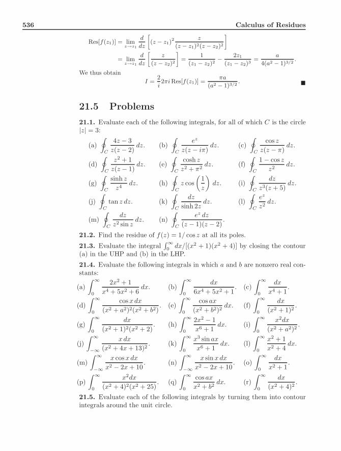
21.5 Problems

21.1. Evaluate each of the following integrals, for all of which C is the circle|z| = 3:

(a)#

C

4z − 3z(z − 2)

dz. (b)#

C

ez

z(z − iπ)dz. (c)

#

C

cos z

z(z − π)dz.

(d)#

C

z2 + 1z(z − 1)

dz. (e)#

C

cosh z

z2 + π2dz. (f)

#

C

1 − cos z

z2dz.

(g)#

C

sinh z

z4dz. (h)

#

Cz cos

$1z

%dz. (i)

#

C

dz

z3(z + 5)dz.

(j)#

Ctan z dz. (k)

#

C

dz

sinh 2zdz. (l)

#

C

ez

z2dz.

(m)#

C

dz

z2 sin zdz. (n)

#

C

ez dz

(z − 1)(z − 2).

21.2. Find the residue of f(z) = 1/ cos z at all its poles.

21.3. Evaluate the integral& ∞0 dx/[(x2 + 1)(x2 + 4)] by closing the contour

(a) in the UHP and (b) in the LHP.21.4. Evaluate the following integrals in which a and b are nonzero real con-stants:

(a)' ∞

0

2x2 + 1x4 + 5x2 + 6

dx. (b)' ∞

0

dx

6x4 + 5x2 + 1. (c)

' ∞

0

dx

x4 + 1.

(d)' ∞

0

cosxdx

(x2 + a2)2(x2 + b2). (e)

' ∞

0

cos ax

(x2 + b2)2dx. (f)

' ∞

0

dx

(x2 + 1)2.

(g)' ∞

0

dx

(x2 + 1)2(x2 + 2). (h)

' ∞

0

2x2 − 1x6 + 1

dx. (i)' ∞

0

x2dx

(x2 + a2)2.

(j)' ∞

−∞

xdx

(x2 + 4x + 13)2. (k)

' ∞

0

x3 sin ax

x6 + 1dx. (l)

' ∞

0

x2 + 1x2 + 4

dx.

(m)' ∞

−∞

x cosxdx

x2 − 2x + 10. (n)

' ∞

−∞

x sin xdx

x2 − 2x + 10. (o)

' ∞

0

dx

x2 + 1.

(p)' ∞

0

x2dx

(x2 + 4)2(x2 + 25). (q)

' ∞

0

cos ax

x2 + b2dx. (r)

' ∞

0

dx

(x2 + 4)2.

21.5. Evaluate each of the following integrals by turning them into contourintegrals around the unit circle.

21.5 Problems 537

(a)! 2π

0

dθ

5 + 4 sin θ. (b)

! 2π

0

dθ

a + cos θwhere a > 1.

(c)! 2π

0

dθ

1 + sin2 θ. (d)

! 2π

0

dθ

(a + b cos2 θ)2where a, b > 0.

(e)! 2π

0

cos2 3θ

5 − 4 cos 2θdθ. (f)

! π

0

dφ

1 − 2a cosφ + a2where a ̸= ±1.

(g)! π

0

cos2 3φ dφ


(h)! π

0

cos 2φ dφ


21.6. Use the method of residues to show that! π

0cos2n θ dθ = π

(2n)!22n(n!)2

21.7. Use the contour in Figure 21.4(a) to show that! ∞

−∞

sin x

xdx = π

by letting X → ∞, Y → ∞, and ϵ → 0.

21.8. Use the contour in Figure 21.4(b) to show that! ∞

0

11 + xn

dx =π/n

sin(π/n)

by letting R → ∞.

21.9. Use the contour in Figure 21.4(c) to show that! ∞

0sin(x2) dx =

! ∞

0cos(x2) dx =

"π

8

by letting R → ∞.

X−X −ε ε

X + iY−X + iY

R

R

π /42π /n

R

R

(a) (c)(b)

Figure 21.4: (a) The contour used for sin x/x. (b) The contour used for 1/(1 + xn).(c) The contour used for sin(x2).

Calculus of Residues

Documents

Transcript of Calculus of Residues