Residues of Weyl Group Multiple Dirichlet Series

byJoel B. Mohler

A DissertationPresented to the Graduate and Research Committee

of Lehigh Universityin Candidacy for the Degree of

Doctor of Philosophy

in

Mathematics

Lehigh University

April 22, 2009

CopyrightJoel B. Mohler

ii

Approved and recommended for acceptance as a dissertation in partial fulfillment ofthe requirements for the degree of Doctor of Philosophy.

Joel B. MohlerResidues of Weyl Group Multiple Dirichlet Series

Defense Date

Approved Date

Committee Members:

Bruce Dodson (Co-Chair)Lehigh University

Gautam Chinta (Co-Chair; Advisor)City College of New York

Paul GunnellsUniversity of Massachusetts

Steven WeintraubLehigh University

iii

Acknowledgments

I thank God for the wonders of the chaotic arrangement of the primes.

I thank my wife, Lydia, and boys, Alexander and Darren, for patiently waiting for me toget a “real” job.

I thank my mentor and friend Gautam Chinta for his professional and mathematicalguidance.

I dedicate this dissertation in loving memory to my father, Allen R. Mohler. He neverdid believe me that the set of prime numbers was infinite, but that didn’t stop him fromdoing beautiful brickwork.

iv

Contents

Abstract 1

1 Introduction 21.1 Background . . . . . . . . . . . . . . . . . . . . . . . . . . . . . . . . 21.2 Common Definitions . . . . . . . . . . . . . . . . . . . . . . . . . . . 41.3 Defining Z(n)

r and Principal Results . . . . . . . . . . . . . . . . . . . 6

2 A Pair of Double Dirichlet Series 82.1 Introduction . . . . . . . . . . . . . . . . . . . . . . . . . . . . . . . . 82.2 Gauss sums and L-Functions . . . . . . . . . . . . . . . . . . . . . . . 132.3 Functional Equation: H1 → H2 . . . . . . . . . . . . . . . . . . . . . . 162.4 Functional Equation: Z1 → Z2 . . . . . . . . . . . . . . . . . . . . . . 182.5 Convolutions . . . . . . . . . . . . . . . . . . . . . . . . . . . . . . . 202.6 Evaluation of Z1 and Z2 . . . . . . . . . . . . . . . . . . . . . . . . . 20

3 Uniqueness of Local Factors 243.1 Introduction . . . . . . . . . . . . . . . . . . . . . . . . . . . . . . . . 243.2 Ar Weyl Group . . . . . . . . . . . . . . . . . . . . . . . . . . . . . . 273.3 An Action on Laurent Series . . . . . . . . . . . . . . . . . . . . . . . 303.4 Invariant Rational Functions . . . . . . . . . . . . . . . . . . . . . . . 37

4 Residues of Weyl Group Multiple Dirichlet Series 424.1 Introduction . . . . . . . . . . . . . . . . . . . . . . . . . . . . . . . . 424.2 Gauss Sum Invariances over Weyl Group Cosets . . . . . . . . . . . . . 464.3 Normalizing Residues . . . . . . . . . . . . . . . . . . . . . . . . . . . 514.4 Global Series Z(n)

r . . . . . . . . . . . . . . . . . . . . . . . . . . . . . 53

5 Conclusion 55

Bibliography 58

Vita 59

v

Abstract

We give explicit computations of a pair of double Dirichlet series first studied by

the Friedberg, Hoffstein, and Lieman. These computations are performed in the rational

function field because, in this context, the series are power series which turn out to be

rational functions.

Recently the Weyl group multiple Dirichlet series have been an area of intense re-

search. We provide an explicit computation for these series associated to the root system

of type Ar, again in the rational function field case. This shows the equivalence of two

different descriptions of the local parts of these series and establishes uniqueness. It is

conjectured that a multiresidue of the Weyl group multiple Dirichlet series correspond

with the double Dirichlet series first noted of Friedberg, Hoffstein, and Lieman. This

conjecture is proven in the rational function field case using the computed rational func-

tions.

1

Chapter 1

Introductionjoy unfound

in lovely sunset;

I turn and see the symmetry

1.1 Background

The techniques of multiple Dirichlet series have arisen in recent decades as a way of

providing estimates and average values of special values of L-functions over various

fields. In just the past 10 years, there has been a concerted effort to unify and extend

these results in a consistent framework. This has resulted in the description of Weyl

group multiple Dirichlet series by Brubaker, Bump, Chinta, Friedberg, Hoffstein, and

Gunnells in the papers [BBC+06, BBF06, CGa] (by some subsets of the aforementioned

authors). These are a generalization of single variable Dirichlet series to multiple com-

plex variables and they satisfy a larger group of functional equations.

There remain a number of unanswered questions in these and related papers. For ex-

ample, Friedberg, Hoffstein, and Lieman described two bivariate multiple Dirichlet se-

ries in [FHL02] which, taken together, satisfy a group of 32 functional equations. These

bivariate series are not actually Weyl group multiple Dirichlet series, but Brubaker and

Bump ([BB06]) provided evidence that they are actually (r − 2)-fold residues of Weyl

group multiple Dirichlet series associated to the root system Ar for r ≥ 2. They veri-

2

fied this conjecture for type A3, but were unable to prove the conjectured relationship in

general. The case r = 3 is manageable because, thanks to Patterson [Pat77a, Pat77b],

we have a complete understanding of the Fourier coefficients of the theta function on

the 3-fold metaplectic cover of SL2 that arise when we take the residues of the Dirichlet

series constructed from cubic Gauss sums. For r > 3 the precise nature of the coef-

ficients of the r-fold cover theta functions remains mysterious. Nevertheless, there is

much evidence in favor of the expectation that the two series constructed by Friedberg,

Hoffstein and Lieman coincide with a multiresidue of a Weyl group multiple Dirichlet

series. The principal work of this dissertation is to explicitly compute these series over

a rational function field and to show that these residue relationships hold for r ≥ 2. In

[Chi08] Chinta has carried out this explicit computation for r = 2. This dissertation

expands on his work by computing these rational functions for all Ar with r ≥ 2.

Another partially open question is to understand the relationship of the construc-

tion in [BBC+06, BBF06] and an alternative construction by Chinta and Gunnells in

[CGa]. Chinta and Gunnells construct Weyl group multiple Dirichlet series by defining

a group action and finding an invariant expression by summing over the Weyl group.

The equivalence of these definitions has been supported by computational comparison

and is proven rigorously for series of type A2 built from quadratic twists in [CFG08].

In this dissertation we extend this result to show that these definitions are equivalent for

stable series of type Ar.

In general, a multiple Dirichlet series has the form

Z(s1, . . . , sr) =∑ a(c1, . . . , cr)

|c1|s1|c2|s2 · · · |cr|sr,

where the sum is over the integer r-tuples (c1, . . . , cr) (or integer ring of some global

field modulo units), | · | is the absolute norm. For the Weyl group multiple Dirichlet

series, the numerator a(c1, . . . , cr) satisfies a twisted multiplicativity, initially we have

3

convergence for <(si) sufficiently large, and the analytic continuation has been estab-

lished for all of Cr. More specifically, the series corresponding to the root system A2 is

heuristically given by

Z(n)2 (s1, s2) =

∑ g(1, c1)g(1, c2)(c1c2

)−1

|c1|s1|c2|s2.

We say “heuristically” since(c1c2

)is only defined for c1, c2 relatively prime. In reality

we define the numerator precisely by defining it for prime powers c1 = pk and c2 = pl

and using the twisted multiplicativity. Here g(1, c) is a Gauss sum constructed from

nth power residue symbols and(c1c2

)is such an nth power residue symbol. Each root

system Ar has an associated series with r complex variables, which can be constructed

from nth order Gauss sums for n ≥ 1. We will indicate such a series by Z(n)r . We will

give a more precise definition for Z(n)r in Section 1.3.

The advantage of limiting ourselves to the rational function field is that the series

Z(n)r can be computed explicitly as a rational function of |ci|−si for 1 ≤ i ≤ r. With this

explicit form, we can then use elementary techniques to evaluate the r − 2 residues and

observe the desired relationship.

1.2 Common Definitions

Throughout this dissertation, n ≥ 2 will be an integer and we construct our various

series with nth power residue symbols. We will work over the finite field Fq with q

elements. Let µn = a ∈ Fq : an = 1 and let χ : F×q → µn be the character a 7→ aq−1n .

Let K be the rational function field Fq(t) with polynomial ring OK = Fq[t]. We let K∞

denote the field of Laurent series in t−1.

In order to define Gauss sums we first need an additive character on K∞. Let e0 be

a nontrivial additive character on Fp. Use e0 to define a character e? of Fq by e?(a) =

4

e0(TrFq/Fpa). Let ω be the global differential dx/x2. Finally define the character e of

K∞ by e(y) = e?(Res∞(ωy)) for y ∈ K∞. Note that

y ∈ K : e|yOK = 1 = OK .

Fix an embedding ε from the the nth roots of unity of Fq to C×.

The most basic Gauss sums we utilize are

g(1, ε, p) =∑y mod p

ε

((y

p

))e

(y

p

)(1.1)

and

τ(ε) =∑j∈Fq

ε(j(q−1)/n

)e0 (j) , (1.2)

which is associated with the field Fq.

A common feature appearing throughout this dissertation is a formal relationship

between the rational function defining the local part and the closed form evaluation of

the series. This will appear in various guises, but the general variable changes

si → 2− si for 1 ≤ i ≤ r|p| → 1

q

g(1, εi, p)/√|p| → τ(εi)/

√q for 1 ≤ i ≤ r

(1.3)

transform the local rational function at p to the global series Z. This similarity arises

as the local series and the global series both satisfy functional equations with a similar

form. We will show that these similar functional equations admit unique solutions,

which must also be similar.

Remark 1.2.1. The classical single variable ζ function associated with Fq[t] exhibits

the variable transformations of equation (1.3). Recall that

ζFq [t](s) =∑d monic

|d|−s =∞∑n=0

# monic polynomials of degree nqns

=∞∑n=0

qn

qns=

1

1− q1−s ,

(1.4)

5

and the p-part for some irreducible p is

ζp(s) =∞∑n=0

|pn|−s =1

1− |p|−s. (1.5)

1.3 Defining Z(n)r and Principal Results

In this section we will give a more precise definition of the Weyl group multiple Dirich-

let series Z(n)r . We will also indicate the theorems which motivate the work in this

dissertation. We define

Z(n)r (s1, . . . , sr) = Ω(s1, . . . , sr)

∑ H(c1, . . . , cr)

|c1|s1|c2|s2 · · · |cr|sr(1.6)

where the sum is over all r-tuples (c1, . . . , cr) with ci, 1 ≤ i ≤ r, monic polynomials in

Fq[t] and Ω is a product of normalizing zeta factors which is entirely defined in Chapter

4. The numerator H(c1, . . . , cr) is defined via a twisted multiplicativity which we now

describe. For fixed (c1 · · · cr, c′1 · · · c′r) = 1, we put

H(c1c′1, . . . , crc

′r) = ξ(c, c′)H(c1, . . . , cr)H(c′1, . . . , c

′r), (1.7)

where

ξ(c, c′) =r∏i=1

(cic′i

)(c′ici

) r∏i=2

(cic′i−1

)(c′ici−1

). (1.8)

The p-part of Z(n)r is given in Theorem 3.1.1. This p-part together with the twisted

multiplicativity entirely determines the coefficients H .

Here is a brief outline of the remainder of this dissertation. In Chapter 2 we compute

a pair of double Dirichlet series over the rational function field. We heuristically define

the first

Z1,FHL(s, w) =∑m

L(s, χm)

|m|w

6

but delay any discussion of the second Z2,FHL until later. Here χm is an nth order power

residue symbol. The series Z1,FHL and Z2,FHL are related by a group of functional

equations induced by the functional equation of L(s, χm).

Chapter 3 lays the foundation for Chapter 4 by establishing properties of the p-part of

Z(n)r . Following [CGa] we use a functional equation which the p-partH(n)

r (s1, . . . , sr; p)

must satisfy to derive an explicit rational function expression for H(n)r . This establishes

the following theorem:

Theorem 1.3.1. Let n > r. Then the p-part of the Weyl group multiple Dirichlet series

Z(n)r described in [BBC+06] matches that of [CGa].

Refer to Theorem 3.1.1 for the rational function.

Finally, in Chapter 4 we show that the Zi,FHL series are a multiresidue of Weyl group

multiple Dirichlet series. We prove the following theorem:

Theorem 1.3.2. Given Z(r)r defined in equation (4.1) and Z1,FHL, Z2,FHL defined in

Chapter 2, we have

Resx2→q−(r+1)/r

· · · Resxr−1→q−(r+1)/r

Z(r)r (x1, x2, . . . , xr) =

ErZ1,FHL(q1/rx1, q

1/rxr)∏r−1i=2 (1− qr−i+2xr1)(1− qr−i+2xrr)

(1.9)

and

Resx3→q−(r+1)/r

· · · Resxr→q−(r+1)/r

Z(r)r (x1, x2, . . . , xr) =

ErZ2,FHL(q1/2x1, q

(r+1)/rx2)∏r−1i=2 (1− qr−i+1xr1x

r2) (1− qr−i+2xr2)

(1.10)

where Er is a constant depending only on r. We have used the notation xi = q−si ,

1 ≤ i ≤ r.

Theorem 4.1.1 specifies the constant Er.

7

Chapter 2

A Pair of Double Dirichlet Seriesto comprehend

the equal equals;

we seek thy bashful face

2.1 Introduction

The main result of this chapter is the explicit computation of an infinite sum of L-

functions associated to nth order Hecke characters of K. The infinite sums we consider

are examples of double Dirichlet series in two complex variables, and can be written as

power series in q−s and q−w. In fact it will turn out that the series we construct will be

rational functions in q−s and q−w.

The series studied in this chapter are not Weyl group multiple Dirichlet series. How-

ever, we will show in Chapter 4 that they are a multiresidue of certain Weyl group

multiple Dirichlet series. We compute them here in the rational function field case in

preparation for these later results.

These series are function field analogs of the series studied by Friedberg, Hoffstein

and Lieman in [FHL02]. In that paper, working over a number field F containing the

nth roots of unity, the authors study a double Dirichlet series that is roughly of the form

∑m

L(s, χm)(Nm)−w,

8

where the sum is over integral ideals m of F , the character χm is the nth order power

residue symbol associated to m, and Nm denotes the absolute norm. The authors show

that this double Dirichlet series has a meromorphic continuation to all (s, w) ∈ C2 and

satisfies a group of functional equations relating it to a second series constructed from

Gauss sums. The main ingredients in the proof are the functional equation of L(s, χm),

properties of the Fourier coefficients of the metaplectic Eisenstein series on the n-fold

cover of GL2, and Bochner’s tube theorem.

In the case n = 2, these ideas were applied by Fisher and Friedberg [FF04] in the

context of a general function field to show the rationality of double Dirichlet series

constructed from quadratic L-functions. The case n = 2 is somewhat easier because

the Gauss sum arising in the functional equation of a quadratic Hecke L-series is trivial,

and the theory of metaplectic Eisenstein series is not needed.

Here we follow a more elementary method originally introduced in [CFH06] in the

case n = 2. We exploit the fact that

∑d∈Fq [t]deg d=k

(d

m

)

vanishes if k is bigger than or equal to the degree of m, unless m is a perfect nth power.

Here(dm

)= χm(d) denotes the nth power residue symbol for m, d relatively prime. If

m and d are monic, then we have the reciprocity law

(md

)=

(d

m

), (2.1)

when q is congruent to 1 mod 2n, see e.g. Rosen [Ros02], Theorem 3.5.

We now describe our results more precisely. We will define two double Dirichlet

series, explicitly compute them as rational functions in q−s, q−w and show that they

satisfy functional equations that relate them to one another. We begin by defining two

9

multiplicative weighting factors a(d,m) and b(d,m) for pairs of monic polynomials, as

in [FHL02]. For a monic prime polynomial p, let

a(pj, pk) =

|p|(n−1)d/n if d = min(j, k) and d ≡ 0 mod n0 otherwise,

(2.2)

and

b(pj, pk) =

1 if k = 0

|p|k/2−1(|p| − 1) if j ≥ k, k ≡ 0 mod n, k > 0

−|p|k/2−1 if j = k − 1, k ≡ 0 mod n, k > 0

|p|(k−1)/2 if j = k − 1, k 6≡ 0 mod n, k > 0

0 otherwise.

(2.3)

Then define

a(d,m) =∏pj ||dpk||m

a(pj, pk), b(d,m) =∏pj ||dpk||m

b(pj, pk).

Here |d| denotes the norm qdeg d.

LetO denote Fq[t] andOmon the set of monic polynomials in Fq[t]. Let ζO(s) be the

zeta function of the ring O, that is

ζO(s) = (1− q1−s)−1.

The first double Dirichlet series we consider is

Z1(s, w) =∑

d,m∈Omon

χm0(d)a(d,m)

|m|w|d|s, (2.4)

where m0 is the nth powerfree part of m and d is the part of d relatively prime to m0.

We show in Section 2.2 that this can be rewritten in terms of L-functions

Z1(s, w) =∑

m∈Omon

L(s, χm0)

|m|wP (s;m), (2.5)

where the P (s;m) are finite Euler products defined in Proposition 2.2.1.

10

The second multiple Dirichlet series is built from Gauss sums. See Section 2.2 for

the precise definition of the Gauss sum g(r, ε, χm). Then

Z2(s, w) = ζO(nw − n

2+ 1)

∑d,m∈Omon

g(1, ε, χm0)√|m[|

χm0(d)b(d,m)

|m|w|d|s(2.6)

where m[ is the squarefree part of the nth powerfree part of m.

We can now state the main theorems of this chapter. The first describes a set of

functional equations relating Z1 and Z2. Specifically, define

Z1(s, w; δi) =∑

d,m∈Omondeg m≡i (mod n)

χm0(d)a(d,m)

|m|w|d|s

and

Z2(s, w; δi) = ζO(nw − n

2+ 1)

∑d,m∈Omon

deg m≡i (mod n)

g(1, ε, χm0)√|m[|

χm0(d)b(d,m)

|m|w|d|s.

Theorem 2.1.1. We have the functional equation

Z1(s, w; δi) =

q2s−1 1−q−s

1−qs−1Z2(1− s, w + s− 12; δ0) for i = 0

q2s−1q1/2−s τ(εi)√qZ2(1− s, w + s− 1

2; δi) for 0 < i < n.

The finite field Gauss sum τ(εi) is defined in equation (1.2).

This is proved in Section 2.4.

The second main theorem is the following:

Theorem 2.1.2. The double Dirichlet series Z1 and Z2 are rational functions of x = q−s

and y = q−w. Explicitly,

Z1(s, w) =1− q2xy

(1− qx)(1− qy)(1− qn+1xnyn), (2.7)

and

Z2(s, w) =1− q3n/2xn−1yn +

∑n−1i=1

(τ(εi)qi−1+i/2xi−1yi − τ(εi)q3i/2xiyi

)(1− qx)(1− qn/2+1yn)(1− q3n/2xnyn)

. (2.8)

11

This theorem is proved in Section 2.6.

When we have need outside of this chapter, we will refer to the series Z1 and Z2 as

Z1,FHL and Z2,FHL respectively. Likewise, their local parts will be denoted as H1,FHL

and H2,FHL. Outside of this chapter, we reserve the notation Zr for the Weyl group

multiple Dirichlet series associated with the root system Ar.

Finally we point out a curious connection between the seriesZi of Theorem 2.1.2 and

their p-parts. Define the following generating series Hi constructed from the respective

p-parts of Z1 and Z2:

H1(X, Y ) =∑j,k≥0

a(pj, pk)XjY k, and

H2(X, Y ) = (1− |p|n/2−1Y n)−1∑j,k≥0

b(pj, pk)g(1, ε, χpk)√|pk[ |

XjY k,(2.9)

where X = |p|−s and Y = |p|−w. We will prove

H1(X, Y ) =1−XY

(1−X)(1− Y )(1− |p|n−1XnY n),

H2(X, Y ) =1− |p|n/2−1X(n−1)Y n +

∑n−1i=1

g(1,εi,χp)√|p|

X(i−1)Y i|p|(i−1)/2(1−X)

(1−X)(1− |p|n/2−1Y n)(1− |p|n/2XnY n).

(2.10)

Note that the substitutions

X → qx,

Y → qy,

|p| → 1/q, and

g(1, εi, p)/√|p| → τ(εi)/

√q for 1 ≤ i ≤ r

(2.11)

transform Hi into Zi for i = 1, 2. This is one manifestation of the general variable

transformations given in equation (1.3).

12

2.2 Gauss sums and L-Functions

In this section we will define the Gauss sums and L-functions that are the constituents

of our double Dirichlet series. We will mostly follow the notation of Patterson [Pat 2]

but with some adjustments to facilitate comparison with [FHL02].

We now define a more general Gauss sum than the one found in the introduction in

equation (1.1). For any c ∈ O, we will use c0 to indicate the nth-power free part of c

and c[ for the squarefree part of c0. For r, c ∈ O we define the Gauss sum

g(r, ε, χc) =∑

y mod c[

ε((y

c

))e

(ry

c[

).

We also need the Gauss sums associated to the finite field Fq. These are defined by

τ(ε) =∑j∈Fq

ε(j(q−1)/n

)e0 (j) .

We define the L-function associated to χm by

L(s, χm) =∑

d∈Omon

χm(d)|d|−s. (2.12)

When m is nth-power free, the L-function satisfies a functional equation that we will

describe now. Denote the conductor of the character χm by cond χm. Thus

|cond χm| =

|m[| deg m ≡ 0(n)

q|m[| deg m 6≡ 0(n).

Then the completed L-function

L∗(s, χm) =

1

1−q−sL(s, χm) deg m ≡ 0(n)

L(s, χm) deg m 6≡ 0(n).(2.13)

satisfies the functional equation

L∗(s, χm) = q2s−1|cond χm|1/2−sg∗(1, ε, χm)

|cond χm|1/2L∗(1− s, χm) (2.14)

13

where

g∗(1, ε, χm) =

g(1, ε, χm) deg m ≡ 0 (mod n)τ(εi)g(1, ε, χm) deg m ≡ i 6≡ 0 (mod n).

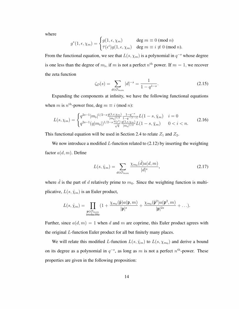
From the functional equation, we see that L(s, χm) is a polynomial in q−s whose degree

is one less than the degree of m[, if m is not a perfect nth power. If m = 1, we recover

the zeta function

ζO(s) =∑

d∈Omon

|d|−s =1

1− q1−s . (2.15)

Expanding the components at infinity, we have the following functional equations

when m is nth-power free, deg m ≡ i (mod n):

L(s, χm) =

q2s−1|m[|1/2−s g(1,ε,χm)

|m[|1/21−q−s

1−q−(1−s)L(1− s, χm) i = 0

q2s−1(q|m[|)1/2−s τ(εi)√qg(1,ε,χm)

|m[|1/2L(1− s, χm) 0 < i < n.

(2.16)

This functional equation will be used in Section 2.4 to relate Z1 and Z2.

We now introduce a modified L-function related to (2.12) by inserting the weighting

factor a(d,m). Define

L(s, χm) =∑

d∈Omon

χm0(d)a(d,m)

|d|s, (2.17)

where d is the part of d relatively prime to m0. Since the weighting function is multi-

plicative, L(s, χm) is an Euler product,

L(s, χm) =∏

p∈Omonirreducible

(1 +χm0(p)a(p,m)

|p|s+χm0(p

2)a(p2,m)

|p|2s+ . . .).

Further, since a(d,m) = 1 when d and m are coprime, this Euler product agrees with

the original L-function Euler product for all but finitely many places.

We will relate this modified L-function L(s, χm) to L(s, χm0) and derive a bound

on its degree as a polynomial in q−s, as long as m is not a perfect nth-power. These

properties are given in the following proposition:

14

Proposition 2.2.1. We have

L(s, χm) = L(s, χm0)P (s;m),

where P (s;m) =∏

p Pp(s;m) and Pp(s;m) =(1− χm0(p)|p|−s

) nα−1∑k=0

χm0(pk)a(pnα, pk)

|p|ks+ |p|−nαs|p|(n−1)α if p - m0

nα∑k=0

a(pnα+i, pk)

|p|ksif pi||m0 and i 6= 0.

Here α and i are the unique integers with 0 ≤ i < n and pnα+i‖m. In particular, for m

not a perfect nth power, the degree of L(s, χm) as a polynomial in q−s is less than the

degree of m.

Proof. Begin with the Euler product

L(s, χm) =∏

p

∞∑k=0

χm0(pk)a(m, pk)

|p|ks

=∏

pnα||m

∞∑k=0

χm0(pk)a(pnα, pk)

|p|ks×

∏pnα+i||m0<i<n

∞∑k=0

a(pnα+i, pk)

|p|ks

For primes p with i = 0—that is p - m0 and pnα||m, say— it follows from (2.2) that the

tails of the sum are a geometric series with common ratio χm0(p)|p|−s. Thus for such p

the p-part isnα−1∑k=0

χm0(pk)a(pnα, pk)

|p|ks+|p|−nαs|p|(n−1)α

1− χm0(p)|p|−s=(1− χm0(p)|p|−s

)−1Pp(s;m),

where

Pp(s;m) =nα−1∑k=0

χm0(pk)a(pnα, pk)

|p|ks(1− χm0(p)|p|−s

)+ |p|−nαs|p|(n−1)α. (2.18)

For primes such that pi||m0 with 0 < i < n, it follows from (2.2) that a(pnα+i, pk) =

0 for k > nα, so the p-part is a finite sum

Pp(s;m) =nα∑k=0

a(pnα+i, pk)

|p|ks.

15

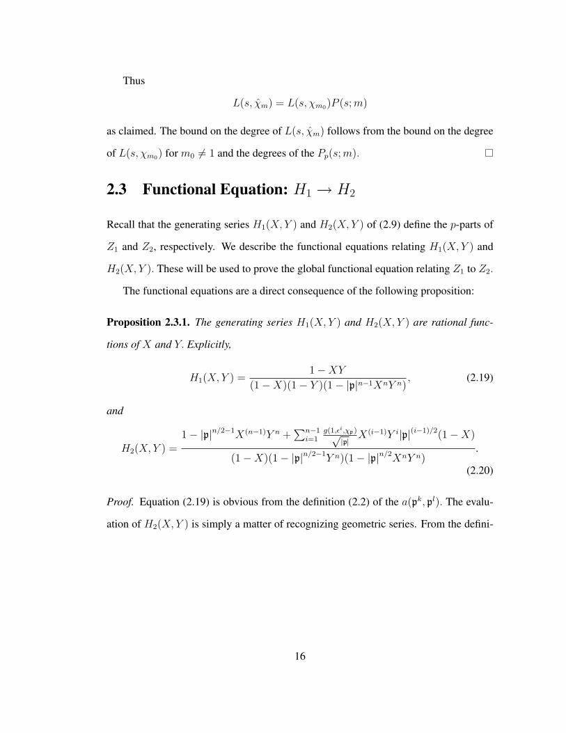
Thus

L(s, χm) = L(s, χm0)P (s;m)

as claimed. The bound on the degree of L(s, χm) follows from the bound on the degree

of L(s, χm0) for m0 6= 1 and the degrees of the Pp(s;m).

2.3 Functional Equation: H1 → H2

Recall that the generating series H1(X, Y ) and H2(X, Y ) of (2.9) define the p-parts of

Z1 and Z2, respectively. We describe the functional equations relating H1(X, Y ) and

H2(X, Y ). These will be used to prove the global functional equation relating Z1 to Z2.

The functional equations are a direct consequence of the following proposition:

Proposition 2.3.1. The generating series H1(X, Y ) and H2(X, Y ) are rational func-

tions of X and Y. Explicitly,

H1(X, Y ) =1−XY

(1−X)(1− Y )(1− |p|n−1XnY n), (2.19)

and

H2(X, Y ) =1− |p|n/2−1X(n−1)Y n +

∑n−1i=1

g(1,εi,χp)√|p|

X(i−1)Y i|p|(i−1)/2(1−X)

(1−X)(1− |p|n/2−1Y n)(1− |p|n/2XnY n).

(2.20)

Proof. Equation (2.19) is obvious from the definition (2.2) of the a(pk, pl). The evalu-

ation of H2(X, Y ) is simply a matter of recognizing geometric series. From the defini-

16

tions of b(pj, pk) in (2.3) and H2 in (2.9), we have

(1− |p|n/2−1Y n)H2(X, Y ) =∞∑j=0

g(1, ε, χp0)√|p0[ |

XjY 0

+∞∑α=1

∞∑j=nα

|p|nα/2−1(|p| − 1)g(1, ε, χpnα)√|pnα[ |

XjY nα

+∞∑α=1

−|p|nα/2−1 g(1, ε, χpnα)√|pnα[ |

Xnα−1Y nα

+∞∑α=0

n−1∑i=1

|p|(nα+i−1)/2 g(1, ε, χpnα+i)√|pnα+i[ |

Xnα+i−1Y nα+i.

Evaluating the geometric series yields

(1− |p|n/2−1Y n)H2(X, Y ) =1

1−X+|p|n/2−1(|p| − 1)XnY n

(1−X)(1− |p|n/2XnY n)

+−|p|n/2−1Xn−1Y n

1− |p|n/2XnY n+

n−1∑i=1

g(1,εi,χp)√|p||p|(i−1)/2X i−1Y i

(1− |p|n/2XnY n).

(2.21)

Equation (2.20) follows by rewriting equation (2.21).

For 0 ≤ i < n, define

H1(X, Y ; δi) =∑j,k≥0k≡i(n)

a(pj, pk)XjY k,

H2(X, Y ; δi) = (1− |p|n/2−1Y n)−1∑j,k≥0k≡i(n)

b(pj, pk)g(1, ε, χpk)√|pk[ |

χpk(pj)XjY k.

(2.22)

We have shown in Proposition 2.3.1 that H1 and H2 are both rational functions in |p|−s

and |p|−w and it is clear from this proposition that

H1(X, Y ; δi) =

1−XY n

(1−X)(1−Y n)(1−|p|n−1XnY n)i ≡ 0

(1−X)Y i

(1−X)(1−Y n)(1−|p|n−1XnY n)i 6≡ 0,

(2.23)

and

H2(X, Y ; δi) =

1−|p|n/2−1X(n−1)Y n

(1−X)(1−|p|n/2−1Y n)(1−|p|n/2XnY n)i ≡ 0

g(1,εi,χp)√|p|

X(i−1)Y i|p|(i−1)/2(1−X)

(1−X)(1−|p|n/2−1Y n)(1−|p|n/2XnY n)i 6≡ 0.

(2.24)

17

The following theorem establishes a functional equation relating H1 to H2:

Theorem 2.3.2. We have the functional equation

H1(p−s, p−w; δi) =

1−|p|−(1−s)

1−|p|−s H2(p−(1−s), p−(w+s−1/2); δ0) i = 0√|p|

g(1,εi,χp)|p|s−1/2H2(p−(1−s), p−(w+s−1/2); δi) 0 < i < n.

Proof. The proof is by a direct computation using Equations (2.23) and (2.24).

2.4 Functional Equation: Z1 → Z2

There is a set of functional equations relating Z1 and Z2. These will be described in this

section. Define

Q(s;m) =P (1− s;m)

(m/m[)s−1/2. (2.25)

With the expansion of P as an Euler product, we see that Q is also an Euler product

supported in the primes dividing m:

Q(s;m) =∏

pnα+i||mi=0

1

|p|nα(s−1/2)Pp(1− s;m)×

∏pnα+i||m0<i<n

1

|p|(nα+i−1)(s−1/2)Pp(1− s;m).

Proposition 2.4.1. Define

Z ′2(s, w) =∑m

g(1, ε, χm0)√|m[|

L(s, χm0)Q(s;m)

|m|w.

We have Z ′2 = Z2.

Proof. Define

H ′2(p−s, p−w; δi) =

(1− p−s)−1∑∞

k=0Q(s;pnk)

pnkwi = 0

g(1,εi,χp)√|p|

∑∞k=0

Q(s;pnk+i)pnkw

0 < i < n.(2.26)

Then H ′2(p−s, p−w) =∑n−1

i=0 H′2(p−s, p−w; δi) is the p-part of Z ′2. We will show that

H ′2 and H2 both satisfy the functional equations with H1 shown in Theorem 2.3.2 and

18

therefore H ′2 = H2. The result follows since, for fixed m, the L-functions, P , and Q

each have Euler products.

As a result of the definition in equation (2.25), the p-parts of Q and P satisfy

P (s; pnα+i) =

pnα(1/2−s)Q(1− s; pnα) i = 0

p(nα+i−1)(1/2−s)Q(1− s; pnα+i) 0 < i < n.

Therefore, we relate H1 to H ′2 by

H1(p−s, p−w; δ0) =(1− |p|−s)−1

∞∑k=0

P (s; pnk)

|p|nkw

=(1− |p|−s)−1

∞∑k=0

Q(1− s; pnk)|p|nk(1/2−s)

|p|nkw

=(1− |p|−s)−1

∞∑k=0

Q(1− s; pnk)|p|nk(w+s−1/2)

=1− |p|−(1−s)

1− |p|−sH ′2(p−(1−s), p−(w+s−1/2); δ0).

This is exactly the functional equation satisfied by H2 in Theorem 2.3.2. A similar

computation shows that

H1(p−s, p−w; δi) =

√|p|

g(1, εi, χp)|p|s−1/2H2(p−(1−s), p−(w+s−1/2); δi)

for 0 < i < n. Thus H ′2(X, Y ; δi) = H2(X, Y ; δi) for all 0 ≤ i < n and this completes

the proof.

For 0 ≤ i < n, define

Z1(s, w; δi) =∑

m∈Omondeg m≡i (mod n)

L(s, χm0)P (s;m)

|m|w

and

Z2(s, w; δi) =∑

m∈Omondeg m≡i (mod n)

g(1, ε, χm0)√|m[|

L(s, χm0)Q(s;m)

|m|w.

19

Theorem 2.4.2. We have the functional equation

Z1(s, w; δi) =

q2s−1 1−q−s

1−qs−1Z2(1− s, w + s− 12; δ0) for i = 0

q2s−1q1/2−s τ(εi)√qZ2(1− s, w + s− 1

2; δi) for 0 < i < n.

Proof. This is a direct computation utilizing the functional equation (2.16) forL(s, χm0).

2.5 Convolutions

We define a convolution operation ? on rational functions in x and y with power series

expansions around the origin. For

A(x, y) =∑j,k≥0

a(j, k)xjyk and B(x, y) =∑j,k≥0

b(j, k)xjyk,

define

(A ? B)(x, y) =∑j,k≥0

a(j, k)b(j, k)xjyk.

We can compute convolutions as the double integral

(A ? B)(x, y) =

(1

2πi

)2 ∫ ∫A(u, v)B(

x

u,y

v)dudv

uv, (2.27)

where each integral is a counterclockwise circuit of a small circle in the complex plane.

(The circle must be small enough that A(x, y) is holomorphic for x, y inside the circle.)

We will utilize the residue theorem to compute this contour integral.

2.6 Evaluation of Z1 and Z2

We will now prove Theorem 2.1.2. We first establish the identity (2.7); then (2.8) will

follow from the functional equation (2.1.1). It follows from Proposition 2.2.1 that

∑d∈Omondeg d=k

χm0(d)a(d,m) = 0 (2.28)

20

when deg m ≤ k unless m is a perfect nth power. To prove (2.7) of Theorem 2.1.2, we

begin by writing

Z1(s, w) = Za(s, w) + Za(w, s)− Zb(s, w) (2.29)

where

Za(s, w) =∑k≥j≥0

1

qjwqks

∑d,m∈Omon

deg m=jdeg d=k

χm0(d)a(d,m)

and

Zb(s, w) =∑k≥0

1

qkwqks

∑m∈Omondeg m=j

∑d∈Omondeg d=k

χm0(d)a(d,m).

First, note that∑m∈Omondeg m=j

∑d∈Omondeg d=k

χm0(d)a(d,m) =∑

m∈Omondeg m=j

∑d∈Omondeg d=k

χd0(m)a(m, d).

When m and d are coprime, the reciprocity law (2.1) guarantees that χm0(d) = χd0(m).

Otherwise, when m and d are not coprime, χm0(d) 6= χd0(m) only when there exists a

prime p such that p|d0 and p|m0. In this case a(d,m) = 0. The symmetry a(d,m) =

a(m, d) is obvious. This establishes the validity of the decomposition (2.29) of Z1.

Now the key observation is that because of equation (2.28), we have

Za(s, w) =∑k≥j≥0

1

qjwqks

∑m∈Omondeg m=jm0=1

∑d∈Omondeg d=k

a(d,m)

and

Zb(s, w) =∑k≥0

1

qkwqks

∑m∈Omondeg m=km0=1

∑d∈Omondeg d=k

a(d,m),

that is, the inner sum vanishes unless m is a perfect nth-power. This leads us to consider

the series

Ta(s, w) =∑

m∈Omonm0=1

∑d∈Omon

a(d,m)

|m|w|d|s,

21

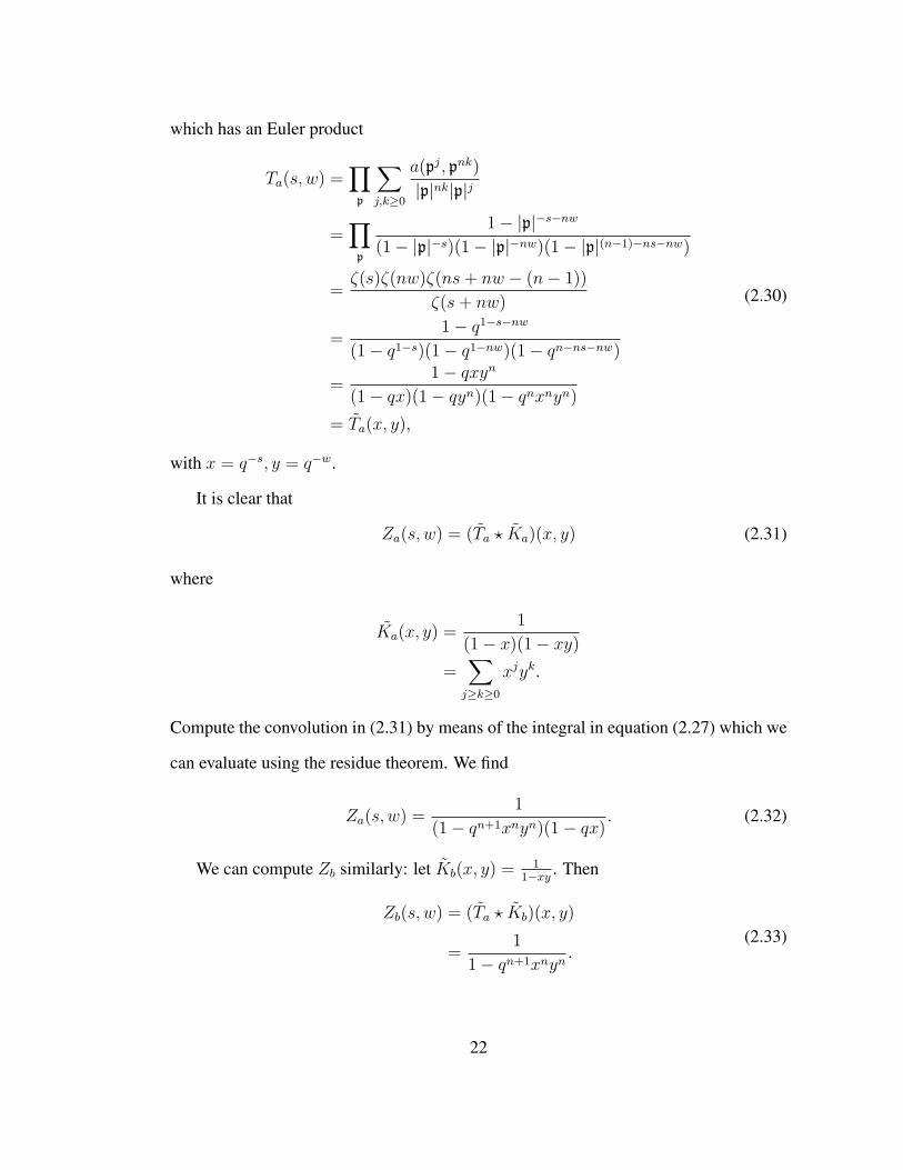
which has an Euler product

Ta(s, w) =∏

p

∑j,k≥0

a(pj, pnk)

|p|nk|p|j

=∏

p

1− |p|−s−nw

(1− |p|−s)(1− |p|−nw)(1− |p|(n−1)−ns−nw)

=ζ(s)ζ(nw)ζ(ns+ nw − (n− 1))

ζ(s+ nw)

=1− q1−s−nw

(1− q1−s)(1− q1−nw)(1− qn−ns−nw)

=1− qxyn

(1− qx)(1− qyn)(1− qnxnyn)

= Ta(x, y),

(2.30)

with x = q−s, y = q−w.

It is clear that

Za(s, w) = (Ta ? Ka)(x, y) (2.31)

where

Ka(x, y) =1

(1− x)(1− xy)

=∑j≥k≥0

xjyk.

Compute the convolution in (2.31) by means of the integral in equation (2.27) which we

can evaluate using the residue theorem. We find

Za(s, w) =1

(1− qn+1xnyn)(1− qx). (2.32)

We can compute Zb similarly: let Kb(x, y) = 11−xy . Then

Zb(s, w) = (Ta ? Kb)(x, y)

=1

1− qn+1xnyn.

(2.33)

22

Putting this all together,

Z1(s, w) =1

(1− qn+1xnyn)(1− qx)+

1

(1− qn+1xnyn)(1− qy)

− 1

1− qn+1xnyn

=1− qy + 1− qx− (1− qy)(1− qx)

(1− qn+1xnyn)(1− qx)(1− qy)

=1− q2xy

(1− qn+1xnyn)(1− qx)(1− qy).

(2.34)

This establishes (2.7).

With the rational function for Z1(s, w), we can use the functional equations relating

Z1(s, w; δi) and Z2(s, w; δi) for 0 ≤ i < n to evaluate Z2(s, w). Expanding the geomet-

ric series 11−qy and collecting terms with the exponent on y congruent to i (mod n), we

arrive at

Z1(s, w; δi) =

1−qn+1xyn

(1−qx)(1−qnyn)(1−qn+1xnyn)i = 0

(qi−qi+1x)yi

(1−qx)(1−qnyn)(1−qn+1xnyn)0 < i < n.

Using the functional equations relating Z1(s, w, δi) and Z2(1− s, w+ s− 12, δi) and

remembering that∣∣∣ τ(εi)√

q

∣∣∣ = 1, we see that

Z2(s, w; δi) =

q2s−1 1−q−s

1−qs−1Z1(1− s, w + s− 12; δi) i = 0

q2s−1q1/2−s τ(εi)√qZ1(1− s, w + s− 1

2; δi) 0 < i < n.

With this in hand, Z2 is

q2s−1 1− q−s

1− qs−1Z1(1− s, w+ s− 1

2; δ0) +

n−1∑i=1

q2s−1q1/2−s τ(εi)√qZ1(1− s, w+ s− 1

2; δi).

(2.35)

When simplified, equation (2.35) is the rational function for Z2 given in Theorem 2.1.2.

23

Chapter 3

Uniqueness of Local Factorsan axiom and acorn;

both humble brothers

give tender shade for weary bones

3.1 Introduction

Prior to attacking our ultimate goal of proving a statement about an (r− 2)-fold residue

of the Weyl group multiple Dirichlet series associated to the the root system of type Ar

built from rth order Gauss sums, we must describe the local part of this series associated

to the prime p. The global series is then built from these local pieces by a twisted

multiplicativity described in Chapter 1. The goal of the current chapter is to derive

this p-part from a set of functional equations. Philosophically, this follows the methods

of Chinta and Gunnells in [CG07, CGa] and, with Friedberg, [CFG08]. This method

stands in contrast to the earlier combinatorial description given by Brubaker, Bump,

Chinta, Friedberg, and Hoffstein in [BBC+06, BBF06]. We briefly describe these two

approaches here focusing on the so-called stable case, which is our main interest in this

dissertation. For root systems of type Ar, the series falls into the stable case precisely

when it is constructed from nth order Gauss sums when n ≥ r. Our principal interest is

when n = r.

The original description given by Brubaker et al. gives the stable coefficients of the

24

numerator of p-part in the following way. Fix a decomposition of the root system Φ =

Ar into positive and negative roots, Φ = Φ+∪Φ−, let α1, . . . , αr be the simple roots and

letW be the Weyl group generated by reflections taking αi to−αi. Let ρ = 12

∑α∈Φ+ α.

A point (k1, . . . , kr) ∈ Zr is called stable if w ∈ W and ρ − wρ =∑r

i=1 kiαi. The

stable points form the vertices of a convex polytope called the permutahedron attached

to Φ. In the stable case, the coefficients of the numerator have the following properties:

1. the coefficient associated to stable vertex (k1, . . . , kr) is a product of l(w) Gauss

sums of order n where l(w) is the length of w,

2. all other coefficients are 0, and

3. therefore, there are |W | non-zero coefficients.

The method of Chinta and Gunnells starts from an axiomatic description of the p-

part by giving a functional equation that the p-part must satisfy. This functional equation

originates from work of Hoffstein in [Hof 1] and is applied to the p-parts by performing

the variable changes of equation (1.3) in reverse. Chinta and Gunnells construct the

p-part by performing a sum over the Weyl group

H(x) =∑w∈W

1

∆(wx)(1|w)(x) (3.1)

where ∆(wx) is a normalizing factor and (1|w) is the rational function action described

in equation (3.16), which incorporates the functional equation.

In theory, all of the coefficients can be found by solving a linear system that we de-

rive in this chapter. However, this linear system has so many variables that it is unlikely

to be efficient computationally without further refinement. The advantage is that the

development here is elementary, although the functional equation may appear unmoti-

vated initially. Both of these methods of constructing the global series utilize the twisted

multiplicativity described in equation (1.7).

25

In [BBF06] and [Hof 1], the poles of the series Z(n)r are established in a very general

context. The denominator D(x) which we define now reflects this understanding:

D(x) =∏α∈Φ+

(1− pn|α|−1xnα). (3.2)

In order to state the next theorem, we introduce a notation which we use in Theorem

3.1.1 and in Chapter 4. Let

Θ =r

2,r

2− 1, . . . ,−r

2+ 1,−r

2

,

then we can think of elements of the symmetric group w ∈ Sr+1 as bijective functions

w : Θ→ Θ. We write wi = w(i).

Our technique proceeds as follows. Instead of summing over the Weyl group as in

[CGa], we derive the coefficients explicitly in the stable case for root systems of type

Ar. This results in an explicit description that matches that of [BBC+06]. We also see

that this p-part is unique up to a constant. Thus, the rational function we derive here

is forced to match the p-part found by Chinta and Gunnells, and we have the following

theorem:

Theorem 3.1.1. Let W be the Weyl group of the root system Ar, that is W is the sym-

metric group Sr+1. The p-part of the Weyl group multiple Dirichlet series Z(n)r de-

scribed in [BBC+06] matches that of [CGa]. Letting x be the vector (x1, . . . , xr) =

(|p|−s1 . . . , |p|−sr), this p-part has the following form

H(n)r (x) =

∑w∈W G(w; p)xρ−wρ

D(x)(3.3)

where

G(w; p) =∏i<j

wi<wj

g(pwj−wi−1, ε, pwj−wi). (3.4)

26

We will prove this in Section 3.4 as a result of Theorems 3.4.4 and 3.4.5.

In the rational function field case, the global Weyl group multiple Dirichlet series

turns out to be a rational function. Since the functional equation described in this chapter

is related to the functional equation of the global series given in [BBC+06] by the vari-

able changes of equation (1.3), we can deduce that global Weyl group multiple Dirichlet

series matches the form of the p-part.

3.2 Ar Weyl Group

In general, Weyl group multiple Dirichlet series have a group of functional equations

isomorphic to the Weyl group of a root system. A classical example of this is the Rie-

mann zeta function, which has a group of functional equations of order 2. This group is

isomorphic to the Weyl group of the A1 root system. This section collects the necessary

background definitions and some minor technical lemmas about root systems. For the

most part, we specialize the definitions and results of this section to the root system Ar.

For a more general development we refer to [CGa], where the notation is similar.

In general, a root system Φ of rank r has a basis of r simple roots αiri=1 which

are vectors in Euclidean space. The Weyl group W of Φ is the group generated by the

simple reflections σiri=1, where σi reflects αi across the hyperplane perpendicular to

α sending αi to −αi. The root system Φ is composed of the image of the simple roots

under the action of W .

If Φ = Ar, the r simple roots have the following arrangement in Euclidean space.

The angle between αi and αj is 2π3

if |i − j| = 1; otherwise αi and αj are orthogonal

if |i − j| > 1. We say that αi and αj are adjacent if |i − j| = 1 and write i ∼ j. The

standard realization of Φ in Rr+1 is given by setting

αi = ei − ei+1, (3.5)

27

where ei is the ith standard basis vector. The reflection σi acts on Rr+1 by swapping the

i and (i + 1)st entry. This is precisely the permutation representation of the symmetric

group Sr+1 on Rr+1 so that the Weyl group for Ar is isomorphic to Sr+1. This will be

very important here and in Chapter 4.

It is customary to write Φ as the disjoint union of positive and negative roots Φ =

Φ+ ∪ Φ−, where Φ+ contains the r simple roots and Φ+ and Φ− are separated by a

hyperplane. The element ρ appears frequently in this work, and is one-half the sum of

the positive roots. Explicitly, for Φ = Ar, we have

ρ = (r

2,r

2− 1, . . . ,−r

2+ 1,−r

2).

As an alternative to linear combinations of the simple roots αi defined in equation

(3.5), we often work in terms of the root lattice Λ; the free abelian group generated by

Φ in Rr+1. An element β ∈ Λ is this a sum∑r

i=1 βiαi, where βi ∈ Z. We define

d(β) =∑r

i=1 βi and di(β) =∑

i∼j βj . In addition, we say that β 0 if βi > 0 for all

1 ≤ i ≤ r, and for β, γ ∈ Λ, β γ if β − γ 0.

In the rest of this section we record several actions of W on the root lattice Λ. The

generators σi ∈ W satisfy

(σiσj)r(i,j) = e, where r(i, j) =

1 i = j

3 i ∼ j

2 otherwise.(3.6)

The standard reflection action of the Weyl group acts by

σiαj =

−αj i = j

αi + αj i ∼ j

αj otherwise.(3.7)

Equation (3.7) implies that for β ∈ Λ we have σiβ = β′, where

β′j =

βj j 6= i

di(β)− βi j = i.(3.8)

28

In the context of multiple Dirichlet series it is natural to define a shifted reflection

defined by

σi · β = ρ− σi(ρ− β). (3.9)

By explicit computation, one can verify that w · v · γ = (wv) · γ for all w, v ∈ W and

γ ∈ Λ. This shows that this action of the simple reflections extends to an action of the

Weyl group W . On the root lattice Λ, this action takes the form σi · β = β′ where

β′j =

βj j 6= i

di(β)− βi + 1 j = i.(3.10)

Observe that ρ−w·ρ = wρ showing that the convex hull of the orbitW ·0 is identical

in size and shape to the orbit Wρ. We utilize this to show the following lemma, which

will be useful in the following sections:

Lemma 3.2.1. The intersection of any line parallel to a simple root and passing through

any vertex of W · 0 with the solid convex hull of W · 0 has length at most r times the

Euclidean length of any simple root.

Proof. As we have stated the image of ρ under the natural reflection action of W is

exactly the image W · 0 translated by ρ. The reflection action of W acts on

ρ =

⟨r

2,r − 1

2, . . . ,

−r − 1

2,−r2

⟩by permutations and is generated by transpositions. We observe that any two elements

of ρ have a difference no greater than r2− −r

2= r. For any element w ∈ W , the length

σiwρ − wρ ≤ r|αi|. The vertices σiwρ and wρ form the end-points of the intersection

with the solid convex hull of Wρ of a line parallel to a simple root.

Let mi(β) denote the coefficient of αi in σi · β − β. One can compute that mi(β) =

di(β)− 2βi + 1. Define µi(β) ∈ Z and `i(β) ∈ Z such that

mi(β) = `i(β)n+ µi(β), 0 ≤ µi(β) < n.

29

Proposition 3.2.2. The action of σi on Λ defined by

σi ? β = β′ where β′j =

βj j 6= i

βi + `i(β)n j = i(3.11)

is an involution.

Proof. It is clear that σi ? (σi ? β) only differs from β in the ith entry. The ith entry of

σi ? (σi ? β) is

βi +

⌊di(β)− 2βi + 1

n

⌋n+

di(β)− 2(βi +

⌊di(β)−2βi+1

n

⌋n)

+ 1

n

n= βi +

⌊di(β)− 2βi + 1

n

⌋n+

⌊di(β)− 2βi + 1

n− 2

⌊di(β)− 2βi + 1

n

⌋⌋n.

Since bxc+ bx− 2bxcc = 0 for all x ∈ R, the final expression above equals βi.

Remark 3.2.3. It can be shown that the action defined in equation (3.11) is an action

of the Weyl group, but it is not necessary in this dissertation.

3.3 An Action on Laurent Series

Let A = C[Λ] be the ring of Laurent polynomials on the lattice Λ. Hence A consists of

all expressions of the form f =∑

β∈Λ cβxβ , where cβ ∈ C and almost all are zero, and

the multiplication of monomials is defined by addition in Λ: xβxλ = xβ+λ. Given f , the

set of β|cβ 6= 0 is called the support of f and denoted by Supp f . We identify A with

C[x1, x−11 , . . . , xr, x

−1r ] via xαi 7→ xi.

Let x = (x1, . . . , xr). First, we define an action on x by

σix = x′ where x′j =

xj |j − i| > 1

pxjxi |j − i| = 1

1/p2xi j = i.(3.12)

30

Again, this action of σi extends to be an action of W on vectors x. It is clear that

σiσjx = σjσix when |i − j| > 2. The rest of the requirements are seen by computing

the following items:

1. Compute the i, i+ 1, i+ 2 components of σiσjx and σjσix when i+ 2 = j.

2. For 1 < i < r, compute the i − 1, i, i + 1 components of σiσix. For i = 1 and

i = r, note that nothing fundamentally changes.

3. For 1 < i < r− 1, compute the i− 1, i, i+ 1, i+ 2 components of σiσi+1σix and

compare to σi+1σiσi+1x. For i = 1 and i = r − 1 perform the same comparison

omitting the i− 1st and i+ 2nd component respectively.

Now let Λ′ ⊂ Λ be the sublattice generated by the set nαα∈Φ. A direct computa-

tion with Cartan matrices shows thatW takes Λ into itself. Let A be the field of fractions

of A. We have the decomposition

A =⊕λ∈Λ/Λ

Aλ, (3.13)

where Aλ consists of the functions f/g(f, g ∈ A) such that Supp g lies in the kernel of

the map ν : Λ→ Λ/Λ, and ν maps Supp f to λ.

Define the normalized Gauss sum

g∗(1, εi, p) =

g(1, εi, p)/|p| if i 6≡ 0 mod n−1 otherwise.

(3.14)

Finally, we define a W -action on A. Let

Pβ,i(x) = (|p|x)1−µi(β)1− 1

|p|

1− |p|n−1xnand

Qβ,i(x) = −g∗(1, ε−µi(β), p)(|p|x)1−n 1− |p|nxn

1− |p|n−1xn.

(3.15)

31

Define Aβ ⊂ A as the collection of rational functions in A such that each monomial

cγxγ has γ ≡ β mod n. Then W acts on f ∈ Aβ by

(f |σi)(x) = Pβ,i(xi)f(σix) +Qσi·β,i(xi)f(σix) (3.16)

and the action extends to all of A by linearity.

Lemma 3.3.1. The action of W = 〈σ1, . . . , σr〉 on A described in equation (3.16) sat-

isfies the relations (3.6) so that equation (3.16) defines an action of W on A.

Proof. The main work of the proof is to establish certain rational function relations

between the P and Q with various inputs when the action is applied to a monomial

f(x) = xβ . This is carried out in detail with the help of tables that were constructed by

computer. That this extends linearly to the entire space A is made clear by the careful

definition of the space A.

To complete these rational function verifications the only Gauss sum identity re-

quired is that

g∗(1, εi, p)g∗(1, ε−i, p) =

1 n|i1|p| n - i.

In the tables in the figures below, we have simplified the notation by letting g∗i =

g∗(1, εi, p) and p = |p|. We have also written (i)n to denote the remainder of i when

dividing by n such 0 ≤ (i)n < n.

Let f ∈ Fβ , then we can see that ((f |σi)|σi) = f using the table in Figure 3.1. Each

line of the table represents a product with two factors selected from P and Q that arise

when applying σi twice in succession. We want to show that the sum of the products of

each row is exactly 1. In the case that µi(β) 6= 0, we can see that

Pβ,i(xi)Pβ,i(σixi) +Qβ,i(xi)Qσi·β,i(σixi) = 1, and

Pσi·β,i(xi)Qσi·β,i(σixi) +Qσi·β,i(xi)Pβ,i(σixi) = 0.

32

σi σi1 Pβ,i(xi) = Pβ,i(σixi) =

(pxi)1−(mi(β))n(1− 1

p)1−pn−1xni

(p( 1p2xi

))1−(mi(β))n(1− 1p)

1−pn−1( 1p2xi

)n

2 Pσi·β,i(xi) = Qσi·β,i(σixi) =

(pxi)1−(−mi(β))n(1− 1

p)1−pn−1xni

−g∗µi(β)

(p( 1p2xi

))1−n„

1−pn( 1p2xi

)n«

1−pn−1( 1p2xi

)n

3 Qσi·β,i(xi) = Pβ,i(σixi) =

−g∗µi(β)

(pxi)1−n(1−pnxni )1−pn−1xni

(p( 1p2xi

))1−(mi(β))n(1− 1p)

1−pn−1( 1p2xi

)n

4 Qσ2i ·β,i(xi) = Qσi·β,i(σixi) =

−g∗−µi(β)

(pxi)1−n(1−pnxni )1−pn−1xni

−g∗µi(β)

(p( 1p2xi

))1−n„

1−pn( 1p2xi

)n«

1−pn−1( 1p2xi

)n

(3.17)

Figure 3.1: P,Q computations for verifying involutions

Alternatively, if µi(β) = 0 we can verify that the sum of the products represented in

each row is 1, but it is necessary to take all four rows together.

33

σi

σj

σi

1Pβ,i(x

i)=

Pβ,j

(σixj)

=Pβ,i(σ

iσjxi)

=(pxi)1−

(mi(β

))n(1−

1 p)

1−pn−

1xn i

(p(pxjxi))

1−

(mj(β

))n(1−

1 p)

1−pn−

1(pxjxi)n

(pxj)1−

(mi(β

))n(1−

1 p)

1−pn−

1xn j

2Pσi·β,i(x

i)=

Pσi·β,j

(σixj)

=Qσi·β,i(σ

iσjxi)

=(pxi)1−

(−mi(β

))n(1−

1 p)

1−pn−

1xn i

(p(pxjxi))

1−

(mi(β

)+mj(β

))n(1−

1 p)

1−pn−

1(pxjxi)n

−g∗ µ i

(β)

(pxj)1−n(1−pnxn j)

1−pn−

1xn j

3Pσj·β,i(x

i)=

Qσj·β,j

(σixj)

=Pβ,i(σ

iσjxi)

=(pxi)1−

(mi(β

)+mj(β

))n(1−

1 p)

1−pn−

1xn i

−g∗ mj(β

)(p

(pxjxi))

1−n

(1−pn

(pxjxi)n

)

1−pn−

1(pxjxi)n

(pxj)1−

(mi(β

))n(1−

1 p)

1−pn−

1xn j

4Pσj·σi·β,i(x

i)=

Qσj·σi·β,j

(σixj)

=Qσi·β,i(σ

iσjxi)

=(pxi)1−

(mj(β

))n(1−

1 p)

1−pn−

1xn i

−g∗ µ i

(β)+mj(β

)(p

(pxjxi))

1−n

(1−pn

(pxjxi)n

)

1−pn−

1(pxjxi)n

−g∗ µ i

(β)

(pxj)1−n(1−pnxn j)

1−pn−

1xn j

5Qσi·β,i(x

i)=

Pβ,j

(σixj)

=Pβ,i(σ

iσjxi)

=

−g∗ µ i

(β)

(pxi)1−n(1−pnxn i)

1−pn−

1xn i

(p(pxjxi))

1−

(mj(β

))n(1−

1 p)

1−pn−

1(pxjxi)n

(pxj)1−

(mi(β

))n(1−

1 p)

1−pn−

1xn j

6Qσ

2 i·β,i(x

i)=

Pσi·β,j

(σixj)

=Qσi·β,i(σ

iσjxi)

=

−g∗ −µi(β

)

(pxi)1−n(1−pnxn i)

1−pn−

1xn i

(p(pxjxi))

1−

(mi(β

)+mj(β

))n(1−

1 p)

1−pn−

1(pxjxi)n

−g∗ µ i

(β)

(pxj)1−n(1−pnxn j)

1−pn−

1xn j

7Qσi·σj·β,i(x

i)=

Qσj·β,j

(σixj)

=Pβ,i(σ

iσjxi)

=

−g∗ µ i

(β)+mj(β

)

(pxi)1−n(1−pnxn i)

1−pn−

1xn i

−g∗ mj(β

)(p

(pxjxi))

1−n

(1−pn

(pxjxi)n

)

1−pn−

1(pxjxi)n

(pxj)1−

(mi(β

))n(1−

1 p)

1−pn−

1xn j

8Qσi·σj·σi·β,i(x

i)=

Qσj·σi·β,j

(σixj)

=Qσi·β,i(σ

iσjxi)

=

−g∗ mj(β

)

(pxi)1−n(1−pnxn i)

1−pn−

1xn i

−g∗ µ i

(β)+mj(β

)(p

(pxjxi))

1−n

(1−pn

(pxjxi)n

)

1−pn−

1(pxjxi)n

−g∗ µ i

(β)

(pxj)1−n(1−pnxn j)

1−pn−

1xn j

(3.1

8)

Figu

re3.

2:P,Q

com

puta

tions

nece

ssar

yto

test

the

brai

dre

latio

nle

ftha

ndsi

de.

34

σj

σi

σj

1Pβ,j

(xj)

=Pβ,i(σ

jxi)

=Pβ,j

(σjσixj)

=(pxj)1−

(mj(β

))n(1−

1 p)

1−pn−

1xn j

(p(pxixj))

1−

(mi(β

))n(1−

1 p)

1−pn−

1(pxixj)n

(pxi)1−

(mj(β

))n(1−

1 p)

1−pn−

1xn i

2Pσj·β,j

(xj)

=Pσj·β,i(σ

jxi)

=Qσj·β,j

(σjσixj)

=(pxj)1−

(−mj(β

))n(1−

1 p)

1−pn−

1xn j

(p(pxixj))

1−

(mi(β

)+mj(β

))n(1−

1 p)

1−pn−

1(pxixj)n

−g∗ mj(β

)

(pxi)1−n(1−pnxn i)

1−pn−

1xn i

3Pσi·β,j

(xj)

=Qσi·β,i(σ

jxi)

=Pβ,j

(σjσixj)

=(pxj)1−

(mi(β

)+mj(β

))n(1−

1 p)

1−pn−

1xn j

−g∗ µ i

(β)

(p(pxixj))

1−n

(1−pn

(pxixj)n

)

1−pn−

1(pxixj)n

(pxi)1−

(mj(β

))n(1−

1 p)

1−pn−

1xn i

4Pσi·σj·β,j

(xj)

=Qσi·σj·β,i(σ

jxi)

=Qσj·β,j

(σjσixj)

=(pxj)1−

(mi(β

))n(1−

1 p)

1−pn−

1xn j

−g∗ µ i

(β)+mj(β

)(p

(pxixj))

1−n

(1−pn

(pxixj)n

)

1−pn−

1(pxixj)n

−g∗ mj(β

)

(pxi)1−n(1−pnxn i)

1−pn−

1xn i

5Qσj·β,j

(xj)

=Pβ,i(σ

jxi)

=Pβ,j

(σjσixj)

=

−g∗ mj(β

)

(pxj)1−n(1−pnxn j)

1−pn−

1xn j

(p(pxixj))

1−

(mi(β

))n(1−

1 p)

1−pn−

1(pxixj)n

(pxi)1−

(mj(β

))n(1−

1 p)

1−pn−

1xn i

6Qσ

2 j·β,j

(xj)

=Pσj·β,i(σ

jxi)

=Qσj·β,j

(σjσixj)

=

−g∗ −mj(β

)

(pxj)1−n(1−pnxn j)

1−pn−

1xn j

(p(pxixj))

1−

(mi(β

)+mj(β

))n(1−

1 p)

1−pn−

1(pxixj)n

−g∗ mj(β

)

(pxi)1−n(1−pnxn i)

1−pn−

1xn i

7Qσj·σi·β,j

(xj)

=Qσi·β,i(σ

jxi)

=Pβ,j

(σjσixj)

=

−g∗ µ i

(β)+mj(β

)

(pxj)1−n(1−pnxn j)

1−pn−

1xn j

−g∗ µ i

(β)

(p(pxixj))

1−n

(1−pn

(pxixj)n

)

1−pn−

1(pxixj)n

(pxi)1−

(mj(β

))n(1−

1 p)

1−pn−

1xn i

8Qσj·σi·σj·β,j

(xj)

=Qσi·σj·β,i(σ

jxi)

=Qσj·β,j

(σjσixj)

=

−g∗ µ i

(β)

(pxj)1−n(1−pnxn j)

1−pn−

1xn j

−g∗ µ i

(β)+mj(β

)(p

(pxixj))

1−n

(1−pn

(pxixj)n

)

1−pn−

1(pxixj)n

−g∗ mj(β

)

(pxi)1−n(1−pnxn i)

1−pn−

1xn i

(3.1

9)

Figu

re3.

3:P,Q

com

puta

tions

nece

ssar

yto

test

the

brai

dre

latio

nri

ghth

and

side

.

35

To show that the braid relation is satisfied, we need to show that f |σiσjσi = f |σjσiσj

for f ∈ Fβ . Figures 3.2 and 3.3 give the details about the rational functions involved

in this verification. One can verify that the following conditioned identities hold. We

suppress the subscripts on P and Q, but note that the products on the left hand side of

the equal sign come from Figure 3.2 and the products on the right hand side come from

Figure 3.3. Independent of µi(β) and µj(β), we have

P (xi)P (σixi)P (σiσjxi) = P (xi)P (σjxi)P (σjσixi),

Q(xi)Q(σixi)Q(σiσjxi) = Q(xi)Q(σjxi)Q(σjσixi),

P (xi)Q(σixi)Q(σiσjxi) = Q(xi)Q(σjxi)P (σjσixi),

Q(xi)Q(σixi)P (σiσjxi) = P (xi)Q(σjxi)Q(σjσixi).

If µi(β) = µj(β) = 0, then

Q(xi)P (σixi)Q(σiσjxi) = Q(xi)P (σjxi)Q(σjσixi),

P (xi)Q(σixi)P (σiσjxi) = P (xi)Q(σjxi)P (σjσixi),

P (xi)P (σixi)Q(σiσjxi) +Q(xi)P (σixi)P (σiσjxi) =

P (xi)P (σjxi)Q(σjσixi) +Q(xi)P (σjxi)P (σjσixi).

Otherwise

P (xi)P (σixi)Q(σiσjxi) +Q(xi)P (σixi)P (σiσjxi) +Q(xi)P (σixi)Q(σiσjxi) =

P (xi)Q(σixi)P (σiσjxi) +Q(xi)P (σixi)Q(σiσjxi), and

and

P (xi)Q(σixi)P (σiσjxi) +Q(xi)P (σixi)Q(σiσjxi) =

P (xi)P (σixi)Q(σiσjxi) +Q(xi)P (σixi)P (σiσjxi) +Q(xi)P (σixi)Q(σiσjxi).

36

3.4 Invariant Rational Functions

We now examine the rational functions with the denominator D(x) defined in equation

(3.2) that are invariant under the action of equation (3.16). We will develop a linear

system that the coefficients of the numerator N(x) must satisfy if f(x) = N(x)D(x)

is to be

invariant. Let

N(x) =∑β∈Λβ0

cβxβ (3.20)

Substituting the expression for f(x) into equation (3.16), we will derive a related func-

tional equation that the numerator N(x) must satisfy. Observe that the action of σi

defined in equation (3.12) permutes the set

pn|α|−1xnα | α ∈ Φ+

∪p−n|αi|−1x−nαi

.

This implies that the factors of D(x) are permuted by σi with the exception of 1 −

pn|αi|−1xnαi . To accommodate this, we define

P β,i(x) = (px)1−µi(β)|p|n+1xn

(1− 1

p

)|p|n+1xn − 1

, and (3.21)

Qβ,i(x) = −g∗(1, ε−µi(β), p)(px)1−n |p|n+1xn(1− |p|nxn)

|p|n+1xn − 1. (3.22)

With this definition, we have

(N |σi)(x) = P β,i(xi)N(σix) +Qσi·β,i(xi)N(σix) (3.23)

Substituting N(x) into equation (3.23)

∑cβx

β =∑

cβ(|p|xi)1−µi(β)|p|n+1xni

(1− 1

|p|

)|p|n+1xn − 1

|p|di(β)−2βixσiβ

−∑

cβg∗(1, ε−µi(σi·β), p)(|p|xi)1−n |p|

n+1xni (1− |p|nxni )

|p|n+1xn − 1pdi(β)−2βixσiβ . (3.24)

37

Now, by equating coefficients of xβ , we arrive at a system of linear equations involving

the coefficients cβ . To actually carry this out, we will rewrite equation (3.24) exhibiting

the actions defined in equation (3.10) and equation (3.11) on Λ:

∑cβ|p|n+1xβ+nαi − cβxβ =∑

cβ

(|p|n`i(β)+n+1xσi?β+nαi − |p|n`i(β)+nxσi?β+nαi

)−∑

cβ

(g∗(1, ε−µi(σi·β), p)|p|mi(β)+1xσi·β − g∗(1, ε−µi(σi·β), p)|p|mi(β)+n+1xσi·β+nαi

).

(3.25)

Finally, equation (3.25) exhibits six terms involving coefficients cβ and we equate coef-

ficients of xβ by observing that the actions σi· and σi? are involutions. Thus, a linear

system for the coefficients cβ is given by

|p|n+1cβ−nαi − cβ − cσi?β+nαi |p|−n`i(β)−n+1 + cσi?β+nαi |p|

−n`i(β)−n

+ cσi·βg∗(1, ε−µi(β), p)|p|−mi(β)+1 − cσi·β+nαig

∗(1, ε−µi(β), p)|p|−mi(β)−n+1 = 0,(3.26)

where β is any element of Λ.

This equation generalizes the equation (3.3) in [CFG08]. To compare the two equa-

tions specialize equation (3.26) by setting n = 2, replace |p| with q, and replace xi by

xi√q.

Theorem 3.4.1. The support of the numerator N(x) is contained in the convex hull of

the vertices ρ− wρ|w ∈ W.

Proof. The proof is computationally identical to that of Theorem 3.2 in [CFG08], al-

though our assumptions here differ somewhat from [CFG08]. By assumption, we are

seeking N(x) to have no polar terms since we are only interested in invariant functions

with the given denominator D(x). Thus, we know that cβ = 0 if β 0.

The proof in [CFG08] proceeds along these lines. Inductively, over the length `(w)

of elements in the Weyl group, we can impose bounds on the support of N(x). The

38

linear equation (3.26) does not eliminate solutions with larger support, but it does show

that such solutions would imply a infinite sequence of non-zero terms emanating from

the origin. Such a series would be a geometric series and imply that f(x) has additional

poles not accounted for in the denominator D(x).

Chinta and Gunnells in [CGa] prove that there exists a rational function that is in-

variant under the functional equation described in equation (3.16). This implies that

the linear system in equation (3.26) is consistent and a solution exists. We show in the

following corollaries that such a solution is unique and derive precisely what it must be:

Corollary 3.4.2. For the stable case, the support of the numerator, N(x), is precisely

the vertices ρ− wρ|w ∈ W.

Proof. We have shown in the proof of Theorem 3.4.1 that the terms associated to vertices

outside the convex hull of ρ− wρ|w ∈ W are 0.

Let β ∈ Λ be such that β is not outside the convex hull of ρ − wρ|w ∈ W and

β /∈ ρ − wρ|w ∈ W. Then, there exists w, v ∈ W such that w · β = v · β. Without

loss of generality assume that β = σiβ. Then equation (3.26) applies and

−cβ − cβ|p|−1 = 0,

which implies that cβ = 0. Since all cγ with γ in the same orbit of β are constant

multiples of cβ , the proof is complete.

Corollary 3.4.3. For any n and β ∈ w · 0|w ∈ W such that σi · β β, we have

cσi·β = cβg(1, ε−µi(β), p)p−mi(β)+1. (3.27)

Proof. Due to the previous corollary, we only need to consider β such that β ∈ ρ −

wρ|w ∈ W and σi · β β. Substituting such a β into equation (3.26) gives the desired

result immediately.

39

We can expand this recursively and find an excellent computational method to com-

pute the stable coefficients. To compute all coefficients in the support of N(x) it is

sufficient to fix the normalization by setting c0 = 1 and enumerate all elements w ∈ W

in order of non-decreasing length. Then, every coefficient can be computed by the multi-

plication of a single new Gauss sum and power of |p| with an already known coefficient.

This is exactly the rational function given in equation 3.3.

Theorem 3.4.4. The rational function in equation 3.3 matches the p-part of the Weyl

group multiple Dirichlet series described in [BBC+06].

Proof. Near the end of Section 2 of [BBC+06], the coefficients are defined as

H(pk1 , . . . , pkr) =∏α∈Φ+

w(α)∈Φ−

g(pd(α)−1, pd(α)). (3.28)

It is clear that this definition has the same number of Gauss sums as the definition in

equation (3.27). They are, in fact, the same Gauss sums. If β = w · 0, then

mi(β) = d ((ρ− wρ)− (ρ− σiwρ)) = d(σiwρ− wρ) = wj − wi.

Thus, the mi(β) measures the difference of the inverted values in the standard notation

for wρ for the generator σi. This is exactly d(α) for the root α ∈ Φ+ such that σiwα ∈

Φ−.

Theorem 3.4.5. The rational function in equation 3.3 matches the p-part of the Weyl

group multiple Dirichlet series described in [CGa] in the case of the root system Ar

stable case.

Proof. Chinta and Gunnells construct a rational function satisfying the functional equa-

tion. The previous corollaries explicitly compute the coefficients of the numerator of

40

this rational function and show that such a rational function is unique. Thus, it is forced

to be the solution found in [CGa].

Together Theorems 3.4.4 and 3.4.5 prove Theorem 3.1.1.

41

Chapter 4

Residues of Weyl Group MultipleDirichlet Series

o sum of Gauss!

you fugitive,

we’ll know you in thy properties

4.1 Introduction

We are now ready to fully define the Weyl group multiple Dirichlet series Z(n)r and state

our main result. Define

Z(n)r (s1, . . . , sr) = Ω(s1, . . . , sr)

∑ H(c1, . . . , cr)

|c1|s1|c2|s2 · · · |cr|sr(4.1)

where the sum is over all r-tuples (c1, . . . , cr) with ci, 1 ≤ i ≤ r, monic polynomials in

Fq[t]. The product of normalizing zeta factors Ω is defined

Ω(s1, . . . , sr) =∏α∈Φ+

(1− qn|α|−nPri=1 kisi)−1, (4.2)

where α =∑r

i=1 kiαi (thus ki = 0, 1 for each 1 ≤ i ≤ r). The goal of this chapter and

this dissertation is to prove the following theorem:

Theorem 4.1.1. Given Z(r)r defined in equation (4.1) and Z1,FHL, Z2,FHL defined in

42

Chapter 2, we have

Resx2→q−(r+1)/r

· · · Resxr−1→q−(r+1)/r

Z(r)r (x1, x2, . . . , xr) =

ErZ1,FHL(q1/rx1, q

1/rxr)∏r−1i=2 (1− qr−i+2xr1)(1− qr−i+2xrr)

(4.3)

and

Resx3→q−(r+1)/r

· · · Resxr→q−(r+1)/r

Z(r)r (x1, x2, . . . , xr) =

ErZ2,FHL(q1/2x1, q

(r+1)/rx2)∏r−1i=2 (1− qr−i+1xr1x

r2) (1− qr−i+2xr2)

(4.4)

where

Er =

∑w∈P T (w)

rr−2∏r−2

i=2 (1− qi+1).

Here P is a parabolic subgroup ofW generated by the reflections about the hyperplanes

of r − 2 adjacent simple roots. The constant Er is precisely a multiresidue (of all r − 2

variables) of the Weyl group multiple Dirichlet series Z(r)r−2.

The proof of Theorem 4.1.1 involves showing that Z(n)r as defined in equation (4.1)

has a similar rational function form as H(n)r . Thus we state another result in terms of

the p-part which will prove in detail and Theorem 4.1.1 will be a simple corollary to the

Theorem 4.1.2.

In Chapter 3 we have established

H(n)r (X1, . . . , Xr; p) =

∑w∈Sr+1

G(w; p)Xρ−wρ∏α∈Φ+(1− |p|r|α|−1Xα)

. (4.5)

We utilize this rational function to prove the following theorem:

Theorem 4.1.2. Given H(r)r as defined above and H1,FHL, H2,FHL defined in Chapter

43

2, we have

ResX2→|p|−1+1

r

· · · ResXr−1→|p|−1+1

r

(H(r)r X1, . . . , Xr; p) =

CrH1,FHL(|p|(r−1)/rX1, |p|(r−1)/rXr)∏r−1

i=2

(1− |p|r+i−2Xr

1

)(1− |p|r+i−2Xr

r

) (4.6)

and

ResX3→|p|−1+1

r

· · · ResXr→|p|−1+1

r

H(r)r (X1, . . . , Xr; p) =

CrH2,FHL(|p|1/2X2, |p|(r−1)/rX1)∏r−1

i=2

(1− |p|r+i−1Xr

1Xr2

)(1− |p|r+i−2Xr

2

) , (4.7)

where

Cr =

∑w∈P G(w; p)

rr−2∏r−2

i=2 (1− |p|i−1).

Here P is a parabolic subgroup ofW generated by the reflections about the hyperplanes

of r − 2 adjacent simple roots. The constant Cr is precisely a multiresidue (of all r − 2

variables) of the p-part H(r)r−2.

The majority of the work to prove Theorem 4.1.2 lies in analyzing the Gauss sums in

the numerator of H(r)r (X1, . . . , Xr; p). This is done in Section 4.2 where we will derive

certain properties of∑

w∈P G(w; p) where P is a certain subgroup of W which we will

describe later. The rest of the proof requires us to account for all the denominator factors

of H(r)r (X1, . . . , Xr; p) and recognize a polynomial factorization and is given in Section

4.3.

A natural question that arises is how the series Z1,FHL and Z2,FHL can have a group

of functional equations of order 32 while the Z3 series associated with A3 has a group

of functional equations of order 48 (the order of the Weyl group is 24 and there is an

additional reflection since the roots α1 and α3 are indistinguishable). We would naturally

44

expect the order of the smaller group to divide the order of the larger but 32 - 48. This

apparent paradox is explained in section 3 of [BB06] where Brubaker and Bump show

that the group of order 32 is really the subgroup of (indeed, isomorphic to) a wreath

product (Z2 × Z2) o S2 where the Z2 × Z2 arises as the group of functional equations

satisfied by Z1,FHL by itself (or, by Z2,FHL by itself).

Recall that

ρ =1

2

∑α∈Φ+

α = (r

2,r

2− 1, . . . ,−r

2+ 1,−r

2).

In what follows, we will identify elements w ∈ W as permutations w : Θ→ Θ where

Θ =r

2,r

2− 1, . . . ,−r

2+ 1,−r

2

=r

2− i | i ∈ Z and 0 ≤ i ≤ r

.

If w ∈ W and i ∈ Θ, then we write wi = w(i). In the previous chapter, we have

represented the action on the root system as a left action. Here, reflecting this new inter-

pretation of elements of Sr+1, permutations will act on the right, meaning that function

composition is left to right. This choice is made to distinguish this from the Weyl group

action which acts by permuting the entries of vectors of r + 1 tuples.

We compute these residues on a linear translation of the s1, . . . , sr that we describe

now. Define a translated version H?r of the local part H(r)

r by

H?r (t1, . . . , tr; p) = H(r)

r (s1 −r − 1

r, . . . , sr −

r − 1

r; p).

Let Yi = |p|−ti for 1 ≤ i ≤ r. The purpose of H? is that using it one can easily see the

factorization that will occur in the numerator when we compute the residues. We also

define a renormalized Gauss sum

ψi =g(pi−1, ε, pi)

|p|(r−i)/r

and a product, Ψ(w; p), over the Gauss sums appearing in the coefficient of xρ−wρ de-

45

fined by

Ψ(w; p) =∏i<j

wi<wj

ψwj−wi .

It is clear that if u, v ∈ 1, 2, . . . , r − 1 and u + v = r, then ψuψv = 1 and ψr = −1.

With this notation, we have

H?r (t1, . . . , tr; p) =

∑w∈Sn+1

Ψ(w; p)Y ρ−wρ∏α∈Φ+(1− p|α|−1Y α)

. (4.8)

4.2 Gauss Sum Invariances over Weyl Group Cosets

This section contains two lemmas, which establish identities about inversions of ele-

ments of the symmetric group. With our choice of domain Θ, we say there is an inver-

sion of i and j for w ∈ W if i > j and w(i) < w(j). Thus, there are no inversions in w

if w( r2) > w( r

2− 1) > · · · > w(− r

2). Note that the products G(w; p) and Ψ(w; p) have

a factor for each inversion of w ∈ W .

We will now motivate the techniques of this section by looking at the numerator of

H?4 , the translated p-part of the Z4 series. Let P = 〈σ2, σ3〉 be the parabolic subgroup

of W that fixes the elements r2

and − r2. In terms of the root system, this subgroup is

generated by the reflections of the central r − 2 simple roots. There are 20 cosets of P ,

Pπij , which can be indexed by i, j ∈ Θ and i 6= j. The function πij exchanges i with

r2

and j with − r2. These 20 cosets are arranged in Figure 4.1 in a way that suggests our

strategy.

We extend the definition of Ψ for subset U ⊂ W by

Ψ(U ; p) =∑w∈U

Ψ(w; p). (4.9)

Typically U will be a coset of a parabolic subgroup such as P . With this definition, we

46

(2, ?, ?, ?,−2) (2, ?, ?, ?,−1) (2, ?, ?, ?, 0) (2, ?, ?, ?, 1)(1, ?, ?, ?,−2) (1, ?, ?, ?,−1) (1, ?, ?, ?, 0) (1, ?, ?, ?, 2)(0, ?, ?, ?,−2) (0, ?, ?, ?,−1) (0, ?, ?, ?, 1) (0, ?, ?, ?, 2)

(−1, ?, ?, ?,−2) (−1, ?, ?, ?, 0) (−1, ?, ?, ?, 1) (−1, ?, ?, ?, 2)(−2, ?, ?, ?,−1) (−2, ?, ?, ?, 0) (−2, ?, ?, ?, 1) (−2, ?, ?, ?, 2)

Figure 4.1: The cosets of the parabolic subgroup P for the series associated with A4

rewrite the numerator of equation (4.8)

∑w∈Sn+1

Ψ(w; p)Y ρ−wρ =∑i,j∈Θi 6=j

Ψ(Pπij; p)Y ρ−wρ. (4.10)

Evaluating the residue of Theorem 4.1.2 will involve specializing Y2 = Y3 = . . . =

Yr−1 = 1 and, thus, we are interested in the coefficients Ψ(Pπij; p) in

∑i,j∈Θi 6=j

∑w∈Pπij

Ψ(w; p)Y ρ−wρ∣∣Y2=Y3=...=Yr−1=1

=∑i,j∈Θi 6=j

Ψ(Pπij; p)Yr/2−i

1 Y j+r/2r . (4.11)

Define γ ∈ Sn+1 by

γ(i) =

i if |i| 6= r

2

−i if |i| = r2.

(4.12)

Lemma 4.2.1. If w ∈ Sr+1, then Ψ(w; p) = −Ψ(wγ; p).

Proof. Without loss of generality, we can assume that w−1( r2) < w−1(− r

2) since γ =

γ−1. If w−1(− r2) − w−1( r

2) = 1 the desired result is clear since the only Gauss sum

introduced by γ is ψr = −1.

Otherwise let i be such that w−1( r2) < i < w−1(− r

2). Each choice of i is associated

with a pair of Gauss sums in the product Ψ(wγ; p) that are not in the product Ψ(w; p).

The product of these two Gauss sums is

ψr/2−wiψwi−(−r/2) = 1,

47

since r/2 − wi + wi + r/2 = r. In this case Ψ(wγ; p) also includes ψr that does not

appear in Ψ(w; p). Every extra Gauss sum in Ψ(wγ; p) that does not appear in Ψ(w; p)

is accounted for in one of these ways.

Thus Ψ(w; p) = ψrΨ(wγ; p), which establishes the lemma.

There are several immediate conclusions about the coefficients Ψ(Pπij; p) in equa-

tion (4.11) that follow from this lemma. First, if i, j∩ r2,− r

2 = ∅, then Ψ(Pπij; p) =

0 since w,wγ ⊂ Pπij . This shows that the coefficients corresponding to the six cosets

in the central square of Figure 4.1 are 0. Next, if |j| < r2

then Pπ r2,jγ = Pπ− r

2,j and

Ψ(Pπ r2,j; p) = −Ψ(Pπ− r

2,j; p). This shows that the coefficients represented in the left

column are negatives of the coefficients represented in the right column. Similarly, if

|i| < r2, then Ψ(Pπi,− r

2; p) = −Ψ(Pπi, r

2; p). This shows that the coefficients repre-

sented in the top row are negations of the coefficients directly below them at the bottom.

Lastly, Ψ(π r2,− r

2; p) = −Ψ(π− r

2, r2; p) showing that the top left coefficient is the negative

of the bottom right coefficient.

To finish the proof, we need to show that the coefficients represented in the left

column and top row are all equal. In other words, we must show that Ψ(Pπi,− r2; p) and

Ψ(Pπ r2,j; p) are independent of i and j. That is the goal of the next lemma.

Define permutations τ and η by

τ(i) =

r2

if i = − r2

+ 1

− r2

if i = − r2

i− 1 otherwise,and η(i) =

r2

if i = r2

− r2

if i = r2− 1

i+ 1 otherwise.(4.13)

Lemma 4.2.2. If w ∈ Sr+1 and − r2

is fixed by w, then G(wτ ; p) = G(w; p).

Analogously, if w ∈ Sr+1 and r2

is fixed by w, then G(wη; p) = G(w; p).

Proof. The two statements are equivalent by the symmetry of the definitions. We pro-

vide details for the first.

48

The inversions represented in the product G(w; p) that do not involve − r2

+ 1 are

preserved in G(wτ ; p). For each i with 0 ≤ i < b r−12c, consider the pair r

2− i and

− r2+2+i. We will show that inversions are introduced in canceling pairs in transforming

G(w; p) to G(wτ ; p), that they are annihilated in pairs, or that they complement each

other on either side of the equal sign.

Consider the following four cases:

Case 1: w−1( r2− i) < w−1(− r

2+ 1) and w−1(− r

2+ 2 + i) < w−1(− r

2+ 1)

The product G(wτ ; p) includes the pair

ψ r2−( r

2−i−1)ψ r

2−(− r

2+2+i−1) = ψi+1ψr−i−1 = 1

that does not appear in G(w; p).

Case 2: w−1( r2− i) > w−1(− r

2+ 1) and w−1(− r

2+ 2 + i) > w−1(− r

2+ 1)

The product G(w; p) includes the pair

ψ r2−i−(− r

2+1)ψ− r

2+2+i−(− r

2+1) = ψr−i−1ψi+1 = 1

that does not appear in G(wτ ; p).

Case 3: w−1( r2− i) < w−1(− r

2+ 1) < w−1(− r

2+ 2 + i)

The product G(w; p) includes the factor ψ r2−( r

2−i−1) = ψi+1 and G(wτ ; p) in-

cludes the same factor ψ− r2

+2+i−(− r2

+1) = ψi+1.

Case 4: w−1( r2− i) > w−1(− r

2+ 1) > w−1(− r

2+ 2 + i)

The product G(w; p) includes the factor ψ r2−i−(− r

2+1) = ψr−i−1 and G(wτ ; p)

includes the same factor ψ r2−(− r

2+2+i−1) = ψr−i−1.

49

If r is even, there is also the possibility that either w or wτ contain an inversion

introducing a factor ψ r2

that would not appear in the other. However, ψ r2

= 1 so this

does not affect the equality. In the context of the pairing argument above, this can be

interpreted as a degenerate pair where r2− i = − r

2+ 2 + i.

We now turn our attention to the multiresidue of H? that yields (a translated version

of)H2,FHL. The Gauss sum identities required are quite similar to the identities required

for the multiresidue yieldingH1,FHL, which we have already outlined. Figure 4.2 shows

the cosets of the parabolic subgroup R = 〈σ3, . . . , σr〉. Note that the entries in Figure

4.2 are arranged so that the ith column corresponds to terms exactly divisible by xi1 and

the jth row corresponds to terms exactly divisible by xj2.

(2, 1, ?, ?, ?) (1, 2, ?, ?, ?)(2, 0, ?, ?, ?) (0, 2, ?, ?, ?)

(2,−1, ?, ?, ?) (1, 0, ?, ?, ?) (0, 1, ?, ?, ?) (−1, 2, ?, ?, ?)(2,−2, ?, ?, ?) (1,−1, ?, ?, ?) (−1, 1, ?, ?, ?) (−2, 2, ?, ?, ?)

(1,−2, ?, ?, ?) (0,−1, ?, ?, ?) (−1, 0, ?, ?, ?) (−2, 1, ?, ?, ?)(0,−2, ?, ?, ?) (−2, 0, ?, ?, ?)

(−1,−2, ?, ?, ?) (−2,−1, ?, ?, ?)

Figure 4.2: The cosets of the parabolic subgroup R for the series associated with A4

In terms of Figure 4.2, we use Lemma 4.2.2 to show that the coefficients of xj2 (in the

first column) are all equal. The coefficients represented on the super-diagonal, namely

the coefficients of xi+11 xi2, are

Ψ(Pηkδ r2−k, r

2; p) = ψkΨ(Pηk; p) = ψkΨ(P ; p). (4.14)

Here δi,j denotes the permutation that fixes all elements other than i, j and swaps those

two. Taking equation (4.14) with k = r = 4 and Lemma 4.2.2, we deduce that the

50

coefficients of x41x

j2 are the negative of the coefficients of xj2. Lemma 4.2.1 shows that

Ψ(Pηk; p) = −Ψ(Pηkγ; p), (4.15)

which implies that the coefficient of xi+11 xi2 is negative that of xi+1

1 xi+42 for 0 < i < r.

The six coefficients represented by the center columns that are not at the top or bottom

are 0 by Lemma 4.2.1 since they correspond to cosets invariant under the action of γ.

This is sufficient to see a factorization of the numerator prerequisite to the residue of

Theorem 4.1.1.

4.3 Normalizing Residues

In this section, we prove Theorem 4.1.2 and note that Theorem 4.1.1 follows by the

formal similarity for the p-part and the global series in the rational function field.

Proof. (of Theorem 4.1.2) The residues in equation (4.6) are all at simple poles so they

are computed by

lims2→1− 1

r

· · · Ressr−1→1− 1

r

(1− |p|(r−1)/r−s2) · · · (1− |p|(r−1)/r−sr−1))H(r)r (s1, . . . , sr; p).

Both residues in the theorem are proven in a very similar way. We will build on the

strategy laid out in Section 4.2 to prove the first. Then, we will point out the novel

features about the second and let the details for the reader.

The main part of the proof is to analyze the numerator of H?r . As before, let πij be

the permutation that exchanges i with r2

and j with − r2. Let

H∗r,num(Y1, . . . , Yr) =∑w∈W

Ψ(w; p)Y ρ−wρ

=∑i,j∈Θi 6=j

∑w∈P

Ψ(wπi,j; p)Y ρ−wπi,jρ (4.16)

51

be the numerator of H?r . In the residue, we need to evaluate

H∗r,num(Y1, 1, 1, 1, . . . , 1, Yr) =∑i,j∈Θi 6=j

Ψ(Pπi,j; p)Y ρ−πi,jρ. (4.17)

As described in Section 4.2, we have

H∗r,num(Y1, 1, 1, 1, . . . , 1, Yr) = Ψ(P ; p)∑i,j∈Θi 6=j

ε(i, j)Y ρ−πi,jρ (4.18)

where

ε(i, j) =

1 i = r

2or j = − r

2

−1 i = − r2

or j = r2

0 otherwise.

It is not difficult to recognize the factorization

H∗r,num(Y1, 1, 1, 1, . . . , 1, Yr) = Ψ(P ; p)(1− Y1Yr)

(r−1∑k=0

Y k1

)(r−1∑k=0

Y kr

). (4.19)

Let α ∈ Φ+. The factors in the denominator are accounted for in the following ways:

• If α1 ⊀ α and αr ⊀ α, then 1 − |p|r|α|−1Xα contributes to the constant Cr in the

residue.

• If α1 ≺ α and αr ≺ α, then 1 − |p|r|α|−1Xα contributes to the denominator of

H1,FHL.

• If α1 ≺ α and αr ⊀ α, then 1− |p|r|α|−1Xα factors and is partially canceled by a

factor from the numerator.

• If α1 ⊀ α and αr ≺ α, then 1− |p|r|α|−1Xα factors and is partially canceled by a

factor from the numerator.

The proof of the second residue has two distinctive features. Let κi,j be the per-

mutation that exchanges i with r2

and j with r2− 1. If j = r

2, then Ψ(Pκi,j; p) =

52

ψj−iΨ(Pκj,i; p) and this introduces non-trivial Gauss sums in the residue. These can be

seen to correspond with the Gauss sums that appear in H2,FHL. One can compute

H?r,num(Y1, Y2, 1, 1, . . .) =

Ψ(P ; p)

(r−1∑k=0

Y k1

)(1− Y r

1 Yr−1

2 +r−1∑k=1

ψkYi

1Yi−1

2 (1− Y2)

). (4.20)

The second distinctive feature is that the translation forH?r does not cancel the trans-

lation of H2,FHL in equation (4.7) as it does for equation (4.6). Thus, the third factor in

equation (4.20) can be recognized as the numerator of H2,FHL in equation (2.10) with

the variable changes Y2 → X and Y1 → |p|(r−2)/2rY .

4.4 Global Series Z(n)r

In [CGb] Chinta and Gunnells describe functional equations which the global seriesZ(n)r

must satisfy. In that paper they specialize to the root system A2, but the generalization

to Ar is not difficult. Let β ∈ Zr, we write (c1, . . . , cr) ∼ β if for all 1 ≤ i ≤ r we have

deg ci ≡ βi mod n. Define

Z(n)r (s1, . . . sr; β) = Ω(s1, . . . , sr)

∑(c1,...,cr)∼β

H(c1, . . . , cr)

|c1|s1 |c2|s2 · · · |cr|sr(4.21)

where the sum only includes monic polynomials. The global functional equation is

Z(n)r (x; β) = Pβ,i(xi)Z

(n)r (σix; β) + Qσi·β,i(xi)Z

(n)r (σix; β), (4.22)

where

Pβ,i(x) = (qx)1−µi(β) 1− q1− qn+1xn

, and

Qβ,i(x) = −τ(ε−µi(β))(qx)1−n 1− qnxn

1− qn+1xn.

(4.23)

Since we have a complete understanding of the poles of Z(n)r , the uniqueness of the

p-part established in Chapter 3 applies to the global series as well. Thus, we have the

following theorem:

53

Theorem 4.4.1. The series Z(n)r is the rational function in the variables xi = q−si ,

1 ≤ i ≤ r, given by

Z(n)r (x1, . . . , xr) =

∑w∈Sr+1

T (w)xρ−wρ∏α∈Φ+(1− qr|α|+1xα)

, (4.24)

where

T (w) =∏i<j

wi<wj

τ ∗(εwj−wi)qwj−wi (4.25)

and

τ ∗(εi) =

τ(εi) if i 6≡ 0 mod nqτ(εi) otherwise.

(4.26)

Thus, the variable transformations (1.3) transform H(n)r to Z(n)

r .

Proof. We observe that the variable transformations (1.3) transform Pβ,i(x) and Qβ,i(x)

from equation (3.15) to Pβ,i(x) and Qβ,i(x) from equation (4.23) respectively. The

expressions on the right hand side of equation (4.24) and Z(n)r defined in equation (4.1)

have the same poles, satisfy the same functional equation, and both have a constant

term of 1. Analogs of Theorem 3.4.1 and Corollaries 3.4.2 and 3.4.3 imply that such an

expression must be unique. The second statement of the theorem is now easily verified.

Finally, we can easily prove the capstone of this dissertation.

Proof. (of Theorem 4.1.1) Recall that the variable transformations (2.11) transform

Hi,FHL to Zi,FHL for i = 1, 2. We have just shown that the variable transformations

(1.3) transform H(n)r to Z(n)

r . With Theorem 4.1.2 in hand, the residues of Theorem

4.1.1 are forced to hold up to some linear translation of the parameters si. It is easy to

verify that the linear translation is as claimed.

54

Chapter 5

Conclusionan oriole

of origami fold

unfurl your colored polygons

It is hoped that the explicit computations of these series in this dissertation can pro-

vide insight for more general fields. However, even within the context of the rational

function field, we expect to be able to use the methods of this current work to explore

conjectural relationships among multiple Dirichlet series.

It should be possible to utilize the theory of Chapter 3 to be able to readily compute

stable and unstable (i.e. when n is small compared to the rank of the root system)

local factors for Weyl group multiple Dirichlet series. It is believed that the derivation

of the linear system in equation (3.26) should generalize in a straightforward way to

more general root systems following the definitions in [CGa]. With that generalization

we expect that we can find an efficient way to compute local factors for any of the

irreducible root systems.

Let Z(n)r denote the Weyl group multiple Dirichlet series associated to Ar with nth

order Gauss sums. An immediate goal of such efficient computation would be to inves-

tigate residues of Z(n)r for n < r. Computational evidence suggests that (r − 1)-fold

residues of Z(r−1)r results in a product of Riemann zeta functions. A multiresidue of

Z(n)r with n < r − 1 also appear to reveal some structure.

55

It is conjectured in [CGa] that a 3-fold residue of the cubic Weyl group multiple

Dirichlet series associated with E6 will recover a series used by Brubaker in [Bru03]

to prove an asymptotic formula for the second moment of a cubic Dirichlet L-series.

This proof should be attainable in general with current techniques since the Fourier

coefficient of the cubic theta function is known. Explicit computations with the local

factor is an easy way to test the conjecture.

56

Bibliography

[BB06] Benjamin Brubaker and Daniel Bump. Residues of Weyl group multipleDirichlet series associated to GL(n + 1). In Multiple Dirichlet Series, Auto-morphic Forms, and Analytic Number Theory, volume 75 of Proc. Sympos.Pure Math., pages 115–134. Amer. Math. Soc., Providence, RI, 2006.

[BBC+06] Benjamin Brubaker, Daniel Bump, Gautam Chinta, Solomon Friedberg, andJeffrey Hoffstein. Weyl group multiple Dirichlet series I. In Multiple Dirich-let Series, Automorphic Forms, and Analytic Number Theory, volume 75 ofProc. Sympos. Pure Math., pages 91–114. Amer. Math. Soc., Providence,RI, 2006.

[BBF06] Benjamin Brubaker, Daniel Bump, and Solomon Friedberg. Weyl groupmultiple Dirichlet series II: The stable case. Invent. Math., 165:325–355,2006.

[Bru03] Ben Brubaker. Analytic continuation for cubic multiple Dirichlet series.PhD thesis, Brown University, 2003.

[CFG08] Gautam Chinta, Solomon Friedberg, and Paul E. Gunnells. On the p-partsof quadratic Weyl group multiple Dirichlet series. J. Reine Angew. Math.,623:1–23, 2008.

[CFH06] Gautam Chinta, Solomon Friedberg, and Jeffrey Hoffstein. Multiple Dirich-let series and automorphic forms. In Multiple Dirichlet Series, Automor-phic Forms, and Analytic Number Theory, volume 75 of Proc. Sympos. PureMath., pages 3–41. Amer. Math. Soc., Providence, RI, 2006.

[CGa] Gautam Chinta and Paul E. Gunnells. Constructing Weyl group multipleDirichlet series. J. Amer. Math. Soc. To appear.

[CGb] Gautam Chinta and Paul E. Gunnells. Weyl group multiple Dirichlet seriesof type A2. Preprint.

[CG07] Gautam Chinta and Paul E. Gunnells. Weyl group multiple Dirichlet seriesconstructed from quadratic characters. Invent. Math., 167:327–353, 2007.

57

[Chi08] Gautam Chinta. Multiple Dirichlet series over rational function fields. ActaArith, 132:377–391, 2008.

[FF04] Benji Fisher and Solomon Friedberg. Double Dirichlet series over functionfields. Compos. Math., 140:613–630, 2004.

[FHL02] Solomon Friedberg, Jeffrey Hoffstein, and Daniel Lieman. Double Dirichletseries and the n-th order twists of Hecke L-series. Mathematische Annalen,2002.

[Hof 1] Jeffery Hoffstein. Theta functions on the n-fold metaplectic cover of SL(2)the function field case. Invent. Math., 107, 1992, no. 1.

[Pat77a] S. J. Patterson. A cubic analogue of the theta series. J. Reine Angew. Math.,296:125–161, 1977.

[Pat77b] S. J. Patterson. A cubic analogue of the theta series. II. J. Reine Angew.Math., 296:217–220, 1977.

[Pat 2] S.J. Patterson. Note on a paper of J. Hoffstein. Glasg. Math. J., 49:243–255,2007 no 2.

[Ros02] Michael Rosen. Function Fields. Springer-Verlag New York Inc., 2002.

58

VitaBorn: January 9, 1979Married, Spouse: Lydia; Two Children

Education:• PhD: May 2009 Lehigh University• MS: May 2005 Lehigh University• BS: December 2002 Millersville University (Mathematics Departmental Honors

and University Honors).

Selected Speaking:• Factoring Multivariate Polynomials - Graduate Student Colloquium at Lehigh

(April 2008)• Sums of L-functions over the Rational Function Field - Stanford University (July

2006); Texas A&M University (March 2008)• A Collatz Sequence Sieve - Graduate Student Colloquium at Lehigh (September

2006)• The Functional Equation for the Riemann Zeta Function - Graduate Student Col-

loquium at Lehigh (October 2005)• Repeating Decimals & Finite Fields - Graduate Student Colloquium at Lehigh

(October 2004)

Writing:• Minimal Paths on Some Simple Surfaces with Singularities (with Ron Umble). Pi

Mu Epsilon Journal, 12(8), 2008.

Other Experience - Software Development:• 2006-present: Contributed significant patches to the SAGE computer algebra sys-

tem.• 2005-2006: Contributed a variety of patches to the SCons opensource build tool

project written in Python.• 1996-2003 and 2006-present (summers): Esh Computer Center. I provided tech-

nical guidance and implementation for an accounting system comprised of ap-proximately 500, 000 lines of C++ source.

59