Document Classification with Latent DirichletAllocation

Semih YavuzComputer Science and EngineeringUniversity of California, San Diego

La Jolla, California 92093-0404syavuz@eng.ucsd.edu

Alican NalciElectrical and Computer EngineeringUniversity of California, San Diego

La Jolla, California 92093-0404analci@eng.ucsd.edu

Abstract—In this paper, we perform multi-label doc-ument classification using latent Dirichlet allocation(LDA). We experiment on two different datasets, namelythe classic400 and 3 Newsgroups. We use collapsedGibbs sampling training method for both of our ex-periments. The goal of the entire training is to assignan appropriate topic to each word in the documents andinvestigate whether the topics of the words learned bythe training are correlated with the domain of the entiredocument. Predicting the topics of the words should infact be considered as just assigning a topic number toa word rather than a semantically meaningful topic.Therefore, the underlying goal is to predict the topicnumbers for words in a way that each topic implicitlycaptures the semantic correlations between words. Thatis, the words in a particular document that have highestprobability of being assigned to a particular topic, areexpected to be semantically correlated to each other.Based on our experiments, we try to find sensibleways of defining the goodness-of-fit for a particulardataset of LDA models with different hyperparame-ters. In addition, we discuss the ways of determiningwhether the trained model is overfitting its trainingdata. Finally, as we are given the ground-truth labelsfor the classic400 dataset, we take the opportunity andcompute the document classification accuracy for thebest hyperparameters as 97.25%

I. INTRODUCTION

In this project, we perform a text mining task,document classification, using an unsupervised train-ing model to recognize the patterns in the text. Textmining can be described as the process of extractingthe desired information from text. The main difficultyof this task is to perform information extraction auto-matically, or better yet algorithmically. The processof automatic derivation of the information is done byvarious statistical pattern learning techniques. There-fore, text mining can be considered as consisting ofthe following steps: preprocessing and representationof the text data input in a structured way, extractingpatterns from the structured data, and inference ac-

cording to the learned model.We train Latent Dirichlet Allocation (LDA) via

Gibbs sampling for learning process. In this section,we provide a general overview about how we repre-sent the text data, how LDA and Gibbs sampling areformulated, and what our ultimate goal is in trainingLDA.

We begin with describing the representation of textdata for our purpose. Representation of the text doc-uments may vary by the objective of the application.Hence, we need a good way of representing ourtext documents so that the required information ispreserved. First observation would be to enumerateall the words occurring at least one in at least oneof the documents by storing them in an array, sayvocabulary array, and use the corresponding integerindex instead of the word itself, and access the stringof the word from vocabulary array when needed.Themain question at this point is whether our applicationnecessarily requires the preservation of the order ofthe words in the document. It turns out that ourapplication does not depend on word order, hencewe use a simple model of representation, called thebag-of-words representation. That is, each documentis represented as an array, length of which is equalto the size of the entire vocabulary, where i-th entryrepresents the number of occurrences of i-th wordof the vocabulary in the document. We then repre-sent a collection of documents as a two-dimensionalmatrix where each row corresponds to an arrayrepresentation of a document as described above.Although, this representation wastes a lot of spacesince the resulting two dimensional matrix is indeedvery sparse, it enables us to have a simple compactstructure in which each document is represented byan array of same length

We do unsupervised learning for our documentclassification task, i.e we do not refer to any informa-

1

tion regarding the true labels of documents while es-timating the parameters of our model. Though we aregiven the true labels of documents, they are used onlyfor investigation of correlation between our learnedtopics and the true labels. For our task, we employa common technique to do unsupervised learning,called generative process. That is, we assume thatour documents are generated by some probabilisticprocess, and we then infer the parameters of thismodel. The generative process is, more precisely, adescription of a parametrized family of distributions.The specific topic model we use for our documentclassification task is called latent Dirichlet allocation(LDA).

LDA is a generative process that is based on theassumption that each document may contain wordsfrom multiple different topics, but the set of candidatetopics themselves are the same for all documents.We now proceed to formulation of LDA. For LDA,we use bag-of-words representation described above.Our goal is to classify documents into K differenttopics, where K is given and hence fixed. Let V bethe size of our dictionary, the number of differentwords that appear in at least once in the corpus. LetM denote the total number of text documents. Hence,one can imagine these two numbers as the dimen-sions of our two-dimensional bag-of-words represen-tation matrix. That is, M and V denote the numberof rows and columns of this matrix, respectively.In addition, for each document m ∈ {1, . . . ,M},we have an associated multinomial topic distributionθm. More precisely, θm specifies the probability of aword w from document m being of topic k for anyk ∈ {1, . . .K}. Similarly, we have another collectionof multinomial distributions {φk}Kk=1 associated toword distribution of topics. That is, φk indicates theprobability that any word m from the entire corpusis of topic k, independent of which documents wbelong to. One can consider these two collectionsof multinomial distributions {θ}Mm=1 and {φ}Kk=1 asdocument-wise and topic-wise probability distribu-tions measuring the likelihood of a word w being oftopic k, respectively. It is important to note that thesedistributions are not fixed. Rather, they are drawnfrom following two different Dirichlet distributionsin our model:

θ ∼ Dir(α)φ ∼ Dir(β)

for fixed α and β vectors of length K and V , respec-tively. Note that we obtain valid multinomial distribu-

tions since Dirichlet prior is conjugate to multinomialdistribution. We require the condition that αi > 0and βj > 0 for all components i ∈ {1, . . . ,K} andj ∈ {1, . . . , V }. For mathematical formulation anddetails of Dirichlet distribution, reader can refer to[1]. For our task, we use the fact that Dirichlet isa valid prior distribution from which we can drawmultinomial distributions without providing furtherdetails.

The goal of learning, based on the terminologyabove, is to infer multinomials θm for each documentm and φk for each topic k. We use Gibbs samplingas a training method for latent Dirichlet allocationmodels. Though we use bag-of-words representationfor our data, Gibbs sampling method is based ondifferent appearances of words. That is, differentoccurrences of the same word may be of differenttopics, i.e each occurrence of every word in the dic-tionary has its own topic. Let Nm denote the numberof words in document m. Let N =

∑Mm=1Nm.

In order to generally describe how Gibbs samplingworks, let us define w̄ as the sequence of wordsof length N considering each occurrence of eachword in the entire corpus. Let z̄ be the sequenceof length N that contains the corresponding hiddentopic values, called z values, for each occurrence ofeach word. Gibbs sampling does not directly infer theθm and φk distributions, rather it infers the hiddenvalue z for each word appearance in each document.Consider w̄ as {wi}Ni=1 and z̄ as {zi}Ni=1, where N isthe size of whole corpus. When learning LDA withGibbs sampling, we sample each zi with respect tothe its conditional probability given all the other zvalues are known. Then, we assume that we knowthis value zi and draw a z value for another word,and so on. We continue this process in each iterationof the algorithm until the distribution of z values foreach w becomes stationary. Referring to [1], we knowthat it can be theoretically proved that after sufficientnumber of iterations, this process converges to acorrect distribution of z values for all words in thecorpus. Once stabilized z values are obtained, we caninfer {θ}Mm=1 and {φ}Kk=1 from these values, whichis the ultimate objective of learning. Having provideda general overview, we now proceed to more detaileddescription of algorithm and experiment design.

2

II. THEORETICAL BACKGROUND

A. Multinomial Distribution

As mentioned in introduction, we use multinomialprobability distribution. Mathematically, it is definedas

p(x; θ) =

(n!∏mj=1 xj !

) m∏j=1

θxj

j

(1)

where data x is a vector of length m consisting ofnon-negative integers and the parameter θ is the samelength vector consisting of real values. Moreover,components of parameter vector θ sum up to 1 andcomponents of data vector x add up to n.

In our settings, data vector x corresponds to adocument where component xj denote the count forword j and m corresponds to the size of dictionary.Intuitively, θj represents the probability of word jas its components sum up to 1. Therefore, eachoccurrence of word j contributes a factor of θj tothe total probability of document j.

First factor in equation 1 is called a multinomialcoefficient. It corresponds to the number of differentword sequences that can be formed by the same wordcounts x1, x2, . . . , xm. The intuition behind havingmultinomial coefficient as a factor in the probabilityis that a particular data vector x = (x1, . . . , xm) inthe bag-of-words representation may correspond tomore than one documents since by this representationwe lose the order of words in documents. More pre-cisely, given a document vector x = (x1, . . . , xm),there are exactly

n!∏mj=1 xj !

many different possible text documents that have thesame data vector x. This can be seen by simplycounting the number of different repetitive permu-tations of n words consisting of x1 many word 1, x2

many word 2, . . ., xm many word m.The second factor in equation 1 is the probability

of a single document whose bag-of-words represen-tation is data vector x = (x1, . . . , xm). Interpretingj-th component of the parameter vector θ as theprobability of word j, derivation of the second factoris straight forward probability computation.

B. LDA with Gibbs Sampling

As briefly mentioned before, in the generative pro-cess assumed by the LDA, we fix a parameter vectorsα and β of length K and V , respectively, and drawmultinomial distributions θm and φk from Dir(α)

and Dir(β), respectively, for each m ∈ {1, . . . ,M}and k ∈ {1, . . . ,K}. Before delving into detailsof training LDA with Gibbs sampling, we providea review for Dirichlet distribution. Mathematically,Dirichlet distribution is defined as

p(γ|α) =1

D(α)

m∏s=1

γαs−1s

where α is a parameter vector of length m satis-fying αs > 0 for all s and γ is a multinomialparameter vector of length m satisfying that γs ≥ 0and

∑ms=1 γs = 1. For a parameter vector α, the

normalizing function D is defined as

D(α) =

∫γ

m∏s=1

γαs−1s

where the integral is taken over all positive real-valued unit vectors γ of length m, i.e

∑ms=1 γs = 1

and γs ≥ 0 for all s ∈ {1, . . . ,m}. More explicitly,

D(α) =

∏ms=1 Γ(αs)

Γ(∏ms=1 αs)

(2)

where Γ is the continuous version of the factorialsuch that Γ(k) = (k − 1)! when k is an integer.

We now proceed to develop required mathematicaltools for training LDA with Gibbs sampling. Recallthat for learning process, our training data are thewords in all text documents. We fix the prior dis-tributions α and β, and the number of topics K.We are given the size of vocabulary V , number ofdocuments M , the length Nm of each documentm ∈ {1, . . . ,M}. Our ultimate goal in learningprocess is to infer a collection of multinomial distri-butions {θm}Mm=1, each corresponding to a particulardocument, and {φk}Kk=1, each corresponding to adistribution of particular topic.

It is noted in previous section that Gibbs samplingalgorithm does not directly infer the θm and φkdistributions, rather it infers the hidden topic valuevector z̄. Therefore, the main step in training LatentDirichlet Allocation with Gibbs sampling algorithmis to select a new topic for position i, namely wordwi, in each iteration over the entire corpus wherew̄ is as described previously. Note that w̄ is nota vector of word counts, rather it is a sequenceof words composing the entire corpus. Also notethat bag-of-words representation of data is not atechnical obstacle for use of w̄ vector since w̄ doesnot require a certain ordering of words in documents.Hence, sequence of word occurrences w̄ may containwords of a particular document in an arbitrary order.

3

Moreover, throughout the algorithm our calculationwill only depend on the counts of the words indocuments, regardless of any particular ordering orsequencing. Thus, LDA model can be learned fromthe standard bag-of-words representation.

Selection of new for position i in Gibbs samplingalgorithm is done by drawing a random value from itsconditional probability distribution given the value ofz̄ is known for every word occurrence in the corpusexcept for occurrence number i. w̄′ is defined as thesequence of words w̄ except the word at positioni, namely wi, so w̄ = {wi, w̄′}. Let z̄′ be definedsimilarly. Therefore, we need to compute

p(zi|z̄′, w̄) =p(z̄, w̄)

p(z̄′, w̄)=

p(w̄|z̄)p(z̄)p(wi|z̄′)p(w̄′|z̄′)p(z̄′)

for zi = 1 to zi = K. Note that we can discardthe entire denominator as it is a constant that isindependent of zi. Nevertheless, we prefer to keepthe second and third terms in the denominator asthey lead to cancellations with the numerator. Thus,we evaluate

p(zi|z̄′, w̄) ∝ p(w̄|z̄)p(z̄)p(w̄′|z̄′)p(z̄′)

(3)

We compute each of the four terms in the fraction(3) separately. Following the derivation steps in [1],we obtain

p(z̄) = p(z̄|α) =

M∏m=1

D(n̄m + α)

D(α)(4)

where we assume that z̄ refer temporarily to justdocument m. Moreover, n̄m denote the vector oftopic counts (nm1, nm2, . . . , nmK) for document mwhere nmk = |{zi = k}| where we consider onlythe subscripts i for which corresponding word wi iswithin document m. Similarly,

p(z̄′) = p(z̄′|α) =

M∏m=1

D(n̄′m + α)

D(α)(5)

where n̄′m is defined as the count vector n̄m exceptthe i-th entry corresponding to count for topic zi.

Referring back to numerator of (3), we computep(w̄|z̄) by following the steps in [1], and one canobtain

p(w̄|z̄) = p(w̄|z̄, β) =

K∏k=1

1

D(β)D(q̄k + β) (6)

where q̄k = (qk1, qk2, . . . , qkV ) is the vector ofcounts of words that occur with topic k over the

entire corpus. Similarly,

p(w̄′|z̄′) = p(w̄′|z̄′, β) =

K∏k=1

1

D(β)D(q̄′k + β) (7)

Combining (4), (5), (6), (7) we obtain that p(zi|z̄′, w̄)is proportional to∏K

k=1D(q̄k+β)D(β)∏K

k=1D(q̄′k+β)

D(β)

∏Mm=1

D(n̄m+α)D(α)∏M

m=1D(n̄′

m+α)D(α)

(8)

Simple cancellations yield the following simplifiedexpression

p(zi|z̄′, w̄) ∝ D(q̄zi + β)

D(q̄′zi + β)

D(n̄m + α)

D(n̄′m) + α(9)

This last expression is further simplified by using ex-plicit definition of Dirichlet normalizing D functionprovided in (2) and the fact that Γ(x+ 1)/Γ(x) = x.After simplification procedure in [1] is followed, wefinally obtain

p(zi = j|z̄′, w̄) ∝q′jwi

+ βwi∑t q′jt + βt

n′mj + αj∑k n′mk + αk

(10)

This result can also be justified intuitively as itsuggests that the probability that word occurrence atposition i, namely wi, belongs to topic j increases byq′jwi

or n′mj . In words, wi is more likely to belongof topic j if the same word occurs frequently withtopic j in other positions, or if topic j occurs oftenwithin document m.

This completes the derivation of required mathe-matical background on which we establish our Gibbssampling algorithm for training latent Dirichlet allo-cation model in Section 3.

C. Perplexity

Perplexity is often used to reveal the quality that amethod models the content of a collection of docu-ments. It is a way to measure the average uncertaintythat a model assigns to each word given a collectionof documents, or dataset. It is defined as the recip-rocal geometric mean of the topic likelihoods in thetest corpus, given the following model:

p(w|M) = exp

(−∑Mm=1 log p(wm̃|M)∑M

m=1Nm

)This can be interpreted as the mean size of a vocab-ulary with uniform word distribution that the modelwould need to generate a topic of the test data [2].Thus low perplexity values on the test set show thatthere is less misinterpretation of the words on the

4

test set by the trained topics. In other words, lessperplexity values indicates lesser uncertainty that amodel assigns to each word given a collection ofdocuments. If we say that ntm̃ is the number of timesthat a term m is observed in document m̃ we cancompute the log perplexity using the formula

log p(wm̃|M) =

V∑t=1

ntm̃ log

(K∑k=1

φk,tθm,k

)The method we use to evaluate perplexity involvesholding out some part of the test data from thetraining corpus, and testing the estimated model onthe hold out data [2].

III. ALGORITHM DESIGN

In this section using the mathematical frameworkdescribed in sections II-B, and II-C we provide thealgorithms of latent Dirichlet allocation using col-lapsed Gibbs sampling, and perplexity computations.

A. Collapsed Gibbs LDA Algorithm

In algorithm 1 we present a pseudo-code fortraining LDA via Gibbs sampling. The M by Karray nkm is called as the document-topic sum, K isthe number of topics and M is the total number oftraining documents. This array counts of how manywords within document m are assigned to topic k.The M by 1 vector nm contains for each documentthe number of assigned topics, and K by V array qtkcontains the topic-term count which is the number oftimes that word t occurs with topic k.

B. Complexity Analysis

In this section, we provide a complexity analysisof Gibbs sampling algorithm for training LDA pre-sented in the previous section. Let P1 denote first partof the algorithm consisting of two nested for loops,and P2 denote the rest of the program consisting oftwo nested for loops within a while loop.

Note that P1 takes constant time to run the insideof inner for loop. Thus, it takes O(Nm) time to runthe entire inner loop for a fixed m. Summing overthe iteration of outer for loop, we conclude that therunning time of P1 is

M∑m=1

O(Nm) = O(

M∑m=1

Nm) = O(N) (11)

In P2, the inside of most inner loop seems totake constant time, but it indeed takes more thanconstant time since the computation of the probabilitydistribution p(zmn|w) is done in that part. That is,

Algorithm 1: Gibbs LDA Algorithmwm,n, α, β, K ← take as input;nkm , nm , qtk , qk ← initialize to zero;for documents m = 1 to M do

for all words n = 1 to Nm in document dosample topic idx k ∼ Uniform(K) ;zm,n ← k;nkm ← nkm + 1;nm ← nm + 1;qtk ← qtk + 1;qk ← qk + 1;

endendwhile not converged and epoch< max epochs do

for documents m = 1 to M dofor n = 1 to Nm in document M do

t ← wm,n ;zm,n ← k̃ ;nkm ← nkm - 1;nm ← nm - 1;qtk ← qtk - 1;qk ← qk - 1;k̃ ∼ p(zm,n|w) ;nk̃m ← nk̃m + 1;nm ← nm + 1;qtk̃← qt

k̃+ 1;

qk̃ ← qk̃ + 1;end

endcheck for convergence according todistribution of z̃ ;epoch number = epoch number+1;

end

we compute p(zmn = k|w) for each k = 1, . . . ,Kaccording to formula (10). This computation takesconstant time as we already maintain the componentsrequired in formula (10), hence computing probabil-ity distribution itself takes O(K) time overall. Notethat all the other operations done in this most innerloop take constant time. Therefore, similar to big−Ocomputation above, summing over the range of innerand outer for loops, we conclude that each epochtakes

M∑m=1

Nm∑n=1

O(K) = O(NK) (12)

Therefore, overall running time of P2 is O(NK)times the number of epochs algorithm does. Since we

5

put a constant upper bound on the maximum numberof epochs, we can conclude that P2 takes O(NK)overall time.

Combining (11) and (12), we conclude that overallrunning time of the algorithm is O(NK).

C. Convergence

Stopping condition in Gibbs sampling algorithmpresented above is the convergence of distribution ofz̄. More precisely, at the end of each epoch, we com-pute the mean squared error between the current andprevious distributions of z̄. When this mean squarederror value drops below a reasonable predeterminedthreshold, a value 0.005 < T < 0.01 depending onthe topic number K, or number of epochs exceedsthe maximum number of epochs, usually set as 100,learning process terminates. Note that computingthe mean squared error above does not increase theasymptotic complexity of the algorithm as it takesonly O(N) time for each epoch, whereas the runningtime of one epoch is already O(NK).

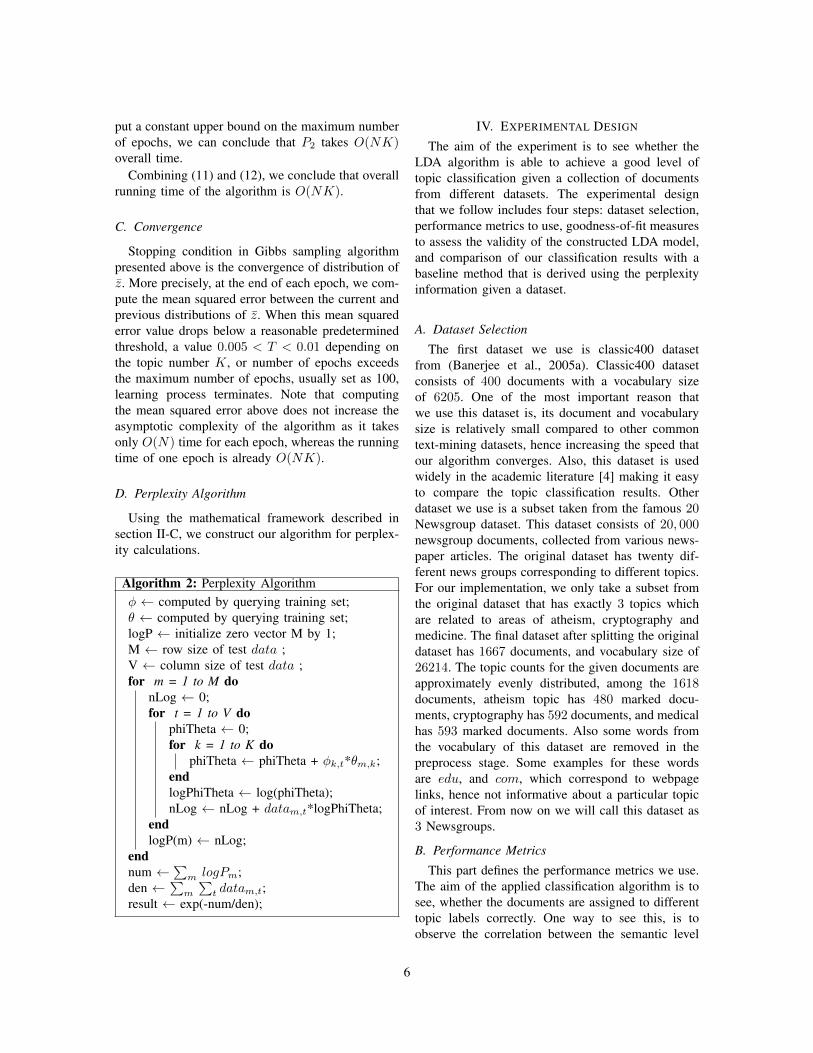
D. Perplexity Algorithm

Using the mathematical framework described insection II-C, we construct our algorithm for perplex-ity calculations.

Algorithm 2: Perplexity Algorithmφ ← computed by querying training set;θ ← computed by querying training set;logP ← initialize zero vector M by 1;M ← row size of test data ;V ← column size of test data ;for m = 1 to M do

nLog ← 0;for t = 1 to V do

phiTheta ← 0;for k = 1 to K do

phiTheta ← phiTheta + φk,t*θm,k;endlogPhiTheta ← log(phiTheta);nLog ← nLog + datam,t*logPhiTheta;

endlogP(m) ← nLog;

endnum ←

∑m logPm;

den ←∑m

∑t datam,t;

result ← exp(-num/den);

IV. EXPERIMENTAL DESIGN

The aim of the experiment is to see whether theLDA algorithm is able to achieve a good level oftopic classification given a collection of documentsfrom different datasets. The experimental designthat we follow includes four steps: dataset selection,performance metrics to use, goodness-of-fit measuresto assess the validity of the constructed LDA model,and comparison of our classification results with abaseline method that is derived using the perplexityinformation given a dataset.

A. Dataset Selection

The first dataset we use is classic400 datasetfrom (Banerjee et al., 2005a). Classic400 datasetconsists of 400 documents with a vocabulary sizeof 6205. One of the most important reason thatwe use this dataset is, its document and vocabularysize is relatively small compared to other commontext-mining datasets, hence increasing the speed thatour algorithm converges. Also, this dataset is usedwidely in the academic literature [4] making it easyto compare the topic classification results. Otherdataset we use is a subset taken from the famous 20Newsgroup dataset. This dataset consists of 20, 000newsgroup documents, collected from various news-paper articles. The original dataset has twenty dif-ferent news groups corresponding to different topics.For our implementation, we only take a subset fromthe original dataset that has exactly 3 topics whichare related to areas of atheism, cryptography andmedicine. The final dataset after splitting the originaldataset has 1667 documents, and vocabulary size of26214. The topic counts for the given documents areapproximately evenly distributed, among the 1618documents, atheism topic has 480 marked docu-ments, cryptography has 592 documents, and medicalhas 593 marked documents. Also some words fromthe vocabulary of this dataset are removed in thepreprocess stage. Some examples for these wordsare edu, and com, which correspond to webpagelinks, hence not informative about a particular topicof interest. From now on we will call this dataset as3 Newsgroups.

B. Performance Metrics

This part defines the performance metrics we use.The aim of the applied classification algorithm is tosee, whether the documents are assigned to differenttopic labels correctly. One way to see this, is toobserve the correlation between the semantic level

6

meanings of the words assigned to particular topic la-bels. That is, the words that have highest probabilityof being assigned to a particular topic, are expectedto be semantically correlated to each other. After theLDA algorithm is executed and documents in thedataset are classified into different topics, we tabulatethe topmost ten words under each possible topic labelto see if the words are semantically correlated witheach other. Another performance metric that is usedis the accuracy of the classification calculated usingthe given ground truth document labels. The ground-truth topic labels are given only for the classic400dataset.

C. Goodness-of-Fit Measures

For a given dataset here we describe a method forassessing the goodness-of-fit of the hyper-parametersK, α, and β both approximately, and numerically.The multinomial distributions Θm, and Φk requirehyperparameters α, and β as prior distributions,therefore depending on the probability densities ofthese two prior distributions the topic classificationresults are expected to change. In order to find thebest hyper-parameter configurations, we run a gridsearch algorithm looping over different values of αand β.The values of α, and β are taken from thefollowing sets:

Sβ = {2, 1, 0.5, 0.1, 0.01}Sα = {50/K, 25/K, 5/K, 3/K, 0.3/K}

Each run of grid search returns a two-dimensionalMxK matrix Θ. Using this matrix Θ, we canconstruct a K − 1 dimensional simplex since∑Kk=1 Θmk = 1 for each m, each point on this

simplex corresponds to a discrete topic probabilitydistribution of a particular document. Therefore, onthis simplex we require all documents to be clusteredaround their correct topic, having the false topicprobabilities of their topic probability distributionsaround zero. One such simplex is given in figure1 for illustration, this simplex is not correspondingto a good model but it shows the scattering of thedocuments-topic probabilities on the 2-simplex.

Fig. 1: Simplex surface showing the distribution ofdocument-topic classification for K=3, β = 2, andα = 50/K

The points (1, 0, 0), (0, 1, 0), and (0, 0, 1) in figure1 corresponds to label centers of the topics, meaningthat document points on the simplex that are closerto point (0, 0, 1) will be labeled as topic 3. This pro-vides a visual approximation for the goodness-of-fitfor the same dataset with different hyperparametersα, and β.

Moreover, another hyper-parameter that we usewhile generating the LDA model is number of topicsK. Depending on the value of K, the algorithmtries to find K many topics to associate with theavailable documents. Since we know that we have alimited number of documents, we know a priori thatK cannot be infinite, but to determine a good valuefor K we use the perplexity, which is defined as theuncertainty that our model assigns to each word ina collection of documents [4]. We point out that byselecting the best value of K we reduce the valueof perplexity as much as possible. For this reasonusing the best α, and β prior distributions that weobtain from the grid search algorithm, we separatethe training set into two smaller subsets. Classic400dataset has 400 documents in total, so we picked 75documents randomly from the whole set as our testset, and for different values of K, we computed theperplexity as described in the theoretical backgroundsection II-C. For the 3 Newsgroup we do the sameprocedure and calculate the perplexity on the sep-arated test set as well. Using the perplexity valueswe we can define the goodness-of-fit for the samedataset with different K values numerically.

Moreover, for the classic400 dataset we have theground-truth labels for document topics, therefore foreach different hyperparameters α, and β. Thus wecompute the document topic accuracy by comparing

7

the results from our classification algorithm with theground-truth labels, then we present our results in atable. This provides another way to define goodness-of-fit numerically.

By finding the optimal values for α, β, and Kas described by the methodology above we ensurewe achieve a sensible way to define the goodness-of-fit, for the same dataset with different hyperpa-rameters K, α, and β. We note that perplexity, andaccuracy can be computed exactly, hence it providesa goodness-of-fit of parameter K numerically.

D. Baseline Method

We compare our classification results with a base-line method that is derived using the perplexityinformation for randomly labeling topics given adataset. We use the best value of K to determine thenumber of topics, then given a set of M documents,we pick a topic label for each of the M documentsfrom a uniform distribution of K possible labels.For example if K turns out to be 3, then for eachdocument we assign its topic as 1,2, or 3, with one-third probability. This method is similar to flipping afair coin, and the output is random.

V. EXPERIMENTAL RESULTS & DISCUSSION

As described previously, using the grid searchalgorithm we first select the best parameter config-urations for the two separately. We use k-simplexfigures below to describe why our selection of hyper-parameters α, and β are the optimum values amongthe ones we perform grid search on. Then we useperplexity figures to show our best value of numberof topics K. We assess semantic level classificationaccuracy of the two datasets by inspecting the mostprobable 10 words for each topic as given in thetables I, and II. Finally, since we are given theground-truth labels for the classic400 dataset wecompute the document topic classification accuracyfor each α, and β pairs in the grid-search.

A. Classic400 Dataset

Figure 2 shows the 2-simplex with superimposeddocument-topic probabilities for classic400 dataset.We see that document-topic probability points on thesimplex are scattered on the simplex rather randomly.Upon close inspection we can see that there arethree weakly observable clusters around the simplexpoints (1, 0, 0), (0, 1, 0), and (0, 0, 1) correspondingto different topics. Since the data-points are scatteredwith a high variance around the cluster means we

can say that this selection of hyper-parameters is nota very good fit for the classic400 dataset.

Fig. 2: 2-simplex with document-topic probabilitiessuperimposed for classic400 dataset with K = 3,α = 25/K, and β = 0.01

Figure 3 shows a different 2-simplex with super-imposed document-topic probabilities for another setof hyper-parameters K = 3, α = 3/K, and β =0.01. Compared with figure 2 we see that clustersare closer to simplex points (1, 0, 0), (0, 1, 0), and(0, 0, 1), meaning that this set of hyper-parameters isa better selection than the previous selection.

Fig. 3: 2-simplex with document-topic probabilitiessuperimposed for classic400 dataset with K = 3,α = 3/K, and β = 0.01

The grid-search algorithm iteratively constructedsuch simplex figures using 25 different parameterconfigurations. The values of α, and β are taken fromthe sets:

Sβ = {2, 1, 0.5, 0.1, 0.01}Sα = {50/K, 25/K, 5/K, 3/K, 0.3/K}

8

Where the hyper-parameter K, is taken as K = 3by observing the perplexity figure 5, this will beexplained later. The following figure corresponds toour best selection of hyper-parameters α = 3/K, andβ = 2. We can see that document-topic probabilitypoints or the Θ matrix points are clustered perfectlyaround the points (1, 0, 0), (0, 1, 0), and (0, 0, 1)corresponding to different topics. Compared with theprevious figures 2, and 3 there is much less ambiguityabout the cluster centers which are separated clearlyon the 2-simplex in figure 4.

Fig. 4: 2-simplex with document-topic probabilitiessuperimposed for classic400 dataset with K = 3,α = 3/K, and β = 2

This can be perceived as a type of overfitting onthe training data because for a different dataset thesehyper-parameters might not cluster the documentlabels as precisely as figure 4 shows because thetrained model fits the training data almost perfectly.However, for the same dataset classic400 this set ofhyper parameters still provide a good fit. Other 2-simplex figures corresponding to different combina-tions α, and β values are available in the appendixsection.

We have selected the number of topics as K = 3,because perplexity values obtained from the test setattains its minimum value as it is shown in figure5. By selecting K = 3, we ensure that we reduceuncertainty that our model assigns to each word inthe the classic400 dataset. In other words we reducetopic redundancy, hence obtain a better classificationresult.

Fig. 5: Perplexity of the testing data versus numberof topics for dataset classic400, beta is fixed as 2,and alpha is 0.1

After we select the optimum hyper-parameters α,β, and K, we run the LDA algorithm and comparethe classified documents with the ground-truth thatis given for classic400 dataset. We achieve anaccuracy of 97.25% over the whole documents inthe dataset, furthermore we also present the mostprobable 10 words by the clustered topics in tableI. We see that semantically, the most probable 10words are strongly correlated with each other. Topic#1 is related with medical terms, words in topic #2is strongly related to science, and topic #3 is relatedto aerospace.

Topic # 1 Topic # 2 Topic # 3patients system boundaryventricular scientific layerfatty retrieval wingnickel research machleft language supersonicacids science wingscases methods ratioaortic systems velocityblood journals shocknormal subject effects

TABLE I: Table showing the most probable tenwords according to each topic for the classic400dataset

9

Moreover, we also use the ground-truth labelsto check the topic classification accuracy for eachiteration of the grid search algorithm, this justifiesthat our selection of hyper-parameters α = 3/K, andβ = 2 is a good-fit for the dataset classic400.

β 2 1 0.5 0.1 0.01α = 50/K 0.6275 0.9200 0.8775 0.8500 0.4625α = 25/K 0.9375 0.6850 0.9425 0.8750 0.5525α = 5/K 0.9075 0.9650 0.9400 0.9400 0.8400α = 3/K 0.9725 0.9325 0.8300 0.9625 0.7975α = 0.3/K 0.9400 0.9450 0.9400 0.9325 0.8225

TABLE II: Table showing the accuracy of the trainingalgorithm with respect to ground-truth labels fordataset classic400

B. 3 Newsgroups Dataset

In this section we present our results from the sec-ond experiment conducted on 3 Newsgroups dataset.We simply follow the same steps as in our previousexperiments. That is, we perform a grid search forα and β values by fixing K, line search for K byusing the notion of perplexity again, and present ourresults for different (α, β,K) triplets, and we discussthem from the goodness-of-fit and overfitting point ofviews.Figure 6 shows the perplexity on the separated testset taken from the training samples of 3 Newsgroupsdataset, we see that the perplexity is minimum ifK = 3, therefore selecting a higher number of topicswill increase topic redundancy similar to the previousdataset. Thus, we select the best value of K as 3.

Fig. 6: Perplexity of the testing data versus numberof topics for dataset 3 Newsgroups, beta is fixed as2, and alpha is 0.1

Moreover, similar to the previous dataset we runanother grid search over the same values of α’s,and β’s. We present two 2-simplex results withsuperimposed document-topic probability points inthe following figures. Figure 7 corresponds to a such2-simplex. The α value for this particular figure is25/K, the β value is 0.5. K is experimentally takenas 3 then confirmed later to be the good value,using the perplexity figure. We see that figure 7consists of three identifiable clusters around simplexcorners. This is a good observation since, this modelcan associate documents with particular labels, andoverfitting seems smaller compared with figure 8.

Fig. 7: 2-simplex with document-topic probabilitiessuperimposed for 3 Newsgroups dataset with K = 3,α = 25/K, and β = 0.5

Figure 8 shows 2-simplex for another set of hyper-parameters α = 0.3/K and β = 2. Compared withfigure 7 this clustering provides a better semanticlevel classification but just for this dataset. Becausethe points are clustered very closely, hence increasesthe chance of overfitting on other test sets.

Fig. 8: 2-simplex with document-topic probabilitiessuperimposed for 3 Newsgroups dataset with K = 3,α = 0.3/K, and β = 2

10

To qualitatively measure the topic classificationaccuracy on the dataset we present the followingtable that includes the topmost 12 probable wordsaccording to different topics. We observe that topic# 1 includes words related to religion and atheism.The meaning of words in topic 1 are strongly corre-lated with each other. Similarly, topic # 2 includeswords that are related with cryptography in computersystems, and topic # 3 includes words that are relatedwith medicine. The words in each individual topic isstrongly related with each other, meaning that thetopic classification is strong qualitatively.

Topic # 1 Topic # 2 Topic # 3god encrypt organatheist key articlwrite chip foodsubject clipper diseasmoral system medicbeliev secur bankislam subject patientexist db healthunivers write doctorchristian comput timereligion privaci causpeopl anonym effect

TABLE III: Table showing the most probable twelvewords according to each topic for the classic400dataset

VI. CONCLUSIONS

We conduct an unsupervised learning for docu-ment classification task in this project. Our specifictopic model is latent Dirichlet allocation which wetrain via collapsed Gibbs sampling algorithm. Weperform two experiments on two different datasets.Since there is no absolute definitions for goodness-of-fit and overfitting of LDA models trained withdifferent hyperparameters K,α, and β, we try toprovide reasonable ways of defining them based onour experiments.

Note that unsupervised learning is designed in away that it does not require true classifications ofdocuments. Hence, in practice, we are not given thetrue labels of our training data. This implies that thereis no definitive way of defining the performance oraccuracy of the trained model. All these points aboutuncertainty made above lead us to try to produceour own answers based on our experiments. Asan exception, we are given the ground-truth labelsof documents for classic400 dataset. Our algorithm

never uses this information throughout the trainingprocess. Yet, after the training process of LDA fora particular hyperparameter terminates, we use it tomeasure our accuracy of trained LDA model in orderjust to justify goodness-of-fit of our selection of hy-perparameters. The way we perform this justificationprocess can be found in Table II.

As mentioned above, computing document classifi-cation accuracy of LDA trained by a particular settingof hyperparameters on classic400 dataset would be areasonable way of justifying whether this particularsetting of hyperparameters results in a good modelin terms of goodness-of-fit. Another intuitive way todefine goodness-of-fit of LDA model with respect totopic number K would be to define f(K) as thenumber of topics k such that Sk > 1/K where Sk isdefined as the number words whose z value is k andthen interpret the ratio f(K)/N as the goodness-of-fit, where N is the total number of words in the entirecorpus. In this respect, notion of perplexity has thesame kind of intuition as the method we speculateabove. Hence, we use the notion of perplexity as atool to approximate the goodness-of-fit for parameterK. We set the best value of parameter K based on theperplexity results. Another way of defining goodness-of-fit is by investigating the semantic correlations ofwords with highest probability for a particular topic.

We also use simplex plots to visually assess thegoodness-of-fit of our model. This is also used toagain visually interpret whether trained LDA modelis overfitting its training data by checking if thecorresponding points on the simplex perfectly fit thetraining data in a clustered way at the corner points.

A sensible way of determining whether trainedLDA model is overfitting its training data would beby using the goodness-of-fit measurement obtainedby perplexity computation. More precisely, we in-terpret the goodness-of-fit of LDA model as beinginversely correlated with its overfitting the trainingdata. In a nutshell, we speculate that overfitting canbe inferred from goodness-of-fit of LDA model bythe reasonable assumption that the better goodness-of-fit the trained LDA has, the higher the probabilitythat it is overfitting the training data.

Lastly, we present our selection of the best hyper-parameter in the table below

Best K Best α Best β

classic400 3−−→3/K

−→2

3Newsgropus 3−−−−→0.3/K

−→2

where the arrow signs on top of the values indicate

11

that α, and β values are uniform vectors having thesame value at each index.

REFERENCES

[1] Elkan, Charles, ’Text mining and topic models’, Access:02/22/2014.

[2] Heinrich, Gregor, ’Parameter estimation for text analysis’,Access: 02/24/2014.

[3] Elkan, Charles, ’Maximum Likelihood, Logistic Regression,and Stochastic Gradient Training’, Access: 02/24/2014.

[4] Elkan, Charles, ’Clustering Documents with an Exponential-Family Approximation of the Dirichlet Compound Multino-mial Distribution’, Access: 02/26/2014.

12

VII. APPENDIX

A. Selected 2-simplexes for classic400 dataset

Fig. 9: 2-simplex with document-topic probabilitiessuperimposed for classic400 dataset with K = 3,α = 3/K, and β = 2

Fig. 10: 2-simplex with document-topic probabilitiessuperimposed for classic400 dataset with K = 3,α = 5/K, and β = 0.01

Fig. 11: 2-simplex with document-topic probabilitiessuperimposed for classic400 dataset with K = 3,α = 25/K, and β = 0.01

Fig. 12: 2-simplex with document-topic probabilitiessuperimposed for classic400 dataset with K = 3,α = 25/K, and β = 0.1

Fig. 13: 2-simplex with document-topic probabilitiessuperimposed for classic400 dataset with K = 3,α = 50/K, and β = 0.01

Fig. 14: 2-simplex with document-topic probabilitiessuperimposed for classic400 dataset with K = 3,α = 0.3/K, and β = 2

13

B. Selected 2-simplexes for 3 Newsgroups dataset

Fig. 15: 2-simplex with document-topic probabilitiessuperimposed for 3 Newsgroups dataset with K = 3,α = 0.3/K, and β = 0.01

Fig. 16: 2-simplex with document-topic probabilitiessuperimposed for 3 Newsgroups dataset with K = 3,α = 0.3/K, and β = 0.1

Fig. 17: 2-simplex with document-topic probabilitiessuperimposed for 3 Newsgroups dataset with K = 3,α = 3/K, and β = 0.01

Fig. 18: 2-simplex with document-topic probabilitiessuperimposed for 3 Newsgroups dataset with K = 3,α = 3/K, and β = 0.1

Fig. 19: 2-simplex with document-topic probabilitiessuperimposed for 3 Newsgroups dataset with K = 3,α = 25/K, and β = 0.1

Fig. 20: 2-simplex with document-topic probabilitiessuperimposed for 3 Newsgroups dataset with K = 3,α = 50/K, and β = 0.5

14