Advantage Amplification in Slowly Evolving Latent-State Environments

Martin Mladenov1 , Ofer Meshi1 , Jayden Ooi1 , Dale Schuurmans1,2 , Craig Boutilier11Google AI, Mountain View, CA, USA

2Department of Computer Science, University of Alberta, Edmonton, AB, Canada{mmldanenov,meshi,jayden,schuurmans,cboutilier}@google.com

AbstractLatent-state environments with long horizons, such asthose faced by recommender systems, pose significantchallenges for reinforcement learning (RL). In this work,we identify and analyze several key hurdles for RL insuch environments, including belief state error and smallaction advantage. We develop a general principle calledadvantage amplification that can overcome these hurdlesthrough the use of temporal abstraction. We proposeseveral aggregation methods and prove they induce am-plification in certain settings. We also bound the lossin optimality incurred by our methods in environmentswhere latent state evolves slowly and demonstrate theirperformance empirically in a stylized user-modeling task.

1 IntroductionLong-term value (LTV) estimation and optimization is ofincreasing importance in the design of recommender sys-tems (RSs), and other user-facing systems. Often the prob-lem is framed as a Markov decision process (MDP) andsolved using MDP algorithms or reinforcement learning (RL)[Shani et al., 2005; Taghipour et al., 2007; Choi et al., 2018;Archak et al., 2012; Mladenov et al., 2017; Zhao et al., 2018;Gauci et al., 2018; Ie et al., 2019]. Typically, the action setis the set of recommendable items;1 states reflect informa-tion about the user (e.g., static attributes, past interactions,context/query); and rewards measure some form of user en-gagement (e.g., clicks, views, time spent, purchase). Suchevent-level models have seen some success, but current state-of-the-art is limited to very short horizons.

When dealing with long-term user behavior, it is vital toconsider the impact of recommendations on user latent state(e.g., satisfaction, latent interests, or item awareness) whichoften governs both immediate and long-term behavior. Indeed,the main promise of using RL/MDP models for RSs is to: (a)identify user latent state (e.g., uncover user interests in newtopics via exploration, or estimate user satisfaction); and (b)influence the latent state (e.g., create new interests, improveawareness or increase satisfaction). That said, evidence isemerging that at least some aspects of user latent state evolvevery slowly. For example, Hohnhold et al. [2015] show that

1Item slates are often recommended, but we ignore this here.

varying ad quality and ad load induces slow, but inexorable(positive or negative) changes in user click propensity overa period of months, while Wilhelm et al. [2018] show thatexplicitly diversifying recommendations in YouTube inducessimilarly slow, persistent changes in user engagement (seesuch slow “user learning” curves in Fig. 1).

Event-level RL in such settings is challenging for severalreasons. First, the effective horizon over which an RS policyinfluences the latent state can extend up to O(104–105) statetransitions. Indeed, the cumulative effect of recommendationsis vital for LTV optimization, but the long-term impact ofany single recommendation is often dwarfed by immediatereward differences. Second, the MDP is partially observable,requiring some form of belief state estimation. Third, theimpact of latent state on immediate observable behavior isoften small and very noisy—the problems have a low signal-to-noise ratio (SNR). We detail below how these factors interact.

Given the importance of LTV optimization in RSs, we pro-pose a new technique called advantage amplification to over-come these challenges. Intuitively, advantage amplificationseeks to overcome the error induced by state estimation byintroducing (explicit or implicit) temporal abstraction acrosspolicy space. We require that policies “commit” to taking aseries of actions, thus allowing more accurate value estimationby mitigating the cumulative effects of state-estimation error.

We first consider temporal aggregation, where an action isheld fixed for a short horizon. We show that this can lead tosignificant amplification of the advantage differences betweenabstract actions (relative to event-level actions). This is aform of MDP/RL temporal abstraction as used in hierarchicalRL [Sutton et al., 1999; Barto and Mahadevan, 2003] andcan be viewed as options designed to allow distinction ofgood and bad behaviors in latent-state domains with low SNR(rather than, say, for subgoal achievement). We generalize thisby analyzing policies with (artificial) action switching costs,which induces similar amplification with more flexibility.

Limiting policies to temporally abstract actions induces po-tential sub-optimality [Parr, 1998; Hauskrecht et al., 1998].However, since the underlying latent state often evolves slowlyw.r.t. the event horizon in RS settings, we identify a “smooth-ness” property that is used to bound the induced error ofadvantage amplification.

Our contributions are as follows. We introduce a stylizedmodel of slow user learning in RSs in Sec. 2. We formalize this

Figure 1: Gradual user response: (a) ad load/quality [Hohnhold et al., 2015]; (b) YouTube recommendation diversity [Wilhelm et al., 2018].

model as a POMDP in Sec. 3 and define several properties thatwe exploit in our analysis. In Sec. 4.1, we show that low SNRin the POMDP interacts poorly with belief-state approxima-tion, and develop advantage amplification as a principle. Weprove that action aggregation (Sec. 4.2) and switching cost reg-ularization (Sec. 4.3) provide strong amplification guaranteeswith minimal policy loss under suitable conditions and suggestpotential extensions in Sec. 4.4. Experiments with stylizedmodels in Sec. 4.5 show the effectiveness of our methods.2

2 User Satisfaction: An Illustrative ExampleBefore formalizing our problem, we describe a stylized modelreflecting the dynamics of user satisfaction as a user interactswith an RS. The model is intentionally stylized to help illus-trate key concepts underlying the formal model and analysisdeveloped in the sequel. While it ignores much of the truecomplexity of user satisfaction and RS interaction, its coreelements permeate many recommendation domains. Finally,though focused on user-RS engagement, the principles applymore broadly to any latent-state system with low SNR andslowly evolving latent state.

Our model captures the relationship between a user and anRS over an extended period (e.g., a content recommender ofnews, video, or music) through overall user satisfaction, whichis not known to the RS. We hypothesize that satisfaction is one(of several) key latent factors that impacts user engagement;and since new treatments often induce slow-moving or delayedeffects on user behavior, we assume this latent variable evolvesslowly as a function of the quality of the content consumed[Hohnhold et al., 2015] (and see Fig. 1 (left)). Finally, themodel captures the tension between (often low-quality) contentthat encourages short-term engagement (e.g., manipulative,provocative or distracting content) at the expense of long-termengagement; and high-quality content that promotes long-termusage but can sacrifice near-term engagement.

Our model includes two classes of recommendable items.Some items induce high immediate engagement, but degradeuser engagement over the long run. We dub these “Choco-late” (Choc)—immediately appealing but not very “nutri-tious.” Other items—dubbed “Kale,” less attractive, but more“nutritious”—induce lower immediate engagement but tend to

2Proofs, auxiliary lemmas and additional experiments are avail-able in an extended version of the paper [Mladenov et al., 2019].

improve long-term engagement.3 We call this the Choc-Kalemodel (CK). A stationary, stochastic policy can be representedby a single scalar 0 ≤ π ≤ 1 representing the probability oftaking action Choc. We sometimes refer to Choc as a “nega-tive” and Kale as a “positive” recommendation.

We use a single latent variable s ∈ [0, 1] to capture auser’s overall satisfaction with the RS. Satisfaction is drivenby net positive exposure p, which measures a user’s total (dis-counted) accrued positive and negative recommendations, witha discount 0 ≤ β < 1 applied to ensure that p is bounded:p ∈

[−11−β ,

11−β

]. (The dynamics of p is detailed below.) We

view p as a user’s learned perception of the RS and s as howthis influences gradual changes in engagement.

A user response to a recommendation a is given by herdegree of engagement g(s, a), and depends stochasticallyon both the quality of the recommendation, and her latentstate s. Engagement g is a random function; e.g., responsesmight be normally distributed: g(s, a) ∼ N(s · µa, σ2

a) for a ∈{Choc,Kale}. We abuse notation and sometimes let g(s, a)denote expected engagement. We require that Choc resultsin greater immediate (expected) engagement than Kale, i.e.,g(s,Kale) < g(s,Choc), for any fixed s.

The dynamics of p is straightforward. A Kale exposureincreases p by 1 and Choc decreases it by 1, with discounting:pt+1 ← βpt + 1 with a Kale recommendation and pt+1 ←βpt − 1 with Choc. Satisfaction s is a user-learned functionof p and follows a sigmoidal learning curve: s(p) = 1/(1 +e−τp), where τ is a temperature/learning rate parameter. Otherlearning curves are possible, but the sigmoidal model capturesboth positive and negative exponential learning as hypothe-sized in psychological-learning literature [Thurstone, 1919;Jaber, 2006] and as observed in the empirical curves in Fig. 1.4

To illustrate the workings of this model, we compute theQ-values of Choc and Kale for each satisfaction level s and

3Our model allows a real-valued continuum of items (e.g., degreeof Choc between [0, 1] as in our experiments) like measures of adquality. We use the binary form to streamline our initial exposition.

4Such learning curves are often reflective of aggregate behavior,obscuring individual differences that are much less “smooth.” How-ever, unless cues are available that allow us to model such individualdifferences, the aggregate model is our best resource, even whenoptimizing for individual users. Indeed, prediction of user responsesin RSs usually relies on fairly coarse user features—and not useridentity—and already relies on similar aggregate behavior.

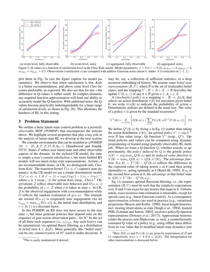
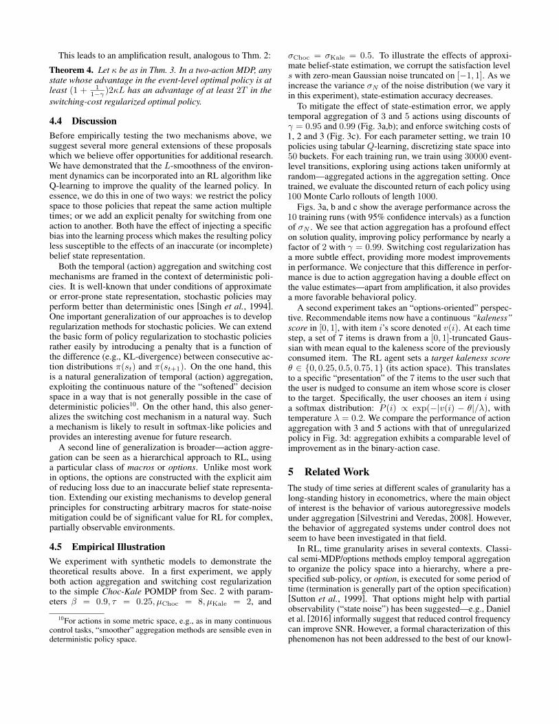
(a) event-level, fully observable (b) event-level, noisy (c) aggregated, fully observable (d) aggregated, noisyFigure 2: Q-values as a function of satisfaction level in the Choc-Kale model. Model parameters: β = 0.9, τ = 0.25, µChoc = 8, µKale = 2,σChoc = σKale = 0.5. Observations (satisfaction s) are corrupted with additive Gaussian noise (mean 0, stddev. 0.3) truncated on [−1, 1].

plot them in Fig. 2a (see the figure caption for model pa-rameters). We observe that when satisfaction is low, Kaleis a better recommendation, and above some level Choc be-comes preferable, as expected. We also see that for any s thedifference in Q-values is rather small. In complex domains,any required function approximation will limit our ability toaccurately model the Q-function. With additional noise, the Q-values become practically indistinguishable for a large rangeof satisfaction levels, as shown in Fig. 2b). This illustrates thehardness of RL in this setting.

3 Problem StatementWe outline a basic latent-state control problem as a partiallyobservable MDP (POMDP) that encompasses the notionsabove. We highlight several properties that play a key role inthe analysis of latent-state RL we develop in the next section.

We consider environments that can be modeled as a POMDPM = 〈S,A, T,Z, O,R, b0, γ〉 [Smallwood and Sondik,1973]. States S reflect user latent state and other observableaspects of the domain. In the stylized CK model, the stateis simply a user’s current satisfaction s, but more faithful RSmodels will use much richer state representations. Actions Aare recommendable items: in CK, we distinguish only Chocfrom Kale. The transition kernel T (s, a, s′) captures state dy-namics: in the CK model we use a simple deterministic model,T (s′, a, s) = 1 if s′ = (1 + exp(β log (1− 1/s) − βτa))−1,where a is 1 (resp., -1) for action Kale (resp., Choc).5 Ob-servations Z reflect observable user behavior and O(s, a, z)the probability of z ∈ Z when a is taken at state s. In CK,Z is the observed engagement with a recommendation whileO reflects the random realization of g(s, a). The immedi-ate reward R(s, a) is (expected) user engagement (we letrmax = maxs,aR(s, a)), b0 the initial state distribution, andγ ∈ [0, 1) is a discount factor.

In this POMDP, an RS does not have access to the truestate s, but must generate policies that depend only on thesequence of past action-observation pairs—letH∗ be the setof all finite such sequences (at, zt)t∈N. Any such history canbe summarized, via optimal Bayes filtering, as a distributionor belief state b ∈ ∆(S). More generally, this “belief state”can be any summarization of H∗ used to make decisions. It

5This is easily randomized if desired.

may be, say, a collection of sufficient statistics, or a deeprecurrent embedding of history. We assume some belief staterepresentation (B, U), where B is the set of (realizable) beliefstates, and the mapping U : B × A × Z → B describes theupdate U(b, a, z) of any b ∈ B given a ∈ A, z ∈ Z .

A (stochastic) policy is a mapping π : B → ∆(A) thatselects an action distribution π(b) for execution given beliefb; we write π(a|b) to indicate the probability of action a.Deterministic policies are defined in the usual way. The valueof a policy π is given by the standard recurrence:6

V π(b)= Ea∼π(b)

[R(b, a)+γ

∑z∈Z

Pr(z|b, a)V π(U(b, a, z))

](1)

We define Qπ(b, a) by fixing a in Eq. (1) (rather than takingthe action distribution π(b)). An optimal policy π∗ = supV π

over B has value (resp., Q) function V ∗ (resp., Q∗). Op-timal policies and values can be computed using dynamicprogramming or learned using (partially observable) RL meth-ods. When we learn a Q-function Q, whether exactly or ap-proximately, the policy induced by Q is the greedy policyπ(b) = arg maxaQ(b, a) and its induced value function isV (b) = maxaQ(b, a) = Q(b, a∗(b)). The advantage func-tion A(a, b) = V ∗(b) − Q∗(b, a) reflects the difference inthe expected value of taking action a at b (and then actingoptimally) vs. acting optimally at b [Baird III, 1999]. If a2 isthe second-best action at b, the advantage at that belief stateis A(b) = V ∗(b)−Q∗(b, a2).

Eq. (1) assumes optimal Bayesian filtering, i.e., the repre-sentation (B, U) must be such that the (implicit) expectationsoverR andO are exact for any history that maps to b. Unfortu-nately, exact recursive state estimation is intractable, except forspecial cases (e.g., linear-Gaussian control). As a consequence,approximation schemes are used in practice (e.g., variationalprojections [Boyen and Koller, 1998]; fixed-length histories,incl. treating observations as state [Singh et al., 1994]; learnedPSRs [Littman and Sutton, 2002]; recursive policy/Q-functionrepresentations [Downey et al., 2017]). Approximate historiesrender the process non-Markovian; as such, a counterfactuallyestimated Q-value of a policy (e.g., using offline data) differsfrom its true value due to modified latent-state dynamics (not

6Here R(b, a) and Pr(z|b, a) are given by expectations of R andO, respectively, w.r.t. s ∼ b if b ∈ ∆(S). The interpretation forother representations is discussed below.

reflected in the data). In this case, any RL method that treatsb as (Markovian) state induces a suboptimal policy. We canbound the induced suboptimality using ε-sufficient statistics[Francois-Lavet et al., 2017]. A function φ : H∗ → B is anε-sufficient statistic if, for all Ht ∈ H∗,

|p(st+1|Ht)− p(st+1|φ(Ht))|TV < ε ,

where | · |TV is the total variation distance. If φ is ε-sufficient,then any MDP/RL algorithm that constructs an “optimal”value function V̂ over B incurs a bounded loss w.r.t. V ∗[Francois-Lavet et al., 2017]:∣∣∣V ∗(φ(H))− V̂ (φ(H))

∣∣∣ ≤ 2εrmax

(1− γ)3. (2)

The errors in Q-value estimation induced by limitations of Bare irresolvable (i.e., they are a form of model bias), in contrastto error induced by limited data. Moreover, any RL methodrelying only on offline data is subject to the above bound,regardless of whether the Q-values are estimated directly ornot. The impact of this error on model performance can berelated to certain properties of the underlying domain as weoutline below. A useful quantity for this purpose is the signal-to-noise ratio (SNR) of a POMDP, defined as:

S ,supbA(b)

sup{A(b) : A(b) ≤ 2εrmax/(1− γ)2}− 1,

(the denominator is treated as 0 if no b meets the condition).As discussed above, many aspects of user latent state, such

as satisfaction, evolve slowly. We say a POMDP is L-smoothif, for all b, b′ ∈ B, and a ∈ A s.t. T (b′, a, b) > 0, we have

|Q∗(b, a)−Q∗(b′, a)| ≤ L.

Smoothness ensures that for any state reachable under anaction a, the optimal Q-value of a does not change much.

4 Advantage AmplificationWe detail how low SNR causes difficulty for RL in POMDPs,especially with long horizons (Sec. 4.1). We introduce theprinciple of advantage amplification to address it (Sec. 4.2)and analyze two realizations of this principle, temporal aggre-gation in Sec. 4.2 and switching cost in Sec. 4.3. We suggestseveral extensions in Sec. 4.4 and conclude with an empiricalillustration of our mechanisms in Sec. 4.5.

4.1 The Impact of Low SNR on RLThe bound given by Eq. (2) can help assess the impact of lowSNR on RL. Assume that policies, values and/or Q-functionsare learned using an approximate belief representation (B, U)that is ε-sufficient. We first show that the error induced by(B, U) is tightly coupled to optimal action advantages.

Consider an RL agent that learns Q-values using a behav-ior (data-generating) policy ρ. The non-Markovian nature of(B, U) means that: (a) the resulting estimated-optimal policyπ will have estimated values Q̂π that differ from its true valuesQπ; and (b) the estimates Q̂π (hence, the choice of π itself)will depend on ρ. We bound the loss of π w.r.t. the optimalπ∗—here π∗ assumes exact filtering—as follows. First, for

any (belief) state-action pair (b, a), let the maximum differ-ence between its inferred and optimal Q-values is bounded forany ρ: |Q∗(b, a)−Qπ(b, a)| ≤ δ. Using Eq. (2), we set

δ =εQmax

1− γ ≤εrmax

(1− γ)2. (3)

If A(b) ≤ 2δ (i.e., b has small advantage), under behaviorpolicy ρ, the estimate Q̂(b, a2) (the second-best action) canexceed that of Q̂(b, a∗(b)), in which case π executes a2. If πvisits b (or states with similarly small advantages) at a constantrate, the loss w.r.t. π∗ compounds, inducing O( 2δ

1−γ ) error.The tightness of the second part of the argument depends

on the structure of the advantage function A(b). To illustrate,consider two extreme regimes. First, ifA(b) ≥ 2δ at all b ∈ B,i.e., if SNR S =∞, state estimation error has no impact onthe recovered policy and incurs no loss. In the second regime,if all A(b) are less than (but on the order of) 2δ, i.e., if S = 0,then the inequality is tight provided ρ saturates the state-actionerror bound. We will see below that low-SNR environmentswith long horizons (e.g., practical RSs, or our stylized CKmodel) often have such small (but non-trivial) advantagesacross a wide range of state space.

The latter situation is illustrated in Fig. 2. In Fig. 2a, theQ-values of the CK model are plotted against the level ofsatisfaction (treating it as fully observable). The small advan-tages are notable. Fig. 2b shows the Q-value estimates for10 independent tabular Q-learning runs when noise is addedto the estimated belief state s (the thin lines show individualruns, the thick lines show the average) . The corrupted Q-values at all but the highest satisfaction levels are essentiallyindistinguishable, leading to extremely poor policies.

4.2 Temporal Abstraction: Action AggregationThere is a third regime in which state error is relatively benign.Suppose the advantage at each state b is either small, A(b) ≤σ, or large, A(b) > Σ for some constants σ � 2δ ≤ Σ. Theinduced policy incurs a loss of σ at small-advantage beliefstates, and no loss on states with large advantages. This leadsto a compounded loss of at most σ

1−γ , which may be muchsmaller than the εrmax

(1−γ)2 error in Eq. (3), depending on σ.If the environment is smooth, action aggregation can be

used to tramsform a problem falling in the second regime intoone that falls in the third regime, with σ depending on the levelof smoothness. This can significantly reduce the impact ofestimation error on policy quality by turning the problem intoone that is essentially Markovian. More specifically, if at stateb, we know that the optimal (stationary) policy takes actiona for the next k decision periods, we consider a reparameteri-zationM×k of the belief-state MDP where, at b, any actiontaken must be executed k times in a row, no matter what thesubsequent k states are. In this new problem, the Q-value ofthe optimal repeated action Q∗(b, a×k) is the same as that ofits event-level counterpart Q∗(b, a), since the same sequenceof expected rewards will be generated. Conversely, all subop-timal actions incur a cumulative reduction in Q-value inM×ksince their suboptimality compounds over k periods. Thus, inM×k, the optimal policy π×k∗ generates the same cumulativediscounted return as the event-level optimal policy, while the

advantage of a×k over any other repeated action a′×k at b islarger than that of a over a′ in the event-level problem.

To derive bounds, note that, for an L-smooth POMDP, atany state where the advantage is at least 2kL, the optimalaction persists for the next k periods (its Q-value can decreaseby at most L while that of the second-best can at most in-crease by L). If we apply aggregation only at such states, theadvantage increases to some value Σ, putting us in regime3 (i.e., the advantage is either less than σ = 2kL or morethan Σ). Of course, we cannot “cherry-pick” only states withhigh advantage for aggregation, but instead apply this actionaggregation uniformly over B. Naturally, aggregating over allstates induces some loss due to the inability to switch actionsquickly. We bound that cost when determining σ and Σ. tocomplete the analysis. This allows us to first lower bound theregret of the best k-aggregate policy:Theorem 1. Let k be a fixed horizon, and let Q∗—the event-level optimal Q function—be L-smooth. Then for all b,|V ∗(b) − V ×k∗(b)| ≤ 2kL

1−γ , where V ×k∗(b) is the value ofstate b under an optimal k-aggregate policy.7

This theorem is proved by constructing a policy whichswitches actions every k events and showing that it hasbounded regret.8 This policy, at the start of any k-event period,adopts the optimal action from the unaggregated MDP at theinitiating state. Due to smoothness, Q-values cannot drift bymore than kL during the period, after which the policy cor-rects itself. This, together with the reasoning above, offers anamplification guarantee:Theorem 2. In an L-smooth MDP, let k be a fixed repetitionhorizon. For any belief state where A(b) ≥ 2kL, the k-aggregate-horizon advantage is bounded below as follows:

Q×k∗(b, a×k)−Q×k∗(b, a′×k)

≥ A(b)1− γk

1− γ − 2Lγ − (1 + k − γk)γk+1

(1− γ)2− 2kL

1− γ .

This result is especially useful when the event-level advan-tage is more than σ = 2kL

1−γ . In this case, an aggregationhorizon of k can mitigate the adverse effects of approximatingbelief state with an ε-sufficient statistic for any ε up to

εmax ≤ Lk(γ − γk)− γ(1− (1 + k − γk)γk)

rmax,

at the cost of the aggregation loss of 2kL1−γ .

Figs. 2c and 2d illustrate the benefit of action aggregation:they show the Q-values of the k-aggregated CK model withk = 5 with both perfect and imperfect state estimation, respec-tively (the amount of noise is the same as in Fig. 2b). As weshow in Sec. 4.5, the recovered policies incur very little lossdue to state estimation error.

We conclude with the following observation.Corollary 1. Optimal repeating policies are near-optimal forthe event-level problem as L→ 0 and amplification at everystate is guaranteed.

7The reparameterized problem is also an MDP, so the optimalvalue function and deterministic policy are well-defined.

8See the full paper [Mladenov et al., 2019] for proofs of all results.

4.3 Temporal Regularization: Switching CostWhile temporal aggregation is guaranteed to improve learningin slow environments, it has certain practical drawbacks dueto its inflexibility. One is that, in the non-Markovian settinginduced by belief-state approximation, training data shouldideally be collected using a k-aggregated behavior policy.9Another drawback arises if the L-smoothness assumption ispartially violated. For example, if certain rare events causelarge changes in state or reward for short periods, the changesin Q-values may be abrupt. Notice that such changes are harm-less from an SNR perspective if they induce large advantagegaps; but an agent “committed” to a constant action during anaggregation period is unable to react to such events. We thuspropose a more flexible advantage amplification mechanism,namely, a switching-cost regularizer. Intuitively, instead offixing an aggregation horizon, we impose a fictitious cost (orpenalty) T on the agent whenever it changes its action.

More formally, the goal in the switching-cost (belief-state)MDP is to find an optimal policy defined as:

π∗ = arg maxπ

∑t

γtEπ (Rt − T · 1[at 6= at−1]) . (4)

This problem is Markovian in the extended state space B ×A representing the current (belief) state and the previouslyexecuted action. This state space allows the switching penaltyto be incorporated into the reward function as R(b, at−1, at) =R(b, at)− T · 1[at 6= at−1].

The switching cost induces an implicit adaptive action ag-gregation—after executing action a, the agent will keep repeat-ing a until the cumulative advantage of switching to a differentaction exceeds the switching cost T . We can use this insightto bound the maximum regret of such a policy (relative to theoptimal event-level policy) and also provide an amplificationguarantee, as is the case with action aggregation.

In the case of problems with two actions, we can analyzethe action of the switching-cost regularizer in a relativelyintuitive way. As with Thm. 1, we bound the regret inducedby the switching cost by constructing a policy that behavesas if it had to pay T with every action switch. In particular,the optimal policy under this penalty adopts the action of theevent-level optimal policy at some state bt, then holds it fixeduntil its expected regret for not switching to a different actiondictated by the event-level optimal policy exceeds T . Supposethe time at which this switch occurs is (t + ω). The regretof this agent is no more than the regret of an agent with theoption of paying T upfront in order to follow the event-leveloptimal policy for ω steps. We can show that the same regretbound holds if the agent were paying to switch to the bestfixed action for ω steps instead of following the event-leveloptimal policy. This allows derivation of the following bound:Theorem 3. The regret of the optimal switching cost policyfor a two-action MDP is less than 2κL

1−γ , where

κ =log γ + (γ − 1)W

(γ1/(1−γ)

γ−1

((1−γ)22γL

T − 1)

log γ)

(γ − 1) log γ,

and where W is the Lambert W-function [Corless et al., 1996].9This is unnecessary if the system is Markovian, since (s, a, r, s′)

tuples may be reordered to emulate any behavioral policy.

This leads to an amplification result, analogous to Thm. 2:

Theorem 4. Let κ be as in Thm. 3. In a two-action MDP, anystate whose advantage in the event-level optimal policy is atleast (1 + 1

1−γ )2κL has an advantage of at least 2T in theswitching-cost regularized optimal policy.

4.4 DiscussionBefore empirically testing the two mechanisms above, wesuggest several more general extensions of these proposalswhich we believe offer opportunities for additional research.We have demonstrated that the L-smoothness of the environ-ment dynamics can be incorporated into an RL algorithm likeQ-learning to improve the quality of the learned policy. Inessence, we do this in one of two ways: we restrict the policyspace to those policies that repeat the same action multipletimes; or we add an explicit penalty for switching from oneaction to another. Both have the effect of injecting a specificbias into the learning process which makes the resulting policyless susceptible to the effects of an inaccurate (or incomplete)belief state representation.

Both the temporal (action) aggregation and switching costmechanisms are framed in the context of deterministic poli-cies. It is well-known that under conditions of approximateor error-prone state representation, stochastic policies mayperform better than deterministic ones [Singh et al., 1994].One important generalization of our approaches is to developregularization methods for stochastic policies. We can extendthe basic form of policy regularization to stochastic policiesrather easily by introducing a penalty that is a function ofthe difference (e.g., KL-divergence) between consecutive ac-tion distributions π(st) and π(st+1). On the one hand, thisis a natural generalization of temporal (action) aggregation,exploiting the continuous nature of the “softened” decisionspace in a way that is not generally possible in the case ofdeterministic policies10. On the other hand, this also gener-alizes the switching cost mechanism in a natural way. Sucha mechanism is likely to result in softmax-like policies andprovides an interesting avenue for future research.

A second line of generalization is broader—action aggre-gation can be seen as a hierarchical approach to RL, usinga particular class of macros or options. Unlike most workin options, the options are constructed with the explicit aimof reducing loss due to an inaccurate belief state representa-tion. Extending our existing mechanisms to develop generalprinciples for constructing arbitrary macros for state-noisemitigation could be of significant value for RL for complex,partially observable environments.

4.5 Empirical IllustrationWe experiment with synthetic models to demonstrate thetheoretical results above. In a first experiment, we applyboth action aggregation and switching cost regularizationto the simple Choc-Kale POMDP from Sec. 2 with param-eters β = 0.9, τ = 0.25, µChoc = 8, µKale = 2, and

10For actions in some metric space, e.g., as in many continuouscontrol tasks, “smoother” aggregation methods are sensible even indeterministic policy space.

σChoc = σKale = 0.5. To illustrate the effects of approxi-mate belief-state estimation, we corrupt the satisfaction levels with zero-mean Gaussian noise truncated on [−1, 1]. As weincrease the variance σN of the noise distribution (we vary itin this experiment), state-estimation accuracy decreases.

To mitigate the effect of state-estimation error, we applytemporal aggregation of 3 and 5 actions using discounts ofγ = 0.95 and 0.99 (Fig. 3a,b); and enforce switching costs of1, 2 and 3 (Fig. 3c). For each parameter setting, we train 10policies using tabular Q-learning, discretizing state space into50 buckets. For each training run, we train using 30000 event-level transitions, exploring using actions taken uniformly atrandom—aggregated actions in the aggregation setting. Oncetrained, we evaluate the discounted return of each policy using100 Monte Carlo rollouts of length 1000.

Figs. 3a, b and c show the average performance across the10 training runs (with 95% confidence intervals) as a functionof σN . We see that action aggregation has a profound effecton solution quality, improving policy performance by nearly afactor of 2 with γ = 0.99. Switching cost regularization hasa more subtle effect, providing more modest improvementsin performance. We conjecture that this difference in perfor-mance is due to action aggregation having a double effect onthe value estimates—apart from amplification, it also providesa more favorable behavioral policy.

A second experiment takes an “options-oriented” perspec-tive. Recommendable items now have a continuous “kaleness”score in [0, 1], with item i’s score denoted v(i). At each timestep, a set of 7 items is drawn from a [0, 1]-truncated Gaus-sian with mean equal to the kaleness score of the previouslyconsumed item. The RL agent sets a target kaleness scoreθ ∈ {0, 0.25, 0.5, 0.75, 1} (its action space). This translatesto a specific “presentation” of the 7 items to the user such thatthe user is nudged to consume an item whose score is closerto the target. Specifically, the user chooses an item i usinga softmax distribution: P (i) ∝ exp(−|v(i) − θ|/λ), withtemperature λ = 0.2. We compare the performance of actionaggregation with 3 and 5 actions with that of unregularizedpolicy in Fig. 3d: aggregation exhibits a comparable level ofimprovement as in the binary-action case.

5 Related WorkThe study of time series at different scales of granularity has along-standing history in econometrics, where the main objectof interest is the behavior of various autoregressive modelsunder aggregation [Silvestrini and Veredas, 2008]. However,the behavior of aggregated systems under control does notseem to have been investigated in that field.

In RL, time granularity arises in several contexts. Classi-cal semi-MDP/options methods employ temporal aggregationto organize the policy space into a hierarchy, where a pre-specified sub-policy, or option, is executed for some period oftime (termination is generally part of the option specification)[Sutton et al., 1999]. That options might help with partialobservability (“state noise”) has been suggested—e.g., Danielet al. [2016] informally suggest that reduced control frequencycan improve SNR. However, a formal characterization of thisphenomenon has not been addressed to the best of our knowl-

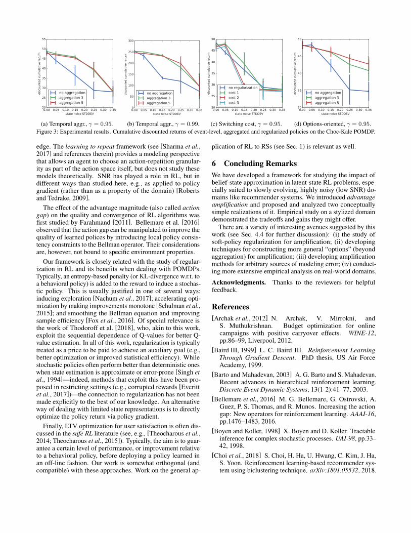
(a) Temporal aggr., γ = 0.95. (b) Temporal aggr., γ = 0.99. (c) Switching cost, γ = 0.95. (d) Options-oriented, γ = 0.95.Figure 3: Experimental results. Cumulative discounted returns of event-level, aggregated and regularized policies on the Choc-Kale POMDP.

edge. The learning to repeat framework (see [Sharma et al.,2017] and references therein) provides a modeling perspectivethat allows an agent to choose an action-repetition granular-ity as part of the action space itself, but does not study thesemodels theoretically. SNR has played a role in RL, but indifferent ways than studied here, e.g., as applied to policygradient (rather than as a property of the domain) [Robertsand Tedrake, 2009].

The effect of the advantage magnitude (also called actiongap) on the quality and convergence of RL algorithms wasfirst studied by Farahmand [2011]. Bellemare et al. [2016]observed that the action gap can be manipulated to improve thequality of learned polices by introducing local policy consis-tency constraints to the Bellman operator. Their considerationsare, however, not bound to specific environment properties.

Our framework is closely related with the study of regular-ization in RL and its benefits when dealing with POMDPs.Typically, an entropy-based penalty (or KL-divergence w.r.t. toa behavioral policy) is added to the reward to induce a stochas-tic policy. This is usually justified in one of several ways:inducing exploration [Nachum et al., 2017]; accelerating opti-mization by making improvements monotone [Schulman et al.,2015]; and smoothing the Bellman equation and improvingsample efficiency [Fox et al., 2016]. Of special relevance isthe work of Thodoroff et al. [2018], who, akin to this work,exploit the sequential dependence of Q-values for better Q-value estimation. In all of this work, regularization is typicallytreated as a price to be paid to achieve an auxiliary goal (e.g.,better optimization or improved statistical efficiency). Whilestochastic policies often perform better than deterministic oneswhen state estimation is approximate or error-prone [Singh etal., 1994]—indeed, methods that exploit this have been pro-posed in restricting settings (e.g., corrupted rewards [Everittet al., 2017])—the connection to regularization has not beenmade explicitly to the best of our knowledge. An alternativeway of dealing with limited state representations is to directlyoptimize the policy return via policy gradient.

Finally, LTV optimization for user satisfaction is often dis-cussed in the safe RL literature (see, e.g., [Theocharous et al.,2014; Theocharous et al., 2015]). Typically, the aim is to guar-antee a certain level of performance, or improvement relativeto a behavioral policy, before deploying a policy learned inan off-line fashion. Our work is somewhat orthogonal (andcompatible) with these approaches. Work on the general ap-

plication of RL to RSs (see Sec. 1) is relevant as well.

6 Concluding RemarksWe have developed a framework for studying the impact ofbelief-state approximation in latent-state RL problems, espe-cially suited to slowly evolving, highly noisy (low SNR) do-mains like recommender systems. We introduced advantageamplification and proposed and analyzed two conceptuallysimple realizations of it. Empirical study on a stylized domaindemonstrated the tradeoffs and gains they might offer.

There are a variety of interesting avenues suggested by thiswork (see Sec. 4.4 for further discussion): (i) the study ofsoft-policy regularization for amplification; (ii) developingtechniques for constructing more general “options” (beyondaggregation) for amplification; (iii) developing amplificationmethods for arbitrary sources of modeling error; (iv) conduct-ing more extensive empirical analysis on real-world domains.

Acknowledgments. Thanks to the reviewers for helpfulfeedback.

References[Archak et al., 2012] N. Archak, V. Mirrokni, and

S. Muthukrishnan. Budget optimization for onlinecampaigns with positive carryover effects. WINE-12,pp.86–99, Liverpool, 2012.

[Baird III, 1999] L. C. Baird III. Reinforcement LearningThrough Gradient Descent. PhD thesis, US Air ForceAcademy, 1999.

[Barto and Mahadevan, 2003] A. G. Barto and S. Mahadevan.Recent advances in hierarchical reinforcement learning.Discrete Event Dynamic Systems, 13(1-2):41–77, 2003.

[Bellemare et al., 2016] M. G. Bellemare, G. Ostrovski, A.Guez, P. S. Thomas, and R. Munos. Increasing the actiongap: New operators for reinforcement learning. AAAI-16,pp.1476–1483, 2016.

[Boyen and Koller, 1998] X. Boyen and D. Koller. Tractableinference for complex stochastic processes. UAI-98, pp.33–42, 1998.

[Choi et al., 2018] S. Choi, H. Ha, U. Hwang, C. Kim, J. Ha,S. Yoon. Reinforcement learning-based recommender sys-tem using biclustering technique. arXiv:1801.05532, 2018.

[Corless et al., 1996] R. M. Corless, G. H. Gonnet, D. E. G.Hare, D. J. Jeffrey, and D. E. Knuth. On the Lambert Wfunction. Adv. in Comp. Math., 5(1):329–359, 1996.

[Daniel et al., 2016] C. Daniel, G. Neumann, O. Kroemer,and J. Peters. Hierarchical relative entropy policy search.JMLR, 17(93):1–50, 2016.

[Downey et al., 2017] C. Downey, A. Hefny, B. Boots, G. J.Gordon, and B. Li. Predictive state recurrent neural net-works. NIPS-17, pp.6053–6064. 2017.

[Everitt et al., 2017] T. Everitt, V. Krakovna, L. Orseau, andS. Legg. Reinforcement learning with a corrupted rewardchannel. IJCAI-17, pp.4705–4713, Melbourne, 2017.

[Farahmand, 2011] A. Farahmand. Action-gap phenomenonin reinforcement learning. NIPS-11, pp.172–180.

[Fox et al., 2016] R. Fox, A. Pakman, and N. Tishby. Tamingthe noise in reinforcement learning via soft updates. UAI-16, pp.1889–1897, New York, 2016.

[Francois-Lavet et al., 2017] V. Francois-Lavet, G.Rabusseau, J. Pineau, D. Ernst, and R. Fonteneau.On overfitting and asymptotic bias in batch reinforcementlearning with partial observability, 2017. To appear, JAIR.

[Gauci et al., 2018] J. Gauci, E. Conti, Y. Liang, K. Vi-rochsiri, Y. He, Z. Kaden, V. Narayanan, and X. Ye. Hori-zon: Facebook’s open source applied reinforcement learn-ing platform. arXiv:1312.5602, 2018.

[Hauskrecht et al., 1998] M. Hauskrecht, N. Meuleau, L. P.Kaelbling, T. Dean, and C. Boutilier. Hierarchical solutionof Markov decision processes using macro-actions. UAI-98,pp.220–229, Madison, WI, 1998.

[Hohnhold et al., 2015] H. Hohnhold, D. O’Brien, and D.Tang. Focusing on the long-term: It’s good for users andbusiness. KDD-15, pp.1849–1858, Sydney, 2015.

[Ie et al., 2019] E. Ie, V. Jain, J. Wang, S. Navrekar, R. Agar-wal, R. Wu, H. Cheng, T. Chandra, and C. Boutilier. SlateQ:A tractable decomposition for reinforcement learning withrecommendation sets. IJCAI-19, 2019. To appear.

[Jaber, 2006] M. Y Jaber. Learning and forgetting modelsand their applications. Handbook of Industrial and SystemsEngineering, 30(1):30–127, 2006.

[Littman and Sutton, 2002] M. L. Littman and R. S. Sutton.Predictive representations of state. NIPS-02, pp.1555–1561,Vancouver, 2002.

[Mladenov et al., 2017] M. Mladenov, C. Boutilier, D. Schu-urmans, O. Meshi, G. Elidan, T. Lu. Logistic Markovdecision processes. IJCAI-17, pp.2486–2493, 2017.

[Mladenov et al., 2019] M. Mladenov, O. Meshi, J. Ooi, D.Schuurmans, and C. Boutilier. Advantage amplification inslowly evolving latent-state environments. arXiv preprint,2019.

[Nachum et al., 2017] O. Nachum, M. Norouzi, K. Xu, andD. Schuurmans. Bridging the gap between value and policybased reinforcement learning. NIPS-17, pp.1476–1483,Long Beach, CA, 2017.

[Parr, 1998] R. Parr. Flexible decomposition algorithmsfor weakly coupled Markov decision processes. UAI-98,pp.422–430, Madison, WI, 1998.

[Roberts and Tedrake, 2009] J. W. Roberts and R. Tedrake.Signal-to-noise ratio analysis of policy gradient algorithms.NIPS-09, pp.1361–1368, Vancouver, 2009.

[Schulman et al., 2015] J. Schulman, S. L., P. Abbeel, M. I.Jordan, and P. Moritz. Trust region policy optimization.ICML-15, pp.1889–1897, Sydney, 2015.

[Shani et al., 2005] G. Shani, D. Heckerman, and R. Brafman.An MDP-based recommender system. JMLR, 6:1265–1295,2005.

[Sharma et al., 2017] S. Sharma, A. S. Lakshminarayanan,and B. Ravindran. Learning to repeat: Fine-grained ac-tion repetition for deep reinforcement learning. ICLR-17,Toulon, France, 2017.

[Silvestrini and Veredas, 2008] A. Silvestrini, D. Veredas.Temporal aggregation of univariate and multivariate timeseries models: A survey. J. Econ. Surv., 22:458–497, 2008.

[Singh et al., 1994] S. P. Singh, T. Jaakkola, and M. I. Jordan.Learning without state-estimation in partially observableMarkovian decision processes. ICML-94, pp.284–292, NewBrunswick, NJ, 1994.

[Smallwood and Sondik, 1973] R. Smallwood, E. Sondik.The optimal control of partially observable Markov pro-cesses over a finite horizon. Op. Res., 21:1071–1088, 1973.

[Sutton et al., 1999] R. S. Sutton, D. Precup, and S. P. Singh.Between MDPs and Semi-MDPs: Learning, planning, andrepresenting knowledge at multiple temporal scales. Artif.Intel., 112:181–211, 1999.

[Taghipour et al., 2007] N. Taghipour, A. Kardan, and S. S.Ghidary. Usage-based web recommendations: A reinforce-ment learning approach. RecSys07, pp.113–120, 2007.

[Theocharous et al., 2014] G. Theocharous, P. S. Thomas,and M. Ghavamzadeh. Safe policy search. ICML-2014Workshop on Customer Life-Time Value Optimization inDigital Marketing, pp.1806–1812, 2014.

[Theocharous et al., 2015] G. Theocharous, P. S. Thomas,and M. Ghavamzadeh. Personalized ad recommendationsystems for life-time value optimization with guarantees.IJCAI-15, pp.1806–1812, 2015.

[Thodoroff et al., 2018] P. Thodoroff, A. Durand, J. Pineau,and D. Precup. Temporal regularization for Markov deci-sion process. NeurIPS-18, pp.1784–1794, Montreal, 2018.

[Thurstone, 1919] L. L. Thurstone. The learning curve equa-tion. Psychological Monographs, 26(3):i, 1919.

[Wilhelm et al., 2018] M. Wilhelm, A. Ramanathan, A.Bonomo, S. Jain, E. H. Chi, and J. Gillenwater. Practical di-versified recommendations on youtube with determinantalpoint processes. CIKM18, pp.2165–2173, Torino, 2018.

[Zhao et al., 2018] X. Zhao, L. Xia, L. Zhang, Z. Ding, D.Yin, and J. Tang. Deep reinforcement learning for page-wise recommendations. RecSys-18, pp.95–103, 2018.