www.ccsenet.org/ibr International Business Research Vol. 4, No. 2; April 2011

ISSN 1913-9004 E-ISSN 1913-9012 38

Causal Latent Semantic Analysis (cLSA): An Illustration

Muhammad Muazzem Hossain (Corresponding author)

School of Business, Grant MacEwan University

10700 – 104 Avenue, Edmonton, Alberta T5M 3L5, Canada

Tel: 1-780-633-3514 E-mail: HossainM4@macewan.ca

Victor Prybutok

College of Business, University of North Texas

1155 Union Circle # 311160, Denton, TX 76201, USA

Tel: 1-940-565-4767 E-mail: prybutok@un.edu

Nicholas Evangelopoulos

College of Business, University of North Texas

1155 Union Circle # 311160, Denton, TX 76201, USA

Tel: 1-940-565-3056 E-mail: evangeln@unt.edu

Received: February10, 2011 Accepted: February 20, 2011 doi:10.5539/ibr.v4n2p38

Abstract

Latent semantic analysis (LSA), a mathematical and statistical technique, is used to uncover latent semantic structure within a text corpus. It is a methodology that can extract the contextual-usage meaning of words and obtain approximate estimates of meaning similarities among words and text passages. While LSA has a plethora of applications such as natural language processing and library indexing, it lacks the ability to validate models that possess interrelations and/or causal relationships between constructs. The objective of this study is to develop a modified latent semantic analysis called the causal latent semantic analysis (cLSA) that can be used both to uncover the latent semantic factors and to establish causal relationships among these factors. The cLSA methodology illustrated in this study will provide academicians with a new approach to test causal models based on quantitative analysis of the textual data. The managerial implication of this study is that managers can get an aggregated understanding of their business models because the cLSA methodology provides a validation of them based on anecdotal evidence.

Keywords: Causal latent semantic analysis, CLSA, Latent semantic analysis, LSA

1. Introduction

Latent semantic analysis (LSA) is both a theory and a method that extracts the contextual-usage meaning of words and obtains approximate estimates of meaning similarities among words and text segments in a large corpus (Landauer et al., 1998). It uses mathematical and statistical techniques to derive the latent semantic structure within a text corpus (Berry, 1992; Deerwester et al., 1990). The text corpus comprises of documents that include text passages, essays, research paper abstracts, or other contexts such as customer comments, interview transcripts, etc. LSA has a plethora of applications. It improves library indexing methods and the performance of search engine queries (Berry et al. 1995; Deerwester et al., 1990; Dumais, 2004). Psychology researchers use LSA to explain natural language processing such as word sorting and category judgments (Landauer, 2002). LSA in combination with document clustering was used on titles and keywords of articles published in 25 animal behavior journals in 1968-2002 (Ord et al., 2005) to produce lists of terms associated with each research theme. The same method was used on titles, abstracts, and full body text of articles published in the Proceedings of the National Academy of Science in 1997-2002 to produce visualization clusters projected on 3 dimensions (Landauer et al., 2004).

Latent Semantic Analysis (LSA) is a methodology akin to Factor Analysis, but applicable to text data, that was introduced in the early 90s. LSA aimed to improve library indexing methods and the performance of search engine queries (Deerwester et al., 1990; Berry et al., 1995; Dumais, 2004). Direct interpretation of the latent semantic

www.ccsenet.org/ibr International Business Research Vol. 4, No. 2; April 2011

Published by Canadian Center of Science and Education 39

factors was never attempted, because the role of the factor space was merely to assist with the investigation of the relationships among text documents. Therefore, LSA lacks the ability to validate models that possess interrelations and/or causal relationships between constructs. In this study, we attempt to fill that void by developing a new approach based on the traditional LSA that will help researchers test causal models based on quantitative analysis of the textual data. Thus, our objective is to illustrate how a modified latent semantic analysis called the causal latent semantic analysis (cLSA) allows uncovering the latent semantic factors and establishing causal relationships among these factors.

The rest of the paper is organized as follows: a brief description of the major steps of LSA is provided followed by an illustration of LSA, a discussion of causal latent semantic analysis (cLSA), and an illustration of cLSA. Finally, we present the conclusions, limitations, and future direction of the study.

2. Latent Semantic Analysis

The major steps involved in LSA are given below.

First, the text corpus is represented as a term-by-document matrix X, in which the rows and the columns stand for unique words and unique documents, respectively. Each cell of matrix X contains the frequency of the word denoted by its row in the document denoted by its column. Figure 1shows the schematic of matrix X.

Second, cell frequencies are transformed (weighted) by using some function. Various transformation schemes can be used in weighting the cell frequencies. For instance, the log-entropy transformation method converts each cell frequency (+1) to its log, computes the entropy of each word ∑ log over all entries in its row, and then divides each cell entry by the row entropy value. The columns of the transformed matrix are usually normalized so the final X matrix is represented in terms of vector space model (VSM). The purpose of the transformation is to show a word’s importance in a particular document and the degree to which it carries information in the domain of discourse in general (Landauer et al., 1998).

Third, Singular value decomposition (SVD) is applied to the X matrix. Using SVD, the rectangular matrix X with rank min , is decomposed into the product of three matrices such that . Matrix T is the

matrix of term eigenvectors of the square symmetric matrix where Y is the matrix of term covariances. Its columns are called the left singular vectors, which are orthonormal (i.e., where I is an

identity matrix). Matrix D is the matrix of document eigenvectors of the square symmetric matrix where Z is the matrix of document covariances. The columns of matrix D are called the right

singular vectors, which are also orthonormal (i.e., where I is an rr identity matrix). Thus, . Matrix S is the diagonal matrix of singular values. These singular values are the square roots of

eigenvalues of both Y and Z.

In general, the matrices T, S, and D are of full rank for . Given min , , the matrices T, S, and D each will have a . Therefore, an SVD of the matrix of terms by documents results in the r number of dimensions. For , this means that each document represents a unique dimension in the domain of discourse. Similarly, for , this means that each term represents a unique dimension in the domain of discourse.

However, the term-by-document matrix X can be decomposed using fewer than the r number of factors, and the reconstructed matrix becomes a least-squares best fit of matrix X (Deerwester et al., 1990; Landauer et al., 1998). The fundamental idea behind using fewer than the necessary number of factors is that the matrix X can be approximated by , where is the diagonal matrix S with the first k largest original singular values and the remaining (r-k) smaller singular values set to zero. The resulting matrix is of rank k (k<r) and is the best approximation of X in the least squares sense. The variability of X is now explained by the first k factors and is equal to the sum of these k squared singular values. The diagonal matrix can be simplified to the diagonal matrix by deleting the rows and columns of containing zeros. The corresponding columns of matrices T and D must also be deleted, resulting in the matrix and the matrix , respectively. Thus, we obtain the rank-k reduced model, , which is the best possible least-squares-fit to X. This truncated representation of the original structure using only the significant factors reduces synonymy and polysemy effects, and was shown to drastically improve query performance (Landauer et al., 1998; Landauer, 2002).

The choice of k is critical in LSA. Small number of dimensions can be used to detect local unique components. On the other hand, large number of dimensions can capture similarities and differences. The selection of k can be dealt with empirically. Deerwester et al. (1990) suggest 70 to 100 dimensions frequently being the optimal choice for collections of about 5,000 terms by 1,000 documents. Efron (2005) selects k based on non-parametric confidence intervals obtained through simulations and bootstrapping. Interestingly, for collections of similar size, his method selects k values in the range of 80 to 100. Other classic k selection approaches include the total variance explained

www.ccsenet.org/ibr International Business Research Vol. 4, No. 2; April 2011

ISSN 1913-9004 E-ISSN 1913-9012 40

method (the number of components that explain 85% of total variance) and the Kaiser-Guttman rule (keeping components whose eigenvalues are greater than ) (Kaiser, 1958).

LSA provides term and factor representation in the same factor space. From truncated SVD of matrix X, , the term and document variance-covariance matrices are given by and , respectively. We see that the term variance-covariance matrix is reproduced as , therefore, is a matrix of factor loadings for terms. Similarly, the factor loadings for the documents are given by . Since both the terms and documents are represented in the same factor space, LSA also provides matrix expressions that allow comparison of terms and documents with each other.

3. Illustration of Latent Semantic Analysis (LSA)

The corpus consists of a collection of seven select article titles published in volume 10 issues 2/3 and 4 of the International Journal of Business Performance Management (IJBPM) in 2008. Table 1 presents the list of these article titles and their reference to IJBPM.

3.1 Data Cleaning

The data were subjected to a data cleaning process, in which (1) the hyphens in key-variables in R2 and in 1980-200 in P2 were removed and a space was used to separate the words, and (2) the colons in P1 and p2 were removed. Note that the data cleaning process may vary from corpus to corpus and based on the LSA automation algorithm. In this illustration, we consider the use of a space to separate the words. Therefore, the above data cleaning method is deemed appropriate. Table 2 presents the corpus after the cleaning process.

3.2 Dictionary of Relevant Terms

The initial dictionary comprises of 70 words, of which 40 words appear only in one document. The elimination of these unique words reduces the dictionary size to 30 words. We then remove the stopwords such as ‘a’, ‘an’, ‘for’, ‘of’, ‘the’, etc. from the dictionary. The list of stopwords consists of the standard 571 common words developed by the System for the Mechanical Analysis and Retrieval of Text (SMART) at Cornell University (Salton and Buckley, 1988). The removal of stopwords from the dictionary reduces its size to 15 words. The dictionary, therefore, consists of 15 relevant words. These words are italicized and boldfaced in Table 2. There are only 5 unique words (i.e., terms) in the dictionary of relevant words: analysis, growth, model, productivity, and risk.

3.3 The Term-by-Document Matrix X

The term-by-document matrix X developed from the dictionary of relevant words is shown in Table 3. The rows of matrix X represent the terms and the columns of matrix X represent the documents. Since there are five terms and seven documents, matrix X is a 5 7 rectangular matrix. Table 3 shows matrix X containing the raw term frequencies for each of the seven documents.

3.4 Transformation of X

The raw frequencies were transformed by using the traditional TF-IDF (term frequency – inverse document frequency) weighting method (Han and Kamber, 2006, p. 619). In the TF-IDF scheme, each raw frequency, , is replaced with its corresponding , where is the raw term frequency of term t in document d,

log ⁄ , N is the number od documents in the corpus, and tn is the number of documents containing term t. The weighted frequencies were then normalized so that ∑ 1 for each document d. Table 4 shows the transformed X matrix.

3.5 Singular Value Decomposition (SVD) of X

Singular value decomposition was applied to matrix X in Table 4. Matrix X is of rank 5. The SVD of X is given by , where T is the 5 5 matrix of term eigenvectors of the square symmetric matrix , Y is the

55 matrix of term covariances, D is the 5 7 matrix of document eigenvectors of the square symmetric matrix , Z is the 7 7 matrix of document covariances, and S is the 5 5 diagonal matrix of singular values

(i.e., the square roots of eigenvalues of both Y and Z). The SVD of X was performed using an online SVD calculator available at http://www.bluebit.gr/matrix-calculator/ and is shown in Figure 2.

3.6 Reduction of Factors

The rank-k reduced model is the best possible least-squares-fit to X. In this illustration, we selected k based on the Kaiser-Guttman rule, which suggests that we keep the factors whose eigenvalues are greater than . The diagonal matrix S contains the singular values si = {1.678, 1.542, 1.067, 0.790, and 0.209}. The corresponding

eigenvalues are i = 2is = {1.295, 1.242, 1.033, 0.889, and 0.457}. Therefore, = 1.40 and the

www.ccsenet.org/ibr International Business Research Vol. 4, No. 2; April 2011

Published by Canadian Center of Science and Education 41

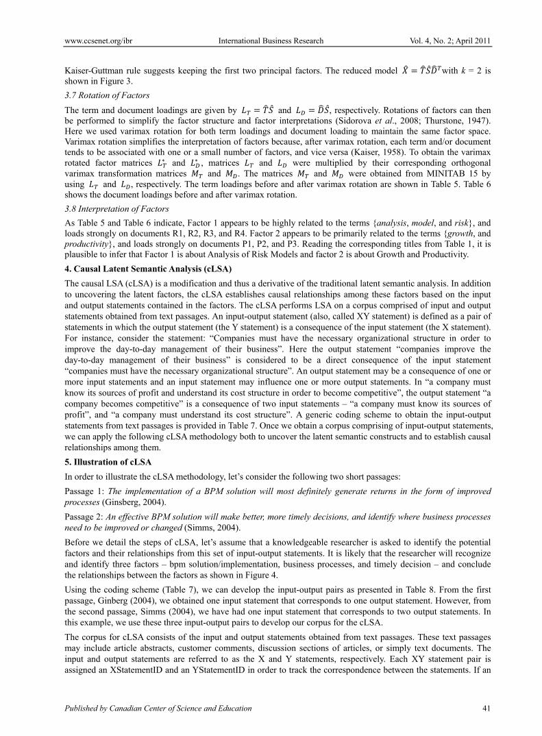
Kaiser-Guttman rule suggests keeping the first two principal factors. The reduced model with k = 2 is shown in Figure 3.

3.7 Rotation of Factors

The term and document loadings are given by and , respectively. Rotations of factors can then be performed to simplify the factor structure and factor interpretations (Sidorova et al., 2008; Thurstone, 1947). Here we used varimax rotation for both term loadings and document loading to maintain the same factor space. Varimax rotation simplifies the interpretation of factors because, after varimax rotation, each term and/or document tends to be associated with one or a small number of factors, and vice versa (Kaiser, 1958). To obtain the varimax rotated factor matrices and , matrices and were multiplied by their corresponding orthogonal varimax transformation matrices and . The matrices and were obtained from MINITAB 15 by using and , respectively. The term loadings before and after varimax rotation are shown in Table 5. Table 6 shows the document loadings before and after varimax rotation.

3.8 Interpretation of Factors

As Table 5 and Table 6 indicate, Factor 1 appears to be highly related to the terms {analysis, model, and risk}, and loads strongly on documents R1, R2, R3, and R4. Factor 2 appears to be primarily related to the terms {growth, and productivity}, and loads strongly on documents P1, P2, and P3. Reading the corresponding titles from Table 1, it is plausible to infer that Factor 1 is about Analysis of Risk Models and factor 2 is about Growth and Productivity.

4. Causal Latent Semantic Analysis (cLSA)

The causal LSA (cLSA) is a modification and thus a derivative of the traditional latent semantic analysis. In addition to uncovering the latent factors, the cLSA establishes causal relationships among these factors based on the input and output statements contained in the factors. The cLSA performs LSA on a corpus comprised of input and output statements obtained from text passages. An input-output statement (also, called XY statement) is defined as a pair of statements in which the output statement (the Y statement) is a consequence of the input statement (the X statement). For instance, consider the statement: “Companies must have the necessary organizational structure in order to improve the day-to-day management of their business”. Here the output statement “companies improve the day-to-day management of their business” is considered to be a direct consequence of the input statement “companies must have the necessary organizational structure”. An output statement may be a consequence of one or more input statements and an input statement may influence one or more output statements. In “a company must know its sources of profit and understand its cost structure in order to become competitive”, the output statement “a company becomes competitive” is a consequence of two input statements – “a company must know its sources of profit”, and “a company must understand its cost structure”. A generic coding scheme to obtain the input-output statements from text passages is provided in Table 7. Once we obtain a corpus comprising of input-output statements, we can apply the following cLSA methodology both to uncover the latent semantic constructs and to establish causal relationships among them.

5. Illustration of cLSA

In order to illustrate the cLSA methodology, let’s consider the following two short passages:

Passage 1: The implementation of a BPM solution will most definitely generate returns in the form of improved processes (Ginsberg, 2004).

Passage 2: An effective BPM solution will make better, more timely decisions, and identify where business processes need to be improved or changed (Simms, 2004).

Before we detail the steps of cLSA, let’s assume that a knowledgeable researcher is asked to identify the potential factors and their relationships from this set of input-output statements. It is likely that the researcher will recognize and identify three factors – bpm solution/implementation, business processes, and timely decision – and conclude the relationships between the factors as shown in Figure 4.

Using the coding scheme (Table 7), we can develop the input-output pairs as presented in Table 8. From the first passage, Ginberg (2004), we obtained one input statement that corresponds to one output statement. However, from the second passage, Simms (2004), we have had one input statement that corresponds to two output statements. In this example, we use these three input-output pairs to develop our corpus for the cLSA.

The corpus for cLSA consists of the input and output statements obtained from text passages. These text passages may include article abstracts, customer comments, discussion sections of articles, or simply text documents. The input and output statements are referred to as the X and Y statements, respectively. Each XY statement pair is assigned an XStatementID and an YStatementID in order to track the correspondence between the statements. If an

www.ccsenet.org/ibr International Business Research Vol. 4, No. 2; April 2011

ISSN 1913-9004 E-ISSN 1913-9012 42

X statement corresponds to more than one Y statement, then the X statement is given only one XStatementID and the corresponding Y statements are given separate YStatementIDs. Similarly, if a Y statement corresponds to more than one X statement, then the Y statement is given only one YStatementID and the corresponding X statements are given separate XStatementIDs. For instance, in Table 8, the X statement an effective bpm solution with an XStatementID Simms 2004 X1 has two corresponding Y statements – will make better, more timely decisions with an YStatementID Simms 2004 Y1, and will identify where business processes need to be improved or changed with an YStatementID Simms 2004 Y2. Assigning statement IDs in such a manner helps not only to track the XY correspondence but also to eliminate duplicate use of statements in the corpus.

To develop the corpus, first, the X statements are combined with the Y statements. Then the duplicate X and/or Y statements are removed. Finally, the unique statements are sorted by StatementID to form the corpus for LSA. The combined statements from Table 8 are shown in Table 9. Table 10 presents the final corpus.

It is now possible to perform LSA on the corpus to extract the latent semantic structure. For stepwise illustration of LSA, refer to Sidorova et al. (2008) and Section 3 above. The corpus consists of a collection of five statements with 30 words. Due to the small size of the corpus, we used the removal of stopwords and term stemming as the only term filtering techniques. Note that for large corpuses, other term filtering techniques such as the elimination of unique words (i.e., the words that appear in only one statement) and communality filtering can be applied. The removal of stopwords such as the, an, is, are, etc. and the Porter term stemming (Porter, 1980) produced a dictionary of 9 relevant terms. Table 11 shows matrix X containing the term frequencies. Matrix X with the TF-IDF (term frequency – inverse document frequency) weighted normalized frequencies is presented in Table 12.

Singular value decomposition (SVD) was applied to matrix X in Table 12. Keeping the first three principal components, the SVD of matrix X, , produced a 9 3 matrix of term eigenvectors of the square symmetric matrix , a 5 3 matrix of statement eigenvectors of the square symmetric matrix , and a

3 3 diagonal matrix S of singular values. The term and statement loadings were obtained by and , respectively. Rotations of factors were then performed to simplify the factor structure and factor

interpretations (Sidorova et al. 2008). We used varimax rotation for both term loadings and statement loading to maintain the same factor space. The term loadings before and after varimax rotation are shown in Table 13. Table 14 shows the statement loadings before and after varimax rotation.

As Table 13 and Table 14 indicate, Factor F1 appears to be highly related to the terms {bpm, solution, effective, and implementation}, and loads strongly on statements {Ginsberg 2004 X1, and Simms 2004 X1}. Factor F2 appears to be primarily related to the terms {business, processes, and returns}, and loads strongly on statements {Ginsberg 2004 Y1 and Simms 2004 Y2}. The terms and statements loading highly on Factor F3 are {decision and timely} and {Simms 2004 Y1}, respectively. Examination of the statements loading in the factors Table 10 reveals that these factors are what the knowledgeable researcher dubbed them earlier.

In cLSA, the X statements and their factor associations from Statement Loadings Matrix (Table 14) are tallied with the corresponding Y statements and their factor associations to determine inter-factor statement frequencies. The factor associations of a statement are determined by the factor loadings of the statement. If a statement has a factor loading of more than zero in a factor, then the statement is said to have an association with that factor. This will yield an matrix F of inter-factor statement frequencies, where f denotes the number of factors. The cell frequencies of a factor with relation to others provide support for that factor leading to those other factors. In this example, we considered a three-factor LSA. Therefore, we will obtain a 3 3 matrix F of inter-factor statement frequencies. The process of obtaining an inter-factor statement frequency matrix is described in the following.

Step 1: The statement loadings (Table 14) are separated into X statement loadings and Y statement loadings. The separated X and Y statement loadings for Table 14 are provided in Table 15 and Table 16, respectively.

Step 2: Each X statement is taken at a time and its factor associations are noted. These factor associations are called the X factor associations or the independent factor associations. For instance, the first X statement Ginsberg 2004 X1 is associated with Factor F1. Therefore, for this statement, Factor F1 acts as an independent factor.

Step 3: The corresponding Y statement(s) of the X statement in Step 2 are determined based on the XY statement pairs (Table 8). For instance, Table 8 indicates that the corresponding Y statement(s) of Ginsberg 2004 X1 is Ginsberg 2004 Y1.

Step 4: The factor associations of each Y statement in Step 3 are noted. These factor associations are called the Y factor associations or the dependent factor associations. The Y statement Ginsberg 2004 Y1 is associated with Factor F2. Therefore, for this statement, Factor F2 is a dependent factor.

Step 5: Each X factor association is tallied with all of its corresponding Y factor associations. A tally of an X factor

www.ccsenet.org/ibr International Business Research Vol. 4, No. 2; April 2011

Published by Canadian Center of Science and Education 43

association with a Y factor association provides an entry to the cell of the matrix F located at the intersection of the X factor and the Y factor. A cell entry of 1 indicates that there is one support for the X factor leading to the Y factor. For Ginsberg 2004 X1 - Ginsberg 2004 Y1 pair, the X factor is Factor F1 (Step 2) and the corresponding Y factor is Factor F2 (Step 4). By using X factors as the column headers and the Y factors as the row headers, this indicates that there will be a cell entry of 1 at the intersection column 1 and row 2. Figure 5(a) shows the schematic view of the inter-factor association of the Ginsberg 2004 X1 - Ginsberg 2004 Y1 pair. Table 17 presents the corresponding cell entry into matrix F.

Step 6: Steps 2 thru 5 are repeated until all X statements (Table 15) are exhausted. Figure 5(b) provides the schematic view of the inter-factor associations of the Simms 2004 X1. The corresponding Y statements of Simms 2004 X1 are Simms 2004 Y1 and Simms 2004 Y2.

The cell frequencies of matrix F are of critical importance. They provide the strength of association between the independent factors and the dependent factors. The percentages that the cell frequencies account for can be used to compare two or more relationships among the factors. Various statistics can be developed using matrix F. Two of these statistics are the X-index and the Y-index. An X-index relates to an X factor and is the sum of the cell frequencies of the column that the factor represents. On the other hand, a Y-index relates to a Y factor and is the sum of the cell frequencies of the row that the factor represents. For example, the X-index for F1 as an independent factor is 3; the X-index for F2 as an independent factor is 0; and the X-index for F3 as an independent factor is 0. On the contrary, the Y-index for F1 as a dependent factor is 0; the Y-index for F2 as a dependent factor is 2; and the Y-index for F3 as a dependent factor is 1. Yet another statistic is the X – Y differential. These statistics are shown in Table 18.

While the X-index of a factor represents the overall impact of the factor as an independent factor, the Y-index shows the overall effect on the factor as a dependent factor. The X – Y differential can be used to decide whether a factor is a net independent or dependent factor. Table 18 indicates that F1 is a net independent factor, and both F2 and F3 are net dependent factors. These statistics along with cell frequencies can be expressed as percentages for better comparison purposes. Table 19 presents these percentages.

Based on the percentage measures in Table 19, the inter-factor relationships and their strength of associations are portrayed in Figure 6.

6. Conclusion, Limitations, and Future Direction

There are several theoretical and practical implications of this study. First, in this study, we developed a variant of the traditional LSA that enables us to test causal models using textual data. This study is the first that has attempted to develop the causal Latent Semantic Analysis (cLSA) that analyzes input-output statements to establish causal relationships between the factors derived from the analysis. The academic implication of this study is that it provides academicians with a new approach to test causal models based on quantitative analysis of the textual data. The managerial implication is that managers should get an aggregated understanding of the models because cLSA provides a validation of them based on anecdotal evidence.

Future works can extend this study in a number of ways and thus address some of the limitations that this study has. Future works can refine the method, especially, with regard to how to reduce the inter-factor causal relationships. This study developed an input-output (XY) coding scheme. This scheme is not comprehensive. Therefore, future studies can also refine and extend this coding scheme.

References

Berry, M. W. (1992). Large scale singular value computations. International Journal of Supercomputer Applications, 6, 13-49.

Berry, M., Dumais, S., & O’Brien, G. (1995). Using linear algebra for intelligent information retrieval. SIAM Review, 37(4), 573-595.

Deerwester, S., Dumais, S., Furnas, G., Landauer, T., & Harshman, R. (1990). Indexing by latent semantic analysis. Journal of the American Society for Information Science, 41(6), 391-407.

Dumais, S. (2004). Latent semantic analysis. Annual Review of Information Science and Technology, 38, 189-230.

Efron, M. (2005). Eigenvalue-based model selection during latent semantic indexing. Journal of the American Society for Information Science and Technology, 56(9), 969-988.

Ginsberg, A. D. (2004). Sarbanes-Oxley and BPM: Selecting software that will enhance compliance, Business Performance Management, October 1, 2004.

www.ccsenet.org/ibr International Business Research Vol. 4, No. 2; April 2011

ISSN 1913-9004 E-ISSN 1913-9012 44

Han, J., and Kamber, M. (2006). Data Mining: Concepts and Techniques, 2nd ed., Morgan Kaufmann Publishers.

Kaiser, H.F. (1958). The varimax criterion for analytic rotation in factor analysis. Psychometrika, 23, 187-200.

Landauer, T. K. (2002). On the computational basis of learning and cognition: Arguments from LSA. In N. Ross (Ed.), The psychology of learning and motivation, 41, 43-84.

Landauer, T., Foltz, P., & Laham, D. (1998). Introduction to latent semantic analysis. Discourse Processes, 25, 259-284.

Landauer, T., Laham, D. & Derr, M. (2004). From paragraph to graph: Latent semantic analysis for information visualization. Proceedings of the National Academy of Sciences of the United States of America (PNAS), 101, 5214-5219.

Ord, T., Martins, E., Thakur, S., Mane, K., & Börner, K. (2005). Trends in animal behaviour research (1968-2002): Ethoinformatics and the mining of library databases. Animal Behaviour, 69, 1399-1413.

Porter, M. (1980). An algorithm for suffix stripping. Program, 14(3), 130–137.

Salton, G., and Buckley, C. (1988). Term-weighting approaches in automatic text retrieval. Information Processing & Management, 24(5), 513–523.

Sidorova, A., Evangelopoulos, N., Valacich, J., and Ramakrishnan, T. (2008). Uncovering the intellectual core of the information systems discipline. MIS Quarterly, 32(3), 467-482.

Simms, E. (2004). Case study: United States sugar corporation. Business Performance Management, March 1, 2004.

Thurstone, L. L. (1947). Multiple Factor Analysis, Chicago, IL: University of Chicago Press.

Table 1. Titles of seven select articles published in IJBPM in 2008

ID Document Title IJBPM Reference

P1 Deregulation and productivity growth: a study of the Indian commercial banking industry v. 10, p. 318 - 343

P2 Global productivity growth from 1980–2000: a regional view using the Malmquist total

factor productivity index

v. 10, p. 374 - 390

P3 Measuring productivity under different incentive structures v. 10, p. 366 - 373

R1 A rating model simulation for risk analysis v. 10, p. 269 - 299

R2 An analysis of the key-variables of default risk using complex systems v. 10, p. 202 - 230

R3 New contents and perspectives in the risk analysis of enterprises v. 10, p. 136 - 173

R4 Risk insolvency predictive model maximum expected utility v. 10, p. 174 - 190

Table 2. The corpus after the data cleaning process

ID Document Title IJBPM Reference

P1 Deregulation and productivity growth a study of the Indian commercial banking industry v. 10, p. 318 - 343

P2 Global productivity growth from 1980 2000 a regional view using the Malmquist total factor

productivity index

v. 10, p. 374 - 390

P3 Measuring productivity under different incentive structures v. 10, p. 366 - 373

R1 A rating model simulation for risk analysis v. 10, p. 269 - 299

R2 An analysis of the key-variables of default risk using complex systems v. 10, p. 202 - 230

R3 New contents and perspectives in the risk analysis of enterprises v. 10, p. 136 - 173

R4 Risk insolvency predictive model maximum expected utility v. 10, p. 174 - 190

Table 3. Matrix X, containing term frequencies

Term

Document P1 P2 P3 R1 R2 R3 R4

analysis 0 0 0 1 1 1 0 growth 1 1 0 0 0 0 0 model 0 0 0 1 0 0 1 productivity 1 2 1 0 0 0 0 risk 0 0 0 1 1 1 1

www.ccsenet.org/ibr International Business Research Vol. 4, No. 2; April 2011

Published by Canadian Center of Science and Education 45

Table 4. Transformed matrix X (TF-IDF)

Term

Document

P1 P2 P3 R1 R2 R3 R4

analysis 0 0 0 0.525 0.834 0.834 0

growth 0.913 0.746 0 0 0 0 0

model 0 0 0 0.777 0 0 0.913

productivity 0.408 0.666 1 0 0 0 0

risk 0 0 0 0.347 0.551 0.551 0.408

Table 5. Term loadings before and after varimax rotation

Term Loadings

Unrotated Orthogonal. Tran.

Matrix (varimax)

After varimax

Term Factor 1 Factor 2 Factor 1 Factor 2

analysis 1.16 0 1.164 0

growth 0 -1.02 1.000 0.000 0 -1.02

model 0.78 0 × = 0.776 0

productivity 0 -1.16 0.000 1.000 0 -1.16

risk 0.93 0 0.926 0

Table 6. Document loadings before and after varimax rotation

Document Loadings

Unrotated Orthogonal. Tran.

Matrix (varimax)

After varimax

Document Factor 1 Factor 2 Factor 1 Factor 2

P1 0 -0.91 0 -0.91

P2 0 -0.99 1.00 0.00 0 -0.993

P3 0 -0.75 × = 0 -0.75

R1 0.92 0 0.00 1.00 0.92 0

R2 0.88 0 0.88 0

R3 0.88 0 0.88 0

R4 0.65 0 0.65 0

www.ccsenet.org/ibr International Business Research Vol. 4, No. 2; April 2011

ISSN 1913-9004 E-ISSN 1913-9012 46

Table 7. Input-output statement (XY statement) coding scheme

Raw Statements Input-Output Statements

In order to (verb) Y, X Or, X in order to (verb) Y Companies must have the necessary organizational structure in order to improve the day-to-day management of their business

Input: X Output: Subject of X (verb) Y Input: companies must have the necessary organizational structure Output: companies improve the day-to-day management of their business

By (verb particle) X, Y By refocusing customer strategy, retooling measurement mechanics, and taking steps to realign the organization around customers, companies can retain and grow existing customers

Input: Subject of Y (verb) X Output: Y Inputs: (1) companies refocus customer strategy, (2) companies retool measurement mechanics, (3) companies take steps to realign the organization around customers Output: companies can retain and grow existing customers

When X then Y When an organization take a methodical approach to performance management, it becomes high-performance organization

Input: X Output: Y Input: an organization take a methodical approach to performance management Output: an organization becomes high-performance organization

X (yields/ provides/ results in/ causes/ allows/ enables/ achieves/ guides/ ensures /brings /etc.) Y Plans that are developed in a more collaborative environment yield more commitment from the people who have to bring them to fruition

Input: X Output: Y Input: plans are developed in a more collaborative environment Output: plans yield more commitment from the people who have to bring them to fruition

If X, then Y If companies do not provide exceptional customer service, customers will not renew their contracts

Input: X Output: Y Input: companies do not provide exceptional customer service Output: customers will not renew their contracts

For X to (verb) Y, X (be) to (verb) Z For BPM to provide the benefits that make it worth the investment, it has to focus on the right data

Input: X (be) to (verb) Z Output: X (verb) Y Input: BPM has to focus on the right data Output: BPM provides the benefits that make it worth the investment

X because Y Companies add OLAP technology to their BPM solution because they need to extract transaction information from all parts of their IT infrastructure

Input: X Output: Y Input: companies add OLAP technology to their BPM solution Output: companies need to extract transaction information from all parts of their IT infrastructure

To (do) Y, (need) X To integrate the data from the acquisition's IT systems into its BPM reporting framework, Logistics USA layers OLAP software on top of the acquired organization's disparate data sources

Input: X Output: Y Input: Logistics USA layers OLAP software on top of the acquired organization's disparate data sources Output: Logistics USA integrates the data from the acquisition's IT systems into its BPM reporting framework

Y requires X Or X is required for Y Establishing and sustaining a complexity management program requires dedicated resources and the involvement of the organization's top management

Input: X Output: Y Input: dedicated resources and the involvement of the organization's top management Output: establishing and sustaining a complexity management program

X so as to Y Maintenance should be managed better so as to cultivate a sense of ownership in the operators

Input: X Output: Y Input: maintenance should be managed better Output: cultivate a sense of ownership in the operators

Because of X, Y Because of the wide acclaim received by the Malcolm Baldrige Award, it has served as a model for national quality awards by many countries throughout the world

Input: X Output: Y Input: the wide acclaim received by the Malcolm Baldrige Award Output: it has served as a model for national quality awards by many countries throughout the world

X is associated to/likely to create/etc. Y Firms with higher amounts of intangible assets are more likely to create shareholder value

Input: X Output: Y Input: firms with higher amounts of intangible assets Output: create shareholder value

www.ccsenet.org/ibr International Business Research Vol. 4, No. 2; April 2011

Published by Canadian Center of Science and Education 47

Z uses X to improve/cause/enhance/etc. Y faculty members have used the Criteria for Performance Excellence and the underlying concepts of the MBNQA to enhance the learning experiences of their students

Input: X Output: Y Input: the Criteria for Performance Excellence and the underlying concepts of the MBNQA Output: the learning experiences of students

By means of X, Y By means of concrete exercises and experiences, Dale's Cone of Experience is employed to better leverage the student's ability to understand the abstract concepts

Input: X Output: Y Input: concrete exercises and experiences Output: Dale's Cone of Experience is employed to better leverage the student's ability to understand the abstract concepts

Y through X OR Through X, Y The West has created competitiveness through fostering a culture of entrepreneurship

Input: X Output: Y Input: fostering a culture of entrepreneurship Output: the West has created competitiveness

Table 8. Input-output pairs

XStatementID YStatementID X Statement Y Statement

Ginsberg 2004 X1 Ginsberg 2004 Y1 implementation of a bpm solution

results in improved processes

Simms 2004 X1 Simms 2004 Y1 an effective bpm solution enables organizations to change or improve processes

Simms 2004 X1 Simms 2004 Y2 an effective bpm solution enables organizations to make better, more timely decisions

Table 9. Combined X and Y statements

StatementID Statement

Ginsberg 2004 X1 the implementation of a bpm solution

Ginsberg 2004 Y1 will most definitely generate returns in the form of improved processes

Simms 2004 X1 an effective bpm solution

Simms 2004 X1 an effective bpm solution

Simms 2004 Y1 will make better, more timely decisions

Simms 2004 Y2 will identify where business processes need to be improved or changed

Table 10. Final corpus

StatementID Statement

Ginsberg 2004 X1 the implementation of a bpm solution

Ginsberg 2004 Y1 will most definitely generate returns in the form of improved processes

Simms 2004 X1 an effective bpm solution

Simms 2004 Y1 will make better, more timely decisions

Simms 2004 Y2 will identify where business processes need to be improved or changed

Table 11. Matrix X, containing term frequencies

Ginsberg 2004 X1 Ginsberg 2004 Y1 Simms 2004 X1 Simms 2004 Y1 Simms 2004 Y2

bpm 1 0 1 0 0

business 0 0 0 0 1

decisions 0 0 0 1 0

effective 0 0 1 0 0

implementation 1 0 0 0 0

processes 0 1 0 0 1

returns 0 1 0 0 0

solution 1 0 1 0 0

timely 0 0 0 1 0

www.ccsenet.org/ibr International Business Research Vol. 4, No. 2; April 2011

ISSN 1913-9004 E-ISSN 1913-9012 48

Table 12. Matrix X, containing TF-IDF weighted normalized frequencies

Ginsberg 2004 X1 Ginsberg 2004 Y1 Simms 2004 X1 Simms 2004 Y1 Simms 2004 Y2

bpm 0.4435 0 0.4435 0 0

business 0 0 0 0 0.869

decisions 0 0 0 0.7071 0

effective 0 0 0.7789 0 0

implementation 0.7789 0 0 0 0

processes 0 0.4948 0 0 0.4948

returns 0 0.869 0 0 0

solution 0.4435 0 0.4435 0 0

timely 0 0 0 0.7071 0

Table 13. Term loadings before and after varimax rotation

Terms

Term Loadings

Unrotated Rotated

F1 F2 F3 F1 F2 F3

bpm 0.6271 0 0 0.6271 0 0

business 0 0.6145 0 0 0.6145 0

decisions 0 0 -0.7071 0 0 0.7071

effective 0.5508 0 0 0.5508 0 0

implementation 0.5508 0 0 0.5508 0 0

processes 0 0.6997 0 0 0.6997 0

returns 0 0.6145 0 0 0.6145 0

solution 0.6271 0 0 0.6271 0 0

timely 0 0 -0.7071 0 0 0.7071

Table 14. Statement loadings before and after varimax rotation

Statements

Statement Loadings

Unrotated Rotated

F1 F2 F3 F1 F2 F3

Ginsberg 2004 X1 0.8347 0 0 0.8347 0 0

Ginsberg 2004 Y1 0 0.7889 0 0 0.7889 0

Simms 2004 X1 0.8347 0 0 0.8347 0 0

Simms 2004 Y1 0 0 -1 0 0 1

Simms 2004 Y2 0 0.7889 0 0 0.7889 0

Table 15. X statement loadings

X Statements

Factors

F1 F2 F3

Ginsberg 2004 X1 0.8347 0 0

Simms 2004 X1 0.8347 0 0

Table 16. Y statement loadings

Y Statements

Factors

F1 F2 F3

Ginsberg 2004 Y1 0 0.7889 0

Simms 2004 Y1 0 0 1

Simms 2004 Y2 0 0.7889 0

www.ccsenet.org/ibr International Business Research Vol. 4, No. 2; April 2011

Published by Canadian Center of Science and Education 49

Table 17. Inter-factor matrix F

X Factors lead to Y Factors X Factors

F1 F2 F3

Y

Fac

tors

F1

F2 2

F3 1

Table 18. X-index, Y-index, and X-Y differential

X Factors lead to Y Factors

X Factors F1 F2 F3 Y-index

Y

Fac

tors

F1 0 F2 2 2 F3 1 1

X-index 3 0 0 X - Y differential 3 -2 -1

Table 19. Matrix F – percentage measures

X Factors lead to Y Factors X Factors

F1 F2 F3 Y-index

Y

Fac

tors

F1 0

F2 0.67 0.67

F3 0.33 0.33

X-index 1 0 0

X - Y differential 1 -0.67 -0.33

Figure 1. Schematic of the term-by-document matrix X

Figure 2. The SVD of matrix X (X = TSDT)

www.ccsenet.org/ibr International Business Research Vol. 4, No. 2; April 2011

ISSN 1913-9004 E-ISSN 1913-9012 50

Figure 3. The SVD of the reduced model ( )

Figure 4. Relationships between BPM solution, business processes, and timely decisions

Figure 5(a). Inter-factor associations and support

Figure 5(b). Inter-factor associations and support

Figure 6. Inter-factor relationships and their strength of association