PLEASE SCROLL DOWN FOR ARTICLE

This article was downloaded by: [Harbor UCLA Medical Centre]On: 30 September 2009Access details: Access Details: [subscription number 907137979]Publisher RoutledgeInforma Ltd Registered in England and Wales Registered Number: 1072954 Registered office: Mortimer House,37-41 Mortimer Street, London W1T 3JH, UK

Journal of Personality AssessmentPublication details, including instructions for authors and subscription information:http://www.informaworld.com/smpp/title~content=t775653663

An Illustration of Multilevel Factor AnalysisSteven P. Reise a; Joseph Ventura b; Keith H. Nuechterlein c; Kevin H. Kim a

a Department of Psychology, University of California, Los Angeles. b Department of Psychiatry, University ofCalifornia, Los Angeles. c Departments of Psychiatry and Psychology, University of California, Los Angeles.

Online Publication Date: 01 January 2005

To cite this Article Reise, Steven P., Ventura, Joseph, Nuechterlein, Keith H. and Kim, Kevin H.(2005)'An Illustration of MultilevelFactor Analysis',Journal of Personality Assessment,84:2,126 — 136

To link to this Article: DOI: 10.1207/s15327752jpa8402_02

URL: http://dx.doi.org/10.1207/s15327752jpa8402_02

Full terms and conditions of use: http://www.informaworld.com/terms-and-conditions-of-access.pdf

This article may be used for research, teaching and private study purposes. Any substantial orsystematic reproduction, re-distribution, re-selling, loan or sub-licensing, systematic supply ordistribution in any form to anyone is expressly forbidden.

The publisher does not give any warranty express or implied or make any representation that the contentswill be complete or accurate or up to date. The accuracy of any instructions, formulae and drug dosesshould be independently verified with primary sources. The publisher shall not be liable for any loss,actions, claims, proceedings, demand or costs or damages whatsoever or howsoever caused arising directlyor indirectly in connection with or arising out of the use of this material.

REISE, VENTURA, NUECHTERLEIN, KIMMULTILEVEL FACTOR

STATISTICAL DEVELOPMENTS AND APPLICATIONS

An Illustration of Multilevel Factor Analysis

Steven P. ReiseDepartment of Psychology

University of California, Los Angeles

Joseph VenturaDepartment of Psychiatry

University of California, Los Angeles

Keith H. NuechterleinDepartments of Psychiatry and Psychology

University of California, Los Angeles

Kevin H. KimDepartment of Psychology

University of California, Los Angeles

The factor analysis of repeated measures psychiatric data presents interesting challenges for re-searchers in terms of identifying the latent structure of an assessment instrument. Specifically,repeated measures contain both within and between individual sources of variance. Although anumber of techniques exist for separating out these 2 sources of variance, all are problematic.Recently, researchers have proposed that exploratory multilevel factor analysis (MFA) be usedto appropriately analyze the latent structure of repeated measures data. The chief objective ofthis report is to provide a didactic step-by-step guide on how MFA may be applied to psychiat-ric data. In the discussion, we describe difficulties associated with MFA and consider chal-lenges in factor analyzing life event appraisals in psychiatric samples.

Investigating the latent (factor) structure of a multiitem psy-chiatric measure is a fundamental task of personality assess-ment researchers. For example, determining the factor struc-ture of a measure plays an important role in establishing aninstrument’s construct validity and in guiding the interpreta-tion of scale scores. However, the collection of repeated mea-sures on a multi-item self-report instrument creates interest-ing challenges for multivariate analysis in general and factoranalysis in particular (Hox, 1993; Longford & Muthén,1992; Nezlek, 2001; Wood & Brown, 1994). For example,ordinary R-type factor analytic procedures (factor analysis ofvariables) assume that observations are independent. This as-sumption is unlikely to be true in repeated measures designsbecause the same individual contributes multiple records tothe database. Moreover, with repeated measures, the varianceof item ratings is influenced by both within- and be-

tween-individual sources. That is, the total variance of eachitem and the covariance/correlation between items is influ-enced by the variation of item ratings within individuals overtime and by the variation between individuals in their aver-age rating.

Traditionally, researchers have taken two approaches tothe factor analysis of repeated measurements.1 First, some

JOURNAL OF PERSONALITY ASSESSMENT, 84(2), 126–136Copyright © 2005, Lawrence Erlbaum Associates, Inc.

1Another approach that is unexplored in this article is the use ofP-technique factor analysis. In P-technique factor analysis, repeatedobservations within an individual are factor analyzed. Consider 30people in a sample who each rated a 10-item mood scale for 90 days.Then, by treating days as repeated measurements, a researcher maycreate 30 separate within-individuals correlation matrices and factoranalyze each one separately. Potentially, 30 separate solutions mayresult. This technique is not useful in this context for several reasons.

Downloaded By: [Harbor UCLA Medical Centre] At: 00:56 30 September 2009

researchers have implemented work-around strategies suchas selecting one observation at random from each study par-ticipant. This approach avoids problems caused by depend-encies in the data, but it suffers in terms of sample size andwastes much of the data. Moreover, by ignoring (via throw-ing out) between-individual differences, this approachmisses potentially interesting findings. That is, a researchermay miss the opportunity to study the between-individualfactor structure. Second, some researchers simply ignore thenested data structure and treat all observations as independ-ent. The factor analysis is then based on the total correlationmatrix. This approach uses all the data; however, by ignoringthe dependencies in the data, the standard errors for parame-ter estimates and the model fit statistics may be misleading.More important, the factor analytic results may be substan-tively wrong because the structure is contaminated by twosources of variance.

To avoid the traditional problems inherent with the factoranalysis of repeated measures, researchers need to consideranalyticprocedures thatproperlyaccount forwithin-individu-als and between-individual variance. One appropriate meth-odological tool that is gaining attention is called multilevelfactor analysis (MFA; Heck, 1999; Muthén, 1991, 1994).MFA models, which can be estimated with common structuralequation modeling software such as EQS (Bentler & Wu,2002) and Mplus (Muthén & Muthén, 2004), are a subclass ofmultilevel covariance structure models designed to addressthe statistical challenges inherent in nested data structures.Nested data structures occur when one sampling unit is nestedwithin another such as when children are nested withinschools or clients are nested within clinicians. With this data,wehave lifeeventappraisal ratingscollectedover time that arenested within individual study participants.

Imagine that a researcher has collected symptom ratings(e.g., on a scale ranging from 1 to 7) on a sample of individuals(N = 100) once a week for 50 weeks. Assume that the 24-itemversion of the Brief Psychiatric Rating Scale (BPRS; Venturaet al., 1993) was administered. The data thus contain psychiat-ric symptom scores for 100 individuals measured on 24 vari-ables over 50 occasions. Furthermore, assume the researcherdesires to conduct an exploratory factor analysis of the BPRSitems to study dimensions of psychopathology. In turn, the re-searcher is interested instudyingcovariates thatpredict theav-erage levels of psychopathology across the study period (e.g.,treatment program) and covariates that account forwithin-individuals variations in the psychopathology dimen-

sions across time (e.g., stressful life events). This is an idealcontext for application of MFA procedures because MFA cannot only control for confounding sources of variance but canalso provide factor scores to represent both within-individualsdifferences and between-individual differences. We discussthese further in subsequent sections.

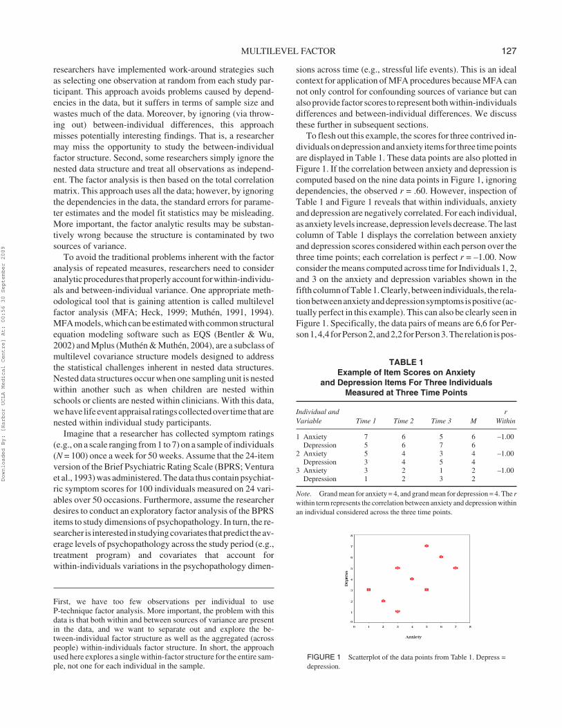
To flesh out this example, the scores for three contrived in-dividualsondepressionandanxiety items for three timepointsare displayed in Table 1. These data points are also plotted inFigure 1. If the correlation between anxiety and depression iscomputed based on the nine data points in Figure 1, ignoringdependencies, the observed r = .60. However, inspection ofTable 1 and Figure 1 reveals that within individuals, anxietyand depression are negatively correlated. For each individual,as anxiety levels increase, depression levels decrease. The lastcolumn of Table 1 displays the correlation between anxietyand depression scores considered within each person over thethree time points; each correlation is perfect r = –1.00. Nowconsider the means computed across time for Individuals 1, 2,and 3 on the anxiety and depression variables shown in thefifth column of Table 1. Clearly, between individuals, the rela-tionbetweenanxietyanddepressionsymptoms ispositive (ac-tually perfect in this example). This can also be clearly seen inFigure 1. Specifically, the data pairs of means are 6,6 for Per-son1,4,4 forPerson2,and2,2 forPerson3.Therelation ispos-

MULTILEVEL FACTOR 127

First, we have too few observations per individual to useP-technique factor analysis. More important, the problem with thisdata is that both within and between sources of variance are presentin the data, and we want to separate out and explore the be-tween-individual factor structure as well as the aggregated (acrosspeople) within-individuals factor structure. In short, the approachused here explores a single within-factor structure for the entire sam-ple, not one for each individual in the sample.

TABLE 1Example of Item Scores on Anxiety

and Depression Items For Three IndividualsMeasured at Three Time Points

Individual andVariable Time 1 Time 2 Time 3 M

rWithin

1 Anxiety 7 6 5 6 –1.00Depression 5 6 7 6

2 Anxiety 5 4 3 4 –1.00Depression 3 4 5 4

3 Anxiety 3 2 1 2 –1.00Depression 1 2 3 2

Note. Grand mean for anxiety = 4, and grand mean for depression = 4. The rwithin term represents the correlation between anxiety and depression withinan individual considered across the three time points.

FIGURE 1 Scatterplot of the data points from Table 1. Depress =depression.

Downloaded By: [Harbor UCLA Medical Centre] At: 00:56 30 September 2009

itive because people who are, on average, high on anxiety alsotend to be high, on average, on depression.

Now consider an exploratory factor analysis of BPRSsymptom ratings from our hypothetical experimental situa-tion. In this analysis, the nested data structure is ignored, andall scores are treated as coming from separate individuals. Ifthe factor analysis showed that anxiety and depression itemsload highly on a common factor (i.e., they covary highly,e.g., r = .60), what would the conclusion be? First, we couldclaim to have found evidence that people who are high onanxiety (on average) also tend to score high on depression(on average). This would be a between or interindividual in-terpretation. We could also claim that within individuals, asanxiety increases so do their depressive symptoms whenconsidered within individuals over time. This would be awithin-individuals or intraindividual interpretation. Theproblem, as Figure 1 and Table 1 illustrate, is that neitherconclusion can be fully trusted because within and betweensources of variance are confounded in the analysis. For ex-ample, drawing again from the data in Table 1, the analysiscompletely misses the fact that anxiety and depression arenegatively related within persons.

What is called for in this situation is exploratory MFA. Inexploratory MFA of repeated measures data, a researcher firstcomputes a statistical quantity called the intraclass correlation(ICC; Koch, 1983). Note that one ICC would be produced foreach itemon themeasure.The ICCestimates theamountof thetotal item variance that is due to between-individual variance(see Snijders & Bosker, 1999). In terms of our running exam-ple, an ICC would estimate the degree to which variance in theBPRS items is due to between-individual differences in theiraverage item rating over time: in other words, the amount dueto the variation of individual means around the grand mean asopposed to the variation of an individual’s ratings around hisor her own mean.2

When the ICC equals zero, all variation is within individu-als. In turn, an ICC of zero indicates that the item is not be-having in a trait-like manner. Most important, an ICC of 1means that the data are independent, and there is no need for

MFA. To the degree that the ICC is greater than zero, itemvariation is due to between-individual differences in theirmean level considered over time. In turn, as the ICC ap-proaches 1, this indicates that the item is behaving more traitlike. Also, as the ICC approaches 1, the effective sample sizeis really the number of individuals and not the total numberof observations. Most important, MFA is an appropriate andnecessary analytic strategy. It is necessary to correctly sepa-rate out the within-persons source of variance from the be-tween-person source of item variance so that ultimately, theinterpretation of the factor structure is correct.

Having established a nonzero ICC, MFA proceeds by par-titioning the total covariance or correlation matrix into twoparts (see Heck, 1999): (a) a between matrix and (b) a(pooled across individuals) within matrix. The between(interindividual) matrix reflects the relations among themeans of the measured variables when considered over thestudy period. If two variables are highly correlated in the be-tween matrix, this indicates that people who are, on average,high on one variable also tend to be high, on average, on theother variable. The within (intraindividual) matrix reflectsthe relations among variables within individuals across timepooled across individuals. If two variables are highly corre-lated in the within matrix, this indicates that elevations or de-pressions (relative to a person’s mean) on the first variabletend to co-occur with elevations or depressions (relative to aperson’s mean) on the second variable within individuals.

Having calculated the appropriate covariance or correla-tion matrices, ordinary factor analysis is conducted on eachmatrix separately. The factor structure can but need not beequivalent across the two levels. For example, a two-factormodel may best fit the within structure, but a one-factor modelmay be appropriate for the between structure. Each of thesefactor structures in turn is of substantive interest, and factorscores could be estimated for both within and between struc-tures. In our running example of the BPRS, each time pointwithin each person would receive one (or more depending onthe number of factors) within-factors score(s). In addition,each person would receive one (or more depending on thenumber of factors) estimated between-factor scores. In turn,these estimated factor scores (Grice, 2001) derived from thewithin-factors and between-factor structure can be used toevaluate how a factor relates to between individual (e.g., gen-der, treatment groups) or within individuals, time varying(e.g., symptomratings, stressful events) studyvariables. In theremainder of this article, we illustrate these concepts usingdata from a research project with schizophrenic patients.

METHOD

Participants

The sample was drawn from the Developmental Processes inSchizophrenic Disorders project (Nuechterlein et al., 1992).Detailed descriptive information for the entire project as well

128 REISE, VENTURA, NUECHTERLEIN, KIM

2There are a variety of formulas for estimating an ICC dependingon the context. To keep things simple, one way to think about anitem’s ICC in this context is as follows. First, for a single item acrossall people and time points, a grand item mean is calculated and a totalsum of squares is computed around that grand item mean. For theanxiety measure in Table 1, the total sum of squares (SST) is 30. Sec-ond, for each person, compute the mean item score considered overtime. Then, compute the sum of squares of these person meansaround the grand mean. This is the between sum of squares (SSB). Forthe anxiety measure, the between sum of squares is 24. The ICC isthen simply ICC = SSB/SST or .80 in the anxiety example. To the ex-tent to which all people are similar on average (i.e., have the samemean item score), the total variance will be due to within-personsfluctuations across time, and the ICC will be near zero. If within aperson, item scores stay constant, but people differ widely in itemmeans, the ICC will approach 1 because all variance will be due tobetween-person differences.

Downloaded By: [Harbor UCLA Medical Centre] At: 00:56 30 September 2009

as information on medication and behaviorally orientedtreatment regimens can be found elsewhere (e.g.,Nuechterlein et al., 1992). Briefly, this research project in-cludes 73 patients with a recent onset of schizophrenia,schizoaffective disorder, or schizophreniform disorder whowere defined as having had a first psychotic episode thatstarted no longer than 2 years before study entry. Mean age atstudy entry was 23.5 years (SD = 4.5) and mean educationwas 12.4 years (SD = 1.7). Of the participants, 62 (85%) weremen. Patients had a mean age of onset of illness of 22.3 years(SD = 4.5). Prior to study entry, patients had been psychiatri-cally ill, including prodromal periods, for an average of 16.2months (SD = 12.3). The patients were assessed for the oc-currence of life events and psychiatric symptoms for 1 yearfollowing a period of stabilization of outpatient medications.

Patients were recruited primarily from four large publicpsychiatric hospitals in Los Angeles, California. A modifiedversion of the Present State Exam (Wing, Cooper, & Sarto-rius, 1974) was used to determine if patients met research di-agnostic criteria (Spitzer, Endicott, & Robins, 1978) forschizophrenia (n = 58) or schizoaffective disorder, depressedtype, mainly schizophrenic (n = 15). By Diagnostic and Sta-tistical Manual of Mental Disorders (4th ed.; American Psy-chiatric Association, 1994) criteria, the entry diagnoses wereschizophrenia (n = 53), schizoaffective disorder (n = 13), orschizophreniform disorder (n = 7).

Each patient received individual and group therapy aimedat developing social and independent living skills throughthe University of California, Los Angeles (UCLA) AftercareResearch Program. Treatment typically included the admin-istration every 2 weeks of 12.5 mg of fluphenazine(Prolixin®) decanoate via injection. The antipsychotic medi-cation dosage was increased if symptoms worsened or re-duced if intolerable side effects occurred. Based on clinicalneed, patients were treated with adjunctive medications (e.g.,antidepressants). All participants gave written informed con-sent after oral and written information regarding this projectwas provided. The research project was approved by theUCLA Institutional Review Board.

LES

To obtain data on the occurrence of life events, study partici-pants were interviewed approximately every 4 weeks usingthe Life Events Schedule (LES; Ventura et al., 1989; VenturaNuechterlein, Hardesty, & Gitlin, 1992). The interview con-sisted of 111 discrete life events, 102 of which were adaptedfrom the Psychiatric Epidemiology Research Interview forLife Events (Dohrenwend, Krasnoff, Askenasy, &Dohrenwend, 1978). We used open-ended questions to elicitthe occurrence of additional life events and to obtain detailedinformation about each reported event (Brown & Harris,1978). A member of the research team determined whethereach event was of sufficient magnitude or associated withsufficient change in role status to meet the criteria for a life

event (Brown & Harris, 1978). Additional information onour life events data collection procedures is available else-where (Ventura et al., 1989; Ventura et al., 1992).

Life events were coded as positive (e.g., making a newfriend), or as negative (e.g., argument with a family member)and as small in magnitude (e.g., parking ticket) or as large inmagnitude (e.g., fired from a full-time job). In addition,events were coded as being “independent” of the patient’s ill-ness and beyond his ability to influence the event, or “de-pendent” involving a personal choice, or as “symptomrelated,” that is, related to the patient’s symptoms. Theseanalyses focus on 940 large and small negative life events.The number of negative life events varied widely across par-ticipants. For example, two individuals had only two nega-tive life events during the entire study period and oneindividual reported 35 negative events. The median andmodal number of negative life events was 13.

CALES

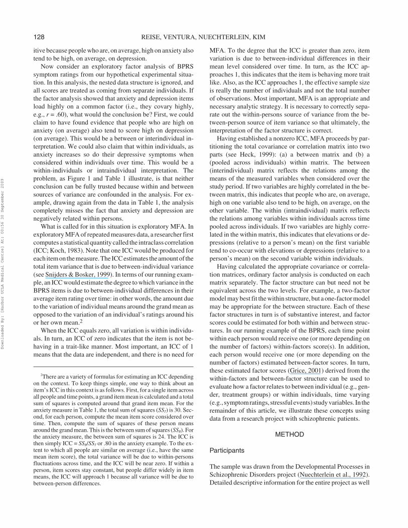
We explored the factor structure of an 8-item Cognitive Ap-praisal of Life Events Scale (CALES; Ventura &Nuechterlein, 1994). The CALES is a self-administered scalethat measures the patient’s perception of the stressful aspectsof life events. The CALES was rated on eight dimensions foreach life event reported by the patient in the 4 weeks prior tothe interview during the 1-year follow-through period. Eachappraisal item was rated on an adjectival scale ranging from 1(not at all) to 9 (extremely) (see Table 2). Descriptive statis-tics for the CALES items are shown in Table 3.

There are two things of particular note. First, notice that in-dividuals tended to use only the odd numbers for their ratings.This phenomenon appears to be due to the fact that only theodd numbers had anchor descriptions. Although this strangepattern of response illustrates the dangers inherent in using too

MULTILEVEL FACTOR 129

TABLE 2The Cognitive Appraisal of Life Events Scale

Content and Response Option Extremes

1. How desirable was the event? (Desire)1 = not at all desirable; 9 = extremely desirable

2. Has this event ever happened to you before? (Familiar)1 = not at all familiar; 9 = extremely familiar

3. How much control did you have over the happening of this event?(Control)1 = no control at all; 9 = extreme degree of control

4. Did you have any advance notice about the event? (Notice)1 = no advance notice at all; 9 = extreme degree of advance notice

5. How much of the time has the event been on your mind? (On Mind)1 = not at all on my mind; 9 = on my mind all of the time

6. How much of a change in your daily routine has the event caused?(Routine)1 = no change at all; 9 = extreme degree of change

7. Were you successful at handling the event? (Handled)1 = not at all successful; 9 = extremely successful

8. How upsetting was this event for you? (Upset)1 = not at all upsetting; 9 = as upsetting as anything that’s everhappened to me

Downloaded By: [Harbor UCLA Medical Centre] At: 00:56 30 September 2009

many scale points in a sample of individuals with schizophre-nia, it should have little impact on subsequent analysis. Sec-ond,around70of the940negative lifeeventswere ratedas6orabove on the desirability item. In a few cases, inspection of theprotocols revealed that this appears to be due to the individ-ual’s own perspective on the item. For example, an individualmay report a life event, “interviewed, but didn’t get a job.” In-stead of rating this event as undesirable because a job was notoffered, the individual apparently rated success in obtainingan interview as highly desirable. Given that we cannot abso-lutelydetermine that these ratingsaremistakes,weanalyze thedata as they are without any corrections.

ANALYSES AND RESULTS

The Four-Step Process

Muthén (1991, 1994) elaborated an explicit set of proceduresto follow when conducting confirmatory MFA. Translatedinto the context of exploratory MFA, these steps are as fol-lows. First, conduct an ordinary exploratory factor analysisof the total correlation matrix. This “incorrect” analysis isbased on treating all the observations as independent. Theobjective of the first step is to obtain a rough sense of the un-derlying factor structure. The second step is to estimate theICC for each item. This step establishes whether an MFA isnecessary. The third and fourth steps, respectively, are to esti-mate a within-correlations and between correlation matrixand conduct factor analysis for each matrix separately. In thefollowing, we flesh out each of these four steps as we proceedto discuss the results.

Step 1: Factor Analysis of the TotalCorrelation Matrix

The data matrix consists of 940 appraisals of life eventsdrawn from 73 individuals. For this total analysis, the dataare treated as independent, and therefore, 940 data vectors (ofeight items each) are used to compute the total covariance(ST) and correlation matrix (RT). The formula for the totalcovariance matrix is:

(1)

In Equation 1, I = 73 = number of individuals in the sample;N = total number of observations; Ji = total number of obser-vations within an individual; xij = vector of scores for indi-vidual i at time point j; and, = vector of means (i.e., thegrand means). The correlation matrix (RT) is found by divid-ing each term in ST by the appropriate standard deviations.This matrix is shown at the top in Table 4.

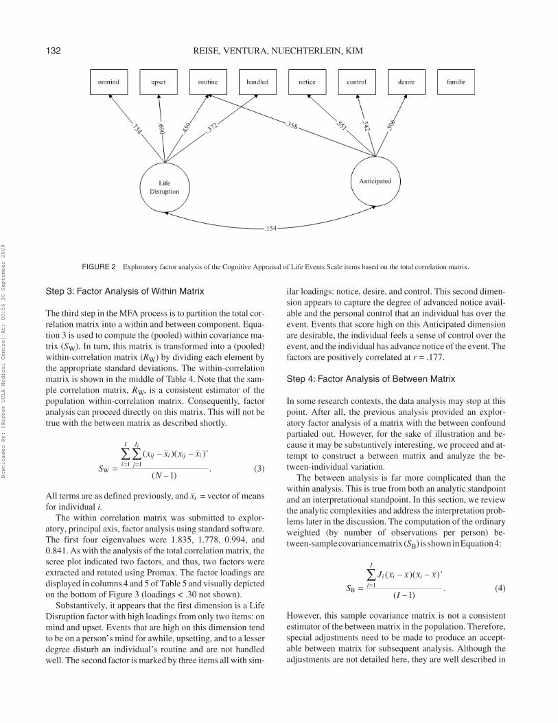
The total correlation matrix was submitted to exploratory,principal axis, factor analysis using standard software. Thefirst four eigenvalues were 1.970, 1.812, 0.974, and 0.819.The resulting scree plot clearly indicated two factors, andthus, two factors were extracted and rotated using Promax. Arotation that allowed the factors to be correlated was selectedto avoid the distortions that can occur by forcing a varimax(orthogonal) rotation onto the data. The resulting factor load-ings are displayed in columns 2 and 3 of Table 5 and visuallydepicted in Figure 2 (loadings < .30 are not shown).

Substantively, it appears that the first dimension is a LifeDisruption factor with very high loadings from on mindand upset and smaller loadings from routine and handled(negative) items. This factor appears to represent life eventsthat cause significant disturbance in functioning and thatare not handled well. The second factor has high loadingsfrom notice, control, and desire items. This factor, whichwe call Anticipated, appears to be capturing life events thatare expected by the individual, are controllable, and viewedas desirable. These events, to a lesser degree, are also han-dled well and not upsetting. The factors are slightly corre-lated at r = .154.

Step 2: Establishing Between-Individual Variation

The preceding analyses are technically incorrect and poten-tially substantively misleading in that they assume that thebetween correlation matrix is zero. That is, the analysis of the

130 REISE, VENTURA, NUECHTERLEIN, KIM

TABLE 3Descriptive Statistics For Negative Events For Cognitive Appraisal of Life Events Scale

Frequency for Response Option

Item 1 2 3 4 5 6 7 8 9 M Skew

Desire 688 33 99 3 48 11 29 1 28 1.95 2.25Familiar 263 52 250 19 182 15 91 5 63 3.65 0.68Control 501 64 176 8 100 14 47 6 24 2.51 1.40Notice 451 62 198 17 106 15 47 5 39 2.74 1.28On Mind 118 86 339 49 195 41 67 7 38 3.80 0.71Routine 342 90 223 17 134 22 75 4 33 3.10 0.94Handled 99 42 258 19 211 42 170 20 79 4.68 0.20Upset 123 50 255 24 173 56 191 12 56 4.49 0.17

Note. Individual N = 73; number of total observations = 940.

1 1

( – )( – ) '

.( –1)

iI J

ij ij

i jT

x x x x

SN

= ==∑∑

x

Downloaded By: [Harbor UCLA Medical Centre] At: 00:56 30 September 2009

total correlation matrix assumes that no reliable be-tween-individual differences in elevation are present in thedata. To explore the extent to which this is true or false, wecomputed the ICCs for each of the eight appraisal items. TheICC is estimated by:

(2)

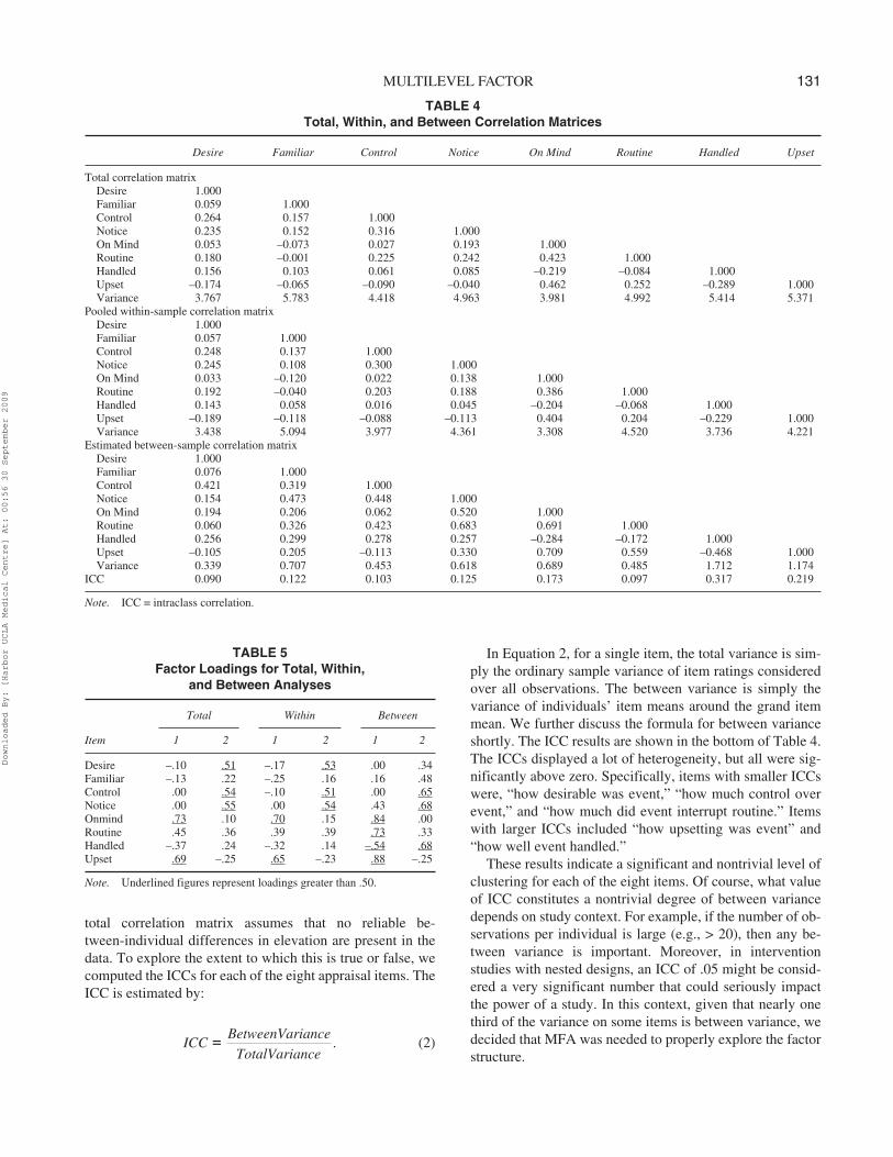
In Equation 2, for a single item, the total variance is sim-ply the ordinary sample variance of item ratings consideredover all observations. The between variance is simply thevariance of individuals’ item means around the grand itemmean. We further discuss the formula for between varianceshortly. The ICC results are shown in the bottom of Table 4.The ICCs displayed a lot of heterogeneity, but all were sig-nificantly above zero. Specifically, items with smaller ICCswere, “how desirable was event,” “how much control overevent,” and “how much did event interrupt routine.” Itemswith larger ICCs included “how upsetting was event” and“how well event handled.”

These results indicate a significant and nontrivial level ofclustering for each of the eight items. Of course, what valueof ICC constitutes a nontrivial degree of between variancedepends on study context. For example, if the number of ob-servations per individual is large (e.g., > 20), then any be-tween variance is important. Moreover, in interventionstudies with nested designs, an ICC of .05 might be consid-ered a very significant number that could seriously impactthe power of a study. In this context, given that nearly onethird of the variance on some items is between variance, wedecided that MFA was needed to properly explore the factorstructure.

MULTILEVEL FACTOR 131

TABLE 5Factor Loadings for Total, Within,

and Between Analyses

Total Within Between

Item 1 2 1 2 1 2

Desire –.10 .51 –.17 .53 .00 .34Familiar –.13 .22 –.25 .16 .16 .48Control .00 .54 –.10 .51 .00 .65Notice .00 .55 .00 .54 .43 .68Onmind .73 .10 .70 .15 .84 .00Routine .45 .36 .39 .39 .73 .33Handled –.37 .24 –.32 .14 –.54 .68Upset .69 –.25 .65 –.23 .88 –.25

Note. Underlined figures represent loadings greater than .50.

TABLE 4Total, Within, and Between Correlation Matrices

Desire Familiar Control Notice On Mind Routine Handled Upset

Total correlation matrixDesire 1.000Familiar 0.059 1.000Control 0.264 0.157 1.000Notice 0.235 0.152 0.316 1.000On Mind 0.053 –0.073 0.027 0.193 1.000Routine 0.180 –0.001 0.225 0.242 0.423 1.000Handled 0.156 0.103 0.061 0.085 –0.219 –0.084 1.000Upset –0.174 –0.065 –0.090 –0.040 0.462 0.252 –0.289 1.000Variance 3.767 5.783 4.418 4.963 3.981 4.992 5.414 5.371

Pooled within-sample correlation matrixDesire 1.000Familiar 0.057 1.000Control 0.248 0.137 1.000Notice 0.245 0.108 0.300 1.000On Mind 0.033 –0.120 0.022 0.138 1.000Routine 0.192 –0.040 0.203 0.188 0.386 1.000Handled 0.143 0.058 0.016 0.045 –0.204 –0.068 1.000Upset –0.189 –0.118 –0.088 –0.113 0.404 0.204 –0.229 1.000Variance 3.438 5.094 3.977 4.361 3.308 4.520 3.736 4.221

Estimated between-sample correlation matrixDesire 1.000Familiar 0.076 1.000Control 0.421 0.319 1.000Notice 0.154 0.473 0.448 1.000On Mind 0.194 0.206 0.062 0.520 1.000Routine 0.060 0.326 0.423 0.683 0.691 1.000Handled 0.256 0.299 0.278 0.257 –0.284 –0.172 1.000Upset –0.105 0.205 –0.113 0.330 0.709 0.559 –0.468 1.000Variance 0.339 0.707 0.453 0.618 0.689 0.485 1.712 1.174

ICC 0.090 0.122 0.103 0.125 0.173 0.097 0.317 0.219

Note. ICC = intraclass correlation.

.BetweenVariance

ICCTotalVariance

=

Downloaded By: [Harbor UCLA Medical Centre] At: 00:56 30 September 2009

Step 3: Factor Analysis of Within Matrix

The third step in the MFA process is to partition the total cor-relation matrix into a within and between component. Equa-tion 3 is used to compute the (pooled) within covariance ma-trix (SW). In turn, this matrix is transformed into a (pooled)within-correlation matrix (RW) by dividing each element bythe appropriate standard deviations. The within-correlationmatrix is shown in the middle of Table 4. Note that the sam-ple correlation matrix, RW, is a consistent estimator of thepopulation within-correlation matrix. Consequently, factoranalysis can proceed directly on this matrix. This will not betrue with the between matrix as described shortly.

(3)

All terms are as defined previously, and = vector of meansfor individual i.

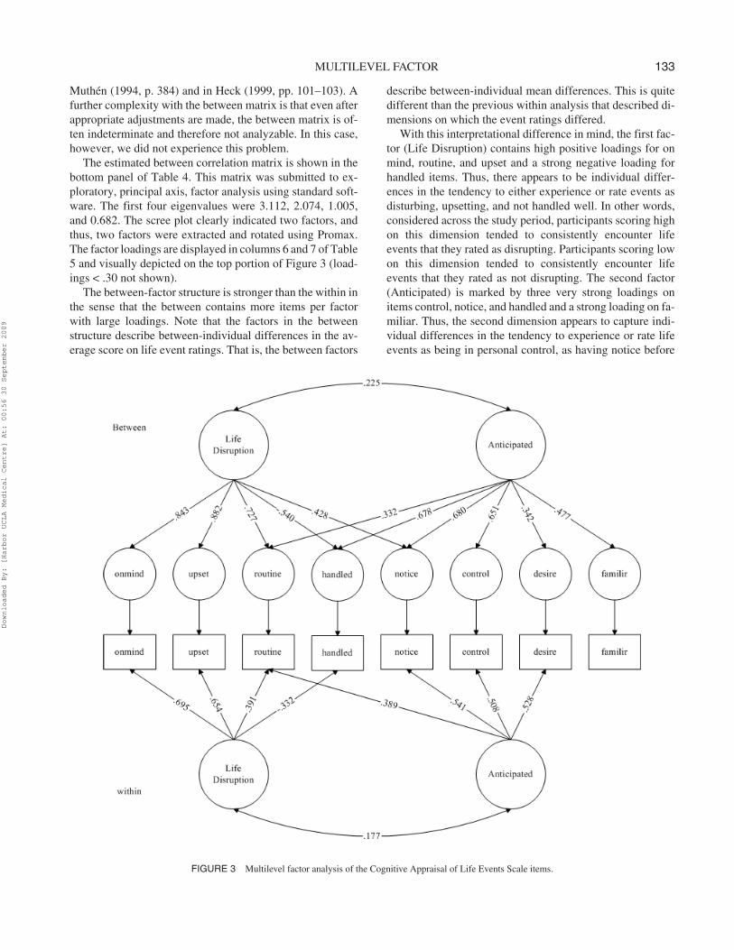
The within correlation matrix was submitted to explor-atory, principal axis, factor analysis using standard software.The first four eigenvalues were 1.835, 1.778, 0.994, and0.841. As with the analysis of the total correlation matrix, thescree plot indicated two factors, and thus, two factors wereextracted and rotated using Promax. The factor loadings aredisplayed in columns 4 and 5 of Table 5 and visually depictedon the bottom of Figure 3 (loadings < .30 not shown).

Substantively, it appears that the first dimension is a LifeDisruption factor with high loadings from only two items: onmind and upset. Events that are high on this dimension tendto be on a person’s mind for awhile, upsetting, and to a lesserdegree disturb an individual’s routine and are not handledwell. The second factor is marked by three items all with sim-

ilar loadings: notice, desire, and control. This second dimen-sion appears to capture the degree of advanced notice avail-able and the personal control that an individual has over theevent. Events that score high on this Anticipated dimensionare desirable, the individual feels a sense of control over theevent, and the individual has advance notice of the event. Thefactors are positively correlated at r = .177.

Step 4: Factor Analysis of Between Matrix

In some research contexts, the data analysis may stop at thispoint. After all, the previous analysis provided an explor-atory factor analysis of a matrix with the between confoundpartialed out. However, for the sake of illustration and be-cause it may be substantively interesting, we proceed and at-tempt to construct a between matrix and analyze the be-tween-individual variation.

The between analysis is far more complicated than thewithin analysis. This is true from both an analytic standpointand an interpretational standpoint. In this section, we reviewthe analytic complexities and address the interpretation prob-lems later in the discussion. The computation of the ordinaryweighted (by number of observations per person) be-tween-samplecovariancematrix (SB) isshowninEquation4:

(4)

However, this sample covariance matrix is not a consistentestimator of the between matrix in the population. Therefore,special adjustments need to be made to produce an accept-able between matrix for subsequent analysis. Although theadjustments are not detailed here, they are well described in

132 REISE, VENTURA, NUECHTERLEIN, KIM

FIGURE 2 Exploratory factor analysis of the Cognitive Appraisal of Life Events Scale items based on the total correlation matrix.

1 1W

( – )( – ) '

.( –1)

iI J

ij i ij i

i j

x x x x

SN

= ==∑∑

ix

1B

( – )( – ) '

.( –1)

I

i i i

i

J x x x x

SI

==∑

Downloaded By: [Harbor UCLA Medical Centre] At: 00:56 30 September 2009

Muthén (1994, p. 384) and in Heck (1999, pp. 101–103). Afurther complexity with the between matrix is that even afterappropriate adjustments are made, the between matrix is of-ten indeterminate and therefore not analyzable. In this case,however, we did not experience this problem.

The estimated between correlation matrix is shown in thebottom panel of Table 4. This matrix was submitted to ex-ploratory, principal axis, factor analysis using standard soft-ware. The first four eigenvalues were 3.112, 2.074, 1.005,and 0.682. The scree plot clearly indicated two factors, andthus, two factors were extracted and rotated using Promax.The factor loadings are displayed in columns 6 and 7 of Table5 and visually depicted on the top portion of Figure 3 (load-ings < .30 not shown).

The between-factor structure is stronger than the within inthe sense that the between contains more items per factorwith large loadings. Note that the factors in the betweenstructure describe between-individual differences in the av-erage score on life event ratings. That is, the between factors

describe between-individual mean differences. This is quitedifferent than the previous within analysis that described di-mensions on which the event ratings differed.

With this interpretational difference in mind, the first fac-tor (Life Disruption) contains high positive loadings for onmind, routine, and upset and a strong negative loading forhandled items. Thus, there appears to be individual differ-ences in the tendency to either experience or rate events asdisturbing, upsetting, and not handled well. In other words,considered across the study period, participants scoring highon this dimension tended to consistently encounter lifeevents that they rated as disrupting. Participants scoring lowon this dimension tended to consistently encounter lifeevents that they rated as not disrupting. The second factor(Anticipated) is marked by three very strong loadings onitems control, notice, and handled and a strong loading on fa-miliar. Thus, the second dimension appears to capture indi-vidual differences in the tendency to experience or rate lifeevents as being in personal control, as having notice before

MULTILEVEL FACTOR 133

FIGURE 3 Multilevel factor analysis of the Cognitive Appraisal of Life Events Scale items.

Downloaded By: [Harbor UCLA Medical Centre] At: 00:56 30 September 2009

the event occurs, and handling the event well. The factors aremodestly correlated at r = .225.

Factor Scores

Given that we have estimated the loadings for two dimen-sions from both between-correlation and within-correlationsmatrices, it is instructive and substantively interesting to ex-plore the meaning of these factors. To accomplish this, we es-timated factor scores for both the within and between dimen-sions using the regression method (Grice, 2001). We discussthe problems inherent in estimating and interpreting thesefactor scores in the Discussion section.

The within-factors and between-factor scores have differ-ent meanings in this context. Note that each individual was as-signed one between-factor score for each of the two betweendimensions.Thesebetween-factor scores represent individualdifferences in the extent to which people tend to score high (onaverage) or low (on average) on the items that load strongly oneachdimension.Thesebetween-factor scoresareanalogous tofactor scores computed in ordinary R-type analysis (i.e., no re-peated observations). These factor scores simply reflect indi-vidual differences on the dimensions considered across thestudy period. For the within factors, each life event is assigneda factor score on each within dimension. These within-factorsscores reflect within-individuals differences among the lifeevents in their tendency to be rated high or low on the variablesthat load on each dimension.

In what follows, we provide examples to help flesh out thewithin dimensions. We limit our discussion to within factorsbecause interpreting the between would involve a lengthycharacterization of persons, and their life event histories,who score high or low on each of the two between dimen-sions. The within-factors scores each had a mean of 0 withstandard deviations of .81 and .75 and skewness of .28 and.80 for Factors 1 and 2, respectively.

Within Factor 1. The type of life events that tend toscore high on within Factor 1 (Life Disruption) are problemsin school, married couple separated, family argument otherthan spouse, family member admitted to regular hospital,family member (other than child or spouse) died, suffered afinancial loss, expected check that did not come, broke upwith friend, and injury (but not hospitalized). The type of lifeevents that tend to score low on within Factor 1 are sharplyreduced work load; stopped working for an extended period;argument with spouse or girlfriend or boyfriend; stopped bypolice for traffic violation; dropped a hobby, sport, craft, orrecreational activity; and physical illness—not hospitalized.

Within Factor 2. The type of life events that tend toscore high on within Factor 2 (Anticipated) are problemswith school and training; sharply reduced work load; stoppedworking for an extended period; new person moved intohousehold; moved to a worse residence or neighborhood; got

involved in a court case; and dropped a hobby, sport, craft, orrecreational activity. Life events that score low on Factor 2are had trouble with a boss, argument with spouse (or boy-friend or girlfriend), someone stayed on in household after hewas expected to leave, assaulted, robbed, accident in whichthere were no physical injuries, accused of something forwhich a person could be sent to jail, suffered a financial loss,pet died, and physical illness but not hospitalized.

DISCUSSION

The primary goal of this study was to introduce readers to theapplication of MFA procedures (Muthén, 1991, 1994) in ex-ploring the structure of instruments collected in a repeatedmeasures context. To accomplish this, we explored the latentstructure of the CALES in a sample of recent onset schizo-phrenia outpatients. Our substantive motivation for factor an-alyzing this data set was that we wanted to identify dimen-sions of appraisal that could in turn be scored and used toestablish relations with other study variables that were col-lected at the between-individual (e.g., stationary variables)and within-individuals (e.g., time-varying covariates) levels.

Our chief finding, stemming from the analysis of thewithin matrix, is that the CALES appears to be characterizedby two dimensions. The first dimension is a Life Disruptionfactor indicated primarily by items on mind and upset. Lifeevents such as “family member died” tended to score high onthis dimension, whereas life events such as “argument withspouse” tended to score low on this dimension. The seconddimension we called Anticipated events and it appears to re-flect positive control over the event and is indicated by threeitems: notice, control, and desire. Life events such as “re-duced work load” tended to score high on this dimension,whereas life events such as “robbed” tended to score low onthis dimension.

In the between analysis, we also identified two factors.However, the between factors were characterized by higherloadings and more items loading on each factor relative to thewithin. It is important to note that the factor scores in the be-tween analysis were quite different than those in the within.For the within, each reported life event received two factorscores, whereas in the between each individual schizophre-nia patient received two factor scores. In turn, the betweenfactor scores indicated the degree to which an individual wasrelatively high or low in their average ratings of groups of re-lated appraisal scale items. People who scored high on be-tween Factor 1 tended to rate their negative life events asstaying on a person’s mind, upsetting, breaking up a person’sroutine, and as not handled well. Individuals who scored highon between Factor 2 tended to rate their negative life eventsas anticipated, that they have a sense of control over theevent, and the events are handled well. Note that without fur-ther detailed study, it is not possible to separate out whetheran individual actually had “objectively” upsetting events or

134 REISE, VENTURA, NUECHTERLEIN, KIM

Downloaded By: [Harbor UCLA Medical Centre] At: 00:56 30 September 2009

whether they had a response disposition to “subjectively”rate events as upsetting.

Substantively, the within and between factors were highlysimilar, but they were not identical. The items had somewhatdifferent loadings, with the between that tended to be higherthan the within factor. Moreover, the pattern of loadings dif-fered across the structures. For example, the item handledloaded on both dimensions in the between structure, but onlyloaded on the Disruption factor in the within structure.Whether these differences are “meaningful” or not dependson the context of the research and how the factors will beused in practice.

Ideally, if the pattern of factor loadings is equivalent acrossthe between and within levels (i.e., invariance is established),then itbecomespossible to studywithinandbetweenvariationat the level of the latent factor. This is advantageous becausethe latentvariablesareuncontaminatedbymeasurementerror.In this research because we cannot establish factor invariance,we were left with studying within and between variations andcomputing the ICC at the item level. Of course, the observeditem ratings were subject to measurement error that in turnmayhavecaused thewithinvarianceestimates tobe too low.

Problems in MFA

MFA is appropriate for any research context in which there isnesting (e.g., clients nested within clinics, children nestedwithin schools, individual’s nested within communities,etc.), not just for repeated measures data. Thus, we fully ex-pect that the approach will see increasing application in thefuture. Nevertheless, in closing, we highlight several impor-tant considerations in applying the MFA technique.

First, with this data, the results were somewhat disappoint-ing in that the MFA did not tell us anything truly different thanan analysis of the total correlation matrix. That is, we wouldhave come to basically the same substantive conclusionsabout the factor structure whether we had simply ignored thenestingandanalyzed the total correlationmatrixorusedMFA.Whether this type of finding is a typical result in social/psy-chological research can only be answered by future investiga-tions. Regardless, even if results with and without MFA do notdiffer dramatically, it is still important to separate out betweenfrom within variation prior to conducting analyses to avoidanypossiblecontaminationbetween these twosourcesofvari-ance. In general, MFA will be needed most to the degree towhich the ICC is large or, stated differently, the degree towhich between variation is influencing item scores.

Second, MFA has many obvious advantages over tradi-tional analysis as highlighted in the introduction of this re-port. However, there are many complexities to the methodthat need to be considered, especially if a researcher decidesto attempt a confirmatory MFA. For example, in this data, thenesting was caused by having repeated measurements. In theMFA, we made an assumption of independent normally dis-tributed errors at the within level. With repeated measures

data, however, more complex error structures may need to beconsidered (see Goldstein, Healy, & Rasbash, 1994). More-over, in confirmatory, multilevel factor models, the problemof correlated error terms may need to be considered as well.

A third issue that needs to be considered in conductingMFA centers around the between correlation matrix. Simplystated, between variation is very difficult to study, not only interms of estimation of a between matrix but also in interpre-tation of between factors. The reason between factors are dif-ficult to interpret, especially in repeated measurements, isthat they are based on covariances/correlations among aver-ages. In our data, for example, some individual’s average ap-praisal ratings of life events were based on only a fewobservations, whereas other individual’s average appraisalratings were based on many observations. Consider a personwith only five negative events over the year. This personcould have a high between-factor score (i.e., he or she had ahigh average negative appraisal) merely because they hadseveral negatively appraised events, whereas for another per-son who had 30 negative life events, his or her appraisal pat-tern could be quite different.

Finally, a fourth critical problem that arises in MFA stud-ies is the question of how many groups (or individuals) andhow many observations per group (or time points within anindividual) are needed to conduct proper analysis. There areno established rules of thumb for addressing this question inthe MFA context. Of course, in repeated measures designs, itis always better to have as many observations per person aspossible so that the within correlations are estimated pre-cisely for each person. The number of individuals is gener-ally less important than the number of observers perindividual. Moreover, it should be noted that estimation dif-ficulties might be encountered if the number of repeatedmeasures varies widely across individuals.

SUMMARY

The collection of repeated measurement data is becoming in-creasingly common in psychiatric and personality research.This type of nested data presents interesting challenges forthe data analyst because two types of variation need to be rec-ognized—between and within. If these two types of variationare not recognized, we run the risk of drawing erroneous con-clusions. In this article, we provided an overview of the useof MFA techniques and how they are used to explore the be-tween-factor and within-factors structure of a clinical instru-ment. Although MFA and its confirmatory extensions offersinteresting future data analytic opportunities, much researchneeds to be conducted to further explore how these modelsfunction in realistic data sets.

REFERENCES

American Psychiatric Association. (1994). Diagnostic and statistical man-ual of mental disorders (4th ed.). Washington, DC: Author.

MULTILEVEL FACTOR 135

Downloaded By: [Harbor UCLA Medical Centre] At: 00:56 30 September 2009

Bentler, P. M., & Wu, E. J. C. (2002). EQS 6 for Windows user’s guide.Encino, CA: Multivariate Software.

Brown, G. W., & Birley, J. L. T. (1978). Crisis and life change and the onsetof schizophrenia. Journal of Health and Social Behavior, 9, 203–214.

Dohrenwend, B. C., Krasnoff, L., Askenasy, A. R., & Dohrenwend, B. P.(1978). Exemplification of a method for scaling life events: The PERILife Events Scale. Journal of Health and Social Behavior, 19, 205–229.

Goldstein, H., Healy, M. J. R., & Rasbash, J. (1994). Multilevel time seriesmodels with applications to repeated measures data. Statistics in Medi-cine, 13, 1643–1655.

Grice, J. W. (2001). Computing and evaluating factor scores. PsychologicalMethods, 6, 430–450.

Heck, R. H. (1999). Multilevel modeling with SEM. In S. L. Thomas & R. H.Heck (Eds.), Introduction to multilevel modeling techniques (pp. 89–127).Mahwah, NJ: Lawrence Erlbaum Associates, Inc.

Hox, J. (1993). Factor analysis of multilevel data: Gauging the Muthénmodel. In J. Oud & R. van Blokland-Bogelesang (Eds.), Advances in lon-gitudinal and multivariate analysis in the behavioral sciences (pp.141–156). Nijmegen, The Netherlands: ITS.

Koch, G. G. (1983). Intraclass correlation coefficient. Encyclopedia of Sta-tistical Sciences, 4, 212–217.

Longford, N. T., & Muthén, B. O. (1992). Factor analysis for clustered ob-servations. Psychometrika, 57, 581–597.

Muthén, B. O. (1991). Multilevel factor analysis of class and student achieve-ment components. Journal of Educational Measurement, 28, 338–354.

Muthén, B. O. (1994). Multilevel covariance structure analysis. SociologicalMethods & Research, 22, 376–398.

Muthén, B. O., & Muthén, L. (2004). MPLUS user’s guide. Los Angeles:Author.

Nezlek, J. B. (2001). Multilevel random coefficient analyses of event- andinterval-contingent data in social and personality psychology research.Personality and Social Psychology Bulletin, 27, 771–785.

Nuechterlein, K. H., Dawson, M. E., Gitlin, M., Ventura, J., Goldstein, M. J.,Snyder, K. S., et al. (1992). Developmental processes in schizophrenicdisorders: Longitudinal studies of vulnerability and stress. SchizophreniaBulletin, 18, 387–425.

Snijders, T. A. B., & Bosker, R. J. (1999). Multilevel analysis: An introduc-tion to basic and advanced multilevel modeling. London: Sage.

Spitzer, R. L., Endicott, J., & Robins, E. (1978). Research diagnostic crite-ria: Rationale and reliability. Archives of General Psychiatry, 35,773–782.

Ventura, J., Lukoff, D., Nuechterlein, K. H., Liberman, R. P., Green, M., &Shaner, A. (1993). Appendix 1: Brief Psychiatric Rating Scale (BPRS)expanded version (4.0) scales, anchor points and administration manual.International Journal of Methods in Psychiatric Research, 3, 227–243.

Ventura J., & Nuechterlein, K. H. (1994, May). Stressful life events and theearly course of schizophrenia. Paper presented at the 147th annual meet-ing of the American Psychiatric Association, Philadelphia.

Ventura, J., Nuechterlein, K. H., Hardesty, J., & Gitlin, M. J. (1992). Lifeevents and schizophrenic relapse during medication withdrawal. BritishJournal of Psychiatry, 161, 615–620.

Ventura, J., Nuechterlein, K. H., Lukoff, D., & Hardesty, J. P. (1989). A pro-spective study of stressful life events and schizophrenic relapse. Journalof Abnormal Psychology, 98, 407–411.

Wing, J. K., Cooper, J. E., & Sartorius, N. (1974). The measurement and clas-sification of psychiatric sysmptoms. London: Cambridge University Press.

Wood, P., & Brown, D. (1994). The study of intraindividual differences bymeans of dynamic factor models: Rationale, implementation, and inter-pretation. Psychological Bulletin, 116, 166–186.

Steven ReiseDepartment of PsychologyFranz HallUniversity of California, Los AngelesLos Angeles, CA 90095Email: reise@psych.ucla.edu

Received January 12, 2004Revised June 2, 2004

136 REISE, VENTURA, NUECHTERLEIN, KIM

Downloaded By: [Harbor UCLA Medical Centre] At: 00:56 30 September 2009