Multilevel Mesh Partitioning for Aspect Ratio

C. Walshaw1, M. Cross1, R. Diekmann2, and F. Schlimbach21 School of Computing and Mathematical Sciences, The University of Greenwich,London, SE18 6PF, UK. fC.Walshaw, M.Crossg@gre.ac.uk2 Department of Computer Science, University of Paderborn, Furstenallee 11,

D-33102 Paderborn, Germany. fdiek, schlimbog@uni-paderborn.deAbstract. Multilevel algorithms are a successful class of optimisation techniqueswhich address the mesh partitioning problem. They usually combine a graph con-traction algorithm together with a local optimisation method which refines the par-tition at each graph level. To date these algorithms have been used almost exclu-sively to minimise the cut-edge weight, however it has been shown that for certainclasses of solution algorithm, the convergence of the solver is strongly influencedby the subdomain aspect ratio. In this paper therefore, we modify the multilevelalgorithms in order to optimise a cost function based on aspect ratio. Several vari-ants of the algorithms are tested and shown to provide excellent results.

1 Introduction

The need for mesh partitioning arises naturally in many finite element (FE) and finitevolume (FV) applications. Meshes composed of elements such as triangles or tetrahe-dra are often better suited than regularly structured grids for representing completelygeneral geometries and resolving wide variations in behaviour via variable mesh densi-ties. Meanwhile, the modelling of complex behaviour patterns means that the problemsare often too large to fit onto serial computers, either because of memory limitations orcomputational demands, or both. Distributingthe mesh across a parallel computer so thatthe computational load is evenly balanced and the data locality maximised is known asmesh partitioning. It is well known that this problem is NP-complete, so in recent yearsmuch attention has been focused on developing suitable heuristics, and some powerfulmethods, many based on a graph corresponding to the communication requirements ofthe mesh, have been devised, e.g. [12].

A particularly popular and successful class of algorithms which address this meshpartitioning problem are known as multilevel algorithms. They usually combine a graphcontraction algorithm which creates a series of progressively smaller and coarser graphstogether with a local optimisationmethod which, starting with the coarsest graph, refinesthe partition at each graph level. These algorithms have been used almost exclusivelyto minimise the cut-edge weight, a cost which approximates the total communicationsvolume in the underlying solver. This is an important goal in any parallel application,to minimise the communications overhead, however, it has been shown, [18], that forcertain classes of solution algorithm, the convergence of the solver is actually heavilyinfluenced by the shape or aspect ratio (AR) of the subdomains. In this paper therefore,we modify the multilevel algorithms (the matching and local optimisation) in order tooptimise a cost function based on AR. We also abstract the process of modification inorder to suggest how the multilevel strategy can be modified into a generic techniquewhich can optimise arbitrary cost functions.

1.1 Domain decomposition preconditioners and aspect ratio

To motivate the need for aspect ratio we consider the requirements of a class of solu-tion techniques. A natural parallel solution strategy for the underlying problem is to usean iterative solver such as the conjugate gradient (CG) algorithm together with domaindecomposition (DD) preconditioning, e.g. [2]. DD methods take advantage of the par-tition of the mesh into subdomains by imposing artificial boundary conditions on thesubdomain boundaries and solving the original problem on these subdomains, [4]. Thesubdomain solutions are independent of each other, and thus can be determined in par-allel without any communication between processors. In a second step, an ‘interface’problem is solved on the inner boundaries which depends on the jump of the subdomainsolutions over the boundaries. This interface problem gives new conditions on the innerboundaries for the next step of subdomain solution. Adding the results of the third stepto the first gives the new conjugate search direction in the CG algorithm.

The time needed by such a preconditioned CG solver is determined by two factors,the maximum time needed by any of the subdomain solutions and the number of itera-tions of the global CG. Both are at least partially determined by the shape of the subdo-mains. Whilst an algorithm such as the multigridmethod as the solver on the subdomainsis relatively robust against shape, the number of global iterations are heavily influencedby the AR of subdomains, [17]. Essentially, the subdomains can be viewed as elementsof the interface problem, [7, 8], and just as with the normal finite element method, wherethe condition of the matrix system is determined by the AR of elements, the conditionof the preconditioning matrix is here dependent on the AR of subdomains.

1.2 Overview

Below, in Section 2, we introduce the mesh partitioningproblem and establish some ter-minology. We then discuss the mesh partitioning problem as applied to AR optimisationand describe how the graph needs to be modified to carry this out. Next, in Section 3,we describe the multilevel paradigm and present and compare three possible matchingalgorithms which take account of AR. In Section 4 we then describe a Kernighan-Lin(KL) type iterative local optimisationalgorithm and describe two possible modificationswhich aim to optimise AR. Finally in Section 5 we compare the results with a cut edgepartitioner, suggest how the multilevel strategy can be modified into a generic techniqueand present some ideas for further investigation.

The principal innovations described in this paper are:

– In x2.2 we describe how the graph can be modified to take AR into account.– In x3.2 we describe three matching algorithms based on AR.– In x4.3 we describe two ways of using the cost function to optimise for AR.– In x4.4 we describe how the bucket sort can be modified to take into account non-

integer gains.

2 The mesh partitioning problem

To define the mesh partitioning problem, let G = G(V;E) be an undirected graph ofvertices V , with edges E which represent the data dependencies in the mesh. We assumethat both vertices and edges can be weighted (with positive integer values) and that jvjdenotes the weight of a vertex v and similarly for edges and sets of vertices and edges.Given that the mesh needs to be distributed to P processors, define a partition � to be a

mapping of V into P disjoint subdomains Sp such thatSP Sp = V . To evenly balance

the load, the optimal subdomain weight is given by S := djV j=P e (where the ceilingfunction dxe returns the smallest integer � x) and the imbalance is then defined as themaximum subdomain weight divided by the optimal (since the computational speed ofthe underlying application is determined by the most heavily weighted processor).

The definition of the mesh-partitioning problem is to find a partition which evenlybalances the load or vertex weight in each subdomain whilst minimising some cost func-tion � . Typically this cost function is simply the total weight of cut edges, but in thispaper we describe a cost function based on AR. A more precise definition of the mesh-partitioning problem is therefore to find � such that Sp � S and such that � is min-imised.

2.1 The aspect ratio and cost function

We seek to modify the methods by optimising the partition on the basis of AR rather thancut-edge weight. In order to do this it is necessary to define a cost function which we seekto minimise and a logical choice would be maxp AR(Sp), where AR(Sp) is the AR ofthe subdomain Sp. However maximum functions are notoriously difficult to optimise(indeed it is for this reason that most mesh partitioning algorithms attempt to minimisethe total cut-edge weight rather than the maximum between any two subdomains) andso instead we choose to minimise the average AR�AR =Xp AR(Sp)P : (1)

There are several definitions of AR, however, and for example, for a given poly-gon S, a typical definition, [15], is the ratio of the largest circle which can be containedentirely within S (inscribed circle) to the smallest circle which entirely contains S (cir-cumcircle). However these circles are not easy to calculate for arbitrary polygons andin an optimisation code where ARs may need to be calculated very frequently, we donot believe this to be a practical metric. It may also fail to express certain irregularitiesof shape. A careful discussion of the relative merits of different ways of measuring ARmay be found in [16] and for the purposes of this paper we follow the ideas therein anddefine the AR of a given shape by measuring the ratio of its perimeter length (surfacearea in 3d) over that of some ideal shape with identical area (volume in 3d).

Suppose then that in 2d the ideal shape is chosen to be a square. Given a polygon Swith area S and perimeter length @S, the ideal perimeter length (the perimeter lengthof a square with area S) is 4pS and so the AR is defined as @S=4pS. Alterna-tively, if the ideal shape is chosen to be a circle then the same argument gives the AR of@S=2p�S. In fact, given the definition of the cost function (1) it can be seen that thesetwo definitions will produce the same optimisationproblem (and hence the same results)with the cost just modified by a constant C (where C = 1=4 for the square and 1=2p�for circle). These definitions of AR are easily extendible to 3d and given a polyhedronS with volume S and surface area @S, the AR can be calculated as C@S=(S)2=3,where C = 1=4 if the cube is chosen as the optimal shape and C = 1=(4�)1=332=3 forthe sphere. Note that henceforth, in order to talk in general terms for both 2d & 3d, givenan object S we shall use the terms @S or surface for the surface area (3d) or perimeterlength (2d) of the object and S or volume for the volume (3d) or area (2d).

Of the above definitions of AR we choose to use the square/cube based formulae fortwo reasons; firstly because we are attempting to partition a mesh into interlocking sub-domains (and circles/spheres are not known for their interlockingqualities) and secondlybecause it gives a convenient formula for the cost function of:�template = 1CXp @Sp(Sp) d�1d (2)

where C = 2dP and d (= 2 or 3) is the dimension of the mesh. We refer to this costfunction as �template or �t because of the way it tries to match shapes to chosen templates.

In fact, it will turn out (see for example x3.2) that even this function may be toocomplex for certain optimisation needs and we can define a simpler one by assumingthat all subdomains have approximately the same volume, Sp � M=P , where Mis the total volume of the mesh. This assumption may not necessarily be true, but it islikely to be true locally (see x4.5). We can then approximate (2) by�template � 1C0Xp @Sp (3)

where C 0 = 2dP 1d (M ) d�1d . This can be simplified still further by noting that thesurface of each subdomain Sp consists of two components, the exterior surface, @eSp,where the surface of the subdomain coincides with the surface of the mesh @M , and theinterior surface, @iSp, where Sp is adjacent to other subdomains and the surface cutsthrough the mesh. Thus we can break the

Pp @Sp term in (3) into two partsPp @iSp

andPp @eSp and simplify (3) further by noting that

Pp @eSp is just @M , the exteriorsurface of the mesh M . This then gives us a second cost function to optimise:�surface = 1K1 Xp @iSp +K2 (4)

where K1 = 2dP 1d (M ) d�1d and K2 = @M=K1. We refer to this cost function as�surface or �s because it is just concerned with optimising surfaces.

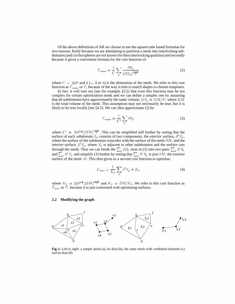
2.2 Modifying the graph

f

e

d

ca

b f

e

d

ca

b

E1 E2

E3v1 v2

v3

v4 v5V2

V3

V1

e1e2

e3

e5e4

Fig. 1. Left to right: a simple mesh (a), its dual (b), the same mesh with combined elements (c)and its dual (d)

To use these cost functions in a graph-partitioningcontext, we must add some additionalqualities to the graph. Figure 1 shows a very simple mesh (1a) and its dual graph (1b).Each element of the mesh corresponds to a vertex in the graph. The vertices of the graphcan be weighted as is usual (to carry out load-balancing) but in addition, vertices storethe volume and total surface of their corresponding element (e.g.v1 = e1 and @v1 =@e1). We also weight the edges of the graph with the size of the surface they correspondto. Thus, in Figure 1, if D(b; c) refers to the distance between points b and c, then theweight of edge (v1; v2) is set to D(b; c). In this way, for vertices vi corresponding toelements which have no exterior surface, the sum of their edge weights is equivalentto their surface (@vi = PE j(vi; vj)j). Thus for vertex v2, @v2 = @e2 = D(b; c) +D(c; e) +D(e; b) = j(v2; v1)j+ j(v2; v3)j+ j(v2; v5)j.

When it comes to combining elements together, either into subdomains, or for themultilevel matching (x3) these properties, volume and surface can be easily combined.Thus in Figure 1c where E1 = e1+ e4, E2 = e3+ e5 and E3 = e3 we see that volumescan be directly summed, for example V1 = E1 = e1+e4 = v1+v4, as canedge weights, e.g. j(V1; V2)j = D(b; c) +D(c; d) = j(v1; v2)j+ j(v4; v5)j. The surfaceof a combined object S is the sum of the surfaces of its constituent parts less twice theinterior surface, e.g. @V1 = @E1 = @e1+@e4�2�D(a; c) = @v1+@v1�2j(v1; v4)j.These properties are very similar to properties in conventional graph algorithms, wherethe volume combines in the same way as weight and surfaces combine as the sum of edgeweights (although including an additional term which expresses the exterior surface @e).The edge weights function identically.

Note that with these modifications to the graph, it can be seen that if we optimiseusing the �s cost function (4), the AR mesh partitioning problem is identical to the cut-edge weight mesh partitioning problem with a special edge weighting. However, the in-clusion of non integer edge weights does have an effect on the some of the techniquesthat can be used (e.g. see x4.4).

2.3 Testing the algorithms

Table 1. Test meshesmesh no. vertices no. edges type aspect ratio mesh grading

uk 4824 6837 2d triangles 3.39 7.98e+02t60k 60005 89440 2d triangles 1.60 2.00e+00dime20 224843 336024 2d triangles 1.87 3.70e+03cs4 22499 43858 3d tetrahedra 1.07 9.64e+01mesh100 103081 200976 3d tetrahedra 1.63 2.45e+02cyl3 232362 457853 3d tetrahedra 1.28 8.42e+00

Throughout this paper we compare the effectiveness of different approaches using aset of test meshes. The algorithms have been implemented within the framework of JOS-TLE, a mesh partitioning software tool developed at the University of Greenwich andfreely available for academic and research purposes under a licensing agreement (avail-able from http://www.gre.ac.uk/˜c.walshaw/jostle). The experimentswere carried out on a DEC Alpha with a 466 MHz CPU and 1 Gbyte of memory. Dueto space considerations we only include 6 test meshes but they have been chosen to bea representative sample of medium to large scale real-life problems and include both 2dand 3d examples. Table 1 gives a list of the meshes and their sizes in terms of the numberof vertices and edges. The table also shows the aspect ratio of each entire mesh and themesh grading, which here we define as the maximum surface of any element over theminimum surface, and these two figures give a guide as to how difficult the optimisation

may be. For example, ‘uk’ is simply a triangulation of the British mainland and hencehas a very intricate boundary and therefore a high aspect ratio. Meanwhile, ‘dime20’which has a moderate aspect ratio, has been very heavily refined in parts and thus hasa high mesh grading – the largest element has a surface around 3,700 times larger thanthat of the smallest.Table 2. Final results using template cost matching and surface gain/template cost optimisationP = 16 P = 32 P = 64 P = 128mesh �t jEcj ts �t jEcj ts �t jEcj ts �t jEcj tsuk 1.48 206 0.12 1.31 331 0.12 1.23 543 0.22 1.25 917 0.50t60k 1.16 1003 1.63 1.10 1547 2.07 1.11 2437 2.33 1.11 3647 2.65dime20 1.22 1623 5.78 1.20 2868 5.17 1.15 4406 5.70 1.12 6620 7.57cs4 1.22 2727 0.85 1.22 3738 0.90 1.23 5066 1.12 1.23 6747 1.60mesh100 1.25 5950 3.20 1.24 8752 3.53 1.26 12467 4.13 1.28 17346 5.13cyl3 1.21 11141 10.05 1.21 15944 10.77 1.23 22378 13.02 1.22 29719 13.18

Table 2 shows the results of the final combination of algorithms – TCM (see x3.2)and SGTC (see x4.3) – which were chosen as a benchmark for the other combinations.For the 4 different values of P (the number of subdomains), the table shows the averageaspect ratio as given by �t, the edge cut jEcj (that is the number of cut edges, not theweight of cut edges weighted by surface size) and the time in seconds, ts, to partitionthe mesh. Notice that with the exception of the ‘uk’ mesh, all partitions have averageaspect ratios of less than 1.30 which is well within the target range suggested in [6].Indeed for the ‘uk’ mesh it is no surprise that the results are not optimal because thesubdomains inherit some of the poor AR from the original mesh (which has an AR of3.39) and it is only when the mesh is split into small enough pieces, P = 64 or 128, thatthe optimisation succeeds in ameliorating this effect. Intuitively this also gives a hint asto why DD methods are a very successful technique as a solver.

3 The multilevel paradigm

In recent years it has been recognised that an effective way of both speeding up partitionrefinement and, perhaps more importantly giving it a global perspective is to use multi-level techniques. The idea is to match pairs of vertices to form clusters, use the clusters todefine a new graph and recursively iterate this procedure until the graph size falls belowsome threshold. The coarsest graph is then partitioned and the partition is successivelyoptimised on all the graphs starting with the coarsest and ending with the original. Thissequence of contraction followed by repeated expansion/optimisation loops is known asthe multilevel paradigm and has been successfully developed as a strategy for overcom-ing the localised nature of the KL (and other) optimisation algorithms. The multilevelidea was first proposed by Barnard & Simon, [1], as a method of speeding up spectralbisection and improved by Hendrickson & Leland, [11], who generalised it to encom-pass local refinement algorithms. Several algorithms for carrying out the matching havebeen devised by Karypis & Kumar, [13], while Walshaw & Cross describe a method forutilising imbalance in the coarsest graphs to enhance the final partition quality, [19].

3.1 Implementation

Graph contraction. To create a coarser graph Gl+1(Vl+1; El+1) from Gl(Vl; El) weuse a variant of the edge contraction algorithm proposed by Hendrickson & Leland,

[11]. The idea is to find a maximal independent subset of graph edges, or a matchingof vertices, and then collapse them. The set is independent because no two edges inthe set are incident on the same vertex (so no two edges in the set are adjacent), andmaximal because no more edges can be added to the set without breaking the indepen-dence criterion. Having found such a set, each selected edge is collapsed and the vertices,u1; u2 2 Vl say, at either end of it are merged to form a new vertex v 2 Vl+1 with weightjvj = ju1j+ ju2j.

The initial partition. Having constructed the series of graphs until the number ofvertices in the coarsest graph is smaller than some threshold, the normal practice of themultilevel strategy is to carry out an initial partition. Here, following the idea of Gupta,[10], we contract until the number of vertices in the coarsest graph is the same as thenumber of subdomains, P , and then simply assign vertex i to subdomain Si. UnlikeGupta, however, we do not carry out repeated expansion/contractioncycles of the coars-est graphs to find a well balanced initial partition but instead, since our optimisation al-gorithm incorporates balancing, we commence on the expansion/optimisationsequenceimmediately.

Partition expansion. Having optimised the partition on a graph Gl, the partitionmust be interpolated onto its parent Gl�1. The interpolation itself is a trivial matter; ifa vertex v 2 Vl is in subdomain Sp then the matched pair of vertices that it represents,v1; v2 2 Vl�1, will be in Sp.

3.2 Incorporating aspect ratio

The matching part of the multilevel strategy can be easily modified in several ways totake into account AR and in each case the vertices are visited (at most once) using arandomly ordered linked list. Each vertex is then matched with an unmatched neighbourusing the chosen matching algorithm and it and its match removed from the list. Verticeswith no unmatched neighbours remain unmatched and are also removed. In addition toRandom Matching (RM), [12], where vertices are matched with random neighbours,we propose and have tested 3 matching algorithms:

Surface Matching (SM). As we have seen in x2.2, the AR partitioning problem canbe approximated by the cut-edge weight problem using (4), the �s cost function, andso the simplest matching is to use the Heavy Edge approach of Karypis & Kumar, [13],where the vertex matches across the heaviest edge to any of its unmatched neighbours.This is the same as matching across the largest surface (since here edge weights representsurfaces) and we refer to this as surface matching.

Template Cost Matching (TCM). A second approach follows the ideas of Bouh-mala, [3], and matches with the neighbour which minimises the cost function. In thiscase, the chosen vertex matches with the unmatched neighbour which gives the result-ing element the best aspect ratio. Using the �t cost function, we refer to this as templatecost matching.

Surface Cost Matching (SCM). This is the same idea as TCM only using the �scost function, (4), which is faster to calculate.

3.3 Results for different matching functions

In Tables 3, 4 & 5 we compare the results in Table 2, where TCM was used, with RM, SM& SCM respectively. In all cases the SGTC optimisation algorithm (see x4.3) was used.For each value of P , the first column shows the average AR, �t of the partitioning. Thesecond column for each value of P then compares results with those in Table 2 using the

metric � (RM)�1� (TCM)�1 for RM, etc. Thus a figure > 1 means that RM has produced worse

results than TCM. These comparisons are then averaged and so it can be seen, e.g. forP = 16 that RM produces results 24% (1.24) worse on average than TCM. Indeed theaverage quality of partitions produced by RM was 30% worse than TCM. This is notaltogether surprising since the AR of elements in the coarsest graph could be very poorif the matching takes no account of it, and hence the optimisationhas to work with badlyshaped elements.

Table 3. Random matching results compared with template cost matchingP = 16 P = 32 P = 64 P = 128mesh �t � (RM)�1� (TCM)�1 �t � (RM)�1� (TCM)�1 �t � (RM)�1� (TCM)�1 �t � (RM)�1� (TCM)�1uk 1.50 1.04 1.38 1.25 1.25 1.06 1.23 0.91t60k 1.20 1.28 1.16 1.59 1.17 1.53 1.17 1.54dime20 1.30 1.37 1.31 1.57 1.27 1.79 1.23 1.89cs4 1.29 1.31 1.27 1.21 1.30 1.30 1.26 1.15mesh100 1.31 1.24 1.29 1.24 1.31 1.19 1.32 1.15cyl3 1.25 1.19 1.25 1.19 1.26 1.15 1.27 1.22Average 1.24 1.34 1.34 1.31

When it comes to comparing TCM with SM & SCM (Tables 4 & 5) there is actuallyvery little difference; SM is about 3.5% worse and SCM only about 1.5%. This suggeststhat the multilevel strategy is relatively robust to the matching algorithm provided theAR is taken into account in some way.

Table 4. Surface matching results compared with template cost matchingP = 16 P = 32 P = 64 P = 128mesh �t � (SM)�1� (TCM)�1 �t � (SM)�1� (TCM)�1 �t � (SM)�1� (TCM)�1 �t � (SM)�1� (TCM)�1uk 1.54 1.13 1.34 1.11 1.24 1.01 1.28 1.10t60k 1.14 0.87 1.11 1.05 1.12 1.10 1.12 1.08dime20 1.26 1.18 1.24 1.23 1.15 1.00 1.13 1.04cs4 1.22 0.97 1.24 1.08 1.24 1.04 1.23 1.00mesh100 1.20 0.78 1.24 1.03 1.27 1.04 1.26 0.94cyl3 1.19 0.93 1.21 1.02 1.24 1.05 1.24 1.08Average 0.98 1.08 1.04 1.04

Table 5. Surface cost matching results compared with template cost matchingP = 16 P = 32 P = 64 P = 128mesh �t � (SCM)�1� (TCM)�1 �t � (SCM)�1� (TCM)�1 �t � (SCM)�1� (TCM)�1 �t � (SCM)�1� (TCM)�1uk 1.47 0.99 1.31 1.00 1.27 1.14 1.25 0.98t60k 1.11 0.69 1.10 0.99 1.14 1.23 1.13 1.14dime20 1.23 1.06 1.18 0.91 1.14 0.93 1.13 1.02cs4 1.23 1.04 1.23 1.04 1.24 1.03 1.23 1.00mesh100 1.23 0.91 1.25 1.07 1.25 0.99 1.27 0.97cyl3 1.22 1.06 1.23 1.10 1.23 1.02 1.24 1.06Average 0.96 1.02 1.05 1.03

We are not primarily concerned with partitioning times here, but for the record, RMwas about 0.5% slower than TCM (although this is well within the limits of noise). Thisis because the optimisation stage took considerably longer (although the matching was

much faster than TCM). SM & SCM were 3.3% & 1.8% faster respectively than TCM.Overall this suggests that TCM is the algorithm of choice although there is little benefitover SM & SCM.

4 The Kernighan-Lin optimisation algorithm

In this section we discuss the key features of an optimisation algorithm, fully describedin [19] and then in x4.3 describe how it can be modified to optimise for AR. It is aKernighan-Lin (KL) type algorithm incorporating a hill-climbing mechanism to enableit to escape from local minima. The algorithm uses bucket sorting (x4.4), the linear timecomplexity improvement of Fiduccia & Mattheyses, [9], and is a partition optimisationformulation; in other words it optimises a partition of P subdomains rather than a bisec-tion.

4.1 The gain function

A key concept in the method is the idea of gain. The gain g(v; q) of a vertex v in sub-domain Sp can be calculated for every other subdomain, Sq, q 6= p, and expresses howmuch the cost of a given partition would be improved were v to migrate to Sq . Thus,if � denotes the current partition and �0 the partition if v migrates to Sq then for a costfunction� , the gain g(v; q) = � (�0)�� (�). Assuming the migration of v only affectsthe cost of Sp and Sq (as is true for �t and �s) then we getg(v; q) = AR(Sq + v) � AR(Sq) + AR(Sp � v) � AR(Sp): (5)

For �t this gives an expression which cannot be further simplified, however, for �s,since

AR(Sq + v) � AR(Sq) = 1K1 �@i(Sq + v) � @iSq= 1K1 �@iSq + @iv � 2j(Sq; v)j � @iSq= 1K1 �@iv � 2j(Sq; v)j(where j(Sq ; v)j denotes the sum of edge weights between Sq and v), we getgsurface(v; q) = 2K1 fj(Sp; v)j � j(Sq; v)jg (6)

Notice in particular that gsurface is the same as the cut-edge weight gain function and that itis entirely localised, i.e. the gain of a vertex only depends on the length of its boundarieswith a subdomain and not on any intrinsic qualities of the subdomain which could bechanged by non-local migration.

4.2 The iterative optimisation algorithm

The serial optimisation algorithm, as is typical for KL type algorithms, has inner andouter iterative loops with the outer loop terminating when no migration takes place dur-ing an inner loop. The optimisation uses two bucket sorting structures or bucket trees

(see below, x4.4) and is initialised by calculating the gain for all border vertices and in-serting them into one of the bucket trees. These vertices will subsequently be referred toas candidate vertices and the tree containing them as the candidate tree.

The inner loop proceeds by examining candidate vertices, highest gain first (by al-ways picking vertices from the highest ranked bucket), testing whether the vertex is ac-ceptable for migration and then transferring it to the other bucket tree (the tree of exam-ined vertices). This inner loop terminates when the candidate tree is empty although itmay terminate early if the partition cost (i.e. the number of cut edges) rises too far abovethe cost of the best partition found so far. Once the inner loop has terminated any verticesremaining in the candidate tree are transferred to the examined tree and finally pointersto the two trees are swapped ready for the next pass through the inner loop.

The algorithm also uses a KL type hill-climbing strategy; in other words vertex mi-gration from subdomain to subdomain can be accepted even if it degrades the parti-tion quality and later, based on the subsequent evolution of the partition, either rejectedor confirmed. During each pass through the inner loop, a record of the optimal parti-tion achieved by migration within that loop is maintained together with a list of verticeswhich have migrated since that value was attained. If subsequent migration finds a ‘bet-ter’ partition then the migration is confirmed and the list is reset. Once the inner loopis terminated, any vertices remaining in the list (vertices whose migration has not beenconfirmed) are migrated back to the subdomains they came from when the optimal costwas attained.

The algorithm, together with conditions for vertex migration acceptance and confir-mation is fully described in [19].

4.3 Incorporating aspect ratio: localisation

One of the advantages of using cut-edge weight as a cost function is its localised nature.When a graph vertex migrates from one subdomain to another, only the gains of adja-cent vertices are affected. In contrast, when using the graph to optimise AR, if a vertex vmigrates from Sp to Sq, the volume and surface of both subdomains will change. This inturn means that, when using the template cost function (2), the gain of all border verticesboth within and abutting subdomains Sp and Sq will change. Strictly speaking, all thesegains should be adjusted with the huge disadvantage that this may involve thousands offloating point operations and hence be prohibitively expensive. As an alternative, there-fore, we propose two localised variants:

Surface Gain/Surface Cost (SGSC). The simplest way to localise the updating ofthe gains is to make the assumption in x2.1 that the subdomains all have approximatelyequal volume and to use the surface cost function�s from (4). As mentioned in x2.2 theproblem immediately reduces to the cut-edge weight problem, albeit with non-integeredge weights, and from (6) only the gains of the vertices adjacent to the migrating vertexwill need updating. However, if this assumption is not true, it is not clear how well �swill optimise the AR and below we provide some experimental results.

Surface Gain/Template Cost (SGTC). The second method we propose for localis-ing the updates of gain relies on the observation that the gain is simply used as a methodof rating the elements so that the algorithm always visits those with highest gain first(using the bucket sort). It is not clear how crucial this rating is to the success of the al-gorithm and indeed Karypis & Kumar demonstrated that (at least when optimising forcut-edge weight) almost as good results can be achieved by simply visiting the verticesin random order, [14]. We therefore propose approximating the gain with the surface costfunction�s from (4) to rate the elements and store them in the bucket tree structure, but

using the template cost function �t from (2) to assess the change in cost when actuallymigrating an element. This localises the gain function.

4.4 Incorporating aspect ratio: bucket sorting with non-integer gains

The bucket sort is an essential tool for the efficient and rapid sorting and adjustment ofvertices by their gain. The concept was first suggested by Fiduccia & Mattheyses in [9]and the idea is that all vertices of a given gain g are placed together in a ‘bucket’ whichis ranked g. Finding a vertex with maximum gain then simply consists of finding the(non-empty) bucket with the highest rank and picking a vertex from it. If the vertex issubsequently migrated from one subdomain to another then the gains of any affectedvertices have to be adjusted and the list of vertices which are candidates for migrationresorted by gain. Using a bucket sort for this operation simply requires recalculating thegains and transferring the affected vertices to the appropriate buckets. If a bucket sortwere not used and, say, the vertices were simply stored in a list in gain order, then theentire list would require resorting (or at least merge-sort ing with the sorted list of ad-justed vertices), an essentially O(N ) operation for every migration.

The implementation of the bucket sort is fully described in [19]. It includes a rankingfor prioritising vertices for migration which incorporates their weight as well as theirgain. The non-empty buckets are stored in a binary-tree to save excessive memory use(since we do not know a priori how many buckets will be needed) and this structure isreferred to above as a bucket tree.

The only difficulty in adapting this procedure to AR optimisation is that with non-integer edge weight, the gains are also real non-integer numbers. This is not a majorproblem in itself as we can just give buckets an interval of gains rather than a single in-teger, i.e. the bucket ranked 1 could contain any vertex with gain in the interval [1:0; 2:0).However, if using the surface gain function, the issue of scaling then arises since for amesh entirely contained within the unit square/cube, all the vertices are likely to end upin one of two buckets (dependent only on whether they have positive or negative gains).Fortunately, if using �s as a gain function, as in SGSC and SGTC, we can easily calcu-late the maximum possible gain. This would occur if the vertex with the largest surface,v 2 Sp say, were entirely surrounded by neighbours in Sq . The maximum possible gainis then 2maxv2V @v (strictly speaking 2maxv2V @iv) and similarly the minimum gainis�2maxv2V @v. This means we can easily choose the number of buckets and scale thegain accordingly. A problem still arises for meshes with a high grading because manyof the elements will have an insignificant surface area compared to the maximum. How-ever the experiments carried out here all used a scaling which allowed a maximum of100 buckets and we have tested the algorithm with up to 10,000 buckets without signif-icant penalty in terms either memory or run-time.

4.5 Results for different optimisation functions

Table 6 compares SGSC against the SGTC results in Table 2. Both set of results usetemplate cost matching (TCM). The table is in the same form as those in x3.3 and showsthat there is on average only a tiny difference between the two (SGTC is 0.5% better thanSGSC) and again, with the exception of the ‘uk’ mesh for P = 16 & 32, all results havean average AR of less than 1.30. This implication of this table is that the assumptionmade in x2.1, that all subdomains have approximately the same volume, is reasonablygood. However this assumption is not necessarily true, because for example, for P =128, the ‘dime20’ mesh, with its high grading, has a ratio of maxSp=minSp =

2723. A possible explanation is that although the assumption is false globally, it is truelocally, since the mesh density does not change too gradually (as should be the case withmost meshes generated by adaptive refinement) and so the volume of each subdomainis approximately equal to that of its neighbours.

Table 6. Surface gain/surface cost optimisation compared with surface gain/template costP = 16 P = 32 P = 64 P = 128mesh �t � (SGSC)�1� (SGTC)�1 �t � (SGSC)�1� (SGTC)�1 �t � (SGSC)�1� (SGTC)�1 �t � (SGSC)�1� (SGTC)�1uk 1.49 1.02 1.32 1.05 1.24 1.02 1.23 0.92t60k 1.15 0.95 1.10 0.96 1.12 1.07 1.12 1.11dime20 1.23 1.03 1.17 0.86 1.15 0.98 1.11 0.91cs4 1.20 0.90 1.23 1.05 1.24 1.03 1.22 0.97mesh100 1.24 0.95 1.26 1.10 1.27 1.06 1.27 0.97cyl3 1.23 1.10 1.22 1.08 1.24 1.06 1.22 1.00Average 0.99 1.01 1.04 0.98

Again we are not not primarily concerned with partitioning times, but it was surpris-ing to see that SGSC was an average 30% slower than SGTC. A possible explanation isthat although the cost function�s is a good approximation,�t is a more global functionand so the optimisation converges more quickly.

5 Discussion

5.1 Comparison with cut-edge weight partitioning

In Table 7 we compare AR as produced by the edge cut partitioner (EC) described in[19] with the results in Table 2. On average AR partitioning produces results which are16% better than those of the edge cut partitioner (as could be expected). However, forthe mesh ‘cs4’ EC partitioning is consistently better and this is a subject for further in-vestigation.

Table 7. AR results for the edge cut partitioner compared with the AR partitionerP = 16 P = 32 P = 64 P = 128mesh �t � (EC)�1� (AR)�1 �t � (EC)�1� (AR)�1 �t � (EC)�1� (AR)�1 �t � (EC)�1� (AR)�1uk 1.52 1.09 1.33 1.07 1.26 1.09 1.28 1.14t60k 1.19 1.18 1.18 1.76 1.17 1.47 1.17 1.55dime20 1.32 1.45 1.26 1.34 1.25 1.65 1.21 1.72cs4 1.19 0.86 1.21 0.93 1.20 0.87 1.21 0.92mesh100 1.22 0.89 1.22 0.91 1.26 1.03 1.24 0.86cyl3 1.22 1.05 1.23 1.09 1.23 1.00 1.23 1.02Average 1.09 1.18 1.19 1.20

Meanwhile in Table 8 we compare the edge cut produced by the EC partitioner withthat of the AR partitioner. Again as expected, EC partitioning produces the best results(about 11% better than AR). In terms of time, the EC partitioner is about 26% faster thanAR on average. Again this is no surprise since the AR partitioninginvolves floating pointoperations (assessing cost and combining elements) while EC partitioningonly requiresinteger operations.

Table 8. jEcj results for the edge cut partitioner compared with the AR partitionerP = 16 P = 32 P = 64 P = 128mesh jEcj jEc j(RM)jEc j(AR) jEcj jEc j(RM)jEc j(AR) jEcj jEc j(RM)jEc j(AR) jEcj jEc j(RM)jEc j(AR)uk 189 0.92 290 0.88 478 0.88 845 0.92t60k 974 0.97 1588 1.03 2440 1.00 3646 1.00dime20 1326 0.82 2294 0.80 3637 0.83 5497 0.83cs4 2343 0.86 3351 0.90 4534 0.89 6101 0.90mesh100 4577 0.77 7109 0.81 10740 0.86 14313 0.83cyl3 10458 0.94 14986 0.94 20765 0.93 27869 0.94Average 0.88 0.89 0.90 0.90

5.2 Generic multilevel mesh partitioning

In this paper we have adapted a mesh partitioning technique originallydesigned to solvethe edge cut partitioning problem to a different cost function. The question then arises,is the multilevel strategy an appropriate technique for solving partitioning problems (orindeed other optimisation problems) with different cost functions? Clearly this is an im-possible question to answer in general but a few pertinent remarks can be made:

– For the AR based cost functions at least, the method seems relatively sensitive towhether the cost is included in the matching. This suggests that, if possible, a genericmultilevel partitioner should use the cost function to minimise the cost of the match-ings. Note, however, that this may not be possible as a cost function which, say, mea-sured the cost of a mapping onto a particular processor topology would be unableto function since at the matching stage no partition, and hence no mapping exists.

– The optimisation relies, for efficiency at least, on having a local gain function inorder that the migration of a vertex does not involve an O(N ) update. Here we wereable to localise the cost function by making a simple approximation to give a localgain function, however, it is not clear that this is always possible.

– The bucket sort is reasonably simple to convert to non-integer gains, however thisrelies on being able to estimate the maximum gain. If this is not possible it may notbe easy to generate a good scaling which separates vertices of different gains intodifferent buckets.

5.3 Conclusion and future research

We have shown that the multilevel strategy can be modified to optimise for aspect ra-tio. To fully validate the method, however, we need to demonstrate that the measure ofaspect ratio used here does indeed provide the benefits for DD preconditioners that thetheoretical results suggest. It is also desirable to measure the correlation between aspectratio and convergence in the solver.

Also, although parallel implementations of the multilevel strategy do exist, e.g. [20],it is not clear how well AR optimisation, with its more global cost function, will work inparallel and this is another direction for future research. Some related work already ex-ists in the context of a parallel dynamic adaptive mesh environment, [5, 6, 16], but theseare not multilevel methods and it was necessary to use a combination of several com-plex cost functions in order to achieve reasonable results so the question arises whethermultilevel techniques can help to overcome this.

References

1. S. T. Barnard and H. D. Simon. A Fast Multilevel Implementation of Recursive SpectralBisection for Partitioning Unstructured Problems. Concurrency: Practice & Experience,6(2):101–117, 1994.

2. S. Blazy, W. Borchers, and U. Dralle. Parallelization methods for a characteristic’s pressurecorrection scheme. In E. H. Hirschel, editor, Flow Simulation with High Performance Com-puters II, Notes on Numerical Fluid Mechanics, 1995.

3. N. Bouhmala. Partitioning of UnstructuredMeshes for Parallel Processing. PhD thesis, Inst.d’Informatique, Univ. Neuchatel, 1998.

4. J. H. Bramble, J. E. Pasciac, and A. H. Schatz. The Construction of Preconditioners for El-liptic Problems by Substructuring I+II. Math. Comp., 47+49, 1986+87.

5. R. Diekmann, B. Meyer, and B. Monien. Parallel Decomposition of Unstructured FEM-Meshes. Concurrency: Practice & Experience, 10(1):53–72, 1998.

6. R. Diekmann, F. Schlimbach, and C. Walshaw. Quality Balancing for Parallel Adaptive FEM.To appear in Proc. Irregular ’98.

7. C. Farhat, N. Maman, and G. Brown. Mesh Partitioning for Implicit Computations via Do-main Decomposition. Int. J. Num. Meth. Engng., 38:989–1000, 1995.

8. C. Farhat, J. Mandel, and F. X. Roux. Optimal convergence properties of the FETI domaindecomposition method. Comp. Meth. Appl. Mech. Engrg., 115:367–388, 1994.

9. C. M. Fiduccia and R. M. Mattheyses. A Linear Time Heuristic for Improving Network Par-titions. In Proc. 19th IEEE Design Automation Conf., pages 175–181, IEEE, Piscataway, NJ,1982.

10. A. Gupta. Fast and effective algorithms for graph partitioning and sparse matrix reordering.IBM Journal of Research and Development, 41(1/2):171–183, 1996.

11. B. Hendrickson and R. Leland. A Multilevel Algorithm for Partitioning Graphs. Tech. Rep.SAND 93-1301, Sandia National Labs, Albuquerque, NM, 1993.

12. B. Hendrickson and R. Leland. A Multilevel Algorithm for Partitioning Graphs. In Proc.Supercomputing ’95, 1995.

13. G. Karypis and V. Kumar. A Fast and High Quality Multilevel Scheme for Partitioning Ir-regular Graphs. TR 95-035, Dept. Comp. Sci., Univ. Minnesota, Minneapolis, MN 55455,1995.

14. G. Karypis and V. Kumar. Multilevel k-way partitioning scheme for irregular graphs. TR95-064, Dept. Comp. Sci., Univ. Minnesota, Minneapolis, MN 55455, 1995.

15. S. A. Mitchell and S. A. Vasavis. Quality Mesh Generation in Three Dimensions. In Proc.ACM Conf. Comp Geometry, pages 212–221, 1992.

16. F. Schlimbach. Load Balancing Heuristics Optimising Subdomain Shapes for Adaptive FiniteElement Simulations. Diploma Thesis, Dept. Math. Comp. Sci., Univ. Paderborn, 1998.

17. D. Vanderstraeten,C. Farhat, P. S. Chen, R. Keunings, and O. Zone. A Retrofit Based Method-ology for the Fast Generation and Optimization of Large-Scale Mesh Partitions: Beyond theMinimum Interface Size Criterion. Comp. Meth. Appl. Mech. Engrg., 133:25–45, 1996.

18. D. Vanderstraeten, R. Keunings, and C. Farhat. Beyond Conventional Mesh Partitioning Al-gorithms and the Minimum Edge Cut Criterion: Impact on Realistic Applications. In D. Bai-ley et al, editor, Parallel Processing for Scientific Computing, pages 611–614. SIAM, 1995.

19. C. Walshaw and M. Cross. Mesh Partitioning: a Multilevel Balancing and Refinement Algo-rithm. Tech. Rep. 98/IM/35, Univ. Greenwich, London SE18 6PF, UK, March 1998.

20. C. Walshaw, M. Cross, and M. Everett. Parallel Dynamic Graph Partitioning for AdaptiveUnstructured Meshes. J. Par. Dist. Comput., 47(2):102–108, 1997.