INTERNATIONAL JOURNAL FOR NUMERICAL METHODS IN ENGINEERINGInt. J. Numer. Meth. Engng 2000; 49:1327–1350

E�cient unstructured quadrilateral mesh generation

Josep Sarrate and Antonio Huerta∗;†

Department de Matem�atica Aplicada III; E.T.S. de Ingenieros de Caminos; Canales y Puertos;Universitat Polit�ecnica de Catalunya; Campus Nord; E-08034 Barcelona; Spain

SUMMARY

This work is devoted to the description of an algorithm for automatic quadrilateral mesh generation. Thetechnique is based on a recursive decomposition of the domain into quadrilateral elements. This automaticallygenerates meshes composed entirely by quadrilaterals over complex geometries (there is no need for a previousstep where triangles are generated). A background mesh with the desired element sizes allows to obtainthe preferred sizes anywhere in the domain. The �nal mesh can be viewed as the optimal one given theobjective function is de�ned. The recursive algorithm induces an e�cient data structure which optimizes thecomputer cost. Several examples are presented to show the e�ciency of this algorithm. Copyright ? 2000John Wiley & Sons, Ltd.

KEY WORDS: mesh generation; mesh reasoning; unstructured; quadrilateral; �nite elements

1. INTRODUCTION

In the past decades, computational methods aiming an accurate approximation to the solution ofpartial di�erential equations have received considerable attention. In particular, the �nite elementmethod has steadily increased its range of applicability and its computational e�ciency. However,it is hampered by the need to generate a discretization adapted to a general geometry and to thedesired distribution of element sizes. In fact, the preparation of accurate data is usually, in realapplications, the largest portion of the overall cost of the analysis. Consequently, a large numberof automatic mesh generation techniques have been devised to overcome these problems. Most ofthese e�orts, and also most of the important achievements, concern unstructured triangular meshgenerators [1–4], while the inherent di�culties associated to unstructured quadrilateral mesh gener-ators have precluded, until very recently, general e�cient methodologies [5–12]. Nevertheless, theuse of mixed formulations in incompressible uid and solid mechanics where quadrilateral elementsare preferred by several authors, have increased the general interest in unstructured quadrilateraldiscretizations.

∗Correspondence to: Antonio Huerta; Departament de Matem�atica Aplicada III; E.T.S. de Ingenieros de Caminos; Canales yPuertosa, Universitat Polit�ecnica de Catalunya; Campus Nord; E-08034 Barcelona; Spain

†E-mail: antonio.huerta@upc.es

Contract/grant sponsor: Ministerio de Educaci�on y Cultura; contract/grant number: TAP98-0421

Received 2 August 1999Copyright ? 2000 John Wiley & Sons, Ltd. Revised 18 February 2000

1328 J. SARRATE AND A. HUERTA

E�cient automated meshing techniques are expected to have certain features in order to ensureits applicability in a wide scope of cases, which can range from regular domains with uniformelement sizes to non-singly connected domains with large boundary curvatures and non-uniformelement sizes. Haber et al. [13] present an excellent discussion of such features: precise modellingof the boundaries; good correlation between the interior mesh and the information prescribedat the boundary; minimal input e�ort; broad range of applicability; general topology; automatictopology generation; and favorable element shapes. Some of these features can be easily imple-mented; for instance, B�ezier or B-splines interpolation curves allow a precise modelling of theboundaries. Others, such as minimal input e�ort and broad range of applicability are much moredi�cult to obtain. Therefore, all the developed techniques for mesh generation should include mostof the previous features and this is the goal of the proposed algorithm.However, from a practical point of view, the basic task of a mesher is to generate the nodal

co-ordinates and the element connectivity. Ho-Le [14] classi�es the mesh generation techniquesaccording to the sequence used by the algorithm: topology �rst and then nodal co-ordinates, nodalco-ordinates previous to the element connectivity or both at the same time.The unstructured quadrilateral mesh generator presented here is one of the latter. It is based

in the original algorithm proposed by Sluiter and Hansen [5] and further developed by Talbertand Parkinson [7]. It automatically generates meshes composed by quadrilaterals over complexgeometries. The algorithm proposed here di�ers from Reference [7] in several crucial points. Nowthe user-de�ned element size can be speci�ed anywhere in the domain. This point is crucialin adaptive techniques based on error estimation [15; 16], where the mesh size distribution isdecided by the estimated error everywhere in the domain. Moreover, the technique proposed hereis organized, for computational e�ciently, in three phases. The �rst one, determination of the bestsplitting line is based in an improved optimality function. The second one node placement is theone associated with the desired element size. The �nal step, which is usual in mesh generators, ischarged of mesh quality enhancement.Previous to the domain discretization, the boundary nodes are de�ned using any interpolation

technique. Then, the mesh generation process starts: the initial domain is partitioned by a splittingline that connects two boundary nodes. The splitting line is chosen minimizing an objective func-tion. Second, the nodes are positioned along the splitting line with the desired spacing. Two newsubdomains are now considered and the splitting process is repeated recursively up to the desiredelement size. Finally, a continuous reasoning method is developed to obtain a non-distorted mesh.The outline of the remainder of the paper is as follows. In Section 2 a brief classi�cation of

the mesh generation algorithms is presented. Then, basic concepts on background meshes andboundary processing information are reviewed. In Section 3 the two basic phases of the new meshgenerator algorithm are developed: determination of the best splitting line and node placement.In Section 4 the mesh quality enhancement procedures are presented. Section 5 is devoted to theanalysis of the computational cost of the developed algorithm. Finally, in Section 6, we presentand discuss several examples.

2. BASIC CONSIDERATIONS/INPUT DATA

2.1. Classi�cation of mesh generation methods

Several authors [11; 17] have presented classi�cations of mesh generation methods. Apart from themanual or semi-automatic generation techniques which are left for simple cases or academic studies,

Copyright ? 2000 John Wiley & Sons, Ltd. Int. J. Numer. Meth. Engng 2000; 49:1327–1350

EFFICIENT UNSTRUCTURED QUADRILATERAL MESH GENERATION 1329

three main categories are devised. First, the methods based on adaptation of mesh templates arede�ned. The simplest of such techniques is the Grid-based approach which consists of superpositionof a grid template over the domain, the cells that fall outside the domain are discarded and thosewhich intersect the contour of the object are readapted to �t into the domain of analysis [2; 18].This induces a regular discretization in the interior of the domain but an extremely poor onealong the boundaries, and it is not always possible to keep the o�set elements as quadrilaterals[2]. Instead of a regular template a grid based on a quadtree construction (in 2D and octree in3D) can be used, it is the Quadtree–octree method [17]. These meshes which are usually of goodquality far away from the boundaries are generally very poor in their vicinity.Second, the generalized mappings methods are based, for general objects, in a previous subdi-

vision of the general domain into simpler regions; then, adequate mappings are used to discretiseeach subdomain. The Transport-mapping methods, discussed in detail in Haber et al. [13], areprobably the most popular techniques of this category. In this case, the general object is �rstsubdivided in simpler domains with usually three or four sides and then the mappings referredto prede�ned templates. One of the �rst of such techniques was itself based on the �nite ele-ment interpolation functions, the isoparametric mapping method [19]. Then trans�nite mappingsor discrete trans�nite mappings were developed [13; 20] to generalize the interpolations, to bet-ter describe the boundaries (curves and surfaces are described exactly), and to prescribe speci�cconstraint curves where the mesh lines must pass. Although, these latter developments allow forsubdomains having more than four sides and even with non-simply connected regions, the initialpartition of the original object reduces the advantages of these methods. This drawback is alsopresent in the Conformal mapping methods [21] which could be viewed as a generalization ofthe original transport-mapping methods. In fact, they can deal with simply connected regions withmore than four sides. However, they su�er from the fact that element shape and mesh density aredi�cult to control.Other generalized mapping methods are the Partial di�erential equations methods [22–24]. Due

to their importance and extended use, they usually are in a category by themselves. However,they also rely on a mapping, although in this case the mapping is not de�ned explicitly but itis computed by solving a predetermined system of partial di�erential equations. The Laplacianmesh generation is probably the better known technique in this case. In fact, these techniques arewidely used in �nite di�erences because they induce structured meshes. However, one of the mainadvantages of �nite elements is the possibility of employing unstructured meshes.Finally, the geometric decomposition methods have become the most representative and used.

Delaunay triangulations, [4; 25–28] among others, are, due to their mathematical basis, robust ande�cient in two and three-dimensional simplex generation. However, they cannot be generalizedfor quadrilaterals or hexahedral elements. Moreover, stretching of elements is non-trivial. This isnot the case of Advancing Front Methods [3; 9; 10; 29–31]. These methods are among the mostwidely used. Finally, methods based on Recursive decomposition of the domain have been usedfor triangular elements [11] and quadrilaterals [7].The technique developed here is based on the later family of methods.

2.2. Background mesh

The user-de�ned element size can be speci�ed either (i) at the boundary [7], the node spacingand therefore the element size inside the domain are determined by the boundary values throughinterpolation, or (ii) at the nodes of a background mesh [3; 10], the element size is determined

Copyright ? 2000 John Wiley & Sons, Ltd. Int. J. Numer. Meth. Engng 2000; 49:1327–1350

1330 J. SARRATE AND A. HUERTA

anywhere in the domain through linear interpolation inside the corresponding triangle. Other pos-sibilities do exist, see for instance, Reference [31]. While the former is much more e�cient froma computational point of view (extensive search algorithms are avoided), the latter allows an ac-curate distribution of the desired mesh size. As usual, the requirements for the background meshare very relaxed. It must cover the domain completely to be discretized but most of them do notdescribe the geometry accurately. The quadrilateral mesh generator proposed here can work witheither approach to prescribe the user-de�ned element size.

2.3. Boundary processing/information

In order to minimize the input e�ort, the boundary of the domain is de�ned by some base pointswhich de�ne any user-preferred interpolation technique. Usually, B�ezier or B-splines is employed.Once the parametrization of the contour is de�ned, the nodes along the boundary are generatedaccording to the prescribed element density. Note that the total number of nodes must be even toensure that a quadrilateral tessellation is possible (this requirement also applies to any subdomainboundary that will be generated during the splitting process). Multiconnected domains are easilytransformed in singly connected ones by making the necessary cuts. These cuts, or return segments,consist of two superposed contour segments along which the generated nodes coincide. When themeshing process is completed, these return segments are erased and the twin nodes which mighthave appeared are disregarded. This procedure is standard, see, for instance Reference [10].

3. THE QUADRILATERAL MESH GENERATOR

3.1. Determination of the best splitting line

As previously mentioned, the mesh generator is based on a recursive decomposition of the domain,until only quadrilaterals are left. After the initial boundary is processed, it is transformed into asimple closed polygonal line. The possible splitting lines must have their endpoints over two non-consecutive nodes of this polygon. Once the optimal line has been chosen, its corresponding newnodes are generated (in the node placement phase); this leads to two new singly closed polygonallines, where the recursivity of the algorithm is exploited.The splitting line cannot be arbitrary, moreover, the optimal one should be chosen. In order to

�nd the best splitting line an objective function (cost function) is de�ned. In fact, the search forthe optimal line is a discrete minimization problem with constrains because all the lines are notacceptable.The total number of possible lines between two non-consecutive vertexes of an n-vertex polygon

is (n2−3n−2)=2; all these lines are not acceptable. First, lines joining two aligned vertexes alongone contour segment must be disregarded. Second, lines that may, entirely or in part, run outsidethe boundary in non-convex domains must also be eliminated, see Figure 1. In Reference 7 analgorithm for node visibility is proposed, but others are also possible.The de�nition of objective function is a basic point to ensure proper results. It is evaluated a

large number of times. Thus, the objective function must be simple to evaluate and include thenecessary criteria for mesh optimality. It is de�ned as a linear combination of �ve indicators thatquantify geometrical criteria, namely

Objective Function = c1�+ c2� + c3�+ c4‘ + c5� (1)

Copyright ? 2000 John Wiley & Sons, Ltd. Int. J. Numer. Meth. Engng 2000; 49:1327–1350

EFFICIENT UNSTRUCTURED QUADRILATERAL MESH GENERATION 1331

Figure 1. Line r is not acceptable because it runsoutside the domain, line s is acceptable.

Figure 2. Angles formed by a candidate splitting line.

where ci, i=1; : : : ; 5, are used as weighting values. Equation (1) is evaluated for each acceptablesplitting line. The best one, which will decompose the domain into two polygons, is the one thatminimizes (1). The geometrical criteria are presented next.1. Splitting angles. This criterion favours splitting lines that coincide with bisecting lines. Each

candidate splitting line between nodes Pi and Pj forms four angles, as it is shown in Figure 2. Thebasic goal is to choose a splitting line as close to the bisecting line as possible and to penalizesplitting lines bisecting contours with angles less than �=2. To this end, the splitting angle criterionis de�ned as

�=

1 if (�1 + �2¡�=2) and (�3 + �4¡�=2)

�(�1; �2) if (�=26�1 + �262�=3) or

(�=26�3 + �462�=3)

(�1 + �2; �3 + �4) if (�1 + �2¿2�=3) and (�2¿2�=3)

(2)

where �1, �2, �3 and �4 are the angles between the splitting line and the subdomain boundary (seeFigure 2), (�1 + �2; �3 + �4) is a function that tends to select splitting lines close to the bisectingline:

(�1 + �2; �3 + �4)=|�1 − �2|+ |�3 − �4|(�1 + �2) + (�3 + �4)

(3)

and �(�1; �2) is a function that allows a smooth transition between the extreme values. It is de�ned as

�(�1; �2)= (1− �1�2) + �1�2 (�1 + �2; �3 + �4) (4)

where

�1 =

(�1 + �2)− 2�=3

�=6if �=26�1 + �262�=3

1 otherwise

Copyright ? 2000 John Wiley & Sons, Ltd. Int. J. Numer. Meth. Engng 2000; 49:1327–1350

1332 J. SARRATE AND A. HUERTA

Table I. Local structuring index values.

Inner nodes

Common Elements �i

3 5.64 4.05 36.06 60.0Any Other 80.0

Nodes on initial boundary�i �i

06 �i¡2�=3 100.02�=36 �i6 2� 0.0

Nodes on subdomain boundary�i �i

06 �i¡2�=3 80.02�=36 �i6 2� 0.0

and

�2 =

(�3 + �4)− 2�=3

�=6if �=26�3 + �462�=3

1 otherwise

It should be noted that 06�61. Moreover, for rectangular subdomains with a prescribed constantelement size, � will be zero when both bisecting lines coincide with the splitting line.2. Structuring index. This criterion tries to construct structured meshes if possible. The algorithm

considers every created subdomain independent of its neighbours. Nevertheless, the goal of thealgorithm is to obtain elements with a distortion that is as small as possible. Therefore, it seemsreasonable to have a measure of the desirable number of elements to which every node belongs.This is called local structuring. This may be evaluated by assigning a score that measures thestructure at each endpoint of the candidate splitting line. Then, the estimator of the local structuringfor a splitting line between points Pi and Pj is found by averaging the scores at each endpoint,leading to

�=�i + �j

200(5)

For inner nodes in a quadrilateral mesh, it seems reasonable that the optimal number of commonelements should be four. Then, the mesh will be as structured as possible and the four formedangles will tend to �=2. When this number is four at one node i the mesh is called locallystructured at node i. Table I shows the assigned scores for inner nodes. Note that for locallystructured nodes a minimum score is assigned.The score assigned to a node i on the boundary depends on the angle �i de�ned by the adjacent

segments xi−1xi and xixi+1, where xi−1, xi, xi+1 are the co-ordinates of nodes i− 1, i and i+ 1,respectively. Two cases are considered: (i) initial boundary and (ii) subdomain boundary. Asshown in Table I, the main idea is to penalize a splitting line departing from (or reaching) a node

Copyright ? 2000 John Wiley & Sons, Ltd. Int. J. Numer. Meth. Engng 2000; 49:1327–1350

EFFICIENT UNSTRUCTURED QUADRILATERAL MESH GENERATION 1333

on the subdomain boundary with �i6 2�=3. It should be noted that slightly bigger penalization isassigned to nodes on the original boundary that meet this criterion, see Table I. This is becausemesh quality enhancement techniques will not be able to improve either their position nor theirconnectivity.3. Node placement error. This criterion allows to choose the best splitting line in limit cases.

On every splitting line, new nodes are generated according to an interpolation between its endnodes or values de�ned on a background mesh. However, it is not always possible to �nd aninteger number of new nodes which �ts the prescribed density, and the actual chosen positionwill introduce an error that should be quanti�ed. To this end, we �rst compute the ‘theoretical’number of element sides to be generated along the splitting line, n∗e . Then, we approximate it bya positive integer number (at least one element per splitting line), n. This integer number mustalso meet the parity requirement in order to generate two subdomains with an even number ofelement sides. Then, the node placement parameter is de�ned as

�= |n∗e − n| (6)

where 06 �6 1. Note that for practical purposes this di�erence is only signi�cant when splittinglines partitioned in few element sides are considered. Therefore, parameter (6) is only taken intoaccount when subdomains de�ned by six nodes, i.e. small subdomains, are treated and, is notconsidered for a general subdomain (its weight is set to zero in this case).4. Splitting line length. A splitting line must join two points which are as close as possible. The

reason is that information on mesh density may sit on its endpoints. A line which is too long mayhave some of its intermediate points near a zone with a very di�erent assigned density, leadingto a great inconsistency of the results. This is the case shown in Figure 3. A nondimensionalestimation ‘ of the splitting line length between two nodes Pi and Pj can be obtained by dividingits natural length by the domain characteristic length de�ned as, see Figure 4,

lchar =√(xmax − xmin)2 + (ymax − ymin)2 (7)

Hence

‘=lijlchar

(8)

and, as usual, 06‘61.5. Symmetry. When the domain presents clear symmetries, the �nal mesh should maintain these

symmetries. Unfortunately, unstructured mesh generators do not usually create symmetric grids. Anestimation of the symmetry is used in the developed algorithm. It uses the di�erence between theareas of the subdomains de�ned by every splitting line. Obviously, this is a very simple measureof the domain symmetry and it has no e�ect on non-symmetrical domains. However, it has provedto be really useful for simple cases or symmetrical domains (especially those with parallel sides).The non-dimensional estimator that has been used is

�=|a2 − a1|a2 + a1

; (9)

where a1 and a2 are the respective areas closed by each subdomain de�ned by the candidatesplitting line. In fact, parameter (9) measures the areas in both sides of a splitting line. However,a line which divides the domain into two parts with both areas as similar as possible, seems to

Copyright ? 2000 John Wiley & Sons, Ltd. Int. J. Numer. Meth. Engng 2000; 49:1327–1350

1334 J. SARRATE AND A. HUERTA

Figure 3. In uence of the splitting line length in the results. In the case on right, the centre of the domainwill not be meshed with the proper density.

Figure 4. De�nition of the characteristic length of a given domain.

be the best option, even in non-symmetrical domains. Note that some ags can be added in orderto check that domains with the same area are symmetrical. However, in order to increase thecomputational e�ciency of the algorithm they are not added.Based on numerical experiments over a wide range of problems, the best set of weighting values

are: c1 = 0:52, c2 = 0:17, c3 = 0:00, c4 = 0:17, c5 = 0:14.Note that the cost function de�nition (1) is a generalization the one developed by Talbert

and Parkinson, [7]. However, in (1) two new criteria are added (structuring index and symmetrycriteria) and the remaining criteria have a di�erent de�nition (splitting angle, node placement errorand splitting line length). For instance, in the new splitting angle criterion, the splitting line tendstoward the bisecting line instead to the normal line. An absolute error instead of a relative error isused to measure the node placement. Moreover, in each subdomain a characteristic length, insteadof the maximum length, is used to normalize (7) in the present algorithm to speed up the meshingprocess. Finally, it must be remarked that the weighting coe�cients are normalized.

3.2. Six-node closure

The recursive splitting algorithm previously introduced �nishes when a domain containing onlyfour nodes (an element) is found. However, a six-node subdomain appears in a variety of �nalcon�gurations during the partition process. The manner in which these domains are transformedinto quadrilaterals is important for the �nal mesh quality. Although Talbert and Parkinson [7]have used a template-based method to split up the six-node subdomains, in the present algorithmthe same objective function, see Equation (1), has been used. Nevertheless, two modi�cations areintroduced. First, the splitting angle criterion has been modi�ed in order to enforce �=2 angles.Obviously, in most cases this will not be possible at all. The measure of the deviation of the

Copyright ? 2000 John Wiley & Sons, Ltd. Int. J. Numer. Meth. Engng 2000; 49:1327–1350

EFFICIENT UNSTRUCTURED QUADRILATERAL MESH GENERATION 1335

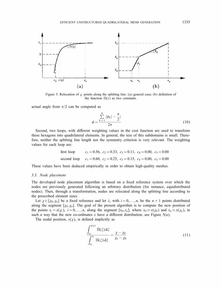
Figure 5. Relocation of �i points along the splitting line: (a) general case; (b) de�nition ofthe function �(x) as two constants.

actual angle from �=2 can be computed as

�=

4∑k = 1

|�k | − �2|

2�(10)

Second, two loops, with di�erent weighting values in the cost function are used to transformthese hexagons into quadrilateral elements. In general, the size of this subdomains is small. There-fore, neither the splitting line length nor the symmetry criterion is very relevant. The weightingvalues for each loop are:

�rst loop c1 = 0:56; c2 = 0:33; c3 = 0:11; c4 = 0:00; c5 = 0:00

second loop c1 = 0:60; c2 = 0:25; c3 = 0:15; c4 = 0:00; c5 = 0:00

These values have been deduced empirically in order to obtain high-quality meshes.

3.3. Node placement

The developed node placement algorithm is based on a �xed reference system over which thenodes are previously generated following an arbitrary distribution (for instance, equidistributednodes). Then, through a transformation, nodes are relocated along the splitting line according tothe prescribed element sizes.Let �∈ [�0; �n] be a �xed reference and let �i with i=0; : : : ; n; be the n + 1 points distributed

along the segment [�0; �n]. The goal of the present algorithm is to compute the new position ofthe points xi= x(�i); i=0; : : : ; n, along the segment [x0; xn], where x0≡ x(�0) and xn ≡ x(�n), insuch a way that the new co-ordinates x have a di�erent distribution, see Figure 5(a).The nodal position, x(�), is de�ned implicitly as∫ x(�)

x0�(�) d�∫ xn

x0�(�) d�

=� − �0�n − �0

(11)

Copyright ? 2000 John Wiley & Sons, Ltd. Int. J. Numer. Meth. Engng 2000; 49:1327–1350

1336 J. SARRATE AND A. HUERTA

where �(x) is a function de�ned over [x0; xn]. Note that if �(x)=K; K being an arbitrary constant,then

x(�)− x0xn − x0

=� − �0�n − �0

=⇒ x(�)=xn − x0�n − �0

(� − �0) + x0

and nodes will be relocated proportionally to the �xed reference distribution. On the other hand,if �(x) is de�ned as

�(x)=

{K1 if �06�6�b

K2 if �b¡�6�n

being K1¿K2, see Figure 5(b), then the distance between nodes in the interval [x0; xb] will besmaller than the distance between nodes in the interval [xb; xn]. Therefore, high values of K tendto reduce the distance between nodes along the splitting line. In fact, �(x) can be understood asthe inverse of the prescribed element side size, h(x):

�(x)=1

h(x)(12)

Thus, the theoretical number of element sides along a splitting line is

n∗e =∫ xn

x0�(�) d�=

∫ xn

x0

1h(�)

d� (13)

Finally, the position of node xk = x(�k) can be computed from Equations (11) and (12) as∫ xk

x0

d�h(�)

=kn

∫ xn

x0

d�h(�)

Therefore, the new position of any node can be computed recurrently as∫ xk+1

xk

d�h(�)

=k + 1n

∫ xn

x0

d�h(�)

− kn

∫ xn

x0

d�h(�)

=n∗en

(14)

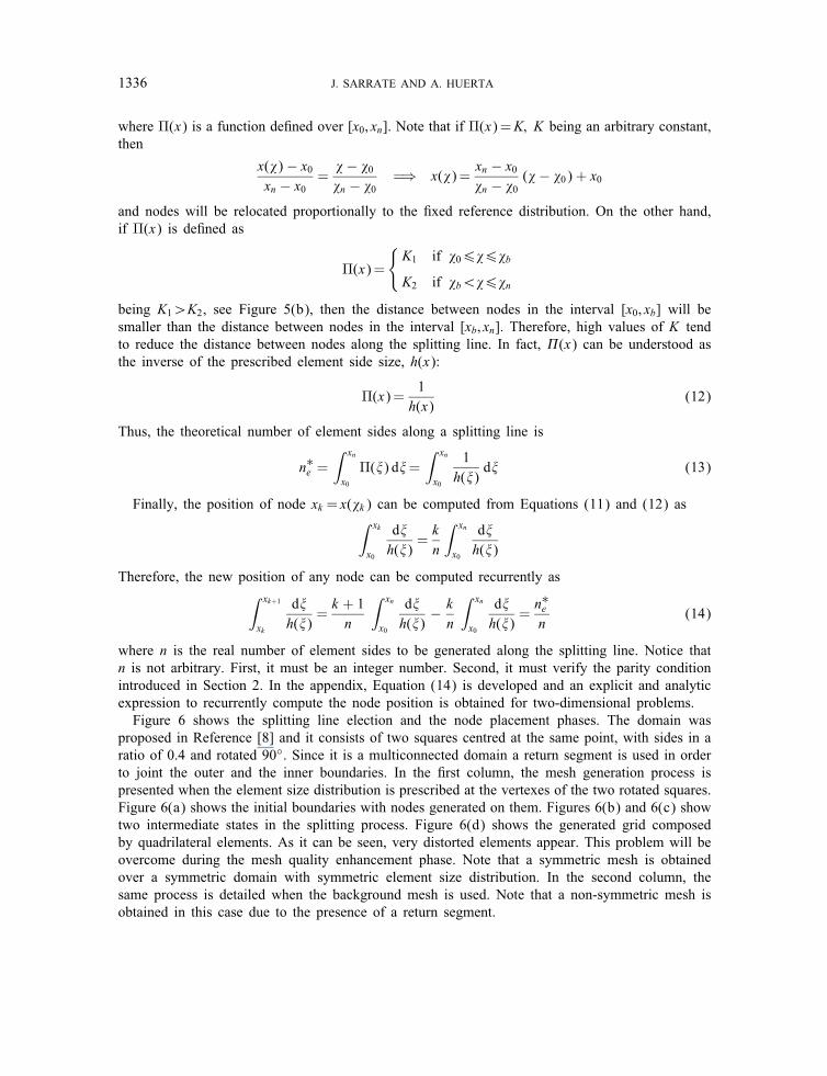
where n is the real number of element sides to be generated along the splitting line. Notice thatn is not arbitrary. First, it must be an integer number. Second, it must verify the parity conditionintroduced in Section 2. In the appendix, Equation (14) is developed and an explicit and analyticexpression to recurrently compute the node position is obtained for two-dimensional problems.Figure 6 shows the splitting line election and the node placement phases. The domain was

proposed in Reference [8] and it consists of two squares centred at the same point, with sides in aratio of 0.4 and rotated 90◦. Since it is a multiconnected domain a return segment is used in orderto joint the outer and the inner boundaries. In the �rst column, the mesh generation process ispresented when the element size distribution is prescribed at the vertexes of the two rotated squares.Figure 6(a) shows the initial boundaries with nodes generated on them. Figures 6(b) and 6(c) showtwo intermediate states in the splitting process. Figure 6(d) shows the generated grid composedby quadrilateral elements. As it can be seen, very distorted elements appear. This problem will beovercome during the mesh quality enhancement phase. Note that a symmetric mesh is obtainedover a symmetric domain with symmetric element size distribution. In the second column, thesame process is detailed when the background mesh is used. Note that a non-symmetric mesh isobtained in this case due to the presence of a return segment.

Copyright ? 2000 John Wiley & Sons, Ltd. Int. J. Numer. Meth. Engng 2000; 49:1327–1350

EFFICIENT UNSTRUCTURED QUADRILATERAL MESH GENERATION 1337

Figure 6. Several steps in the mesh generation process for the two rotated squares problem.

Copyright ? 2000 John Wiley & Sons, Ltd. Int. J. Numer. Meth. Engng 2000; 49:1327–1350

1338 J. SARRATE AND A. HUERTA

4. MESH QUALITY ENHANCEMENT

4.1. Introduction

The recursive splitting algorithm described in the previous section may generate elements thatare very distorted. Therefore, mesh quality enhancement procedure has to be developed in orderto improve the overall mesh quality. As it is usual in quadrilateral mesh generation algorithms[7–10; 12], two types of procedures are considered. The �rst one, often called make-up techniques,is focused in the improvement of the mesh topology. The second one, called mesh smoothing,improves the shape of the elements by modifying the position of the inner nodes once the topologyis �xed.

4.2. Make-up techniques

After the split process is completed, some topological properties are improved. Since one of thegoals of the present discretization algorithm is to generate meshes as structured as possible, it seemsreasonable to favour four elements per interior node (NE=4, NE being the number of elementsper node). However, for unstructured meshes some nodes with NE bigger or smaller than fourwill appear. Nevertheless, it is better to enforce NE close to four. Note that this condition alsoprecludes very distorted elements. In fact, the number of elements that meet one node has alreadybeen taken into account in the selection of the best splitting line (structuring index criterion).Therefore, only two techniques of those developed in others mesh generators have been introducedin our algorithm: node elimination and element elimination (see References [9; 10; 12] for details).It should be noted that any make-up techniques is used if a node on the boundary is concerned.

4.3. Smoothing algorithm

Since make-up techniques only modify the mesh topology, after they are applied very distorted el-ements still appear. Then, it is necessary to apply a smoothing technique to improve the mesh qual-ity. The most commonly used technique is the so-called Laplacian method [32], which computesthe new nodal position solving the Laplace equation. This technique has an important drawbackbecause it is possible that, in non-convex domains, nodes run outside it. Techniques to precludesuch a pitfall either increase the computational cost enormously or introduce new terms in theformulation that are particular for each geometry. Giuliani [33] developed a new reasoning algo-rithm based on geometrical criteria. This method modi�es the position of every node in order tominimize a geometric-oriented average distortion of elements meeting on it. These modi�cationsare done with an explicit iterative procedure. In this case, nodes cannot depart from the domainbecause this is an unstable position in terms of distortion and squeeze.

h-adaptive techniques [15; 16] �rst compute a solution on a given coarse mesh. Then, a newelement size distribution is computed from a local measure of the estimated error. Therefore, itis crucial in these processes that the mesh generator preserves the prescribed element size. In thissense, it is essential that the smoothing algorithm also maintains the size. Giuliani method givesproven results in a smooth element size distributions for both 2D and 3D problems. However, ityields unsatisfactory meshes when sharp changes of density appear. This is due to the fact thatzones with high density tend to lose it after several remeshing iterations at advanced stages of theanalysis.

Copyright ? 2000 John Wiley & Sons, Ltd. Int. J. Numer. Meth. Engng 2000; 49:1327–1350

EFFICIENT UNSTRUCTURED QUADRILATERAL MESH GENERATION 1339

Figure 7. Representation of the set of triangles (shadowed) around node Pi.

Figure 8. Final mesh for the two rotated squares example: (a) without background mesh;(b) with background mesh.

The cause of this problem may be found at its basic reasoning principle, see Reference [33] fordetails. For each node Pi in a quadrilateral grid, a local measure of the mesh distortion is de�nedin terms of a set of triangles. These triangles are obtained by joining all nodes connected to nodePi via the element sides, see Figure 7. The new position of Pi is found by minimizing the sumof their distortions. This is iteratively repeated for all the nodes in a Gauss–Seidel like procedure,until convergence is achieved. In the original method, the distortion of the triangles is de�ned inorder to obtain triangles of similar sizes. Thus, the �nal mesh will show smooth variations of theelement size, and zones where high element density is prescribed will tend to lose it. In order toovercome this problem a modi�cation of the distortion of the triangles is introduced, see Reference[34] for details. It tends to preserve the original size of the triangles, and therefore, the �nal meshwill maintain the prescribed element size. Examples presented in Reference [34] prove that thismodi�cation produces a robust algorithm that generates well-shaped elements of the prescribedsize.Figure 8(a) shows the �nal mesh of the two rotated squares problem after the mesh quality

enhancement phase has been applied, for the uniform element size distribution case. Note that asymmetric mesh is obtained and that the prescribed element size is preserved. Figure 8(b) shows

Copyright ? 2000 John Wiley & Sons, Ltd. Int. J. Numer. Meth. Engng 2000; 49:1327–1350

1340 J. SARRATE AND A. HUERTA

Figure 9. Bin-tree representation of the proposed algorithm.

the �nal mesh for a non-uniform element size distribution imposed with a background grid. Asmooth variation in the element size is obtained notwithstanding the remarkable element sizegradient. In both cases very few distorted elements are generated.

5. ALGORITHM EFFICIENCY

This section is devoted to the analysis of the computational cost of the developed meshing algo-rithm. In this analysis it is assumed that a uniform nodal density is prescribed. However, numericalexamples show that the derived estimation of the computational cost can also be used with non-uniform meshes. The computational cost is de�ned as the number of objective function evaluation,(1). It is important to note that the described algorithm is naturally suited for a bin-tree structure ofthe element data. A recursive binary structure may be constructed since every domain is split intoa ‘left’ and ‘right’ subdomains, see Figure 9. Hence, the total cost is the number of evaluationsof the objective function in every level of the bin-tree representation. Note that for each level, theobjective function has to be evaluated in several subdomains in order to �nd the best splitting linefor every subdomain, see Figure 9.To this end, we �rst compute the cost involved in obtaining the best splitting line for a subdo-

main with Ni nodes on its boundary. If it is assumed that (i) the cost of each evaluation of theobjective function is always constant, and that (ii) the cost of the visibility algorithm is at leastequal to the cost of the lines whose objective function is not evaluated. Therefore, the objectivefunction is evaluated

(Ni − 1) + (Ni − 2) + · · ·+ 1 = 12Ni(Ni − 1) (15)

times in each subdomain with Ni nodes on its boundary.Second, we evaluate an upper bound of the number of nodes in each subdomain of the ith

partition. Given a certain level, i− 1, in the partition process, let Ni−1 be the number of nodes onits boundary. We assume that the best splitting line generates two new subdomains with Ri Ni−1and Li Ni−1 nodes each (0¡ Ri ¡1 and 0¡ Li ¡1). Let N0 be the number of nodes of the initialboundary and = maxk=0; :::; i−1{ Rk ; Lk }. Then, the upper bound of the number of nodes in eachsubdomain of the ith partition can be approximated by

Ni= iN0 (16)

Copyright ? 2000 John Wiley & Sons, Ltd. Int. J. Numer. Meth. Engng 2000; 49:1327–1350

EFFICIENT UNSTRUCTURED QUADRILATERAL MESH GENERATION 1341

Third, we evaluate the number of subdomains in a given ith partition. If it is assumed that allbranches in the bin-tree representation always reach the same level (note that this is equivalent toassume that a uniform nodal density is prescribed). Then, the total number of subdomains is 2i,see Figure 9.Now, it is possible to compute the number of times the objective function is evaluated for the

ith partition (the cost in the ith partition). Moreover, it can be written in terms of the number ofnodes on the initial boundary

Ci= 12

iN0( iN0 − 1)2i ≈ 12N

20 k

i

where k =2 2.Since the total cost of the developed algorithm can be evaluated as the sum of the cost of all

partitions (levels in the bin-tree representation), the number of partitions required to generate thewhole mesh has to be deduced. Starting from an initial boundary with N0 nodes, the domain isrecursively subdivided until quadrilateral elements are left. Let p be the number of partitions neededto obtain a quadrilateral element. Taking into account Equation (16), the number of partitions canbe approximated by

pN0 = 4 (17)

From (17) an estimate of the number of partitions can be deduced,

p= a ln N0 + b (18)

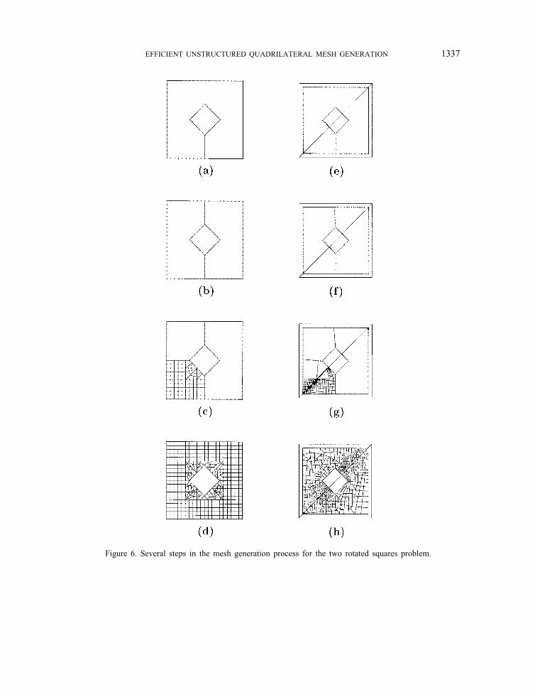
where a and b are two constants independent of N0; a= − 1= ln and b= ln 4. Note thatp=O(ln N0).Finally, the total cost of the developed algorithm can be evaluated as

TC =p∑

i=0Ci=

12N 20

(1 + k2 + k3 + · · ·+ kp)= 1

2N 20kp+1 − 1k − 1 ≈N 2

0 ka ln (N0)+b+1

where the relationship (18) has been taken into account. Therefore,

TC =O(N 20 k

a ln(N0)+b+1)=O(N 2+a ln (k)0

)(19)

In order to relate in a simple manner the computational cost with the generated mesh, comparisonwill be made with the total number of nodes of the �nal mesh, NT . For simple domains, the �nalmesh has approximately NT ≈N 2

0 nodes. This assumption is corroborated in the examples shownbelow. Thus, the total computational cost is

TC =O(N 1+a=2 ln (k)

T

)≡O(N�T ) (20)

Note that, for an initial square domain with a constant element size prescribed distribution, =3=4 because the best splitting line is always the shorter one. Therefore, k =2 2 = 9=8; a=− 1= ln = − 1= ln 3=4 and �=1:2.A numerical experiment has been carried out in order to �nd the numerical value of � in expres-

sion (20). The examples presented in Figures 6 and 8 as well as the four �rst examples presentedin the next section have been meshed several times with di�erent element size distributions foreach domain. In all cases, the minimum value of the total number of elements has been 5000.

Copyright ? 2000 John Wiley & Sons, Ltd. Int. J. Numer. Meth. Engng 2000; 49:1327–1350

1342 J. SARRATE AND A. HUERTA

Table II. Slopes of the linear regressions.

Example NT vs N0 CPU vs N0 CPU vs NT

Only examples without background mesh 1.96 2.32 1.15Only examples with background mesh 1.75 2.27 1.25All examples 1.74 2.01 1.21

Notice that these examples contain all the characteristics that a general domain could show: simple-connected and multi-connected domains, constant and variable element size distributions, as wellas the utilization of background meshes. For each case, the following linear regression have beenperformed:

ln NT = c1 ln (N0) + d1

ln TC= c2 ln (N0) + d2

ln TC= c3 ln (NT ) + d3

where the total cost has been approximated by the CPU time spent to generate the whole mesh.Table II shows the obtained values for ci, i = 1; : : : ; 3. These results corroborate the assumptionthat NT ≈ N 2

0 . Moreover, when all cases are considered, the general performance of the algorithmis in concordance with expression (20) with � = 1:2.

6. EXAMPLES

In order to assess the quality of the mesh generation algorithm described above, �ve numericalexamples are presented. They illustrate the capabilities of the new meshing algorithm in severalenvironments: (i) constant element size distribution prescribed on the boundary of the domain,(ii) variable element size distribution prescribed on the boundary of the domain, (iii) element sizedistribution prescribed on a background mesh, (iv) domain surrounded by a ragged boundary and(v) application to adaptive techniques based on error estimation.In the �rst example, the water around a dock is discretized. A constant element size distribution

is prescribed on its boundary. Figure 10(a) shows an intermediate state in the meshing process.The �nal mesh, composed by 8291 nodes and 7600 elements, is presented in Figure 10(b). It isimportant to note that with a simple input (just the co-ordinates of the vertexes of the contourand the prescribed element size) a complex domain is discretized with a structured mesh withoutany previous partition of the domain.The second example corresponds to a rail cross-section. The element size distribution is pre-

scribed at its vertexes and a high element concentration is de�ned in the load zone. Figure 11shows the �nal mesh. It is composed by 1541 nodes and 1413 elements. As it can be observed, astructured mesh is generated where the geometry and prescribed values allow it. Also, a symmetricmesh is generated at the base of the rail. Moreover, a smooth transition is obtained between low-and high-density areas.

Copyright ? 2000 John Wiley & Sons, Ltd. Int. J. Numer. Meth. Engng 2000; 49:1327–1350

EFFICIENT UNSTRUCTURED QUADRILATERAL MESH GENERATION 1343

Figure 10. Discretization of a dock: (a) intermediate state in the meshing process; (b) �nal mesh.

The third example is the discretization of a gear. In this case a background mesh is used toconcentrate elements along one direction. The �nal mesh and the background mesh are shownin Figures 12(a) and 12(b), respectively. The �nal mesh is composed of 1654 nodes and 1568elements. As it can be seen, well-shaped elements are generated in this case, even on the curvedpart of the boundary. Furthermore, smooth size transitions are also obtained and spurious elementconcentration does not appear.In the fourth example the developed algorithm is applied to the discretization of a domain de�ned

by a ragged boundary. In particular, a mesh for inner part of the port of Barcelona (Spain) isgenerated. It is composed of 29 691 nodes and 28 537 elements. Figure 13 shows the �nal mesh.The boundary corresponding to the harbor mouth is de�ned by a circular arc on the right-handside of the mesh. The breakwater corresponds to the boundary on the top of the mesh, whereasquays on the dry land corresponds to the left-hand side and bottom boundaries.

Copyright ? 2000 John Wiley & Sons, Ltd. Int. J. Numer. Meth. Engng 2000; 49:1327–1350

1344 J. SARRATE AND A. HUERTA

Figure 11. Discretization of a rail cross section.

Figure 12. Discretization of a gear: (a) generated mesh; (b) background mesh.

Copyright ? 2000 John Wiley & Sons, Ltd. Int. J. Numer. Meth. Engng 2000; 49:1327–1350

EFFICIENT UNSTRUCTURED QUADRILATERAL MESH GENERATION 1345

Figure 13. Discretization of the port of Barcelona.

Figure 14. Detail of a part of the outer dock of the port of Barcelona.

Due to some boundary details (small docks, sharp corners), di�erent values of the element sizeare prescribed. For instance, small elements are used near small docks whereas bigger elements areused near straight boundaries or in the harbor mouth. Figure 14 shows the generated mesh aroundsmall docks located between the dry land and the breakwater. As it can be seen, well-shapedelements are obtained and the �nal mesh tends towards a structured mesh when possible. A detailof the �nal mesh around two small docks near the harbor mouth is presented in Figure 15. Asit can be observed, a smooth transition between high and low element density areas is obtained.Moreover, well-shaped elements are generated even in non-convex corners.The �fth example shows how the developed algorithm can be applied to adaptive techniques.

The error estimator developed in References [35; 36], is applied to the adaptive computation of

Copyright ? 2000 John Wiley & Sons, Ltd. Int. J. Numer. Meth. Engng 2000; 49:1327–1350

1346 J. SARRATE AND A. HUERTA

Figure 15. Detail of a part of the inner dock near the mouth of the port of Barcelona.

the compression of a plane strain rectangular specimen with two imperfections (circular openingsinside the material) [37]. The mesh generator algorithm is included in the adaptive process asfollows. Given an initial quadrilateral mesh, the �nite element solution and error estimation arecomputed on it. From this error estimation, a desired element size is evaluated at the nodes.Then, the initial mesh is transformed into a triangular mesh by connecting two opposed nodes ofeach element. Finally, this new mesh together with the evaluated new element size are used asbackground mesh to generate a new one. This process is repeated until the prescribed accuracyis reached, see Reference [37]. Figure 16 shows a succession of generated meshes. It is worthnoting that, as the adaptive process evolves the elements concentrates in two bands according tothe error estimation. Note that regular and well-shaped elements are generated even in a smallregion where a high gradient of the element size is prescribed.

7. CONCLUSIONS

In this paper a new automatic and e�cient two-dimensional unstructured quadrilateral elementmesh generator is presented. The user interaction has been reduced to the speci�cation of theboundary geometry and the desired element size at some base point on the boundary or at thenodes of a background mesh. The technique is based on a recursive splitting of the domain untilonly quadrilateral elements of the desired size are left. Moreover, the algorithm is decomposed, forcomputational e�ciency, into three phases: (i) determination of the best splitting line (where newcriteria have been developed in order to de�ne the objective function), (ii) node placement (where a

Copyright ? 2000 John Wiley & Sons, Ltd. Int. J. Numer. Meth. Engng 2000; 49:1327–1350

EFFICIENT UNSTRUCTURED QUADRILATERAL MESH GENERATION 1347

Figure 16. Application of the mesh generation algorithm to adaptive computations: (a) Initial mesh (462elements); (b) Second mesh (856 elements); (c) Third mesh (2235 elements); (d) Final mesh (3307 elements).

new algorithm has been deduced), and (iii) mesh quality enhancement (where a modi�cation of thesmoothing method developed by Giuliani has been presented). The �nal mesh can be interpreted asthe mesh that optimizes the given objective function. The recursive algorithm induces an e�cientbin-tree structure which has been used to prove that the cost of the new algorithm is O(N 1:2

T ). Awide range of numerical experiments have veri�ed this result. Finally, several examples have beenpresented to show the new algorithm capabilities.

APPENDIX

Our goal here is, �rst generalize Equation (14) for the two-dimensional problem, and second,develop an explicit and analytic expression to recurrently compute the node position. To this end,consider a segment de�ned by the end points [P0; Pn] (a candidate to splitting line). Along [P0; Pn]nodes, Pk , k = 1; 2; : : : ; n− 1, must be placed with the desired distance, i.e. the requested elementsize. The distance between two consecutive nodes is given by a background mesh of triangles. Iftwo consecutive nodes Pk and Pk+1 lie inside one triangle, the following equation is veri�ed:∫ Pk+1

Pk

d�h(�)

=n∗en

(A1)

where n∗e is given by Equation (13), namely

n∗e =∫ Pn

P0�(�) d�=

∫ Pn

P0

1h(�)

d� (A2)

Copyright ? 2000 John Wiley & Sons, Ltd. Int. J. Numer. Meth. Engng 2000; 49:1327–1350

1348 J. SARRATE AND A. HUERTA

Since [Pk; Pk+1] lies inside a triangle, the element size along this segment is linear [3; 7], thatis,

�(�)=1

h(�)=

1a�+ b

(A3)

where a and b are two constants. These constants are computed from the values of the elementsize hi and hj at the intersection of the line de�ned by Pk and Pk+1 and the background triangle.Let us denote by Pi and Pj the points where the line PkPk+1 intersects its corresponding triangle,and by �i and �j the values of parameter � assigned to points Pi and Pj. Then,

a=hj − hi�j − �i

b= hi − �i

[hj − hi�j − �i

]

Note that function h(�) is always positive because it is the element size. Therefore, Equation (A3)can be used to compute the integral that appears on the left-hand side of expression (A1). On anarbitrary element side de�ned by Pk and Pk+1 that lies on a segment limited by the end points Pj

and Pj+1 the following equality applies:∫ Pk+1

Pk

d�h(�)

=d(Pj; Pj+1)

hj+1 − hjln(hk+1

hk

)

where d(·; ·) denotes the distance between two points. Replacing the previous result in Equation(A1)

hk+1 − hk = hk

{exp

[n∗en

hj+1 − hjd(Pj; Pj+1)

]− 1}

(A4)

Finally, since a linear interpolation has been used between the prescribed values at points Pj andPj+1, we get

hj+1 − hjd(Pj; Pj+1)

=hk+1 − hk

d(Pk; Pk+1)

which can be replaced in Equation (A4)

d(Pk+1; Pk)=d(Pj; Pj+1)

hj+1 − hjhk

{exp

[n∗en

hj+1 − hjd(Pj; Pj+1)

]− 1}

(A5)

Equation (A5) is the keystone in the node placement algorithm. It allows to compute the positionof the nodes along the splitting line in a recurrent manner when a background mesh is used. Notethat if background mesh is not used, expression (A5) is still valid. In this case, the prescribedvalues are de�ned at the splitting line end points. Note that Equation (A5) has been deduced

Copyright ? 2000 John Wiley & Sons, Ltd. Int. J. Numer. Meth. Engng 2000; 49:1327–1350

EFFICIENT UNSTRUCTURED QUADRILATERAL MESH GENERATION 1349

assuming that nodes Pk and Pk+1 lie in the same triangle. If they lie in di�erent triangles, segment[Pk; Pk+1] is partitioned in two parts, and the same expression applies.In Equation (A5), the theoretical number of elements side to be generated along the splitting

line, n∗e , must be evaluated. According to (A3), between two consecutive intersections of thesplitting line with the background mesh, Pi and Pj, the following equation is veri�ed:∫ Pj

Pi

d�h(�)

=1aln(a � + b)

∣∣∣∣�j

�i

=�j − �i

hj − hiln

(hjhi

)(A6)

Using the previous equation, it is possible to �nd an analytic expression for the theoretical numberof elements side to be generated along the segment de�ned by the end points [P0; Pn]:

n∗e =∫ Pn

P0

d�h(�)

=∫ P1

P0

d�h(�)

+m−1∑i=1

∫ Pi+1

Pi

d�h(�)

+∫ Pn

Pm

d�h(�)

=d(P0; P1)

h1 − h0ln

(h1h0

)+

m−1∑i=1

d(Pi; Pi+1)

hi+1 − hiln

(hi+1hi

)+

d(Pm; Pn)

hn − hmln(

hn

hm

)(A7)

where P1; : : : ; Pm denotes the intersection points between the splitting line [P0; Pn] and the back-ground mesh.

REFERENCES

1. Cavendish JC. Automatic triangulation of arbitrary planar domains for the �nite element method. International Journalfor Numerical Methods in Engineering 1974; 8:679–697.

2. Kikuchi N. Adaptive grid-design methods for �nite element analysis. Computer Methods in Applied Mechanics andEngineering 1986; 55:129–160.

3. Peraire J, Vahdati M, Morgan K, Zienkiewicz OC. Adaptive remeshing for compressible ow computations. Journalof Computational Physics 1987; 72:449–466.

4. Rebay S. E�cient unstructured mesh generation by means of delaunay triangulation and Bowyer–Watson algorithm.Journal of Computational Physics 1993; 106(1):125–138.

5. Sluiter MLC, Hansen DL. A general purpose automatic mesh generator for shell and solid �nite elements. Proceedingsof the 2nd International Computer Engineering Conference. Computers in Engineering, ASME: Computer EngineeringDivision, 1993:29–34.

6. Wordenweber B. Finite element mesh generation. Computer Aided Design 1984; 16:285–291.7. Talbert JA, Parkinson AR. Development of an automatic two-dimensional �nite element mesh generator usingquadrilateral elements and B�ezier curve boundary de�nition. International Journal for Numerical Methods inEngineering 1990; 29:1551–1567.

8. Liu YC, El Maraghy HA, Zhang KF. An expert system for forming quadrilateral �nite elements. EngineeringComputations 1990; 7:249–257.

9. Blacker TD, Stephenson MB. Paving: a new approach to automated quadrilateral mesh generation. International Journalfor Numerical Methods in Engineering 1991; 32:811–847.

10. Zhu JZ, Zienkiewicz OC, Hinton E, Wu J. A new approach to the development of automatic quadrilateral meshgeneration. International Journal for Numerical Methods in Engineering 1991; 32:849–866.

11. Rank E, Schweingruber M, Sommer M. Adaptive mesh generation and transformation of triangular to quadrilateralmeshes. Communications in Numerical Methods in Engineering 1993; 9:121–129.

12. Lee CK, Lo SH. A new scheme for the generation of a graded quadrilateral mesh. Computers and Structures 1994;52(5):847–857.

13. Haber R, Shephard MS, Abel JF, Gallagher RH, Greenberg DP. A general two-dimensional graphical �nite elementpreprocessor utilizing discrete trans�nite mappings. International Journal for Numerical Methods in Engineering 1981;17:1015–1044.

14. Ho-Le K. Finite element mesh generation methods: a review and classi�cation. Computer Aided Design 1988; 20(1):27–38.

Copyright ? 2000 John Wiley & Sons, Ltd. Int. J. Numer. Meth. Engng 2000; 49:1327–1350

1350 J. SARRATE AND A. HUERTA

15. D��ez P, Huerta A. A uni�ed approach to remeshing strategies for �nite element h–adaptivity. Computer Methods inApplied Mechanics and Engineering 1999; 176(1-4):215–229.

16. Huerta A, Rodr��guez–Ferran A, D��ez P, Sarrate J. Adaptive �nite element strategies based on error assessment.International Journal for Numerical Methods in Engineering 1999; 46:1803–1818.

17. George PL. Automatic Mesh Generation. Application to Finite Element Methods. Wiley: Paris, 1991.18. Thacker WC, Gonz�alez A, Putland GE. A method for automating the construction of irregular computational grids for

storm surge forecast models. Journal of Computational Physics 1980; 37:371–387.19. Zienkiewicz OC, Phillips DV. An automatic mesh generation scheme for plane and curved surfaces by isoparametric

co-ordinates. International Journal for Numerical Methods in Engineering 1971; 3:519–528.20. Gordon WJ, Hall CA. Construction of curvilinear co-ordinate systems and applications to mesh generation. International

Journal for Numerical Methods in Engineering 1973; 7:461–477.21. Brown PR. A non-interactive method for automatic generation of �nite element meshes using the Schwarz–Christo�el

transformation. Computer Methods in Applied Mechanics and Engineering 1981; 25:101–126.22. Thompson JF, Warsi ZUA, Mastin CW. Numerical Grid Generation. Foundations and Applications. Elsevier:

New York, 1985.23. Thompson JF. A general three-dimensional elliptic grid generation system on a composite structure. Computer Methods

in Applied Mechanics and Engineering 1987; 64:377–411.24. Knupp PM. A robust elliptic grid generator. Journal of Computational Physics 1992; 100:409–418.25. Cavendish JC, Field DA, Frey WH. An approach to automatic three-dimensional �nite element mesh generation.

International Journal for Numerical Methods in Engineering 1985; 21:329–347.26. Lewis RW, Zheng Y, Gethin DT. Three-dimensional unstructured mesh generation: Part 3. Volume meshes. Computer

Methods in Applied Mechanics and Engineering 1996; 134:285–310.27. Zheng Y, Lewis RW, Gethin DT. Three-dimensional unstructured mesh generation: Part 1. Fundamental aspects of

triangulation and point creation. Computer Methods in Applied Mechanics and Engineering 1996; 134:249–268.28. Zheng Y, Lewis RW, Gethin DT. Three-dimensional unstructured mesh generation: Part 2. Surface meshes. Computer

Methods in Applied Mechanics and Engineering 1996; 134:269–284.29. Lo SH. A new generation scheme for arbitrary planar domains. International Journal for Numerical Methods in

Engineering 1985; 21:1403–1426.30. L�ohner R, Parikh P. Three-dimensional grid generation by the advancing-front method. International Journal for

Numerical Methods in Fluids 1988; 8:1135–1149.31. Jin H, Wiberg NE. Two-dimensional mesh generation, adaptive remeshing and re�nement. International Journal for

Numerical Methods in Engineering 1990; 29:1501–1526.32. Herrmann LR. Laplacian–isoparametric grid generation scheme. Journal End. Mechanical Division. ASCE 1976;

102:749–756.33. Giuliani S. An algorithm for continuous reasoning of the hydrodynamic grid in Arbitrary Lagrangian–Eulerian codes.

Nuclear Engineering and Design 1982; 72(2):205–212.34. Sarrate J, Huerta A. An improved algorithm to smooth graded quadrilateral meshes preserving the prescribed element

size. Communications in Numerical Methods in Engineering (in press).35. D��ez P, Egozcue JJ, Huerta A. A posteriori error estimation for standard �nite element analysis. Computer Methods

in Applied Mechanics and Engineering 1998; 163(1-4):141–157.36. Huerta A, D��ez P. Error estimation including pollution assessment for non linear �nite element analysis. Computer

Methods in Applied Mechanics and Engineering 2000; 181:21–41.37. D��ez P, Arroyo M, Huerta A. Adaptivity based on error estimation for viscoplastic softening materials. Mechanics of

Cohesive and Frictional Materials 2000; 5:87–112.

Copyright ? 2000 John Wiley & Sons, Ltd. Int. J. Numer. Meth. Engng 2000; 49:1327–1350