Adaptive Mesh Refinement for Storm Surge

Kyle T. Mandlia, Clint N. Dawsona

aInstitute for Computational Engineering and Science, University of Texas at Austin, 201 E 24th ST. StopC0200, Austin, TX 78712-1229, USA

Abstract

An approach to utilizing adaptive mesh refinement algorithms for storm surge modeling isproposed. Currently numerical models exist that can resolve the details of coastal regionsbut are often too costly to be run in an ensemble forecasting framework without significantcomputing resources. The application of adaptive mesh refinement algorithms substantiallylowers the computational cost of a storm surge model run while retaining much of the desiredcoastal resolution. The approach presented is implemented in the GeoClaw frameworkand compared to ADCIRC for Hurricane Ike along with observed tide gauge data and thecomputational cost of each model run.

Keywords: storm surge, Hurricane Ike, adaptive mesh refinement, finite volume methods,shallow water equations

1. Introduction

As computer technology advances, scientists continually attempt to use numerical mod-eling to better predict a growing number of high-impact geophysical events. In particular,coastal hazards have become an increasing concern as the world’s population continues togrow and move towards the coastline, in fact 44% of the world’s population lives within150 km of the coast and 8 of the 10 largest cities in the world lie in that range [1]. As aconsequence, loss of life and property is becoming a larger concern than ever before. One ofthe most recurring and wide spread hazards to many coastal communities is the inundationof coastlines that is associated with strong storms, one part of which is known as stormsurge. A storm surge is a rise in the sea accompanying extratropical or tropical cyclones, thestrongest examples of which are hurricanes and typhoons. Storm surges can cause massiveamounts of damage, as was demonstrated by Hurricane Katrina, which caused an estimated$81 billion of damage [2]. Of the world’s largest cities, 4 lie within threat zones from tropi-cal cyclones. With the mounting evidence that severe storms may be increasingly common[3], the task of modeling these events becomes even more critical to communities along thecoasts.

Email address: kyle@ices.utexas.edu (Kyle T. Mandli)URL: http://users.ices.utexas.edu/~kyle (Kyle T. Mandli)

Preprint submitted to Elsevier January 23, 2014

arX

iv:1

401.

5744

v1 [

mat

h.N

A]

22

Jan

2014

Modeling of storm surges was first carried out by local empirical observations. Un-fortunately, for more severe storms such as Katrina, these types of prediction can grosslyunder-predict storm surge size and effect. By the 1960’s, scientists started using computersimulations to predict storm surge but, because these simulations were limited in resolutionand size, these models had the same short-comings as the empirically-based models. It wasnot until recently with increased observational evidence, improved efforts in modeling un-derlying physical processes, and increases in available computational power that substantialprogress has been made simulating large-scale storm surge for use in hazard planning.

The current state-of-the-art numerical models for storm surge simulations rely on single-layer depth-averaged equations for the ocean and make assumptions about the ocean’s re-sponse to a storm. The National Weather Service (NWS) utilizes a storm surge model called“Sea, Lake and Overland Surges from Hurricanes”, or SLOSH, which uses local grids definedfor many regions of the United States coastline, to make predictions [4]. These simulationsare efficient enough that ensembles of runs can be made quickly for multiple different hur-ricane paths and intensities. This capability can be critical for effective forecasting due tothe uncertainty in the storm forecast. The primary drawback to using the SLOSH model isthe limited domain size and extents allowed due to the grid mapping used and formulationof the equations.

Another model currently in use is the Advanced Circulation Model (ADCIRC), a finiteelement model which has been applied to southern Louisiana [5] and recently to Hurricane Ike[6]. One of the key advantages ADCIRC has it its use of an unstructured grid. Unstructuredmodels allow easy application of variable resolution, especially at the coastline where finescale features need to be resolved. They can also map to coastlines in a way even a cleverlymapped structured grid cannot. Another advantage of unstructured grids relates to theimportance of including entire ocean basins for surge predictions [7, 8]. Unstructured gridscan allow the domain of the numerical model to stretch well away from coastlines to includeocean basins while reducing the cost of the model by substantially decreasing resolution inthe basin compared to the coastal regions. Unfortunately these models, even with the aboveadvantages, can still be computationally costly and require a large amount of computingresources in order to compute ensemble forecasts without the degradation of their resolutionbenefits.

In this paper we present an alternative computational framework and methodology tobridge the gap between the numerical cost of the unstructured grid storm surge models andthe efficient but unresolved models currently in use at the NWS. The approach leveragesadaptive mesh refinement (AMR) algorithms to retain the resolution required to resolvecoastal inundation but only when necessary so that ensemble calculations are still feasible.This is accomplished by allowing nested structured grids of variable resolution to vary intime and space thereby capturing the spatial advantages of the unstructured grid approachbut only when needed, and therefore decreasing the computational cost substantially. Theframework in question, GeoClaw, has successfully been used previously for tsunami mod-eling where similar computational requirements are present [9].

2

2. Numerical Approach

The mathematical model for storm surge we will consider uses the classical shallow waterequations with the addition of appropriate source terms for bathymetry, bottom friction,wind friction, non-constant surface pressure and Coriolis forcing which can be written as

∂

∂th+

∂

∂x(hu) +

∂

∂y(hv) = 0,

∂

∂t(hu) +

∂

∂x

(hu2 +

1

2gh2

)+

∂

∂y(huv) = fhv − gh ∂

∂xb+

h

ρ

(− ∂

∂xPA + ρairCw|W |Wx − Cf |~u|u

)∂

∂t(hv) +

∂

∂x(huv) +

∂

∂y

(hv2 +

1

2gh2

)= −fhu− gh ∂

∂yb+

h

ρ

(− ∂

∂yPA + ρairCw|W |Wy − Cf |~u|v

)(1)

where h is the fluid depth, u and v the depth-averaged horizontal velocity components, g theacceleration due to gravity, ρ the density of water, ρair the density of air, b the bathymetry,f the Coriolis parameter, W = [Wx,Wy] is the wind velocity at 10 meters above the seasurface, Cw the wind friction coefficient, and Cf the bottom friction coefficient. The valueof Cw is defined by Garratt’s drag formula [10] as

Cw = min(2× 10−3, (0.75 + 0.067|W |)× 10−3) (2)

and the value of the friction coefficient Cf is determined using a hybrid Chezy-Manning’s ntype friction law

Cf =gn2

h4/3

[1−

(hbreak

h

)θf]γf/θf(3)

where n is the Manning’s n coefficient and hbreak = 2, θf = 10 and γf = 4/3 parameterscontrol the form of the friction law.

The numerical approach proposed to solve (1) falls under a general class of high resolutionfinite volume methods known as wave-propagation methods, described in detail in [11]. Thesemethods are Godunov-type finite volume methods requiring the specification of a Riemannsolver to update each grid cell in the domain. On top of these methods adaptive meshrefinement is employed to allow for variable spatial and temporal resolution as the simulationprogresses. These methods have been implemented together in GeoClaw, a package thatwas originally designed to model tsunamis [12] and other depth-averaged flows [9, 13, 14].The rest of this section is dedicated to describing the salient points of the AMR approach andhow storm surge physics are represented in GeoClaw. A brief review of wave-propagationmethods can be found in Appendix A along with a basic outline of the Riemann solveremployed in Appendix B.

2.1. Adaptive Mesh Refinement

Adaptive mesh refinement is a core capability of GeoClaw as it allows the resolutionof disparate spatial and temporal scales common to geophysical applications such as stormsurge and tsunamis. The patch-based AMR approach used in GeoClaw employs a set of

3

overlapping logically rectangular grids that correspond to one of many levels of refinement.The first of these levels, enumerated starting at ` = 1, contains grids that cover the entiredomain at the coarsest resolution. The subsequent levels ` ≥ 2 represent progressively finerresolutions by a set of prescribed ratios r` in time and space such that

∆x(`+1) = ∆x(`)/r(`)x , ∆y(`+1) = ∆y(`)/r(`)

y , and ∆t(`+1) = ∆t(`)/r(`)t .

Each subsequent level is properly nested within the union of grids in the next level coarser(see Figure 1 for an example of the structure of these nested grids). With this hierarchy ofgrids, the evolution of the solution follows as:

1. Evolve the level 1 (coarsest) grids one time step to tn+1.

2. Fill the ghost cells of all level 2 grids by temporal and spatial interpolation.

3. Evolve the level 2 grids the number of time steps determined by ∆t(2) needed to reachtn+1.

4. Recursively continue to fill in ghost cells, evolving each level ` after the coarser level`− 1 has been evolved until all levels are at time tn+1.

5. Fill in regions where the grids overlap with the best available data using interpolation.

6. Adjust coarse cell values adjacent to finer cells to preserve conservation of mass (see[15] for a discussion on this topic).

The key benefit of adaptive mesh refinement is the ability to change resolution as thesimulation progresses. This is done in a process that involves using a local criteria to flag eachcell that requires refinement to the next level. The algorithm then clusters the flagged cellsinto new rectangular patches which attempts to minimize the number of grids created andthe number of grid cells unnecessarily refined [16]. After the new grid structure is created,the previous solution values are copied into the new grid cells if no change in resolution wasrequired or an interpolation and averaging is performed to either coarsen or refine the dataavailable from a different level of refinement.

For the shallow water equations there are three primary areas where care must betaken when implementing adaptive mesh refinement. The first involves the interpolationof the solution and bathymetry. When interpolating where the water column is at rest butbathymetry is varying, using the depth h as the interpolation field will lead to a sea surface ηthat is not at rest and will result in the creation of spurious waves. To avoid this, interpola-tion is done with the sea surface instead. From this the depth is computed and the resultingmomentum interpolated. This process can be perfomed in wet cells while conserving massand momentum. This is not the case in the near shore where cells may change from their wet(or dry) state. In order to avoid spurious waves being created mass cannot be conserved andis either lost or gained. This is a result of different grid resolutions of bathymetry being usedthrough the computation. For these cases it is often desirable to refine coast lines before awave arrives such that the loss or gain in mass does not effect the wave itself and overallleads to a negligible increase in mass overall in the simulation. In the end, the followingproperties are true for the interpolation approach used.

• Mass is conserved except possibly near coast lines.

4

Level 3

Level 2Level 1

x

y

(a)

Level 3

Level 2

Level 1x

y

(b)

Figure 1: Views of a sample patch-based AMR grid. Figure 1a shows a planar view withthree levels of refinement. In this instance, there are 3 level 3 grids, 2 level 2 grids, and 1level 1 grid. Figure 1b shows an isometric view of the same grid layout with the z-directionrepresenting different levels.

• Momentum is conserved if mass is conserved or gained and lost if mass is lost.

• New extrema in the sea surface and velocity are not created.

More discussion and the derivation of the rules for coarsening and refinement can be foundin [12].

The second area of concern is the form and types of refinement criteria that should beused. In GeoClaw, a number of different solution based criteria are used to determinerefinement. The first criteria is triggered if the absolute difference between the initial sea-level ηsea-level and the calculated sea-surface η in cell i,j is greater than some tolerance Twave,i.e.

Twave < |ηi,j − ηsea-level|

will mark the ith, jth cell as needing refinement. Additionally water currents can be used asa refinement criteria. This criteria uses a set of speed tolerances specified at each level, onlymarking a cell as needing refinement if the tolerance Tspeed for the corresponding level is lessthan the current speed in that cell. For example, if tolerances for level 1, 2, and 3 were setto 2, 2.5, and 3 m/s respectively, a cell with a speed of 2.6 m/s currently at level 1 thenwould be marked as needing refinement. Conversely, if the cell is already at level 2 thenno refinement is necessary. In addition to these physics based criteria, a user can specify

5

regions with minimum or maximum refinement constraints. There are also constraints basedon initial depth of the water allowing restriction of refinement to only shallower depths. Inan instance where a conflict between the physics based criteria and the region constraintsoccurs the region constraints take precedence.

The last concern of note involves the relative spatial and temporal refinement ratios.Isotropic refinement ratios, when the spatial and temporal refinement ratios are identical,are generally needed in AMR to satisfy the CFL condition. In the case of the shallow waterequations and inundation modeling the desired spatial refinement is usually highest at thecoastline where the wave speeds are lowest. This allows for the use of anisotropic refinementbetween the spatial and temporal directions to take advantage of the slower wave speedslocated near shore. Along with anisotropic refinement, GeoClaw allows for the automaticdetermination of the optimal temporal refinement ratios since the wave speed estimate forthe shallow water equations is inexpensive to evaluate.

2.1.1. Storm Based AMR Criteria

Additional criteria related to the location and strength of the storm can also be importantto resolving storm surge. The first available criteria is based on the distance of a cell fromthe eye of the storm. As was the case with the speed criteria, these tolerances are specifiedby level such that a cell will be flagged as needing refinement if it is within the specifiedradius of the storm’s eye, i.e.

T `r < reye

for level `. The second criteria flags based on storm intensity, wind speed tolerances are usedin a similar way. Often the wind speed tolerances and eye distance tolerances give similarbut slightly different regions of refinement depending, for instance, on the strength of thestorm.

2.2. Source Term Evaluation

Since the storm’s impact on the ocean depends only on the momentum source terms forthe wind-stress and pressure gradients, it is important that all the momentum source termsare handled carefully. Apart from the storm’s impact, the rest of the momentum sourceterms are bathymetric, friction and Coriolis source terms. The bathymetric source terms arehandled in the Riemann solver so that well-balancedness can be maintained along with otheruseful properties (see Appendix B and [17] for these details). For the remaining source terms,GeoClaw uses an operator-splitting approach to evaluate the remaining source terms. Thisinvolves solving two simpler problems, qt + A(q)qz + B(q)qy = S1(q) and qt = S2(q), andcombining updates of the vector q in a consistent manner. The method employed usesGodunov splitting which involves solving each simpler system alternately for the full timestep ∆t. Although this approach is formally only first-order accurate, observed errors dueto the splitting do not dominate the overall error in practice (see [11] for a more thoroughdiscussion of these issues).

Starting with the friction and Coriolis, the bottom friction terms can be evaluated as

(hu)t = Cfhu and (hv)t = Cfhv

6

and are solved using a backwards Euler method for computing the loss of momentum so that

(hu)n+1ij =

(hu)nij1 + (Cf )ij∆t

and (hv)n+1ij =

(hv)nij1 + (Cf )ij∆t

where the drag coefficient is computed using the previous time step’s state as

(Cf )ij =gn2

ij

(hnij)−7/3

√[(hu)nij]

2 + [(hv)nij]2

[1−

(hbreak

hnij

)θf]γf/θf.

The values hbreak, θf , and γf are constant parameters that define the hybridization betweenthe Chezy and Manning’s n formulation from (3). The Coriolis terms

(hu)t = −fhv and (hv)t = fhu

are evaluated using a matrix exponential up to the 4th term in the series such that theupdate becomes[

huhv

]n+1

ij

=

[huhv

]nij

·[1− 1

2(f∆t)2 + 1

24(f∆t)4 f∆t− 1

6(f∆t)3

−f∆t+ 16(f∆t)3 1− 1

2(f∆t)2 + 1

24(f∆t)4

]where f = 2Ω sin y with Ω = 2π/8.61642× 104 and y the longitudinal coordinate in radians.

2.2.1. Storm Representation and Source Term Evaluation

One of the significant additions to GeoClaw needed to model storm surge is the rep-resentation of the storm fields and their source terms. In the forecasting setting that weare targeting, pressure and wind fields of a storm are often evaluated based on the empir-ically derived Holland model which provides profiles of the wind speed and pressure in ahurricane based on storm characteristics [18]. These profiles are then rotated to produce atwo-dimensional, rotationally symmetric field. The wind speed profile W (r, t) takes the form

W (r, t) =

√(rw

r

)BW 2

maxe(1−(rw/r)B) +

(rf)2

4− rf

2(4)

where r is the radial coordinate centered at the eye of the storm and the parameters rw

and Wmax are given by the storm forecast and represent the radius of maximum winds,and the maximum wind speed, respectively. The Holland B parameter, an empirical fittingparameter from [18], takes the form

B =ρair(W

′max)2e

Pn − Pcwhere Pn and Pc are the background and central storm atmospheric pressures. The valueW ′

max is a correction form of Wmax that accounts for storm translation and movement inspherical coordinates. The pressure profile is similarly

PA = Pc + (Pn − Pc)e−(rw/r)B . (5)

7

The Holland wind field velocities from (4) are converted to a cyclonic wind field via

~W =

[−W sin θW cos θ

]where θ is the azimuthal angle with respect to the storm’s eye. Furthermore, the stormtranslation speed is added to take into account the relative motion of the storm and atmo-sphere. The last modification to the fields is a ramping function, R(r), applied at a radialdistance from the storm to smoothly decrease the wind velocity to zero and the pressure tothe background pressure via

R(r) =1

2

(1− tanh

(r −Rp

Rw

))where r is the radial distance from the eye of the storm, Rw the width of the rampingfunction, and Rp the storm parameter recording the radius of the last closed iso-bar. R(r, t)is then applied to the wind and pressure fields as

W (r) = W (r) · R(r) and P (r) = Pn + (P (r)− Pn) · R(r).

A storm’s intensity, speed, and location is allowed to vary in time via forecasted and best-track data at the times specified. GeoClaw then reconstructs the wind and pressure fieldsusing linear interpolation between time points so that the storm forecast evolves continuouslyrather than only at the time points available. In addition to the intensity of the storm, thevelocity and location are linearly interpolated taking into account that the storm is travelingon the surface of a sphere. Once the simulation passes the end of the forecasted data, theseparameters are extrapolated in time and kept constant.

Turning now to the evaluation of the source terms due to the wind and pressure fields,we utilize source term splitting as described earlier. The wind source term ρairCw|W |W isevaluated using a single forward Euler time-step with

(hu)n+1ij =

hnijρρair(Cw)nij|W n

ij|(Wx)nij and (hv)n+1

ij =hnijρρair(Cw)nij|W n

ij|(Wy)nij

where the coefficient of drag is defined in (2). The pressure term is also handled via a forwardEuler approach such that

(hu)n+1ij =

hnijρ

Pi−1j − Pi+1j

2∆xand (hv)n+1

ij =hnijρ

Pij−1 − Pij+1

2∆y.

The values of ∆x and ∆y for the second order-centered finite difference used for the pressuregradient were also converted from the latitude-longitude coordinate system to meters.

3. Comparisons

As a demonstration of the advantages of using adaptive mesh refinement for storm surge,GeoClaw was used to simulate Hurricane Ike. GeoClaw’s results were then compared to

8

gauge data taken during the storm from [19], and to ADCIRC results, previously validatedfor Hurricane Ike in [6]. The intention was to do the comparison in a forecasting typeof scenario and as a consequence some forcing terms and resolution were sacrificed. Eachsimulation was computed 3 days ahead of the approximate landfall time and run to 18 hoursafter landfall.

3.1. Hurricane IkeHurricane Ike was a storm that caused significant devastation with maximum sustained

winds of 54 m/s (10 minutes average) and a minimum pressure of 935 mbar, making landfallin the United States near Galveston, TX on September 13th, 2008 [6]. One of the key featuresof the U.S. landfall was a prominent forerunner, a rise in water elevation that arrived priorto the arrival of the storm, leading to an increase of the overall surge throughout the storm.The source of this prominent forerunner is thought to be Ekman setup on the Louisiana-Texas shelf [19] as the storm moved parallel to the shelf. This also lead to significant setupin the relatively low lying coastal areas of Louisiana and Texas east of Galveston as thestorm winds pushed the surge westward. For a more complete description of the processesof interest during Hurricane Ike see [6].

3.2. ADCIRC Run DescriptionADCIRC uses a continuous Galerkin finite element method that solves the modified

shallow water equations [5, 20, 21]. It has been validated using hindcasted storm datafor a variety of hurricanes, in particular for Louisiana and Texas. A key advantage ofADCIRC over many other available models is the unstructured grids it employs to modelstorm surge allowing for high levels of resolution near the coasts and less in the Gulf of Mexicoand Atlantic Ocean. Even with an unstructured grid, however, the number of nodes andelements required to run a storm surge simulation is massive due to the required domain sizeand resolution. Because of this, ADCIRC employs multi-process parallelism via the messagepassing interface (MPI) standard to produce results in a reasonable amount of time. Workhas been done to make this parallelization as efficient and scalable (on the order of 10,000processes) as possible [22].

The ADCIRC simulation compared here is based on a forecasting mode commonly used tomodel surge along the Texas coastline. The grid used contains 3,331,560 nodes and 6,633,623elements concentrated along the Texas coastline and identical in that region to the grid usedto hindcast Hurricane Ike in [6]. The grid cell sizes range from 30 kilometers to 37 meterswith a mean size of 700 meters. Along with the bathymetry, the bottom friction coefficientis allowed to vary at every node of the grid. Additionally, because the simulation was runin forecast mode, a Holland [18] based storm model was used and tides, wave-stress, andriverine input were not included in the computation.

3.3. GeoClaw Run DescriptionIn this section we describe the setup for the GeoClaw simulation. The data and set-

tings used for this simulation can be obtained at http://github.com/clawpack/apps/

tree/master/storm_surge/gulf/ike along with the GeoClaw software itself at http:

//www.clawpack.org.

9

(a) (b)

Figure 2: Characteristics of the grid used in the ADCIRC comparison run. Figure 2a showsthe bathymetry used in the ADCIRC grid, Figure 2b shows the resolution of the elementsused.

3.3.1. Bathymetry Sources

The bathymetry data used is from the NOAA NGDC US coastal relief model grids with3 seconds of resolution in the Louisiana-Texas shelf and coastal regions [23]. Outside ofthese regions, the ETOPO1 global relief bathymetry was used [24]. Sea-level was set to 0.28meters above the sea-level in the bathymetric sources. This is to account primarily for theswelling of the Gulf of Mexico during the summer along with other effects such as upperlayer warming, seasonal riverine discharges, and the measured sea level rise [6].

3.3.2. Variable Friction Field

As was mentioned previously, variable friction can be important to take into accountin storm surge simulations. For the GeoClaw results presented, a simple variable frictionfield was specified based on bathymetry contours relative to sea-level. For regions which wereinitially above sea-level, a Manning’s n coefficient of 0.030 was used and 0.022 for regionsinitially below sea-level. The one exception to this is in the Louisiana-Texas shelf region(defined as (25.25N, 98W)× (30N, 90W) in the simulation) where additional contours at5 and 200 meters depth were used such that

n =

0.030 if b > ηsea-level − 10

0.012 if ηsea-level − 5 > b > ηsea-level − 200

0.022 if ηsea-level − 200 > b

where ηsea-level = 0.28 meters as mentioned before. Figure 3b illustrates the resulting valuesof n through the entire domain. The seemingly counter-intuitive change in friction on the

10

shelf was suggested in [19] as a means to explain the anomalously large forerunner observedfrom Ike.

It should be noted that the value of n can change due to refinement. This is currentlyhandled by evaluating the cell depth at the current resolution. For example, in the nearshore region a grid cell could be refined to 4 cells which may not have all been above sea-level independently. When this is the case, the depth of each new cell would determine itsvalue of n. If the fields were set based on a given resolution grid (for instance from NASAland use data), a consistent averaging or interpolation is needed.

(a) (b)

Figure 3: Figure 3a represents the entire simulation domain including the starting positionof the hurricane and refinement patches. Figure 3b shows the Manning’s n coefficients usedthroughout the domain.

3.4. Adaptive Grids

As there was significant setup in the low lying coastal areas east of Galveston, the regionof greatest interest, higher refinement was forced in these areas before the storm arrivedto capture this effect. The original domain is defined as the region 8 N to 32 N and 99

W to 70 W at 1/4 degree resolution. From this coarsest grid 6 more levels of refinementwere used with ratios and resolutions detailed in Table 1. As mentioned in Section 2.1, anoptimal refinement ratio in time is used based on the CFL condition on each level. Therefinement criteria included sea-level, speed, and storm based criteria and are specified inTable 2. These values were chosen after doing multiple simulations of both Hurricanes Ikeand Irene to determine qualitatively the best values in Table 2. Maximum refinement overthe entire domain was limited to level 5 away from the coasts of Louisiana and Texas wherethe full resolution was allowed. As mentioned in Section 2.1, there was an increase in totalmass of approximately 0.0015% compared to the original total mass of the domain.

11

Level r`∆x,∆y Resolution (m)Latitude Longitude

1 25250 277002 2 12600 138503 2 6300 69254 2 3150 34605 6 525 5756 4 130 1447 4 32.9 36.1

Table 1: Refinement ratios r`∆x,∆y and effective resolutions at each level. Since the grid isdefined in latitude-longitude coordinates, the meters are an approximate resolution in eachdirection.

Criteria TolerancesTwave 1 mTspeed [1, 2, 3, 4] m/sTr [60, 40, 20] kmTwind [20, 40, 60] m/s

Table 2: Refinement criteria tolerances for the sea-surface height Twave, the water speedTspeed, the radial distance from the eye Tr, and the wind speed Twind. The lists of tolerancescorrespond to level criteria, i.e. the first entry is the tolerance for moving from level 1 tolevel 2.

3.5. Simulation Results

Comparisons of the sea-surface and currents produced by GeoClaw and ADCIRC attimes before and after land-fall are shown in some of the relevant regions, in particular onthe Texas-Louisiana shelf and near Galveston Island and Galveston Bay. For clarity of thecomparison the GeoClaw grid patches were not drawn on the plots.

Figure 4 shows the surface displacement in the Texas-Louisiana shelf region produced byGeoClaw and ADCIRC. The simulations match well over most of the shelf and only showdifferences in regions where the GeoClaw simulation did not fully resolve the features ofthe surge. Similarly, Figure 5 shows the comparison for the currents in the same region.Again, in the primary surge region, the simulations match well but away from the regionsof interest we see additional structure in the ADCIRC simulations, probably due to greaterresolution in these areas. These differences may also be due to the more complex frictionalfield included in the ADCIRC model.

Zooming in on the landfall region, Figures 6 and 7 show surface elevations in the Galvestonarea before and after landfall respectively. Here, at 18 hours before landfall, we can seethat the refinement criteria for GeoClaw has not refined the region significantly. This is

12

primarily due to the fact that we are plotting from the datum’s sea-level rather than theinitial sea-level (0.28 meters) used in both simulations. The real difference in sea-level iswell below the refinement threshold of 1 meter of surge and therefore refinement has notbeen triggered. Looking at Figures 8 and 9 that show currents in the Galveston area beforeand after landfall, we can see that the velocity of the water in the area at 18 hours beforelandfall is near zero and again refinement is not triggered. Beyond the first snap-shot, we cansee that GeoClaw and ADCIRC produce currents that are structurally very similar withGeoClaw producing slightly more diffusive results. Again it should be noted, especiallywhen comparing the current plots, that the ADCIRC simulation has a much more complexfriction field than the GeoClaw simulation.

3.5.1. Gauge Data Comparisons

Gauge data was collected during Hurricane Ike off the Texas coast near Galveston [19].As another point of comparison, this gauge data was compared to both the GeoClaw andADCIRC numerical gauges. In GeoClaw this data is obtained by nearest neighbor spatialinterpolation to the location of the gauge and output in time every time step on the finest gridcontaining the gauge location. In ADCIRC spatial interpolation is also used and is output ata user defined frequency no smaller than the constant time step taken everywhere. Table 3describes the location of each gauge and Figures 11, 12, 13, and 14 provide a comparisonbetween the data collected, and the GeoClaw and ADCIRC gauge data.

The first observation that can be made is that the numerical gauges in the GeoClawsimulation are consistently lower than the ADCIRC gauges. This could be due to the res-olution near the gauges as the GeoClaw simulation never refines to the highest level ofresolution in the gauge locations (as shown by the shading below each gauge figure) whereas the ADCIRC simulation’s resolution at these gauge locations is approximately . Apartfrom this, both simulations agree on the timing of the peak surge. Neither the GeoClawnor the ADCIRC simulations capture the initial peak of surge (the forerunner). This maybe due to the use of the Holland based approximated storm fields or model inaccuracies.

Gauge Latitude Longitude Figure1 29.07 N 95.04 W 112 29.28 N 94.71 W 123 29.49 N 94.39 W 134 29.58 N 94.13 W 14

Table 3: Locations of gauges presented. The background field is of the sea-surface at landfall.

3.5.2. Computational Cost

As one of the objectives of introducing AMR to storm surge forecasting was to reducethe computational cost, we report the overall wall clock time and computational cost of each

13

of the compared simulations. The ADCIRC simulation was run on 4000 cores of the Stam-pede computer cluster at the Texas Advanced Computing Center. Stampede is comprised ofnodes containing two 8 core Xeon ES-2680 processors with 32GB of memory. These nodesalso contain Intel Xeon Phi SE10P co-processors but these were not utilized in the simu-lation. The GeoClaw simulation was run on a MacBook Pro with an Intel Core i7 chipcontaining 4 cores and 16GB of memory. As mentioned earlier, ADCIRC utilizes MPI forparallelism while GeoClaw uses OpenMP. Table 4 contains the raw performance and over-all computational costs of the ADCIRC and GeoClaw simulations. As another measure ofthe computational cost in time of the GeoClaw simulation, Figure 15 records the numberof grids and grid cells used as a function of time. Although GeoClaw has an overall wallclock time approximately 3.4 times that of the ADCIRC simulation, the computational costis significantly lessened. It is difficult to fairly compare the equivalent number of degrees offreedom between the GeoClaw and ADCIRC simulations but taking the maximum num-ber of grid cells GeoClaw ever uses as a base, Figure 15 shows the probable source of thisdecrease in computational cost, the number of grid cells used drastically changes over time.

Package Cores Used Wall Clock Time Core HoursADCIRC 4000 35 minutes 2333 hoursGeoClaw 4 2 hours 8 hours

Table 4: Timing and computational cost comparisons between ADCIRC and GeoClaw.

3.6. Discussion

We close this section with some general observations and conclusions regarding the com-parison presented. First of all, the GeoClaw simulation compares favorably with the AD-CIRC simulation. The peaks surge characteristics are similar although GeoClaw appearsmore diffusive in this comparison. This may partly be due to the differences between the twosimulations in the friction coefficient field but it is more likely to be a combination of insuffi-cient resolution and the nature of the structured grid GeoClaw uses. The ADCIRC grid isdesigned to mesh waterways and coastlines well where as GeoClaw has to rely on sufficientresolution to represent a channel (unless said waterway is aligned with the chosen grid). Itis also interesting to consider Figure 15 that provides some insight into the behavior of thepresented simulation. As the storm approaches shore, GeoClaw does not refine much untilthe storm is approximately 18 hours away from landfall. At this time the resolution increasesdramatically and stays relatively high, only decreasing slowly for the rest of the simulationtime. An improved refinement criteria may be able to address the apparent discrepancy inresolution while balancing that with decrease of resolution later in the simulation.

Neither simulation fully captures the true surge as was seen in Figures 11, 12, 13, and14. In a forecasting scenario, capturing the forerunner would be a pertinent feature and it isunclear what caused both simulations to miss this feature. We have also purposely excludeda number of forcing functions (e.g. tidal constituents) which may have been important. Cur-rently tides have not been implemented in conjunction with AMR and may be an important

14

issue to address in the future, especially where tidal forcing is more important such as thenorthern Atlantic coast.

One important issue that should be mentioned is that the performance of an AMRscheme, in this case GeoClaw, is highly dependent on the type of refinement criteria inconjunction with the base resolution and ratios used. The setup here was picked after someexperience running models with GeoClaw but should not be taken as the optimal settings.In the course of writing this article these settings were changed and run multiple timesleading to speed-up of a factor of 10 from the initial settings. Clearly more work needs tobe spent on what are optimal AMR settings for storm surge modeling.

4. Conclusions

At the outset of this article two capabilities were mentioned as essential for storm surgeforecasting, ensemble based calculations and simulations containing resolution sufficient tocapture multiple length scales. The numerical models SLOSH and ADCIRC address each ofthese capabilities independently but not simultaneously. The question that is addressed herethen is not if an AMR based code, such as GeoClaw, is better at either of these capabilitiesseparately but if it can satisfy both without overly sacrificing either need. The capability tocalculate ensemble based forecasts is answered in Table 4. Given a roughly 2 hour forecastingwindow, on the same machine running 4 ADCIRC simulations in this window, GeoClawcould be run over 1000 times. It is also clear from the simulations presented that with AMRwe are able to capture many of the fine-scale features near coastlines that ADCIRC is able tocapture. Combined, these results strongly suggest that AMR is a compelling way to forecaststorm surge with both ensemble calculation and high-resolution capabilities.

An ancillary impact of using AMR relates to the amount of effort needed to createthe detailed unstructured grids that the ADCIRC modelers actively improve upon. Thisis an especially important consideration for regions at risk which do not have the type ofresources required to create these detailed grids ahead of a storm, both in terms of personneland software. GeoClaw substantially reduces the effort needed and resources required inorder to reach solutions, considering the growing ubiquity of bathymetry and land-use data.Furthermore, GeoClaw also allows the grid to adapt to the storm being run, reducingcomputational cost.

Future improvements to the GeoClaw framework, as it pertains to storm surge model-ing, primarily involve incorporating detailed variable friction fields and investigating possibleimprovements to the storm field representations. The parallelism present in GeoClaw viaOpenMP could be improved. In particular, load-balancing and scalability on high numbersof threads will be critical in the future due to the current trend of higher core counts onconsumer chips and the emerging many-core architectures. More broadly, the use of AMRin storm surge forecasting will require additional work on the refinement criteria, balancingresolution with cost. It may also be worthwhile to further delve into what aspect of the AMRimplemented here provided the largest impact and adopt them into existing codes which arealready in operational use.

15

Acknowledgments. The authors would like to thank Andrew Kennedy for the gaugeobservations and the reviewers for their time and effort in editing this article. This researchwas supported in part by ONR Grant N00014-09-1-0649, the ICES postdoctoral fellowshipprogram, the Gulf of Mexico Research Initiative Center for Advanced Research on Transportof Hydrocarbons in the Environment, and the King Abdullah University of Science andTechnology Academic Excellence Alliance.

References

[1] UN Atlas of the Oceans [online].

[2] E. S. Blake, E. N. Rappaport, C. W. Landsea, The Deadliest, Costliest, and MostIntense United States Tropical Cyclones from 1851 to 2006, Tech. Rep. NWS TPC-5,NHC Miami (Apr. 7).

[3] Contribution of Working Group I to the Fourth Assessment Report of the Intergovern-mental Panel on Climate Change, 2007, Tech. rep.

[4] C. P. Jelesnianski, J. Chen, W. A. Shaffer, SLOSH: Sea, Lake and Overland Surges fromHurricanes, Tech. rep., NOAA (1992).

[5] J. J. Westerink, R. A. Luettich, J. C. Feyen, J. H. Atkinson, C. Dawson, H. J. Roberts,M. D. Powell, J. P. Dunion, E. J. Kubatko, H. Pourtaheri, A Basin- to Channel-Scale Un-structured Grid Hurricane Storm Surge Model Applied to Southern Louisiana, MonthlyWeather Review (2008) 833.

[6] M. E. Hope, J. J. Westerink, A. B. Kennedy, P. C. Kerr, J. C. Dietrich, C. Dawson, C. J.Bender, J. M. Smith, R. E. Jensen, M. Zijlema, L. H. Holthuijsen, R. A. Luettich, Jr,M. D. Powell, V. J. Cardone, A. T. Cox, H. Pourtaheri, H. J. Roberts, J. H. Atkinson,S. Tanaka, H. J. Westerink, L. G. Westerink, Hindcast and validation of Hurricane Ike(2008) waves, forerunner, and storm surge, Journal of Geophysical Research: Oceans118 (2013) 1–37.

[7] C. A. Blain, J. J. Westerink, R. A. Luettich, Jr, The influence of domain size on theresponse characteristics of a hurricane storm surge model, Journal of Geophysical Re-search 99 (C9) (2007) 467–479.

[8] R. Li, L. Xie, B. Liu, C. Guan, On the sensitivity of hurricane storm surge simulationto domain size, Ocean Modelling 67 (C) (2013) 1–12.

[9] M. J. Berger, D. L. George, R. J. LeVeque, K. T. Mandli, The GeoClaw software fordepth-averaged flows with adaptive refinement, Advances in Water Resources 34 (9)(2011) 1195–1206.

[10] J. R. Garratt, Review of Drag Coefficients over Oceans and Continents, MonthlyWeather Review 105 (7) (1977) 915–929.

16

[11] R. LeVeque, Finite Volume Methods for Hyperbolic Problems, Cambridge Texts inApplied Mathematics, Cambridge University Press, Cambridge, UK, 2002.

[12] R. J. LeVeque, D. L. George, M. J. Berger, Tsunami Propagation and inundation withadaptively refined finite volume methods, Acta Numerica (2011) 211–289.

[13] D. L. George, R. M. Iverson, A two-phase debris-flow model that includes coupledevolution of volume fractions, granular dilatancy, and pore-fluid pressure, Debris-flowHazards Mitigation, Mechanics, Prediction, and Assessment (2011) 367–374.

[14] K. T. Mandli, Finite Volume Methods for the Multilayer Shallow Water Equations withApplications to Storm Surges, Ph.D. thesis, University of Washington (Jun. 2011).

[15] M. J. Berger, R. J. LeVeque, Adaptive Mesh Refinement using Wave-Propagation Algo-rithms for Hyperbolic Systems, SIAM Journal on Numerical Analysis 35 (1998) 2298–2316.

[16] M. Berger, I. Rigoutsos, An algorithm for point clustering and grid generation, Systems,Man and Cybernetics, IEEE Transactions on 21 (5) (1991) 1278–1286.

[17] D. L. George, Augmented Riemann solvers for the shallow water equations over vari-able topography with steady states and inundation, Journal of Computational Physics227 (6) (2008) 3089–3113.

[18] G. J. Holland, An Analytic Model of the Wind and Pressure Profiles in Hurricanes,Monthly Weather Review 108 (1980) 1212–1218.

[19] A. B. Kennedy, U. Gravois, B. C. Zachry, J. J. Westerink, M. E. Hope, J. C. Dietrich,M. D. Powell, A. T. Cox, R. A. Luettich, Jr., R. G. Dean, Origin of the Hurricane Ikeforerunner surge, Geophysical Research Letters 38 (8) (2011) L08608.

[20] R. A. Luettich, Jr., J. J. Westerink, Formulation and Numerical Implementation of the2D/3D ADCIRC Finite Element Model Version 44.XX, Tech. rep. (Jun. 2004).

[21] C. Dawson, J. J. Westerink, J. C. Feyen, D. Pothina, Continuous, discontinuous andcoupled discontinuous–continuous Galerkin finite element methods for the shallow waterequations, International Journal for Numerical Methods in Fluids 52 (1) (2006) 63–88.

[22] S. Tanaka, S. Bunya, J. J. Westerink, C. Dawson, R. A. Luettich, Jr, Scalability of anunstructured grid continuous Galerkin based hurricane storm surge model, Journal ofScientific Computing 46 (3) (2011) 329–358.

[23] U.S. Coastal Relief Model, NOAA National Geophysical Data Center.

[24] C. Amante, B. W. Eakins, ETOPO1 1 Arc-Minute Global Relief Model: Procedures,Data Sources and Analysis, Tech. Rep. NGDC-24, NOAA (Mar. 2009).

17

Appendix A. Wave Propagation Methods

Wave-propagation methods start with the finite volume discretization of the domain intocells Ci and the objective to evolve the grid cell average defined as Qn

i ≡ 1∆xi

∫Ci q(x, t

n)dx.The goal then is to evolve these cell averages forward in time as the system of PDEsqt + f(q)x = 0 prescribes. To accomplish this, the grid cell averages are used to recon-struct a piece-wise constant representation of the function q throughout the domain. Thisreconstruction leads naturally to the formulation of Riemann problems at each grid cell in-terface. A Riemann problem consists of the original system of PDEs on an infinite domainwith a jump-discontinuity located at x = 0. The solution to a Riemann problem generallyconsists of m waves (often m is equal to the number of equations in the system of PDEsbut this is not a requirement) denoted by Wp ∈ Rm propagating away from the locationof the jump-discontinuity traveling at speeds sp. These waves are related to the originaljump-discontinuity via

Qi −Qi−1 =m∑p=1

Wpi−1/2. (A.1)

From these waves, a first-order upwind method can be written as

Qn+1i = Qn

i −∆t

∆x

[A+∆Qi−1/2 −A−∆Qi+1/2

]where A+∆Q and A−∆Q represent fluctuations coming from the right and left cell interfacesrespectively and can be defined in terms of the waves as

A±∆Qi−1/2 =m∑p=1

(spi−1/2)±Wpi−1/2

where s+i−1/2 = max(spi−1/2, 0) and s−i−1/2 = min(spi−1/2, 0). Extensions to 2nd-order are possi-

ble using limiters applied to each wave such that the update becomes

Qn+1i = Qn

i −∆t

∆x(A−∆Qi+1/2 +A+∆Qi−1/2)− ∆t

∆x(Fi+1/2 − Fi−1/2)

where

Fi−1/2 =1

2

m∑p=1

|spi−1/2|(

1− ∆t

∆x|spi−1/2|

)Wp

i−1/2

and Wpi−1/2 are limited versions of Wp

i−1/2.In the case where the system being considered is linear, the waves Wp can be written as

scalar multiples αp of the right eigenvectors rp of the flux where f(q)x = Aqx such that

Wpi−1/2 = (`pi−1/2)T (Qi −Qi−1)rpi−1/2

where `p are the left eigenvectors of A. If the system is non-linear often local linearizationsare employed to find an approximate flux Jacobian Ai−1/2 whose eigenvectors are again usedto find Wp.

18

An alternative formulation to the splitting in (A.1) is to instead split the jump in thefluxes at each cell interface as

f(Qi)− f(Qi−1) =m∑p=1

Zpi−1/2

where now Zpi−1/2 waves carrying a jump in the fluxes. This formulation, called the f-waveapproach, has the advantage that spatially dependent flux functions and source terms canbe incorporated directly into the Riemann solver. In the case of an f-wave splitting, thefluctuations A+∆Q and A−∆Q can be written as

A±∆Qi−1/2 =m∑p=1

sgn(spi−1/2)Zpi−1/2.

The accuracy again can be improved as before by limiting the f-waves.

Appendix B. Augmented Riemann Solver

The augmented Riemann solver used in GeoClaw was originally proposed in [17] wherethe novel approach of splitting both the conserved quantities Q and the fluxes f(Q) intowaves was explored. Here the augmented set of waves take the form[

Qi −Qi−1

f(Qi)− f(Qi−1)

]=

[∑mp=1W

pi−1/2∑m

p=1Zpi−1/2

](B.1)

leading to 2m waves. Since only m waves are needed to update the m equations, these extrawaves can be used to provide many desirable properties to the Riemann solution.

Another primary feature of the Riemann solver in GeoClaw is the direct inclusion of thebathymetry source term −ghbx into the Riemann solver. One important consequence of thisincorporation in conjunction with the augmented approach is the genesis of a “steady state”wave. As was shown in [17] this additional wave preserves steady states where (hu)x = 0, amuch more general class of steady states than is usually considered. Additionally this extrawave can be used to better represent large rarefaction waves which are commonly found atthe wet-dry front.

19

Figure 4: Surface elevations on the Texas-Louisiana shelf produced by GeoClaw (on theleft) and ADCIRC (on the right) before and after Hurricane Ike makes landfall.

20

Figure 5: Currents on the Texas-Louisiana shelf produced by GeoClaw (on the left) andADCIRC (on the right) before and after Hurricane Ike makes landfall.

21

Figure 6: Surface elevations in the Galveston Bay region produced by GeoClaw (on theleft) and ADCIRC (on the right) before Hurricane Ike made landfall.

22

Figure 7: Surface elevations in the Galveston Bay region produced by GeoClaw (on theleft) and ADCIRC (on the right) after Hurricane Ike made landfall.

23

Figure 8: Currents in the Galveston Bay region produced by GeoClaw (on the left) andADCIRC (on the right) before Hurricane Ike makes landfall.

24

Figure 9: Currents in the Galveston Bay region produced by GeoClaw (on the left) andADCIRC (on the right) after Hurricane Ike makes landfall.

25

Figure 10: Locations of gauges presented. The color is indicative of the surge heights atlandfall (see Figure 7) to give a perspective on where the gauges are relative to the surge.

26

Figure 11: Comparison of numerical gauge data from GeoClaw and ADCIRC and collecteddata during Hurricane Ike at location 1 from Table 3. The shading below the gauge datarepresents the refinement level used to record the gauge.

27

Figure 12: Comparison of numerical gauge data from GeoClaw and ADCIRC and collecteddata during Hurricane Ike at location 2 from Table 3. The shading below the gauge datarepresents the refinement level used to record the gauge.

28

Figure 13: Comparison of numerical gauge data from GeoClaw and ADCIRC and collecteddata during Hurricane Ike at location 3 from Table 3. The shading below the gauge datarepresents the refinement level used to record the gauge.

29

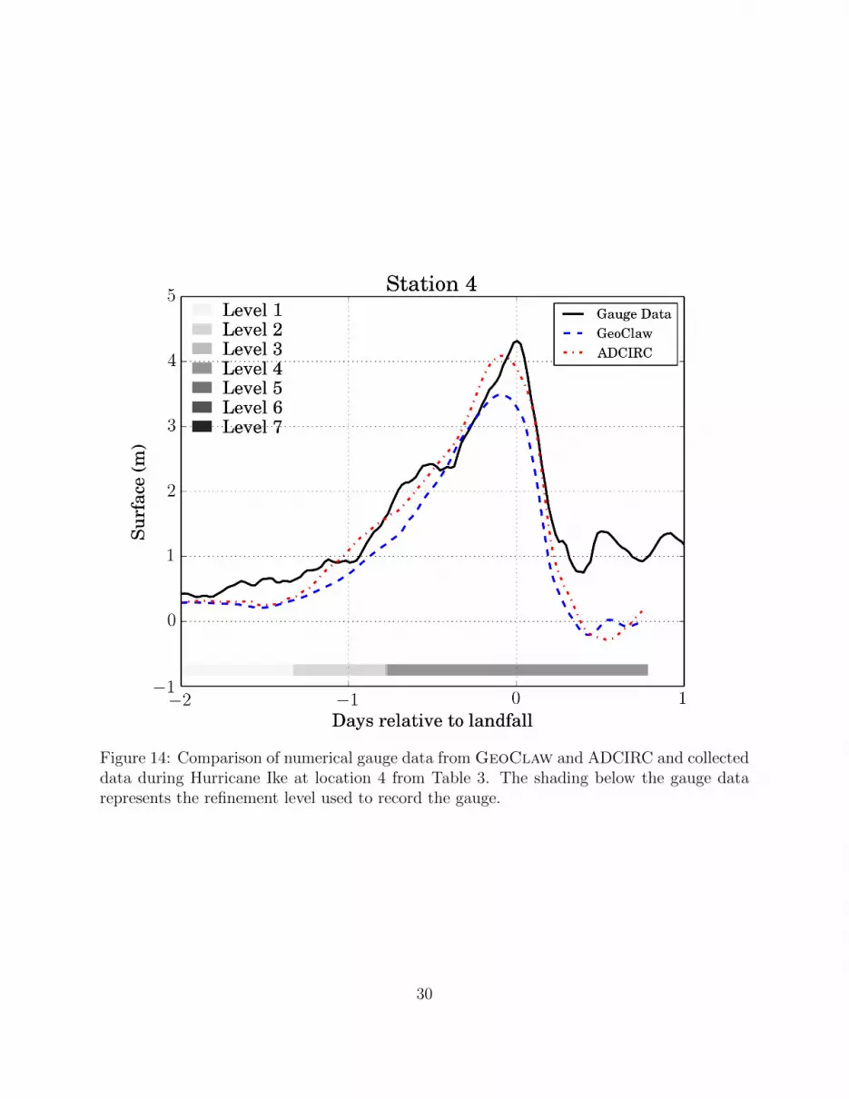
Figure 14: Comparison of numerical gauge data from GeoClaw and ADCIRC and collecteddata during Hurricane Ike at location 4 from Table 3. The shading below the gauge datarepresents the refinement level used to record the gauge.

30

(a) (b)

Figure 15: Domain resolution statistics for the GeoClaw simulation. In Figure 15a astack plot is shown representing the total number of grids per level and total. Similarly inFigure 15b the number of grids cells is shown.

31