arX

iv:p

hysi

cs/0

3070

36v1

[ph

ysic

s.co

mp-

ph]

5 J

ul 2

003

Interface Conditions for Wave Propagation

Through Mesh Refinement Boundaries

Dae-Il Choi a,b, J. David Brown a,c,1, Breno Imbiriba a,d,Joan Centrella a, Peter MacNeice e

aLaboratory for High Energy Astrophysics, NASA/Goddard Space Flight Center,Greenbelt, MD 20771 USA

bUniversities Space Research Association, 7501 Forbes Boulevard, #206, Seabrook,MD 20706 USA

cDepartment of Physics, North Carolina State University, Raleigh, NC 27695 USAdDepartment of Physics, University of Maryland, College Park, MD 20742 USA

eDepartment of Physics, Drexel University, Philadelphia, PA 19104 USA

Abstract

We study the propagation of waves across fixed mesh refinement boundaries in linearand nonlinear model equations in 1–D and 2–D, and in the 3–D Einstein equations ofgeneral relativity. We demonstrate that using linear interpolation to set the data inguard cells leads to the production of reflected waves at the refinement boundaries.Implementing quadratic interpolation to fill the guard cells suppresses these spurioussignals.

Key words: Partial differential equations, Computational techniques, Finitedifference methods, Mesh generation and refinement, Numerical relativity,Gravitational wavesPACS: 02.70.-c, 02.70.Bf, 04.25.Dm, 04.30.-w, 04.30.Db

Email addresses: choi@milkyway.gsfc.nasa.gov (Dae-Il Choi),david brown@ncsu.edu (J. David Brown), imbiriba@milkyway.gsfc.nasa.gov(Breno Imbiriba), jcentrel@milkyway.gsfc.nasa.gov (Joan Centrella),macneice@alfven.gsfc.nasa.gov (Peter MacNeice).1 Senior NRC Associate

Preprint submitted to Elsevier Science 6 December 2013

1 Introduction

Wave propagation is an important phenomenon throughout all areas of physics,with applications typically involving multiple spatial and temporal scales. Innumerical modeling of such problems, one strategy for dealing with the dis-parity in spatial and temporal scales is the use of a nonuniform or adaptivecomputational mesh. In this case waves can cross mesh refinement boundariesas they propagate through the computational domain. This paper focuses oninterface conditions that will allow waves to travel smoothly across fixed re-finement boundaries, minimizing spurious reflections.

The specific application that motivated this study is modeling the emission ofgravitational waves from astrophysical sources such as binary black hole andneutron star coalescences. Such systems are among the most important sourcesfor ground-based gravitational wave detectors such as LIGO and VIRGO [1,2],as well as the planned space-based LISA mission [3]. The gravitational wavesproduced typically have wavelengths ∼ 10 − 100 times the scales of theirsources Numerical simulations of such systems must therefore allow the signalsto propagate from finely resolved regions around the sources into more coarselyresolved regions in the wave zones. Since the waveforms must be computed atlarge distances from their sources (i.e., effectivelly at infinity) for comparisonwith observations from gravitational wave detectors, the simulation domainsmust be made as large as possible. This can be achieved by incorporatingseveral levels of successively coarser grids.

The propagation of gravitational waves is governed by the Einstein equations,which are a coupled set of nonlinear partial differential equations [4]. Theseequations can be written in a variety of ways, but current practice in nu-merical relativity favors the use of the so–called BSSN formalism [5,6]. In thisformalism, the Einstein equations are written as a system of quasi-linear equa-tions with first–order time derivatives and second–order spatial derivatives. Inthis paper we restrict our analysis to the “iterated Crank–Nicholson” updatescheme, which is a second order accurate, explicit finite difference method thatis currently in widespread use in the relativity community. It should also benoted that we consider mesh refinement only in space, not in time. In par-ticular, for our present analysis we use a common timestep across the entirecomputational domain.

Adaptive mesh refinement (AMR) was first applied in numerical relativity tostudy critical phenomena in the 1–D collapse of a scalar field to form a blackhole [7]. An early 3–D application focussed on evolving a single black hole[8]; this was followed by the use of fixed mesh refinement (FMR) to evolvea short part of a binary black hole evolution [9]. AMR was also employed tofollow the propagation of gravitational waves through spacetime, first using

2

a single model equation that describes perturbations of a non-rotating blackhole [10] and later in the 3–D Einstein equations [11], and to study inhomo-geneous cosmological models [12]. In these AMR studies the refinement andderefinement conditions were generally tuned so that the gravitational wavesremained within the finely resolved regions.

In this paper, we address the challenge of evolving gravitational wave signalsacross mesh refinement boundaries using FMR. Success in this endeavor is anessential component of gravitational wave source modeling, due to the largedisparity in the scales of the sources and the waves. Our challenge amountsto choosing a prescription for coupling adjacent grid blocks when the blockshave different resolutions. Grid blocks are coupled through their guard cells,which must be filled using data from the blocks’ interior cells. In hydrody-namics codes it is common practice to use a linear interpolation scheme forguard cell filling, with a possible adjustment for flux conservation across theinterface between blocks [13,14,15]. We have found that this prescription is notadequate for the BSSN formulation of the Einstein equations. In particular,linear guard cell filling leads to unacceptably large reflections and distortionsof the gravitational waves as they propagate from fine grid blocks to coarse gridblocks. Our solution to this problem is to use a guard cell filling procedurewith quadratic–order accuracy orthogonal to the coarse–fine grid interface.The need for quadratic order guard cell filling has been previously demon-strated for elliptic boundary value problems with second order derivatives in[16,17]. With this prescription spurious wave reflections and distortions arereduced dramatically.

Given the complexity of the full system of Einstein equations, we have chosento analyze first a set of model wave equations in 1-D and 2-D that mimic someof the properties of the Einstein equations, as expressed in BSSN form.Thesesimplified test beds have proved essential to understanding and correctingthe problems that arise in the propagation of waves across mesh refinementboundaries. Since the solution we uncovered using these model equations hasproved effective in curing the difficulties encountered in the Einstein equa-tions, we expect this work to be useful across a broad range of related wavepropagation problems.

2 Linear Wave Equation in 1-D: Evolution on a Uniform Grid

The linear wave equation in 1-D is generally written in the form

∂2φ

∂t2=∂2φ

∂x2, (1)

3

where φ = φ(x, t). Introducing the auxiliary variable Π(x, t), we can castEq. (1) in a form that uses only first time derivatives:

∂φ

∂t= Π (2)

∂Π

∂t=∂2φ

∂x2. (3)

In this section we examine the system of equations (2)–(3) to understandthe interface conditions needed for smooth propagation of waves across meshrefinement boundaries. In later sections, these conditions are applied to non-linear and multidimensional wave equations.

2.1 Discretization

For the spatial discretization of equations (2)–(3), we take the data to be de-fined at the centers of the spatial grid cells and use standard O(∆x)2 centeredspatial differences [18]. To advance this system of ordinary differential equa-tions in time we use an O(∆t)2 iterative method first suggested by M. Chop-tuik (see Ref. [19]). In the numerical relativity literature, this explicit updatescheme is refered to as “iterated Crank–Nicholson”. Each iteration has theform

φn+1i = φni + ∆t Πi (4)

Πn+1i =Πn

i +∆t

(∆x)2(φi+1 − 2φi + φi−1)

=Πni +

∆t

(∆x)2F (φ), (5)

where we use i to label the spatial grid, n to label the time steps, and φi, Πi

to indicate intermediate values calculated during the iteration process. Notethat the familiar Crank–Nicholson algorithm is obtained by setting φi and Πi

equal to their time averages, (φn+1i + φni )/2 and (Πn+1

i + Πni )/2, respectively.

For two iterations, the specific steps are as follows. Begin by applying thediscretization (4)–(5) with φ = φn, Π = Πn to calculate a first approximationto φn+1 and Πn+1:

(1)φn+1i = φni + ∆t Πn

i (6)

4

(1)Πn+1i = Πn

i +∆t

(∆x)2F (φn). (7)

Average these new values with those at the starting time level n to get newvalues for φ and Π:

(1)φi = 12((1)φn+1

i + φni ) (8)

(1)Πi = 12((1)Πn+1

i + Πni ). (9)

Now perform a second iteration. Again applying (4)–(5) we find a secondapproximation to φn+1 and Πn+1:

(2)φn+1i = φni + ∆t (1)Πi (10)

(2)Πn+1i = Πn

i +∆t

(∆x)2F ((1)φ). (11)

Averaging again with the values at level n yields

(2)φi = 12((2)φn+1

i + φni ) (12)

(2)Πi = 12((2)Πn+1

i + Πni ). (13)

A final update is carried out using these twice-iterated values:

φn+1i = φni + ∆t (2)Πi (14)

Πn+1i = Πn

i +∆t

∆x2F ((2)φ). (15)

Clearly this algorithm can be carried out for any number of iterations. In theformal limit of an infinite number of iterations, it yields the usual Crank–Nicholson scheme. However, a von Neumann stability analysis shows that thisiterative scheme is stable only when the number of iterations equals 2, 3, 6, 7,10, 11, etc, and the Courant condition ∆t ≤ ∆x is satisfied. This was shownby Teukolsky [19] for the advection equation, but the conclusion holds as wellfor the wave equation in the form (2)–(3). Furthermore, the accuracy of theiterative scheme is second order for any number of iterations. We must carryout at least two iterations for stability, but continuing beyond two iterationsdoes not reduce the truncation error. In this paper we follow the commoncurrent practice in numerical relativity and carry out precisely two iterationsfor our tests.

5

2.2 Evolutions on a Uniform Grid

We first carried out uniform grid, or unigrid, evolutions of the discretized waveequation to provide a basis for comparison with mesh refinement runs. Theinitial data for φ is taken to be a Gaussian wavepacket,

φ(x, t = 0) = A e−x2/σ2

, Π(x, t = 0) = 0, (16)

with A = 1 and σ = 0.25. The spatial domain extends from x = −4 tox = +4. Time evolution of this data produces two packets traveling withvelocity v = ±1, each having amplitude A = 0.5 and the same value of σas the original packet. Here we will consider only the packet traveling to theright, in the region 0 ≤ x ≤ 4.

Figure 1 shows the evolution of this packet for two different resolutions. Thecoarser resolution is given by H = ∆x = 0.045 (dotted line), which has ∼ 10zones across the width of the packet at half its maximum amplitude. Thesolid line shows resolution h = H/2 = 0.0225. The time step is chosen tobe ∆t = ∆x/4 for a given spatial resolution, ∆x. In the last few panelsof Fig. 1 one can see a slight separation between the two curves. This isprimarily due to numerical dispersion, which causes the phase velocities todeviate from unity. The phase velocity for a monochromatic wave propogatingon a discrete, uniform grid is calculated in the Appendix, with the resultdisplayed in Eq. (A.11). According to this formula we expect the pulse (whichhas wavelength ∼ 1) to propagate with speed ∼ 0.999 on the fine grid andspeed ∼ 0.996 on the coarse grid. This translates into a separation between thetwo pulses of about 0.01 at time t = 3.37, which is the approximate separationseen in the last panel of Fig. 1.

The time evolution of the absolute errors ǫ ≡ |φanalytic − φnumerical| is shownin Fig. 2. The dotted line shows the errors ǫH for the coarse resolution H ,and the solid line is 4× ǫh. Inspection of Fig. 2 shows that the two curves arenearly identical, demonstrating the second–order convergence of these runs.Note that the errors are approximately antisymmetric about the location ofthe pulse center. This is because the dominant source of numerical error isdispersion, which has the principle effect of shifting each wave pulse relativeto the exact solution.

3 Implementation of Mesh Refinement

We use the Paramesh package [20] to implement the mesh refinement andparallelization in our codes. All of our codes use cell–centered data. Paramesh

6

works on logically Cartesian, or structured, grids and carries out mesh refine-ment on grid blocks. The underlying mesh refinement technique is similar tothat of Ref. [21], in which grid blocks are bisected in each coordinate directionwhen refinement is needed. The grid blocks all have the same logical struc-ture, with nxb zones in the x−direction, and similarly for nyb and nzb. Thus,refinement of a block in 1-D yields two child blocks, each having nxb zonesbut with zone sizes a factor of two smaller than in the parent block. Whenneeded, refinement can continue on the child blocks, with the restriction thatthe grid spacing can change only by a factor of two, or one refinement level,at any location in the spatial domain. Each grid block is surrounded by anumber of guard cell layers that are used in computing finite difference spatialderivatives near the block’s boundary. These guard cells must be filled usingdata from the interior cells of the given block and the adjacent block.

Figure 3 shows a section of a 1-D grid in the vicinity of an interlevel boundarybetween two neighboring grid blocks. The fine grid covers the left half ofthe 1-D space, with cell–centered grid points labeled −1/2, −3/2, etc. Thecoarse grid covers the right half with cell–centered grid points labeled 1/2,3/2, etc. The fine and coarse blocks are offset from one another for clarity ofpresentation. One layer of guard cells is shown, with “G” marking the coarsegrid guard cell and “g” the fine grid guard cell. These guard cells are filledwith data from neighboring blocks or, if the block forms part of the edge ofthe computational domain, from appropriate outer boundary conditions.

Paramesh can be used in applications requiring AMR, FMR, or a combina-tion of these. It handles the creation of grid blocks, and builds and maintainsthe data structures needed to track the spatial relationships between blocks.It takes care of all inter-block communications and keeps track of physicalboundaries on which particular conditions are set, guaranteeing that the childblocks inherit this information from the parent blocks. In a parallel envi-ronment, Paramesh distributes the blocks among the available processors toachieve load balance, maximize block locality, and minimize inter-processorcommunications.

For the work described in this paper, we are using FMR. For simplicity, weuse the same timestep, chosen for stability on the finest grid, over the entirecomputational domain. At the mesh refinement boundaries, we use a singlelayer of guard cells as shown in Fig. 3; special attention is paid to the restriction(transfer of data from fine to coarse grids) and prolongation (coarse to fine)operations used to set the data in these guard cells, as discussed in the nextsubsection.

7

4 Linear Wave Equation in 1-D: Evolutions with Fixed Mesh Re-

finement

We now carry out evolutions of 1-D linear waves that encounter a change in thegrid resolution at a fixed location. For the gravitational wave applications inwhich we are interested, waves will be generated in a finely resolved region andthen travel out into more coarsely resolved regions. We thus start our initialwave packet, given by Eq. (16), in a region of fine resolution h = 0.0225 aroundthe origin. The spatial domain is again −4 ≤ x ≤ 4. As before, the initialwave packet splits into two identical packets traveling in opposite directions.Each of these packets then encounters a fixed refinement boundary, locatedat x = ±2.1, and crosses into a region of coarser resolution H = 2h. In thefollowing discussions, we focus only on the region x ≥ 0.

We first use the default Paramesh linear interpolation to set the value of thedata in the guard cells on both the coarse and fine grids. With this prescriptionfor guard cell filling, the coarse grid guard cell value of any function f is givenby linear interpolation,

fG =1

2(f−3/2 + f−1/2). (17)

The value of f in the fine grid guard cell “g” is then given by a linear interpo-lation using coarse grid values, fg = (fG + 3f1/2)/4. Combined with Eq. (17),this gives

fg =1

8(f−3/2 + f−1/2 + 6f1/2). (18)

Note that this guard cell filling (GCF) procedure uses the points fG and f1/2

on the coarse grid to obtain fg; this is in contrast to the direct approach, whichuses the nearest points f−1/2 and f1/2 (cf. Eq. (23)). The prescription (17)–(18) for GCF has errors of order h2 and is the default linear GCF methodin Paramesh. We will refer to this procedure as linear GCF in this paper.The results of using linear GCF are displayed in Fig. 4, which shows the timeevolution of the absolute errors ǫ. The dotted line shows the run with linear in-terpolation at the interface boundary, and the solid line the results of a unigridrun at the fine grid resolution. As the packet passes through this boundary,a reflected wave is generated propagating to the left. The transmitted wavecontinues traveling to the right into the coarse grid region.

In large scale simulations of the Einstein equations with several levels of re-finement, such spurious reflected waves can seriously degrade the quality ofthe results. Globally increasing the resolution until the reflected waves reach

8

acceptably small amplitudes is generally not possible in 3-D. We thus need abetter way to control the behavior of the signals crossing the interfaces.

To this end, we implemented direct quadratic interpolation (i.e., using thenearest 3 data points) to set the data in the coarse and fine grid guard cells.Refer again to Fig. 3. For the fine grid guardcell “g”, quadratic interpolationyields [18]

fg =1

15(−3f−3/2 + 10f−1/2 + 8f1/2). (19)

The coarse grid guard cell “G” is filled by matching first derivatives acrossthe interface,

f1/2 − fG

H=fg − f−1/2

h, (20)

where H = 2h. This step, which ensures that the solution is smooth acrossthe interface, can be viewed as “flux matching” where the gradient of f playsthe role of the flux. By combining the derivative matching condition with theformula for fg we find

fG =1

15(6f−3/2 + 10f−1/2 − f1/2). (21)

This same result for fG can be obtained by direct quadratic interpolation.These formulae for GCF have errors of order h3.

The absolute errors obtained when using quadratic interpolation are shown asthe dashed line in Fig. 4. Note that the reflected wave has been greatly reduced.Additional simulations, in which the size of the zones is everywhere decreasedby successive factors of two, show that with quadratic GCF the code is second–order convergent. On the other hand, with linear GCF, the reflected pulse isfirst–order convergent. The transmitted pulse also aquires first–order errors atthe interface with linear GCF. As the transmitted wave propagates throughthe coarse grid region, second–order errors due to dispersion and dissipationeventually dominate over the first–order errors introduced at the interface. Atthat point, the transmitted pulse can appear second–order convergent.

We also conducted tests using a one–dimensional periodic domain consisting of20% fine grid and 80% coarse grid. A wave pulse was allowed to cycle throughthe domain multiple times. These tests clearly show that with quadratic guardcell filling, but not with linear guard cell filling, the code is second–orderconvergent. We also used this test code to check the stability of the interfaceconditions. After thousands of cycles of the wave pulse through the refined

9

region, there were no signs of instability with either linear or quadratic guardcell filling.

In the appendix we present a detailed analytic treatment of wave propagationacross mesh refinement boundaries that complements our numerical experi-ments. There we compute the reflection coefficient R and transmission coeffi-cient T for a monochromatic (single frequency) wave traveling on a grid withfixed mesh refinement, for various methods of GCF. The wave travels from afine grid region with resolution h into a coarse grid region with resolution 2h.Figure 5 shows the absolute value of the reflection coefficient |R| for linearGCF (17)–(18) (dashed curve) and quadratic GCF (21)–(19) (solid curve).The dotted curve shows the results for direct linear interpolation, defined by

fG =1

2(f−3/2 + f−1/2). (22)

for the coarse grid guard cell and

fg =1

3(f−1/2 + 2f1/2). (23)

for the fine grid guard cell. Direct linear interpolation, like the default linearGCF in Paramesh, has errors of order h2. The curves of Fig. 5 are plotted asfunctions of the wavelength in the fine grid region divided by the fine grid cellsize h. Equivalently, we can interpret the horizontal–axis values as the numberof fine grid points per wavelength.

For our 1-D wave equation tests, the Gaussian packet behaves roughly likea wave of wavelength λ ∼ 1. With h = 0.0225, this corresponds to aboutλ/h = 44 fine grid points per wavelength. From Fig. 5 we see that the reflectioncoefficient for linear interpolation is about |R| = 0.02 while that for quadraticGCF is |R| = 0.0003. With an incident pulse amplitude of 0.5, we expect areflected wave amplitude of about 0.01 for linear GCF and less than 0.0002for quadratic GCF. This reflected pulse for the linear case is clearly seen inFig. 4.

The importance of minimizing spurious reflections from grid interfaces hasbeen emphasized above. It is equally important to minimize the distortion ofwaves that pass through a grid interface. The errors in the transmitted wavepulse for linear and quadratic GCF are shown in the region x > 2.1 of the lastfew panels of Fig. 4. Note that the errors for quadratic GCF are actually largerthan the errors for linear GCF. This surprising result is explained as follows.Observe that the errors for the two fixed mesh refinement simulations, as wellas for the unigrid run (solid curve), are approximately antisymmetric aboutthe pulse center. The errors in each case, as in the unigrid tests discussed in

10

Section 2, are primarily due to dispersion. Dispersion causes the wave pulsesto fall behind the exact solution during propagation, giving rise to the errorsshown in Fig. 4. This effect is greater for the two runs with fixed mesh re-finement because, beyond x = 2.1, the grid resolution is lower than for theunigrid run. However, with mesh refinement, the transmitted pulse will alsosuffer a phase error which has the effect of artificially shifting the pulse alongthe x–axis. In the case of linear GCF, there is a relatively large positive phaseerror in the transmitted wave. This phase shift partially compensates for thenegative shift caused by dispersion. As a result the size of the largest peaksin the error for the transmitted wave, for the particular test shown in Fig. 4,is smaller with linear GCF than with quadratic GCF.

Figures 6 and 7 show the absolute value of the transmission coefficient |T|and the phase of the transmission coefficient ϕ = arctan(ℑ(T)/ℜ(T)) for amonochromatic wave, for linear, quadratic, and direct linear interpolation.These graphs are obtained from the analysis in the Appendix. From Fig. 6it is clear that at any wavelength (any resolution) the error in amplitude forthe transmitted wave is smaller for quadratic GCF than for linear GCF. 2

The dominant source of error for the transmitted wave is actually phase error,shown in Fig. 7. The magnitude of this error for quadratic GCF is muchsmaller than that for linear GCF. For a wavelength of λ ∼ 1, the linear guardcell filling produces a phase shift of about ϕ = 0.024, while quadratic GCFgives a phase shift of about ϕ = −0.00028. For the tests shown in Fig. 4, thepositive phase for linear GCF translates into a shift along the positive x–axisof about δx = λϕ/(2π) ≈ 0.004. With quadratic GCF, the pulse is shifted inthe negative direction, but by a much smaller amount δx ≈ −0.00004. Closeinspection of the data for the two transmitted pulses shows that they indeedhave a separation of δx ≈ 0.004. For linear GCF, this phase shift pushesthe wave pulse forward and artificially compensates for the phase lag causedby dispersion. In general, there is no reason to expect the cumulative phaselag due to dispersion to be close in magnitude (but opposite in sign) to thephase advance caused by transmission through various grid interfaces. Thus,the relatively small transmission error seen in Fig. 4 for linear GCF should beviewed as an accident of the particular example, not a generic result.

2 At low resolution, that is, for wavelengths less than about 28h, direct linear GCFhas the smallest error for the transmitted wave amplitude. However, as discussedin the Appendix, as the resolution is increased |T| is much closer to 1 for quadraticGCF. Also note from Fig. 7 that direct linear GCF has large phase errors for thetransmitted wave.

11

5 Nonlinear Wave Equation in 1-D

The next step in developing model equations to test these interface conditionsis to add nonlinear terms similar to those found in the Einstein equations.This produces the following nonlinear wave equation

∂2φ

∂t2=∂2φ

∂x2+ d

(

∂φ

∂t

)2

+ e

(

∂φ

∂x

)2

, (24)

where d and e are arbitrary contants. Again introducing the auxiliary variableΠ(x, t), we get the first order system

∂φ

∂t= Π (25)

∂Π

∂t=∂2φ

∂x2+ d Π2 + e

(

∂φ

∂x

)2

. (26)

Using the discretization introduced in § 2.1, we have

φn+1i = φni + (∆t)Πi (27)

Πn+1i =Πn

i +∆t

(∆x)2(φi+1 − 2φi + φi−1) + d(∆t)(Πi)

2

+e(∆t)

(

φi+1 − φi−1

2∆x

)2

. (28)

Equations (27) and (28) are updated following the steps given in (6)–(15).

We consider the case d = −e = 1 and set up an initial Gaussian wave packetcentered on the origin using the prescription given by Eq. (16), with Π(x, t =0) = 0. This splits into two identical packets traveling in opposite directions,each having amplitude A = 0.38 and width σ = 0.25. We use the spatialdomain −4 ≤ x ≤ 4 and set fixed refinement boundaries at x = ±2.1. Thefine grid around the origin has resolution h = 0.0225 and the coarse gridregions have resolution H = 2h. We focus on the region x ≥ 0.

The results are shown in Figure 8. Since we do not have an analytic solution forEq. (24), we display the actual solution and use unigrid runs for comparison.In addition, the vertical scale is chosen to zoom in on the region around thebase of the packet (i.e., near φ = 0), where the differences between the runs arethe most apparent. The thin solid line shows the solution for a unigrid run at

12

the coarse resolution H , and the thick solid line shows a unigrid run at the fineresolution h. Runs in which the packet encounters a refinement boundary areshown using a dotted line (linear GCF) and a dashed line (quadratic GCF).As we saw before, a reflected wave is generated when the packet crosses therefinement boundary using linear GCF; these effects are much less noticeablewhen using quadratic GCF. As in the case of the linear wave equation, thecode is second–order convergent when using quadratic GCF.

6 Wave Equation in 2–D

As a next step, we consider the wave equation in 2–D. The evolution of cylin-drically symmetric waves on a 2–D Cartesian mesh provides an ideal testproblem in which the signals cross mesh refinement boundaries that are, ingeneral, not perpendicular to their directions of propagation.

The 2–D model wave equation takes the form

∂2φ

∂t2=∂2φ

∂x2+∂2φ

∂y2+ d

(

∂φ

∂t

)2

+ e1

(

∂φ

∂x

)2

+ e2

(

∂φ

∂y

)2

, (29)

where d, e1, e2 are contants. With the auxiliary variable Π(x, y, t), we can writethis in a form using only first–order time derivatives:

∂φ

∂t= Π (30)

∂Π

∂t=∂2φ

∂x2+∂2φ

∂y2+ d (Π)2 + e1

(

∂φ

∂x

)2

+ e2

(

∂φ

∂y

)2

. (31)

Using the discretization introduced in § 2.1, we have

φn+1ij = φnij + (∆t)Πij (32)

Πn+1ij =Πn

ij +∆t

(∆x)2(φi+1,j − 2φij + φi−1,j)

+∆t

(∆y)2(φi,j+1 − 2φij + φi,j−1)

+ d(∆t)(Πij)2 + e1(∆t)

(

φi+1,j − φi−1,j

2∆x

)2

13

+ e2(∆t)

(

φi,j+1 − φi,j−1

2∆y

)2

. (33)

As before, Eqs. (32) and (33) are updated following the steps given in Eqs. (6)–(15).

In this section we consider two types of GCF, the default Paramesh linear orderGCF and a quadratic GCF scheme. The linear GCF is depicted in Fig. 9. First,each coarse grid guard cell (open diamond) is filled as a linear combination ofthe surrounding fine grid points (solid circles). The fine grid guard cells (opencircles) are then filled using a linear combination of the surrounding coarsegrid points (open and solid diamonds).

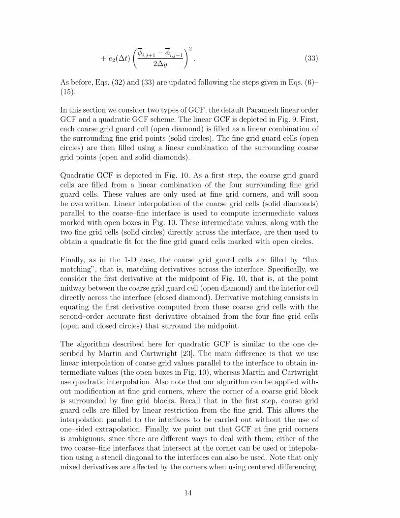
Quadratic GCF is depicted in Fig. 10. As a first step, the coarse grid guardcells are filled from a linear combination of the four surrounding fine gridguard cells. These values are only used at fine grid corners, and will soonbe overwritten. Linear interpolation of the coarse grid cells (solid diamonds)parallel to the coarse–fine interface is used to compute intermediate valuesmarked with open boxes in Fig. 10. These intermediate values, along with thetwo fine grid cells (solid circles) directly across the interface, are then used toobtain a quadratic fit for the fine grid guard cells marked with open circles.

Finally, as in the 1-D case, the coarse grid guard cells are filled by “fluxmatching”, that is, matching derivatives across the interface. Specifically, weconsider the first derivative at the midpoint of Fig. 10, that is, at the pointmidway between the coarse grid guard cell (open diamond) and the interior celldirectly across the interface (closed diamond). Derivative matching consists inequating the first derivative computed from these coarse grid cells with thesecond–order accurate first derivative obtained from the four fine grid cells(open and closed circles) that surround the midpoint.

The algorithm described here for quadratic GCF is similar to the one de-scribed by Martin and Cartwright [23]. The main difference is that we uselinear interpolation of coarse grid values parallel to the interface to obtain in-termediate values (the open boxes in Fig. 10), whereas Martin and Cartwrightuse quadratic interpolation. Also note that our algorithm can be applied with-out modification at fine grid corners, where the corner of a coarse grid blockis surrounded by fine grid blocks. Recall that in the first step, coarse gridguard cells are filled by linear restriction from the fine grid. This allows theinterpolation parallel to the interfaces to be carried out without the use ofone–sided extrapolation. Finally, we point out that GCF at fine grid cornersis ambiguous, since there are different ways to deal with them; either of thetwo coarse–fine interfaces that intersect at the corner can be used or intepola-tion using a stencil diagonal to the interfaces can also be used. Note that onlymixed derivatives are affected by the corners when using centered differencing.

14

In our code we do not treat the corners as special. At a corner our code nat-urally selects one of the two interfaces and carries out a linear interpolationparallel to that face to obtain intermediate values.

The initial data for our tests is taken to be a cylindrically symmetric wavepacketcentered on the origin, with

φ(x, y, t = 0) = Ae−(x2+y2)/σ2

(34)

and Π(x, y, t = 0) = 0. We choose the amplitude A = 1, and the width of thepulse by σ = 0.25. Quadrant symmetry is imposed by using mirror-symmetryboundary conditions along x = 0 and y = 0. The computational domain thencovers the region 0 ≤ x ≤ 4.3125 and 0 ≤ y ≤ 4.3125. This packet is initiallyconfined to a fine grid region of resolution h = 0.0225. As the packet expands,the wavefront crosses a fixed mesh refinement boundary into a region of coarserresolution H = 2h.

Setting d = e1 = e2 = 0 in Eqs. (30) and (31) allows this packet to evolveunder a linear equation. Figure 11 shows the results of using quadratic GCFto set the values of the guard cell data. Here, φ is shown at four consecutivetimes. The expanding wavefront encounters mesh refinement boundaries atx = 2.1 along the x−axis and at y = 2.1 along the y−axis. Note that the wavepasses smoothly across the interface.

A comparison of unigrid and fixed refinement runs is shown in Fig. 12. Here,φ is plotted along a portion of the x−axis at a fixed time. The unigrid run(solid line) at the fine grid resolution shows the extended “tail” of the out-going cylindrical wave front. The run with linear GCF (dotted line) showsa reflected wave traveling back into the fine grid region as the wave passesthrough the refinement boundary. In the run with quadratic GCF (dashedline), this spurious signal has been nearly eliminated.

Similar results are achieved when this wave packet is evolved according to anonlinear equation, d = −e1 = −e2 = 1. The structure of the grid and loca-tion of the refinement boundary are the same as for the 2-D linear equation.Figure 13 displays the results of φ along the x−axis at a fixed time. Noticethat the run with linear GCF (dotted line) shows a significant reflected wave.In contrast, the run with quadratic GCF (dashed line) is close to the one witha uniform grid (solid line).

15

7 The Einstein Equations in 3–D

We are now ready to apply the techniques developed in our model equationsto the propagation of gravitational waves in 3–D, which is governed by thevacuum (or source–free) Einstein equations. We write these equations in termsof the “3 + 1” spacetime split [4], in which the initial data is specified on some3–D spacelike slice and then evolved forward in time. Within this framework,the metric takes the form

ds2 = −α2dt2 + gij(dxi + βidt)(dxj + βjdt). (35)

We use units in which both the speed of light c = 1 and the gravitationalconstant G = 1. Lowercase Latin letters are used to denote spatial indices, sothat i, j = 1, 2, 3. To simplify the notation throughout this section, we use thesummation convention: if any expression has one index as a superscript andthe same index as a subscript, summation over all values that index can takeis implied [22]. The geometry of the given spacelike slice is described by the3–metric gij. The lapse function α governs the advance of proper time acrossthe surface, and the shift vector βi the motion of the spatial coordinates withinthe hypersurface as the data is evolved forward in time. Both α and βi arefreely–specifiable functions of space and time; for the rest of this section, weuse the choice α = 1 and βi = 0.

In the standard ADM spacetime split [4], the Einstein equations can be writtenin terms of gij and the extrinsic curvature of the hypersurface Kij , where

Kij = −1

2

∂gij∂t

. (36)

Following current practice in numerical relativity, we use the BSSN formalism[5,6] in which the Einstein equations are written in terms of conformal variables{ψ,K, gij, Aij , Γi} defined as follows:

e4ψ ≡ det(gij)1/3 (37)

gij ≡ e−4ψgij (38)

K ≡ gijKij (39)

Aij ≡ e−4ψ(Kij −1

3gijK) (40)

Γi ≡ −∂j gij . (41)

16

Here gij is the inverse of the conformal metric gij. We use the notation ∂j ≡∂/∂xj for spatial derivatives.

In terms of these conformal variables, with the gauge choices α = 1 and βi = 0,the vacuum Einstein equations become

∂ψ

∂t= −1

6αK (42)

∂gij∂t

= −2Aij (43)

∂K

∂t=

1

3K2 + AijA

ij (44)

∂Aij∂t

= RTFij + AijK − 2AilA

lj (45)

∂Γi

∂t= 2(ΓijkA

kj − 2

3gij∂jK + 6Aij∂jψ). (46)

Here, Γijk are the connection coefficients associated with gij, defined by

Γkji =1

2gmk(∂igmj + ∂j gmi − ∂mgji), (47)

and

Aij = gilgjkAlk, Alj = gliAij . (48)

The superscript “TF” denotes the trace-free part of a tensor, so that RTFij =

Rij − gijR/3, where R = gmkRmk. The Ricci curvature tensor Rij is definedby

Rij = ∂kΓkij − ∂jΓ

kik + ΓkmkΓ

mij − ΓkmjΓ

mik. (49)

Although the set of equations (42)–(46) is considerably more complicated thanour model equations, there are notable similarities. In particular, the conformalmetric gij plays the role of the function φ, while Aij takes the role of Π. Lookingat (47) and (49), we also see that the RTF

ij term in Eq. (45) contains secondspatial derivatives of gij.

The lessons learned from the model equations in 1–D and 2–D can be appliedsuccessfully to the Einstein equations in 3–D, as we demonstrate by evolving aweak gravitational wave. We use the analytic solution to the linearized Einstein

17

equations found by Teukolsky [24]; since this is given in closed form, we canthen compare the numerical results directly with this analytic solution. Wechoose the even parity, L = 2, M = 0 solution, which is given by

ds2 =−dt2 + (1 + Afrr)dr2 + (2Bfrθ)rdrdθ

+(2Bfrφ)r sin θdrdφ+ (1 + Cf(1)θθ + Af

(2)θθ )r2dθ2

+[2(A− 2C)fθφ]r2 sin θdθdφ

+(1 + Cf(1)φφ + Af

(2)φφ )r2 sin2 θdφ2. (50)

Here,

A=3

[

F (2)

r3+

3F (1)

r4+

3F

r5

]

(51)

B=−[

F (3)

r4+

3F (2)

r3+

6F (1)

r4+

6F

r5

]

(52)

C =1

4

[

F (4)

r+

2F (3)

r2+

9F (2)

r3+

21F (1)

r4+

21F

r5

]

(53)

F =F (t− r), F (n) ≡[

dnF (x)

dxn

]

x=t−r

, (54)

where F is a generating function. We use the form

F (x) =Ax

ω2e−x

2/ω2

, (55)

with two free parameters, A and ω. Here we have specified an outgoing wavesolution F = F (t − r); an ingoing wave solution can be obtained by usingF = F (t+ r).

For this even-parity, M = 0 case, the angular functions fij are:

frr =2 − 3 sin2 θ (56)

frθ =−3 sin θ cos θ (57)

frφ =0 (58)

f(1)θθ =3 sin2 θ (59)

f(2)θθ =−1 (60)

fθφ =0 (61)

f(1)φφ =−f (1)

θθ (62)

f(2)φφ =3 sin2 θ − 1. (63)

18

We present results for a gravitational wave crossing two fixed mesh refinementboundaries into regions with successively coarser resolution. We start with awave packet composed of a linear combination of one initially ingoing and oneoutgoing wave, each having amplitude A = 10−6 and width ω = 1. This packetis centered on the origin in a fine grid region of resolution h = 0.0416667.The successively coarser regions have resolutions 2h and 4h, with the firstrefinement boundary at r =

√x2 + y2 + z2 = 4.5 and the second at r = 9.0.

To complete the initial data we take Kij = 0 so that K = 0 and Aij = 0.Octant symmetry is imposed by using mirror-symmetry boundary conditionsalong x = 0, y = 0, and z = 0. The computational domain covers the regions0 ≤ x ≤ 12 and similarly for y and z.

As the evolution proceeds, the outgoing waves travel directly toward the outerboundary of the grid. The initially ingoing waves first travel toward the origin,then reflect and move outward. As the overall signal propagates outward, itleaves flat spacetime behind.

Figure 14 shows the evolution of these waves when linear GCF is used. Thefunction gzz − 1 is plotted as a function of x and y in the z = 0 plane at 4successive times. Note the presence of spurious reflected signals as the wavespass through the fixed mesh boundaries. These problems are greatly reducedwhen quadratic GCF is used, as shown in Fig. 15. A comparison of runs withlinear (dotted line) and quadratic (dashed line) GCF and the analytic solution(solid line) is shown in Fig. 16. The reflected waves are essentially eliminatedby the use of quadratic GCF.

Finally, Fig. 17 demonstrates the second–order convergence of the code bycomparing the results of the run in Fig. 15 with a run that differs only byhaving the size of the grid zones a factor of 2 larger throughout. Both runsuse quadratic GCF. The L2 norm of the absolute error ǫ is calculated overeach simulation domain, and plotted as a function of time. The solid trianglesconnected by the solid line show ǫ for the run in Fig. 15, and the filled boxesconnected by the dotted line show the errors for the lower resolution runmultiplied by 4.

8 Summary

We have examined the propagation of waves across fixed mesh refinementboundaries, starting with simplified linear and nonlinear model equations in1–D and 2–D, and progressing to the 3–D Einstein equations of general rela-tivity. The numerical evolutions were carried out using centered spatial differ-ences and the explicit iterated Crank-Nicholson time update method, givingsecond–order accuracy. Our results show that using linear GCF produces spu-

19

rious reflected waves as the signals cross refinement boundaries, and that theseare greatly suppressed by using quadratic GCF. In particular, quadratic GCFpreserves the second–order convergence of the numerical evolutions. Our nu-merical results are complemented by a detailed analytic treatment of wavescrosing refinement boundaries in 1–D in the Appendix.

While quadratic GCF is straightforward to describe and implement in 1–D, thesituation becomes more complicated in 2–D. In particular, intermediate valuesparallel to the mesh refinement interface must be calculated in the 2–D case.We have found that using linear interpolation to obtain these intermediatevalues, combined with quadratic interpolation for the final values, maintainsthe second–order convergence. The procedure used for quadratic GCF in 2–Dgeneralizes in a straightforward manner to the 3–D case.

The techniques presented here appear to be robust in the sense that they con-tinue to produce excellent results as our test problems increase in complexity.Quadratic GCF successfully eliminates most of the spurious reflected waves inboth linear and nonlinear model equations in 1–D and 2–D. The 3–D Einsteinequations present a much larger and more complex system of equations. In thetest case presented here, the evolution of a weak gravitational wave, quadraticGCF continues to perform well, even as the signals cross two successive meshrefinement boundaries. We fully expect that these techniques will also yieldexcellent results for strong gravitational waves, which activate the nonlinearterms in the Einstein equations. Such evolutions require various technical dif-ferences in the gauge choices (α and βi) as well as in the formulation of theinitial data. We are currently working on such models, and will report on themelsewhere.

Acknowledgements

It is a pleasure to thank John Baker, Phillip Colella, Kevin Olson, and SteveZalesak for helpful and stimulating discussions. The work was supported inpart by NSF grant PHY-0070892.

A Appendix: Analysis of Numerical Wave Propagation in 1-D

In this appendix, we present a more detailed analysis of the propagation oflinear waves in 1-D with the discretization described in Sec. 2. We begin byderiving some basic results for uniform grids (Sec. A.1) and follow with a studyof wave propagation across a fixed mesh refinement boundary (Sec. A.2). Here,we do not address the issue of instabilities that might arise due to coupling

20

between fine and coarse meshes [25]. However, as noted in Sec. 4, our numericaltests show no signs of instability.

A.1 Wave Propagation on a Uniform Mesh

We will employ matrix notation to facilitate the analysis in this Appendix.First, we collect the field variables φ, Π into the column vector

V =(

φΠ

)

. (A.1)

Equations (2)–(3) can now be written as

∂V

∂t=(

0 1∂2/∂x2 0

)

V . (A.2)

As usual V nj will denote the vector of grid functions at timestep n and grid

point j.

The iterated Crank–Nicholson method described in Sec. 2.1 is built from suc-cessive applications of the basic operator

Q =(

0 1∂2 0

)

, (A.3)

where ∂2V nj ≡ (V n

j+1 − 2V nj + V n

j−1)/∆x2. With two iterations, the update of

the variables V nj by one full timestep is accomplished by the operator

M = I + ∆tQ[

I +∆t

2Q(

I +∆t

2Q)]

. (A.4)

The stability, dissipation, and dispersion properties are obtained by consider-ing discrete plane wave solutions,

V nj = Weiωn∆te−ikj∆x , (A.5)

where W is a constant vector (independent of n and j). Inserting this ansatzinto the update equation V n+1

j = MV nj , we find

eiω∆tW =(

1 − 2Λ2 ∆t(1 − Λ2)−4Λ2(1 − Λ2)/∆t 1 − 2Λ2

)

W , (A.6)

21

where

Λ ≡ ∆t

∆xsin(k∆x/2) . (A.7)

Thus, W is an eigenvector with eigenvalue eiω∆t for the matrix that appearsin Eq. (A.6). The eigenvalues are obtained in the usual way with the resulteiω∆t = 1 − 2Λ2 ± 2iΛ(1 − Λ2). This is the dispersion relation giving thecomplex frequency ω as a function of wave number k. We can, without lossof generality, consider only plane wave solutions (A.5) with positive frequencyξ > 0, where ξ = ℜ(ω) is the real part of ω. Then the ± sign in the dispersionrelation must be set equal to the sign of the wave number k. The dispersionrelation then becomes

eiω∆t = 1 − 2Λ2 + 2i|Λ|(1 − Λ2) (A.8)

and ξ = ℜ(ω) is positive. The eigenvectors W corresponding to these eigen-values are straightforward to compute. Choosing the first component of W tobe unity, we find

W =(

12i|Λ|/∆t

)

. (A.9)

We note for later reference that We−ikj∆x is an eigenvector of the basic oper-ator Q with eigenvalue 2i|Λ|/∆t.

The finite difference scheme is unstable if the magnitude of the amplificationfactor, |eiω∆t|, is greater than unity. From Eq. (A.8) we find that |eiω∆t|2 ≤ 1implies Λ2 ≤ 1. This inequality will be satisfied for all wave numbers k only if∆t ≤ ∆x. This is the Courant limitation on the timestep for the wave equation(2)–(3) discretized with twice–iterated Crank–Nicholson.

The phase velocity is found from the real part of the frequency ξ = ℜ(ω).From the dispersion relation (A.8), we find

ξ∆t = arcsin

2|Λ|(1 − Λ2)√

1 − 4Λ4(1 − Λ2)

. (A.10)

The phase velocity is then

c(λ) =ξ

k=ξ∆t

2πα

λ

∆x, (A.11)

22

where α ≡ ∆t/∆x is the Courant factor and λ = 2π/k is the wavelength. Thedissipation is found from the imaginary part of the frequency, η = ℑ(ω). Sincethe wave amplitude varies like φ ∼ e−ηn∆t, we see that the amplitude dropsby a factor

e−η∆t = |eiω∆t| =√

1 − 4Λ4(1 − Λ2) . (A.12)

for each timestep.

A.2 Wave Propagation with FMR

Now consider a two–level refined mesh, with fine grid ∆xf on the left andcoarse grid ∆xc on the right. We will assume that the refinement jumps by afactor of 2, that is, ∆xc = 2∆xf . The mesh will be labeled as shown in Fig. 3.Thus, V n

−1/2, Vn−3/2, etc. are the fine grid functions and V n

1/2, Vn3/2, etc. are the

coarse grid functions.

As a first step towards analyzing the wave reflection and transmission at theinterface, we relate the wave numbers in the coarse and fine grid regions.Consider a monochromatic solution that varies like φ ∼ eiξn∆t across theentire mesh. Specifically, we assume that the coarse and fine grid frequenciesare the same, ξc = ξf , and that the coarse and fine grid time steps are thesame, ∆tc = ∆tf . From the dispersion relation, Eq. (A.8), we can computetan(ξ∆t) in the coarse and fine grid regions and equate the results:

2|Λc|(1 − Λ2c)

1 − 2Λ2c

=2|Λf |(1 − Λ2

f)

1 − 2Λ2f

. (A.13)

Here, Λc = (∆t/∆xc) sin(kc∆xc/2) and similarly for Λf . This relation has theform f(|Λc|) = f(|Λf |) where |Λc| and |Λf | vary between 0 and 1. It is easy toshow that the function f(|Λ|) is monotonic and therefore invertible. It followsthat the only solution of Eq. (A.13) is

|Λc| = |Λf | . (A.14)

This equation shows that the coarse and fine grid wave numbers kc and kf arerelated by

kc = ± 2

∆xcarcsin

[

∆xc∆xf

sin(kf∆xf/2)

]

. (A.15)

23

The two cases corresponding to the ± sign indicate that the wave propagationdirection on the coarse and fine sides of the interface need not match. Thus,we can have a right moving wave in the coarse grid region connected to bothright moving and left moving waves in the fine grid region.

From the result (A.14) we see that the rate of dissipation (A.12) of a wave,governed by η = ℑ(ω), is the same in the coarse and fine grid regions. We alsosee that the relative phase between the two components φ and Π of the wave,Eq. (A.9), is the same in coarse and fine regions. The phase velocity (A.11),and hence the amount of dispersion, differ in the coarse and fine grid regions,since the wave numbers kc and kf are not equal.

According to Eq. (A.15) kc is real only for kf∆xf ≤ π/3, that is, for λf/∆xf ≥6. If λf/∆xf < 6, then kc is complex and the plane wave solution (A.5) willcontain a spatial dependence in the coarse grid region that is either expo-nentially damped or grows exponentially. Note that, although kc might becomplex, Λc is real (assuming kf is real) and equal to ±Λf . It follows that,whether kc is real or complex, the Courant stability condition |eiω∆t|2 ≤ 1 issatisfied in the coarse grid region if it is satisfied in the fine grid region.

For the remainder of this appendix we will focus on the case of practicalinterest, where λf/∆xf ≥ 6 and kc is real. The plots in Figures 5, 6, and 7have been restricted to λf/∆xf ≥ 10 for clarity of presentation. Each of thecurves in those plots reaches a finite value at λf/∆xf = 6.

A.2.1 Matching solutions

At this point we have shown that waves of frequency ξ have wave number kcon a coarse grid, wave number kf on a fine grid, and that these values arerelated as in Eq. (A.15). We will now construct a solution with frequency ξthat spans the entire non-uniform grid. To begin, consider the vector

Vj =

W(

e−ikf j∆xf + Reikf j∆xf

)

, j < 0 ;

W(

Te−ikcj∆xc

)

, j > 0 .(A.16)

We will show that for an appropriate choice of the coefficients R and T thevector Vj is an eigenvector of the basic operator Q with eigenvalue 2i|Λ|/∆t.For points away from the interface, namely, the points j ≤ −3/2 and j ≥3/2, this conclusion follows from our earlier observation that on a uniformgrid We±ikj∆x is an eigenvector of Q with eigenvalue 2i|Λ|/∆t. The sameargument cannot be applied to the points 1/2 and −1/2 surrounding theinterface because the stencil for the discrete derivative operator ∂2 appearingin Q extends across the interface. Thus, when computing ∂2Vj for j = ±1/2,we must use guard cell information.

24

In the main text we discussed various choices for guard cell filling, such as theParamesh linear GCF of Eqs. (17)–(18) and the quadratic GCF of Eqs. (19)–(21). For the purpose of presenting the analysis, we will focus instead on thedirect linear GCF of Eqs. (22)–(23). In the present notation, these relationsare

V nG =

1

2(V n

−3/2 + V n−1/2), V n

g =1

3(V n

−1/2 + 2V n1/2) (A.17)

Now, for grid points that are not adjacent to the interface, the operator ∂2

takes the usual form,

∂2V nj =

{

(V nj+1 − 2V n

j + V nj−1)/∆x

2f , j ≤ −3/2 ,

(V nj+1 − 2V n

j + V nj−1)/∆x

2c , j ≥ 3/2 .

(A.18)

But for grid points adjacent to the interface, ∂2 must use guard cell valuesgiven by (A.17). Consequently, we find

∂2V n−1/2 =(V n

g − 2V n−1/2 + V n

−3/2)/∆x2f

=(2V n1/2 − 5V n

−1/2 + 3V n−3/2)/(3∆x2

f) (A.19)

and

∂2V n1/2 =(V n

3/2 − 2V n1/2 + V n

G )/∆x2c

=(2V n3/2 − 4V n

1/2 + V n−1/2 + V n

−3/2)/(2∆x2c) . (A.20)

for ∂2 acting at grid points j = ±1/2.

We now impose the requirement that the vector Vj of Eq. (A.16) is an eigenvec-tor of Q with eigenvalue 2i|Λ|/∆t at the points j = ±1/2 adjacent to the in-terface. Using the discretization (A.19) the relation QV−1/2 = (2i|Λ|/∆t)V−1/2

yields

1

3(2φ1/2 − 5φ−1/2 + 3φ−3/2) =

(

2i|Λ|αf

)2

φ−1/2 . (A.21)

Here, φj is the first component of the ansatz vector Vj . Similarly, with thediscrete operator (A.20), we find that QV1/2 = (2i|Λ|/∆t)V1/2 implies

1

2(2φ3/2 − 4φ1/2 + φ−1/2 + φ−3/2) =

(

2i|Λ|αc

)2

φ1/2 . (A.22)

25

These two equations can be solved for the two coefficients R and T. The resultis

R=3E2

cE2f −E4

f − E2cE

4f − E6

f

1 + E2f + E2

cE2f − 3E2

cE4f

,

T=Ec(3 + 2E2

f − 2E6f − 3E8

f)/(2Ef)

1 + E2f + E2

cE2f − 3E2

cE4f

, (A.23)

where the shorthand notation

Ec ≡ eikc∆xc/2 , Ef ≡ eikf ∆xf/2 (A.24)

has been used.

At this point we have succeeded in showing that the vector Vj of Eq. (A.16),with R and T chosen as in Eqs. (A.23), is an eigenvector of Q on the non–uniform grid. The corresponding eigenvalue is 2i|Λ|/∆t. A short calculationshows that Vj is also an eigenvector for M , Eq. (A.4), with eigenvalue 1 −2Λ2 +2i|Λ|(1−Λ2). Since M evolves the discrete system by one time step, wesee that

V nj =

Weiωn∆t(

e−ikf j∆xf + Reikf j∆xf

)

, j < 0 ;

Weiωn∆t(

Te−ikcj∆xc

)

, j > 0 .(A.25)

is a solution of the finite difference equations V n+1j = MV n

j across the entiregrid. Here, the complex frequency ω is given by the dispersion relation (A.8).The solution (A.25) represents a wave that travels from the fine grid region tothe coarse grid region. At the interface it splits into reflected and transmittedpieces. The coefficient R is the reflection coefficient, and T is the transmissioncoefficient.

The results of this analysis can be checked numerically. For example, in Fig. A.1the solid lines show the magnitude of the reflection coefficient calculated fromEq. (A.23). The squares and triangles display the results of a numerical test,in which we modeled the propagation of a sine wave contained in a broadGaussian envelope,

φ(x, t) = Ae−(x−x0−t)2/w2

sin k(x− t) . (A.26)

The initial data were obtained by discretizing φ and dφ/dt at t = 0. Theconstant x0 was chosen so that initially the wave packet was situated in thefine grid region, far from the interface. We set the Gaussian half–width tow = 63∆x, significantly larger than the longest wavelength shown in the

26

figures. The magnitude of R was obtained by evolving the wave packet pastits interaction with the interface, typically about 1000 time steps, and thenextracting from the numerical data the largest value of |φ| in the reflectedpulse. The Courant factor for these numerical runs was ∆t/∆xf = 0.4.

The squares show raw numerical data. The deviation of these data from theanalytical curves is due to dissipation and dispersion of the wave pulse. Dissi-pation can be accounted for rather easily, using the analytical result given inEq. (A.12). The triangles show the numerical data with correction for dissi-pation. The numerical and analytical results for the reflection coefficient arein excellent agreement, as seen in Fig. (A.1).

The above analysis can be repeated for other choices of GCF. In particu-lar, for the quadratic GCF of Eqs. (19)–(21), the reflection and transmissioncoefficients are

R=E2f(−1 + 6E2

f + 3E4f + E2

c (−15 + 10E2f − 3E4

f ))

3 + 6E2f − E4

f −E2c (3 − 10E2

f + 15E4f )

,

T=2Ec(−3 − 2E2

f + 2E6f + 3E8

f )/Ef

3 + 6E2f − E4

f −E2c (3 − 10E2

f + 15E4f ), (A.27)

with Ec and Ef defined as before. Figures (5)–(7) compare the reflection andtransmission coefficients for linear, direct linear, and quadratic GCF. FromFig. 5 we see that quadratic GCF produces a much smaller reflected wavethan either linear or direct linear GCF. For example, at 20 fine grid pointsper wavelength, linear (direct linear) GCF produces a reflected wave withamplitude about 5.6% (4.3%) that of the incident wave. With quadratic GCFthe reflected wave amplitude is only about 0.31% that of the incident wave.For the transmitted wave, Fig. 7 shows that the phase error at 20 fine gridpoints per wavelength is smaller in magnitude by more than a factor of 10with quadratic GCF compared to linear or direct linear GCF. Figure 6 shows,perhaps surprisingly, that direct linear GCF does the best job of keeping themagnitude of T close to 1 at wavelengths less than about 28∆xf . For longerwavelengths, λ > 28∆xf , quadratic GCF is best. Note, however, that withany of these choices of GCF, the deviation of |T| away from unity is relativelysmall. Over the entire range shown in the graphs, λ > 10∆xf , the maximumerror for quadratic GCF is less than 1%. For the reflection coefficient, onthe other hand, the maximum error for direct linear GCF is about 11%. Formost situations the problem of spurious reflections at an interface will be moresevere than the problem of inaccurate wave transmission through the interface.

27

A.2.2 Discussion of guard cell filling

The results thus far indicate that quadratic GCF is generally better thaneither linear or direct linear GCF at keeping the reflection coefficient smalland the transmission coefficient close to unity. The question naturally arises:can one do better than quadratic GCF? We will restrict our attention to rulesfor GCF that use a three–point stencil. That is, the fine and coarse grid guardcell values V n

g and V nG are obtained from linear combinations of three grid

points,

V nG = c1V

n1/2 + c2V

n−1/2 + c3V

n−3/2 , (A.28)

V ng = f1V

n1/2 + f2V

n−1/2 + f3V

n−3/2 , (A.29)

where c1, f1, etc. are constants.

The analysis of Sec. A.2.1 can be repeated with the guard cells defined asabove. The resulting reflection and transmission coefficients are functions ofthe constants c1, f1, etc. Although there are certain combinations of the con-stants that outperform quadratic GCF at low resolution, quadratic GCF isunique in the following sense. If we consider the high resolution limit, in whichkf∆xf is small, quadratic GCF yields

R =3

32i(kf∆xf )

3 + O(kf∆xf )4 , (A.30)

T = 1 − 3

32i(kf∆xf )

3 + O(kf∆xf )4 . (A.31)

The magnitudes of the reflection and transmission coefficients behave like|R| = O(kf∆xf )

3 and |T| = 1 + O(kf∆xf )4. For any other choice of con-

stants c1, f1, etc., the reflection and transmission coefficients approach 0 and1, respectively, more slowly (if at all) than for quadratic GCF. For example,for direct linear GCF, we have

R=1

8i(kf∆xf ) + O(kf∆xf )

2 , (A.32)

T= 1 +1

8i(kf∆xf ) + O(kf∆xf )

2 . (A.33)

Thus, for high resolution, quadratic GCF is the best possible choice given thethree–point stencil (A.28)– (A.29). Because R and T approach 0 and 1 rapidly,as the third power of kf∆xf , quadratic GCF performs well at all resolutions.

28

References

[1] B. Barish, First Generation Interferometers, in: J. Centrella, ed., AstropohysicalSources for Ground-Based Gravitational Wave Detectors (AIP, Melville, NW,2001), 3

[2] P. Fritschel, The Second Generation LIGO Interferometers, in: J. Centrella, ed.,Astropohysical Sources for Ground-Based Gravitational Wave Detectors (AIP,Melville, NW, 2001), 15

[3] P. Bender, et al., LISA, Pre-Phase A Report, 2nd. edition (1998), unpublished(available online at: http://lisa.jpl.nasa.gov/documents/ppa2-09.pdf)

[4] C. Misner, K. Thorne, and J. Wheeler, Gravitation (W. H. Freeman, New York,1973)

[5] M. Shibata and T. Nakamura, Evolution of three-dimensional gravitationalwaves: Harmonic slicing case, Phys. Rev. D52, 5428 (1995).

[6] T. Baumgarte and S. Shapiro, Numerical integration of Einstein’s fieldequations, Phys. Rev. D59, 024007 (1998).

[7] M. Choptuik, Universality and scaling in gravitational collapse of a masslessscalar field, Phys. Rev. Lett. 70, 9 (1993).

[8] B. Brugmann, Adaptive mesh and geodesically sliced Schwarzschild spacetimein 3+1 dimensions, Phys. Rev. D54, 7361 (1996).

[9] B. Brugmann, Binary Black Hole Mergers in 3d Numerical Relativity, Int. J.Mod. Phys. D8, 85 (1999).

[10] P. Papadopoulos, E. Seidel, and L. Wild, Adaptive computation of gravitationalwaves from black hole interactions, Phys. Rev. D58, 084002 (1998).

[11] K. New, D. Choi, J. Centrella, P. MacNeice, M. Huq, and K. Olson, Three-dimensional adaptive evolution of gravitational waves in numerical relativity,Phys. Rev. D62, 084039 (2000).

[12] S. Hern, Numerical Relativity and Inhomogeneous Cosmologies, (Ph.D.Thesis, Dept. Applied Maths. and Theoretical Physics, Cambridge University,Cambridge, UK, 2000) (http://arxiv.org/abs/gr-qc/0001070).

[13] M.J. Berger and J. Oliger, Adaptive mesh refinement for hyperbolic partialdifferential equations, J. Computat. Phys. 53, 484 (1984).

[14] M.J. Berger and P. Colella, Local adaptive mesh refinement for shockhydrodynamics, J. Comput. Phys. 82, 64 (1989).

[15] M. J. Berger, On conservation at grid interfaces, SIAM J. Numer. Anal. 24,967 (1987).

[16] G. Chesshire and W. D. Henshaw, J. Comput. Phys. 90, 1-64 (1990).

29

[17] W. D. Henshaw and D. W. Schwendeman, submitted to J. Comput. Phys.(2003).

[18] W. Press, S. Teukolsky, W. Vetterling, and B. Flannery, Numerical Recipies(2nd edition) (Cambridge University Press, New York, 1994).

[19] S. Teukolsky, On the stability of the iterated Crank-Nicholson method innumerical relativity, Phys. Rev. D61, 087501 (2000).

[20] P. MacNeice, K. Olson, C. Mobarry, R. de Fainchtein, and C. Packer,PARAMESH: A parallel adaptive mesh refinement community toolkit,Computer Physics Comm. 126, 330 (2000).

[21] D. DeZeeuw and K. Powell, An Adaptively Refined Cartesian Mesh Solver forthe Euler Equations, J. Computat. Phys. 104, 56 (1993).

[22] B. Schutz, A first course in general relativity (Cambridge University Press, NewYork, 1985).

[23] D. Martin and K. Cartwright, Solving Poisson’s Equation using Adaptive MeshRefinement, unpublished notes (1996).

[24] S. Teukolsky, Linearized quadrupole waves in general relativity and the motionof test particles Equation using Adaptive Mesh Refinement, Phys. Rev. D26,745 (1982).

[25] F. Olsson and N. Anders Petersson, Stability of interpolation on overlappinggrids, Comput. Fluids 25, 583 (1996).

30

Fig. 1. The evolution of a Gaussian wavepacket on a uniform grid according to thelinear 1–D wave equation is shown for two different resolutions: H = ∆x = 0.045(dotted line) and h = H/2 (solid line).

31

Fig. 2. The evolution of the absolute errors ǫ for the two runs in Fig. 1 is shown.The dotted line shows ǫH and the solid line 4 × ǫh.

−5/2 −3/2 g−1/2

G 1/2 3/2

Fig. 3. An interlevel boundary between a coarse and fine grid in 1-D is shown. Thecoarse grid data points are marked with filled diamonds and positive half integers,the fine grid data points are marked with filled circles and negative half integers.The coarse and fine guard cells are marked with the corresponding open symbolsand are denoted by “G” and “g,” respectively.

32

Fig. 4. The evolution of the absolute errors ǫ is shown for a Gaussian packet crossinga fixed refinement boundary at x = 2.1 with linear (dotted line) and quadratic(dashed line) GCF. The solid line shows ǫ for a unigrid run at the fine grid resolution.

33

/h

||

10 20 30 40 500

0.025

0.05

0.075

0.1

λ

R

Fig. 5. Absolute values of the reflection coefficient |R| for linear (dashed curve),quadratic (solid curve), and direct linear (dotted curve) GCF for a wave with wave-length λ crossing a single fixed mesh boundary. The resolution of the fine grid ish.

34

/h

||

10 20 30 40 500.999

1

1.001

1.002

1.003

1.004

1.005

1.006

1.007

1.008

1.009

1.01

λ

T

Fig. 6. Absolute values of the transmission coefficients for linear (dashed line),quadratic (solid line), and direct linear (dotted) GCF.

35

/h

phas

e

10 20 30 40 50-0.04

-0.02

0

0.02

0.04

0.06

0.08

λ

Fig. 7. The phase of the transmission coefficients for linear (dashed line), quadratic(solid line), and direct linear (dotted) GCF.

36

Fig. 8. The time evolution of the solution φ to the nonlinear 1-D wave equationis shown. Unigrid runs are shown at the coarse resolution H (thin solid line) andthe fine resolution h = H/2 (thick solid line). Runs in which the packet encountersa mesh refinement boundary at x = 2.1 are shown for linear interpolation (dottedline) and quadratic (dashed line) GCF.

37

Fig. 9. Paramesh default linear GCF in 2-D. Points on the coarse grid are denotedby diamonds, and points on the fine grid by circles. First, the coarse grid guard cells(open diamonds) are filled by averaging the surrounding fine grid points. Then thefine grid guard cells (open circles) are filled by taking linear combinations of thefour surrounding coarse grid points.

Fig. 10. Quadratic GCF in 2-D. Coarse grid guard cells (open diamonds) are tem-porarily filled by averaging the surrounding fine grid points. Intermediate values(open boxes) are obtained by linear interpolation of coarse grid values (solid dia-monds) parallel to the interface. Fine grid guard cells (open circles) are then filledfrom a quadratic fit using two fine grid points and one intermediate value. Finally,the coarse grid guard cells are filled by matching the coarse and fine grid firstderivatives across the interface.

38

Fig. 11. The evolution of φ with a linear 2-D wave equation is shown at 4 consecutivetimes for a run using quadratic GCF to set the data in the guard cells. Each of thegrid blocks shown has 8 × 8 zones.

39

Fig. 12. φ is shown along a portion of the x−axis for the 2-D linear wave equation.The solid line shows the results of a unigrid run at the fine grid resolution h = 0.0225,the dotted line the results of a run with linear GCF, and the dashed line a run withquadratic GCF.

40

Fig. 13. Same as Fig. 12 except that the 2-D nonlinear wave equation is solved.

41

Fig. 14. Evolution of gravitational waves in the 3–D Einstein equations using linearGCF. gzz − 1 is plotted 1n the z = 0 plane. Three levels of resolution (h,2h,4h) areused, with h = 0.0416667. Each of the grid blocks shown has 6 × 6 × 6 zones.

42

Fig. 15. Same as Fig. 14 except that quadratic GCF is used.

43

Fig. 16. The evolution of gzz − 1 is shown along the y-axis for the 3–D Einsteinequations. The analytic solution (solid line) and numerical solutions using linear(dotted line) and quadratic (dashed line) GCF are shown. The resolution levels aregiven by (h,2h,4h) with h = 0.0416667.

44

Fig. 17. The L2 norm of the absolute error ǫ is shown for two gravitational waveruns differing in resolution by a factor of 2 throughout. Both runs have 2 refinementboundaries and use quadratic GCF. The solid triangles connected by the solid lineshow ǫ for the run at higher overall resolution, and the solid boxes connected by thedotted line show 4 × ǫ for the run with lower overall resolution.

45

/h

||

5 10 15 200

0.1

0.2

0.3

0.4

0.5

0.6

0.7

0.8

0.9

1

λ

R

Fig. A.1. Absolute value of the reflection coefficient for direct linear guard cellfilling. The raw numerical data are shown as boxes, while the triangles show thedata corrected for dissipation.

46