HURRICANE INDUCED WAVE AND SURGE FORCES ON ...
102
HURRICANE INDUCED WAVE AND SURGE FORCES ON BRIDGE DECKS A Thesis by RONALD LEE MCPHERSON Submitted to the Office of Graduate Studies of Texas A&M University in partial fulfillment of the requirements for the degree of MASTER OF SCIENCE August 2008 Major Subject: Ocean Engineering
-
Upload
khangminh22 -
Category
Documents
-
view
2 -
download
0
Transcript of HURRICANE INDUCED WAVE AND SURGE FORCES ON ...

HURRICANE INDUCED WAVE AND SURGE FORCES ON BRIDGE DECKS
A Thesis
by
RONALD LEE MCPHERSON
Submitted to the Office of Graduate Studies of
Texas A&M University
in partial fulfillment of the requirements for the degree of
MASTER OF SCIENCE
August 2008
Major Subject: Ocean Engineering

HURRICANE INDUCED WAVE AND SURGE FORCES ON BRIDGE DECKS
A Thesis
by
RONALD LEE MCPHERSON
Submitted to the Office of Graduate Studies of
Texas A&M University
in partial fulfillment of the requirements for the degree of
MASTER OF SCIENCE
Approved by:
Chair of Committee, Billy L. Edge
Committee Members, James Kaihatu
Alejandro Orsi
Head of Department, David Rosowsky
August 2008
Major Subject: Ocean Engineering

iii
ABSTRACT
Hurricane Induced Wave and Surge Forces on Bridge Decks.
(August 2008)
Ronald Lee McPherson, B.S., Texas A&M University
Chair of Advisory Committee: Dr. Billy L. Edge
The damaging effects of hurricane landfall on U.S. coastal bridges have been
studied using physical model testing. Hurricane bridge damage and failure susceptibility
has become very evident, especially during hurricane seasons 2004 and 2005 in the Gulf
of Mexico. The combination of storm surge and high waves caused by a hurricane can
produce substantial loads on bridge decks leading to complete bridge failure. Several
theoretical methods have been developed to estimate these forces but have not been
tested in a laboratory setting for a typical bridge section. Experiments were done using a
large-scale 3-D wave basin located at the Haynes Coastal Engineering Laboratory at
Texas A&M University to provide estimates of the horizontal and vertical forces for
several conditions to compare with the forces predicted with the existing models. The
wave force results show no strong correlation between the actual force measured and the
predicted force of existing theoretical methods. A new method is derived from the
existing theoretical methods. This model shows a strong correlation with both the
measured horizontal and vertical forces.

iv
To my mother, father, family, and adored wife, Lauren.

v
ACKNOWLEDGEMENTS
There are several people I would like to acknowledge for their assistance in
completing this research. I would like to extend my sincere gratitude to Dr. Billy Edge
for his support and direction in all of my graduate studies. I would also like to express
my thanks to Oscar and Carmen Cruz-Castro for their assistance in running tests, as well
as their invaluable guidance and support in creating accurate physical model tests. Also,
I would like to thank Dr. Kaihatu and Dr. Orsi for serving as committee members. I
would like to acknowledge the support of the Federal Highway Administration as well as
several state transportation departments for specific knowledge. Also, the forensic
information obtained by several firms and institutions following the 2004 and 2005
hurricane seasons is greatly appreciated.

vi
TABLE OF CONTENTS
Page
ABSTRACT .............................................................................................................. iii
DEDICATION .......................................................................................................... iv
ACKNOWLEDGEMENTS ...................................................................................... v
TABLE OF CONTENTS .......................................................................................... vi
LIST OF FIGURES ................................................................................................... viii
LIST OF TABLES .................................................................................................... xii
CHAPTER
I INTRODUCTION ................................................................................ 1
Background .................................................................................... 1
Purpose ........................................................................................... 3
II PREVIOUS LITERATURE ................................................................. 6
Kaplan (1992) and Kaplan et al. (1995) ......................................... 6
Bea et al. (2001) ............................................................................. 8
Tirindelli et al. (2002) .................................................................... 10
McConnell et al. (2004) ................................................................. 12
Douglass et al. (2006)..................................................................... 15
III RESEARCH METHODOLOGY ......................................................... 18
Facility ............................................................................................ 18
Physical Model ............................................................................... 19
Testing Equipment ......................................................................... 24
Experimental Setup ........................................................................ 26
IV DISCUSSION OF RESULTS .............................................................. 34
Waves ............................................................................................. 34

vii
CHAPTER Page
Forces ............................................................................................. 35
Force Profile ................................................................................... 38
Solitary Wave Results .................................................................... 41
Air Entrapment ............................................................................... 49
V COMPARISON OF PREVIOUS METHODOLOGIES ...................... 50
Bea .................................................................................................. 50
Kaplan ............................................................................................ 52
McConnell and Douglass ............................................................... 54
Correlation of Previous Methods and Measured Forces ................ 55
Conclusion of Previous Methods Comparison ............................... 65
VI SUGGESTED METHOD .................................................................... 66
Wave Height and Vertical Force Correlation ................................. 66
Maximum Water Depth and Vertical Force Correlation ................ 68
Reversing the Correlation............................................................... 70
Estimating Uplift Forces for a Complex Geometry ....................... 72
Solitary Wave Comparison ............................................................ 75
Suggested Method for Calculating Horizontal Forces ................... 77
Hydrodynamic Consideration ........................................................ 80
Biloxi Case Study ........................................................................... 82
VII CONCLUSION .................................................................................... 85
REFERENCES .......................................................................................................... 88
VITA ......................................................................................................................... 90

viii
LIST OF FIGURES
Page
Figure 1-1 U.S. Highway 90 over Biloxi Bay after Hurricane Katrina
(Douglass et al. 2006)........................................................................... 1
Figure 1-2 Schematic of bridge deck subject to surge and waves during storm
conditions ............................................................................................. 3
Figure 2-1 H. R. Wallingford test configurations .................................................. 11
Figure 2-2 Schematic of vertical and horizontal force applied to a deck or beam
element ................................................................................................. 13
Figure 2-3 Definition of quasi-static force parameters (Kerenyi 2005)................. 14
Figure 2-4 Definition sketch for the Douglass method .......................................... 17
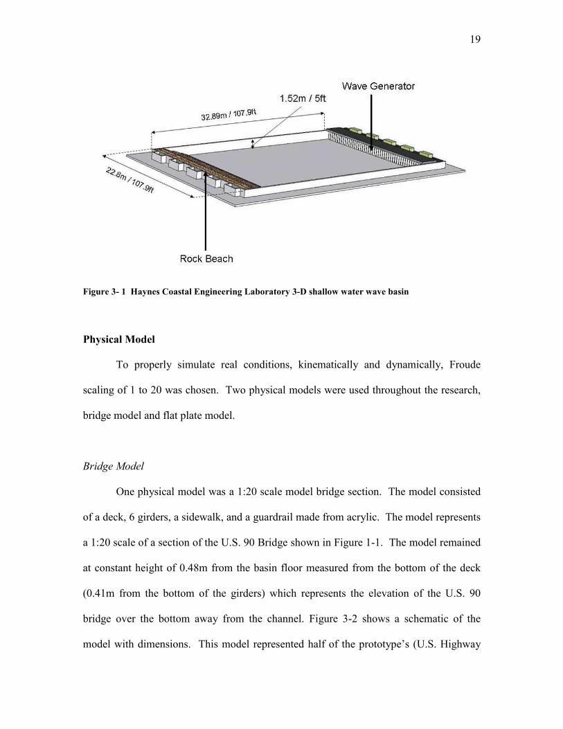
Figure 3-1 Haynes Coastal Engineering Laboratory 3-D shallow water wave
basin ..................................................................................................... 19
Figure 3-2 Bridge model schematic with dimensions ............................................ 20
Figure 3-3 3-D rendering of prototype section. Note the colored region is the
portion tested by the physical model .................................................... 21
Figure 3-4 Actual bridge model with acrylic side panels to account for boundary
effects ................................................................................................... 22
Figure 3-5 Dummy bridge sections to account for boundary effects ..................... 23
Figure 3-6 Flat plate model schematic with dimensions ....................................... 24
Figure 3-7 Hanging box apparatus attached to basin bridge .................................. 25
Figure 3-8 Basin schematic for experimental set I ................................................ 28

ix
Page
Figure 3-9 Schematic of angle of incidence with respect to model bridge and wave
generator ............................................................................................... 33
Figure 4-1 Typical varying period ......................................................................... 36
Figure 4-2 Typical varying wave height ................................................................ 37
Figure 4-3 Varying depth bridge and flat plate vertical force................................ 38
Figure 4-4 Force progression as water depth increases (1 of 2) ............................ 39
Figure 4-5 Force progression as water depth increases (2 of 2) ............................ 40
Figure 4-6 Solitary wave and force time history at 0.39m depth ........................... 43
Figure 4-7 Solitary wave and force time history at 0.41m depth ........................... 44
Figure 4-8 Solitary wave and force time history at 0.48m depth ........................... 45
Figure 4-9 Solitary wave and force time history at 0.54m depth ........................... 46
Figure 4-10 Vertical force compared to water surface height above model ............ 47
Figure 4-11 Horizontal force compared to water surface height above model ........ 48
Figure 5-1 Bea et al. 2001 vertical force over a wave length ................................ 51
Figure 5-2 Kaplan et al. 1995 vertical force over a wave length ........................... 53
Figure 5-3 Kaplan et al. 1995 vertical force varying period trend ......................... 54
Figure 5-4 Kaplan method compared to vertical force measurements .................. 56
Figure 5-5 Bea method compared to vertical force measurements ........................ 56
Figure 5-6 McConnell method compared to vertical force measurements ............ 57
Figure 5-7 Douglass method compared to vertical force measurements ............... 57
Figure 5-8 Kaplan vs. experimental vertical force ................................................. 59
Figure 5-9 Bea vs. experimental vertical force ...................................................... 60

x
Page
Figure 5-10 McConnell vs. experimental vertical force .......................................... 60
Figure 5-11 Douglass vs. experimental vertical force ............................................. 61
Figure 5-12 McConnell vs. experimental vertical force solitary wave results ........ 62
Figure 5-13 Douglass vs. experimental horizontal force solitary wave results ....... 63
Figure 5-14 McConnell vs. experimental horizontal force solitary wave results .... 64
Figure 5-15 Douglass vs. experimental horizontal force solitary wave results ....... 64
Figure 6-1 Vertical force compared to wave height .............................................. 67
Figure 6-2 Profile of overtopping water weight (lower water depth) .................... 68
Figure 6-3 Profile of overtopping water weight (higher water depth) ................... 69
Figure 6-4 Correlation of maximum wave crest above the SWL, η, and vertical
force ...................................................................................................... 70
Figure 6-5 Suggested method compared to measured vertical force on a flat
plate ...................................................................................................... 71
Figure 6-6 Vertical force schematic for complex geometry .................................. 73
Figure 6-7 Suggested method vs. measured vertical force (experimental set I) .... 74
Figure 6-8 Suggested method vs. measured vertical force (experimental set III) . 75
Figure 6-9 Suggested method vs. measured vertical force (experimental set V) .. 76
Figure 6-10 Suggested method vs. measured vertical force with modified overtopping
(experimental set V) ............................................................................. 76
Figure 6-11 Schematic of realistic overtopping weight ........................................... 77
Figure 6-12 Horizontal force suggested method schematic ..................................... 78
Figure 6-13 Definition sketch for horizontal force suggested method .................... 79

xi
Page
Figure 6-14 Suggested method vs. measured horizontal force (experimental
set V) .................................................................................................... 80
Figure 6-15 U.S. 90 highway bridge over Biloxi Bay simplified schematic ........... 82

xii
LIST OF TABLES
Page
Table 2-1 Coefficients defined by McConnell et al. 2004 for evaluating the
quasi-static forces for beam and deck elements ................................... 15
Table 5-1 Previous methods vertical force statistical bias.................................... 58
Table 5-2 Previous methods horizontal force statistical bias ............................... 61
Table 6-1 Correlation coefficient for wave height compared to vertical force .... 67
Table 6-2 Hydrostatic contribution example ........................................................ 81

1
CHAPTER I
INTRODUCTION
Background
Hurricanes can generate forces which cause hydraulically induced failure in
coastal bridges. This was especially apparent in the recent hurricanes: Ivan and Katrina.
The predominant mechanisms that cause failure on bridge decks during a hurricane are
surge and waves. Figure 1-1 shows U.S. Highway 90 crossing the Biloxi Bay in
Mississippi after Hurricane Katrina. In the foreground of the image, the short bridge
height allows the bridge decks to be subjected to surge and waves. The bridge decks in
this section are completely displaced. In the background of the image, the bridge height
increases to allow passage for large boats.
Figure 1- 1 U.S. Highway 90 over Biloxi Bay after Hurricane Katrina (Douglass et al. 2006)
______________
This thesis follows the style of Journal of Waterway, Port, Coastal and Ocean Engineering.

2
This section of the bridge was only subjected to the winds of the hurricane and
experienced no bridge deck displacement.
Numerous bridges have failed during hurricanes. Of the recent hurricanes: Ivan
and Katrina, the notable bridges that have experienced damage include the I-10 bridge
across Escambia Bay, the I-10 bridge across Lake Pontchartrain, the U.S. 90 bridges
across the Biloxi Bay and Bay of St. Louis, and the on ramp to the I-10 bridge across
Mobile Bay (Douglass et al. 2006). During Hurricane Katrina alone, 44 bridges
experienced damage (Padgett et al. 2008).
During a hurricane event, the sustained strong winds essentially blow water up
against the coast causing the water level to rise above the normal water level (Dean and
Dalrymple 2002). This rise in water level is termed “surge”. According to Dean and
Dalrymple, there are several contributors to the total surge experienced during a storm
event. These include: barometric tide, wind stress tide, and Coriolis tide. Of these, wind
stress tide is the dominant contributor to the total surge during a storm.
The width and depth of a shelf adjacent to a shoreline is an important contributor
to the severity of surge during a storm event. A classic example of this is Hurricane
Katrina. The continental shelf in the Gulf of Mexico is relatively wide and shallow
especially when compared to Hawaii and the Atlantic side of Florida. Surge is inversely
proportional to water depth and therefore as the water depth decreases the surge increases
(Dean and Dalrymple 2002). As Hurricane Katrina traveled across the wide shallow
continental shelf, the surge continued to increase for the length of the shelf resulting in
surge exceeding 20 ft in some areas (Douglass et al. 2006). In locations with little or no

3
shelf, less of the water column is affected by the wind. Thus, these locations experience
smaller surge.
The other predominant damaging mechanism that causes bridge failure is wave
induced loads. During storm events waves become significantly larger. When
accompanied by an increased water level, the waves are then able to come into contact
with the structure. This is shown in Figure 1-2. The energy carried by the waves is then
partially transferred to the structure. This combined with buoyancy can cause the bridge
to fail.
Figure 1- 2 Schematic of bridge deck subject to surge and waves during storm conditions
Purpose
There are several methods of estimating the forces applied to bridge decks;
however they are based on unverified theoretical or empirical methods. Currently there
has been little experimental work done to estimate the forces subjected to coastal bridge
decks (Cruz-Castro et al. 2006). Structures other than bridges such as piers and platforms
are subject to wave forces with and without surge and have been the subject of a great

4
deal of research. This previous research is valuable to the present because of the wave
loading on similar horizontal deck geometries. However, this work does not include
experiments with the structure submerged. The transportation community does not have
adequate design tools to prevent the devastating effects of bridge failure due to hurricane
conditions. Moreover, there is no agreed upon method to appropriately estimate the
forces a coastal bridge will endure from wave and surge conditions during a hurricane
(Cruz-Castro et al 2006).
The reason for bridge deck displacement has been widely agreed upon as the
combination of an upward force (vertical force) and lateral force (horizontal force).
However, specific mechanisms such as buoyancy caused by air-entrapment and
quantifiable horizontal and vertical forces are still in debate. To better understand these
mechanisms, a physical model was constructed in the Haynes Coastal Engineering
Laboratory at Texas A&M to test forces on bridge decks caused by both waves and surge.
The physical model was subjected to several combinations of water depths and wave
heights as well as different types of waves. The forces and moments experienced by the
physical model as well as wave conditions at various locations during the tests were
measured. From this information forces and moments can be broken down in to
components (x, y, z) and analyzed in detail and compared with previous theoretical
methods.
The ultimate goal of this research is to quantify the forces on a bridge deck given
a known wave and surge condition. Preexisting research on hurricanes can provide
information on possible wave conditions near coastal bridges for past storms or potential
storms. With this information, force estimations can be made for actual coastal bridges.
5
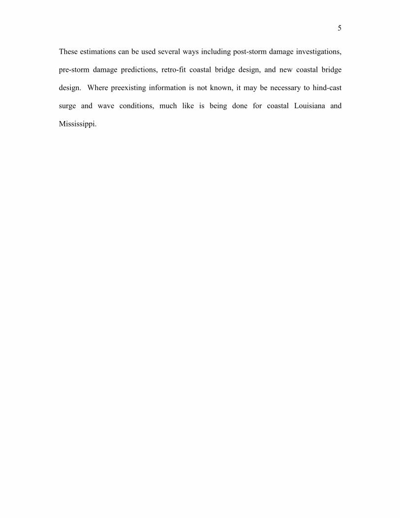
These estimations can be used several ways including post-storm damage investigations,
pre-storm damage predictions, retro-fit coastal bridge design, and new coastal bridge
design. Where preexisting information is not known, it may be necessary to hind-cast
surge and wave conditions, much like is being done for coastal Louisiana and
Mississippi.

6
CHAPTER II
PREVIOUS LITERATURE
Wave forces on highway bridge decks have only recently been a topic of interest
in engineering literature. Therefore there is limited information relating directly to
highway bridges. However, various nearshore and offshore structures with similar
geometries such as piers and offshore platforms have received a substantial amount of
attention. This body of information has a large potential of application to wave forces on
highway bridge decks. The following are summaries of various literatures found to be
relevant to the subject material and have developed some form of theoretical model to
estimate wave forces on deck-like structures. Sarpkaya and Isaacson (1981) and others
have presented detailed descriptions of the effects of wave forces in general. Much of the
work has been focused on piles or slender structural elements for platforms but there has
been little information related to vertical uplift forces on complex geometries.
Kaplan (1992) and Kaplan et al. (1995)
Kaplan, in the 1992 Offshore Technology Conference proceedings, discusses a
theoretical approach to time histories of wave impact forces on offshore decks. Kaplan
focuses on impact forces on vertical circular cylinders and vertical forces on flat plates.
Kaplan in 1995 Offshore Mechanics and Artic Engineering conference proceedings
further develops the theory by adding more applications such as horizontal wave forces
on cross members.

7
Kaplan uses a combination of momentum change and drag effects to estimate
wave forces on the various offshore platform members. The inertia term of the vertical
force is derived by taking the time derivative of the product of the three-dimensional
added mass of a flat plate and the vertical velocity. The drag term of the vertical force is
found in the same manner as developed by Morrison 1950. Equation (2-1) and (2-2) are
the vertical force equations condensed and expanded, respectively.
Ft
M w blC w wz D= +∂
∂
ρ( )3
2 (2-1)
=
+
+
+
+
+ρπ
ρπ ρ
81
4
11
2
1
2
2
21 2
2
21
2
bl
l
b
w bldl
dt
l
b
l
b
w blC w wD& (2-2)
M3 is defined as the three-dimensional added mass of the flat plate. This is defined in
Equation (2-3).
Mbl
l
b
3
2
21
28
1
=
+
ρπ
(2-3)
The terms l and dl
dtrepresent the horizontal deck wetted length and time rate of change of
the deck wetted length. dl
dtcan be represented by the wave celerity while the wave crest
is traveling along the length of the horizontal deck y. After the wave has reached the end
of the deck the dl
dtterm retains a value of zero.

8
The theory presented in Kaplan et al. 1995 was compared to preexisting
experimental research. The comparisons were represented by bias, defined as the ratio of
measured force and theoretical force. Horizontal force from one data set was compared
to theory, and the bias varied from 0.92 to 1.26. Also, both horizontal and vertical force
from another data set was compared to theory. The horizontal force bias varied from
0.79 to 1.23, and the vertical force bias varied from 0.63 to 1.46.
Bea et al. (2001)
Bea et al. discusses wave crest forces on the lower decks of offshore platforms. It
is stated that the extreme condition storm wave would be higher than the lower deck of
many older platforms. By using the American Petroleum Institute (API) wave force
guidelines, it was found that most platforms would not survive the extreme storm
condition. An analytical solution is used to re-qualify several platforms subject to
possible inundating storm wave crests. The analytical solution is an application and
modification of the equations developed by Morrison 1950. The total force “imposed” on
the platform is given in Equation (2-4).
Ftw Fb Fs Fd Fl Fi= + + + + (2-4)
Where Fb is the buoyancy force (vertical), Fs is the slamming force, Fd is the drag force
(horizontal), Fl is the lift force (vertical), and Fi is the inertial force.
The horizontal slamming force is defined as follows:

9
Fs C Aus= 05 2. ρ (2-5)
Where ρ is the mass density of seawater, A is the vertical deck area subject to wave crest,
u is the horizontal fluid velocity in the wave crest, and Cs is the coefficient of slamming
which can vary from Cs=π to Cs=2π. An “effective” slamming force is also discussed
which uses a dynamic load factor coefficient, Fe which reduces the slamming force
evaluated from Equation (2-5) by:
Fs FeFs'= (2-6)
The inundation forces are developed as well. The horizontal drag force using the
drag coefficient, Cd is given in Equation (2-7).
Fd C Aud= 05 2. ρ (2-7)
The vertical lift force is given in Equation (2-8).
Fl C Aul= 05 2. ρ (2-8)
Cl is defined as the lift coefficient. The forces in the vertical direction are not discussed
in detail because the platforms under investigation have open or grated floors. These
floors have shown to incur significantly less vertical force than horizontal force.
The inertial force is given in Equation (2-9).

10
Fi C Vam= ρ (2-9)
Where V is the volume of deck inundated, a is the water acceleration, and Cm is the
inertia coefficient.
Field experience is also presented in the literature. Damage incurred to platforms
affected by Hurricanes Andrew, Roxanne, Camille, and Hilda is discussed. A “good”
correlation is found between damage and “green water” exposed to the lower decks of the
platforms.
Laboratory results from Finnigan and Petrauskas were used to compare the API
and modified procedures. Statistical information, including mean, standard deviation and
coefficient of variance is given in terms of bias (ratio of measured maximum horizontal
force to analytical maximum horizontal force). Certain test setups show promising
results with mean bias close to 1 while other setups show bias reaching 2+.
Tirindelli et al. (2002)
Tirindelli et al. (2002) reviews existing methods for evaluating wave loads on
exposed jetties and related structures. Flume tests to measure wave induced forces on
beam and deck structures were carried out at H. R. Wallingford. A 1:25 scale model of a
jetty was used in three different configurations: panels, no panels, and flat plate. The
panel configuration is designed to eliminate three-dimensional effects as the wave
inundates the structure. The no panel configuration is designed to simulate an actual jetty
of similar geometry. The three configurations are shown in Figure 2-1.

11
Figure 2- 1 H. R. Wallingford test configurations
The specimen has four testing elements built in which measure pressure on an exterior
beam, interior beam, exterior deck, and interior deck.
Of the data collected, the horizontal and vertical forces were compared to
significant wave height. It was shown that both horizontal and vertical forces increased
as significant wave height increased. There was no discernable difference between the
test configurations for the horizontal force. It was observed that after ignoring a few
outliers the vertical force for both beam and deck increased in a linear fashion where the
uplift force depended on the element size and not shape.
The existing models by Kaplan (1992) and Shih & Anastasiou (1992) were
compared to the exterior deck element. The downward forces were also compared to the
Kaplan model. In general, both the Kaplan and Shih models under predicted the
magnitude of the uplift force. The Kaplan model also under predicted the magnitude of
the downward forces.

12
McConnell et al. (2004)
McConnell et al. (2004) is a comprehensive literature survey that covers many
aspects of hydraulic loading on piers and jetties exposed to “green water”. Within the
literature review a different approach for quantifying vertical and horizontal wave crest
loads on structures using the experimental data from H. R. Wallingford is presented. The
design structure under investigation was the same jetty used in Tirindelli (2002). The
experiments were done in a wave flume with modern wave-generation capabilities. A
typical loading found by the experiments show a slow-varying load that corresponds to
the period of the wave and a short duration impact load when the wave first hits the
structure.
The analytical method used to estimate the forces is based on a hydrostatic
approach. Individual components of the jetty (seaward beam, internal beam, and internal
deck) are calculated separately and later added together to find a total force. The “base
vertical force”, Fv* is found by multiplying the pressure under the component by the
projected area of the component in the horizontal plane. The pressure is defined by the
difference in the elevation of the maximum wave crest and the elevation of the bottom of
the deck. The “base horizontal force”, Fh* is found similarly by multiplying the pressure
of the component face (vertical plane) by its area. The pressure is defined by the
difference in the elevation of the maximum wave crest and the centroid of the component
face. The “base vertical force” and “base horizontal force” are demonstrated in Figure 2-
2.

13
Figure 2- 2 Schematic of vertical and horizontal force applied to a deck or beam element
The equations for the basic wave forces are as follows:
F b b pv w l
* = 2 (2-10)
F b cp
h w l
*
max( )= −η 2
2 for ηmax ≤ cl + bh (2-11)
( )F b b
p ph w h
* =+1 2
2 for ηmax > cl + bh (2-12)
From the basic force parameters Fv* and Fh
*, a quasi-static force parameter is defined.
Figure 2-3 demonstrates the quasi-static force parameter during a typical force loading.

14
Figure 2- 3 Definition of quasi-static force parameters (Kerenyi 2005)
The equation for the quasi-static force is given as:
( )
F
F
a
c
H
qs
l
b*
max
=−
η (2-13)
Where Fqs is the quasi-static force, F* is the basic wave force (vertical or horizontal), cl is
the clearance defined in Figure 2-2, H is the wave height, ηmax is the maximum wave crest
elevation relative to the SWL, and the coefficients a and b are empirical.
The empirical coefficients a and b differ for each element, upward and downward
loading, and vertical and horizontal forces. These coefficients are given in Table 2-1.

15
Table 2- 1 Coefficients defined by McConnell et al. 2004 for evaluating the quasi-static forces for
beam and deck elements
Wave Load and Configuration a b
Upward vertical forces (seaward beam and deck) 0.82 0.61
Upward vertical forces (internal beam only) 0.84 0.66
Upward vertical forces (internal deck, 2D and 3D effects) 0.71 0.71
Downward vertical forces (seaward beam and deck) -0.54 0.91
Downward vertical forces (internal beam only) -0.35 1.12
Downward vertical forces (internal deck, 2D effects) -0.12 0.85
Downward vertical forces (internal deck, 3D effects) -0.80 0.34
Shoreward horizontal forces, Fhqs+ (seaward beam) 0.45 1.56
Shoreward horizontal forces, Fhqs+ (internal beam) 0.72 2.30
Seaward horizontal forces, Fhqs- (seaward beam) -0.20 1.09
Seaward horizontal forces, Fhqs- (internal beam) -0.14 2.82
Douglass et al. (2006)
Douglass, at the University of South Alabama, uses a similar method to the
McConnell approach, however this method is simplified. The area of interest of the
literature is U.S. Highway bridge decks. Douglass et al. (2006) uses the same hydrostatic
approach as McConnell but does not separate the structure into various components.
The “reference” vertical force, Fv* of the entire bridge is found by multiplying the
pressure under the bridge deck by its projected area in the horizontal plane. The pressure
is found by taking product of gravity, density, and the difference of the maximum
elevation of the wave crest and the elevation of the bottom of the deck. The estimated

16
vertical force, Fv is then found by multiplying the “reference” vertical force by an
empirical coefficient for a varying load, Cv-va. This is shown in Equations (2-14) and (2-
15).
( )F Z Av v v
* = γ ∆ (2-14)
F c Fv v va v= −
* (2-15)
The “reference” horizontal force is found by multiplying the pressure and area of
the vertical face of the bridge. The pressure is found by taking the product of gravity,
density, and the difference in the maximum elevation of the wave crest and centroid
elevation of the bridge front face The estimated horizontal force, Fh is then found by
multiplying the “reference” horizontal force, Fh* with an empirical coefficient for a
varying load, ch-va and a reduction empirical coefficient, cr that takes in to account the
number of girders on the deck, N. This is shown in Equations (2-16) and (2-17).
( )F Z Ah h h
* = γ ∆ (2-16)
( )[ ]F c N c Fh r h va h= + − −1 1 * (2-17)
Figure 2-4 is a definition sketch for ∆Zh, ∆Zv, Ah, Av, and ηmax of the hydraulic loads on a
bridge deck.

17
Figure 2- 4 Definition sketch for the Douglass method

18
CHAPTER III
RESEARCH METHODOLOGY
Several experiments were completed to investigate forces caused by various
combinations of surge and waves on a physical model. Wave and force measurements as
well as observational data were recorded. Several sets of experiments were completed
for this research. In each set of experiments a variety of parameters were tested such as
water depth, period, wave height, and wave type on a particular physical model. After
each set of experiments, the recorded data were analyzed. Due to the progressive nature
of research, the test setup for each set of experiments was usually enhanced in an effort to
create a more accurate test.
Facility
The only testing facility used during the research was the Haynes Coastal
Engineering Laboratory at Texas A&M University. The facility contains a shallow water
3-D basin equipped with a 48 paddle servo-powered wave generator. The paddles are
independently driven allowing the wave generator to create a large array of waves
including (but not limited to): monochromatic, nonlinear, solitary, multidirectional, and
spectral (i.e. TMA and JONSWAP). A rock beach lines the opposite wall of the wave
generator which dissipates a majority of the wave energy reducing undesirable wave
reflection. While the basin is capable of producing a current in conjunction with waves,
this feature was not utilized since the damaging mechanisms under investigation included
only surge and waves. Figure 3-1 shows a 3-D rendering of the facility.
19
Figure 3- 1 Haynes Coastal Engineering Laboratory 3-D shallow water wave basin
Physical Model
To properly simulate real conditions, kinematically and dynamically, Froude
scaling of 1 to 20 was chosen. Two physical models were used throughout the research,
bridge model and flat plate model.
Bridge Model
One physical model was a 1:20 scale model bridge section. The model consisted
of a deck, 6 girders, a sidewalk, and a guardrail made from acrylic. The model represents
a 1:20 scale of a section of the U.S. 90 Bridge shown in Figure 1-1. The model remained
at constant height of 0.48m from the basin floor measured from the bottom of the deck
(0.41m from the bottom of the girders) which represents the elevation of the U.S. 90
bridge over the bottom away from the channel. Figure 3-2 shows a schematic of the
model with dimensions. This model represented half of the prototype’s (U.S. Highway

20
90 over Biloxi Bay) actual width, in essence, one concrete deck piece. Figure 3-3 shows
a 3-D rendering of the prototype emphasizing the model representation.
Figure 3- 2 Bridge model schematic with dimensions

21
Figure 3- 3 3-D rendering of prototype section. Note the colored region is the portion tested by the
physical model
Figure 3-4 shows the actual physical model during a test where a wave, traveling
from right to left has inundated the specimen. Boundary effects present a significant
problem with physical model test. In reality, the prototype bridge segment is continuous
and spans across the bay. In order to take eliminate the boundary effects acrylic panels
were placed on the sides of the model. The consequence of not having the acrylic panels
would result in unrealistic 3 dimensional effects. These side panels can be seen in Figure
3-4. The acrylic sidewalls allowed for excellent underwater video during tests; however,

22
Figure 3- 4 Actual bridge model with acrylic side panels to account for boundary effects
its accuracy was questioned. Later in the research, dummy bridge sections were built and
placed on both sides of the bridge model. This solution was speculated to be more
accurate for two reasons. (1) The boundaries of the system were now pulled farther away
than the physical model and (2) bridge pilings supported the dummy bridge sections
creating a more realistic scenario. Figure 3-5 shows the two dummy bridge sections
without the model bridge in between them.

23
Figure 3- 5 Dummy bridge sections to account for boundary effects
Flat Plate Model
The second physical model used during the research was a simple flat plate. The
dimensions of this physical model were identical in plan form to that of the bridge model
(L: 1.06m W: 0.6858m). The model also remained at a constant height of 0.48m from the
basin floor measured from the bottom of the plate. The original purpose of this physical
model was to determine the force implications due to girders on a bridge deck.
Moreover, the flat plate model provided the simplest geometry to evaluate uplift
mechanisms. Boundary effects were also an issue with the flat plate model. Most
previous theories are 2-dimensional with the assumption the structure is infinitely long.
Therefore the same acrylic sidewalls used for the model bridge were used for the flat
plate model. The schematic of the flat plate with sidewalls is shown in Figure 3-6.

24
Figure 3- 6 Flat plate model schematic with dimensions
Testing Equipment
Several instruments were used to record information such as forces, waves, and
visual data needed to complete the research. Other equipment was also needed to
logistically accomplish the physical model experiments.
Logistical Equipment
The physical model was suspended from the top of the deck in order to make the
experiment as non-intrusive as possible. To accomplish this, a catwalk bridge that spans
the width of the basin was utilized. A large steel box apparatus was fabricated to hang
securely (stiff) from the basin’s bridge. The physical model was then attached to the box
apparatus by a single cylindrical rod. The overall goal of the box apparatus was to

25
provide a stiff non-intrusive foundation to attach the physical model during testing.
Figure 3-7 shows the box-apparatus (gray) attached to basin’s catwalk bridge (blue).
Figure 3- 7 Hanging box apparatus attached to basin bridge
Force Measurements
The forces were measured from a single force transducer attached to the top
center of the physical model. The force transducer separates the physical model from the
stiff box apparatus. It delivers an analog signal with six degrees of freedom (Fx, Fy, Fz,
Mx, My, and Mz) to an amplifier and then to a computer. The signal can be recorded at up
to 200 Hz digitally or 1000 Hz analog.

26
Wave Measurements
Four resistance wave gages were used to measure the water surface at various
locations in the basin at a sampling rate of 25 Hz. While the location of the gages
differed between the test setups, there was typically a gage located well in front of the
physical model, directly or closely in front of the physical model, and to the side of the
physical model. The purpose of the side gage was to measure the water surface at the
same distance from the wave generator as the physical model however unobstructed by
the physical model itself. During some tests a wave gage was placed directly behind the
physical model.
Visual Data
For some of the tests an underwater video camera was used. The camera was a
simple USB video camera housed in a water proof capsule securely attached to the basin
floor. The location of the camera varied to gain multiple perspectives. This provided
valuable information for underwater and surface conditions during experimentation.
Also used in some tests was a normal portable video camera. This was typically placed
on the front side of the basin and provided a macro scale view as the physical model was
inundated by waves.
Experimental Setup
As stated earlier, several sets of experiments were completed throughout the
research. Each set was generally enhanced building off the last set in an effort to create

27
more accurate and informative tests. Items that varied throughout the research included
physical model type, physical model placement, gage placement, boundary condition
solution, and test procedure. The following outlines in detail the test setup for each set of
experiments.
Experimental Set I
The main objective of this experiment was to test the bridge model at varying
wave heights (H), periods (T), and water depths (h) for monochromatic waves. In all, 24
tests were run using wave periods of 1.3s, 1.8s, and 2.5s, wave heights of 0.10m, 0.12m,
and 0.14m, and water depths of 0.41m, 0.48m, and 0.54. Each test consisted of 100
seconds of monochromatic waves. The physical model was moved to the rear-center of
the wave basin. This allowed for a longer test time before the beginning waves corrupted
the experiment due to the sequential reflection of the rock beach and wave generator. Of
the four wave gages used, two gages were placed either side of the model equidistant
from the wave generator. A third gage was set up approximately 0.1 m in front of the
bridge specimen. The final gage was placed farther in front of the bridge model. Figure
3-8 shows a schematic of the basin for this experimental set. Acrylic sidewalls were
attached to the bridge model to account for boundary effects.
Two underwater cameras were used during this round to record occurrences that
were difficult to see while the tests were running. Several camera angles were tried
throughout the testing period.

28
Figure 3- 8 Basin schematic for experimental set I

29
Experimental Set II
The main objective of this experiment was to test the flat plate model at varying
wave heights, periods, and water depths for monochromatic waves. The physical model
position, test procedure, and wave gage positions were identical to that of Experimental
Set I. However, the test parameters varied slightly to investigate the effects of larger
waves when the water depth had not fully inundated the structure. Thus, increased wave
heights of 0.16m and 0.18m were tested for the water depth of 0.41m. In all 31 tests were
run. Only one underwater camera was used during this set and filmed specifically the
side view of the model as the waves passed. Unfortunately for this set, no side plates
were installed on the flat plate and thus boundary effects were not taken into account.
This consequently made the data from this experimental set difficult to work with.
Experimental Set III
The main objective of this experiment was to investigate in more detail the effects
of varying water depth on the model bridge using monochromatic waves. During the
analysis of the data from Experimental Sets I and II, an unexpected nonlinear trend in
vertical force appeared when water depth alone was altered. Since the previous
experiments only measured three water depths, this experiment was designed to
investigate more increments of water depth. The wave height and period were kept
constant at 0.14 m and 1.8 s respectively. In all 7 tests were run. The depths tested
during Experimental Set III were 0.39m, 0.41m, 0.43m, 0.46m, 0.48m, 0.51m, and
0.54m. The same water depths 0.41 m, 0.48m, and 0.54m were tested to demonstrate

30
repeatability of the experiments. Again, each test consisted of 100 seconds of
monochromatic waves.
The physical model was again located identically to that of Experimental Sets I
and II. All of the wave gages except for the immediate front wave gage were set up
identically to that of Experimental Sets I and II. The immediate front wave gage was
now placed immediately in front of the bridge model instead of a distance 0.1 m.
The sampling rate of the force transducer was altered during this set to 1000 Hz.
The previous tests were sampled at 200 Hz. The higher sampling rate was chosen to
more accurately record the maximum force. Several previous literature state a short
impact force accompanies the slow varying force. If the maximum force peak occurs in
between samples, the true maximum force will not be recorded. The error of the smaller
sampling rate depends on the sharpness of the force peak. It was found however, the
difference in the maximum force peaks when recording at 200 Hz and 1000 Hz was
indiscernible.
Experimental Set IV
The main objective of this experiment was to run the same tests as Experimental
Set III with the flat plate model. Since the flat plate model is inherently thinner than the
model bridge, the first water depth in which waves come into contact with the model is at
0.43m. Thus, the water depths tested were 0.43m, 0.46m, 0.48m, 0.51m, 0.54m. The
wave height and period were again kept constant at 0.14 m and 1.8 s respectively.
The test setup and procedure, including the location of the model and gage
placement was identical to that of Experimental Set III. However, the flat plate model for

31
this experiment had been drastically modified. Acrylic sidewalls were installed that were
identical to the sidewalls on the model bridge to account for the boundary effects. It was
also visually observed during Experimental Set II that the flat plate model undesirably
flexed during wave inundation. This flexibility of the model absorbs a portion of the
energy when a wave passes consequently producing inaccurate force measurements.
Steel leading and trailing edges were attached to the flat plate to stiffen the overall model.
Experimental Set V
The main objective of this experiment was to test various water depths and wave
heights on the bridge model using solitary waves. Experiments using monochromatic
waves did not experience uniform waves or forces after the first half dozen waves
because of wave diffraction from the incident waves coming into contact with the model
and wave reflection off the sidewalls and rock beach. When a solitary wave is used there
are no longer reflection and/or diffraction problems. On the down side, however, the
sample size of the experiment is small compared to monochromatic wave tests. Each test
consisted of a single wave.
Similar to Experimental Sets III and IV the smaller increments of water depth
were tested and the period was kept constant. However, during Experimental Set V the
wave height was altered using heights of 0.10m, 0.12m, 0.14, and 0.16m.
In order to more accurately represent the boundary affects the dummy bridge
sections were implemented during this experimental set. As stated earlier the dummy
bridge sections pushed the boundary effects farther away from the model bridge possibly
making the test measurements more accurate. The dummy bridge sections also introduce

32
pile caps and pilings into the model which make the tests more realistic. Monochromatic
waves were also run at each depth for comparison of boundary effect solutions.
The location of the bridge model was moved more towards the middle of the
basin since each test consisted of only one wave and reflection was no longer an issue.
The closer location of the model also allows the solitary waves to fully develop with
minimal effects from the basin floor. Wave gage locations also differed. Only one gage
was kept at the side of the bridge. One gage was placed well in front of the model and
one gage was placed directly in front of the model. During this experiment set a wave
gage was also placed directly behind the model.
Experimental Set VI
The main objective of this experiment was to investigate the effects of
multidirectional waves on the model bridge using monochromatic waves. The test setup,
including model position and dummy bridge sections was identical to that of
Experimental Set V. The test procedure used monochromatic waves at varying angles of
incidence. The water depth, wave height, and wave period were kept constant at 0.48 m,
0.14m, and 1.8 s respectively. In all there were 3 tests run. The angle of incidence tested
was 0, 10, and 20 degrees. Figure 3-9 shows the model bridge in respect to the angle of
incidence.

33
Figure 3- 9 Schematic of angle of incidence with respect to model bridge and wave generator
34
CHAPTER IV
DISCUSSION OF RESULTS
Three forms of data were recorded throughout the tests. Wave and force data
were measured using resistance wave gages and a force transducer respectively. Visual
data were recorded using video cameras. An underwater camera was used for some tests
to observe occurrences underwater and at the water surface. A typical portable video
camera was used for some tests to demonstrate the overall tests visually.
The goal of the research is to quantify forces on the physical models given a
known wave condition. During the experiments using monochromatic waves, several
waves inundated the physical model. The recorded wave and force measurements were
synchronized. This provided the ability to match a forcing event with its corresponding
wave event.
Waves
The water surface elevation was measured in the time domain. The raw data
collected provided the water surface elevation with respect to the still water level, SWL
versus time. While the waves created in these experiments could be intuitively identified
visually, a technical wave event was identified using the zero up-crossing method.
Monochromatic waves in theory are perfectly uniform with each wave having
identical wave conditions. In the laboratory the wave generator was designated a target
wave condition. Once a wave was generated, it was then subject to the boundary effects
of the floor and sidewalls of the basin. These boundary effects have a non-linear effect
on the target wave by lengthening the trough and sharpening the crest. Because the water

35
depth is shallow, the waves generated during the research were not perfectly linear. Once
reflection began and turbulent conditions were created at the bridge the wave were no
longer identical. This however does not make the experiments invalid. To compensate
for the variation, either each force event was identified with its corresponding specific
wave condition instead of the target wave condition or the data were filtered to analyze
only those force events associated with wave events that matched the target wave
condition.
Forces
Forces acting on the bridge were recorded in three directions, x, y, and z. Since a
majority of the tests were run with a zero degree angle of incidence the x component was
ignored. Thus, the y and z components represented horizontal and vertical forces
respectively. Due to the non-uniform nature of the waves, the force measurements were
also not uniform for each wave event. It was found as expected after Experimental Set I
that the vertical force experienced by the physical model was substantially greater than
the horizontal force. Therefore the beginning of the research focused mostly on the uplift
force.
General Trends
After completion of Experimental Sets I and II, the forces were analyzed by
independently increasing the three parameters leaving the others constant. To more
accurately analyze the data the wave measurements were filtered. The wave events that

36
best matched the target wave height were used with their corresponding force event.
These force events were then averaged.
The effect of varying the wave period while keeping the water depth and wave
height constant was reviewed. A general trend was found that the vertical force slightly
increased as wave period increased. The change was not largely dramatic. Figure 4-1
shows a plot of typical increasing trend of vertical force as period increases.
Varying Period
0
50
100
150
200
250
300
350
400
450
1.3 1.5 1.7 1.9 2.1 2.3 2.5
Period (s)
Vert
ical Forc
e (N
)
Height 10cm
Height 12cm
Height 14cm
Figure 4- 1 Typical varying period
The effect of varying the wave height while keeping the water depth and wave
period the same was also reviewed. A general trend was also found that the vertical force

37
increased as wave height increased. This trend was expected. Figure 4-2 shows a typical
plot of the vertical force as the wave height increased.
Varying Wave Height
0
50
100
150
200
250
300
350
400
450
10 11 12 13 14
Wave Height (cm)
Forc
e (N
)
Period 1.3s
Period 1.8s
Period 2.5s
Figure 4- 2 Typical varying wave height
The effect of varying the water depth while keeping the wave height and period
constant produced a substantially non-linear trend. Experimental Set III and IV more
closely investigated this observation to better represent the trend. Figure 4-3 shows this
trend for the model bridge and flat plate when the wave height and period had been kept
constant at 0.14m and 1.8s respectively. An important note about Figure 4-3 is the
buoyancy of the structures under the SWL has been removed (zeroed-out). The forces
seen in the figure are caused solely by the wave. Both the model bridge and flat plate

38
Bridge and Flat Plate Vertical Force Varying Water Depth
Wave Height: 0.14m Period: 1.8s
0
100
200
300
400
500
600
0.39 0.41 0.43 0.45 0.47 0.49 0.51 0.53
Depth (m)
Vert
ical Forc
e (N
)
Bridge
Flat Plate
Figure 4- 3 Varying depth bridge and flat plate vertical force
showed similar non-linear trends, however the model bridge is more dramatic. It can be
observed that the forces from the models converge at a depth of 0.48m. At this depth the
SWL is at the base of the deck level for both models. At higher depths the uplift forces
deviate very little.
Force Profile
Since the reason for this non-linear trend was not fully understood, the forces
were then investigated in more detail by analyzing the force time series. Figures 4-4 and
4-5 shows the progression of the flat plate model force profiles as the water depth

39
increases. The flat plate model was chosen for the detailed analysis because of its simple
geometry. When the SWL is significantly lower than the specimen (depth of 0.43m)
Figure 4- 4 Force progression as water depth increases (1 of 2)

40
Figure 4- 5 Force progression as water depth increases (2 of 2)
this allows only a small portion of the wave to hit the model. The result is a short
duration impact. As the depth increases the impact load is lessened. Eventually the
depth reaches to a point where the model is fully submersed (Depths 0.51m and 0.54m)

41
and the force profile simulates an oscillating curve with a corresponding frequency of the
wave’s natural period.
An important observation from these plots is the location of the wave crest to the
maximum force. The wave data shown in these figures is the wave train taken from the
Gage 1 (refer to Figure 3-8). Recall the position of Gage 1 is equidistant with the leading
edge of the physical model from the wave generator but unobstructed by the physical
model. This represents the water surface that would exist if there had been no structure
in the water. For the most part, the maximum force occurs at or just before the wave
crest. In spatial terms, this means the maximum force occurs when the wave crest
reaches the leading edge of the specimen (if the specimen were a bridge, the leading edge
would be where the guard rails are). This observation suggests that the dominant uplift
forcing on the model is hydrostatic. The maximum hydrostatic force for any object
occurs when there is the largest height difference in water levels. This occurs for the
model when the largest height above the deck level (wave crest) reaches the leading edge.
In contrast, the maximum hydrodynamic force occurs closer to the center of the model
which is explained in more detail in the next chapter.
Solitary Wave Results
The purpose of the solitary wave experiment was to gather more discernable data
than that of the monochromatic experiments. As discussed earlier, after the first few
waves passed the structure the wave train became non-uniform. Since the solitary wave
tests consisted of a single wave event, contamination of the waves due to basin boundary
effects was no longer a concern.

42
An item of extreme interest from the experiment was the location of the wave
during the maximum vertical force. It was observed again that the location of the wave
during the maximum vertical force was a short time before the crest reached the front of
the structure. It was also now clearly observed that the location of the maximum
horizontal force changed in reference to location of the maximum vertical force over the
water depth. At lower water depths the location of the maximum horizontal force was
aligned with the locations of the maximum vertical force. As the water depth fully
inundated the model the maximum horizontal force was then delayed slightly (out of
phase) with the vertical force. This suggests a possible hydrodynamic influence as the
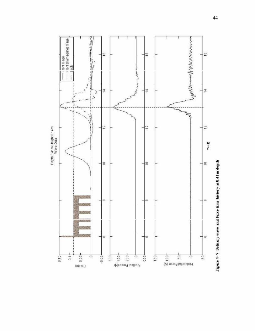
model becomes further submerged. Figures 4-6, 4-7, 4-8, and 4-9 show vertical and
horizontal force profiles aligned with wave profiles taken well in front of the bridge,
immediately in front of the bridge, and immediately behind the bridge over varying water
depth. The bridge model is superimposed into the figures to provide a height reference
for the waves as they impact the bridge model. The high frequency vibrations seen in the
force plots, especially the horizontal force, are the natural vibrations of the structure.

43
Figure 4- 6 Solitary wave and force time history at 0.39m Depth
44
Figure 4- 7 Solitary wave and force time history at 0.41m Depth

45
Figure 4- 8 Solitary wave and force time history at 0.48m Depth
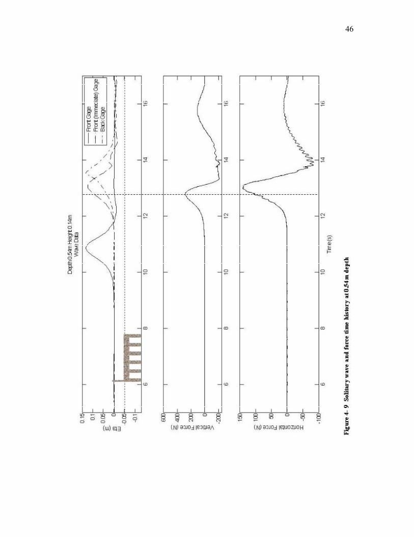
46
Figure 4- 9 Solitary wave and force time history at 0.54m Depth

47
As stated earlier, when force trends were investigated using the monochromatic
experiments, the data needed to be filtered to provide forces that corresponded to the
waves that best fit the target wave condition. Once again since the solitary wave is a
single event, filtering was not needed. This provided a more discernable force trend over
varying depth. Figure 4-10 and 4-11 show how the vertical force and horizontal force
vary over water depth, respectively. The forces are plotted with respect to the water
Maximum Vertical Force
100
200
300
400
500
600
700
0 0.05 0.1 0.15 0.2 0.25 0.3
(Eta_max + h)-h_girder (m)
Forc
e (N
) Height 10cm
Height 12cm
Height 14cm
Height 16cm
Figure 4- 10 Vertical force compared to water surface height above model

48
Maximum Horizontal Force
0
20
40
60
80
100
120
140
160
180
200
0 0.05 0.1 0.15 0.2 0.25 0.3
(Eta_max + h)-h_girder (m)
Forc
e (N
) Height 10cm
Height 12cm
Height 14cm
Height 16cm
Figure 4- 11 Horizontal Force compared to water surface height above model
surface measured from the basin floor. Each point represents an individual solitary wave
tests. The dominant parameter in hydrostatic forcing is the difference in overall water
surface height and the structure. Therefore these plots will show a hydrostatic trend if it
is present. Indeed a clear trend is seen in both vertical and horizontal force plots. The
vertical forces rise, peak, and subsequently fall. The rise associated with each water
depth seems to follow the same linear path. Each water depth then peaks at different
level and falls. The horizontal force rises linearly and seems to level out at a certain
point. Since neither plot show a conveniently straight line correlation, it can be
concluded that vertical and horizontal force are not a simple function of maximum water
height. Instead, there must be other factors or parameters involved. The suggested
method for force estimation discussed in Chapter VI presents a theory of possible factors.

49
Air Entrapment
Post-storm investigations of coastal bridge failures often speculate about uplift
force due to air entrapment between the bridge girders. The consequences of air-
entrapment to coastal bridges could be devastating. If 100% of the air was trapped
between the girders during a surge event, this could create a buoyancy force on the same
order of the actual weight of the bridge. Understanding the presence or absence of air-
entrapment is a large contribution to the overall uplift force produced during a storm
event.
To investigate if air-entrapment actually occurs, underwater cameras were placed
on the side of the model bridge. After tests were run, air-entrapment was indeed
observed for water depths below the deck height. During the tests in which acrylic panels
were attached to the model bridge a clear view of the space between the girders could be
recorded. As a wave inundated the bridge, water was unable to completely fill in the
space between the girders. The amount of air trapped between the girders was observed
to change with every wave event. However, it was never observed that 100% of the air
was trapped between girders.

50
CHAPTER V
COMPARISON OF PREVIOUS METHODOLOGIES
Previous literature offering force prediction methodologies were compared to
measured horizontal and vertical forces from the various experiments. The literature
used for the comparison was Bea et al. (2001), Kaplan et al. (1995), McConnell et al.
(2004), and Douglass et al. (2006). As stated in Chapter II, the Kaplan and Bea methods
are based on the equations from Morrison (1950). The forces prediction for these
methods is purely hydrodynamic. This means the accelerations and velocities of the fluid
provide the dominant forcing on the physical model. The McConnell and Douglass
methods are purely hydrostatic. This means the dominant factor in the force prediction is
the height of the water surface compared to the physical model.
Bea
As previously stated, Bea (2001) does not explicitly describe vertical force on
decks. However, the method described for horizontal forces can be used to determine
vertical forces by changing the horizontal components of velocity and acceleration to the
vertical components. Linear wave theory states that the water particle velocity and
acceleration are sinusoidal and 90o out of phase. Therefore to accurately represent the
force on a structure, the force components needed to be superimposed over an entire
wave length. Recall that the vertical force components equations of the total vertical
force are as follows.
51
Fs C Aus= 05 2. ρ (5-1)
Fl C Aul= 05 2. ρ (5-2)
Fi C Vam= ρ (5-3)
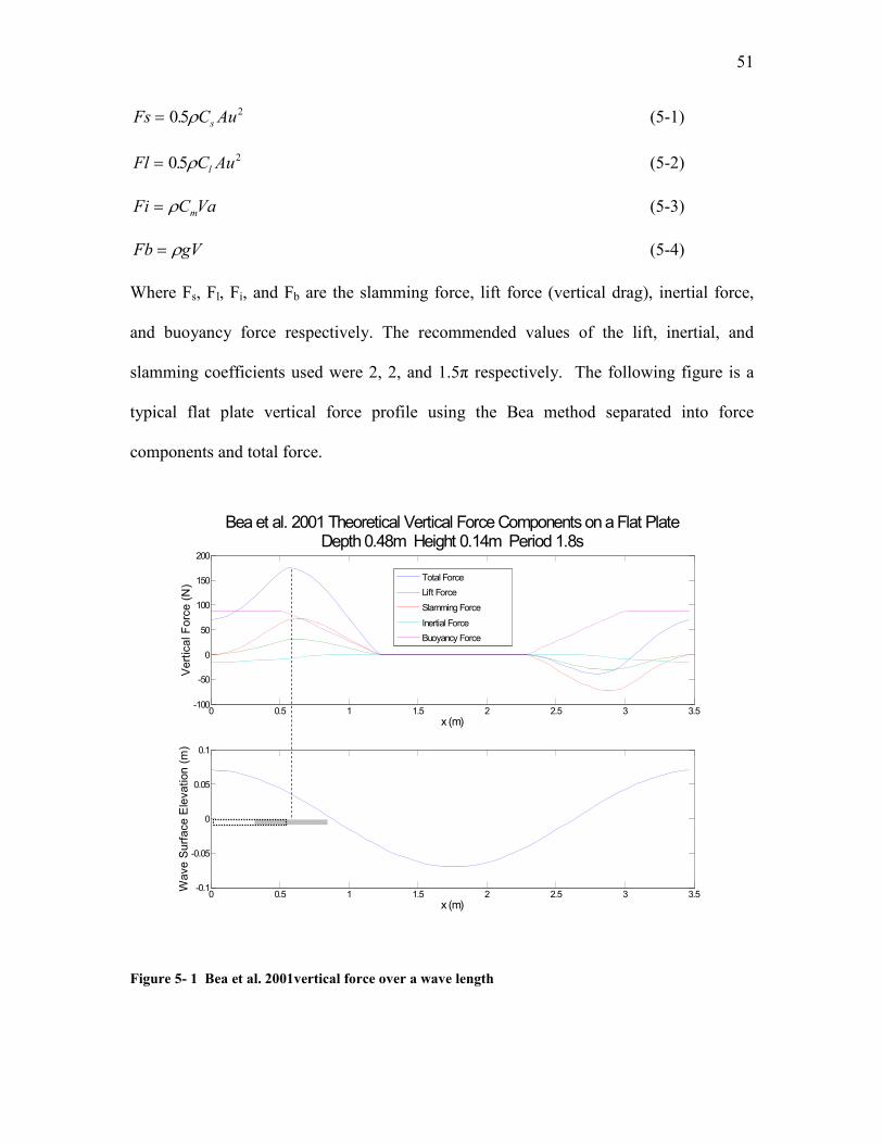
Fb gV= ρ (5-4)
Where Fs, Fl, Fi, and Fb are the slamming force, lift force (vertical drag), inertial force,
and buoyancy force respectively. The recommended values of the lift, inertial, and
slamming coefficients used were 2, 2, and 1.5π respectively. The following figure is a
typical flat plate vertical force profile using the Bea method separated into force
components and total force.
0 0.5 1 1.5 2 2.5 3 3.5-100
-50
0
50
100
150
200
x (m)
Ve
rtic
al F
orc
e (
N)
Bea et al. 2001 Theoretical Vertical Force Components on a Flat PlateDepth 0.48m Height 0.14m Period 1.8s
Total Force
Lift Force
Slamming Force
Inertial Force
Buoyancy Force
0 0.5 1 1.5 2 2.5 3 3.5-0.1
-0.05
0
0.05
0.1
x (m)
Wa
ve
Su
rfa
ce
Ele
va
tion
(m
)
Figure 5- 1 Bea et al. 2001vertical force over a wave length

52
According to the Bea method, the location of the flat plate relative to the water
surface during the maximum vertical force is shown in Figure 5-1 by the gray box. It can
be seen that the location of the flat plate during the maximum vertical force in the
experiments happens just before or right when the crest arrives at the leading edge of the
structure. This is shown in Figure 5-1 by the dotted box. These locations of maximum
vertical force are not in congruence.
It can also be observed in Figure 5-1 all of the force components go to zero for
some duration. This is due to the wetted surface area going to zero. As the wave trough
passes the structure, according to linear theory, no water will be in contact with the
structure and therefore the force is zero.
Kaplan
The Kaplan et al. (1995) method is very similar to the Bea et al. (2001) method
except there is no slamming component and the vertical inertial force, Fi is found using
the 3-dimensional added mass of the structure. Once again the total force needs to be
calculated by superimposing the force components over an entire wave length. Recall
that the condensed vertical force equation for Kaplan et al. (1995) is as follows.
Ft
M w blC w wz D= +∂
∂
ρ( )3
2 (5-5)
Figure 5-2 shows the vertical force components and the total force over an entire wave
length for a flat plate at a distance 0.48m from the floor with a wave condition of
H=0.14m, T= 1.8s, and h=0.48m. A drag coefficient of 2 was used to determine the
lifting force component. The maximum force occurs at about halfway between the crest

53
and the trough. This location of the maximum force is not congruent with the
experimental data.
0 0.5 1 1.5 2 2.5 3 3.5-300
-200
-100
0
100
200
300
x (m)
Vert
ical F
orc
e (
N)
Kaplan (1995) Flat Plate: Depth 0.48m Height 0.14m Period 1.8s
0 0.5 1 1.5 2 2.5 3 3.5-0.1
-0.05
0
0.05
0.1
x (m)
Wave H
eig
ht
(m)
Total Force
Lift Force
Inertial Force
Buoancy Force
Total Force
Lift Force
Inertial Force
Buoyancy Force
Figure 5- 2 Kaplan et al. 1995 vertical force over a wave length
It was observed from the bridge specimen that as the period of the wave increased
keeping the wave height and water depth constant the vertical force increased. Figure 5-3
shows how the Kaplan method predicts the vertical force as the period is varied keeping
the water depth and wave height constant.

54
0 1 2 3 4 5 6-400
-300
-200
-100
0
100
200
300
x (m)
Vert
ical F
orc
e (
N)
Kaplan - Varying PeriodFlat Plate: Depth 0.48m Height 0.14m
0 1 2 3 4 5 6-0.1
-0.05
0
0.05
0.1
x (m)
Wave E
levation (
m)
Figure 5- 3 Kaplan et al. 1995 vertical force varying period trend
The red, green, and purple lines represent the 1.3s, 1.8s, and 2.5s period waves
respectively. As the wave period increases the maximum vertical force begins to
decrease nonlinearly. This is opposite of what was observed during experimentation.
McConnell and Douglass
The McConnell and Douglass methods are hydrostatic and do not require
analyzing over a wave length. The main factor in force prediction for these methods is
the height between the wave crest elevation and the structure. Both methods are

55
empirical. The recommended empirical coefficients from the literature were used for the
comparison of the methods to experimental data.
Correlation of Previous Methods and Measured Forces
Numerous waves and consequently force events were generated and recorded
over all the experiments. This data were accumulated and made into comparison plots to
visually and quantitatively show the comparison of previous methodologies to measured
forces. The data from each wave event was used to calculate an estimated force for each
method and then compared to the corresponding force recorded from that wave event.
Since the Bea and Kaplan methods are based on wave height, period, and water
depth each wave event had to be individually processed. The period and water depth
used for the Kaplan and Bea calculations was the target wave period and basin water
depth. The wave height was determined using the zero up-crossing method where the
wave height was calculated by subtracting the wave crest elevation from the wave trough
elevation of the determined wave event. The McConnell and Douglass methods used
only the wave crest elevation from each wave event to calculate the estimated force.
Monochromatic Waves
Figures 5-4 – 5-7 show each of the previous methods compared to the actual
measured vertical forces on the flat plate using monochromatic waves. The data for
Figures 5-4 – 5-7 were collected during Experimental Set IV

56
0 100 200 300 400 500 6000
200
400
600
800
1000
1200
Measured Force (N)
Calc
ula
ted
Fo
rce
(N
)
Kaplan vs Experimental Flat Plate
0.43m Depth
0.46m Depth
0.48m Depth
0.51m Depth
0.54m Depth
Figure 5- 4 Kaplan method compared to vertical force measurements
0 100 200 300 400 500 6000
200
400
600
800
1000
1200
Measured Force Force (N)
Calc
ula
ted
Fo
rce
(N
)
Bea vs ExperimentalFlat Plate
0.43m Depth
0.46m Depth
0.48m Depth
0.51m Depth
0.54m Depth
Figure 5- 5 Bea method compared to vertical force measurements

57
0 100 200 300 400 500 6000
200
400
600
800
1000
1200
Measured Force (N)
Ca
lcu
late
d F
orc
e (
N)
McConnell vs Experimental Flat Plate
0.43m Depth
0.46m Depth
0.48m Depth
0.51m Depth
0.54m Depth
Figure 5- 6 McConnell method compared to vertical force measurements
0 100 200 300 400 500 6000
200
400
600
800
1000
1200
Measured Force (N)
Ca
lcula
ted F
orc
e (
N)
Douglass vs ExperimentalFlat Plate
0.43m Depth
0.46m Depth
0.48m Depth
0.51m Depth
0.54m Depth
Figure 5- 7 Douglass method compared to vertical force measurements

58
Each point that is graphed represents the force produced by one wave event. On each
figure, 5 tests with varying water depth are shown. The forces vary within the individual
depths due to the non-uniform waves which were discussed in Chapter IV.
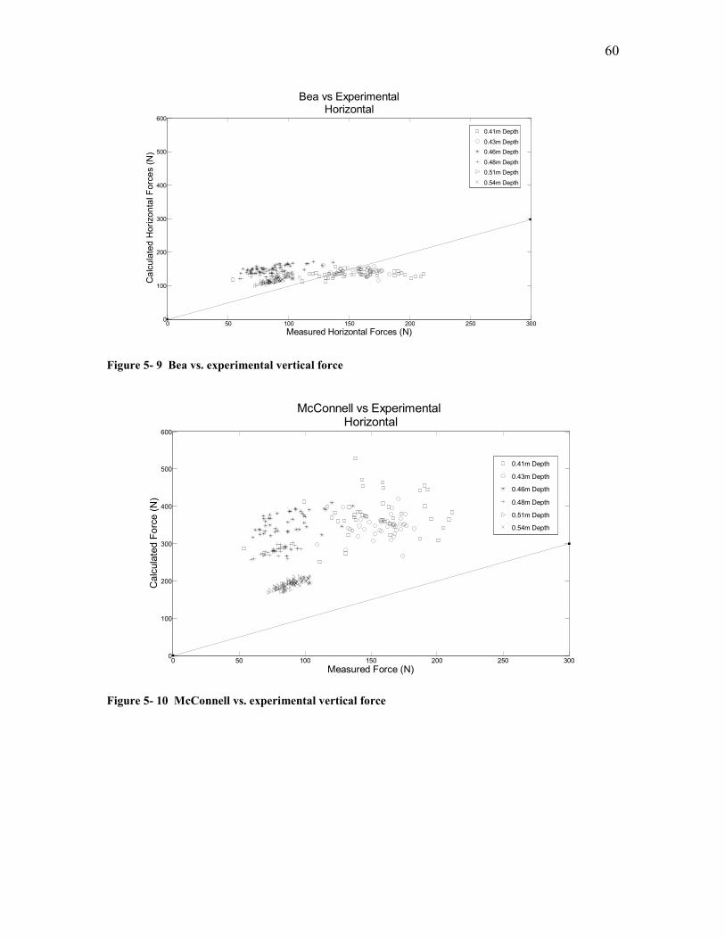
In general the hydrodynamic methods (Kaplan and Bea) tend to underestimate the
vertical forces and the hydrostatic methods (McConnell and Douglass) tend to
overestimate the vertical forces. No method showed a perfectly linear correlation with
the measured vertical forces. The Douglass method in particular showed the best overall
bias (measured vertical force mean divided by calculated vertical force mean) at lower
water depths. Table 5-1 shows the vertical force bias for all four methods for individual
water depths and overall as well the standard deviation for the overall bias. It is apparent
that no method was able to sufficiently predict the change in vertical force due to water
depth.
Table 5- 1 Previous methods vertical force statistical bias
Water Depth Kaplan Bea McConnell Douglass
0.43 m 1.585 2.190 0.652 1.180
0.46 m 2.104 2.800 0.663 0.890
0.48 m 1.571 2.060 0.560 0.669
0.51 m 1.111 1.674 0.463 0.444
0 54 m 1.280 2.140 0.506 0.413
Overall Bias 1.523 2.175 0.511 0.716
Standard Deviation 0.421 0.521 0.121 0.324

59
Comparing the measured horizontal forces to the existing methods similarly
showed no perfect correlation. Figures 5-8 – 5-11 shows the four methods under
investigation compared to horizontal measurements gathered during Experimental Set III.
Again each point represents one wave event during a test. In each figure, 6 tests are
shown representing different water depths. Table 5-2 shows the horizontal force bias for
all four methods for individual water depths and overall as well the standard deviation for
the overall bias.
0 50 100 150 200 250 3000
100
200
300
400
500
600
Measured Force (N)
Ca
lcula
ted F
orc
e (
N)
Kaplan vs ExperimentalHorizontal
0.41m Depth
0.43m Depth
0.46m Depth
0.48m Depth
0.51m Depth
0.54m Depth
Figure 5- 8 Kaplan vs. experimental vertical force
60
0 50 100 150 200 250 3000
100
200
300
400
500
600
Measured Horizontal Forces (N)
Ca
lcula
ted
Hori
zon
tal F
orc
es (
N)
Bea vs ExperimentalHorizontal
0.41m Depth
0.43m Depth
0.46m Depth
0.48m Depth
0.51m Depth
0.54m Depth
Figure 5- 9 Bea vs. experimental vertical force
0 50 100 150 200 250 3000
100
200
300
400
500
600
Measured Force (N)
Calc
ula
ted F
orc
e (
N)
McConnell vs Experimental Horizontal
0.41m Depth
0.43m Depth
0.46m Depth
0.48m Depth
0.51m Depth
0.54m Depth
Figure 5- 10 McConnell vs. experimental vertical force

61
0 50 100 150 200 250 3000
100
200
300
400
500
600
Measured Force (N)
Calc
ula
ted F
orc
e (
N)
Douglass vs ExperimentalHorizontal
0.41m Depth
0.43m Depth
0.46m Depth
0.48m Depth
0.51m Depth
0.54m Depth
Figure 5- 11 Douglass vs. experimental vertical force
Table 5- 2 Previous methods horizontal force statistical bias
Depth Kaplan Bea McConnell Douglass
0.41 m 13.403 1.145 0.403 2.222
0.43 m 14.626 1.111 0.457 1.662
0.46 m 7.514 0.566 0.243 0.653
0.48 m 8.376 0.576 0.284 0.515
0.51 m 12.544 0.738 0.454 0.464
0.54 m 21.510 0.778 0.485 0.399
Overall Bias 11.6 1.05 0.389 0.99
Standard Deviation 3.23 0.3386 0.106 0.748

62
Solitary Wave Experiment
The solitary wave experiment provided a more definitive data set than the
monochromatic wave experiments. The model bridge was used for the solitary wave
experiment. The McConnell and Douglass methods were compared to the measured
vertical and horizontal forces.
Figures 5-12 and 5-13 show the McConnell and Douglass methods compared to
the measured vertical force for the solitary wave experiments. Each point represents one
wave event (one solitary wave test). During Experimental Set V the water depths tested
were 0.39m, 0.41m, 0.43m, 0.46m, 0.48m, 0.51m, and 0.54m and the wave heights tested
were 0.1m, 0.12m, 0.14m, and 0.16m.
McConnell vs Experimental
Vertical
0
100
200
300
400
500
600
700
0 100 200 300 400 500 600 700
Measured Force (N)
Calc
ula
ted F
orc
e (N
)
0.39m Depth
0.41m Depth
0.43m Depth
0.46m Depth
0.48m Depth
0.51m Depth
0.54m Depth
Figure 5- 12 McConnell vs. experimental vertical force solitary wave results

63
Douglass vs Experimental
Vertical
0
200
400
600
800
1000
1200
1400
1600
0 100 200 300 400 500 600 700
Measured Force (N)
Calc
ula
ted F
orc
e (N
)
0.39m Depth
0.41m Depth
0.43m Depth
0.46m Depth
0.48m Depth
0.51m Depth
0.54m Depth
Figure 5- 13 Douglass vs. experimental vertical force solitary wave results
It can be observed that in both methods several points (tests) are overestimated.
These points represent the tests carried out at higher water depths (h>0.48m). Recall
from Figure 4-10 that as the water depth increased the vertical force raised linearly and
peaked when the water depth reached the deck level. Neither method predicts this peak
as the water depth increases.
Figures 5-14 and 5-15 show the McConnell and Douglass methods compared to
measured horizontal force.
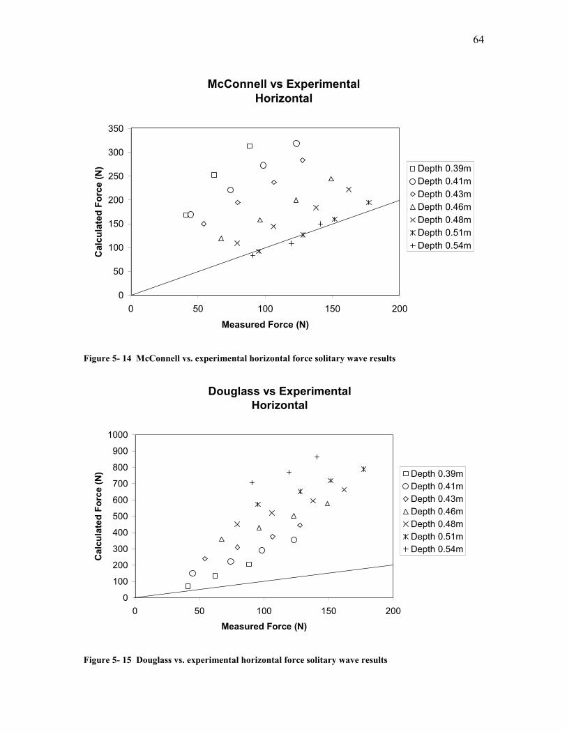
64
McConnell vs Experimental
Horizontal
0
50
100
150
200
250
300
350
0 50 100 150 200
Measured Force (N)
Calc
ula
ted F
orc
e (N
) Depth 0.39m
Depth 0.41m
Depth 0.43m
Depth 0.46m
Depth 0.48m
Depth 0.51m
Depth 0.54m
Figure 5- 14 McConnell vs. experimental horizontal force solitary wave results
Douglass vs Experimental
Horizontal
0
100
200
300
400
500
600
700
800
900
1000
0 50 100 150 200
Measured Force (N)
Calc
ula
ted F
orc
e (N
) Depth 0.39m
Depth 0.41m
Depth 0.43m
Depth 0.46m
Depth 0.48m
Depth 0.51m
Depth 0.54m
Figure 5- 15 Douglass vs. experimental horizontal force solitary wave results

65
Both methods overestimate the measured horizontal force. It appears the McConnell
method increases in accuracy as the water depth increases. This trend is opposite to the
Douglass prediction of the vertical force. The Douglass method increasingly over
predicts the horizontal force as the water depth rises.
Conclusion of Previous Methods Comparison
None of the existing methods showed a perfect correlation with measured forces
for all water depths tested. The hydrodynamic methods seemed to have less correlation
compared to the hydrostatic methods. By observing the wave location when the
maximum force occurs, a hydrostatic forcing is suggested.

66
CHAPTER VI
SUGGESTED METHOD
In chapter IV it was observed that the dominant forcing in both the vertical and
horizontal direction is hydrostatic. No clear advantage was observed between the
McConnell and Douglass methods. Thus, a suggested method for estimating forces on
bridge structures is proposed herein. The Douglass method was used as a base for this
suggested method due to its simplicity. The flat plate will first be discussed and used for
developing the suggested method because of its simple geometry. Later, the effects of a
complex geometry are discussed and force estimation methods are developed.
Wave Height and Vertical Force Correlation
A wave height correlation to vertical force is needed before continuing the
development of the suggested method which is dominantly hydrostatic and only quasi-
dependent on wave height. Hydrodynamic methods estimate forces on structures using
fluid velocities and accelerations. These velocities and accelerations are direct functions
of wave height among other parameters. The logic is that if the vertical force was
dominantly dependent on hydrodynamic forcing then it should be linearly correlated to
the wave height. The following figure is a plot of wave height versus vertical force from
the data collected during the Experimental Set IV for several water depths. Each point
represents a single wave event. The data is sorted by water depth. Within a water depth
there is variation in wave heights due to non-uniform waves. Observing the 0.43m depth

67
0.08 0.09 0.1 0.11 0.12 0.13 0.14 0.15 0.160
50
100
150
200
250
300
350
400
450
500
Wave Height (m)
Vert
ical F
orc
e (
N)
Force Dependency on Wave Height
0.43m Depth
0.46m Depth
0.48m Depth
0.51m Depth
0.54m Depth
Figure 6- 1 Vertical force compared to wave height
visually a correlation exists between increased wave height and vertical force. However,
as the depth increases the correlation becomes difficult to observe. Table 6-1 shows the
correlation coefficient for each depth shown in Figure 6-1. The large scatter of data
Table 6- 1 Correlation coefficient for wave height compared to vertical force
Depth 0.43m 0.46m 0.48m 0.51m 0.54m
r .8404 -0.0834 0.711 0.6742 0.05
makes it still difficult to discern any information about the correlation between wave
height and vertical force. However, it appears as the water depth increases the correlation

68
decreases. This leads to the assumption that as water depth increases the wave height
becomes less important.
Maximum Water Depth and Vertical Force Correlation
The maximum water depth is defined as the sum of the maximum η (wave crest
elevation) and the water depth. Both hydrostatic methods reviewed calculated the
vertical force without accounting for water to flow over the structure. It was observed
visually that as a wave inundated the structure, the water would overtop or flow over the
model if the wave crest was higher than the deck level.
If maximum water depth is plotted against vertical force, no obvious relationship
exists. However, if the weight of the water that overtops the flat plate is added to the
maximum vertical force a linear relationship is apparent. To quantify this, the
overtopping water was simplified into a horizontal triangular column of water. The
profile of this is shown in Figure 6-2. If the SWL is above the deck level the overtopping
Figure 6- 2 Profile of overtopping water weight (lower water depth)

69
water weight is represented by a triangular column with the addition of a parallelepiped.
The profile of this is shown in Figure 6-3. The equations for the weight of this simplified
Figure 6- 3 Profile of overtopping water weight (higher water depth)
shape of overtopping water are given in the following equations.
F Aw =1
2γδ (6-1)
for h ≤ hmodel
F A h h Aw el= + −1
2γδ γ ( )mod
(6-2)
For h > hmodel
Where A is the wetted surface area of the flat plate.
Figure 6-4 shows the comparison of the modified vertical force (Vertical Force +
Weight of Overtopping Water using equations 6-1 and 6-2) and maximum water height.
The relationship is surprisingly linear and corresponds directly with Douglass (2006).
The 0.43m data are not on the same line as the rest of the data because of the difference

70
0.48 0.5 0.52 0.54 0.56 0.58 0.6 0.62 0.64 0.660
200
400
600
800
1000
1200
Maximum Water Height (m)
Vert
ical F
orc
e +
Weig
ht
of
Overt
oppin
g W
ate
r (N
)
Force Dependency on Maximum Water Height
0.43m Depth
0.46m Depth
0.48m Depth
0.51m Depth
0.54m Depth
Figure 6- 4 Correlation of maximum wave crest above the SWL, η, and vertical force
in wetted surface area. At the depth of 0.43m the wetted surface area is not completely
covered therefore it yields a lower upward force and follows a line shifted slightly down.
The rest of the water depths’ wetted surface area is equal to the surface area of the flat
plate and consequently follow the same line.
Reversing the Correlation
The correlation between the maximum water height and vertical force clearly
suggests a hydrostatic force behavior. If the previous method for determining the
correlation of the maximum water height and vertical force were reversed, then a simple
modified hydrostatic formula could estimate the vertical loads. The method the author
suggests for calculating the vertical force on a flat plate is essentially the same as
formulated in Douglass (2006) however the weight of the overtopping water would be

71
subtracted from the vertical force which the flat plate experiences. The suggested
equation for estimating vertical force on a flat plate is shown in the following equation.
F A Fvertical w= −γδ (6-3)
This method was used with the zero-upcrossing analysis to estimate the vertical
forces from each wave crest. The estimated forces were then compared to the measured
force resulting from the corresponding wave crest. Figure 6-5 shows the comparison of
the empirical solution and the experimental measurements.
0 50 100 150 200 250 300 350 400 450 5000
50
100
150
200
250
300
350
400
450
500
Measured Vertical Force (N)
Ca
lcu
late
d V
ert
ica
l F
orc
e (
N)
Suggested Method vs ExperimentalExperimental Set IV
0.43m Depth
0.46m Depth
0.48m Depth
0.51m Depth
0.54m Depth
Figure 6- 5 Suggested method compared to measured vertical force on a flat plate
If the bias for each point (measured divided by calculated) is averaged, then the
overall bias is 1.14 with a standard deviation of 0.251. There is still a great deal of

72
scatter, however this is somewhat to be expected due to the oversimplification of the
force estimation.
Estimating Uplift Force for a Complex Geometry
It is important to be able to predict the forces on a complex geometry since the
structures under investigation are highway bridges and not simple flat plates. The
following outlines how the suggested method is modified to predict vertical forces on
more complex geometries such as the bridge model. The actual theory behind estimating
the uplift forces on a structure is simple. The total force equals the sum of the buoyancy
of the inundated bridge and hydrostatic uplift minus the weight of the overtopping water.
However, accurately calculating this can be complex if a great deal of accuracy is
desired. For a structure with girders air-entrapment needs to be factored into the
inundated bridge buoyancy term.
A visual way of understanding how the forces act on a structure is by “freeze
framing” the inundating wave just when the wave crest reaches the leading edge of the
structure. The hydrostatic uplift force is caused by the difference in elevation between
the wave crest and the deck. The buoyancy force is caused by the amount of volume the
bridge is displacing. If the SWL is below the deck level the buoyancy force needs to
incorporate the volume displaced by air entrapment between the girders. The downward
overtopping force is caused by the weight of the water on the deck.
Figure 6-6 shows a schematic of the forces acting on typical bridge deck when the
SWL is at or below deck level. It should be noted that the hydrostatic force in this
schematic incorporates the simplified overtopping water weight. From visual
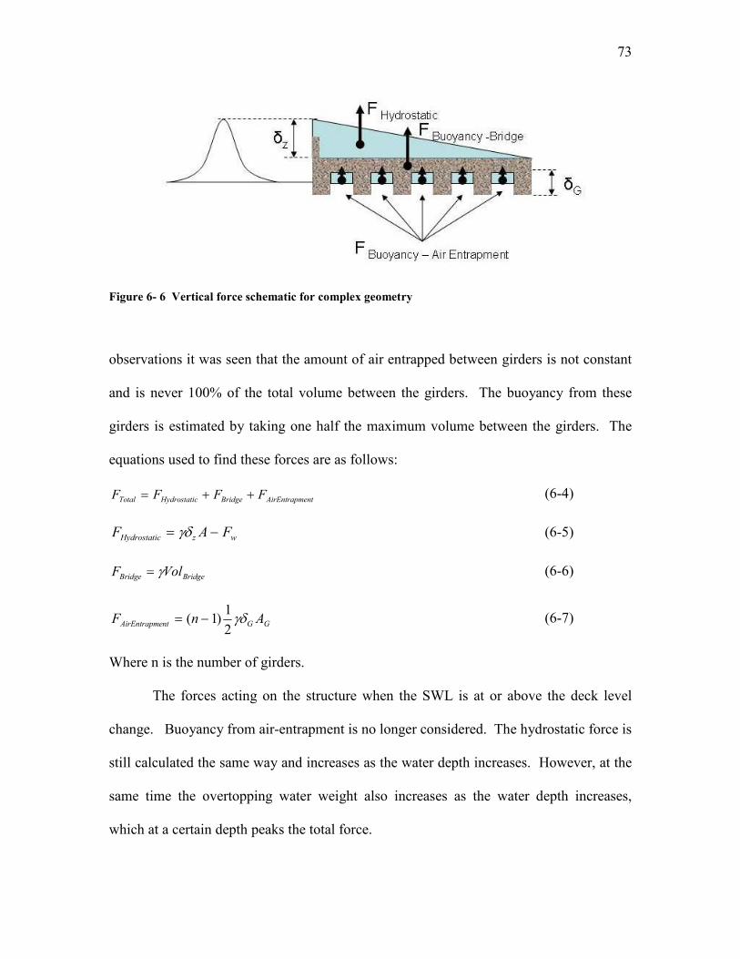
73
Figure 6- 6 Vertical force schematic for complex geometry
observations it was seen that the amount of air entrapped between girders is not constant
and is never 100% of the total volume between the girders. The buoyancy from these
girders is estimated by taking one half the maximum volume between the girders. The
equations used to find these forces are as follows:
F F F FTotal Hydrostatic Bridge AirEntrapment= + + (6-4)
F A FHydrostatic z w= −γδ (6-5)
F VolBridge Bridge= γ (6-6)
F n AAirEntrapment G G= −( )11
2γδ (6-7)
Where n is the number of girders.
The forces acting on the structure when the SWL is at or above the deck level
change. Buoyancy from air-entrapment is no longer considered. The hydrostatic force is
still calculated the same way and increases as the water depth increases. However, at the
same time the overtopping water weight also increases as the water depth increases,
which at a certain depth peaks the total force.

74
The following figures show this method compared to the forces calculated during
the monochromatic bridge tests from Experimental Set I and III respectively. Each point
on the figures represents a single wave event. Figure 6-7 is separated into various wave
heights and water depths with a constant period of 1.8s. Figure 6-8 is separated into
varying water depths. The overall bias for the suggested method compared to
Experimental Set I is 1.056 with a standard deviation of 0.192. The overall bias for the
suggested method compared to Experimental Set III is 0.969 with a standard deviation of
0.154. These figures show repeatability in both the experiments and the suggested
method. It is clear from these figures that the dominant forcing is hydrostatic. However,
a significant amount of scatter is still present.
0 100 200 300 400 500 600 7000
100
200
300
400
500
600
700
Measured Vertical Force (N)
Calc
ula
ted
Vert
ca
l F
orc
e (
N)
Suggested Method vs ExperimentalExperimental Set I
0.41m Depth0.14m Target Wave Height
0.48m Depth0.14m Target Wave Height
0.54m Depth0.14m Target Wave Height
0.41m Depth0.12m Target Wave Height
0.48m Depth0.12m Target Wave Height
0.54m Depth0.12m Target Wave Height
0.48m Depth0.10m Target Wave Height
0.54m Depth0.10m Target Wave Height
Figure 6- 7 Suggested method vs. measured vertical force (experimental set I)

75
0 100 200 300 400 500 600 7000
100
200
300
400
500
600
700
Measured Vertical Force (N)
Ca
lcu
late
d V
ert
ical F
orc
e (
N)
Suggested Method vs ExperimentalExperimental Set III
0.41m Depth
0.43m Depth
0.46m Depth
0.48m Depth
0.51m Depth
0.54m Depth
Figure 6- 8 Suggested method vs. measured vertical force (experimental set III)
Solitary Wave Comparison
The suggested method was applied to the solitary wave experiment. The more
discernable data produced from the Experimental Set V gives an indication of the validity
of the suggested method. Figure 6-9 shows vertical force calculated using the suggested
method compared to the measured data from Experimental Set V. The overall bias for
the suggested method compared to Experimental Set V is 0.849 with a standard deviation
of 0.83. It can be observed from the comparison plot that the suggested method tends to
over estimate the measured vertical velocities. Recall that these calculations are done
using an oversimplified model of the wave impacting the structure “freeze-framed” when
the wave crest is located at the leading edge. If the overtopping weight is increased from
the 0.5 factor to 0.65 factor a better relationship is seen. This is shown in Figure 6-10.
The overall bias when modifying the overtopping weight for the vertical suggested

76
Suggested Method vs Experimental
Experimental Set V (Overtopping = 0.5)
0
100
200
300
400
500
600
700
800
900
0 100 200 300 400 500 600 700
Measured Vertical Force (N)
Calc
ula
ted V
ert
ical Forc
e (N
)
0.39m
0.41m
0.43m
0.46m
0.48m
0.51m
0.54m
Figure 6- 9 Suggested method vs. measured vertical force (experimental set V)
method compared to Experimental Set V is 0.925 with a standard deviation of 0.077.
Suggested Method vs Experimental
Experimental Set V (Overtopping = 0.6)
0
100
200
300
400
500
600
700
800
0 100 200 300 400 500 600 700
Measured Vertical Force (N)
Calc
ula
ted V
ert
ical Forc
e (N
)
0.39m
0.41m
0.43m
0.46m
0.48m
0.51m
0.54m
Figure 6- 10 Suggested method vs. measured vertical force with modified overtopping (experimental
set V)

77
To demonstrate the increase in overtopping weight, refer to Figure 6-11. Computation of
the original overtopping weight uses a simple horizontal triangular column or
combination of a horizontal triangular column and parallelepiped to represent the water
flowing over the top of the structure. It is speculated the actual weight of the overtopping
water is greater than that represented by the simple triangular column. This justifies
slight alterations in the overtopping weight done in Figure 6-9 to create a better
relationship.
Figure 6- 11 Schematic of realistic overtopping weight
Suggested Method for Calculating Horizontal Forces
As discussed in Chapter V the measured horizontal force was found from the
solitary wave experiment to increase linearly. The Douglass method increased linearly,
but substantially overestimated the force. Again for developing a horizontal suggested
method the Douglass method was used as a base.
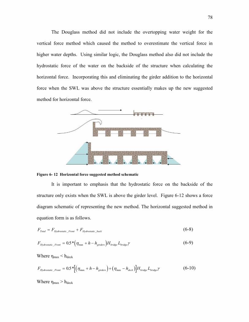
78
The Douglass method did not include the overtopping water weight for the
vertical force method which caused the method to overestimate the vertical force in
higher water depths. Using similar logic, the Douglass method also did not include the
hydrostatic force of the water on the backside of the structure when calculating the
horizontal force. Incorporating this and eliminating the girder addition to the horizontal
force when the SWL was above the structure essentially makes up the new suggested
method for horizontal force.
Figure 6- 12 Horizontal force suggested method schematic
It is important to emphasis that the hydrostatic force on the backside of the
structure only exists when the SWL is above the girder level. Figure 6-12 shows a force
diagram schematic of representing the new method. The horizontal suggested method in
equation form is as follows.
F F FTotal Hydrostatic Front Hydrostatic back= +_ _ (6-8)
( )F h h H LHydrostatic Front girders bridge bridge_ max. *= + −05 η γ (6-9)
Where ηmax < hdeck
( ) ( )[ ]F h h h H LHydrostatic Front girders deck bridge bridge_ max max. *= + − + −05 η η γ (6-10)
Where ηmax > hdeck

79
FHydrostatic back_ = 0 (6-11)
Where SWL < hgirders
F h h LHydrostatic back girder bridge_ . ( )= −05 2 γ (6-12)
Where SWL > hgirders
Figure 6-13 is a definition sketch of the terms used in Equations 6-8 to 6-12.
hgird
er
hd
eck
Hbridge
Lbridge
ηmaxSWL
h
Figure 6- 13 Definition sketch for horizontal force suggested method
The suggested horizontal method was compared to the solitary wave measured
horizontal forces. Figure 6-14 shows the suggested method horizontal force calculation
compared to the measured data from Experimental Set V. The overall bias for the
horizontal suggested method compared to Experimental Set V is 0.949 with a standard
deviation of 0.124.

80
Suggested Method vs Experimental
Experimental Set V
0
50
100
150
200
0 50 100 150 200
Measured Horizontal Force (N)
Calc
ula
ted H
ori
zonta
l Forc
e (N
)
0.39m
0.41m
0.43m
0.46m
0.48m
0.51m
0.54m
Figure 6- 14 Suggested method vs. measured horizontal force (experimental set V)
As opposed to the Douglass method where the horizontal prediction severely
overestimated the measured forces, the new method has reduced the predicted force by
subtracting the hydrostatic force caused by the water on the backside of the structure
when the SWL was above the girders.
Hydrodynamic Consideration
The suggested method is based on the hydrostatic forcing method. The method
was developed by essentially “freeze-framing” the wave as it impacted the bridge and
summing all of the forces. However, in reality the wave is in motion and therefore the
water particles are in motion. Therefore, hydrodynamic effects are still present during a
wave event.

81
Using linear theory, wave particle velocities and accelerations were calculated for
sample wave conditions. They were then used to calculate vertical and horizontal forces
using the Morison equations (Morison et al., 1950) used in the Bea method (excluding
slamming) by integrating along the appropriate area of the model. However, differing
from the Bea method, the forces were calculated when wave crest approached the leading
edge of the model as observed from the measured data. When this was done, force
calculations were found to be on the order of the error associated with the suggested
method.
Table 6- 2 Hydrostatic contribution example
Wave Height (H) Wave Period (T) Water Depth (h)
14cm 1.8s 48cm
Hydrodynamic Contribution Buoyancy Contribution Total Vertical Force
~15N 85N ~525 +/-20N
Table 6-2 demonstrates the hydrodynamic contribution for a sample wave on the
flat plate model. The hydrodynamic contribution was calculated using the Bea method
(excluding slamming) when the wave crest approaches the leading edge of the structure.
The total force is the measured value from Experimental Set IV. This value and the error
(scatter) can be seen visually in Figure 6-14. The dynamic contribution is significantly
smaller than the total vertical force even if the buoyancy is removed.
In conclusion, hydrodynamic forces are present during a wave event however at
the moment of maximum force, the hydrostatic component is dominant. When the
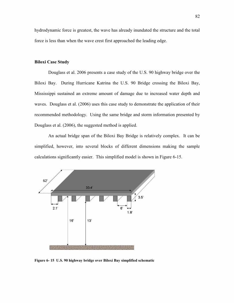
82
hydrodynamic force is greatest, the wave has already inundated the structure and the total
force is less than when the wave crest first approached the leading edge.
Biloxi Case Study
Douglass et al. 2006 presents a case study of the U.S. 90 highway bridge over the
Biloxi Bay. During Hurricane Katrina the U.S. 90 Bridge crossing the Biloxi Bay,
Mississippi sustained an extreme amount of damage due to increased water depth and
waves. Douglass et al. (2006) uses this case study to demonstrate the application of their
recommended methodology. Using the same bridge and storm information presented by
Douglass et al. (2006), the suggested method is applied.
An actual bridge span of the Biloxi Bay Bridge is relatively complex. It can be
simplified, however, into several blocks of different dimensions making the sample
calculations significantly easier. This simplified model is shown in Figure 6-15.
Figure 6- 15 U.S. 90 highway bridge over Biloxi Bay simplified schematic

83
The SWL and ηmax provided in the literature are 11.9ft and 8.06ft respectively.
The following calculates the vertical and horizontal forces using the suggested method.
Vertical Force
The vertical force equations and calculations are listed below.
F F F FTotal Hydrostatic Bridge AirEntrapment= + + (6-13)
F A FHydrostatic z w= −γδ (6-14)
F VolBridge Bridge= γ (6-15)
F n AAirEntrapment G G= −( )11
2γδ (6-16)
F Aw z= 05. γδ
( )( )( )F lbsw = + − =05 62 4 119 8 06 165 52 334 187 491. * . * . . . * . ,
( )( )( )F lbsHydrostatic = + − − =62 4 119 8 06 165 52 334 187 491 187 491. . . . * . , ,
( ) ( )( )F lbsBridge = + =62 4 334 52 5 6 18 3 52 159 319. . * *. . * * ,
F lbsAirEntrapment = − =( ) . * * * ,6 11
262 4 3 6 52 146 016
F lbs lbs lbs lbs tonsTotal = + + = =187 491 159 319 146 016 492 826 246 4, , , , .
Horizontal Force
The horizontal force equations and calculations are listed below.
F F FTotal Hydrostatic Front Hydrostatic back= +_ _ (6-17)
( ) ( )[ ]F h h H LHydrostatic Front girders deck bridge bridge_ max max. *= − + −05 η η γ (6-18)
FHydrostatic back_ = 0 (6-19)
( ) ( )[ ]F lbs tonsHydrostatic Front_ . * . . . . . * * . , .= + − + + − = =05 8 06 119 13 8 06 119 16 35 52 62 4 62 008 310

84
F lbs tonsTotal = =62 008 310, .
The predicted vertical and horizontal force using the suggested method is 493,000lbs and
62,000lbs respectively. Douglass et al. (2006) method predicts the vertical and horizontal
forces to be 440,000lbs and 230,000lbs. The vertical force predictions for the two
methods are very similar. This is to be expected since the suggested method does not
differ greatly from the Douglass method until the SWL comes above the deck level.

85
CHAPTER VII
CONCLUSION
Research was conducted to investigate wave and surge forces on deck structures.
Two physical models, a 1:20 bridge model and flat plate were used during the
experimentation. Varied wave conditions and water depths were tested on both physical
models. Force and wave measurements and visual data were recorded. The data were
then analyzed and force mechanisms and trends were investigated. The goal of this
research was to evaluate a method to estimate wave and surge loads on bridge decks
given a specific wave condition.
Four preexisting theoretical methods for calculating forces on deck-like structures
were compared to the measured force data from the experiments. The literature for the
selected methods under investigation include Kaplan et al. (1995), Bea et al. (2001),
McConnell et al. (2004), and Douglass et al. (2006). The following conclusions were
made from the comparisons:
• No method under review sufficiently predicted the measured forces for all wave
conditions
• Both the Kaplan and Bea methods which are based on hydrodynamic theory
consistently underestimated the forces.
• Both the McConnell and Douglass methods which are based on hydrostatic theory
in general overestimated the forces, especially at a SWL above or at deck level.
• The Douglass method provided the best relative correlation for uplift forces for a
SWL below the deck elevation.

86
Due to the unsatisfactory prediction of the preexisting methods, the forcing events
were investigated in greater detail to better understand the damaging mechanisms during
a wave event. After reviewing force events, it was observed that the maximum vertical
force occurred as the crest of the wave approached the leading edge of the structure. It
was also observed that the maximum horizontal force occurred at the same time as the
maximum vertical force when the SWL was below the deck level. When the SWL was
above the deck level and structure was then fully submerged the maximum horizontal
force was slightly delayed in reference to the vertical force. In the hydrostatic theories
developed by Douglass and McConnell it can be determined that the maximum force will
occur when there is the greatest difference in the water immediately in front of the
structure and the structure itself. This corresponds to the experimental observations.
In contrast, in the hydrodynamic theories developed by Kaplan and Bea the
maximum force will occur when the wave crest has reached close to the middle of the
structure. Also, using underwater video cameras, it was observed that air was trapped
between girders when the SWL was below the deck level. This leads to the following
conclusions:
• The dominant uplift force mechanism is caused by hydrostatic pressure
differences when the wave crest reaches the leading edge of the structure.
• Air-entrapment does exist between girders when the SWL is below the deck in
experimental tests. Air-entrapment has the potential to contribute a significant
uplift buoyancy force.

87
Using the Douglass method for calculating forces on bridges decks as a base, an
improved method was developed. The improved method includes uplift forces incurred
by overtopping water and air-entrapment. It was found that adding the buoyancy effects
for air-entrapment and the downward force of overtopping created the non-linear
variation in vertical force as the water depth varied observed in the measured data. The
improved method also includes lateral forces incurred by stabilizing hydrostatic forces on
the trailing edge of the structure when the SWL is above the girder level. It was found
that adding the opposing hydrostatic force on the trailing edge of the structure reduced
the over-estimation from the Douglass method. Incorporating these effects for both
vertical and horizontal forces, significantly improved the correlation between the
experimental results and calculated forces.
Hydrodynamic effects were also investigated. Using linear theory and the
Morrison theory used by Bea and Kaplan, it was found that the force contribution from
the hydrodynamic forces when the wave crest approached the leading edge (location of
maximum uplift force) was of the same order of the error associated with using the
hydrostatic theory. This leads to the following conclusions:
• Hydrodynamic force accompanies the hydrostatic force in the overall
hydraulic loading of the structure.
• The hydrodynamic contribution to the maximum force is significantly less
than the hydrostatic contribution.

88
REFERENCES
Bea, R. G., Xu, T., Stear, J., and Ramos, R. (2001). “Wave Forces on Decks of Offshore
Platforms.” Journal of Waterways, Port, Coastal & Coastal Engineering, ASCE,
125(3), 136-144.
Cruz-Castro O., Edge B., and Douglass S. (2006). “Hurricane Forces Measurements on
Bridge Decks.” Proceedings of the Conference on the Application of Physical
Modeling to Port and Coastal Protection, Portugal, 83-86.
Dean, R. G., and Dalrymple, R. A. (2002) Coastal processes: with engineering
application. Cambridge University Press, New York.
Douglas, S., Chen, Q., Olsen, J., and Edge, B. (2006).”Wave Forces on Bridge Decks.”
U.S Department of Transportation Report, Federal Highway Administration,
McLean, VA.
Kaplan, P., (1992). “Wave Impact Forces on Offshore Structures: Re-examination and
New Interpretations.” Offshore Technology Conference Paper 6814, 24th
Offshore
Technology Conference, Houston, 79-98.
Kaplan, P., Murray, J.J., and Yu, W.C. (1995). “ Theoretical Analysis of Wave Impact
Forces on Platform Deck Structures." Proceedings of the 14th International
Conference on Offshore Mechanics and Arctic Engineering, Copenhagen,
Denmark, 1(A), 189-198.
Kerenyi, K (2005). “Wave Forces on Bridge Decks.” U.S. Dept. of Transportation
Technical Note, Federal Highway Administration, McLean, VA.
McConnell, K., Allsop, W., and Cruickshank, I. (2004). Piers, jetties, and related
structures exposed to waves: Guidelines for hydraulic loadings. Thomas Telford
Press, London.
Morison, J.R., O’Brien, M.P.O., Johnsen, J.W., and Schaff, S.A., (1950). “The Forces
Exerted by Surface Waves on Piles.” Petrol Trans., 189, 149-157.
Padgett, J., DesRoches, R., Nielson, B., Yashinsky, M., Kwon, O., Burdette, N., and
Tavera, E. (2008). “Bridge Damage and Repair Costs from Hurricane Katrina.”
Journal of Bridge Engineering, 13(1), 6-14 .
Sarpkaya, T., and Isaacson, M., (1981), Mechanics of wave forces on offshore structures. Van Nostrand Reinhold, New York.

89
Tirindelli, M., McConnell, K., Allsop, N.W.H., and Cuomo, G., (2002). “Exposed jetties:
inconsistencies and gaps in design methods for wave-induced forces.”Proceedings of the 28
th ICCE, Cardiff, UK, 1684-1696.

90
VITA
Name: Ronald Lee McPherson
Address: 2836 Las Campanas, Farmers Branch, TX 75234
Email Address: [email protected]
Education: B.S., Aerospace Engineering, Texas A&M University, 2006