This article was originally published in a journal published byElsevier, and the attached copy is provided by Elsevier for the

author’s benefit and for the benefit of the author’s institution, fornon-commercial research and educational use including without

limitation use in instruction at your institution, sending it to specificcolleagues that you know, and providing a copy to your institution’s

administrator.

All other uses, reproduction and distribution, including withoutlimitation commercial reprints, selling or licensing copies or access,

or posting on open internet sites, your personal or institution’swebsite or repository, are prohibited. For exceptions, permission

may be sought for such use through Elsevier’s permissions site at:

http://www.elsevier.com/locate/permissionusematerial

Autho

r's

pers

onal

co

py

Wind-generated waves in Hurricane Juan

Fumin Xu a,b, Will Perrie b,*, Bechara Toulany b, Peter C. Smith b

a College of Ocean Engineering, Hohai University, PR Chinab Fisheries and Oceans Canada, Bedford Institute of Oceanography, Dartmouth, Canada

Received 11 July 2006; received in revised form 20 September 2006; accepted 21 September 2006Available online 30 October 2006

Abstract

We present numerical simulations of the ocean surface waves generated by hurricane Juan in 2003 as it reached itsmature stage (travelling from deep waters off Bermuda to Nova Scotia and making landfall near Halifax) using SWAN(v.40.31) nested within WAVEWATCH-III (v.2.22; denoted WW3) wave models, implemented on multiple-nesteddomains. As for all storm-wave simulations, spectral wave development is highly dependent on accurate simulations ofstorm winds during its life cycle. Due to Juan’s rapid translation speed (accelerating from 2.28 m s�1 on 27 September,1200 UTC to 20 m s�1 on 29 September, 1200 UTC), an interpolation method is developed to blend observed hurricanewinds with numerical weather prediction (NWP) model winds accurately. Wave model results are compared to in situ sur-face buoys and ADCP wave data along Juan’s track. At landfall, Juan’s maximum waves are mainly swell-dominated andpeak waves lag the occurrence of the maximum winds. We explore the influence of surface waves on the wind and showthat the accuracy of the wave simulation is enhanced by introducing swell and Stokes drift feedback mechanisms to modifythe winds, and by limiting the peak drag coefficient under high wind conditions, in accordance with recent theoretical andexperimental results.Crown Copyright � 2006 Published by Elsevier Ltd. All rights reserved.

1. Introduction

The simulation and forecasting of intense cyclones and their associated extreme waves have become impor-tant issues in recent years due to the increased potential for severe damage to human activities and societalinfrastructure. About half of all North Atlantic hurricanes have trajectories that track to the Northwest Atlan-tic, becoming extratropical storms, and about half of these experience an extratropical transition and inten-sification stage, in which their translation speed tends to accelerate rapidly (Hart and Evans, 2001).Although Juan did not achieve more than the initial phases of extratropical transition (Zhang and Perrie, sub-mitted for publication; Fogarty et al., in press), it did achieve 10 m reference height wind speeds (U10) andaccelerating translation speeds typical of extratropical hurricanes. In the two-day stage of its lifecycle when

1463-5003/$ - see front matter Crown Copyright � 2006 Published by Elsevier Ltd. All rights reserved.

doi:10.1016/j.ocemod.2006.09.001

* Corresponding author. Tel.: +1 902 426 3985; fax: +1 902 426 7827.E-mail address: perriew@dfo-mpo.gc.ca (W. Perrie).

Ocean Modelling 16 (2007) 188–205

www.elsevier.com/locate/ocemod

Autho

r's

pers

onal

co

py

it proceeded from Bermuda to its landfall in Nova Scotia, its translational speed increased from 2.28 m s�1 to20 m s�1, and its maximum U10 reached 45 m s�1 for almost all of this two-day period (Fogarty et al., inpress). Juan generated ocean surface waves with dramatic spatial and temporal variations and wave heightsin excess of the estimated 100-year wave climate in some locations. Simulations of these waves require accuratewinds. Although there always remain uncertainties in the winds and in wave model dynamics, state-of-the-artmodels show impressive skill in simulating hurricane-generated waves (Moon et al., 2003).

Errors in representing Juan’s winds are complicated by the fact that besides errors in temporal resolution,there may also be errors in spatial position, because of Juan’s rapidly accelerating translation speed. Winderrors can introduce biases in interpolated wind estimates and thus lead to notable errors in wave simulations.In turn, errors in wave spectra can result in errors in estimates for the drag coefficient, CD, (and wind stress),which is a function of sea state and atmospheric stability (Drennan, 2006). Recent analyses and observationssuggest that CD increases with increasing U10N, for neutral 10 m winds up to about 30 m s�1, and then stopsincreasing for winds beyond 30 m s�1 (Powell et al., 2003; Donelan et al., 2004; Moon et al., 2004; Makin andKudryavtsev, 2005; Bye and Jenkins, 2006). Further modulation of CD can occur due to swell and Stokes drift(Bourassa, 2006).

Section 2 describes the set up and implementation of the WW3 and SWAN wave models in computationalnested grid domains. Section 3 presents the interpolation methodology that is used to define Juan’s winds.Section 4 gives simulation results compared to observations, including translation speed impacts on waveproperties. Section 5 presents improvements in simulations taking into account high wind speed modulationsof the drag coefficient, CD, and swell and Stokes drift feedback mechanisms to modify the wind, followingrecent theoretical and experimental results. Section 6 gives the conclusions.

2. The wave models

WW3 (version 2.22) is implemented in this study. This is a WAM-type ocean surface wave model developedat NOAA/NCEP by Tolman and Chalikov (1996) and Tolman (2002). It has been successfully applied inglobal- and regional-scale studies in many areas throughout the world ocean, including the North Atlantic,and it has proven to be an effective tool to study wave spectral evaluation, air–sea interactions and nonlinearwave–wave interactions. For regional and global applications, the balance equation for the action spectrumN(k,h,x, t) is usually expressed in spherical coordinates (Komen et al., 1994):

oNotþ 1

cos /o

o/_/N cos hþ o

ok_kN þ o

ok_kN þ o

oh_hgN ¼ S

rð1Þ

where k is longitude, / is latitude, h is wave propagation direction, derivatives are _/ ¼ cg cos hþU/

R , _k ¼ cg sin hþUk

R cos / ,_hg ¼ _h� cg tan / cos h

R , r is angular frequency, R is the radius of the earth, and U/ and Uk are current components

in / and k directions. The net source term S consists of wind input (Sin), dissipation (Sds), nonlinear wave–wave interactions (Snl), and bottom friction (Sbot).

In coastal, lake, estuary and nearshore areas where water depth is shallow, fine-resolution computationaldomains are needed, nested within coarser–resolution basin-scale domains, in order to resolve complex topo-graphy, coastline features, and shallow water wave physics. The shallow water SWAN wave model (version40.31) is applied (Ris et al., 1994; Booij et al., 1996; Booij et al., 1999; Holthuijsen and Booij, 2003; Booij,2004) in those areas. The physics of SWAN are different from that of WW3, especially for shallow waterwaves. SWAN can simulate shoaling, refraction, bottom friction, and depth-induced wave breaking, besidesthe processes for whitecapping, wind input and nonlinear wave–wave interactions that are present in WW3.SWAN is formulated in terms of an action balance equation.

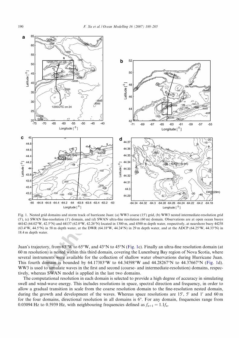
Computational domains are chosen according to the hurricane’s path, swell propagation characteristics andthe storm’s translation speed, in order to optimally simulate the hurricane-generated wave energy. The coarse-resolution (at 150) domain is from 40�W to 75�W and 20�N to 65�N, as shown in Fig. 1a. An intermediate-resolution domain (at 50) is nested within this first region, covering most of the waters off eastern Canadaand the New England States, bounded by 55�W to 71�W and 42�N to 52�N as shown in Fig. 1b. A fineresolution domain (at 10) is nested within this second domain covering the Scotian Shelf domain of Hurricane

F. Xu et al. / Ocean Modelling 16 (2007) 188–205 189

Autho

r's

pers

onal

co

py

Juan’s trajectory, from 63�W to 65�W, and 43�N to 45�N (Fig. 1c). Finally an ultra-fine resolution domain (at60 m resolution) is nested within this third domain, covering the Lunenburg Bay region of Nova Scotia, whereseveral instruments were available for the collection of shallow water observations during Hurricane Juan.This fourth domain is bounded by 64.17383�W to 64.34598�W and 44.28267�N to 44.37667�N (Fig. 1d).WW3 is used to simulate waves in the first and second (coarse- and intermediate-resolution) domains, respec-tively, whereas SWAN model is applied in the last two domains.

The computational resolution in each domain is selected to provide a high degree of accuracy in simulatingswell and wind-wave energy. This includes resolutions in space, spectral direction and frequency, in order toallow a gradual transition in scale from the coarse resolution domain to the fine-resolution nested domain,during the growth and development of the waves. Whereas space resolutions are 150, 50 and 10 and 60 mfor the four domains, directional resolution in all domains is 6�. For any domain, frequencies range from0.03094 Hz to 0.5939 Hz, with neighbouring frequencies defined as fn+1 = 1.1fn.

Fig. 1. Nested grid domains and storm track of hurricane Juan: (a) WW3 coarse (150) grid, (b) WW3 nested intermediate-resolution grid(50), (c) SWAN fine-resolution (10) domain, and (d) SWAN ultra-fine resolution (60 m) domain. Observations are at open ocean buoys44142 (64.02�W, 42.5�N) and 44137 (62.0�W, 42.26�N) located in 1300 m, and 4500 m depth water, respectively, at nearshore buoy 44258(63.4�W, 44.5�N) in 58 m depth water, at the DWR (64.18�W, 44.24�N) in 29 m depth water, and at the ADCP (64.25�W, 44.33�N) in18.4 m depth water.

190 F. Xu et al. / Ocean Modelling 16 (2007) 188–205

Autho

r's

pers

onal

co

py

3. Wind fields

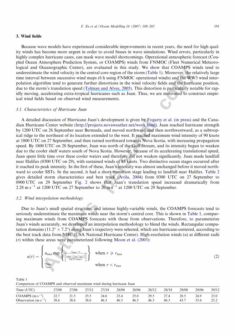
Because wave models have experienced considerable improvements in recent years, the need for high qual-ity winds has become more urgent in order to avoid biases in wave simulations. Wind errors, particularly inhighly complex hurricane cases, can mask wave model shortcomings. Operational atmospheric forecast (Cou-pled Ocean Atmosphere Prediction System, or COAMPS) winds from FNMOC (Fleet Numerical Meteoro-logical and Oceanographic Center), are evaluated in this study. We show that COAMPS winds tend tounderestimate the wind velocity in the central core region of the storm (Table 1). Moreover, the relatively largetime interval between successive wind maps (6 h using FNMOC operational winds) and the WW3 wind inter-polation algorithm tend to generate further distortions in the wind velocity fields and the hurricane position,due to the storm’s translation speed (Tolman and Alves, 2005). This distortion is particularly notable for rap-idly moving, accelerating extra-tropical hurricanes such as Juan. Thus, we are motivated to construct empir-ical wind fields based on observed wind measurements.

3.1. Characteristics of Hurricane Juan

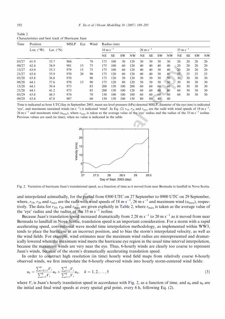
A detailed discussion of Hurricane Juan’s development is given by Fogarty et al. (in press) and the Cana-dian Hurricane Center website (http://projects.novaweather.net/work.html). Juan reached hurricane strengthby 1200 UTC on 26 September near Bermuda, and moved northward and then northwestward, as a subtrop-ical ridge to the northeast of its location extended to the west. It reached maximum wind intensity of 90 knotsat 1800 UTC on 27 September, and then turned northward towards Nova Scotia, with increasing propagationspeed. By 1800 UTC on 28 September, Juan was north of the Gulf Stream, and its intensity began to weakendue to the cooler shelf waters south of Nova Scotia. However, because of its accelerating translational speed,Juan spent little time over these cooler waters and therefore did not weaken significantly. Juan made landfallnear Halifax (0300 UTC on 29), with sustained winds of 85 knots. Two distinctive ocean stages occurred afterit reached its peak intensity. In the first of these, Juan’s intensity was almost unchanged before it moved north-ward to cooler SSTs. In the second, it had a short transition stage leading to landfall near Halifax. Table 2gives detailed storm characteristics and best track (Avila, 2004) from 0300 UTC on 27 September to0900 UTC on 29 September Fig. 2 shows that Juan’s translation speed increased dramatically from2.28 m s�1 at 1200 UTC on 27 September to 20 m s�1 at 1200 UTC on 29 September.

3.2. Wind interpolation methodology

Due to Juan’s small spatial structure, and intense highly-variable winds, the COAMPS forecasts tend toseriously underestimate the maximum winds near the storm’s central core. This is shown in Table 1, compar-ing maximum winds from COAMPS forecasts with those from observations. Therefore, to parameterizeJuan’s winds accurately, we developed an interpolation methodology to blend the winds. Rectangular compu-tation domains (11.2� � 7.2�) along Juan’s trajectory were selected, which are hurricane-centered, according tothe best track data from NHC (USA National Hurricane Center). High-resolution winds (u) at different radii(r) within these areas were parameterized following Moon et al. (2003):

uðrÞ ¼umax exp rmax�r

rmax�ðr18þr26Þ=2

logð22=umaxÞ

h i8<:

9=; when r P rmax

rumax

rmaxwhen r < rmax

8>>><>>>:

ð2Þ

Table 1Comparison of COAMPS and observed maximum wind during hurricane Juan

Time (UTC) 27/00 27/06 27/12 27/18 28/00 28/06 28/12 28/18 29/00 29/06 29/12

COAMPS (m s�1) 22.7 21.5 25.5 24.6 23.4 25.0 29.5 27.4 28.5 24.9 23.0Observation (m s�1) 38.6 38.6 38.6 46.3 46.3 46.3 46.3 46.3 43.7 33.4 23.2

F. Xu et al. / Ocean Modelling 16 (2007) 188–205 191

Autho

r's

pers

onal

co

pyand interpolated azimuthally, for the period from 0300 UTC on 27 September to 0900 UTC on 29 September,where, r18, r26 and rmax are the radii with wind speeds of 18 m s�1, 26 m s�1 and maximum wind (umax), respec-tively. The data for r18, r26 and rmax are given explicitly in Table 2, where rmax is taken as the average value ofthe ‘eye’ radius and the radius of the 33 m s�1 isoline.

Because Juan’s translation speed increased dramatically from 2.28 m s�1 to 20 m s�1 as it moved from nearBermuda to landfall in Nova Scotia, translation speed is an important consideration. For a storm with a rapidaccelerating speed, conventional wave model time interpolation methodology, as implemented within WW3,tends to place the hurricane at an incorrect position, and to bias the storm’s interpolated velocity, as well asthe wind fields. For example, wind estimates near the maximum wind radius are misrepresented and dramat-ically lowered when the maximum wind meets the hurricane eye region in the usual time interval interpolation,because the maximum winds are very near the eye. Thus, 6-hourly winds are clearly too coarse to representJuan’s winds, because of the storm’s dramatically accelerating translation speed.

In order to construct high resolution (in time) hourly wind field maps from relatively coarse 6-hourlyobserved winds, we first interpolate the 6-hourly observed winds into hourly storm-centered wind fields:

uk ¼P6

i¼kþ1V iP6i¼1V i

u0 þPk

i¼1V iP6i¼1V i

u6; k ¼ 1; 2; . . . ; 5 ð3Þ

where Vi is Juan’s hourly translation speed in accordance with Fig. 2, as a function of time, and u0 and u6 arethe initial and final wind speeds at every spatial grid point, every 6 h, following Eq. (2).

Table 2Characteristics and best track of Hurricane Juan

Time Position MSLP Eye Wind Radius (nm)

Lon. (�W) Lat. (�N) 18 m s�1 26 m s�1 33 m s�1

NE SE SW NW NE SE SW NW NE SE SW NW

03/27 61.9 33.7 984 70 175 100 50 120 30 30 30 30 20 20 20 2009/27 62.4 34.9 981 15 75 175 100 60 120 40 40 40 40 20 20 20 2015/27 63.0 35.3 979 15 75 175 100 60 120 40 40 30 40 20 20 20 2021/27 63.4 35.9 970 20 90 175 120 60 120 40 40 30 40 25 25 25 2503/28 63.8 36.8 970 90 175 120 50 120 50 50 50 50 30 30 30 3009/28 64.1 37.6 970 15 90 175 120 80 120 50 50 50 50 30 30 30 3015/28 64.1 39.4 973 85 200 150 100 200 60 60 60 60 60 30 30 3021/28 64.1 41.2 973 85 200 150 100 120 60 60 60 60 60 30 30 3003/29 63.8 44.5 974 70 150 100 100 100 60 60 60 60 60 30 30 3009/29 63.4 47.8 987 60 150 150 100 150 80 80 40 40

Time is indicated as hour UTC/day in September 2003, mean sea level pressure (hPa) denoted MSLP, diameter of the eye (nm) is indicated‘eye’, and maximum sustained winds (m s�1) is indicated ‘wind’. In Eq. (2) r18, r26 and rmax are the radii with wind speeds of 18 m s�1,26 m s�1 and maximum wind (umax), where rmax is taken as the average value of the ‘eye’ radius and the radius of the 33 m s�1 isoline.Previous values are used (in time), when no value is indicated in the table.

27 27.5 28 28.5 29 29.50

5

10

15

20

25

Day of Sept. 2003 (day)

Vel

ocity

[m/s

]

Fig. 2. Variation of hurricane Juan’s translational speed, as a function of time as it moved from near Bermuda to landfall in Nova Scotia.

192 F. Xu et al. / Ocean Modelling 16 (2007) 188–205

Autho

r's

pers

onal

co

py

Secondly, we interpolate the observed 6-hourly storm track data into 1-hourly positions (xi,yi), following:

ðxk; ykÞ ¼P6

i¼kþ1V iP6i¼1V i

ðx0; y0Þ þPk

i¼1V iP6i¼1V i

ðx6; y6Þ; k ¼ 1; 2; . . . ; 5 ð4Þ

where (x0,y0) and (x6,y6) are the initial and final best track positions for Juan, every 6 h.Finally, COAMPS winds are interpolated to hourly wind fields, and the new spatially and temporally inter-

polated Juan-centered winds (using Eqs. (3) and (4)), are used at grid points inside the rectangular domains(11.2� � 7.2�) along Juan’s trajectory, in place of COAMPS winds. Outside this wind replacement area, hourlyCOAMPS winds are used.

4. Model-observation comparisons

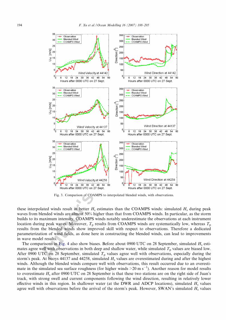
Observed in situ wind and wave data are available from Canadian Meteorological Service of Canada(MSC) operational buoys 44142 and 44137 located in water depths of 1300 m and 4500 m, on Scotian Slopeand Rise off Nova Scotia (Fig. 1b). Data are also available in shallower water, from buoy 44258 (Fig. 1b and c)near the mouth of Halifax Harbour in 58 m depth, and from a directional waverider (denoted DWR) and anADCP (Acoustic Doppler Current Profiler) at the mouth and interior of Lunenburg Bay, respectively in waterdepths of 29 m and 18.4 m (Fig. 1c and d). These instruments were located on Juan’s storm track (44142), onthe right side of the track and beyond the radius of maximum wind (44137); on the right side at the radius ofmaximum wind (44258), and on the left side near the radius of maximum wind (DWR, ADCP). Fig. 3 com-pares COAMPS winds with parameterized interpolated blended winds constructed from the methodology ofEqs. (2)–(4). It is evident that the winds from the new methodology are more consistent with the observedwind data than are the COAMPS winds.

4.1. Observed wind and waves

Buoy 44137 was about 150 km to the right side of Juan’s track. As shown in Fig. 3 and Table 3, this loca-tion experienced winds that increased from 18.4 m s�1 to 21.4 m s�1 and then decreased to 19.3 m s�1 over thetime interval from 2220 UTC on 28 September to 0020 UTC on 29 September. Corresponding significant waveheights (Hs) lagged the winds in time, but covered values from 6.1 m to 6.9 m and then decreased. By compar-ison, buoy 44142 was located slightly to the east of, and almost on Juan’s track with winds that increased from20 m s�1 to 28.1 m s�1 and then decreased to 18.7 m s�1 during the time from 2120 to 2320 UTC on 28September, with associated Hs values that increased from 8.0 m to 12.1 m and then decreased. Therefore,winds and waves at buoys 44142 and 44137 are very different, reflecting different locations with respect tothe storm, and different wave physics related to the passage of hurricane Juan.

Buoy 44258, the DWR, and the ADCP are all near the coast in somewhat shallower water. Both 44258 andthe DWR are exposed to the open ocean, whereas the ADCP is partially sheltered behind Cross Island, nearthe mouth of Lunenburg Bay. Buoy 44258 was about 30 km to the right of Juan’s track, with winds (Fig. 3,Table 3) similar to those of buoy 44142, increasing from 18.6 m s�1 to 27.5 m s�1 then decreasing to 18.3 m s�1

during the time 0020–0320 UTC on 29 September, and time-lagged Hs values from 5.9 m to 8.5 m. The DWRwas about 25 km to the left of Juan’s track, and recorded Hs values that increased from 6.8 m to 9.2 m andthen decreased during the time 0311–0511 UTC on 29 September; and corresponding peak wave directions of186�, and 183� respectively. The ADCP was about 30 km to the left of Juan’s track, and recorded Hs values of2.8 m, increasing to 5.3 m, and the decreasing to 2.8 m in the time 0300–0700 UTC on 29 September. Refrac-tion, bottom friction and nearshore processes are factors that can contribute to wave development at theselocations.

4.2. Simulated wave height and peak period

The Hs and peak period (Tp) comparisons (shown in Fig. 4) suggest that WW3 and SWAN are capable ofsimulating hurricane-generated waves reasonably well, using the interpolated blended winds. It is evident that

F. Xu et al. / Ocean Modelling 16 (2007) 188–205 193

Autho

r's

pers

onal

co

py

these interpolated winds result in better Hs estimates than the COAMPS winds: simulated Hs during peakwaves from blended winds are almost 50% higher than that from COAMPS winds. In particular, as the stormbuilds to its maximum intensity, COAMPS winds notably underestimate the observations at each instrumentlocation during peak waves. Moreover, Tp results from COAMPS winds are systematically low, whereas Tp

results from the blended winds show improved skill with respect to observations. Therefore a dedicatedparameterization of wind fields, as done here in constructing the blended winds, can lead to improvementsin wave model results.

The comparisons in Fig. 4 also show biases. Before about 0900 UTC on 28 September, simulated Hs esti-mates agree well with observations in both deep and shallow water, while simulated Tp values are biased low.After 0900 UTC on 28 September, simulated Tp values agree well with observations, especially during thestorm’s peak. At buoys 44137 and 44258, simulated Hs values are overestimated during and after the highestwinds. Although the blended winds compare well with observations, this result occurred due to an overesti-mate in the simulated sea surface roughness (for higher winds >20 m s�1). Another reason for model resultsto overestimate Hs after 0900 UTC on 28 September is that these two stations are on the right side of Juan’strack, with strong swell and current components following the wind direction, resulting in relatively lowereffective winds in this region. In shallower water (at the DWR and ADCP locations), simulated Hs valuesagree well with observations before the arrival of the storm’s peak. However, SWAN’s simulated Hs values

Fig. 3. Comparison of COAMPS to interpolated blended winds, with observations.

194 F. Xu et al. / Ocean Modelling 16 (2007) 188–205

Autho

r's

pers

onal

co

pyare slightly lower than those of the ADCP during peak waves, reflecting the complex shallow water wavephysics.

4.3. Wave spectra

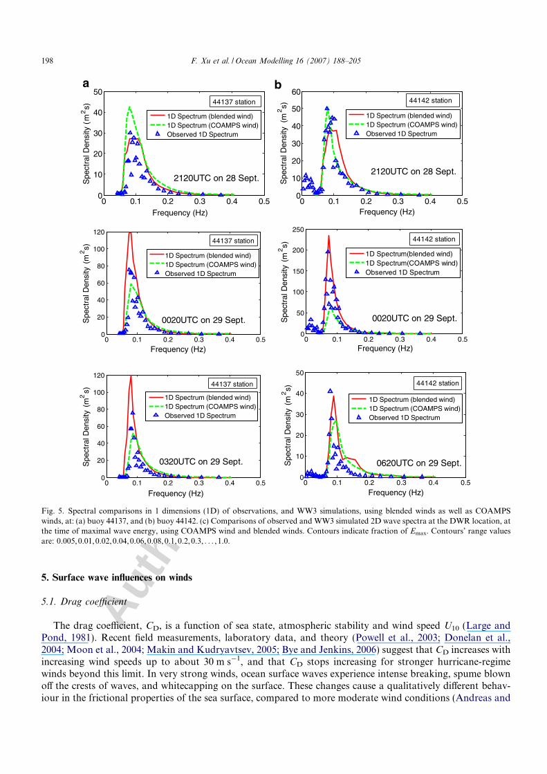
Observed 1D wave spectra data were collected at buoys 44137 and 44142, and observed 2D wave spectradata, at the DWR. Fig. 5a and b compare the simulated 1D spectra (from blended winds and COAMPSwinds) with observations at buoys 44137 and 44142. Overall, the simulated 1D spectra from the blended windsachieve a somewhat better match to observations than those resulting from COAMPS winds. This is suggestedover the entire frequency range, before, during, and after the highest winds occurrences, under wind wave-dominated as well as swell-dominated conditions. This is illustrated at 44142; the simulated 1D spectral peakis improved by 200% during peak waves (0020 UTC on 29 September), whereas at 44137 the simulated 1Dspectra from the blended winds overestimate the observed data by as much as 45% during peak waves(0020 UTC on 29 September). By comparison, the 1D spectra from COAMPS winds underestimate the obser-vations at both buoys, especially during the storm peaks.

Fig. 5c compares SWAN-simulated 2D wave spectra (driven by blended winds and COAMPS winds) withthe shallow water DWR observations at the time of maximum waves. To some extent, this shows that the sim-ulated 2D spectra from the blended winds are an improvement compared to those resulting from COAMPSwinds in terms of their ability to simulate the peak wave intensity. While wind-waves dominate before themaximum waves are observed, swell is dominant afterwards; at the time of maximum spectral intensity, thespectra are relatively narrow in directional and frequency range (see Fig. 5c). However, whether from blendedwinds or from COAMP winds, the simulated 2D spectrum at the DWR location from SWAN have wide direc-tional and frequency range distributions, and do not capture the extent of the narrowing of the observed spec-trum. Improvements in the next generation of SWAN need to take into account further studies of shallow

Table 3Observed time series

Location Time UTC/day in September Wind (m s�1) Hs (m) Peak wave direction

Buoy 44137 2220/28 18.42320/28 21.4 6.10020/29 19.3 6.90120/29 6.7

Buoy 44142 2120/28 20.02200/28 28.1 8.02320/28 18.7 12.10020/29 9.8

Buoy 44137 2220/28 18.42320/28 21.4 6.10020/29 19.3 6.90120/29 6.7

Buoy 44258 0020/29 18.60220/29 27.0 5.90320/29 27.5 8.20420/29 18.3 8.50520/29 7.1

DWR 0311/29 6.8 186�0341/29 9.2 183�0511/29 6.7 181�

ADCP 0300/29 2.8 156�0500/29 5.3 151�0700/29 2.8 159�

Time series of winds and significant wave heights as measured at buoys 44137, 44142, 44258, the DWR and ADCP, and presented in Figs.3, 4a and 4b. No wave direction information is available at buoys 44137, 44142 and 44258. Wave directions reported from ADCP andDWR data follow the nautical convention (direction from).

F. Xu et al. / Ocean Modelling 16 (2007) 188–205 195

Autho

r's

pers

onal

co

py

water wave processes, as recorded in data as the DWR observations, and also as recorded in very recent exper-imental studies by Young and Babanin (2006a,b).

4.4. Translation speed impact on waves

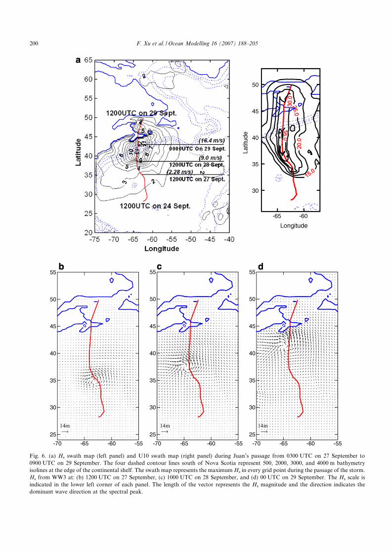
Juan’s translation speed varied dramatically from 2.28 m s�1 at 1200 UTC on 27 September to 20 m s�1 at1200 UTC on 29 September (Fig. 2). Midway through this period, at 1200 UTC on 28 September, Juan’stranslation speed was 9 m s�1 (Fig. 6a), its simulated wave length near the storm track was about 210 m(Fig. 7a), and the dominant group velocity was about 9 m s�1. Thus, Juan’s translation speed was approxi-mately equivalent to the group velocity of the dominant waves, which represents the wave energy propagationspeed. This effectively increases the duration and fetch for growing waves, which acts as a resonance to greatlyincrease Hs. The highest wind speeds occurred after 1800 UTC on 27 September. Figs. 6 and 7 show thatextreme wave heights (larger than 12 m) and wave lengths (longer than 210 m) occurred after 1200 UTC on28 September, although maximum winds remained almost unchanged until 2100 UTC on 28 September.

Juan’s translation speed increased dramatically from 9 m s�1 at 1200 UTC on 28 September, to 20 m s�1 at1200 UTC on 29 September. During this time, the average wave length (L) along the track increased from210 m to 250 m, the wave group velocity increased from 9 m s�1 to 10 m s�1, and Hs remained about

Fig. 4a. Comparison of simulated and observed estimates for Hs.

196 F. Xu et al. / Ocean Modelling 16 (2007) 188–205

Autho

r's

pers

onal

co

py

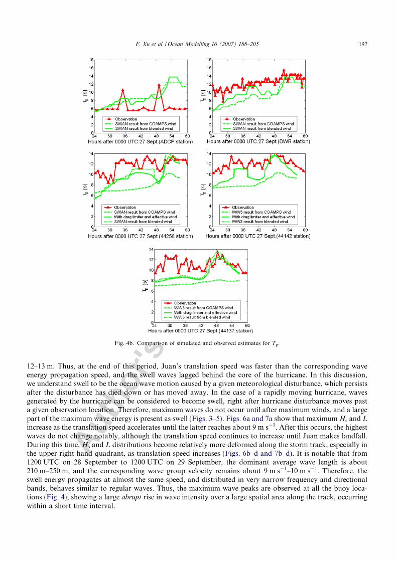
12–13 m. Thus, at the end of this period, Juan’s translation speed was faster than the corresponding waveenergy propagation speed, and the swell waves lagged behind the core of the hurricane. In this discussion,we understand swell to be the ocean wave motion caused by a given meteorological disturbance, which persistsafter the disturbance has died down or has moved away. In the case of a rapidly moving hurricane, wavesgenerated by the hurricane can be considered to become swell, right after hurricane disturbance moves pasta given observation location. Therefore, maximum waves do not occur until after maximum winds, and a largepart of the maximum wave energy is present as swell (Figs. 3–5). Figs. 6a and 7a show that maximum Hs and L

increase as the translation speed accelerates until the latter reaches about 9 m s�1. After this occurs, the highestwaves do not change notably, although the translation speed continues to increase until Juan makes landfall.During this time, Hs and L distributions become relatively more deformed along the storm track, especially inthe upper right hand quadrant, as translation speed increases (Figs. 6b–d and 7b–d). It is notable that from1200 UTC on 28 September to 1200 UTC on 29 September, the dominant average wave length is about210 m–250 m, and the corresponding wave group velocity remains about 9 m s�1–10 m s�1. Therefore, theswell energy propagates at almost the same speed, and distributed in very narrow frequency and directionalbands, behaves similar to regular waves. Thus, the maximum wave peaks are observed at all the buoy loca-tions (Fig. 4), showing a large abrupt rise in wave intensity over a large spatial area along the track, occurringwithin a short time interval.

Fig. 4b. Comparison of simulated and observed estimates for Tp.

F. Xu et al. / Ocean Modelling 16 (2007) 188–205 197

Autho

r's

pers

onal

co

py

5. Surface wave influences on winds

5.1. Drag coefficient

The drag coefficient, CD, is a function of sea state, atmospheric stability and wind speed U10 (Large andPond, 1981). Recent field measurements, laboratory data, and theory (Powell et al., 2003; Donelan et al.,2004; Moon et al., 2004; Makin and Kudryavtsev, 2005; Bye and Jenkins, 2006) suggest that CD increases withincreasing wind speeds up to about 30 m s�1, and that CD stops increasing for stronger hurricane-regimewinds beyond this limit. In very strong winds, ocean surface waves experience intense breaking, spume blownoff the crests of waves, and whitecapping on the surface. These changes cause a qualitatively different behav-iour in the frictional properties of the sea surface, compared to more moderate wind conditions (Andreas and

0 0.1 0.2 0.3 0.4 0.50

10

20

30

40

50

2120UTC on 28 Sept.

Frequency (Hz) Frequency (Hz)

Frequency (Hz) Frequency (Hz)

Frequency (Hz) Frequency (Hz)

Spe

ctra

l Den

sity

(m

2s)

44137 station

0 0.1 0.2 0.3 0.4 0.50

10

20

30

40

50

60

2120UTC on 28 Sept.

Spe

ctra

l Den

sity

(m2s)

44142 station

0 0.1 0.2 0.3 0.4 0.50

20

40

60

80

100

120

0020UTC on 29 Sept.Spe

ctra

l Den

sity

(m2 s)

44137 station

0 0.1 0.2 0.3 0.4 0.50

50

100

150

200

250

0020UTC on 29 Sept.Spe

ctra

l Den

sity

(m2s)

1D Spectrum(blended wind)1D Spectrum(COAMPS wind)Observed 1D Spectrum

44142 station

0 0.1 0.2 0.3 0.4 0.50

20

40

60

80

100

120

0320UTC on 29 Sept.Spe

ctra

l Den

sity

(m2

s)

1D Spectrum (blended wind)1D Spectrum (COAMPS wind)Observed 1D Spectrum

44137 station

0 0.1 0.2 0.3 0.4 0.50

10

20

30

40

50

0620UTC on 29 Sept.Spe

ctra

l Den

sity

(m2s)

44142 station

1D Spectrum (blended wind)1D Spectrum (COAMPS wind)Observed 1D Spectrum

1D Spectrum (blended wind)1D Spectrum (COAMPS wind)Observed 1D Spectrum

1D Spectrum (blended wind)1D Spectrum (COAMPS wind)Observed 1D Spectrum

1D Spectrum (blended wind)1D Spectrum (COAMPS wind)Observed 1D Spectrum

Fig. 5. Spectral comparisons in 1 dimensions (1D) of observations, and WW3 simulations, using blended winds as well as COAMPSwinds, at: (a) buoy 44137, and (b) buoy 44142. (c) Comparisons of observed and WW3 simulated 2D wave spectra at the DWR location, atthe time of maximal wave energy, using COAMPS wind and blended winds. Contours indicate fraction of Emax. Contours’ range valuesare: 0.005,0.01,0.02,0.04,0.06,0.08,0.1,0.2,0.3, . . . , 1.0.

198 F. Xu et al. / Ocean Modelling 16 (2007) 188–205

Autho

r's

pers

onal

co

py

Emanuel, 2001; Zhang et al., in press). In hurricane conditions, the air is filled with foam and spray, the sea iscompletely white with spray, and the surface roughness is affected by wave-breaking.

Fig. 8 presents the variation in CD from 0300 UTC on 27 September to 0900 UTC on 29 September, asestimated by the wave-induced stress formulation within WW3. This implies that (WW3) CD was larger than0.003 for 5 h after 2000 UTC on 28 September at buoy 44142, and for almost 2 h after 2140 UTC at buoy

Fig. 5 (continued)

F. Xu et al. / Ocean Modelling 16 (2007) 188–205 199

Autho

r's

pers

onal

co

py

Fig. 6. (a) Hs swath map (left panel) and U10 swath map (right panel) during Juan’s passage from 0300 UTC on 27 September to0900 UTC on 29 September. The four dashed contour lines south of Nova Scotia represent 500, 2000, 3000, and 4000 m bathymetryisolines at the edge of the continental shelf. The swath map represents the maximum Hs in every grid point during the passage of the storm.Hs from WW3 at: (b) 1200 UTC on 27 September, (c) 1000 UTC on 28 September, and (d) 00 UTC on 29 September. The Hs scale isindicated in the lower left corner of each panel. The length of the vector represents the Hs magnitude and the direction indicates thedominant wave direction at the spectral peak.

200 F. Xu et al. / Ocean Modelling 16 (2007) 188–205

Autho

r's

pers

onal

co

py

44137, with an overall CD peak of 0.0044. During this time, simulated wave heights and spectra are overesti-mated compared to observations (Figs. 4 and 5). However, according to observations, laboratory experimentsand theoretical studies (Powell et al., 2003; Donelan et al., 2004; Moon et al., 2004), maximum values of CD

should not exceed about 0.003. Here, we restrict the maximum drag coefficient CD to 0.0035.

5.2. Effective wind velocity and swell

Sea state has a potentially large impact on the winds not only due to wave roughness, but also due to waveparticle movement properties and surface currents. The log-wind profile is altered due to the modification ofthe near surface boundary conditions for wind velocity by the horizontal component of the dominant waves’orbital velocity. According to direct CD measurements, counter swell can significantly enhance CD, whereasfollowing swell significantly reduces CD, because swell modifies both the wind profile and turbulent kineticenergy budget (Drennan et al., 1999; Donelan et al., 1997).

In hurricane Juan, overestimates of wave energy occur, during and after the highest winds, on the right sideof Juan’s track, especially at buoys 44137 and 44258. During and after the highest winds, swell waves dom-inate with almost the same direction as that of the maximum winds on the right side of Juan’s storm track.At the time of highest winds, the dominant following swell (Fig. 6d) reduces the effective wind strength to

-75 -70 -65 -60 -55 -50 -45 -4020

25

30

35

40

45

50

55

60

65

Fig. 7. (a) As in Fig. 6a for average wavelength swath from 0300 UTC on 27 September to 0900 UTC on 29 September. Averagewavelength from WW3 at (b) 1200 UTC on 27 September, (c) 1000 UTC on 28 September, and (d) 0000 UTC on 29 September.

F. Xu et al. / Ocean Modelling 16 (2007) 188–205 201

Autho

r's

pers

onal

co

py

some extent, and the large wave orbital motion modifies the lower atmospheric boundary condition. More-over, large waves generate large Stokes drift, which is also in approximately the same direction as thedominant wave propagation. The combination of surface wave particle motion and Stokes drift also modifiesthe driving winds, and therefore impacts on the generated waves.

The influence of sea state enters through modification of the vertical shear in the wind speed due to a non-zero lower boundary condition. An effective wind ~UEðzÞ is approximated by introducing the surface wave par-ticle trajectory velocity ~uorb and current ~ucurrent (Bourassa, 2006),

~U EðzÞ ¼ ½~UðzÞ � c~uorb �~ucurrent� �~ei ð5Þ

where ~UðzÞ is wind velocity at height z above the local mean surface, ~uorb is orbital speed related to thesignificant slope (Taylor and Yelland, 2001) and interacts with the wind near the wave crests and troughs,~uorb ¼ p � ~H s=T p; ~e1 and ~e2 are unit vectors parallel and perpendicular to the mean wave direction; and the

-70 -65 -60 -55

25

30

35

40

45

50

55

-70 -65 -60 -55

25

30

35

40

45

50

55

-70 -65 -60 -55

25

30

35

40

45

50

55

Fig. 7 (continued)

0 6 12 18 24 30 36 42 48 54 600

1

2

3

4

5x 10-3

Hours after 0000 UTC on 27 Sept.

Drag coefficient at 44142

Drag coefficient at 44137

2000UTC on 28

0100UTC on 292330UTC on 282140UTC on 28

Fig. 8. Drag coefficient variations from 0300 UTC on 27 September to 0900 UTC on 29 September at 44142 and 44137 stations.

202 F. Xu et al. / Ocean Modelling 16 (2007) 188–205

Autho

r's

pers

onal

co

py

fraction of the orbital motion velocity c was set as: c = 0.8. Stokes drift~us is used to approximate and replace~ucurrent, because other current contributions can be neglected in intense storms (Perrie et al., 2003), where

~us ¼ 4pZ Z

f~ke2kzEðf ; hÞdf dh: ð6Þ

5.3. Simulation results

Fig. 4 compares the simulation results (with the CD restriction and wave modifications to the winds) withobservations at buoys 44142, 44137 and 44258. It can be seen that at 44137 and 44258, the formerly overes-timated significant wave heights are notably improved, while at 44142, results are almost unchanged. Thisresult occurs because buoy 44142 is on the storm track and the wind direction at this buoy is almost perpen-dicular with the swell and Stokes drift directions during, and after, the passing of the highest wind. At buoy44142, the effective winds are almost equal to the non-corrected winds, and thus the waves are almostunchanged. It is evident that the drag limitation is important at buoy 44142, but not at 44137 (Fig. 8), becauseonly a small reduction in Hs at buoy 44142 is due to the drag coefficient limitation, whereas the relatively largeimprovement at buoys 44137 and 44258 can be attributed to swell and Stokes drift feedback on the wind.

6. Conclusions

Hurricane Juan was one of the most damaging storms in the modern history of Nova Scotia. Juan had highwinds and a rapid translation speed, which accelerated from 2.28 m s�1 (1200 UTC on 27 September) to20 m s�1 (1200 UTC on 29 September). This hurricane generated complex high waves in deep and shallowwaters off Nova Scotia. Two models, WW3 and SWAN, are applied on multiply-nested domains to simulatethe waves generated by Juan. SWAN was implemented on a fine-resolution grid, nested within coarser gridimplementations of WW3.

In order to correct biases in the operational winds due to Juan’s rapid accelerating translation speed, wedeveloped an interpolation methodology to blend observations with COAMPS operational forecast winds.This method ensures accurate hurricane wind fields, and also uses the operational COAMPS winds withina large-scale area. Comparisons show that the interpolated blended winds compare well with buoy wind obser-vations, relative to COAMPS winds. Corresponding wave simulations from WW3 and SWAN models arenotably improved, for integrated parameters such as significant wave height Hs, as well as for detailed wavespectra. The simulated 1D wave spectra from the blended winds are in better agreement with observationsthan those from COAMPS winds, over the entire frequency range, especially during the highest storm waves,at deep water locations. The simulated 2D spectra from the blended winds are better than those fromCOAMPS winds during peak waves. At the DWR location, these spectra capture the observed spectral peakwaves to some extent, but still cannot simulate the narrow directional and frequency bands of dominant swellwaves.

Our study shows that translation speed is a key factor. Wave heights and wave length increase withincreased translation speed, and reach maximal values when the wave energy propagation speed is aboutthe same as the translation speed. When this occurs, the largest waves of the storm are generated by theresonance between the waves and propagating storm, and these large waves soon become swell, whichaccounts for most of the energy, compared to storm-generated wind-waves. When the translation speedbecomes higher than the wave energy propagation speed, swell lags behind locally-generated wind waves,and neither Hs nor average wavelengths increase notably. Thus, extremely high waves are not simultaneouswith peak winds, but occur after peak winds have passed. Narrow-band low-frequency swell waves containthe maximum energy and occur for very short duration at all buoys near the storm track. Moreover, whenJuan moved slowly, both the Hs and the average wave length distributions have a vortex shape, whereas withas Juan moves faster, these two distributions become more distinctly deformed.

In our simulations, large waves generated during and after the peak winds, tend to be overestimated, espe-cially on the right side of the Juan’s track. To account for this, two processes are considered: (a) an upperbound is imposed on the drag coefficient, motivated by recent experimental and theory results (Powell

F. Xu et al. / Ocean Modelling 16 (2007) 188–205 203

Autho

r's

pers

onal

co

py

et al., 2003; Donelan et al., 2004; Moon et al., 2004); and (b) winds are corrected by taking into account theswell orbital velocities and Stokes drift. Simulation results show that the modified wave fields are improvedespecially on the right side of the storm track during and after the occurrence of peak waves. Results suggestthat the impact of swell waves and Stokes drift on waves is larger than that of the modified drag coefficient.

Acknowledgements

We thank Murray Scotney from BIO for maintaining the ADCP and DWR at the mouth of LunenburgBay during Hurricane Juan. Support is from the Canadian Panel on Energy Research and Development(Offshore Environmental Factors Program), the China Scholarship Council, GoMOOS – the Gulf of MaineOcean Observing System, CFCAS (Canada Foundation for Climate and Atmospheric Studies), and SCOOP,the Southeast Universities Research Association Coastal Ocean Observing and Prediction program.

References

Andreas, E.L., Emanuel, K.A., 2001. Effects of sea spray on tropical cyclone intensity. J. Atmos. Sci. 58, 3741–3751.Avila, L.A., 2004. Hurricane Juan 24–29 September 2003. NOAA National Hurricane Center/Tropical Prediction Center. Available from:

<http://www.nhc.noaa.gov/2003Juan.shtml>.Booij, N., 2004. SWAN Cycle III version 40.41 user manual. Available from: <http://fluidmechanics.tudelft.nl/swan/index.htm>.Booij, N., Holthuijsen, L.H., Ris, R.C., 1996. The ‘‘SWAN” wave model for shallow water. Coastal Eng. 1, 668–672.Booij, N., Ris, R.C., Holthuijsen, L.H., 1999. A third-generation wave model for coastal regions. Part I. Model description and validation.

J. Geophys. Res. 104 (C4), 7649–7666.Bourassa, M.A., 2006. Satellite-based observations of surface turbulent stress during severe weather. In: Perrie, W. (Ed.), Atmosphere–

Ocean Interactions, Vol. 2. WIT Press, pp. 35–47.Bye, J.A.T., Jenkins, A.D., 2006. Drag coefficient reduction at very high wind speeds. J. Geophys. Res. 111 (C3), C03024. doi:10.1029/

2005JC003114.31, March 2006.Donelan, M.A., Drennan, W.M., Katsaros, K.B., 1997. The air–sea momentum flux in conditions of mixed wind sea and swell. J. Phys.

Oceanogr. 27, 2087–2099.Donelan, M.A., Haus, B.K., Reul, N., Plant, W.J., Stiassnie, M., Graber, H.C., Brown, O.B., Saltzman, E.S., 2004. On the limiting

aerodynamic roughness of the ocean in very strong winds. Geophys. Research Lett. 31, L18306. doi:10.1029/2004GL019460.Drennan, W.M., 2006. On parameterisations of air–sea fluxes. In: Perrie, W. (Ed.), Atmosphere–Ocean Interactions, vol. 2. WIT Press, pp.

1–34.Drennan, W.M., Kahma, K.K., Donelan, M.A., 1999. On momentum flux and velocity spectra over waves. Bound-Layer Meteorol. 92,

489–515.Fogarty, T.C., Greatbatch, J.R. Ritchie, H., (in press). The role of anomalously warm sea surface temperatures on the intensity of

Hurricane Juan (2003) during its approach to Nova Scotia. Monthly Weather Rev.Hart, R.E., Evans, J.L., 2001. A climatology of the extratropical transition of Atlantic tropical cyclones. J. Climate 14, 546–564.Holthuijsen, L.H., Booij, H.N., 2003. Phase-decoupled refraction–diffraction for spectral wave models. Coastal Eng. 49, 291–305.Komen, G.J., Cavaleri, L., Donelan, M., Hasselmann, M., Hasselmann, S., Janssen, P.A.E.M., 1994. Dynamics and Modeling of Ocean

Waves. Cambridge University Press, p. 520.Large, W.G., Pond, S., 1981. Open ocean momentum flux measurements in moderate to strong winds. J. Phys. Oceanogr. 11, 324–336.Makin, V., Kudryavtsev, V., 2005. The drag of the sea surface at hurricane winds. Bound. Layer Meteorology 1, 2005.Moon, I.-J., Ginis, I., Hara, T., Tolman, H.L., Wright, C.W., Walsh, E.J., 2003. Numerical simulation of sea surface directional wave

spectra under hurricane wind forcing. J. Phys. Oceanogr 33, 1680–1705.Moon, I.-J., Ginis, I., Hara, T., 2004a. Effect of surface waves on air–sea momentum exchange. Part II: Behavior of drag coefficient under

tropical cyclones. J. Atmos. Sci. 61 (19), 2334–2348.Moon, I.-J., Hara, T., Ginis, I., Belcher, S.E., Tolman, H.L., 2004b. Effect of surface waves on air–sea momentum exchange. Part I: Effect

of mature and growing seas. J. Atmos. Sci. 61 (19), 2321–2333.Perrie, W., Tang, C.L., Hu, Y., DeTracey, B.M., 2003. The impact of waves on surface currents. J. Phys. Oceanogr. 33, 2126–2141.Powell, M.D., Vickery, P.J., Reinhold, T.A., 2003. Reduced drag coefficient for high wind speeds in tropical cyclones. Nature 422, 279–

283.Ris, R.C., Holthuijsen, L.H., Booij, N., 1994. A spectral model for waves in the near shore zone. Coastal Eng. 1, 68–78.Taylor, P.K., Yelland, M.J., 2001. The dependence of sea surface roughness on the height and steepness of the waves. J. Phys. Oceanogr.

18, 572–590.Tolman, H.L., 2002. User manual and system documentation of WAVEWATCH-III version 2.22. Technical Note. Available from:

<http://polar.ncep.noaa.gov/waves>.Tolman, H.L., Alves, J.-H.G.M., 2005. Numerical modeling of wind waves generated by tropical cyclones using moving grid. Ocean

Modell. 9, 305–323.Tolman, H.L., Chalikov, D.V., 1996. Source terms in a third-generation wind-wave model. J. Phys. Oceanogr. 26, 2497–2518.

204 F. Xu et al. / Ocean Modelling 16 (2007) 188–205

Autho

r's

pers

onal

co

py

Young, I.R., Babanin, A.V., 2006a. The form of the asymptotic depth-limited wind wave frequency spectrum. J. Geophys. Res. 111,C06031. doi:10.1029/2005JC003398.

Young, I.R., Babanin, A.V., 2006b. Spectral distribution of energy dissipation of wind-generated waves due to dominant wave breaking.J. Phys. Oceanogr. 36 (3), 376–394.

Zhang, W., Perrie, W., submitted for publication. Extratropical Hurricane Juan: Structure and Maintenance. J. Atmos. Sci.Zhang, W., Perrie, W., Li, W., in press. Impacts of waves and sea spray on midlatitude storm structure and intensity. Monthly Wealthy

Rev.

F. Xu et al. / Ocean Modelling 16 (2007) 188–205 205