Simulation of storm surge, wave, currents, and inundation in the Outer Banks and Chesapeake Bay...

Simulation of storm surge, wave, currents, and inundation in the

Outer Banks and Chesapeake Bay during Hurricane Isabel in 2003:

The importance of waves

Y. Peter Sheng,1 Vadim Alymov,1 and Vladimir A. Paramygin1

Received 24 March 2009; revised 7 October 2009; accepted 22 October 2009; published 7 April 2010.

[1] This paper investigates the effects of waves on storm surge, currents, and inundationin the Outer Banks and Chesapeake Bay during Hurricane Isabel in 2003 through detailedcomparison between observed wind, wave, surge, and inundation data and results froman integrated storm surge modeling system, CH3D-SSMS. CH3D-SSMS, which includescoupled coastal and basin-scale storm surge and wave models, successfully simulatedmeasured winds, waves, storm surge, currents, and inundation during Isabel.Comprehensive modeling and data analysis revealed noticeable effects of waves on stormsurge, currents, and inundation. Among the processes that represent wave effects, radiationstress (outside the estuaries) and wave-induced stress (outside and inside the estuaries)are more important than wave-induced bottom stress in affecting the water level.Maximum surge was 3 m, while maximum wave height was 20 m offshore and 2.5 minside the Chesapeake Bay, where the maximum wave-induced water level reached 1 m.Significant waves reached 3.5 m and 16 s at Duck Pier, North Carolina, and 1.6 m and 5 sat Gloucester, Virginia. At Duck, wave effects accounted for �36 cm or 20% of thepeak surge elevation of 1.71m. Inside the Chesapeake Bay, wave effects account for 5–10%of observed peak surge level. A two-layer flow is found at Kitty Hawk, North Carolina,during the peak of storm surge owing to the combined effects of wind and wave breaking.Higher surge elevations result when the 3-D surge model, instead of the 2-D surge model,is coupled with the 2-D wave model owing to its relatively lower bottom friction.Wave heights obtained with 3- and 2-D surge models show little difference.

Citation: Sheng, Y. P., V. Alymov, and V. A. Paramygin (2010), Simulation of storm surge, wave, currents, and inundation in the

Outer Banks and Chesapeake Bay during Hurricane Isabel in 2003: The importance of waves, J. Geophys. Res., 115, C04008,

doi:10.1029/2009JC005402.

1. Introduction

1.1. Storm Surge Modeling

[2] The major damage caused by hurricanes is associatedwith storm surges and coastal flooding. A storm surge is ahuge mass of water, tens to hundreds km wide, that sweepsacross the coastline where a hurricane makes landfall. Thepeak storm surge level can reach more than 3 m. The surgeof high water topped by waves can be devastating. Alongthe coast, storm surge is the greatest threat to life andproperty. Accurate prediction of storm surge and coastalflooding is essential for developing cost effective stormmitigation and preparation.[3] Numerous numerical models have been developed to

simulate storm surges [e.g., Sheng, 1987, 1990; Flather,1994; Jelesnianski et al., 1992; Luettich et al., 1992;Hubbert and McInnes, 1999; Casulli and Walters, 2000;

Sheng et al., 2006]. Bode and Hardy [1997] reviewed thestatus of storm surge modeling.[4] The accuracy of storm surge simulations depends on

many factors: (1) input data (e.g., bathymetry, topography,and wind/pressure fields), (2) representation of importantprocesses (e.g., flooding and drying, bottom friction, andeffects of wave and tide), (3) model grid resolution, and(4) open boundary conditions. For example, Houston et al.[1999] compared the storm surge simulations produced byusing the HRD wind field and the SLOSH wind field.Hubbert and McInnes [1999] showed that their modeloverestimated storm surge by 17% if the ‘‘flooding anddrying’’ feature of their model is turned off owing to waterpiled up near the coast by the action of high wind and notallowing the water to propagate inland. Mastenbroek et al.[1993] and Zhang and Li [1996] showed that includingwave-dependent surface wind stress significantly improvedthe surge height prediction. Shen et al. [2006] simulateddiagnostically the effect of offshore surge on storm tideinside the Chesapeake Bay, without considering the effect ofwaves.Morey et al. [2006] showed that it is important to usea large model domain to incorporate the effect of remoteforcing contribution to storm surge during Hurricane Dennis.

JOURNAL OF GEOPHYSICAL RESEARCH, VOL. 115, C04008, doi:10.1029/2009JC005402, 2010ClickHere

for

FullArticle

1Civil and Coastal Engineering Department, University of Florida,Gainesville, Florida, USA.

Copyright 2010 by the American Geophysical Union.0148-0227/10/2009JC005402

C04008 1 of 27

http://dx.doi.org/10.1029/2009JC005402

Interagency Performance Evaluation Taskforce (IPET)[2006] simulated the storm surge and wave during HurricaneKatrina. Zhang and Sheng [2008] and Lee and Sheng [2008]simulated the storm surge and inundation during Ivan.[5] This study aims to simulate the surge, wave, and

inundation during Hurricane Isabel and to answer thefollowing fundamental questions: How significantly doesthe wave affect storm surge? What is the relative importanceof various wave processes (radiation stress, wave-induceddrag, wave-induced bottom stress) in affecting storm surgeand currents? Can a coupled 2-D wave model and a 3-Dsurge model simulate the vertical flow structure in coastaland estuarine water during hurricanes? Can a 2-D wavemodel accurately simulate the wave in coastal and estuarinewater during hurricanes? To answer these questions, we usean integrated storm surge modeling system, CH3D-SSMS(see http://ch3d-ssms.coastal.ufl.edu and Sheng et al.[2006]), to conduct a comprehensive sensitivity study tosimulate the storm surge and wave effects in the OuterBanks and Chesapeake Bay during Hurricane Isabel. Sincewave effects cannot be easily extracted from the field data insuch a complex environment, the integrated modelingsystem enables numerous model simulations to ensure thatwind, wave, and water elevation can all be accuratelysimulated so that the wave effect can be accuratelyquantified.

1.2. Hurricane Isabel

[6] Hurricane Isabel of 2003, the track for which isshown in Figure 1, is considered one of the most significanttropical cyclones to affect portions of northeastern NorthCarolina and east-central Virginia since Hurricane Hazel of1954 and the Chesapeake-Potomac Hurricane of 1933. Thehurricane reached Category 5 status on the Saffir-SimpsonHurricane Scale. It made landfall near Drum Inlet on theOuter Banks of North Carolina as a Category 2 hurricanearound 1730 UT on 18 September. According to NOAA[2004], 51 people died as a result of the storm (17 directly),with an official damage estimate of $3.37 billion. Most of

the losses were incurred by Virginia ($925M), Maryland($410M), and North Carolina ($170M).[7] Isabel brought hurricane conditions to portions of

eastern North Carolina and southeastern Virginia. Accord-ing to NOAA’s National Hurricane Center, the highestobserved sustained wind over land was 35 m/s with gustsup to 44 m/s at an instrumented tower near Cape Hatteras,North Carolina, at 1622 UT on 18 September. Anothertower in Elizabeth City, North Carolina, reported 33 m/ssustained wind with a gust to 43 m/s at 1853 UT that day.The National Ocean Service station at Cape Hatterasreported 35 m/s sustained wind with a gust to 43 m/s beforecontact was lost. The Coastal Marine Automated Stations(C-MAN) at Chesapeake Light, Virginia, and Duck, NorthCarolina, reported similar winds. However, the wind recordfrom the most seriously affected areas is incomplete, asseveral observing stations were destroyed or lost power asIsabel passed.[8] According to NOAA [2004], the storm surge during

Hurricane Isabel reached 2.5 m along the Outer Banks,1.3 m at Duck, North Carolina, and almost 2.5 m in theupper Chesapeake Bay, generally 0.3 to 1.0 m higher thanthe NOAA SLOSH forecast that did not include any waveeffect. During Isabel, waves were 12–15 m near the OuterBanks, a chain of emergent barrier islands separating themainland from the Atlantic Ocean. Figure 2 shows theIsabel track and locations of all data stations for this study.It should be noted that, throughout this paper, water levelwill be reported in NAVD88 vertical datum unless other-wise noted. There have been a few studies investigating theeffect of the hurricane on the Outer Banks and ChesapeakeBay. Valle-Levinson et al. [2002] studied the response ofChesapeake Bay circulation and salinity to Hurricane Floyd.Preller et al. [2005] applied the PCTides tide-surge forecastsystem, which is composed of a 2-D barotropic ocean modeldriven by tidal forcing and wind, to study the response ofthe ocean to Isabel in the Outer Banks and Chesapeake Bayareas. Using forecast wind fields produced by NOGAPS,COAMPS and analytical wind model, they simulated and

Figure 1. Best track of Hurricane Isabel. (Courtesy of the NOAA National Hurricane Center.)

C04008 SHENG ET AL.: SIMULATING SURGE AND WAVES DURING HURRICANE ISABEL

2 of 27

C04008

compared the water elevation to observed water elevation ateight locations throughout the computational domain with3 km grid spacing. Shen et al. [2006] simulated storm tide inthe Chesapeake Bay using an unstructured grid modelUnTRIM, The model was forced by nine tidal harmonicconstituents at the open boundary and an analytical windfield. A hindcast simulation of Isabel was able to capturepeak storm tide and surge evolution at various sites of theChesapeake Bay. Their study showed that the high surge inthe upper Chesapeake Bay was caused by the forcedsoutherly wind, while offshore surge and southeasterlyand northeasterly winds contributed to surge in the lowerChesapeake Bay. Li et al. [2006] observed the phenomenonof complete destratification during Isabel in the mainchannel of the Chesapeake Bay. C. D. Rowley et al.(http://www.nrl.navy.mil/Review06/images/06Simulation(Rowley).pdf) simulated the storm surge, tide, and duneerosion and breaching at Cape Hatteras National Seashoreduring Isabel. However, none of the previous studiesconsidered the effect of wave on storm surge and inunda-tion. This study simulates the storm surge, wave, and

inundation during Isabel and answers the fundamentalquestions raised in section 1.[9] A very brief description of the integrated storm surge

modeling system CH3D-SSMS is first given in the follow-ing. Observed water elevation in the Outer Banks andChesapeake Bay during Hurricane Isabel are then comparedwith those simulated by CH3D-SSMS. Results of modelsimulations are then presented to quantify the effects ofwave processes: radiation stress, wave-induced surfacestress, and wave-induced bottom friction on storm surge.

2. An Integrated Storm Surge Modeling System:CH3D-SSMS

2.1. CH3D-SSMS

[10] CH3D-SSMS (see http://ch3d-ssms.coastal.ufl.eduand Sheng et al. [2006]), the storm surge modeling systemused for this study, is composed of a local/coastal surgemodel, CH3D, and a local/coastal wave model, SWAN,which are coupled to a regional/basin-scale surge model,ADCIRC or UFDVM, and a regional/basin-scale wavemode, WW3.

Figure 2. Isabel track showing locations of measured data and definition of the Chesapeake Bay majoraxis. Light blue circles represent radiuses of maximum wind at each time.


3 of 27

C04008

[11] The Curvilinear-Grid Hydrodynamics in 3-D(CH3D) model was originally developed by Sheng [1987,1990]. The governing equations for CH3D are based on thewave- and Reynolds-averaged Navier-Stokes equations in ahorizontally boundary-fitted curvilinear grid and a verticallyterrain-following sigma grid, with assumptions of incom-pressible water, hydrostatic pressure, Boussinesq approxi-mation and eddy-viscosity concept. The nonorthogonalboundary-fitted grid enables CH3D to more accuratelyrepresent the complex geometry than orthogonal grids usedby such models as POM [Blumberg and Mellor, 1987] andROMS [Song and Haidvogel, 1994]. CH3D uses a second-order closure turbulence model [Sheng and Villaret, 1989]for vertical turbulent mixing, and Smargorinsky-type hori-zontal eddy coefficients. Recent additions to the CH3Dfeatures include flooding and drying [e.g., Davis and Sheng,2003], wave-induced radiation stress, wave–current bottomstress [Sheng and Villaret, 1989; Alymov, 2005], and wave-induced surface stress [Alymov, 2005].[12] CH3D-SSMS has been used to simulate many of the

hurricanes during 2003–2005 as well to provide real-timeforecast of hurricane wind, storm surge, wave, and coastalinundation for various regions along the Gulf and Atlanticcoasts. In this study, only hindcasting simulation of Isabelwill be presented with a main focus on the sensitivity ofmodel results to wind fields and model process formulation,particularly wave effects and 3-D effects. The governingequations of CH3D in Cartesian and boundary-fitted non-orthogonal curvilinear coordinates, along with boundaryconditions, are given in Appendix A.[13] Because of the use of an efficient conjugate gradi-

ent solver for solving the external mode of CH3D semi-implicitly, a relatively large time step (60–120 s) cangenerally be used with a minimum horizontal grid spacingof 25–50 m in the coastal domain. However, CH3D is notused for the basin-scale surge simulation in the Atlantic andGulf coasts, because that would require too many grid cells

and hence a huge increase in computational resources.Rather, to achieve efficient simulation with limited computerresources, we couple CH3D in the coastal domain with aregional/basin-scale surge model (e.g., ADCIRC) that uses arelatively coarse grid. A typical hurricane simulation byCH3D-SSMS requires approximately 1–2 h (2-D) or 7–8 h(3-D) on a single-CPU Dell computer (3.2 GHz), using ahigh-resolution grid (minimum spacing of 25 m, averagespacing of 450 m, and maximum spacing of 1700 m) andless than 250,000 cells in the coastal domain of CH3D and atime step of approximately 60–120 s. The coastal domain asshown in Figure 2 has 548,240 grid cells. The track ofIsabel and locations of data stations are also shown inFigure 2. As an example, Figure 3 shows the detailedCH3D grid in the vicinity of Duck, North Carolina.[14] We use the 2-D vertically averaged version of

ADCIRC [Luettich et al., 1992; IPET, 2006] or UFDVM[Lee and Sheng, 2008] to simulate the regional/basin-scalesurge over the entire Gulf of Mexico and western NorthAtlantic represented by the EC95d (ADCIRC Tidal Data-base, version ec_95d; see http://www.unc.edu/ims/ccats/tides/tides.htm) grid with 31,435 nodes, and to providewater elevation along the open boundaries of the coastalsurge model CH3D. The EC95d grid has a minimumspacing of 200 m, an average spacing of 3 km, and amaximum spacing of 25 km. With a time step of 30 s, itrequires about 3 h for ADCIRC to simulate Isabel on asingle CPU Dell with 3.2 GHz. If a high-resolution gridcomparable to the CH3D grid in Figure 2 were used byADCIRC, it would require a time step of 1 s and prohib-itively long computational time on the single CPU Dell. Tosave computational time, we use CH3D with the high-resolution grid and ADCIRC with the coarse offshore grid.Tides along the CH3D open boundaries are provided by theADCIRC tidal constituents [Mukai et al., 2002].[15] For wave simulation in the CH3D domain, we use

the Simulating Waves Nearshore (SWAN) model [Booij etal., 1999], a third-generation wave model which computesrandom, short-crested wind-generated waves in coastalregions and inland waters. SWAN accounts for wavepropagation in time and space, shoaling, refraction owingto current and depth, frequency shifting owing to currentsand nonstationary depth, wave generation by wind, bottomfriction, depth-induced breaking, and transmission throughand reflection from obstacles. SWAN can use the exactmodel domain and curvilinear grid of CH3D, thus allowingthe two models to achieve dynamic coupling without havingto spatially interpolate the results of one model to another.Since SWAN is not considered a robust model for the deepwater, we use the model results of WAVEWATCH-III(WW3) to provide the wave conditions along the openboundaries of the coastal CH3D/SWAN domain. SWANexecutes much slower than CH3D, hence in this study it isrun every 20 min to save computational time. Whilenonstationary SWAN (with small time step of up to 3 s)should generally be used to simulate waves in a fast movingstorm, the stationary SWAN was found to yield quitereasonable wave conditions versus data in a rather slowmoving storm such as Isabel. In fact, the nonstationarySWAN yielded results that are comparable to the stationarySWAN results.

Figure 3. CH3D/SWAN grid zoom-in into Duck Pier andKitty Hawk.


4 of 27

C04008

[16] WAVEWATCH III, also known as WW3 [Tolman1999], is a third-generation wave model developed atNOAA/NCEP in the spirit of the WAM model [The WamdiGroup, 1988; Komen et al., 1994]. Two basic modelassumptions limit the model application to spatial scales(grid increments) larger than 1 to 10 km and outside the surfzone. We use WW3 results to provide the wave conditionsalong the open boundaries of the CH3D/SWAN domain.The domain of the WW3 model is similar to the ADCIRCdomain. WW3 uses the WNA wind, which is based on theGFDL hurricane wind model.

2.2. Modeling Current-Wave Interaction in CoastalRegion

[17] In this study, three aspects of current-wave interac-tion are considered: (1) wave-induced radiation stress basedon the formulation of Longuet-Higgins and Stewart [1964];(2) wave-enhanced wind stress [Donelan et al., 1993];(3) wave-enhanced bottom stress (the modified Grant andMadsen [1979] formula developed by Signell et al. [1990])and a bottom stress lookup table developed by Alymov[2005] using the turbulent boundary model of Sheng andVillaret [1989]; and (4) wave-enhanced turbulent mixing. Abrief description of these four aspects, which are included inour model simulations, are given here.2.2.1. Wave-Enhanced Surface Drag Coefficientand Roughness[18] Wave-enhanced surface roughness, z0, and drag

coefficient, Cde, developed by Donelan et al. [1993], areused to calculate wind stress at the free surface (equations(1) and (2)). Both the surface roughness and the dragcoefficient are functions of wave age. When waves areyoung the roughness increases making the wind stresshigher as opposed to when waves are fully developed.

z0 ¼ 3:7 � 10�5 W 2s

g

� �Ws

Cp

� �0:9

ð1Þ

where Ws is the wind speed at 10 m above air–seainterface. Following the relation between z0 and Cde, z0 =z � exp(�k/

ffiffiffiffiffiffiffiffiffiffiffiffiffiCde zð Þ

p), yields the wave-enhanced drag

coefficient

Cde ¼k

lnz

3:7 � 10�5 W 2s

g

� �Ws

Cp

� �0:9 !

266666664

377777775

2

ð2Þ

where Cp is wave phase speed and Ws/Cp represents theinverse wave age. Wave-induced wind stress is obtained bysubtracting the wind stress in a wind-only (no wave) modelsimulation, where Garratt formula for Cd as shown inAppendix A is used, from the wave-enhanced wind stress ina simulation with both wind and wave.2.2.2. Wave-Enhanced Bottom Stress[19] Wave-enhanced bottom stress is implemented in

CH3D using two methods. The first method uses a simpli-fied formulation developed by Signell et al. [1990] on thebasis of the Grant and Madsen [1979] theory for a wave-averaged bottom boundary layer, while the second methoduses a comprehensive lookup table for wave–current bot-tom stress developed with a turbulent closure model ofSheng and Villaret [1989] for a wave-resolving turbulentwave–current boundary layer.[20] The Grant and Madsen [1979] formulation is given

by the typical quadratic law with one distinction where Cde

is the wave-enhanced drag coefficient.

tbx ¼ rCdeub

ffiffiffiffiffiffiffiffiffiffiffiffiffiffiffiu2b þ v2b

qð3Þ

tby ¼ rCdevb


qð4Þ

[21] The main assumption used in the formulation is thatfor a colinear flow, the maximum bottom shear stress isdefined as

tb;max ¼ tc þ tw ð5Þ

where tc is the bottom stress owing to current and tw is themaximum stress owing to waves which can be determinedfrom

tw ¼1

2rfwu2w ð6Þ

where uw is the near-bottom wave orbital velocity and fw isthe wave friction factor which depends on the bottomroughness, ks. The final expression for the wave-enhanceddrag coefficient at the reference height, zr, chosen to lieabove the wave boundary layer is

Cde ¼k

ln 30zr=kbcð Þ

� �2

ð7Þ

where kbc is an apparent bottom roughness which includesthe effect of wave [Grant and Madsen, 1979].[22] Following Signell et al. [1990], where k = 0.4 is the

von Karman constant, the reference height zr was specifiedas 20 cm and ks = 0.1 cm was selected to correspond to adrag coefficient of 1.5 � 10�3 at one meter above the bed inthe absence of waves. Once the effective drag coefficientCde is calculated, it is used in CH3D to compute bottomstress as defined by equations (3) and (4).[23] The second formulation uses a turbulent closure

model [Sheng and Villaret, 1989] to calculate the wave–current bottom shear stress inside a turbulent wave–currentbottom boundary layer. The wave-resolving governing

Table 1. Parameters Used to Create the Lookup Table for Wave-

Enhanced Bottom Stress

Parameter Value

Water depth 0.5–5.0 m with 0.5 m incrementsWave height 0.0–2.0 m with 0.2 m incrementsWave period 2–16 s with 1 s incrementsWave direction 0–315 deg with 45 deg incrementsCurrent 0.0–1.0 m/s with 0.1 m/s increments


5 of 27

C04008

equations for the combined wave–current bottom boundarylayer are:

@u

@t¼ � 1

r@p

@xþ @

@zAv

@u

@z

� �ð8Þ

@v

@t¼ � 1

r@p

@yþ @

@zAv

@v

@z

� �ð9Þ

with the following bottom boundary conditions:

tbx ¼ Av

@u

@z¼ rCdu1

ffiffiffiffiffiffiffiffiffiffiffiffiffiffiffiu21 þ v21

qð10Þ

tby ¼ Av

@v

@z¼ rCdu2

ffiffiffiffiffiffiffiffiffiffiffiffiffiffiffiu21 þ v21

qð11Þ

where u1, v1 are velocity components at the lowest gridpoint, z1, and Cd is computed by:

Cd ¼k

ln z1=z0ð Þ

� �2ð12Þ

where z0 is the bottom roughness which was set to 0.1 cm.The smallest grid spacing near the bottom is 0.03 cm.[24] Boundary conditions at the top of the bottom bound-

ary layer, which was set to 30 cm, are:

tsx ¼ Av

@u

@z¼ 0 ð13Þ

Figure 4. Measured/simulated wind at (a) Duck Pier, (b) Gloucester Point, (c) Cape Lookout, and(d) HPLWS.


6 of 27

C04008

tsy ¼ Av

@v

@z¼ 0 ð14Þ

[25] To drive a wave-induced oscillatory motion insidethe boundary layer, a pressure gradient from the linear wavetheory is applied:

� 1

r@p

@x

� �w

¼ 1

2gkH

cosh kzð Þcosh khð Þ sin8 cos stð Þ ð15Þ

� 1

r@p

@y

� �w

¼ 1

2gkH

cosh kzð Þcosh khð Þ cos8 cos stð Þ ð16Þ

where g is gravitational acceleration, k is wave number, H iswave height, 8 is wave direction, and s is angular wavefrequency.

[26] To drive a current inside the boundary layer, aconstant pressure gradient is applied in the y direction:

� 1

r@p

@y

� �c

¼ const ð17Þ

[27] The vertical turbulent eddy viscosity Av inside theturbulent wave–current boundary layer is determined usinga TKE closure model developed by Sheng and Villaret[1989] and a very small time step which is 1/100 of thewave period. A total of 145,200 model runs (see Table 1)are made, taking into account of various combinations offive different model parameters: water depth, wave height,wave period, wave direction and current magnitude. Theseruns resulted in a comprehensive lookup table of bottomshear stress in a wave–current boundary layer. During aCH3D simulation, the bottom stress value at each grid cellis determined by interpolation of the bottom stress values in

Figure 4. (continued)


7 of 27

C04008

the lookup table in a five-dimensional space (i.e., waterdepth, wave height, wave period, wave direction, currentmagnitude). The current is specified at the lowest grid point,z1, where CH3D calculates its currents.[28] Therefore, the water depth within the 1-D model is

defined as half of the vertical grid spacing subtracted by theroughness length, and the wave height corresponded to thez1 point is determined according to the linear wave theory:

H z¼z1ð Þ ¼ H z¼zð Þsinh k hþ z1ð Þsinh k hþ zð Þ ð18Þ

where h is local water depth, z is water surface elevation,and H(z=z) is wave height at the surface.2.2.3. Wave-Induced Radiation Stress[29] The CH3D governing equations as shown in

Appendix A include wave-induced radiation stress termswhich contribute to wave setup in the nearshore region.

Within CH3D, the classical formulation of Longuet-Higginsand Stewart [1964], which assumes vertically uniformradiation stress throughout the entire water column, plusa contribution owing to surface roller [Svendsen, 1987;Haas and Svendsen, 2000], which only exists in the toplayer between the free surface and the wave trough, areimplemented.[30] The vertically uniform radiation stress terms are:

Sxx ¼ E n cos2 qþ 1� �

� 1

2

� �ð19Þ

Syy ¼ E n sin2 qþ 1� �

� 1

2

� �ð20Þ

where E is total wave energy, q is angle between thedirection of wave propagation and the x axis (representing



8 of 27

C04008

onshore direction), and n is the ratio of group velocity towave celerity.[31] The radiation stress term representing the flux of the

longshore component in the onshore direction is:

Sxy ¼E

2n sin 2q ð21Þ

[32] While vertically varying radiation stress formulationshave been developed, some formulation [Mellor, 2003]contains error and other [Mellor, 2008] requires additionaleffort for incorporation into the curvilinear-grid CH3Dmodeling system. Hence these formulations are not usedin this study.2.2.4. Wave-Enhanced Turbulent Mixing[33] For the vertical eddy viscosity, the equilibrium tur-

bulence closure scheme developed by Sheng and Villaret

[1989] was modified to take into account wave effects. Totake into account the wave effects, an additional term wasadded to the vertical eddy viscosity:

Az ¼ Azc þMh Db=rð Þ1=3 ð22Þ

where Azc is the eddy viscosity owing to the mean currentsas computed by Sheng and Villaret’s equilibrium closuremodel, Db is the wave energy dissipation resulted fromwave breaking and bottom friction, h is the water depth andM is a constant. The second term on the right-hand side ofequation (22) represents the contribution to turbulence bywaves, following Battjes [1975] and De Vriend and Stive[1987].



9 of 27

C04008

2.3. Coupling Coastal and Basin-Scale Surge and WaveModels

[34] In a CH3D-SSMS simulation, there is couplingbetween surge and wave models as well as couplingbetween local and regional models. Both one-way andtwo-way couplings are involved. In one-way coupling, suchas between ADCIRC (model A) and CH3D (model B),results of model A are fed to model B whose results are notfed back to model A. Since the ADCIRC domain coversthe western North Atlantic, the Gulf of Mexico and theCaribbean Sea, ADCIRC can provide water elevation alongopen boundaries of the CH3D domain during hurricaneevents even when the hurricane is located thousands ofkilometers away. Both models are run concurrently usingthe same time step. ADCIRC results are not affected byresults of CH3D. The same one-way coupling is used tocouple WW3 and SWAN, where SWAN open boundaryconditions (significant wave height, peak wave period anddirection, etc) are provided by the WW3. CH3D and SWANalways use the same wind field; that is, either WNA, WGN(WINDGEN; seeGraber et al. [2006]), or ANA (Analytical)[Holland, 1980].[35] In two-way coupling between CH3D (model A) and

SWAN (model B), results calculated by model A are

frequently fed to model B whose results are fed back tomodel A during a simulation. The exact steps are: (1) incor-porating the updated water depths from the surge model intothe wave model; (2) incorporating the updated currents fromthe surge model into the wave model; (3) including thewave effects on currents by the radiation stress terms in thesurge model; and (4) including wave-current bottom stressesin the surge model. For CH3D simulation, wave-enhancedsurface roughness and drag coefficient described in equa-tions (1) and (2) are used. For simplicity, surge and wavecoupling in the basin-scale models is not implemented.[36] To enable seamless wave-surge coupling, CH3D and

SWAN use the same boundary-fitted curvilinear grid whichallows flooding and drying. However, since SWAN is quitetime consuming, SWAN simulation is typically conductedevery 20 min to ease the computational burden. This meansthat after twenty 60 s CH3D time steps, the two modelsmutually exchange information: CH3D receives waveinformation (wave height, wave period, and wave direction)to allow calculation of radiation stresses and wave setup,while SWAN, in return, updates bathymetry that haschanged owing to tide, storm surge, wave setup, andinundation of previously dry areas. The current field usedin the SWAN simulation gets updated, and the updated windfield is passed via CH3D. Isabel was a slow moving storm

Figure 5. Measured and WW3 wave conditions at 41001 and 41002 along the open boundaries ofSWAN/CH3D.


10 of 27

C04008

(with a forward speed of around 6–8 kt as it was approach-ing the United States coast but increased to 15–20 kt afterthe storm landfall), so the change in wind speed anddirection was not too abrupt in the open water. Hence thewave results simulated by stationary (run every 20 min) andnonstationary (with 3 min time step) SWAN were onlyslightly different, on the basis of comparison of the simu-lated significant wave height and period as well as energyspectra at several stations versus data at Duck. Perhaps other

reasons why nonstationary SWAN did not give very differ-ent results from the stationary SWAN simulation are relatedto (1) a significant amount of wind energy is allowed to capduring each SWAN step and (2) the boundary conditions forSWAN are provided by the WW3 model results which areavailable at 3 h intervals which are then linearly interpolatedin time.

2.4. Computational Domain: Outer Banks andChesapeake Bay

[37] Hurricane Isabel made landfall along the south OuterBanks area near Drum Inlet, North Carolina. The impact ofIsabel, however, was spread out over a vast domain includ-ing east Outer Banks, Croatan-Albemarle-Pamlico EstuarySystem, and Chesapeake Bay. A computational grid thatcovers all the affected areas was created for CH3D andSWAN. As shown in Figure 2, the grid contains twoopen boundaries: the southern open boundary starts atWilmington, North Carolina, and extends 300 km to theeast where the continental shelf ends, while the eastern openboundary extends from there by 578 km to the north. Bothopen boundaries are far away from the coastline of the areasaffected by Isabel. The distance from the south Outer Banksto the southern open boundary ranges from 40 to 80 kmwhereas the distance from the east Outer Banks to theeastern open boundary is between 40 and 60 km.

Figure 6. Measured versus SWAN simulated waveconditions at Duck 630.

Figure 7. Measured versus SWAN simulated waveconditions at Duck 625.


11 of 27

C04008

[38] The area of the computational domain is 134,385 km2

with a total of 548,240 computational grid cells and anaverage grid spacing of 500 m. A total of 192,608 (35%) ofthose computational cells are water cells. The grid coversthe entire Chesapeake Bay and all of its river basinsincluding land cells for calculation of flooding and drying.The USGS National Elevation Data set (http://seamless.usgs.gov/) data, with a resolution of 1 arc second (�30 m),were interpolated spatially to provide the overland topog-raphy for the CH3D grid. The GEODAS bathymetric datawere interpolated spatially over the water cells of CH3Dgrid. Both data sets were converted to the standard NAVD88vertical datum. The high-resolution USDOT shoreline wasutilized to distinguish between land and water. A boundary-fitted curvilinear grid for CH3D was created to fit thecomplex shoreline and small-scale features, such as inletsand islands. The grid extends far inland to elevation of tensof meters where coastal water could not reach the inlandboundaries during Isabel.[39] For simulation of Isabel over the CH3D domain,

water levels along the open boundaries are obtained bycombining the surge elevations simulated by the ADCIRCmodel and tidal constituents (M2, S2, N2, K1, O1, K2, andQ1) provided from the ADCIRC tidal database for thewestern North Atlantic, Caribbean and Gulf of Mexico.While the ADCIRC tidal database was partially validated

(except nonlinearly generated constituents M4, M6, andSTEADY) by Mukai et al. [2002], there are some errorsassociated with the constituents. To reduce the errorsassociated with the ADCIRC constituents along the openboundaries of the CH3D domain, ADCIRC tidal constitu-ents are compared to tidal constituents calculated frommeasured data using the IOS tidal analysis program[Foreman, 1977]. Water level data at Duck Pier, NorthCarolina (on the eastern open boundary), and Beaufort,North Carolina (on the southern open boundary), during a2 month period, 15 September to 15 November 2003, wereused for the IOS program. To improve CH3D simulation ofsurge and wave during Hurricane Isabel, the ADCIRC tidalconstituents along the open boundaries of CH3D wereadjusted accordingly.

2.5. How Accurate Are ANA, WNA, and WGNWinds?

[40] Accuracy of the wind field plays a major role inaffecting the accuracy of the storm surge and wave simu-lations during hurricanes. In this study, we use the WNAwind provided by NCEP, the WINDGEN (WGN) windprovided through the University of Miami, and the Analyt-ical (ANA) wind based on a relatively simple parametricwind model slightly modified from Holland [1980]. Theresolution of the WGN wind is 0.2 degrees andthe resolution of the WNA wind is 0.25 degrees, whilethe ANA wind is calculated at each cell of the modeldomain without spatial interpolation or extrapolation. More-over, WGN and WNAwinds are available every 3 h, hencetemporal interpolation is needed to obtain the instantaneouswinds, while ANA wind is calculated at every time stephence no temporal or spatial interpolation is needed. There-fore, the ANA wind is expected to contain more accuratehurricane structure than the WGN or WNA winds.[41] Figure 4 shows a comparison between measured and

simulated wind vectors at four wind stations (Duck Pier,North Carolina; Gloucester Point, Virginia; Cape Lookout,North Carolina; and HPLWS, Maryland) within the com-putational domain during Isabel. The simulated windscompare quite well with measured wind at the Outer Banksand near the mouth of the Chesapeake Bay. Inside theChesapeake Bay, the simulated winds are slightly higherthan the observed wind at land stations with the ANAwindsbeing more organized, while WNA and WGN winds areless organized owing to spatial and temporal interpolationsfrom the available 3 hourly wind fields. Overall comparisonof these three winds over the model domain did not revealdrastic differences, but ANA winds are generally slightlystronger than WGN and WNA winds in open water areasaway from land. Unfortunately, not enough wind data fromopen water wind stations are available for comparison.

3. Validation of Hydrodynamic and WaveSimulations

3.1. Wave Conditions Along Open Boundariesof CH3D/SWAN Model Domain

[42] Wave conditions along the open boundaries of theSWAN/CH3D model domain during Isabel are obtainedfrom the regional wave model WW3. Figure 5 shows acomparison between WW3 results and measured significantwave height and peak wave period at NDBC buoys 41001

Figure 8. Measured versus SWAN simulated waveconditions at the VIMS station.


12 of 27

C04008

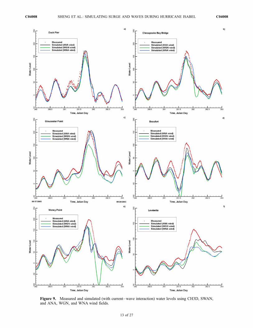
Figure 9. Measured and simulated (with current–wave interaction) water levels using CH3D, SWAN,and ANA, WGN, and WNA wind fields.


13 of 27

C04008

and 41002, located a couple of hundred kilometers off thecoast of North Carolina, during September 2003. Theseplots show that the simulated and measured wave parame-ters are in good agreement, although the significant waveheight at 41002 is underestimated just before the waveheight peaked owing to Isabel around Julian Day 260.

3.2. Simulated Versus Measured Wave at Duck andGloucester

[43] In the nearshore zone, spatial gradients of radiationstresses produced by breaking waves can create wave setup;that is, a rise in water elevation from the breaker zone to theshoreline. The radiation stresses depend on such waveparameters as wave height, wave period, and wave direc-tion. Depending on the wave condition and the local

bathymetry, wave setup can contribute significantly to thestorm surge elevation and affect the local currents. To obtainaccurate simulation of wave setup and storm surge, it isessential to have accurate simulation of nearshore wave-fields. We assess the accuracy of simulated wave conditionsduring Isabel using SWAN and three sets of wave data: twodata sets from the Field Research Facilities (FRF) at Duck,North Carolina, and one set from Gloucester Point, Virginia,provided by Virginia Institute of Marine Science (VIMS).[44] The measured and SWAN simulated wave conditions

at the FRF Waverider, approximately 4 km offshore (to bereferred to as Duck 630) where the depth is 17 m, arecompared. The maximum measured significant wave heightat the FRF Waverider buoy during Hurricane Isabel was

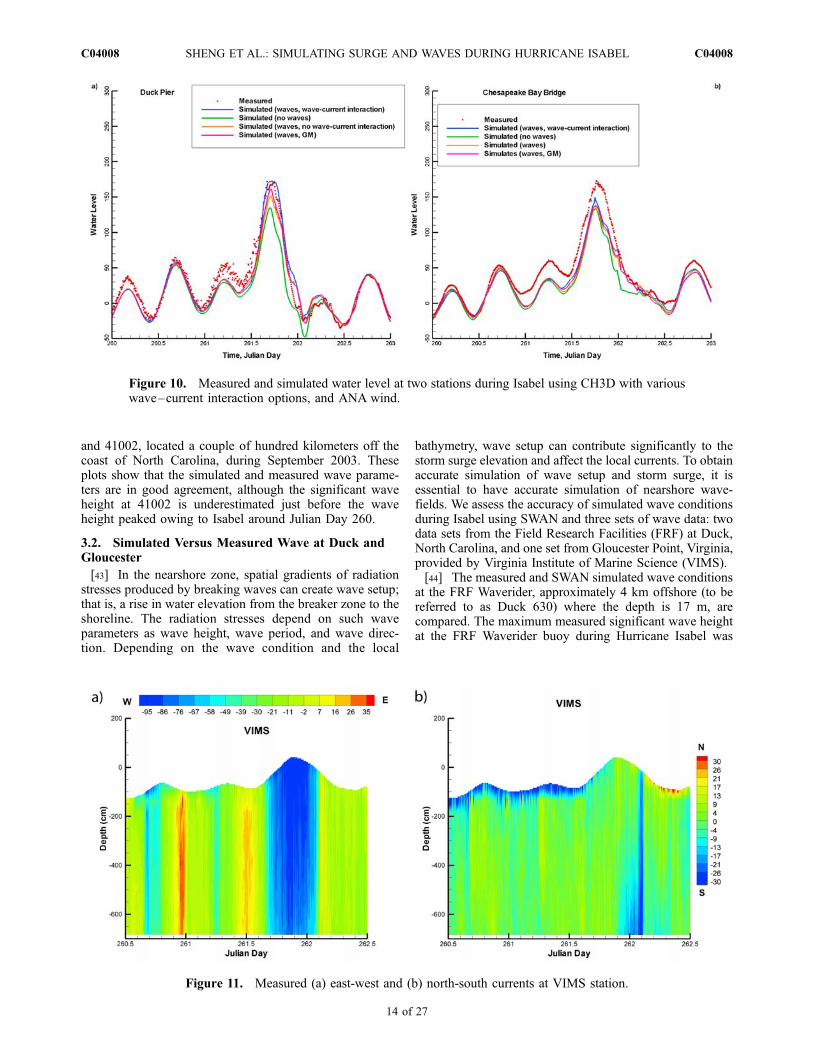
Figure 10. Measured and simulated water level at two stations during Isabel using CH3D with variouswave–current interaction options, and ANA wind.

Figure 11. Measured (a) east-west and (b) north-south currents at VIMS station.


14 of 27

C04008

8.1 m, while the largest wave (crest to trough) recorded on18 September at 1911 UT, was 12.1 m. The ratio of thelargest wave to local water depth, 0.71, indicates waveswere starting to break. The simulated versus measuredsignificant wave height, peak wave period and wave direc-tion are shown in Figure 6. The simulated results presentedhere are obtained using the WNA wind, since the WGNwind for Isabel was slightly less accurate. The simulatedwave height matches well with the measured data withslight underestimation at the peak. There is also a phase lagjust before the peak that may be due to swell wavesgenerated outside of the computational domain which couldnot be properly simulated by the SWAN model. This isbecause the wave height boundary conditions obtained from

the regional WW3 model are slightly below the measuredvalues right before Hurricane Isabel passed over the area,thus resulting in lower than expected wave setup rightbefore the peak of the storm. Nevertheless, the simulatedand measured peak wave height and period values appear tomatch well.[45] Figure 7 shows the simulated and measured wave

parameters at the end of the FRF Pier approximately 600 moffshore (to be referred to as Duck Pier 625) where thedepth is 8.4 m and the maximum measured significant waveheight during Hurricane Isabel was 3.7 m. Again, thesimulated and measured peak significant wave height andpeak wave period compare quite well, although the wave

Figure 13. (left) Measured onshore-offshore currents and (right) downshore-upshore currents at KittyHawk, North Carolina, during Hurricane Isabel.

Figure 12. Simulated (a) east-west and (b) north-south currents at VIMS station obtained using coupledCH3D/SWAN with a lookup table for wave–current bottom stress and ANA wind field.


15 of 27

C04008

height was slightly underestimated approximately one daybefore the peak storm wind arrived.[46] Waves are quite significant at Gloucester Point,

Virginia (referred to as ‘‘VIMS,’’ the data provider), wherethe depth at the location is around 8.5 m, with a maximummeasured significant wave height of 1.7 m. Both thesignificant wave height and the peak wave period are wellsimulated, as shown in Figure 8. Errors in wave simulationcan be attributed primarily to errors in the open boundarycondition provide by WW3, and partially to errors in theWNA wind that often slightly exceeds the measured windlocally. The simulated peak wave period agrees well withthe observed.

3.3. Validation of Storm Surge Simulations

[47] Several simulations were carried out using ANA/WNA/WGN wind while including or excluding waveeffects. Simulated water elevations, using ANA/WNA/WGN wind and including wave effects, are compared withmeasured water elevations at six stations in Figure 9.Figure 9 shows that simulated water levels obtained withthe ANA wind compare the best with observation data. Atany particular data station, the response of water level towind and storm surge depends significantly on the localcondition (e.g., any sheltering effect of land or structure).For example, at Gloucester Point, the relatively lower waterlevel owing to the WGN wind was because of the lowersoutheasterly (parallel to the York River) wind compared tothe ANA and WNA winds. The stronger southerly ANAwind did not cause higher water level owing to the narrowriver width in the north-south direction. At Money Point,which is at a far upstream station, significant ‘‘set down’’ ofwater level was caused by the WGN wind which errone-ously lined up with the river channel. Such errors in localwind conditions are often created owing to spatial andtemporal interpolation from wind fields with relativelycoarse spatial and temporal resolutions.

[48] The simulated winds along the Outer Banks and inlower Chesapeake Bay agree well with data and, as a result,the simulated water elevations agree well with measureddata. It is noted that the simulated peak water surfaceelevations match the measured ones well at Duck,Chesapeake Bay Bridge Tunnel, and Gloucester Point. Aslight underestimation just before the peak elevation can beobserved at all the stations. As pointed out in section 3.2,the simulated wave height before the peak are underesti-mated owing to the underestimated open boundary waveconditions provided by the WW3 model. This underesti-mation resulted in lower than expected wave setup rightbefore the peak of the storm. However, wave height at thepeak of the storm was accurately simulated, which resultedin adequate contribution of calculated wave setup to thesimulated water level at that time.[49] Figure 10 shows the measured and simulated water

level at two stations using ANA wind input and CH3D/SWAN with various wave–current interaction options: nowave effects, no wave–current interaction, with waveeffects but different formulas for wave–current bottomstress. It is apparent that the best results are obtained whencurrent–wave interaction is included and bottom stress isincluded using the lookup table produced by the Sheng-Villaret (SV) model.

3.4. Simulated Versus Measured Current Profilesat Gloucester and Kitty Hawk

[50] Measured surface elevation and currents at the VIMSstation exhibit periods of the M2 tide as Figure 11a showssignificant eastward currents around Julian Day 261 and261.5. From Julian Day 261.75 to 262.1, the incomingstorm surge caused strong westward currents throughout thewater column (�8 m). Simulated currents obtained usingcoupled CH3D/SWAN and wave–current interaction bot-tom stress lookup table and ANA wind input show similarresults in Figure 12. Significant eastward currents are foundat Julian Day 261 and 261.5, while strong westward

Figure 14. (a) Onshore-offshore currents and (b) downshore and upshore currents at Kitty Hawksimulated using CH3D-SSMS with a wave–current bottom stress lookup table and WNA wind.


16 of 27

C04008

currents are found during Julian Day 261.75 and 262.1.Both measured and simulated north-south currents showflow reversal between the surface and bottom watersbetween Julian Day 261.9 and 262.1.[51] Measured and simulated currents at Kitty Hawk are

also presented here. Figure 13 shows the measured onshore-offshore and downshore-upshore currents at Kitty Hawk,while Figure 14 (with WNA wind) shows the simulatedcurrents. Prior to the arrival of hurricane wind around JulianDay 261.7, data showed strong southeastward (offshore anddownshore) currents which are apparently wind driven butare underestimated by the model owing to lower simulatedwind. During Julian Day 261.7 and 261.9, peak easterly andsoutheasterly wind caused strong currents in onshore andupshore directions and both measured and simulated cur-rents show a vertical structure with onshore flow near thesurface and offshore flow near the bottom. Results (notshown) obtained using ANA wind, which is weaker thanWNAwind at Duck, are slightly worse. While the simulatedcurrents do not agree completely with the observed currents,

the results are encouraging considering the relatively coarsegrid resolution (eight vertical layers and four to six hori-zontal cells between the Kitty Hawk station and the shore-line) and uncertainty in bathymetry in the vicinity.Measured and simulated onshore-offshore velocity at KittyHawk at the peak of storm surge exhibits a two-layer flowstructure as shown in Figure 15. This two-layer flowstructure is apparently caused by hurricane force wind aswell as breaking hurricane wave. Before and after the peakstorm surge, this two-layer flow structure did not exist.

4. Discussion

4.1. Evolution of Storm Surge During Isabel

[52] Five snapshots of instantaneous water level in theChesapeake Bay and Outer Banks are shown in Figures 16a–16e to illustrate the evolution of storm surge during Isabel onthe basis of model simulations using ANAwind. For clarity,water levels over land areas are not shown. At 1330 UT on18 September (Julian Day 261), as shown in Figure 16a, a

Figure 15. Measured and simulated onshore-offshore currents at Kitty Hawk during Isabel.


17 of 27

C04008

few hours before Isabel made landfall, wind starts toincrease and switch from northeasterly to easterly, and peakwater level is found inside the Pamlico Sound. At 1730 UT,as shown in Figure 16b, Isabel landfalls to the east of CapeOutlook and Beaufort, and wind starts to switch fromeasterly to southeasterly. As shown in Figure 9, waterelevations at Duck, Beaufort, Chesapeake Bay Bridge, andGloucester all peaked around this time when tide at Duckalso peaked. Between 1730 and 2400 UT (Figure 16c),

strong southeasterly wind pushes the surge and high waterinto Chesapeake Bay, leading to high water level in south-ern Chesapeake Bay, James River, and York River. From2400 UT on, southerly wind persists for more than 12 h inmost of the Chesapeake Bay, and generates a significantsouth-to-north setup of water level, as shown in Figure 16d(1130 on 19 September) and Figure 16e (1700 UT on19 September).

Figure 16. Snapshots of water level at five instants in study area during Isabel.

Figure 17. Evolution of water level along the major axis during Isabel.


18 of 27

C04008

[53] To illustrate the more detailed evolution of waterlevel during Isabel, the simulated water level along themajor axis of Chesapeake Bay (Figure 2) is plotted as afunction of space and time in Figure 17. The result as shown

in Figure 17 compares qualitatively well with that producedby Shen et al. [2006] using a different storm surge modelbut without a wave model. Results obtained with WNA andWGN winds are also similar with slight differences in peakelevation and timing.

4.2. Simulated Maximum Envelope of Water

[54] Maximum envelope of water (MEOW) is the max-imum simulated water elevations (including tide, surge andwave setup) throughout a model simulation. Figure 18shows the MEOW in the Outer Banks and ChesapeakeBay during Isabel, calculated using the WGN wind. TheMEOW simulated using ANA wind shows slightly higherinundation in the land area owing to generally slightlystronger ANA wind inside Chesapeake Bay.

4.3. Effect of Wave on MEOW

[55] To examine the effect of wave on the maximumwater level during Isabel, we calculate the maximum waterlevel owing to wave effect by subtracting the MEOWowingto wind and tide from the MEOW owing to wind, tide, andwave. The resulting maximum envelope of water gives theMEOW owing to wave effect only (MEOWW). Figure 19ashows the maximum envelope of significant wave height(MESWH) during Isabel, while Figure 19b shows themaximum envelope of water owing to wave (MEOWW).As shown in Figures 19a and 19b, high wave is found incoastal region as well as inside Chesapeake Bay, and theeffect of wave on maximum water elevation is very signif-icant, reaching 30–100 cm within most of the ChesapeakeBay and the major rivers. High waves along the CapeHatteras National Seashore, in combination with the highsurge, most likely resulted in inundation and breaching ofthe barrier island during Isabel.

Figure 18. Maximum envelope of water (MEOW)simulated using WGN wind.

Figure 19. (a) Maximum envelope of significant wave height simulated using WNA wind.(b) Maximum envelope of water due to wave simulated using WNA wind.


19 of 27

C04008

[56] It is interesting to point out that while wave heightnear the mouth of Chesapeake Bay and along the northshore of North Carolina is comparable to that along thesouth shore of North Carolina, wave-induced water eleva-tion is much lower along the south shore because winddirection during Isabel was mostly parallel to the shorehence did not generate much wave setup. Wave-inducedwater level is quite significant inside the Chesapeake Bay,because of favorable wind direction (particularly insideJames River) and significance of wave-induced wind stress.Wave-induced water level along the north shore of NorthCarolina, including the Duck area, is significant because ofquite significant radiation stress gradients perpendicular tothe shoreline associated with the onshore-directed wind ofIsabel.

4.4. Effect of Wave on Wind Stress and HorizontalMomentum

[57] We show the maximum wave-enhanced wind stress,maximum wind stress (without wave effect), and maximumwave-induced surface stress in the model domain generatedby the WNA wind during Hurricane Isabel in Figures 20a,20b, and 20c, respectively. The wave-induced surface stressshown in Figure 20c is quite significant particularly insidethe southern Chesapeake Bay and Pamlico Sound, whichexplains the significant wave-induced water level thereshown in Figure 19b. Therefore, inside the southern Ches-apeake Bay and Pamlico Sound, wave-induced water levelincreases mainly owing to the increased wave-inducedsurface stress, while the wave-induced radiation stressgradient is negligible there as shown in Figure 21. Signif-icant radiation stress gradients are found along the northshore of North Carolina including Duck, plus the deeperwater off the south shore of North Carolina. The significant

Figure 20. (a) Maximum wave-enhanced wind stress, (b) maximum wind stress, and (c) maximumwave-induced surface stress during Hurricane Isabel.

Figure 21. Maximum radiation stress gradients duringIsabel.


20 of 27

C04008

Figure 22. (a) Evolution of dimensionless wave-enhanced surface stress, wave-induced surface stress,radiation stress gradient, and wave-enhanced bottom stress in onshore-offshore direction at a coastalstation near Duck, North Carolina, during Hurricane Isabel. (b) Evolution of dimensionless wave-enhanced surface stress, wave-induced surface stress, radiation stress gradient, and wave-enhancedbottom stress in the north-south direction at a Chesapeake Bay station during Hurricane Isabel.

Figure 23. Simulated versus measured HWMs.


21 of 27

C04008

radiation stress gradients along the north shore of NorthCarolina associated with the onshore-directed wind duringIsabel caused the significant wave-induced surge shown inFigure 19b and the two-layer flow shown in Figures 13–15.The significant radiation stress gradients in the open wateroff the south shore of North Carolina did not causesignificant wave-induced water level owing to the generallyalongshore wind direction. The dominance of wind-inducedstress versus wave-induced stress in the region resulted inpredominantly wind-induced water level.[58] To further illustrate the relative importance of radi-

ation stress gradients versus wave-induced surface stress inaffecting the storm surge, we show the evolution of four

quantities at two stations: a coastal station near Duck and anestuarine station inside the Chesapeake Bay (about 15 km tothe northeast of Gloucester Point, Virginia) in Figures 22aand 22b, respectively. The four plotted quantities include:(1) wave-enhanced surface stress, (2) wave-induced surfacestress, (3) radiation stress gradients, and (4) wave-enhancedbottom stress; calculated from the dimensionless verticallyintegrated momentum equations (vertically integrated ver-sion of equations (A5) and (A6)) in the onshore-offshoredirection (for the coastal station) and the north-south direc-tion (for the estuarine station). As shown in Figure 22a,radiation stress gradient and wave-induced surface stress areboth important at the coastal station, while Figure 22b

Table 2. Simulation Categories With Various Combinations of Five Model Features

FactorsSimulation

1Simulation

2Simulation

3Simulation

4aSimulation

4b

Tide yes yes yes yes yesWind yes yes yes yes yesWave-enhancedsurface stressa

no no yes yes yes

Bottom stress currentinduced only

currentinduced only

current inducedonly

wave-currentb wave-currentc

Radiation stress none formulationof Longuet-Higginsand Stewart [1964]

formulationof Longuet-Higginsand Stewart [1964]



aDonelan et al. [1993] formulation.bGrant and Madsen [1979] formulation.cLookup table based on the Sheng and Villaret [1989] formulation.

Table 3. Errors of Simulated Water Elevation at Tide Stations During Hurricane Isabel Based on Comparison Between Model Results

and Data Every 15 min

Tide

WNA Wind WGN Wind ANA Wind

Simulation2

Simulation4a

Simulation2

Simulation4a

Simulation1

Simulation2

Simulation3

Simulation4a

Simulation4b

Beauforta

RMS error (cm) 3.8 16.2 16.0 17.0 17.5 18.0 16.5 16.8 17.0 17.1Error at peak (cm) . . . �32 �26 �43 �37 �27 �22 �25 �19 �21Timing at peak (min) . . . 16 14 18 13 �24 �11 �7 �6 �6

Duckb

RMS error (cm) 3.6 10.2 10.0 10.7 11.1 11.2 11.0 11.0 10.6 10.2Error at peak (cm) . . . �33 �11 �35 �19 �37 �20 �20 0 �1Timing at peak (min) . . . 51 52 59 57 53 53 52 53 53

Chesapeake Bay Bridgec

RMS error (cm) 4.1 10.2 9.8 11.2 10.8 11.4 11.0 10.7 10.8 10.7Error at peak (cm) . . . �28 �28 �19 �19 �39 �34 �30 �22 �24Timing at peak (min) . . . 7 7 17 17 16 16 16 16 16

Gloucester Pointd

RMS error (cm) 5.7 11.2 10.0 19.3 18.2 11.0 10.3 10.5 9.8 9.9Error at peak (cm) . . . �5 �18 �60 �47 �8 �1 1 3 6Timing at peak (min) . . . 122 120 3 6 114 110 112 108 113

Money Pointe

RMS error (cm) 9.8 20.2 17.5 17.9 17.7 18.2 16.8 19.5 18.6 18.4Error at peak (cm) . . . �37 �24 �40 �29 �34 �25 �26 �22 �20Timing at peak (min) . . . �48 �51 �19 �22 �105 �112 �112 �118 �115

Lewisettaf

RMS error (cm) 5.6 16.8 18.2 18.3 17.8 18.0 16.8 19.5 19.8 19.5Error at peak (cm) . . . �62 �58 �55 �43 �54 �50 �45 �32 �30Timing at peak (min) . . . �146 �158 130 132 98 115 105 105 103

aDepth, 4.0 m; maximum tidal range, 115 cm; measured peak during Isabel, 107 cm.bDepth, 5.8 m; maximum tidal range, 140 cm; measured peak during Isabel, 171 cm.cDepth, 10.6 m; maximum tidal range, 110 cm; measured peak during Isabel, 168 cm.dDepth, 8.5 m; maximum tidal range, 80; measured peak during Isabel, 199 cm.eDepth, 13.1 m; maximum tidal range, 100 cm; measured peak during Isabel, 192 cm.fDepth, 3.0 m; maximum tidal range, 45 cm; measured peak during Isabel, 131 cm.


22 of 27

C04008

shows that wave-induced surface stress clearly dominatesthe radiation stress gradient at the Chesapeake Bay station.

4.5. Accuracy of Simulated High Water Marks

[59] High water marks (HWMs) at numerous stationsshown in Figure 2 are used to compare with simulatedHWMs obtained using WGN, WNA, and ANA winds. Asshown in Figure 23, HWMs simulated using the ANAwindagree the best with the measured ones, while HWMsproduced using WGN and WNA winds are generallyslightly underestimated.

4.6. How Sensitive Is Simulated Storm Surge Elevationto Various Model Features?

[60] In order to assess the effects of various factors onsimulated storm surge throughout the model domain duringIsabel, several simulations were made. Table 2 specifies thefive specific model features included in five simulationcategories. Table 3 shows the RMS error of simulated waterelevation at six stations during Isabel. Errors of peak values(measured peak elevation minus simulated peak elevation)and ‘‘timing’’ errors (the time when measured peak eleva-tion occurred minus the time when simulated peak elevationoccurred) are also shown. A separate column displays theerrors associated with the ‘‘pure’’ tide simulation, whichonly included tidal forcing at the open boundaries.[61] On the basis of this error analysis, particularly the

average RMS errors and average absolute errors at the peakwater elevation, it can be concluded that the ANA windproduced generally more accurate water level at all stations.

This is consistent with the earlier analysis which showedthat WNA and WGN winds, because of spatial and temporalinterpolation from rather sparse and coarse-resolution windfields, are somewhat less accurate than the ANAwind insidethe Chesapeake Bay. Temporal interpolation of sparse windfields, particularly near landfall time, tends to distorthurricane structures and generate artificially lower windspeed and erroneous direction. However, ANA wind isgenerated at every grid cell every time step, hence retainsthe hurricane structure throughout the simulation. Theaccuracy of the simulated water elevation, which includestide, depends on the accurate simulation of tide which isaccurate across the Outer Banks up to the mouth of theChesapeake Bay, with the average RMS error of approxi-mately 4 cm. Inside the bay, the accuracy of the simulatedtide worsens, with the average RMS error increasing to6 cm. So did the accuracy of the simulated water elevation,which was also accompanied with the worse accuracy of theWNA wind inside the Chesapeake Bay as opposed to thatover the Outer Banks. In general, ANAwind produced moreaccurate water elevation and inundation (as measured byHWMs) inside the Chesapeake Bay, as shown in Figures 23and 24.[62] On the basis of Table 2 and Figure 24, simulation 4

produces the best overall water level agreement with slightlysmaller RMS errors and better comparison with measuredwater surface elevation at its peak. In the Outer Banksregion, the inclusion of WNA wind led to good simulatedwater elevation. After Isabel made landfall, the simulatedwater elevation at Beaufort is not very good because the

Figure 24. Comparison between simulated and measured water level at six stations during Isabel.


23 of 27

C04008

effect of land dissipation on wind is not included. InsideChesapeake Bay, the WNAwind (based on extrapolation ofcoastal wind) gives less accurate results. WGN wind, whichis slightly more accurate than the extrapolated WNA windinside Chesapeake Bay, provided a slightly more accuratewater elevation prediction. The ANA wind gives generallymore accurate water elevation results over the entire modeldomain. However, the effect of land dissipation on hurri-cane wind [e.g., IPET, 2006] has not been included in thissimple analytical wind model.

4.7. Three-Dimensional Effects on Simulated StormSurge, Wave, and Inundation

[63] The Maximum Envelope of Water (MEOW) resultsduring Isabel obtained by the 2- and 3-D simulations arecompared and the difference between the 3- and 2-D waterlevel is shown in Figure 25. Both models include the waveeffects; the 2-D simulation was based on coupled SWANand the 2-D version of CH3D, the 3-D simulation is basedon coupled SWAN with the 3-D version of CH3D. Whilethe radiation stress formulation is the same for both the 2-and 3-D simulations, the wave–current bottom stress for-mulation is different. In the 2-D simulation, wave-inducedbottom stress is kinematically combined with current-in-duced bottom stress to produce the total bottom stressaveraged over the wave cycle [Sheng and Lick, 1979; Bijker1966, 1986]. The 3-D bottom stress is obtained from the

lookup table which is based on the results of nonlinearlycoupled wave turbulence model of Sheng and Villaret[1989]. Therefore the wave–current bottom stress in the2-D simulation tends to be higher than that in the 3-Dsimulation. This explains the slightly higher maximumwater elevation in the 3-D results throughout most of themodel domain, as shown in Figure 25. Using the 2- or 3-Dversions of CH3D only made very slight difference (nomore than 5 cm) on the maximum significant wave heightthroughout the model domain.

5. Conclusions

[64] An integrated modeling system CH3D-SSMS hasbeen used to simulate the storm surge, wave effect, andinundation in the Outer Banks and Chesapeake Bay areaduring Hurricane Isabel. Model results are found to reason-ably reproduce the observed wind, storm surge, wave,currents, and inundation in the study area. The three windfields (ANA, WGN, and WNA) all give reasonable wind atthe coastal stations prior to Isabel landfall, while the ANAwind is found to be generally slightly more accurate than theWGN and WNA winds in the Chesapeake Bay region afterthe landfall. Producing accurate over-the-land wind afterhurricane landfall remains a major challenge.[65] The most notable results are that the model simulated

the significant effects of waves on storm surge, currents, andinundation. Among the three resolved processes whichrepresent wave effects, wave-induced radiation stress (out-side the estuaries) and wave-induced surface stress (outsideand inside the estuaries) are the dominant ones, while wave-induced bottom stress is of secondary importance. The bestresults are obtained when SWAN is coupled to the 3-Dversion of CH3D, with all three wave effects included. Theinclusion of radiation stress improved the computed stormsurge by up to 18%, with the most significant improvementat Beaufort and Duck where high breaking waves causedsignificant setup. Including wave-induced surface stressimproved the calculated storm surge by up to 16%, whileincluding wave-induced bottom friction led to up to 5%reduction in the peak storm surge level. Wave-enhancedbottom stress in the coupled CH3D-SWAN is higher whenthe 2-D version of CH3D is used.[66] Observation data and model simulation yielded the

following interesting results. Maximum water elevation inthe study area reached 2.5 m during Isabel, while maximumwave height reached �20 m offshore and up to 4 m insidethe Chesapeake Bay. Maximum wave-induced water levelreached 1 m inside the Chesapeake Bay. Significant wavesreached 3.5 m and 16 s at the Duck Pier, and 1.6 m and 5 sat Gloucester, Virginia. Offshore waves led to breaking andlarge wave setup, which accounted for �36 cm or 20% ofthe peak surge elevation of 1.71 m at Duck. Inside theChesapeake Bay, wave setup accounts for 5–10% ofobserved peak surge elevation. At Kitty Hawk, a two-layerflow (with onshore surface current and offshore currentunderneath) is found during the peak of storm surge owingto combined effects of wind and wave breaking. Currentsaround 1 m/s were found at Gloucester.[67] Although water levels simulated by 2- and 3-D

models do not differ significantly at selected stations, the3-D results show noticeably more inundation. The 3-D

Figure 25. Difference between the maximum envelope ofwater during Isabel obtained by the 2- and 3-D simulationsusing ANA wind.


24 of 27

C04008

model is necessary for accurate simulation of observedcurrents at Gloucester and Kitty Hawk that are driven bywind, tide, and radiation stress. The 3-D model also allowsinclusion of more robust wave–current interaction process-es, including the radiation stress formulation and wave-enhanced bottom stress. The use of the 3-D model and alookup table provides a novel method for calculating wave-enhanced bottom stress. Further model validation can beconducted if high-resolution field data of wave and turbu-lence within the bottom boundary layer and the surfacelayer in the surf zone become available. The modelingsystem can be used as a framework for testing newlydeveloped current–wave interaction model [e.g., Mellor,2008], or wave model. Additional insight on the waveprocesses can be gained by comparing simulated andmeasured directional wave spectra at data stations.Although the stationary SWAN produced reasonably accu-rate wave simulation for the Isabel simulation, its applica-tion to a faster moving storm needs to be furtherinvestigated.

Appendix A: Equations and BoundaryConditions of the Coastal Surge Model CH3D

A1. Equations of the Coastal Surge Model CH3D

[68] In Cartesian coordinate system, the governing equa-tions for water continuity, X momentum, and Y momentumequations are:

@u

@xþ @v@yþ @w@z¼ 0 ðA1Þ

@u

@tþ @uu@xþ @uv@yþ @uw

@zþ 1

rw

@Sxx@xþ 1

rw

@Sxy@y

¼ �g @V@x� 1

rw

@Pa

@xþ fvþ AH

@2u

@xþ @

2u

@y

� �þ @

@zAV

@u

@z

� �ðA2Þ

@v

@tþ @uv@xþ @vv@yþ @vw

@zþ 1

rw

@Syx@xþ 1

rw

@Syy@y

¼ �g @V@y� 1

rw

@Pa

@y� fuþ AH

@2v

@xþ @

2v

@y

� �þ @

@zAV

@v

@z

� �ðA3Þ

where u(x; y; z; t), v(x; y; z; t), and w(x; y; z; t) are thevelocity vector components in x, y, and z coordinatedirections, respectively; t is time; V(x; y; t) is the freesurface elevation; g is the acceleration of gravity; AH and AVare the horizontal and vertical turbulent eddy coefficients,respectively; Sxx, Sxy, Syy are radiation stresses, Pa isatmospheric pressure and f is the Coriolis parameter. AV iscalculated by the vertical turbulence model described in thework of Sheng and Villaret [1989], and AH by aSmargorinsky-type formula.[69] Following Sheng [1987, 1990], the nondimensional

form of above equations in curvilinear, boundary-fitted gridsystem can be written as:

@z@tþ bffiffiffiffiffi

g0p

@

@xffiffiffiffiffig0p

Hu� �

þ @

@hffiffiffiffiffig0p

Hv� ��

þ b@Hw@s¼ 0 ðA4Þ

1

H

@ Hu

@ t¼ � g11

@z@xþ g12

@z@h

� �þ� g11

@P

@xþ g12

@P

@h

� �

þ g12ffiffiffiffiffig0p uþ g22ffiffiffiffiffi

g0p v

� �� R0

g0xh

@

@xyx

ffiffiffiffiffig0p

Sxx þ yhffiffiffiffiffig0p

Sxh� ��

þ @

@hyx

ffiffiffiffiffig0p

Sxh þ yhffiffiffiffiffig0p

Shh� ��

�yh@

@xxx

ffiffiffiffiffig0p

Sxx þ xhffiffiffiffiffig0p

Sxh� ��

þ @

@hxx

ffiffiffiffiffig0p

Sxh þ xhffiffiffiffiffig0p

Shh� ��

� R0

g0Hxh

@

@xyx

ffiffiffiffiffig0p

Huu��

þ yhffiffiffiffiffig0p

Huv�þ @

@hyx

ffiffiffiffiffig0p

Huvþ yhffiffiffiffiffig0p

Hvv� ��

� yh@

@xxx

ffiffiffiffiffig0p

Huuþ xhffiffiffiffiffig0p

Huv� ��

þ @

@hxx

ffiffiffiffiffig0p

Huvþ xhffiffiffiffiffig0p

Hvv� ��

� g0@Huw@s

þ Ev

H2

@

@sAv

@u

@s

� �þ EHAH Horizontal Diffusion of uð Þ

� R0

F2r

H

Z 0

sg11

@r@xþ g12

@r@h

� �ds

�

þ g11@H

@xþ g12

@H

@h

� � Z 0

srds þ sp

� ��ðA5Þ

1

H

@ Hv

@ t¼ � g21

@z@xþ g22

@z@h

� �� g21

@P

@xþ g22

@P

@h

� �

� g11ffiffiffiffiffig0p uþ g21ffiffiffiffiffi

g0p v

� �� R0

g0xx

@

@xyx

ffiffiffiffiffig0p

Shx þ yhffiffiffiffiffig0p

Shh� ��

þ @

@hyx

ffiffiffiffiffig0p

Shx þ yhffiffiffiffiffig0p

Shh� ��

�yh@

@xxx

ffiffiffiffiffig0p

Sxx þ xhffiffiffiffiffig0p

Shx� ��

þ @

@hxx

ffiffiffiffiffig0p

Shx þ xhffiffiffiffiffig0p

Shh� ��

� R0

g0Hxx

@

@xyx

ffiffiffiffiffig0p

Huv��

þ yhffiffiffiffiffig0p

Hvv�þ @

@hyx

ffiffiffiffiffig0p

Huvþ yhffiffiffiffiffig0p

Hvv� ��

� yh@

@xxx

ffiffiffiffiffig0p

Huuþ xhffiffiffiffiffig0p

Huv� �

þ @

@hxx

ffiffiffiffiffig0p

Huvþ xhffiffiffiffiffig0p

Hvv� ��

� g0@Hvw@s

þ Ev

H2

@

@sAv

@v

@s

� �þ EHAH Horizontal Diffusion of vð Þ

� R0

F2r

H

Z 0

sg21

@r@xþ g22

@r@h

� �ds þ g21

@H

@xþ g22

@H

@h

� ��

�Z 0

srds þ sp

� ��ðA6Þ

where

x, h and s are the transformed coordinates;u, v, w are nondimensional contravariant

velocities in curvilinear grid (x, h, s).ffiffiffiffiffig0p

is the Jacobian of horizontal trans-formation;

g11, g22, g11, g12, g22 are the metric coefficients of coordi-nate transformations;

b is nondimensional parameter;z is water level;

[70] It can be shown that thewave-averaged equations (A4)–(A6) are valid for two regions: the region between the freesurface (mean sea level) and the wave trough, as well as


25 of 27

C04008

the region between the wave trough and the bottom. In theregion above the wave trough, the wave-averaged horizontalcurrents include the mean currents and the Stokes drift,while the radiation stress includes the vertically uniformradiation stress according to Longuet-Higgins and Stewart[1964] plus that owing to the surface roller [Svendsen, 1984;Haas and Svendsen, 2000]. Below the wave trough, theStokes drift is zero, while the radiation stress does not havethe surface roller contribution. Equations (A4)–(A6) can besolved numerically using the conjugate gradient algorithmmodified from that used by Casulli and Cheng [1992] forCartesian grids, given sufficient boundary conditions (windstresses, river inflows, precipitation, and open boundarywater elevation), initial conditions (water level), and otherdata (bathymetry and topography). In practical applications,it is possible to solve only the vertically integrated 2-Dversion of the CH3D model, instead of solving the complete3-D equations. The 2-D model generally results in signifi-cant saving in computational time and comparable waterlevel simulation in shallow coastal regions.

A2. Boundary Conditions for the Coastal Surge ModelCH3D

[71] The boundary condition at the free surface is calcu-lated using

twx ¼ raCduwWs ðA7Þ

twy ¼ raCdvwWs ðA8Þ

where uw and vw are wind speed components, and Ws is thetotal wind speed. The drag coefficient, Cd is calculatedusing the Garratt [1977] formulation:

Cd ¼ 0:001� 0:75þ 0:067Wsð Þ ðA9Þ

When waves are present, the drag coefficient is calculatedfollowing the Donelan et al. [1993] formula described inequations (1) and (2).[72] The boundary condition at the bottom is expressed in

terms of bottom stress given by the quadratic law:

tbx ¼ rwCdub


qðA10Þ

tby ¼ rwCdvb


qðA11Þ

where ub and vb are bottom velocities and Cd is the dragcoefficient which is defined using the formulation by Sheng[1983]:

Cd ¼k

ln z1=z0ð Þ

� �2ðA12Þ

where k is the von Karman constant. The formulation statesthat the coefficient is a function of the size of the bottomroughness, z0, and the height at which ub is measured, z1 iswithin the constant flux layer above the bottom. The size of

the bottom roughness can be expressed in terms of theNikuradse equivalent sand grain size, ks, using the relationz0 = ks/30.[73] In the two-dimensional mode, the bottom boundary

conditions are given using the Chezy-Manning formulation:

tbx ¼ rAv

@ub@z¼

gub


qC2z

ðA13Þ

tby ¼ rAv

@vb@z¼

gvb


qC2z

ðA14Þ

where Cz is the Chezy friction coefficient defined as

Cz ¼ 4:64R

16

nðA15Þ

where R is the hydraulic radius which can be approxi-mated by the total depth given in centimeters, and n isManning’s n.

[74] Acknowledgments. We appreciate the partial support ofFlorida Sea Grant project R/C-S47, SURA, and NOAA IOOS grantNA07NOS47302111. We thank H. Chen of NOAA for providing theWAVEWATCH-III data, H. Graber of University of Miami for providingthe WINDGEN data, L. Brasseur of VIMS for providing the wave andcurrent data at Gloucester Point, and K. Hathaway and B. Birkemeier ofUSACE/FRF for providing the ADCP data at Kitty Hawk. We alsoappreciate the comments of two anonymous reviewers.

ReferencesAlymov, V. (2005), Integrated modeling of storm surges during HurricanesIsabel, Charley, and Frances, Ph.D. dissertation, Univ. of Fla., Gainesville.

Battjes, J. A. (1975), A note on modeling of turbulence in the surf-zone, inSymposium on Modeling Techniques, pp. 1050–1061, Am. Soc. of Civ.Eng., Reston, Va.

Bijker, E. W. (1966), The increase of bed shear in a current due to waveaction, in Proceedings of the 10th International Conference on CoastalEngineering, pp. 746–765, Am. Soc. of Civ. Eng., Reston, Va.

Bijker, E. W. (1986), Scour around structures, in Proceedings of the 21stInternational Conference on Coastal Engineering, pp. 1754–1768, Am.Soc. of Civ. Eng., Reston, Va.

Blumberg, A., and G. L. Mellor (1987), A description of a three-dimen-sional coastal ocean circulation model, in Three-Dimensional CoastalOcean Models, Coastal Estuarine Sci., vol. 4, edited by N. S. Heaps,pp. 1–16, AGU, Washington, D. C.

Bode, L., and T. A. Hardy (1997), Progress and prospects in storm surgemodeling, J. Hydraul. Eng., 123, 315–331, doi:10.1061/(ASCE)0733-9429(1997)123:4(315).

Booij, N., R. C. Ris, and L. H. Holthuijsen (1999), A third-generation wavemodel for coastal regions: 1. Model description and validation, J. Geo-phys. Res., 104, 7649–7666, doi:10.1029/98JC02622.

Casulli, V., and R. T. Cheng (1992), Semi-implicit finite difference methodsfor three-dimensional shallow water flow, Int. J. Numer. Methods Fluids,15, 629–648, doi:10.1002/fld.1650150602.

Casulli, V., and R. A. Walters (2000), An unstructured, three-dimensionalmodel based on the shallow water equations, Int. J. Numer. MethodsFluids, 32, 331 – 348, doi:10.1002/(SICI)1097-0363(20000215)32:3<331::AID-FLD941>3.0.CO;2-C.

Davis, J. R., and Y. P. Sheng (2003), Development of a parallel storm surgemodel, Int. J. Numer. Methods Fluids, 42, 549–580, doi:10.1002/fld.531.

De Vriend, H. J., and M. J. F. Stive (1987), Quasi-3D modelling of near-shore currents, Coastal Eng., 11, 565 – 601, doi:10.1016/0378-3839(87)90027-5.

Donelan, M. A., F. W. Dobson, S. D. Smith, and R. J. Anderson (1993), Onthe dependence of sea-surface roughness on wave development, J. Phys.Oceanogr., 23, 2143 – 2149, doi:10.1175/1520-0485(1993)023<2143:OTDOSS>2.0.CO;2.


26 of 27

C04008

Flather, R. A. (1994), A storm prediction model for the northern Bay ofBengal with application to the cyclone disaster in April 1991, J. Phys.Oceanogr. , 24 , 172 – 190, doi:10.1175/1520-0485(1994)024<0172:ASSPMF>2.0.CO;2.

Foreman, M. G. G. (1977), Manual for tidal heights analysis and prediction,Pac. Mar. Sci. Rep. 77-10, Inst. of Ocean Sci., Patricia Bay, Sidney, B. C.

Garratt, J. R. (1977), Review of drag coefficients over oceans and conti-nents, Mon. Weather Rev., 105, 915 – 929, doi:10.1175/1520-0493(1977)105<0915:RODCOO>2.0.CO;2.

Graber, H. C., V. J. Cardone, R. E. Jensen, D. N. Slinn, S. C. Hagen,A. T. Cox, M. D. Powell, and C. Grassl (2006), Coastal forecasts andstorm surge predictions for tropical cyclones: A timely partnershipprogram, Oceanography, 19, 130–141.

Grant, W. D., and O. S. Madsen (1979), Combined wave and currentinteraction with a rough bottom, J. Geophys. Res., 84, 1797–1808,doi:10.1029/JC084iC04p01797.

Haas, K. A., and I. A. Svendsen (2000), Three-dimensional modeling of ripcurrent systems, Rep. CACR-00-06, 250 pp., Cent. for Appl. CoastalRes., Univ. of Del., Newark.

Holland, G. (1980), An analytic model of the wind and pressure profiles inhurricanes, Mon. Weather Rev., 108, 1212–1218, doi:10.1175/1520-0493(1980)108<1212:AAMOTW>2.0.CO;2.

Houston, S. H., W. A. Shaffer, M. D. Powell, and J. Chen (1999), Compar-isons of HRD and SLOSH surface wind fields in hurricanes: Implicationsfor storm surge modeling, Weather Forecast., 14, 671–686, doi:10.1175/1520-0434(1999)014<0671:COHASS>2.0.CO;2.

Hubbert, G. D., and K. L. McInnes (1999), A storm surge inundation modelfor coastal planning and impact studies, J. Coastal Res., 15, 168–185.

Interagency Performance Evaluation Taskforce (IPET) (2006), Performanceevaluation of the New Orleans and Southeast Lousiana hurricane protec-tion system, technical report, U.S. Army Corps of Eng., Vicksburg, Miss.

Jelesnianski, C. P., J. Chen, and W. A. Shaffer (1992), SLOSH: Sea, Lake,and Overland Surges from Hurricane Phenomena, NOAA Tech. Rep. NWS48, Natl. Weather Serv., Silver Spring, Md.

Komen, G. J., L. Cavaleri, M. Donelan, K. Hasselmann, S. Hasselmann,and P. A. E. M. Janssen (1994), Dynamics and Modelling of OceanWaves, 532 pp., Cambridge Univ. Press, New York.

Lee, J., and Y. P. Sheng (2008), Simulation of storm surge induced byHurricane Ivan using an unstructured grid hydrodynamic model, paperpresented at the 2008 Ocean Sciences Meeting, Am. Soc. of Limnol. andOceanogr., Orlando, Fla.

Li, M., L. Zhong, W. C. Boicourt, S. Zhang, and D.-L. Zhang (2006),Hurricane-induced storm surges, currents and destratification in a semi-enclosed bay, Geophys. Res. Lett., 33, L02604, doi:10.1029/2005GL024992.

Longuet-Higgins, M. S., and R. W. Stewart (1964), Radiation stresses inwater waves: A physical discussion, with applications, Deep Sea Res., 11,529–562.

Luettich, R., J. J. Westerink, and N. W. Scheffner (1992), ADCIRC: Anadvanced three-dimensional circulation model for shelves coasts andestuaries, report 1: Theory and methodology of ADCIRC-2DDI andADCIRC-3DL, Dredging Res. Program Tech. Rep. DRP-92-6, U.S.Army Corps of Eng., Washington, D. C.

Mastenbroek, C., G. Burgers, and P. A. E. M. Janssen (1993), The dyna-mical coupling of a wave model and a storm-surge model through theatmospheric boundary-layer, J. Phys. Oceanogr., 23, 1856 – 1866,doi:10.1175/1520-0485(1993)023<1856:TDCOAW>2.0.CO;2.

Mellor, G. (2003), The three-dimensional current and surface wave equa-tion, J. Phys. Oceanogr., 33, 1978 – 1989, doi:10.1175/1520-0485(2003)033<1978:TTCASW>2.0.CO;2.

Mellor, G. (2008), The depth-dependent current and wave interaction equa-tions: A revision, J. Phys. Oceanogr., 38, 2587–2596, doi:10.1175/2008JPO3971.1.

Morey, S. L., S. Baig, M. A. Bourassa, D. S. Dukhovskoy, and J. J. O’Brien(2006), Remote forcing contribution to storm-induced sea level rise dur-ing Hurricane Dennis, Geophys. Res. Lett., 33, L19603, doi:10.1029/2006GL027021.

Mukai, A. Y., J. J. Westerink, and R. A. Luettich (2002), Guidelines forusing the East Coast 2001 database of tidal constituents within the wes-tern NorthAtlantic Ocean, Gulf ofMexico andCaribbean Sea,Coastal andHydraul. Eng. Tech. Note IV-XX, U.S. Army Corps of Eng., Washington,D. C.

NOAA (2004), National Weather Service service assessment: HurricaneIsabel September 18–19, 2003, Silver Spring, Md.

Preller, R. H., P. G. Posey, and G. M. Dawson (2005), Hurricane Isabel: Anumerical model study of storm surge along the east coast of the UnitedStates, paper presented at 6th Conference on Coastal Atmospheric andOceanic Prediction and Processes, San Diego, Calif., 9–13 Jan.

Shen, J., H. Wang, M. Sisson, and W. Gong (2006), Storm tide simulationin the Chesapeake Bay using an unstructured grid model, EstuarineCoastal Shelf Sci., 68, 1–16, doi:10.1016/j.ecss.2005.12.018.

Sheng, Y. P. (1983), Mathematical modeling of three-dimensional coastalcurrents and sediment dispersion: Model development and application,Tech. Rep. CERC-83-2, Aeronaut. Res. Assoc. of Princeton, Princeton,N. J.

Sheng, Y. P. (1987), On modeling three-dimensional estuarine and marinehydrodynamics, in Three-Dimensional Models of Marine and EstuarineDynamics, edited by B. M. Jamart, pp. 35–54, Elsevier, New York.

Sheng, Y. P. (1990), Evolution of a three-dimensional curvilinear-gridhydrodynamic model for estuaries, lakes and coastal waters: CH3D, inEstuarine and Coastal Modeling 1990, edited by M. L. Spaulding,pp. 40–49, Am. Soc. of Civ. Eng., Reston, Va.

Sheng, Y. P., and W. Lick (1979), The transport and resuspension of sedi-ments in a shallow lake, J. Geophys. Res., 84, 1809–1826, doi:10.1029/JC084iC04p01809.

Sheng, Y. P., and C. Villaret (1989), Modeling the effect of suspendedsediment stratification on bottom exchange process, J. Geophys. Res.,94, 14,429–14,444, doi:10.1029/JC094iC10p14429.

Sheng, Y. P., V. Alymov, V. Paramygin, and J. R. Davis (2006), An inte-grated modeling system for forecasting of storm surge and coastal inun-dation, in Estuarine and Coastal Modeling IX, edited by M. L. Spaulding,pp. 585–602, Am. Soc. of Civ. Eng., Reston, Va.

Signell, R. P., R. C. Beardsley, H. C. Graber, and A. Capotondi (1990),Effect of wave-current interaction on steady wind-driven circulation innarrow, shallow embayments, J. Geophys. Res., 95, 9671 – 9678,doi:10.1029/JC095iC06p09671.

Song, Y., and D. B. Haidvogel (1994), A semi-implicit ocean circulationmodel using a generalized topography-following coordinate system,J. Comput. Phys., 115, 228–244, doi:10.1006/jcph.1994.1189.

Svendsen, I. A. (1984), Mass flux and undertow in a surf zone, CoastalEng., 8, 347–365, doi:10.1016/0378-3839(84)90030-9.

Svendsen, I. A. (1987), Analysis of surf zone turbulence, J. Geophys. Res.,92, 5115–5124, doi:10.1029/JC092iC05p05115.

The Wamdi Group (1988), The WAM model—A third generation oceanwave prediction model, J. Phys. Oceanogr., 18, 1775–1810.

Tolman, H. L. (1999), User manual and system documentation of WAVE-WATCH-III version 1.18, OMB Tech. Note 167, Natl. Cent. for Environ.Predict., Washington, D. C.

Valle-Levinson, A., K.-C. Wong, and K. T. Bosley (2002), Response of thelower Chesapeake Bay to forcing from Hurricane Floyd, Cont. Shelf Res.,22, 1715–1729, doi:10.1016/S0278-4343(02)00034-1.

Zhang, M. Y., and Y. S. Li (1996), The synchronous coupling of a third-generation wave model and a two-dimensional storm surge model, OceanEng., 23, 533–543, doi:10.1016/0029-8018(95)00067-4.

Zhang, Y., and Y. P. Sheng (2008), Simulation of storm surge, wave, andinundation during Hurricane Ivan using CH3D-SSMS, paper presented atthe 2008 Ocean Sciences Meeting, Am. Soc. of Limnol. and Oceanogr.,Orlando, Fla.

��V. Alymov, V. A. Paramygin, and Y. P. Sheng, Civil and Coastal

Engineering Department, University of Florida, 365 Weil Hall, P.O. Box116580, Gainesville, FL 32611, USA. ([email protected])


27 of 27

C04008

Simulation of storm surge, wave, currents, and inundation in the Outer Banks and Chesapeake Bay...

Documents

Transcript of Simulation of storm surge, wave, currents, and inundation in the Outer Banks and Chesapeake Bay...