Inundation Assessment of the 2019 Typhoon Hagibis in Japan ...

remote sensing

Article

Inundation Assessment of the 2019 Typhoon Hagibis in JapanUsing Multi-Temporal Sentinel-1 Intensity Images

Wen Liu 1,* , Kiho Fujii 1, Yoshihisa Maruyama 1 and Fumio Yamazaki 2

��

Citation: Liu, W.; Fujii, K.;

Maruyama, Y.; Yamazaki, F.

Inundation Assessment of the 2019

Typhoon Hagibis in Japan Using

Multi-Temporal Sentinel-1 Intensity

Images. Remote Sens. 2021, 13, 639.

https://doi.org/10.3390/rs13040639

Received: 12 January 2021

Accepted: 8 February 2021

Published: 10 February 2021

Publisher’s Note: MDPI stays neutral

with regard to jurisdictional claims in

published maps and institutional affil-

iations.

Copyright: © 2021 by the authors.

Licensee MDPI, Basel, Switzerland.

This article is an open access article

distributed under the terms and

conditions of the Creative Commons

Attribution (CC BY) license (https://

creativecommons.org/licenses/by/

4.0/).

1 Graduate School of Engineering, Chiba University, Chiba, Chiba 263-8522, Japan; [email protected] (K.F.);[email protected] (Y.M.)

2 National Research Institute for Earth Science and Disaster Resilience, Tsukuba, Ibaraki 305-0006, Japan;[email protected]

* Correspondence: [email protected]; Tel.: +81-43-290-3557

Abstract: Typhoon Hagibis passed through Japan on October 12, 2019, bringing heavy rainfall overhalf of Japan. Twelve banks of seven state-managed rivers collapsed, flooding a wide area. Quickand accurate damage proximity maps are helpful for emergency responses and relief activities aftersuch disasters. In this study, we propose a quick analysis procedure to estimate inundations due toTyphoon Hagibis using multi-temporal Sentinel-1 SAR intensity images. The study area was IbarakiPrefecture, Japan, including two flooded state-managed rivers, Naka and Kuji. First, the completelyflooded areas were detected by two traditional methods, the change detection and the thresholdingmethods. By comparing the results in a part of the affected area with our field survey, the changedetection was adopted due to its higher recall accuracy. Then, a new index combining the averagevalue and the standard deviation of the differences was proposed for extracting partially floodedbuilt-up areas. Finally, inundation maps were created by merging the completely and partiallyflooded areas. The final inundation map was evaluated via comparison with the flooding boundaryproduced by the Geospatial Information Authority (GSI) and the Ministry of Land, Infrastructure,Transport, and Tourism (MLIT) of Japan. As a result, 74% of the inundated areas were able to beidentified successfully using the proposed quick procedure.

Keywords: Typhoon Hagibis; inundation; backscattering model; Sentinel-1

1. Introduction

In recent years, meteorological disasters have occurred frequently all over the word.According to numbers of the Center for Research on the Epidemiology of Disasters (CRED),the number of flood events in 2019 was 194, totaling 49% of the natural disasters in theperiod [1]. This number was 35 higher than the annual average between 2009 and 2018.Floods were also the deadliest type of disaster in 2019, accounting for 44% of deaths. Stormswere the second most frequent events, affecting 35% of people, followed by floods with33% [1]. Japan suffered from two damaging events in 2019, Typhoon Faxai in Septemberand Typhoon Hagibis in October. The economic losses of these two events reached 26 billiondollars [1]. Typhoon Hagibis also led to the top economic losses among global disastersin 2019.

Typhoon Hagibis developed from a tropical disturbance on October 1, 2019. Rapidintensification started on October 5, and the storm changed to a typhoon early on October 6.Hagibis made its landfall in the Shizuoka Prefecture of Japan at 19:00 on October 12 (JST)and made its second landfall in the Greater Tokyo area one hour later. Before landfall,the center pressure of the typhoon reached 955 hPa, with 10 min sustained winds of40 m/s. The typhoon passed from the Kanto region to the Tohoku region and became anextratropical low-pressure system on October 13. The path of Typhoon Hagibis aroundJapan is shown in Figure 1a. As the typhoon passed through the country, it brought heavyrainfall to half of Japan. According to the 613 stations of the Automatic Meteorological Data

Remote Sens. 2021, 13, 639. https://doi.org/10.3390/rs13040639 https://www.mdpi.com/journal/remotesensing

Remote Sens. 2021, 13, 639 2 of 22

Acquisition System (AMeDAS) in Northern and Eastern Japan, the cumulative rainfall untilOctober 12 was over 73,075 mm [2]. Due to this heavy rainfall in a short period, many riverswere overflown, and wide areas of agriculture and urban land were flooded. Fourteenbanks in seven state-managed rivers broke, and 128 banks in 67 prefecture-managed riverscollapsed. Due to these floods and landslides, 97 people were killed, and three people wentmissing [3]. Moreover, a total of 3308 buildings were heavily damaged, and more than30 thousand buildings were flooded.

The International Charter Space and Major Disasters (Charter) is a worldwide collabo-ration scheme to share satellite data to countries affected by natural or man-made disasters.The Charter was activated for this event on October 11, 2019, in response to a request fromthe Japanese Government [4]. Many optical and synthetic-aperture radar (SAR) satelliteimages were provided through the website of the Charter. Then, different agencies andexperts generated various damage maps using these satellite images. The rapid responseproducts provided useful information for lifesaving and future reconstructions.

Remote sensing is an effective tool to analyze damage after natural disasters [5–11].Klemas [12] and Lin et al. [13] summarized recent studies on flood assessments usingoptical and SAR sensors. Koshimura et al. [14] published a review on the application ofremote sensing to tsunami disasters. Optical satellites are often used to collect post-floodinformation but are limited by weather conditions, making it difficult to monitor floodsituations continuously. The most common techniques used for identifying water bodiesfrom optical images can be categorized into two basic types: (1) single or multispectralband thresholding [15–18] and (2) classification methods [19–22].

SAR sensors, however, can penetrate cloud cover. Thus, SAR imagery has been widelyused for estimating and monitoring various floods. Because water bodies provide specularreflection and show low backscattering intensity in SAR images, the water surface can beidentified easily from such bodies. The thresholding method is commonly used to extractwater from single or multi-temporal SAR images [23–28], and threshold values for wateror floods are defined by supervised or unsupervised classifications. In [8,24,25], existingwater and/or land areas were adopted as training data to determine the threshold values.In [26–28], the threshold values were defined from sub-tiled images automatedly. However,the results from a single SAR image are complex and affected by various factors, suchas radar shadows and land cover. The authors used the thresholding method to extractinundation and its recession in Joso City, Ibaraki Prefecture, Japan, after the torrential rainin Kanto and Tohoku in 2015 [25]. Because floods generally occur in the flat area with alow elevation, topography information is useful for flood detections. However, withoutintroducing elevation data, more than 60% of inundation could be detected in our previousstudy. By introducing high resolution terrain data, Martinis’ group [26,27] extractedmore than 80% inundation automatedly from TerraSAR-X intensity images successfully.Change detection is another common method used to highlight surface changes due tofloods. There are two types of change detection methods: amplitude (intensity) changedetection and coherence change detection [29]. Coherence change detection methods, usingboth the amplitude and the phase information, are more sensitive for identifying floodedurban areas and have less misclassification in agriculture fields [29–32]. However, theirapplicability is limited by their strict requirements for temporal and spatial baselines [33].In addition, most emergency SAR data are provided as intensity images through theCharter. Thus, coherence change detection is difficult to conduct in emergency phases.For another torrential rain event in July 2018 in Western Japan, the authors tried both thethresholding method and coherence change detection [32]. Overall, 54% of inundation wasidentified using the thresholding method, and 72% of the inundated area was extractedby the coherence method. Both studies used L-band ALOS-2 images. Notably, a 10 mland-cover map was introduced to assist the analysis [34]. The commission errors willincrease, however, if these procedures are applied to countries without land-cover maps.

Besides traditional methods, machine learning and statistical models have been used toinvestigate the probability of being flooded [35–38]. Different topographical, hydrological,

Remote Sens. 2021, 13, 639 3 of 22

and geological condition factors were applied to the existing machine learning models;then, the best conditioning factors and the models with the best results were adoptedto generate flood susceptibility maps [35,36]. Moya et al. [37] introduced a supervisedmachine learning classifier to learn from a past event to identify flooded areas duringTyphoon Habibis. Using the pre- and co-event coherences, the overall accuracy of thepredication was 0.77, and the kappa coefficient was 0.54. The major problem of machinelearning models is the necessary collection of numerous ground truth data for training andtesting. The damage conditions and affected areas have a wide variety depending on thedisasters. When a model generated by studying one event is applied to a new event withdifferent conditions, e.g., different satellite images and different land-covers, the accuracyof the predication would decrease.

In this study, we propose a simple procedure to extract inundation due to the 2019Typhoon Hagibis from pre- and post-event Sentinel-1 intensity images. The proposed pro-cedure can generate a quick inundation map using only one pre- and post-event intensitypair via several additions and subtractions. Because it requires minimum number of satel-lite images and takes short time, it can be applied to various flood events for emergencyresponses. First, the target area and Sentinel-1 images are introduced in Section 2. Therestoration conditions of three inundated areas visited by the present authors are describedin Section 3. Then, both the thresholding method (mono-temporal determination) and thechange detection method (multi-temporal comparison) are applied to identify the com-pletely inundated areas (Section 4). The backscatter models of partly inundated buildingsare investigated in Section 5. According to the models, a new index is then proposed fordetecting inundated built-up areas. Finally, the proposed procedure is applied to the wholetarget area. In Section 6, the obtained results are verified by comparing them with fieldsurvey data, a maximum boundary of inundation [39], and a visual interpretation resultfrom aerial photos [40]. Section 7 provides a summary of the study.

Figure 1. (a) The path of Typhoon Hagibis and the coverage of the four temporal Sentinel-1 images. The study area isenclosed by the red frame. (b) Close-up of the study area with the field survey route on October 28, 2019 (by the presentauthors). Stars (a), (b), and (c) are the locations we visited in the field survey.

Remote Sens. 2021, 13, 639 4 of 22

2. Study Area and Sentinel-1 Imagery

2.1. Study Area of Ibaraki Prefurcture, Japan

The study area is a part of Ibaraki Prefecture, Japan, and is located within the redframe shown in Figure 1. There are two state-managed rivers, Naka and Kuji, in thisarea. The Typhoon Hagibis passed the study area in the period between 21:00 and 24:00on October 12, 2019. According the Hitachi–Omiya observation station of the AMeDASlocated in the upstream area of the two rivers, the 24 h cumulative rainfall on October 12was 216.0 mm [41]. The records of six flow observation stations from October 12 to 14are shown in Figure 2 [42]. The water levels at all stations increased starting at 13:00 onOctober 12. The upstream station K1 along Kuji River recorded a 5.7 m maximum waterlevel at 4:00 AM on October 13, which was 2.2 m higher than the critical water level. Thepeaks of the water levels at stations K2 and K3 were missing. The recorded maximumvalues were 8.3 m at the midstream station K2 and 3.6 m at the downstream station K3.The times of the maximum values were both 5:00 on October 13. The data from the stationsalong Naka River were also missing. The upstream station N1 recorded a 6.5 m maximumwater level at 6:00 on October 13. The midstream station N2 recorded the maximumwater level at 8:00, whereas the downstream station N3 recorded the maximum at 11:00on October 13, later than the stations on the Kuji River. The maximum values were 11.4 mat station N2 and 2.7 m at station N3. The heights of the banks at these stations are alsoshown in Figure 2. The peak water levels at stations N1, N2, N3, and K2 were higherthan the values at their banks, which caused an overflow at these locations. Besides theoverflow, three bank collapses occurred in the mainstreams of the two rivers, and six bankcollapses occurred in their tributaries in total. Our study area includes the four locations ofthe bank collapses.

Figure 2. One-hour records of the water levels from Oct. 6 to 8 and Oct. 12 to 14, 2019 observed in the upstream, midstream,and downstream stations of the Kuji and Naka Rivers, respectively.

Remote Sens. 2021, 13, 639 5 of 22

2.2. Sentinel-1 Images and Pre-Processing

Two pairs of pre- and co-event Sentinel-1 (S1) intensity images were used to assessinundation. One pair was acquired in the descending path and the other was in the ascend-ing path. The two pre-event images were taken on the same day (October 7, 2019), and thetwo post-event images were also taken on the same day (October 13, 2019). The descendingpair was acquired at 5:42, and the ascending pair was at taken at 17:34. The coverages ofthe four temporal images are shown in Figure 1a. All images were downloaded from theCopernicus Open Access Hub as Level-1 Ground Range Detected (GRD) products [43]. Theimages were taken in the Interferometric Wide Swatch (IW) high resolution mode, includ-ing VV and VH polarizations. The acquisition conditions of the used S1 images are shownin Table 1. In this study, only the VV polarization data with the strongest backscatteringintensity were used for the inundation assessment. The pre-processing was conductedby the ENVI SARscape software. First, the geo-referenced GRD images were projectedon a WGS 84 reference ellipsoid by employing 30 m elevation data from the shuttle ratertopography mission (SRTM). The pixel spacing was 10 m. Radiometric calibration wascarried out to convert the amplitude data to the backscattering coefficient (sigma naught)values. Then, the post-event images were registered based on the pre-event images. Finally,an enhanced Lee filter with 3 × 3 pixels was applied to reduce the speckle-noise whileretaining the details [44].

Table 1. Acquisition conditions of the four temporal Sentinel-1 Ground Range Detected (GRD) images.

Path Descending Ascending

Date Oct. 7, 2019 Oct. 13, 2019 Oct. 7, 2019 Oct. 13, 2019Time 5:42 17:34

Sensors S1A S1B S1B S1AIncident angle [◦] 39.0 39.0Heading angle [◦] −166.8 −13.1

Polarizations VV + VHResolution [m] 10 × 10 (R × A)

Figure 3. Color composites of the pre- and post-event Sentinel-1 backscattering coefficient images after pre-processing.

Remote Sens. 2021, 13, 639 6 of 22

The color composites of the pre- and post-event S1 backscattering coefficient imagesafter pre-processing are shown in Figure 3. Wide red regions, which indicate a decreaseof the backscatter can be confirmed around the two target rivers. These regions werepossibly inundated. In the descending pair at 5:42, a decrease in the backscatter wasobserved along the whole Kuji River, from the upstream to the midstream of Naka River,and at Hinuma River, which is a branch of Naka River. On the other hand, an increase inthe backscatter was confirmed at Hinuma Lake. According to the neighboring AMeDASstation, the rainfall stopped before 3:00. The increase in the backscatter might be due to thewaves in the lake caused by the typhoon wind. In the ascending pair at 17:33, the region ofdecreased backscatter around Kuji and Hinuma Rivers became smaller but expanded atthe midstream and downstream areas of Naka River. The time lag of inundation betweenthe Kuji and Naka Rivers matched the water level records shown in Figure 2.

3. The Field Survey

A field survey was conducted by the authors on October 28, 2019, two weeks afterthe typhoon passed by. The route of the survey is shown in Figure 1b. We visited fourseverely flooded locations, (a), (b), and (c), shown in Figure 1b, and the other location nearstation N1. Besides location a, bank failure also occurred at the other three locations. Anenlarged aerial photo of location (a), taken by the Geospatial Information Authority ofJapan (GSI) on October 17, 2019, is shown in Figure 4a [39]. This area is the intersection ofNaka River and its branch Tano River, 600 m away from the right bank of Naka River. Thebank of Tano River collapsed near this location [45], and overflows from both the Nakaand Tano Rivers caused wide inundation in this area. The GSI captured the aerial photoon October 17, four days after the typhoon passed by. At this time, the flood water hadalready dried up, but the mud on the ground indicted that this area was flooded. Whenwe visited this area on October 28, the debris brought by the flood still remained. Twoground photos of buildings (i) and (ii) are shown in Figure 4b. Building (i) is a two-storydental clinic. According to the debris on the roof, the maximum flood depth was estimatedat about 3.9 m. Building (ii) is a do-it-yourself (DIY) store. This store was closed due torestoration work when we visited. The watermark on the exterior wall was around 2.1 mhigh. The elevation of the dental clinic is 5.5 m, whereas that of the DIY store is 7.1 m. Thus,the maximum water level at location a was estimated to be approximately higher than 9 m.

Figure 4. (a) Aerial photo of location a in Figure 1b, taken by GSI on October 17, 2019. (b) Groundphotos of two flooded buildings (i and ii) taken by the authors on October 28, 2019.

Remote Sens. 2021, 13, 639 7 of 22

An enlarged aerial photo of location (b) is shown in Figure 5a. Location (b) is sur-rounded by Naka River and its branch, Fujii River. One of the two bank collapses alongFujii River occurred here. In the aerial photo on October 17, the restoration work was stillongoing, and a temporary bank had been built at the time of our field survey. We took aphoto from a UAV (DJI Phantom 4 Pro), as shown in Figure 5b. A ground photo of woodenhouse iii is also shown in Figure 5b. This building is located 160 m away from the collapsedbank, and the ground floor was severely damaged by the flood water from Fujii River.According to the watermark, the flood depth was higher than 2 m in this area.

The enlarged aerial photo of location (c) is shown in Figure 6a. Location (c) is locatedin the upstream area of Kuji River, near flow observation station K1. Both the left andright banks broke at this location. The length of the broken right bank was 40 m, and therestoration of the right bank was finished when we visited. The length of the broken leftbank was 390 m. The restoration work was finished on November 5. Two photos taken bythe UAV are shown in Figure 6b. A watermark was observed on the fence of building v,which was about 1.5 m high.

Figure 5. (a) Aerial photo of location (b) in Figure 1b, taken by GSI on October 17, 2019. (b) A groundphoto of a flooded house (iii), and a UAV photo of the temporary bank (iv), which failed due to the flood.

Figure 6. (a) Aerial photo of location (c) in Figure 1b, taken by GSI on October 17, 2019. (b) A ground photo of a floodedhouse (v) and two UAV photos of the repaired banks (vi) and (vii), which were collapsed by the flood.

Remote Sens. 2021, 13, 639 8 of 22

4. Extraction of Completely Inundated Areas

A flowchart of all processing steps is shown in Figure 7. The completely inundatedareas are easily identified from SAR images by the significant decrease in their backscatter-ing intensity. Because it is important to grasp a damage situation quickly and accurately,two simple methods were applied in this study: multi-temporal comparison and mono-temporal determination.

4.1. Multi-Temporal Comparison

The water surface shows the lowest backscattering due to specular reflection. Thus,the backscattering intensity of other landcovers will decrease if they are flooded completely.As the color composites in Figure 3 indicate, a decrease in backscattering intensity wasconfirmed in the surrounding rivers after the typhoon passed by. The differences betweenthe pre- and post-event SAR intensity images (multi-temporal comparison) were calculatedand are shown in Figure 8a,b. Because the unflooded regions were much larger than theinundations, the histograms of the differences obtained in the two pairs were similar to theGaussian distribution. The significant changed regions with the difference away from themean were considered as the inundations. Thus, a combination of the average value andthe standard deviation (STD) was used to extract the inundated areas. The average value ofthe descending pair was 0.15 dB with a STD of 2.50 dB. The average value of the ascendingpair was −0.19 dB with a STD of 2.34 dB. The threshold values of the differences were setby subtracting n1 times of the STD from the average value. We tried several n1 values, suchas 0.5, 1.0, 1.5, and 2.0. Comparing the results at locations a and (b), n1 was ultimately setas 1.0. The threshold values are shown in Table 2. Then, the areas with differences lowerthan the threshold value were extracted as areas with complete inundation. To reducethe noise, the extracted regions smaller than 100 pixels (0.01 km2) were removed from theresults. Slope information was introduced to reduce commission (false positive) errors. Theslope was calculated using the 30 m SRTM, which was also used in the preprocessing step.The extracted regions located on slopes larger than 10 degrees were removed. From thedescending path, 52.3 km2 regions were extracted as inundation. From the ascending path,the inundated regions totaled 40.2 km2. The inundated regions were 72.9 km2 in total aftermerging the two temporal results. The obtained results are shown in Figure 8c, where theinundation at 5:42 is presented in a blue color, the inundation at 17:34 is shown in a greencolor, and areas inundated at both times are shown in a cyan color. From these results, wecan see that the inundated regions moved from the upstream to the downstream as timepassed by. The flooded regions in the midstream lasted a longer period, as detected fromboth pairs.

Figure 7. Flowchart of the processing steps conducted in this study.

Remote Sens. 2021, 13, 639 9 of 22

Figure 8. (a,b) Difference in the backscattering intensity obtained by subtracting the pre-event image from the post-eventone. (c) Extracted inundation at 5:42 and 17:34 on October 13 using the multi-temporal comparison.

Table 2. Threshold values used to extract the completely inundated areas.

(a) Multi-Temporal Comparison


Average μd [dB] 0.15 −0.19Standard deviation σd [dB] 2.50 2.34

Threshold value [dB] (< μd − σd) −2.35 −2.53

(b) Mono-Temporal Determination


Date Oct. 7, 2019 Oct. 13, 2019 Oct. 7, 2019 Oct. 13, 2019Average of water μw [dB] −19.50 −20.15 −19.58 −19.79

Standard deviation of water σw [dB] 1.54 1.67 1.45 1.52Threshold value [dB] (< μw + 2σw) −16.42 −16.81 −16.68 −16.75

4.2. Mono-Temporal Determination

The thresholding of low backscattering intensity (mono-temporal determination) wasalso applied to extract the completely inundated areas. We also used this method to extractinundation caused by the 2015 Kanto and Tohoku torrential rain events in Japan and theJuly 2018 Western Japan torrential rain event [25]. These studies showed positive results,according to which, the threshold value of the water regions can be estimated by using theaverage value and the STD of existing water regions. In this study, we used Hinuma Lakeas the existing water region to define the threshold value. The shape data of Hinuma Lakereleased by the GSI [46] was thus downloaded. The threshold values for the ascendingimages were obtained as the average value plus twice the STD within Hinuma Lake. Thethreshold values for the descending images on October 7 were also defined in the same way.However, this method did not work well for the descending image. As shown in Figure 3a,the water surface of Hinuma Lake was not quiet at 5:42 on October 13. Its backscatteringintensity, therefore, did not represent normal water regions. Thus, several pixels from thequiet surface of Hinuma Lake and several pixels from the existing water regions of Nakaand Kuji Rivers were selected. The threshold value was selected via the same combinationof the average value and the STD. The threshold value of the water region used in eachS1 intensity image is shown in Table 2. The accuracy of the threshold values for the twopre-event images is verified in the dashed frame in Figure 2. The overall accuracies of boththe descending and ascending pre-event images were higher than 96%, and the Kappacoefficients were higher than 0.92, indicating very good agreement.

Then, the water regions were extracted by the threshold values from the four temporalintensity images. Like with the extraction process using differences, the extracted regionssmaller than 100 pixels (0.01 km2) or located on slopes larger than 10 degrees were removed

Remote Sens. 2021, 13, 639 10 of 22

from the results. Color composites of the extracted water regions from the pre- and post-event images are shown in Figure 9a,b. The existing water regions are shown in a whitecolor and were extracted from both the pre- and post-event images. The inundation isshown in a red color and represents increased water regions. Because strong backscatteringintensity was observed in Hinuma Lake at 5:42 on October 13, Hinuma Lake is shown in acyan color in Figure 9a. The extracted inundation area at 5:42 on October 13 was 32.7 km2

and that at 17:34 was 23.0 km2. These results are shown in Figure 9c. The inundated areasextracted by the mono-temporal determination were 20 km2 smaller than those extractedusing the multi-temporal comparison.

Figure 9. (a,b) Color composite of the extracted water regions from the pre- and post-event images, where the increasedwater regions were completely inundated. (c) Extracted inundation at 5:42 and 17:34 on October 13 using the increase in lowbackscatter regions.

4.3. Comparison and Verificiation

A comparison of the inundation extraction using the two methods is shown inFigure 10, which provides a close-up of the black frame in Figures 8c and 9c. This areaincludes the inundated locations (a) and (b), which we visited during the field survey.This area also includes two bank collapses in Fuji River and one in Tano River, as shownby the red crosses. The extracted results around the bank failure locations were similar.However, the inundations surrounding buildings (i) and (ii) were only extracted using themulti-temporal comparison. To verify these results, a maximum inundation boundary wasintroduced. This boundary was created via GSI [39] and was estimated based on severalinundation locations and their elevation data. The inundation limits were obtained fromaerial photos and the information was taken from SNS, as shown in Figure 10 in red lines.

The confusion matrixes for the close-up area are shown in Table 3, using the GSIboundary as the ground truth of inundation and the pixels outside of the boundary as theground truth of the others. In the results obtained from the multi-temporal comparison,61% of the inundated areas could be accurately extracted as inundation (recall), and 54%of the extracted areas featured real inundation (precision). The overall accuracy was85%, and the Kappa coefficient was 0.48. In the results obtained from the mono-temporaldetermination from the S1 image pairs, the recall of the inundation was 40%, and theprecision was 60%. The mono-temporal determination had more omission (false negative)errors but less commission (false positive) errors. This method’s overall accuracy was 86%,and its kappa coefficient was 0.40. These results showed a moderate level of agreementwith the GSI’s flood boundary.

Remote Sens. 2021, 13, 639 11 of 22

Figure 10. A close-up of the extracted results in Figures 8c and 9c: (a) using the multi-temporalcomparison and (b) using the mono-temporal determination. The red crosses are the locations ofbank failures in the Fuji and Tano rivers.

Table 3. Confusion matrixes of the extracted inundations using the boundary of the maximuminundation by GSI.

(a) Multi-Temporal Comparison

Ground Truth [km2]

Inundation Others Total Precision

The extractedresults [km2]

Inundation 5.76 4.98 10.74 53.6%Others 3.73 44.83 48.56 92.1%Total 9.49 49.81 59.30Recall 60.7% 90.0% 85.3%

(b) Mono-Temporal Determination

Ground Truth [km2]




Most of the commission errors were caused by the inundation of high-water channelsthat were out of water and used for playgrounds or crop fields during normal periods.Because the widths of water surfaces are narrow in normal periods, the expansion of watersurfaces within the rivers in the flood period was extracted using our methods. However,these areas were not included in the flood boundary of the GSI. The extraction of theseregions produced the low precision in the confusion matrices. The omission errors weremainly caused by buildings. The building footprints are also shown in Figure 10. Thesefootprints were downloaded from the base information of the GSI [46]. Compared with themaximum inundation boundary, the areas surrounded by the extracted water pixels butnot detected were mainly built-up regions. Because our objective was to extract inundation,we selected the results obtained by the multitemporal comparison for further analysis.Both the multitemporal comparison and the mono-temporal determination detected thecompletely inundated areas, which changed to water surface areas, or mostly inundated

Remote Sens. 2021, 13, 639 12 of 22

areas, such as buildings (i) and (ii). Thus, partly inundated buildings could not be identifiedby these methods.

5. Extraction of the Partly Inundated Built-Up Areas

As shown in Figure 10, the buildings within the inundation could not be identifiedby either the multi-temporal comparison or the mono-temporal determination becausetheir backscattering intensities did not decrease significantly. We also used the increaseof the backscatter to extract inundated buildings in the 2015 Kanto and Tohoku torrentialrain event in Japan [13]. The decrease of coherence is another effective way to identifyinundated buildings and has been used in several studies [25,29–32,37]. However, thecoherence change needs three or more complex temporal SAR images under the sameacquisition conditions. In addition, the SAR data were mostly provided as intensityimages for emergency analyses [4]. Thus, a method to identify inundated buildingsusing intensity images remains useful. In this study, we investigate a backscatter changemodel after the buildings are inundated. Then, an index is proposed to extract the partlyinundated buildings.

5.1. Backscatter Model of Partly Inundated Buildings

Inundated buildings (i) and (ii) at location a of the field survey were used for themodeling. A close-up of the color composite in the ascending path at location a is shown inFigure 11a. At 17:34 on October 13, this area was completely inundated. The backscattermodels before and after the flood for building (i), which was inundated up to the roof level,are shown at the top of Figure 11b. According to this model, a decrease of backscatteringoccurred in the layover, whereas an increase occurred within the footprint. Because thewalls completely sank into the water, the double-bounce and surface reflection from thewalls disappeared. Although the water surface showed low backscattering, it was strongerthan the radar shadow due to the high sensitivity of the C-band. The speckle profile of thered line crossing building (i) along the range direction is shown at the bottom of Figure 11b.A decrease in backscattering was observed in the layover and far-range directions, whereasa litter increase was confirmed within the building footprint. The speckle profile matchedour backscattering model.

Figure 11. Cont.

Remote Sens. 2021, 13, 639 13 of 22

Figure 11. (a) Color composite of the ascending pair at location a of the field survey. (b,c) Backscattermodels and speckle profiles of the inundated building (i) and (ii).

The model for building (ii) is shown at the top of Figure 11c, which was partlyinundated. Because parts of the walls were higher than the water surface, double-bouncestill occurred but shifted to the near-range. The moved double-bounce and the shortenedradar shadow demonstrated an increase in backscattering, whereas the other areas showeda decrease in backscattering. The speckle profile of the red line crossing building (ii) in therange direction is shown at the bottom of Figure 11c. A decrease in backscattering wasconfirmed in the layover. However, the shift of the double-bounce could not be observed.According to the watermark, the inundation depth (h) for this building was about 2 m.The incident angle (θ) for the ascending images was 39.0 degree. Thus, the movement ofdouble-bounce should be 2.5 m (h/ tan θ). The pixel spacing for the S1 images was 10 m.The backscattering intensity of the double-bounce was averaged by the mixed-pixel effect.Because the backscattering intensity within the footprint did not change much, it could notbe identified as inundation via the method mentioned in the previous section.

5.2. Index for Inundated Buildings

According to the backscatter models of buildings (i) and (ii), we confirmed the changesin the backscattering intensity after buildings were inundated. The layover and surround-ings of single inundated buildings showed a decrease in backscattering, whereas theirfootprints showed no change or an increase in backscattering. This is why the buildingswithin the flood water could not be detected, as shown in Figure 10. Then, we investigatedthe characteristics of the built-up areas with many buildings. A close-up of Figure 8b withinthe white frame is shown in Figure 12a. Two built-up areas were selected as examples. Onearea was close to the bank failure of Fujii River and surrounded by inundated agriculturefields. The other was located outside of the flooded area. Aerial photos of the two areastaken on October 17, 2019 by the GSI are also shown in Figure 12a. A histogram of thebackscattering of the two sample areas is shown in Figure 12b. The peak of the backscatterdifferences for the unflooded built-up area was around 0, and the variation was small.Conversely, the variation in the flooded built-up area was large in both the positive andnegative sides.

Firstly, the increase in the backscattering intensity was used to identify inundatedbuildings, which obtained good results in the previous study [15]. The areas with increasedbackscattering larger than the average value plus n2 times the STD were extracted as

Remote Sens. 2021, 13, 639 14 of 22

inundated buildings, where n2 was set as 0.5, 1.0, 1.5, and 2.0. When n2 was small, theextracted pixels included considerable noise. When n2 was large, some inundated buildingscould not be extracted. However, both results included many commission errors. Theseresults were not as good as those in the previous study, which may be due to the shortwavelength of the C-band SAR.

Thus, an index (I) was proposed to identify inundated built-up areas for the C-band.This index was calculated by the following equation:

I = μdw + σdw (1)

where μdw and σdw are the average value and standard deviation of the differences calcu-lated within a moving window.

The window size was set to 7 × 7 pixels, 15 × 15 pixels, and 21 × 21 pixels. Comparingthese results, the 15 × 15 pixels window was adopted for the extraction of inundated built-up areas. Using this window size, the differences of I between flooded and unfloodedbuilt-up areas were significant, and the neighboring flooded buildings were merged as onebuilt-up area. The index obtained for the same area in Figure 12a is shown in Figure 13a.The flooded built-up area shows a high value, whereas the unflooded built-up area showsa low value. This index was proposed to estimate the increased part of the backscatteringintensity within the flooded buildings. Thus, the threshold for μdw was expected to belarger than the average value (μd) plus one standard deviation (σd) from the differences forthe whole target area. This threshold value was used in a previous study [15]. Accordingto the histograms in Figure 12b, the standard deviation of the flooded built-up area wastwice that of the unflooded built-up area. The threshold for σdw was set to be larger than2σd. Thus, the index for the flooded built-up area should be larger than μd + 3σd, whichcorresponds to 7.65 dB for the descending pair and 6.83 dB for the ascending pair.

However, the boundary of inundation also showed high values. Thus, we used thebuilding footprints to specify the built-up area. Considering the pixel spacing of theS1 images, a 10 m buffer was created for each building. Then, most of the neighboringbuildings could be merged as one area. The extracted area with an index larger than thethreshold value within the built-up area was identified as the flooded built-up area. Theinundation extracted in the previous section was then updated by adding the floodedbuilt-up area. The improved inundation at 17:34 is shown in Figure 13b. The green coloredpixels represent inundated areas with decreased backscattering, and the light green pixelsrepresent the flooded built-up areas. The buildings within the maximum flood boundaryof the GSI were detected successfully. The improved results at 5:42 are shown in Figure 13c,and the merged maximum inundation is shown in Figure 13d.

Figure 12. (a) Close-up of Figure 8b within the white frame and the aerial photos for the samples of flooded and unfloodedbuilt-up areas. (b) Histogram of the backscatter differences for the flooded and unflooded built-up areas within the squares in (a).

Remote Sens. 2021, 13, 639 15 of 22

Figure 13. (a) Proposed index for inundated buildings; (b) improved results of inundation by addinginundated buildings at 17:34 on October 13; (c) improved results of inundation at 5:42 on October 13;(d) total inundation by merging the two temporal results.

5.3. Verfication

The confusion matrix of the improved total inundation shown in Figure 13d is sum-marized in Table 4. Compared with Table 3, both the recall and precision of inundationincreased. Although the extraction of flooded built-up areas included new commissionerrors, the improvement of inundation was larger than the commission errors. Thus, theprecision increased by 1%. The recall increased significantly from 61% to 70%, whichindicates the notable effect of the proposed inundation index for flooded buildings. Theoverall accuracy slightly increased, but the kappa coefficient improved significantly from0.48 to 0.53. The low precision was mainly caused by the inundation extracted in thehigh-water channel (between the banks). In the maximum flood boundary of the GSI, theinundation in the high-water channel was not counted. If we removed it from our results,the precision would be improved to 68%, and the overall accuracy and the kappa coefficientwould be increased to 90% and 0.65, respectively. According to this kappa coefficient, ourresults show good agreement with the flood boundary of the GSI. The comparison of therecalls and the precisions for the two classes in the different extraction steps is shown inFigure 14. Case 4, the completed inundation extracted via the multi-temporal comparisonand the partly inundated built-up areas after masking the high-water channel, shows thebest accuracy.

Remote Sens. 2021, 13, 639 16 of 22

Table 4. Confusion matrix of the improved inundations using the maximum inundation boundaryfrom the GSI.

Ground Truth [km2]




Figure 14. Comparison of the recall and the precision obtained in four different cases: 1. Multi-Table 2.Mon-temporal determination; 3. The combination of the result from case 1 and the inundated built-upareas; 4. Masking the high-water channels from the result of case 3.

6. Final Inundation Maps and Discussion

The final inundation maps of the study area at 5:42 and 17:43 on October 13, 2019,were obtained by combining the results in Sections 4 and 5. These results are shown inFigure 15a,b, respectively. A total of 4.95 km2 of built-up area was extracted as inunda-tions at 5:42, whereas 5.15 km2 was extracted at 17:43. Because more people live in thedownstream area of the Naka and Kuji rivers, the number of affected buildings increasedas time elapsed. The total inundation areas are shown in Figure 15c by merging the twoinundation maps. The total flooded built-up area reached 8.18 km2, and the total area ofinundation was 80.88 km2 in the study area.

6.1. Verfication Using the GSI’s Boundary

The confusion matrix of the total inundation was calculated via comparison with themaximum flood boundary of the GSI, as shown in Table 5. Verification was conductedin the light-red colored regions, representing the coverage of the GSI data. The recall ofthe inundation extraction was 73%, which is higher than that of the close-up region inSection 5. This high recall means most of the inundated area could be identified by theproposed method. However, several regions enclosed by the flood boundary of the GSIcould not be extracted in our results. One region was enlarged and is shown in Figure 16.The precision here was 37%, which indicates many commission errors. However, theprecision was improved to 45% after masking the inundation in the high-water channel.Before the masking, the overall accuracy was 83%, and the Kappa coefficient was 0.40,which increase to 86% and 0.48, respectively, after the masking.

Because the GSI’s boundary was developed according to the locations of the inunda-tion limits and their elevations, it does not represent the real inundated areas. Thus, if thereare no reports of inundation at a given site under a flood situation, those areas would bemissed in the GSI data. Several agriculture fields were identified as inundation areas in ourstudy, but they were not included in the GSI data.

Remote Sens. 2021, 13, 639 17 of 22

6.2. Verfication Using the MLIT’s Boundary

Then, another inundation map provided by the Ministry of Land, Infrastructure,Transport, and Tourism (MLIT) of Japan was introduced to verify our results. This mapwas created according to the observations from a helicopter flight at around 11:00 onOctober 13, 2019. As shown by the water levels in Figure 2, 11:00 is considered themaximum inundation time. The inundation outline is shown in Figure 15c by purple lines.Comparing our results with the GSI data, our results show better agreement with theoutline from the MLIT.

The confusion matrix using the MLIT’s outline as the truth is shown in Table 5. Theverification region is shown in a light-purple color, which represents the coverage of theMLIT’s data. The recall is 74%, which is slightly higher than the recall using the GSI’s dataas the truth. The precision is 48.5%, showing an increase of more than 10%. Moreover, theoverall accuracy is 85%, and the kappa coefficient is 0.5, both of which are higher than thevalues using the GSI’s data as the truth. The expanded water surface in the high-waterchannel was also counted as inundation. When masking these pixels, the precision increasesto 57%, the overall accuracy to 88%, and the kappa coefficient to 0.57. These numbersindicate that our proposed method possesses good potential in inundation assessments.

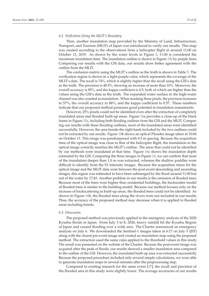
However, 25% pixels could not be identified even after the extraction of completelyinundated areas and flooded built-up areas. Figure 16a provides a close-up of the blackframe in Figure 15c, including both flooding outlines from the GSI and the MLIT. Compar-ing our results with these flooding outlines, most of the inundated areas were identifiedsuccessfully. However, the area beside the right bank included by the two outlines couldnot be extracted by our results. Figure 16b shows an optical Pleiades image taken at 10:06on October 13. This image was pansharpened with 0.5 m spacing. Because the acquisitiontime of the optical image was close to that of the helicopter flight, the inundation in theoptical image correctly matches the MLIT’s outline. The areas that could not be identifiedby our methods were inundated at that time. Figure 16c shows the inundation depthestimated by the GSI. Comparing the three images in Figure 16, we can confirm that mostof the inundation deeper than 1.0 m was extracted, whereas the shallow puddles weredifficult to identify from the S1 intensity images. Because the acquisition times for theoptical image and the MLIT data were between the post-event descending and ascendingimages, this region was estimated to have been submerged by the flood around 11:00 butout of the water by 17:43. Another problem in our results is the omission of flooded trees.Because most of the trees were higher than residential buildings, the backscatter modelof flooded trees is similar to the building model. Because our method focuses only on theincrease of backscattering in built-up areas, the flooded trees could not be identified. Asshown in Figure 16b, the flooded trees along the rivers were not included in our results.Thus, the accuracy of the proposed method may decrease when it is applied to floodedareas including forests.

6.3. Disscusion

The proposed method was previously applied to the emergency analysis of the 2020Kyushu floods in Japan. From July 3 to 8, 2020, heavy rainfall hit the Kyushu Regionof Japan and caused flooding over a wide area. The Charter announced an emergencyanalysis on July 6. We downloaded the Sentinel-1 images taken at 6:17 on July 5 (JST)along with the closest pre-event image and created an inundation map using the proposedmethod. The extraction used the same rules applied to the threshold values in this study.The result was presented on the website of the Charter. Because the post-event image wasacquired after the peak of floods, our results showed a smaller inundation area comparedto the outline of the GSI. However, the inundated built-up area was extracted successfully.Because the proposed procedure included only several simple calculations, we were ableto generate inundation maps in several minutes after the preprocessing step.

Compared to existing research for the same event [37], the recall and precision ofthe flooded area in this study were slightly lower. The average accuracies of our results

Remote Sens. 2021, 13, 639 18 of 22

after masking the high-water channels were 0.82 for the recall, 0.76 for the precision, and0.79 for the F1-measure, which are the same levels found in existing research. However,our procedure needs only one pre- and one post-event SAR intensity image, whereas theprevious study used two pre- and one post-event SAR complex data. Machine learningtechniques can obtain higher accuracy results; however, the accuracy depends on thetraining data. Conversely, our methods can be applied to any location and are thusmore versatile.

Figure 15. (a) Inundation map at 5:42 on October 13, 2019; (b) inundation map at 17:34 on October 13, 2019, where the redlines are the maximum flood boundary of the GSI; (c) total inundations by merging the two temporal inundation maps,where the purple lines are the flood polygons from the MLIT.

Remote Sens. 2021, 13, 639 19 of 22

Table 5. Confusion matrixes of the final inundation maps.

(a) Verification Using the Inundation Boundary of the GSI.

Ground Truth [km2]




(b) Verification Using the Inundation Polygon of the MLIT.

Ground Truth [km2]




Figure 16. (a) Close-up of Figure 15c within the black frame; (b) pansharpened Pleiades image taken at 10:06 on October 13;(c) estimated inundation depth according to GSI.

7. Conclusions

In this study, a simple procedure to create accurate inundation maps for an emergencyresponse was proposed. Descending and ascending pre- and post-event Sentinel-1 intensityimages were used to estimate the inundated areas in Ibaraki Prefecture, Japan, where twostate-managed rivers were flooded due to the heavy rainfall during the 2019 TyphoonHagibis. The completely inundated areas were extracted by both the multi-temporalcomparison and the mono-temporal determination. Compared with the results of our fieldsurvey and the maximum flood boundary according to the GSI, the results obtained bythe multi-temporal comparison extracted 61% of the inundation, showing better accuracy.Thus, the results using the difference of the pre- and post-event backscattering intensitywere adopted for the future steps.

The backscatter models for the two inundated buildings were also investigated. Ac-cording to the characteristics of these models, an index was proposed to identify inundatedbuildings. This index was calculated within a moving window via a combination of theaverage value and the standard deviation of the difference. The building footprints wereintroduced to identify the built-up regions. Then, the built-up regions with higher indexvalues were extracted as inundated built-up areas. After adding the extracted floodedbuilt-up area, the recall of inundation increased to more than 70%. In this study, we usedthe building footprints provided by the GSI. Recently, OpenStreetMap has begun to providebuilding footprints around the world. Thus, our proposed method can be applied globally.

Remote Sens. 2021, 13, 639 20 of 22

Finally, the inundation maps at 5:42 and 17:43 on October 13, 2020, were generated.By comparing the two temporal inundation maps, the change in the flooded areas from theupstream to the downstream could be observed. The total inundated areas were verifiedby comparing them with two flood outlines provided by the GSI and the MLIT. In eachcomparison, 73% of the inundated areas could be identified successfully by the proposedsimple procedure. A comparison of our results and the outlines by the MLIT showed goodagreement, with 88% overall accuracy and a 0.57 kappa coefficient.

Our method was applied to other events for emergency analysis, and positive resultswere obtained. Generally, the member space agencies would provide archived satelliteimages and plan an emergency observation soon after the Charter is activated. The thresh-old values in the proposed procedure are all defined by the statistical values (average andSTD) that can be obtained automatically from images. Thus, our procedure can generatean inundation map within one hour after images’ downloading. It would be helpful foremergency response. However, our results still include many commission errors. Theproposed procedure still has difficulty in identifying flooded forests. In the future, theseproblems could be overcome by improving built-up masking for the index.

Author Contributions: Data curation, Y.M. and F.Y.; Formal analysis, W.L.; Funding acquisition, F.Y.;Investigation, W.L., K.F., Y.M. and F.Y.; Methodology, W.L.; Project administration, F.Y.; Software,W.L.; Validation, W.L., K.F. and Y.M.; Writing—original draft, W.L.; Writing—review & editing, Y.M.All authors have read and agreed to the published version of the manuscript.

Funding: This research was funded by JSPS KAKENHI Grant Number [17H02066].

Institutional Review Board Statement: Not applicable.

Informed Consent Statement: Not applicable.

Data Availability Statement: No new data were created in this study. Data sharing is not applicableto this article.

Acknowledgments: The Sentinel-1 images are owned and provided by European Space Agency(ESA). The Pleiades images are owned by Centre National D’Etudes Spatiales (CNES) and distributedby Airbus Defence and Space.

Conflicts of Interest: The authors declare no conflict of interest.

References

1. Centre for Research on the Epidemiology of Disasters—CRED. Natural Disasters 2019: Now Is the Time to Not Give Up. 2020.Available online: https://cred.be/sites/default/files/adsr_2019.pdf (accessed on 20 December 2020).

2. Japan Meteorological Agency. Breaking News of the Features and the Factors of the 2020 Typhoon Hagibis. 2019. Available online:https://www.jma.go.jp/jma/press/1910/24a/20191024_mechanism.pdf (accessed on 20 December 2020). (In Japanese)

3. Cabinet Office, Government of Japan. Report of the Damage Situation Related to the Typhoon No. 19 (Hagibis) until 09:00 on 10 April2020. Available online: http://www.bousai.go.jp/updates/r1typhoon19/pdf/r1typhoon19_45.pdf (accessed on 20 December 2020).(In Japanese)

4. The International Charter Space and Major Disaster. Typhoon Hagibis in Japan. Available online: https://disasterscharter.org/web/guest/activations/-/article/storm-hurricane-urban-in-japan-activation-625- (accessed on 20 December 2020).

5. Dell’Acqua, F.; Gamba, P. Remote sensing and earthquake damage assessment: Experiences, limits, and perspectives. Proc. IEEE2012, 100, 2876–2890. [CrossRef]

6. Nakmuenwai, P.; Yamazaki, F.; Liu, W. Multi-temporal correlation method for damage assessment of buildings from high-resolution SAR images of the 2013 Typhoon Haiyan. J. Disaster Res. 2016, 11, 557–592. [CrossRef]

7. Wieland, M.; Liu, W.; Yamazaki, F. Learning change from Synthetic Aperture Radar images: Performance evaluation of a SupportVector Machine to detect earthquake and tsunami-induced changes. Remote Sens. 2016, 8, 792. [CrossRef]

8. Nakmuenwai, P.; Yamazaki, F.; Liu, W. Automated extraction of inundated areas from multi-temporal dualpolarizationRADARSAT-2 images of the 2011 central Thailand flood. Remote Sens. 2017, 9, 78. [CrossRef]

9. Karimzadeh, S.; Matsuoka, M. Building damage assessment using multisensor dualpolarized synthetic aperture radar data forthe 2016 M 6.2 Amatrice earthquake, Italy. Remote Sens. 2017, 9, 330. [CrossRef]

10. Fan, Y.; Wen, Q.; Wang, W.; Wang, P.; Li, L.; Zhang, P. Quantifying disaster physical damage using remote sensing data—Atechnical work flow and case study of the 2014 Ludian earthquake in China. Int. J. Disaster Risk Sci. 2017, 8, 471–492. [CrossRef]

Remote Sens. 2021, 13, 639 21 of 22

11. Ferrentino, E.; Marino, A.; Nunziata, F.; Migliaccio, M. A dual-polarimetric approach to earthquake damage assessment. Int. J.Remote Sens. 2019, 40, 197–217. [CrossRef]

12. Klemas, V. Remote sensing of floods and flood-prone areas: An overview. J. Coast. Res. 2015, 31, 1005–1013. [CrossRef]13. Lin, L.; Di, L.; Yu, E.G.; Kang, L.; Shrestha, R.; Rahman, M.S.; Tang, J.; Deng, M.; Sun, Z.; Zhang, C.; et al. A review of remote

sensing in flood assessment. In Proceedings of the 2016 Fifth International Conference on Agro-Geoinformatics, Tianjin, China,18–20 July 2016. [CrossRef]

14. Koshimura, S.; Moya, L.; Mas, E.; Bai, Y. Tsunami damage detection with remote sensing: A review. Geosciences 2020, 10, 177.[CrossRef]

15. McFeeters, S.K. The use of the normalized difference water index (NDWI) in the delineation of open water features. Int. J.Remote Sens. 1996, 17, 1425–1432. [CrossRef]

16. Xu, H. Modification of normalised difference water index (NDWI) to enhance open water features in remotely sensed imagery.Int. J. Remote Sens. 2006, 27, 3025–3033. [CrossRef]

17. Feyisa, G.L.; Meilby, H.; Fensholt, R.; Proud, S.R. Automated water extraction index: A new technique for surface water mappingusing Landsat imagery. Remote Sens. Environ. 2014, 140, 23–35. [CrossRef]

18. Xie, H.; Luo, X.; Xu, X.; Tong, X.; Jin, Y.; Pan, H.; Zhou, B. New hyperspectral difference water index for the extraction of urbanwater bodies by the use of airborne hyperspectral images. J. Appl. Remote Sens. 2014, 8, 085098. [CrossRef]

19. Ko, B.C.; Kim, H.H.; Nam, J.Y. Classification of potential water bodies using Landsat 8 OLI and a combination of two boostedrandom forest classifiers. Sensors 2015, 15, 13763–13777. [CrossRef]

20. Ogilvie, A.; Belaud, G.; Delenne, C.; Bailly, J.-S.; Bader, J.-C.; Oleksiak, A.; Ferry, L.; Martin, D. Decadal monitoring of the NigerInner Delta flood dynamics using MODIS optical data. J. Hydrol. 2015, 523, 368–383. [CrossRef]

21. Hakkenberg, C.; Dannenberg, M.; Song, C.; Ensor, K. Characterizing multi-decadal, annual land cover change dynamics inHouston, TX based on automated classification of Landsat imagery. Int. J. Remote Sens. 2018, 40, 693–718. [CrossRef]

22. Nandi, I.; Srivastava, P.K.; Shah, K. Floodplain Mapping through Support Vector Machine and Optical/Infrared ImagesfromLandsat 8 OLI/TIRS Sensors: Case Study from Varanasi. Water Resour. Manag. 2017, 31, 1157–1171. [CrossRef]

23. Pulvirenti, L.; Pierdicca, N.; Chini, M.; Guerriero, L. An algorithm for operational flood mapping from Synthetic Aperture Radar(SAR) data using fuzzy logic. Nat. Hazards Earth Syst. Sci. 2011, 11, 529–540. [CrossRef]

24. Westerhoff, R.S.; Kleuskens, M.P.; Winsemius, H.C.; Huizinga, H.J.; Brakenridge, G.R.; Bishop, C. Automated global watermapping based on wide-swath orbital synthetic-aperture radar. Hydrol. Earth Syst. Sci. 2013, 17, 651–663. [CrossRef]

25. Liu, W.; Yamazaki, F. Detection of inundation areas due to the 2015 Kanto and Tohoku torrential rain in Japan based onmulti-temporal ALOS-2 imagery. Nat. Hazards Earth Syst. Sci. 2018, 18, 1905–1918. [CrossRef]

26. Martinis, S.; Twele, A.; Voigt, S. Towards operational near real-time flood detection using a split-based automatic thresholdingprocedure on high resolution TerraSAR-X data. Nat. Hazards Earth Syst. Sci. 2009, 9, 303–314. [CrossRef]

27. Martinis, S.; Kersten, J.; Twele, A. A fully automated TerraSAR-X based flood service. ISPRS J. Photogramm. Remote Sens. 2015,104, 203–212. [CrossRef]

28. Giustarini, L.; Hostache, R.; Kavetski, D.; Chini, M.; Corato, G.; Schlaffer, S.; Matgen, P. Probabilistic Flood Mapping UsingSynthetic Aperture Radar Data. IEEE Trans. Geosci. Remote Sens. 2016, 54, 6958–6969. [CrossRef]

29. Nico, G.; Pappalepore, M.; Pasquariello, G.; Refice, A.; Samarelli, S. Comparison of SAR amplitude vs. coherence flood detectionmethods—A GIS application. Int. J. Remote Sens. 2010, 21, 1619–1631. [CrossRef]

30. Chini, M.; Pulvirenti, L.; Pierdicca, N. Analysis and interpretation of the COSMO-SkyMed observation of the 2011 Tsunami.IEEE Trans. Geosci. Remote Sens. 2012, 9, 467–571. [CrossRef]

31. Pulvirenti, L.; Chini, M.; Pierdicca, N.; Boni, G. Use of SAR data for detecting floodwater in urban and agricultural areas: The roleof the interferometric coherence. IEEE Trans. Geosci. Remote Sens. 2016, 54, 1532–1544. [CrossRef]

32. Liu, W.; Yamazaki, F.; Maruyama, Y. Extraction of inundation areas due to the July 2018 Western Japan torrential rain event usingmulti-temporal ALOS-2 images. J. Disaster Res. 2019, 14, 445–455. [CrossRef]

33. Ohki, M.; Yamamoto, K.; Tadono, T.; Yoshimura, K. Automated Processing for Flood Area Detection Using ALOS-2 andHydrodynamic Simulation Data. Remote Sens. 2020, 12, 2709. [CrossRef]

34. Hashimoto, S.; Tadono, T.; Onosata, M.; Hori, M.; Shiomi, K. A new method to derive precise land-use and land-cover mapsusing multi-temporal optical data. J. Remote Sens. Soc. Jpn. 2014, 34, 102–112. (In Japanese) [CrossRef]

35. Esfandiari, M.; Jabari, S.; McGrath, H.; Coleman, D. Flood mapping using Random Forest and identifying the essential condition-ing factors; A case study in Fredericton, New Brunswick, Canada. ISPRS Ann. Photogramm. Remote Sens. Spat. Inf. Sci. 2020,3, 609–615. [CrossRef]

36. Esfandiari, M.; Abdi, G.; Jabari, S.; McGrath, H.; Coleman, D. Flood hazard risk mapping using a pseudo supervised RandomForest. Remote Sens. 2020, 12, 3206. [CrossRef]

37. Moya, L.; Mas, E.; Koshimura, S. Learning from the 2018 Western Japan heavy rains to detect floods during the 2019 HagibisTyphoon. Remote Sens. 2020, 12, 2244. [CrossRef]

38. Elmahdy, S.; Ali, T.; Mohamed, M. Flash flood susceptibility modeling and magnitude index using machine learning andgeohydrological models: A modified hybrid approach. Remote Sens. 2020, 12, 2695. [CrossRef]

39. Geospatial Information Authority of Japan. Information about the 2019 Typhoon Hagibis. Available online: https://www.gsi.go.jp/BOUSAI/R1.taihuu19gou.html (accessed on 25 December 2020). (In Japanese)

Remote Sens. 2021, 13, 639 22 of 22

40. Geospatial Information Authority of Japan. Digital Map (Basic Geospatial Information). Available online: https://maps.gsi.go.jp/(accessed on 25 December 2020). (In Japanese)

41. Japan Meteorological Agency. Available online: https://www.data.jma.go.jp/obd/stats/etrn/index.php (accessed on 25 December 2020).(In Japanese).

42. Water Information System, Ministry of Land, Infrastructure, Transport and Tourism. Available online: http://www1.river.go.jp/(accessed on 25 December 2020).

43. Copernicus Open Access Hub. Available online: https://scihub.copernicus.eu/dhus/#/home (accessed on 25 December 2020).44. Lopes, A.; Touzi, R.; Nezry, E. Adaptive Speckle Filters and Scene Heterogeneity. IEEE Trans. Geosci. Remote Sens. 1990,

28, 992–1000. [CrossRef]45. Ibaraki University. The First Report of the Typhoon Hagibis Investigation Team. Available online: https://www.ibaraki.ac.jp/

hagibis2019/researchers/IU2019hagibisresearch1streport.pdf (accessed on 25 December 2020). (In Japanese)46. Geospatial Information Authority of Japan. Basic Map information. Available online: https://fgd.gsi.go.jp/download/menu.php

(accessed on 25 December 2020). (In Japanese)

Inundation Assessment of the 2019 Typhoon Hagibis in Japan ...

Documents

Transcript of Inundation Assessment of the 2019 Typhoon Hagibis in Japan ...