The Hurricane Intensity Issue

T. N. KRISHNAMURTI, S. PATTNAIK, L. STEFANOVA, T. S. V. VIJAYA KUMAR, B. P. MACKEY, AND

A. J. O’SHAY

Department of Meteorology, The Florida State University, Tallahassee, Florida

RICHARD J. PASCH

Tropical Prediction Center, National Hurricane Center, NOAA/NWS, Miami, Florida

(Manuscript received 7 June 2004, in final form 14 December 2004)

ABSTRACT

The intensity issue of hurricanes is addressed in this paper using the angular momentum budget of ahurricane in storm-relative cylindrical coordinates and a scale-interaction approach. In the angular mo-mentum budget in storm-relative coordinates, a large outer angular momentum of the hurricane is depletedcontinually along inflowing trajectories. This depletion occurs via surface and planetary boundary layerfriction, model diffusion, and “cloud torques”; the latter is a principal contributor to the diminution of outerangular momentum. The eventual angular momentum of the parcel near the storm center determines thestorm’s final intensity. The scale-interaction approach is the familiar energetics in the wavenumber domainwhere the eddy and zonal kinetic energy on the hurricane scale offer some insights on its intensity. Here,however, these are cast in storm-centered local cylindrical coordinates as a point of reference. The wave-numbers include azimuthally averaged wavenumber 0, principal hurricane-scale asymmetries (wavenumbers1 and 2, determined from datasets) and other scales. The main questions asked here relate to the role of theindividual cloud scales in supplying energy to the scales of the hurricane, thus contributing to its intensity.A principal finding is that cloud scales carry most of their variance, via organized convection, directly on thescales of the hurricane. The generation of available potential energy and the transformation of eddy kineticenergy from the cloud scale are in fact directly passed on to the hurricane scale by the vertical overturningprocesses on the hurricane scale. Less of the kinetic energy is generated on the scales of individual cloudsthat are of the order of a few kilometers. The other major components of the energetics are the kinetic-to-kinetic energy exchange and available potential-to-available potential energy exchange among differentscales. These occur via triad interaction and were noted to be essentially downscale transfer, that is, acascading process. It is the balance among these processes that seems to dictate the final intensity.

1. Introduction

In this paper we explore two avenues for the hurri-cane intensity issue. Both of these are diagnostic ap-proaches and are applied here to the datasets derivedfrom a very high resolution forecast model. A some-what reasonable hurricane intensity forecast from ahigh-resolution model was necessary in order to portraythe workings of the proposed diagnostic frameworks.The two approaches described here can be labeled theangular-momentum-based diagnosis of hurricane inten-

sity and a scale-interaction-based diagnosis of thestorm’s energetics. In the former approach, a reservoirof high-angular-momentum air from the outer reachesof the hurricane has a large control on its intensity. Thatouter angular momentum is affected by the torques theparcels experience as they move toward the high-intensity region. The latter approach asks about impli-cations of the cloud scales on the eventual energy(which indirectly relates to the intensity) of a hurricane.

The initial datasets for this study came from the Eu-ropean Centre for Medium-Range Weather Forecasts(ECMWF) operational analysis plus dropwindsondedatasets from research aircraft and satellite data. A listof acronyms appears in Table 1. Furthermore, thisstudy is based on a somewhat realistic simulation of ahurricane (Hurricane Bonnie of 1998) that was gener-ated using a nonhydrostatic microphysical mesoscale

Corresponding author address: Prof. T. N. Krishnamurti, De-partment of Meteorology, The Florida State University, Tallahas-see, FL 32306-4520.E-mail: tnk@io.met.fsu.edu

1886 M O N T H L Y W E A T H E R R E V I E W VOLUME 133

© 2005 American Meteorological Society

MWR2954

model [the fifth-generation Pennsylvania State Univer-sity–National Center for Atmospheric Research (PSU–NCAR) Mesoscale Model (MM5)]. The model outputdatasets were used here to carry out the diagnostic en-quiries.

This study became possible because of two recentadvancements in data and modeling. The third andfourth Convection and Moisture Experiments(CAMEX-3 and -4, respectively) are recent field ex-periments in which joint data initiatives of the NationalAeronautics and Space Administration (NASA), Na-tional Oceanic and Atmospheric Administration (NOAA),and the U.S. Air Force provided an extensive coverageof observations. These agencies deployed as many assix research/operational aircraft for the surveillance ofhurricanes on a daily basis. These research aircraft de-ployed as many as a total of 100 dropsondes per dayproviding profiles of winds, temperature, humidity, andpressure. In addition to these, a NASA aircraft pro-vided specialized moisture profiles from the Lidar At-mospheric Sensing Experiment (LASE). Another ma-jor dataset was composed of 1⁄2° latitude � 1⁄2° longi-tude operational analysis data from the ECMWF.Using these datasets, we performed variational data as-similation (Rizvi et al. 2002; Kamineni et al. 2003, 2005)to analyze the CAMEX storms of the years 1998 and2001. This mix of datasets provides a unique coverageof observations for hurricane modeling.

In the modeling area, it is now possible to carry outhigh-resolution simulation with mesoscale nonhydro-static microphysical models. Numerous recent applica-tions with the MM5 have shown the possibility for suchsimulation. Braun (2002) analyzed the storm structureand eyewall buoyancy of Hurricane Bob using a multi-ply nested MM5 with moving nest capability and dem-

onstrated reasonable distributions of vertical motion inthe eyewall. Similar studies were carried out by differ-ent research groups to resolve the cloud-scale featuresof hurricanes using MM5, for example, Bao et al. (2000),Braun and Tao (2000), Chen and Yau (2001), Davis andBosart (2001), Davis and Trier (2002), Zhang andWang (2003), and Liu et al. (1999). A multiply nestedmodel with an inner resolution of 1 km provides thepossibility for asking questions on the role of the mod-el’s deep convection on the intensity changes of hurri-canes.

In his seminal papers on atmospheric energetics inthe wavenumber domain, Saltzman (1957, 1970) laidthe foundations for studies of scale interactions. Ex-ploring the energy exchange between waves and waves,and between waves and zonal flows, he portrayed themechanism for the driving of the middle-latitude zonalflows (i.e., the zonally averaged jets) in the atmosphere.That framework was in spherical coordinates. For stud-ies of a hurricane, it is relatively straightforward to castthis system onto a cylindrical coordinate system, thedetails of which are provided in the appendix. Thistransformation provides information on the kinetic andavailable potential energy exchange among the azi-muthally averaged flows and other azimuthal waves.The cloud (convection) scale being much smaller thanthat of the hurricane, the mode of communication ofinformation from the cloud scale to the hurricane scalewas not clearly apparent. The scale of convection (up-drafts and adjacent downdrafts) is of the order of a fewkilometers, whereas the scale of the hurricane is of theorder of several hundreds of kilometers. Clearly theissue of scale interaction needs exploring in this con-text. A budget of kinetic energy for the scales of thehurricane can be revealing about its intensity.

The angular momentum perspective starts with alarge reservoir of high angular momentum air at largeradii. That air is generally brought into the storm’s in-terior along inflow channels of the lower troposphere.That large angular momentum (following parcel mo-tion) is depleted by the surface and internal frictiontorques (cloud torques) and by the pressure torques.The parcel arrives at inner radii where the storm inten-sity (the maximum sustained near-surface wind of thehurricane) is explicitly determined from the value ofthe angular momentum the parcel arrives with. Thispaper attempts to provide some insight on these twodifferent approaches for the understanding of hurricaneintensity.

2. Observational aspects

Hurricane Bonnie developed from a vigorous tropi-cal wave that spawned a tropical depression to the east

TABLE 1. List of acronyms.

MM5 Fifth-generation PSU–NCAR Mesoscale ModelNCAR National Center for Atmospheric ResearchPSU Pennsylvania State UniversityECMWF European Centre for Medium-Range

Weather ForecastsCAMEX Convection and Moisture ExperimentNASA National Aeronautics and Space AdministrationNOAA National Oceanic and Atmospheric

AdministrationLASE Lidar Atmospheric Sensing ExperimentUTC Coordinated universal timeFSU The Florida State UniversityTRMM Tropical Rainfall Measuring MissionDMSP Defense Meteorological Satellite ProgramPBL Planetary boundary layerMRF Medium-Range Forecasting

JULY 2005 K R I S H N A M U R T I E T A L . 1887

of the Lesser Antilles, near 15°N, 48°W, around 1200UTC 19 August 1998. After moving west-northwest-ward for several days, the tropical cyclone turned to-ward the northwest and north-northwest, as shown inFig. 1. Bonnie became a tropical storm at about 1200UTC 20 August, and the system strengthened into ahurricane by 0000 UTC 22 August. This hurricanemade a recurvature and landfall along the coast ofNorth Carolina. It weakened to a tropical storm around1800 UTC 27 August, but reintensified into a hurricanewhen it moved back over the Atlantic. Bonnie thenmoved on a generally northeastward-to-eastward trackand lost its tropical characteristics on 30 August. Thehurricane was rather intensively monitored by hurri-cane reconnaissance and surveillance aircraft. Our

study covers a 72-h period between 22 and 25 August1998. During this period, Bonnie’s maximum winds var-ied from 33.5 to about 51.5 m s�1. A visible satelliteimage [Geostationary Operational Environmental Sat-ellite (GOES)] during this period (Fig. 2) at 1615 UTC23 August 1998 showed a well-defined storm with ac-tive banding to its south. However after Bonnie re-curved and interacted with a frontal system, the cloudcover became elongated northeastward. The satelliteimagery of the storm during our study period is similarto that seen in many category 3 hurricanes of the At-lantic basin having winds close to 100 kt (51.5 m s�1).We shall not describe the detailed structure of Hurri-cane Bonnie here since this is a well-studied storm andis described in some detail by Pasch et al. (2001) in their

FIG. 1. Observed and model-predicted track of Hurricane Bonnie. Boxes in the illustrationdemonstrate the MM5 nested grids at 27, 9, 3, and 1 km.

1888 M O N T H L Y W E A T H E R R E V I E W VOLUME 133

seasonal summary and by our laboratory (Rizvi et al.2002).

a. Data and method of analysis

The datasets for this study came from diversesources: ECMWF, CAMEX-3, and satellite datasets.The procedure of generating the analysis includes thefollowing steps: 1) The initial state and boundary con-ditions for this modeling study were prepared using op-erational real-time ECMWF analyzed data files (pro-vided at 0.5° latitude � 0.5° longitude grid and 28 ver-tical levels. 2) Six research aircraft provided dropsondeand special moisture-profiling datasets (the LASE in-strument). There was midtropospheric surveillancefrom two NOAA WP3 aircraft, a NOAA G-IV near thetropopause level, a NASA P3 aircraft, a NASA DC-8(flying near the 250-hPa level), and a NASA ER-2 fly-ing near 60 000 ft in the lower stratosphere. Thesedatasets were analyzed using our Florida State Univer-sity (FSU) three-dimensional variational data assimila-tion (3DVAR) following Rizvi et al. (2002) and Ka-mineni et al. (2003, 2004, manuscript submitted to J.Atmos. Sci.) where the hurricane forecast impacts fromthese additional observations of the CAMEX fieldcampaign were addressed. This analysis was carried outon a spectral resolution of T170 (transform grid spacingapproximately 70 km). 3) These datasets were next sub-jected to physical initialization (i.e., rain-rate initializa-tion) following Krishnamurti et al. (1991, 2001). Hererain-rate estimates were derived from the microwaveinstruments on board the Tropical Rainfall MeasuringMission (TRMM) [the TRMM Microwave Imager(TMI)] and three Defense Meteorological Satellite Pro-

gram (DMSP) satellites [(Special Sensor MicrowaveImager (SSM/I)]. These analyzed datasets were simplyinterpolated using bicubic splines onto a variable gridresolution of the MM5 used in this study.

b. The PSU–NCAR Mesoscale Model

The numerical simulation of Hurricane Bonnie of1998 was carried out using the nonhydrostatic PSU–NCAR Mesoscale Model (version 3.6) (Dudhia 1993).A 72-h simulation of Hurricane Bonnie (0000 UTC 22August 1998–0000 UTC 25 August 1998) was made us-ing a variable-resolution nested configuration. Here weused four domains (Fig. 1) with a horizontal grid spac-ing of 27, 9, 3, and 1 km and having domain size of 98� 94, 186 � 222, 369 � 444, and 501 � 501 grid points,respectively. These grid meshes included 23 verticalhalf-sigma (�) levels. The 27- and 9-km domains wereone-way nested whereas the 3- and 1-km nests weretwo-way nested. The physics options used for thecoarser grids at 27 and 9 km included the Betts–Millercumulus parameterization (Betts and Miller 1986,1993), a simple ice explicit scale cloud microphysicsscheme (Dudhia 1989), the Medium-Range Forecast(MRF) planetary boundary scheme (Hong and Pan1996), and a cloud radiative scheme of Dudhia (1989).The physics options for the 3- and 1-km grids weresimilar to the coarse grid simulations except that nocumulus parameterization scheme was used, and con-vection was explicitly handled.

The combined six-aircraft CAMEX flights for thesurveillance of an entire storm were only conducted ona few successive days. Thus it was not possible to vali-date in detail the performance of the MM5 using thesefield campaign observations. However, the simulateddetails, at the high resolution, were sufficiently realisticin terms of structure, motion, and intensity to carry outthe main objectives of this study, which are the angularmomentum and the scale-interaction perspectives.The observed maximum reported winds from the Na-tional Hurricane Center for days 1, 2, and 3 of this studywere 46, 51, and 51 m s�1 and the corresponding model-predicted maximum winds at the 850-hPa level werearound 27, 35, and 45 m s�1, respectively. The centralpressure comparisons were observed estimates 962,954, and 963 hPa, and the model-predicted valueswere 1002, 996, and 984 hPa. It is to be noted here thatthere is a clear lack of ability of MM5 in simulating thestorm efficiently. The model wind speeds and pressuredo not capture the actual intensity and that may havesome impact on the results presented in this paper. Theobserved and predicted tracks of Hurricane Bonniewere illustrated in Fig. 1. There are clearly some track

FIG. 2. Visible GOES-8 image of Hurricane Bonnie at 1615UTC 23 Aug 1998.

JULY 2005 K R I S H N A M U R T I E T A L . 1889

errors but that was not a primary issue here. It is ourexperience that ensemble averaging of tracks frommultimodels appears to generally do better than sin-gle models (Krishnamurti et al. 2000; Williford et al.2003).

Some of the initial state fields of this study are illus-trated in Figs. 3a and 3b. The sea level pressure on 22August at 0000 UTC, shown in Fig. 3a, depicts a lowpressure system to the southeast of the outer modeldomain. The MM5’s initial central pressure at this timewas approximately 1006 hPa and the maximum windswere 24 m s�1 (the best-track values were 991 hPa and32 m s�1). Strong pressure gradient to the north wasindicative of the strong trades. The scale of this closed

low pressure field extended from 71° to 65°W. The tan-gential wind maxima (Fig. 3b) at the initial time werearound 24 m s�1 to the north of the storm and were ofthe order of 13 m s�1 to the south of the storm. Theweakest winds are located over the storm center. Fig-ures 4a–c show the streamlines at the 850-hPa levelfrom the forecasts of the mesoscale model at the end ofdays 1, 2, and 3. The northwestward motion of thestorm is reasonably captured by the forecast. An inter-esting and prominent feature is the evolution of an as-ymptote of convergence to the south (by day 3 of fore-cast; Fig. 4c). This feature, in storm-relative coordi-nates, was an important inflow channel for HurricaneBonnie.

FIG. 3. Initial distribution of (a) sea level pressure (hPa) and (b) tangential wind at 850hPa (m s�1) of Hurricane Bonnie, valid on 0000 UTC 22 Aug 1998.

1890 M O N T H L Y W E A T H E R R E V I E W VOLUME 133

3. The angular momentum approach on theinterpretation of hurricane intensity

The angular momentum perspective starts with alarge reservoir of high angular momentum air at the

large radii. That air is generally being brought into thestorm’s interior mainly along inflow channels of thelower troposphere. That large angular momentum (fol-lowing parcel motions) is depleted by the surface andinternal frictional torques, by pressure torques, and by

FIG. 4. Streamlines at 850 hPa derived from model output at (a) day 1, (b) day 2, and (c) day 3 of forecasts.

JULY 2005 K R I S H N A M U R T I E T A L . 1891

cloud torques. The parcel arrives at the inner radiiwhere the storm intensity (the maximum surface windof the hurricane) is determined by the value of theangular momentum with which the parcel arrives atthat location. This could be called an “outer thrust” thatseemingly determines the hurricane’s intensity. Theweakness of this argument is that the inflow channel isassumed to be a prescribed entity here. One can ask,how did that come about? An “inner thrust,” a secondperspective, calls for a detailed knowledge of the struc-ture of the convective storm clouds. Knowing bettermicrophysics, we can perhaps model these clouds moreaccurately and precisely, and these clouds may carveout the inflow channels in the first place. The angularmomentum story could well be a consequence of a sys-tematic and organized cloud growth.

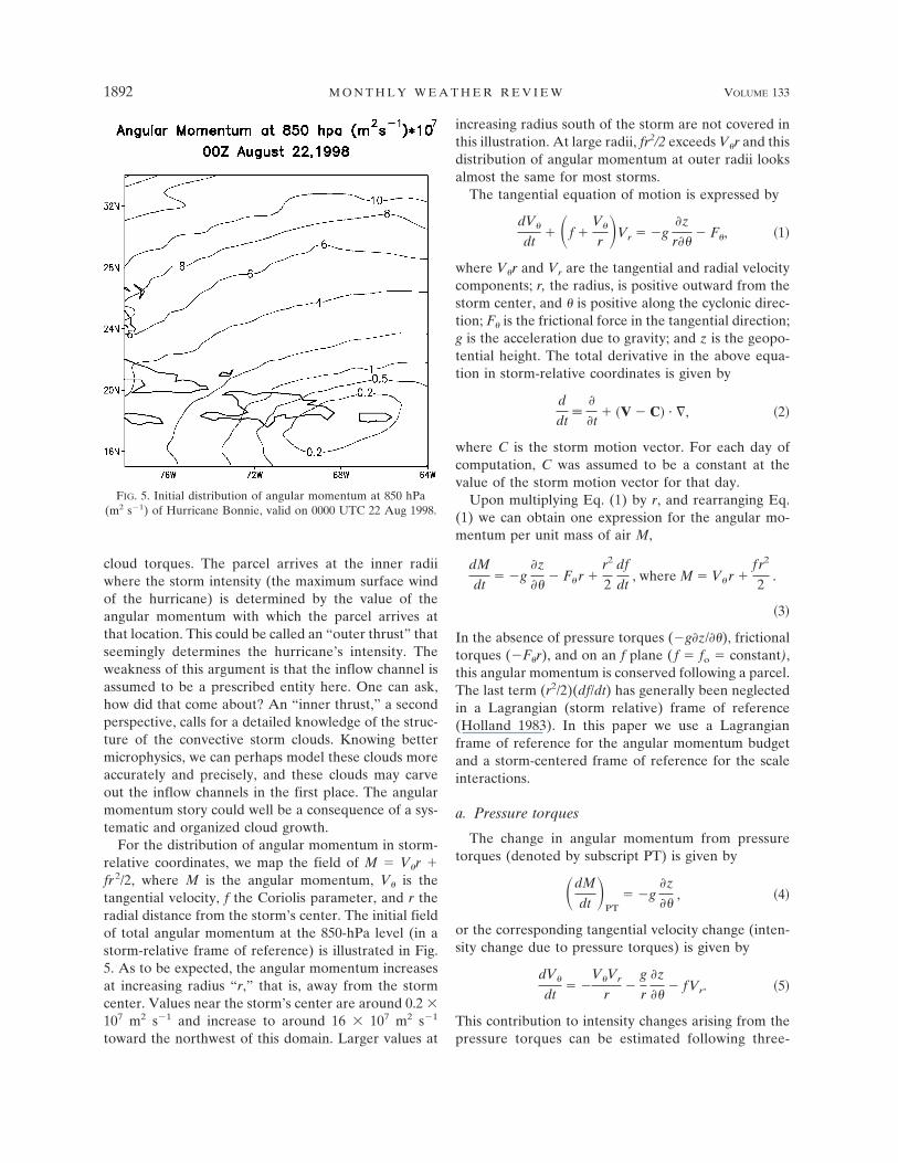
For the distribution of angular momentum in storm-relative coordinates, we map the field of M � V�r �fr2/2, where M is the angular momentum, V� is thetangential velocity, f the Coriolis parameter, and r theradial distance from the storm’s center. The initial fieldof total angular momentum at the 850-hPa level (in astorm-relative frame of reference) is illustrated in Fig.5. As to be expected, the angular momentum increasesat increasing radius “r,” that is, away from the stormcenter. Values near the storm’s center are around 0.2 �107 m2 s�1 and increase to around 16 � 107 m2 s�1

toward the northwest of this domain. Larger values at

increasing radius south of the storm are not covered inthis illustration. At large radii, fr2/2 exceeds V�r and thisdistribution of angular momentum at outer radii looksalmost the same for most storms.

The tangential equation of motion is expressed by

dV�

dt� �f �

V�

r �Vr � �g�z

r��� F�, �1�

where V�r and Vr are the tangential and radial velocitycomponents; r, the radius, is positive outward from thestorm center, and � is positive along the cyclonic direc-tion; F� is the frictional force in the tangential direction;g is the acceleration due to gravity; and z is the geopo-tential height. The total derivative in the above equa-tion in storm-relative coordinates is given by

d

dt

�

�t� �V � C� � �, �2�

where C is the storm motion vector. For each day ofcomputation, C was assumed to be a constant at thevalue of the storm motion vector for that day.

Upon multiplying Eq. (1) by r, and rearranging Eq.(1) we can obtain one expression for the angular mo-mentum per unit mass of air M,

dM

dt� �g

�z

��� F�r �

r2

2df

dt, where M � V�r �

fr2

2.

�3�

In the absence of pressure torques (�gz/�), frictionaltorques (�F�r), and on an f plane ( f � fo � constant),this angular momentum is conserved following a parcel.The last term (r2/2)(df/dt) has generally been neglectedin a Lagrangian (storm relative) frame of reference(Holland 1983). In this paper we use a Lagrangianframe of reference for the angular momentum budgetand a storm-centered frame of reference for the scaleinteractions.

a. Pressure torques

The change in angular momentum from pressuretorques (denoted by subscript PT) is given by

�dM

dt �PT� �g

�z

��, �4�

or the corresponding tangential velocity change (inten-sity change due to pressure torques) is given by

dV�

dt� �

V�Vr

r�

g

r

�z

��� fVr. �5�

This contribution to intensity changes arising from thepressure torques can be estimated following three-

FIG. 5. Initial distribution of angular momentum at 850 hPa(m2 s�1) of Hurricane Bonnie, valid on 0000 UTC 22 Aug 1998.

1892 M O N T H L Y W E A T H E R R E V I E W VOLUME 133

dimensional parcel trajectories. Once the change in an-gular momentum (M) contributed by torques is known,then it is easy to compute the change in the intensity(V�) following segments of parcel motions that arisefrom effects of each type of torque. Specifically, we cantailor such a budget to the maximum intensity of thestorm. This is further discussed in section 5 of this paper.

One well-known pressure asymmetry in hurricanesarises from the so-called beta gyres (Chan and Williams1987, 1994). If the symmetric part of the pressure fieldof a hurricane is removed from its total pressure field,then one can visualize these beta gyre structures. Thestructure generally contains higher pressures to theright of the storm’s center and lower pressure to its left.Figure 6 illustrates this structure for Hurricane Bonnie(1998) for the sea level pressure from day 3 of the fore-cast. The beta gyre represents one of the most promi-nent pressure asymmetries of a hurricane. The presenceof a beta gyre implies the presence of pressure torques.

This is usually on rather larger scales, that is, azimuthalwavenumbers 1 and 2, and the amplitude of this torqueis rather small. Another contributor to pressure torquecomes from the deep convective elements (simulatedby the high-resolution model) that carry pressure per-turbations vertically. With vertical motions of the orderof 1 to 10 m s�1, small-scale pressure perturbations, onthe order of a few hectopascals on the scale of thesedeep convective elements, abound in the predictedpressure fields. Because of the smaller horizontal scalesof these convective elements, these perturbations canconvey robust local pressure torques. However, on ei-ther side of these pressure perturbations, opposite signsof the azimuthal pressure gradients are found; thus, theincrease and decrease of angular momentum essentiallycancel along segments of inflowing trajectories fromthese pressure perturbations. The effect of frictionaland cloud torques is described in the following subsec-tions.

FIG. 6. Beta gyre structure for Hurricane Bonnie. Shown is the sea level pressure (hPa)distribution after removing the zonal (azimuthal) mean values. The large arrow at the topshows the direction of storm motion.

JULY 2005 K R I S H N A M U R T I E T A L . 1893

b. Frictional torques

In the version of the MM5 that is used in our study,the surface fluxes of momentum are defined via a bulkaerodynamic formula (Deardorff 1972; Grell et al.1995). Here the constant flux layer is 86 m deep. Thedisposition of surface fluxes above the constant fluxlayer within a PBL follows the MRF PBL scheme thatwas based on the work of Hong and Pan (1996). This isa nonlocal scheme that permits countergradient fluxesof moisture by large-scale eddies. The eddy diffusivitycoefficient for momentum is a function of the frictionvelocity u* and the PBL height is a function of a criticalbulk Richardson number. The vertical disposition ofthese subgrid-scale surface momentum fluxes is carriedout using the K theory. The profiles of implied subgrideddy momentum fluxes determine the vertical distribu-tion of surface fluxes. The frictional torques, �F�r, thushave vertical distributions. They largely mimic the sur-face torques through several vertical levels.

The outputs of the vertical fluxes of momentum be-tween the surface level and the top of the PBL werestored for each hour of the forecast. In addition tothese, the MM5 includes parameterization for the sub-grid-scale vertical diffusion of momentum that was alsoretrieved and stored. The resolved vertical fluxes ofmomentum by shallow and deep convection were ex-plicitly calculated from the fields of u, �, and w. Thesewere also stored at intervals of 1 h. These provided acomplete inventory of the momentum fluxes at the sur-face, in the PBL, and in the rest of the model column.The large outer angular momentum of inflowing air isconstantly eroded by the frictional torques. This fieldvaries from hurricane to hurricane largely due to dif-ferent distribution of wind speeds, storm size, and fromthe dependence of the diffusive exchange coefficientsas a function of height and the Richardson number.

In this study, we divide the frictional toques �F�rinto several parts, those arising from surface friction,those arising from planetary boundary layer friction,and the explicit cloud layer friction determined fromthe torque of the vertical eddy flux convergence of mo-mentum. In addition to these there are also torquesarising from model diffusion. All these torques, exceptthe cloud torque, are added together in the term, �F�r,whereas the cloud torque is separately considered. Thisis done deliberately to focus on the impact of cloudtorques on the angular momentum budget and intensitychanges in a hurricane environment.

c. Cloud torques

Along segments of parcel trajectories, active cloudelements contribute to sizeable torques—we have des-

ignated these as cloud torques. The cloud torques ap-pear to be a major contributor to the modification ofangular momentum of inflowing parcel segments wheremodel clouds were present. In the x–y–p frame of ref-erence, cloud torques (denoted by subscript CT) can beexpressed by

�dM

dt �CT� �r

�

�zW�V�� , �6�

where W� is the eddy vertical velocity and the overbardenotes an average value across model-simulated cloudelements within a trajectory segment (here we are dis-regarding the horizontal eddy fluxes). Along the in-flowing trajectory we identify a segment traversed bythe parcel in a time t (across significant cloud ele-ment). The corresponding change of angular momen-tum across that segment is

��M�CT � �r�

�zW�V���t. �7�

A net vertical divergence of eddy flux of momentumr(/z)W�V�� results in a net diminution of angular mo-mentum. This is consistent with the increase of resolv-able eddy flux W�V�� as we go up from the ocean sur-face. The outer angular momentum is constantly beingdrained to the upper levels by the cloud turbulence.These results are presented in section 5. If a modelforecast provides reasonable storm intensity, then it ispossible to carry out an intensity budget using the an-gular momentum principle as a frame of reference.

4. The scale-interaction perspective

The hurricane’s scale can be described by a few azi-muthal wavenumbers (e.g., wavenumbers 0, 1, 2), whichwas noted in our analysis of the rainwater mixing ratio(Krishnamurti and Jian 1985a,b). The field of rainwatermixing ratio in these high-resolution forecasts carriesthe signature of individual deep convective cloud ele-ments. Figures 7a and 7b illustrate the predicted rain-water mixing ratio at the 850-hPa level for days 2 and 3of the forecast. An azimuthal spectral analysis of thesefields shows that a sizeable portion of the variance ofthe rainwater mixing ratio is accounted for by the firstfew harmonics in the innermost region. In Figs. 8a and8b we show the power spectra of the rainwater mixingratio for the initial time (shown as t � 1) and at hour 24(shown as t � 2). The results for radii 0–40, 40–200, and200–380 km are presented here. At radii less than 200km, a considerable amount of the power resides inthese low wavenumbers. At the outer radii (200–380km) the distribution shifts to smaller scales. The same

1894 M O N T H L Y W E A T H E R R E V I E W VOLUME 133

FIG. 7. Distribution of rainwater mixing ratio (kg kg�1) at 850 hPa for (a) day-2 and (b)day-3 forecasts of Hurricane Bonnie.

JULY 2005 K R I S H N A M U R T I E T A L . 1895

Fig 7 live 4/C

result emerges when we examine the azimuthal spectraof the tangential velocity. The larger scales of the rain-water mixing ratio spectra are a clear reflection of theorganization of convection. It thus appeared reasonableto designate wavenumbers 0, 1, and 2 as the hurricanescales. On the other hand, the scales of the individualdeep convective clouds appear to reside around the azi-muthal wavenumbers 20 to 30. Following Saltzman(1957, 1970), it is of interest here to explore the inter-actions between the hurricane and the cloud scales.These interactions can be broadly described by (a)available potential to eddy kinetic; (b) eddy kinetic toeddy kinetic; and (c) available potential to available

potential. In somewhat further detail, the following are12 salient and grouped energy exchange componentsthat comprise the total system. (The appendix includesthe mathematical details.)

(i) �APEoKo� is the conversion of azimuthally aver-aged (subscript o) available potential energy(APE) to the azimuthally averaged kinetic en-ergy (K). This is a mechanism for the mainte-nance of hurricane intensity. This is akin to warmair rising and relatively colder air sinking fromthe Hadley-type vertical overturning. In our hur-ricane domain, which encloses the entire tropo-

FIG. 8. Power spectrum of variance of the liquid water mixing ratio at (top) initial time (t � 1) and (bottom) at 24-h forecast (t �2) for (left to right) three different radii (0–40 km, the inner region; 40–200 km, the high wind region; and 200–380 km, the outer region)of Hurricane Bonnie.

1896 M O N T H L Y W E A T H E R R E V I E W VOLUME 133

sphere below 100 hPa and the entire atmospherewithin r � 500 km, the rising of warmer air occursnear the eyewall clouds and the rainbands. Thesinking of relatively cooler air occurs outside ofthe rainband and inside of the eyewall.

(ii) �APElKl� denotes long-wave (subscript l) verticaloverturnings on the salient asymmetric scale ofthe hurricane such as azimuthal wavenumbers 1and 2. Since this overturning arises from a qua-dratic nonlinearity among vertical velocity andtemperature on the individual long-wave scales,this can only contribute to an in-scale energy ex-change; that is, available potential energy ofwavenumber 1 can only generate eddy kinetic en-ergy for wavenumber 1, with the same being truefor wavenumber 2. These overturnings generateeddy kinetic energy, thus contributing to anasymmetric velocity maximum. These waves gen-erally exhibit phase locking, thus normally addingup to a single velocity maximum describing theprincipal hurricane asymmetry. It is relevant tomake a note on the eyewall convection here.There has been much discussion on eyewall con-vection and its possible impact on hurricane in-tensity (Braun 2002). Along a circular eyewall, ifseveral tall cumulonimbus clouds are locatedalong its circular geometry, then the possibilityclearly exists for the clouds to directly impactwavenumber 0. The azimuthally averaged heat-ing along the eyewall would generate azimuthallyaveraged available potential energy. That can bedirectly converted to azimuthally averaged ki-netic energy (on the scale of wavenumber 0) fromthe vertical overturnings (ascend along the eye-wall and descend inside and outside of the eye-wall). Here we can see a direct role of organizedclouds amplifying the hurricane intensity. Fur-thermore, local variations of deep convectionalong the eyewall can also produce local asym-metry in vertical circulations, local generation ofavailable potential energy, and local conversionto eddy kinetic energy for higher wavenumberssuch as 1, 2, and 3. Thus, local enhancement ofintensity can also arise from the presence of or-ganized local manifestation of the cloud-scalevertical overturnings (akin to local Hadley-typeoverturning).

(iii) �APEsKs� is the contribution from the smaller-scale (subscript s) overturning. This can only pro-duce eddy kinetic energy on the same scalesbecause of the previously stated quadratic non-linearity ��i(�ciTci/p), where � is the vertical ve-locity and T is the temperature at those scales.

(iv) �HoAPEo� is the generation of available potentialenergy from heating (H), also arising from a qua-dratic nonlinearity (i.e., the product of heatingand temperature) and as such can only generatepotential energy on the scale of that heating. Theazimuthally averaged (wavenumber 0) heatinggenerates available potential energy only on thisscale.

(v) �HlAPEl� is an in-scale generation of availablepotential energy from the long-wave scales ofheating.

(vi) �HsAPEs� is the smaller-scale heating and canonly generate available potential energy on thesame (smaller) scales.

(vii) �APEsAPEl� is the nonlinear exchange of avail-able potential energy from waves to waves. Theavailable potential to available potential is a triadinteraction among waves that satisfy certaintrigonometric selection rules. Here, the possibil-ity exists for smaller cloud scale (a pair of waves)to transfer available potential energy to anotherazimuthal wave or vice versa. Once such a transferoccurs, the “in-scale vertical overturning” can inprinciple transfer the available potential energyof azimuthal waves to the kinetic energy of thatscale. This in turn can, in principle, indirectly con-tribute to the intensity of the hurricane. In thesetriple product nonlinearities, energy exchangesare dictated by selection rules. If three scales m,n, and p interact, then p has to be equal to m � n,m � n, or n � m in order for a nonvanishingexchange to occur. This is the basis for triad in-teractions (Krishnamurti et al. 2003). This callsfor two scales interacting with a third scale result-ing in the growth or decay of the potential energyof a scale. This invokes sensible heat transfersfrom (or to) the other two scales or vice versa.The available potential energy generated by heat-ing on cloud scales could perhaps be transferredup the scale to the available potential energy ofthe larger scales. That available potential energyof the larger scales can get converted to kineticenergy of the larger azimuthal scales by in-scalevertical overturning. The alternate possibility isthat an organization of convection along the azi-muthal coordinate can directly contribute to thegrowth of azimuthally averaged kinetic energyfrom the azimuthally averaged available potentialenergy of the hurricane, and these upscale non-linear transfers may not prove to be important forthe driving of the hurricane scale. A purpose ofthis paper is to formally compute these interac-tions among the cloud scales and the hurricane

JULY 2005 K R I S H N A M U R T I E T A L . 1897

scales toward addressing the hurricane intensityissue from such possibilities (see section 5).

(viii) �KsKl� is the nonlinear exchange of kinetic energyamong different scales. This is another possibleexchange of energy among waves. The equationfor the kinetic energy exchange among differentwaves is nonlinear, and also invokes triple prod-ucts. Thus, two waves from among the long wavescan in principle interact with smaller cloud scalesto provide nonlinear energy exchanges. These areexchanges among various waves in the azimuthaldirection. Here the same trigonometric selectionrules apply for these energy exchanges. For thehurricane intensity problem, we might be inter-ested in the growth of kinetic energy of a low wave-number such as 1 or 2 at the expense of otherpairs of azimuthal waves. Triads such as 1, 7, and8; 1, 8, and 9; 2, 15, and 13; and 2, 12, and 10 arepossible examples that satisfy the selection rules.Thus a pair of scales within the dimensions ofclouds can in principle transfer energy to the lowerwavenumbers that describe a hurricane. This is adirect way by which a cloud scale can drive ahurricane scale. The possibility exists for such en-ergy exchanges to go up- or downscale. A formalcomputation, presented in section 5, clarifiesthese issues in the context of the model output.

(ix) �KoKl� is an exchange of kinetic energy betweenthe azimuthally averaged flows and the long azi-muthal wavenumbers. This is akin to the familiarbarotropic energy exchange. It invokes the co-variance among the azimuthally averaged tangen-tial motion and the eddy convergence of flux ofmomentum. This can go either way depending onthe stabilizing or the destabilizing nature of theshear flows within the hurricane.

(x) �KoKs� is the same kind of energy as described in(ix) above except that shorter scales replace theazimuthal long waves. The mathematical formu-lation is the same as for (ix) above.

(xi) �APEoAPEl� is the available potential energy ex-change among azimuthally average flows and azi-muthal long waves. This is analogous to a wavezonal exchange of available potential energy. Thedirection of this exchange depends on the radialtemperature gradients for wavenumber 0 and theradial transport and convergence of flux of heat(CpT) by the long waves. The signs of computa-tions dictate whether this heat transfer is up ordown the thermal gradient.

(xii) �APEoAPEs� is the available potential energy ex-change among azimuthally averaged flows andshorter waves. The mathematical treatment of

this exchange is presented in the appendix, andthe explanation is the same as (xi) above exceptthat long waves are to be replaced by shorterwaves.

All these components of energetics presented in thispaper were formulated using quasi-static primitiveequations (see the appendix for mathematical details ofthe formulation).

5. Results of computations

a. Angular momentum budget following inflowingtrajectories in the storm-relative frame ofreference

In Fig. 9, we illustrate a trajectory of an air parcelconstructed using the motion field (u, �, w in storm-relative coordinates, following the method described inKrishnamurti and Bounoua (1995). Also shown are the850-hPa horizontal wind isopleths for a final map timeof 0000 UTC 25 August. This trajectory terminates inthe vicinity of the velocity maxima of the hurricane atthe 850-hPa level. Based on our forecasts, this parceloriginates on 22 August at 0000 UTC from the 336-hPalevel. A 3-day motion of the parcel is illustrated here.This parcel generally descends from the upper tropo-sphere to the 850-hPa level.

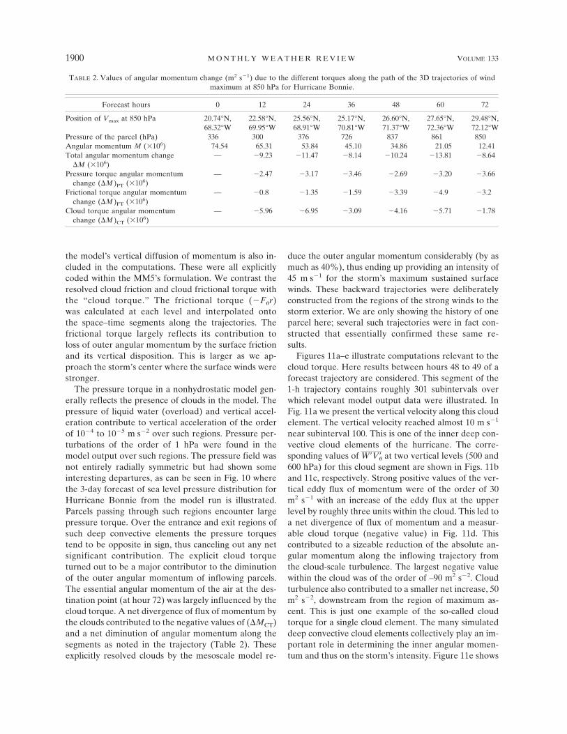
We next illustrate in Table 2 the angular momentumbudget following a parcel’s history. This table shows theparcel’s positions (as a function of time), the parcel’spressure, the angular momentum (M) of the parcel, thechange in angular momentum ( M) across 12-hourlyparcel motion segments, the contribution from pressuretorque experienced over 12-hourly parcel motion seg-ments, the contribution by net frictional torque (ex-cluding cloud torque) experienced by the parcel alongthese segments, and finally the effects of cloud torquein its contribution (computed as a residual) to thechanges of angular momentum of the parcel. The an-gular momentum change due to the pressure torquewas of the order of 106 m2 s�1. The negative values canbe related to a beta-gyre-type asymmetry that the par-cel encountered to the right of the storm motion whereit moved toward higher pressure, z/� � 0. The netchange in angular momentum for the inflowing parcelwas negative throughout, since the parcel was movingcloser to r � 0 for most of the time. The angular mo-mentum change due to frictional torque (excluding thecloud torques) above the 850-hPa surface arises fromhorizontal and vertical subgrid-scale diffusion in thefree atmosphere, while above the 850-hPa level theseeffects were small. The angular momentum change dueto cloud torque was another manifestation of explicitfrictional torque resolved by the model (see Fig. 11 for

1898 M O N T H L Y W E A T H E R R E V I E W VOLUME 133

an example of such computation). The values along thetrajectory, over all 12-hourly segments, were negative,implying that cloud torque contributed to a net diver-gence of eddy flux of momentum of the parcel. This actsto reduce the angular momentum for the inflowing par-cel. It is also clear from the table that the largest change

of the angular momentum (in storm-relative coordi-nates) arises from the parcel encountering such cloudturbulence.

Explicit friction is that part of the model friction thatcomes from the parameterization of the surface layerand the planetary boundary layer physics. Furthermore,

FIG. 9. The 72-h 3D backward trajectory of maximum wind at 850 hPa (m s�1) for HurricaneBonnie. Shown here is a trajectory terminating at the wind maxima in the vicinity of the centerof the hurricane at the end of the 72-h forecast. Isopleths indicate the maximum wind distri-bution at 72-h forecast time.

JULY 2005 K R I S H N A M U R T I E T A L . 1899

the model’s vertical diffusion of momentum is also in-cluded in the computations. These were all explicitlycoded within the MM5’s formulation. We contrast theresolved cloud friction and cloud frictional torque withthe “cloud torque.” The frictional torque (�F�r)was calculated at each level and interpolated ontothe space–time segments along the trajectories. Thefrictional torque largely reflects its contribution toloss of outer angular momentum by the surface frictionand its vertical disposition. This is larger as we ap-proach the storm’s center where the surface winds werestronger.

The pressure torque in a nonhydrostatic model gen-erally reflects the presence of clouds in the model. Thepressure of liquid water (overload) and vertical accel-eration contribute to vertical acceleration of the orderof 10�4 to 10�5 m s�2 over such regions. Pressure per-turbations of the order of 1 hPa were found in themodel output over such regions. The pressure field wasnot entirely radially symmetric but had shown someinteresting departures, as can be seen in Fig. 10 wherethe 3-day forecast of sea level pressure distribution forHurricane Bonnie from the model run is illustrated.Parcels passing through such regions encounter largepressure torque. Over the entrance and exit regions ofsuch deep convective elements the pressure torquestend to be opposite in sign, thus canceling out any netsignificant contribution. The explicit cloud torqueturned out to be a major contributor to the diminutionof the outer angular momentum of inflowing parcels.The essential angular momentum of the air at the des-tination point (at hour 72) was largely influenced by thecloud torque. A net divergence of flux of momentum bythe clouds contributed to the negative values of ( MCT)and a net diminution of angular momentum along thesegments as noted in the trajectory (Table 2). Theseexplicitly resolved clouds by the mesoscale model re-

duce the outer angular momentum considerably (by asmuch as 40%), thus ending up providing an intensity of45 m s�1 for the storm’s maximum sustained surfacewinds. These backward trajectories were deliberatelyconstructed from the regions of the strong winds to thestorm exterior. We are only showing the history of oneparcel here; several such trajectories were in fact con-structed that essentially confirmed these same re-sults.

Figures 11a–e illustrate computations relevant to thecloud torque. Here results between hours 48 to 49 of aforecast trajectory are considered. This segment of the1-h trajectory contains roughly 301 subintervals overwhich relevant model output data were illustrated. InFig. 11a we present the vertical velocity along this cloudelement. The vertical velocity reached almost 10 m s�1

near subinterval 100. This is one of the inner deep con-vective cloud elements of the hurricane. The corre-sponding values of W�V�� at two vertical levels (500 and600 hPa) for this cloud segment are shown in Figs. 11band 11c, respectively. Strong positive values of the ver-tical eddy flux of momentum were of the order of 30m2 s�1 with an increase of the eddy flux at the upperlevel by roughly three units within the cloud. This led toa net divergence of flux of momentum and a measur-able cloud torque (negative value) in Fig. 11d. Thiscontributed to a sizeable reduction of the absolute an-gular momentum along the inflowing trajectory fromthe cloud-scale turbulence. The largest negative valuewithin the cloud was of the order of –90 m2 s�2. Cloudturbulence also contributed to a smaller net increase, 50m2 s�2, downstream from the region of maximum as-cent. This is just one example of the so-called cloudtorque for a single cloud element. The many simulateddeep convective cloud elements collectively play an im-portant role in determining the inner angular momen-tum and thus on the storm’s intensity. Figure 11e shows

TABLE 2. Values of angular momentum change (m2 s�1) due to the different torques along the path of the 3D trajectories of windmaximum at 850 hPa for Hurricane Bonnie.

Forecast hours 0 12 24 36 48 60 72

Position of Vmax at 850 hPa 20.74°N,68.32°W

22.58°N,69.95°W

25.56°N,68.91°W

25.17°N,70.81°W

26.60°N,71.37°W

27.65°N,72.36°W

29.48°N,72.12°W

Pressure of the parcel (hPa) 336 300 376 726 837 861 850Angular momentum M (�106) 74.54 65.31 53.84 45.10 34.86 21.05 12.41Total angular momentum change

M (�106)— �9.23 �11.47 �8.14 �10.24 �13.81 �8.64

Pressure torque angular momentumchange ( M )PT (�106)

— �2.47 �3.17 �3.46 �2.69 �3.20 �3.66

Frictional torque angular momentumchange ( M )FT (�106)

— �0.8 �1.35 �1.59 �3.39 �4.9 �3.2

Cloud torque angular momentumchange ( M )CT (�106)

— �5.96 �6.95 �3.09 �4.16 �5.71 �1.78

1900 M O N T H L Y W E A T H E R R E V I E W VOLUME 133

FIG. 10. The 3-day mean sea level pressure (hPa) forecast of Hurricane Bonnie.

JULY 2005 K R I S H N A M U R T I E T A L . 1901

a longer trace along a 3-h trajectory (between hours 48and 51) of W�V�� that illustrates the nature of the cloudturbulence in a hurricane model. The mean value ofW�V�� during these 3 h was around �7 m2 s–1, whichshows that clouds at this level (600 hPa) contributed toa net upward flux of momentum.

b. Scale interactions

We have formulated the energetics for a quasi-steadysystem. Since the storm was over the ocean, the use ofa pressure coordinate was felt quite suitable. The quasi-static components of the datasets were easily derived

FIG. 11. (a) Vertical velocity (m s�1) at 500 hPa, (b) vertical eddy flux of momentum (m2 s�1) at 500 hPa, (c) vertical eddy flux ofmomentum (m2 s�1) at 600 hPa, (d) cloud torque (m2 s�2) during every time step of a 1-h forecast between the 48th and 49th hour ofmodel integration. (e) Same as (c) but for a longer duration, from the 48th to 51st hour of integration.

1902 M O N T H L Y W E A T H E R R E V I E W VOLUME 133

from the model’s earth-following sigma to the pressurecoordinate system. We first present the results for theseprocesses that invoke quadratic in-scale energy conver-sions. All of the results presented here are in storm-centered cylindrical coordinates and are mass integralsbetween radii r1 and r2, around the azimuthal coordi-nate, and between 100 hPa and the earth’s surface.

1) GENERATION OF AVAILABLE POTENTIAL

ENERGY

The generation of available potential energy is mea-sured by the covariances of heating (H) and tempera-ture (T) and is expressed by

�H, T� � �m

�HTdm, � � ��

T � R

Cpp����

�p, �8�

where � is a static stability parameter, � is the potentialtemperature, R is the universal gas constant, and Cp isthe specific heat at constant pressure; � varies withpressure. The covariance �H, T � can be broken downinto in-scale harmonic components,

�H, T� � �Ho, To� � �H1, T1� � . . . � �Hn, Tn�,

�9�

where o denotes the azimuthally averaged contributionand 1 denotes the first harmonic. Hence, the net gen-eration can be expressed by �m��n

i�0HiTidm. The re-sults of these computations are shown in Figs. 12a–f.The different panels show the results from forecasts forhours 12 through 72. Within each panel, the results ofcomputations averaged over cylindrical mass elementsfrom r � 0 to r � 40 km, r � 40 km to r � 200 km, andr � 200 to r � 380 km are displayed. These carry themass integrals of the generation term within these do-mains. Separate histograms are presented for the azi-muthally averaged wavenumber 0; wavenumbers 1 and2; wavenumbers 0, 1, and 2; and wavenumbers 3through 180. These results show that the largest gen-eration occurred at wavenumber 0. Wavenumbers 1and 2 contributed about one-third of the total genera-tion of the eddy available potential energy. The contri-butions from the other scales were much smaller. Thewarm core of the model hurricane extends fromroughly r � 0 to r � 180 km. The heating within thisregion and the cooling outside of this region contributeto the hurricane-scale generations of APE for wave-numbers 0, 1, and 2. Clearly, the cloud-scale heatingtranscends to the hurricane scales from the organiza-tion of convection. This breakdown among scales is es-sentially similar during the entire 72 h of the model run.There appears to be a direct generation of available

potential energy on the hurricane scale. This evidentlyis a result of the organization of convection on the hur-ricane scales.

2) GENERATION OF KINETIC ENERGY FROM

VERTICAL OVERTURNING

The total contribution of eddy kinetic energy (EKE)over a mass m is given by

�APE, EKE� � �Cp�m

�T�

pdm. �10�

This is a quadratic nonlinearity; hence we can express itas �Cp�m(1/p)�n�nTndm, where n denotes azimuthalwavenumbers. Thus, it is possible to separately evaluatethe contributions for each wavenumber. We can alsoseparately evaluate the contributions for the azimuth-ally averaged component (i.e., wavenumber 0), that is,�Cp�m(�oTo/p)dm. These are contributions from “inscale” vertical overturnings that generate kinetic en-ergy. Since each active deep convective element withscales of the order of a few kilometers has its strongestupward and downward motions on the cloud scale, wemight expect to see a large contribution for thesesmaller scales. However, the organization of convectionis more robust than the size of a single cloud. Thesecontributions seem to prefer the hurricane scale (i.e.,azimuthal wavenumbers 0, 1, and 2), reflecting the or-ganization of convection. This is shown in Figs. 13a–f.The histograms reflect the results over the same threeregions as in Fig. 12. The different panels [(a)–(f)] showthe results from the forecast datasets for hours 12through 72 at intervals of 12 h. The histograms in eachpanel show the energy conversions (available potentialto kinetic) for wavenumber 0, wavenumbers 1 and 2,wavenumbers 0, 1, and 2, and the rest of the waves. Theresults are quite similar at all these forecast intervals.The largest contribution was found at the azimuthallyaveraged wavenumber 0. This shows that clouds havean organization along the circular geometry, thus shift-ing the scale of overturning from the cloud scales (fewkilometers) to the hurricane scale. The conversion forwavenumbers 1 and 2 were about half as large as thosefor wavenumber 0. If we identify wavenumbers 0, 1, and2 as the hurricane scales, we see a substantial conver-sion of APE into EKE on this scale, again attributed tothis large-scale organization of convection. The contri-bution for wavenumbers 3 through 180 was in fact quitesmall and even fluctuating in sign for different smallerscales. The energetics in the wavenumber domain forthe middle-latitude zonally averaged jet, wavenumber

JULY 2005 K R I S H N A M U R T I E T A L . 1903

0, is opposite to that for a hurricane’s azimuthal wave-number 0. Waves provide energy to the wavenumber 0in the former case whereas they seem to remove theenergy from the hurricane circulation. The former isgenerally regarded as a low Rossby number phenom-enon whereas the latter is clearly one where the Rossbynumber exceeds one.

3) ENERGY EXCHANGES DUE TO NONLINEAR

TRIAD INTERACTIONS

In Figs. 14a and 14b we show the gain or loss ofenergy for wavenumbers 1 and 2 for the eddy kineticenergy (Fig. 14a) and eddy available potential energy(Fig. 14b), which arise from interactions of these scales

FIG. 12. Generation of available potential energy for Hurricane Bonnie. Three different histograms in each panel represent threeregions—inner area (0–40 km), fast winds (40–200 km), and outer area (200–380 km). Forecast times are (a) 12, (b) 24, (c) 36, (d) 48,(e) 60, and (f) 72 h of the model output. Units are m2 s�3 (� 10�6).

1904 M O N T H L Y W E A T H E R R E V I E W VOLUME 133

with all other permitted scales. Along the abscissa weshow the forecast hours. The results shown here arevertically integrated values through the troposphereover the three different regions, that is, inner, middle,

and outer radii bound. The obvious result is a net lossof energy at all radii for the hurricane scale (wavenum-bers 1 and 2) from these scale interactions. The largestlosses occurred at hour 72 when the storm had the

FIG. 13. Generation of kinetic energy by vertical overturning for Hurricane Bonnie. Three different histograms in each panelrepresent three regions—inner area (0–40 km), fast winds (40–200 km), and outer area (200–380 km). Forecast times are (a) 12, (b) 24,(c) 36, (d) 48, (e) 60, and (f) 72 h of the model output. Units are m2 s�3 (� 10�6).

JULY 2005 K R I S H N A M U R T I E T A L . 1905

strongest intensity. The cascade was strongest forwavenumber 1 when it interacts with other permittedscales.

4) SUMMARY OF OVERALL ENERGY EXCHANGES

IN THE AZIMUTHAL WAVENUMBER DOMAIN

The overall results of the energy exchanges are sum-marized in Fig. 15. These are 72-h averages during thisentire time Bonnie had hurricane wind strength. Theseenergy exchanges are mass averaged based on theequations given in the appendix. The vertical integralscover the atmosphere between the ocean surface andthe 100-hPa level. Three colors distinguish the resultsover different radial belts. (All units of energy ex-change are normalized to m2 s�3). Three categories ofenergy exchange are grouped here: (a) azimuthally av-eraged wavenumber 0, (b) azimuthal long waves, wave-numbers 1 and 2, and (c) azimuthal short waves, wave-numbers 3 to 180. The first two categories are desig-nated as the hurricane scales, and the third one isarbitrarily labeled as the cloud scales (subscript s), al-

though this naming is not entirely correct. This energydiagram is not a complete energy cycle. We have notdiscussed the dissipation of energy terms here; only thetransformation of energy terms is presented in this dia-gram.

For all of these scales, the generation of availablepotential energy from heating and the conversion ofavailable potential energy to eddy kinetic energy aredescribed by the in-scale processes. These are interest-ingly the largest in the inner 40-km radii for wavenum-ber 0. That reflects the hurricane-scale organization ofheating and of the covariances of heating and tempera-ture, and vertical velocity and temperature. This arisesfrom the organization of clouds along azimuthal wave-number 0. The next in magnitude is contribution for thelong waves, where again clearly there is a contributionfrom the organization of clouds on the azimuthal wave-numbers 1 and 2. The combined contribution for wave-numbers 3 to 180 is less than 10% of those for wave-number 0. The largest values of the generation of APEand its conversion to EKE occur at the inner radii

FIG. 14. Rate of change of (a) kinetic and (b) available potential energy of wavenumbersn � 1 and n � 2 due to interactions with pairs of waves with wavenumbers (l, m) �2. Unitsare m2 s�3. The forecast hour is indicated along the abscissa.

1906 M O N T H L Y W E A T H E R R E V I E W VOLUME 133

0 � r � 40 km. This is the region of the heaviest rainsin the MM5’s simulation of Hurricane Bonnie. The valuesfall off rapidly as we proceed to the outer radial belts.

The barotropic energy exchange comprises kineticenergy exchange from wavenumber 0 to the other

waves. The long waves as well as the cloud scales es-sentially extract energy from the azimuthally averagedwavenumber 0. Among these, some of the largest baro-tropic energy exchanges are from the wavenumber 0 tothe long waves. At the different radial belts these val-

FIG. 15. Summary of energy exchange computations resulting in the final intensity of Hurricane Bonnie. Different colors in thenumbers represent three different regions of computations (red for inner area between 0 and 40 km, green for fast wind region between40 and 200 km, and blue for outer area between 200 and 380 km of radius). Arrow marks indicate the direction of energy exchange.

JULY 2005 K R I S H N A M U R T I E T A L . 1907

Fig 15 live 4/C

ues range from 78.6 to 58.4 to 30.75 m2 s�3 (� 10�6).This shows that the hurricane scale (azimuthally aver-aged wavenumber 0) is barotropically unstable to thelong-wave scales (wavenumbers 1 and 2). Thus we caninfer that the large-scale asymmetries in the hurricane’sintense winds can arise from barotropic dynamics—thatis in addition to the possible translation asymmetry,which arises from the motion of a symmetric vortex ina uniform steering flow. This kinetic energy exchangefrom the wavenumber 0 to the long wave is largest inthe inner radial belt from 0 to 40 km where the maximaof the cyclonic vorticity of the hurricane reside.

The other areas of energy exchange are the kinetic tokinetic and available potential-to-available potential.These are the nonlinear three-component exchangesamong different scales. The arrows connecting Kl to Ks

and APEl to APEs show the collective exchanges fromthe long- to the short-wave scales summarized here.This is essentially a cascading process where energy isconveyed from the larger to the smaller scales. Thekinetic energy exchange Kl to Ks is much larger in mag-nitude compared to those of Pl to Ps. The inner radialbelt 0 � r �40 km carries the largest nonlinear energytransfers. There are also available potential energy ex-changes between the azimuthally averaged wavenum-ber 0 and the waves. Those exchanges are all directedfrom waves to the wavenumber 0. The largest such ex-changes are at the inner radii 0 � r � 40 km. The mag-nitude of the energy transferred by the long waves arelarger compared to that from the short waves to thezonal. These exchanges are related to the radial trans-fer of heat (up the gradient) toward wavenumber 0. Thelonger waves seem more efficient in reinforcing thewarm core of the hurricane in this sense. This is theoverall energy exchange scenario from the very highresolution simulation of Hurricane Bonnie of 1998.

6. Concluding remarks and future work

The hurricane intensity issue is among the major un-solved scientific problems presently. This paper pre-sents two possible frameworks—scale interactionsamong clouds and hurricane and an angular momentumperspective for this problem. The deep convective ele-ments within a hurricane have dimension of the orderof a few kilometers each. The role of cloud-scale heat-ing, generation of available potential energy, and itstransformation to eddy kinetic energy can only be anin-scale (i.e., individual cloud scale) process since theseprocesses involve quadratic nonlinearities. The qua-dratic nonlinearities are the covariances among heatingand temperature, and vertical velocity and tempera-ture. Hence, the only avenue for that energy to drive

the hurricane would be through nonlinear triad inter-actions between kinetic and kinetic energy, and avail-able potential to available potential energy amongcloud scales and the hurricane scale. That naïve pictureis not what is borne out by the computations based ondatasets derived from mesoscale nonhydrostatic micro-physical models. The key finding is the organization ofconvection on the azimuthally averaged wavenumber 0and the large-scale asymmetric scales of the hurricane;that is, wavenumbers 1 and 2 precede all that. Thosescales are inferred from the decomposition of the liquidwater mixing ratio fields that carry clearly the deepconvective cloud signatures. The generation of avail-able potential energy and its transformation to kineticenergy thus takes place directly on the larger scales ofthe hurricane. This is brought about by the organizationof convection—a topic that is not addressed in this pa-per. The other major component in the framework ofscale interactions is the energy exchanges among scalesvia triad interactions. These are the exchanges fromkinetic to kinetic and available potential to availablepotential energies. Those results among a triplet ofwaves (hurricane scales and other scales) show largely acascade of energy; that is, hurricane scales lose energywhen they interact with other scales. The issue of or-ganization of convection can be addressed by startingfrom an unorganized prehurricane state and by a con-tinual monitoring of the spectral form of the liquid wa-ter mixing ratio and its interactions with the rest of thedynamics, physics, and microphysics. Such a study canprovide insights on the scale interactions that lead to anorganization of convection. This study required a high-resolution (up to 1 km) multiple-nested regional meso-scale model that resolves clouds explicitly. A recentversion of the PSU–NCAR Mesoscale Model (nonhy-drostatic with microphysics) was used in this study.

A second aspect of this study was on the angularmomentum perspective, on the torques that diminishthe angular momentum along inflowing trajectories ofair parcels. They reveal that “cloud torques” play amajor role in this diminution of outer angular momen-tum and in the eventual intensity of the hurricane thatit attains. The important role of cloud torques alongsegments of the entire trajectory of a parcel with maxi-mum storm wind suggests that improved microphysicalparameterizations may have an important role on thefinal intensity of a predicted storm. Since all of thesefindings are based on model output datasets, futurestudies on model sensitivity are needed on areas thatimpact the intensity the most. These are the verticaloverturnings by organized convection and the cloudtorques. This suggests that even details of microphysi-cal parameterizations within clouds might require care-

1908 M O N T H L Y W E A T H E R R E V I E W VOLUME 133

ful testing within these explicitly cloud resolving meso-scale models. Clearly, carefully designed numerical ex-periments are needed to sort out these outer and innerthrust issues in their correct perspectives for addressingthe sensitivity of hurricane intensity to various param-eters. Most likely, these issues are intercoupled. Fieldexperiments that carry out detailed measurements ofmicrophysical parameters that affect the life cycle ofclouds may also provide insights for model sensitivitystudies. Understanding of hurricane intensity may re-quire a rather large series of model sensitivity studieson resolution (horizontal and vertical), data coverage,data assimilation, nonconvective rain (definition ofthreshold relative humidity), PBL physics, radiativetransfer and clouds, and parameterizations within theequations of water vapor, cloud water, rainwater, cloudice, snow, graupel, and number concentrations of cloudice.

Acknowledgments. The research work reported herewas supported by NSF Grant ATM-0108741, NASATRMM Grant NAG5-9662, NASA CAMEX GrantNAG8-1848, and FSU Research Foundation Grant1338-895-45. We acknowledge the data support fromthe European Centre for Medium-Range WeatherForecasts, especially through the help of Dr. Tony Holl-ingsworth. The authors thank the anonymous reviewersfor their helpful comments to improve the quality of themanuscript.

APPENDIX

Scale Interactions in Storm-Centered PolarCoordinates

The equations of motion in the storm-centered cylin-drical coordinate system are

��

�t� ��

��

r��� r

��

�r�

��

�p�

r�

r� fr

� g�z

r��� F�, �A1�

�r

�t� ��

�r

r��� r

�r

�r�

�r

�p�

�2

r� f�

� g�z

�r� Fr; �A2�

and the continuity equation is

0 � ���

r���

�r

�r�

r

r�

�

�p. �A3�

The independent variables in this coordinate system arethe azimuthal angle �, the radial distance from the cen-

ter r, and the pressure p. The tangential and radialwinds are �� (positive anticlockwise) and �r (positiveoutward), respectively. The vertical velocity in pressurecoordinates is �, f is the Coriolis parameter, gz is thegeopotential height, and F� and Fr are the tangentialand radial components of the frictional force per unitmass. Any of the dependent variables can be subjectedto Fourier transform along the azimuthal (�) direction:

f��� � �n���

�

F �n�ein�, �A4�

where the complex Fourier coefficients F(n) are given by

F �n� �1

2� �0

2�

f���e�in�d�. �A5�

The Fourier transform of the product of two functionsis given by

12� �

0

2�

f���g���e�in�d� � �m���

�

F �n�G�n � m�.

�A6�

Let us consider only the nonlinear terms in Eqs. (A1)and (A2). If we multiply both equations by (1/2�)e�in�,integrate along an azimuthal circle, and apply (A4),(A5), and (A6), we obtain

�V��n�

�t� � �

m���

� imV��m�

rV��n � m�

� ��V��m�

�r�

V��m�

r �Vr�n � m�

��V��m�

�p �n � m�, �A7�

�Vr�n�

�t� � �

m���

� �imVr�m�

r�

V��m�

r �V��n � m�

��Vr�m�

�rVr�n � m� �

�Vr�m�

�p �n � m�,

�A8�

where V�(n), Vr(n), and �(n) are the nth Fourier coef-ficients of ��, �r, and �. From the continuity equation weget

� �n�

�p�

inV��n�

r�

�Vr�n�

�r�

Vr�n�

r� 0. �A9�

JULY 2005 K R I S H N A M U R T I E T A L . 1909

By multiplying (A7) and (A8) with V�(�n) and Vr(�n),and the complex conjugates of (A7) and (A8) withV�(n) and Vr(n), respectively, we obtain

��V��n��2

�t� � �

m���

� imV��m�

r�V���n�V��n � m�

� V��n�V���n � m�� � ��V��m�

�r�

V��m�

r �× �V���n�Vr�n � m� � V��n�Vr��n � m��

��V��m�

�p�V���n� �n � m�

� V��n� ��n � m��, �A10�

�APE�0�APE�n�� � �M

��n�1

� �Cp��Tr�n�

�T

�r

��p�

��T�n��

���

�p��R

pT

� ��T�h���dM. �A11�

Now if we apply (A9) and add (A10) and (A11), weobtain an expression for the local rate of change ofkinetic energy of wavenumber n due to nonlinear in-teractions as

�K�n�

�t� �

m���m�0

�

V��m��1r

����������m, n� � �r��� ��r��m, n� � ���� ��p��m, n� �1r

��r�m, n��

� Vr�m��1r

����r �����m, n� � �r��r ��r��m, n� � ���r ��p��m, n� �1r

����m, n��

�1r

�

�rr�V��m��r�

�m, n� � Vr�m��rr�m, n�� �

�

�p�V��m���

�m, n� � Vr�m��r�m, n��,

�A12�

where �ab(m, n) � A(n�m)B(�n) � A(�n�m) B(n).The last term in (A12) vanishes upon integration

from top to bottom of the atmosphere, provided�(ptop) � �(pbottom) � 0. With a similar approach,we can find the rate of change of potential energydue to nonlinear interactions in a cylindrical coordi-nate system. The local change in temperature is given by

�T

�t� ��

�T

r��� r

�T

�r�

�T

�p�

RT

Cpp �

Q

Cp.

�A13�

If we denote the Fourier transform of T as B(n), mul-

tiply both equations by (1/2�)e�in�, integrate along anazimuthal circle, and apply (A4), (A5), and (A6), andconsider only the nonlinear terms, we obtain

�B�n�

�t� � �

m���

� imB�m�

rV��n � m� �

�B�m�

�rVr�n � m�

� ��B�m�

�p�

RB�m�

Cpp � �n � m�. �A14�

Following the same procedure as for (A13), and de-fining the available potential energy as APE(n) �Cp� |B(n) |2, where � � (��/T)(R/CpP)(�/P)�1 is thestatic stability factor, we obtain

��APE�n��

�t� Cp� �

m���m�0

�

B�m��1r

����T�����m, n� � �r��T��r��m, n� � ���T��p��m, n� �R

Cpp�T�m, n��

�1r

�

�rrB�m��rT

�n, m� ��

�pB�m��T �A15�

as the expression for the local rate of changeof the available potential energy of frequency ndue to nonlinear interactions with frequencies m

and n � m. Similarly to (A12), the last term van-ishes upon integration over the depth of the atmo-sphere.

1910 M O N T H L Y W E A T H E R R E V I E W VOLUME 133

For azimuthal wavenumber 0 the generation of avail-able potential energy is given by

G�APE0� � �m

��H � H� �T � T� dm, �A16�

where � is the static stability parameter. The doubleoverbars indicate a horizontal area average and thesquare bracket is an azimuthal mean; H is the heatingrate and T is the temperature. The generation at anywavenumber is simply expressed by

G�n� � �m

� Hn Tn dm. �A17�

This is what is used for each wave within the long- and

the shorter-scale waves. For azimuthal wavenumber 0the conversion of available potential to kinetic energy isgiven by

�APE0K0� � ��m

CP

�0 � � �T0 � T�

Pdm,

�A18�

and for all other scales

�APEnKn� � ��m

CP

nTn

Pdm. �A19�

Here � is the vertical velocity. The exchange amongazimuthally averaged flows and other waves are ex-pressed by the following equations:

�K�0�K�n�� � �M

��n�1

� ���r�n�

��

�r� �rr

�n��r

�r� ���n�

��

�p� �r

�n��r

�p�

1r

����n�r �

1r

��r�n���

� gr

�z

�r� d�dM and �A20�

�APE�0�APE�n�� � �M

��n�1

� �Cp��Tr�n�

�T

�r�

�p�

��T�n��

���

�p��R

pT � ��T�h���dM, �A21�

where �ab(n) � A(n)B(�n) � A(�n)B(n).Expressions (A20) and (A21) are both used for long-

and short-wave exchanges with the azimuthally aver-aged flows.

REFERENCES

Bao, J.-W., J. M. Wilczak, J.-K. Chio, and L. H. Kantha, 2000:Numerical simulation of air–sea interaction under high windconditions using a coupled model: A study of hurricane de-velopment. Mon. Wea. Rev., 128, 2190–2210.

Betts, A. K., and M. J. Miller, 1986: A new convective adjustmentscheme. Part II: Single column test using GATE-wave,BOMEX, ATEX and Arctic airmass data sets. Quart. J. Roy.Meteor. Soc., 112, 693–709.

——, and ——, 1993: The Betts–Miller scheme. The Representa-tion of Cumulus Convection in Numerical Models, Meteor.Monogr., No. 46, Amer. Meteor. Soc., 107–122.

Braun, S. A., 2002: A cloud-resolving simulation of HurricaneBob (1991): Storm structure and eyewall buoyancy. Mon.Wea. Rev., 130, 1573–1592.

——, and W.-K. Tao, 2000: Sensitivity of high-resolution simula-tions of Hurricane Bob (1991) to planetary boundary layerparameterizations. Mon. Wea. Rev., 128, 3941–3961.

Chan, J. C.-L., and R. Y. Williams, 1987: Numerical studies of thebeta effect in tropical cyclone motion. Part I: Zero mean flow.J. Atmos. Sci., 44, 1257–1265.

——, and ——, 1994: Numerical studies of the beta effect in tropi-

cal cyclone motion. Part II: Zonal mean flow effects. J. At-mos. Sci., 51, 1065–1076.

Chen, Y.-S., and M. K. Yau, 2001: Spiral bands in a simulatedhurricane. Part I: Vortex Rossby wave verification. J. Atmos.Sci., 58, 2128–2145.

Davis, C. A., and L. F. Bosart, 2001: Numerical simulations of thegenesis of Hurricane Diana (1984): Part I: Control simula-tion. Mon. Wea. Rev., 129, 1859–1881.

——, and S. B. Trier, 2002: Cloud-resolving simulations of meso-scale vortex intensification and its effect on a serial mesoscaleconvective system. Mon. Wea. Rev., 130, 2839–2858.

Deardorff, J. W., 1972: Parameterization of the planetary bound-ary layer for use in general circulation models. Mon. Wea.Rev., 100, 93–106.

Dudhia, J., 1989: Numerical study of convection observed duringthe winter monsoon experiments using a mesoscale two-dimensional model. J. Atmos. Sci., 46, 3077–3107.

——, 1993: A non-hydrostatic version of the Penn State–NCARMesoscale Model: Validation tests and simulation of an At-lantic cyclone and cold front. Mon. Wea. Rev., 121, 1493–1513.

Grell, G. A., J. Dudhia, and D. R. Stauffer, 1995: A description ofthe fifth-generation Penn State/NCAR Mesoscale Model(MM5). National Center for Atmospheric Research, Boul-der, CO, 122 pp.

Holland, G. J., 1983: Angular-momentum transports in tropicalcyclones. Quart. J. Roy. Meteor. Soc., 109, 187–209.

Hong, S. H., and H. L. Pan, 1996: Nonlocal boundary layer ver-

JULY 2005 K R I S H N A M U R T I E T A L . 1911

tical diffusion in a medium-range forecast model. Mon. Wea.Rev., 124, 2322–2339.

Kamineni, R., T. N. Krishnamurti, R. A. Ferrare, S. Ismail, andE. V. Browell, 2003: Impact of high resolution water vaporcross-sectional data on hurricane forecasting. Geophys. Res.Lett., 30, 1234, doi:10.1029/2002GL016741.

——, ——, S. Pattnaik, E. V. Browell, S. Ismail, and R. A. Fer-rare, 2005: Impact of CAMEX-4 datasets for hurricane fore-casts using a global model. J. Atmos. Sci., in press.

Krishnamurti, T. N., and S. Jian, 1985a: The heating field in anasymmetric hurricane—Part I: Scale analysis. Adv. Atmos.Sci., 2, 402–413.

——, and ——, 1985b: The heating field in an asymmetric hurri-cane—Part II: Results of computations. Adv. Atmos. Sci., 2,426–445.

——, and L. Bounoua, 1995: An Introduction to NumericalWeather Prediction Techniques. CRC Press, 293 pp.

——, J. Xue, H. S. Bedi, K. Ingles, and D. Oosterhof, 1991: Physi-cal initialization for numerical weather prediction over theTropics. Tellus, 43, 53–81.

——, C. M. Kishtawal, T. LaRow, D. Bachiochi, Z. Zhang, C. E.Williford, S. Gadgil, and S. Surendran, 2000: Multi-modelsuperensemble forecasts for weather and seasonal climate. J.Climate, 13, 4196–4216.

——, and Coauthors, 2001: Real-time multianalysis/multimodelsuperensemble forecasts of precipitation using TRMM andSSM/I products. Mon. Wea. Rev., 129, 2861–2883.

——, D. R. Chakraborty, N. Cubukcu, L. Stefanova, and T. S. V. V.Kumar, 2003: A mechanism of the MJO based on interactionsin the frequency domain. Quart. J. Roy. Meteor. Soc., 129,2559–2590.

Liu, Y., D.-L. Zhang, and M. K. Yau, 1999: A multiscale numeri-cal study of Hurricane Andrew (1992). Part II: Kinematicsand inner-core structures. Mon. Wea. Rev., 127, 2597–2616.

Pasch, R. J., L. A. Avila, and J. L. Guiney, 2001: Atlantic Hurri-cane Season of 1998. Mon. Wea. Rev., 129, 3085–3123.

Rizvi, S. R. H., E. L. Bensman, T. S. V. V. Kumar, A.Chakraborty, and T. N. Krishnamurti, 2002: Impact ofCAMEX-3 data on the analysis and forecasts of Atlantic hur-ricanes. Meteor. Atmos. Phys., 79, 13–32.

Saltzman, B., 1957: Equations governing the energetics of thelarger scales of atmospheric turbulence in the domain ofwave number. J. Meteor., 14, 513–523.

——, 1970: Large scale atmospheric energetics in the wave num-ber domain. Rev. Geophys. Space Phys., 8, 289–302.

Williford, C. E., T. N. Krishnamurti, R. Correa-Torres, S. Cocke,Z. Christidis, and T. S. V. V. Kumar, 2003: Real-time mul-timodel superensemble forecasts of Atlantic tropical systemsof 1999. Mon. Wea. Rev., 131, 1878–1894.

Zhang, D.-L., and X. Wang, 2003: Dependence of hurricane in-tensity and structures on vertical resolution and time-stepsize. Adv. Atmos. Sci., 20, 711–725.

1912 M O N T H L Y W E A T H E R R E V I E W VOLUME 133