Symmetrization of lopsided vorticity monopoles and offset hurricane eyes

Q. J. R. Meteoml. Soc. (2001). 127, pp. 2307-2327

Symmetrization of lopsided vorticity monopoles and offset hurricane eyes

By R. PRIETO'*, J. P. KOSSIN2 and W. H. SCHUBERT' National Autonomous University of Mexico, Mexico

'Colorado State University, USA

(Received I5 January 2001; revised 31 May 2001)

SUMMARY This paper is a contribution towards better understanding of the continually occurring symmetrization

processes in tropical cyclones. Before a tropical cyclone develops an eye, it can often possess an asymmetric monopolar vorticity distribution. As an idealized initial condition in a non-divergent barotropic model, we use a lopsided monopole with different degrees of asymmetry of the monotonic vorticity field. We then study the axi-symmetrization process which involves the ejection of a winding spiral band. For extreme asymmetric initial conditions, the band can produce regions of barotropic instability, resulting in nonlinear mixing of vorticity and the formation of polygonal structures. In a second series of experiments, we study the case of a tropical cyclone with a developed eye, modelled as a hollow-tower vorticity distribution, i.e. an annular region of elevated vorticity, with low vorticity in the eye. If the eye is offset and the annular region of elevated vorticity is not of uniform width, complex symmetrization processes can occur, sometimes leading to a tripole structure of the humcane's vorticity field. Long-lived humcane eyes are found for initial conditions with a slight offset. For such initial conditions, passive tracers can remain in the eye for as long as 72 hours, showing that in this model it is possible for air inside the eye to remain there for long periods of time, while moving coherently with the storm. Predictions of the axi-symmetric final equilibrium states of the flow are obtained using the statistical mechanics theory of maximum Boltzmann mixing entropy. These predictions are then compared with results from the direct numerical integrations for both the lopsided monopole and the offset hurricane eye. The distribution of air-parcel tracers initially placed in selective regions of vorticity for the direct numerical integrations are compared with results from the statistical theory.

KEYWORDS: Humcane dynamics Maximum-entropy flows

1. INTRODUCTION

When studying sequences of satellite images of tropical weather disturbances, one is often impressed by how a fairly asymmetric pattern of convection can evolve, within a day, into a highly axi-symmetric form. A typical example of this is illustrated in Figs. l(a) and (b), which show infrared images of Hurricane Howard at 0400 UTC, 24 August 1998 and 0400 UTC, 25 August 1998, respectively.

One of the major deficiencies in our ability to analyse tropical-cyclone dynamics lies in the difficulty of constructing high-resolution potential vorticity (PV) maps to accompany satellite images such as those shown in Figs. l(a) and (b). Based on experience with numerical models, we suspect that the PV distribution for Fig. l(a) is quite asymmetric and filamented, while that for Fig. l(b) is more axi-symmetric and smooth. We also suspect that an important dynamical aspect of the evolution from Fig. l(a) to (b) is nonlinear and lies in the horizontal advection of PV. We explore these ideas in section 3, where a non-divergent barotropic model (described in section 2) is used to study the evolution of lopsided vorticity monopoles, i.e. monopolar vorticity distributions whose maxima are not collocated with the vorticity centroid.

"ho other interesting aspects of tropical cyclones are the variety of eye diameters and the fact that the eye is often not centred within the region of intense convection. For example, the small eye in Fig. l(b) is offset to the north-east. Such offset eyes are also common in radar reflectivity patterns such as the 3 August 1997 radar composite of Hurricane Guillermo, which is shown in Fig. l(c). Kossin and Eastin (2001) have recently presented observational evidence that the eye is often a region of low PV * Corresponding author: Centro de Ciencias de la Atm6sfera, UNAM, Circuit0 de la Investigaci6n Cientifica, CU, M6xico 04510, DF, Mexico. e-mail: [email protected] @ Royal Meteorological Society, 2001.

2307

2308 R. PRIETO et al.

Figure 1. (a) Infrared (IR) image of Humcane Howard at 0400 UTC, 24 August 1998. (b) Same as (a) but for 0400 UTC, 25 August 1998. (c) WP-3D lower-fuselage radar composite of Humcane Guillermo on 3 August 1997. Images (a) and (b) are from the IR image archive of the Cooperative Institute for Research in the Atmosphere (Zehr et al. 1999); image (c) is courtesy of the National Oceanic and Atmospheric AdministratiodAtlantic

Oceanographic and Meteorological LaboratoriesRIunicane Research Division.

surrounded by an annular region of very high PV. In section 4 we shall model offset eyes using the non-divergent barotropic model with initial conditions consisting of offset hollow annular regions of elevated vorticity.

Of course, to describe fully all the moist physical processes occurring in hurricanes, one must consider models that are three-dimensional, non-hydrostatic, and include prediction equations for the amounts of the various categories of condensed water substance. Properly formulated and run at high spatial resolution, such models are capable of simulating both the non-hydrostatic dynamics of individual cumulonimbus clouds and the larger-scale, quasi-static, quasi-balanced dynamics of the hurricane vortex. To understand the evolution of the quasi-balanced vortex in such full-physics models, it is useful to construct PV maps from the model output. The formula used for the PV should be one that is consistent with the full-physics model, i.e. exactly derived from the governing equations of the model. In addition, under appropriate balance conditions, this PV should be invertible, i.e. it should carry the essential dynamical information about the quasi-balanced flow. Recently, Schubert et al. (2001) have derived such a PV principle for the full-physics model developed by Ooyama (1990,2001). This

SYMMETRIZATION OF LOPSIDED MONOPOLES AND OFFSET EYES 2309

PV principle takes the form

P

D P j . (V x F) k .Vb, - = P ( +- k . V0, + Dt j . C

where

1 P

P = -( . ve, (2)

is the potential vorticity. In Eq. (l), D/Dt = a/at + u - V is the material derivative, u the three-dimensional vector velocity of the dry air and the airborne water, 3 = 2Q + V x u the absolute vorticity vector, p the total density (consisting of the sum of the densities of dry air, water vapour, airborne condensate, and precipitation), Pr the density of precipitation, U the vector velocity of precipitation relative to u, 0, the virtual potential temperature, 8, the material rate of change of 0,, F the frictional force per unit mass, j = VeP/(VO,l the unit vector perpendicular to the B,-surface, and k = (/I( 1 the unit vector pointing along the absolute-vorticity vector. Based on Eq. (1) we can say that there are four aspects to understanding the PV structure in hurricanes: (i) the advective aspects embodied in the D/Dt operator on the left-hand side of Eq. ( I ) ; (ii) the frictional sourcehink Pdj - (V x F)/Q - ()I; (iii) the diabatic sourcehink P{(k - VbP)/(k - Ve,)]; and (iv) the effect of precipitation P{V - (/+U)/p]. The precipitation term (iv) tends to be of secondary importance, so the major non- conservative effects are the frictional sourcehink (ii) and the diabatic source/sink (iii). It is the diabatic sourcehink which is responsible for the extremely large PV (- 100 PV units) found in humcanes. Briefly, this aspect of the dynamics can be described as follows. First note that k V is the derivative along the vorticity vector and that, in the intense convective region of the eye wall, the absolute-vorticity vector tends to point upward and radially outward. Since bP tends to be a maximum at mid-tropospheric levels, air parcels flowing upward in the eye wall experience a material increase in PV due to the P { ( k . Vb,)/(k - VO,)] term. This material increase of PV can be especially rapid in lower-tropospheric regions where both P and (k Vb,)/(k - V0,) are large. In general the ‘efficiency’ of a given diabatic forcing (k Vb,)/(k - V0,) is higher in the inner eye-wall region because P is higher there. Although the k - Vb, term reverses sign at upper-tropospheric levels, large PV is often found there because the large lower- tropospheric values of PV are carried upward into the upper troposphere (Moller and Smith 1994).

In the present paper we shall be concerned only with the advective aspects of the PV evolution, and in particular with the horizontal advective aspects. To isolate these aspects of the flow evolution, we consider the non-divergent barotropic model. Although this is obviously a drastic simplification, the non-divergent barotropic model is a useful device that allows us to focus purely on the horizontal advective aspects of the problem.

2. NON-DIVERGENT BAROTROPIC SPECTRAL MODEL

Since the non-divergent barotropic model does not make a distinction between potential vorticity and absolute vorticity, the f-plane non-divergent barotropic analogue of Eq. (1) is D(/Dt = uV2(, where ( is the relative vorticity, and where the material derivative simplifies to D/Dt = a/at + ua/ax + va/ay. Expressing the velocity com- ponents in terms of the stream function by u = -a+/ay and u = a+/ax, we can write

23 10 R. PRIETO et al.

the vorticity equation as

where

is the invertibility principle, a( , )/a(x, y) is the Jacobian operator, and where we have included a diffusion term with constant viscosity v to control the spectral blocking associated with the enstrophy cascade to higher wave numbers. Note that we have avoided the use of hyperviscosity (higher iterations of the Laplacian operator on the right-hand side of Eq. (3)) because of the unrealistic oscillations it can cause in the vorticity field (see, for example, Jimknez 1994).

'Itvo integral properties associated with Eqs. (3) and (4) are the energy and enstrophy relations

V2$ = C (4)

_ - - -2vz, d& dt dZ - = -2v9, dt

where & = 11(1/2)V$ - V$ dx dy is the energy, 2 = 11(1/2)(2 dx dy is the enstrophy, and P = 11(1/2)V{ - VC dx dy is the palinstrophy. Equations (5) and (6) are obtained by multiplying Eq. (3) by -$ and ( respectively, and then integrating over the entire periodic domain.

We shall now present numerical integrations of Eqs. (3) and (4) that demonstrate the symmetrization processes for lopsided vorticity monopoles and offset hurricane eyes. The solutions presented here were obtained with a double Fourier pseudo-spectral code having 5 12 x 5 12 equally spaced collocation points on a doubly periodic domain of size 200 km x 200 km. The code was run with a de-aliased calculation of the quadratic nonlinearity in Eq. (3). This results in 170 x 170 Fourier modes. Although the collocation points are only 0.39 km apart, a more realistic estimate of resolution is the wavelength of the highest Fourier mode, which is 1.176 km. Time differencing was accomplished with a standard fourth-order Runge-Kutta scheme using a 6.0-second time step. The chosen value of viscosity in Fq. (3) was 6.5 m2s-'. This gives a l /e damping time of 45 minutes for all modes having total wave number 170, but for modes having total wave number 85, the damping time lengthens to 3 hours.

3. AXI-SYMMETRIZATION OF LOPSIDED VORTICITY MONOPOLES

The initial conditions for the lopsided monopole experiments are illustrated in the upper-left panels of Figs. 2 and 6. These initial conditions consist of a circular region (radius a, centre x = xc, y = yc) of elevated vorticity surrounded by an environment with a constant, slightly negative, vorticity Ce. The maximum vorticity, which is elevated above the environmental value by the amount r, is not at the centre of the circular region but occurs at x = xm, y = yc. The specific mathematical form of the initial condition is

C(X, Y, 0)

SYMMETRIZATION OF LOPSIDED MONOPOLES AND OFFSET EYES 231 1

TABLE 1. PARAMETERS FOR THE SIZE, POSITION AND VORTICITY VALUES OF THREE DIFFERENT LOPSIDED VORTICITY MONOPOLES. THE RESULTING MAXIMUM WIND SPEED

(lVmmi) IS ALSO SHOWN. A

U Xc Xm X c - X m i- Se Ivmm I Experiment (km) (km) (km) (km) ( x ~ O - ~ S - ' ) ( x ~ O - ~ s-') (rns-l)

A 45 116.1 76.1 40 300 -13 31.1 B 45 112.1 82.1 30 300 -13 29.7 C 45 108.1 88.1 20 300 - 13 28.8

See text for further information.

where

is a smooth interpolation function with the property that S(r) + 1 as r approaches unity from below, and S ( r ) + 0 as r approaches zero from above, and where

sin(A + B) d = a

sin A ' with

A = arctan (-) IY - Ycl , B = arcsin X - Xm

(9)

The adjustable parameter K controls the peakedness of the initial vorticity field. In the experiments shown here we have chosen K = (1/2) exp(2) ln(2) M 2.5609, which yields S(1/2) = 1/2. In addition, we have chosen the model domain 0 < x < 200 km and 0 < y < 200 km, with the centre of the circle (x - x, )~ + (y - Y , ) ~ = a2 given by yc = 100 km and xc determined from

where the double integrals are over the entire doubly periodic domain. In this way the centre of the circle (x - xc)2 + (y - Y , ) ~ = a2 is shifted from the centre of the model domain in such a way that the vorticity centroid lies exactly at the centre of the model domain. The value of the constant <e is chosen so that the domain-averaged vorticity is zero, as required by the doubly periodic Fourier representation. As summarized in Table 1, we have chosen a = 45 km, and have run three experiments for the offsets xc - x m = 40,30,20 km, with ?= 300 x s-'. Note that the maximum wind speeds in all three initial vortices are slightly below hurricane strength.

The time evolution of the vorticity field for Experiment A is presented in Fig. 2. The area shown is 45 km 5 x, y 5 155 km and the initial maximum wind speed is 3 1.1 m s-l. This is the most extreme case of the lopsided monopoles we have run. The vorticity maximum at t = 0 (Fig. 2(a)) is close to the left edge of the elevated-vorticity region, and the vorticity is monotonic in all directions from this maximum point. We can see in Fig. 2(b) (t = 2 h) that the vorticity maximum quickly moves towards the centre of the domain, and there is deformation of the outer regions of the vortex, with the production of a long spiral band carrying most of the tracers with it. At later times the spiral band thins and makes several turns around the centre of the vortex. Most of


Figure 2. Vorticity fields at (a) 0 h, (b) 2 h, (c) 8 h, (d) 14 h, (e) 20 h, and (f) 36 h, for Experiment A (see text). The label bar for the vorticity field is given in units of lop5 s-l, so that the black area has vorticity larger than 245 x s-'. At the initial time, the maximum vorticity lies 40 km west of the centre of the large circular area (radius 45 km) of elevated vorticity, i.e. x,,, = x, - 40 km. The centre of the model domain (x = 100 km, y = 100 Ian) is also the vorticity centroid (see Eq. (11)). Initially, the region with 0 Q 5 Q 35 x s-' is uniformly covered with 366 tracers (small circles). Note that the symmetrization process involves the entrainment

of low-vorticity environmental air and the development of secondary barotropic instability (e.g. at t = 14 h).

the tracers remain within the band, even though it is extremely narrow at its outer end (Fig. 2(c)). The spiral band traps some negative-vorticity fluid that initially surrounded the vortex, and at t = 8 h, has captured small regions of negative vorticity between each of its windings. This pattern is dynamically unstable, and the unstable regions tend to roll up into small vortices that mix the vorticity (Figs. 2(d) and (e)). Polygonal patterns can be observed during different stages of this instability process. In the last stages of the simulation, the vortex axi-symmetrizes and by t = 36 h (Fig. 2(f)), the vorticity


Percent of initial

value

Percent of initial

value

!

300

200,

____._ 1 I I 0 10 20 30 40 50 0 10 20 30 40 50

Time (hours) Time (hours)

Figure 3. Time dependence of (a) kinetic energy (dashed line) and enstrophy (solid line), and (b) palinstrophy, relative to their initial values for Experiment A (see text).

isolines are nearly concentric. Although most of the tracers at t = 36 h occupy the region between the same pair of isolines between which they started, there has been some spread both inward and outward. Tracer parcels that spiral inward become surrounded by high-vorticity fluid and experience additional mixing due to the barotropic instability process. Diffusion then raises their vorticity. By 36 hours these mixed parcels are found just outside the highest vorticity region (black area). Thus, most of the mixing that occurs during symmetrization is confined to the annular region surrounding the high- vorticity core. Experiment A was also run with a larger, 300 km x 300 km, domain, but with the same grid spacing. The results showed no sensitivity with respect to the domain size.

Figure 3 shows the kinetic energy & ( t ) , the enstrophy Z(t) , and the palinstrophy P ( t ) during the evolution of Experiment A. The kinetic energy was nearly conserved during the experiment, decaying by only 0.52% of the initial value. In contrast, the enstrophy decayed 6.38%, while the palinstrophy had a strong increase of nearly 775% at 11 hours and a steady decrease thereafter. These results are typical of high-Reynolds- number two-dimensional turbulent flows, which show selective decay of enstrophy over kinetic energy. When these plots are compared with Fig. 8 of Schubert et al. (1999), which shows the &, 2, and P evolution for an initial hollow-tower vorticity field, we observe a qualitatively similar behaviour, but with the observation that in the lopsided- monopole experiment the process in action is mainly axi-symmetrization, while in the Schubert et al. (1999) experiment the relevant process is shear instability through phase locking of vortex Rossby waves.

Since actual hurricanes have Reynolds numbers much higher than those in our numerical simulations, it is of interest to note how the curves in Fig. 3 change as the non- divergent barotropic model is mn at increasingly finer resolution with decreasing values of u. Because 2 is bounded by its initial value, the right-hand side of Eq. ( 5 ) approaches zero as u + 0, so that d&/dt + 0 and the kinetic energy is conserved exactly in this limit. The behaviour of the right-hand side of Eq. (6) is quite different. As u is decreased, vorticity structures appear at finer scales before diffusion is effective, with the result that local vorticity gradients are larger and P is, therefore, larger. In this way dZ/dt may not vanish as u + 0. This is an important part of the argument given by Batchelor (1969) and recently tested by Chasnov (1997). Thus, the & and 2 curves in Fig. 3(a) would not be expected to change significantly as u is decreased, while the palinstrophy shown in Fig. 3(b) pulses to higher values.

The flow field in Fig. 2(f) can be considered a state of near equilibrium, that is, a state where the vorticity field preserves the same structure, except for the slow decay due to the diffusion term on the right-hand side of Eq. (3). An alternative approach to determine this equilibrium state follows the basic ideas of statistical mechanics and is known as

2314 R. PRIETO ef al.

0.6/ 0 . 4 \ O 4 \

_i 80 100

Figure 4. Vorticity profiles for Experiment A (see text). The direct numerical integration at t = 36 h is shown by the solid line and the maximum-entropy prediction by the dashed line.

maximum-entropy theory. This theory has been developed recently by Miller ( 1990), Robert and Sommeria (1991), Sommeria et al. (1991) and Chavanis and Sommeria (1996). The basic method of maximum-entropy theory consists of looking at the flow in a probabilistic, or ‘macroscopic’, sense. In other words, we do not follow the precise changes of the small-scale vorticity features, but rather look at the flow as an averaged behaviour of a large collection of systems with different fine-grain structure, but with the same macroscopic state specified by the total energy, circulation and vorticity centroid. Maximum-entropy theory predicts the most probable macroscopic state of the flow, which is consistent with the largest number of microscopic states, and that macroscopic state corresponds to the equilibrium configuration of the flow.

This maximum-entropy method, the mathematical details of which are discussed in the appendix, was used to compute the equilibrium state of Experiment A. The initial condition was represented by a piecewise constant-vorticity field with a total of ten vorticity levels that approximately fit the continuous vorticity profile of Fig. 2(a). The macroscopic quantities that are preserved in the maximum-entropy vortex are the total kinetic energy, the area (circulation) of each of the ten vorticity levels, and the centroid coordinates. Although the total angular momentum of inviscid flow is conserved in the doubly periodic (square) domain, we are not considering it as one of the macroscopic invariants since it is related to a central point in circular geometry and, thus, is not appropriate for our domain. However, we note that the conservation of the vorticity centroid in the doubly period domain has the same form as the angular momentum conservation in a (singly periodic) spherical domain (see Prieto and Schubert 2001).

The maximum-entropy vortex was obtained using 96 x 96 grid points on a 200 km x 200 km domain, retaining a total of 63 x 63 Fourier modes. Since the maximum-entropy final-state solution is expected to be a smooth function, and there is no additional information in computing it with higher resolution, the following maximum-entropy results are not sensitive to an increase of the number of grid points and/or Fourier modes. The vorticity-profile comparison of the azimuthally averaged vortex (with respect to the vorticity maximum) of Fig. 2(f) and the azimuthally averaged maximum-entropy solution is shown in Fig. 4. There is a good fit between the two curves in most of the domain, although in the central core of the vortex (r c 10 km) and in the interval 30 km c r c 40 km, the maximum-entropy prediction is slightly below the direct numerical integration.

A theoretical prediction of maximum-entropy theory for the spread of the air parcels shown as small circles in Fig. 2 is given by the density function p l ( r ) for the vorticity level 71 = 17.9 x s-*, which represents the region 0 5 < 5 35 x

s-I of Fig. 2. The density function p l ( r ) is plotted in Fig. 5 together with the


0 . 2 5

Probability

1

Figure 5. Tracer positions as a function of radius at t = 36 h for Experiment A. The histogram refers to the positions counted within annular rings of 5 km width and the area under the histogram has been normalized to

unity. The smooth curve is the probability density function predicted by maximumentropy theory.

histogram of tracer positions from Fig. 2(f). It is clear that the density function is a good approximation of the tracer-position histogram, capturing the amplitude of the maximum, the shape of the curve and the regions where the expectation of finding tracers is minimal. This agreement, along with the agreement found by Schubert et al. (1999), indicates that maximum-entropy theory is capable of providing useful predictions for tropical-cyclone mixing problems, and that it would be useful to extend the theory to a stratified fluid.

Two other lopsided-monopole experiments were performed (Experiments B and C), with the parameters listed in Table 1. Figure 6 shows the flow evolution for Experiment C, for which xc - Xm = 20 km (with a maximum wind speed of 28.8 m s-I). Figure 6 presents vorticity fields for the same times and grey scales as Fig. 2, in order to allow easy comparison between the two experiments. The most relevant difference in the initial conditions is that in Experiment C (Fig. 6(a)) the region with the highest vorticity is closer to the centre of the vortex and, as a result, the vorticity gradient on the left side is smaller than in Experiment A (Fig. 2(a)). The flow evolution of Fig. 6 is similar to that of the first experiment, with the formation and winding of a spiral band, the redistribution of the vorticity field towards axi-symmetry and the spreading of the tracers, most of them ending within the last two vorticity contours. The main differences in the evolution are that the winding of the spiral is slower in Experiment C, and that secondary instabilities due to vorticity of alternating sign (as in Fig. 2(d)) were not detected. Further insight into the differences between these two experiments can be obtained from Fig. 7, which shows cross-sections of the normalized vorticity field at y = 100 km for t = 0, 8 and 36 h. The curve for Experiment A (Fig. 7(a)) at t = 8 h, has strong vorticity oscillations which interact to produce shear instability, while for Experiment C (Fig. 7(b)), the vorticity oscillations at t = 8 h are not as dramatic and are insufficient to produce evidence of shear instability. Figure 7 also illustrates the differences between the two initial conditions and shows that the vortices at t = 36 h have reached axi-symmetric states.

The flow evolution (not shown) for Experiment B had a behaviour intermediate between Fig. 2 and Fig. 6, with the spiral winding slower than in Experiment A but faster than in Experiment C, and with the presence of some secondary instabilities that were weaker than in Fig. 2(d). The state of the flow at t = 36 h for Experiment B was also an axi-symmetric vortex.


Figure 6. text). The

Vorticity fields at (a) 0 h, (b) 2 h, (c) 8 h, (d) 14 h, (e) 20 h, and (f) 36 h, for Experiment C (see shading interval is the same as in Fig, 2. Initially, the region with 0 Q 5 < 35 x lo-' s-' is uniformly

covered with 357 tracers (small circles).

I I ' I

Figure 7. Cross-sections of the normalized vorticity field at y = 100 km for t = 0 (dashed line), t = 8 h (solid line), and f = 36 h (dotted line) for (a) Experiment A, and (b) Experiment C. See text for further explanation.


180 a) Large oilset eye 1 1 b) Medium size offset eye

180 1 c) Small, alightly offset eye j 1 d) Small. extremely offaet eye

40 80 120 180 40 80 120 180

x (km) (km)

U S

210

176

140

106

70

36

Figure 8. Initial vorticity fields (in lop5 s-') for (a) Experiment D, (b) Experiment E, (c) Experiment F, and (d) Experiment G. The region with 0 < 5 < 35 x lop5 s-' is uniformly covered with tracers (small circles). See

text for further explanation.

4. SYMMETRIZATION OF OFFSET HURRICANE EYES

The initial conditions for the offset-hurricane-eye experiments are illustrated in the four panels of Fig. 8. These will be referred to respectively as a large offset eye (Exper- iment D), a medium-size offset eye (Experiment E), a small, slightly offset eye (Exper- iment F), and a small, extremely offset eye (Experiment G). These initial conditions are idealizations of hurricanes with an offset eye having lower vorticity than the surrounding convective area. The total domain in these simulations is 200 km x 200 km, but only the central 140 km x 140 km is shown. The specific mathematical form of the initial condition is

<I f O <F< rl

(ISIF- ri)/di} + (2S{(r1 -?)/di}, ri <F< ri + di C2, rl + d l < F a n d r <r2 J2SI(r - r2)/d2), r2 < r < r2 + d2 0, otherwise

< ( x , Y , 0) = <e +

(12)

where F= { ( x - X O ) ~ + Y ~ } ( ' / ~ ) , r = ( x 2 + Y ~ ) ( ' / ~ ) , and r l , r2, xo, d l , d2, {I, (2 are independently specified parameters. The constant (e is determined in such a way that the domain average of ( ( x , y, 0) vanishes, which results in a (e which is weakly negative. Thus, the fluid surrounding the last vorticity contour in Figs. 8-10 has negative vorticity.

I

2318 R. PRIETO etal.

TABLE 2. PARAMETERS FOR THE SIZE, POSITION, TRANSITION REGIONS AND VORTICITY VALUES FOR VORTICES WITH OFFSET EYES. THE RESULTING MAXIMUM WIND SPEED (IVmaxl) IS ALSO SHOWN.

rl r2 xo dl d2 Ce Cl (2 lvmaxl

D 24 45 10 7 7 -26.4 60 300 37.9 9 2 4 4 5 0 7 7 -26.4 60 300 33.3 D3 2 4 4 5 5 7 I -26.4 60 300 35.6 E 18 45 10 9 10 -28.2 60 300 39.8 F 12 45 5 4 I -36.9 60 300 47.9 G 12 45 22 4 7 -36.9 60 300 49.5

Experiment (km) (km) (km) (km) (km) ( x ~ O - ~ s-l) ( x ~ O - ~ s-l) (xlO-’s-’) (ms-l)

See text for further explanation.

Here S(s) = 1 - 3s2 + 2s3 is the basic cubic Hermite shape function satisfying S(0) = 1, S(1) = 0, S’(0) = S’(1) = 0. The values of the parameters for the four experiments are listed in Table 2.

Figure 9 shows the flow evolution for the case of the medium-size offset eye (Experiment E) where the vorticity region 0 5 5 5 35 x s-l has been uniformily covered with a total of 560 tracers shown as small circles. The initial asymmetry produces waves on both sides of the high-vorticity region, with the outer region quickly creating a long, thin filament extending outward and encircling some of the negative- vorticity air. At the same time, the air in the eye of the hurricane orbits coherently, but with deformation of the initially circular shape. The region with the highest vorticity (black area) breaks apart as lower-vorticity air from outside of the eye wall curves inward towards the edge of the eye (Fig. 9(b)). At t = 8 h some of the negative-vorticity fluid gets completely trapped within a filament while strong mixing is occurring in the highest-vorticity region. Most of the tracers remain closely packed at later times (16 and 24 hours). The central core area of the vortex resists the mixing process and the trapped negative-vorticity region takes an elliptical shape which remains coherent for the rest of the simulation. At t = 48 h the vortex has a tripolar structure with the highest vorticity at the centre, surrounded by two satellites of lower vorticity. One of the satellite regions has formed from the remnants of the eye and the other satellite region consists of fluid that was trapped from outside the initial vortex during the first 8 hours of the experiment. It should be noted that the details of the formation of the tripolar vorticity structure in Fig. 9 are quite different from those illustrated by Kossin et al. (2000). They considered an initial condition with a region of strong central vorticity surrounded by a ring of elevated vorticity, with these two regions separated by an annular moat of low vorticity. Such structures can be dynamically unstable and, during the nonlinear evolution, the moat of low vorticity can split in two, forming the two satellite regions of a tripole. Thus, there are different ways that a tripole can form. Since such tripolar structures possess an elliptically shaped central region of high vorticity, they remain a candidate for the explanation of elliptically shaped regions of radar reflectivity, as observed in Typhoon Herb (Kuo et al. 1999) and Hurricane Olivia (Reasor et al. 2000).

The case with the large offset eye (Experiment D, Fig. 8(a)) has an evolution similar to the medium-size offset eye (Figs. 8(b) and 9), but with stronger mixing. At t = 72 h, Experiment D has evolved to a tripole (Fig. 10(a)). The central region has a slightly elliptical shape with a nearly complete absence of tracers. In the surrounding region, the tracers are uniformily mixed, except in the satellite vortex that formed from the surroundings of the initial vortex. The other satellite vortex contains more tracers, since it is mostly composed of air that initially was in the eye of the storm.


Figure 9. Vorticity field (in units of s-I) and tracer positions for selected snapshots of Experiment E (medium-size offset eye, see text), with 560 tracers (small circles).

We performed two other runs similar to Experiment D, but with different offsets xo. The first (Experiment D2) used xo = 0 km and evolved similarly to the experiment of Schubert et al. (1999). The state of the flow at t = 72 h was tripolar, but the two satellite vortices were smaller than those of Experiment D (Fig. lO(a)). The next experiment (Experiment D3) used xo = 5 km and also evolved to a tripole.

Figures 8(b) and 10(b) show the vorticity field at t=O and t = 72 h, respectively, for the medium-size offset eye shown in more detail in Fig. 9. Comparing Figs. 9(f) and 10(b), it is apparent that the tripole pattern persists during the last 24 hours of integration, with additional smoothing of the small-scale structures that surrounded the core of the vortex in Fig. 9(f).

2320 R . PRIETO et al.

Figure 10. Vorticity fields (in s-I) and tracer positions at t = 72 h for (a) Experiment D, (b) Experiment E, (c) Experiment F, and (d) Experiment G. See text for further explanation.

In the case of the small, slightly offset eye (Experiment F, Figs. 8(c) and lO(c)) the flow remains mostly unchanged during the first 24 h of integration, but with a translation of the vortex similar to that observed by Nolan and Montgomery (2000) and Nolan et al. (2001), who studied the possible algebraic instability of wave-number- one disturbances and the implications for trochoidal oscillations in humcane tracks. During the last 48 h of integration in Experiment F, some low-vorticity air is advected towards the centre of the domain, creating a pool inside the high-vorticity region. It is remarkable that the eye is preserved during the 72 h of simulation and that all of the tracers that started inside the eye remain there for that period of time. However, the eye at t = 72 h is farther from the vorticity centroid, making Experiment F at t = 72 h look similar to Experiment G at t = 0 h and to Fig. l(c). The evolution of Experiment G is similar to the medium-size offset eye (Experiment E, Fig. 9), except that vorticity mixing happens faster and the negative-vorticity air trapped by the filamentation of the vortex forms four smaller vortices instead of one (Figs. 9(d),(e) and (f)). These small vortices rotate on the periphery of the vortex for a good part of the simulation, but they slowly elongate and merge with the fluid between the two weakest vorticity contours of the vortex. At t = 72 h (Fig. 10(d)) the vorticity field has become symmetric and the tracers that were in the hurricane eye are now in the periphery of the highest-vorticity region, with a complete absence of tracers in the centre of the storm.

Similarly to section 3, we now consider the predictions of maximum-entropy theory applied to the initial conditions with offset eyes. These predictions were found to be monopoles for all of the cases of the present section, demonstrating that the theory does not predict tripolar structures as the equilibrium states for Experiments D and E.


0 . 4

0 . 2

0- 3 \

.... ~

Figure 11. Vorticity profiles for Experiment G (small, extremely offset eye, see text). The direct numerical integration at t = 72 h is shown by the solid line and the maximum-entropy prediction by the dashed line.

Probability

0.14

0.12

0.1

0.08

0.06

0.04

0.02

0 20 40 60 80 100

f (km)

Figure 12. Tracer positions as a function of radius fort = 72 h of the direct numerical integration of Experiment G (small, extremely offset eye, see text). The histogram refers to the positions counted within annular rings of 5 km width and the area under the histogram has been normalized to unity. The smooth curve is the probability

density function predicted by maximum-entropy theory.

Next we discuss the maximum-entropy prediction for Experiment G. As in section 3, a total of ten vorticity levels were defined for the maximum-entropy initial condition, one for the region of the eye, one for the area shown in black in Figs. 8(d) and 10(d), and one for the negative region surrounding the vortex ({e in Table 2); the seven levels remaining represent the smooth regions that connect the first three vorticity regions. The solution was again obtained for a domain of 96 x 96 grid points representing a size 200 km x 200 km, retaining a total of 63 x 63 Fourier modes. The vorticity profiles of the azimuthally averaged vortex (with respect to the vorticity maximum) of Fig. 10(d) and the azimuthally averaged maximum-entropy solution are compared in Fig. 11. Although the inner (r < 20 km) and outer (r > 60 km) vorticity regions coincide, the slope between those regions is steeper for the maximum-entropy prediction, and the secondary flat region between 45 km and 50 km from the centre of the direct numerical integration is not predicted by maximum-entropy theory.

Figure 12 shows the histogram of the tracer positions for Experiment G at t = 72 h (Fig. 10(d)). The area below the histogram has been normalized to unity in order to compare it with the density function pt that represents the vorticity level of the eye of the hurricane in maximum-entropy theory. The density function qualitatively captures the behaviour of the tracers, predicting a zero probability within a 20 km radius, a maximum between 40 and 45 km, and some tracers near 100 km radius. However, the density function underestimates the value of the peak of the histogram and overestimates the region between 50 and 90 km radius.

The predictions of maximum-entropy theory are not as accurate for the offset eye (Experiment G, Figs. 11 and 12) as for the lopsided monopole (Experiment A, Figs. 4


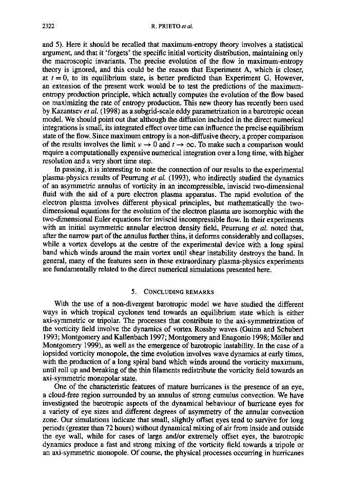
and 5). Here it should be recalled that maximum-entropy theory involves a statistical argument, and that it ‘forgets’ the specific initial vorticity distribution, maintaining only the macroscopic invariants. The precise evolution of the flow in maximum-entropy theory is ignored, and this could be the reason that Experiment A, which is closer, at t = 0, to its equilibrium state, is better predicted than Experiment G. However, an extension of the present work would be to test the predictions of the maximum- entropy production principle, which actually computes the evolution of the flow based on maximizing the rate of entropy production. This new theory has recently been used by Kazantsev et al. (1998) as a subgrid-scale eddy parametrization in a barotropic ocean model. We should point out hat although the diffusion included in the direct numerical integrations is small, its integrated effect over time can influence the precise equilibrium state of the flow. Since maximum entropy is a non-diffusive theory, a proper comparison of the results involves the limit u + 0 and t + 00. To make such a comparison would require a computationally expensive numerical integration over a long time, with higher resolution and a very short time step.

In passing, it is interesting to note the connection of our results to the experimental plasma-physics results of Peurmng et al. (1993), who indirectly studied the dynamics of an asymmetric annulus of vorticity in an incompressible, inviscid two-dimensional fluid with the aid of a pure electron plasma apparatus. The rapid evolution of the electron plasma involves different physical principles, but mathematically the two- dimensional equations for the evolution of the electron plasma are isomorphic with the two-dimensional Euler equations for inviscid incompressible flow. In their experiments with an initial asymmetric annular electron density field, Peurmng et al. noted that, after the narrow part of the annulus further thins, it deforms considerably and collapses, while a vortex develops at the centre of the experimental device with a long spiral band which winds around the main vortex until shear instability destroys the band. In general, many of the features seen in these extraordinary plasma-physics experiments are fundamentally related to the direct numerical simulations presented here.

5 . CONCLUDING REMARKS

With the use of a non-divergent barotropic model we have studied the different ways in which tropical cyclones tend towards an equilibrium state which is either axi-symmetric or tripolar. The processes that contribute to the axi-symmetrization of the vorticity field involve the dynamics of vortex Rossby waves (Guinn and Schubert 1993; Montgomery and Kallenbach 1997; Montgomery and Enagonio 1998; Moller and Montgomery 1999), as well as the emergence of barotropic instability. In the case of a lopsided vorticity monopole, the time evolution involves wave dynamics at early times, with the production of a long spiral band which winds around the vorticity maximum, until roll up and breaking of the thin filaments redistribute the vorticity field towards an axi-symmetric monopolar state.

One of the characteristic features of mature hurricanes is the presence of an eye, a cloud-free region surrounded by an annulus of strong cumulus convection. We have investigated the barotropic aspects of the dynamical behaviour of hurricane eyes for a variety of eye sizes and different degrees of asymmetry of the annular convection zone. Our simulations indicate that small, slightly offset eyes tend to survive for long periods (greater than 72 hours) without dynamical mixing of air from inside and outside the eye wall, while for cases of large and/or extremely offset eyes, the barotropic dynamics produce a fast and strong mixing of the vorticity field towards a tripole or an axi-symmetric monopole. Of course, the physical processes occurring in hurricanes


are much more complex than our non-divergent barotropic model, but the numerical simulations indicate that once a hurricane has formed a symmetric vorticity field with a relatively small eye at its centre (or close to it), the barotropic dynamics of the flow cannot destroy it in less than a few days. This behaviour is consistent with the hypothesis (e.g. Newell et al. 1996; Willoughby 1998) that air aloft in the eye can remain inside the eye since it was enclosed when the eye wall formed, in contrast with air inside the eye and close to the surface, which has a shorter residence time due to mixing processes. This hypothesis remains controversial however (e.g. Malkus 1958; Emanuel 1997; Kossin and Eastin 2001). On the other hand, for cases where there is a strong asymmetry in the convective field, as in landfalling storms for example, the vorticity field can be completely redistributed within a period of 24 hours, producing major changes in the hurricane structure.

Finally, maximum-entropy theory was able to successfully predict the vorticity field and the redistribution of the mass field (air parcels) for the case of the axi- symmetrization of lopsided monopoles. However, the prediction was less accurate in the case of the axi-symmetrization of a small, extremely offset eye. Maximum-entropy theory, for all the experiments of this paper, predicted a monopolar structure, suggesting either that the tripoles found as relaxed states in two of our numerical simulations are only quasi-steady structures, or that the mixing occurring during the time evolution does not maximize the Boltzmann mixing entropy of the flow.

ACKNOWLEDGEMENTS

The authors would like to thank Michael Montgomery, David Nolan, John Knaff, Matthew Eastin and Richard Taft for helpful comments, discussions, and assistance. This work was supported by National Science Foundation Grants ATM-9729970 and ATM-0087072, National Oceanic and Atmospheric Administration Grant NA67RJO 152 (Amendment 19), and by the Direccidn General de Asuntos del Personal Academic0 and the Centro de Ciencias de la Atm6sfera of the National Autonomous University of Mexico.

APPENDIX

Maximum-entropy theory In this appendix we develop maximum-entropy theory for a two-dimensional, dou-

bly periodic geometry in order to compare its predictions with the equilibrium configu-

Consider an initial state consisting of L levels of vorticity {t with areas At, l = 1, . . . , L. The initial parameters 6 and At are not all independent, but must satisfy Ct=l At = A, where A is the total area, and cf=, zdt = 0 (since the vorticity integrated over the doubly periodic domain must vanish). Denoting the initial vorticity by { ~ ( x , y ) and the initial stream function by @o(x, y), we note that V2+o = 50.

After the initial vorticity field has become intricately stretched and folded, suppose we sample it at N points within a small neighbourhood of x , y. Let nl denote the number of sampled points at which the absolute vorticity value is found. Then p l ( x , y) = n t / N denotes the probability, at point ( x , y), of finding the vorticity 6, and the macroscopic vorticity at point ( x , y) is

rations found by direct numerical integration. h

L


From the statistical-mechanics view, the macroscopic equilibrium state is that which has a maximum number of distributions of the sampled points with vorticity $, in other words, the most mixed state. Therefore, we must count the total number W of corresponding distributions. The number of possible arrangements having nl points with vorticityT1, n2 points with vorticity 6, etc. is the multiplicity function W, which is given by

N! W = (A.2)

The division by nl!n2! - . . n ~ ! comes from the fact that two sampled points of vorticity with the same vorticity value are indistinguishable if their positions are inter- changed. The logarithm of the multiplicity function is In W = In N! - Ck==l In ne!. Us- ing the Stirling approximation (e.g. In N! = N In N - N for large N), we obtain In W %

N In N - cf=l ne In ne = - ne = N. We conclude that

n1!n2! * ' * n L ! '

L ne l n ( n e / N ) , where we have used

We now define the Boltzmann mixing entropy S{pl (x, y), . . . , p ~ ( x , y)} as

where the area integral extends over the doubly periodic domain. The functional S{pl (x, y), . . . , p ~ ( x , y)} measures the loss of information in going

from the fine-grain (microscopic) view to the coarse-grain (macroscopic) view. To find the most probable macroscopic state, we must find the particular set of functions pe(x, y), C = 1, . . . , L, which maximize S { p l ( x , y), . . . , p ~ ( x , y)} subject to all the integral constraints associated with the inviscid vorticity dynamics. The kinetic-energy constraint requires that the final and initial kinetic energies be equal, i.e. ]1(1/2)(u2 + v 2 ) dx dy = 11(1/2)(ui + v;) dx dy, where the subscript zero denotes the initial state. With the aid of (u , v ) = (-a@/ay, a@/ax) and (uo, vo) = ( - a @ o / a y , a@o/ax), we can use integration by parts to express the kinetic-energy constraint as 11 @( dx dy = 11 +o(o dx dy. Another constraint that states the conservation of the vorticity centroid in the x-direction can be expressed as j 1 x( dx dy = 1s x(0 dx dy, while for the y- direction 11 y( dx dy = $1 y(0 dx dy. In other words, the variational problem is to find the expectation functions pe(x, y) by maximizing Eq. (A.4) subject to the circulation constraint

the energy constraint


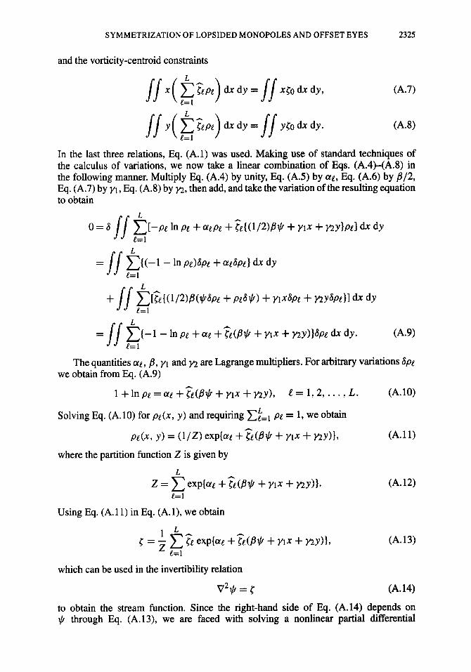
and the vorticity-centroid constraints

In the last three relations, Eq. (A.l) was used. Making use of standard techniques of the calculus of variations, we now take a linear combination of Eqs. (A.4)-(A.8) in the following manner. Multiply Eq. (A.4) by unity, Eq. (AS) by at, Eq. (A.6) by B/2, Eq. (A.7) by y1, Eq. (A.8) by m, then add, and take the variation of the resulting equation to obtain

The quantities at, B, y1 and ~2 are Lagrange multipliers. For arbitrary variations 8pe

(A. 10)

we obtain from Eq. (A.9)

1 + In pe = at + (B+ + y l x + my), L = 1,2 , . . . , L .

Solving Eq. (A.lO) for pe(x, y) and requiring zkl pi = 1, we obtain

Pe(x, Y) = ( 1 / ~ ) exp{ae +Z(P+ + ~ i x + my)}, (A. 1 1)

where the partition function Z is given by

L

Using Eq. (A. 1 1) in Eq. (A. l), we obtain

(A.12)

(A. 13)

which can be used in the invertibility relation

V2+ = ( (A. 14)

to obtain the stream function. Since the right-hand side of Eq. (A.14) depends on $I through Eq. (A.13), we are faced with solving a nonlinear partial differential

2326 R. PRIETO et ul.

equation for $ ( x , y) with yet to be determined Lagrange multipliers a[, B, y1, m. The equations for at, /I, y1, M are obtained by enforcing the constraints Eqs. (A.5)- (A.8). In summary, the solution of the maximum-entropy flow problem involves solving the nonlinear system Eqs. (AS), (A.6), (A.7), (A.8), (A.13) and (A.14) for a!, /I, y1, y2, { ( x , y), $ ( x , y), given the initial flow. Analytical solutions of this system are not easily obtained, and numerical methods are required.

Turkington and Whitaker (1996) have proposed an iterative algorithm based on the variational structure of the constrained optimization problem. The extension of this algorithm to the present geometry generates the urh iterate of the quantities a:), /I(”), y1(”), $), pj”’(x, Y), P ( x , Y), P ( x , y) from P--”(x, y), @-‘)(x, y) by maximizing S ( p ~ ’ ) ( x , y), . . . , p?’(x, y)}, subject to the circulation, energy, and vorticity-centroid constraints. Given the initial condition, the iteration proceeds as follows:

1. Knowing {(”-‘)(x, y) and $(”-‘)(x, y) from the previous iteration (or from an

2. Substitute the a:”), B(” ) , y;”), y;”’ into Eq. (A.13) to obtain C(”)(x, y). 3. Knowing ( ( ” ) ( x , y), solve the invertibility relation Eq. (A.14) for $ ( ” ) ( x , y), and

return to step 1. As in Whitaker and Turkington (1994), the stopping criteria for the iteration is

chosen to be - E(’)I < 0.0051E(O)l, where E(O) = -11(1/2)$0<0 dx dy, E(”) = -$$(1/2)$(”){(”) dx dy; the number of iterations required for convergence varies depending on the initialization, but typically around five iterations are sufficient to satisfy this stopping criterion.

initial guess), solve L + 3 algebraic equations for a;”), B(”) , y1 (‘1 , y2 (“1 .

Batchelor, G. K.

Chasnov, J. R.

Chavanis, P. H. and Sommeria, J.

Emanuel, K. A.

Guinn, T. A. and Schubert, W. H. Jimknez, J. Kazantsev, E., Sommeria, J. and

Kossin, J. P. and Eastin, M. D. Vernon, J.

Kossin, J. P., Schubert, W. H. and Montgomery, M. T.

Chen, J.-H. Kuo, H.-C., Williams, R. T. and

Malkus, J. S.

Miller, J.

Mtiller, J. D. and Montgomery, M. T.

Moller, J. D. and Smith, R. K.

1969

1997

19%

1997

1993 1994 1998

2001

2000

1999

1958

1990

1999

1994

REFERENCES Computation of the energy spectrum in homogeneous two-

dimensional turbulence. Phys. Fluids Suppl. 11,12,233-239 On the decay of two-dimensional homogeneous turbulence. Phys.

Classification of self-organid vortices in two-dimensional turbulence: The case of a bounded domain. J. Fluid Mech., 314,

Some aspects of hurricane inner-core dynamics and energetics. J. Atmos. Sci., 54,1014-1026

Hurricane spiral bands. J. Atmos. Sci., 50,3380-3403 Hyperviscous vortices. J. FluidMech.. 279,169-176 Subgrid-scale eddy parameterization by statistical mechanics in a

bmtropic ocean model. J. Phys. Oceumgx ,a, 10 1 7- 1042 ’ h o distinct regimes in the kinematic and thermodynamic struc-

ture of the hurricane eye and eyewall. J. Atmos. Sci.. 58,

Unstable interactions between a hurricane’s primary eyewall and a secondary ring of enhanced vorticity. J. Atmos. Sci., 57,

Fluids, 9,171-180

267-297

1079-1090

3893-3917 - A Dossible mechanism for the eve rotation of ’hahoon Herb.

I.

J. Amos. Sci., 56,1659-167i

J. Meteoml., 15,337-349

Rev. Lett., 65,2 137-2 140

model. J. Atmos. Sci., 56, 1674-1687

Q. J. R. Meteoml. SOC., 120,1255-1265

On the structure and maintenance of the mature humcane eye.

Statistical mechanics of Euler equations in two dimensions. Phys.

Vortex Rossby waves and hurricane intensification in a bmtropic

The development of potential vorticity in a hurricane-like vortex.


Montgomery, M. T. and Enagonio, J.

Montgomery, M. T. and Kallenbach, R. J.

Newell, R. E., Hu, W., Wu, Z-X., Zhu, Y., Akimoto, H., Anderson, B. E., Browell, E. V., Gregory, G. L., Sachse, G. W., Shipham, M. C., Bachmeier, A. S., Bandy, A. R., Thornton, D. C., Blake, D. R., Rowland, F. S., Bradshaw, J. D., Crawford, J. H., Davis, D. D., Sandholm, S. T., Brockett, W., DeGreef, L., Lewis, D., McCormick, D., Monitz, E., Collins Jr., J. E., Heikes, B. G., Memll, J. T., Kelly, K. K., Liu, S. C., Kondo, Y., Koike, M., Liu, C.-M., Sakamaki, F., Singh, H., Dibb, J. E. and Talbot, R. W.

Montgomery, M. T.

and Grasso, L. D.

Nolan, D. S. and

Nolan, D. S., Montgomery, M. T.

Ooyama, K. V.

Peumng, A. J., Notte, J. and

Prieto, R. and Schubert, W. H.

Reasor, P. D., Montgomery, M. T., Marks Jr., F. D. and Gamache, J. F.

Robert, R. and Sommeria, J.

Schubert, W. H., Hausman, S. A.,

Fajans, J.

Garcia, M., Ooyama, K. V. and KUO, H.-C.

Schubert, W. H., Montgomery, M. T., Taft, R. K., Guinn, T. A., Fulton, S. R., Kossin, J. P. and Edwards, J. P.

Robert, R. Sommeria, J., Staquet, C. and

Turkington, B. and Whitaker, N.

Whitaker, N. and Turkington, B.

Willoughby, H. E.

Zehr, R. M., DeMaria, M., Horsfall, F. and Knaff, J.

1998

1997

1996

2000

2001

1990

2001

1993

2001

2000

1991

2001

1999

1991

1996

1994

1998

1999

Tropical cyclogenesis via convectively forced vortex Rossby waves in a three-dimensional quasigeostrophic model. J. Atmos. Sci., 55,3176-3207

A theory for vortex Rossby-waves and its application to spiral bands and intensity changes in hurricanes. Q. J. R. Meteoml. SOC., 123,435465

Atmospheric sampling of super typhoon Mireille with NASA DC-8 aircraft on September 27, 1991, during PEM-West A. J. Geophys. Res., 101 (Dl), 1853-1871

The algebraic growth of wavenumber one disturbances in hurricane-like vortices. J . Atmos. Sci.. 57,3514-3538

The wavenumber one instability and trochoidal motion of hurricane-like vortices. J . Atmos. Sci., 58, in press

A thermodynamic foundation for modeling the moist atmosphere. J . Amos. Sci., 47,2580-2593

A dynamic and thermodynamic foundation for modeling the moist atmosphere with parameterized microphysics. J. Amos. Sci., 58,2073-2102

Collapse and winding of an asymmetric annulus of vorticity. J. Fluid Mech., 252,7 13-720

Analytical predictions for zonally-symmetric equilibrium states of the stratospheric polar vortex. J. Armos. Sci., 58, in press

Low-wavenumber structure and evolution of the humcane inner core observed by airborne dual-Doppler radar. Mon. Weather Rev., 128,1653-1680

Statistical equilibrium states for two-dimensional flows. J. Fluid Mech., 229,291-310

Potential vorticity in a moist atmosphere. J. Amos. Sci., 58, in press

Polygonal eyewalls, asymmetric eye contraction, and potential vorticity mixing in hurricanes. J. Atmos. Sci., 56,1197-1 223

Final equilibrium state of a two-dimensional shear layer. J. Fluid

Statistical equilibrium computations of coherent structures in tur-

Maximum entropy states for rotating vortex patches. Phys. Fluids,

Tropical cyclone eye thermodynamics. Mon. Weather Rev., 126,

‘Observational tropical cyclone data archive and research’. P. A.24 in Roceedings of the 53rd Interdepartmental Hur- ricane Conference, 8-12 February 1999, Biloxi, MS, USA

Mech., 233,661-689

bulent shear layers. SLAM J. Sci. Comput., 17,1414-1433

6,3963-3973

3053-3067

Symmetrization of lopsided vorticity monopoles and offset hurricane eyes

Documents

Transcript of Symmetrization of lopsided vorticity monopoles and offset hurricane eyes