influence of Solar MagneticSector Structure on Terrestrial

Atmospheric Vorticityl 17 U b1 a

by e (

John M. Wilcox, Philip H. Scherrer, o Wo.Leif Svalgaard, Walter Orr Roberts, CHavRoger H. Olson, and Roy L. Jenne un (o

July 1973 C bOP. 0

h rtH w t4Reproduction in whole or in part (.jDis permitted for any purpose of Ln t i- Hthe United Sta es Government. 0 -. P-

0

and

GSUIPR Reporant GA-311No. 53038

STANFORD UNIVERSITY, STANFORD, CALIFORNIA

~~43 STANFORD UNIVERSITY, STANFORD, CALIFRIAL

UNCLASS F FED

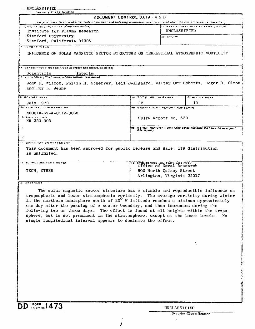
DOCUMENT CONTROL DATA -R & DScurtry clseasitication of title, body of abstract and indexing annotatikn mu.: S dehrd ther. th ,a o rall r.pRrt I cl ra..filed

S;RGINA ING ACTIVIT (Corporate authoW) 24, RLPORT SECURITY CLASSIFICATION

Institute for Plasma Research UNCLASSIFIEDStanford University 2b. GROUP

Stanford, California 94305' LPORT TITLE

INFLUENCE OF SOLAR MAGNETIC SECTOR STRUCTURE ON TERRESTRIAL ATMOSPHERIC VORTICITY

DESCRIPTIVE NOTES (Type of report and incluelve dilee)

Scientific Interim5 AU THOR(S) (First name, middle Initial. ladt neise)

John M. Wilcox, Philip H. Scherrer, Leif Svalgaard, Walter Orr Roberts, Roger H. Olsonand Roy L. Jenne

6 REPORT DATE 7a. TOT4L NO. OE PAGES 7b. NO. OF REFS

July 1973 32 138a. C ONTRACT OR GRANT NO 1e. ORIGINATOR

'S REPORT NUMBERIS)

N00014-67-A-0112-0068b. P ROJ ECTNO SUIPR Report No. 530

NR 323-003Report No. 530

9b. OTHER REPORT NO(S) (Any other nLnbere that may be a ignedthli report)

1') DI TRIB TION STATEMENT

This document has been approved for public release and sale; its distributionis unlimited.

II SUPPLEMENTARY NOTES IS2. SPONSORING MILITARY ACTIVITY

Office of Naval ResearchTECH, OTHER 800 North Quincy Street

Arlington, Virginia 22217

13 ARSTRACT

The solar magnetic sector structure has a sizable and reproducible influence on

tropospheric and lower stratospheric vorticity. The average vorticity during winterin the northern hemisphere north of 200 N latitude reaches a minimum approximatelyone day after the passing of a sector boundary, and then increases during thefollowing two or three days. The effect is found at all heights within the tropo-sphere, but is not prominent in the stratosphere, except at the lower levels. Nosingle longitudinal interval appears to dominate the effect.

DD, ..ov 1473 UNCLASSIFIEDSecurity Classification

/

UNCLASS IFIEDSecurity Classitication

w14o L-N A LINK B LINK CKEY WORDS

ROLE WT ROLE I WT ROLE WT

SOLAR MAGNETIC SECTOR

ATMOSPHERIC VORTICITY

WEATHER

I II

I I I i i ,

UNCLASS IFIEDSecurity Classification

ii

INFLUENCE OF SOLAR MAGNETIC SECTOR STRUCTURE

ON TERRESTRIAL ATMOSPHERIC VORTICITY

by

John M. Wilcox, Philip H. Scherrer, Leif Svalgaard,

Walter Orr Roberts, Roger H. Olson and Roy L. Jenne

Office of Naval Research

Contract N00014-67-A-0112-0068

National Aeronautics and Space Administration

Grant NGR 05-020-559

and

National Science Foundation

Grant GA-31138

Reproduction in whole or in part is

permitted for any purpose of the

United States Government

SUIPR Report No. 530

July 1973

Institute for Plasma Research

Stanford University

Stanford, California

INFLUENCE OF SOLAR MAGNETIC SECTOR STRUCTURE

ON TERRESTRIAL ATMOSPHERIC VORTICITY

John M. Wilcox, Philip H. Scherrer, Leif Svalgaard

Institute for Plasma Research, Stanford University,Stanford, California 94305

Walter Orr Roberts

University Corporation for Atmospheric Research,

Boulder, Colorado 80302

Roger H. Olson

National Oceanic and Atmospheric Administration,

Environmental Data Services, Boulder, Colorado 80302

and

Roy L. Jenne

National Center for Atmospheric Research,Boulder, Colorado 80302

Abstract.

The solar magnetic sector structure has a sizable and repro-

ducible influence on tropospheric and lower stratospheric vorticity.

The average vorticity during winter in the northern hemisphere north of

200 N latitude reaches a minimum approximately one day after the passing

of a sector boundary, and then increases during the following two or

three days. The effect is found at all heights within the troposphere,

but is not prominent in the stratosphere, except at the lower levels.

No single longitudinal interval appears to dominate the effect.

1.

INFLUENCE OF SOLAR MAGNETIC SECTOR STRUCTURE

ON TERRESTRIAL ATMOSPHERIC VORTICITY

John M. Wilcox, Philip H. Scherrer, Leif Svalgaard

Institute for Plasma Research, Stanford University,

Stanford, California 94305

Walter Orr Roberts

University Corporation for Atmospheric Research,

Boulder, Colorado 80302

Roger H. Olson

National Oceanic and Atmospheric Administration,

Environmental Data Services, Boulder, Colorado 80302

and

Roy L. Jenne

National Center for Atmospheric Research,

Boulder, Colorado 80302

1. Introduction.

A relation between the solar magnetic sector structure and a

vorticity area index at the 300 mb height has recently been reported

(Wilcox et al., 1973). For recent reviews of related work see Roberts

and Olson, 1973a and Svalgaard, 1973. The solar magnetic sector struc-

ture is a large-scale persistent pattern in the sun that has been dis-

covered through spacecraft observations of the interplanetary, magnetic

field (Wilcox, 1968), and it is a consequence of the solar magnetic

field as extended in space by the solar wind. The solar magnetic sec-

tor structure is generally known to solar physicists, but is not so

well known to meteorologists. We therefore start with a brief descrip-

tion of this structure.

2.

2. The Solar Magnetic Sector Structure.

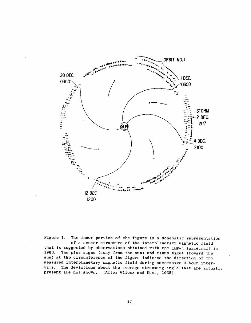
Figure 1 shows spacecraft observations of the polarity (away

from or toward the sun) of the interplanetary magnetic field observed

near the earth during two and one-half solar rotations. The plus (away)

and minus (toward) signs at the periphery of the figure represent the

field polarity during three-hour intervals. The four Archimedes spiral

lines coming from the sun represent sector boundaries inferred from the

spacecraft observations. Within each sector the polarity of the inter-

planetary field is predominantly in one direction. The interplanetary

field lines are rooted in the sun, and so the entire field pattern

rotates with the sun with an approximately 27-day period. The solar

magnetic sector structure is extended outward from the sun by the radi-

ally flowing solar wind. The sector boundaries are often very thin,

sometimes approaching a proton gyro radius in thickness. The time at

which such boundaries are swept past the earth by the solar wind can

therefore often be defined to within a fraction of an hour.

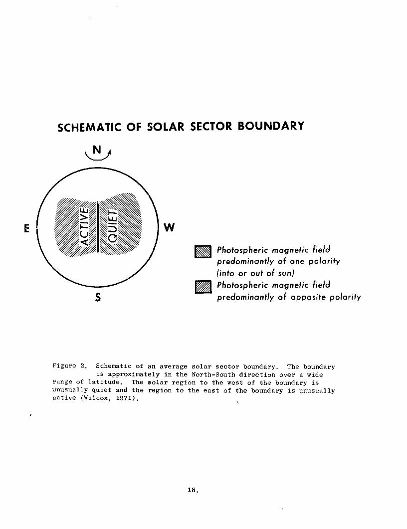
What would a sector boundary shown in Figure 1 look like on

the visible solar disk? Wilcox and Howard (1968) have compared the

interplanetary field observed by spacecraft near the earth with the

solar photospheric magnetic field deduced from the longitudinal Zeeman

effect measured at the 150-foot solar tower telescope at Mount Wilson

Observatory. This analysis suggested that an average solar sector

boundary is similar to the schematic shown in Figure 2. The boundary

is approximately in the North-South direction over a wide range of

latitudes on both sides of the equator. A large area to the right of

3.

the boundary has a large-scale field of one polarity and a large-scale

region to the left of the boundary has field of the opposite polarity.

Suppose we observe the mean solar magnetic field when the con-

figuration is as shown in Figure 2. The mean solar magnetic field is

defined as the average field of the entire visible solar disk, i.e.,

the field of the sun observed as though it were a star. In the circum-

stances shown in Figure 2, such an observation would yield a field

close to zero, since there would tend to be equal and opposite contri-

butions from the left and right sides of the figure. One day later the

boundary will have rotated with the sun 130 westward, and the visible

disk will be dominated by the sector at the left in Figure 2. A mean

field observation will now yield a field having the polarity appropriate

to the dominant sector. This same polarity will be observed during

several subsequent days, until the next sector boundary passes central

meridian and reverses the polarity of the observed mean solar field.

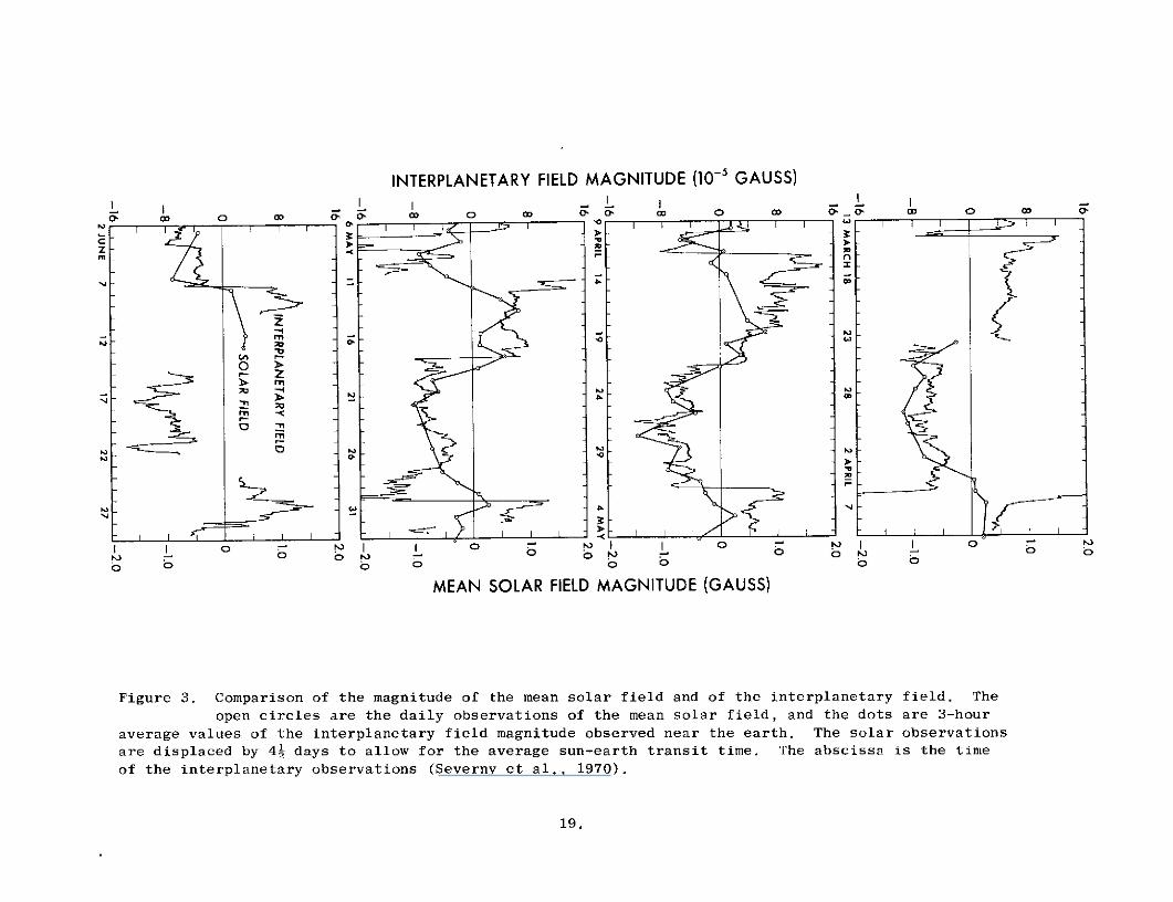
Figure 3 shows a comparison of the mean solar field observed

at the Crimean Astrophysical Observatory with the interplanetary magnetic

field observed with spacecraft near the earth (Severny et al., 1970).

In this comparison the mean solar field has been displaced by four and

one-half days to allow for the average transit time from near the sun

to the earth of the solar wind plasma that is transporting the solar

field lines past the earth. We see in Figure 3 that in polarity and

also to a considerable extent in magnitude the interplanetary field

carried past the earth is very similar to the mean solar magnetic field.

If we use the observed interplanetary field to investigate effects on

the earth's weather, we are using a structure that is clearly of solar

4.

origin but is observed at precise times near the earth.

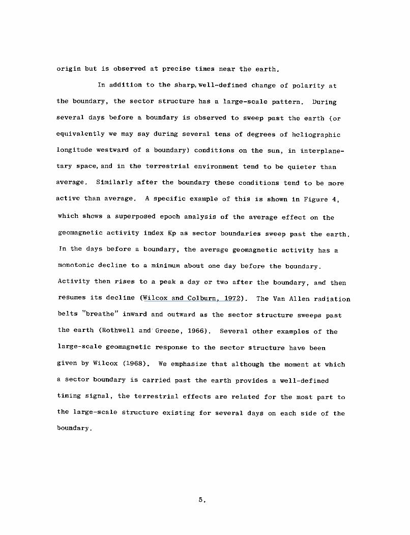
In addition to the sharp,well-defined change of polarity at

the boundary, the sector structure has a large-scale pattern. During

several days before a boundary is observed to sweep past the earth (or

equivalently we may say during several tens of degrees of heliographic

longitude westward of a boundary) conditions on the sun, in interplane-

tary space,and in the terrestrial environment tend to be quieter than

average. Similarly after the boundary these conditions tend to be more

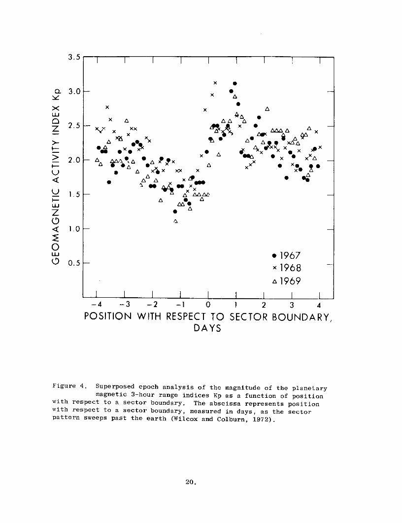
active than average. A specific example of this is shown in Figure 4,

which shows a superposed epoch analysis of the average effect on the

geomagnetic activity index Kp as sector boundaries sweep past the earth.

In the days before a boundary, the average geomagnetic activity has a

monotonic decline to a minimum about one day before the boundary.

Activity then rises to a peak a day or two after the boundary, and then

resumes its decline (Wilcox and Colburn, 1972). The Van Allen radiation

belts "breathe" inward and outward as the sector structure sweeps past

the earth (Rothwell and Greene, 1966). Several other examples of the

large-scale geomagnetic response to the sector structure have been

given by Wilcox (1968). We emphasize that although the moment at which

a sector boundary is carried past the earth provides a well-defined

timing signal, the terrestrial effects are related for the most part to

the large-scale structure existing for several days on each side of the

boundary.

5.

3. Advantages of Solar Magnetic Sector Structure for Investigations of

Effects on Weather.

From the above discussion, it appears reasonable to use the

solar magnetic sector structure in an investigation of possible effects

on the earth's weather. The use of the sector structure for this pur-

pose has several advantages. We are using a fundamental large-scale

property of the sun. There can then be no doubt that any observed atmo-

spheric response to the passing of a sector boundary is ultimately caused

by the solar magnetic sector structure. We emphasize that "solar mag-

netic sector structure" is a name for the entire structure discussed

above. When we say that an atmospheric response is caused by the solar

magnetic sector structure, we include possibilities that the effect has

been transmitted through interplanetary space in the form of magnetic

fields, solar wind plasma, energetic particles, or radiation. Similarly,

an atmospheric effect observed in the troposphere may flow through the

higher atmospheric layers in an exceedingly complex manner. We discuss

in this paper only the start (the solar magnetic sector structure) and

the result (an effect in the troposphere) of what may be an exceedingly

complex flow of physical processes.

We discuss some further advantages of the sector structure for

this investigation. In the sense discussed above, a tropospheric response

does not have its ultimate cause in other atmospheric processes. Some

earlier investigations of solar activity and the weather have been

criticized in this respect by Hines (1973). Because of the four or

five day transit time of the solar wind plasma from the sun to the

6.

earth, we can have, by observing the mean solar magnetic field, a four

or five day forecast of the time at which a sector boundary will sweep

past the earth. By improving the solar observation procedure, we may

be enabled to detect a sector boundary two or three days after it has

rotated past the eastern limb of the sun. This would add an additional

four or five days to the forecast interval.

From one solar rotation to the next, the sector structure

usually does not change very much. In the course of a year there are

often significant changes in the sector structure, which appears to have

significant variations through the 11-year sunspot cycle (Svalgaard,

1972). All of these regularities and recurrence properties may be of

significant assistance in forecasting. As the solar magnetic sector

structure and its interplanetary and terrestrial consequences becomes

better understood in the coming years, the possibilities of using solar

data in weather forecasting should also improve.

4. Response of Vorticity Area to Sector Structure.

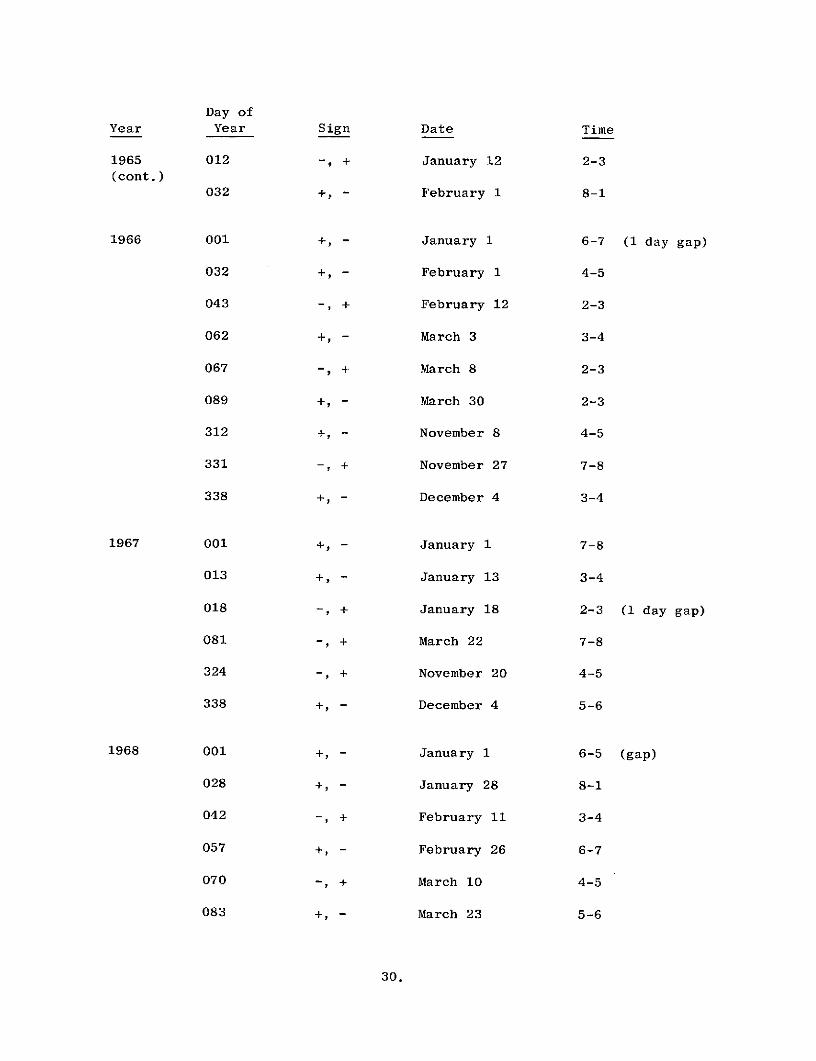
In the present investigation the method of superposed epochs

is used to give the average response of a vorticity area index to the

passage of 54 sector boundaries. These boundaries, which are listed in

Table 1, were observed with spacecraft near the earth during 1964 through

1970 during the winter months November through March (the effects

described below did not appear during the summer months). These bound-

aries were observed to have one predominant polarity of the interplane-

tary magnetic field for at least four days before the boundary, and the

other polarity of the interplanetary magnetic field during at least

7.

four days after the boundary. A list of well-defined sector boundaries

was published by Wilcox and Colburn (1972), before we began the present

investigation. To this we have added boundaries for the year 1970.

The vorticity area index was devised by Roberts and Olson

(1973b). Pressure height maps at 0 UT and 12 UT for each day are used

to compute vorticity maps at the 300 mb level of the atmosphere. Prom-

inent features on such vorticity maps are the regions of high vorticity,

and these coincide closely with the low pressure troughs visible on

contour maps of the heights of given pressure surfaces at the same

level. The region of the northern hemisphere north of 200 N latitude

-5 -1is shown on these maps. A "discriminator" of 20 x 10 sec is applied

to a vorticity map, and the area in km2 in which the vorticity exceeds

-5 -1this value is recorded. The discriminator is then set at 24 x 10 sec

and the area in which the vorticity exceeds this value is added to the

previously computed area. (In some of the investigations reported in

the present paper, we have used a single discriminator setting, usually

-5 -120 x 10 sec In the vorticity area index of Roberts and Olson, the

-5 -1discriminator setting at 24 x 10 sec usually contributed about 15

percent to the total index, so that a single discriminator setting of

-5 -120 x 10 sec gives results that are very similar to those obtained

with the vorticity area index.)

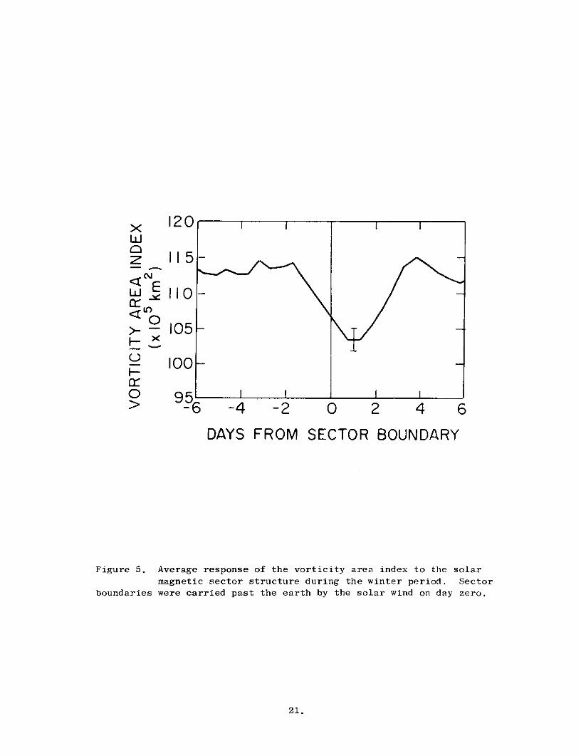
The average response of the vorticity area index to the 54

well-defined sector boundary crossings described above is shown in the

superposed epoch analysis of Figure 5. The vorticity area index reaches

a minimum approximately one day after the boundary, and then increases

during the next two or three days. At the 300 mb height shown in

8.

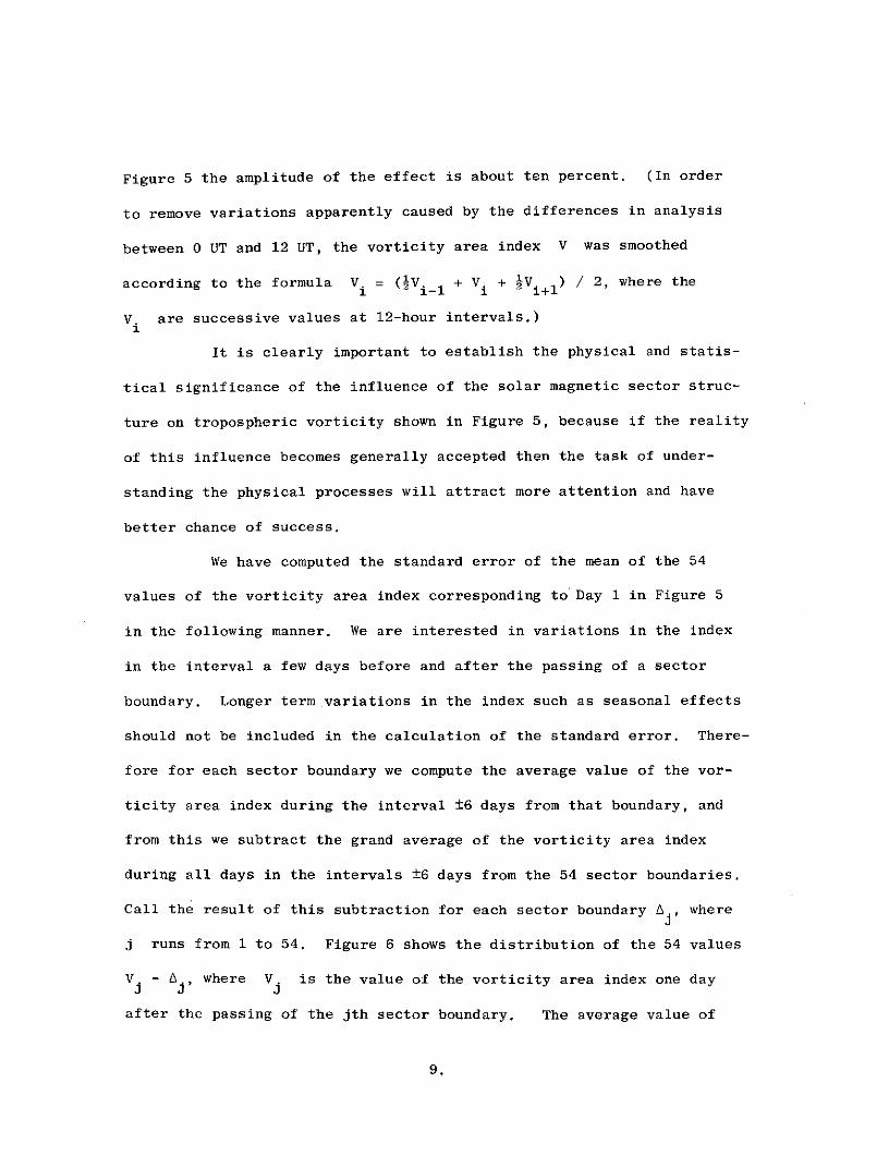
Figure 5 the amplitude of the effect is about ten percent. (In order

to remove variations apparently caused by the differences in analysis

between 0 UT and 12 UT, the vorticity area index V was smoothed

according to the formula V = (Vi_ + V. + 1V ) / 2, where the1 i-1 i i+l

V. are successive values at 12-hour intervals.)1

It is clearly important to establish the physical and statis-

tical significance of the influence of the solar magnetic sector struc-

ture on tropospheric vorticity shown in Figure 5, because if the reality

of this influence becomes generally accepted then the task of under-

standing the physical processes will attract more attention and have

better chance of success.

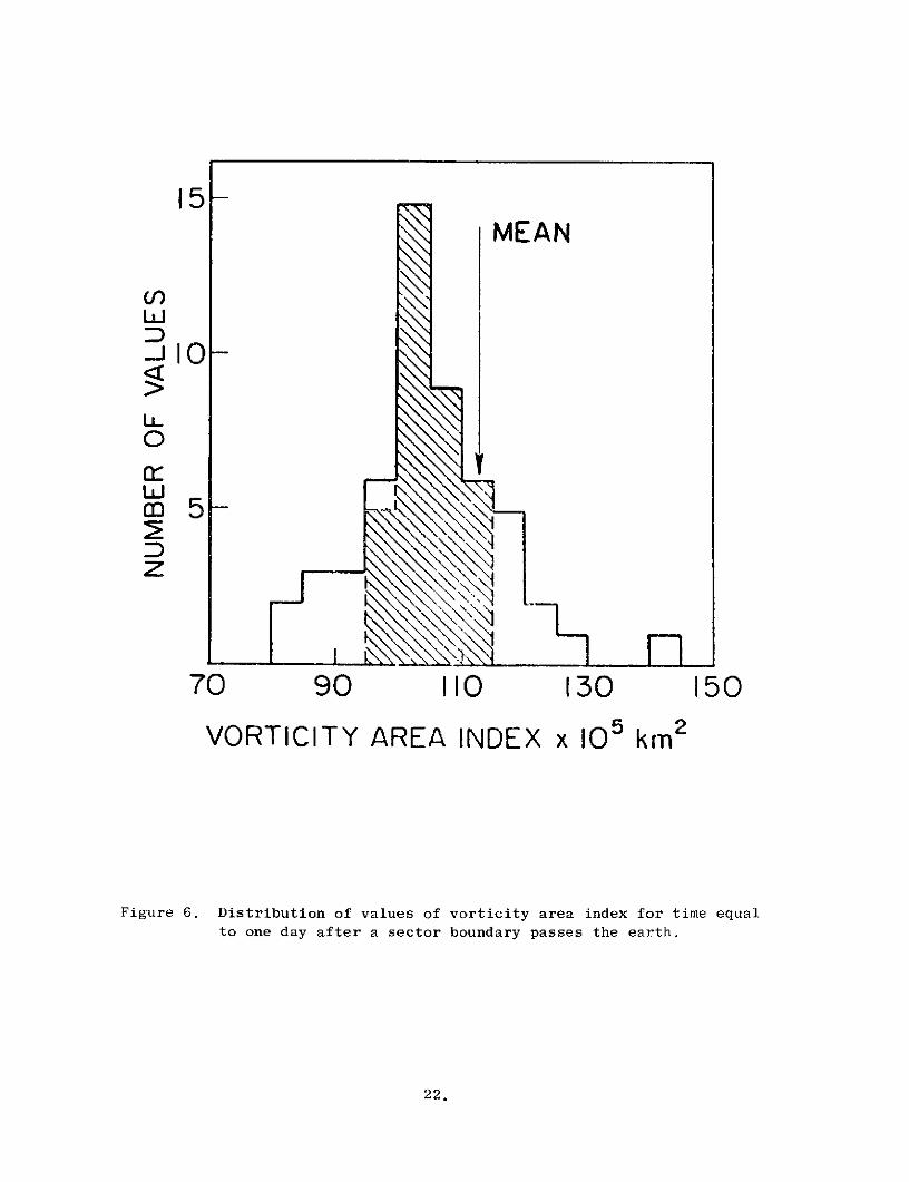
We have computed the standard error of the mean of the 54

values of the vorticity area index corresponding to Day 1 in Figure 5

in the following manner. We are interested in variations in the index

in the interval a few days before and after the passing of a sector

boundary. Longer term.variations in the index such as seasonal effects

should not be included in the calculation of the standard error. There-

fore for each sector boundary we compute the average value of the vor-

ticity area index during the interval ±6 days from that boundary, and

from this we subtract the grand average of the vorticity area index

during all days in the intervals ±6 days from the 54 sector boundaries.

Call the result of this subtraction for each sector boundary Aj, where

j runs from 1 to 54. Figure 6 shows the distribution of the 54 values

V. - Aj, where V. is the value of the vorticity area index one day

after the passing of the jth sector boundary. The average value of

9.

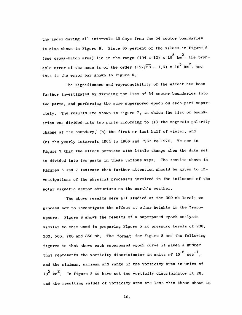
the index during all intervals ±6 days from the 54 sector boundaries

is also shown in Figure 6. Since 65 percent of the values in Figure 6

(see cross-hatch area) lie in the range (104 ± 12) x 10 km , the prob-

able error of the mean is of the order (12/5V = 1.6) x 105 km2 , and

this is the error bar shown in Figure 5.

The significance and reproducibility of the effect has been

further investigated by dividing the list of 54 sector boundaries into

two parts, and performing the same superposed epoch on each part separ-

ately. The results are shown in Figure 7, in which the list of bound-

aries was divided into two parts according to (a) the magnetic polarity

change at the boundary, (b) the first or last half of winter, and

(c) the yearly intervals 1964 to 1966 and 1967 to 1970. We see in

Figure 7 that the effect persists with little change when the data set

is divided into two parts in these various ways. The results shown in

Figures 5 and 7 indicate that further attention should be given to in-

vestigations of the physical processes involved in the influence of the

solar magnetic sector structure on the earth's weather.

The above results were all studied at the 300 mb level; we

proceed now to investigate the effect at other heights in the tropo-

sphere. Figure 8 shows the results of a superposed epoch analysis

similar to that used in preparing Figure 5 at pressure levels of 200,

300, 500, 700 and 850 mb. The format for Figure 8 and the following

figures is that above each superposed epoch curve is given a number

-5 -1that represents the vorticity discriminator in units of 10 sec ,

and the minimum, maximum and range of the vorticity area in units of

105 km 2 In Figure 8 we have set the vorticity discriminator at 20,

and the resulting values of vorticity area are less than those shown in

10.

Figure 5, which had an additional contribution from a discriminator

setting of 24. However, if we compare the graph in Figure 8 for the

300 mb height with Figure 5 which is at the same height we see that

the effect is very similar. In Figure 8 we see an ordered response of

the vorticity area to the passing of a sector boundary at all heights

within the troposphere. As we go from the top of the troposphere (or

the lowest levels of the stratosphere) down to ground level, the width

of the minimum near the boundary increases considerably. An increase

from about one day after the boundary to three days after the boundary

is a persistent feature of the response at all heights in the tropo-

sphere.

We now examine a somewhat technical point in the analysis.

We note in Figure 8 that when we hold the vorticity discriminator con-

stant at 20, we find that the resulting areas change by a considerable

factor over the range of heights investigated. Another method of anal-

ysis could be to adjust the vorticity discriminator such as to keep the

area approximately constant, near a value such as 40 x 105 km2 . This

approach has been followed in preparing Figure 9, which is otherwise

similar to Figure 8. The graphs in the two figures are very similar,

showing that the response is essentially the same for these two methods

of investigation.

We next investigate the response of the vorticity area in the

stratosphere. The result is shown in Figure 10, which is similar in

format to Figure 8. We see that the effect discussed above in the

troposphere is not prominent in the stratosphere, though at 100 mb the

peak at four days after the boundary is evident and probably significant.

11.

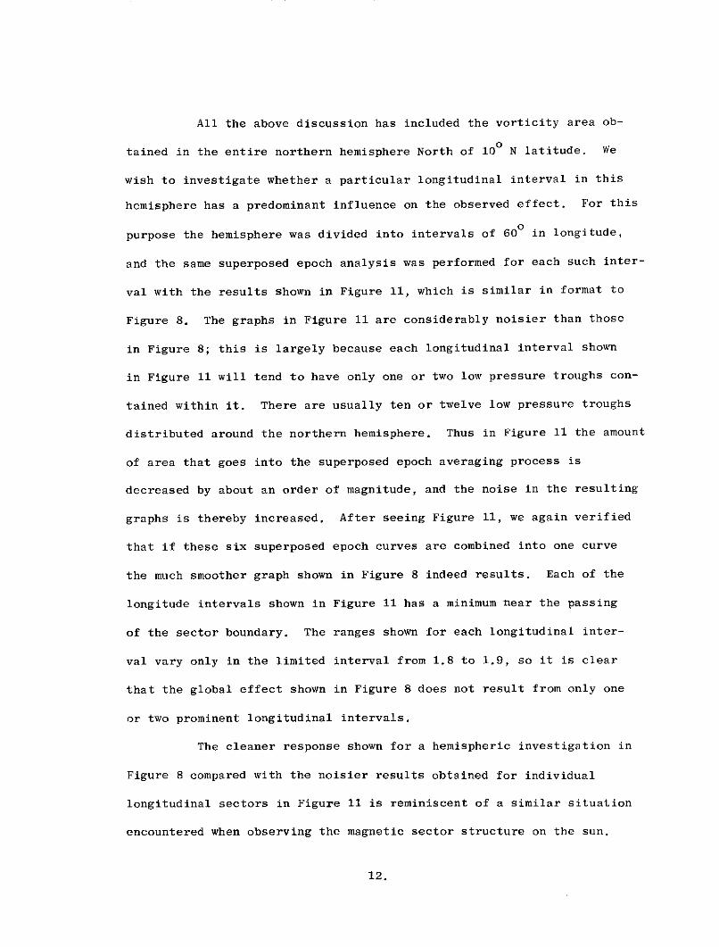
All the above discussion has included the vorticity area ob-

tained in the entire northern hemisphere North of 100 N latitude. We

wish to investigate whether a particular longitudinal interval in this

hemisphere has a predominant influence on the observed effect. For this

purpose the hemisphere was divided into intervals of 600 in longitude,

and the same superposed epoch analysis was performed for each such inter-

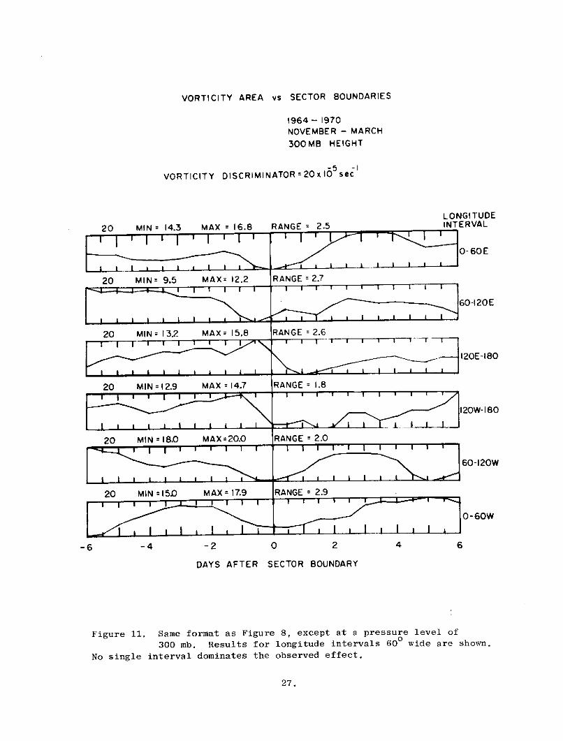
val with the results shown in Figure 11, which is similar in format to

Figure 8. The graphs in Figure 11 are considerably noisier than those

in Figure 8; this is largely because each longitudinal interval shown

in Figure 11 will tend to have only one or two low pressure troughs con-

tained within it. There are usually ten or twelve low pressure troughs

distributed around the northern hemisphere. Thus in Figure 11 the amount

of area that goes into the superposed epoch averaging process is

decreased by about an order of magnitude, and the noise in the resulting

graphs is thereby increased. After seeing Figure 11, we again verified

that if these six superposed epoch curves are combined into one curve

the much smoother graph shown in Figure 8 indeed results. Each of the

longitude intervals shown in Figure 11 has a minimum near the passing

of the sector boundary. The ranges shown for each longitudinal inter-

val vary only in the limited interval from 1.8 to 1.9, so it is clear

that the global effect shown in Figure 8 does not result from only one

or two prominent longitudinal intervals.

The cleaner response shown for a hemispheric investigation in

Figure 8 compared with the noisier results obtained for individual

longitudinal sectors in Figure 11 is reminiscent of a similar situation

encountered when observing the magnetic sector structure on the sun.

12.

When the field of the entire visible disk of the sun is averaged in the

observation a clear sector pattern is observed for each individual sec-

tor, as shown in Figure 3. If on the other hand only a limited area of

the sun is observed, then the structure of individual sectors is less

clear and statistical techniques involving observations of several sec-

tors usually must be employed (Wilcox, 1968).

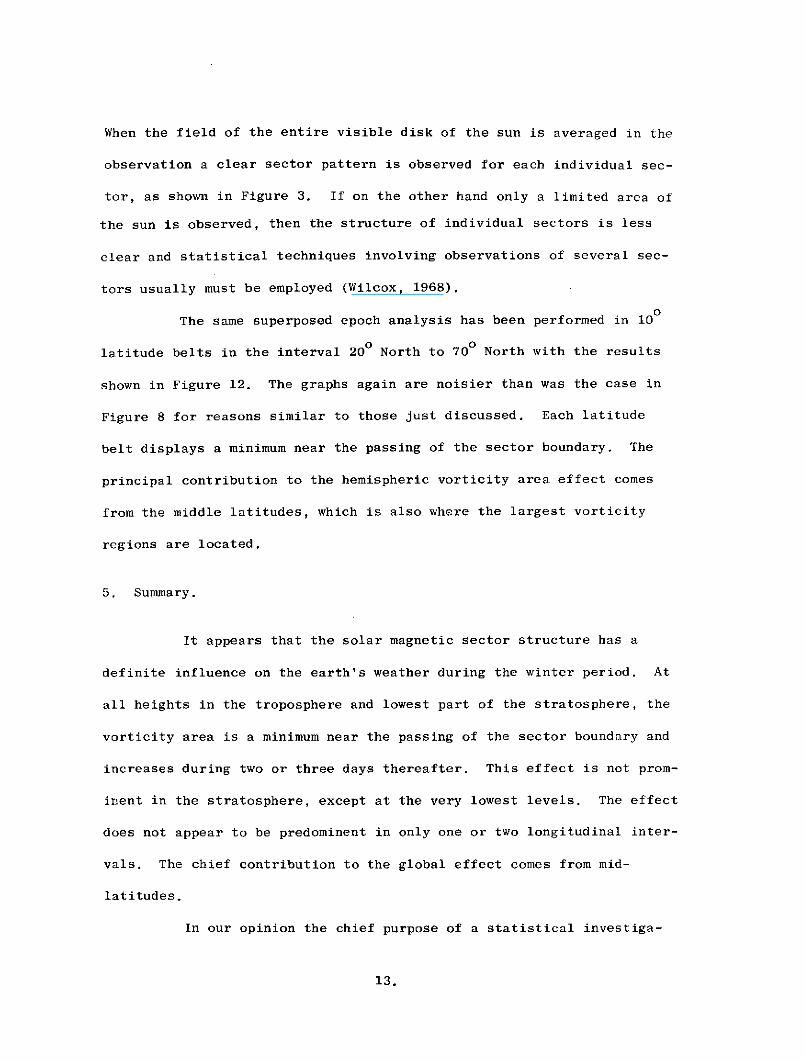
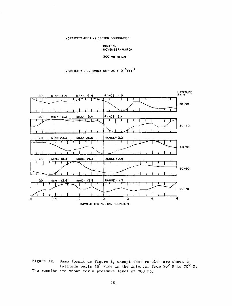
The same superposed epoch analysis has been performed in 100

latitude belts in the interval 200 North to 700 North with the results

shown in Figure 12. The graphs again are noisier than was the case in

Figure 8 for reasons similar to those just discussed. Each latitude

belt displays a minimum near the passing of the sector boundary. The

principal contribution to the hemispheric vorticity area effect comes

from the middle latitudes, which is also where the largest vorticity

regions are located.

5. Summary.

It appears that the solar magnetic sector structure has a

definite influence on the earth's weather during the winter period. At

all heights in the troposphere and lowest part of the stratosphere, the

vorticity area is a minimum near the passing of the sector boundary and

increases during two or three days thereafter. This effect is not prom-

inent in the stratosphere, except at the very lowest levels. The effect

does not appear to be predominent in only one or two longitudinal inter-

vals. The chief contribution to the global effect comes from mid-

latitudes.

In our opinion the chief purpose of a statistical investiga-

13.

tion such as that reported here is to point the way toward specific

investigations directed toward understanding the physical processes in-

volved in the influence of the solar sector structure upon the earth's

weather. We look forward to pursuing such investigations.

Acknowledgments.

This work was supported in part by the Office of Naval Research

under Contract N00014-67-A-0112-0068, by the National Aeronautics and

Space Administration under Grant NGR 05-020-559, and by the Atmospheric

Sciences Section of the National Science Foundation under Grant

GA-31138. The work was also supported in part by the National Center

for Atmospheric Research, which is sponsored by the National Science

Foundation.

14.

References.

Hines, C. 0., 1973: Comments on "A test of an apparent response of the

lower atmosphere to solar corpuscular radiation". J. Atmos. Sci.,

30, 739-744.

Roberts, W. 0. and R. H. Olson, 1973a: New evidence for effects of vari-

able solar corpuscular emission upon the weather. Rev. Geophys.

Space Phys., (in press).

Roberts, W. 0. and R. H. Olson, 1973b: Geomagnetic storms and wintertime

300-mb trough development in the North Pacific-North At antic area.

J. Atmos. Sci., 30, 135-140.

Rothwell, P. and C. Greene, 1966: Spatial and temporal distribution of

energetic electrons in the outer radiation belt, University of

Southhampton Report.

Severny, A., J. M. Wilcox, P. H. Scherrer and D. S. Colburn, 1970:

Comparison of the mean photospheric magnetic field and the inter-

planetary magnetic field. Solar Physics, 15, 3-14.

Svalgaard, L., 1972: Interplanetary magnetic-sector structure, 1926-1971.

J. Geophys. Res., 77, 4027-4034.

Svalgaard, L., 1973: Solar activity and the weather. Proceedings of

Seventh ESLAB Symposium, 22-25 May 1973, Saulgau, West Germany,

D. Reidel Publishing Co., Dordrecht, Holland, (to be published).

15.

Wilcox, J. M., 1968: The interplanetary magnetic field. Solar origin

and terrestrial effects. Space Science Rev., 8, 258-328.

Wilcox, J. M., 1971: Solar sector magnetism. Comments on Astrophysics

and Space Physics, 3, 133-139.

Wilcox, J. M. and D. S. Colburn, 1972: Interplanetary sector structure

at solar maximum. J. Geophys. Res., 77, 751-756.

Wilcox, J. M. and R. Howard, 1968: A large-scale pattern in the solar

magnetic field. Solar Physics, 5, 564-574.

Wilcox, J. M. and N. F. Ness, 1965: Quaisi-stationary corotating struc-

ture in the interplanetary medium. J. Geophys. Res., 70, 5793-

5805.

Wilcox, J. M., P. H. Scherrer, L. Svalgaard, W. O. Roberts and R. H.

Olson, 1973: Solar magnetic sector structure: Relation to circu-

lation of the earth's atmosphere. Science, 180, 185-186.

16.

.. ORBIT NO. I+ ++ - + +4. + 4. 4 +_

+ ++ .++++_20 DEC. .4 .++ I DEC-0300 + 0300

STORM''--2 DEC.

2117

- 4 DEC.

2100

+ +/++ ++ +

+++ +

12 DEC

1200

Figure 1. The inner portion of the figure is a schematic representationof a sector structure of the interplanetary magnetic field

that is suggested by observations obtained with the IMP-1 spacecraft in1963. The plus signs (away from the sun) and minus signs (toward thesun) at the circumference of the figure indicate the direction of themeasured interplanetary magnetic field during successive 3-hour inter-vals. The deviations about the average streaming angle that are actuallypresent are not shown. (After Wilcox and Ness, 1965).

17.

SCHEMATIC OF SOLAR SECTOR BOUNDARY

E 3 W

Q WPhotospheric magnetic fieldpredominantly of one polarity

(into or out of sun)SPhotospheric magnetic field

S predominantly of opposite polarity

Figure 2. Schematic of an average solar sector boundary. The boundaryis approximately in the North-South direction over a wide

range of latitude. The solar region to the west of the boundary isunusually quiet and the region to the east of the boundary is unusuallyactive (Wilcox, 1971).

18.

INTERPLANETARY FIELD MAGNITUDE (10- 5 GAUSS)

i .. I I I I I0 o O 0 O o 0 0 0 OD 0 O o 0O

2 1

0 >

C oI o M oz>

00C.

oo Oo /-- I -u

o or-

VI.)

N

I ~ ,I 3 I I IZ I _________

Pi 7 0 0 0 0-

MEAN SOLAR FIELD MAGNITUDE (GAUSS)

Figure 3. Comparison of the magnitude of the mean solar field and of the interplanetary field. The

open circles are the daily observations of the mean solar field, and the dots are 3-hour

average values of the interplanetary field magnitude observed near the earth. The solar observations

are displaced by 41 days to allow for the average sun-earth transit time. The abscissa is the time

S21

of the interplanetary observations (Severny et al., 1970).

19.

3.5

x *S3.0- x

X x x

Z 2.5 - x

ZA ** •<( * A -A

. 1.5 -- X -

z A

< 1.0

0"' * 1967

x 1968

a 1969

-4 -3 -2 -1 0 1 2 3 4POSITION WITH RESPECT TO SECTOR BOUNDARY,

DAYS

Figure 4. Superposed epoch analysis of the magnitude of the planetarymagnetic 3-hour range indices Kp as a function of position

with respect to a sector boundary. The abscissa represents positionwith respect to a sector boundary, measured in days, as the sectorpattern sweeps past the earth (Wilcox and Colburn, 1972).

20.

S120

oz 115-

- 105

100-

0 9I I I> -6 -4 -2 0 2 4 6

DAYS FROM SECTOR BOUNDARY

Figure 5. Average response of the vorticity area index to the solar

magnetic sector structure during the winter period. Sector

boundaries were carried past the earth by the solar wind on day zero.

21.

15-MEAN

i)

Lu

O

70 90 110 130 150

VORTICITY AREA INDEX x 105 km2

Figure 6. Distribution of values of vorticity area index for time equal

to one day after a sector boundary passes the earth.

22.

/* 0 .

0 /.

\ / •

" I.

CN \ '* .. ,"

-6 -4 -2 2 4 6.

winter, and (c) the yearly intervals 1964 to 1966 and 1967 to 1970.

dashed curve 30 boundaries in which the polarity changed from away to

S/ 23.

," I

./0*00. }.0 _7

/r"

-6 -4 -2 0 2 4 6DAYS FROM SECTOR BOUNDARY

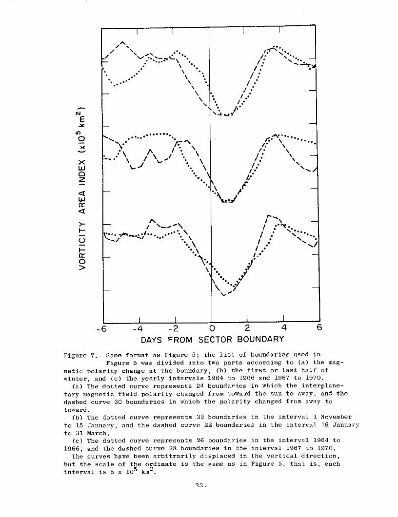
Figure 7. Same format as Figure 5; the list of boundaries used in

Figure 5 was divided into two parts according to (a) the mag-

netic polarity change at the boundary, (b) the first or last half of

winter, and (c) the yearly intervals 1964 to 1966 and 1967 to 1970.

(a) The dotted curve represents 24 boundaries in which the interplane-

tary magnetic field polarity changed from toward the sun to away, and the

dashed curve 30 boundaries in which the polarity changed from away to

toward.

(b) The dotted curve represents 32 boundaries in the interval 1 November

to 15 January, and the dashed curve 22 boundaries in the interval 16 Januay

to 31 March.

(c) The dotted curve represents 26 boundaries in the interval 1964 to

1966, and the dashed curve 28 boundaries in the interval 1967 to 1970.

The curves have been arbitrarily displaced in the vertical direction,

but the scale of the ordinate is the same as in Figure 5, that is, each

interval is 5 x 105 km 2 .

23.

HEMISPHERIC VORTICITY AREA vs SECTOR BOUNDARIES

1964 - 1970NOVEMBER - MARCH

ALL LONGITUDES

-5 -1VORTICITY DISCRIMINATOR = 20x1O sec

PRESSURE20 MIN = 41.2 MAX = 48.1 RANGE = 6.9 HEIGHT

200 MB

20 MIN=85.6 MAX:92.7 RANGE 7.1i I I - I

300 MB

20 MIN = 40.0 MAX 45.3 RANGE = 6.3

S II i I I I I 500TM

20 MIN= 9.7 MAX =12.3 RANGE =2.6

700 MB

20 MIN = 8.4 MAX = 10.9 RANGE = 2.5

850 MB

-6 -4 -2 0 2 4 6

DAYS AFTER SECTOR BOUNDARY

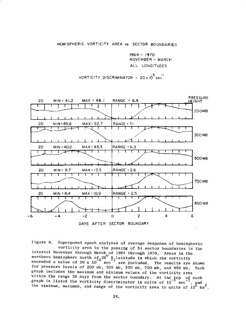
Figure 8. Superposed epoch analyses of average response of hemisphericvorticity area to the passing of 54 sector boundaries in the

interval November through March of 1964 through 1970. Areas in thenorthern hemisphere north of 20 N latitude in which the vorticityexceeded a value of 20 x 10 sec are included. The results are shownfor pressure levels of 200 mb, 300 mb, 500 mb, 700 mb, and 850 mb. Eachgraph includes the maximum and minimum values of the vorticity areawithin the range ±6 days from the sector boundary. At the _op of eachgraph is listed the vorticity discriminator in units of 10 sec andthe minimum, maximum, and range of the vorticity area in units of 105 km2

24.

HEMISPHERIC VORTICITY AREA vs SECTOR BOUNDARIES

1964- 1970NOVEMBER - MARCH

ALL LONGITUDES

KEEP VORTICITY AREA INDEX NEAR 40 x 10 km

PRESSURE

20 MIN =41.2 MAX = 48.1 RANGE = 6.9 HEIGHT

200 MB

22 MIN =41.1 MAX 47.5 RANGE : 6.4

300 MB

20 MIN = 40.0 MAX £ 46.3 RANGE = 6.3

500MB

18 MIN 33.7 MAX 38.1 RANGE = 4.4

700MB

18 MIN 260 MAX = 30.5 RANGE 4.5

850MB

-6 -4 -2 O 2 4 6

DAYS AFTER SECTOR BOUNDARY

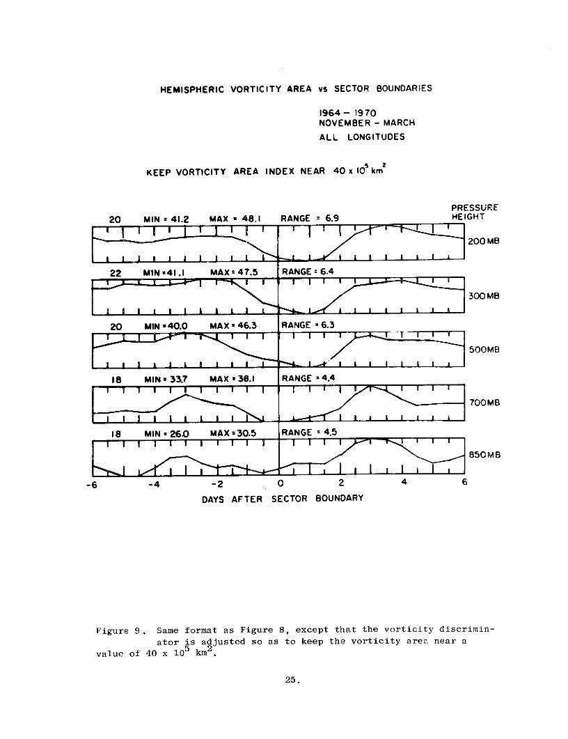
Figure 9. Same format as Figure 8, except that the vorticity discrimin-

ator is adjusted so as to keep the vorticity area near a

value of 40 x 105 km2

25.

HEMISPHERIC VORTICITY AREA vs SECTOR BOUNDARIES

1964 - 1970

NOVEMBER - MARCH

ALL LONGITUDES

-5 -VORTICITY DISCRIMINATOR = 20 x 10 sec

PRESSURE20 MIN 28.5 MAX 35.2 RANGE = 6.7 HEIGHT

10 MB

20 MIN= 9.6 MAX= 13,1 RANGE= 3.5

30 MB

20 MIN 2.7 MAX: 5.2 RANGE 2.5

50MB

20 MIN= 4.7 MAX= 7.3 RANGE =2.6i I I I I I I I I i I I "

100 MB

-6 -4 -2 0 2 4 6

DAYS AFTER SECTOR BOUNDARY

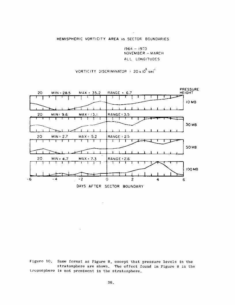
Figure 10. Same format as Figure 8, except that pressure levels in thestratosphere are shown. The effect found in Figure 8 in the

troposphere is not prominent in the stratosphere.

26.

VORTICITY AREA vs SECTOR BOUNDARIES

1964- 1970NOVEMBER - MARCH

300MB HEIGHT

VORTICITY DISCRIMINATOR = 20x10 sec

LONGITUDE

20 MIN = 14.3 MAX =16.8 RANGE = 2.5 INTERVAL

O-60E

20 MIN = 9.5 MAX= 12.2 RANGE : 2.7

-6 -4 - 0 2 4

60-120E

120E-180

20 MIN 12.9 MAX 14.7 RANGE = 1.8

120W-18

20 MIN = 18.0 MAX=20.0 RANGE = 2.0

60-120

20 MIN = 150 MAX= 17.9 RANGE = 2.9

0-60W

-6 -4 -2 0 2 4 6

DAYS AFTER SECTOR BOUNDARY

Figure 11. Same format as Figure 8, except at a pressure level of

300 mb. Results for longitude intervals 60 wide are shown.

No single interval dominates the observed effect.

27.

VORTICITY AREA vs SECTOR BOUNDARIES

1964-70NOVEMBER-MARCH

300 MB HEIGHT

VORTICITY DISCRIMINATOR = 20 x 10 sec -

LATITUDE20 MIN= 3.4 MAX= 4.4 RANGE= 1.0 BELT

20-30

20 MIN 13.3 MAX= 15.4 RANGE 2.1

30-40

20 MIN= 23.3 MAX= 26.5 RANGE: 3.2

40-50

20 MIN= 18.4 MAX= 21.3 RANGE= 2.9

50-60

20 MIN: 12.6 MAX: 13.9 RANGE: 1.3

60-70

-6 -4 -2 0 2 4 6

DAYS AFTER SECTOR BOUNDARY

Figure 12. Same format as Fi ure 8, except that results are shown in

latitude belts 10 wide in the interval from 200 N to 700 N.

The results are shown for a pressure level of 300 mb.

28.

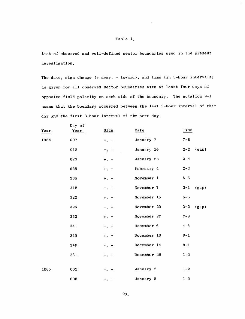
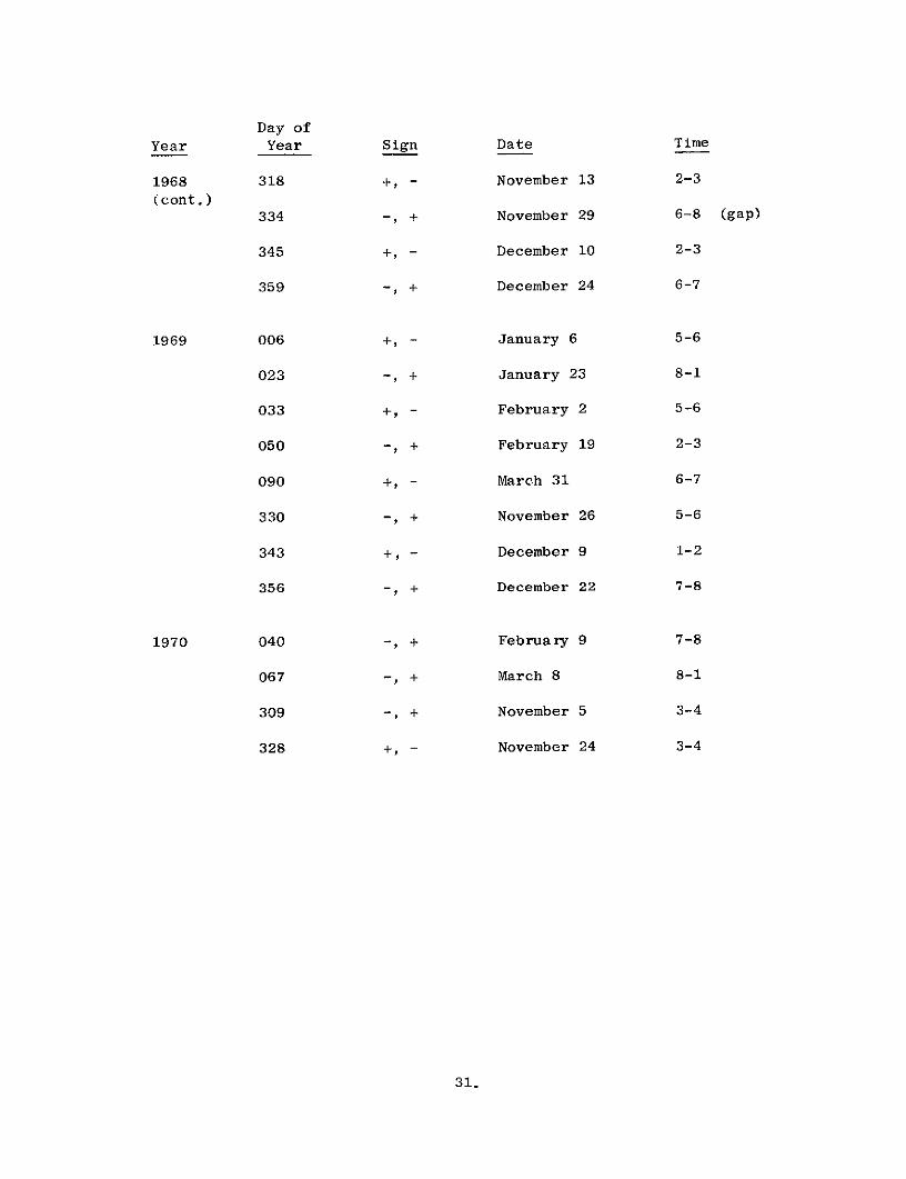
Table 1.

List of observed and well-defined sector boundaries used in the present

investigation.

The date, sign change (+ away, - toward), and time (in 3-hour intervals)

is given for all observed sector boundaries with at least four days of

opposite field polarity on each side of the boundary. The notation 8-1

means that the boundary occurred between the last 3-hour interval of that

day and the first 3-hour interval of the next day.

Day of

Year Year Sign Date Time

1964 007 +, - January 7 7-8

016 -, + January 16 2-2 (gap)

023 +, - January 23 3-4

035 +, - February 4 2-3

306 +, - November 1 5-6

312 -, + November 7 2-1 (gap)

320 +, - November 15 5-6

325 -, + November 20 3-2 (gap)

332 +, - November 27 7-8

341 -, + December 6 4-5

345 +, - December 10 8-1

349 -, + December 14 8-1

361 +, - December 26 1-2

1965 002 -, + January 2 1-2

008 +, - January 8 1-2

29.

Day ofYear Year Sign Date Time

1965 012 -, + January 12 2-3(cont.)

032 +, - February 1 8-1

1966 001 +, - January 1 6-7 (1 day gap)

032 +, - February 1 4-5

043 -, + February 12 2-3

062 +, - March 3 3-4

067 -, + March 8 2-3

089 +, - March 30 2-3

312 +, - November 8 4-5

331 -, + November 27 7-8

338 +, - December 4 3-4

1967 001 +, - January 1 7-8

013 +, - January 13 3-4

018 -, + January 18 2-3 (1 day gap)

081 -, + March 22 7-8

324 -, + November 20 4-5

338 +, - December 4 5-6

1968 001 +, - January 1 6-5 (gap)

028 +, - January 28 8-1

042 -, + February 11 3-4

057 +, - February 26 6-7

070 -, + March 10 4-5

083 +, - March 23 5-6

30.

Day of

Year Year Sign Date Time

1968 318 +, - November 13 2-3

(cont.)334 -, + November 29 6-8 (gap)

345 +, - December 10 2-3

359 -, + December 24 6-7

1969 006 +, - January 6 5-6

023 -, + January 23 8-1

033 +, - February 2 5-6

050 -, + February 19 2-3

090 +, - March 31 6-7

330 -, + November 26 5-6

343 +, - December 9 1-2

356 -, + December 22 7-8

1970 040 -, + February 9 7-8

067 -, + March 8 8-1

309 -, + November 5 3-4

328 +, - November 24 3-4

31.