Kepler: A Search for Terrestrial Planets

Kepler: A Search for Terrestrial Planets

Kepler Data Characteristics Handbook

KSCI-19040-001 Data Analysis Working Group (DAWG)

1 February 2011

NASA Ames Research Center

Moffett Field, CA. 94035

KSCI-19040: Kepler Data Characteristics Handbook

Prepared by:

Prepared by:

Approved by:

Approved by:

01/31/2011

Date Z.t \ I' \

Date~

Date 2! I / IIJ..dllJenkins, Ke~ Co-Investigator for Data Analysis

flJ.-.R- 1<. ~ Date 2/'//1Michael R. Haas; Science Office Director

Approved by: £"0/ThomasN. Gautier, Kepler Project Scientist

2 of 48

Date 7,/1 / I (

KSCI-19040-001: Kepler Data Characteristics Handbook 02/1/201

3 of 47

The Data Characteristics Handbook is the collective effort of the Data Analysis Working Group (DAWG), composed of Science Office (SO), Science Operations Center (SOC), Guest Observer (GO) Office and Science Team (ST) members as listed below:

Jon Jenkins*, Chair

Doug Caldwell*, Co-Chair

Allen, Christopher L. Bryson, Stephen T. Christiansen, Jessie L. Clarke, Bruce D. Cote, Miles T. Fanelli, Michael N. Gilliland*, Ron (STSci) Girouard, Forrest Haas, Michael R. Hall, Jennifer Ibrahim, Khadeejah Kinemuchi, Karen Klaus, Todd Kolodziejczak, Jeff (MSFC) Li, Jie Machalek, Pavel McCauliff, Sean D. Middour, Christopher K. Morris, Robert L. Mullally, Fergal Quintana, Elisa V. Rowe, Jason F. Seader, Shawn Smith, Jeffrey Claiborne Still, Martin Stumpe, Martin Tenenbaum, Peter G. Thompson, Susan E. Twicken, Joe Uddin, Akm Kamal Van Cleve, Jeffrey Wohler, Bill

*Science Team


4 of 47

Document Control

This document is part of the Kepler Project Documentation that is controlled by the Kepler Project Office, NASA/Ames Research Center, Moffett Field, California.

Ownership

This document will be controlled under KPO @ Ames Configuration Management system. Changes to this document shall be controlled.

Control Level

The physical location of this document will be in the KPO @ Ames Data Center.

Physical Location

To be placed on the distribution list for additional revisions of this document, please address your request to the Kepler Science Office:

Distribution Requests

Michael R. Haas

Kepler Science Office Director MS 244-30

NASA Ames Research Center

Moffett Field, CA 94035-1000

[email protected]


5 of 47

Table of Contents

Prefatory Admonition to Users ............................................................................................................. 7 1. Introduction ................................................................................................................................ 8

1.1 Dates, Cadence numbers, and units ......................................................................................... 8 1.2 Document overview ............................................................................................................... 9

2. Release Description ................................................................................................................... 10 3. Evaluation of Performance ......................................................................................................... 11

3.1 Overall ............................................................................................................................... 11 4. Historical Events ....................................................................................................................... 13

4.1 Kepler mission timeline to date ............................................................................................. 13 4.2 Safe Mode .......................................................................................................................... 13 4.3 Loss of Fine Point ............................................................................................................... 14 4.4 Attitude Tweaks .................................................................................................................. 14 4.5 Variable FGS Guide Stars .................................................................................................... 15 4.6 Module 3 Failure ................................................................................................................. 16

5. Ongoing Phenomena .................................................................................................................. 18 5.1 Image Motion...................................................................................................................... 18 5.2 Focus Changes .................................................................................................................... 19 5.3 Momentum Desaturation ...................................................................................................... 22 5.4 Reaction Wheel Zero Crossings ............................................................................................ 24 5.5 Downlink Earth Point .......................................................................................................... 26 5.6 Manually Excluded Cadences ............................................................................................... 26 5.7 Incomplete Apertures Give Flux and Feature Discontinuities at Quarter Boundaries ................. 26 5.8 Argabrightening .................................................................................................................. 27 5.9 Background Time Series ...................................................................................................... 29 5.10 Pixel Sensitivity Dropouts .................................................................................................. 32 5.11 Short Cadence Requantization Gaps .................................................................................... 33 5.12 Spurious Frequencies in SC Data ........................................................................................ 34

5.12.1 Integer Multiples of Inverse LC Period ......................................................................... 34 5.12.2 Other Frequencies ....................................................................................................... 35

5.13 Anomaly Summary Table ................................................................................................... 36 6. Time and Time Stamps .............................................................................................................. 38

6.1 Overview ............................................................................................................................ 38 6.2 Time Transformations, VTC to BKJD ................................................................................... 38

6.2.1 Vehicle Time Code ....................................................................................................... 38


6 of 47

6.2.2 Barycentric Corrections ................................................................................................ 38 6.2.3 Time slice offsets ......................................................................................................... 38 6.2.4 Barycentric Kepler Julian Date ...................................................................................... 39

6.3 Caveats and Uncertainties .................................................................................................... 39 6.4 Times in MAST FITS files ................................................................................................... 39

6.4.1 Target Pixels ................................................................................................................ 39 6.4.2 Light Curves ................................................................................................................ 40

7. Contents of Supplement ............................................................................................................. 41 7.1 Pipeline Instance Detail Reports ........................................................................................... 41 7.2 Data for Systematic Error Correction .................................................................................... 41

7.2.1 Mod.out Central Motion ................................................................................................ 41 7.2.2 Average LDE board Temperature .................................................................................. 42 7.2.3 Reaction Wheel Housing Temperature ........................................................................... 42 7.2.4 Launch Vehicle Adapter Temperature ............................................................................ 42

7.3 Background Time Series ...................................................................................................... 42 7.4 Flight System Events ........................................................................................................... 43 7.5 Calibration File READMEs .................................................................................................. 43 7.6 Supplement package descriptions .......................................................................................... 44

8. References ................................................................................................................................ 45 9. List of Acronyms and Abbreviations ........................................................................................... 46


7 of 47

Admonition to Users

The corrected light-curve product generated by the PDC (Pre-search Data Conditioning) pipeline module is designed to enable the Kepler planetary transit search. Although significant effort has been expended to preserve the natural variability of targets in the corrected light curves in order to enable astrophysical exploitation of the PDC data, it is not possible to perfectly preserve general stellar variability, and PDC currently is known to remove or distort astrophysical features in a subset of the corrected light curves. In those cases where PDC fails, or where the requirements of an astrophysical investigation are in conflict with those for transit planet search, the investigator should use the ‘raw’ light-curve product, for which basic calibration has been performed but correction for instrumental systematics has not, instead of the PDC (‘corrected’) light-curve product. Where appropriate, the investigator can then use the ancillary engineering data and image motion time series provided in the relevant Data Release Notes Supplement/s for systematic error correction. Investigators are strongly encouraged to study the specific Data Release Notes for any data sets they intend to use. The Science Office advises against publication of results based on Kepler data without careful consideration and due diligence by the end user, and dialog with the Science Office and/or Guest Observer Office where appropriate. Known issues with the PDC (‘corrected’) light curve product, which have been historically documented in the Data Release Notes (KSCI-19042 to KSCI-19048) are currently documented in the Kepler Data Processing Handbook (KSCI-19081). Users are encouraged to notice and document artifacts, either in the raw or processed data, and report them to the Science Office at [email protected].

Users who neglect this Admonition risk seeing their works crumble into ruin before their time.

Photo credit: Mayan Observatory at Chichen Itza, Jeffrey Van Cleve

mailto:[email protected]�


8 of 47

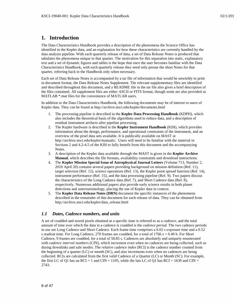
1. Introduction The Data Characteristics Handbook provides a description of the phenomena the Science Office has identified in the Kepler data, and an explanation for how these characteristics are currently handled by the data analysis pipeline. With each quarterly release of data, a set of Data Release Notes is produced that tabulates the phenomena unique to that quarter. The motivation for this separation into static, explanatory text and a set of dynamic figures and tables is the hope that once the user becomes familiar with the Data Characteristics Handbook, with each quarterly release they need only peruse the short Notes for that quarter, referring back to the Handbook only when necessary.

Each set of Data Release Notes is accompanied by a tar file of information that would be unwieldy to print in document format, the Data Release Notes Supplement. The relevant supplementary files are identified and described throughout this document, and a README file in the tar file also gives a brief description of the files contained. All supplement files are either ASCII or FITS format, though some are also provided as MATLAB *.mat files for the convenience of MATLAB users.

In addition to the Data Characteristics Handbook, the following documents may be of interest to users of Kepler data. They can be found at http://archive.stsci.edu/kepler/documents.html

1. The processing pipeline is described in the Kepler Data Processing Handbook (KDPH), which also includes the theoretical basis of the algorithms used to reduce data, and a description of residual instrument artifacts after pipeline processing.

2. The Kepler hardware is described in the Kepler Instrument Handbook (KIH), which provides information about the design, performance, and operational constraints of the instrument, and an overview of the pixel data sets available. It is publically available on MAST at http://archive.stsci.edu/kepler/manuals/. Users will need to be familiar with the material in Sections 2 and 4.2-4.5 of the KIH to fully benefit from this document and the accompanying Notes.

3. A description of the Kepler data available through the MAST is given in the Kepler Archive Manual, which describes the file formats, availability constraints and download instructions.

4. The Kepler Mission Special Issue of Astrophysical Journal Letters (Volume 713, Number 2, 2010 April 20) contains several papers providing background on mission definition (Ref. 11), target selection (Ref. 12), science operations (Ref. 13), the Kepler point spread function (Ref. 14), instrument performance (Ref. 15), and the data processing pipeline (Ref. 9). Two papers discuss the characteristics of the Long Cadence data (Ref. 7), and Short Cadence data (Ref. 8), respectively. Numerous additional papers also provide early science results in both planet detections and asteroseismology, placing the use of Kepler data in context.

5. The Kepler Data Release Notes (DRN) document the specific instances of the phenomena described in the remainder of this document for each release of data. They can be obtained from http://archive.stsci.edu/kepler/data_release.html

1.1 Dates, Cadence numbers, and units A set of coadded and stored pixels obtained at a specific time is referred to as a cadence, and the total amount of time over which the data in a cadence is coadded is the cadence period. The two cadence periods in use are Long Cadence and Short Cadence. Each frame time comprises a 6.02 s exposure time and a 0.52 s readout time. For Long Cadence, 270 frames are coadded, for a total of 1766 s = 0.49 h. For Short Cadence, 9 frames are coadded, for a total of 58.85 s. Cadences are absolutely and uniquely enumerated with cadence interval numbers (CIN), which increment even when no cadences are being collected, such as during downlinks and safe modes. The relative cadence index (RCI) is the cadence number counted from the beginning of a quarter (LC) or month (SC), and also increments even when no cadences are being collected. RCIs are calculated from the first valid Cadence of a Quarter (LC) or Month (SC). For example, the first LC of Q1 has an RCI = 1 and CIN = 1105, while the last LC of Q1 has RCI = 1639 and CIN = 2743.


9 of 47

Figures and tables in this document and the DRN will present results in CIN, RCI, or Modified Julian Date (MJD), since MJD is the preferred time base of the Flight System and pipeline, and can be mapped one-to-one onto CIN or RCI. On the other hand, the preferred time base for scientific results is Barycentric Julian Date (BJD); the correction to BJD, as described in detail in Section 6.2.2, is done on a target-by-target basis in the files users download from MAST. Unless otherwise specified, the MJD of a cadence refers to the time at the midpoint of the cadence.

1.2 Document overview In Section 2, we describe the generation and contents of a data release. Our evaluation of the current precision of the data is outlined in Section 3. A description of the historical events that have affected the Kepler data is provided in Section 4; similarly a description of the ongoing phenomena affecting the data is provided in Section 5. Section 6 outlines the generation and precision of the time stamps associated with Kepler data. Section 7 details the contents of the Data Release Notes Supplement. A list of references is included in Section 8, and the acronyms used throughout this and other Kepler documentation are explained in Section 9.


10 of 47

2. Release Description A data set refers to the data type and observation interval during which the data were collected. The observation interval for Long Cadence data is usually a quarter, indicated by Q[n], though Q0 and Q1 are 10 days and one month duration respectively, instead of the typical 3-month quarter. Short Cadence targets can be changed every month, so SC observation intervals are indicated by Q[n]M[m], where m = 1 to 3 is the Month within that Quarter. The data processing descriptor is the internal Kepler Science Operations (KSOP) ticket used to request and track the data processing. The KSOP ticket contains a “Pipeline Instance Detail (PID) Report”, included in the Supplement, which describes the version of the software used to process the data, and a list of parameter values used. Released Science Operations Center (SOC) software has both a release label in the form of a version number (e.g. 6.1), and a revision number (preceded by “r”) which precisely identifies the revision of the code corresponding to that label. For example, the code used to produce Data Release 7 has the release label “SOC Pipeline 6.1” and the revision number r37663. Unreleased software will, in general, have only a revision number for identification.

A given data set will, in general, be reprocessed as the software improves, and will hence be the subject of multiple releases. The combination of data set and data processing description defines a data product, and a set of data products simultaneously delivered to MAST for either public or proprietary (Science Team or GO) access is called a data release. The first release of data products for a given set of data is referred to as “new,” while subsequent releases are referred to as “reprocessed.” Each data release is accompanied by a set of Data Release Notes, which tabulates the phenomena occurring during that quarter, and includes an extensive Supplement of data relevant to the release.

Data products are made available to MAST users as FITS files, described in the Kepler Archive Manual. The data are available both as target light curves and as target pixel files; also available are the monthly full frame images (FFIs). The target light curve files include both corrected and uncorrected flux time series for both simple aperture photometry and difference image analysis (the latter is not yet populated). While the Kepler Archive Manual refers to the light curves which have not been corrected for systematic errors as ‘raw’ light curves, in this document and in the Data Release Notes they will be referred to as ‘uncorrected’, since the uncorrected light curves are formed from calibrated pixels. We shall use ‘raw’ to refer specifically to the pixel values for which only decompression has been performed. The FITS files contain the header keyword DATA_REL, which allows users to unambiguously associate a data release with the relevant Data Release Notes and the header keyword QUARTER, which identifies when the data were acquired.

Target pixel files contain the raw and calibrated pixels collected with the Kepler spacecraft. Similar to the light curve files, the target pixel files are FITS binary tables, organized by target. For the target pixel files, the FITS binary table contains a time series of images for the raw counts, the calibrated pixels, the background flux, and the removed cosmic rays. The intent of the pixel level data is to provide users enough information to perform their own photometry independent of the SOC pipeline. For details on how these files are formatted, please see the Archive Manual.


11 of 47

3. Evaluation of Performance 3.1 Overall The Combined Differential Photometric Precision (CDPP) of a photometric time series is the effective white noise standard deviation over a specified time interval, typically the duration of a transit or other phenomenon that is searched for in the time series. In the case of a transit, CDPP can be used to calculate the S/N of a transit of specified duration and depth. For example, a 6.5 hr CDPP of 20 ppm for a star with a planet exhibiting 84 ppm transits lasting 6.5 hours leads to a single transit S/N of 4.1 σ.

The CDPP performance has been discussed by Borucki et al. (Ref. 2) and Jenkins et al. (Ref. 7). Jenkins et al. examine the 33.5-day long Quarter 1 (Q1) observations that ended 2009 June 15, and find that the lower envelope of the photometric precision on transit timescales is consistent with expected random noise sources. Nonetheless, the following cautions apply for interpreting data at this point in our understanding of the Instrument’s performance:

1. Stellar variability and many instrumental effects are not, in general, white noise processes. 2. Many stars remain unclassified until Kepler and other data can be used to ascertain whether

they are giants or otherwise peculiar. Since giant stars are intrinsically variable at the level of Kepler’s precision, they must be excluded from calculations of CDPP performance. A simple, but not foolproof, way to do this is to include only stars with high surface gravity (log g > 4).

3. Given the image artifacts discussed in detail in the KIH and Ref. 15, it is not generally possible to extrapolate noise as 1/sqrt(time) for those channels afflicted by artifacts which are presently not corrected or flagged by the pipeline.

4. There is evidence from the noise statistics of Q0 and Q1 (see the Release 5 Notes) that the pipeline is overfitting the data for shorter data sets (a month or less of LC data) and fainter stars, so users are urged to compare uncorrected and corrected light curves for evidence of signal distortion or attenuation. The problem is less evident in the Q2-Q4 data sets than in the Q0 and Q1 data of Release 5.

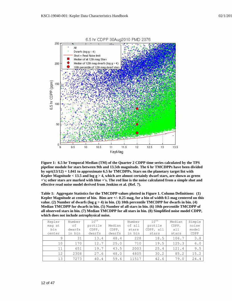
Example published data is shown in Refs. 2 and 10. The Transiting Planet Search (TPS) software module formally calculates CDPP on 6 hour timescales as a function of cadence for each target. The temporal median of the CDPP (TMCDPP) for each target is then divided by sqrt(13/12) to scale the results from 6 hours to the 6.5 hour benchmark time scale, which is the average transit duration of an Earth-size planet transiting a solar type star. The distribution of TMCDPP with Kepler magnitude separates into two branches, mostly corresponding to giants with log g < 4 and dwarfs with log g > 4; Figure 1 shows an example distribution from Q2. Further information may be gleaned from examining the TMCDPP of subsets of the full target list, such as all targets with magnitude between 11.75 and 12.25 and log g > 4, loosely referred to as “12th magnitude dwarfs”. Table 1 summarizes the median and percentile results for various target subsets in Q2; each set of Notes will include an updated version of this table for the relevant quarter. Note that the median CDPP for all stars in a given magnitude bin actually decreases as stars get fainter beyond 10th magnitude, since the proportion of all stars which are (quiet) dwarfs increases as the stars get fainter. A simple model of the noise floor can be calculated from the root-sum-square sum of shot noise and effective read noise - calculating this model over the benchmark 6.5 hour transit time gives the theoretical noise floor shown in Figure 1 and Table 1.


12 of 47

Figure 1: 6.5 hr Temporal Median (TM) of the Quarter 2 CDPP time series calculated by the TPS pipeline module for stars between 9th and 13.5th magnitude. The 6 hr TMCDPPs have been divided by sqrt(13/12) = 1.041 to approximate 6.5 hr TMCDPPs. Stars on the planetary target list with Kepler Magnitude < 13.5 and log g > 4, which are almost certainly dwarf stars, are shown as green +'s; other stars are marked with blue +'s. The red line is the noise calculated from a simple shot and effective read noise model derived from Jenkins et al. (Ref. 7).

Table 1: Aggregate Statistics for the TMCDPP values plotted in Figure 1. Column Definitions: (1) Kepler Magnitude at center of bin. Bins are +/- 0.25 mag, for a bin of width 0.5 mag centered on this value. (2) Number of dwarfs (log g > 4) in bin. (3) 10th percentile TMCDPP for dwarfs in bin. (4) Median TMCDPP for dwarfs in bin. (5) Number of all stars in bin. (6) 10th percentile TMCDPP of all observed stars in bin. (7) Median TMCDPP for all stars in bin. (8) Simplified noise model CDPP, which does not include astrophysical noise.

Kepler mag at bin

center

Number of

dwarfs in bin

10th prctile CDPP, dwarfs

Median CDPP, dwarfs

Number of all stars in bin

10th prctile CDPP, all

stars

Median CDPP, all stars

Simple noise model CDPP

9 31 13.4 48.4 228 18.5 106.7 3.8 10 170 12.7 25.0 710 19.5 125.3 6.0 11 651 19.7 43.5 2003 25.4 121.4 9.5 12 2308 27.6 48.0 4805 30.2 85.2 15.2 13 7273 40.4 59.6 11517 42.6 79.0 24.4


13 of 47

4. Historical Events This Section describes the various avenues by which some Kepler data has been lost or degraded. More recent quarters of data suffer less from most of these effects since they have been mitigated where possible. For each quarter, a table is produced summarizing the data anomalies that occurred in that quarter and included in the relevant Data Release Notes. The types of anomalies included in this table are described below.

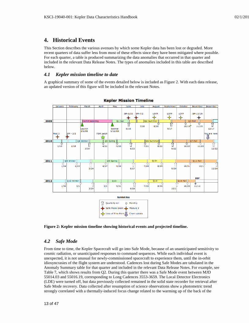
4.1 Kepler mission timeline to date A graphical summary of some of the events detailed below is included as Figure 2. With each data release, an updated version of this figure will be included in the relevant Notes.

Figure 2: Kepler mission timeline showing historical events and projected timeline.

4.2 Safe Mode From time to time, the Kepler Spacecraft will go into Safe Mode, because of an unanticipated sensitivity to cosmic radiation, or unanticipated responses to command sequences. While each individual event is unexpected, it is not unusual for newly-commissioned spacecraft to experience them, until the in-orbit idiosyncrasies of the flight system are understood. Cadences lost during Safe Modes are tabulated in the Anomaly Summary table for that quarter and included in the relevant Data Release Notes. For example, see Table 7, which shows results from Q2. During this quarter there was a Safe Mode event between MJD 55014.03 and 55016.19, corresponding to Long Cadences 3553-3659. The Local Detector Electronics (LDE) were turned off, but data previously collected remained in the solid state recorder for retrieval after Safe Mode recovery. Data collected after resumption of science observations show a photometric trend strongly correlated with a thermally-induced focus change related to the warming up of the back of the


14 of 47

spacecraft, which is for the most part mitigated within the PDC module of the pipeline. The Kepler Flight Software has subsequently been modified to leave the LDE on during radiation-induced resets of the RAD750 processor, so that data degradation due to thermal transients after an LDE power cycle does not occur during this kind of Safe Mode.

4.3 Loss of Fine Point From time to time, the Kepler spacecraft will lose fine pointing control, rendering the cadences collected with no better than 1% photometric precision. While the data obtained during LOFPs (Losses Of Fine Point) are treated as lost data by the pipeline, users with sources for which ~1% photometry is scientifically interesting may wish to look at the pixel data corresponding to those cadences, shown in Table 7. Cadences affected by LOFPs are listed in the relevant quarter Anomaly Summary table.

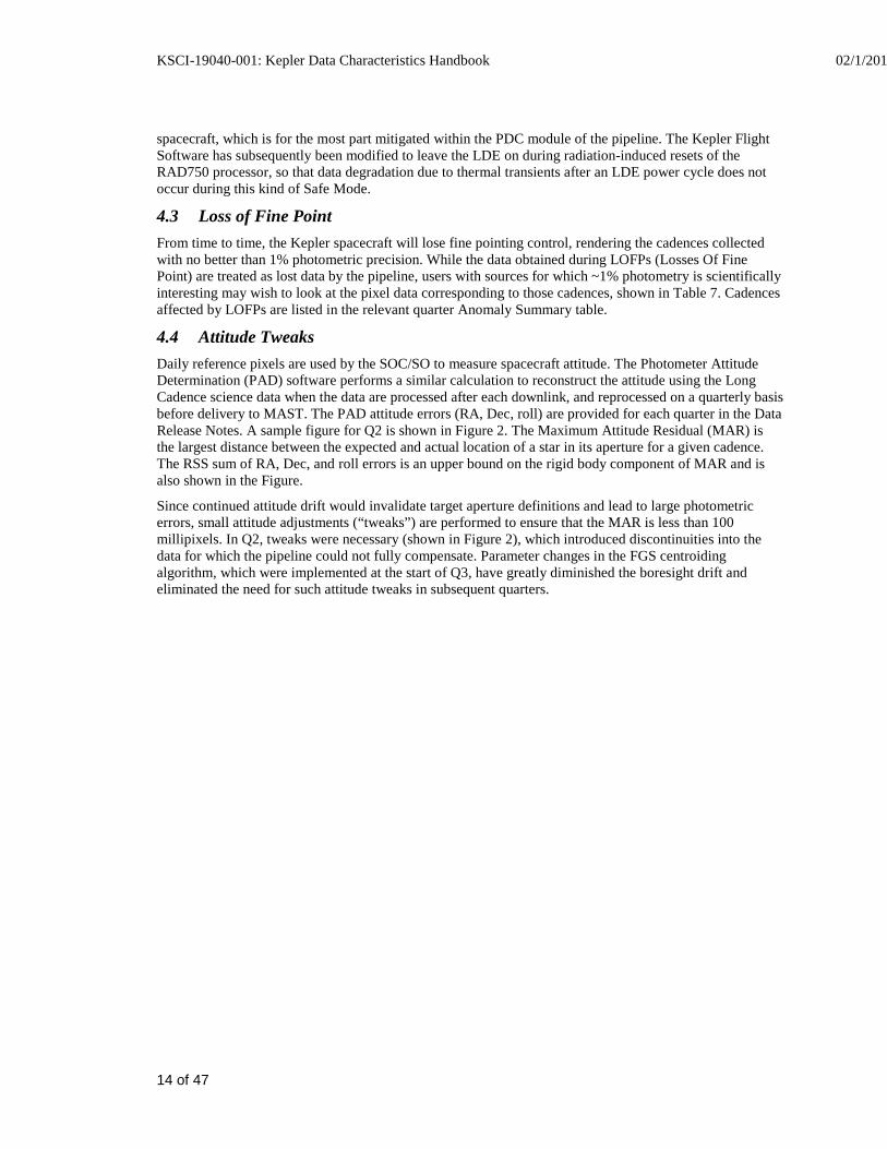
4.4 Attitude Tweaks Daily reference pixels are used by the SOC/SO to measure spacecraft attitude. The Photometer Attitude Determination (PAD) software performs a similar calculation to reconstruct the attitude using the Long Cadence science data when the data are processed after each downlink, and reprocessed on a quarterly basis before delivery to MAST. The PAD attitude errors (RA, Dec, roll) are provided for each quarter in the Data Release Notes. A sample figure for Q2 is shown in Figure 2. The Maximum Attitude Residual (MAR) is the largest distance between the expected and actual location of a star in its aperture for a given cadence. The RSS sum of RA, Dec, and roll errors is an upper bound on the rigid body component of MAR and is also shown in the Figure.

Since continued attitude drift would invalidate target aperture definitions and lead to large photometric errors, small attitude adjustments (“tweaks”) are performed to ensure that the MAR is less than 100 millipixels. In Q2, tweaks were necessary (shown in Figure 2), which introduced discontinuities into the data for which the pipeline could not fully compensate. Parameter changes in the FGS centroiding algorithm, which were implemented at the start of Q3, have greatly diminished the boresight drift and eliminated the need for such attitude tweaks in subsequent quarters.


15 of 47

Figure 3: Attitude Error in Quarter 2, calculated by PAD using Long Cadence data. The four large deviations near days 2, 32, 62 and 79 days (MJD-55000) are the result of attitude tweaks. The safe mode occurred around day 15 (MJD-55000). The roll is calculated for the edge of the focal plane.

4.5 Variable FGS Guide Stars The first-moment centroiding algorithm used by the FGS (Fine Guidance System) did not originally subtract all of the instrumental bias from the FGS pixels. Thus, the calculated centroid of an FGS star depended on the FGS star’s flux when the star was not located at the center of the centroiding aperture. Variable stars then induced a variation in the attitude solution calculated from the centroids of 40 guide stars, 10 in each FGS module. The ADCS (Attitude Determination and Control System), which attempts to keep the calculated attitude of the spacecraft constant, then moved the spacecraft to respond to this varying input, with the result that the boresight of the telescope moved while the ADCS reported a constant attitude. Science target star centroids and pixel time series, and to a lesser extent aperture flux, then showed systematic errors proportional to the FGS star flux variation. While the detrending against motion polynomials described in Section 4.1 should have removed these errors, users wishing to work with uncorrected light curves or with the calibrated pixels need to be aware of possible FGS variability-induced signatures and not mistake them for features of their target light curves.

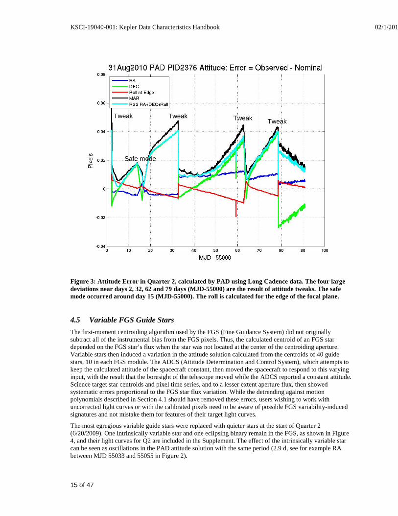
The most egregious variable guide stars were replaced with quieter stars at the start of Quarter 2 (6/20/2009). One intrinsically variable star and one eclipsing binary remain in the FGS, as shown in Figure 4, and their light curves for Q2 are included in the Supplement. The effect of the intrinsically variable star can be seen as oscillations in the PAD attitude solution with the same period (2.9 d, see for example RA between MJD 55033 and 55055 in Figure 2).

Tweak Tweak Tweak Tweak

Safe mode


16 of 47

The centroiding algorithm was updated to remove all of the instrumental background after the start of Quarter 3 (9/19/2009), greatly diminishing the effect of stellar variability on calculated centroids. The sky background is not removed, but is expected to be negligible. FGS guide star variability is not a factor from Q3 onwards.

Figure 4: Quarter 2 attitude residual and the light curves of two variable FGS guide stars. One of the stars is an eclipsing binary with a period of 18.25 days, the other is an intrinsic variable with a period of 2.9 days. Only 10 days of data are shown here for illustration.

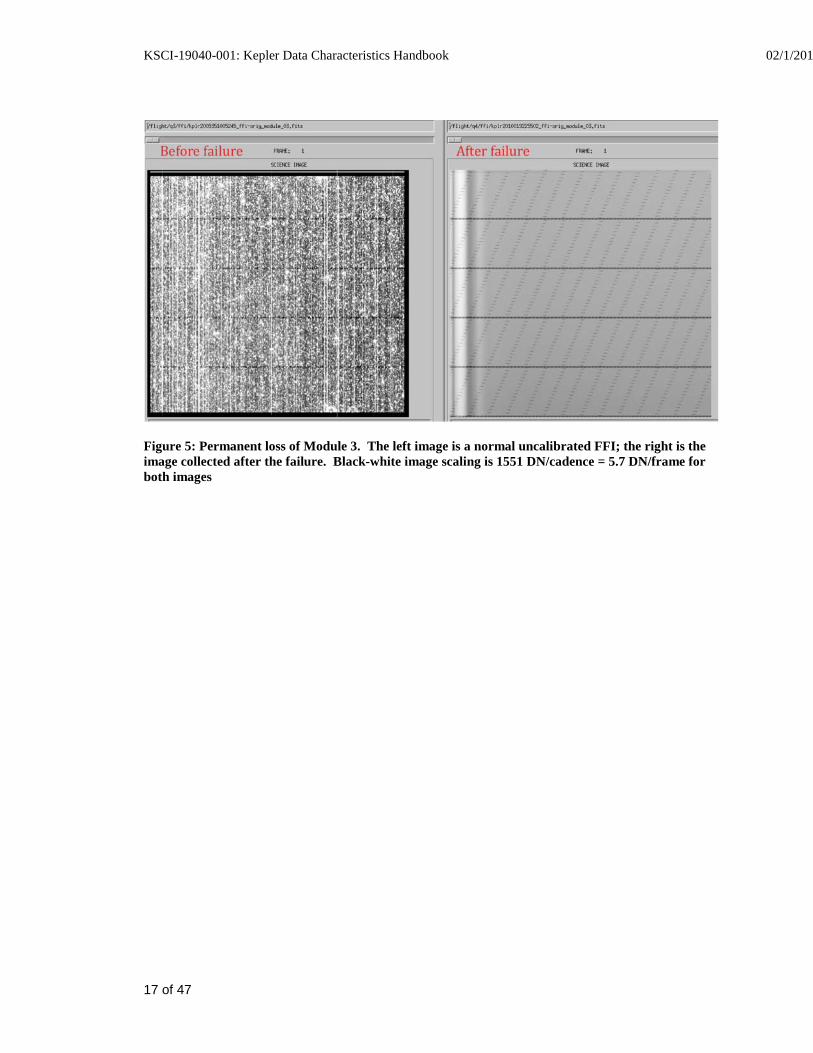
4.6 Module 3 Failure All 4 outputs of Module 3 failed at 17:52 UTC Jan 9, 2010, during LC CIN 12935. Reference pixels showed loss of stars and black levels decreased by 75 to 100 DN per frame. FFIs show no evidence of photons or electrically injected signals. The start of line ringing and FGS crosstalk (see KIH, Sections 6.5 and 6.2 respectively) are still present after the anomaly, as shown in Figure 4.

The loss of the module led to consistent temperature drops within the LDE, telescope structure, Schmidt corrector, primary mirror, FPA modules, and acquisition/driver boards – which in turn affected photometry and centroids as shown in various Figures in this document and in the Data Release 4 Notes (KSCI-19044).

After a review of probable causes, it was concluded that the probability of a subsequent failure was remote, a conclusion supported by continued operation of all the other Modules in the last year.

The impact on science observations is that 20% of the FOV will suffer a one-Quarter data outage every year as Kepler performs its quarterly rolls.


17 of 47

Figure 5: Permanent loss of Module 3. The left image is a normal uncalibrated FFI; the right is the image collected after the failure. Black-white image scaling is 1551 DN/cadence = 5.7 DN/frame for both images


18 of 47

5. Ongoing Phenomena This Section discusses systematic errors arising in nominal on-orbit operations, most of which will be removed from flux time series by the scientific pipeline if one uses the “corrected” light cure product (but see the Prefatory Admonition on page 7). The data are currently cotrended against image motion (as represented by the cadence-to-cadence coefficients of the motion polynomials calculated by PA) as well as LDE board temperatures; other telemetry items which may be used for cotrending the data in future releases are included in the Supplements so that users can assess whether features in the time series look suspiciously like features in the telemetry items. This telemetry has been filtered and gapped as described in the file headers, but the user may need to resample the data to match the LC or SC sampling. In addition, systematic effects are only corrected in the flux time series, and this Section and Supplement files may be useful for users interested in centroids or pixel data.

Most of the events described in this section are reported by the spacecraft or detected in the pipeline, then either corrected or marked as gaps (-Infs in the current flux time series, NaNs in the target pixel files). This section reports some events at lower thresholds than the pipeline, these may affect the light curves and therefore may be of interest to some users.

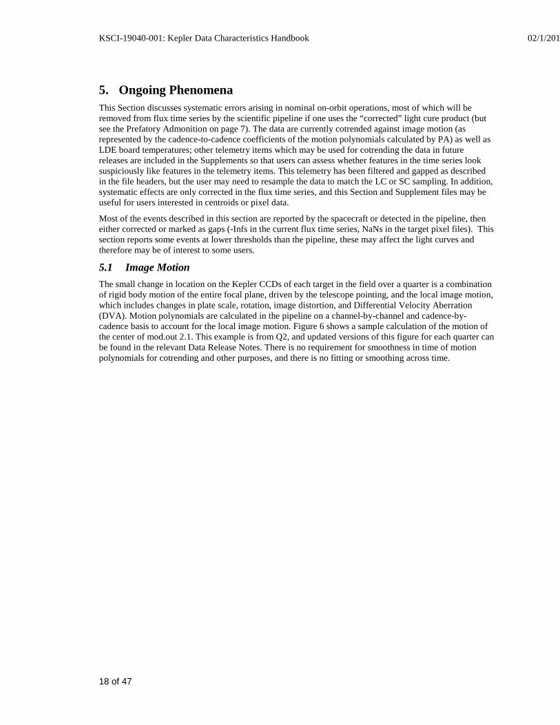
5.1 Image Motion The small change in location on the Kepler CCDs of each target in the field over a quarter is a combination of rigid body motion of the entire focal plane, driven by the telescope pointing, and the local image motion, which includes changes in plate scale, rotation, image distortion, and Differential Velocity Aberration (DVA). Motion polynomials are calculated in the pipeline on a channel-by-channel and cadence-by-cadence basis to account for the local image motion. Figure 6 shows a sample calculation of the motion of the center of mod.out 2.1. This example is from Q2, and updated versions of this figure for each quarter can be found in the relevant Data Release Notes. There is no requirement for smoothness in time of motion polynomials for cotrending and other purposes, and there is no fitting or smoothing across time.


19 of 47

Figure 6: Mod.out 2.1 Center Motion Time Series for Q2, calculated from motion polynomials. The median row and column values have been subtracted. Since this mod.out is at the edge of the field, it shows large differential velocity aberration (DVA) with respect to the center of the field, as well as a higher sensitivity to focus jitter and drift. The four large discontinuities near days 2, 32, 62 and 79 days (MJD-55000) are the result of attitude tweaks. A safe mode occurred around day 15 (MJD-55000).

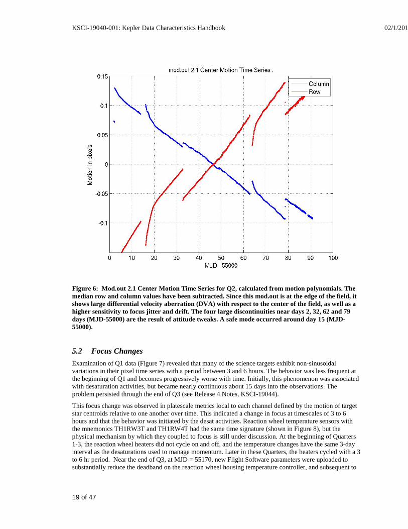
5.2 Focus Changes Examination of Q1 data (Figure 7) revealed that many of the science targets exhibit non-sinusoidal variations in their pixel time series with a period between 3 and 6 hours. The behavior was less frequent at the beginning of Q1 and becomes progressively worse with time. Initially, this phenomenon was associated with desaturation activities, but became nearly continuous about 15 days into the observations. The problem persisted through the end of Q3 (see Release 4 Notes, KSCI-19044).

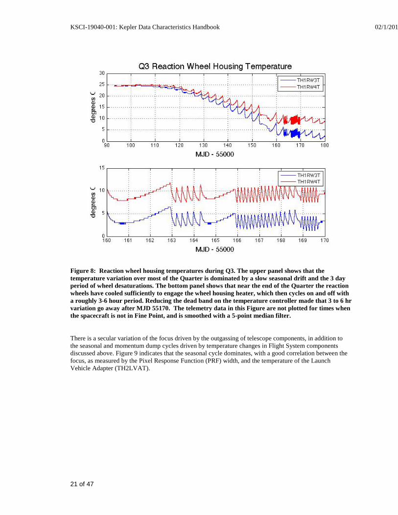
This focus change was observed in platescale metrics local to each channel defined by the motion of target star centroids relative to one another over time. This indicated a change in focus at timescales of 3 to 6 hours and that the behavior was initiated by the desat activities. Reaction wheel temperature sensors with the mnemonics TH1RW3T and TH1RW4T had the same time signature (shown in Figure 8), but the physical mechanism by which they coupled to focus is still under discussion. At the beginning of Quarters 1-3, the reaction wheel heaters did not cycle on and off, and the temperature changes have the same 3-day interval as the desaturations used to manage momentum. Later in these Quarters, the heaters cycled with a 3 to 6 hr period. Near the end of Q3, at MJD = 55170, new Flight Software parameters were uploaded to substantially reduce the deadband on the reaction wheel housing temperature controller, and subsequent to


20 of 47

that date the 3 to 6 hr cycle in both the temperature telemetry and the focus metric were eliminated, leaving only a slow seasonal drift and the 3 day signature of the momentum management cycle.

[Reference: KAR-503 and KAR-527]

Figure 7: A good example of the 3 to 6 hr focus oscillation in a single raw pixel time series from Quarter 1. Similar signatures are seen in flux and plate scale. The large negative-going spikes are caused by desaturations (Section 5.3), which have not been removed from this time series in this plot. The abscissa is the Q1 relative cadence index, and the ordinate is Data Numbers (DN) per Long Cadence (LC).


21 of 47

Figure 8: Reaction wheel housing temperatures during Q3. The upper panel shows that the temperature variation over most of the Quarter is dominated by a slow seasonal drift and the 3 day period of wheel desaturations. The bottom panel shows that near the end of the Quarter the reaction wheels have cooled sufficiently to engage the wheel housing heater, which then cycles on and off with a roughly 3-6 hour period. Reducing the dead band on the temperature controller made that 3 to 6 hr variation go away after MJD 55170. The telemetry data in this Figure are not plotted for times when the spacecraft is not in Fine Point, and is smoothed with a 5-point median filter.

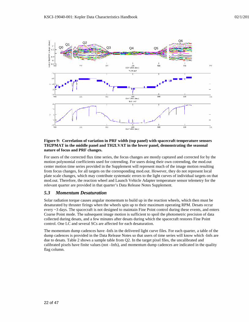
There is a secular variation of the focus driven by the outgassing of telescope components, in addition to the seasonal and momentum dump cycles driven by temperature changes in Flight System components discussed above. Figure 9 indicates that the seasonal cycle dominates, with a good correlation between the focus, as measured by the Pixel Response Function (PRF) width, and the temperature of the Launch Vehicle Adapter (TH2LVAT).


22 of 47

Figure 9: Correlation of variation in PRF width (top panel) with spacecraft temperature sensors TH2PMAT in the middle panel and TH2LVAT in the lower panel, demonstrating the seasonal nature of focus and PRF changes.

For users of the corrected flux time series, the focus changes are mostly captured and corrected for by the motion polynomial coefficients used for cotrending. For users doing their own cotrending, the mod.out center motion time series provided in the Supplement will represent much of the image motion resulting from focus changes, for all targets on the corresponding mod.out. However, they do not represent local plate scale changes, which may contribute systematic errors to the light curves of individual targets on that mod.out. Therefore, the reaction wheel and Launch Vehicle Adapter temperature sensor telemetry for the relevant quarter are provided in that quarter’s Data Release Notes Supplement.

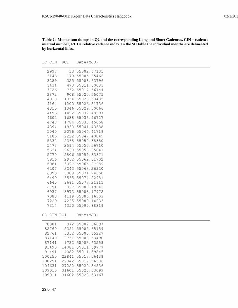
5.3 Momentum Desaturation Solar radiation torque causes angular momentum to build up in the reaction wheels, which then must be desaturated by thruster firings when the wheels spin up to their maximum operating RPM. Desats occur every ~3 days. The spacecraft is not designed to maintain Fine Point control during these events, and enters Coarse Point mode. The subsequent image motion is sufficient to spoil the photometric precision of data collected during desats, and a few minutes after desats during which the spacecraft restores Fine Point control. One LC and several SCs are affected for each desaturation.

The momentum dump cadences have -Infs in the delivered light curve files. For each quarter, a table of the dump cadences is provided in the Data Release Notes so that users of time series will know which -Infs are due to desats. Table 2 shows a sample table from Q2. In the target pixel files, the uncalibrated and calibrated pixels have finite values (not –Infs), and momentum dump cadences are indicated in the quality flag column.

Q0 Q1 Q2

Q3 Q4 Q5

Q6


23 of 47

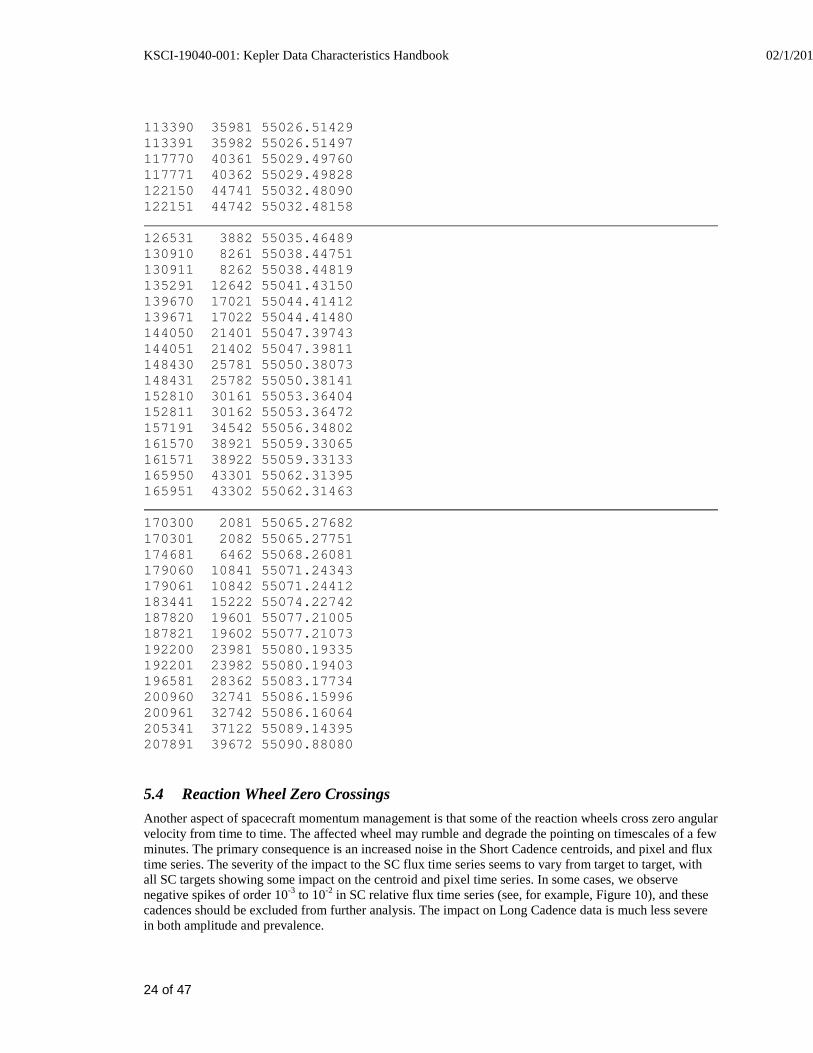
Table 2: Momentum dumps in Q2 and the corresponding Long and Short Cadences. CIN = cadence interval number, RCI = relative cadence index. In the SC table the individual months are delineated by horizontal lines.

LC CIN RCI Date(MJD)

2997 33 55002.67135 3143 179 55005.65466 3289 325 55008.63796 3434 470 55011.60083 3726 762 55017.56744 3872 908 55020.55075 4018 1054 55023.53405 4164 1200 55026.51736 4310 1346 55029.50066 4456 1492 55032.48397 4602 1638 55035.46727 4748 1784 55038.45058 4894 1930 55041.43388 5040 2076 55044.41719 5186 2222 55047.40049 5332 2368 55050.38380 5478 2514 55053.36710 5624 2660 55056.35041 5770 2806 55059.33371 5916 2952 55062.31702 6061 3097 55065.27989 6207 3243 55068.26320 6353 3389 55071.24650 6499 3535 55074.22981 6645 3681 55077.21311 6791 3827 55080.19642 6937 3973 55083.17972 7083 4119 55086.16303 7229 4265 55089.14633 7314 4350 55090.88319 SC CIN RCI Date(MJD)

78381 972 55002.66897 82760 5351 55005.65159 82761 5352 55005.65227 87140 9731 55008.63490 87141 9732 55008.63558 91490 14081 55011.59777 91491 14082 55011.59845 100250 22841 55017.56438 100251 22842 55017.56506 104631 27222 55020.54836 109010 31601 55023.53099 109011 31602 55023.53167


24 of 47

113390 35981 55026.51429 113391 35982 55026.51497 117770 40361 55029.49760 117771 40362 55029.49828 122150 44741 55032.48090 122151 44742 55032.48158

126531 3882 55035.46489 130910 8261 55038.44751 130911 8262 55038.44819 135291 12642 55041.43150 139670 17021 55044.41412 139671 17022 55044.41480 144050 21401 55047.39743 144051 21402 55047.39811 148430 25781 55050.38073 148431 25782 55050.38141 152810 30161 55053.36404 152811 30162 55053.36472 157191 34542 55056.34802 161570 38921 55059.33065 161571 38922 55059.33133 165950 43301 55062.31395 165951 43302 55062.31463

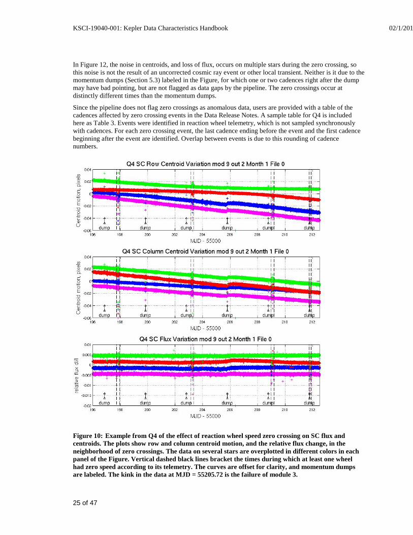
170300 2081 55065.27682 170301 2082 55065.27751 174681 6462 55068.26081 179060 10841 55071.24343 179061 10842 55071.24412 183441 15222 55074.22742 187820 19601 55077.21005 187821 19602 55077.21073 192200 23981 55080.19335 192201 23982 55080.19403 196581 28362 55083.17734 200960 32741 55086.15996 200961 32742 55086.16064 205341 37122 55089.14395 207891 39672 55090.88080 5.4 Reaction Wheel Zero Crossings Another aspect of spacecraft momentum management is that some of the reaction wheels cross zero angular velocity from time to time. The affected wheel may rumble and degrade the pointing on timescales of a few minutes. The primary consequence is an increased noise in the Short Cadence centroids, and pixel and flux time series. The severity of the impact to the SC flux time series seems to vary from target to target, with all SC targets showing some impact on the centroid and pixel time series. In some cases, we observe negative spikes of order 10-3 to 10-2 in SC relative flux time series (see, for example, Figure 10), and these cadences should be excluded from further analysis. The impact on Long Cadence data is much less severe in both amplitude and prevalence.


25 of 47

In Figure 12, the noise in centroids, and loss of flux, occurs on multiple stars during the zero crossing, so this noise is not the result of an uncorrected cosmic ray event or other local transient. Neither is it due to the momentum dumps (Section 5.3) labeled in the Figure, for which one or two cadences right after the dump may have bad pointing, but are not flagged as data gaps by the pipeline. The zero crossings occur at distinctly different times than the momentum dumps.

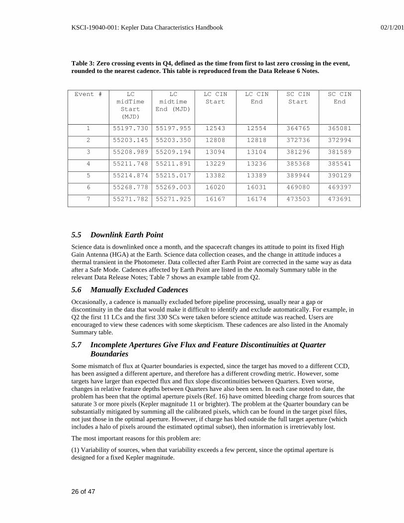
Since the pipeline does not flag zero crossings as anomalous data, users are provided with a table of the cadences affected by zero crossing events in the Data Release Notes. A sample table for Q4 is included here as Table 3. Events were identified in reaction wheel telemetry, which is not sampled synchronously with cadences. For each zero crossing event, the last cadence ending before the event and the first cadence beginning after the event are identified. Overlap between events is due to this rounding of cadence numbers.

Figure 10: Example from Q4 of the effect of reaction wheel speed zero crossing on SC flux and centroids. The plots show row and column centroid motion, and the relative flux change, in the neighborhood of zero crossings. The data on several stars are overplotted in different colors in each panel of the Figure. Vertical dashed black lines bracket the times during which at least one wheel had zero speed according to its telemetry. The curves are offset for clarity, and momentum dumps are labeled. The kink in the data at MJD = 55205.72 is the failure of module 3.


26 of 47

Table 3: Zero crossing events in Q4, defined as the time from first to last zero crossing in the event, rounded to the nearest cadence. This table is reproduced from the Data Release 6 Notes.

Event # LC midTime Start (MJD)

LC midtime

End (MJD)

LC CIN Start

LC CIN End

SC CIN Start

SC CIN End

1 55197.730 55197.955 12543 12554 364765 365081

2 55203.145 55203.350 12808 12818 372736 372994

3 55208.989 55209.194 13094 13104 381296 381589

4 55211.748 55211.891 13229 13236 385368 385541

5 55214.874 55215.017 13382 13389 389944 390129

6 55268.778 55269.003 16020 16031 469080 469397

7 55271.782 55271.925 16167 16174 473503 473691

5.5 Downlink Earth Point Science data is downlinked once a month, and the spacecraft changes its attitude to point its fixed High Gain Antenna (HGA) at the Earth. Science data collection ceases, and the change in attitude induces a thermal transient in the Photometer. Data collected after Earth Point are corrected in the same way as data after a Safe Mode. Cadences affected by Earth Point are listed in the Anomaly Summary table in the relevant Data Release Notes; Table 7 shows an example table from Q2.

5.6 Manually Excluded Cadences Occasionally, a cadence is manually excluded before pipeline processing, usually near a gap or discontinuity in the data that would make it difficult to identify and exclude automatically. For example, in Q2 the first 11 LCs and the first 330 SCs were taken before science attitude was reached. Users are encouraged to view these cadences with some skepticism. These cadences are also listed in the Anomaly Summary table.

5.7 Incomplete Apertures Give Flux and Feature Discontinuities at Quarter Boundaries

Some mismatch of flux at Quarter boundaries is expected, since the target has moved to a different CCD, has been assigned a different aperture, and therefore has a different crowding metric. However, some targets have larger than expected flux and flux slope discontinuities between Quarters. Even worse, changes in relative feature depths between Quarters have also been seen. In each case noted to date, the problem has been that the optimal aperture pixels (Ref. 16) have omitted bleeding charge from sources that saturate 3 or more pixels (Kepler magnitude 11 or brighter). The problem at the Quarter boundary can be substantially mitigated by summing all the calibrated pixels, which can be found in the target pixel files, not just those in the optimal aperture. However, if charge has bled outside the full target aperture (which includes a halo of pixels around the estimated optimal subset), then information is irretrievably lost.

The most important reasons for this problem are:

(1) Variability of sources, when that variability exceeds a few percent, since the optimal aperture is designed for a fixed Kepler magnitude.


27 of 47

(2) Inability of the focal plane nonlinearity model to predict in detail the length and position of the charge bleed pixels in a column containing a saturating source. For example, a bright source may have 75% of the saturating pixels at lower rows, and 25% at higher rows than the row on which the source is centered – while an equally bright source in another location on the same mod.out might have 50% above and 50% below, or even 25% below and 75% above. The saturation model currently in use can accommodate 25/75 to 75/25 asymmetries by collecting extra pixels along the saturating column, but larger asymmetries will not capture all of the bleeding charge.

As the mission has progressed, visual inspection has revealed those stars with poorly captured saturation. The Kepler magnitudes of these stars have been adjusted so that they are assigned larger apertures in subsequent quarters. Therefore more targets will have problems with incomplete apertures early in the mission, though incomplete optimal aperture problems have been reported as late as Q6.

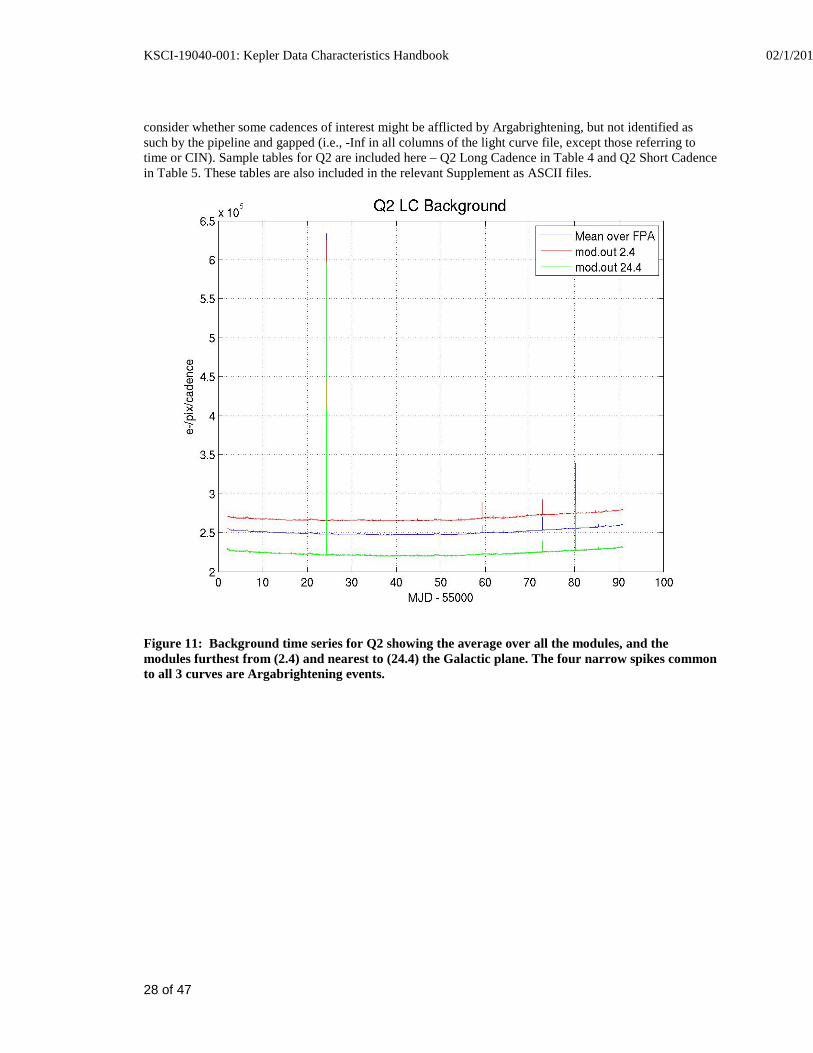
5.8 Argabrightening Argabrightening, named after its discoverer, V. Argabright of BATC, is a diffuse illumination of the focal plane, lasting on the order of a few minutes, possibly due to impact-generated debris (Ref. 18). It is known to be illumination rather than an electronic offset since it appears in calibrated pixel data from which the electronic black level has been removed using the collateral data. It is not a result of gain change, or of targets moving in their apertures, since the phenomenon appears with the same amplitude in background pixels (in LC) or pixels outside the optimal aperture (in SC) as well as stellar target pixels. Many channels are affected simultaneously, and the amplitude of the event on each channel is many standard deviations above the trend, as shown in Figure 11. Spatial variation within a mod.out is significant for some events (Figure 12). While low-spatial-frequency changes in background are removed by subtraction of Pipeline-generated background polynomials for Long Cadence data, users are cautioned about Argabrightening cadences because of the possible fine spatial structure, possible errors in the nonlinearity model, and the absence of direct background measurements for Short Cadence, for which interpolation of Long Cadence background polynomials is required.

The method of detection is

1. Calculate the median, for each cadence and mod.out, of the calibrated background (LC) or out-of-optimal-aperture (SC) pixels,

2. Detrend the data by fitting a parabola to the resulting time series and subtract the fit.

3. High-pass filter the detrended data by median filtering with a 25 cadence wide filter, and subtracting that median-filtered curve from the detrended data to form the residual background light curve.

4. Calculate the Median Absolute Deviation (MAD) of the residual. The Argabrightening statistic SArg is then the ratio of the residual to the MAD.

5. Find values of SArg which exceed TMAD, the single-channel threshold, and subsequently treat those cadences as gaps for all pixels in that channel. In the current version of the pipeline, TMAD is the same for all channels.

6. A multichannel event is detected on a given cadence if the number of channels for which SArg > TMAD on that cadence exceeds the multi-channel event threshold TMCE . Then all channels on that cadence are marked as gaps, even those channels which did not individually exceed TMAD. Multichannel event detection allows the use of lower TMAD while still discriminating against spurious events on isolated channels.

7. For multichannel events, average SArg over all 84 outputs of the FPA to form <SArg>FPA

The pipeline uses a rather high TMAD = 100 for LC and 60 for SC, and a high TMCE = 42 (half of the channels). Events that exceed these thresholds are gapped in the data delivered to the MAST. However, there may also be significant Argabrightening events in both LC and SC that do not exceed the thresholds. In each set of quarterly Data Release Notes, users are provided with a list of cadences affected by Argabrightening events with the lower thresholds set to TMAD = 10 and TMCE = 10, so that the user may


28 of 47

consider whether some cadences of interest might be afflicted by Argabrightening, but not identified as such by the pipeline and gapped (i.e., -Inf in all columns of the light curve file, except those referring to time or CIN). Sample tables for Q2 are included here – Q2 Long Cadence in Table 4 and Q2 Short Cadence in Table 5. These tables are also included in the relevant Supplement as ASCII files.

Figure 11: Background time series for Q2 showing the average over all the modules, and the modules furthest from (2.4) and nearest to (24.4) the Galactic plane. The four narrow spikes common to all 3 curves are Argabrightening events.


29 of 47

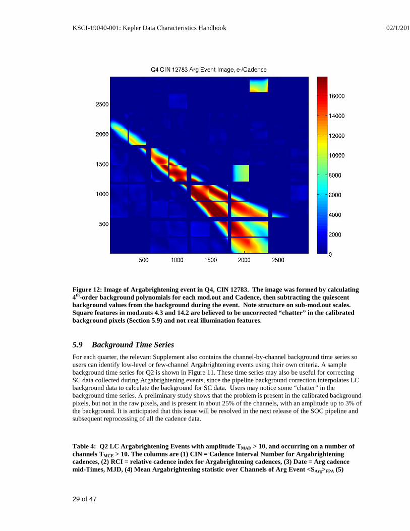
Figure 12: Image of Argabrightening event in Q4, CIN 12783. The image was formed by calculating 4th-order background polynomials for each mod.out and Cadence, then subtracting the quiescent background values from the background during the event. Note structure on sub-mod.out scales. Square features in mod.outs 4.3 and 14.2 are believed to be uncorrected “chatter” in the calibrated background pixels (Section 5.9) and not real illumination features.

5.9 Background Time Series For each quarter, the relevant Supplement also contains the channel-by-channel background time series so users can identify low-level or few-channel Argabrightening events using their own criteria. A sample background time series for Q2 is shown in Figure 11. These time series may also be useful for correcting SC data collected during Argabrightening events, since the pipeline background correction interpolates LC background data to calculate the background for SC data. Users may notice some “chatter” in the background time series. A preliminary study shows that the problem is present in the calibrated background pixels, but not in the raw pixels, and is present in about 25% of the channels, with an amplitude up to 3% of the background. It is anticipated that this issue will be resolved in the next release of the SOC pipeline and subsequent reprocessing of all the cadence data.

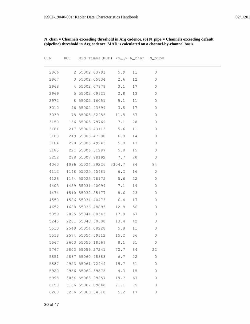
Table 4: Q2 LC Argabrightening Events with amplitude TMAD > 10, and occurring on a number of channels TMCE > 10. The columns are (1) CIN = Cadence Interval Number for Argabrightening cadences, (2) RCI = relative cadence index for Argabrightening cadences, (3) Date = Arg cadence mid-Times, MJD, (4) Mean Argabrightening statistic over Channels of Arg Event <SArg>FPA (5)


30 of 47

N_chan = Channels exceeding threshold in Arg cadence, (6) N_pipe = Channels exceeding default (pipeline) threshold in Arg cadence. MAD is calculated on a channel-by-channel basis.

CIN RCI Mid-Times(MJD) <SArg> N_chan N_pipe

2966 2 55002.03791 5.9 11 0

2967 3 55002.05834 2.6 12 0

2968 4 55002.07878 3.1 17 0

2969 5 55002.09921 2.8 13 0

2972 8 55002.16051 5.1 11 0

3010 46 55002.93699 3.8 17 0

3039 75 55003.52956 11.8 57 0

3150 186 55005.79769 7.1 28 0

3181 217 55006.43113 5.6 11 0

3183 219 55006.47200 6.8 14 0

3184 220 55006.49243 5.8 13 0

3185 221 55006.51287 5.8 15 0

3252 288 55007.88192 7.7 20 0

4060 1096 55024.39226 3304.7 84 84

4112 1148 55025.45481 6.2 16 0

4128 1164 55025.78175 5.6 22 0

4403 1439 55031.40099 7.1 19 0

4474 1510 55032.85177 8.6 23 0

4550 1586 55034.40473 6.4 17 0

4652 1688 55036.48895 12.8 56 0

5059 2095 55044.80543 17.8 67 0

5245 2281 55048.60608 13.4 42 0

5513 2549 55054.08228 5.8 11 0

5538 2574 55054.59312 15.2 36 0

5567 2603 55055.18569 8.1 31 0

5767 2803 55059.27241 72.7 84 22

5851 2887 55060.98883 6.7 22 0

5887 2923 55061.72444 19.7 51 0

5920 2956 55062.39875 4.3 15 0

5998 3034 55063.99257 19.7 67 0

6150 3186 55067.09848 21.1 75 0

6260 3296 55069.34618 5.2 17 0


31 of 47

6432 3468 55072.86075 147.6 83 62

6447 3483 55073.16726 11.0 45 0

6670 3706 55077.72395 7.3 25 0

6796 3832 55080.29858 554.7 84 84

6797 3833 55080.31902 6.8 17 0

7017 4053 55084.81441 9.1 31 0

7045 4081 55085.38655 26.1 74 0

7216 4252 55088.88069 10.0 44 0

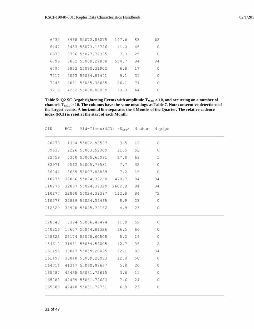
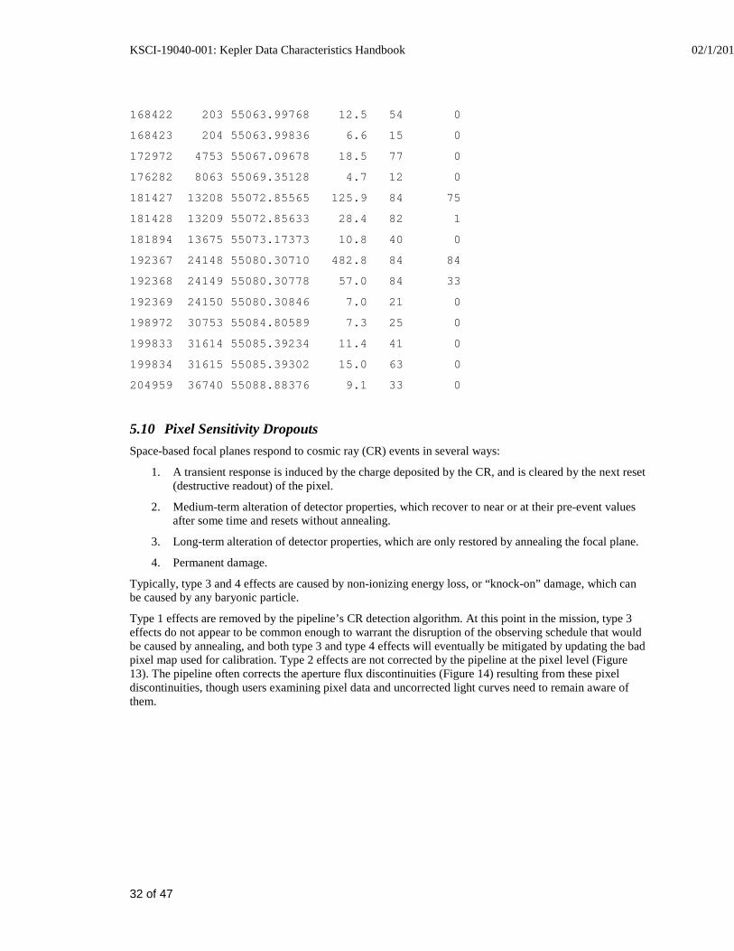
Table 5: Q2 SC Argabrightening Events with amplitude TMAD > 10, and occurring on a number of channels TMCE > 10. The columns have the same meanings as Table 7. Note consecutive detections of the largest events. A horizontal line separates the 3 Months of the Quarter. The relative cadence index (RCI) is reset at the start of each Month.

CIN RCI Mid-Times(MJD) <SArg> N_chan N_pipe

78773 1364 55002.93597 3.5 12 0

79635 2226 55003.52309 11.5 52 0

82759 5350 55005.65091 17.8 63 1

82971 5562 55005.79531 7.7 32 0

86044 8635 55007.88839 7.2 16 0

110275 32866 55024.39260 470.7 84 84

110276 32867 55024.39329 2602.8 84 84

110277 32868 55024.39397 112.8 84 72

110278 32869 55024.39465 8.9 23 0

112329 34920 55025.79162 4.9 23 0

128043 5394 55036.49474 11.9 52 0

140256 17607 55044.81326 16.5 66 0

145823 23174 55048.60505 5.2 19 0

154610 31961 55054.59005 12.7 36 2

161496 38847 55059.28025 52.1 82 34

161497 38848 55059.28093 12.8 50 0

164016 41367 55060.99667 5.8 20 0

165087 42438 55061.72615 3.6 11 0

165088 42439 55061.72683 7.6 24 0

165089 42440 55061.72751 6.9 23 0


32 of 47

168422 203 55063.99768 12.5 54 0

168423 204 55063.99836 6.6 15 0

172972 4753 55067.09678 18.5 77 0

176282 8063 55069.35128 4.7 12 0

181427 13208 55072.85565 125.9 84 75

181428 13209 55072.85633 28.4 82 1

181894 13675 55073.17373 10.8 40 0

192367 24148 55080.30710 482.8 84 84

192368 24149 55080.30778 57.0 84 33

192369 24150 55080.30846 7.0 21 0

198972 30753 55084.80589 7.3 25 0

199833 31614 55085.39234 11.4 41 0

199834 31615 55085.39302 15.0 63 0

204959 36740 55088.88376 9.1 33 0

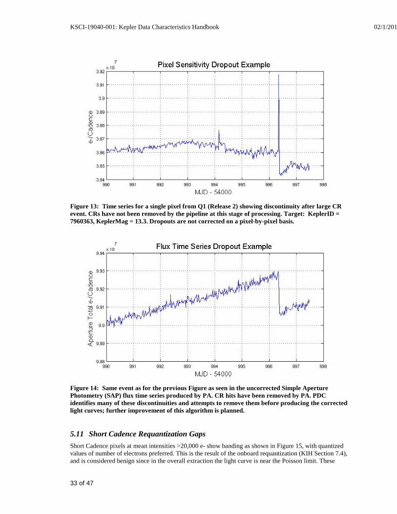
5.10 Pixel Sensitivity Dropouts Space-based focal planes respond to cosmic ray (CR) events in several ways:

1. A transient response is induced by the charge deposited by the CR, and is cleared by the next reset (destructive readout) of the pixel.

2. Medium-term alteration of detector properties, which recover to near or at their pre-event values after some time and resets without annealing.

3. Long-term alteration of detector properties, which are only restored by annealing the focal plane.

4. Permanent damage.

Typically, type 3 and 4 effects are caused by non-ionizing energy loss, or “knock-on” damage, which can be caused by any baryonic particle.

Type 1 effects are removed by the pipeline’s CR detection algorithm. At this point in the mission, type 3 effects do not appear to be common enough to warrant the disruption of the observing schedule that would be caused by annealing, and both type 3 and type 4 effects will eventually be mitigated by updating the bad pixel map used for calibration. Type 2 effects are not corrected by the pipeline at the pixel level (Figure 13). The pipeline often corrects the aperture flux discontinuities (Figure 14) resulting from these pixel discontinuities, though users examining pixel data and uncorrected light curves need to remain aware of them.


33 of 47

Figure 13: Time series for a single pixel from Q1 (Release 2) showing discontinuity after large CR event. CRs have not been removed by the pipeline at this stage of processing. Target: KeplerID = 7960363, KeplerMag = 13.3. Dropouts are not corrected on a pixel-by-pixel basis.

Figure 14: Same event as for the previous Figure as seen in the uncorrected Simple Aperture Photometry (SAP) flux time series produced by PA. CR hits have been removed by PA. PDC identifies many of these discontinuities and attempts to remove them before producing the corrected light curves; further improvement of this algorithm is planned.

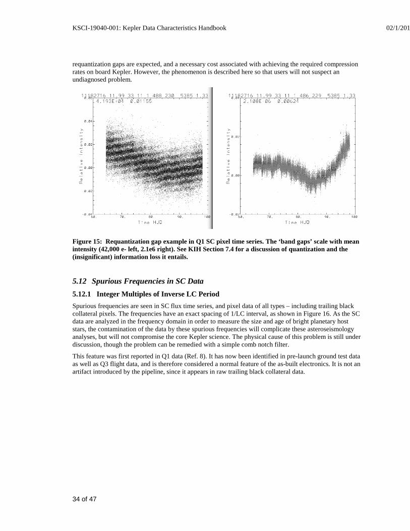
5.11 Short Cadence Requantization Gaps Short Cadence pixels at mean intensities >20,000 e- show banding as shown in Figure 15, with quantized values of number of electrons preferred. This is the result of the onboard requantization (KIH Section 7.4), and is considered benign since in the overall extraction the light curve is near the Poisson limit. These


34 of 47

requantization gaps are expected, and a necessary cost associated with achieving the required compression rates on board Kepler. However, the phenomenon is described here so that users will not suspect an undiagnosed problem.

Figure 15: Requantization gap example in Q1 SC pixel time series. The ‘band gaps’ scale with mean intensity (42,000 e- left, 2.1e6 right). See KIH Section 7.4 for a discussion of quantization and the (insignificant) information loss it entails.

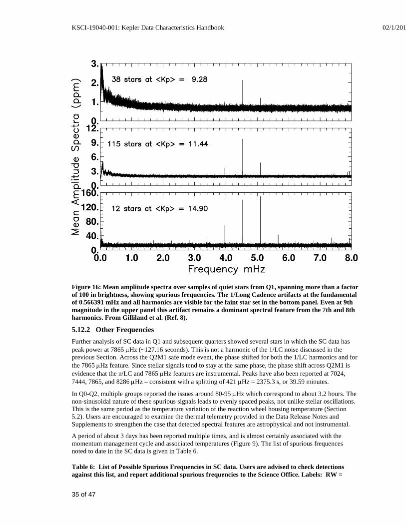
5.12 Spurious Frequencies in SC Data 5.12.1 Integer Multiples of Inverse LC Period Spurious frequencies are seen in SC flux time series, and pixel data of all types – including trailing black collateral pixels. The frequencies have an exact spacing of 1/LC interval, as shown in Figure 16. As the SC data are analyzed in the frequency domain in order to measure the size and age of bright planetary host stars, the contamination of the data by these spurious frequencies will complicate these asteroseismology analyses, but will not compromise the core Kepler science. The physical cause of this problem is still under discussion, though the problem can be remedied with a simple comb notch filter.

This feature was first reported in Q1 data (Ref. 8). It has now been identified in pre-launch ground test data as well as Q3 flight data, and is therefore considered a normal feature of the as-built electronics. It is not an artifact introduced by the pipeline, since it appears in raw trailing black collateral data.


35 of 47

Figure 16: Mean amplitude spectra over samples of quiet stars from Q1, spanning more than a factor of 100 in brightness, showing spurious frequencies. The 1/Long Cadence artifacts at the fundamental of 0.566391 mHz and all harmonics are visible for the faint star set in the bottom panel. Even at 9th magnitude in the upper panel this artifact remains a dominant spectral feature from the 7th and 8th harmonics. From Gilliland et al. (Ref. 8).

5.12.2 Other Frequencies Further analysis of SC data in Q1 and subsequent quarters showed several stars in which the SC data has peak power at 7865 µHz (~127.16 seconds). This is not a harmonic of the 1/LC noise discussed in the previous Section. Across the Q2M1 safe mode event, the phase shifted for both the 1/LC harmonics and for the 7865 µHz feature. Since stellar signals tend to stay at the same phase, the phase shift across Q2M1 is evidence that the n/LC and 7865 µHz features are instrumental. Peaks have also been reported at 7024, 7444, 7865, and 8286 µHz – consistent with a splitting of 421 µHz = 2375.3 s, or 39.59 minutes.

In Q0-Q2, multiple groups reported the issues around 80-95 µHz which correspond to about 3.2 hours. The non-sinusoidal nature of these spurious signals leads to evenly spaced peaks, not unlike stellar oscillations. This is the same period as the temperature variation of the reaction wheel housing temperature (Section 5.2). Users are encouraged to examine the thermal telemetry provided in the Data Release Notes and Supplements to strengthen the case that detected spectral features are astrophysical and not instrumental.

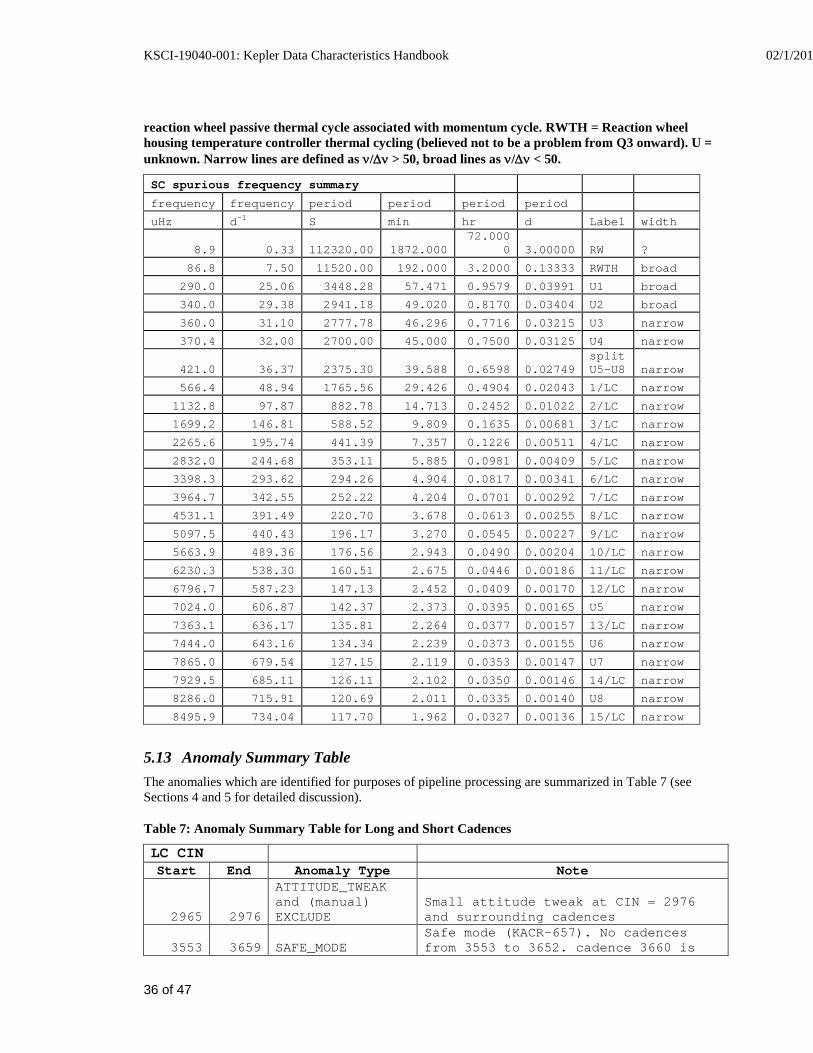
A period of about 3 days has been reported multiple times, and is almost certainly associated with the momentum management cycle and associated temperatures (Figure 9). The list of spurious frequences noted to date in the SC data is given in Table 6.

Table 6: List of Possible Spurious Frequencies in SC data. Users are advised to check detections against this list, and report additional spurious frequencies to the Science Office. Labels: RW =


36 of 47

reaction wheel passive thermal cycle associated with momentum cycle. RWTH = Reaction wheel housing temperature controller thermal cycling (believed not to be a problem from Q3 onward). U = unknown. Narrow lines are defined as ν/∆ν > 50, broad lines as ν/∆ν < 50.

SC spurious frequency summary

frequency frequency period period period period

uHz d-1 S min hr d Label width

8.9 0.33 112320.00 1872.000 72.000

0 3.00000 RW ?

86.8 7.50 11520.00 192.000 3.2000 0.13333 RWTH broad

290.0 25.06 3448.28 57.471 0.9579 0.03991 U1 broad

340.0 29.38 2941.18 49.020 0.8170 0.03404 U2 broad

360.0 31.10 2777.78 46.296 0.7716 0.03215 U3 narrow

370.4 32.00 2700.00 45.000 0.7500 0.03125 U4 narrow

421.0 36.37 2375.30 39.588 0.6598 0.02749 split U5-U8 narrow

566.4 48.94 1765.56 29.426 0.4904 0.02043 1/LC narrow

1132.8 97.87 882.78 14.713 0.2452 0.01022 2/LC narrow

1699.2 146.81 588.52 9.809 0.1635 0.00681 3/LC narrow

2265.6 195.74 441.39 7.357 0.1226 0.00511 4/LC narrow

2832.0 244.68 353.11 5.885 0.0981 0.00409 5/LC narrow

3398.3 293.62 294.26 4.904 0.0817 0.00341 6/LC narrow

3964.7 342.55 252.22 4.204 0.0701 0.00292 7/LC narrow

4531.1 391.49 220.70 3.678 0.0613 0.00255 8/LC narrow

5097.5 440.43 196.17 3.270 0.0545 0.00227 9/LC narrow

5663.9 489.36 176.56 2.943 0.0490 0.00204 10/LC narrow

6230.3 538.30 160.51 2.675 0.0446 0.00186 11/LC narrow

6796.7 587.23 147.13 2.452 0.0409 0.00170 12/LC narrow

7024.0 606.87 142.37 2.373 0.0395 0.00165 U5 narrow

7363.1 636.17 135.81 2.264 0.0377 0.00157 13/LC narrow

7444.0 643.16 134.34 2.239 0.0373 0.00155 U6 narrow

7865.0 679.54 127.15 2.119 0.0353 0.00147 U7 narrow

7929.5 685.11 126.11 2.102 0.0350 0.00146 14/LC narrow

8286.0 715.91 120.69 2.011 0.0335 0.00140 U8 narrow

8495.9 734.04 117.70 1.962 0.0327 0.00136 15/LC narrow

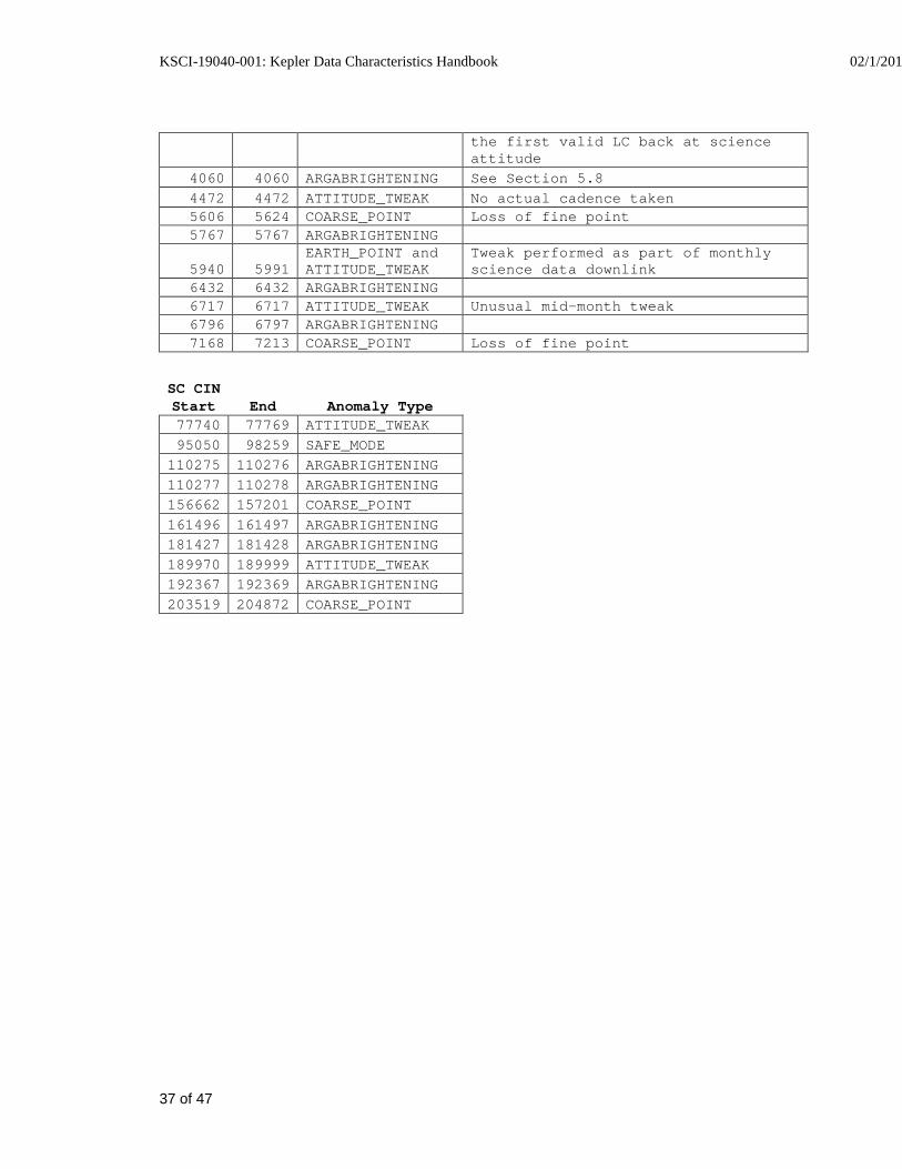
5.13 Anomaly Summary Table The anomalies which are identified for purposes of pipeline processing are summarized in Table 7 (see Sections 4 and 5 for detailed discussion).

Table 7: Anomaly Summary Table for Long and Short Cadences

LC CIN Start End Anomaly Type Note

2965 2976

ATTITUDE_TWEAK and (manual) EXCLUDE

Small attitude tweak at CIN = 2976 and surrounding cadences

3553 3659 SAFE_MODE Safe mode (KACR-657). No cadences from 3553 to 3652. cadence 3660 is


37 of 47

the first valid LC back at science attitude

4060 4060 ARGABRIGHTENING See Section 5.8 4472 4472 ATTITUDE_TWEAK No actual cadence taken 5606 5624 COARSE_POINT Loss of fine point 5767 5767 ARGABRIGHTENING

5940 5991 EARTH_POINT and ATTITUDE_TWEAK

Tweak performed as part of monthly science data downlink

6432 6432 ARGABRIGHTENING 6717 6717 ATTITUDE_TWEAK Unusual mid-month tweak 6796 6797 ARGABRIGHTENING 7168 7213 COARSE_POINT Loss of fine point

SC CIN Start End Anomaly Type 77740 77769 ATTITUDE_TWEAK 95050 98259 SAFE_MODE

110275 110276 ARGABRIGHTENING 110277 110278 ARGABRIGHTENING 156662 157201 COARSE_POINT 161496 161497 ARGABRIGHTENING 181427 181428 ARGABRIGHTENING 189970 189999 ATTITUDE_TWEAK 192367 192369 ARGABRIGHTENING 203519 204872 COARSE_POINT


38 of 47

6. Time and Time Stamps 6.1 Overview The arrow of time moves in one direction – and hopefully so does our understanding of the Kepler time stamps. This section will continue to be updated as improvements are identified. The primary time stamps available for each cadence in both LC and SC time series provide barycentric corrected times at the mid-point of the cadence. This is the temporal coordinate that the majority of science users will want to use. The quoted times for any cadence are accurate to within ±50 ms. This requirement was developed so that knowledge of astrophysical event times would be limited by the characteristics of the event, rather than the characteristics of the flight system, even for high SNR events. Users who require temporal accuracy of better than 1 minute should read this section carefully.

6.2 Time Transformations, VTC to BKJD 6.2.1 Vehicle Time Code The readout time for each recorded cadence is recorded as a Vehicle Time Code (VTC). This timestamp is produced within 4 ms of the readout of the last pixel of the last frame of the last time slice (see below).

When the data is downloaded to Earth, the Mission Operations Center converts VTC to Coordinated Universal Time (UTC), correcting for leap seconds and any drift in the spacecraft clock, as measured from telemetry.

6.2.2 Barycentric Corrections UTC times are converted to Barycentric Dynamical Time (TDB) then corrected for the motion of the spacecraft around the centre of mass of the solar system. Times so corrected are known as Barycentric Julian Dates (BJD). The amplitude of the barycentric correction is approximately (aK/c) cos β, where aK ~ 1.02 AU is the semi-major axis of Kepler's approximately circular (eK < 0.04) orbit around the Sun, c the speed of light, and β is the ecliptic latitude of the target. In the case of the center of the Kepler FOV, with β = 65 degrees, the amplitude of the UTC to barycentric correction is approximately ±211 s. For any given cadence the correction varies widely in amplitude and phase over the field of view, and is therefore calculated individually for each target, for each cadence. BJD is later than UTC when Kepler is on the half of its orbit closest to Cygnus (roughly May 1 - Nov 1) and earlier than UTC on the other half of the orbit.

6.2.3 Time slice offsets The readout of different modules is staggered in time as described in Section 5.1 of the Kepler Instrument Handbook. Most modules have a readout time that is a 0.25-3.35 seconds before the recorded timestamp for the cadence. The magnitude of this difference, known as the time slice offset, is given by

tts = 0.25 + 0.62(5 - nslice) seconds,

where nslice is the module's time slice index. The (module dependent) value for nslice is given in Figure 34 of the Instrument Handbook, and it is also provided in the FITS headers for each target. This value is included in BJD times seen by the end user. Because of the quarterly rotation of the spacecraft, a target will lie on a different module each quarter, and is likely to have a different time slice offset from quarter to quarter.


39 of 47

6.2.4 Barycentric Kepler Julian Date The contemporary value of BJD (~2.5 million days) is too large to be stored with milli-second precision in an eight byte, double precision, floating point number1

6.3 Caveats and Uncertainties

. To compensate, in the target pixel files, Kepler reports the value of BJD-2454833.0. This time system is referred to as Barycentric Kepler Julian Date (BKJD). The offset is equal to the value of JD at midday on 2009-01-01. BKJD has the added advantage that it is only used for corrected dates, so it is more difficult to confuse BKJD dates with uncorrected JD or MJD. In the light curve files, the Barycentric Reduced Julian Date (BRJD, BJD-2400000.0) is reported. Revisions to the light curve keywords are in progress.

Factors that users should consider before basing scientific conclusions on time stamps include:

1. The existing corrections have yet to be verified with flight data.

2. When comparing Kepler data to data from other sources, users should take care that they are comparing times from the same systems.

6.4 Times in MAST FITS files 6.4.1 Target Pixels The following keywords, found in the header of a target pixel file, relate to time. The comment for the keyword TIMESYS may be confusing; see Section 6.2.2 for clarification. TIMEREF = 'SOLARSYSTEM' / barycentric correction applied to times TASSIGN = 'SPACECRAFT' / where time is assigned TIMESYS = 'TDB ' / time system is barycentric JD BJDREFI = 2454833 / integer part of BJD reference date BJDREFF = 0.00000000 / fraction of the day in BJD reference date TIMEUNIT= 'd ' / time unit for TIME, TSTART and TSTOP

BJDREFI and BJDREFF refer to the offset needed to convert times in BKJD to JD (see above). DATE-OBS= '2010-03-20T23:32:33' / TSTART a UT calendar date DATE-END= '2010-06-23T16:05:09' / TSTOP a UT calendar date

DATE-OBS and DATE-END contain the UTC date of the start of the first cadence and the end of the last cadence in the file. These dates have the correction for onboard spacecraft clock drift applied. LC_START= 55275.99115492 / observation start time in MJD LC_END = 55370.66003002 / observation stop time in MJD

LC_START and LC_END contain the Modified Julian Date (MJD = JD-2400000.5) of the mid-time of the first and last exposure. Note that the comments for these fields are misleading, and the times refer to the mid-times of cadences, not the start and end. TIMESYS = 'TDB ' / time system is barycentric JD TSTART = 443.47928144 / observation start time in BJD-BJDREF TSTOP = 538.17221987 / observation stop time in BJD-BJDREF

TSTART and TSTOP contain the barycentric corrected time of the start of the first exposure, and end of the last exposure. TDB is a time system that does not include the leap seconds that bedevil calculations of periods in the UTC system. TDB agrees with the time systems TDT and TT to better than 2ms at all times. See Ref. 20 for a recent discussion of the various time systems common in astronomy.

1 This is not quite true. JD (and BJD) can be stored to millisecond precision in a double precision value, but any calculations will have unacceptably large rounding errors.


40 of 47

Column 1 of the binary table in the first FITS extension is labeled TIME. The value in this field represents the (barycentric corrected) BKJD mid-time of each cadence. BJD can be calculated from the formula2

BJD[i] = TIME[i] + BJDREFI + BJDREFF

= TIME[i] + 2454833.0

Column 2 is labeled TIMECORR. This column contains the combination of the applied barycentric correction, and the time slice offset correction. Subtracting the value of TIMECORR from BJD gives the Julian Date of the cadence time stamp. However, the mid-time of the cadence for this particular target may be earlier than cadence time stamp because of the time slice offset correction. The Julian Date (JD) of the mid-time of the cadence for this target should be calculated by

JD[i] = BJD[i] - TIMECORR[i] + time_slice_correction

= BJD[i] - TIMECORR[i] + (0.25 + 0.62(5- nslice))/secondsPerDay

where secondsPerDay = 86400.0, and nslice can be found by referring to Fig. 34 of the Instrument Handbook.

6.4.2 Light Curves The header of a lightcurve file currently contains less detail than a target pixel file. LC_START= 54998.518332653446 / start of time series (UTC MJD days) LC_END = 55001.56293878777 / end of time series (UTC MJD days)

LC_START and LC_END contain the MJD of the mid-time of the first and last exposure. Note that the comments for these fields are misleading, and the times refer to the mid-times of cadences, not the start and end times. COMMENT STARTBJD is the the UTC time in Julian Date - 2400000 at the mid-point COMMENT of the first cadence of the time series. It is barycentric corrected. COMMENT ENDBJD is the UTC time in Julian Date - 2400000 at the mid-point of the COMMENT last cadence of the time series. It is barycentric corrected. STARTBJD= 54999.02038774057 / barycentric start (JD - 2400000 days) ENDBJD = 55002.06510106966 / barycentric end (JD - 2400000 days) STARTBJD and ENDBJD contain the barycentric corrected time of the start of the first exposure, and end of the last exposure. The comments are incorrect: barycentric times are calculated in TDB, not UTC. Note that these keywords are given in units of BRJD, not Barycentric Modified Julian Date. Revisions to the light curve keywords are in progress.

2 Performing this calculation in code is not advised unless you understand how computers store floating point numbers, as you may lose a critical level of timing precision.


41 of 47

7. Contents of Supplement The supplemental files discussed throughout Sections 3-5 are summarized here in a general way. The files describe Q[q] M[m] Release [r] data, which can be found attached to the relevant Data Release Notes.

7.1 Pipeline Instance Detail Reports These files list the Pipeline version and parameters used to process the data, so that the Pipeline results in a given Release can be reconstructed precisely at some future time. Multiple files for the same data set are needed if the Pipeline needs to be re-run from a particular step, or to process anomalous modules (like mod 3 in Q4) separately. Typical file names are:

Q4M1_SC_Mod3_pa_pdc_pipeline_instance_report_100527.txt

Q4M1_SC_excludeMod3_pipeline_instance_report_100526.txt

Q4M2_SC_r6.1_ksop479_pre-run_Trigger_Report_100609.txt

Q4M3_SC_r6.1_exclude_mod3_KSOP-479-Instance-Detail_Report_100603.txt

Q4_LC_excludeMod3_cal_pipeline_instance_report_100520.txt

Q4_LC_excludeMod3_pa_pdc_pipeline_instance_report_100522.txt

Q4_SC_Mod3_cal_pipeline_instance_report_100525.txt

7.2 Data for Systematic Error Correction These files are provided so that users can perform their own systematic error correction, if they conclude that the methods used by PDC are not suitable for their targets and scientific goals (see Prefatory Admonition, page 7). It is important to remember that inclusion of additional time series to the cotrending basis set may not improve the results if the cotrending time series are noisy, poorly sampled, or nearly degenerate. The thermal AED (ancillary engineering data) will, in general, have to be resampled to match the Cadence times, and on physical grounds it may be more effective to cotrend against bandpass-filtered AED as separate basis vectors. See the SPIE PDC paper (Ref. 5) for a brief discussion of synchronizing ancillary data to mid-Cadence timestamps, and the use of synchronized AED as a cotrending basis set.

7.2.1 Mod.out Central Motion On rare occasions (<2% of the points), users may notice some “chatter” in the motion time series, which results from a known problem with the motion polynomial fitting algorithm and not actual jumps in telescope attitude or CCD position. A more robust, iterative algorithm has been identified and will be implemented in future Pipeline software to remedy this problem. Users will also clearly see differential velocity aberration and the signatures of the variable FGS guide stars (Section 4.4) and the reaction wheel heaters (Section 5.4) in the motion time series.

Files: Q[q]-MAST-R[r]_central_column_motion.txt and Q[q]-MAST-R[r]_central_row_motion.txt – These files are the channel central column motion and central row motion from motion polynomials for all channels, sampled at the Long Cadence period.

Column Descriptions

1. Cadence Interval Number

2. Relative Cadence Index

3. Gap Indicator. 1 = Momentum Dump or Loss of Fine Point

4. Cadence mid-Times, MJD


42 of 47

5-88. Mod.out center column (row) for each channel. Units: pixels.

Q[q]-MAST-R[r]_central_motion.mat – This is the MATLAB file containing both row and column motion; this will spare MATLAB users the drudgery of parsing the text files.

7.2.2 Average LDE board Temperature The file Q[q]_LDE_averageBoardTemp.txt contains the average of the ten LDE board temperatures.

Column descriptions:

1. MJD - 55000, units: d, sampling 6.92E-04 d = 59.75 s

2. Average temperature, units: C

7.2.3 Reaction Wheel Housing Temperature The file Q[q]_TH1RW34T_MJD_gap.txt contains the reaction wheel housing temperature. Data are gapped for desats and median-filtered with a box width = 5 samples.

Column definitions:

1. MJD, units: d, sampling (unfiltered) = 58.0 s

2. TH1RW3T – units: C

3. TH1RW4T – units: C

7.2.4 Launch Vehicle Adapter Temperature The file Q[q]_TH12LVAT_MJD_gap.txt contains the Launch Vehicle Adapter Temperature. Data are gapped for desats and median-filtered with a box width = 5 samples.

Column definitions:

1. MJD – 55000, units: d, sampling (unfiltered) = 58.0 s

2. TH1LVAT – units: C

3. TH2LVAT – units: C

7.3 Background Time Series The background time series provide the median calibrated background pixel value on a given mod.out and Cadence. For LC, the background pixels are the dedicated background pixel set. For SC, the background pixels are the target pixels which are not in the optimal apertures. These values are calculated directly from the pixel sets, not from the Pipeline-derived background polynomials.

Q[q]-LC-MAST-R[r]_background.txt

Q[q]M1-SC_background.txt



Column definitions:

1. Cadence Interval Number.

2. Relative Cadence Index for Argabrightening Cadences.

3. Gap Indicator. 1 = No Data, Momentum Dump, or Loss of Fine Point.

4. Cadence mid-Times, MJD.


43 of 47

5. Median background current averaged over FPA, e-/Cadence. All zeros = no SC targets.

6-89. Mod.out background in e-/Cadence for each channel.

Corresponding MATLAB files are provided to spare MATLAB users the drudgery of parsing the text files.

7.4 Flight System Events

ArgAgg_Q[q]-R[r]_LC_PID1676_MADT010_MCT10_Summary.txt

Argabrightening Detections

ArgAgg_Q[q]M1-R[r]_SC_PID1756_MADT010_MCT10_Summary.txt



Column Definitions:

1. Cadence Interval Number for Argabrightening Cadences

2. Relative Cadence Index for Argabrightening Cadences

3. Arg Cadence mid-Times, MJD

4. Mean SNR over Channels of Arg Event

5. Channels exceeding threshold in Arg Cadence

6. Channels exceeding default threshold in ArgCadence

Q[q]M1_SC_isNotFinePoint.txt

Out of Fine Point Cadence Lists



Q[q]_LC_isNotFinePoint.txt

7.5 Calibration File READMEs The calibration file names are not listed in the headers of the light curves and target pixel files. The calibration file names listed in the FITS headers of Cadence files and FFIs are not all correct. The README files for the calibration files actually used for all releases to date are:

kplr2008072318_gain.readme.txt

kplr2008102416_read-noise.readme.txt

kplr2008102809_undershoot.readme.txt

kplr2009060215_linearity_readme.txt

kplr2009060615-mmo_2d-black.readme.txt

kplr2009062300_lsflat.readme.txt

kplr2009062414-MMO_ssflat.readme.txt

They are supplied with the early Data Release Notes Supplements, up to Release 8.


44 of 47

7.6 Supplement package descriptions The Supplement is available as a full package (DataReleaseNotes_qq_SupplementFull.tar) and a short package suitable for emailing (DataReleaseNotes_qq_SupplementSmall.tar). The small package does not contain the following files:




Q[q]-LC-MAST-R[r]_background.txt

Q[q]-MAST-R[r]_central_column_motion.txt

Q[q]-MAST-R[r]_central_row_motion.txt

Q[q]_TH12LVAT_MJD_gap.txt

Q[q]_TH1RW34T_MJD_gap.txt


45 of 47

8. References

1. “Initial Assessment Of The Kepler Photometeric Precision,” W.J. Borucki, NASA Ames Research Center, J. Jenkins, SETI Institute, and the Kepler Science Team (May 30, 2009)

2. “Kepler’s Optical Phase Curve of the Exoplanet HAT-P-7,” W. J. Borucki et al., Science Vol 325 7 August 2009 p. 709

3. “Pixel Level Calibration in the Kepler Science Operations Center Pipeline,” E. V. Quintana et al., SPIE Astronomical Instrumentation conference, June 2010.

4. “Photometric Analysis in the Kepler Science Operations Center Pipeline,” J. D. Twicken et al., SPIE Astronomical Instrumentation conference, June 2010.

5. “Presearch Data Conditioning in the Kepler Science Operations Center Pipeline,” J. D. Twicken et al., SPIE Astronomical Instrumentation conference, June 2010.

6. Dave Monet, private communication.

7. “Initial Characteristics of Kepler Long Cadence Data for Detecting Transiting Planets,” J. M. Jenkins et al., ApJ Letters 713, L120-L125 (2010)

8. “Initial Characteristics of Kepler Short Cadence Data,” R. L. Gilliland et al., ApJ Letters 713, L160-163 (2010)

9. “Overview of the Kepler Science Processing Pipeline,” Jon M. Jenkins et al., ApJ Letters 713, L87-L91 (2010)

10. “Discovery and Rossiter-McLaughlin Effect of Exoplanet Kepler-8b,” J. M. Jenkins et al., submitted to ApJ ://arxiv.org/abs/1001.0416

11. “Kepler Mission Design, Realized Photometric Performance, and Early Science,” D. Koch et al., ApJ Letters 713, L79-L86 (2010)

12. “Selection, Prioritization, and Characteristics of Kepler Target Stars,” N. Batalha et al., ApJ Letters 713, L109-L114 (2010)

13. “Kepler Science Operations,” M. Haas et al., ApJ Letters 713, L115-L119 (2010)

14. “The Kepler Pixel Response Function,” S. Bryson et al., ApJ Letters 713, L97-L102 (2010)

15. “Instrument Performance in Kepler’s First Months,” D. Caldwell et al., ApJ Letters 713, L92-L96 (2010)

16. “Selecting Pixels for Kepler Downlink,” S. Bryson et al., SPIE Astronomical Instrumentation conference, June 2010.

17. “Achieving Better Than One-Minute Accuracy In The Heliocentric And Barycentric Julian Dates,” Jason Eastman, Robert Siverd, B. Scott Gaudi, submitted to ApJ ://arxiv.org/abs/1005.4415v2

18. “Diffuse Brightening of the Kepler Field: the Case for Impact-Generated Debris,” F. Witteborn, J. Van Cleve, and W. Borucki, in preparation.

19. “Correcting Systematic Effects in a Large Set of Photometric Light Curves,” O. Tamuz, T. Mazeh, and S. Zucker, MNRAS 356, 1466 (2005).

20. “Achieving Better Than 1 Minute Accuracy in the Heliocentric and Barycentric Julian Dates,” J. Eastman, R. Siverd, B. S. Gaudi, PASP, 122, 953 (2010).

http://arxiv.org/abs/1001.0416�

http://arxiv.org/abs/1005.4415v2�


46 of 47

9. List of Acronyms and Abbreviations ADCS Attitude Determination and Control Subsystem AED Ancillary Engineering Data ARG Argabrightening BATC Ball Aerospace & Technologies Corp. BJD Barycentric Julian Date BKJD Barycentric Kepler Julian Date BRJD Barycentric Reduced Julian Date CAL Calibration (pipeline software) CCD Charge Coupled Device CDPP Combined Differential Photometric Precision CR Cosmic Ray DAWG Data Analysis Working Group DV Data Validation (pipeline software) DVA Differential Velocity Aberration FFI Full Field Image FGS Fine Guidance Sensor FOV Field of View FPA Focal Plane Assembly GO Guest Observer HGA High-Gain Antenna JD Julian Date KACR Kepler Activity Change Request (project-wide tracking system for

operations) KAR Kepler Anomaly Report (project-wide tracking system for anomalies) KSOP Kepler Science OPerations (tracking system for SOC operations) LC Long Cadence LDE Local Detector Electronics LV Launch Vehicle MAD Median Absolute Deviation MAST Multi-mission Archive at STSci MJD Modified Julian Date = JD - 2400000.5 PA Photometric Analysis (pipeline software) PAD Photometer Attitude Determination (pipeline software) PDC Pre-search Data Conditioning (pipeline software) PID Pipeline instance IDentifier (unique number assigned to each run of the

Pipeline) PPA Photometer Performance Assessment (pipeline software) ppm parts per million PRF Pixel Response Function SC Short Cadence


47 of 47

SNR Signal-to-Noise Ratio SO Science Office SOC Science Operations Center STScI Space Telescope Science Institute SVD Singular Value Decomposition TDB Barycentric Dynamical Time TDT Terrestrial Dynamical Time TPS Transiting Planet Search (pipeline software) TT Terrestrial Time UTC Coordinated Universal Time VTC Vehicle Time Code

Kepler: A Search for Terrestrial Planets

Documents

Transcript of Kepler: A Search for Terrestrial Planets