A&A 630, A126 (2019)https://doi.org/10.1051/0004-6361/201936126c© ESO 2019

Astronomy&Astrophysics

Revisiting Kepler-444

I. Seismic modeling and inversions of stellar structure

G. Buldgen1, M. Farnir2, C. Pezzotti1, P. Eggenberger1, S. J. A. J. Salmon2, J. Montalban3, J. W. Ferguson4,S. Khan3, V. Bourrier1, B. M. Rendle3, G. Meynet1, A. Miglio3, and A. Noels2

1 Observatoire de Genève, Université de Genève, 51 Ch. Des Maillettes, 1290 Sauverny, Switzerlande-mail: gael.buldgen@unige.ch

2 STAR Institute, Université de Liège, Allée du Six Août 19C, 4000 Liège, Belgium3 School of Physics and Astronomy, University of Birmingham, Edgbaston, Birmingham B15 2TT, UK4 Department of Physics, Wichita State University, Wichita, KS 67260-0032, USA

Received 18 June 2019 / Accepted 23 July 2019

ABSTRACT

Context. The CoRoT and Kepler missions have paved the way for synergies between exoplanetology and asteroseismology. The useof seismic data helps providing stringent constraints on the stellar properties which directly impact the results of planetary studies.Amongst the most interesting planetary systems discovered by Kepler, Kepler-444 is unique by the quality of its seismic and classicalstellar constraints. Its magnitude, age and the presence of 5 small-sized planets orbiting this target makes it an exceptional testbed forexoplanetology.Aims. We aim at providing a detailed characterization of Kepler-444, focusing on the dependency of the results on variations ofkey ingredients of the theoretical stellar models. This thorough study will serve as a basis for future investigations of the planetaryevolution of the system orbiting Kepler-444.Methods. We use local and global minimization techniques to study the internal structure of the exoplanet-host star Kepler-444. Wecombine seismic observations from the Kepler mission, Gaia DR2 data, and revised spectroscopic parameters to precisely constrainits internal structure and evolution.Results. We provide updated robust and precise determinations of the fundamental parameters of Kepler-444 and demonstrate thatthis low-mass star bore a convective core during a significant portion of its life on the main sequence. Using seismic data, we are ableto estimate the lifetime of the convective core to approximately 8 Gyr out of the 11 Gyr of the evolution of Kepler-444. The revisedstellar parameters found by our thorough study are M = 0.754 ± 0.03 M�, R = 0.753 ± 0.01 R�, and Age = 11 ± 1 Gyr.

Key words. stars: interiors – stars: fundamental parameters – asteroseismology – stars: oscillations – planetary systems

1. IntroductionWith the advent of space-based photometry missions such asCoRoT (Baglin et al. 2009), Kepler (Borucki et al. 2010)and TESS (Ricker et al. 2015), and with the future launch ofthe PLATO mission (Rauer et al. 2014), asteroseismology hasbeen established as a standard discipline to derive fundamentalstellar properties. These capabilities led naturally to synergiesbetween stellar seismologists and exoplanetologists, as planetarydetections almost exclusively use stellar-dependent approaches.Consequently, a better characterization of the host star also sig-nificantly improves the accuracy and precision of the derivedplanetary parameters.

Good examples of such synergies are found in Christensen-Dalsgaard et al. (2010), Batalha et al. (2011), Huber et al.(2013a,b), Huber (2018), and Campante et al. (2018), where theuse of stellar seismology can be seen as a key component ofthe studies of the planetary system. Moreover, the importance ofstellar evolution for planets is not only limited to the determina-tion of stellar fundamental parameters, but also to the dynamicalevolution of planetary systems and the potential evaporation ofplanetary atmospheres. In this context, understanding transportproperties of both angular momentum and chemical elements iscrucial, as transport affects rotation, which affects activity, whichin turn alters the planetary properties.

In this study, we revisit one of the most well-known planet-host stars for which a detailed seismic characterization has beencarried out by Campante et al. (2015), Kepler-444 (also iden-tified as HIP 94931, KIC 6278762, KOI-3158, and LHS 3450).Kepler-444 has been extensively studied in recent years, withattempts to put upper limits on the planetary masses and den-sities to constrain the formation history of the system (Dupuyet al. 2016; Mills & Fabrycky 2017; Hadden & Lithwick 2017).It is composed of five small planets, orbiting within 0.1 AU oftheir host star with periods shorter than 10 days. Their estimateddensities imply the presence of volatile elements and the factthat they transit a luminous star (MG = 8.64, with MG being themean photometric magnitude of Gaia in G-band as described inEvans et al. 2018) make them excellent targets for in-depth atmo-spheric characterization. Such tightly packed planetary systemsare particularly interesting in terms of formation history; somestudies suggest that such systems should form locally, whilethe low density of some of these planets, especially in the caseof Kepler-444 argues in favor of a formation scenario wherethe two outermost planets form behind the snowline followedby a migration phase (Mills & Fabrycky 2017). Kepler-444 ishowever rather specific as the star is a triple system with apair of spatially unresolved M-dwarf companions (Campanteet al. 2015; Dupuy et al. 2016) which could have influenced the

Article published by EDP Sciences A126, page 1 of 11

A&A 630, A126 (2019)

protoplanetary disk (Kraus et al. 2016; Hirsch et al. 2017; Bazsóet al. 2017). From a planetary perspective, Kepler-444 is notunique, as many other such systems have already been observedand studied to characterize the correlation between low stellarmetallicity and the occurrence of multi-planet systems (Hobson& Gomez 2017; Brewer et al. 2018). These systems of packed,small, inner-planets are also of particular interest as they mayexhibit tidally stressed plate tectonics (Zanazzi & Triaud 2019).

In addition, Kepler-444 is of particular interest to study theatmospheric properties of exoplanets close to their host stars.Recently, Bourrier et al. (2017) detected a strong variation ofthe HI Ly−α signal during transiting and nontransiting periodsof the system. These strong variations could either be due to stel-lar variability or to the presence of a strong hydrogen exospherearound the two outermost exoplanets. The hypothesis of stellaractivity, although supported by the presence of variations dur-ing a nontransiting period, is still unlikely given the old age ofthe star. However, increased stellar activity would of course alsohave dramatic consequences for the evaporation of the planetaryatmospheres and could be of importance when studying othercompact systems. Meanwhile, confirmation of the planetary ori-gin of the signal would imply that Kepler-444e and Kepler-444fcould be the first known ocean planets with vast amounts ofwater at their surface capable of replenishing a hydrogen richexosphere, itself capable of reproducing the strong HI Ly−αvariations (Bourrier et al. 2017).

In this first study, we rather focus on the details of the stel-lar seismic modeling, for example the variations of the transportof chemicals, opacity and abundance tables. We use the recentlypublished Gaia parallaxes (Gaia Collaboration 2016, 2018) aswell as revised spectroscopic parameters of Kepler-444 and dis-cuss their impact on the stellar fundamental parameters. Wecarry out seismic inversions of the stellar mean density follow-ing Reese et al. (2012), Buldgen et al. (2015a, 2018). Section 2lays out the seismic and classical constraints used in the forwardmodeling, the minimization strategy as well as the model prop-erties and the various physical ingredients that have been testedin our study. Section 3 presents the results of mean density inver-sions applied to Kepler-444 and discusses the model-dependencyand the impact of various surface corrections. Section 4 dis-cusses the details of the core conditions of the star, namely thesurvival of a convective core during an extended portion of themain sequence. Section 5 summarizes our results and discussesfuture studies of Kepler-444 and their potential impact in thecontext of the TESS (Ricker et al. 2015) and PLATO missions(Rauer et al. 2014).

Our future studies will use these results to model of Kepler-444 including transport processes of angular momentum fol-lowing the prescriptions for magnetic instabilities used byEggenberger et al. (2010). These models will then be used toconstrain the dynamical evolution of the planetary system, usingapproaches of Privitera et al. (2016a,b,c), Meynet et al. (2017)and including the effects of dynamical tides following Rao et al.(2018).

2. Forward modeling

In this section, we discuss the forward modeling proceduresused to study the internal structure of Kepler-444 and determineits fundamental parameters. We used the Liège stellar evolu-tion code (CLES; Scuflaire et al. 2008a) and the Liège stellaroscillation code (LOSC; Scuflaire et al. 2008b) to compute themodels and the adiabatic frequencies used in the modeling pro-cedure both in the AIMS software (Rendle et al. 2019) and in the

Levenberg-Marquardt algorithm as well as in the inversion pro-cedures discussed in Sect. 3. The minimization procedure both inAIMS and in the Levenberg-Marquardt algorithm used four freeparameters, namely mass, age and initial chemical composition(X0 and Z0) of Kepler-444.

The forward modeling of Kepler-444 is carried out using acombination of classical and seismic data. We used the indi-vidual frequencies corrected for the line-of-sight Doppler veloc-ity shifts (see Davies et al. 2014) provided in Campante et al.(2015), which have been obtained from the observations ofKepler-444 during the nominal phase of the Kepler mission. Inaddition, we used the seismic log g value from Campante et al.(2015) and the values for Teff from Campante et al. (2015) andMack et al. (2018). We considered the [Fe/H] and [α/Fe] val-ues from Mack et al. (2018) for the models using α−enrichedabundance tables. For the models using solar-scaled abundancetables, we considered the correction of Salaris et al. (1993) andused [M/H]≈−0.37 ± 0.09 dex, as in Campante et al. (2015)

We carried out the modeling using the metallicity correctionof Salaris et al. (1993) when using solar-scaled abundance tables,and considered both the OPAL opacity tables (Iglesias & Rogers1996) and the more recent OPLIB opacity tables (Colgan et al.2016) to test the dependence of the modeling results in the opac-ity tables. We also used adequately α−enriched abundance tablesand their corresponding OPAL opacity tables (Iglesias & Rogers1996). In all cases, we included low temperature opacities ofFerguson et al. (2005) as well as the effects of conduction fol-lowing Potekhin et al. (1999), Cassisi et al. (2007).

In addition to these parameters, we determined the luminos-ity from the parallax values given in the second Gaia data release(Gaia Collaboration 2016, 2018). The luminosity was computedas follows

log(

LL�

)= −0.4 ×

(mλ + BCλ − 5 × log d + 5 − Aλ − Mbol,�

),

(1)

where mλ, BCλ, and Aλ are the magnitude, bolometric correc-tion, and extinction in a given band λ, d is the distance, and weadopt Mbol,� = 4.75 for the bolometric magnitude of the Sun.We use the 2MASS K-band magnitude properties: the bolomet-ric correction is derived using the code written by Casagrande& VandenBerg (2014, 2018a,b), while the extinction is inferredvia the Green et al. (2018) dust map. We obtain the distance intwo ways: by inverting the Gaia parallax or using the distancepublished by Bailer-Jones et al. (2018). Because the relative par-allax error is very small for Kepler-444, the parallax inversiondoes not introduce any significant bias in the computation ofthe distance. This is why, in both cases, we obtain a similarvalue for the luminosity: L ≈ 0.39 ± 0.02 L�, which is at theverge of perfect agreement with the value derived from the Hip-parcos parallax of L ≈ 0.37 ± 0.03 L� reported in Campanteet al. (2015). Considering the revised spectroscopic parametersof Mack et al. (2018), the luminosity derived from the Gaia datais L ≈ 0.417±0.019 L�. This increase is due to the change in Teff

between the two studies that significantly impacts the bolomet-ric correction, BCλ. Indeed, Mack et al. (2018) provide a valueof Teff = 5172 ± 75 K, whereas Campante et al. (2015) deriveda value of 5046 ± 74 K. Considering one or the other luminos-ity value with its nominal uncertainties may impact the modelcharacteristics. Here, we make a compromise between the twostudies by choosing a value of 0.40±0.04 L� in our modeling, asno comment was made in Mack et al. (2018) regarding their dis-crepancies with Campante et al. (2015) in effective temperature.

A126, page 2 of 11

G. Buldgen et al.: Revisiting Kepler-444. I.

0.72 0.74 0.76 0.78 0.80Mass (M⊙)

9000 10000 11000 12000 13000 14000Age (in Myrs), t

2.40 2.45 2.50 2.55 2.60Density (g.cm−3), ρ

0.73 0.74 0.75 0.76 0.77 0.78Radius, R/R⊙

Fig. 1. Probability distribution functions for the mass (upper left), age(upper right), mean density (lower left), and radius (lower right) forKepler-444, obtained using AIMS. The vertical lines indicate the posi-tion of the best model obtained from a simple scan of the grid.

2.1. Global minimization technique

First, we used the AIMS software (Rendle et al. 2019) to carryout a wide-range exploration of the parameter space using differ-ent constraints for the modeling. AIMS is a global minimizationtool using a Monte Carlo Markov chain (MCMC) approach andBayesian statistics to provide probability distribution functionsfor stellar parameters from a set of observational constraints.The result of one of these runs is illustrated in Fig. 1 for acase where we used the following combination of seismic andclassical constraints: the r0,1 and r0,2 frequency ratios, followingthe definition of Roxburgh & Vorontsov (2003), the luminosity,the effective temperature, the seismic log g, and the [Fe/H]. Wealso included a mean density estimate of 2.495 ± 0.050 g cm−3,using a reference model built with AIMS using the individualfrequencies as constraints and carrying out an initial inversion asin Sect. 3.1. We adopted conservative error bars as no analysisof the model dependencies had been carried out at that stage. Wedid not rely on the results from the run using individual frequen-cies to determine other fundamental parameters of Kepler-444,but rather favored the use of the frequency ratios as they are lesssensitive to the surface effects. The results between the two runswere however compatible within 1.5σ. The model grid, requiredby AIMS to carry out the minimization, was built using theFreeEOS equation of state (Irwin 2012), the OPAL opacities, theAGSS09 abundances (Asplund et al. 2009), the mixing-lengththeory of convection (following Cox & Giuli 1968), and tak-ing into account microscopic diffusion following the approachof the original work done by Thoul et al. (1994), without includ-ing the Paquette et al. (1986) screened potentials. As upperboundary conditions, the models used an Eddington gray atmo-sphere (Eddington 1959).

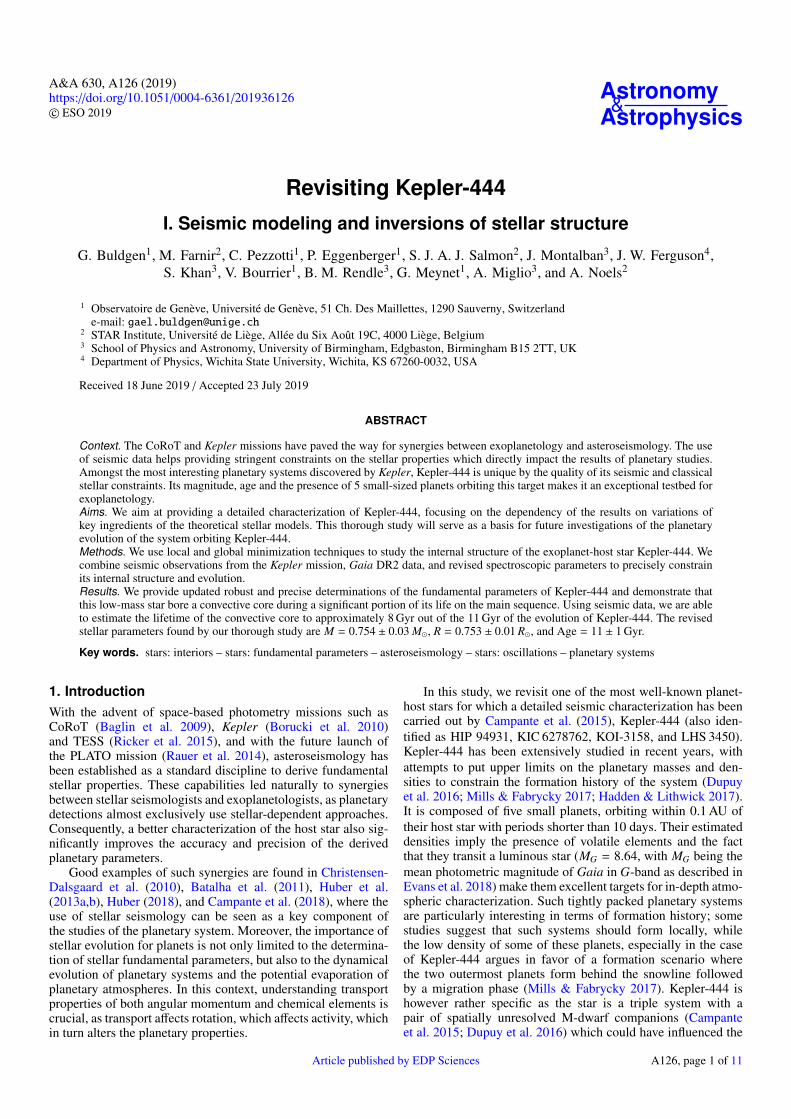
An illustration of the impact of using different observationalconstraints is shown in Fig. 2, where we show the results formodels built using either the individual frequencies or the fre-

50 100 150

3500

4000

4500

5000

5500

Fig. 2. Echelle diagram for Kepler-444. The observational values areplotted in blue while the green and red symbols refer to two referencemodels computed using different seismic constraints. ∆ν is the averagelarge frequency separation (determined here following a least-squarefitting of the individual large frequency separations for all modes).

quency ratios besides the nonseismic parameters listed above.As can be seen, some differences between the model frequen-cies are observed. The model built fitting the individual frequen-cies included the Ball et al. (2016) correction for the surfaceeffects. We plot here the uncorrected frequencies for this modelto illustrate the impact of the surface correction at the higherfrequencies. The amplitude of the empirical surface correctionis actually much larger than the observational uncertainties onthe individual frequencies themselves. The model built using thefrequency ratios does not show the same behavior, but shows aslightly worse agreement at low frequencies.

However, both models have similar fundamental parame-ters. The main difference is in the estimated precision of theseparameters. Using the individual frequencies as direct constraintsimproves the precision by a factor 2.5 compared to that obtainedwhen using the frequency ratios. Similar effects were seen inRendle et al. (2019) when testing AIMS on theoretical mod-els and on the Sun. In practice, such precision is unrealistic asthe individual frequencies are strongly affected by the surfacecorrections. Moreover, from a theoretical point of view, eachfrequency does not provide independent information on the inter-nal structure of the star as the link between pulsation frequenciesand the internal structure of a star can be expressed using only afew parameters1. Consequently, directly using them as constraintsin a stellar model selection procedure will lead to an overesti-mated precision on the inferred stellar model parameters. As wesee below, changing the physical ingredients may lead to modifi-cations of the fundamental parameters at a non-negligible order ofmagnitude with respect to the precision of inferences from Kepler

1 Typically, seismic indices such as the large and small frequency sep-aration for pressure modes or the period spacing for gravity modes willprovide the link between seismic data and stellar stucture in the asymp-totic regime.

A126, page 3 of 11

A&A 630, A126 (2019)

Table 1. Parameters of the models of Kepler-444 computed in this study.

Name Mass (M�) Radius (R�) Age (Gyr) X0 Z0 EOS Opacity Abundances Diffusion Convection Atmosphere

Model1 0.752 ± 0.019 0.748 ± 0.006 11.57 ± 0.59 0.747 0.0082 FreeEOS OPAL AGSS09 Thoul MLT EddingtonModel2 0.756 ± 0.017 0.754 ± 0.006 11.39 ± 0.48 0.733 0.0116 FreeEOS OPAL GN93 Thoul MLT EddingtonModel3 0.751 ± 0.018 0.752 ± 0.006 11.53 ± 0.61 0.742 0.0083 OPAL OPAL AGSS09 Thoul MLT EddingtonModel4 0.756 ± 0.021 0.754 ± 0.007 11.68 ± 0.62 0.745 0.0085 CEFF OPAL AGSS09 Thoul MLT EddingtonModel5 0.742 ± 0.019 0.749 ± 0.006 11.42 ± 0.47 0.748 0.0083 FreeEOS OPLIB AGSS09 Thoul MLT EddingtonModel6 0.737 ± 0.020 0.752 ± 0.007 11.72 ± 0.53 0.742 0.0074 FreeEOS OPAL AGSS09 Thoul CM EddingtonModel7 0.747 ± 0.017 0.749 ± 0.006 11.20 ± 0.44 0.750 0.0073 FreeEOS OPAL AGSS09 Thoul MLT Krishna SwamyModel8 0.746 ± 0.019 0.750 ± 0.006 11.66 ± 0.60 0.746 0.0079 FreeEOS OPAL AGSS09 Thoul MLT VAL-CModel9 0.747 ± 0.018 0.746 ± 0.006 11.73 ± 0.54 0.741 0.0084 FreeEOS OPAL AGSS09 Paquette MLT EddingtonModel10 0.750 ± 0.022 0.746 ± 0.007 11.72 ± 0.62 0.745 0.0082 FreeEOS OPAL AGSS09 Paquette + PartIon MLT EddingtonModel11 0.750 ± 0.019 0.751 ± 0.006 11.16 ± 0.55 0.743 0.0076 FreeEOS OPAL AGSS09 + [α/Fe] = 0.2 Paquette + PartIon MLT EddingtonModel12 0.753 ± 0.018 0.752 ± 0.006 11.13 ± 0.57 0.746 0.0076 FreeEOS OPAL AGSS09 + [α/Fe] = 0.3 Paquette + PartIon MLT EddingtonModel13 0.755 ± 0.020 0.753 ± 0.007 10.95 ± 0.61 0.750 0.0069 FreeEOS OPAL AGSS09 + [α/Fe] = 0.2 Paquette + PartIon MLT + OV Eddington

data. This casts some doubt on the level of precision announcedby the modeling of the individual frequencies.

This first step of modeling using AIMS allowed us to derivea limited subspace of stellar parameters on which additionalinvestigations can then be attempted with local minimizationtechniques. Therefore, to fully explore the dependences of thederived stellar parameters on the model input physics, we car-ried out an additional exploration of the parameter space usinga Levenberg-Marquardt algorithm. This allowed us to refine theresults obtained with the global minimization and compute a widerange of models on the fly, using different physical ingredients.

2.2. Local minimization and impact of model ingredients

We considered a wide range of physical ingredients for themodels built for the local analysis using the Levenberg-Marquardt algorithm. For the equation of state, we tested theCEFF (Christensen-Dalsgaard & Däppen 1992), FreeEOS (Irwin2012), and OPAL (Rogers & Nayfonov 2002) equations of state.For the abundances, we tested the AGSS09 (Asplund et al.2009), GN93 (Grevesse & Noels 1993), and α-enriched AGSS09tables with [α/Fe] = 0.2 and 0.3. We considered various opacitytables, namely the OPAL (Iglesias & Rogers 1996) and OPLIBtables (Colgan et al. 2016) for a scaled solar mixture, as well asOPAL tables for α-enriched abundances. We also investigatedthe impact of varying the hypotheses linked to the transportof chemicals by microscopic diffusion, namely the use of thePaquette et al. (1986) screened potentials as well as the impactof the hypothesis of partial ionization, which ought to have animpact on the evolutionary track (Schlattl 2002). We also variedthe outer boundary conditions of the models, testing the impactof Krishna Swamy (1966), Vernazza et al. (1981) and Eddingtongray T (τ) relations on the results. The convection theory ofCanuto et al. (1996) was also used in a model and comparedto the classical mixing-length theory, implemented in CLES fol-lowing the approach described in Cox & Giuli (1968). We useda solar-calibrated mixing length parameter for all our minimiza-tions, adapting it accordingly to the outer boundary conditionsand convection formalism used in the modeling.

The fundamental parameters obtained using these variousphysical ingredients are summarized in Table 12. The minimiza-

2 MLT denotes the use of the classical mixing-length theory as in Cox& Giuli (1968), whereas CM denotes the use of the Canuto et al. (1996)formalism of convection. PartIon implies the use of partial ionizationin the treatment of microscopic diffusion, OV implies the inclusion ofconvective overshooting in the core. VAL-C and Krishna-Swamy denotethe use of a Vernazza et al. (1981) and a Krishna Swamy (1966) T (τ)relations.

tion procedure was carried out starting from various initial con-ditions, inside and outside of the range provided by AIMS, forthe different sets of ingredients, using the same set of classicalconstraints as in AIMS and the frequency ratios. Overall, theLevenberg-Marquardt minimization confirmed the values pro-vided with the MCMC approach.

Some minimizations were also performed including αMLT asone of the free parameters. We found that the value remainedclose to solar and did not significantly improve the fit. Thedegeneracy of the problem did not allow us to find an “optimal”value of αMLT from the modeling. Also, following the analyticalformulas of Magic et al. (2015) would lead to a slight increase ofthe mixing-length parameter with respect to the solar value. Thiswould lead the optimal model to lie within the “higher-mass”range of the interval we find.

First, we notice that the variations induced by the physi-cal parameters on the Levenberg-Marquardt results remain lim-ited, although not negligible. For most cases, they are smallerthan the uncertainties given by AIMS and those reported inCampante et al. (2015). This is not surprising, but it shouldbe noted that some of these variations are still significant withrespect to the uncertainties provided by AIMS. The largest varia-tions are observed when using the Canuto et al. (1996) formalismof convection3, leading to a significantly lower mass. Unsurpris-ingly, the OPLIB opacities also significantly alter the modelingresult, leading to a lower mass value. Changing the solar mix-ture or using α-enhanced mixtures does not significantly alter theparameters, as already noted by Campante et al. (2015). However,in our test cases, using α-enhanced tables lead to a much better fitof nonseismic constraints while keeping the agreement with theseismic data.

On a sidenote, given the age and low metallicity of Kepler-444, the helium abundance is naturally bound to be close tothe primordial abundance. In our study, we considered theprimordial helium values determined by Peimbert et al. (2016)and Fernández et al. (2018) of respectively YP = 0.2446±0.0029and YP = 0.244±0.006 as lower boundaries for our models. Thisvalue actually imposes an upper boundary on the mass of Kepler-444 and from our investigations using a solar-calibrated mixing-length, models of 0.77 M� and more could only agree with seis-mic data if their initial helium abundance was lower than theprimordial value. This higher-mass regime could potentially bereached if a significant modification was made to the radiativeopacities or if one uses a nonsolar calibrated mixing-length. This

3 Explicitely, we use here the expression of the convective flux byCanuto et al. (1996) and the expression of the scale length by Canuto& Mazzitelli (1991).

A126, page 4 of 11

G. Buldgen et al.: Revisiting Kepler-444. I.

is for example the case if we use a mixing-length value calibratedfrom the 3D simulations, following the formulas of Magic et al.(2015).

The fundamental parameters found after these investigationsconfirm the results of Campante et al. (2015). However, our thor-ough modeling has shown that changes in the physical ingredi-ents of the stellar model could easily induce variations of thedetermined stellar fundamental parameters at a level significantfor the reported observational uncertainties of Kepler data. Thisimplies that fundamental parameter determinations of Keplertargets must consider the systematics of the model uncertaintiesin order to provide reliable precision estimates to other fields ofastrophysics, as is attempted in Table 3 of Silva Aguirre et al.(2015). In the particular case of Kepler-444, the modeling withAIMS using the frequency ratios can provide more realistic esti-mates of the uncertainties on the fundamental parameters stem-ming from the observational uncertainties. These can be assessedfrom Fig. 1. To these estimates, we can add the maximal sys-tematic variations found from the tests using various physics tohave a more robust precision4. From a simple arithmetic aver-age of the values obtained from the Levenberg-Marquardt fits,we determine the fundamental parameters of Kepler-444 to be0.749 ± 0.045 M�, 0.750 ± 0.015 R� and 11.45 ± 1.0 Gyr forthe mass, radius and age, respectively. In this last step, we haveincreased the error bars to take into account the dispersion wesaw when varying the physical ingredients in our detailed anal-ysis with the Levenberg-Marquardt minimization algorithm. Weremain conservative with respect to the error bars provided bythe Levenberg-Marquardt algorithm itself, which are typicallya factor two lower, for all quantities (i.e., ≈0.02 M� for mass,≈0.007 R� for radius and ≈0.5 Gyr for age). Here, we haveadded the dispersion between the various models in Table 1 tothese uncertainties to obtain an increased precision for the stel-lar parameter determinations. We also note that these values arein good agreement with those found using AIMS.

In Sect. 3, we carry out mean density inversions and computea second set of models using a similar strategy to that shown in thissection to determine updated values of the fundamental parame-ters. These values are given in Sect. 3.2. Moreover, we will discussin Sect. 4 some additional aspects of the modeling that have beenbrought to light by our extended modeling procedure.

3. Inversions for stellar structure

To further increase the thoroughness of the seismic modeling ofKepler-444, we supplemented our forward approach with seis-mic inversions of global quantities, so-called indicators, as inReese et al. (2012), Buldgen et al. (2015a,b, 2018). In the spe-cific case of Kepler-444, we limit ourselves to inversions of themean density. The reason of these limitations is found in thequality of the seismic data. Indeed, in the specific case of Kepler-444, the high radial order of the observed modes and the uncer-tainties on the frequency values do not allow us to use otherquantities such as the tu or the SEnv indicators (unlike the case ofthe study of the 16Cyg binary system in Buldgen et al. 2016a,b).We performed tests on one core condition indicator, denotedSCore in Buldgen et al. (2018) and found that it confirmed theproperties of the models already fitting the frequency ratios.

The inversions of structural indicators are based on the linearapproximation between relative frequency differences and struc-

4 Significant revisions of the physical ingredients in the future may ofcourse induce additional variations. We therefore try to remain conser-vative in the 1σ error bars we provide.

tural corrections derived by Dziembowski et al. (1990) and usedfor helioseismic inversions. The linear formulation of the inverseproblem results from the variational principle of adiabatic stellaroscillations (Lynden-Bell & Ostriker 1967). In this context, thelinear relation writes

δνi

νi=

∫ R

0Ki

s1,s2

δs1

s1dr +

∫ R

0Ki

s2,s1

δs2

s2dr + F (ν), (2)

with Kis j,sk

being the structural kernel functions, related to thereference model used for the inversion and the eigenfunctionsof the oscillation modes. Here, F is the function related to thesurface effect correction and the relative differences in quantitiesdenoted as “δ” follow the definition

δxx

=xobs − xref

xref, (3)

where the subscript “ref” is related to quantities of the refer-ence model (frequencies, sound speed or density for example)and the subscript “obs” denotes the quantities related to theobserved star. The goal of the inversion procedure is to estimatethe observed structural quantities (s1,obs, s2,obs) from a given setof observed frequencies (ν1,obs, ν2,obs).

In practice, Eq. (2) can be written for a large variety of struc-tural variables, for which corrections can then be inferred. Thevariables will always come in pairs, such as for example: (c2, ρ),(c2,Γ1), (ρ,Y), (u,Y), or (S5/3,Y) with Γ1 =

(∂ ln P∂ ln ρ

)S

, c2 = Γ1Pρ

the squared adiabatic sound speed, with P the local pressureand ρ the local density, Y the helium mass fraction, u = P

ρand

S5/3 = Pρ5/3 , a proxy of the entropy of the stellar material. In these

last three cases, one assumes the equation of state of the stellarmaterial to be known and thus the relative differences in Γ1 canbe developed linearly according to

δΓ1

Γ1=

(∂ ln Γ1

∂ ln P

)ρ,Y,Z

δPP

+

(∂ ln Γ1

∂ ln ρ

)P,Y,Z

δρ

ρ

+

(∂ ln Γ1

∂Y

)P,ρ,Z

δY +

(∂ ln Γ1

∂Z

)P,ρ,Y

δZ, (4)

with Z being the heavy elements abundance. In practice, this lastterm is often omitted in asteroseismic inversions due to the lowamplitude of the metallicity differences compared to the otherterms. In general, the use of Γ1 or Y as a secondary variablecan help to mitigate the amplitude of the cross-term of the inver-sion and thus increase the accuracy of the inference (see Buldgenet al. 2015b, for a discussion in the case of asteroseismic inver-sions).

The surface correction term, F , is considered to be a slowlyvarying function of the frequency and modeled using empiricalformulations (see e.g. Ball & Gizon 2014; Sonoi et al. 2015; Ballet al. 2016). In the following section, we test various approachesto quantify the robustness of our results with respect to the sur-face corrections.

In this study, we use the Substractive Optimally LocalizedAverages (SOLA) inversion technique (Pijpers & Thompson1994) to determine structural indicators for Kepler-444. Otherapproaches have also been used to solve the inverse problem,complementary to that using the variational formulation (see e.g.Roxburgh 2002; Roxburgh & Vorontsov 2002a,b; Appourchauxet al. 2015). These could potentially provide a strong comple-ment to the linear formalism, which is intrinsically limited andcan be model-dependent.

A126, page 5 of 11

A&A 630, A126 (2019)

3.1. Mean density inversions

Mean density inversions have been formalized by Reese et al.(2012) as a way to exploit individual oscillation frequencies toextract this key quantity from seismic observations in a model-independent way. The method has since been thoroughly tested(Reese et al. 2012; Buldgen et al. 2015a, 2019) and applied tovarious cases (see Buldgen et al. 2016a,b, 2017). The inversionprocedure is based on Eq. (2), written for the (ρ,Γ1) structuralpair.

The inversion for the mean density using the SOLA tech-nique is carried out by defining a target function related to theintegral definition of the mean density,

δρ̄

ρ̄=

34πR3ρ̄

∫ R

04πr2δρdr. (5)

From Eq. (5), nondimensionalizing the integral and slightlymodifying the expression gives the definition of the target func-tion of the inversion:

Tρ̄ = 4πx2 ρ

ρR, (6)

with x = r/R being the normalized radial position of an elementof stellar matter, R the photospheric radius, and ρR = M/R3, withM the mass of the star.

Following these definitions, the cost function of the SOLAinversion then reads

Jρ̄(ci) =

∫ 1

0

[KAvg − Tρ̄

]2dx + β

∫ 1

0(KCross)2 dx

+ λ

2 −∑i

ci

+ tan θ∑

i (ciσi)2

〈σ2〉+ FSurf(ν). (7)

In Eq. (7), we have defined the averaging and cross-term kernelsof the inversion, which are related to the structural kernels

KAvg =∑

i

ciKiρ,Γ1

, (8)

KCross =∑

i

ciKiΓ1,ρ

. (9)

We have also introduced the so-called trade-off parameters, βand θ, which are used to adjust the balance between fitting thetarget function, mitigating the amplitude of the cross term con-tribution of the inversion and the amplification of observationalerror bars of the individual frequencies (σi). In addition, wehave defined 〈σ2〉 = 1

N∑N

i=1 σ2i with N the number of observed

frequencies and introduced the inversion coefficients ci and aLagrange multiplier λ.

The third term of Eq. (7) stems from homologous reasoning(see Reese et al. 2012), which defines a crude nonlinear gen-eralization of the method to determine ρ̄Inv, the inverted meandensity, from

ρ̄Inv =

1 +12

∑i

ciδνi

νi

2

ρ̄Ref , (10)

with ρ̄Ref the mean density of the reference model and δνiνi

the rel-ative differences between the observed and theoretical frequen-cies defined as in Eq. (2). In this study, we apply the nonlinearformula to all inversion procedures. Using this formalism, the

error propagation of the inversion is also modified and thus theuncertainties on the inverted mean density are given by

σρ̄Inv = ρ̄Ref

1 +12

∑i

ciδνi

νi

√∑i

c2i σ

2i . (11)

The last term of Eq. (7) is related to the correction of surfaceeffects. Various procedures have been suggested in the litera-ture to tackle this tedious issue, which results from the intrinsicnature of solar-like oscillations. In helioseismology, the surfacecorrection function is defined as a series of Legendre polyno-mials, which can go up to order six or seven depending on theconsidered dataset. This approach is however not suitablefor asteroseismic applications, where the number of observedindividual frequencies is insufficient to simultaneously fit thetarget function, mitigate the cross-term and the error propraga-tion, while also reproducing the expected trend of the surfacecorrection.

Consequently, early mean density inversions limited the sur-face correction to a linear term. However, comparisons in hare-and-hounds exercises showed that this approach was not robustand could bias the inverted values (Reese et al. 2016). In practice,more recent parametrizations of the surface effect are favoredand included in the inversion procedure. Buldgen et al. (2019)investigated the effects of these corrections on mean densityinversions for red giant stars and found that they could induceslight modifications of the results. Moreover, they also investi-gated the impact of nonadiabatic effects of the frequencies onthe inverted results.

In this study, we test various approaches for the correction ofthe surface effect. The first one is to directly introduce the for-mulation of Ball et al. (2016) or Sonoi et al. (2015) in the SOLAcost-function and consider the coefficients of these correctionlaws to be free parameters to be determined by the inversionprocedure, as is done for the classical helioseismic correctionapproach. Another approach is to correct a priori for the surfaceeffects using either the empirical law depending on Teff and log gdescribed in Sonoi et al. (2015) or using pre-determined valuesof the coefficients of the Ball et al. (2016) formula.

In the case of Kepler-444, we computed the mean densityinversions for a wide range of reference models described inSect. 2, varying the correction for the surface effects. The inver-sion results are illustrated in Fig. 3. As can be seen, the inversionis robust well within 1%, despite changing the reference modeland the surface correction applied to the frequencies. More-over, we found that the largest variations of the inversion resultsare observed when changing the surface correction law. Morespecifically, implementing directly the Ball et al. (2016) sur-face correction as additional free parameters leads to the largestdeviations, as well as a significant reduction of the quality ofthe averaging kernel. This confirms the results already found inBuldgen et al. (2019) for red giant stars.

In Fig. 3, the effect of the Ball et al. (2016) surface correctionlaw can be seen for the inverted points with larger error bars thatare above 2.5 g cm−3. Typically, using the Ball et al. (2016) surfacecorrection induces a shift of 0.008 g cm−3, whereas the Sonoi et al.(2015) formula induces a shift of 0.005 g cm−3. Both methodsshift the inversion results in the same direction, namely towardshigher mean density values. The spread of values obtained fromthe model dependency is slightly smaller, typically of the order of0.004 g cm−3 and located between 2.486 and 2.490 g cm−3.

Another way of assessing the robustness of the inversion isto inspect the behavior of the averaging and cross-term kernels.This is done in Fig. 4 for Model1 of Table 1. The agreement

A126, page 6 of 11

G. Buldgen et al.: Revisiting Kepler-444. I.

2.44 2.46 2.48 2.5 2.52 2.54

0.74

0.75

0.76

0.77

0.78

0.79

0.8

0.81

Fig. 3. Results of mean density inversion for various reference mod-els and surface corrections plotted against the masses of the referencemodels. The vertical lines indicate the limiting values considered to beconsistent with the inversion procedure.

with the target function and the amplitude of the cross-term isvery similar to what has been obtained in previous studies ana-lyzing the accuracy and robustness of mean density inversions5.Looking at Fig. 3, we can state that, by using various referencemodels and surface effect corrections, the mean density inver-sion still provides a very accurate and robust determination ofthe mean density of Kepler-444, beyond what would have beenachievable by standard forward modeling.

Overall, the behavior of the inversion is satisfactory. Wetherefore conservatively assess that the mean density of Kepler-444 must lie within 2.496 ± 0.012 g cm−3. This result agreeswith the value reported by Campante et al. (2015), who found2.493 ± 0.028 g cm−3. Unsurprisingly, the inversion technique,making full use of the information of the frequency spectrumto determine the value of the indicator, provides a more preciseestimate of the sought integrated quantity, by a factor two in thisinstance. This value can then be used to constrain stellar andplanetary parameters to a higher degree of precision. We notethat some of the models computed in Sect. 2 already fitted themean density within its uncertainties.

On a sidenote, it is also worth noticing that even the mean den-sity inversions show some degree of model-dependency, and, toan even greater degree, a dependency on the surface correctionapproach used when computing the inversion. This confirms thatasteroseismic inversions, at least within the linear formalism6, arenot fully model-independent. Consequently, assessing their trueprecision cannot be done by merely propagating the observationalerror bars of the individual frequencies derived from Eq. (11).

3.2. Revised forward modeling and impact on planetaryparameters

Thanks to the very precise determination of the mean densityof Kepler-444 from the inversion procedure, we can re-run a

5 The value of the cross-term is multiplied by the relative differencesin Γ1 between the reference model and the target, leading typically tonegligible errors in the procedure (see Reese et al. 2012; Buldgen et al.2015a, for a discussion).6 Although similar issues have been reported in Appourchaux et al.(2015) for nonlinear inversion.

set of models using the Levenberg-Marquardt minimization anddetermine updated values for the fundamental parameters. Weused the same set of constraints as in Sect. 2, but reduced theuncertainties on the mean density from 0.05 to 0.012 g cm−3, inagreement with the inversion procedure. As stated in Sect. 3.1,some of the reference models already agreed with the invertedmean density within the precision of the inversion procedure.However, this was not the case for all models, particulary thoseresponsible for the largest spread in fundamental parameterssuch as those using the Canuto et al. (1996) formalism of convec-tion or the OPLIB opacity tables. Whenever possible, we usedthe α-enriched opacities and abundance tables to compute thissecond set of models.

While the mean values of the fundamental parameters did notchange significantly, recomputing the whole set of models usingthis more accurate value of the mean density allowed for a higherprecision of their determination. The final values for this con-solidated stellar seismic modeling are summarized in Table 2.For this last set of values, we have kept the error bars conser-vative and have combined the errors from the remaining disper-sion between the various models and those from the uncertaintieson the observational constraints. We note that these final valuesare in excellent agreement with those found in Campante et al.(2015); they are however, slightly more precise, as Campanteet al. (2015) report a 0.043 M� uncertainty on mass, a 0.013 R�uncertainty on radius, and a +0.91 and −0.99 Gyr uncertaintyon age. This is likely a consequence on the improved precisionon the stellar mean density as a result of the use of the seismicinversion as we used a slightly larger uncertainty on the luminos-ity than Campante et al. (2015), as a result of the disagreementsin Teff between the recent determinations found in the literature.

Using these updated stellar parameters, we revise the mostrecent estimates of the planetary parameters derived by Mills &Fabrycky (2017). These results are summarized in Table 3 andwe illustrate the position of planet (e) and (f) on a mass-radiusdiagram in Fig. 5.

As could already be guessed from comparisons withCampante et al. (2015), we find no significant modifications tothe values of the planetary masses and radii. Changes in the pre-cision of the planetary radii are minimal, due to the reducedchanges on the precision on the stellar radii. Similarly, the uncer-tainties on the mass values from Mills & Fabrycky (2017) arelargely dominated by the uncertainties on the TTV data. Thus,revising the stellar parameters has little to no impact on the plan-etary masses. However, other systems where the uncertainties onthe host star dominate could significantly benefit from a detailedseismic study such as the one carried out here. Consequently,we find that Kepler-444e and Kepler-444f remain excellent can-didates of ocean planets. As noted by Mills & Fabrycky (2017),future observations with PLATO may provide the additional datarequired to more precisely determine the masses and radii of theplanets orbiting Kepler-444, confirming their nature.

4. Survival of a convective core in Kepler-444

In Sect. 2, we show that the spread of the fundamental parame-ters we obtained remained small, but not negligible, comparedto the uncertainties obtained from AIMS and the Levenberg-Marquardt minimization using one set of physical ingredients.The extended testing procedure we used allowed us to concludethat the derived parameters are robust. However, further inves-tigations have led us to consider whether the accuracy of the fitcould be further improved. It appeared that, despite convergingsystematically on the same results, all models presented a slight

A126, page 7 of 11

A&A 630, A126 (2019)

0 0.2 0.4 0.6 0.8 1-10

-5

0

5

10

0 0.2 0.4 0.6 0.8 10

10

20

30

40

Fig. 4. Left panel: target function of the mean density inversion (green) and averaging kernel of the inversion (blue) as a function of the adimen-sional stellar radius. Right panel: cross-term kernel of the mean density inversion (blue) and its target value (zero; green), as a function of theadimensional stellar radius.

Table 2. Improved stellar parameter values for Kepler-444.

Mass (M�) Radius (R�) Age (Gyr)

0.754 ± 0.030 M� 0.753 ± 0.010 R� 11.00 ± 0.8

Table 3. Revised planetary parameters for Kepler-444 system.

Name Mass (M⊕) Radius (R⊕)

Kepler-444b – 0.408 ± 0.014Kepler-444c – 0.528 ± 0.017Kepler-444d 0.0364+0.0652

−0.0203 0.543 ± 0.018Kepler-444e 0.0336+0.0585

−0.0186 0.559 ± 0.017Kepler-444f – 0.772 ± 0.019

disagreement in the frequency ratios. We illustrate this effect inthe right panel of Fig. 6, where we show in red the results for abest-fit model “Model11” of Table 1. One can clearly see that thehigher range of frequency ratios is not well fitted by this model.This disagreement is present in all models considered, regardlessof the physical ingredients used to fit the ratios.

One solution to improve the agreement with these seismicindices is to include a moderate amount of overshooting in themodeling (typically αOv ≈ 0.18HP, with HP being the pressurescale height defined as dr

dlnP ). The results for such a model ofKepler-444, including overshooting, namely Model13 of Table 1,are illustrated in green in the right panel of Fig. 6. The variationin χ2 is relatively small, as one goes from 1.24 for the reducedχ2 of a model without overshooting to 0.99 for a model includ-ing overshooting. The largest contributions to the χ2 in the casewith overshooting stem from the r0,1 ratio of the n = 21 andn = 20 modes for the seismic constraints and from Teff for thenonseismic constraints. We note however that the values of Teff

tend to favor the revised determination of Mack et al. (2018),but no firm conclusions can be drawn given the relatively largeuncertainties.

Further increasing the extent of the mixed region leads, inthis case, to the survival of the convective core on the mainsequence for the model of Kepler-444 and significantly altersits present-day sound speed profile. In the left panel of Fig. 6,we illustrate the sound speed profile of two optimal models forKepler-444 with and without a surviving convective core on themain sequence. In the left panel of Fig. 7, we illustrate the extent

0 0.05 0.10.5

0.52

0.54

0.56

0.58

0.6

0.62

0.64

Fig. 5. Comparisons between the masses and radii of Kepler-444d and Kepler-444e determined from this study and the study ofMills & Fabrycky (2017).

of the convective core as a function of the age of the model. Ascan be seen, including overshooting helps the convective coreto maintain itself for a significant portion of the main sequence,despite the very low mass of the star.

Such a situation, although unexpected at first glance, is notuncommon, as Deheuvels et al. (2010) reported a similar featurein HD203608, a low-mass low-metallicity, and alpha-enrichedsolar-like oscillator observed by CoRoT. In the case of Kepler-444, the signature of the convective core appears fainter. Tofurther confirm this result, we computed the so-called smallfrequency spacing used by Deheuvels et al. (2010) to discriminatemodels without overshooting and tested whether these indicescould also keep trace of the survival of a convective core in Kepler-444. We found that the small spacings were not as constrainingas the frequency ratios. Their behavior could be altered by otheringredients such as the upper boundary conditions and the use ofthe Canuto et al. (1996) formalism of convection in the envelope.The fact that we were not able to see the trace of the convectivecore in the small spacings might stem from the fact that it hasalready disappeared in Kepler-444 at the time of observation. This

A126, page 8 of 11

G. Buldgen et al.: Revisiting Kepler-444. I.

0 0.2 0.4 0.6 0.8 10

0.2

0.4

0.6

0.8

1

1.2

3500 4000 4500 50000

0.01

0.02

0.03

0.04

0.05

0.06

0.07

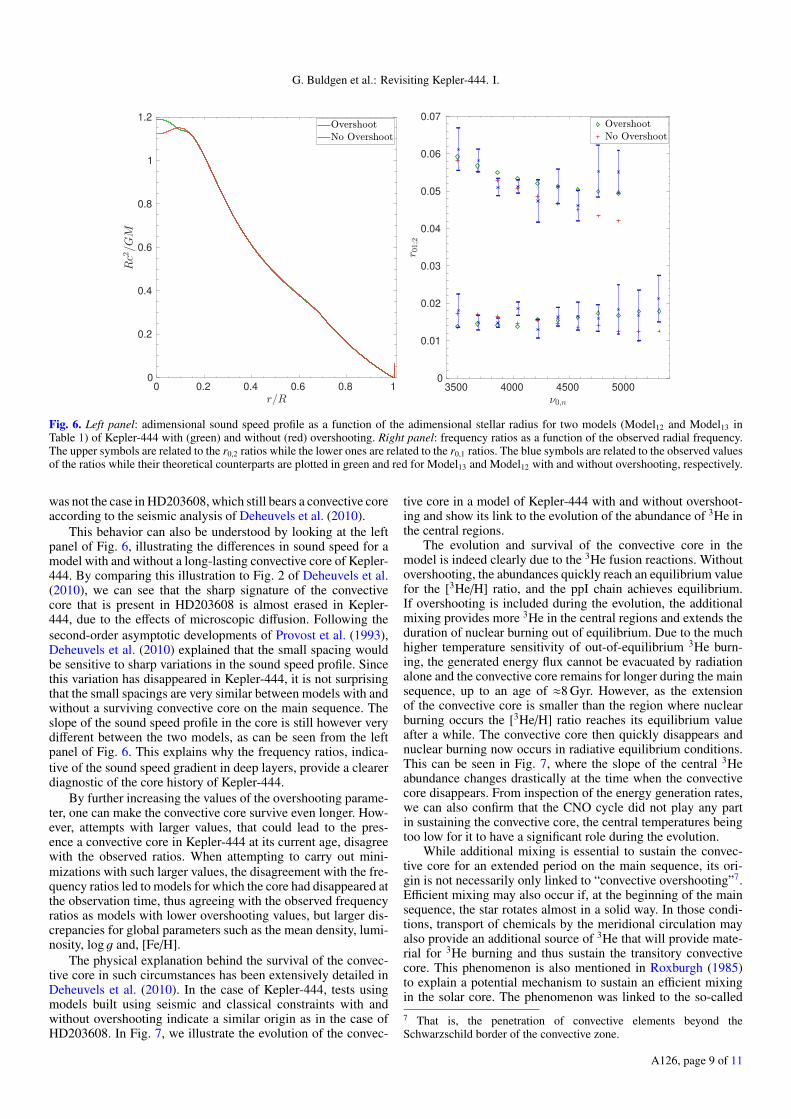
Fig. 6. Left panel: adimensional sound speed profile as a function of the adimensional stellar radius for two models (Model12 and Model13 inTable 1) of Kepler-444 with (green) and without (red) overshooting. Right panel: frequency ratios as a function of the observed radial frequency.The upper symbols are related to the r0,2 ratios while the lower ones are related to the r0,1 ratios. The blue symbols are related to the observed valuesof the ratios while their theoretical counterparts are plotted in green and red for Model13 and Model12 with and without overshooting, respectively.

was not the case in HD203608, which still bears a convective coreaccording to the seismic analysis of Deheuvels et al. (2010).

This behavior can also be understood by looking at the leftpanel of Fig. 6, illustrating the differences in sound speed for amodel with and without a long-lasting convective core of Kepler-444. By comparing this illustration to Fig. 2 of Deheuvels et al.(2010), we can see that the sharp signature of the convectivecore that is present in HD203608 is almost erased in Kepler-444, due to the effects of microscopic diffusion. Following thesecond-order asymptotic developments of Provost et al. (1993),Deheuvels et al. (2010) explained that the small spacing wouldbe sensitive to sharp variations in the sound speed profile. Sincethis variation has disappeared in Kepler-444, it is not surprisingthat the small spacings are very similar between models with andwithout a surviving convective core on the main sequence. Theslope of the sound speed profile in the core is still however verydifferent between the two models, as can be seen from the leftpanel of Fig. 6. This explains why the frequency ratios, indica-tive of the sound speed gradient in deep layers, provide a clearerdiagnostic of the core history of Kepler-444.

By further increasing the values of the overshooting parame-ter, one can make the convective core survive even longer. How-ever, attempts with larger values, that could lead to the pres-ence a convective core in Kepler-444 at its current age, disagreewith the observed ratios. When attempting to carry out mini-mizations with such larger values, the disagreement with the fre-quency ratios led to models for which the core had disappeared atthe observation time, thus agreeing with the observed frequencyratios as models with lower overshooting values, but larger dis-crepancies for global parameters such as the mean density, lumi-nosity, log g and, [Fe/H].

The physical explanation behind the survival of the convec-tive core in such circumstances has been extensively detailed inDeheuvels et al. (2010). In the case of Kepler-444, tests usingmodels built using seismic and classical constraints with andwithout overshooting indicate a similar origin as in the case ofHD203608. In Fig. 7, we illustrate the evolution of the convec-

tive core in a model of Kepler-444 with and without overshoot-ing and show its link to the evolution of the abundance of 3He inthe central regions.

The evolution and survival of the convective core in themodel is indeed clearly due to the 3He fusion reactions. Withoutovershooting, the abundances quickly reach an equilibrium valuefor the [3He/H] ratio, and the ppI chain achieves equilibrium.If overshooting is included during the evolution, the additionalmixing provides more 3He in the central regions and extends theduration of nuclear burning out of equilibrium. Due to the muchhigher temperature sensitivity of out-of-equilibrium 3He burn-ing, the generated energy flux cannot be evacuated by radiationalone and the convective core remains for longer during the mainsequence, up to an age of ≈8 Gyr. However, as the extensionof the convective core is smaller than the region where nuclearburning occurs the [3He/H] ratio reaches its equilibrium valueafter a while. The convective core then quickly disappears andnuclear burning now occurs in radiative equilibrium conditions.This can be seen in Fig. 7, where the slope of the central 3Heabundance changes drastically at the time when the convectivecore disappears. From inspection of the energy generation rates,we can also confirm that the CNO cycle did not play any partin sustaining the convective core, the central temperatures beingtoo low for it to have a significant role during the evolution.

While additional mixing is essential to sustain the convec-tive core for an extended period on the main sequence, its ori-gin is not necessarily only linked to “convective overshooting”7.Efficient mixing may also occur if, at the beginning of the mainsequence, the star rotates almost in a solid way. In those condi-tions, transport of chemicals by the meridional circulation mayalso provide an additional source of 3He that will provide mate-rial for 3He burning and thus sustain the transitory convectivecore. This phenomenon is also mentioned in Roxburgh (1985)to explain a potential mechanism to sustain an efficient mixingin the solar core. The phenomenon was linked to the so-called7 That is, the penetration of convective elements beyond theSchwarzschild border of the convective zone.

A126, page 9 of 11

A&A 630, A126 (2019)

Fig. 7. Left panel: mass of the convective core expressed as a fraction of the stellar mass in Model13 (with overshooting, green) and Model12(without overshooting, red) of Kepler-444 as a function of age. Right panel: central 3He abundance as a function of age for Model12 (red) andModel13 (green) of Kepler-444.

“solar-spoon” mechanism presented by Dilke & Gough (1972)which was extensively discussed (see e.g. Ulrich & Rood 1973;Christensen-Dalsgaard et al. 1974; Unno 1975; Shibahashi et al.1975, for a few references) and also investigated for PopulationIII stars (Sonoi & Shibahashi 2012). In the latter case, the mix-ing results from the transport of chemicals by the nonlinear grav-ity modes generated by a form ε-mechanism due to the nuclearburning of 3He. Seismic data alone are not sufficient to distin-guish between the two cases, or to confirm that a combinationof both effects is at play. To that end, additional constraints onthe lithium and beryllium abundances may provide an indicationof the efficiency of rotational mixing in the early stages of evo-lution and thus inform us on whether rotation would be able toprovide the required mixing of chemicals.

As seen from the seismic modeling results, the survivalof the convective core does not affect the global stellarparameters. The main reason is that its extension is smaller thanthe region of nuclear burning, and therefore, it does not signifi-cantly modify the evolutionary track of Kepler-444. However, itcould potentially affect the angular momentum transport proper-ties and lead to discrepancies in later evolutionary stages. Thisaspect still remains rather speculative and will be further inves-tigated in future studies.

5. Conclusion

Here, we carried out a thorough modeling of Kepler-444 usingupdated parallax values from Gaia DR2 (Gaia Collaboration2018) as well as updated spectroscopic parameters (Macket al. 2018). We combined global and local forward modelingapproaches to structural inversion techniques to derive robustfundamental parameters for this exoplanet-host star. To do so,we tested a wide range of physical ingredients and analyzed thespread of the fundamental parameters obtained. Amongst oth-ers, we investigated the impact of α-enriched abundance tablesand their corresponding opacities rather than solar-scaled abun-dances. Overall, we confirm the results of Campante et al. (2015)and also find relatively good agreement with the results of SilvaAguirre et al. (2015). We note, however, that the luminosityderived from the Gaia parallax is significantly higher than thoseobtained in these studies, especially if we consider recent spec-troscopic constraints. Some of these discrepancies stem from theGaia parallax itself, but also from differences in the effective

temperature values reported in the literature. The case of Kepler-444 is therefore a good illustration of where the use of the veryprecise Gaia parallaxes can be limited by other spectroscopicconstraints.

In addition to forward modeling, we used mean densityinversions to provide a very precise, nearly model-independentvalue for the stellar mean density of 2.496 ± 0.012 g cm−3. Thisvalue was then used as a direct constraint for a second set of for-ward modeling, combined with the other classical and seismicconstraints used in the modeling. Using this two-step approach,we determine the mass, radius and age of Kepler-444 to be0.754±0.030 M�, 0.753±0.010 R� and 11.00±0.8 Gyr. As theseparameters are very similar to those of Campante et al. (2015),we find no significant modifications of the planetary parametersusing our modeling results.

However, we have determined that Kepler-444 bore a con-vective core during a significant fraction of its main-sequenceevolution, as was found by Deheuvels et al. (2010) for theCoRoT target HD203608. The origin of the convective core inthe case of Kepler-444 is similar to the case of HD203608 andcan be linked to the nuclear burning of 3He out of equilibrium.The absence of equilibrium conditions for a prolongated por-tion of time after the ZAMS is due to an additional mixing, pro-viding more nuclear fuel for the He3 combustion. The origin ofthis mixing is unclear and could be due to rotation, overshoot-ing, or even nonlinear gravity modes, although this latter caseseems less plausible considering the stability analyses of Sonoi& Shibahashi (2012). The seismic data alone cannot disentanglebetween these processes. Promising indicators of the efficiencyof rotational mixing in the early stages that could help lift thisdegeneracy are the lithium and beryllium abundances, yet to bedetermined in the case of Kepler-444. So far, using seismology,we are however able to estimate the lifetime of the convectivecore to be of around 8 Gyr.

The survival of the convective core, as noted by Deheuvelset al. (2010), does not affect the fundamental parameters of thestar, but it could play a key role in the angular momentum trans-port in later stages of evolution. A thorough modeling of thestar including rotation and transport by magnetic instabilitiesas in Eggenberger et al. (2010) will be undertaken in a futurepaper. These transport prescriptions will then be used to char-acterize the dynamical properties of the system, following theapproach of Privitera et al. (2016a) and Rao et al. (2018). In turn,

A126, page 10 of 11

G. Buldgen et al.: Revisiting Kepler-444. I.

such detailed studies will pave the way for joint analyses of thestellar-planetary system as a whole, including atmospheric char-acterizations and the change of these properties when coupled toseismically calibrated nonstandard stellar evolution models.

With the advent of TESS and PLATO, such synergiesbetween exoplanetology and asteroseismology will be furtherreinforced. For the best targets, a thorough modeling and inves-tigation of the history of the system with respect to the evolu-tion of its host star can be foreseen. In this series of papers, wewill illustrate these possibilities for a promising target observedby Kepler. In the specific case of Kepler-444, Mills & Fabrycky(2017) estimate that PLATO observations could help to signifi-cantly reduce the current uncertainties on the planetary masses.

Acknowledgements. This work is sponsored by the Swiss National ScienceFoundation (project number 200020-172505). M.F. is supported by the FNRS(“Fonds National de la Recherche Scientifique”) through a FRIA (“Fonds pourla Formation à la Recherche dans l’Industrie et l’Agriculture”) doctoral fellow-ship. S.J.A.J.S. is funded by the Wallonia-Brussels Federation ARC grant forConcerted Research Actions. A.M. and J.M. acknowledge support from the ERCConsolidator Grant funding scheme (project ASTEROCHRONOMETRY, G.A. n.772293). We gratefully acknowledge the support of the UK Science and Tech-nology Facilities Council (STFC). V.B. acknowledges by the Swiss National Sci-ence Fundation (SNSF) in the frame of the National Centre for Competences inResearch PlanetS and has received fundings from the European Research Coun-cil (ERC) under the European Union’s Horizon 2020 research and innovationprogramme (project Four Aces; grant agreement number 724427). This articleused an adapted version of InversionKit, a software developed within the HELASand SPACEINN networks, funded by the European Commissions’s Sixth andSeventh Framework Programmes.

ReferencesAppourchaux, T., Antia, H. M., Ball, W., et al. 2015, A&A, 582, A25Asplund, M., Grevesse, N., Sauval, A. J., & Scott, P. 2009, ARA&A, 47, 481Baglin, A., Auvergne, M., Barge, P., et al. 2009, in IAU Symposium, eds. F. Pont,

D. Sasselov, & M. J. Holman, 253, 71Bailer-Jones, C. A. L., Rybizki, J., Fouesneau, M., Mantelet, G., & Andrae, R.

2018, AJ, 156, 58Ball, W. H., & Gizon, L. 2014, A&A, 568, A123Ball, W. H., Beeck, B., Cameron, R. H., & Gizon, L. 2016, A&A, 592, A159Batalha, N. M., Borucki, W. J., Bryson, S. T., et al. 2011, ApJ, 729, 27Bazsó, Á., Pilat-Lohinger, E., Eggl, S., et al. 2017, MNRAS, 466, 1555Borucki, W. J., Koch, D., Basri, G., et al. 2010, Science, 327, 977Bourrier, V., Ehrenreich, D., Allart, R., et al. 2017, A&A, 602, A106Brewer, J. M., Wang, S., Fischer, D. A., & Foreman-Mackey, D. 2018, ApJ, 867,

L3Buldgen, G., Reese, D. R., Dupret, M. A., & Samadi, R. 2015a, A&A, 574, A42Buldgen, G., Reese, D. R., & Dupret, M. A. 2015b, A&A, 583, A62Buldgen, G., Reese, D. R., & Dupret, M. A. 2016a, A&A, 585, A109Buldgen, G., Salmon, S. J. A. J., Reese, D. R., & Dupret, M. A. 2016b, A&A,

596, A73Buldgen, G., Reese, D., & Dupret, M.-A. 2017, Eur. Phys. J. Web Conf., 160,

03005Buldgen, G., Reese, D. R., & Dupret, M. A. 2018, A&A, 609, A95Buldgen, G., Rendle, B., Sonoi, T., et al. 2019, MNRAS, 482, 2305Campante, T. L., Barclay, T., Swift, J. J., et al. 2015, ApJ, 799, 170Campante, T. L., Santos, N. C., & Monteiro, M. J. P. F. G. 2018,

Asteroseismology and Exoplanets: Listening to the Stars and Searching forNew Worlds (Springer International Publishing AG), 49

Canuto, V. M., & Mazzitelli, I. 1991, ApJ, 370, 295Canuto, V. M., Goldman, I., & Mazzitelli, I. 1996, ApJ, 473, 550Casagrande, L., & VandenBerg, D. A. 2014, MNRAS, 444, 392Casagrande, L., & VandenBerg, D. A. 2018a, MNRAS, 475, 5023Casagrande, L., & VandenBerg, D. A. 2018b, MNRAS, 479, L102Cassisi, S., Potekhin, A. Y., Pietrinferni, A., Catelan, M., & Salaris, M. 2007,

ApJ, 661, 1094Christensen-Dalsgaard, J., & Däppen, W. 1992, A&ARv, 4, 267Christensen-Dalsgaard, J., Dilke, F. W. W., & Gough, D. O. 1974, MNRAS, 169,

429Christensen-Dalsgaard, J., Kjeldsen, H., Brown, T. M., et al. 2010, ApJ, 713,

L164Colgan, J., Kilcrease, D. P., Magee, N. H., et al. 2016, ApJ, 817, 116Cox, J. P., & Giuli, R. T. 1968, Principles of Stellar Structure (New York: Gordon

and Breach)

Davies, G. R., Handberg, R., Miglio, A., et al. 2014, MNRAS, 445, L94Deheuvels, S., Michel, E., Goupil, M. J., et al. 2010, A&A, 514, A31Dilke, F. W. W., & Gough, D. O. 1972, Nature, 240, 262Dupuy, T. J., Kratter, K. M., Kraus, A. L., et al. 2016, ApJ, 817, 80Dziembowski, W. A., Pamyatnykh, A. A., & Sienkiewicz, R. 1990, MNRAS,

244, 542Eddington, A. S. 1959, The Internal Constitution of the Stars (New York: Dover

Publication)Eggenberger, P., Maeder, A., & Meynet, G. 2010, A&A, 519, L2Evans, D. W., Riello, M., De Angeli, F., et al. 2018, A&A, 616, A4Ferguson, J. W., Alexander, D. R., Allard, F., et al. 2005, ApJ, 623, 585Fernández, V., Terlevich, E., Díaz, A. I., Terlevich, R., & Rosales-Ortega, F. F.

2018, MNRAS, 478, 5301Gaia Collaboration (Prusti, T., et al.) 2016, A&A, 595, A1Gaia Collaboration (Brown, A. G. A., et al.) 2018, A&A, 616, A1Green, G. M., Schlafly, E. F., Finkbeiner, D., et al. 2018, MNRAS, 478, 651Grevesse, N., & Noels, A. 1993, in Origin and Evolution of the Elements, eds.

N. Prantzos, E. Vangioni-Flam, & M. Casse, 15Hadden, S., & Lithwick, Y. 2017, AJ, 154, 5Hirsch, L. A., Ciardi, D. R., Howard, A. W., et al. 2017, AJ, 153, 117Hobson, M. J., & Gomez, M. 2017, New A, 55, 1Huber, D. 2018, Asteroseismology and Exoplanets: Listening to the Stars and

Searching for New Worlds (Springer International Publishing AG), 49, 119Huber, D., Chaplin, W. J., Christensen-Dalsgaard, J., et al. 2013a, ApJ, 767,

127Huber, D., Carter, J. A., Barbieri, M., et al. 2013b, Science, 342, 331Iglesias, C. A., & Rogers, F. J. 1996, ApJ, 464, 943Irwin, A. W. 2012, Astrophysics Source Code Library [record ascl:1211.002]Kraus, A. L., Ireland, M. J., Huber, D., Mann, A. W., & Dupuy, T. J. 2016, AJ,

152, 8Krishna Swamy, K. S. 1966, ApJ, 145, 174Lynden-Bell, D., & Ostriker, J. P. 1967, MNRAS, 136, 293Mack, C. E., Strassmeier, K. G., Ilyin, I., et al. 2018, A&A, 612, A46Magic, Z., Chiavassa, A., Collet, R., & Asplund, M. 2015, A&A, 573, A90Meynet, G., Eggenberger, P., Privitera, G., et al. 2017, A&A, 602, L7Mills, S. M., & Fabrycky, D. C. 2017, ApJ, 838, L11Paquette, C., Pelletier, C., Fontaine, G., & Michaud, G. 1986, ApJS, 61, 177Peimbert, A., Peimbert, M., & Luridiana, V. 2016, Rev. Mex. Astron. Astrofis.,

52, 419Pijpers, F. P., & Thompson, M. J. 1994, A&A, 281, 231Potekhin, A. Y., Baiko, D. A., Haensel, P., & Yakovlev, D. G. 1999, A&A, 346,

345Privitera, G., Meynet, G., Eggenberger, P., et al. 2016a, A&A, 591, A45Privitera, G., Meynet, G., Eggenberger, P., et al. 2016b, A&A, 593, A128Privitera, G., Meynet, G., Eggenberger, P., et al. 2016c, A&A, 593, L15Provost, J., Mosser, B., & Berthomieu, G. 1993, A&A, 274, 595Rao, S., Meynet, G., Eggenberger, P., et al. 2018, A&A, 618, A18Rauer, H., Catala, C., Aerts, C., et al. 2014, Exp. Astron., 38, 249Reese, D. R., Marques, J. P., Goupil, M. J., Thompson, M. J., & Deheuvels, S.

2012, A&A, 539, A63Reese, D. R., Chaplin, W. J., Davies, G. R., et al. 2016, A&A, 592, A14Rendle, B. M., Buldgen, G., Miglio, A., et al. 2019, MNRAS, 484, 771Ricker, G. R., Winn, J. N., Vanderspek, R., et al. 2015, J. Astron. Telesc. Instrum.

Syst., 1, 014003Rogers, F. J., & Nayfonov, A. 2002, ApJ, 576, 1064Roxburgh, I. W. 1985, Sol. Phys., 100, 21Roxburgh, I. W. 2002, in Stellar Structure and Habitable Planet Finding, eds. B.

Battrick, F. Favata, I. W. Roxburgh, & D. Galadi, ESA Spec. Publ., 485, 75Roxburgh, I. W., & Vorontsov, S. V. 2002a, in Stellar Structure and Habitable

Planet Finding, eds. B. Battrick, F. Favata, I. W. Roxburgh, & D. Galadi, ESASpec. Publ., 485, 337

Roxburgh, I. W., & Vorontsov, S. V. 2002b, in Stellar Structure and HabitablePlanet Finding, eds. B. Battrick, F. Favata, I. W. Roxburgh, & D. Galadi, ESASpec. Publ., 485, 341

Roxburgh, I. W., & Vorontsov, S. V. 2003, A&A, 411, 215Salaris, M., Chieffi, A., & Straniero, O. 1993, ApJ, 414, 580Schlattl, H. 2002, A&A, 395, 85Scuflaire, R., Théado, S., Montalbán, J., et al. 2008a, Ap&SS, 316, 83Scuflaire, R., Montalbán, J., Théado, S., et al. 2008b, Ap&SS, 316, 149Shibahashi, H., Osaki, Y., & Unno, W. 1975, PASJ, 27, 401Silva Aguirre, V., Davies, G. R., Basu, S., et al. 2015, MNRAS, 452, 2127Sonoi, T., & Shibahashi, H. 2012, MNRAS, 422, 2642Sonoi, T., Samadi, R., Belkacem, K., et al. 2015, A&A, 583, A112Thoul, A. A., Bahcall, J. N., & Loeb, A. 1994, ApJ, 421, 828Ulrich, R. K., & Rood, R. T. 1973, Nat. Phys. Sci., 241, 111Unno, W. 1975, PASJ, 27, 81Vernazza, J. E., Avrett, E. H., & Loeser, R. 1981, ApJS, 45, 635Zanazzi, J. J., & Triaud, A. H. M. J. 2019, Icarus, 325, 55

A126, page 11 of 11