arX

iv:1

207.

0615

v1 [

astr

o-ph

.SR

] 3

Jul 2

012

Astronomy & Astrophysicsmanuscript no. comparison2˙accepted c© ESO 2012July 4, 2012

Solar-like oscillations in red giants observed with Kepler : influenceof increased timespan on global oscillation parameters ⋆

S. Hekker1,2, Y. Elsworth2, B. Mosser3, T.Kallinger4, W.J Chaplin2, J. De Ridder4, R.A. Garcıa5, D. Stello6, B.D.Clarke7, J.R. Hall8, and K.A. Ibrahim8

1 Astronomical institute ‘Anton Pannekoek’, University of Amsterdam, Science Park 904, 1098 XH, Amsterdam, the Netherlands2 University of Birmingham, School of Physics and Astronomy,Edgbaston, Birmingham B15 2TT, United Kingdom3 LESIA, UMR8109, Universite Pierre et Marie Curie, Universite Denis Diderot, Observatoire de Paris, 92195 Meudon Cedex,

France4 Instituut voor Sterrenkunde, KU Leuven, Celestijnenlaan 200D, 3001 Leuven, Belgium5 Laboratoire AIM, CEA/DSM-CNRS, Universite Paris 7 Diderot, IRFU/SAp, Centre de Saclay, 91191, GIf-sur-Yvette, France6 Sydney Institute for Astronomy (SIfA), School of Physics, University of Sydney, NSW 2006, Australia7 SETI Institute/NASA Ames Research Center, Moffet Field,, CA 94035, USA8 Orbital Sciences Corporation/NASA Ames Research Center, Moffet Field, CA 94035, USA

Received ; accepted

ABSTRACT

Context. The length of the asteroseismic timeseries obtained from theKepler satellite analysed here span 19 months.Kepler providesthe longest continuous timeseries currently available, which calls for a study of the influence of the increased timespan on the accuracyand precision of the obtained results.Aims. We aim to investigate how the increased timespan influences the detectability of the oscillation modes, and the absolutevaluesand uncertainties of the global oscillation parameters, i.e., frequency of maximum oscillation power,νmax, and large frequency sepa-ration between modes of the same degree and consecutive orders, 〈∆ν〉.Methods. We use published methods to deriveνmax and〈∆ν〉 for timeseries ranging from 50 to 600 days and compare these results asa function of method, timespan and〈∆ν〉.Results. We find that in general a minimum of the order of 400 day long timeseries are necessary to obtain reliable results for theglobal oscillation parameters in more than 95% of the stars,but this does depend on〈∆ν〉. In a statistical sense the quoted uncertaintiesseem to provide a reasonable indication of the precision of the obtained results in short (50-day) runs, they do however seem to beoverestimated for results of longer runs. Furthermore, thedifferent definitions of the global parameters used in the different methodshave non-negligible effects on the obtained values. Additionally, we show that there is a correlation betweenνmax and the flux variance.Conclusions. We conclude that longer timeseries improve the likelihood to detect oscillations with automated codes (from∼60% in50 day runs to> 95% in 400 day runs with a slight method dependence) and the precision of the obtained global oscillation param-eters. The trends suggest that the improvement will continue for even longer timeseries than the 600 days considered here, with areduction in the median absolute deviation of more than a factor of 10 for an increase in timespan from 50 to 2000 days (the currentlyforeseen length of the mission). This work shows that globalparameters determined with high precision - thus from long datasets -using different definitions can be used to identify the evolutionary state of the stars.

Key words. stars: red giants – stars: oscillations – stars: interior – techniques: photometric

1. Introduction

Many breakthrough results for red-giant (G-K) stars have beenpresented using data obtained by the CoRoT (Baglin et al. 2006)and NASA Kepler (Borucki et al. 2010) missions. These re-sults include statistical ensemble studies of global oscillation pa-5rameters, i.e., frequency of maximum oscillation power,νmax,mean frequency separation between modes of the same de-gree and consecutive orders,〈∆ν〉, small frequency separa-tions between modes of different degree,ℓ, amplitudes andvisibilities of the oscillations, and tests of scaling relations10

(e.g., De Ridder et al. 2009; Hekker et al. 2009; Bedding et al.

Send offprint requests to: S. Hekker,email: S.Hekker@uva.nl⋆ Values of the global oscillation parameters can be obtainedfrom

the authors upon request.

2010; Huber et al. 2010; Hekker et al. 2011d; Huber et al. 2011;Mosser et al. 2012). Additionally, it has been possible to deter-mine stellar parameters such as masses and radii (Kallingeret al.2010b,a). In addition to these results, asteroseismic investiga- 15tions into the granulation (Mathur et al. 2011), red giants in clus-ters (Basu et al. 2011; Hekker et al. 2011b; Stello et al. 2011b,a)and red giants in eclipsing binaries (Hekker et al. 2010b) havebeen performed, as well as detailed investigations into theinternal structure of single stars (e.g., Di Mauro et al. 2011; 20Jiang et al. 2011; Baudin et al. 2012). TheKepler results re-ferred to are based on timeseries with a near regular cadenceofeither 29.4 min or 58.85 s and a timespan ranging from∼30 daysup to more than 1.5 yr. These are the first datasets from space-based telescopes with such long timespan and high fill (&90%) 25and frequency resolution (≈ 0.019µHz). Underpinning much ofthis work is the ability to determine global oscillation param-

1

Hekker et al.: Influence of increased timespan on global oscillation parameters

eters and the uncertainties in these values. It is reasonable toask if there are now enough data available and whether thereare any gains to be obtained from observing individual starsfor30longer periods. In this paper we address the precision and relia-bility of the determination of some of the global seismic param-eters. There are other areas where there is a clear need for data oflonger duration because the features detected in the power spec-tra are narrow and hence barely resolved even by the current35

datasets. In particular, we highlight the detection of g-p mixedmodes (Beck et al. 2011). The observed mean period spacingsappear to have different values for stars that burn only H (ina shell) and those that also burn He in the core (Bedding et al.2011; Mosser et al. 2011a), hence the period spacing can be used40to distinguish between different evolutionary states in which redgiants are observed using the characteristics of their frequencyspectra. Another method to distinguish between different evo-lutionary phases is based on the difference in frequency depen-dence of radial modes (Kallinger et al. 2012). Furthermore,re-45cently, the timeseries obtained withKepler have become longenough to study rotational splitting of the oscillation modes,which led to the detection of differential rotation in red giants(Beck et al. 2012).

In this work, we use the 19 months of data available from Q050to Q7 to investigate how the increased timespan influences thedetectability of the oscillation modes, and the absolute valuesand uncertainties of the global oscillation parameters,νmax and〈∆ν〉. These are important in several ways. Knowing the depen-dence of the precision on data duration is a guide for observing55

strategies, and for the determination of those secondary param-eters that are derived from the primary global oscillation param-eters, such as stellar mass and radius. Furthermore, it is crucialto be able to estimate the proportion of false negatives and falsepositives for population studies. Also, for detailed modelling of60individual oscillation frequenciesνmax turned out to be of greatdiagnostic potential (Gruberbauer et al. 2012). We will includein our considerations the impact of other relevant parameterssuch as the observed height-to-background ratio of the oscilla-tion excess. This work is a follow-up of Hekker et al. (2011c,65

hereafter paper I) on the red giants and Verner et al. (2011) onsolar-type stars, in which results obtained with different meth-ods have been compared and validated.

Paper I described the comparison of global oscillation pa-rameters extracted from about four month ofKepler data using70

different methods. From this comparison, it was concluded that1) the results from the different methods agree for most starswithin a few percent; 2) at least five methods (out of the seventested) obtained results for 92% of stars forνmax within the rangeof 50 µHz to 170µHz, and this percentage decreased to 69%75when all stars withνmax covering the complete frequency range,i.e., 0 – 283.4µHz (the Nyquist frequency) were included; 3) thescatter due to realization noise, originating from the stochasticnature of the oscillations, is non-negligible and can be at leastas important as the internal uncertainty of the results due to the80method used, but this depends on the frequency of maximumoscillation power,νmax, and on the methods. In case a model isused to describe the variation of∆νwith frequency the results areless sensitive to realization noise than others; 4) the influence ofthe obtained value of〈∆ν〉 is less dependent on the frequency85

range over which it is computed than is the case for solar-typestars. A theoretical follow-up study to explain the latter has beenperformed by Hekker et al. (2011a).

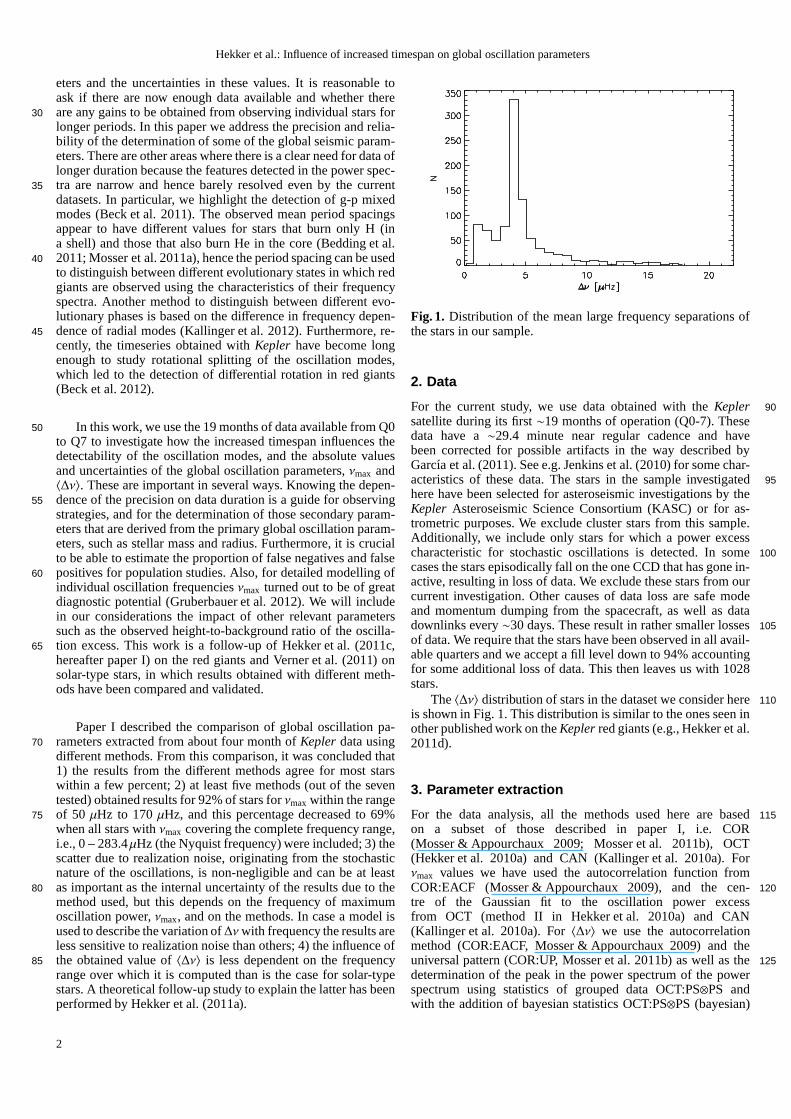
Fig. 1. Distribution of the mean large frequency separations ofthe stars in our sample.

2. Data

For the current study, we use data obtained with theKepler 90

satellite during its first∼19 months of operation (Q0-7). Thesedata have a∼29.4 minute near regular cadence and havebeen corrected for possible artifacts in the way described byGarcıa et al. (2011). See e.g. Jenkins et al. (2010) for somechar-acteristics of these data. The stars in the sample investigated 95here have been selected for asteroseismic investigations by theKepler Asteroseismic Science Consortium (KASC) or for as-trometric purposes. We exclude cluster stars from this sample.Additionally, we include only stars for which a power excesscharacteristic for stochastic oscillations is detected. In some 100cases the stars episodically fall on the one CCD that has gonein-active, resulting in loss of data. We exclude these stars from ourcurrent investigation. Other causes of data loss are safe modeand momentum dumping from the spacecraft, as well as datadownlinks every∼30 days. These result in rather smaller losses105

of data. We require that the stars have been observed in all avail-able quarters and we accept a fill level down to 94% accountingfor some additional loss of data. This then leaves us with 1028stars.

The〈∆ν〉 distribution of stars in the dataset we consider here110is shown in Fig. 1. This distribution is similar to the ones seen inother published work on theKepler red giants (e.g., Hekker et al.2011d).

3. Parameter extraction

For the data analysis, all the methods used here are based115on a subset of those described in paper I, i.e. COR(Mosser & Appourchaux 2009; Mosser et al. 2011b), OCT(Hekker et al. 2010a) and CAN (Kallinger et al. 2010a). Forνmax values we have used the autocorrelation function fromCOR:EACF (Mosser & Appourchaux 2009), and the cen-120tre of the Gaussian fit to the oscillation power excessfrom OCT (method II in Hekker et al. 2010a) and CAN(Kallinger et al. 2010a). For〈∆ν〉 we use the autocorrelationmethod (COR:EACF, Mosser & Appourchaux 2009) and theuniversal pattern (COR:UP, Mosser et al. 2011b) as well as the 125

determination of the peak in the power spectrum of the powerspectrum using statistics of grouped data OCT:PS⊗PS andwith the addition of bayesian statistics OCT:PS⊗PS (bayesian)

2

Hekker et al.: Influence of increased timespan on global oscillation parameters

(Hekker et al. 2010a), and finally, fitting of the central three ra-dial orders (CAN, Kallinger et al. 2010a).130

A homogeneous comparison between the values of theshorter timeseries as presented in paper I, and of longer time-series cannot be performed directly, as continuous improvementsto the methods have been made. These improvements have beenmade as a result of our increasing knowledge of the data from135earlier runs and to deal with the longer timeseries. The changesare of numerical nature and do not alter the underlying princi-ples of the methods. Hence, the references cited above are stillvalid. To perform a uniform study of the impact of the length ofthe timeseries, the (Q0-Q7) dataset (∼600 days) has been used140both as a whole and divided into subsets. These datasets are allanalysed with the latest versions of the analysis methods.

4. Likelihood of detecting oscillation power infrequency spectra

Recently, Hekker et al. (2011d) analysed one-month data sets of145

publicly available data for over 16 000 red giants selected on thebasis of effective temperature and surface gravity. They foundthat in ∼70% of the stars, oscillations could be detected. Thisraises questions as to whether this fraction is telling us some-thing about the ability of red giants to sustain stochastically-150driven oscillations, or if it is just a reflection of the difficulties inthe automated detections of oscillations for relatively short datasets? Perhaps also, some of the stars were so faint that theirnoiselevels prevented the oscillations being detected. Alternatively,can some other feature in the star suppress the oscillationsin155the same manner as activity is known to suppress the oscilla-tions in solar-like stars (Mosser et al. 2009; Chaplin et al.2011a;Huber et al. 2011)? Here we will first give consideration to theimportance of the amplitude of the oscillations and apparentbrightness of the stars and we will subsequently consider the160

problems associated with the automated methods.We consider how we might estimate the likelihood of detect-

ing oscillation power when it is present in the data. We use thesame method as given in (Chaplin et al. 2011b), adapted for thered giants, to show that there is a high expectation that we will165be able to detect the modes of oscillations in all the red giantsin the Kepler data set. It is important to note that, although thecorrect identification of the frequency range in which the modesare located is of fundamental importance, most current methodsdo not use this as their primary consideration when determin-170

ing if there is oscillation power in the spectrum. For most ofthemethods, the determination of∆ν is done first. If this fails then‘no detection’ is reported. This may not be the best strategy, butbefore we construct that discussion we should first explore theexisting predictions for the amplitudes of the modes of oscilla-175tions in red giants.

4.1. Prediction for mode power

Kjeldsen & Bedding (1995) devised scaling relations predict-ing that the amplitude of solar-like oscillations scale withtheir luminosity to mass ratio, which implies that the ampli-180tude of the oscillations increases with increasing stellarra-dius. Hence, solar-like oscillations in red giants are expected tohave higher amplitudes than oscillations in solar-type stars ofequal masses. These scaling relations have recently been revised(Kjeldsen & Bedding 2011), and also tested, both theoretically185(e.g. Samadi et al. 2007) and observationally (e.g. Baudin et al.2011a,b; Huber et al. 2011; Stello et al. 2011a).

To determine if it is possible to detect the modes, we are in-terested in the signal-to-noise ratio in the vicinity of themodes.In Mosser et al. (2012) it was shown that, with a small de-190pendence on evolutionary status, the ratio of the height of thesmoothed power spectrum to the granulation noise backgroundevaluated atνmax is between 3.7 and 4.0 for clump and red-giantbranch stars, respectively. Accordingly, we will use the lowerlimit of this to work out the signal-to-noise in the integrated 195

spectral power excess. For all the red giants that we considerhere, the intrinsic photon shot noise is negligible and we neglectit. This removes a consideration of the stellar luminosity fromthe calculations.

A commonly accepted model of the envelope of the oscil-200

lation power is a Gaussian function whose width,Wenv, scaleswith the frequency of maximum powerνmax asWenv = 0.59ν0.9max(Mosser et al. 2010). We can determine the average power in theoscillations by smoothing the power spectrum over a range ofatleast one large spacing so that no trace of the individual modes 205remains. It is recognized that doing this in practice requires con-siderable care as is spelt out in Mosser et al. (2012). We willtaketwice the full-width half-maximum of the underlying Gaussianas the range over which we will integrate to determine the av-erage power. This range contains all but a few per cent of the210oscillation power. The granulation background in the vicinity ofthe modes can be modeled with a power law with index of−2.1(Mosser et al. 2012). Integration of these two functions, over thesame range, leads to an integrated height-to-background ratio(H/Bint ) of 1.55 (0.42 the height-to-background ratio atνmax). 215

The averaging of the data during the sampling interval in thetime domain causes an attenuation of the amplitudes in the fre-quency spectrum according to a sinc function and we can use theratio of νmax to νNyq, the Nyquist frequency which is 283.4µHzfor theKepler long cadence data, to quantify the size of this re-220

duction. The majority of stars in our sample haveνmax ≪ νNyqand for these stars this sinc term is negligible and we do notconsider it further.

4.2. Model of detection probability

Here we present a model, based on predicted integrated height- 225to-background in the vicinity of the oscillations, for how de-tectable the oscillations are. To do this we adapt the formula-tion devised by Chaplin et al. (2011b) for solar-type stars to redgiants. The principle of the method is to compare the powerpresent in the modes with that present in the background and230then to use probability distributions to ascertain the likelihoodof the mode power being reliably detected.

The question that we now wish to answer is ‘given theH/Bintwhat is the chance of a false detection?’. We set a probability,pfalse, at which we are prepared to risk a false positive detec-235tion. In general, this level should be low. Typically for this workwe have usedpfalse=0.01 (i.e.1%). As detailed in Chaplin et al.(2011b), we compute a threshold value,θ, in a χ2 distributionwith 2n degrees of freedom (dof) such that the probability thatsome random variable is greater than the threshold value sup- 240

plied is equal topfalse. In this, we taken, the number of degreesof freedom, as the number of independent frequency bins usedto computeH/Bint. We must also take account of the chance that,because of random noise in the data, we will miss a true detec-tion for a star with sufficient signal-to-noise for detection which245leads to a new threshold valueθ2.

θ2 =θ + 1

H/Bint + 1. (1)

3

Hekker et al.: Influence of increased timespan on global oscillation parameters

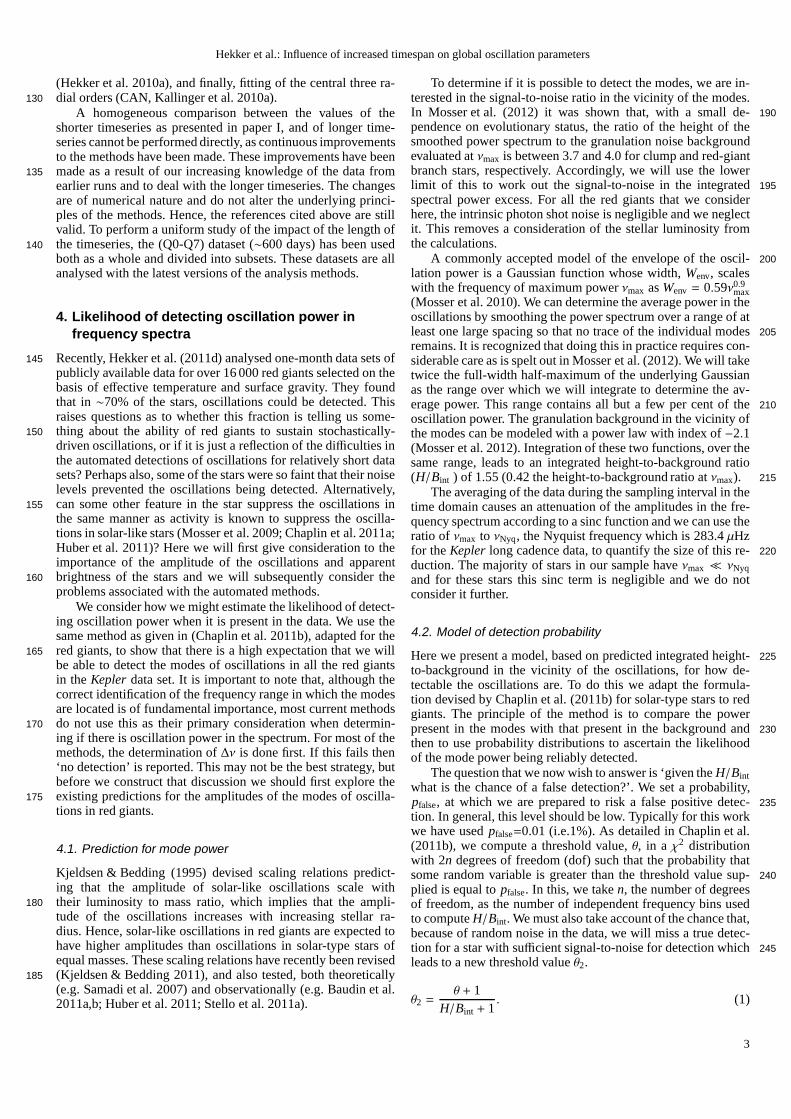
Fig. 2.Fraction of runs with returned values for each star per∆ν interval. Each panel shows the results of a certain method (A: COR- Universal Pattern, B: COR - EACF, C: OCT - PS⊗PS, D: OCT - PS⊗PS (bayesian), E: CAN) with run length 50, 200, 400, 600days in red, blue, cyan and black, respectively. Note that the 50 and 600 day curves in panel E overlap due to the fact that the 600day results were used to constrain the input for the 50 day runs. No results for 200 and 400 day long runs were obtained by CAN.

This valueθ2 is then used to derive probabilityp, wherep is theprobability that in aχ2 distribution with 2n dof a random variableis less than or equal to the cut off level specified. Finally we have250the probability we sought which ispfinal = 1− p the probabilitythat a givenH/Bint will exceed the computed thresholdθ.

The recipe as described predicts that for all stars consideredhere (even for datasets as short as 50 days) we are likely to detectthe oscillations. In general, the lower probabilities are at about25593% likelihood for stars which haveνmax below 10µHz. For oneparticular star the detection probability dropped to 75%. Notethat these predictions are not sensitive to the shape of the oscil-lation power excess nor to any structure, such as the large fre-quency separation in it, and that we have taken the worst case260

scenario for theH/B of Helium-core-burning evolutionary sta-tus. These results are based on the integrated power of the oscil-lations. So from this test it appears that a detection rate higherthan 70% as quoted by Hekker et al. (2011d) would be expectedwhen using theH/B indications. But how does this compare with265observational results from longer timeseries? We now considerthis issue in the next section.

5. Observational results

For observed stars we do not know the true values of the seis-mic parameters. All that we can do is to estimate them using270the observations. In order to obtain such estimates of the seis-

mic parametersνmax and∆ν, the COR and OCT methods areused to analyse the full timespan of just under 600 days of thecomplete set of stellar data. The analysis was ‘blind’ in that nomanual checks were made on the outcomes. We therefore ex-275

pect to have some errors in the results. We did not use the CANmethod because, for computational reasons (the multinest proce-dure is very time consuming), not all available stars were anal-ysed with it. For 974 stars there is close agreement between theresults from OCT and COR forνmax and〈∆ν〉. In this context, 280close agreement is taken to be that the two completely indepen-dent methods identify the oscillations in the same region ofthespectrum to within half the expected width of the envelope ofthe oscillation power, with the width of the oscillation envelopeas defined by Mosser et al. (2010). Taking this relatively relaxed 285constraint is justified by the fact that we want to select a statis-tically significant sample of stars with oscillations detected bydifferent methods in the same frequency range. For the remain-ing 54 stars, there are disagreements between the values obtainedwith the different methods. We inspected these stars by eye and290

for 39 stars the oscillations are at low frequencies (ν < 5 µHz),for four stars the oscillations straddle the Nyquist frequency andfor 11 stars we do not have the standard red-giant oscillationspectrum due to the presence of artefacts or these could possiblybe mis-classified as red giants. 295

For the 974 stars for which there is agreement, we createreference values which are the mean values ofνmax and 〈∆ν〉,

4

Hekker et al.: Influence of increased timespan on global oscillation parameters

respectively. These reference values are essentially an arbitraryzeropoint used to select reliable results and to discard outliers.

5.1. Outlier removal in short datasets300

When short datasets are considered there will be occasions whenthe returned values are unreliable. We wish to remove some ofthese so that we can look at the spread in the reliable results. Avery simple outlier rejection algorithm is used whose purpose isto reject patently wrong answers. This is the same as described in305paper I and depends on comparing the reference value with theindividual values. The results presented in Verner et al. (2011)suggest that for solar-type stars it is appropriate to use rejectioncriteria that scale with theνmax of the star. However, it was shownin paper I that this is not appropriate for red-giant stars. The310

process adopted here first rejects points that are more than 50%different from the reference value, irrespective ofνmax or 〈∆ν〉,and then applies an absolute cut. For these absolute cuts a valueof 10 µHz has been used for all but the low values ofνmax anda cut of 2µHz has been used for〈∆ν〉. The cross-over position315where the absolute cut off is more stringent than the relative oneoccurs at aboutνmax= 20µHz.

5.2. Is a data duration of 50 days enough to reliably detectthe presence of modes?

The statistical tests considered in Sect. 4.2 suggested that32050 days of data were sufficient to reliably detect the presenceof the oscillation power based on the height-to-backgroundra-tio. We can now see if that is true with the algorithms used. Aswe used only stars for which we had firm detections of oscil-lations in the 600-day dataset, we expected to have results for325

each of the 50-day runs, i.e. 12 results per star. For runs of du-ration 200 days we expect to have 3 returns etc. This is notthe case as can be seen from Fig. 2 where for each of the dif-ferent methods we plot the fraction of returns for the differentdata durations as a function of∆ν on a logarithmic scale. The330data have been binned for this graph. In general the bin widthused is just under 1µHz but bins are combined at high frequen-cies to improve the statistics where there are few stars in theoriginal sample as can be seen in Fig. 1. As expected, as therun duration increases the general efficacy of each method im-335proves. The exception to this is for the CAN method where thedata from the long runs are used to constrain the fitted param-eter ranges in the short runs and the method is not ‘blind’. Theresults are summarised in Table 1. Although all methods havedifficulties at low frequency, the different methods are clearly340

somewhat different in the spectral regions where their responseis reliable. Additionally, COR is less effective for mid-range fre-quencies. The detection capabilities of the EACF method under-lie the two methods COR:UP and COR:EACF employed for thedetermination of〈∆ν〉. For this method the value of the parame-345terAmax as given in Mosser & Appourchaux (2009) is important.The threshold value set for a detection is 8 for rejecting theH0hypothesis at the 1% level. They have shown that the value ofAmax improves linearly with the duration of the dataset and sowe expect a marked improvement as longer datasets are used.350This is indeed the case as shown in Table 1. The peak detectionmethods underlying CAN does depend on a predefined list ofstars, and hence this shows the distribution of the type of starson the list used for the analysis presented here. The OCT methodhas issues at the very high frequencies.355

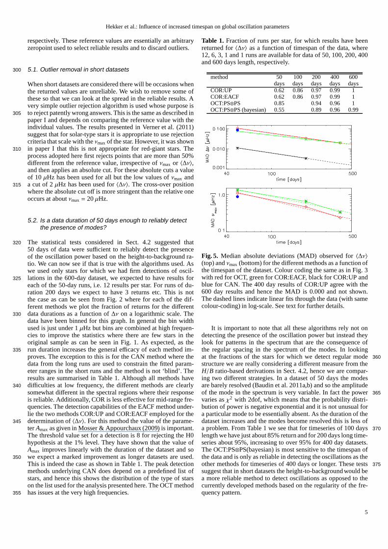
Table 1. Fraction of runs per star, for which results have beenreturned for〈∆ν〉 as a function of timespan of the data, where12, 6, 3, 1 and 1 runs are available for data of 50, 100, 200, 400and 600 days length, respectively.

method 50 100 200 400 600days days days days days

COR:UP 0.62 0.86 0.97 0.99 1COR:EACF 0.62 0.86 0.97 0.99 1OCT:PS⊗PS 0.85 0.94 0.96 1OCT:PS⊗PS (bayesian) 0.55 0.89 0.96 0.99

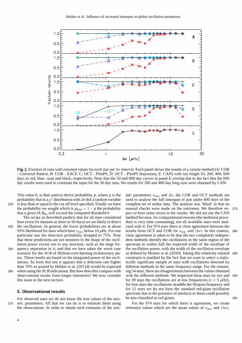
Fig. 5. Median absolute deviations (MAD) observed for〈∆ν〉(top) andνmax (bottom) for the different methods as a function ofthe timespan of the dataset. Colour coding the same as in Fig.3with red for OCT, green for COR:EACF, black for COR:UP andblue for CAN. The 400 day results of COR:UP agree with the600 day results and hence the MAD is 0.000 and not shown.The dashed lines indicate linear fits through the data (with samecolour-coding) in log-scale. See text for further details.

It is important to note that all these algorithms rely not ondetecting the presence of the oscillation power but insteadtheylook for patterns in the spectrum that are the consequence ofthe regular spacing in the spectrum of the modes. In lookingat the fractions of the stars for which we detect regular mode360structure we are really considering a different measure from theH/B ratio-based derivations in Sect. 4.2, hence we are compar-ing two different strategies. In a dataset of 50 days the modesare barely resolved (Baudin et al. 2011a,b) and so the amplitudeof the mode in the spectrum is very variable. In fact the power365varies asχ2 with 2dof, which means that the probability distri-bution of power is negative exponential and it is not unusualfora particular mode to be essentially absent. As the duration of thedataset increases and the modes become resolved this is lessofa problem. From Table 1 we see that for timeseries of 100 days370

length we have just about 85% return and for 200 days long time-series about 95%, increasing to over 95% for 400 day datasets.The OCT:PS⊗PS(bayesian) is most sensitive to the timespan ofthe data and is only as reliable in detecting the oscillations as theother methods for timeseries of 400 days or longer. These tests 375suggest that in short datasets the height-to-background would bea more reliable method to detect oscillations as opposed to thecurrently developed methods based on the regularity of the fre-quency pattern.

5

Hekker et al.: Influence of increased timespan on global oscillation parameters

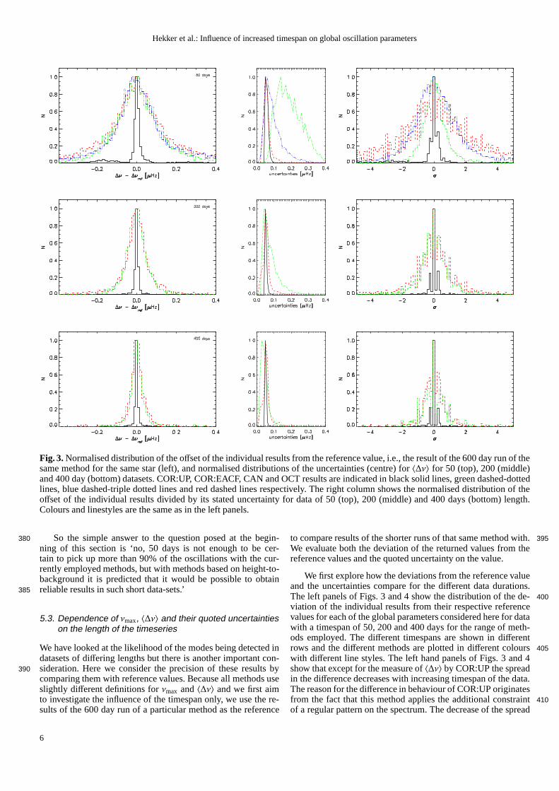
Fig. 3.Normalised distribution of the offset of the individual results from the reference value, i.e., the result of the 600 day run of thesame method for the same star (left), and normalised distributions of the uncertainties (centre) for〈∆ν〉 for 50 (top), 200 (middle)and 400 day (bottom) datasets. COR:UP, COR:EACF, CAN and OCTresults are indicated in black solid lines, green dashed-dottedlines, blue dashed-triple dotted lines and red dashed linesrespectively. The right column shows the normalised distribution of theoffset of the individual results divided by its stated uncertainty for data of 50 (top), 200 (middle) and 400 days (bottom) length.Colours and linestyles are the same as in the left panels.

So the simple answer to the question posed at the begin-380

ning of this section is ‘no, 50 days is not enough to be cer-tain to pick up more than 90% of the oscillations with the cur-rently employed methods, but with methods based on height-to-background it is predicted that it would be possible to obtainreliable results in such short data-sets.’385

5.3. Dependence of νmax, 〈∆ν〉 and their quoted uncertaintieson the length of the timeseries

We have looked at the likelihood of the modes being detected indatasets of differing lengths but there is another important con-sideration. Here we consider the precision of these resultsby390comparing them with reference values. Because all methods useslightly different definitions forνmax and〈∆ν〉 and we first aimto investigate the influence of the timespan only, we use the re-sults of the 600 day run of a particular method as the reference

to compare results of the shorter runs of that same method with. 395

We evaluate both the deviation of the returned values from thereference values and the quoted uncertainty on the value.

We first explore how the deviations from the reference valueand the uncertainties compare for the different data durations.The left panels of Figs. 3 and 4 show the distribution of the de- 400viation of the individual results from their respective referencevalues for each of the global parameters considered here fordatawith a timespan of 50, 200 and 400 days for the range of meth-ods employed. The different timespans are shown in differentrows and the different methods are plotted in different colours 405

with different line styles. The left hand panels of Figs. 3 and 4show that except for the measure of〈∆ν〉 by COR:UP the spreadin the difference decreases with increasing timespan of the data.The reason for the difference in behaviour of COR:UP originatesfrom the fact that this method applies the additional constraint 410of a regular pattern on the spectrum. The decrease of the spread

6

Hekker et al.: Influence of increased timespan on global oscillation parameters

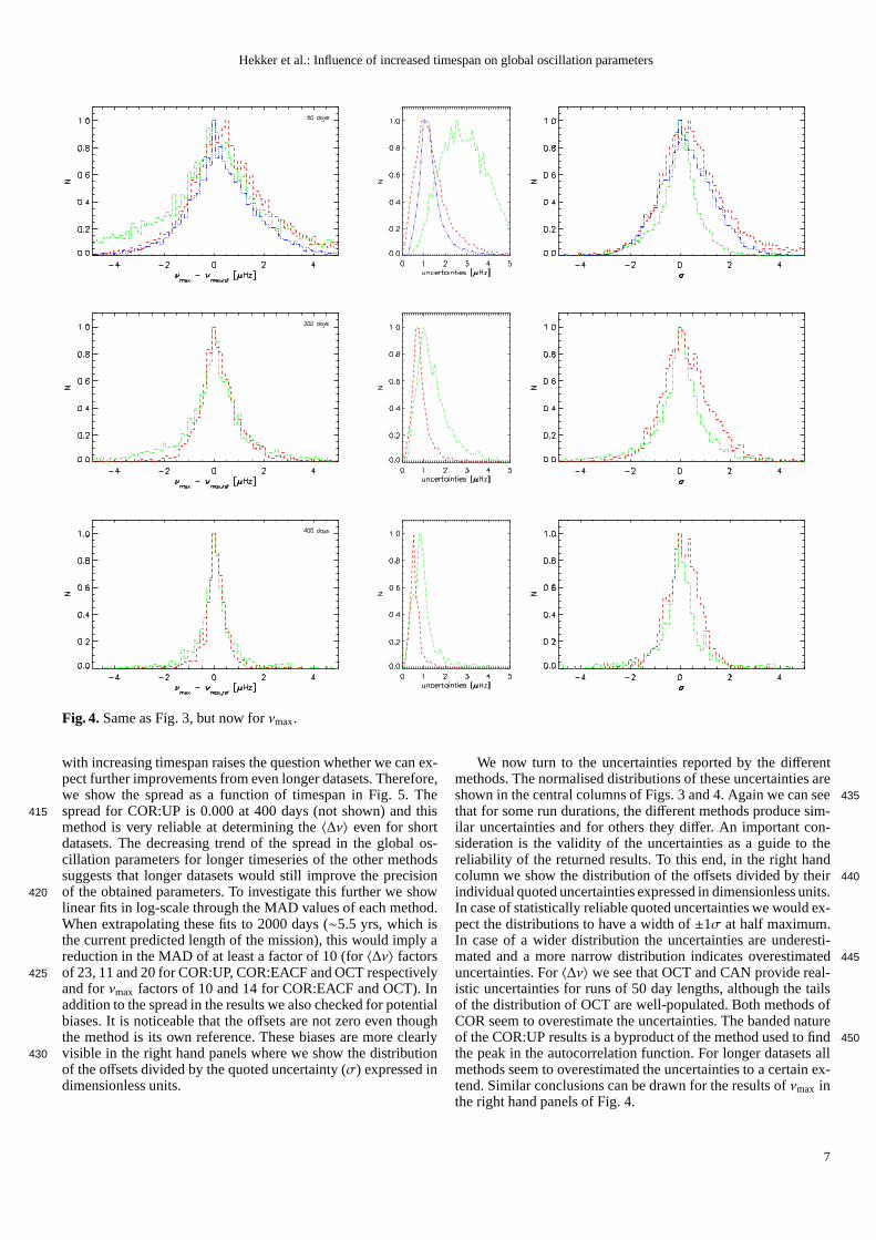
Fig. 4.Same as Fig. 3, but now forνmax.

with increasing timespan raises the question whether we canex-pect further improvements from even longer datasets. Therefore,we show the spread as a function of timespan in Fig. 5. Thespread for COR:UP is 0.000 at 400 days (not shown) and this415method is very reliable at determining the〈∆ν〉 even for shortdatasets. The decreasing trend of the spread in the global os-cillation parameters for longer timeseries of the other methodssuggests that longer datasets would still improve the precisionof the obtained parameters. To investigate this further we show420linear fits in log-scale through the MAD values of each method.When extrapolating these fits to 2000 days (∼5.5 yrs, which isthe current predicted length of the mission), this would imply areduction in the MAD of at least a factor of 10 (for〈∆ν〉 factorsof 23, 11 and 20 for COR:UP, COR:EACF and OCT respectively425and forνmax factors of 10 and 14 for COR:EACF and OCT). Inaddition to the spread in the results we also checked for potentialbiases. It is noticeable that the offsets are not zero even thoughthe method is its own reference. These biases are more clearlyvisible in the right hand panels where we show the distribution430

of the offsets divided by the quoted uncertainty (σ) expressed indimensionless units.

We now turn to the uncertainties reported by the differentmethods. The normalised distributions of these uncertainties areshown in the central columns of Figs. 3 and 4. Again we can see435

that for some run durations, the different methods produce sim-ilar uncertainties and for others they differ. An important con-sideration is the validity of the uncertainties as a guide tothereliability of the returned results. To this end, in the right handcolumn we show the distribution of the offsets divided by their440individual quoted uncertainties expressed in dimensionless units.In case of statistically reliable quoted uncertainties we would ex-pect the distributions to have a width of±1σ at half maximum.In case of a wider distribution the uncertainties are underesti-mated and a more narrow distribution indicates overestimated 445

uncertainties. For〈∆ν〉 we see that OCT and CAN provide real-istic uncertainties for runs of 50 day lengths, although thetailsof the distribution of OCT are well-populated. Both methodsofCOR seem to overestimate the uncertainties. The banded natureof the COR:UP results is a byproduct of the method used to find450the peak in the autocorrelation function. For longer datasets allmethods seem to overestimated the uncertainties to a certain ex-tend. Similar conclusions can be drawn for the results ofνmax inthe right hand panels of Fig. 4.

7

Hekker et al.: Influence of increased timespan on global oscillation parameters

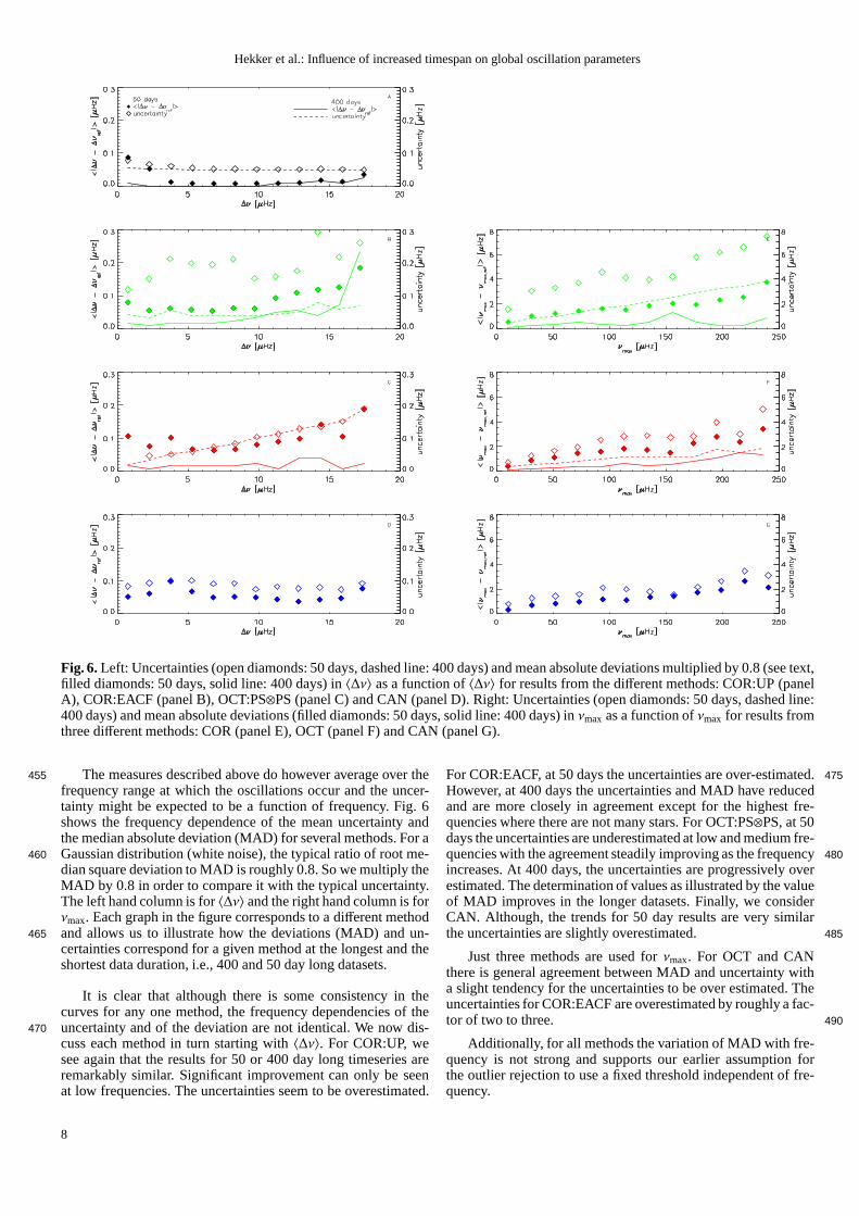
Fig. 6.Left: Uncertainties (open diamonds: 50 days, dashed line: 400 days) and mean absolute deviations multiplied by 0.8 (seetext,filled diamonds: 50 days, solid line: 400 days) in〈∆ν〉 as a function of〈∆ν〉 for results from the different methods: COR:UP (panelA), COR:EACF (panel B), OCT:PS⊗PS (panel C) and CAN (panel D). Right: Uncertainties (open diamonds: 50 days, dashed line:400 days) and mean absolute deviations (filled diamonds: 50 days, solid line: 400 days) inνmax as a function ofνmax for results fromthree different methods: COR (panel E), OCT (panel F) and CAN (panel G).

The measures described above do however average over the455

frequency range at which the oscillations occur and the uncer-tainty might be expected to be a function of frequency. Fig. 6shows the frequency dependence of the mean uncertainty andthe median absolute deviation (MAD) for several methods. For aGaussian distribution (white noise), the typical ratio of root me-460dian square deviation to MAD is roughly 0.8. So we multiply theMAD by 0.8 in order to compare it with the typical uncertainty.The left hand column is for〈∆ν〉 and the right hand column is forνmax. Each graph in the figure corresponds to a different methodand allows us to illustrate how the deviations (MAD) and un-465certainties correspond for a given method at the longest andtheshortest data duration, i.e., 400 and 50 day long datasets.

It is clear that although there is some consistency in thecurves for any one method, the frequency dependencies of theuncertainty and of the deviation are not identical. We now dis-470cuss each method in turn starting with〈∆ν〉. For COR:UP, wesee again that the results for 50 or 400 day long timeseries areremarkably similar. Significant improvement can only be seenat low frequencies. The uncertainties seem to be overestimated.

For COR:EACF, at 50 days the uncertainties are over-estimated. 475

However, at 400 days the uncertainties and MAD have reducedand are more closely in agreement except for the highest fre-quencies where there are not many stars. For OCT:PS⊗PS, at 50days the uncertainties are underestimated at low and mediumfre-quencies with the agreement steadily improving as the frequency 480increases. At 400 days, the uncertainties are progressively overestimated. The determination of values as illustrated by the valueof MAD improves in the longer datasets. Finally, we considerCAN. Although, the trends for 50 day results are very similarthe uncertainties are slightly overestimated. 485

Just three methods are used forνmax. For OCT and CANthere is general agreement between MAD and uncertainty witha slight tendency for the uncertainties to be over estimated. Theuncertainties for COR:EACF are overestimated by roughly a fac-tor of two to three. 490

Additionally, for all methods the variation of MAD with fre-quency is not strong and supports our earlier assumption forthe outlier rejection to use a fixed threshold independent offre-quency.

8

Hekker et al.: Influence of increased timespan on global oscillation parameters

5.4. Offsets between different methods495

In the previous subsection we saw that within any one givenmethod, short datasets can give, on average, slightly biased re-sults when compared with longer sets. Here we concentrate onthe differences between different methods using the results ob-tained with 600 days of data. We know that the different meth-500

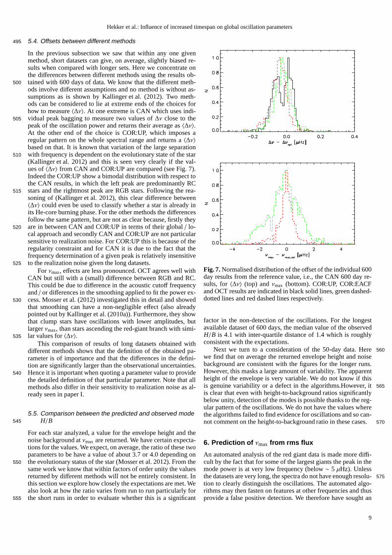
ods involve different assumptions and no method is without as-sumptions as is shown by Kallinger et al. (2012). Two meth-ods can be considered to lie at extreme ends of the choices forhow to measure〈∆ν〉. At one extreme is CAN which uses indi-vidual peak bagging to measure two values of∆ν close to the505peak of the oscillation power and returns their average as〈∆ν〉.At the other end of the choice is COR:UP, which imposes aregular pattern on the whole spectral range and returns a〈∆ν〉based on that. It is known that variation of the large separationwith frequency is dependent on the evolutionary state of thestar510(Kallinger et al. 2012) and this is seen very clearly if the val-ues of〈∆ν〉 from CAN and COR:UP are compared (see Fig. 7).Indeed the COR:UP show a bimodal distribution with respect tothe CAN results, in which the left peak are predominantly RCstars and the rightmost peak are RGB stars. Following the rea-515

soning of (Kallinger et al. 2012), this clear difference between〈∆ν〉 could even be used to classify whether a star is already inits He-core burning phase. For the other methods the differencesfollow the same pattern, but are not as clear because, firstlytheyare in between CAN and COR:UP in terms of their global/ lo-520cal approach and secondly CAN and COR:UP are not particularsensitive to realization noise. For COR:UP this is because of theregularity constraint and for CAN it is due to the fact that thefrequency determination of a given peak is relatively insensitiveto the realization noise given the long datasets.525

For νmax, effects are less pronounced. OCT agrees well withCAN but still with a (small) difference between RGB and RC.This could be due to difference in the acoustic cutoff frequencyand/ or differences in the smoothing applied to fit the power ex-cess. Mosser et al. (2012) investigated this in detail and showed530that smoothing can have a non-negligible effect (also alreadypointed out by Kallinger et al. (2010a)). Furthermore, theyshowthat clump stars have oscillations with lower amplitudes, butlargerνmax, than stars ascending the red-giant branch with simi-lar values for〈∆ν〉.535

This comparison of results of long datasets obtained withdifferent methods shows that the definition of the obtained pa-rameter is of importance and that the differences in the defini-tion are significantly larger than the observational uncertainties.Hence it is important when quoting a parameter value to provide540

the detailed definition of that particular parameter. Note that allmethods also differ in their sensitivity to realization noise as al-ready seen in paper I.

5.5. Comparison between the predicted and observed modeH/B545

For each star analyzed, a value for the envelope height and thenoise background atνmax are returned. We have certain expecta-tions for the values. We expect, on average, the ratio of these twoparameters to be have a value of about 3.7 or 4.0 depending onthe evolutionary status of the star (Mosser et al. 2012). From the550same work we know that within factors of order unity the valuesreturned by different methods will not be entirely consistent. Inthis section we explore how closely the expectations are met. Wealso look at how the ratio varies from run to run particularlyforthe short runs in order to evaluate whether this is a significant555

Fig. 7.Normalised distribution of the offset of the individual 600day results from the reference value, i.e., the CAN 600 day re-sults, for 〈∆ν〉 (top) andνmax (bottom). COR:UP, COR:EACFand OCT results are indicated in black solid lines, green dashed-dotted lines and red dashed lines respectively.

factor in the non-detection of the oscillations. For the longestavailable dataset of 600 days, the median value of the observedH/B is 4.1 with inter-quartile distance of 1.4 which is roughlyconsistent with the expectations.

Next we turn to a consideration of the 50-day data. Here560we find that on average the returned envelope height and noisebackground are consistent with the figures for the longer runs.However, this masks a large amount of variability. The apparentheight of the envelope is very variable. We do not know if thisis genuine variability or a defect in the algorithms.However, it 565is clear that even with height-to-background ratios significantlybelow unity, detection of the modes is possible thanks to thereg-ular pattern of the oscillations. We do not have the values wherethe algorithms failed to find evidence for oscillations and so can-not comment on the height-to-background ratio in these cases. 570

6. Prediction of νmax from rms flux

An automated analysis of the red giant data is made more diffi-cult by the fact that for some of the largest giants the peak inthemode power is at very low frequency (below∼ 5 µHz). Unlessthe datasets are very long, the spectra do not have enough resolu- 575

tion to clearly distinguish the oscillations. The automated algo-rithms may then fasten on features at other frequencies and thusprovide a false positive detection. We therefore have sought an

9

Hekker et al.: Influence of increased timespan on global oscillation parameters

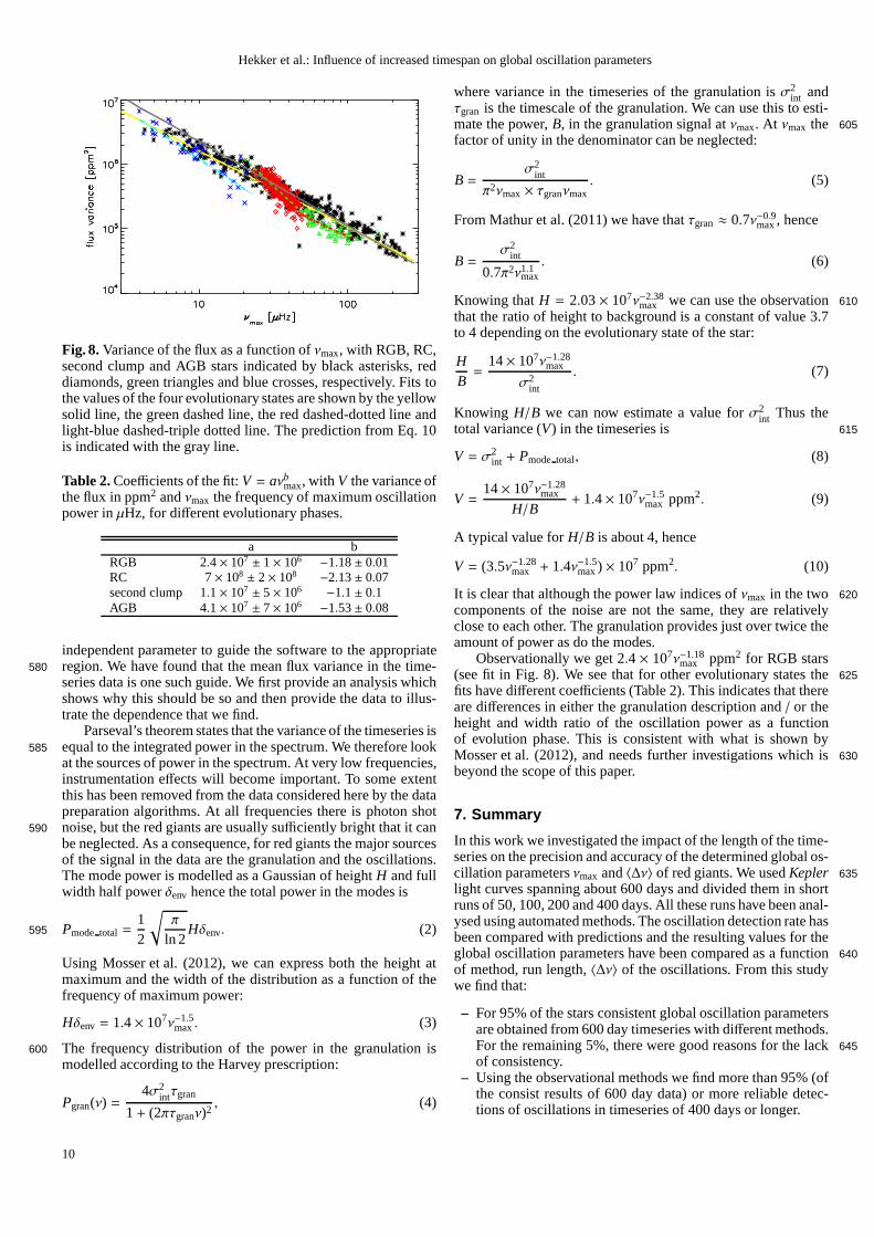
Fig. 8.Variance of the flux as a function ofνmax, with RGB, RC,second clump and AGB stars indicated by black asterisks, reddiamonds, green triangles and blue crosses, respectively.Fits tothe values of the four evolutionary states are shown by the yellowsolid line, the green dashed line, the red dashed-dotted line andlight-blue dashed-triple dotted line. The prediction fromEq. 10is indicated with the gray line.

Table 2.Coefficients of the fit:V = aνbmax, with V the variance ofthe flux in ppm2 andνmax the frequency of maximum oscillationpower inµHz, for different evolutionary phases.

a bRGB 2.4× 107 ± 1× 106 −1.18± 0.01RC 7× 108 ± 2× 108 −2.13± 0.07second clump 1.1× 107 ± 5× 106 −1.1± 0.1AGB 4.1× 107 ± 7× 106 −1.53± 0.08

independent parameter to guide the software to the appropriateregion. We have found that the mean flux variance in the time-580series data is one such guide. We first provide an analysis whichshows why this should be so and then provide the data to illus-trate the dependence that we find.

Parseval’s theorem states that the variance of the timeseries isequal to the integrated power in the spectrum. We therefore look585at the sources of power in the spectrum. At very low frequencies,instrumentation effects will become important. To some extentthis has been removed from the data considered here by the datapreparation algorithms. At all frequencies there is photonshotnoise, but the red giants are usually sufficiently bright that it can590

be neglected. As a consequence, for red giants the major sourcesof the signal in the data are the granulation and the oscillations.The mode power is modelled as a Gaussian of heightH and fullwidth half powerδenv hence the total power in the modes is

Pmode total =12

√

π

ln 2Hδenv. (2)595

Using Mosser et al. (2012), we can express both the height atmaximum and the width of the distribution as a function of thefrequency of maximum power:

Hδenv = 1.4× 107ν−1.5max. (3)

The frequency distribution of the power in the granulation is600modelled according to the Harvey prescription:

Pgran(ν) =4σ2

intτgran

1+ (2πτgranν)2, (4)

where variance in the timeseries of the granulation isσ2int and

τgran is the timescale of the granulation. We can use this to esti-mate the power,B, in the granulation signal atνmax. At νmax the 605factor of unity in the denominator can be neglected:

B =σ2

int

π2νmax× τgranνmax. (5)

From Mathur et al. (2011) we have thatτgran≈ 0.7ν−0.9max, hence

B =σ2

int

0.7π2ν1.1max. (6)

Knowing thatH = 2.03× 107ν−2.38max we can use the observation610

that the ratio of height to background is a constant of value 3.7to 4 depending on the evolutionary state of the star:

HB=

14× 107ν−1.28max

σ2int

. (7)

Knowing H/B we can now estimate a value forσ2int Thus the

total variance (V) in the timeseries is 615

V = σ2int + Pmode total, (8)

V =14× 107ν−1.28

max

H/B+ 1.4× 107ν−1.5

max ppm2. (9)

A typical value forH/B is about 4, hence

V = (3.5ν−1.28max + 1.4ν−1.5

max) × 107 ppm2. (10)

It is clear that although the power law indices ofνmax in the two 620

components of the noise are not the same, they are relativelyclose to each other. The granulation provides just over twice theamount of power as do the modes.

Observationally we get 2.4× 107ν−1.18max ppm2 for RGB stars

(see fit in Fig. 8). We see that for other evolutionary states the 625fits have different coefficients (Table 2). This indicates that thereare differences in either the granulation description and/ or theheight and width ratio of the oscillation power as a functionof evolution phase. This is consistent with what is shown byMosser et al. (2012), and needs further investigations which is 630beyond the scope of this paper.

7. Summary

In this work we investigated the impact of the length of the time-series on the precision and accuracy of the determined global os-cillation parametersνmax and〈∆ν〉 of red giants. We usedKepler 635light curves spanning about 600 days and divided them in shortruns of 50, 100, 200 and 400 days. All these runs have been anal-ysed using automated methods. The oscillation detection rate hasbeen compared with predictions and the resulting values fortheglobal oscillation parameters have been compared as a function 640

of method, run length,〈∆ν〉 of the oscillations. From this studywe find that:

– For 95% of the stars consistent global oscillation parametersare obtained from 600 day timeseries with different methods.For the remaining 5%, there were good reasons for the lack645of consistency.

– Using the observational methods we find more than 95% (ofthe consist results of 600 day data) or more reliable detec-tions of oscillations in timeseries of 400 days or longer.

10

Hekker et al.: Influence of increased timespan on global oscillation parameters

– Current predictions of the detectability of oscillations are650

based on the amplitudes and predict that in the majority ofthe cases the likelihood to detect oscillations are above 90%for both the long and short runs. However, most observa-tional algorithms use the regularity in the power spectrum todetect the oscillations and the regularity has reduced sensi-655tivity for shorter runs.

– The precision of the determined global oscillation parame-ters increases with increasing timeseriess and the trends sug-gest that this continues for even longer timeseries than inves-tigated here. From the extrapolation of fits to the median ab-660

solute deviations a reduction of more than a factor of 10 foran increase in timespan from 50 to 2000 days (the currentlyforeseen length of the mission) is foreseen. Thus, there arereal advantages to be gained from working with even longtimeseries than considered here. We note that the universal665pattern is already effective for short datasets.

– The distributions of the offsets - difference between resultsof short runs with respect to the result obtained with thesame method on the 600-day long timeseries - divided by thequoted uncertainties show that the quoted uncertainties have670a tendency to be overestimated, which is in general more se-vere for longer datasets. However, this does depend on themethod.

– We find that 50 day timeseries are not long enough to becertain to pick up more than 90% of the oscillations with the675

currently employed methods.– When comparing different methods it is clear that the dif-

ferences due to different definitions are non-negligible. Thisdifference is a function of the evolutionary state of the starsand this could be used to determine the evolutionary state.680

– The different strengths, definitions and sensitivity to realiza-tion noise of the different methods indicate that the simulta-neous use of more methods is likely to be profitable.

Additionally, we propose and justify a new method to es-timate the frequency of maximum oscillation power from vari-685ance in the timeseries. We show that the dependence of the fluxvariance onνmax is also a function of evolutionary phase. Theeffectiveness of this method does not depend on the data dura-tion nor on the location of the peak of the spectrum – alwaysassuming that the necessary data detrending is not attenuating690the oscillations signal. We recommend that this method be usedin conjunction with the methods described here as an additionalindependent constraint to detect the oscillations.

Acknowledgements. Funding for this Discovery Mission is provided by NASA’sScience Mission Directorate. TheKepler Team is recognized for helping to make695the mission and these data possible. SH acknowledges financial support fromthe Netherlands Organisation for Scientific Research (NWO). YE and WJC ac-knowledge support from the Science and Technology Facilities Council (STFC).

ReferencesBaglin, A., Auvergne, M., Barge, P., et al. 2006, in ESA Special Publication,700

Vol. 1306, ESA Special Publication, ed. M. Fridlund, A. Baglin, J. Lochard,& L. Conroy, 33

Basu, S., Grundahl, F., Stello, D., et al. 2011, ApJ, 729, L10Baudin, F., Barban, C., Belkacem, K., et al. 2011a, A&A, 529,A84Baudin, F., Barban, C., Belkacem, K., et al. 2011b, A&A, 535,C1705Baudin, F., Barban, C., Goupil, M. J., et al. 2012, A&A, 538, A73Beck, P. G., Bedding, T. R., Mosser, B., et al. 2011, Science,332, 205Beck, P. G., Montalban, J., Kallinger, T., et al. 2012, Nature, 481, 55Bedding, T. R., Huber, D., Stello, D., et al. 2010, ApJ, 713, L176Bedding, T. R., Mosser, B., Huber, D., et al. 2011, Nature, 471, 608710Borucki, W. J., Koch, D., Basri, G., et al. 2010, Science, 327, 977Chaplin, W. J., Bedding, T. R., Bonanno, A., et al. 2011a, ApJ, 732, L5Chaplin, W. J., Kjeldsen, H., Bedding, T. R., et al. 2011b, ApJ, 732, 54

De Ridder, J., Barban, C., Baudin, F., et al. 2009, Nature, 459, 398Di Mauro, M. P., Cardini, D., Catanzaro, G., et al. 2011, MNRAS, 415, 3783 715Garcıa, R. A., Hekker, S., Stello, D., et al. 2011, MNRAS, 414, L6Gruberbauer, M., Guenther, D. B., & Kallinger, T. 2012, ApJ,749, 109Hekker, S., Basu, S., Elsworth, Y., & Chaplin, W. J. 2011a, MNRAS, 418, L119Hekker, S., Basu, S., Stello, D., et al. 2011b, A&A, 530, A100Hekker, S., Broomhall, A.-M., Chaplin, W. J., et al. 2010a, MNRAS, 402, 2049 720Hekker, S., Debosscher, J., Huber, D., et al. 2010b, ApJ, 713, L187Hekker, S., Elsworth, Y., De Ridder, J., et al. 2011c, A&A, 525, A131Hekker, S., Gilliland, R. L., Elsworth, Y., et al. 2011d, MNRAS, 414, 2594Hekker, S., Kallinger, T., Baudin, F., et al. 2009, A&A, 506,465Huber, D., Bedding, T. R., Stello, D., et al. 2011, ApJ, 743, 143 725Huber, D., Bedding, T. R., Stello, D., et al. 2010, ApJ, 723, 1607Jenkins, J. M., Caldwell, D. A., Chandrasekaran, H., et al. 2010, ApJ, 713, L120Jiang, C., Jiang, B. W., Christensen-Dalsgaard, J., et al. 2011, ApJ, 742, 120Kallinger, T., Hekker, S., Mosser, B., et al. 2012, A&A, 541,A51Kallinger, T., Mosser, B., Hekker, S., et al. 2010a, A&A, 522, A1 730Kallinger, T., Weiss, W. W., Barban, C., et al. 2010b, A&A, 509, A77Kjeldsen, H. & Bedding, T. R. 1995, A&A, 293, 87Kjeldsen, H. & Bedding, T. R. 2011, A&A, 529, L8Mathur, S., Hekker, S., Trampedach, R., et al. 2011, ApJ, 741, 119Mosser, B. & Appourchaux, T. 2009, A&A, 508, 877 735Mosser, B., Barban, C., Montalban, J., et al. 2011a, A&A, 532, A86Mosser, B., Belkacem, K., Goupil, M. J., et al. 2011b, A&A, 525, L9Mosser, B., Belkacem, K., Goupil, M.-J., et al. 2010, A&A, 517, A22Mosser, B., Elsworth, Y., Hekker, S., et al. 2012, A&A, 537, A30Mosser, B., Michel, E., Appourchaux, T., et al. 2009, A&A, 506, 33 740Samadi, R., Georgobiani, D., Trampedach, R., et al. 2007, A&A, 463, 297Stello, D., Huber, D., Kallinger, T., et al. 2011a, ApJ, 737,L10Stello, D., Meibom, S., Gilliland, R. L., et al. 2011b, ApJ, 739, 13Verner, G. A., Elsworth, Y., Chaplin, W. J., et al. 2011, MNRAS, 415, 3539

11