Purdue UniversityPurdue e-Pubs

Open Access Dissertations Theses and Dissertations

12-2016

Gravity-assist trajectories to Venus, Mars, and theice giants: Mission design with human and roboticapplicationsKyle M. HughesPurdue University

Follow this and additional works at: https://docs.lib.purdue.edu/open_access_dissertations

Part of the Aerospace Engineering Commons, and the Physics Commons

This document has been made available through Purdue e-Pubs, a service of the Purdue University Libraries. Please contact epubs@purdue.edu foradditional information.

Recommended CitationHughes, Kyle M., "Gravity-assist trajectories to Venus, Mars, and the ice giants: Mission design with human and robotic applications"(2016). Open Access Dissertations. 940.https://docs.lib.purdue.edu/open_access_dissertations/940

GRAVITY-ASSIST TRAJECTORIES TO VENUS, MARS, AND THE ICE

GIANTS: MISSION DESIGN WITH HUMAN AND ROBOTIC APPLICATIONS

A Dissertation

Submitted to the Faculty

of

Purdue University

by

Kyle M. Hughes

In Partial Fulfillment of the

Requirements for the Degree

of

Doctor of Philosophy

December 2016

Purdue University

West Lafayette, Indiana

Graduate School Form

30 Updated

PURDUE UNIVERSITY

GRADUATE SCHOOL

Thesis/Dissertation Acceptance

This is to certify that the thesis/dissertation prepared

By

Entitled

For the degree of

Is approved by the final examining committee:

To the best of my knowledge and as understood by the student in the Thesis/Dissertation

Agreement, Publication Delay, and Certification Disclaimer (Graduate School Form 32),

this thesis/dissertation adheres to the provisions of Purdue University’s “Policy of

Integrity in Research” and the use of copyright material.

Approved by Major Professor(s):

Approved by:

Head of the Departmental Graduate Program Date

Kyle M. Hughes

Gravity-Assist Trajectories to Venus, Mars, and the Ice Giants: Mission Design with Human and Robotic Applications

Doctor of Philosophy

James M. Longuski

Chair

Kathleen C. Howell

Martin J. Corless

William A. Crossley

James M. Longuski

Weinong Wayne Chen 12/7/2016

ii

ACKNOWLEDGMENTS

I would like to thank my advisor Jim Longuski for his invaluable insight through-

out this entire work, and more generally, for teaching me how to be a researcher and

astrodynamicist. Working in his research group has been an invaluable experience

and a great positive influence my life and future career. I am, to say the least, grateful

for having the opportunity to work with Professor Longuski, and I will aim to follow

his example throughout my career. I would also like to thank my committee members

Professors William Crossley, Martin Corless, and Kathleen Howell for their support

and feedback. Professor Howell’s very memorable course on advanced orbital dynam-

ics was the most fascinating and fun experience I’ve had in a classroom. I would also

like to thank my colleagues Sarag Saikia, Jim Moore, Blake Rogers, and Alec Mudek

for all of their help and insight, often through long discussions at Armstrong Hall and

on the phone, which significantly improved in many ways the quality of this thesis.

I would like to thank my collaborators Parul Agrawal, Gary Allen, Helen Hwang,

and Raj Venkatapathy at Ames Research Center for pushing my research into the

atmospheres of the Gas and Ice Giants; Mike Loucks, John Carrico, and Dennis Tito

for their support and interest in my contribution to Inspiration Mars; and Buzz Aldrin

for sharing so many hours of his time with me and our research group, and allowing

me to contribute to his vision for putting a permanent human presence on Mars. I

would also like to thank Alinda Mashiku, Trevor Williams, and Jacob Englander at

Goddard Space Flight Center for letting me pester them with endless questions, and

helping me to find the next step in my career path.

I would like to thank my mom and dad, Paulette and Mike, who many times

helped me financially during this work, and have always given their support and en-

couragement, without which this work may never have taken place. I would especially

like to acknowledge my mom, who we lost in 2013. Her sense of humor, delightful

iii

cynicism, and unfailing ability to help me put things in perspective, helped keep me

sane through most of my life and especially during graduate school. I continually

work to follow her example in all aspects of my life, and be mindful of the advice I

may only speculate she would give. I would also like to thank my sister Laura for

our long phone conversations that helped me get through difficult times of loss and

stress.

Most importantly, I would like to thank my wife Mariah for her support, encour-

agement, and infinite patience with me, which I depend on daily. I will be forever

grateful to her for her sacrifice in leaving her home and effectively postponing her

career so that I may pursue this degree.

iv

TABLE OF CONTENTS

Page

LIST OF TABLES . . . . . . . . . . . . . . . . . . . . . . . . . . . . . . . . vi

LIST OF FIGURES . . . . . . . . . . . . . . . . . . . . . . . . . . . . . . . viii

ABSTRACT . . . . . . . . . . . . . . . . . . . . . . . . . . . . . . . . . . . xiii

1 THE PATCHED-CONIC METHOD OF COMPUTING GRAVITY-ASSISTTRAJECTORIES . . . . . . . . . . . . . . . . . . . . . . . . . . . . . . . 11.1 Lambert’s Problem . . . . . . . . . . . . . . . . . . . . . . . . . . . 31.2 The Tisserand Graph . . . . . . . . . . . . . . . . . . . . . . . . . . 4

1.2.1 Selecting Candidate Paths: Pathfinding . . . . . . . . . . . . 5

2 INTERPLANETARY HYPERBOLIC ENCOUNTERS: APPROACH ANDDEPARTURE TRAJECTORIES NEAR A TARGET BODY . . . . . . . 92.1 Planetocentric Equatorial Frames . . . . . . . . . . . . . . . . . . . 92.2 Hyperbolic Approach Trajectories . . . . . . . . . . . . . . . . . . . 12

2.2.1 Locus of Possible Solutions . . . . . . . . . . . . . . . . . . . 132.2.2 Probe Entry Parameters for an Oblate Body . . . . . . . . . 212.2.3 Consequences of Interplanetary Trajectory Design on Launch 322.2.4 Spacecraft Deflection Maneuver for Probe Release During Flyby 332.2.5 Launch Vehicle Performance . . . . . . . . . . . . . . . . . . 38

3 CATALOG OF TRAJECTORIES TO URANUS FROM 2024 TO 2038 IN-CLUDING AN OPPORTUNITY FOR A SATURN PROBE . . . . . . . 453.1 Background . . . . . . . . . . . . . . . . . . . . . . . . . . . . . . . 453.2 Methods . . . . . . . . . . . . . . . . . . . . . . . . . . . . . . . . . 47

3.2.1 Computing the Trajectory Design Space . . . . . . . . . . . 473.2.2 Defining the Capture Science Orbit and Estimating the Deliv-

ered Mass . . . . . . . . . . . . . . . . . . . . . . . . . . . . 513.2.3 Investigating Select Cases . . . . . . . . . . . . . . . . . . . 52

3.3 Cataloging Trajectories to Uranus . . . . . . . . . . . . . . . . . . . 553.4 Catalogs for Trajectories that Capture Inside the Rings of Uranus . 663.5 Candidate Trajectory for a Saturn-Uranus Mission . . . . . . . . . . 673.6 Aerocapture . . . . . . . . . . . . . . . . . . . . . . . . . . . . . . . 733.7 Conclusion . . . . . . . . . . . . . . . . . . . . . . . . . . . . . . . . 75

4 50-YEAR CATALOG OF GRAVITY-ASSIST TRAJECTORIES TO NEP-TUNE . . . . . . . . . . . . . . . . . . . . . . . . . . . . . . . . . . . . . 814.1 Introduction . . . . . . . . . . . . . . . . . . . . . . . . . . . . . . . 81

v

Page

4.2 Methods . . . . . . . . . . . . . . . . . . . . . . . . . . . . . . . . . 834.3 Uranus-Neptune Alignment . . . . . . . . . . . . . . . . . . . . . . 854.4 Catalog of Trajectories to Neptune . . . . . . . . . . . . . . . . . . 854.5 Neptune Probe and Orbiter Mission using the 2031 M0JN Trajectory 964.6 Candidate Trajectories for Aerocapture . . . . . . . . . . . . . . . . 1004.7 Conclusion . . . . . . . . . . . . . . . . . . . . . . . . . . . . . . . . 102

5 FAST FREE RETURNS TO MARS AND VENUS WITH APPLICATIONTO INSPIRATION MARS . . . . . . . . . . . . . . . . . . . . . . . . . . 1055.1 Introduction . . . . . . . . . . . . . . . . . . . . . . . . . . . . . . . 1065.2 Methods . . . . . . . . . . . . . . . . . . . . . . . . . . . . . . . . . 107

5.2.1 Satellite Tour Design Program (STOUR) . . . . . . . . . . . 1075.2.2 Pareto-Optimal Set . . . . . . . . . . . . . . . . . . . . . . . 1105.2.3 Earth Entry Parameters and Constraints . . . . . . . . . . . 1115.2.4 Gauss Pseudospectral Optimization Software (GPOPS) . . . 116

5.3 Results . . . . . . . . . . . . . . . . . . . . . . . . . . . . . . . . . . 1165.3.1 Rarity of the Nominal Inspiration Mars Free-Return Trajectory 1175.3.2 Investigation of Fast Mars Free-Returns with Venus Gravity

Assist . . . . . . . . . . . . . . . . . . . . . . . . . . . . . . 1275.3.3 Earth Entry Analysis . . . . . . . . . . . . . . . . . . . . . . 1445.3.4 The 2023 EVME High Entry-Speed Free-Returns . . . . . . 1515.3.5 The Case for Venus . . . . . . . . . . . . . . . . . . . . . . . 1555.3.6 Feasibility of Launch . . . . . . . . . . . . . . . . . . . . . . 159

5.4 Conclusion . . . . . . . . . . . . . . . . . . . . . . . . . . . . . . . . 160

6 VERIFICATION OF TRAJECTORIES TO ESTABLISH EARTH-MARSCYCLERS . . . . . . . . . . . . . . . . . . . . . . . . . . . . . . . . . . . 1636.1 Introduction . . . . . . . . . . . . . . . . . . . . . . . . . . . . . . . 1636.2 V∞ Leveraging . . . . . . . . . . . . . . . . . . . . . . . . . . . . . 164

6.2.1 Selected Cyclers and Their Characteristics . . . . . . . . . . 1656.3 Patched Conic Propagator Analysis . . . . . . . . . . . . . . . . . . 1676.4 Low-Thrust Analysis . . . . . . . . . . . . . . . . . . . . . . . . . . 1686.5 Results . . . . . . . . . . . . . . . . . . . . . . . . . . . . . . . . . . 169

6.5.1 STOUR Verification of V∞-Leveraging Establishment Trajec-tories . . . . . . . . . . . . . . . . . . . . . . . . . . . . . . . 169

6.5.2 Validation of Low-Thrust Establishment Trajectories . . . . 1716.6 Conclusion . . . . . . . . . . . . . . . . . . . . . . . . . . . . . . . . 179

7 CONCLUDING REMARKS . . . . . . . . . . . . . . . . . . . . . . . . . 1817.1 Contribution of Work . . . . . . . . . . . . . . . . . . . . . . . . . . 1817.2 Potential Advancement of Work . . . . . . . . . . . . . . . . . . . . 182

REFERENCES . . . . . . . . . . . . . . . . . . . . . . . . . . . . . . . . . . 185

VITA . . . . . . . . . . . . . . . . . . . . . . . . . . . . . . . . . . . . . . . 195

vi

LIST OF TABLES

Table Page

3.1 Trajectory Search Constraints . . . . . . . . . . . . . . . . . . . . . . . 49

3.2 Uranus Trajectory Catalog: SLS Block 1B . . . . . . . . . . . . . . . . 58

3.3 Uranus Trajectory Catalog: Delta IV Heavy . . . . . . . . . . . . . . . 59

3.4 Uranus Trajectory Catalog: Atlas V 551 . . . . . . . . . . . . . . . . . 60

3.5 Uranus Trajectory Catalog: SLS Block 1B—5 Mg or Less of Propellant 63

3.6 Saturn-Uranus Trajectory Catalog: SLS Block 1B . . . . . . . . . . . . 65

3.7 Saturn-Uranus Trajectory Catalog: Delta IV Heavy . . . . . . . . . . . 65

3.8 Uranus Trajectory Catalog: Atlas V 551—Capture Inside Rings . . . . 66

3.9 Uranus Trajectory Catalog: Delta IV Heavy—Capture Inside Rings . . 67

3.10 Uranus Trajectory Catalog: SLS Block 1B—Capture Inside Rings . . . 68

3.11 Uranus Trajectory Catalog: SLS Block 1B—Capture Inside Rings with 5Mg or Less of Propellant . . . . . . . . . . . . . . . . . . . . . . . . . . 77

3.12 July 3, 2028 Trajectory: Entry Parameters at Saturn . . . . . . . . . . 78

3.13 July 3, 2028 Trajectory: Entry Parameters at Uranus . . . . . . . . . . 78

3.14 Preliminary Uranus Aerocapture Trajectory Catalog: Atlas V 551 . . . 78

3.15 Preliminary Uranus Aerocapture Trajectory Catalog: Delta IV Heavy . 79

4.1 Neptune Trajectory Catalog: Atlas V 551—Capture Outside Rings . . 87

4.2 Neptune Trajectory Catalog: Atlas V 551—Capture Inside Rings . . . 87

4.3 Neptune Trajectory Catalog: Delta IV Heavy—Capture Outside Rings 88

4.4 Neptune Trajectory Catalog: Delta IV Heavy—Capture Inside Rings . 89

4.5 Neptune Trajectory Catalog: SLS Block 1B—Capture Outside Rings . 89

4.6 Neptune Trajectory Catalog: SLS Block 1B—Capture Inside Rings . . 91

4.7 Neptune Trajectory Catalog: SLS Block 1B—Capture Outside Rings with5 Mg or Less of Propellant . . . . . . . . . . . . . . . . . . . . . . . . . 94

vii

Table Page

4.8 Neptune Trajectory Catalog: SLS Block 1B—Capture Inside Rings with5 Mg or Less of Propellant . . . . . . . . . . . . . . . . . . . . . . . . . 94

4.9 Feb. 9, 2031 Trajectory: Prograde Entry at Neptune . . . . . . . . . . 99

4.10 Feb. 9, 2031 Trajectory: Near-Polar Entry at Neptune . . . . . . . . . 101

4.11 Preliminary Neptune Aerocapture Trajectory Catalog: Atlas V 551 . . 102

4.12 Preliminary Neptune Aerocapture Trajectory Catalog: Delta IV Heavy 102

5.1 Trajectory Search Parameters . . . . . . . . . . . . . . . . . . . . . . . 108

5.2 Best Case EME Candidates for 100 Years . . . . . . . . . . . . . . . . 120

5.3 Notable EVME Trajectories from Broad 45-Year Search . . . . . . . . . 130

5.4 Best Near-Term EVME Opportunities . . . . . . . . . . . . . . . . . . 136

5.5 High-Fidelity Comparison of 11/22/2021 EVME Opportunity . . . . . 139

5.6 Direct Entry Aerothermal Conditions for Key Free-Return Opportunities 149

5.7 Ablative TPS Material Properties (Adapted from Kolawa et al. [103]) . 150

5.8 2023 EVME Pareto-Set Opportunities . . . . . . . . . . . . . . . . . . 151

5.9 Subset of Best Near-Term EVE Opportunities . . . . . . . . . . . . . . 158

5.10 Declination of Select Free Returns to Mars and Venus . . . . . . . . . . 160

6.1 Orbital Elements and Number of Vehicles for Selected Cycler Trajectories 166

6.2 STOUR Results for the Selected Cyclers in the Analytic Ephemeris . . 170

viii

LIST OF FIGURES

Figure Page

1.1 Tisserand graph with the example path Venus-Earth-Earth-Jupiter-Neptune(VEEJN) indicated by the lines in bold. . . . . . . . . . . . . . . . . . 6

2.1 Body-inertial and body-fixed equatorial frames centered at the targetbody. Both body frames are shown relative to the ICRF, by the angles90° + α0, 90°− δ0, and for the body-fixed frame, the additional angle W .This figure was adapted from a figure in Ref. [10], which also provides thevalues of α0, δ0, and W for each planet. . . . . . . . . . . . . . . . . . . 10

2.2 Locus of approach trajectories at Saturn for a particular V∞ vector. Theapproach trajectories shown span all available inclinations with a rangeof periapsis radii. The trajectories shown in light green have the min-imum possible inclination for a ballistic approach (given this particularV∞ vector). . . . . . . . . . . . . . . . . . . . . . . . . . . . . . . . . . 14

2.3 (a) Coordinate frame rotations from body-inertial equatorial frame anda frame with z′′ axis aligned with the incoming V∞ vector. (b) Inertialframe used to identify a particular hyperbolic approach trajectory, givenvalues for the V∞ vector, rp (magnitude), and ψ. . . . . . . . . . . . . 15

2.4 Hyperbolic approach trajectory with minimum inclination relative to en-counter planet’s equatorial planet (at ψ = 3π/2). The retrograde coun-terpart to this solution (i.e. the approach trajectory opposite the mini-mum inclination solution, and in the same plane) occurs at ψ = π/2, andrepresents the maximum inclination solution. The absolute value of thedeclination angle, δ, of the approach, is equal to the minimum inclination. 16

2.5 Relationship between the inertial x′′, y′′, z′′ frame, and the B-plane T, R,S frame. The vectors B and rp,xy are parallel. . . . . . . . . . . . . . . 20

2.6 Coordinate frames used to define heading angle of (inertial) entry velocityvector. The x-y-z axes represent the body-fixed frame, and the vector nrepresents the surface normal vector on the oblate spheroid at the pointof entry. . . . . . . . . . . . . . . . . . . . . . . . . . . . . . . . . . . . 27

ix

Figure Page

2.7 Performance curve for the Atlas V 551 launch vehicle. The blue curve isthe unmodified performance curve, and the magenta and green points rep-resent the modified performance data with the STAR 48 additional upperstage. The green portion of the modified performance data represents theportion used to fit a 4th-order polynomial curve. . . . . . . . . . . . . . 42

2.8 Performance curve for SLS Block 1B launch vehicle. The blue curve is theunmodified performance curve, and the magenta and green points repre-sent the modified performance data with the STAR 48 additional upperstage. The green portion of the modified performance data represents theportion used to fit an 8th-order polynomial curve. . . . . . . . . . . . . 43

3.1 Capture ∆V at Uranus for various science orbit sizes and arrival V∞. Thesolid lines represent capture inside the rings of Uranus, at an altitude of3000 km. The dotted lines represent capture outside the major rings, ata radius of 52000 km. . . . . . . . . . . . . . . . . . . . . . . . . . . . . 52

3.2 Using visualization tool to adjust a Saturn probe approach trajectory forring avoidance by inspection. . . . . . . . . . . . . . . . . . . . . . . . 53

3.3 Saturn flyby trajectories with atmospheric probes. The visualization showsthat the probe-spacecraft line-of-sight is lost for the trajectory on the left,causing data link difficulties that may have no feasible design solution. 54

3.4 Trajectories to Uranus using SLS Block 1B. . . . . . . . . . . . . . . . 56

3.5 Trajectories to Uranus using SLS Block 1B with STAR-48 as additionalupper stage. . . . . . . . . . . . . . . . . . . . . . . . . . . . . . . . . . 57

3.6 Hyperbolic approach trajectories at (a) Saturn, and (b) Uranus, for theoptimized version of the July 4, 2028 opportunity in Table 3.6. . . . . . 70

3.7 MALTO-optimized Saturn-Uranus trajectory. Launch date on July 3,2028, using SLS Block 1B with STAR 48 additional upper stage. . . . . 72

4.1 Capture ∆V at Neptune for various science orbit sizes and arrival V∞. Thesolid lines represent capture inside the rings of Neptune, at an altitude of3000 km. The dotted lines represent capture outside the major rings, ata radius of 2.5 Neptune (mean equatorial) radii. . . . . . . . . . . . . . 84

4.2 The relative positions of Uranus (inner orbit) and Neptune (outer orbit) on1/1/2020 and 12/31/2070 illustrates that a long flight times (across muchof outer solar system), or possibly large flyby bending angle, is requiredto consecutively fly by Uranus and Neptune, respectively. . . . . . . . . 86

x

Figure Page

4.3 Select candidate trajectory in 2031 for Neptune probe and orbiter mission,using the SLS Block 1B launch vehicle. Flybys occur at Mars and Jupiter,with a small DSM just after Earth launch. . . . . . . . . . . . . . . . . 97

4.4 Approach at Neptune with probe and orbiter entering prograde. Theretrograde orbiter approach is also shown for comparison. . . . . . . . . 99

4.5 Approach at Neptune with orbiter approaching retrograde, with probeentering in a near-polar orbit. . . . . . . . . . . . . . . . . . . . . . . . 100

5.1 Human tolerance limits of deceleration during spacecraft entry, descent,and landing [91]. The acceleration factor is expressed in Earth g’s. . . . 113

5.2 EME free returns from December 1, 2014 to January 31, 2115. The launchyear(s) for each “column” of solutions is annotated on the figure. . . . 118

5.3 Results from 100-year search of EME free returns with arrival V∞ shownon the horizontal axis. The Pareto-optimal set of solutions (i.e. the “best”cases) are shown circled, along with the corresponding launch year. . . 120

5.4 Radial distance from the Sun shown over time for the 12/27/2017 free-return trajectory. . . . . . . . . . . . . . . . . . . . . . . . . . . . . . . 123

5.5 STOUR results showing available opportunities in December 2017 to Jan-uary 2018 with a powered flyby implemented at Mars. . . . . . . . . . 125

5.6 Mars free-return trajectories with intermediate Venus flyby before theMars encounter (gravity assist path EVME). All results shown have anEarth arrival V∞ less than or equal to 9 km/s. . . . . . . . . . . . . . . 128

5.7 Mars free-return trajectories with gravity assist path EVME. Trajectoriesshown in this plot are the same as those shown in Fig. 5.6, with Earthlaunch date exchanged for Earth arrival V∞ on the horizontal axis. . . . 130

5.8 Tisserand graph for heliocentric trajectories, with example EVME trajec-tory (in bold). The plot shows that for an Earth launch V∞ of 5 km/s,Venus can be reached (from an energy assessment), then Mars, and finallyback to Earth with an arrival V∞ of 5 km/s. . . . . . . . . . . . . . . . 133

5.9 Mars free-return trajectories for the gravity assist path EMVE. The longerTOF solutions (up to 5 years) allow for trajectories with similar launch andarrival V∞ compared to the EVME results (as indicated by the Tisserandgraph). . . . . . . . . . . . . . . . . . . . . . . . . . . . . . . . . . . . . 134

5.10 Near-term EVME Mars free-return trajectories with launch dates spanningfrom November 18 to December 21 of 2021. All results shown have anEarth arrival V∞ less than or equal to 9 km/s. . . . . . . . . . . . . . . 136

xi

Figure Page

5.11 Near-term EVME Mars free-return trajectories. Circled trajectories areconsidered to be the best near-term candidates (as defined by a Pareto-optimal set), and are listed explicitly in Table 5.4. . . . . . . . . . . . . 137

5.12 Desirable EVME opportunity generated by STOUR, with launch date on11/22/2021. (See Table 5.4.) The launch, encounter, and arrival dates areannotated on the figure. . . . . . . . . . . . . . . . . . . . . . . . . . . 138

5.13 STK plot of EVME opportunity (propagated using STK’s Astrogator),with launch date on 11/22/2021. By comparison with the STOUR-generatedtrajectory in Fig. 5.12, the STK trajectory is clearly similar. . . . . . . 139

5.14 Radial distance plot of 11/22/2021 EVME opportunity. The plot showsthe eccentric orbits of Venus, Earth, and Mars along with the spacecrafttrajectory. The black dots on the Venus and Mars curves indicate a nodecrossing. All other dots indicate an encounter. . . . . . . . . . . . . . . 141

5.15 Radial distance plot of 8/28/2034 EVME opportunity. . . . . . . . . . 142

5.16 Trajectory plot of 8/28/2034 EVME opportunity. The plot shows thatall transfer arcs have transfer angles that are near 180o (although slightlylarger on the Mars-Earth leg). . . . . . . . . . . . . . . . . . . . . . . . 143

5.17 a) Altitude vs speed, and b) deceleration load, for the three vehicle-opportunity combinations: Dragon-2018, Dragon-2021, and Orion-2021,using bank-angle control. . . . . . . . . . . . . . . . . . . . . . . . . . . 146

5.18 a) Total stagnation-point heat rate, and b) total stagnation-point heatload, for the three vehicle-opportunity combinations: Dragon-2018, Dragon-2021, and Orion-2021, using bank angle control. . . . . . . . . . . . . . 147

5.19 Total, radiative, and convective heat rates for a) Dragon-2021, and b)Orion-2021. . . . . . . . . . . . . . . . . . . . . . . . . . . . . . . . . . 148

5.20 Orion entry analysis for 2023 EVME free returns for both direct entry andaerocapture. The speed profile is shown plotted against altitude in (a),and the deceleration over time is shown in (b). . . . . . . . . . . . . . . 153

5.21 Direct entry and aerocapture results for the 2023 free-return opportunity.Total stagnation-point heat rate (a) and head load (b) are shown, andcorrespond to the same entry trajectories given in Fig. 5.20. . . . . . . 154

5.22 Venus free-return trajectories (gravity assist path Earth-Venus-Earth) withlaunch dates spanning eight years, from January 1, 2019 to January 1,2027. All results shown have an Earth arrival V∞ less than or equal to 9km/s. . . . . . . . . . . . . . . . . . . . . . . . . . . . . . . . . . . . . 157

xii

Figure Page

5.23 Venus free-return trajectories. Candidates in the Pareto set are showncircled and annotated with corresponding launch year. Most Pareto-setcandidates are shown to occur in the year 2026. . . . . . . . . . . . . . 158

6.1 The V∞-leveraging maneuver consists of a (1) ∆Vlaunch followed by a (2)∆Vaphelion to increases the V∞ at the subsequent Earth flyby, which maybe chosen to occur before (3−) or after (3+) perihelion. It should be notedthat the crew does not board the cycler vehicle until the Earth flyby. . 165

6.2 The Aldrin Cycler. The cycler vehicle launches from Earth (E1) andtravels to Mars (M2). The spacecraft next encounters Earth (E3), onesynodic period after launch. A gravity assist is performed, which rotatesthe line of apsides by 1/7 of a revolution. The cycler vehicle continues onto Mars (M4), and repeats the process ad infinitum. After 7 Earth-Marssynodic periods (15 years), the Earth is at the same inertial position aslaunch. . . . . . . . . . . . . . . . . . . . . . . . . . . . . . . . . . . . . 167

6.3 The 4:3(2)− Aldrin establishment-cycler trajectory. The spacecraft launches(1) from the Earth onto the dashed orbit and completes one and a halforbits. At aphelion (2) of this orbit, a maneuver is performed to lower theperihelion and get onto the dotted orbit. The spacecraft completes one fullorbit and returns to aphelion. The spacecraft continues inbound towardperihelion and flies (3) by the Earth. This flyby raises the heliocentricenergy of the orbit and puts the vehicle on the cycler trajectory (the solidline). Mars is encountered (4), but does not significantly affect the tra-jectory. The spacecraft completes its orbit and encounters the Earth (5)once more in order to continue on the cycler trajectory. . . . . . . . . . 171

6.4 Establishment of the S1L1 and Case 3 cyclers using low thrust. Launchfrom Earth begins at E-1, a gravity assist occurs at E0, and placementinto the cycler orbit occurs at E1. Between E-1 and E0, slightly more thanone full revolution of the Sun is completed. More than one full revolutionoccurs between E0 and E1. The E1-to-M2 leg is the first leg of the S1L1and Case 3 cyclers. The next Earth-to-Mars leg (E3-to-M4) occurs twosynodic periods later. . . . . . . . . . . . . . . . . . . . . . . . . . . . . 173

6.5 Position of the cycler vehicle shown in both the Sun-centered J2000 eclipticframe (with axes X-Y-Z) and the Sun-Earth rotating frame (with axes x-y-z). . . . . . . . . . . . . . . . . . . . . . . . . . . . . . . . . . . . . . 174

6.6 Flyby at E1 for the S1L1 establishment trajectory viewed in Sun-centeredJ2000 ecliptic frame. The low-thrust and ballistic trajectories are bothpropagated in the Sun-Earth CR3B model, where the low-thrust arc asconstant applied thrust. . . . . . . . . . . . . . . . . . . . . . . . . . . 178

xiii

ABSTRACT

Hughes, Kyle M. PhD, Purdue University, December 2016. Gravity-Assist Trajecto-ries to Venus, Mars, and the Ice Giants: Mission Design with Human and RoboticApplications. Major Professor: James Longuski.

Gravity-assist trajectories to Uranus and Neptune are found (with the allowance

of impulsive maneuvers using chemical propulsion) for launch dates ranging from

2024 to 2038 for Uranus and 2020 to 2070 for Neptune. Solutions are found using a

patched conic model with analytical ephemeris via the Satellite Tour Design Program

(STOUR), originally developed at the Jet Propulsion Laboratory (JPL). Delivered

payload mass is computed for all solutions for select launch vehicles, and attractive

solutions are identified as those that deliver a specified amount of payload mass into

orbit at the target body in minimum time. The best cases for each launch year

are cataloged for orbiter missions to Uranus and Neptune. Solutions with sufficient

delivered payload for a multi-planet mission (e.g. sending a probe to Saturn on the

way to delivering an orbiter at Uranus) become available when the Space Launch

System (SLS) launch vehicle is employed. A set of possible approach trajectories are

modeled at the target planet to assess what (if any) adjustments are needed for ring

avoidance, and to determine the probe entry conditions.

Mars free-return trajectories are found with an emphasis on short flight times

for application to near-term human flyby missions (similar to that of Inspiration

Mars). Venus free-returns are also investigated and proposed as an alternative to a

human Mars flyby mission. Attractive Earth-Mars free-return opportunities are iden-

tified that use an intermediate Venus flyby. One such opportunity, in 2021, has been

adopted by the Inspiration Mars Foundation as a backup to the currently considered

2018 Mars free-return opportunity.

xiv

Methods to establish spacecraft into Earth-Mars cycler trajectories are also in-

vestigated to reduce the propellant cost required to inject a 95-metric ton spacecraft

into a cycler orbit. The establishment trajectories considered use either a V-infinity

leveraging maneuver or low thrust. The V-infinity leveraging establishment trajec-

tories are validated using patched conics via the STOUR program. Establishment

trajectories that use low-thrust were investigated with particular focus on validating

the patched-conic based solutions at instances where Earth encounter times are not

negligible.

1

1. THE PATCHED-CONIC METHOD OF COMPUTING

GRAVITY-ASSIST TRAJECTORIES

For heliocentric trajectories, the spacecraft will be primarily under the influence of

the Sun’s gravity for the vast majority of time spent on the trajectory. Compared to

the overall time spent on such trajectory, any time taken for the spacecraft to fly by a

celestial body in the Solar System (which in practice may take several hours) is often

approximated as happening instantaneously. This in principle is the patched-conic

approximation (as applied to heliocentric trajectories), and is often used for early

phase mission design to estimate ∆V and propellant mass required for a mission.

For most heliocentric, interplanetary, gravity-assist trajectories, the only other

gravitational bodies that need to be considered are those of the encounter bodies

used for gravity-assist. The patched-conic model assumes that only the gravity of Sun

influences the spacecraft throughout its trajectory, except during a flyby of a gravity-

assist body. During the gravity assist, only the gravity of that body is assumed to

have influence on the spacecraft, and the amount of bending on the spacecraft’s ve-

locity vector do to the hyperbolic flyby can be computed for a given closest approach

distance. With this approximation, the 2-body gravity model can be used for the

heliocentric trajectory, as well as for the gravity-assist encounters, whereby the tra-

jectories between gravity-assists are ”patched” together to create an approximation

to a complete (n-body) heliocentric, gravity-assist trajectory.

In this work, the patched-conic approximation is used for purposes of identifying

the existence of a heliocentric, gravity-assist trajectory, and to determine the feasibil-

ity of the trajectory for use in a mission, by estimating key values such as: DeltaV ,

delivered mass, flight times, planet-relative velocities, and encounter geometries. Of

course the specific values of interest vary depending on the mission requirements, but

2

the values considered in this work are among a typical set of important values in

determining mission feasibility. Since these results are based on the patched-conic

approximation, any continued work on such trajectories will eventually need to be

computed in a high-fidelity force model, such as from the General Mission Analy-

sis Tool (GMAT) or the Systems Tool Kit (STK). For the heliocentric trajectories

presented in this work, it is assumed that the patched-conic solutions are of medium-

fidelity, which we describe as being sufficiently close to the high-fidelity solution that

they may be used as an initial guess for the high-fidelity tool to converge on a trajec-

tory with similar characteristics.

Finding a patched-conic solution typically begins with finding a desired heliocen-

tric trajectory between two Planets (or other celestial bodies), or between a sequence

of Planets for gravity-assist trajectories. If an impulsive maneuver is planned, a he-

liocentric arc may go from a Planet to a point in space where the maneuver is to be

implemented. For the case of gravity-assist trajectories, if the flyby is to be ballis-

tic (without assistance by a maneuver) the V∞ at the arrival body on the incoming

heliocentric arc, must match (in magnitude) the departure V∞ of the outgoing helio-

centric arc. Additionally, the amount the V∞ vector rotates between the incoming

and outgoing heliocentric arcs, must have a feasible closest approach to the gravity-

assist body—that is, without colliding with the Planet, and in most cases, without

significantly interacting with a Planet’s atmosphere or rings.

In trajectory design, the challenge is to find a desirable heliocentric solution,

that: encounters the desired targets at the correct times (according to an ephemeris

model), is feasible for a spacecraft to fly given technology limitations (for example due

to available launch vehicles and thrusters), and meets mission requirements (such as

specified launch date spans, maximum flight times, encounter conditions for a probe

or orbiter, etc.). One such approach to finding these solutions, is to compute the

heliocentric arcs in the ephemeris model by solving Lambert’s problem.

3

1.1 Lambert’s Problem

In orbital mechanics, the problem of computing a trajectory that connects two

position vectors (i.e. at departure and arrival) in a specified amount of time, is often

referred to as Lambert’s problem (and sometimes as the Gauss problem). Solving

Lambert’s problem is fundamental to the computation of interplanetary trajectories

(using the patched-conic model), especially when multiple gravity-assist trajectories

are desired.

For example, take two celestial bodies orbiting the Sun. If we know the date we

wish to depart the first celestial body, and the date we wish to arrive at the second

celestial body, then an ephemeris model of each body’s motion would reveal their po-

sitions on those dates, and the difference in time would reveal a specific time of flight

to travel between the bodies. With such information, we could compute one or more

trajectories between the two bodies by solving Lambert’s problem. Additionally, if

we wanted to then depart the second body and go to a third body, we could compute

a trajectory that would take the spacecraft there by choosing a date of arrival at (or

time of flight to) the third body, and solving Lambert’s problem again for the subse-

quent heliocentric arc. Further analysis is required to determine if such trajectories

are feasible (or desirable) to fly using available technology; however, regardless of

these additional computations, Lambert’s problem is at the heart of nearly all of the

interplanetary trajectories presented in this thesis.

There are several methods for solving Lambert’s problem in literature; however, for

this work, the patched-conic solutions are computed using the Satellite TOUR design

program (STOUR), which solves Lambert’s problem using the Lancaster-Blanchard

method [1]. The ephemeris model used by STOUR to solve Lambert’s problem and

the patched-conic solutions is an analytical model presented by Sturms [2].

Another factor that must be considered in using Lambert’s problem to solve for

heliocentric arcs (or Lambert arcs) between bodies, is matching the incoming and

outgoing V∞ magnitude at a gravity assist. For a ballistic flyby (i.e. where no

4

maneuver is applied during the encounter), the incoming V∞ must equal the outgoing

V∞. The direction of the V∞ vector will change (which is what causes the energy

change for the heliocentric trajectory), but the magnitude remains the same. In

STOUR, this constraint is considered by computing hundreds of outgoing Lambert

arcs (given a fixed incoming Lambert arc) at an encounter, whereby a root solving

method is used to find the all outgoing trajectories that have an outgoing V∞ that

equals the incoming V∞ within a specified tolerance. A complete description of this

C3-matching technique (as implemented in STOUR) is given by Williams in Ref. [3].

1.2 The Tisserand Graph

The Tisserand graph is implemented in this work as a plot of orbital specific energy

versus radius of periapsis, and provides a graphical means of identifying potential

gravity-assist combinations (or “paths”). A detailed description of the theory behind

this graphical method, and how it is developed using Tisserand’s criterion, is provided

by Strange and Longuski [4] and Labunsky et al. [5]. The Tisserand graph has since

been adapted by Johnson and Longuski in 2002 for aerogravity-assist trajectories [6],

by Chen et al. in 2008 for low-thrust gravity-assist trajectories [7], and more recently

by Campagnola and Russell in 2010 for gravity-assist trajectories that implement V∞-

leveraging maneuvers [8], as well as for application to the circular-restricted three-

body problem [9].

In simple terms, the Tisserand graph can be described as follows: The lines on

the Tisserand graph represent the locus of orbits with the same energy relative to a

given planet. The intersection of lines of one planet with those of another indicates

that there exist orbits about each planet with the same heliocentric energy. Thus,

a transfer from one planet to another is possible from an energy standpoint (though

the planet may not be in the correct location at the time the spacecraft crosses

the planet’s orbit). Knowledge of the planetary ephemerides and the solution of

5

Lambert’s problem are then required for pathsolving, in order to find out when in

time the transfer orbit occurs.

In this work, the Tisserand graph is used to primarily to identify candidate tra-

jectory paths to the Ice Giants, Uranus and Neptune (discussed in chapters 3 and

4). The Tisserand graph is also useful for screening out flyby combinations that are

not feasible within the desired launch V∞ bounds, and thus avoid the computational

effort that would otherwise be required to consider such a path.

In this work, the problem of identifying candidate gravity-assist paths based on

orbital energy (i.e. using the Tisserand graph), will be referred to as “pathfinding.”

Whereas, the problem of identifying real trajectories on those paths in the ephemeris

model will be referred to as “pathsolving.”

1.2.1 Selecting Candidate Paths: Pathfinding

To illustrate the use of the Tisserand graph, an example case is shown in Figure

1.1 for the path Venus-Earth-Earth-Jupiter-Neptune (VEEJN). The specific energy

of the orbit is shown on the vertical axis and the radius of periapsis is shown on a

logarithmic scale on the horizontal axis. In this example, lines are shown for Venus,

Earth, Jupiter, and Neptune. The rightmost line for each planet represents a V∞ of

1 km/s. V∞ increases by 2 km/s with each line to the left (i.e. moving from right

to left, the lines represent V∞s of 1 km/s, 3 km/s, 5 km/s, etc.). The dots (or small

circles if obstructed by a line in bold) along the V∞ lines provide reference points

for the amount of energy change that can be accomplished with a single flyby of the

planet, with a closest approach of 200 km altitude. This energy change is based on

the maximum possible amount that the planet can rotate (or bend) the V∞ vector.

A potential VEEJN path is highlighted by the bold lines in Figure 1.1. The path

begins at Earth with 3 km/s as the chosen V∞ of launch. By traversing this line down

and to the left, an intersection with Venus is found at the line representing a V∞ of 5

km/s. Following this line upward, several other V∞ lines for Earth are encountered.

6

Figure 1.1.: Tisserand graph with the example path Venus-Earth-Earth-Jupiter-Neptune (VEEJN) indicated by the lines in bold.

The 9 km/s V∞ line for Earth is of particular interest because it also intersects a

Jupiter V∞ line. The Earth V∞ line for 9 km/s is then followed up and to the right

(past the small circle), and on to an intersection with the Jupiter V∞ line for 7 km/s.

Surpassing the full distance between the two small circles on the Earth V∞ line (while

on route to the Jupiter line at 7 km/s), indicates that the amount of energy required

is more than what can be achieved in a single Earth flyby. Therefore, two Earth

flybys are required to get from Venus to Jupiter on this path. Finally, the Jupiter

V∞ line for 7 km/s is followed up and to the right until it intersects the Neptune

V∞ line at 3 km/s. The overall implication of this result is that a spacecraft with

launch V∞ of 3 km/s is capable of reaching Neptune by means of the flyby sequence

Venus-Earth-Earth-Jupiter, and then arriving at Neptune with a V∞ of 3 km/s.

7

In this work, powered flybys are also considered, but only at one of the flyby

bodies (to reduce computational time). We assume the maneuver is performed 3

days after the point of closest approach so that navigators have time to determine

the location of the spacecraft before implementing the powered flyby maneuver. As

a result of this delay, we conservatively assume that the burn occurs along the de-

parture asymptote—taking no advantage of the additional energy boost gained by

implementing the maneuver within the planets gravity well.

Identifying which flyby body will be most beneficial for a powered flyby is done

by inspection of the Tisserand graph. Since the giant planets provide a substantial

energy boost without a maneuver, powered flybys are only considered at the inner

planets. To approximate the energy boost provided by such a maneuver, we shift

vertically upwards on the Tisserand graph just after a flyby. The amount of the shift

is determined by the maximum allowed maneuver ∆V . For this work, we assume a

maximum ∆V of 3 km/s, which (if applied along the departure asymptote) provides a

+3 km/s V∞ boost to the flyby. This 3-km/s V∞ increase equates to a vertical shift on

the Tisserand graph by 1.5 V∞ curves. For each gravity assist path, the flyby chosen

to implement the powered flyby, is the one that provides the largest heliocentric

orbital energy boost. It was found that this often occurs when the powered flyby is

implemented at the last inner planet flyby.

8

9

2. INTERPLANETARY HYPERBOLIC ENCOUNTERS:

APPROACH AND DEPARTURE TRAJECTORIES NEAR

A TARGET BODY

2.1 Planetocentric Equatorial Frames

To model trajectories near a target body, it is useful to us a coordinate frame

centered at the target body, with the xy-plane of that frame chosen to be the body’s

equatorial plane. In this analysis, two frames are used.

The “body-inertial” frame is defined as follows:

The frame is centered at the body’s center of mass.

The x-axis is along the line formed by the intersection of the body’s equator

and the equator of the International Celestial Reference Frame (ICRF) defined

by the International Astronomical Union (IAU) [10].

The z-axis is along the body’s spin axis.

The y-axis completes the triad (using the “right hand rule”).

The ICRF is a precisely defined inertial frame centered at the barycenter of the

Solar System. To help visualize the ICRF, its axes are oriented nearly identically to

those in the Earth J2000 equatorial frame, with ICRF equator and z-axis, approxi-

mately equal to Earth’s equatorial plane and spin axis, respectively. The ICRF x-axis

is directed towards the Vernal Equinox. The spin axis orientation for a target planet

is defined relative to the ICRF by right ascension angle, α0, and declination angle,

δ0, as defined by the IAU in Ref. [10]. The body-inertial frame is visually depicted in

Fig. 2.1, which has been adapted from a figure in Ref. [10].

10

𝒛𝐵𝐼, 𝒛𝐵𝐹

𝒙𝐵𝐼

𝒚𝐵𝐼

𝒙𝐵𝐹

𝒚𝐵𝐹

𝒙𝐼𝐶𝑅𝐹 𝒛𝐼𝐶𝑅𝐹

𝒚𝐼𝐶𝑅𝐹

Vernal equinox

Figure 2.1.: Body-inertial and body-fixed equatorial frames centered at the targetbody. Both body frames are shown relative to the ICRF, by the angles 90° + α0,90° − δ0, and for the body-fixed frame, the additional angle W . This figure wasadapted from a figure in Ref. [10], which also provides the values of α0, δ0, and Wfor each planet.

To compute the coordinates of a vector in the body-inertial frame, given a vector

in the ICRF, the following rotation matrices are first defined. The direction cosine

matrix for a rotation about the x-axis by angle θ is given by

R1(θ) =

1 0 0

0 cos θ sin θ

0 − sin θ cos θ

(2.1)

Similarly, for a rotation about the z-axis by angle θ, the direction cosine matrix is

11

R3(θ) =

cos θ sin θ 0

− sin θ cos θ 0

0 0 1

(2.2)

Given a vector in the ICRF, two rotations are required to compute such a vector’s

equivalent in the body-inertial frame. First, a rotation about the z-axis by angle

90° + α0 is required, and second, a rotation about the x-axis by angle 90° − δ0 is

required. The calculation is given by

rBI = R1(90°− δ0)R3(90° + α0)rICRF (2.3)

where rBI is a column vector in the body-inertial frame, and rICRF is the equivalent

column vector expressed in the ICRF.

The “body-fixed” frame, rotates with the target body about its spin axis, and is

defined as follows:

The frame is centered at the body’s center of mass.

The x-axis is within the body’s equatorial plane, in the direction of the body’s

prime meridian (which lies in the x-z plane).

The z-axis is along the body’s spin axis.

The y-axis completes the triad (using the “right hand rule”).

Given a vector in the body-inertial frame, that vector’s equivalent in the body-

fixed frame is found via a rotation about the z-axis by angle W . The computation

is

rBF = R3(W )rBI (2.4)

where rBF is a column vector in the body-fixed frame. Depending on how the north

pole is defined, a planet may spin prograde about it’s north pole (i.e. appear to spin

counterclockwise to an observer looking down onto the north pole), or retrograde

12

(i.e. appear to spin clockwise to an observer looking down onto the north pole). In

the body-fixed and body-inertial frames defined above, the positive z-axis is directed

along the spin axis towards the north pole. For the parameters α0, δ0, and W used in

this study to define a body’s orientation (as defined by [10]), the rotation is prograde

if W increases with time, and retrograde if W decreases with time. Of the eight

planets, only Venus and Uranus spin retrograde according to this definition.

Given a vector in ICRF coordinates, the calculation to body-fixed coordinates is

found by substituting Eq. 2.3 into Eq. 2.4, giving

rBF = R3(W )R1(90°− δ0)R3(90° + α0)rICRF (2.5)

For some software tools such as STOUR and MALTO, it is more convenient to

compute vectors in the J2000 ecliptic frame. To compute such a vector’s equivalent

in either the body-inertial frame, or the body-fixed frame, one must first express that

vector in the ICRF. Since, in this work, this calculation is only used for V∞ vectors

found from the low- to mid-fidelity STOUR or MALTO solutions, it is assumed that

the ICRF and the J2000 equatorial frame are equal. With this assumption, the

rotation from the J2000 ecliptic frame, to the ICRF, is simply a rotation about their

mutually shares x-axis by Earth’s axial tilt of 23.44°, giving

rICRF = R1(23.44°)rJ2K,Ec (2.6)

where rJ2K,Ec is a column vector in the J2000 ecliptic frame.

2.2 Hyperbolic Approach Trajectories

When identifying an interplanetary trajectory, the characteristics of the approach

trajectory to a target body can play a key role in assessing whether or not that

trajectory is feasible. Visualizing the approach can also be insightful for identifying

trajectories that pass through a planet’s rings, identifying whether or not line-of-sight

13

is maintained between the spacecraft (or probe) and the Earth or Sun, or simply com-

municating the available approach options to the scientific community. The signifi-

cance of the approach trajectory parameters depend on the mission application, but

the consequences of the approach trajectory (which are dependent on the correspond-

ing interplanetary trajectory) can be just as important to the mission’s feasibility as

the interplanetary trajectory characteristics themselves (e.g. flight time, delivered

payload mass, and arrival V∞).

For example, consider a mission to Uranus, where we are assessing the possible

approach trajectories for an atmospheric probe. Since Uranus has rings and a large

axial tilt (of about 98°to its own orbit), factors such as a high declination angle,

or ring avoidance, may result in approach trajectories with high atmospheric entry

speeds. Depending on the available thermal protection systems for the probe, the

approach trajectories may turn out to be infeasible, and therefore, the corresponding

interplanetary trajectory would not be suitable for such a mission.

2.2.1 Locus of Possible Solutions

Given a V∞ vector in body-inertial coordinates (as defined in Sec. 2.1), the

“locus” of possible hyperbolic approach trajectories can be derived. An example of

the possible approach trajectories for a particular V∞ vector at Saturn is visualized in

Fig. 2.2. The approach trajectories are all constrained by the interplanetary arrival

V∞ vector, and the span of possible approach trajectories is computed by selecting a

range of hyperbolic periapsis radii magnitudes, and a step size for the span of angles

about the ring created by the locus of periapses (shown in green in Fig. 2.2). The

angular position, ψ, on the ring of periapsis radii is defined in Fig. 2.3. With the V∞

vector already given, a chosen periapsis magnitude and value of ψ defines a particular

approach trajectory, which can therefore be calculated from these values.

The equation to express a column vector, rxyz (in xyz-frame coordinates), as an

equivalent vector, rx′y′z′ (in x′y′z′-frame coordinates) is

14

Locus of periapses

x

y

z

V∞

Figure 2.2.: Locus of approach trajectories at Saturn for a particular V∞ vector. Theapproach trajectories shown span all available inclinations with a range of periapsisradii. The trajectories shown in light green have the minimum possible inclinationfor a ballistic approach (given this particular V∞ vector).

rx′y′z′ = R3(φ1)rxyz (2.7)

Similarly, to compute a column vector, rx′′y′′z′′ in x′′y′′z′′-frame coordinates, from an

equivalent vector rx′y′z′ , the equation is

rx′′y′′z′′ = R2(φ2)rx′y′z′ (2.8)

where

R2(θ) =

cos θ 0 − sin θ

0 1 0

sin θ 0 cos θ

(2.9)

and by plugging Eq. 2.7 into Eq. 2.8 gives

15

x

y

z, z'

V∞

Periapsis radii of approach trajectories

β

rp

x' 𝞍1

y', y''

𝞍1

x''

𝞍2

𝞍2 z''

rp

z''

V∞

β

rp

x''

y''

rp,xy 𝜓

(a) (b)

𝜓

Figure 2.3.: (a) Coordinate frame rotations from body-inertial equatorial frame anda frame with z′′ axis aligned with the incoming V∞ vector. (b) Inertial frame used toidentify a particular hyperbolic approach trajectory, given values for the V∞ vector,rp (magnitude), and ψ.

rx′′y′′z′′ = R2(φ2)R3(φ1)rxyz (2.10)

For probe entry, it is often the goal pick the approach trajectory with the minimum

possible inclination (i.e. the approach trajectory with minimum inclination relative

to the equatorial plane of the encounter body). The minimum inclination trajectory

is desired to take the most advantage of the rotation of the planet’s atmosphere,

to reduce the entry “air” speed of the probe, and therefore, the entry heating. By

observation of Fig. 2.3a, it can be found that the minimum inclination approach

trajectories correspond to a value of ψ = 3π/2. This is illustrated more clearly in

Fig. 2.4, which shows a plane containing the approach V∞ vector, the y′′ axis, and the

approach trajectory corresponding to the minimum inclination solution. The solution

opposite the minimum inclination solution (and in the same plane) at ψ = π/2,

16

is the maximum inclination solution, and represents a retrograde solution closest

to the equatorial plane, which minimizes the entry “air” speed for planets such as

Venus and Uranus which spin retrograde about their north pole (as defined by [10]).

Alternatively, a ψ values of π/2 maximizes the air speed for entry at all other planets

(which spin prograde with respect to their north pole). Quantitatively, the minimum

inclination angle is equal to the absolute value of the declination angle, δ (where

−π/2 ≤ δ ≤ π/2), which is the angle between the V∞ vector and the equatorial

plane (i.e. between V∞ and the x′ axis). In other words,

imin = |δ| (2.11)

where imin is the minimum possible orbit inclination (without the use of a maneuver

or perturbation forces) for the hyperbolic approach trajectory.

x

y

z

V∞

Periapsis radii of approach trajectories

rp

y', y''

x''

z''

rp,xy

Plane containing V∞ and y''

(and min. inc. trajectory)

Hyperbolic approach trajectory with

minimum inclination

𝜓, measured from x'' about V∞

𝛿, measured from x' to V∞

rp for retrograde counterpart to minimum inclination

approach (𝜓=𝜋/2)

x' 𝞍1

𝞍2

𝛿

rp for minimum inclination approach

(𝜓=3𝜋/2)

𝜓

Figure 2.4.: Hyperbolic approach trajectory with minimum inclination relative toencounter planet’s equatorial planet (at ψ = 3π/2). The retrograde counterpart tothis solution (i.e. the approach trajectory opposite the minimum inclination solution,and in the same plane) occurs at ψ = π/2, and represents the maximum inclinationsolution. The absolute value of the declination angle, δ, of the approach, is equal tothe minimum inclination.

17

To compute the orbital elements for an approach trajectory (given V∞ (vector), rp

(magnitude), and ψ), the semimajor axis, eccentricity, and angle β are first calculated,

given by

a = −µ/V 2∞ (2.12)

e = 1− rp/a (2.13)

β = cos−1(1/e), 0 < β < π/2 (2.14)

where µ is the gravitational parameter of the encounter body (i.e. the gravitational

constant multiplied by the mass of the encounter body), and the angle β is the

supplement to the true anomaly of the hyperbolic trajectory at infinity (i.e. the true

anomaly of the outgoing asymptote).

The radius, r, at a specified true anomaly, θ∗, can now be computed from

r =a(1− e2)

1 + e cos θ∗(2.15)

To get the remaining orbital elements, the periapsis vector, rp is computed. To

calculate rp, the rotation angles φ1 and φ2 are first found from the components of the

V∞ vector as follows:

φ1 = tan−1

(V∞,yV∞,x

)(2.16)

φ2 = tan−1

(V∞,x′

V∞,z′

)(2.17)

When computing trajectories in this study (e.g. with STOUR or MALTO), the

V∞ vector is typically found in J2000 ecliptic-frame coordinates. From Eqs. 2.6 and

2.3 (using the δ0 and α0 values in Ref. [10] for the desired planet), the V∞ vector

18

coordinates can be quickly converted to body-inertial frame coordinates. Since the

body-inertial coordinates represent the planetocentric equatorial xyz-frame, comput-

ing φ1 from Eq. 2.16 is straightforward. To find an expression for the V∞ components

in x′y′z′-frame coordinates (shown in Fig. 2.3), we use Eq. 2.7, with φ1 and V∞ sub-

stituted for θ and rxyz, respectively. The resulting expressions for the V∞,x′ and V∞,z′

components can then be plugged into Eq. 2.17, giving

φ2 = tan−1

(V∞,x cosφ1 + V∞,y sinφ1

V∞,z

)(2.18)

With φ1 and φ2 known, the periapsis vector, rp can be computed. By inspection

of Fig. 2.3b, rp can be expressed in terms of β and ψ as

rp = rp sin β cosψx′′ + rp sin β sinψy′′ + rp cos βz′′ (2.19)

where x′′, y′′, and z′′ are unit vectors along the x, y, and z axes, respectively. From

Eq. 2.10, the x′′, y′′, and z′′ components of rp can be written in x, y, and z coordinates

(via the φ1 and φ2 rotations as shown in Fig. 2.3a), giving

rp = rp[cosφ1 (sin β cosψ cosφ2 + cos β sinφ2)− sinφ1 sin β sinψ] x

+ [sinφ1 (sin β cosψ cosφ2 + cos β sinφ2) + cosφ1 sin β sinψ] y

+ (cos β cosφ2 − sin β cosψ sinφ2) z

(2.20)

which is expressed entirely in terms of known values.

With rp known, the remaining orbital elements for the hyperbolic approach tra-

jectory can be computed from,

e = erprp

= exx+ eyy + ez z (2.21)

h =√aµ(1− e2) (2.22)

19

h =rp ×V∞|rp ×V∞|

(2.23)

h = hh = hxx+ hyy + hz z (2.24)

i = cos−1

(hzh

)(2.25)

where h is the specific angular momentum, and i is the inclination of the orbit with

respect to the encounter body’s equatorial plane. If we define N as the ”node vec-

tor” (i.e. the vector directed from the origin to the ascending node of the approach

trajectory), given by

N = z × h = Nxx+Nyy +Nz z (2.26)

then the right ascension of the ascending node, Ω, and the argument of periapsis, ω,

can be computed from

Ω =

cos−1(Nx

N

)for Ny ≥ 0

2π − cos−1(Nx

N

)for Ny < 0

(2.27)

ω =

cos−1(N·eNe

)for ez ≥ 0

2π − cos−1(N·eNe

)for ez < 0

(2.28)

The x′′, y′′, z′′ frame can be related to the more commonly used B-plane frame,

for a reference normal vector Nref = z (the planet’s spin axis). The relationship to

B-plane is illustrated in Fig. 2.5, and given by the following equations

B = bB (2.29)

20

Periapsis radii of approach trajectories z'' , 𝑺

V∞

β

rp

x'', 𝑹

y'' rp,xy

𝜓

𝑻 𝜽

𝑩

Figure 2.5.: Relationship between the inertial x′′, y′′, z′′ frame, and the B-plane T,R, S frame. The vectors B and rp,xy are parallel.

b = |a|√e2 − 1 (2.30)

B = S× h (2.31)

where h is the angular momentum of the trajectory and

S = z = V∞ (2.32)

Additionally, the unit vectors T and R can be expressed as

T =S× Nref

|S× Nref |= −y′′ (2.33)

21

R = S× T = x′′ (2.34)

The B-plane angle θ can be related to the design parameter ψ by the simple

relation

θ = ψ + π/2 = ψ + 90° (2.35)

2.2.2 Probe Entry Parameters for an Oblate Body

When approaching and entering the atmosphere of a planet or moon, the oblate-

ness (bulge) of the body may significantly impact the entry conditions, such as entry

flight path angle and entry latitude. The cause is both geometric and gravitational.

The geometric impact is due to the fact that the entry point on the surface of an

oblate spheroid at a specified radius will differ from a corresponding entry point on

that of a sphere. The gravity field of an oblate body will also cause perturbations on

the orbital elements (compared to the gravity field if a spherical body is assumed).

One such change is the precession of the right ascension of the ascending node.

For the Gas-Giant and Ice-Giant planets, the oblateness is particularly pronounced.

For this analysis, the shapes of the giant planets are assumed to be oblate spheroids,

defined by their mean equatorial radius and polar radius. Additionally, only the ge-

ometric consequences of entry on an oblate body are considered. Since the approach

hyperbolic trajectory is only in the vicinity of the planet from (approximately) the

point of entry into the planet’s sphere of influence, to atmospheric entry, any preces-

sion of the elements is assumed small is this relatively short period of time (compared

to the time scale of a spacecraft orbiting the planet).

This work also does not include an analysis of the probe during entry; rather, the

purpose is to compute the probe’s states upon entry into the atmosphere.

22

In this section, a method is presented for computing the following parameters at

the point of atmospheric entry on an oblate spheroid, for a known hyperbolic approach

trajectory:

Inertial velocity magnitude (i.e. orbital velocity in “body inertial” frame)

Entry flight path angle

Heading angle

Latitude

Longitude

Atmosphere-relative entry velocity

To understand whether or not such entry conditions are feasible for a particular

probe design, an entry analysis will need to be conducted. Since entry analyses

often fall outside the expertise of many mission designers, the following derivation

computes entry parameters that are convenient for an entry analysis team to simulate

entry. This process will likely be iterative, where the mission designers adjust the

approach trajectories (or possibly the interplanetary trajectory) and send updated

entry parameters, until a feasible probe design can be found. In this work, much of the

entry insight came from a collaboration with the entry analysis team at NASA Ames

Research Center, who’s entry analysis tools required the entry parameters derived

in this section. One exception is the derivation of the atmospheric-relative entry

velocity. This parameter is more intuitive for the non-entry expert to interpret, and

by comparison to atmosphere-relative entry speeds in the literature for other probe

entry designs, can be used to gauge the feasibility of probe entry, when a complete

entry analysis has yet to be done, or is unavailable.

For the following derivation of the entry parameters, it is assumed that the hyper-

bolic approach trajectory is completely known. The approach trajectory parameters

that are used in this derivation include: rP , V∞, ψ, h, i, Ω, e, and ω. Where h is

the orbital angular momentum vector, i is the inclination, Ω is the right ascension of

the ascending node, e is the eccentricity vector (which points from the focus of the

hyperbolic or elliptical trajectory to the periapsis), and ω is the argument of periapsis.

23

If an approach trajectory has not yet been selected, the following method can

still be used to calculate the entry parameters, but the process must be iterative;

where several approach trajectories are selected and the various entry parameters are

assessed to choose a feasible approach trajectory. (This iterative process was the

primary method used to select an approach trajectory in this work.)

Point of Entry and Inertial Velocity at Entry

The planet shape including its atmosphere is assumed to be an oblate spheroid.

A point on the surface of this oblate spheroid is defined by,

r2x + r2

y

a2+r2z

b2= 1 (2.36)

where r is the position vector pointing to the specified point on the surface of an

oblate spheroid (centered about the origin) expressed in Cartesian coordinates. (For

this derivation, the x-y-z frame refers to the body-inertial frame.) Since the surface of

the oblate spheroid defined for this derivation includes the planet and its atmosphere,

a = REq + EntryAlt (2.37)

b = RPol + EntryAlt (2.38)

where REq and RPol are the planet’s mean equatorial radius and polar radius, and

EntryAlt is the altitude where the entry is defined to occur (i.e. the ”edge” of the

planet’s atmosphere). In this work, the point of entry is assumed to be 1000 km at

Saturn, and 3000 km at Uranus and Neptune. For all giant planets, the ”surface” is

often defined as the point where the atmospheric pressure is 1 bar.

To find the point of entry on an approach trajectory, the position vector r in Eq.

(2.36), must also be a position vector on the approach trajectory. Identifying such

a vector represents the point on the approach trajectory that intersects the surface

24

of the oblate spheroid. Since the approach trajectory is known, identifying the true

anomaly at this intersection will give the entry point. To find the true anomaly, r is

expressed in Cartesian coordinates (in the body-inertial frame) in terms of the orbital

elements Ω, i, and θ,

r = r(cos Ω cos θ − sin Ω cos i sin θ) x

+ (sin Ω cos θ + cos Ω cos i sin θ) y

+ sin i sin θz

= rxx+ ryy + rz z

(2.39)

and

θ = θ∗ + ω (2.40)

were θ∗ is the true anomaly.

Plugging rx, ry, and rz, into Eq. (2.36), replacing θ using Eq. (2.40), and express-

ing r using the conic equation (expressed in terms of h), given by

r =h2/µ

1 + e cos θ∗(2.41)

produces the transcendental equation

µ2(1 + e cos θ∗)

h4=

cos2 (θ∗ + ω) + cos2 i sin2 (θ∗ + ω)

a2+

sin2 i sin2 (θ∗ + ω)

b2(2.42)

Equation (2.42) can be solved for the entry θ∗ using a root solver. A recommended

initial guess, is the entry true anomaly for a spherical body (using either the equatorial

radius as done below, or the polar radius, or an average of the two to define the

sphere), given by

θ∗Sphere = − cos−1

[1

e

(h2

µr− 1

)](2.43)

25

where the negative solution of cos−1(∗) is taken since the approach trajectory is

incoming, and therefore entry occurs before periapsis passage.

With θ∗ at entry known, it can be plugged into Eq. (2.39) to compute rEntry.

The inertial velocity magnitude at the point of entry is then computed from

VEntry =√V 2∞ + 2µ/rEntry (2.44)

where rEntry = |rEntry|.

The velocity vector, VEntry can be computed from the orbital flight path angle

at entry, which should not be confused with the entry flight path angle on an oblate

spheroid. The orbital flight path angle is the angle between the velocity vector,

and the θ direction (in r-θ-h coordinates). The entry flight path angle on an oblate

spheroid is the minimum angle between the velocity vector at entry, and a plane

tangent to the surface of the oblate spheroid at the point of entry (i.e. the angle of

decent into the atmosphere). Only for a spherical atmosphere are these two angles

the same.

The orbital flight path angle at entry is given by

γEntry = − cos−1

(h

rEntryVEntry

)(2.45)

Thus, in r-θ-h coordinates, the entry velocity vector can be expressed as

VEntry = VEntryrEntry

(sin γEntryr + cos γEntryθ

)= Vrr + Vθθ

(2.46)

where the h component of the velocity vector is zero by definition.

Converting to Cartesian coordinates (in the body-inertial frame) using Ω, i, and

θ, gives

26

VEntry = [Vr (cos θ cos Ω− sin θ cos i sin Ω) + Vθ (− sin θ cos Ω− cos θ cos i sin Ω)] x

+ [Vr (cos θ sin Ω + sin θ cos i cos Ω) + Vθ (cos θ cos i cos Ω− sin θ sin Ω)] y

+ [Vr sin θ sin i+ Vθ cos θ sin i] z

= Vxx+ Vyy + Vz z

(2.47)

where Vr and Vθ are the r and θ components of VEntry in Eq. (2.46).

Entry Heading Angle

Heading angle at entry may have several definitions in the literature depending

on the reference direction for which the heading angle is measured. In this work, the

heading angle is defined to be zero degrees if the velocity vector is directed to the

south at entry, and 90 degrees if the velocity is directed to the east. To compute the

heading angle, two new coordinate frames are defined. The frame rotations and the

heading angle are all depicted in Fig. 2.6 relative to the Cartesian x-y-z coordinates

of the body-inertial frame. (The third frame rotation, into the x′′′-y′′′-z′′′ frame, will

be used in the next section to compute the entry flight path angle.) The vector n

represents the surface normal vector on the oblate spheroid at the point of entry.

From Fig. 2.6, it is apparent that the heading angle, H, can be computed from

the inertial entry velocity vector, using

H = tan−1

(Vy′′

Vx′′

)(2.48)

where Vx′′ and Vy′′ are components of the inertial velocity vector written in the x′′-y′′-

z′′ coordinates. From Eq. (2.44), the entry velocity vector is known in body-inertial

coordinates, and so to compute the heading angle, the x-y-z and x′′-y′′-z′′ frames need

to be related.

To relate the x-y-z and x′-y′-z′ frames, note that the primed frame is a rotation

about the z axis by angle ξ1, giving the relations

27

Figure 2.6.: Coordinate frames used to define heading angle of (inertial) entry velocityvector. The x-y-z axes represent the body-fixed frame, and the vector n representsthe surface normal vector on the oblate spheroid at the point of entry.

x′ = cos ξ1x+ sin ξ1y

y′ = − sin ξ1x+ cos ξ1y

z′ = z

(2.49)

To relate the x′-y′-z′ and x′′-y′′-z′′ frames, the double-primed frame is a rotation

about the y′ axis by angle ξ2, giving

x′′ = cos ξ2x′ − sin ξ2z

′

y′′ = y′

z′′ = sin ξ2x′ + cos ξ2z

′

(2.50)

Rearranging Eqs. (2.49) and (2.50) provides their inverse, giving

x = cos ξ1x′ − sin ξ1y

′

y = sin ξ1x′ + cos ξ1y

′

z = z′

(2.51)

28

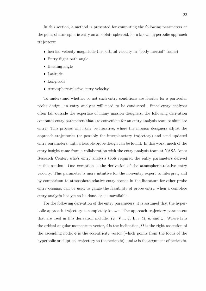
and

x′ = cos ξ2x′′ + sin ξ2z

′′

y′ = y′′

z′ = − sin ξ2x′′ + cos ξ2z

′′

(2.52)

The entry velocity vector can be expressed in the x′′-y′′-z′′ frame coordinates by

first plugging Eq. (2.51) followed by (2.52) into Eq. (2.44), giving

VEntry = (Vx cos ξ1 + Vy sin ξ1) x′ + (Vy cos ξ1 − Vx sin ξ1) y′ + Vz z′

= Vx′x′ + Vy′ y

′ + Vz′ z′

(2.53)

and

VEntry = [(Vx cos ξ1 + Vy sin ξ1) cos ξ2 − Vz sin ξ2] x′′

+ (Vy cos ξ1 − Vx sin ξ1) y′′

+ [(Vx cos ξ1 + Vy sin ξ1) sin ξ2 + Vz cos ξ2] z′′

= Vx′′x′′ + Vy′′ y

′′ + Vz′′ z′′

(2.54)

The angle ξ1 can be computed from the components of rEntry,

ξ1 = tan−1

(ryrx

)(2.55)

where ry and rx are the components of rEntry in the body-inertial frame.

To compute the angle ξ2, the surface normal vector n must first be computed,

which can be computed by taking the gradient of the surface of the oblate spheroid

at the point of entry. First, the variable terms in the equation for an oblate spheroid

are expressed as the function f , given by

f(x, y, z) =x2

a2+y2

a2+z2

b2(2.56)

The gradient of f is then computed, and evaluated at the point of entry, given by

29

n = ∇f(x, y, z)|x=rx,y=ry ,z=rz

= 2rxa2x+ 2ry

a2y + 2rz

b2z

= nxx+ nyy + nz z(2.57)

where rx, ry, and rz are the components of the position vector rEntry in body-inertial

coordinates.

The angle ξ2 can now be expressed (by observation of Fig. 2.6a), as

ξ2 = tan−1

(n′xn′y

)(2.58)

The components of n can be expressed in the primed frame of Fig. 2.6 using Eq.

(2.49), giving

n = (nx cos ξ1 + ny sin ξ1) x′ + (ny cos ξ1 − nx sin ξ1) y′ + nz z′

= nx′x′ + ny′ y

′ + nz′ z′

(2.59)

Plugging nx′ and nz′ into Eq. (2.58), gives

ξ2 = tan−1(nx cos ξ1+ny sin ξ1

nz

)= tan−1

[b2

a2

(rx cos ξ1+ry sin ξ1

rz

)] (2.60)

With ξ1 and ξ2 defined, the heading angle can now be expressed in known terms,

by plugging Eqs. (2.54), (2.55), and (2.60) into (2.48), giving

H = tan−1

[Vy cos ξ1 − Vx sin ξ1

(Vx cos ξ1 + Vy sin ξ1) cos ξ2 − Vz sin ξ2

](2.61)

30

Entry Flight Path Angle on Oblate Spheroid

To compute the entry flight path angle, we first define the x′′′-y′′′-z′′′ frame, illus-

trated in Fig. 2.6. The rotation is about the surface normal, n, by the heading angle,

H.

The entry flight path angle on an oblate spheroid can then be expressed as

γEntry,Ob = tan−1

(Vz′′′

Vx′′′

)(2.62)

The relation between the double-prime and triple-prime frames is given by,

x′′ = cosHx′′′ − sinHy′′′

y′′ = sinHx′′′ + cosHy′′′

z′′ = z′′′

(2.63)

Plugging Eq. (2.63) into (2.54) gives

VEntry = [(Vx cos ξ1 + Vy sin ξ1) cos ξ2 − Vz sin ξ2] cosH

+ [Vy cos ξ1 − Vx sin ξ1] sinHVx′′′

+ (Vy cos ξ1 − Vx sin ξ1) cosH

− [(Vx cos ξ1 + Vy sin ξ1) cos ξ2 − Vz sin ξ2] sinHVy′′′

+ [(Vx cos ξ1 + Vy sin ξ1) sin ξ2 + Vz cos ξ2]Vz′′′

= Vx′′′x′′′ + Vy′′′ y

′′′ + Vz′′′ z′′′

(2.64)

Plugging the Vz′′′ and Vx′′′ components into Eq. (2.62) gives

γEntry,Ob = tan−1(

(Vx cos ξ1 + Vy sin ξ1) sin ξ2 + Vz cos ξ2[(Vx cos ξ1 + Vy sin ξ1) cos ξ2 − Vz sin ξ2] cosH+ [Vy cos ξ1 − Vx sin ξ1] sinH

)(2.65)

31

Entry Latitude and Longitude

To compute the latitude at the point of entry, we use the components of the entry

position vector, rEntry, in the primed frame (as illustrated in Fig. 2.6), given by

Latitude = tan−1

(rz′

rx′

)(2.66)

Plugging the expressions for x′, y′, and z′ from Eq. (2.51) into Eq. (2.39) gives

r = (rx cos ξ1 + ry sin ξ1) x′ + (ry cos ξ1 − rx sin ξ1) y′ + rz z′

= rx′x′ + ry′ y

′ + rz′ z′

(2.67)

and plugging the expressions for rx′ and rz′ into Eq. (2.66) gives

Latitude = tan−1

(rz

rx cos ξ1 + ry sin ξ1

)(2.68)

To compute the longitude at entry, recall that the prime meridian of the body

lies in the x-z plane (on the positive x side) in the Body-Fixed coordinate system,

illustrated in Fig. 2.1. Thus far in this section, the x-y-z coordinates are in the Body-

Inertial frame. To convert from Body-Inertial coordinates to Body-Fixed coordinates,

we use Eq. (2.4). Thus, the entry position vector in Body-Fixed coordinates is given

by

rBF = R3(W )rBI

= rxBF xBF + ryBF yBF + rzBF zBF(2.69)

The longitude can then be computed as the angle between r and the xBF -zBF

plane (i.e. the prime meridian), given by

Longitude = tan−1

(ryBFrxBF

)(2.70)

32

Atmosphere-Relative Entry Velocity

To compute the entry velocity relative to the planet’s rotating atmosphere, we

first compute the velocity of the planet’s atmosphere at the point of entry. For this

calculation, it is assumed that the planet’s atmosphere rotates uniformly about the

body’s spin axis.

In the primed frame illustrated in Fig. 2.6, the velocity of the atmosphere, VAtm,

at the point of entry can be expressed as

VAtm = VAtmy′ (2.71)

where y′ can be expressed in unprimed (i.e. Body-Inertial) coordinates from Eq.

(2.49). The magnitude of the atmosphere velocity VAtm is given by

VAtm = r cos(Latitude)ωRot (2.72)

where ωRot is the rotation rate of the planet’s atmosphere, which has a positive value

for prograde rotation, and a negative value for retrograde rotation.

The velocity of the atmosphere at entry can thus be expressed as

VAtm = r cos(Latitude)ωRot (− sin ξ1x+ cos ξ1y) (2.73)

The atmosphere-relative entry velocity is then given by

VEntry,AtmRel = VEntry −VAtm (2.74)

where VEntry is given by Eq. (2.47) and VAtm is given by Eq. (2.73).

2.2.3 Consequences of Interplanetary Trajectory Design on Launch

In this section, the discussion of the approach trajectory is expanded to relate it to

the launch problem. In principle, departure and approach on a hyperbolic trajectory

33

are identical, with time running in opposite directions. A consequence of this, is that

for any departure hyperbolic trajectory, the declination of the departure asymptote,

constrains the inclination of the departure hyperbola (just as it does with approach)

as expressed in Eq. (2.11) restated here as imin = |δ|.

For example, if a rocket is to be launched from Kennedy Space Center and de-

part Earth on a hyperbolic trajectory, the minimum inclination (of the departure

hyperbola) that can be achieved without a plane change is 28.5°, and the maximum

inclination (due to restrictions on avoiding flight over populated areas) is about 57°.

However, any inclination larger than 28.5° results in launch performance losses, since

the velocity direction is not taking full advantage of the Earth’s rotation. Thus,

any interplanetary departure with declination magnitude, |δ|, less than 28.5° can be

launched into without requiring a plane change. If |δ| is greater than 28.5°, however,

then the launch inclination must be greater than 28.5° since the minimum departure

hyperbolic inclination, imin = |δ|. If the declination magnitude exceeds 57°, a plane

change is required during departure (to avoid flight over populated areas), which

may be feasible for a particular design, but will incur additional launch performance

losses in terms of delivered payload injected into the interplanetary trajectory. In

some cases, the interplanetary trajectory may need to be redesigned to reduce the

declination magnitude.

2.2.4 Spacecraft Deflection Maneuver for Probe Release During Flyby

When a probe is released by a spacecraft, the spacecraft (in previous designs such

as Galileo∗) approaches the target body on an approach trajectory designed for the

probe to enter the atmosphere. This is because the probe does not have its own

propulsion system to target the body, and so the spacecraft then must put itself

back on course for its target (e.g. for orbit insertion or to target fly by conditions

to continue on to another body). The spacecraft’s course adjustment is called a

∗http://nssdc.gsfc.nasa.gov/planetary/galileo.html

34

deflection maneuver. In this work, the ∆V required for such a maneuver is estimated,

for a spacecraft that flies by a body while releasing a probe. In this section, the model

used to estimate the deflection maneuver ∆V is derived.

For this derivation, it is assumed that the approach trajectory for the probe is

known, and the following terms are assumed given: the periapsis vector of the probe

approach trajectory, rp,probe, the approach V∞ (assumed same for both probe and

spacecraft), semimajor axis, a (also same for both probe and spacecraft), and the

probe approach trajectory eccentricity, eprobe, angular momentum, hprobe, argument

of periapsis, ωprobe, right ascension of the ascending node, Ωprobe, and inclination, iprobe.

It is also assumed that the approach trajectory of the spacecraft is known; however,

the spacecraft trajectory will be changed slightly to accommodate the probe release

and (in a single maneuver) return to a nearly identical trajectory to the originally

designed spacecraft approach trajectory (i.e. the trajectory of the spacecraft if it

approached the body from its designed approach trajectory, rather than the probe’s).

In this analysis, we use the periapsis vector of the spacecraft trajectory, rp,sc, from the

(originally designed spacecraft approach), which we target using Lambert’s method

from the position of probe release.

The radius of the deflection maneuver, r∆V , is also assumed known and is chosen

by the designer. Physically, the deflection maneuver will decrease as r∆V increases

(i.e. the maneuver is performed as far from the planet as possible); however, the

precision limitation of the navigation design (to target the correct entry point for the

probe) limits how far away the probe can be released. Without conducting a precise

navigation analysis, in this study we choose the r∆V value, so that the time of flight

of the probe is approximately 150 days to closely match the flight time of the Galileo

probe, which was released 147 days prior to atmospheric entry†. This is determined

iteratively by choosing a value for r∆V and then calculating the TOF from probe

release to probe periapsis passage (which is approximately the same as the TOF to

probe entry for this analysis).

†http://nssdc.gsfc.nasa.gov/planetary/galileo.html

35

To estimate the deflection maneuver δV , we first calculate the true anomaly, angle

θ, and the vector components of r∆V , at the point of probe release, given by

θ∗∆V,probe = − cos−1

[1

eprobe

(h2probe

µr∆V

− 1

)](2.75)

θ∆V,probe = θ∗∆V,probe + ωprobe (2.76)

Plugging θ∆V,probe, Ωprobe, and iprobe into Eq: (2.39) gives the position vector, r∆V ,

at probe release.

The transfer angle, ∆θ∗probe, between the position of probe release and probe tra-

jectory periapsis, and the transfer angle ∆θ∗sc, between the position of probe release

and the spacecraft trajectory periapsis, are given by

∆θ∗probe =∣∣θ∗probe∣∣ (2.77)

∆θ∗sc = cos−1

(rp,sc • r∆V

rp,scrδV

)(2.78)

Next, the velocity vector on the probe’s trajectory at the release point is computed

from the f and g functions

fprobe = 1− rp,probePprobe

(1− cos ∆θ∗probe

)(2.79)

gprobe =r∆V rp,probe√µPprobe

sin ∆θ∗probe (2.80)

where the parameter Pprobe is the semi-lattice rectum of the approach trajectory, given

by

Pprobe = a(1− e2probe) (2.81)

The probe velocity vector at the release point is then given by

36

V∆V,probe = (rp,probe − fprober∆V ) /gprobe (2.82)

To compute the velocity vector of the spacecraft at the point of probe release

(immediately after the deflection maneuver has been performed), Lambert’s method

is used to compute the parameter Psc, and then f and g functions are again used to

calculate the spacecraft velocity vector at probe release.

Using Lambert’s method, the Psc is computed from

Psc =4|a| (S − rp,sc) (S − r∆V )

C2sinh2

(α′ ± β′

2

)(2.83)

where C is the chord length that connects the two position vectors at probe release

and periapsis of the spacecraft trajectory, which is computed using the law of cosines,

given by

C =√r2p,sc + r2

∆V − 2rp,scr∆V cos ∆θ∗sc (2.84)

S is the semi-perimeter of the position vectors and the chord length, given by

S =1

2(rp,sc + r∆V + C) (2.85)

and the angles α′ and β′ are given by

α′ = 2 sinh−1

√S

2|a|(2.86)

β′ = 2 sinh−1

√S − C

2|a|(2.87)

The choice of + or − in Eq. (2.83), was found by calculating both solutions and

identifying the + solution as correct. (We expect the deflection maneuver size to be

on the order of 10s to 100s of m/s. If the − solution is used for an example case, the

maneuver size is on the order of 10s of km/s.)

37

To compute the spacecraft velocity at the point of probe release (just after the

deflection maneuver is performed), the f and g functions are again used, giving

fsc = 1− rp,scPsc

(1− cos ∆θ∗sc) (2.88)

gsc =r∆V rp,sc√µPsc

sin ∆θ∗sc (2.89)

and the spacecraft velocity, V∆V,sc, at probe release is computed from

V∆V,sc = (rp,sc − fscr∆V ) /gsc (2.90)

From Eq. (2.82) and Eq. (2.90), the orbit deflection maneuver is given by

∆VDefl = |V∆V,sc −V∆V,probe| (2.91)

To compute the flight time of the probe from the point of release to the point of

periapsis passage (which is approximately the same flight time as probe release to

atmospheric entry), we use Kepler’s time equation, giving

TOFprobe =

√|a|3µ|eprobe sinh H∆V,probe − H∆V,probe| (2.92)

where H∆V,probe is the hyperbolic anomaly of the probe trajectory at the point of

release, given by

H∆V,probe = 2 tanh−1

[√eprobe − 1

eprobe + 1tan

(θ∗∆V,probe

2

)](2.93)

If the time of flight of the spacecraft from probe release to the spacecraft’s periapsis

is desired, it can be computed from Lambert’s equation, given by

TOFsc =|a|3/2√µ[sinh(α′)− α′]− [sinh(β′)− β′] (2.94)

38

2.2.5 Launch Vehicle Performance

In this work, the maximum launch mass (for a given launch vehicle) is determined

for a particular launch V∞ (or C3), in order to compute the maximum delivered mass

at a target body. The launch vehicles considered in this work are the Atlas V 551,

Delta IV Heavy, and the Space Launch System (SLS) Block 1B. The performance

curves for the Atlas V 551 and Delta IV Heavy are available on NASA’s Launch

Vehicle Performance website‡. The SLS performance data are not yet available on

the NASA website, and so the performance curves presented in Ref. [35] are used.

In post processing the thousands of results found using the trajectory design tool

STOUR, as well as to compute optimal (or low-thrust) trajectories in MALTO, it is

convenient to fit a polynomial curve to the performance data for a particular launch

vehicle. Of the performance curve fits used in this work, the SLS curve fit has the

largest error, which has a maximum error of about 10 kg. The data itself is subject

to human error, however, since the data was obtained by visually inspecting the

performance curve plot given in Ref. [35].

The polynomial curve fits for each of the three launch vehicles considered are

provided below.

mL,AV 551 = 6106.286412675735− 110.6762537571361C3,AV 551

+0.617132837063155C23,AV 551 + 1.655556918721937(10−4)C3

3,AV 551

−1.764489380594721(10−6)C43,AV 551

(2.95)

which is valid for C3 from -10 to 60 km2/s2,

mL,DIV H = 10598.68546670721− 186.4563475807183C3,DIV H

+1.377092176829015C23,DIV H − 0.004579784822348C3

3,DIV H

−1.007433959379602(10−6)C43,DIV H

(2.96)

‡https://elvperf.ksc.nasa.gov/Pages/Default.aspx

39

which is valid for C3 from -10 to 100 km2/s2, and

mL,SLS = 35722.46358080152− 510.5138820643374C3,SLS

+2.932563746865676C23,SLS − 0.011030421338031C3

3,SLS

+2.287772444084514(10−5)C43,SLS

(2.97)

which is valid for C3 from -8 to 140 km2/s2. Note that any of the performance

functions can be written in terms of launch V∞ using the relation C3 = V 2∞.

In this work, it was found that bi-exponential curve fits often worked well, but

polynomial fits are used exclusively in this study, since this is the only format accepted

by the Mission Analysis Low-Thrust Optimization (MALTO) tool.

For some trajectories with high launch V∞, an additional upper stage is used, such

as a STAR 48. In this analysis, we consider the STAR 48 for the Atlas V 551, Delta

IV Heavy, and the SLS Block 1B. To be conservative regarding delivered mass at the

target body, it is assumed that the STAR 48 burn occurs on the departure asymptote

(since a burn closer to periapsis will improve the performance of the STAR 48 burn).

The parameters assumed for the STAR 48 are for the STAR 48A, with an effective

Isp = 183 s, a wet mass of 2574 kg, with propellant mass of 2430 kg (leaving a dry

mass of 144 kg) [11].

To compute the modified performance curve with the STAR 48 additional upper

stage, we first define the following terms:

mL = maximum launch mass by the launch vehicle with STAR 48 (on modified

performance curve, which excludes the wet mass of the STAR 48)

V∞ = launch V∞ corresponding to mPL on modified performance curve with

STAR 48 additional upper stage

mL,LV = maximum launch mass of standard launch vehicle (using unmodified

performance curve)

V∞,LV launch V∞ corresponding to mL,LV on unmodified performance curve

(without STAR 48 additional upper stage)

40

mSTAR48 = total (wet) mass of the STAR 48

mSTAR48,prop = propellant mass of STAR 48

mSTAR48,dry = dry mass of STAR 48

It is assumed that the polynomial (or other function form) fit of the unmodified

launch vehicle performance curve is known, i.e.

mL,LV = f(V∞,LV ) (2.98)

where f(V∞,LV ) is the known polynomial-fit function, and the STAR 48 characteristics

(mSTAR48, mSTAR48,prop, and mSTAR48,dry) are also known.

The launch mass for a launch vehicle with unmodified performance curve in Eq.

(2.98), can be modified to account for the STAR 48 mass, giving

mL,LV = mL +mSTAR48 (2.99)

or inversely

mL = mL,LV −mSTAR48 (2.100)

To compute the boost in velocity provided by the STAR 48, we use the rocket

equation

∆V = g0Isp ln

(m0

mf

)(2.101)

where g0 = 9.80665m/s2 (standard gravity), Isp is the specific impulse of the STAR

48, and

m0 = mL,LV (2.102)

mf = mL,LV −mSTAR48,prop (2.103)

41

Since the STAR 48 burn is (for this study) assumed to burn along the departure

asymptote, the ∆V due too the STAR 48 can be interpreted as a ∆V∞, where the

boost in velocity is simply added to the departure V∞, given by

∆V = V∞ − V∞,LV (2.104)

Plugging Eq. (2.98), (2.102), (2.103), and (2.104) into (2.101), gives

V∞ = V∞,LV + g0Isp ln

[f(V∞,LF )

f(V∞,LF )−mSTAR48,prop

](2.105)

The modified performance curve for a launch vehicle with the additional STAR

48 upper stage can now be computed using the following method:

1. Choose a range of values of V∞,LV for a launch vehicle of choice. Be sure to not

choose values outside the listed performance of your chosen launch vehicle.

2. Compute the corresponding mL,LV from Eq. (2.98). These, along with the

V∞,LV values, are the unmodified performance values for the chosen launch

vehicle. (Equation (2.95), (2.96), or (2.97) can be used if the reader is interested

in the Atlas V 551, Delta IV Heavy, or SLS Block 1B, respectively. The reader is

warned, however, that the performance of these vehicles may have been changed

since the time of writing this document.)

3. For each value of V∞,LV , compute V∞ from Eq. (2.105).

4. For each value of mL,LV , compute mL from Eq. (2.100). The values of V∞ and

mL make up the performance data for the modified performance curve with the

STAR 48 additional upper stage.

5. Fit a curve to the mL and V∞ performance data, with polynomial-fit function

mL = f(V∞). Since most performance curves use C3 rather than V∞ it is

recommended that the V∞ be converted to C3 (using C3 = V 2∞), to make the fit

function mL = f(C3).

42

The modified (and unmodified) performance curve fits for the Atlas V 551 and

SLS Block 1B launch vehicles are given in Figs. 2.8 and 2.8. For each modified curve,

only a portion of the modified data is used to fit a curve, due to the difficulty in fitting

an accurate curve for the shape produced by the modified performance data. For the

Atlas V 551, the unmodified performance is better (i.e. delivers more mass) than the

modified data; however, the modified data provides solutions for higher C3. Thus,

only the modified data greater than a C3 of 60 km2/s2 is considered for the modified

performance curve fit. Similarly, the modified SLS data outperforms the unmodified

data at a C3 of about 80 km2/s2; and therefore, only the modified data greater than

(just under) 80 km2/s2 is used for the modified performance curve fit.

-50 0 50 100 150 200 2500

1000

2000

3000

4000

5000

6000

7000

8000

9000

C3, km

2/s2

Launch Mass, kg

4th-Order Polynomial Fit

Atlas V 551 Fit

AtlasV 551 (STAR48) Data

AtlasV 551 (STAR48) Fit

Figure 2.7.: Performance curve for the Atlas V 551 launch vehicle. The blue curveis the unmodified performance curve, and the magenta and green points representthe modified performance data with the STAR 48 additional upper stage. The greenportion of the modified performance data represents the portion used to fit a 4th-orderpolynomial curve.

43

-50 0 50 100 150 200 250 300 350 400-0.5

0

0.5

1

1.5

2

2.5

3

3.5

4

4.5x 10

4

C3, km

2/s2

Launch Mass, kg

SLS Data Fit

SLS (STAR48) Data

SLS (STAR48) Fit

Figure 2.8.: Performance curve for SLS Block 1B launch vehicle. The blue curve isthe unmodified performance curve, and the magenta and green points represent themodified performance data with the STAR 48 additional upper stage. The greenportion of the modified performance data represents the portion used to fit an 8th-order polynomial curve.

44

45

3. CATALOG OF TRAJECTORIES TO URANUS FROM

2024 TO 2038 INCLUDING AN OPPORTUNITY FOR A

SATURN PROBE

In 1986, the Voyager 2 spacecraft achieved the only close encounter with Uranus,

followed in 1989 by a flyby of Neptune. These two Ice Giants remain among the

least known planets of our Solar System, and are the only class of planet never

to have been explored in detail. In this chapter, we investigate multiple gravity-

assist trajectories (with impulsive, chemical propulsion maneuvers) to Uranus that

explore 89 combinations of gravity-assist paths, using Venus, Earth, Mars, Jupiter,

and Saturn. We consider launch dates spanning from January 2024 to December 2038

with step sizes of 5 days. We use a patched-conic model with an analytic planetary

ephemeris to calculate the trajectories. The launch vehicles considered are the Space

Launch System (SLS) Block 1B, Atlas V 551, and Delta IV Heavy. Trajectories

that can deliver at least 2000 kg of payload in orbit about Uranus in minimum time

are cataloged for each launch year. A preliminary catalog of candidate trajectories

that use aerocapture at Uranus is also provided. Of the 89 total gravity-assist paths

searched, 26 include a flyby of Saturn. The alignment of Saturn and Uranus only

occurs every 45 years, and provides a rare opportunity for a Saturn-Uranus mission.

A trajectory in 2028 is identified as an attractive candidate for such a mission—

delivering a probe at Saturn, as well as a probe and orbiter at Uranus.

3.1 Background

A Uranus orbiter and probe mission (with no solar electric propulsion stage) is

stated in the Decadal Survey for 2013–2022 [12] to be the third highest priority for

46

a Flagship-class mission, and it is recommended (in the survey) that such a mission

should be selected even if the other two higher-priority missions are selected. The two

higher-priority missions, now called Mars 2020 and the Europa Clipper (or Flyby)

have indeed been selected by the time of writing this thesis, and it is likely that

the Uranus orbiter and probe mission will be one of the highest (if not the highest)

priority for a Flagship-class mission for the next Decadal Survey (beyond 2022).

More recently (to the time of writing this work), at the August 2015 meeting of

the Outer Planets Assessment Group, NASA’s Planetary Science Division announced

the initiation of an Ice Giants Study for a Flagship-class mission. The JPL-lead study

is to be part of the next Decadal Survey (beyond 2022) [13].

The announcement of the Ice Giants Study specified, as part of its objectives, to

identify enabling technologies, and assess the capabilities afforded by the SLS [13].

This work identifies mission opportunities to Saturn and Uranus, which would be

enabled with the use of the SLS Block 1B, without the use of technologies such as

low thrust or aerocapture. This mission would not only send a probe and orbiter to

Uranus, but also a probe to Saturn.

In 2011, Spreen et al. [14] investigated ballistic trajectories to Uranus between

2020 and 2060. In their paper, they state that their best case is a trajectory with

launch date on Feb. 14, 2044 that, using an Atlas V 551 launch vehicle, can deliver

just over 2.1 Mg of payload into a 200-day orbit about Uranus, with an Earth-Uranus

flight time of 15.0 years. Between the launch dates of 2024 and 2038 (the years under

consideration for this paper), the best case found by Spreen et al. can deliver 1.4 Mg

of payload to Uranus (into a 200-day orbit) in 14.7 years, with launch date Oct. 5,

2029. Although the trajectories found by Spreen et al. are capable of delivering a

sufficient amount of payload for a Uranus orbiter, the time to reach Uranus (of about

15 years) is long.

Also in 2011, Dankanich and McAdams [15] investigated low-thrust trajectories

to Uranus for the 2013-2022 decadal survey. The recommended trajectory found in

their study, launched in 2019, had a 13-year Earth-Uranus transfer time, and was

47

capable of delivering over 2 Mg into orbit about Uranus. This trajectory used solar

electric propulsion (SEP) and an Atlas V 551 launch vehicle.

In 2009, Landau et al. [16] conducted a search of low-thrust trajectories to Uranus

and Neptune with launch dates ranging from 2015 and 2035. Using SEP and an Atlas

V 551 launch vehicle, they found trajectories launching in 2020 that could deliver as

much as 1.5 Mg into an orbit about Uranus, with an Earth-Uranus transfer time of

10 years. Their study also estimated that, if aerocapture were used (assuming the

thermal protection system, or TPS, takes up 50% of the spacecraft mass at Uranus

arrival) over 2 Mg of delivered mass could be placed in orbit at Uranus within a flight

time of 10 years. These aerocapture trajectories also use SEP, and an Atlas V 551

launch vehicle.

Several other Uranus mission studies have been conducted that investigate both

ballistic, chemical-propulsion trajectories, and low-thrust trajectories [17–27].

3.2 Methods

3.2.1 Computing the Trajectory Design Space

The sweeping search of trajectories that are used to construct the catalogs pre-

sented in this paper, are computed using the program STOUR [3, 28, 29]. STOUR

is a patched-conic propagator with an analytic planetary ephemeris that can rapidly

calculate thousands gravity-assist trajectories. The program imposes a grid search of

all candidate trajectories by stepping through specified launch V∞ and launch dates

(between January of 2024 through December of 2038 in 5-day increments).

When selecting the combinations of flyby bodies in this work, Venus, Earth, Mars,

Jupiter, and Saturn are considered. Mercury is not, however, since its low mass and

close proximity to the Sun make it a poor body for useful gravity assist. Only Venus,

Earth and Mars are considered for repeated flybys of the same body, since doing so

at the outer planets would result in TOFs exceeding our imposed constraint of 15

48

years. Once a flyby of an outer planet has occurred, only planets farther out from

that body are considered for subsequent flybys.

Within the rules specified in the previous paragraph, all combinations of flyby

bodies are investigated for up to 3 total flybys (excluding Earth launch and Uranus

arrival). For sequences of four flyby bodies, only paths from previous studies were

considered. For example, all paths from the work by Petropoulos et al. [53] (for

trajectories to Jupiter) were investigated, with the modification of adding Neptune

as the final body after the Jupiter encounter. Flyby paths from Spreen et al. [14]

were also investigated. The complete list of gravity-assist paths investigated is:

Direct, V0, 0E0, M0, J, S, VV0, VE0, VM0, V0J, V0S, 0EV0, 0EE0, 0E0M, 0E0J,

0E0S, MV0, ME0, MM0, M0J, M0S, JS, VVV0, VVE0, VVM0, VV0J, VV0S,

VEV0, VEE0, VEM0, VE0J, VE0S, VMV0, VME0, VMM0, VM0J, VM0S, V0JS,

0EE0J, 0E0MJ, 0E0MS, 0E0JS, MVV0, MVE0, MVM0, MV0J, MV0S, MEV0,

MEE0, ME0M, ME0J, ME0S, MMV0, MME0, MMM0, MM0J, MM0S, M0JS,

VVV0J, VVV0S, VVE0J, VVE0S, VVMV0, VV0MJ, VV0MS, VEEE0, VEEM0,

VEE0J, VEE0S, VEME0, VEM0J, VMV0J, MEE0J, MEE0S, VVEE0J, VEVE0J,

VEVE0S, VEEE0J, VEEE0S, VEE0MJ, VEE0MS, VEME0J, VEME0S, VMVE0J,

VMEE0J, VMEE0S, MEVE0J, MEME0J, and MEME0S

where “Direct” denotes a direct launch to Uranus from Earth, and V, E, M, J, and

S denote a flyby of Venus, Earth, Mars, Jupiter, and Saturn, respectively. All paths

launch from Earth and arrive at Uranus. A “0” between two flybys, or between the

last flyby and Uranus arrival, denotes an impulsive maneuver, which is implemented

by STOUR’s “maneuver algorithm” developed by Patel [29]. The maneuver algorithm

applies powered flybys and broken plane or “mid-course” maneuvers [29]. A “0” at the

start of the path indicates a maneuver is done before the first encounter; specifically,

at aphelion of a near resonant orbit to leverage the energy change at the subsequent

gravity assist: a maneuver called “V∞ leveraging” [31–33].

Before analyzing a gravity-assist path in STOUR, it is first checked using a Tis-

serand graph, to determine whether the path is possible with regards to orbital energy

49

(i.e. to see if it has sufficient energy to reach Uranus). All flyby paths identified as

infeasible by the Tisserand graph are eliminated from the list of possible candidates.

For the remaining possible candidate gravity-assist paths, STOUR is used to solve

the phasing problem, and determine which of these paths produce trajectories to

Uranus.

In practice, there are several constraints that limit the solution space, such as

minimum flyby altitude for a given flyby body, maximum TOF for the full trajectory

to Uranus, and maximum launch V∞. A summary of the constraints imposed on the

trajectories considered for this broad search study are shown in Table 3.1.

Table 3.1.: Trajectory Search Constraints

Parameter ValueMinimum flyby altitude 300 km (Venus and Earth), 200 km (Mars),

100k km (Jupiter), 50k km (Saturn and Uranus)

Maximum TOF 15 yr

Maximum launch V∞ 20 km/s (Direct Launch), 17 km/s (1 flyby),12 km/s (2 flybys), 9 km/s (3 flybys), 7 (4 and 5 flybys)

Maximum maneuver ∆V 3 km/s

For the case of minimum flyby altitudes used, our goal is to avoid interaction with

the flyby body’s atmosphere, as well as collisions with the body’s rings (whenever ap-

plicable). Since the outer planets can potentially provide a significant energy increase

during a flyby, minimum altitudes were chosen just below the outer most (prominent)

ring altitude to ensure that no trajectory opportunities are missed. The total TOF

for each trajectory was limited to 15 years based on previous decadal studies [22,34].

To determine the maximum allowed launch V∞, many factors were considered.

First and foremost, the goal in choosing these launch values is to encompass all

foreseeable mission types to Neptune during the 2020 to 2070 time frame. Such

mission types include both flyby and capture missions (although capture missions are

50

the focus of this work), as well as low and high payload mass missions. Additionally,

the general reason for using gravity assist bodies (and adding the complexity to the

interplanetary trajectory) is to reduce the required launch V∞ while still gaining

sufficient orbital energy to reach the target body (provided by the gravity assists).

Therefore, the maximum launch V∞ considered is reduced for this analysis as more

flyby bodies are added to the path.

As an example of a single flyby body path, the New Horizons spacecraft trajectory

(an earlier version of which is noted by Patel [29]) launched with a V∞ of about 16

km/s, and then flew by Jupiter on its way to Pluto. Using New Horizons as a

reference, a maximum launch V∞ of 17 km/s was chosen for all paths with only one

flyby body, and 20 km/s was used for direct launch to Uranus. For two, three, and

four flyby bodies, the maximum launch V∞ values used by Landau et al. [16] were

first considered for this study; however, for the case of three and four flyby bodies,

some example simulations indicated that slightly larger launch V∞ values provided a

sizable increase in opportunities to the Ice Giants. Thus, for paths containing three

or four flyby bodies, the maximum launch V∞ values chosen are slightly larger than

those used by Landau et al. All cases considered for 5 flyby bodies are modifications

of select 4-flyby body paths (e.g. adding a Mars flyby after an Earth or Venus flyby

on route to an outer planet); and thus, use the same launch V∞ as paths with 4 flyby

bodies, of 7 km/s.

We note that STOUR is not an optimization tool. It does not find the optimal

deep-space maneuver (DSM) locations and encounter dates to maximize delivered

mass. STOUR computes thousands of trajectories to reveal a grid of the solution

space. Attractive trajectories are then initially characterized by those that can deliver

a targeted amount of mass in orbit at Uranus in minimum time (of the solutions found

in STOUR). We do this by plotting all solutions’ TOF versus delivered mass, and

identifying the best cases from the plot. This optimization can be more formally

described as identifying the nondominated Pareto optimal set of solutions, with flight

time and delivered mass as the optimization objectives.

51

3.2.2 Defining the Capture Science Orbit and Estimating the Delivered

Mass

The launch vehicles we consider for the trajectories found are the Space Launch

System (SLS) Block 1B, Atlas V 551, and Delta IV Heavy. The launch data for

the Atlas V 551 and Delta IV Heavy are available on the NASA Launch Vehicle

Performance website∗. The performance of the SLS is approximated based on the

data provided in [35].

To compute the delivered mass in orbit at Uranus, a science orbit is assumed with

an orbital period of 20 days, and a periapsis of 52,000 km to avoid Uranus’ rings.

The 20-day science orbit is chosen based on previous decadal studies [22, 34], as well

as our own assessment, by observing the variations in capture ∆V for various orbit

sizes and various arrival V∞ at Uranus. Figure 3.1 illustrates the ∆V required for

capture at Uranus for various science orbit sizes and various arrival V∞. The solid

lines represent capture inside the rings of Uranus, at an altitude of 3000 km. The

dotted lines represent capture at a radius of 52000 km, just outside the major rings

(as done in Ref. [22]). At the time of writing this work, it was not yet known if the

risks of capture inside the rings would be tolerable for a Uranus mission. Thus, to

be conservative regarding delivered mass values, (an to be consistent with Ref. [22])

only capture outside the rings was considered. The figure shows that for all arrival

V∞, the capture ∆V spikes for capture orbits just below about 20-days. From these

results (and to be consistent with Refs. [22] and [34]), a 20-day science orbit is used

for all capture orbits in this work.

The thruster characteristics used for the impulsive DSMs and capture at Uranus,

are based on those used by Landau et al. [16], with an Isp = 323 s, and a propellant

mass penalty (to estimate the tank and structure mass) of 12%.

∗https://elvperf.ksc.nasa.gov/Pages/Default.aspx

52

0 20 40 60 80 100 120 140 160 180 2000

1

2

3

4

5

6

Capture Orbit Period, days

Capture ∆V, km/s

Uranus Capture ∆∆∆∆V for Various Science Orbits and Arrival V∞∞∞∞

V∞∞∞∞ = 4 km/s

V∞∞∞∞ = 8 km/s

V∞∞∞∞ = 10 km/s

V∞∞∞∞ = 12 km/s

V∞∞∞∞ = 6 km/s

Figure 3.1.: Capture ∆V at Uranus for various science orbit sizes and arrival V∞.The solid lines represent capture inside the rings of Uranus, at an altitude of 3000km. The dotted lines represent capture outside the major rings, at a radius of 52000km.

3.2.3 Investigating Select Cases

Once attractive trajectories are identified, the maneuver locations and encounter

dates are optimized using trajectory optimization tools such as the Mission Analysis

Low-Thrust Optimization (MALTO) tool [36, 37], or the Evolutionary Mission Tra-

jectory Generator (EMTG) [38–46], to improve the solution in terms of delivering the

maximum mass in minimum time.

Next, the encounter conditions for an orbiter and probe are modeled using MAT-

LAB to compute and visualize the design space of hyperbolic approach trajectories.

The goal is to quickly assess the feasibility of a selected trajectory when considering

factors such as ring avoidance, probe entry speed, line of sight between probe and

orbiter, as well as between the orbiter and Earth. For the case of ring avoidance

for probe entry, the visualization allows the designer to quickly adjust the approach

trajectory, by adjusting the angle (ψ) about the arrival-V∞ vector. This adjustment

53

is illustrated in Fig. 3.2, where the approach trajectory must be rotated slightly

below the minimum inclination approach (which would provide the minimum entry

speed) in order to ensure that the probe enters before crossing the ring plane—all of

which can be adjusted by inspection. By providing a visualization, one does not need

to understand the formulation of the trajectories to spot potential issues with the

design, which is conducive for collaborative mission designs with contributors from a

diverse set of disciplines.

Minimum Inclination

V∞, Arrival

Earth Direction

z x

y

Ring Avoidance

Figure 3.2.: Using visualization tool to adjust a Saturn probe approach trajectory forring avoidance by inspection.

The visualization is a useful learning tool to better understand the challenges

for a mission, as well as serve as a “sanity check” for any major issues with the

encounter. For example, the two trajectories shown in Fig. 3.3 illustrate two different

trajectories that fly by Saturn on route to Uranus. For both trajectories, the probe

must approach Saturn so that it enters prograde with Saturn’s spin, to reduce its

atmosphere-relative entry speed. The spacecraft on the other hand, must fly by

depending on the conditions required by its interplanetary trajectory, to encounter

Uranus. For the trajectory in Fig. 3.3(a) however, the flyby conditions require the

spacecraft to approach Saturn on the opposite side of the planet as the probe. This

interference in line-of-sight between probe and spacecraft will prevent the probe from

54

sending its data to the spacecraft as it enters Saturn. To mitigate such an issue, the

probe must send its data directly to Earth, which requires more transmission power,

and possibly a much larger antenna, which may not be possible to accommodate.

The geometry in Fig. 3.3(b) however, allows the spacecraft to approach Saturn on

the same side as the probe, and; therefore, maintain line-of-sight between the probe

and spacecraft throughout probe entry and descent into Saturn’s atmosphere.

V∞, Arrival

z

x

y

Orbiter Flyby

(a)

V∞, Arrival

z

x y

Orbiter Flyby

(b)

Figure 3.3.: Saturn flyby trajectories with atmospheric probes. The visualizationshows that the probe-spacecraft line-of-sight is lost for the trajectory on the left,causing data link difficulties that may have no feasible design solution.

We will show in this work that the trajectory search results find solutions that can

deliver over 2000 kg into a capture orbit at Uranus, and many of these trajectories

fly by Saturn. Using this knowledge, we target a mass of about 2000 kg in orbit

at Uranus with 600 kg reserved for a Uranus and Saturn probe, which we estimate

to be conservative (based on estimates for a Uranus orbiter and probe in Ref. [22]

and Saturn probe in Ref. [47]) for a multi-planet, Saturn-Uranus mission. In such

a mission, a probe can be delivered at Saturn during the flyby, and a probe and

orbiter can be delivered at Uranus. For these trajectories, the hyperbolic approach

trajectories at both Saturn and Uranus are modeled to assess the feasibility of the

trajectory for such a mission.

55

3.3 Cataloging Trajectories to Uranus

For each trajectory found using STOUR, the mass the trajectory can deliver into

orbit at Uranus is calculated for a specified launch vehicle. To give a sense of the

trajectory solution space, Fig. 3.4 shows the TOF vs. delivered mass using the SLS

Block 1B launch vehicle. In the figure, each dot represents a trajectory to Uranus,

and the color corresponds to the gravity-assist path in the legend, where, the “U” at

the end of each path represents arrival at Uranus (rather than a flyby).

Due to the large number of paths found, the colors in Fig. 3.4 are difficult to

distinguish between adjacent paths in the legend; however, the purpose in showing

this legend is more to give a sense of which paths found results, rather than to identify

which path corresponds to a particular dot. Regardless of the specific path used, the

figure shows that using the SLS, trajectories that deliver 2000 kg will take about 9

years to capture at Uranus; however, if a TOF of 14 years is acceptable, about 15,000

kg can be delivered. In general, the trajectories of interest on this plot are those that

lie on the right diagonal edge of the data set (called the Pareto front), since these are

the cases that can deliver a specified amount of mass in the least amount of time.

The overall trend of this front, suggests that longer flight times are required to deliver

more mass (for up to a 15-year TOF).

We note that if an additional upper stage is used (such as a STAR 48 engine),

trajectories become avail-able that have higher launch C3 than those shown in Fig.

3.4. These high C3 trajectories are shown in Fig. 3.5. We also note that because the

SLS launch vehicle is by far the most capable considered in this study, a subset of the

trajectories found using the SLS (with smaller delivered mass values) are available if

other launch vehicles are used, such as the Delta IV Heavy or the Atlas V 551.

One difficulty with the results shown in Figs. 3.4 and 3.5, is that the launch date

is not visible. Furthermore, many mission proposal calls require that launch occurs

during a specified year. To resolve this issue, Tables 3.2–3.4 show catalogs of the most

attractive trajectories (in terms of delivered mass and TOF) for each launch year. In

56

Figure 3.4.: Trajectories to Uranus using SLS Block 1B.

these tables, we select for each launch year, the trajectory(ies) that can deliver at least

a mass of about 2000 kg to Uranus in minimum time. These trajectories are found

by first computing the delivered mass for a selected launch vehicle, for all trajectories

found. We then isolate the data to only contain solutions within a selected launch

year, and then compare the TOF and delivered mass for that subset.

57

Figure 3.5.: Trajectories to Uranus using SLS Block 1B with STAR-48 as additionalupper stage.

We note that for some years, the case(s) that can deliver at least 2000 kg with the

shortest TOF, may deliver much more than the desired 2000 kg. In other cases, masses

of about 1500 kg could be delivered for significantly less TOF (than those requiring

2000 kg), and are also recorded in the table. Of course, these lower delivered-mass

trajectories would be for a mission that allows for a less massive spacecraft design.

58

Table 3.2.: Uranus Trajectory Catalog: SLS Block 1B

Launch Date Flyby Path TOF, yrs Mass, Mg Prop. Mass, Mg05/20/2024 0E0SU 12.1 3.0 12.902/19/2025 VEE0SU 11.4 2.4 22.203/01/2025 VEE0U 11.5 2.9 21.704/01/2026 VEE0SU 11.8 2.0 24.506/19/2026 0E0SU 11.9 4.1 11.707/09/2026 0E0SU 10.9 ∗∗1.3 10.307/04/2027 0E0SU 12.4 3.8 12.003/20/2028 VEE0U 11.9 2.4 22.209/21/2028 0E0SU 11.3 2.0 14.207/25/2029 ∗SU 9.5 ∗∗1.6 1.410/26/2029 VEE0JU 11.2 2.1 26.101/24/2030 VEE0JU 11.1 2.0 22.608/04/2030 ∗SU 9.5 ∗∗1.6 1.412/20/2030 VE0JU 11.2 2.6 23.907/08/2031 VE0JU 10.4 3.2 19.512/11/2032 VV0JU 9.6 2.3 16.404/28/2033 M0JU 9.3 2.2 14.308/03/2034 0E0U 11.1 2.1 13.708/08/2035 0E0U 11.1 2.1 13.808/12/2036 0E0U 11.0 2.0 13.808/28/2036 ∗JU 11.2 2.5 1.308/23/2036 ∗JU 8.6 ∗∗1.5 1.508/05/2037 ME0U 10.9 2.6 11.908/22/2037 ∗M0U 9.3 2.0 1.809/11/2037 ∗M0U 9.0 ∗∗1.6 1.402/08/2038 VVE0U 11.4 2.1 18.608/22/2038 0E0U 11.0 2.0 13.9

∗Uses STAR 48 as additional upper stage.∗∗Delivers well under 2 Mg.

Delivered masses of about 1800 kg or more may be reported as well that are expected

to meet or exceed 2000 kg after optimization in a program such as MALTO.

The purpose of these tables is to allow systems engineers, scientists, and any other

interested individuals the ability to quickly get a sense of what flight times and masses

are feasible (using chemical propulsion) for a Uranus orbiter mission within a given

launch year. For mission designers, these results may help to identify rare planetary

59

Table 3.3.: Uranus Trajectory Catalog: Delta IV Heavy

Launch Date Flyby Path TOF, yrs Mass, Mg12/21/2024 VEE0U 13.6 2.106/04/2025 0E0SU 14.6 2.110/02/2026 VEE0U 12.7 ∗∗1.510/02/2026 VEE0U 13.4 2.511/26/2027 VVEE0JU 14.5 2.302/24/2028 VEE0U 13.8 1.904/14/2028 VE0JU 14.2 2.210/16/2029 VEE0JU 11.8 ∗∗1.410/16/2029 VEEE0JU 12.4 1.901/04/2030 VEE0JU 13.1 2.312/10/2030 VVE0JU 12.1 ∗∗1.607/18/2031 VE0JU 10.9 ∗∗1.507/23/2031 VE0JU 12.1 2.411/19/2032 VEEM0U 12.4 ∗∗1.412/16/2032 VV0JU 13.2 2.003/19/2033 VEE0JU 13.6 2.004/08/2033 VEEM0U 12.2 ∗∗1.401/28/2034 VEE0U 13.8 2.204/05/2034 VEE0U 13.0 ∗∗1.612/26/2035 VEE0U 13.7 2.001/08/2036 VEME0U 13.8 2.008/17/2036 0E0U 12.2 ∗∗1.311/08/2037 VEE0U 13.0 2.101/19/2038 VVE0U 12.9 1.902/23/2038 VEE0U 12.2 ∗∗1.4

∗Uses STAR 48 as additional upper stage.∗∗Delivers well under 2 Mg.

alignments for gravity assist (such as an alignment of Mars with Jupiter, Saturn, or

Uranus) that may have otherwise gone unnoticed.

Some launch years contain multiple solutions for a few reasons. One reason is

that different gravity-assist paths may be more or less desirable depending on the

details of the mission design; therefore, multiple trajectories may be listed for a given

launch year if the solutions in question can deliver a similar amount of mass in a

similar (minimum) time, but have differing gravity-assist paths. Another reason for

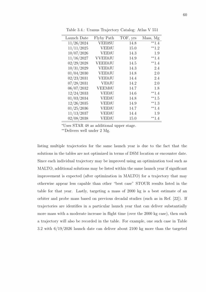
60

Table 3.4.: Uranus Trajectory Catalog: Atlas V 551

Launch Date Flyby Path TOF, yrs Mass, Mg11/26/2024 VEE0SU 14.8 ∗∗1.411/11/2025 VEE0U 15.0 ∗∗1.210/07/2026 VEE0U 14.3 1.911/16/2027 VVEE0JU 14.9 ∗∗1.402/29/2028 VEEE0JU 14.5 ∗∗1.410/31/2029 VEE0JU 14.3 2.401/04/2030 VEE0JU 14.8 2.002/23/2031 VEE0JU 14.4 2.407/28/2031 VE0JU 14.2 2.006/07/2032 VEEM0U 14.7 1.812/24/2033 VEE0U 14.6 ∗∗1.401/03/2034 VEE0U 14.8 ∗∗1.512/26/2035 VEE0U 14.9 ∗∗1.301/25/2036 VEE0U 14.7 ∗∗1.411/13/2037 VEE0U 14.4 1.902/08/2038 VEE0U 15.0 ∗∗1.4

∗Uses STAR 48 as additional upper stage.∗∗Delivers well under 2 Mg.

listing multiple trajectories for the same launch year is due to the fact that the

solutions in the tables are not optimized in terms of DSM location or encounter date.

Since each individual trajectory may be improved using an optimization tool such as

MALTO, additional solutions may be listed within the same launch year if significant

improvement is expected (after optimization in MALTO) for a trajectory that may

otherwise appear less capable than other “best case” STOUR results listed in the

table for that year. Lastly, targeting a mass of 2000 kg is a best estimate of an

orbiter and probe mass based on previous decadal studies (such as in Ref. [22]). If

trajectories are identifies in a particular launch year that can deliver substantially

more mass with a moderate increase in flight time (over the 2000 kg case), then such

a trajectory will also be recorded in the table. For example, one such case in Table

3.2 with 6/19/2026 launch date can deliver about 2100 kg more than the targeted

61

2000 kg case (on 4/1/2026) with only 0.1 more years of flight time using a different

gravity assist path.

To build the catalogs and select the best cases, we use a Python script (which we

call the STOUR Utility) that reads in and stores the output data from all STOUR runs

and allows us to sort the data in post and calculate delivered mass (for an assumed

launch vehicle, DSM Isp, and capture orbit). The STOUR Utility also allows us

to generate plots, such as those shown in Figs. 3.4 and 3.5, where a point can be

selected in the figure to examine the complete list of trajectory characteristics, such

as encounter dates and velocities, ∆V magnitudes, etc. When selecting the cases for

the catalog, the plotted data is isolated to a single launch year.

Examining the results in Tables 3.2–3.4, if a delivered mass of 2000 kg or more is

required, the shortest TOF provided by the SLS is 9.3 years, which occurs both in

2033 and 2037. For the Delta IV Heavy, the shortest TOF solution is 12.1 years with

launch in 2031. If a smaller delivered mass can be designed for a given mission, the

SLS can deliver 1500 kg in only 8.6 years launching in 2036, and the Delta IV Heavy

can deliver 1500 kg in 10.9 years, launching in 2031. For the Atlas V 551, a TOF of

14–15 years is required regardless of whether 1500 kg or 2000 kg of delivered mass is

desired. In all cases, these solutions may be improved after being optimized in a tool

such as MALTO.

Since many of the solutions that launch using the SLS require a large amount

of propellant mass, we include this value for the SLS results in 3.2. The amount in

the table ranges from 1.3 Mg to 26.1 Mg, which is directly related to the required

launch C3 for the trajectory. For lower C3 trajectories, the SLS can lift more mass,

and since we are targeting a delivered mass of 2000 kg, the rest of the launch mass

is then devoted to propellant. Additionally, the lower C3 solutions (and thus high

propellant mass solutions) are more common for trajectories with multiple gravity

assists (particularly of the inner planets), where the gravity assists and DSMs are

increasing the spacecraft’s energy—work that would otherwise be done by the launch

vehicle. Thus, if the propellant mass must be limited for a particular mission design,

62

the SLS is most effective when launching into trajectories that require high C3, which

typically occurs for solutions that only have one flyby (at Jupiter or Saturn) on route

to Neptune. Since the high C3 solutions are also those where the STAR 48 is most

effective, trajectories that use a STAR 48 require less propellant mass than those

without a STAR 48.

To accommodate missions that may require smaller propellant mass values, Table

3.5 shows the catalog of trajectories to Uranus with solutions restricted to only those

with a propellant mass of 5000 kg or less (including the imposed 12% propellant

mass penalty). An interesting trend in the results is that a gravity assist at Saturn

and sometimes no gravity assist provides the better solution, even during years when

Jupiter is available. This trend is suspected to be a direct consequence of needing

higher C3 solutions to reduce the amount of propellant mass required, as a Saturn

flyby (and no flybys) will certainly more often require higher C3 than that of a Jupiter

flyby trajectory. Another factor that may be at play is the logic used in this study to

select attractive trajectories, where we search for solutions with minimum flight time,

and short flight-time solutions often require high C3. Short flight time solutions also

typically have higher arrival V∞ as well; however, since we are capping the allowed

amount of propellant used, the capture maneuver is indirectly limited, which in turn

limits the solution set to those with smaller arrival V∞.

The delivered mass calculations also assume that the launch vehicle is delivering

the maximum amount of mass for a given launch C3; which may not be implemented

in practice if the total amount of propellant mass is constrained. For example, the

trajectory shown in Table 3.5 delivers 4.0 Mg of payload in orbit at Uranus, which

is well over the target value of 2 Mg. If the delivered mass for this same trajectory

were to be fixed at 2 Mg, the corresponding launch mass required to deliver the 2 Mg

(rather than the 4.0 Mg shown in the table) will be reduced; thereby reducing the

required propellant mass, without modifying any of the trajectory characteristics.

The catalogs in Tables 3.2–3.4 also reveal when certain bodies are available for

gravity assist. For example, if Uranus is to be reached in less than 14 years using

63

Table 3.5.: Uranus Trajectory Catalog: SLS Block 1B—5 Mg or Less of Propellant

Launch Date Flyby Path TOF, yrs Mass, Mg Prop. Mass, Mg07/24/2024 ∗U 11.3 ∗∗1.5 0.905/30/2025 ∗SU 11.2 ∗∗1.5 1.512/16/2025 ∗VEEE0U 14.7 2.5 4.706/05/2026 ∗SU 10.4 ∗∗1.5 1.506/10/2026 ∗SU 13.8 2.2 0.806/15/2027 ∗SU 11.1 1.8 1.207/04/2028 ∗SU 11.6 2.6 1.207/14/2028 ∗SU 10.5 1.8 1.207/10/2029 ∗SU 9.0 ∗∗1.5 1.507/15/2029 ∗SU 12.1 2.7 1.111/25/2029 VVV0JU 13.9 4.0 4.807/30/2030 ∗SU 9.3 ∗∗1.6 1.408/09/2030 ∗SU 11.4 2.0 1.011/15/2030 VE0JU 13.6 4.6 4.103/15/2031 ∗M0JU 12.0 2.7 4.508/14/2031 ∗SU 11.0 1.9 1.108/28/2032 ∗SU 13.5 2.0 1.008/31/2032 ∗U 11.7 ∗∗1.5 0.812/11/2032 VEE0U 14.8 4.3 4.409/05/2033 ∗U 11.8 ∗∗1.5 0.811/24/2033 ∗VEEM0U 14.3 3.8 4.901/23/2034 ∗VEE0U 14.5 3.9 4.809/10/2034 ∗U 11.6 ∗∗1.5 0.809/15/2035 ∗U 11.7 ∗∗1.5 0.808/23/2036 ∗JU 8.6 ∗∗1.5 1.508/28/2036 ∗JU 11.2 2.5 1.308/22/2037 ∗M0U 9.3 2.0 1.809/29/2038 ∗U 11.4 ∗∗1.5 0.810/19/2038 ∗ME0U 14.5 2.5 4.7

∗Uses STAR 48 as additional upper stage.∗∗Delivers well under 2 Mg.

either the SLS or the Delta IV Heavy, Jupiter is not available for gravity assist until

about 2029, where it then remains available until the early to mid 2030s. While

Jupiter is unavailable in the near term, Saturn happens to be in good position for

gravity-assist (using the SLS Block 1B) from the early 2020s until about 2029.

64

From the synodic period of Saturn and Uranus, the favorable alignment of these

two planets for gravity assist only occurs about every 45 years. Considering this rare,

near-term opportunity, which has trajectories in the 2020s capable of delivering over

2000 kg at Uranus, a two-planet mission may be possible, using current or near-term

technology. Such a mission could deliver a probe at Saturn, as well as a probe and

orbiter at Uranus.

Of course, other two-planet opportunities could be considered, such as a Jupiter-

Uranus or a Venus-Uranus mission; however, the Jupiter-Uranus and Venus-Uranus

alignments are much more frequent than that of Saturn-Uranus. The Jupiter-Uranus

and Venus-Uranus alignments repeat about every 14 years, and every 2 to 3 years,

respectively. By comparison, the Saturn-Uranus alignment is much more rare (occur-

ring nearly once in a lifetime), and so we focus on the Saturn-Uranus trajectories for

such a two-planet mission in this paper.

If we select Saturn as our flyby target of scientific interest, we then only consider

Uranus trajectories that include Saturn as a flyby body. The best of these trajectories

(in terms of shortest TOF to deliver at least 2000 kg of mass) are given in the

catalogs shown in Tables 3.6 and 3.7, for the SLS Block 1B and the Delta IV Heavy,

respectively.

In Tables 3.6 and 3.7, the reported delivered mass is the mass leftover for an

orbiter, after Uranus orbit insertion (UOI). In calculating this adjusted delivered

mass number, we assume that 600 kg is dropped prior to UOI, which is allocated to a

combined probe mass for the Saturn probe and Uranus probe (which are both released

prior to UOI). This 600-kg combined probe mass is expected to be conservative, based

on a 230-kg Saturn probe mass estimate in Ref. [47].

For some years, there are no trajectories that can deliver an orbiter mass of about

2000 kg. In these cases, we report the trajectory that delivers the most mass for that

year. No solution is reported if the computed orbiter mass is below 1000 kg. For

this reason, some years for the SLS Block 1B and Delta IV Heavy have no reported

65

Table 3.6.: Saturn-Uranus Trajectory Catalog: SLS Block 1B

Launch Date Flyby Path TOF, yrs Mass, Mg Prop. Mass, Mg05/15/2024 0E0SU 11.5 ∗∗1.6 14.405/20/2024 0E0SU 12.2 2.8 13.002/24/2025 VEE0SU 11.3 2.0 24.506/24/2025 0E0SU 11.2 1.7 10.006/19/2026 0E0SU 11.8 3.8 12.106/15/2027 ∗SU 11.1 ∗∗1.5 1.507/04/2027 0E0SU 12.3 3.4 12.407/04/2028 ∗SU 11.6 2.2 1.607/14/2028 ∗SU 10.5 ∗∗1.4 1.509/21/2028 0E0SU 11.2 ∗∗1.6 14.507/10/2029 ∗SU 9.0 ∗∗1.2 1.807/15/2029 ∗SU 12.1 2.2 1.608/04/2030 ∗SU 9.5 ∗∗1.3 1.708/09/2030 ∗SU 11.4 ∗∗1.6 1.408/09/2031 ∗SU 12.0 ∗∗1.6 1.408/28/2032 ∗SU 13.5 ∗∗1.6 1.409/22/2033 ∗SU 13.7 ∗∗1.1 1.309/27/2034 ∗SU 14.6 ∗∗1.0 1.309/26/2037 ∗JSU 14.3 ∗∗1.5 3.2

∗Uses STAR 48 as additional upper stage.∗∗Delivers well under 2 Mg.

Table 3.7.: Saturn-Uranus Trajectory Catalog: Delta IV Heavy

Launch Date Flyby Path TOF, yrs Mass, Mg12/31/2024 VEE0SU 14.3 1.801/05/2025 VEE0SU 14.8 1.806/04/2025 0E0SU 14.6 1.703/26/2026 VEE0SU 13.9 1.803/05/2028 VEE0SU 14.8 ∗∗1.4

∗Uses STAR 48 as additional upper stage.∗∗Delivers well under 2 Mg.

solution. For the Atlas V 551 no solutions were found that provide sufficient delivered

mass.

66

3.4 Catalogs for Trajectories that Capture Inside the Rings of Uranus

Since it has yet to be confirmed (at the time of writing this work) that capture

inside the rings of Uranus will not be permitted (for risk of colliding with debris), in

this section we present a set of catalogs for each the Atlas V 551, Delta IV Heavy,

and SLS Block 1B with capture inside Uranus’ rings. The capture periapsis altitude

for this analysis is assumed to be 3000 km, with a capture orbital period of 20 days.

The catalogs are presented in Tables 3.8–3.10.

Table 3.8.: Uranus Trajectory Catalog: Atlas V 551—Capture Inside Rings

Launch Date Flyby Path TOF, yrs Mass, Mg11/26/2024 VEE0SU 14.8 1.711/11/2025 VEE0U 15.0 ∗∗1.510/07/2026 VEE0U 14.1 2.210/17/2027 VVEE0JU 14.8 1.902/29/2028 VEEE0JU 14.5 1.910/26/2029 VEE0JU 12.7 2.001/24/2030 VEE0JU 14.7 2.105/29/2031 VEEE0JU 13.5 2.008/12/2031 VE0JU 12.6 1.906/07/2032 VEEM0U 14.6 2.112/24/2033 VEE0U 14.6 1.701/03/2034 VEE0U 14.8 1.912/26/2035 VEE0U 14.9 ∗∗1.501/25/2036 VEE0U 14.7 1.711/13/2037 VEE0U 13.8 2.102/08/2038 VEE0U 15.0 ∗∗1.5

∗Uses STAR 48 as additional upper stage.∗∗Delivers well under 2 Mg.

As with the case for capture outside the rings of Uranus, the SLS may require a

large amount of propellant mass (due to its ability to have very high launch mass).

For capture inside the rings, the propellant mass in Table 3.10 ranges from 0.9 Mg to

24.4 kg. If we limit the maximum amount of propellant mass to that of 5000 kg or

less, a completely different catalog of trajectories arises (given the selection criteria

of this study) shown in Table 3.11.

67

Table 3.9.: Uranus Trajectory Catalog: Delta IV Heavy—Capture Inside Rings

Launch Date Flyby Path TOF, yrs Mass, Mg12/06/2024 VEE0U 13.3 2.101/05/2025 VEEE0U 14.4 2.010/02/2026 VEE0U 12.7 1.909/17/2027 VVEE0JU 13.9 2.104/19/2028 VE0JU 13.5 2.112/30/2029 VEE0JU 11.7 2.011/05/2030 MEE0JU 11.7 1.812/10/2030 VVE0JU 12.1 2.107/18/2031 VE0JU 10.9 2.111/19/2032 VEEM0U 12.4 1.912/16/2032 VV0JU 13.2 2.301/05/2033 VEE0U 13.4 2.004/08/2033 VEEM0U 12.2 1.803/26/2034 VVE0U 13.0 2.012/21/2035 VEE0U 13.1 1.802/09/2036 VVE0U 13.2 2.111/10/2037 VEE0U 12.6 2.002/08/2038 VEE0U 12.8 2.1

∗Uses STAR 48 as additional upper stage.∗∗Delivers well under 2 Mg.

3.5 Candidate Trajectory for a Saturn-Uranus Mission

We assume in this study that, of the Saturn-Uranus trajectories available, the

more desirable solutions are those with flight times less than 14 or 15 years, which

leaves only the SLS as a usable launch vehicle (of the trajectories found in this study)

for a Saturn-Uranus mission. Additionally, we assume that such a mission will fall

into the flagship class category of NASA missions. Given this assumption, to avoid

overlapping (due to limited funds) with the Europa flyby mission in the early 2020s, we

put preference on launch dates that occur in the late 2020s. With these considerations

in mind, we selected the July 4, 2028 Saturn-Uranus trajectory (from Table 3.6) for

further analysis.

68

Table 3.10.: Uranus Trajectory Catalog: SLS Block 1B—Capture Inside Rings

Launch Date Flyby Path TOF, yrs Mass, Mg Prop. Mass, Mg07/19/2024 ∗U 9.5 ∗∗1.5 0.905/20/2024 0E0SU 10.6 2.0 13.912/16/2024 VEE0SU 10.9 2.1 24.407/24/2025 ∗U 9.5 ∗∗1.4 0.903/11/2025 VEE0U 10.8 2.4 24.107/29/2026 ∗U 9.7 ∗∗1.5 0.907/09/2026 0E0SU 10.9 2.1 9.506/30/2027 ∗SU 9.1 ∗∗1.5 1.406/15/2027 ∗SU 11.1 2.1 0.907/14/2027 0E0U 11.4 2.1 9.508/07/2028 ∗U 9.8 ∗∗1.5 0.807/14/2028 ∗SU 10.5 2.1 0.909/21/2028 0E0SU 11.3 2.7 13.507/15/2029 ∗SU 8.2 ∗∗1.5 1.507/25/2029 ∗SU 9.5 1.9 1.111/30/2029 VEE0JU 10.6 2.1 22.607/30/2030 ∗SU 9.3 1.9 1.109/13/2031 VV0JU 9.8 2.0 16.611/09/2032 VMV0JU 9.1 2.1 18.612/01/2032 ∗VVE0U 10.4 3.0 5.704/23/2033 M0JU 8.4 2.2 14.408/21/2034 ∗U 9.5 ∗∗1.5 0.806/22/2034 VEE0U 10.8 2.4 10.208/26/2035 ∗U 9.4 ∗∗1.5 0.908/08/2035 0E0U 11.1 2.9 13.008/28/2036 ∗JU 8.4 1.7 1.308/12/2036 0E0U 11.0 2.8 13.109/01/2037 ∗M0U 7.7 ∗∗1.5 1.508/17/2037 ∗M0U 9.1 2.1 1.709/09/2038 ∗U 9.2 ∗∗1.5 0.908/22/2038 0E0U 11.0 2.7 13.2

∗Uses STAR 48 as additional upper stage.∗∗Delivers well under 2 Mg.

First, we use the optimization tool MALTO to ad-just the encounter dates, in an

attempt to improve the STOUR solution. In MALTO, we maximize delivered mass

with a maximum TOF constraint set to the value found in STOUR. Since no DSMs

69

are implemented for this trajectory, the MALTO solution found was very similar to

the solution found in STOUR, with the MALTO solution’s launch date now occurring

on July 3, 2028.

To assess the hyperbolic approach conditions, we use MATLAB to model the

solution space of approach trajectories at Saturn and Uranus. These models allow us

to calculate the probe entry conditions, and estimate the required deflection maneuver

needed for the probe to be released at Saturn. The approach trajectory models also

allow us to visually inspect and adjust the approach trajectories for ring avoidance,

and inspect the line of sight visibility (between the probe and orbiter, and the orbiter

with Earth) for communications. The goal of this analysis is to quickly identify any

“red flags” in the approach conditions (such as high probe entry speed, or loss of line

of sight for communication) that may result in an infeasible trajectory design: the

purpose being to catch these issues early on, and avoid running into them in later

stages of a future, more in-depth conceptual design.

The possible approach trajectories at Saturn and Uranus are illustrated in Figs.

3.6a and 3.6b for the July 3, 2028 MALTO solution. The only inputs to the visual-

ization required from the MALTO solution are the planet-relative velocity vector (i.e.

V∞), and the en-counter date and time. The set of approach trajectories shown in

the figures are computed for various specified periapsis radii, and for various specified

angular values (ψ) about the V∞ vector (shown in red).

The set of bright blue trajectories in Figs. 3.6a and 3.6b represent the trajectories

that have an inclination closest to the equatorial plane, and thus have orbital veloc-

ities (at entry) directed as much as possible in the direction of the planet’s rotating

atmosphere. For Saturn, this is the set of minimum inclination solutions (since Saturn

is defined to spin prograde), and for Uranus, this is the set of maximum inclination

solutions (since Uranus is defined to spin retrograde). If no other factors impact the

trajectory (such as ring avoidance, communications, etc.) then these bright blue tra-

jectories potentially provide the minimum probe entry speed. The choice in which

blue approach trajectory to use for the probe depends on the required entry flight

70

Minimum Inclination

Design Inclination

V∞

z

x

y

Maximum Inclination

Design Inclination

z

xy V∞

a) b)

Figure 3.6.: Hyperbolic approach trajectories at (a) Saturn, and (b) Uranus, for theoptimized version of the July 4, 2028 opportunity in Table 3.6.

path angle, which for the final design comes from a more detailed entry analysis. For

this study, we provide a set of approach trajectories over a range of entry flight path

angles.

The probe entry conditions for a rotating atmosphere are computed for a select

set of approach trajectories. The “design” approach trajectories are selected by ad-

justing (via trial and error) the angle ψ, until the (approximate) minimum inclination

approach at Saturn, and maximum inclination approach at Uranus, is found without

passing through the planets’ rings. These solutions correspond to the approximate

minimum atmosphere-relative entry speed for a range of entry flight path angles. The

approximate maximum atmosphere-relative entry speed for each design is about 27

km/s at Saturn and 22 km/s at Uranus. The entry speed bounds are based on the

previous Saturn and Uranus mission decadal studies in Refs. [47] and [22], respec-

tively. We assume entry occurs at 1000 km altitude at Saturn, and 3000 km altitude

at Uranus (where the “surface” is defined at an atmospheric pres-sure of 1 bar).

The entry flight path angle is primarily determined by the choice in approach

periapsis. For this study a range of entry flight path angles is provided from -25°to -

40°at Uranus (from Ref. [18]) and from -8°to -30°at Saturn (from Ref. [48] and personal

correspondence with Parul Agrawal Ph.D. and Gary Allen Ph.D at NASA Ames

Research Center). These flight path angles (along with corresponding atmosphere-

71

relative entry speeds withing the maximum stated values) are estimates of what is

needed for a feasible probe entry design, with respect to maximum acceleration loads

and heating. A more detailed entry analysis however is needed to confirm that such

a design is feasible (and is beyond the scope of this work).

The purple set of trajectories in Figs. 3.6a and 3.6b represent the inclination

chosen for the final design in this preliminary analysis. Notice that the min (Saturn)

and max (Uranus) inclination solutions were not selected for either the Saturn ap-

proach or the Uranus approach, which (in both cases) was to avoid passing through

the planets’ rings. We note that the approach trajectories at Uranus are all highly

inclined, which is common at Uranus due to its large axial tilt, and can require large

maneuvers after capture if an equatorial science orbit is desired.

The final approach trajectories along with the interplanetary trajectory solution

from MALTO (plotted using MATLAB) are shown in Fig. 3.7. The 130 m/s ∆V

listed at the Saturn encounter is an estimate for the orbit deflection maneuver. This

maneuver is required for the orbiter to release the probe, and then burn its engine to

put itself back on course for the Saturn flyby to continue on to Uranus. Since the two

trajectories converge as the distance from Saturn increases, the earlier the probe is

released, the lower the ∆V required; however, this also requires very precise navigation

to ensure that the probe enters the atmosphere with the desired conditions. For this

analysis, we assume the probe is released 150 days prior to the Saturn encounter,

based on the 147-day release time used by the Galileo spacecraft†.

The masses at each encounter for the 2028 Saturn-Uranus trajectory are adjusted

from the MALTO solution to account for 300 kg dropped at Saturn for the probe,

plus an additional 140 kg for the propellant estimated for the deflection maneuver

(calculated after the Saturn probe mass is dropped). Another 300 kg is assumed

released prior to UOI for the Uranus probe. In total, 740 kg is assumed to be dropped

before the propellant mass is calculated for the UOI maneuver. The remaining mass

in orbit at Uranus then receives the reduction of 12% of the propellant mass used for

†http://nssdc.gsfc.nasa.gov/planetary/galileo.html

72

all DSMs and capture. The remaining mass after the 12% reduction is the reported

orbiter capture mass in Fig. 3.7, of 2.1 Mg.

A range of entry conditions are given in Table 3.12 for entry at Saturn and Table

3.13 for entry at Uranus, where VInertial is the body-inertial velocity, FPA is the flight

path angle, Lat is the latitude, Long is the longitude, and VAtm−Rel is the atmosphere-

relative entry velocity.

Uranus Arrival

Earth

Orbiter Approach

Orbit Insertion

Saturn Flyby

Earth

Spacecraft to Uranus

Flyby on January 22, 2032 • 3.6 yrs after launch • Release 300 kg probe • Atm. entry 27–29 km/s • ΔV = 130 m/s (140 kg)

Arrive on February 23, 2040 • 11.6 yrs after launch • Release 300 kg probe • Atm. entry 21 km/s • Capture 2.1 Mg orbiter

Figure 3.7.: MALTO-optimized Saturn-Uranus trajectory. Launch date on July 3,2028, using SLS Block 1B with STAR 48 additional upper stage.

As a final remark to this section, we note that the trajectory analysis presented

in this paper contributed to the foundational work of a much more thorough Saturn-

Uranus mission concept design, presented by Kolencherry et al. [49]. In their study,

73

they conclude that a mission to deliver a Saturn probe followed by a Uranus probe

and orbiter is feasible, using the 2028 Saturn-Uranus opportunity in Fig. 3.7.

3.6 Aerocapture

So far in this analysis, it appears that heavy lift launch vehicles (such as the SLS

and the Delta IV Heavy) are required for flight times on the order of a decade to be

achievable. The Atlas V 551 is indeed capable of delivering sufficient mass to Uranus,

but the flight times required are much longer: on the order of 15 years. One means

to reduce the flight times for smaller launch vehicles is to employ aerocapture.

Aerocapture uses the atmosphere of a planet or moon to reduce the spacecraft’s

relative velocity enough to enter into orbit about the target body. This capture

maneuver is achieved with the use of a TPS, similar in principle to that used for

atmospheric probes and entry capsules for human missions.

Because aerocapture may be an enabling technology to reduce flight times to the

outer planets, we present a very brief and preliminary analysis to identify candidate

trajectories that may prove to be attractive for aerocapture. A key advantage of

aerocapture is its capability to capture with arrival speeds much larger than what

a chemical propulsion system can provide. Since trajectories with short flight times

often have high encounter velocities, aerocapture is a possible solution for “fast” tra-

jectories to Uranus. Additionally, because propulsive capture is a proven technology

in space travel, any trajectory that is attractive for propulsive capture will likely

not be a good candidate for aerocapture; the point being, the trajectories shown in

Tables 3.2–3.4, 3.6 and 3.7 are not attractive for aerocapture.

In this paper, we consider an attractive aerocapture trajectory to be one that can

deliver at least 1500 kg at Uranus (excluding the TPS mass) in under 10 years. Since

these conditions can be met using chemical capture with the SLS Block 1B, we only

consider the Atlas V 551 and Delta IV Heavy launch vehicles (which may be the only

vehicles available if the development of the SLS does not continue).

74

A challenge then is to identify trajectories that are not attractive for propulsive

capture, but may be attractive for aerocapture, without performing a detailed hy-

personic entry analysis. In this preliminary analysis, we assume (as done by Landau

et al. [16]) that the mass of the TPS is uniformly 50% of the delivered mass before

capture. This mass fraction is by no means guaranteed for any particular aerocapture

trajectory, but is similar to the TPS mass fraction in a Neptune aerocapture study

by Lockwood [50].

The candidate aerocapture trajectories to Uranus are presented in Tables 3.14

and 3.15. The trajectories were found using the same methods as described for all

other trajectories presented in this paper, with the single change that the delivered

mass is now calculated to be 50% of the arrival mass at Uranus (before UOI). As

a result of our blanketed assumption of 50% TPS mass fraction, the delivered mass

values presented in Tables 3.14 and 3.15 are preliminary. We stress that our goal

in this analysis is only to identify candidate trajectories that may be attractive for

aerocapture. We merely point to such trajectories for future detailed aerocapture

studies, where the delivered mass estimates can be refined.

The results in Tables 3.14 and 3.15 indicate that there are several attractive can-

didate opportunities for aerocapture at Uranus in the late 2020s and early 2030s using

either the Atlas V 551 or Delta IV Heavy launch vehicles. Since no hypersonic analy-

sis was done on these trajectories to indicate their feasibility, the arrival V∞ at Uranus

is also listed, for future aerocapture designers to more judiciously select candidates

from these catalogs.

In addition to aerocapture, we note that low thrust may also provide significant

flight time savings with smaller launch vehicles. For the case of solar electric propul-

sion (SEP), energy from a solar array (sufficient for an electric propulsion thruster)

becomes unavailable around Jupiter’s orbital distance due to the reduced sunlight

intensity. Therefore, such a spacecraft would either need to bring with it a chemical

engine, or use aerocapture, for UOI. We do not present a low-thrust analysis in this

75

paper; however, a thorough low-thrust analysis (such as those in [15, 16]) is highly

recommended for continuing Uranus orbiter mission studies.

3.7 Conclusion

The catalogs presented in this paper indicate that the SLS could provide regular

opportunities for capture missions to Uranus with flight times between 9 and 12 years,

using a chemical propulsion system. Smaller launch vehicles (compared to the SLS)

can also deliver an orbiter at Uranus using chemical propulsion, but with longer flight

times: 12-15 years for the Delta IV Heavy, and about 15 years for the Atlas V 551.

Although Jupiter is unavailable for gravity assist in the near term, Saturn is avail-

able until the early 2030s, and may allow for an interesting Saturn-Uranus mission.

One such trajectory is presented in 2028 that delivers a Saturn probe, followed by

a Uranus probe and orbiter: a rare opportunity, since the Saturn-Uranus alignment

only repeats every 45 years.

If a less expensive Saturn-Uranus mission is desired (e.g. for the New Frontiers

program) another potentially attractive mission concept using the Saturn-Uranus

alignment, is to use it for a Saturn probe mission. In such a mission, a spacecraft

could continue on to fly by Uranus (and possibly deliver a Uranus probe), after

delivering the Saturn probe.

If shorter flight times are desired using smaller launch vehicles than the SLS,

several trajectory candidates for aerocapture are found in the late 2020s and early

2030s using an Atlas V 551 or Delta IV Heavy, with flight times under 10 years.

With growing interest in missions to the Ice Giants, it is important for scientists,

systems engineers, and mission designers, to be able to quickly and easily get a sense

of the feasible trajectories to our outermost planets. The catalogs we present in this

work are intended to make identifying realistic trajectory parameters quick and easy

for professionals working on future missions to the Ice Giants. We emphasize that the

trajectories presented in this work are of medium fidelity, and are not ready for flight;

76

however, they are expected to serve as good estimates for delivered mass, flight time,

and launch date. Additionally, since only flight time, delivered mass, and launch

date are used to select attractive cases, the feasibility of the trajectories presented

in this work for any particular mission cannot completely be verified without a full

end-to-end mission concept study, that considers the specific requirements of such a

mission.

One key result of this study is quantifying (in terms of delivered mass to orbit and

flight time) the advantages provided by the SLS. The SLS also provides a means to

enable a complex Uranus orbiter mission (such as the Saturn-Uranus mission concept),

using current, heritage technology, such as chemical propulsion, without requiring

new technology such as aerocapture, or less-flown technology such as low thrust. The

SLS will change how we think about what is feasible for future space exploration

missions, and the Saturn-Uranus opportunity presented in this paper highlights one

such game-changing mission concept.

77

Table 3.11.: Uranus Trajectory Catalog: SLS Block 1B—Capture Inside Rings with5 Mg or Less of Propellant

Launch Date Flyby Path TOF, yrs Mass, Mg Prop. Mass, Mg07/19/2024 ∗U 9.5 ∗∗1.5 0.906/29/2024 VEEE0U 14.4 2.1 4.907/24/2025 ∗U 9.5 ∗∗1.4 0.905/30/2025 ∗SU 11.2 1.8 1.212/21/2025 ∗VEEE0U 14.4 2.4 4.907/29/2026 ∗U 9.7 ∗∗1.5 0.906/05/2026 ∗SU 10.4 1.8 1.206/20/2026 ∗SU 11.9 2.1 0.906/30/2027 ∗SU 9.1 ∗∗1.5 1.406/15/2027 ∗SU 11.1 2.1 0.908/07/2028 ∗U 9.8 ∗∗1.5 0.807/14/2028 ∗SU 10.5 2.1 0.907/04/2028 ∗SU 11.6 2.8 1.007/15/2029 ∗SU 8.2 ∗∗1.5 1.507/25/2029 ∗SU 9.5 1.9 1.107/15/2029 ∗SU 12.1 2.9 0.907/30/2030 ∗SU 9.3 1.9 1.111/10/2030 ∗VE0JU 12.1 4.0 4.708/09/2031 ∗SU 9.3 ∗∗1.4 0.908/14/2031 ∗SU 11.0 2.1 0.903/10/2031 M0JU 12.2 4.6 4.108/11/2032 ∗U 9.7 ∗∗1.5 0.801/26/2032 ∗VVE0U 11.8 4.0 4.708/16/2033 ∗U 9.6 ∗∗1.5 0.811/29/2033 ∗VEEM0U 13.2 3.7 5.008/21/2034 ∗U 9.5 ∗∗1.5 0.804/03/2034 ∗VEE0U 13.7 3.9 4.808/26/2035 ∗U 9.4 ∗∗1.5 0.906/02/2035 ∗VEE0U 14.4 4.0 4.708/28/2036 ∗JU 8.4 1.7 1.308/28/2036 ∗JU 11.2 2.8 1.009/01/2037 ∗M0U 7.7 ∗∗1.5 1.508/17/2037 ∗M0U 9.1 2.1 1.709/09/2038 ∗U 9.2 ∗∗1.5 0.912/23/2038 ∗VEEE0U 13.9 2.3 4.9

∗Uses STAR 48 as additional upper stage.∗∗Delivers well under 2 Mg.

78

Table 3.12.: July 3, 2028 Trajectory: Entry Parameters at Saturn

VInertial, km/s FPA, deg Heading, deg Lat, deg Long, deg VAtm−Rel, km/s36.204 -30.028 110.736 -12.105 0.804 28.87336.191 -28.528 111.401 -11.140 3.199 28.73036.179 -26.961 112.035 -10.115 5.677 28.58836.167 -25.316 112.635 -9.021 8.257 28.44736.155 -23.576 113.198 -7.845 10.966 28.30836.145 -21.716 113.718 -6.571 13.842 28.16936.135 -19.703 114.187 -5.173 16.939 28.03136.127 -17.485 114.590 -3.614 20.340 27.89436.122 -14.971 114.903 -1.826 24.192 27.75836.120 -11.979 115.076 0.323 28.792 27.62336.126 -8.000 114.964 3.206 34.981 27.491

Table 3.13.: July 3, 2028 Trajectory: Entry Parameters at Uranus

VInertial, km/s FPA, deg Heading, deg Lat, deg Long, deg VAtm−Rel, km/s20.777 -40.037 -5.019 18.417 -78.449 20.77420.772 -38.697 -4.953 16.282 -78.642 20.77020.768 -37.333 -4.895 14.112 -78.834 20.76720.765 -35.944 -4.845 11.899 -79.026 20.76420.762 -34.523 -4.802 9.636 -79.219 20.76120.759 -33.067 -4.767 7.314 -79.415 20.75820.758 -31.570 -4.739 4.923 -79.614 20.75520.756 -30.025 -4.721 2.449 -79.819 20.75220.756 -28.424 -4.711 -0.121 -80.031 20.74920.757 -26.756 -4.712 -2.809 -80.253 20.74620.758 -25.009 -4.725 -5.639 -80.487 20.743

Table 3.14.: Preliminary Uranus Aerocapture Trajectory Catalog: Atlas V 551

Launch Date Flyby Path TOF, yrs Mass, Mg V∞,Uranus, km/s11/25/2029 VEE0JU 9.84 2.0 18.712/10/2029 VEE0JU 9.57 1.6 19.801/14/2030 VEE0JU 9.22 1.9 21.2

79

Table 3.15.: Preliminary Uranus Aerocapture Trajectory Catalog: Delta IV Heavy

Launch Date Flyby Path TOF, yrs Mass, Mg V∞,Uranus, km/s12/11/2029 VEE0JU 9.57 2.9 19.810/06/2029 VEE0JU 9.44 1.8 21.601/14/2030 VEE0JU 9.22 3.4 21.203/05/2031 VEE0JU 9.85 2.0 15.105/21/2031 0E0JU 8.53 1.6 17.906/24/2032 0E0JU 8.95 1.6 13.7

80

81

4. 50-YEAR CATALOG OF GRAVITY-ASSIST

TRAJECTORIES TO NEPTUNE

In this study, a similar analysis is performed for trajectories to Neptune, as was

done in the previous chapter for trajectories to Uranus. We investigate ballistic

gravity-assist trajectories to Neptune with launch dates ranging from the years 2020

to 2070. Impulsive maneuvers are considered, with up to 3 km/s ∆V , for each

maneuver. Trajectories are calculated using the patched-conic propagator STOUR,

with an analytical ephemeris model. A total of 84 different flyby combinations are

considered and compared, including less conventional flybys of Mars, Saturn and

Uranus. Trajectories are constrained to flight times of 15 years or less, and desirable

trajectories with regard to parameters such as time of flight and delivered mass are

selected and discussed. The more desirable of these trajectories include a flyby of

Jupiter; however, for launch dates when Jupiter is unavailable (such as around 2022

to 2030), direct launch to Neptune or a flyby of Saturn can be used.

4.1 Introduction

Mission concept studies for the 2010 decadal survey have indicated much interest

in the last two outer planets—Uranus and Neptune [22, 34]. For the case of Nep-

tune, missions for both flyby of and capture into the Neptune system are proposed—

including studies of Neptune’s largest moon Triton. Some of these proposed missions

go beyond the Neptune system to investigate Kuiper Belt Objects (KBOs). Trajec-

tories to Neptune typically require high launch energies, long times of flight (TOF),

and high arrival energies. As a result, nearly all proposed trajectories to Neptune

involve a Jupiter gravity assist (JGA), which in turn restricts most Neptune-bound

missions to take place during periods of time when Jupiter is available.

82

Broad searches for trajectory opportunities to the outer planets have been studied

in previous years. In 1991, Longuski and Williams [51] investigated ballistic trajec-

tories to Pluto, and discovered a four-planet grand tour opportunity in 1996, with

flybys of Jupiter, Uranus, Neptune and Pluto. Ballistic trajectories to Pluto were

also investigated by Sims et al. [52] in 1997, for the Pluto Express mission. These

trajectories were constrained to arrive at Pluto within 12 years, and contain no flybys

of Earth. To obtain such trajectories, Sims et al. allowed for the implementation of

impulsive deep-space maneuvers. All of the trajectories found by Sims et al. included

JGAs, and some allowed for flybys of asteroids such as Seraphina.

In 2000, Petropoulos et al. [53] investigated ballistic trajectories to Jupiter over

a large span of launch dates ranging from 1999 to 2030. In their paper, ‘classical’

sequences of flyby bodies (or ‘paths’) were found, such as of Venus and Earth, respec-

tively, as well as nonconventional paths, such as Venus-Mars-Venus-Earth. In 2011,

Spreen et al. [14] conducted a similar investigation (to that of Petropoulos et al.) for

ballistic trajectories to Uranus for Earth launch dates ranging from the years 2020 to

2060.

In all of these previously mentioned studies, the broad search of trajectories was

done using a patched-conic propagator with analytic ephemeris. Optimization tech-

niques, however, have also been applied to ballistic gravity-assist trajectories, such

as by Melman et al. [54], who implemented genetic algorithms to find an optimal

trajectory to Neptune, as well as an optimal tour of the Neptune system.

Broad searches for low-thrust opportunities to the outer planets have also been in-

vestigated, such as by Landau et al. [16], who found a variety of solar electric propul-

sion (SEP) low-thrust trajectories, with launch dates spanning from 2015 to 2035.

The SEP trajectories were found using the low-thrust optimization tool MALTO [37]

developed at the Jet Propulsion Laboratory (JPL). Other methods for the design of

optimal low-thrust gravity-assist trajectories have been proposed, such as by Casalino

et al. [65], who focused on low-thrust trajectories to escape the Solar System, and

Zimmer and Ocampo [56], who applied analytical gradients to optimize low-thrust

83

trajectories. More recently, Yam et al. [57] used global optimization techniques for

low-thrust gravity-assist trajectories to Jupiter.

4.2 Methods

The overall method of analysis in this study is the same as that followed in the

previous chapter, regarding trajectories to Uranus; however when going to Neptune,

Uranus can now be considered for gravity assist. As in the Uranus trajectory study,

the launch vehicles considered are the Atlas V 551, Delta IV Heavy, and SLS Block

1B; each of which could use a STAR 48 additional upper stage (assumed to be burned

along the departure asymptote). Trajectories are sorted in terms of flight time and

delivered mass, and the most attractive cases are identified as those that can deliver

a specified amount of mass in minimum time. Further analysis is need to determine

whether or not such trajectories meet any mission-particular requirements of interest

to the reader.

The list of gravity-assist paths considered to Neptune is identical to those con-

sidered for missions to Uranus (see Ch. 3), with a few exceptions. Several paths

are investigated that fly by Uranus (denoted “U”), specifically: U, V0U, M0U, JU,

SU, VJU, and VSU. Additionally, the paths VVV0S, VVE0S, VVMV0, VV0MS,

VEEE0, MEE0S, VEVE0S, VEEE0S, VEE0MS, VEME0S, VMEE0S, and MEME0S

took nearly 15 years to arrive at Uranus (as discovered by the search of trajectories

to Uranus in Ch. 3) and are not considered for Neptune, since they would exceed the

15-year flight time constraint.

The capture orbit at Neptune is sized based on the Neptune-Triton-KBO decadal

study [34], with 20-day orbital period, and periapsis of 2.5 Neptune (mean equatorial)

radii. The decision in capture orbit size is also informed by investigating the variation

in capture ∆V for various arrival V∞, shown in 4.1.

Each curve shown in Figure 4.1 represents a particular arrival V∞ at Neptune, as

indicated by the annotations. The solid lines represent capture at a periapsis outside

84

0 20 40 60 80 100 120 140 160 180 2000

1

2

3

4

5

6

Capture Orbit Period, days

Capture ∆V, km/s

Neptune Capture ∆∆∆∆V for Various Science Orbits and Arrival V∞∞∞∞

V∞∞∞∞ = 10 km/s

V∞∞∞∞ = 12 km/s

V∞∞∞∞ = 8 km/s

V∞∞∞∞ = 6 km/s

V∞∞∞∞ = 4 km/s

Figure 4.1.: Capture ∆V at Neptune for various science orbit sizes and arrival V∞.The solid lines represent capture inside the rings of Neptune, at an altitude of 3000km. The dotted lines represent capture outside the major rings, at a radius of 2.5Neptune (mean equatorial) radii.

the rings, at 2.5 Neptune radii; whereas, the dotted lines represent capture inside the

rings at an altitude of 3000 km. In this work, we assume capture occurs outside the

rings, since this may be the only option for capture, and such an assumption provides

more conservative results (with regards to delivered mass at Neptune). We point out

however that capture inside the rings can potentially save significant ∆V (and thus

provide substantially more delivered mass); especially for the higher arrival V∞ values

shown in Fig. 4.1. The figure shows each curve approaching a horizontal asymptote

as the orbit size increases—the limiting case being capture into a parabolic orbit.

The figure also shows that the capture ∆V is essentially at a minimum (for all V∞

curves) once the orbit period exceeds about 40 to 60 days; however, the majority of

∆V reduction is achieved around a period of 20 days.

85

4.3 Uranus-Neptune Alignment

Before presenting the catalog of trajectories to Neptune, we note that no tra-

jectories were found that fly by Uranus on route to Neptune. The issue is the poor

relative alignment of Uranus and Neptune for the years 2020 (the earliest launch year)

through 2085 (the latest launch year plus a 15-year TOF). The locations of Uranus

and Neptune on 1/1/2020 and 12/31/2085 are shown in Figure 4.2, where (for orbital

motion in a counterclockwise direction), an encounter with Neptune after a flyby of

Uranus requires traversing a large section of the outer solar system, which is much

too far to complete withing the 15-year TOF constraint. To put this in context, the

orbital period of Uranus is about 84 years, and that of Neptune is about 165 years.

Another issue with the Uranus-Neptune alignment is that for the 2020s (and the few

following decades), a large bending angle is required if the spacecraft is to avoid com-

pleting nearly a full revolution about the Sun at an orbital distance of Uranus and

greater (which would take about a century to complete). This large bending angle is

apparent in Fig. 4.2 where a clockwise trajectory approaching Uranus at 1/1/2020

must rotate (in the Sun-centered frame shown) by about 270°. To verify that trajecto-

ries with paths containing consecutive Uranus-Neptune encounters are infeasible, the

gravity-assist path UN is propagated (in the patched-conic model) with a minimum

flyby altitude at Uranus of only 300 km, and found no trajectories (within the 15-year

TOF constraint).

4.4 Catalog of Trajectories to Neptune

The launch vehicles considered for this study are the Atlas V 551, Delta IV Heavy,

and SLS Block 1B. In each case the option of an additional STAR 48 upper stage is

considered for high launch C3 trajectories. As with the Uranus trajectory analysis, a

delivered mass of 2000 kg is desired, however lower mass values are also presented if

they provide a substantial reduction in TOF (compared to the 2000-kg solution). If

86

Figure 4.2.: The relative positions of Uranus (inner orbit) and Neptune (outer orbit)on 1/1/2020 and 12/31/2070 illustrates that a long flight times (across much of outersolar system), or possibly large flyby bending angle, is required to consecutively flyby Uranus and Neptune, respectively.

87

no solutions are found for a particular launch year that deliver 2000 kg, the maximum

delivered mass is presented, if it is larger than 1000 kg.

For the Atlas V 551, no solutions are found that deliver over 1000 kg in orbit

at Neptune. The maximum delivered mass solutions for the only three launch years

capable of delivering 500 kg or more are presented in Table 4.1. None of the three

solutions are near term (with the earliest launch date in 2040), all use a Jupiter

gravity assist, and all have long TOFs (with the shortest being 14.0 years). Table

4.2 shows the solutions capable of delivering mass of 1000 kg or more, if we allow

the capture periapsis to be located inside Neptune’s rings at an altitude of 3000 km.

The 2042 and 2053 solutions are the only two launch years that provide a delivered

mass of at least 1000 kg, which is still well below the desired delivered-mass value of

2000 kg. If a flight time longer than 15 years can be tolerated for a particular mission

design, solutions with larger delivered mass values are likely to be found (which may

make the Atlas V 551 a feasible option for a chemical trajectory to Neptune).

Table 4.1.: Neptune Trajectory Catalog: Atlas V 551—Capture Outside Rings

Launch Date Flyby Path TOF, yrs Mass, Mg08/13/2040 VE0JN 14.9 0.507/29/2042 VVE0JN 14.0 0.610/14/2053 VEE0JN 14.8 0.6

Table 4.2.: Neptune Trajectory Catalog: Atlas V 551—Capture Inside Rings

Launch Date Flyby Path TOF, yrs Mass, Mg07/29/2042 VVE0JN 14.0 1.010/14/2053 VEE0JN 14.8 1.2

The trajectory catalog for the Delta IV Heavy is shown in Table 4.3 below. No

solutions are found that deliver our target delivered mass of 2000 kg, and only two

solutions are found that deliver greater than 1000 kg (shown in the table. Since so

88

few solutions are found assuming capture periapsis outside the rings, a second catalog

is provided in Table 4.4 assuming a capture periapsis altitude of 3000 km (with same

capture orbit period of 20 days). Likewise, the trajectory catalog for the SLS Block

1B is given in Table 4.5, using a capture periapsis outside Neptune’s rings. We also

present a catalog of SLS Block 1B trajectories that have capture periapsis inside the

rings, provided in Table 4.6. Even though the SLS is capable of delivering the desired

mass of 2000 kg, capture solutions inside the rings are of interest since they may

provide solutions that can deliver 2000 kg with significantly reduced flight times. As

is the case for the trajectories to Uranus that launched with the SLS, many of the

solutions require a large amount of propellant mass.

Table 4.3.: Neptune Trajectory Catalog: Delta IV Heavy—Capture Outside Rings

Launch Date Flyby Path TOF, yrs Mass, Mg07/29/2042 VVE0JN 14.7 ∗∗1.210/14/2053 VEE0JN 14.8 ∗∗1.1

∗Uses STAR 48 as additional upper stage.∗∗Delivers well under 2 Mg.

89

Table 4.4.: Neptune Trajectory Catalog: Delta IV Heavy—Capture Inside Rings

Launch Date Flyby Path TOF, yrs Mass, Mg7/13/2026 VEE0JN 14.8 ∗∗1.3

10/31/2027 VEE0JN 14.9 ∗∗1.201/24/2028 VVE0JN 14.7 ∗∗1.309/20/2029 VE0JN 14.3 ∗∗1.002/12/2031 M0JN 14.1 ∗∗1.305/11/2039 VEEE0JN 14.8 ∗∗1.106/29/2040 VE0JN 14.9 1.701/15/2041 VVE0JN 14.7 ∗∗1.507/29/2042 VVE0JN 14.0 1.803/01/2043 JN 14.6 ∗∗1.010/08/2051 VEE0JN 14.8 ∗∗1.101/31/2052 VEE0JN 14.9 ∗∗1.211/03/2053 VEE0JN 14.7 2.102/21/2054 VEE0JN 14.7 ∗∗1.312/03/2064 VMVE0JN 15.0 ∗∗1.201/19/2065 VEE0JN 14.1 ∗∗1.0

∗Uses STAR 48 as additional upper stage.∗∗Delivers well under 2 Mg.

Table 4.5.: Neptune Trajectory Catalog: SLS Block 1B—Capture Outside Rings

Launch Date Flyby Path TOF, yrs Mass, Mg Prop. Mass, Mg

03/16/2020 ∗JN 14.02 ∗∗1.6 2.204/05/2021 ∗SN 14.55 ∗∗1.3 1.604/10/2022 ∗SN 13.83 ∗∗1.0 1.308/17/2026 VVE0JN 15.00 ∗∗1.5 25.012/20/2027 VVE0JN 14.73 ∗∗1.6 15.001/24/2028 VVE0JN 14.72 2.6 16.109/20/2029 VE0JN 14.31 ∗∗1.6 24.901/13/2030 JN 12.77 ∗∗1.6 7.101/13/2030 JN 14.46 2.7 6.002/12/2031 M0JN 12.89 2.2 8.402/27/2031 ∗M0JN 14.08 3.0 5.703/04/2031 ∗JN 13.28 2.1 5.103/23/2032 ∗JN 13.46 2.2 3.805/17/2033 ∗JN 14.27 ∗∗1.4 1.608/09/2039 VVE0JN 14.95 ∗∗1.6 19.1

continued on next page

90

Table 4.5.: continued

Launch Date Flyby Path TOF, yrs Mass, Mg Prop. Mass, Mg

11/06/2040 VVE0JN 14.54 2.9 17.801/25/2041 VVE0JN 13.83 2.4 20.307/19/2042 VVE0JN 13.07 2.0 14.607/29/2042 VVE0JN 13.97 4.4 14.303/01/2043 JN 12.92 1.9 6.803/01/2043 JN 14.55 3.0 5.804/09/2044 ∗JN 14.12 2.7 4.505/19/2045 ∗JN 14.16 2.1 2.706/23/2046 ∗JN 14.77 ∗∗1.1 1.211/02/2051 VEE0JN 14.84 ∗∗1.2 23.501/31/2052 VEE0JN 14.94 1.7 21.009/17/2053 VVE0JN 14.16 2.1 16.611/13/2053 VEE0JN 13.63 ∗∗1.5 17.102/16/2054 VEE0JN 14.27 2.0 18.704/17/2055 VEE0JN 14.74 1.8 18.806/06/2055 ∗SN 13.58 ∗∗1.0 2.004/01/2056 ∗JSN 13.00 1.8 5.405/06/2057 ∗JN 12.83 1.8 4.105/26/2057 ∗JSN 13.25 2.0 3.906/20/2058 ∗JN 14.30 1.7 2.112/03/2064 VMVE0JN 14.98 ∗∗1.3 25.202/18/2066 ∗JN 14.90 ∗∗1.4 5.807/23/2066 VV0JN 14.86 ∗∗1.6 17.103/15/2067 ∗JN 14.94 ∗∗1.1 2.604/13/2068 ∗JN 13.87 1.9 5.304/18/2068 ∗JN 14.96 2.5 4.705/28/2069 ∗JN 13.28 2.1 5.106/17/2070 ∗JN 13.54 1.8 3.0

∗Uses STAR 48 as additional upper stage.∗∗Delivers well under 2 Mg.

91

Table 4.6.: Neptune Trajectory Catalog: SLS Block 1B—Capture Inside Rings

Launch Date Flyby Path TOF, yrs Mass, Mg Prop. Mass, Mg

03/21/2020 ∗JN 11.9 ∗∗1.6 2.204/05/2020 ∗JN 13.6 2.1 1.704/05/2021 ∗SN 14.5 1.7 1.204/10/2022 ∗SN 13.8 ∗∗1.3 1.005/10/2023 ∗SN 14.9 ∗∗1.1 0.705/09/2024 ∗SN 14.9 ∗∗1.1 0.709/06/2025 VEE0JN 14.9 1.9 18.808/27/2026 VEE0MJN 13.7 2.2 27.709/11/2026 VEE0JN 13.8 2.5 27.412/20/2027 VVE0JN 13.7 2.8 17.806/07/2028 VVE0JN 14.2 3.3 21.312/29/2029 VEE0JN 14.2 2.0 24.512/29/2029 ∗JN 11.9 ∗∗1.2 3.601/18/2030 JN 12.3 2.5 6.302/12/2031 ∗JN 11.6 2.1 5.103/28/2032 ∗JN 12.0 2.4 3.605/17/2033 ∗JN 14.3 1.8 1.212/12/2037 VEEE0JN 14.8 ∗∗1.0 25.512/12/2038 VEE0JN 14.2 2.0 26.208/14/2039 VVE0JN 13.8 2.2 20.511/16/2040 VVE0JN 13.3 2.2 18.501/20/2041 VVE0JN 12.8 2.7 19.907/19/2042 VVE0JN 12.0 3.3 13.303/11/2043 ∗JN 12.4 2.3 4.904/04/2044 ∗JN 11.3 2.1 5.105/14/2045 ∗JN 12.1 2.1 2.706/23/2046 ∗JN 14.8 ∗∗1.4 0.907/03/2047 ∗N 14.7 ∗∗1.1 0.707/07/2048 ∗N 14.5 ∗∗1.1 0.707/07/2049 ∗N 14.3 ∗∗1.1 0.707/12/2050 ∗N 14.3 ∗∗1.1 0.709/10/2050 VEE0SN 15.0 ∗∗1.6 23.109/10/2051 VEE0JN 14.4 2.2 18.506/16/2052 VVE0JN 13.9 2.5 16.112/03/2053 VEE0JN 13.1 2.6 20.101/17/2054 VEE0JN 13.2 2.7 17.901/25/2055 VE0JN 13.7 1.8 16.804/12/2055 VEE0JN 13.8 2.1 14.5

continued on next page

92

Table 4.6.: continued

Launch Date Flyby Path TOF, yrs Mass, Mg Prop. Mass, Mg

04/01/2056 ∗JN 12.5 2.5 4.704/16/2056 ∗JSN 11.5 1.9 5.305/06/2057 ∗JSN 12.0 2.3 3.606/25/2058 ∗JN 13.3 2.0 1.806/25/2058 ∗JSN 12.9 1.9 1.907/20/2059 ∗SN 14.8 ∗∗1.1 0.712/30/2059 VEE0N 15.0 ∗∗1.3 19.403/24/2060 VEE0N 14.7 ∗∗1.3 23.307/24/2060 ∗N 14.8 ∗∗1.1 0.708/08/2061 ∗N 13.9 ∗∗1.1 0.812/14/2061 VEE0N 15.0 1.8 24.701/08/2062 VEE0N 14.8 ∗∗1.2 21.507/29/2062 ∗N 14.3 ∗∗1.1 0.706/29/2063 VVEE0JN 14.8 ∗∗1.5 26.708/13/2063 ∗N 13.9 ∗∗1.0 0.812/28/2064 VEE0JN 13.8 2.7 25.601/22/2065 VEE0JN 13.6 2.4 25.903/10/2066 ∗JN 14.4 2.1 5.211/08/2066 VEE0JN 13.3 2.1 20.505/29/2067 0E0JN 14.1 1.8 14.004/08/2068 ∗JN 12.8 2.4 4.805/18/2069 ∗JN 11.1 1.8 5.405/28/2069 ∗JN 13.3 3.2 4.106/17/2070 ∗JN 13.5 2.5 2.307/07/2070 ∗JN 11.4 1.7 3.1

∗Uses STAR 48 as additional upper stage.∗∗Delivers well under 2 Mg.

From the results in tables 4.1–4.6, the most attractive trajectories all use a Jupiter

gravity assist. Jupiter is not available, however, for the years 2021–2024, 2034–2036,

2047–2050, and 2059–2062. During such time, the only solutions found that can

deliver a spacecraft mass near 2000 kg are those that capture inside Neptune’s rings.

In 2021, Saturn is available, and the SN path provides about 1700 kg. Saturn is again

available in 2050, delivering about 1600 kg using the gravity-assist path VEE0SN. For

93

many of the years that Jupiter is not available, Saturn can be used for gravity assist.

In 2061, Venus and Earth are able to provide about 1800 kg, using the gravity-assist

path VEE0N.

If the Delta IV Heavy launch vehicle is to be used, only a few trajectories are

capable of delivering 2000 kg (or close to it), which occur in 2040, 2042, and 2053.

The most attractive of these cases, is arguably the VVE0JN trajectory in 2042, as it

is somewhat near-term, has the shortest TOF of 14 years, and delivers about 1800

kg (which can likely be increased to 2000 kg or more after optimization in MALTO,

without much or any increase in TOF).

If the SLS Block 1B is used, several trajectory options are available that can

deliver 2000 kg or more. Of the near-term solutions found for capture outside the

rings (Table 4.5), a particularly attractive solution appears in 2031 using the gravity-

assist path M0JN, which can deliver about 2200 kg in 12.9 years. This solution

also has potential backup opportunities in surrounding years using the path JN,

which can deliver similar mass, but requires longer flight times. Of the near-term

solutions that capture inside Neptune’s rings (Table 4.6), 2031 is also an attractive

year; however, with the reduced capture ∆V from going inside the rings, the JN path

provides sufficient mass with a reduced flight time compared to the M0JN trajectory—

delivering about 2100 kg in about 12.6 years. (We will show in the next section

however, that after optimization in MALTO, the 2031 M0JN trajectory’s flight time

can be reduced significantly.)

For a particular mission design, there will likely be a maximum amount of pro-

pellant that can be considered (which may vary from design to design). Since the

propellant mass values for the SLS are large, we present two new trajectory catalogs

in Tables 4.7 and 4.8 that launch with the SLS Block 1B and consider capture outside

and inside the rings of Neptune, respectively, with an imposed maximum propellant

mass of 5000 kg. As with the case for the trajectories to Uranus, most of the solutions

one or zero flybys. The catalogs also show that with the propellant mass constraint,

94

capturing inside Neptune’s rings dramatically increases the number of launch years

for which trajectories to Neptune are available.

Table 4.7.: Neptune Trajectory Catalog: SLS Block 1B—Capture Outside Rings with5 Mg or Less of Propellant

Launch Date Flyby Path TOF, yrs Mass, Mg Prop. Mass, Mg04/05/2020 ∗JN 13.6 ∗∗1.5 2.301/08/2030 ∗JN 13.6 ∗∗1.5 4.501/13/2030 ∗JN 14.9 2.0 3.902/07/2031 ∗JN 13.5 1.8 4.103/14/2031 ∗M0JN 14.9 2.0 2.803/23/2032 ∗JN 13.5 2.2 3.803/28/2032 ∗JN 12.0 ∗∗1.5 4.402/19/2043 ∗JN 13.7 ∗∗1.6 4.304/09/2044 ∗JN 14.1 2.7 4.505/09/2045 ∗JN 12.4 ∗∗1.5 3.305/19/2045 ∗JN 14.2 2.1 2.702/11/2054 ∗JN 15.0 ∗∗1.5 3.305/06/2057 ∗JSN 12.0 ∗∗1.4 4.505/26/2057 ∗JSN 13.3 2.0 3.906/25/2058 ∗JN 13.3 ∗∗1.5 2.306/30/2058 ∗JSN 13.5 ∗∗1.5 2.304/18/2068 ∗JN 15.0 2.5 4.705/03/2068 ∗JN 14.2 1.7 4.206/17/2070 ∗JN 13.5 1.8 3.0

∗Uses STAR 48 as additional upper stage.∗∗Delivers well under 2 Mg.

Table 4.8.: Neptune Trajectory Catalog: SLS Block 1B—Capture Inside Rings with5 Mg or Less of Propellant

Launch Date Flyby Path TOF, yrs Mass, Mg Prop. Mass, Mg

03/26/2020 ∗JN 11.1 ∗∗1.4 2.404/05/2020 ∗JN 13.6 2.1 1.704/05/2021 ∗SN 14.5 1.7 1.204/10/2022 ∗SN 13.8 ∗∗1.3 1.004/20/2023 ∗SN 14.4 ∗∗1.1 0.705/14/2024 ∗SN 14.6 ∗∗1.1 0.701/04/2027 ∗JN 14.9 ∗∗1.4 4.6

continued on next page

95

Table 4.8.: continued

Launch Date Flyby Path TOF, yrs Mass, Mg Prop. Mass, Mg

01/09/2028 ∗JN 15.0 ∗∗1.0 2.012/29/2029 ∗JN 11.9 ∗∗1.2 3.601/03/2030 ∗JN 12.7 1.9 4.102/02/2030 ∗JN 13.2 2.6 4.602/12/2031 JN 11.6 2.0 4.903/04/2031 ∗M0JN 12.0 2.3 4.903/18/2032 ∗JN 11.0 ∗∗1.5 3.303/28/2032 ∗JN 12.0 2.4 3.605/12/2033 ∗JN 12.8 ∗∗1.5 1.505/17/2033 ∗JN 14.3 1.8 1.212/22/2038 ∗JN 14.9 ∗∗1.0 4.912/22/2039 ∗JN 14.8 ∗∗1.5 4.401/21/2040 ∗JN 14.8 ∗∗1.5 4.402/04/2041 ∗JN 14.9 ∗∗1.4 2.403/11/2043 ∗JN 12.4 2.3 4.903/30/2044 ∗JN 11.4 2.2 5.005/14/2045 ∗JN 12.1 2.1 2.706/23/2046 ∗JN 14.8 ∗∗1.4 0.907/03/2047 ∗N 14.7 ∗∗1.1 0.707/07/2048 ∗N 14.5 ∗∗1.1 0.707/07/2049 ∗N 14.3 ∗∗1.1 0.707/12/2050 ∗N 14.3 ∗∗1.1 0.707/12/2051 ∗N 13.9 ∗∗1.1 0.801/03/2052 ∗JSN 15.0 ∗∗1.3 4.602/11/2053 JSN 14.7 2.0 4.902/11/2054 ∗JN 15.0 2.2 2.606/06/2055 ∗SN 13.6 ∗∗1.4 1.604/01/2056 ∗JN 12.5 2.5 4.705/11/2057 ∗JSN 10.5 ∗∗1.5 4.505/06/2057 ∗JSN 12.0 2.3 3.606/25/2058 ∗JSN 12.9 1.9 1.906/25/2058 ∗JN 13.3 2.0 1.808/04/2059 ∗SN 13.9 ∗∗1.1 0.807/29/2060 ∗N 13.1 ∗∗1.0 0.908/03/2061 ∗N 13.1 ∗∗1.0 0.808/03/2062 ∗N 13.0 ∗∗1.0 0.908/08/2063 ∗N 13.0 ∗∗1.0 0.908/02/2064 ∗N 13.9 ∗∗1.1 0.8

continued on next page

96

Table 4.8.: continued

Launch Date Flyby Path TOF, yrs Mass, Mg Prop. Mass, Mg

02/28/2065 ∗JN 14.9 ∗∗1.5 4.403/05/2066 ∗JN 14.8 2.4 4.803/15/2067 ∗JN 14.9 1.7 2.104/08/2068 ∗JN 12.8 2.4 4.806/02/2069 ∗JN 11.1 ∗∗1.5 4.405/28/2069 ∗JN 13.3 3.2 4.106/22/2070 ∗JN 11.2 ∗∗1.6 3.206/17/2070 ∗JN 13.5 2.5 2.3

∗Uses STAR 48 as additional upper stage.∗∗Delivers well under 2 Mg.

4.5 Neptune Probe and Orbiter Mission using the 2031 M0JN Trajectory

Of the attractive trajectories identified in the previous section, we select the M0JN

trajectory in 2031 (of Table 4.5) for further investigation, since it is one of the most

attractive trajectories that captured outside of Neptune’s rings. The choice was made

to select a trajectory that captures outside the rings, since (at the time of writing this

document) it was unclear as to whether a capture inside the rings would be possible

without damaging the spacecraft due to collisions with debris. The scenario assumed

for this investigation is a mission to deliver an atmospheric probe at Neptune, as well

as an orbiter.

First, we optimize the maneuver locations and encounter dates to maximize the

delivered mass. The optimization is done using an optimization tool such as MALTO

or EMTG, with the goal to minimize flight time, while obtaining a delivered mass

of about 2200–2500 kg. After the optimized solution is obtained, the approach at

Neptune is investigated to confirm that an atmospheric probe could be delivered

before capture, without exceeding an atmosphere-relative entry speed of about 20

km/s. Such an entry speed is based on that used for Uranus in Ref. [22], which is

97

expected to be close to what is acceptable at Neptune; however, if it is not, the TOF

can either be increased somewhat to reduce the probe entry speed, or in the extreme

case, the probe can be released after capture.

For the 2031 M0JN trajectory, the optimization is done using EMTG, which sub-

stantially reduced the flight time to 11.7 years, and provided a greater delivered mass

of 2500 kg. A plot of the trajectory is shown in Fig. 4.3 which also provides trajectory

characteristics at each encounter. We note that the final mass reported in the figure,

does not include the 12% propellant-mass penalty, which (for this trajectory) reduces

the delivered mass value to 2500 kg.

Event # 1:launchEarth2/9/2031C3 = 72.758 km2/s2

DLA = -19.7

m = 10495 kg

Event # 2:chemical burndeep-space2/10/2031∆v = 0.062 km/sm = 10291 kg

Event # 3:unpowered flybyMars5/15/2031v∞ = 17.620 km/sDEC = -11.1

altitude = 544 kmm = 10291 kg

Event # 4:unpowered flybyJupiter11/22/2032v∞ = 8.895 km/sDEC = 3.2

altitude = 605737 kmm = 10291 kg

Event # 5:insertionNeptune10/23/2042v∞ = 11.775 km/sDEC = 8.2

∆v = 3.549 km/sm = 3357 kg

Figure 4.3.: Select candidate trajectory in 2031 for Neptune probe and orbiter mission,using the SLS Block 1B launch vehicle. Flybys occur at Mars and Jupiter, with asmall DSM just after Earth launch.

Other attractive characteristics of the 2031 M0JN trajectory, are its launch and

arrival declination angles. At launch, its declination angle magnitude is 19.6°, which

98

is less than 28.5°, and thus can launch from from Kennedy Space Center heading

directly East, and take full advantage of Earth’s spin (at KSC’s latitude). The arrival

declination angle at Neptune is also relatively small, at 8.24°, which is beneficial for

any mission where an orbit in Neptune’s equatorial plane is desired. An equatorial

orbit will likely be desired in order to tour Neptune’s moons, since an equatorial orbit

provides much slower encounter velocities (in general) than are possible for a capture

orbit highly inclined to the orbital plane of the moons.

The approach at Neptune is shown in Fig. 4.4, which is simulated using MATLAB.

The prograde approach allows the probe to enter Neptune’s atmosphere in the same

direction as the atmosphere rotates, and thus reduce the atmosphere-relative entry

speed which reduces heating on the probe during entry and thereby the TPS mass.

For this prograde approach, the atmosphere-relative entry speed is 22.5 km/s for

an entry flight path angle of -25.0°(both of which computed for an oblate-spheroid

shaped atmosphere). This entry speed is comparable to the entry speed of 22 km/s in

Ref. [22] for Uranus. The approach is very nearly at the minimum inclination solution

(ψ value of 3π/2) with a slight increase in inclination implemented (by decreasing ψ

by 8.6°) so that the probe enters before crossing the ring plane. The orbiter approach

is the minimum inclination solution. Using the same range of entry flight path angles

as for Uranus (-40°to -25°), Table 4.9 provides a set of entry parameters that span

the range of flight path angles.

For reference, the retrograde approach is also shown in Fig. 4.4. At Neptune, a

retrograde approach will likely be preferable to a prograde approach, since Neptune’s

(arguably) most interesting moon Triton is in a retrograde orbit about the planet.

Since an orbiter at Neptune will very likely be conducting flybys of Triton, a retrograde

capture orbit (or even a polar orbit) about Neptune will significantly reduce the

encounter velocities at Triton. The trouble with the retrograde approach however,

is coordinating with the probe. If the probe approaches prograde while the orbiter

approaches retrograde, the probe will loose line of sight with the orbiter during entry

and will not be able to transmit its data. If the probe approaches retrograde near the

99

Orbit Insertion

Figure 4.4.: Approach at Neptune with probe and orbiter entering prograde. Theretrograde orbiter approach is also shown for comparison.

Table 4.9.: Feb. 9, 2031 Trajectory: Prograde Entry at Neptune

VInertial, km/s FPA, deg Heading, deg Lat, deg Long, deg VAtm−Rel, km/s25.126 -40.007 85.398 10.949 -46.539 22.95225.126 -38.689 85.020 10.782 -44.624 22.90425.125 -37.345 84.641 10.600 -42.669 22.85825.125 -35.971 84.259 10.401 -40.667 22.81125.125 -34.564 83.876 10.183 -38.613 22.76625.125 -33.117 83.490 9.944 -36.497 22.72025.124 -31.624 83.102 9.684 -34.309 22.67425.124 -30.077 82.710 9.398 -32.038 22.62925.124 -28.468 82.314 9.084 -29.670 22.58425.124 -26.782 81.913 8.738 -27.183 22.54025.123 -25.005 81.506 8.353 -24.554 22.495

equatorial plane (i.e. in the plane of the retrograde orbiter approach), the atmosphere-

relative entry speed will increase (for this trajectory) by about 6 km/s.

A compromise may be found in the retrograde design shown in Fig. 4.5, which

has the probe enter in a near polar orbit (biased slightly to the retrograde side). This

approach maintains line of sight between the orbiter and probe during entry, and

allows the probe to avoid entering Neptune’s atmosphere (as much as it can) in the

100

opposite direction of the planet’s rotation. For this design, the probe enters with an

atmospheric-relative entry speed of 25.8 km/s for an entry flight path angle of about

-25.0°. This entry speed is significantly larger than the 22 km/s in Ref. [22], and de-

termining whether this value (as well as that for the prograde solution) is acceptable,

is beyond the scope of this work. However, with regards to the feasibility of using

the M0JN trajectory for a probe and orbiter mission, the probe could be released

after the orbiter captures at Uranus. In fact, since the removal of the probe’s mass

is not accounted for before the capture mass at Neptune is calculated, all delivered

mass values at Neptune presented in this paper may be interpreted as mass delivered

assuming the probe is released after capture. As for the case for the prograde probe-

entry scenario, a set of entry parameters spanning a range of entry flight path angles

from -40°to -25°is provided for the near-polar probe entry scenario in Table 4.10.

Earth

Orbit Insertion

Retrograde Orbiter Approach

Figure 4.5.: Approach at Neptune with orbiter approaching retrograde, with probeentering in a near-polar orbit.

4.6 Candidate Trajectories for Aerocapture

As with the investigation of trajectories to Uranus, a preliminary analysis is done

to identify candidate trajectories to Neptune that may be attractive for aerocapture.

Such trajectories may allow for solutions with reduce the flight time, and increased

delivered mass, for a given launch vehicle. In this work, we focus on the use of

101

Table 4.10.: Feb. 9, 2031 Trajectory: Near-Polar Entry at Neptune

VInertial, km/s FPA, deg Heading, deg Lat, deg Long, deg VAtm−Rel, km/s25.259 -40.000 -137.923 73.037 -156.215 25.71425.261 -38.676 -133.147 74.440 -161.178 25.72225.262 -37.328 -127.328 75.738 -167.187 25.73025.264 -35.952 -120.238 76.882 -174.471 25.73925.265 -34.544 -111.695 77.807 176.786 25.74725.265 -33.098 -101.686 78.431 166.570 25.75525.266 -31.607 -90.523 78.664 155.195 25.76325.265 -30.063 -78.906 78.438 143.357 25.77225.265 -28.457 -67.714 77.720 131.933 25.78025.263 -26.775 -57.645 76.520 121.620 25.78825.261 -25.001 -49.015 74.872 112.731 25.797

aerocapture for trajectories launching with the Atlas V 551 and Delta IV Heavy

launch vehicles, since aerocapture may allow these vehicles to provide trajectories

that are comparably attractive to solutions found using the SLS Block 1B (without

aerocapture). For all aerocapture trajectories found in this analysis, we uniformly

assume that the TPS mass required for aerocapture is 50% of the arrival mass at

Neptune. We also only consider solutions that have flight times of 12 years of less.

The catalogs of aerocapture trajectories for the Atlas V 551 and Delta IV Heavy

are given in Tables 4.11 and 4.12. For the Atlas V 551, no solutions are found that can

deliver near 2000 kg at Neptune; however, many of these solutions are likely capable

of delivering more mass once optimized in a tool such as EMTG or MALTO. For the

Delta IV Heavy, three trajectories ae found that deliver about 2000 kg or more. One

of the more interesting solutions, with launch date in 2042, delivers over 2.1 Mg with

a flight time of 9 years—over two years faster than any (non aerocapture) trajectory

found that uses an SLS Block 1B.

102

Table 4.11.: Preliminary Neptune Aerocapture Trajectory Catalog: Atlas V 551

Launch Date Flyby Path TOF, yrs Mass, Mg V∞,Neptune, km/s9/11/2026 VVEE0JN 11.8 1.1 24.29/8/2039 VEE0JN 11.6 1.3 22.2

12/26/2040 VEE0JN 11.0 1.1 19.81/25/2041 VEE0JN 11.6 1.0 17.77/29/2042 VVE0JN 9.0 1.1 21.1

11/19/2051 VEE0JN 11.7 1.1 24.912/13/2053 VEE0JN 10.8 1.0 20.2

1/7/2054 VEE0JN 10.7 1.0 20.3

Table 4.12.: Preliminary Neptune Aerocapture Trajectory Catalog: Delta IV Heavy

Launch Date Flyby Path TOF, yrs Mass, Mg V∞,Neptune, km/s09/11/2026 VVEE0JN 11.8 1.9 24.212/10/2027 VEE0JN 11.2 1.0 21.401/14/2028 VEE0JN 10.8 1.1 22.405/03/2029 0E0JN 10.5 1.1 18.902/17/2031 M0JN 9.3 1.0 16.109/08/2039 VEE0JN 11.6 2.3 22.212/16/2040 VEE0JN 10.4 1.5 21.805/05/2041 0E0JN 10.4 1.2 20.707/29/2042 VVE0JN 9.0 2.1 21.111/22/2051 VEE0JN 11.6 1.1 25.401/08/2052 VEE0JN 11.5 1.5 25.412/18/2053 VEE0JN 10.0 1.2 23.001/10/2054 VEE0JN 9.9 1.2 23.112/25/2065 VEE0JN 11.8 1.1 19.604/19/2066 VEE0JN 10.9 1.1 21.708/02/2067 0E0JN 10.8 1.1 17.9

4.7 Conclusion

Several catalogs of trajectories to Neptune are presented for capture missions

to Neptune for various mission constraints. If capture outside Neptune’s rings is

required, only the SLS Block 1B is capable of delivering a 2000 kg payload in orbit at

103

Neptune, unless an optimization program such as EMTG or MALTO can significantly

improve upon the Atlas V 551 and Delta IV Heavy solutions. If capture inside

Neptune’s rings is found to be acceptable, the Delta IV Heavy was found to be

capable of delivering near 2000 kg in the early 2040s, which may provide a case to

attempt capture inside the rings (especially if the SLS is not available). If the SLS

is available, many trajectories to Neptune are found for capture both outside and

inside Neptune’s rings. One catch with the SLS however is that many of the solutions

require larger amounts of propellant mass, which can be avoided without much loss

in flight time (but potentially a loss in delivered mass for some launch years) by

launching on trajectories with high C3 (often using a STAR 48) with fewer gravity

assist.

In general, the most attractive solutions found use a Jupiter gravity assist; how-

ever, within the constraints of this study, Jupiter is not available for the launch years

2021–2024, 2034–2036, 2047–2050, and 2059–2062. During such times (except for

2034–2036) Saturn gravity assist, and often Venus and Earth gravity assists, can be

used to deliver near 2000 kg of mass at Neptune. Direct launch to Neptune (with no

gravity assists) may also be an option if smaller delivered mass values are acceptable

for the mission, as optimization in EMTG or MALTO is not expected to significantly

improve the direct launch solutions.

A candidate mission for a Neptune probe and orbiter mission is presented, which

(after optimization in EMTG) delivers 2500 kg to Neptune in 11.7 years. The trajec-

tory launches on February 9, 2031 and flies by Mars and Jupiter on route to Neptune.

The declination for this trajectory is relatively small, at 8.2°, which is conducive for

an equatorial orbiter to conduct science at Triton. A candidate approach trajectory

is presented to allow for probe release as well as probe-orbiter communication during

probe entry. Although a Mars flyby may limit the size of the launch window for such

a trajectory, several Jupiter flyby solutions (without Mars) are found in neighboring

years which may be sufficient for such a mission. In such a case, catching the window

104

when Mars is available may simple provide additional propellant for secondary science

and extended mission options.

If the SLS is not available, aerocapture may be a viable option to get similar

performance from the Delta IV Heavy for certain launch years. One particularly in-

teresting case found launches on July 29, 2042, delivers 2100 kg of mass in only 9

years, using a Venus-Venus-Earth-Jupiter gravity assist combination, which outper-

forms the SLS in terms of flight time by over two years. Although not investigated in

this study, technologies other than aerocapture may also provide attractive alternate

trajectories if the SLS is not available. For example, solar electric propulsion (SEP),

or electric propulsion powered by a nuclear (or some other) power source, such as a

radioisotope thermoelectric generator (REP), may prove to be the best options if the

SLS is not available, and may even prove to outperform the SLS. Nuclear powered

electric propulsion in particular may be a very attractive option since the majority of

the time spent on route to Neptune occurs beyond the orbit of Jupiter, where SEP

is (generally) no longer effective.

105

5. FAST FREE RETURNS TO MARS AND VENUS WITH

APPLICATION TO INSPIRATION MARS

Mars free-return trajectories are investigated, both with and without the use of Venus

for gravity assist. Launch dates are searched from 2015 to 2060, and focus is placed

on identifying opportunities that have a short total time of flight (i.e. that are “fast”

among the available free-return opportunities), so that they may be used for a hu-

man mission to fly by Mars. Constraints on Earth launch V∞ and Earth arrival

V∞ are based on those used for the nominal Inspiration Mars opportunity in 2018.

All attractive Mars free-return candidates found are shown to be rare, with launch

opportunities only repeating (approximately) every 15 years, or every 32 years if a

Venus flyby is used. A set of near-term candidate trajectories are found using the

gravity-assist path Earth-Venus-Mars-Earth, that may be suitable for backup to (or

replacement for) the nominal Inspiration Mars free return. One such candidate, with

launch date on November 22, 2021, has an Earth launch V∞ of 4.50 km/s (C3 of

20.25 km2/s2) and an arrival V∞ of 6.53 km/s (entry speed of 12.85 km/s)—both

lower than the nominal Inspiration Mars trajectory—with a total flight time of 582

days. Venus free-return opportunities are also found, with promising application for

a human flyby mission to Venus. An entry analysis is done for select cases (includ-

ing the 2018 and 2021 opportunities) and shown to be feasible using present-day or

near-term technology. An opportunity in 2023 is also found, which may be feasible if

aerocapture is available.

106

5.1 Introduction

In the last several decades, there have been many trajectory designs for human

missions to Mars [58–83]. Despite this effort, humans have yet to stand on the surface

of the red planet, and it remains a long-term goal for many nations.

In 2013, Tito et al. [79] proposed a US-lead human Mars flyby mission, dubbed

“Inspiration Mars,” that could be launched in 2018 with a two-person (one man and

one woman) crew. This proposal was based on a trajectory reported by Patel et al. [67]

who investigated Mars free-return trajectories (i.e. trajectories that flyby Mars and

return to Earth, without the use of any deterministic maneuvers) with launch dates

ranging from 1995 to 2020. In their paper, several notably “fast” trajectories were

highlighted that had relatively short times of flight (TOF) of about 1.4 years. One of

these fast trajectories, with a launch date on January 5, 2018, was selected by Tito

et al. [79] because its 501-day flight time, launch energy, and Earth entry speed, were

considered feasible (by their analysis) with near-term or present day technology.

In 1969, Hollister [84] (and Hollister and Menning in 1970 [85]) found special

case free-returns between Earth and Venus that are capable of repeating indefinitely.

Such trajectories are known as “cyclers,” and were found by Rall and Hollister [68]

to exist between Earth and Mars. Since their discovery, investigations of Earth-Mars

cyclers have continued [69–75], and are usually proposed as a low-cost means (due to

reusability) for transporting humans to Mars.

In 2002, Okutsu and Longuski [76] investigated Mars free-return trajectories that

incorporate an intermediate flyby of Venus, with launch dates ranging from 2010 to

2025. A notable trajectory from their study was found (with launch date in 2014—

clearly too soon for Inspiration Mars) that met all of the energy and TOF constraints

within NASA’s Design Reference Mission [63, 64], and was proposed as a candidate

for a near term human mission to Mars.

In 2010, Foster and Daniels [78] investigated round-trip trajectories to Near-Earth

objects (NEOs), Venus, and Mars (including trajectories to Mars with an intermedi-

107

ate Venus flyby). The trajectories found use impulsive maneuvers at each encounter

(i.e. a powered flyby) and are therefore not free returns, but they do allow a space-

craft to return to Earth using maneuvers that are feasible with present day chemical

propulsion systems.

In 2013, Bailey et al. [80] and Folta et al. [81] found fast round-trip trajectories

with short stay-times in orbit at Mars. Their study includes trajectories that fly

directly to and from Mars, as well as trajectories that use a Venus gravity assist

before and/or after the Mars encounter. The trajectories found achieve short transfer

times with the use of on-orbit staging. Many solutions were found with a total mission

duration of about 1 year.

Trajectories for Mars flyby missions using low-thrust solar electric propulsion

(SEP) were investigated in 2014 by De Smet et al. [82]. These trajectories were

not free-returns, but were aimed for missions similar to Inspiration Mars, with the

use of near-term low-thrust propulsion. In their study, low-thrust trajectories that

use Venus for gravity assist were also found.

5.2 Methods

5.2.1 Satellite Tour Design Program (STOUR)

The STOUR program (developed by the Jet Propulsion Laboratory [28] and by

Purdue University [3, 26]) was used to compute the free-return opportunities pre-

sented in this study. The STOUR program uses a patched-conic model with an

analytic ephemeris (by Sturms [2]) to rapidly compute multiple gravity-assist trajec-

tories. It imposes a search to find trajectories by stepping through specified launch

dates and launch V∞—thereby revealing all candidate trajectories within the search

parameters. Free returns are found using a “vis viva matching” algorithm, as de-

scribed by Longuski and Williams [26], to ensure that the incoming and outgoing

V∞ at an encounter are equal. Furthermore, this algorithm only stores solutions for

which the required closest approach altitude (for the gravity assist) is at or above

108

the user-specified minimum value—providing only solutions that do not require a

deterministic maneuver.

From the list of candidate trajectories found using STOUR, the most desirable

trajectories are selected based on parameters such as launch date, launch V∞, arrival

V∞, and TOF. Of these “best case” opportunities, free-returns that provide charac-

teristics comparable to those for the Inspiration Mars mission can be identified as

potential candidates for a similar, “IM-type,” Mars flyby mission, or perhaps will

provide a second chance opportunity for the Inspiration Mars mission itself.

The nominal Inspiration Mars trajectory (with launch date in 2018) is used as a

baseline to determine the upper bounds for acceptable launch V∞, arrival V∞, and

TOF values (as reported by Tito et al. [79]). Any trajectories found with launch

V∞, arrival V∞, and TOF values within the upper bounds are considered candidates,

however some trajectories are identified as (possibly) being more desirable than others.

Table 5.1 shows the constraints used for the trajectory search in STOUR. In some

cases, searches were performed with bounds set beyond those listed in Table 5.1,

however, only trajectories that meet the Table 5.1 constraints are considered to be

candidates for an IM-type mission. One possible exception is the listed value for

maximum Earth arrival V∞, which is an estimated upper bound (based on the nominal

Inspiration Mars free return) and is investigated in detail in Sec. 5.3.3.

Table 5.1.: Trajectory Search Parameters

Parameter Value

Max V∞,L (C3) 6.5 km/s (42.25 km2/s2)Max V∞,A (Entry Speed) 9.0 km/s (14.27 km/s)Max TOF 600 days

The TOF for long-endurance space flight is difficult to put a constraint on. The

current world record, held by cosmonaut Valeri Polyakov, is 437 consecutive days

in low Earth orbit (LEO)—admittedly under the protection from space radiation by

Earths magnetic field. The maximum TOF constraint of 600 days is chosen in this

109

study (somewhat arbitrarily) to include the fastest known TOF free-returns. From

Bailey et al. [80] and Semones [86], a 600-day TOF would result in a 55-year-old

male (and 60-year-old female) crew member to approximately reach their permissible

exposure limit for their entire career (based on radiation exposure in LEO). However,

research has yet to show that humans cannot tolerate radiation exposure in deep

space for a mission of such duration.

The maximum launch V∞ (or C3) in Table 5.1 is based on the value used by

Tito et al. [79], which is approximately the maximum achievable C3 for a SpaceX

Falcon Heavy to deliver the 10-metric ton payload mass estimated by Tito et al.

for Inspiration Mars. This payload mass is based on the use of a SpaceX Dragon

capsule (with a dry mass of about 4,200 kg), along with a proposed Environmental

Control and Life Support System (ECLSS) with a mass estimated to be less than

6,000 kg [79]. For such a payload mass, the SpaceX Falcon Heavy launch vehicle can

deliver a C3 of approximately 39 km2/s2 (V∞ of 6.25 km/s)—sufficient for the nominal

Inspiration Mars trajectory. (In Table 5.1, the listed Max V∞,L has been rounded up

to the nearest half-km/s to ensure all free-returns near the nominal Inspiration Mars

trajectory are found in the STOUR search.)

The 10 metric ton payload-mass estimate by Tito et al. [79] may be a bit optimistic.

If the payload mass in the final Inspiration Mars design turns out to be larger than 10

metric tons, a larger launch vehicle will likely be needed. The Space Launch System

(SLS), is expected to launch its first human crew in 2021 [87], and is estimated to be

capable of launching a payload mass of over 20 metric tons with a C3 of 40 km2/s2 (V∞

of about 6.3 km/s) [35]. Such a launch capability depends on the choice of upper stage,

but more importantly is more than sufficient for the expected payload mass of the

Inspiration Mars mission. The SLS is not expected to be available by 2018, however,

and therefore cannot be used for the nominal Inspiration Mars opportunity—making

an alternate opportunity essential for the success of Inspiration Mars, or some other

IM-type mission.

110

For the case of the traditional gravity-assist path Earth-Mars-Earth, launch dates

are searched over a 100-year span, from December 1, 2014 to January 31, 2115. This

extended search is to assess the rarity of the nominal Inspiration Mars opportunity

over a broad time period. For all other gravity assist paths, a shorter span of launch

dates is considered; however, it should be noted that (as stated by Okutsu et al. [76])

the inertial geometry of the planets Earth, Venus, and Mars (and therefore for Earth

and Mars as well) approximately repeats every 32 years. Therefore, any search over

32 years is only expected to reproduce trajectories that are very similar to those found

in the initial 32-year search. For the case of the traditional EME Mars free-return

results, a span of 100 years was investigated to identify any small deviations in these

repeated solutions, and assess how the nominal 2018 trajectory for Inspiration Mars

compares to it’s counterparts (when the inertial geometry repeats).

5.2.2 Pareto-Optimal Set

For the case of near-term trajectories, no single trajectory has a minimum of

all three parameters: TOF, V∞,L, and V∞,A. Therefore, the Pareto-optimal set (or

Pareto set) of trajectories are identified as the “best” candidates for backup to the

Inspiration Mars (or similar IM-type) mission.

For a given trajectory, the design objectives (for this study) are TOF, V∞,L, and

V∞,A. When comparing two trajectories (e.g. Trajectory A and Trajectory B) from

the set of all near-term candidates, Trajectory A is said to “dominate” Trajectory B

if all objectives in Trajectory A are less than or equal to (with at least one objective

strictly less than) the objectives of Trajectory B. Otherwise, the two trajectories are

“nondominated.” For example, trajectories A and B are nondominated (with respect

to each other) if Trajectory A has a lower TOF than Trajectory B, but Trajectory B

has a lower launch V∞ than Trajectory A.

By comparing all trajectories found in STOUR, the remaining nondominated tra-

jectories (i.e. the trajectories that are not dominated by any other trajectory in the

111

STOUR results) make up the Pareto-optimal set—any of which could be argued as

the best case. A complete discussion of Pareto-optimal sets is given by Arora [88].

5.2.3 Earth Entry Parameters and Constraints

The ballistic coefficient β, of an entry vehicle is an important parameter and is

defined by

β = m/SCD (5.1)

where m, CD, and S are the vehicle mass, drag coefficient (at zero angle-of-attack),

and reference surface area of the heat shield, respectively. An entry spacecraft with

lower ballistic coefficient is desired as it helps to reduce the deceleration loads and

peak stagnation point heat rates. However, ballistic coefficient is dictated by the

volumetric constraints of a spacecraft.

In this study, two different entry vehicles are considered: the SpaceX Dragon [89],

and NASA’s Orion [90]. Since, the drag area, SCD, of the Dragon entry vehicle is

smaller than that of the Orion, the β value for Dragon is higher than that of Orion (for

a given vehicle mass). However, until a detailed IM-type mission design is done with

a master equipment list, the entry vehicle mass for both Dragon and Orion cannot

be computed. Therefore, it is assumed in this analysis that the ballistic coefficients

of both the Dragon and Orion vehicles are 362 kg/m2 (similar to that of Apollo entry

vehicles), with reference heat shield diameters of 3.7 m and 5.3 m, respectively.

The spacecraft hemispherical nose radius for the Dragon and Orion entry vehicles

are 4.69 m and 6.0 m, respectively [89,90]. The entry vehicles fly at a nominal positive

angle-of-attack which produces a modest maximum lift-to-drag (L/D) capability. The

classical bank angle control method is used to modulate the lift vector that guides

the entry vehicle to the desired landing site and at the same time maintain the

deceleration load and peak heat-rate within tolerable limits. Therefore, limits of the

control on the Dragon is such that −0.18 ≤ L/D ≤ 0.18 and that on the Orion is such

112

that −0.24 ≤ L/D ≤ 0.24. For the entry analysis at Earth, a strictly exponential

atmospheric model is used with a scale height of 7.3 km and a surface atmospheric

density of 1.225 kg/m3.

The most important parameters for manned spacecraft entry trajectory design are

the deceleration loads acting on the crew, peak heat rates and peak dynamic pressure

on the heat shield, and the total heat load. The peak heat rates and peak dynamic

pressure on the heat shield drive the choice in type of thermal protection system

(TPS) material to be used, while the total heat load drives the value of total TPS

mass.

Human body is sensitive to deceleration “loads” (i.e. the deceleration acting on a

human body as a function of time), as well as on the rate of change of acceleration

(i.e. the “jerk”) expressed in m/s3. Guided entry like in the case of Apollo and

Mars Science Laboratory does not exhibit significant jerk except during events like

parachute deployment, where momentary spikes in deceleration can be observed due

to abrupt changes in ballistic coefficient.

In the US, studies on human tolerance of deceleration were done during the 1960s

for the manned spaceflight program. Figure 5.1 shows a plot of deceleration versus

time, and the limits of human tolerance. The tolerance of deceleration during at-

mospheric flight is greatest along the ±x-directions. As a result, all crew are placed

in a seated position for all entry spacecraft. The acceleration (or deceleration) ex-

perienced by the crew is called either “eyeballs out” or “eyeballs in”, depending on

the direction of the acceleration experienced by the crew. The upper bound for such

acceleration on the human body is indicated in Fig. 5.1 by a solid line (with hash

marks above) and labeled “Eyeballs Out or In.”

Figure 5.1 shows that the human tolerance for time spent while experiencing an

acceleration of 10 g’s is 1 minute. For 8 g’s, humans can tolerate 2 minutes, and for

7 g’s, they can tolerate around 4 minutes. The decelerations beyond the limits in

Fig. 5.1 do not necessarily result in death, but are not considered to be acceptable

for crews returning from space missions. For both the Soyuz TMA-10 and TMA-11

113

Figure 5.1.: Human tolerance limits of deceleration during spacecraft entry, descent,and landing [91]. The acceleration factor is expressed in Earth g’s.

missions returning from the International Space Station (ISS) the crew pulled about 8

g’s momentarily during its “unusual” ballistic entry [92]. During the Apollo program,

crew experienced peak decelerations between 6.23 g’s (Apollo 15) and 7.19 g’s (Apollo

16) during entry.

In some cases, astronauts and cosmonauts have experienced more than 8 g’s after

living in microgravity for more than 200 days. However, it is not known what g-

load can be tolerated after a mission exceeding 500 days—which is the case for many

of the trajectories presented in this paper. Because of this uncertainty, and since

only optimal entry trajectory solutions (without stochastic errors) are presented, only

solutions with peak deceleration less than around 7 g’s are considered to be acceptable.

The peak g-load experienced by the crew is largely dictated by the entry speed

at Earth arrival, which is dictated by the interplanetary trajectory. Therefore, there

is little that can be done to reduce the peak g-load beyond the minimization done

by the Gauss Pseudospectral Optimization Software (described in the next section).

114

Additionally, if stochastic errors were to be considered for the solutions presented in

this paper (a topic beyond the scope of this study), the peak g-loads would be even

larger. Thus, it is clear that the Inspiration Mars (or other IM-type) mission will test

the limits of the human body.

With regards to heating, the performance of the TPS during atmospheric flight

is influenced by the total peak heat-rate (W/cm2) and total heat load (J/cm2), both

defined at the stagnation-point. As stated previously, the peak heat rate (along with

the peak dynamic pressure) determines the type of TPS material to be used, and

the total heat load drives the thickness of the TPS (i.e. the TPS mass). During

atmospheric flight, heat is transferred from the high temperature shock layer via

the processes of convection and radiation. For hypervelocity entry (such as for the

trajectories considered in this study), shock layer radiative heating dominates over

convective heating.

The only hypervelocity entry performed to date was by that of NASA’s Stardust

spacecraft, which entered Earth (ballistically) at a speed of 12.9 km/s with a total

stagnation-point heat rate of about 1200 W/cm2. However, the nose radius of Star-

dust was about 0.22 m, which is very small compared to the nose radii of both the

Dragon and Orion entry vehicles. Aerothermal conditions of the Stardust spacecraft

are, therefore, not representative for Dragon and Orion. Furthermore, the entry speed

of the nominal Inspiration Mars opportunity (of about 14 km/s) is greater than that

of Stardust’s entry speed.

The convective heating at the stagnation-point of the spacecraft is given by the

Sutton-Graves relation for Earth entry [93]

qc = 18.8V 3√ρ/Rn (5.2)

where V is the spacecraft speed in m/s, ρ is the freestream flow density in kg/m3,

and Rn is the spacecraft hemispherical nose radius in m.

The classical Tauber-Sutton correlation for radiative heating is valid in the speed

range from 9 to 16 km/s and for freestream densities from 6.66× 10−5 to 6.31× 10−4

115

kg/m3, or altitudes of about 72 to 54 km, respectively [94]. However, the correlation is

only usable for nose radii from 0.3 to 3 m and thus not applicable to the baseline entry

vehicles considered (with nose radii greater than 3 m). Therefore, a new correlation

is used (developed by Brandis and Johnson [95]) for radiative heating at Earth entry,

given by

qr = CRanρ

bf(V ) (5.3)

where qr is the radiative heat flux in W/cm2, C is a nondimensional constant with

a value of 3.416 × 104, Rn is the spacecraft hemispherical nose radius in m, ρ is the

freestream density in kg/m3, and V is the spacecraft speed in m/s. The exponent b

is a nondimensional constant with a value of 1.261. The exponent a is a function of

ρ and V , given by

a = min3.175× 106V −1.8ρ−0.1575, 0.49 (5.4)

and f(V ) is given by

f(V ) = −53.26 + 6555/[1 + (16000/V )8.25] (5.5)

The correlation given by Eq. 5.3 is valid for velocities from 9.5 km/s to 17 km/s

and for freestream densities from 1 × 10−5 to 5 × 10−3 kg/m3, or altitudes from ap-

proximately 83.5 to 38.5 km, and for nose radii from 2 to 10 m. The total stagnation-

point heat rate, q, is the sum of the convective and radiative heat-rates expressed in

W/cm2 (i.e. q = qc + qr). The time integration of the total heat rate gives the total

stagnation-point heat load, Q in J/cm2, given by

Q =

t∫0

(qc + qr)dt (5.6)

116

5.2.4 Gauss Pseudospectral Optimization Software (GPOPS)

Optimal Earth entry trajectories are computed using the Gauss Pseudospectral

Optimization Software (GPOPS) [96]. For trajectories in this paper, GPOPS is used

to find entry trajectories that minimize the total heat load (or equivalently the thermal

protection system mass), while constraining peak g-loads experienced by the crew and

peak stagnation-point heat rates to within acceptable levels, as discussed in Sec. 5.2.3

and Sec. 5.3.3 (Table 5.7), respectively.

GPOPS is a general purpose optimal control software which converts the contin-

uous time-optimal control problem into a nonlinear programming problem, which is

then solved using the Interior Point Optimizer (IPOPT) [96]. In GPOPS, a mesh

tolerance of 10−6 is used. The preference in the search is for a direct entry trajectory,

however, for cases where a feasible direct entry trajectory does not exist, aerocapture

solutions are computed to find trajectories with reduced g-loads and peak heat rates.

The trajectories are computed from an entry altitude of 122 km (a value convention-

ally used for entry interface [97]), to a final altitude of around 3 km, whereupon the

speed reduces to around 95 m/s and the parachute deploys (which is not modeled in

this study). These terminal conditions are similar to those encountered by the Apollo

entry vehicles.

5.3 Results

The traditional Mars free-return gravity assist path Earth-Mars-Earth (EME) is

first examined in this study to assess the rarity (and possible uniqueness) of the

nominal Inspiration Mars opportunity. A search is then conducted for alternate Mars

free-return candidates (in the near term) for Inspiration Mars (or some other IM-type

mission) by incorporating a Venus gravity assist. The rarity of Venus flyby candidates

is investigated, and a comprehensive discussion of all available near-term Mars free-

return opportunities (within the constraints of this study) is given. For select Mars

free-return candidates, the entry problem at Earth is analyzed in depth to charac-

117

terize the feasibility of each candidate regarding current and near-term technologies.

Lastly, Venus free-return trajectories are investigated for human flyby missions to

Venus (without a Mars flyby), in an attempt to account for all available opportuni-

ties for a near-term, human flyby mission to another planet (that is similar in scope

to Inspiration Mars).

5.3.1 Rarity of the Nominal Inspiration Mars Free-Return Trajectory

To assess the nominal Inspiration Mars free-return with regards to how rarely

such a launch opportunity occurs, traditional Mars free-returns (i.e. using the gravity

assist path EME) are searched using the STOUR program for over a 100-year span

of launch dates—from December 1, 2014 to January 31, 2115—with two-day time

steps. The search steps through launch V∞ values up to 7 km/s (C3 of 49 km2/s2)

with incremental steps of 0.1 km/s, and allows for TOF of up to 600 days, and Earth

arrival V∞ of up to 9 km/s (entry speed of 14.27 km/s). The results from this search

are given in Fig. 5.2, where several opportunities over the next century are shown

that meet the IM-type mission constraints. TOF is shown on the vertical axis and

launch date is shown on the horizontal axis. Each data point on the plot (indicated

by a numerical index) represents a Mars free-return trajectory, and the value of the

numerical index corresponds to a launch V∞ value, as indicated by the color bar to

the right of the plot.

For clarity, the launch year is annotated for each set of trajectories in Fig. 5.2,

where columns that show two consecutive years represent opportunities with launch

windows spanning December of the earlier year through January of the later year.

The only near-term opportunities are shown to have launch dates in December of 2017

through January of 2018—the window for the nominal Inspiration Mars opportunity.

One may expect the columns of opportunities to repeat every 2.135 years, since

that is the synodic period of Earth and Mars (assuming circular, coplanar orbits).

However, these results indicate that (in order to meet the constraints for an IM-type

118

!

"#!

$%

$%&'

$%(&

$%)$

$%$

$%$))

$%((

$%&

$%'

2017/2018

2032

2035

2049/2050

2064

2082

2096/2097

2111

Figure 5.2.: EME free returns from December 1, 2014 to January 31, 2115. Thelaunch year(s) for each “column” of solutions is annotated on the figure.

mission) non-circular, and possibly non-coplanar, aspects of the orbit geometries of

Earth and Mars play a significant role in the computation of the candidate free

returns.

In inertial space, the geometries (or positions) of Earth and Mars approximately

repeat in 32 years, and therefore so do any trajectories between the two planets.

That being the case, any inertially dependent characteristics of the planets’ orbits

(such as the non-circular and non-coplanar aspects) will approximately repeat in 32

years, as well as any free-return trajectories that are dependent on such characteristics

(e.g. encounters at Mars during its passing through the ecliptic). This 32-year cycle

occurs because Mars revolves around the Sun almost exactly an integer number of

times (17.014) within 32 Earth revolutions about the Sun—leaving the two planets

in almost exactly the same inertial positions 32 years later. Thus, although solutions

119

do not appear to repeat on a 2.135-year cycle in Fig. 5.2, most of the solutions shown

in Fig. 5.2 do appear to repeat on a 32-year cycle. For example, the 2017/2018

opportunities appear to repeat 32 years later in 2049/2050, and then again in 2082.

Similarly, the opportunities in 2032 appear to repeat in 2064 and 2096/2097. The

opportunities in 2035 and 2111, however, do not appear to have any corresponding

solutions in 32-year intervals (that is, not any corresponding solutions found within

the constraints of this search). It is expected however that corresponding solutions

would be found, if the constraints of the search were relaxed (i.e. if larger launch V∞,

arrival V∞, and TOF values were allowed).

To determine which of the opportunities found in Fig. 5.2 are the most desirable

(over the 100-year search), the Pareto-optimal set of solutions is found. Figure 5.3

shows the same set of trajectories from Fig. 5.2, but now the arrival V∞ at Earth is

shown on the horizontal axis, and thus all three parameters of interest (launch V∞,

arrival V∞, and TOF) are visible on the same plot. The trajectories that make the

Pareto set are indicated by a circle, and are arguably the “best” cases of the search.

Since some of these Pareto-set solutions violate the constrains for an IM-type mission,

Table 5.2 lists only those solutions that meet the constrains. The results in the table

are therefore the best-case (EME) free-return candidates for an IM-type mission in

100 years (as computed by STOUR). With regards to launch for the trajectories listed

in Table 5.2 (and all other trajectories discussed in this paper), it is known that when

the declination of the launch V∞ vector exceeds (in magnitude) the inclination of the

launch site (28.5o for Cape Canaveral), there are losses in launch vehicle performance.

These losses are not investigated in general for this study, with the exception of four

select trajectories discussed in Sec. 5.3.6.

One exception to the best cases listed in Table 5.2 is the opportunity in 2032. This

free-return trajectory is not a member of the Pareto-optimal set, but does meet the

IM-type mission constraints, and is the next available opportunity after the window

in 2017/2018. Therefore, if only the EME gravity-assist path is considered, another

candidate opportunity is not available until 2032 (albeit less desirable).

120

!"#$

%

%

%&'

%(%'

%%

%%((

%'&&

%

%

'

2082

2082

2049

2049

2050 2096

2050

2082

2017

2050

2064

Figure 5.3.: Results from 100-year search of EME free returns with arrival V∞ shownon the horizontal axis. The Pareto-optimal set of solutions (i.e. the “best” cases) areshown circled, along with the corresponding launch year.

Table 5.2.: Best Case EME Candidates for 100 Years

Launch Date V∞,L, km/s C3, km2/s2 TOF, days V∞,A, km/s VEntry, km/s12/27/2017 6.30 39.69 502 8.55 13.99∗11/26/2032 6.40 40.96 507 8.98 14.2601/10/2050 6.50 42.25 503 8.43 13.9201/20/2050 6.40 40.96 501 8.80 14.1512/18/2064 6.20 38.44 503 8.84 14.1712/22/2096 6.50 42.25 507 8.39 13.89

∗Candidate not in Pareto-optimal set

One interesting attribute of the opportunity in 2017 (in Table 5.2) is that the sum

of its launch and arrival V∞ values is the smallest of all Pareto-optimal set candidates,

and therefore may be the closest to a minimum-energy transfer. Of course, (although

121

both of these values are preferably minimized) reducing the V∞ at launch has a much

different impact on the design than reducing the V∞ arrival. Reducing the V∞ at

launch will lower the amount of propellant mass needed for the launch vehicle (for a

given payload mass), and can possibly allow you to use a smaller launch vehicle—both

of which reduce launch costs. For V∞ at arrival however, the concern is related more

to reducing the heating on the spacecraft upon atmospheric entry, as well as keeping

the accelerations experienced by the astronauts to within tolerable amounts.

If the minimum launch energy is to be desired (with acceptable Earth entry speed

and TOF), the best case in the near term remains the 2017 opportunity. Over the 100-

year search however, the candidate found with lowest launch energy is the 12/18/2064

opportunity. (See Table 5.2.) Additionally, the fact that both launch and arrival

velocity values for the entire Pareto-optimal set are near the constraint values, may

be an indication that the imposed constraints are relatively difficult to meet. Forcing

both launch and arrival V∞ values to be small may, in turn, be restricting all solutions

found to only those near the minimum-energy transfer. It is therefore of interest to

investigate all Earth-Mars-Earth free returns near the theoretical minimum-energy

transfer (in an attempt to identify the most desirable Earth-Mars geometries for an

IM-type mission), and compare them to the solutions found in STOUR.

The Minimum-Energy Free Return

When transferring between two coplanar elliptical orbits (assuming collinear lines

of apsides), Lawden [98] showed that for an impulsive ∆V -optimal transfer from one

ellipse to another, the spacecraft must enter (and depart) the transfer arc tangentially,

and at an apse (of the departure ellipse, transfer ellipse, and arrival ellipse). A special

case of this theory is the Hohmann transfer, where the initial and final orbits are

circular.

For ballistic Mars free-return trajectories, there is a complication due to the in-

clination of the orbit of Mars. Because of this inclination, a transfer angle of about

122

180o between Earth and Mars may result in a transfer arc that is inclined by nearly

90o with respect to the ecliptic. This near-90o transfer arc is caused by the Sun-Earth

position vector (on the date of departure), and the Sun-Mars position vector (on the

date of arrival) lying in a plane that is approximately normal to the ecliptic. Such a

transfer between Earth and Mars may require an infeasibly large V∞ at Earth launch

(and possibly at Earth arrival for the Mars to Earth transfer). Additionally, if there is

a large inclination difference between the transfer arcs before and after the Mars en-

counter, Mars may not be capable of providing sufficient gravity-assist (ballistically)

to connect the two transfer arcs—rendering any such solution infeasible without the

use of a maneuver (such as a broken-plane maneuver discussed in Sec. 5.3.2), and

may therefore not appear in the ballistic trajectory search results from STOUR. The

(possibly rare) trajectories that avoid this out-of-plane effect are those that encounter

Mars as it passes through the ecliptic plane (at its ascending or descending node);

placing Earth and Mars (and any connecting transfer arcs) in the ecliptic plane.

Therefore, the characteristics that will identify a minimum (or near minimum)

energy free return, will have near 180o transfers (with Mars possibly near a node

crossing at the time of the flyby), and will encounter Mars and Earth approximately

tangentially, and near an apse (of both the planet’s and the transfer arc’s heliocentric

trajectories).

Figure 5.4 shows the radial distance versus time for the 12/27/2017 free return

candidate (given in Table 5.2). The lower and upper curves (that span the entire

width of the plot) represent the orbits of Earth and Mars, respectively, and the central

curve represents the spacecraft’s free-return trajectory. The black dots on Mars’ orbit

represent the node crossings, where Mars passes through the ecliptic plane. All other

dots represent an encounter at Earth or Mars. The inclination (relative to the ecliptic)

for each leg of the free return is also indicated, and both are shown to be small.

The trajectory is shown to depart Earth near Earth’s perihelion, flyby Mars near

Mars’ perihelion and node crossing, and (to a lesser extent) arrive at Earth near

it’s aphelion. The spacecraft trajectory is also very near its aphelion at the Mars

123

encounter. All of these attributes are characteristic of a (near) minimum-energy

transfer.

Mars

Earth

i = 2.7o

i = 1.8o

Figure 5.4.: Radial distance from the Sun shown over time for the 12/27/2017 free-return trajectory.

Deterministic Maneuvers

Part of the desirability of the 2018 opportunity for Inspiration Mars is that it is

a free return, and therefore does not require any deterministic maneuvers to return

the crew to Earth. Nevertheless, maneuvers are briefly investigated to determine if

significant reductions in TOF, launch V∞, and possibly arrival V∞ can be achieved,

for a moderately sized impulsive ∆V . Only powered flybys at Mars are considered

for this investigation, and are implemented in STOUR using a subroutine that places

the maneuver three days after the Mars encounter (i.e. three days after passage

through hyperbolic periapsis). This three day delay is to allow time for navigators to

124

determine the spacecraft location after the flyby, before implementing a potentially

large maneuver. Additionally, the delay forces STOUR to compute the maneuver

outside of the gravity well of Mars. In practice, it may be the case that navigators

need less than three days to determine the spacecraft states—allowing the maneuver

to take some advantage of the gravity well of Mars—whereby the ∆V computed by

STOUR is expected to be a conservative estimate. A full discussion of how this

maneuver is implemented in STOUR is given in detail by Patel [29]. All maneuvers

in this investigation are assumed impulsive and allowed a maximum ∆V size of 1

km/s.

Only near-term opportunities around the launch date of the nominal Inspiration

Mars free return are considered in the STOUR trajectory search, which uses steps of

1 launch day and 0.25 km/s launch V∞. Figure 5.5 shows the trajectory search results

with regards to the impact of a maneuver on launch and arrival V∞. (Note that due

to the difficulty of viewing such a plot in three dimensions, TOF is not included in

the figure.) Maneuver ∆V , arrival V∞, and launch V∞ are shown on the vertical axis,

horizontal axis, and color bar (to the right of the figure), respectively.

The results show that, for more moderately sized maneuvers with ∆V below 0.5

km/s, an arrival V∞ of 8.29 km/s (entry speed of 13.83 km/s) is achievable for a small

65 m/s maneuver, with launch V∞ of 6.50 km/s (C3 of 42.25 km2/s2). Overall, this is

not much of a decrease from the nominal Inspiration Mars free return on 12/27/2017

(in Table 5.2), with entry speed of 13.99 km/s, which only requires a launch V∞ of

6.30 km/s (C3 of 39.69 km2/s2).

With regards to reducing TOF, it was found that a powered flyby at Mars has

little to no effect, as the trajectories found in the search have TOF ranging from

497 days to 510 days—about the same as those found for the ballistic case (with no

maneuver implemented), which ranged from 501 to 507 days. Specifically, to achieve

a TOF of 497 days requires a fairly large maneuver of 0.41 km/s ∆V . The 497-day

trajectory does however have a reduced launch V∞ of 6.00 km/s (C3 of 36.00 km2/s2),

125

8.1 8.2 8.3 8.4 8.5 8.6 8.7 8.8 8.9 9

0

0.1

0.2

0.3

0.4

0.5

0.6

0.7

0.8

0.9

1 4

4

44

4

4

4

4

4

4

4

4

4

3

4

4

3

4

4

3

4

4

3

4

3

4

3

4

3

4

3

3

4

3

3

3

3

2

3

3

2

3

3

2

3

3

2

3

3

2

3

2

3

2

2

2

2

2

1

2

1

2

2

1

2

1

1

1

2

1

1

11 1111111

TRAJECTORY PATH: 3 4 0 3 VINF : 2.50 TO 6.50 BY 0.25 km/s ALTMIN = 200.KM

LAUNCH DATES SEARCHED: 20161201 TO 20300131 BY 1.0 DAYS TFMAX = 600.0 DAYS

Earth Arrival: V∞, km/s

MANEUVER: ∆V, km/s

1

2

3

4

Earth Launch: V∞, km/s

5.75

5.938

6.125

6.313

6.5

Figure 5.5.: STOUR results showing available opportunities in December 2017 toJanuary 2018 with a powered flyby implemented at Mars.

compared to the nominal free-return on 12/27/2017 (see Table 5.2) with launch V∞

of 6.30 km/s (C3 of 39.69 km2/s2).

To compare these two trajectories, the maximum delivered payload mass is esti-

mated. For the 497-day trajectory (with C3 of 36 km2/s2), Tito et al. [79] estimate

that the Falcon Heavy can launch about 10 metric tons of payload (assuming launch

from Cape Canaveral into a 28.5o-inclined orbit). Using this as the initial mass, an

impulsive maneuver of 0.41 km/s requires about 1.4 metric tons of propellant (assum-

ing an Isp of 300s and adding 10% to the propellant mass to estimate the mass of the

propellant tanks), leaving about 8.6 metric tons for the remainder of the spacecraft.

For the nominal free-return in 2017 (with C3 of 39.69 km2/s2), the Falcon Heavy can

launch about 9.5 metric tons (as estimated by Tito et al. [79]), delivering about 900

kg more payload dry mass (payload mass less the mass of propellant and tanks) than

that capable by the 497-day trajectory. (In the feasibility study conducted by Tito et

126

al., the nominal free return is optimized to find a local minimum C3 solution of 38.8

km2/s2, which is able to deliver a payload dry mass of 9.8 metric tons.)

As with all of the powered-flyby maneuvers presented in Fig. 5.5, the computed

∆V may be a conservative estimate since it is not computed in the Mars gravity

well. This however may bias the previous comparison since the benefits of such a

maneuver may be diminished. With this in mind, an equivalent to the 0.41 km/s

maneuver (computed for the 497-day trajectory) was estimated for the case where

this maneuver is placed at the hyperbolic periapsis of the Mars flyby at a closest

approach altitude of 200 km. This calculation assumes that the 0.41 km/s maneuver

(placed three days after the flyby) is approximately along the outgoing hyperbolic

asymptote (and thus the outgoing V∞ is simply 0.41 km/s larger than the incoming

V∞). For the 497-day trajectory, the incoming V∞ is 5.23 km/s, and the equivalent

∆V at hyperbolic periapsis is estimated to be 0.30 km/s. Using this value for the

maneuver ∆V , the 497-day trajectory can still only deliver 8.9 metric tons of payload

dry mass—600 kg less than the nominal 2017 free return.

With regard to reducing launch V∞, the results in Fig. 5.5 indicate that maneuvers

of at least 0.69 km/s are required to obtain a launch V∞ of 5.75 km/s (C3 of 33.01

km2/s2). For this trajectory, the Falcon Heavy can launch about 10.5 metric tons,

but a ∆V of 0.69 requires 2.2 metric tons of propellant (including the mass for the

propellant tanks) laving 8.3 metric tons for the payload (dry mass)—1.2 metric tons

less than the 9.5 metric tons provided by the nominal 2017 free return. Even if the

maneuver is performed in the gravity well of Mars (with incoming V∞ of 4.92 km/s),

the equivalent maneuver size at hyperbolic periapsis is approximately 0.51 km/s,

which results in a payload dry mass of 8.7 metric tons—800 kg less than that of the

nominal 2017 free return. Additionally, the trajectories that have lower launch V∞

of 5.75 km/s all have relatively large arrival V∞; approaching 9 km/s (entry speed of

14.27 km/s).

127

Therefore, be it for reducing launch V∞, TOF, or arrival V∞, the use of a powered

flyby at Mars seems to provide very little to no advantage over the purely ballistic,

nominal free-return in 2017.

5.3.2 Investigation of Fast Mars Free-Returns with Venus Gravity Assist

Using the STOUR program, Mars free-return trajectories for the gravity-assist

paths Earth-Venus-Mars-Earth (EVME), Earth-Mars-Venus-Earth (EMVE), and Earth-

Venus-Mars-Venus-Earth (EVMVE) are investigated. In all cases, the span of launch

dates searched is over a 45-year period, from December 1, 2014 to January 31, 2060.

The results for the path EVME are shown in Fig. 5.6. The search includes Earth

launch V∞ from 2.5 km/s to 6.5 km/s (in steps of 0.25 km/s), with a minimum allowed

altitude of 200 km at both Venus and Mars.

Venus flybys with minimum altitudes less than 300 km would need further in-

vestigation, for concerns of interaction with the atmosphere of Venus. (Minimum

altitudes of 200 km and 300 km for Mars and Venus, respectfully, are commonly

chosen by convention to avoid the perturbative effect of atmospheric drag at these

planets. For example, see Diehl and Myers [99].) However, of the EVME trajecto-

ries highlighted in this study (in Tables 5.3 and 5.4) all Venus flybys were found to

have closest approach distances well above 300 km (the lowest being the 12/19/2021

opportunity in Table 5.4 with a closest approach of about 5580 km). Additionally,

all of the EVME trajectories in Tables 5.3 and 5.4 have a closest approach to the

Sun of about 0.7 AU. One exception is the 6/24/2036 EVME in Table 5.3, which

has a closest approach distance of 0.54 AU. (The EME free returns in Table 5.2 all

have closest approach distances to the Sun of 0.73 AU or larger.) It is not expected

that this close perihelion will present technological challenges, since several unmanned

spacecraft (e.g. Galileo, Cassini, and MESSENGER) have successfully flown as close

as 0.7 AU (and closer). For example, the Galileo spacecraft (which flew by Venus

on its way to Jupiter) only required multi-layer insulation (MLI) for solar thermal-

128

radiation protection. The MESSENGER spacecraft, which flew much closer to the

Sun at about 0.38 AU, was successfully kept at room temperature using MLI, optical

solar reflectors (OSRs), and a ceramic-cloth sunshade. Thus, for the case of the 2036

EVME, such a close perihelion will likely require additional thermal protection (over

that needed for 0.7 AU).

The results shown in Fig. 5.6 allow a TOF as long as 700 days for purposes of

observing the broader design space, however, only opportunities with TOF of 600

days or less are considered candidates for an IM-type mission.

2020/01/01 2030/01/01 2040/01/01 2050/01/01

500

550

600

650

700 9878766565554444444444

55

6788

910111112

12

11

12

10

11

10

11

10

11

9

10

11

9

10

11

9

10

9

10

8

9

10

8

9

10

8

9

10

8

9

8

999

9

9

91011

9101112

9101112

9101112

9101112

9101112

9101112

9101112

101112

4454

5

4

5

4

5656567567

5

67

5

678678678678978978978910789108910898

8

8

9

9

10

10

1010

11

11

12

12

12

1111101191011910910910910910910910910910910910910910910910910910910910

8

910

8

9

8

9

8989898989898988888888

3

3

3

3

3910

2

210

2

2

2

2

2

9

2

98988888

2

7

11

2

7

1

1

23

7

1

1

234

7

1

1

2345

7

1

1

234567

7

1

1

234567

7

1

1

23457

7

1

1

23457

7

1

1

23451

1

234511

234523452345234582345823482348234234234

9

34

5

9

34

5

934

5

93

555

10

5

10

4

5

10

4

5

6

4

5

6

5

6

5

6

5

6

5

6

5

6

5

6

7

55

6

7

6

7

6

6

7

6

6

7

7

87

7

897

7

8

8

910

7

7

8

8

910

7

7

8

8

910118

8

910118

8

9

9

101112

7

8

8

9

9

101112

8

8

9

9

1011129

9

101112

8

9

9

101112

9

9

10

10

111210

10

1112

9

10

10

1112

10

10

111211

11

12

10

10

11

11

1211

11

12

11

11

1212

12

12

1212

12

12

12

6

7

7

8

8

121111

1010

10101112

12

9999

11109887766

7889101112

99

8

9

8

9

10

8

9

10

7

8

9

7

8

9

7

8

9

7

8

9

7

8

9

6

7

8

6

7

8

6

7

8

6

7

8

6

7

6

777

789101112789101112789101112789101112789101112789101112789101112789101112789

66676

7

6

787878

7

89898910891091091011910111011121010111211121112121212

TRAJECTORY PATH: 3 2 4 3 VINF : 2.50 TO 6.50 BY 0.25 km/s ALTMIN = 200.KMLAUNCH DATES SEARCHED: 20141201 TO 20600131 BY 1.0 DAYS TFMAX = 700.0 DAYS

Earth Launch: Date, yyyy/mm/dd

Earth Arrival: Total Time of Flight, days

1

2

3

4

5

6

7

8

9

10

11

12

Earth Launch: V∞, km/s

3.75

3.979

4.208

4.438

4.667

4.896

5.125

5.354

5.583

5.813

6.042

6.271

6.5

Figure 5.6.: Mars free-return trajectories with intermediate Venus flyby before theMars encounter (gravity assist path EVME). All results shown have an Earth arrivalV∞ less than or equal to 9 km/s.

Although the STOUR program is stepping through launch dates with 1-day in-

crements (a relatively small step size for trajectory design), the results of Fig. 5.6

show trajectories clustered around specific launch dates. This clustering implies that,

in order to meet the imposed constraints, the design space is sensitive to launch date.

129

The clusters of trajectories appear as seven distinct vertical stripes, occurring (from

left to right in the figure) in 2017, 2021, 2034, 2036, 2047, 2049, and 2053. Of these

opportunities, none in 2017 nor 2049 have any solutions with TOF below 600 days,

and are therefore not candidates for an IM-type mission.

With several EVME candidate trajectories available, the results of Fig. 5.6 are

investigated further with regard to Earth arrival V∞ (since this is a key parameter

not explicitly shown in Fig. 5.6). Figure 5.7 shows Earth arrival V∞ on the horizontal

axis, with TOF and Earth launch V∞ on the vertical axis and color bar, respectively.

Because the figure no longer shows launch date, the launch year for notable trajecto-

ries (with emphasis on reduced Earth arrival V∞) is indicated in the figure for 2021,

2034, 2036, 2047, and 2053. The notable trajectories in 2021, 2034, and 2053 appear

to have similar characteristics, and for the 2021 and 2053 trajectories, the 32-year

time difference in launch date is consistent with the time for the inertial geometry

of Earth, Mars, and Venus, to repeat (as discussed by Okutsu et al. [76]). Thus, the

trajectories in 2053 are essentially a recurrence of the opportunities in 2021. (A more

detailed discussion of these reoccurring trajectories is given in Sec. 5.3.2.)

The opportunities in 2021 from Figs. 5.6 and 5.7 are the only realistic EVME

candidates for a second chance to the Inspiration Mars mission since they are the

only opportunities that occur in the near term (apart from the nominal EME Inspi-

ration Mars opportunity in late 2017 to early 2018). Furthermore, the 2021 EVME

trajectories are likely the only practical candidates for some other IM-type mission,

as the purpose of such a mission is to pave the way for humans to explore Mars, and

therefore is more significant if undergone in the near term.

It should also be noted that, as indicated in Fig. 5.7, the opportunities in 2036 and

2047 are near the maximum allowed Earth arrival V∞ of 9 km/s, and may therefore

be less desirable when compared to other notable candidates in 2021, 2034, and

2053, which have much lower entry speeds. The key characteristics of the trajectories

identified in Fig. 5.7 are given in Table 5.3.

130

!"#! $ %&& %''''''%&!("%&

)*+,**-.)/0

)*+,**-.)/1+)/-213/-4,+05)6

)*+, )789,0

'

'

'

2053

2021

2034

2047

2036

Figure 5.7.: Mars free-return trajectories with gravity assist path EVME. Trajectoriesshown in this plot are the same as those shown in Fig. 5.6, with Earth launch dateexchanged for Earth arrival V∞ on the horizontal axis.

Table 5.3.: Notable EVME Trajectories from Broad 45-Year Search

Launch Date V∞,L, km/s C3, km2/s2 TOF, days V∞,A, km/s VEntry, km/s11/22/2021 4.50 20.25 582 6.53 12.8512/08/2021 5.50 30.25 566 6.55 12.8708/28/2034 4.75 22.56 558 6.52 12.8506/24/2036 5.50 30.25 499 8.79 14.1407/02/2047 5.75 33.06 565 8.84 14.1711/28/2053 5.00 25.00 580 6.34 12.76

The free-return search results for the gravity-assist path Earth-Mars-Venus-Earth

(EMVE) are very sparse in comparison to EVME. Because of the extremely low num-

131

ber of trajectories found, the search parameters were expanded slightly to accommo-

date a launch V∞ of up to 7.0 km/s (C3 of 49.00 km2/s2). All other parameters in

the search were kept the same as those used to obtain the EVME results. Despite the

increase in allowable launch V∞ values, only 2 trajectories were found—both of which

exhibited a TOF greater than 600 days. Thus, no trajectories from the EMVE search

satisfied the constraints; thereby leaving EMVE an unlikely gravity-assist path for an

IM-type mission.

For the gravity-assist path Earth-Venus-Mars-Venus-Earth (EVMVE), only near-

term solutions were investigated, with launch dates ranging from 1/1/2018 to 1/1/2030.

The constraints on launch and arrival V∞ imposed on the search were the same as

those listed in Table 5.1. The search results produced many solutions in 2021 and

2028, however, all of these solutions had TOF greater than 600 days, and therefore

are not suitable candidates for an IM-type mission.

Feasibility of Gravity-Assist Paths

When considering the addition of a Venus gravity assist for a Mars free-return

trajectory, the feasibility of the gravity-assist combination (or path) can first be in-

vestigated with the use of a Tisserand graph. The Tisserand graph is a plot of orbital

specific energy (or orbital period) versus radius of periapsis (assuming all planets have

circular and coplanar orbits), and provides a graphical means of identifying (from an

energy perspective) the feasibility of a gravity-assist path. A flyby of a gravitational

body (e.g. Mars) is represented on the Tisserand graph, by plotting a curve (for

a chosen value of V∞) for all possible gravity-assist turn angles. Thus, for a set of

bodies (e.g. Earth, Mars, and Venus), the Tisserand graph provides a plot of curves

(each of constant V∞) for each body. These curves of constant V∞ are also of constant

Tisserand parameter—hence the name Tisserand graph.

A derivation of the Tisserand graph and how it is used for investigating candidate

gravity-assist paths is given by Strange and Longuski [4] and Labunsky et al. [5].

132

This graphical tool has since been adapted for aerogravity-assist trajectories in 2002

by Johnson and Longuski [6], and for low-thrust gravity-assist trajectories in 2008 by

Chen et al. [7]. In 2010, Campagnola and Russell adapted the Tisserand Graph for

gravity-assist trajectories that implement a V∞-leveraging maneuver [100], as well as

for application to the circular-restricted three-body problem [101].

To illustrate the use of the Tisserand graph for assessing the feasibility of a path,

an example is shown in Fig. 5.8 for the path Earth-Venus-Mars-Earth (EVME). Each

curve in the plot is of constant V∞, for odd integer values (e.g. 1 km/s, 3 km/s, 5

km/s, etc.) from right to left on the plot. The dots shown on each curve represent

the maximum amount of energy change possible for a minimum flyby altitude of 200

km. The bold line traced-out on the plot represents the EVME trajectory.

To follow the bold path shown on the graph, Earth launch with V∞ of 5 km/s

occurs along the third (from the right) “Earth” curve. The intersection of the bold

“Venus” curve indicates that a trajectory exists from Earth to Venus with an arrival

V∞ at Venus of 7 km/s. Following along the bold Venus curve represents the energy

increase gained through the Venus gravity assist. The intersection of the bold Venus

and “Mars” curves indicates the existence of a trajectory between Venus and Mars,

with arrival V∞ at Mars of 5 km/s. The gravity assist at Mars (following the bold

Mars curve) shows that a return trajectory to Earth is possible since the Mars curve

intersects Earth’s curve with an Earth arrival V∞ of 5 km/s (coincidentally the same

as the V∞ at Earth launch).

The Tisserand graph is also useful to evaluate the feasibility of (and to compare

from an energy perspective) the path EVME versus EMVE. As shown in Fig. 5.8, the

path EVME can provide trajectories with Earth launch V∞ of 5 km/s (C3 of 25.00

km2/s2) and return to Earth with arrival V∞ as low as 5 km/s, which is not unlike the

trajectories found in STOUR. (See Figs. 5.6 and 5.7 and Table 5.3.) Therefore, it is

clear from the Tisserand graph (and from the STOUR results) that the path EVME

is a promising candidate for providing free-return trajectories within the IM-type

mission constraints.

133

Perihelion3[AU]

Hel

ioce

ntric

3Spe

cific

3Ene

rgy3

[km

2 /s2 ]

10-0.3

10-0.2

10-0.1

100

100.1

100.2

-700

-600

-500

-400

-300

-200

-100

0

Earth

Venus

Mars

V∞3=3331

3km/s33km/s

53km/s

73km/s

V∞3=3331

3km/s33

km/s

53km

/s73

km/s

V∞3=33313km/s33km

/s53km/s73km

/s

Figure 5.8.: Tisserand graph for heliocentric trajectories, with example EVME tra-jectory (in bold). The plot shows that for an Earth launch V∞ of 5 km/s, Venus canbe reached (from an energy assessment), then Mars, and finally back to Earth withan arrival V∞ of 5 km/s.

The concerning issue is that the path EMVE can also be viewed in Fig. 5.8 by

simply following the bold lines in reverse. Thus, the Tisserand graph shows that the

path EMVE is also feasible with an Earth launch V∞ of 5 km/s (C3 of 25.00 km2/s2)

and Earth arrival V∞ of 5 km/s. The STOUR results however clearly show that

EVME is the more feasible path with regards to satisfying the constraints set for this

study. One key constraint however that the Tisserand graph does not show is TOF,

which is a possible indication that the flight time required for the EMVE trajectories

is simply too long. To investigate this idea further, a new STOUR trajectory search

was conducted for EMVE trajectories with TOF of up to 5 years (about 1826 days)—

well beyond the set constraint of 600 days. The results in Fig. 5.9 show that by only

extending TOF (and holding the launch and arrival V∞ constraints the same) many

134

trajectories appear with comparable launch and arrival V∞ values to those found in

the EVME search. All of the EMVE results however, have TOF longer than about

800 days—leaving no suitable EMVE candidates for an IM-type mission.

2020/01/01 2030/01/01 2040/01/01 2050/01/01 2060/01/01

800

1000

1200

1400

1600

1800

13

1313

1211

11

11

11

11

12

12

12

12

6

11

12

1212

13

13

8

11

11

13

1313

99

12

111112121313

137

7

10111213

12

12

12

13

13

13

13

13101178

11

11

678789101112910111213

691113

11

11

11

11

11

11

11

11

11

1212131313

101010111111121212

888999101010

666751213

7778899910

1111121212

1313

13

13

13

13

13

1310

8

8

12

121313

13

13

1012

13

13

1313

13

13

1311

11

11

8910111211121313

1310

10

1213

13

9

9

10

10

11121311

11

121313

13

13

13

13

13

12

12

11

11

13

13

13

13

13

13

12

12

12

13

13

11

11

11

12

12

10

10

10

11

11889910111213667788910111213

13

13

6788913

88

8

8

99

9

10111213

10

11

11

12131213

13

1313131313

13

13

13

13

13

13

1379

9

12

12

13

12

12

1212

12

12

12

12

13

13

12

12

13

13

1313

6

12

121313

1313

13

77

89

12

12

1212

12

12

13

13

1010

1313

13

13

13

12121313

11

11

1213

13

13131313

1011

8

8888

8

8910

10

10101010

118910111213910111213111213

181011

12

12

12

97

6

6

11

11

12

12

13

13 121213

1010111213

8889101178513

6677889101112136

77891011

12121213

12

1212

12

13

1313

1212

TRAJECTORY PATH: 3 4 2 3 VINF : 2.50 TO 7.00 BY 0.25 km/s ALTMIN = 200.KMLAUNCH DATES SEARCHED: 20141201 TO 20600131 BY 5.0 DAYS TFMAX = 1827.0 DAYS

Earth Launch: Date, yyyy/mm/dd

Earth Arrival: Total Time of Flight, days

1

2

3

4

5

6

7

8

9

10

11

12

13

Earth Launch: V∞, km/s

3.5

3.731

3.962

4.192

4.423

4.654

4.885

5.115

5.346

5.577

5.808

6.038

6.269

6.5

Figure 5.9.: Mars free-return trajectories for the gravity assist path EMVE. Thelonger TOF solutions (up to 5 years) allow for trajectories with similar launch andarrival V∞ compared to the EVME results (as indicated by the Tisserand graph).

Since time is not represented on the Tisserand graph, Earth launch dates and

stay times at Mars are also not visible from the Tisserand graph. The issue of Earth

launch date not being shown can be disregarded since the STOUR simulations search

over a span of launch dates beyond the 32 years estimated for the geometry of Earth,

Mars, and Venus to repeat in inertial space. With regards to stay times at Mars,

several studies that incorporate stay times (such as Walberg [62], Casalino et al. [65],

Bailey et al. [80], and Folta et al. [81]) have found solutions with the path EMVE;

however, such opportunities use a maneuver to capture into orbit at Mars, and are

not suitable for an IM-type mission.

135

Near-Term Opportunities

Of the opportunities found (shown in Figs. 5.6 and 5.7), all launch dates near or

beyond 2034 are too distant for a mission like Inspiration Mars, since the primary

purpose of such a mission is to send humans to Mars in the near future. The remaining

near-term opportunities all have launch dates in 2021, which all occur within about

a one-month time span (from November 18, 2021 to December 21, 2021). Such near-

term opportunities are essential if an IM-type mission is to serve as a catalyst for

human missions to Mars, and provide a key stepping stone for subsequent missions

that will land on the Red Planet.

Figures 5.10 and 5.11 show the near-term opportunities, with relatively small

search step sizes (one day for launch date and 0.1 km/s for launch V∞) to show more

precisely the available opportunities in the near term. Since all launch dates in these

figures occur around the same day, Fig. 5.11 shows arrival V∞ on the horizontal axis

in place of launch date.

In Figs. 5.10 and 5.11, no single opportunity exists in the data set that minimizes

TOF, Earth launch V∞, and Earth arrival V∞ simultaneously. Therefore, the Pareto

set (as discussed in Sec. 5.2.2) is found to characterize the set of “best” cases. The

trajectories that make up the Pareto set are circled in Fig. 5.11, and since none are

dominated by any other trajectories shown in the near-term results, are all arguably

the “best” near-term opportunities. The near-term Pareto-set trajectories are listed

in Table 5.4. The circled opportunity with an index of 20 (found near the lower left

corner of Fig. 5.11) is not included in Table 5.4 because its TOF (when rounded to

the nearest day) is equal to the TOF of the 12/17/2021 opportunity (which is the

dominating trajectory).

Of the best opportunities listed in Table 5.4, some stand out as potentially more

desirable. For example, the opportunity on 11/22/2021 has the lowest launch V∞ and

nearly the lowest arrival V∞, but has the longest TOF. Conversely, the opportunity

on 12/19/2021 has the shortest TOF, but has the largest launch V∞ and nearly

136

2021/11/21 2021/11/28 2021/12/05 2021/12/12 2021/12/19

560

565

570

575

580

585

590

595

600

1 1

23

1

2

34

1

2

345

1

2

3456

2

3

4567

2

3

45678

3

4

56789

3

4

5678910

4

5

67891011

4

5

6789101112

5

6

789101112

6

78910111213

6

7

891011121314

7

8

91415

7

7

8

916

8

8

9

9

10

10

10

11

11

14

15

15

16

16

17

17

18

17

18

19

18

19

20

19

20

21

20

21

21

TRAJECTORY PATH: 3 2 4 3 VINF : 2.50 TO 6.50 BY 0.10 km/s ALTMIN = 200.KMLAUNCH DATES SEARCHED: 20161201 TO 20300131 BY 1.0 DAYS TFMAX = 600.0 DAYS

Earth Launch: Date, yyyy/mm/dd

Earth Arrival: Total Tim

e of Flig

ht, days

1

2

3

4

5

6

7

8

9

10

11

12

13

14

15

16

17

18

19

20

21

Earth Launch: V∞, km/s

4.5

4.595

4.69

4.786

4.881

4.976

5.071

5.167

5.262

5.357

5.452

5.548

5.643

5.738

5.833

5.929

6.024

6.119

6.214

6.31

6.405

6.5

Figure 5.10.: Near-term EVME Mars free-return trajectories with launch dates span-ning from November 18 to December 21 of 2021. All results shown have an Eartharrival V∞ less than or equal to 9 km/s.

Table 5.4.: Best Near-Term EVME Opportunities

Launch Date V∞,L, km/s C3, km2/s2 TOF, days V∞,A, km/s VEntry, km/s11/22/2021 4.50 20.25 582 6.53 12.8512/03/2021 5.10 26.01 579 6.95 13.0712/04/2021 5.20 27.04 569 6.46 12.8212/08/2021 5.50 30.25 566 6.55 12.8712/14/2021 6.00 36.00 564 6.81 13.0012/15/2021 6.10 37.21 563 6.78 12.9912/16/2021 6.20 38.44 561 6.77 12.9812/17/2021 6.30 39.69 560 6.78 12.9912/19/2021 6.50 42.25 559 6.84 13.02

137

!"#$"!% &'' &&'"(#&'

)*+,**-.)/0

)*+,**-.)/1+)/-

213/-4

,+05)6

)*+,!)789,0

Figure 5.11.: Near-term EVME Mars free-return trajectories. Circled trajectories areconsidered to be the best near-term candidates (as defined by a Pareto-optimal set),and are listed explicitly in Table 5.4.

the largest arrival V∞. The opportunity with the smallest arrival V∞ (occurring on

12/04/2021) has launch V∞ and TOF values that lie near the middle of the spread

of launch V∞ and TOF values listed in the Pareto set. The truly most desirable

near-term opportunity will ultimately depend on how the importance of minimizing

each parameter is weighted in the final mission design.

The trajectory with launch date on 11/22/2021 is shown in Fig. 5.12, and is repre-

sentative of all trajectories in the near-term Pareto set. All trajectories in the Pareto

set exist primarily in the ecliptic plane, where the only arc with notable inclination

(in each trajectory) occurs on the Earth-Venus legs with a value of approximately

138

5.4o. The closest approach to the Sun is also shown to be near the orbit of Venus (at

approximately 0.7 AU).

Mars Flyby10/11/2022

Launch11/22/2021

Arrival6/27/2023

Venus Flyby4/4/2022

Figure 5.12.: Desirable EVME opportunity generated by STOUR, with launch date on11/22/2021. (See Table 5.4.) The launch, encounter, and arrival dates are annotatedon the figure.

To demonstrate that the EVME trajectories generated by STOUR (using patched

conics with an analytic ephemeris) are valid in a high-fidelity model (such as consid-

ering the gravity force due to multiple bodies simultaneously), the STOUR trajectory

with launch date on 11/22/2021 was reproduced using AGI’s Systems Tool Kit (STK)

with the propagator Astrogator [102]. In the vicinity of Earth (at both launch and

arrival), the high-fidelity STK propagation accounts for the gravity of the Earth,

Moon, and Sun. The Moon and Sun are modeled as point masses, and an eighth-

degree, eighth-order gravity model is used for Earth. Outside of Earth’s vicinity, the

interplanetary, high-fidelity propagation uses STK’s default heliocentric propagator,

which models all planets in the solar system, the Sun, the Moon, and Pluto—all as

point masses. Forces due to solar radiation pressure are not taken into account for any

part of the STK trajectory propagation. The high-fidelity STK trajectory is shown

in Fig. 5.13 and clearly resembles the STOUR trajectory in Fig. 5.12.

139

Mars Flyby

10/12/2022

Launch

11/22/2021

Venus Flyby

4/4/2022

Arrival

6/27/2023

Figure 5.13.: STK plot of EVME opportunity (propagated using STK’s Astroga-tor), with launch date on 11/22/2021. By comparison with the STOUR-generatedtrajectory in Fig. 5.12, the STK trajectory is clearly similar.

Parameters from the STK trajectory are shown in Table 5.5 along with those

from the STOUR solution for comparison. The similarity of the STK and STOUR

solution values indicates that (for the gravity-assist trajectories found in this study)

the patched-conic method with analytic ephemeris (as used in STOUR) provides

solutions that closely approximate the true dynamic motion. The similarity of the

results in Table 5.5 also validates the use of STOUR-generated trajectories as initial

guesses for targeting high-fidelity solutions in tools such as STK.

Table 5.5.: High-Fidelity Comparison of 11/22/2021 EVME Opportunity

Propagator V∞,L, km/s C3, km2/s2 hV , km hM , km TOF, days V∞,A, km/s VEntry, km/sAstrogator 4.511 20.35 11097 363 582.5 6.459 12.87STOUR 4.500 20.25 10868 346 582.2 6.526 12.85

140

Physical Behavior and Rarity of Candidate Trajectories

For each leg (i.e. each trajectory arc between bodies) of the near-term Pareto-set

trajectories in Table 5.4, the transfer angle is nearly 180o—a characteristic resemblant

of a minimum-energy transfer—and is visible in Fig. 5.12 (with a slightly larger

than 180o transfer shown on the Mars-Earth leg). Such behavior may (as with the

EME cases) indicate that the solutions found are near the lowest achievable V∞ at

Earth launch and arrival. However, it may also indicate (as with the EME cases)

that approaching the minimum energy transfer is necessary to meet the imposed

constraints, and may explain the relatively short span of available launch dates for

near-term opportunities. Having 180o transfers between each encounter may also

explain why the lowest found launch and arrival V∞ candidates all have similar TOF—

around 570 days.

As mentioned previously, the 32-year time difference between the 2021 and 2053

opportunities agrees with the estimate of Okutsu et al. [76] as the approximate time

for the orientations of Earth, Venus, and Mars to repeat in inertial space. Thus, it

is expected that the same physical factors are in play for both the 2021 and 2053

opportunities, and by the same logic, that opportunities similar to those in 2034 will

reoccur 32 years later, in 2066. This repetition cycle suggests that the opportunities

found in 2021, 2034, and 2053, are dependent on some inertially fixed characteristics

(such as eccentricity, inclination, and ascending and descending node locations) of the

Earth, Venus, and Mars orbits, and that these inertial characteristics are also playing

a significant role in reducing the V∞ at Earth launch and arrival.

One means to observe what role (if any) inertial characteristics of the planets’

orbits plays on a gravity-assist trajectory, is in a radial distance plot. Figures 5.14

and 5.15 show radial distance plots for the 11/22/2021 and 8/28/2034 opportunities,

respectively. The figures show the radial distance (with respect to the Sun) of each

planet (Earth, Venus, and Mars), as well as for the spacecraft’s trajectory, plotted

against time. To investigate the node crossings of Venus and Mars, the ascending

141

and descending nodes for each planet’s orbit are indicated by the black dots shown

along the curves for Venus and Mars. All other dots shown indicate where in the

spacecraft’s trajectory the gravity assist occurs. Additionally, the inclination of each

leg of the spacecraft’s trajectory is annotated next to the corresponding curve on the

plot.

Mars

Earth

Venus

i = 5.4

i = 1.3

o

o

i = 0.2o

Figure 5.14.: Radial distance plot of 11/22/2021 EVME opportunity. The plot showsthe eccentric orbits of Venus, Earth, and Mars along with the spacecraft trajectory.The black dots on the Venus and Mars curves indicate a node crossing. All other dotsindicate an encounter.

When looking at each radial distance plot, it is important to consider the two key

characteristics that are known to reduce the energy required for a transfer between two

bodies. The first involves the concept discussed by Lawden [98], where the minimum-

energy transfer between two elliptical orbits is found by starting and ending the

transfer arc at an apse. The second characteristic being the high-inclination issue for

transfer arcs at or near 180o between inclined target bodies, which may be damped

out (or eliminated) if the encounter occurs when the departure and target bodies are

in the same plane (i.e. when Mars and Venus are at a node crossing). A trajectory

142

Venus

Earth

Mars

i = 6.4o

i = 3.2o

i = 3.2o

Figure 5.15.: Radial distance plot of 8/28/2034 EVME opportunity.

that has these geometric characteristics may be on (or near) a minimum-energy free

return.

Figure 5.14 shows (from left to right on the plot) that the spacecraft departs Earth

near Earth’s perihelion, encounters Venus near the spacecraft’s perihelion, encounters

Mars near the spacecraft’s aphelia (both on the arrival and departure transfer arcs),

and finally encounters Earth at Earth’s aphelion. Additionally, the figure shows

that the Venus and Mars encounters both occur near their respective node crossings,

which may explain why the transfer arcs with nearly 180o transfer angles can exist

with relatively small inclination. The Venus and Mars encounters also do not occur

very near to either the perihelion or aphelion of Venus’ or Mars’ orbits, nor does

the spacecraft depart Earth or arrive at Earth near either apse of the transfer arcs.

Nevertheless, several transfers do begin and end near an apse, and both encounters

occur near Venus’ and Mars’ node crossings.

Figure 5.15 shows no apse at Earth departure (neither from Earth’s nor the space-

craft’s orbits), but at the Venus encounter, all three orbits (the spacecraft’s arrival

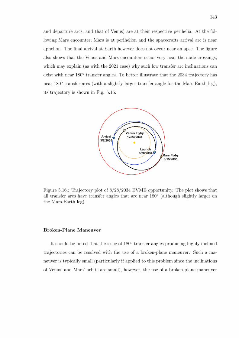
143

and departure arcs, and that of Venus) are at their respective perihelia. At the fol-

lowing Mars encounter, Mars is at perihelion and the spacecrafts arrival arc is near

aphelion. The final arrival at Earth however does not occur near an apse. The figure

also shows that the Venus and Mars encounters occur very near the node crossings,

which may explain (as with the 2021 case) why such low transfer arc inclinations can

exist with near 180o transfer angles. To better illustrate that the 2034 trajectory has

near 180o transfer arcs (with a slightly larger transfer angle for the Mars-Earth leg),

its trajectory is shown in Fig. 5.16.

Mars Flyby8/15/2035

Launch8/28/2034

Venus Flyby12/23/2034Arrival

3/7/2036

Figure 5.16.: Trajectory plot of 8/28/2034 EVME opportunity. The plot shows thatall transfer arcs have transfer angles that are near 180o (although slightly larger onthe Mars-Earth leg).

Broken-Plane Maneuver

It should be noted that the issue of 180o transfer angles producing highly inclined

trajectories can be resolved with the use of a broken-plane maneuver. Such a ma-

neuver is typically small (particularly if applied to this problem since the inclinations

of Venus’ and Mars’ orbits are small), however, the use of a broken-plane maneuver

144

prevents the resulting EVME trajectory from being a true free return, and is therefore

less desirable for an IM-type mission.

Nevertheless, a broken-plane maneuver could potentially allow for transfers closer

to a true 180o-transfer, and thereby (potentially) provide lower Earth launch and

arrival V∞ values than those found in Table 5.4. Such trajectories are not investigated

in this paper, as the primary goal of this study is to find trajectories for an IM-type

mission that are purely ballistic—allowing those aboard the spacecraft to return to

Earth without the need of deterministic maneuvers.

5.3.3 Earth Entry Analysis

In the previous sections, the arrival V∞ constraint was chosen to be 9 km/s, which

was based on the arrival V∞ for the nominal Inspiration Mars mission. Now, a more

in-depth entry analysis is conducted to determine whether or not direct entry can be

used with current technologies, and if not, what is required of new technologies to

make such an entry speed achievable.

Two key trajectories are considered for this entry analysis: the EME free-return

with launch date on 11/27/2017 (the nominal Inspiration Mars trajectory), and the

EVME free-return on 11/22/2021. For the 2017 opportunity, the SpaceX Dragon

capsule [89] parameters were used for a baseline entry vehicle, since Dragon is ex-

pected to be ready for human cargo by the time of launch. (Additionally, Dragon was

the capsule considered in the Inspiration Mars feasibility study by Tito et al. [79].)

For the 2021 opportunity, the Orion capsule [90] is expected to be ready for human

cargo as well. Therefore, both Orion and Dragon were considered for use as baseline

entry vehicles for the 2021 EVME free-return. These three vehicle-opportunity com-

binations will hereafter be addressed as Dragon-2018, Dragon-2021, and Orion-2021,

respectively. The label “2018” is used for the 11/27/2017 opportunity to remain con-

sistent with other literature for the nominal inspiration Mars free-return, which refer

to a later launch date of the same opportunity in January of 2018. It is important to

145

note that the 2018 trajectory mentioned in other literature (such as Tito et al.) and

the 11/27/2017 trajectory are nearly identical, with minor variations in launch V∞,

arrival V∞, and TOF.

The optimal direct entry trajectories that minimize the total heat load (i.e. TPS

mass) of the spacecraft are computed (using GPOPS), such that the deceleration loads

are within human tolerance after a long duration spaceflight, and peak stagnation-

point heat rates are within the performance limits of the TPS materials.

For cases where g-loads exceed the allowed limits for human tolerance, or peak

stagnation-point heat rates exceed that of TPS materials currently available, aero-

capture trajectories are considered. Since aerocapture has yet to be demonstrated (at

the time of writing this paper), direct entry trajectories (if achievable) are preferred

over aerocapture. For all aerocapture trajectories considered in this work, the orbit

post-aerocapture is designed such that the periapsis is within Earth’s atmosphere;

allowing entry to occur on the return leg of the capture orbit. Although, in practice,

a correction maneuver may be necessary after the spacecraft enters its capture orbit,

it is assumed in this study that no deterministic maneuver is required to de-orbit the

spacecraft.

From the GPOPS analysis, it was found that direct entry trajectories are feasible

in terms of g-loading on the crew, using bank-angle control for guided entry. Figures

5.17 (a) and (b) shows the altitude-speed profile and deceleration, respectively, for

the direct-entry solutions of both the 11/27/2017 trajectory (using Dragon) and the

11/22/2021 opportunities (using both Dragon and Orion). The entry speed for the

11/27/2017 free return is 14.2 km/s, which is significantly higher than the entry speed

for the 11/22/2021 opportunity, of 12.8 km/s. For the three cases: Dragon-2018,

Dragon-2021, and Orion-2021, the peak deceleration and corresponding time duration

are denoted by GA, GB, and GC, respectively. For the Dragon-2018 case, GA is 5.5 g’s

for a maximum duration of 30 seconds, whereas for the Dragon-2021 case, GB is 5.2 g’s

for about 3 minutes. On the other hand, for the same 11/22/2021 opportunity, GC is

only 4 g’s for a duration of 4.5 minutes, due to higher lift capability of the Orion. By

146

comparing GA, GB, and GC with Fig. 5.1, it is apparent that the peak decelerations

for all three vehicle-opportunity combinations are within acceptable human tolerance

limits for missions of (at least) about 200 days. However, as mentioned in Sec. 5.2.3,

it is not yet known what g-loads humans may be able to tolerate after more than 500

days in microgravity.

!

"

# $%&

GA

GB

GC

a) b)

Figure 5.17.: a) Altitude vs speed, and b) deceleration load, for the three vehicle-opportunity combinations: Dragon-2018, Dragon-2021, and Orion-2021, using bank-angle control.

The corresponding total stagnation-point heat rate and the total stagnation-point

heat load for the three vehicle-opportunity combinations: Dragon-2018, Dragon-2021,

and Orion-2021 are shown in Figs. 5.18 (a) and (b). For the Dragon-2018 case, the

total stagnation-point peak heat rate and heat load are 1866 W/cm2 and 36.6 kJ/cm2,

respectively. Since, in the Dragon-2021 case, the entry speed is lower, the total

stagnation-point peak heat rate and heat load are 1219 W/cm2 and 25.3 kJ/cm2—

less than the 2018 case. For Orion-2021, the total stagnation-point peak heat rate is

967 W/cm2, due to the higher lift capability of Orion.

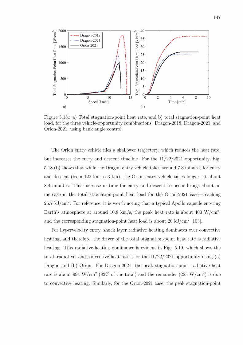
147

!

"

# $ !

%

%

#

&

'

a) b)

Figure 5.18.: a) Total stagnation-point heat rate, and b) total stagnation-point heatload, for the three vehicle-opportunity combinations: Dragon-2018, Dragon-2021, andOrion-2021, using bank angle control.

The Orion entry vehicle flies a shallower trajectory, which reduces the heat rate,

but increases the entry and descent timeline. For the 11/22/2021 opportunity, Fig.

5.18 (b) shows that while the Dragon entry vehicle takes around 7.3 minutes for entry

and descent (from 122 km to 3 km), the Orion entry vehicle takes longer, at about

8.4 minutes. This increase in time for entry and descent to occur brings about an

increase in the total stagnation-point heat load for the Orion-2021 case—reaching

26.7 kJ/cm2. For reference, it is worth noting that a typical Apollo capsule entering

Earth’s atmosphere at around 10.8 km/s, the peak heat rate is about 400 W/cm2,

and the corresponding stagnation-point heat load is about 20 kJ/cm2 [103].

For hypervelocity entry, shock layer radiative heating dominates over convective

heating, and therefore, the driver of the total stagnation-point heat rate is radiative

heating. This radiative-heating dominance is evident in Fig. 5.19, which shows the

total, radiative, and convective heat rates, for the 11/22/2021 opportunity using (a)

Dragon and (b) Orion. For Dragon-2021, the peak stagnation-point radiative heat

rate is about 994 W/cm2 (82% of the total) and the remainder (225 W/cm2) is due

to convective heating. Similarly, for the Orion-2021 case, the peak stagnation-point

148

radiative heat rate is about 971 W/cm2 (81% of the total) and the convective heat

rate is 187 W/cm2.

!

"

#""

a) b)

Figure 5.19.: Total, radiative, and convective heat rates for a) Dragon-2021, and b)Orion-2021.

Brandis-Johnston [95] provides a correlation for radiative heat rate in terms of

parameters such as freestream density, shock speed, gas composition, and vehicle

size, and is only valid for limited ranges of these parameters. As seen in Figs. 5.19

(a) and (b), the radiative heating correlation is invalid (and therefore set equal to

zero) for either speeds less than 8.8 km/s, or altitude less than 57 km and 59 km,

respectively, for the Dragon-2021 and Orion-2021 cases.

Along with the stagnation point heat rate, the peak dynamic pressure on the heat

shield due to the entry vehicle’s motion is important in determining the TPS material.

The dynamic pressure is a function of the free stream density and speed of an entry

spacecraft, given by qdyn = ρV 2/2. The peak dynamic pressure for the Dragon-2018

case is 0.19 atm (19.4 kPa). For the 2021 opportunity, the peak dynamic pressures

are 0.18 atm (18.5 kPa) and 0.14 atm (14.2 kPa) for the Dragon and Orion entry

vehicles, respectively.

149

The aerothermal conditions and deceleration of the three cases are summarized in

Table 5.6. It should be noted that the true peak heat rate and peak dynamic pressure

values will, in practice, likely deviate from the values listed in the table. This deviation

will inevitably arise from various errors due to uncertainly in the arrival conditions

(e.g. from navigation errors), atmospheric model, and vehicle aerodynamics, to name

a few. The goal of this analysis is therefore to merely assess the feasibility of entry for

the free-return trajectories found in this paper, since these cases exhibit exceptionally

high entry speeds compared to previous human missions. A statistical assessment of

the effects of dispersions on these entry trajectories is not the intent of this study.

Table 5.6.: Direct Entry Aerothermal Conditions for Key Free-Return Opportunities

Case Peak q, W/cm2 Peak qdyn, atm Q, kJ/cm2 Peak Decel., Earth g’sDragon-2018 1866 0.19 36.6 5.5Dragon-2021 1219 0.18 25.3 5.2Orion-2021 967 0.14 26.7 4

The TPS mass fraction of an entry vehicle is strongly correlated to the total

stagnation-point heat load given in Eq. 5.6. The Dragon entry vehicle uses a SpaceX

variant of Phenolic Impregnated Carbon Ablator (PICA) for its TPS material called

PICA X [103], and Orion uses a variant of Avcoat [103]. These TPS materials,

however, may not be suitable for the trajectories of interest in this study. Thus, once

the aerothermal conditions are determined from the GPOPS simulation, a suitable

TPS material is identified (which may or may not match the material currently being

used by Dragon and Orion).

TPS materials are often characterized by their density (high, mid, or low) and

capability to withstand various heat rates at a particular stagnation pressure [103].

Table 5.7 summarizes the currently available (or near-term) ablative TPS materials,

as well as their projected performance in terms of heat rate and stagnation pressure.

Flight heritage or Technology Readiness Level (TRL) is also listed.

150

Table 5.7.: Ablative TPS Material Properties (Adapted from Kolawa et al. [103])

TPS Density Heritage or TRL qr, W/cm2 Pres., atmPhenCarb Family Low-Mid TRL 4 – 5 800 – 10000 > 1Adv. Carbon-Carbon (ACC) Low-Mid Genesis > 2000 > 1PICA and PICA X Low-Mid Stardust ∼1200 < 1Avcoat Low-Mid Apollo, Orion ∼1000 ∼1Carbon Phenolic (CP) High Galileo, Pioneer-Venus ∼100000 >>1Chopped Molded CP (CMCP) High Galileo, Pioneer-Venus ∼100000 >>1Tape Wrapped CP (TWCP) High Galileo, Pioneer-Venus ∼100000 >>13 DQP High TRL 3 ∼5000 > 1

Observe that for all three trajectory cases, Dragon-2018, Dragon-2021, and Orion-

2021, both PhenCarb and ACC are suitable TPS materials for withstanding their peak

heat rates of 1866, 1219, and 967 W/cm2, respectively. For Orion-2021, PICA and

PICA X will also work, and possibly Avcoat. The peak heating of Orion-2021 is very

near Avcoat’s listed limit however, and more qualification testing would be needed

to account for deviations from the optimal trajectory found in this study. A similar

situation is true if PICA or PICA X are to be considered for Dragon-2021, since its

peak rate of 1219 W/cm2 is slightly over PICA’s qualified limit and must be qualified

for aerothermal conditions beyond the current limit. In all cases, PhenCarb will need

further development to become flight-ready, due to its current TRL.

For Dragon-2018, ACC may also need to be qualified beyond the listed limit in

Table 5.7, since deviations from the optimal entry trajectory found in this study

may result in a larger heat rate than the 1866 W/cm2, which is already close to the

current qualified limit for ACC. Additionally, the flight-ready carbon phenolic (used

on the Galileo probe to Jupiter and Pioneer Probe to Venus) would be able to easily

withstand all heat rates encountered from the trajectories in this study. However,

carbon phenolic is a high-density TPS material, and will have a significant mass

penalty. It is more likely therefore, that the low-mid density TPS options are a more

attractive choice (pending further trade studies).

151

5.3.4 The 2023 EVME High Entry-Speed Free-Returns

From the Earth entry results in the previous section, it seems that opportunities

with Earth arrival V∞ greater than the 9 km/s constraint may be feasible if carbon

phenolic or aerocapture is used. Of course, these high entry-speed solutions will only

be usable if the g-loads experienced by the crew are kept within acceptable levels.

The goal of such a study being to find near-term opportunities that occur on dates

other than those in 2017, 2018 and 2021, with particular interest in any opportunities

occurring later than 2021.

To find such near-term opportunities, free returns (from STOUR) are identified

that have arrival V∞ as large as 11 km/s. These high entry-speed cases are inves-

tigated for all gravity-assist paths considered in this study: EME, EVME, EMVE,

and EVMVE. For the paths EME, EMVE, and EVMVE, no near-term opportuni-

ties were found with characteristics significantly different from those already found in

2017, 2018 and 2021 (apart from the larger entry speed). Of these paths, the closest

opportunity to meeting the constraints (with high entry speed), is an EVMVE on

12/07/2021, with launch V∞ of 5.5 km/s, arrival V∞ of 10.76 km/s, but TOF of 632

days—a month longer than the 600-day constraint.

Using the gravity assist path EVME however, a group of high entry-speed oppor-

tunities were found that occur in September and October of 2023. These trajectories

all have arrival V∞ near 11 km/s, but have launch V∞ as low as 5 km/s (C3 of 25.00

km2/s2), and TOF as low as 483 days. The Pareto-optimal set (i.e. best cases) from

the 2023 EVME free returns found is listed in Table 5.8.

Table 5.8.: 2023 EVME Pareto-Set Opportunities

Launch Date V∞,L, km/s C3, km2/s2 TOF, days V∞,A, km/s VEntry, km/s09/09/2023 5.00 25.00 501 10.92 15.5509/22/2023 5.50 30.25 486 10.96 15.5809/25/2023 5.70 32.49 483 10.98 15.5910/06/2023 6.00 36.00 500 10.74 15.43

152

Another attribute of the opportunities listed in Table 5.8 is that they have a

relatively close approach to the Sun (compared to the other trajectories highlighted

in this study) of about 0.5 AU. Any risk associated with such a solar distance was

not investigated in this study. However, it is not expected that such a close approach

will be problematic (as discussed in Sec. 5.3.2), and will likely require additional

thermal protection (over the other notable trajectories in this paper, with minimum

solar distances of about 0.7 AU).

The high entry speeds listed in Table 5.8 are of greater concern (at least from a

trajectory standpoint) since they are on the order of 1.5 km/s greater than that of

the nominal Inspiration Mars opportunity, and are further analyzed using GPOPS.

To capture all 2023 opportunities found, the GPOPS analysis is done using an ar-

rival V∞ of 11 km/s (entry speed of 15.6 km/s). Both direct entry and aerocapture

are investigated (using Dragon and Orion as baseline entry vehicles) to determine if

this high speed entry is feasible with regards to human deceleration tolerance and

stagnation-point heat rate.

Using Dragon, no feasible direct entry trajectory was found to exist with a peak

deceleration less than 7.2 g’s. Even when aerocapture was implemented in GPOPS, a

trajectory was not found to exist with peak deceleration less than 7 g’s. Using Orion

however, both direct entry and aerocapture trajectories were found with decelerations

within human tolerances.

Feasible direct entry and aerocapture trajectories of Orion with peak deceleration

of about 6.2 g’s are shown in Figs. 5.20 (a) and (b). For aerocapture, a single peak

in deceleration is shown, whereas for the direct entry there are two peaks shown,

where the crew must withstand the peak g-loads for a longer period of time (about

1 minute) during the second peak. In both cases however, the g-loads are well below

the maximum allowed peak values (and duration) for human tolerance. The two-peak

behavior from direct entry is called a skip-type trajectory, and is a product of the

bank-angle modulation working to satisfy the deceleration constraint.

153

0 5 10 15 200

20

40

60

80

100

120

Speed [km/s]

Alt

itu

de

[km

]

0 2 4 6 8 100

1

2

3

4

5

6

7

Time [min]

Dec

eler

atio

n [

Ear

th g

's]

Direct Entry

Aerocapture

a) b)

Figure 5.20.: Orion entry analysis for 2023 EVME free returns for both direct entryand aerocapture. The speed profile is shown plotted against altitude in (a), and thedeceleration over time is shown in (b).

For the case of aerocapture, Fig. 5.20 (a) shows the trajectory altitude decrease

to just above 60 km, before exiting with a speed of 10.8 km/s (at an altitude of 120

km). The important factor here is that escape velocity at 120 km altitude is 11.1

km/s, and therefore a trajectory with a speed of 10.8 km/s is captured in an orbit

about Earth. The design of the capture orbit post aerocapture is a two-dimensional

problem, and can be determined from various combinations of parameters that define

an orbit in the two-body problem, such as the exit speed and exit flight-path angle,

apoapsis and orbital period, etc. These capture orbit parameters are specified in

GPOPS, which impose additional constraints on the optimal entry solution—thereby

changing the result. Therefore, as different capture orbit parameters are specified,

GPOPS will find solutions with differences in deceleration profiles. As a result, a

more thorough analysis of aerocapture constitutes a more in-depth trade study of

possible final capture orbits. Such a trade is not included in this paper, since the

primary interest in this brief investigation is to merely determine if there exists a

feasible entry solution for the 2023 free-returns.

154

The aerocapture trajectory in Fig. 5.20 results in a capture trajectory with an

apoapsis of 125,500 km (nearly 1/3 the lunar distance) with an orbital period of about

2 days. A larger capture orbit could be chosen to even further reduce the exit speed,

as well as the peak g-loads experienced by the crew. Likewise, the opposite holds true

for smaller capture orbits. The 2-day capture orbit chosen here provides sufficiently

low g-loads for this feasibility analysis, however further trades may prove to find a

more desirable solution.

Figure 5.21 shows the total stagnation-point heat rate and heat load (plotted

against speed and time, respectively) for the same two entry trajectories given in Fig.

5.20. The total heat rates for the direct entry and aerocapture cases are very similar,

with peak heat rates reaching 3040 W/cm2 and 3088 W/cm2, respectively. For both

of these cases, (as observed in Table 5.7) the low-mid density TPS material PhenCarb

would be suitable (pending further development and qualification testing to become

flight ready). ACC may also be suitable, pending further tests to qualify it for heat

rates beyond its current qualified limit.

0 5 10 15 200

500

1000

1500

2000

2500

3000

3500

Speed [km/s]

To

tal

Sta

gn

atio

n-P

oin

t H

eat

Rat

e, [

W/c

m2]

Direct Entry

Aerocapture

0 2 4 6 8 100

10

20

30

40

50

Time [min]

To

tal

Sta

gn

atio

n-P

oin

t H

eat

Lo

ad [

kJ/

cm2]

a) b)

Figure 5.21.: Direct entry and aerocapture results for the 2023 free-return opportu-nity. Total stagnation-point heat rate (a) and head load (b) are shown, and correspondto the same entry trajectories given in Fig. 5.20.

155

There is however a substantial difference in total heat load between the direct

entry and aerocapture cases. For aerocapture, the total heat load is 29.6 kJ/cm2,

and for direct entry, the total heat load is 40.5 kJ/cm2. This direct entry heat load

is nearly double that of what the Apollo command modules encountered, which had

a TPS mass-fraction of about 14% [103] (of the total spacecraft mass). The direct

entry trajectory for the 2023 free-return is estimated to require a TPS mass fraction

of about 22.0% (much larger than that of Apollo), and may provide an argument for

the use of aerocapture, which requires a TPS mass fraction of 18.4%. The increased

heat load for the direct entry case can be attributed to the fact that lift is used to fly a

more shallow trajectory, which is done to reduce the g-loads experienced by the crew.

Flying such a shallow trajectory, however, increases the time that the spacecraft must

be in the atmosphere, which increases the total heat load.

5.3.5 The Case for Venus

Free-return trajectories to Venus have also been investigated. In 1969 Hollis-

ter [84], and in 1970 Hollister and Menning [85], found free-return trajectories that

repeatedly encounter Earth and Venus (also known as Earth-Venus cycler trajecto-

ries). In 2000, Bonfiglio et al. [104] investigated Venus free returns using aerogravity

assists. In general however, far less attention has been paid on human missions to

Venus as it has been for Mars. Nevertheless, the case for Venus has been proposed

(or at least addressed) by some [105–109].

For Inspiration Mars, the results of this study indicate that, apart from the nomi-

nal Inspiration Mars opportunity in December of 2017 to January of 2018 (and apart

from the high entry-speed cases in Table 5.8), the only near-term IM-type mission

candidates are the 2021 EVME trajectories listed in Table 5.4. However, as the 2018

nominal launch date nears, it may turn out that the 2021 EVME opportunity be-

comes the new “nominal” case, and if so, there would be no near-term backup for

such a mission. Since a primary goal of Inspiration Mars is to push human spaceflight

156

into deep space, many of the mission objectives could still be met with a human flyby

of Venus alone—albeit an Inspiration Venus mission.

To investigate such an option, the Venus free-return gravity-assist path Earth-

Venus-Earth (EVE) was searched using STOUR, and many near-term opportunities

were found. Because this is proposed as an alternate for Inspiration Mars (or some

other IM-type mission), the same constraints were imposed on this STOUR search

with regard to Earth launch and arrival V∞ and TOF. Therefore, any vehicle designed

for the EVME 2021 trajectory, should be capable of flying a candidate EVE trajectory.

Figure 5.22 shows the search results over launch dates spanning from 1/1/2019

through 1/1/2027 with steps of one day, and all with Earth arrival V∞ at or below

9 km/s. These dates were chosen as the most relevant near-term launch dates for

backup to the nominal Inspiration Mars trajectory, as well as to the 2021 EVME

opportunities. An eight-year span of launch dates was chosen as it is the approximate

time for the Earth-Venus geometry to repeat in inertial space (approximately 8 Earth

and 13 Venus revolutions about the Sun). A minimum flyby altitude of 300 km at

Venus was also imposed for this search. The figure shows five columns of opportunities

whose launch dates each span about six months. The distance between columns is

consistent with the Earth-Venus synodic period (assuming circular-coplanar orbits)

of about 1.6 years, which repeats approximately five times in the eight years shown.

From the results in the figure, it is clear that many EVE candidates are available for

an IM-type mission.

To identify the most desirable EVE near-term candidates, Fig. 5.23 shows the

same candidate trajectories as shown in Fig. 5.22, but with Earth launch date ex-

changed for Earth arrival V∞ on the horizontal axis. The trajectories that make up

the Pareto set have been circled, and are mostly made up of opportunities in 2026,

although those that exhibit lower arrival V∞ have launch dates in 2019 and 2021 (as

annotated on the figure).

A representative subset of the Pareto-set EVE trajectories is given in Table 5.9.

The cases listed include a case with the overall lowest Earth launch V∞, Earth arrival

157

2020/01/01 2022/01/01 2024/01/01 2026/01/01

350

400

450

500

550

16

16

16

16

16

16

16

16

16

16

16

161616161616161616

15

15

16

15

15

16

15

1516

15

1516

15

1516

15

151615161516151615161516

14

14

1516

14

14

1516

14

14

1516

14

14

1516

14

14

1516

16

16

14

141516

16

16

141516

16

16

141516

16

16

141516

16

16

141516

16

16

141516

16

16

141516

16

16

141516

16

16

141516

16

16

141516

16

16

13

13

1415

16

13

13

14

15

16

13

13

1415

16

13

13

14

15

15

15

16

13

13

14

15

15

15

16

13

13

14

15

15

15

16

13

13

14

15

15

15

16

13

13

1415

15

15

16

13

13

14

15

15

16

13

13

14

1516

13

13

14

15

1616

16

13

13

14

15

1616

16

13

13

14

14

141515

15

1616

16

13

13

14

14

14

14

14

1515

15

1616

16

13

13

14

14

14

14

14

1515

15

1616

16

13

13

1414

14

14

1515

15

16

161414

14

1515

15

16

161414

14

1515

15

161313

1414

14

1515

15

161313

1414

14

1515

15

1613

13

1414

14

15

1516

13

13

1414

14

15

1516

13

13

13

13

1414

14

1516

13

13

13

1414

14

1516

13

13

1414

14

1516

13

13

1414

14

1516

13

13

14

14

1516

13

13

14

1516

13

13

14

1516

13

13

14

1516

13

13

14

1516

13

14

1516

1213

14

1516

12

14

1516

12

14

1516

12

14

1516

12

14

1516

12

141516

141516

141516

11

141516

11

141516

11

141516

13

13

141516

13

13

141516

13

141516

131415

10

131415

131415

131415

13141314

12

12

1314

12

121314

12

121314

1213121312131213

11

1112

11

1112

11

1112

11

1112

11

1111

10

1011

10

1011

10

10

10

10

10

10

10

9

9

10

9

9

10

9

9

999

8

8

9

8

9

8

9

8

9

8

9

8

9

7

8

9

7

8

7

8

7

8

7

8

7

8

6

7

8

6

7

8

6

7

6

7

7678678

4

56789

4

56789

4

5678910

4

5

5

678910

4

5

5

67891011

4

5

5

67891011

4

4

5

5

6789101112

4

4

5

5

6789101112

4

4

5

5

6789101112134

4

5

5

6

6

78910111213

4

4

5

5

6

6

78910111213

4

4

5

5

6

6

789101112

4

4

5

5

6

6

789101112

4

4

5

5

6

6

789101112

4

4

5

5

6

6

789101112

4

4

5

5

6

6

7

7

89101112

4

4

5

5

6

6

7

7

89101112

4

4

5

5

6

6

7

7

89101112

4

5

5

6

6

7

7

891011125

5

6

6

7

7

891011125

5

6

6

7

7

8

8

91011125

5

7

7

8

8

91011125

57

7

8

8

9101112

5

58

8

910111213

5

58

8

910111213

8

8

910111213

9

9

10111213

9

9

10111213

9

9

10111213

10111213

10111213

10

10

111213

10

10

111213

111213

111213

11

11

121312131213

1213

12

131314

1314

1314

13

141414141415

14

1515

15

15

15

16

16

16

16

16

16

16

16

16

16

16

16

16

16

16

16

16

16

16

16

16

16

16

16

16

16

1616161616161616

15

15

16

15

15

16

15

15

16

15

15

16

15

1516

16

16

15

1516

16

16

15

1516

16

16

15

1516

16

16

15

1516

16

16

15

1516

16

16

15

1516

16

16

15

1516

16

16

15

1516

16

16

1516

16

16

1516

16

16

1516

16

16

1516

16

16

1516

16

16

1516

16

16

1516

16

16

1516

16

16

1516

16

16

15

15

15

16

16

16

15

15

15

16

16

16

15

15

15

16

16

15

15

15

16

16

15

15

15

16

16

15

15

15

16

16

15

15

15

16

16

15

15

15

16

16

15

15

15

16

16

15

15

15

16

16

15

15

15

16

16

15

15

15

16

16

15

15

15

16

16

15

15

15

16

16

15

15

15

16

16

14

14

15

15

15

16

16

14

14

15

15

15

16

16

14

14

15

15

161616

1614

14

15

15

161616

1614

14

15

15

16

1616

1614

14

15

15

16

1616

1614

14

15

15

16

1616

1614

14

15

15

16

1616

1614

14

15

15

16

1616

1614

14

15

15

16

1616

1614

14

15

15

16

1616

1614

14

15

15

16

1616

1614

14

15

15

16

1616

16

13

13

14

14

14

14

15

15

16

16

16

13

13

14

14

14

14

15

15

16

16

16

13

13

14

14

14

15

15

16

16

1613

13

14

14

14

15

15

16

1613

13

14

14

14

15

15

16

1613

13

14

14

14

15

15

16

1613

13

14

14

14

15

15

16

1613

13

14

14

14

15

15

16

16

1613

13

14

14

14

15

15

16

16

1613

13

14

14

14

1515

15

15

16

16

1613

13

14

14

14

15

15

15

15

16

16

1613

13

14

14

15

15

15

16

16

12

12

13

14

14

15

15

15

16

16

12

12

13

14

14

15

15

15

16

1612

12

13

14

14

15

15

15

16

1612

12

13

13

13

14

14

15

15

15

16

1612

12

13

13

13

14

14

15

15

16

12

12

13

13

13

14

14

15

15

16

12

12

13

13

13

14

14

15

15

16

12

12

13

13

13

14

14

15

15

16

12

13

13

13

14

14

15

15

16

12

13

13

13

14

14

15

15

16

11

11

12

13

13

14

14

15

15

16

11

11

12

12

12

13

13

14

14

1516

11

11

12

12

12

13

13

14

14

1516

11

11

12

12

12

13

13

14

14

1516

11

11

12

12

12

13

13

14

14

1516

11

11

12

12

12

13

13

14

14

1516

11

12

12

12

13

13

141516

11

12

12

12

13

13

1415

11

12

12

12

13

13

1415

11

11

11

12

12

12

13

13

1415

11

11

11

12

12

12

13

13

1415

10

10

11

11

11

12

12

13

13

14

10

10

11

11

11

12

12

1314

10

10

11

11

11

12

12

1314

10

11

11

11

12

12

1314

10

11

11

11

12

12

1314

10

10

10

11

11

11

12

12

13

10

10

10

11

11

11

1213

10

10

10

11

11

11

1213

10

10

10

11

11

11

1213

10

10

10

11

11

11

12

10

10

10

11

11

11

12

9

10

10

10

11

11

12

9

10

10

10

1112

9

9

9

10

10

10

11

9

9

9

10

10

10

11

9

9

9

10

10

10

11

9

9

9

10

10

10

11

9

9

9

10

10

9

9

9

10

10

9

9

9

10

10

8

8

9

9

9

10

8

8

8

9

9

8

8

8

9

9

8

8

8

9

9

8

8

9

9

8

8

9

9

8

8

9

8

8

9

8

8

9

7

7

8

8

9

7

7

8

8

9

7

7

8

9

7

7

8

7

7

8

7

7

8

7

8

7

8

7

8

6

6

7

8

6

6

7

8

6

7

8

6

7

8

6

7

8

6

7

8

6

7

6

7

5

6

7

5

6

7

5

6

7

5

6

7

5

6

7

5

6

7

5

6

7

5

6

778

5

6

77

8

5

6

77

8

5

6

77

8

4

5

677

8

4

5

677

8

4

5

6

677

8

4

5

6

677

8

8

9

4

5

6

677

8

8

910

4

5

6

6

7

77

8

8

910

4

5

6

6

7

77

8

8

91011

4

5

6

6

7

7

8

8

91011

4

5

6

6

6

7

7

8

8

91011

4

5

6

6

6

7

7

8

8

9101112

4

5

6

6

6

7

7

8

8

9101112

4

5

6

6

6

7

7

8

8

9

9

101112

4

5

6

6

6

7

7

8

8

9

9

10111213

4

5

6

6

6

7

7

8

8

9

9

10111213

4

5

6

6

6

7

7

8

8

9

9

10111213

4

5

5

5

6

6

6

7

7

8

8

9

9

10111213

4

5

5

5

6

6

6

7

7

8

8

9

9

10111213

4

5

5

5

6

6

7

7

8

8

9

9

1011121314

4

5

5

5

6

6

7

7

8

8

9

9

1011121314

4

5

5

5

6

6

7

7

8

8

9

9

10111213145

5

6

6

7

7

8

8

9

9

10

10

111213145

5

7

7

8

8

9

9

10

10

111213145

58

8

9

9

10

10

111213145

58

8

9

9

10

10

11121314155

59

9

10

10

1112131415

9

9

10

10

1112131415

9

9

10

10

1112131415

510

10

1112131415

5

10

10

1112131415

5

10

10

11

11

12131415

11

11

12131415

11

11

12131415

11

11

1213141516

11

11

1213141516

1213141516

12131415166

12

131415166

12

131415166

12

13141516

13141516

13

141516

7

13

141516

7

13

141516

7

7

13

141516

14

1516

8

14

1516

8

14

1516

14

1516

9

15

9

91011

11

1112

12

1213

13

1314

14

14

151516

16

16

16

16

16

16

16

16

16

16

16

16

16

16

16

16

16

16

16

16

16

16

16

16

16

16

16

16

15

15

16

16

16

16

15

15

16

16

16

16

15

15

16

16

16

16

15

15

15

15

16

16

16

16

15

15

15

15

16

16

16

15

15

15

15

16

16

16

15

15

15

15

16

16

16

15

15

15

15

16

16

15

15

15

15

16

16

14

14

15

15

15

15

16

1614

14

15

15

15

15

16

16

14

14

14

14

15

15

15

15

16

16

14

14

14

14

15

15

15

15

16

16

14

14

14

14

15

15

15

16

16

14

14

14

14

15

15

15

16

16

14

14

14

14

15

15

15

16

16

14

14

14

14

15

15

16

16

14

14

14

14

15

15

16

16

1313

13

13

14

14

14

14

15

15

16

16

13

13

13

13

14

14

14

14

15

15

16

16

13

13

13

13

14

14

14

14

15

15

16

16

13

13

13

13

14

14

14

15

15

1616

13

13

13

13

14

14

14

15

15

1616

13

13

13

13

14

14

14

15

15

1616

13

13

13

13

14

14

15

15

1616

12

12

13

13

13

13

14

14

15

151616

12

12

12

12

13

13

13

13

14

14

15

151616

12

12

12

12

13

13

13

13

14

14

15

151616

12

12

12

12

13

13

13

14

14

15

151616

12

12

12

12

13

13

13

14

14

15

151616

12

12

12

12

13

13

13

14

14

15

151616

12

12

12

12

13

13

13

14

14

15

151616

12

12

12

12

13

13

13

14

14

15

151616

11

11

12

12

12

12

13

13

14

14

15

151616

11

11

12

12

12

12

13

13

14

14

15

151616

11

11

11

11

12

12

12

12

13

13

14

14

15

151616

11

11

11

11

12

12

12

12

13

13

14

14

15

151616

11

11

11

11

12

12

12

13

13

14

14

15

151616

11

11

11

11

12

12

12

13

13

14

14

15

151616

11

11

11

11

12

12

12

13

13

14

14

15

15

1616

11

11

11

11

12

12

12

13

13

14

14

15

15

1616

10

10

11

11

11

11

12

12

12

13

13

14

14

15

1516

10

10

11

11

11

11

12

12

13

13

14

14

15

1516

10

10

11

11

11

11

12

12

13

13

14

14

15

1516

10

10

11

11

11

11

12

12

13

13

14

14

15

1516

10

1011

11

11

12

12

13

13

14

14

15

1516

10

10

10

10

11

11

11

12

12

13

13

14

14

15

1516

10

10

10

10

11

11

11

12

12

13

13

14

141516

9

9

10

10

10

10

11

11

11

12

12

13

13

14

141516

9

9

10

10

10

10

11

11

11

12

12

13

13

14

141516

9

9

10

10

10

10

11

11

12

12

13

13

14

141516

9

9

10

10

10

10

11

11

12

12

13

13

14

141516

9

910

10

10

11

11

12

12

13

13

14

141516

9

910

10

10

11

11

12

12

13

131415

9

910

10

10

11

11

12

12

13

131415

8

8

9

910

10

10

11

11

12

12

13

131415

8

8

9

910

10

10

11

11

12

12

13

131415

8

8

9

910

10

10

11

11

12

12

13

131415

8

8

9

9

9

9

10

10

10

11

11

12

121314

8

8

9

9

9

9

10

10

11

11

12

121314

8

8

9

9

9

9

10

10

11

11

12

121314

8

89

9

9

10

10

11

11

12

121314

8

89

9

9

10

10

11

11

12

121314

77

8

89

9

9

10

10

11

11

12

121314

7

7

8

89

9

9

10

10

11

111213

7

7

8

89

9

9

10

10

11

111213

7

7

8

89

9

9

10

10

11

111213

7

7

8

89

9

9

10

10

11

111213

7

7

8

89

9

9

10

10

11

111213

7

7

8

89

9

10

10

11

111213

7

789

9

10

101112

7

78

8

8

9

9

10

101112

6

6

7

78

8

8

9

9

10

101112

6

6

7

78

8

8

9

9

10

101112

6

6

7

78

8

8

9

9

10

101112

6

6

7

78

8

8

9

9

10

1011

6

6

7

78

8

8

9

91011

6

6

7

78

8

9

91011

6

6

7

78

8

9

91011

6

6

7

78

8

9

910

5

5

6

678

8

9

910

5

5

6

67

7

7

8

8

9

910

5

5

6

67

7

7

8

8

9

910

5

5

6

67

7

7

8

8910

5

5

6

67

7

8

89

5

5

6

67

7

8

89

5

5

6

67

7

8

89

5

5

6

67

7

8

89

5

5

6

67

7

8

89

11

4

4

5

5

6

67

7

8

89

1011

4

4

5

5

6

67

78

1011124

4

5

5

6

67

78

1011124

4

5

5

6

67

78

1011124

4

5

56

6

7

78

101112

4

4

5

56

6

7

78

10111213

4

4

5

56

6

7

7

910111213

4

4

5

56

6

7

7

910111213

4

4

5

56

67

910111213

4

4

5

56

67

910111213

4

4

5

56

67

89101112133

3

4

4

5

56

6

891011123

3

4

4

5

56

6

891011123

3

4

4

5

56

6

891011123

3

4

4

5

56

6

89101112

3

3

4

4

5

56

7789101112

3

3

4

4

5

5

789101112

3

3

4

4

5

5

789101112

3

3

4

4

5

5

789101112

3

3

4

4

5

5

789101112

3

3

4

4

5

5

789101112

3

3

4

4

5

5

667

8

89101112

3

3

4

4

5

5

66

7

7

8

8

9

9101112

3

3

4

4

5

5

66

7

7

8

8

9

9101112

3

3

4

4

5

5

6

7

7

8

8

9

9

10

101112

3

3

4

4

5

6

6

7

7

8

8

9

9

10

101112

3

3

4

4

5

6

6

7

7

8

8

9

9

10

101112

3

3

4

4

5

6

6

7

7

8

8

9

9

10

10

11122

2

3

3

4

4

5

6

68

8

9

9

10

10

11122

2

3

3

4

4

5

5

559

9

10

10

11

112

2

3

3

4

4

5

5

559

9

10

10

11

112

2

3

3

4

4

5510

10

11

112

2

3

3

4

4

5510

10

11

112

2

3

3

4

4

55

10

10

11

112

2

3

3

4

4

5511

11

3

3

4

4

55

6

11

11

3

3

4

4

55

6

11

11

3

3

4

4

4

55

6

11

11

3

3

4

4

4

55

6

12

3

3

4

4

4

5

6

12

3

3

4

4

4

5

6

12

3

3

4

4

4

5

6

12

3

3

4

4

4

5

6

12

3

3

4

4

4

5

6

123

3

4

4

4

5

6

3

3

4

4

4

5

6

7

3

3

4

4

4

5

5

6

7

3

3

4

4

4

5

5

6

7

3

3

4

4

4

5

5

6

7

3

3

4

4

4

5

5

6

7

3

3

4

4

4

4

5

5

6

7

3

3

4

4

5

5

6

7

8

3

3

4

4

5

5

6

7

8

4

4

5

5

6

7

8

4

4

5

5

6

7

8

4

4

5

5

6

7

8

56

4

4

5

5

5

6

6

7

8

9

4

4

5

6

6

7

89

4

4

5

6

6

7

8

9

5

5

6

6

7

8

910

5

5

6

6

7

7

8

910

5

5

6

7

7

8

910

5

5

6

7

7

8

910

5

5

6

7

7

8

91011

5

5

6

7

7

7

8

8

91011

6

7

8

8

91011

6

6

7

8

8

91011

6

6

7

8

8

8

9

9

1011

6

6

7

8

9

9

1011

6

6

7

8

9

9

1011

7

8

9

9

9

10

1011

7

8

9

10

1011

12

7

7

8

9

10

10

11

11

12

7

7

8

9

10

11

11

11

12

8

9

10

11

11

11

12

12

8

9

10

1111

11

11

12

12

8

8

9

10

11

12

12

13

9

10

11

12

12

12

12

13

13

9

10

1112

13

13

14

9

10

11

12

13

13

14

10

11

12

1415

10

11

12

1414

15

10

11

12

15

1516

11

12

16

11

12

13

16

16

12

13

12

13131414

15

15

15

16

16

1616

16

16

16

16

16

16

16

16

16

16

16

16

16

16

16

16

16

16

16

16

16

16

16

16

16

16

16

16

16

16

16

16

16

16

16

16

16

16

16

16

16

16

16

16

16

16

16

16

16

16

16

16

16

15

15

15

15

16

16

16

15

15

15

15

16

16

16

15

15

15

15

16

16

16

15

15

15

15

16

16

16

15

15

15

15

16

16

16

15

15

15

15

1616

16

15

15

15

15

1616

16

1515

15

1616

16

14

14

14

14

1515

15

1616

16

14

14

14

14

1515

15

1616

16

14

14

14

14

1515

15

1616

16

14

1414

14

1515

15

1616

14

1414

14

1515

15

1616

14

1414

14

1515

15

1616

14

1414

14

1515

15

1616

14

1414

14

1515

15

1616

14

1414

14

1515

15

1616

14

1414

14

1515

15

16161414

14

1515

15

161614

14

14

1515

15

1616

13

1314

14

14

1515

15

1616

13

1314

14

14

1515

15

1616

13

1314

14

14

15

15

15

1616

13

1314

14

14

15

15

15

1616

13

1314

14

14

15

151616

13

1314

14

14

15

15

1616

13

1314

14

14

15

15

16

16

13

1314

14

14

15

15

16

16

12

121314

14

14

15

1516

12

121314

14

14

15

1516

12

121314

14

14

15

1516

12

121314

14

14

15

1516

12

1213

13

13

14

14

15

1516

12

1213

13

13

14

14

15

1516

12

1213

13

13

14

14

15

1516

12

1213

13

13

14

141516

12

1213

13

13

14

141516

11

11

12

1213

13

13

14

141516

11

11

1213

13

13

14

141516

11

111213

13

13

14

141516

11

111213

13

13

14

141516

11

111213

13

13

141516

11

111213

13141516

11

111213

13141516

11

111213

13141516

11

111213

131415

11

111213

131415

10

10

11

111213

131415

10

10

1112

131415

10

10

1112

131415

10

101112

1314

10

101112

1314

10

101112

1314

10

101112

1314

10

1011

13

10

1011

13

9

9

10

1011

13

9

9

1011

9

9

1011

9

9

1011

9

910

9

910

9

910

9

910

8

8

9

910

8

8

9

910

8

8

9

910

8

8

9

8

8

9

8

8

9

8

8

9

8

89

8

89

8

89

7

7

8

8

7

7

8

8

7

7

8

8

7

7

8

8

7

7

8

7

7

8

7

7

8

14

7

7

8

13146

6

7

7

1314

6

6

7

7

1314

6

6

7

7

1314

6

6

7

7

121314

6

6

7

7

121314

6

6

7

7

12131415

6

6

7

111112131415

6

6

1112131415

6

6

1112131415

5

5

6

6

1112131415

5

5

6

6

10101112131415

5

5

6

6

101011121314

5

5

6

6

1011121314

5

5

6

6

991011121314

5

5

6

991011121314

5

5

6

991011121314

5

5

6

9

9

9

10

10

11

121314

5

5

6

88911

121314

5

5

6

8

11

11

12

1314

4

4

5

5

6

8

12

13

4

4

5

5

6

78

12

13

4

4

5

5

6

78

12

13

4

4

5

6

78

13

4

4

5

6

7

13

4

4

5

6

6

7

13

4

4

5

6

6

74

4

5

6

6

74

4

5

6

6

74

4

5

5

6

6

74

4

5

5

6

6

4

4

5

5

6

6

3

3

45

5

6

6

3

3

45

5

6

6

3

3

4

445

5

6

6

3

3

445

5

6

6

3

3

445

5

6

3

3

445

5

6

3

3

445

5

6

3

3

445

5

63

3

3

3

445

5

6

3

3

3

3

445

5

6

3

3

3

445

5

6

3

3

3

44

5

67

3

3

3

44

5

67

3

3

3

44

567

3

3

3

44

567

3

3

3

44

567

3

3

3

44

567

3

3

3

44

567

3

3

3

44

5678

3

3

3

44

5678

34

4

5678

34

4

5678

34

4

5678

34

4

56789

34

4

56789

34

4

56789

34

4

56789

34

4

5678910

34

4

5

678910

34

4

5

678910

34

4

5

678934

5

67893

4

5

6789

3

3

4

5

67894

5

67894

5

6784

6

78

4

6

78

4

4

5

6

78

5

6

78

5

6

78

5

78

5

5

6

7

8

6

7

8

6

7

8

6

6

8

7

8

7

8

7

7

8

889

9

91010111112

12

1213

13

131415

15

1516

16

16

16

16

16

16

16

16

16

16

16

16

16

16

16

16

16

16

16

16

16

16

16

16

16

16

16

16

16

16

16

16

16

16

16

16

16

15

15

15

15

16

16

16

15

15

15

15

16

16

16

15

15

15

15

16

16

16

15

15

15

16

16

16

15

15

15

16

16

16

15

15

15

16

16

16

15

15

15

16

16

16

15

15

15

16

16

16

14

14

14

14

15

15

15

16

16

16

14

14

14

14

15

15

15

1616

16

14

14

14

14

1515

15

1616

16

14

14

14

14

1515

15

16161414

14

1515

15

16161414

14

1515

15

16161414

14

1515

15

16161414

14

1515

15

16161414

14

1515

15

1616

13

131414

14

1515

15

1616

13

1314

14

14

1515

15

1616

13

1314

14

14

1515

15

1616

13

1314

14

14

1515

15

1616

13

1314

14

14

15

15

15

1616

13

1314

14

14

15

15

15

1616

1314

14

14

15

15

15

1616

1314

14

14

15

15

16

16

1314

14

14

15

15

16

16

12

121314

14

14

15

15

16

16

12

121314

14

14

15

15

16

16

12

121314

14

14

15

15

16

16

12

121314

14

14

15

15

16

16

12

121314

14

14

15

15

16

16

12

121314

14

14

15

15

16

16

1213

13

13

14

14

14

15

15

16

16

1213

13

13

14

14

14

15

15

16

16

1213

13

13

14

14

14

15

15

16

16

11

11

1213

13

13

14

14

14

15

15

16

16

11

11

1213

13

13

14

14

15

15

16

16

11

111213

13

13

14

14

15

15

16

16

11

111213

13

13

14

14

15

15

16

16

11

111213

13

13

14

14

15

15

16

16

11

111213

13

13

14

14

15

15

16

16

11

111213

13

13

14

14

15

15

16

16

111213

13

13

14

14

15

15

16

16

111213

13

13

14

14

15

15

16

16

111213

13

13

14

14

15

15

16

16

10

10

111213

13

13

14

14

15

15

16

16

10

10

111213

13

13

14

14

15

15

16

16

10

10

111213

13

13

14

14

15

15

16

16

10

10

111213

13

13

14

14

15

1516

10

10

111213

13

13

14

14

15

1516

10

10111213

13

14

14

15

1516

10

10111213

13

14

14

15

1516

10111213

13

14

14

15

1516

10111213

13

14

14

15

1516

101112

12

12

13

13

14

14

15

1516

9

9

101112

12

12

13

13

14

141516

9

9

101112

12

12

13

13

14

141516

9

9

101112

12

12

13

13

14

141516

9

9

101112

12

12

13

13

14

141516

9

9

101112

12

12

13

13

14

141516

9

9

101112

12

12

13

13

14

141516

9

9

101112

12

12

13

13

14

141516

9101112

12

12

13

13141516

9101112

12

13

13141516

8

8

9101112

12

13

13141516

8

8

9101112

12

13

13141516

8

8

9101112

12

13

13141516

8

8

9101112

12

13

13141516

8

8

91011

11

11

12

12

13

13141516

8

8

91011

11

11

12

12131415

1616

16

8

8

91011

11

11

12

12131415

16

16

8

8

91011

11

11

12

12131415

16

8

8

91011

11

11

12

12131415

16

8

91011

11

11

12

121314

1515

15

16

8

91011

11

11

12

121314

15

15

15

16

7

7

8

91011

11

11

12

121314

15

15

15

16

7

7

8

91011

11

11

12

121314

15

1516

7

7

8

91011

11121314

1516

7

7

891011

111213

14

14

14

1516

7

7

891011

111213

14

14

14

1516

7

7

891011

111213

14

14

14

1516

7

7

891011

111213

14

14

14

1516

7

7

891011

1112

13

13

13

14

141516

7

7

8910

10

10

11

1112

13

13

13

14

1415167

8910

10

10

1112

13

13

13

141516

6

6

7

8910

10

10

1112

13

13

13

141516

6

6

7

8910

1011

12

12

12

13

13

13

141516

6

6

7

8910

1011

12

12

12

13

131415

6

6

7

8910

1011

12

12

12

13

131415

6

6

7

89

1010

10

10

1111

11

12

12

12

13

131415

6

6

7

89

1010

10

10

1111

11

12

12

12

131415

6

6

789

1010

10

10

1111

11

12

12131415

6

6

78

99

9

1010

10

1111

11

12

12131415

6

6

78

9

9

9

9

1010

10

1111

11

12

12131415

5

5

6

6

7

8

8

8

8

9

9

9

9

10

10

10

10

1111

11

12

12131415

5

5

6

7

8

8

9

9

9

10

10

1111

11

12

12

1314

5

5

6

7

7

7

8

8

9

9

9

10

10

1111

11

12

1314

5

5

6

7

7

89

9

10

10

11

5

5

6

7

7

8

8

9

9

9

10

10

11

12

1314

5

5

6

6

6

7

7

8

8

9

9

9

10

10

11

12

1314

5

5

6

6

6

7

7

8

8

9

9

9

10

10

11

12

1314

5

5

6

6

7

7

8

8

9

9

10

10

11

12

13

14

5

5

6

6

7

7

8

8

9

9

10

10

11

12

13

5

5

5

5

6

6

7

7

8

8

9

9

10

12

13

5

5

5

5

6

6

7

7

8

8

9

9

10

12

13

4

4

5

5

5

5

6

6

7

7

8

8

9

9

10

13

4

4

5

5

5

6

6

7

7

8

8

9

9

10

13

4

4

5

5

5

6

6

7

7

8

8

8

9

9

10

13

4

4

4

4

5

5

5

6

6

7

7

8

8

8

910

13

4

4

4

4

5

5

5

6

6

7

7

8

8

8

910

4

4

4

4

5

5

5

6

6

7

7

8

8

8

9

4

4

4

4

5

5

5

6

6

7

7

8

8

94

4

4

5

5

5

6

6

7

7

8

8

94

4

4

5

5

5

6

6

7

7

894

4

4

5

5

5

6

6

7

7

894

4

4

5

5

5

6

6

7

7

895

5

5

6

6

7

7

84

4

4

5

5

5

6

6

7

7

8

3

3

3

3

4

4

4

5

5

5

6

6

7

7

8

3

3

3

3

4

4

4

5

5

5

6

6

7

7

83

3

3

4

4

4

5

5

5

6

6

783

3

3

4

4

4

5

5

5

6

6

783

3

3

4

4

4

5

5

5

6

6

73

3

3

4

4

4

5

5

5

6

6

73

3

3

4

4

4

5

5

5

6

6

7

2

2

2

23

3

3

4

4

4

5

5

5

6

6

7

2

2

2

2

3

3

3

4

4

4

5

5

5

6

6

7

2

2

2

2

3

3

3

4

4

4

5

5

5

6

6

7

2

2

2

2

3

3

3

4

4

4

5

5

5

6

6

6

7

2

2

2

2

3

3

3

4

4

4

5

5

5

6

6

6

73

3

3

4

4

4

5

5

5

6

6

6

11

3

3

3

4

4

4

5

5

5

6

6

6

3

3

3

4

4

4

5

5

5

6

6

6

3

3

3

4

4

4

5

5

5

6

6

6

2

2

2

3

3

3

4

4

4

5

5

5

6

6

2

2

2

3

3

3

4

4

4

5

5

5

6

67

2

2

2

3

3

3

4

4

4

5

5

5

6

67

10

10

2

2

2

3

3

3

4

4

4

5

5

5

6

67

10

10

2

2

2

3

3

3

4

4

4

5

5

5

67

10

10

2

2

2

3

3

3

4

4

4

5

5

5

67

10

10

1

1

1

12

2

2

3

3

3

4

4

4

5

5

5

678

10

1

12

2

2

3

3

3

4

4

4

5

5

5

678

9

9

1

12

2

2

3

3

3

4

4

4

5

5

5

678

9

9

1

12

2

2

3

3

3

4

4

4

5

5

5

678

9

9

1

12

2

2

3

3

3

4

4

4

5

5

5

6789

9

2

2

2

3

3

3

4

4

4

5

5

5

678

8

8

9

9

2

2

2

3

3

3

4

4

4

5

5

5

678

8

9

9

2

2

2

3

3

3

4

4

4

5

5

678

8

9

9

2

2

2

3

3

3

4

4

4

5

5

678

8

9

9

10

122

2

3

3

3

4

4

4

5

5

67

7

8

8

9

9

10

1

122

2

3

3

3

4

4

4

5

5

67

7

8

8

9

9

10

1

122

2

3

3

3

4

4

4

5

5

67

7

8

8

9

9

1011

1

123

3

3

4

4

4

5

5

67

7

8

8

9

9

1011

1

1233

3

4

4

4

5

5

67

7

8

8

9

9

1011

1

1233

3

4

4

4

5

5

67

7

8

8

9

9

1011121

1233

3

4

4

4

5

5

67

7

8

8

9

9

101112

233

3

44

4

5

5

67

7

8

8

9

9

101112

233

3

44

4

5

5

67

7

8

8

9

9

10111213

233

3

44

4

5

5

678

8

9

9

10111213

2344

4

5

5

678

8

9

9

1011121314

2344

4

5

5

678

8

9

9

1011121314

2344

4

5

5

6

6

7891011121314

2344

4

5

5

6

6

789101112131415

234

4

4

5

5

6

6

789101112131415

2

234

4

4

5

5

6

6

789101112131415

345

5

6

6

789101112131415

345

5

6

6

789101112131415

345

5

5

6

6

789101112131415

345

5

5

6

6

789101112131415

345

5

5

6

6

789101112131415

3

345

5

5

6

6

789101112131415

45

6

6

789101112131415

45

6

6

7

7

89101112131415

45

6

6

7

7

89101112131415

4

456

6

6

7

7

89101112131415

56

7

7

89101112131415

56

7

7

89101112131415

56

7

7

89101112131415

67

7

7

8

8

9101112131415

67

8

8

910111213141567

8

8

91011121314157

8

8

910111213141578

8

8

9101112131415

7

78

9

9

10111213141589

9

9

10111213141589

9

9

1011121314159

9

9

101112131415910

101112131415

9

9

10

10

10

1112131415

10

10

10

11

1112131415

10

1011

1112131415

11

11

12

12131415

11

11

11

11

12

12131415

12

12

13

131415

12

12

12

13

13141516

12

12

13

13

14

141516

13

13

13

14

14

15

1516

13

14

14

15

1516

13

13

14

15

15

16

16

14

15

15

15

16

16

1415

16

1615

16

16

1615161616

TRAJECTORY PATH: 3 2 3 VINF : 2.00 TO 6.50 BY 0.25 km/s ALTMIN = 300.KMLAUNCH DATES SEARCHED: 20190101 TO 20301231 BY 1.0 DAYS TFMAX = 600.0 DAYS

Earth Launch: Date, yyyy/mm/dd

Earth Arrival: Total Time of Flight, days

1

2

3

4

5

6

7

8

9

10

11

12

13

14

15

16

Earth Launch: V∞, km/s

2.75

2.984

3.219

3.453

3.688

3.922

4.156

4.391

4.625

4.859

5.094

5.328

5.563

5.797

6.031

6.266

6.5

Figure 5.22.: Venus free-return trajectories (gravity assist path Earth-Venus-Earth)with launch dates spanning eight years, from January 1, 2019 to January 1, 2027. Allresults shown have an Earth arrival V∞ less than or equal to 9 km/s.

V∞, and TOF, respectively. Since the Pareto set does not include many of the candi-

dates from other launch years, the case from 2019 is included in the list. Additionally,

candidates that more closely follow the 2021 EVME launch dates (such as in 2023)

are not included in the Pareto set, but due to more convenient launch dates, may be

of interest for backup to the EVME candidates in 2021. Therefore, one such EVE

case with launch date in 2023 is also included in Table 5.9. (All trajectories listed in

Table 5.9 have a minimum solar distance no smaller than that of the orbit of Venus;

at about 0.72 AU.)

One immediate observation of the results in Table 5.9 is that the EVE trajectories

are capable of providing much lower launch and arrival V∞ and TOF values than the

EVME cases. The difference is even more extreme when compared to the nominal

158

!"#! $%&&%''''''%&!("%&

)*+,**-.)/0

)*+,**-.)/1+)/-213/-4,+05)6

)*+, )789,0

'

'

'

'

2021

2019

2026

2026

2026

Figure 5.23.: Venus free-return trajectories. Candidates in the Pareto set are showncircled and annotated with corresponding launch year. Most Pareto-set candidatesare shown to occur in the year 2026.

Table 5.9.: Subset of Best Near-Term EVE Opportunities

Launch Date V∞,L, km/s C3, km2/s2 TOF, days V∞,A, km/s VEntry, km/s07/31/2026 2.75 7.56 366 7.09 13.1505/07/2021 6.50 42.25 400 4.34 11.9009/18/2026 6.25 39.06 327 7.25 13.2411/18/2019 6.00 36.00 417 6.39 12.79∗07/02/2023 5.75 33.06 347 7.83 13.56∗Not in Pareto-optimal set of trajectories from Fig. 5.23.

2018 Inspiration Mars trajectory. In fact, the EVE trajectories appear so attractive

that a Venus-only flyby mission may be more desirable than the EVME opportunity

as a backup, or in the extreme case, a replacement for the nominal Inspiration Mars

trajectory in early 2018. Additionally, a set of desirable EVE trajectories similar

159

to those in 2026 will also occur in 2018 (since the Earth-Venus inertial geometry

approximately repeats every 8 years).

Regarding Earth entry, the nominal Inspiration Mars opportunity was found to

undergo direct entry within acceptable g-loads for the crew, and nearly acceptable

heat rates. Since (among the best cases) the maximum EVE arrival V∞ found of 7.83

km/s (entry speed of 13.56 km/s) is more than 1 km/s less than that of the nominal

Inspiration Mars EME opportunity, direct entry for the EVE was (to within the scope

of this study) deemed feasible, and a separate entry analysis for the EVE cases was

not done.

5.3.6 Feasibility of Launch

For both launch vehicles suspected to be used for such an IM-type mission (the

Falcon 9 Heavy and SLS), the launch site location will be at Kennedy Space Center

(KSC). To avoid flying over populated areas, KSC has a maximum allowable incli-

nation of 57o relative to Earth’s equatorial plane [110]. If the desired orbit has an

inclination larger than 57o (and if launch must occur at KSC), then a plane change

maneuver is required [111], which may have a prohibitively large ∆V . The minimum

possible inclination is limited by the latitude at KSC of 28.5o.

For a given interplanetary trajectory, there is also the geometric constraint [111]

i ≥ |δ| (5.7)

where i is the inclination of the desired departure hyperbolic trajectory, and δ is

the declination angle of the Earth departure V∞ vector (i.e. the angle between the

vector and the equatorial plane). These inclination constraints must be satisfied for

a trajectory (launching from KSC) to be feasible, without the need of a plane change

maneuver. Thus, the declination angle for a particular interplanetary trajectory can

(if larger than 57o) render that trajectory infeasible if launch is to take place from

KSC. Additionally, any trajectory launching from KSC that requires an inclination

160

larger than 28.5o will suffer further losses in launch vehicle performance by not taking

full advantage of Earth’s rotational velocity [112].

The declination angles (found using STOUR) for a select set of free returns to Mars

and Venus are are listed in Table 5.10. By applying Eq. 5.7 and the constraint for KSC

that 57o ≤ i ≤ 28.5o, Table 5.10 shows that nearly all listed trajectories can launch

due east from KSC, with 28.5o inclination. The exception is the EVME opportunity

on 11/22/2021, which will require an inclination of at least 56.6o. This inclination

would normally be of some concern since it is larger than 28.5o and is nearly reaching

the 57o-limit for KSC; however, a recent study by Post and Loucks [113] shows that

such a launch is feasible (for this EVME opportunity) using the SLS, with a payload

mass of approximately 25.3 metric tons.

Table 5.10.: Declination of Select Free Returns to Mars and Venus

Path Launch Date δ, degEME 12/27/2017 -9.8EVME 11/22/2021 -56.6EVME 09/09/2023 -21.5EVE 07/02/2023 7.0

5.4 Conclusion

The nominal Inspiration Mars trajectory, with launch date in December 2017 to

January 2018, was shown to be one of the best achievable free returns, if Venus is not

to be used for gravity assist. A caveat to this statement however is that direct entry

for this trajectory (of 14 km/s) has a total heat rate that nearly reaches that of the

flight ready ACC TPS material, and may need additional qualification testing to be

used for Inspiration Mars.

This study has also found key alternate opportunities, such as the EVME Mars

free-return on November 22, 2021, for application to Inspiration Mars (or similar

161

IM-type) mission. These trajectories were found to possess significantly lower V∞

values at Earth launch and arrival (with a moderate increase in TOF) compared to

those exhibited by the nominal Inspiration Mars trajectory (with launch date in late

2017 – early 2018). One major advantage to the 2021 free return being that the

flight-ready TPS material ACC is suitable for direct entry using Dragon. If Orion is

used instead, ACC, PICA, and possibly Avcoat (pending further qualification testing)

can be used—making the 2021 opportunity achievable (from a trajectory standpoint)

using present-day technology.

All trajectories of the gravity-assist path EMVE were found to provide similar

launch and arrival V∞ values, but all with TOF greater than about 800 days—much

too long for an IM-type mission. Similarly, the path EVMVE produced solutions

with acceptable launch and arrival V∞, but all with TOF longer than the 600-day

constraint.

The existence of the low launch and low arrival V∞ values found from the EVME

search results can be attributed to the near-minimum-energy transfer arcs between

the bodies. The Earth-Venus-Mars geometry that allows for such opportunities occurs

in 2021 and 2034, whereupon each set of solutions approximately reoccurs every 32

years thereafter.

An EVME opportunity could also serve as a replacement for the nominal In-

spiration Mars trajectory in 2018. In fact, the November 22, 2021 opportunity was

proposed to the United States House of Representatives Committee on Science, Space,

and Technology, on February 27, 2014. The proposal was for an IM-type mission (us-

ing the November 2021 opportunity) to be the first human-crew, deep-space mission

for the Orion and Space Launch System.

For the Inspiration Mars mission, if the 2021 EVME free-return becomes the new

nominal opportunity, a backup will be needed. EVME trajectories with high entry

speeds were found in 2023, that may serve as a suitable backup. The feasibility of

such a trajectory will depend on further development of PhenCarb TPS materials, or

qualification of other heritage TPS materials (such as ACC) at increased heat rates

162

on the order of 3000 W/cm2. Additionally, if the TPS mass fraction for direct entry

(of 22.0%) is found to be unacceptably high, aerocapture must be developed for the

2023 opportunity to be feasible (presuming its TPS mass fractions of 18.4% is found

to be acceptable).

Venus free-return opportunities (using the gravity-assist path Earth-Venus-Earth)

were also found with the same search constraints on Earth launch and arrival V∞, and

TOF as those for the Mars free-return cases. Many candidate EVE opportunities were

found with either lower launch V∞, arrival V∞, or TOF than any found for the EME

or EVME Mars flyby opportunities. Although Mars is the ultimate goal, the EVE

opportunities may prove to be essential for an IM-type mission, with Venus as the

primary flyby target, if a mission to flyby Mars becomes unobtainable by the desired

launch dates. A Venus free-return would allow for a human deep-space mission, and

thereby meet many of the primary mission objectives of Inspiration Mars.

There is a need for a second-chance opportunity to the nominal Inspiration Mars

trajectory in late 2017 to early 2018. Several near-term EVME opportunities found

in this study are suitable candidates to (and with regards to launch and arrival V∞,

more desirable than) the nominal trajectory. If the launch date in early 2018 cannot

be met, the EVME gravity-assist path provides this opportunity in 2021—essential

for keeping the Inspiration Mars mission alive. Be it with the 2018 or the 2021

opportunity, if an IM-type, human-crewed, Mars-flyby mission is to happen before

the mid 2030’s, we must go now!

163

6. VERIFICATION OF TRAJECTORIES TO ESTABLISH

EARTH-MARS CYCLERS

6.1 Introduction

In the late 1960s and early 1970s, Hollister [84, 114] and Hollister and Menning

[115, 116] discovered trajectories that use gravity-assists to repeatedly encounter the

Earth and Venus. Rall [117] and Rall and Hollister [118] were the first to show that

these types of trajectories also exist between Earth and Mars.

Trajectories that repeatedly encounter the same planets on a regular schedule

without stopping are now known as cycler trajectories, or cyclers. Two varieties of

such trajectories are ballistic cyclers and powered cyclers. Powered cyclers, however,

require large propellant expenditures compared to ballistic cyclers. Another variety

of cycler (known as a “semi-cycler”) involves occasional stops (or stay times) at a

planet, but requires an expenditure of propellant to capture into (and depart from)

an orbit about that planet [119].

The advantage of a ballistic cycler is that the vehicle can be more massive than

a powered cycler. Massive vehicles are preferable for long human missions because

they allow for increased space, and therefore comfort, for the crew. Cycler vehicles

can also be made safer by adding a significant amount of material between the source

and the crew for radiation protection.

Perhaps the simplest and most famous of the Mars cyclers is the Aldrin cycler,

named for Buzz Aldrin [120–122]. Several other types of cycler trajectories have been

offered as possible solutions by Niehoff [123, 124]; Friedlander et al. [125]; Brynes et

al. [126]; McConaghy et al. [127]; and Russell and Ocampo [128]. Each of these have

their advantages and disadvantages, but the problem of getting cycler vehicles into

164

their cycler orbits is significant, and establishing these transfer trajectories has not

been investigated.

The simplest way to get onto the desired cycler trajectory is to perform a sin-

gle, large maneuver at Earth, but this method would be expensive with regards to

propellant consumption. In light of this, a more efficacious method of constructing

“establishment trajectories” is attempted by Rogers et al. [83]. In their paper, the

term“establishment-cycler” is introduced to designate the two combined trajectories,

namely the establishment trajectory and the cycler trajectory.

6.2 V∞ Leveraging

V∞ leveraging is the use of a small deep-space maneuver to modify the V∞ at a

body. This maneuver, when used in conjunction with a gravity assist maneuver to

get onto the desired cycler orbit, reduces the overall ∆V for the mission. Figure 6.1

illustrates the concept of V∞ leveraging, and a detailed description of it (as well as

an introduction to the notation used in this section) is given by Sims et al. [32] as

follows:

First, a nominal orbit is chosen that has a period that will intercept the Earth after

an integer number of periods. To find such nominal orbits, one chooses the number

of Earth orbit revolutions (K) and the number of spacecraft orbit revolutions (L). If

the spacecraft is on this orbit and no other maneuver is performed, the spacecraft

would intercept the Earth tangentially in K years.

Next, an initial tangential ∆V is performed so that the resulting V∞ is slightly

larger than the V∞ required to get onto the nominal orbit.

On some revolution number (M) of the orbit, a retrograde maneuver is performed

at aphelion. This maneuver causes the orbit of the spacecraft to intersect the orbit

of the Earth non-tangentially at two locations. The notation used to specify a given

V∞-leveraging technique is K:L(M)±. The trajectory after the flyby is determined by

165

ΔVaphelion

ΔVlaunch(1)

(2)

(3-) (3+)

EarthOrbit

Figure 6.1.: The V∞-leveraging maneuver consists of a (1) ∆Vlaunch followed by a (2)∆Vaphelion to increases the V∞ at the subsequent Earth flyby, which may be chosento occur before (3−) or after (3+) perihelion. It should be noted that the crew doesnot board the cycler vehicle until the Earth flyby.

whether the encounter is selected to be before (–) or after (+) perihelion and by the

altitude of the flyby.

The maneuver is performed at aphelion because the shape of the orbit is the

most efficiently altered when the velocity is the lowest. Therefore, performing the

maneuver at aphelion produces the largest encounter angle between the Earth and

the spacecraft [129]. Sims found [32] that for aphelion radii at the orbital distance

of Mars, flybys before perihelion require less total ∆V. The trajectories considered in

this paper will all have aphelia close to Mars.

6.2.1 Selected Cyclers and Their Characteristics

The trajectories considered for establishment via V∞ leveraging are the Aldrin

Cycler [121], the VISIT cyclers [123–125], and various two synodic period cyclers

[126,127]. The orbital elements of the first legs of the various cycling trajectories are

166

presented in Table 6.1. To illustrate an example of a cycler trajectory, the Aldrin

Cycler is shown in Figure 6.2.

Table 6.1.: Orbital Elements and Number of Vehicles for Selected Cycler

Trajectories

Type Number of Semimajor Eccentricity Aphelion, Perihelion,

vehicles axis, AU AU AU

Aldrin Cycler 2 1.60 0.393 2.23 0.97

VISIT-1 14a 1.17 0.193 1.40 0.94

VISIT-2 14a 1.31 0.275 1.67 0.95

Case 1 4 1.22 0.238 1.51 0.93

Case 2 4 1.21 0.202 1.45 0.96

Case 3 4 1.30 0.268 1.65 0.95

S1L1 4 1.30 0.257 1.64 0.97

U0L1 4 2.05 0.563 3.20 0.90

a These cyclers repeat every 7 Earth-Mars synodic periods, which usually means

that 14 vehicles are needed. However, the VISIT cyclers encounter Earth and

Mars more often than once every 15 years, so fewer vehicles could be used [127].

Several of the trajectories have multiple legs that change orbit characteristics after

flybys of the Earth. However, to establish the cycler vehicle, only the characteristics

of the first leg are used (i.e. E1 to M2).

The number of cycler vehicles is the amount needed to take advantage of each

opportunity on both the outbound cycler (ascending or up escalator) and inbound

cycler (descending cycler or down escalator). Each cycler trajectory passes through

Earth orbit and Mars orbit at least twice each, so it is crucial to know at which

passage the spacecraft would encounter each planet. The Aldrin and Case 1 cyclers

launch from Earth before perihelion, and all of the cyclers, with the exception of Case

1, encounter Mars before aphelion.

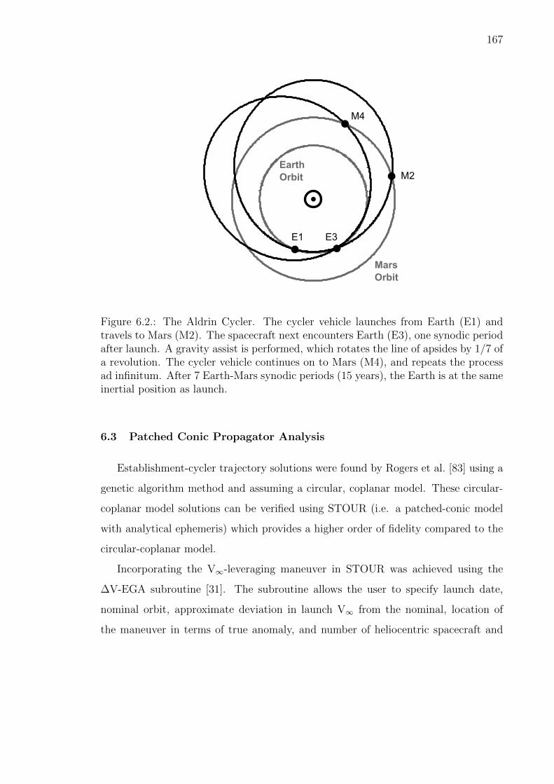
167

MarsOrbit

EarthOrbit

E1 E3

M2

M4

Figure 6.2.: The Aldrin Cycler. The cycler vehicle launches from Earth (E1) andtravels to Mars (M2). The spacecraft next encounters Earth (E3), one synodic periodafter launch. A gravity assist is performed, which rotates the line of apsides by 1/7 ofa revolution. The cycler vehicle continues on to Mars (M4), and repeats the processad infinitum. After 7 Earth-Mars synodic periods (15 years), the Earth is at the sameinertial position as launch.

6.3 Patched Conic Propagator Analysis

Establishment-cycler trajectory solutions were found by Rogers et al. [83] using a

genetic algorithm method and assuming a circular, coplanar model. These circular-

coplanar model solutions can be verified using STOUR (i.e. a patched-conic model

with analytical ephemeris) which provides a higher order of fidelity compared to the

circular-coplanar model.

Incorporating the V∞-leveraging maneuver in STOUR was achieved using the

∆V-EGA subroutine [31]. The subroutine allows the user to specify launch date,

nominal orbit, approximate deviation in launch V∞ from the nominal, location of

the maneuver in terms of true anomaly, and number of heliocentric spacecraft and

168

Earth revolutions between the maneuver and the Earth flyby. With the parameters of

the V∞-leveraging maneuver specified, STOUR then finds all possible patched-conic

trajectories to the subsequent Mars encounter. To ensure that the desired cycler

trajectory is found, launch dates were searched over a three-year period in order to

encompass the 217

year Earth-Mars synodic period. The starting launch date was

chosen to be no sooner than 2022. For cycler trajectories with aphelion radii near

that of the perihelion of Mars, search windows larger than three years were required,

as the relative orientation between Earth and Mars must occur when Mars is near its

perihelion.

Once STOUR calculates the trajectories for the specified span of launch dates,

those trajectories that have orbit characteristics similar to the cycler trajectory of

interest are identified. First, trajectories with the desired cycler shape are found by

matching the aphelion and perihelion radii for the Earth to Mars arc to the theoretical

aphelion and perihelion radii of the cycler (in the circular, co-planar model). The

trajectory then must be checked to ensure the transfer occurs on the correct segment

of the orbit. For example, on the Earth-to-Mars leg of the outbound Aldrin cycler, the

spacecraft must encounter Earth (at E1) just before perihelion and arrive at Mars (at

M2) before reaching aphelion. The final trajectories chosen from the STOUR output

over the three-year search were those that most closely matched the desired cycler

orbit shape (i.e. aphelion and perihelion radii) while also providing the desired orbit

segment on the trip from Earth to Mars for the first leg of the trajectory.

6.4 Low-Thrust Analysis

An alternative to using the impulsive methods described above to place the cycler

vehicle into the desired orbit is low-thrust propulsion. Electric propulsion systems

employ low thrust in order to increase the mass delivered or reduce the time of flight

compared to chemical propulsion systems that use impulsive maneuvers [130,131].

169

For this application, low thrust can be used to shape an orbit so that it acts

similar to the V∞-leveraging trajectories. Instead of using two impulsive maneuvers,

there are thrusting arcs spread out over large portions of the orbit.

The low-thrust establishment trajectories were constructed by Rogers et al. [83]

using MALTO [37], assuming that the V∞ of launch from Earth is 0 km/s. A series

of low-thrust maneuvers are performed in order to encounter the first Earth flyby of

the cycler trajectory at the proper time and with the correct V∞ and to continue

on the cycler trajectory to Mars. Unlike the case using the V∞-leveraging technique,

multiple encounters during the establishment phase are allowed, and these encounters

are added until the launch V∞ is reduced to 0 km/s.

MALTO approximates continuous thrust by dividing each planet-planet leg of the

trajectory into segments with an impulsive ∆V at each of the midpoints. The propa-

gation of the trajectory between these impulsive maneuvers assumes conic trajectories

and also assumes that all flybys are instantaneous and modeled by the rotation of the

V∞ vectors. This method results in a constrained nonlinear optimization problem,

which MALTO solves by using the nonlinear programming software Sparse Nonlinear

OPTimizer (SNOPT) [132,133]. MALTO solves for the cycler trajectory in which the

final mass is maximized.

6.5 Results

6.5.1 STOUR Verification of V∞-Leveraging Establishment Trajectories

STOUR trajectory data for the given establishment-cycler trajectories are shown

in Table 6.2. According to NASA’s Mars Design Reference Architecture [134], the

Earth-to-Mars time of flight should be 180 days or less for the health of the crew.

The results from STOUR confirm that the Aldrin, Case 2, and U0L1 cyclers have

times of flight that satisfy this requirement. The 4:3(2)− Case 3 and 4:3(2)− S1L1

establishment-cycler trajectories have the smallest Earth launch V∞ values, as well

as some of the smallest maneuver ∆V values. The lowest maneuver ∆V values come

170

from the 4:3(2)− VISIT-1 and 4:3(2)− Case 2 establishment-cycler trajectories, 0.043

km/s and 0.059 km/s, respectively. Unfortunately, the VISIT-1 cycler requires more

than 180 days to reach Mars, and, requires a large number of cycler vehicles (up to 14

for missions that return the crew back to Earth). The 4:3(2)− Case 2 establishment-

cycler trajectory, on the other hand, has an Earth launch V∞ of only 2.522 km/s,

and has an Earth-Mars flight time of 171 days. Another notable establishment-cycler

trajectory is the 4:3(2)− Aldrin cycler, which has a time of flight of 161 days, an

Earth launch V∞ of 2.608 km/s, and a maneuver ∆V of 0.568 km/s. It should also

be noted that for all of the trajectories considered in Table 6.2, the closest approach

flyby altitude is well above the safe altitude of 300 km.

Table 6.2.: STOUR Results for the Selected Cyclers in the Analytic Ephemeris

Type K:L(M)LD TOFa rp ra V∞,L ∆VDSM V∞,flyby hflyby

days AU AU km/s km/s km/s km

Aldrin 4:3(2)− 01/03/2023 161 0.983 2.229 2.608 0.568 5.509 10,4833:2(1)− 12/09/2023 172 0.964 2.229 3.449 0.530 6.546 20,745

VISIT-1 4:3(2)− 06/12/2046 201 1.012 1.470 2.540 0.043 2.834 120,625VISIT-2 4:3(2)− 12/27/2022 207 0.985 1.670 2.503 0.221 3.878 7,696Case 1 4:3(2)− 12/14/2024 365 0.946 1.503 2.558 0.346 4.526 140,286Case 2 4:3(2)− 04/22/2029 171 0.997 1.433 2.522 0.059 2.910 56,068Case 3 4:3(2)− 12/20/2022 216 0.988 1.651 2.492 0.187 3.688 13,291S1L1 4:3(2)− 12/20/2022 221 0.987 1.635 2.492 0.182 3.657 12,965U0L1 3:2(1)− 11/25/2025 97 0.960 3.189 3.702 0.794 8.049 6,633

a Time of flight from Earth flyby to Mars.

The savings from V∞ leveraging, in terms of both launch V∞ and overall ∆V

(compared to launching the cycler directly into its orbit) are discussed in detail by

Rogers et al. [83] An example of the 4:3(2)− Aldrin establishment-cycler trajectory

(produced using STOUR) is illustrated in Figure 6.3.

When the establishment-cycler trajectories given in Table 6.2 were determined,

the aphelion of the cycler trajectories was usually the first parameter examined to

find a match to a particular cycler trajectory (out of the many trajectories found in

STOUR). Once a match was found for the aphelion (usually to within a hundredth

of an AU), the cycler trajectory with the closest to the desired perihelion was chosen

171

as the candidate match. Because of this selection order (aphelion first, perihelion

second), the aphelion values tend to match more closely to those determined by the

circular, co-planar model than do the perihelion values, as observed in Table 6.2 and

Table 6.1.

(1)(2)

(3)

(5)

(4)

EarthOrbit

MarsOrbit

Figure 6.3.: The 4:3(2)− Aldrin establishment-cycler trajectory. The spacecraftlaunches (1) from the Earth onto the dashed orbit and completes one and a halforbits. At aphelion (2) of this orbit, a maneuver is performed to lower the perihelionand get onto the dotted orbit. The spacecraft completes one full orbit and returnsto aphelion. The spacecraft continues inbound toward perihelion and flies (3) by theEarth. This flyby raises the heliocentric energy of the orbit and puts the vehicle onthe cycler trajectory (the solid line). Mars is encountered (4), but does not signif-icantly affect the trajectory. The spacecraft completes its orbit and encounters theEarth (5) once more in order to continue on the cycler trajectory.

6.5.2 Validation of Low-Thrust Establishment Trajectories

One concern with the low-thrust establishment-cycler trajectories designed by

Rogers et al. [83], is that the time taken for the spacecraft to fly by Earth is relatively

long compared to other missions. In this analysis, the spacecraft is considered to

be in Earth’s vicinity when it is within Earth’s Hill sphere (of radius 1.5×106 km

or 0.01 AU). For the Aldrin establishment-cycler trajectory, the spacecraft is within

172

the Earth’s Hill sphere for about 80 days at launch, 14 days at the next flyby, and

then about 6 days at the final establishment flyby. (For comparison, the Galileo

spacecraft spent only about 4 days inside Earth’s Hill sphere for its two Earth flybys,

and the Cassini spacecraft’s Earth flyby only took about 3 days.) The 80 days at

launch is considered to be a simple targeting problem and it is assumed for this study

that the states upon exit of the Earth’s Hill sphere could indeed be targeted using

the given propulsion system. The other two Earth flybys however could prove to be

problematic.

The issues come from the model assumptions used in the solutions generated by

MALTO. The low-thrust trajectories produced by MALTO use patched-conics to

model each gravity assist, and therefore the effect of Earth’s gravity during a flyby is

assumed to occur instantaneously. In practice of course, flybys take time!

This long flyby time also occurs for the S1L1 establishment trajectory, where the

first Earth flyby takes approximately 18 days (the longest of all encounters considered

in this study), and the second Earth flyby takes approximately 6 days. The VISIT-2

establishment trajectory’s single Earth flyby is less of a concern as it takes only about

8 days. For illustrative purposed the S1L1 low-thrust establishment-cycler trajectory

is shown in Figure 6.4.

To verify that the low-thrust establishment trajectories generated by MALTO are

indeed feasible, the solution for the S1L1 establishment trajectory (the ‘worst’ case

with regards to long flyby times) was recomputed with the additional considerations

of both the time spent during the Earth encounters and the gravitational effects of

the Sun during these encounters. This simulation was carried out in the following

way:

1. Upon entry into Earth’s Hill sphere (at the start of an Earth encounter), the

position and velocity states from the MALTO solution were propagated in MAT-

LAB using the Sun-Earth circular-restricted three-body (CR3B) model. The

propagation continued until the vehicle exited the Hill sphere, and the final

states were compared to the states from the MALTO trajectory.

173

EarthOrbit

CyclerOrbit

E-1E0

E1

M2

MarsOrbit

Figure 6.4.: Establishment of the S1L1 and Case 3 cyclers using low thrust. Launchfrom Earth begins at E-1, a gravity assist occurs at E0, and placement into the cyclerorbit occurs at E1. Between E-1 and E0, slightly more than one full revolution ofthe Sun is completed. More than one full revolution occurs between E0 and E1. TheE1-to-M2 leg is the first leg of the S1L1 and Case 3 cyclers. The next Earth-to-Marsleg (E3-to-M4) occurs two synodic periods later.

2. To aid in targeting the exit states of the MALTO trajectory, constant low-thrust

(with respect to the Sun-Earth rotating frame) was applied to the propagated

three-body model trajectory. The amount of constant thrust applied was found

via trial and error.

3. Using the exit states from the propagated circular-restricted three-body trajec-

tory (with constant low thrust), a new MALTO trajectory leg was found (i.e.

the leg from E0 to E1). To ensure that the newly found MALTO trajectory

remained ‘close’ to the originally found MALTO trajectory, the entry states for

the next Earth encounter (from the originally found MALTO trajectory at E1)

were targeted.

This process was then repeated for the second Earth encounter (at E1), and a

new MALTO trajectory leg was found (from E1 to M2), where the states from the

original MALTO trajectory at M2 were targeted.

174

To interface the patched conic model with the CR3B model, the coordinate frame

that each model is computed in must be related. In this case, the patched conic

solution in MALTO is computed in the Sun-centered J2000 ecliptic frame, and the

CR3B model in MATLAB is computed in the Sun-Earth rotating frame.

The two frames are illustrated in Fig. 6.5, where

µ = mEarth/m∗ (6.1)

m∗ = mSun +mEarth (6.2)

and mEarth and mSun are the masses of the Earth and Sun, respectively.

Y

θ

X

𝜇

𝑦 𝑦′

s/c

𝐫 𝐑

Figure 6.5.: Position of the cycler vehicle shown in both the Sun-centered J2000ecliptic frame (with axes X-Y-Z) and the Sun-Earth rotating frame (with axes x-y-z).

In the figure, the Sun-centered J2000 frame, which we denote as the I frame, has

axes X-Y-Z, and the Sun-Earth rotating frame, which we denote as the B frame, has

axes x-y-z. To relate the I and B frames, we first relate values in x-y-z coordinates

to coordinates in the intermediate-frame, B′, with axes x′-y′-z′, given by

175

x = x′ − µ

y = y′

x = z′

(6.3)

where x, y, z, x′, y′, and z′ are expressed in nondimensional units, by dividing each

by the Sun-Earth distance. To nondimensionalize distance and time units, values are

divided by l∗ Sun-Earth distance and t∗, respectively, when appropriate, which are

given by

l∗ = Sun-Earth distance

t∗ =√

(l∗)3/(Gm∗)(6.4)

where G is the gravitational constant.

We denote the position of the spacecraft in the I and B frames as, R and r,

respectively, giving

R = RxX +RyY +RzZ

r = rxx+ ryy + rz z(6.5)

The I and B frames can then be related by first rotating from X-Y-Z to x′-y′-z′

about the Z=z′ axis by angle θ, and then converting from B′ to B coordinates using

Eq. (6.3), giving

rx = Rx cos θ +Ry sin θ − µ

ry = Ry cos θ −Rx sin θ

rz = Rz

(6.6)

or more compactly as

r = ICB′R +

µ

0

0

(6.7)

176

where r and R are expressed as column vectors, and the direction cosine matrix, ICB′

is given by,

ICB′=

cos θ sin θ 0

− sin θ cos θ 0

0 0 1

(6.8)

Thus, given position states from MALTO in Sun-centered J2000 coordinates (i.e.

given R), Eqs. (6.6) and (6.7) can be used to compute the equivalent position vector

in the Sun-Earth rotating frame.

To compute relate the velocity states, we use the basic kinematic equation (BKE),

giving

Id

dtR =

Bd

dtR + IωB ×R (6.9)

where IωB is the rotation (i.e. angular velocity vector) of the B frame with respect

to the I frame, given in nondimensional units (revolutions per time) by

IωB = 1Z = 1z (6.10)

The time derivativeIddt

R represents the derivative of R with respect to the I frame,

andBddt

R represents the derivative of R with respect to the Sun-Earth rotating frame.

By expressing R as,

R = µx+ r (6.11)

and plugging into Eq. (6.9), and noting that the derivative of the constant µ with

respect to time is zero, gives

177

Id

dtR =

Bd

dtr + IωB × (µx + r) (6.12)

Noting thatIddt

R is the spacecraft velocity with respect to the Sun-centered J2000

ecliptic frame, andBddt

r is the velocity of the spacecraft with respect to the Sun-Earth

rotating frame, Eq. (6.12) can be written as

ν = ICB′V − IωB × (µx + r) (6.13)

where ν is the spacecraft velocity with respect to the Sun-Earth rotating frame writ-

ten in nondimensional B-frame coordinates, and V is the spacecraft velocity with

respect to the Sun-centered J2000 ecliptic frame written in nondimensional I-frame

coordinates (and thus is left multiplied by ICB′to convert to B-frame coordinates).

Thus, given the velocity states from MALTO in Sun-centered J2000 ecliptic frame,

the corresponding velocity states in the Sun-Earth rotating frame can be computed

using Eq. (6.13).

Once in the Earth’s Hill sphere and the position and velocity states are converted

into the Sun-Earth rotating frame, the CR3B model can be propagated by integrating

the CR3B equations of motion with the modification of the added nondimensional

acceleration due to the applied thrust, with components aTx , aTy , and aTz . The

equations of motion (in nondimensional units) are given by

rx = 2ry + rx − (1−µ)(rx+µ)d3

− µ(rx−1+µ)r3

+ aTx

ry = −2rx + ry − (1−µ)ryd3− µry

r3+ aTy

rz = − (1−µ)rzd3− µrz

r3+ aTz

(6.14)

where

d =√

(rx + µ)2 + r2y + r2

z

r =√

(rx − 1 + µ)2 + r2y + r2

z

(6.15)

178

An example of a flyby at E1 propagated (using MATLAB) in the CR3B model

for the S1L1 cycler trajectory is shown in Fig. 6.6 as viewed in the Sun-centered

J2000 ecliptic frame. The size of Earth shown is not to scale, but the grey circular

region around the Earth, which represents the Hill sphere, is shown to scale. The

CR3B propagation with low thrust is shown in red, and without thrust (labeled as

“ballistic” in the figure) is shown as the dashed black line. The MALTO solution is

also shown. The flyby begins at the top right of the figure, where the spacecraft enters

the Hill sphere, and ends at the bottom left of the figure, where the spacecraft departs

the Hill sphere (during which time Earth is moving faster than the spacecraft and

“overtakes” it). The figure clearly shows that the CR3B propagated flyby matches

much more closely with the MALTO solution when constant low-thrust is applied.

We also note that the MALTO solution has a “kink” in the middle of the flyby, which

is attributed to MALTO’s modeling of low thrust as discrete impulses (one of which

occurs at the kink).

Ballistic

MALTO

Solution

Low Thrust

Hill Sphere (Entry)

Sun

S1L1 Establishment

Figure 6.6.: Flyby at E1 for the S1L1 establishment trajectory viewed in Sun-centeredJ2000 ecliptic frame. The low-thrust and ballistic trajectories are both propagatedin the Sun-Earth CR3B model, where the low-thrust arc as constant applied thrust.

179

Using the verification method presented in this section, the position and velocity

states at each encounter of the original MALTO solution (i.e. the solution assuming

instantaneous flybys) were successfully targeted, with negligible variance in spacecraft

mass upon departure of the Hill sphere at E1—on the order of 10s of kg for a 75 Mg

spacecraft. Much of this propellant mass agreement may be attributed to the robust

nature of low-thrust trajectories, which may adjust for perturbations over months (or

even years) of burn time, and effectively wash out the effects of such perturbations

with little to no cost in propellant mass. Additionally, by thrusting with constant

thrust through the flyby, the low-thrust burn takes advantage of burning through

closest approach (where the velocity is greatest). Thrusting through the flyby makes

the burn more efficient for the higher-fidelity flyby model, than for the patched conic

MALTO solution, and may make up for any propellant that would otherwise be lost

due to the slow flyby (if any is to be lost at all). In the patched conic model, the

gravity of the flyby body is ignored (other than computing the bending of the velocity

vector). For the S1L1 establishment trajectory used for this verification, the required

propellant mass for the higher-order flyby model solution is found to be slightly less

(by a few 10s of kg) than that found by the original MALTO solution, which may be

attributed to the increased efficiency of the low-thrust burns taking place throughout

the flyby and within Earth’s gravity well.

6.6 Conclusion

It was found by Rogers et al. that, from the perspective of propellant savings, low-

thrust establishment is superior to V∞-leveraging establishment trajectories; however,

V∞-leveraging establishment trajectories can have times of flight that are several years

shorter than low-thrust establishment.

The use of the circular-coplanar model to find suitable V∞-leveraging establish-

ment trajectories proved to be accurate. This validation was achieved using the JPL

program STOUR, which uses a patched-conic model with analytic ephemeris.

180

By modeling the flybys using the CR3B model, perturbations in the low-thrust

establishment trajectories (constructed using JPL’s MALTO) due to the extended

amount of time taken for the Earth flybys to occur were shown to be correctable (for

the case of the S1L1 establishment trajectory) with the given low-thrust engine and

with a negligible difference in required propellant mass.

181

7. CONCLUDING REMARKS

7.1 Contribution of Work

The primary contribution of this work are the candidate trajectories found for

various missions to Mars, Venus, and the Ice Giants, which are intended to be a

convenient source for mission designers, systems engineers, and scientists, to quickly

assess the trajectory characteristics and derived mission requirements for relevant

mission concepts. Rare free-return trajectories are identified for a near-term human

flyby mission to either Mars, Venus, or both. Additionally, several broad-search

trajectory catalogs (for chemical missions) are provided for a future orbiter mission

to Uranus and Neptune, which will hopefully contribute to future decadal studies for

such a mission. In particular, this investigation is one of the first to look closely at

the benefits provided by the SLS for outer-planet science missions, one of which found

in this work is the ability to do probe science at multiple outer-planet targets (such

as the Saturn-Uranus mission opportunity proposed in Ch. 3).

The techniques and corresponding tools developed for this work are also a con-

tribution to the field of astrodynamics. In previous studies, trajectories found using

STOUR required designers to sort through the results of each gravity assist path sep-

arately. Using the post-processing python script (the STOUR Utility) developed for

this work allows designers to compile the STOUR data from all gravity-assist paths,

as well as incorporate various launch vehicles and thruster models, and compute rel-

evant trajectory parameters (not computed by STOUR) such as delivered mass at

the target body. This structure will enable future designers to incorporate other

systems-level factors, such as a communications link analysis during probe entry.

For select cases, the development of the MATLAB script to model the approach

trajectory at the target body, allows designers to visually modify the approach and

182

quickly assess the feasibility of a particular trajectory design before committing to

a high-fidelity tool such as STK or GMAT. The formulation of the approach tra-

jectory computations in this work is also intended on being a more convenient (and

conceptually more understandable) approach than that presented in Ref. [111]. The

formulation of the probe entry parameters on a rotating, oblate-spheroid atmosphere,

is also intended on being a direct and convenient means to quickly estimate probe en-

try parameters to be shared with probe entry modeling specialist to model the probe

entry and design the TPS. The calculation is fast and, when used in combination with

the approach visualization, allows the designer to easily modify the approach while

keeping in mind constraints such as ring avoidance, and is conducive for an iterative

design environment between the mission designer and the probe entry modeling spe-

cialist. (For this work, the parameters for entry are specifically suited for the probe

entry specialists at Ames Research Center, but may be easily adapted to compute

any entry analysis parameters that are needed.)

7.2 Potential Advancement of Work

Most of the research presented in this thesis is based on solving a larger portion of

the gravity-assist trajectory design space in a grid-like fashion, using patched-conics

with an analytic ephemeris. Select cases can then be optimized using tools such as

MALTO or EMTG; however, this occurs after the unoptimized has been sorted to

identify the most attractive candidates for optimization. A potential issue with this

technique is that the optimization process may dramatically improve the select cases,

but the amount of improvement varies depending on how close to the optimal solution

the STOUR solution happens to be. Solutions that are farther from their optimized

performance may not make it through the initial sorting filter when select cases are

identified, and the most attractive solution may be lost. Future work should automate

the process of optimizing trajectories from STOUR in MALTO or EMTG before the

solutions are sorted.

183

Future work may also incorporate more systems-level parameters and constraints

into the STOUR Utility post processing script. A simplified form of the approach

trajectory calculation could be implemented for a chosen approach ψ value (or incli-

nation) to estimate the feasibility of the interplanetary trajectory for probe missions.

With this information, a link analysis could also be incorporated to estimate the

amount of data that could be transmitted (if any link is possible) from the probe to

the spacecraft (and Earth) for a give trajectory. This will allow such mission compo-

nents to be considered at the initial trajectory design phase, and potentially eliminate

the need to trajectory redesigns later on in the design process.

For any outer-planet orbiter mission, a tour of the planet’s moons is likely going

to be desired. A moon-tour design is typically done as a point design separate of

the interplanetary design, but has some common characteristics that are generally

desirable. To keep the encounter velocities at each moon small, near-equatorial orbits

are typically desired, which (to reduce propellant) need a low declination angle and

low V∞ at arrival. If low declination is not possible, a maneuver strategy must

be implemented (after capture) to get the spacecraft into an equatorial orbit with

minimal propellant. Future work could incorporate these constraints into the STOUR

Utility, to improve the designers ability to find attractive and relevant trajectories for

a moon tour.

In this work, any trajectories considered for aerocapture uniformly assumed a

TPS mass fraction of 50%. Future work could incorporate a low- to mid-fidelity

aerocapture model into the STOUR Utility, to more accurately estimate the TPS mass

required, to more precisely identify attractive trajectory candidates for aerocapture.

Options for a hybrid capture could also be implemented, where the atmosphere is

used to dramatically reduce the planet-relative velocity, but then a thruster is used

to implement the final ∆V needed for capture.

Lastly, for some trajectories, perturbations from third bodies (such as trajectories

in a planet-moon system), non-spherical gravity terms (such as J2), and solar radia-

tion pressure (SRP), may significantly influence an interplanetary trajectory. Future

184

work for select cases could include a medium-high fidelity integrated form of the

patched conic solution, which may include influences of third bodies, J2, and SRP.

If perturbations need to be considered during the initial trajectory sweep, computa-

tional speed could be improved by only integrating sections of the trajectory where

the perturbation is most significant (e.g. only integrating the trajectory with SRP

during times when the spacecraft is within 1 AU of the Sun). Such integrated, or

patched-integrated, solutions may be necessary to improve a patched-conic solution

in a high-perturbation environment, in order for it to serve as a suitable initial guess

for a high-fidelity tool such as STK or GMAT.

REFERENCES

185

REFERENCES

[1] Lancaster, E. R. and Blanchard R. C., “A Unified Form of Lambert’s Theorem,”NASA Technical Note, No. NASA TN D-5368, Goddard Space Flight Center,Greenbelt, MD, Sept., 1969.

[2] Sturms, F. M. “Polynomial Expressions for Planetary Equators and Orbit Ele-ments with respect to Mean 1950.0 Coordinate System,” NASA Technical Re-port, JPL 32-1508, Pasadena, CA, Jan. 15, 1971.

[3] Williams, S. N., “Automated Design of Multiple Encounter Gravity-Assist Tra-jectories,” M.S. Thesis, School of Aeronautics and Astronautics, Purdue Univer-sity, West Lafayette, IN, Aug. 1990.

[4] Strange, N.J. and Longuski, J.M., “Graphical Methods for Gravity-Assist Tra-jectory Design,” Journal of Spacecraft and Rockets, Vol. 39, No. 1, Jan.–Feb.2002.

[5] Labunsky, A., Papkov, O., and Sukhanov, K., “Multiple Gravity Assist Inter-planetary Trajectories,” Earth Space Institute Book Series, Gordon and Breach,London, 1998, pp. 33–68.

[6] Johnson, W.R. and Longuski, J.M., “Design of Aerogravity-Assist Trajectories,”Journal of Spacecraft and Rockets, Vol. 39, No. 1, Jan.–Feb. 2002.

[7] Chen, K.J., Kloster, K.W., and Longuski, J.M., “A Graphical Method for Prelim-inary Design of Low-Thrust Gravity-Assist Trajectories,” AIAA Paper No. 2008-6952, AIAA/AAS Astrodynamics Specialist Conference, Honolulu, HI, Aug. 18–21, 2008.

[8] Campagnola, S. and Russell, R.P., “Endgame Problem Part 1: V∞-LeveragingTechnique and the Leveraging Graph,” Journal of Guidance, Control, and Dy-namics, Vol. 33, No. 2, March–April 2010.

[9] Campagnola, S. and Russell, R.P., “Endgame Problem Part 2: Multibody Tech-nique and the Tisserand-Poincare Graph,” Journal of Guidance, Control, andDynamics, Vol. 33, No. 2, March–April 2010.

[10] Archinal, B. A., A’Hearn, M. F., Bowell, E., Conrad, A., Consolmagno, G. J.,Courtin, R., Fukushima, T., Hestroffer, D., Hilton, J. L., Krasinsky, G. A., Neu-mann, G., Oberst, J., Seidelmann, P. K., Stooke, P., Tholen, D. J., Thomas,P. C., Williams, I. P., “Report of the IAU Working Group on Cartographic Co-ordinates and Rotational Elements: 2009,” Celestial Mechanics and DynamicalAstronomy, Vol. 109, pp. 101–135, 2011.

[11] Orbital ATK, “Space Propulsion Products Catalog,” OSR No. 12-S-1902, Sept.2012.

186

[12] Squyres S., “Vision and voyages for planetary science in the decade 2013–2022,”National Research Council Publications, 2011.

[13] Green, J. L., “Planetary Science Division Status Report,” Presentation at theAug. 2015 Meeting of the Outer Planets Assessment Group.

[14] Spreen, C.M., Mueterthies, M.J., Kloster, K.W., and Longuski, J.M., “Prelim-inary Analysis of Ballistic Trajectories to Uranus Using Gravity-Assists fromVenus, Earth, Mars, Jupiter, and Saturn,” AAS Paper No. 11-623, AAS/AIAAAstrodynamics Specialist Conference, Girdwood, AK, July 31–Aug. 4, 2011.

[15] Dankanich, J. W. and McAdams, J., “Interplanetary Electric PropulsionUranus Mission Trades Supporting the Decadal Survey,”AAS Paper No. 11-189,AAS/AIAA Astrodynamics Specialist Conference, Girdwood, AK, July 31–Aug.4, 2011.

[16] Landau, D., Lam, T., and Strange, N., “Broad Search and Optimization ofSolar Electric Propulsion Trajectories to Uranus and Neptune,” Advances in theAstronautical Sciences, Vol. 135, Part 3, No. AAS 09-428, 2009, pp. 2093–2112.

[17] Bocanegra-Bahamon, T., Bracken, C., Sitja, M. C., Dirkx, D., Gerth, I., Kon-stantinidis, K., Labrianidis, C., Laneuville, M., Luntzer, A., MacArthur, J. L.,Maier, A., Morschhauser, A., Nordheim, T. A., Sallantin, R., and Tlustos, R.,“MUSE – Mission to the Uranian System: Unveiling the Evolution and Forma-tion of Ice Giants,” Advances in Space Research, Vol. 55, 2015, pp. 2190–2216.

[18] Agrawal, P., Allen, G. A. Jr., Sklyanskiy, E. B., Hwang, H. H., Huynh, L. C.,McGuire, K., Marley, M. S., Garcia, J. A., Aliaga, J. F., and Moses, R. W.,“Atmospheric Entry Studies for Uranus,” IEEE Aerospace Conference, PaperNo. 978-1-4799-1622-1, 2014.

[19] Saikia, S. J., et al., “MUSEings on Uranus: An Enhanced New Frontiers ClassMission to Uranus,” Presentation at 11th International Planetary Probe Work-shop, Pasadena, CA, June 16–20, 2014.

[20] Okutsu, M., Yam, C. H., Longuski, J. M., and Strange, N. J., “Cassini Saturn-Escape Trajectories to Jupiter, Uranus, and Neptune,” Acta Astronautica, Vol.79, 2012, pp. 157–167.

[21] McAdams, J., Scott, C., Guo, Y., Dankanich, J., and Russell, R., “ConceptualMission Design of a Polar Uranus Orbiter and Satellite Tour,” AAS Paper No.11-188, AAS/AIAA Astrodynamics Specialist Conference, Girdwood, AK, July31–Aug. 4, 2011.

[22] Hubbard, W.B., “Ice Giants Decadal Study,” Planetary Science Decadal Survey:Mission Concept Study Final Report, National Aeronautics and Space Adminis-tration, June 2010, SDO-12345.

[23] Yam, C. H., McConaghy, T. T., Chen, K. J., and Longuski, J. M., “Designof Low-Thrust Gravity-Assist Trajectories to the Outer Planets,” InternationalAstronautical Congress, Paper No. IAC-04-A.6.02, Oct. 4–8, 2004.

[24] Yam, C. H., McConaghy, T. T., Chen, K. J., and Longuski, J. M., “Prelim-inary Design of Nuclear Electric Propulsion Missions to the Outer Planets,”AIAA/AAS Astrodynamics Specialist Conference, Paper No. AIAA 2004-5393,Providence, RI, Aug. 16–19, 2004.

187

[25] Heaton A. F. and Longuski, J. M., “The Feasibility of a Galileo-Style Tour ofthe Uranian Satellites,” AAS/AIAA Astrodynamics Specialist Conference, PaperNo. AAS 01-464, Quebec City, Quebec, Canada, July 30–Aug. 2, 2001.

[26] Longuski, J.M. and Williams, S.N., “Automated Design of Gravity-Assist Tra-jectories to Mars and the Outer Planets,” Celestial Mechanics and DynamicalAstronomy, Vol. 52, No. 3, Aug. 1991, pp. 207 – 220.

[27] Kohlhase, C. E. and Penzo, P. A., “Voyager Mission Description,” Space ScienceReviews, Vol. 21, 1977, pp. 77–101.

[28] Rinderle, E. A., “Galileo Users Guide, Mission Design System, Satellite TourAnalysis and Design Subsystem,” Jet Propulsion Laboratory, Report JPL D-263, California Institute of Technology, Pasadena, CA, July 1986.

[29] Patel, M. R., “Automated Design of Delta-V Gravity-Assist Trajectories forSolar System Exploration,” M.S. Thesis, School of Aeronautics and Astronautics,Purdue University, West Lafayette, IN, Aug. 1990.

[30] Petropoulos, A.E., Longuski, J.M., and Bonfiglio, E.P., “Trajectories to Jupitervia Gravity Assists from Venus, Earth, and Mars,” Journal of Spacecraft andRockets, Vol. 37, No. 6 Nov.–Dec. 2000.

[31] Staugler, A.J., “STOUR (Satellite Tour Design Program) User’s Guide for the∆V -EGA and V∞-Leveraging Routines,” School of Aeronautics and Astronau-tics, Purdue University, West Lafayette, IN, June 1996.

[32] Sims, J.A., Longuski, J.M., and Staugler, A.J., “V∞ Leveraging for Interplan-etary Missions: Multiple-Revolution Orbit Techniques,” Journal of Guidance,Control, and Dynamics, Vol. 20, No. 3, 1997, pp. 409–415.

[33] Sims, J.A., “Delta-V Gravity-Assist Trajectory Design: Theory and Practice,”PhD Thesis, School of Aeronautics and Astronautics, Purdue University, WestLafayette, IN, 1996.

[34] Marley, M. S., “Planetary Science Decadal Survey, JPL Rapid Mission Architec-ture: Neptune-Triton-KBO Study Final Report,” NASA-JPL Mission ConceptStudy, Feb. 2010.

[35] NASA, “Space Launch System (SLS) Program Mission Planner’s Guide (MPG)Executive Overview,” Version 1, No. SLS-MNL-201, Aug. 22, 2014.

[36] Sims, J. A., and Flanagan, S. N., “Preliminary Design of Low-Thrust Interplan-etary Missions,” AAS/AIAA Astrodynamics Specialist Conference, AAS PaperNo. 99-338, Girdwood, AK, August 1999.

[37] Sims, J. A., Finlayson, P. A., Rinderle, E. A., Vavrina, M. A., and Kowalkowski,T. D., “Implementation of a Low-Thrust Trajectory Optimization Algorithm forPreliminary Design,” AIAA/AAS Astrodynamics Specialist Conference, AIAAPaper No. 2006-6746, Keystone, CO, Aug. 21–24, 2006.

[38] Englander, J. A., Conway, B. A., and Williams, T., “Automated Mission Plan-ning via Evolutionary Algorithms, Journal of Guidance, Control, and Dynamics,Vol. 35, Nov. 2012, pp. 1878–1887.

188

[39] Englander, J. A., “Automated Trajectory Planning for Multiple-Flyby Interplan-etary Missions,” PhD thesis, University of Illinois at Urbana-Champaign, April2013.

[40] Englander, J. A. and Englander, A. C., “Tuning Monotonic Basin Hopping: Im-proving the Efficiency of Stochastic Search as Applied to Low-Thrust TrajectoryOptimization,” 24th International Symposium on Space Flight Dynamics, Lau-rel, MD, May 2014.

[41] Englander, J. A., Ellison, D. H., and Conway, B. A., “Global Optimizationof Low-Thrust, Multiple-Flyby Trajectories at Medium and Medium-High Fi-delity,” AAS/AIAA Space-Flight Mechanics Meeting, Santa Fe, NM, January2014.

[42] Englander, J. A. and Conway, B. A., “An Automated Solution of the Low-Thrust Interplanetary Trajectory Problem, Journal of Guidance, Control, andDynamics, 2016. Accepted.

[43] Vavrina, M. A., Englander, J. A., and Ghosh, A., “Coupled Low-Thrust Trajec-tory and Systems Optimization via Multi-objective Hybrid Optimal Control,”AAS/AIAA Space Flight Mechanics Meeting Williamsburg, Virginia, January2015.

[44] Englander, J. A., Vavrina, M. A., Ghosh, A.R., “Multi-objective Hybrid Opti-mal Control for Multiple-Flyby Low-Thrust Mission Design,” AAS/AIAA SpaceFlight Mechanics Meeting, Williamsburg, Virginia, January 2015.

[45] Englander, J. A., and Vavrina, M. A., “Multi-Objective Hybrid Optimal ControlFor Multiple-Flyby Interplanetary Mission Design Using Chemical Propulsion,”AAS/AIAA Astrodynamics Conference, Vail, Colorado, August 2015.

[46] Vavrina, M. A., Englander, J. A., and Ellison, D. H., “Global Optimiza-tion of N-Maneuver, High-Thrust Trajectories Using Direct Multiple Shooting,”AAS/AIAA Spaceflight Mechanics Meeting, AAS Paper No. 16-272, Napa, CA,Feb. 14–18, 2016.

[47] Beebe, R., “Planetary Science Decadal Survey: Saturn Atmospheric Entry ProbeTrade Study,” NASA-JPL Mission Concept Study, Sept. 2010.

[48] Beebe, R., “Planetary Science Decadal Survey: Saturn Atmospheric Entry ProbeMission Study,” NASA-JPL Mission Concept Study, April 2010.

[49] Kolencherry, N., Mansell, J. R., Hughes, K. M., Mudek, A. J., Podesta, L. P.,Libben, B., Chye, H. S., Millane, J., Fulton, S., Shibata, E., Coleman, K., Arora,A., Lu, Y., Tackett, B., Elliott, J., Smith, G., Ukai, T., Pouplin, J., Hobar, N.,Witsberger, P., and Saikia, S. J., “A Multi-Planet, Multi-Spacecraft FlagshipClass Mission Concept to Explore a Gas Giant and an Ice Giant Planet,” 13thInternational Planetary Probe Workshop, Laurel, MD, June 13–17, 2016, Paperand Poster Presentation.

[50] Lockwood, M. K., “Neptune Aerocapture Systems Analysis,” AIAA AtmosphericFlight Mechanics Conference and Exhibit, AIAA Paper No. 2004-4951, Provi-dence, RI, Aug. 16–19, 2004.

189

[51] Longuski, J.M. and Williams, S.N., “The Last Grand Tour Opportunity toPluto,” The Journal of the Astronautical Sciences, Vol. 39, No. 3, July – Sep.1991, pp. 359–365.

[52] Sims, J.A., Staugler, A.J., and Longuski, J.M., “Trajectory Options to Plutovia Gravity Assists from Venus, Mars, and Jupiter,” Journal of Spacecraft andRockets, Vol. 34, No. 3, May–June 1997, pp. 347–353.

[53] Petropoulos, A.E., Longuski, J.M., and Bonfiglio, E.P., “Trajectories to Jupitervia Gravity Assists from Venus, Earth, and Mars,” Journal of Spacecraft andRockets, Vol. 37, No. 6 Nov.–Dec. 2000.

[54] Melman, J., Orlando, G., Safipour, E., Mooij, E., and Noomen, R., “TrajectoryOptimization for a Mission to Neptune and Triton,” AIAA Paper No. 2008-7366,AIAA/AAS Astrodynamics Specialist Conference, Honolulu, HI, Aug. 18–21,2008.

[55] Casalino, L., Colasurdo, G., and Pastrone, D., “Optimal Low-Thrust EscapeTrajectories Using Gravity Assist,” Journal of Guidance, Control, and Dynamics,Vol. 22, No. 5, Sep.–Oct. 1999.

[56] Zimmer, S. and Ocampo, C., “Use of Analytical Gradients to Calculate OptimalGravity-Assist Trajectories,” Journal of Guidance, Control and Dynamics, Vol.28, No. 2, March–April 2005.

[57] Yam, C.H., Di Lorenzo, D., and Izzo, D., “Constrained Global Optimization ofLow-Thrust Interplanetary Trajectories,” IEEE Congress on Evolutionary Com-putation, Barcelona, Spain, July 18–23, 2010.

[58] Hollister, W. M., “Mars Transfer via Venus,” AIAA/ION Astrodynamics Guid-ance and Control Conference, Los Angeles, CA, Aug. 24–26, 1964, AIAA 64-647.

[59] Sohn, R.L., “Manned Mars Trips Using Venus Flyby Modes,” Journal of Space-craft and Rockets, Vol. 3, No. 2, 1966, pp. 161–169.

[60] Wilson, S., “Fast Round Trip Mars Trajectories,” AIAA/AAS AstrodynamicsConference, Portland, OR, Aug. 20–22, 1990, AIAA 90-2934.

[61] Wolf, A. A., “Free Return Trajectories for Mars Missions,” AAS/AIAA AnnualSpaceflight Mechanics Meeting, Houston, TX, Feb. 11–13, 1991.

[62] Walberg, G., “How Shall We Go to Mars? A Review of Mission Scenarios,”Journal of Spacecraft and Rockets, Vol. 30, No. 3, March–April 1993.

[63] Hoffman, S.J. and Kaplan, D.I. (eds.), “Human Exploration of Mars: The Ref-erence Mission of the NASA Mars Exploration Study Team,” NASA SP 6107,Houston, TX, March 1997.

[64] Drake, B.G. (ed.), “Reference Mission Version 3.0 Addendum to the HumanExploration of Mars: The Reference Mission of the NASA Mars ExplorationStudy Team,” NASA SP-6107-ADD, EX13-98-036, Houston, TX, June 1998.

[65] Casalino, L., Colasurdo, G., and Patrone, D., “Mission Opportunities for HumanExploration of Mars,” Planetary and Space Science, Vol. 46, No. 11/12, pp. 1613–1622, 1998.

190

[66] Lyne, J. E., and Townsend, L. W., “Critical Need for a Swingby Return Optionfor Early Manned Mars Missions,” Journal of Spacecraft and Rockets, Vol. 35,No. 6, 1998, pp. 855, 856.

[67] Patel M.R., Longuski, J.M., and Sims, J.A., “Mars Free Return Trajectories,”Journal of Spacecraft and Rockets, Vol. 35, No. 3, May–June 1998.

[68] Rall, C. and Hollister, W., “Free-Fall Periodic Orbits Connecting Earth andMars,” 1971, AIAA 71-92.

[69] Friedlander, A. L., Niehoff, J. C., Byrnes, D. V., and Longuski, J. M., “Circulat-ing Transportation Orbits Between Earth and Mars,” AIAA/AAS Astrodynam-ics Conference, Williamsburg, VA, Aug. 1986, AIAA 86-2009-CP.

[70] Byrnes, D. V., Longuski, J. M., and Aldrin, B., “Cycler Orbit Between Earthand Mars,” Journal of Spacecraft and Rockets, Vol. 3, 1993, pp. 334–336.

[71] McConaghy, T. T., Longuski, J. M., and Byrnes, D. V., “Analysis of a BroadClass of Earth-Mars Cycler Trajectories,” AIAA/AAS Astrodynamics SpecialistConference, Monterey, CA, Aug. 5–8, 2002, AIAA 2002-4420.

[72] Russell, R. P. and Ocampo, C. A., “Systematic Method for Constructing Earth-Mars Cyclers Using Free-Return Trajectories,” Journal of Guidance, Control,and Dynamics, Vol. 27, No. 3, May–June 2004, pp. 321-335.

[73] Russell, R. P. and Ocampo, C. A., “Global Search for Idealized Free-ReturnEarth-Mars Cyclers,” Journal of Guidance, Control, and Dynamics, Vol. 28, No.2, March–April 2005, pp. 194-208.

[74] Landau, D.F. and Longuski, J.M., “Trajectories for Human Missions to Mars,Part I: Impulsive Transfers,” Journal of Spacecraft and Rockets, Vol. 43, No. 5,Sept.–Oct. 2006, pp. 1035–1042.

[75] Landau, D. F., Longuski, J. M., and Aldrin, B., “Continuous Mars Habitationwith a Limited Number of Cycler Vehicles,” Journal of the British InterplanetarySociety, Vol. 60, No. 4, April 2007, pp. 122–128.

[76] Okutsu, M. and Longuski, J.M., “Mars Free Returns via Gravity Assist fromVenus,” Journal of Spacecraft and Rockets, Vol. 39, No. 1, Jan.–Feb. 2002.

[77] Landau, D.F. and Longuski, J.M., “Trajectories for Human Missions to Mars,Part II: Low-Thrust Transfers,” Journal of Spacecraft and Rockets, Vol. 43, No.5, Sept.–Oct. 2006, pp. 1043–1047.

[78] Foster, C. and Daniels, M., “Mission Opportunities for Human Exploration ofNearby Planetary Bodies,” AIAA SPACE Conference and Exposition, Anaheim,CA, Aug.–Sept. 2010.

[79] Tito, D.A., Anderson, G., Carrico, J.P., Clark, J., Finger, B., Lantz, G.A.,Loucks, M.E., MacCallum, T., Poynter, J., Squire, T.H., and Worden, S.P.,“Feasibility Analysis for a Manned Mars Free-Return Mission in 2018,” IEEEAerospace Conference, Big Sky, MT, March 2013.

191

[80] Bailey, L., Folta, D., Barbee, B., Vaughn, F., Kirchman, F., Englander, J.,Campbell, B., Thronson, H., and Lin, T.Y., “A Lean, Fast Mars Round-TripMission Architecture: Using Current Technologies for a Human Mission in the2030s,” AIAA SPACE Conference and Exposition, San Diego, CA, Sept. 10–12,2013, AIAA 2013-5507.

[81] Folta, D., Barbee, B. W., Englander, J., Vaughn, F., and Lin, T.Y., “OptimalRound-Trip Trajectories for Short Duration Mars Missions,” AAS/AIAA As-trodynamics Specialist Conference, Hilton Head, SC, Aug. 11–15, 2013, AAS13-808.

[82] De Smet, S., Parker, J.S., Herman, J., and Noomen, R., “Preliminary MissionDesign for a Crewed Earth-Mars Flyby Mission Using Solar Electric Propulsion(SEP),” AAS/AIAA Space Flight Mechanics Meeting, Santa Fe, NM, Jan. 2014,AAS 14-366.

[83] Rogers, B.A., Hughes, K.M., Longuski, J.M., and Aldrin, B., “Establishing Cy-cler Trajectories between Earth and Mars,” Acta Astronautica, Vol. 112, 2015,pp 114–125.

[84] Hollister, W., “Periodic Orbits for Interplanetary Flight,” Journal of Spacecraftand Rockets, Vol. 6, No. 4, April 1969, pp. 366–369.

[85] Hollister, W. and Menning, M., “Periodic Swing-By Orbits between Earth andVenus,” Journal of Spacecraft and Rockets, Vol. 7, No. 10, Oct. 1970, pp. 1193–1199.

[86] Semones, E., “Radiation Limits for Astronauts,” NASA Technical Report, JSC,Houston, TX, Dec. 2011.

[87] May, T. A. and Creech, S. D., “NASA’s Space Launch System (SLS) Program:Mars Program Utilization,” Proceedings from the Concepts and Approaches forMars Exploration workshop, Houston, TX, June 12–14, 2012, Paper No. 4098.

[88] Arora, J. S., “Introduction to Optimum Design,” Third Edition, Elsevier Inc.,Waltham, MA, 2012, pp. 663–667.

[89] Trevino, L., “SpaceX Dragon Re-Entry Vehicle: Aerodynamics and Aerother-modynamics with Application to Base Heat-Shield Design,” 6th InternationalPlanetary Probe Workshop, June 21–27, 2008, Atlanta, GA.

[90] Bibb, K.L., Walker, E.L., Brauckmann, G.J., and Robinson, P.E., “Developmentof the Orion Crew Module Static Aerodynamic Database, Part I: Hypersonic,”29th AIAA Applied Aerodynamics Conference, June 27–30, 2011, Honolulu, HI,AIAA 2011-3506.

[91] Creer, B.Y., Smedal, H.A., and Wingrove, R.C., “Centrifuge Study of PilotTolerance to Acceleration and the Effects of Acceleration on Pilot Performance,”NASA Ames Research Center, NASA TN D-337, Moffett Field, CA, Nov. 1960.

[92] Morring, F., “Soyuz Ballistic Re-entry Explained,” Aviation Week and SpaceTechnology, 2008.

[93] Sutton, K. and Graves Jr., R., “A General Stagnation-Point Convective HeatingEquation for Arbitrary Gas Mixtures,” NASA TR-R-376, Hampton, VA, Nov.1971.

192

[94] Tauber, M. and Sutton, K., “Stagnation-Point Radiative Heating Relations forEarth and Mars Entries,” Journal of Spacecraft and Rockets, Vol. 28, No. 1, 1991,pp. 40–42.

[95] Brandis, A. M. and Johnston, C. O., “Characterization of Stagnation-Point HeatFlux for Earth Entry,” 45th AIAA Plasmadynamics and Lasers Conference, June2014, Atlanta, GA,

[96] Rao, A. V., Benson, D. A., Darby, C. L., Francolin, C., Patterson, M. A., Sanders,I., and Huntington, G. T., “Algorithm 902: GPOPS, A Matlab Software for Solv-ing Multiple-Phase Optimal Control Problems Using the Gauss PseudospectralMethod,” ACM Transactions on Mathematical Software, Vol. 37, No. 2, April–June 2010.

[97] Griffin, M.D. and French, J.R., “Space Vehicle Design,” Second Edition, Ameri-can Institute of Aeronautics and Astronautics, Inc., Reston, VA, 2004, p. 277.

[98] Leitmann, G. (Editor), “Optimization Techniques With Applications toAerospace Systems,” Academic Press, London, 1962, pp. 323–351.

[99] Diehl, R.E. and Myers, M.R. “Gravity-Assist Trajectories to the Outer SolarSystem,” Jet Propulsion Laboratory, JPL Publication D-4677, Pasadena, CA,Sept. 1987.

[100] Campagnola, S. and Russell, R.P., “Endgame Problem Part 1: V∞-LeveragingTechnique and the Leveraging Graph,” Journal of Guidance, Control, and Dy-namics, Vol. 33, No. 2, March–April 2010.

[101] Campagnola, S. and Russell, R.P., “Endgame Problem Part 2: Multibody Tech-nique and the Tisserand-Poincare Graph,” Journal of Guidance, Control, andDynamics, Vol. 33, No. 2, March–April 2010.

[102] Carrico, J. and Fletcher, E., “Software Architecture and Use of Satellite ToolKits’s Astrogator Module for Libration Point Orbit Missions,” Proceedings of theConference Libration Point Orbits and Applications, Aiguablava, Spain, June10–14, 2002. Edited by Gomez, G., Lo, M.W., and Masdemont, J.J., Publishedby World Scientific, 2003.

[103] Kolawa, E., Balint, T.S., Birur, G., Brandon, E., Del Castillo, L., Hall, J.,Johnson, M., Kirschman, R., Manvi, R., Mojarradi, M., Moussessian, A., Patel,J., Pauken, M., Peterson, C., Whitacre, J., Martinez, E., Venkatapathy, E.,Newdeck, P., and Okojie R., “Extreme Environment Technologies for FutureSpace Science Missions,” NASA Technical Report, JPL D-32832, Pasadena, CA,Sept. 19, 2007.

[104] Bonfiglio, E. P., Longuski, J. M., and Vinh, N. X., “Automated Design ofAerogravity-Assist Trajectories,” Journal of Spacecraft and Rockets, Vol. 37, No.6, Nov. – Dec. 2000. pp. 768–775.

[105] Lowe, R. E. and Gervais, R. L., “Manned Entry Missions to Mars and Venus,”ARS Journal, Vol. 32, No. 11, 1962, pp. 1660–1668.

[106] Sagan, C., Pale Blue Dot: A Vision of the Human Future in Space, RandomHouse, Nov. 1994.

193

[107] Landis, G. A., “Colonization of Venus,” Conference on Human Space Explo-ration, Space Technology and Applications International Forum, Albuquerque,NM, Feb. 26, 2003. AIP Conference Proceedings, 654, pp. 1193–1198.

[108] Landis, G. A., Lamarre, C., and Colozza, A., “Atmospheric Flight on Venus:A Conceptual Design,” Journal of Spacecraft and Rockets, Vol. 40, No. 5, Sept.–Oct. 2003, pp. 672–677.

[109] Landis, G. A., “Astrobiology: The Case for Venus,” NASA Technical Memo-randum 2003-212310, Cleveland, OH, July 2003.

[110] Wertz, J. and Wiley L., Editors, Space Mission Analysis & Design, 3rd Edition,Microcosm, 1999.

[111] Sergeyevsky, A.B., Snyder, G.C., and Cunniff, R.A., ”Interplanetary MissionDesign Handbook,” Vol. 1, Pt. 2, Jet Propulsion Laboratory, JPL Publication82-43, Pasadena, CA, Sept. 15, 1983.

[112] Curtis, H.D., Orbital Mechanics for Engineering Students, ElsevierButterworth-Heinemann, 2005.

[113] Post, K. and Loucks, M., “Inspiraiton Mars 2021 Mission Design,” 65th In-ternational Astronautical Congress, Sept. 29–Oct. 3, 2014, Toronto, Canada,IAC-14,A3,3B,1,x22690.

[114] Hollister, W., “Periodic Orbits for Interplanetary Flight,” Journal of Spacecraftand Rockets, Vol. 6, No. 4, April 1969, pp. 366 – 369.

[115] Hollister, W. and Menning, M., “Interplanetary Orbits for Multiple SwingbyMissions,” August 1969, AIAA Paper 69 – 931.

[116] Hollister, W. and Menning, M., “Periodic Swing-By Orbits between Earth andVenus,” Journal of Spacecraft and Rockets, Vol. 7, No. 10, October 1970, pp.1193 – 1199.

[117] Rall, C., “Free-Fall Periodic Orbits Connecting Earth and Mars,” Sc.D. disser-tation, Department of Aeronautics and Astronautics, Massachusetts Institute ofTechnology, Cambridge, MA, October 1969.

[118] Rall, C. and Hollister, W., “Free-Fall Periodic Orbits Connecting Earth andMars,” AIAA Paper 71-92, January 1971.

[119] Landau, D. F., Longuski, J. M., and Aldrin, B., “Continuous Mars Habitationwith a Limited Number of Cycler Vehicles,” Journal of the British InterplanetarySociety, Vol. 60, No. 4, April 2007, pp. 122 – 128.

[120] Aldrin, B., “Cyclic Trajectory Concepts,” SAIC presentation to the Interplan-etary Rapid Transit Study Meeting, Jet Propulsion Laboratory, Pasadena, CA.

[121] Byrnes, D. V., Longuski, J. M., and Aldrin, B., “Cycler Orbit Between Earthand Mars,” Journal of Spacecraft and Rockets, Vol. 3, 1993, pp. 334 – 336.

[122] Aldrin, B. and David, L., Mission to Mars: My Vision for Space Exploration,National Geographic, Washington, D.C., 2013.

194

[123] Niehoff, J., “Manned Mars Mission Design,” Steps to Mars, JointAIAA/Planetary Society Conference, National Academy of Sciences, Washing-ton, DC, 1985.

[124] Niehoff, J., “Integrated Mars Unmanned Surface Exploration (IMUSE), A NewStrategy for the Intensive Science Exploration of Mars,” Space Science Board,Woods Hole, MA, July 1985.

[125] Friedlander, A. L., Niehoff, J. C., Byrnes, D. V., and Longuski, J. M., “Circu-lating Transportation Orbits Between Earth and Mars,” AIAA/AAS Astrody-namics Conference, Williamsburg, Virginia, August 1986, AIAA 86-2009-CP.

[126] Byrnes, D. V., McConaghy, T. T., and Longuski, J. M., “Analysis of VariousTwo Syndoic Period Earth-Mars Cycler Trajectories,” AIAA/AAS Astrodynam-ics Specialist Conference, Monterey, CA, August 5 – 8 2002, AIAA 2002-4423.

[127] McConaghy, T. T., Longuski, J. M., and Byrnes, D. V., “Analysis of a BroadClass of Earth-Mars Cycler Trajectories,” AIAA/AAS Astrodynamics SpecialistConference, Monterey, CA, August 5 – 8 2002, AIAA 2002-4420.

[128] Russell, R. P. and Ocampo, C. A., “Systematic Method for Constructing Earth-Mars Cyclers Using Free-Return Trajectories,” Journal of Guidance, Control,and Dynamics, Vol. 27, No. 3, May – June 2004, pp. 321 – 335.

[129] Sweetser, T. H., “Jacobi’s Integral and ∆V-Earth-Gravity-Assist (∆V-EGA) Trajectories,” AAS/AIAA Astrodynamics Specialist Conference, VictoriaCanada, August 1993, AAS Paper 93-635.

[130] Williams, S. N. and Coverstone-Carroll, V.,“Benefits of Solar Electric Propul-sion for the Next Generation of Planetary Exploration Missions,” Journal of theAstronautical Sciences, Vol. 45, No. 2, April – June 1997, pp. 143 – 159.

[131] Sauer, Jr., C. G. and Yen, C.-W. L., “Planetary Mission Capability of SmallLow Power Solar Electric Propulsion Systems,” IAA International Conference onLow-Cost Planetary Missions, No. IAA-L-0706, April 1994.

[132] Gill, P., Murray, W., and Saunders, M., “SNOPT: An SQP Algorithm for Large-Scale Constrained Optimization,” SIAM Journal on Optimization, Vol. 12, 2002,pp. 979 – 1006.

[133] McConaghy, T. T., Debban, T., Petropoulos, A., and Longuski, J. M., “Designand Optimization of Low-Thrust Trajectories with Gravity Assists,” Journal ofSpacecraft and Rockets, Vol. 40, No. 3, May – June 2003, pp. 380 – 387.

[134] Drake, B. G., “Human Exploration of Mars Design Reference Architecture 5.0,”Tech. rep., NASA, 2009, NASA/SP-2009-566.

VITA

195

VITA

Kyle Hughes earned his Bachelor of Science in Aeronautical and Astronautical

Engineering from the University of Washington, where he graduated Magna Cum

Laude in 2008. He earned his Master of Science in Aeronautics and Astronautics

from the University of Washington in 2010, where he also worked as a Teaching As-

sistant in the Aeronautics and Astronautics Department throughout his M.S. studies.

In the following fall, Kyle began his Ph.D. graduate studies in astrodynamics at Pur-

due University under the advisement of Professor Jim Longuski. During his Ph.D.

studies, Kyle worked as an instructor for the Department of Mathematics at Purdue

from 2010–2013, where he taught algebra, trigonometry, and calculus. From 2014–

2016 Kyle was a Graduate Assistant for the College of Engineering, where he planned

and organized the Summer Undergraduate Research Fellowship (SURF) program.

In 2014, Kyle worked on high-fidelity SRP modeling for the Origins Spectral Inter-

pretation Resource Identification Security Regolith Explorer (OSIRIS-REx) mission

at NASA-Goddard Space Flight Center. Currently, Kyle is working at NASA God-

dard in the Navigation and Mission Design Branch, where he designs chemical and

low-thrust trajectories for various missions and mission proposals, with a focus on

destinations in the outer solar system.