Lithospheric flexure on Venus
22
Geophys. J. Int. (1994) 119, 627-647 Lithospheric flexure on Venus Catherine L. Johnson and David T. Sandwell Scripps Institution of Oceanography, La Jolla, CA 92093-022.5, USA Accepted 1994 March 15. Received 1994 March 9; in original form 1993 September 1.5 SUMMARY Topographic flexural signatures on Venus are generally associated with the outer edges of coronae, with some chasmata and with rift zones. Using Magellan altimetry pro- files and grids of Venusian topography, we identified 17 potential flexure sites. Both 2-D Cartesian and 2-D axisymmetric, thin-elastic plate models were used to establish the flexural parameter and applied load/bending moment. These parameters can be used to infer the thickness, strength and possibly the dynamics of the Venusian lithosphere. Numerical simulations show that the 2-D model provides an accurate representation of the flexural parameter as long as the radius of the feature is several times the flexural parameter. However, an axisymmetric model must be used to obtain a reliable estimate of load/bending moment. 12 of the 17 areas were modelled with a 2-D thin elastic plate model, yielding best-fit effective elastic thicknesses in the range 12 to 34 km. We find no convincing evidence for flexure around smaller coronae, though five possible candidates have been identified. These five features show circumferential topographic signatures which, if interpreted as flexure, yield mean elastic thicknesses ranging from 6 to 22 km. We adopt a yield strength envelope for the Venusian lithosphere based on a dry olivine rheology and on the additional assumption that strain rates on Venus are similar to, or lower than, strain rates on Earth. Many of the flexural signatures correspond to relatively high plate-bending curvatures so the upper and lower parts of the lithosphere should theoretically exhibit brittle fracture and flow, respectively. For areas where the curvatures are not too extreme, the estimated elastic thickness is used to estimate the larger mechanical thickness of the lithosphere. The large amplitude flexures in Aphrodite Terra predict complete failure of the plate, rendering mechanical thickness estimates from these features unreliable. One smaller corona also yielded an unreliable mechanical thickness estimate based on the marginal quality of the profile data. Reliable mechanical thicknesses found by forward modelling in this study are 21 km-37 km, significantly greater than the 13 km-20 km predictions based on heat-flow scaling arguments and chondritic thermal models. If the modelled topography is the result of lithospheric flexure, then our results for mechanical thickness, combined with the lack of evidence for flexure around smaller features, are consistent with a Venusian lithosphere somewhat thicker than pre- dicted. Dynamical models for bending of a viscous lithosphere at low strain rates predict a thick lithosphere, also consistent with low temperature gradients. Recent laboratory measurements indicate that dry crustal materials are much stronger than previously believed. Corresponding time-scales for gravitational relaxation are 108-109 yr, making gravitational relaxation an unlikely mechanism for the genera- tion of the few inferred flexural features. If dry olivine is also found to be stronger than previously believed, the mechanical thickness estimates for Venus will be reduced, and will be more consistent with the predictions of global heat scaling models. Key words: axisymmetric, elastic, rheology, topographic flexure, Venusian litho- sphere, viscous. 627
Transcript of Lithospheric flexure on Venus

Geophys. J. Int. (1994) 119, 627-647
Lithospheric flexure on Venus
Catherine L. Johnson and David T. Sandwell Scripps Institution of Oceanography, La Jolla, CA 92093-022.5, USA
Accepted 1994 March 15. Received 1994 March 9; in original form 1993 September 1.5
S U M M A R Y Topographic flexural signatures on Venus are generally associated with the outer edges of coronae, with some chasmata and with rift zones. Using Magellan altimetry pro- files and grids of Venusian topography, we identified 17 potential flexure sites. Both 2-D Cartesian and 2-D axisymmetric, thin-elastic plate models were used to establish the flexural parameter and applied load/bending moment. These parameters can be used to infer the thickness, strength and possibly the dynamics of the Venusian lithosphere. Numerical simulations show that the 2-D model provides an accurate representation of the flexural parameter as long as the radius of the feature is several times the flexural parameter. However, an axisymmetric model must be used to obtain a reliable estimate of load/bending moment. 12 of the 17 areas were modelled with a 2-D thin elastic plate model, yielding best-fit effective elastic thicknesses in the range 12 to 34 km. We find no convincing evidence for flexure around smaller coronae, though five possible candidates have been identified. These five features show circumferential topographic signatures which, if interpreted as flexure, yield mean elastic thicknesses ranging from 6 to 22 km. We adopt a yield strength envelope for the Venusian lithosphere based on a dry olivine rheology and on the additional assumption that strain rates on Venus are similar to, or lower than, strain rates on Earth. Many of the flexural signatures correspond to relatively high plate-bending curvatures so the upper and lower parts of the lithosphere should theoretically exhibit brittle fracture and flow, respectively. For areas where the curvatures are not too extreme, the estimated elastic thickness is used to estimate the larger mechanical thickness of the lithosphere. The large amplitude flexures in Aphrodite Terra predict complete failure of the plate, rendering mechanical thickness estimates from these features unreliable. One smaller corona also yielded an unreliable mechanical thickness estimate based on the marginal quality of the profile data. Reliable mechanical thicknesses found by forward modelling in this study are 21 km-37 km, significantly greater than the 13 km-20 km predictions based on heat-flow scaling arguments and chondritic thermal models. If the modelled topography is the result of lithospheric flexure, then our results for mechanical thickness, combined with the lack of evidence for flexure around smaller features, are consistent with a Venusian lithosphere somewhat thicker than pre- dicted. Dynamical models for bending of a viscous lithosphere at low strain rates predict a thick lithosphere, also consistent with low temperature gradients. Recent laboratory measurements indicate that dry crustal materials are much stronger than previously believed. Corresponding time-scales for gravitational relaxation are 108-109 yr, making gravitational relaxation an unlikely mechanism for the genera- tion of the few inferred flexural features. If dry olivine is also found to be stronger than previously believed, the mechanical thickness estimates for Venus will be reduced, and will be more consistent with the predictions of global heat scaling models.
Key words: axisymmetric, elastic, rheology, topographic flexure, Venusian litho- sphere, viscous.
627

628 C. L. Johnson and D. T. Sandwell
INTRODUCTION
Lithospheric flexure can result from static or dynamic processes and provides constraints on spatial and/or temporal variations in lithospheric thickness and strength. Lithospheric thickness may be determined solely from modelling topographic flexure or by combining gravity and topography data. On Venus, the highest resolution Magellan gravity data is insufficient for modelling all but the longest wavelength flexural features so we rely heavily on altimetry data (Ford & Pettengill 1992) for information about lithospheric thickness. Lithospheric flexure on Venus was first inferred from the Pioneer Venus altimetry data over Freyja Montes (Solomon & Head 1990). Magellan altimetry has revealed additional sites of possibje flexural signatures; these are associated with coronae (Johnson & Sandwell 1992a, 1993; Sandwell & Schubert 1992a), chasmata (McKenzie et al. 1992) and rifts (Evans, Simons & Solomon 1992).
Coronae are unique to Venus and are circular to elongate features, at least partially surrounded by an annulus of ridges and grooves (Pronin & Stofan 1990). They have complex interiors, which often exhibit substantial tectonic deformation and volcanism. The interior elevations range from local topographic highs to local topographic lows surrounded by an elevated ring. Some larger coronae have an elevated outer ring or elevated interior surrounded by a trench outer-rise signature that is characteristic of plate flexure.
On Earth, flexure is predominantly observed at seamounts and subduction zones. If the flexure has persisted on geological time-scales, models involving the bending of a thin elastic or elastic-plastic plate may be appropriate and may provide an estimate of the elastic plate thickness. A purely elastic flexure model also assumes that the lithosphere can sustain infinite stresses; however, laboratory studies suggest that the strength of the upper lithosphere is limited by pressure-dependent brittle failure (Byerlee 1978) and the strength of the lower lithosphere is limited by temperature and strain-rate dependent ductile flow (Goetze & Evans 1979). We are interested in that part of the lithosphere which can support stresses over geological time-scales: this is known as the mechanical lithospheric thickness. McNutt (1984) developed a method for using inferred elastic-plate thicknesses and plate curvatures to estimate mechanical thicknesses; this has been applied to many terrestrial examples of flexure (for a review see Wessel 1992). While purely elastic models can explain trench/outer rise topography at most subduction zones (Caldwell & Turcotte 1979), they predict that the thin elastic part of the lithosphere must maintain large fibre stresses over long time-scales. To reduce the maximum stress and also account for plate motion at subduction zones, several authors (e.g. DeBremaecker 1977; Melosh 1978) have proposed dynamical models in which the observed topography is supported by the horizontal motion of a thick viscous/viscoelastic lithosphere. The important parameters are the strain rate, viscosity and viscous/viscoelastic plate thickness as compared with the strain, flexural rigidity and elastic-plate thickness of the elastic models. Both static and dynamical models fit the observations equally well, and so cannot discriminate between these models using topography data alone.
Preliminary results involving simple 2-D Cartesian elastic plate models (Solomon & Head 1990; Evans et al. 1992; Johnson & Sandwell 1992a, 1993; Sandwell & Schubert 1992a; Brown & Grimm 1993) and 2-D axisymmetric models (Moore, Schubert & Sandwell 1992) have been reported for some topographic flexures on Venus. In this paper we present the results of a global study of possible flexural features as identified in the Magellan data. Initially we model seven features using a 2-D Cartesian elastic model and summarize the results for five features previously modelled in this way (Sandwell & Schubert 1992a). Many of these flexural signatures are associated with the outer edges of coronae and thus the question of the validity of a 2-D Cartesian model is important. Axisymmetric models for simple loading geometries have previously been derived (Brotchie & Sylvester 1969; Brotchie 1971; Turcotte 1979), and we address quantitatively the limiting cases for which a 2;D Cartesian model is valid. Based on these results we re-examine the topography around one corona with an axisymmetric model and compare these results with the earlier 2-D results. Flexure associated with smaller coronae requires either a full 3-D model, or a 2-D axisymmetric model: we consider a few 2-D axisymmetric cases. Elastic thicknesses and curvatures obtained from these models are used to estimate mechanical thicknesses (Solomon & Head 1990). Mueller & Phillips (1992) suggest modifications to the approach used in the conversion of elastic to mechanical thickness (McNutt 1984) which result in a more reliable estimate of mechanical thickness. We discuss these different approaches applied to our study areas. We consider flexure of a viscous lithosphere, using a simple model developed for terrestrial flexure (DeBremaecker 1977). Time-scales for viscous relaxation consistent with the number and form of the inferred flexural signatures are derived, and the corresponding viscous plate thicknesses calculated. Finally we discuss the implications of gravitational relaxation as a mechanism for generating flexural topography.
DATA
Locations of all our study areas are shown in Fig. 1 (Ford & Pettengill 1992). 23 potential flexure areas were initially identified in the gridded topography images. Results from five of these sites have been reported elsewhere (Sandwell & Schubert 1992a). All altimetry profiles crossing each site were extracted from the publicly available Magellan CDs (Saunders et al. 1992). We selected features with a large planform radius of curvature which could be approximated as 2-D Cartesian (Fig. 1, squares); smaller quasi-circular features were also selected (Fig. 1, circles). One restriction on our selection of areas was that we looked for topographic flexures with profiles oriented roughly along the satellite ground tracks, so that original profiles could be used rather than the gridded topography. The gridded data are smoother than the profiles and may contain cross-track errors due to radial orbit error. Inspection of the topography map shows that in practice this restriction was not too severe: the strike of most of the major features modelled has a significant E-W component. The main disadvantage of this approach is in the modelling of small axisymmetric features where it would be much easier to take radial profiles from a regular grid than to work with the original along-track profiles.

Figu
re 1.
Mer
cato
r-pr
ojec
tion
Ven
us to
pogr
aphy
map
illu
min
ated
fro
m n
orth
(Fo
rd &
Pet
teng
ill 1
992)
. Squ
are
sym
bols
rep
rese
nt 1
4 of
the
15
linea
r fl
exur
al s
igna
ture
s (o
ne a
rea,
Fre
yja
Mon
tes,
is
at
78"N
. 33
S"E)
. Sol
id w
hite
squ
ares
are
are
as r
ejec
ted
afte
r in
spec
ting
the
altim
etry
orb
it da
ta;
the
larg
er b
lack
and
whi
te s
ymbo
ls r
epre
sent
are
as m
odel
led
with
a C
arte
sian
fl, nx
ure
mod
el.
Cir
cles
rep
rese
nt s
mal
ler
coro
nae
iden
tifie
d as
pos
sibl
y ha
ving
fle
xure
aro
und
thei
r ou
ter
edge
s. S
olid
whi
te c
ircl
es w
ere
reje
cted
on
the
basi
s of
the
orb
it da
ta:
the
larg
er b
lack
and
whi
te c
ircl
es
are
area
s di
scus
sed
in t
he t
ext.
For
site
des
crip
tions
see
App
endi
x A
.

Lithospheric flexure on Venus 629
a bending moment applied to the end of a plate (c, # c, # 0). The load and/or bending moment are applied at x , ) and a is the flexural parameter. Given a particular flexure profile we can solve for x o , a, c,, c2 . However, in practice the position of the load is known at least approximately and so it is not necessary t o solve explicitly for x g . When fitting the Magellan profiles we also included the mean and regional gradient terms. A regional gradient term was included because many of the larger amplitude flexures have a prominent regional slope that is downward away from the trench axis. The complete solution is
Profiles were selected based on their trench outer-rise signature that consists of a topographic low (generally referred to in flexure literature as a moat or trench) adjacent to a lower amplitude topographic high. In practice, however, topographic noise can mask the low amplitude outer rise. Another complication is that faulting on the outer trench wall can lead to very rough topographic profiles that are difficult to model. After examining the altimetry profiles across all of the 23 areas initially identified as potential flexure sites, we rejected six areas because topographic noise would have made it difficult to obtain any reliable estimates of lithospheric thickness based on flexure models.
Magellan synthetic aperture radar (SAR) data is also useful in flexure modelling as the fracture patterns may reflect the regional tectonics. For each area chosen, we superposed the SAR and altimetry data to produce an image with topography represented by colour and S A R backscatter represented by brightness. This facilitated correlation of surface stresses and topography and allowed comparison with the locations of stresses predicted by the various flexure models.
A summary of each of the 12 new areas retained for modelling (after examining the gridded topography and the profile data) is provided in Appendix 1. (Descriptions of the five areas previously modelled are given in Sandwell & Schubert 1992a.) A brief description of the topography and the S A R characteristics of the possible flexure and the feature with which it is associated are given.
T H I N ELASTIC PLATE MODELS
Thin elastic plate models are based on the assumption that the plate thickness is small compared with the flexural wavelength. While this type of model provides a good first-order fit to the available data, Turcotte (1979) has noted that the 'thin' plate approximation is often only marginally valid. We have modelled flexural features on Venus using either Cartesian models in which the topography is assumed to be continuous along-strike or axisymmetric models (ring or disk loads).
2-D Cartesian model
The differential equation for flexure problems where there is no in-plane force is
d4w dx4
D- + Apgw = 0 ,
where x is horizontal distance perpendicular t o the strike of the trench, w is the vertical deflection, Ap is the density difference at the upper horizontal boundary, g is the gravitational' acceleration and D is the flexural rigidity. (1) has the following general solution
In terrestrial problems the flexure is usually modelled as due to: (a) a line load on a continuous plate (c, = c2), o r (b) a line load on a broken plate (c2 = a), or (c) a line load and
0 cos (3 w ( x ) = d , exp
+ d , exp (E) sin (f) + d,x + d , ( 3 )
where d , and d , now incorporate both the magnitude of the sinusoidal terms and small changes in the estimated origin position, and d, and d , are the gradient and mean respectively. It is important to note that in any flexure problem we cannot obtain independent estimates of the load, origin position and flexural parameter as the individual terms in (2) and (3) are not orthogonal even though they are linearly independent.
Expressions for the flexural parameter a (in terms of the elastic plate thickness he) , the bending moment, M , and the surface stresses grX, are given in Turcotte & Schubert (1982), and in eqs (2)-(5) of Sandwell & Schubert (1992a). Values for all the parameters used in this paper are given in Table 1.
The Cartesian solution was used to model features having large planform radius; profiles across each feature were modelled by setting h , and then minimizing the RMS misfit between the model and the observations, thereby solving linearly for the coefficients d, -d , . This procedure was repeated for a range of he to establish the RMS misfit versus elastic thickness. Surface stress, bending moment, and curvature were also computed for the minimum misfit model. Plate curvature a t the first zero crossing of the model topography profile (or the maximum curvature) was used with the elastic plate thickness estimate to convert elastic thickness to mechanical thickness.
2-D axisymmetric model
The model presented above is valid for linear loads or loads with a sufficiently large radius of curvature. However, most
Table 1. Parameters relating to Venusian lithosphere.
Parameter Ya!!E
mantle temperature. temperature at base of mechanical lithosphere surface temperature thermal expansivity Young's modulus mantle density thermal conductivity Poisson's ratio gravitational acceleration
14CQOC 74OOC
455OC 3.1 10-5 K-1
65 GPa 3000 kg m-3 3.3 W m-1 K-I
0.25 8.87 m s-2

630 C. L. Johnson and D. T. Sandwell
coronae have an elevated outer ring, or partial ring (Stofan et a/ 1992; Squyres et al. 1992; Janes et al. 1992), so a 2-D axisymmetric model or even a full 3-D flexure model may be more appropriate. To establish the validity of the linear load geometry, we investigate flexure due to an axisymmetric load for which some solutions have already been derived (Brotchie & Sylvester 1969; Brotchie 1971; Turcotte 1979). On Venus, where there is a large range in the size of coronae, it is important to determine how large the planform radius of curvature needs to be before a Cartesian approximation is valid. For readers primarily interested in the Venusian results we suggest skimming over this section briefly. The results are summarized in Fig. 3 which illustrates the percentage errors introduced in estimating the load and flexural wavelength from a 2-D model when the real load geometry is axisymmetric. Note that our analysis does not take into account failure of the plate.
Consider a topographic flexural signature due to a ring load of outer radius a and ring width h a , on a continuous plate (Fig. 2). For a given radius a, as Aa increases the ring load behaves more and more like a disk load of radius a. Alternatively we can imagine fixing Aa and increasing a. As a becomes very large relative to h a the ring can be approximated by a bar load of width Aa. In fact, it can be shown that as a tends to infinity the limit of the ring load is indeed a bar load of width Aa (Fig. 2)-the proof is given in Appendix B.
We investigated the effect of approximating a ring load by a bar load for different ring load geometries using the following approach. First, a synthetic flexure profile due to a ring geometry of known outer radius. width and load was generated. The deflection due to a ring load, outer radius a and width Aa can be derived by subtracting the effect of a disk load, radius a - Aa from that of a disk load, radius a. The deflection due to a disk load, radius u is given by (4) and that due to a ring load, outer radius a and width Aa is given by ( 5 ) :
w ( r ) = La [ ber' ($) ker id) + bei' ($) kei (f)) hPg a
r ? a (4)
( 5 )
a - ha a - Aa c i = [(:) ber' (x) - (7) her' ( 7 1 1
u - AU u - ha' c2 = [ (7) bei' (7) - ($1 bei' (%)I.
Here p o is the loading force per unit area; ber, bei, ker, kei are Besw-Kelvin functions of zero order and r IS the radial distance from the centre of the ring or disk load.
A5 the outer ring radius increases, the ring load behaves more like a bar load if the outer ring radius is also large compared with both the flexural parameter, a, and the ring width, Aa. I t should be noted that the flexural parameter defined in the literature for axisymmetric models a,,, (eqs 4 and 5 ) differs from that defined for Cartesian models a,.,, (eqs 2 and 3) by a constant factor:
(a) Ring Load: outer radius = a, width = Aa
(b) Bar Load: width = Aa
Figure 2. Schematic demonstrating the Cartesian approximation of a ring-load outer radius a and width Aa by a bar load with width ha. As the ratio of outer radius to flexural parameter tends to infinity the ring load behaves like the equivalent bar load.
To avoid confusion, results quoted for the flexural parameter a in this paper will always refer to the Cartesian flexural parameter or the axisymmetric parameter multiplied by q 2 to facilitate comparisons between different models.
Flexure due to a bar load can be described by convolving a bar-load geometry with the response due to a line load (Green's function for a Cartesian flexure model):
w ( x ) = B ( x ) * s ( x ) (7)
where s (x ) describes the response due to a line load (YJ on a coptinuous plate
and B ( x ) describes the bar load, width 21 and centred on the origin (box-car function)
B ( x ) = II(;)
Thus flexure due to a bar load is given by
(9)
where p o is defined earlier. To investigate the effect of approximating a truly
axisymmetric load by a Cartesian load we next modelled the synthetic data profile with a bar load solution (10). The best-fit profile in a least-squares sense was sought, simultaneously solving for the load ( p o ) and origin position (x(J of the assumed bar load and for the flexural parameter. This procedure was repeated for several different ratios of ring load width to flexural parameter (hula); for each ratio a series of profiles was generated where the ratio of outer ring radius to the flexural parameter ( a / a ) was varied. Results for four choices of Aa/a and for a disk load are shown in Fig. 3. In all cases we expect that as a/a increases, our approximation of a truly axisymmetric load by a Cartesian load is increasingly valid and so we should be better able to retrieve xo, p,) and a. This can indeed be seen to be the case from Figs 3(a)-(c). The misfit of the

Lithospheric flexure on Venus 631
1.10
1.05
2 a" 1.00 \
a" t; 0.95
0.90
- \
0.8511 1 1 I I I
0 2 4 6 . ~ 8 10
0.6 c D&
t 0.4
' 0.0
z -0.2
c? 0.2
0
-0.4
0 2 4 6 8 10
a / a t m e
t 1.2 Tiu g 1.0 4 ' 0.8
g 0.6 4
0.4
u VI
Ti"
100
80
2 3 60
40
20
0
5 K
I I I I 0 2 4 6 8 10
1)
- v N i g h t i n g a l e
% N i s h t i g r i N e y t e r k o b
2~:- =:---- 0.1.0.5 1 .o
2 . 0 ----__
Disk
- - --
v N i g h t i n g a l e % N i s h t i g r i
N e y t e r k o b
2~:- =:---- 0.1.0.5 1 .o
2 . 0 ----__
Disk
- - --
0 2 4 6 8 10
a /, a t m e Figure 3. The effect of the Cartesian approximation to an axisymmetric geometry on estimating the model parameters-flexural parameter (a), load magnitude (b), load position (c). The horizontal axis is the ratio of the outer-ring radius to the true flexural parameter (axisymmetric flexural parameter). The vertical axis is normalized to indicate relative error in the particular parameter being estimated. Comparison of the curve shapes in (a), (b) and ( c ) demonstrates the inability of the flexure model to estimate the parameters independently. Fig. (d) represents a 'goodness of fit' criteria of the Cartesian model to the axisymmetric geometry. Misfit over the outer rise was calculated and expressed as a percentage of the maximum deHection over the outer rise. Different curves in each figure correspond to different ratios of ring width to Hexural parameter: the value of this ratio is indicated next to each curve. The results for a disk load are also shown. Three study areas have also been plotted on each figure, to investigate the validity of the Cartesian approximation.
Cartesian model to the synthetic profile generated from a ring load decreases as u / a increases for a given A u / a (Fig. 3d). For a given u / a both pt, and a are better estimated for a thin ring as expected. While a can always be estimated to within about 10 per cent of the true value using a Cartesian model, the magnitude of the load is severely under- estimated. For example, modelling a disk load with u/a = 2 using a Cartesian model results in less than a 10 per cent error in esttmating the flexural parameter but approximately a 40 per cent error in estimating the magnitude of the load. It can be seen that the validity of a Cartesian
approximation to an axisymmetric geometry is dependent on the specifics of the axisymmetric geometry. Say we choose certain 'acceptable' limits to the errors introduced in estimating x g , pa and a. Our study suggests that the errors introduced in estimating a are always less than 10 per cent for any detectable axisymmetric load, providing virtually no constraint on when the Cartesian approximation is valid.
When modelling real topographic flexure profiles, noise in the data usually results in variations much greater than 10 per cent in the flexural parameter estimated for a particular feature. It should also be noted that we have not taken into account the fact that topographic profiles may not pass through the centre of the axisymmetric feature. This is the case for most of the Magellan orbit tracks across Venusian features. In these cases the topographic profile may change considerably when elevation is plotted against distance from the centre of the feature rather than against distance along the profile. Plotting topography versus distance along the profile, rather than topography versus radial distance, gives an apparent flexural wavelength which is longer than the true flexural wavelength.
In contrast to the results concerning the flexural parameter, errors in estimating the magnitude of the load, p o , can be large. If we choose a cut-off of say 20 per cent for our allowed error then we see that we need u / a > -2 for a
632 C. L. Johnson and D. T. Sandwell
thin ring load and >-6 for a disk load. In estimating the origin position a sensible choice of allowable error is 25 per cent, i.e. we are specifying that the origin position must be correctly estimated to within a quarter of the flexural parameter. This means we require u / a to be >-3.S for any axisymmetric load-ring or disk. The misfit of the Cartesian model to the axisymmetric synthetic shown in Fig. 3(d) is the root mean square (RMS) misfit calculated over the outer rise expressed as a percentage of the maximum true deflection on the outer rise (i.e. we are looking at the RMS misfit relative to the signal). This misfit is always less for a disk load than for a ring load of the same outer radius since the outer rise is larger for the disk load. Thus if we choose say 40 per cent as our cut-off we would require a/a-2 for a disk and >-3 for a thin ring.
The above discussion demonstrates that it is not easy to establish a generhl rule for when an axisymmetric model is required. If we can assume that the flexural parameter estimated by a Cartesian analysis is roughly correct, as Fig. 3(a) suggests, we can use a,,, to get an estimate of u / a and Au/a for a given feature. Then the curves in Fig. 3 can be used as master curves and our given feature plotted on each figure. Using this approach a more quantitative estimate of the validity of the Cartesian approximation to the axisymmetric geometry can be obtained. It should be remembered that this is a 'best-case' scenario, assuming that (a) the profiles pass though the centre of the feature and (b) that the effect of topographic noise is negligible.
Our results contrast somewhat with those of Watts et al. (1988), who investigated the effect of the assumed load geometry on flexure inferred from SEASAT gravity data across the Louisville Ridge. They investigated only the effect on the flexural parameter of incorrectly using a Cartesian approximation where the data warrant an axisymmetric model. Their analysis was based on the fact that there is a significant difference in the theoretical gravity/topography admittance corresponding to Cartesian and axisymmetric topography (Ribe 1982). Their gravity/topography analysis found that the Cartesian approximation could lead to overestimation of the flexural parameter and the effective elastic thickness. As mentioned above our topography analysis using synthetic profiles illustrated that the Cartesian approximation results in estimating the flexural parameter to within 10 per cent. The gravity/topography analysis is more sensitive to the model geometry because it attempts to match the gravity amplitude, especially over the load. Thus in these analyses the load is matched at the expense of the flexural parameter. We also show that load estimates are very sensitive to the radio of a /a . Thus, topographic studies attempting to estimate the flexural wavelength are less sensitive to an accurate geometrical representation of the load than are grauity/topography studies.
Flexure due to a disk load or a ring load is given by (4) or ( 5 ) respectively. The corresponding bending moment is given by
d2w u d w dr2 r dr
M ( r ) = -D- f--.
Again when modelling Magellan altimetry data we include the mean and regional gradient and the fitting procedure is analogous to that performed for the Cartesian model. As
discussed later only one feature was modelled with an axisymmetric load geometry.
ELASTIC PLATE MODELLING RESULTS
Cartesian features
Inspection of the gridded Magellan topography led to the identification of 10 new candidates for Cartesian flexure modelling. Of these, three were rejected after analysing the altimetry orbit data, based on a lack of clear evidence for flexure. The best-fit Cartesian elastic models and the altimetry profiles are shown in Fig. 4. The results for best-fit thickness, RMS misfit, the first zero crossing of the profile (x") and the curvature (K,J and bending moment (M,,) at this position are tabulated in Table 2. The best-fit elastic thicknesses for each feature and the range of acceptable thicknesses are given in Table 3. The best-fit elastic thicknesses range from 12 km for Nishtigri Corona to 34 km for West Dali Chasma. We defined the range of acceptable thicknesses to be that over which the RMS misfit was within 10 per cent of its minimum value. It a n be seen that there is a wide variation in the goodness of fit of the models to the profiles (Fig. 5). The absolute value of the RMS misfit increases in topographically rough areas. The predicted surface stresses at five of the seven areas are extremely high and could not be sustained by the lithosphere. Fracturing at these locations (Neyterkob Corona, Demeter Corona and W. Dali Chasma) is evident in the SAR images. At Nightingale Corona and Nishtigri Corona lower surface stresses are predicted, although they are still sufficiently high to suggest some faulting. At Nightingale Corona no concentric fractures associated with the flexure can be identified in the SAR images. There is evidence for volcanism postdating the flexure with polygonal fracture patterns possibly related to this later lithospheric reheating, (Johnson & Sandwell 1992b); these fractures may obscure earlier flexure-related deformation. Concentric fractures possibly associated with the flexure are seen at Nishtigri Corona. On the north side of Demeter Corona there appears to be extensive tectonism and volcanism and the relative stratigraphy of the different events is difficult to identify. West Dali Chasma lies in an intensely tectonized region. This, coupled with the very high curvatures and surface stresses predicted by the flexure model, implies that either the lithosphere here was indeed flexed, but was flexed past its elastic limit, or that the faulting and lithospheric failure is associated with some other tectonic process.
Table 3 shows the best-fit elastic thickness, the corresponding values of the flexural parameter a, and the disk radius u, and ring width Au, for the seven areas modelled in this paper with a Cartesian model. Four of the features are coronae; however, the inferred flexure north and south of Demeter corona corresponds to a part of the elevated rim that is almost linear in geometry. Thus there are three features (Nishtigri, Nightingale and Neyterkob coronae) for which the validity of the Cartesian approxima- tion is important and u/ac,, and A U / ( Y ~ ; , ~ are also given for these features. We use the results from the numerical simulations to justify the assumption that the ratio u/ty,,, is approximately equal to a/az,xi and similarly for Aa/a,.,,. The parameters a/a,,, and Aa/acar can then be used together

Lithospheric flexure on Venus 633
D e m e t e r C o r o n a ( S o u t h )
? N i s h t i g r i C o r o n a 9
- - - - . 24.0 -0.5 -- -1.0
- -_ - I I I I I I
0 I00 200 300 400 500 600
D i s t a n c e ( k m )
N i g h t i n g a l e Corona
;j. 500 & I I I I 1 g I00 $ 0
0 100 200 300 400 500 600 crl
5 -
7 4 - 2
.$ u 3 - E)
18.0 18.0
2 G 2 -
1 - 18.0
28.0
"C!J 100 200 300 400 500 600 I I I I I I
D i s t a n c e ( k m )
100 200 300 400
D i s t a n c e ( k m )
D e m e t e r C o r o n a (Nor th)
1000,
3.0
2.5
2.0 - 1.5 - 1.0 - 0.5 - 0.0 -0.5 -
- -
-
' \
I I I
0 100 200 300 400 -1.0'
D i s t a n c e ( k m )
Figure 4. Results of Cartesian flexure modelling of seven areas. Vertical and horizontal scales are the same in all the figures, except the vertical scale for W. Dali Chasma. For each area the lower plot shows altimetry orbits modelled (solid line), with the best-fit Cartesian elastic model (dashed line). Distance is calculated relative to the highest point of the topography inboard of the flexural moat. Elastic thickness corresponding to the best-fit model is given at the end of each profile. The upper figure shows the surface stresses predicted by the best fit models. The three anomalous surface-stress profiles for Nightingale Corona correspond to the upper two and lowermost altimetry profiles in the lower figure (those fit by a thicker plate).

634 C. L. Johnson and D. T. Sandwell
Nwtorkob Cmona
.7nL .
Figure 4. (Continued.)
Ridge - 13'". 70°E
a 500
300
200
8 100 illlE $ 0 0 100 200 300
Distance (km)
with the master curves in Fig. 3 to investigate errors in the estimated parameters (load and flexural wavelength) introduced by assuming a Cartesian geometry.
Nishtigri Corona has the largest errors associated with estimating the parameters xo, po and a. The Cartesian model appears only marginally valid, consistent with the small corona size and the fact that it is better approximated by a disk load as compared with the ring load geometry of Neyterkob and Nightingale Coronae. We remodelled the topography to the south of Nishtigri Corona as flexure due to a disk. First, distance along each orbit track was recalculated as distance from the corona centre (effectively radial distance) and then a flexure profile described by (4) but including the mean and regional gradient was fit to the recalculated profile. A gray-scale image of Nishtigri corona with the orbits modelled is shown in Fig. 6(a). The results of the Cartesian modelling are shown in Fig. 6(b), where distance is calculated from the highest point just inboard of the coronal moat. In the Cartesian models the profiles are always projected onto the normal to the topographic moat. The results of the axisymmetric model are shown in Fig. 6(c), where distance is radial distance. The main point to notice is that plotting elevation against radial distance effectively compresses the profile more at small radial distances than at large radial distances, having a marked effect on the best-fit elastic thickness, We recalculated distances along the profile using this method rather than the simpler reprojection used for the Cartesian model as the corona is not perfectly circular. Thus the normal to the moat will not necessarily pass through the corona centre and distance along a normal is not radial distance. Also the profiles shown in Figs 6(b) and (c) are only marginally acceptable in terms of being regarded as flexure because they have topographic noise on a critical part of the flexure.
0 200
; 4 0 0 [ , x o , * 0 100 200
36.0
35.0
L 0 100 200 300 400 500 600
-21
Distance (km)
This last point is common to altimetry orbits across many of the smaller coronae, rendering these features unsuitable for detailed flexural modelling.
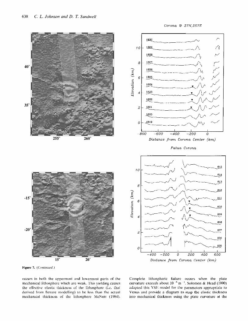
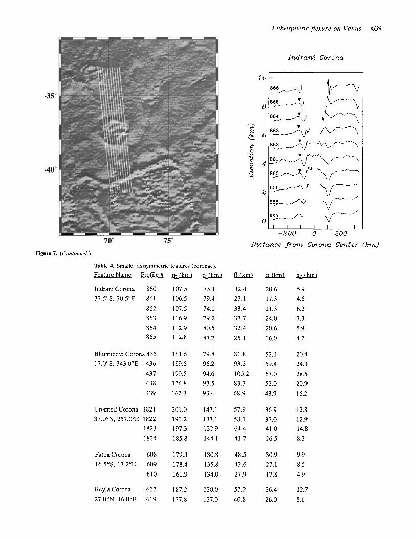
Axisymmetric features
Initially eight small coronae were identified from the gridded topography as possible candidates for flexure modelling. Three of these were rejected after inspecting the orbit data, as the signal-to-noise ratio meant that it was difficult to identify a clear consistent flexural signature. Brief descriptions of the remaining five features and the surrounding areas are given in Appendix 1. The five coronae are shown in Fig. 7; for each feature a gray-scale image of the topography is given, together with the altimetry orbits analysed. As in Fig. 6(c), distance is calculated relative to the corona centre. The gray scale image for each corona suggests a fairly continuous moat around the corona which is easily identified in the orbit data. However, although some of the profiles exhibit flexure-like signals, these signals can vary substantially from one orbit to the next. In some cases the amplitude of the topographic signal is small making it difficult to distinguish, e.g. the north side of Fatua Corona. Other features have more periodic topography with amplitudes which d o not decay exponentially with radius as predicted by simple flexure models. As a result, we consider these data unsuitable for detailed flexure modelling. Never- theless, there does appear to be a characteristic wave- length associated with these smaller features. We use this characteristic wavelength to provide a crude estimate of the elastic plate thickness. The distance between the deepest part of the moat around the corona and the maximum deflection outboard of the moat, i.e. the peak of the possible
Lithospheric flexure on Venus 635
Table 2. Best-fit 2-D models
Feature
Demeter (N) Demeter (N) Demeter (N) Demeter (N) Demeter (N) Demeter (N) Demeter (N)
Demeter ( S ) Demeter ( S ) Demeter ( S ) Demeter ( S ) Demeter ( S )
Nightingale Nightingale Nightingale Nightingale Nightingale Nightingale Nightingale Nightingale Nightingale Nightingale
Nishtigri Nisht igri Nishtigri Nishtigri
Neyterkob Ney t er kob Neyt erkob Ney t er kob
Ridge Ridge Ridge Ridge Ridge
W Dali W Dali W Dali W Dali W Dali
Orbit
2 0 3 6 2037 2 0 3 8 2039 2 0 4 0 2 0 4 1 2042
2 0 1 8 2 0 2 0 2 0 2 1 2022 2 0 2 3
1 2 1 2 1 2 1 4 1 2 1 6 1 2 1 8 1 2 2 0 1 2 2 2 1 2 2 4 1 2 2 6 1 2 2 8 1 2 3 0
8 7 4 8 7 5 87 6 877
1 5 7 0 1 5 7 1 1 5 7 2 1 5 7 3
877 8 7 8 8 7 9 8 8 0 8 8 1
1 3 1 5 1 3 1 6 1 3 1 7 1 3 1 8 1 3 1 9
he ( k m )
2 6 . 0 2 8 . 0 2 4 . 0 2 2 . 0 2 2 . 0 1 8 . 0 1 8 . 0
2 4 . 0 2 2 . 0 2 2 . 0 2 2 . 0 e 2 . 0
2 8 . 0 1 8 . 0 1 8 . 0 1 8 . 0 1 6 . 0 1 6 . 0 16.0 16.0 2 2 . 0 2 2 . 0
12.. 0 1 0 . 0 1 2 . 0 1 0 . 0
1 2 . 0 1 4 . 0 1 4 . 0 1 4 . 0
2 2 . 0 1 8 . 0 1 6 . 0 1 6 . 0 2 0 . 0
4 5 . 0 3 0 . 0 2 5 . 0 3 5 . 0 3 5 . 0
RMS xo (m) ( k m )
60 1 3 4 . 6 5 56 1 0 5 . 6 5 63 9 6 . 9 8 7 0 9 1 . 8 9 7 6 9 2 . 9 4 65 1 0 7 . 4 4 52 1 0 8 . 1 5
4 8 4 6 . 2 3 5 3 4 3 . 3 1 62 4 3 . 3 1 6 5 4 3 . 3 1 77 4 3 . 3 1
3 6 1 5 3 . 8 9 3 5 1 1 1 . 7 8 33 1 0 8 . 2 8 36 1 1 1 . 7 8 4 5 1 0 2 . 3 3 46 1 0 2 . 3 3 37 1 0 1 . 8 8 3 5 1 0 2 . 3 2 30 8 9 . 0 0 27 9 1 . 5 3
3 1 8 0 . 4 8 39 7 1 . 9 3 4 1 1 6 . 5 8 42 6 7 . 2 2
89 8 2 . 4 1 1 0 3 9 2 . 5 8
9 1 9 2 . 5 8 93 9 2 . 5 8
24 8 6 . 6 2 1 9 7 5 . 7 5 1 9 1 2 . 4 8 24 7 3 . 1 0 34 8 5 . 6 5
1 4 8 1 6 5 . 4 1 1 5 3 1 4 3 . 9 0 1 4 6 1 4 3 . 0 1 1 9 4 1 2 5 . 4 1 1 6 6 1 2 2 . 7 1
Table 3. Best-fit 2-D models for larger features.
Feature Name w Best-FiL Range
Nishtigri Corona 12 10- 16
Neyterkob Corona 14 12 - 18
Ridge 18 14 - 22
Nightingale Corona 22 16 - 30
S. Demeter Corona 22 16 - 32
N.Derneter Corona 24 18 - 28
W. Dali Chasrna 34 2 6 - 4 0
1 . 7 0 4 . 3 7 4 . 4 5 3 . 9 1 4 . 2 5 1 . 5 1 1 . 3 3
1 . 5 0 1 . 8 9 2 . 1 2 2 . 2 1 2 . 3 9
0 . 8 8 0 . 5 1 0 . 5 7 0 . 5 6 0 . 4 3 0 . 4 5 0 . 3 9 0 . 4 6 1 . 2 0 1 . 4 3
0 . 2 6 0 . 1 8 0 . 2 5 0 . 1 7
0 . 5 8 0 . 8 3 0 . 8 7 1.11
0.64 0 . 5 5 0 . 4 7 0 . 7 8 1 . 3 1
8 . 8 3 5 . 5 4 4 . 6 8
2 5 . 6 0 1 6 . 4 4
1 6 . 7 0 3 4 . 4 5 5 5 . 7 7 6 3 . 5 9 6 9 . 1 2 4 4 . 9 4 3 9 . 4 2
1 8 . 7 9 3 0 . 6 6 3 4 . 3 9 3 5 . 9 3 3 8 . 8 0
6 . 9 7 1 5 . 0 5 1 6 . 9 8 1 6 . 7 7 1 8 . 1 8 1 8 . 8 1 1 6 . 2 8 1 9 . 3 1 1 9 . 5 3 2 3 . 2 3
2 6 . 1 6 3 1 . 8 5 2 4 . 7 4 3 0 . 0 9
5 8 . 3 1 5 2 . 4 4 5 4 . 5 6 7 0 . 3 2
1 0 . 4 1 1 6 . 3 9 1 9 . 8 9 3 2 . 9 3 2 8 . 3 1
1 6 . 7 7 3 5 . 4 8 5 1 . 8 6
1 0 3 . 3 3 6 6 . 3 5
3 0 . 0 3 9 . 0 3 6 . 0 3 5 . 0 3 4 . 0 2 6 . 0 2 5 . 0
2 6 . 0 2 5 . 0 2 6 . 0 2 5 . 0 2 7 . 0
3 0 . 0 2 1 . 0 2 1 . 0 2 1 . 0 1 9 . 0 1 9 . 0 1 9 . 0 1 9 . 0 2 5 . 0 2 6 . 0
1 4 . 5 1 4 . 0 1 4 . 0 1 4 . 0
1 8 . 0 2 1 . 0 2 2 . 0 2 3 . 0
2 4 . 0 2 1 . 0 1 9 . 0 2 1 . 0 2 6 . 0
5 7 . 0 4 5 . 0 4 0 . 0 6 7 . 0 6 6 . 0
dT/dz ( K / k m )
9 . 7 7 . 4 8 . 1 8 . 3 8.5
11.1 1 1 . 6
11.1 1 1 . 6 11.1 1 1 . 6 1 0 . 7
9 . 7 1 3 . 8 1 3 . 8 1 3 . 8 1 5 . 3 1 5 . 3 1 5 . 3 1 5 . 3 1 1 . 6 12.1
2 0 . 0 2 0 . 7 2 0 . 7 2 0 . 7
1 6 . 1 1 3 . 8 1 3 . 2 1 2 . 6
1 2 . 1 1 3 . 8 1 5 . 3 1 3 . 8 11.1
5 . 1 6 . 4 7 . 3 4 . 3 4 . 4
35.0 140 Disk
39.3 105 50
47.4 ----
55.1 280 100
----
-___ 55.1 ----
58.8 ----
76.4 ----
-___ ----
4.0 Disk
2.7 1.3
5.1 1.8

636 C. L. Johnson and D. T. Sandwell
I 180 '.,
140
2 L 120 u q
l o o
80
'. 60
40
- _...__.. - - - _ _ _ _ - - - - -....-- ___.-- _,_.- Neyterkob
- - N. Demeter - - < ' .-
r
S. Demeter '\ r, \
Nishtidii - . Nightingale /
Ridge
I \ /
' J, '
20' 1'0 20 30 410 5!0 61
Elastic Thickness ( k m ) Figure 5. RMS miqfit versus elastic thickness for each of the seven areas. Misfit was calculated for 2 km increments in elastic thickness. Solid triangles denote average best-fit elastic thickness for each feature. Figs 5 and 4 together demonstrate the increase in the minimum RMS misfit in topographically rough areas and Fig. 5 shows the variation in how well constrained the best-fit models are.
outer rise is given by the following approximate expression
Ira p = r,, - r, = - 2
where r, is the distance to the point of maximum deflection on the outer rise and r, is the distance to the deepest part of the moat. We can thus obtain the equivalent elastic plate thickness he. The distances r,, and r, were determined for as many profiles as possible for each of the five coronae and then a and h, were calculated. The results are given in Table 4. If the topography represents flexure of the lithosphere the mean elastic plate thickness varies from -6 km to -22 km. Note that the result of -8 km for Fatua Corona differs from the 15 km derived previously by Moore et a[. (1992). This could be due to the fact that the topography north of Fatua has a longer wavelength than the topography that we modelled on the south side. However, on the north side the amplitude of the outer rise (and also the moat) is extremely small rendering it difficult to obtain a well-constrained flexural wavelength for the corona as a whole.
MECHANICAL THICKNESS ESTIMATES
The parameters of the best-fitting thin elastic plate models can be used to estimate the depth to the base of the mechanically strong layer. Assuming this corresponds to an isotherm, the geothermal gradient can also be calculated. However, this conversion from elastic thickness to mechanical thickness is highly dependent on the rheological properties of the ductile lower lithosphere. Without a good
0 100 200 300 400 500
D i s t a n c e f r o m C o r o n a Center ( k m )
/ -0.5 1 I I 1 I J
0 100 200 300 400 500
D i s t a n c e ( k r n )
Figure 6. Comparison of Cartesian and axisymmetric flexure models for Nishtigri Corona. The lower figure (a) shows the corona with the tracks of the altimetry orbits modelled. Altimetry profiles with the best-fit Cartesian models (as in Fig. 4) are shown in the middle plot. The upper plot shows the profile data replotted SO that distance is now calculated from the centre of the corona. The best-fit elastic models calculated using a disk model are shown by the dashed lines, with the best-fit elastic thickness given at the end of each profile.
knowledge of lithospheric rheology on Venus, one can only adopt characteristic values used for the Earth's oceanic lithosphere (Goetze & Evans 1979; Brace & Kohlstedt 1980). Here we follow McNutt (1984) and Solomon & Head (1990) where they characterized the strength of the upper

Lithospheric flexure on Venus 637
Beyla Corona
I I
615
6 4
“““^“s- 0 I L I I I I I I -600 -400 -200 0 200 400 600
Distance f r o m Carona Center ( k m )
Bhumidev i C o r o n a
I r I - 0 I I I I I I -800 -600 -400 -200 0
Distance f r o m Corona Center ( k m )
Figure 7. Topography with orbit tracks and profile data for the five smaller axisymmetric features discussed in the text. Again distance along the profile is calculated relative to the corona centre. Gaps in the profiles are due to the fact that the orbit tracks pass at different distances from the corona centre. Distances north of the corona centre are negative, distances south of the corona centre are positive. The triangles mark the positions of the possible outer rise measured and tabulated. Also measured was the distance to the trench just inboard (closer to the origin) of the outer rise. The topographic highs inboard of the trench are the interior of the coronae. The orbit number is given at the end of each profile.
brittle portion of the lithosphere using a frictional sliding corresponds to the 740°C isotherm, and is consistent with law, zero pore pressure, (Byerlee 1978) and the strength of the observation that the maximum depths of earthquakes in the lower lithosphere using a ductile flow law for dry olivine the oceanic lithosphere correspond roughly to the 740°C (10-”s- ’ strain rate). These two failure criteria define a isotherm. yield strength envelope (YSE) (Goetze & Evans 1979), When the lithosphere is flexed, the largest deviatoric where the base of the YSE is defined as the depth where the stresses occur at the top and bottom of the layer. For ductile yield strength drops below 50-100 MPa. This moderate plate curvatures (-lo-’ r n - I ) , significant yielding
638 C. L. Johnson and D. T. Sandwell
Corona @ 37N,257E
i o
8
-2 Y L
6 e 0 .+ 8 74
$ 4 G
2
0
- 1
10
8
Figure 7. (Conrinued.)
r-
- 0 1828 rJ 1827
1828
1824
1822
1821 OJ-
I I I I 10 -600 -400 -200 0
D i s t a n c e f r o m Corona C e n t e r ( k m )
F a t u a Corona
I I I I I I I -400 -200 0 200 400 600
D i s t a n c e f r o m Corona Cen ter ( k m )
occurs in both the uppermost and lowermost parts of the Complete lithospheric failure occurs when the plate mechanical lithosphere which are weak. This yielding causes curvature exceeds about 10-'m-'. Solomon & Head (1990) the effective elastic thickness of the lithosphere (i.e. that adapted this YSE model for the parameters appropriate t o derived from flexure modelling) to be less than the actual Venus and provide a diagram to map the elastic thickness mechanical thickness of the lithosphere McNutt (1984). into mechanical thickness using the plate curvature at the
Lithospheric flexure on Venus 639
I n d r a n i Corona
Figure 7. (Continued.)
Table 4. Smaller axisymmetric features (coronae).
Feature Name Profile #
Indrani Corona 860 37SoS, 70.5"E 861
862 863 8 64 865
Bhumidevi Corona 435 17.OoS, 343.0°E 436
437 438 439
Unamed Corona 1821 37.0°N, 257.0"E 1822
1823 1824
Fatua Corona 608 16SoS, 17.2"E 609
610
Beyla Corona 6 17 27.O"N. 16.0°E 619
-$f!md
107.5 106.5 107.5 116.9 112.9 112.8
161.6 189.5 199.8 176.8 162.3
201.0 191.2 197.3 185.8
179.3 178.4 161.9
187.2 177.8
rtm
75.1 79.4 74.1 79.2 80.5 87.7
79.8 96.2 94.6 93.5 93.4
143.1 133.1 132.9 144.1
130.8 135.8 134.0
130.0 137.0
-200 0 200 Dis tance from Corona Center ( km)
w 32.4 27.1 33.4 37.7 32.4 25.1
81.8 93.3 105.2 83.3 68.9
57.9 58.1 64.4 41.7
48.5 42.6 27.9
57.2 40.8
m 20.6 17.3 21.3 24.0 20.6 16.0
52.1 59.4 67.0 53.0 43.9
36.9 37.0 41.0 26.5
30.9 27.1 17.8
36.4 26.0
u 5.9 4.6 6.2 7.3 5.9 4.2
20.4 24.3 28.5 20.9 16.2
12.8 12.9 14.8 8.3
9.9 8.5 4.9
12.7 8.1

640 C. L. Johnson and D. T, Sandwell
first zero crossing of the flexure model (Fig. 4 of their paper). Based on synthetic models of bending of plates with realistic non-linear rheologies, Mueller & Phillips (1992) proposed that it is better to use the maximum curvature along the flexure profile, rather than the curvature at the first zero crossing, when converting elastic thickness to mechanical thickness; we use both the first zero crossing of the synthetic profile and the point of maximum curvature of the synthetic profile. The results for the seven new features modelled with a Cartesian model are shown in Fig. 8, together with the five earlier results of Sandwell & Schubert (1992a) for comparison. For a given feature the conversion was performed using the curvatures and moments corresponding to the best-fit model for each profile. The uncertainties in Fig. 8 represent the range of h, for each feature. Note that if we used the range in h, given in Table 3 (based on the 10 per cent increase in misfit criteria) some of the uncertainties in h, would be substantially larger. We prefer the former method as there is a specific curvature associated with each value of h,: we caution that the error bars in Fig. 8 are in most cases minimum uncertainty estimates. The conversion of h, to h, was not possible for the five smaller coronae, as curvatures could not be reliably estimated. However, the crude estimates for elastic thickness provide a lower bound on h, at these locations.
0 2 4
DISCUSSION
Static flexure
The global study presented in this paper has revealed surprisingly few examples of lithospheric flexure on Venus. (Note that we have excluded flexure at rift zones as this study is currently being pursued by Evans et al. 1992). We have found only seven areas exhibiting well-defined flexure, in addition to the five areas previously found by Sandwell & Schubert (1992a). These areas give values for effective elastic thickness ranging from 12km to 34km. Of these seven examples the result for Nishtigri Corona should be regarded with caution based on the profile data and the Cartesian versus axisymmetric analysis described earlier. The remaining six areas have sufficiently large radii of curvature to be modelled with a Cartesian model. The result obtained for West Dali Chasma is similar to that obtained for Latona and Artemis Coronae by Sandwell & Schubert (1992a). Profiles across other parts of Aphrodite were extracted, e.g. Diana Chasma to the west of Dali Chasma. Although initially appearing very similar to the profiles from W. Dali Chasma the profiles from other parts of Aphrodite could not be satisfactorily fit with a flexure model due to extensive faulting evident in the SAR images and reflected in the
6 8 10 12 I I
cs 3 I 0
1
I Figure 8. Mechanical thicknesses for all 12 areas modelled with a Cartesian flexure model. The area names in italics represent results presented previously (Sandwell & Schubert 1992a). Areas whose names are capitalized are believed to be moment saturated and thus do not provide a reliable estimate of mechanical thickness. The dashed lines represent the range of mechanical thickness predicted for Venus based on heat-flow scaling arguments (Solomon & Head 1982). The solid symbols represent the mean mechanical thickness for each area and the uncertainties are the range. The square symbols and error bars represent the mechanical thickness obtained by performing the conversion from elastic to mechanical thickness based on the moment and curvature at the first zero crossing of the synthetic profiles (McNutt 1984). The stars and error bars represent the same conversion performed at six of the seven new areas using the point of maximum curvature along the synthetic profile (Mueller & Phillips 1992). The latter method was not used at W. Dali Chasma as the mechanical thicknesses even from the McNutt method are unreliable.

Lithospheric flexure on Venus 641
topography. It should be noted that the best-fit models for West Dali Chasma, Artemis and Latona Coronae d o not extend to the base of what should be the trench. There appears to be a step in the topography part way down the trench wall, corresponding t o extensive faulting evident in the radar images. If the profiles are fit to the base of the trench the result is unconvincing. These characteristics, common to altimetry profiles from several parts of Aphrodite, including the larger coronae, suggest that either the lithosphere in this area is flexed but moment saturated, or has been extensively deformed as the result of other processes. The five remaining features provide more reliable estimates of the mechanical thickness of the lithosphere. From Fig. 8 the mean thicknesses are in the range 21-37 km. The corresponding range of average thermal gradients is 14-8Kkm-' and the range of surface heat flow is 46.2-26.4 mW m-2 (using the parameters given in Table 1). It should be noted that these values for mechanical thickness, and the derived thermal gradient and heat flow, may not be the current lithospheric conditions, they rather reflect the conditions at the time the flexural signature was frozen in.
Predictions for the average surface heat flux/thermal gradient/lithospheric thickness were made on the basis of heat flow scaling arguments and chondritic thermal models (Solomon & Head 1982; Phillips & Malin 1983). Heat-flux estimates ranged from 50 mW m-2 from the chondritic thermal models, to 74 mW m p 2 from the heat-flow scaling argument, with equivalent mechanical thicknesses of 21-13 km. Our results for static flexure suggest a thicker lithosphere than predicted, although not as thick as that proposed by Sandwell & Schubert (1992a). Surface stresses predicted by thin elastic plate models are much higher (in most cases) than could be supported by the lithosphere, and there is evidence in the S A R images of failure at the appropriate locations. A thicker lithosphere is consistent with the general lack of evidence for flexural signatures around smaller coronae-we would not expect small loads to be able to deflect a thick plate. Thinner values for elastic thickness around two large volcanoes on Venus (McGovern & Solomon 1992) could be associated with lithospheric reheating and thinning of the plate. Localized thermal rejuvenation would explain some of the smaller values for elastic thickness in Table 4, and is consistent with plume models for coronae formation and evolution. The large gravity signatures over some of the smaller coronae require either a thick lithosphere (based on preliminary results from isostatic compensation models, Moore, personal com- munication 1993) or dynamic support.
An important consideration is that the assumed rheological properties of the Venusian lithosphere are based on our knowledge of oceanic lithosphere. The extremely low abundance of water at the surface of Venus relative to the Earth (Oyama et al. 1980), suggests that models for the Venusian lithosphere require a dry rheology such as that used by Solomon & Head (1990). It is known that dry olivine is stronger than wet olivine (Goetze & Evans 1979) under terrestrial conditions: however it is quite possible that the Venusian lithosphere is drier than could be attainable in a laboratory. Although the difference in the percentage of water present in the Venus lithosphere and terrestrial laboratory experiments may be small, it may have significant
effects on the rheology, especially given the Venusian surface conditions. In particular, the Venusian lithosphere could be much stronger than predicted. Recent measurements suggest that dry diabase is much stronger than previously believed (Mackwell et al. 1993); it is quite feasible that the same will be found to be true of dry olivine.
Flexure of a viscous plate
The flexure model assumes that the trench/outer rise features are statically maintained by large fiber stresses within a thin elastic lithosphere. However, it is possible that the flexure inferred from topography is the result of deformation of a viscous lithosphere. We discuss three mechanisms that can produce apparent topographic flexural signatures. In the first two cases the lithosphere is currently dynamically supported and the estimated viscous plate thickness depends upon the assumed strain rate or stress distribution. In the third case the process generating the flexural signature has ceased recently, relative to the characteristic time-scales for viscous relaxation.
In the first scenario, flexural signatures can be generated by a hydrostatically supported viscous lithosphere, loaded at the trench and moving horizontally toward the trench (DeBremaecker 1977). This type of model has been applied to terrestrial subduction zones, and predicts a thick viscous lithosphere (on the order of 120 km) in which the deviatoric stresses are lower (Melosh 1978) than the stresses predicted by the elastic flexure model. The equation describing the vertical deflection is
W ( X ) = d , exp [ - (y) x - x cos (:)I x sin [ (7) sin (:)I + d 2 x + d3
(DeBremaecker 1977), where p5 = (vUb:)/(27pg); 17 is the viscosity, b, is the viscous plate thickness and U the horizontal velocity. As an example we fit such a model to Latona Corona as this has been proposed to be the site of possible subduction on Venus (McKenzie er at. 1992: Sandwell & Schubert 1992a, 1992b), and appears to display evidence for back-arc-type extension (Sandwell & Schubert 1993). If we fix the viscosity to the terrestrial value of lo2' Ns mp2, the best-fit model has a viscous plate thickness of 80 km for U = 50 mm yr-' and 172 km for U = 5 mm yr-'. Latona has a mean radius of approximately 400 km, and so a plate velocity of 50 mm yrp' would imply the corona has developed only over the last 8Myr, whereas the lower velocity of 5 mm yr-' would imply development over the last 80Myr. The main problem with this kind of model for Venus is that a t most locations with flexural-like topography there is n o evidence for retrograde subduction, and as yet, no independent evidence for plate motions has been observed. These considerations lead us to favour low horizontal strain rates, which in turn imply a thick viscous lithosphere at most of our study areas. Thus, viscous plate models, like the elastic plate models, are compatible with low temperature gradients in the lithosphere.
In a second scenario, the inferred flexural signatures result from vertical stresses, acting on the base of a viscous lithosphere. Flexure inferred around coronae would imply a

642 C. L. Johnson and D. T. Sandwell
ring geometry to the stress field; it is difficult to imagine how this could be generated by a mantle flow field consistent with models for coronae evolution. Regardless of the mechanism by which the stresses could be generated, the resulting models would produce results analogous to those of the previous discussion. That is, low bending stresses would imply a thick viscous lithosphere, high stresses would correspond to a thin viscous lithosphere.
In a third scenario, the inferred flexures are the result of dynamic processes which are n o longer active. One concern with an elastic plate flexure model is that only a small percentage of coronae exhibit topographic signatures consistent with flexure. The size distribution of coronae is described by a power-law decay (Stofan et al. 1992). Smaller loads (coronae) will result in a smaller deflection of an elastic plate and it is possible that the topography around many coronae contains a low-amplitude flexural signature which is masked by topographic noise. It is very likely that coronae are at different stages of evolution, and also that different coronae may be generated by different processes, so we would not expect flexural signatures to be associated with all coronae. However, it is possible that a topographic flexural signature, associated with most or all coronae when they are formed, relaxes due to viscous flow, once it is n o longer dynamically maintained. If this is the case, then we can make some predictions concerning the characteristic time-scales for viscous flow, based on the percentage of coronae with associated inferred flexure.
The governing equation for flexure of a viscous plate is
d'W
d l ax4 F - + Apgw = 0,
where F = ~ h 1 / 2 7 is the instantaneous flexural rigidity. We assume that sinusoidal topography of wavelength a decays exponentially with time with a time constant of A:
~ ( x , t ) = A cos ( x / a ) exp ( -At) . (15) The characteristic decay time of this topography is given by
1 vh: 7 =-=- 'I A 27Apga4
Thus an initial flexural signature will be undetectable (due to viscous flow) after a time that depends upon the initial amplitude of the flexure. If we assume that typical initial outer rise heights are on the order of 100-300 m (consistent with the larger inferred flexural signatures from Aphrodite Terra), then the outer rise will be undetectable after a time,
equal to twice the characteristic decay time. If we also assume that the production rate of coronae has been uniform over the mean surface age of the planet, then we can calculate Tf from the number of coronae with inferred flexural signals, N,, and the total number of coronae, N, (approximately 250, Stofan er al. 1992):
T*N, q =- N,
T is the mean surface age of the planet, which we take to be 500Myr (Phillips et al. 1992; Schaber et al. 1992). This gives Tf = 18Myr, so r = 9 M y r . Thus if we assume the flexural wavelength has not changed significantly as the topography has relaxed, we can use (16) and the flexural
wavelengths given in Tables 3 and 4 to obtain the corresponding viscous plate thickness for each feature. Values for h, calculated in this manner (assuming 17 = lo2' Pa s) are in the range 69-291 km.
It is evident that we can calculate viscous plate thicknesses consistent with the observed number and form of inferred flexural features, however, the results are dependent on many assumptions that cannot be independently verified. Relaxation time-scales consistent with the observed number of inferred flexural features predict a thick lithosphere at most of the sites, again consistent with a low-temperature gradient in the lithosphere. If the viscous plate thicknesses are lower than this analysis suggests, the corresponding time-scales for relaxation would be much shorter. It is possible that there are smaller lateral variations in viscous thickness than the above analysis suggests; however, we would then expect a larger percentage of short-wavelength flexural signatures compared with the long-wavelength flexural signals, due to the shorter characteristic decay time of long-wavelength topography. Our study has not revealed such a distribution of features, however, the statistics may be biased by the fact that low-amplitude, short-wavelength signals are not easily detectable above the topographic noise.
The above discussion concerns relaxation of a flexural signature previously generated in a viscous lithosphere. Gravitational relaxation of surface topography produces vertical stresses that can result in very similar topographic signatures to those which would be generated by flexure of an elastic, viscoelastic or viscous plate. This mechanism has been proposed to account for the topography around coronae on Venus (Stofan et al. 1991; Janes et al. 1992). The time-scales for crustal flow for Venus are 10,000-100,000 yr (Smrekar & Solomon 1992), based on previous experimental results for diabase rheology. However, recent measurements on dry diabase (Mackwell et al. 1993) suggest a much stronger rheology, comparable to that previously published for websterite. Smrekar & Solomon (1992) found that the time-scales for gravitational relaxation assuming a webster- ite rheology were on the order of several hundred million years. These long time-scales would predict a much higher abundance of flexure-like topographic signals than is observed.
CONCLUSIONS
We have presented results from a global study of flexure on Venus, excluding flexure at rift zones and around volcanoes. Most prominent examples of downward flexure are associated with the outer edges of coronae. A s coronae vary considerably in diameter, we investigated the validity of a Cartesian approximation to an axisymmetric load geometry. The important parameters are the ratio of outer load radius to the flexural parameter a/a, and, if a ring load is appropriate, the ratio of ring load width to the flexural parameter Aa/a. Our analysis indicates that for a given a / a , loads with a smaller value of Aa/a (thin rings) are better approximated with a Cartesian model than loads with a larger value of Aa/a (wide rings or disks). A s a / a increases for any given h a / a the Cartesian approximation becomes increasingly valid, especially for estimating a when a / a is greater than about two. In contrast, the magnitude of the

Lithospheric flexure on Venus 643
load is severely underestimated even when a / a is about five; this is important as it directly translates into an underestimation of the bending moment. Modelling of profiles which do not pass through the centre of the axisymmetric feature with a Cartesian model can overestim- ate the flexural wavelength. Criteria can be set up specifying the acceptable error in each of the parameters estimated by the flexure model-load magnitude, load position and flexural parameter. These criteria can then be used together with the curves in Fig. 3 to establish critical values of a /a and A a l a for which a Cartesian approximation to a ring load or disk load geometry is acceptable. We modelled seven features, in addition to five previously modelled, with a Cartesian model. We remodelled one of these features, Nishtigri Corona, with a disk load model and found significantly different results. The difference c3n be partly attributed to the fact that the Cartesian approximation was, in this case, a poor approximation, and partly to the fact that this was a poor example of flexure. Based on the curvatures and surface stresses obtained from thin elastic plate models, the topography at W. Dali Chasma, Latona and Artemis Coronae is either representative of extreme flexure (the lithosphere is moment saturated) or it is the result of a tectonic history not involving lithospheric flexure. Mean mechanical thicknesses calculated for the remaining examples fall in the range 21 km-37 km, reflecting lithospheric thicknesses at the time of loading. We found no clear examples of flexure around smaller corona, though five areas could not be completely ruled out. Estimates of effective elastic thickness based on a flexure model for these examples fell in the range 4 km-28 km and did not correlate with corona diameter. The elastic thicknesses provide a lower bound on mechanical thickness at these sites. Of these five examples, only Fatua Corona has a strong gravity signal which is well correlated with the topography (Moore, personal communication 1993).
An alternative interpretation of the apparent flexural signatures modelled in this paper is that they are the result of flexure of a viscous lithosphere. A dynamical model derived for terrestrial subduction zones (DeBremaecker 1977) was applied to the topographic profiles from Latona Corona. The viscous plate thickness corresponding to low strain rates was found to be 170km, greater than the comparable thickness derived for terrestrial subduction zones. The number of observed apparent flexural signatures is consistent with characteristic time-scales for viscous relaxation of 9 Myr. Based on these time-scales the derived viscous plate thicknesses are again high. Thus, viscous plate models are also consistent with low temperature gradients in the lithosphere. The main problem with viscous models is that there is a trade-off between the strain rate (or stress distribution or relaxation time-scales) and the viscous plate thickness. Unfortunately, we have almost no information on time-scales on Venus, so if a viscous rheology is appropriate we can, at best, propose a family of models consistent with the observations.
Models for the formation of coronae have suggested that an apparent flexural signature may form during the late stages of evolution, as a result of gravitational relaxation (Stofan et al. 1991; Janes et al. 1992). However, recent measurements on dry diabase indicate that dry crustal materials are much stronger than previously believed
(Mackwell 1993). Time-scales for gravitational relaxation of a strong Venusian crust are on the order of 10X-lO'yr (Smrekar & Solomon 1992), comparable to the inferred average surface age of approximately 500 Myr (Phillips et ul. 1992; Schaber et al. 1992). Thus, based on the current available information, it is unlikely that flexural topography is generated by gravitational relaxation.
Another possibility is that the trench and outer-rise signatures could be Airy compensated and simply reflect variations in crustal thickness. The improved gravity- anomaly data being collected by Magellan may shed light on this final possibility. On Earth, gravity-anomaly data are used to reject this hypothesis.
Assuming the trench and outer rise topographic features that we have identified are supported by larger fiber stresses within a thin plate, our results indicate that the Venusian elastic lithosphere is thicker than predicted based on the global heat-scaling argument. This has implications for the style and timing of tectonic activity on Venus. Scenarios consistent with a thick lithosphere have been proposed in which either most of the heat escapes through localized heat pipes (Turcotte 1989), or mantle convection on Venus is highly episodic (Turcotte 1992; Parmentier & Hess 1992). The localized heat-pipe model is problematic as it predicts a global volcanic flux much greater than that inferred from radar observations (Solomon & Head 1991; Head et al. 1992). Also a natural choice of locations for such heat pipes would be the coronae themselves and this model would then predict hotter, thinner lithosphere at coronae. Current episodic convection models require global synchroneity of the initiation and termination of convection. I t is more realistic to expect regional variations in the extent and duration of the episodes of increased convection. Such modifications to the current models would be more consistent with the range in lithospheric thicknesses reported here and with the fact that many coronae do not exhibit any flexural signature. A recent tectonic model for resurfacing on Venus has been proposed in which a period of rapid crustal deformation existed in the past due to a higher surface heat flux than at present and a correspond- ingly weaker lower crust (Solomon 1993). In this model a gradual decrease in surface heat flux can lead to a much more abrupt change in the crustal deformation rates because of the exponential dependence of strain rate upon temperature. High strain rates would be expected to persist over a longer time period in elevated regions, (compared with the lowlands) due to a weaker crust. Our results are broadly consistent with this model as the features exhibiting apparent flexural signatures are mostly in or around the edge of the lowlands, where a lower heat flux and thicker lithosphere would be expected. Recent laboratory experi- ments on terrestrial diabase indicate that dry crustal materials are significantly stronger than previously believed (Mackwell 1993). If similar results are found for dry olivine, this will suggest a strong Venusian lithosphere, and the mechanical thickness estimates in this paper will be reduced. Finally, although it will not be able to directly model flexure profiles using the Magellan gravity data we hope that it will provide more information on variations in lithospheric thickness on Venus and on the relative contributions of static and dynamic processes to the support of topographic features.

644 C. L. Johnson and D. T. Sandwell
ACKNOWLEDGMENTS
We would like to thank Dan McKenzie, Chris Small, Cathy Constable, Bill Moore and Jerry Schubert for many valuable discussions throughout the duration of this project. Marc Parmentier and Mark Simons provided constructive reviews, which improved the clarity of the paper. In particular Marc Parmentier made helpful suggestions regarding the discus- sion of viscous models. This research was supported by NASA under the Venus Data Analysis Program NAGW- 3503 and the Jet Propulsion Laboratory under the Magellan Project, Contract No. 958950.
REFERENCES
Brace, W.F. & Kohlstedt, D.L., 1980. Limits on lithospheric stress imposed by laboratory experiments, J . geophys. Res., 85, 6248-6252.
Brotchie, J.F., 1971. Flexure of a liquid filled spherical shell in a radial gravity field, Mod. Geol. 3, 15-23.
Brotchie, J.F. & Silvester, R., 1969. On crustal flexure, J . geophys. Res., 74, 5240-5252.
Brown, C.D. & Grimm, R.E., 1993. Flexure and the role of implane force around coronae on Venus, Lunar & Planetary Science Conference, XXIV, 199-200.
Byerlee, J.D., 1978. Friction of rocks, Pageoph., 116, 615-626. Caldwell, J.G. & Turcotte, D.L., 1979. Dependence of the thickness
of the elastic oceanic lithosphere on age, J . geophys. Res., 84, 7572-7576.
DeBremaecker, J.C., 1977. Is the oceanic lithosphere elastic or viscous?, J . geophys. Res., 82, 2001-2004.
Evans, S.A., Simons, M. & Solomon, S.C., 1992. Flexural Analysis of Uplifted Rift Flanks on Venus, International Colloquium on Venus, LPI Contribution No. 789, 30-32.
Ford, P.G. & Pettengill, G.H., 1992. Venus topography and kilometer-scale slopes, J . geophys. Res., 97, 13 103-13 114.
Goetze, C. & Evans, B., 1979. Stress and temperature in the bending lithophere as constrained by experimental rock mechanics, Geophys. J.R. astr. Soc., 59, 463-478.
Head, J.W., Crumpler, L.S., Aubele, J.C., Guest, J.E. & Saunders, R.S., 1992. Venus volcanism: classification of volcanic features and structures, associations and global distribution from Magellan data, J . geophys. Res., 97, 13 153-13 197.
Janes, D.M., Squyres, S.W., Bindschadler, D.L., Baer, G., Schubert, G., Sharpton, V.L. & Stofan, E.R., 1992. Geophysical models for the formation and evolution of coronae on Venus, J . geophys. Res., 97, 16 055-16067.
Johnson, C.L. & Sandwell, D.T., 1992a. Flexure on Venus: implications for lithospheric elastic thickness and strength. Lunar & Planetary Science Conference, XXIII, 619-620.
Johnson, C.L. & Sandwell, D.T., 1992b. Joints in Venusian Lava Flows, J . geophys. Rex , 97, 13601-13610.
Johnson, C.L. & Sandwell, D.T., 1993. Estimates of lithospheric thickness on Venus, Lunar & Planetary Science Conference, XXIV, 721 -722.
Mackwell, S.J., Kohlstedt, D.L., Scherbcr, D.S. & Zimmerman, M.E., 1993. High temperature deformation of diabase: Implications for Tectonics on Venus, EOS, Trans. Am. geophys. Un., 74, 378.
McKenzie, D.P., 1967. Some remarks on heat flow and gravity anomalies, J . geophys. H a . , 72, 6261 -6273.
McKenzie, D., Ford, P.G., Johnson, C., Parsons, B., Pettengill, G.H., Sandwell, D., Saundcrs, S. & Solomon, S.C., 1992. Features on Venus generated by plate boundary processes, J . geophys. Res.. 97, 13 533-13 544.
McNutt, M.K., 1984. Lithospheric flexure and thermal anomalies, J . geophys. Res., 89, 11 1XGl I 194.
McNutt, M.K. & Menard, H.W., 1992. Constraints on yield strength
in the oceanic lithosphere: derived from observations of flexure, Geophys. J.R. astr. Soc., 71, 363-394.
Melosh, H.J., 1978. Dynamic support of outer rise topography, Geophys. Res. Lett., 5, 321-324.
McGovern, P.J. & Solomon, S.C., 1992. Estimates of elastic plate thicknesses beneath large volcanoes on Venus, International Colloquium on Venus, LPI Contribution No. 789, 68-70.
Moore, W., Schubert, G. & Sandwell, D.T., 1992. Flexural models of trench/outer rise topography of coronae on Venus with axisymmetric spherical shell thin elastic plates, I~fernatjonal Colloquium on Venus, LPI Conrrihution No. 789, 72-73.
Mueller, S. & Phillips, R.J., 1992. Inelastic lithospheric flexure, Geophys. J . Int., submitted.
Oyama, V.I., Carle, G.C., Woeller, F., Pollack, J.B., Reynolds, R.T. & Craig, R.A., 1980. Pioneer Venus gas chromatography of the lower atmosphere of Venus, J . geophys. Res., 85, 7891-7902.
Parmentier, E.M. & Hess, P.C., 1992. Chemical differentiation of a convecting planetary interior: Consequences for a one plate planet such as Venus, Geophys. Res. Left., 19, 2015-2018.
Parsons, B. & Sclater, J., 1977. An analysis of the variation of ocean floor bathymetry and heat flow with age, J . geophys. Res., 82, 803-827.
Pettengill, G.H., Ford, P.G. & Wilt, R.J., 1992. Venus surface radiothermal emission as observed by Magellan, J . geophys. Res., 97, 13091-13 102.
Phillips, R.J. & Malin, M.C., 1983. The interior of Venus and tectonic implications, in Venus, eds Hunten, D.M., Colin, L., Donahue, T.M. & Moroz, V.I., University of Arizona Press, Tucson, AZ.
Phillips, R.J., Raubertas, R.E., Arvidson, R.E., Sarkar, I.C., Herrick, R.R., Izenberg, N. & Grimm, R.E., 1992. Impact craters and Venus resurfacing history, J . geophys. Rex , 97,
Pronin, A.A. & Stofan, E.R., 1990. Coronae on Venus: morphology and distribution, Icarus, 87, 452-474.
Ribe, N.M., 1992. On the interpretation of frequency response functions for oceanic gravity and bathymetry, Geophys. J . R. astr. Soc., 70, 273-294.
Sandwell, D.T. & Schubert, G., 1992. Flexural ridges, trenches and outer rises around Venus coronae, J . geophys. Res., 97,
Sandwell, D.T. & Schubert, G., 1992. Evidence for retrograde lithospheric subduction on Venus, Science, 257, 766-770.
Sandwell, D.T. & Schubert, G., 1993. A global survey of possible sites of subduction on Venus, EOS, Trans. Am. geophys. Un., 74, 376.
Saundcrs, R.S., Spear, A.J., Allin. P.C., Austin, R.S.. Berman, A.L., Chandlee, R.C., Clark, J., DeCharon, A.V., DeJong, E.M., Grifith, D.G., Gunn, J.M., Hensley, S., Johnson, W.T.K., Kirby, C.E., Leung, L.S., Lyons, D.T., Michaels. G.A., Miller, J., Morris, R.B., Morrison, A.D., Piereson, R.G., Scott, J.F., Shatfer, S.J., Slonski, J.P., Stofan, E.R., Thompson, T.W. & Wall, S.D., 1992. Magellan mission summary, J . geophys. Res., 97, 13 067- 13 090.
Schaber, G.G., Strom, R.G., Moore, H.J., Soderblom, L.A., Kirk, R.L., Chadwick, D.J., Dawson, D.D., Caddis, L.R., Boyce. J.M. & Russell, J., 1992. Geology and distribution of impact craters on Venus: What are they telling us?, J . geophys. Res., 97, 13257-13301.
Smrekar, S.E. & Solomon, S.C., 1992. Gravitational sprcading of high terrain in Ishtar Terra, Venus, J . geophys. Res.. 97, 16 121-16 148.
Solomon, S.C. & Head, J.W., 1982. Mechanisms for lithospheric heat transport on Venus: implications for tectonic style and volcanism, J . geophys. Res., 87, 9236-9246.
Solomon, S.C. & Head, J.W., 1990. Lithospheric flexure beneath the Freyja Montes foredecp, Venus: constraints on lithospheric thermal gradient and heat flow. Geophys. Res. Lett., 17, 1393-1396.
15 923-15 948.
16 069-16 083.

Lithospheric flexure on Venus 645
substantial volcanism associated with Nightingale both interior to and exterior to the corona. In particular there is evidence for flows possibly postdating the flexure on the south side of the corona. Polygonal fracture patterns rather than fractures concentric to the corona are seen.
Solomon, S.C. & Head, J.W., 1991. Fundamental issues in the geology and geophysics of Venus, Science, 252,252-260.
Solomon, S.C., 1993. The geophysics of Venus, Phys. Today. 46, 48-55.
Squyres, S.W., Janes, D.M., Baer, G., Bindschadler, D.L., Schubert, G., Sharpton, V.L. & Stofan, E.R.. 1992. The morphology and evolution of coronae and novae on Venus, J . geophys. Res., 97,
Stein, S., 1994. Introduction to seismology, earthquakes, and earth structure, in press.
Stofan, E.R., Bindschadler. D.L., Head, J.W. & Parmentier, E.M., 1991. Corona structures on Venus: models of origin, 1. gcophys. Res., 96, 20 933-20 946.
Stofan, E.R., Sharpton, G., Schubert, G., Baer, G., Bindschadler, D.L., Janes, D.M. & Squyres, S.W.. 1992. Global distribution and characteristics of coronae and related features on Venus: implications for origin and relation to ,'mantle processes. J . geophys. R e x , 97, 13 347- 13 378.
13 61 1-13 634.
Turcotte, D.L., 1979. Flexure, Adu. Geophys., 21, 51-86, Turcotte, D.L., 1989. A heat pipe mechanism for volcanism and
tectonics on Venus, J . geophys. Res., 94, 2779-2785. Turcotte, D.L., 1992. Episodic plate tectonics on Venus, EOS,
Trans. A m . geophys. Un., 73, 332. Watts, A.B., Weissel, J.K., Duncan, R.A. & Larson, R.L., 1988.
Origin of the Louisville Ridge and its relationship to the Eltanin fracture zone system, J . geophys. Re%, 93, 3051-3077.
Wessel, P., 1992. Thermal stresses and the bimodal distribution of elastic thickness estimates of the oceanic lithosphere, J . geophys. Res., 10, 14 177-14 193.
A P P E N D I X A: DESCRIPTIONS OF F L E X U R E LOCATIONS
Ala Larger features modelled with a Cartesian flexure model
Nishtigri Corona (24.5"S, 72.0OE)
Asymmetric corona with maximum radius of 140 km. The interior is elevated about 1 km above surrounding plains regions. The topographic moat around the corona is about 45 km wide. The topography to the north of the corona is elevated and rough, so no flexure signature could be detected. Possible flexure is visible on the south side of Nishtigri. A moderate number of volcanic features associated with Nishtigri are evident in the S A R image (ClMIDR 30S063;l) mostly small domes in the elevated interior and flows surrounding the corona. Concentric fractures around Nishtigri coincide with the location of the outer rise in the flexure profiles.
Nightingale Corona (63.0°N, 132.0OE)
Concentric corona (a well-defined tectonic annulus, Stofan et al. 1992) with a maximum radius of -280km. The tectonic annulus is elevated up to -2.5 km above the surrounding plains. This elevated rim is extremely tectonically disturbed as evidenced in the S A R images (e.g. C l M I D R 60N125E;l). Tessera-like terrain to the north of the corona masks any flexure which may have been associated with Nightingale. There is a well-defined flexural signature to the south, superposed on a regional sope that is downhill in the SSE direction. No concentric fractures associated with the flexure are seen, however, there is
Demeter Corona (55.0°N, 295OE)
Concentric elongate corona with maximum radii -35 km (NE-SW direction) and -165 km (NW-SE direction). The corona interior is at approximately the same elevation as the surrounding plains but the corona rim is elevated by up to 1 km. Flexure is evident to the north and south of the corona and the coronal rim at these locations is almost straight. Concentric fractures associated with the rim and the flexural moat are evident in the SAR images (e.g. C l M I D R 60N291). To the north of the corona there is considerable tectonism probably unassociated with the corona. Volcanism is visible in the form of small volcanoes in the corona interior and flows in the surrounding plains.
Neyterkoh Corona (49.OoN, 203.0"E)
Neyterkob is defined as a multiple corona (Stofan et a/ . 1992), the east and west parts being distinct. The interior of both parts of the corona is not elevated but there is a topographically high rim defining the edge of the corona. The topography surrounding the corona is very rough. However, to the south and south-east of the eastern part of the corona the topography is relatively flat and there is evidence for flexure associated with the coronal outer rim. Volcanism is evident in the S A R images (e.g. ClMIDR 45N2012;l) and there is extensive tectonism associated with the corona and with the ridge belts in the surrounding plains. Concentric fractures possibly associated with the topographic flexure can be seen though they are somewhat masked by other tectonic features and lava flows.
Ridge ( I 9.0 ON, 70.0 "E)
This is a narrow E-W-trending ridge reaching a maximum height of about 1 km above the plains to the north. There is no evidence of a flexural moat to the south but a possible low-amplitude flexure to the north can be seen in the gridded topography. Some fracturing parallel to the ridge and to the north can be identified in the SAR image (ClMIDR 15N077;l). Volcanism in the areas immediately adjacent to the ridge is mainly in the form of flows of small areal extent.
W . Dali Chasrna (ISON, 16OOE)
West Dali Chasma is located in Eastern Aphrodite Terra and is an extremely deep (-2-4 km) roughly E-W-trend- ing asymmetric chasma. The highest part of the topography is just to the north of the chasma. The topography on the south side of the chasma was identified as a possible example of flexure. The region is extremely tectonically deformed as evidenced in the S A R images of this area. The tectonic deformation appears to post-date several volcanic flows. An extremly bright region in the SAR image correlates with the highest topography in agreement with previous observations of an increase in reflectivity at high
646 C. L. Johnson and D. T. Sandwell
elevations (Pettengill, Ford & Witt 1992). Extensive closely spaced fractures on the south side of the chasma and parallel to it are easily identified in the S A R data.
Alb Smaller axisymmetric features (coronae) Fatua Corona (16.5 "S, 17.2 "E)
Concentric corona with interior high ring (up to -1 km), surrounding moat and outer elevated ring. Maximum radius is -155 km. Gridded topography suggests outer lower amplitude ring may be a flexural feature, although the part of the outer ring to the SW of the corona has too high an amplitude to be flexure caused by the inner corona load. SAR image (ClMIDR 1SS026;l) shows conqentric fractures associated with the corona moat and outer elevated rim. Small volcanoes are evident in the corona interior and flows associated with the corona can be seen.
Beyla Corona (27.0°N, 16.O"E)
Asymmetric corona (elongate in a NW-SE direction) with maximum radius of 145 km. Has little associated volcanism. The centre of the corona is less than 500m above the surrounding plains. There is a pronounced moat around the northern edge of the corona, although the topography to the north is too rough to distinguish any topographic flexure. The gridded topography suggests possible flexure to the south. The S A R image (ClMIDR 30N009;l) shows almost no concentric fractures around the southern edge of the corona. Quasi-concentric fractures are seen associated with the moat around the northern edge. Corona interior exhibits roughly NW-SE-trending bright lineations.
Indrani Corona M7.5 "S, 70.5 "E)
Concentric corona with a maximum radius of -100 km. The topography surrounding the corona is moderately rough making flexure difficult to identify. There is a narrow moat which is almost continuous around the corona. There are no distinguishing features associated with the corona evident in the S A R images (ClMIDR 45S074;l).
Bhumideui Corona ( I 7.05, 343.O"E)
Concentric corona with maximum radius of l00km. The centre of the corona is low relative to the surrounding plains, but there is an elevated rim (up to -1 km) surrounded by a moat that is continuous except on the south-east side of the corona. There is evidence in the gridded topography for possible flexure associated with the moat around the north-west side of the corona. A narrow band of concentric fractures around the outer edge of the corona are visible in the S A R image (ClMIDR 1SS352;l).
Unnamed Corona (.?7.OoN, 257.0"E)
Concentric corona with maximum radius of -100 km. Moderate volcanism is associated with the corona, although the corona itself is difficult to identify in the S A R data alone. The corona lies to the north of a region of rough
topography. The interior is at approximately the same elevation as the plains to the north but there is an elevated ring surrounded by a topographic low on the northern side of the corona. Possible flexure to the north.
APPENDIX B: THE BAR LOAD APPROXIMATION TO THE R I N G LOAD
In this appendix we demonstrate that in the limit of large a J a a ring load of outer radius a and width Au can be approximated by a bar load width ha.
The expression for deflection due to a ring load outer radius a and width h a (eq. 5 in the main text) can be written explicitly as the deflection due to a disk load of radius a minus the deflection due to a disk load of radius a - h a :
[d ber' ( d ) ker (x) - 6 ber' (6) ker (x)
1 + [S bei' (6) kei (x) - d bei' ( d ) kei (x)
x > = a J a (Bl )
where
a - h a r d = a J a ; 6=-; x = - ff ff
We are interested in the limit of w(r ) as a / a becomes very large. The limit of each of the terms inside the square brackets can be taken using the following relations
x - d
ber' ( d ) ker (x) = 2 6
x [S,,(d) cos (dd) - 7;,(d) sin (dd)j
x [L,,( -x) cos (xx) + M,)( -x) sin (xx)]
(B2)
x {q , (d) cos (dd) + S,,(d) sin (dd)]
x [M,,( -x) cos (xx) - L,)( -x) sin (xx)]
(B3) where
1.3 l ! 8x
1 '. 3*.5.7
S,,(x) = 1 - -cos
_____ cos ($1 - 3! (Xx)"
1.3 l! 8x
?;,(x) = -sin
1*.3*.5.7 3! ( 8 x y
+-sin ($1 +
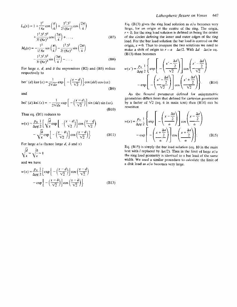
Lithospheric flexure on Venus 647
Eq. (B13) gives the ring load solution as a / a becomes very large, for an origin at the centre of the ring. The origin, r = 0, for the ring load solution is defined as being the centre of the circles defining the inner and outer edges of the ring load. For the bar load solution the bar load is centred on the origin, x = 0. Thus to compare the two solutions we need to make a shift of origin to r = a - Aa/2. With Ad = Aa/a eq. (B13) then becomes
1’ ! 8x
1 ’. 3’. 5’
L,(x) = 1 + - cos
+-cos (?) + . . . , (B7) 3! (8x)3
sin ($) 1’ 1’.3’ ~ , ( x ) = --sin (f) - __
l! 8x 2! (8x)’
1’.3’.5’ 3! ( 8 ~ ) ~ sin($)- . . . , (B8) --
For large x, d, and S the expressions (B2) and (B3) reduce respectively to
1 x - d ber’ (d) ker (x) = __ cos (dd) cos (xx)
and
1 x - d bei’ (d) kei (x) = - - exp [ - ( T)] sin (dd) sin (xx ) .
Thus eq. (Bl) reduces to
2 6 (B10)
As the flexural parameter defined for axisymmetric geometries differs from that defined for Cartesian geometries by a factor of d 2 (eq. 6 in main text) then (B14) can be rewritten
w ( x ) = - - P o [ exp [ -($,)]cOs($) APg 2
- exp [ - ( 5)] cos ( 311. (B15)
Eq. (B15) is simply the bar load solution (eq. 10 in the main text with 1 replaced by Aal2). Thus in the limit of large a / a the ring load geometry is identical to a bar load of the same width. We used a similar procedure to calculate the limit of a disk load as a / a becomes very large.