Hybrid Multi-Objective Optimization of Left Ventricular Assist ...

University of Central Florida University of Central Florida

STARS STARS

Electronic Theses and Dissertations

2019

Hybrid Multi-Objective Optimization of Left Ventricular Assist Hybrid Multi-Objective Optimization of Left Ventricular Assist

Device Outflow Graft Anastomosis Orientation to Minimize Stroke Device Outflow Graft Anastomosis Orientation to Minimize Stroke

Rate Rate

Blake Lozinski University of Central Florida

Part of the Aerodynamics and Fluid Mechanics Commons

Find similar works at: https://stars.library.ucf.edu/etd

University of Central Florida Libraries http://library.ucf.edu

This Masters Thesis (Open Access) is brought to you for free and open access by STARS. It has been accepted for

inclusion in Electronic Theses and Dissertations by an authorized administrator of STARS. For more information,

please contact [email protected].

STARS Citation STARS Citation Lozinski, Blake, "Hybrid Multi-Objective Optimization of Left Ventricular Assist Device Outflow Graft Anastomosis Orientation to Minimize Stroke Rate" (2019). Electronic Theses and Dissertations. 6698. https://stars.library.ucf.edu/etd/6698

https://stars.library.ucf.edu/



https://stars.library.ucf.edu/etd

http://network.bepress.com/hgg/discipline/222?utm_source=stars.library.ucf.edu%2Fetd%2F6698&utm_medium=PDF&utm_campaign=PDFCoverPages

https://stars.library.ucf.edu/etd

http://library.ucf.edu/

mailto:[email protected]

https://stars.library.ucf.edu/etd/6698?utm_source=stars.library.ucf.edu%2Fetd%2F6698&utm_medium=PDF&utm_campaign=PDFCoverPages



HYBRID MULTI-OBJECTIVE OPTIMIZATION OF LEFT VENTRICULAR ASSIST DEVICEOUTFLOW GRAFT ANASTOMOSIS ORIENTATION TO MINIMIZE STROKE RATE

by

BLAKE E. LOZINSKIB.S. University of Central Florida, 2017

A thesis submitted in partial fulfilment of the requirementsfor the degree of Master of Science in Aerospace Engineeringin the Department of Mechanical and Aerospace Engineering

in the College of Engineering and Computer Scienceat the University of Central Florida

Orlando, Florida

Fall Term2019

c© 2019 Blake E. Lozinski

ii

ABSTRACT

A Left Ventricular Assist Device (LVAD) is a mechanical pump that is utilized as a bridge to

transplantation for patients with a Heart Failure (HF) condition. More recently, LVADs have been

also used as destination therapy and have provided an increase in the quality of life for patients with

HF. However, despite improvements in VAD design and anticoagulation treatment, there remains

a significant problem with VAD therapy, namely drive line infection and thromboembolic events

leading to stroke. This thesis focuses on a surgical maneuver to address the second of these issues,

guided by previous steady flow hemodynamic studies that have shown the potential of tailoring the

VAD outflow graft (VAD-OG) implantation in providing up to 50% reduction in embolization rates.

In the current study, multi-scale pulsatile hemodynamics of the VAD bed is modeled and integrated

in a fully automated multi-objective shape optimization scheme in which the VAD-OG anastomosis

along the Ascending Aorta (AA) is optimized to minimize the objective function which include

thromboembolic events to the cerebral vessels and wall shear stress (WSS). The model is driven

by a time dependent pressure and flow boundary conditions located at the boundaries of the 3D

domain through a 50 degree of freedom 0D lumped parameter model (LPM). The model includes

a time dependent multi-scale Computational Fluid Dynamics (CFD) analysis of a patient specific

geometry. Blood rheology is modeled as using the non-Newtonian Carreua-Yasuda model, while

the hemodynamics are that of a laminar and constant density fluid. The pulsatile hemodynamics

are resolved using the commercial CFD solver StarCCM+ while a Lagrangian particle tracking

scheme is used to track constant density particles modeling thromobi released from the cannula to

determine embolization rated of thrombi. The results show that cannula anastomosis orientation

plays a large role when minimizing the objective function for patient derived aortic bed geometry

used in this study. The scheme determined the optimal location of the cannula is located at 5.5 cm

from the aortic root, cannula angle at 90 degrees and coronal angle at 8 degrees along the AA with

iii

a peak surface average WSS of 55.97 dy/cm2 and stroke percentile of 12.51%. A Pareto front was

generated showing the range of 9.7% to 44.08% for stroke and WSS of 55.97 to 81.47 dy/cm2

ranged over 22 implantation configurations for the specific case studied. These results will further

assist in the treatment planning for clinicians when implementing a LVAD.

iv

To my family, this one is for you

v

ACKNOWLEDGMENTS

I want to thank my advisor Dr. Alain Kassab and Dr. William DeCampli for the opportunity to

perform this study, the support throughout and the knowledge I have gained through their expertise

in this field.

I want to thank Dr. Ray Prather for assisting and utilizing his knowledge in the computational

aspect of this study.

I want to thank lab mates Kyle Beggs, Marwan Hameed, and Abubakar Dankano for assisting in

various parts of the study.

I want to thank my family and Caylin Levin for the endless support throughout my studies.

Lastly, I want to thank Steve Dick for the maintenance, expertise and assistance with the cluster.

As well as the people at the UCF Advance Research Computing Center for the time on Stokes.

vi

TABLE OF CONTENTS

LIST OF FIGURES . . . . . . . . . . . . . . . . . . . . . . . . . . . . . . . . . . . . . . ix

LIST OF TABLES . . . . . . . . . . . . . . . . . . . . . . . . . . . . . . . . . . . . . . . xii

CHAPTER 1: INTRODUCTION . . . . . . . . . . . . . . . . . . . . . . . . . . . . . . . 1

1.1 Introduction . . . . . . . . . . . . . . . . . . . . . . . . . . . . . . . . . . . . . . 1

1.2 Stroke . . . . . . . . . . . . . . . . . . . . . . . . . . . . . . . . . . . . . . . . . 2

1.3 Lumped Parameter Model (Vascular Organization) . . . . . . . . . . . . . . . . . 3

1.4 Modeling . . . . . . . . . . . . . . . . . . . . . . . . . . . . . . . . . . . . . . . 5

1.5 Optimization Method . . . . . . . . . . . . . . . . . . . . . . . . . . . . . . . . . 6

1.6 Application . . . . . . . . . . . . . . . . . . . . . . . . . . . . . . . . . . . . . . 7

CHAPTER 2: LITERATURE REVIEW . . . . . . . . . . . . . . . . . . . . . . . . . . . 8

2.1 Heart Failure . . . . . . . . . . . . . . . . . . . . . . . . . . . . . . . . . . . . . 8

2.2 Left Ventricular Assist Devices . . . . . . . . . . . . . . . . . . . . . . . . . . . . 8

2.3 Cannula Implantation . . . . . . . . . . . . . . . . . . . . . . . . . . . . . . . . . 9

CHAPTER 3: METHODOLOGY . . . . . . . . . . . . . . . . . . . . . . . . . . . . . . 11

vii

3.1 Preliminary Studies . . . . . . . . . . . . . . . . . . . . . . . . . . . . . . . . . . 12

3.2 Geometry Rendering . . . . . . . . . . . . . . . . . . . . . . . . . . . . . . . . . 13

3.3 Computational Fluid Dynamics Model . . . . . . . . . . . . . . . . . . . . . . . . 15

3.4 Grid Structure . . . . . . . . . . . . . . . . . . . . . . . . . . . . . . . . . . . . . 16

3.5 Thrombi Modeling . . . . . . . . . . . . . . . . . . . . . . . . . . . . . . . . . . 19

3.6 Lumped Parameter Model . . . . . . . . . . . . . . . . . . . . . . . . . . . . . . 21

3.7 Optimization Algorithm . . . . . . . . . . . . . . . . . . . . . . . . . . . . . . . . 25

3.8 Coupling Optimization Scheme . . . . . . . . . . . . . . . . . . . . . . . . . . . . 31

3.9 Statistical Analysis . . . . . . . . . . . . . . . . . . . . . . . . . . . . . . . . . . 32

CHAPTER 4: RESULTS . . . . . . . . . . . . . . . . . . . . . . . . . . . . . . . . . . . 34

CHAPTER 5: CONCLUSION . . . . . . . . . . . . . . . . . . . . . . . . . . . . . . . . 45

5.1 Future Work . . . . . . . . . . . . . . . . . . . . . . . . . . . . . . . . . . . . . . 45

APPENDIX A: CIRCUIT DIAGRAMS AND LPM EQUATIONS . . . . . . . . . . . . . 46

APPENDIX B: Codes . . . . . . . . . . . . . . . . . . . . . . . . . . . . . . . . . . . . . 56

REFERENCES . . . . . . . . . . . . . . . . . . . . . . . . . . . . . . . . . . . . . . . . . 88

viii

LIST OF FIGURES

1.1 LVAD implantation on heart (blausen.com) . . . . . . . . . . . . . . . . . . 3

1.2 LVAD implantation and components (mayoclinic.org) . . . . . . . . . . . . . 4

1.3 Circulatory system (theheartfoundation.orm) . . . . . . . . . . . . . . . . . . 5

1.4 Parameters optimized in study . . . . . . . . . . . . . . . . . . . . . . . . . 7

3.1 Model Generation [1] . . . . . . . . . . . . . . . . . . . . . . . . . . . . . . 13

3.2 Patient specific Geometry . . . . . . . . . . . . . . . . . . . . . . . . . . . . 14

3.3 Computational grid of fluid domain . . . . . . . . . . . . . . . . . . . . . . . 17

3.4 Computational grid of fluid domain from the Aortic root view . . . . . . . . . 18

3.5 Particle injector location for the cannula outflow graft . . . . . . . . . . . . . 20

3.6 Full LPM circuit to drive the flow field for the CFD model . . . . . . . . . . 22

3.7 The physical meaning of each circuit element . . . . . . . . . . . . . . . . . 23

3.8 Elastance function plot of a healthy heart . . . . . . . . . . . . . . . . . . . . 24

3.9 Elastance function plot of a healthy heart . . . . . . . . . . . . . . . . . . . . 25

3.10 Cannula orientation visual to show the three parameters of interest. . . . . . . 27

3.11 Cannula movement on ascending aorta (δ) showing automatic shape opti-

mization. . . . . . . . . . . . . . . . . . . . . . . . . . . . . . . . . . . . . 28

ix

3.12 Cannula angle (β) movement on ascending aorta showing automatic shape

optimization. . . . . . . . . . . . . . . . . . . . . . . . . . . . . . . . . . . 29

3.13 Coronal angle (θ) movement on ascending aorta showing automatic shape

optimization. . . . . . . . . . . . . . . . . . . . . . . . . . . . . . . . . . . 30

3.14 Optimization scheme which combines a shape optimization algorithm based

on user design parameter inputs such as cannula anastomosis location and angle 31

3.15 Particle injector location for 2mm, 4mm, and 5mm particles for 5 cycles . . . 33

4.1 Cannula orientation visual to show the three parameters of interest . . . . . . 36

4.2 Pareto plot showing the objective functions against each other where the

baseline initial guess for the model is represented at ”1” . . . . . . . . . . . 37

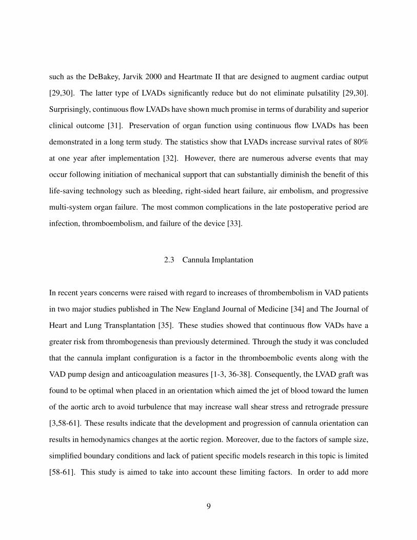
4.3 Changing bounds on pareto plot showing the objective functions against each

other where the baseline initial guess for the model is represented at ”1” . . . 38

4.4 Contour plots for the objective function minimizing Wall Shear Stress for 3

orientation parameters . . . . . . . . . . . . . . . . . . . . . . . . . . . . . . 39

4.5 Contour plots for the objective function minimizing stroke percentile for 3

orientation parameters . . . . . . . . . . . . . . . . . . . . . . . . . . . . . . 40

4.6 Lagrangian particle transport of solution for Design 13 (early systole, peak

systole, early diastole and late diastole). . . . . . . . . . . . . . . . . . . . . 41

4.7 Wall Shear Stress of solution for Design 13 (early systole, peak systole, early

diastole and late diastole). . . . . . . . . . . . . . . . . . . . . . . . . . . . . 42

x

4.8 CFD Vector field of solution for Design 13 (early systole, peak systole, early


4.9 Lagrangian particle transport of solution for Design 15 (early systole, peak

systole, early diastole and late diastole). . . . . . . . . . . . . . . . . . . . . 43

4.10 Wall Shear Stress of solution for Design 15 (early systole, peak systole, early


4.11 CFD Vector field of solution for Design 15 (early systole, peak systole, early


A.1 Full LVAD circuit schematic . . . . . . . . . . . . . . . . . . . . . . . . . . 47

A.2 Fluid domain boundaries (LVAD-Left Ventricular Assist Device inflow can-

nula, AA-Ascending Aorta, LCor-Left Coronary Artery, RCor-Right Coro-

nary Artery, DA-Descending Aorta, RSA-Right Subclavian Artery, RCA-

Right Carotid Artery, RVert-Right Vertebral Artery, LCA-Left Carotid Artery,

LVert-Left Vertebral Artery and LSA-Left Subclavian Artery). . . . . . . . . 55

xi

LIST OF TABLES

3.1 Tabulated constants obtained from curve fitting Carreau-Yasuda . . . . . . . 15

3.2 Calculation representation to generate the values for the stroke percentile for

DESIGN 22 . . . . . . . . . . . . . . . . . . . . . . . . . . . . . . . . . . . 32

4.1 Design manager solutions showing the design number, parameter changed

and values for the objective functions . . . . . . . . . . . . . . . . . . . . . . 35

xii

CHAPTER 1: INTRODUCTION

1.1 Introduction

The American Heart Association (AHA) estimates that 5.8 million people in the United States

alone are affected from heart failure (HF). Due to that statistic cardiovascular disease is the leading

cause of death globally [1,2]. This includes the condition in which the heart cannot pump enough

blood to circulatory system ultimately leaving the body starving for nutrient rich blood [2,3]. This

occurs because the heart is too weak to pumping blood from the left ventricle through the ascending

aorta that will in turn supply oxygenated blood to the rest of the body. In general, it is possible

to quantify heart failure by Ejection Fraction (EF), that relates the stroke volume (SV) to the end-

diastolic volume (EDV) and end-systolic volume (ESV) which can correlate to a value associated

with heart failure shown in equation 1.1. Ejection Fraction (EF) can be calculated by the division

of SV and EDV shown in equation 1.2. A healthy adult should fall in the range of 50%-70% EF

[1]. This percent will decrease with age due to the hearts efficiency aging with time where a VAD

may come into play for someone with a low EF.

EF (%) = SV /EDV ∗ 100 (1.1)

SV = EDV − ESV (1.2)

Patients with end stage heart failure who cannot be treated depending on availability are fitted with

an LVAD as a bridge to transplantation until a suitable donor heart becomes available. Due to

the high demand of heart transplants, LVADs have continuously increased in their effectiveness

1

and longevity while in the human body. However, despite these advances in VAD design and

anti coagulation treatment a patient is likely to endure a thrombo-embolism within 6 months [1,4-

6]. Given the current rate of thromboembolic events in VADs it has been hypothesized that the

occurrence of a stroke can be decreased by adjusting the outflow cannula implantation to direct

clots away from the cerebral vessels and direct them toward the descending aorta (DA). Studies

have shown up to a 50 percent reduction in embolization rates depending on the outflow cannula

location [8,9].

In order to accomplish this a formal computational framework is established consisting of: (1) 3D

pulsititle CFD simulation of the VAD bed hemodynamics and thrombus transport. (2) Lumped Pa-

rameter Model (LPM) of the peripheral circulation providing the boundary conditions at the edges

of the computational domain, and (3) a formal shape optimization algorithm that automatically

adjusts the input design parameters to meet the end goal of minimizing stroke rate and wall shear

stress. A brief overview of the analysis component is provided next and detailed in chapter 3.

1.2 Stroke

Stroke remains as the major source of morbidity and mortality for patients fitted for LVADs. This

is due to adverse hemodynamics, such as re-circulation zones, stagnation regions, and high shear

stress regions causing platelet activation and thrombogenesis or the formation of blood clots. Once

dislodged, these clots can travel from the LVAD to cerebral vessels causing stroke. The design

of the device, rotational speed as well as the location of the outflow graft all play a role in the

hemodynamics and thrombogenisis [4-6]. Clots originate in the ventricle itself, between the pump

impeller and the blades, and the inflow and/or outflow cannula. Despite these factors, LVAD

implantation is a treatment for HF, whose complications includes VAD induced stoke incidence

anywhere from 14%-47% from 6 months to over a year and survival rates of 80% at 12 months

2

and 70% at 24 months [7].

Figure 1.1: LVAD implantation on heart (blausen.com)

1.3 Lumped Parameter Model (Vascular Organization)

The human vascular organization allows the transportation oxygenated and nutrient rich blood from

the heart to the body. The human systemic and pulmonary vasculature is illustrated in figure 1.3.

The combined length of all the vessels is estimated to be 60,000 - 100,000 miles. This is impossible

to model completely where the CFD analysis focuses on a small portion of interest. In this study

the use of a ”lumped” vessel system derived from a Windkessel model can be incorporated to

simplify the problem and provide the necessary boundary conditions for the 3D CFD analysis [1].

The Windkessel model relies on the analogy between the 3D hemodynamics and a 0D electric

circuit lumped parameter model of the peripheral circulation.

In this study, the focus of the 3D pulsatile model is on that portion of the arterial system that in-

cludes Carotid and Vertebral arteries that supply blood to the brain that come from the ascending

aorta from the left ventricle. The Subclavian arteries that supply blood to the arms and the coro-

3

Figure 1.2: LVAD implantation and components (mayoclinic.org)

naries that supply blood to the heart. Lastly, descending aorta that supplies the lower body with

blood. A typical adult at rest will have a cardiac output of 5 L/min. The LPM is coupled with a 3D

CFD model in this case allowing the analysis to be preformed. From the LPM the pulsatile inflow

and outflow boundary conditions for the model can be generated which are a critical component in

the analysis.

4

Figure 1.3: Circulatory system (theheartfoundation.orm)

1.4 Modeling

The 3D model of the VAD bed is generated from the de-identified patient Computed Tomography

(CT) scans to allow for a CFD analysis. This is accomplished using medical segmentation soft-

ware, Mimics, along with the use of solidworks for needed adjustments. The Ordinary Differential

Equations (ODEs) derived from the LPM are solved using Runge-Kutta methods and the LPM is

tuned to match catheter data and provide boundary conditions to the CFD. In the CFD flow solver

a no slip condition is imposed at the boundary walls as the viscous fluid has a zero velocity at the

wall [1-3].

The tracking of particles or thrombi is accomplished using a Lagrangian approach where the par-

5

ticles are traced in space and time. When a simulation is running, the particles can be released at

a critical location in the computational domain while embolization statistical analysis can be car-

ried out; here the optimization can come into play to decrease the particles reaching the cerebral

vessels.

1.5 Optimization Method

Optimization in engineering is of great importance in solving complex problems. In optimization

a set of values are found to allow the objective function to be satisfied [4,19]. In multi-objective

problems there are several objectives to be optimized for, not leading to a single best solution but

a range of suggested best solutions known as a Pareto front [3]. In the StarCCM+ commercial

software utilized in the study, the optimization tool Design Manager incorporates the HEEDS and

SHERPA optimization software scheme [53,55].

HEEDS (Hierarchical Evolutionary Engineering Design System) is a software package that allows

the interface with commercial CAD software to assist in the improvement of designs with the

use of optimization. HEEDS includes SHERPA (Simultaneous Hybrid Exploration that is Robust,

Progressive, and Adaptive) that is an efficient and Robust optimization search algorithm. HEEDS

uses this hybrid and adaptive algorithm, SHERPA, as its default search method during an analysis.

SHERPA is a unique search algorithm that performs a Simultaneous Hybrid Exploration that is Ro-

bust, Progressive, and Adaptive that is developed by Red Cedar Technology. During a single

search, SHERPA uses multiple search methods for example gradient based and non-gradient based

search algorithms simultaneously rather than sequentially. This approach uses the best attributes

of each search method. If a particular search method is deemed to be ineffective, SHERPA reduces

its participation. The number of different methods that are used can range between two and ten. As

6

SHERPA learns more about the design space, it determines when and to what extent to use each

search method.

In this study the parameters, cannula angle angle of incidence (β), cannula location along the

ascending aorta distance from IA (δ) and the coronal angle (θ) are optimized to meet the response

of minimizing particles reaching the cerebral vessels, stroke percentile, and the minimizing of Wall

Shear Stress (WSS).

Figure 1.4: Parameters optimized in study

1.6 Application

In the combination of CFD and optimization to model the cannula outflow graft it is possible to

replicate the conditions found in a patient. With the improvements in high performance computing

and imaging techniques a robust model is made to help in the treatment planning. These methods

of optimization and computational analysis can be found in other applications in an engineering

setting.

7

CHAPTER 2: LITERATURE REVIEW

2.1 Heart Failure

Therapy with a LVAD is an established treatment for patients with end stage HF. In the United

States Heart Failure (HF) can be seen in over 5 million people and is a major health problem [20].

Studies show that developed HF is predicted to increase by 46% in the next 15 years [21]. VADs

are the current therapy for HF patients that are waiting for a heart transplant to become available

as the list for transplants exceeds the number of donors [22]. For those patients that do not qualify

for a heart transplant VADs can serve as a permanent attempt at a solution to help the failing heart

[23]. VADs were originally created to assist in this bridge to transplantation but through the years

however with the success of short term cardiac VAD support led to research and trials in devices

that could provide long term support with LVADs [24].

2.2 Left Ventricular Assist Devices

To date mechanical pumps are the most promising support for patients needing a cardiac transplant.

The success of short-term bridge devices led to clinical trials evaluating the clinical suitability of

long-term support with left ventricular assist devices (LVADs). The first larger-scale, randomized

trial that tested long-term support with a LVAD reported a 44% reduction in the risk of stroke or

death in patients with end-stage HF [25]. The well-documented imbalance between the number

of potential transplant recipients and available donor organs, and the technological advances in

device design and miniaturization have allowed LVADs to become a well-established therapy for

adults and children [26-28]. There are two types of LVADs: 1st generation pulsatile-type that

were designed to mimic cyclic cardiac flow and 2nd generation continuous axial-flow LVADs

8

such as the DeBakey, Jarvik 2000 and Heartmate II that are designed to augment cardiac output

[29,30]. The latter type of LVADs significantly reduce but do not eliminate pulsatility [29,30].

Surprisingly, continuous flow LVADs have shown much promise in terms of durability and superior

clinical outcome [31]. Preservation of organ function using continuous flow LVADs has been

demonstrated in a long term study. The statistics show that LVADs increase survival rates of 80%

at one year after implementation [32]. However, there are numerous adverse events that may

occur following initiation of mechanical support that can substantially diminish the benefit of this

life-saving technology such as bleeding, right-sided heart failure, air embolism, and progressive

multi-system organ failure. The most common complications in the late postoperative period are

infection, thromboembolism, and failure of the device [33].

2.3 Cannula Implantation

In recent years concerns were raised with regard to increases of thrombembolism in VAD patients

in two major studies published in The New England Journal of Medicine [34] and The Journal of

Heart and Lung Transplantation [35]. These studies showed that continuous flow VADs have a

greater risk from thrombogenesis than previously determined. Through the study it was concluded

that the cannula implant configuration is a factor in the thromboembolic events along with the

VAD pump design and anticoagulation measures [1-3, 36-38]. Consequently, the LVAD graft was

found to be optimal when placed in an orientation which aimed the jet of blood toward the lumen

of the aortic arch to avoid turbulence that may increase wall shear stress and retrograde pressure

[3,58-61]. These results indicate that the development and progression of cannula orientation can

results in hemodynamics changes at the aortic region. Moreover, due to the factors of sample size,

simplified boundary conditions and lack of patient specific models research in this topic is limited

[58-61]. This study is aimed to take into account these limiting factors. In order to add more

9

fidelity to the computational model, the utilization of optimization methods coupled to a electrical

circuit LPM, to provide a robust CFD simulation, and a patient specific geometry are included to

achieve an accurate solution.

10

CHAPTER 3: METHODOLOGY

A pulsatile multi-scale computational fluid dynamics study is established a physiology augmented

by a continuous-flow VAD. The existence of an optimal configuration of LVAD conduit angle

and anastomosis location (distance from the innominate) that significantly reduces the number of

thrombi reaching the carotid and vertebral arteries leading to stroke is investigated. The main

outcome of the study will thus establish whether our hypothesized VAD-OG optimal implantation

effectively reduces stroke incidence under realistic pulsatile conditions.

The Multiscale model in this study consists of:

• 3D solid model of the VAD-assisted circulation

• A CFD flow solver that will provide the full 3D and temporal resolution of the hemodynam-

ics within the anatomy

• A 0D lumped parameter model (LPM) consisting of an electrical circuit analog of the pe-

ripheral circulation that provides the time dependent boundary conditions necessary to drive

the CFD solution

• Lagrangian Phase Model to allow tracking of particles ranging in size and randomized time

at the VAD inlet and AA

• A automated optimization coupling algorithm to allow the cannula outflow graft location be

optimized while coupled with the LPM

The CFD study entails multi-scale 3D simulations of the pulsatile flow conditions in the aortic-

LVAD circuit and the prediction of thrombus transport for sizes ranging from 2mm, 4mm and

11

5mm to the left carotid artery (LCA), the right carotid artery (RCA), the vertebral and coronaries

arteries. The LPM driving the CFD simulation will be tuned to achieve targeted outflow flow rates

and pressure waveforms as well as VAD to Cardiac Ejection ratios (4:1 and 5:0), and vary the

incidence angle (β) and location of the LVAD conduit anastomosis (θ and δ) in order to determine

which configuration leads to a significant reduction in the incidence of thrombi reaching the carotid

and vertebral arteries and coronaries (figure 3.9). The study utilizes a realistic aortic arch geometry

extracted from an adult CT-scan with the Mimics medical imaging software. All computations are

carried out on the 250 CPU cluster in the computational mechanics lab and the advanced research

computing center at the University of Central Florida.

3.1 Preliminary Studies

Researchers at UCF carried out and published steady-flow 3D CFD analyses for a synthetic anatomy

of a typical adult aorta, as well as a patient-specific anatomy imposing typical flow split outlet con-

ditions for the human adult [1, 6-7, 10-13]. Continuous flow LVADs significantly reduce pulsatility

and, in contrast to the cardiac pulse, produce a steady baseline flow with diminished periodicity.

Follow-up work has been done by designing and tuning a 0D multi-degree to freedom lumped

parameter model (LPM) for a continuous flow LVAD assisted circulation, incorporating the LVAD

pump-model has been carried out [13]. Later, Prather integrated the LPM to the 3D CFD model for

the patient specific aortic arch geometry utilized in previous published steady state flow investiga-

tions. All carried out computations so far were using a Newtonian blood model exploring a single

diameter thrombus model and a ratio of 4 L/min VAD flow to 1 L/min cardiac output to compare

the intermediate and perpendicular VAD-OG anastomoses. Particles released were randomized in

both space (VAD-OG inlet plane) and time (over the cardiac cycle). Results exhibited a correlation

between VADOG anastomosis and incidence of released thrombi reaching the cerebral vessels.

12

3.2 Geometry Rendering

The model geometry consists of a patient specific model that was retrieved from Computed Tomog-

raphy (CT) Angiographic de-identified images of an adult to generate a 3D model using the medical

segmentation software Mimics R© and 3-matic provided by collaborators at Orlando Health. The

CAD model generated is imported in the CFD destination software. Mimics is a medical seg-

mentation software that allows the user to extract components form a CT scan where 3 matic is a

advanced CAD program allowing the complex design to be rendered. In the figure below the model

generation and fluid domain can be seen. The model includes the ascending aorta, subclavian, ver-

tebral, common carotids, cornaries and the LVAD cannula that is varying in the problem. The

LVAD cannula implantation parameters include the coronal angle, cannula angle and the cannula

location along the ascending aorta. These 3 parameters will be changing resulting in th movement

of the cannula to find the optimal location based on the responses of the system.

Figure 3.1: Model Generation [1]

13

Figure 3.2: Patient specific Geometry

14

3.3 Computational Fluid Dynamics Model

The commercial CFD software StarCCM+ 3.04.010 (CD-Adapco) that numerically solves the con-

servation equations of fluid flow. Blood is modeled as an incompressible shear-thinning Non-

Newtonian fluid with density of 1060 kg/m3 while blood viscosity as function of shear rate (γ) is

taken as a modified three-parameter Carreau-Yasuda model.

µ(γ) = µ∞ + (µ0 − µ∞)(1 + (λγ)2)−1/3 (3.1)

Table 3.1: Tabulated constants obtained from curve fitting Carreau-Yasuda

Hematocrit(%) µ∞ [cP] µ0 [cP] λ [cP]

40 4.3989 8.4248 0.3013

Where depending on the hematocrit, each model constant, viscosity at high shear rate µ∞, vis-

cosity at zero shear rate µ0, and relaxation time λ and n the power constant have been computed

by mean of least squares curve fit. This model is implemented in the multi-scale simulation for a

40% hematocrit level and will characterize the viscosity on a local level allowing for more precise

statistical inferences. To retain great accuracy second order temporal discretization is employed

for the transient term. Convective terms are resolved with to a second order upwind scheme. Star-

CCM+ is a finite volume CFD software capable of solving 2D and 3D flows including transients

and steady state simulations in the viscous, turbulent, laminar sub-sonic and super-sonic realms.

The time-depedent boundary conditions imposed on the flow field are described in terms of inlet

flow rates (cardiac ejection and VAD-OG outflow) and boundary conditions imposed by the LPM.

The CFD code uses algorithms to solve the conservation of mass and momentum that govern the

15

fluid mechanics known as the Navier-Stokes equations.

∇ ∗ ~V = 0 (3.2)

ρd~V

dt+ ρ(~V ∗ ∇)~V = −∇p+∇ ∗ σ + ~Fb (3.3)

3.4 Grid Structure

The grid is generated using the Surface Wrapper, Surface Remesher, and Prism Layer modules of

StarCCM+. Surface Wrapper and Remesher modules repair imported geometries to produce high

quality meshes. The Prism Layer module allows refinement of the mesh near the walls permitting

the user to control the size of the first element as well as the element growth rate in order to

accurately capture the boundary layer.

16

Figure 3.3: Computational grid of fluid domain

17

Figure 3.4: Computational grid of fluid domain from the Aortic root view

18

3.5 Thrombi Modeling

In order to track particle (thrombi) trajectories with properties analogous to the blood clots, Star-

CMM+ utilizes a Lagrangian Phase Model that solve the Maxey-Reily equation [53,55]. Here,

particles are introduced in the computational domain by means of an injector; and the evolution of

the particle trajectory is governed by the momentum conservation equation in terms of the particle

velocity and sum of the forces acting on the particle that include the body, surface and wall. The

conservation equation of momentum for a particle is written in the Lagrangian framework. The

change in momentum is balanced by surface and body forces that act on the particle. The equation

of conservation of (linear) momentum for a material or DEM particle of mass mp is given by:

mpd~vpdt

= ~Fbody + ~Fsurface (3.4)

where vp denotes the instantaneous particle velocity, Fsurface is the resultant of the forces that act

on the surface of the particle, and Fbody is the resultant of the body forces. These forces in turn are

decomposed into:

∑~Fsurface = ~Fdrag + ~Faddedmass + ~Fsaffman + ~Fwall (3.5)

The main body force acting on the thrombi is the added mass, with the buoyancy force playing a

nearly negligible role due to the fact the density ratio between blood and the thrombus particle is

1.097. The density of thrombi is taken from the literature to be 1116.73 kg/m3. The main surface

force is that due to viscous drag force caused by the relative velocity of the particles with respect to

the continuous phase, and it is expressed in terms of a drag coefficient, (estimated by the Schiller-

Naumman or a user-defined correlation) the particle cross-section and the particle slip velocity.

19

Other surface forces that are incorporated in the model are the Saffman lift force and the correction

due to pressure.

Figure 3.5: Particle injector location for the cannula outflow graft

The Lagrangian tracking models includes solid spherical particles shown as a mass of set diameter

of 2, 4 and 5 mm that are released form the bottom of the cannula. The release of particles is

random utilizing an excel sheet bounded by 0 and 1 that impose a time step that releases a constant

number of particles at the nodes of the grid. As the model injects the particles they can be tracked in

space and time throughout the model allowing the final simulation to count the number of particles

at the outlets and signifying where they went. Real time plots and images can be generated to show

and tabulate the results as the model runs. By performing five or more cycles it can be determined

the statistics of thromboembolization to the carotid and vertebral arteries for a given VAD-OG

implantation configuration. Under varying conduit configurations, we can determine statistical

significance of differences in thrombo-embolization rates.

20

3.6 Lumped Parameter Model

The fluid domain is coupled with a 0D electrical circuit to provide the boundary conditions for

the model. Pulsatile flow boundary conditions for the 3D CFD analysis of the aortic-LVAD hemo-

dynamics are interactively provided by a 0D electrical circuit lumped parameter model (LPM) of

the entire circulation via a 0D-3D iterative loose coupling. The LVAD circulation can be modeled

using multi-DOF Windkessel models. The resistance, R accounts for the vascular resistance, the

capacitance C accounts for compliance, the inductance L accounts for the inertial terms, the diodes

model the atrio-ventricular valves, the tricuspid, and mitral valves and these operate on an on/off

mode Heaviside step function, triggered by pressure gradient across the valve (typically 15 mmHg)

characterized by its own resistance.

The elastance function En is the ratio of ventricular pressure to volume which can be shown by

the inverse of the capacitance and drives the pulsitility. Equation 3.2 shows two sections where

the first bracket of the equation is the systolic phase the growth is controlled by the exponent. The

second bracket is the diastole the function decreases shown in the large power in the denominator.

E(t) = 1.55 ∗[

( tn0.7

)1.9

(1 + tn0.7

)1.9

][1

(1 + tn1.17

)21.9

](3.6)

E(t) = (Emax − Emin) ∗ En(tn) + Emin (3.7)

tn =t

tc(3.8)

21

Figure 3.6: Full LPM circuit to drive the flow field for the CFD model

tc =60

HR(3.9)

∆V = IR → ∆p = QR (3.10)

the voltage difference (∆V ) is analogous to the pressure drop over a distance in the vessel (∆p)

and the current (I) is the volume flow rate of blood through that same segment of vessel (Q). The

circuit elements can be described in mathematical form as follows, where Cvr, Cvc, and Cvl are

tuning parameters used to adjust the nominal values obtained from Poiseuille and linearized flow

arguments.

22

∆p = QR → R =8µl

πr4Cvr (3.11)

Q = Cdp

dt→ C =

3πlr3

2EhCvc (3.12)

∆p = LdQ

dt→ L =

9ρl

4πr2Cvl (3.13)

(a) Compliance (Capacitance) (b) Fluid Resistance (Resistance) (c) Inertia (Inductance)

Figure 3.7: The physical meaning of each circuit element

A time-dependent compliance models the heart pumping action driving the circulation. The elas-

tance ratio of ventricular pressure to ventricular volume is a measure of the level of heart disease:

an adult healthy heart has a typical maximum elastance of 2 [mmHg/ml], while the severely dis-

eased heart value is 1 [mmHg/ml]. This model is tuned to provide a given waveform for the cardiac

outputs. The LVAD modeled on a rotary mechanical pump connected with two cannulae between

the left ventricle and the aorta. The LVAD pumps blood continuously from the left ventricle into

the aorta [4]. Here the pressure difference between the left ventricle and the aorta is characterized

by the relationship:

LV P (t)−AoP (t) = Ri ∗Q+LidQ

dt+Ro ∗Q+Lo

dQ

dt+Rp ∗Q+Lp

dQ

dt−Hp +Rk ∗Q (3.14)

23

Figure 3.8: Elastance function plot of a healthy heart

Where Hp is the pressure head gain across the pump. Q is the blood flow rate through the pump.

The parameters, Li, Lo, and Lp represent the flow inertances and Ri, Ro, and Rp represent the flow

resistances of the pump and cannulae, respectively.

The basic relations utilized relate the flow rate across a compliance and inductance in series is that

the pressure drop is given in the circuit element (figure 3.7). The pump functions in parallel to the

heart of the patient, here the parallel connection of the LVAD pump between the left ventricle and

the aorta [4]. The resulting coupled set of non-linear ODE’s are solved by Runge-Kutta-Felhberg

adaptive time-stepping.

24

Figure 3.9: Elastance function plot of a healthy heart

Using Kirchhoff node and loop laws the LPM circuit can be represented by 50 first order ODEs

where the equations are solved using an in house 4th order Runge-Kutta adaptive time stepping

scheme. The components of the circuit are tuned to output flows and pressure wave forms similar

to wave forms that can be generated from catheter or clinical studies. The boundary conditions are

then sent to the CFD. The overall systemic flow is taken as 5 [L/min] where the split between VAD

and aortic root are 4 [L/min] and 1 [L/min] respectively.

3.7 Optimization Algorithm

The optimization in this study is setup as a multi objective solver utilizing the SHERPA algorithm.

During the analysis (SHERPA) identifies the parameter values for the designs so as to best meet

the analysis objectives. This is done by running several designs. For each design generated by the

25

optimization scheme, a loose coupling is implemented between the LPM and the CFD to generate

converged flow fields. The responses and parameters are shown below:

Objective function:

• min J(δ, β, θ) = SR(δ,β,θ)SRbaseline(δ,β,θ)

+ WSS(δ,β,θ)WSSbaseline(δ,β,θ)

• Subject to: 4.7≤ δ ≤5.7 cm, 50 ≤ β ≤ 130 Degrees, 0 ≤ θ ≤ 40 Degrees

Responses:

• Minimize Stroke Rate (SR) (%)

• Minimize Wall Shear Stress (WSS) (dy/cm2)

Parameters of interest with constraints:

• Cannula location (δ): 4.7≤ δ ≤5.7 cm from the AA

• Cannula angle (β): 50 ≤ β ≤ 130 Degrees

• Coronal angle (θ): 0 ≤ θ ≤ 40 Degrees

The objective function is normalized by the baseline geometry that was found from Prather [1] in

the objective function. From image 3.9 the baseline can allow for an appreciation of the movement

of the cannula. Moreover, in figures 3.10-3.12 a sequence of figures illustrate the movement of the

cannula as seen in the optimization algorithm.

26

Figure 3.10: Cannula orientation visual to show the three parameters of interest.

27

Figure 3.11: Cannula movement on ascending aorta (δ) showing automatic shape optimization.

28

Figure 3.12: Cannula angle (β) movement on ascending aorta showing automatic shape optimiza-tion.

29

Figure 3.13: Coronal angle (θ) movement on ascending aorta showing automatic shape optimiza-tion.

30

3.8 Coupling Optimization Scheme

The automation optimization scheme is setup to allow the coupling of the LPM to the CFD which is

then combined with the Design Manager optimization package in StarCCM+ (figure 3.13). In order

to do this, a batch file is submitted that calls to two java files, the first file controls the running of the

Design Manager optimization program where the other controls the coupling of the simulation to

the LPM. From the second java file the Runge-Kutta solver will run with the C++ code to generate

the flow conditions for the simulation. This all has to be packaged into one submission file that can

be submitted to the cluster to run (see appendix). Currently the optimization scheme runs on 120

cores for 8 days that produces 22 designs.

Figure 3.14: Optimization scheme which combines a shape optimization algorithm based on userdesign parameter inputs such as cannula anastomosis location and angle

31

3.9 Statistical Analysis

In the Design Manager package the reporting of particle count at the outlets is automated in a

script to generate the statistics for the current design objective function evaluation. Particles are

released at random throughout the transient simulation according to a random number sequence

using a routine in excel. The model run 5 times in which the particles are released for the varying

2mm, 4mm and 5mm diameters over the interval of 3 heart cycles. The particles are released from

a part injector randomly in space and time over the inlet plane. After the simulation is complete

the number of particles at the outlets are counted to give the stroke percentile for the design run.

Particle(%) =Number of particles at cerebral vessels outlets

Number of particles at all outlets∗ 100 (3.15)

The wall shear stress of the model is given by the surface average peak wall shear stress for the

transient simulation. This includes the all surfaces of the entire model shown in dy/cm2 These

two objectives allow for the SHERPA algorithm to generate the next set of design based on these

responses.

Table 3.2: Calculation representation to generate the values for the stroke percentile for DESIGN22

SizeParticle(mm)

DA%

LCOR%

LVert%

LCA%

LSA%

LVAD%

RCor%

RVert%

RCA%

RSA%

StrokeTotal %

2 77.46 0.40 3.43 3.23 8.11 0.00 0.09 1.23 2.82 3.22 10.724 78.47 0.20 2.02 4.03 5.35 0.09 0.14 2.08 3.65 3.96 11.795 74.06 0.16 2.61 4.80 6.36 1.51 0.19 2.06 3.66 4.58 13.14

Mean 76.66 0.25 2.69 4.02 6.61 0.54 0.14 1.79 3.38 3.92 11.88

32

Figure 3.15: Particle injector location for 2mm, 4mm, and 5mm particles for 5 cycles

33

CHAPTER 4: RESULTS

In the automated optimization scheme 22 design were run giving the objective function of min-

imizing stroke rate and wall shear stress where these objectives are equal weight. The cannnula

angle, cannula location and coronal angle are the parameters of interest. The data for each design

can be found in the table, design 13 and 15 are of interest were the objective function is satisfied.

The baseline geometry was derived from previous studies that stands as the initial guess for the

optimization study noted as design 1 [1,12]

Design number 15 meets the criteria for minimizing the stroke percentile and design 13 meets the

requirement for minimizing wall shear stress. These are two competing objectives in nature where

there is not a single optimal design in a multi objective study rather a front of designs that meet

the objective functions. In such cases, there is no single optimum design. Instead, the optimization

returns a curve along which all designs are optimum in one objective for a given value in the

other objective. This curve, known as Pareto front, expresses the optimum trade-off relationship

between two competing objectives. When plotting these objectives against each other the user can

determine which deign meets the end solutions. A Pareto front was generated showing the range

of 9.7% to 44.08% for stroke and WSS of 55.97 to 81.47 dynes/cm2 ranged over 22 implantation

configurations for the specific case studied shown in figure 4.2 and 4.3.

34

Table 4.1: Design manager solutions showing the design number, parameter changed and valuesfor the objective functions

DesignNumber

CannulaAngle β

(Deg)

CannulaShift δ(cm)

CoronalAngle θ(Deg)

Stroke(%)

WallShearStress( dycm2 )

1 90 5.7 0 31.69 81.472 122 5.4 4 16.54 65.773 94 4.8 36 22.47 63.874 72 5.7 8 20.79 60.385 116 4.9 10 14.1 62.936 130 5 30 19.98 62.057 58 5.2 0 31.97 59.178 86 5.2 14 18.41 68.399 80 4.7 18 17.87 62.0710 64 5.5 32 32.62 68.6511 50 5.1 26 36.45 73.2512 108 5.6 22 13.25 67.7713 90 5.5 8 12.51 55.9714 66 5.2 18 30 65.5615 112 5.2 0 9.7 64.2316 54 4.9 12 39.39 60.3317 50 5.7 0 44.08 73.3618 50 5.1 10 51.63 66.5519 130 5.7 8 16.72 66.5420 72 5 30 23.5 64.6821 80 4.9 18 15.58 67.7122 100 5.4 10 11.94 61.10

35

Figure 4.1: Cannula orientation visual to show the three parameters of interest

Contour plots of varied parameters based on the objective function are generated to show the effect

of these changes to the LVAD model. The contours of WSS shown in figure 4.4 signify the lowest

WSS found at the dark purple or darkest location on the plot. The contour for the smallest WSS

should directly correlate to table 4.1 where the best design is shown as design 13. From the coutour,

the darkest location represented the cannula angle, coronal angle, and cannula Z which can be seen

as 90, 8 and 5.5 respectively.

36

Figure 4.2: Pareto plot showing the objective functions against each other where the baseline initialguess for the model is represented at ”1”

The contour of stroke percentile shown in figure 4.5 will replicate the same objective of the plot in

figure 4.3 here the smallest stroke percentile can be found at the darkest point represented as design

15 at 9.7%. Where the coutours darkest location represented the cannula angle, coronal angle, and

cannula Z which can be seen as 112, 0 and 5.2 respectively.

37

Figure 4.3: Changing bounds on pareto plot showing the objective functions against each otherwhere the baseline initial guess for the model is represented at ”1”

38

Figure 4.4: Contour plots for the objective function minimizing Wall Shear Stress for 3 orientationparameters

39

Figure 4.5: Contour plots for the objective function minimizing stroke percentile for 3 orientationparameters

40

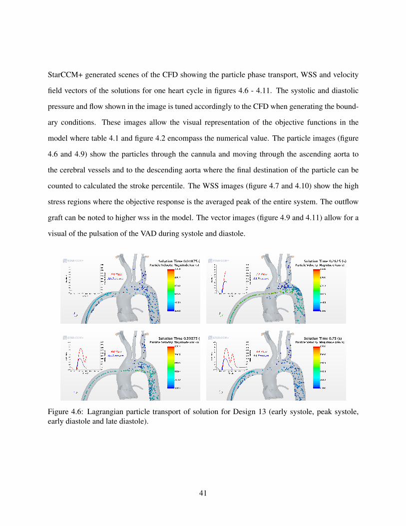
StarCCM+ generated scenes of the CFD showing the particle phase transport, WSS and velocity

field vectors of the solutions for one heart cycle in figures 4.6 - 4.11. The systolic and diastolic

pressure and flow shown in the image is tuned accordingly to the CFD when generating the bound-

ary conditions. These images allow the visual representation of the objective functions in the

model where table 4.1 and figure 4.2 encompass the numerical value. The particle images (figure

4.6 and 4.9) show the particles through the cannula and moving through the ascending aorta to

the cerebral vessels and to the descending aorta where the final destination of the particle can be

counted to calculated the stroke percentile. The WSS images (figure 4.7 and 4.10) show the high

stress regions where the objective response is the averaged peak of the entire system. The outflow

graft can be noted to higher wss in the model. The vector images (figure 4.9 and 4.11) allow for a

visual of the pulsation of the VAD during systole and diastole.

Figure 4.6: Lagrangian particle transport of solution for Design 13 (early systole, peak systole,early diastole and late diastole).

41

Figure 4.7: Wall Shear Stress of solution for Design 13 (early systole, peak systole, early diastoleand late diastole).

Figure 4.8: CFD Vector field of solution for Design 13 (early systole, peak systole, early diastoleand late diastole).

42

Figure 4.9: Lagrangian particle transport of solution for Design 15 (early systole, peak systole,early diastole and late diastole).

Figure 4.10: Wall Shear Stress of solution for Design 15 (early systole, peak systole, early diastoleand late diastole).

43

Figure 4.11: CFD Vector field of solution for Design 15 (early systole, peak systole, early diastoleand late diastole).

44

CHAPTER 5: CONCLUSION

The fully automated optimization of the LVAD outflow graft anastomosis orientation to minimize

stroke rate and WSS successfully generated a set of 22 designs where the Pareto plot showed two

optimal designs. The Pareto front was generated showing the range of 9.7% to 44.08% for stroke

and WSS of 55.97 to 81.47 dy/cm2 ranged over 22 implantation configurations for the specific case

studied. The countur plots signify the importance of the parameter optimized where design 13 and

design 15 best suit these objectives. These solutions can be seen in design 13 and 15 where the

stroke percentile and wall shear are 12.5% and 55 dy/cm2 for design 13 and 9.6% and 64 dy/cm2

for design 15. This study provides the foundation of future LVAD cannula optimizations studies

aiming to assist clinicians in the placement of the cannula based on a patient specific geometry to

reduce stroke and potential thrombogenicity.

5.1 Future Work

This study finds limitations in the assumption that the vessel wall are considered rigid and that par-

ticle interactions are limited to particle-to-wall and particle-to-fluid. Future studies may implement

wall compliance in the form of fluid-structure interaction modeling and the inclusion of discrete

element model to allow for particle-to-particle interactions. After more data is generated the user

may come to find limiting the optimization parameters range will increase in fidelity of the model

and give a exact solution. Future runs may include optimization for 40 or more designs, limiting

the movement of the 3 cannula parameters and including particles from the arotic root.

45

APPENDIX A: CIRCUIT DIAGRAMS AND LPM EQUATIONS

46

Figure A.1: Full LVAD circuit schematic

47

Current Auxiliary Equations

48

Voltage Auxiliary Equations

CFD Voltage Auxiliary Equations

Circuit ODEs

49

Figure A.2: Fluid domain boundaries (LVAD-Left Ventricular Assist Device inflow cannula,AA-Ascending Aorta, LCor-Left Coronary Artery, RCor-Right Coronary Artery, DA-DescendingAorta, RSA-Right Subclavian Artery, RCA-Right Carotid Artery, RVert-Right Vertebral Artery,LCA-Left Carotid Artery, LVert-Left Vertebral Artery and LSA-Left Subclavian Artery).

55

APPENDIX B: Codes

Batch submission script

#!/bin/bash

#SBATCH --job-name=lvadOpt

##SBATCH --distribution=cyclic

##SBATCH --ntasks=120

#SBATCH --ntasks-per-node=16

#SBATCH --nodes=7

##SBATCH --nodelist=c2-5,c2-6,c2-7

##SBATCH --mem-per-cpu=3900

#SBATCH --output=job.%J.out

#SBATCH --time=200:00:00

#Select how logs get stored

mkdir $SLURM_JOB_ID

export debug_logs="$SLURM_JOB_ID/job_$SLURM_JOB_ID.log"

export benchmark_logs="$SLURM_JOB_ID/job_$SLURM_JOB_ID.log"

# Point to the license server

export [email protected]

# Load Modules

module load starccm/starccm-13.04.010

56

#module load starccm/starccm-13.04.010

unset SLURM_GTIDS

# Enter Working Directory

cd $SLURM_SUBMIT_DIR

# Create Log File

echo $SLURM_SUBMIT_DIR

echo "JobID: $SLURM_JOB_ID" >> $debug_logs

echo "Running on $SLURM_NODELIST" >> $debug_logs

echo "Running on $SLURM_NNODES nodes." >> $debug_logs

echo "Running on $SLURM_NPROCS processors." >> $debug_logs

echo "Current working directory is ‘pwd‘" >> $debug_logs

# Module debugging

module list >> $debug_logs

date >> $benchmark_logs

echo "ulimit -l: " >> $benchmark_logs

ulimit -l >> $benchmark_logs

# Run job

sim_file="ps_lvad_opt.dmprj"

STARTMACRO="OptimizationAutomation.java"

#STARTMACRO="run.java"

#NODEFILE="$(pwd)/$SLURM_JOB_ID/slurmhosts.$SLURM_JOB_ID.txt"

#srun hostname -s &> $NODEFILE

57

hostlist=$(hostlistprocessing.pl)

NODEFILE="$(pwd)/nodelistalloc.txt"

starlaunch jobmanager --command "starccm+ -np $SLURM_NTASKS $sim_file

-batch $STARTMACRO -batch-report" --slots 0 --resourcefile $NODEFILE

echo "Program is finished with exit code $? at: ‘date‘"

sleep 3

date >> $benchmark_logs

echo "ulimit -l" >> $benchmark_logs

ulimit -l >> $benchmark_logs

mv job.$SLURM_JOB_ID.out $SLURM_JOB_ID/

58

JAVA file used to control simulation file

package macro;

import java.nio.file.*;

import static java.nio.file.StandardCopyOption.*;

import java.nio.file.attribute.*;

import static java.nio.file.FileVisitResult.*;

import java.io.IOException;

import java.util.*;

import java.lang.*;

import star.common.*;

import star.base.neo.*;

import star.vis.*;

import java.io.*;

import star.lagrangian.*;

// Note: To get macro commands from the CFD simply hit the record

button and save the Java file. Once you are done with the in

software commands, hit stop and all the

// commands will be saved in the Java file you created. These commands

can be used below.

// USER TODO: update file paths accordingly as well as coupling

59

variable to modify CFD-LPM interaction

public class LVADCoupler extends StarMacro

{

// TODO: user needs to choose if the simulation is a steady or

unsteady one, make sim file changes accordingly

public String state = "unsteady";

// TODO: user needs to set up the number of coupling cycles and the

number of sampling cycles for particle data collection

public int num_cycles = 15;

public int num_sampling_cycles = 3;

public int num_heart_cycles = 3;

// TODO: user can set up the error threshold for the coupling (the

error is calculated as the difference between LPM-BC cycles)

public double e = 0.001;

// TODO: user can set up the number of time-steps

public int steps_per_cycle = 400;

// TODO: user can set up the number of rk time-steps

public int LPM_steps_per_cycle = 8000;

// TODO: user can set up HR

public double heart_rate = 80.0;

60

// TODO: user can set up number of inner iteration for CFD

public int iters_per_step = 100;

public int iters_per_step_final = 50;

// TODO: user must set up paths to ensure proper data backup and data

transfer

public String simName = "ps_lvad_opt";

public String parentDir = "/lustre/fs0/home/blozinski/LVAD1/";

public String mainPath = parentDir + simName + "/";

public String simFolder = mainPath + "sim/";

public String resultsFolder = mainPath + "results/";

public String simPath = simFolder + simName + ".sim";

public String backUpDir = mainPath + "lpm/backUps/";

public String rkExePath = mainPath + "lpm/RK_LPM";

public String rkOutputTablePath = mainPath + "lpm/Outputs/LVAD.csv";

public String cfdOutputTablePath = mainPath + "lpm/Outputs/CFDOut.csv";

public String CV_path = mainPath + "lpm/Outputs/ConvergenceValues.csv";

// TODO: this step conputes time-step

public double dt = 60.0/heart_rate/steps_per_cycle;

public void execute()

{

if (state == "unsteady")

61

{

System.out.println("Simulation will be: " + state);

// This step initializes the solution

deleteFiles();

setOutputPaths();

switchPlotsScenes(false);

setTimestep();

lagrangianModelSwitch(true);

setPhysicalTime(60.0/heart_rate);

// This step perform an initialization run to generate the flow field

(user can modify low loop for mulitple runs)

runRK();

reloadTable();

clearHistory();

for (int i = 0; i < 1; i++)

runSim();

ReadData ConvVals = new ReadData();

int counter = 0;

double d = 1000.0;

// This steps runs the loose coupling to converge the model

while ((d > e) && (counter < num_cycles))

{

62

clearHistory();

reloadTable();

runSim();

updateRKInputs();

runRK();

System.out.println("Loading : Convergence Value Reading");

ConvVals.ReadInValues(CV_path);

d = ConvVals.GetConvergenceValue();

saveSim(counter);

saveDataFiles(counter);

counter++;

}

// This step run particle data collection

System.out.println("\nPhase 1: coupling converged");

System.out.println("Phase 2: particle data colleciton\n");

lagrangianModelSwitch(false);

switchPlotsScenes(true);

setPhysicalTime(60.0/heart_rate*num_heart_cycles);

for (int i = 0; i < num_sampling_cycles; i++)

{

clearHistory();

63

runSim();

getParticleTables(i);

}

}

else if (state == "steady")

{

System.out.println("Simulation will be: " + state);

setOutputPaths();

switchPlotsScenes(false);

setTimestep();

lagrangianModelSwitch(true);

setPhysicalTime(60.0/heart_rate);

clearHistory();

for (int i = 0; i < 1; i++)

runSim();

lagrangianModelSwitch(false);

switchPlotsScenes(true);

setPhysicalTime(60.0/heart_rate*num_heart_cycles);

for (int i = 0; i < num_sampling_cycles; i++)

{

clearHistory();

runSim();

getParticleTables(i);

64

}

}

else

{

System.out.println("Check what you are doing...");

}

}

// This set up the time-step in the CFD

public void setTimestep()

{

System.out.println("Loading: updating time-step");

Simulation simulation = getActiveSimulation();

ImplicitUnsteadySolver unsteadySolver = ((ImplicitUnsteadySolver)

simulation.getSolverManager().getSolver(ImplicitUnsteadySolver.class));

unsteadySolver.getTimeStep().setValue(dt);

}

// This set up the maximum physical time criterion

private void setPhysicalTime(double physicalTime)

{

System.out.println("Loading: updating physical time to " +

physicalTime);


65

PhysicalTimeStoppingCriterion physicalTimeStoppingCriterion =

((PhysicalTimeStoppingCriterion)

simulation.getSolverStoppingCriterionManager().getSolverStoppingCriterion

("Maximum Physical Time"));

physicalTimeStoppingCriterion.getMaximumTime().setValue(physicalTime);

}

// This set up to clear the CFD history but not fields

private void clearHistory() {

System.out.println("Loading: clearing sim history");


Solution solution = simulation.getSolution();

solution.clearSolution(Solution.Clear.History);

}

// This turns the lagrangian modeling on (false) and off (true)

private void lagrangianModelSwitch(Boolean state)

{

System.out.println("Loading: lagrangian model frozen - " + state);


LagrangianMultiphaseSolver lagrangianMultiphaseSolver =

((LagrangianMultiphaseSolver)

66

simulation.getSolverManager().getSolver(LagrangianMultiphaseSolver.class));

lagrangianMultiphaseSolver.setFrozen(state);

}

// This saves the simulation for backup

public void saveSim(int cycleNumber) {

System.out.println("Loading: saving simulation...");

Simulation simulation_0 =

getActiveSimulation();

String s_cycle = Integer.toString(cycleNumber);

simulation_0.saveState(resolvePath(simFolder + simName + "-" + s_cycle

+ ".sim"));

}

// This save the sata from the LPM and CFD for backup

public void saveDataFiles(int cycleNumber)

{

System.out.print("Loading: data backup...");

try

{

Runtime run = Runtime.getRuntime();

String copyRKOutput = "cp " + rkOutputTablePath + " " + backUpDir +

67

"LVAD_" + cycleNumber + ".csv";

String copyCFDOutput = "cp " + cfdOutputTablePath + " " + backUpDir +

"CFDOut_" + cycleNumber + ".csv";

Process p1 = run.exec(copyRKOutput);

Process p2 = run.exec(copyCFDOutput);

System.out.println("successful");

}

catch(IOException e)

{

System.out.println("Error while backing up data: "+ e.toString());

}

}

// This deletes old files and ensures initialization is carried out

correctly

public void deleteFiles()

{

System.out.print("Loading: deleting old files...");

try

{

Runtime run = Runtime.getRuntime();

String delRKOutput1 = "rm " + mainPath + "lpm/Outputs/LVAD.csv";

String delRKOutput2 = "rm " + mainPath + "lpm/Outputs/LVAD_prev.csv";

68

//String delSimFiles = "rm -r " + simFolder + simName + "-*";

Process p1 = run.exec(delRKOutput1);

Process p2 = run.exec(delRKOutput2);

//Process p3 = run.exec(delSimFiles);

System.out.println("successful...");

}

catch(IOException e)

{

System.out.println("Error while backing up data: "+ e.toString());

}

}

// This runs the RK solver

public void runRK()

{

System.out.println("Loading: running RK loader");

try

{

// Define the location of the RK solver executable

File rkExe = new File(rkExePath);

ProcessBuilder rkpb = new ProcessBuilder(rkExe.getAbsolutePath());

// Define the working directory of the RK solver

rkpb.directory(new File(rkExe.getParent()));

69

System.out.println("About to start RK solver");

Process rkp = rkpb.start();

// This is the waiting function that will wait for your RK Solver to

finish before starting the sim

rkp.waitFor();

System.out.println("Finished RK solver");

}

catch(Exception e)

{

System.out.println("Error while running RK solver: " + e.toString());

}

}

// This reloads the table after the LPM generates the BCs

public void reloadTable()

{

System.out.println("Loading: reload BC table LVAD.csv from LPM

initialization");


FileTable bcs = ((FileTable)

simulation.getTableManager().getTable("LVAD"));

70

bcs.setFileName(rkOutputTablePath);

//bcs.extract();

}

// This runs tbe simulation

public void runSim()

{

System.out.println("Loading: simulation launcher");

Simulation sim = getActiveSimulation();

InnerIterationStoppingCriterion innerIters =

(InnerIterationStoppingCriterion)

(sim.getSolverStoppingCriterionManager().getSolverStoppingCriterion

("Maximum Inner Iterations"));

//innerIters.setMaximumNumberInnerIterations(iters_per_step);

//sim.getSimulationIterator().step(1);

innerIters.setMaximumNumberInnerIterations(iters_per_step_final);

sim.getSimulationIterator().run();

}

// Backs up the current version of the simulation in a new folder

// called "<sim’s parent directory>- Cycle #"

public void backupCycle(int cycleNum)

{

System.out.println("Loading: databackup");

71

System.out.println("Started backup of cycle #" + cycleNum);

File simFile = new File(simPath);

Path srcDir = Paths.get(simFile.getParent());

Path destDir = Paths.get(simFile.getParent() + String.format("- Cycle

%d", cycleNum));

try

{

copyDirRecursive(srcDir, destDir);

System.out.println("Finished backup of current cycle");

}

catch(Exception e)

{

System.out.println("Error occured while backing up current cycle: " +

e);

}

}

// Program to update the Lumped model with new resistances for the

Lumped parameter model (RK solver)

public void updateRKInputs()

{

System.out.println("Loading: CFD table output to LPM");

72

Simulation sim = getActiveSimulation();

MonitorPlot plot = ((MonitorPlot)

sim.getPlotManager().getObject("CFDOut"));

plot.export(resolvePath(cfdOutputTablePath), ",");

}

// This saves the particle tables for backup

private void getParticleTables(int cycleNum)

{


MonitorPlot monitorPlot_0 = ((MonitorPlot)

simulation.getPlotManager().getPlot("Particles"));


simulation.getPlotManager().getPlot("Particles Domain"));

monitorPlot_0.export(resolvePath(resultsFolder +

"plot-particles/particles_" + cycleNum + ".csv"), ",");

monitorPlot_1.export(resolvePath(resultsFolder +

"plot-particles-domain/particles-domain_" + cycleNum + ".csv"),

",");

}

// Recursively copies the contents of srcDir to destDir

public void copyDirRecursive(final Path srcDir, final Path destDir)

73

throws IOException

{

EnumSet options = EnumSet.of(FileVisitOption.FOLLOW_LINKS);

if(Files.isDirectory(srcDir))

{

Files.walkFileTree(srcDir, options, Integer.MAX_VALUE, new

FileVisitor<Path>() {

@Override

public FileVisitResult postVisitDirectory(Path dir, IOException exc)

throws IOException

{

return FileVisitResult.CONTINUE;

}

@Override

public FileVisitResult preVisitDirectory(Path dir, BasicFileAttributes

attrs)

{

CopyOption[] opt = new CopyOption[]{COPY_ATTRIBUTES,REPLACE_EXISTING};

Path newDirectory = destDir.resolve(srcDir.relativize(dir));

try

{

Files.copy(dir, newDirectory, opt);

74

}

catch(FileAlreadyExistsException x)

{

}

catch(IOException x)

{

return FileVisitResult.SKIP_SUBTREE;

}

return CONTINUE;

}

@Override

public FileVisitResult visitFile(Path file, BasicFileAttributes attrs)

throws IOException

{

copyFile(file, destDir.resolve(srcDir.relativize(file)));

return CONTINUE;

}

@Override

public FileVisitResult visitFileFailed(Path file, IOException exc)

throws IOException

{

return CONTINUE;

}

75

});

}

}

public static void copyFile(Path src, Path dest) throws IOException

{

CopyOption[] options = new

CopyOption[]{REPLACE_EXISTING,COPY_ATTRIBUTES};

Files.copy(src, dest, options);

}

private void switchPlotsScenes(Boolean state)

{

System.out.println("Loading: scene and plot save - " + state);



simulation.getPlotManager().getPlot("Output Flow"));

PlotUpdate plotUpdate_0 = monitorPlot_0.getPlotUpdate();

plotUpdate_0.setSaveAnimation(state);


simulation.getPlotManager().getPlot("Output Pressure"));



76

//MonitorPlot monitorPlot_2 = ((MonitorPlot)


//PlotUpdate plotUpdate_2 = monitorPlot_2.getPlotUpdate();

//plotUpdate_2.setSaveAnimation(state);

//MonitorPlot monitorPlot_3 = ((MonitorPlot)


//PlotUpdate plotUpdate_3 = monitorPlot_3.getPlotUpdate();

//plotUpdate_3.setSaveAnimation(state);

ResidualPlot residualPlot_0 = ((ResidualPlot)

simulation.getPlotManager().getPlot("Residuals"));

PlotUpdate plotUpdate_4 = residualPlot_0.getPlotUpdate();


Scene scene_0 = simulation.getSceneManager().getScene("Pressure");

scene_0.initializeAndWait();

SceneUpdate sceneUpdate_0 = scene_0.getSceneUpdate();

sceneUpdate_0.setSaveAnimation(state);

Scene scene_1 = simulation.getSceneManager().getScene("Streamlines");



Scene scene_2 = simulation.getSceneManager().getScene("Particles 2-1");



77







Scene scene_5 = simulation.getSceneManager().getScene("Vectors");



Scene scene_6 = simulation.getSceneManager().getScene("WSS");



}

// This ensures that the file paths for scenes and plots are set

correctly

private void setOutputPaths()

{

System.out.println("Loading: scene and plots save directory...");



78

simulation.getPlotManager().getPlot("Output Flow"));


plotUpdate_0.setAnimationFilePath(mainPath + "/results/plot-flow");


simulation.getPlotManager().getPlot("Output Pressure"));


plotUpdate_1.setAnimationFilePath(mainPath + "/results/plot-pressure");




plotUpdate_2.setAnimationFilePath(mainPath +

"/results/plot-particles");





"/results/plot-particles-domain");

ResidualPlot residualPlot_0 = ((ResidualPlot)

simulation.getPlotManager().getPlot("Residuals"));

PlotUpdate plotUpdate_4 = residualPlot_0.getPlotUpdate();


"/results/plot-residuals");

79

Scene scene_0 = simulation.getSceneManager().getScene("Pressure");


sceneUpdate_0.setAnimationFilePath(mainPath + "/results/pressure");

Scene scene_1 = simulation.getSceneManager().getScene("Streamlines");


sceneUpdate_1.setAnimationFilePath(mainPath + "/results/streamlines");



sceneUpdate_2.setAnimationFilePath(mainPath + "/results/particles");







Scene scene_5 = simulation.getSceneManager().getScene("Vectors");


sceneUpdate_5.setAnimationFilePath(mainPath + "/results/vectors");

Scene scene_6 = simulation.getSceneManager().getScene("WSS");


sceneUpdate_6.setAnimationFilePath(mainPath + "/results/wss");

80

}

public class ReadData {

double LPMvalue;

String filePath;

public ReadData(){

LPMvalue = 1000.0;

filePath = null;

}

public void setFilePath(String path){

filePath = path;

}

public void ReadInValues(String path){

BufferedReader in = null;

try {

in = new BufferedReader(new FileReader(path));

String text = null;

text = in.readLine();

LPMvalue = Double.parseDouble(text);

in.close();

} catch (Exception e){

e.printStackTrace();

}

}

public double GetLPMValue(){

81

return LPMvalue;

}

public double GetConvergenceValue(){

return LPMvalue;

}

}

}

82

JAVA file to control Design Manager

package macro;

import java.util.*;

import star.base.neo.*;

import star.mdx.*;

/* TO DO:

1. user needs to upadte the file paths to the design study and mcros

2. user needs to decide if optimizer runs jobs serially or in parallel

*/

public class OptimizationAutomation extends MdxMacro {

public static String parentPath =

"/lustre/fs0/home/blozinski/LVAD1/ps_lvad_opt";

public static String saveFolder = "/results/designset";

public static String simFolder = "/sim";

public static String macroFile = "/LVADCoupler.java";

public static int numberOfParallelProc = 1;

public static int numberOfCpusProc = 112;

public void execute() {

83

clearDesigns();

setMacroFile();

setNumberParallelProcesses();

setStudySaveModes();

runDesignStudy();

exportDesignSetTable();

}

// This clear orevious design solution, necessary to star new run

private void clearDesigns() {

System.out.println("Loading: clearing previous runs...");

MdxProject mdxProject = getActiveMdxProject();

MdxDesignStudy mdxDesignStudy =

mdxProject.getDesignStudyManager().getDesignStudy("Design Study");

mdxDesignStudy.clearDesignStudy();

}

// This ensures the design manager sets the correct file path for the

macro

private void setMacroFile() {

System.out.print("Loading: coupling macro file upload...");

84




MdxStudySettings mdxStudySettings = mdxDesignStudy.getStudySettings();

MdxMacroFile mdxMacroFile = ((MdxMacroFile)

mdxStudySettings.getMacroFiles().getObject("Macro 1"));

mdxMacroFile.setMacroInsertType(MdxMacroFile.MacroInsertType.AFTER_MESHING);

mdxMacroFile.setMacroFileName(parentPath + simFolder + macroFile);

System.out.println("done.");

}

// This sets the number of parallel processes

private void setNumberParallelProcesses() {

System.out.println("Loading: setting number of parallel processes...");

System.out.println("\tThe job will run " + numberOfParallelProc + "

designs");

System.out.println("\tEach process will have " + numberOfCpusProc + "

CPUS allocated");





MdxLaunchSettings mdxLaunchSettings =

mdxStudySettings.getLaunchSettings();

85

mdxLaunchSettings.setNumSimultaneousJobs(numberOfParallelProc);

mdxLaunchSettings.setNumComputeProcesses(numberOfCpusProc);

System.out.println("...done.");

}

// This lauches the design manager

private void runDesignStudy () {

System.out.print("Loading: launching desgin study...");


mdxProject.getDesignStudyManager().runAllDesignStudy();


}

// This esure data is save for best desgin

private void setStudySaveModes() {

System.out.print("Loading: setting save modes...");





MdxLaunchSettings mdxLaunchSettings =

86

mdxStudySettings.getLaunchSettings();

mdxLaunchSettings.setSaveLogs(true);

mdxLaunchSettings.setAutoSaveOnDesignCompletion(true);

mdxLaunchSettings.getSaveOption().setSelected

(MdxSaveOption.Type.ALL_BEST_DESIGNS);


}

// This save deign table once the run is complete or failed

private void exportDesignSetTable() {

System.out.print("Loading: saving data...");




MdxAllDesignSet mdxAllDesignSet = ((MdxAllDesignSet)

mdxDesignStudy.getDesignSets().getDesignSet("All"));

mdxAllDesignSet.exportCsvFile(parentPath + saveFolder +

"/All_Export.csv");


}

}

87

REFERENCES

[1] Prather, R.O., Multi-Scale Fluid-Structure Interaction Model Analysis of Patient-Specific Ge-

ometry for Optimization of LVAD Outflow Graft Implantation: An Investigation Aimed at Reduc-

ing Stroke Risk, University of Central Florida, Doctoral Dissertation Thesis, 2018.

[2] Tsukui, H., Abla, A., Teuteberg, J., McNamara, D., Mathier, M., Cadaret, L. and Kormos,

R. (2007). Cerebrovascular accidents in patients with a ventricular assist device. The Journal of

Thoracic and Cardiovascular Surgery, 134(1), pp.114-123.

[3] Kasinpila, P., Kong, S., Fong, R., Mulumba, Y., Nissan, R., Banerjee, D., Boyd, J., Lee, A.,

Shudo, Y., Teuteberg, J., Joseph Woo, Y., Hiesinger, W., 184. Use of Patient-Specific Compu-

tational Models for Optimization of Left Ventricular Assist Device Outflow Graft Orientation,

Invited Discussant, AATS 99th Annual Meeting

[4] Faragallah, G., Wang, Y., Divo, E., and Simaan, M. (n.d.). A new control system for left

ventricular assist devices based on patient-specific physiological demand. Inverse Problems in

Science and Engineering, 721-734.

[5] Amili, O., Maciver, R., and Coletti, F. (2019). MRI-based flow field and Lagrangian par-

ticle tracking from a left ventricle assist device. Journal of Biomechanical Engineering. doi:

10.1115/1.4043939

[6] Osorio, A., Osorio, R., Ceballos, A., Tran, R., Clark, W., Divo, E., Argueta-Morales, I., Kassab,

A. and DeCampli, W. (2013). Computational fluid dynamics analysis of surgical adjustment of left

ventricular assist device implantation to minimise stroke risk. Computer Methods in Biomechanics

and Biomedical Engineering, 16(6), pp.622-638.

88

[7] Argueta-Morales, I., Tran, R., Clark, W., Divo, E., Kassab, A. and DeCampli, W. (2010).

Use of computational fluid dynamics (CFD) to tailor the surgical implantation of a ventricular

assist device (VAD): A patient-specific approach to reduce risk of stroke. Journal of the American

College of Surgeons, 211(3), pp. S26-S27.

[8] Schmid, C., Weyand, M., Nabavi, D., Hammel, D., Deng, M., Ringelstein, E. and Scheld, H.

(1998). Cerebral and Systemic Embolization During Left Ventricular Support With the Novacor

N100 Device. The Annals of Thoracic Surgery, 65(6), pp.1703-1710.

[9] Tsukui, H., Abla, A., Teuteberg, J., McNamara, D., Mathier, M., Cadaret, L. and Kormos,

R. (2007). Cerebrovascular accidents in patients with a ventricular assist device. The Journal of

Thoracic and Cardiovascular Surgery, 134(1), pp.114-123.

[10] Argueta-Morales, I.R., Tran, R., Ceballos, A., Osorio, R., Clark, W., Divo, E., Kassab, A.,

William M. DeCampli, “Mathematical modeling of patient-specific ventricular assist device im-

plantation to reduce particulate embolization rate to cerebral vessels”, ASME Journal of Biome-

chanical Engineering, 2014, 136(7).

[11] Nguyen, T., Argueta-Morales, I., Guimond, S., Clark, W., Ceballos, A., Osorio, R., Divo, E.,

De Campli, W. and Kassab, A. (2015). Computational analysis of pediatric ventricular assist device

implantation to decrease cerebral particulate embolization. Computer Methods in Biomechanics

and Biomedical Engineering, 19(7), pp.789-799.

[12] Prather, R.O., A Multi-Scale CFD Analysis of Patient-Specific Geometries to Tailor LVAD

Cannula Implantation Under Pulsatile Flow Conditions: an investigation aimed at reducing stroke

incidence in LVADs, University of Central Florida, MSME Thesis, 2015.

[13] Prather, Ray O et al. ”Multi-Scale Pulsatile CFD Modeling of Thrombus Transport In A

Patient-Specific LVAD Implantation”. International Journal of Numerical Methods for Heat and

89

Fluid Flow 27.5 (2017), Vol. 27, No. 5, pp. 1022-1039.

[14] Shimizu, S., Une, D., Kawada, T., Hayama, Y., Kamiya, A., Shishido, T., & Sugimachi, M.

(2018). Lumped parameter model for hemodynamic simulation of congenital heart diseases. The

Journal of Physiological Sciences, 68(2), 103-111.

[15] Simaan, M. A., Ferreira, A., Chen, S., Antaki, J. F., & Galati, D. G. (2008). A dynamical

state space representation and performance analysis of a feedback-controlled rotary left ventricular

assist device. IEEE Transactions on Control Systems Technology, 17(1), 15-28.

[16] Quarteroni, A., & Veneziani, A. (2003). Analysis of a geometrical multiscale model based

on the coupling of ODE and PDE for blood flow simulations. Multiscale Modeling & Simulation,

1(2), 173-195.

[17] El Zahab, Z., Divo, E., & Kassab, A. (2010). Minimisation of the wall shear stress gradients

in bypass grafts anastomoses using meshless CFD and genetic algorithms optimisation. Computer

Methods in Biomechanics and Biomedical Engineering, 13(1), 35-47.

[19] Rao, S. S. (2009). Engineering optimization: theory and practice. John Wiley & Sons.

[20] Lietz K, Long JW, Kfoury AG, Slaughter MS, Silver MA, Milano CA, Rogers JG, Miller LW,

Deng M, Naka Y, Mancini D. Impact of center volume on outcomes of left ventricular assist device

implantation as destination therapy: analysis of the Thoratec HeartMate Registry, 1998 to 2005,”

Circ Heart Fail, 2009 Jan;2(1):3-10.

[21] Go AS, Mozaffarian D, Roger VL, Benjamin EJ, Berry JD, Blaha MJ, Dai S, Ford ES, Fox

CS, Franco S, Fullerton HJ, Gillespie C, Hailpern SM, Heit JA, Howard VJ, Huffman MD, Judd

SE, Kissela BM, Kittner SJ, Lackland DT, Lichtman JH, Lisabeth LD, Mackey RH, Magid DJ,

Marcus GM, Marelli A, Matchar DB, McGuire DK, Mohler ER 3rd, Moy CS, Mussolino ME,

90

Neumar RW, Nichol G, Pandey DK, Paynter NP, Reeves MJ, Sorlie PD, Stein J, Towfighi A, Turan

TN, Virani SS, Wong ND, Woo D, Turner MB; Heart disease and stroke statistics–2018 update: a

report from the American Heart Association. Circulation. 2014 Jan 21;129(3):e28-e292. PubMed

PMID: 24352519.

[22] Pal JD, Piacentino V, Cuevas AD, Depp T, Daneshmand MA, Hernandez AF, Felker GM,

Lodge AJ, Rogers JG, Milano CA.,”Impact of left ventricular assist device bridging on posttrans-

plant Outcomes,” Ann Thorac Surg., 2009 Nov;88(5):1457-61; discussion 1461.

[23] Drakos SG. The odessy of chronic cardiac mecahnical support. The Journal of the American

College of Cardiology. 2014 May;63(17):1758-60. PubMed PMID: 24613332

[24] Goldstein D.J., Oz M.C., and Rose E. “Implantable left ventricular assist devices,” N. England

J. Med. 1998; 339:1522-33 and Stroke,1997, 28:2453-6.

[25] Lazar RM, Shapiro PA, Jaski BE, Parides MK, Bourge RC, Watson JT, Damme L, Dembitsky

W, Hosenpud JD, Gupta L, Tierney A, Kraus T, Naka Y.,”Neurological events during long-term

mechanical circulatory support for heart failure: the Randomized Evaluation of mechanical Assis-

tance for the Treatment of Congestive Heart Failure (REMATCH) experience,” Circulation, 2004

25;109(20):2423-7.

[26] Slater JP, Rose EA, Levin HR, Frazier OH, Roberts JK, Weinberg AD, Oz MC., ”Low throm-

boembolic risk without anticoagulation using advanced-design left ventricular assist devices,” Cir-

culation, 1995;1;92(9 Suppl):II467-71.

[27] Ruygrok PN, Esmore DS, Alison PM, Finucane KA, McGuinness SP, McGeorge AD, Negri J,

Jones K, Gibbs HC., “Pediatric experience with the VentrAssist LVAD,” Ann Thorac Surg., 2008,

Vol. 86(2), pp. 622-626.

91

[28] Gever, J., “Cheney Gets LVAD,” http://www.medpagetoday.com/Cardiology/CHF/21169, July

14, 2010

[29] Miller LW, Pagani FD, Russell SD, John R, Boyle AJ, Aaronson KD, Conte JV, Naka Y,

Mancini D, Delgado RM, MacGillivray TE, Farrar DJ, Frazier OH;, “Use of a continuousflow

device in patients waiting heart Transplantation,” N Engl J Med, 2007, Vol. 357, pp. 885–896.

[30] Pagani FD, Miller LW, Russell SD, Aaronson KD, John R, Boyle AJ, Conte JV, Bogaev RC,

MacGillivray TE, Naka Y, Mancini D, Massey HT, Chen L, Klodell CT, Aranda JM, Moazami N,

Ewald GA, Farrar, Frazier OH, “Extended Mechanical Circulatory Support With a Continuous-

Flow Rotary Left Ventricular Assist Device,” Journal of the American College of Cardiology, Vol.

54, No. 4, 2009.

[31] Radovancevic B, Vrtovec B, de Kort E, Radovancevic R, Gregoric ID, Frazier OH, “Endor-

gan function in patients on long- term circulatory support with continuous- or pulsatileflow assist

devices,“ J. Heart Lung Transplant., 2007;26: 815–8.

[32] Davies RR, Russo MJ, Hong KN, O’Byrne ML, Cork DP, Moskowitz AJ, Gelijns AC, Mital

S, Mosca, RS, Chen JM.,”The use of mechanical circulatory support as a bridge to transplantation

in pediatric patients: an analysis of the United Network for Organ Sharing database,” J. Thorac

Cardiovasc. Surg., 2008 Feb;135(2):421-7, 427.e1.

[33] Frazier OH, Kirklin James K., Mechanical circulatory support, ISHLT Monograph series 1,

2006, pp. 1-8, Elsevier. United States of America

[34] Randall C. Starling, M.D., M.P.H., Nader Moazami, M.D., Scott C. Silvestry, M.D., Gre-

gory Ewald, M.D., Joseph G. Rogers, M.D., Carmelo A. Milano, M.D., J. Eduardo Rame, M.D.,

Michael A. Acker, M.D., Eugene H. Blackstone, M.D., John Ehrlinger, Ph.D., Lucy Thuita, M.S.,

Maria M. Mountis, D.O., Edward G. Soltesz, M.D., M.P.H., Bruce W. Lytle, M.D., and Nicholas

92

G. Smedira, M.D. ”Unexpected Abrupt Increase in Left Ventricular Assist Device Thrombosis.” N

Engl J Med, 2014 Jan 2; 370:33-40.

[35] Kirklin JK, Naftel DC, Kormos RL, Pagani FD, Myers SL, Stevenson LW, Acker MA, Gold-

stein DL, Silvestry SC, Milano CA, Timothy Baldwin J, Pinney S, Eduardo Rame J, Miller MA.

“Interagency Registry for Mechanically Assisted Circulatory Support (INTERMCAS) analysis of

pump thrombosis in the Heartmate II left ventricular assist device,” The Journal of Heart and Lung

Transplantation, 2014, Vo. 33, pp. 12-22.

[36] May-Newman K, Hillen B, Sironda C, Dembitsky W. Effect of LVAD outflow conduit inser-

tion angle on flow through native aorta. J Med Eng Technol. 2004:105-9.

[37] Taghavi, S., Ward, C., Jayarajan, S., Gaughan, J., Wilson, L. and Mangi, A. (2013). Surgical

Technique Influences HeartMate II Left Ventricular Assist Device Thrombosis. The Annals of

Thoracic Surgery, 96(4), pp.1259-1265.

[38] Beck, Debra L., ”Device Positioning May Be Culprit behind Post-LVAD Pump Thrombosis”,

Thoracic Surgery News. Frontline Medical Communications Inc., 11 July 2014. Web. 8 Aug.

2014.

[39] Drummond, A., Onur Dur, O., Pekkan, K. and Antaki, J., “Simulation of Optimal Surgical

Anastomosis of Pediatric Aortic Cannula,” ASME Paper SBC2008-193064, Proceedings of the

ASME 2008 Summer Bioengineering Conference (SBC2008) June 25-29, Marriott Resort, Marco

Island, Florida, USA.

[40] N. Shahcheraghi, H. A. Dwyer, A. Y. Cheer, A. I. Barakat and T. Rutaganira, “Unsteady

and Three-Dimensional Simulation of Blood Flow in the Human Aortic Arch,” ASME Journal of

Biomechanical Engineering, 2002, 124: pp. 378-387.

93

[41] Mardsen, A., Bazilevs, Y., Long, C., and M. Behr, Recent Advances in Computational Method-

ology of Mechanical Circulatory Assist Devices, WIREs Syst. Bio. Med. 2014, doi:10.1002/wsbm.1260.

[42] Burkhoff D., Alexander J., Schipke J., Assessment of Windkessel as a model of aortic impedance,

American Journal of Physiology, 1988, 255(4 Pt 2):H742-53.

[43] Stergiopulos N., Meister JJ., Westerhof N., Simple and accurate way for estimating total and

segmental arterial compliance: The pulse pressure method, Annals of Biomedical Engineering,

1994, 22:pp. 392-397.

[44] Cappello A., Gnudi G., Lamberti C., Identification of the three-element windkessel model

incorporating a pressure-dependent compliance, Annals of Biomedical Engineering, 1995, 23:pp.

164-177.

[45] Stergiopulos N., Meister JJ., Westerhof N., Evaluation of methods for estimation of total

arterial compliance, American Journal of Physiology, 1995, 268(4 Pt 2):pp. H1540-8.

[46] Stergiopulos N., Westerhof BE., Westerhof N., Total arterial inertance as the fourth element

of the windkessel model, American Journal of Physiology, 1999, 276(1 Pt 2):pp. H81-88.

[47] Westerhof N., Lankhaar JW., Westerhof BE., The arterial windkessel, Medical and Biological

Engineering and Computing, 2009, 47(2):pp. 131-41.

[48] Reymond P, Merenda F, Perren F, Rufenacht D, Stergiopulos N., Validation of a onedimen-

sional model of the systemic arterial tree, Amereican Journal of Physiology Heart and Circulation

Physiology, 2009, 297:pp. H208-22.

[49] Kung EO., Taylor CA, Development of a physical windkessel module to re-create in-vivo

vascular flow impedance for in-vitro experiments, Cardiovascular Engineering and Technology,

2010, 2(1):pp 2-14.

94

[50] Cappocia M., Development and characterization of the arterial windkessel and its role during

left ventricular assist device assistance, Artificial Organs, 2015, 39(8):pp. E138-53.

[51] Freed BH, Jeevanandam V, Jolly N. “Aortic root and valve thrombosis after implantation of a

left ventricular assist device”. J Invasive Cardiol. 2011;23(4):E63- 65.

[52] Hansen, K. and Shadden, S. (2015). A reduced-dimensional model for near-wall transport in

cardiovascular flows. Biomechanics and Modeling in Mechanobiology, 15(3), pp.713-722.

[53] ”Simcenter STAR-CCM+ Documentation” N.p., 2019. Web. 7 September 2019.

[54] Myers TJ, Bolmers M, Gregoric ID, Kar B, Frazier OH., “Assessment of arterial blood pres-

sure during support with an axial flow left ventricular assist device,” J Heart Lung Transplant. 2009

May;28(5):423-7.

[55] ”STAR-CCM+13.04.010-R8”. N.p., 2019. Web. 7 September 2019.

[56] Devore, Jay L. Probability and Statistics For Engineering And The Sciences. 8th ed. Boston:

Cengage Learning, 2010. Print.

[57] Chandran, K., Rittgers, S. and Yoganathan, A. (2012). Biofluid mechanics. Boca Raton: CRC

Press, Taylor and Francis Group.

[58] Karmonik, C., Partovi, S., Loebe, M., Schmack, B., Weymann, A., Lumsden, A. B., ... &

Ruhparwar, A. (2014). Computational fluid dynamics in patients with continuous-flow left ven-

tricular assist device support show hemodynamic alterations in the ascending aorta. The Journal

of thoracic and cardiovascular surgery, 147(4), 1326-1333.

[59] Bouabdallaoui, N., El-Hamamsy, I., Pham, M., Giraldeau, G., Parent, M. C., Carrier, M., ...

& Ducharme, A. (2018). Aortic regurgitation in patients with a left ventricular assist device: A

95

contemporary review. The Journal of Heart and Lung Transplantation, 37(11), 1289-1297.

[60] May-Newman, K., Hillen, B., & Dembitsky, W. (2006). Effect of left ventricular assist device

outflow conduit anastomosis location on flow patterns in the native aorta. ASAIO journal, 52(2),

132-139.

[61] Callington, A., Long, Q., Mohite, P., Simon, A., & Mittal, T. K. (2015). Computational

fluid dynamic study of hemodynamic effects on aortic root blood flow of systematically varied

left ventricular assist device graft anastomosis design. The Journal of thoracic and cardiovascular

surgery, 150(3), 696-704.

96

Hybrid Multi-Objective Optimization of Left Ventricular Assist ...

Documents

Transcript of Hybrid Multi-Objective Optimization of Left Ventricular Assist ...