Three Flavor Oscillation Analysis of AtmosphericNeutrinos in Super-Kamiokande

byRoger Alexandre Wendell

A dissertation submitted to the faculty of the University of North Carolina at ChapelHill in partial fulfillment of the requirements for the degree of Doctor of Philosophy inthe Department of Physics and Astronomy.

Chapel Hill2008

Approved by:

Kate Scholberg

Hugon Karwowski

Tom Clegg

Ryan Rohm

Bruce Carney

c©2008Roger Alexandre WendellAll Rights Reserved

ii

ABSTRACTRoger Alexandre Wendell: Three Flavor Oscillation Analysis of Atmospheric

Neutrinos in Super-Kamiokande(Under the Direction of Kate Scholberg)

In this dissertation atmospheric neutrino data from the 50 kiloton water-Cherenkov

detector, Super-Kamiokande, are studied in the context of neutrino oscillations. Data

presented here are taken from the 1489-day SK-I and 803-day SK-II exposures. Super-

Kamiokande’s atmospheric neutrino sample exhibits a zenith angle dependent deficit

of νµ interactions which is well explained by maximal two-flavor νµ ↔ ντ oscillations.

This analysis extends the two-flavor framework to include all active neutrino flavors

and searches for sub-dominant oscillation effects in the oscillations of atmospheric

neutrinos. If the last unknown mixing angle, θ13, is non-zero there is enhancement

(suppression) of the νµ → νe three-flavor oscillation probability in matter for several

GeV neutrinos with long baselines under the normal (inverted) mass hierarchy. At

Super-Kamiokande this effect would manifest itself as an increase in the high energy

νe event rate coming from below the detector. Searching the SK-I, SK-II and their

combined data finds no evidence of a rate excess and yields a best fit to θ13 of zero

assuming either hierarchy. This extended analysis remains consistent with the current

knowledge of two-flavor atmospheric mixing finding best fit values sin2θ23 = 0.5 and

∆m2 = 2.6×10−3eV2. No preference for either the normal or inverted mass hierarchy

is found in the data.

iii

ACKNOWLEDGMENTS

I would like to offer my humblest thanks to all of the people whose efforts have

contributed to this work. Special thanks to Kate Scholberg for her kind patience and

guidance throughout the thesis process and to Hugon Karwowski for his efforts to

ensure that I left graduate school successful and in a timely manner. Chris Walter

has also contributed largely to the success of this dissertation and I am grateful for his

mentoring. Many thanks to my committee for their useful insights and comments on

my dissertation. In particular I would like to thank Ryan Rohm for his extraordinary

generosity of time and ideas and Tom Clegg for introducing me to Carolina BBQ six

years ago.

In many ways the graduate experience was only survivable with the support of

my friends and colleagues. My original cadre of unlikely heroes in graduate school

includes Mike Kavic, Joe Newton, Han Zhang and Dmitri Spivak who through their

efforts to keep me well rounded outside of the halls of the physics department have

enriched my experience to no end. Jentry Mitchell and Bob Ryan have done their best

to keep track of me across the many miles and years to remind me that no matter how

long I am strapped to academia I am never that far from where we all started. For

that I am particularly grateful. I offer my heartfelt appreciation to Aashish Majethia

not only for his collaboration on our dehydrated water patent but more importantly

for his open laughter, ears and friendship. I would not have made it here without the

enduring support of Emma Huang, nor would I want to have.

As an undergraduate I was fortunate to work in the research group of Richard

Kurtz and Roger Stockbauer. Though the work was different from where my path

in science has eventually led, the foundations of research they instilled in me nearly

iv

ten years ago are still present today. Their two postdocs during my tenure, Regi-

naldt Madjoe and Alexey Koveshnikov, deserve special recognition for showing me

the “ropes” down to their tiniest threads. I would also like to acknowledge Jonathan

Toups for his infectious zeal of scientific exploration both in and outside of the lab.

Though I have had many courses and professors who taught them during my time

as a student, I would like to single out two for their efforts to improve me as a scholar

and human being. Ravi Rau, through his example and mentoring, has instilled within

me a critical eye for the details of the scientific method and with a responsibility to

partake in the greater world at large outside of physics. I am humbly grateful for his

time and tutelage. Carruth McGehee gave me my first introduction to the beauty in

the world of mathematics. Moreover, throughout my time as an undergraduate his

careful attention to fostering my interests in physics, mathematics, and beyond have

made him a valuable mentor and more importantly a great friend.

I would like to thank my collaborators on the Super-Kamiokande experiment.

Special thanks goes to Parker Cravens for his unquenchable conversation and to Mike

Litos for ensuring I graduate by not attending a North Carolina institution himself. To

Jen Raaf I offer my warm thanks for her advice, compassionate ready-to-be-lent-ears

and above all, her friendship.

Thanks kindly to Maxim Fechner for his need to protect his family of varying

ethnicities and for his sage advice; to Ariana Minot for her warm friendship, mints

and bubble teas; to Naho Tanimoto for enriching my life and understanding; and to

the neutrino group at Duke, which has been an excellent source of friendship and

collaboration - my gratitude goes to you all.

In closing, the love and support of my family, extended and immediate, has been

invaluable. Most of all, I thank Dad, Moppy and Amby for their many words of

advice, congratulations, encouragement and love.

v

To My Family

vi

CONTENTS

Page

LIST OF ABBREVIATIONS . . . . . . . . . . . . . . . . . . . . . . . . . . . xi

LIST OF FIGURES . . . . . . . . . . . . . . . . . . . . . . . . . . . . . . . . xii

LIST OF TABLES . . . . . . . . . . . . . . . . . . . . . . . . . . . . . . . . . xix

Chapter

I. Introduction . . . . . . . . . . . . . . . . . . . . . . . . . . . . . . . . . 1

1.1 Atmospheric Neutrinos . . . . . . . . . . . . . . . . . . . . . . . . 2

1.2 Neutrino Masses . . . . . . . . . . . . . . . . . . . . . . . . . . . . 3

1.3 Experimental Status . . . . . . . . . . . . . . . . . . . . . . . . . 5

1.3.1 Solar Neutrino Oscillation Experiments . . . . . . . . . . . 5

1.3.2 Atmospheric Neutrino Oscillation Experiments . . . . . . . 7

1.3.3 Accelerator and Reactor Experiments . . . . . . . . . . . . 9

1.4 Unresolved Issues . . . . . . . . . . . . . . . . . . . . . . . . . . . 12

1.5 Dissertation Summary . . . . . . . . . . . . . . . . . . . . . . . . 14

II. Neutrino Oscillations . . . . . . . . . . . . . . . . . . . . . . . . . . . . 16

2.1 Oscillations in Vacuum . . . . . . . . . . . . . . . . . . . . . . . . 16

2.2 Two-Flavor Oscillations in Vacuum . . . . . . . . . . . . . . . . . 18

2.3 Matter Oscillations . . . . . . . . . . . . . . . . . . . . . . . . . . 19

2.3.1 Two Flavor Matter Oscillations . . . . . . . . . . . . . . . 22

2.3.2 Three Flavor Matter Oscillations . . . . . . . . . . . . . . 24

III. Super-Kamiokande . . . . . . . . . . . . . . . . . . . . . . . . . . . . . 27

3.1 The SK Detector . . . . . . . . . . . . . . . . . . . . . . . . . . . 27

3.2 Cherenkov Radiation . . . . . . . . . . . . . . . . . . . . . . . . . 28

vii

3.3 PMTs . . . . . . . . . . . . . . . . . . . . . . . . . . . . . . . . 29

3.4 2001 Accident . . . . . . . . . . . . . . . . . . . . . . . . . . . . 30

3.5 Data Acquisition System . . . . . . . . . . . . . . . . . . . . . . 33

3.5.1 ID . . . . . . . . . . . . . . . . . . . . . . . . . . . . . . 33

3.5.2 OD . . . . . . . . . . . . . . . . . . . . . . . . . . . . . . 34

3.5.3 Triggering . . . . . . . . . . . . . . . . . . . . . . . . . . 34

3.6 Background Reduction . . . . . . . . . . . . . . . . . . . . . . . 35

3.6.1 Water Purification . . . . . . . . . . . . . . . . . . . . . . 35

3.6.2 Radon Free Air . . . . . . . . . . . . . . . . . . . . . . . 35

3.7 Detector Calibration . . . . . . . . . . . . . . . . . . . . . . . . 36

3.7.1 Relative PMT Gain . . . . . . . . . . . . . . . . . . . . . 36

3.7.2 Absolute PMT Gain . . . . . . . . . . . . . . . . . . . . 36

3.7.3 Relative Timing Calibration . . . . . . . . . . . . . . . . 38

3.7.4 Direct Water Transparency Measurement . . . . . . . . . 38

3.7.5 Indirect Water Transparency Measurement . . . . . . . . 40

IV. Super-Kamiokande Monte Carlo . . . . . . . . . . . . . . . . . . . . . . 43

4.1 Atmospheric Neutrino Flux . . . . . . . . . . . . . . . . . . . . . 43

4.2 Interaction Monte Carlo . . . . . . . . . . . . . . . . . . . . . . . 45

4.2.1 Elastic Scattering . . . . . . . . . . . . . . . . . . . . . . . 45

4.2.2 Single Meson Production . . . . . . . . . . . . . . . . . . . 46

4.2.3 Deep Inelastic Scattering . . . . . . . . . . . . . . . . . . 47

4.2.4 Nuclear Effects . . . . . . . . . . . . . . . . . . . . . . . 47

4.3 Detector Simulation . . . . . . . . . . . . . . . . . . . . . . . . . . 48

4.3.1 Tuning the OD Monte Carlo . . . . . . . . . . . . . . . . . 49

V. Atmospheric Neutrino Event Reduction . . . . . . . . . . . . . . . . . . 55

5.1 Fully Contained Reduction . . . . . . . . . . . . . . . . . . . . . . 55

5.2 Fully Contained Reduction . . . . . . . . . . . . . . . . . . . . . . 56

5.2.1 First and Second Reduction . . . . . . . . . . . . . . . . . 56

5.2.2 Third FC Reduction . . . . . . . . . . . . . . . . . . . . . 57

viii

5.2.3 Fourth FC Reduction . . . . . . . . . . . . . . . . . . . . . 58

5.2.4 Fifth FC Reduction . . . . . . . . . . . . . . . . . . . . . . 58

5.2.5 Final FC Sample . . . . . . . . . . . . . . . . . . . . . . . 59

5.3 Partially Contained Reduction . . . . . . . . . . . . . . . . . . . . 59

5.3.1 First PC Reduction . . . . . . . . . . . . . . . . . . . . . . 60

5.3.2 Second and Third PC Reduction . . . . . . . . . . . . . . 60

5.3.3 Fourth PC Reduction . . . . . . . . . . . . . . . . . . . . 61

5.3.4 Fifth PC Reduction . . . . . . . . . . . . . . . . . . . . . . 61

5.3.5 Final PC Selection . . . . . . . . . . . . . . . . . . . . . . 62

5.4 Upward-Going Muon Reduction . . . . . . . . . . . . . . . . . . . 63

5.4.1 Main Reduction . . . . . . . . . . . . . . . . . . . . . . . . 63

5.4.2 Eye Scanning and Final Sample . . . . . . . . . . . . . . . 64

5.4.3 Event Summary . . . . . . . . . . . . . . . . . . . . . . . . 65

VI. Event Reconstruction . . . . . . . . . . . . . . . . . . . . . . . . . . . . 67

6.1 Vertex Fitting . . . . . . . . . . . . . . . . . . . . . . . . . . . . . 67

6.2 Ring Counting . . . . . . . . . . . . . . . . . . . . . . . . . . . . . 68

6.3 E-like and Mu-like . . . . . . . . . . . . . . . . . . . . . . . . . . . 69

6.4 Particle Identification . . . . . . . . . . . . . . . . . . . . . . . . . 70

6.5 Momentum Determination . . . . . . . . . . . . . . . . . . . . . . 71

6.6 Precision Vertex Determination . . . . . . . . . . . . . . . . . . . 72

VII. Signatures of θ13 At Super-K . . . . . . . . . . . . . . . . . . . . . . . . 73

7.1 Preliminaries . . . . . . . . . . . . . . . . . . . . . . . . . . . . . 73

7.2 Pure Probabilities . . . . . . . . . . . . . . . . . . . . . . . . . . . 76

7.3 Folding in the Neutrino Flux . . . . . . . . . . . . . . . . . . . . . 77

7.4 High Energy e-like Enhancement . . . . . . . . . . . . . . . . . . . 79

7.5 Incorporating Reconstruction . . . . . . . . . . . . . . . . . . . . 81

7.6 Normal vs. Inverted Hierarchy . . . . . . . . . . . . . . . . . . . . 82

VIII. Oscillation Analysis . . . . . . . . . . . . . . . . . . . . . . . . . . . . . 84

8.1 Oscillation Space . . . . . . . . . . . . . . . . . . . . . . . . . . . 84

ix

8.2 Monte Carlo Manipulations . . . . . . . . . . . . . . . . . . . . . 85

8.2.1 Oscillation Probabilities and Weights . . . . . . . . . . . . 85

8.2.2 Averaging . . . . . . . . . . . . . . . . . . . . . . . . . . . 86

8.2.3 Neutrino Production Height . . . . . . . . . . . . . . . . . 88

8.2.4 Mantle Averaging . . . . . . . . . . . . . . . . . . . . . . . 89

8.2.5 Nearest Neighbor Averaging . . . . . . . . . . . . . . . . . 89

8.3 Formulation of χ2 . . . . . . . . . . . . . . . . . . . . . . . . . . . 91

8.4 Pull Method of Systematic Errors . . . . . . . . . . . . . . . . . . 92

8.5 Systematic Errors . . . . . . . . . . . . . . . . . . . . . . . . . . . 93

8.5.1 Listing of Systematic Errors . . . . . . . . . . . . . . . . . 94

8.6 Analysis Binning . . . . . . . . . . . . . . . . . . . . . . . . . . . 101

8.7 Results . . . . . . . . . . . . . . . . . . . . . . . . . . . . . . . . . 104

8.7.1 Normal Hierarchy . . . . . . . . . . . . . . . . . . . . . . . 104

8.7.2 Inverted Hierarchy . . . . . . . . . . . . . . . . . . . . . . 108

8.7.3 θ13 in the Normal Hierarchy . . . . . . . . . . . . . . . . . 110

IX. Conclusion . . . . . . . . . . . . . . . . . . . . . . . . . . . . . . . . . . 118

Appendix A: Oscillation Software . . . . . . . . . . . . . . . . . . . . . . . . 120

REFERENCES . . . . . . . . . . . . . . . . . . . . . . . . . . . . . . . . . . . 124

x

LIST OF ABBREVIATIONS

MC Monte Carlo

CC Charged Current

NC Neutral Current

FC Fully Contained

PC Partially Contained

C.L. Confidence Level

ID Inner Detector

OD Outer Detector

QE Quasi-Elastic

xi

LIST OF FIGURES

1.1 8B ν fluxes extracted from each of the SNO salt phase[25] datasamples shown as colored bands whose width represents 1-σ con-fidence. Dashed lines are the prediction from [24] and the circularcontours represent the best fit to all of the data. The Super-Kelastic scattering measurement appears in grey. . . . . . . . . . . . . . . 7

1.2 The oscillation contours from a global fit of solar neutrino data,taken from Ref. [25] . . . . . . . . . . . . . . . . . . . . . . . . . . . . . 8

1.3 90% C.L. contours for νµ ↔ ντ oscillations. The best fit pointshown is from the MINOS data at ∆m2 = 2.74 × 10−3 eV2 withmaximal mixing. Taken from [35]. . . . . . . . . . . . . . . . . . . . . . 9

1.4 Allowed and exclusion contours for various experiments searchingfor νe appearance at large values of ∆m2. The LSND anomalydiscussed in the text has been addressed by the MiniBooNE col-laboration in Ref. [40] from which this plot is taken. . . . . . . . . . . . 11

1.5 Combined analysis of the global data on θ13 is showed as the redallowed region. The constraints from the CHOOZ experiment aswell as other contributing analyses are also shown. Plot is takenfrom [1]. . . . . . . . . . . . . . . . . . . . . . . . . . . . . . . . . . . . 12

2.1 The L/E dependence of the neutrino survival probability for thetwo-flavor oscillation framework. The oscillation parameters are(∆m2, sin22θ) = (2.5× 10−3eV2, 1.0). . . . . . . . . . . . . . . . . . . . . 19

2.2 Matter mixing angle θM as a function of the local density for∆m2 > 0 (red) and ∆m2 < 0 (green). The curves have beengenerated at E/|∆m2| = 4000 (dashed), 400 (solid) and 40 (dot-ted) GeV/eV2. Vacuum mixing has been set to sin22θ = 0.1. TheEarth’s rock varies in density from 1 to ∼ 15g/cm3. . . . . . . . . . . . 22

2.3 Three-flavor νµ → νe oscillation probability for passage through1000 km of vacuum (red line) and matter with density 13.0 g/cm3

(green line) . The oscillation parameters are within the 2 − σbounds of the global best-fit data, (∆m2

23, sin22θ23, ∆m221, sin22θ21, sin22θ13) =

(2.5×10−3eV2, 1.0, 7.9×10−5eV2, 0.825, 0.1536), see for instanceRef. [1]. . . . . . . . . . . . . . . . . . . . . . . . . . . . . . . . . . . . . 25

3.1 Schematic of the layout of the Super-Kamiokande detector. Takenfrom Ref. [57]. . . . . . . . . . . . . . . . . . . . . . . . . . . . . . . . . 29

3.2 Schematic of the Cherenkov wavefront. . . . . . . . . . . . . . . . . . . 30

xii

3.3 Diagram of 20 inch (50 cm) photomultiplier tube from Ref. [56]. . . . . 31

3.4 Diagram of the FRP+Acrylic PMT casing found in SK-II andSK-III. Units are in mm. Taken from Ref. [58]. . . . . . . . . . . . . . . 31

3.5 Diagram of the module structure of the PMT support frame. Fig-ure taken from Ref. [56]. . . . . . . . . . . . . . . . . . . . . . . . . . . 33

3.6 Schematic of Ni-Cf source used in absolute gain measurements.Taken from Ref. [57]. . . . . . . . . . . . . . . . . . . . . . . . . . . . . 37

3.7 Single-photoelectron distribution of a typical ID PMT. The bumpat around 2.0 pC corresponds to one p.e.. Taken from Ref. [58]. . . . . 37

3.8 Schematic of the laser calibration system used to make TQ mapsfor the relative timing calibration of the PMTs. The figure is takenfrom Ref. [57]. . . . . . . . . . . . . . . . . . . . . . . . . . . . . . . . . 39

3.9 A characteristic TQ map for an ID PMT. Taken from Ref. [56]. . . . . . 39

3.10 Experimental apparatus for measuring water transparency with atitanium-sapphire laser. Taken from Ref. [56]. . . . . . . . . . . . . . . 40

3.11 Fitted result of direct water transparency measurements at 420nm from Ref. [56]. . . . . . . . . . . . . . . . . . . . . . . . . . . . . . . 41

3.12 Result of water transparency measurement using cosmic-ray muonsfrom Ref. [56]. . . . . . . . . . . . . . . . . . . . . . . . . . . . . . . . . 42

4.1 Flux of atmospheric neutrinos as predicted by [60] (solid), [62](dashed) and [61] (dotted) as function of zenith angle for severalenergies. . . . . . . . . . . . . . . . . . . . . . . . . . . . . . . . . . . . 44

4.2 Direction averaged flux of νµ + νµ as predicted by different calcu-lations as a function of energy appears in the top panel. The ratioof the predictions relative to [60] are shown in the bottom panel.Taken from [33]. . . . . . . . . . . . . . . . . . . . . . . . . . . . . . . . 46

4.3 Total neutrino(a) and anti-neutrino(b) cross sections as a functionof energy. The calculated quasi-elastic scattering cross section isshown in the dashed line, that of single meson production appearsin the dotted line, and the dash-dotted line shows deep inelasticscattering. Overlaid are data from several experiments. Takenfrom [33]. . . . . . . . . . . . . . . . . . . . . . . . . . . . . . . . . . . . 48

xiii

4.4 The angle of reflection distribution for simulated photons at anincident angle of 50◦ on the OD Tyvek overlaid with a Gaussianand Lambertian fit is shown in the left panel. At right, a com-parison of the SK-I simulated (red) and measured (data) singlephotoelectron charge distribution for OD PMTs. The measuredresponse is taken from hits preceding the main trigger window. . . . . . 50

4.5 Average charge as a function of distance from the particle’s fittedentrance (top left) and exit (bottom left) for the through-goingmuon sample entering the top and bottom regions of the detec-tor. Saturation effects in the PMTs become visible at distances< 200 cm. The distributions of PMT hits as a function of distancefrom the entrance (top right) and exit (bottom right) points arealso shown. . . . . . . . . . . . . . . . . . . . . . . . . . . . . . . . . . . 51

4.6 Tuning distributions for the SK-I MC (red) in comparison withthe data (black). The variables are described in the text. . . . . . . . . 53

5.1 Schematic of fully contained, partially contained and upward-goingmuon event categories at Super-K. . . . . . . . . . . . . . . . . . . . . . 56

6.1 The ring counting likelihood distribution for sub-GeV events (left)and multi-GeV events (right). The data is shown by the blackdots, and the MC with neutrino oscillations applied at ∆m2 =2.1 × 10−3 eV2 and sin22θ = 1.0 is shown as the histogram. Acut at zero in the likelihood is used to separate single-ring frommulti-ring events. Taken from [33]. . . . . . . . . . . . . . . . . . . . . . 69

6.2 Typical MC single ring FC e-like(left) and µ-like(right) eventsshown in an unrolled event display of SK. The smaller cylinderin the upper left represents the OD activity and in both frames,dots represent individual hit PMT’s with a radius proportional tothe charge accumulated in the tube. . . . . . . . . . . . . . . . . . . . . 70

6.3 The distribution of particle identification likelihoods for Sub-GeV(top) and Multi-GeV (bottom) single-ring FC events. The hatchedhistogram shows the MC contribution due to CC νµ interactions,the black dots show the data and the empty histogram shows thetotal MC with neutrino oscillations applied as in Figure 6.1. . . . . . . . 71

7.1 The PREM model[88] of the Earth’s density in blue overlaid withthe model used in this dissertation in red appears in the left panel.From left to right, the main features of the red model are denotedthe inner core, outer core, mantle and crust. The right panel showsthe difference between the two models on the νµ → νe oscillationprobability for θ13 at the CHOOZ limit. . . . . . . . . . . . . . . . . . . 74

xiv

7.2 Two-flavor νµ survival probability as a function of energy andzenith angle (left panel). For this oscillation mode matter effectsin the Earth contribute only an overall phase and do not alterthe probability. The cosine of the zenith angle represents a pathlength as given in Equation 2.9. The relationship between the twois nearly linear (right panel) below the horizon. . . . . . . . . . . . . . . 75

7.3 Three-flavor oscillation probabilities for θ13 at the CHOOZ limitfor neutrinos under the normal hierarchy. The large resonanceregion between 3-10 GeV in the right panel arises because of theresonance effect in the Earth. Note that under the assumption ofan inverted hierarchy, this resonance disappears in the neutrinochannel, and instead manifests itself in the oscillations of anti-neutrinos. The effect of solar terms at the global best-fit [26] ap-pears as the islands of probability at lower energies. Atmosphericmixing is included at (∆m2

23, sin2θ23) = (2.5× 10−3 eV2, 0.5). . . . . . . 75

7.4 νµ → νe oscillations in the normal hierarchy for increasing θ13

up to near the CHOOZ limit. From left to right, sin2θ13 is 0.0,0.004 and 0.03 and all other oscillation parameters are as in Figure7.3. The CHOOZ limit is ∼ 0.04 at these atmospheric mixingvariables. Note that the intensity scales among the three imagesare the same. . . . . . . . . . . . . . . . . . . . . . . . . . . . . . . . . . 77

7.5 Excess of neutrino events in the SK-I 100 year MC sample for os-cillations with θ13 at the CHOOZ limit relative to those at 0. At-mospheric and solar mixing parameters are the same as in Figure7.3. The main MSW resonance remains visible in the νe event rate(right). For νµ events (left) the intensity scale has been restrictedto a maximum of 200% relative increase to highlight alternatingexcess/deficit structure. . . . . . . . . . . . . . . . . . . . . . . . . . . . 78

7.6 Probability density functions used to select multi-ring e-like eventswith total energy between 5 and 10 GeV for SK-I MC events whosemost energetic ring is reconstructed as e-like. From left to rightthe variables are the PID of the event’s most energetic ring, thenumber of decay electrons in the event, the fraction of momentumcarried by the most energetic ring, and the maximum distanceto a decay electron from the reconstructed event vertex dividedby the energy of the most energetic ring. The blue histogramcontains the signal CC νe and νe events and the red histogramcontains the background. The corresponding SK-II plots do notdiffer appreciably. . . . . . . . . . . . . . . . . . . . . . . . . . . . . . . 80

xv

7.7 Excess of multi-ring e-like events in the SK-I 100 year MC samplefor oscillations with θ13 at the CHOOZ limit relative to those atθ13 = 0 and binned in reconstructed quantities (left). The plotreflects the potential signature of non-zero θ13 after incorporatingthe neutrino fluxes, oscillation probabilities and effects of the eventreconstruction. Etot refers to the total energy of all rings in theevent. The MSW resonance is still visible but its magnitude hasdecreased significantly relative to Figures 7.5 and 7.3. The numberof MC events after oscillations at the CHOOZ limit in the samebinning is shown for the SK-I livetime (right). . . . . . . . . . . . . . . 82

7.8 As in Figure 7.7 but for the PC through-going sample which isdominated by νµ. Here the horizontal axis specifies the visibleenergy of the event. . . . . . . . . . . . . . . . . . . . . . . . . . . . . . 83

7.9 As in Figure 7.7 but under the inverted mass hierarchy assump-tion. . . . . . . . . . . . . . . . . . . . . . . . . . . . . . . . . . . . . . 83

8.1 Muon MC event weights as a function of L/E after oscillationswith and without averaging effects at (∆m2, sin2θ23, sin

2θ13) =(2.5 × 10−3 eV2, 0.5, 0.0). The left panel illustrates clearly thesinusoidal dependence on L/E reminiscent of Equation 2.9 for os-cillation without any averaging. At right, the effects of simplephase averaging for 1.2667∆m2L/E > 2π (black) and for the fullaveraging performed in this dissertation (red) are shown (see Sec-tions 8.2.4 and 8.2.5). . . . . . . . . . . . . . . . . . . . . . . . . . . . . 88

8.2 The effect of mantle averaging on the νµ → νµ survival probability.The unaveraged probability appears in the left panel of Figure 7.2. . . . 90

8.3 The 20 nearest neighbor energies for a single ring muon event inthe SK-I MC with reconstructed lepton momentum of 578 MeV/c.The width of this distribution makes the oscillation probabilitiescomputed in the nearest neighobr avergaing scheme to be diffuse. . . . . 91

8.4 Average contribution to the reduced χ2 for the χ2 defined in Equa-tion 8.6 as a function of the expected number of events in a bin.Incomplete estimation of the expected number of events for vari-ous amounts of MC is also shown. MC factors of 5× (green), 20×(blue) , 100× (red) and no error (black) are shown. The SK-I andSK-II MC have both been generated at 20 times their respectiveaccumulated livetimes and are described by the blue line. . . . . . . . . 102

8.5 Binning for SK-I (top) and SK-II (bottom) for each of the tensamples used in the analysis. SK-I has a total of 320 bins andSK-II has 270. . . . . . . . . . . . . . . . . . . . . . . . . . . . . . . . . 103

xvi

8.6 Sensitivity contours for SK-I (blue) and SK-II (red-dashed) at 90%confidence level for the normal hierarchy. The sensitivity has beencomputed at different values of the atmospheric mass splittingand results in the displacement between the two contours. SK-I has been generated at ∆m2 = 2.5 × 10−3 eV2 and SK-II at3.2 × 10−3 eV2. Both have been generated at (sin2θ13, sin

2θ23) =(0.0, 0.5). . . . . . . . . . . . . . . . . . . . . . . . . . . . . . . . . . . . 105

8.7 The 90% (red) and 99% (green) confidence level contours for theSK-I (top) and SK-II (bottom) data sets for the three combina-tions of variables fit during the normal hierarchy analysis. Ineach plot the third variable has been minimized over when draw-ing the contours. The best fit is at (∆m2

23, sin2θ23, sin

2θ13) =(2.5 × 10−3 eV2, 0.5, 0.0) in SK-I and (2.8 × 10−3 eV2, 0.5, 0.0) inSK-II. . . . . . . . . . . . . . . . . . . . . . . . . . . . . . . . . . . . . . 106

8.8 The 90% (red) and 99% (green) confidence level contours for thecombined SK-I+SK-II data set for the three combinations of vari-ables fit during the normal hierarchy analysis. In each plot thethird variable has been minimized over when drawing the contours.The best fit is at (∆m2

23, sin2θ23, sin

2θ13) = (2.6×10−3 eV2, 0.5, 0.0).107

8.9 The ∆χ2 = χ2−χ2min distributions minimized over over the appro-

priate variables for each of ∆m223, sin

2θ23 and sin2θ13 in the normalhierarchy. The SK-I+SK-II distribution appears as the solid line,SK-I alone is the dotted line, and SK-II is the dashed line. The90% and 99% confidence level cuts are shown as the red and greenhorizontal lines, respectively. . . . . . . . . . . . . . . . . . . . . . . . . 108

8.10 The 90% (red) and 99% (green) confidence level contours for theSK-I (top) and SK-II (bottom) data sets for the three combina-tions of variables fit during the inverted hierarchy analysis. Ineach plot the third variable has been marginalized when draw-ing the contours. The best fit is at (∆m2

23, sin2θ23, sin

2θ13) =(2.5 × 10−3 eV2, 0.5, 0.0) for SK-I and (2.8 × 10−3 eV2, 0.5, 0.0)for SK-II. . . . . . . . . . . . . . . . . . . . . . . . . . . . . . . . . . . . 109

8.11 The 90% (red) and 99% (green) confidence level contours for thecombined SK-I+SK-II data set for the three combinations of vari-ables fit during the inverted hierarchy analysis. In each plot thethird variable has been marginalized when drawing the contours.The best fit is at (∆m2

23, sin2θ23, sin

2θ13) = (2.6×10−3 eV2, 0.5, 0.0).110

xvii

8.12 The ∆χ2 = χ2 − χ2min distributions for each of the fit variables

∆m223, sin

2θ23, sin2θ13 in the inverted hierarchy. The SK-I+SK-II

distribution appears as the solid line, SK-I alone is the dotted line,and SK-II is the dashed line. The 90% and 99% confidence levelcuts are shown as the red and green horizontal lines, respectively. . . . . 111

8.13 Results of the fit to sin2θ13 for (from left to right) SK-I, SK-II andthe SK-I+SK-II data set with the CHOOZ 90% exclusion region(shaded). The exclusion result has been taken from [42]. . . . . . . . . . 112

8.14 The up-down asymmetry of the SK-I (left) and SK-II (right) multi-GeV multi-ring e-like samples as a function of total energy. Notethat the vertical axes between the two plots differ. The black dotsrepresent the data while the blue line is the MC prediction at thebest fit point. The red bars denote the excess expected at the bestfit with θ13 at the CHOOZ limit. . . . . . . . . . . . . . . . . . . . . . . 113

8.15 As in Figure 8.14 for the single ring e-like sample. . . . . . . . . . . . . 113

8.16 The fitted contours (solid) overlaid with the expected sensitivity(dashed) generated at the best fit point for the SK-I+SK-II dataset appears in the left panel. Red lines indicate the 90% C.L.and the 99% C.L. appears in green. In the right hand panel, thedistribution of the upper limit of the 90% C.L. on the measurementof sin2θ13 for 500 toy MC data sets generated at the data’s best fitpoint. Nearly 20% of the toy data sets fell at or below that of thedata (red line) and 57% fell below the expected sensitivity (blueline). The last bin is the integrated contents of sin2θ13 ≥ 0.20. . . . . . . 117

xviii

LIST OF TABLES

1.1 Summary table of the global best-fit to recent neutrino oscillationdata. Reproduced from Ref. [1]. . . . . . . . . . . . . . . . . . . . . . . 15

5.1 FC event rate after each stage of the reduction. “Final” refers tothe fidicial volume and visible energy cuts. . . . . . . . . . . . . . . . . 59

5.2 PC event rate after each stage of the reduction with estimatedefficiencies. “Final” refers to the fiducial volume and eye-scanningperformed on the sample. . . . . . . . . . . . . . . . . . . . . . . . . . . 62

5.3 Summary of the event samples used in this thesis. The 100 yearSK-I and the 60 year SK-II MC are unoscillated and have beenscaled to the indicated livetimes. . . . . . . . . . . . . . . . . . . . . . . 65

6.1 The vertex resolution as estimated by MC for the FC and PCevent samples after the precision vertex fitter is applied. . . . . . . . . . 72

7.1 The expected number of events for each interaction component ofthe multi-ring multi-GeV e-like sample after likelihood selectionfor the SK-I and SK-II MC scaled to 1489.2 and 803.9 livetimedays respectively. Two-flavor neutrino oscillations νµ ↔ ντ havebeen applied at ∆m2 = 2.5× 10−3 eV2 and sin22θ = 1.0. . . . . . . . . . 81

8.1 Details of the oscillation space considered in the analysis. Thesolar terms, sin2θ12 and ∆m2

21, have been excluded. . . . . . . . . . . . . 85

8.2 Summary table of the results of the fits to the SK-I, SK-II and SK-I+SK-II data under the assumption of a normal mass hierarchy. . . . . 106

8.3 Summary table of the results of the fits to the SK-I, SK-II and SK-I+SK-II data under the assumption of at inverted mass hierarchy. . . . 109

8.4 Fitted systematic error parameters for systematics common amongthe data sets. The columns show ε/σ at the best fit. . . . . . . . . . . . 114

8.5 Summary of the fitted systematic error parameters that are spe-cific to SK-I, for SK-I and the Combined data under the normalmass hierarchy. The columns show ε/σ for each of the errors. . . . . . . 115

8.6 Summary of the fitted systematic error parameters that are spe-cific to SK-II, for SK-II and the Combined data under the normalmass hierarchy. The columns show ε/σ for each of the errors. . . . . . . 116

xix

Chapter 1

Introduction

Physical theories involving neutrinos have existed for more than 70 years and

though neutrinos have been the subject of experimental studies for more than 50

years, neutrino physics did not enter the realm of precision science until roughly the

last decade. In light of how extremely ubiquitous neutrino are, with billions traversing

each cubic centimeter of the Earth every second, this protracted period of scientific

development is a testament to their mysterious nature. Indeed, they enter the sea of

ordinary particle discourse only through the weak interaction making their reactions

with other matter rare and hence difficult to observe despite their large numbers. The

problem is further complicated by their ability to spontaneously convert from one

observable type (flavor) into another. It is the combination of these two phenomena

which has generated increasing interest in their behavior recently.

Wolfgang Pauli postulated the existence of the neutrino in 1930 in an attempt

to explain the continuous energy spectrum of β particles emitted in nuclear decays.

The process was thought to be a two-body decay which should accordingly produce

a discrete energy spectrum. Pauli realized that the spectrum could be explained if

a hitherto unobserved neutral spin-1/2 particle with mass not more than that of the

electron were among the decay products [2]. In 1934 Fermi created a successful theory

based on this three-body decay, modeling the process as the conversion of a neutron

into a proton, electron and calling Pauli’s third particle the “neutrino [3].”

Pontecorvo suggested [4] in 1946 that by using an inverse β decay process, ν+p→

n + e+ it is possible to observe neutrinos. Using CdCl2-doped water, Reines and

Cowan exploited this reaction to make coincidence measurements of gamma rays from

the positron’s annihilation with gamma rays from the neutron’s delayed capture on

cadmium. The experiment was performed at the Savannah River nuclear facility and

was the first observation of this electron anti-neutrino [5, 6], for which Reines earned

the 1995 Nobel Prize in physics.

Since its discovery the neutrino has enjoyed a considerable amount of attention.

It is now known to be a neutral spin-1/2 fundamental particle and is a member of the

family of leptons. For each of the charged leptons there is an associated neutrino, the

muon neutrino being first observed in 1962 [7] and the tau neutrino in 2001 [8]. With

the unification of the electromagnetic and weak forces, the neutrino was thought to be

massless and after precision measurements of the width of the Z0 decay it was shown

that there are only three light active neutrinos [9]. Neutrinos are now known to be

produced in the nuclear processes of stars, in the natural decays of elements within

the Earth’s interior, and through the interaction of cosmic rays with the atmosphere.

They can even be created artificially at beam lines through the decays of hadrons.

Against this backdrop there remains a wealth of information to be learned about their

nature.

1.1 Atmospheric Neutrinos

Neutrinos born in the Earth’s atmosphere are the focus of this dissertation. Cosmic

rays impinging on the atmosphere collide with air nuclei creating pions and occasion-

ally kaons whose subsequent decays produce neutrinos:

p+Nair → π+ + . . . (1.1)

Á

µ+ + νµ (1.2)

Á

e+ + νe + νµ. (1.3)

Note that there are two muon neutrinos and only one electron neutrino. The sister

decay of the π− has in its final state the same pair of muon neutrinos and one electron

2

anti-neutrino. With this observation the ratio (νµ + νµ)/(νe + νe) is expected to be

around two below 1 GeV. Higher energy neutrinos come from more energetic parents,

which in the case of muons may reach the surface of the Earth before decaying.

Consequently, the number of electron neutrinos decreases and the ratio increases with

energy (see for instance Figure 4.2).

Though the uncertainty on the individual fluxes below 100 GeV is roughly 14%,

the present error on their ratio is ∼ 2% [10]. Moreover, since the flux of cosmic rays

is isotropic about the planet, the flux of neutrinos coming from above the horizon

is expected to be roughly the same as from below. Coupled with their enormous

variation in path length ( O(10) − O(104) km ) and energy (100 MeV - 1 TeV),

this attribute makes atmospheric neutrinos a robust source for studying neutrino

oscillations.

1.2 Neutrino Masses

Several limits exist on the masses of the neutrinos. Direct measurements of the

electron neutrino mass are made by studying the tail end of tritium β-decay energy

spectrum. Currently its mass is constrained to be less than 2.3 eV/c2 [11], well below

the electron’s mass. Similarly, by measuring the muon energy spectrum from pion

decay at rest, π+ → µ+ + νµ, an upper limit on the mass of the muon neutrino has

been set at 170 keV/c2 [12]. Limits on the mass of the tau neutrino have been based

on the hadronic decays of the tau lepton such as, τ− → 2π−π+ντ , and restrict its

value to be less than 18.2 MeV/c2 [13].

Direct measurements are not the only means of studying the neutrino mass. Since

relativistic neutrino do not cluster they effect the formation galaxy clusters and mas-

sive neutrinos lead to a suppression of the matter power spectrum at small scales.

Using this property, the authors of Ref. [14] have used data from several experiments

measuring comosological structure to compute an upper limit on the sum of the neu-

trino mass eigenvalues,∑

imi < 0.75 eV/c2. Neutrinoless double-β decay experiments

3

search for the decay

ZAN →Z+2

A M + 2e+, (1.4)

a reaction which is only possible if neutrinos are Majorana fermions. The decay rate

is proportional to a weighted average of the Majorana mass states whose upper limit

has recently been measured as 〈mν〉 < 0.19− 0.68 eV/c2 [15].

Despite the consistent smallness of these measured limits there is now firm evi-

dence that the neutrino mass is non-zero. This evidence comes in the form of neutrino

oscillations. If the neutrino electroweak eigenstates are a superposition of their mass

eigenstates, and the mass eigenvalues are non-degenerate and non-zero, then the neu-

trino may “oscillate” from one flavor to another repeatedly as it travels. In the

simplest of oscillation modes the frequency is proportional to the difference between

the squares of the masses, ∆m2 ≡ m22−m2

1, and its oscillation amplitude is controlled

by a mixing angle θ:

P (να → νβ) = sin22θsin2

(1.27∆m2L

E

), (1.5)

where L (km) is the neutrino path length in and E GeV its energy. Oscillation

experiments using a variety of neutrino sources have determined that there are two

such independent mass splittings, and three associated mixing angles that control the

amount of oscillation among the neutrino flavors.

Oscillation experiments use Equation 1.5 to search for energy and path length

dependent differences in a known flux of neutrinos. Appearance experiments search

for an excess of νβ in a beam of να. The amount of appearance may then be used

to infer limits on ∆m2 and sin22θ. On the other hand, disappearance measurements

look for a reduction in the να rate as an indication of oscillations to νβ.

The current status of experimental knowledge of neutrino oscillations is summa-

rized below and the theoretical details are presented in Chapter 2.

4

1.3 Experimental Status

Neutrino oscillation probabilities are a function of both the neutrino energy and

the distance that the neutrino travels. By a suitable choice of either or both, exper-

iments become sensitive to particular domains of oscillation space. Currently there

are two primary domains of oscillation: lower frequency “solar” oscillations driven by

a small mass splitting and higher frequency “atmospheric” oscillations regulated by

a comparatively large mass splitting.

1.3.1 Solar Neutrino Oscillation Experiments

Solar neutrino oscillations have been studied through measurements of the low

energy neutrinos produced by the sun’s nuclear processes. Approximately 98% of the

neutrino flux comes directly from the fusion of protons into helium,

4p→4He + 2e + 2νe.

However, the neutrinos produced at this stage are difficult to observe because of their

low energy. Other significant sources of the flux however come from the β-decay

of heavier nuclei produced in separate branches of this process. The fusion of an

intermediate 3He nucleus to an existing 4He creates 8B,

3He + 4He → 7Be + γ

7Be + p→ 8B + γ,

whose decay produces a neutrino with an energy peaking near a more readily observ-

able 8 MeV.

Early radiochemical experiments measured this flux by counting nuclei which are

converted into chemically separable species by the electron neutrino’s charged current

interaction. The Homestake experiment extracted 37Ar atoms from the inverse β-

decay of Cl atoms in a reservoir of C2Cl4. The experiment ran continuously for nearly

30 years, reporting a final rate of 2.56 interactions per 1036 target atoms per second

(SNU) [16, 17], against a solar model prediction of 7.6 SNU. Other experiments using

5

71Ga based targets, SAGE[18, 19] and GALLEX [20, 21] observed this flux deficit

which became known as the “solar neutrino problem.”

The Kamiokande and Super-Kamiokande water-Cherenkov experiments observe

solar 8B neutrinos via neutrino-electron elastic scattering (ES), νe + e− → νe + e−.

Both the observed flux at Kamiokande, 2.80± 0.19(stat.)± 0.33(syst.)× 106 cm−2s−1

[22], and at Super-Kamiokande, 2.35± 0.02± 0.08 [23], exhibit a deficit relative to a

predicted flux of 5.6 from the model in Ref. [24]. However, they are consistent with

neutrino oscillations arising from a mass splitting 10−8 < ∆m2 < 10−4 eV2.

Experiments at the Sudbury Neutrino Observatory (SNO) confirmed the oscil-

lation hypothesis by showing there exists an active component to the solar 8B flux

beyond the νe flux observed above. Using a heavy-water target the SNO experiment

studied both neutral-current (NC) and charged-current (CC) scattering off deuterium

nuclei in addition to the ES process through the reactions

CC : νe + d → e− + p+ p (1.6)

NC : νx + d → νx + p+ n, (1.7)

where νx indicates any neutrino flavor. A neutron liberated in the NC reaction will

later thermalize and capture on deuterium producing a 6.5 MeV gamma ray. Separa-

tion of this signature from the Cherenkov light produced in the ES and CC reaction

is done statistically and provides the result shown in Figure 1.1. For each of the three

interaction types, the fluxes of νe and non-νe (νµ, ντ ) components are shown in three

bands which intersect. This intersection suggests strongly that the solar neutrino flux

is not composed entirely of νe. That is, the νe flux deficit can be accounted for by

oscillations into the other active neutrino flavors, νµ and ντ .

Another important contribution to solar neutrino oscillation physics came from

the KamLAND experiment. KamLAND uses an organic liquid scintillator to observe

νe coming from local nuclear power plants. These neutrinos have energies similar to

those of solar neutrinos and should therefore be subject to the same kind of oscillation

phenomena. In the reaction of interest, νe + p→ e+ +n , prompt scintillation light is

seen from the outgoing positron and light from a 2.2 MeV gamma ray emitted when the

6

)-1 s-2 cm6 10× (eφ0 0.5 1 1.5 2 2.5 3 3.5

)-1

s-2

cm

6 1

0×

( τµφ

0

1

2

3

4

5

6

68% C.L.CCSNOφ

68% C.L.NCSNOφ

68% C.L.ESSNOφ

68% C.L.ESSKφ

68% C.L.SSMBS05φ

68%, 95%, 99% C.L.τµNCφ

Figure 1.1: 8B ν fluxes extracted from each of the SNO salt phase[25] data samplesshown as colored bands whose width represents 1-σ confidence. Dashed lines are theprediction from [24] and the circular contours represent the best fit to all of the data.The Super-K elastic scattering measurement appears in grey.

neutron captures on a proton is seen some 200 µs later. After a 764 ton-year exposure

KamLAND observed 258 νe candidates against an expectation of 365.2 ± 23.7. This

discrepancy is consistent with neutrino oscillations at ∆m2 = 7.9+0.6−0.5× 10−5 eV2 [26].

Assuming CPT invariance this result can be added to the global oscillation fit among

all solar neutrino measurements to place a strong constraint on the mass splitting as

well as the mixing angle as shown in Figure 1.2.

1.3.2 Atmospheric Neutrino Oscillation Experiments

Early atmospheric neutrino experiments sought to measure the flux of muon neu-

trinos relative to electron neutrinos, R ≡ (νµ + νµ)/(νe + νe) and frequently reported

the double ratio, Rdata/RMC . The Kamiokande experiment measured this double ratio

to be 0.60+0.07−0.06(stat.)± 0.05(syst.) [27]. When the IMB water-Cherenkov experiment

and the Soudan-2 iron tracking-calorimeter experiment later reported similar values

[28, 29, 30] the existence of an “atmospheric neutrino anomaly” was established.

Much like the solar neutrino problem, however, the deficit of muon events can be

interpreted as evidence for neutrino oscillations but at a mass difference much larger

7

Figure 1.2: The oscillation contours from a global fit of solar neutrino data, takenfrom Ref. [25]

than that of the solar oscillations. The Kamiokande collaboration observed a high

energy zenith angle dependence in the distribution of the double ratio [31] consistent

with νµ disappearance at ∆m2 ≈ 10−2 eV2 and sin22θ = 1.0.

Other experiments confirmed this disappearance with measurements of the flux of

high energy muons coming from beneath the horizon. These muons are created by

CC νµ interactions in the rock below the detector and hence changes in the neutrino

flux translate into changes in the observed muon flux. Soudan-2 observed a 50%

reduction relative to Monte Carlo expectation in its upward going muon-like events,

with no deviation seen in the electron-like sample [30]. This measurement is described

well by no νe oscillations and νµ disappearance bounded by ∆m2 < 0.025eV2 with a

large mixing angle. Later, the MACRO experiment, a large underground composite

detector, refined this measurement after observing a clear deficit of upward going

muons corresponding to oscillations at 10−3 < ∆m2 < 6.5×10−3 eV2 and sin22θ > 0.8

[32].

8

Figure 1.3: 90% C.L. contours for νµ ↔ ντ oscillations. The best fit point shown isfrom the MINOS data at ∆m2 = 2.74× 10−3 eV2 with maximal mixing. Taken from[35].

Super-Kamiokande has also made measurements of atmospheric neutrino oscil-

lation parameters using several event sub-samples and analysis techniques. Several

of its muon-like samples show good agreement with the oscillation hypothesis, while

electron-like samples remain consistent with no disappearance of νe. Analyzing these

data in a two-flavor oscillation framework further confines the oscillation parameters

to the region defined by sin22θ > 0.92 and 1.5× 10−3 < ∆m2 < 3.4× 10−3 eV2 [33].

Using a sub-sample with reconstructed resolution in the ratio of path length to energy

ratio (L/E) better than 70%, Super-K also observed a dip in the L/E distribution

corresponding to the first maximum of the neutrino oscillation probability. This re-

sult is direct evidence that the atmospheric data can be explained by the sinusoidal

predictions given by νµ ↔ ντ oscillations and disfavors other neutrino disappearance

models [34]. Allowed regions from the analyses are shown in Figure 1.3.

1.3.3 Accelerator and Reactor Experiments

Neutrinos can also be produced for study artificially as by-products of nuclear

power generation, or from the decays of particles produced at an accelerator. Exper-

iments observing using these sources have the advantage of being able to choose the

9

neutrino path length (baseline) and energy, allowing selective study of specific regions

of the oscillation parameter space.

The K2K long baseline experiment creates neutrinos through the decay of pions

created when energetic protons collide with an aluminum target. Pions streaming out

the target are magnetically focused into a decay volume where their decay provides a

highly pure beam of roughly 1.5 GeV νµ. An ensemble of detectors near the beamline

is used to measure the beam energy and profile to predict the spectrum at the far

detector, Super-K, some 250 km away. At this baseline and energy K2K is able to

explore the same region of oscillation parameter space as atmospheric neutrino exper-

iments. K2K observed 112 interactions at Super-K against an expectation of 158.1+9.2−8.6

events in the absence of neutrino oscillations[36]. Together with the distortion of the

Super-K event’s energy spectrum this deficit is well described by νµ ↔ ντ oscillations

with 1.9× 10−3 < ∆m2 < 3.5× 10−3 eV2 [36].

MINOS is another long-baseline beamline experiment using hadron decays to cre-

ate a nearly pure beam of νµ. The far detector is 735 km away from the 3 GeV

neutrino source. Like the K2K experiment, the MINOS data is again at odds with

the no-oscillation hypothesis: it has an observed 215 events relative to an expected

336 ± 14. These data are best fit by an oscillation model in the atmospheric regime

with maximal mixing at ∆m2 = 2.74×10−3 eV2 [35]. Figure 1.3 shows the oscillation

contours for several experiments including the MINOS result.

An experiment at Los Alamos National Laboratory, LSND, observed evidence of

neutrino oscillations that did not fit well with results above. LSND used 167 tons of

liquid scintillator located 30 m from the neutrino source to observe both νe and νe

appearance in a beam of muon neutrinos. Neutrinos were produced using a decay-

in-flight technique similar to the MINOS and K2K, but because of the lower proton

beam energy of 800 MeV the resulting neutrino energies range up to 50 MeV. The

LSND observation was made using the at-rest decay of positive muons from stopped

pions to produce anti-neutrinos and an excess of 87.9±22.4±6.0 events was reported.

Combining these two measurements under an oscillation hypothesis suggests neutrino

10

Figure 1.4: Allowed and exclusion contours for various experiments searching for νe

appearance at large values of ∆m2. The LSND anomaly discussed in the text hasbeen addressed by the MiniBooNE collaboration in Ref. [40] from which this plot istaken.

oscillations νµ ↔ νe occur with small mixing at ∆m2 ∼ 1 eV2 [37], a value two orders

of magnitude larger than the atmospheric mixing mass-squared difference.

What later became know as the LSND anomaly has been further studied by two

other collaborations. The KARMEN2 liquid scintillator experiment looked for the

appearance of νe in a beam of νµ using a decay at rest source. Their observations were

consistent with no excess of νe and exclude a large swath of the LSND signal region[38].

However, the experiments were still shown to be compatible at the 64% C.L.[39].

More recently, the MiniBooNE experiment, also a liquid scintillator experiment, built

with the intent of testing the LSND result, has published a search for νµ → νe in

a neutrino beam produced by the in-flight decay of muons. MiniBooNE observes

no excess of νe for events excluding two-flavor neutrino oscillations of the LSND

type at 90% confidence [40]. Figure 1.4 shows the allowed and subsequent excluded

regions surrounding the LSND question. Though MiniBooNE appears to resolve the

LSND anomaly, the authors of Ref. [41] have suggested that the two experiments are

compatible if there exists CP-violation and multiple non-interacting sterile neutrinos.

11

Figure 1.5: Combined analysis of the global data on θ13 is showed as the red allowedregion. The constraints from the CHOOZ experiment as well as other contributinganalyses are also shown. Plot is taken from [1].

The CHOOZ reactor experiment has placed the most stringent independent limit

to date on the disappearance of νe for mass splittings ∆m2 > 10 × 10−3 eV2. It

used liquid scintillator in conjunction with an inverse β-decay process to look for

distortions in the νe energy spectrum produced by a nuclear reactor 1 km away. The

experiment ended with no observed deviation and confirmed that the atmospheric

neutrino problem was not caused by νµ ↔ νe oscillations, instead producing a limit

on νe disappearance at sin22θ > 0.16 for ∆m2 × 10−3[42]; see Figure 1.5.

1.4 Unresolved Issues

The collection of experiments described in the previous sections has contributed

to a global understanding of neutrino oscillations governed by three massive neu-

trino states, m{1,2,3}, and two dominant oscillation modes: solar oscillations driven

12

by ∆m2¯ ≡ m2

2 −m21 and θ¯ and atmospheric oscillations from ∆m2

A ≡ m23 −m2

2 and

θA. The two regimes differ notably in magnitude and may be interconnected by a

third mixing angle, θ13, which governs, for instance, the amount of νe appearance in

a high energy beam of νµ. Despite the success of oscillation experiments summarized

in Table 1.1, there remain a few open questions.

Whether or not θ13 is non-zero is perhaps the most pressing issue in neutrino

physics. A non-zero value of the parameter has yet to be measured and the CHOOZ

result above is interpreted as its upper limit. While the other mixing angles have

been observed to be large, θ13 remains constrained in large part only by the CHOOZ

limit. If θ13 is found to be non-zero it then becomes possible to address the question

of CP-violation in leptons, another long-standing issue. Should it be identically zero

or extremely small this question will remain out of the reach of current and next

generation experiments.

Several experiments have made searches for signs of θ13 including [43, 44] and

several proposals for future measurements are underway. The T2K experiment will

send a νµ beam 295 km across Japan and look for νe appearance in its far detector,

Super-K, using an off-axis technique to measure θ13 [45]. The NOνA experiment will

similarly be placed off-axis of the NUMI beam at Fermilab to search for νe apperance

810 km away from the beam source in a 30 kton tracking calorimeter [46, 47]. Finally,

the Double CHOOZ reactor experiment will use two liquid scintillator detectors, one

in the same experimental hall as the original CHOOZ experiment and another a few

hundred meters from the neutrino source. A non-zero θ13 will manifest itself as a

distortion of the neutrino energy spectrum seen in the far detector relative to that

measured in the near detector [48].

Since oscillation experiments are sensitive to ∆m2 and not the absolute neutrino

masses, it is currently not known what the mass ordering is. That is, under the

“normal hierarchy” the atmospheric splitting (m23 −m2

1) is at a larger absolute value

than the solar splitting (m22 −m2

1), m3 À m2 > m1. Alternatively, the present data

can be equally well described by an “inverted hierarchy”, m2 > m1 À m3. Matter

13

effects in neutrino oscillation have the possibility of determining the nature of the

ordering, particularly in the event that θ13 is not too small.

It is the questions of the neutrino mass hierarchy and non-zero θ13 that provide

the main motivation for this dissertation.

1.5 Dissertation Summary

The organization of this dissertation is as follows. In Chapter 2 a detailed treat-

ment of the theory of neutrino oscillations is presented. Chapter 3 provides the

physical description of the Super-Kamiokande detector and Chapter 4 outlines the

simulation of neutrino interactions within it. Subsequently, the reduction and event

reconstruction algorithms applied to both the data and the Monte Carlo (MC) simula-

tion are discussed in Chapters 5 and 6. Including this introduction, these six chapters

represent the core of the experiment upon which the final analyis in Chapter 8 is

based. My contributions to the analysis are outlined below.

The central analysis is an extension of a search for non-zero θ13 using data taken

during the SK-I run period and presented in Ref. [44]. In this dissertation I expanded

the data set to include the SK-II run period and implemented several other changes

as well. I have perfomed the fit to the SK-I again after these improvements. Further,

I undertook a novel, detailed study of the possible signatures a positive value of θ13

would provide at Super-K that is presented in Chapter 7.

My improvements to the analysis include refinements to the binning and averag-

ing schemes. I performed detailed studies of the sensitivity to θ13 for various binning

schemes and the results are presented in Chapter 8. Althought not discussed here,

I also studied possible improved sensitivity to the neutrino mass hierarchy in the

context of the anti-neutrino induced neutron capture on Gd nuclei in the Super-K

water. Tagging of neutrons by adding Gd to Super-K was proposed in Ref. [49].

Studying alternative averaging schemes, I developed an analysis method using tables

of oscillation probabilities to improve the analysis run time and combine the neutrino

flux weighting and averaging. However, this method is not used in this dissertation.

14

Table 1.1: Summary table of the global best-fit to recent neutrino oscillation data.Reproduced from Ref. [1].

Parameter Best-Fit 2 σ C.L.

∆m221 [10−5 eV2] 7.6 [7.3,8.1]

∆m231 [10−3 eV2] 2.4 [2.1,2.7]

sin2θ12 0.32 [0.23,0.37]

sin2θ23 0.50 [0.38,0.63]

sin2θ13 0.007 [0.0,0.033]

Finally, since there are many similarities among the oscillation analyses at Super-K,

I have rewritten the analysis software to provide a flexible, modular framework in-

corporating object oriented programming concepts suitable for more generic analyses.

Analyses at Super-K not limited to oscillation studies are now using this software and

I present further details in Appendix A.

15

Chapter 2

Neutrino Oscillations

Neutrino oscillations arise from the non-equivalence of neutrino mass states and

the eigenstates of the weak interaction Hamiltonian. The latter describe the the

neutrino state being of the same flavor as the accompanying lepton at its creation or

annihilation. For instance, in the reaction,

να + n→ l−α + p, (2.1)

the neutrino ν is of flavor α, since it is paired with the lepton, lα, where α is one of

e, µ or τ . Generally, these flavor states may be written as a coherent superposition of

N mass states, νi,

|να〉 =∑

i

U∗α,i|νi〉, (2.2)

where U is a unitary matrix. In this context, oscillations refer to a neutrino of flavor

α at birth being later observed as flavor β. This phenomenon is a result of quantum

interference induced by differences in the masses of the νi and is discussed below.

2.1 Oscillations in Vacuum

In vacuum the neutrino mass states’ time evolution is governed by a Schrodinger

equation,

∂t|νi〉 = −i∑

j

Hij|νj〉. (2.3)

The free particle Hamiltonian, having no time dependence itself, allows for an expo-

nential solution to the differential equation,

|νi(t)〉 =∑

j

e−Hijt|νj(0)〉, (2.4)

where Hij = δij√p2 +m2

i . For neutrinos whose momentum is much greater than

the masses of any of the |νi〉, these eigenvalues may be re-written using a Taylor

expansion, Hij ≈ (p+m2

i

p)δij.

Neutrino oscillations appear when this evolution is recast in the flavor basis. Using

Equation 2.2, the transition amplitude connecting states of flavor β and α after time

t is then (neglecting an irrelevant phase factor),

Aαβ(t) = 〈νβ|να〉t= e−ip

∑i

U∗αie−i

m2i t

2p Uβi. (2.5)

The probability that a neutrino of flavor α is later found to be of flavor β is the

modulus of this amplitude [50]

P (να → νβ) = |Aαβ|2

= δαβ − 4∑i>j

<{U∗αiUβiUαjU∗βj}sin2(

∆m2ijL

4E)

+2∑i>j

={U∗αiUβiUαjU∗βj}sin(

∆m2ijL

2E), (2.6)

where ∆m2ij = m2

j − m2i and < (=) represents the real (imaginary) part of what

follows it. Often the neutrino is highly relativistic and thus the propagation time and

neutrino momentum can be replaced by the propagation distance L and the neutrino

energy E in this equation. Note that if neutrinos were not massive, or if there were no

difference between the masses, there would be no oscillations. Similarly, oscillations

vanish when U is diagonal. Completely solving the neutrino problem in vacuum thus

only requires specifying the mixing matrix U .

For mixing of three active neutrinos, each associated with one of the three charged

leptons, the mixing matrix U is 3 × 3 and unitary. Unitarity imposes six conditions

17

which allow for three independent mixing angles, each describing the interference

between one state and the remaining two, and one phase. Accordingly, the matrix

can be parametrized as the product of three rotations between the states:

U =

1 0 0

0 c23 s23

0 −s23 c23

c13 0 s13e−iδ

0 1 0

−s13eiδ 0 c13

c12 s12 0

−s12 c12 0

0 0 1

, (2.7)

where cij ≡ cos(θij), sij ≡ sin(θij) and θij is the mixing between the ith and jth mass

states [50]. A fourth parameter, δ, describes the amount of charge-parity symmetry

violation among the neutrinos. This matrix is often referred to as the MNS matrix

[51].

2.2 Two-Flavor Oscillations in Vacuum

Often it is sufficient to consider a domain where two-flavor mixing with two mass

states is the dominant form of oscillation. With only two mass states there is only one

mass squared difference, ∆m2, in Equation 2.6 and the mixing matrix U reduces to a

single rotation among them. Up to a phase factor, U can generically be expressed as

U =

cos θ sin θ

−sin θ cos θ

. (2.8)

Accordingly, Equation 2.6 reduces to a convenient closed form

P (να → νβ) =

1− sin22θ sin2(1.27∆m2LE

), α = β

sin22θ sin2(1.27∆m2LE

), α 6= β

(2.9)

where to convert from natural units to laboratory units, the change,

∆m2L

E→ 1.27∆m2L

E

[eV2 · km

GeV

], (2.10)

has been made to the argument of the sine functions above. It is this argument,

notably the L/E dependence, that gives rise to neutrino oscillations. From Equation

18

L/E [km/GeV]1 10 210 310 410

) αν → αν

P(

0.2

0.4

0.6

0.8

1

Figure 2.1: The L/E dependence of the neutrino survival probability for the two-flavor oscillation framework. The oscillation parameters are (∆m2, sin22θ) = (2.5 ×10−3eV2, 1.0).

2.9 the oscillation length is Losc = 4πE/∆m2, approximately ≈ 5, 000 km for 1 GeV

neutrinos with ∆m2 = 2.5×10−3 eV2. Figure 2.1 illustrates the oscillation probability

as a function of L/E.

Though the oscillation probabilities for two-flavor oscillations are tidy and suc-

cinct, three-flavor oscillations in vacuum are less straightforward. The probabilities

maintain the L/E oscillation characteristic and are best obtained through Equation

2.6. Matter effects in three-flavor oscillations are more relevant to the present work

so further discussion is postponed until the next section.

2.3 Matter Oscillations

Neutrinos reaching terrestrial detectors do not travel solely in vacuum. In par-

ticular, many atmospheric neutrinos travel large distances through the Earth before

19

detection. Therefore as particles undergoing weak interactions these neutrinos are

subject to scattering effects in matter. Any neutrino may scatter in the medium

through the exchange of a Z-boson. Since this reaction is flavor-blind, though, it

gives rise to only a common phase factor in the propagation Hamiltonian and is typ-

ically ignored in the study of active neutrinos. However, since the Earth contains a

large number of electrons, electron neutrinos may additionally interact with them via

the W± boson while muon and tau neutrinos do not. This asymmetry among the

flavors induces an effective potential which is proportional to the density of electrons,

ne, in the surrounding matter,

V = ±√

2GFne. (2.11)

In Equation 2.11 GF is the weak interaction coupling constant and the contribution

is positive for νe and negative for νe. If the Earth were instead composed primarily

of muons an analogous effective potential would arise from interactions with muon

neutrinos, and not electron neutrinos. The influence of matter on neutrino oscillations

was first pointed out by Wolfenstein [52] and Mikheyev and Smirnov [53] and is often

referred to as the MSW effect.

Introducing this potential alters the Schrodinger Equation 2.3 considerably. Let

Ψ be the vector of neutrino flavor states and x be the propagation distance,

Ψ(x) =

νe

νµ

ντ

(x) (2.12)

then the evolution equation with the matter potential in Equation 2.11 may be ex-

pressed as [54]:

i∂xΨ(x) =1

2E(UMU † + A)Ψ(x), (2.13)

where M = diag(m21,m

22,m

23) and A = diag(±√2GFne(x), 0, 0). It is possible to

rewrite M in terms of mass splittings, diag(0,∆m221,∆m

231) + m2

3I, since terms pro-

portional to the identity only contribute an overall phase to the solution and can

20

thus be discarded. Since the Hamiltonian is now position-dependent it is not possi-

ble to write a simple closed form for the oscillation probability as in Equation 2.6.

For an arbitrary matter potential this equation may be integrated numerically, but

in one which is well represented by piecewise constant slabs of matter the problem

is approachable in a few ways. Equation 2.13 is then similarly piecewise constant

and can be solved with a product of exponential functions in each of the slabs. By

matching wavefunctions propagated across the interfaces and taking the initial value

of Ψ to be a pure flavor state the final contents of Ψ can be constructed. However,

since this method involves finding the eigenvalues of the matrix U †MU + A, though

conceptually straightforward it is computationally intensive. A more elegant, less

intensive approach incorporating similar ideas is given by Barger et al.[55] and is

followed closely in the presentation below.

Consider the Hamiltonian in Equation 2.13 instead in the mass basis and let ψi(x)

represent a wavefunction in this basis,

i∂xψi(x) =m2

i

2Eψi(x) +

√2GFne

∑j

U †ieUjeψj(x) (2.14)

≡ Hjiψj. (2.15)

Starting with the initial condition that each of the ψi are in a pure mass eigenstate,

ψ(j)i (0) = δij, they can be arranged to form a square matrix Xij ≡ ψ

(i)j . The matrix

X thus contains the evolution of each of the mass states. At time zero it is the unit

matrix, and under the evolution of Equation 2.15 Xij contains the amplitude for the

ith eigenstate to change into the jth. Using the mixing matrix this amplitude can be

cast into the flavor basis as

A(να → νβ) =∑ij

UαiXijU†jβ. (2.16)

For matter of constant density the solution of Equation 2.15 in the variable X is again

exponential. Once the eigenvalues, Mi/2E, of the Hamiltonian H are known, X may

be expressed as

X =∑

k

(∏

j 6=k

2EH −M2j I

∆M2kj

)exp−i

M2kL

2E , (2.17)

21

]3 [g/cmρ1 10 210 310

Mθ 2

2

sin

-310

-210

-110

1

Figure 2.2: Matter mixing angle θM as a function of the local density for ∆m2 > 0(red) and ∆m2 < 0 (green). The curves have been generated at E/|∆m2| = 4000(dashed), 400 (solid) and 40 (dotted) GeV/eV2. Vacuum mixing has been set tosin22θ = 0.1. The Earth’s rock varies in density from 1 to ∼ 15g/cm3.

where ∆M2ij ≡ M2

j − M2i . With X in hand, oscillation probabilities are obtained

through the modulus of Equation 2.16.

Traversing multiple layers of constant density is equally accessible. Solving for X

in each of the layers yields a set of amplitudes whose product becomes the complete

transition amplitude. For three active neutrino flavors, this approach is particularly

useful since the eigenvalues of the Hamiltonian in Equation 2.15 can be found alge-

braically. The details may be found in Section 2.3.2. Oscillation schemes including

more than three flavors can be treated well to first order but are not discussed here.

2.3.1 Two Flavor Matter Oscillations

Like two-flavor oscillations in vacuum, neutrinos traversing matter can be treated

in an elegant fashion. In the two-flavor framework U is as in Equation 2.8. Here

22

the two flavors are labeled as those undergoing matter interactions, e, and those that

do not, α. After subtracting a piece proportional to the identity matrix, V/2 I, and

performing some trigonometric substitutions the evolution Equation 2.13 becomes,

i∂xΨ(x) =∆m2

4E

cos 2θ sin 2θ

−sin 2θ cos 2θ

Ψ(x) +

V2

0

0 −V2

Ψ(x). (2.18)

Under the change of variables,

∆M2 = ∆m2√

sin22θ + (Γ− cos 2θ)2 (2.19)

sin22θM =sin22θ

sin22θ + (Γ− cos 2θ)2(2.20)

where Γ = ±2√

2GfneE/∆m2, Equation 2.18 becomes,

i∂xΨ(x) =∆M2

4E

cos 2θM sin 2θM

−sin 2θM cos 2θM

Ψ(x). (2.21)

In the transformed variables the evolution equation in matter bears a striking re-

semblance to the two-flavor evolution in vacuum as described by Equation 2.18 with

V = 0. Indeed, for constant density the matter evolution leads to an oscillation

probability analogous to Equation 2.9 but in the “matter” variables ∆M2 and θM ,

P (νe → να) = sin22θM sin2

(1.27∆M2L

E

). (2.22)

Accordingly, in low density matter, Γ ¿ 1 , these variables and therefore the proba-

bility in Equation 2.22 reduce to their vacuum counterparts.

Since the “matter” mixing angle now depends on the local matter density, maximal

mixing occurs when the vacuum mixing angle θ is non-maximal. That is, a resonance

condition can be achieved for any set of vacuum mixing parameters if

cos 2θ = Γ

= ± fρE

6.5× 103∆m2

[g/cm3 ·GeV

eV2

], (2.23)

where ρ is the matter density in g/cm3 and f is the proton to nucleon ratio in the

matter. The sign is positive for neutrinos and negative for anti-neutrinos. Accordingly,

23

for positive values of cos 2θ neutrinos are capable of experiencing this resonance when

∆m2 > 0 while anti-neutrinos do not. If ∆m2 < 0 the roles are reversed. From

Equations 2.23 and 2.22 it is clear that for large values of ρ or E oscillations in matter

are suppressed.

Figure 2.2 shows the matter mixing angle in Equation 2.20 as a function of density

for neutrinos. The curves in red (green) show positive (negative) ∆m2 values of the

parameter for neutrino mixing at small vacuum mixing. Depending on the value of

E/|∆m2| the resonance position for ∆m2 > 0 peaks at different locations and the

∆m2 < 0 line shows no resonance. However, for densities beyond the resonance

the matter mixing is suppressed as discussed above. These characteristics manifest

themselves in three-flavor oscillations as well, which are discussed below.

2.3.2 Three Flavor Matter Oscillations

The three neutrino problem in matter cannot generally be solved in a transparent

form. With three flavors there are now two independent mass differences and three

mixing angles. Despite these additional layers of complexity the system can be solved

for constant matter density once the eigenvalues of the Hamiltonian in Equation 2.15

are known. The authors of [55] have found a method to compute them algebraically:

M2i = −2

3(α2 − 3β)1/2cos

(1

3cos−1[

2α3 − 9αβ + 27γ

2(α2 − 3β)3/2]

)+m2

1 −α

3, (2.24)

where,

α = −2√

2EGFne + ∆m212 + ∆m2

13 (2.25)

β = ∆m212∆m

213 − 2

√2EGFne[∆m

212(1− |Ue2|2) + ∆m2

13(1− |Ue3|2)]γ = −2

√2EGFne∆m

212∆m

213|Ue1|2.

Since only ∆M2 appears in Equation 2.17 and not the individual eigenvalues, the

dynamics of the problem are contained entirely in the vacuum mass differences ∆m2ij.

24

Energy [GeV]

-210 -110 1 10 210

) eν → µν

P(

0

0.1

0.2

0.3

0.4

0.5

0.6

0.7

0.8

Figure 2.3: Three-flavor νµ → νe oscillation probability for passage through1000 km of vacuum (red line) and matter with density 13.0 g/cm3 (green line). The oscillation parameters are within the 2 − σ bounds of the global best-fit data, (∆m2

23, sin22θ23, ∆m221, sin22θ21, sin22θ13) = (2.5 × 10−3eV2, 1.0, 7.9 ×

10−5eV2, 0.825, 0.1536), see for instance Ref. [1].

Each of the “matter” eigenvalues is represented by one of the distinct roots of the

trigonometric function in Equation 2.24.

Oscillation probabilities computed using this result are shown in Figure 2.3 for

two mass differences of considerably different scales. The oscillation parameters used

are consistent with the current state of experimental knowledge. Probabilities for

oscillations in matter of density 13 g/cm3 are shown in green and vacuum oscillations

appear in red. The νµ → νe probability has two interesting features. At low energies

the dominant oscillation is controlled by the smaller of the two mass splitting. In the

figure this phenomenon is illustrated by the low frequency sinusoid below 200 MeV

that is convolved with another higher frequency sinusoid. Introducing matter has the

consequence of slightly augmenting the oscillation probability below 30 MeV while

25

suppressing it noticeably around 100 MeV. Remembering the parallel effects of energy

and matter density, this trend mimics the shape seen in Figure 2.2. The convolved

sinusoid is the result of oscillations driven by the larger of the mass splittings and

becomes the dominant mode above a few hundred MeV. For these higher frequency

oscillations the matter effect appears as a resonance near 2 GeV. The height of this

resonance is a function of both the matter density and the size of the parameter θ13.

These general features will persist even when considering oscillations through

piece-wise constant matter profiles such as that of the Earth. In this thesis the

effects of the smaller, “solar”, mass splitting will be neglected as an indirect result

of a 100 MeV analysis threshold presented in this analysis. More details concerning

oscillations using the three-flavor framework in the Earth are presented in Chapter 7.

26

Chapter 3

Super-Kamiokande

Super-Kamiokande (Super-K, SK) is the successor experiment to Kamiokande and

is a large water Cherenkov detector. It is located 2 km within Mt Ikenoyama in western

Japan at a rock overburden of 1,200 m. This overburden reduces the flux of cosmic

rays reaching the detector to ∼ 3 Hz and corresponds to 2,700 equivalent meters

of water. SK functions as a standalone experiment studying proton decay as well as

various astrophysics topics and neutrino oscillations. Since 1999 the detector has been

integrated into the K2K experiment [36] as the far detector, a role it will play again

when the T2K experiment starts taking data [45]. Super-K has been taking data

since 1996 in two phases, the SK-I period spanning 1996-2001 and the SK-II period

from 2002 to 2005. The physical characteristics of both phases and primary detection

methods are described here. More detailed information can be found in Ref. [56].

3.1 The SK Detector

Super-K is a right cylinder filled with 50 kt of ultra pure water. It measures

41.4 meters in height and 39.3 meters in diameter, and is optically separated into

two concentric cylinders. The inner volume is referred to as the inner detector (ID)

and the outer volume, which serves as both an active and passive veto, is the outer

detector (OD). The OD is defined as the region extending 2.05 m inward from the

walls of the SK cylinder, and 2.2 m from its top and bottom. Inward of this region is

a 55 cm dead-space spanned by a steel support structure that houses photomultiplier

tubes (PMTs) viewing each of the detector regions. On the ID side of the structure

PMTs are arranged in modules of 3x4 20 inch tubes spaced 70 cm from each other. To

prevent light leaks into the OD the space between the PMTs is lined with a reflective

black sheet. The OD side of each module includes only two 8 inch tubes, so light

collection efficiency is improved by covering the outer walls of the detector and the

empty region of the modules in reflective Tyvek. Tyvek’s reflectivity is ∼ 90% at

400 nm. Additionally, to diminish the effect of the earth’s 450 mG magnetic field on

photoelectrons in the PMTs, 26 Helmholtz coils line the walls of the SK tank reduce

it to 50 mG.

The experimental hall has been coated with Mineguard polyurethane in order to

prevent naturally occurring radon in the rock from finding its way into the detector

volume. The hall itself consists of a dome atop the physical detector and separated

from it by a layer of concrete. Inside the dome there are 5 huts containing the front

end electronics for the experiment. The dome is connected by tunnel to a control room

where the detector can be monitored continuously. Typically, the morning shift runs

the experiment from the control room while the evening and midnight shifts are run

offsite, remotely accessing the machines in this room. The layout of the experimental

site, including a schematic of the SK tank is shown in Figure 3.1.

3.2 Cherenkov Radiation

Charged particles traveling in matter at speeds faster than the speed of light in the

medium emit a cone of light in the forward direction. The light production is known

as the Cherenkov effect. It can be thought of as an electromagnetic analogue to a sonic

boom that occurs when β > 1/n, where n is the refractive index of the propagation

material. Photons are emitted along the Cherenkov cone at an angle cos θ = 1/βn as

shown in Figure 3.2. For water , n ≈ 1.33 at 580 nm, which corresponds to a critical

angle θc ≈ 42◦. The number of photons emitted per unit track length and per unit

28

Figure 3.1: Schematic of the layout of the Super-Kamiokande detector. Taken fromRef. [57].

wavelength is given by the expression,

d2N

dxdλ=

2πα

λ2

(1− 1

n2β2

), (3.1)

or about 3,400 photons per cm at λ = 300 − 550 nm. In this region the Super-K

PMTs are the most sensitive.

Neutrinos are neutral particles that do not produce Cherenkov radiation. Instead

their presence is inferred from the light emitted by the charged particles produced

in their interactions. Conical light emitted from these particles paints the walls of

the detector, leaving ring-shaped images across the PMTs. The timing, amount of

charge in the PMTs and the shape of these rings gives information about the kinds of

particles that are present in the detector. In water, the energy threshold for Cherenkov

radiation is 0.76 MeV for electrons and 158.7 MeV for muons.

3.3 PMTs

The ID contains approximately 32 kt of water viewed by 11,146 ( 5183 ) inward

facing Hamamatsu PMTs in SK-I (SK-II) each with a 4∼5 mm thick Pyrex window.

29

Figure 3.2: Schematic of the Cherenkov wavefront.

The PMT’s photocathode is 20 inches (50 cm) in diameter yielding 40% photocoverage

in SK-I and 19% in SK-II. These photocathodes are composed of a bialkali material

and top an 11 stage dynode chain with a gain of 107 between 1.7 and 2.7 kV. The peak

quantum efficiency of the PMTs rises sharply to 21% at 400 nm and drops steadily

to 11% at 500nm. A diagram of a PMT is shown in Figure 3.3 and a schematic of the

PMT support structure can be seen in Figure 3.5.

The OD contains 1885 20 cm Hamamatsu PMTs surrounded by 60 cm square

acrylic wavelength-shifting plates to improve light collection. These plates emit blue-

green light upon absorption of UV light. Though the light is delayed an additional

5 ns by the wavelength shifters there is a 60% gain in light collection. Since the OD

functions primarily as a veto this gain is sufficient compensation for the loss in timing

resolution.

3.4 2001 Accident

At the end of the SK-I run period in July 2001 the detector was shut down for

scheduled upgrades and PMT refurbishing. By September the work had been com-

pleted and the tank filling began. On November 12 the water had been refilled to a

30

Figure 3.3: Diagram of 20 inch (50 cm) photomultiplier tube from Ref. [56].

Figure 3.4: Diagram of the FRP+Acrylic PMT casing found in SK-II and SK-III.Units are in mm. Taken from Ref. [58].

31

height of 32 meters, and under the pressure, a PMT on the bottom of the detector

imploded. The implosion created a shock wave which propagated through the water

destroying 6779 ID and 885 OD PMTs. Data were being continuously taken during

the water filling process, and an examination of the data up to the moments before

the accident determined the its source to be among a cluster of nine tubes. Only

one of these PMTs had been upgraded that summer. For the older PMTs, pressure

incurred by walking atop Styrofoam pads placed over the PMTs during maintenance

activities may have caused a failure. In the case of the newer tube, a crack sustained

during transportation or rough handling during its installation may have resulted in

its failure.

Though it is not possible to fully prevent all failures of either of these kinds,

measures have since been taken to prevent a possible shock wave from destroying

other PMTs. Each ID tube is encased in a fiber reinforced plastic shell (FRP) at

the base and topped with an acrylic window over the photo-sensitive area (see Figure

3.4). These cases have been shown to protect against shock waves from the implosion

of neighboring tubes.

Due to time constraints the detector was rebuilt with about half of the original

number of ID photo tubes in a configuration known as SK-II. The OD was fully

reconstructed. Super-K took data as SK-II from the start of 2003 until fall of 2005

when reconstruction was started to bring the detector back to its full complement of

tubes. Reconstruction was finished in the summer of 2006 and data have since been

taken as SK-III. This dissertation uses data collected in only SK-I and SK-II , so

further discussion of SK-III is omitted. More information on the accident itself may

be found in Ref. [59].

32

Figure 3.5: Diagram of the module structure of the PMT support frame. Figure takenfrom Ref. [56].

3.5 Data Acquisition System

3.5.1 ID

Each of the ID’s PMTs is connected to one of 12 inputs on an Analogue Timing

Module (ATM) for signal processing. The ATMs have two-channel switching at each

input allowing one channel to be active while the previous one is digitized. Each

is set at a threshold of 1/4 photo-electron (p.e.) equivalent. When a PMT is hit

and the channel is triggered, a 15 mV 200 ns wide square wave is issued to the

ATM front panel and a 900 ns veto is placed on the channel to prevent after-pulsing

hits. An analog sum of all such pulses is known as the “hitsum” and forces a global

trigger at 29 PMT hits. This trigger threshold corresponds to roughly 5 MeV of

energy. On a trigger, event number information distributed by GONG (Go/No-Go)

modules and other header information is stored along with the integrated time and

charge information read from all ATM channels to Super Memory Partner boards

(SMP). Data stored in the SMPs are later read out by online computers via VME

33

and assembled as events. There are 946 ATMs, 48 GONGs and 48 SMPs housed in

the 4 electronics huts atop the SK tank. The modules themselves are organized into

custom designed TRISTAN KEK Online (TK0) modules specially adapted for SK’s

large number of triggering channels. More details of the DAQ process can be found

in Ref. [56].

3.5.2 OD

The Outer Detector phototubes are connected to a separate set of front end elec-

tronics. High voltage is distributed to the OD PMTs via “paddle cards.” Each paddle

card supplies 12 PMTs and is itself powered by one of 4 LeCroy 1454 mainframes.

OD tubes receive high voltage and transmit analog signals across a single cable, the

latter being extracted by electronics on the paddle card. The extracted signals are

fed to custom built charge-to-time conversion (QTC) modules. Hit timing is recorded

in the leading edge of the QTC pulse (ECL level) and the integrated charge stored

in the channel is recorded in its width. This pulse is generated along with a 25 mV

high 200 ns wide analog signal used to create an OD “hitsum,” much like its ID

counterpart, whenever a PMT exceeds a 0.25 p.e. threshold in a 200 ns wide time

window. The logical pulse from the QTC is then fed to a time-to-digital converter

(TDC) which is read out across all OD channels when a global trigger is issued. OD

data are stored 10 µs before and 6 µs after the trigger and is read out via VME to

online computers for analysis.

3.5.3 Triggering

SK triggers on various conditions corresponding roughly to separate physics anal-

yses of interest. As the analog sum of ATM outputs, the ID hitsum signal is propor-

tional to the number of tubes hit in a time window. This number can be subdivided

to provide three trigger thresholds. The High Energy trigger corresponds to 31 hits in

a 200 ns time window which corresponds to a threshold of -341 mV and fires at a rate

of ∼ 5 Hz. The Low Energy trigger functions at 29 hits and has a rate of ∼ 11 Hz.

34

Finally, the Super Low Energy trigger has a threshold of -220 mV at 20 in-time hits.

This threshold corresponds to roughly 3.5 MeV of energy and is not typically used

for atmospheric analysis. These together with the OD trigger (19 hits) represent the

four triggers at SK. When a trigger is issued it is sent to a hardware trigger module

TRG, which signals the readout of the PMT channels.

3.6 Background Reduction

3.6.1 Water Purification

Since light reaching the PMTs must first travel through water it is important

that the SK water be as pure as possible. Water is taken from the mine and passed

through a 1 µm filter to remove large particles and cooled to 13◦ to limit the growth

of bacteria. Any bacteria present in the water are killed using UV light. The water is

passed through an ion exchanger and radon gas is removed using a cartridge polisher.

In the final stage ultra filters are used to remove particulate matter down to 10 nm.

Water circulates through the system at about 50m3/hr and the entire SK tank can

be filled in about 40 days.

3.6.2 Radon Free Air

The air in the mine housing SK naturally contains 100-5,000 Bq/m3 of radon

throughout the year. Varied concentrations occur due to changes in the ventilation

of air in the mine. In the cool season air flows from the mine entrance closest to the

experiment. In the summer months, though, air flows in the opposite direction and

is exposed to more rock before reaching SK and picks up more radon. To limit the

amount of this background reaching the detector volume, radon free air is provided

to the control room and dome areas of the experiment. The air is purified in a “radon

hut” located outside of the mine via a series of compressors and activated charcoal

filters and pumped in at a rate of 10 m3/min. Radon concentrations at the dome are

consistently below 100 Bq/m3 throughout the year and typically measure about 40

35

Bq/m3 when supplied with purified air.

3.7 Detector Calibration

3.7.1 Relative PMT Gain

The high voltage for each PMT is set so that all of the PMT gains are approxi-

mately the same. To measure the relative gains, an acrylic ball loaded with a wave-

length shifting organic scintillator, BBOT, and a powder diffuser, MgO, is lowered

into the tank. A Xe lamp generates light which is passed through a UV filter and

then fed via an optical fiber into the acrylic ball. The remaining UV light is absorbed

and re-emitted by the BBOT at a wavelength of 440 nm. Each PMT observes order

10 p.e. and the intensity of the UV is monitored by two photodiodes and a 2-inch

PMT that also serves to trigger the detector. PMT high voltages are set by requir-

ing that the charge accumulated in each tube after corrections for light attenuation,

acceptance, and shape of the scintillator ball agree between all of the phototubes.

The measurement is performed at various positions of the ball within the tank and

at the beginning of SK-I the relative gains distribution had width of 7.0%. Further

discrepancies in the distribution are later corrected in analysis software.

3.7.2 Absolute PMT Gain

The absolute gain of each PMT is set by measuring its single-photoelectron distri-

bution (s.p.e), the charge response for one collected photoelectron (p.e.). Knowledge

of this distribution can be used to convert the observed charge in a PMT, measured in

pico-Coulombs (pC) into p.e.. The s.p.e. response is measured using 9.0 MeV gamma

rays isotropically liberated from neutron capture on 58Ni. The apparatus consists of

a 252Cf source surrounded by nickel wire shown in Figure 3.6. Neutrons produced by

the spontaneous fission of 252Cf (half-life 2.5 years) are emitted with energies of 2-14.2

MeV, but thermalize before being absorbed on a 58Ni nucleus. SK is triggered off of

an ionization counter which detects the fission products. Since the emitted photons

36

Figure 3.6: Schematic of Ni-Cf source used in absolute gain measurements. Takenfrom Ref. [57].

are lower in energy, PMTs typically do not register more than one photoelectron. A

characteristic distribution appears in Figure 3.7. The conversion from pC to p.e. is

taken using the mean of each distribution, which on average is 2.0 pC/p.e.. The large

spike near zero in this distribution results from electrons which do not strike the first

stage of the dynode chain.

Figure 3.7: Single-photoelectron distribution of a typical ID PMT. The bump ataround 2.0 pC corresponds to one p.e.. Taken from Ref. [58].

37

3.7.3 Relative Timing Calibration

The hit timing of PMTs varies across the detector caused by several factors. Since

the SK tank is very large, timing effects arising from differing PMT cable lengths

becomes important. Similarly, the timing is a function of the amount of charge col-

lected by a PMT due to slewing in the discriminators. Each PMT’s timing response

is therefore measured as a function of charge and stored as a look-up table called

the time-charge (TQ) map. TQ maps are created using the apparatus in Figure 3.8.

Light from an N2 laser is split into two beams, one feeding a diffuser ball placed in

the SK tank and the other to a reference PMT. The laser gives 3 ns long pulses of

light shifted to 384 nm and its intensity through the diffuser ball is varied with an

optical filter. In this way the PMT timing at differing pulse heights can be measured.

At the center of the diffuser ball is a TiO2 tip which works in conjunction with a

silica gel comprised of 20 nm shards of glass to diffuse light without smearing its time

profile. A typical TQ map is shown in Figure 3.9 where the width of the distribution

at a given charge represents the PMT’s timing resolution. Typically the resolution is

better than 3 ns at single photoelectron charge level.

3.7.4 Direct Water Transparency Measurement

As light travels through the water it is attenuated by scattering and absorption

on molecules. The amount of attenuation is measured directly at Super-K using a

laser/CCD camera system. A tunable titanium-sapphire laser pumped by a Nd:YAG

laser provides monochromatic light in the range 350-500 nm. The light is dispersed

in the tank using the diffuser ball described in Section 3.7.3 and is also coupled to

a reference PMT as shown in Figure 3.10. A CCD camera at the top of the tank

measures the light intensity at the diffuser ball. By repeating the measurement at

several positions within the tank, a fit is made to

IccdIPMT ref

= I0exp

( −lL(λ)

)(3.2)

to extract the attenuation length, L, at a wavelength λ. Here l is the distance to the

38

Figure 3.8: Schematic of the laser calibration system used to make TQ maps for therelative timing calibration of the PMTs. The figure is taken from Ref. [57].

Figure 3.9: A characteristic TQ map for an ID PMT. Taken from Ref. [56].

39

Figure 3.10: Experimental apparatus for measuring water transparency with atitanium-sapphire laser. Taken from Ref. [56].

diffuser ball. The measurement is performed at several wavelengths and at 420 nm

the attenuation length is found to be 97.9± 3.5 m as can be seen in Figure 3.11.

3.7.5 Indirect Water Transparency Measurement

The water transparency can also be measured using natural sources, namely muons

traversing the detector. Muons continuously pass through SK allowing for a contin-

uous measurement of the water transparency. Since they emit a constant number of

photons per unit track length through ionization, they serve as an effectively constant

source of light. The charge observed by a PMT at a distance l from a muon track can

therefore be expressed as,

Q = Q0f(θ)

lexp

(−lL

), (3.3)

where Q0 is a constant and f(θ) is a factor describing the PMT acceptance. Plotting

the quantity Ql/f(θ) as a function of the path length and fitting to the above expo-

nential yields the absorption length. One measurement is shown in Figure 3.12 and

gives an absorption length of 105.4± 0.5 m.

The separate scattering and absorption components of the water transparency are

40

Figure 3.11: Fitted result of direct water transparency measurements at 420 nm fromRef. [56].

also measured at Super-K and details of the method can be found in Ref. [56].

41

Figure 3.12: Result of water transparency measurement using cosmic-ray muons fromRef. [56].

42

Chapter 4

Super-Kamiokande Monte Carlo

Super-Kamiokande’s measurements rely critically on the expected event distribu-

tions in the detector. This expectation is not a simple function or formula and is

therefore simulated using the Monte Carlo (MC) method to predict neutrino interac-

tion rates in the detector. Measurements are made by comparing the observed data

with this prediction, so it is important that the simulation be as robust as possible.

The Monte Carlo simulation at Super-K is done in stages modeling the initial neutrino

interactions in the water, subsequent particle tracking inside of the detector volume

and the detector’s response to those particles. Each of these stages is discussed below.

4.1 Atmospheric Neutrino Flux

Atmospheric neutrino interactions at Super-K are modeled using the Honda [60]

flux calculations. Two other flux calculations, the Fluka flux [61] and Bartol flux [62],

are also used to compute flux-related systematic errors and as cross-checks for other

parts of the analysis. Each of these computations employs a 3-dimensional scheme

for tracking the passage of cosmic rays through the atmosphere. Secondary particles

are allowed to take trajectories different from their parent particles, unlike previous

generations of calculations (c.f. Refs [63, 64]).

The Honda flux takes into consideration several environmental factors in addition

to using 3-dimensional tracking. The primary flux is composed almost entirely of H

0

100

200

300

400

500

600

700

-1 0 1

0.3-0.5 GeV

νµ+ν–

µ

νe+ν–

eIn

tegr

ated

neu

trin

o flu

x (m

-2se

c-1sr

-1)

0

25

50

75

100

125

150

175

200

-1 0 1

0.9-1.5 GeV

νµ+ν–

µ

νe+ν–

e

cosΘ

0

5

10

15

20

25

30

-1 0 1

3.0-5.0 GeV

νµ+ν–

µ

νe+ν–

e

Figure 4.1: Flux of atmospheric neutrinos as predicted by [60] (solid), [62] (dashed)and [61] (dotted) as function of zenith angle for several energies.

nuclei and is influenced by the solar wind. During periods of high solar activity (solar

maximum) the flux of low energy ( ∼ 1 GeV ) cosmic rays is lower by nearly a factor of

two relative to periods of lower activity because of the solar wind’s stronger magnetic

field. Similarly these low energy primary particles are influenced by the Earth’s

magnetic field, which gives a rigidity cutoff. Particles lacking sufficient momentum

to penetrate the Earth’s field are deflected and do not contribute to the neutrino

flux. Further, the strength of the magnetic field is at Kamioka is slightly larger than

the global average, resulting in a slightly up-down asymmetric neutrino flux. The

influence of these phenomena is negligible for higher energy cosmic rays ( > 10 GeV

), and the effects of both on the neutrino flux are included in the flux calculation.

Figure 4.1 shows the zenith angle distribution of the neutrino flux in the Honda

model, which peaks sharply near the horizon. Primary cosmic rays coming near the

horizon spend more time traversing the upper atmosphere giving them more time

to decay. This effect is more pronounced at lower energies because of deflection of

secondaries by the geomagnetic field. The flux at the horizon is enhanced in the

Honda calculation, relative to its 1-dimensional predecessors, since the effective area

from which a horizontal neutrino can originate is larger when the neutrino is not

confined to the direction of its parent. Though not shown in the figure, this effect

44

gives a lower production height (altitude) for these neutrinos and will play a role in

the analysis section. The energy dependence of the neutrino flux and the ratio of flux

predictions for different models is shown in Figure 4.2.

4.2 Interaction Monte Carlo

Neutrino interactions within the detector and in the surrounding rock are simu-

lated using the NEUT [65] model. A second model, NUANCE [66], has also been used

for various cross-checks but is not discussed here. Within NEUT the interaction of

neutrinos is considered on protons, oxygen, and sodium through the following modes,

CC/NC elastic scattering ν +N → l +N ′ (4.1)

CC/NC meson production ν +N → l +N ′ +m

CC/NC coherent pion production ν +16O → l +16O + π

deep inelastic scatting ν +N → l +N ′ +X

where l is a lepton, N,N ′ are nucleons, m is a meson, and X is a hadron. The neutrino

cross section for interaction on electrons is a factor of 103 times smaller than that on

nucleons and is therefore ignored in these simulations. A more detailed account of

these interactions is given in Ref. [57].

4.2.1 Elastic Scattering

Elastic scattering in NEUT is implemented through two models. Scattering on free

protons is based on the Llewellyn-Smith[67] model and scattering on bound nucleons in

16O nuclei is computed using that of Smith and Moniz [68]. In the latter, the nucleons

are approximated as a relativistic Fermi gas where individual nucleon momenta are

drawn from a flat distribution up to 225 MeV/c Fermi surface. Pauli-blocking is

45

10-1

1

10

10 2

10 3

Flu

x×E

ν2 (m

-2se

c-1sr

-1G

eV)

Honda fluxBartol fluxFluka flux

(a)

0.60.70.80.9

11.11.21.31.4

10-1

1 10 102

103

Eν(GeV)

Flu

x ra

tio

Bartol/HondaFluka /Honda

(b)

Figure 4.2: Direction averaged flux of νµ + νµ as predicted by different calculations asa function of energy appears in the top panel. The ratio of the predictions relative to[60] are shown in the bottom panel. Taken from [33].

considered by requiring the recoiling nucleon’s momentum be greater than the Fermi-

surface momentum. Neutral current interactions are derived from the charged current

cross sections. The axial vector mass, MA, a parameter in the quasi-elastic form factor,

has recently been measured as 1.2 GeV at the K2K near detector [69]. However, the

simulation used the previous value of 1.1 GeV.

4.2.2 Single Meson Production

Single π, K, and η production is simulated using the Rein and Sehgal model [70, 71]

with an intermediate baryon resonance. The excited resonance is restricted to have

mass < 2 GeV/c2 and allowed to decay into a meson and a nucleon. Decay modes

producing K and η are important in the prediction of proton decay backgrounds.

Pions make up the majority of the produced mesons and their angular distribution is

computed from the decay of the ∆(1232). Pions produced through other resonance

decays are assumed to be isotropically distributed. The distribution of π+ for νµ+p→

46

µ− + p + π+ has been measured in [72] and is in agreement with these simulations.

Roughly 20% of ∆ decays, though, will have no pion in the final state [73], an effect

that is also simulated.

Instead of interacting with an individual nucleon the neutrino may scatter off the

entire 16O nucleus. Since the nucleus is much heavier than the neutrino it is only

slightly perturbed and the resulting pion exits with an angular distribution peaked in

the forward direction. This coherent production is simulated using the model in Ref.

[74].

4.2.3 Deep Inelastic Scattering

The GRV94 [75] parton distribution functions are used to simulate deep inelastic

scattering. Hadronic masses greater that 1.3 GeV/c2 are considered. Since single pion

production is handled separately, only multiple pion production is considered in the

overlap region between the modes. At masses up to 2.0 GeV/c2 hadronic final states

are computed by [76] and above this threshold PYTHIA/JETSET[77] is used.

The total scattering cross section broken down into the individual components

discussed above is shown as a function of neutrino energy in Figure 4.3.

4.2.4 Nuclear Effects

Hadrons generated inside of 16O undergo interactions with the surrounding nucle-

ons before exiting. Since pion production is large around 1 GeV and the interaction

cross section for pions with nucleons is also large at these energies their effect is impor-

tant. In the SK simulation pions are allowed to undergo charge exchange, absorption,

and inelastic scattering while inside the nucleus. The position of pions within the

nucleus is generated using the Woods-Saxon nucleon density distribution[78]. The

mean free path of the pion is calculated using Ref. [79] and used to determine which

of the nuclear interactions the pion undergoes. Pauli-blocking is considered in the

same manner as above. These simulations were verified using pion scattering on 12C,

16O and pion photo production on carbon from data found in Ref. [80].

47

0

0.2

0.4

0.6

0.8

1

1.2

1.4

10-1

1 10

CCFR 90CDHSW 87IHEP-JINR 96IHEP-ITEP 79CCFRR 84BNL 82

ANL 82BNL 86

ANLGGM 77GGM 79Serpukhov

CCQE CC single π Total σ

Eν (GeV)

σ/E

ν (1

0-38 c

m-2

GeV

-1)

(a)

0

0.1

0.2

0.3

0.4

0.5

0.6

0.7

10-1

1 10

CCFR 90CDHSW 87IHEP-JINR 96

IHEP-ITEP 79CCFRR 84

GGM 77GGM 79Serpukhov

CCQE Total σ

Eν (GeV)

σ/ E

ν (1

0-38 c

m-2

GeV

-1)

(b)

Figure 4.3: Total neutrino(a) and anti-neutrino(b) cross sections as a function ofenergy. The calculated quasi-elastic scattering cross section is shown in the dashedline, that of single meson production appears in the dotted line, and the dash-dottedline shows deep inelastic scattering. Overlaid are data from several experiments.Taken from [33].

4.3 Detector Simulation

After the simulation of the initial neutrino interaction outgoing particles are input

into a detector simulation responsible for tracking. During the tracking particles un-

dergo physics processes which may create secondary particles which are subsequently

followed through the detector. The purpose of the simulation is to provide an accurate

model of the Super-K tank itself as well as its electronic response to particles in the

detector volume.

The simulation is implemented using CERN’s GEANT[81] package modified to the

detector geometry. Within GEANT particle decays and the production of Cherenkov

light are simulated on request, though their interactions with SK specific materials,

such as Tyvek, are handled by subroutines in the program framework. As Cherenkov

photons travel through water they are subject to scattering effects. Rayleigh and Mie

scattering effects in the water are simulated and tuned to match calibration data. At

very long wavelengths absorption effects dominate and are similarly tuned. Light re-

48

flection off the black sheet and Tyvek surfaces of the detector is modeled and optimized

separately. For the OD Tyvek in SK-I, isotropic reflection in both the azimuthal and

polar angle was used, and then later upgraded to a combination of isotropic, Gaus-

sian and Lambertian reflection for SK-II. The latter is more representative of the true

Tyvek reflectivity and is correlated with the photon’s incident angle. More details are

presented below.

Hadronic processes with momenta above 500 MeV/c are simulated using the

CALOR[82] package. Down to ∼ 1 GeV/c this package reproduces the interaction of

pions well, but for lower pion momenta a separate custom program based on the data

in [83] and [84] is used.

Additionally NEUT is used to simulate the production of upward-going muons in

SK from the interactions of neutrinos in the rock surrounding the detector. The rock

is assumed to be “standard” SiO2, with an average density of 2.65 g/cm3. Before

reaching the detector volume most particles emerging from such interactions will stop

inside the rock, and therefore only energetic muons are input to the detector simu-

lation. These neutrino interactions are restricted to have an invariant mass greater

than 1.4 GeV/c2, and are also allowed to originate in the OD volume.

The detector electronics are simulated at the PMT signal level. The measured

quantum efficiency and single photoelectron distributions of SK PMTs are used as

inputs to simulate the amount of charge collected in a simulated PMT. Dark noise

and saturation effects are included, and further in the analysis chain, physical PMTs

which have been disconnected or failed during the experiment are masked-out of

the simulation. The simulation’s electronic response, when compared with the true

detector response to data events helps determine the absolute energy scale of the

detector.

4.3.1 Tuning the OD Monte Carlo

Recently the Super-K MC has undergone a series of upgrades. After these im-

provements, the OD portion of the simulation has been optimized under a new Tyvek

49

Reflected Angle [degrees]-100 -50 0 50 1000

200

400

600

800

1000

1200° Incident Angle 50

G/(L+G) 0.575334° Fit Angle -49.8219° Fit Sigma 22.9602

q [p.e.]

0 0.5 1 1.5 2 2.5 30

5

10

15

20

25

Figure 4.4: The angle of reflection distribution for simulated photons at an incidentangle of 50◦ on the OD Tyvek overlaid with a Gaussian and Lambertian fit is shownin the left panel. At right, a comparison of the SK-I simulated (red) and measured(data) single photoelectron charge distribution for OD PMTs. The measured responseis taken from hits preceding the main trigger window.

reflectivity model. The optimization (tuning) procedure is outlined in this section to

provide a reference suitable for future modifications to the simulation. However, none

of the MC generated under the new model is used in this dissertation.

The new OD MC is optimized using two cosmic ray muon samples and 14 tuning

parameters that control the Tyvek optical model and the simulated PMT response.

The top, bottom and barrel portions of the OD are independently tuned. However,

since the number of parameters is large it is not efficient to tune them by a χ2 method.

Instead, a physicist is responsible for comparing the data and MC distributions of

several event variables and adjusting the tuning parameters until they agree.

Cosmic ray muons provide a good tuning sample since they pass through the OD,

are abundant and are usually well fit by the detector reconstruction algorithms. To

tune the MC, a sample of through-going muons that enter the detector in the top

region and exit out the bottom, as well as muons which enter the detector through

the barrel region and stop in the ID are selected from the data. Reconstructing each

muon’s path length and energy, a muon with the same parameters is simulated with

50

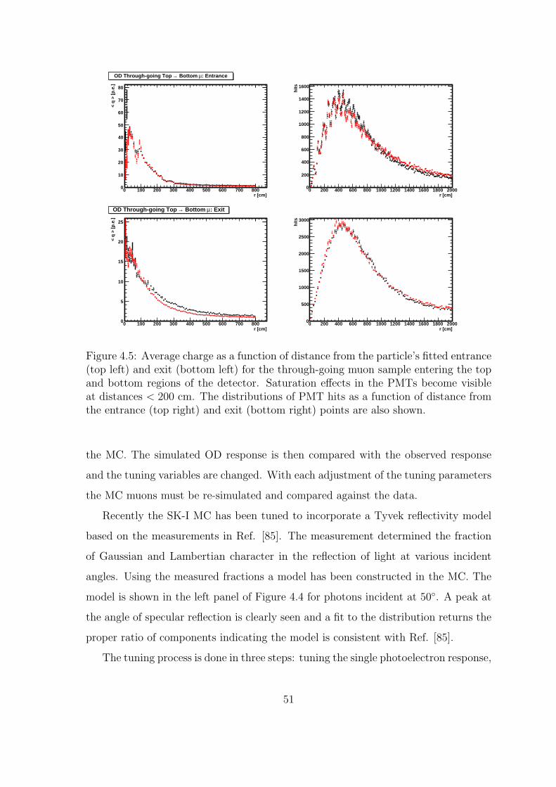
r [cm]0 100 200 300 400 500 600 700 800

< q

> [

p.e

.]

0

10

20

30

40

50

60

70

80

: Entranceµ Bottom →OD Through-going Top

r [cm]0 100 200 300 400 500 600 700 800

< q

> [

p.e

.]

0

5

10

15

20

25

: Exitµ Bottom →OD Through-going Top

r [cm]0 200 400 600 800 1000 1200 1400 1600 1800 2000

hit

s

0

200

400

600

800

1000

1200

1400

1600

r [cm]0 200 400 600 800 1000 1200 1400 1600 1800 2000

hit

s

0

500

1000

1500

2000

2500

3000

Figure 4.5: Average charge as a function of distance from the particle’s fitted entrance(top left) and exit (bottom left) for the through-going muon sample entering the topand bottom regions of the detector. Saturation effects in the PMTs become visibleat distances < 200 cm. The distributions of PMT hits as a function of distance fromthe entrance (top right) and exit (bottom right) points are also shown.

the MC. The simulated OD response is then compared with the observed response

and the tuning variables are changed. With each adjustment of the tuning parameters

the MC muons must be re-simulated and compared against the data.

Recently the SK-I MC has been tuned to incorporate a Tyvek reflectivity model

based on the measurements in Ref. [85]. The measurement determined the fraction

of Gaussian and Lambertian character in the reflection of light at various incident

angles. Using the measured fractions a model has been constructed in the MC. The

model is shown in the left panel of Figure 4.4 for photons incident at 50◦. A peak at

the angle of specular reflection is clearly seen and a fit to the distribution returns the

proper ratio of components indicating the model is consistent with Ref. [85].

The tuning process is done in three steps: tuning the single photoelectron response,

51

tuning the PMT saturation and tuning the Tyvek reflection properties. The single

photoelectron response is measured in the muon data by considering hits occurring

prior to the main event window. In the data these dark noise hits usually represent

one photoelectron, an effect which is also accounted for in the MC. For SK-I the

OD tubes are well described by the combination of a plateau response at low charge

and an exponential response at higher charges. The number of photoelectrons for a

given PMT hit in the simulation is drawn randomly from this combined distribution.

During the tuning process, parameters controlling the relative amount of plateau and

exponential character in the distribution are adjusted. A discriminator threshold is

simulated by discarding hits for which a generated uniform random number is below

a tunable threshold. The results of adjusting these parameters on the PMT single

photoelectron distribution are shown in the right panel of Figure 4.4.

Tuning the PMT saturation and collection efficiency is done using two distribu-

tions. Saturation effects become relevant in PMTs close to the exit or entry of an

energetic particle in the tank. PMT saturation is modeled using the relation

Q =s0q0

1 + s1q0, (4.2)

where Q is the saturation adjusted charge, q0 is the charge drawn from the single

photoelectron distribution above and s0,1 are tuning parameters. Plotting the aver-

age charge as a function of distance from these points then provides a useful tuning

distribution. The left panels of Figure 4.5 show this distribution for the fitted entrance

and exit points of the through-going muon sample. In these plots saturation effects

are most visible at distances less than ∼ 200 cm. The data appear in black, the MC

in red, and the entrance on the top shows good agreement between the two. Near the

exit on the bottom the agreement is also good but the data and MC differ farther out.

The right panel shows the distribution of hits as a function of distance from the en-

trance and exit points. This distribution is useful for tuning the efficiency for a PMT

registering a hit in the simulation. Both the exit and entrance points show good

agreement between data and MC. Note that the PMT efficiencies are independent

among the top, bottom and barrel regions of the OD.

52

Top Tubes0 20 40 60 80 100 120

0

20

40

60

80

100

120

140

160

Bottom Tubes0 20 40 60 80 100 120

0

20

40

60

80

100

120

140

160

Barrel Tubes0 50 100 150 200 250 300

0

50

100

150

200

250

300

350

400

nhitac0 50 100 150

0

20

40

60

80

100

120

140

160

180

200

220

OD rmean0 1000 2000 3000 4000

0

100

200

300

400

500

Total Charge [p.e.]0 200 400 600 800 1000

0

50

100

150

200

250

Figure 4.6: Tuning distributions for the SK-I MC (red) in comparison with the data(black). The variables are described in the text.

Up to this point the tuning parameters have been adjusted to provide agreement

with the data at a very basic level. The next phase of the tuning is arguably more vital

since tuning remaining pieces of the optical model is done using variables that appear

in several aspects of the reduction process. Figure 4.6 shows the tuning variables for

the through-going top to bottom muon sample. In the top row, the number of hit

PMTs in the top, barrel and bottom portions of the detector are shown. Adjusting

the probability of reflection on the Tyvek in each of these sections shifts the MC

distribution. Larger reflection probabilities generally move the distribution towards a

higher number of hit tubes. These distributions agree well in the figure, and though

these plots are for through-going muons essentially traversing the detector vertically

through its top, the distribution of barrel PMTs is also in agreement.

53

In the bottom row of the figure, from left to right, are the “nhitac”, “OD rmean”

and total charge distributions. Nhitac is a variable which records the number of hit

PMTs in the cluster of OD PMTs that has the highest amount of charge among all

clusters. This parameter is used in the PC reduction, (see Section ??) and in terms of

tuning parameters is related closely to the PMT collection efficiency and the Tyvek

reflection probability. That is, if the charge distributions and reflection probabilities

have been tuned in the previous steps the nhitac distribution agrees to a reasonable

extent. Small discrepancies can be tuned with changes in the PMT collection efficien-

cies. The OD rmean parameter is the average distance taken among all pairs of hits

and larger values indicate events that are more diffuse in the detector. Tuning this

distribution is similar to tuning nhitac. Total charge is the sum of all charge accumu-

lated in the OD and is tuned primarily by the PMT collection efficiencies provided

the single photon distributions are in agreement. The distributions in Figure 4.6 are

in good agreement.

54

Chapter 5

Atmospheric Neutrino Event

Reduction

5.1 Fully Contained Reduction

Atmospheric neutrino events at Super-Kamiokande are classified into four main

categories based upon their topology. Neutrino interactions that originate within the

ID with no particles exiting into the OD are classified as “fully contained” (FC).

Events that originate inside the ID but have one or more particles depositing visible

light in the OD are classified as “partially contained”(PC). Muons produced by the

interaction of neutrinos in the rock below the detector are subdivided into two cate-

gories. Upward-going muons (upmu) which originate in the OD but lose energy and

stop in the ID are labeled “upward stopping muons”, while those that continue on to

traverse the detector volume are “upward through-going muon” events. Figure 5.1 is

a schematic of each of the event types.

At SK roughly 10 atmospheric neutrino events per day are expected amidst a

background of more than a million events. Each of the event categories above goes

through a series of reduction steps to select candidate events from this background.

Generally the initial steps of the reduction are not computationally intense and are

designed to remove apparent backgrounds quickly and efficiently, while later steps

focus on finer subtleties between events. The steps of the atmospheric reduction are

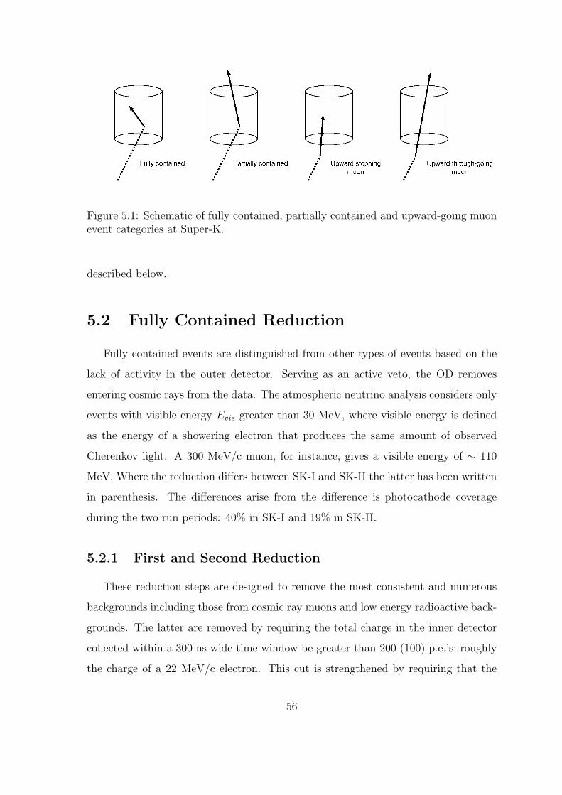
Figure 5.1: Schematic of fully contained, partially contained and upward-going muonevent categories at Super-K.

described below.

5.2 Fully Contained Reduction

Fully contained events are distinguished from other types of events based on the

lack of activity in the outer detector. Serving as an active veto, the OD removes

entering cosmic rays from the data. The atmospheric neutrino analysis considers only

events with visible energy Evis greater than 30 MeV, where visible energy is defined

as the energy of a showering electron that produces the same amount of observed

Cherenkov light. A 300 MeV/c muon, for instance, gives a visible energy of ∼ 110

MeV. Where the reduction differs between SK-I and SK-II the latter has been written

in parenthesis. The differences arise from the difference is photocathode coverage

during the two run periods: 40% in SK-I and 19% in SK-II.

5.2.1 First and Second Reduction

These reduction steps are designed to remove the most consistent and numerous

backgrounds including those from cosmic ray muons and low energy radioactive back-

grounds. The latter are removed by requiring the total charge in the inner detector

collected within a 300 ns wide time window be greater than 200 (100) p.e.’s; roughly

the charge of a 22 MeV/c electron. This cut is strengthened by requiring that the

56

ratio of p.e.’s collected in any single ID PMT be less than half of the the total in the

ID in a 300 ns window. Cosmic ray muons are in large part eliminated by requiring

that less than 25 PMTs in the OD are hit within ± 400 ns of the initial trigger and

< 1×106(5×105) p.e. in the ID. Finally, decay electrons coming from muons travers-

ing the detector below the Cherenkov threshold are rejected by demanding that events

precede each other by not less that 100 µs.

5.2.2 Third FC Reduction

Beyond the first two reduction steps the process begins to focus on muon events

with little activity in the OD and electronic noise. Events are rejected if they are

fit as a through-going muon with a goodness-of-fit > 0.75. Assuming the event’s ID

light pattern came from such a muon, events are cut if there are more than 10 hit

OD PMTs within 8 m of the supposed muon’s entrance and exit points on the ID.

Candidate events are also fit under a stopping muon assumption and are rejected if

the fit’s goodness is > 0.5 and there are ≥ 5 OD PMTs hit within 8 m of the ID

entrance point in 800 ns. Events passing this condition may still be rejected if there

are ≥ 10 hit tubes in this window, regardless of the fit’s goodness.

Muons which travel through one of the four large cable bundles supplying the

detector PMTs leave little light in the OD and are therefore monitored by 2x2.5 m

plastic scintillation counters placed atop the bundles. Events fail this stage of the

reduction if there is a hit in one of these veto counters or if the reconstructed vertex

of the event is within four meters of the cable hole.

Accidental coincidence events occur when a low energy event accompanies a cosmic

ray muon in the same trigger. This class of background is eliminated by requiring

≤ 20 OD hits and ≤ 5000 (2500) p.e.’s in the ID within a 500 ns wide time window 400

ns after the main trigger. Separate low energy events are further reduced by removing

any event with ≥ 50(25) hit ID PMTs in a sliding 50 ns time window if all of the

event’s light is assumed to originate at a single vertex. Finally, events originating

from “flasher” PMTs (see Section 5.2.3) are cut when ≥ 15(20) ID PMTs fire within

57

a sliding 100 ns window 300 ns and up to 800 ns after the main event trigger. For

SK-I only, if fewer than 800 ID tubes are hit in total, this criteria is reduced to ≥ 10

PMTs.

5.2.3 Fourth FC Reduction

The fourth step of the reduction is dedicated to removing events caused by the

repetitive electrical discharge of PMTs, known as “flashers”. These events therefore

have characteristic patterns which occur successively and can be used to create a

correlation parameter between the candidate event and other data events. Often

these patterns include a cluster of rapidly firing PMTs. Accordingly, the correlation

parameter is constructed using the charge accumulated in 1450 patches of 6 ∼ 9 PMTs

in the detector. The correlation is computed between the candidate event and 10,000

events before and after. Highly correlated events are removed.

5.2.4 Fifth FC Reduction

In the fifth reduction step, remaining muon backgrounds are targeted for removal.

Muons with momenta below the Cherenkov threshold may decay and produce an

electron above threshold creating a spurious event. These invisible muon events are

rejected if there are ≥ 10 OD hits in any 200 ns wide time window between 800 and

100 ns preceding the event trigger. Another stopping muon cut like that of the third

reduction is performed, but using a more precise fitter to find the entrance point.

Remaining coincident muon events are identified and cut when there are < 300(150)

p.e. in the ID accumulated between -100 ns and +400 ns around the main trigger

accompanied by ≥ 20 OD PMTs firing in a sliding 200 ns window in the 800 ns

starting at +400 ns. An additional cut to remove flashers is performed only for SK-II.

58

Table 5.1: FC event rate after each stage of the reduction. “Final” refers to the fidicialvolume and visible energy cuts.

Reduction Step Event Rate ( ∼ evt/day)

Trigger 106

First 3× 103

Second 2× 102

Third 45

Fourth 18

Fifth 16

Final 10

5.2.5 Final FC Sample

The complete FC sample used for analysis is obtained after requiring each event’s

reconstructed vertex be within 2 m of the ID walls. This cut defines a fiducial vol-

ume (FV) of 22.5 kt at SK. A 30 MeV visible energy analysis threshold is set, and

OD activity is restricted to be ≤ 9(15) PMTs to separate the FC and PC samples.

This process has an efficiency of 99.4% for keeping neutrino events with a systematic

uncertainty estimated below 1%.

The effect of each reduction step on the FC event rate is show in Table 5.1.

5.3 Partially Contained Reduction

PC events are most readily distinguished from FC events by the amount of activity

in the OD. Accordingly, cuts based on OD information are used in the FC reduction

to eliminate cosmic ray backgrounds. Such straight-forward cuts are not as useful

for PC events, since by definition a particle is exiting the ID and depositing light in

the OD, so the PC reduction focuses on more elaborate means of rejection of muon

backgrounds. Where the cuts differ between SK-I and SK-II the latter has been

included in parenthesis.

59

5.3.1 First PC Reduction

Particles in a PC event must travel a minimum of ∼ 2.5 m in the ID, which re-

quires muons have a momentum ≥ 700 MeV/c. A conservative cut of 1000 (500) p.e.,

corresponding to muon momenta of 310 MeV/c, accumulated in the inner detector

PMTs is applied to reject events unable to reach the OD. Many through-going muons

are rejected at this stage by requiring that the width of the OD PMT timing distri-

bution is ≤ 260 ns. For SK-I only there must also be no more than one cluster of

PMTs collecting more than 8 p.e. within 8 m of the event’s entrance into the OD.

Through-going muons and those that clip the corner of the inner volume frequently

have multiple clusters of hit PMTs well separated geometrically. Finally, as for the

FC reduction, candidate events must be separated by at least 100 µs.

5.3.2 Second and Third PC Reduction

Muon backgrounds remaining at this point are targeted using a cluster-based cut

slightly different than the first reduction. The OD is divided into 11 × 11 patches

of PMTs and clusters are formed based upon charge gradients between patches. If

there is exactly one such cluster found it must also have a corresponding cluster in

the ID with Γ > 1000 p.e., to help eliminate stopping muons. Here Γ is the number

of p.e. collected within 200 cm of highest charge ID PMT in the ID cluster. Further,

events are rejected if the minimum number of hit OD tubes among the top, bottom

and barrel regions is ≥ 7. Events are rejected if there are more than 6(10) tubes hit

in the second highest charge cluster in the OD.

For SK-II only, events are cut if they have more hit PMTs among the top and

bottom regions than a threshold returned by a function dependent upon the number

of hit barrel tubes. Events are similarly cut if the number of top and bottom tubes

exceeds 20. Candidate events also fail if there are more than 12 + 0.085Γ tubes in

the highest charge OD cluster.

At the third step flashers are rejected using the same cut as the FC third reduction.

Further, stopping muons are pared by requiring ≤ 10 hit OD PMTs within 8 m of the

60

OD entrance point in 500 ns. The entry point is determined by a simple point vertex

fit of the ID and a p.e. weighted direction estimation.

5.3.3 Fourth PC Reduction

The fourth reduction focuses again on muons which have passed previous stages

of the reduction due to limited OD activity. Two fits are employed: the simple point

vertex fit and a full through-going muon fit. PC events which start in the ID should

be fit poorly, particularly in terms of the entrance point to the ID and therefore have

a low goodness-of-fit. Using the point fit, events are rejected if cos θ ≤ −0.8 , where θ

is the angle between the fitted direction and the direction from the fitted vertex to the

earliest saturated ID PMT. These two directions are anti-parallel for through-going

muons. Events are also rejected if their reconstructed vertex is less than 150 cm to

the nearest corner of the ID. Finally, events with a through-going muon fit goodness

> 0.85 and a fitted track length > 30 m are removed.

5.3.4 Fifth PC Reduction

The fifth reduction is a series of specialized cuts designed to eliminate the most

difficult remaining backgrounds. Low energy backgrounds are rejected if the ID ob-

serves less than 3000 (1500) p.e.. Next, if the distance between the highest charge OD

hit cluster and the next highest one with more than 10 p.e. is more than 20 m the

event is tagged as a through-going muon and removed. To detect other muons with

more subtle OD signals, the OD is divided into patches containing 6×6 PMTs like in

the second reduction. This time, the charge threshold for forming clusters is reduced

to 0.5 p.e. per PMT, and if there are two or more clusters of ≥ 9 hit PMTs the event

is rejected. If there are at least 7 hit PMTs in an 8 m sphere with more than 10

p.e. centered on each of the ID and OD fringes, and the difference between average

timing among hits in each sphere is between 100 and 200 ns, the event is eliminated.

This rather elaborate cut is designed to reject muons that travel very close to the ID

wall and are reconstructed poorly. Finally, muons going through cable bundles are

61

Table 5.2: PC event rate after each stage of the reduction with estimated efficiencies.“Final” refers to the fiducial volume and eye-scanning performed on the sample.

Reduction Step Event Rate ( ∼ evt/day) Efficiency (%)

Trigger 106 100.0

First 2× 104 99.0

Second 3× 103 94.2

Third 255 93.2

Fourth 36 87.9

Fifth 1 84.6

Final 0.6 79.7

rejected using the same counters noted in FC third reduction.

Stopping muons are considered by applying a more intensive fitter, MS-fit, which

gives a better estimate of the event vertex and direction. The new vertex is projected

backwards onto the ID wall to give a new entrance point, and the event is cut if there

are ≥ 10 OD PMTs within 8 m of the entrance. Next, a separate precision fitter,

TDC-fit, is applied and the angle between the reconstructed ring direction and the

direction from the vertex to an OD cluster is estimated. This angle is expected to be

small for PC events, and the candidate event is rejected when it is larger than 90◦.

Finally, a third stopping muon fit is applied. If the charge in a 42◦ cone defined by the

reconstructed direction exceeds 60% of the total ID charge and there are more than 6

OD PMTs within 8 m of the fitted entrance position, the event is rejected when the

fit goodness is > 0.

5.3.5 Final PC Selection

The final PC sample is also subject to the 2 m fiducial volume cut. Additionally

PC events must have at least 10 (16) OD PMT hits in the highest charge OD cluster

and more than 3000 (1500) p.e.’s seen in the ID. Each PC event is scanned by two

physicists as a final check and the resulting sample is only 0.2% contaminated by

62

backgrounds. The list of event rates and selection efficiencies at each stage of the

reduction is listed in Table 5.2. For the final data set, the PC events are divided into

“OD stopping“ and “OD through-going” depending on whether the particle exiting

the ID stops in the OD. After a fit to the exiting particle’s track, its projected length

is used to compute the amount of charge expected in the OD. Events whose ratio

of observed to expected charge is < 0.66 are classified as stopping and events whose

ratio is larger than this cut are through-going.

5.4 Upward-Going Muon Reduction

Muon events created by the interaction of neutrinos below the detector are iden-

tical to other cosmic ray muon events in every way except for their direction. Con-

sequently, most backgrounds arise in near horizontal bins as a result of limitations of

the detector resolution. At event rates on the order of a few upward-going muons per

day, the main job of the reduction is to separate these relatively few events from the

continuous hail of O(105) cosmic ray events. Each event passes through a variety of

fitting algorithms and the final event sample is verified by eye.

5.4.1 Main Reduction

Upmu candidate events are required to have at least 10 in-time OD PMT hits

within 8 m of a track’s entry or exit point to the OD, as determined by the methods

outlined in the PC reduction. Further, each event must have more than 8,000 but not

more than 1.75× 106 p.e. in the inner detector. The latter high energy cut is applied

due to poor reconstruction ability of saturated electronics. Finally, corner clipping

events or events with estimated track lengths less than 7 m are rejected.

The automated portion of the upmu reduction is based on the results of seven

different muon fitters. Some fitters are designed to search for stopping muons and

others are optimized for through-going muons or showering muons. Events are given

successively to each fitter until all events have been classified, rejected or passed

63

through all the fitters. An event is kept if it is fit as an upward-going event with

goodness above the particular fitter’s threshold. Events are immediately rejected if

they are fit as downward-going with goodness above threshold. If the event was below

the goodness cut-off, or if it is classified as horizontal with high goodness, the event is

passed on to the next fitting algorithm. After passing through all the fitters the event

is kept if it was classified as horizontal by any one of the fitters, and it is rejected if

it could not be fit accurately by any fitter.

Events which have made it beyond this step are passed to a more computationally

intensive algorithm for estimating the event’s direction. Its resolution based on MC

studies is 1.5◦ for stopping and 1.05◦ for through-going muons. Details of these fitting

algorithms may be found in [58, 86].

5.4.2 Eye Scanning and Final Sample

All events that have been labeled as an upward-going muon by the precise fitter are

eye-scanned by two physicists for validity. If both experts agree the event is upward-

going or horizontal the event is added to the final upmu sample. Discrepancies are

resolved by the opinion of a third party, and about 50% of the events passing the

automated portion are removed by eye-scan. The reconstructed information provided

by the precise fitter is used as the official variables in the upmu sample. The detection

efficiencies after the entire process are estimated at 96.2% for stopping muons and

97.2% for through-goers with 1.25% and 0.54% estimated systematic uncertainty,

respectively.

After the eye-scan the final classification between stopping and through-going is

made based on the following criteria. The upmu is considered stopping if there are

≥ 10 OD hits within 8 m of the projected entry in a 500 ns wide window 800 ns after

the main trigger, and if there are less than 10 hits in the same time window 8 m

around the exit point. If there are ≥ 10 hits near the exit point, the event is classified

as through-going.

64

Table 5.3: Summary of the event samples used in this thesis. The 100 year SK-I andthe 60 year SK-II MC are unoscillated and have been scaled to the indicated livetimes.

SK-I SK-II

Event Sample Data MC Data MC

FC Livetime [days] 1489.2 803.9

Sub-GeV e-like 3353 2891.1 1842 1613.5

Sub-GeV µ-like 3227 4286.7 1723 2320.8

Multi-GeV e-like 746 744.8 417 436.2

Multi-GeV µ-like 651 936.4 379 532.8

Multi-Ring e-like 469 645.1 247 280.8

Multi-Ring µ-like 647 1081.6 349 536.6

Upmu Livetime [days] 1645.9 827.7

Up Through-going µ 1841 1681.4 880 1408.4

Up Stopping µ 417 714.3 208 350.7

PC Livetime [days] 1489.2 803.9

PC Stopping 171 205.7 100 110.6

PC Through-going 740 931.5 327 488.4

Total 12262 14118.5 6472 8078.9

5.4.3 Event Summary

Both the data and MC are passed through the reduction and classified into sub-

samples for analysis. The FC sample, is subdivided into six categories. Events with

only one Cherenkov ring are labeled “single-ring” and separated into multi-GeV (vis-

ible energy > 1.33 GeV) and sub-Gev (visible energy < 1.33 GeV). Each of these

is further classified as e- or µ-like based on the shape of the ring. This distinction

is discussed in more detail in Section 6.3. If the event has more than one ring it

is “multi-ring” and the most energetic ring determines whether it is e-like or µ-like.

The PC sample and the upward-going muon samples are partitioned into “stopping”

65

and “through-going” as discussed above. The requirements cast upon the PC sample

effectively select penetrating muons as the particle exiting the ID. Accordingly, the

PC events are a very pure sample of νµ events. A summary of these subsamples and

their respective livetimes is shown in Table 5.3.

66

Chapter 6

Event Reconstruction

The classification of each event discussed in the previous chapter relies heavily on

the algorithms that convert the PMT charge and timing information into kinematic

variables. The events used in this thesis are binned in the outgoing lepton momentum,

and its direction. Direction is taken to be the cosine of the zenith angle, where by

convention directly downward-going events are at an angle of zero radians relative to

the vertical axis of the detector (see Figure 3.1). In this chapter the reconstruction

of the vertex, direction, number of rings and particle type for contained events is

discussed.

6.1 Vertex Fitting

The event vertex is estimated using two methods. Initially a vertex is sought under

the assumption that all of the light collected in the inner detector was generated at

a single point. Subtracting the time of flight from a tested vertex a distribution of

residual PMT hit times is constructed. The point which gives maximal goodness-of-fit,

defined by a Gaussian fit to this distribution, is taken as the event vertex. Then, the

direction of the event is estimated as the vector sum of the charge weighted directions

from the reconstructed vertex to each hit PMT. This fitting procedure is known as

the point-fit.

With this vertex in hand, the opening angle of the Cherenkov cone of the brightest

ring in the event is measured to find the ring’s edge. This angle is taken from the axis

defined by the particle’s direction. Using the amount of charge collected at an angle

θ, q(θ), a pair of directions and opening angles is to tested to define a goodness-of-fit

parameter,

G =

∫ θt

0q(θ)dθ

sinθt

× e−(θt−θ0)2

2σ2 , (6.1)

where θ0 is the critical Cherenkov angle, θt is the tested opening angle and σ is

resolution of hits taken around θt. Varying the direction returned by point-fit and

testing various opening angles, the ring edge is found to be at the pair which maximizes

G.

Now that the outer edge of the Cherenkov ring has been found, a more precise

fit to the event vertex is made using an algorithm called TDC-fit. In this algorithm,

PMTs that fall within the Cherenkov ring are treated differently than those outside of

it when determining the best vertex and particle direction. Unlike point-fit, photons

are assumed to be generated along the particle’s track and the timing residual for

PMTs inside of the Cherenkov ring incorporates this effect. The residual for those

outside the ring is computed assuming all of the light originated at the vertex. The

goodness-of-fit for a test vertex and direction is formulated incorporating this change

and including the effect of water scattering.

6.2 Ring Counting

The number of rings is determined using a technique based on a Hough trans-

formation [87] in combination with the likelihood method. The initial ring found by

point-fit is treated as the main ring and other ring candidates found by the Hough

method are tested against the hypothesis of a second ring. If a second ring is found to

be more likely than just a single ring, the process is repeated against a possible third

ring, and on up to a maximum of five rings. During this process previously found

rings are kept fixed. When all rings have been found, particle type and momenta can

68

Figure 6.1: The ring counting likelihood distribution for sub-GeV events (left) andmulti-GeV events (right). The data is shown by the black dots, and the MC withneutrino oscillations applied at ∆m2 = 2.1 × 10−3 eV2 and sin22θ = 1.0 is shown asthe histogram. A cut at zero in the likelihood is used to separate single-ring frommulti-ring events. Taken from [33].

be estimated for each of them. Using ring-separation algorithms, charge accumulated

in an event can be allotted to each PMT based upon how much light it is expected to

see from each ring. Finally, the FC data are separated into single-ring and multi-ring

event categories based on a cut in the likelihood distribution at zero as shown in

Figure 6.1.

6.3 E-like and Mu-like

Events are often further subdivided into two “e-like” and “µ-like” categories de-

pending on whether their Cherenkov light pattern more closely resembles that of an

electron or a muon. FC events are classified as such and for other reductions, individ-

ual Cherenkov rings receive the same designation. The nomenclature derives from the

difference between the light projected onto the detector walls for electrons and muons.

Electrons, having low mass, are continually scattered as they travel in water. As the

electron scatters it emits a hard photon which, with sufficient energy may produce

a separate e−e+ pair. Both the new electron and positron may produce Cherenkov

69

Figure 6.2: Typical MC single ring FC e-like(left) and µ-like(right) events shown inan unrolled event display of SK. The smaller cylinder in the upper left represents theOD activity and in both frames, dots represent individual hit PMT’s with a radiusproportional to the charge accumulated in the tube.

radiation of their own and may similarly be scattered themselves. The overlapping

Cherenkov cones from the resulting electromagnetic shower coupled with the multiple

scattering of the electron produces a diffuse ring in the detector. This is in sharp

contrast to muons, whose large mass prevents them from being significantly deflected

and therefore leave a ring with a well defined edge. Typical examples of e- and µ-like

events are shown in Figure 6.2.

6.4 Particle Identification

Determining whether a ring is more e-like or µ-like is done using expected light

patterns. The expected distribution of light for e-like events is computed using Monte

Carlo simulations of electrons with momenta 100, 300 and 1000 MeV/c and recorded

at 16.9 m from a test vertex. By interpolating these momenta the expected light

pattern at a large range of distances and momenta can be extrapolated and projected

onto the detector walls. For µ-like events the expected light distribution is computed

analytically using muon energy loss and Cherenkov emission models. A term for

knock-on electrons is also added. In both cases, the light reaching a given PMT is

70

0

50

100

150

200

250

300

-10 -8 -6 -4 -2 0 2 4 6 8 10

e-like µ-like

020406080

100120140

-30 -20 -10 0 10 20 30

e-like µ-like

PID likelihood

Num

ber

of e

vent

s

Figure 6.3: The distribution of particle identification likelihoods for Sub-GeV (top)and Multi-GeV (bottom) single-ring FC events. The hatched histogram shows theMC contribution due to CC νµ interactions, the black dots show the data and theempty histogram shows the total MC with neutrino oscillations applied as in Figure6.1.

corrected for its acceptance, and the effects of water scattering and attenuation.

Using these expected light distributions the likelihood that each ring of the event is

e-like or µ-like is computed. The distribution of the likelihood variable for single-ring

events is shown in Figure 6.3. More details of the likelihood function can be found in

Ref. [57].

6.5 Momentum Determination

After ring-separation and particle ID have been performed on the rings, precise

momenta are assigned to them. The assigned momentum is dependent upon the

fraction of charge accumulated in the PMTs falling within a 70◦ cone around target

ring’s reconstructed direction. Light reaching these tubes is corrected for the angular

acceptance of the PMT and light attenuation in the water, and is restricted to hits

falling within -50 and +250 ns of the peak of the residual timing distribution. The

final charge is then combined with the particle ID results to estimate the momentum of

the particle. The muon and electron reconstructed momentum resolution is estimated

71

Table 6.1: The vertex resolution as estimated by MC for the FC and PC event samplesafter the precision vertex fitter is applied.

Event Type Resolution (cm)

Sub-GeV e-like 27

Sub-GeV µ-like 24

Multi-GeV µ-like 24

Multi-GeV e-like 49

Multi-Ring µ-like 67

PC 69

at 1.7 + 0.7/√P GeV/c% and 0.6 + 2.6/

√P GeV/c% respectively.

6.6 Precision Vertex Determination

TDC-fit is based on timing information and gives a relatively poor reconstructed

vertex for µ-like events. Longer track length muons are particularly susceptible due to

the large time-of-flight correction to photons produced far away from TDC-fits point

vertex. A more precise fitter, MS-fit, which incorporates the results of the particle

identification and Cherenkov ring angle reconstruction at previous steps of the process

is used to correct for this bias. The Cherenkov angle is held constant throughout the

fit while the direction and vertex position are varied, comparing the expected light

pattern with the observed patten. The fit is iterated to maximize both the goodness-

of-fit and the particle ID likelihood. The reconstructed vertex resolutions for the

contained data samples after MS-fit are shown in Table 6.1.

72

Chapter 7

Signatures of θ13 At Super-K

A non-zero θ13 can have a considerable effect on neutrino oscillations particularly

when matter effects are involved. The interplay of the neutrino flux and detector

resolutions with the matter structure of the Earth further complicate understanding

the possible signatures of this parameter in the atmospheric neutrino sample. The

effects of θ13 on Super-K data, and how the data are selected to highlight those

effects using the probabilities laid out in Chapter 2 and the detector Monte Carlo are

discussed below.

7.1 Preliminaries

The analysis presented in this thesis uses a radial density structure for the Earth

based on the PREM model[88]. However, to save computation time, the full PREM

model has been modified to provide roughly the median density predicted within its

four most prominent regions: inner core (0 ≤ r < 1220km) 13.0 g/cm3, outer core

(1220 ≤ r < 3480km) 11.3 g/cm3, mantle (3480 ≤ r < 5701km) 5.0 g/cm3 and the

crust (5701 ≤ r < 6371km) 3.3 g/cm3. Both models are shown in Figure 7.1. In the

right panel of the figure the difference between the νµ → νe oscillation probabilities at

θ13 near the CHOOZ limit for the two models is shown. Aside from a few islands, the

probabilities are consistent between the full and simplified models, and when smearing

introduced by the detector resolution is considered, these small differences have little

Radius [km]

0 2000 4000 6000

]3D

ensi

ty [

g/c

m

4

6

8

10

12

-0.15

-0.1

-0.05

0

0.05

0.1

Energy [GeV]

1 10 210

Co

sin

e Z

enit

h A

ng

le

-0.8

-0.6

-0.4

-0.2

-0

0.2

0.4

0.6

0.8

Figure 7.1: The PREM model[88] of the Earth’s density in blue overlaid with themodel used in this dissertation in red appears in the left panel. From left to right,the main features of the red model are denoted the inner core, outer core, mantle andcrust. The right panel shows the difference between the two models on the νµ → νe

oscillation probability for θ13 at the CHOOZ limit.

effect on the final analysis.

When θ13 and the solar mixing terms are zero, the oscillation mechanism reverts

to an effective two flavor scheme (νµ ↔ ντ ). The survival probability, νµ → νµ, in

this scenario is shown in Figure 7.2 and forms the baseline for the analysis presented

in [33]. It is used here as a reference against what can be expected when solar terms

and θ13 are allowed to be non-zero for the present analysis. The vertical axis of this

plot denotes the cosine of the angle the neutrino trajectory makes with the Super-K

zenith. Here cos Θ = −1 corresponds to a neutrino traveling upward from beneath the

detector and cos Θ = 0 represents a neutrino coming in from the horizon. Accounting

for the production height in the atmosphere, Ph, the relationship between the neutrino

path length, l, and cos Θ is,

l =√

(R⊕ + Ph)2 − R2⊕(1− cos2Θ)− R⊕cos Θ, (7.1)

where R⊕ is the Earth’s radius. The relation is linear from below to very near the

horizon as shown in Figure 7.2.

74

0

0.1

0.2

0.3

0.4

0.5

0.6

0.7

0.8

0.9

1

Energy [GeV]

1 10 210

Co

sin

e Z

enit

h A

ng

le

-1

-0.5

0

0.5

1

µν→µν3 Flavor Pµν→µν3 Flavor P

Distance [km]

0 5000 10000

Co

sin

ce Z

enit

h A

ng

le

-1

-0.5

0

0.5

1

Figure 7.2: Two-flavor νµ survival probability as a function of energy and zenithangle (left panel). For this oscillation mode matter effects in the Earth contributeonly an overall phase and do not alter the probability. The cosine of the zenith anglerepresents a path length as given in Equation 2.9. The relationship between the twois nearly linear (right panel) below the horizon.

0

0.1

0.2

0.3

0.4

0.5

0.6

0.7

0.8

0.9

1

Energy [GeV]

1 10 210

Co

sin

e Z

enit

h A

ng

le

-1

-0.5

0

0.5

1

µν→µν3 Flavor Pµν→µν3 Flavor P

0

0.1

0.2

0.3

0.4

0.5

Energy [GeV]

1 10 210

Co

sin

e Z

enit

h A

ng

le

-1

-0.5

0

0.5

1

eν→µν3 Flavor Peν→µν3 Flavor P

Figure 7.3: Three-flavor oscillation probabilities for θ13 at the CHOOZ limit for neu-trinos under the normal hierarchy. The large resonance region between 3-10 GeV inthe right panel arises because of the resonance effect in the Earth. Note that underthe assumption of an inverted hierarchy, this resonance disappears in the neutrinochannel, and instead manifests itself in the oscillations of anti-neutrinos. The effectof solar terms at the global best-fit [26] appears as the islands of probability at lowerenergies. Atmospheric mixing is included at (∆m2

23, sin2θ23) = (2.5× 10−3 eV2, 0.5).

75

7.2 Pure Probabilities

In the context of this analysis the effect of θ13 is of the utmost importance. A non-

zero value of this parameter implies that νµ oscillate into νe. At the CHOOZ limit

the appearance probability can be quite large as shown in Figure 7.3. Interactions

with the Earth’s matter cause upward-going νµ neutrinos between 3 and 10 GeV to

have up to a 50% chance of converting to νe. There are three main features in the

figure. Resonant enhancement of the transistion probability by the MSW mechanism

occurs in the Earth’s core and mantle layers and is represented by the regions of large

probability at 3 GeV and 7 GeV respectively. The region seen at 5 GeV and zenith

angles < −0.8 arises because of interference arising at the boundary of the mantle

and core layers [89]. Horizontal discontinuities appearing in the figure are a result of

similar discontinuities at the boundaries of the density profile.

Depending on the magnitude of θ13, the strength of this resonance varies. Figure

7.4 shows from left to right the effect of increasing θ13 on the νe appearance probability.

Furthest left at zero θ13, the GeV resonance structure has disappeared. At center,

with a small but non-zero value of θ13, the resonance is present but lacks both the

breadth and intensity seen for values near the CHOOZ limit (right panel).

The inclusion of the solar mixing terms can be important as it leads to a non-

zero νµ → νe probability even for zero θ13. Finger-like protrusions of probability for

upward-going neutrinos at energies less than 1 GeV appearing in the figure illustrate

this phenomenon. As the value of θ13 increases to the CHOOZ limit the extent and

intensity of these structures increase correspondingly. For reasons outlined in Chapter

8 they are neglected in the final analysis but are included here for completeness.

At the same energies where νe appearance is largest there is a corresponding

region of disappearance seen in the νµ survival probability. However, the effect of

the resonance cuts across several bands of probability maxima and minima driven

by the underlying atmospheric mixing. Whether this results in a possible overall

observable excess or deficit of muon-like events is difficult to ascertain from the pure

probability alone and is discussed below. In short, a non-zero θ13 would manifest itself

76

0

0.1

0.2

0.3

0.4

0.5

1 10

Co

sin

e Z

enit

h A

ng

le

-1

-0.5

0

0.5

1

eν→µν3 Flavor Peν→µν3 Flavor P

0

0.1

0.2

0.3

0.4

0.5

1 10-1

-0.5

0

0.5

1

0

0.1

0.2

0.3

0.4

0.5

Energy [GeV]

1 10-1

-0.5

0

0.5

1

Figure 7.4: νµ → νe oscillations in the normal hierarchy for increasing θ13 up to nearthe CHOOZ limit. From left to right, sin2θ13 is 0.0, 0.004 and 0.03 and all otheroscillation parameters are as in Figure 7.3. The CHOOZ limit is ∼ 0.04 at theseatmospheric mixing variables. Note that the intensity scales among the three imagesare the same.

at Super-K primarily as an increase in the high energy e-like event rate coming from

below. Possible effects on the muon-like event rate are further discussed below.

7.3 Folding in the Neutrino Flux

Folding the expected neutrino flux at Super-K with the probabilities discussed

in the previous section is used to determine the observable signals arising from θ13.

Since the analysis in [33] shows that the atmospheric neutrino signal at Super-K is

well described by maximal two-flavor νµ disappearance, it is instructive to consider

the influence of θ13 as a possible sub-leading effect relative to this more dominant

mixing. In the three-flavor framework, not only is the transition νµ → νe allowed, the

disappearance of the νe flux through oscillations to νµ,τ becomes a competing process.

Therefore, considering the νµ → νe oscillation probability alone gives an incomplete

picture of the effect of θ13. Instead the net appearance of νe against the now allowed

disappearance transitions needs to be examined.

Figure 7.5 shows the excess of MC events oscillated with θ13 at the CHOOZ limit

77

Energy [GeV]

1 10

Co

sin

e Z

enit

h A

ng

le

-1

-0.8

-0.6

-0.4

-0.2

0

0.2

0.4

0.6

0.8

-0.5

0

0.5

1

1.5

2

- 1 3f0µν

3fCHOOZµν

: µνExcess

-0.2

0

0.2

0.4

0.6

0.8

1

1.2

Energy [GeV]

1 10

Co

sin

e Z

enit

h A

ng

le

-1

-0.8

-0.6

-0.4

-0.2

0

0.2

0.4

0.6

0.8

- 1 3f0eν

3fCHOOZeν

: eνExcess - 1 3f0eν

3fCHOOZeν

: eνExcess

Figure 7.5: Excess of neutrino events in the SK-I 100 year MC sample for oscillationswith θ13 at the CHOOZ limit relative to those at 0. Atmospheric and solar mixingparameters are the same as in Figure 7.3. The main MSW resonance remains visible inthe νe event rate (right). For νµ events (left) the intensity scale has been restricted toa maximum of 200% relative increase to highlight alternating excess/deficit structure.

relative to oscillations at θ13 = 0. Here, solar mixing is included, making the latter

case not strictly two-flavor oscillations but representing only a small correction to

the atmospheric mixing at these energies. The νµ event rate shows alternating bands

of both excess and deficit. Deficits of near 40% next to excesses of 100% or 200%

could be a useful constraint on the parameter if the neutrino energy could be perfectly

reconstructed. Although energy reconstruction is imperfect, the plot indicates that

µ-like events may offer additional clues from their high upward-going flux.

Electron neutrino events, however, still provide the clearest indication of θ13. The

high energy resonance remains visible in the atmospheric sample after incorporation

of the flux. To make the most out of this expectation, the Super-K data have been

refined to add a high purity high-energy e-like sample. The enhancement process is

discussed in the next section.

78

7.4 High Energy e-like Enhancement

To exploit this possible excess of higher energy electron neutrino events, a refined

multi-ring multi-GeV e-like sample has been added to the analysis. Previous analyses

such as that in Ref. [33] used only single-ring e-like samples. A multi-ring e-like

sample is extracted from the pool of multi-ring events using a likelihood method.

A likelihood function is constructed for each of five energy bins: 1.33-2.5 GeV,

2.5-5 GeV, 5-10 GeV, 10-20 GeV and > 20 GeV using probability density functions

(PDFs) built from Monte Carlo events whose most energetic ring is e-like. Four

observed quantities are used to select signal events: the number of decay electrons,

the maximum distance between the neutrino vertex and any muon decay electrons,

the fraction of momentum carried by the event’s most energetic ring, and the PID of

the most energetic ring. For a given energy bin, j, the likelihood is,

Lj =4∑

i=1

log(ΓSi (xi))− log(ΓB

i (xi)), (7.2)

where Γi represents the PDF for the ith observable and xi is the observable’s measured

value. The superscripts S and B label the signal and background PDFs respectively.

In selecting electron neutrino events, the signal is taken to be CC νe + νe, while the

background is composed of NC and CC νµ + νµ events. An event makes it into the

final sample if it passes all cuts in the FC reduction, if the event’s most energetic ring

is e-like, and if Lj > 0.

An example PDF for the 5 GeV bin are shown in Figure 7.6. For both signal and

background the predominant interaction mode is deep inelastic scattering. However,

single pion production modes also contribute. Pions, through their decays to muons,

are the main source of decay electrons in both the signal and the NC portion of the

background. Signal events, though, must distribute the parent neutrino energy among

the outgoing lepton as well as any pions. For this reason, pions produced by back-

ground events should in general be more energetic and thus their subsequent decay

electrons should be further separated from the neutrino interaction vertex. Similarly,

79

PID-40 -30 -20 -10 0

1

10

210

PID 5 - 10 GeV PID 5 - 10 GeV

-n e0 2 4 6 8 10

1

10

210

310

-Number Decay e -Number Decay e

f0 0.2 0.4 0.6 0.8 1

1

10

210

P Fraction of Most Energetic Ring P Fraction of Most Energetic Ring

]21

d [ (cm / MeV)0 0.2 0.4 0.6 0.8 1

1

10

210

310

- Max Dist to Decay e - Max Dist to Decay e

Figure 7.6: Probability density functions used to select multi-ring e-like events withtotal energy between 5 and 10 GeV for SK-I MC events whose most energetic ring isreconstructed as e-like. From left to right the variables are the PID of the event’s mostenergetic ring, the number of decay electrons in the event, the fraction of momentumcarried by the most energetic ring, and the maximum distance to a decay electronfrom the reconstructed event vertex divided by the energy of the most energetic ring.The blue histogram contains the signal CC νe and νe events and the red histogramcontains the background. The corresponding SK-II plots do not differ appreciably.

background events should have more such electrons. These ideas are reflected in the

figure. The PID variable is itself the output of a likelihood function. More negative

numbers indicate a stronger agreement with the e-like hypothesis for the ring.

The most clearly distinct variable between the signal and background is the frac-

tion of momentum carried by the most energetic ring, f. Charged current νµ events in

the multi-GeV energy regime do not differ appreciably from νe’s in terms of this vari-

able and should therefore be peaked at higher fractions. Plotting the same variable

for νµ events whose leading ring is properly reconstructed as µ-like yields a distribu-

tion with the same shape as the νe histogram in the figure. However in these plots

each event’s primary ring has already been reconstructed as e-like, which for νµ events

represent failures of the reconstruction algorithm. Using this variable is thus an ex-

ploitation of those failures and results in background events more often having lower

values of f.

The method is the same as in Ref. [44] and the resulting sample purities after the

likelihood selection for both SK-I and SK-II appear in Table 7.1.

80

Table 7.1: The expected number of events for each interaction component of themulti-ring multi-GeV e-like sample after likelihood selection for the SK-I and SK-II MC scaled to 1489.2 and 803.9 livetime days respectively. Two-flavor neutrinooscillations νµ ↔ ντ have been applied at ∆m2 = 2.5× 10−3 eV2 and sin22θ = 1.0.

CC νe + νe CC νµ + νµ NC Total

SK-I 421.5 47.5 86.5 555.2

Percentage (%) 75.8 8.6 15.6 100.0

SK-II 196.2 27.1 46.4 269.6

Percentage (%) 72.8 10.0 17.2 100.0

7.5 Incorporating Reconstruction

With the enriched multi-ring multi-GeV e-like sample, the signature of a large

θ13 in the νe and νµ fluxes would manifest itself according to Figure 7.5. However,

this plot does not include the various smearing effects the event reconstruction has

on the final analysis bin contents. Plots illustrating the relative excess binned using

reconstructed information appear in Figures 7.7 and 7.8.

Unfortunately the effect of imperfect reconstruction is rather striking. Though

the main MSW resonance is still clearly visible in the multi-ring e-like sample, its

strength has been cut by nearly a factor of two and distributed across several bins.

As seen in the right panel of each figure there are still roughly 10 or more events in

each of the bins in the affected region. Such an observable change will become the

primary signal for the analysis in this thesis. The single-ring multi-GeV e-like sample

exhibits similar effects but with slightly smaller statistics.

On the other hand, the possible alternating signatures in the high energy µ-like

samples are less promising. The PC OD through-going sample, which is comprised

mostly of νµ events, indeed illustrates bands of relative excess and deficit at high

energies. However, the magnitude of the net change in each bin is small relative to

the predictions of Figure 7.5. despite the relatively strong bin populations. Other

muon-based samples offer slightly larger expected changes in the bin contents but

81

-0.05

0

0.05

0.1

0.15

0.2

[ log GeV ]totE

3 3.5 4 4.5 5

Co

sin

e Z

enit

h A

ng

le

-1

-0.5

0

0.5

1

- 1 = 013θ = Chooz13θ

MultiRing_elike - 1 = 013θ = Chooz13θ

MultiRing_elike

5

10

15

20

25

[ log GeV ]totE

3 3.5 4 4.5 5

Co

sin

e Z

enit

h A

ng

le

-1

-0.5

0

0.5

1

EventsEvents

Figure 7.7: Excess of multi-ring e-like events in the SK-I 100 year MC sample foroscillations with θ13 at the CHOOZ limit relative to those at θ13 = 0 and binned inreconstructed quantities (left). The plot reflects the potential signature of non-zeroθ13 after incorporating the neutrino fluxes, oscillation probabilities and effects of theevent reconstruction. Etot refers to the total energy of all rings in the event. TheMSW resonance is still visible but its magnitude has decreased significantly relativeto Figures 7.5 and 7.3. The number of MC events after oscillations at the CHOOZlimit in the same binning is shown for the SK-I livetime (right).

with smaller statistics. Certainly the µ-like events will provide additional constraints

on the size of θ13, but their effect is much smaller relative to that of the high energy

e-like samples. Accordingly, they are considered a much weaker potential signal here.

7.6 Normal vs. Inverted Hierarchy

The plots presented above have all been created under the assumption of the

normal mass hierarchy. If the inverted hierarchy is used instead, the resonance will

affect anti-neutrino events. Due to the lower cross section for νe interaction (see

Figure 4.3), the overall effect of a large θ13 is expected to be smaller than for the

normal hierarchy. Figure 7.9 shows that at the strongest point of the resonance, the

expected excess has been cut by more than a factor of two. In consequence, less

sensitivity is expected from an analysis using the inverted scheme.

82

-0.06

-0.05

-0.04

-0.03

-0.02

-0.01

0

0.01

0.02

[ log GeV ]visE

2 2.5 3 3.5 4 4.5 5

Co

sin

e Z

enit

h A

ng

le

-1

-0.5

0

0.5

1

- 1 = 013θ

= Chooz13θ PCThru - 1

= 013θ = Chooz13θ

PCThru

0

10

20

30

40

50

[ log GeV ]visE

2 2.5 3 3.5 4 4.5 5

Co

sin

e Z

enit

h A

ng

le

-1

-0.5

0

0.5

1

EventsEvents

Figure 7.8: As in Figure 7.7 but for the PC through-going sample which is dominatedby νµ. Here the horizontal axis specifies the visible energy of the event.

-0.04

-0.02

0

0.02

0.04

0.06

0.08

[ log GeV ]totE

3 3.5 4 4.5 5

Co

sin

e Z

enit

h A

ng

le

-1

-0.5

0

0.5

1

- 1 = 013θ = Chooz13θ

MultiRing_elike - 1 = 013θ = Chooz13θ

MultiRing_elike

Figure 7.9: As in Figure 7.7 but under the inverted mass hierarchy assumption.

83

Chapter 8

Oscillation Analysis

After the reduction and reconstruction phases of reprocessing, the data and MC

are suitable for analysis. The general analysis framework aims to compare the data

against the MC for different oscillation models. A particular oscillation model specifies

a value of each of the oscillation parameters and the MC is then oscillated according

to that model. To test a model’s compatibility with the data, a goodness of fit

statistic is computed between the two. A set of oscillation models forming a grid in

the parameter space is chosen and this analysis performs a search over the lattice for

the best agreement with the data. This condition is defined as the minimum χ2 among

the test points. Confidence level contours are then drawn expressing the degree of

agreement with the data relative to the model giving the best fit. Both the SK-I

and SK-II datasets are fit individually and then combined and re-fit jointly as the

SK-I+SK-II data. Further, each of these is fit under the assumption of both a normal

and inverted mass hierarchy. Detailed descriptions of the process and the results are

presented below.

8.1 Oscillation Space

To perform the analysis a lattice consisting of 83,025 points is chosen among three

oscillation parameters. The dimensions of the grid are specified in Table 8.1. Only

three parameters are considered because the analysis adopts a single dominant mass

Table 8.1: Details of the oscillation space considered in the analysis. The solar terms,sin2θ12 and ∆m2

21, have been excluded.

Parameter Points Minimum Maximum

sin2θ13 81 0.0 0.5

sin2θ23 25 0.2 0.8

∆m223 [eV2] 41 1 ×10−3 1 ×10−2

framework. That is, experimentally the “solar” mass splitting, ∆m212, is known to

be much smaller than the “atmospheric” mass splitting ∆m223 in magnitude [25, 23,

33]. For neutrinos with a few hundred MeV of energy the effect on the oscillation

probability of the solar mass splitting is the most relevant. Excesses in the νe event

rate at these energies arising from νµ → νe transitions driven by this mass splitting

when the ratio of the neutrino fluxes νµ/νe ∼ 2 can be upwards of 5% but are strongly

suppressed in the atmospheric sample when sin2θ23 = 0.5 [90]. This latter condition is

favored by [33] suggesting that in conjunction with averaging performed in this region

(see below) it is reasonable to exclude this parameter from the analysis. Accordingly,

only the atmospheric splitting is considered with ∆m223 > 0 representing the normal

mass hierarchy and ∆m223 < 0 the inverted hierarchy. The solar terms, ∆m2

21 and

sin2θ21, are set to zero in this analysis.

8.2 Monte Carlo Manipulations

The analysis presented here relies on 100 years of SK-I and 60 years of SK-II Monte

Carlo constructed as discussed in Chapter 4. However, individual events contribute

differently to the analysis bins as described below.

8.2.1 Oscillation Probabilities and Weights

Each CC MC event’s true zenith angle direction is used to compute an event

path length. If the event is coming from below the horizon the matter density profile

85

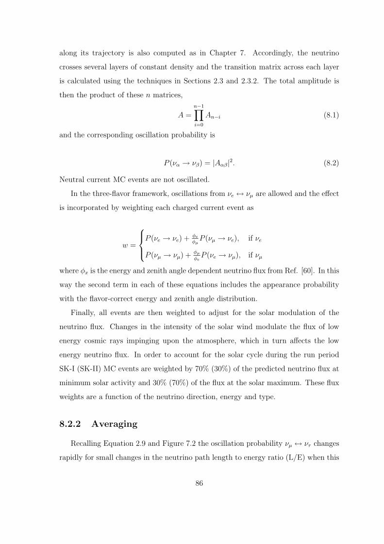
along its trajectory is also computed as in Chapter 7. Accordingly, the neutrino

crosses several layers of constant density and the transition matrix across each layer

is calculated using the techniques in Sections 2.3 and 2.3.2. The total amplitude is

then the product of these n matrices,

A =n−1∏i=0

An−i (8.1)

and the corresponding oscillation probability is

P (να → νβ) = |Aαβ|2. (8.2)

Neutral current MC events are not oscillated.

In the three-flavor framework, oscillations from νe ↔ νµ are allowed and the effect

is incorporated by weighting each charged current event as

w =

P (νe → νe) + φe

φµP (νµ → νe), if νe

P (νµ → νµ) + φµ

φeP (νe → νµ), if νµ

where φx is the energy and zenith angle dependent neutrino flux from Ref. [60]. In this

way the second term in each of these equations includes the appearance probability

with the flavor-correct energy and zenith angle distribution.

Finally, all events are then weighted to adjust for the solar modulation of the

neutrino flux. Changes in the intensity of the solar wind modulate the flux of low

energy cosmic rays impinging upon the atmosphere, which in turn affects the low

energy neutrino flux. In order to account for the solar cycle during the run period

SK-I (SK-II) MC events are weighted by 70% (30%) of the predicted neutrino flux at

minimum solar activity and 30% (70%) of the flux at the solar maximum. These flux

weights are a function of the neutrino direction, energy and type.

8.2.2 Averaging

Recalling Equation 2.9 and Figure 7.2 the oscillation probability νµ ↔ ντ changes

rapidly for small changes in the neutrino path length to energy ratio (L/E) when this

86

ratio is large. Rapid changes in this oscillation phase are difficult to sample completely

when the accumulated statistics are small, making the final oscillation contours more

sensitive to statistical fluctuations in the MC. Given a large amount of MC, the effect

of incomplete sampling can be alleviated, but alternative methods are employed when

the MC statistics are not sufficient.

For each of SK-I and SK-II there are 20 times more MC than collected data but

because of the large value of the oscillation phase in several bins of the analysis this

is not sufficient. In the case of a pure νµ disappearance analysis, where a two-flavor

oscillation scheme is valid and matter effects are not considered, a simple cut can be

made. The standard zenith angle analysis at Super-K [33] averages the second sine

function in Equation 2.9 to 0.5 when its argument is > 2π, roughly corresponding to

L/E > 2 × 103 km/GeV. Making the cut at 2π is a somewhat arbitrary choice and

is made based on changes in the expected sensitivity to oscillations. Since this aver-

aging implies a loss of information on one of the measured parameters, ∆m2, care is

appropriate. Increasing values for this cut imply fewer averaged events but beyond 2π

the effect on the extent of the expected sensitivity to ∆m2 ceases to change. Averag-

ing more events by lowering the cut, though, begins to erode sensitivity, particularly

below π.

The effect of this averaging is shown in Figure 8.1. In both panels the weight

including two-flavor oscillations assigned to each CC νµ event in the MC is shown as

a function of its L/E value. Oscillations without any averaging are shown in the left

panel. The change induced by the above averaging is shown as the cluster of black

points around 0.5 extending above the cut value in the right panel. In both cases

the sinusoidal nature of the oscillations is clear but has a width that results from the

application of the solar flux weights discussed in Section 8.2.1.

Averaging in this manner is straightforward. However, as discussed in Chapter

2 the three-neutrino oscillation probability in varying matter cannot be written in a

simple closed form. Further, the presence of matter obfuscates quantities one might

average with such as the oscillation length. The problems associated with “low” MC

87

Oscillation Weight0 0.2 0.4 0.6 0.8 1 1.2

km

/GeV

]3

L/E

[ 1

0

-110

1

10

Oscillation Weight0 0.2 0.4 0.6 0.8 1 1.2

km

/GeV

]3

L/E

[ 1

0

-110

1

10

Figure 8.1: Muon MC event weights as a function of L/E after oscillations withand without averaging effects at (∆m2, sin2θ23, sin

2θ13) = (2.5 × 10−3 eV2, 0.5, 0.0).The left panel illustrates clearly the sinusoidal dependence on L/E reminiscent ofEquation 2.9 for oscillation without any averaging. At right, the effects of simplephase averaging for 1.2667∆m2L/E > 2π (black) and for the full averaging performedin this dissertation (red) are shown (see Sections 8.2.4 and 8.2.5).

statistics are still present in the three-flavor analysis, however, so alternative methods

to overcome the deficiency must be invoked. Since the two-flavor disappearance is

the dominant oscillation effect, the three-flavor averaging scheme must also remain

consistent with the two-flavor result. This is achieved using the production height,

mantle and nearest neighboring averaging schemes discussed below.

8.2.3 Neutrino Production Height

It is not possible to know the production height above ground level in the atmo-

sphere of neutrino events entering Super-K. For low energy neutrinos near the horizon

the effect of small changes in the production height can lead to changes in the total

path length large enough to significantly alter the oscillation probability. Events com-

ing from well below the horizon on the other hand are only marginally affected by this

uncertainty as the production height represents only a small fraction of the overall

path length. To account for this effect in near-horizontal and downward-going events,

88

the production height is averaged over. Using 20 production heights chosen from the

data in Ref. [60], 20 oscillation probabilities are computed for each MC event. The

final probability assigned to the event, however, is their average. Production heights

vary as a function of neutrino energy, direction and flavor but are typically less than

40 km.

8.2.4 Mantle Averaging

Incorporating matter effects into the oscillation framework prohibits the use of

simple cuts on the oscillation phase since this phase is no longer well defined along

the entire neutrino path. Statements can be made, however, piecewise along its length.

The path length in the mantle region (see Figure 7.1), lm, of each event is compared

to its vacuum oscillation length, λ. If lm > 2λ four probabilities are computed for the

event using lm + nλ/2, n = 0, .., 3 as the path length in the mantle. The probability

assigned to the event is then the average of these four. For events whose trajectory

through the mantle is interrupted by passage through the core region, lm is taken as

the distance across the section of the mantle nearest the detector.

Using this procedure many events in the high L/E region are averaged while pre-

serving the effect of interactions with the matter beneath the mantle. Figure 8.2

shows the effect this averaging has on the νµ survival probability from Figure 7.3.

Notice that averaging in the mantle does not extend into the MSW region and hence

does not affect this analysis’ main sensitivity to θ13. On the other hand, the averaging

only partially covers the high phase oscillation region in Figure 8.2 and is not by itself

sufficient.

8.2.5 Nearest Neighbor Averaging

To complement the mantle averaging, a third averaging scheme based on the Super-

K Monte Carlo is employed. Before computing oscillation effects, the 20 nearest

neighbors in reconstructed energy (lepton momentum if single-ring) for each event

are found. Then, the true neutrino energy of each of these neighbor events is used to

89

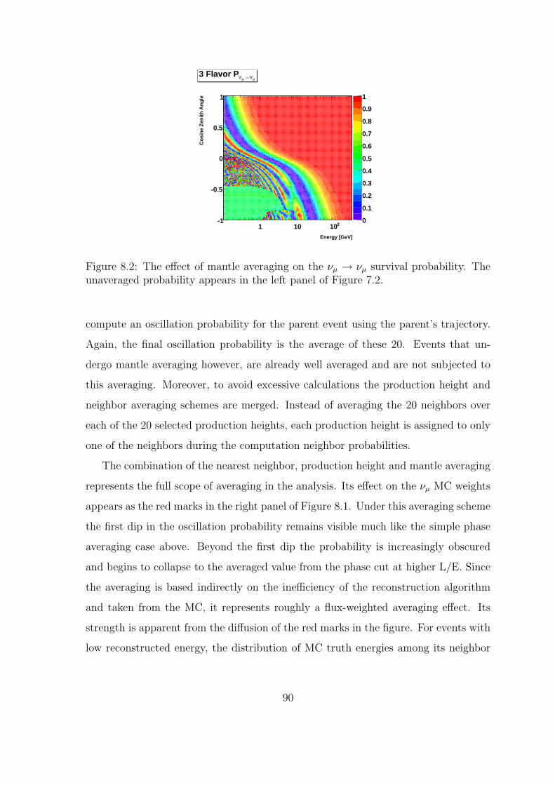
0

0.1

0.2

0.3

0.4

0.5

0.6

0.7

0.8

0.9

1

Energy [GeV]

1 10 210

Co

sin

e Z

enit

h A

ng

le

-1

-0.5

0

0.5

1

µν→µν3 Flavor Pµν→µν3 Flavor P

Figure 8.2: The effect of mantle averaging on the νµ → νµ survival probability. Theunaveraged probability appears in the left panel of Figure 7.2.

compute an oscillation probability for the parent event using the parent’s trajectory.

Again, the final oscillation probability is the average of these 20. Events that un-

dergo mantle averaging however, are already well averaged and are not subjected to

this averaging. Moreover, to avoid excessive calculations the production height and

neighbor averaging schemes are merged. Instead of averaging the 20 neighbors over

each of the 20 selected production heights, each production height is assigned to only

one of the neighbors during the computation neighbor probabilities.

The combination of the nearest neighbor, production height and mantle averaging

represents the full scope of averaging in the analysis. Its effect on the νµ MC weights

appears as the red marks in the right panel of Figure 8.1. Under this averaging scheme

the first dip in the oscillation probability remains visible much like the simple phase

averaging case above. Beyond the first dip the probability is increasingly obscured

and begins to collapse to the averaged value from the phase cut at higher L/E. Since

the averaging is based indirectly on the inefficiency of the reconstruction algorithm

and taken from the MC, it represents roughly a flux-weighted averaging effect. Its

strength is apparent from the diffusion of the red marks in the figure. For events with

low reconstructed energy, the distribution of MC truth energies among its neighbor

90

[ GeV ]trueνE

0.6 0.8 1 1.2 1.4 1.6 1.8 2 2.2 2.40

0.5

1

1.5

2

2.5

3

3.5

4

Lepton P 578 MeV/cLepton P 578 MeV/c

Figure 8.3: The 20 nearest neighbor energies for a single ring muon event in the SK-IMC with reconstructed lepton momentum of 578 MeV/c. The width of this distribu-tion makes the oscillation probabilities computed in the nearest neighobr avergaingscheme to be diffuse.

events can be broad and thereby result in a well averaged probability. See Figure 8.3.

Since this type of averaging depends heavily on the choice of MC sample used it is

not an ideal averaging scheme.

8.3 Formulation of χ2

In order to take advantage of the improved sensitivity accompanying a finer binning

scheme, the likelihood in this thesis is based on Poisson probabilities. For ∼ O(1)

number of expected events, with small error on that expectation, the resulting reduced

χ2 of a sparsely populated bin is only marginally larger than 1.0. The likelihood for

N bins indexed by n is taken to be

L(E,O) =∏n

e−EnEOnn

On!(8.3)

In this equation En and On are the expected and observed bin contents respectively.

91

Defining a χ2 as the log likelihood ratio yields

χ2 ≡ −2 ln L(E,O)L(O,O)

= 2∑

n

(En −On +On ln

On

En

). (8.4)

8.4 Pull Method of Systematic Errors

A prescription given by the authors of Ref. [91] can be used to incorporate the

effect of systematic errors into the bin expectation for independent sources of error.

That is, the expected number of events in a bin changes with changes to an added

systematic error parameter. In this scheme Equation 8.4 can be rewritten with the

substitution

En → En(1 +∑

i

f inεi). (8.5)

In this equation the quantity f in represents the fractional change in the nth bin’s event

rate due to a variation of the systematic error parameter εi. For each error, i, the

parameter εi is estimated during the fit to the χ2 and the resulting distribution of the

quantity εi/σi is Gaussian univariate. In this way, the size of the fitted ε and hence

the strength of its systematic error’s effect is constrained through the addition of a

penalty term to Equation 8.4. The full χ2 becomes

χ2 = 2∑

n

(En −On +On ln

On

En

)+

∑i

(εiσi

)2

. (8.6)

χ2 = 2∑

n

En(1 +

∑i

f inεi)−On +On ln

On

En(1 +∑

i

f inεi)

+

∑i

(εiσi

)2

. (8.7)

The advantage of using this method is that with the incorporation of the “pulls”

in Equation 8.5 the χ2 can be minimized over the εi readily. At the χ2 minimum

∂χ2/εl = 0 for every l. Therefore, differentiating χ2 and grouping terms in only one

power of ε the minimization problem is specified by the solution of a K × K linear

92

matrix equation,

∑

k

Mlkεk = Vl (8.8)

⇒∑

k,n

(f l

nfknOn + δlk

1

σ2k

)εk =

∑n

Onfln

(1

1 +∑

i finεi

+∑

i

f inεi +

En

On

). (8.9)

The matrix, M , is symmetric and invertible so long as there does not exist an error

i with f in = 0 for every n. If the number of bins is much larger than the number

of systematic errors this method has considerable advantage relative to a covariance-

matrix approach as the solution is found by inverting a K ×K matrix, rather than

an N ×N matrix. Since the right hand side of Equation 8.9 itself contains terms in ε

this equation is solved iteratively beginning with εi = 1 for every i until the value of

χ2 stabilizes.

8.5 Systematic Errors

By using the “pull” method, the incorporation of the effect of systematic errors

is handled by the systematic error coefficients, f in , in Equation 8.5. In this analysis

these f in are calculated using the atmospheric neutrino Monte Carlo. The systematic

error coefficients are assumed to have a linear effect on the bin content B0 and f in is

taken to be the slope of the line between its contents at ±σ,

f in =

Bn(+σi)−Bn(−σi)

2B0n

. (8.10)

Bn(±σ) is the sum of the weights, γ±i , of each MC event falling in the bin adjusted

by the effect of the ith systematic error. The weights are of the form

γ±i = (1± gi)Ps, (8.11)

where Ps is the event’s survival probability computed at (∆m2, sin2θ23, sin2θ13) =

(2.0 × 10−3 eV2, 0.5, 0.0) and gi is a function dependent upon the event kinematics.

Equation 8.10 is often different from one due to errors being applied asymmetrically

93

across the bin via g. That is, not every event in a bin is subject in the same way to

the effect of a particular error.

As an example, for the systematic error on the νµ to νe flux ratio whose uncertainty

is σj, gj is taken to be

gj =

σj/2, if νµ

−σj/2, if νe.

Since the number of each flavor in a given bin is not the same due to differences in the

respective fluxes, the corresponding f in is different from one. The weighting function

for the systematic uncertainty in the ratio (νµ + νµ)/(νe + νe) is

gk =

0.1 log10E2.7 − 0.004, if νµ or νµ

−0.1 log10E2.7 − 0.004, if νe or νe,

where E is the event’s energy. Now the weight has an explicit energy dependence

and therefore the value of the corresponding f in is sensitive to the bin size and event

reconstruction. Note that depending on the bin populations an individual f in may

be either positive or negative. More detail on the systematic errors is presented in

Section 8.5.1.

From Equation 8.11 the systematic error coefficients are dependent upon the choice

of oscillation parameters in Ps. Accordingly, f in should be computed for every point

in the oscillation space of the analysis. The effect of computing a different f in for each

point in the oscillation space under investigation here, though, is small. Therefore

they have been computed only at the best fit oscillation parameters from Ref. [33] as

stated above.

8.5.1 Listing of Systematic Errors

Below is a brief description of the systematic errors considered in this analysis and

their corresponding widths, σ. Where these widths differ between SK-I and SK-II,

the value for the latter has been included in parentheses. In total there are 66 sources

94

of systematic error considered for the fit to SK-I+SK-II, 26 of which are common

between SK-I and SK-II. When the data sets are fit individually the 20 errors from

the unused data set are excluded giving a total of 46 systematic errors.

Neutrino Flux Errors

Errors on the neutrino flux, spectrum and flavor ratios are considered common

between the SK-I and SK-II data sets.

1. Absolute Normalization

The absolute normalization is known poorly and its error is considered free dur-

ing the fitting. The systematic does not contribute to the penalty factor in

Equation 8.6.

2. Flux Ratios

Though the absolute value of the neutrino flux is known relatively poorly, the

νµ to νe flux ratio is much better understood. The error on the quantity (νµ +

νµ)/(νe + νe) is taken to be 3% for neutrino energies both below 5 GeV. Above

5 GeV the error scales linearly with log Eν from 3% to 10% at 100 GeV. During

the fit a positive value of the ε corresponding to this error indicates an increase

in the total flux of muon neutrinos. Further, the error on the νµ/νµ and νe/νe

ratios below 10 GeV is taken to be 5% uncertain. Beyond 5 GeV however, the

uncertainty again rises log-linearly in Eν from 5% to 10% for νe and to 25% for

νµ at 100 GeV. Positive values of the fitted parameter indicate an increase in

MC neutrino events, while negative values indicate an increase in anti-neutrino

events. The rigidity cutoff of the Earth’s magnetic field contributes an energy-

dependent uncertainty on the ratio of upward-going to downward-going events.

For each of the event subsamples this uncertainty is less than 5%. The error

is assumed to be fully correlated among the samples through a single ε which

95

when fit positively increases the number of upward-going events. Accordingly,

the penalty term for this systematic uses a conservative value of σ = 5%. Fi-

nally, the enhancement of the horizontal flux relative to the vertical flux is also

treated as a systematic that is fully correlated among the various subsamples.

Conservatively, the error is again set to 5%.

Production Uncertainties

1. K/π Ratio

There is a 20% uncertainty placed on the ratio of K to π production by cosmic

ray interactions in the atmosphere. At increasingly large primary cosmic ray

energies neutrino production becomes dominated by K decays and uncertainty

in this ratio contributes to the uncertainty in the high energy portion of the flux

ratios.

2. ν Production Height

Uncertainty in the neutrino production height in the atmosphere affects only

the oscillation probability assigned to the MC as discussed above. For upward-

going events this uncertainty produces a negligible effect, but for events near and

above the horizon it is treated as a systematic error. This error is treated by

considering the effect on the production height and hence oscillation probability

in the f in computation stemming from a 10% change in the atmospheric density.

Accordingly, the width assigned is 10%.

3. Energy Spectrum And Sample-by-Sample Normalization

The energy spectrum of the primary proton flux is well described by E−2.74 where

E is the proton energy. The uncertainty in this spectral index above 100 GeV

96

is estimated as 0.05% and 0.03% below. Changes in the predicted flux are made

arbitrarily around 10 GeV. However, an error on the spectral index is not suffi-

cient to account for the differences in various flux calculations. Variations among

these models are accounted for via a normalization error on the FC multi-GeV

and PC+upward stopping muon samples, whose energy spectra peak above 10

GeV and thereby avoid overlapping with the energy spectrum systematic. The

size of the uncertainty in both of these samples is estimated as 5%.

Neutrino Interaction Systematics

Systematic errors arising from the interaction cross sections and the resulting kine-

matics are common between SK-I and SK-II.

1. Axial Mass

A 10% error on the axial mass parameter, MA, is assumed in the analysis. Fit-

ting a positive value for the systematic results in a larger axial mass and hence

a larger quasi-elastic CC interaction cross section. The SK interaction MC has

been generated at MA = 1.1 GeV though more recent measurements measure

its value at 1.2 GeV[69].

2. Meson Production

The systematic uncertainty on the single meson production cross section is as-

sumed to be 10%. For multiple π production there are two sources of error.

First, there is a 5% uncertainty in the cross section. The difference in the q2 de-

pendence of the cross section between the models in Refs [92] and [93] is applied

as an additional 1-σ systematic error of width 1%. Coherent-pion production is

also assigned a 30% systematic error, though this production mode represents

only a small fraction of the events in the MC.

97

3. Quasi-Elastic Scattering

Quasi-elastic (QE) scattering off bound nucleons in 16O is modeled using the

relativistic Fermi-gas model in [68] which assumes a flat momentum distribution

up to a fixed Fermi-momentum. However, an independent model by Singh and

Oset [94] uses a local and varying Fermi-momentum distribution. Therefore,

a model dependent systematic error is ascribed as the difference between the

cross-section predictions of the two with σ = 1%. Additionally, a separate 10%

systematic is assigned representing the total uncertainty in the QE scattering

cross section.

4. Nuclear Effect in 16O

The uncertainty in the mean free path of hadrons inside of the 16O nucleus is

considered as a 30% error. Pion scattering and absorption processes are consid-

ered in tandem and a positive fit to this ε implies stronger nuclear interactions.

The 1− σ uncertainty in the out-going pion energy spectrum is taken to be the

difference in the predictions of [65] and [66] and is 1%.

5. Other Cross Section Uncertainties

An uncertainty of 20% is attributed to the NC to CC ratio. The large neutrino

energy needed to produce the τ lepton makes ντ interactions in SK relatively

rare, but they are nonetheless present in the data [95]. Accordingly, ντ events

are added to the MC and an error on the CC cross-section is included as a 30%

systematic.

Event Selection Systematics

Since the photo-coverage differs between SK-I and SK-II the two phases differ in

98

their event reconstruction ability. Improvements to the reduction and reconstruction

algorithms in SK-II, though, have in parts compensated for its decreased coverage.

1. Contained Reduction

Systematic errors are placed on the FC and PC reduction processes outlined

in Chapter 5. The errors themselves are measured by comparison between the

data and MC for cuts made in the reduction process. For FC reduction in SK-I

(SK-II) the error assigned is 0.2%(0.19%). PC reduction is 2.6% (4.0%) uncer-

tain. An additional error is placed on the separation of FC and PC events due

to systematic uncertainty in the discriminating cut on the number of hit tubes

in an OD cluster. This systematic is therefore assumed to be completely anti-

correlated such that a positive fit to the error parameter simultaneously provides

more FC and less PC events. Its width is 0.9%(0.5%). Similarly an uncertainty

of 12%(12%) is placed on the cut separating PC stopping from PC through-going

events.

2. Upward-Going Muons

A goodness parameter is used to select the upward-going muon sample. The

MC and data have different distributions of the parameter and that difference is

taken as a correlated error between upward-stopping and upward-through-going

events. This error is taken to be σ = 1%(1%) in the analysis. Additionally

the uncertainty in the separation of stopping and through-going is taken to be

0.4%(0.3%).

3. Event Contamination

Systematic uncertainties in the propagation of hadrons arising from the differ-

ences between the GEANT and FLUKA simulation packages are considered.

99

This systematic error affects the number of hadrons that are reconstructed as

µ-like for single-ring NC events and has a width of 1.0%. Backgrounds arising in

e-like events, such as PMT flasher and neutron-induced events, are considered

a source of systematic error with uncertainty 1.0%(1.0%). The contamination

of µ-like events by cosmic rays is similarly a 1.0%(1.0%) error. Finally, non-ν

backgrounds are considered in the most horizontal bin of the upward-going muon

samples and are described by an error of width 3%(3%) for the through-going

sample and by a separate error of width 17%(24%) for stopping muons.

4. Multi-GeV e-like Backgrounds

Contamination of the multi-ring multi-GeV sample by CC νµ events is considered

as a separate systematic error. The size of the error is computed by performing

a fit of the MC to the data likelihood distribution discussed in Section 7.4. Dur-

ing the fit the CC νµ normalization in the MC is changed independently of the

signal + NC normalization. By comparing the ratio of the fitted fraction of νµ

events to the unfitted fraction a systematic uncertainty of 20%(55%) is assigned.

A similar procedure is followed to estimate the contamination in the single-ring

multi-GeV e-like sample, but using the ring counting likelihood instead. The

results provide a systematic uncertainty of 14%(32.6%) on this sample.

Event Reconstruction Systematics

1. Ring Separation

Like the sample reduction errors the ring separation error is considered by ex-

amining the differences in reduction variables between the data and MC. For

this analysis, the ring separation determines the whether an event falls into the

single-ring or multi-ring sample and therefore the systematic error on this selec-

tion is assumed to be fully anti-correlated. That is, an increase in the number

100

of single-ring events, whether e- or µ-like is accompanied by a decrease in the

number of multi-ring events. The width assigned is 10%(10%).

2. Particle Identification

Particle identification systematic errors are treated similarly. The uncertainty is

assumed to be anti-correlated between e-like and µ-like events but there is no

correlation among single- and multi-ring events. Single-ring PID is assigned an

uncertainty of 1%(1%) and multi-ring PID is 10%(10%).

3. Energy Scales

A 2.0% (2.5%) uncertainty is assigned to the absolute energy scale of SK such

that a positive fitted parameter increases the amount of visible energy in the

MC. This change in visible energy affects the binning and oscillation probabil-

ity assigned to MC events. The up/down asymmetry of the energy scale in the

detector effects the visible energy of upward-going events relative to down-ward

going ones and is estimated to be 0.6%(0.6%). Finally, the effect of the energy

scale on the 1.6 GeV/c momentum cut used in the reconstruction of stopping

muon events induces another source of uncertainty for that sample only and is

taken as a 1.1%(1.1%) systematic.

8.6 Analysis Binning

The analysis bins have been chosen to optimize two conditions, the sensitivity to

θ13 and the robustness of the χ2 in Equation 8.6. Due to the nature of the resonant

enhancement in the νµ → νe transition probability, it is advantageous to select binning

narrow enough to be sensitive to the effect. However, for an increasingly fine binning

scheme, the number of expected events from the MC decreases accordingly and the

101

Expected0 2 4 6 8 10

2 χR

edu

ced

0

0.2

0.4

0.6

0.8

1

1.2

1.4

Figure 8.4: Average contribution to the reduced χ2 for the χ2 defined in Equation8.6 as a function of the expected number of events in a bin. Incomplete estimation ofthe expected number of events for various amounts of MC is also shown. MC factorsof 5× (green), 20× (blue) , 100× (red) and no error (black) are shown. The SK-Iand SK-II MC have both been generated at 20 times their respective accumulatedlivetimes and are described by the blue line.

contribution to the χ2 can become artificially large if the error on the expectation is

sufficiently large. That is, the formulation of χ2 may not be χ2-distributed for very

low bin populations.

If the true number of expected events in a bin is assumed to be µT for an amount

of livetime l, the number of expected events µM in a MC with livetime αl will be

αµT . In practice, however, µT is unknown and due to the finite nature of the MC

itself, the number of events generated in the bin will be Poisson distributed about

αµT . For a given value, n, from this distribution the best estimate of µT is therefore

n/α. Computing the average contribution to the reduced χ2 is thus an average over

the possible values of n and all possible observations, i, from the Poisson distribution

about µT ,

h(µT ) =∞∑i=0

λ(i, µT )∞∑

n=0

λ(n, αµT )χ2(i,n

α). (8.12)

Here χ2(O, E) is as in Equation 8.4 and λ(n, µ) is the probability of observing n events

102

-1.0 0.0 1.0

cosθ

Sub-GeV e-Like

2.0

2.4

2.6

2.8

3.0

-1.0 0.0 1.0

cosθ

Sub-GeV µ-Like

2.0

2.4

2.6

2.8

3.0

Multi-GeV e-Like

3.0

3.4

3.7

4.0Multi-GeV µ-Like

3.0

3.4

Multi-Ring e-Like

3.0

3.4

3.7

4.0Multi-Ring µ-Like

2.0

3.1

3.4

3.7

-1.0 0.0 1.0

cosθ

PC Stopping

3.4

2.0

PC Through-Going

3.1

2.0

3.4

3.7

-1.0 0.0

cosθ

Upward Stopping µ

Upward Through-Going µ

SK-I lo

g(P

) [lo

g(M

eV/c

)]320 Bins

-1.0 0.0 1.0

cosθ

Sub-GeV e-Like

2.0

2.4

2.6

2.8

3.0

-1.0 0.0 1.0

cosθ

Sub-GeV µ-Like

2.0

2.4

2.6

2.8

3.0

Multi-GeV e-Like

3.0

3.4

3.7

Multi-GeV µ-Like

3.0

3.4

Multi-Ring e-Like

3.0

3.4

3.7

Multi-Ring µ-Like

2.0

3.1

3.4

-1.0 0.0 1.0

cosθ

PC Stopping

PC Through-Going

2.0

3.4

3.7

-1.0 0.0

cosθ

Upward Stopping µ

Upward Through-Going µ

SK-II

log(

P)

[log(

MeV

/c)]

270 Bins

Figure 8.5: Binning for SK-I (top) and SK-II (bottom) for each of the ten samplesused in the analysis. SK-I has a total of 320 bins and SK-II has 270.

103

from a Poisson distribution of mean µ. Figure 8.4 this average reduced χ2 for varying

amounts of uncertainty in the expected number of events arising from the MC.

At present, the SK-I and SK-II MC have been generated with 20 times the livetime

of their respective data and are therefore subject to the behavior of the blue line. For

less than three expected events, the contribution to the χ2 is considerably greater

than one. Around five expected events the curve begins to flatten appreciably and

continues smoothly with an increasing number of expected events. Therefore, to avoid

the feature at low expectation, analysis binning has been chosen such that there are

≥ 6 expected events in each bin. Since the livetimes between SK-I and SK-II differ

they similarly have different binning.

The resulting bin scheme is summarized in Figure 8.5. Based on the MC the

expected sensitivity to each of the oscillation parameters can be computed using this

binning. Choosing a point in the oscillation space the MC is binned and oscillated.

The result is then treated as the observed data and the MC is then re-oscillated at

all of the points in the oscillation space and fit against the presumed observation.

Contours are then drawn as they are normally made in the full analysis (see below).

Sensitivity contours at 90 % C.L. from the SK-I and SK-II MC are shown in Figure

8.6. Note that in all of the variables SK-II is less sensitive than SK-I. The sensitivities

have been generated at different values of ∆m2 for SK-I and SK-II and results in their

relative displacement.

8.7 Results

8.7.1 Normal Hierarchy

The results of the fit to the SK-I, SK-II and SK-I+SK-II data sets appear in Figures

8.7 and 8.8 and the numerical details are summarized in Table 8.2. Each figure shows

the 90% and 99% confidence level contours for each pairwise combination of the three

parameters considered. The remaining parameter has been minimized over, meaning

that instead of taking the contour as the ∆χ2 projection in the two variables of interest

104

13θ2sin0 0.1 0.2 0.3 0.4 0.5

)2 (

eV2 23

m∆

-310

-210

23θ2sin0.2 0.3 0.4 0.5 0.6 0.7 0.8

)2 (

eV2 23

m∆

-310

-210

Figure 8.6: Sensitivity contours for SK-I (blue) and SK-II (red-dashed) at 90% confi-dence level for the normal hierarchy. The sensitivity has been computed at differentvalues of the atmospheric mass splitting and results in the displacement betweenthe two contours. SK-I has been generated at ∆m2 = 2.5 × 10−3 eV2 and SK-II at3.2× 10−3 eV2. Both have been generated at (sin2θ13, sin

2θ23) = (0.0, 0.5).

at the best fit point of the third, the projection is made along a path on the three-

dimensional ∆χ2 surface. The path is taken at the minimum value on the surface in

the direction of the third parameter for each fixed pair of the other two parameters.

The ∆χ2 surface is constructed as ∆χ2 ≡ χ2−χ2min, where χ2

min is the χ2 at the best

fit in the parameter space. A cut is made on the ∆χ2 to describe the confidence levels

as specified by the coverage probability for simultaneously estimating two parameters

[50]. The 90% C.L. satisfies ∆χ2 ≤ 4.61 and the 99% C.L. satisfies ∆χ2 ≤ 9.2.

For SK-I the fit results in the atmospheric variables can be compared against

the two-flavor analysis presented in Ref. [33]. Notably, the best fit point (see Table

8.2) is consistent with the 90% C.L. in the reference. At θ13 = 0 the three-flavor

oscillation probabilities are equivalent to the two-flavor case in the present scheme so

this consistency is a good cross-check of the current analysis. Further, the extent of the

∆m2 contour is consistent though slightly improved over Ref. [33]. The improvement

stems primarily from the finer binning scheme used in the present analysis. Finally,

consistency between the two schemes suggests that the current analysis framework is

robust and can suitably be applied to the SK-II and SK-I+SK-II data sets.

The SK-II results can best be categorized by their larger atmospheric parameters

contours relative to SK-I. This is consistent with the factor of almost two difference

105

Table 8.2: Summary table of the results of the fits to the SK-I, SK-II and SK-I+SK-IIdata under the assumption of a normal mass hierarchy.

Normal Hierarchy SK-I SK-II SK-I+SK-II

χ2min 317.4 289.6 602.7

D.O.F 318 268 587

sin2θ13 0.0 0.0 0.0

90% C.L. ≤ 0.12 ≤ 0.10 ≤ 0.03

sin2θ23 0.5 0.5 0.5

90% C.L. [0.40, 0.63] [0.35, 0.65] [0.40, 0.60]

∆m2 [eV2] 2.5× 10−3 2.8× 10−3 2.6× 10−3

90% C.L. ×10−3 [0.18, 0.30] [0.17, 0.42] [0.21, 0.30]

13θ2sin0 0.1 0.2 0.3 0.4 0.5

)2 (

eV2 23

m∆

-310

-210

23θ2sin0.2 0.3 0.4 0.5 0.6 0.7 0.8

)2 (

eV2 23

m∆

-310

-210

23θ2sin0.2 0.3 0.4 0.5 0.6 0.7 0.8

13θ2si

n

0

0.1

0.2

0.3

0.4

0.5

13θ2sin0 0.1 0.2 0.3 0.4 0.5

)2 (

eV2 23

m∆

-310

-210

23θ2sin0.2 0.3 0.4 0.5 0.6 0.7 0.8

)2 (

eV2 23

m∆

-310

-210

23θ2sin0.2 0.3 0.4 0.5 0.6 0.7 0.8

13θ2si

n

0

0.1

0.2

0.3

0.4

0.5

Figure 8.7: The 90% (red) and 99% (green) confidence level contours for the SK-I(top) and SK-II (bottom) data sets for the three combinations of variables fit duringthe normal hierarchy analysis. In each plot the third variable has been minimizedover when drawing the contours. The best fit is at (∆m2

23, sin2θ23, sin

2θ13) = (2.5 ×10−3 eV2, 0.5, 0.0) in SK-I and (2.8× 10−3 eV2, 0.5, 0.0) in SK-II.

106

13θ2sin0 0.1 0.2 0.3 0.4 0.5

)2 (

eV2 23

m∆

-310

-210

23θ2sin0.2 0.3 0.4 0.5 0.6 0.7 0.8

)2 (

eV2 23

m∆

-310

-210

23θ2sin0.2 0.3 0.4 0.5 0.6 0.7 0.8

13θ2si

n

0

0.1

0.2

0.3

0.4

0.5

Figure 8.8: The 90% (red) and 99% (green) confidence level contours for the combinedSK-I+SK-II data set for the three combinations of variables fit during the normal hier-archy analysis. In each plot the third variable has been minimized over when drawingthe contours. The best fit is at (∆m2

23, sin2θ23, sin

2θ13) = (2.6× 10−3 eV2, 0.5, 0.0).

in livetime between the two data sets and the decreased resolution of SK-II. In terms

of the sensitivity shown in Figure 8.6 the data contours are slightly smaller in all of

the parameters. Though the contours among all the variables overlap with the SK-I

result the best fit for SK-II is at a slightly higher value, 2.8 × 103 eV2 compared to

2.5× 103 eV2, and displaces the contours. However, the SK-I value is consistent with

the SK-II contour, and the broad shape of the ∆χ2 distribution of ∆m2 shown in

Figure 8.9 indicates that there is almost no difference between the two models from

the perspective of the SK-II data. Finally, the extent of the sin2θ13 contours is less

than that of SK-I, a point which is discussed more below.

Adding SK-II to SK-I gives atmospheric contours that are slightly smaller than

SK-I alone. Since the SK-II contour is so much larger in these variables this is not

too surprising. Further, the best fit in these variables is consistent with the result

from the two-flavor analysis in Ref. [33]. On the other hand the SK-I+SK-II data set

provides a considerable improvement in sin2θ13 over SK-I alone. Interestingly, the 90%

confidence level is more restrictive than the CHOOZ [42] result. Further discussion

of this variable is postponed until Section 8.7.3.

Fitted values of the systematic error parameters, εi, for each of the data sets are

listed in Tables 8.4, 8.5 and 8.6.

107

13θ2sin

0 0.1 0.2 0.3 0.4 0.5

min

2 χ -2 χ

0

10

20

30

40

50

60

70

23θ2sin

0.2 0.3 0.4 0.5 0.6 0.7 0.8

min

2 χ -2 χ

0

10

20

30

40

50

60

70

80

90

)2 (eV22

23 m∆

-310 -210

min

2 χ -2 χ

0

10

20

30

40

50

Figure 8.9: The ∆χ2 = χ2 − χ2min distributions minimized over over the appropriate

variables for each of ∆m223, sin

2θ23 and sin2θ13 in the normal hierarchy. The SK-I+SK-II distribution appears as the solid line, SK-I alone is the dotted line, and SK-II is thedashed line. The 90% and 99% confidence level cuts are shown as the red and greenhorizontal lines, respectively.

8.7.2 Inverted Hierarchy

Similar results for fits to the inverted hierarchy hypothesis appear in Figures 8.10

and 8.11 and the fit information is summarized in Table 8.3. At a glance the best fit

points among all of the data sets are similar in the normal and inverted hierarchies.

Moreover, except for SK-I the best fit points are all at sin2θ13 = 0, a model which

is equivalent to two-flavor oscillations. In this mode there is no νµ → νe transition

driven by matter effects. Therefore the MC oscillated at this point is the same between

the normal and inverted hierarchies and explains the equivalence of the respective χ2

minima. SK-I in the inverted hierarchy, though, is fit to a value of sin2θ13 marginally

different from 0, and to the same atmospheric variables so the small difference between

its minimum χ2 values is expected.

In each of the fits the resulting contours are larger than their normal hierarchy

counterparts. The decrease in sensitivity arises from two sources. Under the inverted

hierarchy anti-neutrinos are subject to the MSW resonance while neutrinos remain

unaffected. However, due to the roughly factor of two reduction in the anti-neutrino

interaction cross section relative to the neutrino cross section, there is a corresponding

108

Table 8.3: Summary table of the results of the fits to the SK-I, SK-II and SK-I+SK-IIdata under the assumption of at inverted mass hierarchy.

Inverted Hierarchy SK-I SK-II SK-I + SK-II

χ2min 317.2 289.6 602.7

D.O.F 318 268 587

sin2θ13 0.006 0.0 0.0

90% C.L. ≤ 0.27 ≤ 0.15 ≤ 0.12

sin2θ23 0.5 0.5 0.5

90% C.L. [0.40, 0.68] [0.35, 0.65] [0.40, 0.63]

∆m2 [eV2] 2.51× 10−3 2.8× 10−3 2.6× 10−3

90% C.L. ×10−3 [0.18, 0.35] [0.17, 0.42] [0.20, 0.30]

13θ2sin0 0.1 0.2 0.3 0.4 0.5

)2 (

eV2 23

m∆

-310

-210

23θ2sin0.2 0.3 0.4 0.5 0.6 0.7 0.8

)2 (

eV2 23

m∆

-310

-210

23θ2sin0.2 0.3 0.4 0.5 0.6 0.7 0.8

13θ2si

n

0

0.1

0.2

0.3

0.4

0.5

13θ2sin0 0.1 0.2 0.3 0.4 0.5

)2 (

eV2 23

m∆

-310

-210

23θ2sin0.2 0.3 0.4 0.5 0.6 0.7 0.8

)2 (

eV2 23

m∆

-310

-210

23θ2sin0.2 0.3 0.4 0.5 0.6 0.7 0.8

13θ2si

n

0

0.1

0.2

0.3

0.4

0.5

Figure 8.10: The 90% (red) and 99% (green) confidence level contours for the SK-I (top) and SK-II (bottom) data sets for the three combinations of variables fitduring the inverted hierarchy analysis. In each plot the third variable has beenmarginalized when drawing the contours. The best fit is at (∆m2

23, sin2θ23, sin

2θ13) =(2.5× 10−3 eV2, 0.5, 0.0) for SK-I and (2.8× 10−3 eV2, 0.5, 0.0) for SK-II.

109

13θ2sin0 0.1 0.2 0.3 0.4 0.5

)2 (

eV2 23

m∆

-310

-210

23θ2sin0.2 0.3 0.4 0.5 0.6 0.7 0.8

)2 (

eV2 23

m∆

-310

-210

23θ2sin0.2 0.3 0.4 0.5 0.6 0.7 0.8

13θ2si

n

0

0.1

0.2

0.3

0.4

0.5

Figure 8.11: The 90% (red) and 99% (green) confidence level contours for the com-bined SK-I+SK-II data set for the three combinations of variables fit during theinverted hierarchy analysis. In each plot the third variable has been marginal-ized when drawing the contours. The best fit is at (∆m2

23, sin2θ23, sin

2θ13) =(2.6× 10−3 eV2, 0.5, 0.0).

reduction of anti-neutrino events in the data sets. Accordingly, a larger θ13 is required

to produce an observable excess of anti-neutrino events relative to the normal hierar-

chy. These ideas are represented here in the the data and are consistent with the MC

studies presented in Section 7.5. This in conjunction with the equivalence of the χ2

at the best fit points suggests that the data are consistent with both the normal and

inverted hierarchies.

8.7.3 θ13 in the Normal Hierarchy

Under the assumption of the normal mass hierarchy the combination of SK-I and

SK-II data sets provides a strong constraint on the value of sin2θ13. The 90% C.L.

constraint is more restrictive than the CHOOZ limit. Figure 8.13 shows the fits to this

variable for the three data sets overlaid on the CHOOZ exclusion region. Both SK-I

and SK-II have 90% C.L. contours that are comfortably overlapping with the CHOOZ

result. The SK-I+SK-II data set, however, is completely outside of the exclusion at

90% confidence. Note that this contour is considerably smaller than the expected

sensitivity shown in the left panel of Figure 8.16.

To address the question of why the contour is so unexpectedly small it is beneficial

110

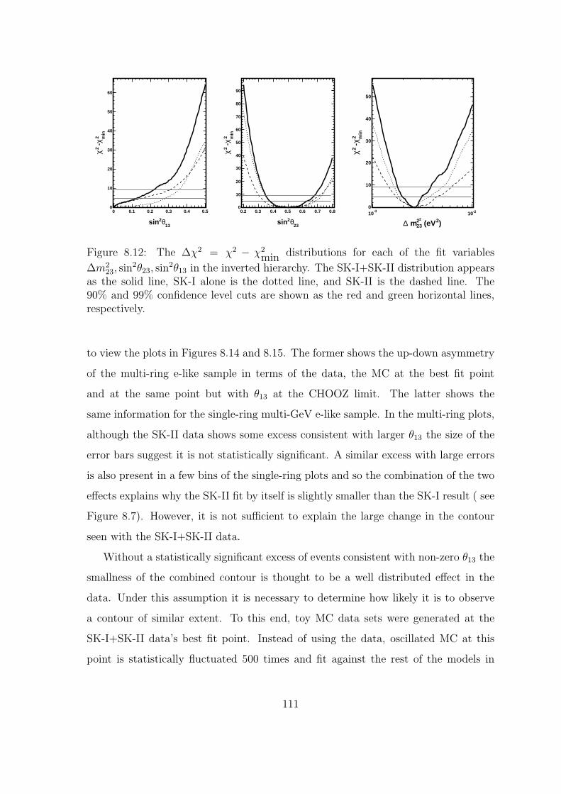
13θ2sin

0 0.1 0.2 0.3 0.4 0.5

min

2 χ -2 χ

0

10

20

30

40

50

60

23θ2sin

0.2 0.3 0.4 0.5 0.6 0.7 0.8

min

2 χ -2 χ

0

10

20

30

40

50

60

70

80

90

)2 (eV22

23 m∆

-310 -210

min

2 χ -2 χ

0

10

20

30

40

50

Figure 8.12: The ∆χ2 = χ2 − χ2min distributions for each of the fit variables

∆m223, sin

2θ23, sin2θ13 in the inverted hierarchy. The SK-I+SK-II distribution appears

as the solid line, SK-I alone is the dotted line, and SK-II is the dashed line. The90% and 99% confidence level cuts are shown as the red and green horizontal lines,respectively.

to view the plots in Figures 8.14 and 8.15. The former shows the up-down asymmetry

of the multi-ring e-like sample in terms of the data, the MC at the best fit point

and at the same point but with θ13 at the CHOOZ limit. The latter shows the

same information for the single-ring multi-GeV e-like sample. In the multi-ring plots,

although the SK-II data shows some excess consistent with larger θ13 the size of the

error bars suggest it is not statistically significant. A similar excess with large errors

is also present in a few bins of the single-ring plots and so the combination of the two

effects explains why the SK-II fit by itself is slightly smaller than the SK-I result ( see

Figure 8.7). However, it is not sufficient to explain the large change in the contour

seen with the SK-I+SK-II data.

Without a statistically significant excess of events consistent with non-zero θ13 the

smallness of the combined contour is thought to be a well distributed effect in the

data. Under this assumption it is necessary to determine how likely it is to observe

a contour of similar extent. To this end, toy MC data sets were generated at the

SK-I+SK-II data’s best fit point. Instead of using the data, oscillated MC at this

point is statistically fluctuated 500 times and fit against the rest of the models in

111

13θ2sin0 0.1 0.2 0.3 0.4 0.5

)2 (

eV2 23

m∆

-310

-210

13θ2sin0 0.1 0.2 0.3 0.4 0.5

)2 (

eV2 23

m∆

-310

-210

13θ2sin0 0.1 0.2 0.3 0.4 0.5

)2 (

eV2 23

m∆

-310

-210

Figure 8.13: Results of the fit to sin2θ13 for (from left to right) SK-I, SK-II and theSK-I+SK-II data set with the CHOOZ 90% exclusion region (shaded). The exclusionresult has been taken from [42].

the parameter space. The effect is to simulate 500 experiments under the assumption

that the data is indeed drawn from the distribution specified by the best fit oscillation

model. After fitting, the extent of the sin2θ13 contours can be compared against the

data.

Figure 8.16 shows the distribution of the maximum end-point of the 90% C.L.

sin2θ13 contour for these simulated experiments. The red line shows the location of

the data’s contour in the distribution and the blue line indicates that of the expected

sensitivity. Of the 500 experiments, 98 were fit at or below the data’s extent. In

comparison, the sensitivity contour represented the lower 57% of the experiments.

Since these numbers are not appreciably close to zero, the SK-I+SK-II data’s result

is sufficiently likely. Accordingly, though the data’s contour is more restrictive than

the CHOOZ limit, based on the MC studies above it is consistent with statistical

fluctuations and occurs 20% of the time.

112

Total Energy [ MeV ]

310 410 510

( U

p-D

ow

n )

/ (

Up

+ D

ow

n )

-0.4

-0.3

-0.2

-0.1

-0

0.1

0.2

0.3

0.4

Total Energy [ MeV ]

310 410 510

( U

p-D

ow

n )

/ (

Up

+ D

ow

n )

-0.4

-0.3

-0.2

-0.1

-0

0.1

0.2

0.3

0.4

Total Energy [ MeV ]

310 410 510

( U

p-D

ow

n )

/ (

Up

+ D

ow

n )

-0.4

-0.3

-0.2

-0.1

-0

0.1

0.2

0.3

0.4

Total Energy [ MeV ]

310 410 510

( U

p-D

ow

n )

/ (

Up

+ D

ow

n )

-0.5

-0.4

-0.3

-0.2

-0.1

-0

0.1

0.2

0.3

0.4

0.5

Total Energy [ MeV ]

310 410 510

( U

p-D

ow

n )

/ (

Up

+ D

ow

n )

-0.5

-0.4

-0.3

-0.2

-0.1

-0

0.1

0.2

0.3

0.4

0.5

Total Energy [ MeV ]

310 410 510

( U

p-D

ow

n )

/ (

Up

+ D

ow

n )

-0.5

-0.4

-0.3

-0.2

-0.1

-0

0.1

0.2

0.3

0.4

0.5

Figure 8.14: The up-down asymmetry of the SK-I (left) and SK-II (right) multi-GeVmulti-ring e-like samples as a function of total energy. Note that the vertical axesbetween the two plots differ. The black dots represent the data while the blue line isthe MC prediction at the best fit point. The red bars denote the excess expected atthe best fit with θ13 at the CHOOZ limit.

Momentum [ MeV / c ]

310 410 510

( U

p-D

ow

n )

/ (

Up

+ D

ow

n )

-0.4

-0.3

-0.2

-0.1

-0

0.1

0.2

0.3

0.4

Momentum [ MeV / c ]

310 410 510

( U

p-D

ow

n )

/ (

Up

+ D

ow

n )

-0.4

-0.3

-0.2

-0.1

-0

0.1

0.2

0.3

0.4

Momentum [ MeV / c ]

310 410 510

( U

p-D

ow

n )

/ (

Up

+ D

ow

n )

-0.4

-0.3

-0.2

-0.1

-0

0.1

0.2

0.3

0.4

Momentum [ MeV / c ]

310 410 510

( U

p-D

ow

n )

/ (

Up

+ D

ow

n )

-0.6

-0.4

-0.2

0

0.2

0.4

0.6

Momentum [ MeV / c ]

310 410 510

( U

p-D

ow

n )

/ (

Up

+ D

ow

n )

-0.6

-0.4

-0.2

0

0.2

0.4

0.6

Momentum [ MeV / c ]

310 410 510

( U

p-D

ow

n )

/ (

Up

+ D

ow

n )

-0.6

-0.4

-0.2

0

0.2

0.4

0.6

Figure 8.15: As in Figure 8.14 for the single ring e-like sample.

113

Table 8.4: Fitted systematic error parameters for systematics common among thedata sets. The columns show ε/σ at the best fit.

Flux Errors SK-I SK-II SK-I + SK-II

Absolute Normalization -0.83 -0.47 -0.94

νµ/νe Eν < 5 GeV 0.56 0.61 0.82

νµ/νe Eν > 5 GeV 0.37 0.3 0.49

νe/νe Eν < 5 GeV -0.089 -0.096 -0.16

νe/νe Eν > 5 GeV -0.23 -0.16 -0.27

νµ/νµ Eν < 5 GeV 0.33 0.47 0.56

νµ/νµ Eν > 5 GeV 0.39 -0.46 0.044

Up/down 0.15 0.22 0.28

Horizontal/vertical -0.29 -0.14 -0.41

K/π 0.1 0.0048 0.12

Neutrino production height 1 0.73 0.97

Cosmic ray energy spectrum -1.2 -1.1 -1.3

FC multi-GeV norm. -1.1 -1 -1.4

PC + upward-stopping norm. 0.25 0.05 0.3

ν Interaction Errors

MA, axial mass -1.2 0.085 -0.9

QE (model) 0.92 0.66 0.98

QE (cross-section) -0.5 -0.25 -0.46

Single-π cross-section 1.1 1.5 1.2

Multi-π (model) -0.21 -0.22 -0.26

Multi-π (cross-section) -0.061 0.1 -0.007

Coherent-π cross section -0.17 -0.34 -0.49

NC/CC -0.33 0.48 -0.05

Nuclear Effect in 16O -0.39 -0.037 -0.31

CC ντ cross-section -0.22 -0.17 -0.31

π energy spectrum -0.0059 0.0 -0.028

FC NC Background 0.47 0.57 0.46

114

Table 8.5: Summary of the fitted systematic error parameters that are specific to SK-I, for SK-I and the Combined data under the normal mass hierarchy. The columnsshow ε/σ for each of the errors.

Reduction Errors SK-I SK-I + SK-II

FC reduction 0.0042 0.24

PC reduction -0.16 -0.04

Upward-going muon Reduction -0.32 -0.41

FC/PC separation 0.11 0.042

non-ν e-like Background -0.13 -0.13

non-ν µ-like Background -0.13 -0.12

Upward stopping/through-going 0.43 0.36

Reconstruction Errors

Ring separation -0.2 -0.17

Single-ring PID -0.53 -0.26

Multi-ring PID -0.35 -0.27

Energy calibration -0.24 -0.17

1.6 GeV muon cut -0.065 -0.013

Energy calibration Up/Down -0.082 -0.096

Upward-through going background 0.13 0.22

Upward-stopping background -0.042 -0.048

Multi-GeV single-ring e-like BG -0.15 -0.14

Multi-ring e-like BG -0.01 -0.0076

Multi-ring e-like normalization 0.41 0.41

PC stop/through-going separation 0.26 -0.017

Solar Activity 0.011 0.03

115

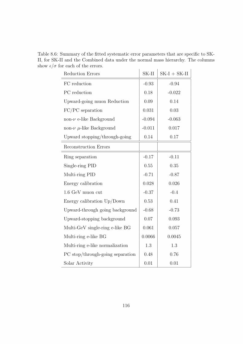
Table 8.6: Summary of the fitted systematic error parameters that are specific to SK-II, for SK-II and the Combined data under the normal mass hierarchy. The columnsshow ε/σ for each of the errors.

Reduction Errors SK-II SK-I + SK-II

FC reduction -0.93 -0.94

PC reduction 0.18 -0.022

Upward-going muon Reduction 0.09 0.14

FC/PC separation 0.031 0.03

non-ν e-like Background -0.094 -0.063

non-ν µ-like Background -0.011 0.017

Upward stopping/through-going 0.14 0.17

Reconstruction Errors

Ring separation -0.17 -0.11

Single-ring PID 0.55 0.35

Multi-ring PID -0.71 -0.87

Energy calibration 0.028 0.026

1.6 GeV muon cut -0.37 -0.4

Energy calibration Up/Down 0.53 0.41

Upward-through going background -0.68 -0.73

Upward-stopping background 0.07 0.093

Multi-GeV single-ring e-like BG 0.061 0.057

Multi-ring e-like BG 0.0066 0.0045

Multi-ring e-like normalization 1.3 1.3

PC stop/through-going separation 0.48 0.76

Solar Activity 0.01 0.01

116

13θ2sin0 0.1 0.2 0.3 0.4 0.5

)2 (

eV2 23

m∆

-310

-210

13θ 2sin0 0.05 0.1 0.15 0.20

10

20

30

40

50

SK-I+SK-II Distribution of Extent of Toy MC 90% C.L.

Figure 8.16: The fitted contours (solid) overlaid with the expected sensitivity (dashed)generated at the best fit point for the SK-I+SK-II data set appears in the left panel.Red lines indicate the 90% C.L. and the 99% C.L. appears in green. In the righthand panel, the distribution of the upper limit of the 90% C.L. on the measurementof sin2θ13 for 500 toy MC data sets generated at the data’s best fit point. Nearly20% of the toy data sets fell at or below that of the data (red line) and 57% fellbelow the expected sensitivity (blue line). The last bin is the integrated contents ofsin2θ13 ≥ 0.20.

117

Chapter 9

Conclusion

Super-Kamiokande has collected more than 18,000 atmospheric neutrino events

over the combined 1489 day SK-I and 803 day SK-II running periods. The SK-I data

has already been used to provide strong evidence for two-flavor νµ ↔ νµ oscillations

at sin22θ = 1.0 and ∆m2 = 2.4× 10−3eV2 [34, 33]. These oscillations have a marked

zenith angle dependence and to leading order there are no oscillation effects seen in

the e-like samples.

The analysis presented in this dissertation searches for the appearance of νe events

at high energy as a signature of sub-leading oscillations in the atmospheric data

driven by non-zero θ13. Further, θ13-induced resonant enhancement of the three-flavor

νµ → νe transition probability in the Earth’s matter has been studied to explore

the question of the neutrino mass hierarchy. Fits have been performed using a χ2

analysis with “pulled” systematic errors to the SK-I, SK-II and their combination

under both the normal and inverted hierarchies. Each result remains consistent with

the previous Super-K analyses and the present knowledge of the atmospheric mixing

parameters. The best fit to the SK-I+SK-II data set is (∆m2, sin2 θ23, sin2 θ13) =

(2.6 × 10−3eV2, 0.5, 0.0) for both hierarchies with χ2min = 602.7 for 587 degrees of

freedom.

The SK-I and SK-II data sets are both consistent with the CHOOZ experiment’s

limit on θ13 in both hierarchies as is the inverted hierarchy fit to the SK-I+SK-II data.

Under the normal hierarchy the this data set’s 90% C.L., however, is slightly more

restrictive than the current best limit and below its expected sensitivity. Since there

is not a significant excess of νe events in the data and because similar contours appear

in ∼ 20% of toy MC samples, the data is consistent with statistical fluctuations. With

the current data, this analysis is not capable of differentiating between the normal

and inverted neutrino mass hierarchies.

Super-Kamiokande is currently taking data as SK-III after detector upgrades in

2006. Recent improvements to the Super-K reconstruction algorithms and the detec-

tor MC will offer a better understanding of the current atmospheric neutrino data.

Further, as data accumulates, so too does the possibility of improved measurements

of the oscillation parameters.

119

Appendix A

Oscillation Software

The analysis performed in this dissertation is an extension of a search for non-

zero θ13 presented in ref [44]. To extend and improve existing features of the search,

the analysis has been modernized and rewritten in C++ to utilize object oriented

programming techniques. Further, since oscillation analyses at Super-K have many

common aspects, the code was written as to provide a generalized analysis package

allowing for more modular program design. A description of the concept of the soft-

ware and how it is applied to perform the oscillation analysis in this dissertation is

presented below. The software maybe obtained from the Super-K CVS repository

under analysis/Osc3++.

A.1 Generic Oscillation Analyses

The oscillation analyses at Super-K, and other analyses for that matter, have

several features in common. First, the analysis chain is nearly identical. Given a set

of data and a corresponding MC, the MC is oscillated at every point in the oscillation

space and fit against the data. Acceptance regions are then drawn around all points

in the oscillation space that differ from the best fit point in their χ2 value by less

than some threshold. In principal, the differences in the analyses amount mostly to

the type and number of bins, the number of points in the oscillation space and the

type of oscillations. However, from the point of view of performing a fit to the data

the software doesn’t need to know these particulars. Instead, a listing of bins in no

particular order, filled with data and the MC to be tested is the minimum amount of

necessary information. The meaning, or edges of the bins are secondary concerns and

120

can be abstracted away. This abstraction is at the heart of the software used in this

analysis.

A.2 Design Strategy

The analysis software has been written with the GEANT4 [96] framework in mind.

That is, its backbone is a set of global parent classes that in principal can run nearly

independently, requiring only minimal input from the user. However, in order to

make the analysis more productive the user is responsible for deriving child classes

from these parents which specify particular actions. Since inherited objects retain the

characteristics of their parent, generic calls to parent functions in the backbone of the

software exist in their children classes but may be overridden. By demanding sufficient

generality in the arguments of the parent routines there is no need to define analysis

specific functions in the backbone code. The parent module responsible for oscillating

an event, for instance, is generically termed Oscillator and its default action is to

return a two-flavor oscillation probability at the best fit point of ref [33]. However, the

analysis in this thesis derives an object ThreeFlavorOscillator from this class,

which overrides the default method to return a full three-flavor probability. Several

objects in the software follow this scheme.

GEANT has provided one other major source of inspiration for the development

of the analysis code, the use of input cards. Since certain parameters change while

studying an analysis, the number of oscillation points to consider or the amount

of averaging to apply (see section 8.2.2), for instance, these otherwise hard-coded

parameters have been moved to card based inputs. Not only does this eliminate the

need to recompile when testing new parameters but it also provides a possible record

of the parameters used for executions of the software.

121

A.3 Code Layout

There are two main pieces to the analysis: oscillation of the MC and fitting the

MC against the observed data. The ensemble of code that performs these tasks is

managed by a central object, the profiler. Profiler manages information that

is more specific to the analysis and is registered by the user. By using an inherited

class ThreeFlavorProfiler, the user registers, for instance, the number, range

and step size for the oscillation parameters. The profiler automatically generates

a ProfileSpace object for each of the requisite oscillation points. The binning

scheme is also maintained in this manner.

After registering, the profiler then brokers the exchange of information between

other objects in the software. When the data and MC are being binned, for instance,

objects provide profiler with an event’s kinematic variables and are returned the

bin into which the event should be filled. In this way it is not necessary to pass and

store indexing information among other classes. The profiler is instantiated in the

main program loop and passed to the objects that interface with it at their creation.

Events are passed to the analysis software through an Event object. This struc-

ture is registered with profiler and used by an EventParser object to pass

information from a ROOT tree to the analysis. The tree should be prepared before

hand and for the analysis in this dissertation represents the final reconstructed and

reduced atmospheric neutrino data and MC. During the analysis sequence a loop is

performed over this tree and the Event object is overwritten at each iteration. A

particular event’s information is disseminated to other parts of the software via the

interactions of EventParser and profiler.

Binning in the analysis is handled by bin objects and each bin in the analysis

is an instantiation of this class. A bin object maintains a variable representing the

data content and an array of MC content (one index for each point in the oscillation

space), but its dimensions are kept separate. Instead it is assigned a unique label at

its instantiation that is maintained by the profiler. Bin creation is handled by

a container class, BinContainer, which interacts with profiler to produce the

122

registered number of bins.

The oscillation of the MC is performed by the parent class OscMaestro. Gener-

ically this class holds a BinContainer, a pointer to an Oscillator and one to a

profiler. OscMaestro is provided events from the data and MC externally and

by interacting with these objects manipulates the bin contents. Fitting the output of

these oscillations is done with a FitMaestro that houses the same objects and ad-

ditionally an instance of the ChiSquared class. By inheriting from these “maestro”

classes the user is able to maintain control over specific parts of the program flow.

Fitting is the most generic aspect of the analysis. The ChiSquared object per-

forms the fit and maintains pointers to a profiler and a BinContainer. If the

user has registered bins with profiler that should not be included during a fit to a

subset of the data ChiSquared has access to this information. However, the parent

profiler is sufficiently general that a ChiSquared object can function without a

user having registered any detailed information. ChiSquared can then use a simple

text file containing the data and MC to be compared. In this way fits to data from

non-oscillation analyses can be performed readily.

A.4 Summary

The Osc3++ code suite is designed for optimal flexibility. Based on this flexibility

it has been used at Super-K for other non-oscillation analyses. The analysis output

is written in ROOT files and is independent in large part from Super-K specific

libraries. For this reason the code is portable and continually evolving. More details

are available in the documentation of the software in the Super-K CVS repository.

123

REFERENCES

[1] T. Schwetz, Plenary talk at NuFact07, Okayama Japan, CERN-PH-TH-207 , hep-ph/07105027.

[2] W. Pauli, Open Letter to Radioactive Ladies and Gentlemen (1930), PhysicsToday 31, 27 (1978).

[3] E. Fermi, Z. Phys. 88, 161 (1934).

[4] B. Pontecorvo, Chalk River Laboratory Report PD-205 (1946), unpub-lished.

[5] F. Reines and C. Cowan, Nature 178, 446 (1953).

[6] F. Reines and C. Cowan, Phys. Rev. 92, 830 (1953).

[7] G. D. et. al, Phys. Rev. Lett. 9, 36 (1962).

[8] K. K. et. al, Phys. Lett. B 504, 218 (2001).

[9] L. Collaborations and the LEP Electroweak Working Group, XX Inter-national Symposium on Lepton and Photon Interatcitons at HighEnergy, Rome, Italy (2001).

[10] M. Honda et. al , Phys. Rev. D75, 043006 (2007).

[11] Ch. Kraus et. al , Euro. Phys. J. C40, 447 (2005).

[12] K.A. Assamagan et. al , Phys. Rev. D53, 6065 (1996).

[13] R. Barate et. al , Euro. Phys. J. C2, 395 (1998).

[14] V. Barger et. al , Phys. Lett. B595, 55 (2004).

[15] C. Arnaboldi et. al , hep-ex/08023439.

[16] B. Cleveland et. al , ApJ 496, 505 (1998).

[17] R. Davis, Harmer, and K. Hoffman, Phys. Rev. Lett. 21, 1205 (1968).

[18] A.I. Abazov et. al , Phys. Rev. Lett. 67, 3332 (1991).

[19] D.N. Abdurashitov et. al, Phys. Rev. Lett. 77, 4708 (1996).

[20] P. Anselmann et. al, Phys. Lett. B235, 376 (1992).

[21] W. Hampel et. al, Phys. Lett. B388, 384 (1996).

[22] Y. Fukuda et. al, Phys. Rev. Lett. 77, 1683 (1996).

[23] J. Hosaka et. al, Phys. Rev. D73, 112001 (2006).

124

[24] Bahcall and Serenelli and Basu, ApJ 621, L85 (2005).

[25] B. Aharmim et. al , Phys. Rev. C72, 055502 (2005).

[26] T. Araki et. al, Phys. Rev. Lett. 94, 081801 (2005).

[27] K.S. Hirata et. al, Phys. Lett. B280, 146 (1992).

[28] D. Casper et. al, Phys. Lett. B66, 2561 (1991).

[29] W.W.M. Allison et. al, Phys. Lett. B391, 491 (1997).

[30] M. Sanchez et. al, Phys. Lett. B566, 35 (2003).

[31] Y. Fukuda et. al, Phys. Lett. B335, 237 (1994).

[32] G. Giacomelli et. al, Phys. Atom. Nucl. 67, 1139 (2004).

[33] Y. Ashie et. al, Phys. Rev. D71, 112005 (2005).

[34] Y. Ashie et. al, Phys. Rev. Lett. 93, 101801 (2004).

[35] P. Adamson et. al, in submission to Phys. Rev. D (hep-ex/0711.0769 ).

[36] M.H. Ahn et. al, Phys. Rev. D74, 072003 (2006).

[37] A. Aguilar et. al, Phys. Rev. D64, 112007 (2001).

[38] B. Armbruster et. al, Phys. Rev. D65, 112001 (2002).

[39] E. Church et. al, Phys. Rev. D66, 013001 (2002).

[40] A.A. Aguilar-Arevalo et. al, Phys. Rev. Lett. 98, 231801 (2007).

[41] M. Maltoni and T. Schwetz, Phys. Rev. D76, 093005 (2007).

[42] M. Apollonio et. al, Eur. Phys. J. C27, 331 (2003).

[43] S. Yamamoto et. al, Phys. Rev. Lett. 96, 181801 (2006).

[44] J. Hosaka et. al, Phys. Rev. D74, 032002 (2006).

[45] Y. I. et al., hep-ex/0106019.

[46] See For Instance M.G. Albrow et. al, FERMILAB-FN-0778-AD-E (hep-ex/0509019 ).

[47] D. A. et al., hep-ex/0503053.

[48] M. G. et al., hep-ex/0503053.

[49] J. Beacom and M. Vagins, Phys. Rev. Lett. 93, 171101 (2004).

[50] W.M. Yao et. al, Journal of Physics G 33, 1 (2006).

[51] Z. Maki, N. Nakagawa, and S. Sakata, Prog. Theor. Phys. 28, 870 (1962).

[52] L. Wolfenstein, Phys. Rev. D17, 2369 (1978).

125

[53] S.P. Mikheyev and A.Y. Smirnov, Sov. J. Nucl. Phys. 42, 1441 (1985).

[54] M. Blom and H. Minakata, New J. Phys. 6, 130 (2004).

[55] V. Barger et. al, Phys. Rev. D22, 2718 (1980).

[56] Super-Kamiokande Collaboration, Nucl. Inst. Meth. 501A, 418 (2003).

[57] M. Ishitsuka, Ph.D. Thesis, University of Tokyo (2004).

[58] S. Desai, Ph.D. Thesis, Boston University (2004).

[59] http://www-sk.icrr.u-tokyo.ac.jp/cause-committee/index-e.html.

[60] M. Honda et. al, Phys. Rev. D64, 053011 (2001).

[61] G. Battistoni et. al, Astropart. Phys. 19, 269 (2003).

[62] G. Barr et. al, Phys. Rev. D70, 023006 (2004).

[63] P. Lipari, Astropart. Phys. 1, 195 (1993).

[64] D. Perkins, Astropart. Phys. 2, 249 (1994).

[65] Y. Hayato, Nucl. Phys. Proc. Supl. 112, 171 (2002).

[66] D. Casper, Nucl. Phys. Proc. Supl. 112, 161 (2002).

[67] C.H. Llewellyn-Smith, Phys. Rept. 3, 261 (1972).

[68] R.H. Smith and E.J. Moniz, Nucl. Phys. B43, 605 (2002).

[69] R. Gran et. al, Phys. Rev. D74, 052002 (2006).

[70] D. Rein and L.M. Sehgal, Ann. Phys. 133, 79 (1981).

[71] D. Rein, Z. Phys. C35, 43 (1987).

[72] T. Kitagaki et. al, Phys. Rev. D34, 2554 (1986).

[73] S.K. Singh et. al, Phys. Rev. B416, 23 (1998).

[74] D. Rein and L.M. Sehgal, Nucl. Phys. B223, 29 (1983).

[75] M. Gluck et. al, Z. Phys. C67, 433 (1995).

[76] M. Nakahata et. al, J. Phys. Soc. Jap 55, 3786 (1986).

[77] T. Sjostrand, Compt. Phys. Commun. 84, 72 (1994).

[78] R. Woods and D. Saxon, Phys. Rev. 95, 577 (1954).

[79] L.L. Salcedo et. al, Nucl. Phys. A484, 577 (1954).

[80] D. Ashery et. al, Phys. Rev. C23, 2173 (1981).

[81] R. Brun and F. Carminati, CERN Programming Long Writeup W5013(1993).

126

[82] C. Zeitnitz and T.A. Gabriel, Nucl. Instrum. Meth. A349, 106 (1994).

[83] E. Bracci, CERN/HERA 72-1 (1972).

[84] A.S. Carroll et. al, Phys. Rev. C14, 635 (1976).

[85] A. Chavarria, http://www.phy.duke.edu/˜schol/superk/alvaro thesis.pdf,Senior Thesis, Duke University (2007).

[86] K. Nitta, Ph.D. Thesis, Osaka University (2003).

[87] E. Davies, Machine Vision: Theory, Algorithms, Practicalities(Academic Press, San Diego, 1976).

[88] A.M. Dziewonski and D.L. Anderson, Phys. Earth, Planet, Interiors 25,297 (1981).

[89] M. Chizhov, M. Maris and S.T. Petcov, hep-ph/9810501 .

[90] O.L.G Peres and A.Yu. Smirnov, Nucl. Phys. B680, 479 (2004).

[91] G.L. Fogli et. al, Phys. Rev. D66, 053010 (2002).

[92] C.H. Albright and C. Jarlskog, Nucl. Phys. B84, 467 (1975).

[93] A. Bodek and U.K. Yang, Nucl. Phys. Proc. Suppl. 112, 70 (2002).

[94] S.K. Singh and E. Oset, Phys. Rev. C48, 1246 (1993).

[95] K. Abe et. al, Phys. Rev. Lett. 97, 171801 (2006).

[96] S. Agostinelli, Nucl. Instrum. Meth. A506, 250 (2003).

127