Prepared for submission to JCAP

Detecting non-relativistic cosmicneutrinos by capture on tritium:phenomenology and physics potential

Andrew J. Long, Cecilia Lunardini, Eray Sabancilar

Physics Department, Arizona State University, Tempe, Arizona 85287, USA.

E-mail: andrewjlong@asu.edu, Cecilia.Lunardini@asu.edu, Eray.Sabancilar@asu.edu

Abstract. We study the physics potential of the detection of the Cosmic Neutrino Backgroundvia neutrino capture on tritium, taking the proposed PTOLEMY experiment as a case study. Withthe projected energy resolution of ∆ ∼ 0.15 eV, the experiment will be sensitive to neutrino masseswith degenerate spectrum, m1 ' m2 ' m3 = mν & 0.1 eV. These neutrinos are non-relativistictoday; detecting them would be a unique opportunity to probe this unexplored kinematical regime.The signature of neutrino capture is a peak in the electron spectrum that is displaced by 2mν abovethe beta decay endpoint. The signal would exceed the background from beta decay if the energyresolution is ∆ . 0.7 mν . Interestingly, the total capture rate depends on the origin of the neutrinomass, being ΓD ' 4 and ΓM ' 8 events per year (for a 100 g tritium target) for unclustered Diracand Majorana neutrinos, respectively. An enhancement of the rate of up to O(1) is expected due togravitational clustering, with the unique potential to probe the local overdensity of neutrinos. Turningto more exotic neutrino physics, PTOLEMY could be sensitive to a lepton asymmetry, and revealthe eV-scale sterile neutrino that is favored by short baseline oscillation searches. The experimentwould also be sensitive to a neutrino lifetime on the order of the age of the universe and break thedegeneracy between neutrino mass and lifetime which affects existing bounds.

arX

iv:1

405.

7654

v2 [

hep-

ph]

12

Nov

201

4

Contents

1 Introduction 1

2 Cosmic background neutrinos and their capture on tritum 32.1 Thermal history of the CνB 32.2 Helicity composition of the CνB 52.3 Detection of the CνB 7

3 Detection prospects at a PTOLEMY-like experiment 10

4 Detection prospects for varying neutrino properties 134.1 Majorana vs. Dirac neutrinos 134.2 Clustering and annual modulation 144.3 The hierarchical mass spectrum 15

5 Probing sterile neutrinos 165.1 eV-scale sterile neutrinos 165.2 keV-scale warm dark matter sterile neutrinos 17

6 Sensitivity to other non-standard neutrino physics 186.1 Lepton asymmetry 186.2 Neutrino decay 196.3 Non-standard thermal history 21

7 Discussion 22

A Amplitude and cross section for polarized neutrinos 23A.1 Kinematics 23A.2 The polarized neutrino capture amplitude 25

1 Introduction

The Cosmic Neutrino Background (CνB) is a cardinal feature of early universe cosmology, and holdsthe key to understanding many of its most interesting and well-studied phenomena: from the primor-dial synthesis of elements, to the anisotropies of the cosmic microwave background (CMB), and evento the formation of dark matter halos (for a review see, e.g., [1–4]).

The body of information from cosmological probes, on the composition and distribution of matterand energy in the early universe, constitutes a very strong indirect evidence that the CνB exists andconfirms the Standard Model’s prediction of its energy density. Specifically, measurements of theCMB anisotropies and the large scale distribution of galaxies have already supplied two key pieces ofdata: a measurement of the effective number of neutrino species, Neff , and a strikingly strong upperbound on the sum of the neutrino masses,

∑mν . The most recent values from the Planck satellite

read as follows [5]:

Neff = 3.30± 0.27 and∑

mν < 0.23 eV at 95% CL . (1.1)

With the next generation of CMB telescopes, the sensitivity to∑mν will be reduced to the 0.05 eV

level, which could allow for a measurement [6].At this time, however, we still lack the truly golden signature of the CνB that only a laboratory-

controlled, direct detection experiment could provide. Such a detection would not only complementother cosmological probes, and thereby help to resolve degeneracies among the neutrino model pa-rameters, but it would access a whole array of phenomena that are beyond the reach of cosmological

– 1 –

Electron Kinetic Energy H Ke L

Ele

ctro

nS

pect

rum

HdG

dE

eL +m4

+mΝ-mΝ

Kend0

»18.6

keV

Β-decay

endpointHK

end L

CΝB

Sterile Ν

Figure 1. A cartoon illustrating the expected signal from the three active CνB neutrinos of mass m1 'm2 ' m3 = mν (solid line), and from a hypothetical, mostly sterile, neutrino mass state, ν4, of mass m4

(dashed line). The CνB signal is displaced from the beta decay endpoint by 2mν , and the ν4 signal wouldbe displaced by mν + m4. The signal and background are not represented to scale. Here Ke = Ee −me isthe electron kinetic energy, and K0

end denoted by the vertical dashed line refers to the beta decay end pointkinetic energy in the mν = 0 limit. For a details, see Sec. 2.3 and Sec. 3.

measurements. In the first place, a direct detection would confirm that the relic neutrinos are stillpresent in the universe today – a reasonable assumption if the neutrinos are stable, but one whichhas no empirical confirmation from cosmological observations alone. To put this less dramatically,a direct detection of the CνB would probe late time effects, those occurring after recombination,such as neutrino clustering (and therefore the neutrino coupling to gravity), changes in the CνBflavor composition or number density due to neutrino decay, or decay of heavy relics into neutri-nos, and so on. Perhaps even more importantly, a direct detection of the CνB would constitute thefirst probe of non-relativistic neutrinos (since current detectors are only sensitive to relatively largeneutrino masses), and thereby open the window onto an entirely new kinematical regime. Studyingnon-relativistic neutrinos could allow for tests of certain neutrino properties that are difficult to accessat high momentum such as the Dirac or Majorana character of neutrinos.

Given the importance of a direct detection of the CνB, it is not surprising that research in thisfield has been active and uninterrupted. In 1962 Weinberg was the first to advocate for CνB detectionvia neutrino capture on beta-decaying nuclei (NCB) since this process requires no threshold energy[7]. The NCB technique is primarily limited by availability of the target material and by the needfor extremely high precision in measuring the electron energy1. Other detection methods have theirown challenges. The Stodolsky effect, for instance, could allow CνB neutrinos to be detected bytheir coherent scattering on a torsion balance [8, 9], but the expected accelerations are well below thesensitivity of current detectors [10, 11], and vanishes if the CνB is lepton-symmetric. In the last fewyears, attention has focused again on Weinberg’s NCB technique, and a number of detailed studieshave assessed the prospects for detection with a tritium target [12–16]. In this type of an experiment,the smoking gun signature of CνB capture, ν+ H3 → He3 + e−, is a peak in the electron spectrum atan energy of 2mν above the beta decay endpoint; see Fig. 1. Detecting this peak requires an energyresolution below the level of mν = O(0.1 eV). Compared to other beta-decaying nuclei, tritiummakes a particularly attractive candidate target because of its availability, high neutrino capturecross section, long lifetime (12 years), and low Q-value [12]. For a 100 gram target, the expected

1In his paper, Weinberg reports of an experimental attempt being carried out by R. W. P. Drever at the Universityof Glasgow at the time of his writing, resulting in a preliminary bound on the CνB Fermi energy EF < 500 eV. Wehave been unable to retrieve any other information on this early experiment.

– 2 –

capture rate is approximately 10 events per year [12]. So far, however, difficulties in achieving thenecessary sub-eV energy resolution, and in controlling broadening of the electron energy distributionhave precluded any serious experimental effort.

In 2012/2013 the Princeton Tritium Observatory for Light, Early-Universe, Massive-NeutrinoYield (PTOLEMY), located at the Princeton Plasma Physics Laboratory, began developing a tech-nology that could help to solve the energy resolution challenges [17]. The tritium nuclei will bedeposited onto a source disk, such as a graphene substrate. This geometry helps to reduce electronbackscatter, and thereby achieve an energy resolution of ∆ ∼ 0.15 eV, of the order of the neutrinomass scale. With this resolution and a 100 gram sample of tritium, PTOLEMY could transform CνBdetection from fantasy into reality.

These recent advances, and especially the prospect of an having an experimental search in thenear future, motivate studying the phenomenology of NCB in more detail. This is the spirit of ourpaper. In particular, the main novelties of our study are the sensitivity to the Dirac or Majorananature of the neutrino, a more detailed analysis of the background rate, and the potential of the NCBto study a number of effects ranging from expected standard phenomenology, such as gravitationalclustering and mass hierarchy, to more exotic ideas like lepton asymmetry, sterile neutrinos, neutrinodecay and non-standard thermal history.

The plan of the paper is as follows. In Sec. 2, we discuss the creation and evolution of theCνB neutrinos, and calculate the polarized neutrino capture cross section and the capture rate fortritium nucleus to clarify the difference between the Dirac and Majorana neutrinos. A detailedcalculation of the neutrino capture kinematics and the polarized neutrino scattering amplitude isgiven in Appendix A. In Sec. 3, we focus on a PTOLEMY-like experiment, and treat the tritium betadecay as the main background for the tritium neutrino capture signal. In particular, we study thesignal to noise ratio by taking into account the finite energy resolution of the detector, and find therequired energy resolution for various neutrino masses. In Sec. 4, we discuss the difference betweenthe Dirac and the Majorana neutrinos, the effect of the mass hierarchy, and gravitational clusteringof neutrinos. In Sec. 5, we discuss the sensitivity to an eV (and sub-eV) scale sterile neutrino and akeV-scale warm dark matter sterile neutrino. In Sec. 6, we discuss various effects of new physics thatcan lead to an enhancement or suppression of the CνB number density, such as lepton asymmetryin the neutrino sector, neutrino decay, and late time entropy injection. A summary and discussionfollow in Sec. 7.

2 Cosmic background neutrinos and their capture on tritum

In this section we will trace the history of a CνB neutrino, considering its production, propagationand detection. In reviewing the physics of these, we emphasize two critical points: the distinctionbetween Dirac and Majorana neutrinos and the distinction between helicity and chirality. These areimportant to derive one of the main conclusions, namely that the CνB capture rate for Dirac andMajorana neutrinos differ by a factor of 2.

2.1 Thermal history of the CνB

Let us first discuss the production of neutrinos in the early universe, i.e., their properties up tothe point when they start free streaming. In the hot, dense conditions of the early universe, theneutrinos maintained thermal equilibrium with the plasma (electrons, positrons, and photons) throughscattering processes such as

νe←→ νe and e+e− ←→ νν . (2.1)

These processes are mediated by the weak interaction, therefore the neutrinos are produced as flavoreigenstates, νe, νµ, ντ , νe, νµ, ντ . The scattering rate of the processes in Eq. (2.1) depends stronglyon the temperature T , as Γ ≈ G2

FT5, where GF ≈ 1.2 × 10−5 GeV−2 is the Fermi constant. At this

time the spectrum of the neutrinos is thermal, given by the Fermi-Dirac distribution, fFD(p, T ) =

– 3 –

(1 + eE/T )−1, where E =√p2 +m2

ν and T is the temperature of the plasma. Integrating over thephase space gives the number density of neutrinos per degree of freedom (flavor and spin):

nν(T ) =3ζ(3)

4π2T 3 . (2.2)

(We will neglect the possibility of a lepton asymmetry for now, and return to this point in Sec. 6.1.)At a temperature of Tfo ∼ MeV, the scattering rate dropped below the Hubble expansion rate,

H ≈ T 2/MP (where MP ≈ 2.4 × 1018 GeV), and as a consequence the neutrinos fell out of thermalequilibrium (“freeze out”). Effectively, the time of freeze out can be considered as the instant ofproduction of the CνB neutrinos that we hope to detect today, since after this time the neutrinossimply free stream. In any case, it is easy to recognize that our conclusions do not depend on theexact instant of production of each neutrino.

Between freeze out and the present epoch, neutrinos undergo a number of interesting effects,that we summarize below.

(i) redshift.In the sudden freeze out approximation, the phase space distribution function after decoupling isgiven by an appropriate redshifting of the distribution function that was realized at decoupling. Thisleads to a modified Fermi-Dirac distribution23

fν [p(z) , Tν(z)] =1

ep(z)/Tν(z) + 1, dnν =

d3p(z)

(2π)3fν [p(z) , Tν(z)] , (2.3)

where

p(z) =1 + z

1 + zfopfo , Tν(z) =

1 + z

1 + zfoTfo (2.4)

are the neutrino momentum and the effective neutrino temperature, respectively. Here they areexpressed in terms of the momentum variable pfo, the neutrino temperature and redshift at freezeout, Tfo and zfo ' 6× 1010.

After neutrino freeze out, the CνB relic abundance is given by Eq. (2.2), where Eq. (2.4) gives theeffective neutrino temperature. As the universe expands, z decreases and so too does Tν . Meanwhilethe photons redshift like

Tγ(z) =1 + z

1 + zfo

g∗(zfo)1/3

g∗(z)1/3Tfo , (2.5)

where g∗(z) = 45s(z)/[2π2T (z)3] and s(z) is the entropy density at epoch z. After electron-positronannihilation freezes out at T ≈ 100 keV, this entropy is transferred to the photons, which causes themto cool less quickly. This leaves the CνB at a relatively lower temperature,

Tν ≈ (4/11)1/3Tγ . (2.6)

We can extrapolate until today when the temperature of the CMB is measured to be Tγ = 0.235 meV[5]. Then, the relationship above predicts the current temperature of the CνB to be Tν = 0.168 meV.Using Eq. (2.2) this corresponds to a number density of

nν(z) = n0(1 + z)3, (2.7)

where

n0 ≈ 56 cm−3 (2.8)

2This approximation agrees with exact solutions of the Boltzmann equation to within O(0.2%) [18].3Note that Eq. (2.3) is valid for any value of p and of the neutrino mass. In it, the mass term is suppressed by a

factor of (1 + z)/(1 + zfo) 1, which we neglect.

– 4 –

per degree of freedom or 6n0 ≈ 336 cm−3 for the entire CνB. Using Eq. (2.3), the root mean squaremomentum of neutrinos in the present epoch can be found to be

p0 ≈ 0.603 meV . (2.9)

Since we are only interested in mν & 0.1 eV for the direct detection purposes, and p0 mν ∼ 0.1 eV,we assume that the CνB neutrinos are extremely non-relativistic today.

(ii) quantum decoherence.As previously mentioned, neutrinos are produced as flavor eigenstates, να, which are a coherentsuperposition of mass eigenstates, νi: να =

∑i Uαi νi, with U being the Pontecorvo-Maki-Nakagawa-

Sakata (PMNS) matrix [19–21] probed by oscillation experiments.Over time, the neutrino wavepacket decoheres as the different mass eigenstates νi propagate

at different velocities [22]. The timescale for this decoherence, ∆t, can be estimated by solving(v1− v2)∆t ≈ λ where vi ≈ p/

√p2 +m2

i ≈ 1−m2i /2p

2 are the velocities of two mass eigenstates andλ ≈ p−1 is the Compton wavelength of the wavepacket. The solution for ∆t, in units of Hubble time(H−1 ≈MP /T

2), is:

∆t

H−1≈ 2p

m22 −m2

1

T 2

MP≈ 10−7 , (2.10)

where we used m2 ≈ 2m1 ≈ 0.1 eV and p ≈ Tfo ≈ 1 MeV. It is found that the flavor eigenstate CνBneutrinos quickly decohere into their mass eigenstates on a time scale much less than one Hubble time[23]. Since we do not expect the decoherence to affect the relative abundances, we then conclude thatneutrinos with the mass values of interest here, are present in the universe today as mass eigenstates,equally populated with an abundance given by Eq. (2.2).

2.2 Helicity composition of the CνB

Next, let us turn to the question of the neutrino spin state at production. Recall that a field’s chiralitydetermines its transformation property under the Lorentz group, and that the weak interaction ischiral in nature, e.g., the left-chiral component of the electron interacts with the weak bosons, butthe right-chiral component does not. Therefore neutrinos (anti-neutrinos) are only produced in theleft-chiral (right-chiral) state. Chirality should not be confused with a particle’s helicity, which isgiven by the projection of its momentum vector onto its spin vector.

Since the CνB neutrinos are ultra-relativistic at freeze out (Tfo mν), we do not (yet) need toexplicitly distinguish helicity and chirality, which exactly coincide for massless particles. For simplicity,here we will use the terminology “left-handed” to refer to a relativistic state that is left-helical andleft-chiral, and we do similarly with the right-handed states.

At this point is it convenient to enumerate all possible spin states. If the neutrinos are Diracparticles then we have four degrees of freedom per generation, which we will label as

νL left-handed active neutrinoνR right-handed active anti-neutrinoνR right-handed sterile neutrinoνL left-handed sterile anti-neutrino

. (2.11)

Neutrinos and anti-neutrinos are distinguished by their lepton number, which is a conserved quantity.The states νL and νR are active in the sense that they interact via the weak interaction, while incontrast νR and νL are labeled as sterile because they interact only via the Higgs boson (i.e., the massterm). This interaction is suppressed by a very small Yukawa coupling yν ≈ mν/v ≈ 10−12, wherev ≈ 246 GeV is the vacuum expectation value of the Higgs field.

The production mechanisms we have discussed above clearly apply only to the active states,which therefore acquire the abundance, nν(z), given by Eq. (2.7). Meanwhile, the sterile neutrinoscan not come into thermal equilibrium with the SM, so it is reasonable to assume that their relic

– 5 –

abundance is negligible compared to that of the active states4. Then, for the Dirac case, we expectthe spin state abundances to be

n(νL) = nν(z)n(νR) = nν(z)n(νR) ≈ 0n(νL) ≈ 0

(2.12)

where nν(z) is given by Eq. (2.7). The total CνB abundance is given by 6nν(z) after summing overspin and flavor states.

If the neutrinos are Majorana particles then lepton number is not a good quantum number,and we should avoid using the language “neutrino” and “anti-neutrino”5. Instead, we will label thedegrees of freedom as

νL left-handed active neutrinoνR right-handed active neutrinoNR right-handed sterile neutrinoNL left-handed sterile neutrino

. (2.13)

As in the Dirac case, the active neutrinos interact weakly, and both the left- and right-handed statesare populated at freeze out. The sterile neutrinos interact only through the Higgs boson, like inthe Dirac case, but now they are typically much heavier than even the electroweak scale (see, e.g.,[24–26]). As such, they will decay into a Higgs boson and a lepton, and their relic abundance todayis zero. To summarize the Majorana case, we have

n(νL) = nν(z)n(νR) = nν(z)n(NR) = 0n(NL) = 0

(2.14)

where once again the total CνB abundance is 6nν(t).Let us discuss how the neutrino quantum states evolve starting from the composition at freezeout,

Eqs. (2.12) and (2.14). To describe the cooling of neutrinos down to the present time, we needto abandon the ultrarelativistic approximation, and therefore study the regime where helicity andchirality do not coincide. To do so, a key point to consider is that the helicity operator commutes withthe free particle Hamiltonian, and its conservation is tied to the conservation of angular momentum.Instead, the chirality operator does not commute because of the mass term. Consequently, whilethe neutrinos are freely streaming, it is their helicity and not their chirality that is conserved [10].Thus, we can determine the abundances today from Eqs. (2.12) and (2.14) upon recognizing that“handedness” at freeze out translates into “helicity” today. Let us denote n(νhL) as the numberdensity of left-helical neutrinos, n(νhR) as the number density of right-helical neutrinos, and so on.Then the abundances today are, for Dirac neutrinos:

n(νhL) = n0

n(νhR) = n0

n(νhR) ≈ 0n(νhL) ≈ 0

(2.15)

4 One cannot exclude the possibility that there was a primordial abundance of sterile neutrinos, and to answerthis question unambiguously one would have to specify the physics of the reheating phase that followed inflation.Nevertheless, it seems unlikely that this abundance was as large as nν(z) at the time of neutrino freeze out. As each ofthe SM fermion species froze out during the thermal history, they transferred their entropy to the remaining thermalspecies. Each of these entropy injections would have diluted the decoupled sterile neutrinos. (The physics is identicalto the suppression of the CνB abundance relative to the CMB abundance after e+e− annihilation.)

5Our language here differs from conventions in the literature. When discussing Majorana neutrinos, it is customaryto equate lepton number with chirality, such that the left-chiral particle is called a neutrino and the right-chiral particleis called an anti-neutrino. This language is very useful for discussing relativistic neutrinos, but impractical for non-relativistic neutrinos, for which we must distinguish helicity and chirality.

– 6 –

and, for Majorana neutrinos:

n(νhL) = n0

n(νhR) = n0

n(NhR) = 0n(NhL) = 0

(2.16)

where n0 is given by Eq. (2.8). Note that the total abundance is the same, 6n0, in both cases.However, the CνB contains both left- and right-helical active neutrinos in the Majorana case, butonly left-helical active neutrinos in the Dirac case.

Finally, we note that, if the neutrinos are not exactly free streaming, but instead they are allowedto interact, then the helicity can be flipped. This leads to a redistribution of the abundances in theDirac case, n(νhL) = n(νhR) = n(νhR) = n(νhL) = n0/2, but no change in the Majorana case since theheavy neutrinos are decoupled. We will return to this point in Sec. 4.2 when we discuss gravitationalclustering.

2.3 Detection of the CνB

In this section the rate of CνB capture on tritium is worked out. To best illustrate the role of helicityeigenstates, we start by discussing the case of the more elementary process of neutrino scattering ona neutron, and then generalize to the case of tritium.

(i) neutrino absorption on a free neutron.Let us consider the process

νj + n→ p+ e− , (2.17)

where the incident neutrino is taken to be in a mass eigenstate νj , following the discussion in theprevious section. For this process, the kinematics can be easily worked out in the rest frame ofthe neutron. As per the discussion of Sec. 2.2, the neutrino is very non-relativistic, so we can takeEν ≈ mν . After properly including the recoil of the proton, we find that the electron is ejected witha kinetic energy Ke = Ee −me, given by (see Appendix A.1)

Kcνbe ≈ Kend + 2mν , (2.18)

where

Kend =(mn −me)

2 − (mν +mp)2

2mn= Q− meQ

mn− Q2

2mp(2.19)

is the beta decay endpoint energy6 and Q ≡ mn −mp −me −mν .We calculate the scattering amplitude for the processes in Eq. (2.17). Due to the low ener-

gies involved, we can safely work in the four-fermion interaction approximation, and obtain (seeAppendix A.2 for details):

iMj = −iGF√2VudU

∗ej

[ueγ

α(1− γ5)uνj] [upγ

β(f(0)− g(0)γ5

)un]ηαβ , (2.20)

where ux is the Dirac spinor for species x, and Vud ≈ 0.97425 is an element of the Cabibbo-Kobayashi-Maskawa (CKM) matrix [27]. The element Uej of the PMNS matrix appears because only the electroncomponent of each mass eigenstate can participate in the process (2.17). The functions f(q) and g(q)are nuclear form factors, and in the limit of small momentum transfer they approach f ≡ f(0) ≈ 1and g ≡ g(0) ≈ 1.2695 [27].

6 Neglecting nucleon recoil is equivalent to neglecting the last two terms in in Eq. (2.19), and gives the morefamiliar result Kcνb

e ≈ Q + 2mν . This approximation is not really legitimate, however, since the size of the neglectedterms exceeds the neutrino mass: e.g., for mν = 0 we get Q0 ≈ 0.7823 MeV, K0

end ≈ 0.7816 MeV, and thereforeK0

end −Q0 ≈ −0.7 keV.

– 7 –

We proceed to calculate the cross section by squaring the amplitude and performing the ap-propriate spin sums. In the neutrino capture experiment under consideration, the spins of the finalstate electron and nucleus are not measured, and therefore we must sum over the possible final states.Similarly, the initial nucleus is not prepared with a definite spin, and therefore we must sum over itstwo possible spins. However, as we discussed in Sec. 2.2, Dirac neutrinos are prepared in a definitespin state, they are left-helical, whereas both helicities are present if the neutrinos are Majorana. Wewill keep the calculation general for now. We denote the neutrino helicity by sν where sν = +1/2corresponds to right-handed helicity and −1/2 to left-handed.

Having performed the spin sums as discussed above, one finds the squared matrix element to be(see Appendix A.2 for details)

|M|2j (sν) = 8G2F |Vud|2|Uej |2mnmpEeEν

[A(sν)(f2 + 3g2) +B(sν)(f2 − g2)ve cos θ

], (2.21)

where θ is the angle between the neutrino and electron momenta, cos θ = pe · pνj/(|pe|∣∣pνj ∣∣), and vi

is the velocity of the species i: vi ≡ |pi| /Ei. The spin-dependent factors are

A(sν) ≡ 1− 2sνvνj =

1− vνj , sν = +1/2 right helical

1 + vνj , sν = −1/2 left helical ,

B(sν) ≡ vνj − 2sν =

vνj − 1 , sν = +1/2 right helical

vνj + 1 , sν = −1/2 left helical. (2.22)

If the neutrinos were relativistic, vνj ' 1, then we would find A = B = 0 for right-helical neutrinos,which implies that these particles cannot be captured, and A = B = 2 for left-helical neutrinos. Thisreproduces the familiar finding that in the relativistic limit helicity and chirality coincide, and onlythe left-chiral neutrinos interact with the weak force. In the non-relativistic limit, which is relevanthere, we have A(±1/2) = ∓B(±1/2) = 1, indicating that both left- and right-helical neutrinos canbe captured.

We calculate the differential cross section from the squared amplitude, Eq. (2.21), in the standardway (see Appendix A.2), and get:

dσj(sν)

d cos θ=G2F

4π|Vud|2|Uej |2F (Z,Ee)

mpEepemnvνj

[A(sν)(f2 + 3g2) +B(sν)(f2 − g2)ve cos θ

](2.23)

where F (Z,Ee) is the Fermi function describing the enhancement of the cross section due to theCoulombic attraction between the outgoing electron and proton. It can be modeled as [28]

F (Z,Ee) =2πη

1− e−2πη, (2.24)

with η = ZαEe/pe, and Z being the atomic number of the daughter nucleus (Z = 1 here); α ≈1/137.036 is the fine structure constant.

Since the incoming neutrino is practically at rest, pν pe, the kinematics allow for isotropicemission of the electron. Then the integral over θ is trivial, and one obtains the total capture crosssection multiplied by the neutrino velocity, which is the quantity relevant for the capture rate:

σj(sν)vνj =G2F

2π|Vud|2|Uej |2F (Z,Ee)

mp

mnEe peA(sν)(f2 + 3g2) . (2.25)

Since A(±1/2) = 1 in the approximation vνj 1, the cross section is identical for the two spin states.Therefore any differences in the capture rate of different spin states must arise from their abundancetoday, as will be seen below.

(ii) neutrino absorption on tritium.Finally, let us generalize our results to the process

νj + H3 → He3 + e− . (2.26)

– 8 –

The calculation of the cross section runs parallel to the derivation of Eq. (2.25), upon replacing n→ H3

and p → He3 . The neutron and proton masses are replaced with the nuclear masses of the speciesinvolved: mn → m H3 ≈ 2808.92 MeV and mp → m He3 ≈ 2808.39 MeV. The same replacement mustbe done in Eqs. (2.18) and (2.19) to find the Q-value and the beta spectrum endpoint. Neglectingthe neutrino mass, these evaluate to7:

Q0 ≈ 18.6 keV and K0end −Q0 ≈ −3.4 eV . (2.27)

Instead of the form factors, f(q) and g(q), one now encounters nuclear matrix elements that quantifythe probability of finding a neutron in the H3 , on which the neutrino can scatter, and a proton inthe He3 . This requires the replacement f2 → 〈fF 〉2 ≈ 0.9987 and 3g2 → (gA/gV )2〈gGT 〉2 where〈gGT 〉2 ≈ 2.788, gA ≈ 1.2695, and gV ≈ 1 [29].

After making the replacements described above, we obtain the velocity-multiplied capture crosssection for mass eigenstate j:

σj(sν)vνj = A(sν) |Uej |2σ , (2.28)

where

σ ≡ G2F

2π|Vud|2F (Z,Ee)

m He3

m H3Ee pe

(〈fF 〉2 + (gA/gV )

2 〈gGT 〉2)' 3.834× 10−45 cm2 . (2.29)

In the numerical estimate we use Ee = me + KCνBe and Eq. (A.21). Considering that for non-

relativistic neutrinos, A(+1/2) = A(−1/2) = 1, we obtain again that the capture cross section is thesame for the left- and right-helical states, and is given by:∑

j=1,2,3

σj(sν = ±1/2)vνj

∣∣∣vνj1

= σ , (2.30)

after summing over the mass eigenstates and using the unitarity of the PMNS matrix,∑j |Uej |2 = 1.

To clarify possible confusions, it is worth noting how this result is related to other commonlyencountered cross sections, namely:

(i) the spin-averaged and mass summed cross sectionThis cross section is velocity-independent, because A(+1/2) + A(−1/2) = 2 independent of vνj , andis:

1

2

∑sν=±1/2

∑j=1,2,3

σj(sν)vνj = σ , (2.31)

(ii) the cross section to capture relativistic neutrinosThis cross section vanishes for the right-helical state and for the left-helical state it is equal to twiceour result: ∑

j=1,2,3

σj(sν = −1/2)vνj

∣∣∣vνj=1

= 2σ = 7.6× 10−45 cm2 . (2.32)

A cross section of this value has been used before in the context of CνB capture on tritium in bothRefs. [12] and [13], and the followup works in Refs. [14–16]. We emphasize that this is leads to anoverestimate of the capture rate, and therefore it should be avoided.

Moving on, finally we can calculate the total capture rate expected in a sample of tritium withmass MT. In Eq. (2.28) we have the capture cross section for a given neutrino mass and helicity

7 We would like to stress that one expects to find the CνB signal at an energy that is displaced by 2mν = O(0.1 eV)above the beta decay endpoint, Ke = Kend, and that the endpoint itself is displaced by 3.4 eV below the Q-value ofthe decay. Since 3.4 eV mν one should take care not to confuse the endpoint and the Q-value.

– 9 –

eigenstate. This requires summing over the cross section for each of the six initial states (j = 1, 2, 3and sν = ±1/2) weighted by the appropriate flux:

Γcνb =

3∑j=1

[σj(+1/2) vνj nj(νhR) + σj(−1/2) vνj nj(νhL)

]NT , (2.33)

where NT = MT/m H3 is the approximate number of nuclei in the sample. Using Eq. (2.28) thecapture rate can be written as

Γcνb =

3∑j=1

|Uej |2 σ [nj(νhR) + nj(νhL)]NT = σ[n(νhR) + n(νhL)

]NT , (2.34)

where σ was given by Eq. (2.29), and we used the fact that different neutrino mass eigenstates areequally populated [18] to perform the sum over j. Here n(νhL) and n(νhR) are the number densitiesof left- and right-helical neutrinos per degree of freedom. We have also used A(−1/2) ≈ A(+1/2) ≈ 1in the non-relativistic limit.

Eq. (2.34) is the central result of this section. Let us see how it applies to the cases of Dirac andMajorana neutrinos, using the results of Sec. 2.2. If the neutrinos are Dirac particles, we saw thatn(νhL) = n0 and n(νhR) = 0, and the capture rate becomes

ΓDcνb = σn0NT . (2.35)

Alternatively, for the Majorana case we found n(νhL) = n(νhR) = n0, and the capture rate becomes

ΓMcνb = 2σn0NT . (2.36)

That is, the capture rate in the Majorana case is twice that in the Dirac case:

ΓMcνb = 2 ΓD

cνb . (2.37)

The relative factor of 2 is a central result of our paper. It can be understood as follows. In the Diraccase, we found that the CνB consists of only left-helical neutrinos and right-helical anti-neutrinos. Ifthese neutrinos were in the relativistic limit, where helicity and chirality coincide, only the left-helicalstates could interact weakly. The right-helical states would be sterile, and only half of the backgroundneutrinos would be available for capture. Since the CνB is non-relativistic, both the left- and right-helical states contain some left-chiral component, and therefore they both interact. The right-helicalanti-neutrinos cannot be captured because the process ν + p→ n+ e+ is kinematically forbidden: itrequires Eν > (mn +me −mp) ≈ 2 MeV in the proton rest frame, but the CνB neutrinos only carryEν ≈ mν . eV (similarly for the tritium). Thus in the Dirac case, only half of the CνB abundanceis available for capture. On the other hand, for the Majorana case one does not distinguish neutrinosand anti-neutrinos; instead we find that the CνB consists of left-helical neutrinos and right-helicalneutrinos, which both interact weakly and therefore are available for capture.

3 Detection prospects at a PTOLEMY-like experiment

Let us now turn to the phenomenology of a tritium-based experiment. Considering a target mass of100 g, as is proposed for PTOLEMY [17], Eqs. (2.35) and (2.36) evaluate to

ΓMcνb ≈ 8.12 yr−1 and ΓD

cνb ≈ 4.06 yr−1 (3.1)

for the Dirac and Majorana neutrino cases, respectively. These rates are limited only by the samplesize, since they are independent of the neutrino mass (as long as the neutrinos are non-relativistic),and the CνB neutrino flux is fixed (in absence of exotica).

One of the main challenges for a neutrino capture experiment is the energy resolution. Theresolution of a detector quantifies the smallest separation at which two spectral features (e.g., two

– 10 –

peaks) can be distinguished. For instance, two Gaussian curves centered at E1 and E2, having equalamplitude, and having equal standard deviation σ can be distinguished provided that |E1 −E2| & ∆where

∆ =√

8 ln 2σ ≈ 2.35σ (3.2)

is the full width at half maximum (FWHM) of the Gaussian [30]. The FWHM is conventionallytaken to be the detector resolution. Applied to our case, this argument means that the spectralexcess due to the CνB can be resolved if its separation from the beta endpoint exceeds the resolution:∆Ke = 2mν >∼ ∆.

PTOLEMY is expected to achieve an energy resolution of ∆ = 0.15 eV [17], just enough to probethe upper end of the neutrino mass spectrum, where the three masses mj are degenerate or quasidegenerate: |mi−mj | mj , i.e., m1 ' m2 ' m3 = mν . In this situation, the mass splittings can notbe resolved by the detector, and the signature of the CνB reduces to a single excess corresponding tothe effective mass mν . Most of the discussion from here on will refer to this case. A brief discussionon possibly resolving the individual masses is given in Sec. 4.3.

Tritium beta decay is the best known and likely the main source of background8 for the CνBneutrino capture events. The effect of the finite energy resolution is that the most energetic electronsfrom beta decay might have measured energy that extends beyond the endpoint Kend, into the regionwhere the signal is expected.

To estimate the rate of such events, consider first the beta decay spectrum [31]:

dΓβdEe

=

3∑j=1

|Uej |2σ

π2H(Ee,mνj )NT , (3.3)

where

H(Ee,mνj ) ≡1−m2

e/(Eem H3 )

(1− 2Ee/m H3 +m2e/m

2H3 )2

√y

(y +

2mνjm He3

m H3

)[y +

mνj

m H3

(m He3 +mνj

)], (3.4)

and y = me +Kend − Ee and the other variables are as in Sec. 2.3.After integrating over energy, the total tritium beta decay rate is found to be

Γβ =

∫ me+Kend

me

dEedΓβdEe

≈ 1024

(MT

100 g

)yr−1 . (3.5)

Comparing with the signal rate in Eq. (3.1), it appears immediately that even an extremely smallcontamination of beta decay events in the signal region can represent a serious challenge for CνBdetection.

To calculate the number of background events, we model the observed spectrum by convolvingthe beta decay and CνB event “true” spectra with a Gaussian envelope of FWHM ∆ [Eq. (3.2)]:

dΓMcνb

dEe=

1√2π σ

∫ ∞−∞

dE′e ΓMcνb(E′e) δ[E

′e − (Eend + 2mν)] exp

[− (E′e − Ee)2

2σ2

](3.6)

dΓβdEe

=1√2π σ

∫ ∞−∞

dE′edΓβdEe

(E′e) exp[− (E′e − Ee)2

2σ2

]. (3.7)

In Fig. 2 we show the smoothed spectra and their sum for various different combinations of detectorresolution and neutrino mass. For ∆ ≈ mν , the smoothed beta decay spectrum extends well beyondthe endpoint energy at Ke − K0

end ≈ −mν and contaminates the neutrino capture signal region atKe −K0

end ≈ +mν .To estimate the potential to distinguish the signal from the background, we calculate the signal-

to-noise ratio. Following [12], the calculation is done for an (observed) energy bin of width ∆ that is

8See Ref. [17] for a discussion of additional backgrounds.

– 11 –

-0.4 -0.2 0.0 0.2 0.4 0.60.1

100

105

108

1011

Ke - Kend0 @ eV D

dGd

Ee

@yr-

1eV

-1

D

0.0 0.1 0.2 0.3 0.4 0.5 0.60

10

20

30

40

50

D = 0.2 eV

mΝ = 0.2 eVmΝ = 0.3 eVmΝ = 0.4 eV

-0.4 -0.2 0.0 0.2 0.40.1

100

105

108

1011

Ke - Kend0 @ eV D

dGd

Ee

@yr-

1eV

-1

D

-0.1 0.0 0.1 0.2 0.3 0.4 0.50

20

40

60

80

D = 0.1 eV

mΝ = 0.1 eVmΝ = 0.2 eVmΝ = 0.3 eV

Figure 2. Solid lines: the expected spectrum of electrons in terms of observed energy, obtained fromEqs. (3.6) and (3.7), for detector resolution (FWHM) ∆ and neutrino mass mν . The dashed lines give the twocontributions (signal and background) separately. The dotted lines show the spectrum of beta decay electronsfor the ideal case of perfect energy resolution, ∆ ' 0. The zero of the horizontal axis coincides with betadecay endpoint (for perfect resolution) for massless neutrinos.

centered on the neutrino capture signal peak. In this bin, the signal and background event rates are:

ΓMcνb(∆) =

∫ Ecνbe +∆/2

Ecνbe −∆/2

dEedΓcνb

dEe(Ee) , (3.8)

Γβ(∆) =

∫ Ecνbe +∆/2

Ecνbe −∆/2

dEedΓβdEe

(Ee) , (3.9)

respectively, where Ecνbe ≡ Kcνb

e +me + 2mν , and their ratio is:

rsn =ΓMcνb(∆)

Γβ(∆). (3.10)

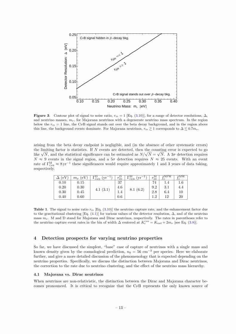
In Fig. 3, contour plot of rsn = 1 is shown for a range of detector resolutions and neutrino masses.Successful detection of the CνB signal is impossible if rsn 1, and it is very likely if rsn 1. Fora given ∆, the signal-to-noise ratio is a rapidly rising function of the neutrino mass (and therefore ofthe width of the gap in energy between the CνB signal and the beta spectrum endpoint), because theendpoint electrons are exponentially suppressed in the tail of the Gaussian. As a rule of thumb, forMajorana neutrinos we find that

rsn & 1 for ∆ . 0.7mν . (3.11)

This condition is only slightly different for Dirac neutrinos, although the signal rate itself is lower bya factor of 2 [Eq. (3.1)].

This conclusion on the signal-to-noise ratio differs slightly from that in the similar analysis ofRef. [12]. The difference is due to two aspects: (i) here rsn is obtained by numerically evaluatingEqs. (3.8) and (3.9). Instead, in Ref. [12] the convolution integral is approximated by a factorizedform for the beta decay background, which tends to underestimate rsn, and the CνB signal was notconvolved with a Gaussian, which tends to overestimate the signal. (ii) here ∆, is identified with theGaussian FWHM (under the advice of the PTOLEMY collaboration, [32]), and not with the Gaussianstandard deviation σ as in Ref. [12]. In terms of σ, our condition reads mν & 1.4(

√8 ln 2σ) ≈ 3.3σ,

which is compatible with Ref. [12].In Table 1 we consider various values for the detector resolution and neutrino masses, and we

show the expected signal event rates and signal-to-noise ratios for the Dirac and Majorana cases. Wealso show the effect of neutrino clustering; see Sec. 4.2 below. If rsn is large then the systematic error

– 12 –

0.10 0.15 0.20 0.25 0.30 0.35 0.400.05

0.10

0.15

0.20

0.25

Neutrino Mass: mΝ @eVD

Det

ecto

rR

esol

utio

n:D

@eV

DrSN

<<1

rSN>>

1

CΝB signal hidden in Β-decay bkg.

CΝB signal stands out over Β-decay bkg.

Figure 3. Contour plot of signal to noise ratio, rsn = 1 [Eq. (3.10)], for a range of detector resolutions, ∆,and neutrino masses, mν , for Majorana neutrinos with a degenerate neutrino mass spectrum. In the regionbelow the rsn = 1 line, the CνB signal stands out over the beta decay background, and in the region abovethis line, the background events dominate. For Majorana neutrinos, rsn & 1 corresponds to ∆ . 0.7mν .

arising from the beta decay endpoint is negligible, and (in the absence of other systematic errors)the limiting factor is statistics. If N events are detected, then the counting error is expected to golike√N , and the statistical significance can be estimated as N/

√N =

√N . A 3σ detection requires

N ≈ 9 events in the signal region, and a 5σ detection requires N ≈ 25 events. With an eventrate of ΓM

cνb ≈ 8 yr−1 these significances would require approximately 1 and 3 years of data taking,respectively.

∆ (eV) mν (eV) ΓDcνb (yr−1) rD

sn ΓMcνb (yr−1) rM

sn fNFWc fMW

c

0.10 0.15

4.1 (3.1)

37

8.1 (6.2)

74 1.4 1.60.20 0.30 4.6 9.2 3.1 4.40.30 0.45 1.4 2.8 6.4 100.40 0.60 0.6 1.2 12 20

Table 1. The signal to noise ratio rsn [Eq. (3.10)] the neutrino capture rate, and the enhancement factor dueto the gravitational clustering [Eq. (4.1)] for various values of the detector resolution, ∆, and of the neutrinomass mν . M and D stand for Majorana and Dirac neutrinos, respectively. The rates in parentheses refer tothe neutrino capture event rates in the bin of width ∆ centered at Kcνb

e = Kend + 2mν [see Eq. (3.8)].

4 Detection prospects for varying neutrino properties

So far, we have discussed the simplest, “base” case of capture of neutrinos with a single mass andknown density given by the cosmological prediction, n0 = 56 cm−3 per species. Here we elaboratefurther, and give a more detailed discussion of the phenomenology that is expected depending on theneutrino properties. Specifically, we discuss the distinction between Majorana and Dirac neutrinos,the correction to the rate due to neutrino clustering, and the effect of the neutrino mass hierarchy.

4.1 Majorana vs. Dirac neutrinos

When neutrinos are non-relativistic, the distinction between the Dirac and Majorana character be-comes pronounced. It is critical to recognize that the CνB represents the only known source of

– 13 –

non-relativistic neutrinos in the universe. As we saw in Sec. 2.3, the Dirac or Majorana character ofthe CνB neutrinos has a significant effect on CνB neutrino capture: the capture rate for Majorananeutrinos is double that of Dirac neutrinos [see Eq. (2.37)]. The factor of two difference can be under-stood as follows. For the Dirac case, only the left-helical neutrinos are available for capture since theright-helical neutrino population is absent from the CνB, and the anti-neutrinos cannot be captured.For the Majorana case, the CνB contains both left- and right-helical neutrinos, and the capture rateis doubled. In Table 1 we compare the signal rates for Dirac and Majorana neutrinos, as well as thecorresponding signal to noise ratios, rsn.

4.2 Clustering and annual modulation

Like all massive particles, neutrinos should cluster in the gravitational potential wells of galaxies andclusters of galaxies. Due to clustering, the local number density, ncν , is larger than the unclusteredcase, n0, and the capture rate should therefore be enhanced by a factor

fc =ncν

n0. (4.1)

The calculation of fc requires solving the Boltzmann equation for the cosmic evolution of a systemconsisting of both cold dark matter and neutrinos, where they are treated as warm dark matter.A variety of approaches, based on different approximations and numerical techniques, have beenpresented [33, 34]. We show the results of Ref. [34] in the last two columns of Table 1. There, fc isgiven for two different models of the dark matter halo of our galaxy, the so called Milky Way model[35] and the Navarro-Frenk-White profile [36]. For masses of the order of mν ∼ 0.1 eV, the effectof clustering should be at the level of few tens of per cent, comparable to the 1σ statistical errorexpected at PTOLEMY in a few years or running (see Sec. 3). Therefore, the experiment may notbe able to measure the local value of fc, but at least it will place a first stringent constraint on it. Ifthe effect of clustering is indeed modest, it may be subdominant to the factor of 2 difference expectedbetween Dirac and Majorana neutrinos, which could still be distinguished.

An additional consequence of clustering is the mixing of neutrino helicities [10]. As a gravi-tationally bound – but otherwise non-interacting – neutrino orbits around the halo, its momentumchanges direction and magnitude, but its spin remains fixed. This causes helicity to change, so thata population of neutrinos initially prepared in a given helicity state (e.g., 100% initially right-helical)will in time grow a component of the opposite helicity, and ultimately reach an equilibrium wherethe right-helical and left-helical states are equally populated. We saw in Sec. 2.2 that the cosmolog-ical population of Dirac neutrinos (anti-neutrinos) consists of 100% left-helical (right-helical) states[Eq. (2.15)]. Assuming complete clustering (i.e., all the neutrinos available for capture are bound grav-itationally to the halo), the populations will equilibrate: n(νhL) = n(νhR) = n(νhR) = n(νhL) = n0/2.Majorana, neutrinos on the other hand are already equilibrated initially [Eq. (2.16)] and clusteringwill simply conserve the equilibrium: n(νhL) = n(νhR) = n0. After repeating the argument in Sec. 2.3,one finds that even with complete clustering the Majorana capture rate is still double that of the Diracneutrinos. This is because for clustered Dirac neutrinos, the new population of right-helical states,n(νhR), compensates for the loss of the left-helical ones in Eq. (2.34).

Finally, let us consider the possibility that the CνB signal rate could exhibit an annual modula-tion, similar to the one predicted for dark matter direct detection. This modulation could be due tothe fact that if neutrinos are substantially clustered, then their velocity distribution relative to Earthis not isotropic and static, as it is usually assumed. The modulation should then follow the relativevelocity of the Earth’s motion with respect to the galactic disk9.

In fact, the answer to the question of modulation is negative [37]. As we saw in Eq. (2.34), thecapture rate depends on the product of number density, cross section and neutrino velocity, vν . Since

9 Clustering also produces a modified momentum distribution compared to unclustered neutrinos, specifically, forstrong clustering the average momentum will be higher than that of the Femi-Dirac prediction [34]. Additionally, themomentum distribution in the rest frame of the Earth will depend on the Earth’s motion relative to the galactic plane.As long as the neutrinos are non-relativistic, however, changes in the neutrino momentum distribution do not affect thecapture rate.

– 14 –

neutrino capture is an exothermic process, i.e., some of the nuclear binding energy is liberated, thecross section scales as σ ∝ 1/vν [13, 38]. Since the velocity cancels in Eq. (2.34), the rate is insensitiveto the neutrino velocity, and thus, there should be no annual modulation of the signal. This is differentfrom DM direct detection, which is an elastic scattering process, with Γ ∝ v. In contrast with DM,then, for CνB detection the astrophysical uncertainties on the velocity profile are not an issue. In thissense, CνB detection is cleaner than DM detection. If an annual modulation does appear at a CνBdetector, its origin would have to be traced elsewhere. For instance, an O(0.1− 1%) modulation mayarise from the gravitational focusing from the Sun [37], even if the neutrinos are not clustered on thescale of the Milky Way.

4.3 The hierarchical mass spectrum

Let us now consider the mass differences between the different neutrino states. From the observationof oscillations, the degeneracy splitting is measured to be [27]:

∆m221 ≈ (8.66 meV)2 and

∣∣∆m232

∣∣ ≈ ∣∣∆m231

∣∣ ≈ (48 meV)2 . (4.2)

The sign of ∆m231 is yet unknown, allowing for two possible mass hierarchies (or “orderings”):

normal hierarchy (NH): ∆m231 > 0 m1 < m2 < m3 (4.3)

inverted hierarchy (IH): ∆m231 < 0 m3 < m1 < m2 . (4.4)

In the coming years, long baseline experiments hope to distinguish these two scenarios [39].If the masses mj are comparable with the largest splitting, mj ∼

√|∆m2

31| ≈ 0.05 eV, thedegenerate, single-mass, approximation used so far becomes inadequate. This is likely to be the case:indeed, if the stringent cosmological bound on the masses, Eq. (1.1), is saturated then the spectrumcan only be marginally degenerate, mνj ≈ 0.07 eV. In the hierarchical regime, CνB detection will notbe possible without a significant improvement in the detector resolution. Nevertheless, we feel thatit is illustrative to discuss how the signal qualitatively changes in this case. A detailed discussion isalso given in Refs. [14, 15].

For a detector with an arbitrarily good energy resolution, ∆ mν , each mass eigenstate νj wouldmake a distinguishable contribution to the CνB capture and to the beta decay spectrum as well. Thebeta decay spectrum would be the sum of three spectra, and its endpoint would be determined by thelightest neutrino mass, mmin = min[mj ] (mmin = m1 for NH, mmin = m3 for IH): Kend = K0

end−mmin.For the CνB capture signal, each state νj would produce a distinct line at an electron kinetic energyof Ke j = K0

end +mνj , or, equivalently:

Kcνbe j = Kend +mmin +mνj , (4.5)

which recovers Eq. (2.18) in the degenerate regime. The total signal rate is still given by Eq. (2.34),but the three terms of the sum will appear as three separate excesses in the energy spectrum, eachwith weight |Uej |2, where [27]:

|Ue1|2 ' 0.68 , |Ue2|2 ' 0.30 , and |Ue3|2 ' 0.02 . (4.6)

Therefore, the signal is the strongest for ν1, weaker for ν2, and the weakest for ν3, as shown in Fig. 4.From the figure one can clearly see that, if we consider the effect of finite detector resolution, theCνB detection is easier in the IH case than for NH. Indeed, the IH case, ν1 and ν2 have the largestseparation from the beta decay endpoint, and they have the strongest signal, making them easier todistinguish from the background. In the NH case, ν3 has the largest separation, but it has the weakestsignal. Note that the intensity of the beta decay background also differs between the IH and NH cases.For the IH case, the endpoint is determined by ν3, which however contributes only proportionally to|Ue3|2, hence the lower background rate. Instead, for the NH case the suppression of the beta spectrumnear the endpoint is only |Ue1|2 [see Eq. (3.3)], corresponding to a higher background.

In Fig. 4, two values of ∆ are considered. For ∆ = 0.01 eV, in the NH case the signal is lostbehind the background, but in the IH case the signal is clearly seen. The ν2 and ν1 eigenstates appear

– 15 –

-0.02 0.00 0.02 0.04 0.060

200

400

600

800

Ke - Kend0 @ eV D

dGd

Ee

@yr-

1eV

-1

DD = 0.01 eV

mmin = 0.001 eV

NH HsolidLIH HdashedL

-0.02 0.00 0.02 0.04 0.060

1000

2000

3000

4000

5000

6000

7000

Ke - Kend0 @ eV D

dGd

Ee

@yr-

1eV

-1

D

D = 0.001 eVmmin = 0.001 eV

NH HsolidLIH HdashedL

Figure 4. The CνB signal at an ultra-high-resolution detector. Each panel shows both hierarchies (NH andIH), with lightest neutrino being almost massless, mmin ≈ 1 meV. The Gaussian peaks are the CνB signaland the sloped lines are the beta decay background. The detector resolution is ∆ = 0.01 eV in the left paneland ∆ = 0.001 eV in the right panel.

as a single peak, because the resolution is insufficient to resolve the small mass gap between them:√∆m2

21 ≈ 8.66 meV < 0.015 eV. For an even more ambitious resolution, ∆ = 0.001 eV, and NH, wecan see the signal, and resolve both the ν2 and ν3 eigenstates. For IH, the signal is still visible, butthe ν2 and ν1 eigenstates are still not resolved.

5 Probing sterile neutrinos

5.1 eV-scale sterile neutrinos

In addition to the three known flavor eigenstates of active neutrinos, there might exist other statesthat are inert, or “sterile” with respect to the Standard Model gauge interactions. Here we discusssterile states that mix with the active states, and share their same helicity, so that they can beproduced via active-sterile oscillations. Within this scenario, the most interesting case is that of asterile neutrino, νs, and its corresponding mass eigenstate, ν4, with mass at the eV scale, m4 ∼ 1 eV.This additional sterile neutrino state is the favored interpretation of the anomalous excess of νe and νeobserved in νµ and νµ beams at LSND [40, 41] and MiniBooNE [42]. It is also a possible explanationof the flux deficits observed in reactor neutrinos [43–45] and at solar neutrino calibration tests usinggallium [46–48].

In presence of a fourth state, flavor mixing is described by a 4× 4 matrix, with the elements Uα4

(α = e, µ, τ, s) describing the flavor composition of ν4. The LSND / MiniBooNE experiments favor[49]

sin2 2θ = 4|Ue4|2|Uµ4|2 ∼ (1− 10) · 10−3 and ∆m241 = m2

4 −m21 ∼ (0.1− 10) eV2 , (5.1)

while global fits of all the anomalies favor the “democratic” value [50]

|Uµ4|2 ∼ |Ue4|2 ' 3× 10−2 . (5.2)

Here the electron-sterile mixing, Ue4, is of interest.With the values of mixings and masses given above, and in absence of other exotica, νs should

be produced (via νµ→ νs and νe→ νs oscillations) before BBN with abundance at or close to thermal,so that its contribution to the radiation energy density is comparable to that of the active neutrinos.Interestingly, this is compatible with, or even favored by, recent cosmological data. Roughly, thesituation is as follows:

– 16 –

(i) recent cosmological observations of an excess of radiation, Neff > 3, from both the BBN [51, 52]and CMB data [53–55], which therefore further support the indication of the existence of νs. (ii) Themeasurement of the Hubble constant by Planck [5] is at tension with the local H0 data [56]. (iii)The measurement of tensor perturbations by BICEP2 [57], is at tension with bounds on tensors fromPlanck’s CMB temperature data [5].

It has been argued very recently that including a sterile neutrino yielding∑jmνj ∼ 0.5 eV and

∆Neff ∼ 0.96 can resolve both the tensions at (ii) [58, 59] and (iii) [60–65]. It has to be noted,however, that data lends themselves to multiple interpretations and the situation is still evolving atthis time (see e.g., Ref. [66] for a different view).

The signature of ν4 at a tritium neutrino capture experiment is a line displaced by

∆Ke = m4 +mν (5.3)

above the endpoint of the beta decay spectrum [see Eq. (4.5)] (see also Ref. [15]). The detection rateis proportional to the local number density of sterile neutrinos, n(νs), and to the appropriate mixingfactor, |Ue4|2. Let us consider a basic scenario in which νs is produced via oscillations, in absence ofother exotica, and accounts for the entire excess of radiation, ∆Neff = Neff − 3.046. It can be shown(see, e.g., [67, 68]) that its momentum distribution is the same as the one of the active neutrinos, upto a constant scaling factor, and therefore the local number density of ν4 is [68]

n(νs) ' fc n0 ∆Neff , (5.4)

where fc . 50 [34] is the enhancement factor due to gravitational clustering (see Sec. 4.2 and Table 1).Thus, the ratio of the ν4 capture rate to the CνB active (Majorana) neutrino capture rate is

Γν4ΓMcνb

≈ 0.6 ∆Neff

(|Ue4|2

3× 10−2

)(fc

20

), (5.5)

or Γν4 ≈ 4.9 yr−1. The result in Eq. (5.5) refers to rather optimistic parameters, and therefore shouldbe considered as the best case scenario. Although the rate is smaller than for the active species, itssignificance in the detector might be boosted by its larger separation from the the endpoint of thebeta decay spectrum. The reason is twofold: first, the excess due to ν4 would be more easily resolved,even with a worse resolution than PTOLEMY; second, the region near the ν4 peak would be nearlybackground-free, since the beta decay spectrum falls exponentially with energy. These aspects areillustrated in Fig. 1.

5.2 keV-scale warm dark matter sterile neutrinos

The above discussion carries over for a sterile neutrino in the keV mass range (see Ref. [69]), whichis a candidate for warm dark matter, and has number of interesting manifestations depending on itsmixing with the active species. The strongest constraints on Ue4 in this mass range are

|Ue4|2 . O(10−9) ; (5.6)

they come from bounds on the abundance of νs in the early universe, and specifically from dataon the spectrum of Large Scale Structures, on observations of the Lyman-α forest, and from X-rayobservations constraining ν4 radiative decay (see e.g., [70, 71] and references therein). Besides bounds,there are positive claims hinting at the existence of a keV-scale νs. Recently a 3.5 keV X-ray line hasbeen identified in various galaxy clusters [72, 73]. Interpreting this line with a decaying sterile neutrinostate yields the parameters m4 ' 7 keV and mixing sin2 2θ = 4|Uα4|2 ' (2 − 20) × 10−11 [72, 73].Such small mixing values will lead to a corresponding suppression of the neutrino detection rate atPTOLEMY. However, this suppression is partially offset by an enhancement: with its larger mass,ν4 can cluster much more efficiently, and therefore its local abundance could be much larger than theunclustered CνB abundance. Specifically, if we assume that ν4 account for 100% of the dark matterlocal density, ρDM ' 0.3 GeV cm−3 [74], the clustering enhancement factor is:

fc ≈ρDM/m4

n0' 7.6× 102

(7 keV

m4

), (5.7)

– 17 –

Taking both the mixing suppression and the clustering enhancement into account, the expected rateat PTOLEMY is given by

Γν4ΓMcνb

' |Ue4|2fc ' 7.6× 10−9

(|Ue4|2

10−11

)(7 keV

m4

). (5.8)

Thus, we conclude that the interesting region of the parameter space is out of reach of this type ofexperiment, although interesting, complementary bounds on νs could be obtained [17].

6 Sensitivity to other non-standard neutrino physics

We now turn to other possible effects that might enhance or suppress the CνB capture signal, suchas the lepton asymmetry in the neutrino sector, neutrino decay, and the entropy injection after theneutrino decoupling.

6.1 Lepton asymmetry

It is established that the universe possesses a cosmic baryon asymmetry, defined as the differencebetween the number density of baryons and that of anti-baryons: nB = nb − nb. Normalized to thephoton density, the asymmetry is nB/nγ ≈ 10−10 [5]. A neutrino asymmetry, nL = nν − nν , is alsoexpected in many models of baryogenesis. In most models it is expected to be comparable to nB ,however there are cases (e.g., [75–77]), where O(10−3)−O(1) lepton asymmetry in the neutrino sectorcan be created, and the current constraints are at the level of nL/nγ . 0.1− 0.5 [78].

In Eqs. (2.11) and (2.13) we enumerated the degrees of freedom for Dirac and Majorana neutrinos.An asymmetry may arise between states which are CP conjugates to one another. If the neutrinos areDirac particles, then this asymmetry is manifest as n(νhL) 6= n(νhR), and is conserved in the absenceof lepton-number violating interactions. In the Majorana case, the asymmetry means n(νhL) 6=n(νhR), and is approximately conserved as long as the helicity-flipping rate is smaller than the Hubbleexpansion rate [79]. As discussed in Sec. 2.2, this is the case for free-streaming neutrinos.

Let us start by considering the Dirac case, and generalize the neutrino distribution function,Eq. (2.3), to include an asymmetry. We will assume that each of the three mass eigenstates carriesthe same asymmetry, because equilibration of flavor is generally expected due to oscillations (see e.g.,[80, 81]). Let µν be the chemical potential and ξν = µν/Tν . Then the number density and energydensity of neutrinos are:

n(νhL) = Nf

∫d3p

(2π)3

1

e(p−µν)/Tν + 1≈ 3Nfζ(3)

4π2T 3ν +

Nf12ξνT

3ν +O(µ2

νTν) , (6.1)

ρ(νhL) = Nf

∫d3p

(2π)3

p

e(p−µν)/Tν + 1≈ 7Nfπ

2

240T 4ν +

9Nfζ(3)

4π2ξνT

4ν +

Nf8ξ2νT

4ν +O(µ3

νTν) ,

where Nf = 3 reflects the sum over flavors, p ≡ |p|, and we have assumed ξν 1 in the expansionson the left side. The corresponding quantities for anti-neutrinos are given by a change of the sign inξν : n(νhR) = n(νhL)|ξν→−ξν , etc.

As we saw in Sec. 2.3, only n(νhL) is relevant for CνB detection. We immediately see that,compared to the symmetric case (ξν = 0) n(νhL) is enhanced (suppressed) if ξν > 0 (ξν < 0).Therefore, the CνB capture rate will have a corresponding enhancement (suppression) factor:

fDξ =

n(νhL)

n(νhL)|ξν=0' 1 +

π2

9ζ(3)ξν ≈ 1 + 0.91ξν . (6.2)

For Majorana neutrinos, the calculation proceeds from Eq. (6.1) in a similar way, however here thequantity relevant to CνB detection is the sum n(νhL) + n(νhR) [see Eq. (2.34)]. Upon summing, theterm linear in ξν cancels out, and the enhancement factor in this case is instead

fMξ =

n(νhL) + n(νhR)

[n(νhL) + n(νhR)]ξν=0' 1 +

2 ln 2

3ζ(3)ξ2ν ≈ 1 + 0.38ξ2

ν , (6.3)

– 18 –

ξν fDξ fM

ξ ∆Neff

0.30 1.31 1.03 0.120.45 1.50 1.08 0.270.60 1.71 1.14 0.480.90 2.21 1.32 1.10-0.30 0.76 1.03 0.12-0.45 0.66 1.08 0.27-0.60 0.57 1.14 0.48-0.90 0.43 1.32 1.10

Table 2. The Dirac and Majorana capture enhancement factors, fDξ and fM

ξ , as well as ∆Neff , for given valuesof the lepton asymmetry parameter ξν . Results are obtained by exact calculation [phase space integrationson the left hand side in Eq. (6.1)].

therefore, for Majorana neutrinos capture is always enhanced by asymmetry.The lepton asymmetry also translates into an additional energy density,

ρtotν = ρ(νhL) + ρ(νhR) ≈ 7Nfπ

2

120T 4ν +

Nf4ξ2νT

4ν , (6.4)

that increases regardless of the sign of ξν . In cosmology the proxy for ρtotν is the commonly quoted

effective number of neutrinos, Neff [Eq. (1.1)]:

Neff = Nfρtotν

ρtotν |ξν=0

≈ Nf +30Nf7π2

ξ2ν , (6.5)

where we can immediately read the excess due to the asymmetry:

∆Neff = Neff −Nf '30Nf7π2

ξ2ν ' 1.3 ξ2

ν . (6.6)

The bound on Neff , Eq. (1.1), thus imply a bound on ξν . Additionally, a strong bound on ξν arisesfrom constrains on the neutron to proton ratio at BBN.

Table 2 shows fDξ , fM

ξ and ∆Neff for a set of values of ξν . From this table, and from Eq. (6.6), wecan infer the maximum capture enhancement allowed by cosmology. The Planck satellite constraint on∆Neff , Eq. (1.1), translates into |ξν | . 0.5. A more careful analysis of CMB data (WMAP9, SPT, andACT) finds that an anti-neutrino excess is preferred, roughly −0.4 . ξν . 0.2 [78], where the exactrange depends on the combination of data sets used. This interval corresponds to 0.6 . fD

ξ . 1.2 and

1.0 . fMξ . 1.1. When the He4 abundance is folded in, the bound tightens to −0.091 . ξν . 0.051

[78], corresponding to a negligible effect on the neutrino capture rate.

6.2 Neutrino decay

Being massive and lepton flavor-violating, neutrinos could be unstable. Given the neutrino masseigenstate νi, with proper lifetime τi, observational constraints on its decay are usually expressed interms of lifetime-to-mass ratio, τi/mi (see, e.g., Ref. [27] for a collection of the current limits). Thebest model-independent constraint derives from the measured supernova neutrino flux in SN1987A[82]:

τ

m> 105 s · eV−1 (6.7)

for the mass eigenstates ν1 and ν2. In order to discuss model-dependent constraints, it is convenientto classify the decay channels as:

• Radiative, “visible”, decay. One of the decay products is a photon.

– 19 –

• “Weak” decay. One of the decay products is a (lighter) neutrino, and the other products areinvisible. For example, it could be that all the neutrinos ultimately decay down to the lightestneutrino species.

• Invisible decay. The decay products are exotic, non-interacting particles such as sterile neutrinos.

Very strong limits are placed on the radiative decay channel from solar ν and γ fluxes [83]

τ

m& 7× 109 s · eV−1 (6.8)

for the ν1 ≈ νe mass eigenstate. Because visible decay channels are already strongly constrained, wewill focus on the weak and invisible decay channels.

(i) invisible decay.If a neutrino completely decays into invisible particles, then the expected CνB capture rate will besuppressed or vanish completely depending on the lifetime. For neutrinos with proper lifetime τ0

ν , thesuppression factor due to the decay of into invisible particles is (see, e.g., [84])

f invd = e−λν , (6.9)

where

λν =

∫dt

τν=

∫ zfo

0

dz

(1 + z)H(z)γ(z)τ0ν

. (6.10)

Here τν(z) = τ0ν γ(z) is the Lorentz-dilated lifetime at epoch z, zfo ' 6×109 is the neutrino decoupling

epoch, and the Hubble parameter and the Lorentz factor of a neutrino are respectively given by

H(z) = H0

√Ωr(1 + z)4 + Ωm(1 + z)3 + ΩΛ , γ(z) =

Eνmν

=

√p2

0

m2ν

(1 + z)2 + 1 , (6.11)

where H0 = 67.04 km s−1 Mpc−1, Ωr = 9.35 × 10−5, Ωm = 0.3183, ΩΛ = 0.6817 [5] and p0 is theneutrino momentum in the present epoch [Eq. (2.9)].

The calculation of λν is greatly simplified by considering that the integral in Eq. (6.10) is dom-inated by the recent epoch, z 1, and that for masses of interest here, the neutrinos were alreadynon-relativistic at that time: mν ∼ 0.1 eV p0 [Eq. (2.9)]. Thus, one expects (and the full calculationconfirms this) the non-relativistic result λν ∼ t0/τ0

ν , and hence,

f invd ∼ e−t0/τ

0ν , (6.12)

where the age of the universe is t0 = 4.36 × 1017 s. From Eq. (6.12) it follows that a detection ofthe CνB at PTOLEMY, at a rate consistent with the standard value, would place constraints on theinvisible decay rate at the order τ0

ν ∼ t0. Instead, a significant suppression, resulting in a negativesearch, could be evidence for neutrino decay implying a upper bound on the lifetime, τ0

ν . t0.Interestingly, the sensitivity to the lifetime is not of the usual form τ/mν : we can really con-

strain the lifetime regardless of the mass, provided that the mass is in the range of sensitivity of theexperiment. This is because this decay test is done with non-relativistic neutrinos, a unique aspect ofthis setup. For comparison with currently available limits, however, we can express the sensitivity as

τ/mν ∼ t0/mν ≈ 4.36× 1018 s · eV−1

(0.1 eV

mν

), (6.13)

which is enormously better than the current model-independent limit, Eq. (6.7), and competitive withthe cosmological limit for radiative decay, Eq. (6.8)10. In this way, a CνB direct detection experimentwould serve as a complementary probe to other astrophysical searches for neutrino decay.

10Strong indirect limits are available, see for instance [27, 85].

– 20 –

(ii) weak decay.Let us consider the case of complete decay of all the CνB neutrinos down into the lightest masseigenstate, which is ν1 for NH or ν3 for IH, see Sec. 4.3. As a consequence, the neutrino populationtoday is entirely made of this state, which is therefore three times more abundant than for stableneutrinos. This means that Eq. (2.34) should be modified by replacing

∑j |Uej |2 = 1 with 3|Uei|2,

where i = 1 for NH and 3 for IH. The result is that the capture rate is enhanced or suppressed by afactor

fwd =

3|Uei|2∑j |Uej |2

=

3|Ue1|2 ≈ 2.03 NH

3|Ue3|2 ≈ 0.068 IH. (6.14)

For the IH case, neutrino weak decay would lead to a null result. On the other hand, detection wouldbe enhanced in the NH case, provided that the detector resolution is good enough to resolve m1. Theobservation of an anomalous rate compatible with Eq. (6.14) would result in a lower or upper boundon the neutrino proper lifetime, along the same argument as in the case of invisible decay. In case ofan incomplete decay, the value fw

d is intermediate between 1 and the results in Eq. (6.14).

6.3 Non-standard thermal history

The predicted CνB detection rate depends sensitively on the temperature of the relic neutrinos, viathe relationship between the temperature and the number density [Eq. (2.2)]. For example, in theMajorana neutrino case our calculated rate is

ΓMcνb ' 8 yr−1

(Tν

1.9K

)3

. (6.15)

Supposing that new physics were to affect the CνB temperature (while maintaining the thermaldistribution), it is immediately clear from Eq. (6.15) that the CνB detection rate could be altereddramatically with even a small temperature change: for Tν ' 4K we would have Γcνb ' 64 yr−1.Conversely, a colder CνB leads to a smaller capture rate.

Needless to say, the CνB temperature has never been directly measured. Its value is predicted tobe Tν = T std

ν ' 1.9K using the observed temperature of the CMB, Tγ ' 2.7K, and the relationshipbetween Tν and Tγ [see Eq. (2.5)]:

TνTγ

=g

1/3∗ (0)

g1/3∗ (zfo)

=

(4

11

)1/3

, (6.16)

Here g∗(z) is the effective number of relativistic species. After neutrino freeze out, the plasma consistedof electrons, positrons, and photons giving g∗(zfo) = 2 + (7/8)4 = 11/2. After e+e− annihilation allthe the entropy is transferred to the photons for which g∗(0) = 2.

It is possible that the CνB temperature could be substantially different than Tν if the thermalhistory of the universe were modified. Specifically, we will suppose that physics beyond the StandardModel is responsible for an entropy injection. For example, in analogy with the e+e− annihilationscenario, we can consider a new species of particle that is initially coupled to the plasma but decouplesand transfers its entropy to the remaining thermalized species. Alternatively, the entropy injectioncould arise from an out-of-equilibrium decay or a first order phase transition. If the injection occursbefore neutrino decoupling, then both the photons and the neutrinos are heated. This delays neutrinodecoupling, but once the neutrinos have frozen out, the ratio Tν/Tγ is unaffected; it is still controlledby e+e− annihilation.

Next suppose that entropy is injected into the photons after neutrino decoupling but beforerecombination. This heats the photons, which must cool for a longer time to reach the measuredvalue of 2.7K, and causes the neutrinos to be relatively colder. The CνB temperature is calculatedusing Eq. (6.16) where g∗(0) = 2 and g∗(zfo) = 11/2 + ∆g where ∆g counts the additional degreesof freedom that were in equilibrium prior to the entropy injection. For instance, if the entropy arises

– 21 –

from the freeze out of a single Dirac species then ∆g = (7/8)4 and Tν/Tγ = (2/9)1/3. This implies acolder CνB, Tν ' 1.6K, and a lower CνB capture rate, Γcνb ' 5 yr−1.

It seems unlikely that an entropy injection could result in a heating of the CνB neutrinos. Evenif the species that freezes out decays into neutrinos (see, e.g., [86]), this will not increase the CνBtemperature, but instead it will lead to a non-thermal spectrum, since the neutrinos are already freestreaming.

A constraint on the CνB temperature, and therefore on entropy injection, arises from the mea-surement of Neff ' 3 from the CMB. Recall that Neff gives the energy density of relativistic species atthe surface of last scattering normalized to the expected CνB temperature. In the standard thermalhistory, the CνB temperature is equal to T std

ν at the surface of last scattering, and the neutrinos con-tribute Neff ' 3. If the neutrinos had a non-standard temperature Tν < T std

ν then their contributionis suppressed as Neff ' 3(Tν/T

stdν )4. The Planck measurement of Neff , Eq. (1.1), translates into the

interval 1.95K < Tν < 2.03K. To allow a larger deviation of Tν from the standard value, one wouldhave to introduce new relativistic degrees of freedom with just the right energy density to compensatefor the energy lost by considering the colder CνB.

7 Discussion

The detection of the CνB via capture on tritium is conceptually interesting, and, for the first time,possibly realistic. The existence of a specific experimental proposal, PTOLEMY, motivates the presentstudy on the phenomenology of this technique. The planned active mass of PTOLEMY is 100 g oftritium, for which the predicted rate is Γ ' (4− 8) yr−1.

Some of the major challenges for a CνB capture experiment are the energy resolution and thebackground control. The signal (if any) due to the CνB will partially overlap with the background frombeta decay, and it is reasonable to expect that the signal and the background might be comparable.The estimated energy resolution at PTOLEMY will be ∆ ∼ 0.15 eV; if the neutrino masses are onthe order of 0.07 eV close to the upper limit allowed by cosmology [Eq. (1.1)], then this resolutionis nearly enough to distinguish the signal from the background [Eq. (3.11)], but it is not sufficient ifthe neutrinos are substantially lighter, in the hierarchical spectrum regime. Since PTOLEMY willprobe only a portion of the parameter space, it is not guaranteed to succeed. Still, it will representan important first step towards the development of more sophisticated technologies for CνB capture.

The spirit of our study is to address the question of what fundamental physics can be learnedfrom a CνB capture experiment, with emphasis on PTOLEMY, but an open mind towards even moreambitious possibilities. Below, the main results of our study are summarized.

1. For 100 grams of tritium, the CνB capture rate is found to be ΓDcνb ' 4 yr−1 for Dirac neutrinos

and ΓMcνb ' 8 yr−1 for Majorana neutrinos [Eq. (3.1)]. This confirms previous calculations

[12, 13] where the rate was also found to be 8 yr−1, although without distinguishing the natureof the neutrinos or working with the polarized capture cross section [see below Eq. (2.32)], as wehave done here. This relative factor of 2 between the Dirac and Majorana cases has to be takeninto account when planning an experimental setup, as it could spell the difference between anindication of the CνB and its discovery.

2. A CνB capture experiment will probe non-relativistic neutrinos. This kinematical regime iscompletely unexplored at this time, and may reveal interesting properties that are not accessiblein the ordinary relativistic regime, such as the distinction between Dirac and Majorana nature ofneutrinos, as we discussed above. This is in striking contrast with the smallness of correctionsat the relativistic regime [87, 88]. In principle, the PTOLEMY concept combines two veryattractive features that are traditionally separated: the kinematic measurement of the neutrinomass from nuclear decays (which is relatively well-understood but insensitive to the origin ofneutrino mass) and the ability to distinguish between Dirac and Majorana neutrinos. The latterso far has been an exclusive feature of neutrinoless double beta decay [89–91].

3. The m4 ∼ 1 eV sterile neutrino favored by MiniBooNE and other oscillation searches couldappear at PTOLEMY with a remarkably clean and unambiguous signature: an excess of up to

– 22 –

5 events per year [Eq. (5.5)] with an electron kinetic energy that should easily be distinguishedfrom that caused by the active neutrinos and the beta decay endpoint [Eq. (5.3)]. In absenceof other exotica, this neutrino should be produced copiously (at or close to thermal abundance)in the early universe. This detection could completely resolve the confused situation that wehave inherited from oscillation experiments, where different searches lead to conflicting resultsand open questions exist on systematic uncertainties and parameter degeneracies. Additionally,it could also help to resolve the tension between cosmological probes of neutrinos, specificallymeasurements of Neff , as well as resolving the tension between B-mode polarization data fromBICEP2 and the Planck bound. It should be noted, though, that the absence of an excess at theeV-scale would not exclude the LSND / MiniBooNE sterile neutrino, but instead restrict theallowed region of |Ue4|. The keV-scale sterile neutrinos require much smaller mixing angles ifthey are to be the dark matter, and this implies a correspondingly small capture rate [Eq. (5.8)].

4. A direct detection of the CνB would be a unique probe of what happened to neutrinos sincethe CMB decoupling time. In principle, it can vastly improve constraints on neutrino decay,and a detection of the CνB would imply a neutrino lifetime longer than the age of the universe[Eq. (6.13)]. Interestingly, this bound would be on the neutrino lifetime itself, and not on theratio of lifetime and mass that is probed with relativistic neutrinos. A direct detection wouldalso provide the unique opportunity to probe the coupling of neutrinos to gravity through thelocal neutrino overdensity, and thereby explore late-time phenomena such as neutrino clustering.Since the CνB capture rate goes like the third power of the CνB temperature, direct detectionmay be used to test non-standard thermal histories in which the neutrinos are heated or cooledby a late-time entropy injection.

5. We have found that many of the variants on standard neutrino physics lead to enhancementsor suppressions of the CνB capture rate. These include gravitational clustering [Eq. (4.1) and Ta-ble 1], weak decay of neutrinos [Eq. (6.14)], the presence of a lepton asymmetry [Eqs. (6.2) and (6.3)and Table 2], and a non-standard thermal history [Sec. 6.3]. Certainly, one has to be mindful ofuncertainties and degeneracies. Since a direct detection of the CνB will only provide two piecesof data, the ν mass scale and the detection rate, it would be impossible to distinguish betweendifferent causes of enhancement or suppression of the CνB, unless the neutrino capture data arecombined with the indirect information from cosmological measurements.

By the time that the PTOLEMY experiment becomes operational, some of the neutrino param-eters will hopefully have been measured by other experiments, e.g., the mass hierarchy by acceleratorexperiments, the mass scale via cosmology and beta decay, and the Dirac or Majorana character vianeutrinoless double beta decay. This information will be a great advantage to PTOLEMY by helpingto break the degeneracies in neutrino parameters (discussed above) and thereby allow PTOLEMY todraw more solid conclusions about the physics of the CνB. We want to emphasize that the detectionof the CνB will not only be a boon to the field of neutrino physics and cosmology, but also could leadto interesting and unexpected new physics that could manifest itself in the regime where neutrinosare non-relativistic. Therefore, the agenda for PTOLEMY and similar proposals might become richerthan previously considered.

Acknowledgments

We are grateful to D. Chung, R. Gran, G. Mangano, M. Messina, C. Quigg and C. Tully for very usefuldiscussions. C.L. and E.S. acknowledge the National Science Foundation grant number PHY-1205745.A.J.L. is supported by the DOE under Grant No. DE-SC0008016.

A Amplitude and cross section for polarized neutrinos

A.1 Kinematics

In this section, we present the kinematic relations that arise in the calculations of tritium beta decayand neutrino capture on tritium. The calculation treats only the nuclear process (masses m H3 and

– 23 –

m He3 are nuclear masses), and we comment on the role of the atomic electron at the end. We workin the rest frame of the tritium nucleus.

Since tritium beta decay is a three-body process, H3 → He3 + e− + νj , the electron can beemitted with a range of momenta. The maximum possible momentum is obtained when the electronis emitted anti-parallel to both the helium-3 nucleus and the neutrino. This momentum demarcatesthe beta decay endpoint,

pend =1

2m H3

√m2

H3 − (m He3 +mν +me)2√m2

H3 − (m He3 +mν −me)2 . (A.1)

The corresponding electron kinetic energy is given by Kend =√p2

end +m2e −me or

Kend =(m H3 −me)

2 − (m He3 +mν)2

2m H3. (A.2)

It is convenient to introduce the Q-value, defined by11

Q ≡ m H3 −m He3 −me −mν , (A.3)

which corresponds to the total kinetic energy carried away by all three decay products. Note thatno single particle can have a kinetic energy equal to Q because this would require a violation ofmomentum conservation, that it, it would neglect the recoil of the other decay products. In terms ofQ, the endpoint energy can be written

Kend = Q−Krecoil (A.4)

where

Krecoil =me

m H3Q+

Q2

2m H3(A.5)

is the amount of kinetic energy unavailable to the electron, because it goes into the recoil of thehelium-3 nucleus and the neutrino. It is also convenient to identify the energy

K0end =

(m H3 −me)2 −m2

He3

2m H3, (A.6)

which is where the endpoint would be located if the neutrino were massless.Next let us consider the kinematics of the neutrino capture process, νj + H3 → He3 + e−. The

calculation simplifies greatly if we neglect the momentum of the incident neutrino. For typical CνBneutrinos, which have a momentum p0 ≈ 6 × 10−4 eV and a mass mν ≈ 0.1 eV, this is a very goodapproximation. A simple calculation gives the kinetic energy of the emitted electron to be

KCνBe =

(m H3 −me +mν)2 −m2He3

2(m H3 +mν). (A.7)

This is the energy at which the CνB signal will be located. Its displacement above the beta decayendpoint is given by

∆K = KCνBe −Kend =

(m H3 +m He3 +mν)2 −m2e

2m H3 (m H3 +mν)mν . (A.8)

If we now make the well-justified approximations m H3 ≈ m He3 me mν , we arrive at the simpleresult ∆K ≈ 2mν or equivalently,

KCνBe ≈ Kend + 2mν . (A.9)

11Alternatively, the Q-value may be defined as Q = M H3 −M He3 where these are the atomic masses of tritium and

helium-3. The difference between Q and Q is the O(10 eV) atomic binding energies.

– 24 –

Since mν p0, we were justified in dropping the neutrino momentum at the start.We have focused here on the kinematics of the nuclear processes, but the system we are really

interested in is a neutral tritium atom converting into a helium ion. The energy of the emittedelectron, however, should be insensitive to the presence of an atomic cloud, both in the beta decayand neutrino capture process. The nuclear process occurs on a short time scale, and on a muchlonger time scale the bound electron finds itself in an excited state of the helium atom. The heliumion relaxes to its ground state by emitting a photon. For this reason, one should not calculate thekinematics using the atomic states; the photon energy must be included as well, and this approachmakes the calculation unnecessarily complicated.

We will conclude this appendix by numerically evaluating the kinematical variables using themeasured masses. Although it is not necessary to perform this exercise, since Eq. (A.9) depends onlyon the neutrino mass, we feel that it is illustrative to the reader. The nuclear masses of tritium andhelium-3 are not provided directly in the AME2003 tables [92]. Instead they must be derived fromthe atomic masses, which are

M H3 (atomic) = 3 016 049 . 2777(25)µu (A.10)

M He3 (atomic) = 3 016 029 . 3191(26)µu (A.11)

where u = 931.4940090(71) MeV. The nuclear masses are then calculated as

m H3 (nuclear) = M H3 (atomic)−me + 13.59811 eV (A.12)

m He3 (nuclear) = M He3 (atomic)− 2me + 24.58678 eV (A.13)

where the last term on each line is the atomic binding energy [93]. The parenthetical values showthe 1σ errors, and the binding energies have negligible error. Taking also the measured electron massfrom Ref. [27] we have

me ≈ 510 . 998 910(13) keV (A.14)

m H3 ≈ 2 808 920. 8205(23) keV (A.15)

m He3 ≈ 2 808 391. 2193(24) keV (A.16)

and

Q ≈ 18.6023(34) keV −mν (A.17)

Krecoil ≈ 0.003445729(86) keV +O(m2ν) (A.18)

K0end ≈ 18.5988(34) keV (A.19)

Kend ≈ 18.5988(34) keV −mν (A.20)

KCνBe ≈ 18.5988(34) keV +mν (A.21)

∆K ≈ 2mν . (A.22)

The error is dominated by the uncertainty in the atomic masses. Although the error bars on Kend andKCνBe are on the order of 3.4 eV, and therefore much larger than the neutrino mass, the displacement

∆K is insensitive to these uncertainties.

A.2 The polarized neutrino capture amplitude

Here we provide some of the details behind the cross section calculation in Sec. 2.3. To our knowledgethe literature does not contain an explicit calculation of the polarized neutrino capture cross sectionfor this process.

Starting with the matrix element in Eq. (2.20), we first calculate the modulus

|M|2 =G2F

2|Vud|2|U∗ej |2T

αγ1 T

βδ2 ηαβηγδ , (A.23)

– 25 –

where

T αγ1 ≡ Tr[γα(1− γ5)uνuνγ

γ(1− γ5)ueue]

(A.24)

T βδ2 ≡ Tr[γβ(f − γ5g

)ununγ

δ(f − γ5g

)upup

]. (A.25)

To reduce notion clutter, we have dropped the index j that indicates the neutrino mass eigenstate.As described in the text, we will sum the spins of the final state electron and proton, and we willaverage the spin of the initial state neutron. Doing so gives

|M|2 =1

2

∑sn,se,sp=±1/2

|M|2 =G2F

4|Vud|2|U∗ej |2T

αγ1 T βδ2 ηαβηγδ , (A.26)

where

T αγ1 =∑

se=±1/2

Tr[γα(1− γ5)uνuνγ

γ(1− γ5)ueue], (A.27)

T βδ2 =∑

sn,sp=±1/2

Tr[γβ(f − γ5g

)ununγ

δ(f − γ5g

)upup

]. (A.28)

We now require the completeness relations,∑si=±1/2

uiui =(/pi +Mi

)for i = n, p, e ,

uνuν =1

2

(/pν +Mν

)(1 + 2sνγ

5/Sν), (A.29)

where

(Sν)α =

(|pν |mν

,Eνmν

pν

)(A.30)

is the neutrino spin vector. Inserting Eq. (A.29) into Eq. (A.27) yields

T αγ1 =1

2Tr[γα(1− γ5)

(/pν +mνj

)(1 + 2sνγ

5/Sν)γγ(1− γ5)

(/pe +me

)](A.31)

T βδ2 = Tr[γβ(f − γ5

)(/pn +mn

)γδ(f − γ5g

)(/pp +mp

)]. (A.32)

The traces are evaluated using the Mathematica package “Tracer” [94], and we find

T αγ1 T βδ2 ηαβηγδ = 32

(g + f)2

[(pe · pp)(pν · pn)

]+ (g − f)2

[(pe · pn)(pν · pp)

]+ (g2 − f2)

[mnmp(pe · pν)

]− 2sνmνj

(g + f)2

[(pe · pp)(Sν · pn)

]+ (g − f)2

[(pe · pn)(Sν · pp)

]+ (g2 − f2)

[mnmp(pe · Sν)

]. (A.33)

The spin-independent terms (sν = 0) match with Ref. [13], and the spin-dependent terms are new.

We now specify to the rest frame of the neutron (parent nucleus) where

(pn)µ = mn;0 , (pν)µ = Eν ;pν , (pp)µ = Ep;pp , (pe)

µ = Ee;pe . (A.34)

– 26 –

Neglecting the proton (daughter nucleus) recoil, pp mp, we obtain

T αγ1 T βδ2 ηαβηγδ = 32mnmpEeEν

2(g2 + f2) + (g2 − f2)

[1− pe

Ee· pνEν

]

− 2sνmnmpEe |pν |

2(g2 + f2) + (g2 − f2)

[1− Eν|pν |

peEe· pν|pν |

]= 32mnmpEeEν

[(f2 + 3g2)(1− 2sνvν) + (f2 − g2)(vν − 2sν)ve cos θ

], (A.35)

where cos θ = pe · pνj/(|pe|∣∣pνj ∣∣) and vi ≡ |pi| /Ei. Inserting Eq. (A.35) into Eq. (A.26) gives

Eq. (2.21).In the center of momentum frame the differential cross section is [27]

dσ

dt=

1

64π

1

s

1

|pν cm|2|M|2 , (A.36)

where s = (pn+pν)2 and t = (pe−pν)2. The Mandelstam variables can be evaluated in the lab frameusing Eq. (A.34) to find

s = (mn + Eν)2 − |pν |2 = m2n + 2mnEν +m2

ν ' m2n , (A.37)

t = (Ee − Eν)2 − |pe − pν |2 ' (me −mν)2 + 2|pe||pν | cos θ , (A.38)

and dt/d cos θ = 2|pe||pν |. After also making the replacement pν cm = pν lab(mn/√s) ' pν , we obtain

dσ

d cos θ=

1

32π

1

m2n

|pe||pν ||M|2 . (A.39)

References

[1] A. Dolgov, Neutrinos in cosmology, Phys.Rept. 370 (2002) 333–535, [hep-ph/0202122].

[2] J. Lesgourgues and S. Pastor, Massive neutrinos and cosmology, Phys.Rept. 429 (2006) 307–379,[astro-ph/0603494].

[3] C. Quigg, Cosmic Neutrinos, arXiv:0802.0013.

[4] A. Dolgov, Cosmology and Neutrino Properties, Phys.Atom.Nucl. 71 (2008) 2152–2164,[arXiv:0803.3887].

[5] Planck Collaboration Collaboration, P. Ade et. al., Planck 2013 results. XVI. Cosmologicalparameters, arXiv:1303.5076.

[6] EPIC Collaboration Collaboration, J. Bock et. al., Study of the Experimental Probe of InflationaryCosmology (EPIC)-Intemediate Mission for NASA’s Einstein Inflation Probe, arXiv:0906.1188.

[7] S. Weinberg, Universal Neutrino Degeneracy, Phys.Rev. 128 (1962) 1457–1473.

[8] L. Stodolsky, Speculations on Detection of the Neutrino Sea, Phys.Rev.Lett. 34 (1975) 110.

[9] B. Shvartsman, V. Braginsky, S. Gershtein, Y. Zeldovich, M. Y. Khlopov, et. al., Possibility ofdetecting relic massive neutrinos, JETP Lett. 36 (1982) 277–279.

[10] G. Duda, G. Gelmini, and S. Nussinov, Expected signals in relic neutrino detectors, Phys.Rev. D64(2001) 122001, [hep-ph/0107027].

[11] M. Hedman, Efficiently extracting energy from cosmological neutrinos, JCAP 1309 (2013) 029,[arXiv:1307.0652].

[12] A. G. Cocco, G. Mangano, and M. Messina, Probing low energy neutrino backgrounds with neutrinocapture on beta decaying nuclei, JCAP 0706 (2007) 015, [hep-ph/0703075].

– 27 –

[13] R. Lazauskas, P. Vogel, and C. Volpe, Charged current cross section for massive cosmologicalneutrinos impinging on radioactive nuclei, J.Phys. G35 (2008) 025001, [arXiv:0710.5312].

[14] M. Blennow, Prospects for cosmic neutrino detection in tritium experiments in the case of hierarchicalneutrino masses, Phys.Rev. D77 (2008) 113014, [arXiv:0803.3762].

[15] Y. Li, Z.-z. Xing, and S. Luo, Direct Detection of the Cosmic Neutrino Background Including LightSterile Neutrinos, Phys.Lett. B692 (2010) 261–267, [arXiv:1007.0914].

[16] R. Hodak, S. Kovalenko, F. Simkovic, and A. Faessler, Beta decaying nuclei as a probe of cosmicneutrino background, arXiv:1102.1799.

[17] S. Betts, W. Blanchard, R. Carnevale, C. Chang, C. Chen, et. al., Development of a Relic NeutrinoDetection Experiment at PTOLEMY: Princeton Tritium Observatory for Light, Early-Universe,Massive-Neutrino Yield, arXiv:1307.4738.

[18] N. Y. Gnedin and O. Y. Gnedin, Cosmological neutrino background revisited, Astrophys.J. 509 (1998)11–15, [astro-ph/9712199].

[19] B. Pontecorvo, Mesonium and anti-mesonium, Sov.Phys.JETP 6 (1957) 429.

[20] B. Pontecorvo, Neutrino Experiments and the Problem of Conservation of Leptonic Charge,Sov.Phys.JETP 26 (1968) 984–988.

[21] Z. Maki, M. Nakagawa, and S. Sakata, Remarks on the unified model of elementary particles,Prog.Theor.Phys. 28 (1962) 870–880.

[22] E. K. Akhmedov and A. Y. Smirnov, Paradoxes of neutrino oscillations, Phys.Atom.Nucl. 72 (2009)1363–1381, [arXiv:0905.1903].

[23] B. Eberle, A. Ringwald, L. Song, and T. J. Weiler, Relic neutrino absorption spectroscopy, Phys.Rev.D70 (2004) 023007, [hep-ph/0401203].

[24] M. Gell-Mann, P. Ramond, and R. Slansky, Complex Spinors and Unified Theories, Conf.Proc.C790927 (1979) 315–321, [arXiv:1306.4669].

[25] R. N. Mohapatra and G. Senjanovic, Neutrino Mass and Spontaneous Parity Violation, Phys.Rev.Lett.44 (1980) 912.

[26] T. Yanagida, Horizontal Symmetry and Masses of Neutrinos, Prog.Theor.Phys. 64 (1980) 1103.

[27] Particle Data Group Collaboration, J. Beringer et. al., Review of Particle Physics (RPP),Phys.Rev. D86 (2012) 010001.

[28] M. Fukugita and T. Yanagida, Physics of Neutrinos and Applications to Astrophysics.Springer-Verlag, Berlin, 2003.

[29] R. Schiavilla, V. Stoks, W. Gloeckle, H. Kamada, A. Nogga, et. al., Weak capture of protons byprotons, Phys.Rev. C58 (1998) 1263, [nucl-th/9808010].

[30] R. L. William, Techniques for Nuclear and Particle Physics Experiments: A How-To Approach.Springer, Berlin, 1994.

[31] S. Masood, S. Nasri, J. Schechter, M. Tortola, J. Valle, et. al., Exact relativistic beta decay endpointspectrum, Phys.Rev. C76 (2007) 045501, [arXiv:0706.0897].

[32] C. Tully, Private communication, .

[33] S. Singh and C.-P. Ma, Neutrino clustering in cold dark matter halos : Implications forultrahigh-energy cosmic rays, Phys.Rev. D67 (2003) 023506, [astro-ph/0208419].

[34] A. Ringwald and Y. Y. Wong, Gravitational clustering of relic neutrinos and implications for theirdetection, JCAP 0412 (2004) 005, [hep-ph/0408241].

[35] A. Klypin, H. Zhao, and R. S. Somerville, Lambda CDM-based models for the Milky Way and M31 I:Dynamical models, Astrophys.J. 573 (2002) 597–613, [astro-ph/0110390].

[36] J. F. Navarro, C. S. Frenk, and S. D. M. White, A Universal Density Profile from HierarchicalClustering, Astrophys. J. 490 (1997) 493–508, [astro-ph/9611107].

– 28 –

[37] B. R. Safdi, M. Lisanti, J. Spitz, and J. A. Formaggio, Annual Modulation of Cosmic Relic Neutrinos,arXiv:1404.0680.

[38] L. D. Landau and E. M. Lifshitz, Quantum Mechanics: Non-relativistic Theory. Pergamon Press,Oxford, Berlin, 1977.

[39] S.-F. Ge, K. Hagiwara, N. Okamura, and Y. Takaesu, Determination of mass hierarchy with mediumbaseline reactor neutrino experiments, JHEP 1305 (2013) 131, [arXiv:1210.8141].

[40] LSND Collaboration Collaboration, A. Aguilar-Arevalo et. al., Evidence for neutrino oscillationsfrom the observation of anti-neutrino(electron) appearance in a anti-neutrino(muon) beam, Phys.Rev.D64 (2001) 112007, [hep-ex/0104049].

[41] LSND Collaboration Collaboration, C. Athanassopoulos et. al., Candidate events in a search foranti-muon-neutrino into anti-electron-neutrino oscillations, Phys.Rev.Lett. 75 (1995) 2650–2653,[nucl-ex/9504002].

[42] MiniBooNE Collaboration Collaboration, A. Aguilar-Arevalo et. al., Unexplained Excess ofElectron-Like Events From a 1-GeV Neutrino Beam, Phys.Rev.Lett. 102 (2009) 101802,[arXiv:0812.2243].

[43] G. Mention, M. Fechner, T. Lasserre, T. Mueller, D. Lhuillier, et. al., The Reactor AntineutrinoAnomaly, Phys.Rev. D83 (2011) 073006, [arXiv:1101.2755].

[44] T. Mueller, D. Lhuillier, M. Fallot, A. Letourneau, S. Cormon, et. al., Improved Predictions of ReactorAntineutrino Spectra, Phys.Rev. C83 (2011) 054615, [arXiv:1101.2663].

[45] P. Huber, On the determination of anti-neutrino spectra from nuclear reactors, Phys.Rev. C84 (2011)024617, [arXiv:1106.0687].

[46] GALLEX Collaboration. Collaboration, P. Anselmann et. al., First results from the Cr-51 neutrinosource experiment with the GALLEX detector, Phys.Lett. B342 (1995) 440–450.

[47] GALLEX Collaboration Collaboration, W. Hampel et. al., Final results of the Cr-51 neutrinosource experiments in GALLEX, Phys.Lett. B420 (1998) 114–126.

[48] SAGE Collaboration Collaboration, J. Abdurashitov et. al., Measurement of the response of theRussian-American gallium experiment to neutrinos from a Cr-51 source, Phys.Rev. C59 (1999)2246–2263, [hep-ph/9803418].

[49] MiniBooNE Collaboration Collaboration, A. Aguilar-Arevalo et. al., Improved Search for νµ → νeOscillations in the MiniBooNE Experiment, Phys.Rev.Lett. 110 (2013) 161801, [arXiv:1207.4809].

[50] C. Giunti, M. Laveder, Y. Li, and H. Long, Pragmatic View of Short-Baseline Neutrino Oscillations,Phys.Rev. D88 (2013) 073008, [arXiv:1308.5288].

[51] R. Cooke, M. Pettini, R. A. Jorgenson, M. T. Murphy, and C. C. Steidel, Precision measures of theprimordial abundance of deuterium, arXiv:1308.3240.

[52] Y. Izotov, G. Stasinska, and N. Guseva, Primordial 4He abundance: a determination based on thelargest sample of HII regions with a methodology tested on model HII regions, arXiv:1308.2100.

[53] Z. Hou, C. Reichardt, K. Story, B. Follin, R. Keisler, et. al., Constraints on Cosmology from theCosmic Microwave Background Power Spectrum of the 2500-square degree SPT-SZ Survey,Astrophys.J. 782 (2014) 74, [arXiv:1212.6267].

[54] WMAP Collaboration, G. Hinshaw et. al., Nine-Year Wilkinson Microwave Anisotropy Probe(WMAP) Observations: Cosmological Parameter Results, Astrophys.J.Suppl. 208 (2013) 19,[arXiv:1212.5226].

[55] Atacama Cosmology Telescope Collaboration, J. L. Sievers et. al., The Atacama CosmologyTelescope: Cosmological parameters from three seasons of data, JCAP 1310 (2013) 060,[arXiv:1301.0824].

[56] A. G. Riess, L. Macri, S. Casertano, H. Lampeitl, H. C. Ferguson, et. al., A 3 % Solution:Determination of the Hubble Constant with the Hubble Space Telescope and Wide Field Camera 3,Astrophys.J. 730 (2011) 119, [arXiv:1103.2976].

– 29 –

[57] BICEP2 Collaboration Collaboration, P. Ade et. al., BICEP2 I: Detection Of B-mode Polarizationat Degree Angular Scales, arXiv:1403.3985.

[58] R. A. Battye and A. Moss, Evidence for massive neutrinos from CMB and lensing observations,Phys.Rev.Lett. 112 (2014) 051303, [arXiv:1308.5870].

[59] J.-W. Hu, R.-G. Cai, Z.-K. Guo, and B. Hu, Cosmological parameter estimation from CMB and X-rayclusters after Planck, arXiv:1401.0717.

[60] J.-F. Zhang, Y.-H. Li, and X. Zhang, Sterile neutrinos help reconcile the observational results ofprimordial gravitational waves from Planck and BICEP2, arXiv:1403.7028.

[61] C. Dvorkin, M. Wyman, D. H. Rudd, and W. Hu, Neutrinos help reconcile Planck measurements withboth Early and Local Universe, arXiv:1403.8049.

[62] J.-F. Zhang, Y.-H. Li, and X. Zhang, Cosmological constraints on neutrinos after BICEP2,arXiv:1404.3598.

[63] H. Li, J.-Q. Xia, and X. Zhang, Global fitting analysis on cosmological models after BICEP2,arXiv:1404.0238.

[64] M. Archidiacono, N. Fornengo, S. Gariazzo, C. Giunti, S. Hannestad, et. al., Light sterile neutrinosafter BICEP-2, arXiv:1404.1794.

[65] E. Giusarma, E. Di Valentino, M. Lattanzi, A. Melchiorri, and O. Mena, Relic Neutrinos, thermalaxions and cosmology in early 2014, arXiv:1403.4852.

[66] B. Leistedt, H. V. Peiris, and L. Verde, No new cosmological concordance with massive sterileneutrinos, arXiv:1404.5950.

[67] S. Dodelson and L. M. Widrow, Sterile-neutrinos as dark matter, Phys.Rev.Lett. 72 (1994) 17–20,[hep-ph/9303287].

[68] T. D. Jacques, L. M. Krauss, and C. Lunardini, Additional Light Sterile Neutrinos and Cosmology,Phys.Rev. D87 (2013), no. 8 083515, [arXiv:1301.3119].

[69] Y. Li and Z.-z. Xing, Possible Capture of keV Sterile Neutrino Dark Matter on Radioactive β-decayingNuclei, Phys.Lett. B695 (2011) 205–210, [arXiv:1009.5870].

[70] A. Y. Smirnov and R. Zukanovich Funchal, Sterile neutrinos: Direct mixing effects versus inducedmass matrix of active neutrinos, Phys.Rev. D74 (2006) 013001, [hep-ph/0603009].

[71] A. Kusenko, Sterile neutrinos: The Dark side of the light fermions, Phys.Rept. 481 (2009) 1–28,[arXiv:0906.2968].

[72] E. Bulbul, M. Markevitch, A. Foster, R. K. Smith, M. Loewenstein, et. al., Detection of AnUnidentified Emission Line in the Stacked X-ray spectrum of Galaxy Clusters, arXiv:1402.2301.

[73] A. Boyarsky, O. Ruchayskiy, D. Iakubovskyi, and J. Franse, An unidentified line in X-ray spectra ofthe Andromeda galaxy and Perseus galaxy cluster, arXiv:1402.4119.

[74] J. Bovy and S. Tremaine, On the local dark matter density, Astrophys.J. 756 (2012) 89,[arXiv:1205.4033].

[75] X.-D. Shi and G. M. Fuller, A New dark matter candidate: Nonthermal sterile neutrinos,Phys.Rev.Lett. 82 (1999) 2832–2835, [astro-ph/9810076].

[76] M. Laine and M. Shaposhnikov, Sterile neutrino dark matter as a consequence of nuMSM-inducedlepton asymmetry, JCAP 0806 (2008) 031, [arXiv:0804.4543].

[77] A. Boyarsky, O. Ruchayskiy, and M. Shaposhnikov, The Role of sterile neutrinos in cosmology andastrophysics, Ann.Rev.Nucl.Part.Sci. 59 (2009) 191–214, [arXiv:0901.0011].

[78] D. J. Schwarz and M. Stuke, Does the CMB prefer a leptonic Universe?, New J. Phys. 15 (2013)033021, [arXiv:1211.6721].

[79] P. Langacker, G. Segre, and S. Soni, Majorana Neutrinos, Nucleosynthesis, and the Lepton Asymmetryof the Universe, Phys.Rev. D26 (1982) 3425.

[80] C. Lunardini and A. Y. Smirnov, High-energy neutrino conversion and the lepton asymmetry in theuniverse, Phys.Rev. D64 (2001) 073006, [hep-ph/0012056].

– 30 –

[81] A. Dolgov, S. Hansen, S. Pastor, S. Petcov, G. Raffelt, et. al., Cosmological bounds on neutrinodegeneracy improved by flavor oscillations, Nucl.Phys. B632 (2002) 363–382, [hep-ph/0201287].

[82] K. Hirata et al. [KAMIOKANDE-II Collaboration], “Observation of a Neutrino Burst from theSupernova SN 1987a”, Phys. Rev. Lett. 58 (1987) 1490.

[83] G. Raffelt, Neutrino radiative lifetime limits from the absence of solar gamma rays, Phys.Rev. D31(1985) 3002–3004.

[84] P. Baerwald, M. Bustamante, and W. Winter, Neutrino Decays over Cosmological Distances and theImplications for Neutrino Telescopes, JCAP 1210 (2012) 020, [arXiv:1208.4600].

[85] S. Pakvasa, “Do neutrinos decay?”, AIP Conf. Proc. 542 (2000) 99 [hep-ph/0004077].

[86] T. Kanzaki, M. Kawasaki, K. Kohri, and T. Moroi, Cosmological Constraints on Neutrino Injection,Phys.Rev. D76 (2007) 105017, [arXiv:0705.1200].

[87] M. Zralek, On the possibilities of distinguishing Dirac from Majorana neutrinos, Acta Phys.Polon.B28 (1997) 2225–2257, [hep-ph/9711506].

[88] M. Czakon, J. Gluza, and M. Zralek, Nature of neutrinos in the light of present and futureexperiments, Phys.Lett. B465 (1999) 211–218, [hep-ph/9906381].

[89] CUORICINO Collaboration Collaboration, C. Arnaboldi et. al., Results from a search for the 0neutrino beta beta-decay of Te-130, Phys.Rev. C78 (2008) 035502, [arXiv:0802.3439].

[90] F. Alessandria, E. Andreotti, R. Ardito, C. Arnaboldi, I. Avignone, F.T., et. al., Sensitivity ofCUORE to Neutrinoless Double-Beta Decay, arXiv:1109.0494.

[91] GERDA Collaboration Collaboration, M. Agostini et. al., Results on Neutrinoless Double-β Decayof 76Ge from Phase I of the GERDA Experiment, Phys.Rev.Lett. 111 (2013), no. 12 122503,[arXiv:1307.4720].

[92] G. Audi, A. Wapstra, and C. Thibault, The Ame2003 atomic mass evaluation (II). Tables, graphs andreferences, Nucl.Phys. A729 (2002) 337–676.

[93] J. A. BEARDEN and A. F. BURR, Reevaluation of x-ray atomic energy levels, Rev. Mod. Phys. 39(Jan, 1967) 125–142.

[94] M. Jamin and M. E. Lautenbacher, TRACER: Version 1.1: A Mathematica package for gammaalgebra in arbitrary dimensions, Comput.Phys.Commun. 74 (1993) 265–288.

– 31 –