arX

iv:a

stro

-ph/

0205

109v

1 7

May

200

2

Observation of High Energy Atmospheric Neutrinos with the Antarctic Muon and

Neutrino Detector Array

J. Ahrens,9 E. Andres,14 X. Bai,1 G. Barouch,11 S.W. Barwick,8 R.C. Bay,7 T. Becka,9 K.-H. Becker,2 D. Bertrand,3

F. Binon,3 A. Biron,4 J. Booth,8 O. Botner,13 A. Bouchta,4∗ O. Bouhali,3 M.M. Boyce,11 S. Carius,5 A. Chen,11

D. Chirkin,7 J. Conrad,13 J. Cooley,11 C.G.S. Costa,3 D.F. Cowen,10 E. Dalberg,14† C. De Clercq,15 T. DeYoung,11‡

P. Desiati,11 J.-P. Dewulf,3 P. Doksus,11 J. Edsjo,14 P. Ekstrom,14 T. Feser,9 J.-M. Frere,3 T.K. Gaisser,1

M. Gaug4§ A. Goldschmidt,6 A. Hallgren,13 F. Halzen,11 K. Hanson,10 R. Hardtke,11 T. Hauschildt,4 M. Hellwig,9

H. Heukenkamp,4 G.C. Hill,11 P.O. Hulth,14 S. Hundertmark,8 J. Jacobsen,6 A. Karle,11 J. Kim,8 B. Koci,11

L. Kopke,9 M. Kowalski,4 J.I. Lamoureux,6 H. Leich,4 M. Leuthold,4 P. Lindahl,5 I. Liubarsky,11 P. Loaiza,13

D.M. Lowder,7¶ J. Madsen,12 P. Marciniewski,13∗∗ H.S. Matis,6 C.P. McParland,6 T.C. Miller,1††, Y. Minaeva,14

P. Miocinovic,7 P.C. Mock,8‡‡, R. Morse,11 T. Neunhoffer,9 P. Niessen,4,15 D.R. Nygren,6 H. Ogelman,11

Ph. Olbrechts,15 C. Perez de los Heros,13 A.C. Pohl,5 R. Porrata,8§§ P.B. Price,7 G.T. Przybylski,6 K. Rawlins,11

C. Reed,8¶¶, W. Rhode,2 M. Ribordy,4 S. Richter,11 J. Rodrıguez Martino,14 P. Romenesko,11 D. Ross,8

H.-G. Sander,9 T. Schmidt,4 D. Schneider,11 R. Schwarz,11 A. Silvestri,2,4 M. Solarz,7 G.M. Spiczak,12 C. Spiering,4

N. Starinsky,11∗∗∗, D. Steele,11 P. Steffen,4 R.G. Stokstad,6 O. Streicher,4 P. Sudhoff,4 K.-H. Sulanke,4

I. Taboada,10 L. Thollander,14 T. Thon,4 S. Tilav,1 M. Vander Donckt,3 C. Walck,14 C. Weinheimer,9

C.H. Wiebusch,4∗ C. Wiedeman,14 R. Wischnewski,4 H. Wissing,4 K. Woschnagg,7 W. Wu,8 G. Yodh,8 S. Young8

(AMANDA Collaboration)1 Bartol Research Institute, University of Delaware, Newark, DE 19716, USA

2 Fachbereich 8 Physik, BUGH Wuppertal, D-42097 Wuppertal, Germany3 Universite Libre de Bruxelles, Science Faculty CP230,

Boulevard du Triomphe, B-1050 Brussels, Belgium4 DESY-Zeuthen, D-15735 Zeuthen, Germany

5 Dept. of Technology, Kalmar University, S-39182 Kalmar, Sweden6 Lawrence Berkeley National Laboratory, Berkeley, CA 94720, USA

7 Dept. of Physics, University of California, Berkeley, CA 94720, USA8 Dept. of Physics and Astronomy, University of California, Irvine, CA 92697, USA

9 Institute of Physics, University of Mainz, Staudinger Weg 7, D-55099 Mainz, Germany10 Dept. of Physics and Astronomy, University of Pennsylvania, Philadelphia, PA 19104, USA

11 Dept. of Physics, University of Wisconsin, Madison, WI 53706, USA12 Physics Department, University of Wisconsin, River Falls, WI 54022, USA

13 Division of High Energy Physics, Uppsala University, S-75121 Uppsala, Sweden14 Dept. of Physics, Stockholm University, SCFAB, SE-10691 Stockholm, Sweden and

15 Vrije Universiteit Brussel, Dienst ELEM, B-1050 Brussel, Belgium

(Dated: December 17, 2013)

The Antarctic Muon and Neutrino Detector Array (AMANDA) began collecting data with tenstrings in 1997. Results from the first year of operation are presented. Neutrinos coming throughthe Earth from the Northern Hemisphere are identified by secondary muons moving upward throughthe array. Cosmic rays in the atmosphere generate a background of downward moving muons, whichare about 106 times more abundant than the upward moving muons. Over 130 days of exposure, weobserved a total of about 300 neutrino events. In the same period, a background of 1.05 ·109 cosmicray muon events was recorded. The observed neutrino flux is consistent with atmospheric neutrinopredictions. Monte Carlo simulations indicate that 90% of these events lie in the energy range 66GeV to 3.4 TeV. The observation of atmospheric neutrinos consistent with expectations establishesAMANDA-B10 as a working neutrino telescope.

PACS numbers: 95.55.Vj, 95.85.Ry, 96.40.Tv

∗now at CERN, CH-1211, Geneve 23, Switzerland†now at Defense Research Establishment (FOA), S-17290 Stock-holm, Sweden‡now at Santa Cruz Institute for Particle Physics, University ofCalifornia - Santa Cruz, Santa Cruz, CA 95064§now at IFAE, 08193 Barcelona, Spain

¶now at MontaVista Software, 1237 E. Arques Ave., Sunnyvale,CA 94085, USA∗∗now at The Svedberg Laboratory, S-75121 Uppsala, Sweden††now at Johns Hopkins University, Applied Physics Laboratory,Laurel, MD 20723, USA‡‡now at Optical Networks Research, JDS Uniphase, 100 Willow-

2

I. INTRODUCTION

Energetic cosmic ray particles entering the Earth’s at-mosphere generate a steady flux of secondary particlessuch as electrons, muons and neutrinos. The electroniccomponent of cosmic rays is quickly absorbed. High en-ergy muons penetrate the Earth’s surface for several kilo-meters, while atmospheric neutrinos can easily pass theEarth up to very high energies. Interactions of hadronicparticles, similar to the ones that create the atmosphericneutrino flux, will generate neutrinos at sites where cos-mic rays are generated and where they interact as theytravel through the Universe. The goal of observing neu-trinos of astrophysical origin determines the design andthe size of neutrino telescopes.

The primary channel through which neutrino tele-scopes detect neutrinos above energies of a few tens ofGeV is by observing the Cherenkov light from secondarymuons produced in νµ-nucleon interactions in or near thetelescope. To ensure that the observed muons are pro-duced by neutrinos, the Earth is used as a filter and onlyupward moving muons are selected. A neutrino telescopeconsists of an array of photosensors embedded deeply in atransparent medium. The tracks of high energy muons —which can travel many hundreds of meters, or even kilo-meters, through water or ice — can be reconstructed withreasonable precision even with a coarsely instrumenteddetector, provided the medium is sufficiently transparent.A location deep below the surface serves to minimize theflux of cosmic-ray muons.

In this paper we demonstrate the observation of at-mospheric muon neutrinos with the Antarctic Muon andNeutrino Detector Array (AMANDA). These neutrinosconstitute a convenient flux of fairly well known strength,angular distribution, and energy spectrum, which can beused to verify the response of the detector. The paperwill focus on the methods of data analysis and the com-parison of observed data with simulations. After a briefdescription of the detector, the data and the methods ofsimulation are introduced in Section III and the generalmethods of event reconstruction are described in Sec-tion IV. Two AMANDA working groups analyzed thedata in parallel. The methods and results of both analy-ses are described in Sections V and VI. After a discussionof systematic uncertainties in Section VII we present thefinal results and conclusions.

brook Rd., Freehold, NJ 07728- 2879, USA§§now at L-174, Lawrence Livermore National Laboratory, 7000East Ave., Livermore, CA 9455 0, USA¶¶Dept. of Physics, Massachussetts Institute of Technology, Cam-bridge, MA USA∗∗∗now at SNO Institute, Lively, ON, P3Y 1M3 Canada

120 m

snow layer

��������

optical module (OM)

housingpressure

OpticalModule

silicon gel

HV divider

light diffuser ball

60 m

AMANDA as of 2000

zoomed in on one

(true scaling)

200 m

Eiffel Tower as comparison

Depth

surface50 m

1000 m

2350 m

2000 m

1500 m

810 m

1150 m

AMANDA-A (top)

zoomed in on

AMANDA-B10 (bottom)

AMANDA-A

AMANDA-B10

main cable

PMT

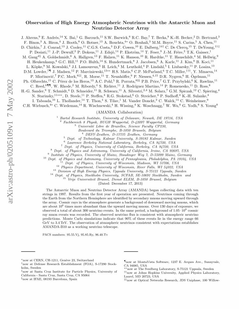
FIG. 1: The present AMANDA detector. This paper de-scribes data taken with the ten inner strings shown in ex-panded view in the bottom center.

II. THE AMANDA DETECTOR

The AMANDA detector uses the 2.8 km thick icesheet at the South Pole as a neutrino target, Cherenkovmedium and cosmic ray flux attenuator. The detectorconsists of vertical strings of optical modules (OMs) —photomultiplier tubes sealed in glass pressure vessels —frozen into the ice at depths of 1500–2000 m below thesurface. Figure 1 shows the current configuration of theAMANDA detector. The shallow array, AMANDA-A,was deployed at depths of 800 to 1000m in 1993–94 inan exploratory phase of the project. Studies of the op-tical properties of the ice carried out with AMANDA-A showed a high concentration of air bubbles at thesedepths, leading to strong scattering of light and makingaccurate track reconstruction impossible. Therefore, adeeper array of ten strings with 302 OMs was deployed inthe austral summers of 1995–96 and 1996–97 at depths of1500–2000m. This detector is referred to as AMANDA-B10, and is shown in the center of Fig. 1. The detectorwas augmented by three additional strings in 1997–98and six in 1999–2000, forming the AMANDA-II array.

In AMANDA B10, an optical module consists of a sin-gle 8” Hamamatsu R5912-2 photomultiplier tube (PMT)housed in a glass pressure vessel. The PMT is optically

3

effective scattering coefficient [m-1]

(z-1

730

m)

[m

]

-350

-300

-250

-200

-150

-100

-50

0

50

100

150

200

250

0.01 0.02 0.03 0.04 0.05 0.06 0.07

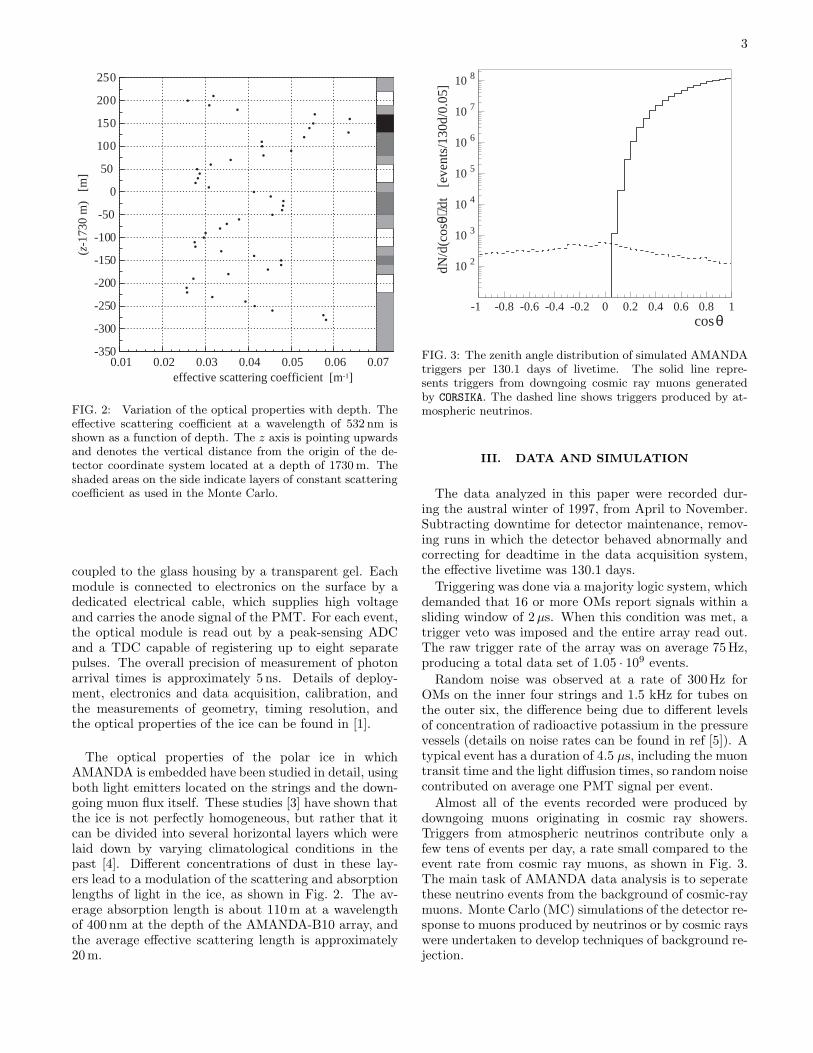
FIG. 2: Variation of the optical properties with depth. Theeffective scattering coefficient at a wavelength of 532 nm isshown as a function of depth. The z axis is pointing upwardsand denotes the vertical distance from the origin of the de-tector coordinate system located at a depth of 1730 m. Theshaded areas on the side indicate layers of constant scatteringcoefficient as used in the Monte Carlo.

coupled to the glass housing by a transparent gel. Eachmodule is connected to electronics on the surface by adedicated electrical cable, which supplies high voltageand carries the anode signal of the PMT. For each event,the optical module is read out by a peak-sensing ADCand a TDC capable of registering up to eight separatepulses. The overall precision of measurement of photonarrival times is approximately 5 ns. Details of deploy-ment, electronics and data acquisition, calibration, andthe measurements of geometry, timing resolution, andthe optical properties of the ice can be found in [1].

The optical properties of the polar ice in whichAMANDA is embedded have been studied in detail, usingboth light emitters located on the strings and the down-going muon flux itself. These studies [3] have shown thatthe ice is not perfectly homogeneous, but rather that itcan be divided into several horizontal layers which werelaid down by varying climatological conditions in thepast [4]. Different concentrations of dust in these lay-ers lead to a modulation of the scattering and absorptionlengths of light in the ice, as shown in Fig. 2. The av-erage absorption length is about 110m at a wavelengthof 400 nm at the depth of the AMANDA-B10 array, andthe average effective scattering length is approximately20m.

cosθ

10 2

10 3

10 4

10 5

10 6

10 7

10 8

-1 -0.8 -0.6 -0.4 -0.2 0 0.2 0.4 0.6 0.8 1

dN/d

(cos

θ)/d

t [e

vent

s/13

0d/0

.05]

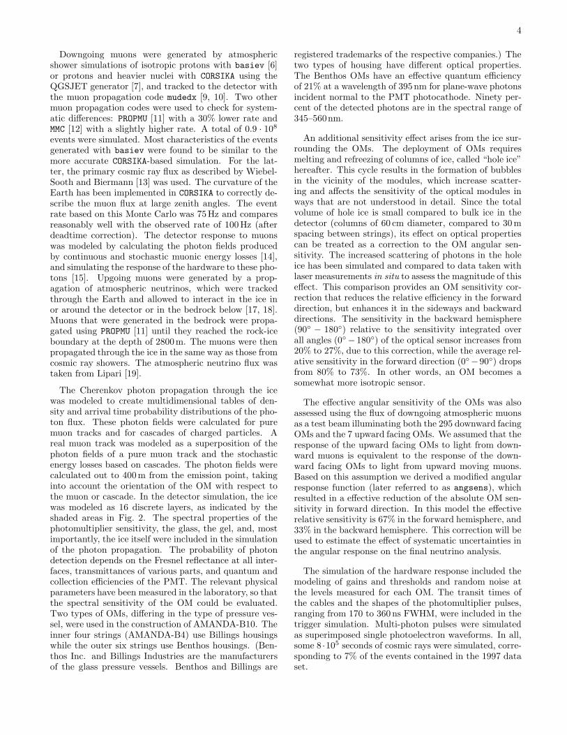
FIG. 3: The zenith angle distribution of simulated AMANDAtriggers per 130.1 days of livetime. The solid line repre-sents triggers from downgoing cosmic ray muons generatedby CORSIKA. The dashed line shows triggers produced by at-mospheric neutrinos.

III. DATA AND SIMULATION

The data analyzed in this paper were recorded dur-ing the austral winter of 1997, from April to November.Subtracting downtime for detector maintenance, remov-ing runs in which the detector behaved abnormally andcorrecting for deadtime in the data acquisition system,the effective livetime was 130.1 days.

Triggering was done via a majority logic system, whichdemanded that 16 or more OMs report signals within asliding window of 2µs. When this condition was met, atrigger veto was imposed and the entire array read out.The raw trigger rate of the array was on average 75Hz,producing a total data set of 1.05 · 109 events.

Random noise was observed at a rate of 300Hz forOMs on the inner four strings and 1.5 kHz for tubes onthe outer six, the difference being due to different levelsof concentration of radioactive potassium in the pressurevessels (details on noise rates can be found in ref [5]). Atypical event has a duration of 4.5 µs, including the muontransit time and the light diffusion times, so random noisecontributed on average one PMT signal per event.

Almost all of the events recorded were produced bydowngoing muons originating in cosmic ray showers.Triggers from atmospheric neutrinos contribute only afew tens of events per day, a rate small compared to theevent rate from cosmic ray muons, as shown in Fig. 3.The main task of AMANDA data analysis is to seperatethese neutrino events from the background of cosmic-raymuons. Monte Carlo (MC) simulations of the detector re-sponse to muons produced by neutrinos or by cosmic rayswere undertaken to develop techniques of background re-jection.

4

Downgoing muons were generated by atmosphericshower simulations of isotropic protons with basiev [6]or protons and heavier nuclei with CORSIKA using theQGSJET generator [7], and tracked to the detector withthe muon propagation code mudedx [9, 10]. Two othermuon propagation codes were used to check for system-atic differences: PROPMU [11] with a 30% lower rate andMMC [12] with a slightly higher rate. A total of 0.9 · 108

events were simulated. Most characteristics of the eventsgenerated with basiev were found to be similar to themore accurate CORSIKA-based simulation. For the lat-ter, the primary cosmic ray flux as described by Wiebel-Sooth and Biermann [13] was used. The curvature of theEarth has been implemented in CORSIKA to correctly de-scribe the muon flux at large zenith angles. The eventrate based on this Monte Carlo was 75Hz and comparesreasonably well with the observed rate of 100Hz (afterdeadtime correction). The detector response to muonswas modeled by calculating the photon fields producedby continuous and stochastic muonic energy losses [14],and simulating the response of the hardware to these pho-tons [15]. Upgoing muons were generated by a prop-agation of atmospheric neutrinos, which were trackedthrough the Earth and allowed to interact in the ice inor around the detector or in the bedrock below [17, 18].Muons that were generated in the bedrock were propa-gated using PROPMU [11] until they reached the rock-iceboundary at the depth of 2800m. The muons were thenpropagated through the ice in the same way as those fromcosmic ray showers. The atmospheric neutrino flux wastaken from Lipari [19].

The Cherenkov photon propagation through the icewas modeled to create multidimensional tables of den-sity and arrival time probability distributions of the pho-ton flux. These photon fields were calculated for puremuon tracks and for cascades of charged particles. Areal muon track was modeled as a superposition of thephoton fields of a pure muon track and the stochasticenergy losses based on cascades. The photon fields werecalculated out to 400m from the emission point, takinginto account the orientation of the OM with respect tothe muon or cascade. In the detector simulation, the icewas modeled as 16 discrete layers, as indicated by theshaded areas in Fig. 2. The spectral properties of thephotomultiplier sensitivity, the glass, the gel, and, mostimportantly, the ice itself were included in the simulationof the photon propagation. The probability of photondetection depends on the Fresnel reflectance at all inter-faces, transmittances of various parts, and quantum andcollection efficiencies of the PMT. The relevant physicalparameters have been measured in the laboratory, so thatthe spectral sensitivity of the OM could be evaluated.Two types of OMs, differing in the type of pressure ves-sel, were used in the construction of AMANDA-B10. Theinner four strings (AMANDA-B4) use Billings housingswhile the outer six strings use Benthos housings. (Ben-thos Inc. and Billings Industries are the manufacturersof the glass pressure vessels. Benthos and Billings are

registered trademarks of the respective companies.) Thetwo types of housing have different optical properties.The Benthos OMs have an effective quantum efficiencyof 21% at a wavelength of 395nm for plane-wave photonsincident normal to the PMT photocathode. Ninety per-cent of the detected photons are in the spectral range of345–560nm.

An additional sensitivity effect arises from the ice sur-rounding the OMs. The deployment of OMs requiresmelting and refreezing of columns of ice, called “hole ice”hereafter. This cycle results in the formation of bubblesin the vicinity of the modules, which increase scatter-ing and affects the sensitivity of the optical modules inways that are not understood in detail. Since the totalvolume of hole ice is small compared to bulk ice in thedetector (columns of 60 cm diameter, compared to 30mspacing between strings), its effect on optical propertiescan be treated as a correction to the OM angular sen-sitivity. The increased scattering of photons in the holeice has been simulated and compared to data taken withlaser measurements in situ to assess the magnitude of thiseffect. This comparison provides an OM sensitivity cor-rection that reduces the relative efficiency in the forwarddirection, but enhances it in the sideways and backwarddirections. The sensitivity in the backward hemisphere(90◦ − 180◦) relative to the sensitivity integrated overall angles (0◦− 180◦) of the optical sensor increases from20% to 27%, due to this correction, while the average rel-ative sensitivity in the forward direction (0◦−90◦) dropsfrom 80% to 73%. In other words, an OM becomes asomewhat more isotropic sensor.

The effective angular sensitivity of the OMs was alsoassessed using the flux of downgoing atmospheric muonsas a test beam illuminating both the 295 downward facingOMs and the 7 upward facing OMs. We assumed that theresponse of the upward facing OMs to light from down-ward muons is equivalent to the response of the down-ward facing OMs to light from upward moving muons.Based on this assumption we derived a modified angularresponse function (later referred to as angsens), whichresulted in a effective reduction of the absolute OM sen-sitivity in forward direction. In this model the effectiverelative sensitivity is 67% in the forward hemisphere, and33% in the backward hemisphere. This correction will beused to estimate the effect of systematic uncertainties inthe angular response on the final neutrino analysis.

The simulation of the hardware response included themodeling of gains and thresholds and random noise atthe levels measured for each OM. The transit times ofthe cables and the shapes of the photomultiplier pulses,ranging from 170 to 360 ns FWHM, were included in thetrigger simulation. Multi-photon pulses were simulatedas superimposed single photoelectron waveforms. In all,some 8 ·105 seconds of cosmic rays were simulated, corre-sponding to 7% of the events contained in the 1997 dataset.

5

IV. EVENT RECONSTRUCTION

The reconstruction of muon events in AMANDA isdone offline, in several stages. First, the data are“cleaned” by removing unstable PMTs and spuriousPMT signals (or “hits”) due to electronic or PMT noise.The cleaned events are then passed through a fast filter-ing algorithm, which reduces the background of down-going muons by one order of magnitude. This reductionallows the application of more sophisticated reconstruc-tion algorithms to the remaining data set.

Because of the complexity of the task, and in order toincrease the robustness of the results, two separate analy-ses of the 1997 data set were undertaken. Both proceededalong the general lines described above, but differ in thedetails of implementation. The preliminary stages, whichare very similar in both analyses, are described here. Theparticulars of each analysis will be described in SectionsV and VI. A more detailed description of the reconstruc-tion procedure will be published elsewhere [20].

A. Cleaning and Filtering

The first step in reconstructing events is to clean andcalibrate the data recorded by the detector. Unstablechannels (OMs) are identified and removed on a run-to-run basis. On average, 260 of the 302 OMs deployedare used in the analyses. The recorded times of the hitsare corrected for delays in the cables leading from theOMs to the surface electronics and for the amplitude-dependent time required for a pulse to cross the discrim-inator threshold. Hits are removed from the event if theyare identified as being due to instrumental noise, eitherby their low amplitudes or short pulse lengths, or be-cause they are isolated in space by more than 80m andtime by more than 500ns from the other hits recorded inthe event. Pulses with short duration, measured as thetime over threshold (TOT), are often related to electroniccross-talk in the signal cables or the surface electronics.In Analysis II, TOT cuts are applied to individual chan-nels beyond the standard cleaning common to both anal-yses (see Section VI).

Following the cleaning and the calibration, a “line fit”is calculated for each event. This fit is a simple χ2 mini-mization of the apparent photon flux direction, for whichan analytic solution can be calculated quickly [21] (seealso [1]). It contains no details of Cherenkov radiationor propagation of light in the ice. Hits arriving at timeti at PMT i located at ~ri are projected onto a line. Theminimization of χ2 =

∑

i(~ri − ~r0 − ~vlf · ti)2 gives a solu-tion for ~r0 and a velocity ~vlf . The results of this fit – atthe first stage the direction ~vlf/|~vlf |, at later stages theabsolute value of the velocity – are used to filter the dataset. Approximately 80–90% of the data, for which theline fit solution is steeply downgoing, are rejected at thisstage.

B. Maximum Likelihood Reconstruction

After the data have been passed through the fast fil-ter, tracks are reconstructed using a maximum likelihoodmethod. The observed photon arrival times do not followa simple Gaussian distribution attributable to electronicjitter; instead, a tail of delayed photons is observed. Thephotons can be delayed predominantly by scattering inthe ice that causes them to travel on paths longer thanthe length of the straight line inclined at the Cherenkovangle to the track. Also, photons emitted by scatteredsecondary electrons generated along the track will haveemission angles other than the muon Cherenkov angle.These effects generate a distribution of arrival times witha long tail of delayed photons.

We construct a probability distribution function de-scribing the expected distribution of arrival times, andcalculate the likelihood Ltime of a given reconstructionhypothesis as the product of the probabilities of the ob-served arrival times in each hit OM:

Ltime =

Nhit∏

i=1

p(t(i)res | d(i)⊥ , θ

(i)ori) (1)

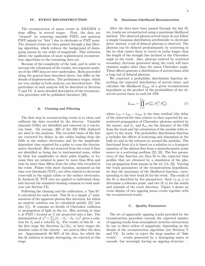
where tres = tobs − tCher is the time residual (the delayof the observed hit time relative to that expected for un-scattered propagation of Cherenkov photons emitted bythe muon), and d⊥ and θori are the distance of the OMfrom the track and the orientation of the module with re-spect to the track. The probability distribution functionp includes the effects of scattering and absorption in thebulk ice and in the refrozen ice around the modules. Thefunctional form of p is based on a solution to a transportequation of the photon flux from a monochromatic pointsource in a scattering medium [22, 23]. The free param-eters of this function are then fit to the expected timeprofiles that are obtained by a simulation of the pho-ton propagation from muons in the ice [14, 22]. Varyingthe track parameters of the reconstruction hypothesis,we find the maximum of the likelihood function, corre-sponding to the best track fit for the event. The result ofthe fit is described by five parameters: three (x, y, z) todetermine a reference point, and two (θ, φ) for the zenithand azimuth of the track direction. Figure 4 shows anevent display of two upgoing muon events together withthe reconstructed tracks.

C. Quality Parameters

The set of apparently upgoing tracks provided by thereconstruction procedure exceeds the expected numberof upgoing tracks from atmospheric neutrino interactionsby one to three orders of magnitude, depending on thedetails of the reconstruction algorithm (see Sections Vand VI). In order to reject the large number of “fakeevents” — events generated by a downgoing muon orcascade, but seemingly having an upgoing structure —

6

FIG. 4: Event display of an upgoing muon event. The greyscale indicates the flow of time, with early hits at the bottomand the latest hits at the top of the array. The arrival timesmatch the speed of light. The sizes of the circles correspondsto the measured amplitudes.

we impose additional requirements on the reconstructedevents to obtain a relatively pure neutrino sample. Theserequirements consist of cuts on observables derived fromthe reconstruction and on topological event parameters.Below, we describe the most relevant of the parametersused.

1. Reduced Likelihood, L

In analogy to a reduced χ2, we define a reduced likeli-hood

L =− lnLtime

Nhit − 5(2)

where Nhit − 5, the number of recorded hits in the eventless the five track fit parameters, is the number of degreesof freedom. A smaller L corresponds to a higher qualityof the fit.

2. Number of Direct Hits, Ndir

The number of direct hits is defined as the number ofhits with time delays tres smaller than a certain value. Weuse time intervals of [-15 ns,+25ns] and [-15 ns,+75ns],

and denote the corresponding parameters as N(25)dir and

N(75)dir , respectively. The negative extent of the window

allows for jitter in PMT rise times and for small errors ingeometry and calibration, while the positive side includesthese effects as well as delays due to scattering of thephotons. Events with many direct hits (i.e., only slightlydelayed photons) are likely to be well reconstructed.

3. Track Length, Ldir

The track length is defined by projecting each of thedirect hits onto the reconstructed track, and measuringthe distance between the first and the last hit. A cuton this parameter rejects events with a small lever armfor the reconstruction. Direct hits with time residualsof [-15 ns,+75ns] are used for the measurement of thetrack length. Cuts on the absolute length, as well aszenith angle dependent cuts (which take into account thecylindrical shape of the detector) have been used. Therequirement of a minimum track length corresponds toimposing a muon energy threshold. For example, a tracklength of 100 m translates into a muon energy thresholdof about 25 GeV.

4. Smoothness, S

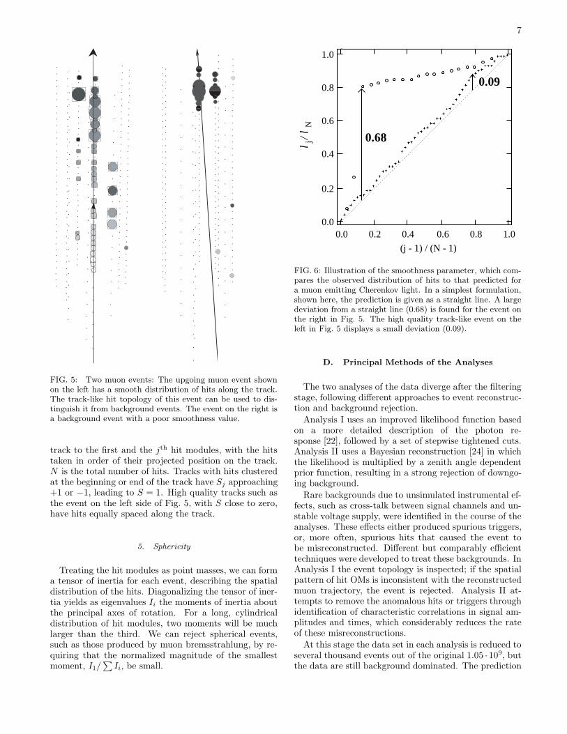
The “smoothness” parameter is a check on the self-consistency of the fitted track. It measures the constancyof light output along the track. Highly variable apparentemission of light usually indicates that the track eitherhas been completely misreconstructed or that an under-laying muonic Cherenkov light was obscured by a verybright stochastic light emission, which usually leads topoor reconstruction. The smoothness parameter was in-spired by the Kolmogorov-Smirnov test of the consistencyof two distributions; in our case the consistency of the ob-served hit pattern with the hypothesis of constant lightemission by a muon.

Figure 5 shows two events to illustrate the character-istics of the smoothness parameter. One event is a longuniform track, which was well reconstructed. The otherevent is a background event which displays a very poorsmoothness.

The simplest definition of the smoothness is given by

S = max(|Sj |) where Sj =j − 1

N − 1− lj

lN. (3)

Figure 6 illustrates the smoothness parameter for the twoevents displayed in Fig. 5. Here lj is the distance alongthe track between the points of closest approach of the

7

FIG. 5: Two muon events: The upgoing muon event shownon the left has a smooth distribution of hits along the track.The track-like hit topology of this event can be used to dis-tinguish it from background events. The event on the right isa background event with a poor smoothness value.

track to the first and the jth hit modules, with the hitstaken in order of their projected position on the track.N is the total number of hits. Tracks with hits clusteredat the beginning or end of the track have Sj approaching+1 or −1, leading to S = 1. High quality tracks such asthe event on the left side of Fig. 5, with S close to zero,have hits equally spaced along the track.

5. Sphericity

Treating the hit modules as point masses, we can forma tensor of inertia for each event, describing the spatialdistribution of the hits. Diagonalizing the tensor of iner-tia yields as eigenvalues Ii the moments of inertia aboutthe principal axes of rotation. For a long, cylindricaldistribution of hit modules, two moments will be muchlarger than the third. We can reject spherical events,such as those produced by muon bremsstrahlung, by re-quiring that the normalized magnitude of the smallestmoment, I1/

∑

Ii, be small.

(j - 1) / (N - 1)

jl / l

N

0.0 0.2 0.4 0.6 0.8 1.00.0

0.2

0.4

0.6

0.8

1.0

0.09

0.68

FIG. 6: Illustration of the smoothness parameter, which com-pares the observed distribution of hits to that predicted fora muon emitting Cherenkov light. In a simplest formulation,shown here, the prediction is given as a straight line. A largedeviation from a straight line (0.68) is found for the event onthe right in Fig. 5. The high quality track-like event on theleft in Fig. 5 displays a small deviation (0.09).

D. Principal Methods of the Analyses

The two analyses of the data diverge after the filteringstage, following different approaches to event reconstruc-tion and background rejection.

Analysis I uses an improved likelihood function basedon a more detailed description of the photon re-sponse [22], followed by a set of stepwise tightened cuts.Analysis II uses a Bayesian reconstruction [24] in whichthe likelihood is multiplied by a zenith angle dependentprior function, resulting in a strong rejection of downgo-ing background.

Rare backgrounds due to unsimulated instrumental ef-fects, such as cross-talk between signal channels and un-stable voltage supply, were identified in the course of theanalyses. These effects either produced spurious triggers,or, more often, spurious hits that caused the event tobe misreconstructed. Different but comparably efficienttechniques were developed to treat these backgrounds. InAnalysis I the event topology is inspected; if the spatialpattern of hit OMs is inconsistent with the reconstructedmuon trajectory, the event is rejected. Analysis II at-tempts to remove the anomalous hits or triggers throughidentification of characteristic correlations in signal am-plitudes and times, which considerably reduces the rateof these misreconstructions.

At this stage the data set in each analysis is reduced toseveral thousand events out of the original 1.05 · 109, butthe data are still background dominated. The prediction

8

for atmospheric neutrinos is about 500 at this point.

For the final selection of a nearly pure sample ofneutrino induced events, cuts on characteristic observ-ables are tightened until the remaining background dis-appears. The two analyses use different techniques tochoose their final cuts, but obtain comparable efficiencies.Further details of the analyses can be found in references[25, 26, 27].

V. ANALYSIS I

In this analysis the data were processed through threelevels of initial cuts, designed to reduce the number ofbackground events to a manageable size for the final cutevaluation. After a first filtering based on the line fit(level 1), cuts on the zenith angle, the number of directphotons, and the likelihood of the fitted track obtainedby the maximum likelihood reconstruction were applied(level 2).

A. Removal of Cascade-Like Events and Detector

Artifacts

A third filter level used the results of an iterative like-lihood reconstruction with varying track initializations,a fit based on the hit probabilities (see Eq. 4) and a re-construction to the hypothesis of a high energy cascade,e.g. due to a bright seconday muon bremsstrahlung in-teraction.

The first two levels of filtering consisted of relativelyweak cuts on basic parameters like the zenith angle andlikelihood. They reduced the data set to about 4 · 105

events. At this stage, residual unsimulated instrumen-tal features become apparent, e.g., comparatively highamplitude cross-talk produced when a downgoing muonemits a bright shower in the center of the detector. Suchevents are predominantly reconstructed as moving verti-cally upward and can be identified in the distribution ofthe center of gravity (COG) of hits. Its vertical compo-nent (zCOG) shows unpredicted peaks in the middle andthe bottom of the detector (see also Fig. 14 (top), demon-strating the effect for Analysis II), while the horizontalcomponents (xCOG and yCOG) show an enhancement ofhits towards the outer strings. These strings are read outvia twisted pair cables, as opposed to the coaxial cablesused on the inner strings. The twisted pair cables werefound to be more susceptible to cross-talk signals. Notethat variations in the optical parameters of the ice dueto past climatological episodes also produce some verticalstructure.

We developed additional COG cuts on the topology ofthe events in order to remove these backgrounds. Thesecuts, which depend on the reconstructed zenith angle,use the track lengths Ldir and the normalized smallesteigenvalues of the tensor of inertia (I1/

∑

Ii).

-100

0

100

200

-1 -0.75 -0.5 -0.25 0

cos(zenith)

z CO

G (

m)

-50

0

50

-50 0 50

xCOG (m)

y CO

G (

m)

1

2

345

6 7

8

910

-100

0

100

200

-1 -0.75 -0.5 -0.25 0

cos(zenith)

z CO

G (

m)

-50

0

50

-50 0 50

xCOG (m)

y CO

G (

m)

1

2

345

6 7

8

910

-100

0

100

200

-1 -0.75 -0.5 -0.25 0

cos(zenith )z C

OG (

m)

-50

0

50

-50 0 50

xCOG (m)

y CO

G (

m)

1

2

345

6 7

8

910

FIG. 7: Characteristic distributions of the center of gravity(COG) of events. The figures on the left show the distributionof the depth zCOG versus the reconstructed zenith angle. Thefigures on the right show the horizontal location of events inthe xCOG-yCOG plane of events with 0 m < zCOG < 50 m.The positions of the strings are marked by stars. Top: Ex-perimental data before application of the COG cuts. Middle:Experimental data after application of the COG cuts. Bot-tom: Expectation from the BG simulation after cuts.

Figure 7 shows the different components of the centerof gravity of the hits and the reconstructed zenith an-gle before and after application of the COG cuts, andthe Monte Carlo prediction for fake upward events stem-ming from misreconstructed downgoing muons. The cutsremove most of the unsimulated background – in partic-ular that far from the horizon – and bring experimentand simulation into much better agreement.

In order to verify the signal passing rates, these cutsand those from the previous levels were applied to a sub-sample of unfiltered (i.e. downgoing) events but with thezenith angle dependence of the cuts reversed, thus usingthe abundant cosmic ray muons as stand-ins for upgoingmuons.

In all, these three levels of filtering reduced the dataset by a factor of approximately 105 (see Table II).

B. Multi-Photoelectron Likelihood and Hit

Likelihood

Before the final cut optimization the last, most elab-orate reconstruction was applied, combining the likeli-

9

hoods for the arrival time of the first of muliple photonsin a PMT with the likelihoods for PMTs to have beenhit or have not been hit.

The probability densities p(t(i)res | d(i)

⊥ , θ(i)ori) (see eq.1, Sec-

tion IVB) describe only the arrival times of single pho-tons. Density functions for the multi-photoelectron casehave to include the effect of repeatedly sampling the dis-tribution of photon arrival times. For several detectedphotons, the first of them is usually less scattered thanthe average photon (which defines the single photoelec-tron case). Therefore the leading edge of a PMT pulsecomposed of multiple photoelectrons (MPE) will be sys-tematically shifted to earlier times compared to a singlephotoelectron. The MPE likelihood LMPE

time [22] uses therecorded amplitude information to model this shift.

In the reconstructions mentioned so far, the timing in-formation from hit PMTs was used. However, a PMTwhich was not hit also delivers information. The hit like-lihood Lhit does not depend on the arrival times but rep-resents the probability that the track produced the ob-served hit pattern. It is constructed from the probability

densities phit(d(i)⊥ , θ

(i)ori) that a given PMT i was hit if it

was in fact hit, and the probabilities (1 − phit(d(j)⊥ , θ

(j)ori )

that a given PMT j was not hit if it was not hit:

Lhit =∏Nhit

i=1 phit(d(i)⊥ , θ

(i)ori) · ∏NOM

i=Nhit+1

(

1 − phit(d(i)⊥ , θ

(i)ori)

)

(4)

where the first product runs over all hit PMTs and thesecond over all non-hit PMTs.

The likelihood combining these two probabilities is

L = LMPEtime · Lhit (5)

A cut on the reconstructed zenith angle obtained fromfitting with L leaves less than 104 events in the data set,defined as level 4 in Fig. 8.

C. Final Separation of the Neutrino Sample

For the final stage of filtering, a method (CutEval)was developed to select and optimize the cuts taking intoaccount correlations between the cut parameters. A de-tailed description of this method can be found in [27].The principle of CutEval is to numerically optimize theratio of signal to

√background by variation of the selec-

tion of cut parameters, as well as the actual cut values.Parameters are used only if they improve the efficiencyof separation over optimized cuts on all other already in-cluded parameters. A first optimization was based purelyon Monte Carlo, with simulated atmospheric neutrinosfor signal and simulated downgoing muons forming thebackground. This optimization yielded four such inde-pendent parameters. Two other optimizations involvedexperimental data. In both cases, experimental data have

been defined as the background sample. In one case, thesignal was represented by atmospheric neutrino MonteCarlo, in the other by experimental data subjected tozenith angle inverted cuts (i.e. to downward events pass-ing the quality cuts, but being “good” events with respectto the upper hemisphere instead – like neutrino candi-dates – with respect to the lower hemisphere). Theselatter optimizations yielded two additional parameters,which rejected a small contribution of residual unsimu-lated backgrounds: coincident muons from simultaneousindependent air showers and events accompanied by in-strumental artifacts such as cross-talk. After applicationof these two cuts to simulated and experimental data,the distributions of observables agree to a satisfactoryprecision.

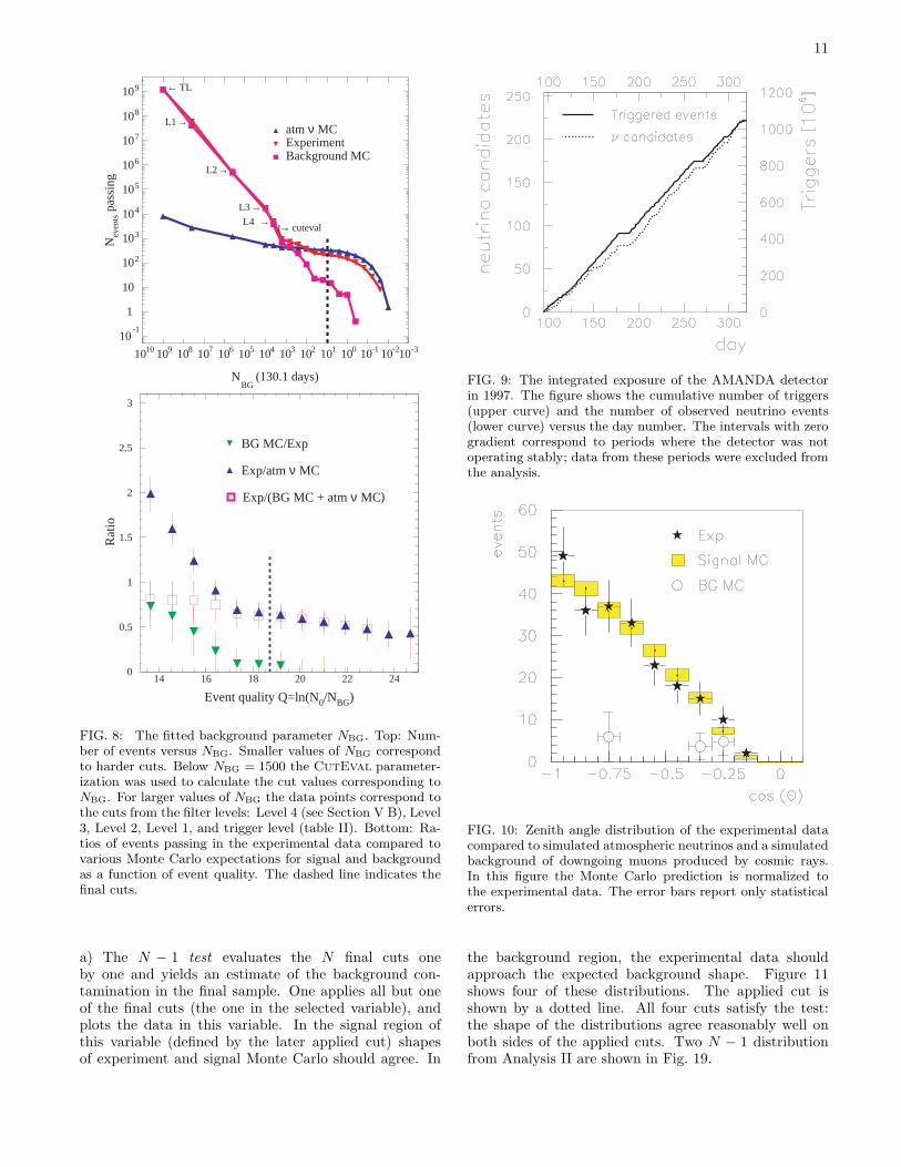
Once the minimal set of parameters is found, the op-timal cut values can be represented as a function of thenumber of background events NBG passing the cuts. Theresult is a path through the cut parameter space whichyields the best signal efficiency for any desired purity ofthe signal, characterized by NBG. Using this represen-tation, one can calculate the number of events passingthe cuts as a function of the fitted NBG for signal andfor background Monte Carlo. Figure 8 (top) shows thisdependence for simulations as well as for experimentaldata, with NBG varying from trigger level to a level thatleaves only a few events in the data set. One observesthat the actual background expectation falls roughly lin-early as the fitted NBG is reduced. Below values of a fewhundred events the signal is expected to dominate theevent sample. The experimental curve follows the ex-pectation from the sum of background and signal MonteCarlo. For large NBG, the observed event rate followsthe background expectation. At smaller NBG, the ex-perimental shape turns over into the signal expectationand follows it nicely down to the sample of events withhighest quality (the smallest values of NBG). For a mod-erate background contamination of NBG = 10, one getsa total of 223 neutrino candidates. The parameters andcut values as obtained by the CutEval procedure aresummarized in Table I.

Figure 8 (bottom) translates the background parame-ter NBG into an event quality parameter Q, defined asQ ≡ ln(N0/NBG) = ln(1.05 · 109/NBG). The plotshows the ratios of events from the upper figure as afunction of Q. At higher qualities (Q > 17), the ratio ofobserved events to the atmospheric neutrino simulationflattens out with a further variation of only 30%. Thevalue at Q = 17 is approximately unity for the angsens

Monte Carlo and about 0.6 for the standard Monte Carlo(chosen in Fig. 8, top) and approximately unity for theangsens Monte Carlo (chosen in Fig. 8, bottom).

Table II lists the cut efficiencies for the atmosphericneutrino simulation (with and without the implementa-tion of the angular sensitivity fitted model angsens ofthe OMs — see Sections III and VII), the backgroundsimulation of atmospheric muons from air showers (with-out angsens) and the experimental data. Again, the

10

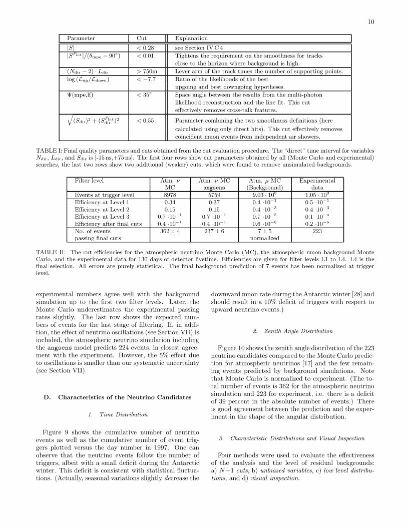
Parameter Cut Explanation

|S| < 0.28 see Section IVC4

|SPhit |/(θmpe − 90◦) < 0.01 Tightens the requirement on the smoothness for tracks

close to the horizon where background is high.

(Ndir − 2) · Ldir > 750m Lever arm of the track times the number of supporting points.

log (Lup/Ldown) < −7.7 Ratio of the likelihoods of the best

upgoing and best downgoing hypotheses.

Ψ(mpe,lf) < 35◦ Space angle between the results from the multi-photon

likelihood reconstruction and the line fit. This cut

effectively removes cross-talk features.√

(Sdir)2 + (SPhit

dir )2 < 0.55 Parameter combining the two smoothness definitions (here

calculated using only direct hits). This cut effectively removes

coincident muon events from independent air showers.

TABLE I: Final quality parameters and cuts obtained from the cut evaluation procedure. The “direct” time interval for variablesNdir, Ldir, and Sdir is [-15 ns,+75 ns]. The first four rows show cut parameters obtained by all (Monte Carlo and experimental)searches, the last two rows show two additional (weaker) cuts, which were found to remove unsimulated backgrounds.

Filter level Atm. ν Atm. ν MC Atm. µ MC ExperimentalMC angsens (Background) data

Events at trigger level 8978 5759 9.03 · 108 1.05 · 109

Efficiency at Level 1 0.34 0.37 0.4 ·10−1 0.5 ·10−1

Efficiency at Level 2 0.15 0.15 0.4 ·10−3 0.4 ·10−3

Efficiency at Level 3 0.7 ·10−1 0.7 ·10−1 0.7 ·10−5 0.1 ·10−4

Efficiency after final cuts 0.4 ·10−1 0.4 ·10−1 0.6 ·10−8 0.2 ·10−6

No. of events 362 ± 4 237 ± 6 7 ± 5 223passing final cuts normalized

TABLE II: The cut efficiencies for the atmospheric neutrino Monte Carlo (MC), the atmospheric muon background MonteCarlo, and the experimental data for 130 days of detector livetime. Efficiencies are given for filter levels L1 to L4. L4 is thefinal selection. All errors are purely statistical. The final background prediction of 7 events has been normalized at triggerlevel.

experimental numbers agree well with the backgroundsimulation up to the first two filter levels. Later, theMonte Carlo underestimates the experimental passingrates slightly. The last row shows the expected num-bers of events for the last stage of filtering. If, in addi-tion, the effect of neutrino oscillations (see Section VII) isincluded, the atmospheric neutrino simulation includingthe angsens model predicts 224 events, in closest agree-ment with the experiment. However, the 5% effect dueto oscillations is smaller than our systematic uncertainty(see Section VII).

D. Characteristics of the Neutrino Candidates

1. Time Distribution

Figure 9 shows the cumulative number of neutrinoevents as well as the cumulative number of event trig-gers plotted versus the day number in 1997. One canobserve that the neutrino events follow the number oftriggers, albeit with a small deficit during the Antarcticwinter. This deficit is consistent with statistical fluctua-tions. (Actually, seasonal variations slightly decrease the

downward muon rate during the Antarctic winter [28] andshould result in a 10% deficit of triggers with respect toupward neutrino events.)

2. Zenith Angle Distribution

Figure 10 shows the zenith angle distribution of the 223neutrino candidates compared to the Monte Carlo predic-tion for atmospheric neutrinos [17] and the few remain-ing events predicted by background simulations. Notethat Monte Carlo is normalized to experiment. (The to-tal number of events is 362 for the atmospheric neutrinosimulation and 223 for experiment, i.e. there is a deficitof 39 percent in the absolute number of events.) Thereis good agreement between the prediction and the exper-iment in the shape of the angular distribution.

3. Characteristic Distributions and Visual Inspection

Four methods were used to evaluate the effectivenessof the analysis and the level of residual backgrounds:a) N−1 cuts, b) unbiased variables, c) low level distribu-tions, and d) visual inspection.

11

10-1

1

10

102

103

104

105

106

107

108

109

1010109 108 107 106 105 104 103 102 101 100 10-1 10-210-3

atm ν MCExperimentBackground MC

Ι→ cuteval→L4

→L3

→L2

→L1

← TL

NBG

(130.1 days)

Nev

ents p

assi

ng

0

0.5

1

1.5

2

2.5

3

14 16 18 20 22 24

BG MC/Exp

Exp/atm ν MC

Exp/(BG MC + atmν MC)

Event quality Q=ln(N0/NBG)

Rat

io

FIG. 8: The fitted background parameter NBG. Top: Num-ber of events versus NBG. Smaller values of NBG correspondto harder cuts. Below NBG = 1500 the CutEval parameter-ization was used to calculate the cut values corresponding toNBG. For larger values of NBG the data points correspond tothe cuts from the filter levels: Level 4 (see Section V B), Level3, Level 2, Level 1, and trigger level (table II). Bottom: Ra-tios of events passing in the experimental data compared tovarious Monte Carlo expectations for signal and backgroundas a function of event quality. The dashed line indicates thefinal cuts.

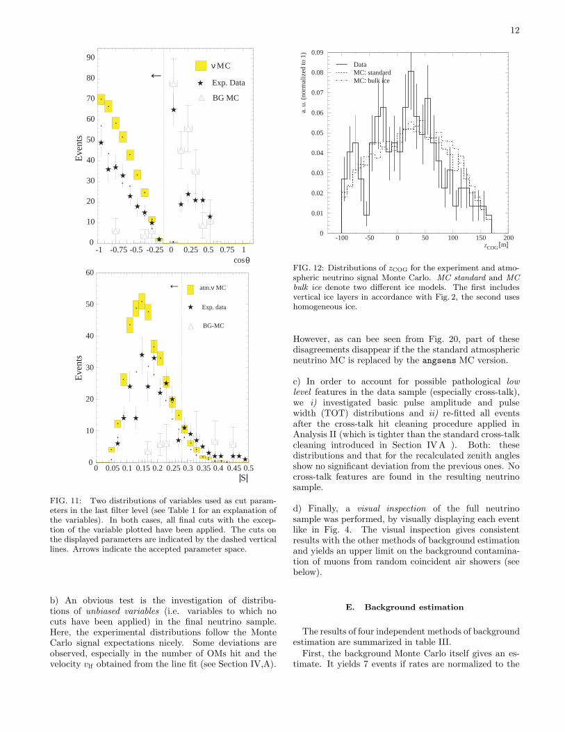
a) The N − 1 test evaluates the N final cuts oneby one and yields an estimate of the background con-tamination in the final sample. One applies all but oneof the final cuts (the one in the selected variable), andplots the data in this variable. In the signal region ofthis variable (defined by the later applied cut) shapesof experiment and signal Monte Carlo should agree. In

FIG. 9: The integrated exposure of the AMANDA detectorin 1997. The figure shows the cumulative number of triggers(upper curve) and the number of observed neutrino events(lower curve) versus the day number. The intervals with zerogradient correspond to periods where the detector was notoperating stably; data from these periods were excluded fromthe analysis.

FIG. 10: Zenith angle distribution of the experimental datacompared to simulated atmospheric neutrinos and a simulatedbackground of downgoing muons produced by cosmic rays.In this figure the Monte Carlo prediction is normalized tothe experimental data. The error bars report only statisticalerrors.

the background region, the experimental data shouldapproach the expected background shape. Figure 11shows four of these distributions. The applied cut isshown by a dotted line. All four cuts satisfy the test:the shape of the distributions agree reasonably well onboth sides of the applied cuts. Two N − 1 distributionfrom Analysis II are shown in Fig. 19.

12

0

10

20

30

40

50

60

70

80

90

-1 -0.75 -0.5 -0.25 0 0.25 0.5 0.751

ν MC

Exp. Data

BG MC

←

cos θ

Eve

nts

0

10

20

30

40

50

60

0 0.05 0.1 0.15 0.2 0.25 0.3 0.35 0.4 0.450.5

atm.ν MC

Exp. data

BG-MC

←

|S|

Eve

nts

FIG. 11: Two distributions of variables used as cut param-eters in the last filter level (see Table 1 for an explanation ofthe variables). In both cases, all final cuts with the excep-tion of the variable plotted have been applied. The cuts onthe displayed parameters are indicated by the dashed verticallines. Arrows indicate the accepted parameter space.

b) An obvious test is the investigation of distribu-tions of unbiased variables (i.e. variables to which nocuts have been applied) in the final neutrino sample.Here, the experimental distributions follow the MonteCarlo signal expectations nicely. Some deviations areobserved, especially in the number of OMs hit and thevelocity vlf obtained from the line fit (see Section IV,A).

COGZ [m]

a. u

. (no

rmal

ized

to 1

)

DataMC: standard

:

0

0.01

0.02

0.03

0.04

0.05

0.06

0.07

0.08

0.09

-100 -50 0 50 100 150 200

MC: bulk ice

FIG. 12: Distributions of zCOG for the experiment and atmo-spheric neutrino signal Monte Carlo. MC standard and MC

bulk ice denote two different ice models. The first includesvertical ice layers in accordance with Fig. 2, the second useshomogeneous ice.

However, as can bee seen from Fig. 20, part of thesedisagreements disappear if the the standard atmosphericneutrino MC is replaced by the angsens MC version.

c) In order to account for possible pathological lowlevel features in the data sample (especially cross-talk),we i) investigated basic pulse amplitude and pulsewidth (TOT) distributions and ii) re-fitted all eventsafter the cross-talk hit cleaning procedure applied inAnalysis II (which is tighter than the standard cross-talkcleaning introduced in Section IVA ). Both: thesedistributions and that for the recalculated zenith anglesshow no significant deviation from the previous ones. Nocross-talk features are found in the resulting neutrinosample.

d) Finally, a visual inspection of the full neutrinosample was performed, by visually displaying each eventlike in Fig. 4. The visual inspection gives consistentresults with the other methods of background estimationand yields an upper limit on the background contamina-tion of muons from random coincident air showers (seebelow).

E. Background estimation

The results of four independent methods of backgroundestimation are summarized in table III.

First, the background Monte Carlo itself gives an es-timate. It yields 7 events if rates are normalized to the

13

trigger level (see table II). Because the passing ratesdiffer slightly between the experiment (higher) and thebackground Monte Carlo (lower), we made the conserva-tive choice to renormalize the background Monte Carloto the level 3 experimental passing rate. This gives anestimate of about 16 background events in our final sam-ple.

BG estimation method estimationBG MC 16 ± 8N−1 cuts 14 ± 4zCOG distributions < 35Visual inspection < 23

TABLE III: Various estimates of the background remainingin the experimental data sample of 223 neutrino candidates.

From the N−1 distributions we obtained an alterna-tive approximation of the residual background. We re-normalized both signal and background MCs in the back-ground region to fit the number of experimental eventsin the background region. The number of re-normalizedbackground MC events in the signal region is then a back-ground estimate. This estimate was performed N times(once for each N−1 distribution). The average over allN estimations yields 14 background events. Note thatthis averaging procedure is reasonable only for the caseof independent cuts. With the method by which we havechosen the cut parameters, this condition is fulfilled tofirst approximation.

We have found that cross-talk hits are related to thecharacteristic triple-peak structure in the distribution ofthe vertical component of the center of gravity of hits(zCOG) which has been discussed in Section VA – seeFig.7 and also Fig.14 (top). Since there are remainingcross talk hits which have survived the standard cleaning(see section IVA), this distribution was studied in de-tail. As shown in Fig. 12, the final experimental sampleof neutrino candidates shows no statistically significantexcess with respect to the atmospheric neutrino MonteCarlo prediction in the regions of the characteristic peaks.Therefore, an upper limit on this special class of back-ground was derived and yields < 35 events.

The visual inspection of the neutrino sample yields 13events. Seven of them show the signature of coincidentmuons from independent air showers; i.e., two well sep-arated spatial concentrations of hits, each with a down-ward time flow but with the lower group appearing earlierthan the upper one. Taking into account the scanning ef-ficiencies which were determined by scanning signal andbackground Monte Carlo events, an upper limit of 23events is obtained from visual inspection.

Combining the results from the above methods, theexpected background is estimated to amount to 4 to 10%of the 223 experimental events.

VI. ANALYSIS II

The second analysis follows a different approach; in-stead of optimizing cuts to reject misreconstructed cos-mic ray muons, this analysis concentrates on improv-ing the reconstruction algorithm with respect to back-ground rejection. The large downgoing muon flux impliesthat even a small fraction of downgoing muons misrecon-structed as upgoing will produce a very large backgroundrate. Equivalently, for each apparently upgoing event,there were many more downgoing muons passing the de-tector than there were upgoing muons; even though anysingle downgoing muon had only a small probability offaking an upgoing event, the total probability that theevent was a fake is quite high.

A. Bayesian Reconstruction

This analysis of the problem motivates a Bayesian ap-proach [24] to event reconstruction. Bayes’ Theorem inprobability theory states that for two assertions A andB,

P (A |B) P (B) = P (B |A) P (A),

where P (A |B) is the probability of assertion A giventhat B is true. Identifying A with a particular muontrack hypothesis µ and B with the data recorded for anevent in the detector, we have

P (µ | data) = Ltime(data |µ) P (µ),

where we have dropped a normalization factor P (data)which is a constant for the observed event. The functionLtime is the regular likelihood function of Eq. 1, and P (µ)is the so-called prior function, the probability of a muonµ = µ(x, y, z, θ, φ) passing through the detector.

For this analysis, we have used a simple one-dimensional prior function, containing the zenith angleinformation at trigger level in Fig. 3. By accounting inthe reconstruction for the fact that the flux of downgo-ing muons from cosmic rays is many orders of magnitudelarger than that of upgoing neutrino-induced muons, thenumber of downgoing muons that are misreconstructedas upgoing is greatly reduced. It should be noted thatthe objections that are often raised with respect to theuse of Bayesian statistics in physics are not relevant tothis problem: the prior function is well defined and nor-malized and independently known to relatively good pre-cision, consisting only of the fluxes of cosmic ray muonsand atmospheric muon neutrinos.

B. Removal of Instrumental Artifacts

The Bayesian reconstruction algorithm is highly effi-cient at rejecting downgoing muon events. Of 2.6 · 108

14

events passing the fast filter, only 5.8 · 104 are recon-structed as upgoing. By contrast, the standard maxi-mum likelihood reconstruction produces about 2.4 · 107

false upgoing reconstructions. However, less than a thou-sand neutrino events are predicted by Monte Carlo, so itis clear that a significant number of misreconstructionsremain.

Detailed inspection of the 5.8 · 104 events reveals thatthe vast majority is produced by cross-talk overlaid ontriggers from downgoing muons emitting bright stochas-tic light near the detector. This cross-talk confuses thereconstruction algorithm, producing apparently upgoingtracks. Because cross-talk is not included in the detec-tor simulation, the characteristics of the fakes are notpredicted well by the simulation, and the rate of misre-construction is much higher than predicted.

The cross-talk is removed by additional hit cleaningroutines developed by examination of this cross-talk en-riched data set. For example, cross-talk in many channelscan be identified in scatter plots of pulse width vs. ampli-tude, as shown in Fig. 13. The pulse width is measuredas time-over-threshold (TOT). Real hits form the distri-bution shown on the left. High amplitude pulses shouldhave large pulse width. This is not the case for cross-talkinduced pulses. In channels with high levels of cross-talk,an additional vertical band is found at high amplitudesbut short pulse widths, as seen in the lower figure.

Other hit cleaning algorithms use the time correlationand amplitude relationship between real and cross-talkpulses and a map of channels susceptible to cross-talk andthe channels to which they are coupled. An additionalinstrumental effect, believed to be caused by fluctuatinghigh voltage levels, produces triggers with signals frommost OMs on the outer strings but none on the innerfour strings; some 500 of these bogus triggers were alsoremoved from the data set. The 5.8 · 104 upgoing eventswere again reconstructed after the additional hit cleaningwas applied. Only 4.9 ·103 (8.4%) of the events remainedupgoing, compared to an expectation from Monte Carloof 1855 atmospheric muon events (37.8% of the total be-fore the additional cleaning), and 555 atmospheric neu-trino events. Figure 14 (top) shows that while there hasbeen a significant reduction in the instrumental back-grounds, an unsimulated structure still remains in thecenter-of-gravity (COG) distribution for these remainingdata events. The application of additional quality cri-teria brings this distribution in agreement, as shown inFigure 14 (bottom).

C. Quality Cuts

The improvements in the reliability of the reconstruc-tion algorithm described above obviated the need forlarge numbers of cut parameters or for careful opti-mization of the cuts. Because the signal-to-noise of theupward-reconstructed data is quite high to begin with,we have the possibility of comparing the behavior of real

FIG. 13: Pulse amplitude vs. duration for modules on theouter strings. Normal hits lie in the distribution shown inthe upper figure. High amplitude pulses of more than a fewphotoelectrons are valid only if the pulse width is also large.Cross-talk induced pulses of high amplitude are characterizedby small time-over-threshold (TOT). The cut-off seen at highamplitude is due to saturation of the amplitude readout elec-tronics.

and simulated data over a wide range of cut strengthsto verify that the data agree with the predictions for up-going neutrino-induced muons, not only in number butalso in their characteristics. Using the cut parametersdescribed in Section IVC (with the likelihood replacedby the Bayesian posterior probability) and a requirementthat events fitted as relatively horizontal by the line fit fil-tering algorithm not be reconstructed as steeply upgoingby the full reconstruction (a requirement that suppressesresidual cross-talk misreconstructions), an index of eventquality was formed.

To do so, we rescale the six quality parameters de-scribed above by the cumulative distributions of the sim-ulated atmospheric neutrino signal, and consider the six-dimensional cut space formed by the rescaled parameters.A point in this space corresponds to fixed values of the

15

Data

Atmosph. µ

0

50

100

150

200

250

300

350

400

-150 -100 -50 0 50 100 150 200Vertical position of center of gravity (zcog) [m]

dN/d

z

[1

/10m

]

Data

Atmosph. ν MC

0

2.5

5

7.5

10

12.5

15

17.5

20

22.5

-150 -100 -50 0 50 100 150 200250Vertical position of center of gravity (zcog) [m]

dN/d

z

[1

/10m

]

FIG. 14: Top: Event center of gravity distribution after recon-struction with special cross-talk cleaning algorithms appliedto the events. Unsimulated background remains. Bottom:The data agree with the neutrino signal after application ofadditional quality cuts.

quality parameters, and events can be assigned to loca-tions based on their track length, sphericity, and so forth.

It is difficult to compare the distributions of data andsimulated up- and downgoing muons directly becauseof the high dimensionality of the space. We thereforeproject the space down to a single – “quality” – dimen-sion by dividing it into concentric rectangular shells, asillustrated in Fig. 15. The vertex of each shell lies on aline from the origin through a reference set of cuts whichare believed to isolate a fairly pure set of neutrino events.Events in the full cut space are assigned an overall qualityvalue, based on the shell in which they lie.

With this formulation we can compare the character-istics of the data to simulated neutrino and cosmic-raymuon events. Figure 16 compares the number of eventspassing various levels of cuts; i.e., the integral numberof events above a given quality. At low qualities, q ≤ 3,the data set is dominated by misreconstructed downgoing

Track Length

Sm

ooth

ness

Reference Cuts

FIG. 15: Definition of event quality. Events are plotted inN-dimensional cut space (two dimensions are shown here forclarity). A line is drawn from the origin (no cuts) througha selected set of cuts, and the space is divided into rectan-gular shells of equal width. Events are assigned a quality qaccording to the shell in which they are found.

muons, data as well as the simulated background exceedthe predicted neutrino signal. At higher qualities, thepassing rates of data closely track the simulated neutrinoevents, and the predicted background contamination isvery low.

Data

Atmospheric ν MC

Downgoing µ MC

Event Quality

Eve

nts

Pas

sing

10-1

1

10

10 2

10 3

10 4

0 2.5 5 7.5 10 12.5 15 17.5 20 22.5 25

FIG. 16: Numbers of events above a certain quality level, fordowngoing muon Monte Carlo, atmospheric neutrino MonteCarlo, and experimental data.

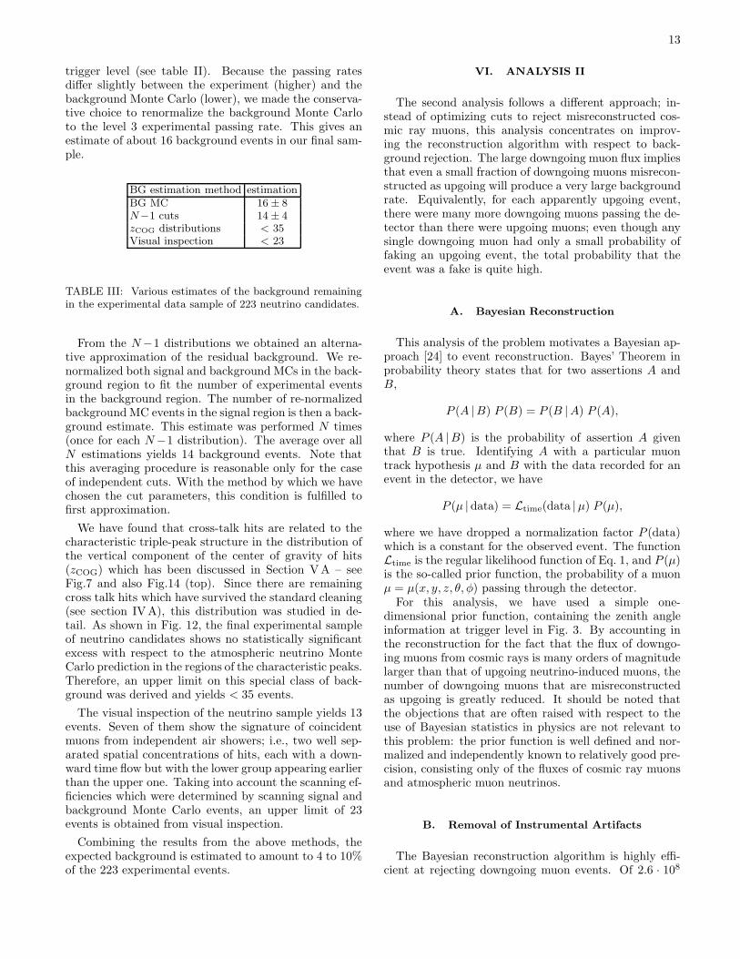
We can investigate the agreement between data andMonte Carlo more systematically by comparing the dif-ferential number of events within individual shells, ratherthan the total number of events passing various levels ofcuts. This is done in Fig. 17, where the ratios of thenumber of events observed to those predicted from thecombined signal and background simulations are shown.One can see that at low quality levels there is an excess

16

Event Quality

Dat

a / Σ

MC

0

1

2

3

4

5

6

0 2.5 5 7.5 10 12.5 15 17.5 20 22.5 25

FIG. 17: Ratio of data to Monte Carlo (cosmic ray muons plusatmospheric neutrinos). Unlike Fig. 16, the plot is differential— the ratio at a particular quality does not include events athigher or lower qualities.

in the number of misreconstructed events observed. Thisis mainly due to remaining cross-talk. There is also anexcess, though statistically less significant, at very highquality levels, which is believed to be caused by slightinaccuracies in the description of the optical parametersof the ice. Nevertheless, over the bulk of the range thereis close agreement between the data and the simulation,apart from an overall normalization factor of 0.58. Theabsolute agreement is consistent with the systematic un-certainties. It should be emphasized that the quality pa-rameter is a convolution of all six quality parameters, andso the flat line in Fig. 17 demonstrates agreement in thecorrelations between cut parameters.

D. Background Estimation and Signal Description

If we reduce the 4,917 upward-reconstructed events byrequiring a quality of at least 7 on the scale of Fig. 16, weobtain a set of 204 neutrino candidates. The backgroundcontamination, which is due to misreconstructed down-going muons, was estimated in three ways. The first wayis to simulate the downgoing muon flux, bearing in mindthat we are looking at a very low tail (10−8) of the to-tal muon distribution. The second way is to renormalizethe signal simulation by the factor of 0.58 obtained fromFig. 17 and subtract the predicted events from the ob-served data set (accepting the excess at extremely highqualities, however, as signal). The third way, a crosscheck on the first two methods, is to examine the datalooking for fakes due to unsimulated effects such as cross-

cosθ

Data

Atmospheric ν MC

0

5

10

15

20

25

30

35

40

-1 -0.9 -0.8 -0.7 -0.6 -0.5 -0.4 -0.3 -0.2 -0.10

dN/d

cosθ

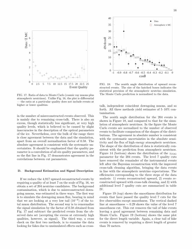
FIG. 18: The zenith angle distribution of upward recon-structed events. The size of the hatched boxes indicates thestatistical precision of the atmospheric neutrino simulation.The Monte Carlo prediction is normalized to the data.

talk, independent coincident downgoing muons, and soforth. All three methods yield estimates of 5–10% con-tamination.

The zenith angle distribution for the 204 events isshown in Figure 18, and compared to that for the simu-lation of atmospheric neutrinos. In the figure the MonteCarlo events are normalized to the number of observedevents to facilitate comparison of the shapes of the distri-butions. The agreement in absolute number is consistentwith the systematic uncertainties in the absolute sensi-tivity and the flux of high energy atmospheric neutrinos.The shape of the distribution of data is statistically con-sistent with the prediction from atmospheric neutrinos.Figure 14 (bottom) shows the distribution of the zCOG

parameter for the 204 events. The level 7 quality cutshave removed the remainder of the instrumental eventsleft after the Bayesian reconstruction with the improvedcross-talk cleaning algorithm, bringing the data eventsin line with the atmospheric neutrino expectations. Theefficiencies corresponding to the three steps of the dataanalysis: 1) events reconstructed upward, 2) events re-constructed upward with cross-talk cleaning, and 3) withadditional level 7 quality cuts are summarized in tableIV.

Figure 19 (top) shows the smoothness distribution forevents that have passed the quality level 7 cuts for thefive observables except smoothness. The vertical dashedline at smoothness ∼ 0.29 shows the value of the level 7smoothness cut. This cut removes the tail of fake eventsleaving a good agreement between remaining data andMonte Carlo. Figure 19 (bottom) shows the same plotfor the direct length variable. Again, a clear tail of fakeevents is removed by requiring a direct length of greaterthan 70 meters.

17

Monte Carlo Monte Carlo Data

Downgoing µ Atmospheric ν

Events triggered 8.8 · 108 8978 1.05 · 109

Efficiency: Reconstructed upgoing 0.55 · 10−5 0.55 · 10−4

Efficiency: Reconstructed upgoing(2.1 ± 0.08) · 10−6 (6.2 ± 0.06) · 10−2 4.7 · 10−6

(w/ cross-talk cleaning)

Efficiency: Final Cuts (q≥7) (1.9 ± 0.6) · 10−8 (3.1 ± 0.03) · 10−2 1.9 · 10−7

No. of events: Quality ≥ 7 17 ± 5 279 ± 3 204

TABLE IV: Event numbers for experimental data and Monte Carlo simulations for four major stages in the analysis. Theerrors quoted are statistical only.

VII. SYSTEMATIC UNCERTAINTIES

As a novel instrument, AMANDA poses a unique chal-lenge of calibration. There are no known natural sourcesof high energy neutrinos, apart from atmospheric neutri-nos, whose observation could be used to measure the de-tector’s response. Understanding the behavior of the de-tector is thus a difficult task, dependent partly on labora-tory measurements of the individual components, partlyon observations of artificial light sources embedded inthe ice, and partly on observations of downgoing muons.Even with these measurements, uncertainties in variousproperties that systematically affect the response of thedetector persist, which prevent us at this time from mak-ing a precise measurement of the atmospheric neutrinoflux. The primary sources of systematic uncertainties,and their approximate effects on the number of upgoingatmospheric neutrinos in the final data sample, as deter-mined by variation of the simulations, are listed below.

As discusssed in Sections 2 and 3, AMANDA is embed-ded in a natural medium, which is the result of millenniaof climatological history, that has left its mark in the formof layers of particulate matter affecting the optical prop-erties of the ice. Furthermore, the deployment of opticalmodules requires the melting and refreezing of columnsof the ice. This cycle results in the formation of bubblesin the vicinity of the modules, which increase scatteringand affect the sensitivity of the optical modules in waysthat are not yet fully understood. The effects of thislocal hole ice are difficult to separate from the intrinsicsensitivity of the OMs. The uncertainties in the neutrinorate are approximately 15% from the bulk ice layer mod-eling in the Monte Carlo, and as much as 50% from thecombined effects of the properties of the refrozen hole iceclose to the OMs, and the intrinsic OM sensitivity, andangular response.

Figure 20 shows two variables that are sensitive to theabsolute OM sensitivity: the number of OMs hit and thevelocity of the line fit. The systematic effects of varyingOM sensitivity on the hit multiplicity for Analysis I areshown on the top. The peak of the multiplicity distri-bution for the standard Monte Carlo (nominal efficiency100% — dashed line) lies at a higher value than for the

data. Reducing the simulated OM sensitivity by 50% re-sults in a peak at lower values than the data. The othervariable strongly affected by the OM sensitivity – thevelocity of the line fit, introduced in Section IVA) – isthe apparent velocity of the observed light front travelingthrough the ice, see Fig. 20 (bottom).

As a next step, we investigated the effect of theangsens OM model (first introduced in Section 3) onthe atmospheric neutrino Monte Carlo simulation. Theresults of this simulation gave a more consistent descrip-tion of the experiment for several variables — e.g., thehit multiplicity (the dotted line in Fig. 20) — and theyproduced the absolute neutrino event prediction closerto what was found in Analysis I (236.9 events predicted,223 observed). Similar effects are seen when this MonteCarlo is used with Analysis II, however the number ofpredicted events is 25% smaller than observed. Thus theangsens model, while encouraging, does not completelypredict the properties of observed events in both analy-ses.

Another uncertainty lies in the Monte Carlo routinesused to propagate muons through the ice and rock sur-rounding the detector. A comparison of codes basedon [9] and [11] indicates that different propagators maychange the event rates by some 25%.

Other factors include the simulation of the data ac-quisition electronics and possible errors in the time cali-brations of individual modules. These effects have beenstudied by systematically varying relevant parameters inthe Monte Carlo simulations. For realistic levels of vari-ation, these effects are well below the 10% level.

Figure 21 demonstrates how the zenith angle distri-bution depends on different atmospheric neutrino eventgenerators (our standard generator nusim [17] and an-other generator nu2mu [29]), and also on the chosen an-gular sensitivity of the optical module. Neutrino flavoroscillations lead to a further reduction of the angsens

prediction by 5.4% (in particular, close to the vertical di-rection), assuming sin2 2θ = 1 and ∆m2 = 2.5 · 10−3 eV2

[30]. The prediction is reduced by 11% if the largest al-lowed ∆m2 is used.

The combined effect of all these systematic uncertain-ties is sufficiently large that simulations of a given at-mospheric neutrino flux can produce predictions for the

18

Smoothness (|SPHit|)

Data

Atmospheric ν MC

0

5

10

15

20

25

30

35

40

45

0 0.1 0.2 0.3 0.4 0.5 0.6 0.7 0.8

dN/d

S PH

it

←

Ldir [m]

Data

Atmospheric ν MC

0

5

10

15

20

25

30

35

0 50 100 150 200 250 300 350400

dN/d

L Dir

[

1/10

m]

←

FIG. 19: Smoothness and direct length variables where qual-ity level 7 cuts have been applied in all but the displayedvariable (N − 1 cuts, see also Section VD 3, Fig. 11). Thevertical dashed lines with the arrow indicate the region of ac-ceptance in the displayed variable. In each case, a clear tailof fake events is removed by application of the cut, leavinggood agreement in shape between the remaining events andthe Monte Carlo expectation.

event rate varying by a factor of two. By contrast, the es-timated theoretical uncertainty in the atmospheric neu-trino flux, at the energies probed by these analyses, is30% [31]. The effect of neutrino oscillations with theSuper-K preferred parameters would be less than 10% atthese energies.

VIII. SYNTHESIS AND GENERAL OVERVIEW

Both Analyses I and II are able to separate more than200 neutrino event candidates from the 130.1 days ofAMANDA-B10 detector livetime in 1997. Based on at-

Experiment

(dN

/dN

)/

Nch

tota

l

chNumber of hit OM (N )10 20 30 50 60

0.05

0.10

0.15

0.20

0.25

40

OM sensitivity 50%

OM sensitivity 100%

angsens OM model

MC:

[m/ns]

0.20 0.25 0.30 0.350.150.10

linefitVelocity from line fit (v )

[(0.

02 m

/ns)

]

-1lin

efit

(dN

/dv

)/N t

otal

0.05

0.10

0.15

0.20

0.25

OM sensitivity 50%

OM sensitivity 100%

angsens OM model

MC:

Experiment

FIG. 20: Distributions of two variables that are affected bythe OM sensitivity, comparing different signal Monte Carlosto the observed data. Top: the number of OMs hit (Nch);bottom: the event velocity for a simplified fit (line fit, vlinefit).

mospheric neutrino simulations we find that about 4% ofthe total number of events triggered by upward movingneutrinos passed the final selection. A total deficit in theevent rate of about 35% with respect to the standard neu-trino Monte Carlo prediction is found for both analyses.An event overlap of 102 experimental events is observed,consistent with a predicted overlap of 119 ± 13 from theatmospheric neutrino Monte Carlo. Thus, the combinedsample of data provides about 300 neutrino candidates.Both analyses estimate their residual background to beabout 10% of the number of neutrino event candidates.

Figure 22 shows the energy distribution of the sim-ulated neutrinos and the corresponding muon events.Ninety percent of all Monte Carlo signal events have

19

cosθ

even

tsnusim (standard)nu2munusim (angsens)Experiment

0

10

20

30

40

50

60

70

80

-1 -0.75 -0.5 -0.25 0

FIG. 21: Distribution of simulated zenith angles for differentneutrino generators and also for a modified angular sensitivityof the OM.

EνEµ (vertex)

Eµ (center)

log (E / GeV)

Eve

nts:

dN

/dlo

g(E

/GeV

) [

1/0.

05]

0

2

4

6

8

10

12

14

16

18

1 1.5 2 2.5 3 3.5 4 4.5 5

FIG. 22: Energy distributions for simulated atmospheric neu-trino events which pass the final neutrino cuts. The effect ofneutrino oscillations has not been taken into account. Thefigure shows the neutrino and muon energies at the interac-tion vertex and the energy of the muons at the point of closestapproach to the detector center.

muon (neutrino) energies between 48 (66) GeV and1.8 (3.4) TeV. The dominant part of the signal events inthis analysis comes from neutrino energies below 1 TeV.Figure 23 shows the effective area as a function of thezenith angle for two ranges of the muon energy at thepoint of closest (POC) approach to the detector. The ef-fective area for muons with energies at POC between 100and 1000GeV is 3.9 · 104 m2 at trigger level and 2800 m2

after application of the neutrino selection cuts. It shouldbe noted that much higher effective areas are possible

muon energy at detector

10-100 GeV100-1000 GeV

cosθ

[ef

fect

ive

area

m2 ]

0

2000

4000

6000

8000

10000

-1 -0.8 -0.6 -0.4 -0.2 0

FIG. 23: Effective area for muons versus zenith angle. Theenergy of the muons is given at the point of closest approachto the detector.

when searching for neutrinos from astrophysical pointsources [32] or from gamma ray bursts [33].

Figure 24 shows the point spread function of the re-constructed muon trajectory with respect to the truemuon direction. Based on Monte Carlo simulations, wefind a median angular resolution of muons from atmo-spheric neutrinos of 3.2◦ for the final sample. A moredetailed study of the angular resolution can be foundin [25, 35, 36]. Figure 25 shows the skyplot (equatorialcoordinates) of all the candidate neutrino events foundacross both analyses. The distribution of the events onthe skyplot is consistent with a random distribution.

IX. CONCLUSIONS

The AMANDA-B10 data from 130.1 days of livetimeduring the austral winter of 1997 have been analyzedin an effort to detect high energy atmospheric neutrinoevents, and to compare their properties to expectations.Two working groups in the collaboration, using differingreconstruction, cut optimization and instrumental eventrejection techniques, produced sets of 223 and 204 neu-trino candidates, respectively. Several methods of back-ground estimation put the residual event contaminationfrom downgoing atmospheric muons and instrumental ar-tifacts at about 10%. Taking into account systematicuncertainties, the observed event numbers are consistentwith systematically varied atmospheric neutrino MonteCarlo predictions, which are from 150–400 events. Therange of these predictions is dominated by uncertaintiesin the neutrino flux, in the understanding of photon prop-agation through the bulk ice and the refrozen hole ice,

20

angular accuracy ∆Ψ (° )

P(∆

Ψ)

0

0.025

0.05

0.075

0.1

0.125

0.15

0.175

0.2

0 2 4 6 8 10 12 14 16 18 20

FIG. 24: Monte Carlo simulation of the angular resolution formuons that pass the final selection criteria. The median erroris 3.2◦.

FIG. 25: Neutrino skyplot of upgoing events as seen withAMANDA-B10 in 1997 in equatorial coordinates. In this fig-ure, neutrino events from both analyses are combined. Thebackground of non-neutrino events is estimated to be less than10%.

and in muon propagation and energy loss. The MonteCarlo suggests that 90% of the selected events are pro-duced by neutrinos in the energy range of ∼ 66GeV to3.4TeV. The observation of atmospheric neutrinos inline with expectations establishes AMANDA-B10 as aworking neutrino telescope. We finally note that manyof the procedures for signal separation simplify consider-ably in larger detectors. In particular, first results fromAMANDA-II [37] demonstrate that the neutrino signalis separated with much higher efficiency and with fewercuts than for AMANDA-B10.

Acknowledgments This research was supported bythe following agencies: U.S. National Science Founda-tion, Office of Polar Programs; U.S. National ScienceFoundation, Physics Division; University of WisconsinAlumni Research Foundation; U.S. Department of En-ergy; Swedish Natural Science Research Council; SwedishResearch Council; Swedish Polar Research Secretariat;Knut and Alice Wallenberg Foundation, Sweden; Ger-man Ministry for Education and Research; U.S. NationalEnergy Research Scientific Computing Center (supportedby the Office of Energy Research of the U.S. Depart-ment of Energy); UC-Irvine AENEAS SupercomputerFacility; Deutsche Forschungsgemeinschaft (DFG). D.F.Cowen acknowledges the support of the NSF CAREERprogram and C. Perez de los Heros acknowledges supportfrom the EU 4th framework of Training and Mobility ofResearchers.

[1] E. Andres et al., Astrop. Phys. 13, 1 (2000).[2] E. Andres et al., Nature 410, 441 (2001).[3] K. Woschnagg (for the AMANDA Collaboration), in Pro-

ceedings of the 26th International Cosmic Ray Confer-

ence (IUPAP, Salt Lake City, Utah, 1999), Vol. 2, pp.200–203.

[4] P. B. Price, K. Woschnagg, and D. Chrikin, Geophys.Res. Lett. 27, 2129 (2000).

[5] J. Ahrens et al., Astrop. Phys. 16, 345 (2002).[6] S. N. Boziev et al., INR-Preprint P–0630 (unpublished).[7] D. Heck et al., Report FZKA 6019, Forschungszentrum

Karlsruhe, Karlsruhe, Germany (unpublished).[8] D. Heck, in Simulation and Analysis Methods for Large

Neutrino Telescopes (DESY, Zeuthen, Germany, 1998),

pp. 228–234, desy-proc–1999–01.[9] W. Lohmann, R. Kopp, and R. Voss, Preprint CERN–

85–03, Geneva, Switzerland (unpublished).[10] R. Kopp, W. Lohmann, and R. Voss, MUDEDX:

Parametrization and Monte Carlo generation of energyloss of high energy muons (1–10000 GeV); for astrophysi-cists up to 100000 GeV, Version 2.02, 1995, private com-munication.

[11] P. Lipari and T. Stanev, Phys. Rev. D 44, 3543 (1991).[12] W. Rhode and D. Chirkin, in Proceedings of the

27th International Cosmic Ray Conference (CopernicusGesellschaft, Hamburg, Germany, 2001), Vol. 3, pp.1017–1020.

[13] B. Wiebel-Sooth and P. L. Biermann, Landolt-Bornstein:

21

Numerical Data and Functional Relationships in Science

and Technology, Vol. VI 3C of New Series (Springer-Verlag, Berlin-Heidelberg, 1998), chapter 7.6, pp. 37–90.

[14] A. Karle, in Simulation and Analysis Methods for Large

Neutrino Telescopes (DESY, Zeuthen, Germany, 1998),pp. 174–185, desy-proc–1999–01.

[15] S. Hundertmark, Ph.D. thesis, Humboldt Universitat zuBerlin, Berlin, Germany, 1999, available at URLhttp://amanda.berkeley.edu/manuscripts/.

[16] S. Hundertmark, in Simulation and Analysis Methods for

Large Neutrino Telescopes (DESY, Zeuthen, Germany,1998), pp. 276–286, desy-proc–1999–01.

[17] G. C. Hill, Astrop. Phys. 6, 215 (1997).[18] G. C. Hill, Ph.D. thesis, University of Adelaide, Adelaide,

Australia, 1996.[19] P. Lipari, Astrop. Phys. 1, 195 (1993).[20] J. Ahrens et al., to be submitted to Nucl.Instr.Meth.[21] V. Stenger, DUMAND Internal Report HDC–1–90 (un-

published).[22] C. Wiebusch, in Simulation and Analysis Methods for

Large Neutrino Telescopes (DESY, Zeuthen, Germany,1998), pp. 302–316, desy-proc–1999–01.

[23] D. Pandel, Diploma thesis, Humboldt-University Berlin,Feb. 1996

[24] G. C. Hill, in Proceedings of the 27th International Cos-

mic Ray Conference (Copernicus Gesellschaft, Hamburg,Germany, 2001), Vol. 3, pp. 1279–1282.

[25] A. Biron, Ph.D. thesis Humboldt Universtitat zuBerlin, Berlin, Germany, 2002, available at URLhttp://amanda.berkeley.edu/manuscripts/.

[26] T. R. DeYoung, Ph.D. thesis, University ofWisconsin, Madison, 2001, available at URLhttp://amanda.berkeley.edu/manuscripts/.

[27] M. Gaug, Diploma thesis, Humboldt Universitat zuBerlin, Berlin, Germany, 2001, desy-thesis–2001–022,available at URLhttp://amanda.berkeley.edu/manuscripts/.

[28] A.Bouchta (for the AMANDA collaboration), in Proceed-

ings of the 26th International Cosmic Ray Conference,

Salt Lake City 1999, HE 3.2.11.[29] E. Dalberg, Ph.D. thesis, Stockholm Univer-

sity, Stockholm, Sweden, 1999, available at URLhttp://amanda.berkeley.edu/manuscripts/.

[30] J. Kameda (for the Super-Kamiokande collaboration), inProceedings of the 27th International Cosmic Ray Con-

ference (Copernicus Gesellschaft, Hamburg, Germany,2001), Vol. 3, pp. 1057–1060.

[31] T. K. Gaisser, Uncertainty in flux of Atmospheric Neu-

trinos: Implications for Upward Muons in Amanda B10,Internal Report 20001201, 2000.

[32] J. Ahrens et al., Search for point sources of high energy

neutrinos with the AMANDA detector, to be submittedto Astrophysical Journal

[33] R. Hardtke and G. Barouch (for the AMANDA Collab-oration), in Proceedings of the 27th International Cos-

mic Ray Conference (Copernicus Gesellschaft, Hamburg,Germany, 2001), Vol. 3, pp. 1121–1124.

[34] P. Desiati and W. Rhode (for the AMANDA Collab-oration), in Proceedings of the 27th International Cos-

mic Ray Conference (Copernicus Gesellschaft, Hamburg,Germany, 2001), Vol. 3, pp. 985–988.

[35] Calibration and Survey of AMANDA with the SPASE

detectors to be submitted to Nuclear Instruments andMethods.

[36] G. Spiczak (for the AMANDA Collaboration), in Pro-

ceedings of the 27th International Cosmic Ray Con-

ference (Copernicus Gesellschaft, Hamburg, Germany,2001). Vol. 3, pp. 977–980.

[37] R. Wischnewski (for the AMANDA Collaboration), inProceedings of the 27th International Cosmic Ray Con-

ference (Copernicus Gesellschaft, Hamburg, Germany,2001), Vol. 3, pp. 1105–1108.

[38] S. W. Barwick (for the AMANDA Collaboration), inProceedings of the 27th International Cosmic Ray Con-

ference (Copernicus Gesellschaft, Hamburg, Germany,2001), Vol. 3, pp. 1105–1108.

[39] S. Fukuda et al., Phys. Rev. Lett. 85, 3999 (2000).[40] J. Ahrens et al., Limits on the muon flux from WIMP an-

nihilation in the center of the Earth with the AMANDA

neutrino detector, submitted to Phys. Rev. D.