The Astrophysical Journal Supplement Series, 214:27 (13pp), 2014 October doi:10.1088/0067-0049/214/2/27C© 2014. The American Astronomical Society. All rights reserved. Printed in the U.S.A.

PROPERTIES OF 42 SOLAR-TYPE KEPLER TARGETS FROM THE ASTEROSEISMIC MODELING PORTAL

T. S. Metcalfe1,2, O. L. Creevey3, G. Dogan2,4, S. Mathur1,4, H. Xu5, T. R. Bedding6, W. J. Chaplin7,J. Christensen-Dalsgaard2, C. Karoff2, R. Trampedach2,8, O. Benomar6,9, B. P. Brown10,11, D. L. Buzasi12,

T. L. Campante7, Z. Celik13, M. S. Cunha14, G. R. Davies7, S. Deheuvels15,16, A. Derekas17,18, M. P. Di Mauro19,R. A. Garcıa20, J. A. Guzik21, R. Howe7, K. B. MacGregor4, A. Mazumdar22, J. Montalban23, M. J. P. F. G. Monteiro14,

D. Salabert20, A. Serenelli24, D. Stello6, M. Steslicki25, M. D. Suran26, M. Yıldız13, C. Aksoy13, Y. Elsworth7,M. Gruberbauer27, D. B. Guenther27, Y. Lebreton28,29, K. Molaverdikhani30, D. Pricopi26,

R. Simoniello31, and T. R. White6,321 Space Science Institute, 4750 Walnut Street Suite 205, Boulder, CO 80301, USA

2 Stellar Astrophysics Centre, Department of Physics and Astronomy, Aarhus University, Ny Munkegade 120, DK-8000 Aarhus C, Denmark3 Institut d’Astrophysique Spatiale, Universite Paris XI, UMR 8617, CNRS, Batiment 121, F-91405 Orsay Cedex, France

4 High Altitude Observatory, NCAR, P.O. Box 3000, Boulder, CO 80307, USA5 Computational & Information Systems Laboratory, NCAR, P.O. Box 3000, Boulder, CO 80307, USA

6 Sydney Institute for Astronomy (SIfA), School of Physics, University of Sydney, NSW 2006, Australia7 School of Physics and Astronomy, University of Birmingham, Birmingham B15 2TT, UK

8 JILA, University of Colorado and National Institute of Standards and Technology, 440 UCB, Boulder, CO 80309, USA9 Department of Astronomy, The University of Tokyo, Tokyo 113-0033, Japan

10 Department of Astronomy and Center for Magnetic Self Organization in Laboratory and Astrophysical Plasmas,University of Wisconsin, Madison, WI 53706, USA

11 Kavli Institute for Theoretical Physics, University of California, Santa Barbara, CA 93106, USA12 Department of Chemistry and Physics, Florida Gulf Coast University, Fort Myers, FL 33965, USA

13 Ege University, Department of Astronomy and Space Sciences, Bornova, 35100, Izmir, Turkey14 Centro de Astrofısica e Faculdade de Ciencias, Universidade do Porto, Rua das Estrelas, 4150-762, Porto, Portugal

15 Universite de Toulouse, UPS-OMP, IRAP, Toulouse, France16 CNRS, IRAP, 14, avenue Edouard Belin, F-31400 Toulouse, France

17 Konkoly Observatory, MTA CSFK, H-1121 Budapest, Konkoly Thege M. ut 15-17, Hungary18 ELTE Gothard Astrophysical Observatory, H-9704 Szombathely, Szent Imre herceg ut 112, Hungary

19 INAF-IAPS Istituto di Astrofisica e Planetologia Spaziali, Via del Fosso del Cavaliere 100, I-00133 Roma, Italy20 Laboratoire AIM, CEA/DSM–CNRS–Univ. Paris Diderot–IRFU/SAp, Centre de Saclay, F-91191 Gif-sur-Yvette Cedex, France

21 Los Alamos National Laboratory, XTD-NTA, MS T-086, Los Alamos, NM 87545, USA22 Homi Bhabha Centre for Science Education, TIFR, V. N. Purav Marg, Mankhurd, Mumbai 400088, India

23 Institut d’Astrophysique et Geophysique, University of Liege, Belgium24 Institute of Space Sciences (CSIC-IEEC), Campus UAB, E-08193, Bellaterra, Spain

25 Space Research Center, Polish Academy of Sciences, Wrocław, Poland26 Astronomical Institute of the Romanian Academy, Str. Cutitul de Argint 5, RO-040557, Bucharest, Romania

27 Institute for Computational Astrophysics, Department of Astronomy and Physics, Saint Mary’s University, Halifax, N.S., B3H 3C3, Canada28 Observatoire de Paris, GEPI, CNRS UMR 8111, F-92195, Meudon, France

29 Institut de Physique de Rennes, Universit de Rennes 1, CNRS UMR 6251, F-35042, Rennes, France30 Laboratory for Atmospheric and Space Physics, University of Colorado, Boulder, CO 80309, USA

31 Laboratoire AIM, CEA/DSM-CNRS-Universit Paris Diderot, IRFU/SAp, Centre de Saclay, F-91191, Gif-sur-Yvette, France32 Institut fur Astrophysik, Georg-August-Universitat Gottingen, Friedrich-Hund-Platz 1, D-37077 Gottingen, Germany

Received 2014 February 14; accepted 2014 September 2; published 2014 October 1

ABSTRACT

Recently the number of main-sequence and subgiant stars exhibiting solar-like oscillations that are resolved intoindividual mode frequencies has increased dramatically. While only a few such data sets were available for detailedmodeling just a decade ago, the Kepler mission has produced suitable observations for hundreds of new targets. Thisrapid expansion in observational capacity has been accompanied by a shift in analysis and modeling strategies toyield uniform sets of derived stellar properties more quickly and easily. We use previously published asteroseismicand spectroscopic data sets to provide a uniform analysis of 42 solar-type Kepler targets from the AsteroseismicModeling Portal. We find that fitting the individual frequencies typically doubles the precision of the asteroseismicradius, mass, and age compared to grid-based modeling of the global oscillation properties, and improves theprecision of the radius and mass by about a factor of three over empirical scaling relations. We demonstrate theutility of the derived properties with several applications.

Key words: methods: numerical – stars: evolution – stars: interiors – stars: oscillations

Online-only material: color figures, extended figure

1. BACKGROUND

It is difficult to overstate the impact of the Kepler mission onthe observation and analysis of solar-like oscillations in main-sequence and subgiant stars. In a review from just a decade ago,Bedding & Kjeldsen (2003) highlighted the tentative detections

of individual oscillation frequencies in just a few such stars fromground-based observations, and Kepler was not even mentioned.Despite funding issues that delayed the mission from an originaldeployment date in 2006, Kepler finally launched in March 2009and operated almost flawlessly for more than four years, slightlyexceeding its design lifetime (Borucki et al. 2010). The archive

1

The Astrophysical Journal Supplement Series, 214:27 (13pp), 2014 October Metcalfe et al.

of public data now includes nearly uninterrupted observationsfor many thousands of solar-type stars, including short-cadencedata (58.85 s sampling; Gilliland et al. 2010) for hundredsof these targets. In the span of a decade, the study of solar-like oscillations has been transformed dramatically (Chaplin &Miglio 2013).

During the first 10 months of science operations, Keplerperformed a survey for solar-like oscillations in more than 2000main-sequence and subgiant stars, yielding detections in morethan 500 targets from the one month data sets. The initialanalysis of this ensemble, using empirical scaling relations(Kjeldsen & Bedding 1995) to generate estimates of radiusand mass, suggested a significant departure from the massdistribution expected from Galactic population synthesis models(Chaplin et al. 2011). Subsequent analysis of the sample, usingupdated effective temperatures (Pinsonneault et al. 2012) anda substantial grid-based modeling effort, led to more preciseestimates of the radii and masses as well as information aboutthe stellar ages (Chaplin et al. 2014). Some of the brightest starsfrom the survey were subjected to a more detailed analysis,including spectroscopic follow-up to determine more preciseatmospheric properties (Bruntt et al. 2012) plus the identificationand detailed modeling of dozens of oscillation frequencies ineach star (Mathur et al. 2012). These studies gave us a previewof what to expect from the subsequent phase of the mission.

Starting with Quarter 5 (Q5), Kepler’s short-cadence studyof solar-like oscillations transitioned to a specific target phase,where extended observations began for a fixed sample of starsidentified during the survey. The target list during this phase gavepriority to stars showing oscillations with the highest signal-to-noise ratio (S/N), but it also retained the brightest main-sequence stars cooler than the Sun, where the lower intrinsicoscillation amplitudes yielded relatively weak detections fromthe survey. From Q5 through the end of the mission (Q17), about200 of the 512 available short-cadence targets were typicallyspecified by the Kepler Asteroseismic Science Consortium(KASC; Kjeldsen et al. 2010) and about half of those wereintended for the study of solar-like oscillations.

Just like the exoplanet side of the mission, the KASC teamgradually improved the data reduction and analysis methodswhile additional data swelled the archive. Never in the historyof the field had such extended monitoring been possible at all,let alone for such a large sample of stars. As a consequence,the availability of reliable sets of input data for stellar modelinglagged well behind the continually expanding time series foreach star in the archive. This delay was primarily due to thechallenge of coordinating the efforts of multiple teams, firstto produce optimized light curves from the raw Kepler data(Garcıa et al. 2011), then to fit the global oscillation propertiesand remove the stellar granulation background from the powerspectra (Verner et al. 2011; Mathur et al. 2011), and finallyto extract and identify the individual oscillation frequenciesusing so-called “peak-bagging” techniques (Appourchaux et al.2012). Also like the exoplanet program, ground-based followup observations were difficult to obtain for the faintest targets,further limiting the number of stars for which detailed modelingwas feasible.

Even after reliable sets of observational constraints becameavailable, an analogous effort was required to consolidate theresults from many stellar modeling teams. Initially this effortsought to define objective metrics of model quality, and to usethe ensemble of results from different codes and methods toestimate the systematic uncertainties for a few specific targets

(Metcalfe et al. 2010, 2012; Creevey et al. 2012; Dogan et al.2013; Silva Aguirre et al. 2013). The first large sample to emergefrom the survey made this “boutique” modeling approachimpractical, and motivated the initial large-scale applicationof the Asteroseismic Modeling Portal (AMP; Metcalfe et al.2009; Woitaszek et al. 2009). Mathur et al. (2012) presenteda uniform analysis of 22 Kepler targets observed for 1 montheach during the survey phase, and compared detailed modelingfrom AMP with empirical scaling relations and with results fromseveral grid-based modeling methods that matched the globaloscillation properties (Δν and νmax, see below) rather than theindividual frequencies from peak-bagging. The results clearlydemonstrated the improved level of precision that was possiblefrom detailed modeling of the individual oscillation frequencies,particularly for stellar ages.

In this paper, we present stellar modeling results from AMPfor the first large sample of Kepler targets with extended ob-servations during the specific target phase of the mission. InSection 2, we describe the sample, which was drawn from themost recently published observations. We outline our stellarmodeling approach in Section 3, including several improve-ments to the previous version of AMP and using slightly cus-tomized procedures for different types of stars. We present themain results and initial applications in Section 4, and we discussconclusions and future prospects in Section 5.

2. OBSERVATIONAL CONSTRAINTS

Solar-like oscillations are stochastically excited and intrinsi-cally damped by turbulent convection near the stellar surface(Goldreich & Keeley 1977; Goldreich & Kumar 1988; Houdeket al. 1999; Samadi & Goupil 2001). Each oscillation mode ischaracterized by its radial order n and spherical degree �, andonly the low-degree (� � 3) modes are generally detectablewithout spatial resolution across the surface. The consecutiveradial orders define the average large separation 〈Δν〉, whichreflects the mean stellar density (Tassoul 1980). The power ineach mode is governed by a roughly Gaussian envelope with amaximum at frequency νmax, which approximately scales withthe acoustic cutoff frequency (Brown et al. 1991; Belkacem et al.2011). These global oscillation properties are well-constrained,even in the relatively short time series obtained during the Keplersurvey phase. Longer observations improve the frequency pre-cision and also reveal additional oscillation modes, with lowerand higher radial orders, as the S/N improves in the wingsof the Gaussian envelope. This is the primary motivation forgathering extended observations: to maximize both the numberand quality of asteroseismic constraints that are available forstellar modeling.

Appourchaux et al. (2012) published asteroseismic datasets for 61 main-sequence and subgiant stars observed byKepler, based on an analysis of 9-month time series. The datawere collected during Q5–Q7 (2010 March 20 through 2010December 22), archived on 2011 April 23, and the final setsof identified frequencies were published about one year later.Most of these frequency sets came from maximum likelihoodestimators (Appourchaux et al. 2008) with errors determinedfrom the inverse of the Hessian matrix, but frequencies for theF-like stars were obtained from a Bayesian analysis withMultiNest (Gruberbauer et al. 2009) and errors were estimatedfrom the 68% credible interval. When asymmetric errors wereprovided, we adopted the mean of the two quoted values.No similar analysis of more extended data sets has yet been

2

The Astrophysical Journal Supplement Series, 214:27 (13pp), 2014 October Metcalfe et al.

Figure 1. Spectroscopic H-R diagram for our final sample of 42 asteroseismictargets, including simple (black), F-like (red), and mixed-mode stars (blue).Points outlined in a different color indicate the original classification byAppourchaux et al. (2012). Error bars were adopted from Chaplin et al. (2014).Solar-composition evolution tracks from ASTEC for masses between 0.9 and1.5 M� are shown as dotted lines, with the position of the Sun indicated by the� symbol. Stars similar to the Sun are missing from the KASC sample becausethe data were sequestered by the Kepler exoplanet team.

(A color version of this figure is available in the online journal.)

published, so we adopted this sample of 61 stars as our uniformsource of asteroseismic constraints.

In addition to the asteroseismic data, precise spectroscopicconstraints on the effective temperature Teff and metallicity[M/H] are also required for detailed stellar modeling. A uni-form spectroscopic analysis of 93 solar-type Kepler targets waspublished by Bruntt et al. (2012), including 46 of the bright-est stars in the Appourchaux et al. sample with magnitudes inthe Kepler bandpass Kp = 7.4–9.8. Six of the 15 missing tar-gets are also in this magnitude range: KIC 3735871, 11772920,12317678, and 12508433, as well as the two bright spectro-scopic binaries KIC 8379927 and 9025370. The remaining9 stars fall in the magnitude range Kp = 9.9–11.4 and aredifficult targets for high-resolution spectroscopy on all but thelargest telescopes.

Recently, Molenda-Zakowicz et al. (2013) published spectro-scopic constraints for a larger sample of 169 stars in the Keplerfield. The overlap with the Appourchaux et al. sample only in-cludes two additional stars (KIC 11772920 and 12508433) forthe low-precision ROTFIT results (Frasca et al. 2003, 2006),while the high-precision ARES+MOOG results (Sousa et al.2007; Sneden 1973) contain fewer asteroseismic targets thanare available in the Bruntt et al. sample. Considering that ourgoal is to produce a uniform analysis, we adopted the spec-troscopic constraints from Bruntt et al. (2012), limiting theavailable sample to 46 stars. Four of these targets are evolvedsubgiants with too many mixed modes for successful automatedmodeling, so our final sample includes 42 stars. Following Chap-lin et al. (2014), we adopted larger uncertainties on Teff (±84K; see Figure 1) that fold in a systematic error of 59 K, assuggested by Torres et al. (2012). For 12 stars with Hipparcosparallaxes (van Leeuwen 2007), we used the spectroscopic Teffto obtain bolometric corrections from Flower (1996). Follow-ing Torres (2010), we adopted Mbol,� = 4.73 ± 0.03 and usedthe extinction estimates from Ammons et al. (2006) to deriveluminosity constraints.

3. STELLAR MODELING APPROACH

The AMP (Woitaszek et al. 2009) is a web-based interfaceto the stellar model-fitting pipeline described in detail byMetcalfe et al. (2009). The underlying science code usesa parallel genetic algorithm (GA; Metcalfe & Charbonneau2003) on XSEDE supercomputing resources to optimize thematch between asteroseismic models produced by the Aarhusstellar evolution code (ASTEC; Christensen-Dalsgaard 2008a)and adiabatic pulsation code (ADIPLS; Christensen-Dalsgaard2008b) and a given set of observational constraints. Mathur et al.(2012) were the first to apply AMP to a large sample of Keplertargets, motivating several improvements to the physical inputsand fitting procedures that are described below.

3.1. Updated Physics

The version of AMP that was used for the models presentedby Mathur et al. (2012) was configured to use the Grevesse& Noels (1993) solar mixture with the OPAL 2005 equationof state (see Rogers & Nayfonov 2002) and the most recentOPAL opacities (see Iglesias & Rogers 1996), supplementedby Alexander & Ferguson (1994) opacities at low temperatures.The updated version of AMP uses the low-T opacities fromFerguson et al. (2005). We have also updated the default nuclearreaction rates, replacing the Bahcall & Pinsonneault (1995) rateswith those from the NACRE collaboration (Angulo et al. 1999).Convection is still described by the mixing-length theory fromBohm-Vitense (1958) without overshoot, and we continue toinclude the effects of helium diffusion and settling as describedby Michaud & Proffitt (1993). To correct the model frequenciesfor so-called “surface effects” due to incomplete modeling ofthe near-surface layers, we use the empirical prescription ofKjeldsen et al. (2008).

We originally performed our analysis shortly after the pub-lication of asteroseismic constraints by Appourchaux et al.(2012), using the updated physics described above but with-out modifying the fitting procedures. The approach used byMathur et al. (2012) simultaneously optimized the match be-tween the models and two sets of constraints: (1) the individualoscillation frequencies and (2) the atmospheric parameters fromspectroscopy. This procedure generally yielded stellar radii,masses, and ages that were consistent with empirical scalingrelations and grid-based modeling of the global oscillation prop-erties (Δν and νmax)—but with significantly improved precision.However, the optimal models for the 22 targets included sixstars with an initial helium mass fraction Yi significantly belowthe primordial value from standard Big Bang nucleosynthesis(YP = 0.2482 ± 0.0007; Steigman 2010), and four additionalstars that were marginally below YP. The original motivation forincluding these sub-primordial values in the search was a recog-nition that there could be systematic errors in the determinationof Yi, but the source of the potential bias was not identified.Our first attempts to fit the data described in Section 2 using thesame methods as Mathur et al. (2012) were plagued by an evenhigher fraction of models with low initial helium, so we revisedour procedures.

3.2. Updated Fitting Procedures

As part of a study of convective cores in two Kepler targets,AMP was compared to several other fitting methods by SilvaAguirre et al. (2013). In addition to the individual frequenciesand spectroscopic constraints, some of these methods alsoused sets of frequency ratios that eliminated the need to

3

The Astrophysical Journal Supplement Series, 214:27 (13pp), 2014 October Metcalfe et al.

correct the model frequencies for surface effects (Roxburgh& Vorontsov 2003). A comparison of the AMP results withmodels that used the frequency ratios as additional constraintsrevealed systematic differences in the interior structure that werecorrelated with the initial helium abundance. We subsequentlymodified the AMP optimization procedure to try to avoid thisbias, by adopting the frequency ratios as additional constraintsand by reducing the weight at higher frequency, where thesurface correction is larger (see details below).

The ratios proposed by Roxburgh & Vorontsov (2003) areconstructed from individual frequency separations, includingthe large separations defined by Δν�(n) = νn,� − νn−1,�, andthe small separations defined by d�,�+2(n) = νn,� − νn−1,�+2.These can be used to define one set of ratios that relates thesmall separation between modes of degree 0 and 2 to the largeseparation of � = 1 modes at the same radial order:

r02(n) = d0,2(n)

Δν1(n). (1)

Note that these ratios involve modes with all three degrees. An-other set of ratios only involves the small and large separationsbetween modes of degree 0 and 1:

r01(n) = d01(n)

Δν1(n), r10(n) = d10(n)

Δν0(n + 1), (2)

where d01(n) and d10(n) are five frequency smoothed smallseparations defined by Equations (4) and (5) in Roxburgh& Vorontsov (2003). This smoothing introduces correlationsbetween the individual ratios that more than double the effectiveuncertainties,33 but it also shifts some weight from the centerof the frequency range toward the edges where the S/N of themodes is lower.34 To account for these correlations withoutshifting weight toward the edges of the frequency range,we adopted 3σ uncorrelated uncertainties on all ratios fromEquation (2). In addition, Silva Aguirre et al. (2013) noted thatthe ratios formed from the highest radial orders were typicallyunreliable due to large line widths, and recommended that theybe excluded from the set of constraints. We excluded all ratiosthat are centered on frequencies from the highest three radialorders. Hereafter, we refer to the set of ratios r02(n) as r02 andthe set of ratios r01(n) and r10(n) as r010.

Although the frequency ratios help to discriminate betweenfamilies of models that provide comparable matches to the othersets of constraints, the individual frequencies contain additionalinformation that we would like to exploit. The primary difficultyis that the model frequencies need to be corrected for surfaceeffects, and the commonly used empirical correction (Kjeldsenet al. 2008) appears to inject a bias in the determination ofsome stellar properties. What is the source of this bias, andhow can we mitigate it? Essentially, Kjeldsen et al. assumedthat the differences between the observed and optimal modelfrequencies can be described by

νobs − νmod ≈ a0

(ν

ν0

)b

, (3)

33 We examined a specific case from Silva Aguirre et al. (2013) and comparedthe quadratic sum of all terms in the covariance matrix to the diagonal elementfor each ratio. We determined that the off-diagonal elements inflate theeffective uncertainty by a factor of two to four with the largest boost near thecenter of the observed frequency range.34 Ratios near the edges of the observed frequency range are directlycorrelated with fewer than four other ratios, so the correlated errors are notinflated as much relative to the diagonal elements of the covariance matrix andthese less certain ratios are assigned higher relative weights.

Figure 2. Comparison of the actual surface effect and the empirical correction ofKjeldsen et al. (2008) for the AMP model of KIC 6116048. Differences betweenthe observed � = 0 frequencies and those of the AMP model (connected points)are reasonably well represented by the empirical correction (dashed line) withamplitude a0 at the reference frequency ν0, but it substantially overestimatesthe correction at high frequencies.

(A color version of this figure is available in the online journal.)

where a0 is the size of the correction at a reference frequencyν0 (typically chosen to be νmax), and the exponent b is fixedat a solar-calibrated value near 4.9. They demonstrated thatthis simple parameterization35 can adequately describe the fre-quency differences between the observations and models of sev-eral solar-type stars, including β Hyi and α Cen A and B. Theycautioned that the value of the exponent depends on the num-ber of radial orders considered for the solar calibration, varyingfrom 4.4–5.25 when including 7–13 orders. To facilitate com-parisons with previous work, we adopted the solar-calibratedvalue b = 4.82 determined by Metcalfe et al. (2009). For mixedmodes we scaled the surface correction by the mode inertia ratio,as described in Brandao et al. (2011).

The actual solar surface effect appears more linear at highfrequencies (Christensen-Dalsgaard et al. 1996), so assumingany fixed exponent will tend to over-correct the highest-ordermodes (see Figure 2). This tendency appears to interact withintrinsic parameter correlations—in particular, the well-knowncorrelation between mass and initial helium abundance instellar models—to favor higher-mass low-helium models thatfit the frequencies better while getting the interior structurewrong. Including the frequency ratios as constraints favorsthe lower-mass higher-helium models, but it does not eliminatethe bias caused by the high-frequency modes. To mitigatethis bias, we adopted an uncertainty for each frequency thatis the quadratic sum of the statistical error and half thesurface correction (Bevington & Robinson 1992). In doingso, we are acknowledging that surface effects represent asystematic error in the models (Guenther & Brown 2004). Wealso imposed a penalty on models with Yi < YP, such thatthe spectroscopic quality metric (see Section 3.3) was inflatedby 1 for every 0.01 that Yi fell below YP. Although this doesnot explicitly rule out low-helium solutions, it does require

35 Note that Kjeldsen et al. (2008) also scaled the model frequencies by ahomology factor r to provide a better match to the observations. By definition,the best model should have r = 1. The net effect of applying homology scalingto every model sampled by the GA is to decrease the dynamic range of thefrequency χ2 space, so we omitted this term from our surface correction.

4

The Astrophysical Journal Supplement Series, 214:27 (13pp), 2014 October Metcalfe et al.

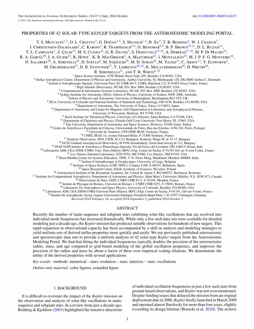
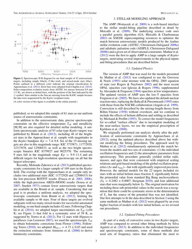
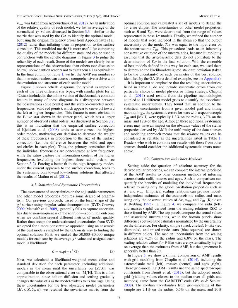
Figure 3. Echelle diagrams for typical examples of the three different star types, including the simple star KIC 12258514 (left), the F-like star KIC 9139163 (center),and the mixed-mode star KIC 5955122 (right). Each plot shows a smoothed grayscale representation of the power spectrum overplotted with the frequencies anderrors from Appourchaux et al. (2012; blue points) and from the surface-corrected AMP model (solid red points). The uncorrected � = 0 model frequencies (open redcircles) are shown to illustrate the size of the surface effect, and the � = 0 radial order is given on the right axis.

(An extended, color version of this figure is available in the online journal.)

that they provide a substantially better match to the other setsof constraints to be considered superior. Without a preciseconstraint on the luminosity and/or radius, this approach isrequired even to recover accurate solar properties from Sun-as-a-star helioseismic data (Metcalfe et al. 2009).

3.3. Customization by Star Type

Appourchaux et al. (2012) categorized their sample of 61asteroseismic targets into three classes, based on the appearanceof the oscillation modes in an echelle diagram (Grec et al. 1980).Dividing the frequency spectrum into segments having widthequal to the large separation and then stacking them vertically,modes with the same spherical degree form approximatelyvertical ridges for simple stars like the Sun (see Figure 3).Significantly hotter main-sequence stars have larger intrinsicline widths, blurring the individual modes and complicating theidentification of mode geometry (F-like stars). Finally, the � = 1ridge in subgiants can be disrupted when buoyancy modes in theevolved stellar core couple with pressure modes in the envelope,creating an avoided crossing (Osaki 1975; Aizenman et al. 1977)that leads to deviations from the regular frequency spacing(mixed-mode stars). This final category is usually unambiguous,but there is no clear dividing line between the first two.

Appourchaux et al. (2012) suggested a boundary between thesimple and F-like stars at an effective temperature near 6400 K ora line width at maximum mode height around 4 μHz (see Whiteet al. 2012). We adopted a slightly different convention basedon whether or not the � = 0 and � = 2 ridges in the echellediagram are cleanly separated. This led us to treat 5 stars asF-like that were identified as simple by Appourchaux et al.:KIC 3632418, 7206837, 8228742, 9139163, and 10162436.In addition, KIC 3424541 (originally classified as F-like) andKIC 10018963 (classified as simple by Appourchaux et al.)both show evidence of avoided crossings, so we treated them asmixed-mode stars.

The use of frequency ratios as additional constraints forasteroseismic model-fitting can improve the uniqueness of thesolution, but the ratios cannot all be used for certain typesof stars. For simple stars, the large and small spacings canbe measured cleanly, and the underlying assumption that the

frequencies are all pure p-modes is justified. In this case,AMP attempts to match four sets of observational constraintssimultaneously: (1) the individual oscillation frequencies, withuncertainties inflated in proportion to the surface correction, (2)the ratios r010 with 3σ uncorrelated statistical uncertainties, (3)the ratios r02 with errors propagated from the quoted frequencyuncertainties, and (4) the spectroscopic and other constraints,such as a luminosity or interferometric radius. A normalized χ2

is calculated for each of these sets of constraints:

χ2 = 1

N

N∑i=1

(Oi − Ci

σi

)2

, (4)

where Oi and Ci are the sets of N observed and calculatedquantities, and σi are the associated uncertainties.36 The GAthen attempts to minimize the average of the χ2 values forthe adopted sets of constraints.37 This approach recognizes thateach oscillation frequency is not completely independent, but ituses the information content in several different ways to createmetrics that can be traded off against each other and/or againstthe spectroscopic constraints.

These procedures must be modified slightly for F-like andmixed-mode stars. In F-like stars, large line widths make themeasurement of � = 0 and � = 2 frequencies more difficult.Consequently, the small spacings d0,2(n) are compromised andthe ratios r02 are unreliable. In this case, set (3) above isexcluded from consideration, and the GA uses the average χ2

for the remaining three sets of constraints. For mixed-modestars, the � = 1 frequencies are not pure p-modes, so thetheoretical insensitivity of the ratios r010 to the near-surfacelayers is no longer valid and they lose their utility. This isnot limited to the modes that are immediately adjacent toan avoided crossing—several radial orders on either side aregenerally perturbed, depending on the strength of the mode

36 We did not consider covariances for any of our quality metrics. Lebreton &Goupil (2014) recently demonstrated that including a full treatment ofcorrelations has a negligible impact on the derived stellar properties.37 This decision compromises the statistical purity of our metric, as discussedin Section 4.1, so future updates to AMP will preserve the individual χ2 valuesfor subsequent error analysis.

5

The Astrophysical Journal Supplement Series, 214:27 (13pp), 2014 October Metcalfe et al.

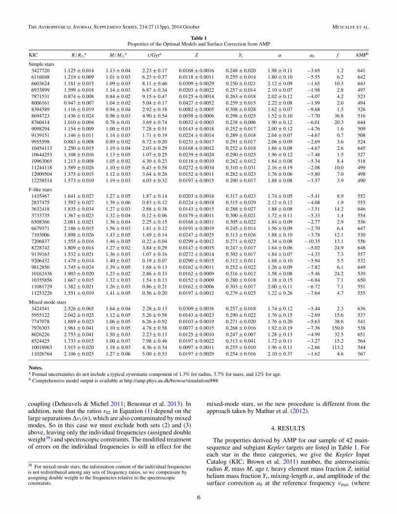
Table 1Properties of the Optimal Models and Surface Correction from AMP

KIC R/R�a M/M�a t/Gyra Z Yi α a0 f AMPb

Simple stars3427720 1.125 ± 0.014 1.13 ± 0.04 2.23 ± 0.17 0.0168 ± 0.0016 0.248 ± 0.020 1.98 ± 0.11 −3.65 1.2 6416116048 1.219 ± 0.009 1.01 ± 0.03 6.23 ± 0.37 0.0118 ± 0.0011 0.255 ± 0.014 1.80 ± 0.10 −5.55 6.2 6426603624 1.181 ± 0.015 1.09 ± 0.03 8.11 ± 0.46 0.0309 ± 0.0029 0.250 ± 0.021 2.12 ± 0.09 −1.65 10.3 6436933899 1.599 ± 0.018 1.14 ± 0.03 6.87 ± 0.34 0.0203 ± 0.0022 0.257 ± 0.014 2.10 ± 0.07 −1.98 2.8 4977871531 0.874 ± 0.008 0.84 ± 0.02 9.15 ± 0.47 0.0125 ± 0.0014 0.263 ± 0.018 2.02 ± 0.12 −4.07 4.2 5238006161 0.947 ± 0.007 1.04 ± 0.02 5.04 ± 0.17 0.0427 ± 0.0052 0.259 ± 0.015 2.22 ± 0.08 −1.99 2.0 4948394589 1.116 ± 0.019 0.94 ± 0.04 2.92 ± 0.18 0.0082 ± 0.0005 0.308 ± 0.028 1.62 ± 0.07 −9.68 1.5 5268694723 1.436 ± 0.024 0.96 ± 0.03 4.90 ± 0.54 0.0058 ± 0.0006 0.298 ± 0.025 1.52 ± 0.10 −7.70 36.8 5168760414 1.010 ± 0.004 0.78 ± 0.01 3.69 ± 0.74 0.0032 ± 0.0003 0.238 ± 0.006 1.90 ± 0.12 −6.01 20.3 6449098294 1.154 ± 0.009 1.00 ± 0.03 7.28 ± 0.51 0.0143 ± 0.0018 0.252 ± 0.017 2.00 ± 0.12 −4.76 1.6 5099139151 1.146 ± 0.011 1.14 ± 0.03 1.71 ± 0.19 0.0224 ± 0.0014 0.289 ± 0.018 2.04 ± 0.07 −4.67 0.7 5089955598 0.883 ± 0.008 0.89 ± 0.02 6.72 ± 0.20 0.0231 ± 0.0017 0.291 ± 0.017 2.06 ± 0.09 −2.69 3.6 52410454113 1.250 ± 0.015 1.19 ± 0.04 2.03 ± 0.29 0.0168 ± 0.0012 0.252 ± 0.018 1.86 ± 0.08 −4.67 2.6 64510644253 1.108 ± 0.016 1.13 ± 0.05 1.07 ± 0.25 0.0239 ± 0.0024 0.290 ± 0.025 1.96 ± 0.12 −7.48 1.5 52710963065 1.213 ± 0.008 1.05 ± 0.02 4.30 ± 0.23 0.0118 ± 0.0010 0.262 ± 0.012 1.84 ± 0.08 −5.34 8.4 51811244118 1.589 ± 0.026 1.10 ± 0.05 6.43 ± 0.58 0.0272 ± 0.0034 0.310 ± 0.031 2.16 ± 0.19 −2.08 10.0 49912009504 1.375 ± 0.015 1.12 ± 0.03 3.64 ± 0.26 0.0152 ± 0.0011 0.282 ± 0.023 1.76 ± 0.06 −5.80 7.0 49812258514 1.573 ± 0.010 1.19 ± 0.03 4.03 ± 0.32 0.0197 ± 0.0015 0.290 ± 0.017 1.88 ± 0.08 −3.57 3.9 490

F-like stars1435467 1.641 ± 0.027 1.27 ± 0.05 1.87 ± 0.14 0.0203 ± 0.0016 0.317 ± 0.023 1.74 ± 0.05 −5.41 8.9 5522837475 1.592 ± 0.027 1.39 ± 0.06 0.83 ± 0.12 0.0224 ± 0.0018 0.315 ± 0.029 2.12 ± 0.12 −4.08 1.9 5533632418 1.835 ± 0.034 1.27 ± 0.03 2.88 ± 0.38 0.0143 ± 0.0015 0.288 ± 0.027 1.88 ± 0.08 −3.51 14.2 6463733735 1.367 ± 0.023 1.32 ± 0.04 0.12 ± 0.06 0.0179 ± 0.0011 0.300 ± 0.021 1.72 ± 0.11 −5.33 1.4 5546508366 2.081 ± 0.021 1.36 ± 0.04 2.25 ± 0.15 0.0168 ± 0.0011 0.305 ± 0.022 1.84 ± 0.09 −2.77 2.9 5366679371 2.186 ± 0.015 1.56 ± 0.03 1.81 ± 0.12 0.0191 ± 0.0019 0.245 ± 0.014 1.56 ± 0.09 −2.70 6.4 6477103006 1.898 ± 0.026 1.43 ± 0.05 1.49 ± 0.14 0.0247 ± 0.0025 0.313 ± 0.026 1.88 ± 0.10 −3.78 12.1 5307206837 1.555 ± 0.016 1.46 ± 0.05 0.22 ± 0.04 0.0299 ± 0.0012 0.271 ± 0.022 1.34 ± 0.08 −10.35 13.1 5568228742 1.809 ± 0.014 1.27 ± 0.02 3.84 ± 0.29 0.0147 ± 0.0015 0.247 ± 0.017 1.64 ± 0.06 −5.02 24.9 6489139163 1.532 ± 0.021 1.36 ± 0.03 1.07 ± 0.16 0.0272 ± 0.0014 0.302 ± 0.017 1.84 ± 0.07 −4.33 7.3 5579206432 1.479 ± 0.014 1.40 ± 0.03 0.19 ± 0.07 0.0290 ± 0.0015 0.312 ± 0.011 1.68 ± 0.10 −5.94 5.5 5329812850 1.745 ± 0.024 1.39 ± 0.05 1.68 ± 0.13 0.0162 ± 0.0011 0.252 ± 0.022 1.26 ± 0.09 −7.82 6.1 64910162436 1.903 ± 0.020 1.23 ± 0.02 2.86 ± 0.33 0.0162 ± 0.0009 0.316 ± 0.012 1.58 ± 0.08 −5.46 24.2 53910355856 1.667 ± 0.015 1.32 ± 0.03 1.54 ± 0.13 0.0152 ± 0.0009 0.280 ± 0.018 1.18 ± 0.15 −6.84 7.1 65011081729 1.382 ± 0.021 1.26 ± 0.03 0.86 ± 0.21 0.0162 ± 0.0006 0.303 ± 0.017 2.00 ± 0.11 −6.72 7.1 55111253226 1.551 ± 0.019 1.41 ± 0.05 0.56 ± 0.20 0.0197 ± 0.0012 0.279 ± 0.025 1.22 ± 0.26 −7.64 4.7 555

Mixed-mode stars3424541 2.526 ± 0.065 1.64 ± 0.04 2.28 ± 0.13 0.0309 ± 0.0036 0.257 ± 0.018 1.74 ± 0.12 −5.44 2.3 6365955122 2.042 ± 0.025 1.12 ± 0.05 5.26 ± 0.58 0.0143 ± 0.0023 0.290 ± 0.022 1.76 ± 0.15 −2.69 15.6 5377747078 1.889 ± 0.023 1.06 ± 0.05 6.26 ± 0.92 0.0103 ± 0.0019 0.271 ± 0.020 1.76 ± 0.20 −5.63 38.6 5417976303 1.961 ± 0.041 1.10 ± 0.05 4.78 ± 0.58 0.0077 ± 0.0015 0.268 ± 0.016 1.92 ± 0.19 −7.36 150.0 5388026226 2.753 ± 0.041 1.50 ± 0.03 2.23 ± 0.13 0.0125 ± 0.0010 0.247 ± 0.007 1.28 ± 0.13 −4.99 32.5 6518524425 1.733 ± 0.015 1.00 ± 0.07 7.98 ± 0.46 0.0197 ± 0.0022 0.313 ± 0.041 1.72 ± 0.11 −3.27 15.2 56410018963 1.915 ± 0.020 1.18 ± 0.03 4.36 ± 0.34 0.0097 ± 0.0011 0.255 ± 0.010 1.96 ± 0.11 −2.66 113.2 54411026764 2.106 ± 0.025 1.27 ± 0.06 5.00 ± 0.53 0.0197 ± 0.0029 0.254 ± 0.016 2.10 ± 0.37 −1.62 4.6 567

Notes.a Formal uncertainties do not include a typical systematic component of 1.3% for radius, 3.7% for mass, and 12% for age.b Comprehensive model output is available at http://amp.phys.au.dk/browse/simulation/###.

coupling (Deheuvels & Michel 2011; Benomar et al. 2013). Inaddition, note that the ratios r02 in Equation (1) depend on thelarge separations Δν1(n), which are also contaminated by mixedmodes. So in this case we must exclude both sets (2) and (3)above, leaving only the individual frequencies (assigned doubleweight38) and spectroscopic constraints. The modified treatmentof errors on the individual frequencies is still in effect for the

38 For mixed-mode stars, the information content of the individual frequenciesis not redistributed among any sets of frequency ratios, so we compensate byassigning double weight to the frequencies relative to the spectroscopicconstraints.

mixed-mode stars, so the new procedure is different from theapproach taken by Mathur et al. (2012).

4. RESULTS

The properties derived by AMP for our sample of 42 main-sequence and subgiant Kepler targets are listed in Table 1. Foreach star in the three categories, we give the Kepler InputCatalog (KIC; Brown et al. 2011) number, the asteroseismicradius R, mass M, age t, heavy element mass fraction Z, initialhelium mass fraction Yi, mixing-length α, and amplitude of thesurface correction a0 at the reference frequency νmax (where

6

The Astrophysical Journal Supplement Series, 214:27 (13pp), 2014 October Metcalfe et al.

νmax was taken from Appourchaux et al. 2012). As an indicationof the relative quality of each model, we list an average of thenormalized χ2 values discussed in Section 3.3—similar to themetric that was used by the GA to identify the optimal model,but using the original frequency errors from Appourchaux et al.(2012) rather than inflating them in proportion to the surfacecorrection. This modified metric f is more useful for comparingthe quality of the models for different stars, and can be used inconjunction with the echelle diagrams in Figure 3 to judge thereliability of each result. Some of the models are clearly betterrepresentations of the observations than others (see discussionbelow), so we caution readers not to treat them all as equivalent.In the final column of Table 1, we list the AMP run number sothat interested readers can access a comprehensive archive withthe evolution and structure of each stellar model.

Figure 3 shows echelle diagrams for typical examples ofeach of the three different star types, with similar plots for all42 stars included in the online version of the Journal. A commonfeature in many of these diagrams is a divergence betweenthe observations (blue points) and the surface-corrected modelfrequencies (solid red points), which appear to curve off towardthe left at higher frequencies. This feature is most obvious inthe F-like star shown in the center panel, which has a largernumber of observed radial orders. As discussed in Section 3.2,this is an indication that the empirical surface correctionof Kjeldsen et al. (2008) tends to over-correct the highestorder modes, motivating our decision to decrease the weightof these frequencies in proportion to the size of the surfacecorrection (i.e., the difference between the solid and openred circles in each plot). Thus, the primary constraints fromthe individual frequencies are concentrated at low frequency,while the ratios capture the information content of the higherfrequencies (excluding the highest three radial orders; seeSection 3.2). Forcing a better fit to the high frequency modes,under the current approach to the surface correction, leads tothe systematic bias toward low-helium solutions that affectedthe results of Mathur et al. (2012).

4.1. Statistical and Systematic Uncertainties

The assessment of uncertainties on the adjustable parametersand other model properties requires some degree of pragma-tism. Our previous approach, based on the local shape of theχ2 surface using singular value decomposition (SVD; Creevey2009; Metcalfe et al. 2009), generally fails to capture uncertain-ties due to non-uniqueness of the solution—a common outcomewhen we combine several different metrics of model quality.Rather than accept the underestimated uncertainties from SVD,we opted for a more conservative approach using an ensembleof the best models sampled by the GA on its way to finding theoptimal solution. First, we ranked the 50,000–80,000 uniquemodels for each star by the average χ2 value and assigned eachmodel a likelihood:

L = exp(−χ2/2). (5)

Next, we calculated a likelihood-weighted mean value andstandard deviation for each parameter, including additionalmodels in the mean until the uncertainty on [Z/X]i wascomparable to the observational error on [M/H]. This is a firstapproximation, since helium diffusion and settling graduallychanges the value of X as the model evolves to its final age. Usingthese uncertainties for the five adjustable model parameters(M, t, Z, Yi, α), we rescaled the covariance matrix from the

optimal solution and calculated a set of models to define the1σ error ellipse. The uncertainties on other model properties,such as R and Teff , were determined from the range of valuesrepresented in these 1σ models. Finally, we refined the numberof models that were included in the mean so that the outputuncertainty on the model Teff was equal to the input error onthe spectroscopic Teff . This procedure leads to an inherentlyconservative estimate of the uncertainties, because it implicitlyassumes that the asteroseismic data do not contribute to thedetermination of Teff in the final solution. With the ensembleof best models defined in this way for each star, we used themto determine the likelihood-weighted standard deviation (takento be the uncertainty) on each parameter of the best solutionidentified by the GA (for a detailed example, see the Appendix).

It is important to emphasize that the resulting uncertainties,listed in Table 1, do not include systematic errors from ourparticular choice of model physics or fitting strategy. Chaplinet al. (2014) used results from six pipeline methodologiescoupled to 11 different model grids to quantify the associatedsystematic uncertainties. They found that, in addition to thestatistical uncertainties from a given model grid and fittingmethodology, the systematic errors for stars with a spectroscopicTeff and [M/H] were typically 1.3% on the radius, 3.7% on themass, and 12% on the age. Although these additional systematicerrors may have an impact on the absolute values of the stellarproperties derived by AMP, the uniformity of the data sourcesand modeling approach means that the relative values can beconsidered as reliable as the uncertainties listed in Table 1.Readers who wish to combine our results with those from othersources should consider the additional systematic errors notedabove.

4.2. Comparison with Other Methods

Setting aside the question of absolute accuracy for thederived stellar properties, we can compare the internal precisionof the AMP results to other common methods of inferringasteroseismic radii, masses and ages. Such a comparison canquantify the benefits of modeling the individual frequencies,relative to using only the global oscillation properties such asΔν and νmax. Empirical scaling relations can provide model-independent estimates of the asteroseismic radius and massusing only the observed values of Δν, νmax and Teff (Kjeldsen& Bedding 1995). In Figure 4, we compare the radii (left)and masses (right) derived from the scaling relations (SR) tothose found by AMP. The top panels compare the actual valuesand associated uncertainties, while the bottom panels showdifferences between the estimates normalized by the uncertaintyon the difference. For clarity, simple (black circles), F-like (reddiamonds), and mixed-mode stars (blue squares) are shownin different colors. The median uncertainties from the scalingrelations are 4.2% on the radius and 6.8% on the mass. Thescaling relation values for F-like stars are systematically higheron average than the estimates from AMP, but the agreement isgenerally better than 2σ .

In Figure 5, we show a similar comparison of AMP resultswith grid-modeling from Chaplin et al. (2014), including theasteroseismic radii (left), masses (center), and ages (right).These grid-modeling (GM) results use the same spectroscopicconstraints from Bruntt et al. (2012), but the adopted modelgrid (yielding values closest to the median over all grids andmethods) came from the GARSTEC code (Weiss & Schlattl2008). The median uncertainties from grid-modeling of thissample are 2.1% on the radius, 5.5% on the mass, and 20%

7

The Astrophysical Journal Supplement Series, 214:27 (13pp), 2014 October Metcalfe et al.

Figure 4. Comparison of the asteroseismic radii (left) and masses (right) derived from scaling relations (SR) with the AMP estimates from Table 1, including thesimple (black circles), F-like (red diamonds), and mixed-mode stars (blue squares). The top panels compare the values and uncertainties, while the bottom panelsshow the differences between the estimates normalized by the uncertainty on the difference.

(A color version of this figure is available in the online journal.)

Figure 5. Comparison of the asteroseismic radii (left), masses (center), and ages (right) derived from grid-modeling (GM; Chaplin et al. 2014) with the AMP estimatesfrom Table 1, including the simple (black circles), F-like (red diamonds), and mixed-mode stars (blue squares). The top panels compare the values and uncertainties,while the bottom panels show the differences between the estimates normalized by the uncertainty on the difference.

(A color version of this figure is available in the online journal.)

on the age—an improvement of a factor of two for the radiusand 25% for the mass compared to the typical precisionfrom scaling relations. The grid-modeling radii for F-like starsare systematically higher compared to AMP, but again theagreement is generally better than 2σ . For all three categoriesof stars, GARSTEC yields ages that are systematically older by∼1 Gyr for most targets with AMP ages below ∼3 Gyr. Chaplinet al. (2014) noted this tendency of GARSTEC with respectto most of the other model grids they explored and attributedthe offset to differences in the treatment of convective coreovershoot, which is not included in the AMP models.

Modeling the individual frequencies with AMP led to asignificant improvement in the internal precision of the derivedstellar properties relative to estimates based on scaling relations

or grid-modeling. The median uncertainties from AMP are 1.2%on the radius, 2.8% on the mass, and 7.9% on the age—about afactor of three improvement over the radius and mass precisionfrom scaling relations, and more precise than grid-modeling byabout a factor of two in radius, mass, and age. It is more difficultto assess the absolute accuracy of the AMP results, but 12 starsin our sample (KIC 3632418, 3733735, 7747078, 8006161,8228742, 9139151, 9139163, 9206432, 10162436, 10454113,11253226, and 12258514) have a parallax from Hipparcos(van Leeuwen 2007), allowing us to compare the predictedluminosities with those of the AMP models that incorporatethis constraint. Ten of the AMP luminosities are within 1σ ofthe predictions, and only two stars show larger deviations (1.7σfor 10162436, and 1.8σ for 10454113)—fewer than expected

8

The Astrophysical Journal Supplement Series, 214:27 (13pp), 2014 October Metcalfe et al.

for Gaussian distributed errors. One star (KIC 8006161) also hasa radius from CHARA interferometry (0.952±0.021 R�; Huberet al. 2012), which is reproduced by the AMP model within 0.2σwhen the constraint was included and 2σ when it was not. Thesesubsamples suggest that, in addition to being more precise thanother methods, the AMP results are also reasonably accurate.

4.3. Applications of the Derived Stellar Properties

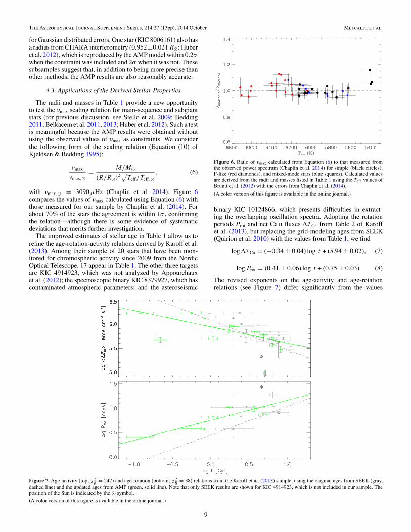
The radii and masses in Table 1 provide a new opportunityto test the νmax scaling relation for main-sequence and subgiantstars (for previous discussion, see Stello et al. 2009; Bedding2011; Belkacem et al. 2011, 2013; Huber et al. 2012). Such a testis meaningful because the AMP results were obtained withoutusing the observed values of νmax as constraints. We considerthe following form of the scaling relation (Equation (10) ofKjeldsen & Bedding 1995):

νmax

νmax,�= M/M�

(R/R�)2√

Teff/Teff,�, (6)

with νmax,� = 3090 μHz (Chaplin et al. 2014). Figure 6compares the values of νmax calculated using Equation (6) withthose measured for our sample by Chaplin et al. (2014). Forabout 70% of the stars the agreement is within 1σ , confirmingthe relation—although there is some evidence of systematicdeviations that merits further investigation.

The improved estimates of stellar age in Table 1 allow us torefine the age-rotation-activity relations derived by Karoff et al.(2013). Among their sample of 20 stars that have been mon-itored for chromospheric activity since 2009 from the NordicOptical Telescope, 17 appear in Table 1. The other three targetsare KIC 4914923, which was not analyzed by Appourchauxet al. (2012); the spectroscopic binary KIC 8379927, which hascontaminated atmospheric parameters; and the asteroseismic

Figure 6. Ratio of νmax calculated from Equation (6) to that measured fromthe observed power spectrum (Chaplin et al. 2014) for simple (black circles),F-like (red diamonds), and mixed-mode stars (blue squares). Calculated valuesare derived from the radii and masses listed in Table 1 using the Teff values ofBruntt et al. (2012) with the errors from Chaplin et al. (2014).

(A color version of this figure is available in the online journal.)

binary KIC 10124866, which presents difficulties in extract-ing the overlapping oscillation spectra. Adopting the rotationperiods Prot and net Ca ii fluxes ΔFCa from Table 2 of Karoffet al. (2013), but replacing the grid-modeling ages from SEEK(Quirion et al. 2010) with the values from Table 1, we find

log ΔFCa = (−0.34 ± 0.04) log t + (5.94 ± 0.02), (7)

log Prot = (0.41 ± 0.06) log t + (0.75 ± 0.03). (8)

The revised exponents on the age-activity and age-rotationrelations (see Figure 7) differ significantly from the values

Figure 7. Age-activity (top; χ2R = 247) and age-rotation (bottom; χ2

R = 38) relations from the Karoff et al. (2013) sample, using the original ages from SEEK (gray,dashed line) and the updated ages from AMP (green, solid line). Note that only SEEK results are shown for KIC 4914923, which is not included in our sample. Theposition of the Sun is indicated by the � symbol.

(A color version of this figure is available in the online journal.)

9

The Astrophysical Journal Supplement Series, 214:27 (13pp), 2014 October Metcalfe et al.

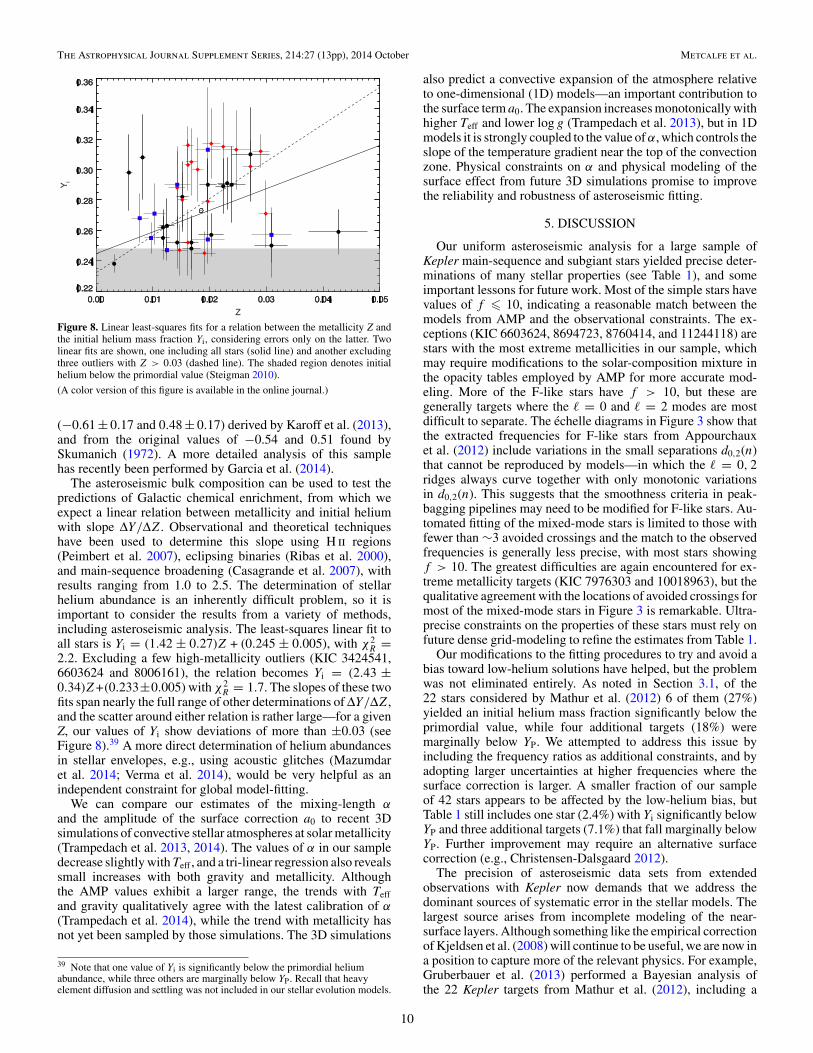
Figure 8. Linear least-squares fits for a relation between the metallicity Z andthe initial helium mass fraction Yi, considering errors only on the latter. Twolinear fits are shown, one including all stars (solid line) and another excludingthree outliers with Z > 0.03 (dashed line). The shaded region denotes initialhelium below the primordial value (Steigman 2010).

(A color version of this figure is available in the online journal.)

(−0.61 ± 0.17 and 0.48 ± 0.17) derived by Karoff et al. (2013),and from the original values of −0.54 and 0.51 found bySkumanich (1972). A more detailed analysis of this samplehas recently been performed by Garcia et al. (2014).

The asteroseismic bulk composition can be used to test thepredictions of Galactic chemical enrichment, from which weexpect a linear relation between metallicity and initial heliumwith slope ΔY/ΔZ. Observational and theoretical techniqueshave been used to determine this slope using H ii regions(Peimbert et al. 2007), eclipsing binaries (Ribas et al. 2000),and main-sequence broadening (Casagrande et al. 2007), withresults ranging from 1.0 to 2.5. The determination of stellarhelium abundance is an inherently difficult problem, so it isimportant to consider the results from a variety of methods,including asteroseismic analysis. The least-squares linear fit toall stars is Yi = (1.42 ± 0.27)Z + (0.245 ± 0.005), with χ2

R =2.2. Excluding a few high-metallicity outliers (KIC 3424541,6603624 and 8006161), the relation becomes Yi = (2.43 ±0.34)Z+(0.233±0.005) with χ2

R = 1.7. The slopes of these twofits span nearly the full range of other determinations of ΔY/ΔZ,and the scatter around either relation is rather large—for a givenZ, our values of Yi show deviations of more than ±0.03 (seeFigure 8).39 A more direct determination of helium abundancesin stellar envelopes, e.g., using acoustic glitches (Mazumdaret al. 2014; Verma et al. 2014), would be very helpful as anindependent constraint for global model-fitting.

We can compare our estimates of the mixing-length αand the amplitude of the surface correction a0 to recent 3Dsimulations of convective stellar atmospheres at solar metallicity(Trampedach et al. 2013, 2014). The values of α in our sampledecrease slightly with Teff , and a tri-linear regression also revealssmall increases with both gravity and metallicity. Althoughthe AMP values exhibit a larger range, the trends with Teffand gravity qualitatively agree with the latest calibration of α(Trampedach et al. 2014), while the trend with metallicity hasnot yet been sampled by those simulations. The 3D simulations

39 Note that one value of Yi is significantly below the primordial heliumabundance, while three others are marginally below YP. Recall that heavyelement diffusion and settling was not included in our stellar evolution models.

also predict a convective expansion of the atmosphere relativeto one-dimensional (1D) models—an important contribution tothe surface term a0. The expansion increases monotonically withhigher Teff and lower log g (Trampedach et al. 2013), but in 1Dmodels it is strongly coupled to the value of α, which controls theslope of the temperature gradient near the top of the convectionzone. Physical constraints on α and physical modeling of thesurface effect from future 3D simulations promise to improvethe reliability and robustness of asteroseismic fitting.

5. DISCUSSION

Our uniform asteroseismic analysis for a large sample ofKepler main-sequence and subgiant stars yielded precise deter-minations of many stellar properties (see Table 1), and someimportant lessons for future work. Most of the simple stars havevalues of f � 10, indicating a reasonable match between themodels from AMP and the observational constraints. The ex-ceptions (KIC 6603624, 8694723, 8760414, and 11244118) arestars with the most extreme metallicities in our sample, whichmay require modifications to the solar-composition mixture inthe opacity tables employed by AMP for more accurate mod-eling. More of the F-like stars have f > 10, but these aregenerally targets where the � = 0 and � = 2 modes are mostdifficult to separate. The echelle diagrams in Figure 3 show thatthe extracted frequencies for F-like stars from Appourchauxet al. (2012) include variations in the small separations d0,2(n)that cannot be reproduced by models—in which the � = 0, 2ridges always curve together with only monotonic variationsin d0,2(n). This suggests that the smoothness criteria in peak-bagging pipelines may need to be modified for F-like stars. Au-tomated fitting of the mixed-mode stars is limited to those withfewer than ∼3 avoided crossings and the match to the observedfrequencies is generally less precise, with most stars showingf > 10. The greatest difficulties are again encountered for ex-treme metallicity targets (KIC 7976303 and 10018963), but thequalitative agreement with the locations of avoided crossings formost of the mixed-mode stars in Figure 3 is remarkable. Ultra-precise constraints on the properties of these stars must rely onfuture dense grid-modeling to refine the estimates from Table 1.

Our modifications to the fitting procedures to try and avoid abias toward low-helium solutions have helped, but the problemwas not eliminated entirely. As noted in Section 3.1, of the22 stars considered by Mathur et al. (2012) 6 of them (27%)yielded an initial helium mass fraction significantly below theprimordial value, while four additional targets (18%) weremarginally below YP. We attempted to address this issue byincluding the frequency ratios as additional constraints, and byadopting larger uncertainties at higher frequencies where thesurface correction is larger. A smaller fraction of our sampleof 42 stars appears to be affected by the low-helium bias, butTable 1 still includes one star (2.4%) with Yi significantly belowYP and three additional targets (7.1%) that fall marginally belowYP. Further improvement may require an alternative surfacecorrection (e.g., Christensen-Dalsgaard 2012).

The precision of asteroseismic data sets from extendedobservations with Kepler now demands that we address thedominant sources of systematic error in the stellar models. Thelargest source arises from incomplete modeling of the near-surface layers. Although something like the empirical correctionof Kjeldsen et al. (2008) will continue to be useful, we are now ina position to capture more of the relevant physics. For example,Gruberbauer et al. (2013) performed a Bayesian analysis ofthe 22 Kepler targets from Mathur et al. (2012), including a

10

The Astrophysical Journal Supplement Series, 214:27 (13pp), 2014 October Metcalfe et al.

simplified non-adiabatic treatment of the pulsations. They foundthat the Bayesian probabilities were higher when non-adiabaticrather than adiabatic frequencies were fit to the observations, andthat for most stars the surface effect was minimized and in somecases even eliminated. Their non-adiabatic model accounted forradiative losses and gains but neglected perturbations to theconvective flux and turbulent pressure (Guenther 1994). In thecase of the Sun, the stability and frequency of the oscillationmodes depends substantially on turbulent pressure and theinclusion of non-local effects in the treatment of convection(Balmforth 1992a, 1992b; Houdek 2010), and the resultingfrequency shift is uncertain. The sensitivity of the results tothe model of convection and the temperature profile in thesuper-adiabatic layer was also emphasized by Rosenthal et al.(1999) and Li et al. (2002). Regardless, the Bayesian approachhas the advantage of incorporating the unknown sources ofsystematic error directly into the uncertainties on the derivedstellar properties, and can reveal which approach to the pulsationcalculations generally improves the model fits.

For future analyses, we intend to augment ADIPLS withthe non-adiabatic stellar oscillation code GYRE (Townsend& Teitler 2013), which currently includes a limited treatmentof non-adiabatic effects but is flexible enough to incorporateadditional contributions. We would also like to take advantageof the numerical stability and modular architecture of the open-source MESA code (Paxton et al. 2013) to explore differentchemical mixtures and to include heavy element diffusion andsettling in the evolutionary models, which is not currently stablefor all types of stars with ASTEC. With these new modulesfor stellar evolution and pulsation calculations, we can embeda Bayesian formalism into the parallel genetic algorithm tocomplement the simple χ2 approach. The complete sampleof asteroseismic targets from extended Kepler observationsspanning up to four years will provide a rich data set to validatethese new ingredients for the next generation of AMP.

The golden age of asteroseismology for main-sequence andsubgiant stars owes a great debt to the Kepler mission, butit promises to continue with the anticipated launch of NASA’sTransiting Exoplanet Survey Satellite (TESS; Ricker et al. 2014)in 2017. While Kepler was able to provide asteroseismic datafor hundreds of targets and could simultaneously monitor 512stars with 1-minute sampling, TESS plans to observe ∼500,000of the brightest G- and K-type stars in the sky at a cadencesufficient to detect solar-like oscillations. The data sets will benearly continuous for at least 27 days, but in two regions nearthe ecliptic poles the fields will overlap for durations up to a fullyear. These brighter stars will generally be much better charac-terized than the Kepler targets—with parallaxes from Hipparcosand ultimately Gaia (Perryman et al. 2001), and reliable atmo-spheric constraints from ground-based spectroscopy—makingasteroseismic characterization more precise and accurate. Withseveral years of development time available, AMP promises tobe ready to convert this avalanche of data into reliable inferenceson the properties of our solar system’s nearest neighbors.

We would like to thank Victor Silva Aguirre for help-ful discussions. This work was supported in part by NASAgrants NNX13AC44G and NNX13AE91G, and by WhiteDwarf Research Corporation through the Pale Blue Dot project(http://whitedwarf.org/palebluedot/). Computational time onKraken at the National Institute of Computational Sciences wasprovided through XSEDE allocation TG-AST090107. Fund-ing for the Stellar Astrophysics Centre is provided by The

Danish National Research Foundation (grant DNRF106). Weacknowledge the ASTERISK project (ASTERoseismic In-vestigations with SONG and Kepler) funded by the Euro-pean Research Council (grant agreement No.: 267864), theScientific and Technological Research Council of Turkey(TUBITAK:112T989), and a European Commission grant forthe SPACEINN project (FP7-SPACE-2012-312844). B.P.B. wassupported in part by NSF Astronomy and Astrophysics post-doctoral fellowship AST 09-02004. C.M.S.O. is supportedby NSF grant PHY 08-21899 and K.I.T.P. is supported byNSF grant PHY 11-25915. M.S.C. is supported by an Inves-tigador FCT contract funded by FCT/MCTES (Portugal) andPOPH/FSE (EC). A.D. has been supported by the HungarianOTKA grants K83790, KTIA URKUT_10-1-2011-0019 grant,the Lendulet-2009 Young Researchers Programme of the Hun-garian Academy of Sciences, the Janos Bolyai Research Schol-arship of the Hungarian Academy of Sciences and the City ofSzombathely under agreement No. S-11-1027. A.D. and R.A.G.acknowledge the support of the European Community SeventhFramework Programme (FP7/2007-2013) under grant agree-ment No. 269194 (IRSES/ASK). R.A.G. and D. Salabert ac-knowledge the support of the CNES grant at CEA-Saclay. A.M.acknowledges support from the NIUS programme of HBCSE(TIFR). A.S. is supported by the MICINN grant AYA2011-24704 and by the ESF EUROCORES Program EuroGENESIS(MICINN grant EUI2009-04170). D. Stello is supported by theAustralian Research Council.

APPENDIX

UNCERTAINTY ESTIMATION PROCEDURE

Our previous approach to uncertainty estimation using SVDis no longer appropriate for several reasons. First, SVD assumesthat the observables are independent. This was reasonablewhen we were only fitting the individual frequencies andspectroscopic constraints. Now that we also fit the frequencyratios r02 and r010 (see Section 3.2), some of the observables areno longer independent and SVD cannot be used. Second, even ifwe do not include the frequency ratios as constraints, the SVDmethod determines the uncertainties from the local shape of theχ2 surface. Such an analysis fails to capture the uncertainties dueto non-uniqueness of the optimal solution, yielding errors thatare too optimistic for practical purposes. Finally, the metric usedby the GA for optimization, which defines the local shape of theχ2 surface, is a composite of normalized χ2 values from severaldistinct sets of observables, making it difficult to interpret in astatistically robust manner.

We can use the ensemble of models sampled by the GAto provide a more conservative and global estimate of theuncertainties. During an AMP run, the parameter values andaverage χ2 metric are recorded for each trial model that iscompared to the observations. The nature of the fitting processensures that each trial model is a much better match to theobservations than a random model in the search space. For eachstellar evolution track generated by AMP, the age is optimizedinternally using a binary decision tree to match the observedlarge separation. In addition, the final age is interpolatedbetween time steps on the track to match the lowest observedradial mode, and the empirical surface correction of Kjeldsenet al. (2008) is applied to improve the match to higher frequencymodes. In effect, the GA is producing the best possible match tothe observations given the four fixed parameters (M,Z, Yi, α)for each trial model. As a consequence, we need to use a subset

11

The Astrophysical Journal Supplement Series, 214:27 (13pp), 2014 October Metcalfe et al.

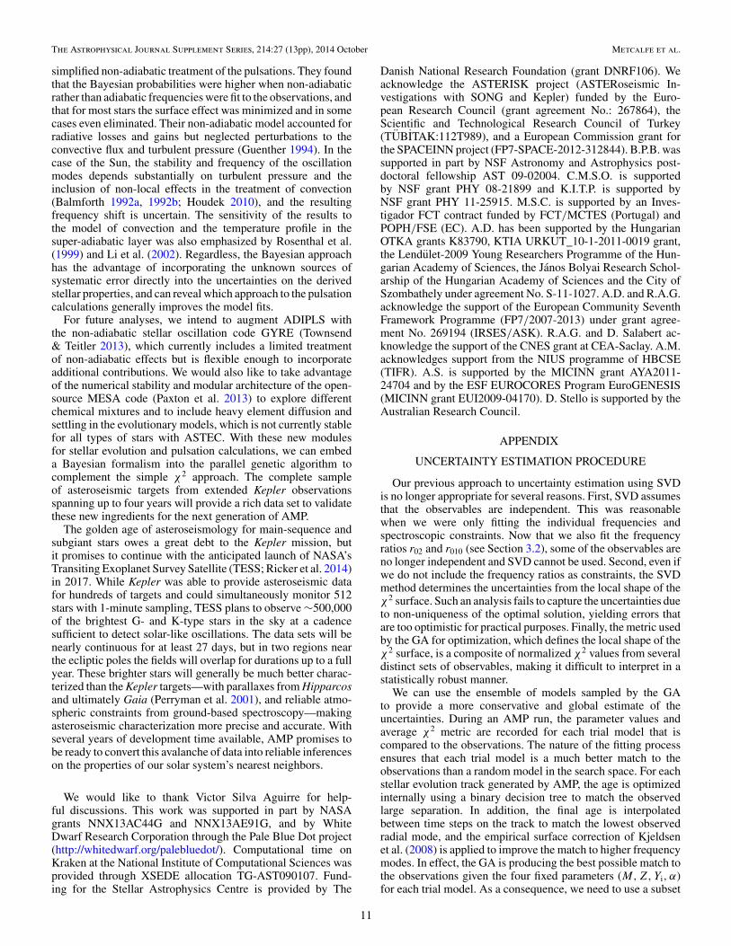
Figure 9. Uncertainties in [Z/X]i (left), Teff (center), and R (right) for KIC 6116048 as the number of models included in the likelihood-weighted mean is increased.Several cuts are defined from the uncertainty in [Z/X]i (left panel, vertical dashed lines), which yield corresponding uncertainties in Teff and R from the 1σ models(center and right panels, + points). Interpolating to yield an uncertainty of 84 K in Teff (center panel, horizontal dotted line) provides the final cut (center and rightpanels, vertical dotted line) that is used to define the uncertainties on all model properties.

of the full ensemble of GA models if we want a reasonableestimate of the uncertainties from the limited information thatis available.

To determine the number of GA trial models that we shouldinclude in our uncertainty estimation procedure, we initiallyattempted to match the observational error on [M/H] (0.09 dex;Chaplin et al. 2014; Bruntt et al. 2012). As outlined brieflyin Section 4.1, we ranked the unique trial models by theiraverage χ2 value and assigned each one a relative likelihoodusing Equation (5). This allowed us to calculate a likelihood-weighted mean and standard deviation for each adjustable modelparameter, including Z and Yi to generate an uncertainty onthe initial composition [Z/X]i as we gradually included moremodels in the mean. We only had access to the initial value ofX, which increases at the surface over time as helium diffusionand settling operates in the models, so this only provided afirst estimate of the appropriate number of models to include.The resulting uncertainty on [Z/X]i for our example starKIC 6116048 is shown in the left panel of Figure 9 as a functionof the number of models included in the likelihood-weightedmean.

Uncertainties on the other properties of the optimal modelscan only be determined after a cut on the number of modelshas been adopted. The cut establishes the uncertainties on theadjustable parameters (M, t, Z, Yi, α) as well as the covariancematrix around the optimal solution. This allows us to calculatea set of models that define the 1σ error ellipse, and then use halfthe range of values for any other property (such as [Z/X]s,Teff , or R) within the 1σ models to define an uncertaintyfor these non-adjustable parameters. For KIC 6116048, wedetermined that by including the best ∼25,000 models in thelikelihood-weighted mean, the resulting uncertainty on thesurface composition [Z/X]s (not shown in Figure 9) wascomparable to the observational error on [M/H]. Using thissame cut, the full range of model values for Teff within the1σ models spanned 290 K, yielding an error estimate of±145 K (see center panel of Figure 9). We repeated the analysisprocedure with a cut at one-half and one-quarter of this numberof models (vertical dashed lines in the left panel of Figure 9)until the resulting uncertainty on the model Teff was below theerror on the observed Teff (84 K; Chaplin et al. 2014; Brunttet al. 2012).

By interpolating the number of models required to reproducethe observed Teff error, we defined the appropriate cut thatwas then used to estimate the final uncertainties on all modelproperties. The center panel of Figure 9 shows the uncertaintyon the model Teff for the three cuts indicated in the left panel.

When the 7370 best models sampled by the GA (vertical dottedline) were used to calculate the likelihood-weighted mean andstandard deviation for each of the adjustable model parameters,the uncertainty on the model Teff from the resulting 1σ modelswas equal to the observational error of 84 K (horizontal dottedline). The range of radii within this same set of 1σ models definethe radius uncertainty of 0.0094 R� (right panel of Figure 9).As noted in Section 4.1, the above procedure yields inherentlyconservative uncertainty estimates because it assumes that theasteroseismic data do not contribute to the determination of Teffin the final solution. This assumption is certainly not valid forthe surface composition, even ignoring the complications fromdiffusion, which explains why the final uncertainty on [Z/X]i iswell below the observational error on [M/H]. We repeated theabove procedure for each star in our sample to yield the final setof uncertainties, which appear in Table 1.

REFERENCES

Aizenman, M., Smeyers, P., & Weigert, A. 1977, A&A, 58, 41Alexander, D. R., & Ferguson, J. W. 1994, ApJ, 437, 879Ammons, S. M., Robinson, S. E., Strader, J., et al. 2006, ApJ, 638, 1004Angulo, C., Arnould, M., Rayet, M., et al. 1999, NuPhA, 656, 3Appourchaux, T., Chaplin, W. J., Garcıa, R. A., et al. 2012, A&A, 543, A54Appourchaux, T., Michel, E., Auvergne, M., et al. 2008, A&A, 488, 705Bahcall, J. N., Pinsonneault, M. H., & Wasserburg, G. J. 1995, RvMP, 67, 781Balmforth, N. J. 1992a, MNRAS, 255, 632Balmforth, N. J. 1992b, MNRAS, 255, 639Bedding, T. R. 2011, Asteroseismology: XXII Canary Islands Winter School of

Astrophysics, ed. P. L. Palle (Cambridge: Cambridge Univ. Press), 60Bedding, T. R., & Kjeldsen, H. 2003, PASA, 20, 203Belkacem, K., Goupil, M. J., Dupret, M. A., et al. 2011, A&A, 530, A142Belkacem, K., Samadi, R., Mosser, B., Goupil, M.-J., & Ludwig, H.-G. 2013,

in ASP Conf. Ser. 479, Progress in Physics of the Sun and Stars: A New Erain Helio- and Asteroseismology, ed. H. Shibahashi & A. E. Lynas-Gray (SanFrancisco, CA: ASP), 61

Benomar, O., Bedding, T. R., Mosser, B., et al. 2013, ApJ, 767, 158Bevington, P. R., & Robinson, D. K. 1992, Data Reduction and Error Analysis

for the Physical Sciences (New York: McGraw-Hill)Bohm-Vitense, E. 1958, ZAp, 46, 108Borucki, W. J., Koch, D., Basri, G., et al. 2010, Sci, 327, 977Brandao, I. M., Dogan, G., Christensen-Dalsgaard, J., et al. 2011, A&A,

527, A37Brown, T. M., Gilliland, R. L., Noyes, R. W., & Ramsey, L. W. 1991, ApJ,

368, 599Brown, T. M., Latham, D. W., Everett, M. E., & Esquerdo, G. A. 2011, AJ,

142, 112Bruntt, H., Basu, S., Smalley, B., et al. 2012, MNRAS, 423, 122Casagrande, L., Flynn, C., Portinari, L., Girardi, L., & Jimenez, R.

2007, MNRAS, 382, 1516Chaplin, W. J., Basu, S., Huber, D., et al. 2014, ApJS, 210, 1Chaplin, W. J., Kjeldsen, H., Christensen-Dalsgaard, J., et al. 2011, Sci,

332, 213

12

The Astrophysical Journal Supplement Series, 214:27 (13pp), 2014 October Metcalfe et al.

Chaplin, W. J., & Miglio, A. 2013, ARA&A, 51, 353Christensen-Dalsgaard, J. 2008a, Ap&SS, 316, 13Christensen-Dalsgaard, J. 2008b, Ap&SS, 316, 113Christensen-Dalsgaard, J. 2012, AN, 333, 914Christensen-Dalsgaard, J., Dappen, W., Ajukov, S. V., et al. 1996, Sci, 272, 1286Creevey, O. L. 2009, in ASP Conf. Ser. 416, Solar-Stellar Dynamos as Revealed

by Helio- and Asteroseismology: GONG 2008/SOHO 21, ed. M. Dikpati,T. Arentoft, I. G. Hernandez, C. Lindsey, & F. Hill (San Francisco, CA:ASP), 363

Creevey, O. L., Dogan, G., Frasca, A., et al. 2012, A&A, 537, A111Deheuvels, S., & Michel, E. 2011, A&A, 535, A91Dogan, G., Metcalfe, T. S., Deheuvels, S., et al. 2013, ApJ, 763, 49Ferguson, J. W., Alexander, D. R., Allard, F., et al. 2005, ApJ, 623, 585Flower, P. J. 1996, ApJ, 469, 355Frasca, A., Alcala, J. M., Covino, E., et al. 2003, A&A, 405, 149Frasca, A., Guillout, P., Marilli, E., et al. 2006, A&A, 454, 301Garcia, R. A., Ceillier, T., Salabert, D., et al. 2014, A&A, submitted

(arXiv:1403.7155)Garcıa, R. A., Hekker, S., Stello, D., et al. 2011, MNRAS, 414, L6Gilliland, R. L., Jenkins, J. M., Borucki, W. J., et al. 2010, ApJL, 713, L160Goldreich, P., & Keeley, D. A. 1977, ApJ, 212, 243Goldreich, P., & Kumar, P. 1988, ApJ, 326, 462Grec, G., Fossat, E., & Pomerantz, M. 1980, Natur, 288, 541Grevesse, N., & Noels, A. 1993, Perfectionnement de l’Association Vaudoise

des Chercheurs en Physique, 205Gruberbauer, M., Guenther, D. B., MacLeod, K., & Kallinger, T. 2013, MNRAS,

435, 242Gruberbauer, M., Kallinger, T., Weiss, W. W., & Guenther, D. B. 2009, A&A,

506, 1043Guenther, D. B. 1994, ApJ, 422, 400Guenther, D. B., & Brown, K. I. T. 2004, ApJ, 600, 419Houdek, G. 2010, AN, 331, 998Houdek, G., Balmforth, N. J., Christensen-Dalsgaard, J., & Gough, D. O. 1999,

A&A, 351, 582Huber, D., Ireland, M. J., Bedding, T. R., et al. 2012, ApJ, 760, 32Iglesias, C. A., & Rogers, F. J. 1996, ApJ, 464, 943Karoff, C., Metcalfe, T. S., Chaplin, W. J., et al. 2013, MNRAS, 433, 3227Kjeldsen, H., & Bedding, T. R. 1995, A&A, 293, 87Kjeldsen, H., Bedding, T. R., & Christensen-Dalsgaard, J. 2008, ApJL,

683, L175Kjeldsen, H., Christensen-Dalsgaard, J., Handberg, R., et al. 2010, AN,

331, 966Lebreton, Y., & Goupil, M.-J. 2014, A&A, 569, 21Li, L. H., Robinson, F. J., Demarque, P., Sofia, S., & Guenther, D. B. 2002, ApJ,

567, 1192Mathur, S., Hekker, S., Trampedach, R., et al. 2011, ApJ, 741, 119Mathur, S., Metcalfe, T. S., Woitaszek, M., et al. 2012, ApJ, 749, 152

Mazumdar, A., Monteiro, M. J. P. F. G., Ballot, J., et al. 2014, ApJ, 782, 18Metcalfe, T. S., Chaplin, W. J., Appourchaux, T., et al. 2012, ApJL, 748, L10Metcalfe, T. S., & Charbonneau, P. 2003, JCoPh, 185, 176Metcalfe, T. S., Creevey, O. L., & Christensen-Dalsgaard, J. 2009, ApJ,

699, 373Metcalfe, T. S., Monteiro, M. J. P. F. G., Thompson, M. J., et al. 2010, ApJ,

723, 1583Michaud, G., & Proffitt, C. R. 1993, in Proc. IAU Colloq. 137, Inside the Stars,

ed. A. Baglin & W. W. Weiss (ASP Conf. Ser. 40; San Francisco, CA: ASP),246

Molenda-Zakowicz, J., Sousa, S. G., Frasca, A., et al. 2013, MNRAS, 434, 1422Osaki, J. 1975, PASJ, 27, 237Paxton, B., Cantiello, M., Arras, P., et al. 2013, ApJS, 208, 4Peimbert, M., Luridiana, V., & Peimbert, A. 2007, ApJ, 666, 636Perryman, M. A. C., de Boer, K. S., Gilmore, G., et al. 2001, A&A, 369, 339Pinsonneault, M. H., An, D., Molenda-Zakowicz, J., et al. 2012, ApJS, 199, 30Quirion, P.-O., Christensen-Dalsgaard, J., & Arentoft, T. 2010, ApJ, 725, 2176Ribas, I., Jordi, C., Torra, J., & Gimenez, A. 2000, MNRAS, 313, 99Ricker, G. R., et al. 2014, SPIE Proceedings, submitted (arXiv:1406.0151)Rogers, F. J., & Nayfonov, A. 2002, ApJ, 576, 1064Rosenthal, C. S., Christensen-Dalsgaard, J., Nordlund, Å., Stein, R. F., &

Trampedach, R. 1999, A&A, 351, 689Roxburgh, I. W., & Vorontsov, S. V. 2003, A&A, 411, 215Samadi, R., & Goupil, M.-J. 2001, A&A, 370, 136Silva Aguirre, V., Basu, S., Brandao, I. M., et al. 2013, ApJ, 769, 141Skumanich, A. 1972, ApJ, 171, 565Sneden, C. A. 1973, PhD thesis, Univ. of TexasSousa, S. G., Santos, N. C., Israelian, G., Mayor, M., & Monteiro, M. J. P. F. G.

2007, A&A, 469, 783Steigman, G. 2010, JCAP, 4, 29Stello, D., Chaplin, W. J., Basu, S., Elsworth, Y., & Bedding, T. R.

2009, MNRAS, 400, L80Tassoul, M. 1980, ApJS, 43, 469Torres, G. 2010, AJ, 140, 1158Torres, G., Fischer, D. A., Sozzetti, A., et al. 2012, ApJ, 757, 161Townsend, R. H. D., & Teitler, S. A. 2013, MNRAS, 435, 3406Trampedach, R., Asplund, M., Collet, R., Nordlund, Å., & Stein, R. F. 2013, ApJ,

769, 18Trampedach, R., Christensen-Dalsgaard, J., Nordlund, Å., Asplund, M., & Stein,

R. F. 2014, MNRAS, 442, 805van Leeuwen, F. 2007, A&A, 474, 653Verma, K., Faria, J. P., Antia, H. M., et al. 2014, ApJ, 790, 138Verner, G. A., Elsworth, Y., Chaplin, W. J., et al. 2011, MNRAS, 415, 3539Weiss, A., & Schlattl, H. 2008, Ap&SS, 316, 99White, T. R., Bedding, T. R., Gruberbauer, M., et al. 2012, ApJL, 751, L36Woitaszek, M., Metcalfe, T., & Shorrock, I. 2009, Proc. of the 5th Grid

Computing Environments Workshop (New York: ACM Press), 1

13