The APOKASC Catalog: An Asteroseismic and Spectroscopic Joint Survey of

Targets in the Kepler Fields

Marc H. Pinsonneault1,2, Yvonne Elsworth3,4, Courtney Epstein1, Saskia Hekker5, Sz. Meszaros6,

William J. Chaplin3,4, Jennifer A. Johnson1,2, Rafael A. Garcıa7, Jon Holtzman8, Savita Mathur9,

Ana Garcıa Perez10, Victor Silva Aguirre4, Leo Girardi11,12, Sarbani Basu13, Matthew Shetrone14,

Dennis Stello4,15, Carlos Allende Prieto16,17, Deokkeun An18, Paul Beck7, Timothy C. Beers19,20,

Dmitry Bizyaev21, Steven Bloemen22, Jo Bovy23, Katia Cunha24,25, Joris De Ridder26, Peter M.

Frinchaboy27, D.A. Garcia-Hernandez16,17, Ronald Gilliland28, Paul Harding29, Fred R. Hearty28,

Daniel Huber30,31, Inese Ivans32, Thomas Kallinger33, Steven R. Majewski10, Travis S. Metcalfe9,

Andrea Miglio3,4, Benoit Mosser34, Demitri Muna1, David L. Nidever35, Donald P. Schneider28,36,

Aldo Serenelli37, Verne V. Smith38, Jamie Tayar1, Olga Zamora16,17,Gail Zasowski39

arX

iv:1

410.

2503

v1 [

astr

o-ph

.SR

] 9

Oct

201

4

– 2 –

1Dept. of Astronomy, The Ohio State University, Columbus, OH 43210, USA

2Center for Cosmology and Astroparticle Physics, The Ohio State University, Columbus OH, 43210 USA

3University of Birmingham, School of Physics and Astronomy, Edgbaston, Birmingham B15 2TT, UK

4Stellar Astrophysics Centre, Department of Physics and Astronomy, Aarhus University, Ny Munkegade 120, DK-

8000 Aarhus C, Denmark

5Max-Planck-Institut fur Sonnensystemforschung, Justus-von-Liebig-Weg 3, 37077 Gottingen, Germany

6Astronomy Department, Indiana University, Bloomington,IN 47405, USA

7Laboratoire AIM, CEA/DSM-CNRS - Universite Denis Diderot-IRFU/SAp, 91191, Gif-sur-Yvette Cedex, France

8Department of Astronomy, MSC 4500, New Mexico State University, P.O. Box 30001, Las Cruces, NM 88003,

USA

9Space Science Institute, 4750 Walnut street Suite 205, Boulder, CO 80301, USA

10Department of Astronomy, University of Virginia, P.O.Box 400325, Charlottesville, VA 22904-4325, USA

11Osservatorio Astronomico di Padova – INAF, Vicolo dell’Osservatorio 5, I-35122 Padova, Italy

12Laboratorio Interinstitucional de e-Astronomia – LIneA, Rua Gal. Jose Cristino 77, Rio de Janeiro, RJ – 20921-

400, Brazil

13Department of Astronomy, Yale University, PO Box 208101, New Haven, CT 06520-8101, USA

14University of Texas at Austin, McDonald Observatory 32 Fowlkes Rd. McDonald Observatory, TX 79734-3005,

USA

15Sydney Institute for Astronomy (SIfA), School of Physics, University of Sydney, NSW 2006, Australia

16Instituto de Astrofsica de Canarias (IAC), C/Va Lactea, s/n, E-38200, La Laguna, Tenerife, Spain

17Departamento de Astrofsica, Universidad de La Laguna, E-38206, La Laguna, Tenerife, Spain

18Department of Science Education, Ewha Womans University, Seoul, Korea

19Department of Physics, University of Notre Dame, 225 Nieuwland Science Hall, Notre Dame, IN 46656, USA

20JINA: Joint Institute for Nuclear Astrophysics, University of Notre Dame, Notre Dame, IN 46556, USA

21Apache Point Observatory and New Mexico State University, P.O. Box 59, Sunspot, NM, 88349-0059, USA

22Department of Astrophysics, IMAPP, Radboud University Nijmegen, PO Box 9010, NL-6500 GL Nijmegen, The

Netherlands

23Institute for Advanced Study, Einstein Drive, Princeton, NJ 08540, USA

24Observatorio Nacional, Sao Cristovao, Rio de Janeiro, Brazil

25Steward Observatory, University of Arizona, Tucson, AZ 85719, USA

26Instituut voor Sterrenkunde, KU Leuven, 3001, Leuven, Belgium

27Department of Physics & Astronomy, Texas Christian University, Fort Worth, TX 76129, USA

28Department of Astronomy and Astrophysics, The Pennsylvania State University, University Park, PA 16802, USA

29Department of Astronomy, Case Western Reserve University, Cleveland, OH 44106-7215, USA

30NASA Ames Research Center, Moffett Field, CA 94035, USA

– 3 –ABSTRACT

We present the first APOKASC catalog of spectroscopic and asteroseismic properties

of 1916 red giants observed in the Kepler fields. The spectroscopic parameters pro-

vided from the Apache Point Observatory Galactic Evolution Experiment project are

complemented with asteroseismic surface gravities, masses, radii, and mean densities de-

termined by members of the Kepler Asteroseismology Science Consortium. We assess

both random and systematic sources of error and include a discussion of sample selection

for giants in the Kepler fields. Total uncertainties in the main catalog properties are of

order 80 K in Teff , 0.06 dex in [M/H], 0.014 dex in log g, and 12% and 5% in mass and

radius, respectively; these reflect a combination of systematic and random errors. Aster-

oseismic surface gravities are substantially more precise and accurate than spectroscopic

ones, and we find good agreement between their mean values and the calibrated spectro-

scopic surface gravities. There are, however, systematic underlying trends with Teff and

log g. Our effective temperature scale is between 0-200 K cooler than that expected from

the Infrared Flux Method, depending on the adopted extinction map, which provides

evidence for a lower value on average than that inferred for the Kepler Input Catalog

(KIC). We find a reasonable correspondence between the photometric KIC and spectro-

scopic APOKASC metallicity scales, with increased dispersion in KIC metallicities as the

absolute metal abundance decreases, and offsets in Teff and log g consistent with those

derived in the literature. We present mean fitting relations between APOKASC and KIC

observables and discuss future prospects, strengths, and limitations of the catalog data.

1. Introduction

We are entering the era of precision stellar astrophysics. Large surveys are yielding data with

unprecedented quality and quantity, and even more ambitious programs are on the near horizon.

This advance is not merely a matter of much larger samples of measurements than were possible

before; there are also fundamentally new observables arising from the advent of asteroseismology

as a practical stellar population tool. These new observables are particularly powerful diagnostics

when complemented with data from more traditional approaches. In this paper we present the first

31SETI Institute, 189 Bernardo Avenue, Mountain View, CA 94043, USA

32Department of Physics and Astronomy, The University of Utah, Salt Lake City, UT 84112, USA

33Institute for Astronomy, University of Vienna, Turkenschanzstrasse 17, 1180 Vienna, Austria

34LESIA, UMR 8109, Universite Pierre et Marie Curie, Universite Denis Diderot, Observatoire de Paris, 92195

Meudon Cedex, France

35Department of Astronomy, University of Michigan, Ann Arbor, MI 48104 USA

36Institute for Gravitation and the Cosmos, The Pennsylvania State University, University Park, PA 16802, USA

37Institute of Space Sciences (IEEC-CSIC), Campus UAB, 08193, Bellaterra, Spain

38National Optical Astronomy Observatories, Tucson, AZ 85719 USA

39Department of Physics & Astronomy, Johns Hopkins University, Baltimore, MD, 21218, USA

– 4 –release of the joint APOKASC asteroseismic and spectroscopic survey for targets with both high-

resolution Apache Point Observatory Galactic Evolution Experiment (APOGEE) spectra analyzed

by members of the third Sloan Digital Sky Survey (SDSS-III) and asteroseismic data obtained by

the Kepler mission and analyzed by members of the Kepler Asteroseismology Science Consortium

(KASC). When completed we anticipate of order 8,000 red giants and 600 dwarfs and subgiants

with asteroseismic data and high-resolution spectra. In this initial paper we catalog the properties

of 1916 red giants observed as part of the Sloan Digital Sky Survey Data Release 10 (Ahn et al.

2014). A catalog for the less-evolved stars will be presented in a separate publication (Serenelli et

al. 2014, in prep.)

Large spectroscopic surveys in the Milky Way galaxy are now a reality, and a variety of sampling

strategies and resolutions have been employed. Low- to medium-resolution surveys such as SEGUE

(Yanny et al. 2009), RAVE (Kordopatis et al. 2013), and LAMOST (Zhao et al. 2006) provide

stellar properties for large samples of stars. High-resolution programs are complementary, with more

detailed abundance mixtures and more precise measurements for still-substantial samples. GALAH

(Freeman 2012) and Gaia-ESO (Gilmore et al. 2012) are optical surveys; APOGEE (Majewski et

al. 2010; Hayden et al. 2014) is instead focusing on the infrared. Infrared spectroscopy is attractive

for Milky Way studies because it is less sensitive to extinction; it also has different systematic

error sources than traditional optical spectroscopy (Garcıa Perez 2014, in prep.) These surveys

permit detailed stellar population reconstructions using chemical tagging, kinematic data, effective

temperature, and surface gravities; see for example, Bovy et al. (2012) for SEGUE, Bergemann

et al. (2014) for Gaia-ESO, or Binney et al. (2014) for RAVE. Spectroscopic properties can be

complemented by photometric parameter estimation, and the Gaia mission (Perryman et al. 2001)

should add critical measurements of distances and proper motions.

Standing alone, however, there are intrinsic limitations in the information from spectroscopic

studies of stellar populations. The fundamental stellar properties of mass and age are only indirectly

inferred from spectra. In the case of red giants, their HR diagram position yields relatively weak

constraints on either mass or age. Chemical tagging - for example, using high [α/Fe] as a marker of

old populations (Wallerstein 1962; Tinsley 1979) - is a valuable method, but the absolute time scale

is uncertain (Matteucci 2009) and the chemical evolution rates in different systems need not have

been the same. Large surveys also require automated pipeline estimation of stellar parameters, and

it can be difficult to calibrate these pipelines. These issue reflect the underlying problem that the

dependence of absorption line strength on stellar atmosphere properties is not completely under-

stood. This is in part due to incomplete and inaccurate atomic data, but there are also important

physical effects that are challenging to model. Traditional atmosphere analysis uses one-dimensional

plane-parallel atmospheres, treats line broading with an ad hoc microturbulence, and assumes local

thermodynamic equilibrium (LTE). Spherical effects, more realistic turbulence modeling from three

dimensional hydrodynamic simulations, and departures from LTE can strongly impact the inter-

pretation of the spectrum (see for example Asplund 2005). The difficulty of modeling the outermost

layers, where real atmospheres transition to a chromosphere, can also play a role in complicating

spectroscopic inferences. Therefore, stellar parameter determinations for large samples require cal-

ibration against standards whose properties are known by other means, or whose membership in a

cluster demands that they have similar composition.

Independently, there have been exciting advances in asteroseismology driven largely by data

– 5 –from space missions. In an important breakthrough, the CoRoT (De Ridder et al. 2009) and Kepler

(Bedding et al. 2010) missions have discovered that virtually all red giants are non-radial oscillators.

Red giant asteroseismology is revolutionizing our understanding of stellar structure and evolution.

Global properties of the oscillations, such as the large frequency spacing ∆ν and frequency of max-

imum oscillation power νmax, are naturally related to the stellar mean density and surface gravity,

respectively (Kjeldsen & Bedding 1995); see also Stello et al. (2009b) and Huber et al. (2011). Basic

pulsation data, combined with measured effective temperatures, permit estimation of stellar masses

and radii in a domain where these crucial stellar properties have been notoriously uncertain. Access

to large numbers of stellar mass measurements has profound implications for stellar population stud-

ies (Miglio et al. 2009; Freeman 2011). Seismology also yields completely new observables for red

giants because of a fortunate coincidence: their physical structure permits coupling between waves

that propagate primarily in the core and those which propagate primarily in the envelope. The net

result is oscillations of mixed character which carry information about the structure of both the core

and envelope. We can therefore use the detailed pattern of observed oscillation frequencies to distin-

guish between first-ascent giants (with H-shell burning only) and red clump stars (with He-core and

H-shell burning) (Bedding et al. 2011). Asymptotic red giant stars, with two shell sources, would

appear with a pattern similar, but not identical, to first-ascent giants; however, most work to date

has focused on lower luminosities where such stars are not expected to be found. Rapid rotation in

the cores of red giants has been discovered (Beck et al. 2012; Deheuvels et al. 2012; Mosser et al.

2012a). Time-series data from Kepler can also measure the surface rotation rates of stars through

starspot modulation of their light curves (Basri et al. 2011; Garcıa et al. 2014; McQuillan et al.

2014). Mapping the angular momentum evolution of giants as a function of mass is another new

frontier with rich astrophysical rewards.

Asteroseismology alone, however, has important limitations on the information that it can

provide. Effective temperatures are required to infer mass and radius separately, and stellar ages

depend on both mass and composition. For example, it was possible to use the Kepler Input Catalog

(KIC) data of Brown et al. (2011) to define a sequence of solar-mass asteroseismic targets from the

main sequence to the giant branch, but abundances are essential for finding true solar analogs (Silva

Aguirre et al. 2011). In the CoRoT fields Miglio et al. (2013) were able to infer mean stellar mass

differences between populations along different sightlines, but interpreting these measurements in

terms of age would require spectroscopic data on metallicity and the mixture of heavy elements.

The scarcity of abundance data for stars in the Kepler field is therefore a major limitation; the sheer

volume of data (roughly 21,000 red giants) has made traditional spectroscopic studies infeasible.

Fortunately, there is a new spectroscopic survey ideally suited for large samples of red giants.

The multi-fiber, high-resolution H-band spectrograph from APOGEE on the SDSS 2.5 m telescope

(Gunn et al. 2006), is ideally suited to observing Kepler targets because it is well matched to the

target density of the fields observed by the mission with 230 science fibers available over a 7 square

degree field. The R = 22, 500 spectra were designed to produce temperatures, [Fe/H] and [X/Fe]

with accuracies of 4%, 0.1 dex, and 0.1 dex respectively (Eisenstein et al. 2011). Actual performance,

as reported by Meszaros et al. (2013), is close to these goals. There is no other spectroscopic sample

of this size and quality available for Kepler red giants. 1

1The APOGEE data used in this paper adopted for an abundance scale the metallicity index [A/H], which corre-

sponds to the metallicity [Fe/H] (see Section 3.1.) Future APOGEE data releases will provide abundance measurements

– 6 –Here we report the first APOKASC data release, which includes red giants whose spectra were

released in the SDSS-III Date Release 10 (DR10), as described in Ahn et al. (2014). Our paper

is organized as follows: We describe our sample selection in Section 2. Our spectroscopic data

calibration is described and compared with photometric temperatures and asteroseismic surface

gravities in Section 3. The asteroseismic analysis is discussed in Section 4. We present the catalog

and compare it to the KIC in Section 5. A look ahead to the full catalog and a discussion is presented

in Section 6.

2. Sample Selection

Our goal is to obtain data for a combined asteroseismic and spectroscopic sample of a large

number of astrophysically interesting targets in the Kepler fields. Understanding the selection effects

in our sample is important for interpreting our results. Selection effects in our sample enter at several

distinct levels: the match between the oscillation frequencies and the time sampling, the selection

of which stars to study for oscillations, and the selection of targets for spectroscopic observation.

The oscillation frequencies span a broad range, from five minutes for the Sun to tens of days

for luminous giants. A single observing strategy will therefore not work across the entire domain.

Fortunately, Kepler has two observing modes: one minute (short-cadence) and thirty minute (long-

cadence). Long-cadence targets are typically observed in 90 day cycles, hereafter referred to as

quarters. The short-cadence mode is ideal for asteroseismic studies of dwarfs and subgiants; however,

there are a limited number of such targets that Kepler was able to observe. Chaplin et al. (2011)

detected oscillations in ∼ 600 of the ∼ 2,000 targets observed in short-cadence mode for at least 30

days. The long-cadence mode is ideal for measuring oscillations in red giants, and a large number

were observed for at least one quarter by the satellite. More than 70% of the long-cadence red giants

were detected as solar-like oscillators even with the first three months of data (Hekker et al. 2011a),

with the non-detections primarily in luminous stars requiring a longer time sequence. Furthermore,

the most precise measurements derived from IR spectra are those for cool and evolved stars, so there

is a natural pairing between APOGEE spectra and asteroseismology of red giants. The bulk of our

sample is therefore composed of red giants, with smaller, separate designated dwarf and subgiant

cohorts, and the duration of the mission and time sampling should not introduce signficant biases

in our sample.

However, there are more bright red giants in the Kepler fields than were observed in long-

cadence mode, and there are more long-cadence targets than the number for which it was practical

to obtain spectra. There are therefore two distinct selection criteria important for this sample:

the criteria for being observed by Kepler and the criteria for being observed spectroscopically by

APOGEE. Furthermore, the initial DR10 sample is a subset of the overall APOKASC sample, and

the properties of these fields need not be representative for the sample as a whole. We therefore begin

with a summary of the Kepler short and long-cadence target selection procedures. We then describe

how we used preliminary asteroseismic data to identify populations for spectroscopic observation.

We then discuss special populations which we targeted for observing, describe our main sample grid,

and how we filled the remaining fibers for the campaign. We end with a brief discussion of the

of 15 elements, including O, Mg, and Fe.

– 7 –properties of the first dataset being released in this paper.

2.1. Kepler target selection

We included 400 of the asteroseismically-detected subgiants and dwarfs reported in Chaplin

et al. (2011) from short-cadence observations. This sample is smaller than that of Chaplin et al.

(2011) because hotter dwarfs did not fit our global criteria for APOGEE observations. The selection

process of targets from the long-cadence sample is more complex than that for the short-cadence

sample. The Kepler mission was designed to search for transits of host stars by extrasolar planets,

with a focus on solar analogs. However, giants are much more numerous than dwarfs in a sample

with the Kepler magnitude limit, which was designed for stars brighter than Kepler magnitude Kp

= 16. The Kepler Input Catalog (KIC; Brown et al. 2011) was therefore constructed to separate

dwarfs and giants and to define the planet candidate target list. There were multiple criteria used

to select giants for long-cadence observations. For our purposes there are two important samples:

the KASC giants, defined below, and the full sample (hereafter referred to as the public giants).

A pre-launch list of 1,006 targets was chosen using only information available from the KIC, and

with the express purpose of providing a uniformly spaced set of stars over the focal plane serving as

low proper motion, small parallax, astrometric controls. As such they were selected on the basis of

a metric that was a combination of: (a) large distance, (b) bright, but not expected to saturate the

detector to allow precise centroiding, (c) uncrowded – also to support precise centroiding, and (d)

spread over the focal plane to give 11 to 12 red giant controls for each of Kepler’s 84 channels. There

was also a sample of ∼ 800 giants for asteroseismic monitoring that was assembled from pre-launch

proposals submitted by KASC working groups. 2 The initial red giant asteroseimology results were

based on the combination of these two datasets; hereafter we refer to these targets as the KASC

giants. Huber et al. (2010) described how the basic seismic parameters were measured; Kallinger

et al. (2010) provided the stellar parameters, such as mass and radius; and Hekker et al. (2011b)

compared different analysis techniques. However, the derived stellar parameters did not include

high-resolution spectroscopic metallicities and effective temperature estimates independent of the

KIC, which APOGEE can now provide.

Characterizing the full public red giant sample is surprisingly challenging. The target list varied

from observing quarter to quarter, as the giants candidates were deprioritized relative to the dwarfs

for planet searches. Using data from the first sixteen quarters in the Q1-Q16 star properties catalog,

Huber et al. (2014) combined the KIC and published literature information to obtain a total of

21,427 stars with log g < 3.5 and Teff < 5500K that were observed for at least one quarter during

the Kepler mission. This sample does not include stars observed during commissioning (Q0) only.

The majority of the Huber et al. (2014) sample, of order 15,000 red giants, were selected as

planet search candidates using the procedure described in Batalha et al. (2010). A total of 5282 red

giants brighter than Kp = 14 were included in the highest priority planet search cohort of 150,000

stars. The remaining red giants were selected from a much larger secondary target list of 57,010

giants, including a large number (11,057) brighter than Kp = 14. In practice this criterion favored

2A full list of proposals can be accessed on the KASOC database.

– 8 –brighter targets that were classifed as smaller red giants; this is roughly equivalent to a sample with

magnitude and surface gravity cuts. The mission also supplemented the target list with a cohort

of 12,000 brighter targets, including stars without KIC classification; ∼ 3,300 of these unclassfied

stars proved to be cool or luminous giants (Huber et al. 2014). Approximately 1,000 giant targets

were also added in the GO program, including ∼ 300 that were observed in Quarters 14-16 as part

of a dedicated APOKASC GO proposal #40033 as described below. There are also an unknown

number of stars classified as dwarfs in the KIC that could be giants, and vice versa. An asteroseismic

luminosity classification of all cool dwarfs is planned and should yield a complete census of giant

stars in 2014.

2.2. Target Selection for the Overall APOKASC Sample

Observing the entire Kepler red giant sample with APOGEE was not feasible, so APOKASC had

to develop an independent spectroscopic target selection process. There are high-priority categories

of targets where we attempted to be as complete as possible - for example, rare but astrophysically

interesting metal-poor stars or open cluster members. We also wanted uniform spectroscopic data

for the stars with the highest quality Kepler light curves, as these could serve as precise calibrators

for stellar population and asteroseismic studies. Another survey goal was to extend the range of

surface gravity and metallicity relative to prior spectroscopic studies. Finally, ages can be inferred

from masses for first-ascent red giants, so it was important to have estimates of evolutionary state

to preferentially target such stars over the more common core-He burning stars where mass loss

complicates the mapping from mass to age.

Our procedures for creating the final target list is described below. For a further discussion of

APOGEE and APOKASC targeting, see Zasowski et al. (2013). For all targets we adopted limits

on the magnitude (7 < H < 11) and effective temperature (Teff < 6500 K) that were necessary for

APOGEE, and we required that the targets fit within the APOGEE field of view. The magnitude

limits guarded against overexposure and ensured a high signal-to-noise ratio in 1 hour observations;

the temperature cut was designed to avoid hot stars with uninformative IR spectra. We performed a

uniform analysis of the Kepler light curves to check for evolutionary diagnostics, rotation, or unusual

asteroseismic properties. We added in external information for interesting populations. We then

defined a reference set of red giants and red clump stars sampling a wide range of surface gravities,

prioritizing stars with more complete time coverage. These datasets left us with free fibers that we

could fill from the remainder of the available giant sample.

2.2.1. Asteroseismic Classification

We employed asteroseismic diagnostics for the full Kepler red giant sample observed in long-

cadence mode to infer their evolutionary state and to identify stars with unusual pulsational proper-

ties. We discuss the methods used for extracting the basic asteroseismic observables for the catalog

in Section 4. Our automated methodology for evolutionary state classification is described in Stello

et al. (2013) and summarized here. The key tasks are identifying the frequencies of the dipole (an-

gular degree l = 1) oscillation modes and inferring whether the pattern is characteristic of a core

He-burning star or one with a degenerate and inert He core. To obtain the frequencies we detrended

– 9 –the time series from the public Q1 to Q8 data by removing discontinuities and applying a high-pass

filter. The SYD pipeline (Huber et al. 2009) was used to derive the large frequency separation, and

we implemented a simple peak bagging approach using different degrees of smoothing to identify all

significant peaks in the power spectra. We associate a degree l to each extracted frequency based

on a method similar to that provided by Mosser et al. (2011a). For the purpose of measuring period

spacings of the dipole modes, which is important for this classification step, we remove the radial

and quadrupole modes.

We only kept stars for which we detected at least five l = 1 modes in order to obtain a more

robust result in the following step. There are more than 8,000 stars that pass this criterion. For

each star we measure the pairwise period spacing, ∆P , between successive peaks, and take the

median of ∆P as the representative period spacing (the median proved to be the most robust

quantity compared to a simple mean or the moment). This method produced our best diagnostic of

evolutionary state. We complemented this approach with a double-check using the methodology of

Mosser et al. (2011b). A subset of our targets (3128) could be unambiguously assigned to either the

red clump or the first-ascent red giant branch. Limited frequency resolution and other backgrounds,

such as rotation, made automated classification ambiguous for the remainder of the sample. This

evolutionary state information was used only for target selection purposes, as our procedure was not

designed to provide complete information for the entire sample.

2.2.2. KASC Giants, Open Cluster Members, Asteroseismic Dwarfs and Subgiants

We began our program by defining the highest-priority targets. The KASC giants described

above are the best studied stars with the highest quality datasets, so we ensured that all of them

would be included as targets. All subgiants and dwarfs from Chaplin et al. (2011) with KIC Teff <

6500K and asteroseismic detections were targeted. Known members of the open clusters NGC 6811,

6819, and 6791 bright enough for APOGEE and with asteroseismic detections were also all included

(Stello et al. 2011a). We also developed criteria to preferentially select metal-poor giants, rapid

rotators, and luminous giants for spectroscopic observation.

2.2.3. Metal-Poor Giants

Observing oscillations in metal-poor giants is critical for both stellar physics (e.g., scaling rela-

tions as a function of metallicity; see Epstein et al. 2014) and stellar populations questions, such as

the age of the halo. A simulation of the stellar populations in the Kepler fields with the TRILEGAL

code (Girardi et al. 2005) indicated that only 0.6% of giants are expected to have [Fe/H] < −2.0,

for a predicted total of ∼ 100 in the entire public giant database. Efficient targeting of these stars

is therefore essential, and we employed several methods to identify candidates. A total of 23 tar-

gets were selected by having kinematics consistent with the halo, defined here as follows: a proper

motion greater than 0.01 arcsec yr−1 and a transverse velocity greater than 200 km s−1 (Brown

et al. 2011). An additional 41 targets were chosen from low-resolution spectra obtained by the

SDSS-III collaboration for MARVELS target pre-selection in the Kepler field. These spectra are

similar to the spectra for the SEGUE and SEGUE2 surveys and were processed by the SEGUE

stellar parameter pipeline, which has been shown to measure [Fe/H] with an uncertainty of 0.25 dex

– 10 –(Lee et al. 2008) and to successfully identify even metal-poor giants (Lai et al. 2009), which are

challenging to study at low resolution. Finally, 67 metal-poor candidates were selected on the basis

of Washington photometry, which has the strongest metallicity sensitivity of any broadband system

(Canterna 1976; Geisler et al. 1991). In combination with DDO51, these filters can reliably identify

metal-poor giants. We therefore selected a total of 128 candidates, of which 27 were new objects

added to the Kepler LC sample in APOKASC GO proposal #40033; there was some overlap in the

lists of potential metal poor targets generated with the criteria above. The process for generating

the metal-poor star candidate list and the yields from the various methods are described in Harding

et al. (2014, in prep). Candidates in any of these three categories are referred to as “Halo” in the

targeting flags.

2.2.4. Rapid Rotators

Rapidly rotating giants (counted as “Rapid Rotators” in Table 1) are relatively rare and may

represent interesting stages of stellar evolution, such as recent mergers; we therefore screened the

long-cadence sample for signatures of rotational modulation. We found 162 targets with such a

signature in the sample.

2.2.5. Luminous Giants

Intrinsically luminous giants (defined here as stars with log g < 2) are under-represented in the

public giant sample relative to the field population because they were specifically selected against

in the Kepelr planet transit survey design. These stars are important targets for both stellar popu-

lation and stellar physics studies because they extend the dynamic range in gravity for testing both

asteroseismic scaling relationships and the seismic properties of giants. More luminous giants in a

magnitude-limited sample will be more distant from both Earth and the Galactic plane than less

luminous ones, making the former more likely to be metal-poor. For our spectroscopic program

we therefore selected all long-cadence targets with KIC log g < 1.6, including 43 M giants and 122

other giants. We also included all long-cadence giants with more than 8 quarters of data and log g

between 1.6 and 2.2, adding 175 additional targets. We also proposed new targets for long-cadence

observations in a GO program that had 4 quarters of data (Q14-Q17) that were screened as likely

high-luminosity targets which met our magnitude and temperature cuts for APOGEE observation,

using KIC properties as a basis. This dataset included all stars with KIC log g between 0.1 and 1.1

and 20 stars randomly selected per 0.1 dex bin in log g between log g of 1.1 and 2. This selection

process added 253 new high-luminosity targets in total to the APOGEE sample. All candidates

satisfying these criteria were counted as “Luminous Giants” in Table 1.

2.2.6. Stars with Unusual Pulsation Properties

Some stars, for poorly understood reasons, have unusually low l = 1 mode amplitudes (Mosser

et al. 2012b; see Garcıa et al. 2014 for a discussion), and spectroscopy of such targets is valuable.

We included 37 such targets. There are 122 stars with good time coverage and unusually large ∆P ,

– 11 –and 15 such targets with unusually small ∆P . Included in our program are 90 stars whose ∆P

values are intermediate between those expected for red clump and red giant branch stars, which is a

possible signature of post-He flash stars (Bildsten et al. 2012). All of these targets were prioritized

for spectroscopic observation.

2.3. Reference Sample Definition and APOKASC Sample Properties

Our initial target list included all of the stars in the special categories described above. We

then defined a reference sample of stars with the highest possible quality of data: this included an

accurate classification of evolutionary state and at most one quarter of data missing. We were left

with 683 first-ascent giants; they comprise the bulk of the sample. We randomly selected 150 red

clump and 50 secondary clump stars from a larger pool (1684) of available candidates of comparable

quality. We supplemented this list with a secondary priority set (from the Kepler GO program) of

targets which otherwise fit our criteria but had less data available. This added 39 first-ascent giants,

58 stars with detected rotation or unusual pulsation properties, 105 secondary red clump, and 227

red clump stars.

The remainder of the list was filled by public red giants (with or without data on their evolution-

ary state) and known red clump stars, identified as such by the diagnostics discussed in the previous

section. The stars with ambigious evolutionary classification were divided into groups based on their

asteroseismically-determined log g. Public red giants with ambiguous evolutionary state measure-

ments were considered possible red clump stars with 2.35 < log g < 2.55 and possible first-ascent

red giant branch stars otherwise. We allocated 210 slots for red clump stars in 21 pointings. If there

were fewer than 10 known red clump stars in a given target APOGEE pointing, the remainder was

filled with possible red clump stars. We then selected all of the possible first-ascent red giant branch

stars. These were prioritized first by the number of quarters observed and then randomized among

stars with the same length of observations. Then, public giants that appeared as asteroseismic out-

liers were prioritized by H-band magnitude. This was followed by the rest of the known red clump

stars, prioritized by brightness. Lastly, the public red giants identified as possible red clump stars

were prioritized first by the number of quarters observed and then randomized among stars with the

same length of observations. We illustrate the net effect of our sample selection in Figure 1.

Our final sample is described in Table 1. Some stars are included in more than one category

(for example, luminous and halo); and there are 1916 in total. “Gold” refers to the targets used as

calibrators for the spectroscopic surface gravity measurements in APOGEE. The full set of targeting

flags are included in our main catalog table (see Section 5). In this table we merge the two different

labels of SEISMIC INTEREST and SEISMIC OUTLIER into one category, as both classes were

targeted because of unusual features in their measursed pulsation properties. Stars in the luminous

giant category do not have direct targeting flags in subsequent tables, but can be identified by their

KIC surface gravity measurements. The targeting flags for each of the other categories are indicated

in parens in the Category column.

There are two particularly important aspects of this sample worth noting. First, a diverse

set of objects can be studied with this dataset; second, the overall sample is far from being a

simple representation of the underlying stellar population. Basic statistics, such as the ratio of core

He-burning to shell H-burning targets, are biased relative to the underlying populations. Not all

– 12 –stars targeted as members of a class are true members. As a concrete example, only a portion of

prospective halo giants satisfied our high-resolution abundance criteria. We therefore urge that care

be employed when using our data for stellar population studies. The full DR12 sample is both more

comprehensive and, arguably, less customized to individual projects; we defer a full discussion of the

impact on population studies to the release of the second dataset. For completeness, there are three

other samples selected in this process and observed in APOGEE that will be released separately

because they are either outside of the Kepler fields or do not involve red giants. We observed all

Kepler Objects of Interest, or KOIs, that fit our magnitude and color cuts, all dwarfs within our

magnitude range that had Teff < 5500 K, and selected targets observed by the CoRoT satellite

(Mosser et al. 2010). A discussion of their properties is beyond the scope of this paper.

3. Spectroscopic Properties

The APOGEE Stellar Parameters and Chemical Abundances Pipeline (ASPCAP) was employed

to infer six atmospheric parameters from the observed spectra: effective temperature (Teff), metal-

licity ([M/H]), surface gravity (log g), carbon ([C/M]), nitrogen ([N/M]), and α ([α/M]) abundance

ratios. Automated pipeline analysis is powerful, but there is always the possibility of systematic

errors in the derived parameters. Meszaros et al. (2013) therefore checked the spectroscopic mea-

surements of surface gravity, effective temperature, and metallicity against literature values using

559 stars in 20 open and globular clusters and derived corrections to place our results on the same

system as these measurements. A limited subset of asteroseismic surface gravities were also used to

calibrate results for higher metallicity stars. The net result are two spectroscopic scales: the “raw”

pipeline values and the “corrected” ones that were a result of the calibration procedure. Details

of the spectroscopic pipeline, its calibration, and the exact equations for the correction terms are

presented by Meszaros et al. (2013).

The APOGEE spectroscopic Teff and metallicity values were used as inputs for deriving the

asteroseismic masses, radii, surface gravities, and mean densities as described in Section 4. We

derived and present results for both the raw and the calibrated spectroscopic scales. In this section

of the paper we use the APOKASC sample to provide two new checks on random and systematic

uncertainties in the spectroscopic surface gravities and effective temperatures from both asteroseis-

mology and photometry. We compare spectroscopic and asteroseismic surface gravities in our full

dataset, which is a much larger sample than that used in the Meszaros et al. (2013) work. The

Kepler fields are relatively low in extinction, and a complete set of griz and JHK photometry is

available for our targets (from the KIC and 2MASS respectively). Our comparison here of photo-

metric and spectroscopic Teff measurements, therefore provides a good external check on the KIC

extinction map used to derive them and on the absolute spectroscopic temperature scale. Finally,

the ASPCAP calibration procedure derived independent corrections to the three major spectroscopic

parameters considered here. In principle, one could instead have imposed an external prior on one

or more of them, and then searched for a refined spectroscopic solution. Because we have precise

asteroseismic surface gravities, we quantify here how our metallicities and temperatures would have

been impacted if we had adopted them as a prior rather than independently calibrating all three.

A detailed comparison of the full sample results with the KIC and optical spectroscopy, which were

not used to calibrate our measurements, is presented in Section 5.

– 13 –

Fig. 1.— We compare stellar properties from the KIC of the full public and KASC giant sample (left),

the full APOKASC sample (center), and the DR10 sample reported in this paper and summarized

in Table 1 (right) in the HR Diagram.

Table 1. Breakdown of APOKASC Targets in DR10

Category (Non-Unique) Number

Gold (GOLD) 286

KASC (KASC) 678

Halo (HALO) 40

Luminous Giant (LUMINOUS) 115

Cluster (CLUSTER) 43

Seismically Interesting or Outlier 221

RC (Seismically Classified) (RC) 204

RGB (Seismically Classified) (RGB) 68

Rapid Rotator (ROTATOR) 17

Total 1916

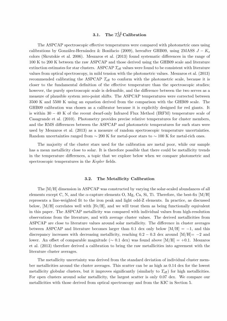
– 14 –3.1. The Teff Calibration

The ASPCAP spectroscopic effective temperatures were compared with photometric ones using

calibrations by Gonzalez-Hernandez & Bonifacio (2009), hereafter GHB09, using 2MASS J − Ks

colors (Skrutskie et al. 2006). Meszaros et al. (2013) found systematic differences in the range of

100 K to 200 K between the raw ASPCAP and those derived using the GHB09 scale and literature

extinction estimates for star clusters. ASPCAP Teff values were found to be consistent with literature

values from optical spectroscopy, in mild tension with the photometric values. Meszaros et al. (2013)

recommended calibrating the ASPCAP Teff to conform with the photometric scale, because it is

closer to the fundamental definition of the effective temperature than the spectroscopic studies;

however, the purely spectroscopic scale is defensible, and the difference between the two serves as a

measure of plausible system zero-point shifts. The ASPCAP temperatures were corrected between

3500 K and 5500 K using an equation derived from the comparison with the GHB09 scale. The

GHB09 calibration was chosen as a calibrator because it is explicitly designed for red giants. It

is within 30 − 40 K of the recent dwarf-only Infrared Flux Method (IRFM) temperature scale of

Casagrande et al. (2010). Photometry provides precise relative temperatures for cluster members,

and the RMS differences between the ASPCAP and photometric temperatures for such stars were

used by Meszaros et al. (2013) as a measure of random spectroscopic temperature uncertainties.

Random uncertainties ranged from ∼ 200 K for metal-poor stars to ∼ 100 K for metal-rich ones.

The majority of the cluster stars used for the calibration are metal poor, while our sample

has a mean metallicity close to solar. It is therefore possible that there could be metallicity trends

in the temperature differences, a topic that we explore below when we compare photometric and

spectroscopic temperatures in the Kepler fields.

3.2. The Metallicity Calibration

The [M/H] dimension in ASPCAP was constructed by varying the solar-scaled abundances of all

elements except C, N, and the α-capture elements O, Mg, Ca, Si, Ti. Therefore, the best-fix [M/H]

represents a line-weighted fit to the iron peak and light odd-Z elements. In practice, as discussed

below, [M/H] correlates well with [Fe/H], and we will treat them as being functionally equivalent

in this paper. The ASPCAP metallicity was compared with individual values from high-resolution

observations from the literature, and with average cluster values. The derived metallicities from

ASPCAP are close to literature values around solar metallicity. The difference in cluster averages

between ASPCAP and literature becomes larger than 0.1 dex only below [M/H] = −1, and this

discrepancy increases with decreasing metallicity, reaching 0.2 − 0.3 dex around [M/H]= −2 and

lower. An offset of comparable magnitude (∼ 0.1 dex) was found above [M/H] = +0.1. Meszaros

et al. (2013) therefore derived a calibration to bring the raw metallicities into agreement with the

literature cluster averages.

The metallicity uncertainty was derived from the standard deviation of individual cluster mem-

ber metallicities around the cluster averages. This scatter can be as high as 0.14 dex for the lowest

metallicity globular clusters, but it improves significantly (similarly to Teff) for high metallicities.

For open clusters around solar metallicity, the largest scatter is only 0.07 dex. We compare our

metallicities with those derived from optical spectroscopy and from the KIC in Section 5.

– 15 –3.3. The Surface Gravity Calibration

Surface gravities can be estimated from isochrones for red giants in star clusters if the distances,

extinctions, and ages of the systems are known. Meszaros et al. (2013) found significant zero-point

offsets between the raw spectroscopic values and those derived from cluster isochrones, motivating

an empirical correction. The cluster-based surface gravity calibration was supplemented with a

preliminary APOKASC sample of asteroseismic gravities. The Kepler targets are concentrated

around solar metallicity, while the cluster sample is predominantly composed of metal-poor systems.

We therefore adopted a hybrid empirical calibration that was solely a function of metallicity and

solely based on the gold standard asteroseismic surface gravities for stars with [Fe/H] > −0.5.

This gold standard sample had to be defined prior to the full analysis, and we briefly describe

how this sample was assembled and analyzed below. The candidates were selected to be those

with the most complete time coverage; see Hekker et al. (2012) for a discussion of the criteria. We

then computed the mean asteroseismic parameters using the Hekker et al. (2010) methodology. We

adopted effective temperatures based on the griz SDSS filters (Fukugita et al. 1996) from Pinson-

neault et al. (2012), using the KIC extinction map. Grid modeling was performed using BaSTI

models and adopting the KIC metallicities. We added 0.007 dex in quadrature to the formal un-

certainties to account for systematic errors; see Hekker et al. (2013) for a discussion. A total of

286 stars from this list were observed in DR10 and used as calibrators; see Meszaros et al. (2013)

for a more complete discussion. We present the asteroseismic properties used for this calibrating

sample in Table 2. We assess the validity of this approach using the full asteroseismic surface gravity

from our data below. Table 2 lists the surface gravities derived for the gold standard candidates.

These were used to calibrate the ASPCAP spectroscopic surface gravities, and are included so that

the results of Meszaros et al. (2013) can be replicated. The first column contains the KIC ID. The

second is the effective temperature inferred from SDSS photometry in Pinsonneault et al. (2012).

The third column is the KIC metallicity, and the fourth is the logarithm (in cgs units) of the surface

gravity returned from the OCT pipeline and its uncertainty. We stress that the gravities presented

later in the paper supercede these values.

Table 2. Gold Standard Surface Gravities

KIC ID Teff [Fe/H] log g

(K) (cgs)

1161618 4907 -0.112 2.426 ± 0.010

1432587 4693 -0.022 1.661 ± 0.024

1433593 5013 -0.141 2.741 ± 0.014

1433730 4829 -0.099 2.504 ± 0.013

1435573 4943 -0.113 2.324 ± 0.012

– 16 –3.4. Tests of the APOKASC Temperature and Surface Gravity Calibrations

In the APOKASC sample we have access to extremely precise asteroseismic surface gravities

(Hekker et al. 2013), which we adopted for the catalog in preference to the spectroscopic solutions.

However, the calibration procedure included only a smaller subset of the data, the gold standard

asteroseismic sample, as a reference. Our mean calibrated spectroscopic and asteroseismic log g

values for the full sample are close, with an average offset of 0.005 dex and a dispersion of 0.15

dex. We therefore conclude that our calibration based on the limited preliminary dataset yielded

reasonable results on average for the full sample (in the sense that the typical differences between

our calibrators and spectroscopic values were similar to the same differences for stars not used as

calibrators). However, there are interesting underlying trends in the differences between asteroseis-

mic and spectroscopic log g, present in both the gold and full samples, which are illustrated as a

function of log g and Teff in Figure 2.

We can obtain further insight into the origin of these differences by adding information on

evolutionary state. When we do so, a clear division in mean difference emerges between core He-

burning, or red clump, stars and first-ascent red giant branch stars (see Figure 3). Some of these

differences can be traced to the temperature and surface gravity trends illustrated above, but the

differences persist even between members of the same star cluster. We are currently investigating

the origin of the gravity offsets between red clump and red giant branch stars. Small differential

offsets (at the 5% level) between asteroseismic radius estimates for red clump and red giant branch

stars were found in NGC 6791 (Miglio et al. 2012) and traced to differences in the sound crossing

time at fixed large frequency spacing. However, the impact of the Miglio corrections on the relative

radii are too small to explain the observed surface gravity discrepancy, and the differential offset

in surface gravity is likely to be at the 0.05 dex level or smaller because of correlations between

asteroseismic masses and radii. An offset between the structures of model atmospheres in stars

with similar HR diagram position but with different evolutionary states (and thus differences in

mass, helium, or CNO) is in principle possible; however, such effects are expected to be small. We

conclude that this offset is an interesting clue that may shed light on both model atmospheres and

asteroseismology, but that the mean values of the corrected asteroseismic and spectroscopic gravities

are in good agreement.

We can also check on the internal consistency of the spectroscopic temperature scale by com-

paring our spectroscopic effective temperatures with those that we would have derived using the

KIC extinction map and the GHB09 IRFM color-temperature relationship employed in the global

spectroscopic calibration. Our results using the KIC extinction map are compared with those in the

zero-extinction limit in Figure 4. The dispersion is reasonable at 80 K, but there is a significant

zero-point offset of −193 K in the former case. The bulk of the calibrating sample was in metal-poor

globular cluster stars, so this feature could reflect a metallicity-dependent offset in the temperature

scale; the APOKASC sample is predominantly close to solar abundance. Another possibility is an

error in the adopted extinction corrections; as shown above, a zero-extinction case has an average

offset of +11 K. We view this as an unrealistic limit, but the difference between the two certainly

highlights the need for an independent re-assessment of the KIC extinction map. Fortunately, a more

extensive multi-wavelength dataset, especially at longer wavelengths, has been developed since the

time the KIC was constructed. Casagrande et al. (2014) used new Stroemgren filter data in a stripe

within the Kepler fields, along with an extensive set of literature photometry, to derive systemati-

– 17 –

Fig. 2.— Logarithmic difference between the corrected spectroscopic and asteroseismic surface grav-

ity log g as a function of asteroseismic log g (left) and spectroscopic Teff (right) for our full sample.

The points with error bars are the means and standard deviations of the data in 10 ranked cohorts

of log g. The data was divided into 60 bins in log g (left), Teff (right) and delta log g (both), covering

the log g range of 0.5 to 3.5, temperature range 3800 K to 5200 K, and gravity difference range −0.7

to +0.7 respectively. The logarithmic gray scale coding (specified on the right) indicates the number

of targets with those properties in the relevant bin.

Fig. 3.— Stars identified asteroseismically as secondary RC (green), RC (blue), or first-ascent RGB

(red) are compared in the HR Diagram on the left. Gray dots represent stars without explicit

classification. On the right, the difference between asteroseismic surface gravity and spectroscopic

surface gravity is plotted for stars in these evolutionary states as a function of asteroseismic log g.

A clear pattern in the differences is visible.

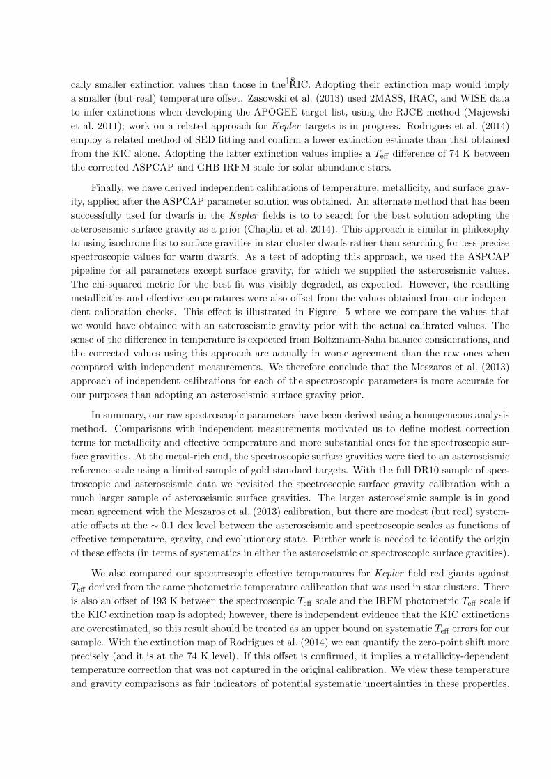
– 18 –cally smaller extinction values than those in the KIC. Adopting their extinction map would imply

a smaller (but real) temperature offset. Zasowski et al. (2013) used 2MASS, IRAC, and WISE data

to infer extinctions when developing the APOGEE target list, using the RJCE method (Majewski

et al. 2011); work on a related approach for Kepler targets is in progress. Rodrigues et al. (2014)

employ a related method of SED fitting and confirm a lower extinction estimate than that obtained

from the KIC alone. Adopting the latter extinction values implies a Teff difference of 74 K between

the corrected ASPCAP and GHB IRFM scale for solar abundance stars.

Finally, we have derived independent calibrations of temperature, metallicity, and surface grav-

ity, applied after the ASPCAP parameter solution was obtained. An alternate method that has been

successfully used for dwarfs in the Kepler fields is to to search for the best solution adopting the

asteroseismic surface gravity as a prior (Chaplin et al. 2014). This approach is similar in philosophy

to using isochrone fits to surface gravities in star cluster dwarfs rather than searching for less precise

spectroscopic values for warm dwarfs. As a test of adopting this approach, we used the ASPCAP

pipeline for all parameters except surface gravity, for which we supplied the asteroseismic values.

The chi-squared metric for the best fit was visibly degraded, as expected. However, the resulting

metallicities and effective temperatures were also offset from the values obtained from our indepen-

dent calibration checks. This effect is illustrated in Figure 5 where we compare the values that

we would have obtained with an asteroseismic gravity prior with the actual calibrated values. The

sense of the difference in temperature is expected from Boltzmann-Saha balance considerations, and

the corrected values using this approach are actually in worse agreement than the raw ones when

compared with independent measurements. We therefore conclude that the Meszaros et al. (2013)

approach of independent calibrations for each of the spectroscopic parameters is more accurate for

our purposes than adopting an asteroseismic surface gravity prior.

In summary, our raw spectroscopic parameters have been derived using a homogeneous analysis

method. Comparisons with independent measurements motivated us to define modest correction

terms for metallicity and effective temperature and more substantial ones for the spectroscopic sur-

face gravities. At the metal-rich end, the spectroscopic surface gravities were tied to an asteroseismic

reference scale using a limited sample of gold standard targets. With the full DR10 sample of spec-

troscopic and asteroseismic data we revisited the spectroscopic surface gravity calibration with a

much larger sample of asteroseismic surface gravities. The larger asteroseismic sample is in good

mean agreement with the Meszaros et al. (2013) calibration, but there are modest (but real) system-

atic offsets at the ∼ 0.1 dex level between the asteroseismic and spectroscopic scales as functions of

effective temperature, gravity, and evolutionary state. Further work is needed to identify the origin

of these effects (in terms of systematics in either the asteroseismic or spectroscopic surface gravities).

We also compared our spectroscopic effective temperatures for Kepler field red giants against

Teff derived from the same photometric temperature calibration that was used in star clusters. There

is also an offset of 193 K between the spectroscopic Teff scale and the IRFM photometric Teff scale if

the KIC extinction map is adopted; however, there is independent evidence that the KIC extinctions

are overestimated, so this result should be treated as an upper bound on systematic Teff errors for our

sample. With the extinction map of Rodrigues et al. (2014) we can quantify the zero-point shift more

precisely (and it is at the 74 K level). If this offset is confirmed, it implies a metallicity-dependent

temperature correction that was not captured in the original calibration. We view these temperature

and gravity comparisons as fair indicators of potential systematic uncertainties in these properties.

– 19 –Neither of these comparisons directly address the accuracy and precision of our metallicity estimates,

which we discuss in Section 5 when comparing our final catalog values with the KIC and optical

spectroscopy.

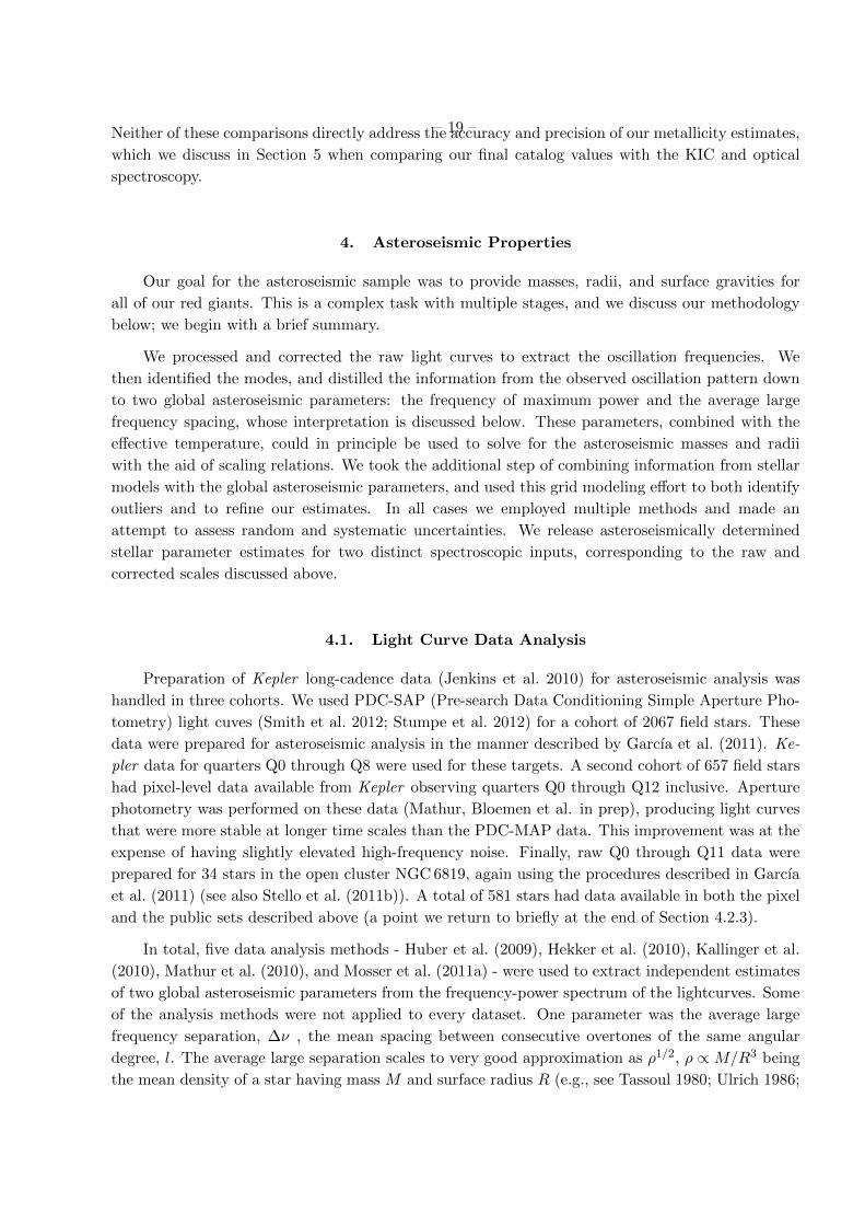
4. Asteroseismic Properties

Our goal for the asteroseismic sample was to provide masses, radii, and surface gravities for

all of our red giants. This is a complex task with multiple stages, and we discuss our methodology

below; we begin with a brief summary.

We processed and corrected the raw light curves to extract the oscillation frequencies. We

then identified the modes, and distilled the information from the observed oscillation pattern down

to two global asteroseismic parameters: the frequency of maximum power and the average large

frequency spacing, whose interpretation is discussed below. These parameters, combined with the

effective temperature, could in principle be used to solve for the asteroseismic masses and radii

with the aid of scaling relations. We took the additional step of combining information from stellar

models with the global asteroseismic parameters, and used this grid modeling effort to both identify

outliers and to refine our estimates. In all cases we employed multiple methods and made an

attempt to assess random and systematic uncertainties. We release asteroseismically determined

stellar parameter estimates for two distinct spectroscopic inputs, corresponding to the raw and

corrected scales discussed above.

4.1. Light Curve Data Analysis

Preparation of Kepler long-cadence data (Jenkins et al. 2010) for asteroseismic analysis was

handled in three cohorts. We used PDC-SAP (Pre-search Data Conditioning Simple Aperture Pho-

tometry) light cuves (Smith et al. 2012; Stumpe et al. 2012) for a cohort of 2067 field stars. These

data were prepared for asteroseismic analysis in the manner described by Garcıa et al. (2011). Ke-

pler data for quarters Q0 through Q8 were used for these targets. A second cohort of 657 field stars

had pixel-level data available from Kepler observing quarters Q0 through Q12 inclusive. Aperture

photometry was performed on these data (Mathur, Bloemen et al. in prep), producing light curves

that were more stable at longer time scales than the PDC-MAP data. This improvement was at the

expense of having slightly elevated high-frequency noise. Finally, raw Q0 through Q11 data were

prepared for 34 stars in the open cluster NGC 6819, again using the procedures described in Garcıa

et al. (2011) (see also Stello et al. (2011b)). A total of 581 stars had data available in both the pixel

and the public sets described above (a point we return to briefly at the end of Section 4.2.3).

In total, five data analysis methods - Huber et al. (2009), Hekker et al. (2010), Kallinger et al.

(2010), Mathur et al. (2010), and Mosser et al. (2011a) - were used to extract independent estimates

of two global asteroseismic parameters from the frequency-power spectrum of the lightcurves. Some

of the analysis methods were not applied to every dataset. One parameter was the average large

frequency separation, ∆ν , the mean spacing between consecutive overtones of the same angular

degree, l. The average large separation scales to very good approximation as ρ1/2, ρ ∝M/R3 being

the mean density of a star having mass M and surface radius R (e.g., see Tassoul 1980; Ulrich 1986;

– 20 –Christensen-Dalsgaard 1993). The dependence of ∆ν on the mean stellar density may be used as a

scaling relation normalized by solar properties and parameters, i.e.,

∆ν

∆ν�'

√M/M�

(R/R�)3. (1)

The second global parameter is νmax, the frequency of maximum oscillation power. It has been

shown to scale to good approximation as gT−1/2eff (Brown et al. 1991; Kjeldsen & Bedding 1995;

Chaplin et al. 2008; Stello et al. 2009b; Belkacem et al. 2011), where g is the surface gravity and Teff

is the effective temperature of the star. The following scaling relation may therefore be adopted:

νmax

νmax,�' M/M�

(R/R�)2√

(Teff/Teff,�). (2)

The completeness of the results (i.e., the fraction of stars with returned estimates) varied, since

some pipelines are better suited to analysing different ranges in νmax.

We selected one data analysis method, OCT(Hekker et al. 2010), to provide the catalog global

asteroseismic parameters of the stars in all three cohorts. This selection was based on the returned

νmax values. The Hekker et al. method had the highest completeness fraction, and results that were

consistent with those given by the other pipelines. This approach ensured we obtained a homogenous

set of global asteroseismic parameters, which were then used to estimate the fundamental stellar

properties (see Section 4.2 below).

For outlier rejection we selected a reference method for each cohort, this being the one whose

νmax estimates lay closest to the median over all stars in that cohort (Mosser et al. for the pixel and

public cohorts; and Kallinger et al. for the cluster cohort). If the Hekker et al. νmax differed from

the reference νmax by more than 10 %, we rejected the asteroseismic parameters for that star. This

procedure removed 28 stars from the pixel cohort, 167 stars from the public cohort, and 1 star from

the cluster cohort.

Uncertainties on the final ∆ν and νmax of each star were obtained by adding, in quadrature,

the formal uncertainty returned by the Hekker et al. method to the standard deviation of the values

returned by all methods. We also allowed for known systematic errors in Equation 1 (e.g., see White

et al. 2011 and Miglio et al. 2012), by including an additional systematic contribution of 1.5 % (also

added in quadrature). Because ∆ν is usually determined more precisely than νmax, we also added

the same systematic contribution to the νmax uncertainties. This is essentially the approach adopted

by Huber et al. (2013) in their analysis of asteroseismic Kepler Objects of Interest.

4.2. Grid-based Modeling

For each star we used the two global asteroseismic parameters, ∆ν and νmax, together with the

estimates of effective temperature Teff and metallicity [Fe/H], as input to “grid-based” estimation of

the fundamental stellar properties. This approach matches the set of observables to theoretical sets

calculated for each model in an evolutionary grid of tracks or isochrones. The fundamental properties

of the models (i.e., R, M and Teff) were used as inputs to the scaling relations (Equations 1 and 2)

to calculate theoretical values of ∆ν and νmax for matching with the observations.

– 21 –Every pipeline adopted solar values ∆ν� = 135.03µHz and νmax,� = 3140µHz, which are the

solar values returned by the pipeline we selected to return final values on our sample (Hekker et al.

2010). The uncertainties in ∆ν� (0.1µHz) and νmax,� (30µHz) were accounted for by increasing the

uncertainties in the ∆ν and νmax data of each star, using simple error propagation. Further details

on grid modeling using asteroseismic data may be found in, for example, Stello et al. (2009a), Basu

et al. (2010, 2012), Gai et al. (2011) and Chaplin et al. (2014).

We adopted a grid-based analysis that coupled six pipeline codes to eleven model grids, com-

prising a selection of widely used sets of stellar evolution tracks and isochrones that have a range

of commonly adopted input physics. In applying several grid-pipeline combinations, we capture im-

plicitly in our final results the impact of model dependencies from adopting different commonly-used

grids, and differences in the detail of the pipeline codes themselves.

4.2.1. Grid Pipelines

Grid-based estimates of the stellar properties were returned by the following pipeline codes:

– The Yale-Birmingham (YB) (Basu et al. 2010, 2012; Gai et al. 2011);

– The Bellaterra Stellar Properties Pipeline (BeSPP) (Serenelli et al. 2013 extended for astero-

seismic analysis);

– PARAM (da Silva et al. 2006; Miglio et al. 2013);

– RADIUS (Stello et al. 2009a);

– AMS (Hekker et al. 2013); and

– The Stellar Fundamental Parameters (SFP) pipeline (Kallinger et al. 2010; Basu et al. 2011).

The YB pipeline was used with 5 different grids: models from the Dartmouth group (Dotter et

al. 2008) and the Padova group (Marigo et al. 2008; Girardi et al. 2000), the set of YY isochrones

(Demarque et al. 2004), a grid constructed using the Yale Stellar Evolution Code (YREC; Demarque

et al. 2008) and described by Gai et al. (2011) (we refer to this set as YREC), and another set of

models constructed with a newer version of YREC with updated input physics (we refer to this grid

as YREC2) that has been described by Basu et al. (2012). The Dotter et al. and Marigo et al.

grids include models of red-clump (RC) stars; YREC and YREC2 include only models of He-core

burning stars of higher mass, which do not go through the He flash); while YY has no RC models.

The BeSPP pipeline was run with two grids. The first grid is comprised of models constructed

with the GARSTEC code (Weiss et al. 2008) and the parameters of the grid are described in Silva

Aguirre et al. (2012). The second grid is comprised of the BaSTI models of Pietrinferni et al. (2004),

computed for use in asteroseismic studies (see Silva Aguirre et al. 2013). Both grids include RC

models. RADIUS was coupled to a grid constructed with the ASTEC code (Christensen-Dalsgaard

et al. 2008), as described in Stello et al. (2009a) and Creevey et al. (2012), which does not include

RC models.

– 22 –The codes above were all employed in the grid-based analysis of solar-type Kepler targets

described in Chaplin et al. (2014), where summary details of the physics employed in the grids may

also be found.

PARAM was run using a grid comprising models of the Padova group (Marigo et al. 2008),

again including RC stars; further details may be found in Miglio et al. (2013). AMS is based on an

independent implementation of the YB pipeline, and was run using the BaSTI models of Pietrinferni

et al. (2004). The SFP pipeline was also coupled to BaSTI models. These grids include RC models.

For this first analysis of the APOKASC red giants an asteroseismic classification (i.e., RGB

or RC) was not available for many of the stars. Therefore, no a priori categorisation information

was used in the grid-based searches. Although the cohort evidently contains many RC stars, we

nevertheless obtained some results using grids comprised of only RGB models, to test the impact

of neglecting the red clump. However, as explained below, our final results are produced using only

those grids that included RC models.

4.2.2. Results from Grid-based Analyses

Fig. 6 is an example of the typical differences we see in the estimated properties returned by

different grid-pipeline combinations, here those between YB/Dotter and BeSPP/BaSTI (the latter

chosen as the reference). Both sets comprise results from grids that included RC models. Results are

plotted from stars in the public data cohort, with ∆ν, νmax, the revised ASPCAP Teff , and [Fe/H]

values used as inputs. We plot fractional differences in R, M and ρ and absolute differences in log g.

Gray lines mark envelopes corresponding to the median of the 1σ uncertainties returned by all grid

pipelines. Medians were calculated in 10-target batches sorted on ∆ν. These lines are included to

help judge the typical precision only; uncertainties in the results of individual targets may of course

be slightly different. Similar trends to those present here are seen in results on the pixel and cluster

target cohorts, and in results from using the raw ASPCAP Teff and [Fe/H] scales as inputs.

On the whole, the differences lie within the median formal uncertainty envelopes, which is

encouraging, i.e., the scatter between different grid-pipeline combinations tends to be smaller than

the typical intrinsic, formal uncertainties returned by those pipelines. However, we do see clear

excess scatter centered on ∆ν ' 4µHz, which corresponds to the location of RC stars. A significant

fraction of our target sample lies in this region. Further analysis presented below suggests that this

is genuine extra scatter, and not a sampling effect (see Fig. 8 in Section 4.2.3 and accompanying

discussion). The presence of this scatter evidently reflects the difficulty of discriminating between

RC and RGB models when no a priori categorisation is used as input, as was the case here.

Differences with respect to the reference results of BeSPP/BaSTI tend, not surprisingly, to

be more pronounced for grids which did not include RC models. Grid-pipeline combinations with

no RC models appear to compensate for the absence of the clump by the inclusion of high-mass

(lower-age) RGB solutions, which are not present in the RC sets. Although at the lowest masses the

results for grids with and without RC models are similar, the mapping to age is of course different:

grid-pipeline combinations with no RC models yield older solutions at the same mass.

The lack of a priori information on the evolutionary state has significant implications for our

ability to return not only robust estimates of the absolute ages, but even accurate measures of the

– 23 –relative ages of the cohort, i.e., the relative chronology will be scrambled if an RC star is incorrectly

matched to a model of an RGB star, or vice versa. Indeed, the problem is even more subtle. The

grid-based codes compute a likelihood for every model that is a reasonable match (within several

sigma) to the observables. Estimated properties are returned from the distributions formed by these

likelihoods, i.e., the analysis is probabilistic in nature. Without information on the evolutionary

state, the distribution functions may be comprised of a mix of RC and RGB information. That is

why, for now, we do not provide ages explicitly in the catalog (although the reader may compute their

own ages from the masses and metallicities provided). Bedding et al. (2011) noted that the oscillation

spectra of the giants can be used to distinguish between RC and RGB stars, and we discussed

methods earlier in the text that could provide automated estimation of evolutionary state for many

targets in the sample. Unfortunately, our initial screening procedure only produced evolutionary

state diagnostics for ∼ 25% of the targets. We are in the process of developing more efficient tools

that will provide measurements for an even larger fraction of the sample. Thus although we do not

have the information now, the desired evolutionary information will be available to help construct

the next version of the catalog.

Fig. 7 shows the impact on the public data cohort results of switching from one set of ASPCAP

Teff and [Fe/H] inputs to the other. Results for the pixel and cluster cohorts show similar trends.

The top left-hand panel plots the corrected ASPCAP Teff minus the raw ASPCAP Teff , showing the

piece-wise correction that was applied to the raw temperatures to yield the corrected scale. The lines

follow the median 1σ envelopes of the uncertainties. The top right-hand panel presents the corrected

ASPCAP [Fe/H] minus the raw ASPCAP [Fe/H]. The other panels display the fractional differences

in estimated properties returned by BeSPP/BaSTI, in the sense corrected ASPCAP minus raw

ASPCAP. As in the previous figures, gray lines mark the median 1σ envelopes (over all pipelines)

of the returned, formal uncertainties.

With reference to the asteroseismic scaling relations, the trends revealed in Fig. 7 may be

understood largely in terms of the changes to the temperature scale. The relations imply that, all

other things being equal, M ∝ T 1.5eff , R ∝ T 0.5

eff and g ∝ T 0.5eff , while the seismic estimates of ρ are

not affected by the change to Teff . The plotted property differences are thus seen to reflect, to good

approximation, the trend in Teff , although this clearly does not explain all the differences, i.e., there

is also the impact of the changes in [Fe/H] to consider (which are for example apparent in the small

differences seen in the estimates of ρ).

4.2.3. Asteroseismic Catalog Properties and Uncertainties

We provide tables of estimated properties for each of the raw ASPCAP and corrected ASPCAP

scales (see Tables 4 and 5 below). For both sets of inputs, the properties in the catalog are those

that were returned by BeSPP/BaSTI. Its results lay closest to the median over all grid-pipelines

and targets. By choosing one grid-pipeline to provide the final properties we avoid mixing results

that are subject to different input physics and pipeline methodology. We instead opted to reflect

those differences in the quoted final uncertainties, by taking into account the scatter between results

returned by the different grid-pipeline combinations. Our approach is therefore similar to that

adopted by Chaplin et al. (2014) for asteroseismic dwarfs and subgiants. We emphasize that in

this consolidation we used only results from grids that included RC models. The BeSPP/BaSTI

– 24 –models did not include convective overshoot or semi-convection and incorporated mass loss with an

efficiency η = 0.4. These choices did not have a major impact on the derived masses and radii.

Fig. 8 plots the median formal uncertainties returned by grid-pipeline combinations including

RC models only (red symbols), again for results from the public data cohort using the corrected

ASPCAP scale inputs. For each property of every star we calculated the standard deviation of the

results returned by the various grid-pipeline combinations. These estimates of the scatter are plotted

in black. The median standard deviations are approximately 4 % in mass, 1 % in radius, 0.003 dex

in log g, and 1 % in density.

The plots demonstrate clearly that the scatter between the grid-pipelines is typically smaller

than the formal uncertainties returned by any one pipeline. Moreover, both the scatter and the

formal uncertainties are larger at the ∆ν where we find RC stars. This result again emphasizes the

extra challenges posed for the grid searches in this part of the parameter space in the absence of an

a priori categorisation.

The above measures of scatter were combined in quadrature with the individual formal un-

certainties returned by BeSPP/BaSTI to yield the final uncertainties on the estimated properties.

Distributions of the scatter between pipelines are shown in Fig. 9. The plotted histograms (here, for

the same cohort of results as the previous figures) were constructed by computing residuals for each

pipeline-grid with respect to BeSPP/BaSTI, and normalizing each residual by the median property

uncertainty given by the pipelines for that star. We then accumulated residuals for all stars in the

cohort, and binned the residuals to give the plotted “super distributions”. The most striking aspect

of all the histograms is their Gaussian-like appearance (see similar results for solar-type stars in

Chaplin et al. 2014). Our median final uncertainties are approximately 12 % in mass, 5 % in radius,

0.01 dex in log g, and 3 % in density. These uncertainties will typically be higher for those stars

which have ∆ν ' 4µHz (i.e., RC stars).

Finally, some targets appeared in both the pixel and public-data samples. In such cases we

adopted the properties estimated from the higher-quality, longer pixel lightcurves to be the catalog

properties. Estimated properties for the cluster stars all came from analyses of the cluster data.

A question that might be legitimately be asked is why should we resort to grid-based modeling,

which makes our results model dependent, when the direct use of Equation 1 and Equation 2 could,

in principle, produce model-independent results. The issue is that the scaling relations assume that

all values of Teff are possible for a star of a given mass and radius and are unconstrained by the

equations of stellar structure and evolution. Thus it is quite possible that observational errors in

Teff , ∆ν and νmax can produce estimated values of mass and radius inconsistent with the theory of

stellar structure and evolution. The grid-based method takes this constraint into account implicitly,

as well as including metallicity information not used in the scaling relations.

Properties of asteroseismic grid-modeling results have been studied in detail by Gai et al. (2011).

They showed that propagated errors are in general smaller in grid-based results than those inferred

from propagating scaling relations. The Gai et al. work dealt with simulated stars over a large part

of the HR diagram, and the gain obtained by grid-based modeling may not persist in the narrow

temperature range occupied by red giants. To test this hypothesis, we have taken the Gai et al.

simulated sample and selected all objects with ∆ν < 20µHz as likely red giants. In Figure 10

we show histograms of the fractional difference between the true and inferred radius and mass for

– 25 –these stars obtained with both the scaling relations and through a grid-based search. In both cases,

the distribution of the deviation between the true and the inferred properties is sharper for the

grid-based method. Although differences between the distributions are not as large as in the case of

main-sequence or subgiant stars, the difference, particularly in mass, is large enough that it is worth

performing grid modeling for our sample to reduce our random uncertainties. As discussed above,

grid modeling is more challenging in the log g regime where both the RGB and RC are present, and

RC models and stars are not included in this comparison.

5. The APOKASC Catalog and Its Properties

5.1. The APOKASC Catalog

We present our data in three tables. Table 3 contains basic information on the stars, and our

asteroseismic parameters for the raw and corrected temperature scale are given in Tables 4 and 5.

We begin in Table 3 with the information in common for both sets of spectroscopic inputs. We

begin with star identifiers and positional information: the KIC (first column) and 2MASS (second

column) IDs of the targets; RA and Dec (J2000), Galactic longitude l and latitude b (all in degrees)

are presented in columns 3-6. We present two different Teff measurements (in K) estimates using

the GHB09 methodology in columns 7 and 8: one with the KIC extinction and the other with zero

extinction. The uncertainties reflect random errors in the J − K color used for the temperature

estimates. This is distinct from the published effective temperatures presented in Pinsonneault et

al. (2012), which used either SDSS filters or the Casagrande et al. (2010) IRFM temperatures from

2MASS colors. For each star that passed our internal consistency checks, we then provide the mean

asteroseismic properties ∆ν and νmax (in µHz) and their uncertainties in columns 9 and 10. The

final column includes the targeting flags used to select the stars for APOGEE observations. Stars

included in GO proposal #40033 are labelled GO; stars targeted as public giants are PUBLIC (note

that this includes almost all targets not newly observed for the GO program.) A small number of

asteroseismic ”dwarfs” with long cadence frequency measurements are labeled as SEIS DWARF.

Our detection efficiency was a function of surface gravity, which reflects physical and sampling

effects that make obtaining reliable results more challenging for some targets than for others. The

highest gravity stars had oscillation frequencies close to the Nyquist frequency, which can create

model-dependent results. Low gravity stars have fewer modes and their interpretation is also more

model dependent. The stars for which we did not obtain consistent results were clustered around

these two categories. For the analysis of the full DR12 catalog we intend to reanalyze and report

results for all targets with detections, but we did not proceed with the full analysis of such objects

in our initial run.

In Table 4 we present the asteroseismic properties derived from the uncorrected spectroscopic

parameters; we refer to this set of measurement as Scale 1. Table 5 has an identical format except

that it was derived using the corrected spectroscopic parameters, and we refer to these measurements

as Scale 2. We start with the KIC ID, the input Teff in K, and [M/H] (the logarthmic iron to hydrogen

ratio relative to the Sun) for the relevant spectroscopic scale. We then present the mass (in solar

units), radius (in solar units), surface gravity (log base 10 in cgs units), and mean density relative

to that of the Sun. See Section 4 for the methodology used to derive the uncertainties. Although

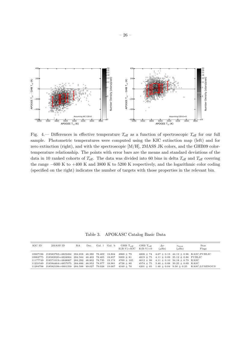
– 26 –

Fig. 4.— Differences in effective temperature Teff as a function of spectroscopic Teff for our full

sample. Photometric temperatures were computed using the KIC extinction map (left) and for

zero extinction (right), and with the spectroscopic [M/H], 2MASS JK colors, and the GHB09 color-

temperature relationship. The points with error bars are the means and standard deviations of the

data in 10 ranked cohorts of Teff . The data was divided into 60 bins in delta Teff and Teff covering

the range −600 K to +400 K and 3800 K to 5200 K respectively, and the logarithmic color coding

(specified on the right) indicates the number of targets with those properties in the relevant bin.

Table 3. APOKASC Catalog Basic Data

KIC ID 2MASS ID RA Dec. Gal. l Gal. b GHB Teff GHB Teff ∆ν νmax Star

E(B-V)=KIC E(B-V)=0 (µHz) (µHz) Flags

10907196 J18583782+4822494 284.658 48.380 78.402 18.804 4969 ± 79 4808 ± 74 4.67 ± 0.13 44.12 ± 0.96 KASC,PUBLIC

10962775 J18582020+4824064 284.584 48.402 78.405 18.857 5009 ± 81 4819 ± 75 4.11 ± 0.09 35.12 ± 0.86 PUBLIC

11177749 J18571019+4848067 284.292 48.802 78.735 19.174 4769 ± 105 4612 ± 99 4.11 ± 0.10 34.18 ± 0.79 KASC

11231549 J18584464+4857075 284.686 48.952 78.977 18.981 4728 ± 80 4574 ± 75 3.40 ± 0.08 30.25 ± 0.69 KASC

11284798 J18582108+4901359 284.588 49.027 79.028 19.067 4349 ± 70 4201 ± 65 1.46 ± 0.04 9.50 ± 0.25 KASC,LUMINOUS

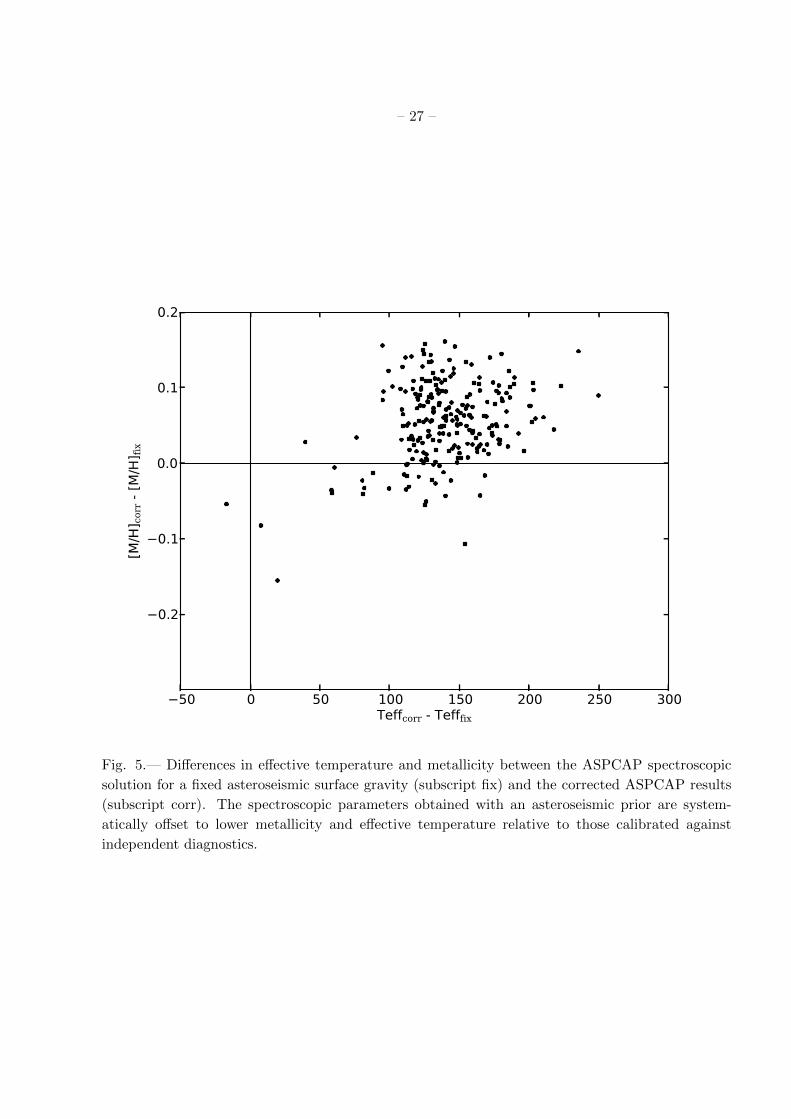
– 27 –

Fig. 5.— Differences in effective temperature and metallicity between the ASPCAP spectroscopic

solution for a fixed asteroseismic surface gravity (subscript fix) and the corrected ASPCAP results

(subscript corr). The spectroscopic parameters obtained with an asteroseismic prior are system-

atically offset to lower metallicity and effective temperature relative to those calibrated against

independent diagnostics.

– 28 –

Fig. 6.— Fractional differences, as a function of ∆ν, in estimated properties returned by YB/Dotter

and BeSPP/BaSTI. The results are shown for an analysis performed on the public data cohort,

with the corrected ASPCAP Teff and [Fe/H] values used as inputs. Gray lines mark the median 1σ

envelope of the grid-pipeline returned, formal uncertainties. These lines are included to help judge

the typical precision only.

– 29 –

Fig. 7.— Fractional differences in estimated properties returned by BeSPP/BaSTI, for analyses

performed on the public data cohort with the two different Teff and [Fe/H] inputs. Differences are

defined as results with corrected ASPCAP scale inputs minus results with raw ASPCAP scale inputs.

Gray lines mark the median 1σ envelope (over all pipelines) of the returned, formal uncertainties. The

top panels show the absolute Teff and [Fe/H] differences between the two sets of input parameters,

while the bottom four panels record the impact on the derived asteroseismic properties. The impact

on the separate mass and radius measurements (in the middle panels) is larger than the impact on

the surface gravity and mean density (in the bottom panels).

– 30 –

Fig. 8.— Median formal uncertainties over all grid pipelines (for grids with RC models; red symbols),

for the public data cohort (corrected ASPCAP scale inputs); and the standard deviations (scatter)

between them (black symbols), both as a function of ∆ν. The excess scatter on the far left reflects

the difficulty of inferring precise astroseismic properties for luminous giants, while the excess scatter

close to 4µHz is caused by ambiguity between RC and RGB solutions.

– 31 –

Fig. 9.— Histograms, for each property, of uncertainty-normalized residuals over all pipeline-grid

combinations (omitting BeSPP/BaSTI) and all stars in the pubic data cohort (corrected ASPCAP

scale inputs). The plotted residuals were calculated with respect to the BeSPP/BaSTI results.

Fig. 10.— Deviations between true and measured radii(left) and mass(right) for simulated data

using scaling relations alone (red) and using grid modeling (black). The simulated dataset is taken

from Gai et al. 2011.

– 32 –one could in principle construct mean densities and surface gravities from the masses and radii, we

solved for these independently. The tabulated density and gravity values are close, but therefore not

identical, to those which could be inferred from the separate M and R.

5.2. APOKASC and the KIC Compared

A natural point of reference for our work are the stellar parameters in the Kepler Input Catalog

(KIC), which were based on photometry. Fig. 11 displays the binned metallicity differences between

our spectroscopic metallicities and those in the KIC inferred from photometry as a function of

APOKASC metallicity. The average metallicities are surprisingly close, with a mean difference of

0.006 dex and a standard deviation of 0.22 dex. However, there are significant metallicity trends in

the difference between the two, in the sense that the KIC metallicity scale is compressed relative to

the APOGEE one. The effective temperature scale is also systematically cooler than that derived

from the KIC, demonstrated in Fig. 12. The offset (−86 K on average) and dispersion (84 K) are

modest. The temperature scale differences are sensitive to the adopted extinction model and to the

color-temperature calibration, an issue that we return to below. Finally, the differences in surface

gravity are illustrated in Fig. 13. The KIC surface gravities have a large scatter of 0.265 dex relative

to our asteroseismic values, with a mean difference of −0.175 dex.

Motivated by these results we derived fitting functions mapping the KIC parameters onto the

spectroscopic system. We emphasize that these results are calibrated for red giants only, and different

relations may well apply for dwarfs or subgiants. The fits between the KIC parameters and the

corrected ASPCAP [M/H], Teff and asteroseismic log g are shown in Figures 14, 15, and 16,

respectively. Our fitting formulae correcting the KIC values to the spectroscopic scale are

[M/H]ASPCAP = 0.72 ∗ [Fe/H]KIC + 0.03. (3)

Teff,ASPCAP = 0.000297 ∗ T 2eff,KIC + 3.54 ∗ Teff,KIC − 5408. (4)

log gASPCAP = 0.41 ∗ log gKIC + 0.00054 ∗ Teff,KIC − 1.13. (5)

Table 4. Scale 1 Asteroseismic Results

KIC ID ASPCAP Teff ASPCAP [M/H] Mass Radius log g ρ

(Raw)(K) (Raw) M� R� solarunits

10907196 4721± 87 −0.08± 0.06 1.47+0.16−0.19 10.77+0.42

−0.64 2.543+0.011−0.011 0.00119+0.00005

−0.00005

10962775 4716± 94 −0.25± 0.06 1.21+0.13−0.12 10.93+0.47

−0.48 2.444+0.011−0.012 0.00093+0.00003

−0.00003

11177749 4591± 83 0.03± 0.05 1.08+0.12−0.11 10.51+0.49

−0.45 2.426+0.011−0.011 0.00093+0.00003

−0.00003

11231549 4451± 86 −0.06± 0.06 1.51+0.17−0.15 13.31+0.58

−0.56 2.368+0.011−0.011 0.00064+0.00002

−0.00002

11284798 4126± 85 −0.04± 0.06 1.22+0.17−0.14 21.76+1.14

−1.05 1.848+0.013−0.013 0.00012+0.00001

−0.00001

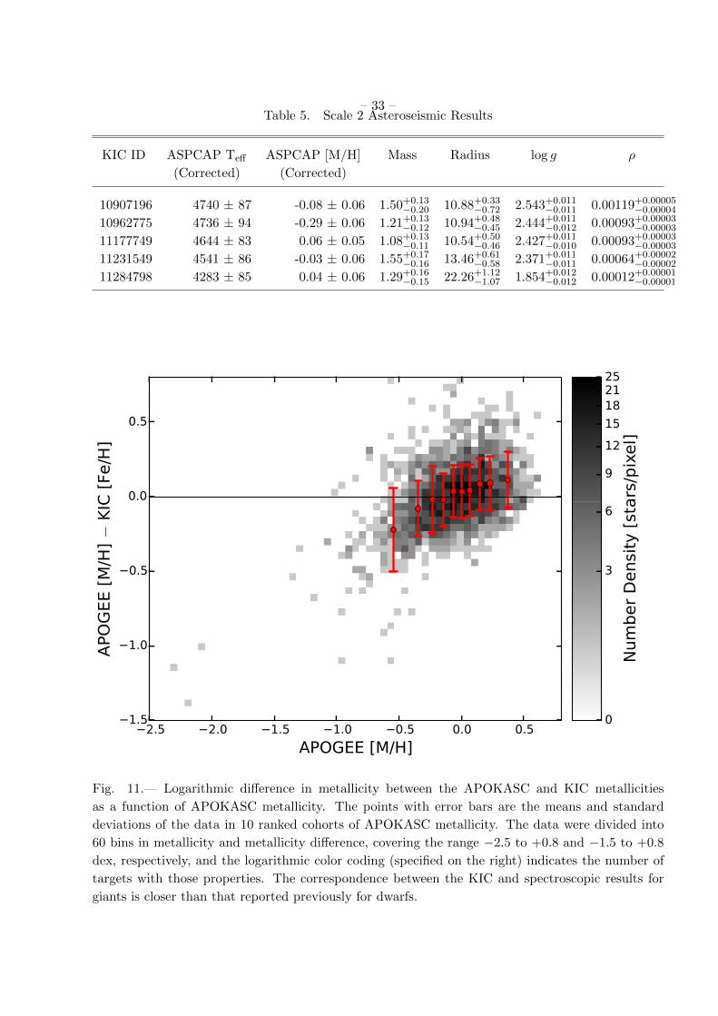
– 33 –Table 5. Scale 2 Asteroseismic Results

KIC ID ASPCAP Teff ASPCAP [M/H] Mass Radius log g ρ

(Corrected) (Corrected)

10907196 4740 ± 87 -0.08 ± 0.06 1.50+0.13−0.20 10.88+0.33

−0.72 2.543+0.011−0.011 0.00119+0.00005

−0.00004

10962775 4736 ± 94 -0.29 ± 0.06 1.21+0.13−0.12 10.94+0.48

−0.45 2.444+0.011−0.012 0.00093+0.00003

−0.00003

11177749 4644 ± 83 0.06 ± 0.05 1.08+0.13−0.11 10.54+0.50

−0.46 2.427+0.011−0.010 0.00093+0.00003

−0.00003

11231549 4541 ± 86 -0.03 ± 0.06 1.55+0.17−0.16 13.46+0.61

−0.58 2.371+0.011−0.011 0.00064+0.00002

−0.00002

11284798 4283 ± 85 0.04 ± 0.06 1.29+0.16−0.15 22.26+1.12

−1.07 1.854+0.012−0.012 0.00012+0.00001

−0.00001

Fig. 11.— Logarithmic difference in metallicity between the APOKASC and KIC metallicities

as a function of APOKASC metallicity. The points with error bars are the means and standard

deviations of the data in 10 ranked cohorts of APOKASC metallicity. The data were divided into

60 bins in metallicity and metallicity difference, covering the range −2.5 to +0.8 and −1.5 to +0.8

dex, respectively, and the logarithmic color coding (specified on the right) indicates the number of

targets with those properties. The correspondence between the KIC and spectroscopic results for

giants is closer than that reported previously for dwarfs.

– 34 –

Fig. 12.— Difference in effective temperature between the APOKASC and KIC values as a function

of APOKASC Teff (K). The points with error bars are the medians and median absolute deviations

of the data in 10 ranked cohorts of APOKASC Teff . The data were divided into 60 bins in Teff and

∆Teff , covering the range 3800 K to 5200 K and −400 to +300 K, respectively, and the logarithmic

color coding (specified on the right) indicates the number of targets with those properties. The

major difference between the two systems is a zero-point offset.

– 35 –

Fig. 13.— Logarithmic difference in surface gravity log g between the APOKASC and KIC values

as a function of APOKASC log g. The points with error bars are the medians and median absolute

deviations of the data in 10 ranked cohorts of APOKASC log g. The data was divided into 60 bins in

log g and delta log g, covering the range 0.5 to 3.5 and −2.0 to +1.0, respectively, and the logarithmic

color coding (specified on the right) indicates the number of targets with those properties.

– 36 –The top panel of each figure shows the best-fit line compared to the data, with the function

in the lower right. The dark and light blues curves are the weighted mean and magnitude of

the standard deviation respectively (computed by dividing the data into 40 bins containing equal

numbers of stars). A linear function was a good fit for Equation 3. Curvature in the differences

at high temperatures made a quadratic function a better fit than a linear one for Equation 4,

and correlations between the gravity offsets, Teff , and log g drove our choice of functional form for

Equation 5. The scatter around the KIC [Fe/H]-corrected ASPCAP [M/H] relationship increases

toward lower metallicity stars; this result is not surprising for a photometric system, which tends

to lose sensitivity for more metal-poor objects. Dong et al. (2013) performed a related exercise

comparing LAMOST and KIC metallicities for dwarfs. In their case, they reported a comparable

dispersion in the relative metallicities but a different functional form for the fit. This discrepancy is

likely to be tied to the difference between the photometric calibrations for giants and dwarfs. Similar

effects are also seen for Teff and log g, in the sense that the dwarf and giant offsets between the KIC

and comparison samples are not the same.

Our final external check is against an sample of results from optical spectroscopy obtained by

Thygesen et al. (2012). Those authors compared their spectroscopic results against both asteroseis-

mic surface gravities and the KIC. That paper reported a close correspondence between the mean

KIC and spectroscopic properties, with spectroscopic minus KIC differences ∆ Teff , ∆ log g, and

∆[Fe/H] of 3 K (σ = 105 K), −0.003 dex (σ = 0.67 dex) and 0.003 dex (σ = 0.50 dex) respectively.

Relative to the asteroseismic surface gravities, Thygesen et al. (2012) reported a smaller offset than

the one that we obtain (−0.05 dex) with a slightly larger scatter (0.30 dex). Further insight can

be obtained from the stars in common between the two samples (Figure 17). The ASPCAP and

optical spectroscopy results are in good agreement in both metallicity and surface gravity, and dis-

agree only in effective temperature (at the 86 K level). The close agreement between our results

and those of Thygesen et al. (2012) for stars in common between the two samples indicates that

there is no global log g offset between the two spectroscopic methods. Because our sample is large

and the uncertainties in the asteroseismic gravities are small, our mean offset of -0.175 dex between

the KIC and asteroseismic scales is highly statistically significant, which differs from the -0.05 dex

offset reported by Thygesen et al. (2012). Since the two methods agree in their results for the stars

in common, the origin of this difference is likely to be in sampling effects (e.g. our sample includes

stars where the asteroseismic and KIC surface gravities simply disagree more on average than a

typical star in the smaller Thygesen sample). The zero point offset between the corrected spectro-

scopic temperatures and those of Thygesen is comparable in magnitude and sign with that inferred

relative to the photometric GHB09 scale. The temperature zero-point offsets, however, appear to

have minimal impact on the metallicities or surface gravities.

5.3. Global Properties of the APOKASC Sample

The combination of asteroseismic and spectroscopic data adds new dimensions to traditional

stellar population studies. As an example, we present three different HR diagrams for the stars in

our sample in Figure 18. The left panel reflects the photometric parameters inferred from the KIC.

With the addition of spectroscopic data distinct features begin to emerge, in particular a prominent

red clump. However, with the addition of asteroseismic surface gravities, fine structure can clearly

be seen in a field population without parallax data. Both the red clump and the secondary red

– 37 –

Fig. 14.— Results of a linear fit between the KIC and ASPCAP corrected metallicities. A strong

metallicity trend is seen in the residuals, indicating a lower precision for photometric metallicity

estimates in metal-poor stars.

– 38 –

Fig. 15.— Results of a quadratic fit between the KIC and ASPCAP corrected Teff values. There

are only weak trends in uncertainties with effective temperature. Hot stars, which are mostly in the

secondary clump in our sample, are largely responsible for the curvature in the fitting function.

– 39 –

Fig. 16.— Results of a bilinear fit between the KIC and ASPCAP corrected Teff values. Our best

fit relations for cool and hot giants correspond to the two lines on the figure.

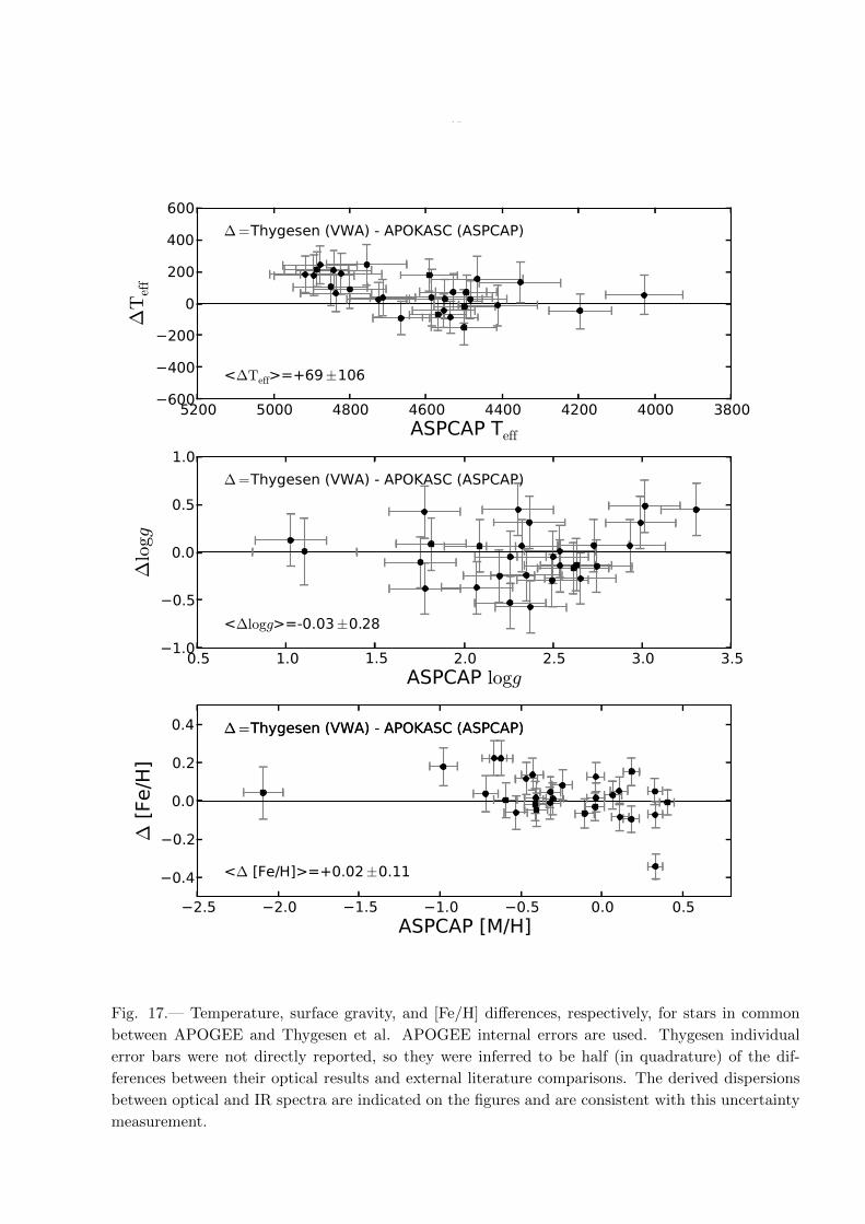
– 40 –

Fig. 17.— Temperature, surface gravity, and [Fe/H] differences, respectively, for stars in common

between APOGEE and Thygesen et al. APOGEE internal errors are used. Thygesen individual

error bars were not directly reported, so they were inferred to be half (in quadrature) of the dif-

ferences between their optical results and external literature comparisons. The derived dispersions

between optical and IR spectra are indicated on the figures and are consistent with this uncertainty

measurement.

– 41 –clump can be clearly distinguished, and the red giant branch bump (typically detected only in star

clusters) is clearly visible.

We can also examine trends in mass at fixed metallicity (illustrated in Figure 19) and in metal-

licity at fixed mass (illustrated in Figure 20). The overall trends predicted by stellar models are

clearly seen, with metal-poor stars being systematically hotter at fixed log g and mass than metal-

rich ones. Similarly, higher mass stars, as expected, are systematically hotter at fixed metallicity

than lower mass stars. The agreement between theory and data degrades for the lowest mass stars,

which could imply a mass-dependent shift in the locus of the giant branch. However, this may simply

be a stellar population effect: the limited age of the disk places a hard lower bound on the true

mass of evolved red giants. Stars with formal mass estimates at or close to this value are likely to be

higher mass stars scattered to a low apparent mass by errors in their data, and they will thus appear

offset relative to expectations. For the YREC models there is good agreement at low metallicity

but there appears to be an offset in the temperature locus between the metal-rich track and the

metal-rich data. This result is more robust than that in the mass plane and is tentative evidence

for a metallicity-dependent offset between the expected and observed HR diagram position at fixed

mass. Thygesen et al. (2012) reported evidence for a metallicity (but not mass) dependent shift

in the HR diagram position of stars with asteroseismic masses and gravities relative to theoretical

expectations. Our results are consistent with those that they derived from their sample.

6. Conclusions, Cautions, and Future Prospects

Asteroseismology and high-resolution spectroscopy are powerful and complementary astrophys-

ical tools. In this paper we present the APOKASC catalog, which is the first large and homogenous

catalog containing data from both high-resolution spectroscopy and asteroseismology. This effort

provides new tools for studying stellar populations and testing the theories of both stellar atmo-

spheres and stellar interiors. We now have a dataset measured in the natural co-ordinate for stellar

evolution calculations, namely mass. This permits direct tests of stellar evolution tracks using iso-

lated field stars, as opposed to relying on membership in well-studied binary systems or star clusters.

Asteroseismic data is particularly precise and accurate for surface gravities, which is a stringent test

of model atmospheres theory. Our combined data delineate stellar populations in the field with

a precision usually associated with star clusters, and asteroseismic evolutionary state diagnostics

confirm the assignments (such as red clump, secondary red clump, or red giant branch) that would

have been expected from the HR diagram positions of the stars. Differential mass trends (at fixed

metallicity) and metallicity trends (at fixed mass) are in the expected sense, which is a powerful

confirmation of expectations from stellar interiors theory. At a deeper level, interesting trends in the

differences between theory and data for both atmospheres and interiors models are clearly present

and worthy of further exploration.

Typical uncertainties in our catalog are of order 80 K in Teff , 0.06 dex in [M/H], 0.014 dex

in log g, and 12% and 5% in mass and radius, respectively. There are additional systematic error

sources that could be important and which should be explored. For example, a zero-point shift in

the Teff scale is plausible given the differences between photometric and spectroscopic inferences for

our targets, which would induce correlated changes in the mass and radius values. An improved

extinction map for the Kepler fields would permit a more precisely anchoring of the absolute scale

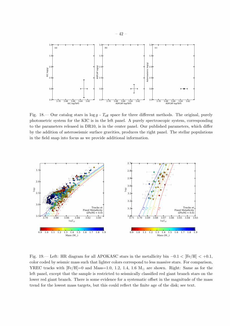
– 42 –

Fig. 18.— Our catalog stars in log g - Teff space for three different methods. The original, purely

photometric system for the KIC is in the left panel. A purely spectroscopic system, corresponding

to the parameters released in DR10, is in the center panel. Our published parameters, which differ

by the addition of asteroseismic surface gravities, produces the right panel. The stellar populations

in the field snap into focus as we provide additional information.

Fig. 19.— Left: HR diagram for all APOKASC stars in the metallicity bin −0.1 < [Fe/H] < +0.1,

color coded by seismic mass such that lighter colors correspond to less massive stars. For comparison,

YREC tracks with [Fe/H]=0 and Mass=1.0, 1.2, 1.4, 1.6 M� are shown. Right: Same as for the

left panel, except that the sample is restricted to seismically classified red giant branch stars on the

lower red giant branch. There is some evidence for a systematic offset in the magnitude of the mass

trend for the lowest mass targets, but this could reflect the finite age of the disk; see text.

– 43 –

Fig. 20.— Left: HR diagram for all APOKASC stars in the mass bin 1.1 < M < 1.3 M�, color coded

by corrected ASPCAP metallicity such that lighter colors correspond to more metal-poor stars. For

comparison, YREC tracks with 1.2 M� and [Fe/H]=-0.4, 0.0, and +0.4 dex are shown. Right: Same

as for the left panel, except that the sample is restricted to seismically classified red giant branch

stars on the lower red giant branch. There is some evidence for a systematic offset in the magnitude

of the metallicity trend for the highest metallicity targets.

– 44 –and constrain this effect. Our metallicities show no evidence of systematic differences from targets

measured with optical spectroscopy. We have derived mappings of KIC properties onto the system

defined in this paper, and find a reasonable correspondence between the KIC and spectrscopic

metallicities for giants. The accurate stellar properties and distances available in the APOKASC

sample in the Kepler field are also useful for calibrating stellar-population tracers, such that the

power of the APOKASC sample can be leveraged to the large Galactic volume covered by the full

APOGEE survey. As an example of this potential, Bovy et al. (2014) recently developed a new

method for selecting RC stars from spectro-photometric data that is calibrated using the precise

seismic log g and evolutionary-state classifications in the APOKASC catalog. The distances to stars

in the resulting APOGEE-RC Catalog are accurate to ∼5 %, allowing for a detailed mapping of the

structure of the Galactic disk. The seismic data are also useful to check for systematic errors in

the RC distance scale, which is calibrated using Hipparcos parallaxes: the direct seismic distances

for 593 RC stars in common between the APOGEE-RC catalog and the Rodrigues et al. (2014)

distance catalog agree to better than 1 %.

At the same time, there are important factors that should be accounted for when interpreting

and using the data. There are significant sample selection effects, imposed by the target selection

process for both Kepler and APOGEE. These selection effects are not simple ones (for example,

magnitude or color cuts), and they reflect the fact that the asteroseismic data was obtained from a

survey designed for a very different purpose (detecting extrasolar planets.) Direct stellar populations

inferences from our targets therefore require careful population modeling, which is outside the scope

of our paper.

The availability of stellar masses is especially valuable for red giant stars, as the natural process

of stellar evolution channels stars of very different masses and ages into similar locations on the

HR diagram. The two major methods for inferring stellar masses also have significant limitations

when applied to evolved stars, making an additional mass diagnostic even more important. Direct

mass measurements from binary stars are uncommon for physically large red giant stars. Indirect

mass estimates for red giants in star clusters are subject to significant systematic uncertainties in

cluster ages, distances, extinctions, and the mapping from turnoff properties to stellar mass. By

the same token, however, our asteroseismic masses have only a limited set of calibrators. Our radii

are based on the same scaling relations used in Silva Aguirre et al. (2012) and Huber et al. (2012),

which reported good agreement with independent tests using stars with measured parallaxes and

interferometric angular size measurements, particularly at solar metallicity. However, data at higher

and lower metallicity are more limited, and there could be metallicity-dependent offsets in the mass

scale. Epstein et al. (2014), for example, found that the masses derived from scaling relations for

metal-poor stars were consistently higher than those expected from other astrophysical constraints.

Miglio et al. (2012) found evolutionary-state dependent differences between the radii inferred for

red clump and red giant branch stars in the metal-rich open cluster NGC 6791. As a result, there

could be systematic trends in our inferred masses and radii not captured in our analysis. There are

systematic differences between the spectroscopic and asteroseismic surface gravities that appear to

be a function of evolutionary state as well. Calibration of the asteroseismic masses and radii, and

understanding the origin of the trends that have been identified, is ongoing.

Work is in progress on the next combined dataset, which will feature much larger numbers of

targets and considerably broader phase space coverage in metallicity and surface gravity. Our as-

– 45 –teroseismic uncertainties reflect a combination of systematic and random error sources, and work is

in progress to assess both separately. We also adopted separate external calibrators for each of our

spectroscopic parameters; in the next version of the catalog we will explore the consequences of iter-

ating between the asteroseismic and spectroscopic parameters and exploring the impact of adopting

an asteroseismic gravity prior for the spectroscopic solution. In the current paper we employed a

conservative concordance criterion for our asteroseismic sample (see Section 4.1), reporting results

only in cases where different analysis methods applied to the same dataset yielded similar asteroseis-

mic parameters. This approach had the net effect of removing most of the highest and lowest gravity

targets from our sample, as their data is the most subject to systematic offsets. Including these in

the next catalog, which will substantially increase our dynamic range in surface gravity, is another

priority. We also plan to take full advantage of the improvements in the ASPCAP spectroscopic

pipeline.

Funding for SDSS-III has been provided by the Alfred P. Sloan Foundation, the Participat-

ing Institutions, the National Science Foundation, and the U.S. Department of Energy Office of

Science. The SDSS-III Web site is http://www.sdss3.org/. SDSS-III is managed by the Astrophys-

ical Research Consortium for the Participating Institutions of the SDSS-III Collaboration including

the University of Arizona, the Brazilian Participation Group, Brookhaven National Laboratory,

Carnegie Mellon University, University of Florida, the French Participation Group, the German

Participation Group, Harvard University, the Instituto de Astrofisica de Canarias, the Michigan

State/Notre Dame/JINA Participation Group, Johns Hopkins University, Lawrence Berkeley Na-

tional Laboratory, Max Planck Institute for Astrophysics, Max Planck Institute for Extraterrestrial

Physics, New Mexico State University, New York University, Ohio State University, Pennsylvania

State University, University of Portsmouth, Princeton University, the Spanish Participation Group,

University of Tokyo, University of Utah, Vanderbilt University, University of Virginia, University of

Washington, and Yale University.

CE, JJ, MP and JT would like to acknowledge support from NSF Grant AST-1211673. DH

acknowledges support by an appointment to the NASA Postdoctoral Program at Ames Research

Center administered by Oak Ridge Associated Universities, and NASA Grant NNX14AB92G issued

through the Kepler Participating Scientist Program. DS acknowledges support from the Australian

Research Council. SB acknowldges partial support from NSF grant AST-1105930 and NASA grant

NNX13AE70G. Funding for the Stellar Astrophysics Center is provided by The Danish National

Research Foundation (Grant agreement no.: DNRF106). VSA was suppoeted by the European

Research Council (Grant agreement no.: 267864). SM acknowledges support from the NASA grant

NNX12AE17G. SH has received funding from the European Research Council under the European

Community’s Seventh Framework Programme (FP7/2007-2013) / ERC grant agreement no 338251

(StellarAges) and by Deutsche Forschungsgemeinschaft (DFG) under grant SFB 963/1 “Astrophysi-

cal flow instabilities and turbulence”. WJC, YE, and AM acknowledge support from the UK Science

and Technology Facilities Council (STFC). D.A. acknowledges support provided by the National Re-

search Foundation of Korea to the Center for Galaxy Evolution Research (No. 2010-0027910). AS is

partially supported by the MICINN grant AYA2011-24704 and by the ESF EUROCORES Program

EuroGENESIS (MICINN grant EUI2009-04170). TCB acknowledges partial support for this work

by grant PHY 08-22648: Physics Frontiers Center/Joint Institute for Nuclear Astrophysics (JINA),

awarded by the U.S. National Science Foundation. We thank an anonymous referee for comments

that improved the paper.

– 46 –REFERENCES

Ahn, C.P., Alexandroff, R., Allende Prieto, C. et al. 2014, ApJSupp 211, 17

Asplund, M. 2005, ARAA, 43, 481

Basu, S., Chaplin, W. J., Elsworth, Y., 2010, ApJ, 710, 1596

Basu, S., Grundahl, F., Stello, D., et al., 2011, ApJ, 729, L10

Basu, S., Verner, G. A., Chaplin, W. J., Elsworth, Y. 2012, ApJ, 746, 76

Basri, G., Walkowicz, L.M., Batalha, N.M. et al. 2011 AJ 141, 20

Batalha, N.M., Borucki, W.J., Koch, D.G. et al. 2010, ApJLett, 713, L109

Beck, P.G., Montalban, J., Kallinger, T. et al. 2012 Nature 481, 55

Bedding, T.R., Huber, D., Stello, D. et al. 2010 ApJLett 713, L176

Bedding, T., Mosser, B., Huber, D. et al. 2011, Nature, 471, 608

Belkacem, K., Goupil, M. J., Dupret, M. A., et al., 2011, A&A, 530, 142

Bergemann, M., Ruchti, G., Serenelli, A. et al. 2014, A&A 565, 89

Bildsten, L., Paxton, B., Moore, K. & Macias, P.J. 2012, ApJLett, 744, L6

Binney, J., Burnett, B., Kordopatis, G. et al. 2014, MNRAS, 439, 1231

Bovy, J., Rix,H.-W., Liu, C., Hogg, D.W., Beers, T.C. & Young Sun, L. 2012, ApJ, 753, 148

Bovy, J., Nidever, D.L., Rix,H.-W., et al. 2014, ApJ, 790, 127

Brown, T. M., Gilliland, R. L., Noyes, R. W., Ramsey, L. W., 1991, ApJ, 368, 599

Brown, T.M., Latham, D.W., Everett, M.E. & Esquerdo, G.A. 2011, AJ, 142, 112

Canterna, R. 1976 AJ 81, 228

Casagrande, L., Ramirez, I., Melendez, J., Bessel, M. & Asplund, M. 2010 A&A 512, 54

Casagrande, L., Silva Aguirre, V., Stello, D. et al. 2014, ApJ, 787, 110

Chaplin, W. J., Houdek, G., Appourchaux, T., Elsworth, Y., New, R., & Toutain, T. 2008, A&A,

485, 813

Chaplin, W.J., Kjeldsen, H., Christensen-Dalsgaard, J. et al. 2011 Science, 332, 213

Chaplin, W.J., Kjeldsen, H., Christensen-Dalsgaard, J. et al. 2014 ApJSupp 210, 1

Christensen-Dalsgaard, J. 1993, Proc. GONG 1992, Seismic Investigation of the Sun and Stars (ASP

Conf. Ser. 42), ed. T. M. Brown (San Francisco, CA: ASP), 347

Creevey, O. L., Dogan G., Frasca, A., et al., 2012, A&A, 537, 111

– 47 –da Silva L., Girardi, L., Pasquini, L. et al., 2006, A&A, 458, 609

Demarque, P., Woo, J.-H., Kim, Y.-C., Yi, S. K. 2004, ApJS, 155, 667

Demarque, P., Guenther, D.B., Li, L.H., Mazumdar, A. & Straka, C.W. 2008, Ap&SS, 316, 31

Deheuvels, S., Garcıa, R.A., Chaplin, W.J. et al. 2012 ApJ 756, 19

De Ridder, J., Barban, C., Baudin, F. et al. 2009 Nature 459, 398

Dong, S., Zheng, Z. & Zhu, Z. 2013, astro-ph/1311.1203

Dotter, A., Chaboyer, B., Jevremovic, D. et al. 2008, ApJS, 178, 89

Eisenstein, D.J., Weinberg, D.H., Agol, E. et al. 2011 AJ 142, 72

Epstein,C.R., Elsworth, Y.P., Johnson, J.A. et al. 2014, ApJLett, 785, L28 (astro-ph/1403.1872)

Freeman, K.C. 2011, EAS Publications Series, 45, 213. doi:10.1051/eas/1045036.

Freeman, K.C. 2012, Galactic Archaeology: Near-Field Cosmology and the Formation of the Milky

Way. Proceedings of the conference held 16-20 May 2011 in Shuzenji, Japan. Edited by W.

Aoki, M. Ishigaki, T. Suda, T. Tsujimoto, and N. Arimoto. ASP Conference Proceedings,

Vol. 458. San Francisco, CA: Astronomical Society of the Pacific, 2012., p.393

Fukugita, M., Ichikawa, T., Gunn, J. E., Doi, M., Shimasaku, K. & Schneider, D. P. 1996 AJ 111,

1748

Gai, N., Basu, S., Chaplin, W. J., Elsworth, Y., 2011, ApJ, 730, 63

Garcıa, R. A., Hekker, S., Stello, D., et al., 2011, MNRAS, 414, 6

Garcıa, R.A., Perez Hernandez, F., Benomar, O. et al. 2014, A&A, 563, 84

Garcıa, R.A. et al. 2014, submitted A&A

Geisler, D., Claria, J.J & Minniti, D. 1991 AJ 102, 1836

Gilmore, G., Randich, S., Asplund, M. et al. 2012 The Messenger 147 25

Girardi, L., Bressan, A., Bertelli, G., & Chiosi, C. 2000, A&AS, 141, 371

Girardi, L., Groenewegen, M.A.T., Hatziminaoglou, E. & da Costa, L. 2005, A&AS, 436, 895

Gonzalez-Hernandez, J. I., & Bonifacio, P. 2009, A&A, 497, 497

Gunn, J.E., Siegmund, W.A. & Al, E.J.M.E. 2006, AJ, 131, 87

Hayden, M.R., Holtzman, J.A., Bovy, J. et al. 2014, AJ, 147, 116

Hekker, S., Broomhall, A.-M., Chaplin, W. J., et al., 2010, MNRAS, 402, 2049

Hekker, S., Gillliland, R.L., Elsworth, Y. et al., 2011a, MNRAS, 414, 2594

Hekker, S., Elsworth, Y., De Ridder, J. et al., 2011b, A&A, 525, 131

– 48 –Hekker,S., Elsworth, Y., Mosser,B. et al. 2012, A&A 544, A90

Hekker, S., Elsworth, Y., Mosser, B. et al. 2013, A&A, 556, 59

Huber, D., Stello, D., Bedding, T. R., et al., 2009, CoAst, 160, 74

Huber, D., Bedding, T.R., Stello, D. et al. 2010, ApJ, 723, 1607

Huber, D., Bedding, T. R., Stello, D., et al., 2011, ApJ, 743, 143

Huber, D., Ireland, M.J., Bedding, T.R., et al., 2012 ApJ 760, 32

Huber, D., Chaplin, W.J., Christensen-Dalsgaard, J. et al. 2013, ApJ 767, 127

Huber, D., Silva Aguirre, V., Matthews, J. et al. 2014, ApJSupp 211, 2

Jenkins, J. M., Caldwell, D. A., Chandrasekaran, H., et al. 2010, ApJ, 713, L120

Kallinger, T., Mosser, B., Hekker, S., et al., 2010, A&A, 522, 1

Kordopatis, G., Gilmore, G., Steinmetz, M. et al. 2013 AJ 146, 134

Kjeldsen, H. & Bedding, T. R. 1995, A&A, 293, 87

Lai, D. K., Rockosi, C. M., Bolte, M., Johnson, J. A., Beers, T. C., Lee, Y. S., Allende Prieto, C. &

Yanny, B. 2009, ApJLett 697, L63

Lee, Y.-S, Beers, T.C., Sirarani, T. et al. 2008 AJ 136, 2050

Majewski, S.R., Wilson, J.C., Hearty, F., Schiavon, R.R. & Skrutskie, M.E. 2010, in ”Chemical

Abundances in the Universe: Connecting First Stars to Planets”, Proceedings of the Interna-

tional Astronomical Union, IAU Symposium, Volume 265, p. 480-481

Majewski, S.R., Zasowski, G. & Nidever, D.L. 2011, ApJ, 739, 25

Marigo, P., Girardi, L., Bressan, A., et al. 2008, A&A, 482, 883

Mathur, S., Garcıa, R. A., Regulo, C., et al., 2010, A&A, 511, 46

Matteucci, F., Spitoni, E., Recchi, S. & Valiante, R. 2009 A&A 501, 531

McQuillan, A., Mazeh, T. & Aigrain, S. 2014, ApJS, 211, 24

Meszaros, S., Holtzman, J., Garcıa Perez, A. E. et al. 2013, AJ146, 133

Miglio, A., Montalban, J., Eggenberger, P. et al., 2009, A&A, 503, L21

Miglio, A., Brogaard, K., Stello, D., et al., 2012, MNRAS, 419, 2077

Miglio, A., Chiappini, C., Morel, T., et al., 2013, MNRAS, 429, 423

Mosser, B., Belkacem, K., Goupil, M.J. et al. 2010 A&A 517, 22

Mosser, B., Belkacem, K., Goupil, M. J., et al., 2011, A&A, 525, L9

Mosser, B., Barban, C., Montalban, J. et al. 2011, A&A, 532, 86

– 49 –Mosser, B., Goupil, M.J., Belkacem, K. et al. 2012a, A&A, 548, 10

Mosser, B., Goupil, M.J., Belkacem, K. et al. 2012b, A&A, 540, 143

Perryman, M.A.C., de Boer, K.S., Gilmore, G. et al. 2001 A&A 369, 339

Pietrinferni, A., Cassisi, S., Salaris, M., & Castelli, F. 2004, ApJ, 612, 168

Pinsonneault, M.H., An, D., Molenda-Zakowicz, J. et al. 2012 ApJSupp 199, 30

Rodrigues, T.S., Girardi, L., Miglio, A. et al. 2014, MNRAS, in press

Serenelli, A., Bergemann,M., Ruchti, G. & Casagrande, L. 2013 MNRAS 429, 3645

Skrutskie, M.F., Cutri, R.M., Stiening, R. et al. 2006, AJ, 131, 1163

Silva Aguirre, V., Chaplin, W.J., Ballot, J., et al. 2011 ApJLett 740, L2

Silva Aguirre, V., Casagrande, L., Basu, S., et al. 2012, ApJ, 757, 99

Silva Aguirre, V., Basu, S., Brandao, I. M., et al. 2013, ApJ, 769, 141

Smith, J.C., Stumpe, M.C.,van Cleve, J.E. et al. 2012, PASP, 124, 1000

Stello, D., Chaplin, W. J., Basu, S., Elsworth, Y. & Bedding, T.R. 2009, MNRAS, 400, L80

Stello, D., Chaplin, W. J., Bruntt, H., et al. 2009, ApJ, 700, 1589

Stello, D., Meibom, S., Gilliland, R.L. et al. 2011, ApJ, 739, 13

Stello, D., Huber, D., Kallinger, T., et al. 2011, ApJ, 737, L10

Stello, D., Huber, D., Bedding, T.R. et al. 2013, ApJLett, 765, L41

Stumpe, M.C., Smith, J.C., van Cleve, J.E. et al. 2012, PASP, 124, 985

Tassoul, M., 1980, ApJS, 43, 469

Thygesen, A.O., Frandsen,S., Bruntt, H. et al. 2012 A&A 543, 160

Tinsley, B. 1979 ApJ 229, 1046

Ulrich R. K., 1986, ApJ, 306, L37

Wallerstein, G. ApJSupp 6, 407

Weiss, A. & Schallt, H. 2008, ApS&S, 316, 99

White, T.R., Bedding, T.R., Stello, D., Christensen-Dalsgaard, J., Huber, D. & Kjeldsen, H. 2011

ApJ 743, 161

Yanny, B., Rockosi, C., Newberg, H.J. et al. 2009 AJ 137, 4377

Zasowski, G., Johnson, J.A., Frinchaboy, P.M. et al. 2013 AJ 146, 81

Zhao, G., Chen, Y.-Q., Shi, J.-R. et al. 2006 ChJAA 6, 265

This preprint was prepared with the AAS LATEX macros v5.2.