Imaging moving targets from scattered waves

This article has been downloaded from IOPscience. Please scroll down to see the full text article.

2008 Inverse Problems 24 035005

(http://iopscience.iop.org/0266-5611/24/3/035005)

Download details:

IP Address: 128.113.83.54

The article was downloaded on 03/02/2009 at 16:02

Please note that terms and conditions apply.

The Table of Contents and more related content is available

HOME | SEARCH | PACS & MSC | JOURNALS | ABOUT | CONTACT US

IOP PUBLISHING INVERSE PROBLEMS

Inverse Problems 24 (2008) 035005 (22pp) doi:10.1088/0266-5611/24/3/035005

Imaging moving targets from scattered waves

Margaret Cheney1 and Brett Borden2

1 Department of Mathematical Sciences, Rensselaer Polytechnic Institute, Troy, NY 12180 USA2 Physics Department, Naval Postgraduate School, Monterey, CA 93943 USA

Received 15 August 2007, in final form 25 January 2008Published 8 April 2008Online at stacks.iop.org/IP/24/035005

AbstractWe develop a linearized imaging theory that combines the spatial, temporaland spectral aspects of scattered waves. We consider the case of fixed sensorsand a general distribution of objects, each undergoing linear motion; thus thetheory deals with imaging distributions in phase space. We derive a model forthe data that is appropriate for any waveform, and show how it specializesto familiar results in the cases when: (a) the targets are moving slowly,(b) the targets are far from the antennas and (c) narrowband waveforms areused. From these models, we develop a phase-space imaging formula thatcan be interpreted in terms of filtered backprojection or matched filtering. Forthis imaging approach, we derive the corresponding point-spread function. Weshow that special cases of the theory reduce to: (a) range-Doppler imaging,(b) inverse synthetic aperture radar (ISAR), (c) synthetic aperture radar (SAR),(d) Doppler SAR, (e) diffraction tomography and (f) tomography of movingtargets. We also show that the theory gives a new SAR imaging algorithm forwaveforms with arbitrary ridge-like ambiguity functions.

1. Introduction

Many imaging techniques are based on measurements of scattered waves and, typically, overallimage resolution is proportional to the ratio of system aperture to signal wavelength. Whenthe physical (real) aperture is small in comparison with wavelength, an extended ‘effectiveaperture’ can sometimes be formed analytically: examples include ultrasound, radar, sonarand seismic prospecting. For the most part, these synthetic-aperture methods rely on time-delay measurements of impulsive echo wavefronts and assume that the region to be imaged isstationary.

For an imaging region containing moving objects, on the other hand, it is well knownthat measurements of the Doppler shift can be used to obtain information about velocities.This principle is the foundation of Doppler ultrasound, police radar systems and some movingtarget indicator (MTI) radar systems. The classical ‘radar ambiguity’ theory [5, 11, 22]for monostatic (backscattering) radar shows that the accuracy to which one can measure theDoppler shift and time delay depends on the transmitted waveform. There is similar theory forthe case when a single transmitter and receiver are at different locations [19–21]. Ambiguity

0266-5611/08/035005+22$30.00 © 2008 IOP Publishing Ltd Printed in the UK 1

Inverse Problems 24 (2008) 035005 M Cheney and B Borden

Figure 1. A diagram of various theories that combine spatial, spectral and temporal aspects ofscattered waves.

theory appears as the bottom plane in figure 1. Some recent work [3] develops a way tocombine range and Doppler information measured at multiple receivers in order to maximizethe probability of detection.

In recent years, a number of attempts to develop imaging techniques that can handlemoving objects have been proposed. Space-time adaptive processing (STAP) [10] uses amoving multiple-element array together with a real-aperture imaging technique to produceground moving target indicator (GMTI) image information. Velocity synthetic aperture radar(VSAR) [8] also uses a moving multiple-element array to form a SAR image from eachelement; then from a comparison of image phases, the system deduces target motion. Thepaper [15] uses a separate transmitter and receiver together with sequential pulses to estimatetarget motion from multiple looks. Another technique [16] uses backscattering data froma single sensor to identify rigid-body target motion, which is then used to form a three-dimensional image. Other work [12] extracts target velocity information by exploiting thesmearing that appears in SAR images when the along-track target velocity is incorrectlyidentified. All of these techniques make use of the so-called start–stop approximation, inwhich a target in motion is assumed to be momentarily stationary while it is being interrogatedby a radar pulse. In other words, Doppler measurements are not actually made by thesesystems. Thus these methods appear on the back plane of figure 1.

Imaging techniques that rely on Doppler data are generally real-aperture systems, andprovide spatial information with very low resolution. A synthetic-aperture approach to imagingfrom a moving sensor and a fixed target was developed in [2]. This Doppler imaging methodappears on the left plane of figure 1. An approach that explicitly considers the Doppler shiftis Tomography of Moving Targets (TMT) [9], which uses multiple transmitters and receivers(together with matched-filter processing) to both form an image and find the velocity.

Below we develop a theory that shows how to unify these different approaches. In theprocess, we will demonstrate how we can fuze the spatial, temporal and spectral aspects ofscattered-field-based imaging. The present discussion deals with the case of fixed distributedsensors, although our results include monostatic configurations (in which a single transmitterand receiver are co-located) as a special case. Methods for imaging stationary scenes in thecase when the transmitter and receiver are not co-located have been particularly well developedin the geophysics literature [1] and have also been explored in the radar literature [19–21].

In section 2, we develop a physics-based mathematical model that incorporates notonly the waveform and wave propagation effects due to moving scatterers, but also the

2

Inverse Problems 24 (2008) 035005 M Cheney and B Borden

effects of spatial diversity of transmitters and receivers. In section 3, we show how amatched-filtering technique produces images that depend on target velocity, and we relatethe resulting point-spread function to the classical wideband and narrowband radar ambiguityfunctions. We also work out the special cases of far-field imaging and narrowband imagingof slowly-moving targets. Finally, in section 4, we show that for special cases, the theorydeveloped in section 3 reduces to familiar results. We also show that the theory provides anew imaging algorithm for certain waveforms.

2. Model for data

We model wave propagation and scattering by the scalar wave equation for the wavefieldψ(t,x) due to a source waveform s(t,x),[∇2 − c−2(t,x)∂2

t

]ψ(t,x) = s(t,x). (1)

For example, a single isotropic source located at y transmitting the waveform s(t) startingat time t = −Ty could be modeled as s(t,x) = δ(x − y)sy(t + Ty), where the subscript yreminds us that different transmitters could transmit different waveforms. For simplicity, inthis paper we consider only localized isotropic sources; the work can easily be extended tomore realistic antenna models [13].

A single scatterer moving at velocity v corresponds to an index-of-refraction distributionn2(x − vt):

c−2(t,x) = c−20 [1 + n2(x − vt)], (2)

where c0 denotes the speed in the stationary background medium (here assumed constant).For radar, c0 is the speed of light in vacuum. We write qv(x − vt) = c−2

0 n2(x − vt). Tomodel multiple moving scatterers, we let qv(x − vt) d3x d3v be the corresponding quantityfor the scatterers in the volume d3x d3v centered at (x,v). Thus qv is the distribution, at timet = 0, of scatterers moving with velocity v. Consequently, the scatterers in the spatial volumed3x (at x) give rise to

c−2(t,x) = c−20 +

∫qv(x − vt) d3v. (3)

We note that the physical interpretation of qv involves a choice of a time origin. A choicethat is particularly appropriate, in view of our assumption about linear target velocities, isa time during which the wave is interacting with targets of interest. This implies that theactivation of the antenna at y takes place at a negative time which we denote by −Ty; we writes(t,x) = sy(t + Ty)δ(x − y). The wave equation corresponding to (3) is then[

∇2 − c−20 ∂2

t −∫

qv(x − vt) d3v∂2t

]ψ(t,x) = sy(t + Ty)δ(x − y). (4)

2.1. The transmitted field

We consider the transmitted field ψ in in the absence of any scatterers; ψ in satisfies the versionof equation (1) in which c is simply the constant background speed c0, namely[∇2 − c−2

0 ∂2t

]ψ in(t,x,y) = sy(t + Ty)δ(x − y). (5)

Henceforth we drop the subscript on c. We use the Green’s function g, which satisfies[∇2 − c−20 ∂2

t

]g(t,x) = −δ(t)δ(x)

3

Inverse Problems 24 (2008) 035005 M Cheney and B Borden

and is given by

g(t, |x|) = δ(t − |x|/c)4π |x| = 1

8π2|x|∫

e−iω(t−|x|/c) dω, (6)

where we have used 2πδ(t) = ∫exp(−iωt) dω. We use (6) to solve (5), obtaining

ψ in(t,x,y) = −∫

g(t − t ′, |x − y|)sy(t ′ + Ty)δ(x − y) dt ′ dy

= − sy(t + Ty − |x − y|/c)4π |x − y| . (7)

2.2. The scattered field

We write ψ = ψ in + ψ sc, which converts (1) into[∇2 − c−20 ∂2

t

]ψ sc =

∫qv(x − vt) d3v∂2

t ψ. (8)

The map q �→ ψ sc can be linearized by replacing the full field ψ on the right-hand side of (8)by ψ in. This substitution results in the Born approximation ψ sc for the scattered field ψ sc atthe location z,

ψ sc(t,z) = −∫

g(t − t ′, |z − x|)∫

qv(x − vt ′) d3v∂2t ′ψ

in(t ′,x) dt ′ d3x

=∫

δ(t − t ′ − |z − x|/c)4π |z − x|

∫qv(x − vt ′) d3v∂2

t ′sy(t ′ + Ty − |x − y|/c)

4π |x − y| d3x dt ′.

(9)

In equation (9), we make the change of variables x �→ x′ = x − vt ′ (i.e., change to the frameof reference in which the scatterer qv is fixed) to obtain

ψ sc(t,z) =∫

δ(t − t ′ − |x′ + vt ′ − z|/c)4π |x′ + vt ′ − z|

×∫

qv(x′)

sy(t ′ + Ty − |x′ + vt ′ − y|/c)4π |x′ + vt ′ − y| d3x ′ d3v dt ′. (10)

The physical interpretation of (10) is as follows: the wave that emanates from y at time −Ty

encounters a target at time t ′. This target, during the time interval [0, t ′], has moved from xto x + vt ′. The wave scatters with strength qv(x), and then propagates from position x + vt ′

to z, arriving at time t.Henceforth we will drop the primes on x. We introduce the notation

Rx,z(t) = x + vt − z R = |R|, and R = R/R. (11)

To evaluate the t ′ integral of (10), we denote by t ′ = tx,v(t) the implicit solution oft − t ′ − Rx,z(t

′)/c = 0, i.e.,

0 = t − tx,v(t) − Rx,z(tx,v(t))/c. (12)

The time tx,v(t) is the time when the wave reaching the receiver at z at time t interacted withthe target that, at time t = 0, was located at x. This target, at time tx,v(t), is actually locatedat x + vtx,v(t). With this notation, equation (10) becomes

ψ sc(t,z) =∫

sy[tx,v(t) + Ty − Rx,y(tx,v(t))/c]

(4π)2Rx,z(tx,v(t))Rx,y(tx,v(t))qv(x) d3x d3v

=∫

sy(t + Ty − Rx,z(tx,v(t))/c − Rx,y(tx,v(t))/c)

(4π)2Rx,z(tx,v(t))Rx,y(tx,v(t))qv(x) d3x d3v, (13)

where, in the second line, we have used (12) to write the argument of s in a more symmetricalform.

4

Inverse Problems 24 (2008) 035005 M Cheney and B Borden

Expression (13) is appropriate under very general circumstances. In particular, thisformula applies to wide-beam imaging where the commonly-used far-field approximationsdo not apply. Equation (13) also applies to rapidly moving targets, where the start–stopapproximation is not valid, and to very distant targets. Finally, this result can be used forarbitrary transmitted waveforms.

2.2.1. The slow-mover case. Here we assume that |v|t and k|v|2t2 are much less than |x−z|and |x − y|, where k = ωmax/c, with ωmax being the (effective) maximum angular frequencyof the signal sy . In this case, we have

Rx,z(t) = |z − (x + vt)| = Rx,z(0) + Rx,z(0) · vt + O

( |vt |2Rx,z

), (14)

where Rx,z(0) = x − z, Rx,z(0) = |Rx,z(0)|, and Rx,z(0) = Rx,z(0)/Rx,z(0). With (14),equation (12) becomes

tx,v ≈ t −[Rx,z(0)

c+ Rx,z(0) · vtx,v

c

], (15)

which can be solved explicitly to obtain

tx,v(t) ≈ t − Rx,z(0)/c

1 + Rx,z(0) · v/c. (16)

The argument of s in equation (13) is then

tx,v(t) + Ty − Rx,y(tx,v(t))

c≈ tx,v(t) + Ty −

(Rx,y(0)

c+

Rx,y(0) · v

ctx,v(t)

)

= 1 − Rx,y(0) · v/c

1 + Rx,z(0) · v/c

(t − Rx,z(0)

c

)− Rx,y(0)

c+ Ty. (17)

The time dilation

αx,v = 1 − Rx,y(0) · v/c

1 + Rx,z(0) · v/c(18)

is the Doppler scale factor, which, as we see below, is closely related to the Doppler shift.With (17) and the notation (18), equation (13) becomes

ψ scs (t,z,y) =

∫sy[αx,v(t − Rx,z(0)/c) − Rx,y(0)/c + Ty]

(4π)2Rx,z(0)Rx,y(0)qv(x) d3x d3v. (19)

2.2.2. The slow-mover, narrow-band case. Many radar systems use a narrowband waveform,defined by

sy(t) = sy(t) e−iωy t , (20)

where s(t,y) is slowly varying, as a function of t, in comparison with exp(−iωyt), where ωy

is the carrier frequency for the transmitter at position y.For the waveform (20), equation (19) becomes

ψ scN (t,z,y) = −

∫ω2

y

(4π)2Rx,z(0)Rx,y(0)e−iωy [αx,v(t−Rx,z(0)/c)−Rx,y(0)/c+Ty ]

× sy(αx,v(t − Rx,z(0)/c) − Rx,y(0)/c + Ty)qv(x) d3x d3v

≈ −∫

ω2y eiϕx,v e−iωy αx,v t

(4π)2Rx,z(0)Rx,y(0)sy(t + Ty − (Rx,z(0) + Rx,y(0))/c)qv(x) d3x d3v.

(21)

5

Inverse Problems 24 (2008) 035005 M Cheney and B Borden

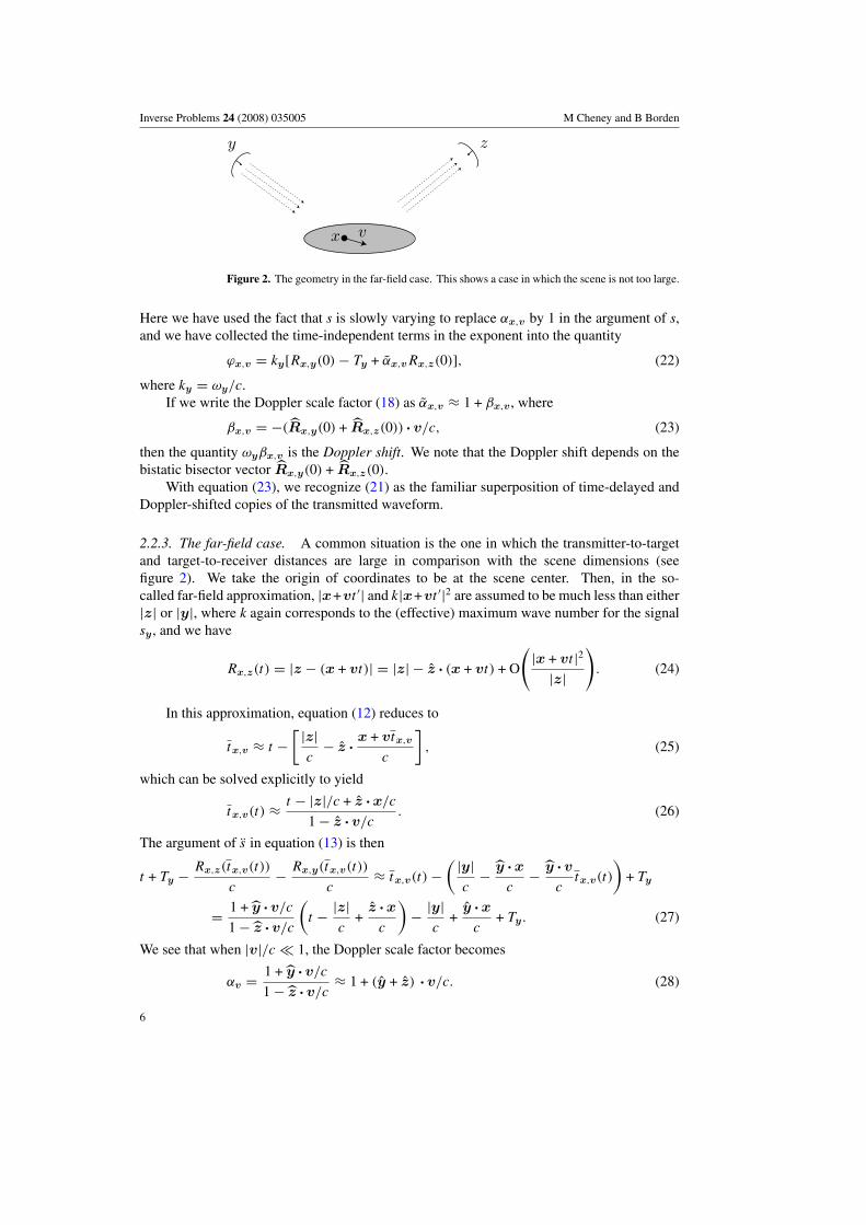
Figure 2. The geometry in the far-field case. This shows a case in which the scene is not too large.

Here we have used the fact that s is slowly varying to replace αx,v by 1 in the argument of s,and we have collected the time-independent terms in the exponent into the quantity

ϕx,v = ky[Rx,y(0) − Ty + αx,vRx,z(0)], (22)

where ky = ωy/c.If we write the Doppler scale factor (18) as αx,v ≈ 1 + βx,v , where

βx,v = −(Rx,y(0) + Rx,z(0)) · v/c, (23)

then the quantity ωyβx,v is the Doppler shift. We note that the Doppler shift depends on thebistatic bisector vector Rx,y(0) + Rx,z(0).

With equation (23), we recognize (21) as the familiar superposition of time-delayed andDoppler-shifted copies of the transmitted waveform.

2.2.3. The far-field case. A common situation is the one in which the transmitter-to-targetand target-to-receiver distances are large in comparison with the scene dimensions (seefigure 2). We take the origin of coordinates to be at the scene center. Then, in the so-called far-field approximation, |x+vt ′| and k|x+vt ′|2 are assumed to be much less than either|z| or |y|, where k again corresponds to the (effective) maximum wave number for the signalsy , and we have

Rx,z(t) = |z − (x + vt)| = |z| − z · (x + vt) + O

(|x + vt |2

|z|

). (24)

In this approximation, equation (12) reduces to

tx,v ≈ t −[ |z|

c− z · x + vtx,v

c

], (25)

which can be solved explicitly to yield

tx,v(t) ≈ t − |z|/c + z · x/c

1 − z · v/c. (26)

The argument of s in equation (13) is then

t + Ty − Rx,z(tx,v(t))

c− Rx,y(tx,v(t))

c≈ tx,v(t) −

( |y|c

− y ·x

c− y ·v

ctx,v(t)

)+ Ty

= 1 + y ·v/c

1 − z · v/c

(t − |z|

c+

z · x

c

)− |y|

c+

y ·x

c+ Ty. (27)

We see that when |v|/c � 1, the Doppler scale factor becomes

αv = 1 + y · v/c

1 − z · v/c≈ 1 + (y + z) · v/c. (28)

6

Inverse Problems 24 (2008) 035005 M Cheney and B Borden

We note that the signs here appear different from those in equation (18) because Rx,z(0) =x − z points in a direction approximately opposite to z = z − 0. The scattered field is

ψ scf (t,z,y) =

∫sy[αv(t − |z|/c + z · x/c) − |y|/c + y · x/c + Ty]

(4π)2|z||y| qv(x′) d3x d3v. (29)

2.2.4. The far-field, narrowband case. With a narrowband waveform (20) and the far-fieldapproximation (24), equation (29) becomes

ψ scfN(t,z,y) = − ω2

y

(4π)2|z||y|∫

sy(t − |z|/c + z · x/c − |y|/c + y · x/c + Ty)

× exp(−iωy[αv(t − |z|/c + z ·x/c) − |y|/c + y ·x/c + Ty])qv(x) d3x d3v

≈ − ω2y

(4π)2|z||y|∫

exp(iϕf

x,v

)exp(−iωyαvt)

× sy(t + Ty − (|z| − z · x + |y| − y · x)/c)qv(x) d3x d3v, (30)

where ϕfx,v = −ωy[αv(−|z| + z · x) − |y| + y ·x]/c.

If the transmitter is activated at times −Ty = −|y|/c, so that the transmitted wave arrivesat the scene center at the time t = 0, and if we evaluate ψ sc

fN at t ′ = t − |z|/c, we have

ψ scfN(t ′,z,y) = −ω2

y

(4π)2|z||y|∫

eiϕx,v e−iωyαv t ′ sy(t ′ + (z + y) · x/c)qv(x) d3x d3v, (31)

where

ϕx,v = −ωy[αvz + y] · x/c (32)

Again if we write αv = 1 + βv , where βv = (y + z) · v/c, we see that equation (31) is asuperposition of delayed and Doppler-shifted versions of the transmitted signal.

Much previous work has dealt with the case of far-field, single-frequency imaging ofa stationary scene. For a stationary scene (v = 0, which implies αv = 1 ), and a singlefrequency ωy = ω0 (which corresponds to s = 1), (31) reduces to the well-known expression

ψ∞ω0

(t,z,y) ≈ e−ik0t

(4π)2|z||y|F∞(y, z), (33)

where the (Born-approximated) far-field pattern or scattering amplitude is

F∞(y, z) =∫

e−ik0(z+y) ·xq(x) d3x, (34)

where k0 = ω0/c. We note that our incident-wave direction convention (from target totransmitter) is the opposite of that used in the classical scattering theory literature (which usestransmitter to target).

3. Imaging via a filtered adjoint

We now address the question of extracting information from the scattered waveform describedby equation (13).

Our image formation algorithm depends on the data we have available. In general, weform a (coherent) image as a filtered adjoint, but the variables we integrate over depend onwhether we have multiple transmitters, multiple receivers and/or multiple frequencies. Thenumber of variables we integrate over, in turn, determines how many image dimensions wecan hope to reconstruct. If our data depends on two variables, for example, then we can

7

Inverse Problems 24 (2008) 035005 M Cheney and B Borden

hope to reconstruct a two-dimensional scene; in this case the scene is commonly assumed tolie on a known surface. If, in addition, we want to reconstruct two-dimensional velocities,then we are seeking a four-dimensional image and thus we will require data depending onat least four variables. More generally, determining a distribution of positions in space andthe corresponding three-dimensional velocities means that we seek to form an image in asix-dimensional phase space.

3.1. Imaging formula in the general case

We form an image I (p,u) of the objects with velocity u that, at time t = 0, were located atposition p. Thus I (p,u) is constructed to be an approximation to qu(p). The strategy for theimaging process is to write the data in terms of a Fourier integral operator F : qv �→ ψ sc, andthen find an approximate inverse for F .

In the general case, we write the data (13) as

ψ sc(t,z,y) = −∫

(iω′)2 e−iω′[tx,v(t)+Ty−Rx,y,v(tx,v(t))/c]

25π3Rx,z,v(tx,v(t))Rx,y,v(tx,v(t))Sy(ω′) dω′qv(xq) d3x d3v, (35)

where we have written sy(t) in terms of its inverse Fourier transform

sy(t) = 1

2π

∫e−iω′t Sy(ω′) dω′. (36)

We note that by the Paley–Weiner theorem, S is analytic since it is the inverse Fourier transformof the finite-duration waveform s.

The corresponding imaging operation is a filtered version of the formal adjoint of the‘forward’ operator F . Thus we form the phase-space image I (p,u) as

I (p,u) =∫

eiω[tp,u(t)+Ty−Rp,y(tp,u(t))/c]Q(ω, t,p,u,z,y) dωψ sc(t,z,y) dt dnz dmy, (37)

where n = 1, 2 or 3, depending on the receiver configuration, and m = 1, 2 or 3, depending onthe transmitter configuration. This image reconstruction operator can be interpreted in termsof filtered backpropagation, where Q is the filter.

The specific choice of filter is dictated by various considerations [1, 23]; here we makechoices that connect the resulting formulae with familiar theories. In particular, we take thefilter Q to be

Q(ω, t,p,u,z,y) = (4π)2

(iω)2Rp,z(tp,u(t))Rp,y(tp,u(t))S∗

y(ω)J (ω,p,u,z,y)αp,u(t), (38)

a choice which leads (below) to the matched filter. The matched filter is well known [22] to bethe optimal filter for enhancing signal to noise in the presence of white Gaussian noise. Thequantity J depends on the geometry and is chosen (see below) to compensate for a certainJacobian that appears; α is the Doppler scale factor for the point p,u and is defined by

αp,u(t) = 1 − Rp,y(tp,u(t)) ·u/c

1 + Rp,z(tp,u(t)) ·u/c. (39)

In allowing (37) and (38) to depend on the transmitter y, we are implicitly assumingthat we can identify the part of the signal that is due to the transmitter at y. In the caseof multiple transmitters, this identification can be accomplished, for example, by having

8

Inverse Problems 24 (2008) 035005 M Cheney and B Borden

different transmitters operate at different frequencies or, possibly, by quasi-orthogonal pulse-coding schemes. We are also assuming a coherent system, i.e., that a common time clock isavailable to all sensors.

For a limited number of discrete receivers (or transmitters), the integral over z (or y) in(37) reduces to a sum.

Interpretation of imaging as matched filtering. In the case when the geometrical factorJ = J/ω2 is independent of ω, we can use (36) to write the imaging operation of equation(37) as

I (p,u) = −(4π)2∫

s∗y[tp,u(t) + Ty − Rp,y(tp,u(t))/c]Rp,z(tp,u(t))Rp,y(tp,u(t))

× J (p,u,z,y)αp,u(t)ψ sc(t,z,y) dt dnz dmy

= −(4π)2∫

s∗y[t + Ty − Rp,z(tp,u(t))/c − Rp,y(tp,u(t))/c]

× Rp,z(tp,u(t))Rp,y(tp,u(t))J (p,u,z,y)αp,u(t)ψ sc(t,z,y) dt dnz dmy, (40)

which has the form of a weighted matched filter. To obtain the second line of (40), we haveused (12) to write the argument of s in a more symmetric form.

3.1.1. The point-spread function for the general case. We substitute equation (35) intoequation (37), obtaining

I (p,u) =∫

K(p,u;x,v)qv(x) d3x d3v, (41)

where K, the point-spread function (PSF), is

K(p,u;x,v) = 1

2π

∫eiω[tp,u(t)+Ty−Rp,y,u(tp,u(t))/c]Rp,z(tp,u(t))Rp,y(tp,u(t))S∗

y(ω)αp,u

× J (ω,p,u,z,y)

(iω)2dω

∫(iω′)2 e−iω′(tx,v(t)+Ty−Rx,y(tx,v(t))/c)

Rx,z(tx,v(t))Rx,y(tx,v(t))

× Sy(ω′) dω′ dt dnz dmy. (42)

Since Sy is smooth, we can carry out a stationary phase reduction of (42) in the variablest and ω′. If we denote by φ the phase of (42), then the critical points are given by

0 = ∂φ

∂t= ω

[∂tp,u

∂t− ∂

∂t

Rp,y(tp,u(t))

c

]− ω′

[∂tx,v

∂t− ∂

∂t

Rx,y(tx,v(t))

c

](43)

0 = ∂φ

∂ω′ = tx,v(t) + Ty − Rx,y(tx,v(t))

c= t + Ty − Rx,z(tx,v(t))

c− Rx,y(tx,v(t))

c, (44)

where in (44) we have used equation (12). These two conditions determine the critical valuesof ω′ and t which give rise to the leading-order contributions to equation (42). We denote byt∗x,v the value of t determined by (44).

We rewrite equation (43) by differentiating (12) implicitly, obtaining

0 = 1 − ∂tx,v

∂t− Rx,z(tx,v(t)) · v

c

∂tx,v

∂t, (45)

which can be solved for ∂tx,v/∂t to obtain

∂tx,v

∂t= 1

1 + Rx,z(tx,v(t)) ·v/c. (46)

9

Inverse Problems 24 (2008) 035005 M Cheney and B Borden

With (46) we see that the terms in brackets in (43) are of the form[∂tx,v

∂t− ∂

∂t

Rx,y(tx,v(t))

c

]= 1 − Rx,y(tx,v(t)) ·v/c

1 + Rx,z(tx,v(t)) ·v/c= αx,v(t). (47)

Thus we find that equation (43) implies that

ω′ = αp,u(t∗x,v)

αx,v(t∗x,v)ω (48)

and that, moreover, the determinant of the Hessian of the phase is∣∣∣∣∣ ∂2φ

∂t2 αx,v

αx,v 0

∣∣∣∣∣ = −α2x,v. (49)

The result of the stationary phase reduction of equation (42) is

K(p,u;x,v) ∼∫

eiω[tp,u(t∗x,v)+Ty−Rp,y(tp,u(t∗x,v))/c] Rp,z(tp,u(t∗))Rp,y(tp,u(t∗))Rx,z(tx,v(t∗))Rx,y(tx,v(t∗))

S∗y(ω)

× Sy

(αp,u(t∗x,v)

αx,v(t∗x,v)ω

)J (ω,p,u,z,y)

α3p,u(t∗x,v)

α3x,v(t

∗x,v)

dω dnz dmy. (50)

The quantity in square brackets in the phase of equation (50) can also be written as

tp,u(t∗x,v) + Ty − Rp,y(tp,u(t∗x,v))

c= t∗x,v + Ty − Rp,z(tp,u(t∗x,v))

c− Rp,y(tp,u(t∗x,v))

c

= Rx,z(tx,v(t∗x,v))

c+

Rx,y(tx,v(t∗x,v))

c− Rp,z(tp,u(t∗x,v))

c− Rp,y(tp,u(t∗x,v))

c+ Ty,

(51)

where in the first line we have used definition (12) of t and in the second line definition (44)of t∗.

We write equation (50) as

K(p,u;x,v) ∼∫

e−iωτy,z(x,p,u,v)S∗y(ω)Sy

(αp,u

αx,vω

)×R(x,y,z,p,u,v)J (ω,p,u,z,y)

α3p,u

α3x,v

dω dnz dmy, (52)

where k = ω/c and where

cτy,z(x,p,u,v) = [Rp,z(tp,u(t∗x,v)) + Rp,y(tp,u(t∗x,v))]

− [Rx,z(tx,v(t∗x,v)) + Rx,y(tx,v(t

∗x,v))] + cTy (53)

and

R(x,y,z,p,u,v) = Rp,z(tp,u(t∗))Rp,y(tp,u(t∗))Rx,z(tx,v(t∗))Rx,y(tx,v(t∗))

. (54)

3.1.2. Relation between point-spread function and ambiguity function in the general case.In equation (52) we use the definition of the inverse Fourier transform

Sy(ω) =∫

eiωt sy(t) dt, (55)

10

Inverse Problems 24 (2008) 035005 M Cheney and B Borden

which, in the case when J = J ω2 with J independent of ω, converts (52) to

K(p,u;x,v) =∫ (

−iωαp,u

αx,v

)e−iωτy,zS∗

y(ω)

∫ (iω

αp,u

αx,v

)exp

(iαp,u

αx,vωt

)sy(t) dt

× R(x,y,z,p,u,v)J (p,u,z,y)αp,u

αx,vdω dnz dmy

∼∫

s∗y

(αp,u

αx,vt − τy,z(x,p,u,v)

)sy(t) dt

× R(x,y,z,p,u,v)J (p,u,z,y)αp,u

αx,vdnz dmy. (56)

Equation (56) can be written as

K(p,u;x,v) ∼∫

Ay

(αp,u

αx,v,τy,z(x,p,u,v)

)R(x,y,z,p,u,v)

αp,u

αx,vJ dnz dmy,

(57)

where Ay is the wideband radar ambiguity function [17] for the waveform s, defined by

Ay(σ, τ ) =∫

s∗y(σ t − τ)sy(t) dt. (58)

Equation (57) is a general form appropriate to any target environment and any finite-durationinterrogating waveform.

For a narrowband waveform (20), the ambiguity function is

Ay(σ, τ ) = ω2y

∫s∗y(σ t − τ)sy(t) eiωt e−iωyτ dt, (59)

where ω = ωy(σ − 1). Since sy(t) is slowly varying, Ay(σ, τ ) ≈ ω2yAy(ω, τ ), where

Ay(ω, τ ) = e−iωyτ

∫s∗y(t − τ)sy(t) eiωt dt. (60)

In this narrowband case, the point-spread function of equation (57) can similarly beapproximated by

KNB(p,u;x,v)∼∫

ω2yAy

(ωy

[αp,u

αx,v−1

],τy,z

)R(x,y,z,p,u,v)

αp,u

αx,vJ dnz dmy,

(61)

where τy,z is given by (53).

3.2. Imaging in the slow-mover case

In the slow-mover case, we write equation (19) as

ψ scs (t,z,y) = −

∫(iω′)2 e−iω′[αx,v(t−Rx,z(0)/c)−Rx,y(0)/c+Ty]

25π3Rx,z(0)Rx,y(0)Sy(ω′) dω′qv(x

′) d3x d3v. (62)

The imaging formula in the slow-mover case is

I (p,u) =∫

eiω[αp,u(t−Rp,z(0)/c)−Rp,y(0)/c+Ty ]Q(ω,p,u,y,z)ψ scs (t,z,y) dω dt d3y d3z. (63)

11

Inverse Problems 24 (2008) 035005 M Cheney and B Borden

The corresponding point-spread function is

Ks(p,u;x,v) = 1

2π

∫eiω[αp,u(t−Rp,z(0)/c)−Rp,y(0)/c+Ty ] e−iω′[αx,v(t−Rx,z(0)/c)−Rx,y(0)/c+Ty ]

× S∗y(ω)Sy(ω′)RJαp,u

ω′2

ω2dω dω′ dt dnz dmy. (64)

In (64), we apply the method of stationary phase in the t and ω′ integrals. The critical set is

0 = αp,uω − αx,vω′

0 = αx,v(t − Rx,z(0)/c) − Rx,y(0)/c + Ty

(65)

and the Hessian of the phase is −α2x,v . The leading-order contribution to (64) is thus

Ks(p,u;x,v)∼∫

exp

(ik

[αp,u

(Rx,y(0)− cTy

αx,v+ Rx,z(0)− Rp,z(0)

)− Rp,y(0) + cTy

])×S∗

y

(ω

αp,u

αx,v

)Sy(ω)RJ

α3p,u

α3x,v

dω dnz dmy, (66)

where k = ω/c, or, in terms of the ambiguity function,

Ks(p,u;x,v) ∼∫

A(

αp,u

αx,v,τ s

y,z(x,p,u,v)

)R(x,y,z,p,u,v)J

αp,u

αx,vdnz dmy

(67)

under the assumption that J = J/ω2 is independent of ω. We note that the delay (second)argument of the ambiguity function can be written as

τ sy,z = αp,u

Rx,z(0) − Rp,z(0)

c+

[αp,u

αx,v

(Rx,y(0)

c− Ty

)− Rp,y(0)

c+ Ty

]= αp,u

Rx,z(0) − Rp,z(0)

c+

(αp,u

αx,v− 1

)Rx,y(0)

c+

(Rx,y(0)

c− Rp,y(0)

c

)−

(αp,u

αx,v− 1

)Ty

= αp,uRx,z(0) − Rp,z(0)

c+

Rx,y(0) − Rp,y(0)

c+

(αp,u

αx,v− 1

) (Rx,y(0)

c− Ty

)≈ x − p

c· (αp,uRx,z(0) + Rx,y(0)) +

u− v

c· (Rx,y(0) + Rx,z(0))

(Rx,y(0)

c− Ty

),

(68)

where in the second line we have added and subtracted Rx,y(0)/c. If the target scene is nottoo large, the transmitters can be activated at times −Ty chosen so that Rx,y(0)/c − Ty isnegligible.

3.3. Imaging in the slow-mover, narrow-band case

Under the slow-mover, narrow-band assumptions, the data (21) can be written as

ψ scN (t,z,y) ≈ −

∫ω2

y eiϕx,v e−iωyαx,v t

(4π)2Rx,z(0)Rx,y(0)sy(t + Ty − (Rx,z(0) + Rx,y(0))/c)qv(x) d3x d3v.

(69)

12

Inverse Problems 24 (2008) 035005 M Cheney and B Borden

The corresponding imaging operation (from equation (40)) is

Icl(p,u) = −(4π)2∫

e−iϕp,u eiωyαp,utRp,z(0)Rp,y(0)

s∗y(t + Ty − (Rp,z(0) + Rp,y(0))/c)ψ sc

N (t,z,y)J dt dnz dmy. (70)

The operation (70) amounts to geometry-corrected, phase-corrected matched filtering with atime-delayed, Doppler-shifted version of the transmitted waveform, where the Doppler shiftis defined in terms of (23).

Under the assumption that J is independent of ω, the point-spread function is

Kcl(p,u;x,v) =∫

ω2y s∗

y(t + Ty − (Rp,z(0) + Rp,y(0))/c)eiωy [βp,u−βx,v]t

× sy(t + Ty − (Rx,z(0) + Rx,y(0))/c) exp(i[ϕx,v − ϕp,u])

× Rp,z(0)Rp,y(0)

Rx,z(0)Rx,y(0)J dt dnz dmy. (71)

In the second exponential of equation (71) we use (22) to write

ϕx,v − ϕp,u = ky[Rx,y(0) − Ty + (1 + βx,v)Rx,z(0)]

− ky[Rp,y(0) − Ty + (1 + βp,u)Rp,z(0)]]

= ky

[−cτ cly,z + βx,vRx,z(0) − βp,uRp,z(0)

], (72)

where

cτ cly,z = [Rp,z(0) + Rp,y(0)] − [Rx,z(0) + Rx,y(0)] (73)

is the difference in bistatic ranges for the points x and p. If in (71) we make the change ofvariables t ′ = t + Ty − (Rx,z(0) + Rx,y(0))/c and use (60), then we obtain

Kcl(p,u;x,v) =∫

ω2yA

(ωy[βp,u − βx,v],τ cl

y,z

)× exp(iωy[βp,u − βx,v][Rx,y(0)/c − Ty])

× exp(−ikyβp,u[Rx,z(0) − Rp,z(0)])Rp,z(0)Rp,y(0)

Rx,z(0)Rx,y(0)J dnz dmy.

(74)

We note that the narrowband ambiguity function of (74) depends on the difference of bistaticranges (73) and on the difference between the velocity projections onto the bistatic bisectors:βp,u − βx,v = (Rx,y(0) + Rx,z(0)) · v/c − (Rp,y(0) + Rp,z(0)) · u/c.

For the case of a single transmitter and single receiver (a case for which J = 1) anda point target (which enables us to choose Ty so that the exponential in the second line of(74) vanishes), and leaving aside the magnitude and phase corrections, (74) reduces to acoordinate-independent version of the ambiguity function of [18].

3.4. Imaging in the far-field case

3.4.1. Imaging in the far-field wideband case. Our filtered-adjoint imaging formula reducesto

I∞(p,u) =∫

eiω[αu(t−|z|/c+z · p/c)−|y|/c+y ·p/c+Ty]

×Q∞(ω,p,u,z,y) dωψ sc(t,z,y) dt dnz dmy, (75)

where we take the filter to be

Q∞(ω,p,u,z,y) = −(4π)2ω−2|z||y|S∗y(ω)J (ω,p,u,z,y)αu. (76)

13

Inverse Problems 24 (2008) 035005 M Cheney and B Borden

To determine the point-spread function, we substitute (29) into (75) to obtain

I∞(p,u) =∫

exp(iω[αu(t − |z|/c + z · p/c) − |y|/c + y · p/c + Ty])Q∞(ω,p,u,z,y)

×∫

exp(−iω′[αv(t − |z|/c + z ·x/c) − |y|/c + y ·x/c + Ty])

× ω′2Sy(ω′)25π3|z||y| dω′ dωqv(x) d3x d3v dt dnz dmy. (77)

For smooth Sy , we can apply the method of stationary phase to the t and ω′ integrationsin (77). The critical conditions are

0 = ωαu − ω′αv

0 = αv(t − |z|/c + z ·x/c) − |y|/c + y ·x/c + Ty

(78)

and the Hessian of the phase is αv . This converts the kernel of (77) into

K∞(p,u;x,v) ∼∫

exp(−iωτ f

y,z

)S∗

y(ω)Sy

(ωαu

αx,v

)Jα3

u

α3v

dω dnz dmy, (79)

where τf is defined by

cτ fy,z = αu

(|z| − z · x +

|y| − y ·x − cTy

αv− |z| + z · p

)− |y| + y · p + cTy

= αuz · (p − x) +

(αu

αv− 1

)(|y| − cTy) − y ·

(αu

αvx − p

)= αuz · (p − x) +

(αu

αv− 1

)(|y| − cTy) − y ·

(αu

αv− 1

)x − y · (x − p)

= (αuz + y) · (p − x) +

(αu

αv− 1

)(|y| − cTy) −

(αu

αv− 1

)y ·x

≈ (αuz + y) · (p − x) +

(u − v

c

)· (y + z) y · x, (80)

where we have made the choice Ty = |y|/c in the last line and where we have used (28) towrite

αu

αv≈ 1 − (u − v) · (y + z)/c. (81)

To write (79) in terms of the ambiguity function, we assume that J = J/ω2 is independentof ω and use (55) to obtain

K∞(p,u;x,v) ∼∫

s∗y

(αu

αvt − τ f

y,z,y

)sy(t)J

αu

αvdt dnz dmy. (82)

Using (58), we obtain for the wideband far-field point-spread function

K∞(p,u;x,v) ∼∫

Ay

(αu

αv,τ f

y,z

)J (p,u,z,y)

αu

αvdnz dmy. (83)

We note that (83) no longer involves a ratio of ranges, because now the corresponding rangesare referenced to the scene center and not to the individual point x or p.

14

Inverse Problems 24 (2008) 035005 M Cheney and B Borden

3.4.2. Imaging in the far-field, narrowband case. In the case of a narrowband waveform(20), we use the matched-filter interpretation of the imaging formula

I∞(p,u) = (4π)2|z||y|−ω2

y

∫e−iϕp,u e+iωy(1+βu)t ′ s∗

y(t ′ + (z + y) · p/c)

×ψ sc(t ′,z,y)J (ωy,p,u,z,y) dt ′ dnz dmy. (84)

Inserting (31) into (84), we obtain for the point-spread function

K(NB)∞ (p,u;x,v) = ω2

y

∫ei(ϕx,v−ϕp,u) eiωy(βu−βv)t ′ s∗

y(t ′ + (z + y) · p/c)

× sy(t ′ + (z + y) · x/c)J dt ′ dnz dmy. (85)

In the first exponential of equation (85) we use (32),

ϕx,v − ϕp,u = ωy

c[[(1 + βu)z + y] ·p − [(1 + βv)z + y] · x]

= ky[(z + y) · (p − x) + z · (βup − βvx)], (86)

where ky = ωy/c.In (85) we also make the change of variables t = t ′ + (z + y) · x/c, use (60) and

βv = (y + z) ·v/c to obtain

K(NB)∞ (p,u;x,v) =

∫ω2

yA(ky(y + z) · (u − v), (z + y) · (x − p)/c)

× exp[i(ϕx,v − ϕp,u)] exp(−iky(βu − βv)(z + y) · x)J dnz dmy,

(87)

Here we see clearly the dependence on the familiar bistatic bisector y + z.

4. Reduction to familiar special cases

4.1. Range-Doppler imaging

In classical range-Doppler imaging, the range and velocity of a moving target are estimatedfrom measurements made by a single transmitter and coincident receiver. Thus we takez = y, J = 1, and remove the integrals in (87) or (74) to show that the point-spread functionis simply proportional to the ambiguity function. In particular, for the case of a slowly-movingdistant target, (87) reduces to the familiar result

K(NB)RD (p,u;x,v) ∝ Ay

(2ωc(u − v) · y

c, 2

(p − x) · y

c

). (88)

We see that only range and down-range velocity information is obtained.

4.1.1. Range-Doppler imaging of a rotating target. If the target is rotating about a point,then we can use the connection between position and velocity to form a target image. Wechoose the center of rotation as the origin of coordinates. In this case, a scatterer at x movesas q(O(t)x), where O denotes an orthogonal matrix. This is not linear motion, but we canstill apply our results by approximating the motion as linear over a small angle.

In particular, we writeO(t) = O(0) + tO(0), and assume thatO(0) is the identity operator.In this case, the velocity at the point x is O(0)x, so in our notation, the phase-space distributionis qv(x) = qO(0)x(x).

15

Inverse Problems 24 (2008) 035005 M Cheney and B Borden

For the case of two-dimensional imaging, we take y = (1, 0), and O is given by

O(t) =[

cos ωt sin ωt

−sin ωt cos ωt

], O(0) = ω

[0 1

−1 0

], (89)

so (88) becomes

K(NB)RD (p,u;x,v) ∝ Ay

(2ωc(u1 − v1)

c, 2

(p1 − x1)

c

)∝ Ay

(2ωcω(p2 − x2)

c, 2

(p1 − x1)

c

).

(90)

Thus we have the familiar result that the delay provides the down-range target componentswhile the Doppler shift provides the cross-range components. Note that even though thevelocity v1 = ωx1 can be estimated from the radar measurements, the cross-range spatialcomponents are distorted by the unknown angular velocity ω.

The PSF depends on only two variables, which implies that the image obtained is anapproximation to

∫q(x1, x2, x3) dx3.

4.2. Inverse synthetic-aperture radar (ISAR)

Modern ISAR methods do not actually require Doppler-shift measurements at all. Rather, thetechnique depends on the target’s rotational motion to establish a pseudo-array of distributedreceivers. To show how ISAR follows from the results of this paper, we fix the coordinatesystem to the rotating target. Succeeding pulses of a pulse train are transmitted from andreceived at positions z = y that rotate around the target as y = y(θ). The pulsestypically used in ISAR are high range-resolution (HRR) ones, so that each pulse yields aridge-like ambiguity function Ay(ν, τ ) = Ay(τ ), with Ay(τ ) sharply peaked around τ = 0.Equation (87) reduces to

K(NB)ISAR(p,u;x,v) = −ω2

0

∫Ay

(2(p − x) · y(θ)

c

)J |y| dθ, (91)

where we have written ωy = ω0 because the pulses typically have the same center frequency.Note that the set of all points p such that (p − x) · y(θ) = 0 forms a plane through x

with normal y(θ). Consequently, since Ay(τ ) is sharply peaked around τ = 0, the support ofthe integral in (91) is a collection of planes, one for each pulse in the pulse train, and ISARimaging is seen to be based on backprojection.

Because knowledge of y(θ) is needed, ISAR depends on knowledge of the rotationalmotion; it is typically assumed to be uniform, and the rotation rate ω must be determined byother means.

Useful information can be obtained from the PSF as follows. If we approximate the HRRambiguity function by

A(τ) =∫

B

exp(iωτ) dω, (92)

where B denotes the bandwidth, then we find that (91) becomes

K(NB)ISAR(p,u;x,v) ∝

∫B

∫exp(i2ω(p − x) · y(θ)/c)J |y| dω dθ

∝∫

exp(i(p − x) · ξ)

∣∣∣∣∂(ω, θ)

∂ξ

∣∣∣∣ J |y| d2ξ, (93)

where we have made the change of variables (ω, θ) �→ ξ = 2ωy(θ)/c. This is a two-dimensional change of variables, so again the PSF depends on only two variables, and theimage involves a projection of the third variable onto the other two.

16

Inverse Problems 24 (2008) 035005 M Cheney and B Borden

Figure 3. For SAR, we consider a stationary scene and a sensor that (in the start–stopapproximation) does not move as it transmits and receives each pulse. Between pulses, thesensor moves to a different location along the flight path.

The factor J of (87) should be chosen to be the Jacobian |∂ξ/(ω, θ)| = ω2J (θ) (i.e., thereciprocal of the factor |∂(ω, θ)/∂ξ| appearing in (91)). The narrowband approximation usesω ≈ ω0, so the result is

K(NB)ISAR(p,u;x,v) ∝

∫�

exp(i(p − x) · ξ) d2ξ, (94)

where � denotes the region in ξ-space for which we have data. This region � is a sectorof an annulus with width 2B and angular extent corresponding to the angular aperture. Theform (94) is useful for determining resolution of the imaging system. In particular, the Fouriercomponents of the target that are visible correspond to the values of ξ that are obtained as ω

ranges over the frequency band of the radar system and θ ranges over the angles of view.

4.3. Synthetic-aperture radar (SAR)

SAR also uses high range-resolution pulses, transmitted and received at locations along theflight path y = y(ζ ), where ζ denotes the flight path parameter (see figure 3). For a stationaryscene, u = v = 0, which implies that βu = βv = 0. In this case, (74) reduces to

K(NB)SAR (p, 0;x, 0) ∝

∫Ay

(2(Rp,y(ζ )(0) − Rx,y(ζ )(0)

c

)R2

p,y(ζ )(0)

R2x,y(ζ )(0)

J |y| dζ, (95)

where again Ay(τ ) is sharply peaked around τ = 0. Thus SAR imaging reduces tobackprojection over circles Rp,y(ζ )(0) = Rx,y(ζ )(0).

If we again approximate the HRR ambiguity function by (92), then we find that (95)becomes

K(NB)SAR (p, 0;x, 0) ∝

∫exp

(i2ω

Rp,y(ζ )(0) − Rx,y(ζ )(0)

c

)R2

p,y(ζ )(0)

R2x,y(ζ )(0)

J |y| dζ dω

∝∫

exp(i(p − x) · ξ)R2

p,y(ζ )(0)

R2x,y(ζ )(0)

∣∣∣∣∂(ω, ζ )

∂ξ

∣∣∣∣ J |y| dξ, (96)

where we have made the Taylor expansion Rp,y(ζ )(0)−Rx,y(ζ )(0) = (x−p) · Rp,y(ζ )(0)+ · · ·and the change of variables (ω, ζ ) �→ ξ = 2ωRp,y(ζ )(0). Again J should be chosen to be thereciprocal of the Jacobian |∂(ω, θ)/∂ξ|, and we note that the reciprocal |∂ξ/∂(ω, θ)| is indeedof the form ω2J , with J independent of ω.

Again the fact that the PSF depends on two variables gives rise to an image of a projectedversion of the target.

17

Inverse Problems 24 (2008) 035005 M Cheney and B Borden

Figure 4. For Doppler SAR, we use a frame of reference in which the sensor is fixed and the planebelow is moving with a uniform velocity.

4.4. Doppler SAR

Doppler SAR uses a high Doppler-resolution waveform, such as an approximation to the idealsingle-frequency waveform s(t) = exp(−iω0t) transmitted from locations along the flightpath y = y(ζ ) (see figure 4). If we transform to the sensor frame of reference, then the entirescene is moving with velocity u = v = −y(ζ ).

Although the stationary phase analysis of section 3.1.1 does not technically apply toa single-frequency waveform, it does apply to the time-limited waveforms that are used inpractice. Consequently, the analysis of section 3.1.1 applies to a realizable system.

For a high Doppler-resolution waveform, Ay(ν, τ ) = Ay(ν), where Ay(ν) is sharplypeaked around ν = 0. In the monostatic case, (74) reduces to

K(NB)HDR (p,−y(ζ );x,−y(ζ )) ∝

∫Ay(ω0[βp(ζ ) − βx(ζ )])

× exp(iω0[βp(ζ ) − βx(ζ )][Rx,y(0) − Ty])

× exp(−ik0βp(ζ )[Rx,y(0) − Rp,y(0)])R2

p,y(ζ )(0)

R2x,y(ζ )(0)

J dζ, (97)

where from (23), βx(ζ ) ≡ βx,−y(ζ ) = −2Rx,y(ζ )(0) · v/c = 2Rx,y(ζ )(0) · y(ζ )/c.Again the imaging process reduces to backprojection over hyperbolas Rp,y(ζ )(0) · y(ζ ) =Rx,y(ζ )(0) · y(ζ ).

If we again approximate the ridge-like ambiguity function by A(ν) = ∫exp(iνt ′) dt ′,

then (97) becomes

K(NB)HDR (p,−y(ζ );x,−y(ζ )) ∝

∫exp(it ′ω0[βp(ζ ) − βx(ζ )])

× exp(iω0[βp(ζ ) − βx(ζ )][Rx,y(0) − Ty])

× exp(−ik0βp(ζ )[Rx,y(0) − Rp,y(0)])R2

p,y(ζ )(0)

R2x,y(ζ )(0)

J dt ′ dζ

∝∫

exp(i(p − x) · ξ) exp(iω0[βp(ζ ) − βx(ζ )][Rx,y(0) − Ty])

× exp(−ik0βp(ζ )[Rx,y(0) − Rp,y(0)]

) R2p,y(ζ )(0)

R2x,y(ζ )(0)

∣∣∣∣∂(t ′, ζ )

∂ξ

∣∣∣∣ J dξ, (98)

18

Inverse Problems 24 (2008) 035005 M Cheney and B Borden

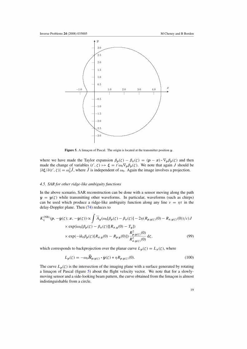
Figure 5. A limacon of Pascal. The origin is located at the transmitter position y.

where we have made the Taylor expansion βp(ζ ) − βx(ζ ) = (p − x) · ∇pβp(ζ ) and thenmade the change of variables (t ′, ζ ) �→ ξ = t ′ω0∇pβp(ζ ). We note that again J should be|∂ξ/∂(t ′, ζ )| = ω2

0J , where J is independent of ω0. Again the image involves a projection.

4.5. SAR for other ridge-like ambiguity functions

In the above scenario, SAR reconstruction can be done with a sensor moving along the pathy = y(ζ ) while transmitting other waveforms. In particular, waveforms (such as chirps)can be used which produce a ridge-like ambiguity function along any line ν = ητ in thedelay-Doppler plane. Then (74) reduces to

K(NB)η (p,−y(ζ );x,−y(ζ ))∝

∫Ay(ω0[βp(ζ )− βx(ζ )] − 2η(Rp,y(ζ )(0)− Rx,y(ζ )(0))/c)J

× exp(iω0[βp(ζ ) − βx(ζ )][Rx,y(0) − Ty])

× exp(−ik0βp(ζ )[Rx,y(0) − Rp,y(0)])R2

p,y(ζ )(0)

R2x,y(ζ )(0)

dζ, (99)

which corresponds to backprojection over the planar curve Lp(ζ ) = Lx(ζ ), where

Lp(ζ ) = −ω0Rp,y(ζ ) · y(ζ ) + ηRp,y(ζ )(0). (100)

The curve Lp(ζ ) is the intersection of the imaging plane with a surface generated by rotatinga limacon of Pascal (figure 5) about the flight velocity vector. We note that for a slowly-moving sensor and a side-looking beam pattern, the curve obtained from the limacon is almostindistinguishable from a circle.

19

Inverse Problems 24 (2008) 035005 M Cheney and B Borden

If we approximate the ridge-like ambiguity function as A(ν−ητ) = ∫exp[iω(ν−ητ)] dω,

then (99) can be written as

K(NB)η (p,u;x,v) ∝

∫exp(2ω[Lp(ζ )− Lx(ζ )]/c)J exp(iω0[βp(ζ )− βx(ζ )][Rx,y(0)− Ty])

× exp(−ik0βp(ζ )[Rx,y(0) − Rp,y(0)])R2

p,y(ζ )(0)

R2x,y(ζ )(0)

dω dζ

∝∫

exp([x − p] · ξ)J exp(iω0[βp(ζ ) − βx(ζ )][Rx,y(0) − Ty])

× exp(−ik0βp(ζ )[Rx,y(0) − Rp,y(0)])R2

p,y(ζ )(0)

R2x,y(ζ )(0)

∣∣∣∣∂(ω, θ)

∂ξ

∣∣∣∣ dξ, (101)

where we have made the Taylor expansion Lp(ζ ) − Lx(ζ ) = (p − x) · ∇pLp(ζ ) + · · · andhave made the change of variables (ω, ζ ) �→ ξ = 2ω∇pLp(ζ )/c.

4.6. Diffraction tomography

In this case the data is the far-field pattern (34). Our inversion formula is (84), where sy = 1and there is no integration over t. The resulting formula is

Ik0(p) =∫

eik0(z+y) · pQk0(z, y)F∞(y, z) dy dz, (102)

where Qk0 is the filter chosen according to [6],

Qk0 = k30

(2π)4|y + z|, (103)

which corrects for the Jacobian that is ultimately needed. Here the factor of k30 corresponds to

three-dimensional imaging.The associated point-spread function is obtained from substituting (34) into (102),

Ik0(p) =∫

eik0(z+y) · pQk0(z, y)

∫e−ik0(z+y) ·xq(x) d3x dy dz

= k30

(2π)4

∫eik0(z+y) · (p−x)|z + y| dy dzq(x) d3x

=∫

χ2k(ξ) eiξ · (p−x) d3ξq(x) d3x, (104)

where χ2k denotes the function that is one inside the ball of radius 2k and zero outside andwhere we have used the Devaney identity [6]∫

χ2k(ξ) eiξ · r d3ξ = k3

(2π)4

∫S2×S2

eik(y+z) · r|y + e′| dy dz. (105)

The proof of this identity is outlined in the appendix. The two-dimensional version is [7]∫χ2k(ξ) eiξ · r d2ξ =

∫S1×S1

eik(y+z) · r

∣∣∣∣ ∂ξ

∂(y, z)

∣∣∣∣ dy dz, (106)

where y = (cos θ, sin θ), z = (cos θ ′, sin θ ′) and∣∣∣∣ ∂ξ

∂(y, z)

∣∣∣∣ =√

1 − (y · z)2. (107)

20

Inverse Problems 24 (2008) 035005 M Cheney and B Borden

4.7. Moving target tomography

Moving target tomography has been proposed in the paper [9], which models the signal usinga simplified version of (21). For this simplified model, our imaging formula (70) reduces tothe approach advocated in [9], namely matched-filter processing with a different filter for eachlocation p and for each possible velocity u.

5. Conclusions and future work

We have developed a linearized imaging theory that combines the spatial, temporal and spectralaspects of scattered waves.

This imaging theory is based on the general (linearized) expression we derived for wavesscattered from moving objects, which we model in terms of a distribution in phase space. Theexpression for the scattered waves is of the form of a Fourier integral operator; consequently,we form a phase-space image as a filtered adjoint of this operator.

The theory allows for activation of multiple transmitters at different times, but the theoryis simpler when they are all activated so that the waves arrive at the target at roughly the sametime.

The general theory in this paper reduces to familiar results in a variety of special cases.We leave for the future further analysis of the point-spread function. We also leave for thefuture the case in which the sensors are moving independently, and the problem of combiningthese ideas with tracking techniques.

Acknowledgments

This work was supported by the Office of Naval Research, by the Air Force Office of ScientificResearch3 under agreement number FA9550-06-1-0017, by Rensselaer Polytechnic Institute,the Institute for Mathematics and its Applications, and by the National Research Council.

Appendix. The Devaney identity in R3

This proof of (105) follows [6]. First we note that for r ∈ R3,∫χ2k(ξ)

|ξ| eiξ · r d3ξ =∫ 2k

0

∫S2

eiξ · r d2ξ|ξ| d|ξ|

= 4π

∫ 2k

0

sin |ξ|r|ξ|r |ξ| d|ξ|

= 8π

r2

1 − cos(2kr)

2= 8π

r2sin2 kr, (A.1)

where we have written r = |r|. Using Stone’s formula [14]sin kr

kr= 1

4π

∫eiky · r d2y, (A.2)

we can write (A.1) as∫χ2k(ξ)

|ξ| eiξ · r d3ξ = k2

(2π)2

∫eik(y+z) · r d2y d2z. (A.3)

3 Consequently, the US Government is authorized to reproduce and distribute reprints for Governmental purposesnotwithstanding any copyright notation thereon. The views and conclusions contained herein are those of the authorsand should not be interpreted as necessarily representing the official policies or endorsements, either expressed orimplied, of the Air Force Research Laboratory or the US Government.

21

Inverse Problems 24 (2008) 035005 M Cheney and B Borden

Next, we write∫χ2k(ξ) eiξ · rd3ξ =

∫χ2k(ξ)

|ξ| eiξ · r|ξ| d3ξ

=∫

eiξ · r

[∫e−iξ · r′

(k2

(2π)4

∫eik(y+e′) · r′ dy de′

)]|ξ| d3ξ dr′. (A.4)

Carrying out the r′ integration results in δ(ξ − k(y + z)); finally, carrying out the ξ integrationresults in (105).

References

[1] Bleistein N, Cohen J K and Stockwell J W 2000 The Mathematics of Multidimensional Seismic Inversion (NewYork: Springer)

[2] Borden B and Cheney M 2005 Synthetic-aperture imaging from high-Doppler-resolution measurements InverseProblems 21 1–11

[3] Bradaric I, Capraro G T, Weiner D D and Wicks M C 2006 Multistatic radar systems signal processing Proc.IEEE Radar Conf.

[4] Cooper J 1980 Scattering of electromagnetic fields by a moving boundary: the one-dimensional case IEEEAntennas Propag. AP-28 791–5

[5] Cook C E and Bernfeld M 1967 Radar Signals (New York: Academic)[6] Devaney A J 1982 Inversion formula for inverse scattering within the Born approximation Opt. Lett. 7 111–2[7] Devaney A J 1982 A filtered backpropagation algorithm for diffraction tomography Ultrason. Imaging 4 336–50[8] Friedlander B and Porat B 1997 VSAR: a high resolution radar system for detection of moving targets IEE

Proc. Radar Sonar Navig. 144 205–18[9] Himed B, Bascom H, Clancy J and Wicks M C 2001 Tomography of moving targets (TMT) Sensors, Systems,

and Next-Generation Satellites V (Proc. SPIE vol 4540) ed H Fujisada, J B Lurie and K Weber pp 608–19[10] Klemm R 2002 Principles of Space-Time Adaptive Processing (London: Institution of Electrical Engineers)[11] Levanon N 1988 Radar Principles (New York: Wiley)[12] Minardi M J, Gorham L A and Zelnio E G 2005 Ground moving target detection and tracking based on

generalized SAR processing and change detection Proc. SPIE 5808 156–65[13] Nolan C J and Cheney M 2002 Synthetic aperture inversion Inverse Problems 18 221–36[14] Reed M and Simon B 1972 Methods of Modern Mathematical Physics: I. Functional Analysis (New York:

Academic)[15] Soumekh M 1991 Bistatic synthetic aperture radar inversion with application in dynamic object imaging IEEE

Trans. Signal Process. 39 2044–55[16] Stuff M, Biancalana M, Arnold G and Garbarino J 2004 Imaging moving objects in 3D from single aperture

synthetic aperture radar Proc. IEEE Radar Conf. pp 94–8[17] Swick D 1969 A review of wideband ambiguity functions Naval Res. Lab. Rep. 6994[18] Tsao T, Slamani M, Varshney P, Weiner D, Schwarzlander H and Borek S 1997 Ambiguity function for a

bistatic radar IEEE Trans. Aerosp. Electron. Syst. 33 1041–51[19] Willis N J 1991 Bistatic Radar (Norwood, MA: Artech House)[20] Willis N J and Griffiths H D 2007 Advances in Bistatic Radar (Raleigh, NC: SciTech Publishing)[21] Willis N J 1990 Bistatic Radar Radar Handbook ed M Skolnik (New York: McGraw-Hill)[22] Woodward P M 1953 Probability and Information Theory, with Applications to Radar (New York: McGraw-

Hill)[23] Yazici B, Cheney M and Yarman C E 2006 Synthetic-aperture inversion in the presence of noise and clutter

Inverse Problems 22 1705–29

22