A Recurrent Quantum Neural Network Model to Describe

Eye Tracking of Moving Targets

Laxmidhar BeheraDepartment of Electrical Engineering

Indian Institute of Technology, Kanpur

208 016, UP, INDIA

email: lbehera@iitk.ac.in

Indrani KarDepartment of Electrical Engineering

Indian Institute of Technology, Kanpur

208 016, UP, INDIA

email: indranik@iitk.ac.in

Avshalom C. Elitzur∗

Unit of Interdisciplinary Studies,

Bar-IIan University,

52900 Ramat-Gan, Israel

email: avshalom.elitzur@weizmann.ac.il

A theoretical quantum neural network model is proposed using a

nonlinear Schrodinger wave equation. The model proposes that there

exists a nonlinear Schrodinger wave equation that mediates the col-

lective response of a neural lattice. The model is used to explain eye

movements when tracking moving targets. Using a Recurrent Quantum

Neural Network(RQNN) while simulating the eye tracking model, two

very interesting phenomena are observed. First, as eye sensor data is

processed in a classical neural network, a wave packet is triggered in

∗ Corresponding author

2

the quantum neural network. This wave packet moves like a particle.

Second, when the eye tracks a fixed target, this wave packet moves

not in a continuous but rather in a discrete mode. This result reminds

one of the saccadic movements of the eye consisting of ’jumps’ and

’rests’. However, such a saccadic movement is intertwined with smooth

pursuit movements when the eye has to track a dynamic trajectory. In

a sense, this is the first theoretical model explaining the experimental

observation reported concerning eye movements in a static scene situa-

tion. The resulting prediction is found to be very precise and efficient in

comparison to classical objective modeling schemes such as the Kalman

filter.

Key words: nonlinear Schrodinger wave equation, quantum dynamics,

saccadic eye movements, neural network, quantum computation

1. INTRODUCTION

Information processing in the brain is mediated by the dynamics of

large, highly interconnected neuronal populations. The activity pat-

terns exhibited by the brain are extremely rich; they include stochastic

weakly correlated local firing, synchronized oscillations and bursts, as

3

well as propagating waves of activity. Perception, emotion etc. are sup-

posed to be emergent properties of such a complex nonlinear neural

circuit.

Instead of considering one of the conventional neural architectures

(Cohen and Grossberg, 1983; Amari, 1983; Behera et al., 1996; Behera

et al., 1998; Amit, 1989), an alternative neural architecture is proposed

here for neural computing. Indeed, there are certain aspects of brain

functions that still appear to have no satisfactory explanation. As an

alternative, researchers (Tuszynski et al., 1995; Vitiello, 1995; Hagan

et al., 2002; Mershin et al., 1999) are investigating whether the brain

can demonstrate quantum mechanical behavior. According to current

research, microtubules, the basic components of neural cytoskeleton,

are very likely to possess quantum mechanical properties due to their

size and structure. The tubulin protein, which is the structural block of

microtubules, has the ability to flip from one conformation to another as

a result of a shift in the electron density localization from one resonace

orbital to another. These two conformations act as two basis states

of the system according to whether the electrons inside the tubuline

hydrophobic pocket are localized closer to α or β tubulin. Moreover the

system can lie in a superposition of these two basis states, that is, being

in both states simultaneously, which can give a plausible mechanism

for creating a coherent state in the brain. To give credence to the

4

possibility of existence of a quantum brain, Penrose (Penrose, 1994)

argued that the human brain must utilize quantum mechanical effects

when demonstrating problem solving feats that cannot be explained

algorithmically.

In this paper, instead of going into biological details of the brain,

we propose a theoretical model to explain eye movements. The model

is referred to as Recurrent Quantum Neural Network (RQNN) in-

spired by the research on quantum neral networks (Gupta and Zia,

2001; Behrman et al., 2000; Behrman et al., 2002). An earlier version

(Behera and Sundaram, 2004) of this model used a linear neural circuit

to set up the potential field that excited the dynamics of Schrodinger

wave equation. The present model uses a nonlinear neural circuit. This

fundamental change in the architecture has yielded two novel features.

The wave packets, f(x, t) =| ψ(x, t) |2, are moving like particles. Here

ψ(x, t) is the solution of the nonlinear Schrodinger wave equation that

describes the closed loop dynamics of quantum neural network model

proposed in this paper to explain eye movements for tracking moving

targets. The other very interesting observation is that the movements

of the wave packets while tracking a fixed target are not continuous

but discrete. These observations accord with the well-known saccadic

movement of the eye (Bahill and Stark, 1979). In a way, our model is

the first of its kind to explain the nature of eye movements in static

5

scenes that consists of ”jumps” (saccades) and ”rests” (fixations). We

expect this result to inspire other researchers to further investigate the

possible quantum dynamics of the brain.

2. A COLLECTIVE RESPONSE MODEL USING

SCHROEDINGER WAVE EQUATION

An impetus to hypothesize a novel neural information processing model

comes from the brain’s necessity to unify the neuronal response into

a single percept. Anatomical, neurophysiological and neuropsycholog-

ical evidence, as well as brain imaging using fMRI and PET scans,

show that separate functional maps exist in the biological brain to

code separate features such as direction of motion, location, color and

orientation. How does the brain compute all this data to have a coherent

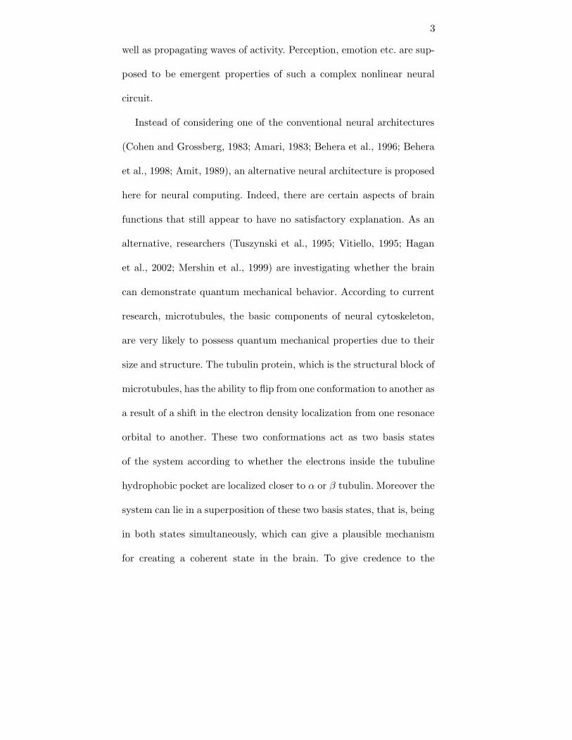
perception? In this paper, a very simple model of a quantum brain is

proposed where a collective response of a neuronal lattice is modeled

using a Schrodinger wave equation as shown in Figure. 1. In this figure,

it is shown that a quantum process models average behavior (collective

response) of a neural lattice.

We suggest that the time evolution of the collective response ψ is

described by the Schrodinger wave equation:

6

i~∂ψ(x, t)

∂t= −

~2

2m∇2ψ(x, t) + V (x)ψ(x, t) (1)

where 2π~ is Planck’s constant, ψ(x, t) is the wave function (proba-

bility amplitude) associated with the quantum object at space-time

point(x, t), and m the mass of the quantum object. Further symbols

such as i and ∇ carry their usual meaning in the context of Schrodinger

wave equation. Another way to look at our proposed quantum neural

network is as follows. A neuronal lattice sets up a spatial potential

field V (x). A quantum process described by a quantum state ψ which

mediates the collective response of a neuronal lattice evolves in the

spatial potential field V (x) according to Eq. 1. Thus the classical neural

lattice sets up a spatio-temporal potential field for the Schrodinger wave

equation and the solution ψ carries the information about the collec-

tive behavior. In the next section, we present a possible eye-movement

model for tracking moving target.

3. AN EYE TRACKING MODEL

Let us consider a plausible biological mechanism for eye tracking us-

ing the RQNN model proposed in section 2. The mechanism of eye

7

movements, tracking a moving target, consists of three stages as shown

in Figure. 2: (i) stochastic filtering of noisy data that impact the eye

sensors; (ii) a predictor that predicts the next spatial position of the

moving target; and (iii) a biological motor control system that aligns

the eye pupil along the moving targets trajectory. The biological eye

sensor fans out the input signal y to a specific neural lattice in the visual

cortex. For clarity, Figure 2 shows a one-dimensional array of neurons

whose receptive fields are excited by the signal input y reaching each

neuron through a synaptic connection described by a nonlinear map.

The neural lattice responds to the stimulus by setting up a spatial

potential field, V (x, t), which is a function of external stimulus y and

estimated trajectory y of the moving target:

V (x, t) =n∑

i=1

Wi(x, t)φi(ν(t)) (2)

where φi(.) is a Gaussian Kernel function, n represents the number of

such Gaussian functions describing the nonlinear map that represents

the synaptic connections, ν(t) represents the difference between y and

y and W represents the synaptic weights as shown in Figure. 2. The

Gaussian kernel function is taken as:

φi(ν(t)) = exp(−(ν(t) − gi)2) (3)

8

where gi is the center of the ith Gaussian function, φi. This center is

chosen from input space described by the input signal, ν(t), through

uniform random sampling.

Our model proposes that a quantum process mediates the collective

response of this neuronal lattice which sets up a spatial potential field

V (x, t). This happens when the quantum state associated with this

quantum process evolves in this potential field. The spatio-temporal

evolution follows as per Eq. 1. We hypothesize that this collective re-

sponse is described by a wave packet, f(x, t) =| ψ(x, t) |2, where the

term ψ(x, t) represents a quantum state. In a generic sense, we assume

that a classical stimulus in a brain triggers a wave packet in the coun-

terpart ’RQNN ’. This subjective response, f(x, t), is quantified using

the following estimate equation:

y(t) =

∫

x(t)f(x, t)dx (4)

The estimate equation is motivated by the fact that the wave packet,

f(x, t) =| ψ(x, t) |2 is interpreted as the probability density function.

Although computation of Eq. 4 using nonlinear Schrodinger wave equa-

tion is straight forward, it may be interesting to see if this computation

can be done through interaction of quantum brain and classical brain

using suitable quantum measurement operator. At this point we will

9

not speculate about the nature of such quantum measurement operator

that will estimate the ψ function that is necessary to compute Eq.

4. Based on this estimate, y, the predictor estimates the next spatial

position of the moving target. To simplify our analysis, the predictor

is made silent. Thus its output is the same as that of y. The biologi-

cal motor control is commanded to fixate the eye pupil to align with

the target position, which is predicted to be at y. Obviously, we have

assumed that biological motor control is ideal.

After the above mentioned simplification, the closed form dynamics

of the model described by Figure 2 becomes:

i~∂ψ(x, t)

∂t= −

~2

2m∇2ψ(x, t) + ζG

(

y(t) −

∫

x | ψ(x, t) |2 dx

)

ψ(x, t)

(5)

where G(.) is a Gaussian kernel map introduced to nonlinearly modu-

late the spatial potential field that excites the dynamics of the quantum

object. In fact ζG(.) = V (x, t) where V (x, t) is given in Eq. 2.

The nonlinear Schrodinger wave equation given by Eq. 5 is one-

dimensional with cubic nonlinearity. Interestingly, the closed form dy-

namics of the Recurrent Quantum Neural Network (Eq. 5) closely re-

sembles a nonlinear Schrodinger wave equation with cubic nonlinearity

studied in quantum electrodynamics (Gupta and Zia, 2001):

10

i~∂ψ(x, t)

∂t=

(

−~

2

2m∇2 −

e2

r

)

ψ(x, t) + e2∫

ψ(x, t) | ψ(x′, t) |2

| x− x′ |dx′

(6)

where m is the electron mass, e the elementary charge and r the

magnitude of | x |. Also, nonlinear Schrodinger wave equations with

cubic nonlinearity of the form ∂

∂tA(t) = c1A + c3 | A |2 A, where

c1 and c3 are constants, frequently appear in nonlinear optics (Boyd,

1991) and in the study of solitons (Jackson, 1991; Bialynicki-Birula

and Mycielski, 1976; Davydov, 1982; Scott et al., 1973). Application of

nonlinear Schrodinger wave equation for the study of quantum systems

can also be found in (Sulem et al., 1999).

In Eq. 5, the unknown parameters are weights Wi(x, t) associated

with the Gaussian kernel, mass m, and ζ, the scaling factor to actuate

the spatial potential field. The weights are updated using the Hebbian

learning algorithm

∂Wi(x, t)

∂t= βφi(ν(t))f(x, t) (7)

where ν(t) = y(t) − y(t).

The idea behind the proposed quantum computing model is as fol-

lows. As an individual observes a moving target, the uncertian spatial

11

position of the moving target triggers a wave packet within RQNN.

The RQNN is so hypothesized that this wave packet turns out to be

a collective response of a classical neural lattice. As we combine Eq.s

5 and 7, it is desired that there exist some parameters m, ζ and β

such that each specific spatial position x(t) triggers a unique wave

packet, f(x, t) =| ψ(x, t) |2, in RQNN. This brings us to the question

whether the closed form dynamics can exhibit soliton properties which

is desirable for target tracking. As pointed out above, our equation has

a form that is known to possess soliton properties for a certain range of

parameters and we just have to find those parameters for each specific

problem.

We would like to reiterate the importance of the soliton properties.

According to our model, eye tracking means tracking of a wave packet in

the domain of RQNN. The biological motor control aligns the eye pupil

along the spatial position of the external target that the eye tracks. As

the eye sensor receives data y from this position, the resulting error

stimulates RQNN dynamics. In a noisy background, if the tracking is

accurate, then this error correcting signal ν(t) has little effect on the

movement of the wave packet. Precisely, it is the actual signal content

in the input y(t) that moves the wave packet along the desired direction

which, in effect, achieves the goal of the stochastic filtering part of the

eye movement for tracking purposes.

12

4. SIMULATION RESULTS

In this section we present simulation results to test target tracking

through eye movement where targets are either fixed or moving.

For fixed target tracking, we have simulated a stochastic filtering

problem of a dc signal embedded in Gaussian noise. As the eye tracks

a fixed target, the corresponding dc signal is taken as ya(t) = 2.0,

embedded in Gaussian noise with SNR (signal to noise ratio)values of

20 dB, 6 dB and 0 dB.

We compare the results with the performance of a Kalman filter

(Grewal and Andrews, 2001) designed for this purpose. It should be

noted that the Kalman filter has the a priori knowledge that the em-

bedded signal is a dc signal whereas the RQNN is not provided with

this knowledge. The Kalman filter also makes use of the fact that the

noise is Gaussian and estimates the variance of the noise based on this

assumption. Thus it is expected that the performance of the Kalman

filter will degrade as the noise becomes non-Gaussian. In contrast, the

RQNN model does not make any assumption about the noise.

It is observed that there are certain values of β, m, ζ and N for

which the model performs optimally. A univariate marginal distribution

algorithm (Behera and Sundaram, 2004) was used to get near optimal

parameters while fixing N = 400 and ~ = 1.0. The selected values of

13

these parameters are as follows for all levels of SNR:

β = 0.86; m = 2.5; ζ = 2000; (8)

The comparative performance of eye tracking in terms of rms error for

all the noise levels is shown in Table I. It is easily seen from Table I

that the rms tracking error of RQNN is much less than that of the

Kalman filter. Moreover, RQNN performs equally well for all the three

categories of noise levels, whereas the performance of the Kalman filter

degrades with the increase in noise level. In this sense we can say that

our model performs the tracking with a greater efficiency compared to

the Kalman filter. The exact nature of trajectory tracking is shown for

0 dB SNR in Figure. 3. In this figure, the noise envelope is shown, and

obviously its size is large due to a high noise content in the signal. The

figure shows the trajectory of the eye movement as the eye focuses on

a fixed target. To better appreciate the tracking performance, an error

plot is shown in Figure. 4. Although Kalman filter tracking is continu-

ous, the RQNN model tracking consists of ’jumps’ and ’fixations’. As

the alignment of the eye pupil becomes closer to the target position,

the ’fixation’ time also increases. Similar tracking behaviour was also

observed for the SNR values of 20 and 6 dB. These theoretical re-

sults are very interesting when compared to experimental results in the

14

Table I. Performance comparison betweenKalman filter and RQNN for various levels ofGaussian noise

Noise level RMS error RMS error

in dB for Kalman filter for RQNN

20 0.0018 0.000040

6 0.0270 0.000062

0 0.0880 0.000090

field of eye-tracking. In eye-tracking experiments, it is known that eye

movements in static scenes are not performed continuously, but consist

of ”jumps” (saccades) and ”rests” (fixations). Eye-tracking results are

represented as lists of fixation data. Furthermore, if the information

is simple or familiar, eye movement is comparatively smooth. If it is

tricky or new, the eye might pause or even flip back and forth between

images. Similar results are given by our simulations. Our model tracks

the dc signal which can be thought of as equivalent to a static scene, in

discrete steps rather than in a continuous fashion. This is very clearly

understood from the tracking error in Figure. 4. The other interesting

aspect of the results is the movement of wave packets. It is observed

that these wave packets move in discrete steps i.e., the movement is

not continuous. In Figure 3 (bottom), snapshots of wave packets are

plotted at different instances corresponding to marker points as shown

along the desired trajectory. It can be noticed that a very flat initial

15

Gaussian wave packet first moves to the left, and then proceeds toward

the right until the mean of the wave packet exactly matches the actual

spatial position. A similar pattern of movement of wave packets was

also noticed in the case of 20 and 6dB SNR. The wave packet movement

is compared with our previous work (Behera and Sundaram, 2004) in

Figure. 5. The initial wave packet in the previous model first splits

into two parts, then moves in a continuous fashion, ultimately going

into a state with a mean of approximately 2 but with high variance. In

contrast, in the present model there is no splitting of the wave packet,

movement is discrete and variance is also much smaller. Thus the soliton

behavior of the present model is very much pronounced.

To analyze the eye movement following a moving target, a sinusoidal

signal ya(t) = 2sin2π10t is taken as the desired dynamic trajectory.

This signal is embedded in 20 dB Gaussian noise. The parameter values

for tracking this signal were fixed at β = 0.01,m = 1.75 and ζ = −250.

It is observed that during the training phase, the wave packet jumps

from time to time, thus changing the tracking error in steps until a

steady state trajectory following is achieved. This feature can be better

understood from the tracking error plot which is shown in Figure. 6.

In this figure we have plotted the tracking error between the actual

sinusoidal signal and the predicted signal using the estimate Eq. 4. It

is clearly seen that in the first stage of tracking, the error is fluctuating

16

very frequently between its local maximum and minimum values in

the negative region. Then this fluctuation settles down in the second

stage. In the third stage this fluctuation started again and the error is

flipping between the local maxima and minima in the positive region.

As the estimation (refer Eq. 4) of the signal is very much dependent

on the nature of wave packet, the error dynamics is also correlated

with the wave packet movement. Discontinuties in error reflect in the

movement of wave packet. It is seen that the position of the wave packet

is changing very frequently in the first stage, thus changing the mean

value correspondingly and it has no connection with the signal mean

value. That means there are a number of discontinuties or ’jumps’ in

the wave packet movement in the first stage. Then in the second stage

the movement becomes continuous with the mean values following the

signal mean values. Again in the third stage the discontinuties took

place several times ultimately achieving a steady state movement in

the last stage. Once steady state is achieved, the tracking is efficient

and the wave packet movement is continuous as shown in Figure. 7. In

this figure, the snapshots of wave packets are plotted for three different

instances of time indicated by the marker points (1,2,3) as shown in the

trajectory tracking. When the signal is at position 1, the corresponding

wave packet has a mean at 0. When the signal is at position 2, the

corresponding wave packet has a mean at +2, and the mean of the wave

17

packet moves to -2 when the signal goes to position 3. As seen in Figure

7 during continuous movement of the wave packets, trajectory tracking

is smooth which is similar to smooth pursuit movement in the context

of biological eye tracking. Moreover eye tracking experiments reveal

that humans track smoothly moving objects with a combination of

saccadic and smooth pursuit eye movements, called dual mode tracking

(Bahill et al., 1980). This experimental result completely agrees with

the obeseravtion when our theoretical model tracks a smoothly varying

trajectory.

5. CONCLUSION

The nature of eye movement has been studied in this article using

the proposed RQNN model, where the predictor and motor control are

assumed to be ideal. The most important finding is that our theoretical

model of eye-tracking agrees with previously observed experimental

results. The model predicts that eye movements will be of saccadic type

while following a static trajectory. In the case of dynamic trajectory

following, eye movement consists of saccades and smooth pursuits. In

this sense, the proposed RQNN concept in this paper is very successful

in explaining the nature of eye movements. Earlier explanation (Bahill

18

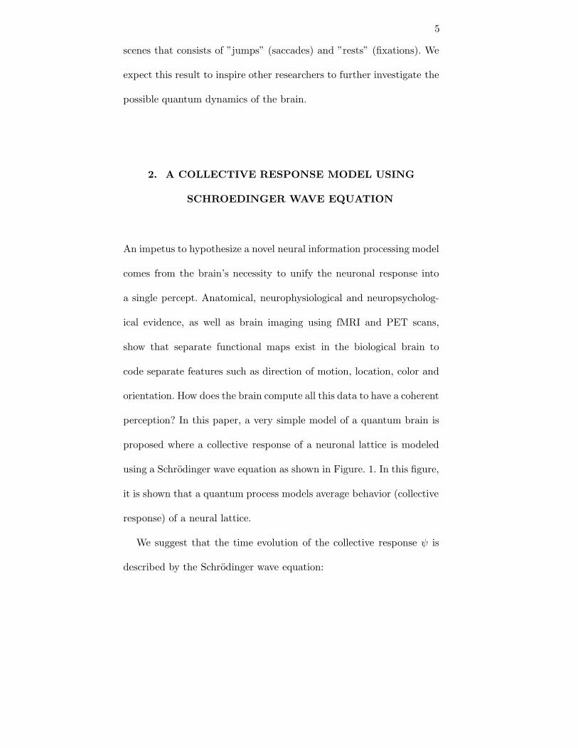
and Stark, 1979) for saccadic movement has been primarily attributed

to motor control mechanism whereas the present model emphasizes that

such eye movements are due to decision making process of the brain -

albeit quantum brain. Thus the significant contribution of this paper

to explain biological eye-movement as a neural information processing

event may inspire researchers to study quantum brain models from the

biological perspective.

The other significant contribution of this paper is the prediction

efficiency of the proposed model over the prevailing model. The stochas-

tic filtering of a dc signal using RQNN is 1000 times more accurate

compared to a Kalman filter.

We intend to replace Schrodinger wave equation by density matrix

approach in our future work. Also, the phase transition analysis of

closed form dynamics, given in Eq. 5 with respect to various parameters

m, ζ, β and N , has been kept for future work.

Finally, we believe that apart from the computational power derived

from quantum computing, quantum learning systems will also provide a

potent framework to study the subjective aspects of the nervous system

(Atmanspacher, 2004). The challenge to bridge the gap between phys-

ical and mental (or objective and subjective) notions of matter may

be most successfully met within the framework of quantum learning

systems. In this framework, we have proposed a notion of RQNN that

19

may trigger further excitement in the field of quantum brain. Infact the

RQNN model proposed in this paper is a first step towards a neural

computing model of eye movement.

References

Amari, S.: “Field theory of self-organizing neural nets,” IEEE TRAN. SMC 13(5),

741–748, (1983).

Amit, D.: Modeling brain function (Springer, Berlin/Heidelberg, 1989).

Atmanspacher, H.: “Quantum theory and consciousness: an overview with selected

examples,” DISCRETE DYNAMICS 8, 51–73, (2004).

Bahill, A. T., M. J. Iandolo, and B. T. Troost: “Smooth Pursuit Eye Movements in

response to unpredictable target waveforms,” VISION RESEARCH 20, 923–931,

(1980).

Bahill, A. T. and L. Stark: “The Trajectories of Saccadic Eye Movements,”

SCIENTIFIC AMERICAN 240, 84–93, (1979).

Behera, L., S. Chaudhury, and M. Gopal: “Applications of self-organizing neural

networks in robot tracking control,” IEE PROC. CONTROL TH. AND APPL.

145, 134–140, (1998).

Behera, L., M. Gopal, and S. Chaudhury: “On adaptive control of a robot manipu-

lator using inversion of its neural emulator,” IEEE TRAN. NEURAL NET. 7,

1401–1414, (1996).

20

Behera, L. and B. Sundaram: “Stochastic filtering and Speech Enhancement using

a Recurrent Quantum Neural Network,” PROCEEDINGS, ICISIP 165–170,

(2004).

Behrman, E. C., V. Chandrashekar, Z. Wang, C. K. Belur, J. Steck, and S. R.

Skinner: “A quantum neural network computes entanglement,” PHYSICAL

REVIEW LETTERS. Submitted, 2002.

Behrman, E. C., L. R. Nash, J. E. Steck, V. G. Chandrashekar, and S. R. Skinner:

“Simulations of Quantum Neural Networks,” INFORMATION SCIENCES 128,

257–269, (2000).

Bialynicki-Birula, I. and J. Mycielski: “Nonlinear wave mechanics,” ANNALS OF

PHYSICS 100, 62–93, (1976).

Boyd, R.: Nonlinear Optics (Academic Press, 1991).

Cohen, M. A. and S. Grossberg: “Absolute stability of global pattern formation and

parallel memory storage by competitive neural networks,” IEEE TRAN. SMC

13, 815–826, (1983).

Davydov, A. S.: Biology and Quantum Mechanics (Pergamon, Oxford, 1982).

Grewal, M. S. and A. P. Andrews: Kalman Filtering : Theory and Practice Using

MATLAB (Wiley-Interscience, 2001).

Gupta, S. and R. Zia: “Quantum neural networks,” JOURNAL OF COMPUTER

AND SYST. SCI. 63, 355–383, (2001).

Hagan, S., S. R. Hameroff, and J. A. Tuszynski: “Quantum Computation in Brain

Microtubules? Dehoherence and Biological Feasibility,” PHYSICAL REVIEW

E 65, 061901, (2002).

Jackson, E. A.: Perspectives of Nonlinear Dynamics (Cambridge, 1999).

Mershin, A., D. V. Nanopoulos, and E. Skoulakis: “Quantum Brain?,” PROC.

ACAD. ATHENS 74, 148–179, (1999).

21

Penrose, R.: Shadows of the Mind (Oxford University Press, 1994).

Scott, A. C., F. Y. F. Chu, and D. W. McLaughlin: “The Soliton: A New Concept

in Applied Science,” PROC. IEEE 61, (1973).

Sulem, C., P. L. Sulem, and C. Sulem: Nonlinear Schrodinger Equations: Self-

Focusing and Wave Collapse (Springer, 1999, Applied Mathematical Sci-

ences/139).

Tuszynski, J. A., S. R. Hameroff, M. V. Sataric, B. Trpisova, and M. L. A.

Nip: “Ferroelectric behavior in microtubule dipole lattices: implications for in-

formation processing, signaling and assembly/disassembly,” JOURNAL OF

THEORETICAL BIOLOGY 174, 371–380, (1995).

Vitiello, G.: “Dissipation and memory capacity in the quantum brain model,” INT.

JOURNAL OF MODERN PHYSICS B 9, 973–989, (1995).

22

Figure Captions

Fig.1: Conceptual framework for the Recurrent Quantum Neural Net-works.

Fig.2: Conceptual framework for the Recurrent Quantum Neural Net-works.

Fig.3: (left) Eye tracking of a fixed target in a noisy environment of0 dB SNR: ’a’ respresents fixed target, ’b’ represents target trackingusing RQNN model and ’c’ represents target tracking using a Kalmanfilter. The noise envelope is represented by the curve ’d’; (right) Thesnapshots of the wave packets at different instances corresponding tothe marker points (1,2,3) as shown in the left figure. The solid linerepresent the initial wave packet assigned to the Schrodinger waveequation.

Fig.4: The continuous line represents tracking error using RQNN modelwhile the broken line represents tracking error using Kalman filter.

Fig.5: Wave packet movements for RQNN with linear weights.Fig.6: Saccadic and pursuit movement of eye during dynamic trajectoryfollowing.

Fig.7: (top) Eye tracking of a moving target in a noisy environmentof 20dB SNR: ’a’ respresents a moving target, ’b’ represents targettracking using RQNN model; (bottom) The snapshots of the wave pack-ets at different instances corresponding to the marker points (1,2,3) asshown in the top figure. The solid line represents the initial wave packetassigned to the Schrodinger wave equation.

23

Figures

y +

y

−

∑

Unified response

is a pdf or a

wave packet

A quantum process

predicts the

average response

of a neural lattice

Figure 1.

y

1 1W11

WnNn N

V (x)

.

.

⊗

..

.

.

motor control predictor

Quantum

activation

function

(Schrodinger

wave equation)

∫

ψ∗xψdxψ

−

+ y

Figure 2.

24

0 1 2 3 4t

-6

-4

-2

0

2

4

6

8

10

y a(t)

abcd

1

2

3

-3 -2 -1 0 1 2 3x

0

2

4

6

8

10

f(x)

123

Initial

Figure 3.

25

0 1 2 3 4t

-0.5

0

0.5

1

1.5

2

2.5

trac

king

err

or

Figure 4.

-20 -10 0 10 20x

0

0.1

0.2

0.3

0.4

f(x)

123

Initial Wave Packet

Figure 5.

26

0 2 4 6 8 10t

-4

-2

0

2

4

6

8

trac

king

err

or

Figure 6.

27

6 6.25 6.5 6.75 7t

-2

0

2

y a(t)

ab

1

2

3

-4 -2 0 2 4x

0

0.5

1

1.5

2

f(x)

123

Initial

Figure 7.