Quantum Stochastic Processes and Quantum non-Markovian ...
81
PRX QUANTUM 2, 030201 (2021) Tutorial Quantum Stochastic Processes and Quantum non-Markovian Phenomena Simon Milz 1, * and Kavan Modi 2, † 1 Institute for Quantum Optics and Quantum Information, Austrian Academy of Sciences, Boltzmanngasse 3, Vienna 1090, Austria 2 School of Physics and Astronomy, Monash University, Clayton, Victoria 3800, Australia (Received 2 November 2020; revised 19 April 2021; published 14 July 2021) The field of classical stochastic processes forms a major branch of mathematics. Stochastic processes are, of course, also very well studied in biology, chemistry, ecology, geology, finance, physics, and many more fields of natural and social sciences. When it comes to quantum stochastic processes, however, the topic is plagued with pathological issues that have led to fierce debates amongst researchers. Recent devel- opments have begun to untangle these issues and paved the way for generalizing the theory of classical stochastic processes to the quantum domain without ambiguities. This tutorial details the structure of quan- tum stochastic processes, in terms of the modern language of quantum combs, and is aimed at students in quantum physics and quantum-information theory. We begin with the basics of classical stochastic pro- cesses and generalize the same ideas to the quantum domain. Along the way, we discuss the subtle structure of quantum physics that has led to troubles in forming an overarching theory for quantum stochastic pro- cesses. We close the tutorial by laying out many exciting problems that lie ahead in this branch of science. DOI: 10.1103/PRXQuantum.2.030201 CONTENTS I. INTRODUCTION 2 II. CLASSICAL STOCHASTIC PROCESSES: SOME EXAMPLES 3 A. Statistical state 3 B. Memoryless process 4 C. Markov process 4 D. Non-Markovian processes 5 E. Stochastic matrix 5 1. Transforming the statistical state 6 2. Random process 6 3. Markov process 7 4. Non-Markovian process 7 F. Hidden Markov model 9 G. (Some) mathematical rigor 11 III. CLASSICAL STOCHASTIC PROCESSES: FORMAL APPROACH 11 A. What then is a stochastic process? 12 B. Kolmogorov extension theorem 12 * [email protected] † [email protected] Published by the American Physical Society under the terms of the Creative Commons Attribution 4.0 International license. Fur- ther distribution of this work must maintain attribution to the author(s) and the published article’s title, journal citation, and DOI. C. Practical features of stochastic processes 14 1. Master equations 14 2. Divisible processes 15 3. Data-processing inequality 16 4. Conditional mutual information 17 D. (Some more) mathematical rigor 18 IV. EARLY PROGRESS ON QUANTUM STOCHASTIC PROCESSES 19 A. Quantum statistical state 20 1. Decomposing quantum states 21 2. Measuring quantum states: POVMs and dual sets 22 B. Quantum stochastic matrix 23 1. Linearity and tomography 24 2. Complete positivity and trace preservation 25 3. Representations 26 4. Purification and dilation 28 C. Quantum master equations 29 D. Witnessing non-Markovianity 31 1. Initial correlations 31 2. Completely positive and divisible processes 33 3. Snapshot 34 4. Quantum data-processing inequalities 34 E. Troubles with quantum stochastic processes 35 1. Breakdown of KET in quantum mechanics 35 2. Input-output processes 36 3. KET and spatial quantum states 37 2691-3399/21/2(3)/030201(81) 030201-1 Published by the American Physical Society
-
Upload
khangminh22 -
Category
Documents
-
view
0 -
download
0
Transcript of Quantum Stochastic Processes and Quantum non-Markovian ...
PRX QUANTUM 2, 030201 (2021)Tutorial
Quantum Stochastic Processes and Quantum non-Markovian Phenomena
Simon Milz 1,* and Kavan Modi 2,†
1Institute for Quantum Optics and Quantum Information, Austrian Academy of Sciences, Boltzmanngasse 3,
Vienna 1090, Austria2School of Physics and Astronomy, Monash University, Clayton, Victoria 3800, Australia
(Received 2 November 2020; revised 19 April 2021; published 14 July 2021)
The field of classical stochastic processes forms a major branch of mathematics. Stochastic processesare, of course, also very well studied in biology, chemistry, ecology, geology, finance, physics, and manymore fields of natural and social sciences. When it comes to quantum stochastic processes, however, thetopic is plagued with pathological issues that have led to fierce debates amongst researchers. Recent devel-opments have begun to untangle these issues and paved the way for generalizing the theory of classicalstochastic processes to the quantum domain without ambiguities. This tutorial details the structure of quan-tum stochastic processes, in terms of the modern language of quantum combs, and is aimed at students inquantum physics and quantum-information theory. We begin with the basics of classical stochastic pro-cesses and generalize the same ideas to the quantum domain. Along the way, we discuss the subtle structureof quantum physics that has led to troubles in forming an overarching theory for quantum stochastic pro-cesses. We close the tutorial by laying out many exciting problems that lie ahead in this branch of science.
DOI: 10.1103/PRXQuantum.2.030201
CONTENTS
I. INTRODUCTION 2II. CLASSICAL STOCHASTIC PROCESSES:
SOME EXAMPLES 3A. Statistical state 3B. Memoryless process 4C. Markov process 4D. Non-Markovian processes 5E. Stochastic matrix 5
1. Transforming the statistical state 62. Random process 63. Markov process 74. Non-Markovian process 7
F. Hidden Markov model 9G. (Some) mathematical rigor 11
III. CLASSICAL STOCHASTIC PROCESSES:FORMAL APPROACH 11A. What then is a stochastic process? 12B. Kolmogorov extension theorem 12
*[email protected]†[email protected]
Published by the American Physical Society under the terms ofthe Creative Commons Attribution 4.0 International license. Fur-ther distribution of this work must maintain attribution to theauthor(s) and the published article’s title, journal citation, andDOI.
C. Practical features of stochastic processes 141. Master equations 142. Divisible processes 153. Data-processing inequality 164. Conditional mutual information 17
D. (Some more) mathematical rigor 18IV. EARLY PROGRESS ON QUANTUM
STOCHASTIC PROCESSES 19A. Quantum statistical state 20
1. Decomposing quantum states 212. Measuring quantum states: POVMs and
dual sets 22B. Quantum stochastic matrix 23
1. Linearity and tomography 242. Complete positivity and trace preservation 253. Representations 264. Purification and dilation 28
C. Quantum master equations 29D. Witnessing non-Markovianity 31
1. Initial correlations 312. Completely positive and divisible
processes 333. Snapshot 344. Quantum data-processing inequalities 34
E. Troubles with quantum stochastic processes 351. Breakdown of KET in quantum mechanics 352. Input-output processes 363. KET and spatial quantum states 37
2691-3399/21/2(3)/030201(81) 030201-1 Published by the American Physical Society
SIMON MILZ and KAVAN MODI PRX QUANTUM 2, 030201 (2021)
V. QUANTUM STOCHASTIC PROCESSES 38A. Subtleties of the quantum state and quantum
measurement 38B. Quantum measurement and instrument 39
1. POVMs, instruments, and probabilityspaces 40
C. Initial correlations and complete positivity 41D. Multitime statistics in quantum processes 44
1. Linearity and tomography 462. Spatiotemporal Born rule and the link
product 473. Many-body Choi state 484. Complete positivity and trace preservation 495. “Reduced” process tensors 506. Testers: temporally correlated
“instruments” 517. Causality and dilation 52
E. Generalized extension theorem (GET) 53VI. PROPERTIES OF QUANTUM STOCHASTIC
PROCESSES 55A. Quantum Markov conditions and causal break 55
1. Quantum Markov processes 572. Examples of divisible non-Markovian
processes 59B. Measures of non-markovianity for
multitime processes 611. Memory bond 612. Schatten measures 633. Relative entropy 64
C. Quantum Markov order 641. Nontrivial example of quantum Markov
order 67VII.CONCLUSIONS 69
ACKNOWLEDGMENTS 70REFERENCES 70
I. INTRODUCTION
Many systems of interest, in both natural and social sci-ences, are not isolated from their environment. However,the environment itself is often far too large and far toocomplex to model efficiently and thus must be treated sta-tistically. This is the core philosophy of open systems; itis a way to render the description of systems immersedin complex environments manageable, even though therespective environments are inaccessible and their fulldescription out of reach. Quantum systems are no excep-tion to this philosophy. If anything, they are more prone tobe affected by their complex environments, be they strayelectromagnetic fields, impurities, or a many-body system.It is for this reason that the study of quantum stochasticprocesses goes back a full century. The field of classicalstochastic processes is a bit older, however, not by much.Still, there are stark contrasts in the development of thesetwo fields; while the latter rests on solid mathematical and
conceptual grounds, the quantum branch is fraught withmathematical and foundational difficulties.
The 1960s and 1970s saw great advancements in lasertechnology, which enabled isolating and manipulating sin-gle quantum systems. However, of course, this did notmean that unwanted environmental degrees of freedomwere eliminated, highlighting the need for a better and for-mal understanding of quantum stochastic processes. It is inthis era great theoretical advancements were made to thisfield. Still going half a century into the future from theseearly developments, there is yet another quantum revolu-tion on the horizon; the one aimed at processing quantuminformation. While quantum engineering was advancing,many of the early results in the field of quantum stochas-tic processes regained importance and new problems havearisen requiring a fresh look at how we characterize andmodel open quantum systems.
Central among these problems is the need to understandthe nature of memory that quantum environments carry.At its core, memory is nothing more than informationabout the past of the system we aim to model and under-stand. However, the presence of this seemingly harmlessfeature leads to highly complex dynamics for the sys-tem that require different tools for their description fromthe ones used in the absence of memory. This is of par-ticular importance for engineering fault-tolerant quantumdevices, which are by design complex and the impact ofmemory effects will rise with increased miniaturizationand read-out frequencies. Consequently, here, one aimsto characterize the underlying processes with the hope tomitigate or outmaneuver complex noise and make the oper-ation of engineered devices robust to external noise. On theother hand, there are natural systems that are immersed incomplex environments that have functional or fundamen-tal importance in, e.g., biological systems. These systemstoo undergo open quantum processes with memory as theyinteract with their complex environments. Here, in orderto exploit them for technological development or to under-stand the underlying physics, one aims to better understandthe mechanisms that are at the heart of complex quantumprocesses observed in nature.
For the reasons stated above, over the years manybooks have been dedicated to this field of research, e.g.,Refs. [1–5]. In addition, the progress, both in experimen-tal and theoretical physics has been fast leading to manyreview papers focusing on different facets of open quantumsystems [6–12] and the complex multilayered structure ofmemory effects in quantum processes [10]. This tutorialadds to this growing literature and has its own distinctfocus. Namely, we aim to answer two questions: how canwe overcome the conceptual problems encountered in thedescription of quantum stochastic processes, and how canwe comprehensively characterize multitime correlationsand memory effects in the quantum regime when thesystem of interest is immersed in a complex environment.
030201-2
QUANTUM STOCHASTIC PROCESSES... PRX QUANTUM 2, 030201 (2021)
A key aim of this tutorial is to render the connectionbetween quantum and classical stochastic processes trans-parent. That is, while there is a well-established formaltheory of classical stochastic processes, does the same holdtrue for open quantum processes? And if so, how are thetwo theories connected? Thus we begin with a pedagogicaltreatment of classical stochastic process centered aroundseveral examples in Sec. II. Next, in Sec. III we formal-ize the elements of the classical theory, as well as presentseveral facets of the theory that are important in practice.In Sec. IV we discuss the early results on the quantumside that are well-known. Here, we also focus on the fun-damental problems in generalizing the theory of quantumstochastic processes such that it is on an equal footing to itsclassical counterpart. Section V begins with identifying thefeatures of quantum theory that impose a fundamentallydifferent structure for quantum stochastic processes thanthat encountered in the description of classical processes.We then go on to detail the framework that allows one togeneralize the classical theory of stochastic processes tothe quantum domain. Finally, in Sec. VI we present vari-ous features of quantum stochastic processes, like, e.g., thedistinction between Markovian and non-Markovian pro-cesses. Throughout the whole tutorial, we give examplesthat build intuition for how one ought to address multitimecorrelations in an open quantum system. We close withseveral applications.
Naturally, we cannot possibly hope to do the vast fieldof open-quantum-system dynamics full justice here. Thetheory of classical stochastic processes is incredibly large,and its quantum counterpart is at least as large and com-plex. Here, we focus on several aspects of the field andintroduce them rather by concrete example than aiming forabsolute rigor. It goes without saying that there are count-less facets of the field that will remain unexplored, and ofwhat is known and well established, we only scratch thesurface in our presentation in this tutorial. We do, how-ever, endeavor to present the intuition at the core of thisvast field. While we aim to provide as many references aspossible for further reading, we do so without a claim tocomprehensiveness, and much of the results that have beenfound in the field will be left unsaid, and far too much willnot even be addressed.
II. CLASSICAL STOCHASTIC PROCESSES:SOME EXAMPLES
A typical textbook on stochastic processes would beginwith a formal mathematical treatment by introducing thetriplet (�,S ,ω) of a sample space, a σ algebra, and a prob-ability measure. Here, we are not going to proceed in thisformal way. Instead, we begin with intuitive features ofclassical stochastic processes and then motivate the formalmathematical language retrospectively. We then introduce
and justify the axioms underpinning the theory of stochas-tic processes and present several key results in the theoryof classical stochastic processes in the next section. Theprincipal reason for introducing the details of the classi-cal theory is that, later in the tutorial, we see that manyof these key results cannot be imported straightforwardlyinto the theory of quantum stochastic processes. We thenpivot to provide resolutions of how to generalize the fea-tures and key ingredients of classical stochastic processesto the quantum realm.
A. Statistical state
Intuitively, a stochastic process consists of sequences ofmeasurement outcomes, and a rule that allocates probabil-ities to each of these possible sequences. Let us start witha motivating example of a simple process—that of tossinga die—to clarify these concepts. After a single toss, a diewill roll to yield one of the following outcomes:
R1 = { , , , , , } . (1)
Here, R (for roll of the die) is called the event space cap-turing all possible outcomes. If we toss the die twice in arow then the event space is
R2 = { , , . . . , , } . (2)
While this looks the same as a single toss of two dice
R2 = { , , . . . , , } , (3)
the two experiments—tossing two dice in parallel, andtossing a single die twice in a row—can, depending onhow the die is tossed, indeed be different. However, in bothcases the event spaces are the same and grow exponentiallywith the number of tosses. For example, for three tosses theevent space R3 has 63 entries.
While the event spaces for different experiments cancoincide, the probabilities for the occurrence of differentevents generally differ. Any possible event rK ∈ RK has aprobability
P(RK = rK), (4)
where the boldface subscript K denotes the number oftimes or the number of dice that are tossed in general,and RK is the random variable corresponding to K tosses.Throughout, we denote the random variable at toss k byRk, and the specific outcome by rk and we use boldfacenotation for sequences. Importantly, two experiments withthe same potential outcomes and the same correspond-ing probabilities cannot be statistically distinguished. Forexample, tossing two dice in parallel, and hard tossing (seebelow) of one die twice in a row yield the same proba-bilities and could not be distinguished, even though the
030201-3
SIMON MILZ and KAVAN MODI PRX QUANTUM 2, 030201 (2021)
underlying mechanisms are different. Consequently, wecall the allocation of probabilities to possible events thestatistical state of the die, as it contains all inferable infor-mation about the experiment at hand. In anticipation ofour later treatment of quantum stochastic processes, weemphasize that this definition of state chimes well with thedefinition of quantum states, which, too, contain all statis-tical information that is inferable from a quantum system.Importantly, the respective probabilities not only dependon how the die is made, i.e., its bias, but also on how itis tossed. Since we are interested in the stochastic processand, as such, sequential measurements in time, we focuson the latter aspects below.
B. Memoryless process
Let us now, to see how the probabilities PK emerge, lookat a concrete “experiment,” the case where the die is tossedhard. For a single toss of a fair die, we expect the outcomesto be equally distributed as
P(R1 = ) = . . . = P(R1 = ) = 1/6. (5)
Now, imagine this fair die is tossed “hard” successively. Byhard, we mean that it is shaken in between tosses—in con-trast to merely being perturbed (see below). Then, impor-tantly, the probability of future events does not depend onthe past events; observing, say, , at some toss, has nobearing on the probabilities of later tosses. In other words,a hard toss of a fair die is a fully random process that has nomemory of the past. Consequently, this successive tossingof a single die at k times is not statistically distinguishablefrom the tossing of k unbiased dice in general.
The memorylessness of the process is not affected if abiased die is tossed, e.g., a die with distribution
P(R = { , , , , }) = 425
and P(R = ) = 15
.(6)
Here, while the bias of the die influences the respec-tive probabilities, the dependence of these probabilitieson prior outcomes solely stems from the way the die istossed. Alternatively, suppose, we toss two identical dicewith event space given in Eq. (3). Now, if we considerthe aggregate outcomes (sum of the outcomes of the twodice) {2, 3, . . . , 12}, they do not occur with uniform prob-ability. Nevertheless, the process itself remains random asthe future outcomes do not depend on the past outcomes.Processes without any dependence on past outcomes areoften referred to as Markov order 0 processes. We nowslightly alter the tossing of a die to encounter processeswith higher Markov order.
C. Markov process
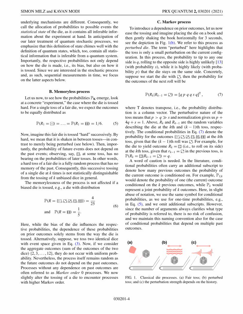
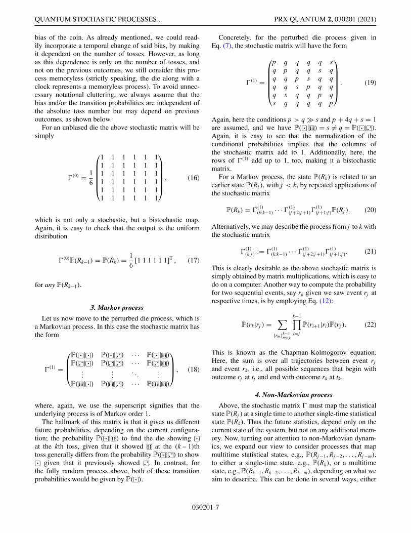
To introduce a dependence on prior outcomes, let us nowease the tossing and imagine placing the die on a book andthen gently shaking the book horizontally for 3 seconds,see the depiction in Fig. 1(b). We refer to this process asperturbed die. The term “perturbed” here highlights thatthe toss is only a small perturbation on the current config-uration. In this process, the probability to tip to any oneside is q, rolling to the opposite side is highly unlikely [13](with probability s), while it is highly likely (with proba-bility p) that the die stays on the same side. Concretely,suppose we start the die with , then the probability forthe outcomes of the next roll will be
P(Rk|Rk−1 = ) = [q p q q s q]T , (7)
where T denotes transpose, i.e., the probability distribu-tion is a column vector. The perturbative nature of thetoss means that p > q � s and normalization gives us p +4q + s = 1. Above, Rk and Rk−1 are the random variablesdescribing the die at the kth and (k − 1)th toss, respec-tively. The conditional probabilities in Eq. (7) denote theprobability for the outcomes { , , , , , } at the kthtoss, given that the (k − 1)th roll was . For example, forthe die to yield outcome Rk = (i.e., to roll on its side)at the kth toss, given that rk−1 = in the previous toss, isP(Rk = |Rk−1 = ) = q.
A word of caution is needed. In the literature, condi-tional probabilities often carry an additional subscript todenote how many previous outcomes the probability ofthe current outcome is conditioned on. For example, P1|kwould denote the probability of one (the current) outcomeconditioned on the k previous outcomes, while Pk wouldrepresent a joint probability of k outcomes. Here, in slightabuse of notation, we use the same symbol for conditionalprobabilities, as we use for one-time probabilities, e.g.,in Eq. (5), and we omit additional subscripts. However,since the number of arguments always clarifies what typeof probability is referred to, there is no risk of confusion,and we maintain this naming convention also for the caseof conditional probabilities that depend on multiple pastoutcomes.
(a) (b) (c)
FIG. 1. Classical die processes. (a) Fair toss; (b) perturbedtoss; and (c) the perturbation strength depends on the history.
030201-4
QUANTUM STOCHASTIC PROCESSES... PRX QUANTUM 2, 030201 (2021)
In this example, even though the die may be unbiased,the toss itself is not and the distribution for the future out-comes of the die depends on its current configuration. Assuch, the process remembers the current state. However,for the probabilities at the kth toss, it is only the outcomeat the (k − 1)th toss that is of relevance, but none of theearlier ones. In other words, only the current configurationmatters for future statistics, but the earlier history does notmatter. Such processes are referred to as Markov processes,or, as they “remember” only the most current outcome,processes of Markov order 1. Importantly, as soon as anykind of memory effects are present, the successive tossingof a die can be distinguished from the independent, paralleltossing of several identical dice, as in this latter case, thestatistics of the kth die cannot depend on the (k − 1)th die(or any other die).
Again, we emphasize that this process will remainMarkovian even if the die is replaced by two dice or bya biased die. Similarly, the above considerations wouldnot change if the perturbation depended on the numberof the toss k, i.e., if the parameters of Eq. (7) were func-tions q(k), p(k), s(k). We now discuss the case where thisassumption is not satisfied, i.e., where the perturbation atthe kth toss can depend on past outcomes, and memoryover longer periods of time starts to play a non-negligiblerole.
D. Non-Markovian processes
Let us now modify the process in the last example a bitby changing the perturbation intensity as we go. Let usonce again consider the process where the die is placed ona book, and the book is shaken for 3 seconds. Suppose thatafter the first shake the die rolls on its side, say �→ .The process is such that, after the number of pips changes,the next perturbation has unit intensity. If this intensityis low enough then we are likely to see �→ , and ifthat happens—i.e., the number of pips is unchanged—thenthe intensity is doubled the next shake; and we keep dou-bling the intensity until either die rolls to a new value orthe intensity reaches the value of eight units (four times),which we assume to be equal to shaking the die so stronglythat its initial value does not influence future outcomes.After this, the shaking intensity is reset to the unit level.We depict this process in Fig. 1(c).
In this example, to predict the future probabilities wenot only need to know the current number of pips the dieshows, but also its past values. That is, the probability ofobserving an event, say , after observing two consecu-tive outcomes is different than if one had previouslyobserved and , i.e.,
P( | , ) �= P( | , ). (8)
The necessity for remembering the past beyond the mostrecent outcomes makes this process non-Markovian. On
the other hand, here, we only have to remember the pastfour outcomes of the die due to the resetting protocol ofthe perturbation strength. Concretely, the future probabil-ities are independent of the past beyond four steps. Forexample, we have
P( | , , , , ) = P( | , , , , ). (9)
To be more precise, predicting the next outcome with cor-rect probabilities requires knowing the die’s configurationfor the past four steps. That is, the future distribution isfully determined by conditional probabilities
P(Rk|Rk−1, . . . , R0) = P(Rk|Rk−1, . . . , Rk−4), (10)
where we need to know only a part of the history, which,in this case, is the last four outcomes.
As mentioned, the size of the memory is often referredto as the Markov order or memory length of the process. Afully random process—like the hard tossing of a die—hasa Markov order 0, and a Markov process has an order of1. A non-Markovian process has an order of 2 or larger.This, in turn, implies that the study of non-Markovianprocesses contains Markovian processes as well as fullyrandom processes as special cases. Indeed, most processesin nature will carry memory, and Markovian processes arethe—well-studied—exception rather than the norm [14].
In general, the complexity of a non-Markovian processis higher than that of the Markov process in the last sub-section; this is because there is more to remember. Put lessprosaically, the process has to keep a ledger of the past out-comes to carry out the correct type of perturbation at eachpoint. And, in general, the size of this ledger, or the com-plexity, grows exponentially with the Markov order m: fora process with d different outcomes at each time (six for adie), it is given by dm. However, sometimes it is possibleto compress the memory. For instance, in the above exam-ple, we only need to know the current configuration andthe number of time steps it has remained unchanged; thusthe size of the memory is linear in the Markov order forthis example. Moreover, looking at histories larger than theMarkov order will not reveal anything new and thus doesnot add to the complexity of the process.
E. Stochastic matrix
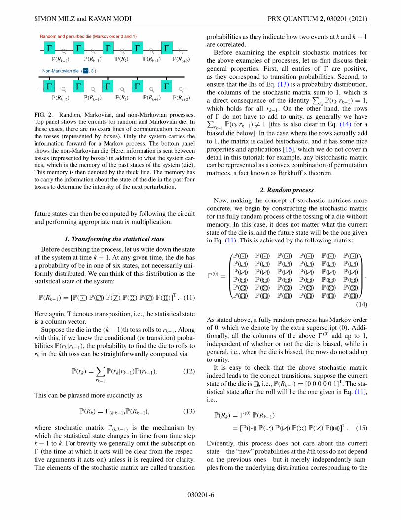
Having discussed stochastic processes and memory at ageneral level, it is now time to look in more detail at themathematical machinery used to describe them. A conve-nient way to model stochastic processes is the stochasticmatrix, which transforms the current state of the systeminto the future state. It also lends itself to a clear graph-ical depiction of the process in terms of a circuit, see,e.g., Fig. 2 for circuits corresponding to the three exam-ples above. In what follows, we write down the stochasticmatrices corresponding to the three processes above. The
030201-5
SIMON MILZ and KAVAN MODI PRX QUANTUM 2, 030201 (2021)
ΓΓΓ Γ ΓRandom and perturbed die (Markov order 0 and 1)
ℙ(Rk−2) ℙ(Rk−1) ℙ(Rk) ℙ(Rk+1) ℙ(Rk+2)
Γ Γ ΓΓΓ
Non-Markovian die ( , 3 )
ℙ(Rk−2) ℙ(Rk−1) ℙ(Rk) ℙ(Rk+1) ℙ(Rk+2)
FIG. 2. Random, Markovian, and non-Markovian processes.Top panel shows the circuits for random and Markovian die. Inthese cases, there are no extra lines of communication betweenthe tosses (represented by boxes). Only the system carries theinformation forward for a Markov process. The bottom panelshows the non-Markovian die. Here, information is sent betweentosses (represented by boxes) in addition to what the system car-ries, which is the memory of the past states of the system (die).This memory is then denoted by the thick line. The memory hasto carry the information about the state of the die in the past fourtosses to determine the intensity of the next perturbation.
future states can then be computed by following the circuitand performing appropriate matrix multiplication.
1. Transforming the statistical state
Before describing the process, let us write down the stateof the system at time k − 1. At any given time, the die hasa probability of be in one of six states, not necessarily uni-formly distributed. We can think of this distribution as thestatistical state of the system:
P(Rk−1) = [P( ) P( ) P( ) P( ) P( ) P( )]T . (11)
Here again, T denotes transposition, i.e., the statistical stateis a column vector.
Suppose the die in the (k − 1)th toss rolls to rk−1. Alongwith this, if we knew the conditional (or transition) proba-bilities P(rk|rk−1), the probability to find the die to rolls tork in the kth toss can be straightforwardly computed via
P(rk) =∑
rk−1
P(rk|rk−1)P(rk−1). (12)
This can be phrased more succinctly as
P(Rk) = �(k:k−1)P(Rk−1), (13)
where stochastic matrix �(k:k−1) is the mechanism bywhich the statistical state changes in time from time stepk − 1 to k. For brevity we generally omit the subscript on� (the time at which it acts will be clear from the respec-tive arguments it acts on) unless it is required for clarity.The elements of the stochastic matrix are called transition
probabilities as they indicate how two events at k and k − 1are correlated.
Before examining the explicit stochastic matrices forthe above examples of processes, let us first discuss theirgeneral properties. First, all entries of � are positive,as they correspond to transition probabilities. Second, toensure that the lhs of Eq. (13) is a probability distribution,the columns of the stochastic matrix sum to 1, which isa direct consequence of the identity
∑rk
P(rk|rk−1) = 1,which holds for all rk−1. On the other hand, the rowsof � do not have to add to unity, as generally we have∑
rk−1P(rk|rk−1) �= 1 [this is also clear in Eq. (14) for a
biased die below]. In the case where the rows actually addto 1, the matrix is called bistochastic, and it has some niceproperties and applications [15], which we do not cover indetail in this tutorial; for example, any bistochastic matrixcan be represented as a convex combination of permutationmatrices, a fact known as Birkhoff’s theorem.
2. Random process
Now, making the concept of stochastic matrices moreconcrete, we begin by constructing the stochastic matrixfor the fully random process of the tossing of a die withoutmemory. In this case, it does not matter what the currentstate of the die is, and the future state will be the one givenin Eq. (11). This is achieved by the following matrix:
�(0) =
⎛
⎜⎜⎜⎜⎜⎝
P( ) P( ) P( ) P( ) P( ) P( )
P( ) P( ) P( ) P( ) P( ) P( )
P( ) P( ) P( ) P( ) P( ) P( )
P( ) P( ) P( ) P( ) P( ) P( )
P( ) P( ) P( ) P( ) P( ) P( )
P( ) P( ) P( ) P( ) P( ) P( )
⎞
⎟⎟⎟⎟⎟⎠.
(14)
As stated above, a fully random process has Markov orderof 0, which we denote by the extra superscript (0). Addi-tionally, all the columns of the above �(0) add up to 1,independent of whether or not the die is biased, while ingeneral, i.e., when the die is biased, the rows do not add upto unity.
It is easy to check that the above stochastic matrixindeed leads to the correct transitions; suppose the currentstate of the die is , i.e., P(Rk−1) = [0 0 0 0 0 1]T. The sta-tistical state after the roll will be the one given in Eq. (11),i.e.,
P(Rk) = �(0)P(Rk−1)
= [P( ) P( ) P( ) P( ) P( ) P( )]T . (15)
Evidently, this process does not care about the currentstate—the “new” probabilities at the kth toss do not dependon the previous ones—but it merely independently sam-ples from the underlying distribution corresponding to the
030201-6
QUANTUM STOCHASTIC PROCESSES... PRX QUANTUM 2, 030201 (2021)
bias of the coin. As already mentioned, we could read-ily incorporate a temporal change of said bias, by makingit dependent on the number of tosses. However, as longas this dependence is only on the number of tosses, andnot on the previous outcomes, we still consider this pro-cess memoryless (strictly speaking, the die along with aclock represents a memoryless process). To avoid unnec-essary notational cluttering, we always assume that thebias and/or the transition probabilities are independent ofthe absolute toss number but may depend on previousoutcomes, as shown below.
For an unbiased die the above stochastic matrix will besimply
�(0) = 16
⎛
⎜⎜⎜⎜⎜⎝
1 1 1 1 1 11 1 1 1 1 11 1 1 1 1 11 1 1 1 1 11 1 1 1 1 11 1 1 1 1 1
⎞
⎟⎟⎟⎟⎟⎠, (16)
which is not only a stochastic, but a bistochastic map.Again, it is easy to check that the output is the uniformdistribution
�(0)P(Rk−1) = P(Rk) = 1
6[1 1 1 1 1 1]T , (17)
for any P(Rk−1).
3. Markov process
Let us now move to the perturbed die process, which isa Markovian process. In this case the stochastic matrix hasthe form
�(1) =
⎛
⎜⎜⎝
P( | ) P( | ) · · · P( | )
P( | ) P( | ) · · · P( | )...
.... . .
...P( | ) P( | ) · · · P( | )
⎞
⎟⎟⎠ , (18)
where, again, we use the superscript signifies that theunderlying process is of Markov order 1.
The hallmark of this matrix is that it gives us differentfuture probabilities, depending on the current configura-tion; the probability P( | ) to find the die showingat the kth toss, given that it showed at the (k – 1)thtoss generally differs from the probability P( | ) to show
given that it previously showed . In contrast, forthe fully random process above, both of these transitionprobabilities would be given by P( ).
Concretely, for the perturbed die process given inEq. (7), the stochastic matrix will have the form
�(1) =
⎛
⎜⎜⎜⎜⎜⎝
p q q q q sq p q q s qq q p s q qq q s p q qq s q q p qs q q q q p
⎞
⎟⎟⎟⎟⎟⎠. (19)
Again, here the conditions p > q � s and p + 4q + s = 1are assumed, and we have P( | ) = s �= q = P( | ).Again, it is easy to see that the normalization of theconditional probabilities implies that the columns ofthe stochastic matrix add to 1. Additionally, here, therows of �(1) add up to 1, too, making it a bistochasticmatrix.
For a Markov process, the state P(Rk) is related to anearlier state P(Rj ), with j < k, by repeated applications ofthe stochastic matrix
P(Rk) = �(1)(k:k−1) · · ·�(1)
(j +2:j +1)�(1)(j +1:j )P(Rj ). (20)
Alternatively, we may describe the process from j to k withthe stochastic matrix
�(1)(k:j ) := �
(1)(k:k−1) · · ·�(1)
(j +2:j +1)�(1)(j +1:j ). (21)
This is clearly desirable as the above stochastic matrix issimply obtained by matrix multiplications, which is easy todo on a computer. Another way to compute the probabilityfor two sequential events, say rk given we saw event rj atrespective times, is by employing Eq. (12):
P(rk|rj ) =∑
{rm}k−1m>j
k−1∏
i=j
P(ri+1|ri)P(rj ). (22)
This is known as the Chapman-Kolmogorov equation.Here, the sum is over all trajectories between event rjand event rk, i.e., all possible sequences that begin withoutcome rj at tj and end with outcome rk at tk.
4. Non-Markovian process
Above, the stochastic matrix � must map the statisticalstate P(Rj ) at a single time to another single-time statisticalstate P(Rk). Thus the future statistics, depend only on thecurrent state of the system, but not on any additional mem-ory. Now, turning our attention to non-Markovian dynam-ics, we expand our view to consider processes that mapmultitime statistical states, e.g., P(Rj −1, Rj −2, . . . , Rj −m),to either a single-time state, e.g., P(Rk), or a multitimestate, e.g., P(Rk−1, Rk−2, . . . , Rk−m), depending on what weaim to describe. This can be done in several ways, either
030201-7
SIMON MILZ and KAVAN MODI PRX QUANTUM 2, 030201 (2021)
by considering collections of stochastic map, or a sin-gle stochastic map that acts on a larger space. We brieflydiscuss both of these options.
First, let us consider the stochastic matrix for the non-Markovian process described in Sec. II D, where the per-turbation intensity depends on the sequence of the previ-ously observed number of pips. As mentioned before, forthis example we need to know the current state and thenumber of times it has not changed—which we denoteby μ—to correctly predict future statistics. As the pertur-bation strength is reset after the die has shown the samenumber of pips three consecutive times, we have μ ∈[0, 1, 2, 3]. For each μ, we can then write the stochasticmatrix as
�(μ) =
⎛
⎜⎜⎝
Pμ( | ) P
μ( | ) · · · Pμ( | )
Pμ( | ) P
μ( | ) · · · Pμ( | )
......
. . ....
Pμ( | ) P
μ( | ) · · · Pμ( | )
⎞
⎟⎟⎠ , (23)
where the superscript on the transition probabilities and thestochastic matrices denotes that they depend on the number
of times the outcome has not changed. For μ = 3, the per-turbation strength is such that the process becomes therandom process given in Eq. (14), and μ = 4 is the same asμ = 0. Evidently, Eq. (23) defines four distinct stochasticmatrices, one for each μ that leads to distinct future statis-tics. For any given μ, �(μ) allows us to correctly predictthe probability of the next toss of the die.
It is always possible to write down a family of stochasticmatrices for any non-Markovian process. Given the currentstate and history, we make use of the appropriate stochas-tic matrix to get the correct future state of the system. Ingeneral, for Markov order m, there are at most dm distincthistories, i.e., μ ∈ {0, . . . , dm−1 − 1}; each such history(prior to the current outcome) then requires a distinctstochastic matrix to correctly predict future probabilities.This exponentially growing storage requirement of dis-tinct pasts highlights the complexity of a non-Markovianprocess.
On the other hand, such a collection of stochasticmatrices for a process of Markov order m could equiv-alently be combined into one d × dm matrix of theform
�(m) =
⎛
⎜⎜⎝
P( | · · · ) P( | · · · ) · · · P( | · · · )
P( | · · · ) P( | · · · ) · · · P( | · · · )...
.... . .
...P( | · · · ) P( | · · · ) · · · P( | · · · )
⎞
⎟⎟⎠ , (24)
that acts on dm-dimensional probability vectors
P(RK) = [P( · · · ) · · · P( · · · ) P( · · · )]T ,(25)
to yield the correct future statistics, i.e., P(Rk) =�(m)
P(RK). Here, K denotes the last m tosses and thusby RK we denote the random variable corresponding tosequences of the last m outcomes starting at the (k − 1)thtoss. As before, �(m) is a stochastic matrix, as all of itsentries are positive, and its columns sum to 1. However,in contrast to the Markovian and the fully random case,it ceases to be a square matrix. We thus have to widenour understanding of a statistical “state” from probabilityvectors of outcomes at one time and toss, to probabilityvectors of outcomes at sequences of times and tosses. Inquantum mechanics, this shift of perspective allows oneto resolve many of the apparent paradoxes that appear toplague the description of quantum stochastic processes. Inthe following section, we see a concrete example of thisway of describing non-Markovian processes.
We graphically depict non-Markovian processes, withMarkov orders 2, 3, and 4, in Fig. 3. Here, the linesabove the boxes denote the memory that is passed to thefuture and required to correctly predict future statistics.Each box simply has to pass the information about thecurrent state—which generally is a multitime object—tofuture boxes, which, again, can make use of this infor-mation. Considering Fig. 3, we can already see that thedescription of stochastic processes with the memory pro-vided above is somewhat incomplete. While �(m) allowsus to compute the probabilities of the next outcome, giventhe last m outcomes, it yields only a one-time state, notan m-time state. While this is sufficient if we are interestedonly in the statistics of the next outcome, it is not enough tocompute statistics further in the future. Concretely, we can-not let �(m) act successively to obtain all future statistics.Expressed more graphically, a map that allows us to fullycompute statistics for a process of Markov order m needsm input and m output lines (see Fig. 3). Naturally, sucha map, which we denote as � can always be constructedfrom �(m), as we discuss in more detail in the next section.
030201-8
QUANTUM STOCHASTIC PROCESSES... PRX QUANTUM 2, 030201 (2021)
ΞΞΞ Ξ Ξ
ΞΞΞ Ξ Ξ
ΞΞΞ Ξ Ξ
Markov order 2
Markov order 3
Markov order 4
ℙ(Rk−2) ℙ(Rk−1) ℙ(Rk) ℙ(Rk+1) ℙ(Rk+2)
ℙ(Rk−2) ℙ(Rk−1) ℙ(Rk) ℙ(Rk+1) ℙ(Rk+2)
ℙ(Rk−2) ℙ(Rk−1) ℙ(Rk) ℙ(Rk+1) ℙ(Rk+2)
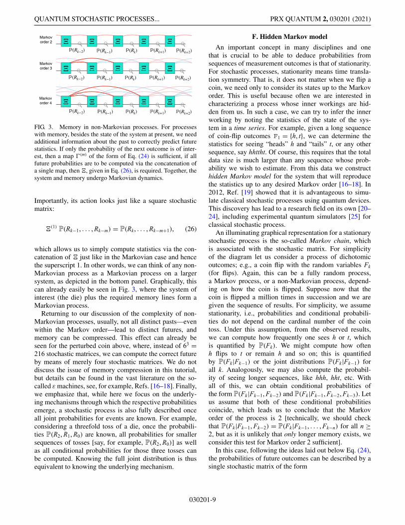
FIG. 3. Memory in non-Markovian processes. For processeswith memory, besides the state of the system at present, we needadditional information about the past to correctly predict futurestatistics. If only the probability of the next outcome is of inter-est, then a map �(m) of the form of Eq. (24) is sufficient, if allfuture probabilities are to be computed via the concatenation ofa single map, then �, given in Eq. (26), is required. Together, thesystem and memory undergo Markovian dynamics.
Importantly, its action looks just like a square stochasticmatrix:
�(1)P(Rk−1, . . . , Rk−m) = P(Rk, . . . , Rk−m+1), (26)
which allows us to simply compute statistics via the con-catenation of � just like in the Markovian case and hencethe superscript 1. In other words, we can think of any non-Markovian process as a Markovian process on a largersystem, as depicted in the bottom panel. Graphically, thiscan already easily be seen in Fig. 3, where the system ofinterest (the die) plus the required memory lines form aMarkovian process.
Returning to our discussion of the complexity of non-Markovian processes, usually, not all distinct pasts—evenwithin the Markov order—lead to distinct futures, andmemory can be compressed. This effect can already beseen for the perturbed coin above, where, instead of 63 =216 stochastic matrices, we can compute the correct futureby means of merely four stochastic matrices. We do notdiscuss the issue of memory compression in this tutorial,but details can be found in the vast literature on the so-called ε machines, see, for example, Refs. [16–18]. Finally,we emphasize that, while here we focus on the underly-ing mechanisms through which the respective probabilitiesemerge, a stochastic process is also fully described onceall joint probabilities for events are known. For example,considering a threefold toss of a die, once the probabili-ties P(R2, R1, R0) are known, all probabilities for smallersequences of tosses [say, for example, P(R2, R0)] as wellas all conditional probabilities for those three tosses canbe computed. Knowing the full joint distribution is thusequivalent to knowing the underlying mechanism.
F. Hidden Markov model
An important concept in many disciplines and onethat is crucial to be able to deduce probabilities fromsequences of measurement outcomes is that of stationarity.For stochastic processes, stationarity means time transla-tion symmetry. That is, it does not matter when we flip acoin, we need only to consider its states up to the Markovorder. This is useful because often we are interested incharacterizing a process whose inner workings are hid-den from us. In such a case, we can try to infer the innerworking by noting the statistics of the state of the sys-tem in a time series. For example, given a long sequenceof coin-flip outcomes F1 = {h, t}, we can determine thestatistics for seeing “heads” h and “tails” t, or any othersequence, say hhttht. Of course, this requires that the totaldata size is much larger than any sequence whose prob-ability we wish to estimate. From this data we constructhidden Markov model for the system that will reproducethe statistics up to any desired Markov order [16–18]. In2012, Ref. [19] showed that it is advantageous to simu-late classical stochastic processes using quantum devices.This discovery has lead to a research field on its own [20–24], including experimental quantum simulators [25] forclassical stochastic process.
An illuminating graphical representation for a stationarystochastic process is the so-called Markov chain, whichis associated with the stochastic matrix. For simplicityof the diagram let us consider a process of dichotomicoutcomes; e.g., a coin flip with the random variables Fk(for flips). Again, this can be a fully random process,a Markov process, or a non-Markovian process, depend-ing on how the coin is flipped. Suppose now that thecoin is flipped a million times in succession and we aregiven the sequence of results. For simplicity, we assumestationarity, i.e., probabilities and conditional probabili-ties do not depend on the cardinal number of the cointoss. Under this assumption, from the observed results,we can compute how frequently one sees h or t, whichis quantified by P(Fk). We might compute how oftenh flips to t or remain h and so on; this is quantifiedby P(Fk|Fk−1) or the joint distributions P(Fk|Fk−1) forall k. Analogously, we may also compute the probabil-ity of seeing longer sequences, like hhh, hht, etc. Withall of this, we can obtain conditional probabilities ofthe form P(Fk|Fk−1, Fk−2) and P(Fk|Fk−1, Fk−2, Fk−3). Letus assume that both of these conditional probabilitiescoincide, which leads us to conclude that the Markovorder of the process is 2 [technically, we should checkthat P(Fk|Fk−1, Fk−2) = P(Fk|Fk−1, . . . , Fk−n) for all n ≥2, but as it is unlikely that only longer memory exists, weconsider this test for Markov order 2 sufficient].
In this case, following the ideas laid out below Eq. (24),the probabilities of future outcomes can be described by asingle stochastic matrix of the form
030201-9
SIMON MILZ and KAVAN MODI PRX QUANTUM 2, 030201 (2021)
�(2) =(
P(h|hh) P(h|ht) P(h|th) P(h|tt)P(t|hh) P(t|ht) P(t|th) P(t|tt)
). (27)
This map will act on a statistical state that has the form
P(Fk, Fk−1) = [P(hh) P(ht) P(th) P(tt)]T . (28)
The action of the stochastic matrix on the statistical stategives us the probability for the next flip.
P(Fk+1) = �(2)P(Fk, Fk−1)
=[∑
xy∈{ht} P(h|xy)P(xy)∑xy∈{ht} P(t|xy)P(xy)
]. (29)
Combining the probabilities for two successive outcomesinto a single probability vector thus allows us to com-pute the probabilities for the next outcome in a Markovianfashion, i.e., by applying a single stochastic matrix to saidprobability vector. However, as already alluded to above,there is a slight mismatch in Eq. (29); while the randomvariables we look at on the rhs are sequences of two suc-cessive outcomes, the random variable on the lhs is a singleoutcome at the k + 1th toss. To obtain a fully Markovianmodel, one would rather desire a stochastic matrix that pro-vides the transition probabilities from one sequence of twooutcomes to another, i.e., a stochastic matrix � that yields
P(Fk+1, Fk) = �(1)P(Fk, Fk−1), (30)
where, for better bookkeeping, we formally distinguishbetween the random variables on the lhs and the rhs. Addi-tionally, we give � an extra superscript to underline thatit describes a process of Markov order 1. To do so, it hasto act on a larger space of random variables, namely, thecombined previous two outcomes.
Now, in our case, it is easy to see that the action of �(1)
can be simply computed from �(2) as
P(Fk+1, Fk) = �(1)P(Fk, Fk−1),
= δFkFk�(2)
P(Fk, Fk−1), (31)
where δ is the Kronecker function. This, in turn, impliesthat �(1) and �(2) contain the same information, andthe distinction between them is more of formal thanof fundamental nature. Importantly though, �(1) can beapplied in succession, e.g., we have P(Fk+n, Fk+n−1) =(�(1))n
P(Fk, Fk−1), while the same is not possible for �(2)
due to the mismatch of input and output spaces.Equation (30) then describes a Markovian model for
the random variable F2, which takes values {hh, ht, th, tt}.As knowledge of all relevant, i.e., within the Markovorder, transition probabilities allows the computation ofall joint probabilities, such an embedding into a higher-dimensional Markovian process via a redefinition of the
considered random variables is always possible. The cor-responding Markovian model is often called the hiddenMarkov model. As a brief aside, we note that the amountof memory that needs to be considered in an experi-ment depends both on the intrinsic Markov order of theprocess at hand, as well as the amount of informationan experimenter can or wants to store. If, for example,one is only interested in correctly recreating transitionprobabilities P(Rk|Rk−1) between adjacent times, but notnecessarily higher-order transition probabilities, like, e.g.,P(Rk|Rk−1, Rk−2), then a Markovian model without anymemory is fully sufficient (but will not properly reproducehigher-order transition probabilities).
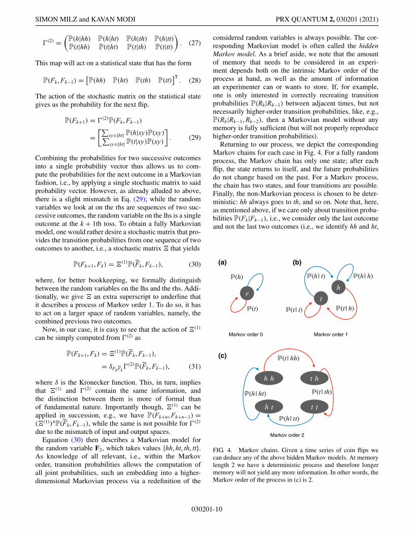
Returning to our process, we depict the correspondingMarkov chains for each case in Fig. 4. For a fully randomprocess, the Markov chain has only one state; after eachflip, the state returns to itself, and the future probabilitiesdo not change based on the past. For a Markov process,the chain has two states, and four transitions are possible.Finally, the non-Markovian process is chosen to be deter-ministic: hh always goes to th, and so on. Note that, here,as mentioned above, if we care only about transition proba-bilities P(Fk|Fk−1), i.e., we consider only the last outcomeand not the last two outcomes (i.e., we identify hh and ht,
th
ℙ(h | t)
ℙ(t | t) ℙ(t | h)
ℙ(h | h)
ℙ(t)
ℙ(h)
r
ℙ(h | tt)
ℙ(t | hh)
ℙ(t | th)ℙ(h | ht)
h h t h
h t t t
Markov order 0 Markov order 1
Markov order 2
(a) (b)
(c)
FIG. 4. Markov chains. Given a time series of coin flips wecan deduce any of the above hidden Markov models. At memorylength 2 we have a deterministic process and therefore longermemory will not yield any more information. In other words, theMarkov order of the process in (c) is 2.
030201-10
QUANTUM STOCHASTIC PROCESSES... PRX QUANTUM 2, 030201 (2021)
and th and tt), then the process of Fig. 4(c) reduces to thesimpler one in (b), but the information is lost.
All of the panels of Fig. 4 describe Markovian pro-cesses, however for different random variables. This is ageneral feature: any non-Markovian process can be rep-resented by a hidden Markov model or a Markov chainby properly combining the past into a “large enough” ran-dom variable [14] [for example, the random variable withvalues {hh, th, ht, tt} in (c)]. This intuition will come inhandy when we move to the case of quantum stochasticprocesses. But first, we need to formalize the theory ofclassical stochastic process and show where the pitfalls liewhen generalizing this theory to the quantum domains.
G. (Some) mathematical rigor
As mentioned, in our presentation of stochastic pro-cesses, we rather opt for intuitive examples than fullmathematical rigor. However, laying the fundamental con-cepts of probability theory in detail provides a morecomprehensive picture of stochastic processes, and ren-ders the generalizations needed to treat quantum processesmathematically straightforward.
The basic ingredient for the discussion of stochastic pro-cesses is the triplet (�,S ,ω) of a sample space �, a σ
algebra S and a probability measure ω. Intuitively, � is theset of all events that can occur in a given experiment (forexample, � could represent the myriad of microstates a diecan assume or the possible numbers of pips it can show),S corresponds to all the outcomes that can be resolvedby the measurement device (for the case of the die, Scould, for example, correspond to the number of pips thedie can show, or to the less fine-grained information “odd”or “even”) and ω allocates a probability to each of theseobservable outcomes.
More rigorously, we have the following definition [26].
Definition (σ algebra): Let � be a set. A σ algebra on �
is a collection S of subsets of �, such that
(a) � ∈ S and ∅ ∈ S;(b) if s ∈ S , then � \ s ∈ S;(c) S is closed under (countable) unions and intersec-
tions, i.e., if s1, s2, . . . ∈ S , then⋃∞
j =1sj ∈ S and⋂∞j =1sj ∈ S .
For example, if the sample space is given by � ={ , . . . , } and we resolve only whether the outcome ofthe toss of a die is odd or even, the corresponding σ alge-bra is given by {{ , , }, { , , }, ∅,�}, while in thecase where we resolve the individual numbers of pips, S issimply the power set of �.
A pair (�,S) is called a measurable space, as now,we can introduce a probability measure for observableoutcomes in a well-defined way.
Definition (Probability measure): Let (�,S) be a mea-surable space. A probability measure ω : S → R is areal-valued function that satisfies
(a) ω(�) = 1;(b) ω(s) ≥ 0 for all s ∈ S;(c) ω is additive for (countable) unions of disjoint
events, i.e., ω(⋃∞
j =1sj
)=∑∞
j ω(sj ) for sj ∈ Sand sj ∩ sj ′ = ∅ when j �= j ′.
The corresponding triplet (�,S ,ω) is then called aprobability space [26]. As the name suggests, ω mapseach event sj to its corresponding probability, and, usingthe convention of the previous sections, we could havedenoted it by P, and do so in what follows. Evidently,in our previous discussions, we already make use of sam-ple spaces, σ algebras, and probability measures, withoutcaring too much about their mathematical underpinnings.
The mathematical machinery of probability spaces pro-vides a versatile framework for the description of stochas-tic processes, both on finitely and infinitely many times(see Sec. III D for an extension of the above concepts tothe multitime case).
So far, we have talked about processes that are discreteboth in time and space. It does not make much sense totalk about the state of a die when it is in midair; nordoes it make sense to attribute a state of 4.4 to a die.On the other hand, of course, there are processes thatare both continuous in time and space. A classic exam-ple is Brownian motion [27], which requires that time betreated continuously. If not, the results lead to patholog-ical situations where the kinetic energy of the Brownianparticle blows up. Moreover, in such instances, the eventspace is the position of the Brownian particle and can takeuncountably many different real values. Nevertheless, thecentral object in the theory of stochastic processes doesnot change; it remains the joint probability distributionfor all events, which in the case of infinitely many timesis a probability distribution on a rather complicated, andnot easy to handle σ algebra. Below, we discuss how, dueto a fundamental result by Kolmogorov, it is sufficient todeal with finite distributions instead of distributions on σ
algebras on infinite Cartesian products of sample spaces.Finally, this machinery straightforwardly generalizes topositive operator-valued measures (POVMs) as well asinstruments, fundamental ingredients for the discussion ofquantum stochastic processes.
III. CLASSICAL STOCHASTIC PROCESSES:FORMAL APPROACH
Up to this point, both in the examples we provided, aswell as the more rigorous formulation, we have somewhatleft open what exactly we mean by a stochastic pro-cess, and what quantity encapsulates it. We close this gap
030201-11
SIMON MILZ and KAVAN MODI PRX QUANTUM 2, 030201 (2021)
now, and provide a fundamental theorem for the theory ofstochastic processes, the Kolmogorov extension theorem(KET), which allows one to properly define stochasticprocesses on infinitely many times, based on finite-timeinformation.
A. What then is a stochastic process?
Intuitively, a stochastic process on a set of times Tk :={t0, t1, . . . , tk} with ti ≤ tj for i ≤ j is the joint probabil-ity distribution over observable events. Namely, the centralquantity that captures everything that can be learned aboutan underlying process is
PTk+1 := P(Rk, tk; Rk−1, tk−1; . . . ; R0, t0), (32)
corresponding to all joint probabilities
{P(Rk = rk, Rk−1 = rk−1, . . . , R0 = r0, )}rk ,...,r0 (33)
to observe all possible realizations Rk = rk at time tk,Rk−1 = rk−1 at time tk−1, and so on. Evidently, the timelabel—which we omit above and for most of this tuto-rial—could also correspond to a label of the number oftosses, etc. We also adopt the compact notation of PTk+1 ,as defined above, to denote a probability distribution on aset of k + 1 times.
More concretely, suppose the process we have in mindis tossing a die five times in a row. This stochastic processis fully characterized by the probability of observing allpossible sequence of events
{P( , , , , ), . . . , P( , , , , ), . . .
......
P( , , , , ), . . . , P( , , , , )},(34)
where, as before, we omit the respective time and the tosslabel.
From the joint distribution for five tosses, one can obtainany desired marginal distributions for fewer tosses, e.g.,P(R3); or any conditional distributions (for five tosses),such as, for example, the conditional probability P(R2 =
|R1 = , R0 = ), to obtain outcome at the third toss,having observed two in a row previously; the conditionaldistributions in turn allows computing the stochastic matri-ces, which in turn allow casting processes as a Markovchain. Having the total distribution is enough to deter-mine whether a process is fully random, Markovian, ornon-Markovian. This statement, however, is contingent onthe respective set of times. Naturally, without any fur-ther assumptions of memory length and/or stationarity,knowing the joint probabilities of outcomes—and thuseverything that can be learned—on a set of times Tk doesnot provide knowledge about the corresponding process on
a different set of times Tk′ . Consequently, we identify astochastic process with the joint probabilities it displayswith respect to a fixed set of times.
While joint probabilities contain all inferable informa-tion about a stochastic process, working with them is notalways desirable because their number of entries growsexponentially. Nevertheless, they are the central quantityin the theory of classical stochastic processes. Our firstaim when extending the notion of stochastic processes tothe quantum domain will thus be to construct the analogyto joint distribution for time-ordered events. Doing so hasbeen troubling for the same foundational reasons that makequantum mechanics so interesting. Most notably, quantumprocesses, in general, do not straightforwardly allow for aKolmogorov extension theorem, which we discuss below.However, upon closer inspection, such obstacles can beovercome by properly generalizing the concept of jointprobabilities to the quantum domain. Before doing so, wefirst return to our more rigorous mathematical treatmentand define stochastic processes in terms of probabilityspaces.
B. Kolmogorov extension theorem
While, for the example of the tossing of a die, a descrip-tion of the process at hand in terms of joint probabilitieson finitely or countably many times and tosses is satisfac-tory, this is not always the case. For example, even thoughit can in practice only be probed at finitely many points intime, when considering Brownian motion, one implicitlyposits the existence of an “underlying” stochastic process,from which the observed joint probabilities stem. Intu-itively, for the case of Brownian motion, this underlyingprocess should be fully described by a probability distribu-tion that ascribes a probability to all possible trajectoriesthe particle can take. Connecting the operationally well-defined finite joint probabilities a physicist can observeand/or model with the concept of an underlying processis the aim of the Kolmogorov extension theorem.
Besides not being experimentally accessible, workingwith probability distributions on infinitely many timeshas the additional drawback that the respective mathe-matical objects are rather cumbersome to use, and wouldmake the modeling of stochastic processes a fairly tediousbusiness. Luckily, the KET allows one to deduce the exis-tence of an underlying process on infinitely many times,from properties of only finite objects. With this, model-ing a proper stochastic process on infinitely many timesamounts to constructing finite time joint probabilities that“fit together” properly.
To see what we mean by this last statement let PTbe
the joint distribution obtained for an experiment for somefixed times. For now, we stick with the case of Brow-nian motion, and PT
could correspond to the probability
030201-12
QUANTUM STOCHASTIC PROCESSES... PRX QUANTUM 2, 030201 (2021)
to find a particle at positions x0, . . . , x−1 when measur-ing it at times T = {t0, . . . , t−1}. As mentioned before,PT
contains all statistical information for fewer times asmarginals, i.e., for any subset Tk ⊆ T we have
PTk =∑
T\Tk
PT=: P
|TkT
, (35)
where we denote the sum over the times in the comple-ment of the intersection of Tk and T by T \ Tk and usean additional superscript to signify that the respective jointprobability distribution is restricted to a subset of timesvia marginalization. For simplicity of notation, here and inwhat follows, we always denote the marginalization by asummation, even though, in the uncountably infinite case,it would correspond to an integration.
For classical stochastic processes, all probabilities on aset of time can be obtained from those on a superset oftimes by marginalization. We call this consistency condi-tion between joint probability distributions of a process ondifferent sets of times Kolmogorov consistency conditions.Naturally, consistency conditions hold in particular if thefinite joint probability distributions stem from an underly-ing process on infinitely many times T ⊇ T ⊇ Tk, wherewe leave the nature of the corresponding probability dis-tribution PT somewhat vague for now (see Sec. III D for amore thorough definition).
Importantly, the KET shows, that satisfaction of the con-sistency condition on all finite sets Tk ⊆ T ⊆ T is alreadysufficient to guarantee the existence of an underlying pro-cess on T. Specifically, the Kolmogorov extension theorem[3,26,28,29] defines the minimal properties finite probabil-ity distributions have to satisfy in order for an underlyingprocess to exist.
Theorem (KET): Let T be a set of times. For each finiteTk ⊆ T, let PTk be a (sufficiently regular) k-step joint prob-ability distribution. There exists an underlying stochasticprocess PT that satisfies PTk = P
|TkT for all finite Tk ⊆ T if
and only if PTk = P|TkT
for all Tk ⊆ T ⊆ T.
Put more intuitively, the KET shows that for a givenfamily of finite joint probability distributions that satisfyconsistency conditions [30], the existence of an underlyingprocess, that contains all of the finite ones as marginals,is ensured. Importantly, this underlying process does notneed to be known explicitly in order to properly model astochastic process.
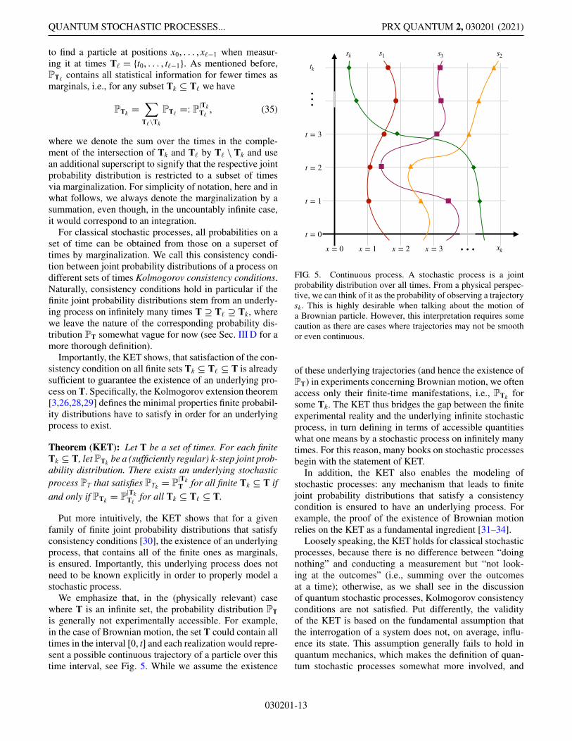
We emphasize that, in the (physically relevant) casewhere T is an infinite set, the probability distribution PTis generally not experimentally accessible. For example,in the case of Brownian motion, the set T could contain alltimes in the interval [0, t] and each realization would repre-sent a possible continuous trajectory of a particle over thistime interval, see Fig. 5. While we assume the existence
x = 0 x = 1 x = 2 x = 3 … xk
t = 0
t = 1
t = 2
t = 3
…
tk
s1 s2sk s3
FIG. 5. Continuous process. A stochastic process is a jointprobability distribution over all times. From a physical perspec-tive, we can think of it as the probability of observing a trajectorysk. This is highly desirable when talking about the motion ofa Brownian particle. However, this interpretation requires somecaution as there are cases where trajectories may not be smoothor even continuous.
of these underlying trajectories (and hence the existence ofPT) in experiments concerning Brownian motion, we oftenaccess only their finite-time manifestations, i.e., PTk forsome Tk. The KET thus bridges the gap between the finiteexperimental reality and the underlying infinite stochasticprocess, in turn defining in terms of accessible quantitieswhat one means by a stochastic process on infinitely manytimes. For this reason, many books on stochastic processesbegin with the statement of KET.
In addition, the KET also enables the modeling ofstochastic processes: any mechanism that leads to finitejoint probability distributions that satisfy a consistencycondition is ensured to have an underlying process. Forexample, the proof of the existence of Brownian motionrelies on the KET as a fundamental ingredient [31–34].
Loosely speaking, the KET holds for classical stochasticprocesses, because there is no difference between “doingnothing” and conducting a measurement but “not look-ing at the outcomes” (i.e., summing over the outcomesat a time); otherwise, as we shall see in the discussionof quantum stochastic processes, Kolmogorov consistencyconditions are not satisfied. Put differently, the validityof the KET is based on the fundamental assumption thatthe interrogation of a system does not, on average, influ-ence its state. This assumption generally fails to hold inquantum mechanics, which makes the definition of quan-tum stochastic processes somewhat more involved, and
030201-13
SIMON MILZ and KAVAN MODI PRX QUANTUM 2, 030201 (2021)
their structure much richer than that of their classicalcounterparts.
C. Practical features of stochastic processes
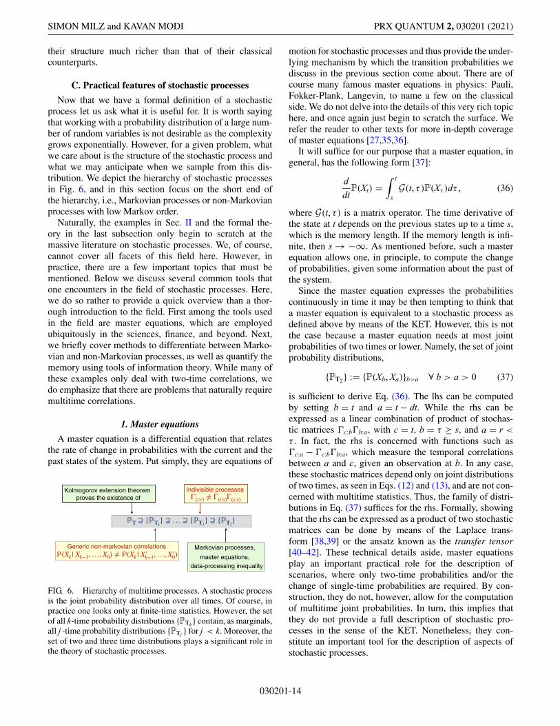
Now that we have a formal definition of a stochasticprocess let us ask what it is useful for. It is worth sayingthat working with a probability distribution of a large num-ber of random variables is not desirable as the complexitygrows exponentially. However, for a given problem, whatwe care about is the structure of the stochastic process andwhat we may anticipate when we sample from this dis-tribution. We depict the hierarchy of stochastic processesin Fig. 6, and in this section focus on the short end ofthe hierarchy, i.e., Markovian processes or non-Markovianprocesses with low Markov order.
Naturally, the examples in Sec. II and the formal the-ory in the last subsection only begin to scratch at themassive literature on stochastic processes. We, of course,cannot cover all facets of this field here. However, inpractice, there are a few important topics that must bementioned. Below we discuss several common tools thatone encounters in the field of stochastic processes. Here,we do so rather to provide a quick overview than a thor-ough introduction to the field. First among the tools usedin the field are master equations, which are employedubiquitously in the sciences, finance, and beyond. Next,we briefly cover methods to differentiate between Marko-vian and non-Markovian processes, as well as quantify thememory using tools of information theory. While many ofthese examples only deal with two-time correlations, wedo emphasize that there are problems that naturally requiremultitime correlations.
1. Master equations
A master equation is a differential equation that relatesthe rate of change in probabilities with the current and thepast states of the system. Put simply, they are equations of
Indivisible processes Γ(t:r) ≠ Γ(t:s)Γ(s:r)
ℙT ⊇ {ℙTk} ⊇ … ⊇ {ℙT3
} ⊇ {ℙT2}
Kolmogorov extension theorem proves the existence of
Markovian processes,
master equations, data-processing inequality
Generic non-markovian correlations ℙ(Xk | Xk−1,…,X0) ≠ ℙ(Xk | X′k−1,…,X′0)
FIG. 6. Hierarchy of multitime processes. A stochastic processis the joint probability distribution over all times. Of course, inpractice one looks only at finite-time statistics. However, the setof all k-time probability distributions {PTk } contain, as marginals,all j -time probability distributions {PTj } for j < k. Moreover, theset of two and three time distributions plays a significant role inthe theory of stochastic processes.
motion for stochastic processes and thus provide the under-lying mechanism by which the transition probabilities wediscuss in the previous section come about. There are ofcourse many famous master equations in physics: Pauli,Fokker-Plank, Langevin, to name a few on the classicalside. We do not delve into the details of this very rich topichere, and once again just begin to scratch the surface. Werefer the reader to other texts for more in-depth coverageof master equations [27,35,36].
It will suffice for our purpose that a master equation, ingeneral, has the following form [37]:
ddt
P(Xt) =∫ t
sG(t, τ)P(Xτ )dτ , (36)
where G(t, τ) is a matrix operator. The time derivative ofthe state at t depends on the previous states up to a time s,which is the memory length. If the memory length is infi-nite, then s → −∞. As mentioned before, such a masterequation allows one, in principle, to compute the changeof probabilities, given some information about the past ofthe system.
Since the master equation expresses the probabilitiescontinuously in time it may be then tempting to think thata master equation is equivalent to a stochastic process asdefined above by means of the KET. However, this is notthe case because a master equation needs at most jointprobabilities of two times or lower. Namely, the set of jointprobability distributions,
{PT2} := {P(Xb, Xa)}b>a ∀ b > a > 0 (37)
is sufficient to derive Eq. (36). The lhs can be computedby setting b = t and a = t − dt. While the rhs can beexpressed as a linear combination of product of stochas-tic matrices �c:b�b:a, with c = t, b = τ ≥ s, and a = r <
τ . In fact, the rhs is concerned with functions such as�c:a − �c:b�b:a, which measure the temporal correlationsbetween a and c, given an observation at b. In any case,these stochastic matrices depend only on joint distributionsof two times, as seen in Eqs. (12) and (13), and are not con-cerned with multitime statistics. Thus, the family of distri-butions in Eq. (37) suffices for the rhs. Formally, showingthat the rhs can be expressed as a product of two stochasticmatrices can be done by means of the Laplace trans-form [38,39] or the ansatz known as the transfer tensor[40–42]. These technical details aside, master equationsplay an important practical role for the description ofscenarios, where only two-time probabilities and/or thechange of single-time probabilities are required. By con-struction, they do not, however, allow for the computationof multitime joint probabilities. In turn, this implies thatthey do not provide a full description of stochastic pro-cesses in the sense of the KET. Nonetheless, they con-stitute an important tool for the description of aspects ofstochastic processes.
030201-14
QUANTUM STOCHASTIC PROCESSES... PRX QUANTUM 2, 030201 (2021)
2. Divisible processes
To shed more light on the concept of master equations,let us consider a special case (which we also encounter inthe quantum setting). Specifically, let us consider a familyof stochastic matrices that satisfy
�(t:r) = �(t:s)�(s:r) ∀ t > s > r. (38)
Processes described by such a family are called divisi-ble. Once the functional dependence of �(t:r) on t and ris known, one can build up the set of distributions con-tained in Eq. (37). It is easy to see that the family ofstochastic matrices in Eq. (38) is a superset of Marko-vian processes. That is, any Markov process will satisfythe above equation. However, there are non-Markovianprocesses that also satisfy the divisibility property [43].Nevertheless, checking for divisibility is often far simplerthan checking for the satisfaction of the Markov condi-tions since the latter requires the collection of multitimestatistics, while the former can be decided based on two-time statistics only. Moreover, as we will see shortly, thedivisibility of the process implies several highly desirableproperties for the process.
A nice property of divisible processes is the corre-sponding master equation. Applying Eq. (38) to the lhs ofEq. (36) we get
P(Xt) − P(Xt−dt)
dt= �(t:t−dt) − 1
dtP(Xt−dt), (39)
where 1 is the identity matrix. Taking the limit dt → 0yields the generator Gt := limdt→0[�(t:t−dt) − 1]/dt. Thisis a time-local master equation in the sense that thederivative of P—in contrast to the more general case ofEq. (36)—depends only on the current time t, but noton previous times. In turn, the generator is related tothe stochastic matrix as �(t:t−dt) = exp(Gtdt), which isobtained by integration. When the process is stationary,i.e., symmetric under time translation, both � and G willbe time independent.
A divisible Markovian process. To make the abovemore concrete, let us consider a two-level system thatundergoes the following infinitesimal process:
�(t:t−dt) = (1 − γ dt)(
1 00 1
)+ γ dt
(g0 g0g1 g1
). (40)
The first part of the process is just the identity process,and the second part is a random process. However, togetherthey form a Markov process. Using Eq. (39) we can derivethe generator for the master equation. This process is verysimilar to the perturbed die in the last section, with the dif-ference that here, we consider a process that is continuous
in time; it takes any state P(Xt−dt) at t − dt to
P(Xt) = (1 − γ dt)P(Xt−dt) + γ dtG, (41)
where G = [g0 g1]T. After some time τ = ndt, i.e., after napplications of the stochastic matrix, we have
P(Xτ ) = (1 − γ dt)nP(Xt) + γ ndt G. (42)
That is, the process relaxes any state of the system to thefixed G exponentially fast with a rate γ . Many processes,such as thermalization, have such a form. In fact, oneoften associates Markov processes with exponential decay.However, as already mentioned above, such an identifica-tion is not exact, since there are non-Markovian processesthat satisfy a divisible master equation as we show nowby means of two explicit examples (we encounter anexplicit example of this phenomenon in the quantum casein Sec. VI A 2).
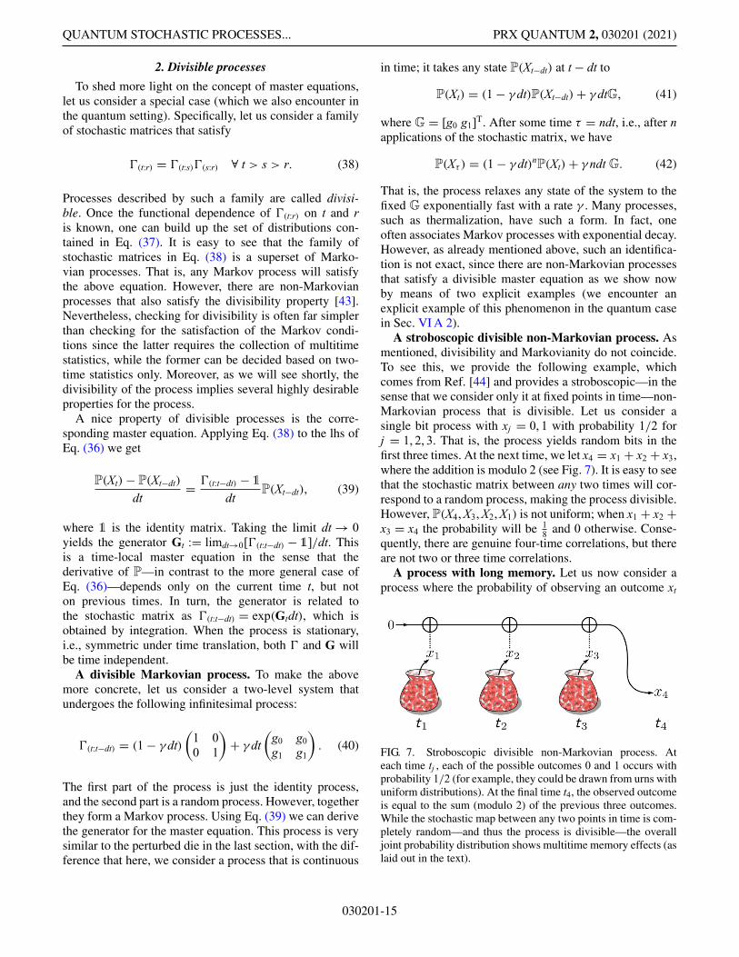
A stroboscopic divisible non-Markovian process. Asmentioned, divisibility and Markovianity do not coincide.To see this, we provide the following example, whichcomes from Ref. [44] and provides a stroboscopic—in thesense that we consider only it at fixed points in time—non-Markovian process that is divisible. Let us consider asingle bit process with xj = 0, 1 with probability 1/2 forj = 1, 2, 3. That is, the process yields random bits in thefirst three times. At the next time, we let x4 = x1 + x2 + x3,where the addition is modulo 2 (see Fig. 7). It is easy to seethat the stochastic matrix between any two times will cor-respond to a random process, making the process divisible.However, P(X4, X3, X2, X1) is not uniform; when x1 + x2 +x3 = x4 the probability will be 1
8 and 0 otherwise. Conse-quently, there are genuine four-time correlations, but thereare not two or three time correlations.
A process with long memory. Let us now consider aprocess where the probability of observing an outcome xt
FIG. 7. Stroboscopic divisible non-Markovian process. Ateach time tj , each of the possible outcomes 0 and 1 occurs withprobability 1/2 (for example, they could be drawn from urns withuniform distributions). At the final time t4, the observed outcomeis equal to the sum (modulo 2) of the previous three outcomes.While the stochastic map between any two points in time is com-pletely random—and thus the process is divisible—the overalljoint probability distribution shows multitime memory effects (aslaid out in the text).
030201-15
SIMON MILZ and KAVAN MODI PRX QUANTUM 2, 030201 (2021)
is correlated with what was observed some time ago xt−swith some probability
P(Xt = xt|Xt−s = xt−s) = p δxt,xt−s + 1 − pd
. (43)
Here d is the size of the system. This process has onlytwo-time correlations, but the process is non-Markovianas the memory is a long-range one. A master equation, ofthe type of Eq. (36), for this process, can be derived bydifferentiating. For sake of brevity, we forego this exercise.
As mentioned, master equations are a ubiquitously usedtool for the description of stochastic processes, both in theclassical as well as the quantum (see below) domain. Theyallow one to model the evolution of the one-time probabil-ity distribution P(Xt). However, they are not well suited forthe description of multitime joint probabilities. This willbe particularly true for the quantum case, where interme-diate measurements—required to collect multitime statis-tics—unavoidably influence the state of the system. Formany real-world applications though, knowledge aboutP(Xt) is sufficient, making master equations an indispens-able tool for the modeling of stochastic processes. On theother hand, in order to analyze memory length and strengthin detail, one must—particularly in the quantum case—gobeyond the description of stochastic processes in terms ofmaster equations (see Sec. V D). This widening of the hori-zon beyond master equations then also enables one to carryover the intuition developed for stochastic processes in theclassical case to the quantum realm, as well as a rigorousdefinition of quantum stochastic processes in the spirit ofthe KET.
At this stage, it is worth pointing out why Markov pro-cesses are of interest in many cases, and how they fit intothe picture. Suppose we are following the trajectory ofa particle at position x at time t, which then moves tox′ at t′. If the difference in time is arbitrarily small, sayδt, then for a physical process, x′ cannot be too differ-ent from x due to continuity. Thus, it is natural to writedown a master equation to describe such a process. Sincethe future state will always depend on the current posi-tion, the process will be at least Markovian. Still, theprocess may have higher-order correlations, but they areoften neglected for simplicity. Importantly, if the process isindeed memoryless, then master equations actually allowfor the computation of all joint probability distributionsand provide a complete picture of the process at hand.Due to their practical importance, we now provide sometools that are frequently used when dealing with memo-ryless processes, and to gauge deviation from Markovianstatistics in an operationally accessible way. As before,this short overview is by no means intended to be com-prehensive but merely aimed at providing a quick glimpseof possible ways to quantify memory.
3. Data-processing inequality
Somewhat abstractly, a stochastic process can be under-stood as a state being processed in time. Memory, then,means that some information about the past of the state ofthe system at hand is stored and used at a later time to influ-ence the future statistics of the system. Unsurprisingly, themathematical means we use to make this intuition man-ifest and quantify the presence of memory are borrowedfrom information theory. Here, we introduce them, startingfrom the special case of divisible processes.
One of the most useful properties of Markov (and, moregenerally, divisible) processes is the satisfaction of thedata-processing inequality (DPI). Suppose we are able toprepare the system in two possible initial states P(X0) andR(X0), and then subject each to a process �(t:0) to yieldP(Xt) = �(t:0)P(X0) and R(Xt) = �t:0R(X0), respectively.The intuition behind DPIs is that the process has no mech-anism to increase the distinguishability between two initialstates unless it has some additional information.
For instance, a natural measure for distinguishing prob-ability distribution is the so-called Kolmogorov distance orthe trace distance
‖P(X ) − R(X )‖1 := 12
∑
x
|P(x) − R(x)|. (44)
When two states are fully distinguishable, the trace dis-tance will be 1, which is the maximal value it can assume.On the other hand, if the two distributions are the samethen the trace distance will be 0. The DPI guarantees thatthe distance between distributions is nonincreasing underthe action of stochastic maps, i.e.,
‖P(X0) − R(X0)‖1 ≥ ‖P(Xt) − R(Xt)‖1 (45)
for all times t > 0 and equality (for all pairs of initial dis-tributions) holds if and only if the process is reversible.Additionally, for Markov processes the DPI will hold forall times t ≥ s, i.e.,
‖P(Xs) − R(Xs)‖1 ≥ ‖P(Xt) − R(Xt)‖1. (46)
Conversely, if the distinguishability between two distribu-tions increases at any point of their evolution, then theunderlying dynamics cannot be Markovian and stochasticmaps �t:s between two points in time do not provide a fullpicture of the process at hand.
There are many metrics and pseudometrics that sat-isfy DPI, but not all. For instance, the Euclidean norm,‖P(X )‖2 := √∑x P(x)2, does not satisfy the DPI. Asan example consider a two-bit process with initial statesP(X0) Pu and R(X0) Pu, where the second bit’s state isthe uniform distribution Pu. If the process simply discardsthe second bit, then the final Euclidean distance is simplyP(X0) − R(X0). However, the initial Euclidean distance is
030201-16
QUANTUM STOCHASTIC PROCESSES... PRX QUANTUM 2, 030201 (2021)
exactly 12 [P(X0) − R(X0)]. Thus the class of functions that
are contractive under the action of a stochastic matrix aretypically good candidates to formulate DPIs.
The DPI plays an important role in information theorybecause it holds for two important metrics, the mutualinformation and the Kullback-Leibler divergence (alsoknown as relative entropy). For a random variable, theShannon entropy is defined as
H(X ) := −∑
x
P(x) log[P(x)]. (47)
The mutual information between two random variables Xand Y, that posses a joint distribution P(X , Y), is defined as
H(X : Y) := H(X ) + H(Y) − H(XY). (48)
Here, H(X ) is computed from the marginal distributionP(X ) =∑y P(X , Y = y); and H(Y) is computed from themarginal distribution P(Y) =∑x P(X = x, Y). The corre-sponding DPI then is
H(X0 : Y0) ≥ H(Xt : Yt), (49)
under the action of a stochastic matrix. For Markov pro-cesses we have a stronger inequality
H(Xs : Ys) ≥ H(Xt : Yt), (50)
for all times t ≥ s.The relative entropy between two distributions P(X )
and P′(X ) is defined as
H [P(X )‖R(X )] := −∑
x
P(x) log[
R(x)P(x)
]. (51)
Note that this is not a quantity that is symmetric in its argu-ments. The relative entropy is endowed with an operationalmeaning as the probability of confusion [45]; that is, ifone is promised R(X ) but given P(X ) instead, then aftern samples the confusion probability is quantitatively givenby P(X ) for R(X )
Prconf = exp{−nH [P(X )‖R(X )]}. (52)
We will see later that a similar expression can be employedin the quantification of memory effects in quantumstochastic processes (see Sec. VI B 3). The correspondingDPI here has the form
H [P(X0)‖R(X0)] ≥ H [P(Xt)‖R(Xt)], (53)
under a stochastic transformation. For Markov processes,we get the stronger version
H [P(Xs)‖R(Xs)] ≥ H [P(Xt)‖R(Xt)], (54)
that holds for all t ≥ s.
The behavior of relative entropy and the related pseu-dometric in quantum and classical dynamics is an ongo-ing research effort [46–48]. The meaning of all of theseDPIs for Markov processes is that the system is pro-gressively loosing information as time marches forward.This clearly has implication on our understanding of thesecond law of thermodynamics and the arrow of time.There are still other inequalities that are being discovered,e.g., see Ref. [44] for the so-called monogamy inequality.For detailed coverage of DPI see Refs. [49,50]. More-over, recently, researchers have employed the so-calledentropy cone [51,52] to infer causality in processes, whichis closely related to many of our interests in this tutorial.However, for brevity, we do not go into these details here.Here, we merely aim to emphasize that metrics that satisfyDPI can be used as a herald for non-Markovian behaviorbased on two-time distributions only.
4. Conditional mutual information
Naturally, we can go further in the investigation ofthe connection of memory and correlation measures frominformation theory. While Markov processes, i.e., pro-cesses with finite Markov order 1, satisfy the DPI, ageneral process with finite Markov order (introduced inSec. II D) has vanishing conditional mutual information(CMI), mirroring the fact that such a process is condition-ally independent of past outcomes that lie further back thana certain memory length (Markov order) of .
For ease of notation, we group the times {tk, . . . , t0}on which the process at hand is defined into three seg-ments: the history H = {t1, . . . , tk−−1}, the memory M ={tk−, . . . , tk−1}, and the future F = {tk, . . . , tn}. With this,the CMI of a joint probability distribution on past, memory,and future is defined as
H(F : H |M ) = H(F|M ) + H(H |M ) − H(F , H |M ),(55)
where the conditional entropy is given by
H(X |Y) = H(XY) − H(Y). (56)
This latter quantity is the entropy of the conditional distri-bution P(X |Y) and has a clear interpretation in informationtheory as the number of bits X must send to Y so the latterparty can reconstruct the full distribution.
Consequently, H(F : H |M ) is a measure of the corre-lations that persist between F and H , once the outcomeson M are known. Intuitively then, for a process of Markovorder , H(F : H |M ) should vanish as soon as M containsmore than times. This can be shown by direct insertion.Recall that by means of (the general form of) Eq. (10), wecan write P(F|M , H) = P(F|M ) for a process of Markov
030201-17
SIMON MILZ and KAVAN MODI PRX QUANTUM 2, 030201 (2021)
order ≤ |M |, implying
P(F , H |M ) = P(F|M )P(H |M ). (57)
This means that H(F , H |M ) = H(F|M ) + H(H |M ) and,consequently, the CMI in Eq. (55) vanishes. Importantly,the CMI vanishes only for processes with finite Markovorder (and |M | ≥ ), but not in general. If the CMI van-ishes, then the future is decoupled from the entire historygiven knowledge of the memory. Vanishing CMI can thusbe used as an alternative, equivalent definition of Markovorder.
Following this interpretation, the Markov order thenencodes the complexity of the process at hand, as it isdirectly related to the number of past outcomes that need tobe remembered to correctly predict future statistics; if thereare d different possible outcomes at each time, then nomore than d different sequences need to be remembered.While, in principle, may be large for many processes,they can often be approximated by processes with shortMarkov order. This is, in fact, the assumption that ismade when real-life processes are modeled by means ofMarkovian master equations.
Additionally, complementing the conditional indepen-dence between history and future, processes with vanish-ing CMI admit a so-called “recovery map” RM→FM thatallows one to deduce P(F , M , H) from P(M , H) by meansof a map that acts only on M (but not on H ). Indeed, wehave
P(F , M , H) = P(F|M )P(M , H),
=: RM→FM [P(M , H)], (58)
where we add additional subscripts to clarify what vari-ables the respective joint probability distributions act on.In spirit, the recovery map is analogous to the map �(1) wediscuss in Sec. II F in the context of hidden Markov mod-els, with the important difference that, here, the input andoutput spaces of RM→FM differ.
While seemingly trivial, the above equation states thatthe future statistics of a process with Markov order
can be recovered by looking only at the memory block.Whenever the memory block one looks at is shorter thanthe Markov order, any recovery map only approximatelyyields the correct future statistics. Importantly, though, theapproximation error is bounded by the CMI between Fand H [53,54], providing an operational interpretation ofthe CMI, as well as quantifiable reasoning for the memorytruncation of non-Markovian processes.
While the treatment of concepts used to detect and quan-tify memory we provide here is necessarily cursory, thereare two simple overall points that will carry over to thequantum case. On the one hand, in a process withoutmemory, the distinguishability between distributions can-not increase, a fact mirrored by the satisfaction of the DPI.
Put more intuitively, in a process without memory, infor-mation is leaked into the environment but never the otherway round, leading to a “wash out” of distributions anda decrease in their distunguishability. On the other hand,memory is generally a question of conditional indepen-dence between outcomes in the future and the past. Oneway to make this concept manifest is by means of the CMI.
As we see in Sec. VI C, many of these properties alsoapply in some form to quantum processes of finite Markovorder, with the caveat that the question of memory lengthpossesses a much more layered answer in the quantum casethan it does in the classical one.
D. (Some more) mathematical rigor
In this section we discuss the master equation as a meansto model aspects of stochastic processes in a fashion that iscontinuous in time. This point of view is somewhat at oddswith the discrete examples and definitions we discuss inthe previous sections. As promised above, we now definewhat we mean by a stochastic process in more rigorousterms, and thus give a concrete meaning to the probabilitydistribution PT when |T| is infinite.
Before advancing, a brief remark is necessary to avoidpotential confusion. In the literature, stochastic processesare generally defined in terms of random variables [3,29],and above, we already phrase some of our examples interms of them. However, both in the previous examples,as well as those that follow, explicit reference to randomvariables is not a necessity, and all of the results we presentcan be phrased in terms of joint probabilities alone. Thus,foregoing the need for a rigorous introduction of randomvariables and trajectories thereof, we phrase our formaldefinition of stochastic processes in terms of probabilitydistributions only. For all intents and purposes, though,there is no difference between our approach and the onegenerally found in the literature.
To obtain a definition of stochastic processes on infi-nite sets of times, we define stochastic processes—first forfinitely many times, then for infinitely many—in termsof probability spaces, which we introduce in Sec. II G.This can be done by merely extending their definition tosequences of measurement outcomes at (finitely many)multiple times, like, for example, the sequential tossing ofa die (with or without memory) we discuss above.
Definition (classical stochastic process): A stochasticprocess on times α ∈ Tk with |Tk| = k < ∞ is a triplet(�Tk ,STk , PTk ) of a sample space
�Tk = ×α∈Tk�α , (59)
a σ algebra STk on �Tk , and a probability measure PTk onSTk with PTk (�Tk ) = 1.
030201-18
QUANTUM STOCHASTIC PROCESSES... PRX QUANTUM 2, 030201 (2021)
The symbol × denotes the Cartesian product for sets.Naturally, as already mentioned, the set Tk the stochas-tic process is defined on does not have to contain times,but could, as in the case of the die tossing, contain gen-eral labels of the observed outcomes. Each �α correspondsto a sample space at tα , and the probability measure PTk :STk → [0, 1] maps any sequence of outcomes at times{tα}α∈Tk to its corresponding probability of being mea-sured. A priori, this definition of stochastic processes isnot concerned with the respective mechanism that leads tothe probability measure PTk ; above, we already see severalexamples of how it emerges from the stochastic matriceswe consider. However, as mentioned, once the full statis-tics PTk are known, all relevant stochastic matrices canbe computed. Put differently, once PTk is known, there isno more information that can be learned about a classicalprocess on Tk.
We now formally define a stochastic process on sets oftimes T, where |T| can be infinite. Using the mathematicalmachinery we introduced, this is surprisingly simple.
Definition: A stochastic process on times α ∈ T is a triplet(PT,�T,ST) of a sample space
�T = ×α∈T�α , (60)
a σ algebra ST on �T, and a probability measure PT onST with PT(�T) = 1.
While almost identical to the analogous definition forfinitely many times, conceptually, there is a crucial differ-ence between the two. Notably, PT is not an experimentallyreconstructable quantity unless |T| is finite. Additionally,here, we simply posit the σ algebra ST. However, gen-erally, the explicit construction of this σ algebra fromscratch is not straightforward, and starting the descrip-tion of a given stochastic process on times T from theconstruction of ST is a daunting task, which is why, forexample, the modeling of Brownian motion processes doesnot follow this route. Nonetheless, we often implicitlyassume the existence of an “underlying” process, givenby (PT,�T,ST) when discussing, for example, Brownianmotion on finite sets of times. Connecting finite joint prob-ability distributions to the concept of an underlying processis the main achievement of the Kolmogorov extensiontheorem, as we lay out in detail below.
IV. EARLY PROGRESS ON QUANTUMSTOCHASTIC PROCESSES
Our goal in the present section, as well as the nextsection, will be to follow the narrative presented in the last
two sections to obtain a consistent description of quantumstochastic processes. However, the subtle structure ofquantum mechanics will generate technical and founda-tional problems that will challenge our attempts to general-ize the theory of classical stochastic processes to the quan-tum domain. Nevertheless, it is instructive to understandthe kernel of these problems before we present the naturalgeneralization in the next section. Thus we begin with theelements of quantum stochastic processes that are widelyaccepted. It should be noted that we assume a certain levelof mastery of quantum mechanics from the reader. Namely,statistical quantum states, generalized quantum measure-ments, composite systems, and unitary dynamics. We referthe readers unfamiliar with these standard elements ofquantum theory to textbooks on quantum-information the-ory, e.g., Refs. [55–57]. However, for completeness, webriefly introduce some of these elements in this section.
The intersection of quantum mechanics and stochasticprocesses dates back to the inception of quantum theory.After all, a quantum measurement itself is a stochasticprocess. However, the term quantum stochastic processmeans a lot more than that a quantum measurement hasto be interpreted probabilistically. Perhaps, the von Neu-mann equation (also due to Landau) is the first instancewhere elements of the stochastic process come togetherwith those of quantum mechanics. Here, the evolution ofa (mixed) quantum state is written as a master equation,though this equation is fully deterministic. Nevertheless,a few years after the von Neumann equation, genuinephenomenological master equations appeared to explainatomic relaxations and particle decays [58]. Later, fur-ther developments were made as necessitated, e.g., Jaynesintroduced what is now known as a random unitarychannel [59].
Serious and formal studies of quantum stochastic pro-cesses began in the late 1950s and early 1960s. Two earlydiscoveries were the exact non-Markovian master equationdue to Nakajima and Zwanzig [60,61] as well as the phe-nomenological study of the maser and laser [62–65]. Ittook another decade for the derivation of the general formof Markovian master equations [66,67]. In the early 1960s,Sudarshan et al. [68,69] generalized the notion of thestochastic matrix to the quantum domain, which was againdiscovered in the early 1970s by Kraus [70].
Here, in a sense, we follow the historic route by notdirectly fully generalizing classical stochastic processes tothe quantum domain, but rather doing it piecewise, with anemphasis on the problems encountered along the way. Webegin by introducing the basic elements of quantum the-ory and move to quantum stochastic matrices (also calledquantum channels, quantum maps, dynamical maps), anddiscuss their properties and representations. This then laysthe groundwork for a consistent description of quantumstochastic processes that allows one to incorporate genuinemultitime probabilities.
030201-19
SIMON MILZ and KAVAN MODI PRX QUANTUM 2, 030201 (2021)
A. Quantum statistical state
As with the classical case we begin with defining thenotion of quantum statistical state. A (pure) quantum state|ψ〉 is a ray in a d-dimensional Hilbert space HS (where weemploy the subscript S for system). Just like in the classicalcase, d corresponds to the number of perfectly distinguish-able outcomes. Any such pure state can be written in termsof a basis:
|ψ〉 =d∑
s=1
cs |s〉 , (61)
where {|s〉} is an orthonormal basis, cs are complex num-ber, and we assume d < ∞ throughout this tutorial. Thusthe quantum state is a complex vector, which is requiredto satisfy the property 〈ψ |ψ〉 = 1, implying
∑s |cs|2 = 1.
It may be tempting to think of |ψ〉 as the quantum gen-eralization of the classical statistical state P. However, asmentioned, a state that is represented in the above formis pure, i.e., there is no uncertainty about what state thesystem is in. To account for potential ignorance, one intro-duces density matrices, which are better suited to fill therole of quantum statistical states.
Density matrices are written in the form
ρ =n∑
j =1
pj |ψj 〉 〈ψj | , (62)
which can be interpreted as an ensemble of pure quan-tum states {|ψj 〉}n
j =1 that are prepared with probabilitiespj such that
∑nj =1 pj = 1. Such a decomposition is also
called a convex mixture. Naturally, pure states are spe-cial cases of density matrices, where pj = 1 for some j .In other words, density matrices represent our ignoranceabout which element of the ensemble or the exact purequantum state we possess. It is important though, to adda qualifier to this statement: seemingly, Eq. (62) providesthe “rule,” by which the statistical quantum state at hand isprepared. However, this decomposition in terms of the purestate is neither unique nor do the states {|ψj 〉} that appear init have to be orthogonal. For any nonpure density matrix,there are infinitely many ways of decomposing it as a con-vex mixture of pure states [71–73]. This is in stark contrastto the classical case, where any probability vector can beuniquely decomposed as a convex mixture of perfectly dis-tinguishable “pure” states, i.e., events that happen with unitprobability.
For a d-dimensional system, the density matrix is ad × d square matrix [i.e., an element of the space B(H)
of bounded operators on the Hilbert space H]
ρ =d∑
r,s=1
ρrs |r〉 〈s| and ρ ∈ B(H). (63)
Due to physical considerations, like the necessity for prob-abilities to be real, positive, and normalized, the densitymatrix must be
(a) Hermitian ρrs = ρ∗sr,
(b) positive semidefinite 〈x|ρ|x〉 ≥ 0 for all |x〉, and(c) unit trace
∑r ρrr = 1.
Throughout, we denote semidefiniteness by ρ ≥ 0. Asnoted above, the density matrix is really the generaliza-tion of the classical probability distribution P. In fact, adensity matrix that is diagonal in the computational basisis just a classical probability distribution. Conversely, theoff-diagonal elements of a density matrix, known as coher-ences, make quantum mechanics noncommutative and areresponsible for the interference effects that give quantummechanics its wavelike nature. However, it is important torealize that a density matrix is like the single-time prob-ability distribution P, in the sense that it provides theprobabilities for any conceivable measurement outcome ata single given time to occur. It will turn out that the keyto the theory of quantum stochastic process lies in clearlydefining a multitime density matrix.
There are many interesting properties and distinct ori-gins for the density matrix. While we have simply heuris-tically introduced it as an object that accounts for theuncertainty about what current state the system at hand isin, there are more rigorous ways to motivate it. One way todo so is, e.g., Gleason’s theorem, which is grounded in thelanguage of measure theory [74,75], and, basically, derivesdensity matrices as the most general statistical object thatprovides “answers” to all questions an experimenter canask.
Concerning its properties, a density matrix is pure if andonly if ρ2 = ρ. Any (nonpure) mixed quantum state ρS,of the system S, can be thought of as the marginal ρS =trS′[|ψ〉SS′ 〈ψ |] of a bipartite pure quantum state |ψ〉SS′ ,which must be entangled. This fact is known as quantumpurification and it is an exceedingly important propertythat we discuss in Sec. IV B 4. Of course, the same stateρS can also be thought as a proper mixture of an ensem-ble of quantum states on the space S alone. However,quantum mechanics does not differentiate between propermixtures and improper mixtures, i.e., mixedness due toentanglement (see Ref. [76] for a discussion of these dif-ferent concepts of mixtures). As mentioned, mixtures arenonunique. The same holds true for purifications; for agiven density matrix ρS, there are infinitely many purestates that have it as a marginal.
Finally, let us say a few words about the mathematicalstructure of density matrices. Density matrices are ele-ments of the vector space of d × d Hermitian matrices,which is d2 dimensional. Consequently, akin to the decom-position of pure state in Eq. (61) in terms of an orthonormalbasis, a density matrix can also be cast in terms of a fixed
030201-20
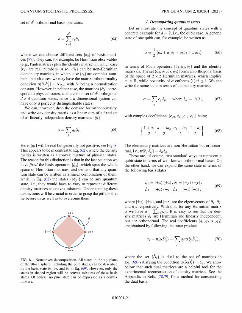
QUANTUM STOCHASTIC PROCESSES... PRX QUANTUM 2, 030201 (2021)
set of d2 orthonormal basis operators:
ρ =d2∑
k=1
rkσk, (64)
where we can choose different sets {σk} of basis matri-ces [77]. They can, for example, be Hermitian observables(e.g., Pauli matrices plus the identity matrix), in which case{rk} are real numbers. Also, {σk} can be non-Hermitianelementary matrices, in which case {rk} are complex num-bers; in both cases, we may have the matrix orthonormalitycondition tr[σj σ
†k ] = Nδjk, with N being a normalization
constant. However, in neither case, the matrices {σk} corre-spond to physical states, as there is no set of d2 orthogonald × d quantum states, since a d-dimensional system canhave only d perfectly distinguishable states.
We can, however, drop the demand for orthonormality,and write any density matrix as a linear sum of a fixed setof d2 linearly independent density matrices {�k}
ρ =∑
k
qk�k. (65)
Here, {qk} will be real but generally not positive, see Fig. 8.This appears to be in contrast to Eq. (62), where the densitymatrix is written as a convex mixture of physical states.The reason for this distinction is that in the last equation wehave fixed the basis operators {�k}, which span the wholespace of Hermitian matrices, and demand that any quan-tum state can be written as a linear combination of them,while in Eq. (62) the states {|ψj 〉} can be any quantumstate, i.e., they would have to vary to represent differentdensity matrices as convex mixtures. Understanding thesedistinctions will be crucial in order to grasp the pitfalls thatlie before us as well as to overcome them.
| x+⟩
| x−⟩
| y−⟩ | y+⟩
ρ
FIG. 8. Nonconvex decomposition. All states in the x-y planeof the Bloch sphere, including the pure states, can be describedby the basis state �1, �2, and �4 in Eq. (69). However, only thestates in shaded region will be convex mixtures of these basisstates. Of course, no pure state can be expressed as a convexmixture.
1. Decomposing quantum states
Let us illustrate the concept of quantum states with aconcrete example for d = 2, i.e., the qubit case. A genericstate of one qubit can, for example, be written as
α = 12(σ0 + a1σ1 + a2σ2 + a3σ3
)(66)
in terms of Pauli operators {σ1, σ2, σ3} and the identitymatrix σ0. The set {σ0, σ1, σ2, σ3} forms an orthogonal basisof the space of 2 × 2 Hermitian matrices, which impliesaj ∈ R, while positivity of α enforces
∑a2
j ≤ 1. We canwrite the same state in terms of elementary matrices
α =∑
ij
eij εij , where εij = |i〉〈j |, (67)
with complex coefficients {e00, e01, e10, e11} being
{1 + a3
2,
a1 − ia2
2,
a1 + ia2
2,
1 − a3
2
}. (68)
The elementary matrices are non-Hermitian but orthonor-mal, i.e., tr[εij ε
†kl] = δikδjl.
These are, of course, two standard ways to represent aqubit state in terms of well-known orthonormal bases. Onthe other hand, we can expand the same state in terms ofthe following basis states:
�1 = |+x〉 〈+x| , �2 = |+y〉 〈+y| ,
�3 = |+z〉 〈+z| , �4 = |−x〉 〈−x| ,(69)
where |±x〉, |±y〉, and |±z〉 are the eigenvectors of σ1, σ2,and σ3, respectively. With this, for any Hermitian matrixα we have α =∑k qk�k. It is easy to see that the den-sity matrices �k are Hermitian and linearly independent,but not orthonormal. The real coefficients {q1, q2, q3, q4}are obtained by following the inner product
qk = tr(αD†k) =∑
j
qj tr(�j D†k), (70)
where the set {Dk} is dual to the set of matrices inEq. (69) satisfying the condition tr(�iD
†j ) = δij . We show
below that such dual matrices are a helpful tool for theexperimental reconstruction of density matrices. See theAppendix in Refs. [78,79] for a method for constructingthe dual basis.
030201-21
SIMON MILZ and KAVAN MODI PRX QUANTUM 2, 030201 (2021)
For example, for the set of density matrices in Eq. (69)the dual set is
D1 = σ0 + σ1 − σ2 − σ3
2, D2 = σ2,
D3 = σ3, D4 = σ0 − σ1 − σ2 − σ3
2.
(71)
Note that, even though the states �k are positive, this dualset {Dk} does not consist of positive matrices (all the dualsof a set of Hermitian matrices are Hermitian, though [79]).Nonetheless, it gives us the coefficient in Eq. (70) as
{1 + a1 − a2 − a3
2, a2, a3,
1 − a1 − a2 − a3
2
}. (72)
Interestingly, the dual set of a basis itself also forms a linearbasis, and we can write any state α as
α =∑
k
pkD†k , (73)
where pk = tr(α�k). Note that, if all basis elements �k arepositive semidefinite, then pk ≥ 0, and we have
∑k pk =
1 if∑
k �k = 1. This decomposition in particular lendsitself nicely to experimental reconstruction of the state α.Specifically, given many copies of α, the value tr(α�k) isobtained by projecting α along directions x, y, z, i.e., mea-suring the observables σ1, σ2, and σ3. The inner producttr(α�k) is then nothing more than a projective measure-ment along direction k and pk is the probability of observ-ing the respective outcomes. Importantly, as the duals {Dk}can be computed from the basis {�k}, these probabilitiesthen allow us to estimate the state via Eq. (73).
Intuitively, this procedure is not unlike the way in whichone determines the classical state of a system; for exam-ple, in order to determine the bias of a coin, one flips itmany times and records the respective outcome probabili-ties for heads and tails. The crucial difference is quantummechanics is that one must measure in different directionsto fully construct the state of interest. Algebraically, thisfact is reflected by the dimension of the space of d × dHermitian matrices, which is d2 dimensional, thus, in orderto fully determine a density matrix, one needs to knowits overlap with d2 linearly independent Hermitian matri-ces. If, however, one knows in which basis the state oneaims to represent is diagonal—as is the case in classicalphysics—then the overlap with the d projectors that makeup its eigenbasis is sufficient.
The procedure to estimate a quantum state by measuringit is called quantum state tomography [80–82]. There aremany sophisticated methods to this nowadays, which weonly briefly touch on in this tutorial.
2. Measuring quantum states: POVMs and dual sets
A quantum state can be reconstructed experimentally,by measuring enough observables (above, with the observ-ables σ1, σ2, and σ3), and collecting the correspondingoutcome probabilities. Performing pure projective mea-surement is not the only way in quantum mechanics togather information about a state. More generally, a mea-surement is described by a POVM, a collection J ={Ek}n
k=1 of positive operators (here, matrices), that add upto the identity, i.e.,
∑k Ek = 1 (we comment on the phys-
ical realizability of POVMs below; for the moment, theycan just be thought of as a natural generalization of pro-jective measurements). Each Ek corresponds to a possiblemeasurement outcome, and the probability to observe saidoutcome is given by the Born rule:
pk = tr(ρEk). (74)
Projective measurements are then a special case ofPOVMs, where Ek = |k〉〈k| and {|k〉} are the eigenstates ofthe measured observable. For example, when measuringthe observable σ3, the corresponding POVM is given byJ = {|+z〉〈+z|, |−z〉〈−z|}, and the respective probabili-ties are computed via p± = 〈±z|ρ| ± z〉 = tr(ρ|±z〉〈±z|).
A less trivial example on a qubit is the symmetricinformationally complete (SIC) POVM [80] J = {Ek =12 |φk〉〈φk|}4
k=1, where
|φ1〉 = |0〉 , (75)
|φk〉 =√
13
|0〉 +√
23
ei(2(k−2)π/3) |1〉 for k = 2, 3, 4.
While still pure (up to normalization), these POVM ele-ments are not orthogonal. However, as they are linearlyindependent, they span the d2 = 4-dimensional space ofHermitian qubit matrices, and every density matrix isfully characterized once the probabilities pk = tr(ρEk)
are known. As this holds true in any dimension forPOVMs consisting of d2 linearly independent elements,such POVMs are called “informationally complete” (IC)[83]. Importantly, using the ideas outlined above, an infor-mationally complete POVM allows one to fully reconstructdensity matrices.
In short, to do so, one measures the system with anIC POVM, whose operators {Ek} linearly span the matrixspace of the system at hand. The POVM yields probabili-ties {pk}, and the measurement operators {Ek} have a dualset {�k}. The density matrix is then of the form [see alsoEq. (73)]
ρ =∑
k
pk�†k , (76)
which can be seen by direct insertion; the above stateyields the correct probability with respect to each of the
030201-22
QUANTUM STOCHASTIC PROCESSES... PRX QUANTUM 2, 030201 (2021)
POVM elements Ek. Concretely, we have
tr(ρEk) =∑
ptr(�Ek) = pk, (77)
where we use tr(�Ek) = δk. As the POVM is infor-mationally complete, this implies the state defined inEq. (76) yields the correct probabilities with respect toevery POVM.
It remains to comment on the existence of IC POVMs,and the physical realizability of POVMs in general, which,at first sight, appear to be a mere mathematical construc-tion. Concerning the former, it is easy to see that therealways exists a basis of d2 × d2 Hermitian matrices thatonly consists of positive elements. Choosing such a set
{Fk}d2
k=1 of positive elements, one can set F :=∑d2
k=1 Fk.By construction, F is positive semidefinite. Without muchloss of generality, let us assume that F is invertible (if itis not, then we could work with the pseudoinverse in whatfollows). Then,
J = {Ek = F−1/2FkF−1/2}d2
k=1 (78)
constitutes a set of positive matrices that add up to 1.To see that the matrices {Ek}d2
k=1 are linearly indepen-dent, let us assume the opposite and that, for example,E1 can be written in terms of the remaining Ek, i.e.,
E1 =∑d2
k=2 akEk. Multiplying this expression from the
left and the right by F1/2 then yields F1 =∑d2
k=2 akFk,which contradicts the original assumption that the matri-ces {Fk}d2
k=1 are linearly independent. Consequently, the set
{Ek}d2
k=1 is an IC POVM. More pragmatically, one couldmake one’s life easier and sample d2 − 1 positive matrices
{Ek}d2−1k=1 according to one’s measure of choice. In general,
these sampled matrices are linearly independent. Then, one
chooses an α > 0 such that Ed2 := 1 −∑k{Ek}d2−1k=1 ≥ 0.
With this, the set {Ek}d2
k=1 is a POVM by construction, andin general also informationally complete.
With respect to the latter, i.e., the physical realizabil-ity of POVMs, due to Neumark’s theorem [84–86], anyPOVM can be realized as a pure projective measurementin a higher-dimensional space, thus putting them on thesame foundational footing as “normal” measurements inquantum mechanics. Without going any deeper into thetheory of POVMs, let us emphasize the take-home mes-sage of the above sections: quantum states can be exper-imentally reconstructed in a very similar way as classicalstates, by simply collecting sufficient statistics; however,the number of necessary measurements is larger and theirstructure is richer. While this latter point seems innocuous,it actually lies at the heart of the problems one encoun-ters when generalizing classical stochastic processes to the
quantum realm, like the breakdown of the KET; if all nec-essary measurements could be chosen to be diagonal in thesame basis, then there would be no fundamental differencebetween classical and quantum processes.
B. Quantum stochastic matrix
Our overarching aim is to generalize the notion ofstochastic processes to quantum theory. Here, after havingdiscussed quantum states and their experimental recon-struction in the previous section, we generalize the notionof classical stochastic matrices. In the classical case astochastic matrix, in Eq. (12), is a mapping of a statisticalstate from time tj to time tk, i.e., �(k:j ) : P(Xj ) �→ P(Xk).As such, in clear analogy, we are looking for a mappingof the form E(k:j ) : ρ(tj ) �→ ρ(tk). While there are differ-ent representations of E(k:j ) (see, for example, Ref. [79]),we start with the one that most closely resembles theclassical case, where a probability vector gets mapped toanother probability vector by means of a matrix �(k:j ). Thedensity matrix is the quantum generalization of the classi-cal probability distribution. Then, consider the followingtransformation that turns a density matrix into a vector:
ρ =∑
rs
ρrs |r〉 〈s| ←→ |ρ〉〉 :=∑
rs
ρrs |rs〉〉 , (79)
where we use the |•〉〉 notation to emphasize that thevector originally stems from a matrix. This procedureis often called vectorization of matrices, for details seeRefs. [56,87–89].
Next, in clear analogy to Eq. (14), we can define a matrixE that maps a density matrix ρ (say, at time tj ) to anotherdensity matrix ρ ′ (say, at time tk); we add the symbol ˘ todistinguish the map E from its matrix representation E .Using the above notation, this matrix can be expressed as
E :=∑
r′s′,rs
Er′s′,rs |r′s′〉〉 〈〈rs| (80)
and the action of E can be written as
|E[ρ]〉〉 = E |ρ〉〉 =∑
r′s′rs
Er′s′,rsρrs |r′s′〉〉 = |ρ ′〉〉 . (81)
Here, E is simply a matrix representing the map E :B(Hi) → B(Ho) [90], very much like the stochasticmatrix, that maps the initial state to the final state. Forbetter bookkeeping, we explicitly distinguish between theinput (i) Hilbert space Hi and output (o) Hilbert space Ho
and denote the space of matrices on said spaces by B(Hx).While for the remainder of this tutorial, the dimensions ofthese two spaces generally agree, in general, the two areallowed to differ, and even in the case where they do not, itproves advantageous to keep track of the different spaces.
030201-23
SIMON MILZ and KAVAN MODI PRX QUANTUM 2, 030201 (2021)
It was with the above intuition Sudarshan et al. calledE the quantum stochastic matrix [68]. In today’s litera-ture, it is often referred to as a quantum channel, quantumdynamical map, etc. Along with many names, it also hasmany representations. We do not go much into these detailshere (see Ref. [79] for further information). We, however,briefly discuss some of its important properties. Note, thatwe stick to discrete level systems and do not touch thetopics of Gaussian quantum information [91,92].
Amplitude damping channel. Before that, let usquickly provide an explicit example of a quantum stochas-tic matrix. Consider a relaxation process that takes anyinput quantum state to the ground state. Such a process is,for example, described by the so-called amplitude dampingchannel
EAD(t:0) =
⎛
⎜⎜⎝
1 0 0 1 − p(t)0√
p(t) 0 00 0
√p(t) 0
0 0 0 p(t)
⎞
⎟⎟⎠ . (82)
This matrix acts on a vectorized density matrix of a qubit,i.e., |ρ(0)〉〉 = [ρ00, ρ01, ρ10, ρ11]T to yield |ρ(t)〉〉 = {ρ00 +[1 − p(t)]ρ11,
√p(t)ρ01,
√p(t)ρ10, p(t)ρ11}T. When p(t) =
exp{−γ t}, we get relaxation exponentially fast in time, andfor t → ∞, any input state will be mapped to [1, 0, 0, 0]T.This example is very close in spirit of the classical examplein Eq. (40).
Here, already, it is easy to see that the matrices E , unliketheir classical counterparts, do not possess nice properties,like Hermiticity, or stochasticity (note that, for example,neither the rows not the columns of EAD
(t:0) sum to unity).However, these shortcomings can be remedied in differentrepresentations of E . Also note that, here, we actually havea family of quantum stochastic matrices parameterized bytime (for each time t we have in general a different map).When we speak of a family of maps we label them withsubscript (t : 0). However, often the stochastic matrix rep-resents only a mapping from the initial time to a final time.In such cases, we omit the subscript and refer to the initialand final states as ρ and ρ ′, respectively.
1. Linearity and tomography
Having formally introduced quantum maps, the gener-alization of stochastic matrices in the classical case, it isnow time to discuss the properties they should display. Webegin with one of the most important features of quantumdynamics. The quantum stochastic map, like its classicalcounterpart, is a linear map:
E[αA + βB] = αE[A] + βE[B]. (83)
This is straightforwardly clear for the specific case ofthe quantum stochastic matrix E because the vectoriza-tion of a density matrix itself is also a linear map, i.e.,
|A + B〉〉 = |A〉〉 + |B〉〉. Once this is done, the rest is justmatrix transformations, which are linear.
The importance of linearity cannot be overstated andexploit this property over and over and, in particular, thelinearity of quantum dynamics plays a crucial role in defin-ing an unambiguous set of Markov conditions in quantummechanics and, as we have seen, it is the fundamentalingredient in the experimental reconstruction of quantumobjects. Due to linearity, a quantum channel is fully definedonce its action on a set of linearly independent states isknown. From a practical point of view, this is importantfor experimentally characterizing quantum dynamics bymeans of a procedure known as quantum process tomog-raphy [80,93] (see, e.g., Refs. [94,95] for a more in-depthdiscussion).
To see how this works out in practice, let us preparea set of linearly independent input states, say {�k}, anddetermine their corresponding outputs {E[�k]} by means ofquantum state tomography (which we discuss above). Thecorresponding input-output relation then fully determinesthe action of the stochastic map on any density matrix
E[ρ] =∑
k
qkE[�k], (84)
where we use Eq. (65), i.e., ρ =∑k qk�k. The aboveequation highlights that, once the output states for a basisof input states are known, the action of the entire map isdetermined.
Using ideas akin to the aforementioned tomography ofquantum states we can also directly use linearity and dualsets to reconstruct the matrix E . Above, we see that a quan-tum state is fully determined, once the probabilities for aninformationally complete POVM are known. In the samevein, a quantum map is fully determined, once the outputstates for a basis {�j }d2
j =1 of input states are known. Con-cretely, setting ρ ′
j = E[�j ], and denoting the dual set of
{�j }d2
j =1 by {Dk}d2
k=1, we have
E =d2∑
j =1
|ρ ′j 〉〉〈〈Dj |. (85)
Indeed, it is easy to see that 〈〈A|B〉〉 = tr(A†B), implyingthat, with the above definition, we have E |�j 〉〉 = |ρ ′
j 〉〉 for
all basis elements. Due to linearity, this implies that Eyields the correct output state for any input state. Mea-suring the output states for a basis of input states is thussufficient to perform process tomography. Specifically, ifthe output states ρ ′
j are measured by means of an informa-tionally complete POVM {Ek} with corresponding dual set{�k}d2
k=1, then ρ ′j =∑k p (j )
k �†k , with p (j )
k = tr(�j Ek) and
030201-24
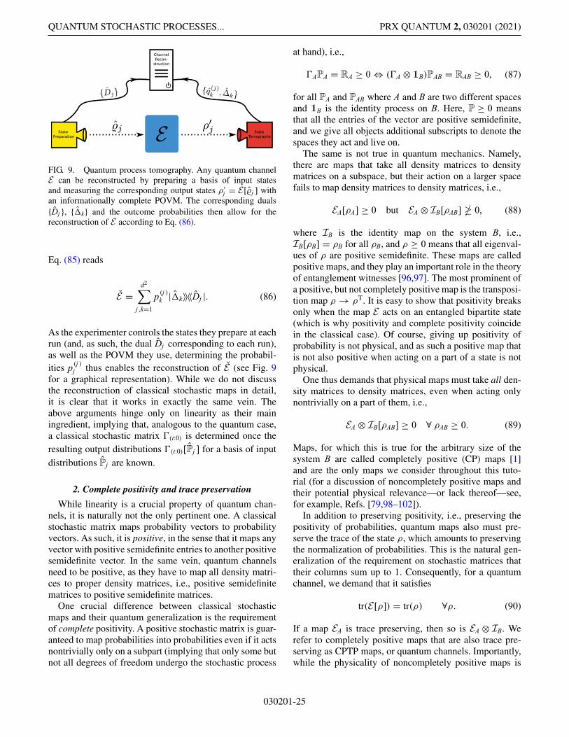
QUANTUM STOCHASTIC PROCESSES... PRX QUANTUM 2, 030201 (2021)
FIG. 9. Quantum process tomography. Any quantum channelE can be reconstructed by preparing a basis of input statesand measuring the corresponding output states ρ ′
j = E[�j ] withan informationally complete POVM. The corresponding duals{Dj }, {�k} and the outcome probabilities then allow for thereconstruction of E according to Eq. (86).
Eq. (85) reads
E =d2∑
j ,k=1
p (j )k |�k〉〉〈〈Dj |. (86)
As the experimenter controls the states they prepare at eachrun (and, as such, the dual Dj corresponding to each run),as well as the POVM they use, determining the probabil-ities p (j )
j thus enables the reconstruction of E (see Fig. 9for a graphical representation). While we do not discussthe reconstruction of classical stochastic maps in detail,it is clear that it works in exactly the same vein. Theabove arguments hinge only on linearity as their mainingredient, implying that, analogous to the quantum case,a classical stochastic matrix �(t:0) is determined once theresulting output distributions �(t:0)[Pj ] for a basis of input
distributions Pj are known.
2. Complete positivity and trace preservation
While linearity is a crucial property of quantum chan-nels, it is naturally not the only pertinent one. A classicalstochastic matrix maps probability vectors to probabilityvectors. As such, it is positive, in the sense that it maps anyvector with positive semidefinite entries to another positivesemidefinite vector. In the same vein, quantum channelsneed to be positive, as they have to map all density matri-ces to proper density matrices, i.e., positive semidefinitematrices to positive semidefinite matrices.
One crucial difference between classical stochasticmaps and their quantum generalization is the requirementof complete positivity. A positive stochastic matrix is guar-anteed to map probabilities into probabilities even if it actsnontrivially only on a subpart (implying that only some butnot all degrees of freedom undergo the stochastic process
at hand), i.e.,
�APA = RA ≥ 0 ⇔ (�A ⊗ 1B)PAB = RAB ≥ 0, (87)
for all PA and PAB where A and B are two different spacesand 1B is the identity process on B. Here, P ≥ 0 meansthat all the entries of the vector are positive semidefinite,and we give all objects additional subscripts to denote thespaces they act and live on.
The same is not true in quantum mechanics. Namely,there are maps that take all density matrices to densitymatrices on a subspace, but their action on a larger spacefails to map density matrices to density matrices, i.e.,
EA[ρA] ≥ 0 but EA ⊗ IB[ρAB] � 0, (88)
where IB is the identity map on the system B, i.e.,IB[ρB] = ρB for all ρB, and ρ ≥ 0 means that all eigenval-ues of ρ are positive semidefinite. These maps are calledpositive maps, and they play an important role in the theoryof entanglement witnesses [96,97]. The most prominent ofa positive, but not completely positive map is the transposi-tion map ρ → ρT. It is easy to show that positivity breaksonly when the map E acts on an entangled bipartite state(which is why positivity and complete positivity coincidein the classical case). Of course, giving up positivity ofprobability is not physical, and as such a positive map thatis not also positive when acting on a part of a state is notphysical.
One thus demands that physical maps must take all den-sity matrices to density matrices, even when acting onlynontrivially on a part of them, i.e.,
EA ⊗ IB[ρAB] ≥ 0 ∀ ρAB ≥ 0. (89)
Maps, for which this is true for the arbitrary size of thesystem B are called completely positive (CP) maps [1]and are the only maps we consider throughout this tuto-rial (for a discussion of noncompletely positive maps andtheir potential physical relevance—or lack thereof—see,for example, Refs. [79,98–102]).
In addition to preserving positivity, i.e., preserving thepositivity of probabilities, quantum maps also must pre-serve the trace of the state ρ, which amounts to preservingthe normalization of probabilities. This is the natural gen-eralization of the requirement on stochastic matrices thattheir columns sum up to 1. Consequently, for a quantumchannel, we demand that it satisfies
tr(E[ρ]) = tr(ρ) ∀ρ. (90)
If a map EA is trace preserving, then so is EA ⊗ IB. Werefer to completely positive maps that are also trace pre-serving as CPTP maps, or quantum channels. Importantly,while the physicality of noncompletely positive maps is
030201-25
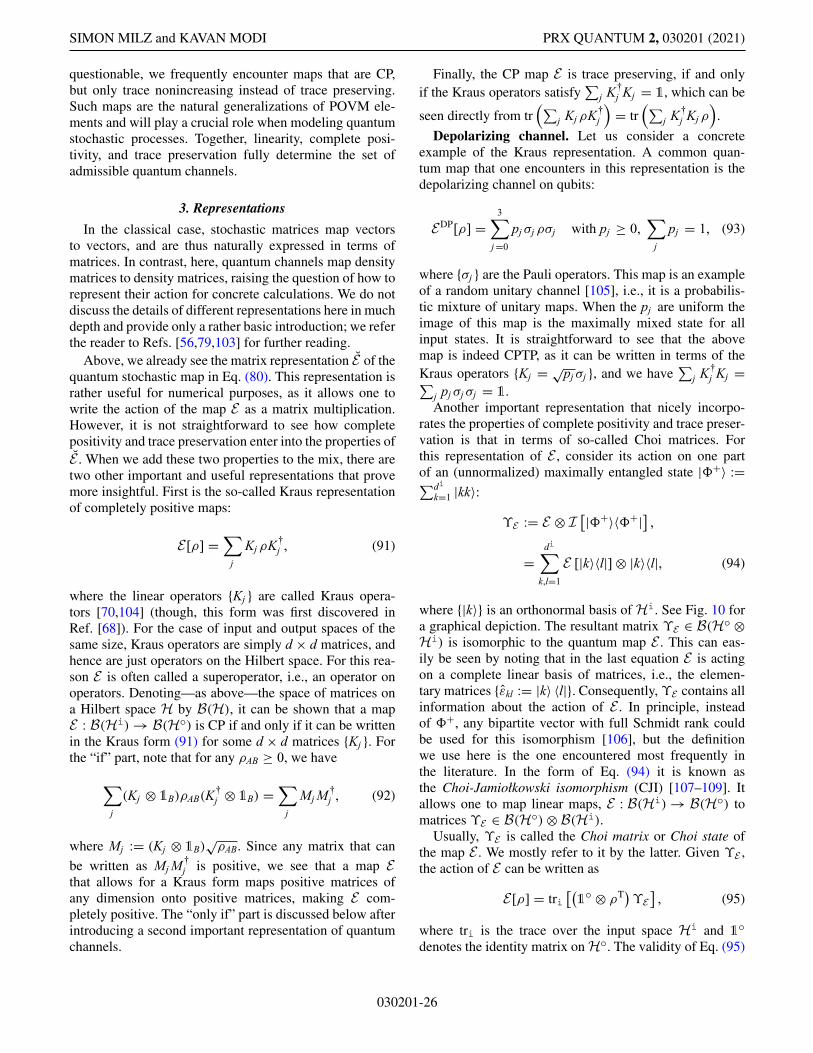
SIMON MILZ and KAVAN MODI PRX QUANTUM 2, 030201 (2021)
questionable, we frequently encounter maps that are CP,but only trace nonincreasing instead of trace preserving.Such maps are the natural generalizations of POVM ele-ments and will play a crucial role when modeling quantumstochastic processes. Together, linearity, complete posi-tivity, and trace preservation fully determine the set ofadmissible quantum channels.
3. Representations
In the classical case, stochastic matrices map vectorsto vectors, and are thus naturally expressed in terms ofmatrices. In contrast, here, quantum channels map densitymatrices to density matrices, raising the question of how torepresent their action for concrete calculations. We do notdiscuss the details of different representations here in muchdepth and provide only a rather basic introduction; we referthe reader to Refs. [56,79,103] for further reading.
Above, we already see the matrix representation E of thequantum stochastic map in Eq. (80). This representation israther useful for numerical purposes, as it allows one towrite the action of the map E as a matrix multiplication.However, it is not straightforward to see how completepositivity and trace preservation enter into the properties ofE . When we add these two properties to the mix, there aretwo other important and useful representations that provemore insightful. First is the so-called Kraus representationof completely positive maps:
E[ρ] =∑
j
Kj ρK†j , (91)
where the linear operators {Kj } are called Kraus opera-tors [70,104] (though, this form was first discovered inRef. [68]). For the case of input and output spaces of thesame size, Kraus operators are simply d × d matrices, andhence are just operators on the Hilbert space. For this rea-son E is often called a superoperator, i.e., an operator onoperators. Denoting—as above—the space of matrices ona Hilbert space H by B(H), it can be shown that a mapE : B(Hi) → B(Ho) is CP if and only if it can be writtenin the Kraus form (91) for some d × d matrices {Kj }. Forthe “if” part, note that for any ρAB ≥ 0, we have
∑
j
(Kj ⊗ 1B)ρAB(K†j ⊗ 1B) =
∑
j
Mj M †j , (92)
where Mj := (Kj ⊗ 1B)√ρAB. Since any matrix that can
be written as Mj M †j is positive, we see that a map E
that allows for a Kraus form maps positive matrices ofany dimension onto positive matrices, making E com-pletely positive. The “only if” part is discussed below afterintroducing a second important representation of quantumchannels.
Finally, the CP map E is trace preserving, if and onlyif the Kraus operators satisfy
∑j K†
j Kj = 1, which can be
seen directly from tr(∑
j Kj ρK†j
)= tr(∑
j K†j Kj ρ)
.
Depolarizing channel. Let us consider a concreteexample of the Kraus representation. A common quan-tum map that one encounters in this representation is thedepolarizing channel on qubits:
EDP[ρ] =3∑
j =0
pj σj ρσj with pj ≥ 0,∑
j
pj = 1, (93)
where {σj } are the Pauli operators. This map is an exampleof a random unitary channel [105], i.e., it is a probabilis-tic mixture of unitary maps. When the pj are uniform theimage of this map is the maximally mixed state for allinput states. It is straightforward to see that the abovemap is indeed CPTP, as it can be written in terms of theKraus operators {Kj = √pj σj }, and we have
∑j K†
j Kj =∑j pj σj σj = 1.Another important representation that nicely incorpo-
rates the properties of complete positivity and trace preser-vation is that in terms of so-called Choi matrices. Forthis representation of E , consider its action on one partof an (unnormalized) maximally entangled state |�+〉 :=∑di
k=1 |kk〉:ϒE := E ⊗ I
[|�+〉〈�+|] ,
=di∑
k,l=1
E [|k〉〈l|] ⊗ |k〉〈l|, (94)
where {|k〉} is an orthonormal basis of Hi. See Fig. 10 fora graphical depiction. The resultant matrix ϒE ∈ B(Ho ⊗Hi) is isomorphic to the quantum map E . This can eas-ily be seen by noting that in the last equation E is actingon a complete linear basis of matrices, i.e., the elemen-tary matrices {εkl := |k〉 〈l|}. Consequently, ϒE contains allinformation about the action of E . In principle, insteadof �+, any bipartite vector with full Schmidt rank couldbe used for this isomorphism [106], but the definitionwe use here is the one encountered most frequently inthe literature. In the form of Eq. (94) it is known asthe Choi-Jamiołkowski isomorphism (CJI) [107–109]. Itallows one to map linear maps, E : B(Hi) → B(Ho) tomatrices ϒE ∈ B(Ho) ⊗ B(Hi).
Usually, ϒE is called the Choi matrix or Choi state ofthe map E . We mostly refer to it by the latter. Given ϒE ,the action of E can be written as
E[ρ] = tri[(1o ⊗ ρT
)ϒE]
, (95)
where tri is the trace over the input space Hi and 1o
denotes the identity matrix on Ho. The validity of Eq. (95)
030201-26
QUANTUM STOCHASTIC PROCESSES... PRX QUANTUM 2, 030201 (2021)
can be seen by direct insertion of Eq. (94):
tri[(1o ⊗ ρT
)ϒE] =
di∑
k,=1
〈|ρT|k〉 E [|k〉〈l|] ,
=di∑
k,=1
E [〈k|ρ|〉 |k〉〈|] ,
= E[ρ], (96)
where we use the linearity of E . A related decompositionof the Choi state is
ϒE =∑
k
ρ ′j ⊗ D∗
j , (97)
where {ρ ′j = E[ρj ]} are the output states corresponding to a
basis of input states. The above equation is simply a reshuf-fling of Eq. (85) from vectors to matrices. As is the case forEq. (85), its validity can be checked by realizing that theChoi state ϒE yields the correct output state for a full basisof input states, which can be seen by direct insertion ofEq. (97) into (95).
For quantum maps, ϒE has particularly nice properties.Complete positivity of E is equivalent to ϒE ≥ 0, and itis straightforward to deduce from Eq. (95) that E is tracepreserving if and only if tro(ϒE) = 1i (see below for aquick justification of these statements). These propertiesare much more transparent, and easier to work with than,for example, the properties that make E a matrix corre-sponding to a CPTP map. Additionally, Eq. (95) allows oneto directly relate the representation of E in terms of Krausoperators to the Choi state ϒE , and, in particular, the mini-mal number of required Kraus operators to the rank of ϒE .Specifically, in terms of its eigenbasis, ϒE can be written asϒE =∑r
α=j λj |�j 〉〈�j |, where r = rank(ϒE) and λj ≥ 0.
FIG. 10. Choi-Jamiołkowski isomorphism. A map E : B(Hi)
→ B(Ho) can be mapped to a matrix ϒE ∈ B(Ho ⊗ Hi) byletting it act on one half on a maximally entangled state. Notethat, for ease of notation, here, we let E act on B(Hi′), such thatϒE ∈ B(Ho ⊗ Hi). As Hi′ ∼= Hi, this is merely a relabelingand not of conceptual relevance.
Inserting this into Eq. (95), we obtain
E[ρ] =r∑
j =1
⎛
⎝√λj
di∑
α=1
〈α|�j 〉 〈α|⎞
⎠ ρ
⎛
⎝√λj
di∑
β=1
|β〉 〈�j |β〉⎞
⎠,
=:r∑
j =1
Kj ρK†j , (98)
where {|α/β〉} is a basis of Hi. The above equation pro-vides a Kraus representation of E with the minimal numberof Kraus operators (for more details on this connectionbetween Choi matrices and Kraus operators, see, for exam-ple, Ref. [110]). Equation (98) directly allows us to providethe missing properties of the Kraus and Choi representa-tions that we alluded to above. Firstly, if E is CP, thennaturally, ϒE is positive, which can be seen from itsdefinition in Eq. (94). On the other hand, if ϒE is positive,then Eq. (98) tells us that it leads to a Kraus form, imply-ing that the corresponding map E is completely positive.In addition, this means that any completely positive mapadmits a Kraus decomposition, a claim we made severalparagraphs above. Finally, from Eq. (95) we see directlythat tro(ϒE) = 1i holds for all for trace-preserving mapsE . Naturally, all representations of quantum maps canbe transformed into one another; details of how this isdone can be found, for example, in Refs. [79,111]; how-ever, for our purposes, it will prove very advantageous topredominantly use Choi states.
Depolarizing channel. For concreteness, let us considerthe above case of the depolarizing channel EDP and provideits Choi state. Inserting Eq. (93) into Eq. (94), we obtain
ϒDPE =
⎛
⎜⎝
p0 + p3 0 0 p0 − p30 p1 + p2 p1 − p2 00 p1 − p2 p1 + p2 0
p0 − p3 0 0 p0 + p3
⎞
⎟⎠ . (99)
The resulting matrix ϒDPE is positive semidefinite (with
corresponding eigenvalues {2p0, 2p1, 2p2, 2p3}), satisfiestroϒDP
E = 1i, and trϒDPE = 2 = di.
Besides its appealing mathematical properties, the CJIis also of experimental importance. Given that a (normal-ized) maximally entangled state can be created in practice,the CJI enables another way of reconstructing a representa-tion of the map E ; letting it act on one half of a maximallyentangled state and reconstructing the resulting state viastate tomography directly yields ϒE . While this so-calledancilla-assisted process tomography [112,113] requiresthe same number of measurements as the input-outputprocedure, it can be—depending on the experimental sit-uation—easier to implement in the laboratory.
Additionally, since they simply correspond to quan-tum states with an additional trace condition, Choi statesstraightforwardly allow for the analysis of correlations in
030201-27
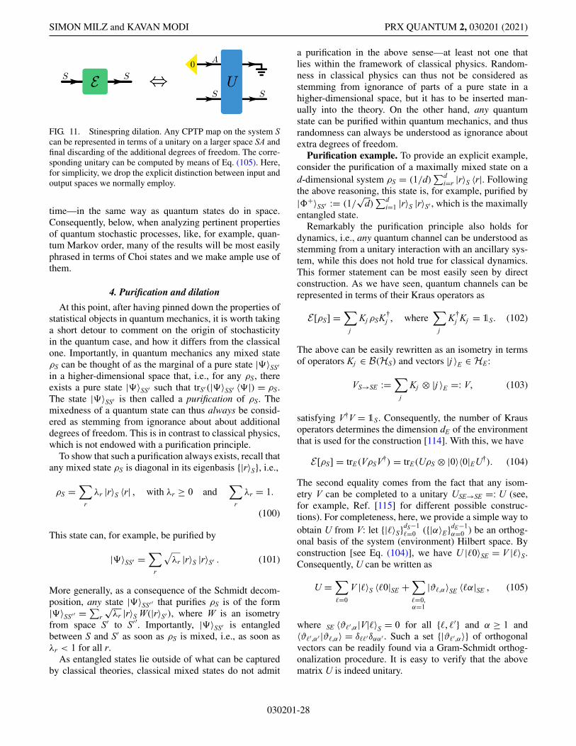
SIMON MILZ and KAVAN MODI PRX QUANTUM 2, 030201 (2021)
FIG. 11. Stinespring dilation. Any CPTP map on the system Scan be represented in terms of a unitary on a larger space SA andfinal discarding of the additional degrees of freedom. The corre-sponding unitary can be computed by means of Eq. (105). Here,for simplicity, we drop the explicit distinction between input andoutput spaces we normally employ.
time—in the same way as quantum states do in space.Consequently, below, when analyzing pertinent propertiesof quantum stochastic processes, like, for example, quan-tum Markov order, many of the results will be most easilyphrased in terms of Choi states and we make ample use ofthem.
4. Purification and dilation
At this point, after having pinned down the properties ofstatistical objects in quantum mechanics, it is worth takinga short detour to comment on the origin of stochasticityin the quantum case, and how it differs from the classicalone. Importantly, in quantum mechanics any mixed stateρS can be thought of as the marginal of a pure state |�〉SS′in a higher-dimensional space that, i.e., for any ρS, thereexists a pure state |�〉SS′ such that trS′(|�〉SS′ 〈�|) = ρS.The state |�〉SS′ is then called a purification of ρS. Themixedness of a quantum state can thus always be consid-ered as stemming from ignorance about about additionaldegrees of freedom. This is in contrast to classical physics,which is not endowed with a purification principle.
To show that such a purification always exists, recall thatany mixed state ρS is diagonal in its eigenbasis {|r〉S}, i.e.,
ρS =∑
r
λr |r〉S 〈r| , with λr ≥ 0 and∑
r
λr = 1.
(100)
This state can, for example, be purified by
|�〉SS′ =∑
r
√λr |r〉S |r〉S′ . (101)
More generally, as a consequence of the Schmidt decom-position, any state |�〉SS′′ that purifies ρS is of the form|�〉SS′′ =∑r
√λr |r〉S W(|r〉S′), where W is an isometry
from space S′ to S′′. Importantly, |�〉SS′ is entangledbetween S and S′ as soon as ρS is mixed, i.e., as soon asλr < 1 for all r.
As entangled states lie outside of what can be capturedby classical theories, classical mixed states do not admit
a purification in the above sense—at least not one thatlies within the framework of classical physics. Random-ness in classical physics can thus not be considered asstemming from ignorance of parts of a pure state in ahigher-dimensional space, but it has to be inserted man-ually into the theory. On the other hand, any quantumstate can be purified within quantum mechanics, and thusrandomness can always be understood as ignorance aboutextra degrees of freedom.
Purification example. To provide an explicit example,consider the purification of a maximally mixed state on ad-dimensional system ρS = (1/d)
∑di=r |r〉S 〈r|. Following
the above reasoning, this state is, for example, purified by|�+〉SS′ := (1/
√d)∑d
i=1 |r〉S |r〉S′ , which is the maximallyentangled state.
Remarkably the purification principle also holds fordynamics, i.e., any quantum channel can be understood asstemming from a unitary interaction with an ancillary sys-tem, while this does not hold true for classical dynamics.This former statement can be most easily seen by directconstruction. As we have seen, quantum channels can berepresented in terms of their Kraus operators as
E[ρS] =∑
j
Kj ρSK†j , where
∑
j
K†j Kj = 1S. (102)
The above can be easily rewritten as an isometry in termsof operators Kj ∈ B(HS) and vectors |j 〉E ∈ HE:
VS→SE :=∑
j
Kj ⊗ |j 〉E =: V, (103)
satisfying V†V = 1S. Consequently, the number of Krausoperators determines the dimension dE of the environmentthat is used for the construction [114]. With this, we have
E[ρS] = trE(VρSV†) = trE(UρS ⊗ |0〉〈0|EU†). (104)
The second equality comes from the fact that any isom-etry V can be completed to a unitary USE→SE =: U (see,for example, Ref. [115] for different possible construc-tions). For completeness, here, we provide a simple way toobtain U from V: let {|〉S}dS−1
=0 ({|α〉E}dE−1α=0 ) be an orthog-
onal basis of the system (environment) Hilbert space. Byconstruction [see Eq. (104)], we have U |0〉SE = V |〉S.Consequently, U can be written as
U =∑
=0
V |〉S 〈0|SE +∑
=0,α=1
|ϑ,α〉SE 〈α|SE , (105)
where SE 〈ϑ′,α|V|〉S = 0 for all {, ′} and α ≥ 1 and〈ϑ′,α′ |ϑ,α〉 = δ′δαα′ . Such a set {|ϑ′,α〉} of orthogonalvectors can be readily found via a Gram-Schmidt orthog-onalization procedure. It is easy to verify that the abovematrix U is indeed unitary.
030201-28
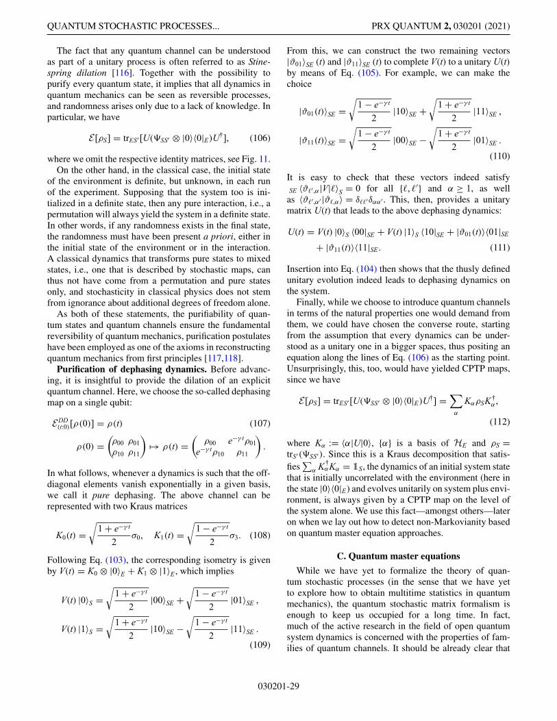
QUANTUM STOCHASTIC PROCESSES... PRX QUANTUM 2, 030201 (2021)
The fact that any quantum channel can be understoodas part of a unitary process is often referred to as Stine-spring dilation [116]. Together with the possibility topurify every quantum state, it implies that all dynamics inquantum mechanics can be seen as reversible processes,and randomness arises only due to a lack of knowledge. Inparticular, we have
E[ρS] = trES′[U(�SS′ ⊗ |0〉〈0|E)U†], (106)
where we omit the respective identity matrices, see Fig. 11.On the other hand, in the classical case, the initial state
of the environment is definite, but unknown, in each runof the experiment. Supposing that the system too is ini-tialized in a definite state, then any pure interaction, i.e., apermutation will always yield the system in a definite state.In other words, if any randomness exists in the final state,the randomness must have been present a priori, either inthe initial state of the environment or in the interaction.A classical dynamics that transforms pure states to mixedstates, i.e., one that is described by stochastic maps, canthus not have come from a permutation and pure statesonly, and stochasticity in classical physics does not stemfrom ignorance about additional degrees of freedom alone.
As both of these statements, the purifiability of quan-tum states and quantum channels ensure the fundamentalreversibility of quantum mechanics, purification postulateshave been employed as one of the axioms in reconstructingquantum mechanics from first principles [117,118].
Purification of dephasing dynamics. Before advanc-ing, it is insightful to provide the dilation of an explicitquantum channel. Here, we choose the so-called dephasingmap on a single qubit:
EDD(t:0)[ρ(0)] = ρ(t) (107)
ρ(0) =(ρ00 ρ01ρ10 ρ11
)�→ ρ(t) =
(ρ00 e−γ tρ01
e−γ tρ10 ρ11
).
In what follows, whenever a dynamics is such that the off-diagonal elements vanish exponentially in a given basis,we call it pure dephasing. The above channel can berepresented with two Kraus matrices
K0(t) =√
1 + e−γ t
2σ0, K1(t) =
√1 − e−γ t
2σ3. (108)
Following Eq. (103), the corresponding isometry is givenby V(t) = K0 ⊗ |0〉E + K1 ⊗ |1〉E , which implies
V(t) |0〉S =√
1 + e−γ t
2|00〉SE +
√1 − e−γ t
2|01〉SE ,
V(t) |1〉S =√
1 + e−γ t
2|10〉SE −
√1 − e−γ t
2|11〉SE .
(109)
From this, we can construct the two remaining vectors|ϑ01〉SE (t) and |ϑ11〉SE (t) to complete V(t) to a unitary U(t)by means of Eq. (105). For example, we can make thechoice
|ϑ01(t)〉SE =√
1 − e−γ t
2|10〉SE +
√1 + e−γ t
2|11〉SE ,
|ϑ11(t)〉SE =√
1 − e−γ t
2|00〉SE −
√1 + e−γ t
2|01〉SE .
(110)
It is easy to check that these vectors indeed satisfySE 〈ϑ′,α|V|〉S = 0 for all {, ′} and α ≥ 1, as wellas 〈ϑ′,α′ |ϑ,α〉 = δ′δαα′ . This, then, provides a unitarymatrix U(t) that leads to the above dephasing dynamics:
U(t) = V(t) |0〉S 〈00|SE + V(t) |1〉S 〈10|SE + |ϑ01(t)〉〈01|SE
+ |ϑ11(t)〉〈11|SE . (111)
Insertion into Eq. (104) then shows that the thusly definedunitary evolution indeed leads to dephasing dynamics onthe system.
Finally, while we choose to introduce quantum channelsin terms of the natural properties one would demand fromthem, we could have chosen the converse route, startingfrom the assumption that every dynamics can be under-stood as a unitary one in a bigger spaces, thus positing anequation along the lines of Eq. (106) as the starting point.Unsurprisingly, this, too, would have yielded CPTP maps,since we have
E[ρS] = trES′[U(�SS′ ⊗ |0〉〈0|E)U†] =∑
α
KαρSK†α ,
(112)
where Kα := 〈α|U|0〉, {α} is a basis of HE and ρS =trS′(�SS′). Since this is a Kraus decomposition that satis-fies∑
α K†αKα = 1S, the dynamics of an initial system state
that is initially uncorrelated with the environment (here inthe state |0〉〈0|E) and evolves unitarily on system plus envi-ronment, is always given by a CPTP map on the level ofthe system alone. We use this fact—amongst others—lateron when we lay out how to detect non-Markovianity basedon quantum master equation approaches.
C. Quantum master equations
While we have yet to formalize the theory of quan-tum stochastic processes (in the sense that we have yetto explore how to obtain multitime statistics in quantummechanics), the quantum stochastic matrix formalism isenough to keep us occupied for a long time. In fact,much of the active research in the field of open quantumsystem dynamics is concerned with the properties of fam-ilies of quantum channels. It should be already clear that
030201-29
SIMON MILZ and KAVAN MODI PRX QUANTUM 2, 030201 (2021)
the quantum stochastic matrix, like its classical counter-part, deals only with two-time correlations, see Figs. 6and 24, and can thus not provide a complete descriptionof quantum stochastic processes. This analogy goes fur-ther; as is the case on the classical side, an importantfamily of stochastic matrices corresponds to quantum mas-ter equations [119]. Before fully generalizing the conceptof stochastic processes to the quantum realm, let us thushave a quick—and very superficial—look at quantum mas-ter equations and witnesses of non-Markovianity that arebased on them.
Quantum master equations have a long and rich historydating back to the 1920s. Right at the inception of mod-ern quantum theory, Landau derived a master equation forlight interacting with charged matter [120]. This shouldnot be surprising because master equations play a keyrole in understanding the real phenomena observed inthe lab. For the same reason, they are widely used toolsfor theoretical physicists and beyond, including quantumchemistry, condensed-matter physics, high-energy physics,material science, and so on. However, the formal deriva-tion of overarching master equations took another 30 years.Nakajima and Zwanzig independently derived exact mem-ory kernel master equations using the so-called projectionoperator method. Since then there have been an enormousnumber of studies of non-Markovian master and stochas-tic equations [121–144], spanning from exploring theirmathematical structure, studying the transition betweenthe Markovian and non-Markovian regime [145,146] andapplying them to chemistry or condensed-matter systems.Here, we do not concern ourselves with these details andlimit our discussion to the overarching structure of themaster equation, and in particular how to tell Markovianones apart from non-Markovian ones. We refer the readerto standard textbooks for more details [2,3,5] on theseaspects as well as proper derivations, which we do notprovide in this section.
The most general quantum master has a form alreadyfamiliar to us. We simply replace the probability distri-bution in Eq. (36) with a density matrix to obtain theNakajima-Zwanzig master equation [147]
ddt
ρ(t) =∫ t
sK(t, τ)[ρ(τ)]dτ . (113)
Above, K(t, τ) is a superoperator [148] that is called thememory kernel. Often, this equation is written in two parts
ddt
ρ(t) = −i[H , ρ(t)] + D[ρ(t)] +∫ t
sK(t, τ)[ρ(τ)]dτ ,
(114)
where D is called the dissipator with the form
D[ρ(t)] =d2∑
n,m=1
γj
(Lj ρ(t)L
†j − 1
2
{L†
j Lj , ρ(t)})
. (115)
Above, the first term on the rhs corresponds to a unitarydynamics, the second term is the dissipative part of theprocess, and the third terms carry the memory (which canalso be dissipative). We note in passing that we have yet todefine what Markovian and non-Markovian actually meanin the quantum realm, and how the ensuing definitionsrelate to their classical counterparts. We provide a rigorousdefinition of these concepts in Sec. VI, while here, for themoment, we content ourselves with the vague “definition”that non-Markovian processes are those where memoryeffects play a non-negligible role; Markovian processes arethose where memory effects are absent.
While the Nakajima-Zwanzig equation is the most gen-eral quantum master equation, the rage in the 1960s and1970s was to derive the most general Markovian masterequation. It took well over a decade to get there, aftermany attempts, see Ref. [149] for more on this historyand Ref. [150] for a pedagogical treatment. Those whofailed in this endeavor were missing a key ingredient, com-plete positivity. In 1976, this feat was finally achievedby Gorini-Kossakowski-Sudarshan [66] and Lindblad [67]independently [151]. A quantum Markov process can bedescribed by this master equation, now known as theGKSL master equation. Equation (114) already containsthe GKSL master equation in the sense that the final termvanishes for the Markov process
ddt
ρt = L[ρt] with L[•] = −i[H , •] + D[•], (116)
and, here L stands for Louivillian, but often called Lind-bladian. Intuitively, the above master equation is consid-ered memoryless, since it does not contain the integralover past states that is present in Eq. (114) (we see inSec. VI A 2 that this intuition is somewhat too simplistic,since there are processes that carry memory effects but cannonetheless be modeled by a GKSL equation). If L is timeindependent, then the above master equation has the formalsolution
ρt = Et:r[ρr] = eL(t−r)[ρr], (117)
where ρr is the system state at time r. From this, we see thatthe respective dynamics between two arbitrary times r andt depends only on t − r, but not the absolute times r andt (or any earlier times). Using eL(t−r) = eL(t−s)eL(s−r), thisimplies the often used semigroup property of Markovian
030201-30
QUANTUM STOCHASTIC PROCESSES... PRX QUANTUM 2, 030201 (2021)
dynamics
Et:r = Et:s ◦ Es:r (118)
for t ≥ s ≥ r.Some remarks are in order. The decomposition in
Eq. (114) is not always unique. Often, a term dubbedas the inhomogeneous term is present and it is due tothe initial system-environment correlations. As we out-line below, describing dynamics with initial correlations interms of quantum channels (and thus, master equations),is operationally dubious and the interpretation of an inho-mogeneous term as stemming from initial correlations thussomewhat misdirected.
In the Markovian case, the superoperators in Eq. (116)should be time independent. In fact, it is possible to derivemaster equations for non-Markovian processes that lookjust like Eq. (116) but then the superoperators will be timedependent and the rates {γj } may be negative [38,135,152–155] (while they are always positive in the Markoviancase). For a Markovian master equation, the operators {Lj }are directly related to the Kraus operators of the result-ing quantum channels [156]. Since Eq. (114) is the mostgeneral form of a quantum master equation it containsequations due to Redfield, Landau, Pauli, and others. Toreach this equation one usually expands and approximatesthe memory kernel. This is a field of its own and we can-not do justice to these methods or the reasoning behind theapproximations here (for a comparison of the validity ofthe different employed approximations, see, for example,Refs. [157,158]).
As with the classical case, the above master equationsexpress the statistical quantum state continuously in time[159]. They can be either derived from first principles bymaking the right approximations, or as adhoc phenomeno-logical dynamical equations that model the pertinent prop-erties of a process at hand (see, for example, Ref. [3] fora wide array of different derivations of quantum masterequations).
As before, it may be tempting to think that the masterequation is equivalent to a stochastic process as definedabove. However, just as in the classical case, the quantummaster equation accounts only for two-point correlations.This can be seen intuitively by realizing that the solutionof a master equation is a family of quantum channels, eachcorresponding to two-time correlations, or, more directly,by employing the transfer tensor method [40–42], whichshows that the rhs of Eq. (114) can be expressed as a lin-ear combination of product of quantum maps E(c:b) ◦ E(b:a),with c being either t or t − dt, b = s, and a being eitherthe initial time. A quantum map E(b:a) is a mapping of apreparation at time a to a density matrix at time b. Thus,it contains only correlations between two times a and b.The lhs can be computed by setting b = t and a = t − dt.Another formal method for showing that the rhs can be
expressed as a product of two stochastic matrices can bedone by means of the Laplace transform [38,39].
This also puts into question our somewhat lax use ofthe term “Markovian” in the above discussion. As we dis-cuss in the classical case, Markovianity is a statementabout conditional independence for multitime probabilitydistributions. How, then, can a master equation that is con-cerned with two-point correlations only, be Markovian?Indeed, as we see below it is possible to have physicalnon-Markovian processes (i.e., processes that do not dis-play the correct conditional independence) that can bedescribed by what we dub a Markovian master equationin Eq. (116). That is, the implication only goes one way;a Markov process always leads to a master equation ofEq. (114) form with the final term vanishing. The conversedoes not hold. We detail an example below, but to fullyappreciate it we must have a better understanding of mul-titime quantum correlations. Nonetheless, while it is notpossible to unambiguously deduce the Markovianity of aprocess from limited statistical data only, one can, just likein the classical case, already use it to detect the presence ofmemory effects.
D. Witnessing non-Markovianity
As mentioned above, Markovian processes will lead tomaster equations of the form of Eq. (116) and, in turn,can be fully described by the resulting family of CPTPmaps. Thus, having access to the stochastic matrix andmaster equation is already sufficient to witness departuresfrom Markovianity. That is, there are certain features andproperties that must belong to any Markovian quantumprocesses, which then allows for discriminating betweenMarkov and non-Markov processes.
1. Initial correlations
Consider the dynamics of a system from an initial timeto some final time. When the system interacts with anenvironment the process on the system can be describedby a map E(t:0). As we show in Eq. (104), such a mapcan be thought to come from unitary system-environmentdynamics, with the caveat that the initial system environ-ment has no correlations [in Eq. (104), it was of the formρS ⊗ |0〉〈0|]. Already in the 1980s and 1990s, researchersbegan to wonder what happens if the initial system-environment state has correlations [98,99,160]. Thoughthis may—at first glance—seem unrelated to the issue ofnon-Markovianity, the detectable presence of initial corre-lation is already a non-Markovian effect. This is becauseinitial correlations indicate past interactions and if the ini-tial correlations affect the future dynamics then the futuredynamics are a function of the state of the system at t = 0,as well as further back in the past. As this is in line with anintuitive definition of non-Markovianity (a thorough one
030201-31
SIMON MILZ and KAVAN MODI PRX QUANTUM 2, 030201 (2021)
will be provided later), the observable presence of ini-tial correlations constitutes an experimentally accessiblewitness for memory [161–166].
We emphasize, that the presence of initial correlationsdoes not make the resulting process non-Markovian perse; suppose there are initial correlations whose presencecannot be detected on the level of the system, then theseinitial system-environment correlations do not lead tonon-Markovianity. If, however, it is possible to detect aninfluence of such correlations on the behavior of the sys-tem (for example, by observing a breakdown of completepositivity [98,101,102] or by means of a local dephas-ing map [162,164]), then the corresponding process isnon-Markovian. With this in mind, in what follows, by“presence” of correlations, we always mean “detectablepresence.”
A pioneering result on initial correlations and open sys-tem dynamics was due to Pechukas in 1995 [98]. Heargued that either there are no initial correlations or wemust give up either the complete positivity or the linearityof the dynamics. Around the same time, many experimentsbegan to experimentally reconstruct quantum maps [167–169]. Surprisingly, many of these experiments revealed notcompletely positive maps. This began a flurry of theo-retical research either arguing for not-completely-positive(NCP) dynamics or reinterpreting the experimental results[101,170,171,171–177]. However, this does not add tothe physical legitimacy of NCP processes [178]. Nev-ertheless, NCP dynamics remains as a witness for non-Markovianity. We show below that all dynamics, includingnon-Markovian ones, must be completely positive. We dothis by getting around the Pechukas theorem by payingattention to what it means to have a state in quantummechanics. For the moment though, the take-home mes-sage is that, one way to detect memory is to deviseexperiments that can detect initial correlations between thesystem and the environment.
Two illustrative examples. Let us conclude this discus-sion of initial correlations with two examples that highlightthe problems encountered in the presence of initial cor-relations. To this end, we consider a single-qubit systeminteracting with a single-qubit environment. We let theinitial correlated state be
ρSE(0) = 14(1S ⊗ 1E + �a · �σS ⊗ 1E + gσ y
S ⊗ σ zE
).
(119)
The system-environment interaction is chosen to be
USE =∏
j =x,y,z
{cos(ωt)1S ⊗ 1E − sin(ωt)σ j
S ⊗ σjE
}.
(120)
We are of course interested in only the reduced dynamicsof the system. The initial state of the system is ρS(0) =
12 (1S + �a · �σS) and under the above unitary, it evolves to
ρS(t) = 12[1S + c2
ω�a · �σS − g cωsωσ xS
]. (121)
where cω := cos(2ωt) and sω := sin(2ωt).Example 1: In the first instance, in order to provide a fullbasis of input states, we fix the correlation term [i.e., thethird term in Eq. (119)] and vary the system state alone. Bychoosing �a to be κ(±1, 0, 0)T, κ(0, 1, 0)T, and κ(0, 0, 1)T
gives us a linearly independent set of input states given inEq. (69). Here, κ is a number less than 1 to ensure that thetotal SE state is positive. The quantum stochastic matrixis straightforwardly constructed plugging the output statesalong with the dual basis in Eq. (71) in Eq. (85).
This process is easily shown to be not completely posi-tivity. To do so, we compute the Choi state using Eq. (97)to get
ϒE = 12
⎛
⎜⎜⎝
1 + c2ω 0 −g cωsω 2c2
ω
0 1 − c2ω 0 −g cωsω
−g cωsω 0 1 − c2ω 0
2c2ω −g cωsω 0 1 + c2
ω
⎞
⎟⎟⎠ .
(122)
Two of the four eigenvalues of this Choi matrix turn out tobe 1
2
[1 − cos2(2ωt) ± g cos(2ωt) sin(2ωt)
], which are not
always positive, i.e., the process is not completely positive.Seemingly then, initial correlations lead to dynamics thatare not CP.
Example 2: One argument against the above procedureis that there is no operational mechanism for varying thestate of the system, while keeping the correlation termfixed. This is indeed true and a major flaw with the pro-gram of NCP dynamics. However, we could envisage thecase where the initial state of the system is prepared,starting from the correlated state of Eq. (119), by meansof projective operations along directions of the vectors�a ∈ {κ(±1, 0, 0)T, κ(0, 1, 0)T, κ(0, 0, 1)T}. The Choi stateof the resulting map, in this case, turns out to be
ϒE = 12
⎛
⎜⎜⎜⎜⎜⎝
1 + c2ω 0 0 f
0 s2ω − ig
2s2ω 0
0ig2
s2ω s2ω 0
f ∗ 0 0 1 + c2ω
⎞
⎟⎟⎟⎟⎟⎠, (123)
where f := −1 − c2ω + (ig/2)s2ω. This map is perfectlyoperational (in the sense that there is a clear procedure ofhow to obtain it experimentally) and still we find that thedynamics are NCP, since the above matrix is not positivesemidefinite.
One of the key assumptions in the construction of CPmaps (and linear maps in general) is that the state of the
030201-32
QUANTUM STOCHASTIC PROCESSES... PRX QUANTUM 2, 030201 (2021)
environment is the same for all possible inputs of thesystem, and thus does not depend on how the system ofinterest is prepared. This is clearly not the case here, as thecorrelation term vanishes for three of these projections, butnot for the projection along eigenvectors of σ y
S . This is thesource of NCP dynamics and this is the reason why NCPdynamics are an indicator for non-Markovianity, sincesystem-environment correlations constitute a memory ofpast interactions.
However, there is a bigger question looming over us:how do we decide whether the first or the second map isthe valid one? Worse yet, we can also construct a thirdmap; let us assume that the initial state has the Bloch vec-tor �a = κ(1, 0, 0), and we prepare the basis of input statesby applying local unitary operations to this initial state. Inthis case, the correlation term will be different for eachpreparation and we get another map that will also be NCP.It turns out that there are infinite ways of preparing theinput states [179] and each will lead to a different dynami-cal map, see Ref. [176] for several examples related to thetwo presented here. This is not tenable as we do not havea unique description for the process (since the maps weobtain depend on how we create the basis of input states)and it violates the CP condition. Moreover, all of thesemaps will further violate the linearity condition. That is, amap should have value in predicting the future state of thesystem, given an arbitrary input state. The above map inExample 2, has little to no predictive power; when prepar-ing an initial system state that is not one of the originalbasis states, the action of the map of Eq. (123) will notyield the correct output state. The map in Example 1 doeshave predictive power, but it is not an operationally feasi-ble object because, as mentioned before, there is no wayto manipulate �a without changing the correlation term. InSec. V C we show how these problems are avoided in asystematic, and operationally well-defined manner.
2. Completely positive and divisible processes
Going beyond this rather static marker of non-Markovianity in terms of initial system-environment cor-relations, we can extend the concept of divisibility thatwe first discuss in Sec. III C 2 for the classical case to thequantum case. A quantum process is called divisible if
E(t:r) = E(t:s) ◦ E(s:r), ∀ r, s, t. (124)
Here, ◦ stands for the composition of two quantum maps.Since they are not necessarily matrices, the compositionmay—depending on the chosen representation—not be asimple matrix product. Moreover, in the quantum case wenow further require that each map here is completely posi-tive and thus such a class of processes is referred to as CPdivisible processes.
Understanding the divisibility of quantum maps and giv-ing it an operational interpretation is a highly active area
of research [180–189], and we scratch only the surface.Importantly, as we have seen above, processes that satisfya GKSL equation are divisible [see Eq. (118)], making thebreakdown of divisibility a witness of non-Markovianity.
Now, if r = 0 then we can certainly run a set of experi-ments to determine the quantum maps {E(t:0)} for all t bymeans of quantum process tomography outlined above.These maps will be CP as long as there are no initialcorrelations. But how do we determine the intermediatedynamics E(t:s) for s > 0? One possible way is to infer anintermediate process from the family of maps {E(t:0)} byinversion
ζ(t:s) := E(t:0) ◦ E−1(s:0), (125)
provided the maps {E(t:0)} are invertible. We deliberatelylabel this map with a different letter ζ , as it may not actu-ally represent a physical process [190]. Now, if the processis Markovian then ζ(t:s) = E(t:s), i.e., it corresponds indeedto the physical evolution between s and t, and it will becompletely positive. Conversely, if we find that ζ(t:s) is notCP then we know that the process is non-Markovian.
Example of an indivisible process. To provide somemore concrete insight, let us provide an example of a pro-cess that is not divisible. To this end, we consider the initialstate in Eq. (119), along with the interaction in Eq. (120).Here, we take the limit of g → 0, thus dropping the cor-relation term and rendering the initial system-environmentstate uncorrelated. The Choi matrix for the dynamics of thesystem is then given by
ϒE = 12
⎛
⎜⎜⎝
1 + c2ω 0 0 −2c2
ω
0 1 − c2ω 0 0
0 0 1 − c2ω 0
−2c2ω 0 0 1 + c2
ω
⎞
⎟⎟⎠ . (126)
While this process is CP when considered from the initialtime (since system and environment are initially uncorre-lated), it is not divisible, simply because it is not possible to“divide” cos(2ωt) into a product of two functions readily.More concretely, due to the oscillatory nature of the pro-cess, many of the possible inferred maps ζ(t:s) of Eq. (125)would be NCP. On the other hand, for a process where cωis replaced by something like exp(−ωt), the process wouldbecome divisible, see Eq. (130).
Working with divisible processes has several advan-tages. Two that we already discuss in the classical case arethe straightforward connection to the master equation anddata-processing inequality (which also holds in the quan-tum case). We can use these to construct further witnessesfor non-Markovianity, such as those based on the trace dis-tance measure [191]. The amplitude damping channel inEq. (82) and the dephasing channel in Eq. (107) are bothdivisible as long as they relax exponentially. Otherwise,they are indivisible processes, which is easily checked
030201-33
SIMON MILZ and KAVAN MODI PRX QUANTUM 2, 030201 (2021)
numerically. As in the classical case, the logic surround-ing CP divisibility and its relationship to Markovianity isas follows: if a process is Markovian, it is also CP divisible(the converse does not necessarily hold). A breakdown ofCP divisibility thus signals non-Markovian effects, withoutthe need to investigate multitime statistics. Pursuing thisline of reasoning further, there are properties that hold forCP divisible processes, like, for example, quantum data-processing inequalities (see below). Instead of checkingfor the breakdown of CP divisibility, one can thus checkthe breakdown of other properties as a proxy. This, how-ever, will lead to successively weaker (but potentially moreeasily accessible) witnesses of non-Markovianity.
We mention briefly that CP divisibility is not the onlytype of divisibility of open quantum system dynamics.There exists a vast body of research on different typesof divisibility for quantum processes, their stratificationand interconnectedness [192–195], as well as the closelyrelated question of simulatability of quantum and classicalchannels and dynamical maps [19,24,196–198]. Here, wedo not dive into these fields in detail.
3. Snapshot
As in the classical case, when a process is divisible itwill be governed by Markovian master equation of GKSLtype of Eq. (116). Following the classical case, in Eq. (39),the Liouvillian for the quantum process can be obtainedvia
ddt
ρ(t) = lim�t→0
Et+�t:t − I�t
ρ(t) = L[ρt]. (127)
This, in turn, means that
ρ(t) = E(t:0)[ρ(0)] with E(t:0) = eLt. (128)
We can now reverse the implication to see if a process isMarkovian by considering the process E(t:0) for some t. Wecan take the log of this map, which has to be done care-fully, to obtain L. If the process is Markovian then exp(Ls)will be CP for all values of s. If this fails then the pro-cess must be non-Markovian, provided it is also symmetricunder time translation. That is, we may have a Markovianprocess that slowly varies in time, and may fail this test.This witness was one of the first proposed for quantumprocesses [192,196]. Once again, note that here only two-time correlations are accounted for and, again, we use theterm “Markovian master equation” in a rather lax sense;most importantly, besides reasoning by intuition, we do notyet define what a Markovian quantum process actually is.Unsurprisingly then, this witness will miss processes thatare non-Markovian at higher orders.
Dephasing dynamics. Let us clarify these concepts bymeans of a concrete example. The dephasing process intro-duced in the previous subsection is divisible and thus can
be described by a Markovian master equation. To obtainthis, we simply differentiate the state at time t to get
ddt
ρ(t) = γ e−γ t
2(σ3ρσ3 − ρ). (129)
The quantum stochastic matrix for this process is
E(t:0) =
⎛
⎜⎝
1 0 0 00 e−γ t 0 00 0 e−γ t 00 0 0 1
⎞
⎟⎠ . (130)
Since the matrix is diagonal, it can be triviallyseen to be divisible by the fact that exp (−γ t) =exp [−γ (t − s)] exp (−γ s). Consequently, the underly-ing process could—in principle—be Markovian. InSec. VI A 2 we revisit this example and show that thereare non-Markovian processes, where the two point corre-lations have this exact form.
4. Quantum data-processing inequalities
As mentioned, just like in the classical case, in quantummechanics, data-processing inequalities hold, with the dis-tinction that here, they do not apply to stochastic matrices,but to quantum channels, i.e., CPTP maps. Specifically,there are several distance measures that are proven to becontractive under CPTP dynamics [199,200]:
f [ρ, σ ] ≥ f [E(ρ), E(σ )]. (131)
Three prominent examples are the quantum trace distance
‖ρ − σ‖1 := tr|ρ − σ |, (132)
the quantum mutual information,
S(A : B) = S(ρA) + S(ρB) − S(ρAB), (133)
and the quantum relative entropy
S(ρ‖σ) = −tr[ρ log(σ ) − log(ρ)]. (134)
All of these are defined as in the classical case, withthe sole difference that for the latter two we replaceShannon entropy with von Neumann entropy, S(ρ) :=−tr[ρ log(ρ)]. Since divisible processes can be composedof independent CPTP maps, they have to satisfy data-processing inequalities between any two points in time.Violation of the DPI thus implies a breakdown of CP divis-ibility, and thus heralds the presence of memory effects.
Two of the most popular witnesses of non-Markovianity[191,201,202], derived using the first two data-processinginequalities, were introduced about a decade ago. In partic-ular, Ref. [202] proposed to prepare a maximally entangled
030201-34
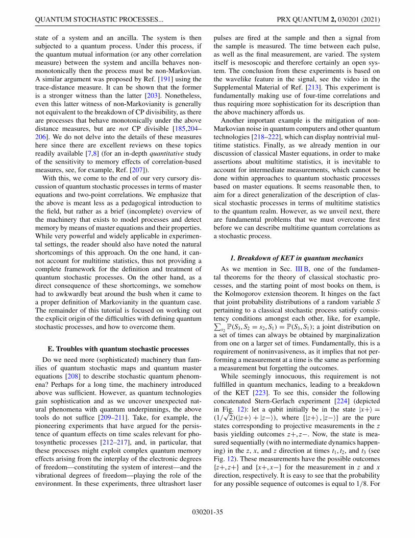
QUANTUM STOCHASTIC PROCESSES... PRX QUANTUM 2, 030201 (2021)
state of a system and an ancilla. The system is thensubjected to a quantum process. Under this process, ifthe quantum mutual information (or any other correlationmeasure) between the system and ancilla behaves non-monotonically then the process must be non-Markovian.A similar argument was proposed by Ref. [191] using thetrace-distance measure. It can be shown that the formeris a stronger witness than the latter [203]. Nonetheless,even this latter witness of non-Markovianity is generallynot equivalent to the breakdown of CP divisibility, as thereare processes that behave monotonically under the abovedistance measures, but are not CP divisible [185,204–206]. We do not delve into the details of these measureshere since there are excellent reviews on these topicsreadily available [7,8] (for an in-depth quantitative studyof the sensitivity to memory effects of correlation-basedmeasures, see, for example, Ref. [207]).
With this, we come to the end of our very cursory dis-cussion of quantum stochastic processes in terms of masterequations and two-point correlations. We emphasize thatthe above is meant less as a pedagogical introduction tothe field, but rather as a brief (incomplete) overview ofthe machinery that exists to model processes and detectmemory by means of master equations and their properties.While very powerful and widely applicable in experimen-tal settings, the reader should also have noted the naturalshortcomings of this approach. On the one hand, it can-not account for multitime statistics, thus not providing acomplete framework for the definition and treatment ofquantum stochastic processes. On the other hand, as adirect consequence of these shortcomings, we somehowhad to awkwardly beat around the bush when it came toa proper definition of Markovianity in the quantum case.The remainder of this tutorial is focused on working outthe explicit origin of the difficulties with defining quantumstochastic processes, and how to overcome them.
E. Troubles with quantum stochastic processes
Do we need more (sophisticated) machinery than fam-ilies of quantum stochastic maps and quantum masterequations [208] to describe stochastic quantum phenom-ena? Perhaps for a long time, the machinery introducedabove was sufficient. However, as quantum technologiesgain sophistication and as we uncover unexpected nat-ural phenomena with quantum underpinnings, the abovetools do not suffice [209–211]. Take, for example, thepioneering experiments that have argued for the persis-tence of quantum effects on time scales relevant for pho-tosynthetic processes [212–217], and, in particular, thatthese processes might exploit complex quantum memoryeffects arising from the interplay of the electronic degreesof freedom—constituting the system of interest—and thevibrational degrees of freedom—playing the role of theenvironment. In these experiments, three ultrashort laser
pulses are fired at the sample and then a signal fromthe sample is measured. The time between each pulse,as well as the final measurement, are varied. The systemitself is mesoscopic and therefore certainly an open sys-tem. The conclusion from these experiments is based onthe wavelike feature in the signal, see the video in theSupplemental Material of Ref. [213]. This experiment isfundamentally making use of four-time correlations andthus requiring more sophistication for its description thanthe above machinery affords us.
Another important example is the mitigation of non-Markovian noise in quantum computers and other quantumtechnologies [218–222], which can display nontrivial mul-titime statistics. Finally, as we already mention in ourdiscussion of classical Master equations, in order to makeassertions about multitime statistics, it is inevitable toaccount for intermediate measurements, which cannot bedone within approaches to quantum stochastic processesbased on master equations. It seems reasonable then, toaim for a direct generalization of the description of clas-sical stochastic processes in terms of multitime statisticsto the quantum realm. However, as we unveil next, thereare fundamental problems that we must overcome firstbefore we can describe multitime quantum correlations asa stochastic process.
1. Breakdown of KET in quantum mechanics
As we mention in Sec. III B, one of the fundamen-tal theorems for the theory of classical stochastic pro-cesses, and the starting point of most books on them, isthe Kolmogorov extension theorem. It hinges on the factthat joint probability distributions of a random variable Spertaining to a classical stochastic process satisfy consis-tency conditions amongst each other, like, for example,∑
s2P(S3, S2 = s2, S1) = P(S3, S1); a joint distribution on
a set of times can always be obtained by marginalizationfrom one on a larger set of times. Fundamentally, this is arequirement of noninvasiveness, as it implies that not per-forming a measurement at a time is the same as performinga measurement but forgetting the outcomes.
While seemingly innocuous, this requirement is notfulfilled in quantum mechanics, leading to a breakdownof the KET [223]. To see this, consider the followingconcatenated Stern-Gerlach experiment [224] (depictedin Fig. 12): let a qubit initially be in the state |x+〉 =(1/
√2)(|z+〉 + |z−〉), where {|z+〉 , |z−〉} are the pure
states corresponding to projective measurements in the zbasis yielding outcomes z+, z−. Now, the state is mea-sured sequentially (with no intermediate dynamics happen-ing) in the z, x, and z direction at times t1, t2, and t3 (seeFig. 12). These measurements have the possible outcomes{z+, z+} and {x+, x−} for the measurement in z and xdirection, respectively. It is easy to see that the probabilityfor any possible sequence of outcomes is equal to 1/8. For
030201-35
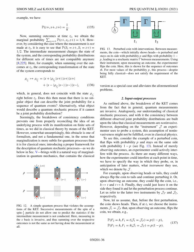
SIMON MILZ and KAVAN MODI PRX QUANTUM 2, 030201 (2021)
example, we have
P(z+, x+, z+) = 18
. (135)
Now, summing outcomes at time t2, we obtain themarginal probability
∑s2=x± P(z+, s2, z+) = 1/4. How-
ever, by considering the case where the measurement is notmade at t2, it is easy to see that P(S3 = z+, S1 = z+) =1/2. The intermediate measurement changes the state ofthe system, and the corresponding probability distributionsfor different sets of times are not compatible anymore[8,225]. Here, for example, when summing over the out-comes at t2, the corresponding transformation of the stateof the system corresponds to
ρt−2�→ ρt+2
= 〈x + |ρt−2|x+〉 |x+〉〈x+|
+ 〈x − |ρt−2|x−〉 |x−〉〈x−|, (136)
which, in general, does not coincide with the state ρt−2right before t2. Does this then mean that there is no sin-gular object that can describe the joint probability for asequence of quantum events? Alternatively, what objectwould describe a quantum stochastic process if it cannotbe a joint probability distribution?
Seemingly, the breakdown of consistency conditionsprevents one from properly reconciling the idea of anunderlying process with its manifestation on finite sets oftimes, as we did in classical theory by means of the KET.However, somewhat unsurprisingly, this obstacle is one offormalism, and not a fundamental one, in the sense thatmarginalization is more subtle for quantum processes thanit is for classical ones; introducing a proper framework forthe description of quantum stochastic processes—as we dobelow in Sec. V—brings with it a natural way of marginal-ization in quantum mechanics, that contains the classical
Z Z
X ZZ| z+⟩
| z−⟩| x−⟩
| z−⟩| z−⟩
ρ
ρ
FIG. 12. A simple quantum process that violates the assump-tions of the KET. Successive measurements of the spin of aspin- 1
2 particle do not allow one to predict the statistics if theintermediate measurement is not conducted. Here, measuring inthe x basis is invasive, and thus summing over the respectiveoutcomes is not the same as not having done the measurement atall.
FIG. 13. Perturbed coin with interventions. Between measure-ments, the coin—which initially shows heads—is perturbed andstays on its side with probability p and flips with probability 1 −p , leading to a stochastic matrix � between measurements. Usingtheir instrument, upon measuring an outcome, the experimenterflips the coin. Here, this is shown for the sequence of outcomesth. For most values of the probability p , this process—despitebeing fully classical—does not satisfy the requirement of theKET.
version as a special case and alleviates the aforementionedproblems.
2. Input-output processes
As outlined above, the breakdown of the KET comesfrom the fact that in general, quantum measurementsare invasive. Analogously, our understanding of classicalstochastic processes, and with it the consistency betweendifferent observed joint probability distributions are builtupon the idea that classical measurements are noninvasive.However, depending on the “instrument” J an experi-menter uses to probe a system, this assumption of nonin-vasiveness might not be fulfilled, even in classical physics.
To see this, consider the example of a perturbed coin,that flips with probability p and stays on the same sidewith probability 1 − p (see Fig. 13). Instead of merelyobserving outcomes, an experimenter could actively inter-fere with the process. As there are many different ways,how the experimenter could interfere at each point in time,we have to specify the way in which they probe, or, inanticipation of later matters, what instrument they use,which we denote by J .
For example, upon observing heads or tails, they couldalways flip the coin to tails and continue perturbing it. Or,upon observing an outcome, they could flip the coin, i.e.,h �→ t and t �→ h. Finally, they could just leave it on theside they found it and let the perturbation process continue.Let us refer to the latter two instruments by JF and JI ,respectively.
Now, let us assume, that, before the first perturbation,the coin shows heads. Then, if at t1 we choose the instru-ments J1 = JF that, upon observing an outcome, flips thecoin, we obtain, e.g.,
P(F2 = h, F1 = t|J1 = JF ) = p(1 − p),
P(F2 = h, F1 = h|J1 = JF ) = p(1 − p).(137)
030201-36
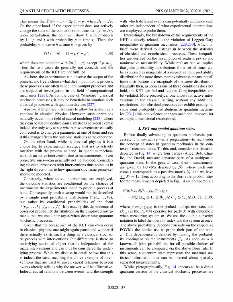
QUANTUM STOCHASTIC PROCESSES... PRX QUANTUM 2, 030201 (2021)
This means that P(F2 = h) = 2p(1 − p) when J1 = JF .On the other hand, if the experimenter does not activelychange the state of the coin at the first time, i.e., J1 = JI ,upon perturbation, the coin will show h with probabil-ity 1 − p and t with probability p at time t1. Then, theprobability to observe h at time t2 is given by
P(F2 = h) = (1 − p)2 + p2, (138)
which does not coincide with 2p(1 − p) except if p = 12 .
Thus the two cases do generally not coincide and therequirements of the KET are not fulfilled.
As, here, the experimenter can observe the output of theprocess, and freely choose what they input into the process,these processes are often called input-output processes andare subject of investigation in the field of computationalmechanics [226]. As for the case of “standard” classicalstochastic processes, it may be beneficial to simulate suchclassical processes with quantum devices [227].
A priori, it might seem arbitrary to allow for active inter-ventions in classical physics. However, such operationsnaturally occur in the field of causal modeling [228], wherethey can be used to deduce causal relations between events;indeed, the only way to see whether two events are causallyconnected is to change a parameter at one of them and seeif this change affects the outcome statistics at the other one.
On the other hand, while in classical physics it is achoice (up to experimental accuracy that is) to activelyinterfere with the process at hand, in quantum mechan-ics such an active intervention due to measurements—evenprojective ones—can generally not be avoided. Consider-ing classical processes with interventions thus points us inthe right direction as to how quantum stochastic processesshould be modeled.
Concretely, when active interventions are employed,the outcome statistics are conditional on the choices ofinstruments the experimenter made to probe a process athand. Consequently, such a setup would not be describedby a single joint probability distribution P(Fn, . . . , F1),but rather by conditional probabilities of the formP(Fn, . . . , F1|Jn, . . . ,J1). It is exactly this dependence ofobserved probability distributions on the employed instru-ments that we encounter again when describing quantumstochastic processes.
Given that the breakdown of the KET can even occurin classical physics, one might again pause and wonder ifthere actually exists such a thing as a classical stochas-tic process with interventions. Put differently, is there anunderlying statistical object that is independent of themade interventions and can thus be considered the under-lying process. While we discuss in detail below that thisis indeed the case, recalling the above example of inter-ventions that are used to unveil causal relations betweenevents already tells us why the answer will be affirmative.Indeed, causal relations between events, and the strength
with which different events can potentially influence eachother are independent of what experimental interventionsare employed to probe them.
Interestingly, the breakdown of the requirements of theKET is closely related to the violation of Leggett-Garginequalities in quantum mechanics [229,230], which, inbrief, were derived to distinguish between the statisticsof classical and nonclassical processes. These inequali-ties are derived on the assumption of realism per se andnoninvasive measurability. While realism per se impliesthat joint probability distributions for a set of times canbe expressed as marginals of a respective joint probabilitydistribution for more times, noninvasiveness means that allfinite distributions are marginals of the same distribution.Naturally then, as soon as one of these conditions does nothold, the KET can fail and Leggett-Garg inequalities canbe violated. More precisely, if one allows for active inter-ventions in the classical setting, without any additionalrestrictions, then classical processes can exhibit exactly thesame joint probability distributions as quantum mechan-ics [231] (this equivalence changes once one imposes, forexample, dimensional restrictions).
3. KET and spatial quantum states
Before finally advancing to quantum stochastic pro-cesses, it is instructive—as a preparation—to reconsiderthe concept of states in quantum mechanics in the con-text of measurements. To this end, consider the situationdepicted in Fig. 14, where four parties (Alice, Bob, Char-lie, and David) measure separate parts of a multipartitequantum state. In the general case, their measurementsare given by POVMs denoted by JX , where each out-come j corresponds to a positive matrix Xj , and we have∑
j Xj = 1. Then, according to the Born rule, probabilitiesfor the measurements depicted in Fig. 14 are computed via
P(a, b, c, d|JA,JB,JC,JD)
= tr[ρ(Aa1 ⊗ 12 ⊗ Bb34 ⊗ Cc5 ⊗ Cc6 ⊗ Dd7)], (139)
where ρ := ρ1234567 is the probed multipartite state, and{Xam} is the POVM operator for party X with outcome awhen measuring system m. We use the double subscriptnotation to label the operator index and the system at once.The above probability depends crucially on the respectivePOVMs the parties use to probe their part of the stateρ. This dependence is denoted by making the probabil-ity contingent on the instruments JX . As soon as ρ isknown, all joint probabilities for all possible choices ofinstruments can be computed via the above Born rule. Inthis sense, a quantum state represents the maximal sta-tistical information that can be inferred about spatiallyseparated measurements.
While, pictographically, Fig. 14 appears to be a directquantum version of the classical stochastic processes we
030201-37
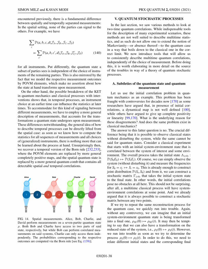
SIMON MILZ and KAVAN MODI PRX QUANTUM 2, 030201 (2021)
encountered previously, there is a fundamental differencebetween spatially and temporally separated measurements:In the spatial setting, none of the parties can signal to theothers. For example, we have
∑
c
P(a, b, c, d|JA,JB,JC,JD)
=∑
c′P(a, b, c′, d|JA,JB,J ′
C,JD) (140)
for all instruments. Put differently, the quantum state asubset of parties sees is independent of the choice of instru-ments of the remaining parties. This is also mirrored by thefact that we model the respective measurement outcomesby POVM elements, which make no assertion about howthe state at hand transforms upon measurement.
On the other hand, the possible breakdown of the KETin quantum mechanics and classical processes with inter-ventions shows that, in temporal processes, an instrumentchoice at an earlier time can influence the statistics at latertimes. To accommodate for this kind of signaling betweendifferent measurements, we have to employ a more generaldescription of measurements, that accounts for the trans-formations a quantum state undergoes upon measurement.These differences notwithstanding, the general idea of howto describe temporal processes can be directly lifted fromthe spatial case: as soon as we know how to compute thestatistics for all sequences of measurements and all choicesof (generalized) instruments, there is nothing more that canbe learned about the process at hand. Unsurprisingly then,we recover a temporal version of the Born rule [232,233],where the POVM elements are replaced by more generalcompletely positive maps, and the spatial quantum state isreplaced by a more general quantum comb that contains alldetectable spatial and temporal correlations.
2 3 4 51 6 71 3 5 64 7
Alice Bob Charlie David
FIG. 14. Spatial measurements. Alice, Bob, Charlie, andDavid perform measurements on a seven-partite quantum stateρ. Both Bob and Charlie have access to two parts of saidstate, respectively, but while Bob can perform correlated mea-surements on said systems, Charlie can only access them inde-pendently. The probabilities corresponding to the respectiveoutcomes are computed via the Born rule [see Eq. (139)].
V. QUANTUM STOCHASTIC PROCESSES
In the last section, we saw various methods to look attwo-time quantum correlations. While indispensable toolsfor the description of many experimental scenarios, thesemethods are not well suited to describe multitime statis-tics, and as such do not allow one to extend the notion ofMarkovianity—or absence thereof—to the quantum casein a way that boils down to the classical one in the cor-rect limit. We now introduce tools that will allow usto consistently describe multitime quantum correlations,independently of the choice of measurement. Before doingthis, it is worth elaborating in more detail on the sourceof the troubles in way of a theory of quantum stochasticprocesses.
A. Subtleties of the quantum state and quantummeasurement
Let us use the initial correlation problem in quan-tum mechanics as an example. This problem has beenfraught with controversies for decades now [170] as someresearchers have argued that, in presence of initial cor-relations, a dynamical map is not well defined [100],while others have argued to give up complete positivityor linearity [99,170]. What is the underlying reason forthese disagreements? And does the same problem exist inclassical mechanics?
The answer to this latter question is no. The crucial dif-ference being that it is possible to observe classical stateswithout disturbing the system, while the same cannot besaid for quantum states. Consider a classical experimentthat starts with an initial system-environment state that iscorrelated between the system of interest and some envi-ronment. The overall process takes the initial state �(t:0) :P(S0E0) �→ P(StEt). Of course, we can simply observe thesystem (without disturbing it) and measure the frequenciesfor S0 = sj �→ St = sk. This is already enough to constructjoint distribution P(St, S0) and from it, we can construct astochastic matrix �(t:0) that takes the initial system stateto the final state. In other words, the initial correlationspose no obstacles at all here. This should not be surprising,after all, a multitime classical process will have system-environment correlations at some point. And we alreadyargued that it is always possible to construct a stochasticmatrix between any two points.
If we try to repeat the same reconstruction process forthe quantum case, we quickly run into trouble. Again,without any controversy, we can imagine that an initialsystem-environment quantum state is being transformedinto a final one, ρSE(0) �→ ρSE(t). It may then be tempt-ing to say that we can also have a transformation on thereduced state of the system, i.e., ρS(0) �→ ρS(t). However,we run into trouble as soon as we try to determine theprocess ρS(0) �→ ρS(t). In order to do this, we need torelate different initial states and the corresponding final
030201-38
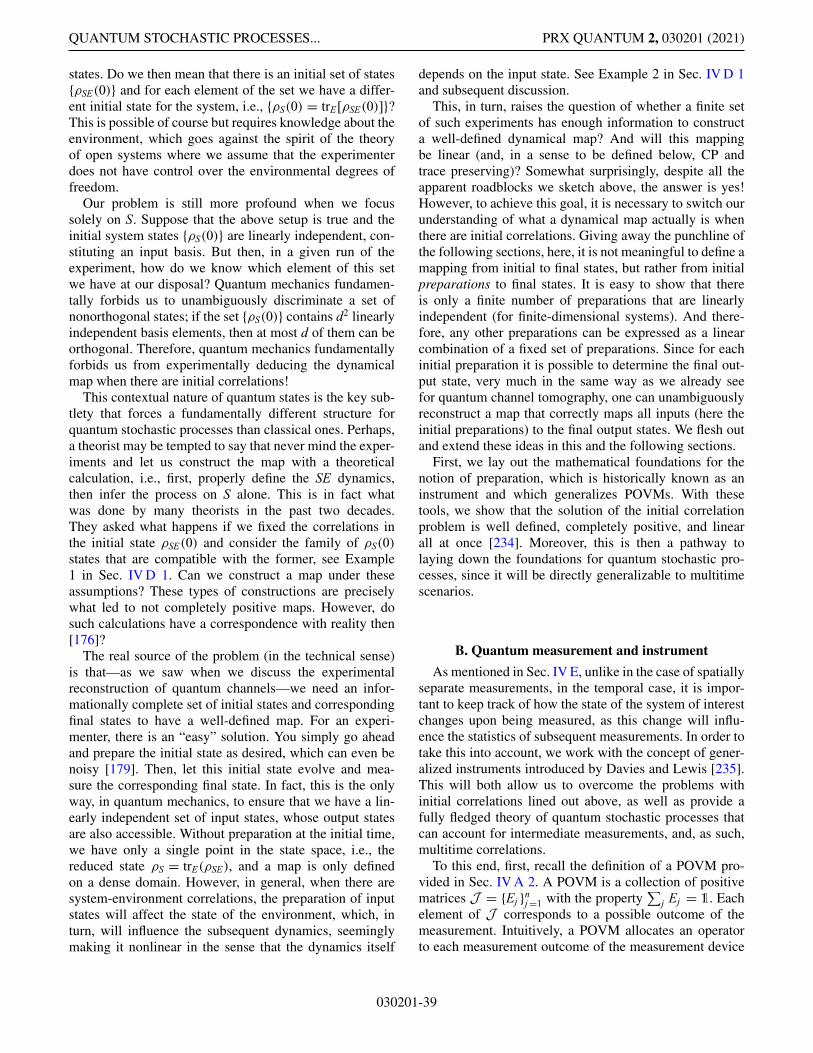
QUANTUM STOCHASTIC PROCESSES... PRX QUANTUM 2, 030201 (2021)
states. Do we then mean that there is an initial set of states{ρSE(0)} and for each element of the set we have a differ-ent initial state for the system, i.e., {ρS(0) = trE[ρSE(0)]}?This is possible of course but requires knowledge about theenvironment, which goes against the spirit of the theoryof open systems where we assume that the experimenterdoes not have control over the environmental degrees offreedom.
Our problem is still more profound when we focussolely on S. Suppose that the above setup is true and theinitial system states {ρS(0)} are linearly independent, con-stituting an input basis. But then, in a given run of theexperiment, how do we know which element of this setwe have at our disposal? Quantum mechanics fundamen-tally forbids us to unambiguously discriminate a set ofnonorthogonal states; if the set {ρS(0)} contains d2 linearlyindependent basis elements, then at most d of them can beorthogonal. Therefore, quantum mechanics fundamentallyforbids us from experimentally deducing the dynamicalmap when there are initial correlations!
This contextual nature of quantum states is the key sub-tlety that forces a fundamentally different structure forquantum stochastic processes than classical ones. Perhaps,a theorist may be tempted to say that never mind the exper-iments and let us construct the map with a theoreticalcalculation, i.e., first, properly define the SE dynamics,then infer the process on S alone. This is in fact whatwas done by many theorists in the past two decades.They asked what happens if we fixed the correlations inthe initial state ρSE(0) and consider the family of ρS(0)states that are compatible with the former, see Example1 in Sec. IV D 1. Can we construct a map under theseassumptions? These types of constructions are preciselywhat led to not completely positive maps. However, dosuch calculations have a correspondence with reality then[176]?
The real source of the problem (in the technical sense)is that—as we saw when we discuss the experimentalreconstruction of quantum channels—we need an infor-mationally complete set of initial states and correspondingfinal states to have a well-defined map. For an experi-menter, there is an “easy” solution. You simply go aheadand prepare the initial state as desired, which can even benoisy [179]. Then, let this initial state evolve and mea-sure the corresponding final state. In fact, this is the onlyway, in quantum mechanics, to ensure that we have a lin-early independent set of input states, whose output statesare also accessible. Without preparation at the initial time,we have only a single point in the state space, i.e., thereduced state ρS = trE(ρSE), and a map is only definedon a dense domain. However, in general, when there aresystem-environment correlations, the preparation of inputstates will affect the state of the environment, which, inturn, will influence the subsequent dynamics, seeminglymaking it nonlinear in the sense that the dynamics itself
depends on the input state. See Example 2 in Sec. IV D 1and subsequent discussion.
This, in turn, raises the question of whether a finite setof such experiments has enough information to constructa well-defined dynamical map? And will this mappingbe linear (and, in a sense to be defined below, CP andtrace preserving)? Somewhat surprisingly, despite all theapparent roadblocks we sketch above, the answer is yes!However, to achieve this goal, it is necessary to switch ourunderstanding of what a dynamical map actually is whenthere are initial correlations. Giving away the punchline ofthe following sections, here, it is not meaningful to define amapping from initial to final states, but rather from initialpreparations to final states. It is easy to show that thereis only a finite number of preparations that are linearlyindependent (for finite-dimensional systems). And there-fore, any other preparations can be expressed as a linearcombination of a fixed set of preparations. Since for eachinitial preparation it is possible to determine the final out-put state, very much in the same way as we already seefor quantum channel tomography, one can unambiguouslyreconstruct a map that correctly maps all inputs (here theinitial preparations) to the final output states. We flesh outand extend these ideas in this and the following sections.
First, we lay out the mathematical foundations for thenotion of preparation, which is historically known as aninstrument and which generalizes POVMs. With thesetools, we show that the solution of the initial correlationproblem is well defined, completely positive, and linearall at once [234]. Moreover, this is then a pathway tolaying down the foundations for quantum stochastic pro-cesses, since it will be directly generalizable to multitimescenarios.
B. Quantum measurement and instrument
As mentioned in Sec. IV E, unlike in the case of spatiallyseparate measurements, in the temporal case, it is impor-tant to keep track of how the state of the system of interestchanges upon being measured, as this change will influ-ence the statistics of subsequent measurements. In order totake this into account, we work with the concept of gener-alized instruments introduced by Davies and Lewis [235].This will both allow us to overcome the problems withinitial correlations lined out above, as well as provide afully fledged theory of quantum stochastic processes thatcan account for intermediate measurements, and, as such,multitime correlations.
To this end, first, recall the definition of a POVM pro-vided in Sec. IV A 2. A POVM is a collection of positivematrices J = {Ej }n
j =1 with the property∑
j Ej = 1. Eachelement of J corresponds to a possible outcome of themeasurement. Intuitively, a POVM allocates an operatorto each measurement outcome of the measurement device
030201-39
SIMON MILZ and KAVAN MODI PRX QUANTUM 2, 030201 (2021)
that allows one to compute outcome statistics for arbi-trary quantum states that are being probed. However, itdoes not enable one to deduce how the state changes uponobservation of one of the outcomes.
To account for state changes, we have to modify theconcept of a POVM; this generalization is known as a gen-eralized instrument [236,237]. As POVMs turn out to be aspecial case of (generalized) instruments, we denote themby J , too. An instrument corresponding to a measurementwith outcomes j = {1, . . . , n} is a collection of CP mapsJ = {Aj } that add up to a CPTP map, i.e., A =∑n
j =1 Aj .Each of the CP maps corresponds to one of the possibleoutcomes, while their sum corresponds to the overall trans-formation of the state at hand due to the application ofthe respective instrument (it is exactly the invasiveness ofsaid map that leads to a breakdown of the KET in quan-tum mechanics). For example, returning to the case of ameasurement of a qubit in the computational basis, thecorresponding instrument is given by
{A0[•] := |0〉〈0| • |0〉〈0|,A1[•] := |1〉〈1| • |1〉〈1|},(141)
assuming, that after projecting the state onto the computa-tional basis, it is sent forward unchanged.
Importantly, an instrument allows one to compute boththe probability to obtain different outcomes and the statechange upon measurement. The latter is given by
ρ ′j = Aj [ρ] (142)
when the system in state ρ is interrogated by the instrumentJ , yielding outcome j . The state after said interrogation,given the outcome, is obtained via the action of the cor-responding element of the instrument. Importantly, thisstate is in general not normalized. Its trace provides theprobability to observe a given outcome. Concretely, wehave
P( j |J ) = tr(Aj [ρ]) = tr(∑
αj
Kαj ρK†αj
), (143)
where the sum runs over all Kraus operators that pertainto the CP map Aj , and we have
∑αj
K†αj Kαj < 1 if Aj is
not trace preserving. The requirement that all CP maps ofan instrument add up to a CPTP map ensures—just likein the analogous case for POVMs—the normalization ofprobabilities:
n∑
j =1
P( j |J ) = tr
⎛
⎝n∑
j =1
∑
αj
Kαj ρK†αj
⎞
⎠ = tr(A[ρ]), (144)
which is 1 for all quantum states ρ. Naturally, the conceptof generalized instruments contains POVMs as a special
case, namely as those generalized instruments, where theoutput space of the respective CP maps is trivial. Put differ-ently, if one simply wants to compute the probabilities ofmeasurements on a quantum state, generalized instrumentsare not necessary. Concretely, we have
P( j |J ) = tr(ρEj ) with Ej =∑
αj
K†αj
Kαj . (145)
This is because for a single measurement, the state trans-formation is not of interest. However, as we see in thenext section, this situation drastically changes, as soon assequential measurements are considered. There, POVMsare not sufficient anymore to correctly compute statistics.
Before advancing, it is insightful to make the connectionbetween the CP maps of an instrument and the elements ofits corresponding POVM explicit. This is most easily donevia the Choi states we introduced in Sec. IV B 3. There,we discuss that the action of a map Aj on a state ρ can beexpressed as
ρ ′j = Aj [ρ] = tri[AT
j (ρ ⊗ 1◦)], (146)
where Aj ∈ B(Hi ⊗ Ho) is the Choi state of the map Ajand ρ ∈ B(Hi), and we move the transposition onto Ajinstead of ρ. Using this expression to compute probabili-ties, we obtain
P( j |J ) = trio[ATj (ρ ⊗ 1o)] = tr(Ej ρ). (147)
Comparing this last expression with the Born rule, we seethat the POVM element Ej corresponding to Aj is given byEj = tro(A
Tj ), where the additional transpose stems from
our definition of the CJI. This relation indeed yields aPOVM, as the partial trace of a positive matrix is also pos-itive, and we have
∑nj =1 Ej =∑n
j =1 tro(ATj ) = 1, where
we use that the Choi state A of A satisfies tro(A) = 1. Dis-carding the outputs of an instruments thus yields a POVM.This implies that different instruments can have the samecorresponding POVM. For example, the instrument thatmeasures in the computational basis and feeds forward theresulting state, has the same corresponding POVM as theinstrument that measures in the computational basis, butfeeds forward a maximally mixed state, indiscriminate ofthe outcome. While both of these instruments lead to thesame POVM, their influence on future statistics can bevery different.
1. POVMs, instruments, and probability spaces
Before advancing to the description of multitime quan-tum processes, let us quickly connect POVMs and instru-ments to the more formal discussion of stochastic pro-cesses we conducted earlier. The benefit of making thisconnection transparent is twofold; on the one hand, it
030201-40
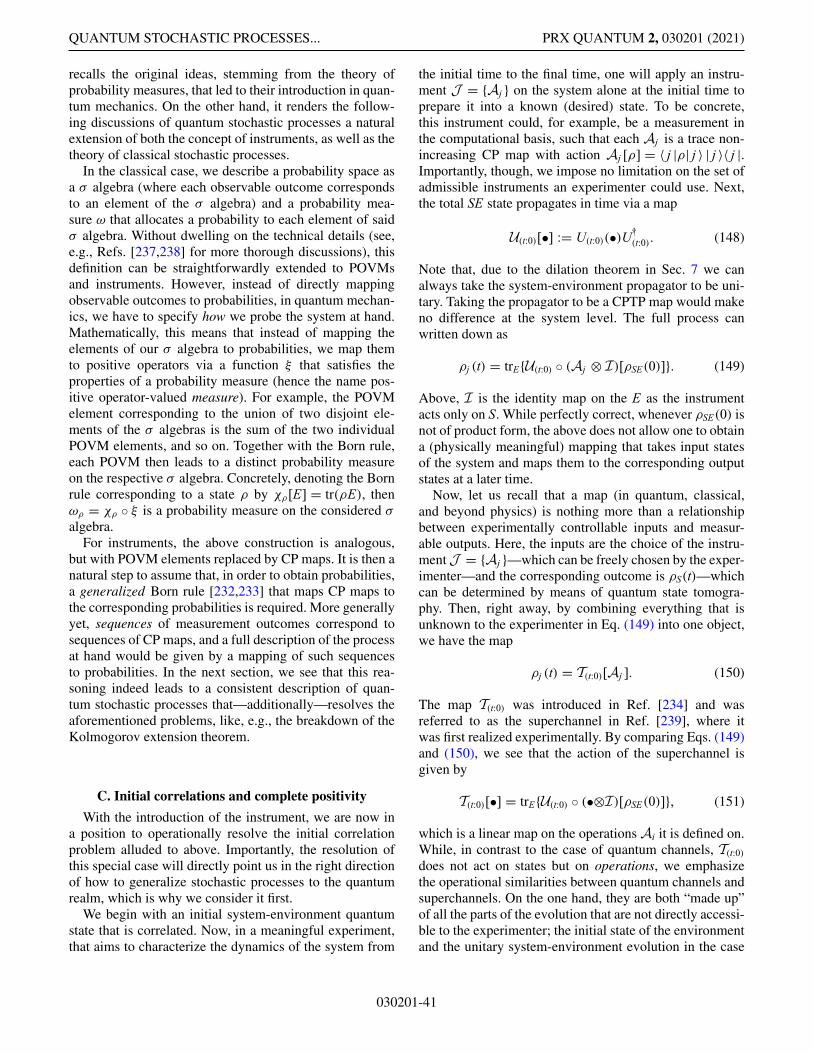
QUANTUM STOCHASTIC PROCESSES... PRX QUANTUM 2, 030201 (2021)
recalls the original ideas, stemming from the theory ofprobability measures, that led to their introduction in quan-tum mechanics. On the other hand, it renders the follow-ing discussions of quantum stochastic processes a naturalextension of both the concept of instruments, as well as thetheory of classical stochastic processes.
In the classical case, we describe a probability space asa σ algebra (where each observable outcome correspondsto an element of the σ algebra) and a probability mea-sure ω that allocates a probability to each element of saidσ algebra. Without dwelling on the technical details (see,e.g., Refs. [237,238] for more thorough discussions), thisdefinition can be straightforwardly extended to POVMsand instruments. However, instead of directly mappingobservable outcomes to probabilities, in quantum mechan-ics, we have to specify how we probe the system at hand.Mathematically, this means that instead of mapping theelements of our σ algebra to probabilities, we map themto positive operators via a function ξ that satisfies theproperties of a probability measure (hence the name pos-itive operator-valued measure). For example, the POVMelement corresponding to the union of two disjoint ele-ments of the σ algebras is the sum of the two individualPOVM elements, and so on. Together with the Born rule,each POVM then leads to a distinct probability measureon the respective σ algebra. Concretely, denoting the Bornrule corresponding to a state ρ by χρ[E] = tr(ρE), thenωρ = χρ ◦ ξ is a probability measure on the considered σ
algebra.For instruments, the above construction is analogous,
but with POVM elements replaced by CP maps. It is then anatural step to assume that, in order to obtain probabilities,a generalized Born rule [232,233] that maps CP maps tothe corresponding probabilities is required. More generallyyet, sequences of measurement outcomes correspond tosequences of CP maps, and a full description of the processat hand would be given by a mapping of such sequencesto probabilities. In the next section, we see that this rea-soning indeed leads to a consistent description of quan-tum stochastic processes that—additionally—resolves theaforementioned problems, like, e.g., the breakdown of theKolmogorov extension theorem.
C. Initial correlations and complete positivity
With the introduction of the instrument, we are now ina position to operationally resolve the initial correlationproblem alluded to above. Importantly, the resolution ofthis special case will directly point us in the right directionof how to generalize stochastic processes to the quantumrealm, which is why we consider it first.
We begin with an initial system-environment quantumstate that is correlated. Now, in a meaningful experiment,that aims to characterize the dynamics of the system from
the initial time to the final time, one will apply an instru-ment J = {Aj } on the system alone at the initial time toprepare it into a known (desired) state. To be concrete,this instrument could, for example, be a measurement inthe computational basis, such that each Aj is a trace non-increasing CP map with action Aj [ρ] = 〈 j |ρ| j 〉 | j 〉〈 j |.Importantly, though, we impose no limitation on the set ofadmissible instruments an experimenter could use. Next,the total SE state propagates in time via a map
U(t:0)[•] := U(t:0)(•)U†(t:0). (148)
Note that, due to the dilation theorem in Sec. 7 we canalways take the system-environment propagator to be uni-tary. Taking the propagator to be a CPTP map would makeno difference at the system level. The full process canwritten down as
ρj (t) = trE{U(t:0) ◦ (Aj ⊗ I)[ρSE(0)]}. (149)
Above, I is the identity map on the E as the instrumentacts only on S. While perfectly correct, whenever ρSE(0) isnot of product form, the above does not allow one to obtaina (physically meaningful) mapping that takes input statesof the system and maps them to the corresponding outputstates at a later time.
Now, let us recall that a map (in quantum, classical,and beyond physics) is nothing more than a relationshipbetween experimentally controllable inputs and measur-able outputs. Here, the inputs are the choice of the instru-mentJ = {Aj }—which can be freely chosen by the exper-imenter—and the corresponding outcome is ρS(t)—whichcan be determined by means of quantum state tomogra-phy. Then, right away, by combining everything that isunknown to the experimenter in Eq. (149) into one object,we have the map
ρj (t) = T(t:0)[Aj ]. (150)
The map T(t:0) was introduced in Ref. [234] and wasreferred to as the superchannel in Ref. [239], where itwas first realized experimentally. By comparing Eqs. (149)and (150), we see that the action of the superchannel isgiven by
T(t:0)[•] = trE{U(t:0) ◦ (•⊗I)[ρSE(0)]}, (151)
which is a linear map on the operations Ai it is defined on.While, in contrast to the case of quantum channels, T(t:0)does not act on states but on operations, we emphasizethe operational similarities between quantum channels andsuperchannels. On the one hand, they are both “made up”of all the parts of the evolution that are not directly accessi-ble to the experimenter; the initial state of the environmentand the unitary system-environment evolution in the case
030201-41
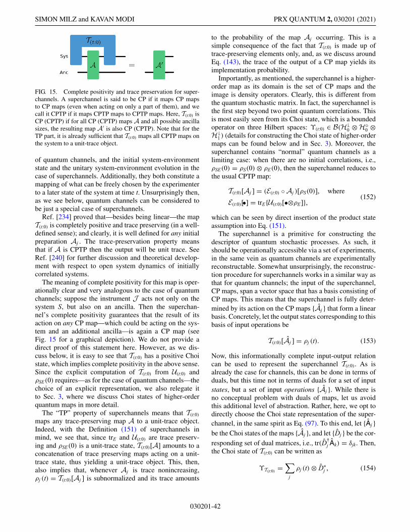
SIMON MILZ and KAVAN MODI PRX QUANTUM 2, 030201 (2021)
FIG. 15. Complete positivity and trace preservation for super-channels. A superchannel is said to be CP if it maps CP mapsto CP maps (even when acting on only a part of them), and wecall it CPTP if it maps CPTP maps to CPTP maps. Here, T(t:0) isCP (CPTP) if for all CP (CPTP) maps A and all possible ancillasizes, the resulting map A′ is also CP (CPTP). Note that for theTP part, it is already sufficient that T(t:0) maps all CPTP maps onthe system to a unit-trace object.
of quantum channels, and the initial system-environmentstate and the unitary system-environment evolution in thecase of superchannels. Additionally, they both constitute amapping of what can be freely chosen by the experimenterto a later state of the system at time t. Unsurprisingly then,as we see below, quantum channels can be considered tobe just a special case of superchannels.
Ref. [234] proved that—besides being linear—the mapT(t:0) is completely positive and trace preserving (in a well-defined sense); and clearly, it is well defined for any initialpreparation Aj . The trace-preservation property meansthat if A is CPTP then the output will be unit trace. SeeRef. [240] for further discussion and theoretical develop-ment with respect to open system dynamics of initiallycorrelated systems.
The meaning of complete positivity for this map is oper-ationally clear and very analogous to the case of quantumchannels; suppose the instrument J acts not only on thesystem S, but also on an ancilla. Then the superchan-nel’s complete positivity guarantees that the result of itsaction on any CP map—which could be acting on the sys-tem and an additional ancilla—is again a CP map (seeFig. 15 for a graphical depiction). We do not provide adirect proof of this statement here. However, as we dis-cuss below, it is easy to see that T(t:0) has a positive Choistate, which implies complete positivity in the above sense.Since the explicit computation of T(t:0) from U(t:0) andρSE(0) requires—as for the case of quantum channels—thechoice of an explicit representation, we also relegate itto Sec. 3, where we discuss Choi states of higher-orderquantum maps in more detail.
The “TP” property of superchannels means that T(t:0)maps any trace-preserving map A to a unit-trace object.Indeed, with the Definition (151) of superchannels inmind, we see that, since trE and U(t:0) are trace preserv-ing and ρSE(0) is a unit-trace state, T(t:0)[A] amounts to aconcatenation of trace preserving maps acting on a unit-trace state, thus yielding a unit-trace object. This, then,also implies that, whenever Aj is trace nonincreasing,ρj (t) = T(t:0)[Aj ] is subnormalized and its trace amounts
to the probability of the map Aj occurring. This is asimple consequence of the fact that T(t:0) is made up oftrace-preserving elements only, and, as we discuss aroundEq. (143), the trace of the output of a CP map yields itsimplementation probability.
Importantly, as mentioned, the superchannel is a higher-order map as its domain is the set of CP maps and theimage is density operators. Clearly, this is different fromthe quantum stochastic matrix. In fact, the superchannel isthe first step beyond two point quantum correlations. Thisis most easily seen from its Choi state, which is a boundedoperator on three Hilbert spaces: ϒ(t:0) ∈ B(Hi
0 ⊗ Ho0 ⊗
Hi1 ) (details for constructing the Choi state of higher-order
maps can be found below and in Sec. 3). Moreover, thesuperchannel contains “normal” quantum channels as alimiting case: when there are no initial correlations, i.e.,ρSE(0) = ρS(0) ⊗ ρE(0), then the superchannel reduces tothe usual CPTP map:
T(t:0)[Aj ] = (E(t:0) ◦ Aj )[ρS(0)], where
E(t:0)[•] = trE{U(t:0)[•⊗ρE]}, (152)
which can be seen by direct insertion of the product stateassumption into Eq. (151).
The superchannel is a primitive for constructing thedescriptor of quantum stochastic processes. As such, itshould be operationally accessible via a set of experiments,in the same vein as quantum channels are experimentallyreconstructable. Somewhat unsurprisingly, the reconstruc-tion procedure for superchannels works in a similar way asthat for quantum channels; the input of the superchannel,CP maps, span a vector space that has a basis consisting ofCP maps. This means that the superchannel is fully deter-mined by its action on the CP maps {Aj } that form a linearbasis. Concretely, let the output states corresponding to thisbasis of input operations be
T(t:0)[Aj ] = ρj (t). (153)
Now, this informationally complete input-output relationcan be used to represent the superchannel T(t:0). As isalready the case for channels, this can be done in terms ofduals, but this time not in terms of duals for a set of inputstates, but a set of input operations {Aj }. While there isno conceptual problem with duals of maps, let us avoidthis additional level of abstraction. Rather, here, we opt todirectly choose the Choi state representation of the super-channel, in the same spirit as Eq. (97). To this end, let {Aj }be the Choi states of the maps {Aj }, and let {Dj } be the cor-
responding set of dual matrices, i.e., tr(D†j Ak) = δjk. Then,
the Choi state of T(t:0) can be written as
ϒT(t:0) =∑
j
ρj (t) ⊗ D∗j , (154)
030201-42
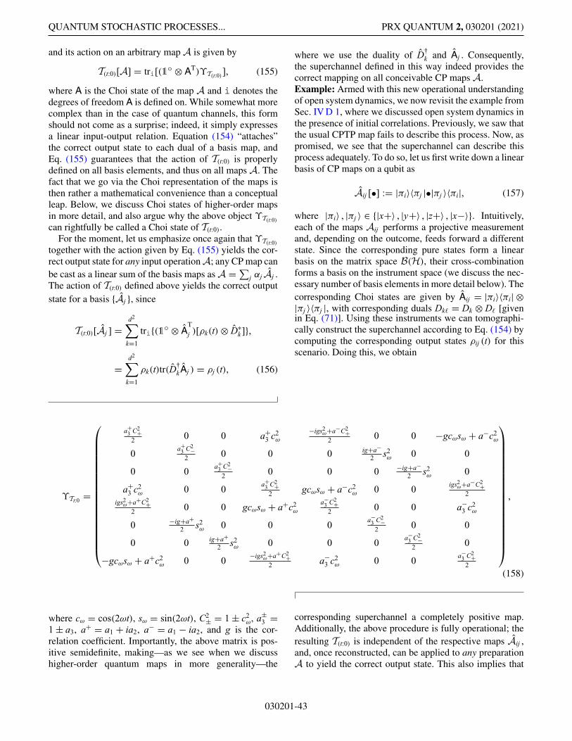
QUANTUM STOCHASTIC PROCESSES... PRX QUANTUM 2, 030201 (2021)
and its action on an arbitrary map A is given by
T(t:0)[A] = tri[(1o ⊗ AT)ϒT(t:0)], (155)
where A is the Choi state of the map A and i denotes thedegrees of freedom A is defined on. While somewhat morecomplex than in the case of quantum channels, this formshould not come as a surprise; indeed, it simply expressesa linear input-output relation. Equation (154) “attaches”the correct output state to each dual of a basis map, andEq. (155) guarantees that the action of T(t:0) is properlydefined on all basis elements, and thus on all maps A. Thefact that we go via the Choi representation of the maps isthen rather a mathematical convenience than a conceptualleap. Below, we discuss Choi states of higher-order mapsin more detail, and also argue why the above object ϒT(t:0)can rightfully be called a Choi state of T(t:0).
For the moment, let us emphasize once again that ϒT(t:0)together with the action given by Eq. (155) yields the cor-rect output state for any input operation A; any CP map canbe cast as a linear sum of the basis maps as A =∑j αj Aj .The action of T(t:0) defined above yields the correct outputstate for a basis {Aj }, since
T(t:0)[Aj ] =d2∑
k=1
tri{(1o ⊗ AT
j )[ρk(t) ⊗ D∗k ]},
=d2∑
k=1
ρk(t)tr(D†kAj ) = ρj (t), (156)
where we use the duality of D†k and Aj . Consequently,
the superchannel defined in this way indeed provides thecorrect mapping on all conceivable CP maps A.Example: Armed with this new operational understandingof open system dynamics, we now revisit the example fromSec. IV D 1, where we discussed open system dynamics inthe presence of initial correlations. Previously, we saw thatthe usual CPTP map fails to describe this process. Now, aspromised, we see that the superchannel can describe thisprocess adequately. To do so, let us first write down a linearbasis of CP maps on a qubit as
Aij [•] := |πi〉〈πj |•|πj 〉〈πi|, (157)
where |πi〉 , |πj 〉 ∈ {|x+〉 , |y+〉 , |z+〉 , |x−〉}. Intuitively,each of the maps Aij performs a projective measurementand, depending on the outcome, feeds forward a differentstate. Since the corresponding pure states form a linearbasis on the matrix space B(H), their cross-combinationforms a basis on the instrument space (we discuss the nec-essary number of basis elements in more detail below). Thecorresponding Choi states are given by Aij = |πi〉〈πi| ⊗|πj 〉〈πj |, with corresponding duals Dk = Dk ⊗ D [givenin Eq. (71)]. Using these instruments we can tomographi-cally construct the superchannel according to Eq. (154) bycomputing the corresponding output states ρij (t) for thisscenario. Doing this, we obtain
ϒTt:0 =
⎛
⎜⎜⎜⎜⎜⎜⎜⎜⎜⎜⎜⎜⎜⎜⎜⎜⎜⎜⎝
a+3 C2+
2 0 0 a+3 c2
ω
−igs2ω+a−C2+
2 0 0 −gcωsω + a−c2ω
0 a+3 C2−
2 0 0 0 ig+a−2 s2
ω 0 0
0 0 a+3 C2−
2 0 0 0 −ig+a−2 s2
ω 0
a+3 c2
ω 0 0 a+3 C2+
2 gcωsω + a−c2ω 0 0 igs2
ω+a−C2+2
igs2ω+a+C2+
2 0 0 gcωsω + a+c2ω
a−3 C2+
2 0 0 a−3 c2
ω
0 −ig+a+2 s2
ω 0 0 0 a−3 C2−
2 0 0
0 0 ig+a+2 s2
ω 0 0 0 a−3 C2−
2 0
−gcωsω + a+c2ω 0 0 −igs2
ω+a+C2+2 a−
3 c2ω 0 0 a−
3 C2+2
⎞
⎟⎟⎟⎟⎟⎟⎟⎟⎟⎟⎟⎟⎟⎟⎟⎟⎟⎟⎠
,
(158)
where cω = cos(2ωt), sω = sin(2ωt), C2± = 1 ± c2
ω, a±3 =
1 ± a3, a+ = a1 + ia2, a− = a1 − ia2, and g is the cor-relation coefficient. Importantly, the above matrix is pos-itive semidefinite, making—as we see when we discusshigher-order quantum maps in more generality—the
corresponding superchannel a completely positive map.Additionally, the above procedure is fully operational; theresulting T(t:0) is independent of the respective maps Aij ,and, once reconstructed, can be applied to any preparationA to yield the correct output state. This also implies that
030201-43
SIMON MILZ and KAVAN MODI PRX QUANTUM 2, 030201 (2021)
the superchannel is constructed with a finite number ofexperiments. Consequently, the examples in Sec. IV D 1are all contained here as limiting cases. Finally, a CPTPmap acting on a d-dimensional system would be repre-sented by d2 × d2 matrix. The superchannel, on the otherhand, is a d3 × d3 matrix that contracts with a CP map toyield an output that is a d × d matrix.
In fact, the superchannel has been observed in the lab-oratory [239] and proven to be effective at dealing withinitial correlations without giving up either linearity orcomplete positivity. One then might wonder how this getsaround Pechukas’ theorem which implied that one of theseproperties would have to be given up in the presence ofinitial correlations? To retain both linearity and completepositivity we have given up the notion of the initial systemstate. In fact, as we argued in Sec. V A, in the presence ofcorrelations, quantum mechanics does not allow for a well-defined local state beyond a singular point in the Hilbertspace. Therefore a map on this singular point alone is notvery meaningful, hence there is no big loss in giving upthe notion of the initial state as a relevant concept for thedynamics [241]. Finally, it should be said that this lineof reasoning is very close to that of Pearl [228] in classi-cal causal modeling, which goes beyond the framework ofclassical stochastic processes and allows for interventions.
At this point, it is insightful to quickly take stock ofwhat we achieved in this section, what we implicitlyassumed, and how to generalize these ideas to finallyobtain a fully fledged description of quantum stochasticprocesses. Firstly, in order to deal with initial correla-tions, we switched perspective and describe the dynamicsin terms of a mapping from initial operations (instead ofinitial states) to final states at time t. While seeminglyodd from a mathematical perspective, from the opera-tional perspective it is only reasonable: experimentallymeaningful maps should map from initial objects that canindependently be controlled and prepared by the experi-menter to objects that can be measured. In the presence ofinitial system-environment correlations, the experimenterdoes not have control over the initial state—at least notwithout potentially influencing the remaining parametersof the dynamics (i.e., the correlations with the environ-ment). However, they have control over what operationthey implemented, and the dynamics from those opera-tions to the final states can be defined and reconstructed,and is fully independent of what the experimenter does (inthe sense that T(t:0) is independent of the experimenter’sactions). Consequently, switching perspective is simplynatural from an operational point of view.
Since the superchannel already deals with “interme-diate” CP maps performed by the experimenter, it alsodirectly points out how to go beyond experimental sce-narios where the experimenter only acts at two times; inprinciple, nothing keeps us from also performing CP mapsat intermediate times, and then reconstructing the final
state for sequences of CP maps, instead of only one CPmap, as we have done here. It should not come as a sur-prise that this is exactly what we are going to do in thenext section.
It remains to quickly comment on the mathematicaldetails that we deliberately brush over in this section. Natu-rally, to make things simpler, we choose the most insightfulrepresentation of the superchannel in terms of a d3 × d3
matrix. Unsurprisingly, there is also a vectorized versionof the superchannel [79], or we could have kept thingsentirely abstract and phrase everything in terms of mapsacting on maps. Again, we emphasize that representationhas no bearing on physical properties, but employing therepresentation we choose proves very advantageous; forexample, it allows us to easily derive the dimension of thespaces we work with, as well as express the properties ofhigher-order quantum maps in a concise way. Addition-ally, as is the case for quantum channels, we see that thisrepresentation indeed has an interpretation in terms of a(multipartite) quantum state, which is why we already callit the Choi representation throughout this section.
D. Multitime statistics in quantum processes
Following the above resolution for the initial correlationproblem in quantum mechanics, we are now in a positionto provide a fully fledged framework for the descriptionof multitime quantum processes. Here, we predominantlyfocus on the case of finitely many times at which theprocess of interest is interrogated (for an in-depth dis-cussion of continuous measurements, see, for example,Refs. [242,243]). Note that we can but scratch the sur-face of the different approaches that exist to the theory ofmultitime quantum processes. For a much more in-depthinvestigation of the relation between different concepts ofmemory in quantum physics, see Ref. [10].
In principle, there are two ways to motivate this frame-work. On the one hand, by generalizing joint probabilities,the descriptor of classical stochastic processes, to the quan-tum realm, and taking into consideration that, in quantummechanics, we have to specify the instruments that areused to interrogate the system. This approach would thenyield a temporal Born rule [232,233], and provide a nat-ural descriptor of quantum stochastic processes in termsof a “quantum state over time.” We circle back to thisapproach below. Here, we take the second possible routeto the description of multitime open quantum processes,which—just like in the case of initial correlations—ismotivated by considering the underlying dynamics of aquantum stochastic process. As we see, though, bothapproaches are equivalent and lead to the same descriptorof quantum stochastic processes.
The initial correlation problem is solved by taking thepreparation procedure into account, and to construct aconsistent mapping of the preparation operations to final
030201-44
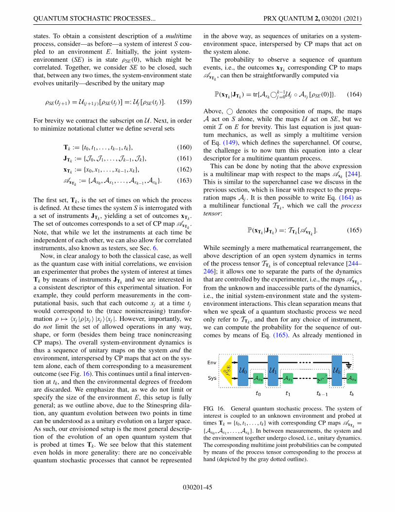
QUANTUM STOCHASTIC PROCESSES... PRX QUANTUM 2, 030201 (2021)
states. To obtain a consistent description of a multitimeprocess, consider—as before—a system of interest S cou-pled to an environment E. Initially, the joint system-environment (SE) is in state ρSE(0), which might becorrelated. Together, we consider SE to be closed, suchthat, between any two times, the system-environment stateevolves unitarily—described by the unitary map
ρSE(tj +1) = U(j +1:j )[ρSE(tj )] =: Uj [ρSE(tj )]. (159)
For brevity we contract the subscript on U . Next, in orderto minimize notational clutter we define several sets
Tk := {t0, t1, . . . , tk−1, tk}, (160)
JTk := {J0,J1, . . . ,Jk−1,Jk}, (161)
xTk := {x0, x1, . . . , xk−1, xk}, (162)
AxTk:= {Ax0 ,Ax1 , . . . ,Axk−1 ,Axk }. (163)
The first set, Tk, is the set of times on which the processis defined. At these times the system S is interrogated witha set of instruments JTk , yielding a set of outcomes xTk .The set of outcomes corresponds to a set of CP map AxTk
.Note, that while we let the instruments at each time beindependent of each other, we can also allow for correlatedinstruments, also known as testers, see Sec. 6.
Now, in clear analogy to both the classical case, as wellas the quantum case with initial correlations, we envisionan experimenter that probes the system of interest at timesTk by means of instruments JTk and we are interested ina consistent descriptor of this experimental situation. Forexample, they could perform measurements in the com-putational basis, such that each outcome xj at a time tjwould correspond to the (trace nonincreasing) transfor-mation ρ �→ 〈xj |ρ|xj 〉 |xj 〉〈xj |. However, importantly, wedo not limit the set of allowed operations in any way,shape, or form (besides them being trace nonincreasingCP maps). The overall system-environment dynamics isthus a sequence of unitary maps on the system and theenvironment, interspersed by CP maps that act on the sys-tem alone, each of them corresponding to a measurementoutcome (see Fig. 16). This continues until a final interven-tion at tk, and then the environmental degrees of freedomare discarded. We emphasize that, as we do not limit orspecify the size of the environment E, this setup is fullygeneral; as we outline above, due to the Stinespring dila-tion, any quantum evolution between two points in timecan be understood as a unitary evolution on a larger space.As such, our envisioned setup is the most general descrip-tion of the evolution of an open quantum system thatis probed at times Tk. We see below that this statementeven holds in more generality: there are no conceivablequantum stochastic processes that cannot be represented
in the above way, as sequences of unitaries on a system-environment space, interspersed by CP maps that act onthe system alone.
The probability to observe a sequence of quantumevents, i.e., the outcomes xTk corresponding CP to mapsAxTk
, can then be straightforwardly computed via
P(xTk |JTk ) = tr{Axk©k−1j =0Uj ◦ Axj [ρSE(0)]}. (164)
Above, © denotes the composition of maps, the mapsA act on S alone, while the maps U act on SE, but weomit I on E for brevity. This last equation is just quan-tum mechanics, as well as simply a multitime versionof Eq. (149), which defines the superchannel. Of course,the challenge is to now turn this equation into a cleardescriptor for a multitime quantum process.
This can be done by noting that the above expressionis a multilinear map with respect to the maps Axk [244].This is similar to the superchannel case we discuss in theprevious section, which is linear with respect to the prepa-ration maps Aj . It is then possible to write Eq. (164) asa multilinear functional TTk , which we call the processtensor:
P(xTk |JTk ) =: TTk [AxTk]. (165)
While seemingly a mere mathematical rearrangement, theabove description of an open system dynamics in termsof the process tensor TTk is of conceptual relevance [244–246]; it allows one to separate the parts of the dynamicsthat are controlled by the experimenter, i.e., the maps AxTk
,from the unknown and inaccessible parts of the dynamics,i.e., the initial system-environment state and the system-environment interactions. This clean separation means thatwhen we speak of a quantum stochastic process we needonly refer to TTk , and then for any choice of instrument,we can compute the probability for the sequence of out-comes by means of Eq. (165). As already mentioned in
FIG. 16. General quantum stochastic process. The system ofinterest is coupled to an unknown environment and probed attimes Tk = {t0, t1, . . . , tk} with corresponding CP maps AxTk
={Ax0 ,Ax1 , . . . ,Axk }. In between measurements, the system andthe environment together undergo closed, i.e., unitary dynamics.The corresponding multitime joint probabilities can be computedby means of the process tensor corresponding to the process athand (depicted by the gray dotted outline).
030201-45
SIMON MILZ and KAVAN MODI PRX QUANTUM 2, 030201 (2021)
the discussion of superchannels, this is akin to the well-known case of quantum channels, where we separate thepart of the process that cannot be controlled—that is, thequantum channel E—from the parts of the process thatare controlled by the experimenter—that is, the initial sys-tem. Here, while the respective objects are somewhat moreinvolved, the underlying idea is exactly the same. Conse-quently, TTk is the clear generalization of the superchannelT(t:0), which is, in turn, is a generalization of CPTP mapsas discussed in Sec. V C.
Moreover, this separation will later help us to resolve theaforementioned issues with the KET in quantum mechan-ics, where, apparently, the possible invasiveness of mea-surements prevented a consistent description of quantumstochastic processes. This will be possible because TTkdoes not depend on the maps AxTk
, and as such providesa description of open quantum system dynamics that isindependent of the way in which the process at hand isprobed.
We now discuss several key properties of the processtensor. To remain close to the classical case in spirit,we focus on probabilities, i.e., understand TTk as a map-ping that allocates the correct probability to any sequenceof measurement outcomes for a given given choice ofinstruments. At first glance, this is not in line with thesuperchannel, which constituted a mapping from CP mapsto final states. However, we could also understand the pro-cess tensor as a mapping from operations to a final stateat time tk; as it can act on all sequences of CP maps, onecan choose to not apply an instrument at the last time tk.Consequently, TTk allows for the construction of a relatedmap
TTk [AxTk−1] = ρ(tk|xTk−1 , JTk−1) (166)
whose output is a quantum state at tk conditioned on thesequence of CP maps AxTk−1
at times Tk−1. Often, in whatfollows, we do not explicitly distinguish between processtensors that return probabilities and those that return states,and the respective case will either be clear from context, orirrelevant for the point we aim to make. With this some-what technical point out of the way, let us now becomemore concrete and discuss both the experimental recon-struction as well as the representation of process tensors.Unsurprisingly, we can directly generalize the ideas wedeveloped above to the multitime case.
1. Linearity and tomography
As mentioned above, TTk is a multilinear functionalon sequences of CP maps AxTk
. Consequently, once allthe probabilities for the occurrence of a basis of suchsequences are known, the full process tensor is deter-mined. This is analogous to the classical case, where thefull process at hand was completely characterized once all
joint probabilities for all possible combinations of differentoutcomes were known. Here, the only difference is that dif-ferent measurements can be applied at each point in time,making the reconstruction a little bit more cumbersome.As the space of sequences of CP maps is finite dimensional(for d < ∞), TTk can be reconstructed in a finite numberof experiments, in a similar vein to the reconstruction ofquantum channels and superchannels discussed above. Theinstrument Jtj at any time tj is a set of CP maps
{Axj : B(Hij ) → B(Ho
j )}. (167)
The space spanned by such CP maps, i.e., the space thatcontains all maps of the form
∑xj
cxj Axj is (dj idj o)2
dimensional since it is—as we see in our discussion ofthe CJI in Sec. IV B 3—isomorphic to the matrix spaceB(Ho
j ⊗ Hij ) (in what follows, we assume dj i = dj o = d).
Since we can choose an instrument at each time inde-pendently of other times, we can form a multitime basisconsisting of basis elements at each time, which forms alinear basis on all times Tk (in the same way as the basisof a multipartite quantum system can be constructed fromcombinations of local basis elements):
JTk ={ ˆAxTk
:= {Axk , . . . , Ax0}}d4
xj =1. (168)
Importantly, any other sequence of operations (and alsotemporally correlated ones, see below) can be writtenas a linear combination of such a complete set of basisoperations.
The action of the process tensor on the multitime basisgives us the probability to observe the sequence xTk as
P(xTk |JTk ) := TTk [ ˆAxTk]. (169)
From our discussion of the reconstruction of the super-channel, reconstructing the multitime object TTk is now astraightforward endeavor, which, again, we carry out usingChoi states. To this end, we note that, since all operationsperformed at different times are uncorrelated, their over-all Choi state AxTk
is simply a tensor product of the Choistates of the individual operations, i.e.,
AxTk= Axk ⊗ Axk−1 ⊗ . . . ⊗ Ax1 ⊗ Ax0 . (170)
The Choi state of the process tensor can then be writ-ten—in the same spirit as Eq. (97)—as
ϒTk =∑
xTk
P(xTk |JTk )D∗xk
⊗ · · · ⊗ D∗x0
, (171)
with the action of the process tensor given by
TTk [A ] = tr[ATxTk
ϒTk ]. (172)
030201-46
QUANTUM STOCHASTIC PROCESSES... PRX QUANTUM 2, 030201 (2021)
Here, again, {Dxk } forms the dual basis to the Choi states
of the basis operations {Axk } at each time tk, i.e., tr[D†xiAxj ]
= δij .Again, by construction, the process tensor above yields
the correct probabilities for any of the basis sequences inJTk [which can be seen by direct insertion of Eq. (171) intoEq. (172)]:
TTk [AxTk] =∑
x′Tk
tr[(AT
xk⊗ . . . ⊗ A
T
x0)
· (P(x′Tk
|JTk )D∗x′
k⊗ · · · ⊗ D∗
x′0)],
=∑
x′Tk
P(x′Tk
|JTk )tr(D†x′
kAxk ) · · · tr(D†
x′0Ax0),
= P(xTk |JTk ), (173)
thus yielding the correct probability for any basis sequenceof measurements, implying that it yields the correct prob-ability for any conceivable operation on the set of timesTk. In order to reconstruct a process tensor on times Tk, anexperimenter would hence have to probe the process usinginformationally complete instruments {Jj }—in the sensethat its elements span the whole space of CP maps. Moreconcretely, the duals Dxj can be computed, the joint proba-
bilities P(xTk |JTk ) can be measured, and Eq. (171) tells ushow to combine them to yield the correct matrix ϒTk (seebelow and Refs. [244,247] for details on the reconstructionof ϒTk ). This reconstruction also applies in the case thatthe experimenter does not have access to informationallycomplete instruments, yielding a “restricted” process ten-sor [221,247], that only meaningfully applies to operationsthat lie in the span of those that can be implemented.
While the number of necessary sequences for the recon-struction of a process tensor scales exponentially withthe number of times (if there are N times, then thereare d4N different sequences, for which the probabilitieswould have to be determined), the number is still finite,and thus, in principle, feasible. We note that classicalprocesses are plagued by a similar exponential scalingproblem. If there are d different outcomes at each time,then the joint probabilities for dN different sequences ofN outcomes need to be determined. Let us now discusssome concrete properties and interpretations of these aboveconsiderations.
2. Spatiotemporal Born rule and the link product
As before, let
AxTk= Axk ⊗ Axk−1 ⊗ . . . ⊗ Ax1 ⊗ Ax0 , (174)
be a set of Choi states corresponding to a sequence of inde-pendent CP maps. Then, as we have seen, the probability
to obtain this sequence is given by
P(xTk |JTk ) = tr[ϒTk ATxTk
], (175)
where ϒTk is the Choi state of TTk (see below for a dis-cussion as to why it actually constitutes a Choi state). Theadvantage of representing the process tensor by its actionin this way is twofold. On the one hand, all objects are nowrather concrete (and not abstract maps), and we can easilytalk about their properties (see below). On the other hand,the fact that ϒTk is a matrix and not an abstract map willallow us to freely talk about temporal correlations in quan-tum mechanics in the same way that we do in the spatialsetting.
Additionally, the above Eq. (175) constitutes a multi-time generalization of the Born rule [232,233], where ϒTkplays the role of a quantum state over time, and the Choistates AxTk
play a role that is analogous to that of POVMelements in the spatial setting. In principle, ϒTk can becomputed from the underlying dynamics by means of thelink product � defined in Ref. [248] as
ϒTk = trE[Uk � . . . � U0 � ρSE(0)]. (176)
Here, Uj is the Choi state of the map Uj andthe link product acts like a matrix product on thespace E and a tensor product on space S. Basi-cally, the link product translates concatenation of mapsonto their corresponding Choi matrices, i.e., if A andC are the Choi states A and C, respectively, thenD = C � A is the Choi state of D = C ◦ A. We donot employ the link product frequently in this tuto-rial, but quickly provide its definition and motiva-tion here (see, for example, Ref. [248] for moredetails).
Concretely, as an exemplary case, let A : B(H1) →B(H3 ⊗ H4) and C : B(H4 ⊗ H5) → B(H6), then D =C ◦ A : B(H1 ⊗ H5) → B(H3 ⊗ H6). Correspondingly,for the respective Choi states we have C ∈ B(H4 ⊗ H5 ⊗H6), A ∈ B(H1 ⊗ H3 ⊗ H4), and D ∈ B(H1 ⊗ H5 ⊗H3 ⊗ H6). Using Eq. (95), one can rewrite the action ofthe resulting map D on an arbitrary matrix ρ ∈ B(H1 ⊗H5) in terms of its Choi state, which yields
D[ρ] = tr15[D(ρT ⊗ 136)] =: tr15[(C � A)(ρT ⊗ 136)],(177)
where 136 is the identity matrix on H3 ⊗ H6. Now, usingthe above equation, one can directly read off the form ofC � A as
C � A = tr4[(C ⊗ 113)(AT4 ⊗ 156)]. (178)
The derivation of the above relation from Eq. (176) isstraightforward but somewhat lengthy and left as an exer-cise to the reader. Intuitively, the above tells us that the
030201-47
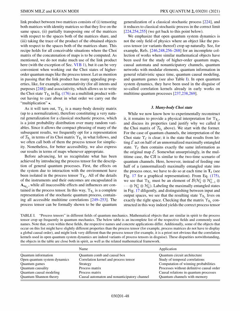
SIMON MILZ and KAVAN MODI PRX QUANTUM 2, 030201 (2021)
link product between two matrices consists of (i) tensoringboth matrices with identity matrices so that they live on thesame space, (ii) partially transposing one of the matriceswith respect to the spaces both of the matrices share, and(iii) taking the trace of the product of the obtained objectswith respect to the spaces both of the matrices share. Thisrecipe holds for all conceivable situations where the Choimatrix of the concatenation of maps is to be computed. Asmentioned, we do not make much use of the link producthere (with the exception of Sec. VI B 1), but it can be veryconvenient when working out the Choi states of higher-order quantum maps like the process tensor. Let us mentionin passing that the link product has many appealing prop-erties, like, for example, commutativity (for all intents andpurposes [248]) and associativity, which allows us to writethe Choi state ϒTk in Eq. (176) as a multilink product with-out having to care about in what order we carry out the“multiplication” �.
As it will turn out, ϒTk is a many-body density matrix(up to a normalization), therefore constituting a very natu-ral generalization for a classical stochastic process, whichis a joint probability distribution over many random vari-ables. Since it allows the compact phrasing of many of thesubsequent results, we frequently opt for a representationof TTk in terms of its Choi matrix ϒTk in what follows, andwe often call both of them the process tensor for simplic-ity. Nonetheless, for better accessibility, we also expressour results in terms of maps whenever appropriate.
Before advancing, let us recapitulate what has beenachieved by introducing the process tensor for the descrip-tion of general quantum processes. First, the effects onthe system due to interaction with the environment havebeen isolated in the process tensor ϒTk . All of the detailsof the instruments and their outcomes are encapsulated inAxTk
, while all inaccessible effects and influences are con-tained in the process tensor. In this way, ϒTk is a completerepresentation of the stochastic quantum process, contain-ing all accessible multitime correlations [249–253]. Theprocess tensor can be formally shown to be the quantum
generalization of a classical stochastic process [224], andit reduces to classical stochastic process in the correct limit[224,254,255] (we get back to this point below).
We emphasize that open quantum system dynamics isnot the only field of physics where an object like the pro-cess tensor (or variants thereof) crop up naturally. See, forexample, Refs. [246,248,256–268] for an incomplete col-lection of works where similar mathematical objects havebeen used for the study of higher-order quantum maps,causal automata and nonanticipatory channels, quantumnetworks with modular elements, quantum information ingeneral relativistic space time, quantum causal modeling,and quantum games (see also Table I). In open quantumsystem dynamics, they have been used in the disguise ofso-called correlation kernels already in early works onmultitime quantum processes [237,238,269].
3. Many-body Choi state
While we now know how to experimentally reconstructit, it remains to provide a physical interpretation for ϒTk ,and discuss its properties (and justify why we called itthe Choi matrix of TTk above). We start with the former.For the case of quantum channels, the interpretation of theChoi state ϒE is clear; it is the state that results from let-ting E act on half of an unnormalized maximally entangledstate. ϒE then contains exactly the same information asthe original map E . Somewhat unsurprisingly, in the mul-titime case, the CJI is similar to the two-time scenario ofquantum channels. Here, however, instead of feeding onehalf of a (unnormalized) maximally entangled state intothe process once, we have to do so at each time in Tk (seeFig. 17 for a graphical representation). From Eq. (175),we see that ϒTk must be an element of B(Hi
k ⊗ Hok−1 ⊗
· · · ⊗ Ho0 ⊗ Hi
0 ). Labeling the maximally entangled statesin Fig. 17 diligently, and distinguishing between input andoutput spaces, we see that the resulting state ϒTk lives onexactly the right space. Checking that the matrix ϒTk con-structed in this way indeed yields the correct process tensor
TABLE I. “Process tensors” in different fields of quantum mechanics. Mathematical objects that are similar in spirit to the processtensor crop up frequently in quantum mechanics. The below table is an incomplete list of the respective fields and commonly usednames. Note that, even within these fields, the respective names and concrete applications differ. Additionally, some of the objects thatoccur on this list might have slightly different properties than the process tensor (for example, process matrices do not have to displaya global causal order), and might look very different than the process tensor (for example, it is a priori not obvious that the correlationkernels used in open quantum system dynamics are indeed variants of process tensors in disguise). These disparities notwithstanding,the objects in the table are close both in spirit, as well as the related mathematical framework.
Name Application
Quantum information Quantum comb and causal box Quantum circuit architectureOpen quantum system dynamics Correlation kernel and process tensor Study of temporal correlationsQuantum games Strategy Computation of winning probabilitiesQuantum causality Process matrix Processes without definitive causal orderQuantum causal modeling Process matrix Causal relations in quantum processesQuantum Shannon theory Causal automaton and nonanticipatory channel Quantum channels with memory
030201-48
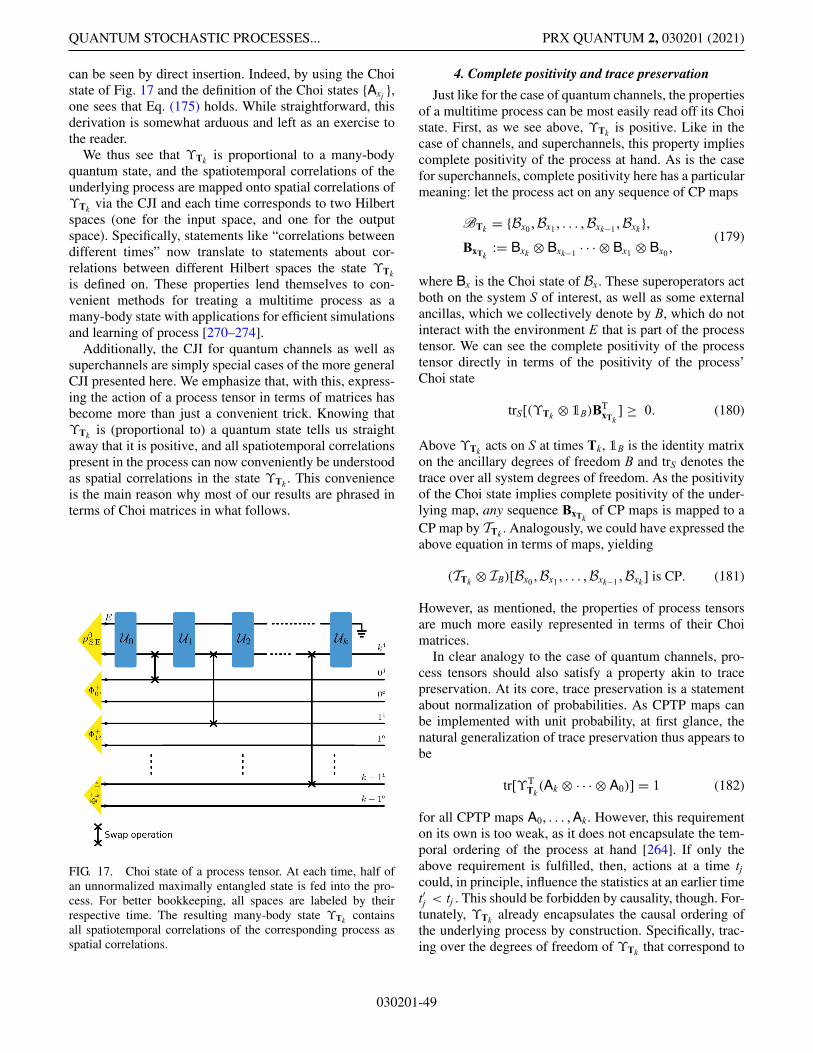
QUANTUM STOCHASTIC PROCESSES... PRX QUANTUM 2, 030201 (2021)
can be seen by direct insertion. Indeed, by using the Choistate of Fig. 17 and the definition of the Choi states {Axj },one sees that Eq. (175) holds. While straightforward, thisderivation is somewhat arduous and left as an exercise tothe reader.
We thus see that ϒTk is proportional to a many-bodyquantum state, and the spatiotemporal correlations of theunderlying process are mapped onto spatial correlations ofϒTk via the CJI and each time corresponds to two Hilbertspaces (one for the input space, and one for the outputspace). Specifically, statements like “correlations betweendifferent times” now translate to statements about cor-relations between different Hilbert spaces the state ϒTkis defined on. These properties lend themselves to con-venient methods for treating a multitime process as amany-body state with applications for efficient simulationsand learning of process [270–274].
Additionally, the CJI for quantum channels as well assuperchannels are simply special cases of the more generalCJI presented here. We emphasize that, with this, express-ing the action of a process tensor in terms of matrices hasbecome more than just a convenient trick. Knowing thatϒTk is (proportional to) a quantum state tells us straightaway that it is positive, and all spatiotemporal correlationspresent in the process can now conveniently be understoodas spatial correlations in the state ϒTk . This convenienceis the main reason why most of our results are phrased interms of Choi matrices in what follows.
FIG. 17. Choi state of a process tensor. At each time, half ofan unnormalized maximally entangled state is fed into the pro-cess. For better bookkeeping, all spaces are labeled by theirrespective time. The resulting many-body state ϒTk containsall spatiotemporal correlations of the corresponding process asspatial correlations.
4. Complete positivity and trace preservation
Just like for the case of quantum channels, the propertiesof a multitime process can be most easily read off its Choistate. First, as we see above, ϒTk is positive. Like in thecase of channels, and superchannels, this property impliescomplete positivity of the process at hand. As is the casefor superchannels, complete positivity here has a particularmeaning: let the process act on any sequence of CP maps
BTk = {Bx0 ,Bx1 , . . . ,Bxk−1 ,Bxk },BxTk
:= Bxk ⊗ Bxk−1 · · · ⊗ Bx1 ⊗ Bx0 ,(179)
where Bx is the Choi state of Bx. These superoperators actboth on the system S of interest, as well as some externalancillas, which we collectively denote by B, which do notinteract with the environment E that is part of the processtensor. We can see the complete positivity of the processtensor directly in terms of the positivity of the process’Choi state
trS[(ϒTk ⊗ 1B)BTxTk
] ≥ 0. (180)
Above ϒTk acts on S at times Tk, 1B is the identity matrixon the ancillary degrees of freedom B and trS denotes thetrace over all system degrees of freedom. As the positivityof the Choi state implies complete positivity of the under-lying map, any sequence BxTk
of CP maps is mapped to aCP map by TTk . Analogously, we could have expressed theabove equation in terms of maps, yielding
(TTk ⊗ IB)[Bx0 ,Bx1 , . . . ,Bxk−1 ,Bxk ] is CP. (181)
However, as mentioned, the properties of process tensorsare much more easily represented in terms of their Choimatrices.
In clear analogy to the case of quantum channels, pro-cess tensors should also satisfy a property akin to tracepreservation. At its core, trace preservation is a statementabout normalization of probabilities. As CPTP maps canbe implemented with unit probability, at first glance, thenatural generalization of trace preservation thus appears tobe
tr[ϒTTk(Ak ⊗ · · · ⊗ A0)] = 1 (182)
for all CPTP maps A0, . . . , Ak. However, this requirementon its own is too weak, as it does not encapsulate the tem-poral ordering of the process at hand [264]. If only theabove requirement is fulfilled, then, actions at a time tjcould, in principle, influence the statistics at an earlier timet′j < tj . This should be forbidden by causality, though. For-tunately, ϒTk already encapsulates the causal ordering ofthe underlying process by construction. Specifically, trac-ing over the degrees of freedom of ϒTk that correspond to
030201-49
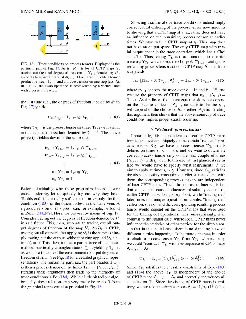
SIMON MILZ and KAVAN MODI PRX QUANTUM 2, 030201 (2021)
FIG. 18. Trace conditions on process tensors. Displayed is thepertinent part of Fig. 17. As tr ◦ U = tr for all CPTP maps U ,tracing out the final degree of freedom of ϒTk , denoted by ki,amounts to a partial trace of �+
k−1o . This, in turn, yields a tensorproduct between 1k−1i and a process tensor on one step less. Asin Fig. 17, the swap operation is represented by a vertical linewith crosses at its ends.
the last time (i.e., the degrees of freedom labeled by ki inFig. 17) yields
trkiϒTk = 1k−1o ⊗ ϒTk−1 , (183)
where ϒTk−1 is the process tensor on times Tk−1 with a finaloutput degree of freedom denoted by k − 1i. The aboveproperty trickles down, in the sense that
trk−1iϒTk−1 = 1k−2o ⊗ ϒTk−2 ,
trk−2iϒTk−2 = 1k−3o ⊗ ϒTk−3 ,
...
tr1iϒT1 = 10o ⊗ ϒT0 ,
tr0iϒT0 = 1.
(184)
Before elucidating why these properties indeed ensurecausal ordering, let us quickly lay out why they hold.To this end, it is actually sufficient to prove only the firstcondition (183), as the others follow in the same vein. Arigorous version of this proof can, for example, be foundin Refs. [244,248]. Here, we prove it by means of Fig. 17.Consider tracing out the degrees of freedom denoted by ki
in said figure. This, then, amounts to tracing out all out-put degrees of freedom of the map Uk. As Uk is CPTP,tracing out all outputs after applying Uk is the same as sim-ply tracing out the outputs without having applied Uk, i.e.,tr ◦ Uk = tr. This, then, implies a partial trace of the unnor-malized maximally entangled state �+
k−1o , yielding 1k−1o ,as well as a trace over the environmental output degrees offreedom of Uk−1 (see Fig. 18 for a detailed graphical repre-sentation). The remaining part, i.e., the part besides 1k−1o
is then a process tensor on the times Tk−1 = {t0, . . . , tk−1}.Iterating these arguments then leads to the hierarchy oftrace conditions in Eq. (184). While a little bit tedious alge-braically, these relations can very easily be read off fromthe graphical representation provided in Fig. 18.
Showing that the above trace conditions indeed implycorrect causal ordering of the process tensor now amountsto showing that a CPTP map at a later time does not havean influence on the remaining process tensor at earliertimes. We start with a CPTP map at tk. This map doesnot have an output space. The only CPTP map with triv-ial output space is the trace operation, which has a Choistate 1ki . Thus, letting ϒTk act on it amounts to a partialtrace trkiϒTk , which is equal to 1k−1o ⊗ ϒTk−1 . Letting thisremaining process tensor act on a CPTP map Ak−1 at timetk−1 yields
trk−1[(1k−1o ⊗ ϒTk−1)ATk−1] = 1k−2o ⊗ ϒTk−2 , (185)
where trk−1 denotes the trace over k − 1i and k − 1o, andwe use the property of CPTP maps that trk−1o(Ak−1) =1k−1i . As the lhs of the above equation does not dependon the specific choice of Ak−1, no statistics before tk−1will depend on the choice of Ak−1 either. Again, iteratingthis argument then shows that the above hierarchy of traceconditions implies proper causal ordering.
5. “Reduced” process tensors
Importantly, this independence on earlier CPTP mapsimplies that we can uniquely define certain “reduced” pro-cess tensors. Say, we have a process tensor ϒTk that isdefined on times t1 < · · · < tk and we want to obtain thecorrect process tensor only on the first couple of times{t0, . . . , tj } with tj < tk. To this end, at first glance, it seemslike we would have to specify what instruments Ji weaim to apply at times ti > tj . However, since ϒTk satisfiesthe above causality constraints, earlier statistics, and withthem, the corresponding process tensors are independentof later CPTP maps. This is in contrast to later statistics,that can, due to causal influences, absolutely depend onearlier CPTP maps. Long story short, while “tracing out”later times is a unique operation on combs, “tracing out”earlier ones is not, and the corresponding resulting processtensor would depend on the CPTP maps that were usedfor the tracing out operations. This, unsurprisingly, is incontrast to the spatial case, where local CPTP maps neverinfluence the statistics of other parties, for the simple rea-son that in the spatial case, there is no signaling betweendifferent parties happening. To be more concrete, in orderto obtain a process tensor ϒTj from ϒTk , where tj < tk,we could “contract” ϒTk with any sequence of CPTP mapsAj +1, . . . , Ak:
ϒTj = trk:j +1[ϒTk (ATj +1 ⊗ · · · ⊗ AT
k )]. (186)
Since ϒTk satisfies the causality constraints of Eqs. (183)and (184) the above ϒTj is independent of the choiceof CPTP maps Aj +1, . . . , Ak and correctly reproduces allstatistics on Tj . Since the choice of CPTP maps is arbi-trary, we can take the simple choice Ai = (1/dio)1
ii ⊗ 1io ,
030201-50
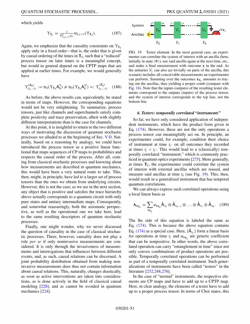
QUANTUM STOCHASTIC PROCESSES... PRX QUANTUM 2, 030201 (2021)
which yields
ϒTj = 1�k
i=j +1diotrk:j +1(ϒTk ). (187)
Again, we emphasize that the causality constraints on ϒTkapply only in a fixed order—that is, the order that is givenby causal ordering of the times in Tk, such that a “reduced”process tensor on later times is a meaningful concept,but would in general depend on the CPTP maps that areapplied at earlier times. For example, we would generallyhave
ϒ(A0)tk ,...,t1 := tr0(ϒTk A
T0 ) �= tr0(ϒTk A
′T0 ) =: ϒ
(A′0)
tk ,...,t1 . (188)
As before, the above results can, equivalently, be statedin terms of maps. However, the corresponding equationswould not be very enlightening. To summarize, processtensors, just like channels and superchannels satisfy com-plete positivity and trace preservation, albeit with slightlydifferent interpretations than is the case for channels.
At this point, it is insightful to return to the two differentways of motivating the discussion of quantum stochasticprocesses we alluded to at the beginning of Sec. V D. Nat-urally, based on a reasoning by analogy, we could haveintroduced the process tensor as a positive linear func-tional that maps sequences of CP maps to probabilities andrespects the causal order of the process. After all, com-ing from classical stochastic processes and knowing abouthow measurements are described in quantum mechanics,this would have been a very natural route to take. This,then, might, in principle, have led to a larger set of processtensors than the ones we obtain from underlying circuits.However, this is not the case; as we see in the next section,any object that is positive and satisfies the trace hierarchyabove actually corresponds to a quantum circuit with onlypure states and unitary intermediate maps. Consequently,and somewhat reassuringly, both the axiomatic perspec-tive, as well as the operational one we take here, leadto the same resulting descriptors of quantum stochasticprocesses.
Finally, one might wonder, why we never discussedthe question of causality in the case of classical stochas-tic processes. There, however, causality does not play arole per se if only noninvasive measurements are con-sidered. It is only through the invasiveness of measure-ments and interrogations that influences between differentevents, and, as such, causal relations can be discerned. Ajoint probability distribution obtained from making non-invasive measurements does thus not contain informationabout causal relations. This, naturally, changes drastically,as soon as active interventions are taken into considera-tions, as is done actively in the field of classical causalmodeling [228], and as cannot be avoided in quantummechanics [224].
FIG. 19. Tester element. In the most general case, an experi-menter can correlate the system of interest with an ancilla (here,initially in state |�〉), use said ancilla again at the next time, etc.,and make a final measurement with outcome x in the end. Asthe unitaries Vj can also act trivially on parts of the ancilla, thisscenario includes all conceivable measurements an experimentercan perform. Summing over the outcomes xTk amounts to trac-ing out the ancillas, thus yielding a proper comb (compare withFig. 16). Note that the inputs (outputs) of the resulting tester ele-ments correspond to the outputs (inputs) of the process tensor,and the system of interest corresponds to the top line, not thebottom line.
6. Testers: temporally correlated “instruments”
So far, we have only considered application of indepen-dent instruments, which have the product form given inEq. (174). However, these are not the only operations aprocess tensor can meaningfully act on. In principle, anexperimenter could, for example, condition their choiceof instrument at time tj ′ on all outcomes they recordedat times tj < tj ′ . This would lead to a (classically) tem-porally correlated “instrument,” which is commonly prac-ticed in quantum optics experiments [275]. More generally,at times Tk, the experimenter could correlate the systemof interest with external ancillas which are reused, andmeasure said ancillas at time tk (see Fig. 19). This, then,would result in a generalized instrument that has temporalquantum correlations.
We can always express such correlated operations usinga local linear basis as
AxTk=∑
xTk
αxTkAxk ⊗ Axk−1 ⊗ . . . ⊗ Ax1 ⊗ Ax0 . (189)
The lhs side of this equation is labeled the same asEq. (174). This is because the above equation containsEq. (174) as a special case. Here, {Axj } form a linear basisfor operations at time tj and αxTk
are generic coefficientthat can be nonpositive. In other words, the above corre-lated operation can carry “entanglement in time” since notonly convex combinations of product operations are pos-sible. Temporally correlated operations can be performedas part of a temporally correlated instrument. Such gener-alizations of instruments have been called “testers” in theliterature [232,248,276].
In the case of “normal” instruments, the respective ele-ments are CP maps and have to add up to a CPTP map.Here, in clear analogy, the elements of a tester have to addup to a proper process tensor. In terms of Choi states, this
030201-51
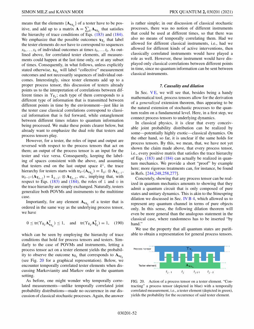
SIMON MILZ and KAVAN MODI PRX QUANTUM 2, 030201 (2021)
means that the elements {AxTk} of a tester have to be pos-
itive, and add up to a matrix A =∑k AxTkthat satisfies
the hierarchy of trace conditions of Eqs. (183) and (184).We emphasize that the possible outcomes xTk that labelthe tester elements do not have to correspond to sequencesx0, . . . xk of individual outcomes at times t0, . . . tk. As out-lined above, for correlated tester elements, all measure-ments could happen at the last time only, or at any subsetof times. Consequently, in what follows, unless explicitlystated otherwise, xTk will label “collective” measurementoutcomes and not necessarily sequences of individual out-comes. Interestingly, since tester elements add up to aproper process tensor, this discussion of testers alreadypoints us to the interpretation of correlations between dif-ferent times in ϒTk ; each type of them corresponds to adifferent type of information that is transmitted betweendifferent points in time by the environment—just like inthe tester case classical correlations correspond to classi-cal information that is fed forward, while entanglementbetween different times relates to quantum informationbeing processed. We make these points clearer below, butalready want to emphasize the dual role that testers andprocess tensors play.
However, for a tester, the roles of input and output arereversed with respect to the process tensors that act onthem; an output of the process tensor is an input for thetester and vice versa. Consequently, keeping the label-ing of spaces consistent with the above, and assumingthat testers end on the last output space ki, the tracehierarchy for testers starts with trko(AxTk
) = 1ki ⊗ ATk−1 ,trk−1o(ATk−1) = 1k−1i ⊗ ATk−2 , etc., implying that, withrespect to Eqs. (183) and (184), the roles of i and o inthe trace hierarchy are simply exchanged. Naturally, testersgeneralize both POVMs and instruments to the multitimecase.
Importantly, for any element AxTkof a tester that is
ordered in the same way as the underlying process tensor,we have
0 ≤ tr(ϒTk ATxTk
) ≤ 1, and tr(ϒTk ATTk) = 1, (190)
which can be seen by employing the hierarchy of traceconditions that hold for process tensors and testers. Sim-ilarly to the case of POVMs and instruments, letting aprocess tensor act on a tester element yields the probabil-ity to observe the outcome xTk that corresponds to AxTk(see Fig. 20 for a graphical representation). Below, weencounter temporally correlated tester elements when dis-cussing Markovianity and Markov order in the quantumsetting.
As before, one might wonder why temporally corre-lated measurements—unlike temporally correlated jointprobability distributions—made no occurrence in our dis-cussion of classical stochastic processes. Again, the answer
is rather simple; in our discussion of classical stochasticprocesses, there was no notion of different instrumentsthat could be used at different times, so that there wasalso no means of temporally correlating them. Had weallowed for different classical instruments, i.e., had weallowed for different kinds of active interventions, thenclassically correlated instruments would have played arole as well. However, these instrument would have dis-played only classical correlations between different pointsin time, since no quantum information can be sent betweenclassical instruments.
7. Causality and dilation
In Sec. V E, we will see that, besides being a handymathematical tool, process tensors allow for the derivationof a generalized extension theorem, thus appearing to bethe natural extension of stochastic processes to the quan-tum realm on a fundamental level. Here, in a first step, weconnect process tensors to underlying dynamics.
In classical physics, it is clear that every conceiv-able joint probability distribution can be realized bysome—potentially highly exotic—classical dynamics. Onthe other hand, so far, it is unclear if the same holds forprocess tensors. By this, we mean, that, we have not yetshown the claim made above, that every process tensor,i.e., every positive matrix that satisfies the trace hierarchyof Eqs. (183) and (184) can actually be realized in quan-tum mechanics. We provide a short “proof” by examplehere; more rigorous treatments can, for instance, be foundin Refs. [244,248,258,277].
Concretely, showing that any process tensor can be real-ized in quantum mechanics amounts to showing that theyadmit a quantum circuit that is only composed of purestates and unitary dynamics. This is akin to the Stinespringdilation we discussed in Sec. IV B 4, which allowed us torepresent any quantum channel in terms of pure objectsonly. In this sense, the following dilation theorem willeven be more general than the analogous statement in theclassical case, where randomness has to be inserted “byhand.”
We use the property that all quantum states are purifi-able to obtain a representation for general process tensors.
FIG. 20. Action of a process tensor on a tester element. “Con-tracting” a process tensor (depicted in blue) with a temporallycorrelated measurement, i.e., a tester element (depicted in green),yields the probability for the occurrence of said tester element.
030201-52
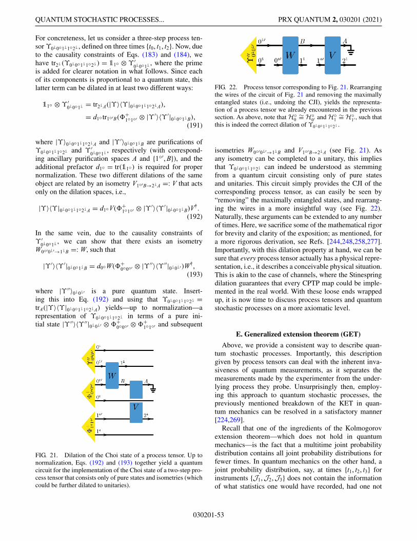
QUANTUM STOCHASTIC PROCESSES... PRX QUANTUM 2, 030201 (2021)
For concreteness, let us consider a three-step process ten-sor ϒ0i0o1i1o2i , defined on three times {t0, t1, t2}. Now, dueto the causality constraints of Eqs. (183) and (184), wehave tr2i(ϒ0i0o1i1o2i) = 11o ⊗ ϒ ′
0i0o1i , where the primeis added for clearer notation in what follows. Since eachof its components is proportional to a quantum state, thislatter term can be dilated in at least two different ways:
11o ⊗ ϒ ′0i0o1i = tr2iA(|ϒ〉〈ϒ |0i0o1i1o2iA),
= d1o tr1o′B(�+1o1o′ ⊗ |ϒ ′〉〈ϒ ′|0i0o1iB),
(191)
where |ϒ〉0i0o1i1o2iA and |ϒ ′〉0i0o1iB are purifications ofϒ0i0o1i1o2i and ϒ ′
0i0o1i , respectively (with correspond-ing ancillary purification spaces A and {1o′, B}), and theadditional prefactor d1o = tr(11o) is required for propernormalization. These two different dilations of the sameobject are related by an isometry V1o′B→2iA =: V that actsonly on the dilation spaces, i.e.,
|ϒ〉〈ϒ |0i0o1i1o2iA = d1oV(�+1o1o′ ⊗ |ϒ ′〉〈ϒ ′|0i0o1iB)V
†.(192)
In the same vein, due to the causality constraints ofϒ ′
0i0o1i , we can show that there exists an isometryW0o′0i′→1iB =: W, such that
|ϒ ′〉〈ϒ ′|0i0o1iB = d0oW(�+0o0o′ ⊗ |ϒ ′′〉〈ϒ ′′|0i0i′)W†,
(193)
where |ϒ ′′〉0i0i′ is a pure quantum state. Insert-ing this into Eq. (192) and using that ϒ0i0o1i1o2i =trA(|ϒ〉〈ϒ |0i0o1i1o2iA) yields—up to normalization—arepresentation of ϒ0i0o1i1o2i in terms of a pure ini-tial state |ϒ ′′〉〈ϒ ′′|0i0i′ ⊗ �+
0o0o′ ⊗ �+1o1o′ and subsequent
FIG. 21. Dilation of the Choi state of a process tensor. Up tonormalization, Eqs. (192) and (193) together yield a quantumcircuit for the implementation of the Choi state of a two-step pro-cess tensor that consists only of pure states and isometries (whichcould be further dilated to unitaries).
FIG. 22. Process tensor corresponding to Fig. 21. Rearrangingthe wires of the circuit of Fig. 21 and removing the maximallyentangled states (i.e., undoing the CJI), yields the representa-tion of a process tensor we already encountered in the previoussection. As above, note that Ho
0∼= Ho
0′ and Ho1
∼= Ho1′ , such that
this is indeed the correct dilation of ϒ0i0o1i1o2i .
isometries W0o′0i′→1iB and V1o′B→2iA (see Fig. 21). Asany isometry can be completed to a unitary, this impliesthat ϒ0i0o1i1o2i can indeed be understood as stemmingfrom a quantum circuit consisting only of pure statesand unitaries. This circuit simply provides the CJI of thecorresponding process tensor, as can easily be seen by“removing” the maximally entangled states, and rearrang-ing the wires in a more insightful way (see Fig. 22).Naturally, these arguments can be extended to any numberof times. Here, we sacrifice some of the mathematical rigorfor brevity and clarity of the exposition; as mentioned, fora more rigorous derivation, see Refs. [244,248,258,277].Importantly, with this dilation property at hand, we can besure that every process tensor actually has a physical repre-sentation, i.e., it describes a conceivable physical situation.This is akin to the case of channels, where the Stinespringdilation guarantees that every CPTP map could be imple-mented in the real world. With these loose ends wrappedup, it is now time to discuss process tensors and quantumstochastic processes on a more axiomatic level.
E. Generalized extension theorem (GET)
Above, we provide a consistent way to describe quan-tum stochastic processes. Importantly, this descriptiongiven by process tensors can deal with the inherent inva-siveness of quantum measurements, as it separates themeasurements made by the experimenter from the under-lying process they probe. Unsurprisingly then, employ-ing this approach to quantum stochastic processes, thepreviously mentioned breakdown of the KET in quan-tum mechanics can be resolved in a satisfactory manner[224,269].
Recall that one of the ingredients of the Kolmogorovextension theorem—which does not hold in quantummechanics—is the fact that a multitime joint probabilitydistribution contains all joint probability distributions forfewer times. In quantum mechanics on the other hand, ajoint probability distribution, say, at times {t1, t2, t3} forinstruments {J1,J2,J3} does not contain the informationof what statistics one would have recorded, had one not
030201-53
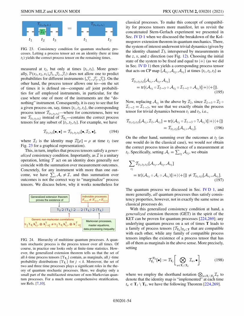
SIMON MILZ and KAVAN MODI PRX QUANTUM 2, 030201 (2021)
FIG. 23. Consistency condition for quantum stochastic pro-cesses. Letting a process tensor act on an identity (here at timet2) yields the correct process tensor on the remaining times.
measured at t2, but only at times {t1, t3}. More gener-ally, P(x3, x2, x1|J3,J2,J1) does not allow one to predictprobabilities for different instruments {J ′
1,J ′2,J ′
3}. On theother hand, the process tensor allows one to—on the setof times it is defined on—compute all joint probabili-ties for all employed instruments, in particular, for thecase where one of more of the instruments are the “do-nothing” instrument. Consequently, it is easy to see that fora given process on, say, times {t1, t2, t3}, the correspondingprocess tensor T{t1,t2,t3}—where for concreteness, here weuse T{t1,t2,t3} instead of TT3—contains the correct processtensors for any subset of {t1, t2, t3}. For example, we have
T{t1,t3}[•, •] = T{t1,t2,t3}[•,I2, •], (194)
where I2 is the identity map I[ρ] = ρ at time t2 (seeFig. 23 for a graphical representation).
This, in turn, implies that process tensors satisfy a gener-alized consistency condition. Importantly, as I is a unitaryoperation, letting T act on an identity does generally notcoincide with the summation over measurement outcomes.Concretely, for any instrument with more than one out-come, we have
∑x Ax �= I , and thus summation over
outcomes is not the correct way to “marginalize” processtensors. We discuss below, why it works nonetheless for
Indivisible processes ℰ(t:r) ≠ ℰ(t:s) ∘ ℰ(s:r)
ΥT ⊇ {ΥTk} ⊇ … ⊇ {ΥT3
} ⊇ {ΥT2}
Generalized extension theorem proves the existence of
Markovian processes,
master equations, data-processing inequality
Generic non-markovian correlations
tr [ΥTkAT
k:j+ ⊗ ATj−:0] ≠ tr [ΥTk
ATk:j+ ⊗ A′Tj−:0]
FIG. 24. Hierarchy of multitime quantum processes. A quan-tum stochastic process is the process tensor over all times. Ofcourse, in practice one looks only at finite-time statistics. How-ever, the generalized extension theorem tells us that the set ofall k-time process tensors {ϒTk } contain, as marginals, all j -timeprobability distributions {ϒTj } for j < k. Moreover, the set oftwo and three time processes plays a significant roles in the the-ory of quantum stochastic processes. Here, we display only asmall part of the multifaceted structure of non-Markovian quan-tum processes. For a much more comprehensive stratification,see Refs. [7,10].
classical processes. To make this concept of compatibil-ity for process tensors more manifest, let us revisit theconcatenated Stern-Gerlach experiment we presented inSec. IV D 1 when we discussed the breakdown of the Kol-mogorov extension theorem in quantum mechanics. There,the system of interest underwent trivial dynamics (given bythe identity channel I), interspersed by measurements inthe z, x, and z direction (see Fig. 12). Choosing the initialstate of the system to be fixed and equal to |+〉 (as we didin Sec. IV D 1) then yields a corresponding process tensorthat acts on CP map {Ax1 ,Az2 ,Ax3} at times {t1, t2, t3} as
T{t1,t2,t3}[Ax1 ,Az2 ,Ax3]
= tr{(Ax3 ◦ I2→3 ◦ Az2 ◦ I1→2 ◦ Ax1)[|+〉〈+|]}.(195)
Now, replacing Az2 in the above by I2, since I2→3 ◦ I2 ◦I1→2 = I1→3, we see that we exactly obtain the processtensor for trivial dynamics between t1 and t3, i.e.,
T{t1,t2,t3}[Ax1 ,I2,Ax3 ] = tr{(Ax3 ◦ I1→3 ◦ 7Ax1)[|+〉〈+|]}= T{t1,t3}[Ax1 ,Ax3]. (196)
On the other hand, summing over the outcomes at t2 (asone would do in the classical case), we would not obtainthe correct process tensor in absence of a measurement att2. Specifically, setting Az =∑z2
Az2 , we obtain
∑
z2
T{t1,t2,t3}[Ax1 ,Az2 ,Ax3]
= tr{(Ax3 ◦ Az ◦ Ax1)[|+〉〈+|]} �= T{t1,t3}[Ax1 ,Ax3].(197)
The quantum process we discussed in Sec. IV D 1, andmore generally, all quantum processes thus satisfy consis-tency properties, however, not in exactly the same sense asclassical processes do.
With this generalized consistency condition at hand, ageneralized extension theorem (GET) in the spirit of theKET can be proven for quantum processes [224,269]; anyunderlying quantum process on a set of times T leads toa family of process tensors {TTk }Tk⊂T that are compatiblewith each other, while any family of compatible processtensors implies the existence of a process tensor that hasall of them as marginals in the above sense. More precisely,setting
T |TkT
[•] := TT
[ ⊗
α∈T\Tk
Iα , •]
, (198)
where we employ the shorthand notation⊗
α∈T\TkIα to
denote that the identity map is “implemented” at each timetα ∈ T \ Tk, we have the following Theorem [224,269].
030201-54
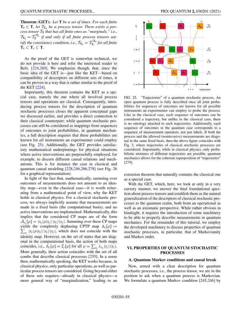
QUANTUM STOCHASTIC PROCESSES... PRX QUANTUM 2, 030201 (2021)
Theorem (GET): Let T be a set of times. For each finiteTk ⊂ T, let TTk be a process tensor. There exists a pro-cess tensor TT that has all finite ones as “marginals,” i.e.,TTk = T |Tk
T if and only if all finite process tensors sat-
isfy the consistency condition, i.e., TTk = T |TkT
for all finiteTk ⊂ T ⊂ T.
As the proof of the GET is somewhat technical, wedo not provide it here and refer the interested reader toRefs. [224,269]. We emphasize though, that, since thebasic idea of the GET is—just like the KET—based oncompatibility of descriptors on different sets of times, itcan be proven in a way that is rather similar to the proof ofthe KET [224].
Importantly, this theorem contains the KET as a spe-cial case, namely the one where all involved processtensors and operations are classical. Consequently, intro-ducing process tensors for the description of quantumstochastic processes closes the apparent conceptual gapswe discussed earlier, and provides a direct connection totheir classical counterpart; while quantum stochastic pro-cesses can still be considered as mappings from sequencesof outcomes to joint probabilities, in quantum mechan-ics, a full description requires that these probabilities areknown for all instruments an experimenter could employ(see Fig. 25). Additionally, the GET provides satisfac-tory mathematical underpinnings for physical situationswhere active interventions are purposefully employed, forexample, to discern different causal relations and mech-anisms. This is for instance the case in classical andquantum causal modeling [228,246,266,278] (see Fig. 26for a graphical representation).
In light of the fact that, mathematically, summing overoutcomes of measurements does not amount to an iden-tity map—even in the classical case—it is worth reiter-ating from a mathematical point of view, why the KETholds in classical physics. For a classical stochastic pro-cess, we always implicitly assume that measurements aremade in a fixed basis (the computational basis), and noactive interventions are implemented. Mathematically, thisimplies that the considered CP maps are of the formAxj [ρ] = 〈xj |ρ|xj 〉 |xj 〉〈xj |. Summing over these CP mapsyields the completely dephasing CPTP map �j [ρ] :=∑
xj〈xj |ρ|xj 〉 |xj 〉〈xj |, which does not coincide with the
identity map. However, on the set of states that are diag-onal in the computational basis, the action of both mapscoincides, i.e., �j [ρ] = Ij [ρ] for all ρ =∑xj
λxj |xj 〉〈xj |.More generally, their action coincides with the set of allcombs that describe classical processes [255]. In a sensethen, mathematically speaking, the KET works because, inclassical physics, only particular operations, as well as par-ticular process tensors are considered. Going beyond eitherof these sets requires—already in classical physics—amore general way of “marginalization,” leading to an
FIG. 25. “Trajectories” of a quantum stochastic process. Anopen quantum process is fully described once all joint proba-bilities for sequences of outcomes are known for all possibleinstruments an experimenter can employ to probe the process.Like in the classical case, each sequence of outcomes can beconsidered a trajectory, but unlike in the classical case, thereis no ontology attached to such trajectories. Additionally, eachsequence of outcomes in the quantum case corresponds to asequence of measurement operators, not just labels. If both theprocess and the allowed (noninvasive) measurements are diago-nal in the same fixed basis, then the above figure coincides withFig. 5, where trajectories of classical stochastic processes areconsidered. Importantly, while in classical physics, only proba-bilistic mixtures of different trajectories are possible, quantummechanics allows for the coherent superposition of “trajectories”[279].
extension theorem that naturally contains the classical oneas a special case.
With the GET, which, here, we look at only in a verycursory manner, we answer the final foundational ques-tion about process tensors and establish them as the naturalgeneralization of the descriptors of classical stochastic pro-cesses to the quantum realm, both from an operational aswell as an axiomatic perspective. While rather obvious inhindsight, it requires the introduction of some machineryto be able to properly describe measurements in quantummechanics. For the remainder of this tutorial, we employthe developed machinery to discuss properties of quantumstochastic processes, in particular, that of Markovianityand Markov order.
VI. PROPERTIES OF QUANTUM STOCHASTICPROCESSES
A. Quantum Markov conditions and causal break
Now, armed with a clear description for quantumstochastic processes, i.e., the process tensor, we are in theposition to ask when a quantum process is Markovian.We formulate a quantum Markov condition [245,246] by
030201-55
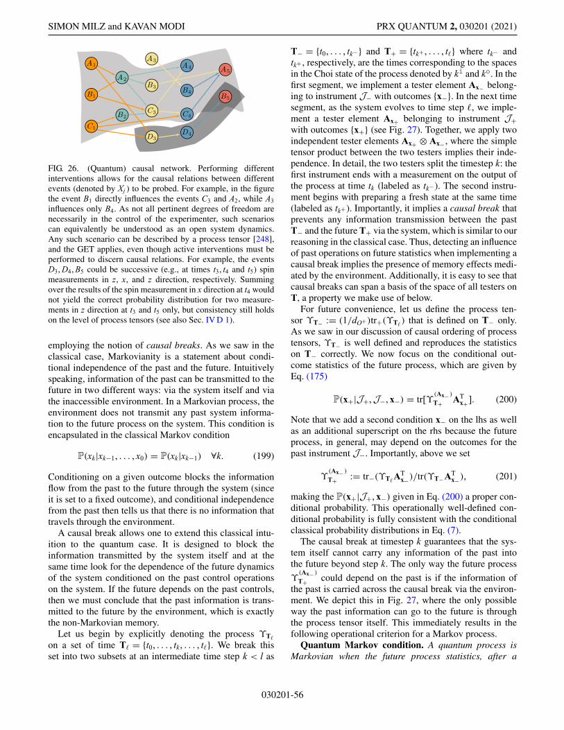
SIMON MILZ and KAVAN MODI PRX QUANTUM 2, 030201 (2021)
FIG. 26. (Quantum) causal network. Performing differentinterventions allows for the causal relations between differentevents (denoted by Xj ) to be probed. For example, in the figurethe event B1 directly influences the events C3 and A2, while A3influences only B4. As not all pertinent degrees of freedom arenecessarily in the control of the experimenter, such scenarioscan equivalently be understood as an open system dynamics.Any such scenario can be described by a process tensor [248],and the GET applies, even though active interventions must beperformed to discern causal relations. For example, the eventsD3, D4, B5 could be successive (e.g., at times t3, t4 and t5) spinmeasurements in z, x, and z direction, respectively. Summingover the results of the spin measurement in x direction at t4 wouldnot yield the correct probability distribution for two measure-ments in z direction at t3 and t5 only, but consistency still holdson the level of process tensors (see also Sec. IV D 1).
employing the notion of causal breaks. As we saw in theclassical case, Markovianity is a statement about condi-tional independence of the past and the future. Intuitivelyspeaking, information of the past can be transmitted to thefuture in two different ways: via the system itself and viathe inaccessible environment. In a Markovian process, theenvironment does not transmit any past system informa-tion to the future process on the system. This condition isencapsulated in the classical Markov condition
P(xk|xk−1, . . . , x0) = P(xk|xk−1) ∀k. (199)
Conditioning on a given outcome blocks the informationflow from the past to the future through the system (sinceit is set to a fixed outcome), and conditional independencefrom the past then tells us that there is no information thattravels through the environment.
A causal break allows one to extend this classical intu-ition to the quantum case. It is designed to block theinformation transmitted by the system itself and at thesame time look for the dependence of the future dynamicsof the system conditioned on the past control operationson the system. If the future depends on the past controls,then we must conclude that the past information is trans-mitted to the future by the environment, which is exactlythe non-Markovian memory.
Let us begin by explicitly denoting the process ϒT
on a set of time T = {t0, . . . , tk, . . . , t}. We break thisset into two subsets at an intermediate time step k < l as
T− = {t0, . . . , tk−} and T+ = {tk+ , . . . , t} where tk− andtk+ , respectively, are the times corresponding to the spacesin the Choi state of the process denoted by ki and ko. In thefirst segment, we implement a tester element Ax− belong-ing to instrument J− with outcomes {x−}. In the next timesegment, as the system evolves to time step , we imple-ment a tester element Ax+ belonging to instrument J+with outcomes {x+} (see Fig. 27). Together, we apply twoindependent tester elements Ax+ ⊗ Ax− , where the simpletensor product between the two testers implies their inde-pendence. In detail, the two testers split the timestep k: thefirst instrument ends with a measurement on the output ofthe process at time tk (labeled as tk−). The second instru-ment begins with preparing a fresh state at the same time(labeled as tk+). Importantly, it implies a causal break thatprevents any information transmission between the pastT− and the future T+ via the system, which is similar to ourreasoning in the classical case. Thus, detecting an influenceof past operations on future statistics when implementing acausal break implies the presence of memory effects medi-ated by the environment. Additionally, it is easy to see thatcausal breaks can span a basis of the space of all testers onT, a property we make use of below.
For future convenience, let us define the process ten-sor ϒT− := (1/dO+)tr+(ϒT
) that is defined on T− only.As we saw in our discussion of causal ordering of processtensors, ϒT− is well defined and reproduces the statisticson T− correctly. We now focus on the conditional out-come statistics of the future process, which are given byEq. (175)
P(x+|J+,J−, x−) = tr[ϒ(Ax− )
T+ ATx+]. (200)
Note that we add a second condition x− on the lhs as wellas an additional superscript on the rhs because the futureprocess, in general, may depend on the outcomes for thepast instrument J−. Importantly, above we set
ϒ(Ax− )
T+ := tr−(ϒTAT
x−)/tr(ϒT−ATx−), (201)
making the P(x+|J+, x−) given in Eq. (200) a proper con-ditional probability. This operationally well-defined con-ditional probability is fully consistent with the conditionalclassical probability distributions in Eq. (7).
The causal break at timestep k guarantees that the sys-tem itself cannot carry any information of the past intothe future beyond step k. The only way the future process
ϒ(Ax− )
T+ could depend on the past is if the information ofthe past is carried across the causal break via the environ-ment. We depict this in Fig. 27, where the only possibleway the past information can go to the future is throughthe process tensor itself. This immediately results in thefollowing operational criterion for a Markov process.
Quantum Markov condition. A quantum process isMarkovian when the future process statistics, after a
030201-56
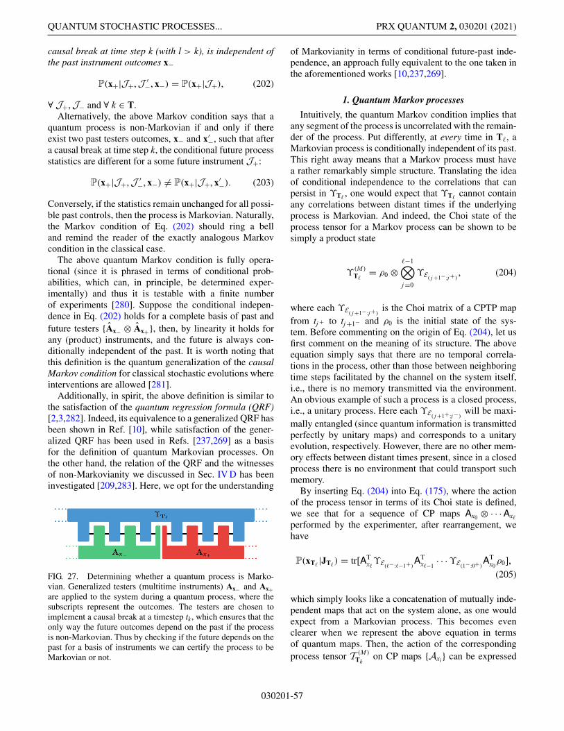
QUANTUM STOCHASTIC PROCESSES... PRX QUANTUM 2, 030201 (2021)
causal break at time step k (with l > k), is independent ofthe past instrument outcomes x−
P(x+|J+,J ′−, x−) = P(x+|J+), (202)
∀ J+,J− and ∀ k ∈ T.Alternatively, the above Markov condition says that a
quantum process is non-Markovian if and only if thereexist two past testers outcomes, x− and x′
−, such that aftera causal break at time step k, the conditional future processstatistics are different for a some future instrument J+:
P(x+|J+,J ′−, x−) �= P(x+|J+, x′
−). (203)
Conversely, if the statistics remain unchanged for all possi-ble past controls, then the process is Markovian. Naturally,the Markov condition of Eq. (202) should ring a belland remind the reader of the exactly analogous Markovcondition in the classical case.
The above quantum Markov condition is fully opera-tional (since it is phrased in terms of conditional prob-abilities, which can, in principle, be determined exper-imentally) and thus it is testable with a finite numberof experiments [280]. Suppose the conditional indepen-dence in Eq. (202) holds for a complete basis of past andfuture testers {Ax− ⊗ Ax+}, then, by linearity it holds forany (product) instruments, and the future is always con-ditionally independent of the past. It is worth noting thatthis definition is the quantum generalization of the causalMarkov condition for classical stochastic evolutions whereinterventions are allowed [281].
Additionally, in spirit, the above definition is similar tothe satisfaction of the quantum regression formula (QRF)[2,3,282]. Indeed, its equivalence to a generalized QRF hasbeen shown in Ref. [10], while satisfaction of the gener-alized QRF has been used in Refs. [237,269] as a basisfor the definition of quantum Markovian processes. Onthe other hand, the relation of the QRF and the witnessesof non-Markovianity we discussed in Sec. IV D has beeninvestigated [209,283]. Here, we opt for the understanding
FIG. 27. Determining whether a quantum process is Marko-vian. Generalized testers (multitime instruments) Ax− and Ax+are applied to the system during a quantum process, where thesubscripts represent the outcomes. The testers are chosen toimplement a causal break at a timestep tk, which ensures that theonly way the future outcomes depend on the past if the processis non-Markovian. Thus by checking if the future depends on thepast for a basis of instruments we can certify the process to beMarkovian or not.
of Markovianity in terms of conditional future-past inde-pendence, an approach fully equivalent to the one taken inthe aforementioned works [10,237,269].
1. Quantum Markov processes
Intuitively, the quantum Markov condition implies thatany segment of the process is uncorrelated with the remain-der of the process. Put differently, at every time in T, aMarkovian process is conditionally independent of its past.This right away means that a Markov process must havea rather remarkably simple structure. Translating the ideaof conditional independence to the correlations that canpersist in ϒT
, one would expect that ϒTcannot contain
any correlations between distant times if the underlyingprocess is Markovian. And indeed, the Choi state of theprocess tensor for a Markov process can be shown to besimply a product state
ϒ(M )T
= ρ0 ⊗−1⊗
j =0
ϒE( j +1−:j +)
, (204)
where each ϒE( j +1−:j +)
is the Choi matrix of a CPTP mapfrom tj + to tj +1− and ρ0 is the initial state of the sys-tem. Before commenting on the origin of Eq. (204), let usfirst comment on the meaning of its structure. The aboveequation simply says that there are no temporal correla-tions in the process, other than those between neighboringtime steps facilitated by the channel on the system itself,i.e., there is no memory transmitted via the environment.An obvious example of such a process is a closed process,i.e., a unitary process. Here each ϒE
( j +1+:j −)will be maxi-
mally entangled (since quantum information is transmittedperfectly by unitary maps) and corresponds to a unitaryevolution, respectively. However, there are no other mem-ory effects between distant times present, since in a closedprocess there is no environment that could transport suchmemory.
By inserting Eq. (204) into Eq. (175), where the actionof the process tensor in terms of its Choi state is defined,we see that for a sequence of CP maps Ax0 ⊗ · · · Axperformed by the experimenter, after rearrangement, wehave
P(xT|JT
) = tr[ATxϒE(−:−1+)
ATx−1
· · ·ϒE(1−:0+)AT
x0ρ0],(205)
which simply looks like a concatenation of mutually inde-pendent maps that act on the system alone, as one wouldexpect from a Markovian process. This becomes evenclearer when we represent the above equation in termsof quantum maps. Then, the action of the correspondingprocess tensor T (M )
Tkon CP maps {Axi} can be expressed
030201-57
SIMON MILZ and KAVAN MODI PRX QUANTUM 2, 030201 (2021)
equivalently to Eq. (205) as
T (M )Tk
[ρ,Ax1 , . . . ,Ak] = tr{(Ak ◦ E(k−:k−1+) ◦ · · · ◦ E(2−:1+)
◦ Ax1 ◦ E(1−:0+))[ρ0]}, (206)
where all E( j +1−:j +) (corresponding to ϒE( j +1−:j +)
) aremutually independent CPTP maps that act on the systemalone, and ρ0 is the initial system state. While this propertyof independent CPTP maps—at first sight—seems equiv-alent to CP divisibility, we emphasize that it is strictlystronger, as the mutual independence of the respectivemaps has to hold for arbitrary interventions at all times inTk [190,244,245] and is thus—unlike CP divisibility—agenuine multitime statement.
As an aside, the above form for Markov processes doesnot mean that we need to do experiments with causalbreaks in order to decide Markovianity of a process. Wesimply need to determine if the process tensor has anycorrelations in time, which can also be done using noisyor temporally correlated instruments that do not corre-spond to causal breaks. We can infer the correlations ina process once we reconstruct the process tensor. Thiscan be done—as outlined above—by tomography, whichrequires only applying a linear basis of instruments, causalbreaks or not. Causal breaks, however, have the conceptualupside that they make the relation to the classical Markovcondition transparent. Additionally, deviation from Marko-vianity can already be witnessed—and assertions aboutthe size of the memory can be made—even if a fullbasis of operations is not available to the experimenter[221,247,271,284], but we do not delve into these detailshere.
Finally, let us comment on how we actually arrive atthe product structure of Markovian process tensors, start-ing from the requirement of conditional independence ofEq. (202). Slightly rewritten in terms of process tensors,conditional independence of the future and the past impliesthat
tr−(ϒTAT
x−) ∝ tr−(ϒTA′T
x−) ∀ Ax− , A′x− , (207)
where the proportionality sign ∝ is used instead of anequality, since Ax− and A′
x− generally occur with differentprobabilities [this has no bearing on the conditional futureprobabilities though, since they are renormalized by therespective past probabilities—see Eqs. (200) and (201)].Since the above equation has to hold for all conceivabletester elements Ax− and A′
x− (and thus, by linearity, forall matrices), it is easy to see that the corresponding ϒT
has to be of product form, i.e., ϒT= ϒ+ ⊗ ϒ−. Demand-
ing that conditional independence holds for all times in T
then implies that ϒTis indeed of the product form postu-
lated in Eq. (204). More detailed proofs of this statementcan, for example, be found in Refs. [244–246].
It is important to emphasize that we did not start out bypostulating this product structure of Markovian processes.While tempting—and eventually correct—it would nothave been an a priori operationally motivated postulate,but rather one guided by purely mathematical consider-ation. Here, we rather started from a fully operationalquantum definition of Markovianity, phrased entirely interms of experimentally accessible quantities, and in linewith its classical counterpart.
Besides following the same logic as the classicaldefinition of Markovianity, that is, conditional indepen-dence of the future and the past, the above notion ofMarkovianity also explicitly boils down to the classicalone in the correct limit: Choosing fixed instruments at eachtime in Tk yields a probability distribution P(xk, . . . , x1) forthe possible combinations of outcomes. Now, if each of theinstruments consists only of causal breaks—which is thecase in the study of classical processes—then a (quantum)Markovian process yields a joint probability distributionfor those instruments that satisfies the classical Markovcondition of Eq. (199). The quantum notion of Markovian-ity thus contains the classical one as a special case. Onemight go further in the restriction to the classical case,by demanding that the resulting statistics also satisfy theKolmogorov consistency conditions we discussed earlier.However, on the one hand, there are quantum processesthat do not satisfy Kolmogorov consistency conditions,independent of the choice of probing instruments [255].On the other hand, Markovianity is also a meaningfulconcept for classical processes with interventions [228],where Kolmogorov conditions are generally not satisfied.Independent of how one aims to restrict to the classicalcase, the notion of Markovianity we introduce here for thequantum case would simplify to the respective notion ofMarkovianity in the classical case.
Below we use the structure of Markovian processesto construct operationally meaningful measures for non-Markovianity that go beyond the witnesses of non-Markovianity based on two-time correlations we presentedin Sec. IV D. We then discuss the concept of quantumMarkov order to close this section.
Before doing this, we shortly discuss how the quan-tum Markov condition we introduce above relates to theaforementioned witnesses of non-Markovianity we alreadyencountered. In contrast to the non-Markovianity wit-nesses discussed in Sec. IV D, the above condition isnecessary and sufficient for memorylessness. That is, ifit holds, then there is no physical experiment that willsee conditional dependence between the past and futureprocesses. If it does not hold then there exists someexperiment that will be able to measure some conditionaldependence between the past and the future processes.In fact, a large list of non-Markovian witnesses, definedin Refs. [161,162,166,174,191,196,202,202,205,234,285–289,289–297], herald the breaking of the quantum Markov
030201-58
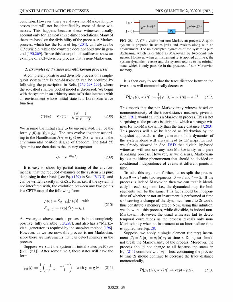
QUANTUM STOCHASTIC PROCESSES... PRX QUANTUM 2, 030201 (2021)
condition. However, there are always non-Markovian pro-cesses that will not be identified by most of these wit-nesses. This happens because these witnesses usuallyaccount only for (at most) three-time correlations. Many ofthem are based on the divisibility of the process. A Markovprocess, which has the form of Eq. (204), will always beCP divisible, while the converse does not hold true in gen-eral [190,269]. To see this latter point, it suffices to show anexample of a CP-divisible process that is non-Markovian.
2. Examples of divisible non-Markovian processes
A completely positive and divisible process on a single-qubit system that is non-Markovian can be acquired byfollowing the prescription in Refs. [269,298,299], wherethe so-called shallow pocket model is discussed. We beginwith the system in an arbitrary state ρ(0) that interacts withan environment whose initial state is a Lorentzian wavefunction
〈x|ψE〉 = ψE(x) =√
G
π
1x + iG
. (208)
We assume the initial state to be uncorrelated, i.e., of theform ρ(0) ⊗ |ψE〉〈ψE|. The two evolve together accord-ing to the Hamiltonian HSE = (g/2)σ3 ⊗ x, where x is theenvironmental position degree of freedom. The total SEdynamics are then due to the unitary operator
Ut = e−iHSEt. (209)
It is easy to show, by partial tracing of the environ-ment E, that the reduced dynamics of the system S is puredephasing in the z basis [see Eq. (129) in Sec. IV D 3], andcan be written exactly in GKSL form, i.e., if the system isnot interfered with, the evolution between any two pointsis a CPTP map of the following form:
ρ(tj ) = E(tj −ti)[ρ(ti)] with
E(tj −ti) = exp{L(tj − ti)}.(210)
As we argue above, such a process is both completelypositive, fully divisible [7,8,297], and also has a “Marko-vian” generator as required by the snapshot method [196].However, as we see now, this process is not Markovian,since there are instruments that can detect memory in theprocess.
Suppose we start the system in initial states ρ±(0) :={|x±〉 〈x±|}. After some time t, these states will have theform
ρ±(t) := 12
(1 ±e−γ t
±e−γ t 1
)with γ = g G . (211)
e−i g2 σ3⊗ x t e−i g
2 σ3⊗ x t{ | x±⟩}
| ψE⟩
σ1
FIG. 28. A CP-divisible but non-Markovian process. A qubitsystem is prepared in states |x±〉 and evolves along with anenvironment. The uninterrupted dynamics of the system is puredephasing, which is certified as Markovian by two-point wit-nesses. However, when an instrument X is applied at time t, thesystem dynamics reverse and the system returns to its originalstate, which is only possible in the presence of non-Markovianmemory.
It is then easy to see that the trace distance between thetwo states will monotonically decrease:
D[ρ+(t), ρ−(t)] := 12‖ρ+(t) − ρ−(t)‖ = e−γ t. (212)
This means that the non-Markovianity witness based onnonmonotonicity of the trace-distance measure, given inRef. [191], would call this a Markovian process. This is notsurprising as the process is divisible, which a stronger wit-ness for non-Markovianity than the trace distance [7,203].This process will also be labeled as Markovian by thesnapshot approach, as the generator of the dynamics ofthe system alone will always lead to CP maps. In fact,we already showed in Sec. IV D that divisibility-basedwitnesses will not see any non-Markovianity in a puredephasing process. However, as we discuss, Markovian-ity is a multitime phenomenon that should be decided onconditional independence of events at different points intime.
To take this argument further, let us split the processfrom 0 → 2t into two segments: 0 → t and t → 2t. If theprocess is indeed Markovian then we can treat it identi-cally in each segment, i.e., the dynamical map for bothsegments will be the same. This fact should be indepen-dent of whether or not an instrument is performed at timet; observing a change of the dynamics from t to 2t wouldthus constitute a memory effect. Now, using this intuition,we show that this process, while divisible, is indeed non-Markovian. However, the usual witnesses fail to detecttemporal correlations as the process reveals only non-Markovianity when an instrument at an intermediate timeis applied, see Fig. 28.
Suppose, we apply a single element (unitary) instru-ment J1 = X [•] := σ1(•)σ1 at time t. Doing so shouldnot break the Markovianity of the process. Moreover, theprocess should not change at all because the states inEq. (211) commute with σ1. Thus, continuing the processto time 2t should continue to decrease the trace distancemonotonically,
D[ρ+(2t), ρ−(2t)] → exp(−γ 2t). (213)
030201-59
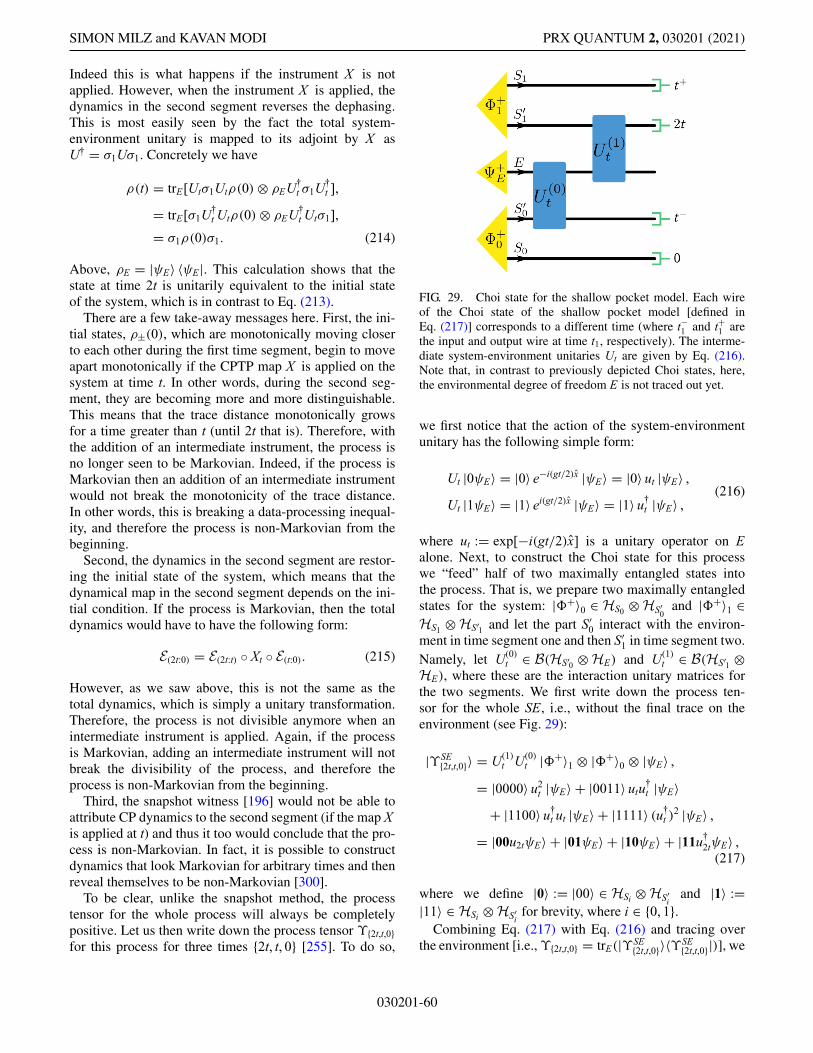
SIMON MILZ and KAVAN MODI PRX QUANTUM 2, 030201 (2021)
Indeed this is what happens if the instrument X is notapplied. However, when the instrument X is applied, thedynamics in the second segment reverses the dephasing.This is most easily seen by the fact the total system-environment unitary is mapped to its adjoint by X asU† = σ1Uσ1. Concretely we have
ρ(t) = trE[Utσ1Utρ(0) ⊗ ρEU†t σ1U†
t ],
= trE[σ1U†t Utρ(0) ⊗ ρEU†
t Utσ1],
= σ1ρ(0)σ1. (214)
Above, ρE = |ψE〉 〈ψE|. This calculation shows that thestate at time 2t is unitarily equivalent to the initial stateof the system, which is in contrast to Eq. (213).
There are a few take-away messages here. First, the ini-tial states, ρ±(0), which are monotonically moving closerto each other during the first time segment, begin to moveapart monotonically if the CPTP map X is applied on thesystem at time t. In other words, during the second seg-ment, they are becoming more and more distinguishable.This means that the trace distance monotonically growsfor a time greater than t (until 2t that is). Therefore, withthe addition of an intermediate instrument, the process isno longer seen to be Markovian. Indeed, if the process isMarkovian then an addition of an intermediate instrumentwould not break the monotonicity of the trace distance.In other words, this is breaking a data-processing inequal-ity, and therefore the process is non-Markovian from thebeginning.
Second, the dynamics in the second segment are restor-ing the initial state of the system, which means that thedynamical map in the second segment depends on the ini-tial condition. If the process is Markovian, then the totaldynamics would have to have the following form:
E(2t:0) = E(2t:t) ◦ Xt ◦ E(t:0). (215)
However, as we saw above, this is not the same as thetotal dynamics, which is simply a unitary transformation.Therefore, the process is not divisible anymore when anintermediate instrument is applied. Again, if the processis Markovian, adding an intermediate instrument will notbreak the divisibility of the process, and therefore theprocess is non-Markovian from the beginning.
Third, the snapshot witness [196] would not be able toattribute CP dynamics to the second segment (if the map Xis applied at t) and thus it too would conclude that the pro-cess is non-Markovian. In fact, it is possible to constructdynamics that look Markovian for arbitrary times and thenreveal themselves to be non-Markovian [300].
To be clear, unlike the snapshot method, the processtensor for the whole process will always be completelypositive. Let us then write down the process tensor ϒ{2t,t,0}for this process for three times {2t, t, 0} [255]. To do so,
FIG. 29. Choi state for the shallow pocket model. Each wireof the Choi state of the shallow pocket model [defined inEq. (217)] corresponds to a different time (where t−1 and t+1 arethe input and output wire at time t1, respectively). The interme-diate system-environment unitaries Ut are given by Eq. (216).Note that, in contrast to previously depicted Choi states, here,the environmental degree of freedom E is not traced out yet.
we first notice that the action of the system-environmentunitary has the following simple form:
Ut |0ψE〉 = |0〉 e−i(gt/2)x |ψE〉 = |0〉 ut |ψE〉 ,
Ut |1ψE〉 = |1〉 ei(gt/2)x |ψE〉 = |1〉 u†t |ψE〉 ,
(216)
where ut := exp[−i(gt/2)x] is a unitary operator on Ealone. Next, to construct the Choi state for this processwe “feed” half of two maximally entangled states intothe process. That is, we prepare two maximally entangledstates for the system: |�+〉0 ∈ HS0 ⊗ HS′
0and |�+〉1 ∈
HS1 ⊗ HS′1 and let the part S′0 interact with the environ-
ment in time segment one and then S′1 in time segment two.
Namely, let U(0)t ∈ B(HS′0 ⊗ HE) and U(1)
t ∈ B(HS′1 ⊗HE), where these are the interaction unitary matrices forthe two segments. We first write down the process ten-sor for the whole SE, i.e., without the final trace on theenvironment (see Fig. 29):
|ϒSE{2t,t,0}〉 = U(1)
t U(0)t |�+〉1 ⊗ |�+〉0 ⊗ |ψE〉 ,
= |0000〉 u2t |ψE〉 + |0011〉 utu
†t |ψE〉
+ |1100〉 u†t ut |ψE〉 + |1111〉 (u†
t )2 |ψE〉 ,
= |00u2tψE〉 + |01ψE〉 + |10ψE〉 + |11u†2tψE〉 ,
(217)
where we define |0〉 := |00〉 ∈ HSi ⊗ HS′i
and |1〉 :=|11〉 ∈ HSi ⊗ HS′
ifor brevity, where i ∈ {0, 1}.
Combining Eq. (217) with Eq. (216) and tracing overthe environment [i.e., ϒ{2t,t,0} = trE(|ϒSE
{2t,t,0}〉〈ϒSE{2t,t,0}|)], we
030201-60
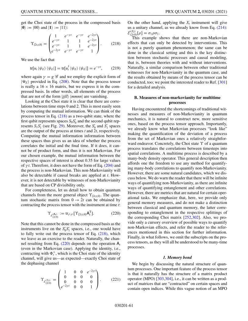
QUANTUM STOCHASTIC PROCESSES... PRX QUANTUM 2, 030201 (2021)
get the Choi state of the process in the compressed basis|0〉 := |00〉 and |1〉 := |11〉:
ϒ{2t,t,0} =
⎛
⎜⎜⎝
1 e−γ t e−γ t e−2γ t
e−γ t 1 1 e−2γ t
e−γ t 1 1 e−2γ t
e−2γ t e−γ t e−γ t 1
⎞
⎟⎟⎠ . (218)
We use the fact that
tr[ut |ψE〉 〈ψE|] = tr[u†t |ψE〉 〈ψE|] = e−γ t, (219)
where again γ = g G and we employ the explicit form of|�E〉 provided in Eq. (208). Note that the process tensoris really a 16 × 16 matrix, but we express it in the com-pressed basis. In other words, all elements of the processthat are not of the form |jjll〉 〈mmnn| are vanishing.
Looking at the Choi state it is clear that there are corre-lations between time steps 0 and 2. This is most easily seenby computing the mutual information. We can think of theprocess tensor in Eq. (218) as a two-qubit state, where thefirst qubit represents spaces S0S′
0 and the second qubit rep-resents S1S′
1 (see Fig. 29). Moreover, the S′0 and S′
1 spacesare the output of the process at times t and 2t, respectively.Computing the mutual information information betweenthese spaces thus gives us an idea of whether the processcorrelates the initial and the final time. If it does, it can-not be of product form, and thus it is not Markovian. Forour chosen example, the mutual information between therespective spaces of interest is about 0.35 for large valuesof γ t. Therefore, it does not have the form of Eq. (204) andthe process is non-Markovian. This non-Markovianity willalso be detectable if causal breaks are applied at t. How-ever, it is not detectable by witnesses of non-Markovianitythat are based on CP divisibility only.
For completeness, let us detail how to obtain quantumchannels from the more general object ϒ{2t,t,0}. The quan-tum stochastic matrix from 0 → 2t can be obtained bycontracting the process tensor with the instrument at time t:
ϒE(At)(2t:0)
:= trtito[ϒ{2t,t,0}ATt ]. (220)
Note that this cannot be done in the compressed basis as theinstruments live on the S′
0S′1 spaces, i.e., one would have
to fully write out the process tensor of Eq. (218), whichwe leave as an exercise to the reader. Naturally, the chan-nel resulting from Eq. (220) depends on the operation At(even in the Markovian case). Applying the identity, i.e.,contracting with �+
t , which is the Choi state of the identitychannel, will give us—as expected—exactly Choi state ofthe dephasing channel
ϒE(It)(2t:0)
=
⎛
⎜⎜⎝
1 0 0 e−2γ t
0 0 0 00 0 0 0
e−2γ t 0 0 1
⎞
⎟⎟⎠ . (221)
On the other hand, applying the Xt instrument will giveus a unitary channel, as we already know from Eq. (214):E (Xt)(2t:0)[ρ] = σ1ρσ1.This example shows that there are non-Markovian
effects that can only be detected by interventions. Thisis not a purely quantum phenomenon; the same can bedone in the classical setting and this is the key distinc-tion between stochastic processes and causal modeling,that is, between theories with and without interventions.Naturally, a similar comparison between other traditionalwitnesses for non-Markovianity in the quantum case, andthe results obtained by means of the process tensor can beconducted, too; we point the interested reader to Ref. [301]for a detailed analysis.
B. Measures of non-markovianity for multitimeprocesses
Having encountered the shortcomings of traditional wit-nesses and measures of non-Markovianity in quantummechanics, it is natural to construct new, more sensitiveones, based on the process tensor approach. Importantly,we already know what Markovian processes “look like”making the quantification of the deviation of a processfrom the set of Markovian ones a relatively straightfor-ward endeavor. Concretely, the Choi state ϒ of a quantumprocess translates the correlations between timesteps intospatial correlations. A multitime process is described by amany-body density operator. This general description thenaffords one the freedom to use any method for quantify-ing many-body correlations to quantify non-Markovianity.However, there are some natural candidates, which we dis-cuss below. We do warn the reader that there will be infiniteways of quantifying non-Markovianity, as there are infiniteways of quantifying entanglement and other correlations.However, there are metrics that are natural for certain oper-ational tasks. We emphasize that, here, we provide onlygeneral memory measures, and do not make a distinctionbetween classical and quantum memory, the latter corre-sponding to entanglement in the respective splittings ofthe corresponding Choi matrix [252,302]. Also, we pro-vide only a cursory overview of possible ways to quantifynon-Markovian effects, and refer the reader to the refer-ences mentioned in this section for further information.Finally, in what follows, we omit the subscripts on the pro-cess tensors, as they will all be understood to be many-timeprocesses.
1. Memory bond
We begin by discussing the natural structure of quan-tum processes. One important feature of the process tensoris that it naturally has the structure of a matrix productoperator (MPO) [303,304], i.e., it can be written as a prod-uct of matrices that are “contracted” on certain spaces andcontain open indices. While this vague notion of an MPO
030201-61
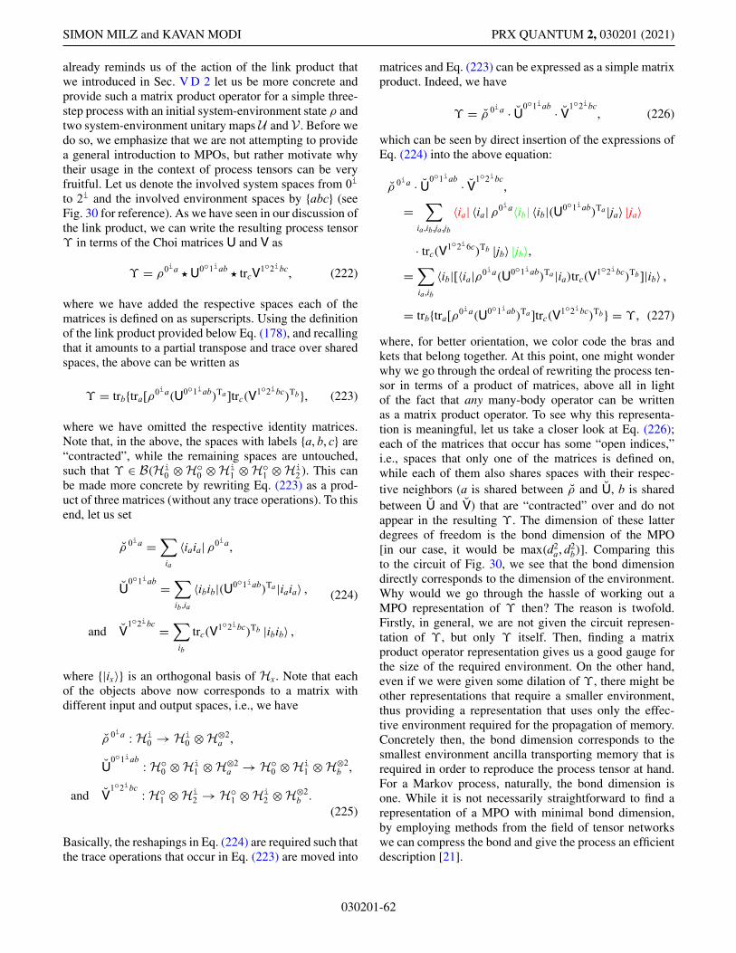
SIMON MILZ and KAVAN MODI PRX QUANTUM 2, 030201 (2021)
already reminds us of the action of the link product thatwe introduced in Sec. V D 2 let us be more concrete andprovide such a matrix product operator for a simple three-step process with an initial system-environment state ρ andtwo system-environment unitary maps U and V . Before wedo so, we emphasize that we are not attempting to providea general introduction to MPOs, but rather motivate whytheir usage in the context of process tensors can be veryfruitful. Let us denote the involved system spaces from 0i
to 2i and the involved environment spaces by {abc} (seeFig. 30 for reference). As we have seen in our discussion ofthe link product, we can write the resulting process tensorϒ in terms of the Choi matrices U and V as
ϒ = ρ0ia � U0o1iab � trcV1o2ibc, (222)
where we have added the respective spaces each of thematrices is defined on as superscripts. Using the definitionof the link product provided below Eq. (178), and recallingthat it amounts to a partial transpose and trace over sharedspaces, the above can be written as
ϒ = trb{tra[ρ0ia(U0o1iab)Ta]trc(V1o2ibc)Tb}, (223)
where we have omitted the respective identity matrices.Note that, in the above, the spaces with labels {a, b, c} are“contracted”, while the remaining spaces are untouched,such that ϒ ∈ B(Hi
0 ⊗ Ho0 ⊗ Hi
1 ⊗ Ho1 ⊗ Hi
2 ). This canbe made more concrete by rewriting Eq. (223) as a prod-uct of three matrices (without any trace operations). To thisend, let us set
ρ 0ia =∑
ia
〈iaia| ρ0ia,
U0o1iab =
∑
ib,ia
〈ibib|(U0o1iab)Ta |iaia〉 ,
and V1o2ibc =
∑
ib
trc(V1o2ibc)Tb |ibib〉 ,
(224)
where {|ix〉} is an orthogonal basis of Hx. Note that eachof the objects above now corresponds to a matrix withdifferent input and output spaces, i.e., we have
ρ 0ia : Hi0 → Hi
0 ⊗ H⊗2a ,
U0o1iab
: Ho0 ⊗ Hi
1 ⊗ H⊗2a → Ho
0 ⊗ Hi1 ⊗ H⊗2
b ,
and V1o2ibc
: Ho1 ⊗ Hi
2 → Ho1 ⊗ Hi
2 ⊗ H⊗2b .
(225)
Basically, the reshapings in Eq. (224) are required such thatthe trace operations that occur in Eq. (223) are moved into
matrices and Eq. (223) can be expressed as a simple matrixproduct. Indeed, we have
ϒ = ρ 0ia · U0o1iab · V
1o2ibc, (226)
which can be seen by direct insertion of the expressions ofEq. (224) into the above equation:
ρ 0ia · U0o1iab · V
1o2ibc,
=∑
ia,ib,ja,jb
〈ia| 〈ia| ρ0ia〈ib| 〈ib|(U0o1iab)Ta |ja〉 |ja〉
· trc(V1o2i6c)Tb |jb〉 |jb〉,
=∑
ia,ib
〈ib|[〈ia|ρ0ia(U0o1iab)Ta |ia)trc(V1o2ibc)Tb]|ib〉 ,
= trb{tra[ρ0ia(U0o1iab)Ta]trc(V1o2ibc)Tb} = ϒ , (227)
where, for better orientation, we color code the bras andkets that belong together. At this point, one might wonderwhy we go through the ordeal of rewriting the process ten-sor in terms of a product of matrices, above all in lightof the fact that any many-body operator can be writtenas a matrix product operator. To see why this representa-tion is meaningful, let us take a closer look at Eq. (226);each of the matrices that occur has some “open indices,”i.e., spaces that only one of the matrices is defined on,while each of them also shares spaces with their respec-tive neighbors (a is shared between ρ and U, b is sharedbetween U and V) that are “contracted” over and do notappear in the resulting ϒ . The dimension of these latterdegrees of freedom is the bond dimension of the MPO[in our case, it would be max(d2
a, d2b)]. Comparing this
to the circuit of Fig. 30, we see that the bond dimensiondirectly corresponds to the dimension of the environment.Why would we go through the hassle of working out aMPO representation of ϒ then? The reason is twofold.Firstly, in general, we are not given the circuit represen-tation of ϒ , but only ϒ itself. Then, finding a matrixproduct operator representation gives us a good gauge forthe size of the required environment. On the other hand,even if we were given some dilation of ϒ , there might beother representations that require a smaller environment,thus providing a representation that uses only the effec-tive environment required for the propagation of memory.Concretely then, the bond dimension corresponds to thesmallest environment ancilla transporting memory that isrequired in order to reproduce the process tensor at hand.For a Markov process, naturally, the bond dimension isone. While it is not necessarily straightforward to find arepresentation of a MPO with minimal bond dimension,by employing methods from the field of tensor networkswe can compress the bond and give the process an efficientdescription [21].
030201-62
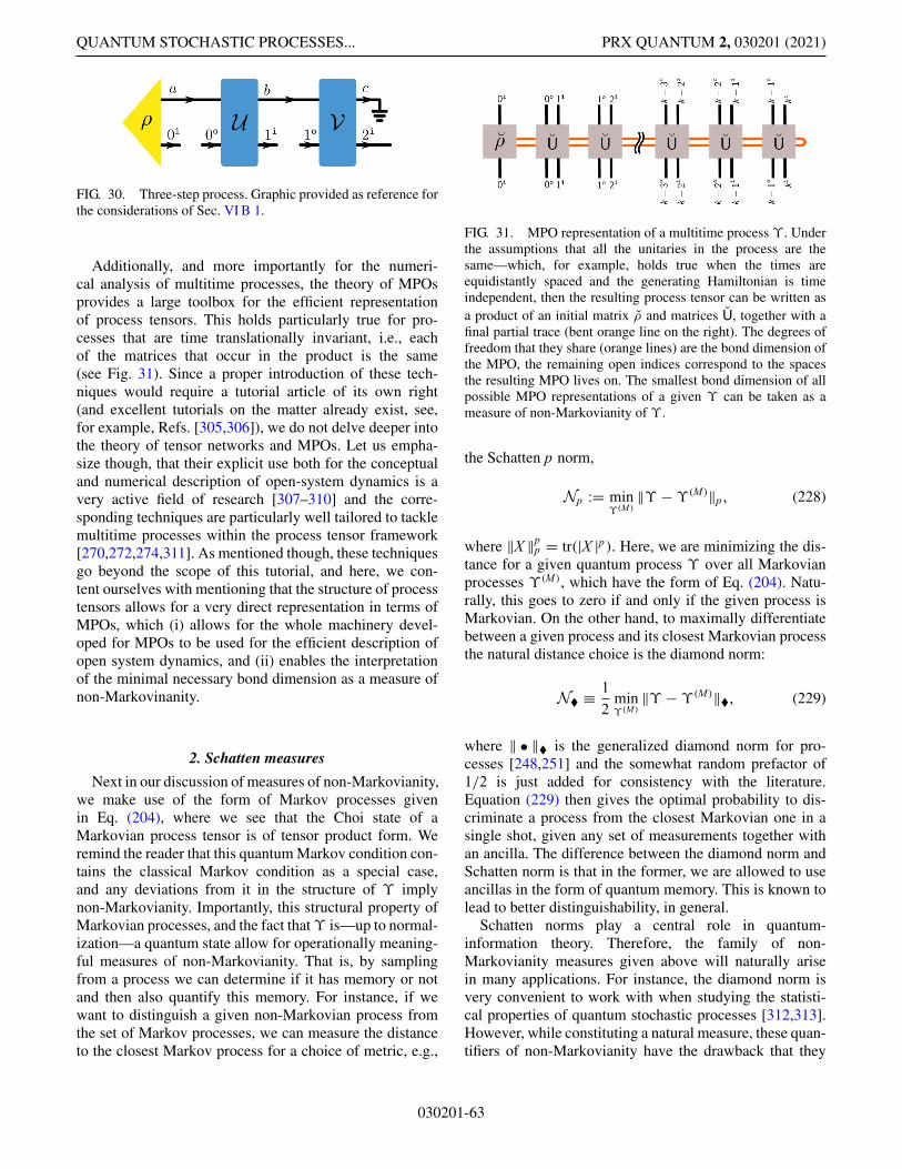
QUANTUM STOCHASTIC PROCESSES... PRX QUANTUM 2, 030201 (2021)
FIG. 30. Three-step process. Graphic provided as reference forthe considerations of Sec. VI B 1.
Additionally, and more importantly for the numeri-cal analysis of multitime processes, the theory of MPOsprovides a large toolbox for the efficient representationof process tensors. This holds particularly true for pro-cesses that are time translationally invariant, i.e., eachof the matrices that occur in the product is the same(see Fig. 31). Since a proper introduction of these tech-niques would require a tutorial article of its own right(and excellent tutorials on the matter already exist, see,for example, Refs. [305,306]), we do not delve deeper intothe theory of tensor networks and MPOs. Let us empha-size though, that their explicit use both for the conceptualand numerical description of open-system dynamics is avery active field of research [307–310] and the corre-sponding techniques are particularly well tailored to tacklemultitime processes within the process tensor framework[270,272,274,311]. As mentioned though, these techniquesgo beyond the scope of this tutorial, and here, we con-tent ourselves with mentioning that the structure of processtensors allows for a very direct representation in terms ofMPOs, which (i) allows for the whole machinery devel-oped for MPOs to be used for the efficient description ofopen system dynamics, and (ii) enables the interpretationof the minimal necessary bond dimension as a measure ofnon-Markovinanity.
2. Schatten measures
Next in our discussion of measures of non-Markovianity,we make use of the form of Markov processes givenin Eq. (204), where we see that the Choi state of aMarkovian process tensor is of tensor product form. Weremind the reader that this quantum Markov condition con-tains the classical Markov condition as a special case,and any deviations from it in the structure of ϒ implynon-Markovianity. Importantly, this structural property ofMarkovian processes, and the fact that ϒ is—up to normal-ization—a quantum state allow for operationally meaning-ful measures of non-Markovianity. That is, by samplingfrom a process we can determine if it has memory or notand then also quantify this memory. For instance, if wewant to distinguish a given non-Markovian process fromthe set of Markov processes, we can measure the distanceto the closest Markov process for a choice of metric, e.g.,
FIG. 31. MPO representation of a multitime process ϒ . Underthe assumptions that all the unitaries in the process are thesame—which, for example, holds true when the times areequidistantly spaced and the generating Hamiltonian is timeindependent, then the resulting process tensor can be written asa product of an initial matrix ρ and matrices U, together with afinal partial trace (bent orange line on the right). The degrees offreedom that they share (orange lines) are the bond dimension ofthe MPO, the remaining open indices correspond to the spacesthe resulting MPO lives on. The smallest bond dimension of allpossible MPO representations of a given ϒ can be taken as ameasure of non-Markovianity of ϒ .
the Schatten p norm,
Np := minϒ(M )
‖ϒ − ϒ(M )‖p , (228)
where ‖X ‖pp = tr(|X |p). Here, we are minimizing the dis-
tance for a given quantum process ϒ over all Markovianprocesses ϒ(M ), which have the form of Eq. (204). Natu-rally, this goes to zero if and only if the given process isMarkovian. On the other hand, to maximally differentiatebetween a given process and its closest Markovian processthe natural distance choice is the diamond norm:
N� ≡ 12
minϒ(M )
‖ϒ − ϒ(M )‖�, (229)
where ‖ • ‖� is the generalized diamond norm for pro-cesses [248,251] and the somewhat random prefactor of1/2 is just added for consistency with the literature.Equation (229) then gives the optimal probability to dis-criminate a process from the closest Markovian one in asingle shot, given any set of measurements together withan ancilla. The difference between the diamond norm andSchatten norm is that in the former, we are allowed to useancillas in the form of quantum memory. This is known tolead to better distinguishability, in general.
Schatten norms play a central role in quantum-information theory. Therefore, the family of non-Markovianity measures given above will naturally arisein many applications. For instance, the diamond norm isvery convenient to work with when studying the statisti-cal properties of quantum stochastic processes [312,313].However, while constituting a natural measure, these quan-tifiers of non-Markovianity have the drawback that they
030201-63
SIMON MILZ and KAVAN MODI PRX QUANTUM 2, 030201 (2021)
require a minimization over the whole set of Marko-vian processes, which makes them computationally hardto access. This problem can be remedied by choosing adifferent metric in Eq. (228).
3. Relative entropy
We could also use any metric or pseudometric D that iscontractive under CP operations
N := minϒ
(M)k:0
D[ϒk:0‖ϒMarkov
k:0
]. (230)
Here, CP contractive means that D[�(X )‖�(Y)] ≤D[X ‖Y] for any CP map � on the space of general-ized Choi states. A metric or pseudometric that is not CPcontractive, may not lead to consistent measures for non-Markovianity since, for example, it could be increased bythe presence of an independent ancillary Markov process.Here, the requirement that D is a pseudometric means thatit satisfies all the properties of a distance except that it maynot be symmetric in its arguments. Different quasidistancemeasures will then have different operational interpreta-tions for the memory. In general though, they will still beplagued by the problem of minimization that appears inEq. (230).
A very convenient pseudometric choice is the quantumrelative entropy [45], which we already encountered inSec. IV D 4 when we discussed quantum data-processinginequalities. In order to be able to use the relative entropy,let us assume for the remainder of this section that allthe process tensors we use are normalized, i.e., trϒ = 1.Besides being contractive under CP maps, this pseudomet-ric is very convenient because for any given process ϒ ,the closest (with respect to the quantum relative entropy)Markovian process is straightforwardly found by discard-ing the correlations. That is, the process made of themarginals of the given process is the closest Markovprocess, such that
NR = D[ϒk:0‖ϒ1−:0+ ⊗ · · · ⊗ ϒk−:k−1+
], (231)
where the CPTP maps {ϒj −:j =1+} are the respectivemarginals (obtained via partial trace) of ϒk:0. This fol-lows from the well-known fact that, with respect to thequantum relative entropy, the closest product state of amultipartite quantum state is the one that is simply a tensorproduct of its marginals [314]. Moreover, besides allevi-ating the minimization problem, this measure has a clearoperational interpretation as a probability of confusing thegiven process for being Markovian [244]:
Pconfusion = exp{−nNR}, (232)
where NR is the relative entropy between the given pro-cess and its marginals. Specifically, this measure quantifies
the following: suppose a process in an experiment is non-Markovian. The employed model for the experiment is,however, Markovian. The above measure is related to theprobability of confusing the model with the experimentafter n samplings. If NR is large, then an experimenter willvery quickly realize that the hypothesis is false, and themodel needs updating, i.e., the experimenter is quick tolearn that the Markovian model poorly approximates the(highly) non-Markovian process.
With this, we conclude our short presentation ofmeasures for non-Markovianity in the multitime setup.The attentive reader will have noticed that we do nottouch on witnesses of non-Markovianity here, unlike inSec. IV D where we discuss (some of the) witnesses fornon-Markovianity in the two-time scenario. In principle,such witnesses can be straightforwardly constructed. Wealready did so in this tutorial, when we discussed theshallow pocket model and its non-Markovian features.Also, experimentally implementing some causal breaksand checking for conditional independence would pro-vide a witness for non-Markovianity. However, to date,no experimentally used witness for non-Markovianity inthe multitime setting has crystallized, and a systematicconstruction of memory witnesses that are attuned toexperimental requirements is subject of ongoing research.
More generally though, “simply” deciding whether aprocess is Markovian or not seems somewhat blunt for amultitime process. After all, it is not just of interest if thereare memory effects, but what kinds of memory effectsthere are. At its core, this latter question is a question ofMarkov order for quantum processes. We thus spend theremainder of this tutorial providing a proper definition ofMarkov order in the quantum case, as well as a nontrivialexample to illustrate these considerations.
C. Quantum Markov order
The process tensor allows one to properly define Marko-vianity for quantum processes. As we have seen, though, inour discussion of the classical case, Markovian processesare not the only possibility. Rather, they constitute the setof processes of Markov order 1 (and 0). It is then naturalto ask if Markov order is a concept that transfers neatly tothe quantum case as well. As we will see, Markov order isindeed a meaningful concept for quantum processes butturns out to be a more layered phenomenon than in theclassical realm. Here, we focus only on a couple of basicaspects of quantum Markov order. For a more in-depthdiscussion, see, for example, Refs. [250,315]. Addition-ally, while it is possible to phrase results on quantumMarkov order in terms of maps, it proves rather cumber-some, which is why the following results are presentedexclusively in terms of Choi states.
Before turning to the quantum case, let us quickly recall(see Sec. III C 4) that for classical processes of Markov
030201-64
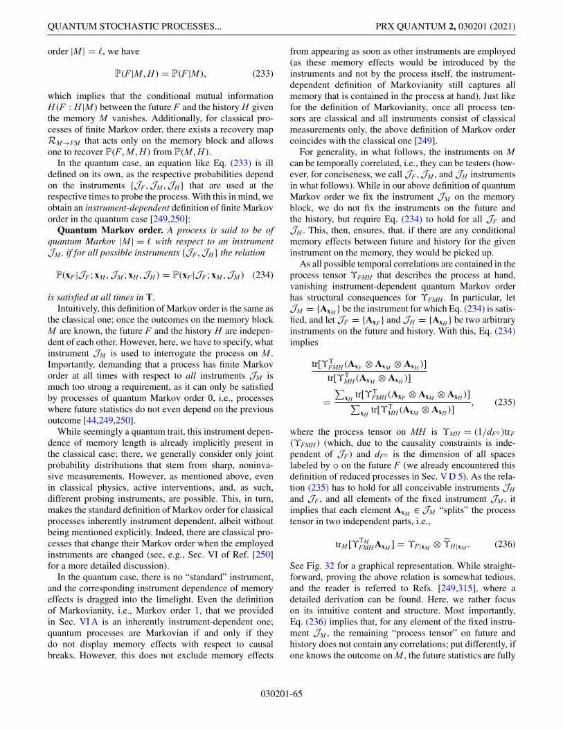
QUANTUM STOCHASTIC PROCESSES... PRX QUANTUM 2, 030201 (2021)
order |M | = , we have
P(F|M , H) = P(F|M ), (233)
which implies that the conditional mutual informationH(F : H |M ) between the future F and the history H giventhe memory M vanishes. Additionally, for classical pro-cesses of finite Markov order, there exists a recovery mapRM→FM that acts only on the memory block and allowsone to recover P(F , M , H) from P(M , H).
In the quantum case, an equation like Eq. (233) is illdefined on its own, as the respective probabilities dependon the instruments {JF ,JM ,JH } that are used at therespective times to probe the process. With this in mind, weobtain an instrument-dependent definition of finite Markovorder in the quantum case [249,250]:
Quantum Markov order. A process is said to be ofquantum Markov |M | = with respect to an instrumentJM , if for all possible instruments {JF ,JH } the relation
P(xF |JF ; xM ,JM ; xH ,JH ) = P(xF |JF ; xM ,JM ) (234)
is satisfied at all times in T.Intuitively, this definition of Markov order is the same as
the classical one; once the outcomes on the memory blockM are known, the future F and the history H are indepen-dent of each other. However, here, we have to specify, whatinstrument JM is used to interrogate the process on M .Importantly, demanding that a process has finite Markovorder at all times with respect to all instruments JM ismuch too strong a requirement, as it can only be satisfiedby processes of quantum Markov order 0, i.e., processeswhere future statistics do not even depend on the previousoutcome [44,249,250].
While seemingly a quantum trait, this instrument depen-dence of memory length is already implicitly present inthe classical case; there, we generally consider only jointprobability distributions that stem from sharp, noninva-sive measurements. However, as mentioned above, evenin classical physics, active interventions, and, as such,different probing instruments, are possible. This, in turn,makes the standard definition of Markov order for classicalprocesses inherently instrument dependent, albeit withoutbeing mentioned explicitly. Indeed, there are classical pro-cesses that change their Markov order when the employedinstruments are changed (see, e.g., Sec. VI of Ref. [250]for a more detailed discussion).
In the quantum case, there is no “standard” instrument,and the corresponding instrument dependence of memoryeffects is dragged into the limelight. Even the definitionof Markovianity, i.e., Markov order 1, that we providedin Sec. VI A is an inherently instrument-dependent one;quantum processes are Markovian if and only if theydo not display memory effects with respect to causalbreaks. However, this does not exclude memory effects
from appearing as soon as other instruments are employed(as these memory effects would be introduced by theinstruments and not by the process itself, the instrument-dependent definition of Markovianity still captures allmemory that is contained in the process at hand). Just likefor the definition of Markovianity, once all process ten-sors are classical and all instruments consist of classicalmeasurements only, the above definition of Markov ordercoincides with the classical one [249].
For generality, in what follows, the instruments on Mcan be temporally correlated, i.e., they can be testers (how-ever, for conciseness, we call JF ,JM , and JH instrumentsin what follows). While in our above definition of quantumMarkov order we fix the instrument JM on the memoryblock, we do not fix the instruments on the future andthe history, but require Eq. (234) to hold for all JF andJH . This, then, ensures, that, if there are any conditionalmemory effects between future and history for the giveninstrument on the memory, they would be picked up.
As all possible temporal correlations are contained in theprocess tensor ϒFMH that describes the process at hand,vanishing instrument-dependent quantum Markov orderhas structural consequences for ϒFMH . In particular, letJM = {AxM } be the instrument for which Eq. (234) is satis-fied, and let JF = {AxF } and JH = {AxH } be two arbitraryinstruments on the future and history. With this, Eq. (234)implies
tr[ϒTFMH (AxF ⊗ AxM ⊗ AxH )]tr[ϒT
MH (AxM ⊗ AxH )]
=∑
xHtr[ϒT
FMH (AxF ⊗ AxM ⊗ AxH )]∑
xHtr[ϒT
MH (AxM ⊗ AxH )], (235)
where the process tensor on MH is ϒMH = (1/dFo)trF(ϒFMH ) (which, due to the causality constraints is inde-pendent of JF ) and dFo is the dimension of all spaceslabeled by o on the future F (we already encountered thisdefinition of reduced processes in Sec. V D 5). As the rela-tion (235) has to hold for all conceivable instruments JHand JF , and all elements of the fixed instrument JM , itimplies that each element AxM ∈ JM “splits” the processtensor in two independent parts, i.e.,
trM [ϒTMFMH AxM ] = ϒF|xM ⊗ ϒH |xM . (236)
See Fig. 32 for a graphical representation. While straight-forward, proving the above relation is somewhat tedious,and the reader is referred to Refs. [249,315], where adetailed derivation can be found. Here, we rather focuson its intuitive content and structure. Most importantly,Eq. (236) implies that, for any element of the fixed instru-ment JM , the remaining “process tensor” on future andhistory does not contain any correlations; put differently, ifone knows the outcome on M , the future statistics are fully
030201-65
SIMON MILZ and KAVAN MODI PRX QUANTUM 2, 030201 (2021)
independent of the past. Conversely, by insertion, it can beseen that any process tensor ϒFMH that satisfies Eq. (236)for some instrument JM also satisfies Eq. (234). As anaside, we already saw this “splitting” of the process ten-sor due to conditional independence when we discussedMarkovian processes. Indeed, the resulting structure ofMarkovian processes is a particular case of the results forMarkov order presented below.
On the structural side, it can be directly seen that theterms {ϒF|xM } in Eq. (236) are proper process tensors, i.e.,they are positive and satisfy the causality constraints ofEqs. (183) and (184). Specifically, contracting ϒFMH witha positive element on the memory block M yields positiveelements, and does not alter satisfaction of the hierarchyof trace conditions on the block F . This fails to gener-ally hold true on the block H . While still positive, theterms ϒH |xM do not necessarily have to satisfy causalityconstraints. However, the set {ϒH |xM } forms a tester, i.e.,∑
xMϒH |xM = ϒH is a process tensor.
Employing Eq. (236), we can derive the most generalform of a process tensor ϒFMH that has finite Markovorder with respect to the instrument JM = {AxM }n
xM =1. Tothis end, without loss of generality, let us assume that alln elements of JM are linearly independent [316]. Then,this set can be completed to a full basis of the space ofmatrices on the memory block M by means of other testerelements {AαM }dM
αM =n+1, where dM is the dimension of thespace spanned by tester elements on the memory block. Asthese two sets together form a linear basis, there exists acorresponding dual basis, which we denote as
{{�xM }n
xM=1
⋃{�αM }dM
αM =n+1
}. (237)
From this, we obtain the general form of a process ten-sor ϒFMH with finite Markov order with respect to the
FIG. 32. Quantum Markov order. If a process ϒFMH has finiteMarkov order with respect to an instrument and tester JM ={AxM } on the memory block, then the application of each of theelements of JM leaves the process in a tensor product betweenfuture F and history H .
instrument JM [250]:
ϒFMH =n∑
xM =1
ϒF|xM ⊗ �∗xM
⊗ ϒH |xM
+dM∑
αM =n+1
ϒFH |αM ⊗ �∗αM
. (238)
It can be seen directly [by insertion into Eq. (236)] that theabove ϒFMH indeed yields the correct term ϒF|xM ⊗ ϒH |xMfor every AxM ∈ JM . Using other tester elements, like, forexample AαM , will however not yield uncorrelated ele-ments on FH (as the terms ϒFH |αM do not necessarilyhave to be uncorrelated). This, basically, is just a differentway of saying that an informationally incomplete instru-ment is not sufficient to fully determine the process at hand[247]. Additionally, most elements of the span of JM willnot yield uncorrelated elements, either, but rather a linearcombination of uncorrelated elements, which is generallycorrelated.
While remaining a meaningful concept in the quantumdomain, quantum Markov order is highly dependent on thechoice of instrument JM , and there exists a whole zoo ofprocesses that show peculiar memory properties for dif-ferent kinds of instruments, like, for example, processesthat have only finite Markov order for unitary instru-ments, or processes, which have finite Markov order withrespect to an informationally complete instrument, but theconditional mutual information does not vanish [249,315].
Before providing a detailed example of a process withfinite quantum Markov order, let us discuss this aforemen-tioned connection between quantum Markov order and thequantum version of the conditional mutual information.In analogy to the classical case, one can define a quan-tum CMI (QCMI) for quantum states ρFMH shared betweenparties F , M , and H as
S(F : H |M ) = S(F|M ) + S(H |M ) − S(FH |M ), (239)
where S(A|B) := S(AB) − S(B) and S(A) := −tr[A log(A)](see Sec. IV D 4) is the von Neumann entropy. Quan-tum states with vanishing QCMI have many appealingproperties, like, for example, the fact that they admit ablock decomposition [317], as well as a CPTP recoverymap WM→FM [ρMH ] = ρFMH that acts only on the blockM [318,319]. Unlike in the classical case, the proof ofthis latter property is far from trivial and a highly cele-brated result. States with vanishing QCMI or, equivalently,states that can be recovered by means of a CPTP mapWM→FM are called quantum Markov chains [53,54,317,319–323]. Importantly, for states with approximately van-ishing QCMI, the recovery error one makes when employ-ing a map WM→FM can be bounded by a function of theQCMI [53,54,322,323].
030201-66
QUANTUM STOCHASTIC PROCESSES... PRX QUANTUM 2, 030201 (2021)
As process tensors ϒFMH are, up to normalization, quan-tum states, all of the aforementioned results can be used forthe study of quantum processes with finite Markov order.However, the relation of quantum processes with finiteMarkov order and the QCMI of the corresponding processtensor is—unsurprisingly—more layered than in the clas-sical case. We present some of the peculiar features herewithout proof to provide a flavor of the fascinating jun-gle that is memory effects in quantum mechanics (see, forexample, Refs. [249,250,315] for in-depth discussions).
Let us begin with a positive result. Using the repre-sentation of quantum states with vanishing QCMI pro-vided in Ref. [317], for any process tensor ϒFMH thatsatisfies S(F : H |M )ϒFMH = 0, one can construct an instru-ment on the memory block M , that blocks the memorybetween H and F . Put differently, vanishing QCMI implies(instrument-dependent) finite quantum order.
However, the converse does not hold. This can alreadybe seen from Eq. (238), where the general form of aprocess tensor with finite Markov order is provided. Theoccurrence of the second set of terms ϒFH |αM ⊗ �αMimplies the existence of a wide range of correlationsbetween H and F that can still persist (but not be picked upby the fixed instrument chosen on M ), making it unlikelythat the QCMI of such a process tensor actually vanishes.On the other hand, if the instrument JM is informationallycomplete, then there is a representation of ϒFMH that con-tains only terms of the form ϒF|xM ⊗ �xM , which looksmore promising in terms of vanishing QCMI (in principle,such a decomposition can also exist when the respectivetester elements are not informationally complete, whichis the case for classical stochastic processes). However,when the tester elements AxM corresponding to the duals�xM do not commute (which, in general they do not), then,again, the QCMI of ϒFMH does not vanish [249,250,315].Nonetheless, for any process tensor of the form
ϒFMH =∑
xM
ϒF|xM ⊗ �∗xM
⊗ ϒH |xM , (240)
knowing the outcomes on the memory block (for theinstrument JB = {AxM }) allows one to reconstruct the fullprocess tensor. Concretely, using
ϒMH = trF(ϒFMH )
dFo
:= 1dFo
∑
xM
cxM �∗xM
⊗ ϒH |xM ,(241)
where we set cxM = tr(ϒF|xM ) and dFo is the dimension ofall output spaces on the future block, we have
ϒFMH = dFo∑
xM
c−1xM
ϒF|xM ⊗ �∗xM
⊗ trM (ϒMH ATxM
)
=: WM→FM [ϒMH ].(242)
Here, the map WM→FM appears to play the role of arecovery map. However, as the duals {�xM } are not nec-essarily positive [324], WM→FM in the above equation isgenerally not CPTP. Nonetheless, with this procedure onecan then construct an ansatz for a quantum process withapproximate Markov order. The crucial point being thatthe difference between the ansatz process and the actualprocess can be quantified by relative entropy between thetwo [251]. Such a construction has applications in tamingquantum non-Markovian memory; as we stated earlier, thecomplexity of a process increases exponentially with thesize of the memory. Thus, contracting the memory with-out the loss of precision, is highly desirable. With this,we conclude our discussion of the properties of quantumprocesses with finite Markov order. We now provide anexplicit example of such a process.
1. Nontrivial example of quantum Markov order
Let us now consider a process, introduced in Ref. [251]and depicted here in Fig. 33, which requires leaving partsof M attached to H and F (as we see shortly). We labelthe input-output spaces associated to each time of the pro-cess as follows: {H , M , F} = {Hi, Ho, Li, Lo, Ri, Ro, Fi},where we subdivide M into left L and right R spaces. Ateach time, the system of interest comprises three qubits,and so each Hilbert space is of the form HX = HXa ⊗HXb ⊗ HXc , where X takes values for the times and a, b, care labels for the three qubits; whenever we refer to an indi-vidual qubit, we label the system appropriately, e.g., Liarefers to the a qubit of the system Li; whenever no suchlabel is specified, we are referring to all three qubits.
The environment first prepares the five-qubit commoncause states
|e+〉 = 1√2(α |ψ0, 00〉 + β |ψ1, 11〉) and
|e−〉 = 1√2(γ |φ0, 01〉 + δ |φ1, 10〉).
(243)
Here, we separate the first register, which is a three-qubitstate, from the second, which consists of two qubits, witha comma. The first parts of the states |e+〉 and |e−〉 are,respectively, sent to Hi and Fi. The second parts aresent either to Li or Ri, according to some probabilitydistribution (see Fig. 33).
030201-67
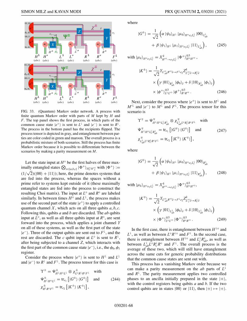
SIMON MILZ and KAVAN MODI PRX QUANTUM 2, 030201 (2021)
FH L L R(abc) (abc) (abc) (abc) (abc) (abc) (abc)
Φ+3
ϕ0,ϕ1
01,10
e+
e−
00,11
ψ0,ψ1Φ+3
e
R
e2
χ±
Ψ±
X
Z
Φ+3
k
e1Y
HL′ R′H′
(abc) (abc) (abc) (abc) (abc) (abc)
Φ+3
ϕ0,ϕ1
01,10
k
χ∓Ψ∓
e+
e−
00,11
ψ0,ψ1Φ+3 X
e
e1Y
(abc)
Φ+3
e2Z
FH L° ° °°°°
L R RHL′ R′H′
°°°
°°°
FIG. 33. (Quantum) Markov order network. A process withfinite quantum Markov order with parts of M kept by H andF . The top panel shows the first process, in which parts of thecommon cause state |e+〉 is sent to Li and |e−〉 is sent to Ri.The process in the bottom panel has the recipients flipped. Theprocess tensor is depicted in gray, and entanglement between par-ties are color coded in green and maroon. The overall process is aprobabilistic mixture of both scenarios. Still the process has finiteMarkov order because it is possible to differentiate between thescenarios by making a parity measurement on M .
Let the state input at Ho be the first halves of three max-imally entangled states
⊗x∈{a,b,c} |�+〉Ho
x H ′ox
with |�+〉 :=(1/
√2)(|00〉 + |11〉); here, the prime denotes systems that
are fed into the process, whereas the spaces without aprime refer to systems kept outside of it (these maximallyentangled states are fed into the process to construct theresulting Choi matrix). The input at Lo and Ro are labeledsimilarly. In between times Ho and Li, the process makesuse of the second part of the state |e+〉 to apply a controlledquantum channel X , which acts on all three qubits a, b, c.Following this, qubits a and b are discarded. The ab qubitsinput at Lo, as well as all three qubits input at Ro, are sentforward into the process, which applies a joint channel Yon all of these systems, as well as the first part of the state|e−〉. Three of the output qubits are sent out to Fi, and therest are discarded. The c qubit input at Lo is sent to Ri,after being subjected to a channel Z, which interacts withthe first part of the common cause state |e−〉, i.e., the φ0,φ1register.
Consider the process where |e+〉 is sent to Hi and Li
and |e−〉 to Ri and Fi. The process tensor for this case is
ϒ± = �±HiHoLi ⊗ χ±
LoRiRoFi with
�±HiHoLi = tre1
[|G±〉 〈G±|] and
χ±RiRoFi = tre2
[|K±〉 〈K±|] ,(244)
where
|G±〉 = 1√2
(α |ψ0〉Hi |μ0〉Hoe1Lic |00〉Liab
+ β |ψ1〉Hi |μ1〉Hoe1Lic |11〉Liab
), (245)
with |μk〉Hoe1Lic = X kH ′o→e1Lic
|�+〉⊗3HoH ′o ,
|K±〉 = 1√2
YL′oabR′o e→Fie2
ZkL′o
c e→Ric e
×(γ |01〉Riab
|φ0〉e + δ |10〉Riab|φ1〉e
)
× |φ+〉⊗3LoL′o |φ+〉⊗3
RoR′o . (246)
Next, consider the process where |e+〉 is sent to Hi andM ′i and |e−〉 to Mi and Fi. The process tensor for thisscenario is
ϒ∓ = �∓HiHoLic Riab
⊗ χ∓LiabLoRic RoFi
with
�∓HiHoLic Riab
= tre1
[|G∓〉 〈G∓|] and
χ∓LiabLoRic RoFi
= tre2
[|K∓〉 〈K∓|] ,(247)
where
|G∓〉 = 1√2
(α |ψ0〉Hi |μ0〉Hoe1Lic |00〉Riab
+ β |ψ1〉Hi |μ1〉Hoe1Lic |11〉Riab
), (248)
with |μk〉Hoe1Lic = X kH ′o→e1Lic
|�+〉⊗3HoH ′o ,
|K∓〉 = 1√2
YL′oabR′o e→Fie2
ZkL′o
c e→Ric e
×(γ |01〉Liab
|φ0〉e + δ |10〉Liab|φ1〉e
)
× |�+〉⊗3LoL′o |�+〉⊗3
RoR′o . (249)
In the first case, there is entanglement between Hio andLi, as well as between LoRio and Fi. In the second case,there is entanglement between Hio and Lic Ri
ab, as well asbetween LiabLoRi
c Ro and Fi. The overall process is theaverage of these two, which will still have entanglementacross the same cuts for generic probability distributionsthat the common cause states are sent out with.
This process has a vanishing Markov order because wecan make a parity measurement on the ab parts of Li
and Ri. The parity measurement applies two controlledphases to an ancilla initially prepared in the state |+〉,with the control registers being qubits a and b. If the twocontrol qubits are in states |00〉 or |11〉, then |+〉 �→ |+〉.
030201-68
QUANTUM STOCHASTIC PROCESSES... PRX QUANTUM 2, 030201 (2021)
However, if the control qubits are in states |01〉 or |10〉,then |+〉 �→ |−〉. By measuring the final ancilla, which canbe perfectly distinguished since it is in one of two orthogo-nal states, we can know which process we have in a givenrun; in either case, there are no FH correlations. Lastly,note that this process also has vanishing QCMI; this agreeswith the analysis in Ref. [250], as the instrument that erasesthe history, comprises only orthogonal projectors.
VII. CONCLUSIONS
We began this tutorial with the basics of classicalstochastic processes by means of concrete examples. Wethen built up to the formal definition of classical stochasticprocesses. Subsequently, we moved to quantum stochas-tic processes, covering the early works from half a cen-tury ago to modern methods used to differentiate betweenMarkovian and non-Markovian processes in the quantumdomain. Our main message throughout is to show howa formal theory of quantum stochastic processes can beconstructed based on ideas akin to those used in the clas-sical domain. The resulting theory is general enough thatit contains the theory of classical stochastic processes asa limiting case. On the structural side, we showed that aquantum stochastic process is described by a many-bodydensity operator (up to a normalization factor). This is anatural generalization for classical processes, which aredescribed by joint probability distributions over randomvariables in time. Along the way, we attempted to buildintuition for the reader by giving several examples.
In particular, the examples in the last section show that,in general, quantum stochastic processes are as complex asmany-body quantum states are. However, there is beautyin the simplicity of the framework that encapsulates com-plex quantum phenomena in an overarching structure. Werestrained our discussion to Markov processes and Markovorder in the final section, but needless to say, there is muchmore to explore. Complex processes, in the quantum orclassical realm, will have many attributes that are of inter-est for foundational or technological reasons. We cannotdo justice to many (most) of these facets of the theoryin this short tutorial. On the plus side, there are a lot ofinteresting problems left unexplored for current and futureresearchers. Our tutorial has barely touched the topic ofquantum probability, and associated techniques such asquantum trajectories, quantum stochastic calculus, and theSLH [325] framework. This is an extremely active area ofresearch [6,223,275,326–328] with many overlaps with theideas presented here; however, a detailed cross comparisonwould form a whole tutorial on its own.
We now bring this tutorial to closure by discussing someimportant open problems and some important applicationsof the theory of open quantum systems.
The vastness of the theory of classical stochastic pro-cesses suggests that there are many open problems in the
quantum realm. In this sense, it is a daunting endeavorto even attempt to make a list of interesting problems,and we make no claims of comprehensiveness. On thefoundational front, understanding the quantum to classi-cal transition for stochastic processes [255] should be afar more manageable problem than the elusive connec-tion between pure-state unitary quantum mechanics andphase-space classical mechanics. In a similar vein, pin-pointing what makes a process tensor genuinely quantumis an active field of research [231,252,302,329–333]; aswe alluded to, classical processes with active interven-tion would—due to the invasiveness of the employedoperations—also require a description in terms of processtensors. With this in mind, it is then a conceptually intrigu-ing, and potentially technologically relevant question whatparts of the formalism are indeed required to capture quan-tum effects (in contrast to merely accounting for “normal”invasiveness), and how this demarcation can be exploitedin concrete applications.
Objectivity of quantum measurements and quantumDarwinism [334] are also enticing topics to reconsiderfrom the process tensor perspective, i.e., as emergent phe-nomena in time rather than in space. It may also bepossible to better understand quantum chaos by analyz-ing multitime correlations in quantum processes (e.g.,out-of-time-ordered correlations already discuss quantumchaos in a similar vein). The list of complex dynamicalphenomena includes dynamical phase transitions [335],dynamical many-body scars [336], measurement inducedphase transition [337], and understanding memory in com-plex quantum processes [312]. For all of these areas,higher-order quantum maps like the process tensor pro-vide an ideal framework to foster future developments.For practical implementations, quantifying and witnessingentanglement in time (i.e., genuinely nonclassical temporalcorrelations) is of utmost importance for complex experi-mental setups that aim to exploit quantum phenomena intime.
On the mathematical side, there are many interestingproblems such as embedding coherent dynamics in clas-sical processes, simulating classical processes on quantumdevices [24], or identifying processes that cannot be classi-cal. Finally, there is still much work to be done approximat-ing quantum processes with ansatz-type considerations.For instance, what are the best ways (in the sense of mini-mal error) to truncate quantum memories, how to quantifycontextual errors due to finite pulse width for the controloperations, i.e., how to deal with experimental operationsthat cannot be considered to be implemented instanta-neously, as we did throughout this tutorial. The processtensor also opens up—as we already mentioned—thewhole toolkit of tensor network calculus to characterize,simulate, and manipulate complex quantum processes andmultitime statistics in quantum mechanics. In particular,
030201-69
SIMON MILZ and KAVAN MODI PRX QUANTUM 2, 030201 (2021)
little attention is devoted so far to understanding criti-cal quantum processes from a multitime perspective, i.e.,to efficiently describing processes where the correlationsdecay is slow (power law).
On the application side, the foremost application of thetheory of quantum stochastic processes is quantum control,e.g., dynamical decoupling [338–341] (and understandingprocesses that cannot be decoupled [342]), decoherence-free subspaces [343,344], quantum error correction [345],and the quantum Zeno effect [346–348]. All of these aredynamical phenomena and it remains to see how theyfit into the theory described in this tutorial. Moreover,small quantum computers are now readily available, butthey suffer from complex noise, i.e., undergo complexnon-Markovian stochastic processes. This forms a fertileground for the process tensor framework to provide newconceptual insights [221]. Additionally, there are naturalsystems that would also be excellent candidates for anapplication of the process tensor framework, for instance,control of biological systems [349]. They are interestingbecause it is possible that these systems harness com-plex noise to achieve efficient and quantum-information-processing tasks [350–354]. Already, and even more soin the future, these tools (will) enable quantum technolo-gies in presence of non-Markovian noise [355–357]. As weattempt to engineer more and more sophisticated quantumdevices we need more sophistication in accounting for thenoise due to the environment. These applications will bewithin reach once we can characterize the noise [358–365] and understand how quantum processes and memoryeffects can serve as resources [366–371].
There are also foundational applications to the frame-works discussed above. For instance to better understandhow the theory of thermodynamics fits with the theory ofquantum mechanics requires better handling of interven-tions and memory, and already there is progress on thisfront [372–375]. This framework also allows for a methodto build a classical-quantum correspondence, i.e., deter-mining quantum stochastic processes that look classical[254,255]. Furthermore, it enables one to understand thestatistical nature of quantum processes, i.e., when is thememory too complex [312,313,376,377], or when does asystem look as if it has equilibrated [378,379]? These lat-ter questions are closely related to ones aiming to derivestatistical mechanics from quantum mechanics [380–383].In general, non-Markovian effects in many-body systems[384–386] and complex single-body systems [387,388]will be of keen interest as they will contain rich physics.
Finally, the tools introduced in the tutorial are closelyrelated to those used to examine the role of causalorder—or absence thereof—in quantum mechanics. Asthey are tailored to account for active interventions, theyare used in the field of quantum causal modeling [246,266,278,389,390] to discern causal relations in quantumprocesses. Beyond such causally ordered situations, the
quantum comb and process matrix framework have beenemployed to explore quantum mechanics in the absence ofglobal causal order [264,391], and it has been shown thatsuch processes would provide advantages in information-processing tasks over causally ordered ones [391–396].The existence of such exotic processes is still under debateand the search for additional principles to limit the setof “allowed” causally disordered processes is an activefield of research [397]. Nonetheless, the tools to describethem are—both mathematically and in spirit—akin to theprocess tensors we introduced for the description of openquantum processes, demonstrating the versatility and wideapplicability of the ideas and concepts employed in thistutorial.
ACKNOWLEDGMENTS
We thank Felix A. Pollock and Philip Taranto for valu-able discussions, and Heinz-Peter Breuer, Daniel Bur-garth, Fabio Costa, Michael Hall, Susana Huelga, JyrkiPiilo, Martin Plenio, Ángel Rivas, Andrea Smirne, PhillippStrasberg, Bassano Vacchini, Howard Wiseman, and KarolZyczkowski for helpful comments on the original tutorial.S.M. acknowledges funding from the European Union’sHorizon 2020 research and innovation programme underthe Marie Skłodowska Curie Grant Agreement No 801110,and the Austrian Federal Ministry of Education, Scienceand Research (BMBWF). K.M. is supported through Aus-tralian Research Council Future Fellowship FT160100073.
[1] R. Alicki and K. Lendi, Quantum Dynamical Semi-Groupsand Applications (Springer, Berlin, 1987).
[2] C. Gardiner and P. Zoller, Quantum Noise (Springer,Berlin, 1991).
[3] H.-P. Breuer and F. Petruccione, The Theory of OpenQuantum Systems (Oxford University Press, Oxford,2002).
[4] L. Accardi, Y. G. Lu, and I. Volovich, Quantum Theoryand Its Stochastic Limit (Springer-Verlag, Berlin, Heidel-berg, 2002).
[5] H. M. Wiseman and G. J. Milburn, Quantum Measurementand Control (Cambridge University Press, Cambridge,2010).
[6] L. Bouten, R. van Handel, and M. James, An introductionto quantum filtering, SIAM J. Control Optim. 46, 2199(2007).
[7] Á. Rivas, S. F. Huelga, and M. B. Plenio, Quantum non-Markovianity: Characterization, quantification and detec-tion, Rep. Prog. Phys. 77, 094001 (2014).
[8] H.-P. Breuer, E.-M. Laine, J. Piilo, and B. Vacchini,Colloquium: Non-Markovian dynamics in open quantumsystems, Rev. Mod. Phys. 88, 021002 (2016).
[9] I. de Vega and D. Alonso, Dynamics of non-Markovianopen quantum systems, Rev. Mod. Phys. 89, 015001(2017).
030201-70
QUANTUM STOCHASTIC PROCESSES... PRX QUANTUM 2, 030201 (2021)
[10] L. Li, M. J. Hall, and H. M. Wiseman, Concepts of quan-tum non-Markovianity: A hierarchy, Phys. Rep. 759, 1(2018).
[11] C. Li, G. Guo, and J. Piilo, Non-Markovian quantumdynamics: What is it good for? EPL 128, 30001 (2020).
[12] C. Li, G. Guo, and J. Piilo, Non-Markovian quantumdynamics: What does it mean? EPL 127, 50001 (2019).
[13] The sum of the opposite ends of a die always equals 7.[14] N. G. van Kampen, Remarks on non-Markov processes,
Braz. J. Phys. 28, 90 (1998).[15] A. W. Marshall, I. Olkin, and B. C. Arnold, Inequalities:
Theory of Majorization and Its Applications, SpringerSeries in Statistics (Springer-Verlag, New York, 2011),2nd ed.
[16] J. P. Crutchfield and K. Young, Inferring Statistical Com-plexity, Phys. Rev. Lett. 63, 105 (1989).
[17] C. R. Shalizi and J. P. Crutchfield, Computational mechan-ics: Pattern and prediction, structure and simplicity, J. Stat.Phys. 104, 817 (2001).
[18] J. P. Crutchfield, Between order and chaos, Nat. Phys. 8,17 (2012).
[19] M. Gu, K. Wiesner, E. Rieper, and V. Vedral, Quantummechanics can reduce the complexity of classical models,Nat. Commun. 3, 762 (2012).
[20] A. J. Garner, Q. Liu, J. Thompson, V. Vedral, et al., Prov-ably unbounded memory advantage in stochastic simula-tion using quantum mechanics, New J. Phys. 19, 103009(2017).
[21] C. Yang, F. C. Binder, V. Narasimhachar, and M. Gu,Matrix Product States for Quantum Stochastic Modeling,Phys. Rev. Lett. 121, 260602 (2018).
[22] F. C. Binder, J. Thompson, and M. Gu, Practical UnitarySimulator for Non-Markovian Complex Processes, Phys.Rev. Lett. 120, 240502 (2018).
[23] J. Thompson, A. J. P. Garner, J. R. Mahoney, J. P. Crutch-field, V. Vedral, and M. Gu, Causal Asymmetry in aQuantum World, Phys. Rev. X 8, 031013 (2018).
[24] K. Korzekwa and M. Lostaglio, Quantum Advantage inSimulating Stochastic Processes, Phys. Rev. X 11, 021019(2021).
[25] M. S. Palsson, M. Gu, J. Ho, H. M. Wiseman, and G. J.Pryde, Experimentally modeling stochastic processes withless memory by the use of a quantum processor, Sci. Adv.3, e1601302 (2017).
[26] T. Tao, An Introduction to Measure Theory (AmericanMathematical Society, 2011).
[27] D. S. Lemons, An Introduction to Stochastic Processesin Physics (Johns Hopkins University Press, Baltimore,2002).
[28] A. N. Kolmogorov, Grundbegriffe der Wahrschein-lichkeitsrechnung (Springer, Berlin, 1933). [Foundationsof the Theory of Probability (Chelsea, New York, 1956)].
[29] W. Feller, An Introduction to Probability Theory and ItsApplications (Wiley, New York, 1971).
[30] Besides consistency, the individual probability distribu-tions also have to be inner regular. We do not concernourselves with this technicality, see Ref. [26] for moredetails.
[31] N. Wiener, A. Siegel, B. Rankin, and W. T. Martin, eds.,Differential Space, Quantum Systems, and Prediction (TheMIT Press, Cambridge, MA, 1966).
[32] M. P. Lévy, Le mouvement brownien plan, Am. J. Math.62, 487 (1940).
[33] Z. Ciesielski, Lectures on Brownian Motion, Heat Con-duction and Potential Theory (Aarhus Universitet, Math-ematisk Institutt, Aarhus, 1966).
[34] R. Bhattacharya and E. C. Waymire, A Basic Course inProbability Theory (Springer, New York, NY, 2017).
[35] N. Van Kampen, Stochastic Processes in Physics andChemistry (Elsevier, New York, 2011).
[36] P. Hänggi and H. Thomas, Stochastic processes: Time evo-lution, symmetries and linear response, Phys. Rep. 88, 207(1982).
[37] Some authors will not call this a master equation due to itstemporal nonlocality [35].
[38] A. Smirne and B. Vacchini, Nakajima-zwanzig ver-sus time-convolutionless master equation for the non-Markovian dynamics of a two-level system, Phys. Rev. A82, 022110 (2010).
[39] B. Vacchini, A. Smirne, E.-M. Laine, J. Piilo, and H.-P.Breuer, Markovianity and non-Markovianity in quantumand classical systems, New J. Phys. 13, 093004 (2011).
[40] J. Cerrillo and J. Cao, Non-Markovian Dynamical Maps:Numerical Processing of Open Quantum Trajectories,Phys. Rev. Lett. 112, 110401 (2014).
[41] R. Rosenbach, J. Cerrillo, S. F. Huelga, J. Cao, and M.B. Plenio, Efficient simulation of non-Markovian system-environment interaction, New J. Phys. 18, 023035 (2016).
[42] F. A. Pollock and K. Modi, Tomographically recon-structed master equations for any open quantum dynam-ics, Quantum 2, 76 (2018).
[43] Due to this inequivalence of divisibility and Markovian-ity, the maps �t : s in Eq. (38) cannot always be con-sidered as matrices containing conditional probabilitiesP(Rt|Rs)—as these conditional probabilities might dependon prior measurement outcomes—but rather as mappingfrom a probability distribution at time s to a probabilitydistribution at time t [36,398]. This breakdown of inter-pretation also occurs in quantum mechanics [190]. Inthe Markovian case, �t : s indeed contains conditionalprobabilities.
[44] M. Capela, L. C. Céleri, K. Modi, and R. Chaves,Monogamy of temporal correlations: Witnessing non-Markovianity beyond data processing, Phys. Rev. Res. 2,013350 (2020).
[45] V. Vedral, The role of relative entropy in quantum infor-mation theory, Rev. Mod. Phys. 74, 197 (2002).
[46] P. Strasberg and M. Esposito, Non-Markovianity and neg-ative entropy production rates, Phys. Rev. E 99, 012120(2019).
[47] M. Polettini and M. Esposito, Nonconvexity of the rela-tive entropy for Markov dynamics: A fisher informationapproach, Phys. Rev. E 88, 012112 (2013).
[48] Á. Rivas, Strong Coupling Thermodynamics of OpenQuantum Systems, Phys. Rev. Lett. 124, 160601 (2020).Publisher: American Physical Society.
[49] R. W. Yeung, A First Course in Information Theory(Information Technology: Transmission, Processing andStorage) (Springer, Berlin, 2002).
[50] R. W. Yeung, Information Theory and Network Coding(Information Technology: Transmission, Processing andStorage) (Springer, Berlin, 2008).
030201-71
SIMON MILZ and KAVAN MODI PRX QUANTUM 2, 030201 (2021)
[51] D. Janzing, D. Balduzzi, M. Grosse-Wentrup, and B.Schölkopf, Quantifying causal influences, Ann. Stat. 41,2324 (2013).
[52] R. Chaves, L. Luft, and D. Gross, Causal structures fromentropic information: Geometry and novel scenarios, NewJ. Phys. 16, 043001 (2014).
[53] O. Fawzi and R. Renner, Quantum conditional mutualinformation and approximate Markov chains, Commun.Math. Phys. 340, 575 (2015).
[54] D. Sutter, O. Fawzi, and R. Renner, Universal recoverymap for approximate Markov chains, Proc. R. Soc. A 472,2186 (2016).
[55] M. A. Nielsen and I. L. Chuang, Quantum Computationand Quantum Information (Cambridge University Press,Cambridge, 2000).
[56] I. Bengtsson and K. Zyczkowski, Geometry of Quan-tum States: An Introduction to Quantum Entanglement(Cambridge University Press, Cambridge, 2007).
[57] M. M. Wilde, Quantum Information Theory (CambridgeUniversity Press, Cambridge, 2013).
[58] W. Pauli, in Festschrift zum 60. Geburtstage A. Sommer-feld (Hirzel, Leipzig, 1928) p. 30.
[59] E. T. Jaynes, Information theory and statistical mechanics,Phys. Rev. 106, 620 (1957).
[60] S. Nakajima, On quantum theory of transport phenomena,Prog. Theor. Phys. 20, 948 (1958).
[61] R. Zwanzig, Ensemble method in the theory of irre-versibility, J. Chem. Phys. 33, 1338 (1960).
[62] W. E. Lamb, Theory of an optical maser, Phys. Rev. 134,A1429 (1964).
[63] W. Weidlich and F. Haake, Coherence-properties of thestatistical operator in a laser model, Z. Phys. 185, 30(1965).
[64] W. Weidlich, H. Risken, and H. Haken, Quantum mechan-ical solutions of the laser master equation I, Z. Phys. 201,396 (1967).
[65] W. Weidlich, H. Risken, and H. Haken, Quantum mechan-ical solutions of the laser master equation. II, Z. Phys. 204,223 (1967).
[66] V. Gorini, A. Kossakowski, and E. C. G. Sudarshan, Com-pletely positive dynamical semigroups of N -level systems,J. Math. Phys. 17, 821 (1976).
[67] G. Lindblad, On the generators of quantum dynamicalsemigroups, Commun. Math. Phys. 48, 119 (1975).
[68] E. Sudarshan, P. Mathews, and J. Rau, Stochastic dynam-ics of quantum-mechanical systems, Phys. Rev. 121, 920(1961).
[69] T. F. Jordan and E. C. G. Sudarshan, Dynamical mappingsof density operators in quantum mechanics, J. Math. Phys.2, 772 (1961).
[70] K. Kraus, General state changes in quantum theory, Ann.Phys. 64, 311 (1971).
[71] E. Schrödinger, Probability relations between separatedsystems, Math. Proc. Cambridge Philos. Soc. 32, 446(1936).
[72] N. Gisin, Quantum Measurements and Stochastic Pro-cesses, Phys. Rev. Lett. 52, 1657 (1984).
[73] L. P. Hughston, R. Jozsa, and W. K. Wootters, A com-plete classification of quantum ensembles having a givendensity matrix, Phys. Lett. A 183, 14 (1993).
[74] A. Gleason, Measures on the closed subspaces of a Hilbertspace, J. Math. Mech. 6, 885 (1957).
[75] P. Busch, Quantum States and Generalized Observables:A Simple Proof of Gleason’s Theorem, Phys. Rev. Lett.91, 120403 (2003).
[76] B. d’Espagnat, in Preludes in Theoretical Physics, (NorthHolland Wiley, Amsterdam, 1966), Chap. chapter Anelementary note about “mixtures”.
[77] We denote operator (and later superoperator) basis ele-ments with hats.
[78] K. Modi, C. A. Rodríguez-Rosario, and A. Aspuru-Guzik,Positivity in the presence of initial system-environmentcorrelation, Phys. Rev. A 86, 064102 (2012).
[79] S. Milz, F. A. Pollock, and K. Modi, An introduction tooperational quantum dynamics, Open Syst. Inf. Dyn. 24,1740016 (2017).
[80] I. L. Chuang and M. A. Nielsen, Prescription for experi-mental determination of the dynamics of a quantum blackbox, J. Mod. Opt. 44, 2455 (1997).
[81] C. Ferrie, Self-Guided Quantum Tomography, Phys. Rev.Lett. 113, 190404 (2014).
[82] A. Kalev, R. L. Kosut, and I. H. Deutsch, Quantum tomog-raphy protocols with positivity are compressed sensingprotocols, npj Quantum Inf. 1, 15018 (2015).
[83] It is easy to construct informationally complete POVMs,adding a symmetric part is hard. For our purposes IC issufficient.
[84] M. Neumark, Self-adjoint extensions of the second kindof a symmetric operator, Izv. Akad. Nauk SSSR Ser. Mat.4, 53 (1940).
[85] A. Peres, Quantum Theory (Kluwer Academic, Amster-dam, 1995).
[86] V. Paulsen, Completely Bounded Maps and Opera-tor Algebras (Cambridge University Press, Cambridge,2003).
[87] G. D’Ariano, L. Maccone, and M. Paris, Orthogonalityrelations in quantum tomography, Phys. Lett. A 276, 25(2000).
[88] T. F. Havel, Robust procedures for converting amonglindblad, Kraus and matrix representations of quantumdynamical semigroups, J. Math. Phys. 44, 534 (2003).
[89] A. Gilchrist, D. R. Terno, and C. J. Wood, Vector-ization of quantum operations and its use, arXiv:0911.2539 (2009).
[90] One should think of the map as an abstract object, andshould be distinguished from its representation, hence wehave E versus E .
[91] J. Eisert and M. M. Wolf, in Quantum Information withContinuous Variables of Atoms and Light (Imperial Col-lege Press, London, 2007) p. 23.
[92] C. Weedbrook, S. Pirandola, R. García-Patrón, N. J. Cerf,T. C. Ralph, J. H. Shapiro, and S. Lloyd, Gaussian quan-tum information, Rev. Mod. Phys. 84, 621 (2012).
[93] J. F. Poyatos, J. I. Cirac, and P. Zoller, Complete Charac-terization of a Quantum Process: The Two-Bit QuantumGate, Phys. Rev. Lett. 78, 390 (1997).
[94] M. Ringbauer, In Exploring Quantum Foundations withSingle Photons (Springer Theses. Springer, Cham, 2017).
[95] C. J. Wood, Ph.D. thesis, University of Waterloo, 2015.http://hdl.handle.net/10012/9557.
030201-72
QUANTUM STOCHASTIC PROCESSES... PRX QUANTUM 2, 030201 (2021)
[96] O. Gühne and G. Tóth, Entanglement detection, Phys. Rep.474, 1 (2009).
[97] N. Friis, G. Vitagliano, M. Malik, and M. Huber, Entan-glement certification from theory to experiment, Nat. Rev.Phys. 1, 72 (2019).
[98] P. Pechukas, Reduced Dynamics Need Not Be CompletelyPositive, Phys. Rev. Lett. 73, 1060 (1994).
[99] R. Alicki, Comment on “Reduced Dynamics Need Not BeCompletely Positive”, Phys. Rev. Lett. 75, 3020 (1995).
[100] P. Pechukas, Pechukas Replies, Phys. Rev. Lett. 75, 3021(1995).
[101] T. F. Jordan, A. Shaji, and E. C. G. Sudarshan, Dynamicsof initially entangled open quantum systems, Phys. Rev. A70, 052110 (2004).
[102] P. Štelmachovic and V. Bužek, Dynamics of open quan-tum systems initially entangled with environment: Beyondthe Kraus representation, Phys. Rev. A 64, 062106(2001).
[103] K. Zyczkowski and I. Bengtsson, On duality betweenquantum maps and quantum states, Open Syst. Inf. Dyn.11, 3 (2004).
[104] K. Kraus, States, Effects, and Operations: FundamentalNotions of Quantum Theory (Springer, Berlin, Heidelberg,1983).
[105] C. B. Mendl and M. M. Wolf, Unital quantumchannels—convex structure and revivals of Birkhoff’stheorem, Commun. Math. Phys. 289, 1057 (2009).
[106] G. M. D’Ariano and P. Lo Presti, Imprinting CompleteInformation About a Quantum Channel on its OutputState, Phys. Rev. Lett. 91, 047902 (2003).
[107] J. D. Pillis, Linear transformations which preserve hermi-tian and positive semidefinite operators, Pacific J. Math.23, 129 (1967).
[108] A. Jamiołkowski, Linear transformations which preservetrace and positive semidefiniteness of operators, Rep.Math. Phys. 3, 275 (1972).
[109] M. D. Choi, Completely positive linear maps on complexmatrices, Linear Algebra Appl. 10, 285 (1975).
[110] F. Verstraete and H. Verschelde, On quantum channels,arXiv:0202124 (2002).
[111] C. J. Wood, J. D. Biamonte, and D. G. Cory, Tensor net-works and graphical calculus for open quantum systems,Quantum Inf. Comput. 15, 759 (2015).
[112] J. B. Altepeter, D. Branning, E. Jeffrey, T. C. Wei, P. G.Kwiat, R. T. Thew, J. L. O’Brien, M. A. Nielsen, andA. G. White, Ancilla-Assisted Quantum Process Tomog-raphy, Phys. Rev. Lett. 90, 193601 (2003).
[113] G. M. D’Ariano and P. Lo Presti, Quantum Tomographyfor Measuring Experimentally the Matrix Elements of anArbitrary Quantum Operation, Phys. Rev. Lett. 86, 4195(2001).
[114] Note that there always exists a minimal number of Krausoperators, and, as such, a minimal environment dimensionthat allows one to dilate the map E . Any map E can bedilated in a space of dimension dE ≤ d2
S .[115] F. Buscemi, G. M. D’Ariano, and M. F. Sacchi, Physi-
cal realizations of quantum operations, Phys. Rev. A 68,042113 (2003).
[116] W. F. Stinespring, Positive functions on c*-algebras, Proc.Am. Math. Soc. 6, 211 (1955).
[117] L. Hardy, Quantum Theory From Five ReasonableAxioms, arXiv:0101012 (2001).
[118] G. M. D’Ariano, G. Chiribella, and P. Perinotti, QuantumTheory from First Principles: An Informational Approach(Cambridge University Press, Cambridge, United King-dom, New York, NY, 2017), 1st ed.
[119] This is a pedagogical statement, not a historical one.[120] L. D. Landau, Das Dämpfungsproblem in der Wellen-
mechanik, Z. Phys. 45, 430 (1927).[121] L. Diósi and W. T. Strunz, The non-Markovian stochastic
Schrödinger equation for open systems, Phys. Lett. A 235,569 (1997).
[122] L. Diósi, N. Gisin, and W. T. Strunz, Non-Markovianquantum state diffusion, Phys. Rev. A 58, 1699 (1998).
[123] W. T. Strunz, L. Diósi, and N. Gisin, Open SystemDynamics with Non-Markovian Quantum Trajectories,Phys. Rev. Lett. 82, 1801 (1999).
[124] T. Yu, L. Diósi, N. Gisin, and W. T. Strunz, Post-Markovmaster equation for the dynamics of open quantum sys-tems, Phys. Lett. A 265, 331 (2000).
[125] H. M. Wiseman and L. Diósi, Complete parameteriza-tion, and invariance, of diffusive quantum trajectories forMarkovian open systems, Chem. Phys. 268, 91 (2001).
[126] H.-P. Breuer and J. Piilo, Stochastic jump processesfor non-Markovian quantum dynamics, EPL 85, 50004(2009).
[127] H.-P. Breuer and B. Vacchini, Structure of completelypositive quantum master equations with memory kernel,Phys. Rev. E 79, 041147 (2009).
[128] H.-P. Breuer, D. Burgarth, and F. Petruccione, Non-Markovian dynamics in a spin star system: Exact solutionand approximation techniques, Phys. Rev. B 70, 045323(2004).
[129] J. Gambetta and H. M. Wiseman, Interpretation of non-Markovian stochastic Schrödinger equations as a hidden-variable theory, Phys. Rev. A 68, 062104 (2003).
[130] H. M. Wiseman and J. M. Gambetta, Pure-State QuantumTrajectories for General Non-Markovian Systems Do NotExist, Phys. Rev. Lett. 101, 140401 (2008).
[131] J. Gambetta and H. M. Wiseman, Non-Markovian stochas-tic Schrödinger equations: Generalization to real-valuednoise using quantum-measurement theory, Phys. Rev. A66, 012108 (2002).
[132] H. Wichterich, M. J. Henrich, H.-P. Breuer, J. Gem-mer, and M. Michel, Modeling heat transport throughcompletely positive maps, Phys. Rev. E 76, 031115(2007).
[133] J. Cerrillo, M. Buser, and T. Brandes, Nonequilib-rium quantum transport coefficients and transient dynam-ics of full counting statistics in the strong-couplingand non-Markovian regimes, Phys. Rev. B 94, 214308(2016).
[134] R. Dann, A. Levy, and R. Kosloff, Time-dependentMarkovian quantum master equation, Phys. Rev. A 98,052129 (2018).
[135] D. Chruscinski and A. Kossakowski, Non-MarkovianQuantum Dynamics: Local Versus Nonlocal, Phys. Rev.Lett. 104, 070406 (2010).
[136] S. N. Filippov and D. Chruscinski, Time deformations ofmaster equations, Phys. Rev. A 98, 022123 (2018).
030201-73
SIMON MILZ and KAVAN MODI PRX QUANTUM 2, 030201 (2021)
[137] G. Cohen and E. Rabani, Memory effects in nonequilib-rium quantum impurity models, Phys. Rev. B 84, 075150(2011).
[138] C. Sutherland, T. A. Brun, and D. A. Lidar, Non-Markovianity of the post-Markovian master equation,Phys. Rev. A 98, 042119 (2018).
[139] A. Shabani and D. A. Lidar, Completely positive post-Markovian master equation via a measurement approach,Phys. Rev. A 71, 020101 (2005).
[140] J. Piilo, S. Maniscalco, K. Härkönen, and K.-A. Suomi-nen, Non-Markovian Quantum Jumps, Phys. Rev. Lett.100, 180402 (2008).
[141] B. Vacchini, Quantum renewal processes, Sci. Rep. 10,5592 (2020).
[142] A. Smirne, M. Caiaffa, and J. Piilo, Rate Operator Unrav-eling for Open Quantum System Dynamics, Phys. Rev.Lett. 124, 190402 (2020).
[143] N. Megier, A. Smirne, and B. Vacchini, The interplaybetween local and non-local master equations: Exact andapproximated dynamics, New J. Phys. 22, 083011 (2020).
[144] N. Megier, A. Smirne, and B. Vacchini, Evolution equa-tions for quantum semi-Markov dynamics, Entropy 22,796 (2020).
[145] B.-H. Liu, L. Li, Y.-F. Huang, C.-F. Li, G.-C. Guo, E.-M. Laine, H.-P. Breuer, and J. Piilo, Experimental con-trol of the transition from Markovian to non-Markoviandynamics of open quantum systems, Nat. Phys. 7, 931(2011).
[146] N. Garrido, T. Gorin, and C. Pineda, Transition fromnon-Markovian to Markovian dynamics for generic envi-ronments, Phys. Rev. A 93, 012113 (2016).
[147] Some authors would not call this a master equation andrefer to it as a memory-kernel equation. We are being a bitliberal here.
[148] In the classical case it is an operator acting on a vector.Here, it is called a superoperator because it acts on ρ,which is an operator on the Hilbert space.
[149] D. Chruscinski and S. Pascazio, A brief history of theGKLS equation, Open Syst. Inf. Dyn. 24, 1740001 (2017).
[150] D. Manzanoa, A short introduction to the Lindblad masterequation, AIP Adv. 10, 025106 (2020).
[151] Around the same time Franke proposed a very similarequation, though he seems to be unaware of completepositivity at that time [399].
[152] H.-P. Breuer, B. Kappler, and F. Petruccione, Stochas-tic wave-function method for non-Markovian quantummaster equations, Phys. Rev. A 59, 1633 (1999).
[153] E. Andersson, J. D. Cresser, and M. J. W. Hall, Findingthe Kraus decomposition from a master equation and viceversa, J. Mod. Opt. 54, 1695 (2007).
[154] E.-M. Laine, K. Luoma, and J. Piilo, Local-in-time masterequations with memory effects: Applicability and inter-pretation, J. Phys. B 45, 154004 (2012).
[155] M. J. W. Hall, J. D. Cresser, L. Li, and E. Andersson,Canonical form of master equations and characterizationof non-Markovianity, Phys. Rev. A 89, 042120 (2014).
[156] C. A. Rodríguez, Ph.D. thesis, The University of Texas,Austin, 2008. https://repositories.lib.utexas.edu/handle/2152/3929.
[157] Á. Rivas, A. D. K. Plato, S. F. Huelga, and M. B. Ple-nio, Markovian master equations: A critical study, New J.Phys. 12, 113032 (2010).
[158] R. Hartmann and W. T. Strunz, Accuracy assessment ofperturbative master equations: Embracing nonpositivity,Phys. Rev. A 101, 012103 (2020).
[159] This fact notwithstanding, many master equations can bederived as limits of discrete time collision models [259,400–406], both in the Markovian [407–409] and the non-Markovian [189,410–419] case.
[160] J. Park and W. Band, Preparation and measurement inquantum physics, Found. Phys. 22, 657 (1992).
[161] E.-M. Laine, J. Piilo, and H.-P. Breuer, Witness for initialsystem-environment correlations in open-system dynam-ics, EPL 92, 60010 (2010).
[162] M. Gessner and H.-P. Breuer, Detecting NonclassicalSystem-Environment Correlations by Local Operations,Phys. Rev. Lett. 107, 180402 (2011).
[163] A. Smirne, D. Brivio, S. Cialdi, B. Vacchini, and M.G. A. Paris, Experimental investigation of initial system-environment correlations via trace-distance evolution,Phys. Rev. A 84, 032112 (2011).
[164] M. Gessner and H.-P. Breuer, Local witness for bipartitequantum discord, Phys. Rev. A 87, 042107 (2013).
[165] A. Smirne, S. Cialdi, G. Anelli, M. G. A. Paris, and B.Vacchini, Quantum probes to experimentally assess corre-lations in a composite system, Phys. Rev. A 88, 012108(2013).
[166] M. Gessner, M. Ramm, T. Pruttivarasin, A. Buchleitner,H.-P. Breuer, and H. Haffner, Local detection of quantumcorrelations with a single trapped ion, Nat. Phys. 10, 105(2014).
[167] Y. S. Weinstein, T. F. Havel, J. Emerson, N. Boulant, M.Saraceno, S. Lloyd, and D. G. Cory, Quantum processtomography of the quantum Fourier transform, J. Chem.Phys. 121, 6117 (2004).
[168] S. H. Myrskog, J. K. Fox, M. W. Mitchell, and A. M.Steinberg, Quantum process tomography on vibrationalstates of atoms in an optical lattice, Phys. Rev. A 72,013615 (2005).
[169] J. L. O’Brien, G. J. Pryde, A. Gilchrist, D. F. V. James, N.K. Langford, T. C. Ralph, and A. G. White, Quantum Pro-cess Tomography of a Controlled-NOT Gate, Phys. Rev.Lett. 93, 080502 (2004).
[170] A. Shaji and E. C. G. Sudarshan, Who’s afraid ofnot completely positive maps? Phys. Lett. A 341, 48(2005).
[171] H. A. Carteret, D. R. Terno, and K. Zyczkowski, Dynam-ics beyond completely positive maps: Some properties andapplications, Phys. Rev. A 77, 042113 (2008).
[172] M. Ziman, M. Plesch, V. Bužek, and P. Štelmachovic, Pro-cess reconstruction: From unphysical to physical mapsvia maximum likelihood, Phys. Rev. A 72, 022106(2005).
[173] M. Ziman, Quantum process tomography: the role ofinitial correlations, arXiv:0603166 (2006).
[174] C. A. Rodríguez-Rosario, K. Modi, A.-M. Kuah, A. Shaji,and E. Sudarshan, Completely positive maps and classicalcorrelations, J. Phys. A 41, 205301 (2008).
030201-74
QUANTUM STOCHASTIC PROCESSES... PRX QUANTUM 2, 030201 (2021)
[175] A. Shabani and D. A. Lidar, Vanishing Quantum Discordis Necessary and Sufficient for Completely Positive Maps,Phys. Rev. Lett. 102, 100402 (2009).
[176] K. Modi and E. C. G. Sudarshan, Role of preparation inquantum process tomography, Phys. Rev. A 81, 052119(2010).
[177] A. Brodutch, A. Datta, K. Modi, A. Rivas, and C. A.Rodríguez-Rosario, Vanishing quantum discord is not nec-essary for completely positive maps, Phys. Rev. A 87,042301 (2013).
[178] B. Vacchini and G. Amato, Reduced dynamical maps inthe presence of initial correlations, Sci. Rep. 6, 37328(2016).
[179] K. Modi, Preparation of states in open quantum Mechan-ics, Open Syst. Inf. Dyn. 18, 253 (2011).
[180] J. Bausch and T. Cubitt, The complexity of divisibility,Linear Algebra Appl. 504, 64 (2016).
[181] F. Buscemi, Complete Positivity, Markovianity, and theQuantum Data-Processing Inequality, in the Presence ofInitial System-Environment Correlations, Phys. Rev. Lett.113, 140502 (2014).
[182] F. Buscemi and N. Datta, Equivalence between divisibilityand monotonic decrease of information in classical andquantum stochastic processes, Phys. Rev. A 93, 012101(2016).
[183] S. N. Filippov, J. Piilo, S. Maniscalco, and M. Ziman,Divisibility of quantum dynamical maps and collisionmodels, Phys. Rev. A 96, 032111 (2017).
[184] J. Bae and D. Chruscinski, Operational Characterizationof Divisibility of Dynamical Maps, Phys. Rev. Lett. 117,050403 (2016).
[185] D. Chruscinski, A. Rivas, and E. Størmer, Divisibilityand Information Flow Notions of Quantum Markovianityfor Noninvertible Dynamical Maps, Phys. Rev. Lett. 121,080407 (2018).
[186] F. Benatti, D. Chruscinski, and S. Filippov, Tensor powerof dynamical maps and positive versus completely posi-tive divisibility, Phys. Rev. A 95, 012112 (2017).
[187] S. Chakraborty and D. Chruscinski, Information flow ver-sus divisibility for qubit evolution, Phys. Rev. A 99,042105 (2019).
[188] F. A. Wudarski and D. Chruscinski, Markovian semigroupfrom non-Markovian evolutions, Phys. Rev. A 93, 042120(2016).
[189] T. Rybàr, S. Filippov, M. Ziman, and V. Bužek, Simulationof indivisible qubit channels in collision models, J. Phys.B 45, 154006 (2012).
[190] S. Milz, M. S. Kim, F. A. Pollock, and K. Modi, Com-pletely Positive Divisibility Does Not Mean Markovianity,Phys. Rev. Lett. 123, 040401 (2019).
[191] H.-P. Breuer, E.-M. Laine, and J. Piilo, Measure for theDegree of Non-Markovian Behavior of Quantum Pro-cesses in Open Systems, Phys. Rev. Lett. 103, 210401(2009).
[192] M. M. Wolf and J. I. Cirac, Dividing quantum channels,Commun. Math. Phys. 279, 147 (2008).
[193] D. Chruscinski and K. Siudzinska, Generalized Paulichannels and a class of non-Markovian quantum evolu-tion, Phys. Rev. A 94, 022118 (2016).
[194] D. Davalos, M. Ziman, and C. Pineda, Divisibility of qubitchannels and dynamical maps, Quantum 3, 144 (2019).
[195] D. Chruscinski and F. Mukhamedov, Dissipative genera-tors, divisible dynamical maps, and the Kadison-Schwarzinequality, Phys. Rev. A 100, 052120 (2019).
[196] M. M. Wolf, J. Eisert, T. S. Cubitt, and J. I. Cirac, Assess-ing Non-Markovian Quantum Dynamics, Phys. Rev. Lett.101, 150402 (2008).
[197] Z. Puchała, Ł. Rudnicki, and K. Zyczkowski, Pauli semi-groups and unistochastic quantum channels, Phys. Lett. A383, 2376 (2019).
[198] F. Shahbeigi, D. Amaro-Alcalá, Z. Puchała, and K.Zyczkowski, Log-Convex set of Lindblad semigroupsacting on N-level system, arXiv:2003.12184 (2020).
[199] G. Lindblad, Expectations and entropy inequalities forfinite quantum systems, Commun. Math. Phys. 39, 111(1974).
[200] G. Lindblad, Completely positive maps and entropyinequalities, Commun. Math. Phys. 40, 147 (1975).
[201] E.-M. Laine, J. Piilo, and H.-P. Breuer, Measure for thenon-Markovianity of quantum processes, Phys. Rev. A 81,062115 (2010).
[202] A. Rivas, S. F. Huelga, and M. B. Plenio, Entanglementand Non-Markovianity of Quantum Evolutions, Phys.Rev. Lett. 105, 050403 (2010).
[203] D. Chruscinski, A. Kossakowski, and A. Rivas, Mea-sures of non-Markovianity: Divisibility versus backflowof information, Phys. Rev. A 83, 052128 (2011).
[204] C. Addis, B. Bylicka, D. Chruscinski, and S. Manis-calco, Comparative study of non-Markovianity measuresin exactly solvable one- and two-qubit models, Phys. Rev.A 90, 052103 (2014).
[205] B. Bylicka, M. Johansson, and A. Acín, ConstructiveMethod for Detecting the Information Backflow of Non-Markovian Dynamics, Phys. Rev. Lett. 118, 120501(2017).
[206] N. Megier, D. Chruscinski, J. Piilo, and W. T. Strunz, Eter-nal non-Markovianity: From random unitary to Markovchain realisations, Sci. Rep. 7, 6379 (2017).
[207] D. De Santis, M. Johansson, B. Bylicka, N. K. Bernardes,and A. Acín, Witnessing non-Markovian dynamicsthrough correlations, Phys. Rev. A 102, 012214 (2020).
[208] We already argue that the two are equivalent, so only onewill suffice.
[209] D. Alonso and I. de Vega, Multiple-Time CorrelationFunctions for Non-Markovian Interaction: Beyond theQuantum Regression Theorem, Phys. Rev. Lett. 94,200403 (2005).
[210] I. de Vega and D. Alonso, Non-Markovian reduced prop-agator, multiple-time correlation functions, and masterequations with general initial conditions in the weak-coupling limit, Phys. Rev. A 73, 022102 (2006).
[211] A. Smirne, D. Egloff, M. G. Díaz, M. B. Plenio, andS. F. Huelga, Coherence and non-classicality of quan-tum Markov processes, Quantum Sci. Technol. 4, 01LT01(2018).
[212] N. Lambert, Y.-N. Chen, Y.-C. Cheng, C.-M. Li, G.-Y.Chen, and F. Nori, Quantum biology, Nat. Phys. 9, 10(2013).
030201-75
SIMON MILZ and KAVAN MODI PRX QUANTUM 2, 030201 (2021)
[213] G. S. Engel, T. R. Calhoun, E. L. Read, T.-K. Ahn,T. Mancal, Y.-C. Cheng, R. E. Blankenship, and G. R.Fleming, Evidence for wavelike energy transfer throughquantum coherence in photosynthetic systems, Nature446, 782 (2007).
[214] M. B. Plenio and S. F. Huelga, Dephasing-assisted trans-port: Quantum networks and biomolecules, New J. Phys.10, 113019 (2008).
[215] A. W. Chin, A. Datta, F. Caruso, S. F. Huelga, and M.B. Plenio, Noise-assisted energy transfer in quantum net-works and light-harvesting complexes, New J. Phys. 12,065002 (2010).
[216] M. Mohseni, P. Rebentrost, S. Lloyd, and A. Aspuru-Guzik, Environment-assisted quantum walks in photo-synthetic energy transfer, J. Chem. Phys. 129, 174106(2008).
[217] F. Caruso, A. W. Chin, A. Datta, S. F. Huelga, and M.B. Plenio, Entanglement and entangling power of thedynamics in light-harvesting complexes, Phys. Rev. A 81,062346 (2010).
[218] N. H. Nickerson and B. J. Brown, Analysing correlatednoise on the surface code using adaptive decoding algo-rithms, Quantum 3, 131 (2019).
[219] R. Blume-Kohout, J. K. Gamble, E. Nielsen, K. Rudinger,J. Mizrahi, K. Fortier, and P. Maunz, Demonstration ofqubit operations below a rigorous fault tolerance thresholdwith gate set tomography, Nat. Commun. 8, 14485 (2017).
[220] R. Harper, S. T. Flammia, and J. J. Wallman, Efficientlearning of quantum noise, Nat. Phys. 16, 1184 (2020).
[221] G. A. L. White, C. D. Hill, F. A. Pollock, L. C. L. Hollen-berg, and K. Modi, Demonstration of non-Markovian pro-cess characterisation and control on a quantum processor,Nat. Commun. 11, 6301 (2020).
[222] D. C. McKay, A. W. Cross, C. J. Wood, and J.M. Gambetta, Correlated randomized benchmarking,arXiv:2003.02354 (2020).
[223] L. Accardi, Topics in quantum probability, Phys. Rep. 77,169 (1981).
[224] S. Milz, F. Sakuldee, F. A. Pollock, and K. Modi, Kol-mogorov extension theorem for (quantum) causal mod-elling and general probabilistic theories, Quantum 4, 255(2020).
[225] S. Shrapnel and F. Costa, Causation does not explaincontextuality, Quantum 2, 63 (2018).
[226] N. Barnett and J. P. Crutchfield, Computational mechanicsof input–output processes: Structured transformations andthe ε-transducer, J. Stat. Phys. 161, 404 (2015).
[227] J. Thompson, A. J. P. Garner, V. Vedral, and M. Gu, Usingquantum theory to simplify input–output processes, npjQuantum Inf. 3, 6 (2017).
[228] J. Pearl, Causality: Models, Reasoning and Inference(Cambridge University Press, Cambridge, UK, New York,2009).
[229] A. J. Leggett and A. Garg, Quantum Mechanics VersusMacroscopic Realism: Is the Flux There When NobodyLooks? Phys. Rev. Lett. 54, 857 (1985).
[230] C. Emary, N. Lambert, and F. Nori, Leggett–Garg inequal-ities, Rep. Prog. Phys. 77, 016001 (2014).
[231] C. Budroni, G. Fagundes, and M. Kleinmann, Memorycost of temporal correlations, New J. Phys. 21, 093018(2019). Publisher: IOP Publishing.
[232] G. Chiribella, G. M. D’Ariano, and P. Perinotti, MemoryEffects in Quantum Channel Discrimination, Phys. Rev.Lett. 101, 180501 (2008).
[233] S. Shrapnel, F. Costa, and G. Milburn, Updating the Bornrule, New J. Phys. 20, 053010 (2018).
[234] K. Modi, Operational approach to open dynamics andquantifying initial correlations, Sci. Rep. 2, 581 (2012).
[235] E. Davies and J. Lewis, An operational approach to quan-tum probability, Commun. Math. Phys. 17, 239 (1970).
[236] E. B. Davies, Quantum Theory of Open Systems (Aca-demic Press Inc, London, New York, 1976).
[237] G. Lindblad, Non-Markovian quantum stochastic pro-cesses and their entropy, Commun. Math. Phys. 65, 281(1979).
[238] E. B. Davies, Quantum stochastic processes, Commun.Math. Phys. 15, 277 (1969).
[239] M. Ringbauer, C. J. Wood, K. Modi, A. Gilchrist, A. G.White, and A. Fedrizzi, Characterizing Quantum Dynam-ics with Initial System-Environment Correlations, Phys.Rev. Lett. 114, 090402 (2015).
[240] G. A. Paz-Silva, M. J. W. Hall, and H. M. Wiseman,Dynamics of initially correlated open quantum systems:Theory and applications, Phys. Rev. A 100, 042120(2019).
[241] The singular point state is contained in T(t:0) and can beobtained by tracing over spaces Ho
0 ⊗ Hi1 .
[242] A. S. Holevo, Statistical Structure of Quantum Theory,Lecture Notes in Physics Monographs (Springer-Verlag,Berlin, Heidelberg, 2001).
[243] A. Barchielli and M. Gregoratti, Quantum Trajectoriesand Measurements in Continuous Time: The DiffusiveCase, Lecture Notes in Physics (Springer-Verlag, Berlin,Heidelberg, 2009).
[244] F. A. Pollock, C. Rodríguez-Rosario, T. Frauenheim, M.Paternostro, and K. Modi, Non-Markovian quantum pro-cesses: Complete framework and efficient characteriza-tion, Phys. Rev. A 97, 012127 (2018).
[245] F. A. Pollock, C. Rodríguez-Rosario, T. Frauenheim, M.Paternostro, and K. Modi, Operational Markov Condi-tion for Quantum Processes, Phys. Rev. Lett. 120, 040405(2018).
[246] F. Costa and S. Shrapnel, Quantum causal modelling, NewJ. Phys. 18, 063032 (2016).
[247] S. Milz, F. A. Pollock, and K. Modi, Reconstructing non-Markovian quantum dynamics with limited control, Phys.Rev. A 98, 012108 (2018).
[248] G. Chiribella, G. M. D’Ariano, and P. Perinotti, Theoret-ical framework for quantum networks, Phys. Rev. A 80,022339 (2009).
[249] P. Taranto, F. A. Pollock, S. Milz, M. Tomamichel, andK. Modi, Quantum Markov Order, Phys. Rev. Lett. 122,140401 (2019).
[250] P. Taranto, S. Milz, F. A. Pollock, and K. Modi, Structureof quantum stochastic processes with finite Markov order,Phys. Rev. A 99, 042108 (2019).
030201-76
QUANTUM STOCHASTIC PROCESSES... PRX QUANTUM 2, 030201 (2021)
[251] P. Taranto, F. A. Pollock, and K. Modi, Memory Strengthand Recoverability of Non-Markovian Quantum Stochas-tic Processes, arXiv:1907.12583 (2019).
[252] C. Giarmatzi and F. Costa, Witnessing quantum mem-ory in non-Markovian processes, Quantum 5, 440(2021).
[253] This tensor, in general, is also a quantum comb, wherethe bond represents information fed forward through anancillary system.
[254] P. Strasberg and M. G. Díaz, Classical quantum stochasticprocesses, Phys. Rev. A 100, 022120 (2019).
[255] S. Milz, D. Egloff, P. Taranto, T. Theurer, M. B. Plenio,A. Smirne, and S. F. Huelga, When Is a Non-MarkovianQuantum Process Classical?, Phys. Rev. X 10, 041049(2020).
[256] G. Chiribella, G. M. D’Ariano, and P. Perinotti, Trans-forming quantum operations: Quantum supermaps, EPL83, 30004 (2008).
[257] G. Chiribella, G. M. D’Ariano, and P. Perinotti, Quan-tum Circuit Architecture, Phys. Rev. Lett. 101, 060401(2008).
[258] D. Kretschmann and R. F. Werner, Quantum channels withmemory, Phys. Rev. A 72, 062323 (2005).
[259] F. Caruso, V. Giovannetti, C. Lupo, and S. Mancini, Quan-tum channels and memory effects, Rev. Mod. Phys. 86,1203 (2014).
[260] C. Portmann, C. Matt, U. Maurer, R. Renner, and B. Tack-mann, Causal boxes: Quantum information-processingsystems closed under composition, IEEE Trans. Inf. The-ory 63, 3277 (2017).
[261] L. Hardy, Operational General Relativity: Possibilistic,Probabilistic, and Quantum, arXiv:1608.06940 (2016).
[262] L. Hardy, The operator tensor formulation of quantumtheory, Philos. Trans. R. Soc. A 370, 3385 (2012).
[263] J. Cotler, C.-M. Jian, X.-L. Qi, and F. Wilczek, Superden-sity operators for spacetime quantum mechanics, J. HighEnergy Phys. 2018, 93 (2018).
[264] O. Oreshkov, F. Costa, and C. Brukner, Quantum cor-relations with no causal order, Nat. Commun. 3, 1092(2012).
[265] O. Oreshkov and C. Giarmatzi, Causal and causally sepa-rable processes, New J. Phys. 18, 093020 (2016).
[266] J.-M. A. Allen, J. Barrett, D. C. Horsman, C. M. Lee, andR. W. Spekkens, Quantum Common Causes and QuantumCausal Models, Phys. Rev. X 7, 031021 (2017).
[267] G. Gutoski and J. Watrous, in Proceedings of the Thirty-Ninth Annual ACM Symposium on Theory of Computing(ACM, 2007), p. 565.
[268] G. Gutoski, A. Rosmanis, and J. Sikora, Fidelity of quan-tum strategies with applications to cryptography, Quantum2, 89 (2018).
[269] L. Accardi, A. Frigerio, and J. T. Lewis, Quantumstochastic processes, Publ. Res. Inst. Math. Sci. 18, 97(1982).
[270] I. A. Luchnikov, S. V. Vintskevich, and S. N. Filippov,Dimension truncation for open quantum systems in termsof tensor networks, arXiv:1801.07418 (2018).
[271] S. Shrapnel, F. Costa, and G. Milburn, Quantum Marko-vianity as a supervised learning task, Int. J. Quantum Inf.16, 1840010 (2018).
[272] I. A. Luchnikov, S. V. Vintskevich, H. Ouerdane, and S.N. Filippov, Simulation Complexity of Open QuantumDynamics: Connection with Tensor Networks, Phys. Rev.Lett. 122, 160401 (2019).
[273] I. A. Luchnikov, S. V. Vintskevich, D. A. Grigoriev, and S.N. Filippov, Machine Learning Non-Markovian QuantumDynamics, Phys. Rev. Lett. 124, 140502 (2020).
[274] C. Guo, K. Modi, and D. Poletti, Tensor-network-basedmachine learning of non-Markovian quantum processes,Phys. Rev. A 102, 062414 (2020).
[275] J. Combes, J. Kerckhoff, and M. Sarovar, The SLH frame-work for modeling quantum input-output networks, Adv.Phys. X 2, 784 (2017).
[276] G. Chiribella and D. Ebler, Optimal quantum networks andone-shot entropies, New J. Phys. 18, 093053 (2016).
[277] T. Eggeling, D. Schlingemann, and R. F. Werner, Sem-icausal operations are semilocalizable, EPL 57, 782(2002).
[278] J. Barrett, R. Lorenz, and O. Oreshkov, Quantum CausalModels, arXiv:1906.10726 (2020).
[279] F. Sakuldee, S. Milz, F. A. Pollock, and K. Modi, Non-Markovian quantum control as coherent stochastic trajec-tories, J. Phys. A 51, 414014 (2018).
[280] It can even be tested for if the ordering of events is notgiven apriori [389].
[281] J. Pearl, Causality (Oxford University Press, Oxford,2000).
[282] H. Carmichael, An Open Systems Approach to Quan-tum Optics, Lecture Notes in Physics Monographs(Springer-Verlag, Berlin, 1993).
[283] G. Guarnieri, A. Smirne, and B. Vacchini, Quantumregression theorem and non-Markovianity of quantumdynamics, Phys. Rev. A 90, 022110 (2014).
[284] J. Morris, F. A. Pollock, and K. Modi, Non-markovianmemory in ibmqx4, arXiv:1902.07980 (2019).
[285] S. C. Hou, X. X. Yi, S. X. Yu, and C. H. Oh, Alternativenon-Markovianity measure by divisibility of dynamicalmaps, Phys. Rev. A 83, 062115 (2011).
[286] X.-M. Lu, X. Wang, and C. P. Sun, Quantum fisherinformation flow and non-Markovian processes of opensystems, Phys. Rev. A 82, 042103 (2010).
[287] L. Mazzola, C. A. Rodríguez-Rosario, K. Modi, and M.Paternostro, Dynamical role of system-environment cor-relations in non-Markovian dynamics, Phys. Rev. A 86,010102 (2012).
[288] A. K. Rajagopal, A. R. Usha Devi, and R. W. Rendell,Kraus representation of quantum evolution and fidelity asmanifestations of Markovian and non-Markovian forms,Phys. Rev. A 82, 042107 (2010).
[289] C. A. Rodríguez-Rosario, K. Modi, L. Mazzola, andA. Aspuru-Guzik, Unification of witnessing initialsystem-environment correlations and witnessing non-Markovianity, EPL 99, 20010 (2012).
[290] S. Luo, S. Fu, and H. Song, Quantifying non-Markovianity via correlations, Phys. Rev. A 86, 044101(2012).
[291] Z. He, H.-S. Zeng, Y. Li, Q. Wang, and C. Yao, Non-Markovianity measure based on the relative entropy ofcoherence in an extended space, Phys. Rev. A 96, 022106(2017).
030201-77
SIMON MILZ and KAVAN MODI PRX QUANTUM 2, 030201 (2021)
[292] F. F. Fanchini, G. Karpat, B. Çakmak, L. K. Castelano, G.H. Aguilar, O. J. Farías, S. P. Walborn, P. H. S. Ribeiro,and M. C. de Oliveira, Non-Markovianity throughAccessible Information, Phys. Rev. Lett. 112, 210402(2014).
[293] B. Bylicka, D. Chruscinski, and S. Maniscalco, Non-Markovianity and reservoir memory of quantum channels:A quantum information theory perspective, Sci. Rep. 4,5720 (2014).
[294] C. Pineda, T. Gorin, D. Davalos, D. A. Wisniacki, andI. García-Mata, Measuring and using non-Markovianity,Phys. Rev. A 93, 022117 (2016).
[295] A. R. Usha Devi, A. K. Rajagopal, Sudha, Open-systemquantum dynamics with correlated initial states, not com-pletely positive maps, and non-Markovianity, Phys. Rev.A 83, 022109 (2011).
[296] A. R. Usha Devi, A. K. Rajagopal, S. Shenoy, and R. W.Rendell, Interplay of quantum stochastic and dynamicalmaps to discern Markovian and non-Markovian transi-tions, J. Quantum Inf. Sci. 2, 47 (2012).
[297] D. Chruscinski and S. Maniscalco, Degree of Non-Markovianity of Quantum Evolution, Phys. Rev. Lett. 112,120404 (2014).
[298] G. Lindblad, Stockholm (unpublished, 1980).[299] C. Arenz, R. Hillier, M. Fraas, and D. Burgarth,
Distinguishing decoherence from alternative quantumtheories by dynamical decoupling, Phys. Rev. A 92,022102 (2015).
[300] D. Burgarth, P. Facchi, M. Ligabò, and D. Lonigro, Hid-den non-Markovianity in open quantum systems, Phys.Rev. A 103, 012203 (2021).
[301] Y.-Y. Hsieh, Z.-Y. Su, and H.-S. Goan, Non-Markovianity,information backflow, and system-environment correla-tion for open-quantum-system processes, Phys. Rev. A100, 012120 (2019).
[302] S. Milz, C. Spee, Z.-P. Xu, F. A. Pollock, K. Modi, and O.Gühne, SciPost Phys. 10, 141 (2021).
[303] F. Verstraete, J. J. García-Ripoll, and J. I. Cirac,Matrix Product Density Operators: Simulation of Finite-Temperature and Dissipative Systems, Phys. Rev. Lett. 93,207204 (2004).
[304] M. Zwolak and G. Vidal, Mixed-State Dynamics inOne-Dimensional Quantum Lattice Systems: A Time-Dependent Superoperator Renormalization Algorithm,Phys. Rev. Lett. 93, 207205 (2004).
[305] J. C. Bridgeman and C. T. Chubb, Hand-waving and inter-pretive dance: An introductory course on tensor networks,J. Phys. A 50, 223001 (2017).
[306] R. Orús, A practical introduction to tensor networks:Matrix product states and projected entangled pair states,Ann. Phys. 349, 117 (2014).
[307] J. Prior, A. W. Chin, S. F. Huelga, and M. B. Ple-nio, Efficient Simulation of Strong System-EnvironmentInteractions, Phys. Rev. Lett. 105, 050404 (2010).
[308] F. A. Y. N. Schröder and A. W. Chin, Simulatingopen quantum dynamics with time-dependent variationalmatrix product states: Towards microscopic correlationof environment dynamics and reduced system evolution,Phys. Rev. B 93, 075105 (2016).
[309] M. L. Wall, A. Safavi-Naini, and A. M. Rey, Simulat-ing generic spin-boson models with matrix product states,Phys. Rev. A 94, 053637 (2016).
[310] A. Strathearn, P. Kirton, D. Kilda, J. Keeling, and B. W.Lovett, Efficient non-Markovian quantum dynamics usingtime-evolving matrix product operators, Nat. Commun. 9,3322 (2018).
[311] M. R. Jørgensen and F. A. Pollock, Exploiting the CausalTensor Network Structure of Quantum Processes to Effi-ciently Simulate Non-Markovian Path Integrals, Phys.Rev. Lett. 123, 240602 (2019).
[312] P. Figueroa-Romero, K. Modi, and F. A. Pollock, AlmostMarkovian processes from closed dynamics, Quantum 3,136 (2019).
[313] P. Figueroa-Romero, F. A. Pollock, and K. Modi, Marko-vianization with approximate unitary designs, Commun.Phys. 4, 127 (2021).
[314] K. Modi, T. Paterek, W. Son, V. Vedral, and M.Williamson, Unified View of Quantum and Classical Cor-relations, Phys. Rev. Lett. 104, 080501 (2010).
[315] P. Taranto, Memory effects in quantum processes, Int. J.Quantum Inf. 18, 1941002 (2020).
[316] If an element Axj is linearly dependent on Axk and Ax ,then either the conditional future and past processes arethe same for both outcomes k and or outcome j doesyield conditional independence.
[317] P. Hayden, R. Jozsa, D. Petz, and A. Winter, Structureof states which satisfy strong subadditivity of quantumentropy with equality, Commun. Math. Phys. 246, 359(2004).
[318] D. Petz, Sufficient subalgebras and the relative entropy ofstates of a von Neumann algebra, Commun. Math. Phys.105, 123 (1986).
[319] D. Petz, Monotonicity of quantum relative entropy revis-ited, Rev. Math. Phys. 15, 79 (2003).
[320] M. B. Ruskai, Inequalities for quantum entropy: A reviewwith conditions for equality, J. Math. Phys. 43, 4358(2002).
[321] B. Ibinson, N. Linden, and A. Winter, Robustness ofquantum Markov chains, Commun. Math. Phys. 277, 289(2008).
[322] M. M. Wilde, Recoverability in quantum informationtheory, Proc. R. Soc. A 471, 2182 (2015).
[323] D. Sutter, M. Berta, and M. Tomamichel, Multivariatetrace inequalities, Commun. Math. Phys. 352, 37 (2017).
[324] The duals are, for example, all positive, if the block-ing instrument consists of elements with Choi that areorthogonal projectors. In this case, WM → FM is a properrecovery map and the QCMI vanishes.
[325] S stands for a scattering matrix, L for jump operators, andH for Hamiltonians.
[326] K. Parthasarathy, An Introduction to Quantum Stochas-tic Calculus, Monographs in Mathematics Vol. 85 (Basel,Birkhäuser Verlag, 1992).
[327] A. J. Daley, Quantum trajectories and open many-bodyquantum systems, Adv. Phys. 63, 77 (2014).
[328] H. I. Nurdin, in Encyclopedia of Systems and Control,edited by J. Baillieul and T. Samad (Springer London,London, 2019), p. 1.
030201-78
QUANTUM STOCHASTIC PROCESSES... PRX QUANTUM 2, 030201 (2021)
[329] A. Feix and C. Brukner, Quantum superpositions of‘common-cause’ and ‘direct-cause’ causal structures,New J. Phys. 19, 123028 (2017).
[330] J.-P. W. MacLean, K. Ried, R. W. Spekkens, andK. J. Resch, In situ click chemistry generation ofcyclooxygenase-2 inhibitors, Nat. Commun. 8, 1 (2017).
[331] J. Hoffmann, C. Spee, O. Gühne, and C. Budroni, Struc-ture of temporal correlations of a qubit, New J. Phys. 20,102001 (2018).
[332] Y. Mao, C. Spee, Z.-P. Xu, and O. Gühne, Structureof dimension-bounded temporal correlations, arXiv:2005.13964 (2020).
[333] M. Nery, M. T. Quintino, P. A. Guérin, T. O. Maciel,and R. O. Vianna, Simple and maximally robust pro-cesses with no classical common-cause or direct-causeexplanation, arXiv:2101.11630 (2021).
[334] W. H. Zurek, Quantum darwinism, Nat. Phys. 5, 181(2009).
[335] M. Heyl, A. Polkovnikov, and S. Kehrein, DynamicalQuantum Phase Transitions in the Transverse-Field IsingModel, Phys. Rev. Lett. 110, 135704 (2013).
[336] C. J. Turner, A. A. Michailidis, D. A. Abanin, M. Serbyn,and Z. Papic, Weak ergodicity breaking from quantummany-body scars, Nat. Phys. 14, 745 (2018).
[337] B. Skinner, J. Ruhman, and A. Nahum, Measurement-Induced Phase Transitions in the Dynamics of Entangle-ment, Phys. Rev. X 9, 031009 (2019).
[338] L. Viola, E. Knill, and S. Lloyd, Dynamical Decoupling ofOpen Quantum Systems, Phys. Rev. Lett. 82, 2417 (1999).
[339] L. Viola, S. Lloyd, and E. Knill, Universal Control ofDecoupled Quantum Systems, Phys. Rev. Lett. 83, 4888(1999).
[340] C. Arenz, D. Burgarth, P. Facchi, and R. Hillier, Dynami-cal decoupling of unbounded Hamiltonians, J. Math. Phys.59, 032203 (2018).
[341] C. Addis, F. Ciccarello, M. Cascio, G. M. Palma, andS. Maniscalco, Dynamical decoupling efficiency versusquantum non-Markovianity, New J. Phys. 17, 123004(2015).
[342] D. Burgarth, P. Facchi, M. Fraas, and R. Hillier, Non-markovian noise that cannot be dynamically decoupled,arXiv:1904.03627 (2020).
[343] P. Zanardi, Symmetrizing evolutions, Phys. Lett. A 258,77 (1999).
[344] D. A. Lidar, I. L. Chuang, and K. B. Whaley,Decoherence-Free Subspaces for Quantum Computation,Phys. Rev. Lett. 81, 2594 (1998).
[345] D. A. Lidar and T. A. Brun, Quantum Error Correction(Cambridge University Press, Cambridge, 2013).
[346] G. A. Paz-Silva, A. T. Rezakhani, J. M. Dominy, and D. A.Lidar, Zeno Effect for Quantum Computation and Control,Phys. Rev. Lett. 108, 080501 (2012).
[347] J. F. Haase, P. J. Vetter, T. Unden, A. Smirne, J. Rosskopf,B. Naydenov, A. Stacey, F. Jelezko, M. B. Plenio, and S. F.Huelga, Controllable Non-Markovianity for a Spin Qubitin Diamond, Phys. Rev. Lett. 121, 060401 (2018).
[348] D. Burgarth, P. Facchi, H. Nakazato, S. Pascazio, and K.Yuasa, Quantum zeno dynamics from general quantumoperations, Quantum 4, 289 (2020).
[349] F. Caruso, S. Montangero, T. Calarco, S. F. Huelga, andM. B. Plenio, Coherent optimal control of photosyntheticmolecules, Phys. Rev. A 85, 042331 (2012).
[350] M. B. Plenio, S. F. Huelga, A. Beige, and P. L. Knight,Cavity-loss-induced generation of entangled atoms, Phys.Rev. A 59, 2468 (1999).
[351] F. Verstraete, M. M. Wolf, and J. I. Cirac, Quantumcomputation and quantum-state engineering driven bydissipation, Nat. Phys. 5, 633 (2009).
[352] F. Caruso, A. W. Chin, A. Datta, S. F. Huelga, andM. B. Plenio, Highly efficient energy excitation trans-fer in light-harvesting complexes: The fundamental roleof noise-assisted transport, J. Chem. Phys. 131, 105106(2009).
[353] F. Caruso, S. F. Huelga, and M. B. Plenio, Noise-EnhancedClassical and Quantum Capacities in Communication Net-works, Phys. Rev. Lett. 105, 190501 (2010).
[354] M. J. Kastoryano, M. M. Wolf, and J. Eisert, PreciselyTiming Dissipative Quantum Information Processing,Phys. Rev. Lett. 110, 110501 (2013).
[355] A. W. Chin, S. F. Huelga, and M. B. Plenio, QuantumMetrology in Non-Markovian Environments, Phys. Rev.Lett. 109, 233601 (2012).
[356] M. Am-Shallem and R. Kosloff, The scaling of weakfield phase-only control in Markovian dynamics, J. Chem.Phys. 141, 044121 (2014).
[357] Z.-D. Liu, Y.-N. Sun, B.-H. Liu, C.-F. Li, G.-C. Guo, S.Hamedani Raja, H. Lyyra, and J. Piilo, Experimental real-ization of high-fidelity teleportation via a non-Markovianopen quantum system, Phys. Rev. A 102, 062208(2020).
[358] S. F. Huelga, A. Rivas, and M. B. Plenio, Non-Markovianity-Assisted Steady State Entanglement, Phys.Rev. Lett. 108, 160402 (2012).
[359] D. K. Burgarth, P. Facchi, V. Giovannetti, H. Nakazato,S. Pascazio, and K. Yuasa, Exponential rise of dynamicalcomplexity in quantum computing through projections,Nat. Commun. 5, 5173 (2014).
[360] L. M. Norris, G. A. Paz-Silva, and L. Viola, Qubit NoiseSpectroscopy for Non-Gaussian Dephasing Environ-ments, Phys. Rev. Lett. 116, 150503(2016).
[361] G. A. Paz-Silva, L. M. Norris, and L. Viola, Multiqubitspectroscopy of Gaussian quantum noise, Phys. Rev. A 95,022121 (2017).
[362] P. Strasberg and M. Esposito, Response Functions asQuantifiers of Non-Markovianity, Phys. Rev. Lett. 121,040601 (2018).
[363] D. Chruscinski, C. Macchiavello, and S. Maniscalco,Detecting Non-Markovianity of Quantum Evolution viaSpectra of Dynamical Maps, Phys. Rev. Lett. 118, 080404(2017).
[364] C. Benedetti, M. G. A. Paris, and S. Maniscalco, Non-Markovianity of colored noisy channels, Phys. Rev. A 89,012114 (2014).
[365] P. Schindler, M. Müller, D. Nigg, J. T. Barreiro, E. A.Martinez, M. Hennrich, T. Monz, S. Diehl, P. Zoller, andR. Blatt, Quantum simulation of dynamical maps withtrapped ions, Nat. Phys. 9, 361 (2013).
030201-79
SIMON MILZ and KAVAN MODI PRX QUANTUM 2, 030201 (2021)
[366] B. Bylicka, D. Chruscinski, and S. Maniscalco, Non-Markovianity as a resource for quantum technologies,arXiv:1301.2585 (2013).
[367] D. Rosset, F. Buscemi, and Y.-C. Liang, Resource Theoryof Quantum Memories and their Faithful Verification withMinimal Assumptions, Phys. Rev. X 8, 021033 (2018).
[368] B. Bylicka, M. Tukiainen, D. Chruscinski, J. Piilo, and S.Maniscalco, Thermodynamic power of non-Markovianity,Sci. Rep. 6, 27989 (2016).
[369] G. D. Berk, A. J. P. Garner, B. Yadin, K. Modi, and F.A. Pollock, Resource theories of multi-time processes: Awindow into quantum non-Markovianity, Quantum 5, 435(2021).
[370] S. Singha Roy and J. Bae, Information-theoretic mean-ing of quantum information flow and its applications toamplitude amplification algorithms, Phys. Rev. A 100,032303 (2019).
[371] P. Abiuso and V. Giovannetti, Non-Markov enhancementof maximum power for quantum thermal machines, Phys.Rev. A 99, 052106 (2019).
[372] P. Strasberg, Operational approach to quantum stochasticthermodynamics, Phys. Rev. E 100, 022127(2019).
[373] P. Strasberg and A. Winter, Stochastic thermodynamicswith arbitrary interventions, Phys. Rev. E 100, 022135(2019).
[374] P. Strasberg, Repeated Interactions and Quantum Stochas-tic Thermodynamics at Strong Coupling, Phys. Rev. Lett.123, 180604 (2019).
[375] P. Strasberg, Thermodynamics of quantum causal mod-els: An inclusive, Hamiltonian approach, Quantum 4, 240(2020).
[376] D. Chruscinski, A. Kossakowski, and S. Pascazio, Long-time memory in non-Markovian evolutions, Phys. Rev. A81, 032101 (2010).
[377] D. Chruscinski and F. A. Wudarski, Non-Markovianitydegree for random unitary evolution, Phys. Rev. A 91,012104 (2015).
[378] L. Banchi, D. Burgarth, and M. J. Kastoryano, DrivenQuantum Dynamics: Will it Blend?, Phys. Rev. X 7,041015 (2017).
[379] P. Figueroa-Romero, K. Modi, and F. A. Pollock,Equilibration on average in quantum processes withfinite temporal resolution, Phys. Rev. E 102, 032144(2020).
[380] S. Popescu, A. J. Short, and A. Winter, Entanglement andthe foundations of statistical mechanics, Nat. Phys. 2, 754(2006).
[381] N. Linden, S. Popescu, A. J. Short, and A. Winter, Quan-tum mechanical evolution towards thermal equilibrium,Phys. Rev. E 79, 061103 (2009).
[382] L. Masanes, A. J. Roncaglia, and A. Acín, Complexity ofenergy eigenstates as a mechanism for equilibration, Phys.Rev. E 87, 032137 (2013).
[383] L. D’Alessio, Y. Kafri, A. Polkovnikov, and M. Rigol,From quantum chaos and eigenstate thermalization to sta-tistical mechanics and thermodynamics, Adv. Phys. 65,239 (2016).
[384] M. B. Plenio and S. Virmani, Spin Chains and Channelswith Memory, Phys. Rev. Lett. 99, 120504 (2007).
[385] M. B. Plenio and S. Virmani, Many-body physics and thecapacity of quantum channels with memory, New J. Phys.10, 043032 (2008).
[386] P. Haikka, S. McEndoo, and S. Maniscalco, Non-Markovian probes in ultracold gases, Phys. Rev. A 87,012127 (2013).
[387] P. Haikka, J. Goold, S. McEndoo, F. Plastina, and S.Maniscalco, Non-Markovianity, loschmidt echo, and crit-icality: A unified picture, Phys. Rev. A 85, 060101(2012).
[388] F. Cosco and S. Maniscalco, Memory effects in aquasiperiodic Fermi lattice, Phys. Rev. A 98, 053608(2018).
[389] C. Giarmatzi and F. Costa, A quantum causal discoveryalgorithm, npj Quantum Inf. 4, 17 (2018).
[390] G. Chiribella and D. Ebler, Quantum speedup in the identi-fication of cause–effect relations, Nat. Commun. 10, 1472(2019).
[391] G. Chiribella, G. M. D’Ariano, P. Perinotti, and B. Valiron,Quantum computations without definite causal structure,Phys. Rev. A 88, 022318 (2013).
[392] L. M. Procopio, A. Moqanaki, M. Araújo, F. Costa, I.Alonso Calafell, E. G. Dowd, D. R. Hamel, L. A. Rozema,C. Brukner, and P. Walther, Experimental superpositionof orders of quantum gates, Nat. Commun. 6, 7913(2015).
[393] G. Rubino, L. A. Rozema, A. Feix, M. Araújo, J. M.Zeuner, L. M. Procopio, C. Brukner, and P. Walther,Experimental verification of an indefinite causal order,Sci. Adv. 3, e1602589 (2017).
[394] D. Ebler, S. Salek, and G. Chiribella, Enhanced Commu-nication with the Assistance of Indefinite Causal Order,Phys. Rev. Lett. 120, 120502 (2018).
[395] K. Goswami, C. Giarmatzi, M. Kewming, F. Costa, C.Branciard, J. Romero, and A. G. White, Indefinite CausalOrder in a Quantum Switch, Phys. Rev. Lett. 121, 090503(2018).
[396] K. Goswami, Y. Cao, G. A. Paz-Silva, J. Romero, and A.G. White, Increasing communication capacity via super-position of order, Phys. Rev. Res. 2, 033292 (2020).
[397] M. Araújo, A. Feix, M. Navascués, and C. Brukner, Apurification postulate for quantum mechanics with indefi-nite causal order, Quantum 1, 10 (2017).
[398] P. Hänggi and H. Thomas, Time evolution, correlations,and linear response of non-Markov processes, Z. Phys. B26, 85 (1977).
[399] V. A. Franke, On the general form of the dynamical trans-formation of density matrices, Theor. Math. Phys. 27, 406(1976).
[400] V. Scarani, M. Ziman, P. Štelmachovic, N. Gisin, and V.Bužek, Thermalizing Quantum Machines: Dissipation andEntanglement, Phys. Rev. Lett. 88, 097905 (2002).
[401] M. Ziman, P. Štelmachovic, V. Bužek, M. Hillery, V.Scarani, and N. Gisin, Diluting quantum information:An analysis of information transfer in system-reservoirinteractions, Phys. Rev. A 65, 042105 (2002).
[402] V. Giovannetti, A dynamical model for quantum memorychannels, J. Phys. A 38, 10989 (2005).
[403] B. Vacchini, Non-Markovian master equations frompiecewise dynamics, Phys. Rev. A 87, 030101 (2013).
030201-80
QUANTUM STOCHASTIC PROCESSES... PRX QUANTUM 2, 030201 (2021)
[404] B. Vacchini, General structure of quantum collisionalmodels, Int. J. Quantum Inf. 12, 1461011 (2014).
[405] B. Vacchini, Generalized Master Equations Leading toCompletely Positive Dynamics, Phys. Rev. Lett. 117,230401 (2016).
[406] F. Ciccarello, Collision models in quantum optics,Quantum Meas. Quantum Metrol. 4, 53 (2017).
[407] M. Ziman, P. Štelmachovic, and V. Bužek, Description ofquantum dynamics of open systems based on collision-like models, Open Syst. Inf. Dyn. 12, 81 (2005).
[408] M. Ziman and V. Bužek, All (qubit) decoherences: Com-plete characterization and physical implementation, Phys.Rev. A 72, 022110 (2005).
[409] S. Attal and Y. Pautrat, From repeated to continuousquantum interactions, Ann. Henri Poincare 7, 59 (2006).
[410] C. Pellegrini and F. Petruccione, Non-Markovian quan-tum repeated interactions and measurements, J. Phys. A42, 425304 (2009).
[411] V. Giovannetti and G. M. Palma, Master Equations forCorrelated Quantum Channels, Phys. Rev. Lett. 108,040401 (2012).
[412] V. Giovannetti and G. M. Palma, Master equation for cas-cade quantum channels: A collisional approach, J. Phys. B45, 154003 (2012).
[413] F. Ciccarello, G. M. Palma, and V. Giovannetti,Collision-model-based approach to non-Markovian quan-tum dynamics, Phys. Rev. A 87, 040103 (2013).
[414] R. McCloskey and M. Paternostro, Non-Markovianity andsystem-environment correlations in a microscopic colli-sion model, Phys. Rev. A 89, 052120 (2014).
[415] S. Lorenzo, A. Farace, F. Ciccarello, G. M. Palma, andV. Giovannetti, Heat flux and quantum correlations indissipative cascaded systems, Phys. Rev. A 91, 022121(2015).
[416] S. Kretschmer, K. Luoma, and W. T. Strunz, Collisionmodel for non-Markovian quantum dynamics, Phys. Rev.A 94, 012106 (2016).
[417] S. Lorenzo, F. Ciccarello, G. M. Palma, and B. Vac-chini, Quantum non-Markovian piecewise dynamics fromcollision models, Open Syst. Inf. Dyn. 24, 1740011(2017).
[418] B. Çakmak, M. Pezzutto, M. Paternostro, and O. E. Müste-caplıoglu, Non-Markovianity, coherence, and system-environment correlations in a long-range collision model,Phys. Rev. A 96, 022109 (2017).
[419] R. R. Camasca and G. T. Landi, Memory kernel and divis-ibility of Gaussian collisional models, Phys. Rev. A 103,022202 (2021).
030201-81