Nuclear Physics B253 (1985) 464-476 ,f North-Holland Publishing Company

STOCHASTIC ANALYTIC REGULARIZATION

J. ALFARO

International Centre for Theoretical Physics, Trieste. Italy and Laboratoire de Physique Thi, ortque de rEcole Normale Supbrieure. 24. rue Lhomond. 75231 Paris. France*

Received 13 August 1984 (Revised 14 December 1984)

Stochastic regularization is reexamined, indicating a restriction on its use due to a new type of divergence not present in the unregulated theo l . Furthermore, we introduce a new form of stochastic regularization which permits the use of a minimal subtraction scheme to define the renormalized Green functions.

1. Introduction

The stochastic quantization method of Parisi and Wu [1] has already found a large set of applications, ranging from quantization of gauge theories without gauge fixing [1] to studies of the large-N reduction of field theories [2] and numerical simulations

of quantum systems [3]. Last year, a new application of the stochastic quantization method was exhibited:

a non-perturbative regularization of the infinities of QFT that preserves all the symmetries of the Langevin equation (stochastic regularization) SR [4]. The main idea is as follows: the initial unregulated theory is obtained as the equilibrium limit of a markovian stochastic process described by a Langevin equation. Stochastic regularization modifies the markovian nature of the process in a well-defined manner that renders the formerly divergent graphs finite.

One purpose of the present work is to analyze stochastic regularization from the point of view of the finite fictitious time theory [5]. We believe this is necessary because stochastic quantization assumes the existence of the finite fictitious time the- ory and thus we obtain the standard formulation when the fictitious time tends to infinity. Following this line of thought, we discover a restriction of stochastic regularization that was unnoticed in the original work [4]: the class of theories which are rendered finite by stochastic regularization is slightly larger than the class of renormalizable theories. Outside this class the stochastic regularization does not

work.

* Permanent address.

464

J. AIfaro / Stochastic analytic regularization 465

A second objective of the work is to present a form of stochastic regularization that makes direct contact with Speer's analytic regularization [6]* and therefore permits the introduction of a minimal subtraction scheme to define the divergent part of one-particle irreducible graphs.

Since the new regularization is a form of stochastic regularization it preserves automatically all the symmetries of the Langevin equation. We illustrate its use with an example and develop the similarities with analytic regularization in a future paper [7].

A word of caution: we assume the reader is familiar with the rules and notation of the perturbative expansion in stochastic quantization (see for instance [8]).

2. Stochastic regularization

In this section we review the rules of stochastic quantization [9]** in order to introduce the concept of stochastic regularization [4].

We are interested in the evaluation of (euclidean) Green functions defined by

O , , ( x ~ ) . . . ~ , ( ~ . ) 5 = f ,,.(x,,)e-S

f ®rke s (2.1)

fi t(x) is a boson field defined on the space-time point x; I denotes internal as well as Lorentz indices. S is the euclidean classical action of the system.

We shall say that ~/t(x, t) is a random variable with gaussian distribution if the following property is satisfied:

07,.( x~, tl),7,2( x2, t2) . . . ,7,2°( x2,,, t~,) L = E I-I {~lt,(x,, t,)*lr(x ~, tj))n. possible pair

combinations

(2.2)

We shall refer to (2.2) as "Wick's decomposition property". Moreover we assume that

( n , ( x , t)n,,(x', t ' ) L = 2 8 , , , 8 ( x - x ' ) ~ ( t - r ) . (2.3)

Below we shall list the steps which should be taken in order to calculate Green's function (2.1) by means of the stochastic quantization.

* I thank Prof. P K . Mi t te r for mak ing these lectures avai lable to me. ** In our expos i t ion we follow the second work of ref. [9].

466 J. Alfaro / StochcL~tic analytic regulari:ation

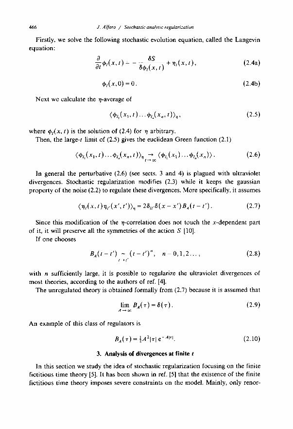
Firstly, we solve the following stochastic evolution equation, called the Langevin equation:

aq'/(x, ~S t ) = 6 ~ t ( x , t ) + r/,(x, t ) , (2.4a)

q)z(x,0) = 0. (2.4b)

Next we calculate the q-average of

(~,,,(x,, t ) . . . ,~ , . (x , , t ) ) , , (2.5)

where q)t(x, t) is the solution of (2.4) for rl arbitrary. Then, the large-t limit of (2.5) gives the euclidean Green function (2.1)

(,/,,,(x], t ) . . .q , , . (x , , t ) ) , --, (4, , ,(x~). . . , / , , . (x,)) . (2.6) l ---* OC

In general the perturbative (2.6) (see sects. 3 and 4) is plagued with ultraviolet divergences. Stochastic regularization modifies (2.3) while it keeps the gaussian property of the noise (2.2) to regulate these divergences. More specifically, it assumes

('O,(x, t ) r lc(x ' , t')),~ = 26 , ,6(x - x ' ) B A ( t -- t ' ) . (2.7)

Since this modification of the rt-correlation does not touch the x-dependent part of it, it will preserve all the symmetries of the action S [10].

If one chooses

B A ( t - - t ' ) - ( t - - t ' ) " , n = 0 , 1 , 2 . . . . (2.8) l ---* i t

with n sufficiently large, it is possible to regularize the ultraviolet divergences of most theories, according to the authors of ref. [4].

The unregulated theory is obtained formally from (2.7) because it is assumed that

lim BA(r ) = 8 ( r ) . (2.9) A ~ o c

An example of this class of regulators is

BA( ~ ) = ½aZl~l e-,41~1 (2.10)

3. Analysis of divergences at finite t

In this section we study the idea of stochastic regularization focusing on the finite fictitious time theory [5]. It has been shown in ref. [5] that the existence of the finite fictitious time theory imposes severe constraints on the model. Mainly, only renor-

J. AIfaro / Stochastic analytic regularization 467

malizable models can be described consistently in a stochastic (Langevin) formula- tion. We want to see now if the same approach can be combined with stochastic regularization.

We are going to show that SR regulates certain ultraviolet divergences (first class), but introduces new ones (second class). Second-class divergences are not regulated by SR although they also contribute to the infinite fictitious time limit. Happily enough, renormalizable theories and a slightly larger set do not have second-class divergences.

Let us calculate the crossed propagator in momentum space [4], according to (2.7). We get

( ( a ( k , t l ) q J ( - k , t 2 ) > , = f o q d ' q ~'2d~ '2e- 'k2"m:)u""+ '2- ' : )BA(r l -~ '2) . (3.1)

Possible ultraviolet divergences appear when the exponent vanishes (later k will be the momentum of one of the lines in a given loop). That is,

B u t

tl - r I + t 2 - T 2 = 0 . (3.2)

tl - ~'l >/0, (3.3a)

t 2 - r 2 >/0. (3.3b)

Therefore the possible singularity is multiplied by

BA(t, -- t2) . (3.4)

Now assume that the vertices t~ and t 2 a r e connected by an uncrossed propagator. To this line we associate the factor (see below)

e - ~ 2 +,,:)It,--,21 (3.5)

The ultraviolet singularity is possible only if, in addition to (3.2), we have

l I - 12 = 0 . ( 3 . 6 )

In this case the would-be singularity is multiplied by (see (3.4)) BA(0 ). Choosing BA(0 ) = 0, according to (2.8), we can regulate this type of singularity.

We call it first-class divergence.

However, a different situation is possible. That is, there is no uncrossed propa- gator connecting the vertices t 1 and t 2. In this case the possible overall divergence is multiplied by [B~(tl - t 2)]g, J being the number of crossed propagators connecting

468 J. Alfaro / Stochtz~tic analytic regularization

, / ~ ' ~ -" ,(

"1 . . . . . . . . . . . . l . . . . . . . . . . ~4

(a) (b)

Fig. 1. (a) One-loop contribution to F ~2~ in hO3 theory. (b) One-loop contribution to S ~2) in hO3 theory.

the vertices t~ and t 2. Clearly SR is unable to regulate this kind of divergence. We call these second class. They could occur when all fictitious times branching from

t D t 2 in the per turbat ive expansion of q'n collapse into t t and t 2 simultaneously. Fig. l a is an example of first-class divergences while fig. l b contains a second-class divergence. Both graphs are assumed to be in 8-dimensional space-time. The

second-class divergence appears in fig. l b when T 1 = I "3 = "1"4 and r 2 = q3 = "~4 simulta- neously.

Since SR does not work for second-class divergences, it is crucial to determine under which condit ions they are absent. To see this, we repeat the power count ing done in ref. [5] with the necessary modificat ions to include second-class divergences.

But, first let us introduce some definitions. (For more details see ref. [5].) Deno te by G ( x t, t~; x 2, t2) the stochastic p ropaga tor connect ing the vertex (x 2, t2)

of a one-par t ic le irreducible (1PI) graph G2 with the vertex (x~, t t) of another 1PI g raph G1. We will say that the line (x~, tx; x 2, t2) is crossed (uncrossed) relative to

G2 if t 1 < t 2 (t 1 > t2). Accord ing to the last definition we can classify 1PI graphs as follows: S (t, ' ' t, >=

1 PI graph with L 0 uncrossed external lines and L~ crossed external lines,

r(n+l)=s(l.n),

S (2) ~_ S (2,0).

The boxes of fig. 1 provide examples of /-(2) (fig. la) and S tz) (fig. lb).

We proceed to find the overall degree of second-class divergence of S (t'''" ~~.

Call m the number of contracted crosses inside S(t'o't '+),lq the number of r - in tegra t ions inside the 1PI graph beside those assigned to the L o uncrossed legs.

The uncrossed legs enter S ( l ' ' t ~ ) at fictitious times r,, i = 1 . . . L 0. As we men- t ioned above, the second-class divergence could occur when all the branching times hj evolving f rom r, in the expansion of q~n collapse into r, simultaneously. We write the following change of variables:

~ j = ~ - r ~ j . (3.7)

Then, when r --, O, r,g --* %

J. Alfaro /I Stochastic analytic regularization 469

The measure of integration is

drrN- '[dOi j] . (3.8)

Since r,j appears only linearly as a coefficient of Ki z in the stochastic propagator (K, is one of the loop momenta to be integrated over), each K, integral will bring down a factor of

r - " /2 . (3.9)

n is the dimension of space-time. That is, in the neighbourhood of (3.7) we have

f0 ~ s(Lo,I.,)~ drr,~ l-(n/2)L (3.10)

L is the number of loops of S tL°'t'c~. We define the overall degree of second-class divergence of the stochastically

regularized S tl"','L,) by

b , = n L - 21(l. (3.11)

If D,, >/0, the stochastically regularized graph is divergent. It should be observed that

fil= N + m - Lo + l , (3.12)

where N is the number of r-integrations inside S tt''''L') in the unregulated theory: the reason being that stochastic regularization introduces additional m r-integra- tions inside the 1PI graph. Of these, (L 0 - 1) are excluded from N because they correspond to the r, of uncrossed legs.

Therefore

b,+ 2 = D, + 2 ( L - m + L 0 - 1). (3.13)

D,, is the naive degree of divergence of S t t.o, L,) in the unregulated theory. The following identity is true for any local theory:

That is,

L - m + L 0 - 1 = 0. (3.14)

b,+ 2 = D,,. (3.15)

Since a renormalizable theory in (n + 2)-dimensional space is superrenormalizable in n-dimensional space, (3.15) reduces the analysis of second-class divergences in this case to the study of a finite number of graphs.

470 J. AIfaro / Stochastic analytic regularization

We illustrate the use of (3.15) with some examples (V is the number of vertices of S ~/.,, ~...)).

(i) ~ 4 theory:

19,= V( n - 4) - Lo( l + ~ n ) + L ~ ( 1 - ~ n ) + n + 2 .

Then

b 4 = - 2 V - 3L o + 4.

Only F ~2) to one loop could be divergent, but it is not second-class divergence. Therefore it is regulated by stochastic regularization.

For n = 5, only I "~2) in 1- and 2-loop order are potentially divergent, but they are

not second class, so they can be regulated by SR.

Instead, for n >/6, there is an infinite set of graphs with second-class divergences, an example being S ~2~ at two-loop order. Stochastic regularization cannot be applied

to this theory.

We see that the class of theories without second-class divergence is slightly larger than renormalizable theories.

(ii))~q~3 theory:

D., : - 3 ) v - (1 + + (1 - + . + 2 .

Then

D 6 = D 4 = - V - 3 L 0 - L ~ + 6 .

By inspection, we can see that there is no second-class divergence. Instead, for n >/8, fig. lb has a second-class divergence and then we cannot use

stochastic regularization in this case. (iii) n = 4 is a special case in this context because any interaction of the field

without derivative coupling is superrenormalizable in n = 2. Therefore these four- dimensional theories can be regularized using SR.

The quest ion arises as to whether the second-class singularities contribute to the equil ibrium theory or are an artifice of the finite-t formulation. An example will

suffice to settle this point. In fact, if one explicitly evaluates fig. l b one finds a divergent contr ibut ion for large t and for any BA(~-) corresponding to the region of

integration "r 3 = ~'4 - ~'1 and ?3 = ~4 - "r2 (n >/8). Therefore second-class singularities are also present in the equilibrium theory

when they are at finite t, invalidating the use of stochastic regularization even in this restricted sense.

J. AIfaro / Stochastic analytic regularizatton 471

4. A new regulator

The type of regulator (2.7) has various disadvantages. First it is not easy to characterize the type of divergence for the large A we shall encounter in a general stochastic graph. In the second place there is no precise prescription for fixing the divergent piece of the 1PI graphs.

The solution of both problems is easy if the singularities of loop integrals appear as poles in the parameters of the regulator. In this case a minimal subtraction scheme is the natural subtraction procedure. That is, we remove the singularity just by removing the pole parts in the Laurent series for the quantity under considera- tion.

The work of Speer [6] realizes this programme for the usual (non-stochastic) graphs. But it has the disadvantage of not being gauge invariant. A gauge-invariant analytic regularization is obtained by introducing the dimension of space-time as a regulator (dimensional regularization [11]). However, dimensional regularization faces difficulties when chiral theories are present and also when massless particles are considered [12].

In this section we want to present a form of stochastic regularization that makes direct contact with analytic regularization. It is a gauge-invariant regularization for which a minimal subtraction scheme is possible. Further, it does not have the limitations of dimensional regularization because it does not involve a change in the dimensionality of space-time. In addition, if renormalization is made at finite t the problem of massless particles never appears.

At present, we content ourselves with the definition of the regulator, leaving for a future publication [7] the detailed analysis of the divergences in arbitrary stochastic graphs. Its use will be illustrated in 2-dimensional U(N) gauge theory.

The authors of ref. [4] introduced the form (2.9) for the ~-function in t. Because the unregulated theory is obtained when A ~ oo, it is impossible to expect analytic behaviour of the theory in the variable A. To remedy this we use a standard method for transforming asymptotic behaviour in a large parameter into an analysis of singularities on the complex plane of a different parameter: the Mellin transform [13].

The Mellin transform of f(x) ~ [0, + o¢] is defined by

F( f l )=~dxx-~ Xf(x). (4.1)

The crucial point is that the Mellin transform of

f ( x ) = { xtJ" ( l n x ) ' ' (n - 1)? for

0 for

x ~ l

O ~ x < l

(4.2)

472

is

J. AIfaro / Stochastic analytic regulartzation

1 F(/3) - (4.3)

(/3 -/3o)"

That is, the asymptotic behaviour of f ( x ) when x ~ ~ is replaced by the behaviour of F(/3) when/3 ~ / 3 0.

The Mellin transform of (2.10) considered as a function of A is, up to a normal izat ion factor,

Ba(t) = ~/3ltl t~-I . (4.4)

It is possible to prove that

lim BB(t ) = 3 ( t ) . ( 4 .5a ) / ~ 0

Therefore (4.4) is acceptable as a stochastic regulator. (4.4) has various nice properties. First it has a zero of arbitrary order at t = 0 (choosing 13 large enough) which regularizes any first-class ultraviolet divergence. In contrast, the regulator (2.10) cannot render finite a quartic divergence.

Secondly since it is only for fl ~ 0 that we get a &funct ion (physical limit), this means, according to (4.2), that we only keep logarithmic divergences. The other singularities are not relevant to the physical limit, a characteristic that our regulator shares with analytic and dimensional regularization.

Moreover , the form (4.4) makes direct contact with the analytic renormalization of Speer [6]. In part icular it is not difficult to see that the ultraviolet divergences will appear as poles in the complex variable fl at /3 = 0. This last property is expected because of (4.2) and (4.3).

An intuitive way of seeing that the singularities at fl = 0 are poles is to compare our crossed propagator (3.1) and regulator (4.4):

(rb( k, t , ) r ~ ( - k , t2)) n = for, dr1 lot2 d~.2e ,k-'

(4.5b)

with the Speer regulator in euclidean momentum space (see eq. (2.4) of the second reference in [6[):

f0 ¢ da a x - le - ,,(~ 2 + ,,,2~ (4.5c)

In the Speer method the singularity appears when ?~ ---, 1, whereas in our case it appears when 13 ~ 0: the difference being due to the fact that (4.5b) contains one

J. Alfaro / Stoch~z*tic analytic regularization 473

more integral than (4.5c). But in the neighbourhood of the first-class singularity we

have t z = t 2 = r x = ~'2 (see sect. 3). And we can write

t2=tz +et[O]2,

"r 2 = t a + ~t[to] 2. (4.5d)

[ ] cor respond to angular variables.

Then

( t0(k , tl)to ( - k , t2)>n - a--*0

(4.5e)

f d,~,~a[d 02][dtol][dq~z]e - <.2 *''2)'~Ie12- I*h - f-h)

Therefore in the neighbourhood of the singularity (4.5b) and (4.5c) are identical if

we identify fl = A - 1 . But Speer has shown that the singularities of canonical

F e y n m a n graphs are poles in the variable A at A = 1 [6]. Therefore we should expect

that the singularities of stochastic graph are poles at fl = 0. The details of this analysis will be reported elsewhere [7].

To illustrate the use of (4.4) we calculate the one-loop contr ibut ion to F <2~ in

two-dimensional gauge theory.

This theory is described by

O (4.6) ~ A ~ = D,F,, + D~a,A, + n.,

Fvt,= O.At,- Ot, A ~ - ie[ A. , A~,] , (4.7)

Dr,= Or,- ie[A. , ] . (4.8)

We have chosen the " L a n d a u gauge" [14].

Fig. 2. (a), (b) One-loop contributions to F t2~ in two-dimensional gauge theory.

474 J. Alfaro / Stochastic analytic regularization

We assume the following form for the ,/-correlation:

( * l , ( x , t ) ~ l , ( x ' , t ' ) ) ~ = f l 6 ( x - x ' ) 8 ~ , l t - t ' l 1~-1 . (4.9)

The one-loop contribution to F (2) is given in fig. 2. Both graphs are primitively logarithmically divergent. If gauge invariance is to be respected the divergence of (a) should cancel the divergence of (b):

(a) = - 4 e 2 ~ , , [ NSadSb, . -- 8,,hBac ]

× ( ~ ) 2 f o ' d q l "r2 ( q l _ ~ 2 ) / ~ - I e - s , , f d 2 q e q ' - (2 , , - , , , , ) ~ 1 d

= _ 4e28~,lNS~dSb,._ 8.hSd~ ] A(fl) e 77;7

X(fl ) flfo"dq, " ( q ' - 72)~-' = f o d ? : 2r : q -~=~Tr .

T o evaluate

s,,, (4.10)

(4.11)

A ( f l ) we adapt Speer's method [6] to our case. By introducing the following change of variables:

72 = rl(1 - a 2 ) ,

rl = r l ( 1 - ala2),

we have

A(fl) = 7rflr~' d%da 2

0 ~< a i~ 1, (4.12)

(1 - - a t ) B - l a B 2 -1

l + a 1 (4.13)

The singularity for fl ~ 0 here reflects the fact that the ot 2 integral diverges when fl - , 0. We integrate by parts over %. Then,

A(,8) = ~ ~r,B'r I da I

7/" = - - + finite. (4.14)

#~0 2fl

J. AIfaro / Stochastic" anal.vtic regularization

Notice that the singularity of A(fl) is a pole at fl = 0. That is,

_ _ e 2 PP(a) = ~_~6,,[ U3,a3b, _8~b6a,.l e .4,,

/3 ,

(b) = 8e2[ N3~a3h,.- 3,hSa,. ]

xf'qd,r:/'~d% f~'d~ f d2q e-q2,,. ,2, 4 4 J0 3 J (2,,)2

Xe-(k-q)2(rl+'r2-r3 "~3)e-Sf2_l/3( T _ , 3 a - '

X {(kt,3 . . . . - 23¢,,~,k~,:)(2p~,3~,,:- p,~3,,,~)+ 2p2,t,~}.

We introduce the following change of variables:

We find that

Therefore

"r3 = TI(1 - a3),

r 3 = "q(1 - ~ 3 0 ¢ 3 ) ,

,i- 2 = ?1 (1 - - ~30t30~2) ,

0 ~ < a 3 ~ < 1 ,

0 ~ < o t 3 ~ 1 ,

0-G<o¢2~< 1 .

e 2 e s,~ PP(b) = ~ 3 u ~ - T [ N3°a3h" - 3'~b3a" ]"

475

(4.15)

(4.16)

(4.17)

(4.18)

PP(a) + PP(b) = O. (4.19)

5. Conclusions

In this work we have shown certain limitations of the method of stochastic regularization. Our analysis shows that SR is still appropriate for regularizing renormalizable theories, which are in any case those for which a consistent stochastic (Langevin) description exists.

In addition to this, we have introduced a form of stochastic regularization for which a minimal subtraction prescription is defined. We believe it to be an important step towards practical utilization of the SR idea.

Further work is necessary to show explicitly the nature of the singularities of arbitrary stochastic graphs in the new parameter/3. Progress made in this direction will be reported elsewhere [7].

476 J. dlfaro / Stochastic analytic regularization

T h e a u t h o r w o u l d like to thank P.K. Mi t te r , J .L. Gerva i s , C. Bachas and G. J o n a

L a s i n i o for usefu l discussions. H e w o u l d also l ike to thank P ro fes so r A b d u s Sa lam,

the I n t e r n a t i o n a l A t o m i c Energy A g e n c y and U N E S C O for hosp i t a l i t y at the

I n t e r n a t i o n a l C e n t r e for Theore t i ca l Physics, Tr ies te .

References

[1} G. Parisi and Y. Wu, Sci. Sin. 24 (1981) 483 [2] J. Alfaro and B. Sakita, Phys. I, ett. 121B (1983) 339;

J. Alfaro, Phys. Rev. D28 (1983) 1001; G. Aldazabal, N. Parga, M. Okawa and A. Gonzales Arroyo, Phys. Lett. 129B (1983) 80

[3] A. Guha and S.C. Lee, Phys. Lett. 134B (1984) 216; H.W. Hamber and U.M. Heller, Phys. Rev. 29D (1984) 928

[4] J.D. Breit, S. Gupta and A. Zaks, Nucl. Phys. B233 (1984) 61 [5] J. Alfaro, Non-renormalizable theories do not have a stochastic interpretation, LPTENS 84/4 [6] E.R. Speer, Generalized Feynman amplitudes (Princeton University Press, 1969): Lectures on

Analytic renormalization, University of Ma~land, Technical Report No. 73-067 (December 1972) [7] J. Alfaro, to be published [8] Refs. [1,4,5] [9] Ref. [1]; J. Alfaro, Stochastic quantization and the large-N reduction of quantum field theorics, PhD

thesis, City University of New York (1983); B. Sakita, Talk given at the 7th Johns Hopkins Workshop, City College of New York, preprint CCNY-83-14

[10] J. Alfaro and B. Sakita, Stochastic quantization and the large-N limit of U(N) gauge theory, in Proc. Conf. Topical Symp. on High energy physics, Tokyo, ed T. Eguchi and Y. Yamaguchi (World Scientific, Singapore, 1983); Ref. [41

[11] (;.'t Hooft and M. Veltman, Nucl. Phys. B44 (1972) 189: G.C. Bollini and J.J. Giambiagi, Phys. Lett. 40B (1972) 566; J.F. Ashmore, Nuovo Cim. Left. 4 (1972) 289

[12] G. l,eibbrandt, Rev. Mod. Phys. 47 (1975) 849 [13] R.J. Eden et al., The analytic S-matrix (Cambridge University Press, 1966) 151 [14] D. Zwanziger, Nucl. Phys. B192 (1981) 259;

L. Baulieu and D. Zwanziger, Nucl. Phys. B193 (1981) 163; E. Floratos and J. lliopoulos, Nucl. Phys. B214 (1983) 392